BACHELOR’S DEGREE PROJECT IN MATHEMATICS

The Method of Characteristics

by

Ida Andersson

MAA043 — Bachelor’s Degree Project in Mathematics

DIVISION OF MATHEMATICS AND PHYSICSMÄLARDALEN UNIVERSITY

SE-721 23 VÄSTERÅS, SWEDEN

MAA043 — Bachelor’s Degree Project in Mathematics

Date of presentation:1st June 2022

Project name:The Method of Characteristics

Author:Ida Andersson

Version:9th June 2022

Supervisor:Linus Carlsson

Examiner:Sergey Korotov

Comprising:15 ECTS credits

Abstract

Differential equations, in particular partial differential equations, are used to mathematicallydescribe many physical phenomenon. The importance of being able to solve these typesof equations can therefore not be overstated. This thesis is going to elucidate one method,the method of characteristics, which can in some cases be used to solve partial differentialequations. To further the reader’s understanding on the method this paper will provide someimportant insights on differential equations as well as show examples on how the method ofcharacteristics can be used to solve partial differential equations of various complexity. Wewillalso in this paper present some important geometric complications for linear partial differentialequations which one might have to take into consideration when using the method.

Acknowledgements

I will dedicate this section to acknowledge some key people that, in various ways, contributedto my work with this thesis. First and foremost I want to give special thanks to my supervisor,Linus Carlsson, for his dedication and encouragement and for providing me with a deeperunderstanding on the subjects covered in this thesis. I would also like to give special thanks tomy fellow classmate and opponent, Jasmine Pedersen, for her support and motivation duringthe time spent working on this thesis, as well as her feedback given at the presentation ofthis thesis. I also give special thanks to my examiner Sergey Korotov for providing valuablefeedback on this thesis.

2

Contents

Acknowledgements 2

Notation and Definitions 5Notation . . . . . . . . . . . . . . . . . . . . . . . . . . . . . . . . . . . . . . . . 5Definitions . . . . . . . . . . . . . . . . . . . . . . . . . . . . . . . . . . . . . . . 5

1 Introduction 61.1 Background . . . . . . . . . . . . . . . . . . . . . . . . . . . . . . . . . . . 61.2 Aim and Purpose . . . . . . . . . . . . . . . . . . . . . . . . . . . . . . . . 71.3 Research Question . . . . . . . . . . . . . . . . . . . . . . . . . . . . . . . 71.4 Literature Review . . . . . . . . . . . . . . . . . . . . . . . . . . . . . . . . 7

2 Differential Equations 92.1 Some Methods For Solving ODE:s . . . . . . . . . . . . . . . . . . . . . . . 9

2.1.1 Separable ODE . . . . . . . . . . . . . . . . . . . . . . . . . . . . . 92.1.2 The Runge-Kutta Methods . . . . . . . . . . . . . . . . . . . . . . . 102.1.3 Local and Global Error . . . . . . . . . . . . . . . . . . . . . . . . . 14

2.2 Partial Differential Equations . . . . . . . . . . . . . . . . . . . . . . . . . . 142.2.1 Physical Interpretation Of PDE:s . . . . . . . . . . . . . . . . . . . . 142.2.2 Some Methods For Solving PDE:s . . . . . . . . . . . . . . . . . . . 16

3 Method of Characteristics 193.1 Method Derivation . . . . . . . . . . . . . . . . . . . . . . . . . . . . . . . 193.2 A Linear Example . . . . . . . . . . . . . . . . . . . . . . . . . . . . . . . . 213.3 A Nonlinear Example . . . . . . . . . . . . . . . . . . . . . . . . . . . . . . 23

4 Solving an Advanced Problem Using Matlab 264.1 A special case . . . . . . . . . . . . . . . . . . . . . . . . . . . . . . . . . . 27

4.1.1 Some Characteristics . . . . . . . . . . . . . . . . . . . . . . . . . . 284.1.2 The Solution . . . . . . . . . . . . . . . . . . . . . . . . . . . . . . 29

5 Geometric Considerations 315.1 Initial Conditions and Boundary Data . . . . . . . . . . . . . . . . . . . . . 315.2 Geometric Considerations for Linear PDE:s . . . . . . . . . . . . . . . . . . 33

3

5.2.1 Special Cases Needed to Consider . . . . . . . . . . . . . . . . . . . 33

6 Conclusion and Discussion 36

A Matlab code for Linear Example 40

B Matlab code for Non-linear Example 41

C Matlab code for an Advanced Example Some Characteristic Curves 42

D Matlab code for an Advanced Example Solution Surface 44

4

Notation and Definitions

This section is an introduction to important notation and definitions which will be used tothroughout the paper.

Notationx = (𝑥1, 𝑥2, ..., 𝑥𝑛), 𝑛 ∈ Z+ Vector𝑑𝑥𝑑𝑡

= ¤𝑥 Time derivative𝜕𝜕𝑥𝑖

𝑦(x) = 𝑦𝑥𝑖 (x), 𝑖 = 1, 2, ..., 𝑛 and 𝑛 ∈ Z+ Partial derivative𝐷𝑦(x) = (𝑦𝑥1 (x), 𝑦𝑥2 (x), ..., 𝑦𝑥𝑛 (x)), 𝑛 ∈ Z+ Gradient𝑓 : 𝐶𝑘 (R𝑛) 𝑓 has continuous derivatives

up to order 𝑘 on R𝑛div 𝐹 (x) = ∇ · 𝐹 (x) = 𝐹𝑥1 (x) + . . . + 𝐹𝑥𝑛 (x) Divergence

Definitions and TheoremsDefinition 1. A set 𝑆 ⊂ R𝑛 is called an open set if for all points 𝑝 ∈ 𝑆 and any given point𝑞 ∈ R𝑛, 𝑞 ≠ 𝑝, there exists an 𝜖 > 0 such that if |𝑞 − 𝑝 | < 𝜖 then 𝑞 ∈ 𝑆.

Definition 2. A function is called smooth if it has continuous derivatives of every order.

5

Chapter 1

Introduction

In this section we are going to provide some background necessary to understand the chaptersthat follow and also present the aim of this thesis, the research question that this thesis paperwill work towards answering and also a literature review.

1.1 BackgroundAn equation that includes one or more derivatives is called a differential equation [9] and arethought to have been first investigated in the mid 1600s [1]. A differential equation in whichonly one independent variable is present, i.e. only ordinary derivatives may be included, iscalled an ordinary differential equation (henceforth referred to as an ODE) and when there aretwo or more independent variables present in the differential equation, i.e. partial derivativesare included in the equation, it is called a partial differential equation (henceforth referred to asa PDE). For both ODE:s and PDE:s there may be one or more dependent variables present [9].Throughout this paper the dependent variable will be denoted as 𝑦. We will also assume thatthe solution 𝑦 is smooth on open sets.Both ODE:s and PDE:s are classified with regards to the order of the highest derivative

of the dependent variable that is included in the equation. This is called the order of thedifferential equation, e.g. a first order differential equation includes at highest a first derivative,a second order a second derivative and so on. It is important to note that differential equationsof order two or higher often includes derivatives of lower order than the order of the equation,it is the highest order derivative that determines the order of the differential equation [9]. Thispaper will mainly be focusing PDE:s of the first order, however it is necessary to understandhow to solve ODE:s of the first order, which we will show in the next section.In order for a differential equation to be called linear the dependent variables and all

their derivatives must appear as first powers. Furthermore, the derivatives of the dependentvariables cannot appear as a multiplication with the dependent variables, i.e. all the dependentvariables and their derivatives can at most be multiplied with functions of the independentvariables. If these conditions are not fulfilled the differential equation is considered to benon-linear [9]. There are however different types of non-linear differential equations, e.g.semi-linear, quasi-linear and fully non-linear [6].

6

For instance, if 𝑦 : R→ R then𝑦′ = 𝑥2

is a linear first order ODE, whereas if 𝑦 : R2 → R then

𝑦𝑥1 + 𝑦𝑥2 + 𝑦2 = 𝑥

is a non-linear first order PDE. This particular example is in fact semi-linear, i.e. non-linearbut linear in the highest order derivative.

1.2 Aim and PurposeThe purpose of this paper is to enlighten the reader on the important area of mathematics whichis differential equations, in particular partial differential equations, and elucidate one methodwhich can sometimes be used to solve these, namely the method of characteristics. We willalso investigate what the limitations of this method are and answer the research questions.

1.3 Research QuestionThe question that we intent to answer in this paper is;

1 (a) When can the method of characteristics be used to solve partial differential equations?

1 (b) When is it problematic to solve PDE:s using the method of characteristics?

1.4 Literature ReviewIn this section we are going to reflect on some of the literature this thesis paper is based on. Themain topic of this thesis is the method of characteristics, which is one of many methods usedto solve partial differential equations, e.g. see Section 2.2.2. The idea of this method is to turna PDE into a system of ODE:s, which shows the importance to have some basic knowledge ofODE:s and how to solve these. The methods for solving ODE:s chosen to emphasize in thispaper is separation of variables and some of the Runge-Kutta variants. The information aboutthe method of separation of variables presented in this paper is based on [9], which shows thederivation of the method. The derivation of the Runge-Kutta variants presented in this papercan be found in [10]. However, there exists Runge-Kutta methods of higher order than what ispresented in this paper, see e.g. [4].The main focus of this paper is the method of characteristics and the majority of the inform-

ation gathered on the topic is based on [6], which is a book intended for educational/researchpurposes and does not only cover the method of characteristics but partial differential equationsin general. The reason a large part of this thesis paper is based on this source is that it providesthe derivation of the method, some applications of the method on different types of PDE:s andalso some geometric considerations that might reveal some flaws in the method. Most of the

7

research found in the literature is mainly covering the application of the method of charac-teristics to solve various engineering problems, see e.g. [13] and [11]. When reviewing theliterature for this thesis it was quite difficult to find literature that added some other insights onthis topic than what is provided in [6]. One paper that was found that covered the subject was[16]. However, this paper was not considered to provide any new information about the methodof characteristics and was therefore not used as a reference in this paper. In [2] the method ofcharacteristics is used to solve PDE:s of second order, namely the hyperbolic Monge-Ampèreequation, which is an application that is not mentioned in [6]. However, in this thesis we onlyinvestigate the usage of the method of characteristics on PDE:s of first order. Another thingthat is missing in [6] is the advantages and disadvantages of this method in comparison to othermethods that can be used to solve PDE:s. This was also not found in any other literature thatwas looked into when researching for this thesis. Given more time, a more thorough literaturereview might have resulted in a better understanding of the differences between the method ofcharacteristics and some other methods that exists.

8

Chapter 2

Differential Equations

In this chapter we are going to dive deeper into differential equations. Since the main focus ofthis paper is on partial differential equations, the majority of this chapter will be concerningthose. We will however present a few methods for solving some types of both ordinary andpartial differential equations as well as present an example on how partial differential equationscan describe a physical phenomenon.

2.1 Some Methods For Solving ODE:sThere are several methods for solving ODE:s and which method is more suitable is dependenton the form of the characteristics of the ODE.Wewill in this section focus on a fewmethods forsolving first order ODE:s, both a analytical method for solving separable differential equationsand a family of numerical methods, called The Runge-Kutta methods.

2.1.1 Separable ODEThe form of ODE:s that is probably the most straight forward to solve is so called separabledifferential equations. The information presented in this section is derived from [9].We will consider an ODE of first order that is expressed on the form

𝑀 (𝑥, 𝑦) + 𝑁 (𝑥, 𝑦) 𝑑𝑦𝑑𝑥

= 0. (2.1)

If we assume that there exists a function 𝑓 (𝑥, 𝑦) for which the following relations are true𝜕 𝑓

𝜕𝑥= 𝑀 (𝑥, 𝑦) and

𝜕 𝑓

𝜕𝑦= 𝑁 (𝑥, 𝑦) (2.2)

the chain rule gives

𝑑

𝑑𝑥𝑓 (𝑥, 𝑦) = 𝜕 𝑓

𝜕𝑥+ 𝜕 𝑓

𝜕𝑦

𝑑𝑦

𝑑𝑥= 𝑀 (𝑥, 𝑦) + 𝑁 (𝑥, 𝑦) 𝑑𝑦

𝑑𝑥= 0,

i.e.𝑓 (𝑥, 𝑦) = 𝑐, (2.3)

9

where 𝑐 is an arbitrary constant. Under the assumtion that 𝑓 ∈ 𝐶2(R2), we know that the orderof the derivatives does not matter and from Equation (2.2) we get

𝜕𝑀

𝜕𝑦=𝜕𝑁

𝜕𝑥. (2.4)

Hence, if the equality in Equation (2.4) holds, there exists a function 𝑓 (𝑥, 𝑦) such that Equa-tion (2.2) holds and Equation (2.3) is therefore the primitive function of Equation (2.1).Equations on this form that fulfill the equality in Equation (2.4) are called exact differentialequations. The case when an exact ODE has the property that 𝑀 is only a function of 𝑥 and𝑁 is a function of 𝑦 it is in particular simple to solve the PDE given in Equation (2.1). In thiscase the solution can be found through integration in such a way that∫

𝑀 (𝑥)𝑑𝑥 +∫

𝑁 (𝑦)𝑑𝑦 = 𝑐.

It is however not quite often that easy to recognize a separable differential equation. Let usconsider the following differential equation

𝑦 + 𝑥𝑑𝑦

𝑑𝑥= 0.

This is in fact a separable differential equation, even though one have to algebraicallymanipulatethe equation to get the desired form. By ”multiplying” with 𝑑𝑥 on both sides and divide by 𝑦and 𝑥 on both sides we now have the following form

1𝑥𝑑𝑥 + 1

𝑦𝑑𝑦 = 0,

where𝑀 (𝑥) = 1

𝑥and 𝑁 (𝑦) = 1

𝑦.

This is now solved quite easily by integration.

2.1.2 The Runge-Kutta MethodsMost ODE:s are hard or impossible to solve analytically (in most physical interpretations it isin fact impossible), but there exists several numerical methods that can be used to solve thesetypes of equations. We are going to focus on one family of iterative methods called the Runge-Kutta methods. They consists of several implicit and explicit variants, although we are goingto limit ourselves in this section to only show three of the explicit variants, namely the explicitfirst order Runge-Kutta method, the explicit second order Runge-Kutta method and the explicitfourth order Runge-Kutta method, which may also be referred to as the classical Runge-Kuttamethod. There also exists Runge-Kutta of higher order, e.g. see [4]. The information presentedin this section can be found in [10].

10

Derivation of Explicit First Order Runge-Kutta Method

Assume that we have a first order ODE on the form

𝑦′(𝑥) = 𝑓 (𝑥, 𝑦), (2.5)𝑦(0) = 𝑦0. (2.6)

If we do a Taylor series expansion we get the following;

𝑦(𝑥𝑘 + Δ𝑥) = 𝑦(𝑥𝑘 ) + 𝑦′(𝑥𝑘 )Δ𝑥 + O(Δ𝑥2).

We will stop the expansion here. This is the reason this is called the first order Runge-Kuttamethod, because we stop the Taylor expansion at the first order derivative. We first includesome new variables by using

𝑥0 = 0𝑥𝑘+1 = 𝑥𝑘 + Δ𝑥, 𝑘 = 1, 2, ...𝑦𝑘+1 = 𝑦𝑘 + Δ𝑥 𝑓 (𝑥𝑘 , 𝑦𝑘 ), 𝑘 = 1, 2, ...

where we have substituted the first derivative by the expression given in Equation (2.5). Wetherefore get

𝑦1 = 𝑦(𝑥1) + O(Δ𝑥2),

where the last term is simply a measurement of how accurate the algorithm is. It tell us thatall other terms will be of order two or higher. We will get into more on algorithm accuracyin Section 2.1.3. We have now derived the first order Runge-Kutta method, or more famouslyknown as Euler’s method. The idea behind this method is that we can project the slope atpoint 𝑥𝑘 to get to 𝑥𝑘+1 and by that predict the function value at that point. Note that we in theRunge-Kutta methods assumes equidistant distances Δ𝑥 = 𝑥𝑘+1 − 𝑥𝑘 for all 𝑘 = 1, 2, . . ..

Derivation of The Family of Explicit Second Order Runge-Kutta Methods

We will again look at a first order ODE on the form

𝑦′(𝑥) = 𝑓 (𝑥, 𝑦), (2.7)𝑦(0) = 𝑦0. (2.8)

The Runge-Kutta method states that

𝑦𝑘+1 = 𝑦𝑘 + 𝑎𝑘1 + 𝑏𝑘2,

where

𝑘1 = Δ𝑥 𝑓 (𝑥𝑘 , 𝑦𝑘 ),𝑘2 = Δ𝑥 𝑓 (𝑥𝑘 + 𝑐Δ𝑥, 𝑦𝑘 + 𝑑𝑘1).

11

By combining these two expressions we get

𝑦𝑘+1 = 𝑦𝑘 + 𝑎Δ𝑥 𝑓 (𝑥𝑘 , 𝑦𝑘 ) + 𝑏Δ𝑥 𝑓 (𝑥𝑘 + 𝑐Δ𝑥, 𝑦𝑘 + 𝑑𝑘1). (2.9)

We therefore have four unknown parameters wewant to determine such that the error is as smallas possible. We again begin with Taylor series expansion of the left hand side of Equation (2.9)up to order two, which is the reason that it is called the second order Runge-Kutta method.We can replace the derivatives of 𝑦 in the Taylor expansion with Equation (2.7) and apply thechain rule to replace the second derivative, which then gives us

𝑦𝑘+1 = 𝑦𝑘 + Δ𝑥 𝑓 (𝑥𝑘 , 𝑦𝑘 ) +Δ𝑥2

2(𝑓𝑥 (𝑥𝑘 , 𝑦𝑘 ) + 𝑓𝑦 (𝑥𝑘 , 𝑦𝑘 ) 𝑓 (𝑥𝑘 , 𝑦𝑘 )

)+ O(Δ𝑥3). (2.10)

If we look at the last factor of last term of Equation (2.9) we see that this is not on a form whereit is possible to compare coefficients with Equation (2.10). Hence, we have to do a Taylorseries expansion for two variables of the last factor of the last term of Equation (2.9), whichgives

𝑓 (𝑥𝑘+𝑐Δ𝑥, 𝑦𝑘 + 𝑑𝑘1) = 𝑓 (𝑥𝑘 , 𝑦𝑘 ) + 𝑐Δ𝑥 𝑓𝑥 (𝑥𝑘 , 𝑦𝑘 ) + 𝑑𝑘1 𝑓𝑦 (𝑥𝑘 , 𝑦𝑘 ) + O(Δ𝑥2)= 𝑓 (𝑥𝑘 , 𝑦𝑘 ) + 𝑐Δ𝑥 𝑓𝑥 (𝑥𝑘 , 𝑦𝑘 ) + 𝑑𝑘1 𝑓 (𝑥𝑘 , 𝑦𝑘 ) 𝑓𝑦 (𝑥𝑘 , 𝑦𝑘 ) + O(Δ𝑥2).

(2.11)

From the information given by equations (2.9) and (2.11) it can be concluded that one way ofwriting the Taylor series expansion of 𝑦𝑘+1 is

𝑦𝑘+1 = 𝑦𝑘 + 𝑎Δ𝑥 𝑓 (𝑥𝑘 , 𝑦𝑘 ) + 𝑏Δ𝑥

(( 𝑓 (𝑥𝑘 , 𝑦𝑘 ) + 𝑐Δ𝑥 𝑓𝑥 (𝑥𝑘 , 𝑦𝑘 ) + 𝑑𝑘1 𝑓𝑦 (𝑥𝑘 , 𝑦𝑘 ) + O(Δ𝑥2)

)= 𝑦𝑘 + (𝑎 + 𝑏)Δ𝑥 𝑓 (𝑥𝑘 , 𝑦𝑘 ) + 𝑏Δ𝑥2(𝑐 𝑓𝑥 (𝑥𝑘 , 𝑦𝑘 ) + 𝑑𝑓 (𝑥𝑘 , 𝑦𝑘 ) 𝑓𝑦 (𝑥𝑘 , 𝑦𝑘 )) + O(Δ𝑥3).

(2.12)

Since Equation (2.10) and Equation (2.12) are equal, and therefore the coefficients shouldmatch, we get the following expressions for the unknown parameters:

𝑎 + 𝑏 = 1, 𝑐 = 𝑑 =12𝑏

.

There are four unknown parameters and three equations, therefore one could simply choosean arbitrary value for one of the parameters and retrieve the corresponding values of the otherparameters. We have now derived the family of explicit second order Runge-Kutta methods,which can be summarized as the following;If we have an ODE on the form

𝑦′(𝑥) = 𝑓 (𝑥, 𝑦),𝑦(0) = 𝑦0

then𝑦𝑘+1 = 𝑦𝑘 + 𝑎𝑘1 + 𝑏𝑘2,

12

where

𝑘1 = Δ𝑥 𝑓 (𝑥𝑘 , 𝑦𝑘 ),𝑘2 = Δ𝑥 𝑓 (𝑥𝑘 + 𝑐Δ𝑥, 𝑦𝑘 + 𝑑𝑘1)

and𝑎 + 𝑏 = 1, 𝑐 = 𝑑 =

12𝑏

.

If the parameters are chosen such that

𝑎 = 𝑏 =12and 𝑐 = 𝑑 = 1

it is called the modified Euler method, whereas if the parameters are chosen such that

𝑎 = 0, 𝑏 = 1 and 𝑐 = 𝑑 =12

it is called the midpoint method.

The Explicit Fourth Order Runge-Kutta Method

The explicit fourth order Runge-Kutta method (also known as the classical Runge-Kuttamethod) is the most widely used numerical method for solving first order ODE:s. Sincethe derivation of this method is quite tedious, we will simply show what the method looks like.The interested reader may be referred to [14] for the derivation of the fourth order Runge-Kuttamethod. If we again have an ODE on the form

𝑦′ = 𝑓 (𝑥, 𝑦),𝑦(0) = 𝑦0

the fourth order Runge-Kutta method gives the numerical function value through

𝑦𝑘+1 = 𝑦𝑘 +16(𝑘1 + 2𝑘2 + 2𝑘3 + 𝑘4)

where the values for 𝑘1, 𝑘2, 𝑘3 and 𝑘4 are

𝑘1 = 𝑓 (𝑥𝑘 , 𝑦𝑘 ),

𝑘2 = 𝑓

(𝑥𝑘 +

12Δ𝑥, 𝑦𝑘 +

12Δ𝑥𝑘1

),

𝑘3 = 𝑓

(𝑥𝑘 +

12Δ𝑥, 𝑦𝑘 +

12Δ𝑥𝑘2

),

𝑘4 = 𝑓 (𝑥𝑘 + Δ𝑥, 𝑦𝑘 + Δ𝑥𝑘1) .

The way that this method works in comparison to the Euler method is that it calculates fourdifferent slopeswithin the same intervalΔ𝑥 and uses aweighted average to estimate the functionvalue at the point 𝑥𝑘+1.

13

2.1.3 Local and Global ErrorThere are clearly several different Runge-Kuttamethods for approximatingODE:s and thereforeit would seem wise to explore the difference between these. The Runge-Kutta methods onlygive approximations of the ODE in question and we are therefore most certainly going to getsome errors when estimating the function values. Obviously, we want the error to be as smallas possible while at the same time use an algorithm that is not too time consuming, so thequestion is; how large is the error going to be for the various methods?Since Δ𝑥 is the step size we have that

Δ𝑥 =1𝑛

where 𝑛 is the amount of steps needed to get from 0 to 1, which, for simplicity, is the intervalwe have chosen to solve the ODE over. The local error is the error of each step, while the globalerror is the difference between the actual function value and the estimated function value, i.e.the global error is the accumulated local errors. We will assume that the solutions are 𝐶2 andtherefore, on bounded subdomains, the second derivatives are uniformly continuous, whichenables us to use the same constant in the big-O notation for all points where we make a Taylorexpansion. If we start by looking at the error for Euler’s method, we saw that the local error isof order two, i.e. O(Δ𝑥2) = 𝐶Δ𝑥2. The global error is then

𝑛 · 𝐶Δ𝑥2 = 1Δ𝑥

𝐶Δ𝑥2 = 𝐶Δ𝑥 = O(Δ𝑥).

Euler’s method is therefore said to be first order accurate. This would mean that if we choosethe stepsize Δ𝑥 = 1 the global error would be 𝐶, which might actually not be a very goodapproximation at all. If we would like the error to be the half of that we have to double theamount of steps taken, which could potentially be quite time consuming.Assuming that the solution function 𝑦 is smooth, we get for the family of second order

Runge-Kutta methods the local error O(Δ𝑥3), which means the global error will be O(Δ𝑥2)and the method is said to be second order accurate. This means that one would make theerror one fourth of the original error by doubling the amount of steps taken. For the classicalRunge-Kutta method the local error is O(Δ𝑥5) and the global error is O(Δ𝑥4).

2.2 Partial Differential EquationsThis section is intended to give further understanding on PDE:s and why they are so importantto study. We will therefore present a real world example when a physical phenomenon isdescribed by PDE:s and also provide basic knowledge on some methods that can be used tosolve PDE:s.

2.2.1 Physical Interpretation Of PDE:sIn this section, which is based on ideas provided in [6] and [8], we are going to derive a veryimportant equation in physics, namely the diffusion equation (also known as the heat diffusion

14

equation) in three dimensional space. The equation describes how the concentration of e.g. achemical diffuses in a liquid or heat diffuses in a solid. To make it easier to visualize, we willonly consider the diffusion of a chemical in a liquid.Let us assume that we have a liquid that takes up a smooth subspace 𝑈 ⊂ R3. The

concentration (i.e. mass of particles per unit volume) of the chemical at a point x ∈ 𝑈 at time𝑡 can be described through some function 𝑦(x, 𝑡). We will assume that the function 𝑦(x, 𝑡) issmooth. We now look at an test volume 𝑉 ⊂⊂ 𝑈 that is contained by a smooth surface 𝑆, i.e.we assume the set 𝑉 to be an open bounded set that is relatively compact in 𝑈 with a smoothboundary. The concentration of the chemical in that whole region is given by∭

𝑉

𝑦(x, 𝑡)𝑑𝑈.

We are interested to know how the concentration of the chemical changes over time. We willassume that no additional amount of the chemical is produced or added in the liquid as wellas no amount of the chemical is destroyed, i.e. the total mass of the chemical is constant. Thechange of the concentration in 𝑉 is therefore equal to the flux of the chemical into the regionminus the flux out of the region, i.e. the net flux of the chemical out of 𝑉 . If we let F(x, 𝑡) bethe flux vector and n(x) be the unit normal vector to the surface 𝑆 with direction outward inpoint x ∈ 𝑆, then the outward rate of flux through the whole surface 𝑆 is given by∬

𝑆

F(x, 𝑡) · n(x)𝑑𝑆.

If the net rate of flux out through the boundary 𝑆 is positive it shouldmean that the concentrationinside 𝑉 should be decreasing. We can therefore set up the following equation for the changeof concentration of the chemical;

𝑑

𝑑𝑡

∭𝑉

𝑦(x, 𝑡)𝑑𝑈 = −∬

𝑆

F(x, 𝑡) · n(x)𝑑𝑆 ⇔∭

𝑉

𝑦𝑡 (x, 𝑡)𝑑𝑈 = −∬

𝑆

F(x, 𝑡) · n(x)𝑑𝑆(2.13)

The Divergence Theorem (also known as Gauss’s Theorem) gives us a relation between theflux out of the surface 𝑆 and the divergence over the whole region 𝑉 , namely∬

𝑆

F(x, 𝑡) · n(x)𝑑𝑆 =

∭𝑉

divF(x, 𝑡)𝑑𝑈

which means that Equation (2.13) can now be simplified to∭𝑉

𝑦𝑡 (x, 𝑡)𝑑𝑈 = −∭

𝑉

divF(x, 𝑡)𝑑𝑈 ⇔∭

𝑉

(𝑦𝑡 (x, 𝑡) + divF(x, 𝑡)) 𝑑𝑈 = 0. (2.14)

Since we want Equation (2.14) to be true for all points for the arbitrary test volume 𝑉 , we get

𝑦𝑡 (x, 𝑡) = − divF(x, 𝑡). (2.15)

We can now use Fick’s law (for heat diffusion the equivalent law is called Fourier’s law) whichprovides a relationship between the concentration and the flux. The concentration gradient

15

points in the direction of highest concentration and Fick’s law states that the flux vector isdirected from higher concentration to lower and is proportional to the concentration gradient,which means

F(x, 𝑡) = −𝐶 · 𝐷𝑦(x, 𝑡),

where 𝐶 is the constant diffusion coefficient. By inserting this into Equation (2.15) gives us

𝑦𝑡 (x, 𝑡) = 𝐶(𝑦𝑥1𝑥1 (x, 𝑡) + 𝑦𝑥2𝑥2 (x, 𝑡) + 𝑦𝑥3𝑥3 (x, 𝑡)

).

We have now showed the derivation of the diffusion equation, which is

𝑦𝑡 (x, 𝑡) − 𝐶Δ𝑦(x, 𝑡) = 0 (2.16)

2.2.2 Some Methods For Solving PDE:sIn this section we will give a brief introduction to two well known methods for solving PDE:s,namely separation of variables and the finite element method, and discuss some advantagesand disadvantages for each method. Beyond these two methods there are several other methodsfor solving PDE:s, e.g. the Escalator Boxcar Train method [3, 5], Transform methods [6],Galerkin methods [19] and the leapfrog algorithm [17].

Separation of Variables

This standard method is taught to undergraduate students and may be found in many bookson PDE:s, see e.g. [6]. The idea behind the method of separation of variables for PDE:s isto assume that the solution to a PDE of order 𝑛 can be written as two separate differentialequations, one depending on only one variable, i.e. one being a ODE, and the other depedingon 𝑛 − 1 variables. We will illustrate how this could be done by looking at the diffusionequation (2.16) from Section 2.2.1, but in R × R+, i.e. only one spatial variable and a timevariable. So what we have then is

𝑦𝑡 (𝑥, 𝑡) = 𝐶𝑦𝑥𝑥 (𝑥, 𝑡), (2.17)

where 𝑦(𝑥, 𝑡) is the solution to this PDE and 𝐶 is a constant. We will make the ansatz that thesolution can be expressed as a product of two single-variable functions, i.e. we assume

𝑦(𝑥, 𝑡) = 𝑢(𝑡)𝑣(𝑥), (2.18)

where 𝑢(𝑡) ≠ 0 and 𝑣(𝑥) ≠ 0. We can then substitute this into Equation (2.17) and get

𝑦𝑡 (𝑥, 𝑡) − 𝐶𝑦𝑥𝑥 (𝑥, 𝑡) = 𝑢′(𝑡)𝑣(𝑥) − 𝐶𝑢(𝑡)𝑣′′(𝑥) = 0.

This equation is not yet separated, but it is separable. By rearranging the functions a bit wecan obtain the following;

𝑢′(𝑡)𝐶𝑢(𝑡) =

𝑣′′(𝑥)𝑣(𝑥) . (2.19)

16

Since the left hand side is only dependent on 𝑡 and the right hand side is only dependent on 𝑥,the only way that this can be true is if both sides equal a constant. We will choose the constantto −_. The left hand side of Equation (2.19) creates a separable first order ODE which we cansolve using the method presented in Section 2.1.1, whereas the right hand side creates a secondorder linear homogeneous ODE with constant coefficients. The method for solving these typesof ODE:s is standard and can be found in many books on ODE:s, see e.g. [20]. We thereforeobtain the following;

𝑢′(𝑡)𝐶𝑢(𝑡) = −_ ⇔ 𝑢′(𝑡) + 𝐶_𝑢(𝑡) = 0⇔ 𝑢(𝑡) = 𝐷𝑒−𝐶_𝑡 ,

𝑣′′(𝑥)𝑣(𝑥) = −_ ⇔ 𝑣′′(𝑥) + _𝑣(𝑥) = 0⇔ 𝑣(𝑥) = 𝐴 sin(

√_𝑥) + 𝐵 cos(

√_𝑥),

where 𝐴, 𝐵 and 𝐷 are constants. By using separation of variables we have reduced the PDEto a system consisting of two ODE:s, one first order and one second order. The total solutionto Equation (2.18) is then given by

𝑦(𝑥, 𝑡) = 𝑢(𝑡)𝑣(𝑥) = 𝐷𝑒−𝐶_𝑡 (𝐴 sin(√_𝑥) + 𝐵 cos(

√_𝑥)).

For each unique value chosen for _we get a different solution. In particular, we get the solutions

𝑦_ (𝑥, 𝑡) = 𝑒−𝐶_𝑡 (𝐴_ sin(√_𝑥) + 𝐵_ cos

√_𝑥)).

This wouldmean that for each _we get two unknown constants 𝐴_ and 𝐵_. Using superpositionof solutions, we get the most general solution 𝑦(𝑥, 𝑡) to the ansatz to be

𝑦(𝑥, 𝑡) =∑︁_

𝑦_ (𝑥, 𝑡) =∑︁_

𝑒−𝐶_𝑡 (𝐴_ sin(√_𝑥) + 𝐵_ cos

√_𝑥)).

Since the initial data in a initial value problem usually is on the form 𝑦(𝑥, 0) = 𝑔(𝑥) we need

𝑦(𝑥, 0) =∑︁_

𝐴_ sin(√_𝑥) + 𝐵_ cos

√_𝑥) = 𝑔(𝑥).

If we chose _ = 𝑛2 and sum up for all 𝑛 ≥ 0 we get what is called a Fourier Series. As longas 𝑔(𝑥) is continuous and we are working in R × R+ it can potentially be a quite easy taskto solve the initial value problem. However, once we start consider PDE:s defined on higherdimensions (which is usually the case in real life applications) it becomes troublesome due tothe fact that the right hand side of Equation (2.19) still being a PDE.

The Finite Element Method

The finite element method is a very useful numerical method for solving partial differentialequations. The way the method works is that it takes a differential equation and transformsit into a system of linear equations which can quite easily be solved by computers. This ismade possible by discretization of the domain, which is essentially accomplished by dividingthe whole geometric region, in which the PDE is defined, into disjoint subregions. Every

17

subregion is called an element and the vertices are called nodes. All elements together createwhat is called a finite element mesh. It is then possible to do an approximation of the solutionon each element separately and then construct an approximate solution on the whole domain[15].Even though this is a very powerful method for solving linear partial differential equations,

it is not always possible to utilize this method to solve real world problems with high accuracy,since the need for small finite elements causes too long computational time, e.g. acoustics withlarge range of wave length, see e.g. [12]. Another issue that might arise when using this methodis dealing with fully nonlinear PDE:s where approximation schemes may be needed [7].

18

Chapter 3

Method of Characteristics

The main idea of the method of characteristics is to transform a PDE, which might be quitehard to solve, into a system of ODE:s, a so called system of characteristic ODE:s, to whichthere are well-known and relatively easy methods to solve. The way that it is achieved is bysearching for the solution along parametrized curves that lie within the region in which wewant to solve the PDE [6]. The method dates back to at least the 1940’s [18] and can be usedto solve various problems, e.g. to exactly solve a bearing capacity problem, see [13], or tosolve the transport equation for solute in ground water in three-dimensional space, see [11].This chapter is dedicated to the derivation of the method of characteristics along with someexamples on the application of the method.

3.1 Method DerivationIn this section we are going to show how the method is derived by using the reasoning of [6].We will begin with considering a general PDE, written in the following way;

𝐹 (𝐷𝑦, 𝑦, x) = 0 in Ω, (3.1)𝑦 = 𝑔 on Γ ⊂ 𝜕Ω (3.2)

where 𝑔 : Γ → R is the boundary data and 𝑦 : 𝐶2(R𝑛) is the supposed solution to this problem.The problem of finding 𝑦(x) can be solved by finding parametrized curves, called characteristiccurves, which lies in Ω, such that they connect points that lie on Γ to some fixed points x ∈ Ω.The characteristic curves are chosen in such a way that the PDE along these curves only isdependent on one variable, hence the PDE transforms into a system of ODE:s along the curve.By using the initial condition it is then possible to solve the system of characteristic ODE:sand find our desired solution of the original PDE.If we describe the curves through the following vector valued function

x(𝑠) = (𝑥1(𝑠), 𝑥2(𝑠), . . . , 𝑥𝑛 (𝑠)),

we can define the solution along the curves as

𝑢(𝑠) = 𝑦(x(𝑠)) (3.3)

19

and the gradient of the solution along the curves is set to be

v(𝑠) = 𝐷𝑦(x(𝑠)), (3.4)

i.e.v(𝑠) = (𝑣1(𝑠), 𝑣2(𝑠), . . . , 𝑣𝑛 (𝑠)) = (𝑦𝑥1 (x(𝑠)), 𝑦𝑥2 (x(𝑠)), . . . , 𝑦𝑥𝑛 (x(𝑠))).

We want to choose x(𝑠) such that we can find 𝑢(𝑠) and v(𝑠). To do this we begin withdifferentiating Equation (3.3) and Equation (3.4), which gives

¤𝑣 𝑗 (𝑠) =𝑑

𝑑𝑠𝑦𝑥 𝑗 (x(𝑠)) = 𝑦𝑥 𝑗𝑥1 (x(𝑠)) ¤𝑥1(𝑠) + 𝑦𝑥 𝑗𝑥2 (x(𝑠)) ¤𝑥2(𝑠) + . . . + 𝑦𝑥 𝑗𝑥𝑛 (x(𝑠)) ¤𝑥𝑛 (𝑠)

=

𝑛∑︁𝑘=1

𝑦𝑥 𝑗𝑥𝑘 (x(𝑠)) ¤𝑥𝑘 (𝑠), 𝑗 = (1, 2, . . . , 𝑛)(3.5)

and

¤𝑢(𝑠) = 𝑑

𝑑𝑠𝑦(x(𝑠)) = 𝑦𝑥1 (x(𝑠)) ¤𝑥1(𝑠) + 𝑦𝑥2 (x(𝑠)) ¤𝑥2(𝑠) + . . . + 𝑦𝑥𝑛 (x(𝑠)) ¤𝑥𝑛 (𝑠)

=

𝑛∑︁𝑘=1

𝑦𝑥𝑘 (x(𝑠)) ¤𝑥𝑘 (𝑠) =𝑛∑︁

𝑘=1𝑣𝑘 (𝑠) ¤𝑥𝑘 (𝑠).

(3.6)

However, in Equation (3.5), a second derivative have appeared which causes some problems.To circumvent this issue we will differentiate Equation (3.1) with respect to 𝑥 𝑗 , which gives us(

𝑛∑︁𝑘=1

𝐹𝑣𝑘 (𝐷𝑦, 𝑦, x)𝑦𝑥 𝑗𝑥𝑘

)+ 𝐹𝑢 (𝐷𝑦, 𝑦, x)𝑦𝑥 𝑗 + 𝐹𝑥 𝑗 (𝐷𝑦, 𝑦, x) = 0

⇔𝑛∑︁

𝑘=1𝐹𝑣𝑘 (𝐷𝑦, 𝑦, x)𝑦𝑥 𝑗𝑥𝑘 = −𝐹𝑢 (𝐷𝑦, 𝑦, x)𝑦𝑥 𝑗 − 𝐹𝑥 𝑗 (𝐷𝑦, 𝑦, x).

If we now choose ¤𝑥𝑘 (𝑠) to be¤𝑥𝑘 (𝑠) = 𝐹𝑣𝑘 (v, 𝑢, x) (3.7)

we can get rid of the second derivative in Equation (3.5). Using Equation (3.7) we can rewriteboth Equation (3.5) and Equation (3.6) to the following;

¤𝑣 𝑗 (𝑠) = −𝐹𝑢 (v(𝑠), 𝑢(𝑠), x(𝑠))𝑣 𝑗 (𝑠) − 𝐹𝑥 𝑗 (v(𝑠), 𝑢(𝑠), x(𝑠)),

¤𝑢(𝑠) =𝑛∑︁

𝑘=1𝑣𝑘 (𝑠)𝐹𝑣𝑘 (v(𝑠), 𝑢(𝑠), x(𝑠)).

We now get the following system of characteristic ODE:s

¤v(𝑠) = −𝐷𝑢𝐹 (v(𝑠), 𝑢(𝑠), x(𝑠))v(𝑠) − 𝐷x𝐹 (v(𝑠), 𝑢(𝑠), x(𝑠)), (3.8)¤𝑢(𝑠) = 𝐷v𝐹 (v(𝑠), 𝑢(𝑠), x(𝑠)) · v(𝑠), (3.9)¤x(𝑠) = 𝐷v𝐹 (v(𝑠), 𝑢(𝑠), x(𝑠)). (3.10)

We have now provided the proof of the following theorem.

20

Theorem 1 (Theorem 1 page 98 in [6] Structure of characteristic ODE). If 𝑦(x) : 𝐶2(Ω) isthe solution to Equation 3.1 and x(𝑠) satisfy Equation 3.10 then, for all 𝑠 such that x(𝑠) ∈ Ω,𝑢(𝑠) satisfy Equation 3.9 and v(𝑠) satisfy Equation 3.8.

To find 𝑦(x) from the system of characteristic ODE:s we need to define appropriate initialdata. We will return to the matter of initial data later and it will be demonstrated on how thisis accomplished in Section 5.1.This method does not always work and we will discuss someproblematic cases in Section 5.2.

3.2 A Linear ExampleAssume that we want to solve a population model given in the following example. Physiolo-gically structured population models can be modelled trough the following PDE

𝜕

𝜕𝑡𝑦(𝑥, 𝑡) + 𝜕

𝜕𝑥(𝑔(𝑥, 𝑡)𝑦(𝑥, 𝑡)) = −`(𝑥, 𝑡)𝑦(𝑥, 𝑡) in Ω, (3.11)

𝑦 = ℎ on Γ ⊂ 𝜕Ω (3.12)

where Ω = {(𝑥, 𝑡) : 𝑥 > 0, 𝑡 > 0}, 𝑦 : R2 → R, ℎ : Γ → R and Γ = {x ∈ R2 : 𝑥2 = 0}. Thefunction 𝑦 represents the density of the population at size 𝑥 at time 𝑡, 𝑔 the growth rate and ` themortality. The task is to find the characteristic equations for this PDE in R2 for (𝑥, 𝑡) = (𝑥1, 𝑥2)and determine the characteristic curves in the (𝑡, 𝑥)-plane 𝑔(𝑥, 𝑡) = 𝑥 and ` = 1.We will start by changing the notation on Equation (3.11). We will also apply the chain

rule for multi-variables on the second term and add the term on the right hand side to bothsides of Equation (3.11). We can now rewrite Equation (3.11) to the following;

𝑦𝑥2 + 𝑔𝑥1𝑦 + 𝑔𝑦𝑥1 + `𝑦 = 0.

We now have the PDE on the form

𝐹 (𝐷𝑦, 𝑦, x) = 𝐹 (𝑦𝑥1 , 𝑦𝑥2 , 𝑦, 𝑥1, 𝑥2) = 𝑦𝑥2 + 𝑔𝑥1𝑦 + 𝑔𝑦𝑥1 + `𝑦 = 0.

We will try to find the solution along parametrized curves given by the function

x(𝑠) = (𝑥1(𝑠), 𝑥2(𝑠)).

The solution will be given by𝑢(𝑠) = 𝑦(𝑥1, 𝑥2)

with gradientv(𝑠) = (𝑣1(𝑠), 𝑣2(𝑠)) = (𝑦𝑥1 , 𝑦𝑥2).

The PDE is now𝐹 (v(𝑠), 𝑢(𝑠), x(𝑠)) = 𝑣2 + 𝑔𝑥1𝑢 + 𝑔𝑣1 + `𝑢 = 0.

If we set the derivatives of the characteristic curves to be

¤x(𝑠) = 𝐷v𝐹︸︷︷︸def. of 𝐷v𝐹

= (𝐹𝑣1 , 𝐹𝑣2) = ( ¤𝑥1(𝑠), ¤𝑥2(𝑠))

21

and we get the following system of equations for the curves;

¤𝑥1(𝑠) =𝜕

𝜕𝑣1(𝑣2 + 𝑔𝑥1𝑢 + 𝑔𝑣1 + `𝑢) = 𝜕

𝜕𝑣1(𝑔𝑥1)𝑢 + 𝑔 + 𝑣1

𝜕

𝜕𝑣1(𝑔),

¤𝑥2(𝑠) =𝜕

𝜕𝑣2(𝑣2 + 𝑔𝑥1𝑢 + 𝑔𝑣1 + `𝑢) = 1 + 𝜕

𝜕𝑣2(𝑔𝑥1)𝑢 + 𝑣1

𝜕

𝜕𝑣2(𝑔).

Using the assumption above that 𝑔(𝑥, 𝑡) = 𝑥 we can simplify these equations. Since (𝑥, 𝑡) =(𝑥1, 𝑥2) we get that 𝑔(𝑥1, 𝑥2) = 𝑥1. We can insert this into the equations and get an easiersystem to solve, namely

¤𝑥1(𝑠) = 𝑥1(𝑠),¤𝑥2(𝑠) = 1.

Since both of these equations are separable first order ODE:s, we can solve these with themethods used in Section 2.1.1 and get the following system of equations;

𝑥1(𝑠) = 𝑥1(0)𝑒𝑠,𝑥2(𝑠) = 𝑠.

The solution along these curves is given by

¤𝑢(𝑠) = 𝐷v𝐹 · v =(𝐹𝑣1 , 𝐹𝑣2

)· (𝑣1, 𝑣2) = (𝑥1, 1) · (𝑣1, 𝑣2) = 𝑥1𝑣1 + 𝑣2.

Since 𝐹 (𝑣1, 𝑣2, 𝑢, 𝑥1, 𝑥2) = 0, we have the following;

𝑣2 + 𝑢 + 𝑥1𝑣1 + 𝑢 = 0⇔ 𝑥1𝑣1 + 𝑣2 = −2𝑢,

i.e.¤𝑢 = −2𝑢.

Using the methods for solving separable ODE:s in Section 2.1.1 we get that

𝑢(𝑠) = 𝑢(0)𝑒−2𝑠

and therefore get𝑢(𝑠) = 𝑦(x(𝑠)) = 𝑦(𝑥1(0)𝑒𝑠, 𝑠) = 𝑢(0)𝑒−2𝑠 .

We want to find the solution for 𝑦(𝑥, 𝑡). Since it was given that Γ = {(𝑥1, 𝑥2) : 𝑥1 > 0, 𝑥2 = 0},we then get the following initial values

𝑥1(0) ∈ Γ,

𝑢(0) = ℎ(𝑥1(0)) ∈ R.With the initial values we can now solve the PDE for 𝑦(𝑥, 𝑡). We have that

𝑦(𝑥, 𝑡) = 𝑦(𝑥1(𝑠), 𝑥2(𝑠)) = 𝑦(𝑥1(0)𝑒𝑠, 𝑠),

22

i.e.𝑠 = 𝑡,

which gives us𝑥 = 𝑥1(0)𝑒𝑡 ⇔ 𝑥1(0) = 𝑒−𝑡𝑥.

The solution to Equation (3.11) with initial value given in Equation (3.12) is therefore

𝑦(𝑥, 𝑡) = ℎ(𝑒−𝑡𝑥)𝑒−2𝑡 .

The solution is complete as long as ℎ is defined for positive arguments. It is also to be notedthat in this example it was not needed to solve Equation (3.8).In Figure 3.1 and Figure 3.2 we have created an illustration of what the surface would look

like if it was given that ℎ(𝑒−𝑡𝑥) = 2 + sin(𝜋𝑒−𝑡𝑥). The Matlab-code for figures 3.1 and 3.2 canbe found in Appendix A. As a final note, the reason why we could find the analytical solutionto this problem was the linearity of the PDE and that we chose the simple growth function𝑔(𝑥1, 𝑥2) = 𝑥1.

Figure 3.1: The solution surface to thePDE where the red curve marks the initialvalue 𝑦 = ℎ on Γ given by the functionℎ(𝑒−𝑡𝑥) = 2 + sin(𝜋𝑒−𝑡𝑥).

Figure 3.2: The solution surface as seen fromabove to the PDE where the red curve marksthe initial value 𝑦 = ℎ on Γ given by thefunction ℎ(𝑒−𝑡𝑥) = 2 + sin(𝜋𝑒−𝑡𝑥).

3.3 A Nonlinear ExampleIn this example we will use the method of characteristics to solve a nonlinear PDE. The PDEwe will solve is a toy example showing the method for a semi-linear PDE. We let x = (𝑥1, 𝑥2)and seek to solve the PDE

𝑦𝑥1 + 𝑦𝑥2 + |x|2𝑦2 = 0 in Ω,𝑦 = 𝑔 on Γ

where Γ = {x ∈ R2 : 𝑥1 = 0}, Ω = R2\Γ and 𝑔 = 𝑔(𝑥2) is a positive function. Since

|x| =√︃𝑥21 + 𝑥22

23

we can simplify the equation a bit and rewrite it as

𝐹 (𝐷𝑦, 𝑦, x) = 𝑦𝑥1 + 𝑦𝑥2 + (𝑥21 + 𝑥22)𝑦2 = 0. (3.13)

We then define the following functions

x(𝑠) = (𝑥1(𝑠), 𝑥2(𝑠)),𝑢(𝑠) = 𝑦(x(𝑠)),v(𝑠) = (𝑣1(𝑠), 𝑣2(𝑠)) = (𝑦𝑥1 (𝑠), 𝑦𝑥2 (𝑠))

and get Equation (3.13) on the form

𝐹 (v, 𝑢, x) = 𝑣1 + 𝑣2 + (𝑥21 + 𝑥22)𝑢2 = 0.

We can now set the characteristic curves to be

¤x(𝑠) = ( ¤𝑥1(𝑠), ¤𝑥2(𝑠)) = 𝐷v𝐹 = (𝐹𝑣1 , 𝐹𝑣2) = (1, 1). (3.14)

We then let 𝑥2(0) = 𝑥02 and solve Equation (3.14) using the method showed in Section 2.1.1and obtain the following characteristic curves;

¤𝑥1(𝑠) = 1⇔ 𝑥(𝑠) = 𝑠, (3.15)¤𝑥2(𝑠) = 1⇔ 𝑥(𝑠) = 𝑥02 + 𝑠. (3.16)

The solution along these curves is given by

¤𝑢(𝑠) = 𝐷v𝐹 · v = (1, 1) · (𝑣1, 𝑣2) = 𝑣1 + 𝑣2.

Since 𝐹 (v, 𝑢, x) = 0 we get¤𝑢(𝑠) + (𝑥21 + 𝑥22)𝑢

2 = 0.

This is a separable ordinary differential equation so we can start with separating the variablesand get

− ¤𝑢𝑢2

= 𝑥21 + 𝑥22 .

We can use the information given in equations (3.15) and (3.16) to simplify this and get

− ¤𝑢𝑢2

= 𝑠2 + (𝑥02 + 𝑠)2 = (𝑥02)2 + 2𝑥02𝑠 + 2𝑠

2.

We can now use the methods presented in Section 2.1.1 to solve the equation, which will giveus

𝑢(𝑠) = 11

𝑢(0) + (𝑥02)2𝑠 + 𝑥02𝑠2 + 23 𝑠3

.

Since𝑢(𝑠) = 𝑦(x(𝑠)) = 𝑦(𝑥1, 𝑥2) = 𝑦(𝑠, 𝑠 + 𝑥02)

24

we have that𝑥1 = 𝑠 and 𝑥2 = 𝑥1 + 𝑥02 ⇔ 𝑥02 = 𝑥2 − 𝑥1.

The initial value also gives us

𝑢(0) = 𝑔(𝑥02) = 𝑔(𝑥2 − 𝑥1).

Hence, the solution for Equation (3.13) with initial value 𝑦 = 𝑔 on Γ is

𝑦(𝑥1, 𝑥2) =1

1𝑔(𝑥2−𝑥1) + (𝑥2 − 𝑥1)2𝑥1 + (𝑥2 − 𝑥1)𝑥21 +

23𝑥31.

For this solution to make sense we need 𝑔(𝑥2 − 𝑥1) ≠ 0 and1

𝑔(𝑥2−𝑥1) + (𝑥2 − 𝑥1)22𝑥1 + (𝑥2 − 𝑥1)𝑥21 +23𝑥31 ≠ 0.

In Figure 3.3 and Figure 3.4 we have created an illustration of what the surface would looklike if it was given that 𝑔(𝑥2 − 𝑥1) = 2 + sin(𝜋(𝑥2 − 𝑥1)). The Matlab-code for figures 3.3 and3.4 can be found in Appendix B. Again, since the structure of the PDE has such a simple form,yielding simple characteristic curves, we could find the analytic solution. In Chapter 4 we willstudy an example that will turn out to be more complicated.

Figure 3.3: The solution surface for thePDE where the red curve marks the initialvalue 𝑦 = 𝑔 on Γ given by the function𝑔(𝑥2 − 𝑥1) = 2 + sin(𝜋(𝑥2 − 𝑥1)).

Figure 3.4: The solution as seen fromabove for the PDE where the red curvemarks the initial value 𝑦 = 𝑔 on Γ

given by the function 𝑦 = 𝑔 on Γ where𝑔(𝑥2 − 𝑥1) = 2 + sin(𝜋(𝑥2 − 𝑥1)).

25

Chapter 4

Solving an Advanced Problem UsingMatlab

In this chapter we are going to look at a PDEwhich gives characteristic curves that might not besolvable using analytical methods. We will therefore make use of Matlab to numerically findthe solution using the classical Runge-Kutta method, see Section 2.1.2 for a deeper discussionof the Runge-Kutta methods. We will start by looking at the PDE

𝐹 (𝐷𝑦, 𝑦, 𝑥1, 𝑥2, 𝑡) = 𝑦𝑡 + 𝐻 (𝑦𝑥1 , 𝑦𝑥2 , 𝑥1, 𝑥2) = 0 in Ω, (4.1)𝑦 = 𝑔 on Γ (4.2)

where Ω = R2 × {𝑡 > 0} and Γ = R2 × {𝑡 = 0}. This equation is called the Hamilton-Jacobiequation. We will begin with defining the characteristic equations the same way as showed inthe examples given in sections 3.2 and 3.3, which gives us

x = (𝑥1, 𝑥2, 𝑡) = (𝑥1, 𝑥2, 𝑥3).

We then define the gradient as

v = (𝑣1, 𝑣2, 𝑣3) = (𝑦𝑥1 , 𝑦𝑥2 , 𝑦𝑥3)

and the solution along the characteristic curves as

𝑢 = 𝑦(x).

We can then rewrite Equation (4.1) and Equation (4.2) as

𝐹 (v, 𝑢, x) = 𝑣3 + 𝐻 (𝑣1, 𝑣2, 𝑥1, 𝑥2) = 0 in Ω, (4.3)𝑢 = 𝑔 on Γ. (4.4)

Since the derivative of the characteristic curves are given by

¤x = 𝐷v𝐹

26

we will choose 𝐻 (𝑣1, 𝑣2, 𝑥1, 𝑥2) in such a way that they might not be possible to solve ana-lytically. We will choose 𝐻 (𝑣1, 𝑣2, 𝑥1, 𝑥2) = 𝑣21𝑥

22 + 𝑣22𝑥

21 and can now write Equation (4.3)

as

𝐹 (v, 𝑢, x) = 𝑣3 + 𝑣21𝑥22 + 𝑣22𝑥

21 = 0 in Ω,

𝑢 = 𝑔 on Γ.

Since 𝐷𝑢𝐹 = 0 we get¤v = −𝐷𝑢𝐹 − 𝐷x𝐹 = −𝐷x𝐹. (4.5)

The system of characteristic equations (compare Equation (3.8)–(3.10)) for this problem istherefore

¤𝑥1(𝑠) = 𝐷𝑣1𝐹 = 2𝑣1(𝑠)𝑥22 (𝑠), (4.6)¤𝑥2(𝑠) = 𝐷𝑣2𝐹 = 2𝑣2(𝑠)𝑥21 (𝑠), (4.7)¤𝑥3(𝑠) = 𝐷𝑣3𝐹 = 1, (4.8)¤𝑣1(𝑠) = −𝐷𝑥1𝐹 = −2𝑣22(𝑠)𝑥1(𝑠), (4.9)¤𝑣2(𝑠) = −𝐷𝑥2𝐹 = −2𝑣21(𝑠)𝑥2(𝑠), (4.10)¤𝑣3(𝑠) = −𝐷𝑥3𝐹 = 0, (4.11)¤𝑢(𝑠) = 𝐷v𝐹 · v. (4.12)

Equation (4.8) gives the relation 𝑠 = 𝑡, i.e. the parameter 𝑠 is equal to the time 𝑡. The solutionto 𝑢(𝑠) is found once the solution to equations (4.6), (4.7), (4.9) and (4.10) are found. Theseare the equations which we intend to solve numerically using Matlab. To solve Equation (4.12)we note that, using Equation (4.5), we get

¤𝑢(𝑠) = 𝐷v𝐹 · v = −(2𝑣1𝑥22, 2𝑣2𝑥21, 1) · (2𝑣

22𝑥1, 2𝑣

21𝑥2, 0)

= −4(𝑣1𝑣22𝑥22𝑥1 + 𝑣2𝑣

21𝑥21𝑥2) = −4𝑣1𝑣2𝑥1𝑥2(𝑣2𝑥2 + 𝑣1𝑥1).

(4.13)

We have thus, in the Matlab solver, exchanged Equation (4.12) with Equation (4.13).

4.1 A special caseTo be able to solve the equations we need the initial data. For the purpose of being able toshow how to solve this we will define the initial data. However, we cannot choose any type offunction. We will have to look at what type of restrictions we have on the function 𝑔. Since𝑦 = 𝑔 on Γ we have 𝑦(𝑥1, 𝑥2, 0) = 𝑔(𝑥1, 𝑥2), which gives us

𝑣1(0) = 𝑣01 =𝜕

𝜕𝑥1𝑦(𝑥1, 𝑥2, 0) =

𝜕

𝜕𝑥1𝑔(𝑥1, 𝑥2),

𝑣2(0) = 𝑣02 =𝜕

𝜕𝑥2𝑦(𝑥1, 𝑥2, 0) =

𝜕

𝜕𝑥2𝑔(𝑥1, 𝑥2).

Thismeans that the function 𝑔 has to be𝐶1. For this example wewill choose 𝑔(𝑥1, 𝑥2) = 𝑥1−𝑥2,which means 𝜕

𝜕𝑥1𝑔(𝑥1, 𝑥2) = 1 and 𝜕

𝜕𝑥2𝑔(𝑥1, 𝑥2) = −1.

27

4.1.1 Some CharacteristicsIn this section we will look at some different characteristic curves created from the PDE in theexample. Depending on what the initial value for 𝑥1 and 𝑥2 is the curves look quite different.Figures 4.1a, 4.1b and 4.1c are illustrations of what the characteristic curves looks like for thetime interval 0 ≤ 𝑡 ≤ 10 with initial values (1, 1), (1, 2) and (0, 0). The initial value and theend value is marked with a red star. The Matlab-code for figures 4.1a, 4.1b and 4.1c can befound in Appendix C.

(a) The initial values given in this figureis 𝑥1 = 1 and 𝑥2 = 1 at time 𝑡 = 0 and theend value is given at time 𝑡 = 10.

(b) The initial values given in this figureis 𝑥1 = 1 and 𝑥2 = 2 at time 𝑡 = 0 and theend value is given at time 𝑡 = 10.

x1

x2

t

(c) The initial values given in this figureis 𝑥1 = 0 and 𝑥2 = 0, i.e. at the origin, attime 𝑡 = 0 and the end value is given attime 𝑡 = 10.

Figure 4.1: Some characteristic curves to the PDE given in Equation 4.1 with initial valuesgiven in Equation 4.2.

28

4.1.2 The SolutionAs mentioned at the beginning of this chapter, the solution surface is created by numericallysolving equations (4.6)–(4.12) using the classical Runge-Kutta method. The endpoints of eachcharacteristic curve represents the solution at the end time, which in Figure 4.2 and Figure 4.3is 𝑡 = 10 whereas in Figure 4.4 and Figure 4.5 is 𝑡 = 2. It is however important to note that,since this problem is solved numerically, Figure 4.2 and Figure 4.4 are not perfectly accurateillustrations of the solution. As seen in Figure 4.3 and Figure 4.5, which are representations ofthe points where the values are actually calculated, there are some gaps where we do not knowthe function value. In Figure 4.2 and Figure 4.4 the solution surface is approximated usinglinear interpolation to better show what the solution surface might look like. The Matlab-codefor figures 4.2, 4.3, 4.4 and 4.5 can be found in Appendix D.

Figure 4.2: The solution surfaceto the Hamilton-Jacobi equation for𝐻 (𝑦𝑥1 , 𝑦𝑥2 , 𝑥1, 𝑥2) = 𝑦2𝑥1𝑥

22 + 𝑦2𝑥2𝑥

21 with

initial value 𝑦0 = 𝑔(𝑥1, 𝑥2) = 𝑥1 − 𝑥2 atthe time 𝑡 = 10. The red star marks thepoint 𝑥1 = 1.4963, 𝑥2 = 0.0170, 𝑡 = 10 and𝑦 = −2.5764

x1

x2

Figure 4.3: A representation ofthe points where the values ofthe Hamilton-Jacobi equation with𝐻 (𝑦𝑥1 , 𝑦𝑥2 , 𝑥1, 𝑥2) = 𝑦2𝑥1𝑥

22 + 𝑦2𝑥2𝑥

21 and

initial value 𝑦0 = 𝑔(𝑥1, 𝑥2) = 𝑥1 − 𝑥2 at thetime 𝑡 = 10 has been calculated.

29

Figure 4.4: The solution surface tothe Hamilton Jacobi equation for𝐻 (𝑦𝑥1 , 𝑦𝑥2 , 𝑥1, 𝑥2) = 𝑦2𝑥1𝑥

22 + 𝑦2𝑥2𝑥

21 and

initial value 𝑦0 = 𝑔(𝑥1, 𝑥2) = 𝑥1 − 𝑥2 at thetime 𝑡 = 2.

x1

x2

Figure 4.5: A representation ofthe points where the values ofthe Hamilton-Jacobi equation with𝐻 (𝑦𝑥1 , 𝑦𝑥2 , 𝑥1, 𝑥2) = 𝑦2𝑥1𝑥

22 + 𝑦2𝑥2𝑥

21 and

initial value 𝑦0 = 𝑔(𝑥1, 𝑥2) = 𝑥1 − 𝑥2 at thetime 𝑡 = 2 has been calculated.

30

Chapter 5

Geometric Considerations

There are a few geometric circumstances that are necessary to consider to get further under-standing as to when the method of characteristic actually can be used in solving a given PDE.This is what we are going to explore in this chapter. The information presented in this chaptercan be found in [6].

5.1 Initial Conditions and Boundary DataIn all three of the foregoing examples presented in this paper, the boundary given has alwaysbeen a plane. This is obviously not always the case in real life applications, which might makesolving the PDE in question quite a lot more troublesome. It is however possible to transforma PDE with a sufficiently smooth boundary that is not flat into a PDE with boundary that is so,at least in a region around the initial point x0 ∈ 𝜕Ω. Let us consider a general PDE which isdefined on a open region Ω with boundary 𝜕Ω that is not flat and a point x0 ∈ 𝜕Ω. The idea isthen to find a vector valued function f such that, for some region Φ and the flat boundary 𝜕Φ,we get

f (Ω) = Φ and f−1(Φ) = Ω,

and alsof (𝜕Ω) = 𝜕Φ and f−1(𝜕Φ) = 𝜕Ω,

in a region around x0. I.e. we want to find a mapping that is one-to-one and "flattens out" theboundary around the point x0. This can be achieved by change of variables and the new PDEretrieved from this, which is now instead defined on the surface Φ with the flat boundary 𝜕Φ,will be on the same form as the original PDE. Therefore, we will during the continuation ofthis chapter assume that the boundary is flat and lying in the plane {𝑥𝑛 = 0}. Further readingon how this is accomplished is found in [6].As mentioned in Section 3.1 it is necessary to define appropriate initial conditions to solve

the system of characteristic equations. Let

v(0) = v0 = (𝑣01, 𝑣02, ..., 𝑣

0𝑛), 𝑢(0) = 𝑢0 and x(0) = x0 = (𝑥01, 𝑥

02, ..., 𝑥

0𝑛−1, 0).

The first thing we need to consider is that 𝑢0 = 𝑔(x0) if the characteristic curves movethrough the point x0. Secondly, we need to establish some restrictions on v0. As mentioned in

31

Section 4.1, we get from the initial condition of the PDE that 𝑦(𝑥1, 𝑥2, ..., 𝑥𝑛−1, 0) = 𝑔(𝑥1, 𝑥2, ..., 𝑥𝑛−1, 0),which gives us the following relationship that needs to be satisfied;

𝑦𝑥 𝑗 (x0) = 𝑣0𝑗 = 𝑔𝑥 𝑗 (x0).

Wealso need the original PDE to be satisfied for the initial values, which gives us 𝐹 (v, 𝑢, x) = 0.Hence, to summarize, the initial conditions x0 ∈ R𝑛, 𝑢0 ∈ R and v0 ∈ R𝑛 are said to beadmissible if they satisfies the following conditions;

x0 ∈ Γ,

𝑢0 = 𝑔(x0),𝑣0𝑗 = 𝑔𝑥 𝑗 (x0) for 𝑗 = 1, 2, ..., 𝑛 − 1,𝐹 (v, 𝑢, x) = 0.

Since our goal is to construct 𝑦(x) such that it is a solution to the PDE in some neighborhoodof x0 ∈ Γ, it is necessary to define admissible initial conditions for all points z ∈ Γ close to x0.What we intend to achieve is to find characteristic curves starting at some point z ∈ Γ, whichis located close to x𝑛, given by x(z, 𝑠), 𝑢(z, 𝑠) and v(z, 𝑠). Hence, the system of characteristicODE:s we want to find is

¤𝑣(z, 𝑠) = −𝐷𝑢𝐹 (v(z, 𝑠), 𝑢(z, 𝑠), x(z, 𝑠))v(z, 𝑠) − 𝐷x𝐹 (v(z, 𝑠), 𝑢(z, 𝑠), x(z, 𝑠)),¤𝑢(z, 𝑠) = 𝐷v𝐹 (v(z, 𝑠), 𝑢(z, 𝑠), x(z, 𝑠)) · v(z, 𝑠),¤𝑥(z, 𝑠) = 𝐷v𝐹 (v(z, 𝑠), 𝑢(z, 𝑠), x(z, 𝑠))

subject to the initial conditions

x(z, 0) = z ∈ Γ, (5.1)𝑢(z, 0) = 𝑔(z), (5.2)v(z, 0) = w(z). (5.3)

In order for the initial conditions to be admissible we need, for the same reasons illustratedearlier in this chapter, the following conditions to be satisfied;

𝑤 𝑗 (z) = 𝑔𝑥 𝑗 (z) for 𝑗 = 1, 2, ..., 𝑛 − 1,𝐹 (w(z), 𝑔(z), z) = 0.

The task is then to find 𝑤𝑛 (z) such that 𝐹 (w(z), 𝑔(z), z) = 0. This is possible if the followingis true;

𝐹𝑣𝑛 (v0, 𝑢0, x0) ≠ 0. (5.4)

The proof of comes from applying The Implicit Function Theorem and both proof and theoremcan be found in [6]. Wewill not provide the proof here, wewill however investigate further whatEquation (5.4) actually indicate. We have the boundary Γ which lies in the plane {𝑥𝑛 = 0} and¤𝑥𝑛 = 𝐹𝑣𝑛 . If Equation (5.4) was not satisfied it would mean that the slope of the characteristiccurve at the initial point x0 would be parallel to the plane in which the boundary lies. What

32

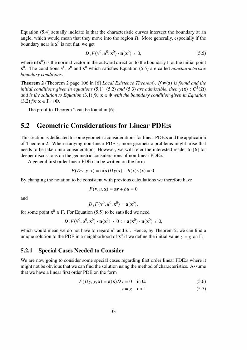
Equation (5.4) actually indicate is that the characteristic curves intersect the boundary at anangle, which would mean that they move into the region Ω. More generally, especially if theboundary near is x0 is not flat, we get

𝐷v𝐹 (v0, 𝑢0, x0) · n(x0) ≠ 0, (5.5)

where n(x0) is the normal vector in the outward direction to the boundary Γ at the initial pointx0. The conditions v0, 𝑢0 and x0 which satisfies Equation (5.5) are called noncharacteristicboundary conditions.

Theorem 2 (Theorem 2 page 106 in [6] Local Existence Theorem). If w(z) is found and theinitial conditions given in equations (5.1), (5.2) and (5.3) are admissible, then 𝑦(x) : 𝐶2(Ω)and is the solution to Equation (3.1) for x ∈ Φ with the boundary condition given in Equation(3.2) for x ∈ 𝚪 ∩𝚽.

The proof to Theorem 2 can be found in [6].

5.2 Geometric Considerations for Linear PDE:sThis section is dedicated to some geometric considerations for linear PDE:s and the applicationof Theorem 2. When studying non-linear PDE:s, more geometric problems might arise thatneeds to be taken into consideration. However, we will refer the interested reader to [6] fordeeper discussions on the geometric considerations of non-linear PDE:s.A general first order linear PDE can be written on the form

𝐹 (𝐷𝑦, 𝑦, x) = a(x)𝐷𝑦(x) + 𝑏(x)𝑦(x) = 0.

By changing the notation to be consistent with previous calculations we therefore have

𝐹 (v, 𝑢, x) = av + 𝑏𝑢 = 0

and𝐷v𝐹 (v0, 𝑢0, x0) = a(x0).

for some point x0 ∈ Γ. For Equation (5.5) to be satisfied we need

𝐷v𝐹 (v0, 𝑢0, x0) · n(x0) ≠ 0⇔ a(x0) · n(x0) ≠ 0,

which would mean we do not have to regard 𝑢0 and z0. Hence, by Theorem 2, we can find aunique solution to the PDE in a neighborhood of x0 if we define the initial value 𝑦 = 𝑔 on Γ.

5.2.1 Special Cases Needed to ConsiderWe are now going to consider some special cases regarding first order linear PDE:s where itmight not be obvious that we can find the solution using the method of characteristics. Assumethat we have a linear first order PDE on the form

𝐹 (𝐷𝑦, 𝑦, x) = a(x)𝐷𝑦 = 0 in Ω (5.6)𝑦 = 𝑔 on Γ. (5.7)

33

If we define the characteristic curves, the solution along the curves and the gradient of thesolution in the same way as before we get the derivative of the solution along the curves to be

¤𝑢 = 𝐷v𝐹 · v = a · v = 𝐹 (v, 𝑢, x) = 0,

which means that the solution 𝑢(x) along the characteristic curves is constant. In the followingsections of this chapter we seek to find the solution to Equation (5.6).

Case 1

We will now look at a special case where the trajectories of the characteristic curves are allflowing towards a single point, 𝑐, as shown in Figure 5.1 and a(x0) · n(x0) < 0. That is, thecharacteristic curves are directed inwards. As shown above, Theorem 2 states that a uniquesolution exists near x0 ∈ Γ and that indeed 𝑦(x0) = 𝑔(x0). What is important to note is howeverthat the solution will only be continuous over the whole geometric region Ω if 𝑔 is constant.The reason for this is that the solution is constant along the characteristic curves and if 𝑔 wouldnot be constant the solution would have different values when approaching the point 𝑐 andcould therefore not be continuous.

Figure 5.1: A case when a(x) disappears in the point 𝑐.

Case 2

In the second case illustrated in Figure 5.2, the characteristic curves flow through Ω witha(x0) · n(x0) < 0 and enters through Γ. In the points 𝑑 and 𝑒 we have that the local existencetheorem fails, since the characteristic curves that passes trough those points are parallel to theboundary. I.e. 𝑑 and 𝑒 are characteristic points. Everywhere else, if the solution is constantalong the characteristic curves the solution 𝑦 exists and is continuous.

34

Figure 5.2: A case when the points 𝑑 and 𝑒 are characteristic points.

Case 3

If we consider the case shown in Figure 5.3 we can see that the point 𝑓 is characteristic sincethe conditions for Theorem 2 are not satisfied in that point. The solution cannot be continuousunless 𝑦 is constant and 𝑔( 𝑓 ) = 𝑔(ℎ).

Figure 5.3: A case when the point 𝑓 is a characteristic point.

35

Chapter 6

Conclusion and Discussion

In this thesis we have derived the method of characteristics and showed its application on dif-ferent types of partial differential equations, both linear and nonlinear. This was accomplishedby using the method to exactly solve two examples (see sections 3.2 and 3.3). In Chapter 4 wethen illustrated how to solve a problem where the system of characteristic ODE:s is not easilysolved by analytical methods. With the use of Matlab we solved the system of characteristicODE:s numerically by applying the fourth order Runge-Kutta Method. The solution surfacewere then found by evaluating the solution at the boundary and then trace some characteristiccurves from the starting point to the end point and create an illustration of the solution at theend point. Another way to approach this problem would be to trace the characteristic curvesfrom the end point of the curve to the starting point where the solution is known, i.e. trace thecharacteristic curves backwards. This would be a more useful approach if one is looking to findthe solution value at a certain point in time and space. However, the way this is accomplishedwould have been too comprehensive to achieve in this thesis.In Section 3.1 we presented Theorem 1 which states that if we assumed that 𝑦 is the solution

to a given PDE, it is possible write this PDE as a system of characteristic ODE:s. Theorem 2which was presented in Section 5.1 however states that if, to the system of characteristic ODE:ssubject to admissible initial conditions, one can find a function 𝑦, then this solution functionis in fact the solution to the PDE that is being sought to solve. It has therefore been shown thatthe method is valid for solving certain PDE:s.We have also in this paper laid out some basics of two other methods which can also be used

to solve PDE:s, namely separation of variables and the finite element method, and presentedsome advantages and disadvantages of the methods (see Section 5.1). The information presen-ted about the three methods gives some insights as to why one method would be preferred overanother. When working in dimensions higher than R2 the method of characteristic is a moreuseful method than separation of variables. Compared to the finite element method which is anumerical method, i.e. it approximates the solution, the method of characteristics is a analyticmethod which gives an exact solution to the PDE as long as the system of characteristic ODE:scan be solved analytically.In Chapter 5 we partly answered the research questions in Section 1.3, at least concerning

first order linear partial differential equations. The method of characteristics can be used tosolve most linear PDE:s. Whether or not the method can be used is dependent on what the

36

area over which we seek to solve the PDE and there are some cases where the method cannotbe used, (see Section 5.2). One important conclusion which can be drawn from this thesis isthat the method of characteristics is a highly useful method for solving various forms of partialdifferential equations of first order when exact solutions are needed.For future work it would be interesting to explore the method of characteristics on PDE:s

of higher order. One could also investigate the limitations of this method on nonlinear PDE:sas well as compare the method to other methods that can be used to solve PDE:s. It mightalso be of interest to solve the example given in Chapter 4 by tracing the characteristic curvesbackwards to find the solution.

37

Bibliography

[1] T. Archibald, C. Fraser, and I. Grattan-Guinness. The history of differential equations,1670–1950. Oberwolfach Reports, 1(4):2729–2794, 2005.

[2] M.W. Bertens, E.M. Vugts, M.J. Anthonissen, J.H. Boonkkamp, and W.L. IJzerman.Numerical methods for the hyperbolic monge-ampère equation based on the method ofcharacteristics. arXiv preprint arXiv:2104.11659, 2021.

[3] Å. Brännström, L. Carlsson, and D. Simpson. On the convergence of the escalator boxcartrain. SIAM Journal on Numerical Analysis, 51(6):3213–3231, 2013.

[4] D.J.L. Chen, J.C. Chang, and C.H. Cheng. Higher order composition runge-kutta meth-ods. Tamkang Journal of Mathematics, 39(3):199–211, 2008.

[5] A.M. de Roos. Numerical methods for structured population models: the escalator boxcartrain. Numerical methods for partial differential equations, 4(3):173–195, 1988.

[6] Lawrence C. Evans. Partial differential equations, volume 19. American MathematicalSoc., 2010.

[7] X. Feng, R. Glowinski, and M. Neilan. Recent developments in numerical methods forfully nonlinear second order partial differential equations. siam REVIEW, 55(2):205–267,2013.

[8] Richard Haberman. Elementary applied partial differential equations, volume 987.Prentice Hall Englewood Cliffs, NJ, 1983.

[9] Edward L. Ince. Ordinary differential equations. Courier Corporation, 1956.

[10] Abdelwahab Kharab and Ronald Guenther. An introduction to numerical methods: aMATLAB® approach. CRC press, 2018.

[11] Leonard F. Konikow, Daniel J. Goode, and George Z. Hornberger. A three-dimensionalmethod-of-characteristics solute-transport model (MOC3D), volume 96. US Departmentof the Interior, US Geological Survey, 1996.

[12] T. Łodygowski and W. Sumelka. Limitations in application of finite element method inacoustic numerical simulation. Journal of theoretical and applied mechanics, 44(4):849–865, 2006.

38

[13] C.M. Martin. Exact bearing capacity calculations using the method of characteristics.Proc. IACMAG. Turin, 11:441–450, 2005.

[14] H. Musa, I. Saidu, and M.Y. Waziri. A simplified derivation and analysis of fourth orderrunge kutta method. International Journal of Computer Applications, 9(8):51–55, 2010.

[15] C.J. Reddy, M.D. Deshpande, C.R. Cockrell, and F.B. Beck. Finite element methodfor eigenvalue problems in electromagnetics, volume 3485. NASA, Langley ResearchCenter, 1994.

[16] A. Salih. Method of characteristics. Indian Institute of Space Science and Technology,Thiruvananthapuram, 2016.

[17] L.F. Shampine. Stability of the leapfrog/midpoint method. Applied mathematics andcomputation, 208(1):293–298, 2009.

[18] C. K. Thornhill. The numerical method of characteristics for hyperbolic problems inthree independent variables. Ministry of Supply, Armament Research Establishment,Fort Halstead, Kent, 1948. Rep. no. 29/48.

[19] J. Yan and C.W. Shu. Local discontinuous galerkin methods for partial differentialequations with higher order derivatives. Journal of Scientific Computing, 17(1):27–47,2002.

[20] Dennis G. Zill. Differential equations with boundary-value problems. Cengage Learning,2016.

39

Appendix A

Matlab code for Linear Example

The following Matlab-code is used to produce figures 3.1 and 3.2 presented in Section 3.2.

1 c l o s e a l l2 x = 0 : 0 . 0 3 : 6 ; %x− i n t e r v a l3 t = 0 : 0 . 0 3 : 1 . 5 ; %t − i n t e r v a l4 f = f i g u r e ;5 %row 6 t o 8 c r e a t e s s o l u t i o n s u r f a c e6 [X,Y] = meshgr id ( x , t ) ;7 Z = g (X,Y) .∗ exp ( −2 .∗Y) ; %t h e s o l u t i o n8 hSu r f a c e = s u r f (X,Y, Z ) ;9 ho ld on10 %row 11 t o 13 c r e a t e s r ed l i n e f o r g ( x , 0 )11 ZZ = g ( x , 0 ) ;12 z e r o = z e r o s ( 1 , l e n g t h ( x ) ) ;13 p l o t 3 ( x , ze ro , ZZ , ’ r ’ , ’ l i n ew i d t h ’ , 3 )14 x l a b e l ( ’ x ’ )15 y l a b e l ( ’ t ’ )16 z l a b e l ( ’ y ’ )17 %row 18 t o 23 a d j u s t s t e x t shown i n f i g u r e18 f . Un i t s = ’ Cen t ime t e r ’ ;19 f . P o s i t i o n =[10 10 15 1 0 ] ;20 axesH = gca ;21 axesH . XAxis . T i c k L a b e l I n t e r p r e t e r = ’ l a t e x ’22 s e t ( gca , ’ T i c k L a b e l I n t e r p r e t e r ’ , ’ l a t e x ’ , ’ Fon tS i z e ’ , 16 )23 l e g end ({ ’ s o l u t i o n ’ , ’ boundary ’ } , ’ I n t e r p r e t e r ’ , ’ l a t e x ’ , ’ Fon tS i z e

’ , 16 )24 f u n c t i o n answer=g ( x , y ) %boundary d a t a25 answer =2+ s i n ( p i . ∗ ( exp (−y ) .∗ x ) ) ;26 end

40

Appendix B

Matlab code for Non-linear Example

The following Matlab-code is used to produce figures 3.3 and 3.4 presented in Section 3.3.

1 c l o s e a l l2 x1 = 0 : 0 . 0 3 : 1 . 5 ; %x_1− i n t e r v a l3 x2 = −4 : 0 . 0 3 : 4 ; %x_2− i n t e r v a l4 %row 5 t o 8 c r e a t e s s o l u t i o n s u r f a c e5 f = f i g u r e ;6 [X,Y] = meshgr id ( x1 , x2 ) ;7 Z = 1 . / ( 1 . / g (X,Y) +(Y−X) . ^ 2 . ∗X+(Y−X) .∗X. ^ 2+ 2 / 3 . ∗X. ^ 3 ) ; %t h e

s o l u t i o n8 hSu r f a c e = s u r f (X,Y, Z ) ;9 ho ld on10 %row 10 t o 13 c r e a t e s r ed l i n e f o r g ( 0 , x_2 )11 ZZ = g ( 0 , x2 ) ;12 z e r o = z e r o s ( 1 , l e n g t h ( x2 ) ) ;13 p l o t 3 ( zero , x2 , ZZ , ’ r ’ , ’ l i n ew i d t h ’ , 3 )14 x l a b e l ( ’ x_1 ’ )15 y l a b e l ( ’ x_2 ’ )16 z l a b e l ( ’ y ’ )17 %row 17 t o 18 a d j u s t s t e x t shown i n f i g u r e and s i z e o f f i g u r e18 f . Un i t s = ’ Cen t ime t e r ’ ;19 f . P o s i t i o n =[10 10 17 1 2 ] ;20 axesH = gca ;21 axesH . XAxis . T i c k L a b e l I n t e r p r e t e r = ’ l a t e x ’22 s e t ( gca , ’ T i c k L a b e l I n t e r p r e t e r ’ , ’ l a t e x ’ , ’ Fon tS i z e ’ , 16 )23 l e g end ({ ’ s o l u t i o n ’ , ’ boundary ’ } , ’ I n t e r p r e t e r ’ , ’ l a t e x ’ , ’ Fon tS i z e

’ , 16 )24 f u n c t i o n answer=g ( x , y ) %boundary d a t a25 answer =2+ s i n ( p i . ∗ ( y−x ) ) ;26 end

41

Appendix C

Matlab code for an Advanced ExampleSome Characteristic Curves

The following Matlab-code is used to produce figures 4.1a, 4.1b and 4.1c presented inSection 4.1.1. Note that the code is not possible to run as it is since there is no initialdata. To enable Matlab to run the code, it has to be modified slightly, e.g. by uncommentingrow 2 to 4.

1 c l o s e a l l2 %y0 = [ 0 ; 0 ; 1 ; − 1 ] ; %i n i t i a l d a t a ( x_1 , x_2 , y_x_1 , y_x_2 ) uncomment

f o r x_1=0 and x_2=03 %y0 = [ 1 ; 2 ; 1 ; − 1 ] ; %i n i t i a l d a t a ( x_1 , x_2 , y_x_1 , y_x_2 ) uncomment

f o r x_1=1 and x_2=24 %y0 = [ 1 ; 1 ; 1 ; − 1 ] ; %i n i t i a l d a t a ( x_1 , x_2 , y_x_1 , y_x_2 ) uncomment

f o r x_1=1 and x_2=15 t s p a n = [0 1 0 ] ; %s t a r t och s t o p t ime f o r t h e s o l u t i o n6 [ t , y ] = ode45 (@ODEsystem , t span , y0 ) ; %use s RK4 method t o s o l v e

sys tem of ODE: s7 %row 8 t o 10 c r e a t e s cu rve i n 3d8 f i g u r e9 p l o t 3 ( y ( : , 1 ) , y ( : , 2 ) , t , ’ LineWidth ’ , 3 )10 ho ld on11 s c a t t e r 3 ( y ( 1 , 1 ) , y ( 1 , 2 ) , t ( 1 ) , ’∗ ’ , ’ r ’ ) %s t a r t p o i n t i n 3d12 s c a t t e r 3 ( y ( end , 1 ) , y ( end , 2 ) , t ( end ) , ’∗ ’ , ’ r ’ ) %end p o i n t i n 3d13 x l a b e l ( ’ x_1 ’ )14 y l a b e l ( ’ x_2 ’ )15 z l a b e l ( ’ t ’ )16 %row 17 t o 19 a d j u s t s t e x t shown i n f i g u r e17 axesH = gca ;18 axesH . XAxis . T i c k L a b e l I n t e r p r e t e r = ’ l a t e x ’19 s e t ( gca , ’ T i c k L a b e l I n t e r p r e t e r ’ , ’ l a t e x ’ , ’ Fon tS i z e ’ , 16 )20 f u n c t i o n dyd t = ODEsystem ( t , y ) %t h e sys tem of ODE: s

42

21 dyd t = z e r o s ( 4 , 1 ) ;22 dyd t ( 1 ) = 2∗y ( 3 ) ∗y ( 2 ) ^2 ;23 dyd t ( 2 ) = 2∗y ( 4 ) ∗y ( 1 ) ^2 ;24 dyd t ( 3 ) = −2∗y ( 4 ) ^2∗y ( 1 ) ;25 dyd t ( 4 ) = −2∗y ( 3 ) ^2∗ y ( 2 ) ;26 end

43

Appendix D

Matlab code for an Advanced ExampleSolution Surface

The following Matlab-code is used to solve the problem presented in Chapter 4 and producefigures 4.2, 4.3, 4.4 and 4.5 presented in Section 4.1.2.

1 c l o s e a l l2 n =200;%amount o f s t e p s i n x_1 and x_23 x s t a r t = 0 . 7 ; %s t a r t f o r x_14 x s l u t = 1 . 6 ; %s t o p f o r x_15 d e l t a x = x s l u t − x s t a r t ;6 y s t a r t = 1 . 6 ; %s t a r t f o r x_27 y s l u t = 2 . 4 ; %s t o p f o r x_28 d e l t a y = y s l u t − y s t a r t ;9 t s p a n = [0 1 0 ] ; %i n t e r v a l f o r t , changed t o [0 2 ] f o r F i g u r e

4 . 4 and 4 . 510 ux= z e r o s ( n , n ) ; %sav e s x_1 a t end of i n t e r v a l o f t11 uy= z e r o s ( n , n ) ; %sav e s x_2 a t end of i n t e r v a l o f t12 uc= z e r o s ( n , n ) ; %sav e s f u n c t i o n v a l u e a t end of i n t e r v a l13 f o r i =1 : n %x− p o i n t14 f o r j =1 : n %x_2− p o i n t15 xx= x s t a r t +( i −1)∗ d e l t a x / ( n−1) ;16 yy= y s t a r t +( j −1)∗ d e l t a y / ( n−1) ;17 y0 =[ xx ; yy ; 1 ; − 1 ; xx−yy ] ; %wi th g ( x_1 , x_2 ) =x_1−x_2 .18 [ t , y ] = ode45 (@ODEsystem , t span , y0 ) ; %us i ng RK4 t o

s o l v e sys tem of ODE: s19 ux ( i , j ) =y ( end , 1 ) ; %x_1 end p o i n t on t h e c h a r a c t e r s t i c

cu rve20 uy ( i , j ) =y ( end , 2 ) ; %x_2 end p o i n t on t h e c h a r a c t e r s t i c

cu rve21 uc ( i , j ) =y ( end , 5 ) ; %f u n c t i o n v a l u e22 end

44

23 end24 f i g u r e %row 24 t o 38 c r e a t e s f i g u r e s 4 . 2 and 4 . 425 ho ld on26 %row 30 t o 32 r e s h a p e ma t r i c e s t o column v e c t o r s27 uxx= r e s h a p e ( ux , [ ] , 1 ) ;28 uyy= r e s h a p e ( uy , [ ] , 1 ) ;29 ucc= r e s h a p e ( uc , [ ] , 1 ) ;30 %row 33 t o 40 c r e a t e s s u r f a c e o f t h e p o i n t s c a l c u l a t e d31 t r i = de l aunay ( uxx , uyy ) ;32 h = t r i s u r f ( t r i , uxx , uyy , ucc ) ;33 l = l i g h t ( ’ P o s i t i o n ’ , [ −50 −15 29 ] ) ;34 s e t ( gca , ’ Came r aPo s i t i on ’ , [ 208 −50 7687 ] )35 l i g h t i n g phong36 s h ad i ng i n t e r p37 c o l o r b a r E a s tOu t s i d e38 s c a t t e r 3 ( uxx ( 791 ) , uyy ( 791 ) , ucc ( 791 ) , ’∗ ’ , ’ r ’ )%marks t h e r ed

s t a r shown i n F i gu r e 4 . 2 . Row no t i n c l u d e d i n F i gu r e 4 . 439 z l a b e l ( ’ y ’ )40 x l a b e l ( ’ x_1 ’ )41 y l a b e l ( ’ x_2 ’ )42 %row 43 t o 45 a d j u s t s t e x t shown i n f i g u r e43 axesH = gca ;44 axesH . XAxis . T i c k L a b e l I n t e r p r e t e r = ’ l a t e x ’45 s e t ( gca , ’ T i c k L a b e l I n t e r p r e t e r ’ , ’ l a t e x ’ , ’ Fon tS i z e ’ , 16 )46 f i g u r e %row 47 c r e a t e s f i g u r e s 4 . 3 and 4 . 547 s c a t t e r ( uxx , uyy , 10 , ’ f i l l e d ’ )48 x l a b e l ( ’ x_1 ’ )49 y l a b e l ( ’ x_2 ’ )50 %row 51 t o 53 a d j u s t s t e x t shown i n f i g u r e51 axesH = gca ;52 axesH . XAxis . T i c k L a b e l I n t e r p r e t e r = ’ l a t e x ’53 s e t ( gca , ’ T i c k L a b e l I n t e r p r e t e r ’ , ’ l a t e x ’ , ’ Fon tS i z e ’ , 16 )54 f u n c t i o n dyd t = ODEsystem ( t , y ) %sys tem of ODE: s55 dyd t = z e r o s ( 4 , 1 ) ;56 dyd t ( 1 ) = 2∗y ( 3 ) ∗y ( 2 ) ^2 ;57 dyd t ( 2 ) = 2∗y ( 4 ) ∗y ( 1 ) ^2 ;58 dyd t ( 3 ) = −2∗y ( 4 ) ^2∗y ( 1 ) ;59 dyd t ( 4 ) = −2∗y ( 3 ) ^2∗ y ( 2 ) ;60 dyd t ( 5 ) = −4∗y ( 3 ) ∗y ( 4 ) ∗y ( 1 ) ∗y ( 2 ) ∗ ( y ( 4 ) ∗y ( 2 ) +y ( 3 ) ∗y ( 1 ) ) ;61 end

45