Palaeogeography, Palaeoclimatology, Palaeoecology 297 (2010) 299–310

Contents lists available at ScienceDirect

Palaeogeography, Palaeoclimatology, Palaeoecology

j ourna l homepage: www.e lsev ie r.com/ locate /pa laeo

The Medieval Climate Anomaly and Little Ice Age in Chesapeake Bay and the NorthAtlantic Ocean

T.M. Cronin a,⁎, K. Hayo b, R.C. Thunell c, G.S. Dwyer d, C. Saenger e, D.A. Willard a

a 926A US Geological Survey National Center, Reston, VA 20192, USAb Institute of Arctic and Alpine Research, University of Colorado, Boulder, CO 80320, USAc Department of Earth and Ocean Sciences, University of South Carolina, Columbia, SC 29208, USAd Division of Earth and Ocean Sciences, Nicholas School of the Environment, Duke University, Durham, NC 27708, USAe Woods Hole Oceanographic Institution, Woods Hole, MA 02543, USA

⁎ Corresponding author. Tel.: +1 703 648 6363; fax:E-mail address: tcronin@usgs.gov (T.M. Cronin).

0031-0182/$ – see front matter. Published by Elsevierdoi:10.1016/j.palaeo.2010.08.009

a b s t r a c t

a r t i c l e i n f o

Article history:Received 21 May 2010Received in revised form 17 August 2010Accepted 18 August 2010Available online 22 August 2010

Keywords:Medieval Climate AnomalyLittle Ice AgeChesapeake BayHolocene climate

A new 2400-year paleoclimate reconstruction from Chesapeake Bay (CB) (eastern US) was compared toother paleoclimate records in the North Atlantic region to evaluate climate variability during the MedievalClimate Anomaly (MCA) and Little Ice Age (LIA). Using Mg/Ca ratios from ostracodes and oxygen isotopesfrom benthic foraminifera as proxies for temperature and precipitation-driven estuarine hydrography,results show that warmest temperatures in CB reached 16–17 °C between 600 and 950 CE (Common Era),centuries before the classic European Medieval Warm Period (950–1100 CE) and peak warming in theNordic Seas (1000–1400 CE). A series of centennial warm/cool cycles began about 1000 CE with temperatureminima of ~8 to 9 °C about 1150, 1350, and 1650–1800 CE, and intervening warm periods (14–15 °C)centered at 1200, 1400, 1500 and 1600 CE. Precipitation variability in the eastern US included multiple dryintervals from 600 to 1200 CE, which contrasts with wet medieval conditions in the Caribbean. The easternUS experienced a wet LIA between 1650 and 1800 CE when the Caribbean was relatively dry. Comparison ofthe CB record with other records shows that the MCA and LIA were characterized by regionally asynchronouswarming and complex spatial patterns of precipitation, possibly related to ocean–atmosphere processes.

+1 703 648 5420.

B.V.

Published by Elsevier B.V.

1. Introduction

NorthernHemispheric atmospheric temperature reconstructions forthe past two millennia show a distinct warm period centered on1000–1100 CE (Common Era and BCE=before CE), called theMedievalClimate Anomaly (MCA, also calledMedievalWarm Period, MWP), thatcontrasts with cooler climate during the Little Ice Age ~1400–1850 CE(Jones and Mann, 2004). Medieval climate was also characterized byhydrometeorological variability across North America (Cook et al.,2007) and Eurasia (Treydte et al., 2006). Solar and volcanic activity(Crowley, 2000; Ammann et al., 2007), solar-oceanic feedbacks (Bondetal., 2001), ocean circulation (Broecker, 2001), Pacific Ocean-atmospher-ic processes (Cook et al., 2007), and land-use changes (Goosse et al.,2006; Ruddiman, 2007) have all been proposed as factors influencingMCA–LIA climate.

In a recent global paleoclimate-modeling study, Mann et al. (2009)concluded that MCA–LIA temperature variability was influenced byboth solar and volcanic radiative forcing and internal climate processes,but they called for additional proxy records to improve regional model

projections of future climate. For example, of more than 1200 proxyreconstructions used in their compilation, only 25 records covered thelast 2000 years and only a few were frommarine sediments (see Mannet al., 2008). Given the potential importance of ocean circulation indriving late Holocene climate (Newton et al., 2006; Oppo et al., 2009),additional high-resolution ocean records are sorely needed. In thisstudy, new temperature and precipitation reconstructions fromMarion-Dufresne core MD03-2661, a 24.5 m-long core from Chesapeake Bay(CB) containing sediments deposited during the past 10 ka arecompared to other proxy records from the North Atlantic region toexamine the amplitude and timing of regional climate variability duringthe last 2400 years. As such, it represents a small step toward theintegration of the ocean records into late Holocene climatereconstructions.

2. Regional setting

2.1. Chesapeake Bay hydrography

CB is a 320 km-long, 6500 km2 estuary located in the mid-Atlanticregion of the eastern US (Fig. 1). Density-driven CB circulation isinfluenced by freshwater river discharge and inflowing marine water.Susquehanna River water, which accounts for up to 62% of the total

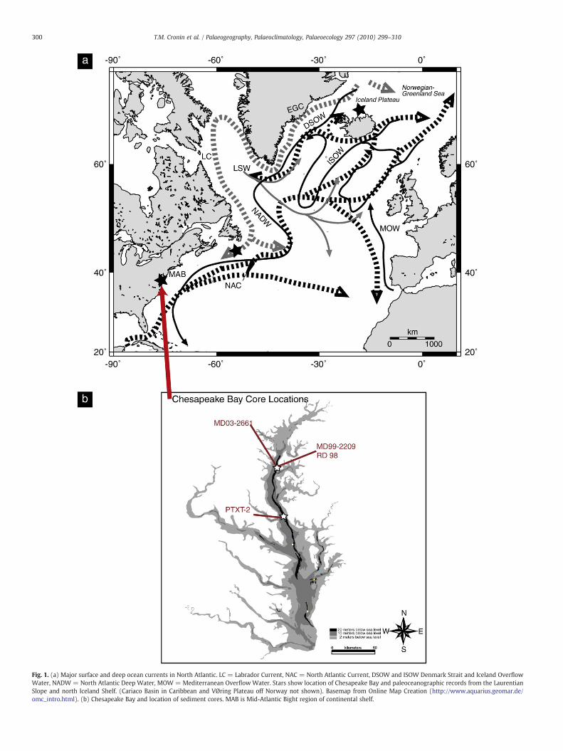
Fig. 1. (a) Major surface and deep ocean currents in North Atlantic. LC = Labrador Current, NAC = North Atlantic Current, DSOW and ISOW Denmark Strait and Iceland OverflowWater, NADW = North Atlantic Deep Water, MOW = Mediterranean Overflow Water. Stars show location of Chesapeake Bay and paleoceanographic records from the LaurentianSlope and north Iceland Shelf. (Cariaco Basin in Caribbean and VØring Plateau off Norway not shown). Basemap from Online Map Creation (http://www.aquarius.geomar.de/omc_intro.html). (b) Chesapeake Bay and location of sediment cores. MAB is Mid-Atlantic Bight region of continental shelf.

300 T.M. Cronin et al. / Palaeogeography, Palaeoclimatology, Palaeoecology 297 (2010) 299–310

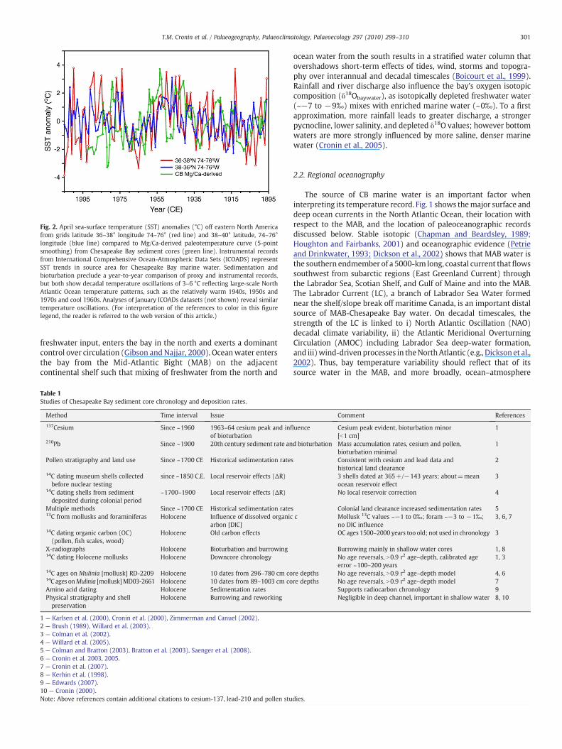
Fig. 2. April sea-surface temperature (SST) anomalies (°C) off eastern North Americafrom grids latitude 36–38° longitude 74–76° (red line) and 38–40° latitude, 74–76°longitude (blue line) compared to Mg/Ca-derived paleotemperature curve (5-pointsmoothing) from Chesapeake Bay sediment cores (green line). Instrumental recordsfrom International Comprehensive Ocean-Atmospheric Data Sets (ICOADS) representSST trends in source area for Chesapeake Bay marine water. Sedimentation andbioturbation preclude a year-to-year comparison of proxy and instrumental records,but both show decadal temperature oscillations of 3–6 °C reflecting large-scale NorthAtlantic Ocean temperature patterns, such as the relatively warm 1940s, 1950s and1970s and cool 1960s. Analyses of January ICOADs datasets (not shown) reveal similartemperature oscillations. (For interpretation of the references to color in this figurelegend, the reader is referred to the web version of this article.)

301T.M. Cronin et al. / Palaeogeography, Palaeoclimatology, Palaeoecology 297 (2010) 299–310

freshwater input, enters the bay in the north and exerts a dominantcontrol over circulation (Gibson and Najjar, 2000). Oceanwater entersthe bay from the Mid-Atlantic Bight (MAB) on the adjacentcontinental shelf such that mixing of freshwater from the north and

Table 1Studies of Chesapeake Bay sediment core chronology and deposition rates.

Method Time interval Issue

137Cesium Since ~1960 1963–64 cesium peak and inflof bioturbation

210Pb Since ~1900 20th century sediment rate an

Pollen stratigraphy and land use Since ~1700 CE Historical sedimentation rates

14C dating museum shells collectedbefore nuclear testing

since ~1850 C.E. Local reservoir effects (ΔR)

14C dating shells from sedimentdeposited during colonial period

~1700–1900 Local reservoir effects (ΔR)

Multiple methods Since ~1700 CE Historical sedimentation rates13C from mollusks and foraminiferas Holocene Influence of dissolved organic

arbon [DIC]14C dating organic carbon (OC)(pollen, fish scales, wood)

Holocene Old carbon effects

X-radiographs Holocene Bioturbation and burrowing14C dating Holocene mollusks Holocene Downcore chronology

14C ages on Mulinia [mollusk] RD-2209 Holocene 10 dates from 296–780 cm co14C ages onMulinia [mollusk]MD03-2661 Holocene 10 dates from 89–1003 cm coAmino acid dating Holocene Sedimentation ratesPhysical stratigraphy and shellpreservation

Holocene Burrowing and reworking

1 — Karlsen et al. (2000), Cronin et al. (2000), Zimmerman and Canuel (2002).2 — Brush (1989), Willard et al. (2003).3 — Colman et al. (2002).4 — Willard et al. (2005).5 — Colman and Bratton (2003), Bratton et al. (2003), Saenger et al. (2008).6 — Cronin et al. 2003, 2005.7 — Cronin et al. (2007).8 — Kerhin et al. (1998).9 — Edwards (2007).10 — Cronin (2000).Note: Above references contain additional citations to cesium-137, lead-210 and pollen stu

ocean water from the south results in a stratified water column thatovershadows short-term effects of tides, wind, storms and topogra-phy over interannual and decadal timescales (Boicourt et al., 1999).Rainfall and river discharge also influence the bay's oxygen isotopiccomposition (δ18Obaywater), as isotopically depleted freshwater water(~−7 to −9‰) mixes with enriched marine water (~0‰). To a firstapproximation, more rainfall leads to greater discharge, a strongerpycnocline, lower salinity, and depleted δ18O values; however bottomwaters are more strongly influenced by more saline, denser marinewater (Cronin et al., 2005).

2.2. Regional oceanography

The source of CB marine water is an important factor wheninterpreting its temperature record. Fig. 1 shows themajor surface anddeep ocean currents in the North Atlantic Ocean, their location withrespect to the MAB, and the location of paleoceanographic recordsdiscussed below. Stable isotopic (Chapman and Beardsley, 1989;Houghton and Fairbanks, 2001) and oceanographic evidence (Petrieand Drinkwater, 1993; Dickson et al., 2002) shows that MAB water isthe southern endmember of a 5000-km long, coastal current thatflowssouthwest from subarctic regions (East Greenland Current) throughthe Labrador Sea, Scotian Shelf, and Gulf of Maine and into the MAB.The Labrador Current (LC), a branch of Labrador Sea Water formednear the shelf/slope break off maritime Canada, is an important distalsource of MAB-Chesapeake Bay water. On decadal timescales, thestrength of the LC is linked to i) North Atlantic Oscillation (NAO)decadal climate variability, ii) the Atlantic Meridional OverturningCirculation (AMOC) including Labrador Sea deep-water formation,and iii)wind-drivenprocesses in theNorthAtlantic (e.g., Dickson et al.,2002). Thus, bay temperature variability should reflect that of itssource water in the MAB, and more broadly, ocean–atmosphere

Comment References

uence Cesium peak evident, bioturbation minor[b1 cm]

1

d bioturbation Mass accumulation rates, cesium and pollen,bioturbation minimal

1

Consistent with cesium and lead data andhistorical land clearance

2

3 shells dated at 365+/−143 years; about=meanocean reservoir effect

3

No local reservoir correction 4

Colonial land clearance increased sedimentation rates 5c Mollusk 13C values ~−1 to 0‰; foram ~−3 to −1‰;

no DIC influence3, 6, 7

OC ages 1500–2000 years too old; not used in chronology 3

Burrowing mainly in shallow water cores 1, 8No age reversals, N0.9 r2 age–depth, calibrated ageerror ~100–200 years

1, 3

re depths No age reversals, N0.9 r2 age–depth model 4, 6re depths No age reversals, N0.9 r2 age–depth model 7

Supports radiocarbon chronology 9Negligible in deep channel, important in shallow water 8, 10

dies.

Fig. 3. Calibrated age–depth plots forMD03-2661 andMD99-2209. Horizontal error bars indicate the 2σ error range for radiocarbon ages. The initial occurrence of ragweed pollen dueto colonial land clearance at 115 cmMD03-2661 core depth is a robust timemarker dated at about 1725 CE in Chesapeake Bay sediments (Willard et al., 2003). Interval 800–820 cm inMD99-2209 is condensed zone. Age model for MD03-2661 samples calculated from core depth as follows: (0.0008⁎depth2)−(1.5417⁎depth)+1884.3 (r2=0.981).

302 T.M. Cronin et al. / Palaeogeography, Palaeoclimatology, Palaeoecology 297 (2010) 299–310

processes originating in subpolar regions of the Northern Hemisphere.This hypothesis is further discussed in the section on proxy methods.

3. Material and methods

3.1. Sediment cores

Sediment cores for this study were taken in the Chesapeake Bayaboard the R/V Marion-Dufresne during IMAGES cruises in 1999 and2003 and earlier cruises with the R/V Kerhin (Kerhin et al., 1998;Cronin et al., 2000; Karlsen et al., 2000) (Fig. 1 inset). These include a17.2-m long core MD99-2209 (38°53.18′N and 76°23.68′W, waterdepth 25 m), nearby core RD-98 (Colman et al., 2002) and core PTXT-2from off the Patuxent River (38°19.58′N and 76°23.55′W,water depth11.5 m) that produced the paleotemperature record discussed inCronin et al. (2003). This composite curve, referred to as RD-2209,covers the last 2200 years and has been incorporated into severalnorthern hemisphere surface temperature reconstructions coveringthe last 2000 years (e.g. Mann and Jones, 2003; Moberg et al., 2005;Mann et al., 2008). However, RD-2209 is a composite of four cores, andone (PTXT-2) that covers the critical Little Ice Age comes fromshallower water and a different location than other cores. The new,continuous paleoclimate record is presented below from MD03-2661(38°53.21′N and 76°23.89′W) taken in CB in 2003. MD03-2661 islocated near and at the same water depth (25 m) as MD99-2209, andits uppermost 10 m provides a continuous record of the MCA and LIAwith 2 to 12-year sampling resolution. MD03-2661 and RD-2209together allow a more critical evaluation of centennial variability intemperature and precipitation during this period.

3.2. Proxy methods

OstracodeMg/Ca andbenthic foraminifer oxygen isotopes (δ18Oforam)were used as proxies of warm-season temperature and estuarinehydrography, respectively. The shallow water genus Loxoconcha isamong several marine ostracode taxa whose shell Mg/Ca ratios havebeen used as paleothermometers (Dwyer et al., 2002). Between two andten adult valves of Loxoconcha from 2-cm spaced samples from MD03-2661were analyzed forMg/Ca ratios at DukeUniversity on a Spectrospan7 direct current plasma emission spectrometer. A total of 258 samplesfrom MD03-2661 yielded L. matagordensis suitable for analysis (seechronology); the RD-2209 record included 450 analyses (Cronin et al.,2003). Mg/Ca ratios were converted to warm-season temperature usingthe calibration equation y=0.644x−2.4284 (r2=0.805) derived fromfield, culturing and laboratory analyses of Loxoconcha from ChesapeakeBay and the adjacent continental shelf (Dwyer et al., 2002; Cronin et al.,2003; Vann et al., 2004). These calibration studies demonstrated that

temperature is the primary factor influencing Chesapeake Bay Loxo-concha Mg/Ca ratios and, at least over the sampled salinity range (~15–35 psu), salinity does not appear to be important.

To validate the field and lab-based Mg/Ca-temperature calibration,the part of the RD-2209 paleotemperature curve covering the lastcentury was compared to International Comprehensive Ocean-Atmo-spheric Data Sets (ICOADS) instrumental SST records from two grid cells(latitude 36–38° longitude 74–76° and 38–40° latitude, 74–76°) locatedoff eastern North America in source regions of CBmarine water (Fig. 2).Despite age uncertainty in the sediment record, both proxy andinstrumental records show decadal temperature anomalies of 3–6 °C,including warm periods during the 1940s, 1950s and 1970s and coolperiod during the 1960s and early 20th century. These regional decadaloscillations are typical of basin-scale atmospheric–oceanic temperaturevariability associatedwith the North Atlantic Oscillation, supporting theidea that the bayand its sourcewater reflect large, basin-scaleprocesses.It is also important to note that the amplitude of decadal oceantemperature variability in both the instrumental and proxy records islarge compared to that observed in tree-ring-based mean NorthernHemisphere surface atmospheric temperature reconstructions dis-cussed below.

Foraminiferal δ18O is generally controlled by water temperatureand the oxygen isotope composition of seawater in which theforaminifera calcified. In CB, the δ18Obaywater mainly reflects dis-charge-driven hydrological variability and the mixing of fresh andmarine endmembers, which influences the δ18O of bay benthicforaminifera (δ18Oforam) (Cronin et al., 2005; Saenger et al., 2006).Five to ten specimens of the benthic foraminifera Elphidium selseyensewere analyzed from each MD03-2661 sample for δ18O at theUniversity of South Carolina stable isotope lab using a GV Isoprimestable isotope ratio mass spectrometer. The long-term standardreproducibility is 0.07‰ for δ18O and results are reported relative toVienna Pee Dee Belemnite (V-PDB). A total of 488 isotopic analyseswere performed yielding a temporal resolution of about 5 years (seechronology). Paired downcore foraminiferal isotope and ostracodeMg/Ca measurements for 354 samples yielding both measurementswere used to correct δ18Oforam values for temperature and to estimateδ18Obaywater following methods in Cronin et al. (2005).

3.3. Chronology

Estuarine sediment records can provide high-resolution paleoclimaterecords, but attention must be paid to processes that influencesedimentation, radiocarbon ages, and other chronologic markers. Alarge literature on CB sediments, summarized in Table 1, includes studiesof stratigraphy, sediment geochemistry, CHIRP sonar geophysicalrecords, X-radiographs of bioturbation, and radiocarbon dating of

Table 2Radiocarbon dates from MD03-2661 core, Chesapeake Bay.

Datenumber*

Core Water depth(m)

Sample depth(cm)

Midpoint depth(cm)

Latitude(N)

Longitude(W)

Material dated δ13C 14C age(conventional)

Error+/−BP

Calibrated age(yr BP)

Calibrated +2 σ(yr BP)

Calibrated −2 σ(yr BP)

Common Era age

NA MD03-2661 25.5 0 0 38 53.21 76 23.89 Pollen Stratigraphy N/A N/A N/A N/A N/A N/A 1850–1880B-235942 MD03-2661 25.5 86–92 89 38 53.21 76 23.89 Mulinia lateralis −1.3 240 40 N/A N/A N/A Post 18th cent.NA MD03-2661 25.5 115 115 38 53.21 76 23.89 Pollen Stratigraphy N/A N/A N/A N/A N/A N/A ~1725B-235943 MD03-2661 25.5 188–194 191 38 53.21 76 23.89 Mulinia lateralis −0.6 320 40 N/A N/A N/A Post 18th cent.B-235944 MD03-2661 25.5 296–302 299 38 53.21 76 23.89 Mulinia lateralis −2.2 740 40 380 470 290 1570180325 MD03-2661 25.5 370–372 371 38 53.21 76 23.89 Mulinia lateralis −1.4 1280 40 820 910 730 1130181991 MD03-2661 25.5 485 485 38 53.21 76 23.89 Mulinia lateralis −1.5 1750 40 1290 1355 1235 660191408 MD03-2661 25.5 574–576 575 38 53.21 76 23.89 Mulinia lateralis −1.4 1730 40 1280 1340 1220 670181992 MD03-2661 25.5 597 597 38 53.21 76 23.89 Mulinia lateralis −1.3 1740 40 1285 1345 1230 665191409 MD03-2661 25.5 712–714 713 38 53.21 76 23.89 Mulinia lateralis −1.4 2000 40 1540 1670 1480 410191410 MD03-2661 25.5 796–798 797 38 53.21 76 23.89 Mulinia lateralis −0.4 2140 40 1710 1820 1620 240181993 MD03-2661 25.5 898 898 38 53.21 76 23.89 Mulinia lateralis −1.8 2390 40 2000 2115 1915 −50181994 MD03-2661 25.5 1003 1003 38 53.21 76 23.89 Mulinia lateralis −1.5 2810 40 2565 2700 2400 −615191411 MD03-2661 25.5 1052–1054 1053 38 53.21 76 23.89 Mulinia lateralis −0.4 2820 40 2600 2700 2430 −650180326 MD03-2661 25.5 1086–1089 1087.5 38 53.21 76 23.89 Mulinia lateralis −0.6 3050 40 2790 2890 2740 −840215879 MD03-2661 25.5 1146–1148 1147 38 53.21 76 23.89 Seed N/A 3420 40 3670 3820 3580 −1720215880 MD03-2661 25.5 1150–1155 1152.5 38 53.21 76 23.89 Shell −1.2 3940 40 3910 4050 3820 −1960191412 MD03-2661 25.5 1216–1218 1217 38 53.21 76 23.89 Mulinia lateralis −0.7 5160 40 5560 5590 5450 −3610191413 MD03-2661 25.5 1300–1302 1301 38 53.21 76 23.89 Mulinia lateralis −0.3 5440 50 5840 5910 5690 −3890191414 MD03-2661 25.5 1398–1400 1399 38 53.21 76 23.89 Mulinia lateralis −0.7 5530 40 5910 5980 5850 −3960191415 MD03-2661 25.5 1412–1414 1413 38 53.21 76 23.89 Mulinia lateralis −0.2 5520 50 5900 5990 5770 −3950191416 MD03-2661 25.5 1458–1460 1459 38 53.21 76 23.89 Mulinia lateralis −0.6 5590 40 5950 6080 5900 −4000180327 MD03-2661 25.5 1476 1476 38 53.21 76 23.89 Mulinia lateralis −1 5600 40 5970 6090 5900 −4020191417 MD03-2661 25.5 1614–1616 1615 38 53.21 76 23.89 Mulinia lateralis −0.7 5820 40 6260 6300 6170 −4310

All dates National Ocean Science Accelerator mass Spectrometry Facility (NOSAMS), Woods Hole Oceanographic except “B-” from Beta Analytic.Radiocarbon dates calibrated using marine calibration curve from Stuiver et al. (1998) with no ΔR correction and assuming no change in ΔR over the last 2400 years.Further discussion of Chesapeake core chronology can be found in Cronin T.M. et al. (2007). Geophys. Res. Lttrs., 34, L20603.Willard et al. (2003). The Holocene, 13, 201–214.Willard et al. (2005). Glob. Planet Change, 47, 17–35.NA = not available.

303T.M

.Croninet

al./Palaeogeography,Palaeoclim

atology,Palaeoecology297

(2010)299

–310

Fig. 4. Comparison of Chesapeake Bay temperature curve from coreMD03-2661 using (a) agemodels 1 and (b) 2 described in chronology section of text. Solid (dashed) lines connectwarm (cool) events. Records prior to 400 CE and since ~1750 CE are comparable. Age discrepancy is seen in the timing of temperature increase to early Medieval Climate Anomaly(600 versus 500 CE in models 1 and 2, respectively), inception of long-term cooling (starting about 900 CE and 650 CE in models 1 and 2), and age of brief warm and cool intervals.See text.

304 T.M. Cronin et al. / Palaeogeography, Palaeoclimatology, Palaeoecology 297 (2010) 299–310

CaCO3 shells (foraminifera and mollusks) and bulk sediment, whichallow the following conclusions regarding the bay's sediment chronol-ogy. 1) A standard 400 year marine reservoir correction applies toaccelerator mass spectrometer (AMS) radiocarbon dates on biogeniccarbonate (mollusks and foraminifers) based on radiocarbon dates onmollusks from 19th century museum collections and from sedimentsdeposited during colonial land clearance dated by pollen stratigraphy. 2)Porewater dissolved organic carbon does not influence biogeniccarbonate dates (Colman et al., 2002). 3) Holocene radiocarbon dateson pollen and bulk organic carbon are systematically older by 1500–2000 years than dates on shell from the same sample, probably due totransport of pollen organic carbon. 4) 137Cs and 210Pb dating and pollen

Fig. 5. Comparison of Chesapeake Bay temperature fromMg/Ca ratios. (a) RD-2209 record in25 m, blue lines), and PTXT-2 (38°19.6′N and 76°23.6′W water depth 11.5 m, green line) (Cusing a 5-point moving average. Red and blue arrows showmajor warming and cooling climafrom 100 to 600 CE and step-wise cooling since ~850–900 CE leading to the LIA (~1350–Medieval Climate Anomaly ~600–1000 CE. Lower temperature estimates at about 1450–160(For interpretation of the references to color in this figure legend, the reader is referred to

stratigraphy tied to colonial land clearance yield consistent ages forsediment deposited during the last 50 to 300 years. 5) Bioturbation,burrowing, and reworking areminimal in cores recovered from themainchannel of Chesapeake Bay, such as those discussed here, where thethickest accumulation of Holocene sediment is found at water depths of10–35 m.

The major limiting factors for Holocene chronology in CB are ageuncertainty for calibrated radiocarbon ages and changes in sedimenta-tion rates at some sites. Fig. 3 presents the age–depth plots for the twolong records MD03-2661 and RD-2209; Table 2 lists radiocarbon agesand pollen data used for datingMD03-2661 from Cronin et al. (2007). InMD03-2661, two pollen horizons and 11 radiocarbon dates were used to

cluding data from cores MD99-2209 and RD-98 (38°53.2′N and 76°23.7′W, water depthronin et al., 2003). (b) MD03-2661 (red line, age model 1). Both records are smoothedtic transitions evident in both records. Both records show relatively stable temperatures1850 CE). The MD03-2661 records shows higher temperature peaks during the early0 CE in Fig. 5a may reflect the shallower water depth of the PTXT-2 core site. See text.the web version of this article.)

Fig. 6. (a) Reconstructed Chesapeake salinity computed from δ18Oforam corrected for temperature estimated from ostracode Mg/Ca ratios, 0.8‰ vital effect in Elphidium, andconverted to salinity using relationships and procedures described in Cronin et al. (2005) and Saenger et al. (2006). (b) uncorrected δ18Oforam record. The two records have similarfirst-order temporal patterns suggesting δ18Oforam values reflect mainly hydrographic changes rather than water temperature.

305T.M. Cronin et al. / Palaeogeography, Palaeoclimatology, Palaeoecology 297 (2010) 299–310

date the upper 1000 cm of the core covering the last ~2600 years(Fig. 3a). The pollen horizon at 155 cm core depth is the first regularoccurrence of ragweedpollen, amarker in CB sediments for early colonialland clearance dated at about 1725 CE (Willard et al., 2003). MD03-2661did not recover the well-known ragweed peak when ragweed pollenreached 10–15% of the total pollen assemblage during maximum landclearance in the late 19th century. Consequently, sediment depositedduring the last century was not recovered at this site, most likely due tothe coring procedure, and we estimate the age of the coretop to beroughly 1880–1885 CE. The radiocarbon dates from MD03-2661 wereobtained on well-preserved shells of the bivalve Mulinia lateralis andcalibrated using the CALIB (Stuiver et al., 1998). The mean 2σ age rangeon nine calibrated M. lateralis dates from MD03-2661 for the last2600 years is 178 years.

Two age models were developed for MD03-2661. Age model1 (AM1) assumes a near constant sedimentation rate and estimates

Fig. 7. Late Holocene Chesapeake Bay. (a) Temperature from Mg/Ca ratios of ostracodes(Loxoconcha matagordensis) and (b) δ18Oforam from benthic foraminifera (Elphidiumselseyense) for upper 1000 cm of core MD03-2661 (5-point smoothing). More negative(positive) δ18Oforam excursions signify enhanced (reduced) river runoff and precipitation;dry periods marked by red circles. (For interpretation of the references to color in thisfigure legend, the reader is referred to the web version of this article.)

sample ages from core depth as follows: (0.0008⁎depth2)−(1.5417⁎depth)+1884.3 (r2=0.981, mean rate ~0.41 cm yr−1). Asecond age model (AM2) was developed to reflect apparent changesin sedimentation rate seen in the age–depth plot, with higher rates atcore depths from 0 to 300 cm and 485 to 713 cm and lower rates from300 to 485 cm and 713 to 1087 cm. Linear sedimentation rates werecomputed for four segments of the core as follows: 0–300 cm—

0.96 cm yr−1, 300–485 cm—0.2 cm yr−1, 485–713 cm—0.91 cm yr−1

and 713–1087 cm—0.3 cm yr−1.Fig. 3b shows 10 radiocarbon dates on M. lateralis from the upper

800 cm at site RD-2209. Sediment at this site was deposited at a nearconstant rate of 0.36 cm yr−1 during the last 2100 years and includesa 20th century sediment record. Sample ages for RD-2209 wereestimated using the age model described fully in Willard et al. (2003).A zone of slow sedimentation or intermittent non-deposition occursat 800–900 cm core depth estimated to represent the interval about2100–5000 calibrated years age (Colman et al., 2002).

4. Results

Fig. 4 compares the MD03-2661 Mg/Ca-derived temperaturecurves using the two age models. Both age models show relativelycool to moderate temperatures (12–14 °C) from 300 BCE to 400 CEand a steep rise in temperature starting around 1750–1800 CE.Several temperature maxima (≥15 °C) and minima (≤10 °C) haveage differences from the two age models ranging from b100 years upto ~250 years. For example, a distinct temperature maximum is datedin both age models at around 1200 CE, whereas the preceding coolinterval is dated at 1000 to 1100 CE. The warmest period in this coreoccurs during the early MCA, dated at about 850–900 in AM1 and600–650 in AM2, after which there is step-wise cooling. Thedifference between the two age models for the youngest LIAtemperature minimum is less than 100 years (1750–1800 CE).

Fig. 5 compares the MD03-2661 (AM1) and RD-2209 temperaturecurves designating those parts of the latter curve derived from theRD-98, PTXT-2 andMD99-2209 cores. Both records show the followingfeatures: multidecadal scale oscillations over a total temperaturerange from ~8 to 17 °C, moderate temperatures (12–14 °C) from~100 BCE to 400 CE, a steep rise in temperature beginning about1750–1800 CE, a cooling 750–850 CE, a step-wise decline starting~850–950 CE, and multiple temperature minima between 1100 and1750 CE. Temperature maxima during the early MCA (400–1050 CE)

Fig. 8. (a) δ18Oforam from benthic foraminifera (Elphidium selseyense) for upper 1000 cmof core MD03-2661 (38°53.21′N and 76°23.89′W, water depth 25 m) (5-pointsmoothing). (b) Cariaco Basin sedimentary% titanium (Haug et al., 2001, 3-pointsmooth). (c) and (d) Cariaco Basin δ18O of the planktic foraminifers Globigerinabulloides and G. ruber (Black et al., 2004), dark blue is 5-point smooth. (Forinterpretation of the references to color in this figure legend, the reader is referred tothe web version of this article.)

306 T.M. Cronin et al. / Palaeogeography, Palaeoclimatology, Palaeoecology 297 (2010) 299–310

are slightly cooler (2–3 °C) in MD99-2209 than those in theMD03-2661 curve. Large temperature oscillations (N5 °C) between1350 and 1750 CE are also greater in MD03-2661, but this may reflectthe shallower water depth for site PTXT-2 (12 m) versus MD03-2661(25 m). The step-wise cooling beginning 850–900 CE reached mini-mum temperatures about 1150–1200 CE that are slightly cooler inMD03-2661. Three brief but distinct warm intervals can be correlatedin the two curves centered on 1200, 1400, and 1630 CE. A fourthwarminterval is seen near 1500 CE in MD03-2661, but this is not so evidentin RD-2209.

There are several periods of cool temperatures during the Little IceAge. For example, temperature estimates for the PTXT-2 recordreached 9.5 °C several times between ~1450 and 1830 CE and theMD03-2661 record reached 8.3–11 °C from 1360 to 1750 CE. The coolperiod from 1700 to 1750 CE is recorded in all three cores and seemsto coincide with widespread LIA cooling during the Maunder solarminimum (see below). In summary, the two temperature records arebroadly similar, but the MD03-2661 curve indicates a slightly warmerearly MCA, higher temperatures during warming events at ~1200 and1400 CE during the lateMCA, and lower temperatures (1–2 °C) duringthe coolest part of the LIA~1650–1750 CE.

The MD03-2661 δ18Oforam values (corrected for vital effects andtemperature) and estimated δ18Obaywater values using AM1 are shownin Fig. 6. The CB δ18Oforam data indicates moderately high salinity and

dry conditions (δ18Oforam maxima) from 200 BCE to 300 CE, andseveral brief dry periods between 600 and 1200 CE. These would be1–2 centuries older using age model AM2. The highest δ18Oforam

values and estimated salinities (25–30) are seen between 500 and1000 CE suggesting reduced freshwater influx and periods of drierregional climate. The δ18Oforam values progressively decrease after1000 CE (650–700 CE in AM2) culminating in minimum values of−2.0 to −2.25‰ and minimum salinities (16–18) around 1650–1800 CE, reflecting a wetter regional climate during the LIA.

Comparison of the MD03-2661 temperature and δ18Oforam recordsindicates that, over centennial timescales, relatively warm baytemperatures generally correspond to enriched δ18Oforam and cooltemperatures correspond to depleted values (Fig. 7). This patternwould suggest alternating warm–dry and cool–wet conditions in themid-Atlantic region. Both records suggest a complex, step-wiseclimatic transition from the MCA to the LIA that is characterized bymultidecadal fluctuations in temperature and rainfall. The emergencefrom Little Ice Age conditions seen in both rising temperature anddecreasing precipitation is abrupt and nearly synchronous.

4.1. Comparison with precipitation records

We compare the CB δ18O record with both the titanium (Ti) andplanktic foraminiferal oxygen isotopes records from Cariaco Basinsediments in the Caribbean in Fig. 8. The Cariaco Basin records areconsidered to be proxies of variability in the position of theIntertropical Convergence Zone (ITCZ) and hence tropical rainfall(Fig. 8). The general shape of the Cariaco %Ti record (Haug et al., 2001)(Fig. 8b) resembles that for MD03-2661 δ18Oforam variability (Fig. 8a),but the two curves are opposite in sign. That is, drier mid-latitudes(higher CB δ18O values) correspond to wetter tropical regions (highertitanium concentrations). The Cariaco planktic foraminiferal δ18Ocurves of Black et al. (2004) (Fig. 8c and d) also suggest multidecadaland centennial variability in Caribbean climate. The long-termincrease in G. ruber δ18O was interpreted by Black as signifying eithera cooling of tropical summer–fall SSTs of as much as 2 °C, perhapsrelated to an increase in upwelling intensity, or regional evaporation/precipitation variability due to changes in themean annual position ofthe ITCZ (see also Tedesco and Thunell, 2003). The former would beconsistent with evidence for a cooler Little Ice Age and the formerwith the Cariaco titanium and CB isotopic records of hydrologicalvariability. Other low-latitude Atlantic hydrologic records support theidea that late Holocene ITCZ variability was an important driver of lateHolocene hydrological variability in the Caribbean and subtropicalNorth Atlantic (e.g. Hodell et al., 2005; Lund and Curry, 2006).

It is also noteworthy that continental-scale droughts during themedieval period have beendocumented in tree-ring records fromNorthAmerica covering the last 1000 years (Cook et al., 2007). Although ageuncertainty and temporal resolution preclude a direct correlation of theCB sediment record with annually-resolved tree-ring records, severalpositive δ18Oforam excursions in Fig. 8 nonetheless coincide withcontinental-scale megadroughts centered at 936, 1034, 1150, 1253,and 1370 CE.

4.2. North Atlantic Ocean Temperature

To investigate SST variability across the North Atlantic, wecombined the MD03-2661 (AM1) and RD-2209 records to produce acomposite SST reconstruction covering the last 2200 years (Fig. 9a).This composite record is compared with temperature reconstructionsfrom the Cariaco Basin (Black et al., 2004), the Laurentian slope upperNorth Atlantic Deep Water (NADW) (Marchitto and deMenocal,2003), off northern Iceland (Sicre et al., 2008), the VØring Plateau(Andersson et al., 2003), and a northern hemisphere compositetemperature curve (Moberg et al., 2005) (Fig. 9b–f). In addition to theCB Mg/Ca curve, the Iceland and VØring records are considered

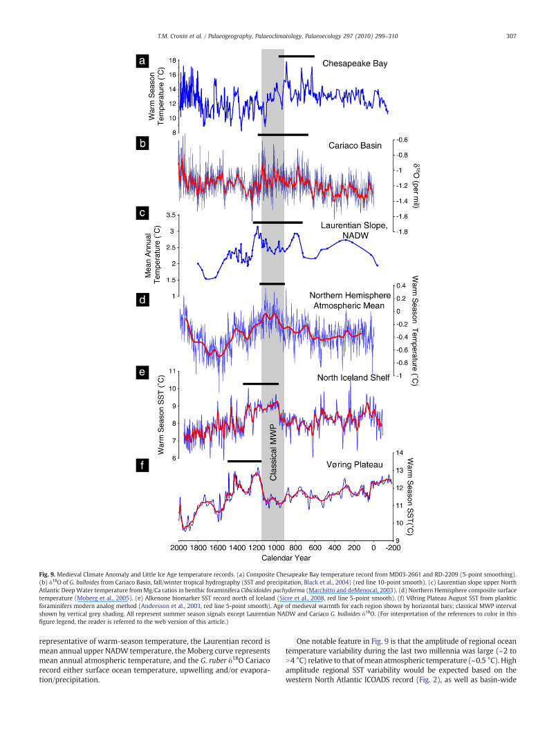
Fig. 9. Medieval Climate Anomaly and Little Ice Age temperature records. (a) Composite Chesapeake Bay temperature record from MD03-2661 and RD-2209 (5-point smoothing).(b) δ18O of G. bulloides from Cariaco Basin, fall/winter tropical hydrography (SST and precipitation, Black et al., 2004) (red line 10-point smooth). (c) Laurentian slope upper NorthAtlantic DeepWater temperature fromMg/Ca ratios in benthic foraminifera Cibicidoides pachyderma (Marchitto and deMenocal, 2003). (d) Northern Hemisphere composite surfacetemperature (Moberg et al., 2005). (e) Alkenone biomarker SST record north of Iceland (Sicre et al., 2008, red line 5-point smooth). (f) VØring Plateau August SST from plankticforaminifers modern analog method (Andersson et al., 2003, red line 5-point smooth). Age of medieval warmth for each region shown by horizontal bars; classical MWP intervalshown by vertical grey shading. All represent summer season signals except Laurentian NADW and Cariaco G. bulloides δ18O. (For interpretation of the references to color in thisfigure legend, the reader is referred to the web version of this article.)

307T.M. Cronin et al. / Palaeogeography, Palaeoclimatology, Palaeoecology 297 (2010) 299–310

representative of warm-season temperature, the Laurentian record ismean annual upper NADW temperature, the Moberg curve representsmean annual atmospheric temperature, and the G. ruber δ18O Cariacorecord either surface ocean temperature, upwelling and/or evapora-tion/precipitation.

One notable feature in Fig. 9 is that the amplitude of regional oceantemperature variability during the last two millennia was large (~2 toN4 °C) relative to that ofmean atmospheric temperature (~0.5 °C). Highamplitude regional SST variability would be expected based on thewestern North Atlantic ICOADS record (Fig. 2), as well as basin-wide

Fig. 10. Comparison of 200-year butterworth low-pass filtered standardized temperatureanomalies (anomaly of timeseries divided by its standard deviation). (a) CompositeChesapeake Bay temperature record. (b) Laurentian Slope upper North Atlantic DeepWater temperature from benthic foraminifera (Cibicidoides pachyderma Mg/Ca ratios(Marchitto anddeMenocal, 2003). (c)NorthernHemisphere surface temperature (Moberget al., 2005, blue; Mann et al., 2008, red). (d) subpolar North Atlantic SST from alkenonebiomarkers, north Iceland Slope (Sicre et al., 2008). (e) Vøring Plateau August SST frommodernanalogmethodofplanktic foraminifers (Anderssonet al., 2003).Anomalouswarmand cool periods falling outside 1σ of the mean are filled. The classical MWP(950–1100 CE) is shaded. (For interpretation of the references to color in this figurelegend, the reader is referred to the web version of this article.)

308 T.M. Cronin et al. / Palaeogeography, Palaeoclimatology, Palaeoecology 297 (2010) 299–310

decadal patterns in instrumental records of North Atlantic SST (e.g.Deser and Blackmon, 1993; Enfield et al., 2001).

A second obvious feature in the comparison of temperaturerecords is that the timing of peak regional warmth for the last2000 years, shown by horizontal black bars, does not always coincidewith the classic MedievalWarm Period centered on 1000–1050 CE. CBwaswarmest in the few centuries before theMWP, the VØring Plateauthe two centuries after, the Laurentian Slope the century before andthe century after, and the North Iceland Shelf during and just after theMWP. All records show a cool interval during all or part of the LIA

1600–1800 CE, although cool intervals also occurred in CB and theLaurentian Slope prior to this time and persisted after the LIA in theVØring and N. Iceland Shelf regions.

To further evaluate low frequency SST variability, compositecurves of low-pass filtered temperature anomalies (Fig. 10) showthat warm CB SSTs between 600 and 1000 CE (Fig. 10a) overlap withthe latter part of what is sometimes called the cool “Dark Ages” inEurope, predating the classical Medieval Warm Period seen inatmospheric temperature curves of Moberg et al. (2005) and Mannet al. (2008) (Fig. 10c). The Laurentian Slope temperature recordshows similarities to the CB record with a maximum near 800 CE(Fig. 10b), which is consistent with evidence for warm SSTs over theLaurentian Fan from 500 to 900 CE (Keigwin and Pickart, 1999) and inthe Gulf of Mexico 600 to 1000 CE (Richey et al., 2007). In contrast, asecond deep-water temperature maximum near 1200 CE coincideswith cool CB temperature before the onset of a 2 °C LIA cooling on theLaurentian slope. SSTs on the North Iceland Shelf are cool during theearly MCA, but reach a peak between 1000 and 1300 CE, whichoverlaps in part with the classic MWP (Fig. 10d). In contrast to sites inthe western North Atlantic, the VØring Plateau was relatively coolduring most of this interval, until a ~2 °C temperature rise beganabout 1200 CE (Fig. 10e).

5. Discussion

Our results for the Chesapeake Bay together with those mentionedabove shed light on patterns of low frequency hemisphere-scaleclimate variability of the last 2000 years (Figs. 9 and 10). Oceantemperature variability during the MCA and LIA exhibited complexspatial and temporal patterns with maximum ocean temperaturesoccurring at different times between 600 and 1400 CE across theNorth Atlantic. In particular, warm surface water conditions occurredbefore the classic MWP in the western North Atlantic, and during orafter the MWP in northeastern regions. Likewise, deep waters in theNorth Atlantic warmed both before and after the MWP. In addition,the inception of cooling that culminated in the LIA began earlier in thewestern North Atlantic (Chesapeake) than in eastern regions (NordicSeas). Such spatial variability has also been observed in terrestrialtemperature records from tree rings (D'Arrigo et al., 2006) and inocean records near Iceland, Norway, Scotland and the IberianPeninsula (Eiríksson et al., 2006).

A related issue pertains to the causes of Holocene climatevariability in the North Atlantic region. It has been proposed that theMCA–LIA interval was themost recent in a series of near-synchronous,solar-driven, 1500-year Holocene climate oscillations recognized insubpolar ice-rafted debris (IRD) records (e.g., Bond et al., 2001).Similarly, Chinese speleothem isotope records showing six Holoceneshifts in the intensity of the East Asian Monsoon that are correlativewith the North Atlantic IRD pulses, implying a common forcingmechanism such as solar irradiance (Wang et al., 2005). Althoughsolar-forcing cannot be ruled out as a triggering mechanism, the SSTvariability discussed above was not synchronous across the NorthAtlantic for theMCA–LIA interval. In fact, west-to-east “provincialism”

in North Atlantic climate has been observed over several timescales: inHolocene millennial-scale sea-ice and surface salinity (de Vernal andHillaire-Marcel, 2006) and SST in the North Atlantic (Keigwin andPickart, 1999; deMenocal et al., 2000), 20th century decadal sea-icefluctuations (Deser et al., 2000), and SST and deep water formationduring the last few decades (Dickson et al., 2002). The temperaturepatterns presented above thus support paleoceanographic evidence(Newton et al., 2006) and model simulations (Renssen et al., 2006,2007; Saenger et al., 2009) that suggest coupled oceanic–atmosphericprocesses, possibly involving deep-water formation in subpolarregions, may have influenced regional climate during the MCA–LIA.Although our emphasis has been on low frequency variability, the ~28brief warm periods seen in the 2200-yr Mg/Ca-derived temperature

309T.M. Cronin et al. / Palaeogeography, Palaeoclimatology, Palaeoecology 297 (2010) 299–310

curve (Fig. 9) suggest changes in Chesapeake source water emanatingin the Mid-Atlantic Bight, the Labrador Sea and farther north aboutevery 75–80 years. This is roughly equivalent to the timing of sea-surface temperature variability associated with the Atlantic Multi-decadal Oscillation. Such a conclusion is also supported by modelingstudies showing that internal Atlantic Ocean variability producesmultidecadal oscillations that can significantly influence meanNorthern Hemisphere surface temperatures (Zhang et al., 2007).

Although our study was limited to the North Atlantic region, itillustrates how large-scale regional climate variability can be lost orsubdued in hemisphere-scale compilations of mean annual surfacetemperature. It also highlights the need for many additional high-resolution ocean records, especially in the subpolar North Atlantic, fora more complete understanding of late Holocene climate dynamics.

Acknowledgements

We are grateful to C. Laj, Y. Balut, and the captain and crew ofMarion-Dufresne, S. Worlsey for ICOADS data, D. Black, T. Marchitto,and J. Sachs for input on Holocene ocean records, and H. Dowsett, J.McGeehin and three anonymous reviewers for comments.We thank E.Tappa, S. Smith, M. Berke, M. Yasuhara, and J. Farmer for lab andmanuscript assistance. We thank the support from the USGS GlobalChange Program.

References

Ammann, C.M., Joos, F., Schimel, D.S., Otto-Bliesner, B., Tomas, R.A., 2007. Solar influenceon climate during the past millennium: results from transient simulations with theNCAR Climate System Model. Proceedings National Academy of Sciences 104,3713–3718.

Andersson, C., Risebrobakken, B., Jansen, E., Dahl, S.O., 2003. Late Holocene surfaceocean conditions of the Norwegian Sea (Vøring Plateau). Paleoceanography 18,1044. doi:10.1029/2001PA000654.

Black, D.E., Thunell, R.C., Kaplan, A., Peterson, L.C., Tappa, E.J., 2004. A 2000-year record ofCaribbean and tropical North Atlantic hydrographic variability. Paleoceanography19, PA2022. doi:10.1029/2003PA000982.

Boicourt, W.C., Kuzmic, M., Hopkins, T.S., 1999. The inland sea: circulation of ChesapeakeBay and the northernAdriatic. In:Malone, T.C., et al. (Ed.), Ecosystems at the Land–SeaMargin: AGU Coastal and Estuarine Studies no. 55, Washington, D.C., pp. 81–129.

Bond, G., Kromer, B., Beer, J., Muscheler, R., et al., 2001. Persistent solar influence onNorth Atlantic Climate during the Holocene. Science 294, 2130–2136.

Bratton, J.F., Colman, S.M., Seal II, R.R., 2003. Eutrophication and carbon sources inChesapeake Bay over the last 2700 yr: human impacts in context. GeochimicaCosmochimica Acta 67, 3385–3402.

Broecker, W.S., 2001. Was the Medieval Warm Period global? Science 291, 1497–1499.Brush, G.S., 1989. Rates and patterns of estuarine sediment accumulation. Limnology

and Oceanography 34, 1235–1246.Chapman, D.C., Beardsley, R.C., 1989. On the origin of shelf water in the Middle Atlantic

Bight. Journal Physical Oceanography 19, 384–391.Colman, S.M., Bratton, J.F., 2003. Anthropogenically induced changes in sediment and

biogenic silica fluxes in Chesapeake Bay. Geology 31, 71–74.Colman, S.M., Baucom, P.C., Bratton, J., Cronin, T.M., McGeehin, J.P., Willard, D.A.,

Zimmerman, A., Vogt, P.R., 2002. Radiocarbon dating of Holocene sediments inChesapeake Bay. Quaternary Research 57, 58–70.

Cook, E.R., Seager, R., Cane, M.A., Stahle, D.H., 2007. North American drought:reconstructions causes and consequences. Earth-Science Reviews 81, 93–134.

Cronin, T.M. (Ed.), 2000. Initial Report on IMAGES V Cruise of Marion-Dufresne toChesapeake Bay June, 1999, US Geological Survey Open-file Report 00-306.

Cronin, T.M., Willard, D.A., Kerhin, R.T., Karlsen, A., Holmes, C., Ishman, S., Verardo, S.,McGeehin, J., Zimmerman, A., 2000. Climatic variability over the last millenniumfrom the Chesapeake Bay sedimentary record. Geology 28, 3–6.

Cronin, T.M., Dwyer, G.S., Kamiya, T., Schwede, S., Willard, D.A., 2003. Medieval WarmPeriod, Little Ice Age and 20th century temperature variability from ChesapeakeBay. Global and Planetary Change 36, 17–29.

Cronin, T.M., Thunell, R., Dwyer, G.S., Saenger, C., Mann, M.E., Vann, C., Seal II, R.R., 2005.Multiproxy evidence of Holocene climate variability from estuarine sediments,eastern North America. Paleoceanography 20, PA4006. doi:10.1029/2005PA001145.

Cronin, T.M., Vogt, P.R., Willard, D.A., Thunell, R., Halka, J., Berke, M., Pohlman, J., 2007.Rapid sea level rise and ice sheet response to 8, 200-year climate event. GeophysicalResearch Letters 34, L20603.

Crowley, T.J., 2000. Causes of climate change over the past 1000 years. Science 289,270–277.

D'Arrigo, R.,Wilson, R., Jacoby, G., 2006. On the long-term context for late twentieth centurywarming. Journal of Geophysical. Research 111, D03103. doi:10.1029/2005JD006352.

de Vernal, A., Hillaire-Marcel, C., 2006. Provincialism in trends and high frequencychanges in the northwest North Atlantic during the Holocene. Global and PlanetaryChange 54, 263–290.

deMenocal, P.B., Ortiz, J., Guilderson, T., Sarnthein, M., 2000. Coherent high- and low-latitude climate variability during the Holocene Warm Period. Science 288,2198–2202.

Deser, C., Blackmon, M.L., 1993. Surface climate variations over the North AtlanticOcean during winter: 1900–1989. Journal of Climate 6, 1743–1753.

Deser, C., Walsh, J.E., Timlin, M.S., 2000. Arctic sea ice variability in the context of recentatmospheric circulation trends. Journal of Climate 13, 617–633.

Dickson, R.R., Yashayaev, I., Meincke, J., Turrell, W., Dye, S., Holfort, J., 2002. Rapidfreshening of the deep North Atlantic over the past four decades. Nature 416,832–837.

Dwyer, G.S., Cronin, T.M., Baker, P.A., 2002. Trace elements in marine ostracodes. In:Holmes, J.A., Chivas, A.R. (Eds.), American Geophysical Union Monograph 131: TheOstracoda: Applications in Quaternary Research, pp. 205–225.

Edwards, A., 2007. Holocene molluscan aminochronology and time averaging inChesapeake Bay sediments. Masters Thesis. University of Delaware.

Eiríksson, J., Bartels-Jónsdóttir, H.B., Cage, A.G., Gudmundsdóttir, E.R., Klitgaard-Kristensen, D., Marret, F., Rodrigues, T., Abrantes, F., Austin, W.E.N., Jiang, H.,Knudsen, K.-L., Sejrup, H.-P., 2006. Variability of the North Atlantic Current duringthe last 2000 years based on shelf bottom water and sea surface temperaturesalong an open ocean/shallow marine transect in western Europe. The Holocene 16,1017–1029.

Enfield, D.B., Mestas-Nunez, A.M., Trimble, P.J., 2001. The Atlantic MultidecadalOscillation and its relationship to rainfall and river flows in the continental U.S.Geophysical Research Letters 28, 2077–2080. doi:10.1029/2000GL012745.

Gibson, J.R., Najjar, R.G., 2000. The response of Chesapeake Bay salinity to climate-induced changes in streamflow. Limnology and Oceanography 45, 1764–1772.

Goosse, H., Arzel, O., Luterbacher, J., Mann, M.E., Renssen, H., Riedwyl, N., Timmermann,A., Xoplaki, E., Wanner, H., 2006. The origin of the European “Medieval WarmPeriod”. Climate of the Past 2, 99–113.

Haug, G.H., Hughen, K.A., Peterson, L.C., Sigman, D.M., Röhl, U., 2001. Southwardmigration of the Intertropical Convergence Zone through the Holocene. Science293, 1304–1308.

Hodell, D.A., Brenner, M., Curtis, J.H., 2005. Terminal Classic drought in the northernMaya lowlands inferred from multiple sediment cores in Lake Chichancanab(Mexico). Quaternary Science Reviews 24, 1413–1427.

Houghton, R.W., Fairbanks, R.G., 2001. Water sources for Georges Bank. Deep-SeaResearch II 48, 95–114.

Jones, P.D., Mann, M.E., 2004. Climate over past millennia. Reviews of Geophysics 42,RG2002. doi:10.1029/2003RG000143.

Karlsen, A.W., Cronin, T.M., Ishman, S.E., Willard, D.A., Holmes, C., Marot, M., Kerhin, R.,2000. Historical trends in Chesapeake Bay dissolved oxygen based on benthicforaminifera from sediment cores. Estuaries 23, 488–508.

Keigwin, L.D., Pickart, R.S., 1999. Slope water current over the Laurentian Fan oninterannual to millennial time scales. Science 286, 520–523.

Kerhin, R.T., Williams, C., Cronin, T.M., 1998. Lithologic descriptions of piston cores fromChesapeake Bay, Maryland: US Geological Survey Open-file Report 98-787.

Lund, D.C., Curry,W., 2006. Florida current surface temperature and salinity variability duringthe last millennium. Paleoceanography 21, PA2009. doi:10.1029/2005PA001218.

Mann, M.E., Jones, P.D., 2003. Global surface temperatures over the past two millennia.Geophysical Research Letters 30, 1820. doi:10.1029/2003GL017814.

Mann, M.E., Zhang, Z., Hughes, M.K., Bradley, R.S., Miller, Sonya K., Rutherford, S.,Fenbiao Ni, F., 2008. Proxy-based reconstructions of hemispheric and global surfacetemperature variations over the past twomillennia. Proceedings National Academyof Sciences 105, 13252–13257.

Mann, M.E., Zhang, Z., Rutherford, S., Bradley, R.S., Hughes, M.K., Shindell, D., Ammann,C., Faluvegi, G., Ni, F., 2009. Global signatures and dynamical origins of the Little IceAge and Medieval Climate Anomaly. Science 326, 1256–1260.

Marchitto, T.M., deMenocal, P.B., 2003. Late Holocene variability of upper North AtlanticDeep Water temperature and salinity. Geochemistry, Geophysics, Geosystems1100. doi:10.1029/2003GC000598.

Moberg, A., Sonechkin, D.M., Holmgren, K., Datsenko, N.M., Karlén, W., 2005. Highlyvariable northern hemisphere temperatures from low- and high-resolution proxydata. Nature 433, 613–617.

Newton, A., Thunell, R., Stott, L., 2006. Climate andhydrographic variability in the Indo-PacificWarm Pool during the last millennium. Geophysical Research Letters 33, L19710.doi:10.1029/2006GL027234.

Oppo, D.W., Rosenthal, Y., Linsley, B.K., 2009. 2, 000-year-long temperature and hydrologyreconstructions from the Indo-Pacific warm pool. Nature 460, 1113–1116.

Petrie, B., Drinkwater, K., 1993. Temperature and salinity variability on the Scotian Shelfand in the Gulf of Maine 1945–1990. Journal of Geophysical Research 98 (C11),20079–20089.

Renssen, H., Goosse, H., Muscheler, R., 2006. Coupled climate model simulation ofHolocene cooling events: oceanic feedback amplifies solar forcing. Climate of thePast 2, 79–90.

Renssen, H., Goosse, H., Fichefet, T., 2007. Simulation of Holocene cooling events in acoupled climate model. Quaternary Science Reviews 26, 2019–2029.

Richey, J.N., Poore, R.Z., Flower, B.P., Quinn, T.M., 2007. 1400 yr multiproxy record ofclimate variability from the northern Gulf of Mexico. Geology 35, 423–426.

Ruddiman, W.F., 2007. The early anthropogenic hypothesis: challenges and responses.Reviews of Geophysics 45, RG4001. doi:10.1029/2006RG000207.

Saenger, C., Cronin, T.M., Thunell, R., Vann, C., 2006. Modeling river discharge andprecipitation from estuarine salinity in the northern Chesapeake Bay: applicationto Holocene paleoclimate. The Holocene 16, 1–11.

310 T.M. Cronin et al. / Palaeogeography, Palaeoclimatology, Palaeoecology 297 (2010) 299–310

Saenger, C., Cronin, T.M., Willard, D., Halka, J., Kerhin, R. 2008. Increased terrestrial toocean sediment fluxes in the northern Chesapeake Baywith twentieth century landalteration. Estuaries and Coasts. doi:10.1007/s12237-008-9048-5.

Saenger, C., Chang, P., Ji, L., Oppo, D.W., Cohen, A.L., 2009. Tropical Atlantic climateresponse to low-latitude and extratropical sea-surface temperature: a Little Ice Ageperspective. Geophysical Research Letters 36, L11703. doi:10.1029/2009GL038677.

Sicre, M.-A., Jacob, J., Ezat, U., Rousse, S., Kissel, C., Yiou, P., Eiríksson, J., Knudsen, K.-L.,Jansen, E., Turon, J.-L., 2008. Decadal variability of sea surface temperatures off NorthIceland over the last 2000 years. Earth and Planetary Science Letters 268, 137–142.

Stuiver, M., Reimer, P.J., Braziunas, T.F., 1998. High-precision radiocarbon age calibrationfor terrestrial and marine samples. Radiocarbon 40, 1127–1151.

Tedesco, K., Thunell, R., 2003. High resolution tropical climate record for the last 6,000 years. Geophysical Research Letters 30, 1891. doi:10.1029/2003GL017959.

Treydte, K.S., Schleser, G.H., Helle, G., Frank, D.C., Winiger, M., Haug, G.H., Esper, J., 2006.The twentieth century was the wettest period in northern Pakistan over the pastmillennium. Nature 440, 1179–1182.

Vann, C.D., Cronin, T.M., Dwyer, G.S., 2004. Population ecology and shell chemistry of aphytal ostracode species (Loxoconcha matagordensis) in the Chesapeake Baywatershed. Marine Micropaleontology 53, 261–277.

Wang, Y.J., Cheng, H., Edwards, R.L., He, Y.Q., Kong, X.G., An, Z.S., Wu, J.Y., Kelly, M.J.,Dykoski, C.A., Li, X.D., 2005. The Holocene Asian monsoon: links to solar changesand North Atlantic climate. Science 308, 854–857.

Willard, D.A., Cronin, T.M., Verardo, S., 2003. Late Holocene climate and ecosystemvariability from Chesapeake Bay sediment cores. The Holocene 13, 201–214.

Willard, D.A., Bernhardt, C.E., Korejwo, D., Meyers, S., 2005. Impact of millennial-scaleHolocene climate variability on eastern North American terrestrial ecosystems.pollen-based climatic reconstruction. Global and Planetary Change 47, 17–35.

Zhang, R., Delworth, T.L., Held, I.M., 2007. Can the Atlantic Ocean drive the observedmultidecadal variability in Northern Hemisphere mean temperature. GeophysicalResearch Letters 34, L02709. doi:10.1029/2006GL028683.

Zimmerman, A.R., Canuel, E.A., 2002. Sediment geochemical records of eutrophicationin the mesohaline Chesapeake Bay. Limnology and Oceanography 47, 1084–1093.