
Classical and Bayesian Analysis of Univariate and Multivariate Stochastic Volatility Models
Upload
khangminh22Category
view
0download
0
Western University Western University
Scholarship@Western Scholarship@Western
Electronic Thesis and Dissertation Repository
2-3-2021 10:00 AM
The Mean-Reverting 4/2 Stochastic Volatility Model: Properties The Mean-Reverting 4/2 Stochastic Volatility Model: Properties
And Financial Applications And Financial Applications
Zhenxian Gong, The University of Western Ontario
Supervisor: Escobar-Anel, Marcos, The University of Western Ontario
A thesis submitted in partial fulfillment of the requirements for the Doctor of Philosophy degree
in Statistics and Actuarial Sciences
© Zhenxian Gong 2021
Follow this and additional works at: https://ir.lib.uwo.ca/etd
Part of the Applied Statistics Commons, Other Applied Mathematics Commons, Probability
Commons, and the Statistical Models Commons
Recommended Citation Recommended Citation Gong, Zhenxian, "The Mean-Reverting 4/2 Stochastic Volatility Model: Properties And Financial Applications" (2021). Electronic Thesis and Dissertation Repository. 7686. https://ir.lib.uwo.ca/etd/7686
This Dissertation/Thesis is brought to you for free and open access by Scholarship@Western. It has been accepted for inclusion in Electronic Thesis and Dissertation Repository by an authorized administrator of Scholarship@Western. For more information, please contact [email protected].
AbstractIn this thesis, we target commodity and volatility index markets, and develop a novel stochasticvolatility model that incorporates mean-reverting property and 4/2 stochastic volatility process.Commodities and volatility indexes have been shown to be mean-reverting. The 4/2 stochasticvolatility process integrates two processes that have contrary behaviors. As a result, not only isthe 4/2 stochastic volatility process able to reproduce “smile” and “skew”, but also model theasset price time series very well even in the most extreme situation like financial crisis wherethe assets’ prices become highly volatile. In the one-dimensional study, we derive a semi-closed form conditional characteristic function (c.f.) for our model and propose two feasibleapproximation approaches. Numerical study shows that the approximations are accurate in alarge region of the parametric space. With the approximations, we are able to price optionsusing c.f. based pricing algorithms which outperform Monte Carlo simulation in speed. Westudy two estimation methods for the 4/2 stochastic volatility process. We show numericallythat the estimation methods produce consistent estimators. By applying our model to empiricaldata, especially volatility index data, we find evidence for an embedded 4/2 stochastic volatil-ity process, which also can be seen by observing drastic spikes from data. In option pricingapplications, we realize there can be 20% difference on option prices if the underlying modelis specified by a 4/2 stochastic volatility process as opposed to a 1/2 stochastic volatility pro-cess. We further test our approximation approaches by comparing the option prices generatedby Monte Carlo simulation and those obtained from Fast Fourier Transform using the approx-imated c.f., the error turns out to be negligible. We next consider a generalized multivariatemodel based on our one-dimensional mean-reverting 4/2 stochastic volatility model and princi-pal component stochastic volatility framework to capture the behavior of multiple commoditiesor volatility indexes. The structure enables us to express the model in terms of a linear combi-nation of independent one-dimensional mean-reverting 4/2 stochastic volatility processes. Wefind a quasi-closed form c.f. for the generalized model and analytic approximations of the c.f.under certain model assumptions. We propose a scaling factor to connect empirical varianceseries to theoretical variances and estimate the parameters with the methodology developedfor our one-dimensional mean-reverting 4/2 stochastic volatility model. The effectiveness ofour approximation approaches is supported by comparing the Value-at-Risk (VaR) values of aportfolio of two risky assets and a cash account using Monte Carlo simulations and the approx-imated distributions.
Keywords: Historical Volatility, Implied Volatility, VIX, Commodity, Multivariate Mod-els, Mean-Reverting Property, Stochastic Volatility, Risk Management, Option Pricing
i
Summary for Lay AudienceFinancial markets and instruments are continuously evolving, displaying new and more refinedstylized facts. This requires regular reviews and empirical evaluations of advanced models.There is evidence in literature that supports stochastic volatility models over constant volatilitymodels in capturing stylized facts such as “smile’ and “skew” presented in implied volatilitysurfaces. In this thesis, we target commodity and volatility index markets, and develop a novelstochastic volatility model that incorporates mean-reverting property and 4/2 stochastic volatil-ity process. Commodities and volatility indexes have been proved to be mean-reverting, whichmeans their prices tend to revert to their long term mean over time; the 4/2 stochastic volatilityprocess is able to reproduce ”smile” and ”skew”, but also model the asset price time series verywell even in situations like financial crisis where the assets’ prices become unstable. In thestudy of single asset, we study theoretical properties of our model and propose two approxi-mation approaches. With the approximations, we are able to price options using fast pricingalgorithms instead of simulations. We are also the first to study two estimation methods forthe 4/2 stochastic volatility process. Our estimation methods can produce accurate estimatorswhen sample size is large enough. By applying our model to empirical data, especially volatil-ity indexes data, we find evidence for an embedded 4/2 stochastic volatility process. In optionpricing applications, we realize there can be 20% difference on option prices if the underlyingmodel is incorrectly specified. We compare the option prices generated by simulation and thoseobtained from approximation approaches, the error turns out to be negligible. We next considera multi-asset setting as an extension of our single asset study aiming to capture the behaviorof multiple commodities or volatility indexes. The model structure enables us to express oneasset as a linear combination of independent artificial ”assets”. We propose a scaling factor toconnect empirical variance series to theoretical variances and estimate the parameters. As anapplication, we further construct a portfolio that consists of two risky assets and a cash accountand calculate Value-at-Risk using simulations and the approximated distributions.
ii

Acknowledgments
I would like to take this opportunity to express my greatest gratitude to the people who havehelped me directly or indirectly in my journey to achieve a Doctor of Philosophy degree instatistics at The University of Western Ontario.
It was not an easy decision for me to make on whether or not to continue my academic careeras a PhD student. My master supervisor at Queen’s University, Dr. Bingshu Chen, stronglyencouraged me to accept the challenge of doing research at PhD level. He convinced me thatthis is a unique experience that few people have the chance to have, and I would benefit fromit in my future life no matter what I do after that. So I decided to take the challenge and evenmore, I decided to challenge myself to do a PhD in an area which I am not familiar with, but Iam passionate about–Financial Modelling.
I still remember the day when I received an email from Prof. Marcos Escobar-Anel. I spent theChinese New Year holiday with my family at the beginning of the winter term of my masterprogram–something I would not do in winter terms when I was a student–because my sisterhad a type of tumor that was rare to see in clinical studies. One day morning, when I woke up Isaw the email from Prof. Marcos Escobar-Anel expressing his interest in taking me as his PhDstudent. This email was definitely the best new year gift I had ever had and also a relief for meand my family after witnessing all the suffer my sister had been through. I took Prof. MarcosEscobar-Anel’s offer knowing that it would be a difficult journey for me.
Prof. Marcos Escobar-Anel carefully designed my PhD career path to make sure that I wouldbe successful. He guided me through all the challenging parts of my research patiently. When-ever I had new ideas, he always had an intuition on the consequences my ideas could lead to,which ensured I was on the right direction. His style of supervision helped me build a strongintuition. Other than research skills, he also offered invaluable advice on the life of a PhD shar-ing his own PhD experience. I would not make this far without Prof. Marcos Escobar-Anel’ssupport. He is not just my PhD supervisor, but also my mentor and friend.
I also would like to thank Prof. Sebastian Ferrando from Ryerson University, Prof. RogemarMamon, Prof. Lars Stentoft and Prof. Xingfu Zou, who served on my PhD thesis committeeand provided remarkable comments on this thesis. Without Ms. Miranda Fullerton’s excellentwork, my thesis defense would not have been so smooth. A big thanks to my friends JunheChen, Yiyang Chen, Boquan Cheng, Yuyang Cheng, Xing Gu, Wenjun Jiang, Yifan Li, AngLi, Yuying Li, Yang Miao and Guqian Zhao who supported me through my PhD career. It ismy honor to study and live with a group of top researchers and life lovers.
As always, my family backs me up for my decisions. They did not push me to live a rou-tine life as most people would. They always understand me and see things more clearly thanme. When I am lost, they always have a way to make me see things through. They have beenthrough hard time for the past couple years, but still supporting me to continue my PhD career.I owe them more than just “Thank you”. A special thanks to Shanshan Liu who always standsby my side.
iii

Declaration
I hereby declare that this thesis proposal and its preliminary results incorporate materials thatare direct results of my efforts.
The content of Chapter 3 is based on the paper Marcos Escobar-Anel and Zhenxian Gong.The mean-reverting 4/2 stochastic volatility model: Properties and financial applications. Ap-plied Stochastic Models in Business and Industry. 2020; 36: 836– 856
The content of Chapter 4 is partially selected from the paper Yuyang Cheng, Marcos Escobar-Anel and Zhenxian Gong. Generalized mean-reverting 4/2 Factor Model. Journal of Risk andFinancial Management; 2019, 12.4: 159.
The content of Chapter 5 is based on a paper in progress titled Multivariate Mean-Reverting4/2 Stochastic Volatility Model.
With the exception of the guidance on formulating modelling frameworks from Dr. MarcosEscobar-Anel and contributions by Yuyang Cheng, I certify that this document is a product ofmy own work.
This research was conducted from June 2017 to present under the supervision of Dr. Mar-cos Escobar-Anel at the University of Western Ontario.
London, Ontario
iv
Contents
Abstract i
List of Figures vii
List of Tables viii
List of Appendices ix
1 Introduction 11.1 Volatility . . . . . . . . . . . . . . . . . . . . . . . . . . . . . . . . . . . . . . 6
1.1.1 Historical Volatility . . . . . . . . . . . . . . . . . . . . . . . . . . . . 61.1.2 Implied Volatility . . . . . . . . . . . . . . . . . . . . . . . . . . . . . 6
1.1.2.1 Model-Based Implied Volatility . . . . . . . . . . . . . . . . 71.1.2.2 Model-Free Implied Volatility . . . . . . . . . . . . . . . . . 8
1.1.3 Integrated Volatility . . . . . . . . . . . . . . . . . . . . . . . . . . . . 101.1.4 Relationship Among The Volatilities . . . . . . . . . . . . . . . . . . . 11
1.2 Commodity . . . . . . . . . . . . . . . . . . . . . . . . . . . . . . . . . . . . 121.2.1 Definition . . . . . . . . . . . . . . . . . . . . . . . . . . . . . . . . . 121.2.2 Financial Markets and Trading . . . . . . . . . . . . . . . . . . . . . . 13
1.3 Mathematical Background . . . . . . . . . . . . . . . . . . . . . . . . . . . . 141.3.1 Probability Spaces and Stochastic Process . . . . . . . . . . . . . . . . 141.3.2 Distribution Functions and Characteristic Functions . . . . . . . . . . . 171.3.3 Ito Process . . . . . . . . . . . . . . . . . . . . . . . . . . . . . . . . 191.3.4 Feynman-Kac Representation in One Dimension . . . . . . . . . . . . 221.3.5 Risk Measures . . . . . . . . . . . . . . . . . . . . . . . . . . . . . . 23
1.3.5.1 The Axioms of Coherence . . . . . . . . . . . . . . . . . . . 231.3.5.2 VaR and Expected Shortfall . . . . . . . . . . . . . . . . . . 24
2 Overview of Relevant Models 272.1 One-Factor Mean-Reverting Models . . . . . . . . . . . . . . . . . . . . . . . 28
2.1.1 One-Factor Schwartz Model . . . . . . . . . . . . . . . . . . . . . . . 282.1.2 Cox-Ingersoll-Ross Model . . . . . . . . . . . . . . . . . . . . . . . . 292.1.3 The 3/2 Process . . . . . . . . . . . . . . . . . . . . . . . . . . . . . . 302.1.4 The Hull-White Model . . . . . . . . . . . . . . . . . . . . . . . . . . 312.1.5 The Black-Karasinski Model . . . . . . . . . . . . . . . . . . . . . . . 32
2.2 Two-Factor Mean-Reverting Models . . . . . . . . . . . . . . . . . . . . . . . 33
v
2.2.1 One-Factor Schwartz Model with CIR Process for Volatility . . . . . . 332.2.2 The Benth Model . . . . . . . . . . . . . . . . . . . . . . . . . . . . . 33
2.3 4/2 Stochastic Volatility Models . . . . . . . . . . . . . . . . . . . . . . . . . 352.3.1 Grasselli’s 4/2 Model . . . . . . . . . . . . . . . . . . . . . . . . . . . 352.3.2 Mean-Reverting 4/2 Stochastic Volatility Model with Time-Dependent
Parameters . . . . . . . . . . . . . . . . . . . . . . . . . . . . . . . . 382.4 Multidimensional Models . . . . . . . . . . . . . . . . . . . . . . . . . . . . . 39
2.4.1 One-Factor Schwartz Model In Multi-dimension . . . . . . . . . . . . 392.4.2 General Multivariate One-factor Schwartz Model . . . . . . . . . . . . 402.4.3 General Multivariate Multifactor Models . . . . . . . . . . . . . . . . . 41
2.4.3.1 Special Case: No Intrinsic Factor . . . . . . . . . . . . . . . 44
3 The Mean-Reverting 4/2 Stochastic Volatility Model 463.1 Definition and Properties . . . . . . . . . . . . . . . . . . . . . . . . . . . . . 46
3.1.1 Model Specifications . . . . . . . . . . . . . . . . . . . . . . . . . . . 473.1.2 Model Simulation . . . . . . . . . . . . . . . . . . . . . . . . . . . . . 48
3.2 Characteristic Function . . . . . . . . . . . . . . . . . . . . . . . . . . . . . . 493.2.1 Approximation to Characteristic Function . . . . . . . . . . . . . . . . 50
3.2.1.1 No Correlation . . . . . . . . . . . . . . . . . . . . . . . . . 523.2.1.2 Schwartz Model With Heston Stochastic Volatility . . . . . . 533.2.1.3 Schwartz Model with Heston Stochastic Volatility with No
Correlation . . . . . . . . . . . . . . . . . . . . . . . . . . . 533.2.2 Characteristic Function Inversion Algorithm . . . . . . . . . . . . . . . 55
3.3 Change of Measure . . . . . . . . . . . . . . . . . . . . . . . . . . . . . . . . 563.4 Estimation . . . . . . . . . . . . . . . . . . . . . . . . . . . . . . . . . . . . . 58
3.4.1 Estimation Method For Volatility Group . . . . . . . . . . . . . . . . . 593.4.2 Estimation Method For Drift Group . . . . . . . . . . . . . . . . . . . 603.4.3 Simulation Results . . . . . . . . . . . . . . . . . . . . . . . . . . . . 613.4.4 Estimation With Empirical Data . . . . . . . . . . . . . . . . . . . . . 62
3.5 Pricing Financial Derivatives . . . . . . . . . . . . . . . . . . . . . . . . . . . 633.5.1 Price VIX Call Options . . . . . . . . . . . . . . . . . . . . . . . . . . 643.5.2 Price USO Call Options . . . . . . . . . . . . . . . . . . . . . . . . . . 653.5.3 Price GLD Options with Schwartz Heston Model . . . . . . . . . . . . 65
3.6 Conclusion . . . . . . . . . . . . . . . . . . . . . . . . . . . . . . . . . . . . 69
4 Generalized Mean-Reverting 4/2 Factor Model 704.1 Model Description . . . . . . . . . . . . . . . . . . . . . . . . . . . . . . . . . 71
4.1.1 Special Case: No Intrinsic Factor . . . . . . . . . . . . . . . . . . . . . 734.2 Results . . . . . . . . . . . . . . . . . . . . . . . . . . . . . . . . . . . . . . . 74
4.2.1 Change of Measure . . . . . . . . . . . . . . . . . . . . . . . . . . . . 744.2.2 Characteristic Function . . . . . . . . . . . . . . . . . . . . . . . . . . 75
4.3 Discussion: One Common Factor in Two Dimensions . . . . . . . . . . . . . . 774.3.1 Pricing Option . . . . . . . . . . . . . . . . . . . . . . . . . . . . . . 78
4.4 Conclusions . . . . . . . . . . . . . . . . . . . . . . . . . . . . . . . . . . . . 82
vi
5 Multivariate Mean-Reverting 4/2 Stochastic Volatility Model 835.1 Model Definition . . . . . . . . . . . . . . . . . . . . . . . . . . . . . . . . . 84
5.1.1 General Model Setup . . . . . . . . . . . . . . . . . . . . . . . . . . . 845.1.1.1 Separable Spillover effect . . . . . . . . . . . . . . . . . . . 875.1.1.2 Model with no Spillover Effects . . . . . . . . . . . . . . . . 87
5.1.2 Properties of The Variance Vector . . . . . . . . . . . . . . . . . . . . 885.2 Characteristic Functions and Approximations. . . . . . . . . . . . . . . . . . . 89
5.2.1 Characteristic Function for Model with Spillover Effects . . . . . . . . 905.2.2 Characteristic Function for Model with Separable Spillover Effects . . . 905.2.3 Characteristic Function for Models with no Spillover Effects . . . . . . 915.2.4 Approximation Principle and Results . . . . . . . . . . . . . . . . . . . 91
5.3 Estimation . . . . . . . . . . . . . . . . . . . . . . . . . . . . . . . . . . . . . 955.3.1 Data Description . . . . . . . . . . . . . . . . . . . . . . . . . . . . . 965.3.2 Estimation of Volatility Group parameters. . . . . . . . . . . . . . . . . 97
5.3.2.1 Estimation of Matrix A and the Scaling Parameters S . . . . . 995.3.2.2 Estimation of Volatility Group . . . . . . . . . . . . . . . . . 101
5.3.3 Estimation of Drift Group . . . . . . . . . . . . . . . . . . . . . . . . 1025.4 Risk Measures . . . . . . . . . . . . . . . . . . . . . . . . . . . . . . . . . . . 107
5.4.1 Portfolio Setup . . . . . . . . . . . . . . . . . . . . . . . . . . . . . . 1075.4.2 The Density Function of The Portfolio Π(t) . . . . . . . . . . . . . . . 109
5.4.2.1 The Density Function via Convolution . . . . . . . . . . . . 1095.4.2.2 Density Function via Fourier Inversion . . . . . . . . . . . . 1105.4.2.3 Numerical Implementation of Selected Method . . . . . . . . 111
5.4.3 VaR For A Portfolio of USO and GLD . . . . . . . . . . . . . . . . . . 1125.5 Conclusion . . . . . . . . . . . . . . . . . . . . . . . . . . . . . . . . . . . . 1165.6 Summary and Future Research . . . . . . . . . . . . . . . . . . . . . . . . . . 116
Bibliography 118
A Proofs for Theoretical Results in Chapter 3 127
B Proofs and Helpful Results for Chapter 4 133B.1 Proofs . . . . . . . . . . . . . . . . . . . . . . . . . . . . . . . . . . . . . . . 133B.2 Helpful Results . . . . . . . . . . . . . . . . . . . . . . . . . . . . . . . . . . 140
Curriculum Vitae 141
vii
List of Figures
3.1 Density with Histogram . . . . . . . . . . . . . . . . . . . . . . . . . . . . . . 563.2 Density with Histogram . . . . . . . . . . . . . . . . . . . . . . . . . . . . . . 573.3 Absolute Relative Change in Implied Volatility . . . . . . . . . . . . . . . . . 663.4 Absolute Relative Change in Implied Volatility . . . . . . . . . . . . . . . . . 66
4.1 Impact of b1 (common factor, 3/2 component) on implied volatility, Scenario A. 804.2 Impact of b1 (common factor, 3/2 component) on implied volatility, Scenario B. 804.3 Impact of commonality (a1) on implied volatility. . . . . . . . . . . . . . . . . 81
5.1 Historical VIX (VVIX) and VSTOXX (VVSTOXX) Data . . . . . . . . . . . . 975.2 Historical USO (OVX) and GLD (GVZ) Data . . . . . . . . . . . . . . . . . . 975.3 Historical SLV (VXSLV) and GLD (GVZ) Data . . . . . . . . . . . . . . . . . 985.4 Principal Components With Volatility Indexes Data. . . . . . . . . . . . . . . . 1035.5 Principal Components With Volatility Indexes Data (Varying A). . . . . . . . . 1035.6 Principal Components. Data: USO (OVX) and GLD (GVZ) . . . . . . . . . . . 1045.7 Principal Components With Volatility Indexes Data. . . . . . . . . . . . . . . . 1045.8 Case 1: Density and Histogram for M∗
1(t) and M∗2(t) . . . . . . . . . . . . . . . 113
5.9 Case 1: Density and Histogram for ln(Π(T )) . . . . . . . . . . . . . . . . . . . 1145.10 Case 2: Density and Histogram for M∗
1(t) and M∗2(t) . . . . . . . . . . . . . . . 115
5.11 Case 2: Density and Histogram for ln(Π(T )) . . . . . . . . . . . . . . . . . . . 115
viii
List of Tables
3.1 Parameters for Density(t=0,T=1). . . . . . . . . . . . . . . . . . . . . . . . . 563.2 |b − b| vs. n for different α, θ, ξ, b . . . . . . . . . . . . . . . . . . . . . . . . . 613.3 Simulation Results for α = 18, θ = 0.02, ξ = 0.3, b = 0.1 With Method 1 . . . . 623.4 Simulation Results for α = 18, θ = 0.02, ξ = 0.3, b = 0.1 With Method 2. . . . . 623.5 Estimated Volatility Group Parameters With Empirical Data . . . . . . . . . . . 633.6 MLE Estimates For OVX and GVZ Data . . . . . . . . . . . . . . . . . . . . . 633.7 Estimated Drift Group Parameters . . . . . . . . . . . . . . . . . . . . . . . . 633.8 Absolute Relative Price Difference: FFT vs. Simulation . . . . . . . . . . . . . 69
4.1 Toy Parametric Values . . . . . . . . . . . . . . . . . . . . . . . . . . . . . . . 784.2 First four moments for scenarios on 3/2 component (b), Scenario A. . . . . . . 784.3 First four moments for scenarios on 3/2 component (b), Scenario B. . . . . . . 784.4 First four moments for scenarios on commonalities (a), Scenario A. . . . . . . 794.5 First four moments for scenarios on commonalities (a), Scenario B. . . . . . . . 79
5.1 Empirical Results . . . . . . . . . . . . . . . . . . . . . . . . . . . . . . . . . 1005.2 Estimated Volatility Group Parameters With Empirical Data (VIX and VSTOXX)1055.3 Estimated Volatility Group Parameters With Empirical Data (USO and GLD) . 1055.4 Estimated Volatility Group Parameters With Empirical Data (SLV and GLD) . . 1055.5 Estimated Drift Group Parameters (VIX and VSTOXX) . . . . . . . . . . . . . 1065.6 Estimated Drift Group Parameters (USO and GLD) . . . . . . . . . . . . . . . 1065.7 Estimated Drift Group Parameters (SLV and GLD) . . . . . . . . . . . . . . . 1065.8 Estimated Original Drift Group Parameters . . . . . . . . . . . . . . . . . . . . 1065.9 Estimated Original Drift Group Parameters . . . . . . . . . . . . . . . . . . . . 1065.10 Estimated Drift Group Parameters (USO and GLD) . . . . . . . . . . . . . . . 1135.11 VaR0.05 for ln(Π(t)) From Four Sources . . . . . . . . . . . . . . . . . . . . . . 1135.12 Estimated Drift Group Parameters (USO and GLD) . . . . . . . . . . . . . . . 1145.13 VaR0.05 for ln(Π(t)) From Four Sources . . . . . . . . . . . . . . . . . . . . . . 114
ix

List of Appendices
Appendix A Proofs for Theoretical Results in Chapter 3 . . . . . . . . . . . . . . . . . . 127Appendix B Proofs and Helpful Results for Chapter 4 . . . . . . . . . . . . . . . . . . . 133
x
Chapter 1
Introduction
In 1900, the publication of a PhD thesis “The theory of speculation” by Louis de Bacheliermarked a milestone in quantitative finance. Bachelier’s masterpiece is recognized as a break-through in finance and arguably considered to be the beginning of modern finance. Bacheliercreatively introduced the concept of Brownian motion from physics to finance as an essentialtool for the study of stochastic processes in his thesis. Despite the fact that Bachelier’s study ofBrownian motion in finance was revolutionary, the theory was largely overlooked for decades.In the middle of the twentieth century, the quantitative finance field was ignited by the redis-covery of Bachelier’s work.
In 1951, the famous Japanese mathematician, Kiyoshi Ito, published his pioneering work “Onstochastic differential equations” , which honored Ito as the founding father of stochastic calcu-lus, placing one more layer of foundation in quantitative finance on top of Bachelier’s theory. InIto’s work, he, in particular, demonstrated the rule that governs differentiating a time-dependentfunction of a stochastic process. The rule is known as Ito’s lemma. Ito’s lemma is so powerfulthat one can derive not only new stochastic differential equations and therefore new stochas-tic processes from existing ones, but also the differential equations describing the value offinancial derivatives. Later in the 1970s, a series of game-changing works were carried out byFischer Black, Myron Scholes, Robert Merton, which revolutionize the world of finance. Inparticular the Nobel prize winning Black-Scholes’ model [21] helped establishing quantitativefinance as a new branch in mathematics. This new branch applies mathematical and statisticaltechniques to solving problems in finance.
Since the 1970s financial markets have seen explosive growth in both volume and types offinancial products. With the new techniques, novel products like exotic and multi-asset optionscan be engineered from traditional financial products using quantitative finance principles. Asa result of increase in the complexity of financial markets, the time series of assets’ prices infinancial markets have developed new stylized facts. Existing quantitative finance methodolo-gies are thus challenged by the complex problems emerging from the evolution of financialmarkets. In this thesis, we focus on one of these problems, which concerns modeling of in-stantaneous volatility using an advanced stochastic volatility framework for commodities andvolatility indexes (VIX, VSTOXX etc.). We propose and study a Schwartz’s one-factor mean-reverting model, as per [122] with a 4/2 stochastic volatility in chapter 3. Before we disclose
1
2 Chapter 1. Introduction
more details about our model, we first briefly present the motivation of our research—why amean-reverting 4/2 stochastic volatility model is appealing and necessary.
The novelty of our research is that we are the first to consider a Schwartz one-factor modelwith a state-of-the-art stochastic volatility process—the 4/2 process. The 4/2 stochastic volatil-ity model was first published in 2016 and originally used to model stocks. Let’s pause herefor a moment and spend some time reviewing some history to help readers understand why 4/2stochastic volatility is necessary, and the strength this unique process possesses.
The renowned Black-Scholes model [21] assumes a constant volatility that drives the processof a stock price; the model leads to a closed-form and easy-to-compute option price formulathanks to its simple construction. On the other hand, the simple construction of Black-Scholesmodel also brings a number of limitations of which the most well-known is its inability in ex-plaining volatility “smile”. Volatility “smile” together with volatility “skew” are characteristicsof the implied volatility surface. We would expect a flat implied volatility surface given differ-ent, say call option, strike prices and maturities if the Black-Scholes’s model were compatiblewith empirical data. Reality shows that this is not true. The shape of the surface is some-what U-shaped (“smile”) or downward sloping (“skew”) with respect to strike prices. To betterexplain the nature of the problem, Heston proposed a stochastic volatility framework [80] as-suming a Cox-Ingersoll-Ross (CIR) process that drives the volatility of a stock in 1993. Theintroduction of stochastic volatility increases the complexity of the underlying model, nonethe-less an analytic option pricing formula can still be derived. More importantly, Heston modelis able to reproduce the volatility “smile” that is not possible in the case of Black-Scholesmodel. Undoubtedly, Heston’s work supports the supremacy of stochastic volatility over con-stant volatility assumption.
The story does not end with Heston’s model. Empirical data shows that Heston model wouldpredict a mild trend in the price time series when “spikes” are actually observed in the stockprice time series due to high volatility in the market. The reason for the converse behaviorpredicted by Heston’s model is that Heston model needs a large volatility of volatility param-eter to capture the “spikes”, which in turn jeopardizes the Feller’s condition for the varianceprocess of Heston’s model. This explains why calibration of Heston’s model to market datasuggests violation of Feller’s condition. In 1997, Heston and Platen independently proposedthe 3/2 stochastic volatility framework as an alternative to Heston’s model, see [81] and [117].3/2 model considers an inverse CIR process—the power of the diffusion term in an inverse CIRprocess is 3/2—instead of the original CIR process for the stochastic volatility component ofthe model. Thus, Heston’s model’s shortcoming when facing “spikes” in stock price time seriesis solved by the 3/2 process, see [49] for a detailed study on the comparison between Heston’smodel and 3/2 model. In particular, the author mentions that calibration to empirical data yieldsa large (−99.0%) correlation parameter for the 3/2 model, which suggests the 3/2 model is lessflexible in capturing smaller leverage than Heston’s model; another difficulty faced by the 3/2model is in the application of pricing options on realized variance, which involves first andsecond moments of the integrated variance. It is shown in [49] that under the 3/2 model, com-putation of the first moment is challenging and the second moment does not have closed-formrepresentation. So it is clear that we cannot use only Heston’s model or the 3/2 model for all the
3
situations, we need both. Recently, Grasselli remarkably combines Heston’s model and the 3/2model together introducing the “ultimate” 4/2 stochastic volatility [76]. The word “ultimate”here does not mean Grasselli’s model is the final model in the world of stochastic volatility,but the state-of-the-art model extending the Heston’s family because it inherits the advantagesof both Heston and 3/2 models, and still maintains an analytical option pricing formula. Re-grettably, it suffers a similar pitfall as 3/2 models does: a risk-neutral measure equivalent to thehistorical measure may not exist. A solution to this problem is to use the Benchmark approachfor derivative pricing as suggested in [76]. The Benchmark approach does not require the ex-istence of an equivalent risk-neutral measure, it is can be done using a portfolio of numeraireunder historical probability measure, see [10] for details.
Grasselli’s 4/2 model is tractable and flexible for equity modeling and equity derivative pricing.Nevertheless, the model is not appropriate for modeling commodity prices or volatility indexesas it lacks mean-reversion, which is considered the principal property evidenced in commodityprices and volatility indexes. We will review in the following context the progress in modelingcommodities and volatility indexes.
Commodity is a popular and widely studied asset class in finance. Arguably, the most cel-ebrated work in the area is a paper written by Schwartz [122] in which the author proposedthree models for commodities: one-factor model, two-factor model, and three-factor model. Inall of Schwartz’s models, volatility is assumed constant; due to mounting evidence support-ing stochastic volatility in commodities, a one-factor Schwartz model with stochastic volatilitywas proposed by Eydeland and Geman in 1998 [63]. More recently Benth [16] studied two ad-vanced stochastic volatility models for the one-factor Schwartz model using Barndoff-Nielsenand Shephard [12]’s O-U process (BNS) and a square-root process for the variance. The latterwas inspired on the Heston’s model [80] from the equity modeling literature. The case forstochastic volatility is nowadays trivial to make. Empirically, CBOE publishes volatility in-dexes based on futures for commodity market, which are becoming popular for traders. Thevolatility indexes can be understood as implied volatilities of options on the underlying com-modities. The randomness of these indexes is a clear indication that the constant volatilityassumption is violated. Therefore, the appropriateness of stochastic volatility for commoditieshas been proved empirically and supported theoretically.
This allows to introduce another asset class—volatility indexes, like VIX and VSTOXX. Thisasset class is quite recent. Introduced by CBOE in 1993, VIX is the first volatility index thatcan be traded in the market. Current VIX is based on S&P 500, and estimates expected volatil-ity by averaging the weighted prices of S&P 500 puts and calls over a wide range of strikeprices. Hence, VIX is model-free and only depends on option prices. Derivatives on VIXdid not receive enough attention before the financial crisis in 2008; now these derivatives arelargely traded (about 2 million contracts exchanged daily) by investors everyday as a new wayto hedge risk. Eurex introduced a similar volatility index for Euro STOXX 50 index–VSTOXXin 2005, and soon after Eurex launched VSTOXX futures contracts. Current data shows thatthe trading volume of VSTOXX derivatives is around 100,000 contracts daily. Other majormarkets have also set up their own volatility indexes, such as VIXC in Canada and VNKY forNikkei 225 in Japan. The modeling methodology of a volatility index can be classified into
4 Chapter 1. Introduction
two categories: indirect modeling and direct modeling. The indirect approach (eg. [130] and[98]) basically models the volatility index in combination and as a byproduct of the underlyingequity index. The direct method treats the volatility index as the underlying asset of interestindependently of the underlying asset that inspires the volatility index. Fernandes et.al [66]studied the time series property of VIX by considering heterogeneous autoregressive (HAR)model. Whaley [128] noted that volatility tends to follow a mean-reverting process, which wasconfirmed by Goard and Mazur [74]. In their work, not only is the mean-reverting propertyof VIX confirmed, the volatility of VIX is also shown to be stochastic. In an early work doneby Kaeck and Alexander [87], they studied one-factor affine and non-affine models as wellas a two-factor stochastic volatility model, see [52] for a detailed treatment on affine models.Kaeck and Alexander [87] concluded that for one-factor models, non-affine structure capturesthe extreme behavior of VIX better than affine models. This finding coincides with Goard andMazur [74] as the 3/2 model is non-affine. Although the non-affine model considered in [87]has diffusion term proportional to the VIX level or log VIX, they also emphasized that a two-factor stochastic volatility model is superior than one-factor models for the behavior of VIX.The historical data of VVIX undeniably proves the randomness of the volatility of VIX, there-fore confirming the point that a two-factor model for VIX shall be better.
The following points outline the contributions of this thesis:
• We study a new stochastic process that incorporates mean-reversion and the state-of-the-art 4/2 stochastic volatility.
• We provide a quasi-closed-form representation for the conditional characteristic function(c.f.) that makes computations more efficient.
• An accurate closed-form approximation of the conditional c.f. is obtained for two rel-evant cases: mean-reverting 1/2 stochastic volatility, and the mean-reverting 4/2 modelwith no leverage.
• Two economically meaningful changes of measure are studied, conditions are providedfor well-definiteness.
• Two estimation methods are studied and the consistency of the estimators is shown nu-merically.
• The appropriateness of the model is confirmed by fitting two financial asset classes:commodity prices and volatility indexes.
• Our model is compared to the nested Heston model, showing a significant impact of upto 20% on option prices.
• We generalize our mean-revering 4/2 stochastic volatility model by considering a multi-variate mean-reverting 4/2 stochastic volatility factor model to capture either multivariatecommodity behavior or multivariate volatility indexes.
• Our setting for the multivariate model reduces the dimension of the parametric spacemaking parameters identifiable, permitting the use of popular estimation methods.
5
• The presence of independent common and intrinsic factors in the multivariate model,each with its own stochastic volatility, enables an elegant separable structure for charac-teristic functions (c.f.s) while capturing several stylized facts, such as: stochastic volatil-ity, stochastic correlation among stocks, co-movements in the variances, multiple factorsin the volatilities, and spillover effects.
• We derive a semi-closed form c.f. for the multivariate model.
• We propose analytic approximations of the semi-closed form c.f..
• A scaling factor inspired by findings in literature is proposed to match empirical varianceseries to theoretical variances in a multivariate setting; we then estimate the parametersfollowing the same methodology developed for the one-dimensional mean-reverting 4/2stochastic volatility model.
• We construct a portfolio of two risky assets and a cash account based on the multivari-ate model. Value-at-Risk (VaR) is computed using both simulation-based method andapproximated distributions. The results support our approximation approaches in multi-dimensions.
In this chapter, we first give a conceptual review of volatilities in section 1.1 introducing threemajor volatility categories: historical volatility, implied volatility and integrated volatility. Insection 1.2, we briefly introduce commodities and commodity markets as well as trading ofcommodities. In section 1.3, we provide some mathematical background related to the mainfindings of the thesis.
The rest of the thesis is organized as follows: chapter 2 offers a collection of models rele-vant to the thesis including existing models and some interesting new models that have eitherbeen studied recently or not been studied at all. Chapter 3 is a comprehensive treatment ofour mean-reverting 4/2 stochastic volatility model—the main topic and major contribution ofthis thesis. We present our model and study its properties and financial applications. We alsopropose approximation approaches that result in closed-form approximation of the character-istic function. Chapter 4 is an extension of the mean-revering 4/2 stochastic volatility modelto multi-dimensions taking into account two categories of factors that drive the diffusion ofthe model: common factors and intrinsic factors. The two categories of factors represent sys-tematic risk and unsystematic risk respectively. We consider a convenient structure for thecovariance matrix for the multivariate model in line with [57], [58], [59] and [60] by consid-ering Principal Component Analysis (PCA). Thanks to principal component decomposition,we are able to boil down the multivariate structure of the model in terms of independent onedimensional mean-reverting 4/2 stochastic volatility processes that we have studied in chapter3. We derive a semi-closed form c.f. for the multivariate model and changes of measure withconditions that guarantee they are well defined. In the application, we study the effects of 3/2process and the factors on European call options and risk measures such as VaR and ExpectedShortfall (ES). In chapter 5, we consider a sub model of the generalized 4/2 factor model inchapter 4, which consists of only common factors (no intrinsic factor, along the lines of PCA).In addition to the results obtained in chapter 4, we further apply our approximation approaches

6 Chapter 1. Introduction
developed in chapter 3 to tackle the semi-closed c.f. with analytic functions. Another im-portant ingredient of chapter 5 is parameter estimation in a higher dimension under principalcomponent framework. The estimation method we use is a generalization of the one describedin chapter 3. In application part of chapter 5, we construct a portfolio with two risky assetsand a cash account with flexible trading strategies. We then compute VaR’s for the portfoliousing two methods: Monte Carlo simulation and approximated density functions. The resultssupport the appropriateness of our approximation approaches.
1.1 VolatilityIn finance, volatility measures the variation of return for an underlying asset using standarddeviation of the return. Therefore, volatility reflects the riskiness of the underlying asset. Highvolatility refers to large dispersion around the mean of the return and small volatility indicatesthat the return is relatively stable at a level. That is why volatility plays a key role in financialrisk management. Depending on the objective, volatility can be subdivided into several cat-egories. In this section, we focus on three major categories of volatility: historical volatility,implied volatility and integrated volatility.
1.1.1 Historical VolatilityHistorical volatility, also interchangeable with realized volatility1, measures the standard de-viation of asset price over a period of time, normally 10 days to 30 days. Hence, historicalvolatility is also referred as statistical volatility.
Historical volatility indicates how volatile the price of an asset is, but it is not simply cal-culating the standard deviation of asset price over a period of time. In fact, the calculationconcerns the return of the asset, which is the same as percentage price changes of the asset.Given daily prices, the returns are calculated for each day with respect to the price on the pre-vious day. A standard deviation is derived from these returns. The standard deviation is thenmultiplied by the square root of the number of trading days in a calendar year (eg.
√250) to
yield the historical volatility because historical volatility is typically an annualized quantity.The probabilistic property of historical volatility has been studied in details in [13].
Historical volatility can also be thought of as percentage. For example, a stock with 10%historical volatility is considered to have very low volatility; while a stock with 80% histor-ical volatility is considered very volatile. Therefore, historical volatility indicates the degreeof riskiness for an asset. Derivatives are also affected by the level of riskiness of an asset, inparticular, derivatives’ premiums for risky assets are larger than they are for lesser risky assets.
1.1.2 Implied VolatilityUnlike historical volatility, implied volatility, as its name suggests, is a volatility that can notbe observed or calculated directly, but it is “hidden” in the option prices. Sometimes the move-
1In the following sections, when we talk about realized volatility, we also mean historical volatility.
1.1. Volatility 7
ment of option prices does not coincide with investors’ expectation when the underlying assetprices make anticipated moves. To see this, we take bearish stock market as an example. In abearish stock market, the value of stocks decreases. Normally, when the value of the underly-ing asset decreases, the prices of related options are also affected in the same way. In a bearishmarket, opposite to the trend in stocks, a surge of the options is often observed. Scenarios likethis can be explained by demand and supply of options—demand for options increases in orderto protect investment in stocks, thus higher implied volatility. In practice, implied volatilityis used as a guidance for investors to perceive how the market is going to react to a series ofevents happening during the life of the option.
Option strike price, underlying asset price and maturity of an option are observable and con-sidered key fundamentals for option pricing. Implied volatility can be extracted from optionprice given the above ingredients under concrete modeling assumptions. Implied volatility isbelieved to be more informative than historical volatility regarding the variations of underlyingasset prices, because option prices reflect investors’ perception of overall market performancein the future. Hence, implied volatility reflects investors’ expectation of the market.
Not only does implied volatility better assess the magnitude of the future movement in theunderlying asset price, it is also considered as an indicator of the risk associated with the un-derlying asset. When the underlying asset is believed to be risky, which results in potentiallarge fluctuation in its price, investors will purchase the options on the asset by a large amountto hedge the risk, and the corresponding implied volatility increases due to surge in the op-tions demand. On the other hand, volatility index provides a direct way to visualize and hedgeagainst implied volatility. For a risky asset, we expect high transaction volume of futures andoptions on the volatility index for the asset for hedging purpose, which in turn drives up theimplied volatility directly. Conversely, options on assets with relatively low risk attracts lowerattention from investors, thus the corresponding implied volatility is low.
The implied volatility can be computed using either model-based or model-free methods. Webriefly discuss both methodologies in the following sections.
1.1.2.1 Model-Based Implied Volatility
Model-based implied volatility is straight forward: the implied volatility is calculated from agiven model. For instance, the model used to derive implied volatility could have both constantvolatility and an analytic option price formula. Given an option price, the constant volatilitythat is traced back from the option price is the implied volatility. One popular model that iswidely used for equity market is the Black-Scholes model. The pricing formula for a Europeancall option has a closed form representation:
8 Chapter 1. Introduction
C(X(t), t) = X(t)e−q(T−t)N(d1) − Ke−r(T−t)N(d2),
d1 =ln( X(t)
K ) + (r − q + σ2
2 )(T − t)
σ√
T − t, d2 =
ln( X(t)K ) + (r − q − σ2
2 )(T − t)
σ√
T − t,
where X(t) is the stock price at time t, K is the strike price, r is the risk-neutral interest rate,q is the continuous dividend rate of the stock and T is the maturity of the option. For everycall option price from the market, we can solve the equation for σ that corresponds to eachcall option price. The theory for the uniqueness of σ is that the Black-Scholes call price is amonotonically increasing function in σ and also continuous (positive vega), so the function isinvertible. The σ value is regarded as implied volatility. The same can be done for Europeanput option, and we expect the same value of σ for the same strike and maturity due to put-callparity for European options.
In this case, if we plot the implied volatilities against strike price, we will see either a U-shape curve with a minimum at-the-money or a downward sloping skew. The former is called“smile”, and latter is known as “skew”. Both “smile” and “skew” are commonly observed factsin option markets. These facts prove that the volatility is not constant as prescribed by Black-Scholes’s model. Therefore, stochastic volatility models such as Heston model are developedto capture these facts.
1.1.2.2 Model-Free Implied Volatility
Model-free implied volatility is calculated without assuming any models for the underlyingasset, in other words, it solely depends on the inputs (the characteristics of an option) from themarket. Hence, it does not suffer from “the inconsistency of forecasting changes in volatilityfrom a model based on constant volatility” [23].
Model-free implied volatility was first studied by Dupire [55], Neuberger [112], Demeterfi et.al(DDKZ) [42]. In the early work, deterministic volatility is considered. However, later researchshows that deterministic volatility is quite restrictive, and thus non-deterministic volatility ispreferred [54] [53] [26]. Britten-Jones and Neuberger [23] then proposed a reverse methodthat takes a complete set of option prices to extract as much information as possible about theunderlying price process. Based on [23], the integrated squared volatility is expressed as theintegration of call option prices:
E[ ∫ T
0
(dX(t)X(t)
)2]= 2
∫ ∞
0
C(T,K) − (X(0) − K)+
K2 dK, (1.1)
where, X(t) denotes the price of the underlying asset at time t. C(T,K) denotes the Europeancall option price at time T , and K is the strike price. In practice, since strike prices are finite
1.1. Volatility 9
and discrete, a discrete approximation to the formula above is:
E[ ∫ T
0
(dX(t)X(t)
)2]≈ 2
n∑i=1
C(T,Ki) − (X(0) − Ki)+
K2i
∆K,
∆K =Kmax − Kmin
n,Ki = Kmin + i∆K.
(1.2)
As a consequence of the approximation, the formula has two types of errors: truncation errorand discretization error. The first type of error arises from the limited range of strikes prices[Kmin,Kmax] instead of (0,∞); the second type derives from discretization of the integral. Jiangand Tian [85], however, discovered that the two types of errors can be ignored under certainconditions: if Kmin < X(0) − 2σX(0) or Kmax > X(0) + 2σX(0), then truncation error is negli-gible as the truncation errors diminish when truncation points Kmin and Kmax move away frominitial price X(0); if ∆K < 0.35σX(0), discretization error can be ignored. In both cases, σ isthe realized volatility of the underlying asset for the remaining maturity of the option. Jiangand Tian [85] also suggested cubic splines to fit the implied volatilities because not all strikeprices in the range are accessible in the market.
According to Jiang and Tian [85], model-free implied volatility “aggregates information acrossoptions with different strike prices and should be informationally more efficient”. They alsoasserted that Equation 1.1 is also satisfied when the underlying asset price process has jumps.More importantly, the model-free implied volatility is found to contain all the information ofthe Black-Scholes implied volatility and of past realized volatility, thus it is a more efficientforecast for future realized volatility [85]. We can see that model-free implied volatility is ad-vantageous over model-based implied volatility except the two errors when using Formula 1.2as noted by Jiang and Tian, which are truncation error and discretization error [85]. Hence, itbeneficial for investors to hedge risk if a list of standardized model-free implied volatilities isavailable for different financial markets.
It is worth noting a useful reference on implied volatility: volatility indexes. In 1993, CBOEpublished the first volatility index—VIX—to reflect implied volatility based on S&P 100 in-dex. Today VIX futures and options are largely traded by investors as a way to hedge risk. VIXwas first developed based on Whaley’s work [127] in 1993 as a model-based implied volatilitybased on Black-Scholes’ model and prices of S&P 100 options. The calculation of VIX tookinto account only eight option contracts to determine the value. The 1993 approach is limitedin that, first, it uses a limited number of American option contracts; second, it focuses on S&P100 index that has a much narrower scope than S&P 500 index in terms of completeness of thestock market. In 2003, CBOE updated the definition and calculation of VIX based on a discreteapproximation to DDKZ, which is in fact equivalent to Britten-Jones and Neuberger [23] theo-retically [86]. The new methodology was developed in collaboration with Goldman Sachs. Themethodology is based on S&P 500 and estimates expected volatility by averaging the weightedprices of S&P 500 puts and calls over a wide range of strike prices. So current VIX is model-free and only depends on option prices. Nowadays there is a broad range of volatility indexesavailable pretty much covering from stock markets to commodity markets.
10 Chapter 1. Introduction
1.1.3 Integrated VolatilityWe talked about realized volatility and implied volatility above. Volatility family has two othermembers that are as important: instantaneous volatility and integrated volatility. Instantaneousvolatility refers to the volatility of an asset over a short period of time, as this period approaches0. We denote instantaneous volatility as σ(t). Integrated volatility is then defined as σ∗(t) =∫ t
0σ(s)ds. An intuitive interpretation of the definition is that integrated volatility is the “total”
or “true” volatility from time 0 to time t. Studying integrated volatility is crucial, especially forstochastic volatility model. The instantaneous volatility component, σ(t), which is the objectmodeled by most stochastic volatility models, is the derivative with respect to (w.r.t) time ofthe integrated volatility. This is why it is important to understand the integrated volatility. Inreality what brings challenges to practitioners is that exact calculation of integrated volatilityis difficult since financial time series are discrete in time. The financial statistic that is closelyrelated to integrated volatility is realized volatility. To see this, suppose we record n log asset
prices Y(ti) for ti ∈ [t − 1, t] and calculate the returns as r(n)ti = Y
(ti
)− Y
(ti −
1n
), ti = t − 1 + i
n for
i = 1, . . . , n. By definition, the realized volatility over the period [t − 1, t] is given by RVt(n) =n∑
i=1r(n)2
t−1+ in. Barndorff-Nielsen and Shepard [13] [14] [15] provide the asymptotic distribution for
RVt(n) over the period [t − 1, t]:
√n(RVt(n) −
∫ t
t−1σ2(s)ds
)→ N
(0, 2
∫ t
t−1σ4(s)ds
).
Hence, realized volatility is a discrete time analog to integrated volatility as well as an estima-tor for integrated volatility, thus there exists estimation error. Meddahi [105] further exploredthe relationship between realized volatility and integrated volatility.
In calculus, to estimate an integral as accurately as possible, taking smaller increment is acommon practice. In finance, the idea refers to using high frequency data to estimate inte-grated volatility because high frequency data is taken at very small time interval for exampleevery 30 seconds, 5 minutes or 10 minutes throughout a trading day. There have been numerouspublications on estimation of integrated volatility using high frequency data since 2000 whenhigh frequency financial data first became available. Some of the articles outline an approx-imation of the integrated volatility using the sum of squared high frequency intraday returns,which is the realized volatility, see [5] and [13]. However, studies also found out that usinghigh frequency data is not necessarily the best approach because of the microstructure effectsin the market, see [6] and [8].
Microstructure or microstructure noise is a property that is hidden in high frequency data. Thecause of microstructure consists of several sources, one of the best known source is the bid-askspread. To see this intuitively, imagine our goal is to estimate intraday volatility. On an hourlyprice time series, a point means the price at that specific hour. If we narrow down the scope oftime to minute, we will observe another time series of prices at every minute, which is morerefined comparing to hourly data. In statistics, larger data size usually gives better results;however, calculating volatility using high frequency leads to unstable realized volatility andtends to overestimate the integrated volatility. In literature, one solution is to use data sampled
1.1. Volatility 11
at lower frequency, for example 15 to 30 minutes for intraday volatility estimation. To solvethe microstructure in high frequency data so that the data can be used for the original purpose,Zhang et.al provided a better solution in [131], which uses high frequency data to produce anunbiased and consistent estimator of integrated volatility.
1.1.4 Relationship Among The Volatilities
So far we have briefly introduced three types of volatilities that attract the most attention bothacademically and practically. In this section, we will talk about the relationship between them.
• Realized Volatility vs. Integrated Volatility In section 1.1.3, we talk about the relation-ship between realized volatility and integrated volatility while we introduce the conceptof integrated volatility. Realized volatility is directly calculated from data. Dependingon the frequency of the data being used to calculate realized volatility, the results will beinterpreted as, for example, the intraday, daily or annual volatility. It reflects the magni-tude of the price change in the given period of time. On the other hand, realized volatilitycan be treated as least squares estimator or maximum likelihood estimator in the contextof parametric volatility. We have learned that realized volatility is also an estimator ofthe derivative with respect to time of the integrated volatility–the “true” volatility, whichis important in stochastic volatility models. When high frequency data became avail-able, estimation of integrated volatility using realized volatility based on high frequencydata was common practice until microstructure effects were discovered. To reduce theseeffects, a solution against using high frequency data was proposed in [131]. Hence theconnection between realized volatility and integrated volatility is tight.
• Realized Volatility vs. Implied Volatility Implied volatility reflects investors expecta-tion on the future trend of market, hence it is tied to investors’ perception of the risk inthe market in the future. Realized volatility, on the other hand, more directly reflectscurrent risk in the market. So a natural connection is that implied volatility can be usedto predict future realized volatility. However, in early research, the results on the fore-casting power of implied volatility are mixed. Christensen and Prabhala [35] carefullyreviewed previous work and argued in their paper that implied volatility is capable of pre-dicting future volatility, confirming that in an efficient option market, implied volatilityshould be an efficient forecast of future realized volatility. Other factors that may affectthe forecasting power of implied volatility are moneyness of options and risk premiums,see [33]. With the introduction of VIX, we have a simpler and straight forward way to as-sess the relationship between realized volatility and implied volatility. Normally impliedvolatility is larger than realized volatility [77]. When compared with S&P 500 realizedvolatility, VIX tends to be larger than realized volatility resulting in overestimation offuture volatility.
We have seen that realized volatility plays a crucial role in finance due to its connection tointegrated volatility and implied volatility. There is a rich literature on the properties of real-ized volatility. It is also the center of the popular stochastic volatility models. Understandingrealized volatility helps us understand the market and its risk.
12 Chapter 1. Introduction
1.2 CommodityNowadays financial markets consist of many different kinds of sub-markets. Among all themarkets, fixed income market (eg. corporate bonds, government bonds) and stock market drawmost attention from the investors due to their liquidity and volume. Commodity market hasa history almost as long as human civilization. Although relatively small today in terms ofmarket volume, it is closely related to our life and affects other major financial markets. If anabnormal movement is witnessed in commodity prices one can foresee crisis and impact in theeconomic cycle. For example, a surge of oil prices caused a global economic crisis in 1970s.Hence, commodity is a vital and widely studied asset classes in finance.
1.2.1 DefinitionA basic economic definition of commodity is that a commodity is a physical good attributableto a natural resource that is tradable and supplied without substantial differentiation by thegeneral public. The concept of commodities varies from industry to industry. For example,corn can be made into menthol and starch, these are considered commodities to, say, medicaland food industries. Hence, it is not easy to classify all the commodities into certain groupsbased on their physical characteristics; however, the commodities used in the initial phase ofproduction cycle are from two types of sources:
• Soft Commodities: Goods that are agricultural products or livestock. For example: rice,corn and wheat.
• Hard Commodities: Typically natural resources that are mined or extracted. For exam-ple: gold, iron ore and oil.
The products made from these commodities are also considered commodities to different in-dustries. Note that being a physical good is not enough to be a commodity. One can noticeanother important characteristic of commodities described in definition is “without substantialdifferentiation by the general public” or “fungibility”, which means the value added to the com-modities due to differentiation based on non-competitive factors is minimum. In other words,the pricing of commodities highly depend on supply and demand and competition as well aslogistics, so the production location and manufacturer of the commodities do not affect thepricing process as much as they do in a monopolistic market2. Then it is worth talking about aconcept called commoditization.
Some goods are not commodities when they are first produced due to scarcity and high tech-nology, so the marginal profits of these good are quite large. As technology evolves, entry levelto the industry lowers and more competitors emerge, which brings down the marginal profitsearly players enjoyed and calls for competition. Eventually these good become commodities.Over-the-counter drugs and health products like fish oils are best examples of commoditization.
2We in no way mean to say that there is absolutely no differentiation among the same type of commodities.For a single type of commodity, say steel, the quality of iron ore and the technology a manufacturer uses and eventhe reputation of the manufacturer or preference of clients are factors that differentiate one steel manufacturerfrom other steel manufacturers. However, the steel price is a result of competition.
1.2. Commodity 13
1.2.2 Financial Markets and Trading
So far we have talked about the definition of commodities. From raw materials to final prod-ucts, there are many kinds of commodities. Among these commodities, hard and soft com-modities draw most attention from investors as they directly determine the prices of all othercommodities. In general, investing in commodities is time consuming and requires specialties,that is why for a long time trading these commodities has been a highly specialized activity.Only some specialized companies or specialized departments of general organizations get in-volved in the trading of commodities.
Today individual investors also have access to trading commodities thanks to the evolutionof financial markets. Trading commodities has various ways, such as investing in the stocks ofcommodity companies and trading ETF’s of the commodities, among which trading in physical(spot) markets and derivative markets are considered the most common and direct ways.
Physical markets, as the name suggests, is where commodities exchange hands physically,so the physical markets are also called exchanges. The exchanges normally only carry a fewcommodities with some specializing in only one kind of commodities like London Metal Ex-change. Before the transaction happens, vendors and buyers mainly negotiate about the pricessince commodities are standardized. Other details like means of delivery and financial trans-action are also negotiated, but prices are the main concern to both parties. If an agreement ona certain price is reached, the transaction is carried out. Upon delivery, if the quality of thecommodities is better than standard, the vendor asks for a higher price, otherwise the buyerasks for a discount [119]. Depending on the agreement, the quality of the commodities maybe inspected upon delivery; under a more standard and strict agreement, such inspection is notnecessary.
Derivative markets consist of derivatives whose values are derived from underlying commodi-ties. Futures contracts, swaps, exchange-traded commodities and forward contracts are mosttraded commodity derivatives. The derivatives are not only used as a convenient way to investin commodities, it is also an important way to hedge risk. As we introduced above, the pricesof commodities depend largely on supply and demand. The demand for oil, for example, isinelastic, so buyers of oil purchase forwards/futures in case suppliers (eg. OPEC) decides toreduce supply or there is political crisis that may boost the oil price. On the other hand, suppli-ers like corn farmers use derivatives in the case of overproduction.
In the end, the prices of commodities are also affected by physical markets and derivative mar-kets since the vendors and buyers from both markets complete the picture of supply and demandof certain commodities. Even tough most commodities see large fluctuations in price [119],unlike stocks, the prices of commodities tend to revert to their overall average over long time.This is a well known property for commodities, hence it is a key to select models for modelingof commodities.
Next, we briefly talk about modeling of commodities. We then review some popular mod-els to model commodities in chapter 2.
14 Chapter 1. Introduction
For modeling of stocks, the most important and famous models are no doubt Black-Scholesmodel [21] and Heston model [80]. Arguably, the most celebrated work in the area is a paperwritten by Schwartz [122], in which the author proposed three models for commodities: one-factor model, two-factor model, and three-factor model. In all of Schwartz’s models, volatil-ity is assumed constant; not long thereafter, due to mounting evidence supporting stochasticvolatility in commodities, a one-factor Schwartz model with stochastic volatility was proposedby Eydeland and Geman in 1998 [63]. More recently Benth [16] studied two advanced stochas-tic volatility models for the one-factor Schwartz model using Barndoff-Nielsen and Shephard’sNon-Gaussian O-U process (BNS) [12] and a square-root process for the variance. The latteris also known as the Heston model [80] in the equity modeling literature. Empirically, CBOEpublishes volatility indexes based on futures for commodity market. The volatility indexes,which are perceived as implied volatilities by investors, show strong volatile nature. The vari-ations in the value of the indexes is an indicator that constant volatility assumption is violated.Therefore, stochastic volatility models are ideal candidates in modeling commodities.
1.3 Mathematical BackgroundIn this section, we cover mathematical preliminaries that are related to our research. In sec-tion 1.3.1, we give brief introduction to probability spaces and stochastic processes; sec-tion 1.3.2 is about characteristic function; in section 1.3.3 we describe Ito’s calculus, corein mathematical finance; section 1.3.4 is a introduction to Feynman-Kac theorem; in section1.3.5, we present the concept of risk measures. We consult the following literature as ref-erences: [7], [17], [65], [88], [93], [101], [100], [104], [114], [125], [129] for the materialspresented in this section.
1.3.1 Probability Spaces and Stochastic ProcessDefinition 1.3.1 (Probability Space) If Ω is a given non-empty set, then a σ-algebra F on Ω
is a family of subsets of Ω with the following properties:
• ∅ ∈ F ,
• A ∈ F =⇒ AC ∈ F ,where AC = Ω \ A is the complement of A ∈ Ω,
• A1, A2, · · · ∈ F =⇒ A :=∞⋃
i=1Ai ∈ F .
The pair (Ω,F ) is called a measurable space. A probability measure P on a measurable space(Ω,F ) is a function P : Ω→ [0, 1] such that
• P(∅) = 0,P(Ω) = 1,
• If A1, A2, · · · ∈ F are pairwise disjoint (i.e Ai ∩ A j = ∅ i f i , j), then
P( ∞⋃
i=1
Ai
)=
∞∑i=1
P(Ai)
1.3. Mathematical Background 15
The triple (Ω,F ,P) is called a probability space. A set A0 ∈ F with P(A0) = 0 is called a nullset. (Ω,F ,P) is called a complete probability space if F contains all subsets of the null sets.
Definition 1.3.2 (Filtration) A filtration F is a non-decreasing family of sub-sigma-algebras(Ft)t≥0 with Ft ⊂ F and Fs ⊂ Ft for all 0 ≤ s < t < ∞. The quadruple (Ω,F ,F,P) is called afiltered probability space if
• F0 contains all subsets of the null sets of F ,
• F is right-continuous, i.e Ft = Ft+ :=⋂s>tFs.
Note that in the rest of the thesis, we may also use (Ω,F , (Ft)t≥0,P) to denote a filtered proba-bility space.
Given a probability space (Ω,F ,P), a function Y : Ω→ Rn is called F − measurable if
Y−1(U) := ω ∈ Ω; Y(ω) ∈ U ∈ F
for all open sets U ∈ Rn (or, equivalently, for all Borel sets U ⊂ Rn) [114].
A random variable is an F − measurable function X : Ω → Rn. Every random variableinduces a probability measure PX on Rn, defined by
PX(B) = P(X−1(B)).
PX is called the distribution of X [114].
Definition 1.3.3 (Random Vector and Distribution Function) A random vector X is a realfunction X : Ω → Rd, d ∈ N, which is measurable with respect to its underlying σ-algebra F .For d = 1, X is a random variable. The function F defined by F(x) = P(X ≤ x) is called thedistribution function of X.
The definitions covered so far are basic definitions in probability theory, and foundational forstochastic processes, which is defined next.
Definition 1.3.4 (Stochastic Process) A stochastic process is a family X(t) = (X(t))t≥0 of ran-dom vectors X(t) defined on the filtered probability space (Ω,F , (Ft)t≥0,P). The stochasticprocess X(t) is called
• adapted to the filtration (Ft)t≥0 if X(t) is Ft measurable for all t ≥ 0,
• measurable if the mapping X(t) : [0,∞)×Ω→ Rd, d ∈ N is (B([0,∞))⊗F ) measurablewith B([0,∞))⊗F denoting the product sigma-algebra of B([0,∞)) and F , where B(A)denotes the Borel σ-algebra of A,
• progressively measurable if the mapping X(t) : [0, t] × Ω → Rd is (B([0,∞)) ⊗ Ft)measurable for each t ≥ 0.

16 Chapter 1. Introduction
Note that for each t fixed, we have a random variable
ω→ X(t, ω), ω ∈ Ω.
When fixing ω, we have a function in t
t → X(t, ω),
which is called a path of X(t). If the paths are continuous, i.e t → X(t, ω) is a continuousfunction for all ω, X(t) is a continuous process.
Definition 1.3.5 (Quadratic Variation) For real-valued stochastic process Xt defined on prob-ability space (Ω,F , (Ft)t≥0,P) with t ≥ 0, the quadratic variation over the time interval [0, t] isdefined as:
〈Xt〉 = lim∆→0
n−1∑i=0
|X(ti+1) − X(ti)|2
for ti ∈ [0, t], i = 0, 2, . . . , n − 1 and ∆ = max(ti+1 − ti)
More generally, the variation of two different processes (let’s call this covariation), say X(t)and Y(t), is defined as:
〈X(t),Y(t)〉 = lim∆→0
n−1∑i=0
(X(ti+1) − X(ti))(Y(ti+1) − Y(ti))
Definition 1.3.6 (Brownian motion) An adapted process W(t) for t ≥ 0 is called a Brownianmotion (or a Wiener process), if W(t) satisfies the following properties:
• W(0) = 0,
• W(t) has independent increments, i.e. W(t)−W(s) is independent of W(t′)−W(s′) where0 ≤ s′ ≤ t′ ≤ s ≤ t < ∞,
• W(t) has Gaussian increments, W(t + s) −W(t) ∼ N(0, s), for all s > 0.
Definition 1.3.7 (n-dimensional Brownian Motion) Wt given by Wt =(W1(t), . . . ,Wn(t)
)′for t ≥ 0 is called a d-dimensional Brownian motion (or n-dimensional Wiener process) if itscomponents W j(t), for j = 1, . . . , n are independent Brownian motions.
Definition 1.3.8 (Martingale) Let (Ω,F ,P, (Ft)t≥0) be a filtered probability space. A stochas-tic process X(t) = (X(t))t≥0 is called a martingale relative to (P, (Ft)t≥0) if X(t) is adapted,E(||X(t)||) < ∞ for all t ≥ 0, and
E(X(t) |Fs) = X(s),∀ 0 ≤ s ≤ t < ∞.

1.3. Mathematical Background 17
1.3.2 Distribution Functions and Characteristic FunctionsIn this section, we give an overview of distribution functions and characteristic function. In thefollowing, we start with introduction of distribution functions, moment generating functionsand characteristic functions in one dimension followed by an introduction to characteristicfunctions in higher dimensions. Then we introduce the class of analytic characteristic func-tions.
Definition 1.3.9 (Distribution Functions) A point function F on a line is a distribution func-tion if
• F is non-decreasing, that is a < b =⇒ F(a) ≤ F(b),
• F is right-continuous, that is F(a) = limx→a+
F(x),
• F(−∞) = 0 and F(∞) < ∞.
F is a probability distribution function is it is a distribution function and F(∞) = 1.
Definition 1.3.10 (Algebraic and Absolute Moments) Let X be a random variable with prob-ability distribution function F. The algebraic moment of oder k of F(x), x ∈ R, is then givenby
E(Xk) =
∫ ∞
−∞
xkdF(x).
Similarly, the absolute moment of order k of F(x) is defined by
E(|X|k) =
∫ ∞
−∞
|x|kdF(x).
Next theorem provides necessary and sufficient conditions for algebraic moment to exist.
Theorem 1.3.1 The algebraic moment of order k of a distribution function F(x) exists if andonly if its absolute moment of order k exists. Suppose that the algebraic moment of order k ofF(x) exists then the moments E(Xn) and E(|X|n) exist for all orders n ≤ k.
See [100] for proof. Now we give the definition for moment generating function and charac-teristic function.
Definition 1.3.11 (Moment Generating Function and Characteristic Function) Let X be arandom variable with probability distribution function F. The moment generating function ofF(x), x ∈ R (or of X) is defined for real u by
φX(u) =
∫ ∞
−∞
euxdF(x).
The characteristic function of X is defined by
ψX(u) =
∫ ∞
−∞
eiuxdF(x) =
∫ ∞
−∞
cos(ux)dF(x) + i∫ ∞
−∞
sin(ux)dF(x).
ψX(u) is also called the Fourier transform of F(X).
18 Chapter 1. Introduction
Note that φX(u) may not be defined for every u ∈ R, but ψX(u) does not suffer from this problemas |ψX(u)| ≤ 1. So φX(iu) = ψX(u) only if φX(u) is defined for every u ∈ R.
Characteristic function is essential to option pricing because Carr and Madan’s Fast FourierTransform (FFT) approach [29] offers a fast yet robust way for option pricing. The followingtheorem is also an important theoretical result that supports the FFT option pricing approach.
Theorem 1.3.2 (Inversion Theorem) Let X be a random variable with probability distribu-tion function F and ψX(u) be the characteristic function of the distribution of X. Then X has abounded continuous density f (x), x ∈ R given by
f (x) = F′(x) =1
2π
∫ ∞
−∞
e−iuxψX(u)du.
See [65] for proof.
The characteristic function in higher dimensions is closely related to the characteristic functionin one dimension.
Definition 1.3.12 (Characteristic Function in Higher Dimensions) Let X be a vector of ran-dom variables X1, . . . , Xn with probability distribution F(X). The characteristic function of Xis the function ψX(u) defined for a vector of real numbers u:
ψX(u) =
∫ ∞
−∞
eiu′xdF(x)
The multidimensional version of Theorem 1.3.2 is still valid.
Theorem 1.3.3 (Inversion Theorem in Higher Dimensions) Let ψX(u) be the characteristicfunction of of X and suppose ψX(u) ∈ L1. Then F(X) has a bounded continuous densityf (x), x ∈ Rn given by
f (x) = F′(x) =1
2π
∫ ∞
−∞
e−iu′xψX(u)du.
Next, we introduce the class of analytic characteristic functions. Suppose now u is a complexnumber defined by u = a + ib where a, b ∈ R.
Definition 1.3.13 (Analytic Characteristic Function) A characteristic function ψ(u) is saidto be an analytic characteristic function is there exists a function e(u) of the complex variableu which is regular in a circle |u| < c (c > 0) and a constant ε > 0 such that e(a) = ψ(a) for|a| < ε.
An informal alternative to express Definition 1.3.13 is by saying that an analytic characteristicfunction is a characteristic function that is equivalent to a holomorphic function in some neigh-borhood of the origin in the complex u-plane. A holomorphic function, according to [93], is acomplex function defined on a region D ⊂ C and is complex differentiable at every point in D.
1.3. Mathematical Background 19
Theorem 1.3.4 If a characteristic function ψ(u) is regular in a neighbourhood of the origin,then it is also regular in a horizontal strip and can be represented by a Fourier integral. Thisstrip is either the whole plane, or it has one or two horizontal lines, The purely imaginary pointson the boundary of the strip of regularity (if this strip is not the whole plane) are singular pointsof ψ(u).
See [100] for a proof.
An example considered in [101] is the characteristic function given by:
ψ(u) =
(1 −
iuλ
)−1
.
We recognize that this is the characteristic function for an exponential random variable withparameter λ if u ∈ R. As we defined u = a + bi, the characteristic function has a singularitywhen u = −iλ and is regular near the origin in the strip −λ < Im(u) < ∞, where Im(u) denotesthe imaginary part of u.
Given a complex number u = a + ib, according to [125], the existence of the Fourier trans-form Ft(u) =
∫ ∞−∞
eiux f (x)dx implies certain restrictions on f (x) at infinity. If Ft(u) does notexist, partial integrals:
Ft+(u) =
∫ ∞
0eiux f (x)dx
Ft−(u) =
∫ 0
−∞
eiux f (x)dx
may exist for sufficiently large positive b and large negative b respectively. For the inversionwe may have:
f (x) =1
2π
( ∫ ib1+∞
ib1−∞
Ft+(u)e−iuxdu +
∫ ib2+∞
ib2−∞
Ft−(u)e−iuxdu)
where b1 is a sufficiently large positive number and b2 is a sufficiently large negative number.
1.3.3 Ito Process
In this section, we briefly introduce core components in Ito calculus, which are also essentialto stochastic processes. Topics we cover in this section are Ito process, Ito’s lemma and Itoisometry. Next we give the definition of Ito process.
Definition 1.3.14 (Ito Process) Let Xt = (X1(t), . . . , Xn(t))′ be an n-dimensional stochasticprocess defined on a probability space (Ω,F , (Ft)t≥0),P). It is called an Ito process if it satisfies
20 Chapter 1. Introduction
the following equation:
Xt =X0 +
∫ t
0µsds +
∫ t
0ΣsdWs (1.3)
=
X1(0) +
∫ t
0µ1(s)ds +
m∑j=1
∫ t
0Σ1, j(s)dW j(s)
...
Xn(0) +∫ t
0µn(s)ds +
m∑j=1
∫ t
0Σm, j(s)dW j(s)
, (1.4)
where:
• X0 = (X1(0), . . . , Xn(0))′ is an n-dimensional F0-measurable random variable,
• µt = (µ1(t), . . . , µn(t))′ is an n-dimensional stochastic process, where µi is adapted and∫ t
0|µi(s)|ds < ∞, for all i = 1, . . . , n,
• Σt =
σ11(t) · · · σ1m(t)... · · ·
...σn1(t) · · · σnm(t)
is an n × m-dimensional stochastic process, where σi j(t) is
adapted, B([0,∞)) ⊗ F -measurable and∫ t
0E[(σi j(t))2]ds < ∞, for all i = 1, . . . , n and
j = 1, . . . ,m,
• Wt = (W1(t), . . . ,Wm(t))′ is an m-dimensional Brownian motion.
For convenience, we can rewrite Equation (1.4) in the following form:
dXt = µtdt + ΣtdWt.
We call this expression a stochastic differential equation (SDE) with drift µt and diffusion termΣt.
Generally speaking, an Ito process is the integral representation of a stochastic differentialequation. Studying an Ito process leads to many statistical properties, for example momentgenerating function and characteristic function of X(T ) conditioning on Ft. For Ito processesX(t) and Y(t) with SDE’s in general forms:
dX(t) = µ(X(t), t)dt + σ(X(t), t)dW(t)dY(t) = µ(Y(t), t)dt + σ(Y(t), s)dB(t)
W(t) and B(t) are two standard Wiener processes with correlation −1 ≤ ρ ≤ 1. The quadraticvariation of dX(t) is given by:
〈dXt〉 = σ2(X(t), t)dt.
The covariation of dW(t) and dB(t) is < dW(t), dB(t) = ρdt, hence the covariation of dX(t) anddY(t) is
〈dX(t), dY(t)〉 = ρσ(X(t), t)σ(Y(t), t)dt
The following theorem is the famous Ito’s lemma, which produces the SDE of a transformedprocess.
1.3. Mathematical Background 21
Theorem 1.3.5 (Ito’s Lemma) Let W(t) be Brownian motion and X(t) be an Ito process sat-isfying following stochastic differential equation:
dX(t) = µ(X(t), t)dt + σ(X(t), t)dW(t).
If f (X(t), t) ∈ C2(R,R), then f (X(t), t) is also an Ito process with the stochastic differentialequation:
d( f (X(t), t)) =∂ f (X(t), t)
∂tdt +
∂ f (X(t), t)∂X(t)
dX(t) +12∂2 f (X(t), t)∂X2(t)
〈dXt〉
=
(∂ f (X(t), t)
∂t+∂ f (X(t), t)∂X(t)
µ(X(t), t) +12∂2 f (X(t), t)∂X2(t)
σ2(X(t), t))dt
+∂ f (X(t), t)∂X(t)
σ(X(t), t)dW(t).
Before we get into Ito isometry, we first briefly introduce another important concept calledIto integral. If Y(t) is some bounded continuous stochastic process which is adapted to thesame filtration Ft generated by W(t), then
∫ T
tY(s)dW(s) is an Ito integral. An Ito integral is a
martingale. Ito isometry is a key fact about Ito integrals, which is given by:
E[( ∫ T
tY(s)dW(s)
)2∣∣∣∣∣Ft
]= E
[ ∫ T
tY2(s)ds
∣∣∣∣∣Ft
].
Next lemma and theorem lead to the theoretical foundation of change of measure for Ito pro-cesses.
Lemma 1.3.1 (Novikov’s condition) Let Wt = (W1(t), . . . ,Wn(t))′ be a n-dimensional Brow-nian motion and γt = (γ1(t), . . . , γn(t))′ for 0 ≤ t ≤ T is a measurable, adapted, n-dimensionalprocess with
∫ T
0γi(t)dt < ∞ a.s., for all i = 1, . . . , n. Assume that
E[
exp(12
∫ T
0||γs||
2ds)]< ∞.
Then process L(t) for 0 ≤ t ≤ T is defined as follows:
L(t) := exp(−
∫ t
0γsdWs −
12
∫ t
0||γs||
2ds)
is a continuous martingale.
Under Novikov’s condition:∫ t
0||γs||
2ds < ∞ a.s., for all t ∈ [0,T ] so that the stochastic integralin L(t) is well-defined. For a detailed explanation see [129].
Novikov’s condition is a critical for change of measure practice in financial mathematics, whichis given in following theorem.
22 Chapter 1. Introduction
Theorem 1.3.6 (Girsanov theorem) Let processes Wt, γt and L(t) be as in Lemma 1.3.1.Define the equivalent probability measure Q on (Ω,FT ) by:
dQdP
= L(T ) i.e. Q(A) = E[1A L(T )] =
∫A
L(T )dP,∀A ∈ FT .
Then, the process Wt = (W1(t), . . . , Wn(t))′ given by:
Wi(t) = Wi(t) +
∫ t
0γi(s)ds,
for t ∈ [0,T ] and i = 1, . . . , n is a Q-Brownian motion. Process L(t) is called the density or thechange of measure from P to Q.
A typical application of Girsanov theorem is to change the probability measure (eg. historicalmeasure) where the model is defined to another equivalent probability measure (eg. risk neutralmeasure). In chapter 2 we will see models defined under historical measure, denoted P as wellas models defined under risk neutral measure, denotedQ. We often interpret historical measureas real world. Models defined under this measure reflects risks undertaken by investors i.einvestors bearing high risk expect high returns. Risk neutral measure, on the other hand, isa world where there is no risk or arbitrage. Everyone is in a fair game with one price. Nextdefinition gives the mathematical aspect of risk neutral measure.
Definition 1.3.15 (Risk Neutral Measure) A measure Q ∼ P such that the discounted priceprocess at risk-free interest rate is a (local) martingale with respect toQ is called an equivalent(local) martingale measure.
The martingale property guarantees that the price under risk neutral measure is unique, thusarbitrage is excluded.
1.3.4 Feynman-Kac Representation in One DimensionFeynman-Kac formula provides stochastic representations for solutions of partial differentialequations. There are formulas for one-simensional and multidimensional cases, we first stateFeynman-Kac’s representation in one dimension.
Theorem 1.3.7 (Feynman-Kac) Define X(t) on the probability space (Ω,F , (Ft)t≥0,P) withfollowing SDE:
dX(t) = µ(X(t), t)dt + σ(X(t), t)dW(t).
with initial condition X(t) = x and u(X(t), t) ∈ C2(R,R+) be a solution for the PDE:
ut + µ(x, t)ux +12σ2(x, t)uxx − V(x, t)u + f (x, t) = 0
where ut =∂u(x,t)∂t , ux =
∂u(x,t)∂x and uxx =
∂2u(x,t)∂x2 for all t ∈ [0,T ] and x ∈ R with terminal
conditionu(X(T ),T ) = h(X(T ))
then
u(x, t) = EP[ ∫ T
te−
∫ st V(X(τ),τ)dτ f (X(s), s)ds + e−
∫ Tt V(X(τ),τ)dτh(X(T ))
∣∣∣∣∣X(t) = x]
1.3. Mathematical Background 23
Next we give Feynman-Kac’s representation in higher dimensions.
Theorem 1.3.8 (Feynman-Kac in Higher Dimensions) Define a vector of n stochastic pro-cesses Xt = (X1(t), . . . , Xn(t))′ and a vector of independent Brownian motions Wt = (W1(t), . . . ,Wn(t))′ on a probability space (Ω,F , (Ft)t≥0),P). The SDE for individual process Xi(t) is givenby
dXi(t) = µi(Xt, t)dt +
n∑j=1
σi j(Xt, t)dW j(t).
with initial condition Xt = x and u(Xt, t) ∈ C2(Rn,R+) be a solution for the PDE:
ut +
n∑i=1
µi(x, t)uxi +
n∑i=1
n∑j=1
12σ2
i j(x, t)uxi xi +
n∑i=1
n∑j,i
σii(x, t)σ ji(x, t)uxi x j − V(x, t)u + f (x, t) = 0
where ut =∂u(x,t)∂t , uxi =
∂u(x,t)∂xi
, uxi xi =∂2u(x,t)∂x2
iand uxi x j =
∂2u(x,t)∂xi∂x j
for all t ∈ [0,T ] and x ∈ Rn withterminal condition
u(XT,T ) = h(XT)
then
u(x, t) = EP[ ∫ T
te−
∫ st V(Xτ,τ)dτ f (Xs, s)ds + e−
∫ Tt V(Xτ,τ)dτh(XT)
∣∣∣∣∣Xt = x]
1.3.5 Risk MeasuresIn this section, we discuss risk measures that are used in the area of financial risk management.Risk management in general is “a discipline for living with the possibility that future eventsmay cause adverse effects” [90]. Financial institutions like banks and insurance companiesmake business by taking on risks in the form of loans and insurance policies. Hence, riskmanagement is the core of banks and insurance companies to keep them away from crisis orcatastrophes. Financial institutions use various approaches to manage risk, part of this processinvolves measuring the risk.
A risk measure is a statistic used to determine the amount of assets to be kept in reserve. Thisamount is set by regulators for the risk taken by financial institutions so that there won’t bedramatically change in the operations in the worst case scenario. In this section, we introduceproperties that a good measure of risk should have by listing a set of properties (axioms) that agood risk measure should have. The risk measures that satisfy these axioms are called coher-ent risk measures. The characteristics of these risk measures are studied by Artzner et.al [7] ingreat detail. Here, we briefly introduce some widely used risk measures in practice.
1.3.5.1 The Axioms of Coherence
We first define a probability space (Ω,F ,P) and a time horizon ∆. Define M be the set of allfinite random variables on (Ω,F ,P), which represents losses over the time horizon ∆. Thenfinancial risks are represented by a subset of M i.e R ⊂ M. It is often assumed that R is aconvex cone i.e R1 ∈ R,R2 ∈ R =⇒ R1 + R2 ∈ R and aR1 ∈ R for every a > 0. Risk measures

24 Chapter 1. Introduction
are real-valued functions ρ : R → R. We follow the interpretation of R ∈ R as in [104] thatR represents a loss rather than future value as in [7]. We also assume zero interest rate so thatthere is no discounting. The axioms are defined in the same way as in [104]. Let ρ(R) denotethe risk measure for random variable R (the amount of capital that should be added to a positiongiven a loss R), a coherent risk measure should satisfy:
• Axiom 1 (Translation Invariance): For all R ∈ R and every a ∈ R, we have ρ(R + a) =
ρ(R) + a;
• Axiom 2 (Subadditivity): For all R1,R2 ∈ R, we have ρ(R1 + R2) ≤ ρ(R1) + ρ(R2);
• Axiom 3 (Positive Homogeneity): For all R ∈ R and every a ∈ R, we have ρ(aR) =
aρ(R);
• Axiom 4 (Monotonicity): For all R1,R2 ∈ R such that R1 ≤ R2, then ρ(R1) ≤ ρ(R2).
The definition of coherent risk measure is given by:
Definition 1.3.16 (Coherent Risk Measure) A risk measure ρwhose domain includes the con-vex cone M is called coherent (on M) if it satisfies Axioms 1-4.
It is worth noting that a risk measure is not equivalent to a coherent risk measure. As Definition1.3.16 suggests, a coherent risk measure is more formally and strictly defined whereas a riskmeasure is a general term. In next section, we discuss two popular risk measures used inpractice.
1.3.5.2 VaR and Expected Shortfall
We start with the definition of VaR. Consider a portfolio of some risky assets over the timehorizon ∆. Let R denote the size of the loss experienced by the portfolio. VaR is defined by
Definition 1.3.17 (Value-at-Risk (VaR)) Given a confidence level α ∈ (0, 1), the VaR of ourportfolio at the confidence level α is given by the smallest number r∗ such that the probabilitythat the loss R exceeds r∗ is no larger than (1 − α):
VaRα(R) = in f r∗ ∈ R : P(R > r∗) ≤ 1 − α = in f r∗ ∈ R : FR(r∗) ≥ α
Another commonly used interpretation of α is that it is the probability that R does exceeds acertain amount r∗. No matter which version of the interpretations of α is used, it does not affectthe fact that VaR is simply a quantile of the loss distribution in a probabilistic context. A formaldefinition of quantiles is given by the next definition.
Definition 1.3.18 (General Inverse and Quantile Function)
• Given an increasing function T : R → R, the generalized inverse of T is defined byT−1(t∗) = in f t ∈ R : T (t) ≥ t∗, where we use the convention that the infimum of anempty set is∞.
1.3. Mathematical Background 25
• Given a distribution function F, the generalized inverse F−1 is called the quantile func-tion of F. For α ∈ (0, 1), the α−th quantile of F is given by
qα(F) = F−1(α) = in f x ∈ R : F(x) ≥ α
Next lemma is a direct result of Definition 1.3.18 and the right-continuity property of distribu-tion functions.
Lemma 1.3.2 A point xα ∈ R is the α−th quantile of a distribution function F iff. the followingtwo conditions are satisfied:
• F(xα) ≥ α;
• F(x) < α for all x < xα.
In practice, normal distribution is usually assumed for the loss distribution and the computationof VaR is straightforward: if the loss R ∼ N(µ, σ2), then the VaR at level α is then:
VaRα(R) = µ + σΦ−1(α),
where Φ−1(α) is the α−th quantile of standard normal distribution. Similarly, if t distribution isassumed with the same mean and variance νσ2
ν−2 when degrees of freedom ν > 2, we have
VaRα(R) = µ + σt−1ν (α),
where tν(x) is the standard t distribution function with degrees of freedom ν. It can be seen thatVaR is easy to calculate under normal or t distribution assumptions. VaR is also recognized asa key statistic in Basel Accords (Basel II and Basel III) for risk measurement and capital re-quirement calculation. However, VaR has been criticized for its weakness in loss aggregations.The critique originally outlined in [7] is that VaR violates subadditivity axiom of coherent riskmeasures. Thus, VaR is not a coherent risk measure.
As a illustration, consider a portfolio with individual loss distribution FR1 and FR2 , and themerged loss distribution S = R1 + R2 for the portfolio is FS . It is not necessarily true thatqα(FS ) ≤ qα(FR1) + qα(FR2). This contradicts our intuition that diversification reduces risk; wecan not use aggregated VaR’s to set a bound for the overall risk either.
Another drawback of VaR comes from model risk. That is the models for modeling the lossesare misspecified or the model assumptions are violated in practice. A typical example is thatthe symmetric distributions (normal or t distribution) are adopted for modeling losses, but infact the distribution of losses is heavy-tailed, in which case symmetric distribution assumptionsare not appropriate, see Figure 12.4 of [83].
To overcome the lack of subadditivity issue of VaR, another loss distribution-based coher-ent risk measure is introduced, the expected shortfall (ES). ES is closely related to VaR andpreferred by risk managers in practice. The formal definition of ES is given as follows.

26 Chapter 1. Introduction
Definition 1.3.19 (Expected Shortfall) For a loss R with E(|R|) < ∞ and distribution functionFR, the expected shortfall (ES) at confidence level α ∈ (0, 1) is defined as
ES α(R) =1
1 − α
∫ 1
α
qu(FR)du,
where qu(FR) is the u−th quantile of FR.
By Definition 1.3.17, therefore the relationship between ES and VaR is established by
ES α(R) =1
1 − α
∫ 1
α
VaRu(R)du.
Again, depending on the interpretation of α, we also have following relationship:
ES α(R) = −1α
∫ α
0VaRu(R)du,
which is also true. See [104] for proof of ES to be coherent risk measure. If the loss distribu-tions are continuous, then a more intuitive expression of ES is given by the next lemma,
Lemma 1.3.3 For an integrable loss R with continuous distribution function FR and for α ∈(0, 1), we have
ES α(R) =E(R; R ≥ qα(R))
1 − α= E(R |R ≥ VaRα)
where E(R; A) denotes E(RIA) for a generic integrable random variable R and a generic setA ∈ F .
See [104] for proof. So for losses with a continuous distribution, the ES α is simply the con-ditional expectation of loss R given the loss already exceeds VaRα or the expected tail loss.Sometimes, this is also called “Tail-Value-at-Risk” (TVaR). For completeness, a formula sim-ilar to Lemma 1.3.3 is also available for a discontinuous loss distribution function FR, but ismore complicated:
ES α(R) =1
1 − α(E(R; R ≥ qα(R)) + qα(R)(1 − α − P(R ≥ qα(R)))).
See [1] for proof.
Next we give the ES for normal distribution with mean µ variance σ2 and t distribution asexamples. For normal distribution:
ES α(R) = µ + σφ(Φ−1(α))
1 − α.
where φ(x) is the density function for standard normal distribution. For t distribution with thesame mean and variance νσ2
ν−2 when degrees of freedom ν > 2, we have
ES α(R) = µ + σgν(t−1
ν (α))1 − α
(ν + (t−1ν (α))2
ν − 1
),
where gν(x) is the density function of standard t distribution.
Chapter 2
Overview of Relevant Models
We dedicate this chapter to provide an overview of relevant models in the literature and inter-esting extensions which has not been studied in literature. Since mean-reverting models andGrasselli’s 4/2 stochastic volatility model [76] are central to this thesis, we will spend mostof the chapter covering mean-reverting models and the 4/2 stochastic volatility model as wellas a few potential innovations based on the 4/2 type of stochastic volatility model. In section1.2.2, we highlighted the most important models in the context of commodities, which is one ofthe oldest asset classes with the mean-reverting property. In finance, mean reversion propertyindicates that the asset prices will eventually revert to their long-run means. Graphically, thetrend of the asset prices’ series moves up and down with respect to their long-run means. Astypical representatives from the mean-reverting family, commodities can be used as a guide toselect models or to develop interesting models. Exchange rates and interest rates are yet otherexamples of well known financial asset classes that behave in a mean-reverting way. Mostrecently, volatility indexes (e.g. VIX) are yet another financial asset class that has been shownto be mean-reverting in the long run. In this perspective, popular models in finance like GBMor Heston model, that does not have mean-reverting property, are not suitable for modelingcommodities, or volatility indexes.
The applications of mean-reverting models are quite versatile in finance. As mentioned above,other than commodities and volatility indexes, mean-reverting models are also used to modelforeign exchange rates and interest rates therefore the whole world of fixed income productsand currency modeling are influenced, but these last two asset classes won’t be the focus ofthe thesis. The most basic yet famous mean-reverting model is the Vasicek model [126],which is better known as an application of Ornstein-Uhlenbeck (O-U) processes to interestrates. A problem or limitation of the Vasicek modelling is that the process can generate neg-ative values, which is not realistic for positive asset classes. Later, Cox et.al [38] proposedthe Cox-Ingersoll-Ross (CIR) model that guarantees positive values given Feller’s conditionon the parameters is satisfied, this way CIR model solves the negative values issue faced byVasicek model [126]. Since then, the mean-revering model family has continued evolving andgrowing with more complex models, developed to better understand the market and to capturenew stylized facts, e.g. stochastic volatility, spillover effects, leverage effect, and multivariatemodels.
27
28 Chapter 2. Overview of RelevantModels
In this chapter, we denote P as historical probability measure and Q as risk-neutral probabilitymeasure. In general, P measure is convenient for parameter estimation while Q measure iscrucial for pricing practice where arbitrage should be excluded. Change of measure is requiredto perform certain task that is not suitable under the probability measure where the model iscurrently defined. For example, if the model is defined under P measure, and we would liketo assess the model performance in option pricing, then we need to change the measure fromP to Q for the model. We will see models defined under P measure as well as Q. The modelswe will be reviewing cover continuous time mean-reverting models and stochastic volatilitymodels that inspire our research. In particular, in section 2.1, we focus on one-factor models,i.e. with only the asset price as the stochastic factor. In section 2.2, we review models that hasa stochastic volatility component, hence two factors. In section 2.3, we provide an overview ofmodels in a multidimensional setting.
Discrete time stochastic volatility models such as ARCH and GARCH models are also es-sential in modelling volatility in econometrics. A continuous limit of GARCH models are alsostudied in e.g [111] [25] [50]. The continuous limit of GARCH(1,1) model found in [111] hasa mean-reverting stochastic variance process that drives by an independent Brownian motion,which is different from the original GARCH(1,1) process in which case both the asset pro-cess and the stochastic variance process are driven by the same white noise. Even though thestochastic variance process has mean-reverting property, unlike the CIR process considered inHeston model [80], it does not preserve positivity. For higher order of GARCH(p, q) whenp > 1, q > 1, it adds more complexity with more parameters to estimate. For these reasons, wedo not consider GARCH family and its continuous time limit in this thesis.
2.1 One-Factor Mean-Reverting ModelsIn this section, we review five fundamental continuous-time mean-reverting models. Thesemodels have either constant volatility or constant elasticity of variance (CEV, local volatility),e.g. they do not use a separated correlated process as a driver for the instantaneous volatility.What all these models have in common is that the asset price is driven by a single stochasticprocess. We will review models with one more stochastic process that drives the stochasticvolatility in section 2.2.
2.1.1 One-Factor Schwartz ModelSchwartz [122] proposed three models to study commodity prices, one of which (the one-factor) assumes the logarithm of the spot price of the commodity follows a mean-revertingprocess of O-U type. The first model is a simple one-factor O-U process driving the logarithmof commodity prices as the factor; the second model adds convenience yield of the commodityas the second factor besides the log of the commodity price; the third model includes stochasticinterest rates as an additional factor. The one-factor Schwartz model can be also considered tomodel volatility indexes in that volatility indexes have the same mean-reverting property andpositivity as commodity prices.
2.1. One-FactorMean-RevertingModels 29
Assume the asset price follows the stochastic process on a probability space (Ω,F , (Ft)t≥0,P)under historical measure P:
dX(t)X(t)
= (L − βln(X(t)))dt + σdWP(t).
β, L and σ are positive constants. Let Y(t) = ln(X(t)) then we obtain the process for Y(t) byIto’s lemma:
dY(t) = (L∗ − βY(t))dt + σdWP(t),
L∗ = L −σ2
2.
We can see that Y(t) is a standard O-U process with β measuring the mean-reverting speed andL∗β
indicating the long-run average of the asset price. σ is the volatility parameter. Hence, Y(t)is a normally distributed random variable with mean and variances [122]:
E(Y(t)|Y(0)) = e−βtY(0) + (1 − e−βt)L∗
β,
Var(Y(t)|Y(0)) =σ2
2β(1 − e−2βt),
while the covariance between two times (autocovariance) is,
Cov(Y(t),Y(s)) =σ2
2β
(e−β|t−s| − e−β(t+s)
).
It directly follows that X(t) has lognormal distribution whose mean and variance can be ob-tained from those of Y(t).
The models to be discussed in the following were originally developed for the term struc-tures of interest rates and commodity prices. Since interest rates (non-negative) and volatilityindexes share mean-reverting and non-negative properties, these models can also be applied inmodeling volatility indexes.
2.1.2 Cox-Ingersoll-Ross ModelCox et.al [38] developed a model (“CIR”) that is defined by the following stochastic differentialequation for X(t) on a probability space (Ω,F , (Ft)t≥0,P) under historical measure P:
dX(t) = κ(θ − X(t))dt + σ√
X(t)dWP(t).
κ and θ are strictly positive constants, which determine the speed of mean reversion and the thelong term mean of X(t), respectively. σ > 0 is the volatility of the process. W(t) is a standardBrownian motion. An important condition (Feller condition) of the model is κθ ≥ σ2
2 whichensures that the process remains positive. So the CIR model itself can be a good candidate tomodel commodities and volatility indexes due to its positivity and mean-reverting properties.
30 Chapter 2. Overview of RelevantModels
Cox et.al [38] also have shown that the conditional distribution of X(t) given X(0) is non-centralχ2, χ2[2cX(0); 2q + 2, 2u] with degrees of freedom 2q + 2 and parameter of noncentrality 2u,where c = 2κ
σ2(1−e−κt) , u = cX(0)e−κt and q = 2κθσ2 − 1. The conditional characteristic function for
X(t) given X(0) can be obtained as follows, see [67]:
ψ(τ) = E(eiτX(t)|X(0)) =
(1 −
σ2
2κ(1 − e−κt)iτ
)− 2κθσ2
exp
e−κtiτX(0)
1 − σ2
2κ (1 − e−κt)iτ
.The mean and variance can be calculated as:
E(X(t)|X(0)) = X(0)e−κt + θ(1 − e−κt),
Var(X(t)|X(0)) = X(0)(σ2
κ)(e−κt − e−2κt) + θ(
σ2
2κ)(1 − e−κt)2.
An autocovariance expression is not given explicitly in the original CIR paper [38]. It is nothard to derive the covariance formula for CIR process, see eg. [103]. For 0 ≤ s ≤ t:
Cov(X(t), X(s)) = X(0)(σ2
κ)(e−κt − e−κ(t+s)) + θ(
σ2
2κ)(e−κ(t−s) − e−κ(t+s))
CIR model is not only used to model asset price or interest rates, it is also used to capturethe instantaneous variance in stochastic volatility models. For instance, the renowned Hestonmodel [80] assumes the variance of the equity process follows a CIR.
2.1.3 The 3/2 ProcessHeston model has been proved to be able to capture many stylized facts observed in equityoption market and it is computationally tractable. However, in reality, Feller condition is notalways satisfied when calibrating on data as seen by Da Fonseca and Grasselli [39]. Hestonmodel is also not sensitive to high volatility-of-volatility because it assigns more weight tolower and vanishing volatility as it predicts that the skew in equity option market will flattenwhen the instantaneous volatility increases [76].
Heston [81] and Platen [117] independently developed a model for the instantaneous volatilityas the inverse of a CIR process, which is known as the 3/2 model, for the purpose of eliminatingthe drawbacks of the original Heston model. Baldeaux and Platen [11] give a brief introductionon 3/2 process. Goard et.al [74] applied this 3/2 process to model VIX and for pricing VIXoptions.
Suppose X(t) is a 3/2 process on a probability space (Ω,F , (Ft)t≥0,P) under historical mea-sure P, the dynamics is given by:
dX(t) = κX(t)(θ − X(t))dt + σX(t)32 dWP(t).
Let X(t) = 1X(t) , we recover the “underlying” CIR process by Ito’s lemma:
dX(t) = (κ + σ2 − κθX(t))dt − σ√
X(t)dWP(t).
2.1. One-FactorMean-RevertingModels 31
If we rearrange the parameters in the dX(t) expression: κ = κθ, θ = κ+σ2
κand σ = −σ, then X(t)
is a CIR process. So the conditional distribution of X(t) is non-central chi-square. We can findthe mean and variance of X(t) given its relationship to X(t). There are methods available to findinverse moments of non-central chi-square random variables analytically [115] or asymptoti-cally [68]. Let X ∼ χ2(n, λ), a general formula for E(Xs), s ∈ R, s > −n
2 is provided in [115]as:
E(Xs) =
∫ ∞
0xs fX(x)dx = 2s
∞∑i=0
ωi,λΓ(n
2 + i + s)Γ( n
2 + i),
ωi,λ is the probability mass function of a Poisson random variable with parameter λ2 .
Even though an expression to calculate the moments of 3/2 process is given above, there isno closed-form c.f. available for us to apply FFT option pricing method [29] directly. Thanksto the relationship between 3/2 process and CIR process, the best way to handle a 3/2 processis via CIR process as Goard et.al did in pricing options with 3/2 process [74] as the underly-ing process. Hence, we can infer the statistical properties of 3/2 process with the help of CIRprocess.
2.1.4 The Hull-White ModelHull and White [84] proposed two models to be consistent with current term structure of in-terest rates and the current volatilities of all interest rates. Their work is an extension ofVasicek [126] model and CIR [38] model. Vasicek and CIR models on a probability space(Ω,F , (Ft)t≥0,P) under historical measure P can be summarized in one expression as:
dX(t) = κ(θ − X(t))dt + σX(t)adWP(t).
When a = 0, it becomes a Vasicek model; when a = 0.5, it is a CIR model. Other parame-ters κ, θ and σ are positive constants controlling mean-reverting speed, long-run average andvolatility. The disadvantages of these two models, as critiqued by Hull and White, “are thatthey involve several unobservable parameters and do not provide a perfect fit to the initial termstructure of interest rates.” [84] Hull and White further assume time-dependent parameters withan extra time-dependent drift term:
dX(t) = [b(t) + κ(t)(θ − X(t))]dt + σ(t)X(t)adWP(t).
The processes in the two models (a = 0 and a = 0.5) can be deduced from the term structureof interest rates and the term structure of spot or forward interest-rate volatilities. The deter-ministic functions b(t) and κ(t) of the process can be determined analytically in the case ofthe extended Vasicek model (a = 0), and numerically in the case of the extended CIR model(a = 0.5). σ(t) should be chosen to reflect the current and future volatilities of X(t) [84].
The distribution for extended Vasicek model (a=0) is normal. Since the parameters are time-varying, the mean and variance depend on time. Let θ(t) = b(t) + κ(t)θ, then the above expres-sion becomes:
dX(t) = (θ(t) − κ(t)X(t))dt + σ(t)dWP(t).
32 Chapter 2. Overview of RelevantModels
Then,
X(t) = e−∫ t
0 κ(s)ds[X(0) +
∫ t
0e∫ s
0 κ(u)duθ(s)ds +
∫ t
0e∫ s
0 κ(u)duσ(s)dWP(s)],
so, X(t) has the following moments conditional on X(0):
E(X(t)|X(0)) = e−∫ t
0 κ(s)ds[X(0) +
∫ t
0e∫ s
0 κ(u)duθ(s)ds],
Var(X(t)|X(0)) = e−2∫ t
0 κ(s)ds∫ t
0e2
∫ s0 κ(u)duσ2(s)ds,
We can also find the autocovariance between X(t) and X(s) for s < t to be:
Cov(X(t), X(s)) = e−∫ t
0 κ(u)du−∫ s
0 κ(u)du∫ s
0e2
∫ u0 κ(v)dvσ2(u)du.
One important limitation of this modelling, for a = 1/2, is the lack of closed-form expressionsfor the conditional distribution, not only in terms of densities but also the lack of an analyticalmoment generating function.
2.1.5 The Black-Karasinski ModelBlack-Karasinski model [20] is a generalization of Black-Derman-Toy (“BDT”) model [19]in continuous time as well as a special case of Hull and White model. BDT model has acontinuous time representation on the risk-neutral probability space (Ω,F , (Ft)t≥0,Q):
dln(X(t)) =
[b(t) +
σ′(t)σ(t)
ln(X(t))]dt + σ(t)dWQ(t).
where σ′(t) denotes first derivative.
Let φ(t) = −σ′(t)σ(t) , Black and Karasinski proposed their model as:
dln(X(t)) = φ(t)(ln(µ(t)) − ln(X(t)))dt + σ(t)dWQ(t).
µ(t) is defined as the “target interest rate” [20].
Black-Karasinski model has a similar form to the one-factor Schwartz model after log transfor-mation, but it takes time-varying parameters instead of constants. We can obtain the Gaussiandistribution for ln(X(t)) given ln(X(0)) the same way as we did for Hull-White extended Va-sicek model:
E(ln(X(t))|ln(X(0))) = e−∫ t
0 φ(s)ds[ln(X(0)) +
∫ t
0e∫ s
0 φ(u)duµ′(s)ds],
Var(ln(X(t))|ln(X(0))) = e−2∫ t
0 φ(s)ds∫ t
0e2
∫ s0 φ(u)duσ2(s)ds
The autocovariance between ln(X(t)) and ln(X(s)) for s < t is:
Cov(ln(X(t)), ln(X(s)) = e−∫ t
0 φ(u)du−∫ s
0 φ(u)du∫ s
0e2
∫ u0 φ(v)dvσ2(u)du.
where µ′(t) = φ(t)ln(µ(t)).
2.2. Two-FactorMean-RevertingModels 33
2.2 Two-Factor Mean-Reverting ModelsIn this section, we review models with two stochastic factors driving the commodity or volatil-ity index X(t). This is because usually a single process is not able to capture all the stylized factsof a financial instrument. For example, Heston model [80] is able to reproduce the “smile” and“skew” surface of implied volatility, which proves that the single factor Black-Scholes model isnot appropriate. So far, we have covered some CEV models in Section 2.1. It is common to as-sume volatility as another stochastic factor that is driven by a different but correlated stochasticprocess due to leverage effect, which refers to the negative correlation between an asset returnand its volatility. The models reviewed in this section are defined on the probability space(Ω,F , (Ft)t≥0,P) with historical probability measure P.
2.2.1 One-Factor Schwartz Model with CIR Process for VolatilityThe model is given by the following system of SDEs: dX(t)
X(t) = (L − βln(X(t)))dt +√ν(t)dWP(t),
dν(t) = α(θ − ν(t))dt + ξ√ν(t)dBP(t).
where α, θ and ξ are all positive constants with αθ ≥ ξ2
2 and < WP(t), BP(t) >= ρt, −1 < ρ ≤ 1.Benth [16] briefly discussed about the distribution of Y(t) = ln(X(t)) with stochastic volatilityfollowing a CIR process while assuming independence between WP(t) and BP(t). In this case,the characteristic function of Y(t) is found to be:
E[exp(iτY(t))|Y(0)] = exp(iτ(e−βtY(0) + (1 − e−βt)Lβ
))E[(−
12τ2
∫ t
0ν(s)e−2β(t−s)ds
)]. (2.1)
The expression involves an expectation term whose value is not possible to evaluate analyti-cally. This is a similar problem as the one encountered in the Hull-White model with a = 1/2where the parameters of the CIR process where time dependent. Also noted by Hikspoorsand Jaimungal [82], the existence of an analytic solution for the forward price with mean-reverting spot dynamics with Heston model is “doubtful”. Benth further analyzed the structureof Equation 2.1 and commented that it “is a Feynman-Kac solution of a partial differential equa-tion...the coefficients in the solution will themselves be solutions of Riccatti equations whichseem difficult to solve analytically” [16]. Hence, both [16] and [82] do not provide analytic so-lution to Equation 2.1. Considering the possibilities of future application to derivative pricing,we have to overcome those shortcomings by using this model. For example, one solution is toapproximate E
[(− 1
2τ2∫ t
0ν(s)e−2β(t−s)ds
)]by a closed form expression. We will explore such
approximation in chapter 3.
2.2.2 The Benth ModelBenth model is essentially a one-factor Schwartz model with the addition of stochastic volatil-ity as a second factor. A Barndorff-Nielsen Shephard non-Gaussian O-U process [12] is delib-erately chosen for the stochastic process so that the model has a simple structure and offers a
34 Chapter 2. Overview of RelevantModels
flexible framework for modeling time dependence structures. Analytic pricing of some deriva-tives is also possible, see [16].
Define the asset process:
dX(t)X(t)
= (L +ν2(t)
2− βln(X(t)))dt +
√ν(t)dWP(t),
then the process for Y(t) = ln(X(t)) is:
dY(t) = (L − βY(t))dt +√ν(t)dWP(t).
Next, we define the process for ν(t). First, define following O-U processes:
dZ j(t) = −γ jZ j(t)dt + dLPj (t), j = 1, . . . , n,
where γ j > 0 is constant, LPj (t) is an increasing and driftless Levy process with Levy measurePL j . The process for ν(t) is defined as:
ν(t) =
n∑j=1
w jZ j(t),
with the conditions that w j > 0 and∑n
j=1 w j = 1. The case of n = 1 would lead to a two-factormodel, appropriate for this section. Any n > 1 would lead to multiple factors driving the vari-ance and therefore a n + 1 factor model.
Recall the process we defined earlier for Y(t), Benth showed that Y(t) − Lβ
is a sum of mean-variance mixture models with limiting properties:
limt→∞E(Y(t)) =
Lβ,
limt→∞
Var(Y(t)) = limt→∞E[ν(t)]/2β.
These results match what we have for one-factor Schwartz models when constant parametersare assumed if σ2 =: limt→∞ E(ν(t)). The autocovariance of Y(t) is proved to be:
Cov(Y(t),Y(t + τ)) = e−βτ∫ t
0E[ν(s)]e−2β(t−s)ds,
where ∫ t
0E[ν(s)]e−2β(t−s)ds =
n∑j=1
w j
[Z j(0)γ
(t; 2β, γ j
)+
∫ ∞
0l jdPL j
∫ t
0γ(u; 2β, γ j
)du,
]with
γ(s; a, b
)=
1a−b
(e−bs − e−as), a , b
se−as, a = b
2.3. 4/2 Stochastic VolatilityModels 35
2.3 4/2 Stochastic Volatility ModelsIn previous two section, we reviewed some important mean-reverting models in the literature.These mean-reverting models lay the foundation for our development of novel mean-revertingmodel in this thesis. Recently, a 4/2 stochastic volatility model has been studied, which expandsthe renowned Heston family, demonstrating interesting properties and versatility. As the otherimportant component in our novel mean-reverting 4/2 stochastic volatility model, we introducethis new member in Heston family and an innovation based on a mean-reverting model in thissection.
2.3.1 Grasselli’s 4/2 ModelGrasselli [76] proposed what he calls a “4/2” model that combines Heston model and 3/2model. This model is proposed to solve issues faced by Heston and by 3/2 separately.
As we pointed out in chapter 1, an issue with Heston model is that it is not capable of mod-eling extreme behaviors of stock prices. In these situations, Heston volatility process requireshigh volatility-of-volatility parameter to capture the extreme behaviors, thus Feller condition islikely violated. This explains why Heston model is not supported as evidenced in calibrationto market data exercises. On the other hand, 3/2 process admits extreme paths, therefore itcan capture the stylized facts such as steep “skew” due to abnormal movements in the stockprices’ series. Despite the capability of modeling extreme behaviors in stock prices’ series, 3/2process is also found to be “wild” and suffer computational difficulties [49]. The 4/2 modelincorporates both Heston and 3/2 models to resolve the issues Heston model and 3/2 model suf-fer. Inspired by Grasselli’s 4/2 model, we extend this model to account for the mean-revertingproperty so that it can also be applied to other markets like commodity market and volatilityindex market. A detailed study of our mean-reverting 4/2 model will be performed in chapter 3.
In the original Heston framework, a geometric Brownian motion is assumed for the under-lying, X(t), with stochastic volatility as a CIR process. In the 4/2 model, an extra inverse ofvolatility term is added: dX(t)
X(t) = rdt + (a√ν(t) + b
√ν(t)
)dWQ(t),
dν(t) = α(θ − ν(t))dt + ξ√ν(t)dBQ(t).
a and b are some constants. α, θ and ξ are defined as usual for a CIR process. The Fellercondition is also required. WQ(t) and BQ(t) are defined on a probability space (Ω,F , (Ft)t≥0,Q)with risk-neutral probability measureQ and 〈WQ(t), BQ(t)〉 = ρt. By defining underQmeasure,it is straightforward to justify the existence of an equivalent Q measure by checking whetherthe discounted price process is a true martingale. If the model is defined under historical mea-sure, it takes redundant steps for the same purpose. When a = 0, this is the 3/2 model while itbecomes the Heston model when b = 0. When a and b are strictly positive, (a
√ν(t) + b
√ν(t)
) is
uniformly bounded away from 0 and also greater than√
ab. This is a new feature that is notpresented in either Heston or 3/2 models. In fact, the discovery of this new feature is in linewith the stylized fact that volatility processes should not be too close to zero, see e.g. [71].
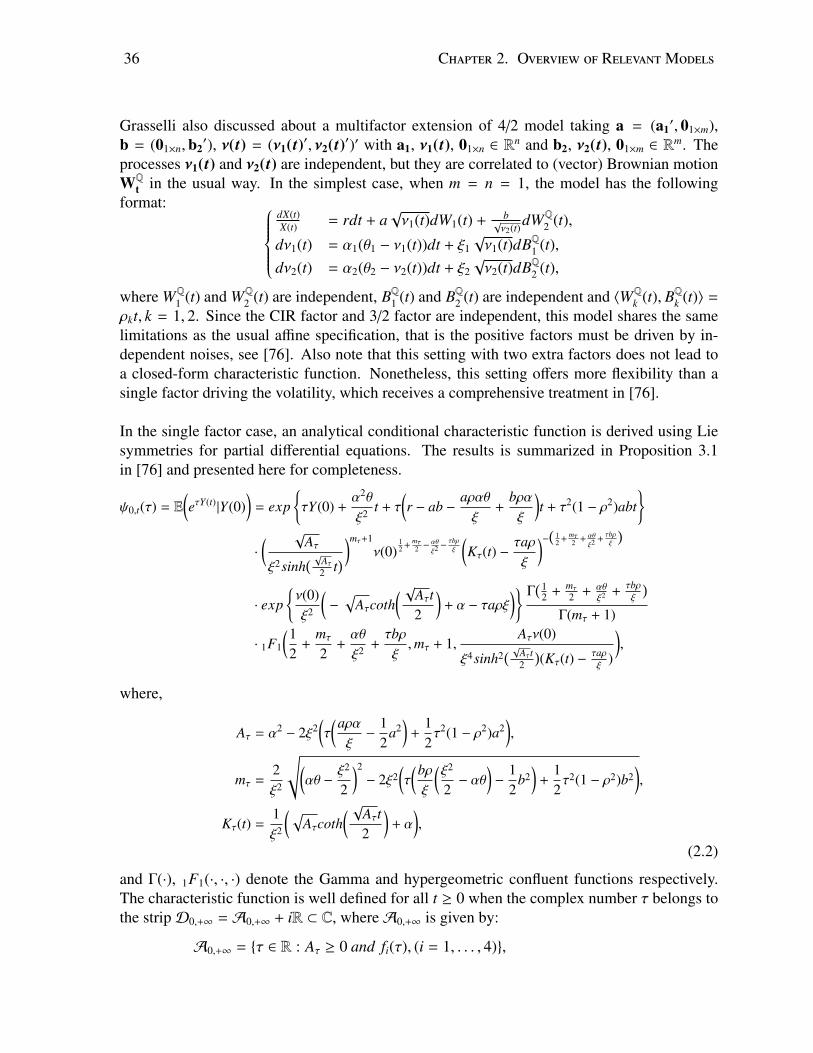
36 Chapter 2. Overview of RelevantModels
Grasselli also discussed about a multifactor extension of 4/2 model taking a = (a1′, 01×m),
b = (01×n,b2′), ν(t) = (ν1(t)′, ν2(t)′)′ with a1, ν1(t), 01×n ∈ R
n and b2, ν2(t), 01×m ∈ Rm. The
processes ν1(t) and ν2(t) are independent, but they are correlated to (vector) Brownian motionWQ
t in the usual way. In the simplest case, when m = n = 1, the model has the followingformat:
dX(t)X(t) = rdt + a
√ν1(t)dW1(t) + b
√ν2(t)
dWQ2 (t),
dν1(t) = α1(θ1 − ν1(t))dt + ξ1√ν1(t)dBQ1 (t),
dν2(t) = α2(θ2 − ν2(t))dt + ξ2√ν2(t)dBQ2 (t),
where WQ1 (t) and WQ
2 (t) are independent, BQ1 (t) and BQ2 (t) are independent and 〈WQk (t), BQk (t)〉 =
ρkt, k = 1, 2. Since the CIR factor and 3/2 factor are independent, this model shares the samelimitations as the usual affine specification, that is the positive factors must be driven by in-dependent noises, see [76]. Also note that this setting with two extra factors does not lead toa closed-form characteristic function. Nonetheless, this setting offers more flexibility than asingle factor driving the volatility, which receives a comprehensive treatment in [76].
In the single factor case, an analytical conditional characteristic function is derived using Liesymmetries for partial differential equations. The results is summarized in Proposition 3.1in [76] and presented here for completeness.
ψ0,t(τ) = E(eτY(t)|Y(0)
)= exp
τY(0) +
α2θ
ξ2 t + τ(r − ab −
aραθξ
+bραξ
)t + τ2(1 − ρ2)abt
·
( √Aτ
ξ2sinh( √Aτ
2 t) )mτ+1
ν(0)12 +
mτ2 −
αθ
ξ2−τbρξ
(Kτ(t) −
τaρξ
)−( 12 +
mτ2 + αθ
ξ2+τbρξ
)
· expν(0)ξ2
(−
√Aτcoth
( √Aτt2
)+ α − τaρξ
) Γ( 1
2 +mτ
2 + αθξ2 +
τbρξ
)Γ(mτ + 1)
· 1F1
(12
+mτ
2+αθ
ξ2 +τbρξ,mτ + 1,
Aτν(0)
ξ4sinh2( √Aτt2
)(Kτ(t) −
τaρξ
)
),
where,
Aτ = α2 − 2ξ2(τ(aραξ−
12
a2)
+12τ2(1 − ρ2)a2
),
mτ =2ξ2
√(αθ −
ξ2
2
)2− 2ξ2
(τ(bρξ
(ξ2
2− αθ
)−
12
b2)
+12τ2(1 − ρ2)b2
),
Kτ(t) =1ξ2
( √Aτcoth
( √Aτt2
)+ α
),
(2.2)
and Γ(·), 1F1(·, ·, ·) denote the Gamma and hypergeometric confluent functions respectively.The characteristic function is well defined for all t ≥ 0 when the complex number τ belongs tothe stripD0,+∞ = A0,+∞ + iR ⊂ C, whereA0,+∞ is given by:
A0,+∞ = τ ∈ R : Aτ ≥ 0 and fi(τ), (i = 1, . . . , 4),
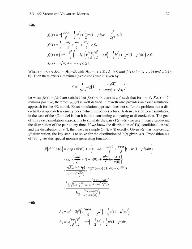
2.3. 4/2 Stochastic VolatilityModels 37
with
f1(τ) = τ(aραξ−
12
a2)
+12τ2(1 − ρ2)a2 −
α2
2ξ2 ≤ 0,
f2(τ) =12
+mτ
2+αθ
ξ2 +τbρξ
> 0,
f3(τ) =
(αθ −
ξ2
2
)2
− 2ξ2(τ(bρξ
(ξ2
2− αθ
)−
12
b2)
+12τ2(1 − ρ2)b2
)≥ 0
f4(τ) =√
Aτ + α − τaρξ ≥ 0.
When t < ∞, τ ∈ D0,t = A0,t+iRwithA0,t = τ ∈ R : Aτ ≥ 0 and fi(τ), (i = 1, . . . , 3) and f4(τ) <0. Then there exists a maximal (explosion) time t∗ given by:
t∗ =1√
Aτ
log(1 −
2√
Aτ
α − τaρξ +√
Aτ
).
i.e when f1(τ) − f3(τ) are satisfied but f4(τ) < 0, there is a t∗ such that for t < t∗, Kτ(t) −τaρξ
remains positive, therefore ψ0,t(τ) is well defined. Grasselli also provides an exact simulationapproach for the 4/2 model. Exact simulation approach does not suffer the problem that a dis-cretization approach normally does, which introduces a bias. A drawback of exact simulationin the case of the 4/2 model is that it is time-consuming comparing to discretization. The goalof this exact simulation approach is to simulate the pair (Y(t), ν(t)) for any t, hence producingthe distribution of the pair at any time. If we know the distribution of Y(t) conditional on ν(t)and the distribution of ν(t), then we can sample (Y(t), ν(t)) exactly. Given ν(t) has non-centralχ2 distribution, the key step is to solve for the distribution of Y(t) given ν(t). Proposition 4.1of [76] gives this special moment generating function:
E(euY(t)|ν(t)
)= exp
uY(0) + u
(r − ab −
aραθξ
+bραξ
)t + u2(1 − ρ2)abt
· exp
uaρξ
(ν(t) − ν(0)) +ubρξ
logν(t)ν(0)
·
√Ausinh
(αt2
)αsinh
( √Aut2
) eν(0)+ν(t)
ξ2
(αcoth
(αt2
)−√
Aucoth( √
Aut2
))
·
I2ξ2
√(αθ−
ξ22
)2+2ξ2Bu
(2√
Auν(t)ν(0)
ξ2 sinh( √
Aut2
))I 2αθξ2−1
(2α√ν(t)ν(0)
ξ2 sinh(αt2
) ) ,
with
Au = α2 − 2ξ2(u(aραξ−
12
a2)
+12
u2(1 − ρ2)a2),
Bu = u(bρξ
(ξ2
2− αθ
)−
12
b2)
+12
u2(1 − ρ2)b2,
38 Chapter 2. Overview of RelevantModels
where Iz(x) is the modified Bessel function of the first kind.
Grasselli puts a note on pricing using 4/2 model that a risk-neutral measure may not exist,which is also the case for the 3/2 model. Further, he shows that if the discounted stock priceis a true martingale under (putative) risk-neutral measure, the process ν(t) has to satisfy Fellercondition under both historical and risk-neutral measure. At the end, the process ν(t) is discov-ered to have different behavior at 0 under the two probability measures if:
2αθ + 2ρξb < ξ2 ≤ 2αθ.
Hence, risk-neutral pricing methodology is not applicable in this case, but one can still usethe Benchmark approach, which only assumes the existence of a numeraire portfolio for bothportfolio optimization and derivative pricing. Using the numeraire portfolio, derivative pricingcan be done with historical probability measure, thus it does not require a risk-neutral measureto exist, see [10] for the theory of benchmark approaches to pricing.
2.3.2 Mean-Reverting 4/2 Stochastic Volatility Model with Time-DependentParameters
The model considered in this section is a variation of the mean-reverting 4/2 stochastic volatil-ity model that will be studied in detail in chapter 3. The model we present here is a partialimprovement as it allows for time-dependent parameters while imposing some structural condi-tions. Let us define the process on the interval [0,T ] on the probability space (Ω,F , (Ft)t≥0,P):
dX(t)X(t) =
[L + c(t)
(a√ν(t) + b
√ν(t)
)2− β(t)ln(X(t))
]dt + g(t)
(a√ν(t) + b
√ν(t)
)dWP(t),
dν(t) = α(θ − ν(t))dt + ξ√ν(t)dBP(t)
〈dWP(t), dBP(t)〉 = ρdt,
where a, b, L are arbitrary constants; α, θ, ξ are positive constants satisfying Feller condition:
αθ ≥ ξ2
2 , and −1 ≤ ρ ≤ 1; c(t) = 12g2(t) + c0, g(t) = exp
(∫ T
tβ(s)ds
)and β(t) are deterministic
functions of time. Let Y(t) = ln(X(t)) then we have:
dY(t) =
[L + c0
(a√ν(t) +
b√ν(t)
)2− β(t)Y(t)
]dt + g(t)
(a√ν(t) +
b√ν(t)
)dWP(t)
Define Z(t) = Y(t) exp(−
∫ T
tβ(s)ds
)then:
dZ(t) =
[L + c0
(a√ν(t) +
b√ν(t)
)2 ]dt +
(a√ν(t) +
b√ν(t)
)dWP(t).
The SDE of Z(t) process represents the SDE of the log stock price in [76], which means we are
able to find a closed-form c.f. for Z(T ) conditional on Ft, i.e ψt,T (τ) = E(eτZ(t)|Ft
), by directly
using the results from [76] with L instead of r.
2.4. MultidimensionalModels 39
A natural question is what the possible candidates for β(t) are. We propose two candidatesfor β(s) in the examples below.
Example 1:
β(t) = β0 > 0g(t) = exp ((T − t)β0)
Note in this example the speed of reversion β(t) is constant β0 but the volatility as controlledby g(t) decreases with time since g(0) = exp (β0T ) is greater than g(T ) = 1, which seemspractically counterintuitive because the volatility should increase as clock tics, in other words,we would expect the underlying asset price to be more volatile further into future due to uncer-tainty becoming more obvious.
Example 2:
β(t) = β0 − β1t > 0 (with 0 ≤ β1 ≤β0
T)
g(t) = exp((T − t)β0 −
(T 2
2−
t2
2
)β1
)In this example, the mean reversion speed decreases with time. On the other hand, we havecontrol on how ”slowly” the variance decreases with time from g(0) = exp
(β0T − T 2
2 β1
)to
g(T ) = 1 compared to Example 1. Note that an increase in β0 leads to drastic decrease in g(t),hence a reduction of the volatility.
2.4 Multidimensional ModelsIn previous sections we review models for a single asset from the basic one-factor model withconstant volatility to complex stochastic volatility models with volatility as another stochasticfactor, and there is potential for more factors. In practice, when it comes to pricing multi-assetoptions, this requires modeling joint behavior of many underlying assets with likely as manyextra factors. That is why we need to study multidimensional models.
In this section we first review some existing multidimensional models in sections 2.4.1-2.4.2.We list some advanced models incorporating the newly developed 4/2 stochastic volatility insection 2.4.3. The model introduced in section 2.4.3.1 has not been studied in details, but it canbe a topic for future research.
Similar to section 2.2, we define the following models on the probability space (Ω,F , (Ft)t≥0,P)under historical measure P.
2.4.1 One-Factor Schwartz Model In Multi-dimensionWare et.al [47] studied a portfolio with multiple commodities and the optimal allocation prob-lem for such portfolio. A multivariate model based on one-factor Schwartz model [122] is
40 Chapter 2. Overview of RelevantModels
proposed in the aforementioned paper. Such model has all the ingredients to be entertained inthe context of multiple volatility indexes.
Suppose we observe prices for n assets. We define the model as follows:
dXi(t)Xi(t)
= (Li − βiln(Xi(t)))dt +∑
j
ai jdWPj (t), Xi(t) > 0, j = 1, . . . , n, (2.3)
where Xi(t) is the price for i-th asset; βi > 0 is the mean-reversion speed; Liβi
is the long termaverage of each Xi(t); WP
j (t) is standard Brownian motion and independent for all j; ai j is thei j-th entry of volatility matrix Σ.
Define Yi(t) = ln(Xi(t)), then by Ito’s lemma Yi(t) is a standard O-U process in the follow-ing form:
dYi(t) = βi(L∗i − Yi(t))dt +∑
j
ai jdWPj (t),
L∗i = Li −
∑j
a2i j
2βi.
So Y(t) = (Y1(t), . . . ,Yn(t)) is a normally distributed random vector with mean and covari-ance [47]:
E(Yi(t)) = e−βitYi(0) + (1 − e−βit)L∗i ,
Cov(Yi(t),Y j(t)) =
∑k aika jk
βi + β j(1 − e−(βi+β j)t).
It directly follows that X(t) = (X1(t), . . . , Xn(t)) is a multivariate lognormal random vector. Themean and variance of Xi(t) can be calculated using the mean and variance of Yi(t).
2.4.2 General Multivariate One-factor Schwartz ModelThe one-factor Schwartz model can be generalized to multidimensions in a way that allows forasset i to influence the expected returns of asset j. Let us take Yi(t)=ln(Xi(t)) where Xi(t) iseither a commodity or a volatility index, the model would be:
dYi(t) = (Li −∑
j
βi jY j(t))dt +∑
j
ai jdWPj (t), j = 1, . . . , n. (2.4)
The above models are present in Larsen’s paper [95] in the context of optimal investmentstrategies in the international economy. The model is used to model short interest rates in twocountries.In practice, one could have used the model for commodities or volatility indexes. For example,one could use the following model for VIX and VIXC jointly:
d(ln(VIXt)) = (L1 − β11ln(VIXt) − β12ln(VIXCt))dt + a11dWP1 (t) + a12dWP
2 (t), (2.5)
d(ln(VIXCt)) = (L2 − β21ln(VIXt) − β22ln(VIXCt))dt + a21dWP1 (t) + a22dWP
2 (t). (2.6)
2.4. MultidimensionalModels 41
Where L1, L2, β11, β12, β21 and β22 are all positive constants. a11, a12, a21 and a22 are entriesaffecting Σ. The correlation between the volatility indexes of two countries (US and Canada inthe example) are incorporated in ai j for i, j = 1, 2. An important property of this model is thatthe interdependence of the drift in volatility indexes across markets can be captured, namelythe spillover effects are taken into account for. Generally speaking, spillover effects refer tothe impact of one asset or underlying stock on the remaining assets/stocks in regards to trends(drift) or the long term average of a second asset. We will emphasize the concept of spillovereffects again in chapter 5.
In such situation, depending on the relative effect that one index has on the other, we canchoose the drift parameters accordingly. In the example, Canadian market is tied to US mar-ket, so VIX is more influential than VIXC. Hence, we can set β12 to 0, and (2.5) becomes astandard O-U process. On the other hand, if we are interested in studying VIX and VSTOXX(the volatility index for Euro STOXX 50) together, then β12 need not be 0 since US marketand European market are comparable, VIX and VSTOXX shall impact one another. It is alsoassumed that
√(β11 − β22)2 + 4β12β21 ≤ β11 + β22. This assumption is originally from [94] to
ensure that the eigenvalues of(−β11 −β12−β21 −β22
)are all negative so that the term structure does not go
to infinity. Later in Larsen’s paper, she shows that zero-coupon bond prices can go to infinity,in finite time, without such assumption. In chapter 5, we also impose this assumption on ourmodel.
Nielsen and Saa-Requejo [113] proposed similar models in 1993 in a Cox-Ingersoll-Rossframework. Larsen argued that “the reason for choosing a Gaussian setup instead of a CIRsetup is the tractability of a Gaussian model.” [95]. The argument again points to the limi-tations of finding closed-form expressions for moment generating function in the context ofmean-reverting stochastic volatility models, obviously affecting larger dimensions.
2.4.3 General Multivariate Multifactor Models
In mathematical finance, factor models are used to explore the relationship between asset re-turns and other market/risk factors. For example, the capital asset pricing model (CAPM) is aone-factor model. The “one” here refers to the number of common factors excluding intrinsicfactor; therefore this is equivalent to a two-factor model in the language of this thesis. Thecommon factor in CAPM, called systematic factor, explains the dependence among stock re-turns. Later, Fama and French [64] extend this basic model to include three common factors:excess market return, stock size and book-to-market equity. These are discrete-time modelstargeting the empirical discrete time data available, the power of these factors in explainingstock returns are empirically studied via linear regression models in the literature.
The extension from discrete-time to continuous-time has been neglected in the literature. Forstochastic processes, one is not only interested in factors that explain the daily behaviour ofstocks, but also in terms of capturing the stylized facts reported on the assets under study. Thefactors in the context of continuous-time stochastic process can be observable (extension ofCAPM) or unobservable (Factor Analysis), naturally they would be continuous-time stochastic
42 Chapter 2. Overview of RelevantModels
processes themselves and could appear in nonlinear ways.
In previous sections we reviewed one-factor Schwartz model, which has only the asset priceas stochastic factor. Schwartz also proposes two-factor and three-factor models which in-clude convenience yield and interest rate as, potentially unobservable/hidden, stochastic fac-tors [122]. The well known Heston model is also a two-factor model with stock price andvolatility as factors. Although Heston outperforms the classic Black-Scholes model in produc-ing “volatility smile” and “volatility skew/smirk”, it cannot “explain such largely independentfluctuations in its level and slope over time” [36]. Christoffersen et.al [36] first performed aprincipal component analysis on Black-Scholes’ implied variance data to investigate the factorsthat determine the variation of the data. They found the first two of the four principal compo-nents explain more than 95% of the variation. Furthermore, the authors found that the firsttwo principal components are highly correlated to volatility level and the slope of the smirk.A simple stylized fact about volatility level and the slope of the smirk is that they are largelyindependent. All the analysis point to a two-factor model which can capture the stylized fact.the authors proposed a multifactor stochastic covariance model based on Heston model tryingto reproduce the shape and term structure of the “smirk”. This is an example of multiple unob-servable stochastic factors been used to capture stylized facts of a single asset.
Similarly, the authors assume a Heston-type multifactor stochastic covariance model withprincipal component analysis treatment for the purpose of modeling foreign exchange ratesin [41]. Escobar and Moreno further studied a multifactor Heston model with jumps in thecontext of dynamic portfolio optimization [62]. Another direction of studying the structureof multifactor covariance models is by applying principal component analysis techniques onthe stochastic covariance matrix, see for example [41] [60]. In [41], the authors consider asimilar setting to [36]. The methodology undertaken in [60] directly goes into the heart ofprincipal component–the authors decompose the covariance matrix using principal componenttechniques yielding constant eigenvectors and stochastic eigenvalues. Structurally the diffu-sions in [41] and [60] may seem the same; however, with the model in [60], we are able torewrite the original multifactor stochastic covariance model in terms of independent one di-mensional processes (the principal components) as the eigenvectors contains the correlationinformation among assets, which in fact reduces the dimension of the model in that theory de-veloped for one dimensional model, in this case Heston, can be directly applied thanks to theindependence property.
In this section, we review advanced stochastic factor models in the spirit of [60] by assumingadvanced processes on the systematic risk factors, which accounts for the total common vari-ance among the assets, and also advanced processes on the idiosyncratic factors. Generally, thesystematic risk is the risk that affects the market and it is therefore non-diversifiable. Withoutthe addition of the systematic factors, the variation of the model only comes from the assetsthemselves. We assume no interaction between the systematic factor and the existing idiosyn-cratic factors. See [32] for details.
We first provide the processes under the historical measure P. Suppose that Xt = (X1(t), ..., Xn(t))′
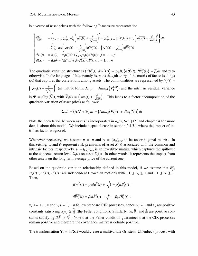
2.4. MultidimensionalModels 43
is a vector of asset prices with the following P-measure representation:
dXi(t)Xi(t)
=
Li + ci∑p
j=1 a2i j
(√v j(t) +
b j√v j(t)
)2
−∑p
j=1 βi j ln(X j(t)) + ci
(√
vi(t) + bi√vi(t)
)2 dt
+∑p
j=1 ai j
(√v j(t) +
b j√v j(t)
)dWPj (t) +
(√
vi(t) + bi√vi(t)
)dWPi (t)
dv j(t) = α j(θ j − v j(t))dt + ξ j√
v j(t)dBPj (t), j = 1, ..., p
dvi(t) = αi(θi − vi(t))dt + ξi√
vi(t)dBPi (t), i = 1, ..., n
The quadratic variation structure is⟨dBPj (t), dWP
j (t)⟩
= ρ jdt,⟨dBPi (t), dWP
i (t)⟩
= ρidt and zerootherwise. In the language of factor analysis, ai j is the i jth entry of the matrix of factor loadings(A) that captures the correlations among assets. The commonalities are represented by V j(t) =(√
v j(t) +b j√v j(t)
)2
(in matrix form, Λnxp = Adiag(V1/2
t
)) and the intrinsic residual variance
is Ψ = diag(Vt), with V j(t) =(√
vi(t) + bi√vi(t)
)2. This leads to a factor decomposition of the
quadratic variation of asset prices as follows:
Σtdt =(ΛΛ′ + Ψ
)dt =
(Adiag(Vt)A′ + diag(Vt)
)dt
Note the correlation between assets is incorporated in ai j’s, See [32] and chapter 4 for moredetails about this model. We include a spacial case in section 2.4.3.1 where the impact of in-trinsic factor is ignored.
Whenever necessary, we assume n = p and A = (ai j)n×p to be an orthogonal matrix. Inthis setting, ci and ci represent risk premiums of asset Xi(t) associated with the common andintrinsic factors, respectively. β = (βi j)n×n is an invertible matrix, which captures the spilloverat the expected return level Xi(t) on asset X j(t). In other words, it represents the impact fromother assets on the long term average price of the current one.
Based on the quadratic variation relationship defined in this model, if we assume that BPj ,BPj (t)
⊥, BPi (t), BPi (t)⊥ are independent Brownian motions with −1 ≤ ρ j ≤ 1 and −1 ≤ ρi ≤ 1.Then,
dWPj (t) = ρ jdBPj (t) +
√1 − ρ2
jdBPj (t)⊥
dWPi (t) = ρidBPi (t) +
√1 − ρ2
i dBPi (t)⊥.
v j j = 1, .., n and vi i = 1, .., n follow standard CIR processes, hence α j, θ j, and ξ j are positive
constants satisfying α jθ j ≥ξ2
j
2 (the Feller condition). Similarly, αi, θi, and ξi are positive con-
stants satisfying αiθi ≥ξi
2
2 . Note that the Feller condition guarantees that the CIR processesremain positive and therefore the covariance matrix is definite positive.
The transformation Yt = ln(Xt) would create a multivariate Ornstein–Uhlenbeck process with
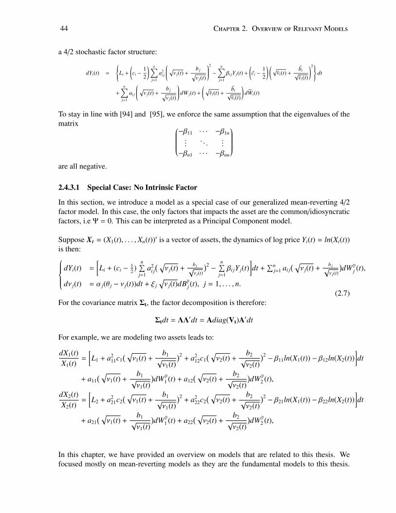
44 Chapter 2. Overview of RelevantModels
a 4/2 stochastic factor structure:
dYi(t) =
Li +
(ci −
12
) n∑j=1
a2i j
√v j(t) +b j√v j(t)
2
−
n∑j=1
βi jY j(t) +
(ci −
12
) (√vi(t) +
bi√
vi(t)
)2 dt
+
n∑j=1
ai j
√v j(t) +b j√v j(t)
dW j(t) +
(√vi(t) +
bi√
vi(t)
)dWi(t)
To stay in line with [94] and [95], we enforce the same assumption that the eigenvalues of thematrix
−β11 · · · −β1n...
. . ....
−βn1 · · · −βnn
are all negative.
2.4.3.1 Special Case: No Intrinsic Factor
In this section, we introduce a model as a special case of our generalized mean-reverting 4/2factor model. In this case, the only factors that impacts the asset are the common/idiosyncraticfactors, i.e Ψ = 0. This can be interpreted as a Principal Component model.
Suppose Xt = (X1(t), . . . , Xn(t))′ is a vector of assets, the dynamics of log price Yi(t) = ln(Xi(t))is then:
dYi(t) =
[Li + (ci −
12 )
n∑j=1
a2i j( √
ν j(t) +b j√ν j(t)
)2−
n∑j=1βi jY j(t)
]dt +
∑nj=1 ai j
( √ν j(t) +
b j√ν j(t)
)dWP
j (t),
dν j(t) = α j(θ j − ν j(t))dt + ξ j√ν j(t)dBPj (t), j = 1, . . . , n.
(2.7)For the covariance matrix Σt, the factor decomposition is therefore:
Σtdt = ΛΛ′dt = Adiag(Vt)A′dt
For example, we are modeling two assets leads to:
dX1(t)X1(t)
=
[L1 + a2
11c1( √
ν1(t) +b1√ν1(t)
)2+ a2
12c1( √
ν2(t) +b2√ν2(t)
)2− β11ln(X1(t)) − β12ln(X2(t))
]dt
+ a11( √
ν1(t) +b1√ν1(t)
)dWP
1 (t) + a12( √
ν2(t) +b2√ν2(t)
)dWP
2 (t),
dX2(t)X2(t)
=
[L2 + a2
21c2( √
ν1(t) +b1√ν1(t)
)2+ a2
22c2( √
ν2(t) +b2√ν2(t)
)2− β21ln(X1(t)) − β22ln(X2(t))
]dt
+ a21( √
ν1(t) +b1√ν1(t)
)dWP
1 (t) + a22( √
ν2(t) +b2√ν2(t)
)dWP
2 (t),
In this chapter, we have provided an overview on models that are related to this thesis. Wefocused mostly on mean-reverting models as they are the fundamental models to this thesis.

2.4. MultidimensionalModels 45
The majority of the models we covered are well-known. In cases like section 2.3.2, the modelis an extension of Grasselli’s 4/2 model, yet has not been studied. We entertain this extensionbecause it is a natural generalization of the 4/2 model with the potential of a closed-form c.f..The challenge is, as we pointed out, how to determine the time-dependent coefficients such thatthey are financially reasonable. The model discussed section 2.4.3 has been studied in a recentpaper by Cheng et.al [32]. The model introduced in Section 2.4.3.1 will be studied in details inchapter 5.
Chapter 3
The Mean-Reverting 4/2 StochasticVolatility Model
In this chapter we define and study a stochastic process that combines two important stylizedfacts of financial data: reversion to the mean, and a flexible generalized stochastic volatilityprocess: the 4/2 process. Our work is motivated by the modeling of at least two financial assetclasses: commodities and volatility indexes. Thus, we do not consider convenience yield inour model since this is not a common property shared by all mean-reverting assets. Our modeltargets a broad range of asset classes, not only commodities. We provide analytical expressionsfor the conditional characteristic functions and closed-form approximations to relevant partic-ular cases such as a mean-reverting Heston stochastic volatility model. The results also coverfeasible changes of measure with the final aim of pricing financial products. The empiricalanalysis and the estimation methodology confirm the need of such a model in several examplesfrom the targeted asset classes. Applications to option pricing corroborate the substantial im-pact on the implied volatility surfaces of the new parameters.
The chapter is organized in as follows: the models (Type I and Type II) and its main propertiesand simulation are covered in section 3.1. We derive a semi-closed conditional characteristicfunctions and provide closed-form approximations to the characteristic function in section 3.2.We study feasible changes of measure in section 3.3. In section 3.4, we propose two estima-tion methods, their performance is shown numerically and they are applied to several financialtime series. In section 3.5, we apply our model to the pricing of vanilla European call optionstwo different markets: VIX and Gold ETF (GLD) using simulation and Fast Fourier Transform(FFT) approaches.
3.1 Definition and Properties
In this section, we first give the definition of the mean-reverting 4/2 stochastic volatility modelas well as volatility process and volatility-of-volatility process. We also derive a representationfor the leverage effect, which displays interesting property and coincides with empirical expe-rience. Next, we outline the Euler discretization scheme for simulation of our model includinga discussion of other available discretization schemes.
46
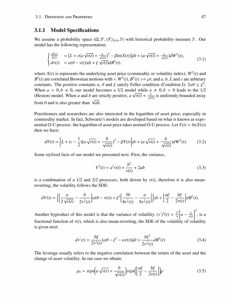
3.1. Definition and Properties 47
3.1.1 Model SpecificationsWe assume a probability space (Ω,F , (Ft)t≥0,P) with historical probability measure P. Ourmodel has the following representation: dX(t)
X(t) =[L + c
(a√ν(t) + b
√ν(t)
)2− βln(X(t))
]dt + (a
√ν(t) + b
√ν(t)
)dWP(t),
dν(t) = α(θ − ν(t))dt + ξ√ν(t)dBP(t).
(3.1)
where X(t) is represents the underlying asset price (commodity or volatility index); WP(t) andBP(t) are correlated Brownian motions with < WP(t), BP(t) >= ρt; and a, b, L and c are arbitraryconstants. The positive constants α, θ and ξ satisfy Feller condition (Condition I): 2αθ ≥ ξ2.When a = 0, b , 0, our model becomes a 3/2 model while a , 0, b = 0 leads to the 1/2(Heston) model. When a and b are strictly positive, a
√ν(t) + b
√ν(t)
is uniformly bounded away
from 0 and is also greater than√
ab.
Practitioners and researchers are also interested in the logarithm of asset price, especially incommodity market. In fact, Schwartz’s models are developed based on what is known as expo-nential O-U process: the logarithm of asset price takes normal O-U process. Let Y(t) = ln(X(t))then we have:
dY(t) =
[L + (c −
12
)(a√ν(t) +
b√ν(t)
)2− βY(t)
]dt + (a
√ν(t) +
b√ν(t)
)dWP(t). (3.2)
Some stylized facts of our model are presented next. First, the variance,
V2(t) = a2ν(t) +b2
ν(t)+ 2ab (3.3)
is a combination of a 1/2 and 3/2 processes, both driven by ν(t), therefore it is also mean-reverting, the volatility follows the SDE:
dV(t) =
[ a2√ν(t)−
b
2ν32 (t)
]α(θ − ν(t)) + ξ2
[ 3b
8ν32 (t)−
a
8ν12 (t)
]dt +
[aξ2−
bξ2ν(t)
]dBP(t).
Another byproduct of this model is that the variance of volatility, (ν′
)2(t) =ξ2
4
[a − b
ν(t)
]2
, is a
fractional function of ν(t), which is also mean-reverting, the SDE of the volatility of volatilityis given next:
dν′
(t) =bξ
2ν2(t)[αθ − ξ2 − αν(t)]dt +
bξ2
2ν32 (t)
dBP(t) (3.4)
The leverage usually refers to the negative correlation between the return of the asset and thechange of asset volatility. In our case we obtain:
ρ0 = sign(a√ν(t) +
b√ν(t)
)sign
([aξ2−
bξ2ν(t)
])ρ (3.5)
48 Chapter 3. TheMean-Reverting 4/2 Stochastic VolatilityModel
Because ξ and ν(t) are positive, then Equation 3.5 is further simplified to:
ρ0 = sign(a +
bν(t)
)sign
(a −
bν(t)
)ρ (3.6)
From Equation 3.5, we can see that the sign of leverage effect is determined by both signof volatility and sign of volatility of volatility, which is not surprising. From Equation 3.6,it is clear that the sign of leverage effect changes over time whenever ν(t) crosses | ba |, this issimilar to Stein and Stein’s model [123]. The changing sign of leverage effect suggests thatthe correlation between the return of the asset and the change of asset volatility is not alwaysnegative over time, sometimes higher volatility leads to better return on asset. This coincideswith the fact that in the long run risky asset tends to generate higher payoff.
3.1.2 Model SimulationThere is rich literature on how to simulate Heston model, see [99] for a summary of discretiza-tion schemes of a CIR process. Andersen[4] proposed two different discretization schemes forvolatility process in Heston model using moment-matching method. Other than discretizationmethods, exact simulation methods are also available. Broadie and Kaya[24] first developedan algorithm for exact simulation of CIR process. Inspired by Broadie and Kaya, Baldeaux[9]proposed an exact simulation method for 3/2 process and Grasselli[76] included an exact sim-ulation method for his 4/2 model. Exact simulation method requires a closed-form expressionfor the characteristic function and does not work well when a full path of the volatility is re-quired. Hence, we will use a discretization method for simulation.
It is widely agreed that traditional Euler-Maruyama scheme leads to negative values for CIRprocess. In practice, two fixes are considered to solve this problem: absorption and reflec-tion. In our case, absorption-like methods can not be considered as they may drive volatilityof underlying asset to infinity due to the 3/2 part. So we choose reflection method for varianceprocess and Euler-Maruyama scheme for underlying asset process. The discretization of ν(t)and Y(t) for simulations looks as follow:
ν(t + ∆t)′
= |ν(t)| + α(θ − |ν(t)|)∆t + ξ√|ν(t)|B∆t,
ν(t + ∆t) = |ν(t + ∆t)′
|.(3.7)
Y(t + ∆t) = Y(t) + (L + (c −12
)(a√ν(t) +
b√ν(t)
)2− βY(t))∆t +
(a√ν(t) +
b√ν(t)
)·(ρB∆t +
√1 − ρ2B⊥∆t
).
(3.8)
where B and B⊥ are independent standard normal variables. As we mentioned at the beginningof this section, exact simulation method generates better results than discretization; however,due to the need of a characteristic function in closed form, it is not always possible for anyprocess to be simulated via an exact simulation method or does an exact simulation methodoutperform discretization when Monte Carlo simulation is required. In our case, we find asemi-closed form characteristic function for our model. Since there is an expectation termwhich is not solved analytically, Monte Carlo method is still required for simulation even we
3.2. Characteristic Function 49
reach an exact simulation scheme for our model. Hence, in our case an exact simulation methoddoes not show absolute advantage over discretization and Monte Carlo. We apply discretiza-tion scheme to simulate our model and then use Monte Carlo for pricing purpose in section 4.
The study of convergence rate of the Euler scheme of our model itself can be an interestingresearch topic, detailed discussion of the convergence rate is beyond the scope of this chapter.However, we briefly touch on the known results of convergence rate for CIR process and Hes-ton model and challenges in finding the convergence rate for our model.
Convergence rate has two categories: strong convergence and weak convergence. Strong con-vergence refers to how fast an approximation converges to the true solution of the SDE onaverage; weak converge concerns such convergence in the values some functions. A typicalexample of weak convergence is studying how fast the option prices from simulation using Eu-ler scheme converges to the prices evaluated from a closed-form solution if one exists. Therehas been rich literature on the study of discretization schemes and their convergence rate forCIR process, see [99] and [89] for a scan of methods in this area. According to [99] and [89]and references therein, the strong convergence rate for certain CIR discretization schemes is12 with conditions on the process coefficients. In particular, the discretization we choose isshown to have weak convergence rate 1 and strong convergence 1
2 in Lp(p ≥ 2) sense undera restrictive condition [46] [22]. In the case of Heston model, Lord et.al show that reflectionscheme has a weak order of convergence slightly under 1
2 . For our model, both strong and weakconvergence are difficult to show due to model complexity and theoretical limitations.
In the end, we would like to comment a little bit on [4] Truncated Gaussian (TG) and QuadraticExponential (QE) method. These two methods also discretize the variance process, but in away that is neither absorption nor reflection style. They are based on the idea of moment-matching. For full details of algorithms for these two methods, please see [4]. Both methodsproduce non-negative values and account for the density of CIR process, as commented byAndersen, QE is accurate enough in practice. In our simulation, QE is also considered, butthis method should be used with caution. Since QE assigns a mass at origin, based on thechoice of parameters, there is probability that simulated variance can hit zero, even thoughall positive values for variance are generated during our simulation process with parameters:α = 1.8, θ = 0.04, ξ = 0.2,∆t = 0.001 and the switching rule 1.5.
3.2 Characteristic Function
In this section we present a semi-closed form solution for the conditional characteristic function(c.f). Define Z(t) = eβtY(t). The dynamics of Z(t) follows Ito’s lemma:
dZ(t) =
[Leβt + eβt(c −
12
)(a√ν(t) +
b√ν(t)
)2]dt + eβt(a
√ν(t) +
b√ν(t)
)dWP(t). (3.9)
50 Chapter 3. TheMean-Reverting 4/2 Stochastic VolatilityModel
In integral form:
Z(T ) = Z(t) +Lβ
(eβT − eβt) +
∫ T
teβs(c −
12
)(a√ν(s) +
b√ν(s)
)2ds +
∫ T
teβs(a
√ν(s) +
b√ν(s)
)dWP(s)
(3.10)
The conditional characteristic function of Z(T ) given Ft is given by next proposition.
Proposition 3.2.1 Let Z(T ) follows Equation 3.10 then the c.f. has the following representa-tion:
E(eiuZ(T )|Ft) =exp
iuZ(t) + iu(L −
aραθξ
+bραξ
+ 2ab(c −12
)) (eβT − eβt)
β− u2(1 − ρ2)
(e2βT − e2βt)ab2β
× exp
−
iuaρeβt
ξν(t) −
iubρeβt
ξln(ν(t))
× E
[ν(T )−Aexp
− Bν(T ) −C
∫ T
teβsln(ν(s))ds
−
∫ T
t
(Deβs + Ee2βs) 1
ν(s)ds −
∫ T
t
(Feβs + Ge2βs)ν(s)ds
∣∣∣∣∣Ft
].
where,
A = −iubρξ
eβT , B = −iuaρξ
eβT ,C =iubρβξ
,D = −iubρξ
(ξ2
2− αθ
)− iub2(c −
12
),
E =12
u2(1 − ρ2)b2, F =iuaρ(β − α)
ξ− iua2(c −
12
),G =12
u2(1 − ρ2)a2.
(3.11)
See the proof in the Appendix.
The characteristic function involves an expected value with respect to only one Brownian mo-tion (B(t)), i.e. the second Brownian W(t) is eliminated. Therefore it constitute a simplificationas oppose to the original expectation; however, the conditional expectation term in the ex-pression can not be solved analytically due to its complex structure. In the next section, wepropose approximation approaches to the conditional expectation term so that the semi-closedcharacteristic function can be approximated by an analytical expression.
3.2.1 Approximation to Characteristic FunctionIn this section, we propose two approaches and apply them to two scenarios in which the semi-closed characteristic function can be approximated by an analytic formula that is available inliterature. Then we show the goodness of our approximation approaches by showing the den-sity functions obtained via inversion of the true and approximated characteristic functions.
Two reasons lead to this semi-closed c.f. First, the expectation of integrated CIR process withtime dependent factor is not easy to solve analytically [16]. Second reason, integrated log ofCIR process with time-dependent factor has not been studied in the literature. Grasselli [72]offers a solution to his geometric 4/2 process, but there is no integrated log of CIR process
3.2. Characteristic Function 51
involved in the conditional expectation that needs to be solved.
Hence, we propose two approximation approaches to approximate the integrals∫ T
t
(Deβs +
Ee2βs) 1ν(s)ds and
∫ T
t
(Feβs + Ge2βs)ν(s)ds so that we can apply existing analytical expressions
to approximate our c.f. We will show our approximations for cases ρ = 0, b , 0; b = 0, ρ , 0;and b = 0, ρ = 0.
We propose midpoint approximation approach and average approximation approach. The goalis two approximate the time-dependent factors by a constant. We will show numerically theperformance of our approximation approaches.
• Midpoint Approximation: g1(t) and g2(t) are bounded functions on [t,T ], so the inte-grals are bounded by:
min[t,T ]
(g1(s))∫ T
t
1ν(s)
ds ≤∫ T
tg1(s)
1ν(s)
ds ≤ max[t,T ]
(g1(s))∫ T
t
1ν(s)
ds,
min[t,T ]
(g2(s))∫ T
tν(s)ds ≤
∫ T
tg2(s)ν(s)ds ≤ max
[t,T ](g2(s))
∫ T
tν(s)ds,
then we approximate the integrals by the midpoints:∫ T
tg1(s)
1ν(s)
ds ≈ m∫ T
t
1ν(s)
ds,∫ T
tg2(s)ν(s)ds ≈ n
∫ T
tν(s)ds,
where,
m =
min[t,T ]
(g1(s)) + max[t,T ]
(g1(s))
2, n =
min[t,T ]
(g2(s)) + max[t,T ]
(g2(s))
2
• Average Approximation: In last example we claim that g1(t) and g2(t) are boundedfunctions and deduce m and n as midpoints. Average is also a choice for approximation.We approximate our target integrals by averages as:∫ T
tg1(s)
1ν(s)
ds ≈1
T − t
∫ T
tg1(s)ds
∫ T
t
1ν(s)
ds = m∫ T
t
1ν(s)
ds∫ T
tg2(s)ν(s)ds ≈
1T − t
∫ T
tg2(s)ds
∫ T
tν(s)ds = n
∫ T
tν(s)ds
where,
m =1
T − t
[D′
β(eβT − eβt) +
E′
2β(e2βT − e2βt)
],
n =1
T − t
[F′
β(eβT − eβt) +
G′
2β(e2βT − e2βt)
].
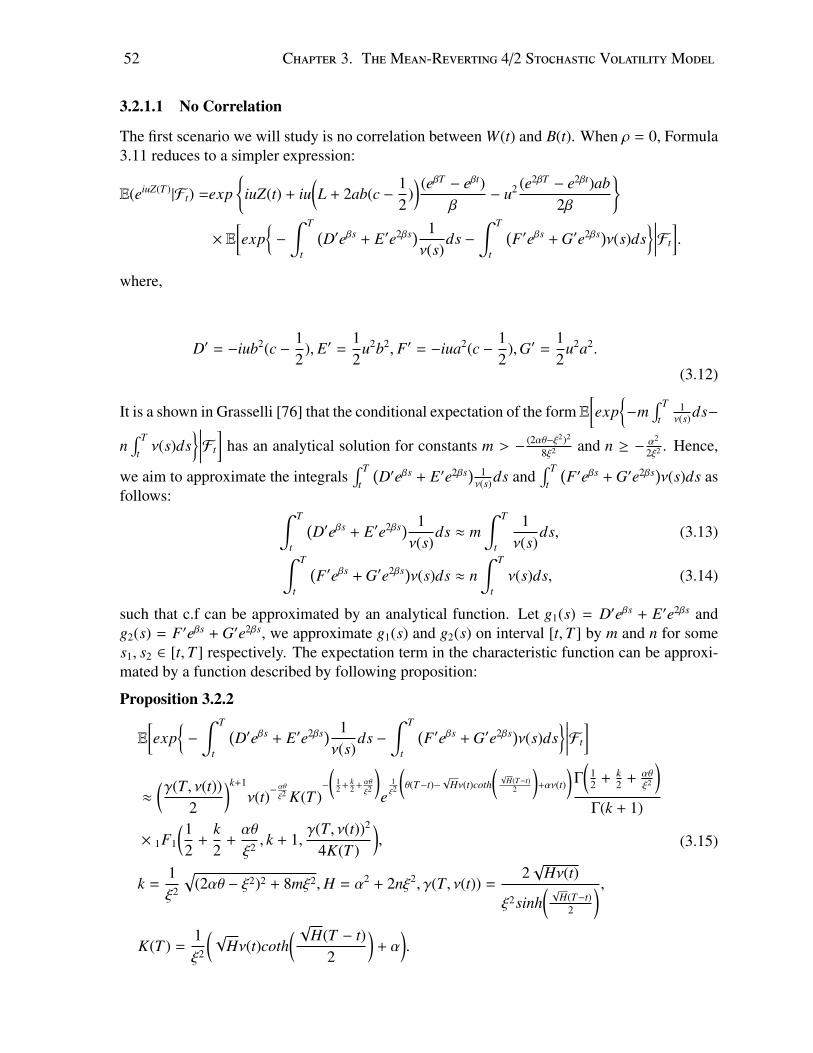
52 Chapter 3. TheMean-Reverting 4/2 Stochastic VolatilityModel
3.2.1.1 No Correlation
The first scenario we will study is no correlation between W(t) and B(t). When ρ = 0, Formula3.11 reduces to a simpler expression:
E(eiuZ(T )|Ft) =exp
iuZ(t) + iu(L + 2ab(c −
12
)) (eβT − eβt)
β− u2 (e2βT − e2βt)ab
2β
× E
[exp
−
∫ T
t
(D′eβs + E′e2βs) 1
ν(s)ds −
∫ T
t
(F′eβs + G′e2βs)ν(s)ds
∣∣∣∣∣Ft
].
where,
D′ = −iub2(c −12
), E′ =12
u2b2, F′ = −iua2(c −12
),G′ =12
u2a2.
(3.12)
It is a shown in Grasselli [76] that the conditional expectation of the form E[exp
−m
∫ T
t1ν(s)ds−
n∫ T
tν(s)ds
∣∣∣∣∣Ft
]has an analytical solution for constants m > − (2αθ−ξ2)2
8ξ2 and n ≥ − α2
2ξ2 . Hence,
we aim to approximate the integrals∫ T
t
(D′eβs + E′e2βs) 1
ν(s)ds and∫ T
t
(F′eβs + G′e2βs)ν(s)ds as
follows: ∫ T
t
(D′eβs + E′e2βs) 1
ν(s)ds ≈ m
∫ T
t
1ν(s)
ds, (3.13)∫ T
t
(F′eβs + G′e2βs)ν(s)ds ≈ n
∫ T
tν(s)ds, (3.14)
such that c.f can be approximated by an analytical function. Let g1(s) = D′eβs + E′e2βs andg2(s) = F′eβs + G′e2βs, we approximate g1(s) and g2(s) on interval [t,T ] by m and n for somes1, s2 ∈ [t,T ] respectively. The expectation term in the characteristic function can be approxi-mated by a function described by following proposition:
Proposition 3.2.2
E[exp
−
∫ T
t
(D′eβs + E′e2βs) 1
ν(s)ds −
∫ T
t
(F′eβs + G′e2βs)ν(s)ds
∣∣∣∣∣Ft
]
≈
(γ(T, ν(t))
2
)k+1
ν(t)−αθ
ξ2 K(T )−
(12 + k
2 + αθ
ξ2
)e
1ξ2
(θ(T−t)−
√Hν(t)coth
(√
H(T−t)2
)+αν(t)
)Γ
(12 + k
2 + αθξ2
)Γ(k + 1)
× 1F1
(12
+k2
+αθ
ξ2 , k + 1,γ(T, ν(t))2
4K(T )
),
k =1ξ2
√(2αθ − ξ2)2 + 8mξ2,H = α2 + 2nξ2, γ(T, ν(t)) =
2√
Hν(t)
ξ2sinh( √
H(T−t)2
) ,K(T ) =
1ξ2
(√Hν(t)coth
( √H(T − t)2
)+ α
).
(3.15)
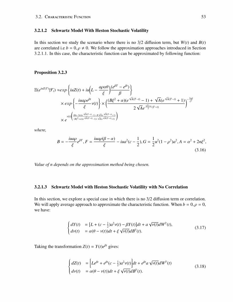
3.2. Characteristic Function 53
3.2.1.2 Schwartz Model With Heston Stochastic Volatility
In this section we study the scenario where there is no 3/2 diffusion term, but W(t) and B(t)are correlated i.e b = 0, ρ , 0. We follow the approximation approaches introduced in Section3.2.1.1. In this case, the characteristic function can be approximated by following function:
Proposition 3.2.3
E(eiuZ(T )|Ft) ≈exp
iuZ(t) + iu(L −
aραθξ
) (eβT − eβt)β
× exp
−
iuaρeβt
ξν(t)
×
( (Bξ2 + α)(e√
A(T−t) − 1) +√
A(e√
A(T−t) + 1)
2√
Ae√
A+α2 (T−t)
)− 2αθξ2
× eν(t)
((Bα−2n)(e
√A(T−t)−1)−B
√A(e√
A(T−t)+1)
(Bξ2+α)(e√
A(T−t)−1)+√
A(e√
A(T−t)+1)
)where,
B = −iuaρξ
eβT , F =iuaρ(β − α)
ξ− iua2(c −
12
),G =12
u2(1 − ρ2)a2, A = α2 + 2nξ2,
(3.16)
Value of n depends on the approximation method being chosen.
3.2.1.3 Schwartz Model with Heston Stochastic Volatility with No Correlation
In this section, we explore a special case in which there is no 3/2 diffusion term or correlation.We will apply average approach to approximate the characteristic function. When b = 0, ρ = 0,we have:
dY(t) =[L + (c − 1
2 )a2ν(t) − βY(t)]dt + a
√ν(t)dWP(t),
dν(t) = α(θ − ν(t))dt + ξ√ν(t)dBP(t).
(3.17)
Taking the transformation Z(t) = Y(t)eβt gives:
dZ(t) =
[Leβt + eβt(c − 1
2 )a2ν(t)]dt + eβta
√ν(t)dWP(t)
dν(t) = α(θ − ν(t))dt + ξ√ν(t)dBP(t).
(3.18)
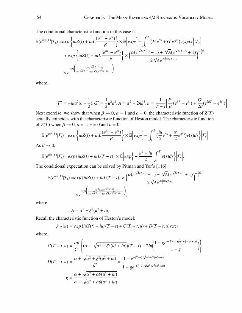
54 Chapter 3. TheMean-Reverting 4/2 Stochastic VolatilityModel
The conditional characteristic function in this case is:
E(eiuZ(T )|Ft) =exp
iuZ(t) + iuL(eβT − eβt)
β
× E
[exp
−
∫ T
t
(F′eβs + G′e2βs)ν(s)ds
∣∣∣∣∣Ft
]≈ exp
iuZ(t) + iuL
(eβT − eβt)β
×
(α(e
√A(T−t) − 1) +
√A(e
√A(T−t) + 1)
2√
Ae√
A+α2 (T−t)
)− 2αθξ2
× eν(t)
(−2n(e
√A(T−t)−1)
α(e√
A(T−t)−1)+√
A(e√
A(T−t)+1)
)where,
F′ = −iua2(c −12
),G′ =12
u2a2, A = α2 + 2nξ2, n =1
T − t
[F′
β(eβT − eβt) +
G′
2β(e2βT − e2βt)
]Next exercise, we show that when β → 0, a = 1 and c = 0, the characteristic function of Z(T )actually coincides with the characteristic function of Heston model. The characteristic functionof Z(T ) when β→ 0, a = 1, c = 0 and ρ = 0:
E(eiuZ(T )|Ft) =exp
iuZ(t) + iuL(eβT − eβt)
β
× E
[exp
−
∫ T
t
( iu2
eβs +u2
2e2βs)ν(s)ds
∣∣∣∣∣Ft
]As β→ 0,
E(eiuZ(T )|Ft) =exp iuZ(t) + iuL(T − t) × E[exp
−
u2 + iu2
∫ T
tν(s)ds
∣∣∣∣∣Ft
].
The conditional expectation can be solved by Pitman and Yor’s [116]:
E(eiuZ(T )|Ft) =exp iuZ(t) + iuL(T − t) ×(α(e
√A(T−t) − 1) +
√A(e
√A(T−t) + 1)
2√
Ae√
A+α2 (T−t)
)− 2αθξ2
× eν(t)
(−(u2+iu)(e
√A(T−t)−1)
α(e√
A(T−t)−1)+√
A(e√
A(T−t)+1)
),
where
A = α2 + ξ2(u2 + iu)
Recall the characteristic function of Heston’s model:
ψt,T (u) = exp iuY(t) + iur(T − t) + C(T − t, u) + D(T − t, u)ν(t)
where,
C(T − t, u) =αθ
ξ2
(α +√α2 + ξ2(u2 + iu))(T − t) − 2ln
(1 − ge−(T−t)√α2+ξ2(u2+iu)
1 − g
)D(T − t, u) =
α +√α2 + ξ2(u2 + iu)
ξ2 ×1 − e−(T−t)
√α2+ξ2(u2+iu)
1 − ge−(T−t)√α2+ξ2(u2+iu)
g =α +
√α2 + αθ(u2 + iu)
α −√α2 + αθ(u2 + iu)
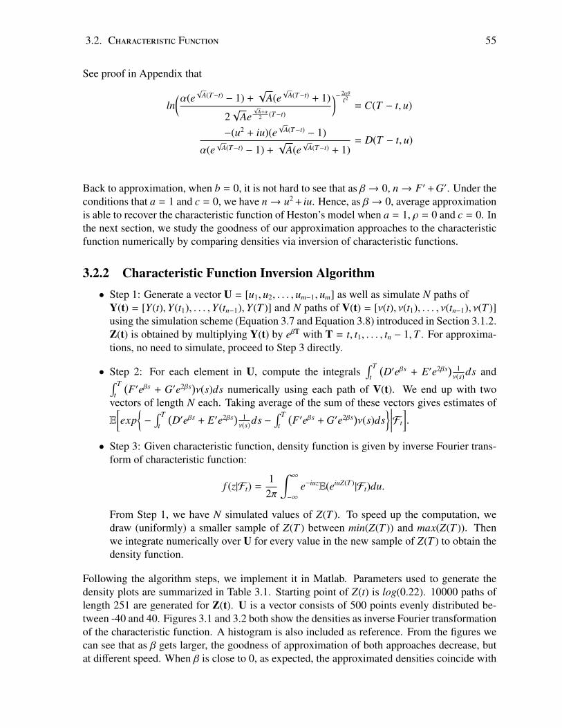
3.2. Characteristic Function 55
See proof in Appendix that
ln(α(e
√A(T−t) − 1) +
√A(e
√A(T−t) + 1)
2√
Ae√
A+α2 (T−t)
)− 2αθξ2
= C(T − t, u)
−(u2 + iu)(e√
A(T−t) − 1)
α(e√
A(T−t) − 1) +√
A(e√
A(T−t) + 1)= D(T − t, u)
Back to approximation, when b = 0, it is not hard to see that as β→ 0, n→ F′ +G′. Under theconditions that a = 1 and c = 0, we have n→ u2 + iu. Hence, as β→ 0, average approximationis able to recover the characteristic function of Heston’s model when a = 1, ρ = 0 and c = 0. Inthe next section, we study the goodness of our approximation approaches to the characteristicfunction numerically by comparing densities via inversion of characteristic functions.
3.2.2 Characteristic Function Inversion Algorithm• Step 1: Generate a vector U = [u1, u2, . . . , um−1, um] as well as simulate N paths of
Y(t) = [Y(t),Y(t1), . . . ,Y(tn−1),Y(T )] and N paths of V(t) = [ν(t), ν(t1), . . . , ν(tn−1), ν(T )]using the simulation scheme (Equation 3.7 and Equation 3.8) introduced in Section 3.1.2.Z(t) is obtained by multiplying Y(t) by eβT with T = t, t1, . . . , tn − 1,T . For approxima-tions, no need to simulate, proceed to Step 3 directly.
• Step 2: For each element in U, compute the integrals∫ T
t
(D′eβs + E′e2βs) 1
ν(s)ds and∫ T
t
(F′eβs + G′e2βs)ν(s)ds numerically using each path of V(t). We end up with two
vectors of length N each. Taking average of the sum of these vectors gives estimates of
E[exp
−
∫ T
t
(D′eβs + E′e2βs) 1
ν(s)ds −∫ T
t
(F′eβs + G′e2βs)ν(s)ds
∣∣∣∣∣Ft
].
• Step 3: Given characteristic function, density function is given by inverse Fourier trans-form of characteristic function:
f (z|Ft) =1
2π
∫ ∞
−∞
e−iuzE(eiuZ(T )|Ft)du.
From Step 1, we have N simulated values of Z(T ). To speed up the computation, wedraw (uniformly) a smaller sample of Z(T ) between min(Z(T )) and max(Z(T )). Thenwe integrate numerically over U for every value in the new sample of Z(T ) to obtain thedensity function.
Following the algorithm steps, we implement it in Matlab. Parameters used to generate thedensity plots are summarized in Table 3.1. Starting point of Z(t) is log(0.22). 10000 paths oflength 251 are generated for Z(t). U is a vector consists of 500 points evenly distributed be-tween -40 and 40. Figures 3.1 and 3.2 both show the densities as inverse Fourier transformationof the characteristic function. A histogram is also included as reference. From the figures wecan see that as β gets larger, the goodness of approximation of both approaches decrease, butat different speed. When β is close to 0, as expected, the approximated densities coincide with

56 Chapter 3. TheMean-Reverting 4/2 Stochastic VolatilityModel
Table 3.1: Parameters for Density(t=0,T=1).
L β c α θ ξ a b ρ
log(0.22) (0.0001,0.5,2) (0,0.5) 17 0.0153 0.27 1 (0,0.1) (0,-0.6)
Figure 3.1: Density with Histogram
the true density. Midpoint approach fails to approximate the true density when β is 2. All ofthe cases, only average approach gives the density that stays close to the true. In particular, thetrue density greatly overlaps with the average approximation as shown in Figure 3.1. Overall,the difference between true density and average approximation is negligible, and the actual sizeof error will be assessed later.
3.3 Change of MeasureSo far we have worked with the historical probability measure. However, this is not appro-priate for option pricing according to the fundamental theorem of asset pricing. Therefore, inthis section we study two families of feasible changes of measure for our model, these familiescome from specifications of the excess return.
Let (Ω,F , (Ft)0≤t≤T ,Q) denote a probability measure space where Q is equivalent to P. Let
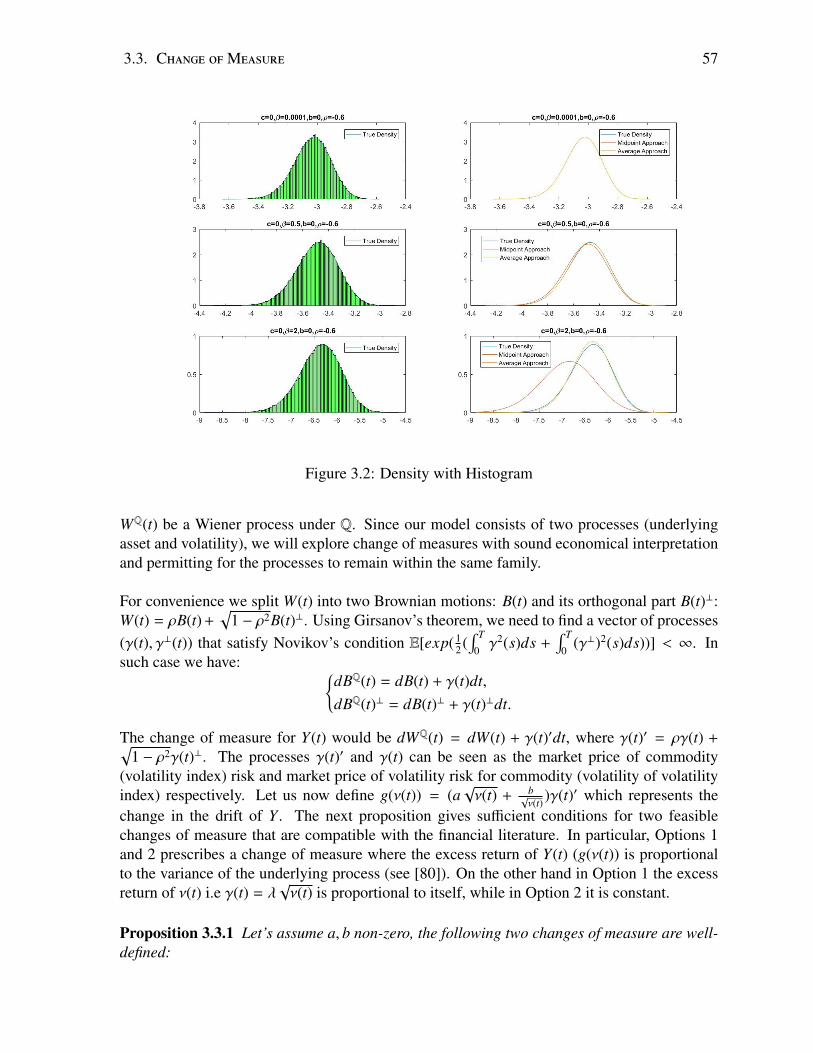
3.3. Change ofMeasure 57
Figure 3.2: Density with Histogram
WQ(t) be a Wiener process under Q. Since our model consists of two processes (underlyingasset and volatility), we will explore change of measures with sound economical interpretationand permitting for the processes to remain within the same family.
For convenience we split W(t) into two Brownian motions: B(t) and its orthogonal part B(t)⊥:W(t) = ρB(t) +
√1 − ρ2B(t)⊥. Using Girsanov’s theorem, we need to find a vector of processes
(γ(t), γ⊥(t)) that satisfy Novikov’s condition E[exp(12 (
∫ T
0γ2(s)ds +
∫ T
0(γ⊥)2(s)ds))] < ∞. In
such case we have: dBQ(t) = dB(t) + γ(t)dt,dBQ(t)⊥ = dB(t)⊥ + γ(t)⊥dt.
The change of measure for Y(t) would be dWQ(t) = dW(t) + γ(t)′dt, where γ(t)′ = ργ(t) +√1 − ρ2γ(t)⊥. The processes γ(t)′ and γ(t) can be seen as the market price of commodity
(volatility index) risk and market price of volatility risk for commodity (volatility of volatilityindex) respectively. Let us now define g(ν(t)) = (a
√ν(t) + b
√ν(t)
)γ(t)′ which represents thechange in the drift of Y . The next proposition gives sufficient conditions for two feasiblechanges of measure that are compatible with the financial literature. In particular, Options 1and 2 prescribes a change of measure where the excess return of Y(t) (g(ν(t)) is proportionalto the variance of the underlying process (see [80]). On the other hand in Option 1 the excessreturn of ν(t) i.e γ(t) = λ
√ν(t) is proportional to itself, while in Option 2 it is constant.
Proposition 3.3.1 Let’s assume a, b non-zero, the following two changes of measure are well-defined:
58 Chapter 3. TheMean-Reverting 4/2 Stochastic VolatilityModel
• Option 1 γ(t) = λ√ν(t)
g(ν(t)) = Λ(a√ν(t) + b
√ν(t)
)2
where (λ,Λ) shall satisfy the following constraints: I =
λ > −α
ξ
and II = Λ3 < Λ < Λ4
with Λ3 = max[
1a
(− α
ξ+ ρλ
),− 1|b|
(αθξ−
ξ
2
)]and Λ4 = min
[1a
(αξ
+ ρλ), 1|b|
(αθξ−
ξ
2
)]Here the model under risk-neutral measure becomes: dX(t)
X(t) =[L + (c − Λ)
(a√ν(t) + b
√ν(t)
)2− βln(X(t))
]dt + (a
√ν(t) + b
√ν(t)
)dWQ(t)
dν(t) = (αθ − (α + λξ)ν(t))dt + ξ√ν(t)dBQ(t)
• Option 2 γ(t) = λ′√ν(t)
g(ν(t)) = Λ′(a√ν(t) + b
√ν(t)
)2
where (λ′,Λ′) shall satisfy the following constraints: I =
− (αθ
ξ−
ξ
2 ) ≤ λ′ ≤ 0
and II =
Λ3 < Λ < Λ4 with Λ3 = max[− 1
b
(αθξ−
ξ
2 −ρλ′),− α|a|ξ
]and Λ4 = min
[1b
(αθξ−
ξ
2 +ρλ′), α|a|ξ
]Here the model under risk-neutral measure is: dX(t)
X(t) =[L + (c − Λ′)
(a√ν(t) + b
√ν(t)
)2− βln(X(t))
]dt + (a
√ν(t) + b
√ν(t)
)dWQ(t)
dν(t) = (αθ − λ′ξ − αν(t))dt + ξ√ν(t)dBQ(t)
The change of measure we studied is different from [76]. In the aforementioned paper, thestock price process is directly defined under the risk-neutral measure. The author checkedwhether the discounted stock price is a true martingale. However, our model is defined underhistorical measure and our change of measure is done by taking into account the market priceof risk and market price of volatility risk.
3.4 EstimationIn our model, there are nine parameters to be determined: L, c, β, a, b, α, θ and ξ plus corre-lation ρ. For estimation we divide them into two groups: drift group (L, c, β, ρ) and volatilitygroup (a, b, α, θ, ξ) with the later being our main objective. Volatility index (eg. VIX andVSTOXX) and commodities (eg. crude oil) are applications of our model, therefore we usedaily observations of VVIX, V-VSTOXX (the volatility of VSTOXX), OVX (volatility of oilETF, USO) and GVZ (volatility of gold ETF, GLD) to estimate parameters in volatility grouprespectively. We use volatility indexes data and commodity price data for estimation of driftgroup parameters. In section 3.4.1, we first estimate b, then propose two methods to estimatethe remaining parameters in the volatility group. We present a method to estimate parametersin the drift group in section 3.4.2. In section 3.4.3 we show, via simulation, the consistency ofthe estimator for volatility group parameters using the methods proposed in 3.4.1. In section3.4.4, we estimate parameters in volatility group and drift group from empirical data.
3.4. Estimation 59
3.4.1 Estimation Method For Volatility Group
In our model, the observed volatility data is modeled by square root of Equation (3.3). LetV(t) denote the observed volatility at time t with a = 1. By setting a = 1 we avoid a potential“identifiability” problem (i.e infinitely many solutions for the pair (a, b)). We can then interpretthe volatility as “Heston plus a fraction of 3/2 model”. This way, the celebrated Heston modelbecomes a benchmark model.
We first estimate b. From V2(t) = ν(t) + b2
ν(t) + 2b, one observes that the infimum value of V2(t)occurs when the process ν(t) hits b. Using the fact that CIR processes can attain any strictlypositive barrier, with probability one (see eg. [3] and [108]), then we conclude b = min
0≤t<∞
V2(t)4 ,
i.e. P( min0≤t<∞
V2(t)4 = b) = 1. Since the data is in discrete time, we propose the following estimator
for b: b =min
ti∈ΩTV2(ti)
4 , where ΩT = tini=0, t0 = 0, tn = T . The consistency of this estimator is
studied numerically in the coming sections.
Next we consider two methods that involve moments to estimate the parameters in the volatil-ity process.
Method 1The first method starts by solving Equation (3.3) as a quadratic function of ν(t), which results
in two solutions. We use V(ti) and b to calculate√ν±(ti) =
V(ti)±√
V2(ti)−4b2 . Then we use MLE
on ν+(ti) and ν−(ti) respectively to obtain two sets of estimates of α, θ and ξ: Θ+ = (α+, θ+, ξ+)and Θ− = (α−, θ−, ξ−). A selection criteria to determine which one of Θ+ and Θ− is a bettercandidate to estimate the true parameters Θ = (α, θ, ξ) is based on the observations and mo-ments of V2(t).We now use [38], the authors proved that as t → ∞, ν(t) is asymptotically gamma distributedwith shape parameter 2αθ
ξ2 and scale parameter ξ2
2α , 1ν(t) is hence asymptotic inverse gamma dis-
tribution with corresponding paramters 2αθξ2 and 2α
ξ2 . Since the moments of gamma distributionand inverse gamma distribution are known, our selection criteria proceeds with calculation ofthe following moments:
µ′
1 = E(ν(t) +
b2
ν(t)
)=
2αb2
2αθ − ξ2 + θ
µ′
2 = E
(ν(t) +
b2
ν(t)
)2=
2αθ(2αθ + ξ2)4α2 +
4α2b4
(2αθ − ξ2)(2αθ − 2ξ2)+ 2b2
µ′
3 = E
(ν(t) +
b2
ν(t)
)3=
2αθ(2αθ + ξ2)(2αθ + 2ξ2)8α3 +
8α3b6
(2αθ − ξ2)(2αθ − 2ξ2)(2αθ − 3ξ2)+ 3b2θ +
6αb4
2αθ − ξ2 ,
where we have used the moments up to third degree from gamma distribution and inversegamma distribution because we have three parameters to estimate. In order for the third mo-
60 Chapter 3. TheMean-Reverting 4/2 Stochastic VolatilityModel
ment of inverse gamma distribution to exist, we need a condition:
2αθ ≥ 3ξ2, (3.19)
which we denote as Condition II. This condition is stronger than Condition I. Then we sub-stitute Θ+ and Θ− for Θ in µ
′
1, µ′
2 and µ′
3 respectively, a candidate is determined by the set ofestimates that minimizes the objective function
F =
(µ′
1 −1
n + 1
n∑i=0
(V2(ti) − 2b))2
+
(µ′
2 −1
n + 1
n∑i=0
(V2(ti) − 2b)2)2
+
(µ′
3 −1
n + 1
n∑i=0
(V2(ti) − 2b)3)2
.
Remark: Because we can obtain Θ+ and Θ− from data directly, they may not satisfy ConditionII. In this case, one can use as many moments as feasible. For example, if the estimates onlysatisfy Condition I, then the selection criteria only concerns µ
′
1.
Method 2This method can be viewed as an improvement over Method 1. Unlike Method 1, we usemethods of moments by taking into account all three moments and imposing Condition II. Weestimate the parameters by minimizing F to find α, θ and ξ over the region 2αθ ≥ 3ξ2. Theoptimization step is done numerically with initial values Θ+ and Θ− leading to two sets ofestimates. The set with smallest F value is our estimate for Θ.
The key of this method is that the series ν(t) + b2
ν(t) is weakly stationary and ergodic underCondition II. [78] has shown stationarity and ergodicity are requirements for method of mo-ments to ensure consistency. It is known that CIR process is stationary and ergodic as shownin [38]. [2] examined conditions under which 3/2 process is stationary and ergodic, which re-quires mean-reverting speed to be positive. Note in our case, the mean-reverting speed of 1
ν(t)
is αθ − ξ2. Hence, a condition for 1ν(t) to be stationary and ergodic is:
αθ ≥ ξ2 (3.20)
denoted as Condition III. Condition III is stronger than Condition I but weaker than ConditionII. By Proposition 2.1.7 and Corollary 2.1.8 of [120], our process ν(t) + b2
ν(t) satisfies weakstationary and ergodic hence we can ensure consistency via method of moments.Remark: In both methods above we estimate b via b. We could have alternatively triedestimating b via method of moments at the expense of much stronger condition 2αθ ≥ 4ξ2
(Condition IV).
3.4.2 Estimation Method For Drift GroupThe method above provides us estimated volatility group parameters. Next, we use leastsquares method to estimate parameters in drift group.We first start with discretization scheme of Y(t) described in Equation (3.8) yielding:
yi = β1x1i + β2x2i + β3x3i + εi, i = 0, . . . , n
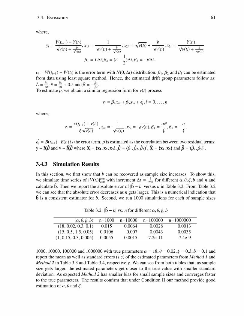
3.4. Estimation 61
where,
yi =Y(ti+1) − Y(ti)√ν(ti) + b
√ν(ti)
, x1i =1
√ν(ti) + b
√ν(ti)
, x2i =√ν(ti) +
b√ν(ti)
, x3i =Y(ti)
√ν(ti) + b
√ν(ti)
,
β1 = L∆t, β2 = (c −12
)∆t, β3 = −β∆t.
εi = W(ti+1) −W(ti) is the error term with N(0,∆t) distribution. β1, β2 and β3 can be estimatedfrom data using least square method. Hence, the estimated drift group parameters follow as:L =
β1∆t , c =
β2∆t + 0.5 and β = −
β3∆t .
To estimate ρ, we obtain a similar regression form for ν(t) process
vi = β4x4i + β5x5i + ε′
i , i = 0, . . . , n
where,
vi =ν(ti+1) − ν(ti)ξ√ν(ti)
, x4i =1√ν(ti)
, x5i =√ν(ti), β4 =
αθ
ξ, β5 = −
α
ξ.
ε′
i = B(ti+1)−B(ti) is the error term. ρ is estimated as the correlation between two residual terms:y − Xβ and v − Xβ where X = x1, x2, x3, β = (β1, β2, β3)
′
, X = x4, x5 and β = (β4, β5)′
.
3.4.3 Simulation Results
In this section, we first show that b can be recovered as sample size increases. To show this,we simulate time series of V(ti)i=n
i=0 with increment ∆t = 1250 for different α, θ, ξ, b and n and
calculate b. Then we report the absolute error of |b − b| versus n in Table 3.2. From Table 3.2we can see that the absolute error decreases as n gets larger. This is a numerical indication thatb is a consistent estimator for b. Second, we run 1000 simulations for each of sample sizes
Table 3.2: |b − b| vs. n for different α, θ, ξ, b
(α, θ, ξ, b) n=1000 n=10000 n=100000 n=1000000(18, 0.02, 0.3, 0.1) 0.015 0.0064 0.0028 0.0013(15, 0.5, 1.5, 0.05) 0.0106 0.007 0.0043 0.0035
(1, 0.15, 0.3, 0.005) 0.0055 0.0015 7.2e-11 7.4e-9
1000, 10000, 100000 and 1000000 with true parameters α = 18, θ = 0.02, ξ = 0.3, b = 0.1 andreport the mean as well as standard errors (s.e) of the estimated parameters from Method 1 andMethod 2 in Table 3.3 and Table 3.4, respectively. We can see from both tables that, as samplesize gets larger, the estimated parameters get closer to the true value with smaller standarddeviation. As expected Method 2 has smaller bias for small sample sizes and converges fasterto the true parameters. The results confirm that under Condition II our method provide goodestimation of α, θ and ξ.
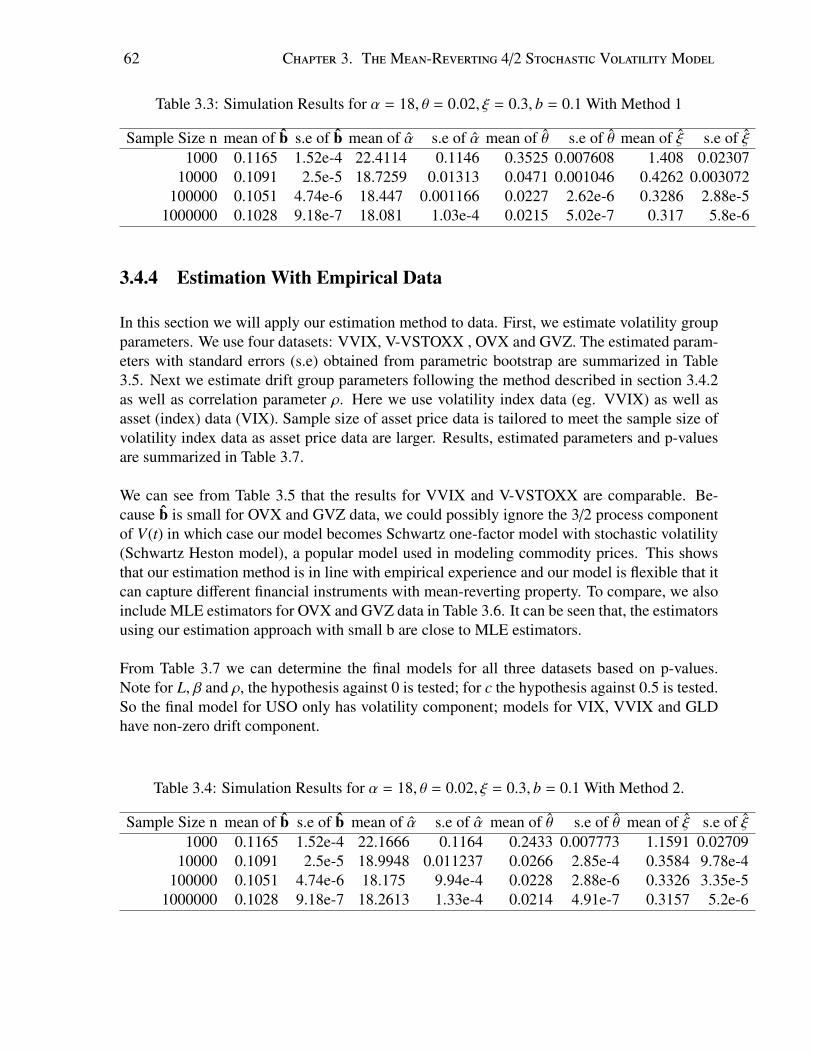
62 Chapter 3. TheMean-Reverting 4/2 Stochastic VolatilityModel
Table 3.3: Simulation Results for α = 18, θ = 0.02, ξ = 0.3, b = 0.1 With Method 1
Sample Size n mean of b s.e of b mean of α s.e of α mean of θ s.e of θ mean of ξ s.e of ξ1000 0.1165 1.52e-4 22.4114 0.1146 0.3525 0.007608 1.408 0.02307
10000 0.1091 2.5e-5 18.7259 0.01313 0.0471 0.001046 0.4262 0.003072100000 0.1051 4.74e-6 18.447 0.001166 0.0227 2.62e-6 0.3286 2.88e-5
1000000 0.1028 9.18e-7 18.081 1.03e-4 0.0215 5.02e-7 0.317 5.8e-6
3.4.4 Estimation With Empirical Data
In this section we will apply our estimation method to data. First, we estimate volatility groupparameters. We use four datasets: VVIX, V-VSTOXX , OVX and GVZ. The estimated param-eters with standard errors (s.e) obtained from parametric bootstrap are summarized in Table3.5. Next we estimate drift group parameters following the method described in section 3.4.2as well as correlation parameter ρ. Here we use volatility index data (eg. VVIX) as well asasset (index) data (VIX). Sample size of asset price data is tailored to meet the sample size ofvolatility index data as asset price data are larger. Results, estimated parameters and p-valuesare summarized in Table 3.7.
We can see from Table 3.5 that the results for VVIX and V-VSTOXX are comparable. Be-cause b is small for OVX and GVZ data, we could possibly ignore the 3/2 process componentof V(t) in which case our model becomes Schwartz one-factor model with stochastic volatility(Schwartz Heston model), a popular model used in modeling commodity prices. This showsthat our estimation method is in line with empirical experience and our model is flexible that itcan capture different financial instruments with mean-reverting property. To compare, we alsoinclude MLE estimators for OVX and GVZ data in Table 3.6. It can be seen that, the estimatorsusing our estimation approach with small b are close to MLE estimators.
From Table 3.7 we can determine the final models for all three datasets based on p-values.Note for L, β and ρ, the hypothesis against 0 is tested; for c the hypothesis against 0.5 is tested.So the final model for USO only has volatility component; models for VIX, VVIX and GLDhave non-zero drift component.
Table 3.4: Simulation Results for α = 18, θ = 0.02, ξ = 0.3, b = 0.1 With Method 2.
Sample Size n mean of b s.e of b mean of α s.e of α mean of θ s.e of θ mean of ξ s.e of ξ1000 0.1165 1.52e-4 22.1666 0.1164 0.2433 0.007773 1.1591 0.02709
10000 0.1091 2.5e-5 18.9948 0.011237 0.0266 2.85e-4 0.3584 9.78e-4100000 0.1051 4.74e-6 18.175 9.94e-4 0.0228 2.88e-6 0.3326 3.35e-5
1000000 0.1028 9.18e-7 18.2613 1.33e-4 0.0214 4.91e-7 0.3157 5.2e-6

3.5. Pricing Financial Derivatives 63
Table 3.5: Estimated Volatility Group Parameters With Empirical Data
Data: VVIX Data: V-VSTOXX Data: OVX Data: GVZb 0.0892 0.067 0.0053 0.002Mean of b (s.e) 0.104 (7.54e-5) 0.0848 (7.99e-5) 0.0061 (1.91e-5) 0.0026 (7.81e-6)α 17.00512 19.48345 3.6754 4.7937Mean of α (s.e) 18.691 (0.06836) 21.309 (0.05850) 4.09 (0.01806) 5.0976 (0.01977)θ 0.015293 0.00961 0.1472 0.0395Mean of θ (s.e) 0.0273 (9.51e-4) 0.0172 (4.28e-5) 0.1444 (3.54e-4) 0.0382 (7.62e-5)ξ 0.27014 0.21462 0.6006 0.2873Mean of ξ (s.e) 0.36 (0.001407) 0.315 (7.15e-4) 0.5946 (9.45e-4) 0.2876 (4.3e-4)
Table 3.6: MLE Estimates For OVX and GVZ Data
Data: OVX Data: GVZα 3.9042 5.028Mean of α (s.e) 4.2791 (0.01785) 5.4036 (0.01878)θ 0.1530 0.0426Mean of θ (s.e) 0.1522 (4.02e-4) 0.0423 (9.33e-5)ξ 0.6849 0.4149Mean of ξ (s.e) 0.6848 (1.8e-4) 0.4149 (1.07e-4)
Table 3.7: Estimated Drift Group Parameters
Data L p-value c p-value β p-vale ρ p-valueVIX&VVIX -1.6411 0.44 -5.320 0.000145 3.7020 3.44e-5 -0.67 0VSTOXX&VVSTOXX -7.060 0.044252 -1.580 0.360 5.4841 0.000483 -0.49 0USO&OVX 0.0870 0.678 -0.579 0.313 -0.0376 0.793 -0.35 0GLD&GVZ 3.7672 0.015 0.572 0.97 0.78 0.014 -0.08 0
3.5 Pricing Financial Derivatives
In this section, we price vanilla European call options based on our model for different assets:VIX, USO Oil ETF and Gold ETF (GLD). We use the parameters estimated in section 3.4.4and assume risk-free interest rate of 2%. Our purpose is to assess the effect of b (as a was setto 1) on the price. We investigate whether the presence of b makes a difference by looking atthe absolute value of the relative change (ARC) in implied volatility (IV):ARC = |
IVb=0−IVb=bIVb=b
|
for b = 0 against b = b (Figure 3.3 and Figure 3.4). We also report the maximum absolutevalue of the relative change in terms of option prices for completeness.
In section 3.5.1, we display how b affects the call option prices for VIX. In section 3.5.2,we study the effect on call option prices for USO. In section 3.5.3, we compare two popu-lar option pricing methods for GLD: Fast Fourier Transform (FFT) developed by Carr andMadan [29] and Monte Carlo simulation in a special setting (Schwartz Heston model) where
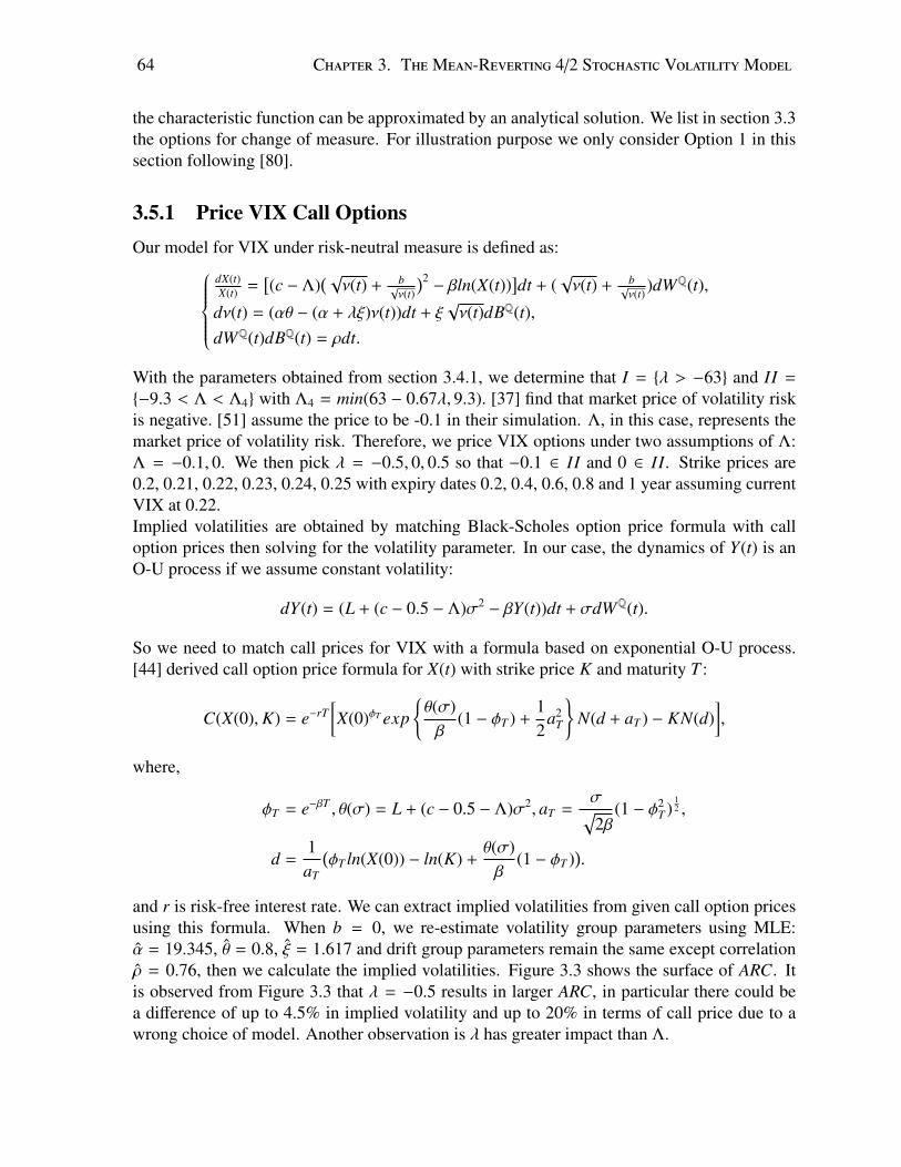
64 Chapter 3. TheMean-Reverting 4/2 Stochastic VolatilityModel
the characteristic function can be approximated by an analytical solution. We list in section 3.3the options for change of measure. For illustration purpose we only consider Option 1 in thissection following [80].
3.5.1 Price VIX Call OptionsOur model for VIX under risk-neutral measure is defined as:
dX(t)X(t) =
[(c − Λ)
(√ν(t) + b
√ν(t)
)2− βln(X(t))
]dt + (
√ν(t) + b
√ν(t)
)dWQ(t),
dν(t) = (αθ − (α + λξ)ν(t))dt + ξ√ν(t)dBQ(t),
dWQ(t)dBQ(t) = ρdt.
With the parameters obtained from section 3.4.1, we determine that I = λ > −63 and II =
−9.3 < Λ < Λ4 with Λ4 = min(63 − 0.67λ, 9.3). [37] find that market price of volatility riskis negative. [51] assume the price to be -0.1 in their simulation. Λ, in this case, represents themarket price of volatility risk. Therefore, we price VIX options under two assumptions of Λ:Λ = −0.1, 0. We then pick λ = −0.5, 0, 0.5 so that −0.1 ∈ II and 0 ∈ II. Strike prices are0.2, 0.21, 0.22, 0.23, 0.24, 0.25 with expiry dates 0.2, 0.4, 0.6, 0.8 and 1 year assuming currentVIX at 0.22.Implied volatilities are obtained by matching Black-Scholes option price formula with calloption prices then solving for the volatility parameter. In our case, the dynamics of Y(t) is anO-U process if we assume constant volatility:
dY(t) = (L + (c − 0.5 − Λ)σ2 − βY(t))dt + σdWQ(t).
So we need to match call prices for VIX with a formula based on exponential O-U process.[44] derived call option price formula for X(t) with strike price K and maturity T :
C(X(0),K) = e−rT[X(0)φT exp
θ(σ)β
(1 − φT ) +12
a2T
N(d + aT ) − KN(d)
],
where,
φT = e−βT , θ(σ) = L + (c − 0.5 − Λ)σ2, aT =σ√2β
(1 − φ2T )
12 ,
d =1aT
(φT ln(X(0)) − ln(K) +
θ(σ)β
(1 − φT )).
and r is risk-free interest rate. We can extract implied volatilities from given call option pricesusing this formula. When b = 0, we re-estimate volatility group parameters using MLE:α = 19.345, θ = 0.8, ξ = 1.617 and drift group parameters remain the same except correlationρ = 0.76, then we calculate the implied volatilities. Figure 3.3 shows the surface of ARC. Itis observed from Figure 3.3 that λ = −0.5 results in larger ARC, in particular there could bea difference of up to 4.5% in implied volatility and up to 20% in terms of call price due to awrong choice of model. Another observation is λ has greater impact than Λ.
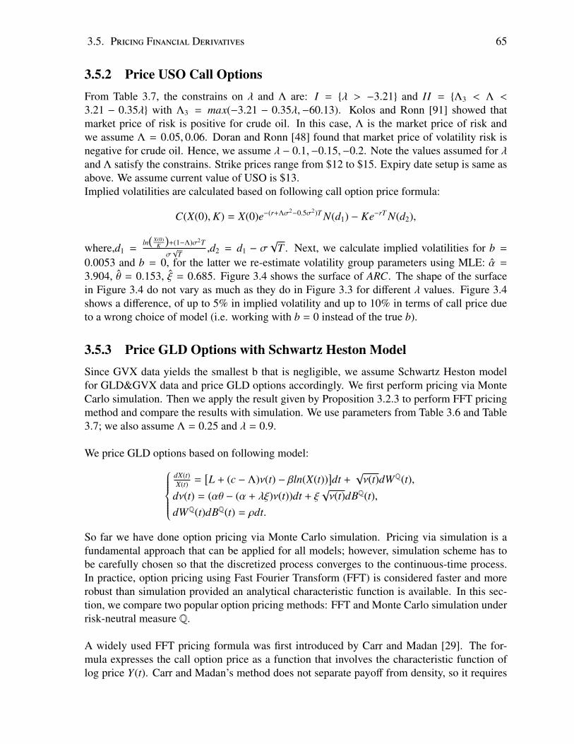
3.5. Pricing Financial Derivatives 65
3.5.2 Price USO Call OptionsFrom Table 3.7, the constrains on λ and Λ are: I = λ > −3.21 and II = Λ3 < Λ <3.21 − 0.35λ with Λ3 = max(−3.21 − 0.35λ,−60.13). Kolos and Ronn [91] showed thatmarket price of risk is positive for crude oil. In this case, Λ is the market price of risk andwe assume Λ = 0.05, 0.06. Doran and Ronn [48] found that market price of volatility risk isnegative for crude oil. Hence, we assume λ − 0.1,−0.15,−0.2. Note the values assumed for λand Λ satisfy the constrains. Strike prices range from $12 to $15. Expiry date setup is same asabove. We assume current value of USO is $13.Implied volatilities are calculated based on following call option price formula:
C(X(0),K) = X(0)e−(r+Λσ2−0.5σ2)T N(d1) − Ke−rT N(d2),
where,d1 =ln(
X(0)K
)+(1−Λ)σ2T
σ√
T,d2 = d1 − σ
√T . Next, we calculate implied volatilities for b =
0.0053 and b = 0, for the latter we re-estimate volatility group parameters using MLE: α =
3.904, θ = 0.153, ξ = 0.685. Figure 3.4 shows the surface of ARC. The shape of the surfacein Figure 3.4 do not vary as much as they do in Figure 3.3 for different λ values. Figure 3.4shows a difference, of up to 5% in implied volatility and up to 10% in terms of call price dueto a wrong choice of model (i.e. working with b = 0 instead of the true b).
3.5.3 Price GLD Options with Schwartz Heston ModelSince GVX data yields the smallest b that is negligible, we assume Schwartz Heston modelfor GLD&GVX data and price GLD options accordingly. We first perform pricing via MonteCarlo simulation. Then we apply the result given by Proposition 3.2.3 to perform FFT pricingmethod and compare the results with simulation. We use parameters from Table 3.6 and Table3.7; we also assume Λ = 0.25 and λ = 0.9.
We price GLD options based on following model:dX(t)X(t) =
[L + (c − Λ)ν(t) − βln(X(t))
]dt +
√ν(t)dWQ(t),
dν(t) = (αθ − (α + λξ)ν(t))dt + ξ√ν(t)dBQ(t),
dWQ(t)dBQ(t) = ρdt.
So far we have done option pricing via Monte Carlo simulation. Pricing via simulation is afundamental approach that can be applied for all models; however, simulation scheme has tobe carefully chosen so that the discretized process converges to the continuous-time process.In practice, option pricing using Fast Fourier Transform (FFT) is considered faster and morerobust than simulation provided an analytical characteristic function is available. In this sec-tion, we compare two popular option pricing methods: FFT and Monte Carlo simulation underrisk-neutral measure Q.
A widely used FFT pricing formula was first introduced by Carr and Madan [29]. The for-mula expresses the call option price as a function that involves the characteristic function oflog price Y(t). Carr and Madan’s method does not separate payoff from density, so it requires
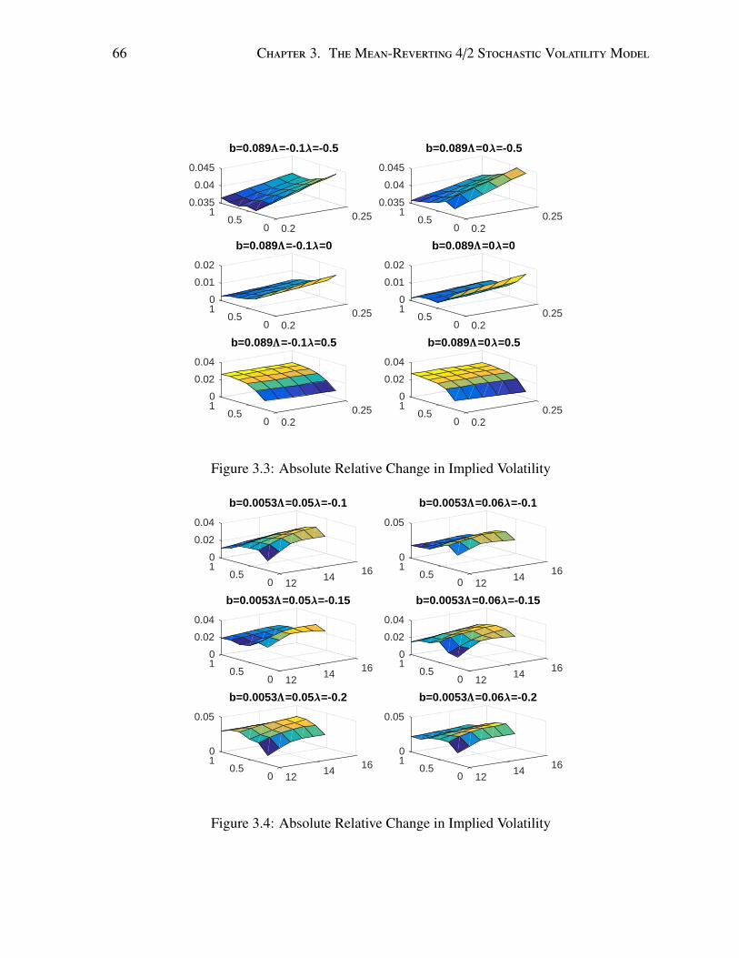
66 Chapter 3. TheMean-Reverting 4/2 Stochastic VolatilityModel
0.0351
0.04
0.25
b=0.089 =-0.1 =-0.5
0.5
0.045
0 0.2
01
0.01
0.25
b=0.089 =-0.1 =0
0.5
0.02
0 0.2
01
0.02
0.25
b=0.089 =-0.1 =0.5
0.5
0.04
0 0.2
0.0351
0.04
0.25
b=0.089 =0 =-0.5
0.5
0.045
0 0.2
01
0.01
0.25
b=0.089 =0 =0
0.5
0.02
0 0.2
01
0.02
0.25
b=0.089 =0 =0.5
0.5
0.04
0 0.2
Figure 3.3: Absolute Relative Change in Implied Volatility
01
0.02
16
b=0.0053 =0.05 =-0.1
0.5
0.04
140 12
01
0.02
16
b=0.0053 =0.05 =-0.15
0.5
0.04
140 12
01 16
b=0.0053 =0.05 =-0.2
0.5
0.05
140 12
01 16
b=0.0053 =0.06 =-0.1
0.5
0.05
140 12
01
0.02
16
b=0.0053 =0.06 =-0.15
0.5
0.04
140 12
01 16
b=0.0053 =0.06 =-0.2
0.5
0.05
140 12
Figure 3.4: Absolute Relative Change in Implied Volatility
3.5. Pricing Financial Derivatives 67
an exponential damping factor to ensure the integrability of option payoff. Lewis [96] furtherproposed a generalized Fourier-transform approach to European options pricing. Both methodsrequire the conditional characteristic function of the underlying process to be known explicitlyor at least efficiently computed. Instead of introducing the damping factor, Lewis’s methodworks with the region where the conditional characteristic function is defined. In this section,we follow Carr and Madan’s framework but modify the formula a little bit since our character-istic function and its approximations are based on Z(t) process instead of Y(t).
Suppose a given option with maturity T and strike K at given time t, t ≥ 0, whose payoff, P, isa function of V(T ), i.e P = F(V(T )) (for a European call option P = F(V(T )) = (V(T ) − K)+).Recall that Z(t) = eβtY(t) and Y(t) = ln(X(t)), so X(t) = exp(e−βtZ(t)), or we express X(t) as afunction of Z(t), i.e X(t) = g(Z(t)). Then we have the relationship between the payoff of theVIX option and Z(T ):
P = F(g(Z(T ))) = G(Z(T )).
The price, C(t,T ), of the option is the conditional expected value of P under risk-neutral mea-sure:
C(t,T ) = e−r(T−t)EQ(P|Ft)
= e−r(T−t)EQ(G(Z(T ))|Ft),
where r is the risk-neutral interest rate.
Let fT (z) be the risk-neutral density function of Z(T ) and the price at t = 0 be CT (k) = C(0,T ),a function of strike price k with k = g−1(K) = eβT ln(K). By definition the characteristic func-tion of Z(T ) is the Fourier transform of fT (z):
ψ(u) =
∫ ∞
−∞
eiuz fT (z)dz,
As we work on European call option on of VIX and Z(T ), hence the payoff function is:
P = G(Z(T )) = (exp(e−βT Z(T )) − exp(e−βT k))+.
So we have the option price expressed in terms of z:
CT (k) = e−rT∫ ∞
k(exp(e−βT z) − exp(e−βT k)) fT (z)dz. (3.21)
An issue with 3.21 is that the integral is not square integrable as k → −∞. To solve the problem,Carr and Madan [29] modified the price by multiplying a damping factor eck to the price. LetcT (k) denote the modified price, so:
cT (k) = eckCT (k).
Now we apply Fourier transform to cT (k):
ψ′
(v) =
∫ ∞
−∞
eivkcT (k)dk,

68 Chapter 3. TheMean-Reverting 4/2 Stochastic VolatilityModel
for v ∈ R. Then CT (k) is the inverse Fourier transform of cT (k):
CT (k) =e−ck
2π
∫ ∞
−∞
e−ivkψ′
(v)dv. (3.22)
The price being real implies that ψ′
(v) is odd in its imaginary part and even in its real part [29].We can also simplify CT (k) to be:
CT (k) =e−ck
π
∫ ∞
0e−ivkψ
′
(v)dv. (3.23)
If we can find an expression for ψ′
(v), we can plug it into 3.23 to find the price numericallyusing Fast Fourier Transform (FFT) algorithm. Therefore, we don’t need to worry about thedensity function fT (z) in 3.21 as long as we have found the characteristic function for the un-derlying process.
From above we have:
ψ′
(v) = e−rT∫ ∞
−∞
eivkeck∫ ∞
k(exp(e−βT z) − exp(e−βT k)) fT (z)dzdk
By Fubini’s Theorem:
ψ′
(v) = e−rT∫ ∞
−∞
( ∫ z
−∞
(exp(e−βT z) − exp(e−βT k))e(iv+c)kdk)
fT (z)dz
= e−rT∫ ∞
−∞
(e(e−βT +iv+c)z
iv + c−
e(e−βT +iv+c)z
e−βT + iv + c
)fT (z)dz
= e−(r+β)T∫ ∞
−∞
e(e−βT +iv+c)z
c2 + e−βT c − v2 + (2c + e−βT )ivfT (z)dz
=e−(r+β)Tψ(v − i(e−βT + c))
c2 + e−βT c − v2 + (2c + e−βT )iv
ψ′
(v) is now a function which involves the characteristic function of Z(T ). So the original priceCT (k) can be written as:
CT (k) =e−ck
π
∫ ∞
0e−ivk e−(r+β)Tψ(v − i(e−βT + c))
c2 + e−βT c − v2 + (2c + e−βT )ivdv. (3.24)
Now we apply FFT to compute the price numerically. Assuming current GLD price is $120,we set the strike prices $118, $119.4, $120.8, $122.2, $123.6, $125 with quarterly maturitythroughout a year i.e t = 0 and T ∈ [0.25, 0.5, 0.75, 1]. We calculate the absolute relative pricedifference with respect to the prices from simulation and summarize our findings in Table 3.8.From the table, we can see that option prices using FFT are less that 1% different from pricesfrom simulation in absolute value. The results, on the other hand, suggest that our approxima-tion approach is able to capture the behavior of the characteristic function of Schwartz Hestonmodel. Hence, we can use FFT method to price options, which is faster than simulation.
3.6. Conclusion 69
Table 3.8: Absolute Relative Price Difference: FFT vs. Simulation
Strike T=0.25 T=0.5 T=0.75 T=1118 0.0027 0.0015 0.0035 0.005
119.4 0.0032 0.0021 0.0036 0.0056120.8 0.0036 0.0026 0.0038 0.0063122.2 0.0042 0.0032 0.004 0.0071123.6 0.005 0.0038 0.0042 0.0079125 0.0059 0.0046 0.0045 0.0087
3.6 ConclusionIn this chapter we define and show properties of a new model displaying mean-reversion andstochastic volatility. We find a semi-analytic solution for the characteristic function. Eventhough simulation is still required to find this characteristic function, the cost of computation isgreatly reduced from simulating two stochastic processes to one process (the underlying CIRprocess that drives the stochastic volatility). The benefit of the semi-closed characteristic func-tion becomes more significant in higher dimensions. We further propose two approximationapproaches to improve the computational efficiency of the characteristic function. The nu-merical results are promising showing our approximation approaches perform well in a wideparametric region, especially the average approach yields negligible approximation errors. Weare also the first proposing a method to estimate the parameters of the 4/2 family of stochasticvolatility models, the methods are simple and requires low computational power. From the ta-bles in section 3.4.4, it can be seen that our estimation method, though biased for low sample,still provides consistent estimates for the true parameters. By adding a 3/2 component in thevolatility, we generate more flexibility in our model than [16]. For volatility index markets(VIX and VSTOXX) and for the commodity USO market, the effect of this 3/2 addition isconfirmed empirically and substantial in terms of impact on option pricing. Since our modelincorporates two models ( [122] and [76]), there could exist various applications to differentmarkets (eg. interest rate and exchange rate). Table 3.8 again supports the appropriatenessof our average approximation approach as the option prices from FFT method using approx-imated characteristic function is close to the option prices from Monte Carlo simulation, theabsolute price difference is at 10−3 level. One exercise that is not demonstrated in this chap-ter is revisiting estimation with approximated characteristic function and methods that dependon closed-form characteristic functions. With semi-closed form characteristic functions, wecannot use estimation methods such as efficient method of moments (EMM) [70], generalizedmethod of moments (GMM) [78] and quasi-maximum likelihood (QML) [110] [79], whichrely on analytic density/transition density functions. We will mention about this again in chap-ter 5. The approximation approaches give us analytic functions, thus the EMM, GMM or QMLcan be used and their performance can be evaluated against our proposed estimation method.This is an interesting exercise for future research.
Chapter 4
Generalized Mean-Reverting 4/2 FactorModel
Continuous-time stochastic covariance models are crucial in capturing many stylized facts infinancial data, from heteroscedasticity and fat tails to changing correlations and leverage ef-fects. Early work in this field focused on discrete time models in the form of generalizedautoregressive conditional heteroskedasticity (GARCH) models (see [56]). The best-knownrepresentatives in continuous time, are the stochastic Wishart family (see [75, 40]) and theOrnstein–Uhlenbeck (OU) family (see [109]) of models, as well as general linear-quadraticjump-diffusions (see [31]). These approaches are more realistic than the classical Black–Scholes lognormal model, but they quickly become intractable as dimensions increase in termsof the number of parameters and simulation paths, commonly known as the “curse of dimen-sionality”. Recent papers (see [57, 41]) have presented models built from linear combination oftractable one-dimensional counterparts. These models involve fewer parameters than Wishart-or OU-type approaches, owing to a reduction in dimensionality while providing a closed-formsolution to financial problems.
In this chapter, we introduce a multivariate mean-reverting stochastic volatility factor modelthat combines 1/2 (Heston-type, [80]) and 3/2 processes [117] for the modeling of volatility.Such underlying volatility processes were coined 4/2 by [76]. In section 4.1, we give thedefinitions of our model. Our model takes advantage of the factor structure in asset prices andallows for a mean-reverting structure on the assets thereby aiming at capturing either multivari-ate commodity behavior or multiple volatility indexes (see [73] for an alternative multivariatenon-mean-reverting generalization based on a pairwise-structure applied to the exchange-ratemarket). In particular, our setting reduces the dimension of the parametric space which is a wayof controlling the “curse of dimensionality” making parameters identifiable and popular esti-mation methods feasible. Secondly, the presence of independent common and intrinsic factors,each with its own stochastic volatility, enables an elegant separable structure for characteristicfunctions (c.f.s) and captures several stylized facts, such as: stochastic volatility, stochasticcorrelation among stocks (see [56]), co-movements in the variances (see [45]), multiple factorsin the volatilities (see [36]) and stock correlations (see [40]). Thirdly, a factor representationis compatible with economical interpretations, where common factors are exogenous variablesexplaining financial markets, and intrinsic factors relate to companies’ intrinsic risks. Lastly,
70
4.1. Model Description 71
closed-form expressions are available for joint c.f.s; this is useful for derivative pricing andrisk management calculations via Fourier transformations, and it makes c.f.-based estimationsmethods feasible (see [29] [69] [27]).
The rationale for a 4/2 volatility process rather than a 1/2 or 3/2 model is masterly presentedin [76] for a one-dimensional structure. For instance, as observed by the author, the 1/2 processpredicts that the implied volatility skew will flatten when the instantaneous volatility increases(crises), while the 3/2 model predicts steepening skews. The empirical violation of the Fellercondition in the 1/2 model is also noted, which makes volatility paths stay closer to 0 fora longer period than empirically supported, while the 3/2 model admits extreme paths withspikes in instantaneous volatility. The two processes complement each other as they implyvery different dynamics for the evolution of the implied volatility surface. It stands to reasonthat such a convenient underlying driver for multidimensional structures should be used to im-prove not only marginal volatility behavior, but also the dependence structure.
In section 4.2, we obtain an analytical representation for the c.f. of the vector of asset prices,which is in closed-form for non-mean-reverting nested cases. This type of c.f. is helpful forderivative pricing purposes. We also produce a second conditional c.f. that can be used forexact simulations of the non-mean reverting assets given the terminal volatilities, where thelatter can be simulated exactly via chi-squares. We identify a set of conditions that not onlyproduces well-defined changes of measure, but also avoids local martingales; hence, it can beused for risk-neutral pricing purposes.
In section 4.3, our results are applied numerically to parameters inspired by commodity prices1.There is a vast literature on commodity modeling (see, for instance, [122] [34], and more re-cently [121]). In our numerical study, we investigated the impact of the new parameters (b,the weight of 3/2 in the overall instantaneous volatility) on the shape of the implied volatilitysurface. This chapter is a result of collaboration with Prof. Marcos Escobar-Anel and YuyangCheng.
4.1 Model Description
Next, we define the model in a filtered probability space (Ω,F ,P, Ftt≥0) where F0 contains allsubsets of the (P−) null sets of F and Ftt≥0 is right-continuous. We first provide the processesunder the historical measure P, then followed by the processes under a (conveniently chosen)risk-neutral measure Q. Suppose that Xt = (X1(t), ..., Xn(t))′ is a vector of asset prices with the
1This can also be applied to volatility indexes, such as those reported by the Chicago Board Options Exchange(CBOE), which are clearly a mean-reverting asset class with stochastic volatility.
72 Chapter 4. GeneralizedMean-Reverting 4/2 FactorModel
following P-measure representation:
dXi(t)Xi(t)
=
Li + ci
p∑j=1
a2i j
√v j(t) +b j√v j(t)
2
−
p∑j=1
βi j ln(X j(t)) + ci
(√vi(t) +
bi√
vi(t)
)2 dt
+
p∑j=1
ai j
√v j(t) +b j√v j(t)
dWPj (t) +
(√vi(t) +
bi√
vi(t)
)dWPi (t)
dv j(t) = α j(θ j − v j(t))dt + ξ j
√v j(t)dBPj (t), j = 1, ..., p
dvi(t) = αi(θi − vi(t))dt + ξi√
vi(t)dBPi (t), i = 1, ..., n
The quadratic variation structure is⟨dBPj (t), dWP
j (t)⟩
= ρ jdt,⟨dBPi (t), dWP
i (t)⟩
= ρidt and zerootherwise. In the language of factor analysis, ai j is the i jth entry of the matrix of factor loadings(A) that captures the correlations among assets. The commonalities are represented by V j(t) =(√
v j(t) +b j√v j(t)
)2
(in matrix form, Λnxp = Adiag(V1/2
t
)) and the intrinsic residual variance is
Ψ = diag(Vt), with V j(t) =(√
vi(t) + bi√vi(t)
)2. This leads to a factors decomposition of the
quadratic variation of asset prices as follows:
Σtdt =(ΛΛ′ + Ψ
)dt =
(Adiag(Vt)A′ + diag(Vt)
)dt
Whenever necessary, we assume n = p and A = (ai j)n×p to be an orthogonal matrix. In thissetting, ci and ci represent risk premiums of asset Xi(t) associated with the common and intrin-sic factors, respectively. B = (βi j)n×n is an invertible matrix, which captures the spillover at theexpected return level Xi(t) on asset X j(t). In other words, it represents the impact from otherassets on the long term average price of the current one.
Based on the quadratic variation relationship defined in this model, if we assume that BPj ,BPj (t)
⊥, BPi (t), BPi (t)⊥ are independent Brownian motions with −1 ≤ ρ j ≤ 1 and −1 ≤ ρi ≤ 1.Then,
dWPj (t) = ρ jdBPj (t) +
√1 − ρ2
jdBPj (t)⊥
dWPi (t) = ρidBPi (t) +
√1 − ρ2
i dBPi (t)⊥.
v j j = 1, .., n and vi i = 1, .., n follow standard CIR processes, hence α j, θ j, and ξ j are posi-
tive constants satisfying α jθ j ≥ξ2
j
2 (the Feller condition). Similarly, αi, θi, and ξi are positive
constants satisfying αiθi ≥ξi
2
2 . Note that the Feller condition in CIR model guarantees that theprocess remains positive.
The transformation Yt = ln(Xt) would create a multivariate Ornstein–Uhlenbeck process witha 4/2 stochastic factor structure:
dYi(t) =
Li +
(ci −
12
) n∑j=1
a2i j
√v j(t) +b j√v j(t)
2
−
n∑j=1
βi jY j(t) +
(ci −
12
) (√vi(t) +
bi√
vi(t)
)2 dt
+
n∑j=1
ai j
√v j(t) +b j√v j(t)
dW j(t) +
(√vi(t) +
bi√
vi(t)
)dWi(t)
4.1. Model Description 73
To stay in line with [94] and [95], we enforce the same assumption that the eigenvalues of thematrix
−β11 · · · −β1n...
. . ....
−βn1 · · · −βnn
are all negative.
This general model includes a notable particular case, which is a direct generalization of [76]to a factor setting when βi j = 0, i, j = 1, .., n ; this case is studied in more detail and it is namedFG, given its analytical flexibility.
4.1.1 Special Case: No Intrinsic FactorIn this section, we introduce a model as a special case of our generalized mean-reverting 4/2factor model. In this case, the only factor that impacts the asset is the common factor of theasset i.e Ψ = 0.
Suppose Xt = (X1(t), . . . , Xn(t))′ is a vector of assets. The dynamics for each asset Xi(t) underhistorical measure P is defined as:
dXi(t)Xi(t)
=
[Li + ci
n∑j=1
a2i j( √
ν j(t) +b j√ν j(t)
)2−
n∑j=1βi jln(X j(t))
]dt +
n∑j=1
ai j( √
ν j(t) +b j√ν j(t)
)dWP
j (t),
dν j(t) = α j(θ j − ν j(t))dt + ξ j√ν j(t)dBPj (t), j = 1, . . . , n
(4.1)The dynamics of log price Yi(t) = ln(Xi(t)) is then:
dYi(t) =
[Li + (ci −
12 )
n∑j=1
a2i j( √
ν j(t) +b j√ν j(t)
)2−
n∑j=1βi jY j(t)
]dt +
∑nj=1 ai j
( √ν j(t) +
b j√ν j(t)
)dWP
j (t),
dν j(t) = α j(θ j − ν j(t))dt + ξ j√ν j(t)dBPj (t), j = 1, . . . , n.
(4.2)For the covariance matrix Σt, the factor decomposition is therefore:
Σtdt = ΛΛ′dt = Adiag(Vt)A′dt
For example, we are modeling two assets with SDE 4.1:
dX1(t)X1(t)
=
[L1 + a2
11c1( √
ν1(t) +b1√ν1(t)
)2+ a2
12c1( √
ν2(t) +b2√ν2(t)
)2− β11ln(X1(t)) − β12ln(X2(t))
]dt
+ a11( √
ν1(t) +b1√ν1(t)
)dWP
1 (t) + a12( √
ν2(t) +b2√ν2(t)
)dWP
2 (t),
dX2(t)X2(t)
=
[L2 + a2
21c2( √
ν1(t) +b1√ν1(t)
)2+ a2
22c2( √
ν2(t) +b2√ν2(t)
)2− β21ln(X1(t)) − β22ln(X2(t))
]dt
+ a21( √
ν1(t) +b1√ν1(t)
)dWP
1 (t) + a22( √
ν2(t) +b2√ν2(t)
)dWP
2 (t),
74 Chapter 4. GeneralizedMean-Reverting 4/2 FactorModel
4.2 ResultsThis section describes viable changes of measure and two key characteristic functions of thetargeted multivariate process; one for pricing and the other for simulations. The proofs arepresented in B.1.
4.2.1 Change of Measure
Here, we explore the topic of creating a risk-neutral measure Q for pricing purposes. As notedby [76] [118] and [10] among others, a risk-neutral measure may not be supported by data inthe presence of a 3/2 model (e.g., 1
√v(t)
), as the parametric constraints needed for the discountedasset price process to be a Q- martingale are violated with real data; hence, we can only pro-duce a strict Q-local martingale (i.e., Q would be absolute continuous but not equivalent toP). In such situation, the standard risk-neutral pricing methodology would fail (biased prices),and we have to turn to the benchmark approach for pricing (see [10]).
The next proposition entertains the following changes of measure with constant λ j, λ⊥j , λi
and λ⊥i (see chapter 3 for other types of changes of measures) then identifies the parametricconditions needed for the existence of a valid risk-neutral measure Q.
dBQj (t) = λ j
√v j(t) +b j√v j(t)
dt + dBPj (t), dBQ
i (t) = λi
(√vi(t) +
bi√
vi(t)
)dt + dBP
i (t)
dBQj (t)⊥ = λ⊥j
√v j(t) +b j√v j(t)
dt + dBPj (t)⊥, dBQ
i (t)⊥ = λ⊥i
(√vi(t) +
bi√
vi(t)
)dt + dBP
i (t)⊥
Proposition 4.2.1 The change of measure is well-defined for pricing purposes under the fol-lowing four conditions:
ξ2j ≤ 2α jθ j − 2ξ j max
∣∣∣b jλ j
∣∣∣ , ∣∣∣λ⊥j b j
∣∣∣ , ∣∣∣b ja1 jρ j
∣∣∣ , ..., ∣∣∣b jan jρ j
∣∣∣ (4.3)
ξ2i ≤ 2αiθi − 2ξi max
∣∣∣∣biλi
∣∣∣∣ , ∣∣∣∣λ⊥i bi
∣∣∣∣ , ∣∣∣∣biρi
∣∣∣∣ (4.4)
max∣∣∣λ j
∣∣∣ , ∣∣∣λ⊥j ∣∣∣ <α j
ξ j(4.5)
max∣∣∣λi
∣∣∣ , ∣∣∣λ⊥i ∣∣∣ <αi
ξi
(4.6)
Moreover, if βi j = 0 for i, j = 1, .., n, then the following must also be satisfied:
Li = r, ci =
n∑j=1
ai j
(ρ jλ j +
√1 − ρ2
jλ⊥j
), ci = ρiλi +
√1 − ρ2
i λ⊥i (4.7)
Proof is included in Appendix.
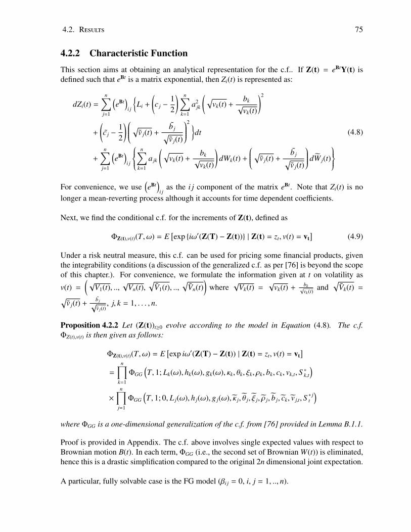
4.2. Results 75
4.2.2 Characteristic Function
This section aims at obtaining an analytical representation for the c.f.. If Z(t) = eBtY(t) isdefined such that eBt is a matrix exponential, then Zi(t) is represented as:
dZi(t) =
n∑j=1
(eBt
)i j
Li +
(c j −
12
) n∑k=1
a2jk
(√vk(t) +
bk√
vk(t)
)2
+
(c j −
12
) √v j(t) +b j√v j(t)
2 dt
+
n∑j=1
(eBt
)i j
n∑k=1
a jk
(√vk(t) +
bk√
vk(t)
)dWk(t) +
√v j(t) +b j√v j(t)
dW j(t)
(4.8)
For convenience, we use(eBt
)i j
as the i j component of the matrix eBt. Note that Zi(t) is nolonger a mean-reverting process although it accounts for time dependent coefficients.
Next, we find the conditional c.f. for the increments of Z(t), defined as
ΦZ(t),v(t)(T, ω) = E[exp iω′(Z(T) − Z(t)) | Z(t) = zt, v(t) = vt
](4.9)
Under a risk neutral measure, this c.f. can be used for pricing some financial products, giventhe integrability conditions (a discussion of the generalized c.f. as per [76] is beyond the scopeof this chapter.). For convenience, we formulate the information given at t on volatility as
v(t) =
(√
V1(t), ..,√
Vn(t),√
V1(t), ..,√
Vn(t))
where√
Vk(t) =√
vk(t) + bk√vk(t)
and√
Vk(t) =√v j(t) +
b j√v j(t)
, j, k = 1, . . . , n.
Proposition 4.2.2 Let (Z(t))t≥0 evolve according to the model in Equation (4.8). The c.f.ΦZ(t),v(t) is then given as follows:
ΦZ(t),v(t)(T, ω) = E[exp iω′(Z(T) − Z(t)) | Z(t) = zt, v(t) = vt
]=
n∏k=1
ΦGG
(T, 1; Lk(ω), hk(ω), gk(ω), κk, θk, ξk, ρk, bk, ck, vk,t, S ∗k,t
)×
n∏j=1
ΦGG
(T, 1; 0, L j(ω), h j(ω), g j(ω), κ j, θ j, ξ j, ρ j, b j, ck, v j,t, S
∗ jt
)where ΦGG is a one-dimensional generalization of the c.f. from [76] provided in Lemma B.1.1.
Proof is provided in Appendix. The c.f. above involves single expected values with respect toBrownian motion B(t). In each term, ΦGG (i.e., the second set of Brownian W(t)) is eliminated,hence this is a drastic simplification compared to the original 2n dimensional joint expectation.
A particular, fully solvable case is the FG model (βi j = 0, i, j = 1, .., n).
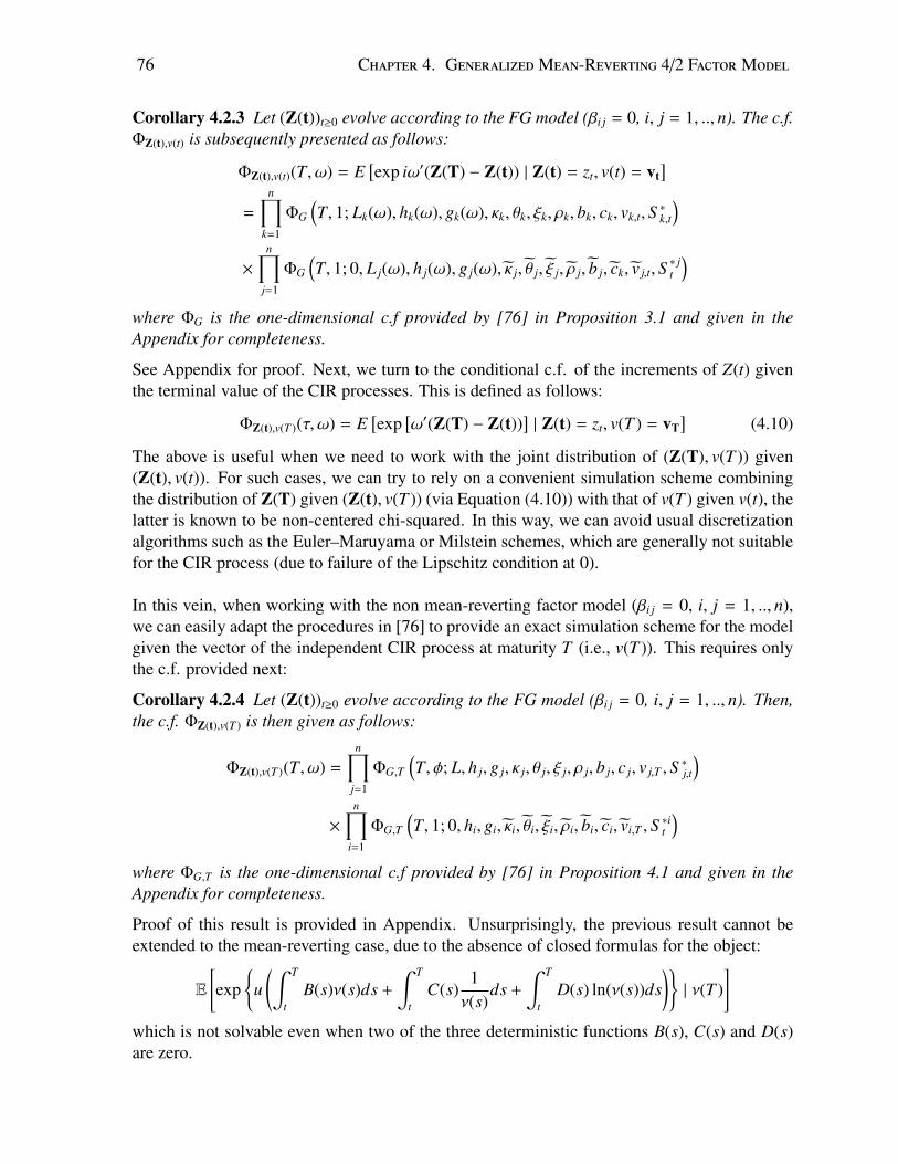
76 Chapter 4. GeneralizedMean-Reverting 4/2 FactorModel
Corollary 4.2.3 Let (Z(t))t≥0 evolve according to the FG model (βi j = 0, i, j = 1, .., n). The c.f.ΦZ(t),v(t) is subsequently presented as follows:
ΦZ(t),v(t)(T, ω) = E[exp iω′(Z(T) − Z(t)) | Z(t) = zt, v(t) = vt
]=
n∏k=1
ΦG
(T, 1; Lk(ω), hk(ω), gk(ω), κk, θk, ξk, ρk, bk, ck, vk,t, S ∗k,t
)×
n∏j=1
ΦG
(T, 1; 0, L j(ω), h j(ω), g j(ω), κ j, θ j, ξ j, ρ j, b j, ck, v j,t, S
∗ jt
)where ΦG is the one-dimensional c.f provided by [76] in Proposition 3.1 and given in theAppendix for completeness.
See Appendix for proof. Next, we turn to the conditional c.f. of the increments of Z(t) giventhe terminal value of the CIR processes. This is defined as follows:
ΦZ(t),v(T )(τ, ω) = E[exp
[ω′(Z(T) − Z(t))
]| Z(t) = zt, v(T ) = vT
](4.10)
The above is useful when we need to work with the joint distribution of (Z(T), v(T )) given(Z(t), v(t)). For such cases, we can try to rely on a convenient simulation scheme combiningthe distribution of Z(T) given (Z(t), v(T )) (via Equation (4.10)) with that of v(T ) given v(t), thelatter is known to be non-centered chi-squared. In this way, we can avoid usual discretizationalgorithms such as the Euler–Maruyama or Milstein schemes, which are generally not suitablefor the CIR process (due to failure of the Lipschitz condition at 0).
In this vein, when working with the non mean-reverting factor model (βi j = 0, i, j = 1, .., n),we can easily adapt the procedures in [76] to provide an exact simulation scheme for the modelgiven the vector of the independent CIR process at maturity T (i.e., v(T )). This requires onlythe c.f. provided next:
Corollary 4.2.4 Let (Z(t))t≥0 evolve according to the FG model (βi j = 0, i, j = 1, .., n). Then,the c.f. ΦZ(t),v(T ) is then given as follows:
ΦZ(t),v(T )(T, ω) =
n∏j=1
ΦG,T
(T, φ; L, h j, g j, κ j, θ j, ξ j, ρ j, b j, c j, v j,T , S ∗j,t
)×
n∏i=1
ΦG,T
(T, 1; 0, hi, gi, κi, θi, ξi, ρi, bi, ci, vi,T , S ∗it
)where ΦG,T is the one-dimensional c.f provided by [76] in Proposition 4.1 and given in theAppendix for completeness.
Proof of this result is provided in Appendix. Unsurprisingly, the previous result cannot beextended to the mean-reverting case, due to the absence of closed formulas for the object:
E
[exp
u(∫ T
tB(s)ν(s)ds +
∫ T
tC(s)
1ν(s)
ds +
∫ T
tD(s) ln(ν(s))ds
)| ν(T )
]which is not solvable even when two of the three deterministic functions B(s), C(s) and D(s)are zero.
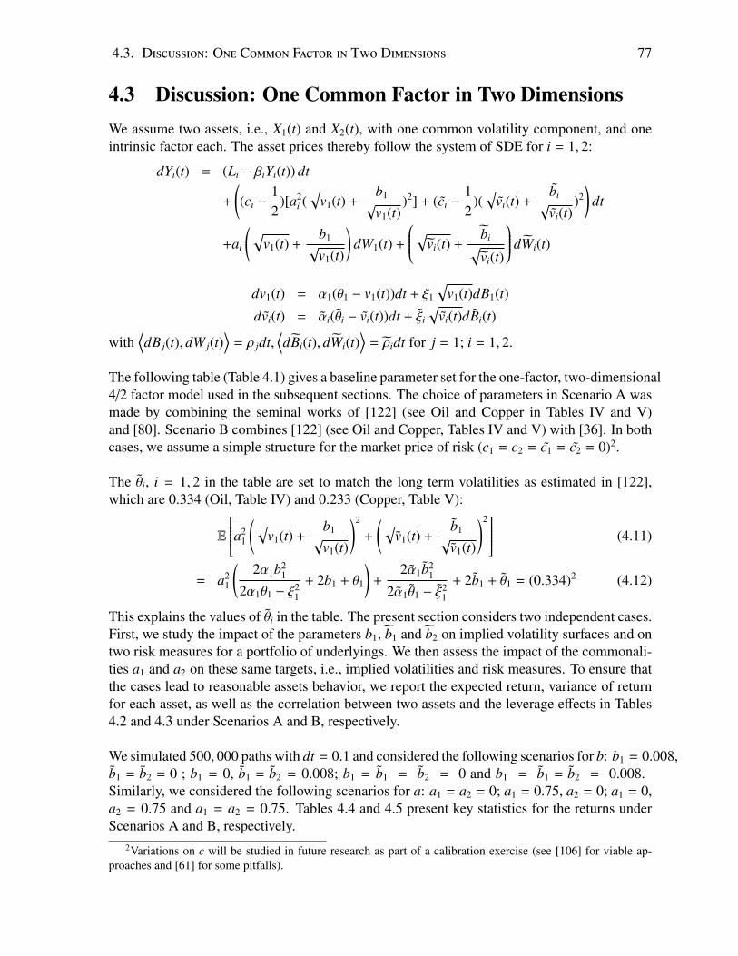
4.3. Discussion: One Common Factor in Two Dimensions 77
4.3 Discussion: One Common Factor in Two DimensionsWe assume two assets, i.e., X1(t) and X2(t), with one common volatility component, and oneintrinsic factor each. The asset prices thereby follow the system of SDE for i = 1, 2:
dYi(t) = (Li − βiYi(t)) dt
+
((ci −
12
)[a2i (
√v1(t) +
b1√
v1(t))2] + (ci −
12
)(√
vi(t) +bi√
vi(t))2)
dt
+ai
(√v1(t) +
b1√
v1(t)
)dW1(t) +
√vi(t) +bi√vi(t)
dWi(t)
dv1(t) = α1(θ1 − v1(t))dt + ξ1
√v1(t)dB1(t)
dvi(t) = αi(θi − vi(t))dt + ξi
√vi(t)dBi(t)
with⟨dB j(t), dW j(t)
⟩= ρ jdt,
⟨dBi(t), dWi(t)
⟩= ρidt for j = 1; i = 1, 2.
The following table (Table 4.1) gives a baseline parameter set for the one-factor, two-dimensional4/2 factor model used in the subsequent sections. The choice of parameters in Scenario A wasmade by combining the seminal works of [122] (see Oil and Copper in Tables IV and V)and [80]. Scenario B combines [122] (see Oil and Copper, Tables IV and V) with [36]. In bothcases, we assume a simple structure for the market price of risk (c1 = c2 = c1 = c2 = 0)2.
The θi, i = 1, 2 in the table are set to match the long term volatilities as estimated in [122],which are 0.334 (Oil, Table IV) and 0.233 (Copper, Table V):
E
a21
(√v1(t) +
b1√
v1(t)
)2
+
(√v1(t) +
b1√
v1(t)
)2 (4.11)
= a21
(2α1b2
1
2α1θ1 − ξ21
+ 2b1 + θ1
)+
2α1b21
2α1θ1 − ξ21
+ 2b1 + θ1 = (0.334)2 (4.12)
This explains the values of θi in the table. The present section considers two independent cases.First, we study the impact of the parameters b1, b1 and b2 on implied volatility surfaces and ontwo risk measures for a portfolio of underlyings. We then assess the impact of the commonali-ties a1 and a2 on these same targets, i.e., implied volatilities and risk measures. To ensure thatthe cases lead to reasonable assets behavior, we report the expected return, variance of returnfor each asset, as well as the correlation between two assets and the leverage effects in Tables4.2 and 4.3 under Scenarios A and B, respectively.
We simulated 500, 000 paths with dt = 0.1 and considered the following scenarios for b: b1 = 0.008,b1 = b2 = 0 ; b1 = 0, b1 = b2 = 0.008; b1 = b1 = b2 = 0 and b1 = b1 = b2 = 0.008.Similarly, we considered the following scenarios for a: a1 = a2 = 0; a1 = 0.75, a2 = 0; a1 = 0,a2 = 0.75 and a1 = a2 = 0.75. Tables 4.4 and 4.5 present key statistics for the returns underScenarios A and B, respectively.
2Variations on c will be studied in future research as part of a calibration exercise (see [106] for viable ap-proaches and [61] for some pitfalls).
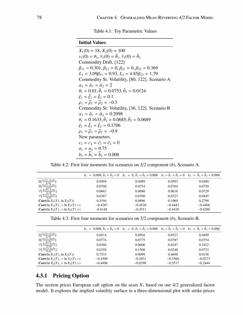
78 Chapter 4. GeneralizedMean-Reverting 4/2 FactorModel
Table 4.1: Toy Parametric Values
Initial Values
X1(0) = 18, X2(0) = 100v1(0) = θ1, v1(0) = θ1, v2(0) = θ2
Commodity Drift, [122]β11 = 0.301, β12 = 0, β21 = 0, β22 = 0.369L1 = 3.09β11 = 0.93, L2 = 4.85β22 = 1.79Commodity St. Volatility, [80, 122]. Scenario Aα1 = α1 = α2 = 2θ1 = 0.01, θ1 = 0.0753, θ2 = 0.0124ξ1 = ξ1 = ξ2 = 0.1ρ1 = ρ1 = ρ2 = −0.5Commodity St. Volatility, [36, 122]. Scenario Bα1 = α1 = α2 = 0.2098θ1 = 0.1633, θ1 = 0.0685, θ2 = 0.0689ξ1 = ξ1 = ξ2 = 0.1706ρ1 = ρ1 = ρ2 = −0.9New parameters.c1 = c2 = c1 = c2 = 0a1 = a2 = 0.75b1 = b1 = b2 = 0.008
Table 4.2: First four moments for scenarios on 3/2 component (b), Scenario A.
b1 = 0.008, b1 = b2 = 0 b1 = 0, b1 = b2 = 0.008 b1 = b1 = b2 = 0 b1 = b1 = b2 = 0.008
E[ X1(T )−X1(0)X1(0) ] 0.0494 0.0489 0.0503 0.0480
E[ X2(T )−X2(0)X2(0) ] 0.0760 0.0754 0.0764 0.0750
V[ X1(T )−X1(0)X1(0) ] 0.0663 0.0680 0.0618 0.0729
V[ X2(T )−X2(0)X2(0) ] 0.0367 0.0390 0.0323 0.0445
Corr(ln X1(T ) , ln X2(T )) 0.3194 0.0896 0.1060 0.2799Corr(ln X1(T ) , < ln X1(T ) >) −0.4287 −0.4520 −0.4443 −0.4406Corr(ln X2(T ) , < ln X2(T ) >) -0.4148 −0.4511 −0.4420 −0.4280
Table 4.3: First four moments for scenarios on 3/2 component (b), Scenario B.
b1 = 0.008, b1 = b2 = 0 b1 = 0, b1 = b2 = 0.008 b1 = b1 = b2 = 0 b1 = b1 = b2 = 0.008
E[ X1(T )−X1(0)X1(0) ] 0.0514 0.0504 0.0527 0.0499
E[ X2(T )−X2(0)X2(0) ] 0.0774 0.0775 0.0787 0.0754
V[ X1(T )−X1(0)X1(0) ] 0.0360 0.0606 0.0247 0.1022
V[ X2(T )−X2(0)X2(0) ] 0.0359 0.1508 0.0248 0.0723
Corr(ln X1(T ) , ln X2(T )) 0.7533 0.0099 0.4698 0.0156Corr(ln X1(T ) , < ln X1(T ) >) −0.4509 −0.2031 −0.5560 −0.0273Corr(ln X2(T ) , < ln X2(T ) >) −0.4496 −0.0398 −0.5517 −0.2444
4.3.1 Pricing OptionThe section prices European call option on the asset X1 based on our 4/2 generalized factormodel. It explores the implied volatility surface in a three-dimensional plot with strike prices
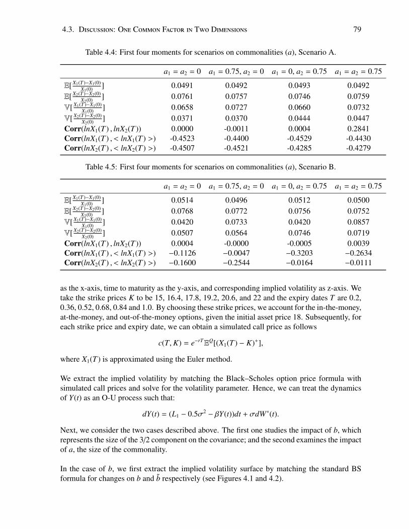
4.3. Discussion: One Common Factor in Two Dimensions 79
Table 4.4: First four moments for scenarios on commonalities (a), Scenario A.
a1 = a2 = 0 a1 = 0.75, a2 = 0 a1 = 0, a2 = 0.75 a1 = a2 = 0.75
E[ X1(T )−X1(0)X1(0) ] 0.0491 0.0492 0.0493 0.0492
E[ X2(T )−X2(0)X2(0) ] 0.0761 0.0757 0.0746 0.0759
V[ X1(T )−X1(0)X1(0) ] 0.0658 0.0727 0.0660 0.0732
V[ X2(T )−X2(0)X2(0) ] 0.0371 0.0370 0.0444 0.0447
Corr(lnX1(T ) , lnX2(T )) 0.0000 -0.0011 0.0004 0.2841Corr(lnX1(T ) , < lnX1(T ) >) -0.4523 -0.4400 -0.4529 -0.4430Corr(lnX2(T ) , < lnX2(T ) >) -0.4507 -0.4521 -0.4285 -0.4279
Table 4.5: First four moments for scenarios on commonalities (a), Scenario B.
a1 = a2 = 0 a1 = 0.75, a2 = 0 a1 = 0, a2 = 0.75 a1 = a2 = 0.75
E[ X1(T )−X1(0)X1(0) ] 0.0514 0.0496 0.0512 0.0500
E[ X2(T )−X2(0)X2(0) ] 0.0768 0.0772 0.0756 0.0752
V[ X1(T )−X1(0)X1(0) ] 0.0420 0.0733 0.0420 0.0857
V[ X2(T )−X2(0)X2(0) ] 0.0507 0.0564 0.0746 0.0719
Corr(lnX1(T ) , lnX2(T )) 0.0004 -0.0000 -0.0005 0.0039Corr(lnX1(T ) , < lnX1(T ) >) −0.1126 −0.0047 −0.3203 −0.2634Corr(lnX2(T ) , < lnX2(T ) >) −0.1600 −0.2544 −0.0164 −0.0111
as the x-axis, time to maturity as the y-axis, and corresponding implied volatility as z-axis. Wetake the strike prices K to be 15, 16.4, 17.8, 19.2, 20.6, and 22 and the expiry dates T are 0.2,0.36, 0.52, 0.68, 0.84 and 1.0. By choosing these strike prices, we account for the in-the-money,at-the-money, and out-of-the-money options, given the initial asset price 18. Subsequently, foreach strike price and expiry date, we can obtain a simulated call price as follows
c(T,K) = e−rTEQ[(X1(T ) − K)+],
where X1(T ) is approximated using the Euler method.
We extract the implied volatility by matching the Black–Scholes option price formula withsimulated call prices and solve for the volatility parameter. Hence, we can treat the dynamicsof Y(t) as an O-U process such that:
dY(t) = (L1 − 0.5σ2 − βY(t))dt + σdW∗(t).
Next, we consider the two cases described above. The first one studies the impact of b, whichrepresents the size of the 3/2 component on the covariance; and the second examines the impactof a, the size of the commonality.
In the case of b, we first extract the implied volatility surface by matching the standard BSformula for changes on b and b respectively (see Figures 4.1 and 4.2).
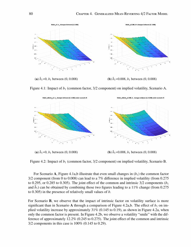
80 Chapter 4. GeneralizedMean-Reverting 4/2 FactorModel
(a) b1=0, b1 between (0, 0.008) (b) b1=0.008, b1 between (0, 0.008)
Figure 4.1: Impact of b1 (common factor, 3/2 component) on implied volatility, Scenario A.
(a) b1=0, b1 between (0, 0.008) (b) b1=0.008, b1 between (0, 0.008)
Figure 4.2: Impact of b1 (common factor, 3/2 component) on implied volatility, Scenario B.
For Scenario A, Figure 4.1a,b illustrate that even small changes in (b1) the common factor3/2 component (from 0 to 0.008) can lead to a 7% difference in implied volatility (from 0.275to 0.295, or 0.285 to 0.305). The joint effect of the common and intrinsic 3/2 components (b1
and b1) can be obtained by combining those two figures leading to a 11% change (from 0.275to 0.305) in the presence of relatively small values of b.
For Scenario B, we observe that the impact of intrinsic factor on volatility surface is moresignificant than in Scenario A through a comparison of Figure 4.2a,b. The effect of b1 on im-plied volatility increase by approximately 31% (0.145 to 0.19), as shown in Figure 4.2a, whenonly the common factor is present. In Figure 4.2b, we observe a volatility “smile” with the dif-ference of approximately 12.2% (0.245 to 0.275). The joint effect of the common and intrinsic3/2 components in this case is 100% (0.145 to 0.29).
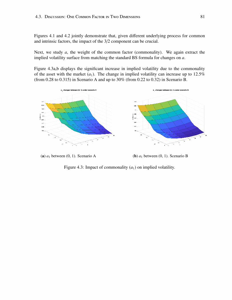
4.3. Discussion: One Common Factor in Two Dimensions 81
Figures 4.1 and 4.2 jointly demonstrate that, given different underlying process for commonand intrinsic factors, the impact of the 3/2 component can be crucial.
Next, we study a, the weight of the common factor (commonality). We again extract theimplied volatility surface from matching the standard BS formula for changes on a.
Figure 4.3a,b displays the significant increase in implied volatility due to the commonalityof the asset with the market (a1). The change in implied volatility can increase up to 12.5%(from 0.28 to 0.315) in Scenario A and up to 30% (from 0.22 to 0.32) in Scenario B.
(a) a1 between (0, 1). Scenario A (b) a1 between (0, 1). Scenario B
Figure 4.3: Impact of commonality (a1) on implied volatility.

82 Chapter 4. GeneralizedMean-Reverting 4/2 FactorModel
4.4 ConclusionsIn previous chapter 3, we consider a single asset whose diffusion is affected by common factoror systematic/market risk, and we assume the factor follows a 4/2 porcess because 4/2 pro-cess is capable of capturing the stylized facts in asset price time series through out the entirebusiness cycle. In this chapter, we propose and explore the generalized mean-reverting 4/2factor model. The generalized model is a more realistic model than the one-dimensional modelsince in the real market there is more than the common factors that influence the asset prices.There are also intrinsic factors and spillover effects from other assets. The generalized modelincorporates spillover effects, common factors and intrinsic factor. We assume 4/2 processesfor both common factor and intrinsic factors not only because 4/2 processes are powerful cap-turing the stylized facts, they are also flexible by adjusting the “weights” of 3/2 components.
In this study, we first provide analytical expressions for key characteristic functions and con-ditions for well-defined changes of measures. Thanks to principal component decomposition,we are able to write the generalized model in terms of a linear combination of independentmean-reverting 4/2 stochastic volatility models. Thus the generalized model inherits the sametheoretical challenges of the mean-reverting 4/2 stochastic volatility model, which is a closed-form solution of the characteristic function is not available. As we mentioned in chapter 3,even with the semi-closed form characteristic function, we can still reduce the computationalcost. We are also able to derive an analytic characteristic function for a special case, whichwe call the generalized Grasselli’s 4/2 model [76]. This opens a new window for studyingmulti-factor model in stock market. In numerical application section, we assess the impact ofb, i.e. the 3/2 component of the model in the volatility process, and a, the commonalities inthe absence and presence of stochastic volatility on the common factor. These impacts weremeasured with respect to implied volatility surfaces and two important risk measures. The re-sults demonstrate that even small values of the 3/2 component (b) can lead to a 100% changein the implied volatility surface, which in turn shows the significance of the 3/2 component inthe factors’ processes. In next chapter, we will focus on a subclass of the generalized modeland further evaluate the model performance.
Chapter 5
Multivariate Mean-Reverting 4/2Stochastic Volatility Model
Chapter 4 introduced a generalized multivariate mean-reverting 4/2 factor model. Thanks toa principal component decomposition (P.C), we expressed the stochastic covariance matrix interms of constant eigenvectors that drives the correlation and stochastic eigenvalues modeledby 4/2 stochastic processes. This means we can rewrite our multidimensional model in theform of linear combination of independent one-dimensional mean-reverting 4/2 processes. Inchapter 4, we entertained interesting structures and studied properties of the model such aschanges of measure and characteristics functions (c.f.s), we also applied the model to optionpricing.
Now, in chapter 5, we extend two of the results of chapter 3 to the principal component settingof chapter 4. These are: 1) obtaining a closed-form approximation of the c.f.s; 2) estimationof the parameters of the model. Moreover we will expose our model to a setting of portfoliooptimization for the fist time, to study its implications.
In particular, we remind the reader that the c.f.’s we found in chapter 4 have quasi-closed formexpressions, which requires simulation of a lower dimensional process. This lack of analyticityis not surprising as we have already shown in chapter 3 the challenges of finding closed-formc.f. in one dimension, which can be traced back to the combination of mean-reverting andstochastic volatility features. As a result, in chapter 3, we were left with a quasi-closed formc.f., and some analytical expressions for very special cases of our model. An alternative so-lution was to find an analytic function that approximates the c.f. with acceptable accuracywithin a region of the parametric space, i.e. for embedded models. In chapter 5, the two ap-proximation approaches developed in chapter 3 are implemented in multidimension: midpointapproximation and average approximation. Here we need to carefully design the embeddedmodels where the methodology works, which leads to three special cases. We illustrate theirperformance in higher dimensions, demonstrating high accuracy of the average approximationin capturing not only marginal densities but also joint behaviour.
This chapter also answers another question that is not addressed in chapter 4, namely esti-mation. We use the estimation approaches developed in chapter 3 to estimate the parameters
83
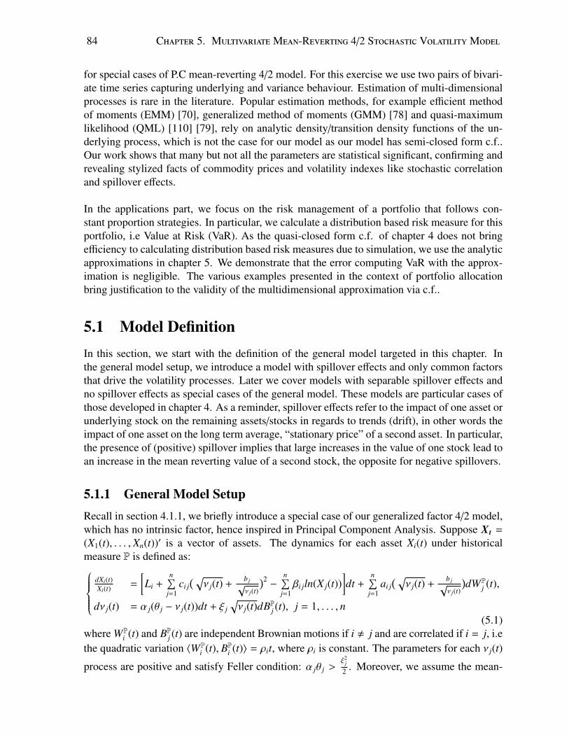
84 Chapter 5. MultivariateMean-Reverting 4/2 Stochastic VolatilityModel
for special cases of P.C mean-reverting 4/2 model. For this exercise we use two pairs of bivari-ate time series capturing underlying and variance behaviour. Estimation of multi-dimensionalprocesses is rare in the literature. Popular estimation methods, for example efficient methodof moments (EMM) [70], generalized method of moments (GMM) [78] and quasi-maximumlikelihood (QML) [110] [79], rely on analytic density/transition density functions of the un-derlying process, which is not the case for our model as our model has semi-closed form c.f..Our work shows that many but not all the parameters are statistical significant, confirming andrevealing stylized facts of commodity prices and volatility indexes like stochastic correlationand spillover effects.
In the applications part, we focus on the risk management of a portfolio that follows con-stant proportion strategies. In particular, we calculate a distribution based risk measure for thisportfolio, i.e Value at Risk (VaR). As the quasi-closed form c.f. of chapter 4 does not bringefficiency to calculating distribution based risk measures due to simulation, we use the analyticapproximations in chapter 5. We demonstrate that the error computing VaR with the approx-imation is negligible. The various examples presented in the context of portfolio allocationbring justification to the validity of the multidimensional approximation via c.f..
5.1 Model DefinitionIn this section, we start with the definition of the general model targeted in this chapter. Inthe general model setup, we introduce a model with spillover effects and only common factorsthat drive the volatility processes. Later we cover models with separable spillover effects andno spillover effects as special cases of the general model. These models are particular cases ofthose developed in chapter 4. As a reminder, spillover effects refer to the impact of one asset orunderlying stock on the remaining assets/stocks in regards to trends (drift), in other words theimpact of one asset on the long term average, “stationary price” of a second asset. In particular,the presence of (positive) spillover implies that large increases in the value of one stock lead toan increase in the mean reverting value of a second stock, the opposite for negative spillovers.
5.1.1 General Model SetupRecall in section 4.1.1, we briefly introduce a special case of our generalized factor 4/2 model,which has no intrinsic factor, hence inspired in Principal Component Analysis. Suppose Xt =
(X1(t), . . . , Xn(t))′ is a vector of assets. The dynamics for each asset Xi(t) under historicalmeasure P is defined as:
dXi(t)Xi(t)
=
[Li +
n∑j=1
ci j( √
ν j(t) +b j√ν j(t)
)2−
n∑j=1βi jln(X j(t))
]dt +
n∑j=1
ai j( √
ν j(t) +b j√ν j(t)
)dWP
j (t),
dν j(t) = α j(θ j − ν j(t))dt + ξ j√ν j(t)dBPj (t), j = 1, . . . , n
(5.1)where WP
i (t) and BPj (t) are independent Brownian motions if i , j and are correlated if i = j, i.ethe quadratic variation 〈WP
i (t), BPi (t)〉 = ρit, where ρi is constant. The parameters for each ν j(t)
process are positive and satisfy Feller condition: α jθ j >ξ2
j
2 . Moreover, we assume the mean-
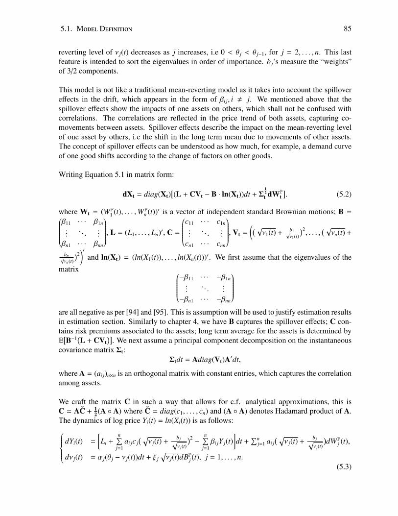
5.1. Model Definition 85
reverting level of ν j(t) decreases as j increases, i.e 0 < θ j < θ j−1, for j = 2, . . . , n. This lastfeature is intended to sort the eigenvalues in order of importance. b j’s measure the “weights”of 3/2 components.
This model is not like a traditional mean-reverting model as it takes into account the spillovereffects in the drift, which appears in the form of βi j, i , j. We mentioned above that thespillover effects show the impacts of one assets on others, which shall not be confused withcorrelations. The correlations are reflected in the price trend of both assets, capturing co-movements between assets. Spillover effects describe the impact on the mean-reverting levelof one asset by others, i.e the shift in the long term mean due to movements of other assets.The concept of spillover effects can be understood as how much, for example, a demand curveof one good shifts according to the change of factors on other goods.
Writing Equation 5.1 in matrix form:
dXt = diag(Xt)[(L + CVt − B · ln(Xt))dt + Σ
12t dWP
t]. (5.2)
where Wt = (WP1 (t), . . . ,WP
n (t))′ is a vector of independent standard Brownian motions; B =β11 · · · β1n...
. . ....
βn1 · · · βnn
, L = (L1, . . . , Ln)′, C =
c11 · · · c1n...
. . ....
cn1 · · · cnn
, Vt =
((√ν1(t) + b1√
ν1(t)
)2, . . . ,
(√νn(t) +
bn√νn(t)
)2)′
and ln(Xt) = (ln(X1(t)), . . . , ln(Xn(t)))′. We first assume that the eigenvalues of the
matrix −β11 · · · −β1n...
. . ....
−βn1 · · · −βnn
are all negative as per [94] and [95]. This is assumption will be used to justify estimation resultsin estimation section. Similarly to chapter 4, we have B captures the spillover effects; C con-tains risk premiums associated to the assets; long term average for the assets is determined byE[B−1(L + CVt
)]. We next assume a principal component decomposition on the instantaneous
covariance matrix Σt:Σtdt = Adiag(Vt)A′dt,
where A = (ai j)n×n is an orthogonal matrix with constant entries, which captures the correlationamong assets.
We craft the matrix C in such a way that allows for c.f. analytical approximations, this isC = AC + 1
2 (A A) where C = diag(c1, . . . , cn) and (A A) denotes Hadamard product of A.The dynamics of log price Yi(t) = ln(Xi(t)) is as follows:
dYi(t) =
[Li +
n∑j=1
ai jc j( √
ν j(t) +b j√ν j(t)
)2−
n∑j=1βi jY j(t)
]dt +
∑nj=1 ai j
( √ν j(t) +
b j√ν j(t)
)dWP
j (t),
dν j(t) = α j(θ j − ν j(t))dt + ξ j√ν j(t)dBPj (t), j = 1, . . . , n.
(5.3)

86 Chapter 5. MultivariateMean-Reverting 4/2 Stochastic VolatilityModel
Based on the applications, our model can be reduced to three sub cases for which we are ableto approximate the c.f. with analytic functions.
• bj = 0, ρj , 0: The advantage of 4/2 model is that it integrates two diffusion processeswith different behavior, which enables the model to capture the stylized facts of the un-derlying asset under different financial situations. During the period when the financialmarkets enjoy stable business cycles, 3/2 diffusion process may be redundant in mod-eling the underlying asset as 1/2 diffusion is good enough to capture the stylized facts.Therefore, the dynamics for log price is defined as:
dYi(t) =
[Li +
n∑j=1
ai jc jν j(t) −n∑
j=1βi jY j(t)
]dt +
∑nj=1 ai j
√ν j(t)dWP
j (t),
dν j(t) = α j(θ j − ν j(t))dt + ξ j√ν j(t)dBPj (t), j = 1, . . . , n,
〈dWPj (t), dBPj (t)〉 = ρ jdt
(5.4)If n = 1, we have a mean-reverting Heston model, which is also considered in [16].
• bj , 0, ρj = 0: This case applies to the assets whose price series demonstrates abnormalincrease or decrease, but there is no leverage effect observed for the assets of interest.The term “leverage effect” was first defined and studied in [18]. It describes the negativecorrelation between asset’s volatility and asset’s return. In this situation, we know thatthe trend of asset’s volatility provides no information on the trend of asset’s return. Themodel for log price is therefore defined as:
dYi(t) =
[Li +
n∑j=1
ai jc j( √
ν j(t) +b j√ν j(t)
)2−
n∑j=1βi jY j(t)
]dt
+∑n
j=1 ai j( √
ν j(t) +b j√ν j(t)
)dWP
j (t),
dν j(t) = α j(θ j − ν j(t))dt + ξ j√ν j(t)dBPj (t), j = 1, . . . , n,
〈dWPj (t), dBPj (t)〉 = 0
(5.5)
• bj = 0, ρj = 0: This case can be generated by either of previous two cases. It betterapplies to assets that exhibit mild behavior in their price series, at the same time noleverage effect is identified. Then the model for log price follows from either Equation5.4 or Equation 5.5:
dYi(t) =
[Li +
n∑j=1
ai jc jν j(t) −n∑
j=1βi jY j(t)
]dt +
∑nj=1 ai j
√ν j(t)dWP
j (t),
dν j(t) = α j(θ j − ν j(t))dt + ξ j√ν j(t)dBPj (t), j = 1, . . . , n,
〈dWPj (t), dBPj (t)〉 = 0
(5.6)
We will show how to approximate the c.f. with analytic functions for these three cases insection 5.2.
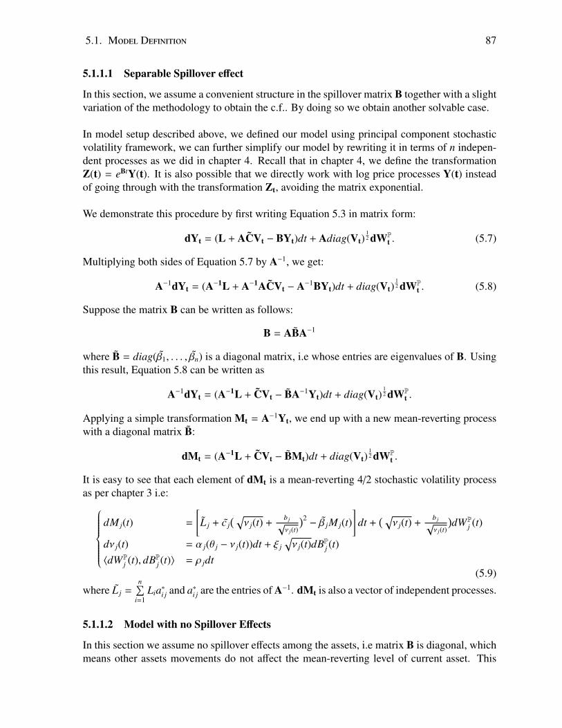
5.1. Model Definition 87
5.1.1.1 Separable Spillover effect
In this section, we assume a convenient structure in the spillover matrix B together with a slightvariation of the methodology to obtain the c.f.. By doing so we obtain another solvable case.
In model setup described above, we defined our model using principal component stochasticvolatility framework, we can further simplify our model by rewriting it in terms of n indepen-dent processes as we did in chapter 4. Recall that in chapter 4, we define the transformationZ(t) = eBtY(t). It is also possible that we directly work with log price processes Y(t) insteadof going through with the transformation Zt, avoiding the matrix exponential.
We demonstrate this procedure by first writing Equation 5.3 in matrix form:
dYt = (L + ACVt − BYt)dt + Adiag(Vt)12 dWP
t . (5.7)
Multiplying both sides of Equation 5.7 by A−1, we get:
A−1dYt = (A−1L + A−1ACVt − A−1BYt)dt + diag(Vt)12 dWP
t . (5.8)
Suppose the matrix B can be written as follows:
B = ABA−1
where B = diag(β1, . . . , βn) is a diagonal matrix, i.e whose entries are eigenvalues of B. Usingthis result, Equation 5.8 can be written as
A−1dYt = (A−1L + CVt − BA−1Yt)dt + diag(Vt)12 dWP
t .
Applying a simple transformation Mt = A−1Yt, we end up with a new mean-reverting processwith a diagonal matrix B:
dMt = (A−1L + CVt − BMt)dt + diag(Vt)12 dWP
t .
It is easy to see that each element of dMt is a mean-reverting 4/2 stochastic volatility processas per chapter 3 i.e:
dM j(t) =
[L j + c j
( √ν j(t) +
b j√ν j(t)
)2− β jM j(t)
]dt +
( √ν j(t) +
b j√ν j(t)
)dWP
j (t)
dν j(t) = α j(θ j − ν j(t))dt + ξ j√ν j(t)dBPj (t)
〈dWPj (t), dBPj (t)〉 = ρ jdt
(5.9)
where L j =n∑
i=1Lia∗i j and a∗i j are the entries of A−1. dMt is also a vector of independent processes.
5.1.1.2 Model with no Spillover Effects
In this section we assume no spillover effects among the assets, i.e matrix B is diagonal, whichmeans other assets movements do not affect the mean-reverting level of current asset. This
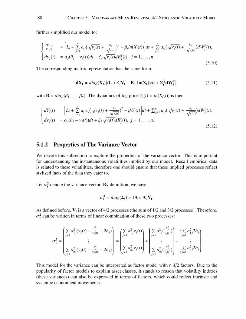
88 Chapter 5. MultivariateMean-Reverting 4/2 Stochastic VolatilityModel
further simplified our model to:dXi(t)Xi(t)
=
[Li +
n∑j=1
ci j( √
ν j(t) +b j√ν j(t)
)2− βiln(Xi(t))
]dt +
n∑j=1
ai j( √
ν j(t) +b j√ν j(t)
)dWP
j (t),
dν j(t) = α j(θ j − ν j(t))dt + ξ j√ν j(t)dBPj (t), j = 1, . . . , n
(5.10)The corresponding matrix representation has the same form:
dXt = diag(Xt)[(L + CVt − B · ln(Xt))dt + Σ
12t dWP
t], (5.11)
with B = diag(β1, . . . , βn). The dynamics of log price Yi(t) = ln(Xi(t)) is then:dYi(t) =
[Li +
n∑j=1
ai jc j( √
ν j(t) +b j√ν j(t)
)2− βiYi(t)
]dt +
∑nj=1 ai j
( √ν j(t) +
b j√ν j(t)
)dWP
j (t),
dν j(t) = α j(θ j − ν j(t))dt + ξ j√ν j(t)dBPj (t), j = 1, . . . , n.
(5.12)
5.1.2 Properties of The Variance Vector
We devote this subsection to explore the properties of the variance vector. This is importantfor understanding the instantaneous volatilities implied by our model. Recall empirical datais related to these volatilities, therefore one should ensure that these implied processes reflectstylized facts of the data they cater to.
Let σ2t denote the variance vector. By definition, we have:
σ2t = diag(Σt) = (A A)Vt.
As defined before, Vt is a vector of 4/2 processes (the sum of 1/2 and 3/2 processes). Therefore,σ2
t can be written in terms of linear combination of these two processes:
σ2t =
∑j=1
a21 j(ν j(t) +
b2j
ν j(t)+ 2b j
)...∑
j=1a2
n j(ν j(t) +
b2j
ν j(t)+ 2b j
)
=
∑j=1
a21 jν j(t)
...∑j=1
a2n jν j(t)
+
∑j=1
a21 j( b2
j
ν j(t)
)...∑
j=1a2
n j( b2
j
ν j(t)
)
+
∑j=1
a21 j2b j
...∑j=1
a2n j2b j
This model for the variance can be interpreted as factor model with n 4/2 factors. Due to thepopularity of factor models to explain asset classes, it stands to reason that volatility indexes(these variances) can also be expressed in terms of factors, which could reflect intrinsic andsystemic economical movements.
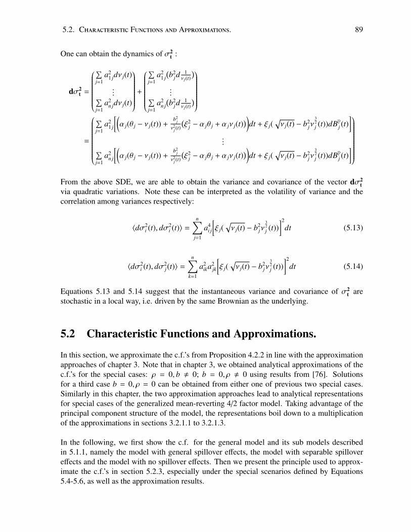
5.2. Characteristic Functions and Approximations. 89
One can obtain the dynamics of σ2t :
dσ2t =
∑j=1
a21 jdν j(t)
...∑j=1
a2n jdν j(t)
+
∑j=1
a21 j(b2
jd1
ν j(t)
)...∑
j=1a2
n j(b2
jd1
ν j(t)
)
=
∑j=1
a21 j
[(α j(θ j − ν j(t)) +
b2j
ν2j (t)
(ξ2
j − α jθ j + α jν j(t)))
dt + ξ j(√ν j(t) − b2
jν32j (t))dBPj (t)
]...∑
j=1a2
n j
[(α j(θ j − ν j(t)) +
b2j
ν2j (t)
(ξ2
j − α jθ j + α jν j(t)))
dt + ξ j(√ν j(t) − b2
jν32j (t))dBPj (t)
]
From the above SDE, we are able to obtain the variance and covariance of the vector dσ2t
via quadratic variations. Note these can be interpreted as the volatility of variance and thecorrelation among variances respectively:
〈dσ2i (t), dσ2
i (t)〉 =
n∑j=1
a4i j
[ξ j(
√ν j(t) − b2
jν32j (t))
]2
dt (5.13)
〈dσ2i (t), dσ2
j(t)〉 =
n∑k=1
a2ika
2jk
[ξ j(
√ν j(t) − b2
jν32j (t))
]2
dt (5.14)
Equations 5.13 and 5.14 suggest that the instantaneous variance and covariance of σ2t are
stochastic in a local way, i.e. driven by the same Brownian as the underlying.
5.2 Characteristic Functions and Approximations.
In this section, we approximate the c.f.’s from Proposition 4.2.2 in line with the approximationapproaches of chapter 3. Note that in chapter 3, we obtained analytical approximations of thec.f.’s for the special cases: ρ = 0, b , 0; b = 0, ρ , 0 using results from [76]. Solutionsfor a third case b = 0, ρ = 0 can be obtained from either one of previous two special cases.Similarly in this chapter, the two approximation approaches lead to analytical representationsfor special cases of the generalized mean-reverting 4/2 factor model. Taking advantage of theprincipal component structure of the model, the representations boil down to a multiplicationof the approximations in sections 3.2.1.1 to 3.2.1.3.
In the following, we first show the c.f. for the general model and its sub models describedin 5.1.1, namely the model with general spillover effects, the model with separable spillovereffects and the model with no spillover effects. Then we present the principle used to approx-imate the c.f.’s in section 5.2.3, especially under the special scenarios defined by Equations5.4-5.6, as well as the approximation results.
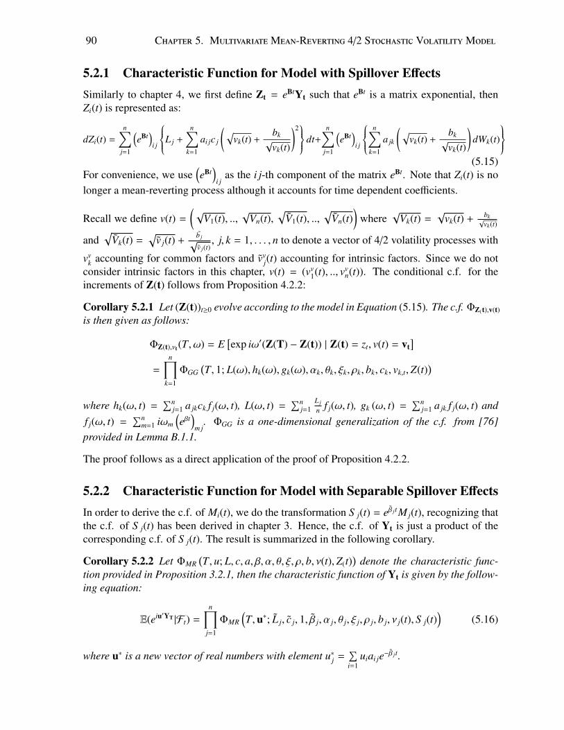
90 Chapter 5. MultivariateMean-Reverting 4/2 Stochastic VolatilityModel
5.2.1 Characteristic Function for Model with Spillover EffectsSimilarly to chapter 4, we first define Zt = eBtYt such that eBt is a matrix exponential, thenZi(t) is represented as:
dZi(t) =
n∑j=1
(eBt
)i j
L j +
n∑k=1
ai jc j
(√vk(t) +
bk√
vk(t)
)2 dt+
n∑j=1
(eBt
)i j
n∑k=1
a jk
(√vk(t) +
bk√
vk(t)
)dWk(t)
(5.15)
For convenience, we use(eBt
)i j
as the i j-th component of the matrix eBt. Note that Zi(t) is nolonger a mean-reverting process although it accounts for time dependent coefficients.
Recall we define v(t) =
(√
V1(t), ..,√
Vn(t),√
V1(t), ..,√
Vn(t))
where√
Vk(t) =√
vk(t) + bk√vk(t)
and√
Vk(t) =√
v j(t) +b j√v j(t)
, j, k = 1, . . . , n to denote a vector of 4/2 volatility processes with
vvk accounting for common factors and vv
j(t) accounting for intrinsic factors. Since we do notconsider intrinsic factors in this chapter, v(t) = (vv
1(t), .., vvn(t)). The conditional c.f. for the
increments of Z(t) follows from Proposition 4.2.2:
Corollary 5.2.1 Let (Z(t))t≥0 evolve according to the model in Equation (5.15). The c.f. ΦZ(t),v(t)is then given as follows:
ΦZ(t),νt(T, ω) = E[exp iω′(Z(T) − Z(t)) | Z(t) = zt, v(t) = vt
]=
n∏k=1
ΦGG(T, 1; L(ω), hk(ω), gk(ω), αk, θk, ξk, ρk, bk, ck, vk,t,Z(t)
)where hk(ω, t) =
∑nj=1 a jkck f j(ω, t), L(ω, t) =
∑nj=1
L j
n f j(ω, t), gk (ω, t) =∑n
j=1 a jk f j(ω, t) andf j(ω, t) =
∑nm=1 iωm
(eβt
)m j
. ΦGG is a one-dimensional generalization of the c.f. from [76]provided in Lemma B.1.1.
The proof follows as a direct application of the proof of Proposition 4.2.2.
5.2.2 Characteristic Function for Model with Separable Spillover EffectsIn order to derive the c.f. of Mi(t), we do the transformation S j(t) = eβ jtM j(t), recognizing thatthe c.f. of S j(t) has been derived in chapter 3. Hence, the c.f. of Yt is just a product of thecorresponding c.f. of S j(t). The result is summarized in the following corollary.
Corollary 5.2.2 Let ΦMR(T, u; L, c, a, β, α, θ, ξ, ρ, b, ν(t),Z(t)
)denote the characteristic func-
tion provided in Proposition 3.2.1, then the characteristic function of Yt is given by the follow-ing equation:
E(eiu′YT |Ft) =
n∏j=1
ΦMR
(T,u∗; L j, c j, 1, β j, α j, θ j, ξ j, ρ j, b j, ν j(t), S j(t)
)(5.16)
where u∗ is a new vector of real numbers with element u∗j =∑i=1
uiai je−β jt.
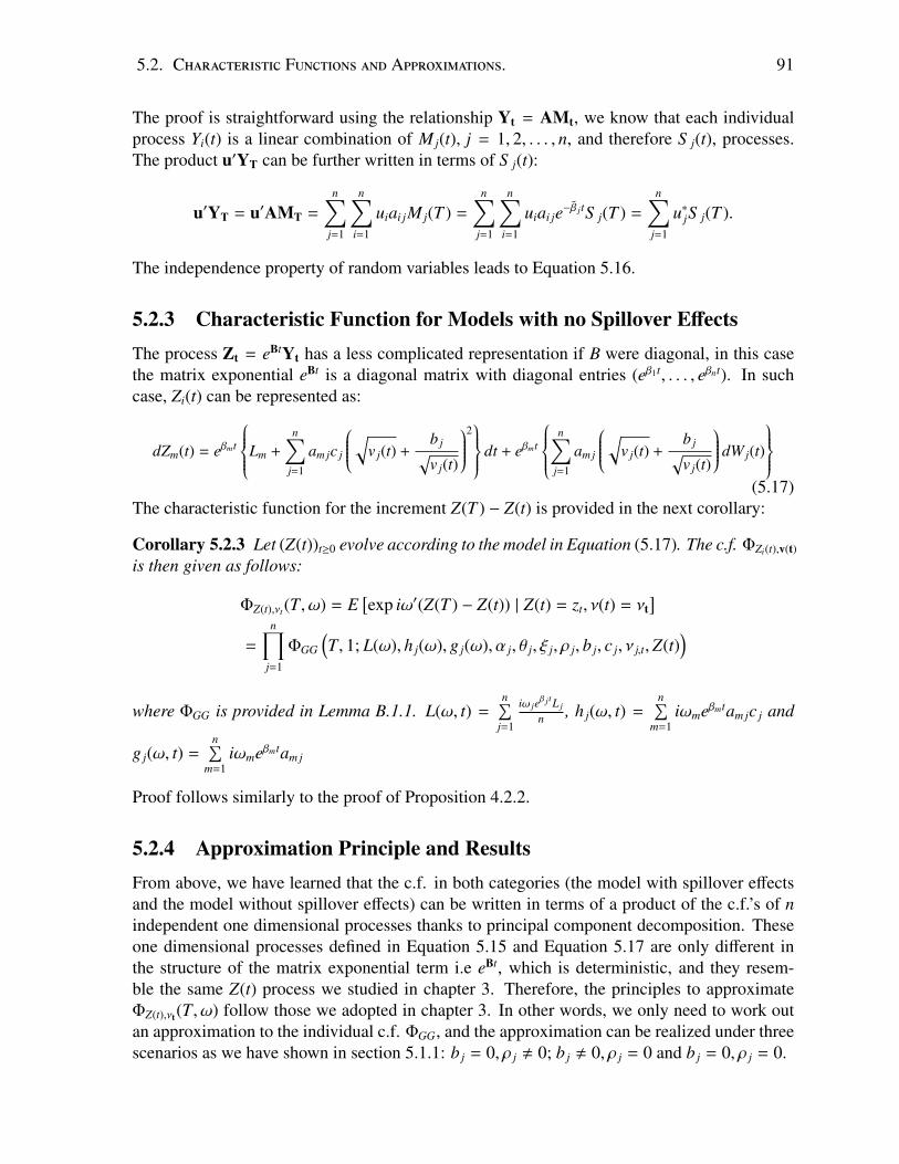
5.2. Characteristic Functions and Approximations. 91
The proof is straightforward using the relationship Yt = AMt, we know that each individualprocess Yi(t) is a linear combination of M j(t), j = 1, 2, . . . , n, and therefore S j(t), processes.The product u′YT can be further written in terms of S j(t):
u′YT = u′AMT =
n∑j=1
n∑i=1
uiai jM j(T ) =
n∑j=1
n∑i=1
uiai je−β jtS j(T ) =
n∑j=1
u∗jS j(T ).
The independence property of random variables leads to Equation 5.16.
5.2.3 Characteristic Function for Models with no Spillover EffectsThe process Zt = eBtYt has a less complicated representation if B were diagonal, in this casethe matrix exponential eBt is a diagonal matrix with diagonal entries (eβ1t, . . . , eβnt). In suchcase, Zi(t) can be represented as:
dZm(t) = eβmt
Lm +
n∑j=1
am jc j
√v j(t) +b j√v j(t)
2 dt + eβmt
n∑
j=1
am j
√v j(t) +b j√v j(t)
dW j(t)
(5.17)
The characteristic function for the increment Z(T ) − Z(t) is provided in the next corollary:
Corollary 5.2.3 Let (Z(t))t≥0 evolve according to the model in Equation (5.17). The c.f. ΦZi(t),v(t)is then given as follows:
ΦZ(t),νt(T, ω) = E[exp iω′(Z(T ) − Z(t)) | Z(t) = zt, ν(t) = νt
]=
n∏j=1
ΦGG
(T, 1; L(ω), h j(ω), g j(ω), α j, θ j, ξ j, ρ j, b j, c j, ν j,t,Z(t)
)
where ΦGG is provided in Lemma B.1.1. L(ω, t) =n∑
j=1
iω jeβ jtL j
n , h j(ω, t) =n∑
m=1iωmeβmtam jc j and
g j(ω, t) =n∑
m=1iωmeβmtam j
Proof follows similarly to the proof of Proposition 4.2.2.
5.2.4 Approximation Principle and ResultsFrom above, we have learned that the c.f. in both categories (the model with spillover effectsand the model without spillover effects) can be written in terms of a product of the c.f.’s of nindependent one dimensional processes thanks to principal component decomposition. Theseone dimensional processes defined in Equation 5.15 and Equation 5.17 are only different inthe structure of the matrix exponential term i.e eBt, which is deterministic, and they resem-ble the same Z(t) process we studied in chapter 3. Therefore, the principles to approximateΦZ(t),νt(T, ω) follow those we adopted in chapter 3. In other words, we only need to work outan approximation to the individual c.f. ΦGG, and the approximation can be realized under threescenarios as we have shown in section 5.1.1: b j = 0, ρ j , 0; b j , 0, ρ j = 0 and b j = 0, ρ j = 0.
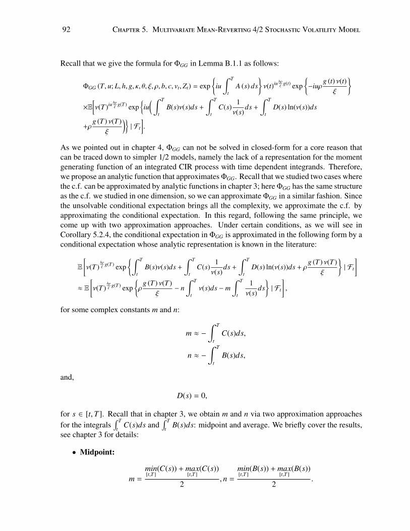
92 Chapter 5. MultivariateMean-Reverting 4/2 Stochastic VolatilityModel
Recall that we give the formula for ΦGG in Lemma B.1.1 as follows:
ΦGG (T, u; L, h, g, κ, θ, ξ, ρ, b, c, vt,Zt) = exp
iu∫ T
tA (s) ds
ν(t)iu bρ
ξ g(t) exp−iuρ
g (t) ν(t)ξ
×E
[ν(T )iu bρ
ξ g(T ) expiu
( ∫ T
tB(s)ν(s)ds +
∫ T
tC(s)
1ν(s)
ds +
∫ T
tD(s) ln(ν(s))ds
+ρg (T ) ν(T )
ξ
)| Ft
].
As we pointed out in chapter 4, ΦGG can not be solved in closed-form for a core reason thatcan be traced down to simpler 1/2 models, namely the lack of a representation for the momentgenerating function of an integrated CIR process with time dependent integrands. Therefore,we propose an analytic function that approximates ΦGG. Recall that we studied two cases wherethe c.f. can be approximated by analytic functions in chapter 3; here ΦGG has the same structureas the c.f. we studied in one dimension, so we can approximate ΦGG in a similar fashion. Sincethe unsolvable conditional expectation brings all the complexity, we approximate the c.f. byapproximating the conditional expectation. In this regard, following the same principle, wecome up with two approximation approaches. Under certain conditions, as we will see inCorollary 5.2.4, the conditional expectation in ΦGG is approximated in the following form by aconditional expectation whose analytic representation is known in the literature:
E
[ν(T )
bρξ g(T ) exp
∫ T
tB(s)ν(s)ds +
∫ T
tC(s)
1ν(s)
ds +
∫ T
tD(s) ln(ν(s))ds + ρ
g (T ) ν(T )ξ
| Ft
]≈ E
[ν(T )
bρξ g(T ) exp
ρ
g (T ) ν(T )ξ
− n∫ T
tν(s)ds − m
∫ T
t
1ν(s)
ds| Ft
],
for some complex constants m and n:
m ≈ −∫ T
tC(s)ds,
n ≈ −∫ T
tB(s)ds,
and,
D(s) = 0,
for s ∈ [t,T ]. Recall that in chapter 3, we obtain m and n via two approximation approachesfor the integrals
∫ T
tC(s)ds and
∫ T
tB(s)ds: midpoint and average. We briefly cover the results,
see chapter 3 for details:
• Midpoint:
m =
min[t,T ]
(C(s)) + max[t,T ]
(C(s))
2, n =
min[t,T ]
(B(s)) + max[t,T ]
(B(s))
2.
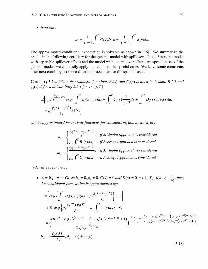
5.2. Characteristic Functions and Approximations. 93
• Average:
m =1
T − t
∫ T
tC(s)ds, n =
1T − t
∫ T
tB(s)ds.
The approximated conditional expectation is solvable as shown in [76]. We summarize theresults in the following corollary for the general model with spillover effects. Since the modelwith separable spillover effects and the model without spillover effects are special cases of thegeneral model, we can easily apply the results to the special cases. We leave some commentsafter next corollary on approximation procedures for the special cases.
Corollary 5.2.4 Given deterministic functions B j(s) and C j(s) defined in Lemma B.1.1 andg j(s) defined in Corollary 5.2.1 for s ∈ [t,T ],
E[ν j(T )
b jρ jξ j
g j(T ) exp ∫ T
tB j(s)ν j(s)ds +
∫ T
tC j(s)
1ν j(s)
ds +
∫ T
tD j(s) ln(ν j(s))ds
+ ρ jg j (T ) ν j(T )
ξ j
| Ft
]can be approximated by analytic functions for constants m j and n j satisfying
n j =
min[t,T ]
(B j(s))+max[t,T ]
(B j(s))
2 , if Midpoint approach is considered1
T−t
∫ T
tB j(s)ds, if Average Approach is considered
m j =
min[t,T ]
(C j(s))+max[t,T ]
(C j(s))
2 , if Midpoint approach is considered1
T−t
∫ T
tC j(s)ds, if Average Approach is considered
under three scenarios:
• bj = 0, ρj , 0: Given b j = 0, ρ j , 0, C(s) = 0 and D(s) = 0, s ∈ [t,T ]. If n j ≥ −α2
j
2ξ2j, then
the conditional expectation is approximated by:
E
[exp
∫ T
tB j(s)ν j(s)ds + ρ j
g j (T ) ν j(T )ξ j
| Ft
]≈ E
[exp
ρ j
g j (T ) ν j(T )ξ j
− n j
∫ T
tν j(s)ds
| Ft
]
=
( (B jξ2j + α)
(e√
A j(T−t)− 1
)+
√A j
(e√
A j(T−t) + 1)
2√
A je√
A j+α j2 (T−t)
)− 2α jθ jξ2j e
ν j(t)
((B jα j−2n j)
(e√
A j(T−t)−1)−B j√
A j
(e√
A j(T−t)+1)
(B jξ2j +α j)
(e√
A j(T−t)−1)
+√
A j
(e√
A j(T−t)+1) )
,
B j = −ρ jg j(T )ξ j
, A j = α2j + 2n jξ
2j ,
(5.18)
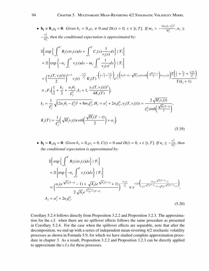
94 Chapter 5. MultivariateMean-Reverting 4/2 Stochastic VolatilityModel
• bj , 0, ρj = 0: Given b j = 0, ρ j , 0 and D(s) = 0, s ∈ [t,T ]. If m j > −(2α jθ j−ξ
2j )
2
8ξ2j
, n j ≥
−α2
j
2ξ2j, then the conditional expectation is approximated by:
E[
exp ∫ T
tB j(s)ν j(s)ds +
∫ T
tC j(s)
1ν j(s)
ds| Ft
]≈ E
[exp
−n j
∫ T
tν j(s)ds − m j
∫ T
t
1ν j(s)
ds| Ft
]
=
(γ j(T, ν j(t))2
)k j+1
ν j(t)−α jθ jξ2j K j(T )
−
(12 +
k j2 +
α jθ jξ2j
)e
1ξ2j
(θ j(T−t)−
√H jν j(t)coth
(√
H j(T−t)2
)+α jν j(t)
)Γ
(12 +
k j
2 +α jθ j
ξ2j
)Γ(k j + 1)
× 1F1
(12
+k j
2+α jθ j
ξ2j
, k j + 1,γ j(T, ν j(t))2
4K j(T )
),
k j =1ξ2
j
√(2α jθ j − ξ
2j )2 + 8m jξ
2j ,H j = α2
j + 2n jξ2j , γ j(T, ν j(t)) =
2√
H jν j(t)
ξ2j sinh
( √H j(T−t)
2
) ,K j(T ) =
1ξ2
j
( √H jν j(t)coth
( √H j(T − t)
2
)+ α j
).
(5.19)
• bj = 0, ρj = 0: Given b j = 0, ρ j = 0, C(t) = 0 and D(t) = 0, s ∈ [t,T ]. If n j ≥ −α2
j
2ξ2j, then
the conditional expectation is approximated by:
E[
exp ∫ T
tB j(s)ν j(s)ds
| Ft
]≈ E
[exp
−n j
∫ T
tν j(s)ds
| Ft
]
=
(α j(e√
A j(T−t)− 1) +
√A j(e√
A j(T−t) + 1)
2√
A je√
A j+α j2 (T−t)
)− 2α jθ jξ2j × e
ν j(t)
(−2n j(e
√A j(T−t)
−1)
α j(e√
A j(T−t)−1)+√
A j(e√
A j(T−t)+1)
),
A j = α2j + 2n jξ
2j .
(5.20)
Corollary 5.2.4 follows directly from Proposition 3.2.2 and Proposition 3.2.3. The approxima-tion for the c.f. when there are no spillover effects follows the same procedure as presentedin Corollary 5.2.4. For the case when the spillover effects are separable, note that after thedecomposition, we end up with a series of independent mean-reverting 4/2 stochastic volatilityprocesses as shown in Formula 5.9, for which we have studied complete approximation proce-dure in chapter 3. As a result, Proposition 3.2.2 and Proposition 3.2.3 can be directly appliedto approximate the c.f.s for these processes.
5.3. Estimation 95
5.3 EstimationIn this section, we consider the model with separable spillover effects as the underlying modelfor estimation. This way we fulfill the purpose of studying spillover effects among assets,and on the other hand we avoid the complexity of matrix exponential. Recall the model withseparable spillover effects can be expressed as follows:
dYt = (L + ACVt − BYt)dt + Adiag(Vt)12 dWP
t .
where B is constructed in a way such that it can be decomposed into a product of three matrices:B = ABA−1. In this case, dYi(t) is a linear combination of independent processes dM j(t), i.edYt = AdMt:
dM j(t) =
[L j + c j
( √ν j(t) +
b j√ν j(t)
)2− β jM j(t)
]dt +
( √ν j(t) +
b j√ν j(t)
)dWP
j (t)
dν j(t) = α j(θ j − ν j(t))dt + ξ j√ν j(t)dBPj (t)
〈dWPj (t), dBPj (t)〉 = ρ jdt
For simplicity, we focus on two dimensions hence studying pairs of assets with their respectivevolatility indexes. For example, VIX (VVIX) and VSTOXX (VVSTOXX); USO (OVX) andGLD (GVZ), or USO (OVX) and SLV (VXSLV). Then we follow the same estimation proce-dure as outlined in chapter 3 splitting the parameters into two groups: volatility group and driftgroup.
After a section on data description in 5.3.1, section 5.3.2 estimates the parameters in thevolatility group. Under the model with separable spillover effects, we first need to estimatecovariance matrix (Σ) from asset data as a long term average of the stochastic covariance ma-trix (Σt). This permits us to produce and estimate for the constant eigenvectors, denoted as A.With the estimated eigenvectors, we decompose our original asset processes into sum of inde-pendent mean-reverting 4/2 models. The volatility group then consists of parameters for theunderlying CIR processes driving the principal components: b j, α j, θ j, ξ j, and the estimationmethod follows along the lines of chapter 3. Section 5.3.3 tackles the estimation of drift groupparameters. This is done using least squares as in chapter 3.
Here we would like to remind the reader about volatility indexes and their meaning before weproceed further. As we discussed in chapter 1, volatility indexes are a kind of implied volatilitythat is model free and directly calculated from option prices from the market, thus they are agood measure of market’s expectation about future volatility. See chapter 1 for a discussion onthe relation among four broadly used volatility measures: realized volatility, implied volatility,instantaneous volatility and integrated volatility, and how tightly connected they are. In chap-ters 3 and 5, we use volatility indexes data as a convenient proxy for instantaneous volatility. Infact, instantaneous volatility is rather impossible to capture from empirical data, even with highfrequency data, as it requires instantaneous periods rather than the available discrete periods.On the other hand, once a model is specified, volatility indexes can be used to represent instan-taneous volatility with some multiplicative (scaling) adjustment or factor, see eg. [102], [130]
96 Chapter 5. MultivariateMean-Reverting 4/2 Stochastic VolatilityModel
and references therein. These works fall under “indirect modelling” methods for volatility in-dexes and assume either Heston’s model or Heston with jumps for the underlying asset process.In these Heston-related modelling methodologies, the relationship between the instantaneousvolatility and the volatility index of interest, for example VIX, can be expressed in terms ofa closed-form equation, where the difference between the two, under some conditions, lies ona multiplicative factor. In a recent paper, see [97], the author assumes Grasselli’s 4/2 modelwith the addition of jumps as the underlying, obtaining a far more complicated relationship,nonetheless still with a multiplicative factor. All these works demonstrate that due to the shorthorizon of volatility indexes (21 day options), the multiplicative factor could be close to one ina large region of the parametric space, which implies that volatility indexes are almost equal toinstantaneous volatilities regardless of the structural choice of underlying model.
Inspired by these pioneer works, we introduce scale parameters to adjust empirical volatil-ity indexes data to estimate instantaneous volatilities. This is done in a way that the empiricalmeans of the observed variance series (Vobs
t ) match the corresponding long term asset vari-ances. These new scaling parameters can be estimated at an early stage of the estimationprocess and are methodologically independent of other parameters. The reason we did notintroduce this scaling parameter earlier in chapter 3 is that in a one-dimensional case, theirvalues would be absorbed by the mean-revering level of the underlying CIR process; in otherwords, the final estimation results already reflect the scaling operation. In this chapter, dueto the multiple dimensions and the principal components decomposition, it turns out that theinformation of the scaling could be absorbed by either the eigenvectors (denoted A), the meanreverting level (MRL) of the principal components (i.e. θ) or both. This creates scenarioswhere the model is not compatible with data, e.g. given A, there is no reasonable θ matchingdata-implied MRLs. This can be fixed by acknowledging scaling parameters for every under-lying CIR process. Hence, the estimation introduces the concept of ”scaling” to accommodatethe instantaneous covariances with the vector of observable volatility indexes.
5.3.1 Data DescriptionBefore we officially engage in estimation procedures with empirical data, we devote this sec-tion to briefly describe the data we use and how we process the data for our purpose.
Generally, the model with separable spillover effects is good for multiple assets. As a demon-stration, we consider the following pairs of assets: VIX and VSTOXX; USO and GLD; SLVand GLD. Recall from chapter 3 that our estimation method is a two-stage method due to thestructure of our model. A two-stage method means that we need the asset data as well as itscorresponding volatility index data, then we estimate a group of the parameters in the first stagewith volatility index data and the other group of parameters next with asset data and volatilityindex data. Therefore, we also consider the related volatility indexes (VVIX and VVSTOXX,OVX and GVZ, VXSLV and GVZ) for the corresponding assets.
The sample size of the raw data is different across all the assets and volatility indexes. Hence,we have to further process the data to better suit our estimation purpose, in particular ensuringwe take only the trading days when both assets and their volatilities can be observed. Fig-
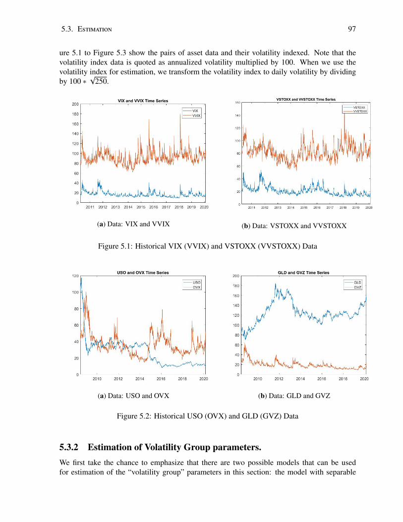
5.3. Estimation 97
ure 5.1 to Figure 5.3 show the pairs of asset data and their volatility indexed. Note that thevolatility index data is quoted as annualized volatility multiplied by 100. When we use thevolatility index for estimation, we transform the volatility index to daily volatility by dividingby 100 ∗
√250.
(a) Data: VIX and VVIX (b) Data: VSTOXX and VVSTOXX
Figure 5.1: Historical VIX (VVIX) and VSTOXX (VVSTOXX) Data
(a) Data: USO and OVX (b) Data: GLD and GVZ
Figure 5.2: Historical USO (OVX) and GLD (GVZ) Data
5.3.2 Estimation of Volatility Group parameters.We first take the chance to emphasize that there are two possible models that can be usedfor estimation of the “volatility group” parameters in this section: the model with separable
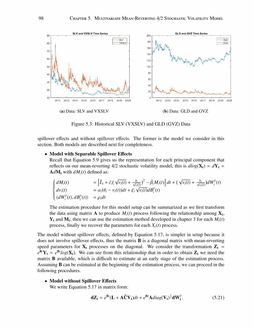
98 Chapter 5. MultivariateMean-Reverting 4/2 Stochastic VolatilityModel
(a) Data: SLV and VXSLV (b) Data: GLD and GVZ
Figure 5.3: Historical SLV (VXSLV) and GLD (GVZ) Data
spillover effects and without spillover effects. The former is the model we consider in thissection. Both models are described next for completeness.
• Model with Separable Spillover EffectsRecall that Equation 5.9 gives us the representation for each principal component thatreflects on our mean-reverting 4/2 stochastic volatility model, this is dlog(Xt) = dYt =
AdMt with dMi(t) defined as:dMi(t) =
[Li + ci
(√νi(t) + bi√
νi(t)
)2− βiMi(t)
]dt +
(√νi(t) + bi√
νi(t)
)dWP
i (t)
dνi(t) = αi(θi − νi(t))dt + ξi√νi(t)dBPi (t)
〈dWPi (t), dBPi (t)〉 = ρidt
The estimation procedure for this model setup can be summarized as we first transformthe data using matrix A to produce Mi(t) process following the relationship among Xt,Yt and Mt; then we can use the estimation method developed in chapter 3 for each Mi(t)process, finally we recover the parameters for each Xi(t) process.
The model without spillover effects, defined by Equation 5.17, is simpler in setup because itdoes not involve spillover effects, thus the matrix B is a diagonal matrix with mean-revertingspeed parameters for Xt processes on the diagonal. We consider the transformation Zt =
eBtYt = eBtlog(Xt). We can see from this relationship that in order to obtain Zt we need thematrix B available, which is difficult to estimate at an early stage of the estimation process.Assuming B can be estimated at the beginning of the estimation process, we can proceed in thefollowing procedures.
• Model without Spillover EffectsWe write Equation 5.17 in matrix form:
dZt = eBt(L + ACVt)dt + eBtAdiag(Vt)12 dWP
t . (5.21)
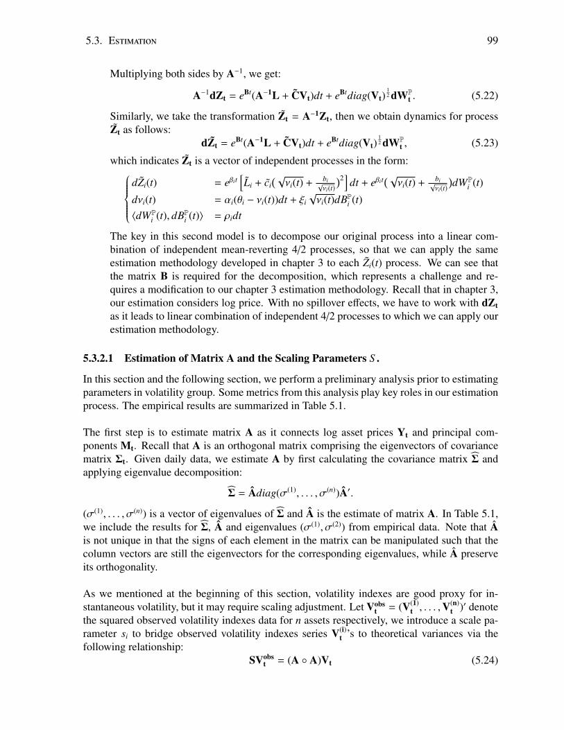
5.3. Estimation 99
Multiplying both sides by A−1, we get:
A−1dZt = eBt(A−1L + CVt)dt + eBtdiag(Vt)12 dWP
t . (5.22)
Similarly, we take the transformation Zt = A−1Zt, then we obtain dynamics for processZt as follows:
dZt = eBt(A−1L + CVt)dt + eBtdiag(Vt)12 dWP
t , (5.23)
which indicates Zt is a vector of independent processes in the form:dZi(t) = eβit
[Li + ci
(√νi(t) + bi√
νi(t)
)2]
dt + eβit(√νi(t) + bi√
νi(t)
)dWP
i (t)
dνi(t) = αi(θi − νi(t))dt + ξi√νi(t)dBPi (t)
〈dWPi (t), dBPi (t)〉 = ρidt
The key in this second model is to decompose our original process into a linear com-bination of independent mean-reverting 4/2 processes, so that we can apply the sameestimation methodology developed in chapter 3 to each Zi(t) process. We can see thatthe matrix B is required for the decomposition, which represents a challenge and re-quires a modification to our chapter 3 estimation methodology. Recall that in chapter 3,our estimation considers log price. With no spillover effects, we have to work with dZtas it leads to linear combination of independent 4/2 processes to which we can apply ourestimation methodology.
5.3.2.1 Estimation of Matrix A and the Scaling Parameters S .
In this section and the following section, we perform a preliminary analysis prior to estimatingparameters in volatility group. Some metrics from this analysis play key roles in our estimationprocess. The empirical results are summarized in Table 5.1.
The first step is to estimate matrix A as it connects log asset prices Yt and principal com-ponents Mt. Recall that A is an orthogonal matrix comprising the eigenvectors of covariancematrix Σt. Given daily data, we estimate A by first calculating the covariance matrix Σ andapplying eigenvalue decomposition:
Σ = Adiag(σ(1), . . . , σ(n))A′.
(σ(1), . . . , σ(n)) is a vector of eigenvalues of Σ and A is the estimate of matrix A. In Table 5.1,we include the results for Σ, A and eigenvalues (σ(1), σ(2)) from empirical data. Note that Ais not unique in that the signs of each element in the matrix can be manipulated such that thecolumn vectors are still the eigenvectors for the corresponding eigenvalues, while A preserveits orthogonality.
As we mentioned at the beginning of this section, volatility indexes are good proxy for in-stantaneous volatility, but it may require scaling adjustment. Let Vobs
t = (V(1)t , . . . ,V(n)
t )′ denotethe squared observed volatility indexes data for n assets respectively, we introduce a scale pa-rameter si to bridge observed volatility indexes series V(i)
t ’s to theoretical variances via thefollowing relationship:
SVobst = (A A)Vt (5.24)

100 Chapter 5. MultivariateMean-Reverting 4/2 Stochastic VolatilityModel
Vt = (A A)−1SVobst . (5.25)
where S is a diagonal matrix with diagonal vector (s1, . . . , sn). In theory, si is a function oft,T, bi, αi, θi, ξi, see [102], [130], some of which fall into volatility group and are to be esti-mated. Hence, it is crucial to come up with an estimate that does not depend on these param-eters. We propose an estimate that matches the long run first empirical moment of both sidesof Equation 5.24. The long term average of the left-hand side of Equation 5.24 can be directlycalculated from squared volatility indexes data. The long term average of the right-hand sidemay not seem as straight forward as it is a stochastic process. In our definition (A A)Vt is thediagonal of covariance matrix and refers to instantaneous variance process. So in the long run,the expectation of the variance process should converge to the variance of the underlying asset.Let σ2
i denote the empirical long term variance of asset i and µi denote the long term averageof the corresponding squared volatility index data. We estimate si as:
si =σ2
i
µi. (5.26)
Substituting Equation 5.26 and A back to the right-hand side of Equation 5.25, then the longterm average gives us:
σ(1)
...σ(n)
= E[(A A)−1SVobs
t
],
which matches the left-hand side of Equation 5.25 in long term average as Vt is the eigenvalueof Σt and converges to (σ(1), . . . , σ(n)) in the long run. Table 5.1 also shows the results for Σ,(σ(1), σ(2)) and (s1, s2).
VIX&VSTOXX USO&GLD SLV&GLD
Σ
(0.0062 0.00300.0030 0.0048
) (4.779e − 4 4.616e − 54.616e − 5 1.2547e − 5
) (0.0724 0.03310.0331 0.0237
)(µ1, µ2) (0.0034,0.0028) (6.0109e-4,1.6689e-4) (3.6258e-4,1.1843e-4)
(a): Covariance Matrix and Long Term Average of Squared Volatility IndexesVIX&VSTOXX USO&GLD SLV&GLD
A(0.7825 −0.62260.6226 0.7825
) (0.9918 −0.12780.1278 0.9918
) (0.8925 −0.4510.451 0.8925
)A
(2.725 −1.725−1.725 2.725
) (1.0169 −0.0169−0.0169 1.0169
) (1.3429 −0.3429−0.3429 1.3429
)(σ(1), σ(2)) (2.1372, 0.592) (0.121, 0.0299) (0.0891, 0.007)(s1, s2) (1.8074, 1.7229) (0.795, 0.7518) (0.799, 0.8)
(b): Eigenvectors, Eigenvalues and Scaling Factors
Table 5.1: Empirical Results
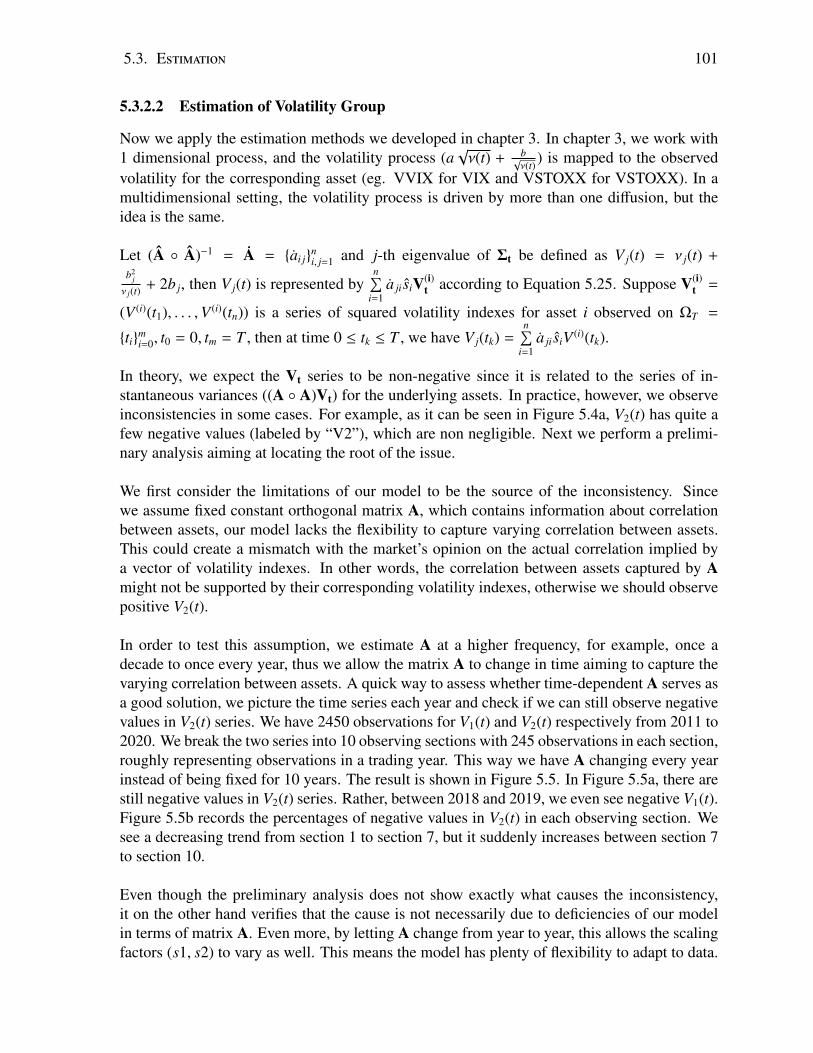
5.3. Estimation 101
5.3.2.2 Estimation of Volatility Group
Now we apply the estimation methods we developed in chapter 3. In chapter 3, we work with1 dimensional process, and the volatility process (a
√ν(t) + b
√ν(t)
) is mapped to the observedvolatility for the corresponding asset (eg. VVIX for VIX and VSTOXX for VSTOXX). In amultidimensional setting, the volatility process is driven by more than one diffusion, but theidea is the same.
Let (A A)−1 = A = ai jni, j=1 and j-th eigenvalue of Σt be defined as V j(t) = ν j(t) +
b2j
ν j(t)+ 2b j, then V j(t) is represented by
n∑i=1
a ji siV(i)t according to Equation 5.25. Suppose V(i)
t =
(V (i)(t1), . . . ,V (i)(tn)) is a series of squared volatility indexes for asset i observed on ΩT =
timi=0, t0 = 0, tm = T , then at time 0 ≤ tk ≤ T , we have V j(tk) =
n∑i=1
a ji siV (i)(tk).
In theory, we expect the Vt series to be non-negative since it is related to the series of in-stantaneous variances ((A A)Vt) for the underlying assets. In practice, however, we observeinconsistencies in some cases. For example, as it can be seen in Figure 5.4a, V2(t) has quite afew negative values (labeled by “V2”), which are non negligible. Next we perform a prelimi-nary analysis aiming at locating the root of the issue.
We first consider the limitations of our model to be the source of the inconsistency. Sincewe assume fixed constant orthogonal matrix A, which contains information about correlationbetween assets, our model lacks the flexibility to capture varying correlation between assets.This could create a mismatch with the market’s opinion on the actual correlation implied bya vector of volatility indexes. In other words, the correlation between assets captured by Amight not be supported by their corresponding volatility indexes, otherwise we should observepositive V2(t).
In order to test this assumption, we estimate A at a higher frequency, for example, once adecade to once every year, thus we allow the matrix A to change in time aiming to capture thevarying correlation between assets. A quick way to assess whether time-dependent A serves asa good solution, we picture the time series each year and check if we can still observe negativevalues in V2(t) series. We have 2450 observations for V1(t) and V2(t) respectively from 2011 to2020. We break the two series into 10 observing sections with 245 observations in each section,roughly representing observations in a trading year. This way we have A changing every yearinstead of being fixed for 10 years. The result is shown in Figure 5.5. In Figure 5.5a, there arestill negative values in V2(t) series. Rather, between 2018 and 2019, we even see negative V1(t).Figure 5.5b records the percentages of negative values in V2(t) in each observing section. Wesee a decreasing trend from section 1 to section 7, but it suddenly increases between section 7to section 10.
Even though the preliminary analysis does not show exactly what causes the inconsistency,it on the other hand verifies that the cause is not necessarily due to deficiencies of our modelin terms of matrix A. Even more, by letting A change from year to year, this allows the scalingfactors (s1, s2) to vary as well. This means the model has plenty of flexibility to adapt to data.
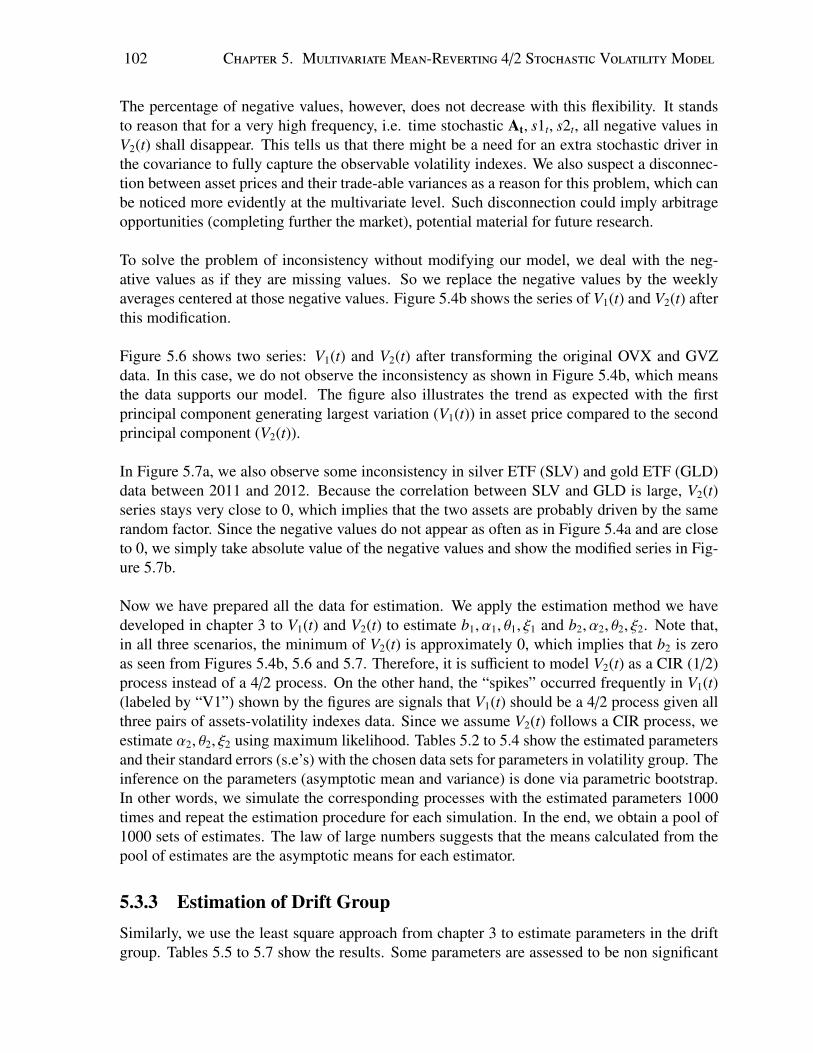
102 Chapter 5. MultivariateMean-Reverting 4/2 Stochastic VolatilityModel
The percentage of negative values, however, does not decrease with this flexibility. It standsto reason that for a very high frequency, i.e. time stochastic At, s1t, s2t, all negative values inV2(t) shall disappear. This tells us that there might be a need for an extra stochastic driver inthe covariance to fully capture the observable volatility indexes. We also suspect a disconnec-tion between asset prices and their trade-able variances as a reason for this problem, which canbe noticed more evidently at the multivariate level. Such disconnection could imply arbitrageopportunities (completing further the market), potential material for future research.
To solve the problem of inconsistency without modifying our model, we deal with the neg-ative values as if they are missing values. So we replace the negative values by the weeklyaverages centered at those negative values. Figure 5.4b shows the series of V1(t) and V2(t) afterthis modification.
Figure 5.6 shows two series: V1(t) and V2(t) after transforming the original OVX and GVZdata. In this case, we do not observe the inconsistency as shown in Figure 5.4b, which meansthe data supports our model. The figure also illustrates the trend as expected with the firstprincipal component generating largest variation (V1(t)) in asset price compared to the secondprincipal component (V2(t)).
In Figure 5.7a, we also observe some inconsistency in silver ETF (SLV) and gold ETF (GLD)data between 2011 and 2012. Because the correlation between SLV and GLD is large, V2(t)series stays very close to 0, which implies that the two assets are probably driven by the samerandom factor. Since the negative values do not appear as often as in Figure 5.4a and are closeto 0, we simply take absolute value of the negative values and show the modified series in Fig-ure 5.7b.
Now we have prepared all the data for estimation. We apply the estimation method we havedeveloped in chapter 3 to V1(t) and V2(t) to estimate b1, α1, θ1, ξ1 and b2, α2, θ2, ξ2. Note that,in all three scenarios, the minimum of V2(t) is approximately 0, which implies that b2 is zeroas seen from Figures 5.4b, 5.6 and 5.7. Therefore, it is sufficient to model V2(t) as a CIR (1/2)process instead of a 4/2 process. On the other hand, the “spikes” occurred frequently in V1(t)(labeled by “V1”) shown by the figures are signals that V1(t) should be a 4/2 process given allthree pairs of assets-volatility indexes data. Since we assume V2(t) follows a CIR process, weestimate α2, θ2, ξ2 using maximum likelihood. Tables 5.2 to 5.4 show the estimated parametersand their standard errors (s.e’s) with the chosen data sets for parameters in volatility group. Theinference on the parameters (asymptotic mean and variance) is done via parametric bootstrap.In other words, we simulate the corresponding processes with the estimated parameters 1000times and repeat the estimation procedure for each simulation. In the end, we obtain a pool of1000 sets of estimates. The law of large numbers suggests that the means calculated from thepool of estimates are the asymptotic means for each estimator.
5.3.3 Estimation of Drift GroupSimilarly, we use the least square approach from chapter 3 to estimate parameters in the driftgroup. Tables 5.5 to 5.7 show the results. Some parameters are assessed to be non significant
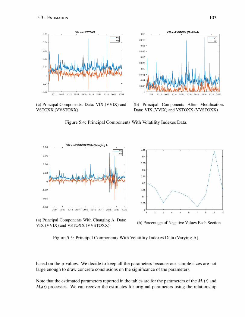
5.3. Estimation 103
(a) Principal Components. Data: VIX (VVIX) andVSTOXX (VVSTOXX)
(b) Principal Components After Modification.Data: VIX (VVIX) and VSTOXX (VVSTOXX)
Figure 5.4: Principal Components With Volatility Indexes Data.
(a) Principal Components With Changing A. Data:VIX (VVIX) and VSTOXX (VVSTOXX)
(b) Percentage of Negative Values Each Section
Figure 5.5: Principal Components With Volatility Indexes Data (Varying A).
based on the p-values. We decide to keep all the parameters because our sample sizes are notlarge enough to draw concrete conclusions on the significance of the parameters.
Note that the estimated parameters reported in the tables are for the parameters of the M1(t) andM2(t) processes. We can recover the estimates for original parameters using the relationship
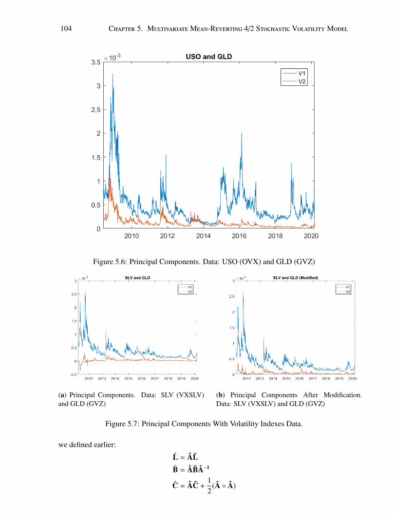
104 Chapter 5. MultivariateMean-Reverting 4/2 Stochastic VolatilityModel
Figure 5.6: Principal Components. Data: USO (OVX) and GLD (GVZ)
(a) Principal Components. Data: SLV (VXSLV)and GLD (GVZ)
(b) Principal Components After Modification.Data: SLV (VXSLV) and GLD (GVZ)
Figure 5.7: Principal Components With Volatility Indexes Data.
we defined earlier:
L = ALB = ABA−1
C = AC +12
(A A)
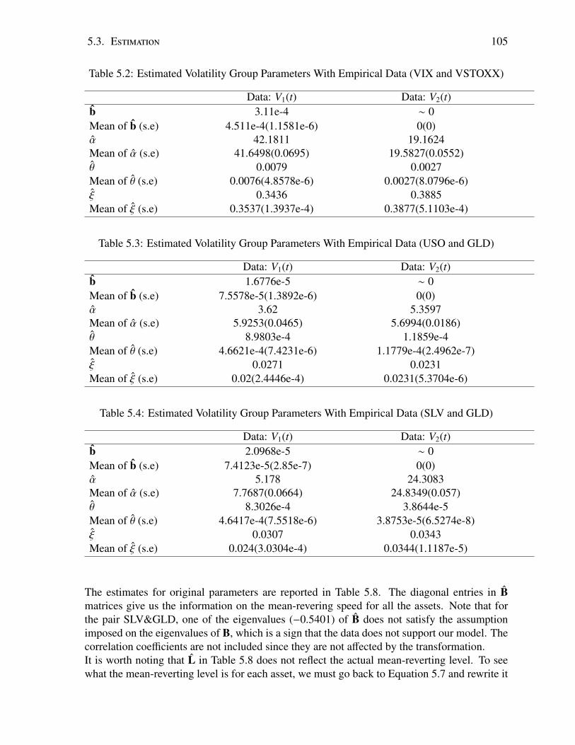
5.3. Estimation 105
Table 5.2: Estimated Volatility Group Parameters With Empirical Data (VIX and VSTOXX)
Data: V1(t) Data: V2(t)b 3.11e-4 ∼ 0Mean of b (s.e) 4.511e-4(1.1581e-6) 0(0)α 42.1811 19.1624Mean of α (s.e) 41.6498(0.0695) 19.5827(0.0552)θ 0.0079 0.0027Mean of θ (s.e) 0.0076(4.8578e-6) 0.0027(8.0796e-6)ξ 0.3436 0.3885Mean of ξ (s.e) 0.3537(1.3937e-4) 0.3877(5.1103e-4)
Table 5.3: Estimated Volatility Group Parameters With Empirical Data (USO and GLD)
Data: V1(t) Data: V2(t)b 1.6776e-5 ∼ 0Mean of b (s.e) 7.5578e-5(1.3892e-6) 0(0)α 3.62 5.3597Mean of α (s.e) 5.9253(0.0465) 5.6994(0.0186)θ 8.9803e-4 1.1859e-4Mean of θ (s.e) 4.6621e-4(7.4231e-6) 1.1779e-4(2.4962e-7)ξ 0.0271 0.0231Mean of ξ (s.e) 0.02(2.4446e-4) 0.0231(5.3704e-6)
Table 5.4: Estimated Volatility Group Parameters With Empirical Data (SLV and GLD)
Data: V1(t) Data: V2(t)b 2.0968e-5 ∼ 0Mean of b (s.e) 7.4123e-5(2.85e-7) 0(0)α 5.178 24.3083Mean of α (s.e) 7.7687(0.0664) 24.8349(0.057)θ 8.3026e-4 3.8644e-5Mean of θ (s.e) 4.6417e-4(7.5518e-6) 3.8753e-5(6.5274e-8)ξ 0.0307 0.0343Mean of ξ (s.e) 0.024(3.0304e-4) 0.0344(1.1187e-5)
The estimates for original parameters are reported in Table 5.8. The diagonal entries in Bmatrices give us the information on the mean-revering speed for all the assets. Note that forthe pair SLV&GLD, one of the eigenvalues (−0.5401) of B does not satisfy the assumptionimposed on the eigenvalues of B, which is a sign that the data does not support our model. Thecorrelation coefficients are not included since they are not affected by the transformation.It is worth noting that L in Table 5.8 does not reflect the actual mean-reverting level. To seewhat the mean-reverting level is for each asset, we must go back to Equation 5.7 and rewrite it
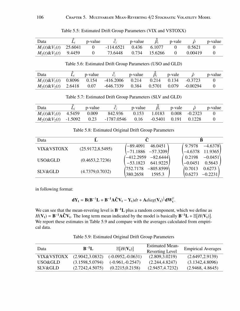
106 Chapter 5. MultivariateMean-Reverting 4/2 Stochastic VolatilityModel
Table 5.5: Estimated Drift Group Parameters (VIX and VSTOXX)
Data ˆLi p-value ˆci p-value ˆβi p-vale ρ p-valueM1(t)&V1(t) 25.6041 0 -114.6521 0.436 6.1077 0 0.5621 0M2(t)&V2(t) 9.4459 0 73.6448 0.734 15.6266 0 0.00419 0
Table 5.6: Estimated Drift Group Parameters (USO and GLD)
Data ˆLi p-value ˆci p-value ˆβi p-vale ρ p-valueM1(t)&V1(t) 0.8096 0.154 -416.2006 0.214 0.214 0.134 -0.3723 0M2(t)&V2(t) 2.6418 0.07 -646.7339 0.384 0.5701 0.079 -0.00294 0
Table 5.7: Estimated Drift Group Parameters (SLV and GLD)
Data ˆLi p-value ˆci p-value ˆβi p-vale ρ p-valueM1(t)&V1(t) 4.5459 0.009 842.936 0.153 1.0183 0.008 -0.2323 0M2(t)&V2(t) -1.5092 0.23 -1787.0546 0.16 -0.5401 0.191 0.1228 0
Table 5.8: Estimated Original Drift Group Parameters
Data L C B
VIX&VSTOXX (25.9172,8.5495)(−89.4091 46.0451−71.1886 −57.3209
) (9.7978 −4.6378−4.6378 11.9365
)USO&GLD (0.4653,2.7236)
(−412.2959 −82.6444−53.1823 641.9225
) (0.2198 −0.0451−0.0451 0.5643
)SLV&GLD (4.7379,0.7032)
(752.7178 −805.8599380.2658 1595.3
) (0.7013 0.62730.6273 −0.2231
)
in following format:
dYt = B(B−1L + B−1ACVt − Yt)dt + Adiag(Vt)12 dWP
t .
We can see that the mean-revering level is B−1L plus a random component, which we define asH(Vt) = B−1ACVt. The long term mean indicated by the model is basically B−1L + E
[H(Vt)
].
We report these estimates in Table 5.9 and compare with the averages calculated from empiri-cal data.
Table 5.9: Estimated Original Drift Group Parameters
Data B−1L E[H(Vt)
] Estimated Mean-Reverting Level Empirical Averages
VIX&VSTOXX (2.9042,3.0832) (-0.0952,-0.0631) (2.809,3.0219) (2.6497,2.9139)USO&GLD (3.1598,5.0794) (-0.961,-0.2547) (2.244,4.8247) (3.1342,4.8096)SLV&GLD (2.7242,4.5075) (0.2215,0.2158) (2.9457,4.7232) (2.9468, 4.8645)
5.4. RiskMeasures 107
From Table 5.9, we can see that the estimated MRLs are closed to empirical log price aver-ages except for USO case where the estimated mean is quite smaller than the empirical mean.This latest point might be due to the impact of the initial value on the stationary value of a4/2 process. We can see that VIX&VSTOXX have the largest mean-reverting speed compar-ing to the other two commodity ETF pairs. This is not a surprise as evidenced by empiricaldata. Volatility indexes tend to return to mean faster due to economic cycle whilst commoditiesnormally have longer time horizon to revert to mean level due to scarcity, demand and supply.
5.4 Risk Measures
In section 1.3.5, we provided some definitions and concepts related to risk measures and finan-cial risk management. Risk measures determine the minimum amount of capital to be kept inreserve in worst case scenarios as a way of protecting financial institutions. There are manyrisk measures in the literature see, for example, [7] and [104], one of which is considered fun-damental yet crucial: Value-at-Risk (VaR). VaR is a distribution-based risk measure, in otherwords, VaR calculation takes into account the distribution of the underlying (VaR is in fact aquantile). It is more robust to outliers than mean and variance.
In this section, we compute the VaR of a portfolio consisting of two assets, for example USOand GLD. To calculate the VaR, we first need to find the distribution of this portfolio, whichmight not be available due to, in particular, the correlation among the underlyings. In languageof mathematical statistics, we need to find the joint distribution of USO and GLD in order tocompute VaR. Theoretically, in general, it is difficult to find closed-form expressions for thejoint distribution of two non-Gaussian stochastic processes. In fact, USO and GLD have verycomplex distribution functions under our multidimensional 4/2 model setting. Fortunately, us-ing principal component decomposition, we can decompose a multidimensional structure intoindependent one dimensional pieces. What is more attractive is that we are able to expressthe joint distribution at any given date of USO and GLD in terms of two independent randomvariables, which simplifies our problem significantly and allow for the use of c.f.s to computeproperties of the portfolio distribution.
5.4.1 Portfolio Setup
Suppose we have a portfolio Π consisting of two assets X1(t) and X2(t):
Π(t) = φ1(t)X1(t) + φ2(t)X2(t) + φ3(t)B(t), (5.27)
where φ1 and φ2 represent the weights of X1(t) and X2(t) in the portfolio and B(t) is a cashaccount with interest rate r. In a short period of time, we can also write the problem using theself-financing condition and relative portfolio weights π1, π2 and (1 − π1 − π2) (i.e. proportionallocated to the assets and cash account, allocations) see [28]:
dΠ(t)Π(t)
= π1dX1(t)X1(t)
+ π2dX2(t)X2(t)
+ (1 − π1 − π2)rdt. (5.28)

108 Chapter 5. MultivariateMean-Reverting 4/2 Stochastic VolatilityModel
For the purpose of this chapter we will only consider constant allocations, i.e. constant π, asthis is the most popular investment strategy in the market, supported by [107]. From the processdXi(t)Xi(t)
, we can easily obtain dYi(t) (Yi(t) = log(Xi(t)) by using Ito’s lemma. When comparingdXi(t)Xi(t)
and dYi(t), we observe that only the drift term is adjusted, diffusion terms stay the same.Assuming (X1(t), X2(t)) are modeled by Equation 5.2, the log prices (Y1(t),Y2(t)) then have theSDE specified in Equation 5.7 under the PCSV framework. Moreover, we can also write dXi(t)
Xi(t)in terms of dYi(t):
dXi(t)Xi(t)
= dYi(t) +12
∑j
a2i j
( √ν j(t) +
b j
ν j(t)
)2
dt.
Hence, we rewrite Equation 5.28 as:
dΠ(t)Π(t)
= π1
[dY1(t) +
12
2∑j=1
a21 j
( √ν j(t) +
b j
ν j(t)
)2
dt]
+ π2
[dY2(t) +
12
2∑j=1
a22 j
( √ν j(t) +
b j
ν j(t)
)2
dt]
+ (1 − π1 − π2)rdt.(5.29)
We have also demonstrated that Y1(t) and Y2(t) are linear combinations of two independentstochastic processes/random variables M1(t) and M2(t), hence we can write the dynamics ofY1(t) and Y2(t) in terms of M1(t) and M2(t) as follows:
dY1(t) = a11dM1(t) + a12dM2(t), (5.30)dY2(t) = a21dM1(t) + a22dM2(t). (5.31)
We now substitute dY1(t) and dY2(t) in Equation 5.29 with Equations 5.30 and 5.31:
dΠ(t)Π(t)
= (π1a11 + π2a21)dM1(t) +12
(π1a211 + π2a2
21)( √
ν1(t) +b1
ν1(t)
)2
dt
+ (π1a12 + π2a22)dM2(t) +12
(π1a212 + π2a2
22)( √
ν2(t) +b2
ν2(t)
)2
dt
+ (1 − π1 − π2)rdt.
(5.32)
From Equation 5.32, we can conclude that dΠ(t)Π(t) is also a linear combination of dM1(t) and
dM2(t) with adjustment done to the drift terms, which does not affect the independent relation-ship between dM1(t) and dM2(t). We organize Equation 5.32 into the following expression:
dΠ(t)Π(t)
= dM∗1(t) + dM∗
2(t) (5.33)
where dM∗1(t) and dM∗
2(t) are independent with
dM∗i (t) =
[L∗i + c∗i
( √νi(t) +
bi√νi(t)
)2− β∗i M∗
i (t)]
dt + a∗i( √
νi(t) +bi√νi(t)
)dWP
i (t),
5.4. RiskMeasures 109
where,
L∗1 = L1a∗1 + (1 − π1 − π2)r, L∗2 = L2a∗2
c∗i = cia∗i +12
a∗∗i ,
β∗i = βia∗i ,
a∗i =
2∑j=1
π ja ji,
a∗∗i =
2∑j=1
π ja2ji.
Note we included the growth rate on the cash account into long term average of M∗1(t) for
convenience. From a mathematical perspective, M∗1(t) is constructed based on M1(t), which
is the first principal component that determines most variation among the assets. As a result,M∗
1(t) affects the performance of Π(t) more than M∗2(t) financially. For this reason, the effect of
the growth rate on the portfolio can also be interpreted as if it impacts the long term average ofM∗
1(t). Now we apply Ito’s lemma to Equation 5.33 to obtain the dynamics for ln(Π(t)):
dln(Π(t)) = dM∗1(t) + dM∗
2(t) (5.34)
where,
dM∗i (t) =
[L∗i +
(c∗i −
12
(a∗i )2)( √νi(t) +bi√νi(t)
)2− β∗i M∗
i (t)]
dt + a∗i( √
νi(t) +bi√νi(t)
)dWP
i (t).
It is straightforward to find the characteristic function of dln(Π(t)) using results from chapter 4and chapter 5.
5.4.2 The Density Function of The Portfolio Π(t)
From Equation 5.34, our portfolio now basically contains two new “assets” that are independentof each other. Thanks to this independence, we can derive the characteristic function as wellas the density function of our portfolio. Since our goal is to calculate VaR, it is convenient touse density function and integrate numerically. In this section, we list two approaches to obtainsuch density function.
5.4.2.1 The Density Function via Convolution
One way to obtain the conditional density function for ln(Π(T )) is via convolution of twoconditional density functions for M∗
1(T ) and M∗2(T ). In probability, if two random variables X
and Y are independent with density functions fX(x) and fY(y) respectively. Let Z = X + Y , thenthe density for Z, fZ(z), can be found via convolution, i.e:
fZ(z) =
∫ ∞
−∞
fX(x) fY(z − x)dx. (5.35)

110 Chapter 5. MultivariateMean-Reverting 4/2 Stochastic VolatilityModel
If X and Y have analytical density functions, then convolution method is straightforward. In ourcase, we obtain the conditional c.f. first. Theoretically, the Fourier inversion of the conditionalc.f. gives the density function. Due to the structure of our original c.f. and the approxi-mations, we need to invert the original c.f. and the approximated c.f.’s numerically for thecorresponding density functions. For M∗
1(T ) and M∗2(T ), we can obtain their conditional cor-
responding density functions f1(m1|Ft) and f2(m2|Ft) by inverting the c.f. of Z∗1(t) = eβ∗1tM∗
1(t)and Z∗2(t) = eβ
∗2tM∗
2(t):
f1(m1|Ft) =1
2π
∫ ∞
−∞
e−ium1ΦMR
(T, u; L∗1, c
∗1, a
∗1, β
∗1, α1, θ1, ξ1, ρ1, a∗1b1, ν1(t), e−β
∗1tZ∗1(t)
)du.
(5.36)
f2(m2|Ft) =1
2π
∫ ∞
−∞
e−ium2ΦMR
(T, u; L∗2, c
∗2, a
∗2, β
∗2, α2, θ2, ξ2, ρ2, a∗2b2, ν2(t), e−β
∗2tZ∗2(t)
)du.
(5.37)We can now write Equation 5.40 as a convolution of Equations 5.36 and 5.37:
f (p|Ft) =
∫ ∞
−∞
f1(m1|Ft) f2(p − m1|Ft)dm1. (5.38)
A challenging part of this method is that we need to invert the semi-closed c.f.s first to obtainthe density functions for M∗
1(t) and M∗2(t) (artificial assets), which involves approximations.
As we have well-developed approximation approaches for ΦMR, we can apply the results toobtain analytic function as approximation of the c.f. for individual artificial asset and then findthe density via Fourier inversion. Then we can use Equation 5.38 to obtain the density of theportfolio. Recall that our approximation approaches work well in a parametric region as seenin Figures 3.1 and 3.2 for three scenarios (bi = 0, ρi , 0; bi , 0, ρi = 0; bi = 0, ρi = 0), thegoodness of approximations depend on L∗i , c
∗i , a∗i , β∗i , αi, θi, ξi, ρi, bi.
Also in the scenario where the 3/2 component is not negligible, we involve a hypergeomet-ric function in the approximated function, which requires numerical computation methods,either we find the hypergeometric function numerically or avoid the hypergeometric functionwith partial simulation (only need to simulate νi(t) process to obtain the c.f.). These are thedifficulties involved in finding the individual c.f. Despite these difficulties, our approximationapproaches have been proved effective in chapter 3. With analytic approximations, we can findthe individual c.f. efficiently.
5.4.2.2 Density Function via Fourier Inversion
Another way to obtain density function is to apply inverse Fourier transform to the charac-teristic function. Before we give the formula for the characteristic function, we consider thetransformation Z∗i (t) = eβ
∗i tM∗
i (t). By Ito’s lemma, we have:
dZ∗i (t) = eβ∗i t
[L∗i +
(c∗i −
12
(a∗i )2)( √νi(t) +bi√νi(t)
)2]
dt + eβ∗i ta∗i
( √νi(t) +
bi√νi(t)
)dWP
i (t).
Next corollary illustrates how to derive the characteristic function:
5.4. RiskMeasures 111
Corollary 5.4.1 Let ΦMR(T, u; L, c, a, β, α, θ, ξ, ρ, b, ν(t),Z(t)
)denote the characteristic func-
tion provided in Proposition 3.2.1, then the characteristic function of ln(Π(T )) is given by thefollowing equation:
E(eiuln(Π(T ))|Ft) =
2∏i=1
ΦMR
(T, u; L∗i , c
∗i , a∗i , β∗i , αi, θi, ξi, ρi, a∗i bi, νi(t), Z∗i (t)
)(5.39)
where L∗1 = L1a∗1 + (1 − π1 − π2)r, L∗2 = L2a∗2, c∗i = cia∗i + 1
2a∗∗i , β∗i = βia∗i , a
∗i =
∑2j=1 π ja ji, a∗∗i =∑2
j=1 π ja2ji.
Let p denote all possible values in the domain of ln(Π(T )), the density function hence follows:
f (p|Ft) =1
2π
∫ ∞
−∞
e−iupE(eiuln(Π(T ))|Ft)du. (5.40)
It is not hard to see that the c.f. of the portfolio does not have a closed-form representation sinceit is a product of semi-closed c.f.s (ΦMR) from chapter 3. As a result, we only have a term (aproduct of conditional expectations in the case of portfolio c.f.) that requires approximationsfor fast computations. Hence, the Fourier inversion method still face both theoretical andnumerical difficulties as we outlined at the end of previous section. The convolution methodand the Fourier inversion method both require finding the c.f.s first, which may require eitherworking with a hypergeometric function, a partial simulation (simulating νi(t) process) or anapproximation.
5.4.2.3 Numerical Implementation of Selected Method
Theoretically, the Fourier inversion method and the convolution method yield the same densityfunction for the portfolio. In a portfolio which only consists of two (artificial) risky assets, bothmethods are not complicated to implement. We decide to implement convolution method withpartial simulation as it directly uses the well-developed algorithm from chapter 3. However,it would be more efficient to use the Fourier inversion method when the portfolio has a largepool of assets (e.g. over 100). To see this, note the convolution method involves, for n, n >> 2assets, the simulation of n processes with n+1 integrations, while the Fourier inversion methodreduces the number of integrations to just one.
We summarize the numerical implementation to compute the conditional density function ofthe portfolio in following steps:
• Step 1: Simulate two CIR processes ν1(t) and ν2(t) and compute ΦMR for M∗1(t) and
M∗2(t).
• Step 2: Invert the c.f.s obtained in Step 1 to get f1(m1|Ft) and f2(m2|Ft).
• Step 3: Integrate numerically the product of the conditional density of M∗1(T ) and M∗
2(T )for the conditional density function of ln(Π(T )).
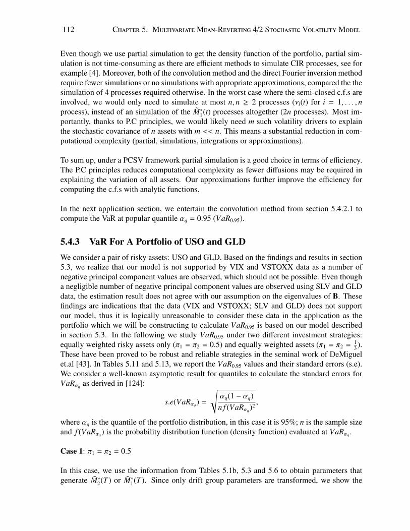
112 Chapter 5. MultivariateMean-Reverting 4/2 Stochastic VolatilityModel
Even though we use partial simulation to get the density function of the portfolio, partial sim-ulation is not time-consuming as there are efficient methods to simulate CIR processes, see forexample [4]. Moreover, both of the convolution method and the direct Fourier inversion methodrequire fewer simulations or no simulations with appropriate approximations, compared the thesimulation of 4 processes required otherwise. In the worst case where the semi-closed c.f.s areinvolved, we would only need to simulate at most n, n ≥ 2 processes (νi(t) for i = 1, . . . , nprocess), instead of an simulation of the M∗
1(t) processes altogether (2n processes). Most im-portantly, thanks to P.C principles, we would likely need m such volatility drivers to explainthe stochastic covariance of n assets with m << n. This means a substantial reduction in com-putational complexity (partial, simulations, integrations or approximations).
To sum up, under a PCSV framework partial simulation is a good choice in terms of efficiency.The P.C principles reduces computational complexity as fewer diffusions may be required inexplaining the variation of all assets. Our approximations further improve the efficiency forcomputing the c.f.s with analytic functions.
In the next application section, we entertain the convolution method from section 5.4.2.1 tocompute the VaR at popular quantile αq = 0.95 (VaR0.95).
5.4.3 VaR For A Portfolio of USO and GLDWe consider a pair of risky assets: USO and GLD. Based on the findings and results in section5.3, we realize that our model is not supported by VIX and VSTOXX data as a number ofnegative principal component values are observed, which should not be possible. Even thougha negligible number of negative principal component values are observed using SLV and GLDdata, the estimation result does not agree with our assumption on the eigenvalues of B. Thesefindings are indications that the data (VIX and VSTOXX; SLV and GLD) does not supportour model, thus it is logically unreasonable to consider these data in the application as theportfolio which we will be constructing to calculate VaR0.95 is based on our model describedin section 5.3. In the following we study VaR0.95 under two different investment strategies:equally weighted risky assets only (π1 = π2 = 0.5) and equally weighted assets (π1 = π2 = 1
3 ).These have been proved to be robust and reliable strategies in the seminal work of DeMiguelet.al [43]. In Tables 5.11 and 5.13, we report the VaR0.95 values and their standard errors (s.e).We consider a well-known asymptotic result for quantiles to calculate the standard errors forVaRαq as derived in [124]:
s.e(VaRαq) =
√αq(1 − αq)n f (VaRαq)2 ,
where αq is the quantile of the portfolio distribution, in this case it is 95%; n is the sample sizeand f (VaRαq) is the probability distribution function (density function) evaluated at VaRαq .
Case 1: π1 = π2 = 0.5
In this case, we use the information from Tables 5.1b, 5.3 and 5.6 to obtain parameters thatgenerate M∗
2(T ) or M∗1(T ). Since only drift group parameters are transformed, we show the
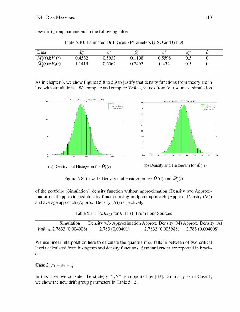
5.4. RiskMeasures 113
new drift group parameters in the following table:
Table 5.10: Estimated Drift Group Parameters (USO and GLD)
Data L∗i c∗i β∗i a∗i a∗∗i ρ
M∗1(t)&V1(t) 0.4532 0.5933 0.1198 0.5598 0.5 0
M∗2(t)&V2(t) 1.1413 0.6567 0.2463 0.432 0.5 0
As in chapter 3, we show Figures 5.8 to 5.9 to justify that density functions from theory are inline with simulations. We compute and compare VaR0.95 values from four sources: simulation
(a) Density and Histogram for M∗1(t) (b) Density and Histogram for M∗2(t)
Figure 5.8: Case 1: Density and Histogram for M∗1(t) and M∗
2(t)
of the portfolio (Simulation), density function without approximation (Density w/o Approxi-mation) and approximated density function using midpoint approach (Approx. Density (M))and average approach (Approx. Density (A)) respectively:
Table 5.11: VaR0.05 for ln(Π(t)) From Four Sources
Simulation Density w/o Approximation Approx. Density (M) Approx. Density (A)VaR0.05 2.7833 (0.004006) 2.783 (0.00401) 2.7832 (0.003988) 2.783 (0.004008)
We use linear interpolation here to calculate the quantile if αq falls in between of two criticallevels calculated from histogram and density functions. Standard errors are reported in brack-ets.
Case 2: π1 = π2 = 13
In this case, we consider the strategy “1/N” as supported by [43]. Similarly as in Case 1,we show the new drift group parameters in Table 5.12.
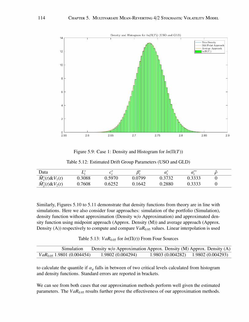
114 Chapter 5. MultivariateMean-Reverting 4/2 Stochastic VolatilityModel
Figure 5.9: Case 1: Density and Histogram for ln(Π(T ))
Table 5.12: Estimated Drift Group Parameters (USO and GLD)
Data L∗i c∗i β∗i a∗i a∗∗i ρ
M∗1(t)&V1(t) 0.3088 0.5970 0.0799 0.3732 0.3333 0
M∗2(t)&V2(t) 0.7608 0.6252 0.1642 0.2880 0.3333 0
Similarly, Figures 5.10 to 5.11 demonstrate that density functions from theory are in line withsimulations. Here we also consider four approaches: simulation of the portfolio (Simulation),density function without approximation (Density w/o Approximation) and approximated den-sity function using midpoint approach (Approx. Density (M)) and average approach (Approx.Density (A)) respectively to compute and compare VaR0.95 values. Linear interpolation is used
Table 5.13: VaR0.05 for ln(Π(t)) From Four Sources
Simulation Density w/o Approximation Approx. Density (M) Approx. Density (A)VaR0.05 1.9801 (0.004454) 1.9802 (0.004294) 1.9803 (0.004282) 1.9802 (0.004293)
to calculate the quantile if αq falls in between of two critical levels calculated from histogramand density functions. Standard errors are reported in brackets.
We can see from both cases that our approximation methods perform well given the estimatedparameters. The VaR0.95 results further prove the effectiveness of our approximation methods.
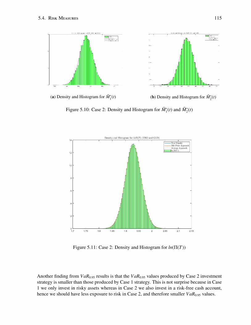
5.4. RiskMeasures 115
(a) Density and Histogram for M∗1(t) (b) Density and Histogram for M∗2(t)
Figure 5.10: Case 2: Density and Histogram for M∗1(t) and M∗
2(t)
Figure 5.11: Case 2: Density and Histogram for ln(Π(T ))
Another finding from VaR0.95 results is that the VaR0.95 values produced by Case 2 investmentstrategy is smaller than those produced by Case 1 strategy. This is not surprise because in Case1 we only invest in risky assets whereas in Case 2 we also invest in a risk-free cash account,hence we should have less exposure to risk in Case 2, and therefore smaller VaR0.95 values.
116 Chapter 5. MultivariateMean-Reverting 4/2 Stochastic VolatilityModel
5.5 Conclusion
In this chapter, we study the properties of a generalized mean-reverting 4/2 model in more de-tails than chapter 4. We study c.f. approximations in the first two sections. In section 5.3, weapplied our estimation methodology developed in chapter 3 to the generalized model. Duringthe study, we confirm the role of the scaling parameters between instantaneous variance andVIX plays in a multidimensional setting. Another issue we find is the flaw of constant eigen-vector matrix assumption imposed on principal component stochastic volatility framework.This can be seen from the estimation exercise on VIX (VVIX) and VSTOXX (VVSTOXX)where we find negative eigenvalues in the analysis of principal components.
In section 5.4, we further test our approximation methods in a risk management setting bycomputing one of the most popular risk measures VaR. Since VaR is a distribution based riskmeasure, it is ideal to assess the effectiveness of our approximation in a multidimensional set-ting. From Figures 5.8 to 5.11, we can see that the approximated density based on the averageapproach still out performs the one based on mid point in overall fitting. Using average approx-imation can greatly saves time in calculating distribution based risk measures. VaR0.95 resultsin Tables 5.11 and 5.13 further prove that our theoretical and approximated density functionsare consistent with simulation. Therefore, our approximation methods are proved to be effec-tive in multidimension.
5.6 Summary and Future Research
In this thesis, we study a novel mean-reverting model with the state-of-the-art 4/2 stochasticvolatility. We first study the theoretical properties of the model in one-dimensional setting inchapter 3. Even though the c.f. we find has quasi-closed form representation, it helps reducescomputational cost for simulation purpose, especially in a multivariate model setting as we seein chapter 4 and 5, as we only need to simulate one process instead of the complete modelthat has two processes. To further improve computational efficiency, we propose two approx-imation approaches. Numerical results show that the approximation approaches have goodperformance in a certain parametric region. With approximated c.f., we can price options withFFT methods, completely avoiding Monte Carlo methods. Later in chapters 4 and 5, we extendthe one-dimensional mean-reverting 4/2 stochastic volatility model to a multivariate case, alsoconsidering risk factors from different sources. We assume a convenient principal componentstochastic volatility framework for the models studied in chapters 4 and 5. The benefit of thisframework is that the original models can eventually be interpreted as linear combinations ofindependent processes after the decomposition of the stochastic covariance, which reduces thedimension of the model. However, the one of the drawback as we see in chapter 5 is that prin-cipal component stochastic volatility framework is not flexible with constant eigenvectors, thusit is not flexible to capture varying correlations.
Since our models are highly parametric, they embed interesting theoretical research topics
5.6. Summary and Future Research 117
as well as numerical research topics. In chapter 3, the structure of the c.f. brings theoreticalchallenge, which is hard to solve given evidence from current literature, one can start witha simpler case by considering models in section 2.3.2 or a Grasselli’s 4/2 model [76] withtime-dependent coefficients. The parametric region is also worth exploring theoretically. Forestimation, we currently claim ν(t) + b2
ν(t) satisfies weak stationary and ergodic properties, a rig-orous proof is helpful to support this claim and also a useful fact about 4/2 process. Anotherinteresting topic emerges from both theory and numerical application is regarding the choiceof the stochastic covariance matrix in the context of chapter 5. As we have seen, the currentchoice or the decomposition of the stochastic covariance matrix is not consistent with someof the applications, which means the empirical data does not support our assumption. So amore robust principal component stochastic volatility framework is worth exploring due to thetheoretical convenience of principal component decomposition. This way principal componentstochastic volatility framework can be considered for a wide range of applications.
Bibliography
[1] Carlo Acerbi and Dirk Tasche. On the coherence of expected shortfall. Journal ofBanking & Finance, 26(7):1487–1503, 2002.
[2] Dong-Hyun Ahn and Bin Gao. A parametric nonlinear model of term structure dynam-ics. The Review of Financial Studies, 12(4):721–762, 1999.
[3] Claudio Albanese and Alexey Kuznetsov. Transformations of markov processes andclassification scheme for solvable driftless diffusions. arXiv preprint arXiv:0710.1596,2007.
[4] Leif BG Andersen. Efficient simulation of the heston stochastic volatility model. 2007.
[5] Torben G Andersen, Tim Bollerslev, Francis X Diebold, and Paul Labys. The distribu-tion of realized exchange rate volatility. Journal of the American statistical association,96(453):42–55, 2001.
[6] Elena Andreou and Eric Ghysels. Rolling-sample volatility estimators: some new the-oretical, simulation and empirical results. Journal of Business & Economic Statistics,20(3):363–376, 2002.
[7] Philippe Artzner, Freddy Delbaen, Jean-Marc Eber, and David Heath. Coherent mea-sures of risk. Mathematical finance, 9(3):203–228, 1999.
[8] Xuezheng Bai. Beyond Merton’s utopia: effects of non-normality and dependence onthe precision of variance estimaters using high-frequency financial data. PhD thesis,University of Chicago, Graduate School of Business, 2000.
[9] Jan Baldeaux. Exact simulation of the 3/2 model. International Journal of Theoreticaland Applied Finance, 15(05):1250032, 2012.
[10] Jan Baldeaux, Martino Grasselli, and Eckhard Platen. Pricing currency derivatives underthe benchmark approach. Journal of Banking & Finance, 53:34–48, 2015.
[11] Jan Baldeaux and Eckhard Platen. Functionals of multidimensional diffusions with ap-plications to finance, volume 5. Springer Science & Business Media, 2013.
[12] Ole E Barndorff-Nielsen and Neil Shephard. Non-gaussian ornstein–uhlenbeck-basedmodels and some of their uses in financial economics. Journal of the Royal Statisti-cal Society: Series B (Statistical Methodology), 63(2):167–241, 2001. Wiley OnlineLibrary.
118
BIBLIOGRAPHY 119
[13] Ole E Barndorff-Nielsen and Neil Shephard. Econometric analysis of realized volatilityand its use in estimating stochastic volatility models. Journal of the Royal StatisticalSociety: Series B (Statistical Methodology), 64(2):253–280, 2002.
[14] Ole E Barndorff-Nielsen and Neil Shephard. Estimating quadratic variation using real-ized variance. Journal of Applied econometrics, 17(5):457–477, 2002.
[15] Ole E Barndorff-Nielsen, Neil Shephard, et al. Realized power variation and stochasticvolatility models. Bernoulli, 9(2):243–265, 2003.
[16] Fred Espen Benth. The stochastic volatility model of barndorff-nielsen and shephard incommodity markets. Mathematical Finance, 21(4):595–625, 2011.
[17] N.H. Bingham and R. Kiesel. Risk-Neutral Valuation: Pricing and Hedging of FinancialDerivatives. Springer Finance. Springer London, 2013.
[18] Fischer Black. Studies of stock market volatility changes. 1976 Proceedings of theAmerican Statistical Association Bisiness and Economic Statistics Section, 1976.
[19] Fischer Black, Emanuel Derman, and William Toy. A one-factor model of interest ratesand its application to treasury bond options. Financial analysts journal, pages 33–39,1990. JSTOR.
[20] Fischer Black and Piotr Karasinski. Bond and option pricing when short rates are log-normal. Financial Analysts Journal, pages 52–59, 1991. JSTOR.
[21] Fischer Black and Myron Scholes. The pricing of options and corporate liabilities.Journal of political economy, 81(3):637–654, 1973.
[22] Mireille Bossy and Awa Diop. An efficient discretisation scheme for one dimensionalSDEs with a diffusion coefficient function of the form— x—ˆ a, a in [1/2, 1. PhD thesis,INRIA, 2007.
[23] Mark Britten-Jones and Anthony Neuberger. Option prices, implied price processes, andstochastic volatility. The Journal of Finance, 55(2):839–866, 2000.
[24] Mark Broadie and Ozgur Kaya. Exact simulation of stochastic volatility and other affinejump diffusion processes. Operations research, 54(2):217–231, 2006.
[25] Peter Brockwell, Erdenebaatar Chadraa, Alexander Lindner, et al. Continuous-timegarch processes. Annals of Applied Probability, 16(2):790–826, 2006.
[26] Andrea Buraschi and Jens Jackwerth. Explaining option prices: Deterministic vs.stochastic models. Technical report, Working Paper, London Business School, 1998.
[27] Ruggero Caldana and Gianluca Fusai. A general closed-form spread option pricingformula. Journal of Banking & Finance, 37(12):4893–4906, 2013.
[28] John Y Campell, Andrew W Lo, and AC MacKinlay. The econometrics of financialmarkets. New Jersey, 1997.
120 BIBLIOGRAPHY
[29] Peter Carr and Dilip Madan. Option valuation using the fast fourier transform. Journalof computational finance, 2(4):61–73, 1999.
[30] Peter Carr and Jian Sun. A new approach for option pricing under stochastic volatility.Review of Derivatives Research, 10(2):87–150, 2007.
[31] Peng Cheng and Olivier Scaillet. Linear-quadratic jump-diffusion modeling. Mathemat-ical Finance, 17(4):575–598, 2007.
[32] Yuyang Cheng, Marcos Escobar-Anel, and Zhenxian Gong. Generalized mean-reverting4/2 factor model. Journal of Risk and Financial Management, 12(4):159, 2019.
[33] Mikhail Chernov. On the role of risk premia in volatility forecasting. Journal of Business& Economic Statistics, 25(4):411–426, 2007.
[34] Carl Chiarella, Boda Kang, Christina Sklibosios Nikitopoulos, and Thuy-Duong To.Humps in the volatility structure of the crude oil futures market: New evidence. EnergyEconomics, 40:989–1000, 2013.
[35] Bent J Christensen and Nagpurnanand R Prabhala. The relation between implied andrealized volatility. Journal of financial economics, 50(2):125–150, 1998.
[36] Peter Christoffersen, Steven Heston, and Kris Jacobs. The shape and term structureof the index option smirk: Why multifactor stochastic volatility models work so well.Management Science, 55(12):1914–1932, 2009.
[37] Joshua D Coval and Tyler Shumway. Expected option returns. The journal of Finance,56(3):983–1009, 2001.
[38] John C Cox, Jonathan E Ingersoll Jr, and Stephen A Ross. A theory of the term structureof interest rates. Econometrica: Journal of the Econometric Society, pages 385–407,1985. JSTOR.
[39] Jose Da Fonseca and Martino Grasselli. Riding on the smiles. Quantitative Finance,11(11):1609–1632, 2011. Taylor & Francis.
[40] Jose Da Fonseca, Martino Grasselli, and Claudio Tebaldi. Option pricing when cor-relations are stochastic: an analytical framework. Review of Derivatives Research,10(2):151–180, 2007.
[41] Alvise De Col, Alessandro Gnoatto, and Martino Grasselli. Smiles all around: Fx jointcalibration in a multi-heston model. Journal of Banking & Finance, 37(10):3799–3818,2013.
[42] Kresimir Demeterfi, Emanuel Derman, Michael Kamal, and Joseph Zou. A guide tovolatility and variance swaps. The Journal of Derivatives, 6(4):9–32, 1999.
[43] Victor DeMiguel, Lorenzo Garlappi, and Raman Uppal. Optimal versus naive diversi-fication: How inefficient is the 1/n portfolio strategy? The review of Financial studies,22(5):1915–1953, 2009.
BIBLIOGRAPHY 121
[44] Jerome Detemple and Carlton Osakwe. The valuation of volatility options. Review ofFinance, 4(1):21–50, 2000.
[45] Francis X Diebold and Marc Nerlove. The dynamics of exchange rate volatility: amultivariate latent factor arch model. Journal of Applied econometrics, 4(1):1–21, 1989.
[46] Awa Diop. Sur la discretisation et le comportement a petit bruit d’EDS unidimension-nelles dont les coefficients sont a derivees singulieres. PhD thesis, 2003. These dedoctorat dirigee par Talay, Denis et Bossy, Mireille Mathematiques Nice 2003.
[47] Gordana Dmitrasinovic-Vidovic and Antony Ware. Optimal portfolios of mean-reverting instruments. SIAM Journal on Financial Mathematics, 2(1):748–767, 2011.SIAM.
[48] James S Doran and Ehud I Ronn. Computing the market price of volatility risk in theenergy commodity markets. Journal of Banking & Finance, 32(12):2541–2552, 2008.
[49] Gabriel G Drimus. Options on realized variance by transform methods: a non-affinestochastic volatility model. Quantitative Finance, 12(11):1679–1694, 2012.
[50] Feike C Drost and Bas JM Werker. Closing the garch gap: Continuous time garchmodeling. Journal of Econometrics, 74(1):31–57, 1996.
[51] Jefferson Duarte and Christopher S Jones. The price of market volatility risk. WorkingPaper, 2007.
[52] Darrell Duffie, Damir Filipovic, Walter Schachermayer, et al. Affine processes andapplications in finance. The Annals of Applied Probability, 13(3):984–1053, 2003.
[53] Bernard Dumas, Jeff Fleming, and Robert E Whaley. Implied volatility functions: Em-pirical tests. The Journal of Finance, 53(6):2059–2106, 1998.
[54] Bruno Dupire. Pricing and hedging with smiles. Mathematics of derivative securities,1(1):103–111, 1997.
[55] Bruno Dupire et al. Pricing with a smile. Risk, 7(1):18–20, 1994.
[56] Robert Engle. Dynamic conditional correlation: A simple class of multivariate gen-eralized autoregressive conditional heteroskedasticity models. Journal of Business &
Economic Statistics, 20(3):339–350, 2002.
[57] Marcos Escobar. A stochastic volatility factor model of heston type. statistical propertiesand estimation. Stochastics, 90(2):172–199, 2018.
[58] Marcos Escobar, Hamidreza Arian, and Luis Seco. Creditgrades framework withinstochastic covariance models. Journal of Mathematical Finance, 2(04):303, 2012. Sci-entific Research Publishing.
[59] Marcos Escobar, Sebastian Ferrando, and Alexey Rubtsov. Optimal investment undermulti-factor stochastic volatility. Quantitative Finance, 17(2):241–260, 2017.
122 BIBLIOGRAPHY
[60] Marcos Escobar, Barbara Gotz, Luis Seco, and Rudi Zagst. Pricing a cdo on stochasti-cally correlated underlyings. Quantitative Finance, 10(3):265–277, 2010.
[61] Marcos Escobar and Christoph Gschnaidtner. Parameters recovery via calibration in theheston model: A comprehensive review. Wilmott, 2016(86):60–81, 2016.
[62] Marcos Escobar-Anel and Harold A Moreno-Franco. Dynamic portfolio strategies undera fully correlated jump-diffusion process. Annals of Finance, 15(3):421–453, 2019.
[63] A. Eydeland and H. Geman. Pricing power derivatives. Risk, 1998.
[64] Eugene F Fama and Kenneth R French. Common risk factors in the returns on stocksand bonds. Journal of financial economics, 33(1):3–56, 1993.
[65] W. Feller. An Introduction to Probability Theory And Its Applications, 2nd ED. Numberv. 2. Wiley India Pvt. Limited, 2008.
[66] Marcelo Fernandes, Marcelo C Medeiros, and Marcel Scharth. Modeling and predictingthe cboe market volatility index. Journal of Banking & Finance, 40:1–10, 2014. Elsevier.
[67] Damir Filipovic and Eberhard Mayerhofer. Affine diffusion processes: Theory and ap-plications. Radon Series Comp. Appl. Math, 8:1–40, 2009.
[68] Teruo Fujioka. Asymptotic approximations of the inverse moment of the noncentralchi-squared variable. Journal of the Japan Statistical Society, 31(1):99–109, 2001. TheJapan Statistical Society.
[69] Gianluca Fusai, Marina Marena, and Andrea Roncoroni. Analytical pricing of discretelymonitored asian-style options: Theory and application to commodity markets. Journalof Banking & Finance, 32(10):2033–2045, 2018.
[70] A Ronald Gallant and George Tauchen. Which moments to match? Econometric theory,pages 657–681, 1996.
[71] Jim Gatheral. Consistent modeling of spx and vix options. In Bachelier congress,volume 37, pages 39–51, 2008.
[72] Paul Glasserman and Kyoung-Kuk Kim. Gamma expansion of the heston stochasticvolatility model. Finance and Stochastics, 15(2):267–296, 2011.
[73] Alessandro Gnoatto, Martino Grasselli, and Eckhard Platen. A penny saved is a pennyearned: Less expensive zero coupon bonds. arXiv preprint arXiv:1608.04683, 2018.
[74] Joanna Goard and Mathew Mazur. Stochastic volatility models and the pricing of vixoptions. Mathematical Finance, 23(3):439–458, 2013. Wiley Online Library.
[75] Christian Gourieroux. Continuous time wishart process for stochastic risk. EconometricReviews, 25(2-3):177–217, 2006.
BIBLIOGRAPHY 123
[76] Martino Grasselli. The 4/2 stochastic volatility model: a unified approach for the hestonand the 3/2 model. Mathematical Finance, 2016. Wiley Online Library.
[77] G.N. Gregoriou, C. Hoppe, and C.S. Wehn. The Risk Modeling Evaluation Handbook:Rethinking Financial Risk Management Methodologies in the Global Capital Markets.McGraw-Hill finance & investing. McGraw-Hill Education, 2010.
[78] Lars Peter Hansen. Large sample properties of generalized method of moments estima-tors. Econometrica: Journal of the Econometric Society, pages 1029–1054, 1982.
[79] Andrew Harvey, Esther Ruiz, and Neil Shephard. Multivariate stochastic variance mod-els. The Review of Economic Studies, 61(2):247–264, 1994.
[80] Steven L Heston. A closed-form solution for options with stochastic volatility withapplications to bond and currency options. Review of financial studies, 6(2):327–343,1993. Soc Financial Studies.
[81] Steven L Heston. A simple new formula for options with stochastic volatility. Technicalreport, 1997. Washington University at St. Louis.
[82] Samuel Hikspoors and Sebastian Jaimungal. Asymptotic pricing of commodity deriva-tives using stochastic volatility spot models. Applied Mathematical Finance, 15(5-6):449–477, 2008. Taylor & Francis.
[83] John Hull. Risk management and financial institutions, volume 743. John Wiley & Sons,2015.
[84] John Hull and Alan White. Pricing interest-rate-derivative securities. Review of financialstudies, 3(4):573–592, 1990. Soc Financial Studies.
[85] George J Jiang and Yisong S Tian. The model-free implied volatility and its informationcontent. The Review of Financial Studies, 18(4):1305–1342, 2005.
[86] George J Jiang and Yisong S Tian. Extracting model-free volatility from option prices:An examination of the vix index. 2007.
[87] Andreas Kaeck and Carol Alexander. Continuous-time vix dynamics: On the role ofstochastic volatility of volatility. International Review of Financial Analysis, 28:46–56,2013.
[88] I. Karatzas and S. Shreve. Brownian Motion and Stochastic Calculus. Graduate Textsin Mathematics. Springer New York, 2014.
[89] Peter Kloeden and Andreas Neuenkirch. Convergence of numerical methods for stochas-tic differential equations in mathematical finance. In Recent Developments in Computa-tional Finance: Foundations, Algorithms and Applications, pages 49–80. World Scien-tific, 2013.
[90] H Felix Kloman. Risk management agonistes 1. Risk Analysis, 10(2):201–205, 1990.
124 BIBLIOGRAPHY
[91] Sergey P Kolos and Ehud I Ronn. Estimating the commodity market price of risk forenergy prices. Energy Economics, 30(2):621–641, 2008.
[92] Holger Kraft. Optimal portfolios and heston’s stochastic volatility model: an explicitsolution for power utility. Quantitative Finance, 5(3):303–313, 2005.
[93] Steven G Krantz and Steven George Krantz. Handbook of complex variables. SpringerScience & Business Media, 1999.
[94] Terence C Langetieg. A multivariate model of the term structure. The Journal of Fi-nance, 35(1):71–97, 1980.
[95] Linda Sandris Larsen. Optimal investment strategies in an international economy withstochastic interest rates. International Review of Economics & Finance, 19(1):145–165,2010. Elsevier.
[96] Alan L Lewis. A simple option formula for general jump-diffusion and other exponentiallevy processes. Working paper, Envision Financial Systems and OptionCity.net.
[97] Wei Lin, Shenghong Li, Xingguo Luo, and Shane Chern. Consistent pricing of vixand equity derivatives with the 4/2 stochastic volatility plus jumps model. Journal ofMathematical Analysis and Applications, 447(2):778–797, 2017.
[98] Yueh-Neng Lin and Chien-Hung Chang. Consistent modeling of s&p 500 and vixderivatives. Journal of Economic Dynamics and Control, 34(11):2302–2319, 2010.
[99] Roger Lord, Remmert Koekkoek, and Dick Van Dijk. A comparison of biased simu-lation schemes for stochastic volatility models. Quantitative Finance, 10(2):177–194,2010.
[100] E. Lukacs. Characteristic Functions. Griffin books of cognate interest. Hafner Publish-ing Company, 1970.
[101] Eugene Lukacs, Otto Szasz, et al. On analytic characteristic functions. Pacific J. Math,2(4):615–625, 1952.
[102] Xingguo Luo and Jin E Zhang. The term structure of vix. Journal of Futures Markets,32(12):1092–1123, 2012.
[103] V. Mackevicius. Stochastic Models of Financial Mathematics. Elsevier Science, 2016.
[104] A.J. McNeil, R. Frey, and P. Embrechts. Quantitative Risk Management: Concepts,Techniques, and Tools. Princeton Series in Finance. Princeton University Press, 2005.
[105] Nour Meddahi. A theoretical comparison between integrated and realized volatility.Journal of Applied Econometrics, 17(5):479–508, 2002.
[106] Alexey Medvedev and Olivier Scaillet. Approximation and calibration of short-termimplied volatilities under jump-diffusion stochastic volatility. The review of FinancialStudies, 20(2):427–459, 2006.
BIBLIOGRAPHY 125
[107] Robert C Merton. Optimum consumption and portfolio rules in a continuous-timemodel. In Stochastic Optimization Models in Finance, pages 621–661. Elsevier, 1975.
[108] Yuliya Mishura, Vladimir I Piterbarg, Kostiantyn Ralchenko, and Anton Yurchenko-Tytarenko. Stochastic representation and pathwise properties of fractional cox-ingersoll-ross process. arXiv preprint arXiv:1708.02712, 2017.
[109] Johannes Muhle-Karbe, Oliver Pfaffel, and Robert Stelzer. Option pricing in multivari-ate stochastic volatility models of ou type. SIAM Journal on Financial Mathematics,3(1):66–94, 2012.
[110] Daniel B Nelson. The time series behavior of stock market volatility and returns. PhDthesis, Massachusetts Institute of Technology, 1988.
[111] Daniel B Nelson. Arch models as diffusion approximations. Journal of econometrics,45(1-2):7–38, 1990.
[112] Anthony Neuberger. The log contract. Journal of portfolio management, 20:74–74,1994.
[113] Lars Tyge Nielsen and Jesus Saa-Requejo. Exchange rate and term structure dynamicsand the pricing of derivative securities. Unpublished manuscript, INSEAD, 1993.
[114] Bernt Øksendal. Stochastic differential equations. In Stochastic differential equations,pages 65–84. Springer, 2003.
[115] Marc S Paolella. Intermediate probability: A computational approach, chapter 10. JohnWiley & Sons, 2007.
[116] Jim Pitman and Marc Yor. A decomposition of bessel bridges. Zeitschrift furWahrscheinlichkeitstheorie und verwandte Gebiete, 59(4):425–457, 1982.
[117] E Platen. A non-linear stochastic volatility model. Financial Mathematics ResearchReport No. FMRR005-97, 1997. Center for Financial Mathematics, Australian NationalUniversity, Canberra.
[118] Eckhard Platen and David Heath. A benchmark approach to quantitative finance.Springer Science & Business Media, 2006.
[119] J. Priolon. Financial Markets for Commodities. Wiley, 2019.
[120] Gennady Samorodnitsky. Stochastic processes and long range dependence, volume 26.Springer, 2016.
[121] Lorenz Schneider and Bertrand Tavin. From the samuelson volatility effect to a samuel-son correlation effect: An analysis of crude oil calendar spread options. Journal ofBanking & Finance, 95:185–202, 2018.
126 BIBLIOGRAPHY
[122] Eduardo S Schwartz. The stochastic behavior of commodity prices: Implications forvaluation and hedging. The Journal of Finance, 52(3):923–973, 1997. Wiley OnlineLibrary.
[123] Elias M Stein and Jeremy C Stein. Stock price distributions with stochastic volatility:an analytic approach. The review of financial studies, 4(4):727–752, 1991.
[124] Alan Stuart, Steven Arnold, J Keith Ord, Anthony O’Hagan, and Jonathan Forster.Kendall’s advanced theory of statistics. Wiley, 1994.
[125] Edward C Titchmarsh. Introduction to the theory of fourier integrals. 1948.
[126] Oldrich Vasicek. An equilibrium characterization of the term structure. Journal offinancial economics, 5(2):177–188, 1977. Elsevier.
[127] Robert E. Whaley. Derivatives on market volatility. The Journal of Derivatives, 1(1):71–84, 1993.
[128] Robert E Whaley. Understanding the vix. The Journal of Portfolio Management,35(3):98–105, 2009.
[129] Rudi Zagst. Interest-rate management. Springer Science & Business Media, 2013.
[130] Jin E Zhang and Yingzi Zhu. Vix futures. Journal of Futures Markets, 26(6):521–531,2006.
[131] Lan Zhang, Per A Mykland, and Yacine Aıt-Sahalia. A tale of two time scales: Deter-mining integrated volatility with noisy high-frequency data. Journal of the AmericanStatistical Association, 100(472):1394–1411, 2005.
Appendix A
Proofs for Theoretical Results in Chapter3
Proof Proof of Proposition 3.2.1: Let ν(t) = eβtν(t) and ν(t) = eβtln(ν(t)), we have following:
dν(t) = αθeβtdt + (β − α)eβtν(t)dt + eβtξ√ν(t)dB(t), (A.1)
and
dν(t) = βν(t)dt +∂ν(t)∂ν(t)
dν(t) +12∂2ν(t)∂ν(t)2 < dν(t) >
= βν(t)dt +eβtξ√ν(t)
dB(t) + eβt(αθ
ν(t)− α)dt − eβt ξ2
2ν(t)dt.
(A.2)
From B.9 and B.10, we solve for∫ T
teβs√ν(s)dB(s) and
∫ T
teβs√ν(s)
dB(s):
∫ T
teβs
√ν(s)dB(s) =
eβTν(T ) − eβtν(t)ξ
−αθ(eβT − eβt)
βξ−β − α
ξ
∫ T
teβsν(s)ds, (A.3)
∫ T
t
eβs
√ν(s)
dB(s) =1ξ
lnν(T )eβT
ν(t)eβt +α(eβT − eβt)
βξ+
1ξ
(ξ2
2− αθ
) ∫ T
t
eβs
ν(s)ds −
β
ξ
∫ T
teβsln(ν(s))ds.
(A.4)Split W(t) into B(t) and its orthogonal part B(t)⊥:
Z(T ) = Z(t) +Lβ
(eβT − eβt) +
∫ T
teβs(c −
12
)(a√ν(s) +
b√ν(s)
)2ds
+
∫ T
teβs(a
√ν(s) +
b√ν(s)
)(ρdB(s) +√
1 − ρ2dB(s)⊥),
127
128 Chapter A. Proofs for Theoretical Results in Chapter 3
then substitute B.11 and B.12 to get rid of dB(t). Z(t) can be rewritten as:
Z(T ) = Z(t) +
(L −
aραθξ
+bραξ
+ 2ab(c −12
)) (eβT − eβt)
β−
[aρ(β − α)ξ
− a2(c −12
)]
×
∫ T
teβsν(s)ds −
bρβξ
∫ T
teβsln(ν(s))ds +
aρ(eβTν(T ) − eβtν(t))ξ
+bρξ
lnν(T )eβT
ν(t)eβt
+
[bρξ
(ξ2
2− αθ
)+ b2(c −
12
)] ∫ T
t
eβs
ν(s)ds +
√1 − ρ2
∫ T
teβs(a
√ν(s) +
b√ν(s)
)dB(s)⊥
(A.5)
Let (Gt)t≥0 denote the filtration generated by ν(t), t ≥ 0. Using a property of iterated expecta-tion, we can write the conditional moment generating function of Z(t) as:
E(euZ(T )|Ft) = E[E[euZ(T )
∣∣∣Ft
⋃Gt
]∣∣∣∣∣Ft
]= exp
uZ(t) + u
(L −
aραθξ
+bραξ
+ 2ab(c −12
)) (eβT − eβt)
β
−uaρξ
eβtν(t) −ubρeβt
ξln(ν(t))
× E
[E[exp
−
ubρβξ
∫ T
teβsln(ν(s))ds + u
[bρξ
(ξ2
2− αθ
)+ b2(c −
12
)]
×
∫ T
t
eβs
ν(s)ds − u
[aρ(β − α)ξ
− a2(c −12
)] ∫ T
teβsν(s)ds
+ u√
1 − ρ2
∫ T
teβs(a
√ν(s) +
b√ν(s)
)dB(s)⊥
+uaρξ
eβTν(T ) +ubρξ
eβT lnν(T )∣∣∣∣∣Ft
⋃Gt
]∣∣∣∣∣Ft
]By independence of random variables, we have:
E[E[euZ(T )
∣∣∣Ft
⋃Gt
]∣∣∣∣∣Ft
]= exp
uZ(t) + u
(L −
aραθξ
+bραξ
+ 2ab(c −12
)) (eβT − eβt)
β
−uaρξ
eβtν(t) −ubρeβt
ξln(ν(t))
× E
[exp
−
ubρβξ
∫ T
teβsln(ν(s))ds + u
[bρξ
(ξ2
2− αθ
)+ b2(c −
12
)]
×
∫ T
t
eβs
ν(s)ds − u
[aρ(β − α)ξ
− a2(c −12
)] ∫ T
teβsν(s)ds
+uaρξ
eβTν(T ) +ubρξ
eβT lnν(T )∣∣∣∣∣Ft
× E
[exp
u√
1 − ρ2
∫ T
teβs(a
√ν(s) +
b√ν(s)
)dB(s)⊥ ∣∣∣∣∣Ft
⋃Gt
]∣∣∣∣∣Ft
](A.6)
129
The inner double expectation of A.6 involves
E[exp
u√
1 − ρ2
∫ T
teβs(a
√ν(s) +
b√ν(s)
)dB(s)⊥∣∣∣∣∣Ft
⋃Gt
].
Conditioning on Ft⋃Gt implies that
√1 − ρ2
∫ T
teβs(a
√ν(s) + b
√ν(s)
)dB(s)⊥ is a normal ran-dom variable with mean 0. By Ito’s Isometry, the variance can be easily found to be (1 −ρ2)
∫ T
te2βs(a2ν(s) + b2
ν(s) + 2ab)ds. So
E[eu√
1−ρ2∫ T
t eβs(a√ν(s)+ b√
ν(s))dB(s)⊥ ∣∣∣Ft
⋃Gt
]= e
12 u2(1−ρ2)
∫ Tt e2βs(a2ν(s)+ b2
ν(s) +2ab)ds.
Consequently, the conditional moment generating function of√
1 − ρ2∫ t
0eβs(a
√ν(s)+ b
√ν(s)
)dB(s)⊥
is found to be:
E[E[eu√
1−ρ2∫ T
t eβs(a√ν(s)+ b√
ν(s))dB(s)⊥
∣∣∣∣∣Ft
⋃Gt
]∣∣∣∣∣Ft
]= E
[e
12 u2(1−ρ2)
∫ Tt e2βs(a2ν(s)+ b2
ν(s) +2ab)ds∣∣∣Ft
](A.7)
After reorganizing E(euZ(T )|Ft), we have:
E(euZ(T )|Ft) =expuZ(t) + u
(L −
aραθξ
+bραξ
+ 2ab(c −12
)) (eβT − eβt)
β+ u2(1 − ρ2)
×(e2βT − e2βt)ab
2β
× exp
−
uaρξ
eβtν(t) −ubρeβt
ξln(ν(t))
× E
[exp
−
ubρβξ
∫ T
teβsln(ν(s))ds + u
[bρξ
(ξ2
2− αθ
)+ b2(c −
12
)] ∫ T
t
eβs
ν(s)ds
+12
u2(1 − ρ2)a2∫ T
te2βsν(s)ds − u
[aρ(β − α)ξ
− a2(c −12
)] ∫ T
teβsν(s)ds
+12
u2(1 − ρ2)b2∫ T
t
e2βs
ν(s)ds +
uaρξ
eβTν(T ) +ubρξ
eβT lnν(T )∣∣∣∣∣Ft
].
(A.8)
Hence,
E(euZ(t)|Ft) =expuZ(t) + u
(L −
aραθξ
+bραξ
+ 2ab(c −12
)) (eβT − eβt)
β+ u2(1 − ρ2)
(e2βT − e2βt)ab2β
× exp
−
uaρeβt
ξν(t) −
ubρeβt
ξln(ν(t))
× E
[ν(T )−Aexp
− Bν(T ) −C
∫ T
teβsln(ν(s))ds
−
∫ T
t
(Deβs + Ee2βs) 1
ν(s)ds −
∫ T
t
(Feβs + Ge2βs)ν(s)ds
∣∣∣∣∣Ft
].
where,
A = −ubρξ
eβT , B = −uaρξ
eβT ,C =ubρβξ
,D = −ubρξ
(ξ2
2− αθ
)− ub2(c −
12
),
E = −12
u2(1 − ρ2)b2, F =uaρ(β − α)
ξ− ua2(c −
12
),G = −12
u2(1 − ρ2)a2.
(A.9)
130 Chapter A. Proofs for Theoretical Results in Chapter 3
Proof Proof of the results in the example of Section 3.2.1.1: First:
ln(α(e
√A(T−t) − 1) +
√A(e
√A(T−t) + 1)
2√
Ae√
A+α2 (T−t)
)− 2αθξ2
=2αθξ2 ln
( 2√
Ae√
A+α2 (T−t)
α(e√
A(T−t) − 1) +√
A(e√
A(T−t) + 1)
)=
2αθξ2
√A + α
2(T − t) + ln
( 2√
A
α(e√
A(T−t) − 1) +√
A(e√
A(T−t) + 1)
)=αθ
ξ2
(√
A + α)(T − t) − 2ln( √A − α + (α +
√A)e
√A(T−t)
2√
A
)=αθ
ξ2
(√
A + α)(T − t) − 2ln(α −√
A − (α +√
A)e√
A(T−t)
−2√
A
)=αθ
ξ2
(α +√α2 + ξ2(u2 + iu))(T − t) − 2ln
(1 − ge−(T−t)√α2+ξ2(u2+iu)
1 − g
) = C(T − t, u)
Next:
−(u2 + iu)(e√
A(T−t) − 1)
α(e√
A(T−t) − 1) +√
A(e√
A(T−t) + 1)=
α2−Aξ2 (e
√A(T−t) − 1)
α(e√
A(T−t) − 1) +√
A(e√
A(T−t) + 1)
=1ξ2
(α +√
A)(α −√
A)(e√
A(T−t) − 1)
α(e√
A(T−t) − 1) +√
A(e√
A(T−t) + 1)=α +√
Aξ2 ×
e√
A(T−t) − 1α
(α−√
A)(e√
A(T−t) − 1) +√
A(α−√
A)(e√
A(T−t) + 1)
=α +√
Aξ2 ×
1 − e√
A(T−t)
1 − ge√
A(T−t)= D(T − t, u)
Proof Proof of Proposition 3.3.1:Option 1Now we define γ(t) = λ
√ν(t) as in [80] for some constant λ such that ν(t) remains in the
family of CIR processes under the risk-neutral measure. The process for volatility becomes:
dν(t) = (αθ − (α + λξ)ν(t))dt + ξ√ν(t)dBQ(t).
Since ν(t) is unbounded from above, we need the conditions under which γ(t) is well definedi.e E[exp( 1
2
∫ T
0γ2(s)ds)] < ∞. Proposition 5.1 of [92] provides a sufficient condition on λ that
for −αξ≤ λ < ∞, Novikov’s condition is satisfied and hence,
E[exp
(−
∫ t
0γ(s)dBQ(s) −
12
∫ t
0γ2(s)ds
)]= 1,
which means γ(t) = λ√ν(t) is well defined for −α
ξ≤ λ < ∞. When λ , −α
ξ, Feller condition
for volatility process after the change of measure is now 2(α + λξ) αθα+λξ
= 2αθ ≥ ξ2, which isthe same as we have under measure P.Next we need to find γ(t)⊥. Under measure Q, we have:
dX(t)X(t)
= (L + c(a√ν(t) +
b√ν(t)
)2− g(ν(t)) − βln(X(t)))dt + (a
√ν(t) +
b√ν(t)
)dWQ(t)
131
where g(ν(t)) = (a√ν(t) + b
√ν(t)
)γ(t)′ and γ(t)′ = ργ(t) +√
1 − ρ2γ(t)⊥. Since the drift termcontains (a
√ν(t) + b
√ν(t)
)2, a natural choice of g(ν(t) is g(ν(t)) = Λ(a√ν(t) + b
√ν(t)
)2. Substituteγ(t) for λ
√ν(t) and solve for γ(t)⊥:
γ(t)⊥ =1√
1 − ρ2
[(Λa − ρλ)
√ν(t) +
Λb√ν(t)
].
γ(t)⊥ is a linear combination of√ν(t) and 1
√ν(t)
, we then write γ(t)⊥ = Λ1√ν(t) + Λ2√
ν(t),
E[exp
(12
∫ T
0γ2(s)⊥ds
)]= E
exp
[12
∫ T
0(Λ2
1ν(t) + 2Λ1Λ2 +Λ2
2
ν(t))ds
]= eΛ1Λ2TE
[exp
(Λ21
2
∫ T
0ν(s)ds +
Λ22
2
∫ T
0
1ν(s)
ds)].
Theorem A.1 of [76] gives a closed form solution for
E[ν(T )−qe−lν(T )−m
∫ T0 ν(s)ds−n
∫ T0
1ν(s) ds
].
With q = 0 and l = 0, the above expectation exists as long as m, n ∈ R, m > − α2
2ξ2 , n ≥
−(2αθ−ξ2)2
8ξ2 . In our case m = −Λ2
12 and n = −
Λ22
2 . From the range of m and n we have for
|Λ1| <αξ
and |Λ2| ≤2αθ−ξ2
2ξ , E[exp
(Λ2
12
∫ T
0ν(s)ds +
Λ22
2
∫ T
01ν(s)ds
)]is finite and thus defined.
We combine the range of Λ1 and Λ2 to get the constrain on Λ: Λ ∈ Λ3 < Λ < Λ4 where
Λ3 = max[
1a
(− α
ξ+ ρλ
),− 1|b|
(αθξ−
ξ
2
)]and Λ4 = min
[1a
(αξ
+ ρλ), 1|b|
(αθξ−
ξ
2
)]for a and b non-zero.
Option 2We define γ(t) = λ′
√ν(t)
for some constant λ′. This change will also keep ν(t) within CIRprocess family under risk-neutral measure by subtracting a constant to mean-reverting level:
dν(t) = (αθ − λ′ξ − αν(t))dt + ξ√ν(t)dBQ(t).
The corresponding Feller condition will be 2ααθ−λ′ξ
α= 2(αθ − λ′ξ) ≥ ξ2 when λ′ ≤ 0. Let’s
check if Novikov’s condition E[exp(λ′2
2
∫ T
01ν(t)ds)] < ∞ is satisfied. Note that 1
ν(t) = ν(t)′ is a3/2 process with
dν(t)′ = ν(t)′(α − (αθ − ξ2)ν(t)′
)dt − ξν(t)′
32 dBP(t).
[30] showed that the conditional Fourier-Laplace transformation of joint log return, R(T ), andintegrated variance, E
[eiuR(T )−s
∫ Tt ν(z)′dz|Ft
]have a closed-form solution for stochastic volatility
model with volatility process being 3/2 process. In our case, setting u = 0 and substituting s =
−λ′2
2 , we get E[exp
(λ′2
2
∫ T
01ν(s)ds
)]and the expectation is finite as long as 1F1
(x; w;− 2
ξ2y(0,ν(0))
)exists, in another word w is positive. The problem simplifies to solve the inequality
(12 +
αθ−ξ2
ξ2
)2
−
λ′2
ξ2 ≥ 0 for the range of λ′: |λ′| ≤ αθξ−
ξ
2 . So when −(αθξ−
ξ
2 ) ≤ λ′ ≤ 0, γ(t) = λ′√ν(t)
is well

132 Chapter A. Proofs for Theoretical Results in Chapter 3
defined.Let g(ν(t)) = Λ′(a
√ν(t) + b
√ν(t)
)2. We repeat the procedures in Option 1 for solving γ(t)⊥:
γ(t)⊥ =1√
1 − ρ2
[(Λ′a
√ν(t) +
Λ′b − ρλ′√ν(t)
].
In this case, Λ1 = Λ′a and Λ2 = Λ′b − ρλ′, the constrain on Λ is Λ ∈Λ3 < Λ
′
< Λ4
where
Λ3 = max[− 1
b
(αθξ−
ξ
2 − ρλ′),− α|a|ξ
]and Λ4 = min
[1b
(αθξ−
ξ
2 + ρλ′), α|a|ξ
]for a and b non-zero.
Data Descriptions:VVIX Data Description: Data is obtained from Cboe website. Dataset consists of daily datastarting from January 3, 2007 to March 13, 2018, 2817 entries in total excluding November 11,2010 data that is not available.V-VSTOXX Data Description: Euro STOXX 50 Volatility of volatility (V-VSTOXX) historicaldaily data is available on STOXX. The data is recorded from March 23, 2010 to March 13,2018 with 15 missing data entries. The missing data entries are not evenly distributed through-out the time frame. Majority of the missing data are in 2017. Almost half month data of August2017 are not available. The size of data is 2017 after excluding missing data.Volatility Index of Crude Oil ETF Data Description: According to Cboe website, “the CboeCrude Oil ETF Volatility index (USO) measures the market’s expectation of 30-day volatilityof crude oil prices by applying the VIX methodology to United States Oil Fund, LP optionsspanning a wide range of strike prices.” We obtain daily data from May 10, 2007 to March 13,2018 with 2730 entries in total.Volatility Index of Gold ETF Data Description: Similar to USO, the Cboe Gold ETF Volatilityindex (GVZ) measures the market’s expectation of 30-day volatility of gold prices by applyingthe VIX methodology Gold ETF options spanning a wide range of strike prices. We obtaindaily data from June 3, 2008 to May 15, 2019 with 2757 entries in total.
Appendix B
Proofs and Helpful Results for Chapter 4
B.1 ProofsProof Proof of Proposition 4.2.1.The first step is to ensure the change of measure is well-defined and for this we use Novikov’scondition, i.e., generically
E
exp
12
∫ T
0λ2
(√ν(t) +
b√ν(t)
)2
ds
= eλ2bTE
[exp
(λ2
2
∫ T
0ν(s)ds +
λ2b2
2
∫ T
0
1ν(s)
ds)]< ∞.
From Grasselli, in order for this expectation to exist, we need two conditions:
−λ2
2> −
α2
2ξ2 =⇒ |λ| <α
ξ(B.1)
and
−λ2b2
2≥ −
(2αθ − ξ2)2
8ξ2 =⇒ |λ| ≤2αθ − ξ2
2|b|ξ=⇒ ξ2 ≤ 2αθ − 2|λ||b|ξ (B.2)
The latter condition in Equation (B.2) implies, in particular, that our volatility processes satisfyFeller’s condition under P and Q; in other words, it ensures all our CIR processes stay awayfrom zero under both measures.
Applying Equation (B.2) to our setting leads to (i, j = 1, .., n):
ξ2j ≤ 2α jθ j − 2ξ j max
∣∣∣λ jb j
∣∣∣ , ∣∣∣λ⊥j b j
∣∣∣ (B.3)
ξ2i ≤ 2αiθi − 2ξi max
∣∣∣∣λibi
∣∣∣∣ , ∣∣∣∣λ⊥i bi
∣∣∣∣ (B.4)
Now, we apply Equation (B.1) producing two extra set of conditions (i, j = 1, .., n):
max∣∣∣λ j
∣∣∣ , ∣∣∣λ⊥j ∣∣∣ <α j
ξ j(B.5)
max∣∣∣λi
∣∣∣ , ∣∣∣λ⊥i ∣∣∣ <αi
ξi
(B.6)
133
134 Chapter B. Proofs and Helpful Results for Chapter 4
The second step applies to the case βi j = 0 for i, j = 1, .., n and it is to ensure the drift of theasset price equal the short rate:
Li = r, ci =
n∑j=1
ai j
(ρ jλ j +
√1 − ρ2
jλ⊥j
), ci = ρiλi +
√1 − ρ2
i λ⊥i
For the most general case (βi j , 0 for some i or j), the second step should be adapted to anyparticular prescribed drift structure under the Q-measure.
The third step is to ensure the drift-less asset price process is a true Q-martingale and notjust a local Q-martingale:
dXi(t)Xi(t)
= (.) dt +
n∑j=1
ai j
√v j(t) +b j√v j(t)
dWQj (t) +
(√vi(t) +
bi√
vi(t)
)dWQ
i (t)
Here, we test the martingale property using the Feller nonexplosion test for volatilities, henceconsidering the following n2 + n changes of Brownian motion for the volatility processes andchecking the processes do not reach zero under the various measures:
dBQi j(t) = ai jρ j
√v j(t) +b j√v j(t)
dt + dBPj (t), dBQ
i (t) = ρi
(√vi(t) +
bi√
vi(t)
)dt + dBP
i (t)
This leads to the following conditions:
ξ2j ≤ 2α jθ j − 2
∣∣∣ai jρ jb j
∣∣∣ ξ j, i, j = 1, ..., n (B.7)
ξ2i ≤ 2αiθi − 2
∣∣∣∣λiρibi
∣∣∣∣ ξi, i = 1, ..., n (B.8)
We can combine the first and third steps in Equations (B.3), (B.7), (B.4) and (4.4) into the finalconditions.
B.1. Proofs 135
Proof Proof of Proposition 4.2.2.We start by defining new processes dS ik,t and dS i j
t with i, j, k = 1, 2, . . . , n and t ≥ 0.
dZi(t) =
n∑j=1
(eβt
)i j
(c j −12
) √v j(t) +b j√v j(t)
dt +
√v j(t) +b j√v j(t)
dW j(t)
+
n∑k=1
n∑
j=1
(eβt
)i j
L j
n
dt +
n∑j=1
(eβt
)i j
(ck −
12
)a2
jk
(√vk(t) +bk√
vk(t)
)2
dt
+
n∑k=1
n∑j=1
(eβt
)i j
a jk
(√vk(t) +bk√
vk(t)
)dWk(t)
=
n∑j=1
dS i jt +
n∑k=1
dS ik,t
By the dependence structure implied by the model, it follows that all S are independent for afix i, hence we can transform the characteristic function using the processes S as follows:
ΦZ(t),v(t)(T, ω) =
n∏k=1
E[expiω′
(S ·k,T − S ·k,t
) | S t, v(t)
] n∏j=1
E[expiωi
(S . j
T − S . jt
) | S t, v(t)
]
For each factor j = 1, 2, . . . , n we define S ∗k,t = ω′S ·k,t =∑n
i=1 ωiS ik,t; the dynamics of S ∗k,t canbe expressed as
dS ∗k,t = ω′dS ·k,t
=
L(ω, t) + hk(ω, t)(√
vk(t) +bk√
vk(t)
)2 dt + gk (ω, t)(√
vk(t) +bk√
vk(t)
)dWk,t
where,
hk(ω, t) =
n∑j=1
(ck −
12
)a2
jk f j(ω, t), L(ω, t) =
n∑j=1
L j
nf j(ω, t), gk (ω, t) =
n∑j=1
a jk f j(ω, t), f j(ω, t) =
n∑i=1
ωi
(eβt
)i j.
These three functions are deterministic, linear combinations of f j(ω, t).
Next, we find the characteristic function for the increments of S ∗k,t:
E[expiφ
(S ∗k,T − S ∗k,t
) | S ∗k,t, vk(t) = vk,t
]= ΦGG
(T, φ; L(ω), hk(ω), gk(ω), κk, θk, ξk, ρk, bk, ck, vk,t, S ∗k,t
).
The generic function ΦGG is provided in Lemma B.1.1. It follows similarly for idiosyncratic

136 Chapter B. Proofs and Helpful Results for Chapter 4
factors:
dS ∗ jt = ω′dS · jt
=
n∑i=1
ωi
n∑j=1
(eβt
)i j
(c j −
12
)√v j(t) +
b j√v j(t)
dt
+
n∑i=1
ωi
n∑j=1
(eβt
)i j
√v j(t) +
b j√v j(t)
dW j,t
= h j(ω, t)
√v j(t) +b j√v j(t)
2
dt + g j (ω, t)
√v j(t) +b j√v j(t)
dW j,t
where h j(ω, t) =∑n
i=1 ωi
(∑nj=1
(eβt
)i j
(c j −
12
))and g j (ω, t) =
∑ni=1 ωi
∑nj=1
(eβt
)i j
.
Combining all pieces together, we obtain:
ΦZ(t),v(t)(T, ω) =
n∏k=1
E[expiω′
(S ·k,T − S ·k,t
) | S t, v(t)
] n∏j=1
E[expiω′
(S · jT − S · jt
) | S t, v(t)
]=
n∏k=1
ΦGG
(T, 1; Lk(ω), hk(ω), gk(ω), κk, θk, ξk, ρk, bk, ck, vk,t, S ∗k,t
)×
n∏j=1
ΦGG
(T, 1; 0, h j(ω), g j(ω), κ j, θ j, ξ j, ρ j, b j, c j, v j,t, S
∗ jt
)Lemma B.1.1 Let the generic process be:
dZ(t) =
L(t) + h(t)(√
v(t) +b√
v(t)
)2 dt + g (t)(√
v(t) +b√
v(t)
)dWt
dv(t) = α(θ − v(t))dt + ξ√
v(t)dB(t)〈dB(t), dW(t)〉 = ρdt
with g (t) differentiable, then
ΦGG (T, φ; L, h, g, κ, θ, ξ, ρ, b, c, vt,Zt) = exp
u∫ T
tA (s) ds
ν(t)u bρ
ξ g(t) exp−uρ
g (t) ν(t)ξ
×E
[ν(T )u bρ
ξ g(T ) exp
u(∫ T
tB(s)ν(s)ds +
∫ T
tC(s)
1ν(s)
ds +
∫ T
tD(s) ln(ν(s))ds + ρ
g (T ) ν(T )ξ
)| Ft
]where A, B, C and D are provided in the proof.
Proof Proof of Lemma B.1.1.Let the generic process be:
dZ(t) =
L(t) + h(t)(√
v(t) +b√
v(t)
)2 dt + g (t)(√
v(t) +b√
v(t)
)dWt
dv(t) = α(θ − v(t))dt + ξ√
v(t)dB(t)〈dB(t), dW(t)〉 = ρdt
B.1. Proofs 137
We want to find
E[euZ(T )|Ft
]= euZ(t)ΦGG (T, φ; L, h, g, κ, θ, ξ, ρ, b, c, vt,Zt)
Letting ν(t) = g (t) ν(t) and ν(t) = g (t) ln(ν(t)), we have following:
dν(t) = αθg (t) dt +(g′ (t) − αg (t)
)ν(t)dt + g (t) ξ
√ν(t)dB(t), (B.9)
and
dν(t) =g′ (t)g (t)
ν(t)dt +∂ν(t)
∂ ln(ν(t))d ln(ν(t)) +
12
∂2ν(t)∂ ln(ν(t))2 < d ln(ν(t)) > (B.10)
=g′ (t)g (t)
ν(t)dt +g (t) ξ√ν(t)
dB(t) + g (t) (αθ
ν(t)− α)dt − g (t)
ξ2
2ν(t)dt
From Equations (B.9) and (B.10), we solve for∫ T
tg (s)
√ν(s)dB(s) and
∫ T
tg(s)√ν(s)
dB(s):∫ T
tg (s)
√ν(s)dB(s) =
g(T )ν(T )−g(t)ν(t)ξ
− αθξ
∫ T
tg (s) ds − 1
ξ
∫ T
t(g′ (s) − αg (s)) ν(s)ds, (B.11)∫ T
tg(s)√ν(s)
dB(s) = 1ξ
ln ν(T )g(T )
ν(t)g(t) + αξ
∫ T
tg (s) ds + 1
ξ
(ξ2
2 − αθ) ∫ T
tg(s)ν(s) ds − 1
ξ
∫ T
tg′ (s) ln(ν(s))ds. (B.12)
Split W(t) into B(t) and its orthogonal part B(t)⊥:
Z(T ) = Z(t) +
∫ T
tL (s) ds +
∫ T
th(s)
(√ν(s) +
b√ν(s)
)2
ds
+
∫ T
tg (s)
(√ν(s) +
b√ν(s)
)(ρdB(s) +
√1 − ρ2dB(s)⊥),
then substitute Equation (B.11) and (B.12) to eliminate dB(t). Z(t) can be rewritten now as:
Z(T ) = Z(t) +
∫ T
tL (s) ds +
∫ T
th(s)
(ν(s) + 2b +
b2
ν(s)
)ds +
√1 − ρ2
∫ T
tg(s)
(a√ν(s) +
b√ν(s)
)dB(s)⊥
+ ρg (T ) ν(T ) − g (t) ν(t)
ξ−αθρ
ξ
∫ T
tg (s) ds −
ρ
ξ
∫ T
t(g′ (s) − αg (s)) ν(s)ds
+bρξ
lnν(T )g(T )
ν(t)g(t) +αbρξ
∫ T
tg (s) ds +
bρξ
(ξ2
2− αθ
) ∫ T
t
g (s)ν(s)
ds −bρξ
∫ T
tg′ (s) ln(ν(s))ds
Grouping conveniently, we obtain:
Z(T ) = Z(t) +
∫ T
tA (s) ds +
∫ T
tB(s)ν(s)ds +
∫ T
tC(s)
1ν(s)
ds +
∫ T
tD(s) ln(ν(s))ds
+bρξ
lnν(T )g(T )
ν(t)g(t) + ρg (T ) ν(T ) − g (t) ν(t)
ξ+
√1 − ρ2
∫ T
tg(s)
(a√ν(s) +
b√ν(s)
)dB(s)⊥
where
A (s) = L (s) + 2bh(s) +
(αbρξ−αθρ
ξ
)g (s)
B(s) = h(s) −ρ
ξ
(g′ (s) − αg (s)
)C(s) = b2h(s) +
bρξ
(ξ2
2− αθ
)g(s)
D(s) = −bρξ
g′ (s)
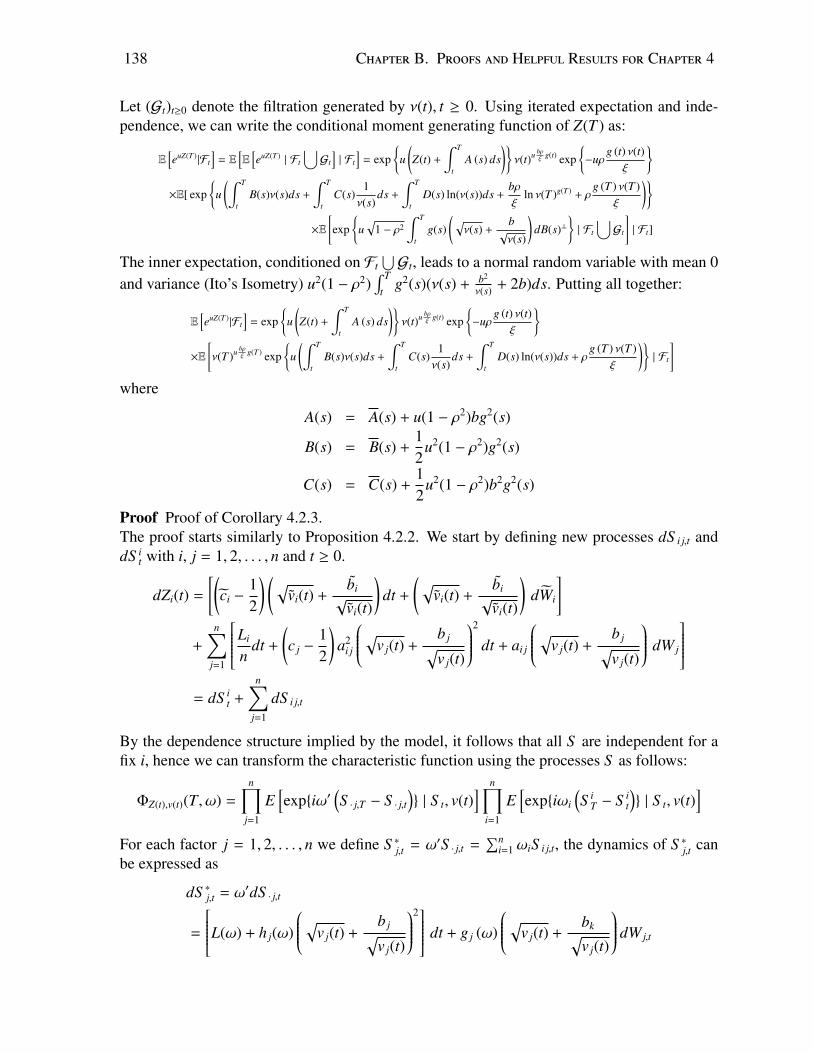
138 Chapter B. Proofs and Helpful Results for Chapter 4
Let (Gt)t≥0 denote the filtration generated by ν(t), t ≥ 0. Using iterated expectation and inde-pendence, we can write the conditional moment generating function of Z(T ) as:
E[euZ(T )|Ft
]= E
[E
[euZ(T ) | Ft
⋃Gt
]| Ft
]= exp
u(Z(t) +
∫ T
tA (s) ds
)ν(t)u bρ
ξ g(t) exp−uρ
g (t) ν(t)ξ
×E[ exp
u(∫ T
tB(s)ν(s)ds +
∫ T
tC(s)
1ν(s)
ds +
∫ T
tD(s) ln(ν(s))ds +
bρξ
ln ν(T )g(T ) + ρg (T ) ν(T )
ξ
)×E
[exp
u√
1 − ρ2
∫ T
tg(s)
(√ν(s) +
b√ν(s)
)dB(s)⊥
| Ft
⋃Gt
]| Ft]
The inner expectation, conditioned on Ft⋃Gt, leads to a normal random variable with mean 0
and variance (Ito’s Isometry) u2(1 − ρ2)∫ T
tg2(s)(ν(s) + b2
ν(s) + 2b)ds. Putting all together:
E[euZ(T )|Ft
]= exp
u(Z(t) +
∫ T
tA (s) ds
)ν(t)u bρ
ξ g(t) exp−uρ
g (t) ν(t)ξ
×E
[ν(T )u bρ
ξ g(T ) exp
u(∫ T
tB(s)ν(s)ds +
∫ T
tC(s)
1ν(s)
ds +
∫ T
tD(s) ln(ν(s))ds + ρ
g (T ) ν(T )ξ
)| Ft
]where
A(s) = A(s) + u(1 − ρ2)bg2(s)
B(s) = B(s) +12
u2(1 − ρ2)g2(s)
C(s) = C(s) +12
u2(1 − ρ2)b2g2(s)
Proof Proof of Corollary 4.2.3.The proof starts similarly to Proposition 4.2.2. We start by defining new processes dS i j,t anddS i
t with i, j = 1, 2, . . . , n and t ≥ 0.
dZi(t) =
[(ci −
12
) (√vi(t) +
bi√
vi(t)
)dt +
(√vi(t) +
bi√
vi(t)
)dWi
]+
n∑j=1
Li
ndt +
(c j −
12
)a2
i j
√v j(t) +b j√v j(t)
2
dt + ai j
√v j(t) +b j√v j(t)
dW j
= dS i
t +
n∑j=1
dS i j,t
By the dependence structure implied by the model, it follows that all S are independent for afix i, hence we can transform the characteristic function using the processes S as follows:
ΦZ(t),v(t)(T, ω) =
n∏j=1
E[expiω′
(S · j,T − S · j,t
) | S t, v(t)
] n∏i=1
E[expiωi
(S i
T − S it
) | S t, v(t)
]For each factor j = 1, 2, . . . , n we define S ∗j,t = ω′S · j,t =
∑ni=1 ωiS i j,t, the dynamics of S ∗j,t can
be expressed as
dS ∗j,t = ω′dS · j,t
=
L(ω) + h j(ω)
√v j(t) +b j√v j(t)
2 dt + g j (ω)
√v j(t) +bk√v j(t)
dW j,t
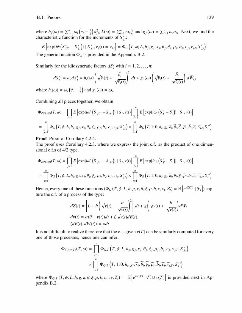
B.1. Proofs 139
where h j(ω) =∑n
i=1 ωi
(ci −
12
)a2
i j, L(ω) =∑n
i=1 ωiLin and g j (ω) =
∑ni=1 ωiai j. Next, we find the
characteristic function for the increments of S ∗j,t:
E[expiφ
(S ∗j,T − S ∗j,t
) | S ∗j,t, v j(t) = v j,t
]= ΦG
(T, φ; L, h j, g j, κ j, θ j, ξ j, ρ j, b j, c j, v j,t, S ∗j,t
).
The generic function ΦG is provided in the Appendix B.2.
Similarly for the idiosyncratic factors dS it with i = 1, 2, . . . , n:
dS ∗it = ωidS it = hi(ω)
(√vi(t) +
bi√
vi(t)
)2
dt + gi (ω)(√
vi(t) +bi√
vi(t)
)dWi,t
where hi(ω) = ωi
(ci −
12
)and gi (ω) = ωi.
Combining all pieces together, we obtain:
ΦZ(t),v(t)(T, ω) =
n∏j=1
E[expiω′
(S · j,T − S · j,t
) | S t, v(t)
] n∏i=1
E[expiωi
(S i
T − S it
) | S t, v(t)
]=
n∏j=1
ΦG
(T, φ; L, h j, g j, κ j, θ j, ξ j, ρ j, b j, c j, v j,t, S ∗j,t
)×
n∏i=1
ΦG
(T, 1; 0, hi, gi, κi, θi, ξi, ρi, bi, ci, vi,t, S ∗it
)Proof Proof of Corollary 4.2.4.The proof uses Corollary 4.2.3, where we express the joint c.f. as the product of one dimen-sional c.f.s of 4/2 type.
ΦZ(t),v(t)(T, ω) =
n∏j=1
E[expiω′
(S · j,T − S · j,t
) | S t, v(t)
] n∏i=1
E[expiωi
(S i
T − S it
) | S t, v(t)
]=
n∏j=1
ΦG
(T, φ; L, h j, g j, κ j, θ j, ξ j, ρ j, b j, c j, v j,t, S ∗j,t
)×
n∏i=1
ΦG
(T, 1; 0, hi, gi, κi, θi, ξi, ρi, bi, ci, vi,t, S ∗it
)Hence, every one of these functions (ΦG (T, φ; L, h, g, κ, θ, ξ, ρ, b, c, vt,Zt) = E
[euZ(T ) | Ft
]) cap-
ture the c.f. of a process of the type:
dZ(t) =
L + h(√
v(t) +b√
v(t)
)2 dt + g(√
v(t) +b√
v(t)
)dWt
dv(t) = α(θ − v(t))dt + ξ√
v(t)dB(t)〈dB(t), dW(t)〉 = ρdt
It is not difficult to realize therefore that the c.f. given v(T ) can be similarly computed for everyone of those processes, hence one can infer:
ΦZ(t),v(T )(T, ω) =
n∏j=1
ΦG,T
(T, φ; L, h j, g j, κ j, θ j, ξ j, ρ j, b j, c j, v j,T , S ∗j,t
)×
n∏i=1
ΦG,T
(T, 1; 0, hi, gi, κi, θi, ξi, ρi, bi, ci, vi,T , S ∗it
)where ΦG,T (T, φ; L, h, g, κ, θ, ξ, ρ, b, c, vT ,Zt) = E
[euZ(T ) | Ft ∪ v(T )
]is provided next in Ap-
pendix B.2.
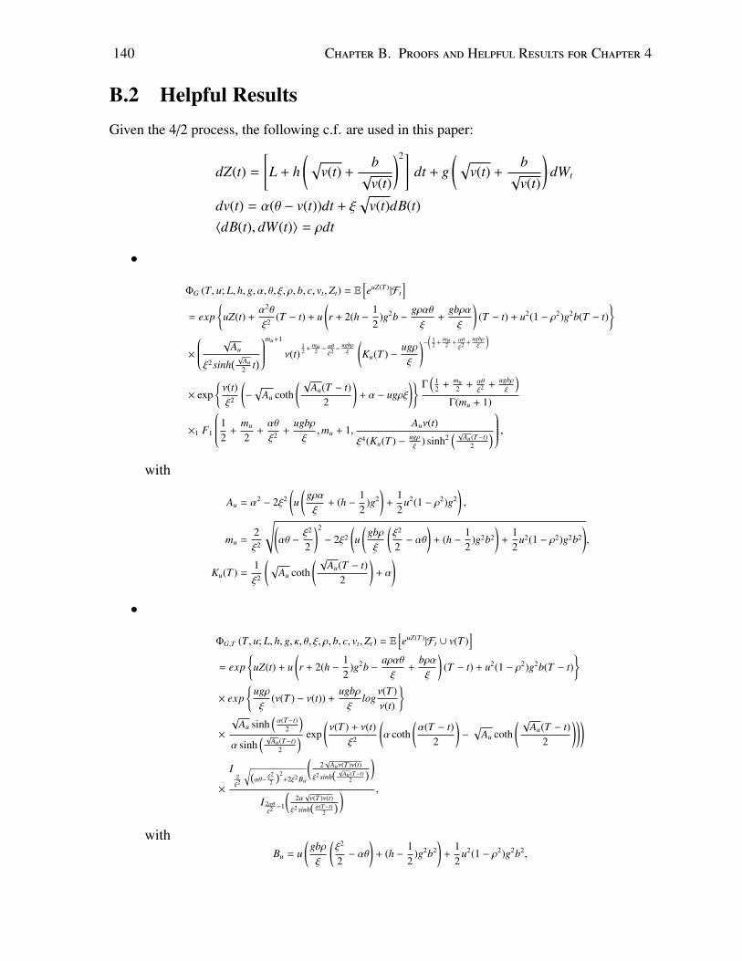
140 Chapter B. Proofs and Helpful Results for Chapter 4
B.2 Helpful ResultsGiven the 4/2 process, the following c.f. are used in this paper:
dZ(t) =
L + h(√
v(t) +b√
v(t)
)2 dt + g(√
v(t) +b√
v(t)
)dWt
dv(t) = α(θ − v(t))dt + ξ√
v(t)dB(t)〈dB(t), dW(t)〉 = ρdt
•
ΦG (T, u; L, h, g, α, θ, ξ, ρ, b, c, vt,Zt) = E[euZ(T )|Ft
]= exp
uZ(t) +
α2θ
ξ2 (T − t) + u(r + 2(h −
12
)g2b −gραθξ
+gbραξ
)(T − t) + u2(1 − ρ2)g2b(T − t)
×
√Au
ξ2 sinh( √Au
2 t)
mu+1
ν(t)12 +
mu2 −
αθ
ξ2−
ugbρξ
(Ku(T ) −
ugρξ
)−( 12 +
mu2 + αθ
ξ2+
ugbρξ
)
× expν(t)ξ2
(−
√Au coth
( √Au(T − t)
2
)+ α − ugρξ
) Γ(
12 + mu
2 + αθξ2 +
ugbρξ
)Γ(mu + 1)
×1 F1
12
+mu
2+αθ
ξ2 +ugbρξ
,mu + 1,Auν(t)
ξ4(Ku(T ) − ugρξ
) sinh2( √
Au(T−t)2
) ,
with
Au = α2 − 2ξ2(u(
gραξ
+ (h −12
)g2)
+12
u2(1 − ρ2)g2),
mu =2ξ2
√(αθ −
ξ2
2
)2
− 2ξ2
(u(
gbρξ
(ξ2
2− αθ
)+ (h −
12
)g2b2
)+
12
u2(1 − ρ2)g2b2
),
Ku(T ) =1ξ2
(√Au coth
( √Au(T − t)
2
)+ α
)
•
ΦG,T (T, u; L, h, g, κ, θ, ξ, ρ, b, c, vt,Zt) = E[euZ(T )|Ft ∪ v(T )
]= exp
uZ(t) + u
(r + 2(h −
12
)g2b −aραθξ
+bραξ
)(T − t) + u2(1 − ρ2)g2b(T − t)
× exp
ugρξ
(ν(T ) − ν(t)) +ugbρξ
logν(T )ν(t)
×
√Au sinh
(α(T−t)
2
)α sinh
( √Au(T−t)
2
) exp(ν(T ) + ν(t)
ξ2
(α coth
(α(T − t)
2
)−
√Au coth
( √Au(T − t)
2
)))
×
I2ξ2
√(αθ−
ξ22
)2+2ξ2 Bu
(2√
Auν(T )ν(t)
ξ2 sinh( √
Au (T−t)2
) )I 2αθξ2−1
(2α√ν(T )ν(t)
ξ2 sinh(α(T−t)
2
) ) ,
withBu = u
(gbρξ
(ξ2
2− αθ
)+ (h −
12
)g2b2)
+12
u2(1 − ρ2)g2b2,
Curriculum Vitae
Name: Zhenxian GongDegrees: The University of Western Ontario
London, ON2016-2021 Ph.D in Statistics
Queen’s UniversityKingston, ON2015-2016 MSc in Statistics
University of AlbertaEdmonton, AB2007-2011 BSc in Statistics
Honours and Western Graduate Research ScholarshipAwards: 2016-2020
Related Work Teaching AssistantExperience: The University of Western Ontario
2016 - 2021
Research AssistantThe University of Western Ontario2017 - 2021
Publications:
Marcos Escobar-Anel and Zhenxian Gong. The mean-reverting 4/2 stochastic volatility model:Properties and financial applications. Applied Stochastic Models in Business and Industry.2020; 36: 836– 856
Yuyang Cheng, Marcos Escobar-Anel and Zhenxian Gong. Generalized mean-reverting 4/2Factor Model. Journal of Risk and Financial Management; 2019, 12.4: 159.
141
Copyright © 2022 FDOKUMEN