Non mean reverting affne processes for stochastic mortality

Non mean reverting affine processes for stochastic mortality∗

Elisa Luciano† Elena Vigna‡

1 May 2005

Abstract

In this paper we use doubly stochastic processes (or Cox processes) in order to model therandom evolution of mortality of an individual. These processes have been widely used in thecredit risk literature in modelling default arrival, and in this context have proved to be quite flex-ible, especially when the intensity process is of the affine class. We investigate the applicabilityof affine processes in describing the individual’s intensity of mortality and the mortality trend.We also provide some calibrations to the UK population. Calibrations suggest that, in spite oftheir popularity in the financial context, mean reverting processes are less suitable for describingthe death intensity of individuals than non mean reverting processes. Among the latter, affineprocesses whose deterministic part increases exponentially seem to be appropriate. As for thestochastic part, negative jumps seem to do a better job than diffusive components alone. Stressanalysis and analytical results indicate that increasing the randomness of the intensity processresults in improvements in survivorship.

JEL classification: G22, J11.

Keywords: doubly stochastic processes (Cox processes), stochastic mortality, affine processes.

∗We thank Bjarne Højgaard and Andrew Cairns, for interesting and stimulating comments. We especially thankSteven Haberman and Russell Gerrard, who pointed out the importance, in this context, of the exponential increasein the observed force of mortality. Any remaining errors are ours.

†Dipartimento di Statistica e Matematica Applicata, University of Turin & ICER, Turin. Email: [email protected]. Tel. +39 011 670 5742. Fax. +39 011 670 5783.

‡Dipartimento di Statistica e Matematica Applicata, University of Turin. Email: [email protected]. Tel.+39 011 670 5754. Fax. +39 011 670 5783.

1 Introduction

The issue of mortality risk – and, in particular, of longevity risk – has been largely addressed inrecent years when dealing with the pricing of insurance products. It is well known from the basicsof actuarial science that the price of any insurance product on the duration of life depends on twomain basis: demographical and financial assumptions. Traditionally, actuaries have been treatingboth the demographic and the financial assumptions in a deterministic way, by considering availablemortality tables for describing the future evolution of mortality and by setting the so-called “bestestimate” of the rate of interest for discounting cash flows over time. More recently, stochasticmodels have been adopted to describe the uncertainty linked both to mortality and to financialfactors. We focus on mortality risk and on modelling the survival function of the individual. Inthe setting proposed here, the extension to stochastic interest rates is straightforward, under thestandard assumption of independence between financial and mortality risks (see, for instance, Dahl(2004) and Biffis (2004)).

2 Modelling mortality risk

In the last decades significant improvements in the duration of life have been experienced in mostdeveloped countries. Two indicators are typically used to describe the mortality of an individual:the survival function and the death curve.

The survival function, denoted with S(t), is defined as follows:

S(t) = P (T0 > t) = 1− FT0(t)

where T0 is the random variable that describes the duration of life of a new-born individual, andFT0 is its distribution function. The survival function indicates the probability that a new-bornindividual will survive at least t years. Via the survival function, one can easily derive the distribu-tion function of the duration of life of an individual aged x, given that he/she is alive at that age(see, for instance, Bowers, Gerber, Hickman, Jones and Nesbitt (1986), Gerber (1997)).

The death curve, x/1q0, is defined as follows:

x/1q0 =S(x)− S(x + 1)

S(0)

and indicates the probability for a new-born individual of dying in year of age [x, x + 1].

An easy way of capturing the mortality trend observed in the past decades consists in lookingat the graphs of the survival function and the death curves of a population in different years (foran accurate report about mortality trends, see Pitacco (2004a)). One can notice that the shapeof the survival function becomes more and more “rectangular” and the mode of the death curvemoves towards right. The first phenomenon is known as rectangularization, the second as expan-sion. Rectangularization occurs since the volatility of the duration of life around the mode of deathdecreases, leading to lower dispersion of ages of death around the most likely age of death. Expan-sion takes place because the age when death is most likely to occur increases as time passes, due toimprovements in economic and social conditions, medicine progresses etc..

It is clear that continuous improvements in the mortality rates have to be allowed for when pricing

Version:

insurance products that heavily depend on the duration of life at old ages, like annuities. Indeed,strong or unexpected reductions in mortality rates can lead to mispricing of these products and canaffect the solvency of the insurance company.

The actuarial literature about modelling and forecasting mortality rates is vaste and has a longhistory: for a detailed survey of the most significant models proposed in the literature, see Pitacco(2004b).Traditionally, a central role has been played by the “force of mortality”, defined as the opposite ofthe derivative of the logarithm of the survival function:

µx = − d

dxlog S(x)

The force of mortality is a good tool for approximating the mortality of the individual at age x,since it can be shown that:

P (x < T0 ≤ x + ∆x|T0 > x) = µx∆x + o(∆x), (2.1)

i.e. the probability of dying in a short period of time after x, between age x and age x + ∆x, canbe approximated by µx∆x, when ∆x is small. The force of mortality is obviously increasing as xincreases, as the probability of imminent death increases when ageing 1.

When allowing for mortality trends over time, it is evident that the force of mortality has toshow a dependence also on calendar year, and not only on age. Thus, the force of mortality can bedescribed by a two variable function µx(y), where y indicates the calendar year. As time y increasesand the age x remains fixed, the decreasing mortality rates over time translate into a decreasingfunction µx(y).

Several contributions have been proposed in the last decade in order to model and forecast theyear- and age-dependent mortality, i.e. “dynamic mortality”. One of the seminal works is the Lee-Carter method (Lee and Carter (1992) and Lee (2000)), that models an actuarial indicator, similarto the force of mortality, known as the central death rate, as a two variable function. Many authorshave modified the Lee-Carter method. Among these are the extensions proposed by Renshaw andHaberman (2003) and Brouhns, Denuit and Vermunt (2002). The latter propose a fairly simplemodel for the force of mortality:

ln(µx(y)) = αx + βxky

where the coefficients αx, βx and ky are to be determined by maximization of the log-likelihoodbased on the assumption that the number of deaths at age x in year y follows a Poisson distribution.

Another way of dealing with mortality trends, largely adopted by insurance companies, is the useof the so-called “projected mortality tables”, that incorporate (forecasts of) survival probabilitiesat any age for different calendar years.

Finally, Milevsky and Promislow (2001) have used a stochastic force of mortality, whose expec-tation at any future date has a Gompertz specification. They have not studied the existence of adeath process which admits their stochastic force of mortality as arrival rate. We will address thisissue below, after having examined the doubly stochastic processes literature, to which the nextsection is devoted.

1With some exceptions, like very small values of x – due to the infant mortality – and values around 20-25 – dueto the young mortality hump.

Version:

3 The mathematical framework

The theory of stochastic intensities, doubly stochastic processes and affine processes underlyingthe actuarial application presented here is enormous and covered in many texts about stochasticprocesses. A detailed and thorough treatment is clearly beyond the scope of this paper, and welimit ourselves to a brief summary of the mathematical tools used, sacrificing scientific rigor andomitting all the proofs. However, we refer the interest reader to Bremaud (1981) and Duffie (2001).

The reason why such a sophisticated mathematical framework has been used in describing themortality risk is the great analytical tractability of the models presented, once some useful and nottoo restrictive assumptions are introduced. These mathematical tools have been extensively usedin the credit risk literature, when modelling time to default of firms. The pioneering works in thisfield are Artzner and Delbaen (1992), Lando (1994) and Duffie and Singleton (1994). Applicationsof this mathematical framework to dynamic mortality modelling and to insurance products pricingcan be found in Biffis (2004), Dahl (2004) and Schrager (2004). The similarity between the time todefault and the remaining duration of life is strong, and, although the factors underlying the deathof an individual and the default of a firm are obviously completely different, the mathematical toolsused in the two literatures are the same.

3.1 Counting processes

In describing the mathematical tools, we will mainly follow Duffie (2002). We are given a completefiltered probability space (Ω,F ,P) and a filtration Gt : t ≥ 0 of sub-σ-algebras of F satisfying theusual conditions.

A counting process (or point process) N is defined using a sequence of increasing random vari-ables T0, T1, ..., with values in [0,∞], s.t. T0 = 0 and Tn < Tn+1 whenever Tn < ∞, in thefollowing way:

Nt = n for t ∈ [Tn, Tn+1)

and Nt = ∞ if t ≥ T∞ = limn→∞ Tn. It is easy to see Tn as the time of the nth jump of the processN and Nt as the number of jumps occurred up to time t, including time t (hence the definition“counting” process). The counting process is said to be nonexplosive if T∞ = ∞ almost surely.

3.2 Stochastic intensity

The definition of random intensity is not uniform in the literature. We will follow Duffie (2001).

Let Ft : t ≥ 0 be a filtration satisfying the usual conditions, with Ft ⊂ Gt, and λ be a nonnegative(Ft)-predictable process s.t.

∫ t0 λ(s)ds < ∞ almost surely. A nonexplosive adapted counting process

N is said to admit the intensity λ if the compensator of N admits the representation∫ t0 λ(s)ds, i.e.

if Mt = Nt−∫ t0 λ(s)ds is a local martingale. If the stronger condition E(

∫ t0 λ(s)ds) < ∞ is satisfied,

Mt = Nt −∫ t0 λ(s)ds is a martingale.

From this, one gets:

E(Nt+∆t −Nt|Ft) = E

(∫ t+∆t

tλ(s)ds|Ft

)

Version:

which, after a few passages and under technical conditions, leads to:

E(Nt+∆t −Nt|Ft) = λ(t)∆t + o(∆t) (3.1)

Equation 3.1 (see the analogy with equation 2.1) stresses the importance of the process λ in givinginformation about the average number of jumps of the process under observation in a small periodof future time. Observe that conditioning is made on the smallest filtration, therefore on theavailability of poorer information. The idea is that the information at time t can give insight aboutthe expected number of jumps in the next future or, in other words, about the likelihood of a jumpin the immediate future. It cannot predict the actual occurrence of a jump, that comes as a “suddensurprise”.

3.3 Doubly stochastic processes

A nonexplosive counting process N with intensity λ is said to be doubly stochastic driven byFt : t ≥ 0, if for all t < s, conditional on the σ−algebra Gt ∨ Fs, generated by Gt ∪ Fs, theprocess Ns −Nt has Poisson distribution with parameter

∫ st λ(u)du.

As an example, we observe that any Poisson process is a doubly stochastic process driven by thefiltration Ft = (∅,Ω) = F0 for any t ≥ 0, in that the intensity is deterministic.

A stopping time τ is said to be doubly stochastic with intensity λ if the underlying counting processwhose first jump time is τ is doubly stochastic with intensity λ.

The mathematical arsenal presented so far is now sufficient to present the first interesting resultthat will be used in the applications. If τ is a stopping time doubly stochastic with intensity λ, itcan be shown, by using the law of iterated expectations, that:

P (τ > s|Gt) = E[e−

∫ st λ(u)du|Gt

](3.2)

Readers who are familiar with mathematical finance can easily see in the r.h.s. of equation (3.2) theprice at current time t of a unitary default-free zero-coupon bond with maturity at time s > t, ifthe short-term interest rate model is given by the process λ. All the mathematical finance literatureabout interest rate models can thus be retrieved in this setting.

Another interesting result that can be used relates to the density function of a doubly stochas-tic stopping time τ . If we let p(t) = P (τ > t) be the survival function, then the density function ofτ , if it exists, is given by −p′(t). Under technical conditions (see for example Grandell (1976)), wehave:

p′(t) = E[−e−

∫ t0 λ(u)duλ(t)|Gt

](3.3)

It is clear how these results can be naturally applied in the actuarial context: if one sees τ asthe future lifetime of an individual aged x, Tx, equations 3.2 and 3.3 can be applied to find thesurvival function and the density function of Tx, given a model for the death intensity λ.

3.4 Affine processes

Our next step will be to show how equations like 3.2 and 3.3 can be approached. It turns out thatit is convenient to specify the stochastic intensity λ as a function Λ of another process X in R,

Version:

whose dynamics are given by the SDE:

dX(t) = f(X(t))dt + g(X(t))dW (t) + dJ(t) (3.4)

where J is a pure jump process and where the drift f(X(t)), the covariance matrix g(X(t))g(X(t))′

and the jump measure associated with J have affine dependence on X(t). Such a process is namedan affine process: interest readers can find a thorough treatment of affine processes in Duffie, Fil-ipovic and Schachermayer (2003).

The financial literature on interest rate modelling is full of examples of affine processes: the Ornstein-Uhlenbeck process, used by Vasicek (1977) for modelling interest rates, is affine, as is the Fellerprocess, used by Cox, Ingersoll and Ross (1985).

The convenience of adopting affine processes in modelling the intensity lies in the fact that, undertechnical conditions (see Duffie and Singleton (2003)), it yields, for any w ∈ R:

E[e∫ T

t −Λ(X(u))du+wX(T )|Gt

]= eα(T−t)+β(T−t)X(t) (3.5)

where the coefficients α(·) and β(·) satisfy generalized Riccati ODEs. The latter can be solved atleast numerically and in some cases analytically. Therefore, the difficult problem of finding thesurvival function 3.2 can be transformed in a tractable problem, whenever affine processes for X(t)are employed.

4 The actuarial application: mean reverting processes

Turning back to our initial problem of modelling adequately the dynamic mortality, we will nowuse some of the mathematical tools presented in the previous section.

As above, the uncertainty is described by a complete filtered probability space (Ω,F ,P) and afiltration Gt : t ≥ 0 of sub-σ-algebras of F satisfying the usual conditions. We consider an indi-vidual aged x and model his/her random future lifetime Tx as a doubly stochastic stopping timewith intensity λx driven by the sub-filtration Ft : t ≥ 0, where Ft ⊂ Gt. In other words, Tx is thefirst jump time of a nonexplosive counting process N with intensity λx. Intuitively, the countingprocess N may be seen as a process that jumps whenever the individual dies: Nt = 0 if t < Tx,Nt > 0 if t ≥ Tx.

According to (3.2) the survival probability is:

Sx(t) = P (Tx > t|G0) = E[e−

∫ t0 λx(u)du|G0

](4.1)

The similarity with the actuarial survival probability for t years for an individual aged x, tpx,expressed in terms of the force of mortality, is strong:

tpx = e−∫ t0 µx+sds

The specification of the intensity process λx is now crucial for the solution of equation 4.1.

Recent studies on the firm’s mortality (as reported in Duffie and Singleton (2003)) indicate thesuitability of the following affine processes for modelling the intensity λx(t):

CIR process : dλx(t) = k(γ − λx(t))dt + σ√

λx(t)dW (t)

Version:

mean reverting with jumps (m.r.j.) : dλx(t) = k(γ − λx(t))dt + dJ(t)

where W (t) is a standard Brownian motion, k > 0, γ > 0, σ ≥ 0 and J(t) is a compound Poissonprocess with intensity l and jumps exponentially distributed with expected value µ.

In addition, we consider the Vasicek process (see Vasicek (1977)) for λx(t):

V AS process : dλx(t) = k(γ − λx(t))dt + σdW (t)

We notice that in all cases, according to the notation introduced before, the choice is w = 0 andΛ(x) = x: the intensity λ is itself an affine process.

Using the result 3.5 and solving the Riccati ODEs, one gets the survival probabilities in closedform for all the specifications of the intensity process:

Sx(t) = eα(t)+β(t)λx(0) (4.2)

where, in the CIR case (see for instance Duffie and Singleton (2003)):

α(t) = −2kγ

σ2ln

(c + debt

b

)+

kγ

ct

β(t) =1− ebt

c + debt

b = −√

k2 + 2σ2 c =b− k

2d =

b + k

2

In the m.r.j. case instead (see again Duffie and Singleton (2003)):

α(t) = −γ(t + β(t))− lµt− ln(1− µβ(t))

µ + k

β(t) =e−kt − 1

k

In the Vasicek (VAS) one (see Vasicek (1977)) β(t) is defined as in the m.r.j. case, while:

α(t) = −(β(t) + t)(k2γ − σ2

2 )k2

− σ2β(t)2

4k

It is possible to calibrate the values of the parameters starting from a time series of survival prob-ability data. We notice that, when t changes, the process λx(t) describes the future intensity ofmortality for any age x + t of an individual aged x at time 0. In other words, our process λ cap-tures the mortality intensity for a particular generation and a particular initial age. This has to beallowed for when choosing the mortality table: the approach adopted here is a “diagonal” one.

Version:

4.1 Calibration to the UK population: projected and observed generation tables

As a first application, we have calibrated the three processes to the UK population.

The mortality tables selected for the calibration are two observed generation tables, for individ-uals born in 1880 and in 1900 respectively, and two projected mortality tables, for individuals bornin 1935 and 1945 respectively. The data relative to the observed mortality tables are taken from theHuman Mortality Database (University of California, Berkeley (USA), and Max Planck Institutefor Demographic Research (Germany) (2002), data downloaded on August 10, 2004). Those for theprojected tables are taken from the Standard tables of mortality 1992 for UK immediate annuitants,IML92 (Institute and Faculty of Actuaries (1990)).

In the calibration, we have set µ < 0. The choice of a negative jump size is motivated by theexpectation of sudden improvements in the force of mortality: jumps should correspond to discon-tinuity points of the intensity process, that can be related, for instance, to medicine progresses. Wemust say that negative jumps in the intensity process render positive the probability that the in-tensity becomes negative. This inconvenient is also observed by Biffis (2004). However, in practicalapplications and calibrations the jump size and frequency result to be so small that the probabilityof negative values can be considered negligible.

In fitting the table, we have adopted the least squares method, considering the spreads between thedifferent model survival probabilities and the table ones. Table 1 reports for each intensity processthe optimal values of the parameters and the calibration error2. We report data only for males, aswell as the corresponding initial value of λ, λ65(0) (which has been chosen equal to − ln(p65)).

TABLE 1

1880 1900 1935 1945λ65(0) 0.03515 0.03797 0.01145 0.00885CIR-error 0.02182 0.01662 0.40945 0.20552CIR-k 0.00448 0.01365 0.06494 0.0078CIR-σ 0.00103 0.00298 0.00005 0CIR-γ 1.24656 0.4301 0.07552 0.41711mrj-error 0.02236 0.01327 0.15816 0.1965mrj-k 0.00571 0.00392 0.005 0.00465mrj-µ -0.00246 -0.00227 -0.00249 -0.00492mrj-l 0.00247 0.00234 0.00249 0.0099mrj-γ 0.99382 1.31818 0.64908 0.67935VAS-error 0.02247 0.01473 0.16191 0.1982VAS-σ 0.00046 0.00048 0.00002 0.00002VAS-k 0.00591 0.00835 0.00604 0.00526VAS-γ 0.96029 0.65393 0.53278 0.59302

In all models, the value of the long term mean for λ, γ, lies between 0.41 and 1.3 and generallydecreases when considering younger generations, which is an expected result. The exceptions to this

2The error is the minimized sum of the squared differences between the survival probabilities of the relevant tableand the ones implied by the model.

Version:

trend are probably due to the fact that the initial value of λ, λ65(0), tends to decrease when movingfrom the left to the right of the table. In particular, when passing from the 1935 generation to the1945 one, it drops from 0.011 to 0.0088, and this dramatic reduction is likely to be counterbalancedin the calibration procedure by a high value of the long term mean (furthermore, notice that theselast two values are only projected and not observed, and refer to the population of immediate annu-itants, who are supposed to experience a lighter mortality than the general population). The speedof convergence k seem to be stable in the last two models (ranging between 0.004 and 0.008), andvolatile in the first one. The size of jumps ranges between -0.002 and -0.005, indicating that negativejumps are part of the optimally calibrated intensity process, though with a very low frequency (thatranges between 0.002 and 0.01). The value of σ is very low in all cases, ranging between 0 and 0.003.

The most remarkable result is the change in the value of the error when passing from the ob-served old tables to the projected ones for younger generations: it more than decuplicates, rangingfor the latter around 0.15-0.4 against 0.01-0.02 for the former. The different magnitude of the errorcan be better perceived when considering the curve of the survival function S65(t) implied by thethree models and the survival probabilities of the relevant table.

Graphs 1, 2, 3 and 4 report, for the different generations, the survival function of the three processesanalyzed (CIR, m.r.j. and VAS) and the ones of the tables considered.

Generation 1880

0

0.1

0.2

0.3

0.4

0.5

0.6

0.7

0.8

0.9

1

66

69

72

75

78

81

84

87

90

93

96

99

102

105

108

Age

S6

5(t

)

1880 CIR mrj VAS

Generation 1900

0

0.1

0.2

0.3

0.4

0.5

0.6

0.7

0.8

0.9

1

66

69

72

75

78

81

84

87

90

93

96

99

102

105

108

Age

S65(t

)

1900 CIR mrj VAS

Graph 1 Graph 2

Generation 1935

0

0.1

0.2

0.3

0.4

0.5

0.6

0.7

0.8

0.9

1

66

69

72

75

78

81

84

87

90

93

96

99

102

105

108

111

114

117

120

Age

S6

5(t

)

IML92-35 CIR mrj VAS

Generation 1945

0

0.1

0.2

0.3

0.4

0.5

0.6

0.7

0.8

0.9

1

66

69

72

75

78

81

84

87

90

93

96

99

102

105

108

111

114

117

120

Age

S65(t

)

IML92-45 mrj VAS

Version:

Graph 3 Graph 4

It is evident from a first inspection of the graphs that, while the fit can be considered satisfactory forthe first two generations, it cannot be considered so for the last two. In particular, one can noticethat, in the last two cases the survival functions implied by the three processes do not capturethe rectangularization phenomenon. In addition, the survival probability at very old ages is muchhigher and at lower ages much lower than in the fitted tables. Therefore, although the last two tablesrefer to projected mortality tables and not to observed ones, these results seem to suggest that inthe presence of high rectangularization phenomenon – which is an expected feature in the futuregeneration tables – the intensity of mortality cannot be properly described by the three proposedprocesses.

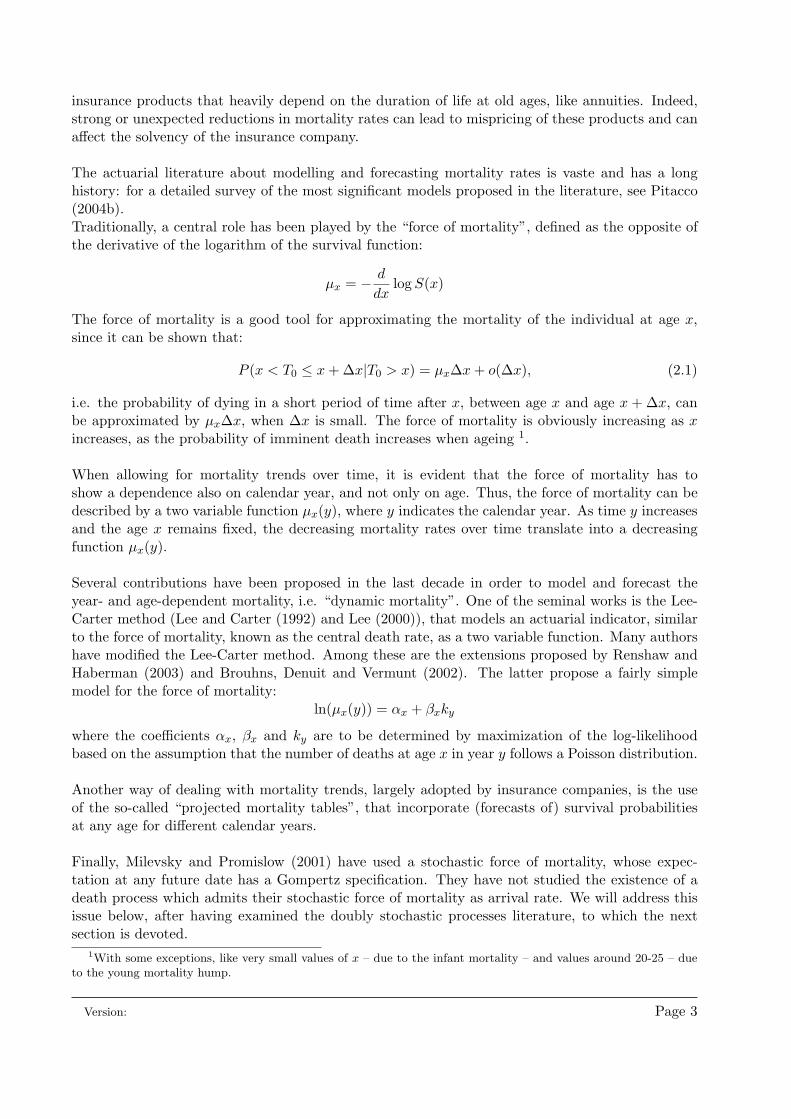
5 The actuarial application: non mean reverting processes

The calibration of the mean reverting processes presented so far gives a survival function that, withrespect to the new generations, fails to capture the rectangularization phenomenon and producesunrealistic survival probabilities at very old ages. The question arises as to whether the commonand disturbing element in those processes is the mean reverting term, as suggested also by Blake,Cairns and Dowd (2004).

Furthermore, the force of mortality observed and/or extrapolated from the mortality tables doesnot seem to present a mean reverting behaviour, but rather an exponential one. This observation,consistent with all the deterministic exponential models presented in the actuarial literature, natu-rally leads to the simple idea of dropping the mean reverting term in the classical affine processesused in finance and choosing processes whose deterministic part increases exponentially. Four affinemodels with these two desired characteristics are presented and discussed below.

5.1 The Ornstein Uhlenbeck process without jumps

The first model candidate for describing the intensity λx(t) is an Ornstein Uhlenbeck process (fromnow on, we omit the initial age x for convenience).

OU process dλ(t) = aλ(t)dt + σdW (t) (5.1)

with a > 0 and σ ≥ 0.By solving it, we get to the following expression for the intensity:

λ(t) = λ(0)eat + σ

∫ t

0et−sdW (s) (5.2)

The main drawback when choosing this process for the intensity is that it becomes negative withpositive probability.

By applying standard results on linear stochastic differential equations (see, for instance, Arnold(1974)) to the process (5.2) we have that λ(t) is normally distributed with mean

E(λ(t)) = λ(0)eat

Version:

and variance

V ar(λ(t)) = σ2 · e2at − 12a

Therefore, the calculation of the probability of λ(t) taking negative values is straightforward:

P (λ(t) ≤ 0) = P

(λ(0)eat + σ

√e2at − 1

2aN ≤ 0

)= P

N ≤ − λ(0)eat

σ√

e2at−12a

= Φ(ζ(σ, a))

with

ζ(σ, a) = − λ(0)eat

σ√

e2at−12a

where N ∼ N (0, 1) and Φ is its distribution function.

It turns out that the function ζ(·, ·) is an increasing function of σ and a decreasing function ofa, and so is the probability of negative values of λ. In practical applications to mortality modellingthis probability tends to be small, since the relevant values of σ and a are respectively small andhigh enough. We will come back to this point later, when presenting the numerical applications.

By applying the framework of equation (3.5) (in particular, see Duffie, Pan and Singleton (2000)pagg. 1350–1351) we have that:

Sx(t) = E(e−

∫ t0 λ(u)du|G0

)= eα(t)+β(t)λ(0) (5.3)

where the functions α and β solve the system of ODEs’:

β′(t) = −1 + aβ(t)α′(t) = 1

2σ2β2(t)(5.4)

with boundary conditionsβ(0) = 0, α(0) = 0 (5.5)

By solving the system 5.4–5.5, we find α and β:

α(t) = σ2

2a2 t− σ2

a3 eat + σ2

4a3 e2at + 3σ2

4a3

β(t) = 1a

(1− eat

) (5.6)

We observe that with a strictly positive value of σ, the survival probability for t large enoughbecomes an increasing function of age; in addition, the probability of surviving forever tends toinfinity. These unrealistic and undesirable features are due to the fact that the survival intensitycan take negative values with positive probability. Thus, from a purely theoretical point of view,the Ornstein Uhlenbeck model can be considered inadequate to describe the intensity of mortality.

However, it can be seen that in the applications this model turns out to be rather appropriate.In fact, the calibration of the model to different mortality tables gives surprising results, leading tovery good fits of the survival probabilities tpx. The reason of its successful application is that thevalues of σ and a resulting from the calibration process are respectively small and high enough tomake negligible the probability of negative values of λ. Furthermore, the period under considerationin the applications is limited to some decades of years, which makes the model applicable for two

Version:

main reasons: firstly, during this period, the survival probability is a decreasing function of age(as it should be); secondly, it avoids the explosion of the survival probability. Thus, the evidenceseems to be an encouraging one, with respect to practical application of the model by actuaries anddemographers, though with an important warning on the theoretical limitations of it.

5.2 The Ornstein Uhlenbeck process with jumps

In the second model we add a jump component in the stochastic part of the mortality process.Therefore, the process λ is given by:

OUj process dλ(t) = aλ(t)dt + σdW (t) + dJ(t) (5.7)

where J is a pure compound Poisson jump process, with Poisson arrival times of intensity l > 0and exponentially distributed jump sizes with mean µ < 0. We assume independence between theBrownian motion W (s) and the Poisson process, as well as between the jump sizes. As in theprevious section, we allow only for negative jumps, which correspond to sudden improvements inthe intensity of mortality.

Applying the formulae of Duffie et al. (2000) we have to solve the following system of ODE’sfor α and β:

β′(t) = −1 + aβ(t)α′(t) = 1

2σ2β2(t) + l µβ(t)1−µβ(t)

(5.8)


The equation for β is the same as before (cfr 5.4), so is the solution. The solution for α is insteaddifferent (due to the inclusion of the jump component), and we have:

α(t) = ( σ2

2a2 + laa−µ)t− σ2

a3 eat + σ2

4a3 e2at + 3σ2

4a3 + la−µ ln(1− µ

a + µaeat)

β(t) = 1a

(1− eat

) (5.10)

The technical condition that has to be satisfied for the solution (5.10) to make sense is:

1− µ

a+

µ

aeat > 0 ∀t ≥ 0 (5.11)

that corresponds to:

β(t) >1µ

∀t ≥ 0

Since the function β is decreasing over time (being a > 0), this requirement is satisfied providedthat

β(T ) >1µ

(5.12)

In the calibration exercise, we will see that adding the jump component improves remarkably thegoodness of the fit.

Version:

5.3 The Feller process without jumps

The third model proposed is the Feller process, already investigated in the previous section as CIRprocess, without the mean reverting term:

FEL process dλ(t) = aλ(t) + σ√

λ(t)dW (t) (5.13)

where a > 0 and σ > 0.

The main advantage of this process is that it does not violate the non-negativity constraint ofthe intensity, provided that the starting point is non-negative.

The solution λ(t) of the SDE (5.13) is

λ(t) = λ(0)eat + σ

∫ t

0ea(t−u)

√λ(u)dW (u) (5.14)

and its distribution can be obtained following Feller (1951)).

The application of the affine framework gives the following system of ODE’s for α and β:

α′(t) = 0β′(t) = −1 + aβ(t) + 1

2σ2β2(t)(5.15)


The solution is:

α(t) = 0β(t) = 1−ebt

c+debt

(5.17)

with:

b = −√a2 + 2σ2

c = b+a2

d = b−a2

(5.18)

Given that the coefficients b, c, d are negative, the survival probability is bounded between 0 and 1,which is a desirable feature. As for the previous two models, the calibration to some given mortalitytables gives very satisfactory results (see next section), and the main theoretical inconvenient ofnegative intensity, with consequent survival probabilities greater than one, is avoided.

5.4 The Feller process with jumps

In the fourth model, we add a jump component in the stochastic part of the Feller process. Theintensity λ is given by:

FELj process dλ(t) = aλ(t)dt + σ√

λ(t)dW (t) + dJ(t) (5.19)

Version:

where J is the pure jump process defined above.

The functions α and β that enter the survival probability (5.3) solve the following system of ODE’sequations:

α′(t) = lµβ(t)1−µβ(t)

β′(t) = −1 + aβ(t) + 12σ2β2(t)

(5.20)


Similarly to the OU case, the equation for β is the same as in the no-jump setting. The jumpcomponent enters only the equation for α. We have:

α(t) = lµ

c−µ t− lµ(c+d)b(d+µ)(c−µ) [ln(µ− c− (d + µ)ebt)− ln(−c− d)]

β(t) = 1−ebt

c+debt

(5.22)

with b, c, d given by the equations (5.18) above.

The introduction of the jump component leads to the requirement

µ− c− (d + µ)ebt > 0 (5.23)

which is equivalent to:

β(t) >1µ

requirement satisfied whenever

β(T ) >1µ

(5.24)

As we will see in the next section, the extra stochastic component to the intensity process givessignificantly better results in terms of goodness of the fit, and adds richness and flexibility to themodel.

6 The link with existing models for the force of mortality

We devote this section to investigating the relationship between our models for the stochasticintensity of mortality and the deterministic force of mortality actuaries are more familiar with.Recall that the force of mortality µx at age x is defined as

µx = limh→0

P (x < T0 ≤ x + h|T0 > x)h

In our case, we have:

µx = limh→0

1h

(1− S(x + h)

S(x)

)= lim

h→0

1h

(1− eα(x+h)−α(x)+λ0(0)(β(x+h)−β(x))

)=

= limh→0

α(x)− α(x + h) + λ0(0)(β(x)− β(x + h))h

= −α′(x)− λ0(0)β′(x)

Version:

For example, in the OU model the force of mortality, after a few passages, becomes:

µx = λ0(0)eax − σ2

2a2(eax − 1)2 (6.1)

If σ = 0 we have:µx = λ0(0)eax = λ0(x)

i.e. in this case the force of mortality coincides with the intensity of mortality for a new bornindividual after x years. Furthermore, the force of mortality is of the Gompertz type. This isstraightforward also observing that if σ = 0 the evolution of λ0(t) is deterministic and given by

dλ0(t) = aλ0(t)dt

However, the coincidence between intensity of mortality and force of mortality is clearly no longertrue when the intensity is stochastic, and equation (6.1), compared with equation (5.2) for λ tellsus that

µx < E(λ0(x)) (6.2)

In other words, the force of mortality decreases, hence the survivorship improves, when the diffusioncoefficient increases. We will come back to this feature later, when considering the impact of therandom part of the process on the survival probabilities 3.

With the other three models, we have:

OUj µx = λ0(0)eax − σ2

2a2(eax − 1)2 − l

a− µ

(1− aµeax

a− µ + µeax

)(6.3)

FEL µx =4λ0(0)b2ebx

[(a + b) + (b− a)ebx]2

FELj µx =4λ0(0)b2ebx

[(a + b) + (b− a)ebx]2+

lµ(1− ebx)µ− c− (d + µ)ebx

It is clear (and easy to check) that also with these three models, when the coefficients σ and lof the random part are set to 0 there is coincidence between intensity of mortality and force ofmortality, which turns out to be of the Gompertz type.

7 The calibration of the non mean reverting processes

In this section we calibrate the four models just introduced (OU, OUj, FEL, FELj) to the samemortality tables used in the previous calibration. The calibration procedure is the same followed insection 4.1. The results are shown in Table 2.

3Observe that the inequality (6.2) is also consistent with the fact that

∫ t

0

µsds <

∫ t

0

E(λ0(s))ds

a result that derives by application of Jensen inequality to the survival function.

Version:

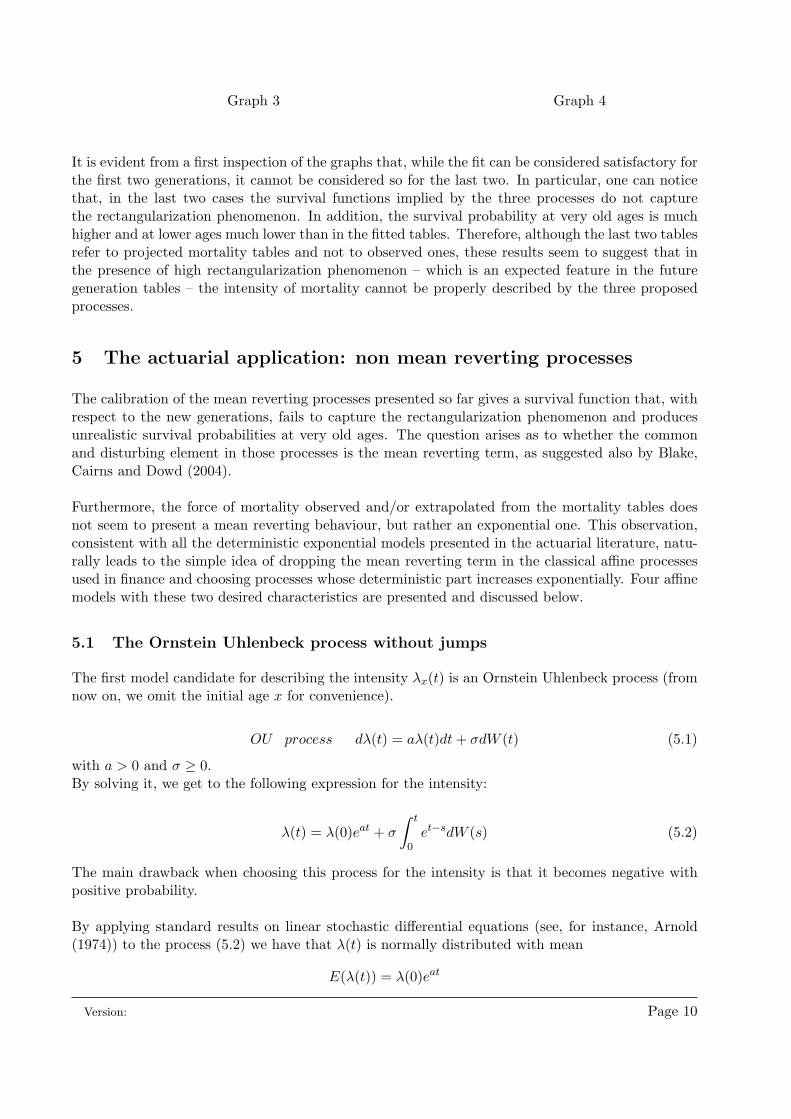
TABLE 2

1880 1900 1935 1945λ65(0) 0.03515 0.03797 0.01145 0.00885OU-error 0.00043 0.00012 0.00085 0.00027OU-a 0.0861 0.07949 0.09856 0.10859OU-σ 0.00183 0.00341 0.0001 0.00048OUj-error 0.0001 0.00004 0.00002 0.00016OUj-a 0.09101 0.08192 0.10014 0.10865OUj-σ 0.00377 0.00414 0.0001 0.00011OUj-l 0.00173 0.00088 0.00105 0.00036OUj-µ -0.00003 -0.00003 -0.00003 -0.00003FEL-error 0.00044 0.00012 0.00084 0.00027FEL-a 0.08553 0.07896 0.09867 0.10811FEL-σ 0.00431 0.01348 0.00005 0.0001FELj-error 0.00043 0.00012 0.00053 0.00027FELj-a 0.0858 0.07897 0.10164 0.10811FELj-σ 0.00735 0.01349 0 0.00001FELj-l 0.001 0.001 0.1856 0.001FELj-µ -0.0001 -0.0001 -0.00034 -0.0001

The main conclusion that can be drawn from the table is that the calibration errors are dramati-cally lower than with mean reverting intensities: they range between 0.00002 and 0.0008. In termsof calibration error, the best fitting model is the OU with jumps, though the differences betweenthe models are quite small 4. Models with jumps generally fit better than the corresponding oneswithout jumps. This result seems to suggest that negative jumps are an appropriate way to describerandom variations in mortality.

Graphs 5, 6, 7 and 8 report the survival probabilities as from the four models analyzed and fromthe relevant tables.

Generation 1880

0

0.1

0.2

0.3

0.4

0.5

0.6

0.7

0.8

0.9

1

66

69

72

75

78

81

84

87

90

93

96

99

102

105

108

Age

S65(t

)

1880 OU OUj FEL FELj

Generation 1900

0

0.1

0.2

0.3

0.4

0.5

0.6

0.7

0.8

0.9

1

66

69

72

75

78

81

84

87

90

93

96

99

102

105

108

Age

S65(t

)

1900 OU OUj FEL FELj

Graph 5 Graph 6

4We notice that with these values of the parameters the probability of negative intensity for the OU model can beconsidered negligible for all practical applications.

Version:

Generation 1935

0

0.1

0.2

0.3

0.4

0.5

0.6

0.7

0.8

0.9

1

66

69

72

75

78

81

84

87

90

93

96

99

102

105

108

111

114

117

120

Age

S65(t

)

IML92-35 OU OUj FEL FELj

Generation 1945

0

0.1

0.2

0.3

0.4

0.5

0.6

0.7

0.8

0.9

1

66

69

72

75

78

81

84

87

90

93

96

99

102

105

108

111

114

117

120

Age

S65(t

)

IML92-45 OU OUj FEL FELj

Graph 7 Graph 8

The fit is very good, also in the presence of strong rectangularization (the last two generation), andall the survival functions cannot be distinguished from each other.

To have a better idea of the goodness of the fit, for each generation we plot the differences betweenthe survival probabilities (tp65) used as data and the survival function implied by the different mod-els (S65(t)). Graphs 9 to 12 report these differences for all the (seven) models considered so far forgenerations 1880 to 1945.

Difference (observed table - survival function),

generation 1880: all models

-0.04

-0.03

-0.02

-0.01

0

0.01

0.02

0.03

0.04

0.05

66

69

72

75

78

81

84

87

90

93

96

99

102

105

108

CIR mrj VAS OU OUj FEL FELj

Graph 9

Version:

Difference (observed table - survival function),

generation 1900: all models

-0.04

-0.03

-0.02

-0.01

0

0.01

0.02

0.03

0.04

66

69

72

75

78

81

84

87

90

93

96

99

102

105

108


Graph 10

Difference (IML35 - survival function): all models

-0.2

-0.15

-0.1

-0.05

0

0.05

0.1

0.15

66

69

72

75

78

81

84

87

90

93

96

99

102

105

108

111

114

117

120


Graph 11

Version:

Difference (IML45 - survival function): all models

-0.15

-0.1

-0.05

0

0.05

0.1

0.15

66

69

72

75

78

81

84

87

90

93

96

99

102

105

108

111

114

117

120


Graph 12

The improvement in the goodness of the fit when choosing a non mean reverting process for theintensity of mortality is evident.

It is not a surprising result that the differences in graphs 9 and 10 are very irregular, whereasthey are smooth curves in graphs 11 and 12. Namely, the survival probabilities tp65 for graphs 9and 10 are observed data, while they are projected probabilities for the generations 1935 and 1945,hence constructed with deterministic algorithms based on regular curves (exponentials of polyno-mials).

To conclude, let us plot in Graph 13 the differences between the IML92-45 survival probabilitiesand their theoretical counterparts, for the non mean reverting processes only (notice the differencein the scale w.r.t. the previous graphs).

Version:

Difference (IML45 - survival function): non mean

reverting processes

-0.004

-0.003

-0.002

-0.001

0

0.001

0.002

0.003

0.004

0.005

0.006

66

69

72

75

78

81

84

87

90

93

96

99

102

105

108

111

114

117

120

OU OUj FEL FELj

Graph 13

The difference between tp65 of the IML92-45 table and S65(t) of each model is positive for t ≤ 20approximately and negative between t = 20 and t = 30 approximately, then approaches 0 fromabove. This means that, in the case considered here, the fitted survival probabilities, in comparisonwith the basic table (on which the calibration is done), underestimate the survival probabilitiesbetween ages 65 and 85, overestimate them between ages 85 and 95 and underestimate them againafter age 95. These considerations become quite important whenever the model were to be usedfor pricing purposes (under the assumption of no stochastic mortality risk premium): for example,underestimation of the survival probability between ages 65 and 75 would lead to lower than neededpremiums for pure endowment policies with duration 10 years, sold to an individual aged 65, andpremiums higher than needed for term assurances with the same duration sold to the same individ-ual5.

8 Impact of higher randomness: analytical results and stress tests

This section moves from the observation that non mean reverting optimally fitted models presentlow diffusion parameters on the one side, and improvements of fit when adding a jump componenton the other side. This feature is evident both in the observed mortality tables and in the projectedtables. Therefore, while the explanation for the low value of σ in the latter case can be the factthat projected mortality tables are constructed in a deterministic way (in UK the CMI bureau inprojecting mortality rates uses a simple formula based on exponentials of polynomials), the sameexplanation cannot apply for the observed generation tables. This seems to indicate that, relyingon the observed data, the future evolution of the intensity of mortality for an individual aged x now(observing his/her current force of mortality) presents low variability.

5These conclusions take for granted that the projected tables which we are calibrating are the correct ones.

Version:

Obviously, this feature does not need to occur also for future generations and the question arises asto the effect of higher variability in the mortality intensity on the survival probabilities. Analyticalresults allow us to answer this question for the first two models, the OU and the OUj. Namely, theforce of mortality in these two cases (see eqs. 6.1 and 6.3) decreases when σ or l increase: therefore,the survival probability increases when the stochastic component increases. Furthermore, it can beshown that the function α of equation (5.6) is an increasing function of σ and the function α ofequation (5.10) is increasing in both σ and l (we observe that β does not depend on σ and l). Thismeans that when we increase the diffusion coefficient or the jump intensity (the latter meaning areduction in the expected arrival time of jumps), both models predict a higher survivorship.

Analytical results help to determine the behaviour of the survival function when σ increases alsoin the FEL case. Indeed, it can be shown that the function β of equation (5.17) is an increasingfunction of σ. This implies that also in the FEL model the survival probability increases whenthe diffusive part increases. As for the model with jumps, FELj, it turns out impossible to saysomething about the dependence of α from σ and l, since this involves the relationship betweenother coefficients like a and µ, which in general is not known.

Therefore, for the FELj model we provide a sensitivity or stress test analysis, in order to assessthe impact of higher stochastic components on the survival function. We do this with reference toa single generation, the 1945 one. The optimal values of the parameters, which we are going tostress, are the ones collected in table 2: these values produce the differences between the table andmodel-implied survival probabilities reported in graph 13. We increase the value of the parametersσ and λ, omitting the stress tests for the average magnitude of the single jumps (µ), since in ourexperiments this has not led to significant changes in survival probabilities.

Graph 14 reports the results from the stress analysis: it presents the difference between the ta-ble and model-implied survival probabilities under the optimal parameter values (optimal diff.), aswell as with a diffusion coefficient σ and an intensity l equal to a thousand times the optimal ones.The reader can appreciate the fact that when we increase the diffusion coefficient or the jump inten-sity, the differences become more negative. The model therefore would predict a higher survivorship,if ever the stochastic components were higher than the ones calibrated from the IML92-45 table.

Version:

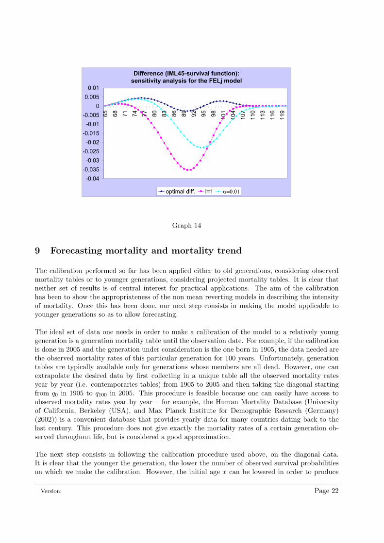
Difference (IML45-survival function):

sensitivity analysis for the FELj model

-0.04

-0.035

-0.03

-0.025

-0.02

-0.015

-0.01

-0.005

0

0.005

0.01

65

68

71

74

77

80

83

86

89

92

95

98

101

104

107

110

113

116

119

optimal diff. l=1

Graph 14

9 Forecasting mortality and mortality trend

The calibration performed so far has been applied either to old generations, considering observedmortality tables or to younger generations, considering projected mortality tables. It is clear thatneither set of results is of central interest for practical applications. The aim of the calibrationhas been to show the appropriateness of the non mean reverting models in describing the intensityof mortality. Once this has been done, our next step consists in making the model applicable toyounger generations so as to allow forecasting.

The ideal set of data one needs in order to make a calibration of the model to a relatively younggeneration is a generation mortality table until the observation date. For example, if the calibrationis done in 2005 and the generation under consideration is the one born in 1905, the data needed arethe observed mortality rates of this particular generation for 100 years. Unfortunately, generationtables are typically available only for generations whose members are all dead. However, one canextrapolate the desired data by first collecting in a unique table all the observed mortality ratesyear by year (i.e. contemporaries tables) from 1905 to 2005 and then taking the diagonal startingfrom q0 in 1905 to q100 in 2005. This procedure is feasible because one can easily have access toobserved mortality rates year by year – for example, the Human Mortality Database (Universityof California, Berkeley (USA), and Max Planck Institute for Demographic Research (Germany)(2002)) is a convenient database that provides yearly data for many countries dating back to thelast century. This procedure does not give exactly the mortality rates of a certain generation ob-served throughout life, but is considered a good approximation.

The next step consists in following the calibration procedure used above, on the diagonal data.It is clear that the younger the generation, the lower the number of observed survival probabilitieson which we make the calibration. However, the initial age x can be lowered in order to produce

Version:

a sufficiently high number of data. For instance, we have reduced the initial age x from 65 to 35and have considered sixteen different generations: persons born in every year from 1900 to 1915.We have followed the diagonal approach described above until 1998 (the last year in which data areavailable in the Human Mortality Database at the time of writing the paper, for males populationof England and Wales).

For a given generation, after having calibrated the intensity process, one can forecast the evo-lution of the survival function in the future, according to the chosen model, by considering its righttail, after the last observation. This mortality forecasting is a first simple way in which futuremortality can be extrapolated by application of this model.

A second, more difficult, way is to consider how the different parameters of the intensity pro-cess change when changing generation: in such a way one can consider the mortality trend. Wewill come back again to these two different procedures in sections 9.1.1 and 9.1.2, and give someexamples in sections 9.2.1 and 9.2.2.

Before proceeding with the calibration results, it is worth spending a few words on the effect ofchanging either the initial age or the generation.

9.1 Some considerations on the effect of changing initial age or generation

It is convenient to make a deeper analysis of the family of intensity processes we are considering.We first want to explain what happens to the value of the parameters of the process when wechange initial age inside the same generation. Then we want to see what happens when we changegeneration, holding the same initial age. The second issue usually refers to the mortality trendphenomenon. Since these two issues are completely different, we will study them separately.

9.1.1 Changing initial age, given the generation

Imagine to describe the evolution of mortality intensity for a given generation6 (in order to keepthings simple, we will not introduce any index for the generation). Observe that the intensityprocess described so far, equation (3.4) should be written more properly as:

dλx(t) = fx(λx(t))dt + gx(λx(t))dW (t) + dJx(t) (9.1)

where the dependence of the drift, the diffusion and the jump components on the initial age x is putinto evidence by the index x. For example, in the case of the OU process, if x and y are differentinitial ages, we will have:

dλx(t) = axλx(t)dt + σxdW (t)

dλy(t) = ayλy(t)dt + σydW (t).

It can be shown that if σ = 0 for any age, then we will have ax = a for any age x. However, ingeneral, the calibrated parameters are age dependent, i.e. it is ax 6= ay and σx 6= σy. The sameconsiderations apply for the other processes and the other parameters (l and µ). Therefore, whenwe change the initial age we expect to find different values for the optimal parameters. The factthat we do find different values when changing initial age (in fact, it is a35 6= a65 in all cases, for eachgeneration analyzed) is a clear confirmation of the fact that it must be σ 6= 0, and that, therefore,assuming a simple Gompertz force of mortality cannot be considered appropriate.

6By generation we mean year of birth.

Version:

9.1.2 Changing generation, given the initial age: mortality trend

Let us consider the intensity of mortality for a given initial age x and different generations. Acomplete description of the intensity surface would be given by a two parameters-family λx,gen (fora description of the intensity mortality surface via random fields with application to the pricing ofinsurance products, see Biffis and Millossovich (2005)). However, for simplicity, here we focus onlyon the change of generation and omit the initial age x. We have a family of intensity processes:

dλgen(t) = fgen(λgen(t))dt + ggen(λgen(t))dW (t) + dJgen(t) (9.2)

where the index gen refers to the year of birth7.

The change in λgen(0) and in the parameters that characterize fgen and ggen gives the descriptionof the mortality trend in our setting.

9.2 The calibration results

9.2.1 Mortality forecasting

As an illustration Graph 15 and Graph 16 report the mortality forecast for the generation 1915for the initial ages 35 and 65, respectively. Both graphs report the observed and the theoreticalsurvival function according to the FELj model.

Generation 1915, initial age 65

0

0.1

0.2

0.3

0.4

0.5

0.6

0.7

0.8

0.9

1

66

69

72

75

78

81

84

87

90

93

96

99

102

105

108

111

114

117

120

Theoretical Observed

Graph 157For example, in the case of the OU process, if we were considering the generations 1880 and 1905, we would have:

dλ1880(t) = a1880λ1880(t)dt + σ1880dW (t)

dλ1905(t) = a1905λ1905(t)dt + σ1905dW (t)

Version:

Generation 1915, initial age 35

0

0.1

0.2

0.3

0.4

0.5

0.6

0.7

0.8

0.9

1

36

41

46

51

56

61

66

71

76

81

86

91

96

101

106

111

116

Observed Theoretical

Graph 16

In both graphs, the right tail of the ”Theoretical” curve gives the forecast of the survival functionafter the observation date (t = 49 for Graph 15, t = 19 for Graph 16) implied by FELj the model.It should be noted that, although the two graphs refer to the same generation, the two right tailsare not the same. This is due to the fact that in the first graph the ”Theoretical” curve reportsthe survival function S35(t) for a person aged 35, whereas the second reports the survival functionS65(t) for a person aged 65.

9.2.2 Mortality trend

In order to investigate the mortality trend, we have made the calibration for the sixteen generationsborn in years 1900 to 1915. The initial age x has been set equal to 65. In what follows, we willadopt the notation:

λgen(t) gen = 1900, ..., 1915

omitting the initial age 65 for notational convenience. The model selected is the FELj. For eachgeneration we calculate the value of λgen(0) and we find a set of optimal parameters:

agen σgen lgen µgen

as well as the calibration error:errorgen

Table 3 reports these values:

Version:

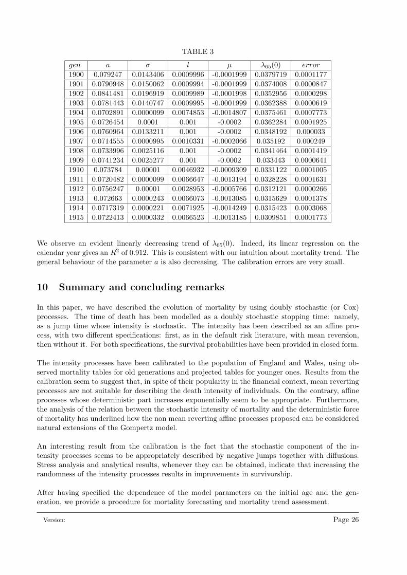
TABLE 3

gen a σ l µ λ65(0) error

1900 0.079247 0.0143406 0.0009996 -0.0001999 0.0379719 0.00011771901 0.0790948 0.0150062 0.0009994 -0.0001999 0.0374008 0.00008471902 0.0841481 0.0196919 0.0009989 -0.0001998 0.0352956 0.00002981903 0.0781443 0.0140747 0.0009995 -0.0001999 0.0362388 0.00006191904 0.0702891 0.0000099 0.0074853 -0.0014807 0.0375461 0.00077731905 0.0726454 0.0001 0.001 -0.0002 0.0362284 0.00019251906 0.0760964 0.0133211 0.001 -0.0002 0.0348192 0.0000331907 0.0714555 0.0000995 0.0010331 -0.0002066 0.035192 0.0002491908 0.0733996 0.0025116 0.001 -0.0002 0.0341464 0.00014191909 0.0741234 0.0025277 0.001 -0.0002 0.033443 0.00006411910 0.073784 0.00001 0.0046932 -0.0009309 0.0331122 0.00010051911 0.0720482 0.0000099 0.0066647 -0.0013194 0.0328228 0.00016311912 0.0756247 0.00001 0.0028953 -0.0005766 0.0312121 0.00002661913 0.072663 0.0000243 0.0066073 -0.0013085 0.0315629 0.00013781914 0.0717319 0.0000221 0.0071925 -0.0014249 0.0315423 0.00030681915 0.0722413 0.0000332 0.0066523 -0.0013185 0.0309851 0.0001773

We observe an evident linearly decreasing trend of λ65(0). Indeed, its linear regression on thecalendar year gives an R2 of 0.912. This is consistent with our intuition about mortality trend. Thegeneral behaviour of the parameter a is also decreasing. The calibration errors are very small.

10 Summary and concluding remarks

In this paper, we have described the evolution of mortality by using doubly stochastic (or Cox)processes. The time of death has been modelled as a doubly stochastic stopping time: namely,as a jump time whose intensity is stochastic. The intensity has been described as an affine pro-cess, with two different specifications: first, as in the default risk literature, with mean reversion,then without it. For both specifications, the survival probabilities have been provided in closed form.

The intensity processes have been calibrated to the population of England and Wales, using ob-served mortality tables for old generations and projected tables for younger ones. Results from thecalibration seem to suggest that, in spite of their popularity in the financial context, mean revertingprocesses are not suitable for describing the death intensity of individuals. On the contrary, affineprocesses whose deterministic part increases exponentially seem to be appropriate. Furthermore,the analysis of the relation between the stochastic intensity of mortality and the deterministic forceof mortality has underlined how the non mean reverting affine processes proposed can be considerednatural extensions of the Gompertz model.

An interesting result from the calibration is the fact that the stochastic component of the in-tensity processes seems to be appropriately described by negative jumps together with diffusions.Stress analysis and analytical results, whenever they can be obtained, indicate that increasing therandomness of the intensity processes results in improvements in survivorship.

After having specified the dependence of the model parameters on the initial age and the gen-eration, we provide a procedure for mortality forecasting and mortality trend assessment.

Version:

In particular, as far as mortality forecast is concerned, we have considered the generation 1915and have calibrated the parameters of the FELj process with the available data at observation date.We have given a forecast for heads aged 35 and 65. Comparisons of similar forecasts with actualexperienced mortality for older generations is in the agenda for future research.

As far as the mortality trend is concerned, we have calibrated the FELj model for the genera-tions 1900-1915, initial age 65. The mortality trend is investigated through the behaviour of theoptimal parameters. A comparison between the expected behaviour of the intensity for differentgenerations is in the agenda for future research.

References

Arnold, L. (1974). Stochastic Differentials Equations: Theory and Applications, John Wiley andSons.

Artzner, P. and Delbaen, F. (1992). Credit risk and prepayment option, ASTIN Bulletin 22: 81–96.

Biffis, E. (2004). Affine processes for dynamic mortality and actuarial valuations, IMQ, Bocconiuniversity, working paper.

Biffis, E. and Millossovich, P. (2005). A bidimensional approach to life portfolio valuation and tothe insurer’s future business, working paper.

Blake, D., Cairns, A. J. G. and Dowd, K. (2004). Pricing death: Framework for the valuation andsecuritization of mortality risk, Preprint.

Bowers, N. L., Gerber, H. U., Hickman, Jones, J. C. and Nesbitt, C. J. (1986). Actuarial Mathe-matics, The Society of Actuaries, Itasca.

Bremaud, P. (1981). Point Processes and Queues – Martingale Dynamics, Springer Verlag, NewYork.

Brouhns, N., Denuit, M. and Vermunt, J. K. (2002). A poisson log-bilinear approach to the con-struction of projected lifetables, Insurance: Mathematics and Economics 31: 373–393.

Cox, J. C., Ingersoll, J. E. and Ross, S. A. (1985). A theory of the term structure of interest rates,Econometrica 53: 385–407.

Dahl, M. (2004). Stochastic mortality in life insurance: market reserves and mortality-linked insur-ance contracts, Insurance: Mathematics and Economics 35: 113–136.

Duffie, D. (2001). Dynamic Asset Pricing Theory, Third Edition, Princeton University Press.

Duffie, D. (2002). A short course on credit risk modeling with affine processes, Associazione Amicidella Scuola Normale Superiore.

Duffie, D. and Singleton, K. J. (1994). Econometric modelling of term structure of defaultablebonds, Graduate School of Business, Stanford University.

Duffie, D. and Singleton, K. J. (2003). Credit risk, Princeton University Press.

Duffie, D., Filipovic, D. and Schachermayer, W. (2003). Affine processes and applications in finance,Annals of Applied Probability 13: 984–1053.

Version:

Duffie, D., Pan, J. and Singleton, K. (2000). Transform analysis and asset pricing for affine jump-diffusions, Econometrica 68: 1343–1376.

Feller, W. (1951). Two singular diffusion problems, The Annals of Mathematics 54: 173–182.

Gerber, H. U. (1997). Life Insurance Mathematics, Springer Verlag, Berlin.

Grandell, J. (1976). Doubly Stochastic Poisson Processes, Lecture Notes in Mathematics, Number529, New York: Springer Verlag.

Institute and Faculty of Actuaries (1990). Standard Tables of Mortality: the ”92” Series, TheInstitute of Actuaries and the Faculty of Actuaries.

Lando, D. (1994). Three essays on contingent claims pricing, PhD Thesis, Cornell University.

Lee, R. D. (2000). The Lee-Carter method for forecasting mortality, its various extensions andapplications, North American Actuarial Journal 4: 80–93.

Lee, R. D. and Carter, L. R. (1992). Modelling and forecasting U.S. mortality, Journal of theAmerican Statistical Association 87: 659–675.

Milevsky, M. and Promislow, S. D. (2001). Mortality derivatives and the option to annuitise,Insurance: Mathematics and Economics 29: 299–318.

Pitacco, E. (2004a). Longevity risk in living benefits, in E. Fornero and E. Luciano (eds), Developingan Annuity Market in Europe, Edward Elgar, Cheltenham, pp. 132–167.

Pitacco, E. (2004b). Survival models in a dynamic context: a survey, Insurance: Mathematics andEconomics 35: 279–298.

Renshaw, A. E. and Haberman, S. (2003). On the forecasting of mortality reductions factors,Insurance: Mathematics and Economics 32: 379–401.

Schrager, D. (2004). Affine stochastic mortality, wp, University of Amsterdam.

University of California, Berkeley (USA), and Max Planck Institute for Demographic Re-search (Germany) (2002). Human Mortality Database, Available at www.mortality.org orwww.humanmortality.de.

Vasicek, O. (1977). An equilibrium characterization of the term structure, Journal of FinancialEconomics 5: 177–188.

Version:

Non mean reverting affne processes for stochastic mortality

Documents

Transcript of Non mean reverting affne processes for stochastic mortality