arX

iv:a

stro

-ph/

9911

524v

1 3

0 N

ov 1

999

The Low End of the Initial Mass Function

in Young LMC Clusters: I. The Case of R1361

Marco Sirianni2,3, Antonella Nota3,4, Claus Leitherer3, Guido De Marchi5,

and Mark Clampin3

To appear in The Astrophysical Journal

1Based on observations with the NASA/ESA Hubble Space Telescope, obtained at the

Space Telescope Science Institute, which is operated by AURA for NASA under contract

NAS5-26555, and observations obtained at the European Southern Observatory, La Silla.

2The Johns Hopkins University: sirianni@pha.jhu.edu

3Space Telescope Science Institute, 3700 San Martin Drive, Baltimore, MD 21218;

nota@stsci.edu, leitherer@stsci.edu, clampin@stsci.edu.

4Affiliated with the Astrophysics Division, Space Science Department of the European

Space Agency.

5European Southern Observatory: gdmarchi@eso.org

– 2 –

Received ; accepted November 28,1999

– 3 –

ABSTRACT

We report the result of a study in which we have used very deep broadband

V and I WFPC2 images of the R136 cluster in the Large Magellanic Cloud

from the HST archive, to sample the luminosity function below the detection

limit of 2.8 M⊙ previously reached. In these new deeper images, we detect

stars down to a limiting magnitude of mF555W = 24.7 (≃ 1 magnitude deeper

than previous works), and identify a population of red stars evenly distributed

in the surrounding of the R136 cluster. A comparison of our color-magnitude

diagram with recentely computed evolutionary tracks indicates that these red

objects are pre-main sequence stars in the mass range 0.6 - 3 M⊙. We construct

the initial mass function (IMF) in the 1.35 - 6.5 M⊙ range and find that, after

correcting for incompleteness, the IMF shows a definite flattening below ≃ 2

M⊙. We discuss the implications of this result for the R136 cluster and for our

understanding of starburst galaxies formation and evolution in general.

Subject headings: Magellanic Clouds – stars: evolution – stars: mass function

– 4 –

1. Introduction

The quest for a universal IMF has been a long standing issue in stellar astrophysics

(Scalo 1998). With the advent of the HST and the improved sophistication of ground based

instrumentation, it has been possible to extend to nearby galaxies studies that were in the

past feasible only in our own Milky Way, and at the same time reach the new domain of

the faintest and least massive stars, even before they approach the main sequence. The

studies of the IMF have expanded in scope but also triggered new questions and added new

uncertainties.

For the field IMF, the uncertainties on distance and star formation can be so huge

(Scalo 1998), that it would be difficult to establish local variations. However, there is

general agreement that a slightly steeper slope than Salpeter’s (Γ = -1.5 – -1.8 vs γ = -1.35

in the mass range 1 – 10 M⊙) is generally found. In the case of the IMF for star clusters and

associations, the distance effects are removed and the star formation history is simpler. For

star clusters, at high masses (10 – 100 M⊙) there is good agreement that the Salpeter IMF

is ubiquitous. At small and intermediate masses (1 - 10 M⊙) the situation is very different.

Even in the LMC itself, deep photometry of clusters has produced wildly discrepant results,

ranging from the very steep IMFs found by Mateo (1988)(Γ = -2.52), to the much shallower

slopes (Γ ≃ 0 - -1) derived by Elson et al. (1989) and Hunter et al. (1995, 1996).

30 Doradus in the LMC is the closest extragalactic HII region (Kennicutt 1991).

It ideally offers a true laboratory for stellar population studies because of its rich star

formation history, and well determined distance. It is the local counterpart to distant

starburst galaxies and it has been repeatedly defined as their Rosetta Stone. However, the

emerging star formation picture is a diverse assembly of results which do not allow a fruitful

comparison, let alone an extrapolation to more distant galaxies. The situation becomes

even more complicated when one considers independent studies of the same region: for

– 5 –

example, Oey and Massey (1995) derived Γ = -1.3 ± 0.2 for the massive stars in the LMC

superbubble LH47, while an independent study by Will et al. (1997) quotes a resulting

slope Γ = -2.1 in the same range of masses, using the same evolutionary models. However,

they then assumed a slope Γ = -1.3 for the cluster over the entire mass range investigated.

At the smallest masses, the discrepancies are even larger: are we observing true deviations

from the Salpeter IMF, most likely triggered by local conditions of stellar density or star

formation history? Or are we simply dominated by the observational uncertainties, related

to the data analysis and interpretation, such as the choice of the evolutionary models or

treatment of completeness?

For all these reasons, we have started a systematic study of a number of young clusters

in the LMC and in the SMC, at different conditions of stellar density, age and metallicity,

with the objective of studying the low end of the stellar IMF and to understand whether at

small masses the IMF is constrained by local conditions. The advantage of such a study is

to reduce the uncertainties associated with data reduction by establishing a homogeneous

data treatment procedure including a unique choice of models. This procedure will be

applied to all the clusters in the study, starting from the best known example, R136, which

we present in this paper. For this cluster, a number of images exists in the HST archive

which could be combined to produce deep images of the cluster, enabling us to reach the

low mass limit of 0.6 M⊙.

2. Observations and data reduction

Multiple images of the R136 cluster were obtained with the WFPC2 on board the HST

in several bandpasses after the first refurbishment mission, as part of the Early Release

Observations and of the WFPC2/GTO program. In particular, two sets of images were

taken in January 1994 and September 1994 as part of proposals 5589 and 5114, which

– 6 –

contained repeated exposures in the filters F555W and F814W. These filters are described

in detail by Biretta (1996) and closely resemble the Johnson V, I filters in their photometric

properties. A journal of all observations eventually combined is provided in Table 1. All

images were taken with a gain of 7 e− ADU−1. In both data sets, the R136 cluster was

centered in the Planetary Camera (PC), which has a field of view of 35′′ × 35′′, with an

effective plate scale of 0′′. 045 pixel−1. The other three WF chips observed flanking fields in

30 Doradus, with the same filter configuration, but a larger field of view of 75′′×75′′ per

chip and a plate scale of 0′′. 1 pixel−1.

The two datasets were processed independently using the standard STScI pipeline

procedure, which adopts standard calibration observations and reference data, such as bias,

flat field, and dark frames constantly updated by the WFPC2 team to track any changes in

the performance of the camera and its detectors. The basic steps of the calibration are the

correction for the errors introduced by the analog to digital conversion, bias level and bias

pixel-to-pixel variations removal, dark image subtraction, flat field image application and

shutter shading corrections.

The images taken in January and September, however, were characterized by different

temperatures of the CCDs, and, therefore, different charge transfer characteristics. In fact,

in March 1994 a significant charge transfer efficiency (CTE) variation had been found in

WFPC2, which caused a 10-15 % gradient in the photometric response of the CCDs along

the columns of each chip. This effect is due to the partial loss of signal when charge is

transferred down the chip during the readout, with the consequence that stars at higher

row numbers appear fainter than they would if they were at low row numbers (Holtzman

et al. 1995a). A significant reduction to the CTE effect was achieved by cooling down the

four CCDs from -76 to -88 oC. The new temperature became operational on April 23 1994,

and the CTE stabilised at a ∼ 4 % level. In order to account for the difference in CTE

– 7 –

between the two data sets, different corrections were performed: a 12% correction ramp was

applied to the -76oC data (January 1994), and a 4% correction was applied to the -88o C

data (September 1994) in order to bring the charge packets of each pixel to the values they

would have had in the absence of the CTE problem.

The images were then registered and combined to remove cosmic rays. A rotation

of 99.85o was applied to the final image from the first set, which was also shifted in the

horizontal and vertical direction by an amount (+74.07, +134.73). The combined images,

670 × 590 pixel in size, have an overall exposure time of 1240 sec and 760 sec in the

filters F555W and F814W respectively. It should be pointed out that due to the presence

of detector read noise, the total combined exposure time is not fully equivalent to the

same time in a single image, and will eventually yield a slightly lower S/N. The combined

Planetary Camera image for the filter F555W is shown in Figure 1, with the R136 cluster

in the center.

3. The photometry

Photometry has been performed on both images, using the PSF fitting routines

provided within DAOPHOT. The first step in the photometric reduction procedure was to

discriminate between true stars and spurios objects which might have been introduced by

both the alignment procedure and the hot pixels removal. This was done by studying in

detail the characteristics of the stellar PSF. We carefully selected by eye a sample of 150

bona fide stars in the final F555W image. A statistical study of this sample allowed us to

define an appropriate range for the parameters that DAOFIND uses as selection criteria.

Two parameters are particularly important: the roundness, which allows us to eliminate

objects which are too elongated along rows or columns, and the sharpness, which eliminates

objects whose profile differs largely from a gaussian profile. From our sample of 150 stars

– 8 –

we found mean values of 0.78 ± 0.1 and 0.045 ± 0.165 for the sharpness and roundness,

respectively.

We then ran DAOFIND on out data, by conservatively setting the detection threshold

at 4 σ above the local background level, but excluded any object with sharpness and

roundness parameters exceeding by more than ±3 σ the average bona fide values (Figure 2).

We inspected the rejected objects and found that almost all of them were noise peaks

associated with hot columns, diffraction spikes or highly saturated stars, with a small

number being isolated hot pixels and extended objects. Due to the extreme saturation of

the central regions, the innermost 2′′ of the cluster core were excluded from our study.

The list of stars detected in the F555W combined image was then used to identify

the stars in the F814W image: 1706 stars were found to be common to both frames. In

order to carry out the photometry with the highest accuracy possible, we first performed

aperture photometry and measured the stellar flux in a very small aperture (2 pixel radius),

selected to match the FWHM of the PSF (≃ 2 pixel). We measured the background as the

mode of the annulus centered on each star with a inner radius of 3 and an outer radius of

7 pixels. We then constructed a sample PSF by combining three moderately bright and

isolated stars, located as close as possible to the unsaturated central region of the frame.

In order to properly subtract the background it was necessary to carefully evaluate the

aperture correction, accounting for the fraction of source light present in the background

annulus. Such a correction is derived by assessing how the PSF encircled energy varies as

a function of the distance from the peak. For each image we have measured the encircled

energy profile for a number of isolated stars and have used these measurements to correct

the fluxes derived with aperture photometry.

The procedure of rotation and shift of the two dataset just marginally modified the final

PSF FWHM from the original values of 1.51 pixel and 1.32 pixel the for the two separate

– 9 –

datasets to 1.76 pixel in the final F555W combined frame. Although this procedure resulted

in a slight degradation of the spatial resolution, photometry tests clearly demonstrate this

to be much preferable to the alternative of performing photometry on the individual images.

The magnitudes of the individual stars were then determined relative to an aperture

of radius 0′′. 5, and transformations were made to translate the on-orbit system to the

WFPC2 photometric system using the calibration provided by Holtzman et al. (1995b).

The zeropoints used were 22.48 mag for the F555W filter and 21.60 mag for the F814W

band. The original zeropoints were provided for a gain of 14 e− ADU−1 to which we have

added the correction for the different gain adopted in these observations (7 e− ADU−1)

(Holtzman et al. 1995b).

In Figure 3 we report the photometric errors assigned by DAOPHOT to all our

measurements: for our study, we discarded all stars with an associated error larger than

0.2 magnitudes in both filters. With this limitation, we find 1604 stars common to both

filters, down to a limiting magnitude mF555W = 24.7, which is ∼1 magnitude deeper than

the individual frames published by Hunter et al. (1995, 1996). Altough we do not include

the full photometry in this paper, the complete table is available in electronic form upon

request.

4. The Color-Magnitude diagram

We generated an observed color-magnitude diagram (CMD) where mF555W is plotted

as a function of the (mF555W - mF814W) color (Figure 4), which includes all the stars

measured in the combined F555W and F814W frames with photometric errors smaller

than 0.2 magnitudes. The CMD immediately reveals the presence of two distinct branches,

segregated in color at (mF555W - mF814W) ≃ 1.1.

– 10 –

This color segregation is very similar to the effect observed in the CMD of NGC 3603,

the galactic clone of R136 (Drissen, 1999). The most likely origin of this effect could be

the presence of differential reddening within the cluster, or to the real presence of a second

population of faint redder stars.

4.1. Differential reddening in R136?

The distribution of gas and dust in the region surrounding R136 is highly

inhomogeneous, as can easily be seen in images of the region taken in the light of Hα, [OIII]

and [SII] (Scowen et al. 1998). Ideally, the most accurate strategy would be to redetermine

the reddening coefficients for each individual star, and indeed Hunter et al. (1995, 1996)

had attempted to do so in their recent papers. Unfortunately, the uncertainties associated

with their data, as well as the red leak present in the UV filter they adopted, made this

task unsuccessful, and they opted instead for the use of ground based measureaments by

Fitzpatrick & Savage (1984). They eventually attributed the spread in color they observed

in their CMD to the use of a single coefficient.

Adopting the same reddening law of Hunter et al. (1995), originally derived by

Fitzpatrick & Savage (1984), we have: E(B-V) = 0.38 and Rv = 3.4. Converted to our

filters, this yields AF555W = 1.37, and AF814W = 0.80. In Figure 4 we have superimposed

such reddening vector on the observed CMD.

There is consensus that differential reddening exists in the R136 region. However, if

differential reddening were the cause for the bimodal distribution observed in our CMD,

the total amount of absorption needed would be very high. We should in fact assume

an extreme value of E(B-V) = 0.51, and Rv = 6.08, to match the two observed features.

This value, which is reported in Figure 4 for comparison, is more than three times higher

than the observed values, and totally inconsistent with the ground based measurements.

– 11 –

We are therefore confident to exclude the possibility of such a high differential extinction

and conclude that the observed split in the CMD is most likely intrinsic, and due to the

presence of a second population of fainter, redder stars.

4.2. The red population: evidence for pre-main sequence stars?

The position of the red stars in the CMD is consistent with a population of pre-main

sequence (PMS) stars, as already suspected by Hunter et al. (1995). In order to establish

whether this scenario is correct, we needed to construct isochrones to assign masses to the

stars and determine ages for the stellar population. We used isochrones constructed from

the stellar evolution models provided by Siess et al. (1997) for PMS evolution. Siess’s

tracks offer the choice of different metallicities: Z = 0.02, 0.04, 0.005. We adopted Z =

0.005 for this study, which closely matches the LMC values of Z = 0.008.

The stellar models are provided in the [log(L/L⊙) vs log(Teff)] plane. In order to

convert the information to the WFPC2 [(mF555W)o vs(mF555W)o - (mF814W)o] system, we

used the model atmospheres of Kurucz (1993) interpolated at metallicity Z = 0.005 and g

= 4.0 and the standard STSDAS SYNPHOT software package to reproduce the WFPC2

photometric response. For each isochrone, we assigned to each point in the plane (Teff ,

log g) the corresponding Kurucz’s atmospheric model and evaluated the intrinsic color

(mF555W - mF814W)o of such a point using SYNPHOT. We then converted log(L/L⊙) into

the (mF555W)o magnitude adopting a distance modulus of 18.6 (Walborn et al. 1997), and

the Bolometric Correction (BC) provided by Bessel et al. (1998) for the same conditions of

gravity.

In Figure 5 we show the dereddened CMD of the R136 cluster, where (mF555W)o is

plotted as a function of (mF555W - mF814W)o. We have superimposed to the CMD the

– 12 –

isochrones corresponding to the PMS evolutionary tracks in the range 5 ×105− 5 × 107 yr.

As expected, the observed red population is very well tracked by these PMS isochrones,

and most likely consists of low mass stars (down to 0.6 M⊙) still approaching the main

sequence. Their age is found to be in the range between 1 and 10 Myr. In Figure 5 we also

show, for comparison, the position of a star of 1.35, 1.5 and 2 M⊙ on the various isochrones.

4.3. The age of the R136 cluster and the pre-main sequence stars

There is consensus in the published work that the mean age of the R136 cluster is less

than 5× 106 yr. Already at the time when the nature of the central object in R136 was still

unclear, Savage et al. (1983) and Schmidt-Kaler & Feitzinger (1982) had proposed an age

of 2 × 106 yr for the supermassive central object. With the discovery of WR features in the

integrated spectrum of the central region, the age determination increased (Melnick 1985).

Later on, Campbell et al. (1992) took high resolution HST/WFPC images of the cluster

core, and argued that the presence of WR stars in the central region suggested an age of at

least 3.5 × 106 yr. Almost at the same time, De Marchi et al. (1993) used the WR stars

to place both a lower and upper limit to the age; in fact, while the simple presence of WR

stars argues in favour of an age higher than 2 × 106 yr, the fact that the WR stars are

of the WNL type, a hydrogen rich subclass which is usually associated with very massive

progenitors (> 50 M⊙), sets a firm upper limit of 5 × 106 yr. Such an evidence, combined

with the lack of red supergiants found by Campbell et al. (1992), led De Marchi et al.

(1993) to conclude in favour of an age determination of 3 × 106 yr for the R136 cluster.

The most recent work by de Koter et al. (1998) suggests that the WR stars in R136 are

younger than classical WNL stars. If so, R136 has an age of at most 2 Myr, and may even

be somewhat younger.

In the cluster, star formation is almost coeval: the R136 cluster core extends over a

– 13 –

linear scale < 10 pc. Consider the typical time scale associated with the star formation

process (t = d/v, where v is the propagation speed of the shock wave triggering star

formation). Typical oberserved values of v are of order 50 km s−1 (e.g., Satyapal et al.

1997), so that the possible age spread is less than 0.5Myr. This is small compared to the

evolutionary timescale of the stars formed (De Marchi et al. 1993). Outside the R136

cluster, star formation is most likely still continuing (Walborn 1984), especially in the outer

filaments of the 30 Doradus region.

If we assume coeval star formation and an age for the cluster of ≃ 2 − 4 × 106 yr, we

find that all stars down to 1M⊙ have already reached their birthline, defined as the locus

in the HR diagram along which young stars first appear as visible objects (Stahler 1983).

In fact, stars of 1 − 2M⊙ reach their birthline in less than 0.5Myr.

As already mentioned, we find that the population of young stars in the R136 CMD

is well fitted by isochrones of 106 – 5 × 107 yr, indicating that we are observing the stars

while they are approaching the ZAMS. Typically it takes ≃ 5 × 107 yr for a star of 1.5 M⊙

to reach the ZAMS (Siess et al. 1997). This interval is shorter for stars of higher mass. A

star of 2 M⊙ will take ≃ 3 × 107 yr, and a star of 3 M⊙ about ≃ 1 × 107 yr. It is safe to

conclude that the red extension of the R136 CMD is made of PMS objects in the 1-3 M⊙

range, observed in their approach to the ZAMS.

Did all these stars form at the same epoch of the R136 cluster? As already pointed out

by Hunter et al. (1995), stars down to 3 M⊙ appear to have formed approximately at the

same time of the more massive stars. However, the least massive stars (1 – 2 M⊙) could

possibly be a few Myr older, but the uncertainties associated with both the theoretical

isochrones and the observational data are such that, at this point, no precise answer can be

provided.

– 14 –

5. The H-R diagram

In an attempt to determine the IMF of R136, we need to locate the stars onto the

H-R diagram (HRD). We do so by converting the photometric information (magnitude and

color) into the (Log Teff vs Log L/L⊙) plane.

To this purpose, we have used the relation (V - I) vs Teff , for g = 4.0, from Bessel et

al. (1998). This relation is suitable for PMS stars as well as normal stars (see Sung et al.

1998). From the same source, we also assume BC as a function of Teff . In order to use these

relations, we have converted mF555W and mF814W into V and I using the equations provided

by Holtzmann et al. (1995b).

We then adopted a distance modulus of (m − M)o = 18.6 (Walborn et al. 1997) to

translate the apparent magnitudes into absolute luminosity, as follows:

Log(L/L⊙) = 0.4 × (4.75 − MV − BC)

where MV = MF555W - C, being C a correction factor derived for each star from the

Holtzmann et al. (1995b). Figure 6 shows the theoretical HRD with the superimposed

evolutionary tracks for the mass range 0.6 – 7 M⊙ from Siess et al. (1997).

The HRD further illustrates the composition of the intermediate-low mass stellar population

in R136 and surroundings: stars with mass above 4 M⊙ are already on the main sequence

or in close proximity. Stars at lower masses (0.6 – 3.0 M⊙) display a higher concentration in

proximity to their birth line (at the redward origin of their evolutionary tracks in Figure 6)

and have not reached the ZAMS yet. It is interesting to notice that while stars above 3 M⊙

evolve at almost constant luminosity to the ZAMS, at smaller masses stars do experience

quite significant variations in effective temperature and luminosity, thus creating a quite

large observed spread in both quantities. The gap observed at approximately Teff ≃ 3.8

– 3.9 between the two populations reflects an evolutionary effect. The evolution from the

– 15 –

birth line is faster for high mass stars: stars of 4 – 7 M⊙ will transition in that Teff region

much faster that the smallest stars, and therefore they will be observed in smaller numbers,

thus creating the observed opening. At the smallest masses (1 – 1.5 M⊙), the gap is less

noticeable.

5.1. The completeness and the photometric errors

Before proceeding to the derivation of the IMF it is also necessary to establish the

completeness of our data. With this objective in mind, we have defined four regions (A,

B, C, D; see Figure 7) surrounding the R136 cluster in the final combined F555W image.

As can be noticed in Figure 7, these four regions have different characteristics in terms of

gas/dust contamination and crowding. Region A is the most crowded, and includes many

very bright stars, while region C displays some obscurations due to dust and gas. Regions

B and D are intermediate in their properties. For each region, and for each filter, the

completeness has been assessed with the following procedure:

• The sample of stars falling within the region has been divided into fifteen half

magnitude bins;

• Artificial stars have been added to each magnitude bin, in quantity not to exceed

10% of the total number, in order not to affect severely the crowding in the region

considered. Numerous tests have been run with the same recipe (100 per bin);

• The artificial stars have been retrieved, using the same selection criteria of sharpness

and roundness adopted in our work. Stars with photometric error larger than 0.2

magnitudes have been discarded.

– 16 –

The results of the test are summarized in Table 2, where for each region (A – D) and

filter, we have reported the completess factor as a percentage of the stars successfully

retrieved vs the total number of stars artificially added. As can be noticed in Table 2, the

completeness is worse in the brightest magnitude bin, where saturation effects prevents the

detection of other very bright objects, and towards the faint end, where S/N effects start

to dominate. In region A, which is characterized by many bright stars, the completeness

drops significantly much earlier than for the other regions. For regions B, C, and D the

agreeement is quite good and the completeness is quite robust (better than 50 %) down to

mF555W = 23.2, mF814W = 22.1. We have used an average of regions B, C, and D to derive

completeness correction factors for our photometry. We have used the completeness factors

determined in this way to draw completeness lines onto the HRD to underline the variation

of the correction factors with luminosity (Figure 8). As it can be seen in the figure, the

completeness is very robust down to Log (L/L⊙) ≃ 0.5. In order to understand how this

result impacts the definition of a conservative lower mass limit to our measurements, we

have constructed in Figure 9, for each of the four regions considered - A,B,C, and D - a

completeness histogram as a function of the corresponding mass. As already discussed,

regions B, C, and D are in quite good agreement, while region A displays the largest

deviation. We have therefore assumed that regions B, C, D are homogeneus in their

properties, and we show in Figure 9 their average completeness (solid line). For the average

of regions B, C and D we find that the completeness correction drops below 50% at ∼ 1.35

M⊙. This will be the conservative lowest mass limit to our measurements.

Having established the completeness of our photometry, it was necessary to estimate

how our photometric errors affect the location of the stars in the HRD and, therefore, the

determination of their mass. To this purpose, we have considered four different regions in

the CMD, which are representative of different luminosities and temperatures, and sample

– 17 –

the range of values present in our CMD. For each region, we have averaged magnitude and

colors for ten stars, in order to derive a single representative point, with a mean magnitude

and color. For this representative point, we also derived a mean error, in magnitude and

color, as an indication of the uncertainties associated with stars in that region of the CMD.

We then transformed these four representative points, and their associated errors, into the

HRD (Figure 10), and found that these typical errors on the photometry translate into a

small error in luminosity and into a larger error in Teff . However, since all evolutionary

tracks down to 3 M⊙ develop at almost constant Teff , we are confident that such an error

in the temperature does not lead to a significant uncertainty in the mass determination, at

least for masses higher than 3 M⊙. For masses below 3 M⊙, a translated error of 0.2 in Log

Teff can affect the mass determination by shifting the star to the adjacent mass bin. This

effect increases towards smaller masses, where we should assume an worse case uncertainty

on the mass determination of ± 0.3 M⊙.

6. The Initial Mass Function

6.1. The Initial Mass Function of the R136 cluster

The IMF, usually indicated by ξ, is defined as the number of stars per logarithmic mass

interval per unit area. The slope of the IMF is given by Γ = d(logξ)/d(logM) where the

standard IMF (Salpeter 1955) has a slope Γ = −1.35. Although we use the term IMF, we

are actually discussing the present day mass function (MF). In the case of the very young

R136, where star formation has been coeval, we can safely assume that the observed MF is

the IMF.

The MF of stellar clusters is usually measured by counting the number of stars as a

function of the magnitude (luminosity function) which is then converted into the number

– 18 –

of stars per unit stellar mass by the use of the appropriate mass-luminosity relation. This

approach, however, can only be applied to stars currently on their main sequence, i.e. to

objects for which a precise correspondence exists between mass and luminosity. As Figure 4

shows, however, R136 hosts a large population of PMS objects, for which such a relation

depends strongly on the age and is, therefore, very difficult to apply.

An alternative avenue to follow, which has the advantage of overcoming this age

degeneracy, is that presented by Tarrab (1982) and based on the use of the HRD and

theoretical isomass tracks in place of the CMD. In order to derive the MF of R136, we have

counted the number of stars falling between each pair of tracks shown in the HR diagram

(Figure 6) and normalized such number to the width of the mass range spanned by the

tracks and to the area of the observed field. As already mentioned, we have adopted the

evolutionary tracks by Siess et al.(1997), which also include PMS stars down to 0.6 M⊙.

The number of stars in each mass bin is shown in Table 3 (column 3), together with the

width of the bin (column 2). To properly account for the effects of crowding, we have

corrected the numbers measured in this way for the incompleteness of our photometry,

using the completeness factors described above (see Table 2). The values corrected in this

way are also listed in Table 3 (column 4).

The determination of the MF has been carried out independently in the four regions

A, B, C, and D. Since these regions are so differently affected by crowding and dust/gas

contamination, and are associated with different completeness corrections, the comparison

of their MFs provides an independent assessment of the solidity of our results. Also, we

have have limited our MF measurements to the magnitude range where the completeness is

robust, that is better than 50%. For the average of regions B, C and D the completeness

correction drops below 50% at ∼ 1.35 M⊙ (see Figure 9). This is the conservative lower

mass limit we have assumed for our MF determination.

– 19 –

We find that, within the limitations imposed by small numbers statistics, there is good

agreement among the four MFs derived in this way. Following a conservative approach,

we have then proceeded to discard the most extreme region (A) (see Figure 9) and have

retained only B, C and D for the construction of the final MF, which is shown in Figure 11,

where the errors on the data points account for both the Poisson statistics of the counting

process and for the uncertainty on the completeness.

Two different trends are distinguishable in the IMF profile of Figure 11: for stars in

the mass range 2.1 − 6.5M⊙ the data points are well fit by a slope with Γ = -1.28 ± 0.05,

while at lower masses the IMF profile flattens out, with a derived slope Γ = -0.27 ± 0.08

(1.35 – 2.1 M⊙). For comparison, the Salpeter slope is provided on the edge of the figure.

6.2. The Mass Function of the surrounding areas of R136

For comparison, we obtained the MF of three flanking fields, which were observed by

the three WF chips while the R136 cluster was centered in the field of view of the Planetary

Camera. These WF fields covered each a region of ≃ 75′′ × 75′′, and together a total area

of ≃ 4.7 arcmin2. At a distance for the LMC of 52.5 Kpc (Walborn et al. 1997), this

corresponds to an area of 1092 pc2. For reference, we provide the central location of all

WF chips in Table 4. Since the January and September datasets were taken with different

orientations, it was not possible to add the two datasets and reach the same depth as in

the combined PC images. Only the September dataset was considered for this work: we

reached a magnitude limit in the summed F555W frame of mF555W = 24 with a combined

exposure time of 840 s. A total of 2836 stars were found in both filters, selected with

the same conservative criterion described above to discard any object with an associated

photometric error larger than 0.2 magnitudes in both filters.

– 20 –

A CMD was constructed in similar fashion to what was done for the R136 cluster,

and is shown in Figure 12. The most relevant difference from the R136 cluster CMD is a

better defined main sequence and the total absence of the second population of red stars.

Although the depth of the flanking field images differs from that of the R136 cluster, we

can exclude the presence of a second redder population, segregated in color. This can be

seen from the insert of Figure 12, which shows the histogram of the number of objects in

function of the color (mF555W - mF814W) for the R136 cluster (solid line) and the flanking

fields (dashed line). The two distributions appear completely different.

The MF was derived following the same procedure described for R136, and the final

result is shown in Figure 13. In this case, the filled circles represent our observational data,

which are also listed in Table 5 together with the completeness correction factors derived

adopting the same procedure. Again, we have used all data points with a photometric

completion better than 50%. The MF slope derived in this way is slightly shallower than

that of Salpeter, with Γ = −1.23 ± 0.11.

Can we directly compare the derived MF to the R136 IMF? Naturally, when considering

field stars, the additional uncertainty on the distance of the stars considered, and their age,

has to be accounted for. Therefore, a direct quantitative comparison cannot be made.

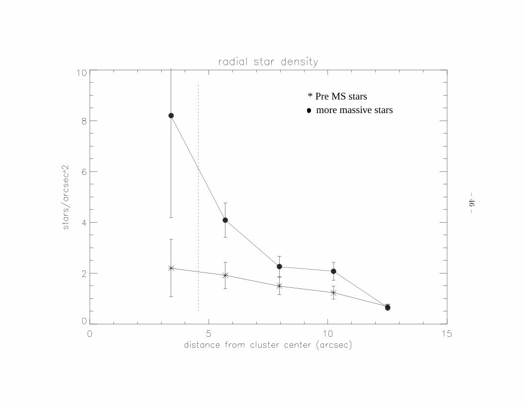
6.3. The spatial distribution of the pre-main sequence stars

A first visual inspection of the images indicates that PMS objects are quite uniformly

distributed within the field of the Planetary Camera. In order to define more accurately

their distribution, we divided the entire field into concentric annuli centered on R136a up

to a distance of 13′′ from the center of the cluster. As already mentioned, we discarded the

inner 2′′ radius region, since the cluster core is highly saturated. We defined each annulus

– 21 –

to be 50 pixels wide, corresponding to 2′′. 25.

We then compared the spatial distribution, averaged within each annulus, of the PMS

stars (mF555W - mF814W > 1.1, M < 3 M⊙) and of the more massive stars (mF555W - mF814W

< 1.1, M > 3 M⊙). The two distributions are illustrated in Figure 14, where the number

of stars per surface area is provided as a function of distance from the cluster center. The

solid line with the star symbols indicates the PMS stars and the solid lines with the filled

circles the more massive ones.

Both distributions have been corrected for incompleteness. To this purpose, we have

performed a second test to establish the completeness level within each annulus, following

the same procedure previously described. The results of this test are listed in Table 6, in

terms of completeness correction factors for the various annuli. Due to the high number of

saturated stars in the central region, we find that the first two annuli (up to 4.5′′ from the

center) are severely affected by incompleteness, and therefore no conclusions can be drawn

in the inner cluster regions.

At a distance of 5′′ from the center and further out, the two distributions are comparable,

although the most massive stars display a somewhat steeper decrease in number as we

move from the center towards the outer regions of the cluster. The population of pre-main

sequence stars appears uniformly distributed in the distance range 5 - 13′′, with a very

slight increase towards the central regions.

7. On the universality of the IMF

The IMF of R136 has been recently studied by Hunter et al. (1995, 1996). Their

determination agrees well with ours down to ∼ 3M⊙, where their data are reliable. Below

this limit, however, their errors are so large to make the IMF determination tremendously

uncertain and, as such, not meaningful. In all cases, the shape of the IMF at masses

– 22 –

larger than ∼ 3M⊙ is compatible with a power law with index Γ ≃ −1.2, extending up

to ∼ 6.5M⊙ in our study and all the way to ∼ 15M⊙ in theirs. The agreement with the

canonical IMF of Salpeter (1955) is thus preserved (see Figure 11). Our determination of

the IMF is consistent with the work of Sagar & Richtler (1991), who have studied the

intermediate mass range in five LMC clusters finding an average slope Γ ≃ −1.1 in the

range 2 − 12M⊙.

At lower masses, however, our data are clearly different, indicating a flattening or

possibly a drop below ∼ 2M⊙ in the logarithmic plane. This does not mean that the

number of objects is no longer increasing with decreasing mass, rather that the increase

proceeds at a lower pace. Although in principle crowding could be at the origin of this

effect, the flattening of the IMF occurs where our photometry is robust, with a completeness

better than ∼ 50%.

A similar effect, i.e. a deficiency of stars in the 1 − 2M⊙ range, is also observed

by Hillenbrand (1997) in the Orion Nebula Cluster, although in that case the plateau is

followed first by a steep increase between 0.5M⊙ and 0.2M⊙ and then by a clear drop all

the way down to the H-burning limit. Although there are several examples of a flat IMF

for stars less massive than ∼ 1M⊙ (see e.g. Comeron, Rieke, & Rieke (1996) in NGC2024

and Scalo (1998) for a review of the IMF in the solar neighborhood), only in ρOph have

Williams et al. (1995) found a flat IMF above 1 M⊙. The question as to whether the

flattening that we observe in R136 is characteristic of this cluster or a general feature cannot

therefore be conclusively addressed, and our finding might simply add on to the conclusion

of Scalo (1998) that, at least in this mass range, the IMF is far from being uniform in the

Universe.

– 23 –

8. Conclusions

The main results of this study are:

• We have detected stars with masses as low as 0.6 M⊙ in the R136 cluster using

archival HST-WFPC2 images. The least massive stars in our study are about 1 mag

fainter than stars known from previous work.

• The lowest mass stars in R136 are identified as a population of pre-main-sequence

stars from a comparison with Siess et al. (1997) evolutionary models.

• By combining the pre-main-sequence and the main-sequence population, we are able

to derive the stellar IMF between 1.35 and 6.5 M⊙. The IMF in this mass range does

no longer follow a power law but begins flattening below ∼2 M⊙.

Should we call the low-mass IMF in R136 peculiar? It would certainly be too

simple-minded to assume that the power-law IMF observed in the high-mass range could

extend all the way to lower and lower masses. Evidence for a flattening of the IMF at the

low-mass end is manifold in the solar neighborhood (Scalo 1998). Yet, this flattening does

not normally set in at masses of ∼2 M⊙. Observations of both field stars and clusters in the

solar neighborhood suggest a flattening around 0.3 M⊙, an order of magnitude lower than

in R136. Almost all Galactic clusters for which the low-mass IMF is known are different

from R136 in their stellar content: they contain few, if any, massive stars with masses above

10 M⊙. R136, in contrast, has now been shown to contain ∼103 O stars and a significant

low-mass population.

The Galactic massive-star formation regions NGC3603 and NGC6231 both have IMF

determinations based on star counts. Eisenhauer et al. (1998) find no evidence for an IMF

flattening in NGC3603 down to about 1 M⊙. Sung, Bessell, & Lee (1998) on the other

– 24 –

hand report a clear deficit of stars with masses below 2.5 M⊙ in NGC6231, the center of

the Sco OB1 association. At the higher masses, the IMF in NGC6231 is close to Salpeter.

R136 and NGC6231 appear to have rather similar IMF over the mass range 1 to 100 M⊙.

Although low-mass stars are clearly forming in R136 (and other Galactic regions of

massive-star formation), they do not form with the same frequency as more massive stars.

This is reminiscent of the IMF in starburst galaxies, for which a deficit of low-mass stars

has been suggested (Rieke 1991). The low-mass end of the starburst IMF is not accessible

to direct observations but must be inferred dynamically. Therefore uncertainties are large

and alternative interpretations have been proposed (e.g., Satyapal et al. 1997). The

low-mass end of the R136 IMF is not completely dissimilar to an IMF truncated at a few

solar masses. The total masses in stars following our derived IMF is very close to the mass

obtained from a power-law IMF with a Salpeter slope (Γ = −1.35) above 1 M⊙ and no

stars below that mass. Although not quite as extreme as the “top-heavy” starburst IMF,

the R136 IMF may indicate a real difference in the mass spectrum of stars formed in- and

outside starbursts, possibly related to the gas density of the interstellar medium.

– 25 –

REFERENCES

Bessel, M.S., Castelli, F. & Plez, B. 1998, A&A 333, 231.

Biretta, J. 1996, WFPC2 Instrument Handbook, STScI.

Campbell, B., Hunter, D.A., Holtzman, J.A., Lauer, T.R., Shayer, E.J., Code, A., Faber,

S.M., Groth, E.J., Light, R.M., Lynds, R., O’Neil, J.Jr., Westphal, J.A. 1992, AJ

104, 1721.

Comeron, F., Rieke, G.H. & Rieke, M.J. 1996, ApJ 463, 294.

De Marchi, G., Nota, A., Leitherer, C., Ragazzoni, R. & Barbieri, C. 1993, ApJ 419, 658.

Drissen, L. 1999 in Wolf Rayet Phenomena in Massive Stars and Starburst Galaxies ed.

K.A. Van der Hucht, G. Koenigsberer, P.R.J Eenens (IAU Symp. n.193)

Eisenhauer, F., Quirrenbach, A., Zinnecker, H. & Genzel, R. 1998, ApJ 498, 278.

Elson, R.A.W., Fall, S.M. & Freeman K.C. 1987, ApJ 323, 54.

Elson, R.A.W., Fall, S.M. & Freeman K.C. 1989, ApJ 336, 734.

Fitzpatrick, E.L. & Savage, B.D. 1984, ApJ 279, 578.

Hillenbrand, L.A. 1997, AJ 114, 198.

Holtzman, J., Hester, J.J., Casertano, S., Trauger, J.T., Watson, A.M., Ballester, G.E.,

Burrows, C.J., Clarke J.T., Crisp, D., Evans, R.W., Gallagher, J.S.III, Griffiths,

R.E., Hoessel, J.G., Matthews, L.D., Mould, J.R., Scowen, P.A., Stapelfeldt, K.R. &

Westphal, J.A. 1995a, PASP 107, 156.

Holtzman, J.A., Burrows, C.J., Casertano, S., Hester, J.J., S., Trauger, J.T., Watson, A.M.,

& Worthey G. 1995b PASP 107, 1065.

– 26 –

Hunter D.A., Shaya E.J., Holtzman J.A., Light R.M., O’Neil E.J.Jr. & Lynds R. 1995, ApJ

448, 179.

Hunter D.A., O’Neil E.J.JR., Lynds R., Shaya E.J., Groth E.J. & Holtzman J.A. 1996, ApJ

459, L27.

Johnson, H. 1966 Ann. Rev. Astron. and Astrophys., 4, 193.

Kennicutt R.C.D. 1991, in Massive Stars in Starburst ed. C. Leitherer, N. Walborn, T.

Heckman, C. Norman (Cambridge: Cambridge University Press), 157.

Kurucz, R.L. 1993, CD-ROM, Smithsonian Astrophysical Observatory – Cambridge, MA.

Mateo M. 1988, ApJ 331, 261.

Melnick, J. 1985, A&A 153, 235.

O’Connell, R.W., Gallagher, J.S. & Hunter, D.A. 1994 ApJ, 433, 65.

Oey, M.S. & Massey, P. 1995 ApJ, 452, 210.

Palla, F. & Stahler, S.W. 1993, ApJ 418, 414.

Rieke, G.H. 1991 in Massive Stars in Starburst ed. C. Leitherer, N. Walborn, T. Heckman,

C. Norman (Cambridge: Cambridge University Press), p.205.

Sagar R. & Richtler T. 1991, A&A 250, 324.

Salpeter, E.E. 1955, ApJ 121, 161.

Satyapal, S., Watson, D.M., Pipher, J.L., Forrest, J., Greenhouse, M.A., Smith H.A.,

Fischer, J. & Woodwar, C.E. 1997 ApJ 483, 148.

Savage, B.D., Fitzpatrick, E.L., Cassinelli, J.P. & Ebbets, D.C. 1983, ApJ 273, 597.

– 27 –

Scalo J. 1998, in The Stellar Initial Mass Function, G. Gilmore and D. Howell (Eds.), vol.

142 of 38th Herstmonceux Conference, San Francisco. ASP Conference Series, p.201.

Scowen, P.A., Hester, J.J., Sankrit, R., Gallagher, J.S., Ballester, G.E., Burrows, C.J.,

Clarke, J.T., Crisp, D., Evans, R.W., Griffiths, R.E., Hoessel, J.G., Holtzman, J.A.,

Krist, J., Mould, J.R., Stapelfeldt, K.R., Trauger, J.T., Watson, A.M., & Westphal,

J.A. 1998, AJ 116, 163.

Siess, L., Fiorentini, M. & Dougados, C. 1997, A&A 324, 556.

Stahler, S.W. 1983, ApJ 274, 822.

Sung, H., Bessel, M.S. & Lee, S.W. 1998 AJ 115, 734.

Tarrab, I. 1982, A&A 109, 285.

Walborn, N.R. 1984, in Structure and Evolution of the Magellanic Clouds, IAU Symp. 108,

eds. S.Van der Bergh & K.S. De Boer (Dordrecht: Reidel), p.243.

Walborn, N.R. & Blades J.C. 1997, ApJS 112, 457.

Will J.M., Bomans D.J. & Dieball A., 1997, A&AS 123, 455.

Williams D.M., Comeron F., Rieke G.H. & Rieke M.J. 1995, ApJ 454, 144.

This manuscript was prepared with the AAS LATEX macros v4.0.

– 28 –

Fig. 1.— Final combined WFPC2 image of the R136 cluster in the F555W filter. The image

shows the portion of the field of view of the Planetary Camera (30′′ × 27′′), where the cluster

is centered. The orientation on the sky is indicated in the image.

Fig. 2.— A sample of bona fide stars selected by eye has been used to statistically derive

the appropriate values for the ”sharpness” and ”roundness” parameters used by DAOFIND

to discern the true stars from spurious artifacts.

Fig. 3.— Photometric errors assigned by DAOPHOT to all our measurements. For our

study, we have discarded all stars with an associated error larger than 0.2 magnitudes in

both filters.

Fig. 4.— Observed Color Magnitude Diagram of R136, for all stars measured in the

combined images with associated photometric error smaller than 0.2 in both filters. We

have superimposed the reddening vector originally derived by Fitzpatrick & Savage (1984),

where E(B-V) = 0.38 and Rv = 3.4. In order to explain with differential reddening the

bimodal distribution observed in our CMD, the total amount of absorption needed would be

E(B-V) = 0.51, and Rv = 6.08. This value is also reported in the figure for comparison.

Fig. 5.— Dereddened Color Magnitude Diagram of the R136 cluster, to which we have

superimposed isochrones corresponding to 5×105−5×107 yr. The red population is well fitted

by pre-main sequence isochrones, and most likely consists of low mass stars still approaching

the main sequence. We also show, for comparison, the position of a star of 1.35, 1.5 and 2

M⊙ on the various isochrones.

Fig. 6.— H-R diagram for all the stars observed with photometric errors lower than 0.2

magnitudes. We have superimposed to the HRD the pre-main sequence evolutionary tracks

for the mass range 0.6 - 7 M⊙ from Siess et al. (1997). The dashed lines indicate post MS

evolution.

– 29 –

Fig. 7.— The final combined image in the F555W filter has been subdivided in four regions

surrounding the R136 cluster, with the objective of establishing the completeness of our

photometry. The four regions display different characteristics in terms of crowding and/or

gas/dust contamination. For each region we indicate nomenclature and size (in ′′.)

Fig. 8.— H-R diagram for all the stars observed with photometric errors lower than 0.2

magnitudes. We have superimposed to the HRD the completeness lines derived from the

execution of the completeness test executed on regions B,C and D.

Fig. 9.— A completeness histogram as a function of mass for the four selected regions around

the R136 cluster: A, B, C, and D. The average completeness for regions B, C and D, which

appear to display homegeneous properties, is drawn as a solid line. The mass corresponding

to the conservative limit of 50% for the completeness correction factor has been chosen as

the lowest limit to our MF determination. This corresponds to M = 1.35 M⊙.

Fig. 10.— H-R diagram for all the stars observed, to which we have superimposed the

error boxes corresponding to four representative stars (and their associated photometric

errors) selected in the CMD. This figure illustrates how the photometric errors propagate

in the transformation to the HRD. While the resulting error in the luminosity is small, the

photometric error translates into a larger error in Teff .

Fig. 11.— The IMF for the R136 cluster, obtained by averaging the IMFs for the regions B,

C, and D, defined as the number of stars per unit logarithmic mass per square parsec. The

full circles indicate the completeness-corrected IMF, while the the open diamonds and the

stars indicate the slopes from Hunter et al. (1995, 1996). A Salpeter slope is provided for

reference.

– 30 –

Fig. 12.— Color Magnitude Diagram for the combination of three fields flanking the R136

cluster, down to a limiting magnitude mF555W = 24. The stars included have associated

photometric error smaller than 0.2 magnitudes in both filters.

Fig. 13.— The IMF for the R136 cluster flanking fields, obtained from the three adjacent

WF chips. The total area investigated is ≃ 4.7 arcmin2, with a limiting magnitude mF555W

= 24.

Fig. 14.— Spatial distribution for the pre-main sequence stars as a function of distance

with respect to the R136 cluster center (crosses) compared with the distribution of the more

massive stars (full dots).

– 31 –

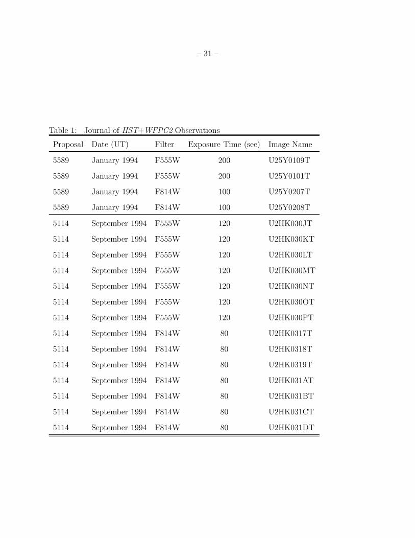
Table 1: Journal of HST+WFPC2 Observations

Proposal Date (UT) Filter Exposure Time (sec) Image Name

5589 January 1994 F555W 200 U25Y0109T

5589 January 1994 F555W 200 U25Y0101T

5589 January 1994 F814W 100 U25Y0207T

5589 January 1994 F814W 100 U25Y0208T

5114 September 1994 F555W 120 U2HK030JT

5114 September 1994 F555W 120 U2HK030KT

5114 September 1994 F555W 120 U2HK030LT

5114 September 1994 F555W 120 U2HK030MT

5114 September 1994 F555W 120 U2HK030NT

5114 September 1994 F555W 120 U2HK030OT

5114 September 1994 F555W 120 U2HK030PT

5114 September 1994 F814W 80 U2HK0317T

5114 September 1994 F814W 80 U2HK0318T

5114 September 1994 F814W 80 U2HK0319T

5114 September 1994 F814W 80 U2HK031AT

5114 September 1994 F814W 80 U2HK031BT

5114 September 1994 F814W 80 U2HK031CT

5114 September 1994 F814W 80 U2HK031DT

– 32 –

Table 2: Completeness correction factor for regions A, B, C and D

mF555W A B C D mF814W A B C D

17.7 64 68 67 70 16.1 87 90 89 91

18.2 84 88 90 89 16.6 89 89 91 93

18.7 85 85 87 89 17.1 89 91 92 93

19.2 80 83 86 89 17.6 85 87 90 90

19.7 79 81 85 87 18.1 85 87 88 90

20.2 69 76 81 84 18.6 79 84 85 88

20.7 67 75 78 83 19.1 74 81 83 85

21.2 61 71 73 83 19.6 70 72 79 85

21.7 54 67 70 80 20.1 64 75 73 83

22.2 44 57 61 78 20.6 57 65 71 81

22.7 32 50 60 69 21.1 45 62 68 71

23.2 25 43 55 63 21.6 41 53 61 71

23.7 14 37 42 48 22.1 25 45 52 61

24.2 8 19 19 22 22.6 11 17 18 19

24.7 0 3 1 2 23.1 2 6 8 8

– 33 –

Table 3: The IMF for the R136 cluster

Mass (M⊙) Bin width (M⊙) # stars/bin corrected # stars/bin

0.650000 0.100000 14 64

0.750000 0.100000 12 181

0.850000 0.100000 20 66

0.950000 0.100000 11 31

1.05000 0.100000 10 76

1.15000 0.100000 15 98

1.25000 0.100000 28 254

1.35000 0.100000 30 70

1.45000 0.100000 43 78

1.55000 0.100000 37 64

1.65000 0.100000 39 60

1.75000 0.100000 34 48

1.85000 0.100000 40 57

1.95000 0.100000 38 51

2.10000 0.200000 63 84

2.35000 0.300000 78 102

2.75000 0.500000 91 116

3.50000 1.00000 92 111

4.50000 1.00000 58 68

5.50000 1.00000 44 53

6.50000 1.00000 20 26

– 34 –

Table 4: Coordinates of the WFPC2 flanking field centers

CHIP R.A. DEC

WF2 5:38:49.27 -69:05:17.50

WF3 5:38:57.23 -69:06:12.72

WF4 5:38:46.68 -69:06:56.70

Table 5: The IMF for the Field

Mass (M⊙) Bin width (M⊙) # stars/bin corrected # stars/bin

1.05000 0.100000 2 5

1.15000 0.100000 14 41

1.25000 0.100000 63 626

1.35000 0.100000 179 484

1.45000 0.100000 156 214

1.55000 0.100000 163 195

1.65000 0.100000 176 201

1.75000 0.100000 129 145

1.85000 0.100000 126 143

1.95000 0.100000 104 111

2.10000 0.200000 179 189

2.35000 0.300000 168 176

2.75000 0.500000 258 267

3.50000 1.00000 331 341

4.50000 1.00000 217 222

5.50000 1.00000 108 110

6.50000 1.00000 85 87

– 35 –

Table 6: Spatial Distribution completeness test

MF555W Distance

3.375’ 5.625” 7.875” 10.125 ” 12.375”

17.7 58 64 64 69 73

18.2 77 86 87 90 88

18.7 71 84 86 90 88

19.2 67 80 81 86 88

19.7 56 74 79 84 80

20.2 50 69 72 81 77

20.7 40 62 71 78 74

21.2 31 56 66 70 67

21.7 25 48 61 66 62

22.2 18 42 53 57 59

22.7 9 33 43 51 52

23.2 2 26 35 42 44

23.7 0 18 28 32 32

24.2 0 7 13 14 15

24.7 0 1 2 3 2

– 36 –

– 37 –

– 38 –

5 105

1 107

1 106

2 106

3 106

5 106

7 106

1.5 Mo ●

yr

5 107

1.35 Mo +

2.0 Mo ▲

– 39 –

0.6

0.8

1.0

1.21.4

1.61.8

2.22.0

2.53.0

4.0

5.0

6.07.0

– 40 –

898786

84

8079

8682

656054

4220

– 41 –

6.55.54.53.52.72.11.81.61.41.21.11.0.950.85

0.750.65 2.3 M/Mo

– 42 –

– 43 –

Salpeter Slope

✴

Hunter et al. 1995

Hunter et al. 1996

6.55.54.53.52.72.11.81.61.41.21.11.0.950.85

0.750.65 2.3 M/Mo

– 44 –

– 45 –

6.55.54.53.52.72.11.81.61.41.21.0 2.3 M/Mo

–46

–

* Pre MS stars more massive stars

This figure "fig1.jpg" is available in "jpg" format from:

http://arXiv.org/ps/astro-ph/9911524v1

This figure "fig2.jpg" is available in "jpg" format from:

http://arXiv.org/ps/astro-ph/9911524v1

This figure "fig7.jpg" is available in "jpg" format from:

http://arXiv.org/ps/astro-ph/9911524v1