The Lockman Hole Project: new constraints on the sub-mJy ...
18
MNRAS 481, 4548–4565 (2018) doi:10.1093/mnras/sty2521 Advance Access publication 2018 September 27 The Lockman Hole Project: new constraints on the sub-mJy source counts from a wide-area 1.4 GHz mosaic I. Prandoni , 1‹ G. Guglielmino, 1,2 R. Morganti , 3,4 M. Vaccari , 1,5 A. Maini, 1,2,6,7 H. J. A. R ¨ ottgering, 8 M. J. Jarvis 5,9 and M. A. Garrett 10,11 1 INAF – Istituto di Radioastronomia, via Gobetti 101, I-40129 Bologna, Italy 2 DIFA, University of Bologna, Via Ranzani 2, I-40126 Bologna, Italy 3 ASTRON, the Netherlands Institute of Radio Astronomy, Postbus 2, NL-7990 AA, Dwingeloo, the Netherlands 4 Kapteyn Astronomical Institute, University of Groningen, PO Box 800, NL-9700 AV Groningen, the Netherlands 5 Department of Physics and Astronomy, University of the Western Cape, Bellville 7535, Cape Town, South Africa 6 Department of Physics and Astronomy, Macquarie University, Balaclava Road, North Ryde, NSW 2109, Australia 7 CSIRO Astronomy and Space Science, PO Box 76, Epping, NSW 1710, Australia 8 Leiden Observatory, Leiden University, PO Box 9513, NL-2300 RA Leiden, the Netherlands 9 Oxford Astrophysics, Denys Wilkinson Building, Keble Road, Oxford OX1 3RH, UK 10 School of Physics and Astronomy, University of Manchester,The Alan Turing Building, Oxford Road, Oxford M13 9PL, UK 11 Jodrell Bank Observatory, Lower Withington, University of Manchester, Macclesfield, Cheshire SK11 9DL, UK Accepted 2018 September 11. Received 2018 September 6; in original form 2018 May 31 ABSTRACT This paper is part of a series discussing the results obtained in the framework of a wide international collaboration – the Lockman Hole Project – aimed at improving the extensive multiband coverage available in the Lockman Hole region, through novel deep, wide-area, multifrequency (60, 150, 350 MHz, and 1.4 GHz) radio surveys. This multifrequency, multi- band information will be exploited to get a comprehensive view of star formation and active galactic nucleus activities in the high-redshift Universe from a radio perspective. In this pa- per, we present novel 1.4 GHz mosaic observations obtained with the Westerbork Synthesis Radio Telescope. With an area coverage of 6.6 deg 2 , this is the largest survey reaching an rms noise of 11 μJy beam −1 . In this paper, we present the source catalogue (∼6000 sources with flux densities S 55 μJy (5σ ), and we discuss the 1.4 GHz source counts derived from it. Our source counts provide very robust statistics in the flux range 0.1 < S < 1 mJy, and are in excellent agreement with other robust determinations obtained at lower and higher flux densities. A clear excess is found with respect to the counts predicted by the semi-empirical radio sky simulations developed in the framework of the Square Kilometre Array Simulated Skies project. A preliminary analysis of the identified (and classified) sources suggests this excess is to be ascribed to star-forming galaxies, which seem to show a steeper evolution than predicted. Key words: catalogues – surveys – galaxies: evolution – radio continuum: galaxies. 1 INTRODUCTION After many years of extensive multiband follow-up studies, it is now established that the sub-mJy population has a composite na- ture. Radio-loud (RL) active galactic nuclei (AGNs) remain largely dominant down to flux densities of 400–500 μJy (e.g. Mignano et al. 2008), while star-forming galaxies (SFGs) become the dom- inant population below ∼100 μJy (e.g. Simpson et al. 2006; Sey- mour et al. 2008; Smolˆ ci´ c et al. 2008). More recently, it has been E-mail: [email protected] shown that a significant fraction of the sources below 100 μJy show signatures of AGN activity at non-radio wavelengths (e.g. Seyfert galaxies or QSO). These AGNs are often referred to in the literature as radio-quiet (RQ) AGN (see e.g. Padovani et al. 2009, 2011, 2015; Bonzini et al. 2013), because the vast majority of them do not dis- play large-scale jets or lobes. It is worth noting that these systems are typically radiatively efficient AGNs, characterized by high accretion rates (1per cent), while the low-luminosity RL AGN population detected at sub-mJy fluxes is largely made of systems hosted by early-type galaxies (Mignano et al. 2008), likely characterized by radiatively inefficient, low accretion rates (<< 1 per cent). In other words, a classification based on radio loudness (despite not being C 2018 The Author(s) Published by Oxford University Press on behalf of the Royal Astronomical Society Downloaded from https://academic.oup.com/mnras/article/481/4/4548/5108199 by guest on 31 May 2022
-
Upload
khangminh22 -
Category
Documents
-
view
2 -
download
0
Transcript of The Lockman Hole Project: new constraints on the sub-mJy ...
MNRAS 481, 4548–4565 (2018) doi:10.1093/mnras/sty2521Advance Access publication 2018 September 27
The Lockman Hole Project: new constraints on the sub-mJy sourcecounts from a wide-area 1.4 GHz mosaic
I. Prandoni ,1‹ G. Guglielmino,1,2 R. Morganti ,3,4 M. Vaccari ,1,5 A. Maini,1,2,6,7
H. J. A. Rottgering,8 M. J. Jarvis5,9 and M. A. Garrett10,11
1INAF – Istituto di Radioastronomia, via Gobetti 101, I-40129 Bologna, Italy2DIFA, University of Bologna, Via Ranzani 2, I-40126 Bologna, Italy3ASTRON, the Netherlands Institute of Radio Astronomy, Postbus 2, NL-7990 AA, Dwingeloo, the Netherlands4Kapteyn Astronomical Institute, University of Groningen, PO Box 800, NL-9700 AV Groningen, the Netherlands5Department of Physics and Astronomy, University of the Western Cape, Bellville 7535, Cape Town, South Africa6Department of Physics and Astronomy, Macquarie University, Balaclava Road, North Ryde, NSW 2109, Australia7CSIRO Astronomy and Space Science, PO Box 76, Epping, NSW 1710, Australia8Leiden Observatory, Leiden University, PO Box 9513, NL-2300 RA Leiden, the Netherlands9Oxford Astrophysics, Denys Wilkinson Building, Keble Road, Oxford OX1 3RH, UK10School of Physics and Astronomy, University of Manchester,The Alan Turing Building, Oxford Road, Oxford M13 9PL, UK11Jodrell Bank Observatory, Lower Withington, University of Manchester, Macclesfield, Cheshire SK11 9DL, UK
Accepted 2018 September 11. Received 2018 September 6; in original form 2018 May 31
ABSTRACTThis paper is part of a series discussing the results obtained in the framework of a wideinternational collaboration – the Lockman Hole Project – aimed at improving the extensivemultiband coverage available in the Lockman Hole region, through novel deep, wide-area,multifrequency (60, 150, 350 MHz, and 1.4 GHz) radio surveys. This multifrequency, multi-band information will be exploited to get a comprehensive view of star formation and activegalactic nucleus activities in the high-redshift Universe from a radio perspective. In this pa-per, we present novel 1.4 GHz mosaic observations obtained with the Westerbork SynthesisRadio Telescope. With an area coverage of 6.6 deg2, this is the largest survey reaching anrms noise of 11 μJy beam−1. In this paper, we present the source catalogue (∼6000 sourceswith flux densities S � 55 μJy (5σ ), and we discuss the 1.4 GHz source counts derived fromit. Our source counts provide very robust statistics in the flux range 0.1 < S < 1 mJy, andare in excellent agreement with other robust determinations obtained at lower and higher fluxdensities. A clear excess is found with respect to the counts predicted by the semi-empiricalradio sky simulations developed in the framework of the Square Kilometre Array SimulatedSkies project. A preliminary analysis of the identified (and classified) sources suggests thisexcess is to be ascribed to star-forming galaxies, which seem to show a steeper evolution thanpredicted.
Key words: catalogues – surveys – galaxies: evolution – radio continuum: galaxies.
1 IN T RO D U C T I O N
After many years of extensive multiband follow-up studies, it isnow established that the sub-mJy population has a composite na-ture. Radio-loud (RL) active galactic nuclei (AGNs) remain largelydominant down to flux densities of 400–500 μJy (e.g. Mignanoet al. 2008), while star-forming galaxies (SFGs) become the dom-inant population below ∼100 μJy (e.g. Simpson et al. 2006; Sey-mour et al. 2008; Smolcic et al. 2008). More recently, it has been
� E-mail: [email protected]
shown that a significant fraction of the sources below 100 μJy showsignatures of AGN activity at non-radio wavelengths (e.g. Seyfertgalaxies or QSO). These AGNs are often referred to in the literatureas radio-quiet (RQ) AGN (see e.g. Padovani et al. 2009, 2011, 2015;Bonzini et al. 2013), because the vast majority of them do not dis-play large-scale jets or lobes. It is worth noting that these systems aretypically radiatively efficient AGNs, characterized by high accretionrates (�1per cent), while the low-luminosity RL AGN populationdetected at sub-mJy fluxes is largely made of systems hosted byearly-type galaxies (Mignano et al. 2008), likely characterized byradiatively inefficient, low accretion rates (<< 1 per cent). In otherwords, a classification based on radio loudness (despite not being
C© 2018 The Author(s)Published by Oxford University Press on behalf of the Royal Astronomical Society
Dow
nloaded from https://academ
ic.oup.com/m
nras/article/481/4/4548/5108199 by guest on 31 May 2022
A 1.4 GHz mosaic of the Lockman Hole region 4549
fully appropriate for faint radio-selected AGNs1) implies, at least ina statistical sense, a more profound distinction between fundamen-tal AGN classes (for a comprehensive review on AGN types andproperties we refer to Heckman & Best 2014).
The presence of large numbers of AGN-related sources at sub-mJy/μJy radio flux densities has given a new interesting scien-tific perspective to deep radio surveys, as they provide a powerfuldust/gas-obscuration-free tool to get a global census of both starformation and AGN activity (and related AGN feedback) up to veryhigh redshift and down to the RQ AGN regime (see Padovani 2016for a comprehensive review). However several uncertainties remaindue to observational issues and limitations. First the radio sourcecounts show a large scatter below ∼1 mJy, resulting in a large un-certainty on the actual radio source number density at sub-mJy fluxdensity levels. This scatter can be largely ascribed to cosmic vari-ance effects (Heywood, Jarvis & Condon 2013), but may also bedue, at least in some cases, to survey systematics (see e.g. Condonet al. 2012, and discussion in Section 7). Secondly, for a full and ro-bust characterization of the faint radio population the availability ofdeep multiwavelength ancillary data sets is essential, but typicallylimited to very small regions of the sky. Mid- and far-infrared (IR)data, as well as deep X-ray information, for example, has provedto be crucial to reliably separate SFGs from RQ AGNs (see e.g.Bonzini et al. 2013, 2015). When available, optical/near-IR spec-troscopy is of extreme value, as it provides source redshifts and, ifof sufficient quality, a very reliable classification of the host galax-ies (SFGs, Seyferts, QSO, etc.), through the analysis of line profiles(broad versus narrow) and line ratios (see e.g. the diagnostic dia-grams introduced by Baldwin, Philllips & Terlevich 1981 and laterrevised by Veilleux & Osterbrock 1987). Alternatively, multibandoptical/IR photometry can be used: host galaxies can be classifiedthrough their colours and/or spectral energy distributions (SEDs),and stellar masses and photometric estimates of the source redshiftscan be derived (several statistical methods and tools are presentedin the literature; for a recent application to deep radio continuumsurveys, see Duncan et al. 2018a,b).
Finally, the origin of the radio emission in RQ AGNs is currentlyhotly debated. Most radio-selected RQ AGNs are characterized bycompact sizes, i.e. they are unresolved or barely resolved at a fewarcsec scale, which is similar to the host galaxy size. RQ AGNshave also been found to share properties with SFGs. They havesimilar radio spectra and luminosities (Bonzini et al. 2013, 2015);their radio luminosity functions show similar evolutionary trends(Padovani et al. 2011); their host galaxies have similar colours,optical morphologies, and stellar masses (Bonzini et al. 2013). Forall these reasons, it was concluded that the radio emission in RQAGNs is triggered by star formation (Padovani et al. 2011; Bonziniet al. 2013, 2015; Ocran et al. 2017). On the other hand, high-resolution radio follow ups of RQ AGN samples with Very LongBaseline Interferometry arrays have shown that a significant fractionof RQ AGNs (20–40 per cent, depending on the sample) containAGN cores that contribute significantly (50 per cent or more) to thetotal radio emission (Maini et al. 2016; Herrera Ruiz et al. 2016,2017). A different approach was followed by Delvecchio et al.(2017) in the framework of the VLA COSMOS 3 GHz Project. Toidentify possible AGN contributions, they first exploited the dense
1A detailed discussion of AGN classification in view of the latest resultsfrom deep radio surveys, is presented in Padovani (2017), who proposes toupdate the terms RL/RQ AGNs into jetted/non-jetted AGNs, based on thepresence/lack of strong relativistic jets.
multiband information in the COSMOS field to derive accurate starformation rates (SFRs) via SED fitting; then they analysed the ratiobetween the 1.4 GHz radio luminosity and the SFR for each source.This resulted in ∼30 per cent of the sources with AGN signatures atnon-radio wavelengths displaying a significant (>3σ ) radio excess.It is worth noticing that radio selection does not seem to play a majorrole here. Controversial results arise also from investigations ofoptically selected QSOs, with authors claiming a pure star formationorigin of their radio emission (Kimball et al. 2011; Condon et al.2013), and others providing evidence of the presence of a radioluminosity excess with respect to SFGs of similar masses (Whiteet al. 2015). Such an excess appears to be correlated with the opticalluminosity (White et al. 2017).
The most likely scenario is that RQ AGN are composite systemswhere star formation and AGN triggered radio emission can co-exist, over a wide range of relative contributions. This scenario issupported by the recent modelling work of Mancuso et al. (2017),who showed that the observed radio counts can be very well repro-duced by a three-component population (SFGs, RL and RQ AGNs),where RQ AGNs are the sum of two sub-components: one dom-inated by star formation (so-called radio silent), and the other byAGN-triggered radio emission.
In order to overcome the aforementioned issues about cosmicvariance and limited multiband information, deep radio samplesover wide areas (>>1 deg2) are needed, in regions where deepmultiband ancillary data are available. This is a pre-requisite to getrobust estimations of the sub-mJy radio source number density andof the fractional contribution of each class of sources as a functionof cosmic time in representative volumes of the Universe (i.e. notbiased by cosmic variance). At the same time, wide-area surveysallow us to probe AGNs and/or star formation activities in a va-riety of different environments. Additional important informationmay come from multifrequency radio coverage: radio spectra mayhelp to constrain the origin of the radio emission in the observedsources and to understand its link to the host galaxy bolometricemission. This is especially true if high-resolution radio data areavailable and source structures can be inferred. SFGs typically havea steep radio spectral index (α ∼ −0.7/−0.8, where S ∝ να), witha relatively small dispersion (±0.24, Condon 1992). Radio spectralindex studies combined with source structure information (radio jetsand lobes) may thus help to disentangle star forming from steep-spectrum radio galaxy populations. A flat (α > −0.5) radio spec-tral index can identify core-dominated AGNs (Blundell & Kuncic2007) and GHz-peaked sources (Gopal-Krishna, Patnaik & Steppe1983; O’Dea 1998; Snellen et al. 2000). Ultra-steep radio spec-tra (α < −1; Rottgering et al. 1994; Chambers et al. 1996; Jarviset al. 2001) are a typical feature of high-redshift (z >>2) radiogalaxies.
The Lockman Hole (LH, Lockman, Jahoda & McCammon 1986)is one of the best studied extragalactic regions of the sky (seeSection 2 for a comprehensive summary of the available multibandcoverage in this region). Given its high declination (∼ +58◦), the LHis also best suited for deep, high-resolution, high-fidelity imagingwith the LOw-Frequency ARray (LOFAR).
The LH Project is an international collaboration aimed atextending the multiband information available in the LH region,through novel multifrequency radio surveys down to 60–150 MHz,a frequency domain that is now accessible for wide-area deepfields thanks to the combination of field of view, sensitivity, andspatial resolution of LOFAR. This information, together with theavailable ancillary data, will allow us to get robust observationalconstraints on the faint extragalactic radio sky, in preparation for
MNRAS 481, 4548–4565 (2018)
Dow
nloaded from https://academ
ic.oup.com/m
nras/article/481/4/4548/5108199 by guest on 31 May 2022
4550 I. Prandoni et al.
next-generation continuum extragalactic surveys with the AustraliaSquare Kilometre Array Pathfinder (ASKAP; Johnston et al.2007), MeerKat (Booth & Jonas 2012), and ultimately the SquareKilometre Array (SKA).
This paper presents a Westerbork (WSRT) 1.4 GHz mosaic cover-ing ∼6.6 deg2 down to 11 μ beam−1 rms and the source catalogueextracted from it. The 345 MHz follow-up, again obtained withthe WSRT, is presented in a following paper (Prandoni et al., inpreparation), while the first LOFAR observations of this region arepresented in Mahony et al. (2016).
This paper is organized as follows. Section 2 gives an overviewof the multiwavelength data available for the LH region. In Sec-tions 3, we describe the WSRT 1.4 GHz observations, the relateddata reduction and the analysis performed to characterize the noiseproperties of the final mosaic. In Section 4, we describe the methodused to extract the sources and the final catalogue obtained. In Sec-tions 5 and 6, we provide estimates of the source parameters’ errorsand we analyse possible systematic effects. In Section 7, we presentthe source counts derived from the present catalogue and we discussthem in comparison with other existing source counts obtained fromwide-area 1.4 GHz surveys. In Section 8, we assess the contributionof each class of sources to our overall radio source counts, basedon a preliminary analysis of the radio source optical/IR properties,and we compare it to existing modelling predictions. In Section 9,we summarize our main results.
2 MU LT I WAV E L E N G T H C OV E R AG E O F TH EL O C K M A N H O L E R E G I O N
The LH is the region of lowest H I column density in the sky. Itslow-IR background (0.38 MJy sr−1 at 100μm; Lonsdale et al. 2003)makes this region particularly well suited for deep-IR observations.The Spitzer Space Telescope (Werner et al. 2004) observed ∼12 deg2
of the LH region in 2004 as part of the Spitzer Wide-area InfraredExtragalactic survey (SWIRE; Lonsdale et al. 2003). Observationswere performed using the Infrared Array Camera (IRAC; Fazioet al. 2004) operating at 3.6, 4.5, 5.8, and 8 μm, and the Multi-band Imaging Photometer for Spitzer (Rieke et al. 2004) at 24,70, and 160 μm. Deeper, confusion-limited observations at 3.6 and4.5 μm were obtained over ∼4 deg2 during the warm mission ofSpitzer as part of the Spitzer Extragalactic Representative VolumeSurvey (SERVS, Mauduit et al. 2012). In addition about 16 deg2
overlapping with the SWIRE survey of the LH have been targetedby the Herschel Space Observatory with the Photoconductor Ar-ray Camera and Spectrometer (100 and 160 μm) and the Spectraland Photometric Imaging REceiver (250, 350, and 500 μm) aspart of the Herschel Multi-tiered Extragalactic Survey (Oliver et al.2012).
A great deal of complementary data have been taken on the LHat other wavelengths in order to exploit the availability of sensi-tive IR observations, including GALEX GR6Plus7 ultraviolet (UV)photometry (Martin et al. 2005), Sloane Digital Sky Survey (SDSS)DR14 optical spectroscopy and photometry in the ugriz bands to adepth of ∼22 mag (Abolfathi et al. 2018), INT Wide Field Cameraoptical photometry (u, g, r, i, z down to AB magnitudes 23.9, 24.5,24.0, 23.3, 22.0 respectively; Gonzales-Solares et al. 2011) and UKInfrared Deep Sky Survey Deep Extragalactic Survey (UKIDSSDXS) DR10Plus photometry in the J and K bands, with a sensi-tivity of K ∼ 21–21.5 mag (Vega; Lawrence et al. 2007). Thereare existing near-IR data across the region from the Two Micron
All Sky Survey (Beichman et al. 2003) to J, H, and Ks band mag-nitudes of 17.8, 16.5, and 16.0. A photometric redshift cataloguecontaining 229 238 galaxies and quasars within the LH has beenconstructed from band-merged data (Rowan-Robinson et al. 2008;but see Rowan-Robinson et al. 2013 for the latest version of theSWIRE photometric redshift catalogue, including photometric red-shifts and SED models based on optical, near-IR, and Spitzer pho-tometry). Deep surveys within the LH region have been undertakenwith the Submillimetre Common-User Bolometer Array (Hollandet al. 1999) at 850 μm (Coppin et al. 2006), and with the X-raysatellites ROSAT (Hasinger et al. 1998), XMM–Newton (Hasingeret al. 2001; Mainieri et al. 2002; Brunner et al. 2008), and Chandra(Polletta et al. 2006).
A variety of radio surveys cover limited areas within the LH re-gion, in coincidence with the two deep X-ray fields (highlighted inFig. 1). The first of these was by de Ruiter et al. (1997), who ob-served an area of 0.35 deg2 at 1.4 GHz centred on the ROSAT/XMMpointing (RA = 10:52:09; Dec.=+57:21:34, J2000), using the VeryLarge Array (VLA) in C-configuration, with an rms noise level of30−55 μJy beam−1. A similar deep observation was carried out byCiliegi et al. (2003), who observed an 0.087 deg2 region at 4.89 GHzusing the VLA in C-configuration, with an rms noise level of 11μJy beam−1. More recently, Biggs & Ivison (2006) observed a 320arcmin2 area, using the VLA at 1.4 GHz operating in the A- andB-configurations, and with an rms noise level of 4.6 μJy beam−1.VLA B-configuration 1.4 GHz observations of a larger region (threeoverlapping VLA pointings) were performed by Ibar et al. (2009),reaching an rms noise of ∼6 μJy beam−1 in the central 100 arcmin2
area. These observations were matched with 610 MHz Giant Metre-wave Radio Telescope (GMRT) observations down to an rms noiseof ∼15 μJy beam−1. Less sensitive GMRT 610 MHz observationsof a much larger area were carried out by Garn et al. (2008a,b), cov-ering ∼5 deg2 down to an rms noise of ∼60 μJy. This survey waslater extended to ∼13 deg2 (Garn et al. 2010). Two fields of the 10C15 GHz survey (AMI consortium, 2011; Whittam et al. 2013) over-lap with the LH region, for a total of ∼4.6 deg2. The rms noise levelsof ∼50−100 μJy were reached at a spatial resolution is 30 arcsec.The deepest 1.4 GHz observations to date (rms noise of ∼2.7 μJybeam−1 were performed by Owen & Morrison (2008) at the locationof the Chandra deep pointing (RA = 10:46, Dec.=+59:00, J2000).This was later matched with very sensitive VLA (C-configuration)324.5 MHz observations down to an rms noise of ∼70 μJy beam−1
in the central part (Owen et al. 2009). This field (also known asLockman North) has been recently the target of wide-band 3 GHzobservations with the upgraded Karl Jansky VLA, reaching an rmsnoise level of 1.01 μJy beam−1 (Condon et al. 2012; Vernstromet al. 2014, 2016a,b). The Faint Images of the Radio Sky at Twentycm (FIRST; Becker, White & Helfand 1995) and NRAO VLA SkySurvey (NVSS; Condon et al. 1998) surveys both cover the entireregion at 1.4 GHz, but only to relatively shallow noise levels of 150and 450 μJy beam−1, respectively.
Finally, as part of the LH Project, the field has been imagedwith WSRT at 350 MHz down to the confusion limit (∼0.5 mJyrms; Prandoni et al. in preparation), and with LOFAR at 150 MHz(∼160 μJy rms; Mahony et al. 2016). Deeper 150 MHz LOFARobservations are ongoing (Mandal et al. in preparation). Mahonyet al. (2016) present a multifrequency study of the radio sources inthe field, based on most of the aforementioned radio observations,including the catalogue presented here. The combination of LOFAR150 MHz and WSRT 1.4 GHz data, resulted in a sample of 1302matched sources (see Mahony et al. 2016, for more details).
MNRAS 481, 4548–4565 (2018)
Dow
nloaded from https://academ
ic.oup.com/m
nras/article/481/4/4548/5108199 by guest on 31 May 2022
A 1.4 GHz mosaic of the Lockman Hole region 4551
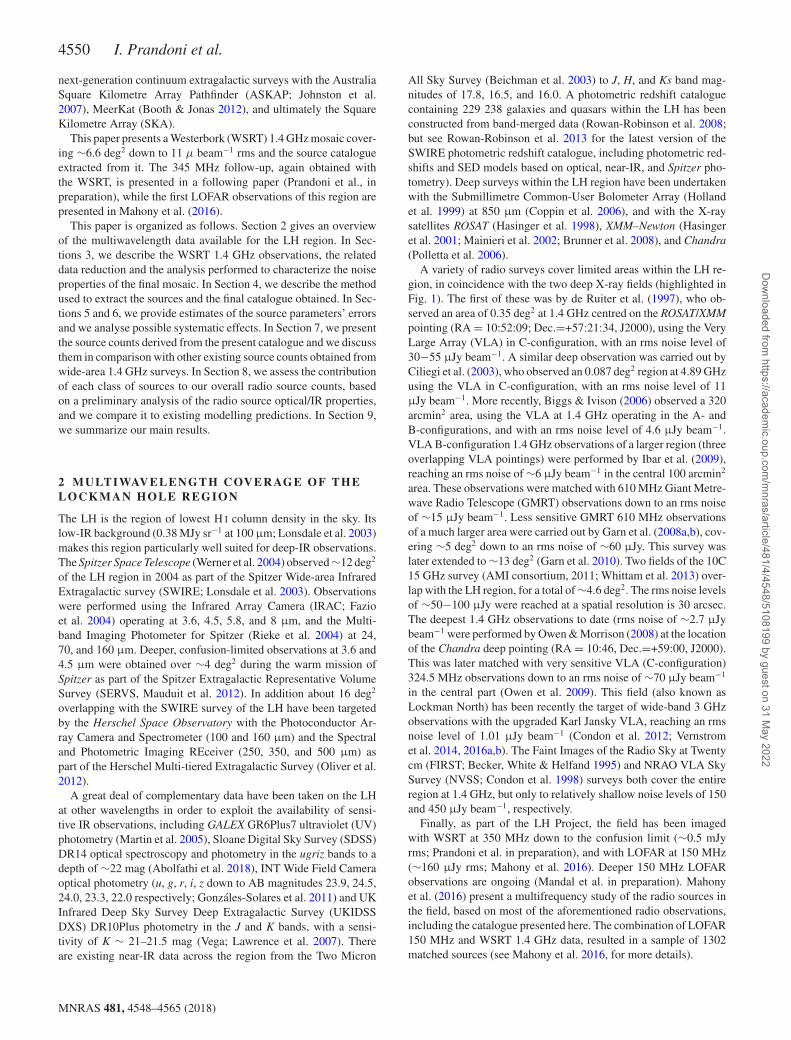
Figure 1. The WSRT 1.4 GHz mosaic: 16 overlapping pointings, with spacing of 22 arcmin in RA and 25 arcmin in Dec. Highlighted are the two locationsof the deep X-ray fields, where most existing deep radio observations have been taken (see text for more details).
3 TH E N E W 1 . 4 G H z M O S A I C
We observed the LH region with the WSRT at 1.4 GHz, in the pe-riod 2006 December–2007 June. The observations covered an areaof ∼6.6 deg2 (mostly overlapping the Spitzer and Herschel surveys),through overlapping pointings. A good compromise between uni-form sensitivity and observing efficiency is generally obtained witha mosaic pattern where pointing spacings, s, are ≈FWHP’, whereFWHP’=FWHP/
√2, and FWHP is the full width at half-power of
the primary beam (see Prandoni et al. 2000a). For our particular caseFWHP∼36 arcmin, and FWHP’∼25.46 arcmin. From noise sim-ulations, we got 5 per cent noise variations with s = 0.85 FWHP’(=22 arcmin) and 10 per cent variations with s = FWHP’. We thendecided to cover the 6.6 deg2 area with 16 overlapping pointings,with spacing of 22 arcmin in RA and 25 arcmin in Dec. Each fieldwas observed for 12 h. The primary calibrator (3C 48) was observed
for 15 min at the beginning of each 12 h run, and the secondarycalibrator (J1035+5628), unresolved on VLBA scale, was observedfor 3 min every hour. The data were recorded in 512 channels, or-ganized in eight 20 MHz sub-bands, 64 channels each. The channelwidth is 312 KHz, and the total bandwidth is 160 MHz.
For the data reduction, we used the MULTICHANNEL IMAGE RE-CONSTRUCTION, IMAGE ANALYSIS AND DISPLAY(MIRIAD) softwarepackage (Sault et al.1995). Each field was calibrated and imagedseparately. Imaging and deconvolution was performed in multi-frequency synthesis mode, taking into proper account the spectralvariation of the dirty beam over the image during the cleaning pro-cess (MRIAD task MFCLEAN). Each field was cleaned to a distanceof 50 arcmin from the phase centre (i.e. down to about the zero-point primary beam width) in order to deconvolve all the sourcesin the field. All the images were produced using uniform weightingto get the maximum spatial resolution. Subsequently, we combined
MNRAS 481, 4548–4565 (2018)
Dow
nloaded from https://academ
ic.oup.com/m
nras/article/481/4/4548/5108199 by guest on 31 May 2022
4552 I. Prandoni et al.
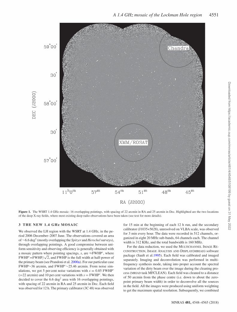
Figure 2. Left: noise map. Contours refer to 1.1, 1.2, 1.3, 1.5, 1.7, 2, 2.5, 3, 4, 5, 10, 20, and 30 multiples of the noise centre value (11 μJy). Right: visibilityarea of the WSRT 1.4 GHz mosaic. Cumulative fraction of the total area of the noise map characterized by a measured noise lower than a given value. Dottedlines indicate the maximum noise value measured over an area of 2, 3, 4 and 5 deg2 .
together all the images to create a single primary beam correctedmosaic (pixel size =2 arcsec). The synthesized beam is 11 arc-sec × 9 arcsec, with position angle PA = 0◦. The resulting 1.4 GHzmosaic, centred at RA = 10:52:16.6; Dec.=+58:01:15 (J2000), isshown in Fig. 1.
3.1 Noise map
To investigate the noise characteristics of our 1.4 GHz image, weconstructed a noise map with the software SEXTRACTOR (Bertin &Arnouts 1996). Although SEXTRACTOR was originally developedfor the analysis of optical data, it is widely used for noise analysisof radio images as well (see e.g. Bondi et al. 2003; Huynh et al.2005; Prandoni et al. 2006). SEXTRACTOR initially estimates thelocal background in each mesh from the pixel data. Then the localbackground histogram is clipped iteratively until convergence isreached at ±3σ around its median. The choice of mesh size isvery important. When it is too small, the background tends to beoverestimated due to the presence of real sources. When it is toolarge, any small-scale variation of the background is washed out.A mesh size of 50 × 50 pixel (approximately 10 × 10 beams),was found to be appropriate for our case (see also discussion inSection 4). However, it should be noted that border effects makethe determination of the local noise less reliable in the outermostregions of the mosaic.
The obtained noise map is shown in Fig. 2 (left-hand panel).The rms was found to be approximately uniform (noise variations< 10 per cent) over the central region, with a value of about 11 μJy.Then, it radially increases up to ∼500 μJy at the very border ofthe mosaic. This is in agreement with the expectations, as betterdiscussed in Section 4. Sub-regions characterized by noise valueshigher than the expected ones are found to correspond to verybright sources, due to dynamic range limits introduced by residual
phase errors. In Fig. 2 (right-hand panel), the total area of the noisemap characterized by noise measurements lower than a given valueis plotted. The inner ∼2 deg2 region is characterized by a noiseincrement ≤ 10 per cent (noise values ≤12 μJy). Noise incrementsto 18, 38, and 90 μJy are measured over the inner 3, 4, and 5 deg2
respectively (see dotted lines in right-hand panel of Fig. 2). Wenotice that border effects are present in the very external mosaicregion characterized by noise values larger than ∼330 μJy (i.e.30 × 11μJy, see last contour in Fig. 2, left-hand panel).
4 TH E 1 . 4 G H z S O U R C E C ATA L O G U E
The source extraction was performed over the entire mosaic (up torms noise values of ∼500 μJy), even though the source catalogueshould be considered reliable and complete only up to local noisevalues of 330 μJy. To take into proper account both local and radialnoise variations, sources were extracted from a signal-to-noise mapproduced by dividing the mosaic by its noise map. A preliminarylist of more than 6000 sources with S/N ≥ 5 was derived using theMIRID task IMSAD.
All the source candidates were visually inspected. The goodnessof Gaussian fit parameters was checked following Prandoni et al.(2000b, see their section 2). Typical fitting problems arise whenever:
(i) Sources are fitted by IMSAD with a single Gaussian but arebetter described by two or more Gaussian;
(ii) Sources are extended and are not well described by a Gaus-sian fit.
In the first case, sources were re-fitted using multiple Gaussiancomponents. The number of successfully split sources is 74 in total(62 in two components, 10 in three components, and 2 in four com-ponents). In the second case (134 non-Gaussian sources or sourcecomponents), integrated flux densities were measured by summing
MNRAS 481, 4548–4565 (2018)
Dow
nloaded from https://academ
ic.oup.com/m
nras/article/481/4/4548/5108199 by guest on 31 May 2022
A 1.4 GHz mosaic of the Lockman Hole region 4553
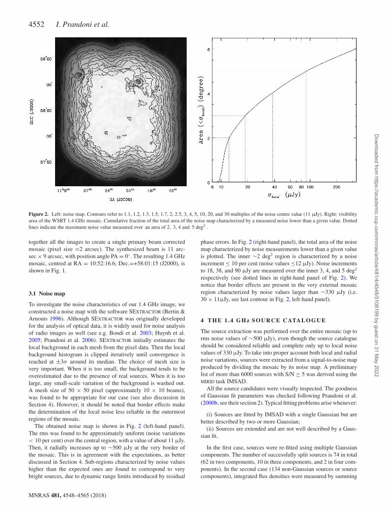
Figure 3. Peak flux density distribution of the radio sources (or sourcecomponents) before (red) and after (black) taking into proper account thenoise variations along the mosaic. In the latter case, the source number isweighted for the reciprocal of the visibility area shown in Fig. 2 (right-handpanel), where we assume Speak > 5σ local.
all the pixels above a reference 3σ threshold, using the MIRIAD taskCGCURS, which also gives the position and flux density of thesource peak. Non-Gaussian sources are flagged as ‘E’ in the cata-logue. In a few additional cases, Gaussian fits were able to providegood values for positions and peak flux densities, but did fail in de-termining the integrated flux densities. This happens typically at lowsignal-to-noise values. Gaussian sources with a poor determinationof the integrated flux are flagged in the catalogue as ‘G∗’. We alsonoticed that in a few cases our procedure (IMSAD+SEXTRACTOR)failed to detect very extended low-surface brightness sources. Thisis due to the fact that the source itself can affect the local noisecomputation, producing a too high detection threshold (5σ local).The few missing large low-surface brightness sources were easilyrecognized by eye, and added to the catalogue.
Once the final source list was produced, we computed the localnoise, σ local, around each source (measured in 50 × 50 pixel regionscentred at each source position in the noise map) and used it totransform the peak and integrated flux densities from S/N units tomJy units.
After accounting for the splitting in multiple Gaussian compo-nents the catalogue lists 6194 sources (or sources components). Thepeak flux distribution of our sources is shown in Fig. 3 before (redhistogram) and after (black histogram) taking into proper accountthe noise variations along the mosaic. Once corrected for the sourcevisibility area (see Fig. 2, right-hand panel), the peak flux distribu-tion gets narrower, showing a steeper increase going to lower fluxdensities. However, some incompleteness can still be seen in thelowest flux density bins. This incompleteness is the expected effectof the noise at the source extraction threshold. Due to its Gaus-sian distribution, whenever a source falls on a noise dip, either thesource flux is underestimated or the source goes undetected. Thisproduces incompleteness in the faintest bins. As a consequence, themeasured fluxes of detected sources are biased toward higher val-ues in the incomplete bins, because only sources that fall on noisepeaks have been detected and measured. As demonstrated through
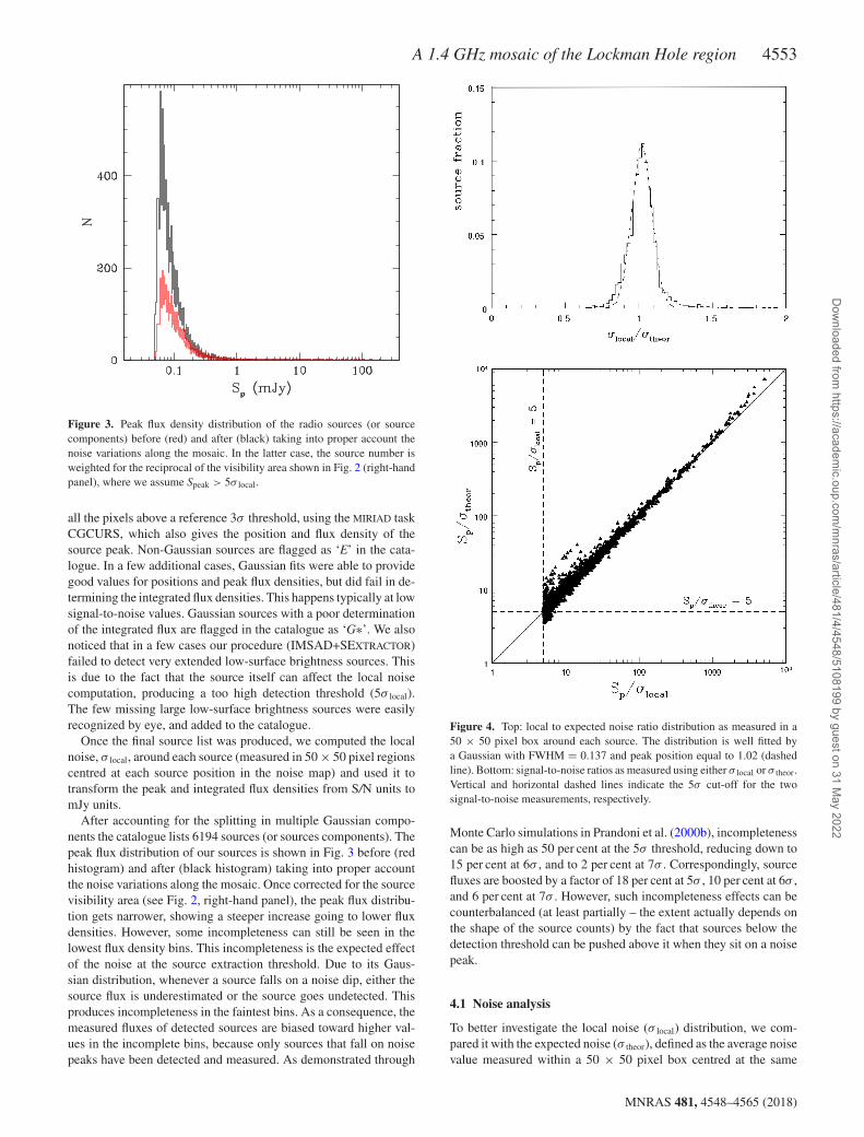
Figure 4. Top: local to expected noise ratio distribution as measured in a50 × 50 pixel box around each source. The distribution is well fitted bya Gaussian with FWHM = 0.137 and peak position equal to 1.02 (dashedline). Bottom: signal-to-noise ratios as measured using either σ local or σ theor.Vertical and horizontal dashed lines indicate the 5σ cut-off for the twosignal-to-noise measurements, respectively.
Monte Carlo simulations in Prandoni et al. (2000b), incompletenesscan be as high as 50 per cent at the 5σ threshold, reducing down to15 per cent at 6σ , and to 2 per cent at 7σ . Correspondingly, sourcefluxes are boosted by a factor of 18 per cent at 5σ , 10 per cent at 6σ ,and 6 per cent at 7σ . However, such incompleteness effects can becounterbalanced (at least partially – the extent actually depends onthe shape of the source counts) by the fact that sources below thedetection threshold can be pushed above it when they sit on a noisepeak.
4.1 Noise analysis
To better investigate the local noise (σ local) distribution, we com-pared it with the expected noise (σ theor), defined as the average noisevalue measured within a 50 × 50 pixel box centred at the same
MNRAS 481, 4548–4565 (2018)
Dow
nloaded from https://academ
ic.oup.com/m
nras/article/481/4/4548/5108199 by guest on 31 May 2022
4554 I. Prandoni et al.
0.1 0.2 0.5 1 2 5 1 0 2 0
S (mJy)
0
0.02
0.04
0.06
0.08
0.10
0.12
FD
R
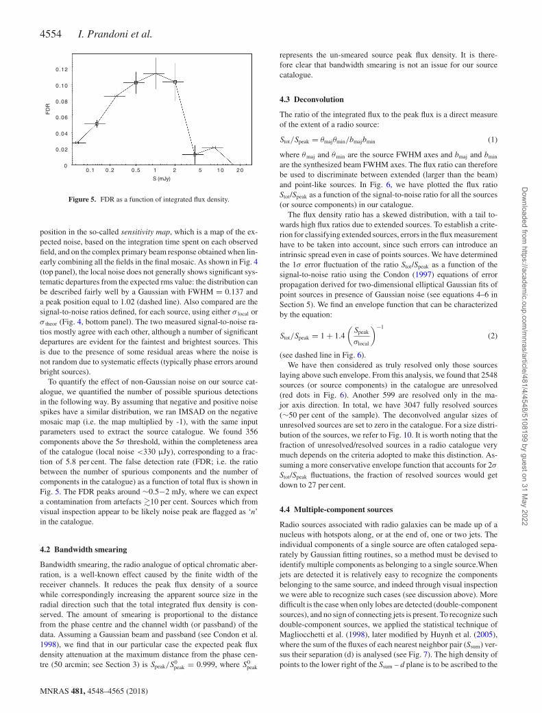
Figure 5. FDR as a function of integrated flux density.
position in the so-called sensitivity map, which is a map of the ex-pected noise, based on the integration time spent on each observedfield, and on the complex primary beam response obtained when lin-early combining all the fields in the final mosaic. As shown in Fig. 4(top panel), the local noise does not generally shows significant sys-tematic departures from the expected rms value: the distribution canbe described fairly well by a Gaussian with FWHM = 0.137 anda peak position equal to 1.02 (dashed line). Also compared are thesignal-to-noise ratios defined, for each source, using either σ local orσ theor (Fig. 4, bottom panel). The two measured signal-to-noise ra-tios mostly agree with each other, although a number of significantdepartures are evident for the faintest and brightest sources. Thisis due to the presence of some residual areas where the noise isnot random due to systematic effects (typically phase errors aroundbright sources).
To quantify the effect of non-Gaussian noise on our source cat-alogue, we quantified the number of possible spurious detectionsin the following way. By assuming that negative and positive noisespikes have a similar distribution, we ran IMSAD on the negativemosaic map (i.e. the map multiplied by -1), with the same inputparameters used to extract the source catalogue. We found 356components above the 5σ threshold, within the completeness areaof the catalogue (local noise <330 μJy), corresponding to a frac-tion of 5.8 per cent. The false detection rate (FDR; i.e. the ratiobetween the number of spurious components and the number ofcomponents in the catalogue) as a function of total flux is shown inFig. 5. The FDR peaks around ∼0.5−2 mJy, where we can expecta contamination from artefacts �10 per cent. Sources which fromvisual inspection appear to be likely noise peak are flagged as ‘n’in the catalogue.
4.2 Bandwidth smearing
Bandwidth smearing, the radio analogue of optical chromatic aber-ration, is a well-known effect caused by the finite width of thereceiver channels. It reduces the peak flux density of a sourcewhile correspondingly increasing the apparent source size in theradial direction such that the total integrated flux density is con-served. The amount of smearing is proportional to the distancefrom the phase centre and the channel width (or passband) of thedata. Assuming a Gaussian beam and passband (see Condon et al.1998), we find that in our particular case the expected peak fluxdensity attenuation at the maximum distance from the phase cen-tre (50 arcmin; see Section 3) is Speak/S
0peak = 0.999, where S0
peak
represents the un-smeared source peak flux density. It is there-fore clear that bandwidth smearing is not an issue for our sourcecatalogue.
4.3 Deconvolution
The ratio of the integrated flux to the peak flux is a direct measureof the extent of a radio source:
Stot/Speak = θmajθmin/bmajbmin (1)
where θmaj and θmin are the source FWHM axes and bmaj and bmin
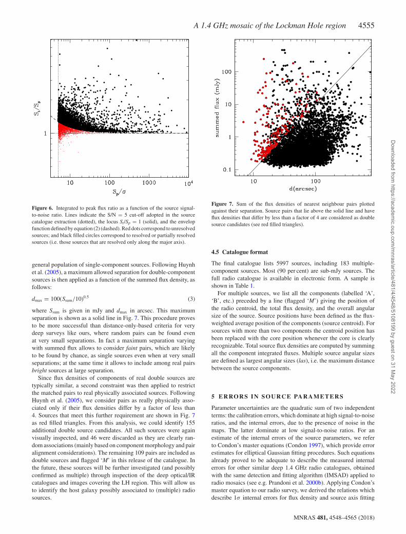
are the synthesized beam FWHM axes. The flux ratio can thereforebe used to discriminate between extended (larger than the beam)and point-like sources. In Fig. 6, we have plotted the flux ratioStot/Speak as a function of the signal-to-noise ratio for all the sources(or source components) in our catalogue.
The flux density ratio has a skewed distribution, with a tail to-wards high flux ratios due to extended sources. To establish a crite-rion for classifying extended sources, errors in the flux measurementhave to be taken into account, since such errors can introduce anintrinsic spread even in case of points sources. We have determinedthe 1σ error fluctuation of the ratio Stot/Speak as a function of thesignal-to-noise ratio using the Condon (1997) equations of errorpropagation derived for two-dimensional elliptical Gaussian fits ofpoint sources in presence of Gaussian noise (see equations 4–6 inSection 5). We find an envelope function that can be characterizedby the equation:
Stot/Speak = 1 + 1.4
(Speak
σlocal
)−1
(2)
(see dashed line in Fig. 6).We have then considered as truly resolved only those sources
laying above such envelope. From this analysis, we found that 2548sources (or source components) in the catalogue are unresolved(red dots in Fig. 6). Another 599 are resolved only in the ma-jor axis direction. In total, we have 3047 fully resolved sources(∼50 per cent of the sample). The deconvolved angular sizes ofunresolved sources are set to zero in the catalogue. For a size distri-bution of the sources, we refer to Fig. 10. It is worth noting that thefraction of unresolved/resolved sources in a radio catalogue verymuch depends on the criteria adopted to make this distinction. As-suming a more conservative envelope function that accounts for 2σ
Stot/Speak fluctuations, the fraction of resolved sources would getdown to 27 per cent.
4.4 Multiple-component sources
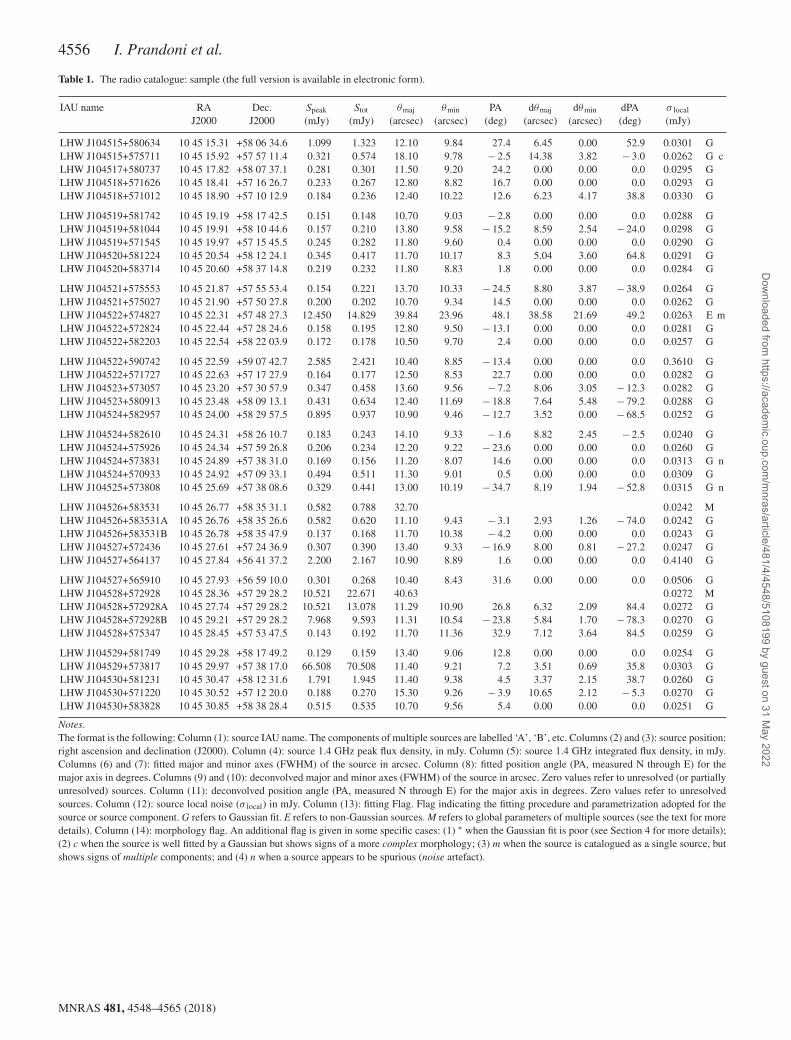
Radio sources associated with radio galaxies can be made up of anucleus with hotspots along, or at the end of, one or two jets. Theindividual components of a single source are often cataloged sepa-rately by Gaussian fitting routines, so a method must be devised toidentify multiple components as belonging to a single source.Whenjets are detected it is relatively easy to recognize the componentsbelonging to the same source, and indeed through visual inspectionwe were able to recognize such cases (see discussion above). Moredifficult is the case when only lobes are detected (double-componentsources), and no sign of connecting jets is present. To recognize suchdouble-component sources, we applied the statistical technique ofMagliocchetti et al. (1998), later modified by Huynh et al. (2005),where the sum of the fluxes of each nearest neighbor pair (Ssum) ver-sus their separation (d) is analysed (see Fig. 7). The high density ofpoints to the lower right of the Ssum – d plane is to be ascribed to the
MNRAS 481, 4548–4565 (2018)
Dow
nloaded from https://academ
ic.oup.com/m
nras/article/481/4/4548/5108199 by guest on 31 May 2022
A 1.4 GHz mosaic of the Lockman Hole region 4555
Figure 6. Integrated to peak flux ratio as a function of the source signal-to-noise ratio. Lines indicate the S/N = 5 cut-off adopted in the sourcecatalogue extraction (dotted), the locus St/Sp = 1 (solid), and the envelopfunction defined by equation (2) (dashed). Red dots correspond to unresolvedsources; and black filled circles correspond to resolved or partially resolvedsources (i.e. those sources that are resolved only along the major axis).
general population of single-component sources. Following Huynhet al. (2005), a maximum allowed separation for double-componentsources is then applied as a function of the summed flux density, asfollows:
dmax = 100(Ssum/10)0.5 (3)
where Ssum is given in mJy and dmax in arcsec. This maximumseparation is shown as a solid line in Fig. 7. This procedure provesto be more successful than distance-only-based criteria for verydeep surveys like ours, where random pairs can be found evenat very small separations. In fact a maximum separation varyingwith summed flux allows to consider faint pairs, which are likelyto be found by chance, as single sources even when at very smallseparations; at the same time it allows to include among real pairsbright sources at large separation.
Since flux densities of components of real double sources aretypically similar, a second constraint was then applied to restrictthe matched pairs to real physically associated sources. FollowingHuynh et al. (2005), we consider pairs as really physically asso-ciated only if their flux densities differ by a factor of less than4. Sources that meet this further requirement are shown in Fig. 7as red filled triangles. From this analysis, we could identify 155additional double source candidates. All such sources were againvisually inspected, and 46 were discarded as they are clearly ran-dom associations (mainly based on component morphology and pairalignment considerations). The remaining 109 pairs are included asdouble sources and flagged ‘M’ in this release of the catalogue. Inthe future, these sources will be further investigated (and possiblyconfirmed as multiple) through inspection of the deep optical/IRcatalogues and images covering the LH region. This will allow usto identify the host galaxy possibly associated to (multiple) radiosources.
Figure 7. Sum of the flux densities of nearest neighbour pairs plottedagainst their separation. Source pairs that lie above the solid line and haveflux densities that differ by less than a factor of 4 are considered as doublesource candidates (see red filled triangles).
4.5 Catalogue format
The final catalogue lists 5997 sources, including 183 multiple-component sources. Most (90 per cent) are sub-mJy sources. Thefull radio catalogue is available in electronic form. A sample isshown in Table 1.
For multiple sources, we list all the components (labelled ‘A’,‘B’, etc.) preceded by a line (flagged ‘M’) giving the position ofthe radio centroid, the total flux density, and the overall angularsize of the source. Source positions have been defined as the flux-weighted average position of the components (source centroid). Forsources with more than two components the centroid position hasbeen replaced with the core position whenever the core is clearlyrecognizable. Total source flux densities are computed by summingall the component integrated fluxes. Multiple source angular sizesare defined as largest angular sizes (las), i.e. the maximum distancebetween the source components.
5 ER RO R S IN SO U R C E PA R A M E T E R S
Parameter uncertainties are the quadratic sum of two independentterms: the calibration errors, which dominate at high signal-to-noiseratios, and the internal errors, due to the presence of noise in themaps. The latter dominate at low signal-to-noise ratios. For anestimate of the internal errors of the source parameters, we referto Condon’s master equations (Condon 1997), which provide errorestimates for elliptical Gaussian fitting procedures. Such equationsalready proved to be adequate to describe the measured internalerrors for other similar deep 1.4 GHz radio catalogues, obtainedwith the same detection and fitting algorithm (IMSAD) applied toradio mosaics (see e.g. Prandoni et al. 2000b). Applying Condon’smaster equation to our radio survey, we derived the relations whichdescribe 1σ internal errors for flux density and source axis fitting
MNRAS 481, 4548–4565 (2018)
Dow
nloaded from https://academ
ic.oup.com/m
nras/article/481/4/4548/5108199 by guest on 31 May 2022
4556 I. Prandoni et al.
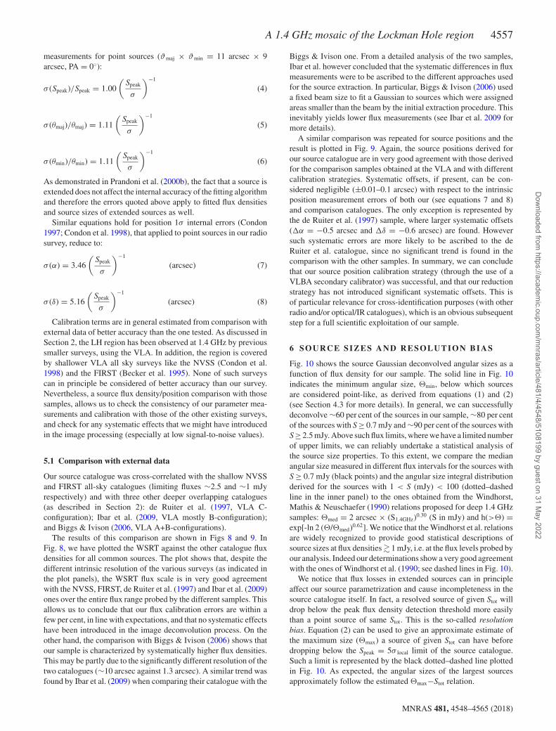
Table 1. The radio catalogue: sample (the full version is available in electronic form).
IAU name RA Dec. Speak Stot θmaj θmin PA dθmaj dθmin dPA σ local
J2000 J2000 (mJy) (mJy) (arcsec) (arcsec) (deg) (arcsec) (arcsec) (deg) (mJy)
LHW J104515+580634 10 45 15.31 +58 06 34.6 1.099 1.323 12.10 9.84 27.4 6.45 0.00 52.9 0.0301 GLHW J104515+575711 10 45 15.92 +57 57 11.4 0.321 0.574 18.10 9.78 − 2.5 14.38 3.82 − 3.0 0.0262 G cLHW J104517+580737 10 45 17.82 +58 07 37.1 0.281 0.301 11.50 9.20 24.2 0.00 0.00 0.0 0.0295 GLHW J104518+571626 10 45 18.41 +57 16 26.7 0.233 0.267 12.80 8.82 16.7 0.00 0.00 0.0 0.0293 GLHW J104518+571012 10 45 18.90 +57 10 12.9 0.184 0.236 12.40 10.22 12.6 6.23 4.17 38.8 0.0330 G
LHW J104519+581742 10 45 19.19 +58 17 42.5 0.151 0.148 10.70 9.03 − 2.8 0.00 0.00 0.0 0.0288 GLHW J104519+581044 10 45 19.91 +58 10 44.6 0.157 0.210 13.80 9.58 − 15.2 8.59 2.54 − 24.0 0.0298 GLHW J104519+571545 10 45 19.97 +57 15 45.5 0.245 0.282 11.80 9.60 0.4 0.00 0.00 0.0 0.0290 GLHW J104520+581224 10 45 20.54 +58 12 24.1 0.345 0.417 11.70 10.17 8.3 5.04 3.60 64.8 0.0291 GLHW J104520+583714 10 45 20.60 +58 37 14.8 0.219 0.232 11.80 8.83 1.8 0.00 0.00 0.0 0.0284 G
LHW J104521+575553 10 45 21.87 +57 55 53.4 0.154 0.221 13.70 10.33 − 24.5 8.80 3.87 − 38.9 0.0264 GLHW J104521+575027 10 45 21.90 +57 50 27.8 0.200 0.202 10.70 9.34 14.5 0.00 0.00 0.0 0.0262 GLHW J104522+574827 10 45 22.31 +57 48 27.3 12.450 14.829 39.84 23.96 48.1 38.58 21.69 49.2 0.0263 E mLHW J104522+572824 10 45 22.44 +57 28 24.6 0.158 0.195 12.80 9.50 − 13.1 0.00 0.00 0.0 0.0281 GLHW J104522+582203 10 45 22.54 +58 22 03.9 0.172 0.178 10.50 9.70 2.4 0.00 0.00 0.0 0.0257 G
LHW J104522+590742 10 45 22.59 +59 07 42.7 2.585 2.421 10.40 8.85 − 13.4 0.00 0.00 0.0 0.3610 GLHW J104522+571727 10 45 22.63 +57 17 27.9 0.164 0.177 12.50 8.53 22.7 0.00 0.00 0.0 0.0282 GLHW J104523+573057 10 45 23.20 +57 30 57.9 0.347 0.458 13.60 9.56 − 7.2 8.06 3.05 − 12.3 0.0282 GLHW J104523+580913 10 45 23.48 +58 09 13.1 0.431 0.634 12.40 11.69 − 18.8 7.64 5.48 − 79.2 0.0288 GLHW J104524+582957 10 45 24.00 +58 29 57.5 0.895 0.937 10.90 9.46 − 12.7 3.52 0.00 − 68.5 0.0252 G
LHW J104524+582610 10 45 24.31 +58 26 10.7 0.183 0.243 14.10 9.33 − 1.6 8.82 2.45 − 2.5 0.0240 GLHW J104524+575926 10 45 24.34 +57 59 26.8 0.206 0.234 12.20 9.22 − 23.6 0.00 0.00 0.0 0.0260 GLHW J104524+573831 10 45 24.89 +57 38 31.0 0.169 0.156 11.20 8.07 14.6 0.00 0.00 0.0 0.0313 G nLHW J104524+570933 10 45 24.92 +57 09 33.1 0.494 0.511 11.30 9.01 0.5 0.00 0.00 0.0 0.0309 GLHW J104525+573808 10 45 25.69 +57 38 08.6 0.329 0.441 13.00 10.19 − 34.7 8.19 1.94 − 52.8 0.0315 G n
LHW J104526+583531 10 45 26.77 +58 35 31.1 0.582 0.788 32.70 0.0242 MLHW J104526+583531A 10 45 26.76 +58 35 26.6 0.582 0.620 11.10 9.43 − 3.1 2.93 1.26 − 74.0 0.0242 GLHW J104526+583531B 10 45 26.78 +58 35 47.9 0.137 0.168 11.70 10.38 − 4.2 0.00 0.00 0.0 0.0243 GLHW J104527+572436 10 45 27.61 +57 24 36.9 0.307 0.390 13.40 9.33 − 16.9 8.00 0.81 − 27.2 0.0247 GLHW J104527+564137 10 45 27.84 +56 41 37.2 2.200 2.167 10.90 8.89 1.6 0.00 0.00 0.0 0.4140 G
LHW J104527+565910 10 45 27.93 +56 59 10.0 0.301 0.268 10.40 8.43 31.6 0.00 0.00 0.0 0.0506 GLHW J104528+572928 10 45 28.36 +57 29 28.2 10.521 22.671 40.63 0.0272 MLHW J104528+572928A 10 45 27.74 +57 29 28.2 10.521 13.078 11.29 10.90 26.8 6.32 2.09 84.4 0.0272 GLHW J104528+572928B 10 45 29.21 +57 29 28.2 7.968 9.593 11.31 10.54 − 23.8 5.84 1.70 − 78.3 0.0270 GLHW J104528+575347 10 45 28.45 +57 53 47.5 0.143 0.192 11.70 11.36 32.9 7.12 3.64 84.5 0.0259 G
LHW J104529+581749 10 45 29.28 +58 17 49.2 0.129 0.159 13.40 9.06 12.8 0.00 0.00 0.0 0.0254 GLHW J104529+573817 10 45 29.97 +57 38 17.0 66.508 70.508 11.40 9.21 7.2 3.51 0.69 35.8 0.0303 GLHW J104530+581231 10 45 30.47 +58 12 31.6 1.791 1.945 11.40 9.38 4.5 3.37 2.15 38.7 0.0260 GLHW J104530+571220 10 45 30.52 +57 12 20.0 0.188 0.270 15.30 9.26 − 3.9 10.65 2.12 − 5.3 0.0270 GLHW J104530+583828 10 45 30.85 +58 38 28.4 0.515 0.535 10.70 9.56 5.4 0.00 0.00 0.0 0.0251 G
Notes.The format is the following: Column (1): source IAU name. The components of multiple sources are labelled ‘A’, ‘B’, etc. Columns (2) and (3): source position:right ascension and declination (J2000). Column (4): source 1.4 GHz peak flux density, in mJy. Column (5): source 1.4 GHz integrated flux density, in mJy.Columns (6) and (7): fitted major and minor axes (FWHM) of the source in arcsec. Column (8): fitted position angle (PA, measured N through E) for themajor axis in degrees. Columns (9) and (10): deconvolved major and minor axes (FWHM) of the source in arcsec. Zero values refer to unresolved (or partiallyunresolved) sources. Column (11): deconvolved position angle (PA, measured N through E) for the major axis in degrees. Zero values refer to unresolvedsources. Column (12): source local noise (σ local) in mJy. Column (13): fitting Flag. Flag indicating the fitting procedure and parametrization adopted for thesource or source component. G refers to Gaussian fit. E refers to non-Gaussian sources. M refers to global parameters of multiple sources (see the text for moredetails). Column (14): morphology flag. An additional flag is given in some specific cases: (1) ∗ when the Gaussian fit is poor (see Section 4 for more details);(2) c when the source is well fitted by a Gaussian but shows signs of a more complex morphology; (3) m when the source is catalogued as a single source, butshows signs of multiple components; and (4) n when a source appears to be spurious (noise artefact).
MNRAS 481, 4548–4565 (2018)
Dow
nloaded from https://academ
ic.oup.com/m
nras/article/481/4/4548/5108199 by guest on 31 May 2022
A 1.4 GHz mosaic of the Lockman Hole region 4557
measurements for point sources (ϑmaj × ϑmin = 11 arcsec × 9arcsec, PA = 0◦):
σ (Speak)/Speak = 1.00
(Speak
σ
)−1
(4)
σ (θmaj)/θmaj) = 1.11
(Speak
σ
)−1
(5)
σ (θmin)/θmin) = 1.11
(Speak
σ
)−1
(6)
As demonstrated in Prandoni et al. (2000b), the fact that a source isextended does not affect the internal accuracy of the fitting algorithmand therefore the errors quoted above apply to fitted flux densitiesand source sizes of extended sources as well.
Similar equations hold for position 1σ internal errors (Condon1997; Condon et al. 1998), that applied to point sources in our radiosurvey, reduce to:
σ (α) = 3.46
(Speak
σ
)−1
(arcsec) (7)
σ (δ) = 5.16
(Speak
σ
)−1
(arcsec) (8)
Calibration terms are in general estimated from comparison withexternal data of better accuracy than the one tested. As discussed inSection 2, the LH region has been observed at 1.4 GHz by previoussmaller surveys, using the VLA. In addition, the region is coveredby shallower VLA all sky surveys like the NVSS (Condon et al.1998) and the FIRST (Becker et al. 1995). None of such surveyscan in principle be considered of better accuracy than our survey.Nevertheless, a source flux density/position comparison with thosesamples, allows us to check the consistency of our parameter mea-surements and calibration with those of the other existing surveys,and check for any systematic effects that we might have introducedin the image processing (especially at low signal-to-noise values).
5.1 Comparison with external data
Our source catalogue was cross-correlated with the shallow NVSSand FIRST all-sky catalogues (limiting fluxes ∼2.5 and ∼1 mJyrespectively) and with three other deeper overlapping catalogues(as described in Section 2): de Ruiter et al. (1997, VLA C-configuration); Ibar et al. (2009, VLA mostly B-configuration);and Biggs & Ivison (2006, VLA A+B-configurations).
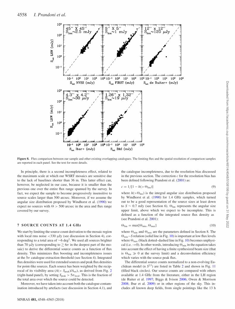
The results of this comparison are shown in Figs 8 and 9. InFig. 8, we have plotted the WSRT against the other catalogue fluxdensities for all common sources. The plot shows that, despite thedifferent intrinsic resolution of the various surveys (as indicated inthe plot panels), the WSRT flux scale is in very good agreementwith the NVSS, FIRST, de Ruiter et al. (1997) and Ibar et al. (2009)ones over the entire flux range probed by the different samples. Thisallows us to conclude that our flux calibration errors are within afew per cent, in line with expectations, and that no systematic effectshave been introduced in the image deconvolution process. On theother hand, the comparison with Biggs & Ivison (2006) shows thatour sample is characterized by systematically higher flux densities.This may be partly due to the significantly different resolution of thetwo catalogues (∼10 arcsec against 1.3 arcsec). A similar trend wasfound by Ibar et al. (2009) when comparing their catalogue with the
Biggs & Ivison one. From a detailed analysis of the two samples,Ibar et al. however concluded that the systematic differences in fluxmeasurements were to be ascribed to the different approaches usedfor the source extraction. In particular, Biggs & Ivison (2006) useda fixed beam size to fit a Gaussian to sources which were assignedareas smaller than the beam by the initial extraction procedure. Thisinevitably yields lower flux measurements (see Ibar et al. 2009 formore details).
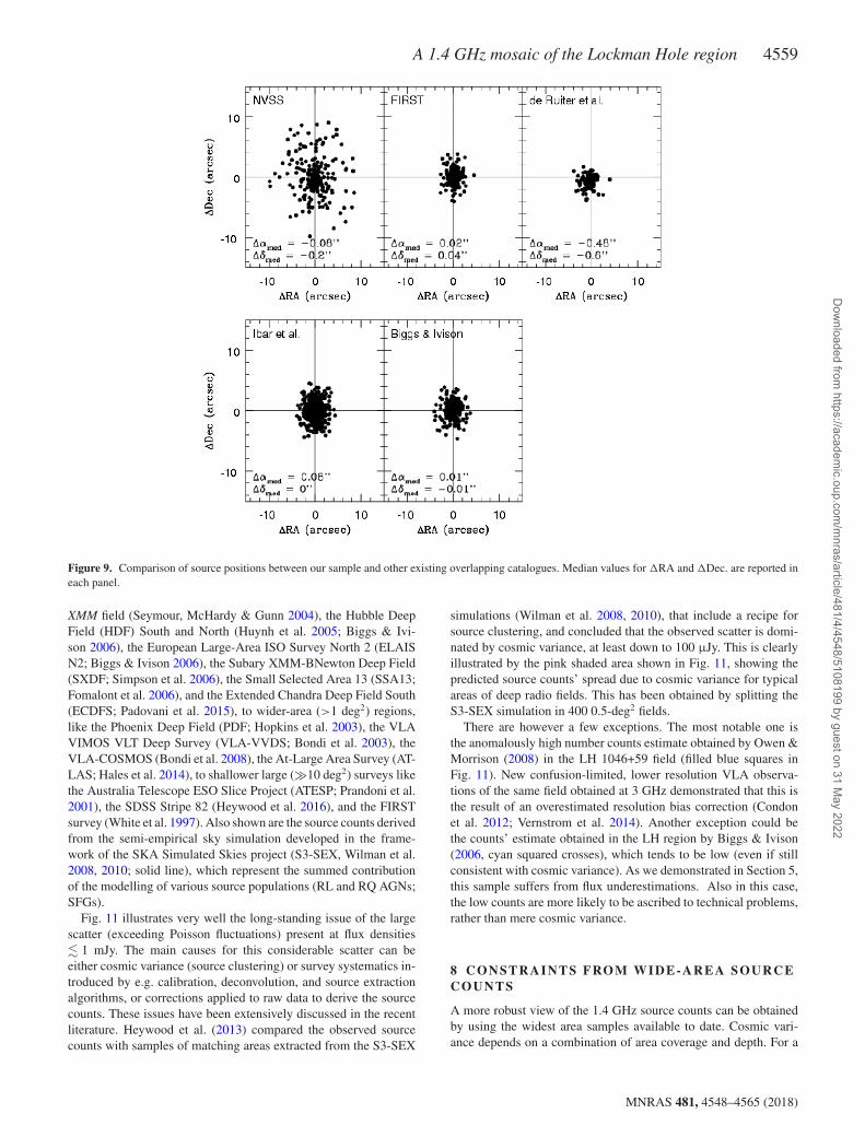
A similar comparison was repeated for source positions and theresult is plotted in Fig. 9. Again, the source positions derived forour source catalogue are in very good agreement with those derivedfor the comparison samples obtained at the VLA and with differentcalibration strategies. Systematic offsets, if present, can be con-sidered negligible (±0.01–0.1 arcsec) with respect to the intrinsicposition measurement errors of both our (see equations 7 and 8)and comparison catalogues. The only exception is represented bythe de Ruiter et al. (1997) sample, where larger systematic offsets(α = −0.5 arcsec and δ = −0.6 arcsec) are found. Howeversuch systematic errors are more likely to be ascribed to the deRuiter et al. catalogue, since no significant trend is found in thecomparison with the other samples. In summary, we can concludethat our source position calibration strategy (through the use of aVLBA secondary calibrator) was successful, and that our reductionstrategy has not introduced significant systematic offsets. This isof particular relevance for cross-identification purposes (with otherradio and/or optical/IR catalogues), which is an obvious subsequentstep for a full scientific exploitation of our sample.
6 SO U R C E SI Z E S A N D R E S O L U T I O N B I A S
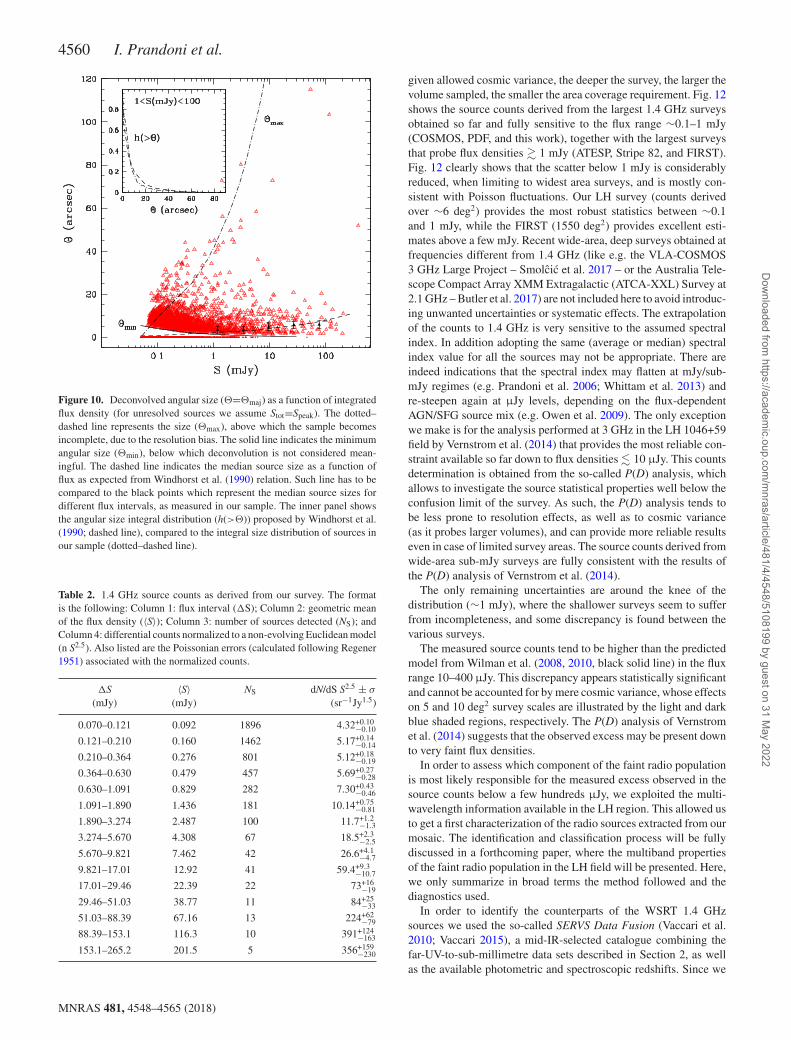
Fig. 10 shows the source Gaussian deconvolved angular sizes as afunction of flux density for our sample. The solid line in Fig. 10indicates the minimum angular size, min, below which sourcesare considered point-like, as derived from equations (1) and (2)(see Section 4.3 for more details). In general, we can successfullydeconvolve ∼60 per cent of the sources in our sample, ∼80 per centof the sources with S ≥ 0.7 mJy and ∼90 per cent of the sources withS ≥ 2.5 mJy. Above such flux limits, where we have a limited numberof upper limits, we can reliably undertake a statistical analysis ofthe source size properties. To this extent, we compare the medianangular size measured in different flux intervals for the sources withS ≥ 0.7 mJy (black points) and the angular size integral distributionderived for the sources with 1 < S (mJy) < 100 (dotted–dashedline in the inner panel) to the ones obtained from the Windhorst,Mathis & Neuschaefer (1990) relations proposed for deep 1.4 GHzsamples: med = 2 arcsec × (S1.4GHz)0.30 (S in mJy) and h(>) =exp[-ln 2 (/med)0.62]. We notice that the Windhorst et al. relationsare widely recognized to provide good statistical descriptions ofsource sizes at flux densities� 1 mJy, i.e. at the flux levels probed byour analysis. Indeed our determinations show a very good agreementwith the ones of Windhorst et al. (1990; see dashed lines in Fig. 10).
We notice that flux losses in extended sources can in principleaffect our source parametrization and cause incompleteness in thesource catalogue itself. In fact, a resolved source of given Stot willdrop below the peak flux density detection threshold more easilythan a point source of same Stot. This is the so-called resolutionbias. Equation (2) can be used to give an approximate estimate ofthe maximum size (max) a source of given Stot can have beforedropping below the Speak = 5σ local limit of the source catalogue.Such a limit is represented by the black dotted–dashed line plottedin Fig. 10. As expected, the angular sizes of the largest sourcesapproximately follow the estimated max−Stot relation.
MNRAS 481, 4548–4565 (2018)
Dow
nloaded from https://academ
ic.oup.com/m
nras/article/481/4/4548/5108199 by guest on 31 May 2022
4558 I. Prandoni et al.
Figure 8. Flux comparison between our sample and other existing overlapping catalogues. The limiting flux and the spatial resolution of comparison samplesare reported in each panel. See the text for more details.
In principle, there is a second incompleteness effect, related tothe maximum scale at which our WSRT mosaics are sensitive dueto the lack of baselines shorter than 36 m. This latter effect can,however, be neglected in our case, because it is smaller than theprevious one over the entire flux range spanned by the survey. Infact, we expect the sample to become progressively insensitive tosource scales larger than 500 arcsec. Moreover, if we assume theangular size distribution proposed by Windhorst et al. (1990) weexpect no sources with > 500 arcsec in the area and flux rangecovered by our survey.
7 SO U R C E C O U N T S AT 1 . 4 G H z
We start by limiting the source count derivation to the mosaic regionwith local rms noise <330 μJy (see discussion in Section 4), cor-responding to a total area of ∼6 deg2. We used all sources brighterthan 70 μJy (corresponding to � 6σ in the deepest part of the mo-saic) to derive the differential source counts as a function of fluxdensity. This minimizes flux boosting and incompleteness issuesat the 5σ catalogue extraction threshold (see Section 4). Integratedflux densities were used for extended sources and peak flux densitiesfor point-like sources. Each source has been weighted by the recip-rocal of its visibility area (A(> Speak)/Atot), as derived from Fig. 2(right-hand panel), by setting Speak > 5σ local. This is the fraction ofthe total area over which the source could be detected.
Moreover, we have taken into account both the catalogue contam-ination introduced by artefacts (see discussion in Section 4.1), and
the catalogue incompleteness, due to the resolution bias discussedin the previous section. The correction c for the resolution bias hasbeen defined following Prandoni et al. (2001) as:
c = 1/[1 − h(>lim)] (9)
where h(>lim) is the integral angular size distribution proposedby Windhorst et al. (1990) for 1.4 GHz samples, which turnedout to be a good representation of the source sizes at least downto S ∼ 0.7 mJy (see Section 6). lim represents the angular sizeupper limit, above which we expect to be incomplete. This isdefined as a function of the integrated source flux density as(see Prandoni et al. 2001):
lim = max[min,max] (10)
where min and max are the parameters defined in Section 8. Themin−S relation (solid line in Fig. 10) is important at low flux levelswhere max (black dotted–dashed line in Fig. 10) becomes unphysi-cal (i.e. →0). In other words, introducing min in the equation takesinto account the effect of having a finite synthesized beam size (thatis lim � 0 at the survey limit) and a deconvolution efficiencywhich varies with the source peak flux.
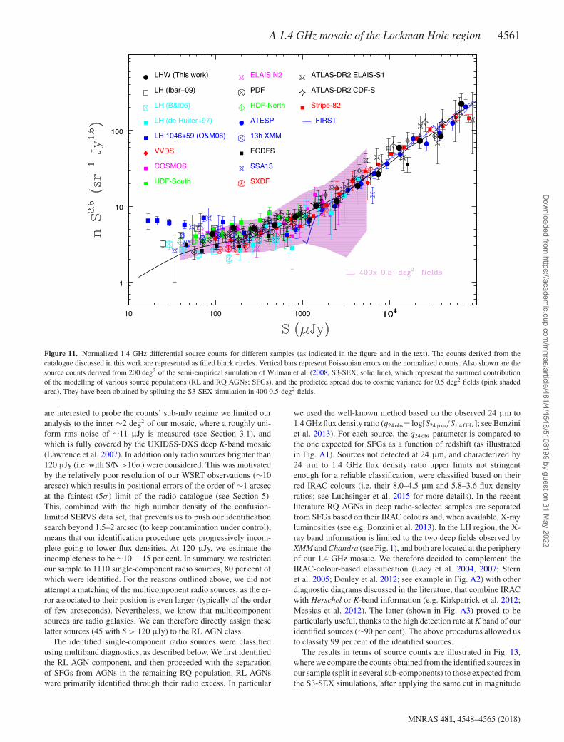
The differential source counts normalized to a non-evolving Eu-clidean model (n S2.5) are listed in Table 2 and shown in Fig. 11(filled black circles). Our source counts are compared with othersavailable at 1.4 GHz from the literature, either in the LH region(de Ruiter et al. 1997; Biggs & Ivison 2006; Owen & Morrison2008; Ibar et al. 2009) or in other regions of the sky. This in-cludes all known deep fields, from single pointings like the 13 h
MNRAS 481, 4548–4565 (2018)
Dow
nloaded from https://academ
ic.oup.com/m
nras/article/481/4/4548/5108199 by guest on 31 May 2022
A 1.4 GHz mosaic of the Lockman Hole region 4559
Figure 9. Comparison of source positions between our sample and other existing overlapping catalogues. Median values for RA and Dec. are reported ineach panel.
XMM field (Seymour, McHardy & Gunn 2004), the Hubble DeepField (HDF) South and North (Huynh et al. 2005; Biggs & Ivi-son 2006), the European Large-Area ISO Survey North 2 (ELAISN2; Biggs & Ivison 2006), the Subary XMM-BNewton Deep Field(SXDF; Simpson et al. 2006), the Small Selected Area 13 (SSA13;Fomalont et al. 2006), and the Extended Chandra Deep Field South(ECDFS; Padovani et al. 2015), to wider-area (>1 deg2) regions,like the Phoenix Deep Field (PDF; Hopkins et al. 2003), the VLAVIMOS VLT Deep Survey (VLA-VVDS; Bondi et al. 2003), theVLA-COSMOS (Bondi et al. 2008), the At-Large Area Survey (AT-LAS; Hales et al. 2014), to shallower large (�10 deg2) surveys likethe Australia Telescope ESO Slice Project (ATESP; Prandoni et al.2001), the SDSS Stripe 82 (Heywood et al. 2016), and the FIRSTsurvey (White et al. 1997). Also shown are the source counts derivedfrom the semi-empirical sky simulation developed in the frame-work of the SKA Simulated Skies project (S3-SEX, Wilman et al.2008, 2010; solid line), which represent the summed contributionof the modelling of various source populations (RL and RQ AGNs;SFGs).
Fig. 11 illustrates very well the long-standing issue of the largescatter (exceeding Poisson fluctuations) present at flux densities� 1 mJy. The main causes for this considerable scatter can beeither cosmic variance (source clustering) or survey systematics in-troduced by e.g. calibration, deconvolution, and source extractionalgorithms, or corrections applied to raw data to derive the sourcecounts. These issues have been extensively discussed in the recentliterature. Heywood et al. (2013) compared the observed sourcecounts with samples of matching areas extracted from the S3-SEX
simulations (Wilman et al. 2008, 2010), that include a recipe forsource clustering, and concluded that the observed scatter is domi-nated by cosmic variance, at least down to 100 μJy. This is clearlyillustrated by the pink shaded area shown in Fig. 11, showing thepredicted source counts’ spread due to cosmic variance for typicalareas of deep radio fields. This has been obtained by splitting theS3-SEX simulation in 400 0.5-deg2 fields.
There are however a few exceptions. The most notable one isthe anomalously high number counts estimate obtained by Owen &Morrison (2008) in the LH 1046+59 field (filled blue squares inFig. 11). New confusion-limited, lower resolution VLA observa-tions of the same field obtained at 3 GHz demonstrated that this isthe result of an overestimated resolution bias correction (Condonet al. 2012; Vernstrom et al. 2014). Another exception could bethe counts’ estimate obtained in the LH region by Biggs & Ivison(2006, cyan squared crosses), which tends to be low (even if stillconsistent with cosmic variance). As we demonstrated in Section 5,this sample suffers from flux underestimations. Also in this case,the low counts are more likely to be ascribed to technical problems,rather than mere cosmic variance.
8 C O N S T R A I N T S FRO M W I D E - A R E A SO U R C EC O U N T S
A more robust view of the 1.4 GHz source counts can be obtainedby using the widest area samples available to date. Cosmic vari-ance depends on a combination of area coverage and depth. For a
MNRAS 481, 4548–4565 (2018)
Dow
nloaded from https://academ
ic.oup.com/m
nras/article/481/4/4548/5108199 by guest on 31 May 2022
4560 I. Prandoni et al.
Figure 10. Deconvolved angular size (=maj) as a function of integratedflux density (for unresolved sources we assume Stot=Speak). The dotted–dashed line represents the size (max), above which the sample becomesincomplete, due to the resolution bias. The solid line indicates the minimumangular size (min), below which deconvolution is not considered mean-ingful. The dashed line indicates the median source size as a function offlux as expected from Windhorst et al. (1990) relation. Such line has to becompared to the black points which represent the median source sizes fordifferent flux intervals, as measured in our sample. The inner panel showsthe angular size integral distribution (h(>)) proposed by Windhorst et al.(1990; dashed line), compared to the integral size distribution of sources inour sample (dotted–dashed line).
Table 2. 1.4 GHz source counts as derived from our survey. The formatis the following: Column 1: flux interval (S); Column 2: geometric meanof the flux density (〈S〉); Column 3: number of sources detected (NS); andColumn 4: differential counts normalized to a non-evolving Euclidean model(n S2.5). Also listed are the Poissonian errors (calculated following Regener1951) associated with the normalized counts.
S 〈S〉 NS dN/dS S2.5 ± σ
(mJy) (mJy) (sr−1Jy1.5)
0.070–0.121 0.092 1896 4.32+0.10−0.10
0.121–0.210 0.160 1462 5.17+0.14−0.14
0.210–0.364 0.276 801 5.12+0.18−0.19
0.364–0.630 0.479 457 5.69+0.27−0.28
0.630–1.091 0.829 282 7.30+0.43−0.46
1.091–1.890 1.436 181 10.14+0.75−0.81
1.890–3.274 2.487 100 11.7+1.2−1.3
3.274–5.670 4.308 67 18.5+2.3−2.5
5.670–9.821 7.462 42 26.6+4.1−4.7
9.821–17.01 12.92 41 59.4+9.3−10.7
17.01–29.46 22.39 22 73+16−19
29.46–51.03 38.77 11 84+25−33
51.03–88.39 67.16 13 224+62−79
88.39–153.1 116.3 10 391+124−163
153.1–265.2 201.5 5 356+159−230
given allowed cosmic variance, the deeper the survey, the larger thevolume sampled, the smaller the area coverage requirement. Fig. 12shows the source counts derived from the largest 1.4 GHz surveysobtained so far and fully sensitive to the flux range ∼0.1–1 mJy(COSMOS, PDF, and this work), together with the largest surveysthat probe flux densities � 1 mJy (ATESP, Stripe 82, and FIRST).Fig. 12 clearly shows that the scatter below 1 mJy is considerablyreduced, when limiting to widest area surveys, and is mostly con-sistent with Poisson fluctuations. Our LH survey (counts derivedover ∼6 deg2) provides the most robust statistics between ∼0.1and 1 mJy, while the FIRST (1550 deg2) provides excellent esti-mates above a few mJy. Recent wide-area, deep surveys obtained atfrequencies different from 1.4 GHz (like e.g. the VLA-COSMOS3 GHz Large Project – Smolcic et al. 2017 – or the Australia Tele-scope Compact Array XMM Extragalactic (ATCA-XXL) Survey at2.1 GHz – Butler et al. 2017) are not included here to avoid introduc-ing unwanted uncertainties or systematic effects. The extrapolationof the counts to 1.4 GHz is very sensitive to the assumed spectralindex. In addition adopting the same (average or median) spectralindex value for all the sources may not be appropriate. There areindeed indications that the spectral index may flatten at mJy/sub-mJy regimes (e.g. Prandoni et al. 2006; Whittam et al. 2013) andre-steepen again at μJy levels, depending on the flux-dependentAGN/SFG source mix (e.g. Owen et al. 2009). The only exceptionwe make is for the analysis performed at 3 GHz in the LH 1046+59field by Vernstrom et al. (2014) that provides the most reliable con-straint available so far down to flux densities � 10 μJy. This countsdetermination is obtained from the so-called P(D) analysis, whichallows to investigate the source statistical properties well below theconfusion limit of the survey. As such, the P(D) analysis tends tobe less prone to resolution effects, as well as to cosmic variance(as it probes larger volumes), and can provide more reliable resultseven in case of limited survey areas. The source counts derived fromwide-area sub-mJy surveys are fully consistent with the results ofthe P(D) analysis of Vernstrom et al. (2014).
The only remaining uncertainties are around the knee of thedistribution (∼1 mJy), where the shallower surveys seem to sufferfrom incompleteness, and some discrepancy is found between thevarious surveys.
The measured source counts tend to be higher than the predictedmodel from Wilman et al. (2008, 2010, black solid line) in the fluxrange 10–400 μJy. This discrepancy appears statistically significantand cannot be accounted for by mere cosmic variance, whose effectson 5 and 10 deg2 survey scales are illustrated by the light and darkblue shaded regions, respectively. The P(D) analysis of Vernstromet al. (2014) suggests that the observed excess may be present downto very faint flux densities.
In order to assess which component of the faint radio populationis most likely responsible for the measured excess observed in thesource counts below a few hundreds μJy, we exploited the multi-wavelength information available in the LH region. This allowed usto get a first characterization of the radio sources extracted from ourmosaic. The identification and classification process will be fullydiscussed in a forthcoming paper, where the multiband propertiesof the faint radio population in the LH field will be presented. Here,we only summarize in broad terms the method followed and thediagnostics used.
In order to identify the counterparts of the WSRT 1.4 GHzsources we used the so-called SERVS Data Fusion (Vaccari et al.2010; Vaccari 2015), a mid-IR-selected catalogue combining thefar-UV-to-sub-millimetre data sets described in Section 2, as wellas the available photometric and spectroscopic redshifts. Since we
MNRAS 481, 4548–4565 (2018)
Dow
nloaded from https://academ
ic.oup.com/m
nras/article/481/4/4548/5108199 by guest on 31 May 2022
A 1.4 GHz mosaic of the Lockman Hole region 4561
000100101
1
10
100
LHW (This work)
LH (Ibar+09)
LH (B&I06)
LH (de Ruiter+97)
LH 1046+59 (O&M08)
VVDS
COSMOS
HDF-South
ELAIS N2
HDF-North
ATESP
13h XMM
ECDFS
SSA13
SXDF
ATLAS-DR2 ELAIS-S1
ATLAS-DR2 CDF-S
Stripe-82
FIRST
Figure 11. Normalized 1.4 GHz differential source counts for different samples (as indicated in the figure and in the text). The counts derived from thecatalogue discussed in this work are represented as filled black circles. Vertical bars represent Poissonian errors on the normalized counts. Also shown are thesource counts derived from 200 deg2 of the semi-empirical simulation of Wilman et al. (2008, S3-SEX, solid line), which represent the summed contributionof the modelling of various source populations (RL and RQ AGNs; SFGs), and the predicted spread due to cosmic variance for 0.5 deg2 fields (pink shadedarea). They have been obtained by splitting the S3-SEX simulation in 400 0.5-deg2 fields.
are interested to probe the counts’ sub-mJy regime we limited ouranalysis to the inner ∼2 deg2 of our mosaic, where a roughly uni-form rms noise of ∼11 μJy is measured (see Section 3.1), andwhich is fully covered by the UKIDSS-DXS deep K-band mosaic(Lawrence et al. 2007). In addition only radio sources brighter than120 μJy (i.e. with S/N >10σ ) were considered. This was motivatedby the relatively poor resolution of our WSRT observations (∼10arcsec) which results in positional errors of the order of ∼1 arcsecat the faintest (5σ ) limit of the radio catalogue (see Section 5).This, combined with the high number density of the confusion-limited SERVS data set, that prevents us to push our identificationsearch beyond 1.5–2 arcsec (to keep contamination under control),means that our identification procedure gets progressively incom-plete going to lower flux densities. At 120 μJy, we estimate theincompleteness to be ∼10 − 15 per cent. In summary, we restrictedour sample to 1110 single-component radio sources, 80 per cent ofwhich were identified. For the reasons outlined above, we did notattempt a matching of the multicomponent radio sources, as the er-ror associated to their position is even larger (typically of the orderof few arcseconds). Nevertheless, we know that multicomponentsources are radio galaxies. We can therefore directly assign theselatter sources (45 with S > 120 μJy) to the RL AGN class.
The identified single-component radio sources were classifiedusing multiband diagnostics, as described below. We first identifiedthe RL AGN component, and then proceeded with the separationof SFGs from AGNs in the remaining RQ population. RL AGNswere primarily identified through their radio excess. In particular
we used the well-known method based on the observed 24 μm to1.4 GHz flux density ratio (q24 obs= log[S24μm/S1.4 GHz]; see Bonziniet al. 2013). For each source, the q24 obs parameter is compared tothe one expected for SFGs as a function of redshift (as illustratedin Fig. A1). Sources not detected at 24 μm, and characterized by24 μm to 1.4 GHz flux density ratio upper limits not stringentenough for a reliable classification, were classified based on theirred IRAC colours (i.e. their 8.0–4.5 μm and 5.8–3.6 flux densityratios; see Luchsinger et al. 2015 for more details). In the recentliterature RQ AGNs in deep radio-selected samples are separatedfrom SFGs based on their IRAC colours and, when available, X-rayluminosities (see e.g. Bonzini et al. 2013). In the LH region, the X-ray band information is limited to the two deep fields observed byXMM and Chandra (see Fig. 1), and both are located at the peripheryof our 1.4 GHz mosaic. We therefore decided to complement theIRAC-colour-based classification (Lacy et al. 2004, 2007; Sternet al. 2005; Donley et al. 2012; see example in Fig. A2) with otherdiagnostic diagrams discussed in the literature, that combine IRACwith Herschel or K-band information (e.g. Kirkpatrick et al. 2012;Messias et al. 2012). The latter (shown in Fig. A3) proved to beparticularly useful, thanks to the high detection rate at K band of ouridentified sources (∼90 per cent). The above procedures allowed usto classify 99 per cent of the identified sources.
The results in terms of source counts are illustrated in Fig. 13,where we compare the counts obtained from the identified sources inour sample (split in several sub-components) to those expected fromthe S3-SEX simulations, after applying the same cut in magnitude
MNRAS 481, 4548–4565 (2018)
Dow
nloaded from https://academ
ic.oup.com/m
nras/article/481/4/4548/5108199 by guest on 31 May 2022
4562 I. Prandoni et al.
10 100 1000
1
10
100
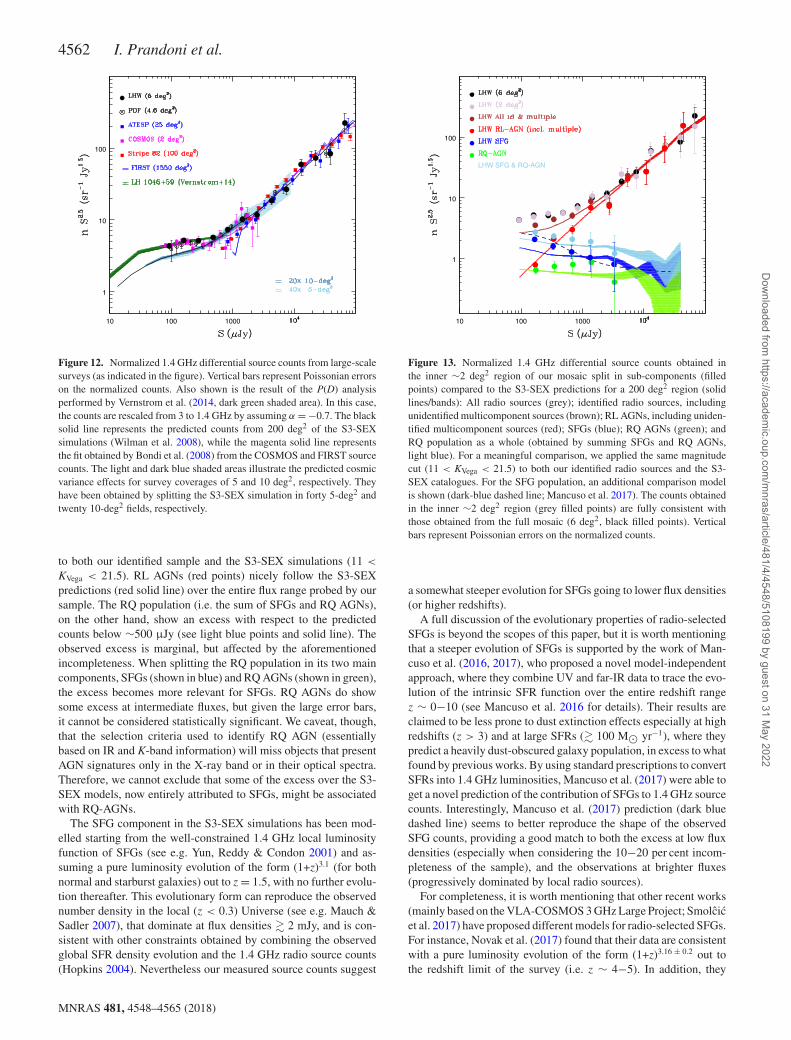
Figure 12. Normalized 1.4 GHz differential source counts from large-scalesurveys (as indicated in the figure). Vertical bars represent Poissonian errorson the normalized counts. Also shown is the result of the P(D) analysisperformed by Vernstrom et al. (2014, dark green shaded area). In this case,the counts are rescaled from 3 to 1.4 GHz by assuming α = −0.7. The blacksolid line represents the predicted counts from 200 deg2 of the S3-SEXsimulations (Wilman et al. 2008), while the magenta solid line representsthe fit obtained by Bondi et al. (2008) from the COSMOS and FIRST sourcecounts. The light and dark blue shaded areas illustrate the predicted cosmicvariance effects for survey coverages of 5 and 10 deg2, respectively. Theyhave been obtained by splitting the S3-SEX simulation in forty 5-deg2 andtwenty 10-deg2 fields, respectively.
to both our identified sample and the S3-SEX simulations (11 <
KVega < 21.5). RL AGNs (red points) nicely follow the S3-SEXpredictions (red solid line) over the entire flux range probed by oursample. The RQ population (i.e. the sum of SFGs and RQ AGNs),on the other hand, show an excess with respect to the predictedcounts below ∼500 μJy (see light blue points and solid line). Theobserved excess is marginal, but affected by the aforementionedincompleteness. When splitting the RQ population in its two maincomponents, SFGs (shown in blue) and RQ AGNs (shown in green),the excess becomes more relevant for SFGs. RQ AGNs do showsome excess at intermediate fluxes, but given the large error bars,it cannot be considered statistically significant. We caveat, though,that the selection criteria used to identify RQ AGN (essentiallybased on IR and K-band information) will miss objects that presentAGN signatures only in the X-ray band or in their optical spectra.Therefore, we cannot exclude that some of the excess over the S3-SEX models, now entirely attributed to SFGs, might be associatedwith RQ-AGNs.
The SFG component in the S3-SEX simulations has been mod-elled starting from the well-constrained 1.4 GHz local luminosityfunction of SFGs (see e.g. Yun, Reddy & Condon 2001) and as-suming a pure luminosity evolution of the form (1+z)3.1 (for bothnormal and starburst galaxies) out to z = 1.5, with no further evolu-tion thereafter. This evolutionary form can reproduce the observednumber density in the local (z < 0.3) Universe (see e.g. Mauch &Sadler 2007), that dominate at flux densities � 2 mJy, and is con-sistent with other constraints obtained by combining the observedglobal SFR density evolution and the 1.4 GHz radio source counts(Hopkins 2004). Nevertheless our measured source counts suggest
10 100 1000
1
10
100
LHW SFG & RQ-AGN
Figure 13. Normalized 1.4 GHz differential source counts obtained inthe inner ∼2 deg2 region of our mosaic split in sub-components (filledpoints) compared to the S3-SEX predictions for a 200 deg2 region (solidlines/bands): All radio sources (grey); identified radio sources, includingunidentified multicomponent sources (brown); RL AGNs, including uniden-tified multicomponent sources (red); SFGs (blue); RQ AGNs (green); andRQ population as a whole (obtained by summing SFGs and RQ AGNs,light blue). For a meaningful comparison, we applied the same magnitudecut (11 < KVega < 21.5) to both our identified radio sources and the S3-SEX catalogues. For the SFG population, an additional comparison modelis shown (dark-blue dashed line; Mancuso et al. 2017). The counts obtainedin the inner ∼2 deg2 region (grey filled points) are fully consistent withthose obtained from the full mosaic (6 deg2, black filled points). Verticalbars represent Poissonian errors on the normalized counts.
a somewhat steeper evolution for SFGs going to lower flux densities(or higher redshifts).
A full discussion of the evolutionary properties of radio-selectedSFGs is beyond the scopes of this paper, but it is worth mentioningthat a steeper evolution of SFGs is supported by the work of Man-cuso et al. (2016, 2017), who proposed a novel model-independentapproach, where they combine UV and far-IR data to trace the evo-lution of the intrinsic SFR function over the entire redshift rangez ∼ 0−10 (see Mancuso et al. 2016 for details). Their results areclaimed to be less prone to dust extinction effects especially at highredshifts (z > 3) and at large SFRs (� 100 M� yr−1), where theypredict a heavily dust-obscured galaxy population, in excess to whatfound by previous works. By using standard prescriptions to convertSFRs into 1.4 GHz luminosities, Mancuso et al. (2017) were able toget a novel prediction of the contribution of SFGs to 1.4 GHz sourcecounts. Interestingly, Mancuso et al. (2017) prediction (dark bluedashed line) seems to better reproduce the shape of the observedSFG counts, providing a good match to both the excess at low fluxdensities (especially when considering the 10−20 per cent incom-pleteness of the sample), and the observations at brighter fluxes(progressively dominated by local radio sources).
For completeness, it is worth mentioning that other recent works(mainly based on the VLA-COSMOS 3 GHz Large Project; Smolcicet al. 2017) have proposed different models for radio-selected SFGs.For instance, Novak et al. (2017) found that their data are consistentwith a pure luminosity evolution of the form (1+z)3.16 ± 0.2 out tothe redshift limit of the survey (i.e. z ∼ 4−5). In addition, they
MNRAS 481, 4548–4565 (2018)
Dow
nloaded from https://academ
ic.oup.com/m
nras/article/481/4/4548/5108199 by guest on 31 May 2022
A 1.4 GHz mosaic of the Lockman Hole region 4563
report a negative evolution of the IR/radio correlation for SFGs. Thisevolution takes the form of ∼(1+z)α , with α =−0.14 ± 0.01. Bonatoet al. (2017) claim that any evolution of the IR/radio correlationshould be mild (|α| � 0.16), as larger values would produce totalsource counts, inconsistent with the ones observed.
9 SUMMARY AND FUTURE PERSPECTIVES
In this paper, part of the LH Project, we have presented a deep1.4 GHz mosaic of the LH area obtained using the WSRT. The finalimage covers an area of 6.6 deg2, has a resolution of 11 x 9 arcsecand reaches an rms of 11 μJy beam−1 at the centre of the field.This is the widest area survey reaching such sensitivity so far. Thecatalogue extracted includes 6000 sources and it has already beenexploited in a number of studies. For instance, Mahony et al. (2016)used it in combination with LOFAR 150 MHz data and other publiccatalogues for a multifrequency radio spectral analysis of the mJyradio population in the LH region. Brienza et al. (2017) expandedthe radio spectral study to remnant radio AGNs in the same region.
The obtained source counts provide very robust statistics in theflux range 0.1 < S < 1 mJy, and are in excellent agreement withother robust determinations obtained at lower and higher flux den-sities. Indeed, when considering only wide-area surveys the sourcecounts are very well constrained down to� 10μJy. This allows us tostart using source counts to constrain source evolutionary models;something that was prevented so far, due to the long-standing issueof the large scatter present at flux densities ≤1 mJy, and mainlymotivated by cosmic variance (Heywood et al. 2013). Notably, theoverall wide-area source counts show a clear excess with respect tothe counts predicted by the semi-empirical radio sky simulations de-veloped in the framework of the S3-SEX (Wilman et al. 2008, 2010),in the flux range 10–400 μJy. This discrepancy appears statisticallysignificant and cannot be accounted for by cosmic variance.
Making use of the multiwavelength information available for theLH area, we have separated the sources in RL-AGN, RQ-AGN, andSFG and derived the source counts for these three separate groups.A preliminary analysis of the identified (and classified) sources sug-gests this excess is to be ascribed to SFGs, which seem to show asteeper evolution than predicted. The counts for RL and RQ AGN,on the other hand, appears to be in line with established models, likethose implemented in the S3-SEX simulations. A steeper evolutionof SFGs is supported by other recent observational work (e.g. No-vak et al. 2017), and in particular by the novel model-independentapproach proposed by Mancuso et al. (2016, 2017), who combineUV and far-IR data to trace the evolution of the intrinsic SFRfunction over the redshift range z ∼ 0−10. A detailed and morecomplete analysis of the evolutionary properties of the LH sources,in comparison with other observational and modelling works willbe the subject of a forthcoming paper. In the future, we also planto make use of upgraded multiband information from the HerschelExtragalactic Legacy Project (Vaccari 2016).
The unique combination of sensitivity and area coverage of theWSRT LH mosaic, makes it ideal to be used as a test case forthe exploitation of future wider area surveys obtained by new (orupgraded) radio facilities. Indeed, significantly larger but equallydeep images will be obtained using the phased-array-feed systemApertif installed now on the WSRT array (Oosterloo et al. 2009)as well as ASKAP. It is worth to notice that the large field ofview of Apertif will ensure a good match in spatial covering withLOFAR 150 MHz fields. The sensitivity of the two radio telescopesis also comparable for radio sources with typical spectral index of
−0.7 (see Shimwell et al. 2017), opening exciting perspectives forstatistical multifrequency studies of the faint radio sky.
Last but not least, new GHz telescopes like Apertif, ASKAP,and MeerKat offer broad-band capability that will allow to obtainsimultaneously radio continuum and atomic neutral hydrogen, HI-21cm, information for the sources in the redshift range sampled bythe observing band. Serendipitous H I detections in famous fields(e.g. the First Look Survey), have been already reported using datafrom traditional radio telescope like the WSRT (see Morganti et al.2004) demonstrating the feasibility. A first stacking experiment tostudy the H I in various classes of radio sources in the LH area hasalso been presented in Gereb et al. (2013). The new generation ofradio telescopes will make this a standard procedure expanding theinformation available for each class of galaxies.
AC K N OW L E D G E M E N T S
IP thanks Claudia Mancuso for providing the evolutionary trackshown in Fig. 13, which refers to the model discussed in Mancusoet al. (2017). This work has been supported by financial contributionfrom PRIN-INAF (2008) and from ASTRON. IP and MV acknowl-edge support from the Ministry of Foreign Affairs and InternationalCooperation, Directorate General for the Country Promotion (Bilat-eral Grant Agreements ZA14GR02 and ZA18GR02). RM gratefullyacknowledges support from the European Research Council underthe European Union’s Seventh Framework Programme (FP/2007-2013)/ERC Advanced Grant RADIOLIFE-320745. This work isbased on research supported by the National Research Foundationof South Africa (Grant Number 113121). The WSRT is operatedby the Netherlands Institute for Radio Astronomy ASTRON, withsupport of NWO.
REFERENCES
Abolfathi B. et al., 2018, ApJS, 235, 42ABaldwin J. A., Phillips M. M., Terlevich R., 1981, PASP, 93, 5Becker R. H., White R. L., Helfand D. J., 1995, ApJ, 450, 559Beichman C. A., Cutri R., Jarrett T., Steining R., Skrutskie M., 2003, AJ,
125, 2521Bertin E., Arnouts S., 1996, A&AS, 117, 393Biggs A. D., Ivison R. J., 2006, MNRAS, 371, 963Blundell K. M., Kuncic Z., 2007, ApJ, 668, L103Bonato M. et al., 2017, MNRAS, 469, 1912Bondi M., Ciliegi P., Schinnerer E., Smolcic V., Jahnke K., Carilli C.,
Zamorani G., 2008, ApJ, 681, 1129Bondi M. et al., 2003, A&A, 403, 857Bonzini M., Padovani P., Mainieri V., Kellermann K. I., Miller N., Rosati
P., Tozzi P., Vattakunnel S., 2013, MNRAS, 436, 3759Bonzini M. et al., 2015, MNRAS, 453, 1079Booth R. S., Jonas J. L., 2012, Afr. Skies, 16, 101Brienza M. et al., 2017, A&A, 606, 98Brunner H., Cappelluti N., Hasinger G., Barcons X., Fabian A. C., Mainieri
V., Szokoly G., 2008, A&A, 479, 283Butler A. et al., 2017, A&A, (in press)Chambers K. C., Miley G. K., Van Breugel W. J. M., Bremer M. A. R.,
Huang J.-S., Trentham N. A., 1996, ApJS, 106, 247Ciliegi P., Zamorani G., Hasinger G., Lehmann I., Szokoly G., Wilson G.,
2003, A&A, 398, 901Condon J. J., 1992, ARA&A, 30, 575Condon J. J., 1997, PASP, 109, 166Condon J. J., Cotton W. D., Greisen E. W., Yin Q. F., Perley R. A., Taylor
G. B., Broderick J. J., 1998, AJ, 115, 1693Condon J. J., Kellermann K. I., Kimball A. E., Ivezic ., Perley R. A., 2013,
ApJ, 768, 37
MNRAS 481, 4548–4565 (2018)
Dow
nloaded from https://academ
ic.oup.com/m
nras/article/481/4/4548/5108199 by guest on 31 May 2022
4564 I. Prandoni et al.
Condon J. J. et al., 2012, ApJ, 758, 23Coppin K. et al., 2006, MNRAS, 372, 1621Delvecchio I. et al., 2017, A&A, 602, A3de Ruiter H. R. et al., 1997, A&A, 319, 7Donley J. L. et al., 2012, ApJ, 748, 142Duncan K. J., Jarvis M. J., Brown M. J. I., Rottgering H. J. A., 2018b,
MNRAS, 477, 5177Duncan K. J. et al., 2018a, MNRAS, 473, 2655Fazio G. et al., 2004, ApJS, 154, 10Fomalont E. B., Kellermann K. I., Cowie L. L., Capak P., Barger A. J.,
Partridge R. B., Windhorst R. A., Richards E. A., 2006, ApJS, 167, 103Garn T. S., Green D. A., Riley J. M., Alexander P., 2008a, MNRAS, 383,
75Garn T. S., Green D. A., Riley J. M., Alexander P., 2008b, MNRAS, 387,
1037Garn T. S., Green D. A., Riley J. M., Alexander P., 2010, Bull. Astron. Soc.
India, 38, 103Gereb K., Morganti R., Oosterloo T. A., Guglielmino G., Prandoni I., 2013,
A&A, 558, A54Gonzalez-Solares E. A. et al., 2011, MNRAS, 416, 927Gopal-Krishna, Patnaik A. R., Steppe H., 1983, A&A, 123, 107Hales C. A. et al., 2014, MNRAS, 441, 2555Hasinger G., Burg R., Giacconi R., Schmidt M., Trumper J., Zamorani G.,
1998, A&A, 329, 482Hasinger G. et al., 2001, A&A, 365, L45Heckman T. M., Best P. N., 2014, ARA&A, 52, 589Herrera Ruiz N., et al., 2017, A&A, 607, 132Herrera Ruiz N., Middelberg E., Norris R. P., Maini A., 2016, A&A, 589,
L2Heywood I., et al., 2016, MNRAS, 460, 4433Heywood I., Jarvis M. J., Condon J. J., 2013, MNRAS, 432, 2625Holland W. S. et al., 1999, MNRAS, 303, 659Hopkins A. M., 2004, ApJ, 615, 209Hopkins A. M., Afonso J., Chan B., Cram L. E., Georgakakis A., Mobasher
B., 2003, AJ, 125, 465Huynh M. T., Jackson C. A., Norris R. P., Prandoni I., 2005, AJ, 130,
1373Ibar E., Ivison R. J., Biggs A. D., Lal D. V., Best P. N., Green D. A., 2009,
MNRAS, 397, 281Jarvis, M. J. et al., 2001, MNRAS, 326, 1563Johnston, S. et al., 2007, PASA, 24, 174Kimball A. E., Kellermann K. I., Condon J. J., Ivezic ., Perley R. A., 2011,
ApJ, 739, L29Kirkpatrick A. et al., 2012, ApJ, 759, 139Lacy M., Petric A. O., Sajina A., Canalizo G., Storrie-Lombardi L. J., Armus
L., Fadda D., Marleau F. R., 2007, AJ, 133, 186Lacy M. et al., 2004, ApJS, 154, 166Lawrence A., Warren S. J., Almaini O., Edge A. C., Hambly N. C., Jameson
R. F., Lucas P., Folger M., 2007, MNRAS, 379, 1599Lockman F. J., Jahoda K., McCammon D., 1986, ApJ, 302, 432Lonsdale C. J., Smith H. E., Rowan-Robinson M., Surace J., Shupe D., Xu
C., Oliver S., Serjeant S., 2003, PASP, 115, 897Luchsinger K. M. et al., 2015, AJ, 150, 87Magliocchetti M., Maddox S. J., Lahav O., Wall J. V., 1998, MNRAS, 300,
257Mahony E. K. et al., 2016, MNRAS, 463, 2997Maini A., Prandoni I., Norris R. P., Giovannini G., Spitler L. R., 2016, A&A,
589, L3Mainieri V., Bergeron J., Hasinger G., Lehmann H., Rosati P., Schmidt M.,
Szokoly G., Della Ceca R., 2002, A&A, 393, 425Mancuso C., Lapi A., Shi J., Gonzalez-Nuevo J., Aversa R., Danese L.,
2016, ApJ, 823, 128Mancuso C. et al., 2017, ApJ, 842, 95Martin D. C. et al., 2005, ApJ, 619, L1Mauch T., Sadler E. M., 2007, MNRAS, 375, 931Mauduit J.-C. et al., 2012, PASP, 124, 714Messias H., Afonso J., Salvato M., Mobasher B., Hopkins A. M., 2012, ApJ,
754, 120
Mignano A., Prandoni I., Gregorini L., Parma P., Wieringa M. H., de RuiterH. R., Vettolani G., Ekers R. D., 2008, A&A, 477, 449
Morganti R., Garrett M. A., Chapman S., Baan W., Helou G., Soifer T.,2004, A&A, 424, 371
Novak M. et al., 2017, A&A, 602, 5Ocran E. F., Taylor A. R., Vaccari M., Green D. A., 2017, MNRAS, 468,
1156Oliver S. J. et al., 2012, MNRAS, 424, 1614Oosterloo T., Verheijen M. A. W., van Cappellen W., Bakker L., Heald G.,
Ivashina M., 2009, in Torchinsky S. A. et al., eds, Wide Field AstronomyTechnology for the Square Kilometre Array, PoS(SKADS 2009)070
Owen F. N., Morrison G. E., 2008, AJ, 136, 1889Owen F. N., Morrison G. E., Klimek M. D., Greisen E. W., 2009, AJ, 137,
4846O’Dea C. P., 1998, PASP, 110, 493Padovani P., 2016, A&ARv, 24, 13Padovani P., 2017, NatAs, 1, 0194Padovani P., Bonzini M., Kellermann K. I., Miller N., Mainieri V., Tozzi P.,
2015, MNRAS, 452, 1263Padovani P., Miller N., Kellerman K. I., Mainieri V., Rosati P., Tozzi P.,
2011, ApJ, 740, 20Padovani P. et al., 2009, ApJ, 694, 235Polletta M., et al., , 2007, ApJ, 663, 81Polletta M. et al., 2006, in Wilson A., ed., ESA SP-604: The X-ray Universe
2005. ESA Publications Division, Noordwijk, p. 807Prandoni I., Gregorini L., Parma P., de Ruiter H. R., Vettolani G., Wieringa
M. H., Ekers R. D., 2000a, A&AS, 146, 31Prandoni I., Gregorini L., Parma P., de Ruiter H. R., Vettolani G., Wieringa
M. H., Ekers R. D., 2000b, A&AS, 146, 41Prandoni I., Gregorini L., Parma P., de Ruiter H. R., Vettolani G., Wieringa
M. H., Ekers R. D., 2001, A&A, 365, 392Prandoni I., Parma P., Wieringa M. H., de Ruiter H. R., Gregorini L.,
Mignano A., Vettolani G., Ekers R. D., 2006, A&A, 457, 517Regener V. H., 1951, Phys. Rev. Lett., 84, 161LRieke G. et al., 2004, ApJS, 154, 25Rottgering H. J. A., Lacy M., Miley G. K., Chambers K. C., Saunders R.,
1994, A&AS, 108, 79Rowan-Robinson M., Gonzalez-Solares E., Vaccari M., Marchetti L., 2013,
MNRAS, 428, 1958Rowan-Robinson M. et al., 2008, MNRAS, 386, 679Sault R. J., Teuben P. J., Wright M. C. H ., 1995, in Shaw R. et al., eds, As-
tronomical Data Analysis Software and Systems IV, ASP Conf. Series,77, p. 433
Seymour N., McHardy I. M., Gunn K. F., 2004, MNRAS, 352, 131Seymour N. et al., 2008, MNRAS, 386, 1695Shimwell T. W. et al., 2017, A&A, 598, A104Simpson C. et al., 2006, MNRAS, 372, 741Smolcic V. et al., 2008, ApJS, 177, 14Smolcic V. et al., 2017, A&A, 602, 1Snellen I. A. G., Schilizzi R. T., Miley G. K., de Bruyn A. G., Bremer M.
N., Rottgering H. J. A., 2000, MNRAS, 319, 445Stern D. et al., 2005, ApJ, 631, 163Vaccari M., 2015, PoS, 267, 27Vaccari M., 2016, The Universe of Digital Sky Surveys, Astrophysics and
Space Science Proc., Vol. 42. Springer International Publishing, Switzer-land, p. 71
Vaccari M. et al., 2010, A&A, 518, L20Veilleux S, Osterbrock D. E., 1987, ApJS, 63, 295Vernstrom T., Scott D., Wall J. V., Condon J. J., Cotton W. D., Kellermann
K., Perley R., 2016b, MNRAS, 462, 2934Vernstrom T., Scott D., Wall J. V., Condon J. J., Cotton W. D., Perley R.,
2016a, MNRAS, 461, 2879Vernstrom T. et al., 2014, MNRAS, 440, 2791Werner M. et al., 2004, ApJS, 154, 1White R. L., Becker R. H., Helfand D. J., Gregg M. D., 1997, ApJ, 475, 479White S. V., Jarvis M. J., Haußler B., Maddox N., 2015, MNRAS, 448, 2665White S. V., Jarvis M. J., Kalfountzou E., Hardcastle M. J., Verma A., Cao
Orjales J. M., Stevens J., 2017, MNRAS, 468, 217
MNRAS 481, 4548–4565 (2018)
Dow
nloaded from https://academ
ic.oup.com/m
nras/article/481/4/4548/5108199 by guest on 31 May 2022
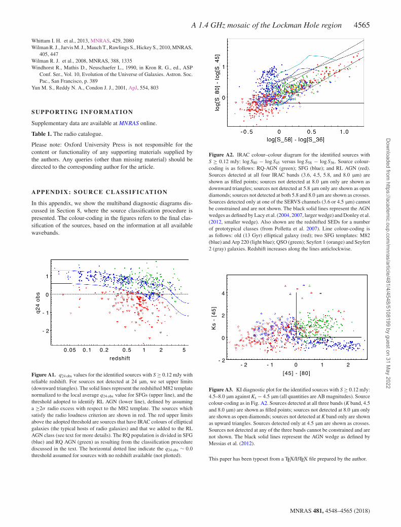
A 1.4 GHz mosaic of the Lockman Hole region 4565
Whittam I. H. et al., 2013, MNRAS, 429, 2080Wilman R. J., Jarvis M. J., Mauch T., Rawlings S., Hickey S., 2010, MNRAS,
405, 447Wilman R. J. et al., 2008, MNRAS, 388, 1335Windhorst R., Mathis D., Neuschaefer L., 1990, in Kron R. G., ed., ASP
Conf. Ser., Vol. 10, Evolution of the Universe of Galaxies. Astron. Soc.Pac., San Francisco, p. 389
Yun M. S., Reddy N. A., Condon J. J., 2001, ApJ, 554, 803
SUPPORTING INFORMATION
Supplementary data are available at MNRAS online.
Table 1. The radio catalogue.
Please note: Oxford University Press is not responsible for thecontent or functionality of any supporting materials supplied bythe authors. Any queries (other than missing material) should bedirected to the corresponding author for the article.
APPENDIX: SOURCE CLASSIFICATION
In this appendix, we show the multiband diagnostic diagrams dis-cussed in Section 8, where the source classification procedure ispresented. The colour-coding in the figures refers to the final clas-sification of the sources, based on the information at all availablewavebands.
0.05 0.1 0.2 0.5 1 2 5
redshift
- 2
- 1
0
1
q2
4 o
bs
Figure A1. q24 obs values for the identified sources with S ≥ 0.12 mJy withreliable redshift. For sources not detected at 24 μm, we set upper limits(downward triangles). The solid lines represent the redshifted M82 templatenormalized to the local average q24 obs value for SFGs (upper line), and thethreshold adopted to identify RL AGN (lower line), defined by assuminga ≥2σ radio excess with respect to the M82 template. The sources whichsatisfy the radio loudness criterion are shown in red. The red upper limitsabove the adopted threshold are sources that have IRAC colours of ellipticalgalaxies (the typical hosts of radio galaxies) and that we added to the RLAGN class (see text for more details). The RQ population is divided in SFG(blue) and RQ AGN (green) as resulting from the classification procedurediscussed in the text. The horizontal dotted line indicate the q24 obs ∼ 0.0threshold assumed for sources with no redshift available (not plotted).
Figure A2. IRAC colour–colour diagram for the identified sources withS ≥ 0.12 mJy: log S80 − log S45 versus log S58 − log S36. Source colour-coding is as follows: RQ-AGN (green); SFG (blue); and RL AGN (red).Sources detected at all four IRAC bands (3.6, 4.5, 5.8, and 8.0 μm) areshown as filled points; sources not detected at 8.0 μm only are shown asdownward triangles; sources not detected at 5.8 μm only are shown as opendiamonds; sources not detected at both 5.8 and 8.0 μm are shown as crosses.Sources detected only at one of the SERVS channels (3.6 or 4.5 μm) cannotbe constrained and are not shown. The black solid lines represent the AGNwedges as defined by Lacy et al. (2004, 2007, larger wedge) and Donley et al.(2012, smaller wedge). Also shown are the redshifted SEDs for a numberof prototypical classes (from Polletta et al. 2007). Line colour-coding isas follows: old (13 Gyr) elliptical galaxy (red); two SFG templates: M82(blue) and Arp 220 (light blue); QSO (green); Seyfert 1 (orange) and Seyfert2 (gray) galaxies. Redshift increases along the lines anticlockwise.
- 2 - 1 0 1 2
[45] - [80]
- 2
0
2
4
Ks
- [4
5]
Figure A3. KI diagnostic plot for the identified sources with S ≥ 0.12 mJy:4.5–8.0 μm against Ks − 4.5 μm (all quantities are AB magnitudes). Sourcecolour-coding as in Fig. A2. Sources detected at all three bands (K band, 4.5and 8.0 μm) are shown as filled points; sources not detected at 8.0 μm onlyare shown as open diamonds; sources not detected at K band only are shownas upward triangles. Sources detected only at 4.5 μm are shown as crosses.Sources not detected at any of the three bands cannot be constrained and arenot shown. The black solid lines represent the AGN wedge as defined byMessias et al. (2012).
This paper has been typeset from a TEX/LATEX file prepared by the author.
MNRAS 481, 4548–4565 (2018)
Dow
nloaded from https://academ
ic.oup.com/m
nras/article/481/4/4548/5108199 by guest on 31 May 2022