Four dimensional Einstein-power-Maxwell black hole solutionsin scale-dependent gravity

Angel Rincon a ∗ Ernesto Contreras b † Pedro Bargueno c ‡ Benjamin Koch d § Grigoris Panotopoulos e ¶a Instituto de Fısica, Pontificia Universidad Catolica de Valparaıso,

Avenida Brasil 2950, Casilla 4059, Valparaıso, Chile.b Departamento de Fısica, Colegio de ciencias e Ingenierıa,

Universidad San Francisco de Quito, Quito, Ecuador.c Departamento de Fısica Aplicada, Universidad de Alicante,

Campus de San Vicente del Raspeig, E-03690 Alicante, Spain.d Instituto de Fısica, Pontificia Universidad Catolica de Chile, Av. Vicuna Mackenna 4860, Santiago, Chile;

Institut fur Theoretische Physik, Technische Universitat Wien,Wiedner Hauptstrasse 8-10, A-1040 Vienna, Austria.

e Centro de Astrofısica e Gravitacao, Instituto Superior Tecnico-IST,Universidade de Lisboa-UL, Av. Rovisco Pais, 1049-001 Lisboa, Portugal.

In the present work, we extend and generalize our previous work regarding the scale dependenceapplied to black holes in the presence of non-linear electrodynamics [1]. The starting point for thisstudy is the Einstein-power-Maxwell theory with a vanishing cosmological constant in (3+1) dimen-sions, assuming a scale dependence of both the gravitational and the electromagnetic coupling. Wefurther examine the corresponding thermodynamic properties and how these quantities experiencedeviations from their classical counterparts. We solve the effective Einstein’s field equations usingthe “null energy condition” to obtain analytical solutions. The implications of quantum correctionsare also briefly discussed. Finally, we analyze our solutions and compare them to related results inthe literature.

I. INTRODUCTION

Einstein’s theory of General Relativity (GR) [2], a geo-metric theory of gravity compatible with Special Relativ-ity, is not only beautiful but also very successful as well[3, 4]. Indeed, both the classical and solar system tests[5], and a few years back the direct detection of gravi-tational waves by the aLIGO/VIRGO observatories [6]have confirmed a series of remarkable predictions of GR,including the existence of gravitational waves. In fact, aseries of additional gravitational wave events from blackhole mergers [7–10], combined with the first image of ablack hole from the Event Horizon Telescope last year[11–13], have provided us with the strongest evidence sofar that black holes (BHs) exist in nature.Despite the phenomenological success of classical GRthere are numerous open questions concerning the quan-tum nature of this theory. The quest for a theory of grav-ity that consistently incorporates quantum mechanics isstill one of the major challenges in modern theoreticalphysics. Most current approaches to the problem foundin the literature (for a partial list, see e.g., [14–22] andreferences therein), seem to share one particular prop-erty. The couplings that enter into the action definingones favorite model, such as the cosmological constant,the gravitational and electromagnetic couplings etc, be-

∗angel.rincon@pucv.cl†econtreras@usfq.edu.ec‡pedro.bargueno@ua.es§bkoch@fis.puc.cl¶grigorios.panotopoulos@tecnico.ulisboa.pt

come scale-dependent (SD) quantities at the level of aneffective averaged action after incorporating quantum ef-fects. This was to be expected in some sense that sincescale dependence at the level of the effective action is ageneric feature of ordinary quantum field theory.On the other hand, classical electrodynamics is basedon a system of linear Maxwell equations. However, asis usual in quantum physics, the effective equations be-come non-linear when quantum effects are taken into ac-count. Many decades back, and in particular in the 30’s,Euler and Heisenberg calculated QED corrections [23],while Born and Infeld managed to obtain a finite self-energy of point-like charges [24]. Those works triggeredthe interest in non-linear electrodynamics (NLE), whichhas attracted a lot of attention for several decades now,and it has been studied over the years in several differ-ent contexts. One advantage of considering non-linearelectromagnetic Lagrangians is the fact that assumingappropriate non-linear electromagnetic sources, which inthe weak field limit are reduced to the usual Maxwell’slinear theory, one can generate a new class of Bardeen-like [25, 26] BH solutions [27–34] with certain desirableproperties. In particular, those solutions, on the onehand, do have a horizon, which is the defining property ofBHs, and, on the other hand, their curvature invariants,such as the Ricci or the Kretschmann scalar, are regu-lar everywhere. This is to be contrasted to the standardReissner-Nordstrom solution [35], which is characterizedby a singularity at the origin.Finally, Maxwell’s theory may be easily generalized ina straightforward manner by a simple model called theEinstein-power-Maxwell (EpM) theory [36–46]. In thistoy model, the theory is described by a Lagrangian den-

2

sity of the form L(F ) ∼ F β , where β is an arbitrary ratio-nal number, F ≡ FµνFµν is the Maxwell invariant, withFµν ≡ ∂µAν − ∂νAµ being the field strength, and Aµ isthe Maxwell potential. Even more, although our observ-able Universe seems to be four-dimensional, the question”How many dimensions are there?” is one of the funda-mental questions that modern High Energy Physics triesto answer. Kaluza-Klein theories [47, 48], Supergravity[49] and Superstring/M-Theory [50, 51] have pushed for-ward the idea that extra spatial dimensions may exist.The advantage of the EpM theory is that it preservesthe nice conformal properties of the four-dimensionalMaxwell’s theory in any number of space-time dimension-ality d, provided the power β is chosen to be β = d/4,as it is easy to verify that for this particular value theelectromagnetic stress-energy tensor becomes traceless.In black hole physics, the impact of the SD scenario onproperties of BHs has been studied over the last years,and it has been found that the scale dependence modifiesthe horizon, the thermodynamics, as well as the quasi-normal spectra of classical BH backgrounds [1, 52–58].To the best of our knowledge, however, the impact of theSD scenario on four-dimensional charged black holes inthe EpM theory has not been studied yet. In the presentwork, we propose to study for the first time the prop-erties of scale-dependent BHs with a net electric chargein the EpM non-linear electrodynamics with a two-foldgoal in mind. First, to fill a gap in the literature and,second, to make a direct comparison between i) SD BHsin the EpM theory versus their four-dimensional classicalcounterparts, and ii) the results obtained in the SD sce-nario versus those obtained by Renormalization Group(RG hereafter) improvement methods.

It is well-known that properties of physical systems de-pend on the dimensionality of space-time, see e.g. [59] forHawking radiation from higher-dimensional black holes,and [60] for quasi-normal modes of black holes in Gauss-Bonnet gravity. Therefore, although EpM theory is bet-ter motivated in dimensions other than four, we still feelit would be interesting to see how the properties of blackholes in this class of non-linear Electrodynamics changeas we move from three to four dimensions.

Our work in the present article is organized as follows:In the next section, we review the classical EpM the-ory, while in section 3, we briefly present the BH solu-tions within EpM non-linear electrodynamics for arbi-trary power β. In the fourth section, we comment on thenull energy condition, an essential ingredient of the SDscenario. After that, in section 5, we discuss the prop-erties of the SD charged BHs in four-dimensional EpM,and a comparison with the results produced by RG im-provement methods is made as well. We finish our workwith some concluding remarks in the last section.

II. CLASSICAL EINSTEIN-POWER-MAXWELLTHEORY

This section is devoted to introducing a particular typeof NLE that we are interested in. To be more precise, wewill use the well–known EpM theory. First, we rememberthat the standard Maxwell contribution to the action isdefined as F ≡ FµνFµν/4. This solution has been ex-tensively studied in the context of black holes in (2+1),(3+1), and in general in d dimensional space-time. Anapparently more complicated contribution to the actionis obtained allowing powers of the aforementioned invari-ant, namely, now we accept a Lagrangian density of theform: L(F ) ≡ D1F +D2F

2 +D3F3 + · · ·+DnF

n. ThisLagrangian density is not easy to investigate because, ingeneral, it does not give exact solutions. A more treatableway to make progress is to take into account the specialcase L(F ) = Dβ |F |β , being D a constant with appropri-ate units and β a free dimensionless parameter.Those theories will then be investigated in the context ofscale-dependent couplings. Thus, we will start consider-ing the so–called EpM action without cosmological con-stant (Λ0 = 0), assuming the aforementioned Lagrangiandensity, namely

I0[gµν , Aµ] ≡∫

d4x√−g[

1

2κ0R− 1

e2β0

L(F )

], (1)

where the parameters are defined as follow: κ0 ≡ 8πG0 isthe gravitational coupling, G0 is the dimensionful New-ton’s constant, e0 is the dimensionful electromagneticcoupling constant, R is the Ricci scalar and F has theusual meaning. We use the metric signature (−,+,+,+),and natural units (c = ~ = kB = 1) such that the actionis dimensionless. The power β also appears in the ex-ponent of the electromagnetic coupling. This inclusionis justified because we need to maintain the action di-mensionless. On the one hand, this generalized actionalso contains the classic Einstein-Maxwell case after thereplacement β = 1. On the other hand, one can obtaindeformed Maxwell solutions when β 6= 1. In what fol-lows, we shall consider the general case, namely, whenβ is taken to be an arbitrary parameter. It is essentialto point out that this generalization should recover theclassical case, at least at a certain limit. At this pointwe could consider a (naive) range β ∈ R+ [74], but oursolution could have restrictions on the values of the pa-rameter β.In the context of SD gravity in the presence of NLE, thecorresponding equations of motion are

Gµν =κ0

e2β0

Tµν . (2)

The energy-momentum tensor Tµν is associated to theelectromagnetic field strength Fµν through

Tµν ≡ TEMµν = L(F )gµν − LFFµγFν γ , (3)

3

remembering that LF = dL/dF . Besides, for staticspherically symmetric solutions the electric field E(r) isgiven by

Fµν = (δrµδtν − δrνδtµ)E(r). (4)

The variation of the classical action with respect to thefield Aµ(x) gives simply

Dµ

(LFFµν

e2β0

)= 0, (5)

where e2β0 is a constant. Combining Eq. (2) with

Eq. (5) we are able to determine the set of functions{f0(r), E0(r)}. Also, it is important to point out that theclassical version of this problem was certainly discussedbefore [74] as well as the corresponding SD Einstein-Maxwell case in (3+1) dimensions [75]. In both cases,the thermodynamic and the asymptotic properties wereinvestigated in detail.

III. BLACK HOLE SOLUTION FOREINSTEIN-MAXWELL MODEL OF ARBITRARY

POWER

The general metric ansatz assuming spherical symmetryis given by

ds2 = −f0(r)dt2 + g0(r)dr2 + r2(dθ2 + sin2(θ)dφ2

), (6)

where f0(r) and g0(r) are the metric functions and canbe linked via the Schwarzschild relation, i.e. g0(r) =f0(r)−1. In GR, one only computes the electric fieldE0(r) and the lapse function f0(r) only by solving: i)the Einstein field equations and ii) the equation obtainedafter the variation of the classical action respect the po-tential Aµ. For practical purposes, we will summarizethe classical solutions for an arbitrary index, β. Solv-ing the Einstein field equations for the classical case weobtain:

f0(r) = 1 +C

r+B

rα, (7)

E0(r) =A

rα, (8)

where the power α is linked to the power-Maxwell expo-nent as follows

α =2

2β − 1, (9)

and the case β = 1/2 is excluded from the solution. The

pair {A, C} are constants of integration directly relatedto the electric charge and the mass, respectively, of theblack hole, while B is given in terms of A as follows[74]

B ≡ κ0

(− 2A2D

)β (1− 2β)2

(2β − 3). (10)

Furthermore, A is identified with the electric charge, Q0,while C = −2G0M0 is proportional to the mass of theblack hole, M0. Throughout the manuscript, all clas-sical quantities carry a sub-index ”0”, whereas scale-dependent quantities carry no sub-indices. Clearly, inthe special case β = 1 and α = 2 the usual Reissner-Nordstrom (RN) black hole solution is recovered.

It is important to point out that M0 is the ADM/Komarmass of the black hole. The ADM mass is defined viathe ADM formalism at spatial infinity only. In practice,it is read off from the decay of g00; the Komar mass isdefined as a flux integral associated to the stationarity,and it can be computed at any closed 2-surface in a space-like surface. The Komar mass coincides with the ADMmass in the case of asymptotically flat space-times, suchas the RN geometry.

Furthermore, we observe two natural ranges that respectthe exponent α, i.e., whether or not 1/rα goes faster tozero than the Schwarzschild potential 1/r. Regarding BHthermodynamics, we first should compute the classicalhorizon, r0,which is obtained demanding that f0(r0) = 0.By writing the lapse function in terms of the horizons,we have

f0(r) =

[1− rA

r

][1−

[1− rA

rB

1− rAr

] [ rAr −

(rAr

)αrArB−(rArB

)α]]. (11)

Firstly, notice that these horizons, {rA, rB}, can belinked to the BH mass and electric charge. Also, theclassical BH horizon is the outer root of the lapse func-tion, i.e., r0 ≡ max{rA, rB}. Given the non-trivial formof the lapse function, it is impossible to obtain the corre-sponding roots for an arbitrary index α, reason why wewrite it down implicitly. Also, to get insights into thismodel, it is always useful to study some thermodynamicproperties. We can then define three quantities, i. e., theHawking temperature, TH , the Bekenstein-Hawking en-tropy, S, and the specific heat, CQ. Their correspondingexpressions are given as follow

T0(r0) =1

4π

∣∣∣∣∣ limr→r0

∂rgtt√−gttgrr

∣∣∣∣∣, (12)

S0(r0) =A0

4G0, (13)

C0(r0) = T∂S

∂T

∣∣∣∣∣r0

, (14)

being A0 the horizon area defined as

A0 =

∮d2x√h = 4πr2

0, (15)

where hij is the induced metric at the horizon, r0.

4

IV. SCALE DEPENDENT COUPLING ANDSCALE SETTING

This section is devoted to summing up the main featuresand equations of motion for the SD EpM theory with anarbitrary index in four dimensions. The idea and spiritfollow references [93–102]. and references therein. Inthe SD formalism, the couplings evolve with the energyscale. In our case, we have two coupling functions toconsider, i. e., i) the Newton’s coupling Gk (which isrelated to the gravitational coupling by κk ≡ 8πGk), andii) the electromagnetic coupling, 1/ek. Besides, thereare three independent fields, which are the metric ten-sor, gµν(x), the electromagnetic four-potential, Aµ(x),and the scale field, k(x), where xµ ≡ x is any space-timepoint. Notice that in Schwarzschild coordinates we canwrite: xµ = {t, r, θ, φ}, and due to the spherical symme-try all quantities depend on the radial coordinate only,e.g. k(r).The effective action for this theory takes the form

Γ[gµν , Aµ, k] =

∫d4x√−g[

1

2κkR− 1

e2βk

L(F )

]. (16)

Following the same strategy used in the non-improvedcase, we can obtain the equation of motion by taking thevariation of (16) with respect to gµν(x), namely

Gµν =κk

e2βk

T effµν , (17)

where the effective energy-momentum tensor is definedin such a way that the classical contribution is shiftedby the inclusion of the Newton’s scale-dependent cou-pling:

T effµν = TEM

µν −e2βk

κk∆tµν . (18)

To be more precise, TEMµν is given by (3) and the extra

contribution ∆tµν is

∆tµν = Gk

(gµν�−∇µ∇ν

)G−1k . (19)

Equivalently, the equations of motion for the four-potential Aµ(x) when the electromagnetic couplingevolves take the following form

Dµ

(LFFµν

e2βk

)= 0. (20)

At this level, some comments are in order. As we pre-viously said, the SD scenario takes advantage of asymp-totically safe gravity. In particular, in any quantum fieldtheory, the renormalization scale k has to be set to aquantity characterizing the physical system under consid-eration. Thus, for background solutions of the gap equa-tions, the renormalization scale can evolve. However, the

price to pay is that the set of equations of motion doesnot close consistently. The latter means that the energy-momentum tensor could not be conserved for almost anychoice of the functional dependence k = k(x), being xan arbitrary coordinate. Also, an appropriated choiceof x depends of the symmetry and the problem itself,so, such identification will be specified later. Also, suchfeature was also extensively investigated in the contextof renormalization group improvement of BHs in asymp-totic safety scenarios [103–119]. The loss of conservationlaws comes from the fact that there is one consistencyequation missing.

Varying the effective action (16) with respect to the scalefield k(x) we can find the missing equation, i.e.

d

dkΓ[gµν , Aµ, k] = 0, (21)

which can be considered as as variational scale settingprocedure [99, 120–123]. To achieve the conservation ofthe stress-energy tensor, we can combine Eq. (21) withthe above equations of motion. Further details regardingthe split symmetry within the functional renormalizationgroup equations support this approach of dynamic scalesetting can be found in [124]. Now, it should be noticedthat the implementation of the variational procedure (21)requires the knowledge of the corresponding β-functionsof the problem. This, however, is a strong disadvantagebecause those are not unique. Thus, to by-pass such aproblem, we will close our system by adding a constrainton one energy condition. The latter has also been usedin some concrete BH solutions [94, 95, 97, 98, 125–127].We then adopt the same route by imposing the so-callednull energy condition (NEC) to study EpM BHs in fourdimensions.

V. THE NULL ENERGY CONDITION

To close our system, we need to select a supplementarycondition. As we have treated in previous works, we willtake advantage of the so-called NEC. In general, an en-ergy condition is an extra relation that we impose onthe energy-momentum tensor to try to capture the ideathat energy should not be negative [128]. We usuallyhave four energy conditions: i) dominant, ii) weak, iii)strong, and finally, iv) the NEC. In a well-defined prob-lem in GR, such restrictions are satisfied, although insome other cases, they can be violated [129, 130].

It is also remarkable that the NEC is a critical ingre-dient in the Penrose singularity theorem [131]. Giventhat our solutions belong to an extension of GR, it isalso suitable to maintain at least one energy condition.In such a sense, the NEC is the less restrictive of them.Assuming as valid the classical NEC, we always have asingularity. Thus, any contracting Universe ends up in asingularity, provided its spatial curvature is dynamicallynegligible [130]. NECs can even be extended to quantum

5

formulations [132, 133]. Given the relevance and partic-ular beauty of the NEC, we will focus our attention onit. Our starting point is to consider certain null vector,called `µ, and to contract it with the matter stress energytensor as the NEC demands, i. e. :

Tmµν`µ`ν ≥ 0. (22)

The latter strategy was also used in Ref. [94] inspiredby Jacobson’s idea [134] on getting acceptable physicalsolutions. Besides, the relevance of the NEC becomesnotorious when we recognize that such a condition isnot optional in proving some fundamental BH theorems,such as the no-hair theorem [135], and the second lawof black hole thermodynamics [136]. In the SD scenariowe maintain the same condition in a more restrictive andthus more useful form by making the inequality an equal-ity

T effµν `

µ`ν =

(TEMµν −

e2βk

κk∆tµν

)`µ`ν = 0. (23)

For the null vector we choose a radial null vector `µ ={f−1/2, f1/2, 0}. Since the electromagnetic contributionto the effective stress energy tensor (3) satisfies the NEC(23) by construction, the same has to hold for the ad-ditional contribution introduced due to the SD of thegravitational coupling:

∆tµν`µ`ν = 0. (24)

VI. SCALE DEPENDENTEINSTEIN-POWER-MAXWELL THEORY

A. Solution

Now, we will compute the solutions for our SD system ofdifferential equations. In classical BH solutions, we needto find the lapse function and the electric field. Instead,we need to compute the same functions in the SD BH ver-sion and the corresponding Newton and electromagneticcouplings. Thus, we can sum up it as follows:

{f0(r), E0(r), G0, e0} → {f(r), E(r), G(r), e(r)} (25)

Notice that in Schwarzschild coordinates we can write:xµ = {t, r, θ, φ}, and then due to spherical symmetryxµ = r only. The first step to find the full solution is tocalculate Newton’s coupling. We first solve it because, inpractice, when the NEC is used, the differential equationfor G(r) is not coupled to the rest of the functions. Wecan then solve it directly. The differential equation iswritten as

G(r)d2G(r)

dr2− 2

(dG(r)

dr

)2

= 0, (26)

which allows us to obtain

G(r) =G0

1 + εr, (27)

after a suitable choice of integration constants. Be awareand notice that the constant ε encodes quantum features;therefore, the classical solution is recovered when ε goesto zero. The second step is to solve the equation of mo-tion for the 4-potential given by Eq. (20).

dE(r)

dr−

[(1 +

1

2α

)e′(r)

e(r)− α

r

]E(r) = 0. (28)

In light of the radial dependency of the electric field,the differential equation can also be solved directly toget

E(r) = A

[e(r)(1+ 1

2α)

rα

]. (29)

At this level, we would like to clarify the meaning of someof the integration constants. Firstly, we introduce the so-called running parameter, ε, which controls the strengthof the scale dependence; G0 is the classical Newton’s cou-pling constant and, finally, A is a coupling constant whichcontrols the strength of the electric field. Solving forthe remaining function f(r) and e(r) we obtain the non-trivial solutions

f(r) =1

6(1 + εr)−(1+ 1

2α)

[6B

rα− (−εr)−α

3α+ 2×

×

{(4α(α+ 1) + ε(6(3α+ 2)C

+ (3α− 2)(7α+ 4)r) + 3α(3α− 2)r2ε2)

×B−rε(α− 1, 1 +

1

2α

)− α(1 + εr)×

×(α(3rε+ 4) + 4

)B−rε

(α− 1,

1

2α

)}],

(30)

e(r)(1+ 12α) = W0

(1 + εr)−α2−2

r×

×

[W0(r, ε) +

rα+1(−rε)−α

3α+ 2×

×

{W1(r, ε)B−rε

(α− 1, 1 +

1

2α

)

+ W2(r, ε)B−rε

(α− 1,

1

2α

)}],

(31)

where we have defined the intermediate functionsas

W0 ≡2

1α−

132 α

3πG0

(AD

12

)−(α+2α )

, (32)

6

1 2 3 4 5-3

-2

-1

0

1

r

f(r)

1 2 3 4 5-0.2

0.0

0.2

0.4

0.6

r

f(r)

1 2 3 4 510

15

20

25

30

r

e2(r)

1 2 3 4 520

40

60

80

100

120

140

r

e5/2(r)

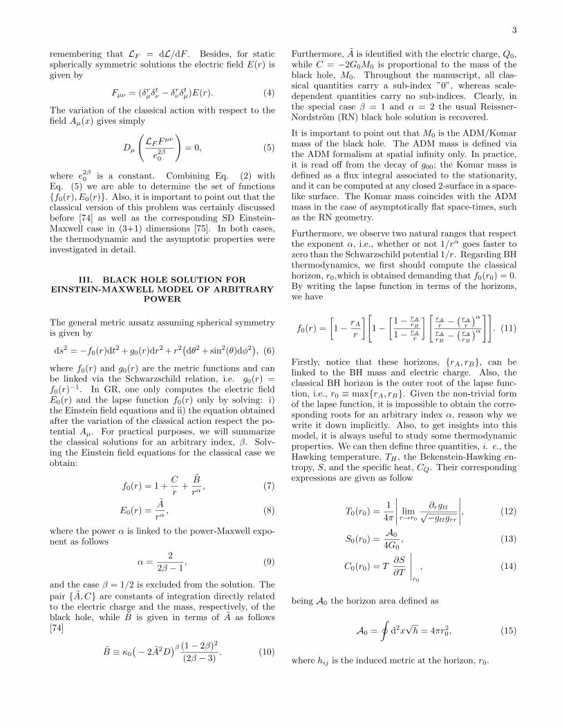
FIG. 1: The lapse function f(r) and the electromagnetic coupling e(r)1+12α versus radial coordinate r for two concrete cases.

The first line correspond to the lapse function while the second line correspond to the electromagnetic coupling. The first (left),and second (right) column correspond to the cases α = {2, 3} respectively. We show the classical model (solid black line) andthree different cases for each figure: i) ε = 0.033 (dashed blue line), ii) ε = 0.067 (dotted red line) and iii) for ε = 0.010 (dotteddashed green line). We have used the set {Q0, e0, G0,M0} = {1, 1/(2

√π), 1/(16π2), 32π2} . The numerical values of the event

horizon are: i) for α = 2, {rH(ε = 0), rH(ε = 0.033), rH(ε = 0.067), rH(ε = 0.010)} = {3.73204, 3.52496, 3.35651, 3.21518} andii) for α = 3, {rH(ε = 0), rH(ε = 0.033), rH(ε = 0.067), rH(ε = 0.010)} = {1.61803, 1.57659, 1.539, 1.50465}.

W0(r, ε) ≡ 6Br(α(3rε+ 2)2 − 2(3rε(rε+ 2) + 2)

)−

2rα(rε+ 1)α2 +1(6C(3rε+ 2)+ (33)

r(3α(rε+ 2)(3rε+ 2)− 4(3rε(rε+ 3) + 5))),

W1(r, ε) ≡ 4α(3rε+ 1)(6ε(C + r)− 3r3ε3 + 4

)+

2α2ε(2r(9rε(3rε(rε+ 4) + 14) + 41)− (34)

9C(3rε+ 2)2)) + 8ε(3C(3rε(rε+ 2) + 2)−2r(2rε+ 1)(3rε+ 4))− α3(3rε+ 2)2×(3rε(3rε+ 7) + 4),

W2(r, ε) ≡ α(rε+ 1)(α2(3rε+ 4)(3rε+ 2)2 − 6αrε (35)

× (rε(3rε+ 10) + 6)− 16(rε+ 1)(3rε+ 1)).

The solution is expressed in terms of the incomplete Betafunction Bz(a, b) defined as

Bz(a, b) ≡∫ z

0

dτ τa−1(1− τ)b−1. (36)

In particular, notice that Bz(a, b) has a branch cut dis-continuity in the complex z plane running from −∞ to 0.Similarly Bz(a, b) can also be defined as follows:

Bz(a, b) = za∞∑n=0

(1− b)nn!(a+ n)

zn, (37)

where (· · · )n is the Pochhammer symbol, i.e.

(· · · )n =Γ(x+ n)

Γ(x). (38)

An interesting case appears when z = 1. In such circum-stance, the incomplete beta function Bz(a, b) becomes tothe usual beta function B(a, b).

B. Setting the integration constants

Up to now, our generalized SD solution has a few ar-bitrary constants. To obtain them, we usually demand

7

that the new solution should converge to the classicalone when ε is taken to be zero. We must emphasize thenumber of integration constants involved in the problem.Analogously to the lower-dimensional case, the SD grav-itational coupling introduces two of them. In this case,they are the classical Newton’s constant G0 and the run-ning parameter ε. Also, the electromagnetic field showsan additional integration constant A, and the solution ofthe lapse function is parametrized by two additional in-tegration constants B and C. As was pointed out above,B and C are related to the electric charge and classicalmass, respectively, and the value A is connected to theconventional charge. Taking the limit when ε → 0 wehave

limε→0

f(r) = f0(r) = 1 +C/(α− 1)

r+B

rα,

limε→0

E(r) = E0(r) = A

[ξ1+ 1

2α

rα

],

limε→0

G(r) = G0, (39)

limε→0

e(r)1+ 12α = ξ1+ 1

2α ≡ Bα(α− 1)

16πG0

[A

[D

2

] 12

]−α+2α

.

Also, for Maxwell electrodynamics (α = 2) we recoverthe well-known family of solutions, i.e.,

limε→0

f(r) = f0(r) = 1 +C

r+B

r2,

limε→0

E(r) = E0(r) = A

[ξ2

r2

],

limε→0

G(r) = G0, (40)

limε→0

e(r)2 = ξ2 =B

4πG0A2D.

We can now take advantage of the SD Maxwell BH solu-tion previously obtained in [127]. Following that setting,

we take the parameters {A, B, C,D} as follow

A =Q2

0

4πe20

, (41)

B =4πG0

e20

Q20, (42)

C = −2G0M0, (43)

D =1

Q20

. (44)

Thus, we will finally have the set {G0, e0, Q0,M0, ε}.Also, we can observe how the running of the gravitationalcoupling distorts the solution.

To get some insights, we expand the solution for smallvalues of the running parameter ε up to second-order to

obtain to get

f(r) ≈ f0(r) +

(α2 − 1

)rε((3α+ 4)rε− 2(α+ 2))

2(α− 1)(α+ 1)(α+ 2)

+1

8Br−α((α+ 2)rε((α+ 4)rε− 4) + 8)

+C(4(α+ 1) + 3(3α+ 2)r2ε2 − 6(α+ 1)rε

)4(α− 1)(α+ 1)r

,

(45)

and

e(r)1+ 12α ≈ ξ1+ 1

2α

24(α− 1)Br

[2Zrα

2 + α− 2α2 − α3+ Y

],

(46)

where Y ≡ Y (r, ε) and Z ≡ Z(r, ε) are supplementaryfunctions defined as

Z(r, ε) = 6(α+ 2)C(α2(rε− 2)(rε+ 1) + rε(1− 4rε) + 2

)+(α2 − 1

)r(−4(α+ 2)(3α− 5) + (α(3α+ 2)

− 44)r2ε2 − 4(α+ 2)(3α− 4)rε), (47)

Y (r, ε) = 3Br(8(α− 1) + (α− 3)(α− 2)(α+ 2)r2ε2−

4(α− 2)(α− 1)rε)+2rα

(6C(rε− 2)(rε+ 1)+

(3α− 4)r2ε(rε− 4) + 4(5− 3α)r). (48)

Finally, the electric field and Newton’s coupling take theform

E(r) ≈ Aξ1+ 12α

24(α− 1)Br1+α

[2Zrα

2 + α− 2α2 − α3+ Y

],

(49)

G(r) ≈ G0

(1− (εr) + (εr)2

). (50)

It is essential to point out that certain values of the powerα are not allowed. We read-off those values from the cor-responding lapse function. Firstly, α = 1 is excludedfrom the solution to satisfy the classical solution. Afterthat, the SD lapse function has other problematic pointsto be excluded from the general solution. Thus, α = −1and α = −2 are ignored too. To show the lapse function’sbehavior, we will take benchmarks to get insights aboutthe underlying physics. Fig (1) can be observed the be-havior of the lapse function and the electromagnetic cou-pling for different values of the parameter α.

VII. INVARIANTS

In this part, we will briefly summarize how the Ricciscalar looks like when Newton’s coupling constant be-comes SD in light of an EpM source. The Kretschmannscalar is optional in this case, the reason why we willomit such a computation. Thus, the Ricci scalar take

8

the complicated form

R =1

24(3α+ 2)

[r−α−3(−rε)−α(rε+ 1)−

α2−3

× (2(−rε)α(rα(rε+ 1)α2 +1(6(3α+ 2)C(2α+ 3αrε− 4)

+ r(4(α− 2)(α(9α− 17)− 14) + 3(α(9α2 − 30α+ 40)

+ 16)r2ε2 + 8(α(3α(3α− 8) + 25) + 16)rε))

− 3(3α+ 2)Br(α2(3rε+ 2)2 − 6α(rε(rε+ 4) + 2) + 8))

+ rα+1((16(α− 2)(α− 1)α(α+ 1) + (3α− 2)r2ε3

× (18α(3α+ 2)C + (3α− 4)(α(33α− 50)− 8)r)(51)

+ 4rε2(18(α− 2)α(3α+ 2)C + (3α− 2)(α(α(27α

− 83) + 34) + 24)r) + 4(α− 2)ε(6(α− 1)(3α+ 2)C

+ (α(α(33α− 53)− 2) + 24)r) + 9(α− 2)α(3α− 4)

× (3α− 2)r4ε4)B−rε

(α− 1,

α

2+ 1)−α(rε+ 1)

× (α3(3rε+ 2)2(3rε+ 4)− 2α2(rε(3rε(15rε+ 32)

+ 70) + 16) + 8α(rε(rε(9rε+ 13) + 1)− 2)

+ 32(rε+ 1)2)B−rε

(α− 1,

α

2

)))

].

Also, notice that, different from the classical case, α =−2/3 makes that the Ricci scalar blows up. Besides, asthe incomplete beta functions are present, negative val-ues of α should be ignored to maintain a non-singularRicci scalar. The classical case can be recovered demand-ing that ε→ 0 to get

R0 ≡ limε→0

R = − B

rα+2(α− 2)(α− 1). (52)

Finally, the Einstein-Maxwell solutions are obtainedwhen α = 2 to achieve a null scalar.

VIII. HORIZON AND THERMODYNAMICS

This section is dedicated to reviewing the main thermo-dynamic properties in the SD scenario. Some details tothe computation of the corresponding thermodynamicsproperties can be consulted,for instance, in [141].

A. Black hole horizon

An essential ingredient to analyze the correspondentthermodynamics is the BH horizon. Thus, the horizonwhere the temperature, entropy, and capacity heat areevaluated is precisely the reason why it will compute it.The BH horizon is found by demanding that f(rH) = 0.In the simplest cases, we might obtain the explicit formof rH . In this case, however, such a task is not possibleto achieve. That problem is indeed present in the clas-sical solution for an arbitrary EpM index. Even though,

when the arbitrary index is fixed, we could then obtain atractable lapse function and an analytical expression forthe horizon. Now, in the SD solution, we will take twoconcrete cases: α = {2, 3}, to show their behavior. Ascan be observed in Fig. (2) (left panel) the BH horizondecreases when the running parameter increases. Thelatter can be confirmed by taking, for instance, α = 2and the running parameter close to zero, namely:

rH(α = 2) = r0

[1− 1

2εr0 +O(ε2)

], (53)

where r0 is the classical BH horizon. We then confirmthat the SD BH horizon is smaller than its classical coun-terpart, its major deviation appearing when εr0 is signif-icant compared to unity. In Fig. (1) we have added thenumerical values of the event horizon for reference. Wehave also checked, and a second-order expansion in ε isenough to make the exact value and the approximatedvalue quite close. Be aware and notice that, for a givenvalue of α, the classical BH mass should be related tothe other parameters of the theory. To be more precise,it should satisfy:

M ≥

(

4πQ20

e20G0

)1/2

if α = 2,(27πQ2

0

e20G20

)1/3

if α = 3,(54)

for the classical solution. The latter bounds are obtainedto bypass troubles due to the appearance of naked singu-larities in the classical solution. It should also be pointedout that the classical black hole mass is not obtainedusing the counter-term method or the Hamiltonian ap-proach. Instead, such a parameter is found under theappropriate identification with the classical black hole so-lution. Keep in mind that the SD BH solution includesthe classical solution. The latter means that such a min-imum value of the mass should be considered as a naiverestriction, still in the SD case. It is remarkable that, atleast for α = 2 in the SD scenario, the minimum boundof the BH mass is maintained, i.e., Mmin does not dependon ε. For α = 3 the situation is blurred due to the spe-cial functions in which the lapse function is written. Thelatter can be understood as follows: considering that theevent horizon rH (which should be higher than zero) isused to read-off some bound for M0, rH should be rela-tively simple. However, for α = 3, the black hole horizonis not analytical; therefore, it is impossible to collect M0

and build the corresponding bound (as was made for theclassical case). Thus, for the SD case, the mass boundfor α = 3 is impossible to obtain.

B. Temperature

In theories beyond Einstein’s gravity, it is still possibleto obtain the Hawking temperature following the usualroute. The starting point is the Euclidean action method

9

[142]. First, note that the metric can be written in termsof the Euclidean time τ after the change t→ −iτ

ds2 = f0(r)dτ2 + g0(r)dr2 + r2(dθ2 + sin2(θ)dφ2

), (55)

we then consider the requirement of the absence ofthe conical singularity in the Euclidean space-time (55)causes the Euclidean time τ to have a period β0, whichvaries that the temperature is given by

TH =1

4π

∣∣∣∣∣ limr→rH

∂rgtt√−gttgrr

∣∣∣∣∣. (56)

The complexity of the metric potentials makes it impos-sible to obtain an explicit form of the temperature. How-ever, implicitly, writing the event horizon and taking ad-vantage of small values of the running parameter mightbypass the problem, at least for concrete cases. In Fig.(2) (middle panel) we show the behaviour of the Hawk-ing temperature for α = {2, 3}. Notice that, startingfrom a certain point, the Hawking temperature increasesto reach a maximum value, and, after that, it decreaseswhen the mass M ≡M0 increases. Also, a small, but stillthe noticeable difference is appreciated when the runningparameter is modified. Thus, when the running parame-ter is turned on, the Hawking temperature increases withrespect to its classical value. To show the impact of SDgravity on classical solutions, we take the simplest case(i.e., Einstein-Maxwell). We observe that the correctionto the background solution appears at second order in εand also increases the effective temperature.

TH(α = 2) ≡ T0(α = 2)

∣∣∣∣∣1 +1

4

(εr0

)2+ O(ε3)

∣∣∣∣∣. (57)

Finally, the case α = 3 is investigated only numericallydue to the complicated expression for the lapse func-tion.

C. Entropy and Heat capacity

The Bekenstein-Hawking entropy in SD gravity can besafely computed by considering the theory as a specialsubclass of scalar-tensor theories. As it is well knownfrom Brans-Dicke theory [143, 144], the entropy of blackhole solutions in d+1 spacetime dimensions with varyingNewton’s constant is computed as follow

S =1

4

∮r=rH

dd−1x

√h

G(x), (58)

where hij is the induced metric at the horizon rH . Forthe present spherically symmetric solution this integralis quite simple. So, G(x) = G(rH) is constant alongthe horizon due to spherical symmetry. Thus, for prac-tical purposes, it is enough to replace G0 → G(r) to

obtain

SH =AH4G0

(1 + εrH). (59)

Thus, for large values of the combination εrH , the cor-responding entropy is considerably disturbed; otherwise,the corrections are practically imperceptible. In this case,we still require a concrete form of the BH horizon. Giventhat we cannot analytically find it, we again take advan-tage of the numerical solutions. Fig. (2) (right panel)shows, from top to down, the Bekenstein-Hawking en-tropy for α = 2 and α = 3 (down) for several valuesof the running parameter, ε. Notice that the entropy issmaller than its classical counterpart, which we think isremarkable. The heat capacity can be obtained from thefollowing definition:

CH ≡ T∂S

∂T

∣∣∣∣∣Q

, (60)

and simplifying, we finally write the compact expres-sion

CH = −S0(rH)(1 + εrH). (61)

Interestingly, the negative sign is maintained in the SDversion of the EpM BH solution. Thus, in this sense, theBH is still unstable when Newton’s coupling is positive.As the combination εrH is always small, the potentialcorrections to the heat capacity are quite weak.

IX. CONCLUSIONS

To summarize, in the present work, we have discusseda charged black hole solution in four-dimensional space-time in light of the scale-dependent scenario, stronglyinspired by asymptotically safe gravity. After a shortpass by the effective action, we have derived the corre-sponding effective Einstein’s field equations coupled tonon-linear electrodynamics. Then, we have computedthe metric potential as well as the basic thermodynamicsproperties. We have observed that all new non-classicaleffects are controlled by the running parameter, ε. Thus,our solution mimics the classical one when ε ∼ 0 and dif-ferences emerge when ε becomes large. Finally, we havepointed out that, to obtain a well-defined solution, theblack hole mass should satisfy a minimum value which ispresent both in the classical and in the scale-dependentsettings.

Acknowledgements

We are grateful to the anonymous reviewer for a care-ful reading of the manuscript as well as for numeroususeful comments and suggestions. The authors wishto thank C. Herdeiro for correspondence. The author

10

160 180 200 220 240 260 280 3001.0

1.5

2.0

2.5

3.0

3.5

M

r H

150 200 250 300 350 400 4500.010

0.015

0.020

0.025

0.030

M

TH

150 200 250 300 350 400 4500

5000

10000

15000

M

S H

300 350 400 450 500 550 600

1.5

2.0

2.5

3.0

3.5

M

r H

300 400 500 600 700 800 9000.010

0.015

0.020

0.025

0.030

M

TH

300 400 500 600 700 800 9000

5000

10000

15000

M

S H

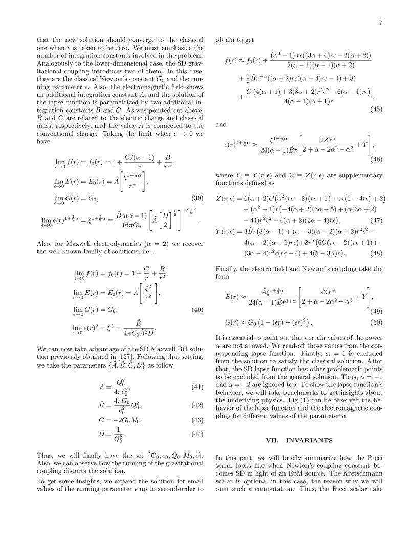
FIG. 2: Left: Scale-dependent black hole horizon rH versus the classical black hole mass, Middle: Hawking temperatureagainst the black hole mass, and, finally, Right: Bekenstein-Hawking entropy versus the classical black hole mass. The firstcolumn correspond to the horizon, the second line correspond to Hawking temperature and finally, SH for the right hand side.The first (left), second (middle) and third (right) column correspond to the cases α = {2, 3} respectively. We show the classicalmodel (solid black line) and three different cases for each figure: i) ε = 0.033 (dashed blue line), ii) ε = 0.067 (dotted red line)and iii) for ε = 0.010 (dotted dashed green line). We have used the set {Q0, e0, G0,M0} = {1, 1/(2

√π), 1/(16π2), 32π2} .

A. R. acknowledges DI-VRIEA for financial supportthrough Proyecto Postdoctorado 2019 VRIEA-PUCV.P. B. is funded by the Beatriz Galindo contract BEA-GAL 18/00207 (Spain). The author G. P. thanks theFundacao para a Ciencia e Tecnologia (FCT), Portu-

gal, for the financial support to the Center for Astro-physics and Gravitation-CENTRA, Instituto SuperiorTecnico, Universidade de Lisboa, through the Grant No.UID/FIS/00099/2013.

[1] A. Rincon, E. Contreras, P. Bargueno, B. Koch, G. Pan-otopoulos and A. Hernandez-Arboleda, Eur. Phys. J. C77 (2017) no.7, 494 [arXiv:1704.04845 [hep-th]].

[2] A. Einstein, Annalen Phys. 49 (1916) 769-822.[3] S. G. Turyshev, Ann. Rev. Nucl. Part. Sci. 58 (2008)

207.[4] C. M. Will, Living Rev. Rel. 17 (2014) 4.[5] E. Asmodelle, arXiv:1705.04397 [gr-qc].[6] B. P. Abbott et al. [LIGO Scientific and Virgo Col-

laborations], Phys. Rev. Lett. 116 (2016) no.6, 061102[arXiv:1602.03837 [gr-qc]].

[7] B. P. Abbott et al. [LIGO Scientific and Virgo Collab-orations], Phys. Rev. Lett. 116 (2016) no.24, 241103[arXiv:1606.04855 [gr-qc]].

[8] B. P. Abbott et al. [LIGO Scientific and VIRGO Col-laborations], Phys. Rev. Lett. 118 (2017) no.22, 221101[arXiv:1706.01812 [gr-qc]].

[9] B. P. Abbott et al. [LIGO Scientific and Virgo Collab-orations], Phys. Rev. Lett. 119 (2017) no.14, 141101[arXiv:1709.09660 [gr-qc]].

[10] B. . P. .Abbott et al. [LIGO Scientific and VirgoCollaborations], Astrophys. J. 851 (2017) no.2, L35[arXiv:1711.05578 [astro-ph.HE]].

[11] K. Akiyama et al. [Event Horizon Telescope Collabora-

tion], Astrophys. J. 875 (2019) no.1, L1.[12] K. Akiyama et al. [Event Horizon Telescope Collabora-

tion], Astrophys. J. 875 (2019) no.1, L5.[13] K. Akiyama et al. [Event Horizon Telescope Collabora-

tion], Astrophys. J. 875 (2019) no.1, L6.[14] T. Jacobson, Phys. Rev. Lett. 75 (1995) 1260 [gr-

qc/9504004].[15] A. Connes, Commun. Math. Phys. 182 (1996) 155 [hep-

th/9603053].[16] M. Reuter, Phys. Rev. D 57 (1998) 971 [hep-

th/9605030].[17] C. Rovelli, Living Rev. Rel. 1 (1998) 1 [gr-qc/9710008].[18] R. Gambini and J. Pullin, Phys. Rev. Lett. 94 (2005)

101302 [gr-qc/0409057].[19] A. Ashtekar, New J. Phys. 7 (2005) 198 [gr-qc/0410054].[20] P. Nicolini, Int. J. Mod. Phys. A 24 (2009) 1229

[arXiv:0807.1939 [hep-th]].[21] P. Horava, Phys. Rev. D 79 (2009) 084008

[arXiv:0901.3775 [hep-th]].[22] E. P. Verlinde, JHEP 1104 (2011) 029 [arXiv:1001.0785

[hep-th]].[23] W. Heisenberg and H. Euler, Z. Phys. 98 (1936) 714

[physics/0605038].[24] M. Born and L. Infeld, Proc. Roy. Soc. Lond. A 144

11

(1934) 425.[25] J. Bardeen, presented at GR5, Tiflis, U.S.S.R., and

published in the conference proceedings in the U.S.S.R.(1968)

[26] A. Borde, Phys. Rev. D 55 (1997) 7615 [gr-qc/9612057].[27] E. Ayon-Beato and A. Garcia, Phys. Rev. Lett. 80

(1998) 5056 [gr-qc/9911046].[28] E. Ayon-Beato and A. Garcia, Gen. Rel. Grav. 31

(1999) 629 [gr-qc/9911084].[29] E. Ayon-Beato and A. Garcia, Phys. Lett. B 464 (1999)

25 [hep-th/9911174].[30] K. A. Bronnikov, Phys. Rev. D 63 (2001) 044005 [gr-

qc/0006014].[31] I. Dymnikova, Class. Quant. Grav. 21 (2004) 4417 [gr-

qc/0407072].[32] S. A. Hayward, Phys. Rev. Lett. 96 (2006) 031103 [gr-

qc/0506126].[33] L. Balart and E. C. Vagenas, Phys. Lett. B 730 (2014)

14 [arXiv:1401.2136 [gr-qc]].[34] L. Balart and E. C. Vagenas, Phys. Rev. D 90 (2014)

no.12, 124045 [arXiv:1408.0306 [gr-qc]].[35] H. Reissner, Annalen Phys. 355 (1916) 106-120.[36] M. Hassaine and C. Martinez, Class. Quant. Grav. 25

(2008) 195023 [arXiv:0803.2946 [hep-th]].

[37] G. Panotopoulos and A. Rincon, Phys. Rev. D 97 (2018)no.8, 085014 [arXiv:1804.04684 [hep-th]].

[38] O. Gurtug, S. H. Mazharimousavi and M. Halilsoy,Phys. Rev. D 85 (2012) 104004 [arXiv:1010.2340 [gr-qc]].

[39] G. Panotopoulos and A. Rincon, Int. J. Mod. Phys. D28 (2018) no.01, 1950016 [arXiv:1808.05171 [gr-qc]].

[40] S. H. Mazharimousavi, O. Gurtug, M. Halilsoyand O. Unver, Phys. Rev. D 84, 124021 (2011)[arXiv:1103.5646 [gr-qc]].

[41] W. Xu and D. C. Zou, Gen. Rel. Grav. 49, no. 6, 73(2017) [arXiv:1408.1998 [hep-th]].

[42] A. Rincon, E. Contreras, P. Bargueno, B. Koch, G. Pan-otopoulos and A. Hernandez-Arboleda, Eur. Phys. J. C77, no. 7, 494 (2017) [arXiv:1704.04845 [hep-th]].

[43] G. Panotopoulos and A. Rincon, Int. J. Mod. Phys. D27 (2017) no.03, 1850034 [arXiv:1711.04146 [hep-th]].

[44] A. Rincon and G. Panotopoulos, Phys. Rev. D 97 (2018)no.2, 024027 [arXiv:1801.03248 [hep-th]].

[45] A. Rincon, E. Contreras, P. Bargueno, B. Koch andG. Panotopoulos, Eur. Phys. J. C 78 (2018) no.8, 641[arXiv:1807.08047 [hep-th]].

[46] G. Panotopoulos, Gen. Rel. Grav. 51 (2019) no.6, 76.[47] T. Kaluza, Sitzungsber. Preuss. Akad. Wiss. Berlin

(Math. Phys. ) 1921 (1921) 966.[48] O. Klein, Z. Phys. 37 (1926) 895 [Surveys High Energ.

Phys. 5 (1986) 241].[49] H. P. Nilles, Phys. Rept. 110 (1984) 1.[50] M. B. Green, J. H. Schwarz and E. Witten, Superstring

Theory, Vol. 1 & 2, Cambridge Monographs on Math-ematical Physics (Cambridge University Press, Cam-bridge, England, 2012).

[51] J. Polchinski, String Theory, Vol. 1 & 2, CambridgeMonographs on Mathematical Physics (Cambridge Uni-versity Press, Cambridge, England, 2005).

[52] B. Koch, I. A. Reyes and A. Rincon, Class. Quant. Grav.33 (2016) no.22, 225010 [arXiv:1606.04123 [hep-th]].

[53] A. Rincon and G. Panotopoulos, Phys. Rev. D 97 (2018)no.2, 024027 [arXiv:1801.03248 [hep-th]].

[54] E. Contreras, A. Rincon, B. Koch and P. Bargueno,Eur. Phys. J. C 78 (2018) no.3, 246 [arXiv:1803.03255[gr-qc]].

[55] A. Rincon and B. Koch, Eur. Phys. J. C 78 (2018) no.12,1022 [arXiv:1806.03024 [hep-th]].

[56] A. Rincon, E. Contreras, P. Bargueno, B. Koch andG. Panotopoulos, Eur. Phys. J. C 78 (2018) no.8, 641[arXiv:1807.08047 [hep-th]].

[57] A. Rincon, E. Contreras, P. Bargueno and B. Koch, Eur.Phys. J. Plus 134 (2019) no.11, 557 [arXiv:1901.03650[gr-qc]].

[58] E. Contreras, A. Rincon, G. Panotopoulos, P. Barguenoand B. Koch, Phys. Rev. D 101 (2020) no.6, 064053[arXiv:1906.06990 [gr-qc]].

[59] P. Kanti and E. Winstanley, Fundam. Theor. Phys. 178(2015), 229-265 [arXiv:1402.3952 [hep-th]].

[60] R. Konoplya, Phys. Rev. D 71 (2005), 024038[arXiv:hep-th/0410057 [hep-th]].

[61] A. Achucarro and P. K. Townsend, Phys. Lett. B 180,89 (1986).

[62] E. Witten, Nucl. Phys.B 311, 46 (1988).[63] E. Witten, arXiv:0706.3359 [hep-th].[64] C. V. Johnson, D-Branes, Cambridge Monographs on

Mathematical Physics;B. Zwiebach, A First Course in String Theory , Cam-bridge University Press.

[65] B. Zwiebach, Phys. Lett. B 156 , 315 (1985).[66] S. Corley, D. A. Lowe and S. Ramgoolam, JHEP 0107,

030 (2001).[67] Y. Kats, L. Motl and M. Padi, JHEP 0712, 068 (2007).[68] D. Anninos and G. Pastras, JHEP 0907, 030 (2009).[69] R. G. Cai, Z. Y. Nie and Y. W. Sun, Phys. Rev. D 78,

126007 (2008).[70] N. Morales-Duran, A.F. Vargas, P. Hoyos-Restrepo and

P. Bargueno, Eur. Phys. J. C 76, 559 (2016).[71] E. Contreras, F. D. Villalba and P. Bargueno, EPL 114,

50009 (2016).[72] P. Bargueno and E. C. Vagenas, EPL 115, 60002(2016)

.[73] O. Gurtug, S. H. Mazharimousavi and M. Halilsoy,

Phys. Rev. D 85, 104004 (2012).[74] M. Hassaine and C. Martinez, Class. Quant. Grav. 25,

195023 (2008).

[75] A. Rincon, E. Contreras, P. Bargueno, B. Koch andG. Panotopoulos, Eur. Phys. J. C 78, no. 8, 641 (2018)

[76] S. H. Hendi and H. R. Rastegar-Sedehi, Gen. Rel. Grav.41, 1355 (2009).

[77] H. Maeda, M. Hassaine and C. Martinez, Phys. Rev. D79, 044012 (2009).

[78] S. H. Hendi and B. E. Panah, Phys. Lett. B 684, 77(2010).

[79] S. H. Hendi and S. Kordestani, Prog. Theor. Phys. 124,1067 (2010).

[80] M. Cataldo, N. Cruz, S. del Campo and A. Garcia, Phys.Lett. B 454, 154 (2000).

[81] Y. Liu and J. L. Jing, Chin. Phys. Lett. 29, 010402(2012).

[82] K. C. K. Chan and R. B. Mann, Phys. Rev. D 50, 6385(1994) Erratum: [Phys. Rev. D 52, 2600 (1995). ]

[83] C. Martinez, C. Teitelboim and J. Zanelli, Phys. Rev.D 61, 104013 (2000).

[84] M. Hassaine and C. Martinez, Phys. Rev. D 75, 027502(2007).

12

[85] H. A. Gonzalez, M. Hassaine and C. Martinez, Phys.Rev. D 80, 104008 (2009)

[86] G. Panotopoulos and A. Rincon, Int. J. Mod. Phys. D27, 1850034 (2017).

[87] G. Panotopoulos and A. Rincon, Phys. Rev. D 97,085014 (2018)

[88] M. K. Zangeneh, A. Sheykhi and M. H. Dehghani, Phys.Rev. D 91, 044035 (2015)

[89] M. K. Zangeneh, A. Sheykhi and M. H. Dehghani, Phys.Rev. D 92, 024050 (2015).

[90] M. K. Zangeneh, M. H. Dehghani and A. Sheykhi, Phys.Rev. D 92, 104035 (2015).

[91] G. Panotopoulos and A. Rincon, Phys. Rev. D 96,025009 (2017).

[92] K. Destounis, G. Panotopoulos and A. Rincon, Eur.Phys. J. C 78, 139 (2018)

[93] A. Rincon, E. Contreras, P. Bargueno, B. Koch, G. Pan-otopoulos and A. Hernandez-Arboleda, Eur. Phys. J. C77, 494 (2017).

[94] B. Koch, I. A. Reyes and A. Rincon, Class. Quant. Grav.33, 225010 (2016).

[95] A. Rincon, B. Koch and I. Reyes, J. Phys. Conf. Ser.831, 012007 (2017)

[96] A. Rincon and B. Koch, J. Phys. Conf. Ser. 1043,012015 (2018)

[97] E. Contreras, A. Rincon, B. Koch and P. Bargueno, Int.J. Mod. Phys. D 27, 1850032 (2017).

[98] E. Contreras, A. Rincon, B. Koch and P. Bargueno, Eur.Phys. J. C 78, 246 (2018).

[99] B. Koch, P. Rioseco and C. Contreras, Phys. Rev. D 91,025009 (2015)

[100] A. Hernandez-Arboleda, A. Rincon, B. Koch, E. Contr-eras and P. Bargueno,

[101] E. Contreras and P. Bargueno, Int. J. Mod. Phys. D 27,1850101 (2018).

[102] A. Rincon and B. Koch, arXiv:1806.03024 [hep-th].[103] A. Bonanno and M. Reuter, Phys. Rev. D 62, 043008

(2000)[104] A. Bonanno and M. Reuter, Phys. Rev. D 73, 083005

(2006)[105] M. Reuter and E. Tuiran, hep-th/0612037.[106] M. Reuter and E. Tuiran, Phys. Rev. D 83, 044041

(2011).[107] K. Falls and D. F. Litim, Phys. Rev. D 89, 084002

(2014).[108] Y. F. Cai and D. A. Easson, JCAP 1009, 002 (2010).[109] D. Becker and M. Reuter, JHEP 1207, 172 (2012).[110] D. Becker and M. Reuter, arXiv:1212.4274 [hep-th].[111] B. Koch and F. Saueressig, Class. Quant. Grav. 31,

015006 (2014).[112] B. Koch, C. Contreras, P. Rioseco and F. Saueressig,

Springer Proc. Phys. 170, 263 (2016).[113] B. F. L. Ward, Acta Phys. Polon. B 37, 1967 (2006).[114] T. Burschil and B. Koch, Zh. Eksp. Teor. Fiz. 92, 219

(2010). [JETP Lett. 92, 193 (2010)][115] K. Falls, D. F. Litim and A. Raghuraman, Int. J. Mod.

Phys. A 27, 1250019 (2012).

[116] B. Koch and F. Saueressig, Int. J. Mod. Phys. A 29,1430011 (2014).

[117] A. Bonanno, B. Koch and A. Platania,arXiv:1610.05299 [gr-qc].

[118] A. Adeifeoba, A. Eichhorn and A. Platania,Class. Quant. Grav. 35, no.22, 225007 (2018)doi:10.1088/1361-6382/aae6ef [arXiv:1808.03472[gr-qc]].

[119] A. Platania, Eur. Phys. J. C 79, no.6, 470 (2019)doi:10.1140/epjc/s10052-019-6990-2 [arXiv:1903.10411[gr-qc]].

[120] M. Reuter and H. Weyer, Phys. Rev. D 69, 104022(2004).

[121] B. Koch and I. Ramirez, Class. Quant. Grav. 28, 055008(2011).

[122] S. Domazet and H. Stefancic, Class. Quant. Grav. 29,235005 (2012).

[123] C. Contreras, B. Koch and P. Rioseco, J. Phys. Conf.Ser. 720, 012020 (2016).

[124] R. Percacci and G. P. Vacca, Eur. Phys. J. C 77, 52(2017).

[125] C. Contreras, B. Koch and P. Rioseco, Class. Quant.Grav. 30, 175009 (2013).

[126] A. Rincon and G. Panotopoulos, Phys. Rev. D 97,024027 (2018)

[127] B. Koch and P. Rioseco, Class. Quant. Grav. 33, 035002(2016).

[128] E. Curiel, Einstein Stud. 13, 43 (2017).[129] R.M. Wald, General Relativity (1984).[130] V. A. Rubakov, Phys. Usp. 57, 128 (2014). [Usp. Fiz.

Nauk 184, no. 2, 137 (2014)][131] R. Penrose, Phys. Rev. Lett. 14, 57 (1965).[132] D. Grumiller, P. Parekh and M. Riegler,

Phys. Rev. Lett. 123, no.12, 121602(2019) doi:10.1103/PhysRevLett.123.121602[arXiv:1907.06650 [hep-th]].

[133] C. Ecker, D. Grumiller, W. van der Schee,M. M. Sheikh-Jabbari and P. Stanzer, SciPost Phys.6, no.3, 036 (2019) doi:10.21468/SciPostPhys.6.3.036[arXiv:1901.04499 [hep-th]].

[134] T. Jacobson, Class. Quant. Grav. 24, 5717 (2007).[135] M. Heusler, Helv. Phys. Acta 69, 501 (1996).[136] J.M. Bardeen, B. Carter, S.W. Hawking, Commun.

Math. Phys. 31, 161 (1973).[137] http://www.wolfram.com

[138] L. Balart and S. Fernando, Mod. Phys. Lett. A 32,1750219 (2017).

[139] D. Ida, Phys. Rev. Lett. 85, 3758 (2000).[140] M. Dehghani, Phys. Rev. D 94, 104071 (2016).[141] A. de la Cruz-Dombriz, A. Dobado and A. L. Maroto,

Phys. Rev. D 80 (2009), 124011 [erratum: Phys. Rev.D 83 (2011), 029903] [arXiv:0907.3872 [gr-qc]].

[142] R. G. Cai, R. K. Su and P. K. N. Yu, Phys. Lett. A 195(1994), 307-311

[143] T. Jacobson, G. Kang and R. C. Myers, Phys. Rev. D49 (1994), 6587-6598 [arXiv:gr-qc/9312023 [gr-qc]].

[144] V. Iyer and R. M. Wald, Phys. Rev. D 52 (1995), 4430-4439 [arXiv:gr-qc/9503052 [gr-qc]].