The JERS Amazon Multi-season Mapping Study (JAMMS): Observation Strategies and Data

Characteristics

Bruce Chapman, Paul Siqueira, and Anthony Freeman Jet Propulsion Laboratory

California Institute of Technology 4800 Oak Grove Drive

Pasadena, California 9 1 109

Tel: (818) 354 3603 Fax: (818) 393 5285

e-mail: bruce.chapman@jpl.nasa.gov

I

Abstract As described by Freeman, et al (this issue), the JERS-1 Amazon Multi-season

Mapping Study (JAMMS), part of the Global Rain Forest Mapping (GRFM) project led by the National Space Development Agency of Japan (NASDA), had an ambitious agenda to completely map the Amazon River floodplain (and surrounding areas) twice at high resolution.

The observation strategy carried out by NASDA for the JAMMS project and the other elements of the GRFM project (1 995-1 997) constituted the first time that a spaceborne S A R successfully implemented a continental scale, coordinated seasonal mapping campaign. This observation strategy, chosen around the flooding cycle of the major river systems, was designed to provide the first high resolution measurement of inundation extent by the Amazon river and its tributaries.

In order for the scientific community at large to be able to exploit this data set, the characteristics of the data (resolution, radiometric and geometric calibration, coverage, and ability to be mosaicked) must be well understood. Here, we will describe in detail important parameters governing the quality of the imagery from this task.

I Introduction The JERS-1 Amazon Multi-Season Mapping Study began in 1995 with the

acquisition by the National Space Development Agency of Japan (NASDA) Japanese Earth Recourses Satellite (JERS-1) Synthetic Aperture Radar (SAR) of its first of two complete, coast-to-coast, single season, high resolution data acquisitions of the Amazon river basin in South America

Table 1 summarizes the basic characteristics of the JERS-1 SAR.

Frequency band L (1275 MHz) I

Polarization IHH I

Bandwidth 11 5 Mhz I

Table 1. JERS- 1 SAR characteristics BASDA EOC, ~~ ~~ ~ ~~~~~ ~~~

19951

. The primary science objective was to map for the first time at high resolution the extent of inundation that occurs along the Amazon river and its tributaries, a task that the JERS-1 SAR was uniquely qualified to measure due to the sensitivity of this L-band SAR to the characteristic “double-bounce” scattering signature of flooded forests.

In order to accomplish this, two mappings were required: one during the low flood season (roughly September to November), and one during the high flood season (roughly May through July). The low flood imagery was acquired in 1995, during historically low flood levels of the Amazon River, while the high flood acquisition began seven months later in 1996.

These two acquisitions also allowed for experimentation in land cover classification methods based solely on single channel (HH) L-band SAR data over tropical forests.

This mapping project, which developed quickly into the NASDA Global Rain Forest Mapping Project (GRFM) encompassing Africa and S.E. Asia as well, demonstrated the complementary aspect of SAR and optical mapping campaigns. While the JERS-1 SAR was not well suited for differentiating between some land cover types (For instance, under some circumstances it is difficult to distinguish between bare ground and open water), it was very capable of distinguishing flooded conditions that are not easily observed by optical instruments such as Landsat. In addition, while some optical instruments are sensitive to subtle changes in land cover that may be quite invisible in SAR imagery, SAR can acquire good quality data during heavy cloud cover that would render optical data useless for land cover mapping (it can take years to acquire cloud-free Landsat data over some locations within the Amazon basin).

Even though the JERS-1 SAR was prevented from pursuing some of its pre- launch objectives due to a poor signal to noise ratio, it was well suited to mapping flooded

L

2

forest conditions and, in a more limited way, mapping land cover conditions. By focusing resources and activities on a task well suited to the instrument's capabilities, NASDA facilitated the demonstration of an important science result which is best achieved by SAR.

2. Observation Strategies A few months after the launch of the JERS-1 SAR, a malhnction within the S A R

instrumentation (arcing between two of the SAR antenna sub-panels).resulted in the S A R operating at half of its designed power output, generating lower than planned signal to noise ratios and a higher than planned noise equivalent oo (normalized radar backscatter coefficient). In addition, due to an unrelated electrical problem concerning an on-board battery, the JERS-I SAR could normally only acquire data during a descending (southerly) path of the orbit. While these difficulties prevented the JERS-1 SAR from meeting some of its pre-flight objectives, its suitability for mapping land cover was not seriously impacted. In fact, since these problems affected the ability to pursue various other applications, an argument could be made that these malfunctions resulted in the emphasis in forest cover mapping during the extended mission.

The orbit chosen for JERS was convenient for mapping large regional areas in an

On any given fifteenth orbit, the roughly North/South along track ground swath would be over the same location as the first orbit, offset to the West by about 70 km at the equator (with about 10% overlap in ground swaths). Therefore, looking only at the descending orbits, the ground swaths for a particular region near the equator advanced westward by one ground swath each day . This meant that when mapping large regional areas with many cross-track orbit paths, each orbit was acquired either the day before or the day after the neighboring orbit path. Meanwhile, in the along track direction, JERS was restricted only by the data acquisition length that could be recorded and downlinked by the on-board tape recorder (8 minutes, or over 2000 km). Therefore, during the span of just three days, almost half a million square kilometers could be imaged.

h efficient fashion. Each day the satellite made slightly more than 14 orbits of the planet.

3

o r b i t 15 o r b i t 3 o r b i t 2 Day 1 Day 0 Day 0

I 1 d f r

I Figure 1: illustration of the ground swath pattern

While the goal was coast-to-coast coverage of Northern South America, occasionally the data could not be obtained as planned (due to scheduling conflicts or acquisition errors). In those cases, an attempt was made to “fill in” the gaps with alternative images acquired during other periods with data as close in season as possible. In addition, since the area to be imaged exceeded 2,000 km in the along track direction, two “passes” were made: the first of the Amazon basin, and the second of the area directly above, to the Northern coast of South America.

Since the primary objective was mapping inundation (Freeman, Chapman, and Siqueira, this issue), two observations were required: one at the high flood of the Amazon River and its tributaries, and one at the low flood. This would enable separate studies at low and high flood, establish areas that are generally flooded year round, and more clearly differentiate seasonal inundation. Since it would take 62 passes to map South America from the East Coast to the West Coast by the JERS-1 SAR, it would take 62 days to complete each mapping cycle.

There are three issues complicating the optimum collection of the two flood- season data sets: first, the Western end of the basin generally floods earlier than the Eastern end; second, the two month East-to-West mapping cycle necessarily encompasses changing flooding conditions from the beginning of the cycle to the end of the cycle; and third, in some areas that were mapped there is only marginal or out-of-

Y O

4

synch seasonal flooding. I fowcvcr, the low flood period of' thc Amazon River during October lcFI5 was exceptionally low, and the high llood period during May 1996 was exceptionally high, hopcUully afYording a good characterization along the length of the Amazon River and its tributaries for low and high tlood conditions.

While the low flood acquisitions were extremely successfill, the acquisitions during the high flood period resulted in some gaps in coverage. These gaps, as best as is possible, were filled in with the closest available season. However, as figure 2 shows, the change in backscatter due to flooding between the nominal high flood period and the period of the gap filling data is evident when the imagery is mosaicked.

Figure 2: Mosaicked gap filled / high flood data.

This unprecedented single season mapping capability is possible because clouds are quite transparent to L-band SAR. Although severe weather conditions have been shown to affect L-band SAR backscatter, i n general the effect is small and difficult to detect in the JERS SAR imagery. Since weather was not a factor in determining the observation strategy, the imagery could be assured of collection (absent any scheduling or instrument errors) in a systematic fashion. Given the persistent cloudiness of a great deal of the Amazon basin, this is a important rationale to justify the collection of SAR data to monitor seasonal and annual land cover change and flooding phenomena in this and similar regions.

I n order for this observation strategy to be successful. the data had to be well calibrated to facilitate ;I visually pleasing and scientitically useful regional mosaic. The

5

Amazon basin was particularly well suited to observation due to its relatively small topographic relief over large stretches of Northern South America (with the notable exception of the Andes in the West) resulting in few topographically induced radiometric calibration errors. A complete description of the calibration of the data follows in the next section.

3. Data Characteristics The collection of JERS-1 imagery over the Northern half of South

American continent occurred between 1995 and 1997, under the auspices of the Global Rain Forest Mapping Project (Rosenqvist et al, 2000), utilized the downlink facilities at both Hatoyama Earth Observation Center (EOC) in Japan and the NASA Alaska S A R Facility (ASF) in Fairbanks, Alaska. Due to the nature of the JERS polar orbit, ASF was well suited for downlinks of the tape-recorded data of South America.

The ASF, in addition to acquiring about two thirds of the data via downlink to its receiving station, also processed the raw signal data into full resolution imagery. However, due to some difficulties ASF encountered in processing some of the imagery, NASDA EOC processed about 20% of the data. Therefore, the JERS-1 S A R imagery comprising the JAMMS project came in two very different data formats and processing

, algorithms, depending on their source.

Comparison between NASDA and ASF Processing The NASDA and ASF processing facilities both generate full resolution imagery

with a pixel spacing of 12.5 m in both the range and azimuth (along track and cross track) directions. The NASDA 2.1 level data product is projected to UTM coordinates, while the ASF projection for data is a constant ground pixel spacing in both range and azimuth. Both processing facilities produce CEOS formatted data.

For the NASDA data products, each scene of data corresponds geographically to the JERS-1 Row/Path definition (NASDA EOC, 1995). There are three CEOS files associated with each scene: a leader file, an image file, and a trailer file. The leader and trailer files are ASCII header files, while the image file is a binary data file. A detailed description of these files may be found in (NASDA EOC, 1996). Each line of data in the image file is preceded by 12 bytes of prefix information.

For the ASF data products, each scene is identified by the revolution (rev) number since launch, and the center latitude. Each frame of data has two associated CEOS files: a leader file and an image file. The header information in the ASCII leader file is organized quite differently from that produced by NASDA, but much of the same information is present, with the notable exception that the ASF leader file includes an estimate of the range dependent noise equivalent 0'. In addition to having to incorporate data from different processing facilities, the format of the ASF files changed in 1996. Prior to late 1996, the image files were preceded on each line with a 12 byte prefix and there was also an ASCII CEOS trailer file. After late 1996, the prefix length increased to 192 bytes. There were changes to the header information as well (Bicknell, 1997). Hence, a

6

considerable amount of post processing was necessary to assemble the two-season, 3500 scene data set into a uniform data set in preparation for the regional mosaicking effort.

The calibration factor to convert the digital number (dn) values to o0 differs between NASDA and ASF processed imagery. For ASF processed imagery, the calibration factor (linear) may be found in the CEOS leader file. For NASDA processed imagery, see Table 2. NASDA carefully monitored backscatter from corner reflectors and updated the calibration factor if analysis of data indicated a change in the correction factor. The dates given below correspond to the date of acquisition of the data.

I ASDA calibration factor F (db) I

eb 1992 - Feb 14,1993 70.0

Feb 15,1993 - Oct 31,1996

-68.3 November 1,1996 - -68.5

I

b S F calibration factor F (db) b

typical value -48.54

found in ceos leader file)

Table 2: calibration factors

In order to calculate the normalized radar backscatter (0') from NASDA or ASF processed imagery (ignoring noise):

Where oo is the normalized radar backscatter in dB, dn is the digital number, and F is the calibration factor in dB. This formula works for all products derived from the NASDA or ASF imagery, including mosaic products and low-resolution imagery. If the noise vector is known, it is possible to remove the noise floor by the following formula:

Where oo is the normalized radar backscatter in dB, f is the linear value of the calibration factor, fn is the noise conversion factor, and N(r) is the normalized noise which varies as a function of range. For ASF processed imagery, N(r) may be found in the CEOS leader file and ranges between 0 and 1 , while fn may be calculated from two calibration constants found in the CEOS leader file (the linear absolute calibration factor and the noise scale factor) by finding the product of the two:

7

f n = 4 . 5 4 7 ~ 1 O-* (typically) (3)

The most significant difference between the NASDA and ASF data products is that the NASDA image product stores the d, values as 16 bit values while the ASF image product is 8 bit. However, a d, value of 4096 (from the NASDA image product requiring 12 bits) corresponds to a Goof +3.7 dB assuming a calibration constant of -68.5 dB. This is a backscatter value that is generally larger than is normally seen in. an image composed of natural targets. Therefore, for most scenes of natural targets, less than 12 of the 16 bits are being used by the NASDA image product. In addition, the d, value of the noise floor (corresponding to oo as low as -20 dB) is about 265; it is therefore rare to find a d, value less than 265. Thus, the additional bits included in the NASDA product do not necessarily translate into a wider range of oo values.

In contrast, if the calibration constant for an ASF image product is standard (e.g. - 48.54 dB), then a d, of 255 corresponds to a Doof only -0.4 dB. For some flooded forest and urban settings, the bright backscatter may be larger than this, causing a saturation effect of their backscatter values.

At low backscatter values (oo= -14 dB), which roughly corresponds to imagery of L open water and low vegetation areas, each change in dn for ASF imagery indicates a change

of 0.17 dB in GO, a rather large quantization. For NASDA imagery, at oo =-14 dB, each change in dn indicates a change of only 0.02 dB. The d, value of the noise floor (corresponding to oo as low as -20 dB) for ASF image products is about 26, where each change in d, corresponds to a change in oo of 0.34 dB (but only 0.03 for NASDA image products).

NASDA Theme oo dn I Aoo Noise Open Water Forest Flooded Forest ASF Maximum NASDA

-20 -14

-7 -2

-0.4

+3.7

0.033 0.0 16

1189 0.007 21 13 0.004

254 1 0.003

4096 0.002 Maximum I I Table 3 : ASF 8 bit versus NASDA 16 bit

ASF d" 26 53

119 21 1

255

N /A

60"

0.34 0.16

0.073 0.041

0.034

N/A

As can be seen from Table 3, since the calibration factors for NASDA and ASF are different by a factor of about 20 dB, the d, values are different by a factor of 10, as are the Aoo values.

8

While the NASDA 16 bit product is better suited to analysis of the data, and does not introduce any quantization noise, the great majority of the data for South America was only processed to the ASF 8 bit product. Therefore, an early decision was made that all NASDA data would be converted to the ASF 8 bit image product, and the 8 bit imagery would be used in composing all JAMMS mosaic products.

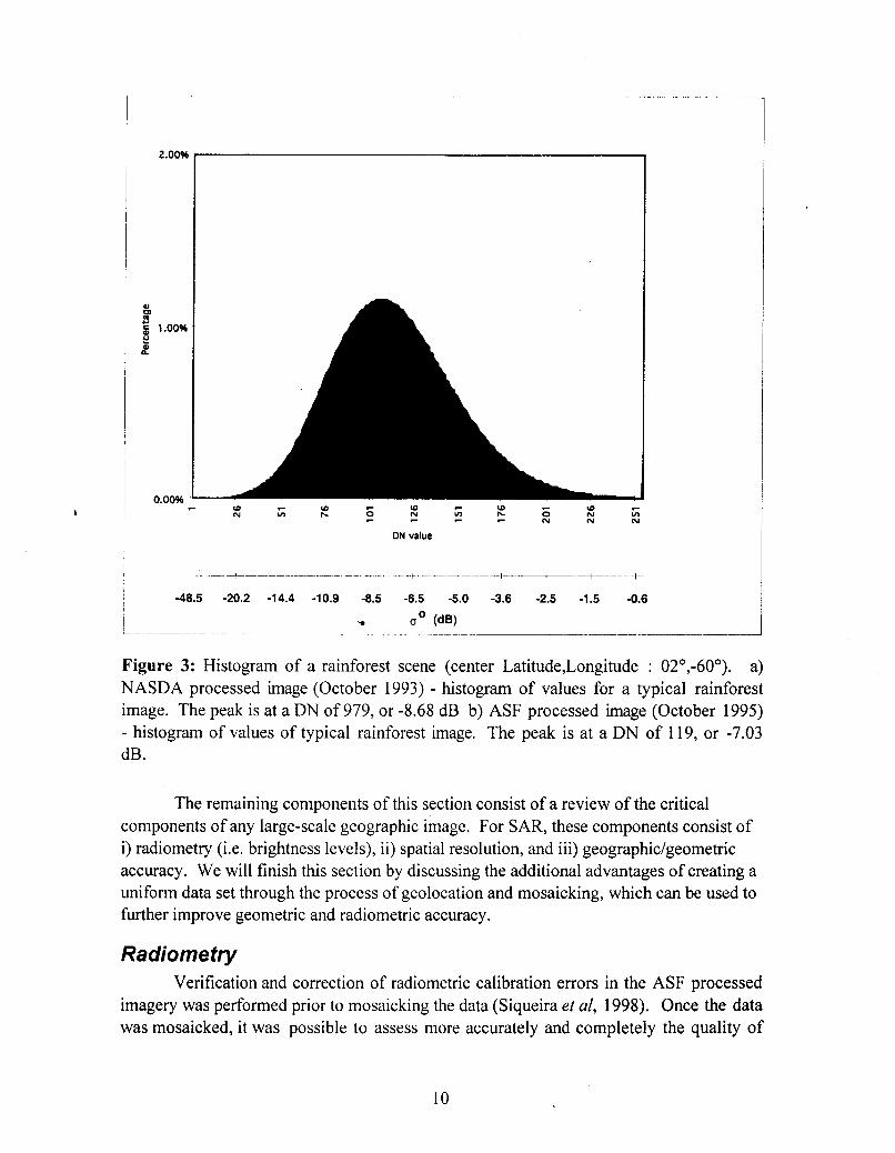
Figure 3 shows a histogram of the values found in a typical NASDA and ASF image over a rain forest region.

0.20%-

0.15%-

u m c g 0.10%" L

0

0.05'8"

c :: c

8 c

c 0 In N

-615 -145 -8.5 -5.0 -2.5 -0.5 1 .o

9

0.00% - W - (0 c v)

In r W - N

W v) IC r r N N

0 N

N In N b 2 - r

DN value

Figure 3: Histogram of a rainforest scene (center Latitude,Longitude : 02",-60"). a) NASDA processed image (October 1993) - histogram of values for a typical rainforest image. The peak is at a DN of 979, or -8.68 dB b) ASF processed image (October 1995) - histogram of values of typical rainforest image. The peak is at a DN of 119, or -7.03 dB.

The remaining components of this section consist of a review of the critical components of any large-scale geographic image. For SAR, these components consist of i) radiometry (i.e. brightness levels), ii) spatial resolution, and iii) geographic/geometric accuracy. We will finish this section by discussing the additional advantages of creating a uniform data set through the process of geolocation and mosaicking, which can be used to further improve geometric and radiometric accuracy.

Radiometry Verification and correction of radiometric calibration errors in the ASF processed

imagery was performed prior to mosaicking the data (Siqueira et ai, 1998). Once the data was mosaicked, it was possible to assess more accurately and completely the quality of

10

the calibration verification process, and to make improvements to provide a radiometrically consistent image.

The calibration of the cross-track radiometry was implemented in a three step process:

1) ASF and NASDA processing facilities applied the standard antenna pattern correction during raw signal data processing.

2) After JPL received the imagery, it was evident that a large cross-track residual error was present. Therefore, after examining a random selection of imagery, a standard correction was made to each image. This improved the cross-track calibration accuracy to better than 0.6 dB.

3) During the mosaicking process, in which calibration errors on the order of 0.2 dB introduced visible banding in the mosaic, a further corrrection was mandated to bring the cross-track calibration error to better than 0.2 dB.

While these three stages of cross-track calibration ideally would occur as one L single step, they are equivalent to applying a single radiometric correction.

Absolute calibration The absolute calibration of the JERS-1 SAR data was verified by analysis of

corner reflectors in Southern California, USA; Delta Junction, Alaska; and Manaus, Brazil (vanZyl et al, 1992). Tables 4 and 5 list the result for several comer reflectors imaged in 1992 and 1993 by the JERS-1 SAR and processed by the NASDA and ASF processors. The results indicate that the calibration factors from table 2 are consistent with the stated calibration accuracy of 1 dB.

Scene calibration Overflight Date image ID offset (dB)

Edwards

c0077a10 Edwards

- 0 . 8 5 93 A p r 30 c0077a10 Edwards

- 0 . 6 1 93 A p r 30 c0077a10

- 0 . 7 8 93 A p r 30

Edwards

0 . 2 8 9 3 Apr 30 c0077a10 Edwards

- 0 . 8 0 93 A p r 30 c0077a10

anaus c 0 2 3 0 b 1 9 0 . 3 1 9 3 J u l 0 6

Table 4: NASDA processed imagery - corner reflector analysis

c e n e c a l i b r a t i o n O v e r f l i g h t r e v 'Image ID D a t e offset (dB)

Delta Junction 3.13 92 Jul 28 2528 1000346

Delta Junction

Table 5 : ASF processed imagery - corner reflector analysis

0.92 92 Oct 26 3876 1000355 Delta Junction

3.70 92 Oct 25 386 1 1000353 Delta Junction

-1.4 92 Oct 23 383 1 1000350 Delta Junction

-0.56 92 Oct 22 38 I 6 1000348

In order to assess the correspondence in absolute calibration between ASF and NASDA processed imagery, a JERS- 1 datatake of a region of uniform' rain forest in South America was processed by the both ASF and NASDA processing facilities and the results analyzed. Since the same raw signal data was processed, the difference between the two image products is due solely to processing differences (including standard calibration) between the ASF and NASDA processors. Analysis showed that there was a slight difference in absolute calibration between the data processed by the two facilities, whereby the ASF processor calibration was generally 0.8 dB brighter than that of NASDA. This error is less than that of the accuracy of the absolute calibration, but left uncorrected, is noticeable in the mosaicked imagery

Relative Calibration Pre-processing The relative calibration between scenes and within each scene must be excellent if

a seamless image mosaic product is desired. Errors in oo greater than about 0.2 dB will negatively impact the visual appearance and analysis of the GRFM mosaic image products as well as make unsupervised classification extremely difficult. As the resolution of the data is reduced, banding in the data becomes even more noticeable. Therefore, for the data acquired of South and Central America, JPL performed a careful verification of the relative calibration of the JERS-1 SAR imagery as processed by ASF and made corrections where necessary.

During processing at both ASF and NASDA, a standard correction is applied to account for the change in antenna gain with look angle. During ASF processing, the inverse of this gain factor is saved as the "noise vector" in the CEOS leader file (for example see Figure 4). This antenna gain is accurately measured and analyzed both before and after launch. While the antenna pattern is not expected to change once the satellite is in orbit, it is not unusual for there to be discrepancies between the actual antenna pattern and the applied antenna pattern on the order of 0.5 dB.

)I

12

b Figure 4: During processing at both ASF and NASDA, a standard correction is applied to account for the change in antenna gain with look angle. During ASF processing, the inverse of this gain factor is saved as the "noise vector'' in the CEOS leader file. This figure shows a typical example.

Since even this small level of error can introduce significant problems when mosaicking the data, an additional procedure was used to verify the relative calibration of JERS-1 data over the Amazon from the ASF imagery, and correct it if necessary:

Each ASF full resolution image was averaged to 100 m pixel spacing in both the range and azimuth directions (i.e. average of 8x8 pixels). The description of the analysis that follows was derived from the low-resolution imagery, but because of the slow- changing nature of the correction (i.e. it is a smooth function), the results may be applied to either the low or full resolution imagery.

A large sample of ASF imagery was analyzed to determine whether any correction to the radiometric calibration was necessary. A geographically and temporally diverse sample of images was selected, where uniform, undisturbed forest areas were binned and averaged in the along track (azimuth) direction to yield a range dependent estimate of the cross track antenna pattern. Uniform rain forests are relatively easy to identify on the SAR imagery because of the moderate level of backscatter return from the canopy volume. Key areas necessary to avoid are low vegetation and open water regions where backscatter is minimal, and often dominated by the instrument's thermal noise characteristics. For a typical scene from either the ASF or NASDA processing facilities, the radar backscatter varies by about 0.6 dB between the near, mid, and far range of the image swath.

13

After averaging a few dozen images containing only uniform rain forest regions, a consistent curve shape (both magnitude and location) was observed. See figure 5 for a polynomial fit as a function of range. The incidence angle over this range varies between 30 and 36 degrees, over the course of which the scattering from the surface will change slightly, but this effect alone is unlikely to account for the magnitude of the curvature of the radar backscatter.

r 0.3

0.2

0.1

0

B -0.1

-0.2

-0.3

-0.4

-0.5

Range L

Figure 5: polynomial fitted to the inverse of radiometric trend.

If no radiometric corrections were necessary, then we would expect the radar backscatter versus range for uniform rain forest regions to be relatively constant. This, however, was not the case in our initial analysis, and thus the polynomial fit shown in figure 6 was divided into each image in order to attempt to correct for the apparent error in all of the imagery. This assumes that the error that was observed in the selected subset would apply to all the imagery. Some images were then examined to insure that the radar backscatter of uniform forest areas as a function of range was indeed uniform. In order to maintain the same absolute calibration, the polynomial was normalized such that the average gain was unity.

1 1

i ~

! i

i

~

I

, i

1

! !

14

-7 I- -7-1 t -7.2+ f

-7.3

-7.4

-7-9 t Figure 6: a typical residual radiometric trend

Out of 1723 ASF processed scenes acquired by JERS-1 between September 27 and December 12, 1995, the same radiometric correction as a function of range was applied for 1666 scenes, or 97% of the total. Similar results were found for the %gh flood" data set. The remaining scenes required a unique radiometric correction. Usually, several adjacent scenes within a rev required the same unique radiometric correction. Again, using uniform rain forest regions to estimate the trend in the error, a polynomial fit to the data was determined and applied against the image swaths.

Noise Equivalent o0 Thermal noise is a natural artifact in SAR imagery. Noise equivalent oo reflects

the minimum backscatter return from a physical target that will rise above this noise floor. Because the gain of the antenna changes in range, as does the degree of free space loss, the noise equivalent oo too varies as a function of range and look angle. Figure 7 is a typical plot of the noise equivalent oo determined by analyzing the radar backscatter over open

15

water (generally the darkest locations in the imagery) at several cross-track (range) locations. This assumption is possible due to the transmitter failure of JERS-I, which makes the signal return from open water generally dominated by thermal noise internal to the instrument rather than the rough-surface backscatter induced by waves on the water.

-15

-16

-17 dB

-18

-19

-20

Range ___)

c

Figure 7: typical plot of the noise equivalent oo, estimated by analyzing the radar backscatter over open water (generally the darkest locations in the imagery) at several cross-track (range) locations. These areas are generally dominated by noise, rather than signal from the waves on the water.

These plots indicate that at worst the noise equivalent CJ' is -15 dB, though these values occur over a small range of incidence angles (near and far swath), while at the middle of the swath, the noise equivalent oo is about -20 dB.

Calibration Errors

easily corrected : There are three types of remaining calibration errors, only one of which can be

1) Absolute calibration error Occasionally (41 out of 1723 "low flood" ASF scenes from

South America), the absolute calibration of an image appears to be incorrect. Approximately the same ratio was found for the ''high flood"

16

data set. This was visually evident after mosaicking, and also from examination of a plot of the radiometry versus range for a scene. The cause for this error is unknown, but it is correctable if there are targets or regions within the scene of known radar backscatter, such as rain forest regions, whose backscatter is relatively well known. Also, the overlapping regions of adjacent scenes may be exactly compared and the errant image corrected. Although most images could be corrected in this manner, some residual uncorrected error on the order of less than 1 dB remained.

2) Residual range dependent calibration error Based on the assumption that any calibration error across

track is due to an error in the antenna pattern, we would expect that all scenes would require the same correction. Therefore, if at all feasible, the same range dependent radiometric correction as discussed above was applied to each scene.

Even after the above corrections were made, when the images were mosaicked calibration offsets became evident in comparison to surrounding images. The magnitude of this difference is relatively small, ranging from 0.2 to 0.6 dB but even these small errors had a large, visually distracting impact which also would likely affect some of the more sensitive classification routines. This indicated that a further, mosaic- based radiometric correction would be required. The process to achieving that correction is described at the end of this section.

3) Along-track calibration error In addition to the correctable cross-track radiometric

calibration errors, it has been noticed that in a small number of scenes an along track radiometric bump in gain occurs over a distance of several hundred meters. These artifacts are perhaps due to uncorrected changes in the processor or instrument gain. While these errors are detectable visibly, they are algorithmically hard to describe and therefore difficult to remove. This is because of their short duration and the possibility that they may be target related, such as would be the case during weather events (ie. Backscatter increases due to increased target moisture). Therefore, these bumps might appear as artificial features in classification, but should in general be ignored in the interpretation of the data.

Terrain correction errors For both NASDA and ASF processed imagery, no terrain height information was

used in calibrating the data, or in projecting the data to the ground range projection. Therefore, the following errors were introduced to the data:

1. Possible radiometric calibration errors due to the change in incidence angle with terrain slope: since o0 is normalized by the scattering area, and since the scattering area is dependent upon the incidence angle, a terrain slope will introduce a calibration error (van Zyl et al, 1993). This error manifests itself as enhanced backscatter on the forward side

17

(with respect to the radar) of steep topographic relief, and diminished returns on the backside. In addition, in the presence of terrain slopes, the scattering behavior of the target may be quite different due to a dramatically different incidence angle.

2. Possible geometric errors due to an incorrect projection to ground range: during processing, the data is projected to the ground range assuming a spherical Earth. Over areas of significant topography, this projection of the imagery onto a spherical Earth will result in a mis-match of the imagery and ground locations.

Resolution In order to assess the resolution in both the azimuth and range direction, and to

estimate the Peak Side Lobe Ratio (PSLR) of the impulse response, spatial analysis of the return from comer reflectors was performed. For NASDA processed imagery, 8 comer reflectors were analyzed, while for ASF imagery, 6 corner reflectors were analyzed. These comer reflectors used for estimating the image resolution were the same as those used to verify the absolute calibration of the data.

As can be seen from Table 6, the azimuth resolution of the ASF processed imagery is about 32 my as opposed to 18 m for NASDA processed imagery. The difference in resolution is because ASF performs 4 look processing, the NASDA

resolution lOOm pixel imagery, the affect of processing on the effective resolution is minimal.

)I processor processes for three looks in order to obtain higher resolution. For the low-

Range Res. Azimuth PSLR Range PSLR Azimuth Res.

(m) (dB) (dB) (m)

NASDA

Table 6: Image quality from comer reflector analysis.

- 14.2 k2.1 -8.2 f 1.9 32.1 f 3.8 18.0 f 1.1 ASF

-21.1 f 1.9 -13.7 f 2.0 18.2 k 1.8 18.2 f00 .6

Geometry In order to assess the geometric accuracy of the data, results from the mosaicking

of the ASF processed data were utilized. First, mosaicking 1500 adjacent ASF scenes from South America resulted in histograms of offsets in Latitude and Longitude (figure 8). The average offset in Longitude was 3 17 f 21 36 meters, while the average offset in Latitude was -1053 f 1250 meters. These offsets with respect to the comer latitude/longitudes (retrieved from the CEOS header) roughly indicate the accuracy of knowledge in absolute location, as determined from the satellite ephemeris by the ASF processor. A more detailed description of the geometric accuracy of the mosaicked GRFM data performed at JPL may be found in Siqueira el al, 2000.

18

40

20

n 11 i 0 0 0 0 0 0

0 0

0 0 0 0 0

0 0

0 0

0 0 0 N m w

8 t 3 F 5! 2

Meters

19

60

50

40

30

20

10

0

Q f

Q T

0 0 s

I

Q c

Meters

0 Q c

IJ

Figure 8: The histogram of offsets in the x (A) and y (B) direction applied to each scene while mosaicking 1500 scenes from South America.

Regional Scale Mosaicking: Methods and Results For performing focused studies, researchers often work with single-scene imagery

covering their field site of interest. Through the GRFM program, NASDA has made available data covering a significant portion of the entire South American continent, thus providing the opportunity to make basin wide studies (such as flooding inundation), while still meeting the needs of researchers wanting to perform local studies. The benefit of creating a mosaic of the SAR data is that it moves the imagery out of a satellite-scene based resource into a geographic one that can be explored in any number of ways.

Because the data was collected over a relatively short time scale, and because of the significant (approximately 30%) overlap between scenes, it was possible to numerically enforce geometric and radiometric consistency between scenes to improve the overall quality of the SAR data product.

For the geolocation problem this was accomplished through a least squares solution which minimized the positional differences of samples extracted from a sample grid overlaying the common region between scenes. The least squares approach was useful because it provided a 'global' solution to minimizing the differences between all scenes simultaneously rather than sequentially as would be the case for a hand adjustment for the geolocation of individual scenes. The absolute geolocation is accomplished by

20

creating a database of targets identifiable in the radar imagery and their known geographic coordinates. The global coordinate system is treated as a pan-regional truth scene which is not allowed to transform in the least squares geolocation solution. The details of this routine are described in Siqueira et al., 2000.

To make the final correction for scene calibration, we use a similar approach to the least squares method applied for the geolocation errors, but this time, overlap regions were used to compare radiometric values. This approach assumes that the radiometric calibration for the range (and perhaps along-track) directions has already been applied, thus flattening out instrument artifacts such as the antenna pattern and range loss. In this process, the physical dependence of backscatter on look angle is also removed, but this is not judged to be a significant change since the range of look angles is relatively small.

Despite the radiometric pre-processing (described previously) which used uniform rainforest to estimate the range correction, it was found during the mosaicking process that a detectable range-dependent error persisted. A new effort, similar to the previous, was implemented for calculating the range-dependendent corrections by averaging over all dn values falling between 80 and 160 in the along-track direction as a function of range. This dn value range represents a broad region of target backscatter consisting mostly of rainforest. The results showed that a significant trend existed in both the ASF and

)I NASDA processed data, with the additional complication that the NASDA correction depended on the date that the data was collected (see Figure 9). Note that this is not a problem endemic to SAR per-se, rather it reflects slight processing adjustments that may not have been implemented in the initial processing algorithm development.

130

125

- 2 9 s 120 s f

. . . . . . . . . . , . , . 115

110

0 100 200 300 400 500 600 700 800 900 1000 Range bin (pixel number)

(a - ASF)

21

P412-960524 P412-960707 ____

, ... , ’ .... I ..

110 - - I 1 I I I I I I

0 1 00 200 300 400 500 600 700 800 900 1000 Range bin (pixel number)

L Figure 9: Range dependent Different solid curves reflect

(b - NASDA) corrections for a) ASF and b) NASDA processed scenes. data collected on various dates, their average (thick, black

line), and one standard deviation from this mean (red dotted lines above and below the mean curve). The thick red dashed line is a low-pass filter of the average of all range curves, and would be the one used if a single radiometric range correction was used for the data set. This set of plots illustrates why it was necessary to make a separate range- correction for each path of the NASDA processed data.

The least squares solution for the radiometric correction assumes a multiplicative model for estimating a single radiometric gain adjustment over each scene (Rauste et al., 1999). While the model is flexible enough to eliminate slope errors from the range and along track directions, this was deemed inappropriate for the JAMMS processing because significant effort had already gone into correcting these errors and any residual slope would likely be due to actual characteristics of the individual scenes. In addition to correcting the normalization factor between scenes in the JAMMS mosaic, the gain offset calculation also was used to improve the absolute radiometric accuracy of the mosaic.

This was accomplished by identifying regions with uniform forest cover and equating those regions to the empirical backscattering cross-section of typical rainforest derived from SIR-C studies (see figure 10). As with the geometric ground-control point specification, these gray-scale control points had the effect of tying the entirety of the mosaic into a ‘global’ standard.

22

JERS patWrow 41 6-306

Figure 10. JERS (NASDA EOC) and SIR-C upland forest backscatter (Laura Hess, 1999) as a function of observation date. Circled values are assumed to be outlyers, perhaps due to weather effects.

As a last step in performing the radiometric correction, it was noticed in our classification studies that the distribution of d, values over the mosaic was often not uniform, with some d, values having a large population of pixels with that value, while other d, values having no corresponding pixels within the image. This was due to the quantization and subsequent multiplication and requantization of the d, values for implementing the radiometric corrections. This data processing artifact was removed by first realizing that each integer dn value actually represented a range of non-integer dn values existing between the individual quantization steps. Assuming that the non-integer range of values had a uniform distribution between the quantization steps, we added a small uniformly distributed random number falling between zero and one to each dn value before scaling and requantizing. This adjustment effectively reintroduced the natural variation that would have been expected in an unquantized data set.

4. JERS-1 SAR South America Data Coverage The JERS-1 SAR was the first SAR to have the capability of acquiring a global

data set. As such, it represents an important historical record for the 1990s. Between October 1992 when JERS-1 SAR began regular operations, until August 1995, the continent of South America was imaged almost entirely, in some places repeatedly, though in many cases sporadically. Between late August 1995 and December 1995, and

23

again between May I990 and August 1996. the GKFM campaigns obtained very good coverage o f thc Northcrn part of South America. Between August 1995 and March 1997, repeated, regular observations evcry 44 days of the central Amazon were acquired. In addition, sporadic coveragc occurred in various locations in South America between August 1995 and March 1997. In this section, the specific coverage and its seasonal characteristics will bc described.

ASF versus NASDA coverage While the coverage for the data acquisition that occurred during the low flood of

the Amazon River was entirely processed by ASF, the coverage during the “high flood” acquisition was processed by both ASF and NASDA. Figure 11 indicates the location of ASF and NASDA processed imagery.

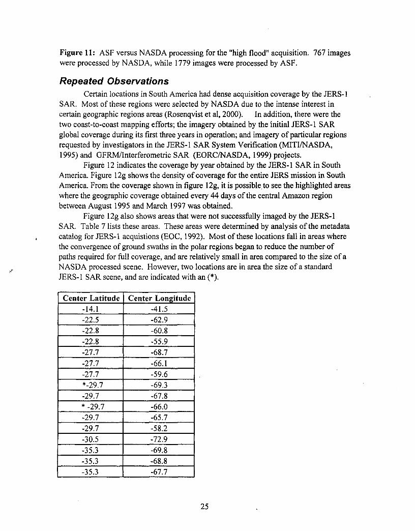
Figure 11: ASF versus NASDA processing for the "high flood" acquisition. 767 images were processed by NASDA, while 1779 images were processed by ASF.

Repeated Observations Certain locations in South America had dense acquisition coverage by the JERS-1

SAR. Most of these regions were selected by NASDA due to the intense interest in certain geographic regions areas (Rosenqvist et al, 2000). In addition, there were the two coast-to-coast mapping efforts; the imagery obtained by the initial JERS-1 SAR global coverage during its first three years in operation; and imagery of particular regions requested by investigators in the JERS- 1 SAR System Verification (MITUNASDA, 1995) and GFWnterferometric SAR (EORC/NASDA, 1999) projects.

America. Figure 12g shows the density of coverage for the entire JERS mission in South America. From the coverage shown in figure 12g, it is possible. to see the highlighted areas where the geographic coverage obtained every 44 days of the central Amazon region between August 1995 and March 1997 was obtained.

Figure 12g also shows areas that were not successfully imaged by the JERS-1 SAR. Table 7 lists these areas. These areas were determined by analysis of the metadata

the convergence of ground swaths in the polar regions began to reduce the number of paths required for full coverage, and are relatively small in area compared to the size of a NASDA processed scene. However, two locations are in area the size of a standard JERS-1 SAR scene, and are indicated with an (*).

Figure 12 indicates the coverage by year obtained by the JERS-1 SAR in South

I catalog for JERS-1 acquistions (EOC, 1992). Most of these locations fall in areas where

-22.8

-59.6 -27.7 -66.1 -27.7 -68.7 -27.7 -55.9

-69.3 *-29.7

~~

-35.3 -67.7 -35.3 -68.8

~~~ ~

25

-35.3

-74.7 -45.1 -72.0 -37 -66.0

Table 6. Gaps in coverage.Scenes indicated by (*) are the size of a full JERS- 1 SAR scene.

To compare the radar coverage with what would be obtained by an optical instrument, figure 12h shows the 11 year average of cloud cover statistics obtained by the ISCCP project (Rossow et al, 1991). As can be seen, there are two regions that are particularly difficult to image optically: a large region to the North of the Amazon River, and the southern tip of South America. In these areas, the JERS-1 SAR data is particularly valuable as in some cases the imagery may be the best representation of forest cover on the ground during that epoch.

26

27

Figure 12: The color bars in each image indicate the density of coverage, ranging from violet representing a single image to red indicating 25 images. Brown indicates no imagery was obtained. A) 1992 coverage. B) 1993 coverage. C) 1994 coverage. D) 1995 coverage. E) 1996 coverage. F) 1997 coverage. G ) 1992-1997 coverage. H) 1 1 years of cloud cover statistics from the ISCCP project (isccp.giss.nasa.gov). For figure H, red indicates over 90% cloudiness, while yellow is between 60% and 90%, green is 40%-60%, and blue is less than 40% cloudiness.

Seasonal diversity The seasonal characteristics of the acquired data is crucially important, as the

JERS-1 SAR is very sensitive to some seasonal conditions. In addition, since optical sensors can not obtain cloud free imagery from certain regions during certain time periods, it is the seasonal diversity of the data set that is one of its strengths.

Figure 13 shows the result of plotting the JERS- 1 SAR 1992- 1997 coverage after dividing the year into four quarters. The first quarter, corresponding through December to February, is shown in 13a, the second quarter corresponding to March through May in 13 b, the third quarter corresponding to June through August in 13c, and the fourth quarter corresponding to September through November is shown in 13d. This region is too large

substantial seasonal diversity for many areas was obtained, in particular for the central Amazon River basin.

L to characterize individual seasons for the entire data set. However, this figure shows that

28

"

.

I

-

Figure 13. Seasonal Diversity. The color bar indicates the density of coverage, ranging from violet (1 image) to blue (6 images). Brown indicates no image was obtained. a) December through February. B) March through May. C) June through August. D) September through November.

5. Conclusions Due to the nature of the orbit of the JERS satellite, continental scale observations

were very simple to obtain in a systematic 'fashion. Also aiding the observation strategy was the knowledge that, absent technical difficulties, the data acquisition could be assured, regardless of cloud and weather conditions of the ground swath. Due to the sensitivity of the JERS-I SAR to inundated forests, the observations were coordinated around the approximate flooding cycle of the main stem of the Amazon River, and conducted both at high and low predicted flood periods.

Detailed knowledge of the characteristics of the data are required for many scientific studies. In addition, the mosaicking process that was implemented required the utmost care in calibration of the imagery. The data quality of the JERS-1 SAR data was

29

found to be very stable, though the processing facilities produced slightly different results for the same raw signal data.

The data coverage of the JERS-1 SAR over South America is also described. This rich data set is an important record of the state of the South American continent for the 1990s.

Acknowledgments The authors wish to thank Japan's National Space Development Agency's Earth

Observation Research Center for establishing the Global Rain forest Mapping Project and the Alaska SAR Facility for processing the data from South and Central America. We also thank the personnel at RESTEC for their invaluable assistance. We would also like to individually thank Bike Rosenqvist, Masanobu Shimada, Diane Wickland, Marcos Alves, Greg McGarragh, Frank DeGrandi, Erika Podest, Laura Hess, John Melack, John Holt, and Dave Curkendall. The work described in this publication was partially carried out by the Jet Propulsion Laboratory, California Institute of Technology, under a contract with the National Aeronautics and Space Administration.

References b CHAPMAN, B., HOLT, J.W., AND HESS, L., 1997, Mapping the extent of inundation of the

Amazon River basin, AGU Fall meeting.,H32A-34, San Francisco, California, 1997.

FREEMAN, A, CHAPMAN, B., AND ALVES, M.,1996, The JERS-1 Amazon Multi-mission Mapping Study (JAMMS), Proc of 1996 Intnl. Geosci. Rem. Sens., pp830-833, Lincoln, Nebraska, 1996.

HESS, L.L., MELACK, J.M., FILOSO, S., AND WANG, Y.,1995, Delineation of inundated areas and vegetation along the Amazon floodplain with the SIR-C Synthetic Aperture Radar, IEEE transactions Geosci. Rem. Sens.,33,896-904.

Hess, L., 1999, personal communication.

JET PROPULSION LABORATORY, 1991, Alaska SAR facility Archive and Catalog Subsystem User's Guide, JPL D-5496, Jet' Propulsion Laboratory, Pasadena, California, USA.

LUCKMAN, ADRIAN, BAKER, JOHN, KUPLICH, TATIANA MORA, YANASSE, CORINA D A COSTA FREITAS, AND FRERY, ALEJANDRO C. , 1997, A study of the relationship between Radar Backscatter and Regenerating Tropical Forest Biomass for spaceborne S A R instruments, Remote Sensing of the Environment, 60, 1 - 1 3.

MITI/NASDA, 1995, Final Report of JERS-l/ERS-1 System Verfication Program, Tokyo, Japan

30

NASDA EARTH OBSERVATION CENTER, 1995, JERS-I SAR Data Users Handbook, NASDA EORC, Tokyo, Japan.

Earth Observation Research Center (EORC)/NASDA, 1999, JERS-1 Science Program 99 .

PI reports, Tokyo, Japan

NASDA EARTH OBSERVATION CENTER, 1996, JERS SAW ERS AMI, Image Data Format, First Issue, NASDA EORC, Tokyo, Japan.

Rauste, Y., Richards, T., DeGrandi, G., Perna, G., Franchino, E. And Rosenqvist, A, 1999, I' Compilation and Validation of the GRFM Africa (SAR) Mosaics using Multi- temporal Block Adjustment, JERS-1 Science Program '99 PI reports, March 1999, EORC, NASDA, Japan.

ROSENQVIST, AKE , 1996, The global rain forest mapping project by JERS-1 S A R , Proc of XVIII ISPRS Cong. In Vienna, Austria, 1996.

k Rosenqvist, A, Shimada, M., Chapman, B., Freeman, A., DeGrandi, G., Saatchi, S., and Rauste, Y.,2000,"The Global Rain Forest Mapping Project - A Review'', Int. J. Rem. Sens., Vol. 21, No. 6 & 7, pp. 1375-1387.

Saatchi, S., Nelson, B., Podest, E., and Holt, J., 2000,"Mapping Land Cover types in the Amazon Basin using lkm JERS-1 mosaic", Int. J. Rem. Sens., Vol. 21, No. 6 & 7, pp. 1201-1234.

Shimada, M., "JERS-1 SAR Calibration and Validation", presented at the CEOS SAR Calibration Workshop, Noordwijk, The Netherlands, September 1993.

SIQUIERA, P., HENSLEY, S., SHAFFER, S., HESS, L., MCGARRAGH, G., CHAPMAN, B., HOLT, J., AND FREEMAN, A., 2000, A continental scale mosaic of the Amazon basin using JERS-1 SAR,accepted, IEEE Transactions Geoscience and Remote Sensing.

Siqueira, P., Hensley, S., Shaffer, S., Hess, L., McGrarragh, G., Chapman, B., Holt, J., and Freeman, A., 2000, "A continental Scale Mosaic of th Amazon Basin using JERS-1 SAR", accepted, IEEE transactions Geoscience and Remote Sensing.

Simard, Marc, Saatchi, Sasan, and DeGrandi, Gianfranco, 2000, I' The use of Decision Tree and Multi-scale Texture for Classification of JERS-1 SAR Data over Tropical Forest, accepted IEEE Geoscience and Remote Sensing, IGARSS99 special issue.

31

VANZYL, J., CHAPMAN, B., DUBOIS, PASCALE C., AND FREEMAN, A., 1992, POLCAL User's Manual version 4.0, JPL Document, D-7715, Jet Propulsion Laboratory, Pasadena, California, USA.

VanZyl, J. J., Chapman, B.D., Dubois, P., and Shi, J., 1993, The effect of topography on .

SAR calibration, IEEE Transactions Geoscience and Remote Sensing,3 1, pplO36- 1043.

YONEYAMA, I(, KOIZUMI, T., SUZUKI, T., KURAMASU, T., ARAKI, T., ISHIDA, C., KOBAYASHI, M., AND KAKUICHI, O., 1989, JERS-1 Development Status, 4th Congress of the International Astonautical Federation, Malaga, Spain, October 1989.

32