eScholarship provides open access, scholarly publishingservices to the University of California and delivers a dynamicresearch platform to scholars worldwide.

University of California

Peer Reviewed

Title:The irreversibility effect in environmental decisionmaking

Author:Narain, Urvashi, Resources for the FutureHanemann, W. Michael, University of California, BerkeleyFisher, Anthony C, University of California, Berkeley and Giannini Foundation

Publication Date:11-01-2007

Publication Info:Postprints, UC Berkeley

Permalink:http://escholarship.org/uc/item/7bc5t8cf

Additional Info:The original publication is available at www.springerlink.com

DOI:10.1007/s10640-007-9083-x

Original Citation:Narain, Urvashi; Hanemann, William Michael; Fisher, Anthony C.,The irreversibility effect inenvironmental decisionmaking. Environmental and resource economics, v.38:3, Nov 2007.

Keywords:decisionmaking under uncertainty, irreversibility effect, necessary and sufficient conditions,nonseparable benefit functions

Abstract:We provide a new, more general definition for the irreversibility effect and demonstrate itsrelevance to problems involving environmental and other decisions under uncertainty. Weestablish several analytical and numerical results that suggest both that the effect holds morewidely that generally recognized, and that an existing result (Epstein's Theorem), giving a sufficientcondition for determining whether the effect holds, can be applied more widely than previouslyindicated, in particular to problems involving intertemporarally nonseparable benefit functions. Wefurther show that a low elasticity of intertemporal substitution will however result in failure of theeffect.

The Irreversibility Effect in EnvironmentalDecisionmaking

Urvashi Narain

Resources for the Future

1616 P Street NW, Washington DC 20036

Michael Hanemann

Department of Agricultural & Resource Economics

University of California, Berkeley CA 94720

Anthony Fisher

Department of Agricultural & Resource Economics

University of California, Berkeley CA 94720

This research received financial support from the National Science Foundation grant No. SES-9818642. The authors gratefully acknowledge comments on earlier drafts of this paper by ananonymous reviewer, Christian Gollier, Christian Traeger, an anonymous reviewer, and participantsat the International Conference on Risk and Uncertainty in Environmental and Resource Economics,Wageningen, The Netherlands, and Columbia Earth Institute Environmental Economics Seminar.Corresponding author: Anthony Fisher, Department of Agricultural and Resource Economics,University of California, Berkeley, CA 94720, Tel: (510) 642-7555, Fax: (510) 643-8911, Email:fisher@are.berkeley.edu.

The Irreversibility Effect in EnvironmentalDecisionmaking

Abstract

We provide a new, more general, definition for the irreversibility effect and demonstrate its rel-

evance to problems involving environmental and other decisions under uncertainty. We establish

several analytical and numerical results that suggest both that the effect holds more widely than

generally recognized, and that an existing result (Epstein’s Theorem), giving a sufficient condition

for determining whether the effect holds, can be applied more widely than previously indicated, in

particular to problems involving intertemporally nonseparable benefit functions. We further show

that a low elasticity of intertemporal substitution will however result in failure of the effect.

JEL: Q20, Q30, Q51

Keywords: decisionmaking under uncertainty, irreversibility effect, necessary and sufficient condi-

tions, nonseparable benefit functions

1. Introduction

Environmental impacts of an investment in resource development can be long lasting, or

even irreversible. This is a feature of environmental valuation and decision problems that

has received a great deal of attention in the literature, based on findings in the natural

sciences. For example, there is both scientific and popular concern today about loss of

biodiversity, the genetic information that is potentially valuable in medicine, agriculture,

and other productive activities. Much of the concern is for endangered species, or their

habitats such as tropical moist forests that are subject to more or less irreversible conversion

to other uses. But even if species survival is not at issue, biological impacts can be very

difficult to reverse over any relevant time span. The clear-cutting of a climax forest species,

for example, removes the results of an ecological succession that may represent centuries of

natural processes. Regeneration may not lead to the original configuration, as opportunistic

species such as hardy grasses come in and preempt the niche otherwise filled by the climax

species (Albers & Goldbach 2000).

Irreversibilities have also been identified as a key feature of the problem of how to respond

to potential impacts of climate change. Emissions of greenhouse gases, in particular carbon

dioxide, accumulate in the atmosphere and decay only slowly. According to one calculation,

assuming business-as-usual use of fossil fuels over the next several decades, after a thousand

years carbon dioxide concentrations will still be well over twice the current level, and nearly

three times the pre-industrial level, and will remain elevated for many thousands of years

(Schultz & Kasting 1997). There is also some prospect of essentially irreversible catastrophic

impact as would result for example from the disintegration of the West Antarctic Ice Sheet

and consequent rise in sea level of 15-20 feet. Recent findings suggest that this possibility

is more serious, and perhaps closer in time, than economists (and others) have realized

((Kerr 1998) and (de Angelis & Skvarca 2003)).

1

Irreversibilities are of course not confined to environmental decisions, but occur in a wide

variety of economic settings, as the definitive work on investment decisions under uncertainty

by Dixit & Pindyck (1994) makes clear.

In the environmental economics literature the analysis of investment decisions under un-

certainty and irreversibility was introduced by Arrow & Fisher (1974) and Henry (1974),

who show that, for a linear net benefit function or an all-or-nothing choice, it will be optimal

to delay or reduce investment, for example in a water resource development project in a nat-

ural environment, if future net benefits are uncertain, investment decisions are irreversible,

and there is a possibility of learning about future benefits. Dixit and Pindyck and others

establish essentially the same result for the more general investment problem, broadening

the treatment to include nonlinear benefit functions and continuous choices, at the same

time greatly enriching the analysis with a rigorous treatment of stochastic optimization.

Beginning with the seminal paper by Epstein (1980) on decision-making and the temporal

resolution of uncertainty, and including important contributions by Freixas & Laffont (1984),

Hanemann (1989), Kolstad (1996), Ulph & Ulph (1997), Gollier, Jullien & Treich (2000),

and Ha-Duong & Treich (2004), another strand of the literature has focused on the question

of whether the rather strong and unambiguous results of Arrow and Fisher, Henry, and

Dixit and Pindyck, continue to hold in still more general settings in which the intertemporal

benefit function exhibits properties not considered by these authors.

In this paper we take up the discussion of several aspects of this question. The next section

reviews existing definitions of the irreversibility effect and proposes a new one, which we show

in Section 3 to be more generally applicable. Section 4 develops a numerical example to prove

that the only necessary condition in the literature is, in fact, sufficient but not necessary,

while Section 5 establishes that one of the mostly widely used sufficient conditions in the

literature, due to Epstein (1980), is more widely applicable than previously believed. This

section also establishes conditions under which the irreversibility effect is likely to be violated.

Section 6 offers some broad conclusions on the status and significance of the irreversibility

effect.2

2. The Irreversibility Effect and the Environment

We begin by presenting two existing definitions, and one new definition, for the irreversibility

effect. For this purpose consider a two-period decision problem, where in the first period the

decision maker chooses a variable x1 and in the second period a variable x2. Net benefits in

the first period, denoted by B1(x1), are deterministic and depend only on x1, but net benefits

in the second period, denoted by B2(x1, x2, zi), are stochastic and are a function both of x1,

x2, and also of z, a random variable that reflects the underlying uncertainty about the nature

of net benefits. We assume that z is a discrete random variable with M possible realizations.

Furthermore, B1 is assumed to be concave and twice continuously differentiable in x1, and

B2 concave and twice continuously differentiable in x1 and x2. An issue that will become

of some importance is whether or not the benefit function is separable in x1 and x2. In the

general case where B2 is a function of x1, the benefit function is said to be nonseparable.

If, on the other hand, B2 were only a function of x2 and z but not of x1, then the benefit

function would be said to be separable.

In principle, there are constraints on the first- and second-period choices. C1 denotes

the constraint function for x1. A crucial issue in the literature is the extent to which the

first period choice of x1 constrains the future choice of x2. In general, we will assume that

the first period choice does constrain the second period choice, the constraint on the latter

being given by C2(x1). The constraint on x2 could take a variety of forms and, in general,

it implies a loss of flexibility in the second period decision. A sharp form of the constraint

would be x1 > x2 which implies that x2 is constrained to be less than x1; we refer to this,

and any such constraint on x2, as the irreversibility constraint. Note that, by using a non-

separable formulation of the second period net benefit function, we already imply that the

first period decision will affect the choice confronting the decision maker in the second period.

Making the second period constraint function depend on x1 introduces a separate element

of interdependence between the two choices.

3

Before the second period decision is made, the decisionmaker receives a signal, denoted by

yj, that reveals some information about z. This is the source of learning. y is also assumed

to be a discrete random variable with N possible realizations. The amount of information

contained in y depends on how closely related z and y are. Let y and y′ denote two potential

signals where the correlation between y and z is greater than the correlation between y′ and z.

y is said to be more informative about z, and leads to greater learning about the true nature

of z, than y′.1 After the signal is received, the decisionmaker updates her prior expectations

about z by formulating a posterior distribution denoted by πij = p(z = zi/y = yj) and then

chooses x2 for each signal to maximize the expected benefit over the different states. Also,

let qj denote the probability distribution for y.

With this notation, the dynamic optimization problem is

(1) maxx1∈C1

(B1(x1) +

∑j

qj maxx2∈C2(x1)

[∑i

πijB2(x1, x2, zi)])

.

Finally, we assume that a unique solution exists, and lies in the interior of C1. Let x∗1

denote the maximum corresponding to the more informative signal y, and x∗∗1 the maximum

corresponding to the less informative signal y′.

The conventional definition of the irreversibility effect in the literature is

(2) either x∗1 ≥ x∗∗

1 or x∗1 ≤ x∗∗

1 .

Which of these two conditions applies depends on the structure of the problem. If the

problem is how much wildlife habitat to keep intact in the first period and not convert to

farmland, then an increase in the fraction of habitat left untouched in anticipation that the

decisionmaker will learn about the relative benefits of wildlife habitats and farmlands prior

1Note that we are adopting the same notion of learning as adopted by Epstein (1980), who, in turn, usesthe notion of greater information discussed by Marschak & Miyasawa (1968). For a more precise definitionof greater learning see Epstein (1980).

4

to the second period, as compared to the amount of habitat left untouched when there is no

possibility of learning, implies an irreversibility effect. Converting a larger fraction of habitat

into farmland in the first period, before uncertainty about the benefits of keeping wildlife

habitats intact is resolved, would force the decisionmaker to accept lower benefits should

it turn out that the benefits of habitats are larger than initially expected. If the benefits

are smaller than expected then the decision maker can choose to convert more habitat into

farmland in the second period, a possibility that is in no way constrained by leaving a larger

fraction of the land as wildlife habitat in the first period. In this case the irreversibility effect

holds if x∗1 ≥ x∗∗

1 , where x1 is the amount of land in wildlife habitat in the first period.

On the other hand, if the decision is how much of a greenhouse gas to emit when damages

due to global warming are uncertain, then a decrease in the amount emitted implies an irre-

versibility effect. Higher first period emissions would lock the decisionmaker into accepting

whatever the nature of the damages are revealed to be, and not being able to avert damages

should these turn out to be higher than expected. Should damages turn out to be lower

than expected, the decisionmaker can always increase emissions in the second period. In this

case the irreversibility effect holds if x∗1 ≤ x∗∗

1 , where x1 is the amount of the greenhouse gas

emitted in the first period.

A related definition, since the conventional definition is really about allowing for more

options in the future, due to Freixas & Laffont (1984), is

(3) C2(x∗1) ⊇ C2(x

∗∗1 ).

In words, the irreversibility effect is said to hold if the second period choice set associated with

x∗1 is at least as large as the choice set associated with x∗∗

1 . In the habitat versus farmlands

example, where the decisionmaker chooses the amount of wildlife habitat to leave intact in

the second period and where C2(x1) is defined as x1 ≥ x2, the second period choice set is

5

larger the larger is the amount of habitat left intact in the first period. The irreversibility

effect is said to hold if x∗1 ≥ x∗∗

1 , which in turn is equivalent to C2(x∗1) ⊇ C2(x

∗∗1 ).

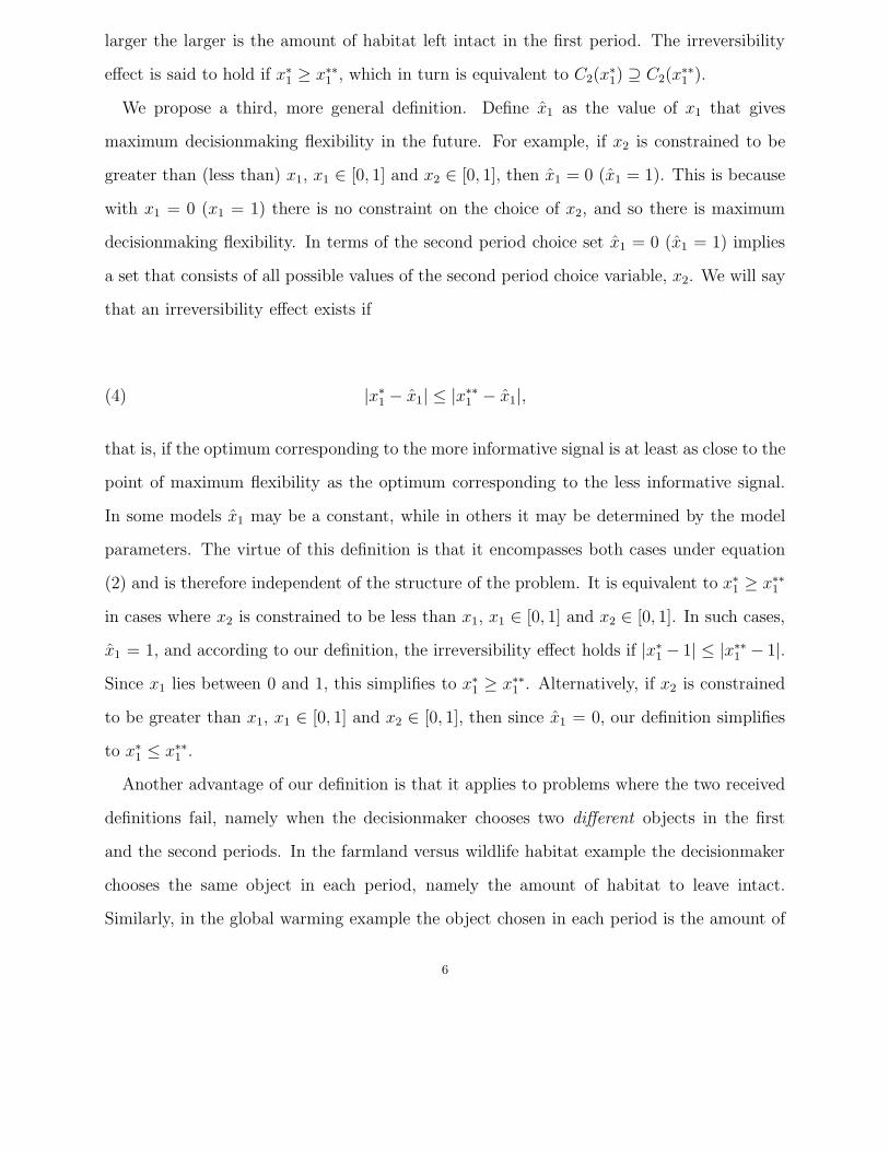
We propose a third, more general definition. Define x1 as the value of x1 that gives

maximum decisionmaking flexibility in the future. For example, if x2 is constrained to be

greater than (less than) x1, x1 ∈ [0, 1] and x2 ∈ [0, 1], then x1 = 0 (x1 = 1). This is because

with x1 = 0 (x1 = 1) there is no constraint on the choice of x2, and so there is maximum

decisionmaking flexibility. In terms of the second period choice set x1 = 0 (x1 = 1) implies

a set that consists of all possible values of the second period choice variable, x2. We will say

that an irreversibility effect exists if

(4) |x∗1 − x1| ≤ |x∗∗

1 − x1|,

that is, if the optimum corresponding to the more informative signal is at least as close to the

point of maximum flexibility as the optimum corresponding to the less informative signal.

In some models x1 may be a constant, while in others it may be determined by the model

parameters. The virtue of this definition is that it encompasses both cases under equation

(2) and is therefore independent of the structure of the problem. It is equivalent to x∗1 ≥ x∗∗

1

in cases where x2 is constrained to be less than x1, x1 ∈ [0, 1] and x2 ∈ [0, 1]. In such cases,

x1 = 1, and according to our definition, the irreversibility effect holds if |x∗1 − 1| ≤ |x∗∗

1 − 1|.Since x1 lies between 0 and 1, this simplifies to x∗

1 ≥ x∗∗1 . Alternatively, if x2 is constrained

to be greater than x1, x1 ∈ [0, 1] and x2 ∈ [0, 1], then since x1 = 0, our definition simplifies

to x∗1 ≤ x∗∗

1 .

Another advantage of our definition is that it applies to problems where the two received

definitions fail, namely when the decisionmaker chooses two different objects in the first

and the second periods. In the farmland versus wildlife habitat example the decisionmaker

chooses the same object in each period, namely the amount of habitat to leave intact.

Similarly, in the global warming example the object chosen in each period is the amount of

6

greenhouse gases to emit. However, in the case of Epstein’s firm’s-demand-for-capital model

(discussed in detail in the next section) a different object is chosen in each period: capital

in the first and labor in the second. Alternatively, faced with a decision to reserve a natural

environment for wildlife habitat or recreation, a manager may choose the amount of land

to set aside in the first period and the number of rangers and complementary personnel to

allocate to monitoring and protection in the second period. In such models with two different

choice variables, the choice made in the first period does not limit the choice set available

in the second period. The amount of capital chosen in the first period does not limit the

amount of labor that can be employed in the second period. The amount of land set aside

for protection does not limit the number of personnel that can be employed. Consequently,

a definition of irreversibility that compares the choice sets in the second period for different

initial choices is not useful and will not yield any predictions about the irreversibility effect.

The other received definition of the irreversibility effect, specified in equation 2, fails as well

because it is not clear which of the two conditions specified under this definition applies

to such models. Our definition, on the other hand, and as we show in the next section,

continues to apply.

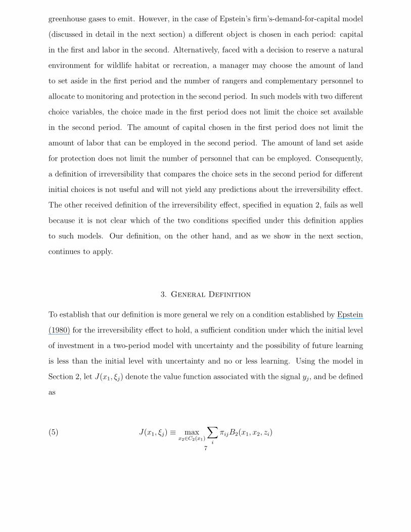
3. General Definition

To establish that our definition is more general we rely on a condition established by Epstein

(1980) for the irreversibility effect to hold, a sufficient condition under which the initial level

of investment in a two-period model with uncertainty and the possibility of future learning

is less than the initial level with uncertainty and no or less learning. Using the model in

Section 2, let J(x1, ξj) denote the value function associated with the signal yj, and be defined

as

(5) J(x1, ξj) ≡ maxx2∈C2(x1)

∑i

πijB2(x1, x2, zi)

7

where ξj = [π1j , π2j , ..πij .., πMj] and is a vector of the posterior probability distribution

corresponding to the signal yj . J(x1, ξ) is then a vector of value functions where ξ =

[ξ1, ξ2, ...ξj, ...ξN ]. Under the assumption that J(x1, ξ) is concave and differentiable with

respect to x1,2 then Epstein’s sufficient condition relating x∗

1 to x∗∗1 is given in Theorem 1.

Theorem 1. If Jx1(x∗1, ξ) is a concave (convex) function of ξ, then x∗

1 ≤ (≥)x∗∗1 . If Jx1(x

∗1, ξ)

is neither convex nor concave, then the sign of x∗1 − x∗∗

1 is ambiguous.

In words, the sufficient condition states that if the slope of the value function with respect to

x1, Jx1(x1, ξ), is concave (convex) in the posterior probability distribution, then the optimal

choice of x1 associated with the more informative signal is less (more) than the optimal

choice associated with the less informative signal.3

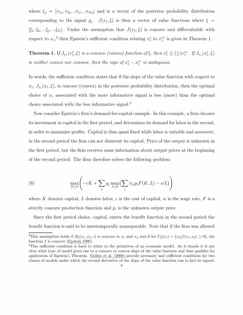
Now consider Epstein’s firm’s-demand-for-capital example. In this example, a firm chooses

its investment in capital in the first period, and determines its demand for labor in the second,

in order to maximize profits. Capital is thus quasi fixed while labor is variable and moreover,

in the second period the firm can not disinvest its capital. Price of the output is unknown in

the first period, but the firm receives some information about output prices at the beginning

of the second period. The firm therefore solves the following problem:

(6) maxK≥0

(−cK +

∑j

qj maxL≥0

(∑i

πijpiF (K, L) − wL))

where K denotes capital, L denotes labor, c is the cost of capital, w is the wage rate, F is a

strictly concave production function and pi is the unknown output price.

Since the first period choice, capital, enters the benefit function in the second period the

benefit function is said to be intertemporally nonseparable. Note that if the firm was allowed

2This assumption holds if B2(x1, x2, z) is concave in x1 and x2 and if for C2(x1) = {x2|f(x1, x2) ≥ 0}, thefunction f is concave (Epstein 1980).3This sufficient condition is hard to relate to the primitives of an economic model. As it stands it is notclear what type of model gives rise to a concave or convex slope of the value function and thus qualifies forapplication of Epstein’s Theorem. Gollier et al. (2000) provide necessary and sufficient conditions for twoclasses of models under which the second derivative of the slope of the value function can in fact be signed.

8

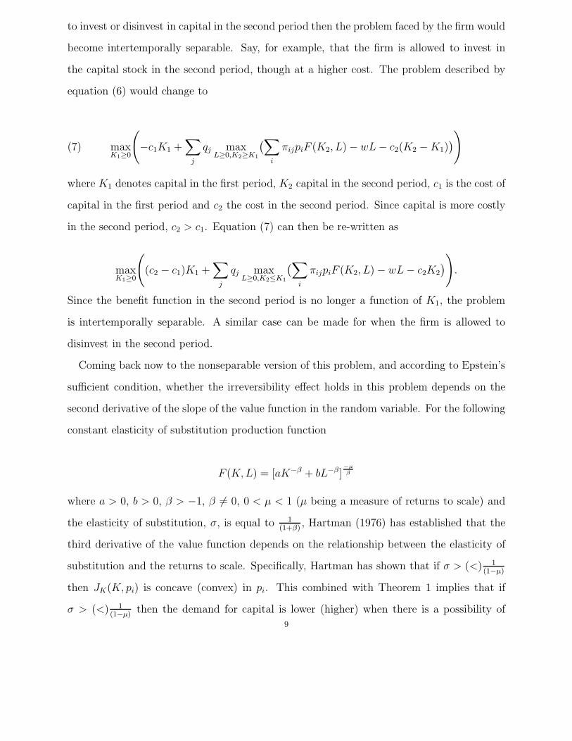
to invest or disinvest in capital in the second period then the problem faced by the firm would

become intertemporally separable. Say, for example, that the firm is allowed to invest in

the capital stock in the second period, though at a higher cost. The problem described by

equation (6) would change to

(7) maxK1≥0

(−c1K1 +

∑j

qj maxL≥0,K2≥K1

(∑i

πijpiF (K2, L) − wL − c2(K2 − K1)))

where K1 denotes capital in the first period, K2 capital in the second period, c1 is the cost of

capital in the first period and c2 the cost in the second period. Since capital is more costly

in the second period, c2 > c1. Equation (7) can then be re-written as

maxK1≥0

((c2 − c1)K1 +

∑j

qj maxL≥0,K2≤K1

(∑i

πijpiF (K2, L) − wL − c2K2

)).

Since the benefit function in the second period is no longer a function of K1, the problem

is intertemporally separable. A similar case can be made for when the firm is allowed to

disinvest in the second period.

Coming back now to the nonseparable version of this problem, and according to Epstein’s

sufficient condition, whether the irreversibility effect holds in this problem depends on the

second derivative of the slope of the value function in the random variable. For the following

constant elasticity of substitution production function

F (K, L) = [aK−β + bL−β ]−µβ

where a > 0, b > 0, β > −1, β �= 0, 0 < µ < 1 (µ being a measure of returns to scale) and

the elasticity of substitution, σ, is equal to 1(1+β)

, Hartman (1976) has established that the

third derivative of the value function depends on the relationship between the elasticity of

substitution and the returns to scale. Specifically, Hartman has shown that if σ > (<) 1(1−µ)

then JK(K, pi) is concave (convex) in pi. This combined with Theorem 1 implies that if

σ > (<) 1(1−µ)

then the demand for capital is lower (higher) when there is a possibility of

9

learning than when there is no possibility of learning. By implicitly relying on the existing

definitions of the irreversibility effect, which, in turn imply that the effect holds either when

K∗ ≤ K∗∗ or when K∗ ≥ K∗∗ (see equation 2), and since the demand for capital does

not unambiguously increase or decrease with learning, Epstein leads the reader to conclude

that the irreversibility effect is violated in this example. However, our definition of the

irreversibility effect establishes that the effect does, in fact, hold in this example.

Observe that the firm can neither increase nor decrease its capital stock in the second

period. Consequently, one cannot tell a priori whether a high or a low demand for capital in

the first period constitutes a flexibility-enhancing decision, and therefore whether K∗ ≤ K∗∗

or K∗ ≥ K∗∗ is required for the irreversibility effect to hold. When σ is high so that capital

and labor can be easily substituted then a lower capital stock today may very well give

the decision maker greater flexibility tomorrow. If it turns out that the decision maker has

underestimated his or her production needs, then he or she can compensate for the low stock

of capital by hiring more labor. The irreversibility effect would then hold if K∗ ≤ K∗∗. On

the other hand, if σ is low so that capital and labor cannot be substituted, a higher capital

stock today may maintain greater flexibility tomorrow and the irreversibility effect would

hold if K∗ ≥ K∗∗. Therefore in order to establish whether or not the irreversibility effect

holds, we need to first define what constitutes flexibility in this problem.

There are two definitions of flexibility in the literature: one due to Freixas & Laffont (1984),

and another due to Jones & Ostroy (1984). By Freixas and Laffont’s definition of flexibility,

which is equivalent to their definition for the irreversibility effect (see equation 3), the choice

of capital that gives the greatest flexibility in the second period is the one that produces

the largest choice set in the second period. Jones and Ostroy similarly define flexibility in

terms of second period choices that can be attained from the first period position with the

additional qualifier that the positions be attained at a given cost and for a particular state

of the world.4 Neither of these definitions apply to our problem, however. If the choice

4Let c(x1, x2, zi) denote the cost of moving from x1 to x2 given that the state of the world is zi. ThenG(x1, zi, α), where

G(x1, zi, α) ≡ {x2 : c(x1, x2, zi) ≤ α},10

set in the second period is defined in terms of capital, then since capital can neither be

increased nor decreased in the second period, irrespective of the level of capital chosen in

the first period, the decision maker has a single element in their choice set in the second

period, namely the level of capital in the first period. No one level of capital gives a larger

or smaller choice set in the second period. Defining the second period choice set in terms of

labor instead does not help define a more or less flexible level of capital either as the first

period’s choice of capital in no way restricts the choice of labor in the second period.

The question then arises, with respect to what variable should flexibility be measured?

So far we have tried to measure flexibility in terms of the choice variables, that is, in terms

of the choices of capital or labor in the second period that are feasible given the choice of

capital in the first period. However, one could instead measure flexibility in terms of the

level of output that can be attained in the second period given the choice of capital in the

first. After all, the firm cares about the level of capital, or any other input, only in so far

as it allows the firm to produce output in the second period. In fact, what the firm really

cares about is the range of outputs5 that can be attained for a given level of capital. If the

firm learns that the price of output is likely to be high tomorrow it would want to produce

more, and conversely if it learns that the price is likely to be low it would want to reduce

production. Flexibility for the firm manifests itself in terms of the range of output that the

firm can produce. With this definition a more flexible level of capital is one that enables the

firm to produce a greater range of output in the second period.

With a production function that exhibits constant elasticity of substitution, the level of

capital that enables the firm to produce the greatest range of output, in fact, depends on

the model parameters. Furthermore, the level of capital that gives the greatest flexibility is

lower (higher) when σ > (<) 11−µ

.

is the set of second period positions attainable from x1 at a cost that does not exceed α in state s. In generalx∗

1 is said to generate more flexibility than x∗∗1 when for all α ≥ 0 and for all zi, G(x∗

1 , zi, α) ⊇ G(x∗∗1 , zi, α).

5Note that this is consistent with Hirshleifer & Riley (1992) who point out that flexibility is different fromthe range of actions which in our example would mean the range of capital or labor. We instead equateflexibility to the range of outputs.

11

Proposition 1. If σ > (<) 11−µ

then K = K(K).

where K is the level of capital that implies the greatest amount of flexibility, K is the

minimum capital stock and K is the maximum capital stock.6

Proof. Let y(K) denote the range of output that can be achieved for a given level of capital

and let γ = −µβ

. Note that when σ > (<) 11−µ

, γ < (>)1 since σ = 11+β

> (<) 11−µ

implies

that µ < (>) − β.

y(K) = (aK−β + bL−β

)γ − (aK−β + bL−β)γ

where L is the minimum labor and L is the maximum labor. The derivative of the range of

output with respect to the capital stock is given by

∂y

∂K= −aγβK−(β+1)

((aK−β + bL

−β)γ−1 − (aK−β + bL−β)γ−1

)

When γ < (>)1, ∂y∂K

< (>)0. This in turn implies that when γ < (>)1 then the level of

capital that gives the maximum range of output, K, is equal to the minimum (maximum)

stock of capital.

�

With the most flexible level of capital so defined, and our definition of the irreversibility

effect, consider whether or not the irreversibility effect holds in this example of a firm’s

demand for capital. According to our definition the irreversibility effect holds if |K∗ − K| ≤|K∗∗ − K|, where K∗ is the level of capital investment in the first period with learning, and

K∗∗ the level with less or no learning. When σ > 11−µ

or γ < 1, then K = K and the

irreversibility effect holds if |K∗ − K| ≤ |K∗∗ − K|, or when K∗ ≤ K∗∗. Since demand

for capital declines with learning under these model parameters, the irreversibility effect

6If σ = 1 so that the production function is a Cobb-Douglas then one can show that a higher level of capitalgives a greater range of output. If σ = 0 so that the production function is a Leontief then it is difficult todetermine what level of capital gives greater flexibility tomorrow.

12

holds. Similarly, it can be established that when σ < 11−µ

, the irreversibility effect holds if

K∗ ≥ K∗∗, and that this is in fact the case.

4. Necessary Versus Sufficient Conditions

Building on the sufficient conditions established by Epstein, the literature has established

other sufficient conditions for the irreversibility effect to hold, but only one necessary, and

therefore more restrictive, condition, namely the condition established by Freixas & Laffont

(1984) for intertemporally separable net benefit functions. With such functions, and using

a sharper irreversibility constraint, x2 ≤ x1, the dynamic optimization problem discussed in

Section 2 simplifies to the following:

(8) maxx1∈C1

(B1(x1) +

∑j

qj maxx2≤x1

∑i

πijB2(x2, zi)

).

Since x2 is constrained to be less than or equal to x1, a larger value of x1 in the first period

gives the decisionmaker more flexibility in the second period. And therefore the irreversibility

effect is said to hold so long as x∗1 ≥ x∗∗

1 . Theorem 2 specifies the condition developed by

Freixas and Laffont for the irreversibility effect to hold given that a unique solution exists.

Theorem 2. x∗1 ≥ x∗∗

1 if B1(x1) +∑

j qjJ(x1, ξ) is quasi-concave.

The theorem states that the irreversibility effect holds if the value function is quasi-concave.

Freixas and Laffont establish sufficiency analytically and then develop a numerical example

to show that the sufficient condition is also necessary. Their numerical example establishes

that if quasi-concavity is violated then, in fact, the irreversibility effect is violated. The

irreversibility effect is also shown to be equivalent to J(x1, ξ′) − J(x1, ξ) being locally in-

creasing in x1 where ξ′ is the more informative signal, ξ is the less informative signal, and

J(x1, ξ′) − J(x1, ξ) is the value of information.

A slight modification, however, of Frexias and Laffont’s numerical example shows that

quasi-concavity is only sufficient. In Freixas and Laffont’s numerical example the random13

0 1 2 pi 4 5 2pi 7 8 3pi 10 −0.2

0

0.2

0.4

0.6

0.8

x1

Val

ue o

f Inf

orm

atio

n

Value of Information for the Freixas−Laffont 1984 Example

Figure 1. Value of Information for the Example in Freixas-Laffont 1984

variable z is assumed to take two possible values, z1 and z2, each with probability 0.5.

Furthermore, there are two levels of learning, perfect or none at all. The functional forms of

the benefit functions are,

B1(x1, 0 ≤ x1 ≤ 2.5π) = π

B1(x1, x1 ≥ 2.5π) = −1.25(x1 − 2.5π) + π

B2(x2, z1) = 2x2

B2(x2, z2) = − cos x2 + 1

With these benefit functions quasi-concavity is violated, x∗1 ≤ x∗∗

1 and J(x1, ξ′) − J(x1, ξ),

the value of information, is not increasing in x1. These results are shown in Figure 1 where

the choice variable in the first period, x1, is drawn on the x-axis and the value of information

on the y-axis. Note that in the range [2π, 3π] the value of information decreases in x1. So

long as the optima lie in this range the irreversibility effect is violated.

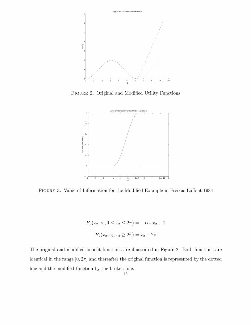
Now consider a slight modification where B1(x1) and B2(x2, z1) remain unchanged and

B2(x2, z2) is given by14

0 1 2 3 4 5 6 7 8 9 100

1

2

3

4

5

6

7

x2U

tility

Orignial and Modified Utility Function

Figure 2. Original and Modified Utility Functions

0 1 2 pi 4 5 2pi 7 8 3pi 10 0 −0.2

0

0.2

0.4

0.6

0.8

1

x1

Val

ue o

f Inf

orm

atio

n

Value of Information for modified F−L example

Figure 3. Value of Information for the Modified Example in Freixas-Laffont 1984

B2(x2, z2, 0 ≤ x2 ≤ 2π) = − cos x2 + 1

B2(x2, z2, x2 ≥ 2π) = x2 − 2π

The original and modified benefit functions are illustrated in Figure 2. Both functions are

identical in the range [0, 2π] and thereafter the original function is represented by the dotted

line and the modified function by the broken line.15

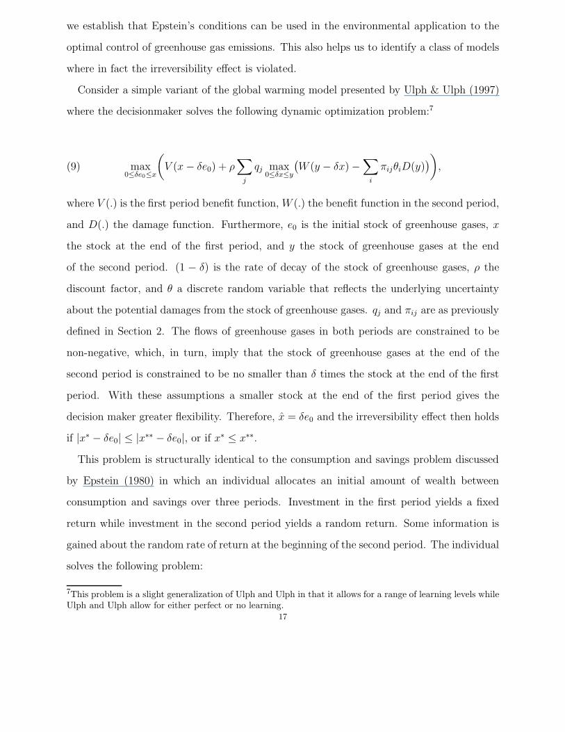
With the modified value function although quasi-concavity is still violated, x∗1 ≥ x∗∗

1

(strictly greater if the optimal lies between π and 2π and equal otherwise) and the value of

information is no longer decreasing over a finite interval of x1. These results are shown in

Figure 3. The irreversibility effect holds though quasi-concavity is violated. Consequently,

quasi-concavity is not necessary, merely sufficient, for the irreversibility effect to hold in the

class of intertemporally separable benefit functions. We note however that quasi-concavity is

a very weak condition. Most, if not all, empirically important benefit functions will exhibit

this property.

In summary, to date a number of sufficient conditions have been established for the ir-

reversibility effect, but not necessary conditions, which would be both more restrictive and

more powerful.

5. Intertemporally Non-separable Benefits

An issue of some importance in the literature is whether or not the benefit function is

separable in x1 and x2. In fact, the existing sufficient conditions in the literature can be

organized into two broad categories: those that apply to models with separable benefit

functions and those that apply to models with non separable functions. Conditions developed

by Freixas & Laffont (1984) and Kolstad (1996), for example, apply to separable models,

while those developed by Epstein (1980), Ulph & Ulph (1997), and Gollier et al. (2000), to

non-separable models.

There is, however, a perception in the literature that Epstein’s condition can not be used

to investigate the irreversibility effect in some models with intertemporally non separable

benefit functions, in particular models of global warming where damages depend on the

amount of accumulated greenhouse gases making the damage function non separable (for

example, see Ulph & Ulph (1997) and Gollier et al. (2000)). As shown in Section 3, so

long as one uses our more general definition of the irreversibility effect, which, in particular,

forces one to determine the point of maximum flexibility, Epstein’s sufficient condition can

be used for at least some intertemporally non separable benefit functions. In this section,16

we establish that Epstein’s conditions can be used in the environmental application to the

optimal control of greenhouse gas emissions. This also helps us to identify a class of models

where in fact the irreversibility effect is violated.

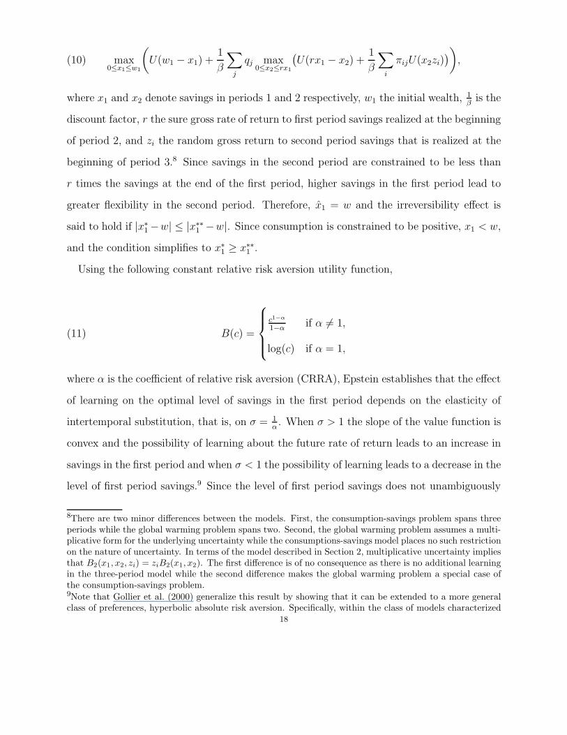
Consider a simple variant of the global warming model presented by Ulph & Ulph (1997)

where the decisionmaker solves the following dynamic optimization problem:7

(9) max0≤δe0≤x

(V (x − δe0) + ρ

∑j

qj max0≤δx≤y

(W (y − δx) −

∑i

πijθiD(y)))

,

where V (.) is the first period benefit function, W (.) the benefit function in the second period,

and D(.) the damage function. Furthermore, e0 is the initial stock of greenhouse gases, x

the stock at the end of the first period, and y the stock of greenhouse gases at the end

of the second period. (1 − δ) is the rate of decay of the stock of greenhouse gases, ρ the

discount factor, and θ a discrete random variable that reflects the underlying uncertainty

about the potential damages from the stock of greenhouse gases. qj and πij are as previously

defined in Section 2. The flows of greenhouse gases in both periods are constrained to be

non-negative, which, in turn, imply that the stock of greenhouse gases at the end of the

second period is constrained to be no smaller than δ times the stock at the end of the first

period. With these assumptions a smaller stock at the end of the first period gives the

decision maker greater flexibility. Therefore, x = δe0 and the irreversibility effect then holds

if |x∗ − δe0| ≤ |x∗∗ − δe0|, or if x∗ ≤ x∗∗.

This problem is structurally identical to the consumption and savings problem discussed

by Epstein (1980) in which an individual allocates an initial amount of wealth between

consumption and savings over three periods. Investment in the first period yields a fixed

return while investment in the second period yields a random return. Some information is

gained about the random rate of return at the beginning of the second period. The individual

solves the following problem:

7This problem is a slight generalization of Ulph and Ulph in that it allows for a range of learning levels whileUlph and Ulph allow for either perfect or no learning.

17

(10) max0≤x1≤w1

(U(w1 − x1) +

1

β

∑j

qj max0≤x2≤rx1

(U(rx1 − x2) +

1

β

∑i

πijU(x2zi)))

,

where x1 and x2 denote savings in periods 1 and 2 respectively, w1 the initial wealth, 1β

is the

discount factor, r the sure gross rate of return to first period savings realized at the beginning

of period 2, and zi the random gross return to second period savings that is realized at the

beginning of period 3.8 Since savings in the second period are constrained to be less than

r times the savings at the end of the first period, higher savings in the first period lead to

greater flexibility in the second period. Therefore, x1 = w and the irreversibility effect is

said to hold if |x∗1 −w| ≤ |x∗∗

1 −w|. Since consumption is constrained to be positive, x1 < w,

and the condition simplifies to x∗1 ≥ x∗∗

1 .

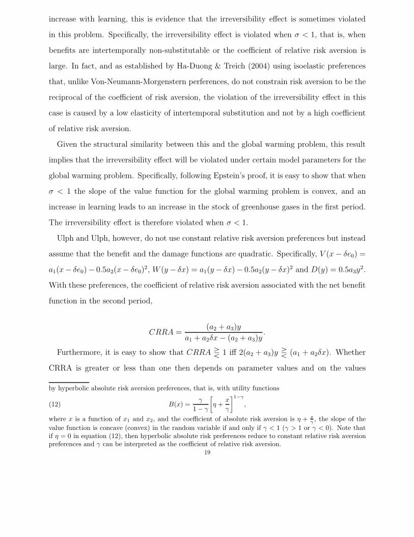
Using the following constant relative risk aversion utility function,

(11) B(c) =

⎧⎪⎪⎨⎪⎪⎩

c1−α

1−αif α �= 1,

log(c) if α = 1,

where α is the coefficient of relative risk aversion (CRRA), Epstein establishes that the effect

of learning on the optimal level of savings in the first period depends on the elasticity of

intertemporal substitution, that is, on σ = 1α. When σ > 1 the slope of the value function is

convex and the possibility of learning about the future rate of return leads to an increase in

savings in the first period and when σ < 1 the possibility of learning leads to a decrease in the

level of first period savings.9 Since the level of first period savings does not unambiguously

8There are two minor differences between the models. First, the consumption-savings problem spans threeperiods while the global warming problem spans two. Second, the global warming problem assumes a multi-plicative form for the underlying uncertainty while the consumptions-savings model places no such restrictionon the nature of uncertainty. In terms of the model described in Section 2, multiplicative uncertainty impliesthat B2(x1, x2, zi) = ziB2(x1, x2). The first difference is of no consequence as there is no additional learningin the three-period model while the second difference makes the global warming problem a special case ofthe consumption-savings problem.9Note that Gollier et al. (2000) generalize this result by showing that it can be extended to a more generalclass of preferences, hyperbolic absolute risk aversion. Specifically, within the class of models characterized

18

increase with learning, this is evidence that the irreversibility effect is sometimes violated

in this problem. Specifically, the irreversibility effect is violated when σ < 1, that is, when

benefits are intertemporally non-substitutable or the coefficient of relative risk aversion is

large. In fact, and as established by Ha-Duong & Treich (2004) using isoelastic preferences

that, unlike Von-Neumann-Morgenstern perferences, do not constrain risk aversion to be the

reciprocal of the coefficient of risk aversion, the violation of the irreversibility effect in this

case is caused by a low elasticity of intertemporal substitution and not by a high coefficient

of relative risk aversion.

Given the structural similarity between this and the global warming problem, this result

implies that the irreversibility effect will be violated under certain model parameters for the

global warming problem. Specifically, following Epstein’s proof, it is easy to show that when

σ < 1 the slope of the value function for the global warming problem is convex, and an

increase in learning leads to an increase in the stock of greenhouse gases in the first period.

The irreversibility effect is therefore violated when σ < 1.

Ulph and Ulph, however, do not use constant relative risk aversion preferences but instead

assume that the benefit and the damage functions are quadratic. Specifically, V (x− δe0) =

a1(x− δe0)− 0.5a2(x− δe0)2, W (y − δx) = a1(y − δx)− 0.5a2(y − δx)2 and D(y) = 0.5a3y

2.

With these preferences, the coefficient of relative risk aversion associated with the net benefit

function in the second period,

CRRA =(a2 + a3)y

a1 + a2δx − (a2 + a3)y.

Furthermore, it is easy to show that CRRA � 1 iff 2(a2 + a3)y � (a1 + a2δx). Whether

CRRA is greater or less than one then depends on parameter values and on the values

by hyperbolic absolute risk aversion preferences, that is, with utility functions

(12) B(x) =γ

1 − γ

[η +

x

γ

]1−γ

,

where x is a function of x1 and x2, and the coefficient of absolute risk aversion is η + xγ , the slope of the

value function is concave (convex) in the random variable if and only if γ < 1 (γ > 1 or γ < 0). Note thatif η = 0 in equation (12), then hyperbolic absolute risk preferences reduce to constant relative risk aversionpreferences and γ can be interpreted as the coefficient of relative risk aversion.

19

of endogenous variables, namely, the stock of greenhouse gases in the first and the second

period. Ulph and Ulph also establish that with these preferences the slope of the value

function is neither concave nor convex, and conclude that Epstein’s sufficient condition

cannot be applied to a model of global warming with non separable benefit functions. The

authors accordingly develop a new sufficient condition: the irreversibility effect is said to

hold if the irreversibility constraint bites when there is no possibility of learning. In terms of

our canonical model, let x∗∗2 and x∗∗

1 denote the optimal decisions in the absence of learning.

If x1 ≤ x2, then x∗∗2 = x∗∗

1 implies that the irreversibility constraint bites in the absence of

learning.10 Note, however, that it is the functional form of the benefit and damage functions

that yields the ambiguity, and causes Epstein’s condition to fail, and not the fact that the

global warming problem is inherently nonseparable.

11

6. Concluding Remarks

In this paper we set out to interpret and extend the strand of the irreversibility effect

literature that has focused on the question of whether the rather strong and unambiguous

results of Arrow and Fisher, Henry, and Dixit and Pindyck, continue to hold in still more

general settings in which the intertemporal benefit function exhibits properties not considered

by these authors. We have tried to build on this literature in a number of ways.

We have introduced a more general definition of the irreversibility effect. Our definition

encompasses the existing ones, and is independent of the structure of the problem. It applies

to problems where the existing definitions fail, namely where the decisionmaker chooses two

10In the same vein Kolstad (1996) shows that the irreversibility effect holds in models with effectiveirreversibility—that is, in models in which the irreversibility constraint bites.11As pointed out by one of our reviewers, there are two types of ambiguities that arise in the application ofEpstein’s conditions. The first, and the one that arises in the firm’s-demand-for-capital example, and in theconsumption-savings example, arises because the slope of the value function varies with model parameters.A priori, and without specifying the values of model parameters, one cannot determine whether the slopeof the value function is concave or convex. However, once the parameter values have been specified, onecan determine unambiguously whether the slope is convex or concave. The second type of ambiguity, theone referred to by Ulph & Ulph (1997), arises when the slope of the first derivative of the value function isneither concave nor convex irrespective of the parameter values. That is, even once the parameter valueshave been specified, one cannot determine whether the slope of the value function is concave or convex.

20

different objects in the first and the second periods, say producible capital or protected land

in the first and the relevant labor complement in the second. In such problems the existing

definitions are not helpful. Our definition, on the other hand, by forcing one to consider

which choice generates the most flexibility, continues to apply.

Applications of our definition, and a numerical example which shows that the only nec-

essary condition in the literature is only sufficient, establish that the irreversibility effect

holds more widely than has perhaps previously been recognized. Another interesting inter-

pretive result is that Epstein’s condition, the original contribution to this literature, and

Theorem 1 in our paper, can in fact be applied more widely, in particular to intertemporally

nonseparable benefit functions, as in the global warming problem, than previously indicated.

21

References

Albers, H. J. & Goldbach, M. J. (2000). Irreversible ecosystem change, species competition, and shifting

cultivation, Land Economics 22.

Arrow, K. J. & Fisher, A. C. (1974). Environmental preservation, uncertainty, and irreversibility, Quarterly

Journal of Economics 88(2): 312–319.

de Angelis, H. & Skvarca, P. (2003). Glacier surge after ice shelf collapse, Science 299.

Dixit, A. K. & Pindyck, R. S. (1994). Investment under Uncertainty, Princeton University Press.

Epstein, L. G. (1980). Decision making and the temporal resolution of uncertainty, International Economic

Review 21: 269–283.

Freixas, X. & Laffont, J.-J. (1984). On the irreversibility effect, in M. Boyer & R. Kihlstrom (eds), Bayesian

Models in Economic Theory, NHPC, pp. 105–114.

Gollier, C., Jullien, B. & Treich, N. (2000). Scientific progress and irreversibility: an economic interpretation

of the precautionary principle, Journal of Public Economics 75: 229–253.

Ha-Duong, M. & Treich, N. (2004). Risk aversion, intergenerational equity and climate change, Environmen-

tal and Resource Economics 28.

Hanemann, W. M. (1989). Information and the concept of option value, Journal of Environmental Economics

and Management 16: 23–37.

Hartman, R. (1976). Factor demand with output price uncertainty, American Economic Review 66: 675–681.

Henry, C. (1974). Investment decisions under uncertainty: The irreversibility effect, American Economic

Review 64: 1006–12.

Hirshleifer, J. & Riley, J. (1992). The Analytics of Uncertainty and Information, Cambridge University Press.

Jones, R. A. & Ostroy, J. M. (1984). Flexibility and uncertainty, Review of Economic Studies 51: 13–32.

Kerr, R. A. (1998). West antarctica’s weak underbelly giving way ?, Science 281: 499–500.

Kolstad, C. D. (1996). Fundamental irreversibilities in stock externalities, Journal of Public Economics

60: 221–233.

Marschak, J. & Miyasawa, K. (1968). Economic comparability of information systems, International Eco-

nomic Review 9: 137–174.

Schultz, P. A. & Kasting, J. F. (1997). Optimal reductions in co2 emissions, Energy Policy 25: 491–500.

Ulph, A. & Ulph, D. (1997). Global warming, irreversibility and learning, The Economic Journal 107: 636–

650.

22