Probing cosmic strings by reconstructing polarization rotation ...
Upload
washingtonCategory
view
0download
0
arX
iv:1
009.
3019
v1 [
astr
o-ph
.EP]
15
Sep
2010
– 1 –
The Increasing Rotation Period of Comet 10P/Tempel 2
Matthew M. Knight1, Tony L. Farnham2, David G. Schleicher1, Edward W. Schwieterman3
Contacting author: [email protected]
The Astronomical Journal
Accepted September 13, 2010
Manuscript pages: 22 pages text
3 tables
6 figures
1Lowell Observatory, 1400 W. Mars Hill Rd, Flagstaff, AZ 86001
2Department of Astronomy, University of Maryland, College Park, MD 20742-2421
3Physics and Space Sciences, Florida Institute of Technology, 150 W. University Blvd, Melbourne, Florida
32901

– 2 –
Abstract
We imaged comet 10P/Tempel 2 on 32 nights from 1999 April through 2000 March.
R-band lightcurves were obtained on 11 of these nights from 1999 April through 1999 June,
prior to both the onset of significant coma activity and perihelion. Phasing of the data
yields a double-peaked lightcurve and indicates a nucleus rotational period of 8.941 ± 0.002
hr with a peak-to-peak amplitude of ∼0.75 mag. Our data are sufficient to rule out all other
possible double-peaked solutions as well as the single- and triple- peaked solutions. This
rotation period agrees with one of five possible solutions found in post-perihelion data from
1994 by Mueller and Ferrin (1996, Icarus, 123, 463–477), and unambiguously eliminates their
remaining four solutions. We applied our same techniques to published lightcurves from 1988
which were obtained at an equivalent orbital position and viewing geometry as in 1999. We
found a rotation period of 8.932 ± 0.001 hr in 1988, consistent with the findings of previous
authors and incompatible with our 1999 solution. This reveals that Tempel 2 spun-down
by ∼32 s between 1988 and 1999 (two intervening perihelion passages). If the spin-down
is due to a systematic torque, then the rotation period prior to perihelion during the 2010
apparition is expected to be an additional 32 s longer than in 1999.
Keywords: comets: general – comets: individual (10P/Tempel 2) – methods: data analysis
– techniques: photometric

– 3 –
1. Introduction
Comet 10P/Tempel 2 was discovered by E.W.L. Tempel on 1873 July 4. It was recov-
ered in 1878, but not during the 1883 or 1889 apparitions. It has been observed on every
return since 1894 except three (1910, 1935, and 1941) when it was particularly poorly placed
for observing (Kronk 2003, 2007, 2009). While telescopic improvements now allow it to be
observed at every apparition, the roughly 5.5 year period results in apparitions which alter-
nate between favorable and unfavorable viewing geometries. Consequently, Tempel 2 was
well placed for observing in 1978, 1988, and 1999, but poorly placed in 1983, 1994, and 2004
when it reached perihelion on the far side of the Sun.
Tempel 2 was extensively observed during its favorable 1988 return. Because it is only
weakly active until shortly before perihelion (Sekanina (1979) and references therein), a
nucleus lightcurve can be measured. This allowed a number of investigators to measure the
rotation period. The earliest results came from Jewitt & Meech (1988) who found likely
periods of 8.9 ± 0.1 hr or 7.5 ± 0.1 hr. Jewitt & Luu (1989) extended these observations
to near perihelion, concluding that the rotation period was 8.95 ± 0.01 hr. Comparable
periods were determined by A’Hearn et al. (1989) (8.9 hr) and Wisniewski (1990) (8.93 hr).
Sekanina (1991) combined these data to determine a sidereal period of 8.93200 ± 0.00006
hr.
Mueller & Ferrin (1996) observed Tempel 2 for three nights 7–9 months after perihelion
in 1994, after coma activity had subsided. Their rotation coverage was insufficient to deter-
mine a unique period solution, and they found five possible periods due to aliasing: 8.877
hr, 8.908 hr, 8.939 hr, 8.971 hr, and 9.002 hr. All of these periods were incompatible with
the 1988 data, and they concluded that “the period is definitely different between the 1988
and the 1994 apparitions.” Because of aliasing, it was not known if Tempel 2 had spun-up
or spun-down since 1988, merely that its rotation period had changed.
The idea of comet rotation periods changing due to outgassing dates to Whipple (1950)
and his icy conglomerate model of the nucleus, with various authors since then arguing
for spin-up or spin-down (see Samarasinha et al. (2004) for a thorough review). Numerical
modeling has shown that, depending on the initial conditions, either spin-up or spin-down
is possible, with sustained outgassing over many orbits leading to spin-up and ultimately
nucleus splitting (Samarasinha & Belton 1995; Neishtadt et al. 2002; Gutierrez et al. 2003).
Measurement of a change in the rotation period of a comet, combined with detailed knowledge
of the spin axis orientation, nucleus size and shape, and the outgassing rate can constrain the
bulk density and internal structure. Due to the difficulty of studying comet nuclei directly,
these properties are only well known for a handful of comets, mostly the result of spacecraft
visits.

– 4 –
While simulations have shown that changes in rotation period should be common, a
strong case can be made for a changing rotation period in only a few comets: 10P/Tempel 2
(sign of the change unknown prior to this work; Mueller & Ferrin (1996)), 2P/Encke (spin-
up; Fernandez et al. (2005)), 9P/Tempel 1 (spin-up; Belton & Drahus (2007); Chesley et al.
(2010)), and Comet Levy (1990c = C/1990 K1; spin-up; Schleicher et al. (1991); Feldman et al.
(1992)). The paucity of clear detections of this phenomenon is probably due to the difficulty
of obtaining high quality datasets of the same comet over multiple apparitions. By combin-
ing our extensive data obtained during the 1999 apparition with those of previous authors
from 1987–1988 and 1994, this work will show that 10P/Tempel 2 is the first comet known
to spin-down.
We observed Tempel 2 from 1999 April until 2000 March, obtaining images in broadband
and narrowband optical wavelengths. Observations prior to perihelion (1999 September 8)
were primarily obtained with a broadband R filter to measure the nucleus lightcurve. Once
activity began in earnest, observations were primarily obtained with narrowband comet
filters (Farnham et al. 2000) to study coma morphology. In this paper, we consider only
the pre-perihelion nucleus lightcurve in order to resolve the ambiguity about the sign of the
change in rotation period and to conclusively demonstrate that Tempel 2 has spun-down
since 1988. A second paper (Paper 2) is planned and will utilize data obtained during 2010
in concert with data obtained during the active phase of the 1999 apparition to determine
the pole orientation and the location of any active areas.
The layout of the paper is as follows. We summarize our observing campaign and data
reductions in Section 2. In Section 3 we analyze the data, determine the rotation period,
compare it with earlier datasets, and consider the effects of viewing geometry, coma contam-
ination, and the lightcurve asymmetry. Finally, in Section 4 we discuss the implications of
our results and make predictions for the 2010 apparition.
2. Observations and Reductions
2.1. Observing Overview
We obtained images of Tempel 2 on a total of 32 nights between 1999 April and 2000
March, with sampling at monthly or shorter intervals. For the study presented here, we use
only the data obtained from 1999 April through 1999 June, with the dates and observing
circumstances listed in Table 1. Additional pre-perihelion data were obtained on 1999 July
10, July 16, August 4, August 5, and September 2. However, these nights all had poor
weather and the data were unusable for the present study. By 1999 October, the observing

– 5 –
window was very short and the comet had extensive coma contamination, making a period
determination challenging.
The April and May observations were obtained at the Lowell Observatory Perkins 1.8-m
telescope with the SITe 2K CCD. On-chip 4×4 binning of the images produced a pixel scale
of 0.61 arcsec. The June observations were obtained at the Hall 1.1-m telescope with the
TI 800 CCD. On-chip 2×2 binning produced images with a pixel scale of 0.71 arcsec. At
various times during these runs, we used broadband Kron-Cousins V and R filters and the
HB narrowband comet filters (Farnham et al. 2000). However, as planned, only the R filter
measurements are extensive enough for the lightcurve analysis discussed here, so we limit
this study to those data. Comet images were guided at the comet’s rate of motion. The
comet showed evidence of a coma throughout the apparition, progressively increasing with
time (see Section 2.4).
2.2. Reductions
The data were reduced using standard bias and flat field techniques. Landolt standard
stars (Landolt 1992) were observed to determine the instrumental magnitude and extinction
coefficients on 1999 June 8–11. We observed HB narrowband standard stars (Farnham et al.
2000) on all photometric nights, and used these stars as a bootstrap to estimate absolute
R-band calibrations for the photometric nights on which Landolt standard stars were not
observed.
Fluxes were extracted by centroiding on the nucleus and integrating inside circular
apertures, with the median sky calculated in an annulus centered on the nucleus with inner
and outer radii ∼33 and ∼40 arcsec, respectively. By extracting fluxes through a series of
circular apertures (3, 6, 9,...30 arcsec radius), we monitored the lightcurve for incursion from
passing stars which show up in the larger apertures earlier than the smaller apertures. The
6 arcsec radius aperture gave the most coherent lightcurve and was used for photometric
analysis; this was selected to be large enough to include most of the light from the nucleus
even when the seeing was poor and the nucleus PSF was large, while avoiding as much
contamination from passing stars as possible.
In order to produce usable lightcurves from non-photometric nights, we applied ex-
tinction corrections and the absolute calibrations from photometric nights with the same
telescope and instrument configuration. Thus, we applied the absolute calibrations from
April 19 to April 17–18 and May 26–27, and the calibrations from June 23 to June 22. The
deviation of the brightness from photometric nights helps give an estimate of how much

– 6 –
obscuration was affecting the non-photometric nights. Field stars on each image were mon-
itored on non-photometric nights to adjust the comet’s magnitude for varying obscuration
during the night (discussed in the following subsection).
2.3. Comparison Star Corrections
Relative photometry of the comet with respect to field stars was carried out. However,
not enough of the same field stars were available during the entire night and we therefore
replaced stars which left the field of view with new ones as they entered. When possible
we used only stars brighter than mR = 15, but if fewer than three were available, we used
fainter stars, going as faint as mR = 16. Typically between three and six comparison stars
were available at a given time.
Reliable catalog magnitudes were not available for enough comparison stars to use com-
parison stars for absolute calibrations. Therefore, we first used the median of the seven
brightest measurements for a given star during the night as its least obscured brightness and
determined the adjustment necessary to bring all fainter measurements into agreement. The
comparison star correction for an image was the median offset from each star’s least obscured
brightness during the night for all comparison stars on a given image. Magnitude corrections
derived from comparison stars were applied on the nights specified as non-photometric in
Table 1. No comparison star corrections were applied for the photometric nights after first
using the comparison stars to confirm that the nights were indeed photometric. Nightly
median comparison star corrections were 0.1–0.4 mag, although some corrections exceeded
1.0 mag on 1999 April 18.
Since the least obscured brightness of the field stars will be fainter than their ideal
brightness if it had been photometric, this technique will introduce a systematic nightly
magnitude offset from night to night. Therefore, after correcting the relative photometry
with field stars, the entire lightcurve for each night was adjusted so that the peaks for all
nights of data were at the same magnitude (∆m2, discussed in Section 2.5). If the conditions
varied during a night such that there was less obscuration while certain stars were observed
but more obscuration while other stars were observed, the uncertainty in the comparison
star correction will increase. Hence, the lightcurves on non-photometric nights may exhibit
more scatter.
The calibrated, extinction corrected, and comparison star corrected R magnitudes (mR)
are plotted in Figure 1 as a function of UT. This indicates how much nightly coverage was
obtained. In April and May, Tempel 2 was observed for about five hours, while in June it

– 7 –
was observed for about seven hours, with the observing window moving earlier each night.
Because the comet brightened during the apparition and the coma increased, the median
magnitude is different in each figure and later nights have smaller amplitudes (the vertical
scale is held fixed in all panels but the range of magnitudes varies from panel to panel). In
order to create a uniform dataset for period analysis and to study the lightcurve amplitudes,
we removed the coma, corrected for changing r, ∆, and φ, and adjusted for nightly offsets.
These adjustments will be discussed in the next two sections.
In Figure 2 we show the same data as in Figure 1 but phased to 8.941 hr (our best period
which will be discussed in Section 3.1). This figure emphasizes the increase in brightness
and decrease in amplitude throughout the run, as later nights are higher in the figure and
have smaller amplitudes. It also demonstrates the phase coverage obtained during each
run, making it possible to determine the rotation period even without removing the coma
contamination.
2.4. Removal of Coma Contamination
While Tempel 2 is not strongly active, some coma was visible throughout the apparition.
The coma contamination is, in general, not large and the rotation period can be determined
without coma removal. However, to ensure that it was not affecting our results and to
compare the amplitude of the lightcurve with those obtained by other authors, we removed
the coma inside the monitoring aperture. For unchanging grains flowing radially outward
from the nucleus at a constant velocity, the coma flux per pixel decreases as ρ−1, where ρ is
the projected distance from the nucleus. Since the area of equally spaced annuli increases as
ρ, the total coma flux in each annulus should be constant. In reality, the coma often does
not fall off as ρ−1 and there are factors which may cause further deviation from a constant
total flux per annulus such as contamination by background stars or cosmic rays, wings of
the nucleus PSF, and imperfect background removal. However, we found that a linear fit
to the total annular flux as a function of annular distance from the nucleus (ρ) provides a
reasonable first order approximation of the coma. This is illustrated in Figure 3 using 1999
June 9 as a representative night.
We calculated the total flux in 3 arcsec wide annuli centered on the nucleus (e.g., 0–3
arcsec, 3–6 arcsec,...27–30 arcsec) to create radial profiles (total annular flux as a function
of ρ) for each image. These are plotted as solid light gray curves (images without significant
contamination from background stars) and dotted dark gray curves (images with significant
contamination from background stars) in Figure 3. We then computed the median total flux
in each annulus for the night, ignoring images with obvious contamination from background

– 8 –
stars. Next, we fit a straight line to the total annular flux as a function of distance from the
nucleus, ρ, (the heavy black line in Figure 3) from ρ = 7.5–19.5 arcsec for each image (where
ρ = 7.5 arcsec was the center of the 6–9 arcsec annulus and ρ = 19.5 arcsec was the center
of the 18–21 arcsec annulus). This range was chosen to exclude as much of the signal from
the nucleus (ρ < 6 arcsec) as possible and to minimize contamination from passing stars
(ρ > 21 arcsec). We extrapolated the fit in to the nucleus (ρ = 0 arcsec) and out to ρ =
30 arcsec. The total coma annular flux was removed from the total annular flux to give the
coma corrected total annular flux (i.e. the total nucleus annular flux), which was integrated
and converted back to magnitudes. Since the monitoring aperture was 6 arcsec in radius,
the total coma which was removed for a night was the sum of the total coma annular flux
in the 0–3 and 3–6 arcsec radius annuli.
When determining the nightly coma, we excluded images with stars which obviously
altered the fit. Stars that contaminate the larger annuli tend to result in an under-removal
of coma in the monitoring aperture, while stars closer to the nucleus tend to result in an
over-removal of the coma in the monitoring aperture. While we excluded the images with
obvious contamination from background stars, fainter stars undoubtedly remain. Since more
background stars pass through the larger annuli than the smaller annuli, this results in a
systematic under-removal of the coma.
As shown in Figure 3, typical profiles appear to have some curvature. This implies that
more coma should be removed than is accomplished with a linear fit. A significant contributor
to the curvature at small ρ is likely the wings of the nucleus PSF, while at large ρ, the coma
signal may simply be too small and is swamped by uncertainty in the background removal.
We considered higher order fits to better match the curvature; a quadratic fit removed 20–
60% more coma while an exponential fit was poor as it often implied negative nucleus counts.
Although these fits removed more coma than the linear fit, they varied more from image to
image, resulting in wider variance in the estimated coma. Also, small fluctuations in the
larger annuli, where there is very little coma, have a large effect on the estimate of the coma
contamination for these fits. Therefore, we concluded that a simple linear fit provided the
best compromise for approximating the coma profile. We note that if a different fit to the
coma were used, it would somewhat alter the amplitude of the lightcurve but would not
change the location of its extrema. Thus, the coma removal technique does not affect the
key result of this paper, the period determination (Section 3.1).
To test that our use of a single nightly coma correction was appropriate, we deter-
mined linear coma fits for each usable image on a night. We saw no systematic variation in
the estimated coma flux within the photometric aperture as a function of rotational phase
throughout the entire campaign, confirming that the use of a single nightly median correc-

– 9 –
tion was reasonable. As another test of the coma removal technique, we investigated the
total annular nucleus flux remaining after coma removal. The median fraction for all nights
of the nucleus flux contained in the 3 arcsec radius aperture relative to the 9 arcsec radius
aperture was 85%. The median for the 6 arcsec radius aperture relative to the 9 arcsec
radius aperture was 99%. Apertures larger than 9 arcsec in radius were within ±1% of the
9 arcsec radius aperture flux before deviating at ρ > 21 arcsec (which was beyond the range
of the coma fit). These ratios were relatively constant throughout the apparition. The ratio
of the 3 arcsec radius aperture relative to the 9 arcsec radius aperture varied with seeing
changes, but the 6 arcsec radius aperture did not change appreciably. This confirms that
the 6 arcsec radius aperture is appropriate for photometric monitoring, and that the light
lost by not going to larger apertures should be minimal and roughly the same fraction in all
images, causing no effect on the amplitude of the lightcurve, regardless of seeing.
2.5. Magnitude Adjustments
The viewing circumstances changed significantly during our observations. Therefore,
we adjusted the nucleus magnitudes using the standard asteroidal normalization
mR(1, 1, 0) = mR,cr − 5log(r∆)− βα (1)
where mR(1,1,0) is the normalized magnitude at r = ∆ = 1 AU and α = 0◦, mR,cr is the ap-
parent magnitude, mR (which has had the absolute calibrations, extinction corrections, and
comparison star corrections applied), with the coma removed, r is the heliocentric distance
(in AU), ∆ is the geocentric distance (in AU), β is the linear phase coefficient, and α is the
phase angle. β is typically 0.03–0.04 mag deg−1 for comets, and we used β = 0.032 mag
deg−1 since it minimized the ∆m2 adjustment (discussed in the following paragraph). Equa-
tion 1 removes the secular variation in brightness and allows comparison of all lightcurves
on a similar scale. The geometric corrections are given as ∆m1 in column (11) in Table 1 at
the midpoint of each night’s observations.
The geometric corrections do not always bring the lightcurves from different nights to
the same peak brightness, with variations as high as 0.33 mag. This is due to a number of
factors, including: bootstrapping Landolt standard stars from HB standards on photometric
nights when Landolt stars were not observed; the application of absolute calibrations on
non-photometric nights; comparison stars that are normalized to their brightest point in
the night rather than a catalog value; and the shape of the coma removed. Therefore, we
introduced an additional adjustment, ∆m2 (column (12) in Table 1), to adjust the individual
lightcurves to a common peak brightness. It should be noted that this factor is introduced

– 10 –
to simplify the rotation period analysis, and should not be interpreted as representing any
particular physical property.
After phasing the data with preliminary ∆m2 values, we refined ∆m2 so that all lightcurves
were aligned at the peak near ∼0.85 phase when possible. April 17 and June 22 were aligned
using the peak near ∼0.35 phase. Since April 18 and June 9 did not have conclusive peaks,
∆m2 for these nights was estimated based on the cluster of points near phase 0.85.
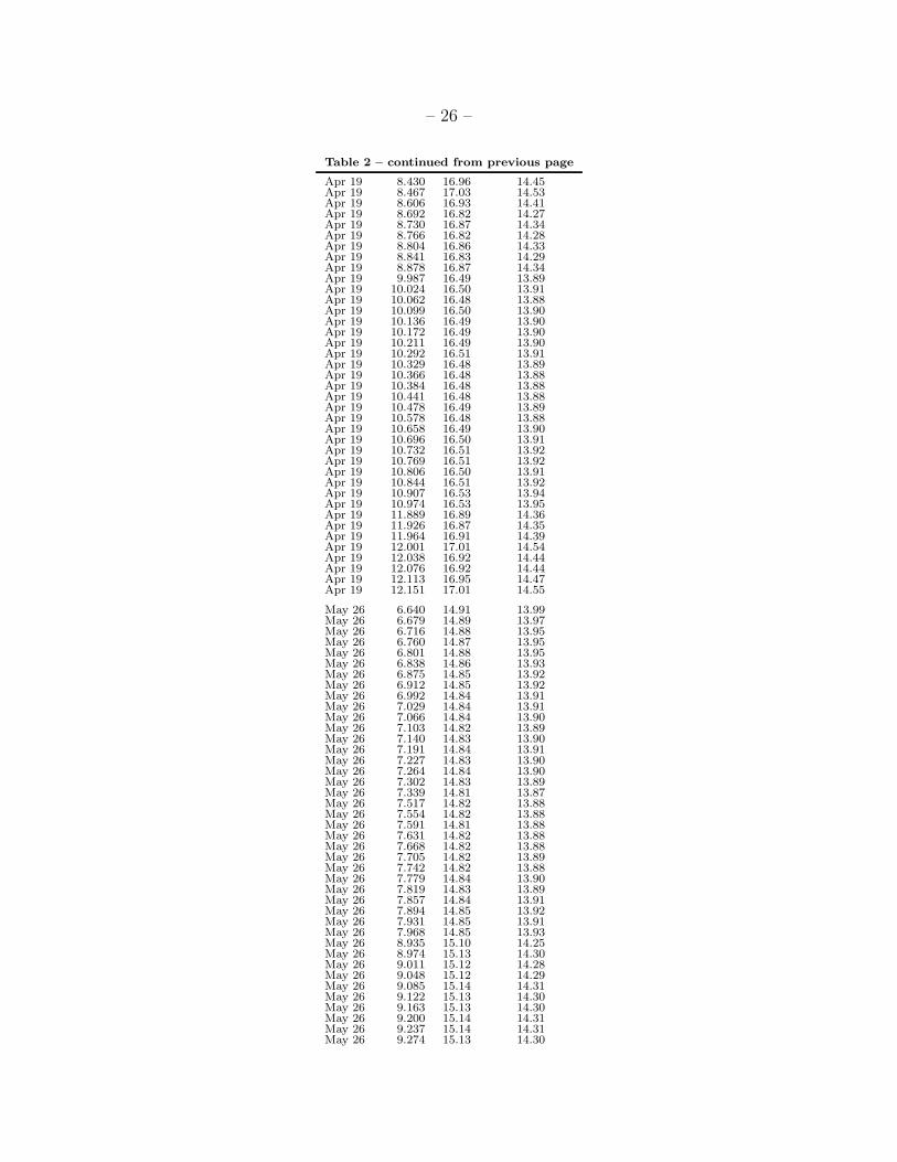
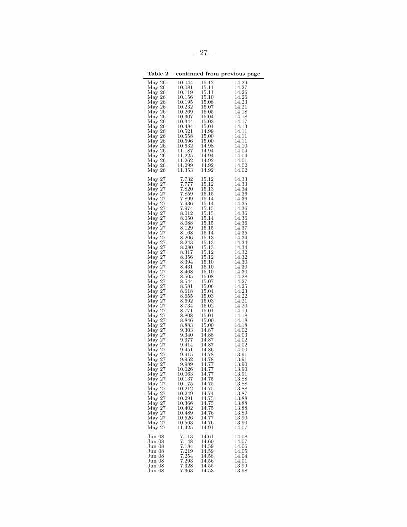
2.6. Data
The photometry is given in Table 2. Columns (1) and (2) are the UT date and time (at
the telescope) at the midpoint of each exposure (adjustments for light travel time are given in
Table 1). Column (3) is mR, the observed R-band magnitude after photometric calibrations,
extinction corrections, and comparison star corrections have been applied. Column (4) is
mR∗, the coma-removed, reduced magnitude mR(1,1,0) corrected by ∆m2 so that all nights
have a similar peak magnitude. We obtained 1016 data points, of which 124 were discarded
due to contamination from background stars, tracking problems, or cosmic ray hits.
While there are several adjustments which have been applied to arrive at the mR∗
values listed in Table 2, they do not affect the primary focus of the paper: the rotation
period determination. The corrections for geometry (∆m1) and nightly offsets (∆m2) shift
individual nightly lightcurves up or down, but the locations of the extrema in rotational
phase do not change. While the choice of coma removal algorithm affects the amplitude
of the lightcurve, it also leaves the phase of the extrema unchanged. Therefore, the same
rotation period could be determined directly from the mR values prior to the corrections.
Due to the large number of sources of error for each data point (photon uncertainty
in comet and background flux, extinction correction, comparison star correction, coma re-
moval), we estimated the effective uncertainty in the magnitude by fitting a smoothed spline
through each night’s lightcurve and subtracting the spline fit. The uncertainty for the night
was estimated as the standard deviation of the residuals. The uncertainty was not always
constant throughout a night since seeing conditions and obscuration varied on the non-
photometric nights, so on some nights we estimated the uncertainty for subsections of the
lightcurve. Variations in the comparison star magnitudes were used as an additional indica-
tor of when the uncertainty changed during a night. The range of uncertainties for a night
are given in column (11) in Table 1.

– 11 –
3. Modeling and Interpretation
3.1. Determining the Rotation Period in 1999
We defined zero phase to be perihelion (1999 September 8.424), and accounted for the
light travel time (column (8) in Table 1) before phasing the data. We used an interactive
period search routine within the Data Desk data analysis package4 which updates the phased
lightcurves on the fly, allowing us to easily scan through potential periods. We looked for
alignment of extrema since they can be identified in phase space even if the magnitudes
or amplitudes are different. As the correct solution is approached, the extrema tend to be
systematically shifted in phase based on the (color-coded) date of observation, making it easy
to quickly hone in on the optimal solution. However, it is difficult to quantitatively estimate
the uncertainty in the period since the alignment of the features is probably well away from
the optimal solution by the time the eye can distinguish it, therefore overestimating the
uncertainty.
We applied this technique to the mR∗ data given in column (4) of Table 2, finding an
observed, i.e. synodic, period of 8.941 ± 0.002 hr for the combined dataset (April–June). We
examined all period solutions between 4.47 hr (the single-peaked solution) and 13.41 hr (the
triple-peaked solution) and 8.941 hr (the double-peaked solution) is the only viable solution
between these extremes. The double-peaked shape is expected for a triaxial ellipsoid and
was observed by previous authors in 1988 and 1994. We plot the mR∗ data phased to 8.941
hr in the top panel of Figure 4. The bottom panel is phased to 8.932 hr (the period solution
from 1988, discussed in the following subsection).
The uncertainty in the period was estimated from the smallest offset that produced
lightcurves that were visibly out of phase. Figure 5 illustrates an exaggeration of this process
using three periods: 8.937 hr (top), 8.941 (middle) and 8.945 (bottom). Note that these
periods are separated by double the estimated error to emphasize the trend in the location
of the extrema. We plot the mR∗ data offset vertically by −0.015 mag day−1 since 1999
April 17 to better show the chronological progression of the lightcurves. In the top panel,
later lightcurves (higher on the plot) occur at a later phase, while in the bottom panel
later lightcurves occur at an early phase. This clearly illustrates that the correct solution is
between the two, making it easy to identify 8.941 hr as the optimal period. The inclusion of
the April data is vital for this process, as the larger separation between April and the later
datasets decreases the range of possible solutions.
4http://www.datadesk.com.

– 12 –
For comparison, we also conducted period searches using Fourier (Deeming 1975) and
phase dispersion minimization (PDM; Stellingwerf (1978)) techniques. The Fourier routine
“Period04”5 (Lenz & Breger 2005) found a single-peaked period of 4.4705 ± 0.0001 hr. Since
we expect the lightcurve to be double-peaked, this implies a rotation period twice as long,
or 8.9409 ± 0.0002 hr (the difference in the last digit is due to rounding). The routine deter-
mined an uncertainty in frequency and we converted this to a period uncertainty, although
we note that the uncertainty of 0.0002 hr seems unrealistically small. We used our own PDM
routine, which found a double-peaked period of 8.941 ± 0.005 hr. We estimated the period
uncertainty by finding the range of solutions that had θ (a measure of the goodness of fit)
within 50% of the minimum θ. The agreement between methods confirms the robustness of
our period solution.
3.2. Different Rotation Periods Due to Geometry?
The default rotation period obtained by simply phasing the data is the synodic period,
the length of time until the brightness appears the same from the Earth. This period changes
during the apparition because the illuminated portion of the nucleus seen by the Earth varies
as both the Earth and the comet move in their orbits. The sidereal rotation period is the
rotation period relative to a fixed position in inertial space. A third period is the solar
period, which is the time until the Sun is in the same place in the sky as seen by the comet.
Because the synodic and solar rotation periods depend on the orientation of the rotational
pole, converting them to a sidereal period requires a pole solution.
Since the synodic period also depends on the position of the Earth, we must consider the
geometry of the Earth-comet-Sun system during our observations to confirm that the synodic
period changes slowly enough that measuring a single synodic period for the whole 10-week
time span is sensible. As seen from the comet, the ecliptic longitude of the Earth (column (9)
of Table 1) and the ecliptic latitudes of the Sun and Earth all changed by less than 5◦ during
our observations, resulting in minimal changes to the measured rotation period. While the
ecliptic longitude of the Sun as seen from the comet (column (10) of Table 1) changed by
∼30◦, the net effect on the rotation period was still small due to the likely pole orientation
(see discussion below), and obtaining a single (synodic) rotation period for the whole time
span was valid.
To confirm this, we investigated the synodic rotation periods which would be observed
at different times for pole solutions within 20◦ in the comet’s orbital coordinate system
5http://www.univie.ac.at/tops/Period04/.

– 13 –
(obliquity and azimuthal angle) of the pole solution given by Sekanina (1987). This range
of solutions was chosen to include the pole solution found by Sekanina (1991) for the 1988
apparition and a preliminary pole solution for our 1999 coma morphology data (we will
explore this in detail in Paper 2). We considered three runs discretely: April 17–19, May
26–27, and June 22–23 (the June 8–11 run gave similar results to the June 22–23 run), and
determined the synodic–sidereal offset which would be observed for all pole solutions under
consideration. The difference between the synodic and sidereal periods was 0.000 to +0.003
hr during the April run, 0.000 to +0.002 hr during the May run, and −0.001 to +0.001
hr during the late-June run. Considering the entire 10-week interval as a single large run
(i.e. April 17–June 23), the best synodic period differed from the sidereal period by 0.000 to
+0.002 hr. Thus, the changing geometry during our observations did not introduce an error
in the period determined from the entire run larger than the estimated uncertainty in the
synodic period of 0.002 hr (although if the April run was considered by itself, the maximum
difference was 0.003 hr). Note that the sign of the synodic–sidereal difference reverses for
a pole orientation in the opposite direction, i.e. when the comet has retrograde spin and
“north” is defined in the opposite hemisphere.
The above example suggests that changes in the synodic period may be detectable during
an apparition. We considered subsets of our 1999 data to look for such a change. There was
no discernible difference when the rotation period was determined using all the April and
May data or all the May and June data (both intervals gave acceptable solutions from 8.940–
8.942 hr with a best period of 8.941 hr). We also determined the synodic period between
every combination of individual nights from different runs for which a synodic period could
be determined. We phased each pair of nights and defined the midpoint between the two
nights as the date corresponding to the measured synodic period. This method suggests an
increase in the synodic period of ∼0.002 hr from early-May to mid-June, although the scatter
in the individual synodic measurements is very large and the range of acceptable solutions
for each pair is generally at least ± 0.002 hr. If correct, this requires that the “north” pole
be in the opposite hemisphere as was determined by Sekanina (1987), i.e. retrograde rather
than prograde rotation.
3.3. Reanalysis of the 1988 Data
We reanalyzed the publicly available datasets from 1988 (Jewitt & Luu (1989), A’Hearn et al.
(1989), and Wisniewski (1990)), defining zero phase at perihelion (1988 September 16.738).
The observing scenarios for these datasets are summarized in Table 3. Jewitt & Luu (1989)
removed coma from their June data but not the February or April data. A’Hearn et al.

– 14 –
(1989) obtained optical and thermal IR data simultaneously on different telescopes, and
removed coma from the optical data but not from the thermal IR data, which were shown
to be nearly free of coma. Wisniewski (1990) did not remove coma from his data. The
1987 data from Jewitt & Meech (1988) were not included in the 1988 period determination
because they were too far away in time and were at a much different location in the orbit,
making it impossible to directly compare the synodic rotation periods.
We normalized the published magnitudes to mR(1,1,0) using β = 0.032 mag deg−1 as
was used with our 1999 data. After this normalization, the optical magnitudes still differed
by several tenths of a magnitude between runs and authors. We therefore adjusted all the
lightcurves to peak at the same magnitude for the maximum near zero phase by applying
nightly ∆m2 values (given in column (12) of Table 3). We call these data mR∗, and used
them for our period search. ∆m2 corrects for nightly differences between datasets due to
differences in the extinction correction, absolute calibration, and coma removal (or lack
thereof). We do not list a ∆m2 for the A’Hearn et al. (1989) 4845 A data, as we did not use
them when phasing the data since the 4845 A and 6840 A data were obtained alternately
throughout both nights, and their lightcurve shapes were nearly identical (although the 6840
A data were brighter).
Visually scanning the 1988 data for a double-peaked solution, as was done for our 1999
data, yielded a period of 8.932 ± 0.001 hr. This period agrees with the synodic periods
determined for the 1988 data by Sekanina (1991) (8.931 ± 0.001 hr, given in his Table 5)
and Mueller & Ferrin (1996) (8.933 ± 0.002)6.
The viewing geometry in 1988 was nearly identical to the viewing geometry in 1999;
the ecliptic latitudes of the Earth and Sun changed minimally and the ecliptic longitudes of
the Earth and Sun (given in columns (9) and (10), respectively, in Table 3) mimicked the
changes in 1999. As with the 1999 data (Section 3.1), we considered discrete runs spanning
the range of 1988 observations: February 24–28, April 8–12, May 18–22, and June 19–23, and
determined the synodic–sidereal difference during each run for the range of pole solutions.
Because of the similar viewing geometry, the synodic–sidereal difference was almost the same
as in 1999: +0.001 to +0.002 hr for February 24–28, +0.001 to +0.002 hr for April 8–12,
0.000 to +0.001 hr for May 18–22, and −0.001 to +0.001 hr for June 19–23. Considering the
entire 1988 time span from February 25 until June 30 as a single large run, the difference
in the synodic and sidereal rotation periods was 0.000 to +0.002 hr for the range of pole
6We did not see evidence of a 13 min offset of the 1988 April data from Jewitt & Luu (1989) as suggested
by Sekanina (1991), but note that ∆m2 could mask this effect. Sekanina (1991) adjusted these data by 13
minutes to derive the quoted synodic period, while Mueller & Ferrin (1996) omitted these data entirely from
their period analysis. We include them with no time adjustment.
– 15 –
solutions. As with 1999, the synodic–sidereal difference changes sign for a pole orientation
in the opposite direction.
Thus we can directly compare our 1988 solution (8.932 hr) with our 1999 solution (8.941
hr). In Figure 6 we plot the 1988 mR∗ data phased to our period solution from 1988 in the
top panel and to our period solution from 1999 in the bottom panel. Similarly, we plot our
1999 mR∗ data phased to 8.941 hr (top panel) and 8.932 hr (bottom panel) in Figure 4.
Figures 4 and 6 demonstrate that the rotation periods were clearly different in 1988 and
1999. Since the synodic periods differed by ∼0.009 hr and synodic–sidereal offsets were
similar each apparition, we can conclude that the sidereal periods also differed by ∼0.009
hr, and thus the rotation period increased from 1988 to 1999.
We looked for a change in the synodic period during the 1988 observations by phasing
every combination of pairs of observing runs, e.g. Jewitt & Luu (1989)’s February data with
A’Hearn et al. (1989)’s June data, Jewitt & Luu (1989)’s February data with Wisniewski
(1990)’s June data, etc. Assigning the date of each pair as the midpoint between the two runs,
there was no discernible trend in the measured synodic period over time, with acceptable
values varying from 8.931–8.933 hr with a typical uncertainty of ±0.001 hr. This is consistent
with the conclusions of Jewitt & Luu (1989) who found no change in the rotation period
within their uncertainty when analyzing their February, April, and June data as discrete
sets. In contrast, Sekanina (1991) found a decrease in the synodic period during the 1988
observations of ∼0.003 hr (his Table 5 and Figure 7). These discrepancies and our possible
finding of a slight increase in the rotation period in 1999 (Section 3.1) suggest that Sekanina
(1987)’s pole solution may not be definitive, with the alternate sense of rotation possible
as well (resulting in a “north” pole in the exact opposite position). We will use the coma
morphology visible in our post-perihelion 1999 images, combined with data we will obtain
in 2010, to attempt to determine a more robust pole solution in Paper 2.
3.4. Reanalysis of the 1994 Data
We also reanalyzed the Mueller & Ferrin (1996) data from 1994, normalizing the pub-
lished magnitudes to mR(1,1,0) and visually scanning for possible solutions. The data do
not yield an unambiguous double-peaked lightcurve due to undersampling. Mueller & Ferrin
(1996) found five possible solutions: 8.877 hr, 8.908 hr, 8.939 hr, 8.971 hr, and 9.002 hr, and
we concur with their results. Only one of these, 8.939 hr, is within the uncertainty of our
1999 solution (8.941 ± 0.002 hr).
Using the same range of pole solutions as in Section 3.2, we find the maximum differ-

– 16 –
ence between the synodic and sidereal periods in October–December 1994 was smaller than
−0.001 hr (actually about −1 s), in agreement with the difference found by Mueller & Ferrin
(1996). Thus, the expected difference between the synodic and sidereal rotation periods is
much less than the difference between the five possible solutions. Furthermore, since there
were no intervening perihelion passages between the 1994 and 1999 observations, the side-
real rotation period was likely unchanged between these observations. Therefore, we rule
out the remaining four possible solutions from Mueller & Ferrin (1996), and conclude that
Tempel 2 had spun-down by ∼0.009 hr (∼ 32 s) between the 1988 and 1994 determinations,
which spanned two perihelion passages, and was unchanged between the 1994 post-perihelion
observations and our 1999 pre-perihelion observations.
3.5. Coma Contamination and Lightcurve Amplitude
Tempel 2 was non-stellar in appearance throughout our 1999 observations. The presence
of a coma suppressed the amplitude of the lightcurve, with the suppression increasing later
in the apparition as activity increased. The mean coma removed from the 6 arcsec radius
monitoring aperture was 0.20 mag from April 17–19, 0.27 mag from May 26–27, 0.40 mag
from June 8–11, and 0.65 mag from June 22–23. We measured lightcurve amplitudes ranging
from 0.2–0.5 mag prior to removal of the coma. After coma removal, the April 17–19 data
exhibited amplitudes of ∼0.75 mag while all subsequent runs had amplitudes of 0.45–0.50
mag. If a quadratic fit to the coma was used instead of a linear fit, the amplitudes increased
to ∼0.80 in April and 0.50–0.60 in May and June. However, note that as discussed in
Section 2.4, we opted for a more conservative linear fit rather than a higher order fit because
the higher order fits varied more from image to image and produced less reliable results. Our
measured amplitudes in 1999 are similar to the maximum optical amplitudes reported by
other authors in 1988 when the comet was at a similar viewing geometry and activity level:
0.65 ± 0.05 mag in February and 0.60 ± 0.05 mag in April (no coma removal; Jewitt & Luu
(1989)), 0.5 mag in May (no coma removal; Wisniewski (1990)), and 0.7 ± 0.1 mag in June
(coma removed; Jewitt & Luu (1989)).
A’Hearn et al. (1989) measured an amplitude of 0.8 mag in their 10.1 µm data in 1988
June, exceeding all measured optical amplitudes at similar times in both 1988 and 1999.
While the amplitudes measured by ourselves and others approach the thermal IR amplitude,
all are somewhat lower, and even a quadratic coma removal from our data cannot bring
the amplitudes into agreement. This discrepancy raises two possible interpretations. First,
the coma removal techniques employed here and by Jewitt & Luu (1989) and A’Hearn et al.
(1989) are not adequately estimating the coma inside the photometric aperture. To push the

– 17 –
amplitude up to ∼0.80, 50–150% more coma would need to be removed from our May and
June data, requiring a significantly steeper curve than even a quadratic fit. Alternatively,
the convergence of multiple authors on an optical amplitude of 0.6–0.7 mag in 1988 June
and 1999 June may indicate that this is in fact the correct optical amplitude, and is different
from the thermal IR amplitude. This possibility was suggested by A’Hearn et al. (1989)
based on work by Brown (1985) who showed that the amplitude of the thermal IR lightcurve
may be dependent on both wavelength and elongation.
The varying lightcurve amplitudes will be utilized in Paper 2 when we determine the
pole solution using the coma morphology from 1999 and 2010. As the viewing geometry
varies during an apparition, the amplitude of the lightcurve will vary because different cross
sections of the nucleus are observed. Thus, the lightcurve amplitudes will be useful in refining
the pole solution and will help in constraining the shape of the nucleus.
We looked for evidence of periodicity in the coma signal by plotting both the total flux
and flux per square arcsec in each photometric annulus as a function of rotational phase.
What structure is visible on individual nights does not repeat in a coherent manner from
night to night or from run to run. There was also no evidence of propagation of any features
(either a maximum or minimum signal) outwards during a night. This is consistent with the
analyses of Jewitt & Luu (1989) and A’Hearn et al. (1989) who did not see a rotation signal
in their data.
3.6. Lightcurve Asymmetry
The rotational lightcurve in 1999 is somewhat asymmetric, allowing identification of
certain features many rotations apart and eliminating N − 0.5, N + 0.5, N + 1.5... (where
N is the number of cycles) as possible solutions. This conclusively rules out the single-
and triple-peaked solutions and reduces the uncertainty in the period determination since it
halves the number of possible rotations. Any clear description of the lightcurve shape is made
challenging because it is never observed completely on a given night. However, we note the
following apparently repeated features: The minimum near 0.6 phase is deeper and steeper
than the minimum near 0.1 phase when comparing lightcurves from the same observing run.
There is a shoulder in the rising portion between 0.15 and 0.30 phase. Finally, while there
are no nights in which both maxima were clearly observed, the maximum near 0.85 phase
may be slightly higher than the maximum near 0.35 phase. We see evidence for each of these

– 18 –
features in the 1988 data when discrete observing runs are considered7. The features are also
seen in the 1994 data from Mueller & Ferrin (1996), although since the viewing geometry
was very different, we cannot be sure that they correspond to the same topographic features
on the nucleus.
4. Summary and Discussion
We imaged Tempel 2 on 32 nights from 1999 April until 2000 March. We present
here R-band nucleus lightcurves obtained on 11 of these nights from April through June
(prior to perihelion), a total of 892 data points. Absolute calibrations and nightly extinction
corrections were determined on photometric nights, and were applied to non-photometric
nights to extract usable lightcurves. Field stars in the image were monitored on all nights
and were used as comparison stars to correct the comet magnitude on non-photometric
nights. A median coma was determined each night and removed from all images on the
night. All magnitudes were normalized to r = ∆ = 1 AU and α = 0◦. A final adjustment,
which accounts for uncertainties in the calibrations that tend to create nightly magnitude
offsets such as the application of absolute calibrations on non-photometric nights, was applied
to make each night peak at the same magnitude.
We determined a synodic rotation period of 8.941 ± 0.002 hr; no other double-peaked
solutions exist. Our dataset is sufficient to rule out all aliases other than the single- and
triple-peaked solutions, and these are ruled out by the differences in shape and brightness
between the two minima. Our period matches one of the possible periods obtained by
Mueller & Ferrin (1996) from post-perihelion data in 1994 (during the same inter-perihelion
time as our 1999 data) and rules out their other four possible solutions. We reanalyzed
published data from 1988 using the same analysis techniques and found a synodic rotation
period of 8.932 ± 0.001 hr. Our 1999 data cannot be fit by the rotation period from 1988,
nor can the 1988 data be fit by the rotation period from 1999, even though the comet had
nearly identical viewing geometries during the two sets of observations. Thus, we conclude
that Tempel 2 spun-down by 0.009 hr (∼32 s) from 1988 to 1999, an interval that included
two perihelion passages.
7The 1988 April data from Jewitt & Luu (1989) showed the deeper minimum to be at ∼0.7 phase, in
contradiction to all other 1988 datasets (see Figure 6). This dataset was the most difficult to normalize
since neither April 9 or 12 contained a clear extremum, and the April 10 and 15 data required very different
∆m2 adjustments to bring the maxima in alignment near zero phase. Given that the minima were observed
only five nights apart and no lightcurve change in shape is expected during this short a time interval, we are
skeptical of this anomalous minimum.

– 19 –
This marks the first conclusive measurement of spin-down in a comet, although three
comets have shown possible evidence of spin-up: 9P/Tempel 1 (Belton & Drahus 2007;
Chesley et al. 2010), 2P/Encke (Fernandez et al. 2005), and Comet Levy (1990c) (Schleicher et al.
1991; Feldman et al. 1992). Modeling by Samarasinha & Belton (1995), Neishtadt et al.
(2002), Gutierrez et al. (2003), and others has shown that either spin-up or spin-down is
possible, with spin-up more likely in the long run. These simulations have shown that un-
der certain conditions the spin period can change by much larger amounts in a single orbit
(e.g. typical changes of 0.01–10 hr per orbit according to Gutierrez et al. (2003)) than the
measured change of 0.009 hr in two orbits for Tempel 2. Thus, the measured spin-down of
10P/Tempel 2 is probably not exceptional, and comparable changes in period could likely be
measured in other comets if similarly high quality data were obtained over several epochs.
Possible causes of a change in spin-state are summarized by Samarasinha et al. (2004).
The spin-down of Tempel 2 may have been caused by either a one-time event or by recurring
torquing each orbit. Scenarios for causing a one-time change in rotation period include
a short-lived, freshly exposed active region (causing temporary torquing), fragmentation
(changing the moment of inertia), collision with another object, and tidal torquing from
Jupiter. The orbit of Tempel 2 is well known and tidal torquing from Jupiter should not have
been significant or more severe between 1988 and 1999 than on other recent orbits. Collisions
are rare in the current solar system, and any collision significant enough to alter the rotation
period of Tempel 2 would likely have resulted in an increase in brightness upon subsequent
orbits, which has not been seen. Fragmentation is known to be relatively common, occurring
on average at least once per century per comet (c.f. Chen & Jewitt (1994); Weissman (1980)).
However, there is no evidence for Tempel 2 having split, such as a companion nucleus or a
sustained increase in brightness as was observed in 73P/Schwassmann-Wachmann 3 (Ferrın
2010). A new active region could be created by fragmention, impact, or outburst. Since
outbursts are known to occur far more frequently than fragmentation or impacts, an outburst
is the most plausible explanation for a one-time change in the rotation period. If the change
in the period was caused by a unique event such as an outburst, it could have occurred
anywhere in the orbit and we would expect no change in the rotation period on subsequent
orbits.
It is challenging to devise a mechanism that is strong enough to affect the rotation
period but lasts for a short time (less than one orbit). Thus, we suspect the spin-down is
due to torques on the nucleus caused by asymmetric outgassing. This is believed to be the
most common means of changing the spin state of a comet (c.f. Samarasinha et al. (2004)).
Seasonal illumination of an active region could cause torquing which slows the rotation of
the nucleus by a comparable amount each orbit. In the case of Tempel 2, the torquing likely
occurs near or shortly after perihelion, when the comet is most active, although the length

– 20 –
of time over which the torquing may occur is unknown. Since Tempel 2 reached perihelion
twice between the 1988 and 1999 observations, in this, our preferred scenario, the rotation
period must be changing by ∼16 s each orbit.
Tempel 2 reached perihelion on 2010 July 4, and we encourage its observation throughout
the apparition to determine the rotation period. Due to a perturbation by Jupiter between
the 1999 and 2005 apparitions, the viewing geometry is different in 2010 than in 1988 or
1999. The post-perihelion viewing geometry will be better this apparition and the comet will
be visible longer each night. The smaller post-perihelion ∆ in 2010 will provide better spatial
resolution, making it easier to separate the nucleus and coma signals even though the coma
is more extensive after perihelion. This may allow measurement of a nucleus lightcurve after
perihelion, despite increased coma contamination relative to the pre-perihelion measurements
in 1988, 1994, and 1999.
Assuming the spin-down is recurrent each orbit, we predict that the pre-perihelion
rotation period should be ∼32 s longer than in 1999 as there have been two intervening
perihelion passages (1999 September 8 and 2005 February 15) since our data were obtained
in 1999. If the pole position given by Sekanina (1987) is correct, the sidereal rotation
period should be 8.950 ± 0.003 hr. Since it is unknown if the spin-down is caused by
an instantaneous impulsive event or a steady change over an extended period of time, we
cannot estimate the rotation period that might be observed shortly after perihelion in 2010.
Observations long enough after perihelion to allow the torquing to have taken effect should
reveal an additional lengthening of the sidereal rotation period by ∼16 s relative to the pre-
perihelion 2010 period. Using again the pole solution of Sekanina (1987), this would yield a
sidereal period 8.954 ± 0.004 hr.
We have begun to observe Tempel 2 in 2010 and will combine these new data with our
observations obtained during its active phase in 1999 as a follow up to the current paper.
As of August 2010 (when the revised manuscript was submitted), we are unaware of any
period determinations from 2010 observations. In Paper 2 we will use the different viewing
geometry provided by the 2010 apparition to investigate the pole orientation and the location
and activity of any jets. We hope to determine the rotation period in 2010, and possibly
obtain additional post-perihelion observations after activity has subsided in 2011 or later to
resolve whether the comet spins down each orbit. With its relatively low inclination (i ∼
12◦) and perihelion close to the Earth’s orbit (q ∼ 1.4 AU), Tempel 2 is frequently on the
short list of targets for comet missions, making further study highly desirable.

– 21 –
Acknowledgements
Thanks to Beatrice Mueller for a thorough and helpful review. We thank Christopher
Henry, Kevin Walsh, and Wendy Williams for helping to obtain these observations, and
Brian Skiff for useful discussions. We are grateful for JPL’s Horizons for generating observ-
ing geometries. The period analysis was greatly facilitated by the use of the Data Desk
exploratory data analysis package from Data Descriptions, Inc. MMK and DGS were sup-
ported by NASA Planetary Astronomy grant NNX09B51G. TLF was supported by multiple
NASA grants. EWS was supported by an NSF grant to Northern Arizona University for the
Research Experiences for Undergraduates program.
REFERENCES
A’Hearn, M. F., Campins, H., Schleicher, D. G., & Millis, R. L. 1989, ApJ, 347, 1155
Belton, M. J., & Drahus, M. 2007, in Bulletin of the American Astronomical Society, vol. 38
of Bulletin of the American Astronomical Society, 498
Brown, R. H. 1985, Icarus, 64, 53
Chen, J., & Jewitt, D. 1994, Icarus, 108, 265
Chesley, S. R., Belton, M. J. S., Gillam, S. D., Meech, K. J., Carcich, B., & Veverka, J. 2010,
in Bulletin of the American Astronomical Society, vol. 41 of Bulletin of the American
Astronomical Society, 936
Deeming, T. J. 1975, Ap&SS, 36, 137
Farnham, T. L., Schleicher, D. G., & A’Hearn, M. F. 2000, Icarus, 147, 180
Feldman, P. D., Budzien, S. A., Festou, M. C., A’Hearn, M. F., & Tozzi, G. P. 1992, Icarus,
95, 65
Fernandez, Y. R., Lowry, S. C., Weissman, P. R., Mueller, B. E. A., Samarasinha, N. H.,
Belton, M. J. S., & Meech, K. J. 2005, Icarus, 175, 194
Ferrın, I. 2010, Planet. Space Sci., 58, 365. 0909.3498
Gutierrez, P. J., Jorda, L., Ortiz, J. L., & Rodrigo, R. 2003, A&A, 406, 1123
Jewitt, D., & Luu, J. 1989, AJ, 97, 1766

– 22 –
Jewitt, D. C., & Meech, K. J. 1988, ApJ, 328, 974
Kronk, G. W. 2003, Cometography: A Catalog of Comets. Volume 2, 1800-1899 (Cambridge,
UK: Cambridge University Press)
— 2007, Cometography: A Catalog of Comets. Volume 3, 1900-1932 (Cambridge, UK: Cam-
bridge University Press)
— 2009, Cometography: A Catalog of Comets. Volume 4, 1933-1959 (Cambridge, UK: Cam-
bridge University Press)
Landolt, A. U. 1992, AJ, 104, 340
Lenz, P., & Breger, M. 2005, Communications in Asteroseismology, 146, 53
Mueller, B. E. A., & Ferrin, I. 1996, Icarus, 123, 463
Neishtadt, A. I., Scheeres, D. J., Sidorenko, V. V., & Vasiliev, A. A. 2002, Icarus, 157, 205
Osborn, W. H., A’Hearn, M. F., Carsenty, U., Millis, R. L., Schleicher, D. G., Birch, P. V.,
Moreno, H., & Gutierrez-Moreno, A. 1990, Icarus, 88, 228
Samarasinha, N. H., & Belton, M. J. S. 1995, Icarus, 116, 340
Samarasinha, N. H., Mueller, B. E. A., Belton, M. J. S., & Jorda, L. 2004, Rotation of
Cometary Nuclei, 281
Schleicher, D. G., Millis, R. L., Osip, D. J., & Birch, P. V. 1991, Icarus, 94, 511
Sekanina, Z. 1979, Icarus, 37, 420
— 1987, in Diversity and Similarity of Comets, edited by E. J. Rolfe & B. Battrick, vol. 278
of ESA Special Publication, 323
— 1991, AJ, 102, 350
Stellingwerf, R. F. 1978, ApJ, 224, 953
Weissman, P. R. 1980, A&A, 85, 191
Whipple, F. L. 1950, ApJ, 111, 375
Wisniewski, W. Z. 1990, Icarus, 86, 52
This preprint was prepared with the AAS LATEX macros v5.2.

– 23 –
Table 1. Summary of Tempel 2 observations and geometric parameters in 1999. a
UT UT Tel. CCD r ∆ α ∆t Ecl. Long. Ecl. Long. ∆m1e ∆m2
f σmRConditions
Date Range Diam. (AU) (AU) (◦) (hr) b Earth (◦) c Sun (◦) d
Apr 17 7:48–11:55 1.8-m SITe 2.025 1.275 24.0 0.177 80.1 56.3 −2.84 −0.02 0.02–0.04 thin cloudsApr 18 7:20–12:11 1.8-m SITe 2.020 1.262 23.8 0.176 80.3 56.7 −2.81 +0.08 0.02–0.06 thin cloudsApr 19 6:53–12:10 1.8-m SITe 2.014 1.248 23.7 0.174 80.5 57.1 −2.77 +0.03 0.03 photometricMay 26 6:37–11:22 1.8-m SITe 1.807 0.839 13.9 0.117 81.9 72.2 −1.36 +0.15 0.01 thin cloudsMay 27 7:43–11:30 1.8-m SITe 1.802 0.831 13.6 0.116 81.8 72.7 −1.33 +0.26 0.01 thin cloudsJun 08 7:05–11:14 1.1-m TI 1.741 0.748 10.7 0.104 80.1 78.4 −0.92 ... 0.02 photometricJun 09 4:45– 9:36 1.1-m TI 1.736 0.743 10.6 0.103 80.0 78.8 −0.90 ... 0.03 photometricJun 10 4:34–11:17 1.1-m TI 1.731 0.737 10.5 0.102 79.7 79.3 −0.87 −0.02 0.02 photometricJun 11 4:30– 9:35 1.1-m TI 1.726 0.732 10.4 0.102 79.6 79.8 −0.85 ... 0.02 photometricJun 22 7:29–11:08 1.1-m TI 1.675 0.685 12.4 0.095 77.5 85.4 −0.69 −0.07 0.02–0.06 thin cloudsJun 23 3:57–11:04 1.1-m TI 1.671 0.682 12.7 0.095 77.4 85.9 −0.69 −0.07 0.02–0.04 photometric
aAll parameters were taken at the midpoint of each night’s observations, and all images were obtained at Lowell Observatory.
bight travel time.
cEcliptic longitude of the Earth as seen from the comet.
dEcliptic longitude of the Sun as seen from the comet.
eMagnitude necessary to correct from mR(r,∆,α) to mR(1,1,0) for the night (in magnitudes).
fOffset (in magnitudes) necessary to make data on all nights peak at the same magnitude.

– 24 –
Table 2:: Table of photometry
UT Date UT a mRb mR* c
Apr 17 7.848 16.93 14.38Apr 17 7.915 16.90 14.34Apr 17 7.952 17.00 14.47Apr 17 7.989 16.90 14.34Apr 17 8.038 16.83 14.25Apr 17 8.076 16.89 14.33Apr 17 8.112 16.84 14.26Apr 17 8.201 16.76 14.16Apr 17 8.294 16.83 14.24Apr 17 8.331 16.74 14.13Apr 17 8.368 16.73 14.13Apr 17 8.421 16.73 14.13Apr 17 8.458 16.68 14.06Apr 17 8.495 16.69 14.07Apr 17 8.547 16.72 14.11Apr 17 8.637 16.71 14.10Apr 17 8.674 16.68 14.07Apr 17 8.711 16.73 14.12Apr 17 8.748 16.71 14.10Apr 17 8.785 16.67 14.04Apr 17 8.821 16.63 14.00Apr 17 8.893 16.64 14.02Apr 17 8.972 16.65 14.02Apr 17 9.067 16.62 13.99Apr 17 9.104 16.59 13.94Apr 17 9.142 16.60 13.96Apr 17 9.179 16.58 13.93Apr 17 9.216 16.61 13.98Apr 17 9.253 16.58 13.93Apr 17 9.315 16.58 13.93Apr 17 9.421 16.56 13.91Apr 17 9.486 16.55 13.91Apr 17 9.523 16.54 13.90Apr 17 9.560 16.56 13.92Apr 17 9.597 16.56 13.91Apr 17 9.634 16.59 13.96Apr 17 9.671 16.57 13.93Apr 17 9.716 16.60 13.96Apr 17 9.807 16.60 13.97Apr 17 9.844 16.63 14.00Apr 17 9.881 16.62 13.98Apr 17 9.918 16.62 13.99Apr 17 9.955 16.62 13.99Apr 17 9.992 16.62 13.99Apr 17 10.037 16.64 14.01Apr 17 10.219 16.67 14.05Apr 17 10.288 16.70 14.09Apr 17 10.325 16.68 14.07Apr 17 10.362 16.71 14.11Apr 17 10.399 16.73 14.13Apr 17 10.436 16.75 14.14Apr 17 10.473 16.75 14.16Apr 17 10.604 16.79 14.21Apr 17 11.689 16.95 14.41Apr 17 11.726 16.95 14.41Apr 17 11.763 16.93 14.38Apr 17 11.800 16.94 14.39Apr 17 11.890 16.91 14.35
Apr 18 7.681 16.47 13.89Apr 18 7.718 16.44 13.86Apr 18 7.755 16.46 13.89Apr 18 7.792 16.48 13.91Apr 18 7.829 16.48 13.90Apr 18 7.867 16.47 13.90Apr 18 7.906 16.49 13.91Apr 18 7.943 16.51 13.94Apr 18 7.980 16.55 13.99Apr 18 8.017 16.55 13.99Apr 18 8.054 16.61 14.05Apr 18 8.091 16.62 14.06Apr 18 8.160 16.61 14.05Apr 18 8.234 16.63 14.08Apr 18 8.395 16.68 14.14Apr 18 8.432 16.69 14.15Apr 18 8.469 16.74 14.21Apr 18 8.506 16.66 14.12

– 25 –
Table 2 – continued from previous page
Apr 18 8.543 16.78 14.25Apr 18 8.580 16.73 14.20Apr 18 8.621 16.74 14.21Apr 18 8.702 16.83 14.31Apr 18 8.739 16.81 14.29Apr 18 8.777 16.84 14.33Apr 18 8.814 16.83 14.32Apr 18 8.851 16.89 14.39Apr 18 8.888 16.90 14.40Apr 18 8.962 16.93 14.44Apr 18 9.028 16.98 14.50Apr 18 9.109 17.00 14.53Apr 18 9.146 16.99 14.52Apr 18 9.183 17.04 14.57Apr 18 9.220 17.01 14.54Apr 18 9.258 17.03 14.56Apr 18 9.295 17.05 14.59Apr 18 9.332 17.07 14.61Apr 18 9.429 17.07 14.61Apr 18 9.535 17.06 14.60Apr 18 9.611 17.02 14.55Apr 18 9.649 17.03 14.56Apr 18 9.686 17.01 14.54Apr 18 9.723 17.01 14.53Apr 18 9.760 17.04 14.57Apr 18 9.797 17.07 14.61Apr 18 9.836 17.04 14.58Apr 18 9.873 17.01 14.54Apr 18 9.910 17.01 14.54Apr 18 9.947 16.98 14.51Apr 18 9.985 16.98 14.50Apr 18 10.022 16.98 14.50Apr 18 10.062 16.99 14.51Apr 18 10.391 16.73 14.20Apr 18 10.460 16.86 14.35Apr 18 10.541 16.87 14.37Apr 18 10.579 16.85 14.35Apr 18 10.616 16.83 14.32Apr 18 10.653 16.80 14.28Apr 18 10.690 16.90 14.40Apr 18 10.811 16.80 14.29Apr 18 10.917 16.75 14.22Apr 18 10.959 16.77 14.24Apr 18 10.996 16.67 14.13Apr 18 11.033 16.74 14.22Apr 18 11.070 16.74 14.21Apr 18 11.107 16.71 14.18Apr 18 11.144 16.70 14.16Apr 18 11.210 16.68 14.14Apr 18 11.277 16.67 14.13Apr 18 11.356 16.62 14.07Apr 18 11.393 16.64 14.09Apr 18 11.431 16.64 14.09Apr 18 11.468 16.66 14.12Apr 18 11.505 16.61 14.06Apr 18 11.542 16.61 14.06Apr 18 11.623 16.60 14.05Apr 18 11.664 16.57 14.01Apr 18 11.702 16.57 14.01Apr 18 11.739 16.58 14.02Apr 18 11.776 16.56 14.01Apr 18 11.813 16.55 13.99Apr 18 11.851 16.54 13.98Apr 18 11.902 16.53 13.96
Apr 19 7.129 16.77 14.22Apr 19 7.170 16.80 14.25Apr 19 7.208 16.74 14.18Apr 19 7.824 17.07 14.57Apr 19 7.889 17.06 14.57Apr 19 7.956 17.08 14.59Apr 19 7.993 17.06 14.56Apr 19 8.031 17.09 14.61Apr 19 8.068 17.12 14.64Apr 19 8.105 17.07 14.58Apr 19 8.142 17.10 14.62Apr 19 8.185 17.07 14.59Apr 19 8.281 17.10 14.62Apr 19 8.319 17.02 14.52Apr 19 8.356 16.99 14.48Apr 19 8.393 17.02 14.52
– 26 –
Table 2 – continued from previous page
Apr 19 8.430 16.96 14.45Apr 19 8.467 17.03 14.53Apr 19 8.606 16.93 14.41Apr 19 8.692 16.82 14.27Apr 19 8.730 16.87 14.34Apr 19 8.766 16.82 14.28Apr 19 8.804 16.86 14.33Apr 19 8.841 16.83 14.29Apr 19 8.878 16.87 14.34Apr 19 9.987 16.49 13.89Apr 19 10.024 16.50 13.91Apr 19 10.062 16.48 13.88Apr 19 10.099 16.50 13.90Apr 19 10.136 16.49 13.90Apr 19 10.172 16.49 13.90Apr 19 10.211 16.49 13.90Apr 19 10.292 16.51 13.91Apr 19 10.329 16.48 13.89Apr 19 10.366 16.48 13.88Apr 19 10.384 16.48 13.88Apr 19 10.441 16.48 13.88Apr 19 10.478 16.49 13.89Apr 19 10.578 16.48 13.88Apr 19 10.658 16.49 13.90Apr 19 10.696 16.50 13.91Apr 19 10.732 16.51 13.92Apr 19 10.769 16.51 13.92Apr 19 10.806 16.50 13.91Apr 19 10.844 16.51 13.92Apr 19 10.907 16.53 13.94Apr 19 10.974 16.53 13.95Apr 19 11.889 16.89 14.36Apr 19 11.926 16.87 14.35Apr 19 11.964 16.91 14.39Apr 19 12.001 17.01 14.54Apr 19 12.038 16.92 14.44Apr 19 12.076 16.92 14.44Apr 19 12.113 16.95 14.47Apr 19 12.151 17.01 14.55
May 26 6.640 14.91 13.99May 26 6.679 14.89 13.97May 26 6.716 14.88 13.95May 26 6.760 14.87 13.95May 26 6.801 14.88 13.95May 26 6.838 14.86 13.93May 26 6.875 14.85 13.92May 26 6.912 14.85 13.92May 26 6.992 14.84 13.91May 26 7.029 14.84 13.91May 26 7.066 14.84 13.90May 26 7.103 14.82 13.89May 26 7.140 14.83 13.90May 26 7.191 14.84 13.91May 26 7.227 14.83 13.90May 26 7.264 14.84 13.90May 26 7.302 14.83 13.89May 26 7.339 14.81 13.87May 26 7.517 14.82 13.88May 26 7.554 14.82 13.88May 26 7.591 14.81 13.88May 26 7.631 14.82 13.88May 26 7.668 14.82 13.88May 26 7.705 14.82 13.89May 26 7.742 14.82 13.88May 26 7.779 14.84 13.90May 26 7.819 14.83 13.89May 26 7.857 14.84 13.91May 26 7.894 14.85 13.92May 26 7.931 14.85 13.91May 26 7.968 14.85 13.93May 26 8.935 15.10 14.25May 26 8.974 15.13 14.30May 26 9.011 15.12 14.28May 26 9.048 15.12 14.29May 26 9.085 15.14 14.31May 26 9.122 15.13 14.30May 26 9.163 15.13 14.30May 26 9.200 15.14 14.31May 26 9.237 15.14 14.31May 26 9.274 15.13 14.30
– 27 –
Table 2 – continued from previous page
May 26 10.044 15.12 14.29May 26 10.081 15.11 14.27May 26 10.119 15.11 14.26May 26 10.156 15.10 14.26May 26 10.195 15.08 14.23May 26 10.232 15.07 14.21May 26 10.269 15.05 14.18May 26 10.307 15.04 14.18May 26 10.344 15.03 14.17May 26 10.484 15.01 14.13May 26 10.521 14.99 14.11May 26 10.558 15.00 14.11May 26 10.596 15.00 14.11May 26 10.632 14.98 14.10May 26 11.187 14.94 14.04May 26 11.225 14.94 14.04May 26 11.262 14.92 14.01May 26 11.299 14.92 14.02May 26 11.353 14.92 14.02
May 27 7.732 15.12 14.33May 27 7.777 15.12 14.33May 27 7.820 15.13 14.34May 27 7.859 15.15 14.36May 27 7.899 15.14 14.36May 27 7.936 15.14 14.35May 27 7.974 15.15 14.36May 27 8.012 15.15 14.36May 27 8.050 15.14 14.36May 27 8.088 15.15 14.36May 27 8.129 15.15 14.37May 27 8.168 15.14 14.35May 27 8.206 15.13 14.34May 27 8.243 15.13 14.34May 27 8.280 15.13 14.34May 27 8.317 15.12 14.32May 27 8.356 15.12 14.32May 27 8.394 15.10 14.30May 27 8.431 15.10 14.30May 27 8.468 15.10 14.30May 27 8.505 15.08 14.28May 27 8.544 15.07 14.27May 27 8.581 15.06 14.25May 27 8.618 15.04 14.23May 27 8.655 15.03 14.22May 27 8.692 15.03 14.21May 27 8.734 15.02 14.20May 27 8.771 15.01 14.19May 27 8.808 15.01 14.18May 27 8.846 15.00 14.18May 27 8.883 15.00 14.18May 27 9.303 14.87 14.02May 27 9.340 14.88 14.03May 27 9.377 14.87 14.02May 27 9.414 14.87 14.02May 27 9.451 14.86 14.00May 27 9.915 14.78 13.91May 27 9.952 14.78 13.91May 27 9.989 14.77 13.90May 27 10.026 14.77 13.90May 27 10.063 14.77 13.91May 27 10.137 14.75 13.88May 27 10.175 14.75 13.88May 27 10.212 14.75 13.88May 27 10.249 14.74 13.87May 27 10.291 14.75 13.88May 27 10.366 14.75 13.88May 27 10.402 14.75 13.88May 27 10.489 14.76 13.89May 27 10.526 14.77 13.90May 27 10.563 14.76 13.90May 27 11.425 14.91 14.07
Jun 08 7.113 14.61 14.08Jun 08 7.148 14.60 14.07Jun 08 7.184 14.59 14.06Jun 08 7.219 14.59 14.05Jun 08 7.254 14.58 14.04Jun 08 7.293 14.56 14.01Jun 08 7.328 14.55 13.99Jun 08 7.363 14.53 13.98

– 28 –
Table 2 – continued from previous page
Jun 08 7.398 14.52 13.96Jun 08 7.434 14.53 13.96Jun 08 7.568 14.50 13.93Jun 08 7.643 14.49 13.92Jun 08 7.680 14.49 13.92Jun 08 7.814 14.48 13.90Jun 08 7.851 14.48 13.90Jun 08 7.890 14.49 13.92Jun 08 8.024 14.49 13.91Jun 08 8.060 14.49 13.91Jun 08 8.095 14.49 13.92Jun 08 8.134 14.48 13.89Jun 08 8.169 14.47 13.89Jun 08 8.204 14.47 13.88Jun 08 8.239 14.47 13.89Jun 08 8.275 14.47 13.88Jun 08 8.312 14.47 13.89Jun 08 8.347 14.46 13.87Jun 08 8.382 14.47 13.88Jun 08 8.418 14.47 13.89Jun 08 8.453 14.47 13.89Jun 08 8.490 14.46 13.88Jun 08 8.525 14.46 13.87Jun 08 8.560 14.47 13.88Jun 08 8.596 14.47 13.89Jun 08 8.631 14.48 13.90Jun 08 8.676 14.48 13.91Jun 08 8.711 14.49 13.91Jun 08 8.746 14.48 13.90Jun 08 8.781 14.49 13.91Jun 08 8.816 14.50 13.93Jun 08 9.065 14.57 14.02Jun 08 9.100 14.56 14.01Jun 08 9.135 14.57 14.03Jun 08 9.170 14.57 14.02Jun 08 9.205 14.59 14.05Jun 08 9.489 14.66 14.15Jun 08 9.525 14.66 14.15Jun 08 9.560 14.67 14.16Jun 08 9.595 14.67 14.17Jun 08 9.630 14.70 14.21Jun 08 9.908 14.72 14.25Jun 08 9.943 14.72 14.24Jun 08 9.978 14.73 14.26Jun 08 10.013 14.74 14.27Jun 08 10.048 14.78 14.33Jun 08 10.194 14.76 14.31Jun 08 10.229 14.77 14.32Jun 08 10.265 14.77 14.31Jun 08 10.300 14.77 14.31Jun 08 10.335 14.77 14.32Jun 08 10.467 14.74 14.27Jun 08 10.502 14.76 14.30Jun 08 10.538 14.74 14.28Jun 08 10.573 14.76 14.30Jun 08 10.608 14.78 14.33Jun 08 10.646 14.77 14.33Jun 08 10.681 14.76 14.31Jun 08 10.716 14.74 14.27Jun 08 10.751 14.74 14.28Jun 08 10.786 14.74 14.28Jun 08 10.837 14.74 14.27Jun 08 10.872 14.74 14.27Jun 08 10.907 14.75 14.29Jun 08 10.942 14.74 14.28Jun 08 10.977 14.74 14.27Jun 08 11.160 14.70 14.21Jun 08 11.195 14.69 14.21Jun 08 11.230 14.71 14.23
Jun 09 4.315 14.76 14.35Jun 09 4.342 14.74 14.32Jun 09 4.368 14.74 14.31Jun 09 4.395 14.70 14.25Jun 09 4.422 14.68 14.22Jun 09 4.451 14.69 14.23Jun 09 4.478 14.69 14.24Jun 09 4.505 14.69 14.23Jun 09 4.531 14.67 14.20Jun 09 4.558 14.72 14.29Jun 09 4.764 14.71 14.27

– 29 –
Table 2 – continued from previous page
Jun 09 4.790 14.72 14.28Jun 09 4.817 14.73 14.30Jun 09 4.844 14.71 14.26Jun 09 4.871 14.71 14.27Jun 09 4.900 14.71 14.27Jun 09 4.926 14.70 14.26Jun 09 4.953 14.70 14.25Jun 09 4.980 14.69 14.23Jun 09 5.007 14.69 14.24Jun 09 5.452 14.64 14.16Jun 09 5.479 14.63 14.15Jun 09 5.506 14.63 14.15Jun 09 5.533 14.62 14.14Jun 09 5.560 14.59 14.09Jun 09 5.587 14.59 14.09Jun 09 5.614 14.58 14.08Jun 09 5.641 14.58 14.07Jun 09 5.668 14.57 14.06Jun 09 5.694 14.57 14.06Jun 09 5.986 14.56 14.04Jun 09 6.012 14.55 14.03Jun 09 6.039 14.54 14.03Jun 09 6.066 14.54 14.02Jun 09 6.093 14.54 14.03Jun 09 6.120 14.55 14.03Jun 09 6.147 14.52 14.00Jun 09 6.174 14.52 14.00Jun 09 6.201 14.54 14.02Jun 09 6.457 14.50 13.97Jun 09 6.484 14.50 13.96Jun 09 6.511 14.49 13.96Jun 09 6.538 14.49 13.95Jun 09 6.565 14.49 13.95Jun 09 6.592 14.48 13.94Jun 09 7.256 14.47 13.92Jun 09 7.283 14.47 13.92Jun 09 7.310 14.48 13.94Jun 09 7.337 14.49 13.94Jun 09 7.364 14.49 13.95Jun 09 7.391 14.50 13.96Jun 09 7.418 14.49 13.96Jun 09 7.444 14.51 13.97Jun 09 7.471 14.49 13.96Jun 09 7.498 14.49 13.96Jun 09 8.011 14.62 14.14Jun 09 8.038 14.63 14.15Jun 09 8.065 14.63 14.15Jun 09 8.092 14.62 14.14Jun 09 8.119 14.63 14.15Jun 09 8.146 14.63 14.15Jun 09 8.173 14.64 14.16Jun 09 8.199 14.66 14.19Jun 09 8.226 14.65 14.17Jun 09 8.253 14.66 14.19Jun 09 8.494 14.70 14.25Jun 09 8.521 14.69 14.24Jun 09 8.548 14.72 14.28Jun 09 8.575 14.71 14.27Jun 09 8.602 14.71 14.27Jun 09 8.629 14.71 14.27Jun 09 8.656 14.72 14.28Jun 09 8.682 14.72 14.28Jun 09 8.709 14.72 14.29Jun 09 8.736 14.72 14.29Jun 09 8.768 14.74 14.31Jun 09 8.795 14.74 14.31Jun 09 8.822 14.72 14.29Jun 09 8.848 14.73 14.31Jun 09 8.875 14.74 14.31Jun 09 8.902 14.74 14.32Jun 09 8.929 14.73 14.30Jun 09 8.956 14.73 14.30Jun 09 8.983 14.73 14.30Jun 09 9.010 14.73 14.30Jun 09 9.346 14.68 14.22Jun 09 9.373 14.67 14.22Jun 09 9.400 14.71 14.27Jun 09 9.427 14.66 14.21Jun 09 9.454 14.66 14.20Jun 09 9.481 14.69 14.25Jun 09 9.507 14.69 14.25

– 30 –
Table 2 – continued from previous page
Jun 09 9.534 14.69 14.25Jun 09 9.561 14.68 14.22Jun 09 9.588 14.67 14.21Jun 09 10.269 14.47 13.93Jun 09 10.561 14.51 13.98Jun 09 10.588 14.55 14.03Jun 09 10.615 14.49 13.96Jun 09 10.642 14.48 13.94Jun 09 10.669 14.45 13.90Jun 09 10.699 14.47 13.93Jun 09 10.726 14.47 13.93Jun 09 10.753 14.46 13.91Jun 09 10.780 14.46 13.91Jun 09 10.807 14.44 13.89Jun 09 10.867 14.47 13.92Jun 09 10.925 14.44 13.89Jun 09 10.952 14.42 13.87Jun 09 10.978 14.45 13.91Jun 09 11.005 14.45 13.90Jun 09 11.032 14.45 13.90Jun 09 11.066 14.43 13.88Jun 09 11.093 14.43 13.88Jun 09 11.120 14.44 13.89
Jun 10 4.648 14.48 13.93Jun 10 4.708 14.48 13.93Jun 10 4.735 14.47 13.92Jun 10 4.762 14.47 13.92Jun 10 4.796 14.47 13.92Jun 10 4.829 14.44 13.88Jun 10 4.856 14.44 13.88Jun 10 4.882 14.45 13.90Jun 10 4.909 14.45 13.90Jun 10 4.936 14.46 13.91Jun 10 4.963 14.42 13.85Jun 10 4.990 14.44 13.88Jun 10 5.017 14.44 13.87Jun 10 5.044 14.44 13.87Jun 10 5.070 14.45 13.89Jun 10 5.249 14.49 13.95Jun 10 5.276 14.47 13.92Jun 10 5.303 14.45 13.90Jun 10 5.329 14.47 13.92Jun 10 5.356 14.44 13.88Jun 10 5.383 14.45 13.90Jun 10 5.410 14.48 13.93Jun 10 5.437 14.47 13.92Jun 10 5.464 14.45 13.89Jun 10 5.491 14.46 13.91Jun 10 5.519 14.47 13.91Jun 10 5.573 14.48 13.93Jun 10 5.600 14.48 13.94Jun 10 5.627 14.49 13.94Jun 10 5.990 14.48 13.94Jun 10 6.017 14.52 13.99Jun 10 6.043 14.50 13.96Jun 10 6.070 14.51 13.98Jun 10 6.097 14.52 13.99Jun 10 6.124 14.54 14.02Jun 10 6.151 14.55 14.03Jun 10 6.178 14.56 14.05Jun 10 6.204 14.54 14.02Jun 10 6.231 14.53 14.01Jun 10 6.460 14.62 14.13Jun 10 6.487 14.65 14.18Jun 10 6.513 14.64 14.16Jun 10 6.540 14.61 14.12Jun 10 6.567 14.63 14.14Jun 10 6.594 14.65 14.18Jun 10 6.621 14.67 14.20Jun 10 6.648 14.65 14.18Jun 10 6.674 14.66 14.19Jun 10 6.701 14.65 14.18Jun 10 6.921 14.71 14.26Jun 10 6.948 14.71 14.26Jun 10 6.974 14.71 14.26Jun 10 7.001 14.72 14.28Jun 10 7.028 14.71 14.27Jun 10 7.055 14.71 14.27Jun 10 7.082 14.72 14.28Jun 10 7.109 14.74 14.31

– 31 –
Table 2 – continued from previous page
Jun 10 7.136 14.74 14.31Jun 10 7.162 14.74 14.32Jun 10 7.231 14.73 14.29Jun 10 7.258 14.73 14.30Jun 10 7.285 14.73 14.29Jun 10 7.339 14.75 14.33Jun 10 7.366 14.73 14.29Jun 10 7.392 14.72 14.28Jun 10 7.446 14.70 14.26Jun 10 7.473 14.70 14.25Jun 10 7.505 14.69 14.24Jun 10 7.532 14.70 14.24Jun 10 7.559 14.70 14.25Jun 10 7.586 14.70 14.24Jun 10 7.613 14.68 14.22Jun 10 7.640 14.68 14.23Jun 10 7.667 14.69 14.23Jun 10 7.693 14.68 14.22Jun 10 7.720 14.67 14.21Jun 10 7.747 14.68 14.21Jun 10 8.012 14.64 14.16Jun 10 8.039 14.64 14.16Jun 10 8.066 14.63 14.14Jun 10 8.092 14.64 14.16Jun 10 8.119 14.63 14.14Jun 10 8.146 14.62 14.13Jun 10 8.227 14.61 14.12Jun 10 8.254 14.61 14.12Jun 10 9.289 14.46 13.91Jun 10 9.315 14.47 13.92Jun 10 9.342 14.45 13.90Jun 10 9.369 14.45 13.90Jun 10 9.396 14.46 13.91Jun 10 9.423 14.45 13.89Jun 10 9.450 14.45 13.90Jun 10 9.477 14.46 13.91Jun 10 9.503 14.44 13.88Jun 10 9.533 14.43 13.88Jun 10 9.560 14.43 13.87Jun 10 9.586 14.43 13.86Jun 10 9.613 14.43 13.87Jun 10 9.640 14.43 13.86Jun 10 9.667 14.42 13.86Jun 10 9.694 14.44 13.88Jun 10 9.721 14.47 13.92Jun 10 9.748 14.46 13.91Jun 10 9.775 14.46 13.91Jun 10 10.024 14.43 13.86Jun 10 10.051 14.43 13.87Jun 10 10.078 14.43 13.86Jun 10 10.105 14.43 13.88Jun 10 10.132 14.43 13.87Jun 10 10.159 14.45 13.90Jun 10 10.185 14.44 13.89Jun 10 10.212 14.45 13.90Jun 10 10.239 14.44 13.89Jun 10 10.266 14.43 13.87Jun 10 10.496 14.45 13.90Jun 10 10.523 14.49 13.95Jun 10 10.550 14.50 13.97Jun 10 10.577 14.51 13.98Jun 10 10.604 14.49 13.95Jun 10 10.769 14.51 13.98Jun 10 10.796 14.51 13.98Jun 10 10.823 14.54 14.02Jun 10 10.850 14.52 13.99Jun 10 10.877 14.55 14.03Jun 10 11.001 14.57 14.06Jun 10 11.028 14.56 14.05Jun 10 11.055 14.59 14.09Jun 10 11.180 14.60 14.11Jun 10 11.207 14.60 14.10Jun 10 11.234 14.62 14.14Jun 10 11.263 14.62 14.13
Jun 11 4.516 14.54 14.14Jun 11 4.544 14.53 14.13Jun 11 4.573 14.50 14.09Jun 11 4.616 14.54 14.14Jun 11 4.644 14.60 14.23Jun 11 5.322 14.70 14.39

– 32 –
Table 2 – continued from previous page
Jun 11 5.349 14.69 14.38Jun 11 5.376 14.68 14.36Jun 11 5.403 14.68 14.36Jun 11 5.429 14.68 14.37Jun 11 5.459 14.68 14.36Jun 11 5.486 14.69 14.38Jun 11 5.513 14.73 14.43Jun 11 5.540 14.69 14.38Jun 11 5.567 14.67 14.35Jun 11 5.596 14.72 14.42Jun 11 5.623 14.69 14.37Jun 11 5.650 14.69 14.37Jun 11 5.677 14.69 14.37Jun 11 5.704 14.69 14.38Jun 11 5.976 14.65 14.31Jun 11 6.003 14.64 14.30Jun 11 6.030 14.64 14.29Jun 11 6.057 14.57 14.19Jun 11 6.084 14.58 14.20Jun 11 6.215 14.58 14.20Jun 11 6.242 14.57 14.19Jun 11 6.269 14.55 14.16Jun 11 6.296 14.55 14.15Jun 11 6.323 14.55 14.15Jun 11 6.487 14.50 14.08Jun 11 6.514 14.50 14.08Jun 11 6.541 14.49 14.06Jun 11 6.568 14.49 14.07Jun 11 6.594 14.49 14.07Jun 11 6.657 14.47 14.04Jun 11 6.684 14.47 14.04Jun 11 6.711 14.47 14.04Jun 11 6.737 14.48 14.06Jun 11 6.764 14.46 14.03Jun 11 6.906 14.45 14.01Jun 11 6.933 14.45 14.02Jun 11 6.960 14.46 14.03Jun 11 6.986 14.44 14.00Jun 11 7.013 14.44 13.99Jun 11 7.076 14.42 13.97Jun 11 7.138 14.41 13.95Jun 11 7.165 14.40 13.94Jun 11 7.192 14.39 13.93Jun 11 7.219 14.38 13.91Jun 11 7.246 14.37 13.90Jun 11 7.515 14.37 13.90Jun 11 7.541 14.37 13.90Jun 11 7.568 14.36 13.88Jun 11 7.595 14.37 13.89Jun 11 7.622 14.35 13.87Jun 11 7.651 14.36 13.88Jun 11 7.678 14.36 13.88Jun 11 7.705 14.35 13.87Jun 11 7.732 14.35 13.87Jun 11 7.759 14.34 13.86Jun 11 7.788 14.35 13.86Jun 11 7.815 14.35 13.87Jun 11 7.842 14.35 13.87Jun 11 7.869 14.36 13.88Jun 11 7.896 14.36 13.89Jun 11 8.093 14.38 13.91Jun 11 8.120 14.38 13.91Jun 11 8.147 14.38 13.90Jun 11 8.174 14.39 13.92Jun 11 8.201 14.39 13.92Jun 11 8.355 14.39 13.92Jun 11 8.382 14.39 13.93Jun 11 8.409 14.40 13.94Jun 11 8.436 14.40 13.94Jun 11 8.463 14.39 13.92Jun 11 8.689 14.42 13.96Jun 11 8.716 14.42 13.97Jun 11 8.743 14.43 13.97Jun 11 8.770 14.42 13.97Jun 11 8.797 14.43 13.98Jun 11 8.920 14.43 13.99Jun 11 8.947 14.43 13.99Jun 11 8.974 14.44 14.01Jun 11 9.001 14.45 14.01Jun 11 9.028 14.45 14.01Jun 11 9.158 14.47 14.04
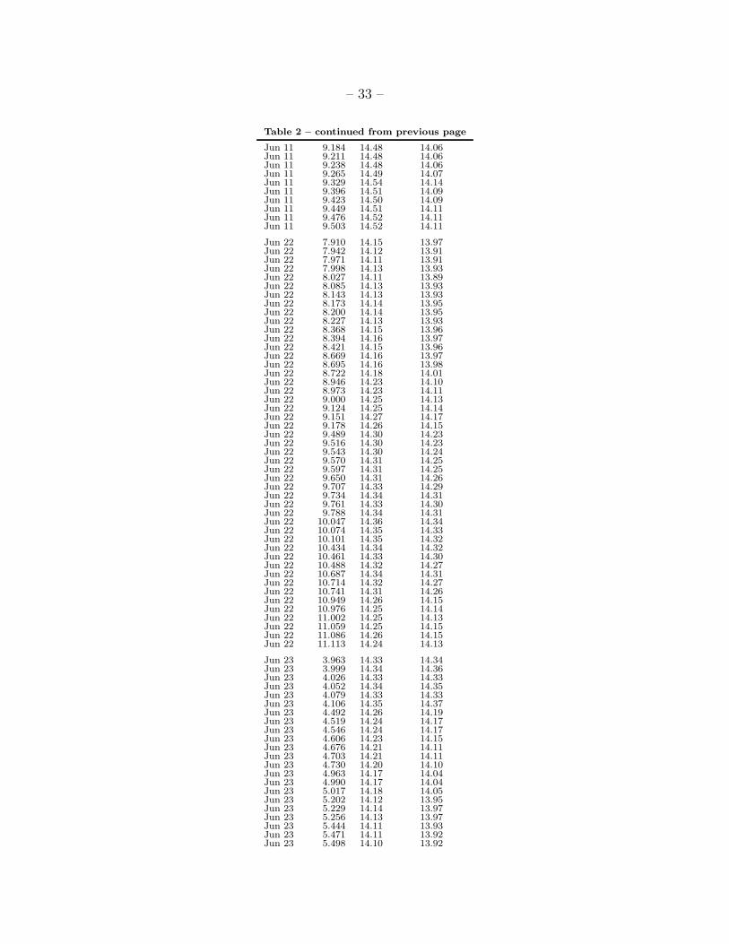
– 33 –
Table 2 – continued from previous page
Jun 11 9.184 14.48 14.06Jun 11 9.211 14.48 14.06Jun 11 9.238 14.48 14.06Jun 11 9.265 14.49 14.07Jun 11 9.329 14.54 14.14Jun 11 9.396 14.51 14.09Jun 11 9.423 14.50 14.09Jun 11 9.449 14.51 14.11Jun 11 9.476 14.52 14.11Jun 11 9.503 14.52 14.11
Jun 22 7.910 14.15 13.97Jun 22 7.942 14.12 13.91Jun 22 7.971 14.11 13.91Jun 22 7.998 14.13 13.93Jun 22 8.027 14.11 13.89Jun 22 8.085 14.13 13.93Jun 22 8.143 14.13 13.93Jun 22 8.173 14.14 13.95Jun 22 8.200 14.14 13.95Jun 22 8.227 14.13 13.93Jun 22 8.368 14.15 13.96Jun 22 8.394 14.16 13.97Jun 22 8.421 14.15 13.96Jun 22 8.669 14.16 13.97Jun 22 8.695 14.16 13.98Jun 22 8.722 14.18 14.01Jun 22 8.946 14.23 14.10Jun 22 8.973 14.23 14.11Jun 22 9.000 14.25 14.13Jun 22 9.124 14.25 14.14Jun 22 9.151 14.27 14.17Jun 22 9.178 14.26 14.15Jun 22 9.489 14.30 14.23Jun 22 9.516 14.30 14.23Jun 22 9.543 14.30 14.24Jun 22 9.570 14.31 14.25Jun 22 9.597 14.31 14.25Jun 22 9.650 14.31 14.26Jun 22 9.707 14.33 14.29Jun 22 9.734 14.34 14.31Jun 22 9.761 14.33 14.30Jun 22 9.788 14.34 14.31Jun 22 10.047 14.36 14.34Jun 22 10.074 14.35 14.33Jun 22 10.101 14.35 14.32Jun 22 10.434 14.34 14.32Jun 22 10.461 14.33 14.30Jun 22 10.488 14.32 14.27Jun 22 10.687 14.34 14.31Jun 22 10.714 14.32 14.27Jun 22 10.741 14.31 14.26Jun 22 10.949 14.26 14.15Jun 22 10.976 14.25 14.14Jun 22 11.002 14.25 14.13Jun 22 11.059 14.25 14.15Jun 22 11.086 14.26 14.15Jun 22 11.113 14.24 14.13
Jun 23 3.963 14.33 14.34Jun 23 3.999 14.34 14.36Jun 23 4.026 14.33 14.33Jun 23 4.052 14.34 14.35Jun 23 4.079 14.33 14.33Jun 23 4.106 14.35 14.37Jun 23 4.492 14.26 14.19Jun 23 4.519 14.24 14.17Jun 23 4.546 14.24 14.17Jun 23 4.606 14.23 14.15Jun 23 4.676 14.21 14.11Jun 23 4.703 14.21 14.11Jun 23 4.730 14.20 14.10Jun 23 4.963 14.17 14.04Jun 23 4.990 14.17 14.04Jun 23 5.017 14.18 14.05Jun 23 5.202 14.12 13.95Jun 23 5.229 14.14 13.97Jun 23 5.256 14.13 13.97Jun 23 5.444 14.11 13.93Jun 23 5.471 14.11 13.92Jun 23 5.498 14.10 13.92

– 34 –
Table 2 – continued from previous page
Jun 23 5.628 14.09 13.90Jun 23 5.655 14.10 13.90Jun 23 5.682 14.11 13.92Jun 23 5.710 14.11 13.92Jun 23 5.737 14.11 13.93Jun 23 5.764 14.10 13.92Jun 23 5.808 14.08 13.88Jun 23 5.834 14.07 13.87Jun 23 5.861 14.08 13.89Jun 23 5.894 14.07 13.87Jun 23 5.921 14.08 13.88Jun 23 5.947 14.09 13.89Jun 23 6.123 14.08 13.88Jun 23 6.150 14.09 13.90Jun 23 6.177 14.09 13.89Jun 23 6.341 14.09 13.89Jun 23 6.368 14.10 13.91Jun 23 6.395 14.11 13.93Jun 23 6.563 14.11 13.93Jun 23 6.590 14.13 13.96Jun 23 6.617 14.12 13.94Jun 23 6.773 14.13 13.96Jun 23 6.800 14.14 13.98Jun 23 6.827 14.14 13.99Jun 23 7.473 14.22 14.12Jun 23 7.500 14.23 14.15Jun 23 7.527 14.23 14.15Jun 23 7.557 14.24 14.17Jun 23 7.584 14.24 14.16Jun 23 7.611 14.24 14.17Jun 23 7.759 14.34 14.35Jun 23 7.786 14.32 14.32Jun 23 7.812 14.28 14.24Jun 23 7.843 14.28 14.24Jun 23 7.870 14.30 14.27Jun 23 7.897 14.30 14.28Jun 23 7.929 14.29 14.26Jun 23 7.956 14.29 14.26Jun 23 7.982 14.30 14.28Jun 23 8.012 14.30 14.29Jun 23 8.039 14.29 14.27Jun 23 8.066 14.30 14.27Jun 23 8.097 14.30 14.28Jun 23 8.124 14.30 14.27Jun 23 8.151 14.31 14.30Jun 23 8.315 14.28 14.24Jun 23 8.342 14.29 14.26Jun 23 8.368 14.30 14.27Jun 23 8.496 14.26 14.20Jun 23 8.523 14.26 14.21Jun 23 8.549 14.26 14.21Jun 23 8.761 14.24 14.16Jun 23 8.788 14.23 14.14Jun 23 8.815 14.24 14.16Jun 23 8.944 14.21 14.11Jun 23 8.971 14.21 14.11Jun 23 8.998 14.20 14.10Jun 23 9.149 14.20 14.08Jun 23 9.176 14.20 14.10Jun 23 9.203 14.20 14.09Jun 23 9.407 14.19 14.07Jun 23 9.434 14.18 14.05Jun 23 9.461 14.17 14.04Jun 23 9.607 14.17 14.03Jun 23 9.634 14.16 14.02Jun 23 9.661 14.17 14.03Jun 23 9.868 14.14 13.99Jun 23 9.895 14.13 13.97Jun 23 9.922 14.15 14.00Jun 23 10.021 14.15 14.00Jun 23 10.048 14.14 13.99Jun 23 10.075 14.15 14.00Jun 23 10.103 14.13 13.97Jun 23 10.130 14.13 13.97Jun 23 10.157 14.11 13.94Jun 23 10.186 14.11 13.93Jun 23 10.213 14.12 13.95Jun 23 10.240 14.12 13.94Jun 23 10.269 14.12 13.95Jun 23 10.296 14.09 13.90Jun 23 10.323 14.09 13.90

– 35 –
Table 2 – continued from previous page
Jun 23 10.357 14.11 13.92Jun 23 10.384 14.09 13.89Jun 23 10.411 14.10 13.91Jun 23 10.524 14.11 13.92Jun 23 10.551 14.11 13.92Jun 23 10.578 14.13 13.96Jun 23 10.709 14.11 13.92Jun 23 10.742 14.12 13.94
aUT at midpoint of the exposure (uncorrected for light travel time).
bObserved R-band magnitude (after applying absolute calibrations, extinction corrections, and compari-
son star corrections) in a circular aperture with radius 6 arcsec.
cComa-removed mR(1,1,0) corrected by ∆m2 (given in Table 1) so that all nights have the same peak
magnitude.

– 36 –
Table 3:: Table of photometry
UT Date a Tel. b Instrument Primary r ∆ α ∆t Ecl. Long. Ecl. Long. ∆m1f ∆m2
g Ref. h
Filter (AU) (AU) (◦) (hr) c Earth (◦) d Sun (◦) e
1987 Mar 31 KP2.1 TI 2 R 3.991 3.162 9.0 0.438 332.6 341.6 −5.79 +0.45 JM1987 Apr 01 KP2.1 TI 2 R 3.987 3.168 9.2 0.439 332.5 341.7 −5.80 +0.45 JM1987 Apr 02 KP2.1 TI 2 R 3.984 3.174 9.4 0.440 332.3 341.8 −5.81 +0.45 JM1987 Apr 03 KP2.1 TI 2 R 3.981 3.181 9.7 0.441 332.2 341.9 −5.82 +0.45 JM1988 Feb 25 MH2.4 MASCOT R 2.384 1.985 24.0 0.275 54.3 29.9 −4.14 −0.05 JL1988 Feb 27 MH2.4 MASCOT R 2.371 1.949 24.1 0.270 54.9 30.4 −4.09 −0.05 JL1988 Feb 28 MH2.4 MASCOT R 2.365 1.932 24.1 0.268 55.1 30.7 −4.07 −0.05 JL1988 Feb 29 MH2.4 MASCOT R 2.359 1.914 24.1 0.265 55.4 30.9 −4.04 −0.05 JL1988 Apr 09 MH1.3 MASCOT R 2.103 1.279 20.0 0.177 61.7 42.8 −2.79 +0.30 JL1988 Apr 10 MH1.3 MASCOT R 2.097 1.265 19.8 0.175 61.7 43.1 −2.75 +0.27 JL1988 Apr 12 MH1.3 MASCOT R 2.084 1.239 19.3 0.172 61.8 43.8 −2.68 +0.30 JL1988 Apr 15 MH1.3 MASCOT R 2.065 1.201 18.6 0.166 61.8 44.8 −2.57 +0.30 JL1988 May 08 SO2.3 TI VRi 1.919 0.959 13.2 0.133 59.3 53.4 −1.75 ... WI1988 May 09 SO2.3 TI VR 1.913 0.951 13.1 0.132 59.1 53.8 −1.72 ... WI1988 May 20 ML1.5 photometer VR 1.845 0.873 12.8 0.121 56.5 58.3 −1.44 −0.10 WI1988 May 21 ML1.5 photometer VR 1.839 0.867 12.9 0.120 56.2 58.7 −1.43 −0.10 WI1988 May 22 ML1.5 photometer VR 1.832 0.861 13.1 0.119 56.0 59.2 −1.41 −0.10 WI1988 Jun 10 IRTF bolometer N 1.720 0.788 19.9 0.109 51.3 68.0 −1.30 +11.80 AH1988 Jun 10 UH2.2 photometer 6840Aj 1.720 0.788 19.9 0.109 51.3 68.0 −1.30 +0.73 AH1988 Jun 11 IRTF bolometer N 1.714 0.785 20.4 0.109 51.1 68.4 −1.30 +11.70 AH1988 Jun 11 UH2.2 photometer 6840Aj 1.714 0.785 20.4 0.109 51.1 68.4 −1.30 +0.73 AH1988 Jun 12 ML1.5 photometer VR 1.708 0.783 20.9 0.108 50.9 68.9 −1.30 +0.25 WI1988 Jun 14 ML1.5 photometer VR 1.697 0.780 21.9 0.108 50.5 69.9 −1.31 +0.25 WI1988 Jun 22 MH2.4 BRICC R 1.653 0.771 25.9 0.107 49.5 74.1 −1.36 +0.23 JL1988 Jun 23 MH2.4 BRICC R 1.647 0.770 26.3 0.107 49.4 74.6 −1.36 +0.28 JL1988 Jun 30 MH2.4 BRICC R 1.611 0.769 29.7 0.107 49.2 78.4 −1.42 +0.45 JL1994 Oct 26 KP0.9 T2KA R 2.498 1.640 14.2 0.227 247.5 234.2 −3.52 ... MF1994 Dec 18 KP0.9 T2KA R 2.802 1.932 11.3 0.268 234.8 245.5 −4.03 ... MF1994 Dec 19 KP0.9 T2KA R 2.807 1.944 11.6 0.269 234.6 245.7 −4.06 ... MF
aParameters were determined for 7:00 UT on the date of observation.
bTelescope abbreviations: IRTF = NASA Infrared Telescope, KP0.9 = Kitt Peak 0.9-m, MH1.3 =
McGraw-Hill 1.3-m, MH2.4 = McGraw-Hill 2.4-m, ML1.5 = Mt. Lemmon 1.5-m, SO2.3 = Steward Ob-
servatory 2.3-m, UH2.2 = University of Hawaii 2.2-m.
cLight travel time.
dEcliptic longitude of the Earth as seen from the comet.
eEcliptic longitude of the Sun as seen from the comet.
fmR(1,1,0) correction for the night (in magnitudes).
gOffset (in magnitudes) necessary to make data on all nights peak at the same magnitude.
hReference abbreviations: AH = (A’Hearn et al. 1989), JL = (Jewitt & Luu 1989), JM =
(Jewitt & Meech 1988), MF = (Mueller & Ferrin 1996), WI = (Wisniewski 1990).
iThe VR filter was centered at 5886 A with a 2160 A half-width (Wisniewski 1990).
jA similar number of observations was also made at 4845 A. However, we primarily used the 6840 A data
and so ∆m2 is only listed for the 6840 A data. Both of these filters are part of the International Halley
Watch filter set (Osborn et al. 1990).

– 37 –
Fig. 1.— Observed R-band magnitudes (mR) for our 1999 data plotted as a function of UT
on each night. The magnitudes have had absolute calibrations, extinction corrections, and
comparison star corrections applied and are given in column (3) of Table 2. Starting with
the bottom panel and moving up, the first panel (circles) displays April 17 (purple), April
18 (blue), and April 19 (cyan). The second panel (crosses) displays May 26 (red) and May
27 (pink). The third panel (triangles) displays June 8 (black), June 9 (light gray), June 10
(medium gray), and June 11 (dark gray). The top panel (squares) displays June 22 (orange)
and June 23 (yellow). Note that throughout the time of interest, decreasing r and ∆ caused
the comet to brighten while at the same time increasing coma damped out the amplitude
variations of the nucleus. Thus the range of magnitudes is different in each panel, although
the vertical scale is held constant at 1 mag to emphasize the decreased amplitude.

– 38 –
Fig. 2.— Observed R-band magnitudes (mR) for our 1999 data phased to our best period
of 8.941 hr (discussed in Section 3.1). The magnitudes have had absolute calibrations,
extinction corrections, and comparison star corrections applied and are given in column (3)
of Table 2. Zero phase was set at perihelion (1999 September 8.424). The points are as given
in Figure 1. Note that throughout the time of interest, decreasing r and ∆ caused the comet
to brighten while at the same time increasing coma damped out the amplitude variations of
the nucleus. This figure illustrates the phase coverage obtained during each run, and shows
that the lightcurves could be phased even without removing coma contamination.

– 39 –
Fig. 3.— Representative nightly radial profile (1999 June 9). Each curve is composed of the
total annular flux (in arbitrary units) in 3 arcsec wide annuli. The solid light gray curves
are the radial profiles for images which were used to estimate a nightly median coma profile.
The dotted dark gray curves are the radial profiles for images which had contamination by
background stars and were not used to determine the nightly median coma profile. The
heavy black curve is the nightly median coma profile. This was determined by taking the
median of all the light gray curves at the midpoint of each annulus, then fitting a straight
line to this nightly radial profile for annuli between 6–21 arcsec (the vertical dashed lines),
and extrapolating the fit in to the nucleus and out to 30 arcsec. If the coma decreased as
ρ−1 the coma profile would be a horizontal line. The coma profile was never a horizontal line
due to the wings of the nucleus PSF, contamination from background stars, and possibly a
non-ρ−1 fall off of the coma. We fit a straight line as a first order approximation. Higher
order fits varied more from image to image. See the text for further discussion.

– 40 –
Fig. 4.— 1999 data phased to the 8.941 hour period (top panel) and the 8.932 hr (bottom
panel). The magnitudes are mR∗ (given in column (4) of Table 2). The midpoint of each
image was used and then corrected for the light travel time, with zero phase set at perihelion
(1999 September 8.424). The points are as given in Figure 1.

– 41 –
Fig. 5.— Our 1999 data phased to 8.937 hr (top panel), 8.941 hr (middle panel), and 8.945 hr
(bottom panel). The magnitudes are mR∗ (given in column (4) of Table 2) offset by −0.015
magnitudes per day from 1999 April 17. This offset has been applied for display purposes
to minimize overlapping data so the trend in the phasing of extrema is more apparent. The
midpoint of each image was used and then corrected for the light travel time before phasing,
with zero phase set at perihelion (1999 September 8.424). The symbols are as given in
Figure 1. By phasing the data in this manner, we found a best period of 8.941 hr and an
uncertainty of ±0.002 hr.

– 42 –
Fig. 6.— 1988 data from the literature phased to the 8.932 hour period (top panel) and the
8.941 hr (bottom panel). The published data have been normalized to mR(1,1,0) and offset
by ∆m2 (given in Table 3) to peak at the same magnitude. The times are as given in the
literature and corrected for the light travel time, and zero phase was defined at perihelion
(1988 September 16.738). The green crosses (AH) are A’Hearn et al. (1989), the blue squares
(JL) are Jewitt & Luu (1989), and the red triangles (WI) are Wisniewski (1990).
Copyright © 2022 FDOKUMEN