
The Impact of the Global Financial Crisis on European ...
304
The Impact of the Global Financial Crisis on European Transition Countries ARTA HOXHA A thesis submitted in partial fulfilment of the requirement of Staffordshire University for the degree of Doctor of Philosophy in Economics February 2018
-
Upload
khangminh22 -
Category
Documents
-
view
0 -
download
0
Transcript of The Impact of the Global Financial Crisis on European ...
The Impact of the Global Financial Crisis on European Transition
Countries
ARTA HOXHA
A thesis submitted in partial fulfilment of the requirement of Staffordshire
University for the degree of Doctor of Philosophy in Economics
February 2018

2
3
Abstract
In spite of a large number of studies on the international transmission of crises, research is still unable to quantify the determinants of severity of crisis across countries. This thesis contributes to knowledge in this area by investigating the impact of the Global Financial Crisis (GFC) on European transition countries. In analysing the transmission of the GFC to these countries and the nature and severity of the spillovers, both trade and financial channels are examined and particular emphasis is placed on the degree of euroisation, integration with the EU, remittances, bank ownership and foreign credit flows.
This thesis firstly provides a critical review of the existing literature on the transmission of the GFC to European transition countries and identifies gaps in knowledge, which are then addressed through empirical investigations. The first empirical investigation explores how GDP and financial shocks in the European advanced countries (EU15) are transmitted to European transition countries, using the recently-developed global vector auto-regression (GVAR) approach. The results suggest that while trade appears to be the strongest linkage between EU15 and European transition countries, the shocks are propagated by both trade and financial channels. Moreover, although the estimated spillovers from GDP and financial shocks in the EU15 to European transition countries are always negative, there are considerable heterogeneities in the size and statistical significance of these effects across regions. The Baltic countries display the most severe impact from the shocks in the EU15, which appear to be propagated mostly through the financial channel: foreign credit flows; FDI; and remittances. The Balkan countries are affected predominantly through exports, FDI and foreign credit flows. The other Central and Eastern European transition countries are less severely affected by shocks to the EU15 GDP. Furthermore, highly euroised, non-EU members and more open transition countries appear to be more severely affected by the shocks in the EU15.
The initial analysis is extended through a firm-level analysis, which investigates whether initial conditions (from 2007) had an impact on firms' sales during the GFC in 2009. The major finding of this firm-level study is the importance of the financial channel in the transmission of the GFC to European transition countries: a higher share of working capital financed by banks, a higher share of foreign currency loans and a higher share of foreign bank ownership each increased the impact of the GFC on the firms operating in these countries. With regards to the export channel, it is found that both exporting and non-exporting firms operating in the countries covered in this study were significantly affected by the crisis. This finding suggests that, although there is a trade channel, the exporting firms are able to cope with the crisis better than non-exporting firms due to their overall superior performance. This finding may also reflect the cross-sectional nature of the data which can reveal only between-firm differences. So exports, or more precisely, exporting firms constitute a transmission channel of the GFC. Yet, exporting firms are also more able to offset effects of crisis and thus contribute to the resilience of transitional economies.

4
5
Contents
Abstract ................................................................................................................................................................... 3
Contents .................................................................................................................................................................. 5
List of tables ....................................................................................................................................................... 10
List of figures ...................................................................................................................................................... 12
Abbreviations ..................................................................................................................................................... 14
Acknowledgements .......................................................................................................................................... 16
Note ....................................................................................................................................................................... 17
CHAPTER 1
INTRODUCTION
1.1 Introduction ............................................................................................................................................... 19
1.2 The transition process in ETEs ........................................................................................................... 20
1.2.1 Output during transition ................................................................................................................... 22
1.2.2 Trade during transition ..................................................................................................................... 24
1.2.3 Financial developments ..................................................................................................................... 28
1.2.4 FDI inflows ............................................................................................................................................. 31
1.2.5 Migration and remittances ............................................................................................................... 33
1.2.6 Integration with the EU and pre-accession support .............................................................. 35
1.3 Causes and nature of the GFC and how it spread ....................................................................... 36
1.4 The impact of the GFC on ETEs .......................................................................................................... 40
1.5 Key research questions and structure of the thesis................................................................... 42
CHAPTER 2
TRANSMISSION OF GLOBAL FINANCIAL CRISES: A REVIEW OF THE THEORETICAL LITERATURE
2.1 Introduction ............................................................................................................................................... 46
2.2 International transmission of the GFC ............................................................................................ 48
2.2.1 Fundamental causes ............................................................................................................................ 49
2.2.2 Investors’ behaviour ........................................................................................................................... 53
2.2.3 Transmission of shocks from the financial sector to the real economy ........................ 55
2.3 Euroisation ................................................................................................................................................. 58
2.3.1 Benefits and costs/risks associated with euroisation........................................................... 60
2.4 Integration with the EU ......................................................................................................................... 63
2.4.1 Benefits associated with European integration ....................................................................... 64
2.4.2 Integration with EU ............................................................................................................................. 65
2.5 Conclusion ................................................................................................................................................... 67
6
CHAPTER 3
TRANSMISSION OF GLOBAL FINANCIAL CRISES: A REVIEW OF THE EMPIRICAL LITERATURE
3.1 Introduction ............................................................................................................................................... 70
3.2 Channels of transmission of global financial crises, shocks and contagion ..................... 71
3.2.1 Cross-market correlation coefficients ......................................................................................... 71
3.2.2 Individual channels of contagion ................................................................................................... 77
3.3 Benefits and costs associated with euroisation........................................................................... 92
3.4 Integration with EU ............................................................................................................................... 101
3.5 Empirical work for European transition economies ............................................................... 107
3.6 Conclusion ................................................................................................................................................. 121
CHAPTER 4
EXPLAINING THE IMPACT OF THE GLOBAL FINANCIAL CRISIS ON EUROPEAN TRANSITION COUNTRIES: A GVAR APPROACH
4.1 Introduction ............................................................................................................................................. 125
4.2 The GVAR approach .............................................................................................................................. 126
4.3 Specification of data and variables ................................................................................................. 129
4.4 Empirical Approach .............................................................................................................................. 131
4.4.1 Specification and estimation of the country-specific models .......................................... 131
4.4.2 GVAR model specification ............................................................................................................... 137
4.4.3 Dynamic analysis using generalized impulse response functions and generalized forecast error variance decomposition ................................................................................................ 148
Impulse response functions of one standard error shock to GDP in EU ................................ 149
Generalized forecast error variance decomposition ...................................................................... 153
4.4.4 Robustness analysis .......................................................................................................................... 154
Impulse response functions of a one standard error shock to GDP in the EU ..................... 155
4.4.5 The effects of increased financial stress in the EU15 .......................................................... 164
Impulse response functions of a one standard error shock to CISS in EU ............................. 165
4.5 Conclusion ................................................................................................................................................. 167
CHAPTER 5
EXPLAINING THE IMPACT OF THE GLOBAL FINANCIAL CRISIS ON EUROPEAN TRANSITION COUNTRIES: IMPACT ON FIRMS' SALES
5.1 Introduction ............................................................................................................................................. 174
5.2 Research design and data description .......................................................................................... 174
5.3 Estimation technique ........................................................................................................................... 183
5.4 Diagnostic tests ....................................................................................................................................... 185
7
5.5 Empirical results .................................................................................................................................... 187
5.6 Discussion and interpretation .......................................................................................................... 208
5.7 Conclusion .................................................................................................................................................. 210
CHAPTER 6
CONCLUSIONS
6.1 Introduction ............................................................................................................................................. 214
6.2 Findings of the thesis ............................................................................................................................ 215
6.3 Contributions to knowledge .............................................................................................................. 224
6.4 Policy implications ................................................................................................................................ 226
6.5 Limitations and recommendations for future research ......................................................... 230
References ........................................................................................................................................................ 234
Appendix to Chapter 4 ................................................................................................................................. 257
Table A4.6 Unit root tests for the domestic variables at 5% significance level ................... 257
Table A4.7 Unit root tests for the foreign variables at 5% significance level ....................... 258
Table A4.8 Tests of residual serial correlation for country-specific VARX* models ......... 260
Figure A4.8 Persistence profiles for the baseline model............................................................... 260
Table A4.11 Proportion of the N-step ahead forecast error variance of Balkan GDP explained by conditioning on contemporaneous and future innovations of the country equations263
Table A4.12 Proportion of the N-step ahead forecast error variance of Baltic GDP explained by conditioning on contemporaneous and future innovations of the country equations264
Table A4.13 Proportion of the N-step ahead forecast error variance of CE GDP explained by conditioning on contemporaneous and future innovations of the country equations ..... 265
Table A4.14 Unit Root Tests for the Domestic Variables at 5% significance level ............. 266
Table A4.15 Weak exogeneity .................................................................................................................. 268
Figure A4.9 Persistence profiles of model 4.2 ................................................................................... 268
Table A4.16 Serial correlation ................................................................................................................. 269
Table A4.17 Unit root tests for the domestic variables at 5% significance level ................ 270
Table A4.18 Weak exogeneity .................................................................................................................. 272
Figure A4.10 Persistence profiles of model 4.3 ................................................................................ 272
Table A4.19 Serial correlation ................................................................................................................. 273
Appendix to Chapter 5 ................................................................................................................................. 272
A5.1 Model 5.1 - estimated results ......................................................................................................... 274
A5.2 Model 5.1 – diagnostic tests ............................................................................................................ 274
Check for multicollinearity - VIF command - Model 5.1 ................................................................ 274
Tests for homoscedasticity - Model 5.1 ................................................................................................ 275
8
A5.3 Model 5.1 - estimated results (robust standard errors) ..................................................... 276
A5.4 Model 5.2 - estimated results (robust standard errors) ..................................................... 276
A5.5 Model 5.2 – diagnostic tests ............................................................................................................ 277
Check for multiocollinearity - model 5.2. Vif...................................................................................... 277
Tests for homoscedasticity - Model 5.2 ................................................................................................ 278
Tests for model specification - Model 5.2 ............................................................................................ 278
A5.6 Model 5.3 - estimated results ......................................................................................................... 278
A5.7 Model 5.3 – diagnostic tests ............................................................................................................ 279
Check for multiocollinearity - model 5.3 Vif ...................................................................................... 279
Test for homoscedasticity - model 5.3 ................................................................................................. 280
Test for functional form - model 5.3 ..................................................................................................... 280
A5.8 Margins of interaction between wcbanks and foreigncurrloans .................................... 281
A5.9 Margins of interaction between wcbanks and foreignabnkownership ........................ 281
A5.10 Model 5.4 - estimated results ...................................................................................................... 281
A5.11 Model 5.4 – diagnostic tests ......................................................................................................... 282
Check for multicollinearity - model 5.4 ................................................................................................ 282
Test for homoscedasticity - model 5.4 .................................................................................................. 283
Test for functional form - model 5.4 ...................................................................................................... 283
A5.12 Model 5.5 - estimated results ...................................................................................................... 283
A5.13 Model 5.5 – diagnostic tests ......................................................................................................... 284
Check for multicollinearity - model 5.5 ................................................................................................ 284
Test for homoscedasticity - model 5.5 .................................................................................................. 284
Test for functional form - model 5.5 ...................................................................................................... 285
Graphic checks to support diagnostic tests ........................................................................................ 286
Figure A5.1 Standardized residuals versus predictor variables ................................................ 286
Figure A5.2 Augmented plus residual plot ......................................................................................... 287
Figure A5.3 Kemel density plot ............................................................................................................... 287
Figure A5.4 pnorm and qnorm plots ..................................................................................................... 288
A5.14 Model 5.6 - estimated results ...................................................................................................... 288
A5.15 Model 5.6 – diagnostic tests ......................................................................................................... 289
Check for multicollineaarity - model 5.6 ............................................................................................. 289
Test for homoscedasticity - model 5.6 .................................................................................................. 289
Test for functional form - model 5.6 ...................................................................................................... 289
A5.16 Predictive margins - model 5.6 ................................................................................................... 290
A5.17 Margins of interaction between directexodumm and changnatsales......................... 291
A5.18 Model 5.7 - estimated results ...................................................................................................... 292
A5.19 Model 5.7 – diagnostic tests ......................................................................................................... 293
Test for homosecdasticity - model 5.7 .................................................................................................. 293
Test for functional form - model 5.7 ...................................................................................................... 293

9
A5.20 Predicive margins form - model 5.7 ......................................................................................... 294
A5.21 Margins of interaction term between directexp and foreigncurr ................................ 295
A5.22 Model 5.8 - estimated results ...................................................................................................... 295
A5.23 – Model 5.8 – diagnostic tests ..................................................................................................... 296
Check for multocollinearity - model 5.8 ............................................................................................... 296
Test for homoscedasticity - model 5.8 .................................................................................................. 296
Test for functional form - model 5.8 ...................................................................................................... 297
A5.24 Predicitve margins - model 5.8 ................................................................................................... 297
A5.25 Margins of interaction term between directexp and foreignown ................................ 298
A5.26 Model 5.9 - estimated results ...................................................................................................... 298
A5.27 Model 5.9 – diagnostis tests ......................................................................................................... 299
Check for multicollinearity - model 5.9 ................................................................................................ 299
Test for homoscedasticity - model 5.9 .................................................................................................. 300
Test for functional form - model 5.9 ...................................................................................................... 300
A5.28 Predictive margins - model 5.9 ................................................................................................... 300
A5.29 Model 5.10 - estimated results ................................................................................................... 301
A5.30 Predictive margins - model 5.10 ................................................................................................ 302
A5.31 Model 5.11 – estimated results ................................................................................................... 302
A5.32 Predictive margins - model 5.11 ................................................................................................ 303
10
List of tables
Table 3.1 Empirical studies investigating financial contagion based on cross-market
correlation coefficients
Table 3.2: Empirical studies investigating financial contagion based on individual
channels
Table 3.3: Empirical studies investigating the impact of dollarization/euroisation on
financial stability/crisis severity
Table 3.4 Empirical studies investigating the degree of integration with EU and
progress with transition
Table 3.5 Empirical studies investigating ETEs
Table 4.1a Trade weights used for computing foreign country-specific variables
Table 4.1b FDI weights used for computing foreign country-specific variables
Table 4.1c Remittance weights used for computing foreign country-specific variables
Table 4.2 Variable specification of country-specific VARX* models
Table 4.3 Number of rejection of the null hypothesis of non-stationarity
Table 4.4 Chosen lag length and cointegration rank
Table 4.5 Test for weak exogeneity at the 5% significance level
Table 4.6 Number of rejection of structural stability hypothesis per variables and
different test statistics
Table 4.7 Summary of main results
Table 5.1 Summary of variables
Table 5.2. Diagnostic tests
Table 5.3 The variance inflation factor (VIF)
Table 5.4 OLS estimates of baseline regression (5.1) and extended models (5.2) and
(5.3)
Table 5.5 Description of country-level variables and interaction terms
Table 5.6 Results of the model (5.4)

11
Table 5.7 Robustness check (dependent variable ∆Employment, model (5.5))
Table 5.8 Predictive margins of directexdumm
Table 5.9 OLS estimates of extended models (5.6) to (5.9)
Table 5.10 Contrasts of marginal effects of changenatsales for exporting vs non-
exporting firms
Table 5.11 Contrasts of marginal effects of foreigncurrr for exporting vs. non-
exporting firms
Table 5.12 Results of the models (5.10) and (5.11)
Table 5.13 Contrasts of marginal effects of currdep for exporting vs. non-exporting firms
Table 5.14 Contrasts of marginal effects of foreign currency loans for currency depreciation vs. no currency depreciation

12
List of figures
Figure 1.1 Annual percentage change of GDP per capita (1989-2015)
Figure 1.2a Exports patterns across ETEs (1995-2015)
Figure 1.2b Exports as a share of GDP (2000, 2009, 2015)
Figure 1.2c Annual percentage growth of exports (2000-2015)
Figure 1.3 Export growth in 2009 versus share of trade with EU15
Figure 1.4 Asset share of foreign-owned banks in total banking assets - 2009
Figure 1.5 Cross-border credit flows to ETEs (2000-2015)
Figure 1.6 Average degree of credit and deposit euroisation (2004-2014)
Figure 1.7a Foreign direct investment, net inflows (1995-2015)
Figure 1.7b Share of FDI inflows from EU15 (2005-2007)
Figure 1.8 Share of remittance inflows from EU15 (2010)
Figure 1.9a Remittances received as a share of GDP, average 1997-2015
Figure 1.9b Annual percentage change of remittances received
Figure 4.1 Regional impulse response functions (point estimates) of GDP to a one
standard error shock to GDP in EU15 - remittance weights vs. trade weights vs. FDI
weights
Figure 4.2. Regional impulse response functions of GDP, exports, FDI, foreign credit
flows and remittances to a one standard error shock to GDP in EU with their 90%
confidence bands
Figure 4.3 Regional impulse response functions of GDP, exports, foreign credit flows
and FDI to a one standard error shock to GDP in the EU15, with 90% confidence
bands (trade weights)
Figure 4.4 Impulse response functions to a one standard error shock to GDP in EU15
with their 90% confidence bands (EU transition countries vs. non-EU transition
countries)
Figure 4.5 Regional impulse response functions to one standard error shock to GDP
in EU15 with their 90% confidence bands (Highly euroised countries vs. lowly
euroised countries)

13
Figure 4.6 Regional impulse response functions to one standard error shock to GDP
in EU15 with their 90% confidence bands (highly open countries vs. lowly open
countries)
Figure 4.7 Regional impulse response functions of GDP to a one standard error shock
to CISS in EU15 with their 90% confidence bands
Figure 5.1 Average marginal effects of interaction terms between working capital
financed by banks and foreign bank ownership
Figure 5.2 Fitted values for channgnatsales and directexp interaction
Figure 5.3 Fitted values for foreigncurr and directexp interaction
Figure 5.4 Fitted values for foreignown and directexp interaction
Figure 5.5 Fitted values for wcbank and directexp interaction
Figure 5.6 Fitted values for currdep and directexp interaction
Figure 5.7 Fitted values for foreigncurr and currdep interaction

14
Abbreviations
BEEPS –Business Environment and Enterprise Performance Survey
CARDS - Community Assistance for Reconstruction, Development and Stabilisation
CC – Common Creditor
CEE – Central and Eastern Europe
CESEE – Central, Eastern and South-Eastern Europe
CEFTA - Central European Free Trade Agreement
CISS – Composite Indicator of Systemic Stress
CLRM – Classical Linear Regression Model
CPI – Consumer Price Index
ECB – European Central Bank
ECM – Error Correction Model
ETE – European Transition Economy
BIS – Bank for International Settlements
EU 15 – 15 advanced EU member states (before the 2004 enlargement)
FDI – Foreign Direct Investment
GDP – Gross Domestic Product
GFC – Global Financial Crisis
GFEVD - Generalized Forecast Error-variance Decomposition
GIRF – Generalized Impulse Response Function
GNP – Gross National Product
GVAR – Global Vector Auto-regression
IMF – International Monetary Fund
IPA - Instrument for Pre-Accession Assistance

15
ISPA - Instrument for Structural Policies for Pre-Accession
NFA – Net Foreign Assets
OECD – Organisation for Economic Co-operation and Development
PSP – Public Sector Prices
R&D – Research & Development
SAP - Stabilisation and Association Process
SAPARD - Special Accession Programme for Agricultural and Rural Development
TFP – Total Factor Productivity
VAR – Vector Autoregression
VECM – Vector Error Correction Model
VIF – Variance Inflation Factor
WDI – World Development Indicators
WTO – World Trade Organization

16
Acknowledgements
First and foremost, I would like to express my deepest gratitude to my supervisors,
Professor Nick Adnett and Professor Geoff Pugh, for their continuous support,
commitment, encouragement, and guidance throughout this research. I would also
like to thank my local supervisor, Dr. Valentin Toçi, for his valuable comments and
suggestions.
My sincere gratitude is extended to Staffordshire University and the Open Society
Foundation whose financial support enabled this research project.
My greatest appreciation goes to my family. I am thankful to my parents for their
love, encouragement and care. A special gratitude goes to my husband for his endless
support, understanding, patience and love. Finally, I would like to thank my lovely
son, Drin, whose love and laugher inspired and motivated me throughout this
journey.

17
Note
A paper based on Chapter 4 of this thesis won the 2017 Olga Radzyner Award of the
Oesterreichische Nationalbank (OeNB) which is bestowed on young economists for
scientific work on European economic integration.
CHAPTER 1
INTRODUCTION
Contents
1.1 Introduction ............................................................................................................................................... 19
1.2 The transition process in ETEs ........................................................................................................... 20
1.2.1 Output during transition ................................................................................................................... 22
1.2.2 Trade during transition ..................................................................................................................... 24
1.2.3 Financial developments ..................................................................................................................... 28
1.2.4 FDI inflows .............................................................................................................................................. 31
1.2.5 Migration and remittances ............................................................................................................... 33
1.2.6 Integration with the EU and pre-accession support .............................................................. 35
1.3 Causes and nature of the GFC and how it spread........................................................................ 36
1.4 The impact of the GFC on ETEs .......................................................................................................... 40
1.5 Key research questions and structure of the thesis ................................................................... 42
19
1.1 Introduction
The aim of this thesis is to investigate the transmission of the global financial crisis
(GFC) to European transition economies (ETEs), taking into account the extent of
euroisation and integration with the EU, remittance flows, exports, pattern of bank
ownership, FDI and foreign credit flows. One particular feature of the GFC has been
the speed and synchronicity with which it spread around the world, affecting, both
emerging and advanced countries. Although there have been a few studies that have
investigated the transmission of the GFC to ETEs (Berglöf et al., 2009; Blanchard et al,
2010; Lane and Milesi-Ferretti, 2011; Rose and Spiegel, 2009a, 2009b, 2011;
Berkmen et al., 2012; Popov and Udell, 2012; Feldkircher, 2014; Park and Mercado,
2014; De Haas et al., 2015; Ongena et al., 2015; Ahmed et al., 2017), the literature is
still unable to provide conclusive results of the determinants of crisis severity across
these countries. This thesis contributes to knowledge in this area by firstly
identifying gaps in the literature, then exploring the channels of the international
transmission of shocks to ETEs, and finally investigating whether the extent of
euroisation and integration with the EU, pattern of bank ownership, exports,
remittances, FDI and foreign credit flows significantly modified the propagation of
the GFC to ETEs.
The objective of this introductory chapter is to provide the context of the research
reported in this thesis. It initially presents an overview of the transition process in
the Central and Eastern European countries, focusing on the key areas relevant to the
research questions addressed in this thesis. Namely, it starts by describing the
process of transition from centrally planned economies towards open, market-
oriented economies, examines the output, trade, FDI and remittance fluctuations
throughout the period and describes financial developments as well as recording the
progress made towards integration with the EU during this period. It then continues
with an overview of the GFC and an investigation of its impact on the ETEs. The last
section of this chapter lists the key research questions addressed in this research
programme and explains the structure of the thesis.

20
1.2 The transition process in ETEs
Almost three decades ago, Central and Eastern European countries started the
transition from centrally planned economies towards open, market-oriented
economies. The long-term objective of transition was to build a successful market
economy able to deliver sustainable growth (Kolodko, 1999). The transition itself
involved a complex process of institutional, structural and behavioural change (De
Melo et al., 1996). Considering that the Central and Eastern European countries
inherited entrenched and inefficient bureaucratic institutions from the previous
decades dominated by the socialist system, they faced many challenges throughout
this process (Carmin and Vandeveer, 2004). Three main objectives dominated
transition: macroeconomic stabilization; real adjustment at the microeconomic level
and creation of a new institutional framework (Piazolo, 2000). Macroeconomic
stabilization aimed to resolve the drop in output and monetary and fiscal instability
that emerged after the start of transition and was an important accompaniment to
liberalization in promoting economic growth during transition (World Bank, 1996).
The microeconomic-level reforms sought to stabilize markets through privatization
of state entities, price liberalization and openness to international trade. The
institutional framework reform was intended to ensure that a decentralization of
economic decisions would occur. These three objectives were interrelated; hence,
simultaneous progress in all of them was required for the overall economic reform to
be successful (Piazolo, 2000). One of the main arguments in favour of moving to a
market-oriented economy was the expectation that the move would improve
productivity in the former socialist economies (Grün and Klasen, 2001). It was
expected that, after a short period of adjustment (the so-called transformational
recession), the new market-oriented system would lead to a rapid recovery and
sustainable economic growth. However, such anticipations were not fulfilled equally
in all transition countries. Some countries recovered rapidly from the initial
recession following the beginning of transition, while others went through a deeper
transitional recession that lasted for a longer period than was initially expected.
Many economists agree that there were three main economic variables which greatly
impacted the recovery period and subsequent economic growth (Falcetti, et al.,
2006). Firstly, the initial conditions played an important role in countries’
21
performance and subsequent development (Fischer and Sahay, 2000; De Melo et al.,
2001; EBRD, 2004; Coricelli and Maurel, 2011, Roaf et al., 2014). However, there is a
general agreement that the impact of initial conditions on performance weakens over
time. Secondly, most studies have shown that higher inflation rates and larger budget
deficits were negatively associated with recovery and growth. Hence, considering
that after the beginning of transition most countries were faced by high inflation and
large fiscal deficits, it was essential to introduce a macroeconomic stabilisation
programme (Falcetti et al. 2006). Finally, most of these studies concluded that
reforms are important for sustainable growth, from early reforms such as price and
trade liberalisation and small-scale privatisation to more profound reforms such as
corporate restructuring, financial sector development and competition policy (De
Melo et al., 2001; Falcetti et al., 2006). Considering that the transition objectives
overlapped with the key criteria required for accession to the EU (Piazolo, 2000),
progress with EU integration has been positively correlated with progress with
transition. Based on different initial conditions and different reform strategies
followed by these countries, the transition literature identifies different
categorisations of transition countries with regards to their economic performance.
In the context of this study, based on the classification of the International Monetary
Fund (IMF) in regard to progress with transition (liberalization, macroeconomic
stabilization, restructuring and privatization and legal and institutional reforms),
together with their economic performance and geographical location, European
transition countries are classified into three main groups:
1. South East European (SEE) countries: Albania, Bosnia and Herzegovina (BH),
Bulgaria, Croatia, Kosovo, Macedonia, Montenegro, Romania and Serbia;
2. Central East European (CEE) countries: the Czech Republic, Hungary, Poland,
the Slovak Republic and Slovenia;
3. Baltic Countries: Estonia, Latvia and Lithuania.
The selection of countries to be studied in this thesis was based on their European
perspective and similar transition history. Even though many of these countries are
22
now post-transition, have joined the EU1 and are today more frequently considered
within the group of 10 new EU member states, they have many common features
with other ETEs as a result of similar transition experiences and are therefore
considered as “transition” countries throughout this thesis. Nevertheless, it has to be
pointed out that Russia, for example, was not included in the study since it would
have dominated and distorted the sample given its larger size.
In order to provide the necessary background to answer the research questions
which will be investigated in this thesis, the rest of this section focuses on output
behaviour, trade integration, financial development, FDI, migration and remittances
and integration with the EU throughout the period of transition starting from 1989 or
from the earliest year for which data is available, usually 1995, up to the latest year
available for most of these countries, usually 2015.
1.2.1 Output during transition
The pattern of output movement since the commencement of transition is illustrated
in Figure 1.1 and can be summarized as follows. The beginning of transition was
associated with a sharp output decline in all transition countries. However, the three
country groups experienced different initial recessions, with the Baltic States being
most severely affected where economic activity declined by around 25%. The timing
of the recovery period varied among the transition country groups. CEE countries
achieved positive economic growth from the beginning of 1992, while SEE countries
achieved positive economic growth in 1993 and Baltic States in 1994. Due to bolder
reforms undertaken, the CEE countries had a faster return to growth and avoided the
second recession that hit the region in 1997 after the initial recession. For the SEE
countries, the reversal repeated twice, in 1997 and 1999. All groups of countries
appear to have recovered quickly from this second recession, and up to 2007
continued having positive and stable economic growth, which averaged 6% for the
region, with no country growing at less than 3 percent annually (World Bank, 2017).
The SEE countries’ growth continued at around 5 percent up to 2007. However,
growth in this period became increasingly imbalanced, driven in many countries by
1 Czech Republic, Latvia, Lithuania, Estonia, Poland, Slovakia and Slovenia became EU members in 2004, Bulgaria and Romania in 2007 and Croatia in 2013.

23
large-scale borrowing for consumption and construction, high current account
deficits and rising external debt (Roaf et al., 2014). The GFC hit the transition
countries with different intensity, with output decline in the region averaging 7% in
2009, a more severe impact than in any other region in the world, including the
EU152 where the output decline averaged 5%. The Baltic States suffered the largest
output decline, which averaged 14% in 2009. The second most affected group of
transition countries appears to have been the CEE countries, with an average GDP
decline of around 4%. The last group of transition countries, the SEE countries, had
an average GDP decline of only around 2%.
Figure 1.1 Annual percentage change of GDP per capita (1989-2017)
Data source: World Bank, World Development Indicators (GDP per capita growth - annual %
change) 2017
All three groups of countries returned to positive economic growth in 2010.
However, during 2012, economic activity in all country groups declined again due to
the intensification of the sovereign debt crisis in the eurozone. Since 2012 growth has
remained relatively weak across those transition countries which were particularly
integrated with the eurozone due to decline in their exports and capital inflows.
2 Austria, Belgium, Denmark, Finland, France, Germany, Greece, Ireland, Italy, Luxembourg, Netherlands, Portugal, Spain, Sweden and United Kingdom.
-25
-20
-15
-10
-5
0
5
10
15
19
89
19
90
19
91
19
92
19
93
19
94
19
95
19
96
19
97
19
98
19
99
20
00
20
01
20
02
20
03
20
04
20
05
20
06
20
07
20
08
20
09
20
10
20
11
20
12
20
13
20
14
20
15
20
16
20
17
GD
P p
er
cap
ita
gro
wth
(a
nn
ua
l %
)
SEE CEE Baltic EU
24
1.2.2 Trade during transition
One of the key outcomes of the transition process in the former communist countries
has been deeper international integration through increased trade and capital flows
(Roaf et al., 2014). Before the transition started, trade in transition countries was
mainly focused inwards. In 1990, around 80 percent of exports from the Baltic
countries went to Russia (Roaf et al., 2014). After the dissolution of the Soviet Union,
these countries experienced a sharp decline in exports. Due to a small manufacturing
base and the small size of the economies, the Baltic countries’ exports remained
relatively low compared to the CEE and SEE countries (see figure 1.2a).
After transition started, considering the failure of the previous system, all countries
stood to gain from price and market liberalisation. New open markets increased
investment opportunities, which resulted in faster economic growth and
improvements in the standards of living. Hence, the transition countries embraced
both internal and external liberalisation (EBRD, 2003). By 2000, most of the ETEs
became members of the World Trade Organization, which offered new markets and
assisted countries in harmonising regulatory and political frameworks and building
stable market institutions (Roaf et al., 2014). In addition, most countries joined the
Central European Free Trade Agreement (CEFTA) during the period 1992-2007
(EBRD, 2012). Therefore, transition and integration have been closely linked during
the past 20 years, with the total value of exports growing significantly during this
period, which included an increase of 382% between 1995 and 2015 for the region
(see Figure 1.2).
25
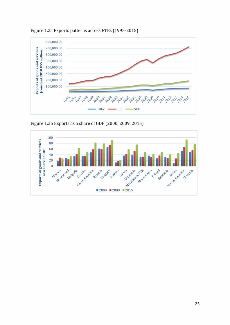
Figure 1.2a Exports patterns across ETEs (1995-2015)
Figure 1.2b Exports as a share of GDP (2000, 2009, 2015)
-
100,000.00
200,000.00
300,000.00
400,000.00
500,000.00
600,000.00
700,000.00
800,000.00
Ex
po
rts
of
go
od
s a
nd
se
rvic
es
(co
nst
an
t 2
01
0 U
S$
mil
lio
n)
Baltic CEE SEE
0
20
40
60
80
100
Ex
po
rts
of
go
od
s a
nd
se
rvic
es
as
a s
ha
re o
f G
DP
2000 2009 2015
26
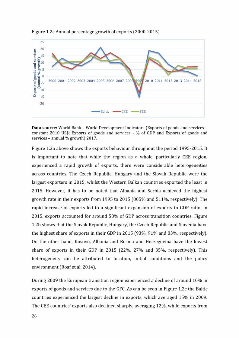
Figure 1.2c Annual percentage growth of exports (2000-2015)
Data source: World Bank – World Development Indicators (Exports of goods and services – constant 2010 US$; Exports of goods and services - % of GDP and Exports of goods and services – annual % growth) 2017.
Figure 1.2a above shows the exports behaviour throughout the period 1995-2015. It
is important to note that while the region as a whole, particularly CEE region,
experienced a rapid growth of exports, there were considerable heterogeneities
across countries. The Czech Republic, Hungary and the Slovak Republic were the
largest exporters in 2015, whilst the Western Balkan countries exported the least in
2015. However, it has to be noted that Albania and Serbia achieved the highest
growth rate in their exports from 1995 to 2015 (805% and 511%, respectively). The
rapid increase of exports led to a significant expansion of exports to GDP ratio. In
2015, exports accounted for around 58% of GDP across transition countries. Figure
1.2b shows that the Slovak Republic, Hungary, the Czech Republic and Slovenia have
the highest share of exports in their GDP in 2015 (93%, 91% and 83%, respectively).
On the other hand, Kosovo, Albania and Bosnia and Herzegovina have the lowest
share of exports in their GDP in 2015 (22%, 27% and 35%, respectively). This
heterogeneity can be attributed to location, initial conditions and the policy
environment (Roaf et al, 2014).
During 2009 the European transition region experienced a decline of around 10% in
exports of goods and services due to the GFC. As can be seen in Figure 1.2c the Baltic
countries experienced the largest decline in exports, which averaged 15% in 2009.
The CEE countries’ exports also declined sharply, averaging 12%, while exports from
-20
-15
-10
-5
0
5
10
15
20
25
2000 2001 2002 2003 2004 2005 2006 2007 2008 2009 2010 2011 2012 2013 2014 2015
Ex
po
rts
of
go
od
s a
nd
se
rvic
es
(an
nu
al
% g
row
th)
Baltic CEE SEE
27
SEE countries dropped by an average of 7%. In terms of individual countries, the
steepest decline in exports in 2009 was experienced in Estonia, Slovak Republic, and
Slovenia (20%, 17% and 16%, respectively), while exports from Kosovo and Albania
continued growing throughout 2009, although at a slower rate compared to previous
years before the GFC (4% and 12% respectively). The variation in export
performance across the region during 2009 can in part be attributed to different
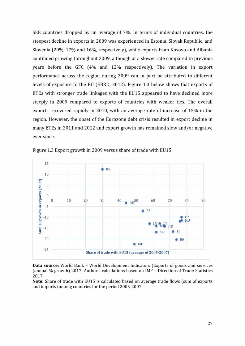
levels of exposure to the EU (EBRD, 2012). Figure 1.3 below shows that exports of
ETEs with stronger trade linkages with the EU15 appeared to have declined more
steeply in 2009 compared to exports of countries with weaker ties. The overall
exports recovered rapidly in 2010, with an average rate of increase of 15% in the
region. However, the onset of the Eurozone debt crisis resulted in export decline in
many ETEs in 2011 and 2012 and export growth has remained slow and/or negative
ever since.
Figure 1.3 Export growth in 2009 versus share of trade with EU15
Data source: World Bank – World Development Indicators (Exports of goods and services (annual % growth) 2017; Author’s calculations based on IMF – Direction of Trade Statistics 2017. Note: Share of trade with EU15 is calculated based on average trade flows (sum of exports and imports) among countries for the period 2005-2007.
BH
BG
HR
CZ
EE
HU
KS
LV LT MK
ME
RS
SK SI
-25
-20
-15
-10
-5
0
5
10
15
0 10 20 30 40 50 60 70 80 90
An
nu
al
gro
wth
in
ex
po
rts
(20
09
)
Share of trade with EU15 (average of 2005-2007)
28
1.2.3 Financial developments
Since the beginning of transition the banking systems have evolved dramatically from
a single institution designed to support the central planning system and responsible
for both monetary policy and commercial banking. During the transition from a
planned to a market-oriented economy, the financial system was transformed from
these single banking institutions into two-tier financial systems. Most countries
started this process by dividing the central and commercial banking activities and by
breaking up the commercial banking activities into multiple smaller units, which
were initially state-owned. However, the banking sector in transition countries faced
many difficulties during this stage, due to the fact that these newly established state-
owned banks inherited portfolios of unknown quality and balance sheets and staff
from the old bureaucratic institutions, which in turn imposed a very heavy
supervisory burden on the central banks which were inexperienced in this task
(Berglof and Bolton, 2002). Initially, most ETEs went through several waves of
restructuring, in an attempt to address these problems in the banking sector. After a
number of unsuccessful attempts, the next step of financial reforms was banks’
privatisation. Within this period, most countries also allowed the entry of new banks.
The ownership structure of the banks has changed dramatically since the beginning
of the transition process. Foreign-owned banks became dominant in Central, Eastern
and South-eastern European countries, by establishing subsidiaries or branches in
this region, mostly stimulated by the high returns in these financial markets due to
their underdeveloped financial systems (Bartlett and Prica, 2012). Foreign bank
presence in transition countries helped to strengthen national banking systems and
improve the low level of financial intermediation (De Haas and Van Lelyveld 2006).
The average degree of financial depth in transition countries, measured by domestic
credit provided by the banking sector to the private sector as a share of GDP,
increased from 25% in 1995 to 49% in 2015 (World Bank, 2017). On the other hand,
the increased role of foreign banks increased the exposure of transition countries to
foreign shocks (Roaf et al., 2014), as the foreign banks’ propensity to experience
positive and negative shocks affects credit possibilities in the same direction
(Piccotti, 2017).

29
The average asset share of foreign banks in total banking sector assets in the
transition region had, by the time the GFC hit the region, reached more than 82%.
Figure 1.4 shows that the degree of foreign bank ownership in 2009 varied from 29%
in Slovenia to 98% in the Czech Republic.
Figure 1.4 Asset share of foreign-owned banks in total banking assets - 2009
Data source: EBRD / Structural Change Indicators 2017 and Claessens and Van Horen, 2015.
Since the early 2000s, an aggressive strategy of expansion of cross-border lending
was pursued by many Western European banks with the ETEs being their main focus
(Roaf et al., 2014). This resulted in a credit boom in the transition region, which
boosted investment and output growth, but also led to large external imbalances
financed by cross-border capital flows (EBRD, 2015). During the GFC and the
subsequent eurozone debt crisis, cross-border bank flows declined sharply in the
region. The average decline of cross-border credit flows reached 13% by the first
quarter of 2009. The countries that experienced the sharpest decline in cross-border
credit flows during 2009 were Slovakia, Romania and the Czech Republic (60%, 21%
and 16%, respectively) (BIS, 2017). Figure 1.5 shows a dramatic decline in cross-
border lending by BIS-reporting banks to the transition region during the years
following the GFC.
0.0 10.0 20.0 30.0 40.0 50.0 60.0 70.0 80.0 90.0 100.0
LithuaniaLatvia
Estonia
SloveniaSlovak Republic
PolandHungary
Czech Republic
SerbiaRomania
MontenegroMacedonia
CroatiaBulgaria
BHAlbania
Foreign bank ownership (in percentage, 2009)
30
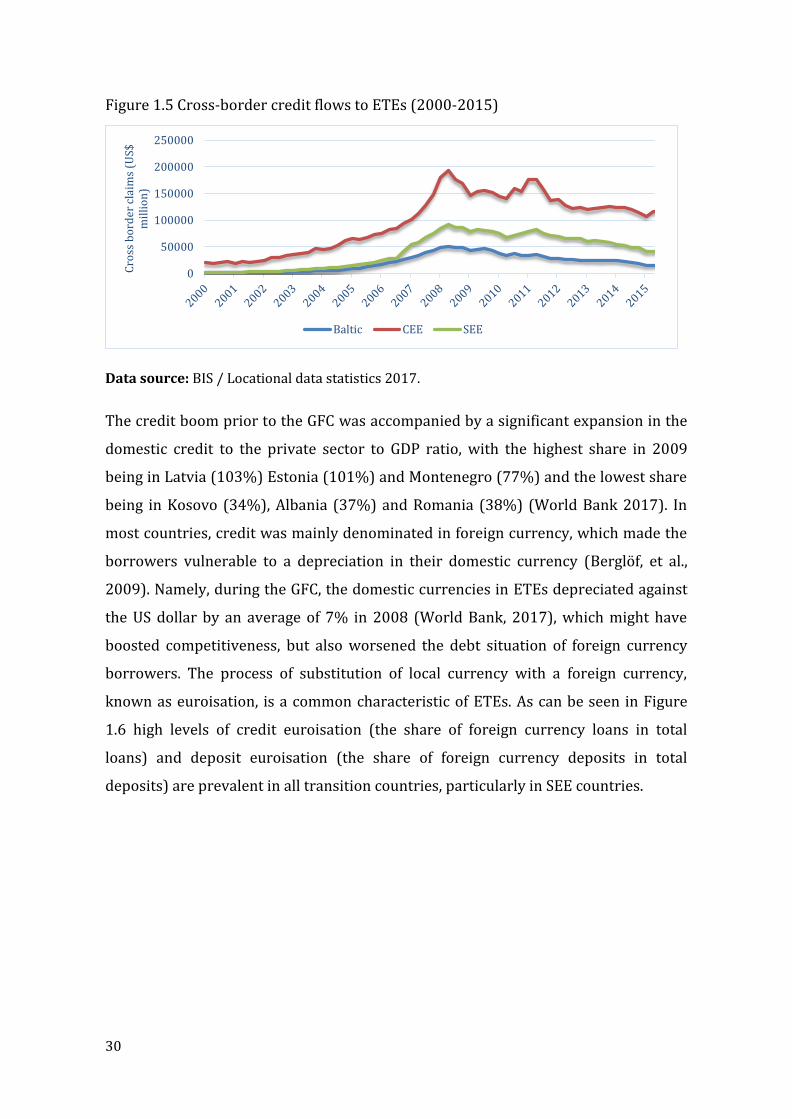
Figure 1.5 Cross-border credit flows to ETEs (2000-2015)
Data source: BIS / Locational data statistics 2017.
The credit boom prior to the GFC was accompanied by a significant expansion in the
domestic credit to the private sector to GDP ratio, with the highest share in 2009
being in Latvia (103%) Estonia (101%) and Montenegro (77%) and the lowest share
being in Kosovo (34%), Albania (37%) and Romania (38%) (World Bank 2017). In
most countries, credit was mainly denominated in foreign currency, which made the
borrowers vulnerable to a depreciation in their domestic currency (Berglöf, et al.,
2009). Namely, during the GFC, the domestic currencies in ETEs depreciated against
the US dollar by an average of 7% in 2008 (World Bank, 2017), which might have
boosted competitiveness, but also worsened the debt situation of foreign currency
borrowers. The process of substitution of local currency with a foreign currency,
known as euroisation, is a common characteristic of ETEs. As can be seen in Figure
1.6 high levels of credit euroisation (the share of foreign currency loans in total
loans) and deposit euroisation (the share of foreign currency deposits in total
deposits) are prevalent in all transition countries, particularly in SEE countries.
0
50000
100000
150000
200000
250000C
ross
bo
rder
cla
ims
(US$
m
illi
on
)
Baltic CEE SEE

31
Figure 1.6 Average degree of credit and deposit euroisation (2004-2014)
Data source: EBRD, central banks (various years).
Figure 1.6 shows that throughout the period 2004-2014, SEE countries have had the
highest degree of euroisation. An exception is Kosovo which had a very low degree of
euroisation, as it adopted Euro as its legal tender, therefore the degree of euroisation
is here measured by share of loans and deposits in foreign currencies other than Euro
(US dollar, Swiss Franc etc.) in total loans and deposits. As for the other countries,
Figure 1.6 shows that credit euroisation varied from 9% in Slovak Republic to 72% in
Serbia. The degree of deposit euroisation also varied from 7% in Slovak Republic to
76% in Serbia.
1.2.4 FDI inflows
The large scale privatisation during the transition process was accompanied by
continuous FDI inflows in ETEs. FDI brought capital, technology and know-how,
contributing to transition countries’ productivity growth and development (Derado,
2013). The largest pre-crisis net FDI inflows during the period 2000-2007 were
achieved by Hungary, Poland, the Czech Republic, Romania and Bulgaria. However,
the GFC considerably reduced international capital flows and almost halved FDI
worldwide, with the most pronounced fall throughout developed countries, including
the EU (by 40-60%). In ETEs, with the exceptions of Albania and Montenegro, FDI
inflows fell sharply in 2009. The average decline of FDI inflows across the ETEs was
57% in 2009. The sharpest falls took place in Slovenia, Hungary, Latvia and Lithuania.
0%10%20%30%40%50%60%70%80%90%
100%
Credit euroisation Deposit euroisation
32
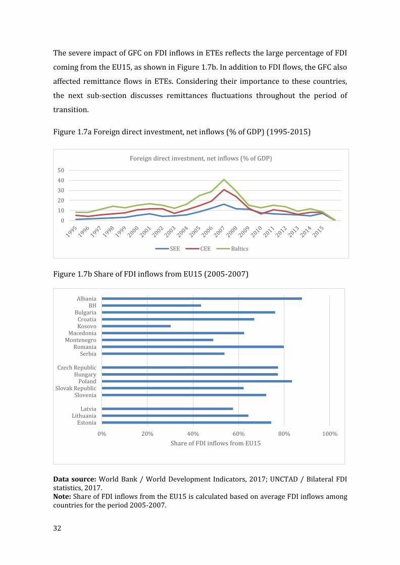
The severe impact of GFC on FDI inflows in ETEs reflects the large percentage of FDI
coming from the EU15, as shown in Figure 1.7b. In addition to FDI flows, the GFC also
affected remittance flows in ETEs. Considering their importance to these countries,
the next sub-section discusses remittances fluctuations throughout the period of
transition.
Figure 1.7a Foreign direct investment, net inflows (% of GDP) (1995-2015)
Figure 1.7b Share of FDI inflows from EU15 (2005-2007)
Data source: World Bank / World Development Indicators, 2017; UNCTAD / Bilateral FDI statistics, 2017. Note: Share of FDI inflows from the EU15 is calculated based on average FDI inflows among countries for the period 2005-2007.
0
10
20
30
40
50
Foreign direct investment, net inflows (% of GDP)
SEE CEE Baltics
0% 20% 40% 60% 80% 100%
EstoniaLithuania
Latvia
SloveniaSlovak Republic
PolandHungary
Czech Republic
SerbiaRomania
MontenegroMacedonia
KosovoCroatia
BulgariaBH
Albania
Share of FDI inflows from EU15

33
1.2.5 Migration and remittances
The transition process initially resulted in massive increases in unemployment rates
in most of the ETEs. Consequently, there was frequently a rapid rise in migration, in
particular to EU countries. High emigration rates also resulted in the high level of
remittance inflows (Roaf et al., 2014). A large percentage of remittances came from
the EU. As can be seen in Figure 1.8 below, the share of remittances coming from
EU15 countries varies between 98% in Albania and Poland to 48% in Bosnia and
Herzegovina.
Figure 1.8 Share of remittance inflows from EU15 (20103)
Data source: World Bank / Bilateral remittance flows (2017) and author’s calculations. Note: Share of remittance inflows from the EU15 is calculated based on bilateral remittance flows among countries during 2010, which is the earliest year the data on bilateral remittance flows are available.
Even though remittances lead to positive economic growth through their impact on
consumption, savings and investment (Catrinescu et al,, 2009), they create channels
of financial contagion throughout periods of economic and financial instability. As a
result, during the GFC and the subsequent Eurozone debt crisis, remittances inflows
dropped substantially in most ETEs. As can be seen in the first graph of Figure 1.9
below, the average amount of remittances received as a share of GDP throughout the
3 2010 is the earliest year bilateral remittance flows are available.
0% 10% 20% 30% 40% 50% 60% 70% 80% 90% 100%
LithuaniaLatvia
Estonia
SloveniaSlovak Republic
PolandHungary
Czech Republic
SerbiaRomania
MontenegroMacedonia
KosovoCroatia
BulgariaBH
Albania
Share of remittance inflows from EU15
34
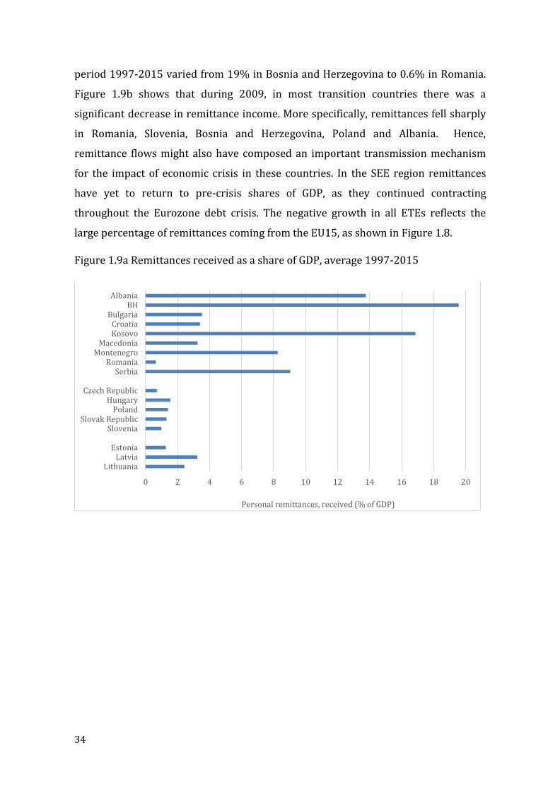
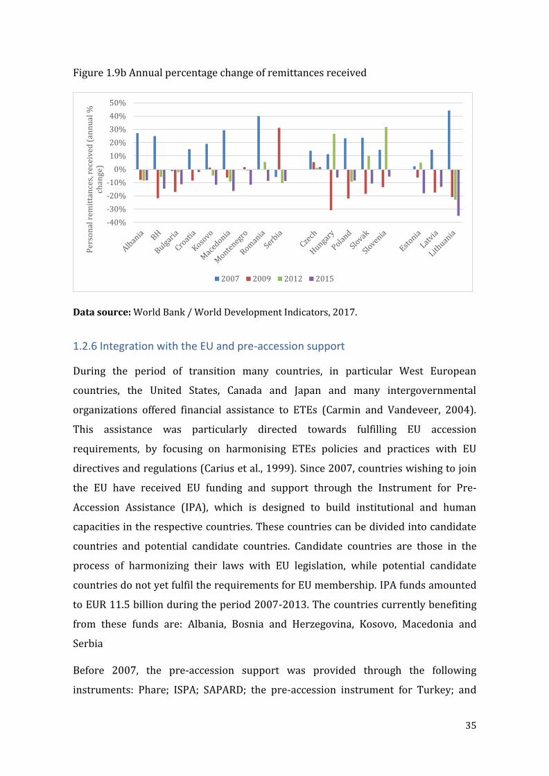
period 1997-2015 varied from 19% in Bosnia and Herzegovina to 0.6% in Romania.
Figure 1.9b shows that during 2009, in most transition countries there was a
significant decrease in remittance income. More specifically, remittances fell sharply
in Romania, Slovenia, Bosnia and Herzegovina, Poland and Albania. Hence,
remittance flows might also have composed an important transmission mechanism
for the impact of economic crisis in these countries. In the SEE region remittances
have yet to return to pre-crisis shares of GDP, as they continued contracting
throughout the Eurozone debt crisis. The negative growth in all ETEs reflects the
large percentage of remittances coming from the EU15, as shown in Figure 1.8.
Figure 1.9a Remittances received as a share of GDP, average 1997-2015
0 2 4 6 8 10 12 14 16 18 20
LithuaniaLatvia
Estonia
SloveniaSlovak Republic
PolandHungary
Czech Republic
SerbiaRomania
MontenegroMacedonia
KosovoCroatia
BulgariaBH
Albania
Personal remittances, received (% of GDP)
35
Figure 1.9b Annual percentage change of remittances received
Data source: World Bank / World Development Indicators, 2017.
1.2.6 Integration with the EU and pre-accession support
During the period of transition many countries, in particular West European
countries, the United States, Canada and Japan and many intergovernmental
organizations offered financial assistance to ETEs (Carmin and Vandeveer, 2004).
This assistance was particularly directed towards fulfilling EU accession
requirements, by focusing on harmonising ETEs policies and practices with EU
directives and regulations (Carius et al., 1999). Since 2007, countries wishing to join
the EU have received EU funding and support through the Instrument for Pre-
Accession Assistance (IPA), which is designed to build institutional and human
capacities in the respective countries. These countries can be divided into candidate
countries and potential candidate countries. Candidate countries are those in the
process of harmonizing their laws with EU legislation, while potential candidate
countries do not yet fulfil the requirements for EU membership. IPA funds amounted
to EUR 11.5 billion during the period 2007-2013. The countries currently benefiting
from these funds are: Albania, Bosnia and Herzegovina, Kosovo, Macedonia and
Serbia
Before 2007, the pre-accession support was provided through the following
instruments: Phare; ISPA; SAPARD; the pre-accession instrument for Turkey; and
-40%
-30%
-20%
-10%
0%
10%
20%
30%
40%
50%
Per
son
al r
emit
tan
ces,
rec
eiv
ed (
ann
ual
%
chan
ge)
2007 2009 2012 2015
36
the financial instrument for the Western Balkans, CARDS. The Phare programme
supported institution-building, associated investment in candidate countries and
economic and social cohesion and cross-border cooperation. The ISPA programme
supported the environmental and transport infrastructure in candidate countries,
whilst the SAPAPRD programme supported agricultural and rural development.
Finally, the CARDS programme was the financial instrument for the Western Balkan
countries and its main objective was to support participation of the Western Balkans
in the Stabilisation and Association Process (SAP), which seeks to promote stability in
the region. Since 2004, 11 ETEs have joined the EU. Hungary, the Czech Republic,
Estonia, Slovenia, the Slovak Republic, Poland, Latvia and Lithuania became EU
members in 2004, while Bulgaria and Romania joined the EU in 2007 and, most
recently, Croatia became an EU member in 2013.
The aim of this section was to present a discussion of the transition process and
economic integration of ETEs throughout this period, in order to provide background
for the investigation of the research questions in this thesis. Despite the well-known
benefits of economic integration, this section showed that it also appears to have
made the countries more vulnerable to the effects of the GFC by creating and/or
strengthening potential channels for contagion through trade, foreign banks, FDI,
remittances and cross-border bank lending. On the other hand, countries that made
more progress with EU integration and institutional reforms may have been better
able to deal with external shocks, since their higher quality institutions may be
expected to contribute to output stability (Balavac and Pugh, 2016). The next section
provides an overview of the origins of the GFC and how it spread, while section 1.4
investigates its impact on the ETEs.
1.3 Causes and nature of the GFC and how it spread
Financial crises have occurred repeatedly throughout modern history, affecting both
developing and developed countries. The literature identifies four major types of
crises: currency crises; sudden stop (or capital account or balance of payments)
crises; debt crises; and banking crises (Claessens and Kose, 2013). In recent decades,
crises have become more frequent. Laeven and Valencia (2013) identify 147 banking
crises, 218 currency crises and 66 debt crises over the period 1970–2011. This rise in
37
frequency has been attributed to an increase in financial market liberalization and
floating exchange rates (Claessens and Kose, 2013). A financial crisis can be
extremely costly. They are associated with larger declines in output, consumption,
investment, employment, exports and imports compared to recessions without
financial crises (Cleassens and Kose, 2013). In addition, a large number of studies
have shown that recoveries from financial crises are slower than from typical
recessions (Reinhart and Rogoff, 2009; Claessens et al., 2012; Papell and Prodan,
2012). Despite its unusual severity, the GFC had many common features with past
crises, the most important being a preceding asset price bubble and credit boom
(Allen and Gale, 2000; Brunnermeier, 2008; Reinhart and Rogoff, 2008a, 2008b, and
2009; Schularick and Taylor 2009). There is general agreement that financial
innovation in the form of asset securitization, global imbalances, expansionary
monetary policy, government policies to increase homeownership and weak
regulatory oversight played a significant role in causing the pre-crisis boom (Taylor,
2009; Keys et al., 2010; Laeven and Valencia, 2013). Many economists consider the
GFC as the worst meltdown since the Great Depression. It resulted in the collapse of
large financial institutions, bailouts of banks by governments and declines in stock
markets all over the world. The crisis had a major impact on business failures and
consumer wealth and economic activity declined, which led to a global recession and
the European sovereign-debt crisis.
The origins of the GFC are by now well-known; it can be traced back to a credit and
housing boom in the United States. The housing boom started in the late 1990s and
reached its peak in mid 2000s (Crotty, 2008). Prices increased at a 7 to 8 percent
annual rate in 1998 and 1999, and at 9 to 11 percent from 2000 to 2003, while the
most rapid price increases were in 2004 and 2005, with house price appreciation
ranging from 15 to 17 percent (Bernanke, 2010). The large inflows of foreign funds
following the Russian debt crisis and Asian financial crisis of 1997–1998, increased
the availability of credit in the U.S., which led to a housing construction boom and
debt-financed consumer spending (Brunnermeier, 2008). Following the housing and
credit boom, a number of financial innovations emerged, such as mortgage-backed
securities and collateralized debt obligations (Simkovic, 2013). These financial
innovations made it easier for investors and institutions around the world to invest

38
in the U.S. A decline in U.S. housing prices caused mortgage-backed financial
securities to experience significant losses, which, by 2008, were estimated to be
approximately 500 billion dollars (Greenlaw et al., 2008). The associated increase in
mortgage delinquencies triggered a liquidity crisis and bank runs. However, this did
not initially occur in the traditional-banking system. Instead, as pointed out by
Gorton and Metrick (2012), it took place in the “securitized-banking” system. As
opposed to traditional banking, which is the business of making and holding loans
with insured demand deposits as the main source of funds, securitized banking is the
business of packaging and reselling loans, with repo agreements as the main source
of funds (Gorton and Metrick, 2012). As such, a traditional-banking run is triggered
by the withdrawal of deposits, while a securitized-banking run is triggered by the
withdrawal of repurchase (repo) agreements. An important element of the repo
agreement is the requirement to post collateral with a higher value than the loan:
Gorton and Metrick (2012) refer to this as a “haircut”. The authors define the
“haircut” as the percentage by which an asset’s market value is reduced for the
purpose of calculating the amount of overcollateralization of the repo agreement.
Since the value of mortgage backed securities fell continuously, the haircuts’ levels
grew up to 50 percent. Hence, the borrowing that could be supported by the same
amount of capital decreased significantly. This led to deleveraging and forced many
financial institutions to sell off assets, which had an adverse effect since the lower
asset values decreased collateral’s value. Uncertainty kept rising, which caused
haircuts levels to continue rising and financial institutions to sell more assets.
One particular feature of the GFC was the speed and synchronicity with which it
spread around the world (Chudik and Fratzscher, 2011). Even though it originated in
the U.S., it spread not only to countries that shared similar vulnerabilities, but also to
most emerging and advanced countries. The international spillovers were
transmitted through a number of phases. The first phase was through direct
exposures and affected a few financial markets which had a heavy exposure to the
U.S. market. As a result of direct exposures to subprime assets, the crisis spread
quickly to European banks, e.g. in France (BNP Paribas, 2007) and in Germany (IKB,
2007) (Claessens et al., 2010). These events as well as housing market stress caused
liquidity and funding problems in some markets. In the UK, Northern Rock, which
39
was disproportionately funded through short-term borrowing in the capital markets
suffered a bank-run in 2007.
The second phase of the transmission of the crisis was through asset markets.
Namely, liquidity shortages, frozen credit markets, foreign exchange fluctuations and
stock price declines accelerated the transmission of the international spillovers.
Policy responses aiming to address liquidity problems were not effective in the short
term. In addition, countries used different approaches to address the liquidity
problems. These ad-hoc interventions worsened the level of confidence among
creditors and investors and were unable to resolve the underlying problems that
caused an almost complete breakdown in market trust and confidence (Claessens et
al., 2010). Following the collapse of Lehman Brothers, the third phase of transmission
of crisis started mainly due to insolvency problems. By October 2008, many of the
major global financial institutions had massive losses and had written off a large
number of illiquid assets. Market confidence continued to deteriorate which resulted
in further failures.
As the crisis developed into a global recession, in many countries economic stimulus
was used as a main tool to attempt to stabilise output. Rescue plans and bailouts
were carried out for banking systems and failing businesses in the U.S, China and EU.
Most policy responses to the economic and financial crisis were taken by individual
nations. Nevertheless, there was some coordination at the European level as well as
global level through the G-20 countries. The first summit dedicated to the crisis took
place in November 2008 and a second summit in April 2009. The main decisions
taken in these summits were to coordinate actions and to stimulate demand and
employment. In addition, G-20 countries committed to maintain the supply of credit
by providing more liquidity. Central banks committed to maintain low interest rate
policies for as long as it was necessary. Moreover, it was also agreed to help the
emerging economies through the International Monetary Fund (IMF).
The crisis in Europe transformed from a banking crisis to a sovereign debt crisis. The
European sovereign debt crisis started in 2008, with the collapse of Iceland's banking
system, and spread primarily to Greece, Ireland and Portugal during 2009 (Arghyrou
and Kontonikas, 2012). The debt crisis led to a crisis of confidence in European
40
businesses and economies. Several countries received bailout packages from the
European Commission, European Central Bank, and IMF. By 2012, many European
countries had improved their budget deficits relative to their GDP and the eurozone’s
recovery started to take hold in 2013.
1.4 The impact of the GFC on ETEs
Even though the GFC commenced in the United States, as a result of the current global
macroeconomic imbalances and financial globalization, the crisis could not be
contained within the United States financial system and quickly spread to the other
major financial centres. The GFC was associated with the worst recession since World
War II. The world GDP per capita declined by 2% in 2009. As discussed in sub-section
1.2.1, the ETEs were severely affected by the GFC with an average GDP decline of
around 7 percent in 2009, a more severe impact than in any other region in the
world, including the EU15, where the output decline averaged 5% in 2009. However,
as identified in sub-section 1.2.1, the impact of the crisis on economic activity varied
extensively across countries in transition, with the Baltic States being most severely
affected where economic activity in 2009 declined, on average, by around 14%, while
the least affected were the Balkan countries with an average GDP decline of only
around 4% in 2009.
ETEs, like other emerging markets, weathered the GFC relatively well up to mid-
2008. The region was first hit by the crisis in the third and fourth quarters of
2008. Until then, most of these countries continued experiencing output and credit
growth, large capital inflows and stable financial markets, despite the fact that the
financial crisis had already hit the advanced economies over a year previously
(EBRD, 2009). Based on the experience of previous emerging market crises, a
dramatic decrease and subsequent reversal in cross-border lending flows was
expected. In particular, ETEs seemed particularly at risk since they generally
financed expansion with foreign bank loans, which resulted in the accumulation of
large external and internal imbalances in many countries. Although a shock of such
a massive proportions at the international financial system‘s centre was expected
to rapidly spread to the transition countries, that did not occur (Berglöf et al., 2009).
With a few exceptions, emerging Europe was left unaffected by the crisis during its
41
first four quarters, since capital inflows held up and credit and output growth
continued. The exceptions include the three Baltic States, where the credit boom
started to reverse even before the beginning of the GFC. However, after the collapse
of Lehman Brothers and Washington Mutual, the crisis finally hit emerging Europe.
By the end of 2008 capital inflows to the ETEs and global trade declined sharply.
More specifically, exports of goods and services dropped by around 10% in 2009. As
shown in Figure 1.2c in sub-section 1.2.2, the Baltic countries experienced the largest
decline in exports, which averaged 15% in 2009. The CEE countries’ exports also
declined sharply, averaging 12% in 2009, while exports from SEE countries dropped
by an average of 7% during 2009. As for individual countries, the steepest decline in
exports in 2009 was experienced in Estonia, Slovak Republic, and Slovenia (20%,
17% and 16%, respectively), while exports from Kosovo and Albania continued
growing throughout 2009, although at a slower rate. The variation of the impact of
GFC on exports in these countries can in part be attributed to different levels of
exposure to the EU (EBRD, 2012). Figure 1.3 in sub-section 1.2.2 showed that exports
of ETEs with stronger trade linkages with the EU15 appear to have declined more
steeply in 2009 compared to exports of countries with weaker ties. Cross-border
bank flows also declined sharply in the region, averaging 13% by the first quarter of
2009. As shown in sub-section 1.2.3, the countries that experienced the sharpest
decline in cross-border credit flows during 2009 were Slovakia, Romania and the
Czech Republic (60%, 21% and 16%, respectively) (BIS, 2017). The average decline
of FDI inflows across the ETEs was 57% in 2009. The sharpest falls took place in
Slovenia, Hungary, Latvia and Lithuania. The GFC also affected the remittance inflows
in ETEs. More specifically, remittances fell sharply in Albania, Bosnia and
Herzegovina, Poland, Romania and Slovenia.
Most of the financial indicators started to point up in 2010, corresponding to the
general recovery in international financial markets. Almost all countries in the
region saw a return to growth in 2010 and early 2011. However, the nature of the
crisis changed fundamentally in 2011-2012. The banking crisis was transformed into
a sovereign debt crisis in the Eurozone. The European banks weakened, which led to
a decline in inflows of funds to emerging Europe. The average decline of the cross-
border bank flows in the region was 7% in 2012 As shown in section 1.2.3, the

42
countries that experienced the sharpest decline in cross-border credit flows during
2012 were Hungary and Slovenia (30% and 29%, respectively) (BIS, 2017).
Nevertheless, the impact of this crisis was not as severe as from the 2008 crisis,
considering that in most transition countries the governments undertook important
adjustment measures. In addition, the Vienna Initiative helped to ensure that an
immediate large-scale withdrawal of foreign banks from the region did not occur;
thus it stabilised lending temporarily by the 17 banks that signed commitment letters
(EBRD, 2015). Even so, transition countries were still vulnerable due to their
dependence on the eurozone and their high levels of non-performing loans and
foreign-currency denominated debt (EBRD, 2011). Consequently, since 2013, growth
has remained relatively weak across many transition countries highly integrated with
the eurozone due to decreases in capital flows and export demand.
Given the severity of the GFC and its impact on ETEs, it is important for policy makers
in these countries to understand the international channels of transmission of the
crisis in order to reduce their vulnerability to future negative shocks.
1.5 Key research questions and structure of the thesis
One of the key outcomes of the transition process in the former communist countries,
as shown in section 1.2, has been deeper international integration through trade and
financial flows. The rapid increase in exports led to a significant expansion of the
exports to GDP ratio, which made these countries vulnerable to a decrease in export
demand. In addition, a large proportion of exports was directed towards the EU,
exposing these countries to shocks in the EU. Moreover, evidence suggests that
countries with stronger trade linkages have more synchronized business cycles
(Juvenal and Monteiro, 2017). In addition, cross-border bank acquisitions composed
an important component of financial integration. The average asset share of foreign
banks in transition region had, by 2009, reached more than 82% (Figure 1.4). Cross-
border lending and foreign bank ownership resulted in a pre-GFC credit boom in the
transition region, which boosted investment and output growth, but also led to large
external imbalances financed by cross-border capital flows. In most of these
countries, debt was mainly denominated in foreign currency, as shown in Figure 1.6,
which made the borrowers vulnerable to a depreciation of the exchange rate.

43
Furthermore, even though remittances are an important source of capital flows in
many transition countries, particularly SEE countries, as shown in sub-section 1.2.5,
they made the countries more vulnerable to external shocks by creating an additional
potential channel for contagion. These possibilities, to our knowledge, have not been
addressed thoroughly in empirical studies related to transmission of the GFC to ETEs.
To sum up, by investigating the transmission of the GFC to ETEs, whilst taking into
account the degree of euroisation, integration with the EU, exports, remittance flows,
bank ownership, FDI and foreign credit flows, this research intends to explore the
extent to which they matter, and consequently make an original contribution to
knowledge. Thus, this thesis will address these three key research questions:
1) What are the relevant models and empirical evidence on the international
transmission of financial crises? What are the gaps in knowledge?
2) Which were the most significant channels of international transmission of shocks
to ETEs?
3) Did the degree of euroisation, integration with the EU, remittance inflows, bank
ownership, trade and foreign credit flows significantly modify the propagation of the
GFC to ETEs?
The first research question is addressed through a review of the literature on
financial contagion presented in Chapters 2 and 3. Chapter 2 identifies the theoretical
framework behind the channels of transmission of the GFC and the influences of the
degree of euroisation, foreign bank ownership, foreign capital flows and integration
with the EU in transmission of the GFC to ETEs. It starts with an overview of the
theory of financial contagion, which is followed by a review of the theory on the
causes of increased euroisation and its main costs and, lastly, the theory of European
integration. Chapter 3 provides a critical review of the empirical studies that have
investigated the international transmission of the GFC and the role of euroisation,
bank ownership, foreign credit flows and integration with the EU in this process. The
aim of both these chapters is to identify the gaps in the literature, which are then
addressed empirically in Chapters 4 and 5.
The analysis presented in Chapters 4 and 5 answer questions 2 and 3 using,
respectively, macro and micro level data and different estimations techniques.
44
Chapter 4 investigates how GDP and financial shocks in European advanced countries
were transmitted to ETEs, using the recently-developed GVAR (global vector auto-
regression) approach. Two samples were employed over the period 1999Q1-2014Q4
and 2003Q1-2014Q4. The first sample encompasses 30 countries (15 ETEs and 15
advanced EU countries) and the second sample encompasses 32 countries (17 ETEs
and 15 advanced EU countries). Two types of variables are used to capture the main
channels of international financial contagion: trade and financial.
Chapter 5 investigates the transmission of the GFC of 2008/2009 by employing firm-
level data. This chapter covers six transition countries and examines whether the
initial conditions (from 2007) had an impact on the firms' sales in 2009. The measure
of sales growth from 2008 to 2009 is used to proxy the impact of the GFC on firms.
The intention of this study is to distinguish between two main channels of
transmission as suggested by theory, namely the trade and financial channels, thus a
wide range of variables is used to capture these channels.
Finally, Chapter 6 presents the key findings of the thesis, establishes their
contribution to knowledge, examines their policy implications, identifies the main
limitations of the research and provides recommendations for future research.
45
CHAPTER 2
TRANSMISSION OF GLOBAL FINANCIAL CRISES: A REVIEW OF THE THEORETICAL
LITERATURE
Contents
2.1 Introduction ............................................................................................................................................... 46
2.2 International transmission of the GFC ............................................................................................ 48
2.2.1 Fundamental causes ............................................................................................................................ 49
2.2.2 Investors’ behaviour ........................................................................................................................... 53
2.2.3 Transmission of shocks from the financial sector to the real economy ........................ 55
2.3 Euroisation ................................................................................................................................................. 58
2.3.1 Benefits and costs/risks associated with euroisation ........................................................... 60
2.4 Integration with the EU ......................................................................................................................... 63
2.4.1 Benefits associated with European integration ....................................................................... 64
2.4.2 Integration with EU ............................................................................................................................. 65
2.5 Conclusion ................................................................................................................................................... 67
46
2.1 Introduction
Having looked at the influences of exports, bank ownership, foreign credit flows, FDI
inflows, remittances, the degree of euroisation and extent of progress towards EU
integration in the transmission of the GFC to ETEs in Chapter 1, this thesis proceeds
with a critical review of the theoretical (Chapter 2) and the empirical literature on
the international transmission of crises (Chapter 3). The reviews presented in these
chapters will provide the basis for developing the models that will be used to explore
the international transmission of GFC to ETEs in the empirical chapters.
The increase in the frequency of crises during recent decades has generated a
growing strand of theoretical and empirical literature on their origins and channels
of transmission. Considering the severe impact of the GFC on transition countries
(see section 1.4), a number of studies have been particularly focused on the
transmission of the crisis from developed to transition countries. Factors that have
been highlighted as playing an important role in explaining why certain countries
were hit by the crisis harder than others include: fast pre-crisis credit growth; large
current account deficits; high trade openness; high international openness of the
banking sector; a higher level of GDP per capita (Berglöf et al., 2009; Blanchard et al,
2010; Lane and Milesi-Ferretti, 2011; Rose and Spiegel, 2009a, 2009b, 2011;
Berkmen et al., 2012; Popov and Udell, 2012; Feldkircher, 2014; Park et al., 2014; De
Haas et al., 2015; Ongena et al., 2015; Ahmed et al., 2017). One potentially important
factor that previous studies neglected, although it is a common characteristic of ETEs,
is the extent to which a country has assets and liabilities denominated in foreign
currencies, namely the degree of euroisation. Consequently, when investigating the
transmission of the GFC to ETEs, it is important to control for the degree of
euroisation. Additionally, the degree of integration with the EU and quality of
institutions may have given rise to different exposure to the transmission
mechanisms and different transmission channels. As highlighted in Chapter 1, these
additional possibilities, to the best of our knowledge, have not been addressed
thoroughly in previous empirical studies related to the transmission of GFC to ETEs.
Accordingly, three main strands of literature are relevant to this research. First, there
is research on financial contagion and transmission channels, which distinguishes
47
between fundamental causes (common shocks, trade linkages and financial linkages)
and investors’ behaviour (liquidity problems, asymmetric information, incentive
problems etc.) (Masson, 1998; Dornbusch et al., 2000; Forbes and Rigobon, 2001).
While these causes shape the transmission of the shock from the advanced
economies, the magnitude to which it gets intensified depends, to a large extent, on
institutional responses and existing macroeconomic vulnerabilities (Berkmen et al.,
2012).
Consequently, the second strand of literature that is relevant to this research is
related to the extent to which a country has assets and liabilities denominated in
foreign currencies, namely the degree of euroisation. The main costs/risks associated
with euroisation are: inability/ineffectiveness to act as a lender of last resort, adverse
currency mismatches and reduction in monetary policy autonomy/effectiveness all of
which can increase the vulnerability of the banking system, increase interest spreads
and reduce the credit supply (Honohan and Shi, 2002; Winkler, et al., 2004; Click,
2007; Honohan, 2007; Chitu, 2013). These three main costs associated with
euroisation might become more evident during periods of severe financial crisis.
Hence, the recent global financial crisis can be considered as a unique opportunity to
investigate the influence of degree of euroisation on the severity of the impact of the
GFC in ETEs.
The third strand of the literature relevant to this research relates to integration with
the EU, which might have provided different exposures to the transmission
mechanisms and different transmission channels. Countries that made more progress
with institutional reforms may have been better able to deal with external shocks,
given their higher quality institutions and/or more effective governments. On the
other hand, countries that made the most progress in integrating with the EU may be
more vulnerable to the crisis, as they were more open to the transmission effects
through financial flows and falling export demand (Bartlett and Prica, 2012).
This chapter identifies the theoretical framework behind the channels of
transmission of the GFC and the influences of the degree of euroisation, trade, foreign
bank ownership, foreign capital flows and integration with the EU in transmission of
the financial crisis to ETEs. It starts with an overview of the theory on international
48
channels of transmission of shocks, which is followed by the theory on the causes of
increased euroisation and its main costs and, lastly, the theory of European
integration.
The chapter is organized as follows. Section 2.2 reviews the theoretical framework on
channels of transmission of the global financial crises. The theory behind euroisation
and its main costs is summarized in section 2.3. Section 2.4 provides some theoretical
background on European integration. The last section of this chapter provides
conclusions and examines their implications for the design and implementation of
this research programme.
2.2 International transmission of the GFC
A rich literature covering both theoretical and empirical research on crises and
transmission channels has emerged in recent years. There are different views on
defining “financial contagion” and modelling the transmission of shocks. According to
Claessens and Forbes (2004), a contagion is defined as the transmission of a crisis
between two countries that are located in different regions and have no direct trade
or financial ties. However, the authors point out that there seems to be some
disagreement on whether this scenario should be defined as contagion, as some
economists prefer to use the term shift contagion to describe this kind of situation.
Moreover, there is also disagreement on whether “financial contagion” is appropriate
to describe a situation where a crisis spreads between two similar and strongly
linked countries. As an example, if there are two countries in the same geographical
location, linked through trade and financial channels and very similar regarding their
market structure, then they tend to be highly inter-connected all the time, during
stable as well as crisis periods (Claessens and Forbes, 2004). Nevertheless, there is a
general agreement that financial contagion can be defined as co-movement in asset
prices or financial flows after a shock to a country or group of countries.
Orthodox theory on the transmission of shocks distinguishes between two groups of
theories that explain contagion: fundamental causes (common shocks, trade and
financial linkages) and investors’ behaviour (liquidity problems, asymmetric
information, incentive problems etc.) (Masson 1998; Dornbusch et al., 2000; Forbes
and Rigobon, 2001; Karolyi, 2003; Claessens and Forbes, 2004). Given the increasing
49
international integration of ETEs through trade and capital flows discussed in section
1.2, sub-section 2.2.1 focuses on explaining the international transmission of shocks
through fundamental causes, in particular trade and financial channels, with a
particular focus on the GFC. Further, investors’ behaviour as a mechanism for the
international transmission of shocks is elaborated in sub-section 2.2.2. However,
given the relatively low level of financial market development in most ETEs,
investors’ behaviour factors are likely to be less important in explaining contagion in
these countries. Nevertheless, it has to be pointed out that there might be some
overlap between these two categories of theories that explain contagion. Namely, if
investors’ behaviour is not completely irrational and if it is partially based on some
macroeconomic fundamentals, then this behaviour might also fit under the theory
that explains contagion based on fundamental causes. Section 2.2.3 provides an
overview of the theory of transmission of shocks from the financial to the real
economy.
2.2.1 Fundamental causes
The first group of theories that explain contagion, fundamental causes, refer to
transmission of shocks due to the usual interdependencies that exists across markets
and economies. Typically, fundamental causes are divided into three categories:
common or global shocks; financial channel; and the trade channel. The first of these
mechanisms of transmission of shocks is the common or global shock, such as a
major change in the relative price of oil, which triggers crises in both developed and
emerging economies (Dornbusch et al, 2000). Common shocks can lead to co-
movements in asset prices or capital flows.
Secondly, trade linkages are considered one of the most important fundamental
causes for the international transmission of crises. This group includes linkages
through direct trade and competitive devaluations (Eichengreen et al. 1996; Glick
and Rose, 1999; Corsetti et al., 2000; Dornbusch et al., 2000; and Forbes, 2002).
During the last two decades, there has been a growing consensus that countries with
stronger trade linkages have more synchronized business cycles (Juvenal and
Monteiro, 2017). Chui et al. (2004) identify a number of potential trade channels. A
crisis in one country by causing a reduction in income may reduce the demand for
50
imports, thus affecting exports, the trade balance, and related economic
fundamentals in other economies through direct trade links. A competitiveness effect
may arise if the initial crisis in one economy causes its currency to be devalued (Chui
et al., 2004). Devaluation temporarily improves the country’s competitiveness, while
reducing the competitiveness (both bilaterally and in common export markets) of
tradables produced by other economies, thus worsening their economic
performance. This can lead to pressuring other countries’ currencies to depreciate.
Therefore, a currency crisis that hits one country may be expected to spread over
time to other countries. Gerlach and Smets (1995) show how the depreciation of one
currency affects the competitiveness of countries with pegged currencies, which
might trigger a crisis and force depreciation of their currency. Moreover, they show
that the contagion impact is higher, the higher the degree of trade integration
between these countries and the lower the degree of integration of these countries
with another country. Similarly, Glick and Rose (1999) concluded that currency
crises spread mainly because of the trade linkages. Specifically, countries may be
attacked because of the actions of their neighbours, who mainly due to
geographic proximity tend to be their major trading partners. A crisis is spread from
one country to another if these two countries share various economic features, such
as a real exchange rate over-valuation, weaknesses in their banking systems and low
international reserves (Sachs et al., 1996). Given that bilateral trade flows are, in
most of the cases, negatively affected by distance, currency crises are likely to be
regional. As shown in section 1.2, during 2009 the European transition region
experienced a decline of around 10% in exports of goods and services that was
attributed to the GFC. It was argued in section 1.2 that the variation in export
performance during the GFC can in part be attributed to different levels of exposure
to the Eurozone: exports of ETEs with stronger trade linkages with the EU15 declined
more steeply in 2009 compared to exports of countries with weaker ties.
The third mechanism for the transmission of shocks through fundamental causes is
the financial channel. Transmission of shocks through this channel has gained
increasing attention in recent years. In a highly integrated region, a crisis that starts
in one country will affect other countries by reducing capital inflows (Claessens and
Forbes, 2004). Therefore, as argued in section 1.2, increased financial integration
51
made the ETEs more vulnerable to international crises by creating and/or
strengthening potential financial channels for contagion through foreign banks,
cross-border bank flows, FDI and remittances. In particular, the crisis in one
country, by reducing the capital supply of that country, will decrease the lending and
investing abilities of that country to another country. Therefore, these reductions in
capital inflows will increase the borrowing costs and put pressure on currency
depreciation for countries that are highly dependent on external funding. According
to Chui et al. (2004), the impact of shocks on the costs of domestic or cross-border
sources of finance will depend on an emerging economy’s sensitivity to each.
Theoretical models of banking crises suggest that an important role in the
propagation of a financial crisis is played by large and highly leveraged financial
institutions, such as international banks (Tirole, 2011; Greenwood et al., 2015).
During the GFC, an important transmission mechanism has been the global
restriction of credit, which has especially affected transition economies with a high
penetration of foreign banks (Lane and Milesi-Ferretti, 2011). As argued in section
1.2, the presence of foreign banks in transition countries helped to strengthen their
national banking systems and improve their low level of financial intermediation. On
the other hand, the growing role of foreign banks increased the exposure of
transition countries to foreign shocks (Roaf et al., 2014).
Árvai et al. (2009) highlight the importance of cross-border finance in transmitting
crises through financial linkages. They illustrate some of the channels of transmission
of contagion through financial linkages. One possible channel is the existence of a
common lender which lends to a number of countries. If one of the countries that
borrows from the banking system of this common lender faces a shock, given that the
common lender’s banking system is largely exposed to this country, it will affect the
liquidity or solvency of the common lender. Therefore, other countries borrowing
from the lending country will also be affected, even though they do not have direct
linkages with the country that was hit by the shock. Similarly, if a parent bank
withdraws its deposit or lending or charges higher interest rates to its subsidiary,
and if the subsidiary is highly dependent on the funding of the parent bank, it will
face liquidity and solvency problems. As a consequence, in heavily concentrated
banking systems with substantial market linkages, liquidity problems can rapidly
52
spread to other domestic or foreign-owned banks and, as a result, their parent banks
and the banking systems in which the parent banks operate. This in turn will affect
the banking sector of the entire region. Árvai et al. (2009), point out that the size of
contagion through financial channel depends on: the size of the exposures of home
banks (common lender) to the host country with a problem and the dependence of
the host country on funds from the home country. “Bank balance-sheet driven
contagion” can also occur through the international banking system when banks
decrease loans in one country as a response to losses in another country. This
indirect financial contagion mechanism was first suggested by Calvo (1998) to
introduce a causal link between the 1998 Russian crisis and the following crisis in
Brazil. Bank balance sheet shocks start from deteriorations in the balance sheets of a
country's foreign bank creditors. Such shocks can be direct or indirect. Direct bank
balance sheet contagion occurs when banks from a creditor country with a
deteriorating risk profile decide to withdraw international funding to comply with
internal rules or prudential regulations such as capital adequacy requirements. On
the other hand, indirect bank balance sheet contagion occurs when banks decrease
loans to a debtor country in response to deteriorations in their loan portfolio in
another country (Ahrend and Goujard, 2013).
Even though, as argued above, trade and financial linkages serve as international
channels of transmission of shocks, the extent to which the shocks get amplified also
depend on the responses of policy-makers and existing domestic vulnerabilities.
During the years following the GFC there has been a growing consensus on the
importance of macroeconomic fundamentals in coping with external shocks. Frankel
and Saravelos (2012) analyse the effects of the GFC by selecting variables from an
extensive review of the previous literature on early warning indicators. They find
that real exchange rate overvaluation and levels of international reserves can explain
the variation of the impact of GFC across countries. Fratzscher (2012) demonstrates
that the heterogeneity of the impact of the GFC across countries can be explained by
differences in country risk, quality of domestic institutions and the strength of
domestic macroeconomic fundamentals. More specifically, the author shows that
countries with high-quality institutions and strong macroeconomic fundamentals
were better able to protect their financial markets from adverse shocks during the
GFC. In addition, the author highlights that trade and financial linkages played a
53
minor role in explaining cross-country heterogeneities in the transmission of the
GFC. Ahmed et al., (2017) show that the financial markets in emerging economies
with better macroeconomic fundamentals (current account balance; foreign
exchange reserves; short-term external debt; the gross government debt; inflation
etc.) were less severely affected by the GFC and the subsequent Eurozone debt crisis
in 2011. They also find that financial conditions worsened more in countries that had
previously experienced larger capital inflows and greater exchange rate appreciation.
In contrast, Eichengreen and Gupta (2015) and Aizenman et al. (2016) do not find
evidence that strong macroeconomic fundamentals (a lower public debt, a lower
budget deficit, a higher level of international reserves and higher economic growth)
protected emerging economies from the effects of the global shocks.
2.2.2 Investors’ behaviour
The second group of theories that explain contagion are based on investors’
behaviour. If fundamentals and common shocks are not able to fully explain the
relationship between countries, then the spillover effects might be explained by
rational or irrational herding behaviour (Dornbusch et al., 2000; Forbes and Rigobon,
2001; Karolyi, 2003; Economou et al., 2011; Galariotis et al., 2016). Claessens and
Forbes (2004) define five main categories of theories explaining contagion based on
investors’ behaviour: liquidity problems; incentive problems; informational
asymmetries; market coordination problems and investor reassessment. One
common feature of all of these theories is that despite the fact that investors’
behaviour is often rational ex-ante, it might still lead to excessive co-movements in
market prices in the sense that market prices are not explained by real
fundamentals (Claessens and Forbes, 2004). However, given the relatively low level
of financial market development in ETEs, investors’ behaviour factors are likely to be
less important in explaining contagion.
The first category focuses on liquidity problems (Goldfajn and Valdés, 1 997;
Dornbusch et al., 2000; Kaminsky et al., 2001; Claessens and Forbes, 2004).
Investors who due to a crisis are faced with liquidity problems tend to sell their
securities in other markets in order to raise cash. This kind of behaviour causes a
decrease in asset prices outside of the crisis region. As a result, the initial

54
disturbances will spread and affect different markets and borrowers.
The second category of theories that explain the impact of investors’ behaviour on
contagion focuses on incentives and risk aversion (Claessens and Forbes, 2004).
Broner et al. (2006) present a model that analyses the effect of changes in investors’
risk aversion on portfolio decisions and stock prices. Their findings suggest that an
investor who cares about his performance relative to that of other investors, would
shift his portfolio towards the average portfolio as a response to an increase in risk
aversion. More specifically, the investor would shift his assets from countries to
which he is overexposed towards those to which he is underexposed. Considering
that crises mostly affect those investors who are most exposed to the crisis country
and those investors, in turn, adjust their portfolios away from other countries in
which they are overexposed, crises are transmitted through overexposed investors.
This type of behaviour could result in widespread price declines and currency
depreciations.
A third type of theories explaining contagion caused by investors’ behaviour is based
on asymmetric and imperfect information. Due to the lack of complete information
about the conditions in each country, a financial crisis in one country can make
investors think that other countries may face the crisis too. Therefore, they start
selling their assets in those countries which they believe will face similar problems.
This type of behaviour can also be a result of actions of other investors (Calvo and
Mendoza, 2000). Due to the lack of information, investors may find it less costly
and easier to follow the example of other informed and uninformed investors.
A fourth group of theories explaining contagion based on investors’ behaviour
focuses on market coordination problems (Masson, 1998). According to this theory,
investors can change their behaviour as a result of self-fulfilling expectations that
can cause multiple equilibria (Dornubusch et al., 2000; Claessens and Forbes, 2004).
In particular, investors could unexpectedly withdraw from a country based on their
beliefs about the future and their fears that unless they act quickly, it will be too late to
utilise the limited foreign exchange reserves (Dornbusch et al, 2000). These types of
market coordination problems are believed to be one of the most important channels
of contagion.

55
As per Claessens and Forbes (2004), the last category of theories that explain
contagion based on investors’ behaviour focuses on the reassessment and beliefs of
investors regarding the stability of rules governing international finance. A country’s
and more generally investors’ concerns regarding the aggressive policies that other
countries might follow during the crisis period with respect to foreign creditors, as
well as their concern that financial institutions will not help countries in difficulties
due to limited funds, would cause investors to sell their assets outside the crisis
country, thus causing contagion.
Having identified the theory behind the international channels of transmission of
shocks, the next sub-section summarizes the theory on transmission of shocks from
the financial sector to the real economy.
2.2.3 Transmission of shocks from the financial sector to the real economy
The recent global crisis prompted many researchers to revise the analysis of the
transmission of shocks from the financial to the real sphere of the economy, both in
general and with regards to particular economies (Blot et al., 2009; Boorman, 2009;
Cardarelli et al., 2011). The literature on the transmission of shocks identifies
channels between real and financial sectors that might work in both directions.
Namely, financial conditions are influenced by the conditions in the real economy,
specifically households’ and firms’ balance sheets, whilst those balance sheets
eventually influence the real economic sector (Foglia et al., 2011). Literature on the
transmission channels between the real and the financial sectors is based on
standard macroeconomic theory (Vousinas, 2013). More specifically, households’ and
businesses’ performance decreases as a result of weaker macroeconomic conditions
that affect their income and profits (Foglia et al., 2011; Lupu, 2012, Vousinas, 2013).
Another potential effect would be a tightening of credit conditions and an increase in
borrowers’ default probabilities, which would directly weaken banks’ net returns and
hence their balance sheets. There is considerable academic research that documents
the link between financial and real sectors. The most well-known categories of these
transmission channels are: the interest rate channel; the wealth effect; and, the
financial accelerator (also referred to as the borrower balance sheet channel and the
bank balance sheet channel).
56
The interest rate channel or cost of capital may be a significant mechanism in the
transmission of interest rate shocks (due to changes of liquidity on interbank market
and/or changes of monetary policy) (Lupu, 2012). A decrease in interest rates, by
causing a reduction in the cost of capital and assuming that prices and wages are
fixed, typically induces a rise in investment spending, therefore leading to a rise in
aggregate demand and in output. A similar rationale applies to investment decisions
in housing or purchases of durable goods by households, with a fall in the interest
rate accounting for a fall in the cost of borrowing. The interest rate channel of
monetary transmission has traditionally been a key component of how monetary
policy effects are transmitted to the economy (Mishkin, 1995). More specifically,
contractionary monetary policy increases the short-term nominal interest rate, then,
due to sticky prices and rational expectations, the long-term interest rate increases as
well (Lupu, 2012). The higher interest rates initially decrease residential investment
and consumption expenditure, which is followed by a decline in business investment,
resulting in an overall decline in aggregate output (Bernanke and Gertler, 1995).
While traditional theory suggests that the interest rate channel may play a key role in
transmission of shocks from the financial to the real sector, the lack of empirical
evidence in this area has led to consideration of other channels, in particular the
wealth effect and the credit channel (Mishkin, 1995; Boschi and Goenka, 2012; Lupu,
2012). The wealth effect is based on Friedman's permanent income hypothesis.
According to this theory, the consumption of households is determined by the wealth
they own through actualizing their current and expected future incomes. A negative
shock on equity price or stock markets, by reducing consumers’ permanent income,
will reduce their consumption expenditure. However, if the shock is perceived as
temporary, consumption will not change, considering that the households actualize
their current and future income. On the contrary, higher equity prices will boost
consumers’ confidence and increase consumption expenditure (Bernanke, 2010).
The borrower balance sheet channel and the bank balance sheet channel highlight
the influence of the net worth of agents on the credit conditions they face. In most of
the cases, these channels result from the information asymmetries and agency costs
as well as regulations on bank capital requirements (Vousinas, 2013). Stiglitz and
Weiss (1981) have suggested that information asymmetries between lenders and

57
borrowers generate agency costs because of the need to monitor and obtain
information on the quality of projects applying for financing. In addition, Bernanke
and Blinder (1988) and Bernanke and Gertler (1995) show that financial
imperfections, due to asymmetric information, can contribute to the transmission
and amplification of the shocks. In models based on the financial accelerator,
borrowers have to pay a premium for external financing that is specific to each
debtor depending on agency costs. (Bernanke and Gertler, 1995). The higher the
informational asymmetries, the more costly external financing and the higher net
wealth, the less costly external financing is. Thus, a shock that decreases the revenues
of non-financial agents or reduces the value of their collateral, will lead to a higher
premium for external financing. As a consequence, agents will modify investment and
consumption projects, which would result in amplification of the initial shock
(Goodhart and Hofmann, 2008, Mishkin, 2007). On the other hand, considering that
the premium for external financing depends on the net wealth of agents, banks may
adjust their balance sheets in favour of larger firms.
The literature related to the bank balance sheet channel is itself divided into two
separate parts. The first part is the bank lending channel which emphasizes that
credit supply is affected by shocks on banks’ balance sheets. The second part is the
bank capital channel. Specifically, a decrease in banking capital would result in an
increase of the cost of financing faced by banks and, as a result, in the cost of credit
faced by borrowers. Regulatory capital requirements also affect lending decisions.
During economic downturns, in addition to loan losses, the increased risk-weighted
assets also decrease the banks’ capital. As a result, banks would be faced with higher
capital needs, but due to difficulties in increasing their capital, they would most likely
de-lever their assets and decrease assets with higher risk weights, such as lending. As
a result of this reduction in credit extended to firms and households, the initial
economic downturn worsens. Peek and Rosengren (1995) have shown that
contractionary shocks to banking capital reduce banks’ credit supply in the case of
regulatory capital requirements, which reactivates the credit channel. Following a
shock which would lower assets’ quality, in order to satisfy their prudential ratios,
banks have either to reduce their exposure to risk (by offering fewer loans) or

58
increase their capital. However, in the context of informational asymmetries, raising
capital is costly, especially in financially and economically “troubled” times.
This section provided an overview of the theory explaining the international and
domestic channels of transmission of shocks, covering the first strand of literature
relevant to this research programme. The next section continues with the second
strand of relevant literature: the theory explaining the causes of increased
euroisation and its main benefits and costs.
2.3 Euroisation
As shown in section 1.2, ETEs are characterized by a high degree of euroisation.
There are various causes of this high degree of euroisation: a lack of macroeconomic
credibility and high inflation volatility, whilst the expected euro adoption in some
countries has also stimulated the use of foreign currency instead of domestic
currency (Zettelmeyer et al., 2010). In addition, the high concentration of foreign
bank ownership in most transition countries and the availability of foreign financing
have further encouraged the use of foreign currency. The presence of euroisation in
these countries made them more vulnerable to the crisis. The remaining discussion in
this section will provide a brief overview of the theory of euroisation, the main costs
and benefits associated with it and relevance to the transmission of international
crises to ETEs.
Euroisation is a process where the domestic currency is substituted by a foreign
currency for conducting transactions. The literature distinguishes between official or
full and unofficial or partial euroisation depending on whether the country has
officially adopted a foreign currency. The literature also recognizes two different
types of partial euroisation: currency substitution when foreign currency is used as a
means of payment and unit of account; and asset substitution when assets are held in
a foreign currency.
Previous research identifies four different streams of theories that explain the
reasons for euroisation: the conventional view; the portfolio view; the market failure
view; and the institutional view (Calvo and Veigh, 1992; Savastano, 1996; Levy Yeyati

59
and Sturzenegger, 2001; Ize and Levy Yeyati, 2003; De Nicolo et al., 2005; Galindo
and Leiderman, 2006; Levy Yeyati, 2006; Sanchez, 2006).
The first stream of theory that explains the presence of euroisation, the conventional
view, relates partial euroisation to macroeconomic instability and considers it as an
obstacle to the conduct of monetary policy. The conventional view mainly derives
from the early literature on currency substitution, whose findings showed a positive
impact of inflation and exchange rate instability on foreign currency presence (Balino
et al., 1999; Reinhart et al., 2003; Court et al., 2010). More specifically, the early
literature on currency substitution argued that in highly euroised economies the
demand for money is more unstable and the price response to monetary shocks is
more elastic, considering that devaluation expectations influence the currency
composition of liquid balances (Levy Yeyati, 2006). In highly euroised economies
monetary policy may be less effective in influencing interest rates (Balino et al., 1999;
Levy Yeyati, 2006; Reinhart et al., 2014).
The second stream of theory behind euroisation, the portfolio approach, justifies the
presence of euroisation as reflecting optimum portfolio choices made by risk-averse
investors based on given distributions of expected returns for each currency (Levy
Yeyati, 2006). According to this view, the degree of financial euroisation is a result of
the interaction between supply and demand for foreign currency assets in the
loanable funds market (Levy Yeyati, 2006). Consequently, financial euroisation is a
result of financial equilibrium between borrowers and creditors who seek to
optimize their assets based on risk/return across currencies. Thus, the return on
domestic currencies depends on changes in the inflation rates, while the return on
euroised assets depends on changes affected by the real exchange rates. If the real
interest rates do not differ across currencies, then investors would choose the
currency composition which would minimize the variance on portfolio returns, which
is affected by changes in inflation rates and real exchange rates. Hence, according to
the portfolio approach, it would be expected that the degree of financial euroisation
will increase if the expected instability of the inflation rate is high in relation to that
of the real exchange rate (Levy Yeyati, 2006).
60
The market failure view relates financial euroisation to the presence of market
imperfections and externalities, and an inadequate regulatory framework which fails
to address them (Levy Yeyati, 2006). More specifically, the market failure view
suggests that financial euroisation increases when economic agents ignore the risks
associated with exchange rates while lending and borrowing in foreign currency.
The final stream of theory behind euroisation, the institutional view, argues that
euroisation is a direct result of the low institutional credibility. Due to low
institutional credibility, borrowers would expect high interest rates and inflation in
domestic currency, which would lead to a higher level of euroisation (Savastano,
1996)
2.3.1 Benefits and costs/risks associated with euroisation
Euroisation was endorsed in ETEs due to the potential benefits expected from it. One
of the expected benefits of full euroisation is the decrease in inflation rates, taking
into account that under full euroisation there is no risk of currency depreciation.
Another expected benefit from full euroisation is the lower cost of borrowing,
considering that full euroisation eliminates the devaluation risk and should therefore
reduce interest rates. In the public sector, the reduction in the cost of borrowing
represents a reduction in the costs of servicing debt, while in the private sector, the
lack of devaluation risk should attract investors and stablise capital flows (Quispe-
Agnoli, 2002). When it comes to benefits from partial euroisation, the research
identifies the following. By allowing the opening of deposits in foreign currency
accounts, monetary authorities have an opportunity to promote higher financial
intermediation, financial sophistication and diversification (Quispe-Agnoli, 2002;
Komarek and Melecky, 2003). Moreover, by lowering the cost of international
financial transactions, euroisation increases the degree of integration with global
financial markets and reduces the possibility of foreign exchange and financial crises
(Quispe-Agnoli, 2002; Click, 2007).
On the other hand, research highlights various costs associated with a high degree of
euroisation. First, there is inability/ineffectiveness to act as a lender of last resort. A
classical explanation of the lender of last resort is that bank runs may occur even if
the banking system is solvent (Broda and Levy Yeyati, 2002). However, Diamond and

61
Dybvig (1983) argue that the lender of last resort can prevent such runs on deposits
if, for example, an excessive number of depositors withdraw their deposits, they can
trigger a general withdrawal. Due to imperfect information about the solvency of the
banks, potential lenders may decline credit to solvent institutions in need. However,
the lender of last resort can provide liquidity, and under such conditions, the
withdrawal of deposits could be stopped and bankruptcy avoided. Nevertheless, it
has been argued that a high degree of euroisation may impair the country’s lender of
last resort function and central bank’s response to emergencies in the financial
system (Berg and Borensztein, 2000). More specifically, a devaluation would pose a
significant threat to unhedged banks, especially if banks are permitted to keep open
currency positions in foreign currencies. Bank runs may be triggered if foreign
currency borrowers earn their income in domestic currency. If devaluation
expectations continue, depositors could withdraw their money which would increase
the demand for foreign currency, hence would further increase the devaluation
expectations. Euroisation does not completely limit the ability of central bank to
provide short term liquidity to the banking system, considering that it may have
foreign currency reserves or may secure credit from international institutions.
However, in a situation where there is a general loss of confidence in the banking
system, the central bank would not be able to fully back bank deposits. Considering
that the central banks do not have the ability to print foreign currencies, then their
function as a lender of last resort would be impaired.
The second cost of euroisation relates to adverse currency mismatches, defined as
differences in the values of the foreign currency denominated assets and liabilities on
the balance sheets of households, firms, the government, and the economy as a whole
(Eichengreen et al., 2003). The banking sector is affected by this imbalance if a bank
borrows in foreign currency and lends in the domestic currency (Levy Yeyati, 2006).
The currency mismatch is the difference between the foreign currency denominated
liabilities and assets. Currency mismatches are mainly present at the firm level. Due
to increased levels of deposit euroisation, banks tend to lend in foreign currency in
order to reduce their currency risk (Abrams and Beato, 1998). Foreign currency
loans are usually made available to borrowers whose income is mainly denominated
in domestic currency, thus the foreign exchange risk is transferred to them (Levy
62
Yeyati, 2006). With regards to firms, the currency mismatch derives from the
relationship between net foreign currency denominated liabilities and the net
present value of domestic currency denominated cash flow. Hence, a firm with a
currency mismatch will be subject to an adverse balance sheet effect if a depreciation
of the exchange rate increases the value of its foreign currency denominated
liabilities in relation to the net present value of its cash flow (Eichengreen et al.,
2003).
Similarly, the sovereign debt denominated in a foreign currency can be a subject to
adverse currency mismatches due to the increased vulnerability of the country to
depreciations of its domestic currency during severe crises. Furthermore, the
exposure to real exchange rate variations would amplify the effect of shocks or
speculations on the currency, which could lead to bankruptcies and financial
collapses (Levy Yeyati, 2006).
The third cost of euroisation is related to a reduction in monetary policy autonomy. A
common view among economists is that a high degree of euroisation makes
monetary policy less effective since it can increase the volatility of demand for
domestic currency due to reduced costs of switching from local to foreign currency in
order to avoid the impact of inflation (Alvares-Plata and García-Herrero, 2007).
However, currency substitution also increases exchange rate volatility. In an
economy with high currency substitution, a policy of devaluation is less effective in
changing the real exchange rate because of significant pass-through effects to
domestic prices (Berg and Borensztein, 2000).
The three main costs associated with euroisation may become more evident during
periods of severe financial crisis. Given the presence of the relatively high degree of
euroisation in ETEs (discussed in section 1.2), the GFC can be considered an
exceptional opportunity to investigate the impact of the degree of euroisation on the
international transmission of crises to these countries. Even though euroisation is
associated with several benefits highlighted above, it is not clear whether they might
have outweighed the costs during the GFC. On the one hand, given the liquidity
problems that many transition countries faced during the GFC, euroisation might
have helped with financial intermediation due to its advantage in reducing

63
transaction costs and leading to a greater financial integration. On the other hand,
euroisation might have made these countries more vulnerable to cross-border
lending, which, as shown in section 1.2, decreased dramatically during the GFC. In
addition, the depreciation of the domestic currencies during the crisis, as mentioned
in section 1.2, might have prevented unhedged borrowers from servicing their loans
in foreign currencies. Hence, it is crucial to investigate the impact of the degree of
euroisation on ETEs during the GFC. The next section provides an overview of the
third strand of literature relevant to this research programme: the degree of
integration with the EU.
2.4 Integration with the EU
In general, economic integration starts with a free trade agreement, which
guarantees free trade between countries that enter this agreement, by eliminating
customs duties and tariff trade barriers within the free trade zone. The establishment
of the customs union in 1968 was the first major achievement of the process of
European integration (Vetter, 2013). A customs union is a free trade area that
requires all member countries to adopt the same policies with regards to tariffs for
trade with non-members, whereas members of the free trade area are entitled to set
their own policies regarding trade with non-member countries. The Single European
Market is a higher level of integration which allows free movement of all factors of
production between member countries. Most countries in the Single Market
participated in the Economic and Monetary Union, which was established in 1999.
With the formation of the Economic and Monetary Union, European economic
integration reached its highest level (Badinger and Breuss, 2011). Many theories
which aim to explain the process of integration with the European Union and its
possible outcomes have emerged during the years. The most influential theories
about the process are the following: neo-functionalism, which places a major
emphasis on the role of “spill-over” effects which would trigger economic and
political dynamics leading to further cooperation and integration;
intergovernmentalism, which rejects the “spill-over” effects proposed by the neo-
functionalism theory and emphasizes the importance of the member states in the
integration process by arguing that the governments of the member states are the
main actors in this process and they get strengthened by the process; liberal
64
intergovernmentalism, which also argues that the national governments are the main
actors in the integration process and stresses the model of preferences, where
governments state their preferences and bargain with other member states;
institutionalism, which gives emphasis to the relevance of institutions during the
process of European integration; and multi-level governance, which argues that
European integration is a too complicated process to be explained by the static
integration theories and considers policy-making in the EU as uneven and frequently
changing (Moravscik, 1993; Puchala, 1999; Rosamond, 2000).
2.4.1 Benefits associated with European integration
The impact of European integration on countries and regions is a much debated topic
in the theoretical and empirical literature. From a theoretical point of view, both
positive and negative effects from increased economic integration are possible
(Badinger, 2005). Smith and Wanke (1993) argue that while the EU as a whole may
benefit from the implementation of the 1992 program and the Maastricht Treaty,
individual countries are expected to be differently affected by the increased economic
integration.
- When it comes to economic benefits that result from European integration,
although there is a general agreement that most of them are related to trade
liberalization, the single market and the common currency, it is widely recognised
that the most important effects are related to economic growth and productivity
(Baldwin, 1989; Baldwin and Seghezza, 1996; Frankel, 2010). The main recognised
economic benefits associated with European integration are the following (Anderson
and Reichert, 1995; Vetter, 2013):
- Cost reductions resulting from the elimination of border formalities and
national regulations due to harmonisation of production and quality standards
(Vetter, 2013). This results in a reduction of import prices, both for companies and
consumers.
- Economies of scale: access to a larger market potentially increases the sales of
companies. In industries characterized by increasing economies of scale, companies
can become more cost-efficient. As such, companies can optimise their production by

65
establishing international manufacturing networks and using comparative cost
advantages. This would in turn increase competitiveness with rival companies
outside the EU as well as attract foreign direct investment from third countries.
- Increased competition as a result of lower entry barriers and easier market
entry for foreign firms. Companies that are inefficient are competed out of the market
by more efficient companies, which reduces the mark-ups in heavily protected and
inefficient markets (Vetter, 2013). Another benefit for consumers is greater product
diversity. In addition, consumers are faced with greater product diversity.
- Increased employment opportunities: EU citizens have equal rights in labours
markets of any Single Market country as domestic workers. Professional and
academic qualifications are mutually recognised, which enhances opportunities
abroad and enables companies to attract skilled employees from abroad (Vetter,
2013).
- Lower financial transaction costs: cross border financial transactions are
cheaper due to liberalisation of capital flows and financial integration. Consumers are
faced with greater package of financial products and have greater portfolio
diversification possibilities.
2.4.2 Integration with EU
The process of accession to the European Union requires countries to fulfil a number
of key criteria, by focusing on harmonising their policies and practices with EU
directives and regulations (Carius et al., 1999). These key criteria overlap with the
objectives that dominated the transition process: macroeconomic stabilization; real
adjustment at the microeconomic level; and creation of a liberal institutional
framework (Piazolo, 2000). Consequently, progress with EU integration has been
positively correlated with progress in transition.
The theory on European integration lacks clear economic arguments to explain the
mechanism by which the degree of European integration and progress with
transition influence the severity of impact of the external shocks on transition
countries. However, there are a few views as to whether progress with transition
and integration to EU better equipped countries with the tools necessary to deal with
66
external shocks, or rather made them more vulnerable to them. Belke et al. (2009)
have shown that progress with EU integration has a positive effect on institutional
quality as measured by the World Bank Governance Indicators. They conclude that
even introducing formal relationships of a country with the EU improves its
institutional quality beyond merely economic institutions. In general, the
institutional characteristics which may shape the impact of external shocks are
related to the quality of developed institutions, progress with transition to a market
economy and the quality of government policy making. On the one hand, the EU-
induced institutional development might have prepared transition countries to better
offset the crisis effects. On the other hand, the increased economic and institutional
integration may facilitate the transmission of the crisis to these countries by creating
and/or strengthening potential channels for contagion through trade, foreign banks,
FDI, remittances and cross-border bank flows. Even though political, trade and
financial integration have been considered as the fundamentals of the development
model for ETEs in the past two decades (Friedrich et al., 2013), the severe impact of
the GFC on the transition countries has shaken the foundations of this model.
Countries that made more progress with integration to EU, were more exposed to
financial and export flows, therefore potentially being more vulnerable to the crisis.
Hence, despite the large potential benefits of European integration for most ETEs,
during periods of instability increased economic and institutional integration may
facilitate the transmission of the crisis to these countries (Bartlett and Prica, 2012).
Moreover, during the recent Eurozone crisis, transition countries outside the EU did
not receive the bailout support from EU funds and policy instruments intended to
help EU member countries to cope with the Eurozone crisis. Namely, while the
Eurozone crisis had impacted the weakest members in the EU, it has not been widely
recognized that it had even more impact on some countries outside the EU (Bartlett
and Uvalic, 2013). These countries’ dependency on the EU appears to have made
them even more vulnerable to the crisis, considering that EU monetary integration
might have amplified the effects of the financial and Eurozone crisis in these
countries (Bartlet and Prica, 2012). Therefore, the current research is needed to
better understand the impact of the degree of European integration on the
transmission of GFC to ETEs.

67
2.5 Conclusion
This chapter has provided a review of theoretical framework on the international
transmission of crises. It initially identified the main strands of literature that are
relevant to the objectives of this thesis, namely: financial contagion; euroisation and
integration with the EU. Next, the discussion revealed that theory on financial
contagion and transmission channels distinguishes between fundamental causes
(common shocks, trade linkages and financial linkages) and investors’ behaviour
(liquidity problems, asymmetric information, incentive problems etc.). Fundamental
causes, in particular trade and financial linkages, are considered as the most
applicable mechanism of transmission of the GFC to ETEs, given the strong trade and
financial ties these countries have with the EU15 recorded in section 1.2. It was
argued that, given the relatively low level of financial market development in
European Transition economies, investors’ behaviour factors are likely to be less
important in explaining contagion in these countries. Nevertheless, it was also
concluded that there might be some overlap between the two categories of theories
that explain contagion. Namely, if investors’ behaviour is not completely irrational
and if it is partially based on some macroeconomic fundamentals, then this behaviour
might also fit under the theory that explains contagion based on fundamental causes.
The chapter continued with elaboration of the theory of the transmission of shocks
from the financial sector to the real economy, identifying the following transmission
channels: the interest rate channel; the wealth effect and the financial accelerator
(also referred to as the borrower balance sheet channel and the bank balance sheet
channel).
Subsequently, the chapter provided an overview of the theory on the causes of
increased euroisation in ETEs and its main benefits and costs. Despite the benefits
associated with euroisation, the chapter argued that it is not yet known whether they
might have been outweighed by the costs during the GFC. It concluded that the main
costs associated with euroisation may become more evident during the periods with
severe financial crisis and, therefore, that the GFC can be considered an exceptional
opportunity to investigate the impact of the degree of euroisation on transmission of
shocks to ETEs.
68
Lastly, the chapter provides a theoretical overview of the third strand of the
literature relevant to this thesis, which is integration with the EU. Initially, it provides
a concise outline of the main theories which aim to explain the process of integration
with the European Union. Next, it continues with a breakdown of the advantages
associated with European integration. The chapter concludes that the theory on
European integration lacks clear economic arguments to explain the mechanism by
which the degree of European integration influences the severity of impact of
external shocks on transition countries. On the one hand, the EU-induced
institutional development might have prepared transition countries to offset the
crisis effects. On the other hand, the increased economic and institutional integration
may facilitate the transmission of the crisis to these countries by creating and/or
strengthening potential channels for contagion through trade, foreign banks, FDI,
remittances and cross-border bank flows. Therefore, the current research is needed
to better understand the impact of European integration on transmission of
international crises to ETEs.
The theoretical review presented in this chapter provides the base for developing the
models that will be used to explore the international transmission of GFC in the
empirical chapters. Specifically, the discussion in this chapter emphasized the
potential importance of trade and financial linkages, as well as the degree of
euroisation and European integration in transmission of the GFC to ETEs. It is clear
that further research is needed to understand these potential transmission channels
and amplification mechanisms. The next chapter of the thesis provides a critical
review of the empirical studies that have investigated the international transmission
of the GFC and the role of euroisation and integration with the EU in this process. The
gaps identified in the literature will be addressed empirically in Chapters 4 and 5.

69
CHAPTER 3
TRANSMISSION OF GLOBAL FINANCIAL CRISES: A REVIEW OF THE EMPIRICAL
LITERATURE
Contents
3.1 Introduction ............................................................................................................................................... 70
3.2 Channels of transmission of global financial crises, shocks and contagion ..................... 71
3.2.1 Cross-market correlation coefficients ......................................................................................... 71
3.2.2 Individual channels of contagion ................................................................................................... 77
3.3 Benefits and costs associated with euroisation ........................................................................... 92
3.4 Integration with EU ............................................................................................................................... 101
3.5 Empirical work for European transition economies ............................................................... 107
3.6 Conclusion ................................................................................................................................................. 121
70
3.1 Introduction
Having established the importance of the GFC’s impact on ETEs in Chapter 1 and
examined the international channels of transmission, as well as other potential
amplification factors, of the crisis in Chapter 2, this chapter reviews previous
empirical studies that have investigated the international transmission of the
financial crises and the roles of both the extent of euroisation and integration with
the EU in this process.
Although there are an extensive number of empirical studies that have investigated
the international transmission of the GFC, the literature is still unable to provide
conclusive results of determinants of crisis severity across countries. The studies
reviewed in the following sections provide a wide range of results, which are
sometimes not in line with the expectations suggested by orthodox theory. Rose and
Spiegel (2011) argue that there seems to be developing a consensus that it is difficult
to understand the determinants of the intensity of the crisis across countries using
simple quantitative models. Moreover, within these empirical studies, a wide range of
measures of crisis severity are used. With respect to crisis definition, the recent
literature has generally focused on the decline of GDP growth (e.g. Berglöf et al.,
2009; Rose and Spiegel, 2010; Brezigar-Masten et al., 2011; Lane and Milesi-Ferretti,
2011; Milesi-Ferretti and Tille 2011; Berkmen et al., 2012). However, other measures
of crisis severity such as cross-market correlation coefficients, financial stress
indexes, changes in capital flows, exchange rate tensions, credit growth and credit
rating downgrades have also been considered (e.g. Balakrishnan et al., 2011; Cetorelli
and Golberg, 2011; Milesi-Ferretti and Tille, 2011; Frankel and Saravelos, 2012;
Ozkan and Unsal, 2012; De Haas and Van Lelyveld, 2014; Ahmed et al., 2017), which
makes it difficult to reach conclusions regarding the severity of the crisis. Even
though there are a large number of studies that have investigated the transmission of
the GFC to developed and developing countries, there is still a lack of studies
focusing on ETEs. Moreover, the latter limited number of studies have not considered
certain factors such as the extent of integration with the EU and, in particular, the
degree of euroisation, although these are common characteristics of ETEs.
71
The rest of this chapter is organised as follows. Section 3.2 reviews empirical studies
that have investigated the channels of transmission of global financial crises, shocks
and contagion. Section 3.3 provides a comprehensive review of studies that have
taken into account the impact of euroisation on financial fragility and transmission of
shocks. Section 3.4 provides a critical review of the empirical studies that have
investigated the costs and benefits associated with the integration with the EU,
focusing on its impact on crises severity. Empirical studies on transmission of the
GFC to ETEs are critically reviewed in section 3.5. Important details such as authors
of the study, sample size, period under investigation, estimation technique adopted,
definition of the crisis (when available), independent variables employed as well as
the main findings of the study are summarized in respective tables (3.1, 3.2, 3.3 and
3.4) in each section. Section 3.6 provides conclusions on the empirical work related
to the impact of the GFC on ETEs and summarizes the main identified limitations and
gaps in the existing empirical studies.
3.2 Channels of transmission of global financial crises, shocks and contagion
Financial crises in the last three decades have attracted extensive empirical research
on financial contagion and international channels of transmission of financial shocks.
The empirical literature on financial contagion can be categorized into two main
frameworks: a framework focusing on the co-movement of asset prices during
periods of crisis; and the other framework focusing on the individual channels of
transmission of financial crises (e.g. trade and financial linkages). The rest of this
section is organized as follows. Sub-section 3.2.1 provides a comprehensive review of
studies that investigate the presence of financial contagion based on cross-market
correlation coefficients, while sub-section 3.2.2 reviews empirical studies that
investigate individual channels of transmission of financial crises. The key features of
the main studies reviewed in these sub-sections are summarized in tables 3.1 and
3.2, respectively.
3.2.1 Cross-market correlation coefficients
The first group of empirical studies that investigate contagion examine changes in the
cross-market correlation coefficients of stock prices, interest rates and sovereign
spreads across different countries from normal periods and periods after a shock.

72
Most of these studies find evidence of a co-movement of asset prices, although there
is no general agreement that such co-movements increase during and after a crisis.
However, the studies that use this framework for testing for contagion find mixed
results partly due to econometric problems with heteroscedacity, omitted variables
and endogeneity. In addition, there may be country, region and time-specific factors
which give rise to differences in results. The results of the main studies investigating
financial contagion based on cross-market asset correlation coefficients are
summarized in Table 3.1 below.
.
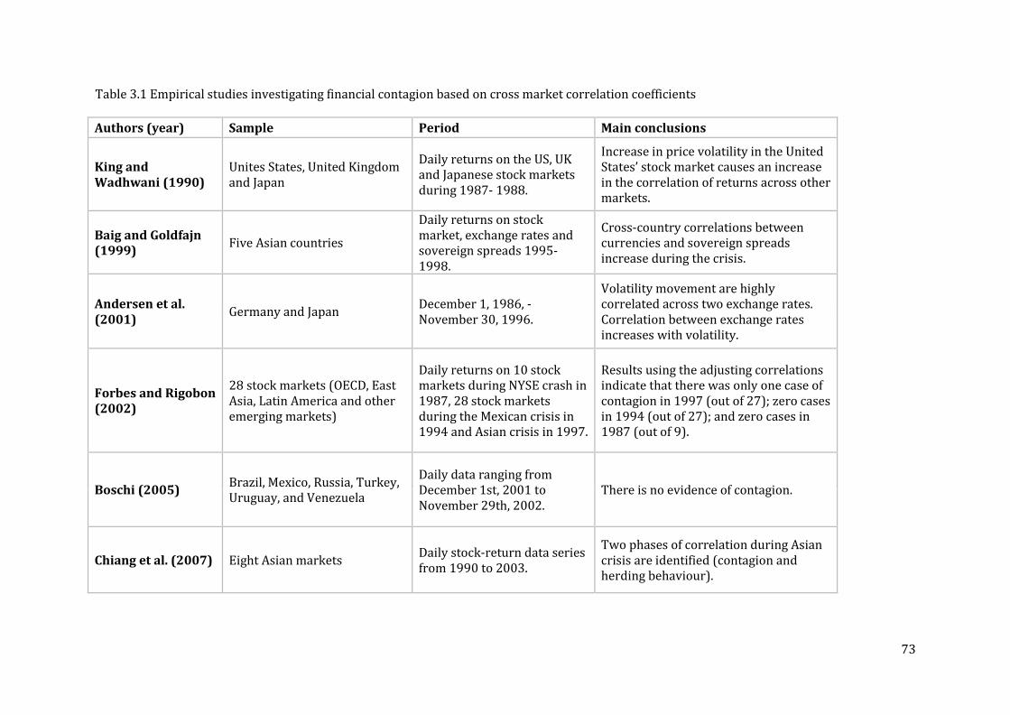
73
Table 3.1 Empirical studies investigating financial contagion based on cross market correlation coefficients
Authors (year) Sample Period Main conclusions
King and Wadhwani (1990)
Unites States, United Kingdom and Japan
Daily returns on the US, UK and Japanese stock markets during 1987- 1988.
Increase in price volatility in the United States’ stock market causes an increase in the correlation of returns across other markets.
Baig and Goldfajn (1999)
Five Asian countries
Daily returns on stock market, exchange rates and sovereign spreads 1995-1998.
Cross-country correlations between currencies and sovereign spreads increase during the crisis.
Andersen et al. (2001)
Germany and Japan December 1, 1986, - November 30, 1996.
Volatility movement are highly correlated across two exchange rates. Correlation between exchange rates increases with volatility.
Forbes and Rigobon (2002)
28 stock markets (OECD, East Asia, Latin America and other emerging markets)
Daily returns on 10 stock markets during NYSE crash in 1987, 28 stock markets during the Mexican crisis in 1994 and Asian crisis in 1997.
Results using the adjusting correlations indicate that there was only one case of contagion in 1997 (out of 27); zero cases in 1994 (out of 27); and zero cases in 1987 (out of 9).
Boschi (2005) Brazil, Mexico, Russia, Turkey, Uruguay, and Venezuela
Daily data ranging from December 1st, 2001 to November 29th, 2002.
There is no evidence of contagion.
Chiang et al. (2007) Eight Asian markets Daily stock-return data series from 1990 to 2003.
Two phases of correlation during Asian crisis are identified (contagion and herding behaviour).
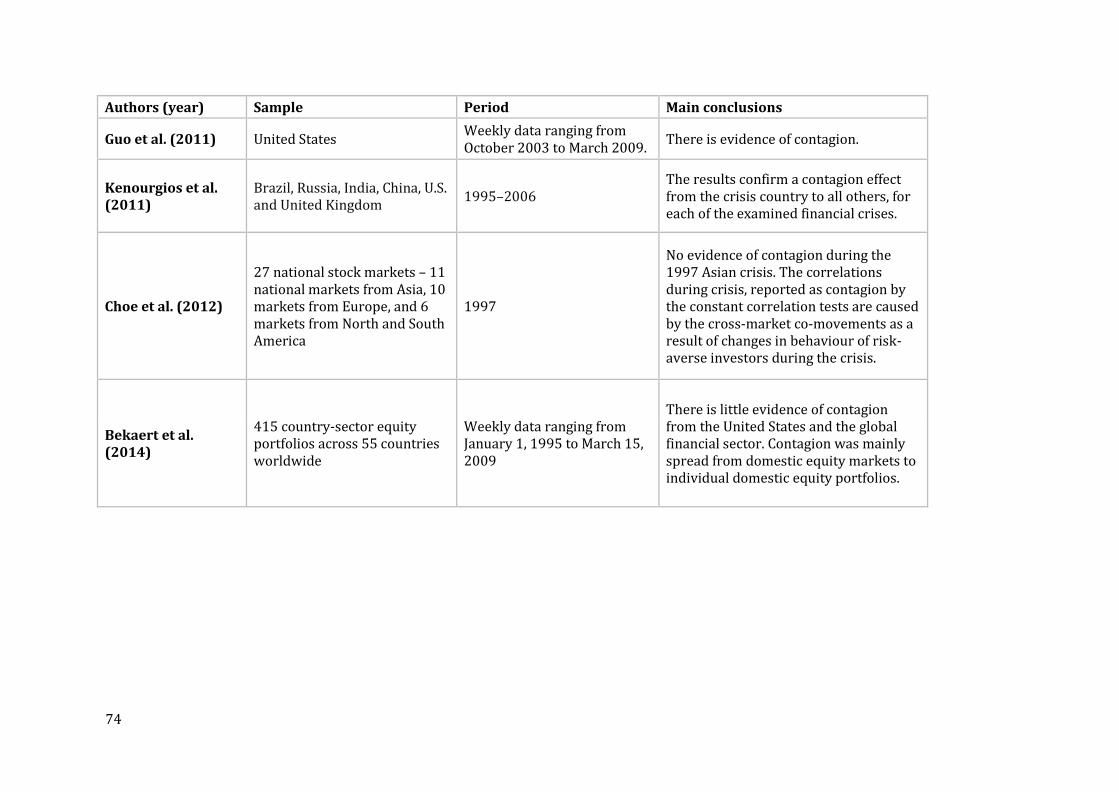
74
Authors (year) Sample Period Main conclusions
Guo et al. (2011) United States Weekly data ranging from October 2003 to March 2009.
There is evidence of contagion.
Kenourgios et al. (2011)
Brazil, Russia, India, China, U.S. and United Kingdom
1995–2006 The results confirm a contagion effect from the crisis country to all others, for each of the examined financial crises.
Choe et al. (2012)
27 national stock markets – 11 national markets from Asia, 10 markets from Europe, and 6 markets from North and South America
1997
No evidence of contagion during the 1997 Asian crisis. The correlations during crisis, reported as contagion by the constant correlation tests are caused by the cross-market co-movements as a result of changes in behaviour of risk-averse investors during the crisis.
Bekaert et al. (2014)
415 country-sector equity portfolios across 55 countries worldwide
Weekly data ranging from January 1, 1995 to March 15, 2009
There is little evidence of contagion from the United States and the global financial sector. Contagion was mainly spread from domestic equity markets to individual domestic equity portfolios.
75
Amongst the first papers that use this framework, King and Wadhwani (1990)
investigate the increased cross-market correlations between stock markets of the
United States, United Kingdom and Japan in 1987 and show that an increase in price
volatility in the United Sates causes an increase in the correlation of returns across
other markets. The authors argue that contagion spread can be attributed to
investors who infer information about price fluctuations in other economies due to
the lack of complete information about the conditions in each economy. In the same
vein, Baig and Goldfajn (1999) test for an increase in cross-market correlations
during the East Asian crisis in the financial markets of Thailand, Malaysia, Indonesia,
Korea and the Philippines. They use daily data for the period 1995-1998 for the five
selected countries. The authors employ VAR methodology to estimate impulse
responses to shocks in each stock and currency markets. They show that correlations
in currency and sovereign spreads increased significantly during the crisis, while
their results for equity market correlations are inconclusive. Andersen et al. (2001)
use high-frequency data on deutschemark and yen returns against the dollar and
estimate a model of daily exchange rate volatility and correlation for a period of 10
years. They find that volatility movement are highly correlated across the two
exchange rates. The authors also show that correlation between exchange rates
increases with volatility. Chiang et al. (2007) by using a dynamic multivariate GARCH
model, analyse financial contagion during the Asian crisis. The authors present
evidence of contagion. They identify two phases of correlation during the Asian crisis
(contagion and herding behaviour). Guo et al. (2011) study the cross-asset contagion
between the stock market, real estate market, credit default market and energy
market during the GFC and find evidence of contagion. However, they only
investigate the cross-asset contagion within the United States and cannot conclude
on the contagion spread to the other economies worldwide.
Kenourgios et al. (2011), using daily data analyse the cross-market correlations
during and immediately after the 1987 Black Monday, the 1998 Russian Crisis, the
burst of the dot-com bubble of 2001, the shock after September, 11, 2001, and the
USA subprime mortgage crisis of 2008. Their results confirm a contagion effect from
the crisis country to all others, for each of the examined financial crises. Results show
that correlations between the crisis country and other countries’ financial markets
76
are higher following shocks than during stable periods, confirming contagion, and
during the more volatile periods, conditional correlations are higher than
unconditional correlations, supporting the presence of asymmetric responses to
shocks. The authors find that the previously conventional policy responses to a crisis
are unlikely to prevent the spread among countries, arguing that changes in
fundamentals do not help to avoid it since cross-market correlation dynamics are
driven by behavioural factors. Bekaert et al. (2014) analyse the transmission of the
GFC to 415 country-industry equity portfolios and find evidence of contagion.
However, despite the origins of the GFC in the United States, the authors find that
contagion was mainly spread from domestic equity markets to individual domestic
equity portfolios. Namely, the authors find that while the co-movements of equity
portfolios across markets during the GFC were low, there was a significant increase
of within-country portfolio co-movements.
Even though most of the studies reviewed above provide evidence of financial
contagion, Forbes and Rigobon (2002), who investigate contagion based on stock
market correlations during the 1997 Asian crisis, the 1994 Mexican devaluation and
the 1987 United States market crash, conclude that tests for contagion based on
cross-market correlations are biased and inaccurate due to heteroscedasticity.
According to the authors, these correlation coefficients depend on the degree of
market volatility. As a result, during the periods of crisis when markets are more
volatile, correlation coefficients tend to increase. Hence, if no adjustment is made for
this bias, tests based on these coefficients usually find evidence of contagion. The
authors argue that it is possible to correct the biasness of the coefficients; however,
this can be done only under assumptions of no endogeneity and no omitted variables.
After correcting for heteroscedsticity, the authors find no evidence of contagion
during these three crises’ periods. Similarly, Boschi (2005) using VAR models tests
for contagion and after adjusting for heteroscedasticity, finds no evidence of
contagion between Argentina and Brazil, Venezuela, Uruguay, Mexico and Russia.
Choe et al. (2012) use the Structural Dynamic Conditional Correlation (SDCC)
multivariate GARCH model to estimate time-varying cross-market correlations
associated with the 1997 Asian crisis and find no evidence of contagion. However,
their conclusions are based on a number of assumptions, which do not appear to be
77
in line with the theory of contagion. More specifically, they define contagion as a
structural break in correlation dynamics during a crisis and assume that a structural
break in time-varying correlation dynamics is a consequence of an excessive cross-
market co-movement beyond the level that can be explained by the risk-return
relation. They do not view a temporal change in the correlation dynamics as evidence
of contagion, as they assume that a temporal variation in the correlation dynamics is
a reflection of time-varying cross-market co-movements induced by the
intertemporal risk-return adjustments by rational, risk-averse investors in response
to changing volatility.
Considering the studies reviewed above, the empirical results concerning the
presence of contagion based on cross-market correlation coefficients are
inconclusive. The first group of studies define contagion as a significant increase in
cross-country asset correlations following a crisis and find evidence of contagion,
whereas the second group of studies argue that, when taking into account
heteroscedasticity, there is no evidence of contagion. The next section presents an
overview of empirical studies that investigate financial contagion based on individual
channels of contagion.
3.2.2 Individual channels of contagion
The second method of testing for contagion is based on measuring the different
channels through which contagion might occur. This method provides more intuition
on how exactly a crisis has been transmitted (Claessens and Forbes, 2004) and given
the limitations of the previous method presented in section 3.2.1 has become the
most popular method to test for financial contagion. The empirical studies focused on
individual channels of transmission of financial crises have provided different results.
The first group of studies that used this method found evidence that trade linkages
were the major factor that explain how a crisis was transmitted. A second group of
studies showed the importance of financial linkages as a channel of transmission of
crises, while a third group found evidence of the importance of macroeconomic
fundamentals on the amplification and severity of financial crises. Table 3.2 below
summarizes the results of the main studies that have investigated the international

78
transmission of financial crises focusing on trade and financial linkages as well as
macroeconomic fundamentals.

79
Table 3.2: Empirical studies investigating financial contagion based on individual channels
Authors (year)
Countries Period Estimation technique
Crisis definition Explanatory variables Main conclusions
Eichengreen et al. (1996)
20 industrial countries
1959 - 1993
Probit and logit model
Extreme values of exchange market; Pressure index calculated as a weighted average of exchange rate changes, reserve changes, and interest rate changes (values measured relative to those prevailing in Germany).
Total non-gold international reserves; period-average exchange rates; short-term interest rates; discount rates otherwise; exports and imports.
The occurrence of a currency crisis in one country increases the probability of a speculative attack in other countries by 8 percentage points. Trade linkages explain contagion better than macroeconomic similarities.
Masson (1998)
13 Asian and South American countries
The 1994 Mexican crisis and the 1997 Asian crisis
Simple balance of payments model
Jumps between equilibria (multiple equilibria).
Level of reserves; trade balance; external debt; foreign interest rate.
Trade was not important in the international transmission of the 1994 Mexican crisis and the 1997 Asian crisis.
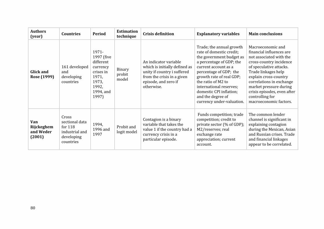
80
Authors (year)
Countries Period Estimation technique
Crisis definition Explanatory variables Main conclusions
Glick and Rose (1999)
161 developed and developing countries
1971-1997 (five different currency crises in 1971, 1973, 1992, 1994, and 1997)
Binary probit model
An indicator variable which is initially defined as unity if country i suffered from the crisis in a given episode, and zero if otherwise.
Trade; the annual growth rate of domestic credit; the government budget as a percentage of GDP; the current account as a percentage of GDP; the growth rate of real GDP; the ratio of M2 to international reserves; domestic CPI inflation; and the degree of currency under-valuation.
Macroeconomic and financial influences are not associated with the cross-country incidence of speculative attacks. Trade linkages help explain cross-country correlations in exchange market pressure during crisis episodes, even after controlling for macroeconomic factors.
Van Rijckeghem and Weder (2001)
Cross sectional data for 118 industrial and developing countries
1994, 1996 and 1997
Probit and logit model
Contagion is a binary variable that takes the value 1 if the country had a currency crisis in a particular episode.
Funds competition; trade competition; credit to private sector (% of GDP); M2/reserves; real exchange rate appreciation; current account.
The common lender channel is significant in explaining contagion during the Mexican, Asian and Russian crises. Trade and financial linkages appear to be correlated.
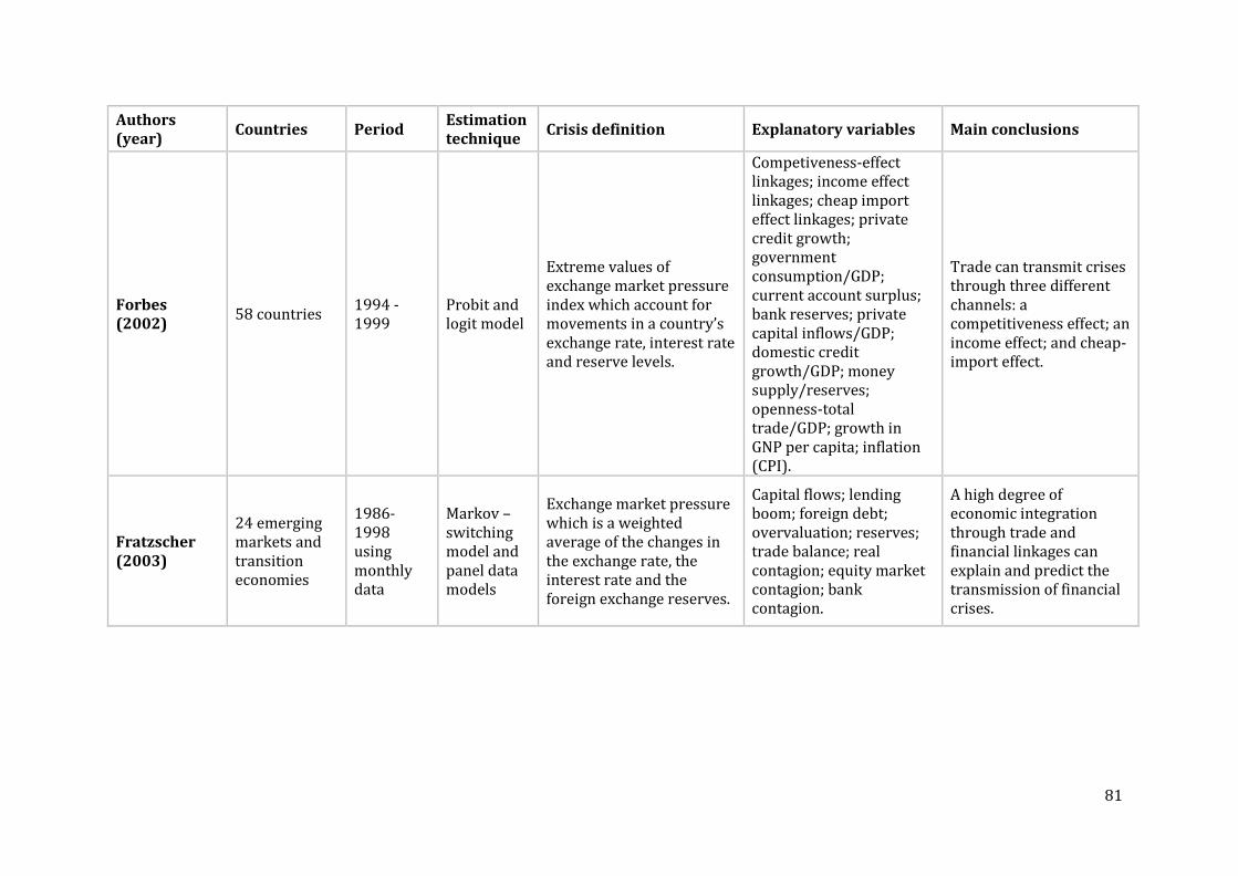
81
Authors (year)
Countries Period Estimation technique
Crisis definition Explanatory variables Main conclusions
Forbes (2002)
58 countries 1994 - 1999
Probit and logit model
Extreme values of exchange market pressure index which account for movements in a country’s exchange rate, interest rate and reserve levels.
Competiveness-effect linkages; income effect linkages; cheap import effect linkages; private credit growth; government consumption/GDP; current account surplus; bank reserves; private capital inflows/GDP; domestic credit growth/GDP; money supply/reserves; openness-total trade/GDP; growth in GNP per capita; inflation (CPI).
Trade can transmit crises through three different channels: a competitiveness effect; an income effect; and cheap-import effect.
Fratzscher (2003)
24 emerging markets and transition economies
1986- 1998 using monthly data
Markov – switching model and panel data models
Exchange market pressure which is a weighted average of the changes in the exchange rate, the interest rate and the foreign exchange reserves.
Capital flows; lending boom; foreign debt; overvaluation; reserves; trade balance; real contagion; equity market contagion; bank contagion.
A high degree of economic integration through trade and financial linkages can explain and predict the transmission of financial crises.
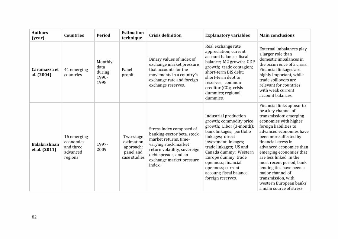
82
Authors (year)
Countries Period Estimation technique
Crisis definition Explanatory variables Main conclusions
Caramazza et al. (2004)
41 emerging countries
Monthly data during 1990-1998
Panel probit
Binary values of index of exchange market pressure that accounts for the movements in a country’s exchange rate and foreign exchange reserves.
Real exchange rate appreciation; current account balance; fiscal balance; M2 growth; GDP growth; trade contagion; short-term BIS debt; short-term debt to reserves; common creditor (CC); crisis dummies; regional dummies.
External imbalances play a larger role than domestic imbalances in the occurrence of a crisis. Financial linkages are highly important, while trade spillovers are relevant for countries with weak current account balances.
Balakrishnan et al. (2011)
16 emerging economies and three advanced regions
1997-2009
Two-stage estimation approach; panel and
case studies
Stress index composed of banking-sector beta, stock market returns, time-varying stock market return volatility, sovereign debt spreads, and an exchange market pressure index.
Industrial production growth; commodity price growth; Libor (3-month); bank linkages; portfolio linkages; direct investment linkages; trade linkages; US and Canada dummy; Western Europe dummy; trade openness; financial openness; current account; fiscal balance; foreign reserves.
Financial links appear to be a key channel of transmission: emerging economies with higher foreign liabilities to advanced economies have been more affected by financial stress in advanced economies than emerging economies that are less linked. In the most recent period, bank lending ties have been a major channel of transmission, with western European banks a main source of stress.
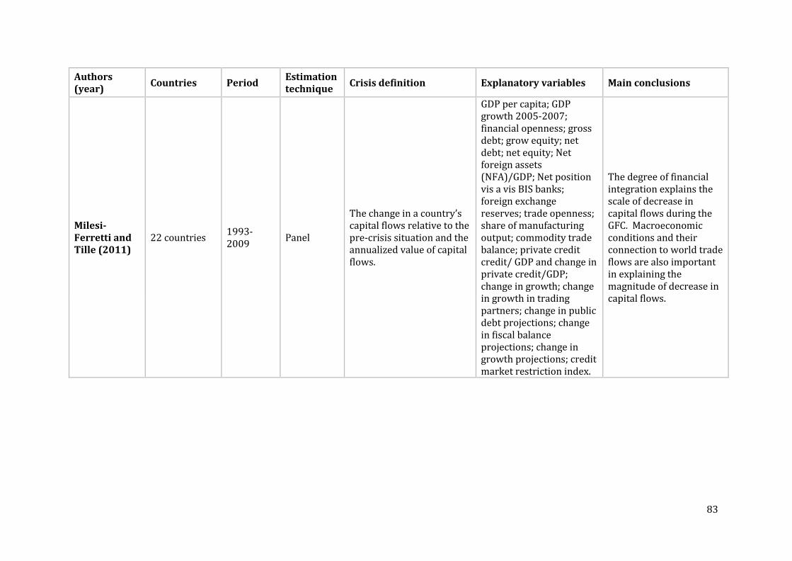
83
Authors (year)
Countries Period Estimation technique
Crisis definition Explanatory variables Main conclusions
Milesi-Ferretti and Tille (2011)
22 countries 1993-2009
Panel
The change in a country’s capital flows relative to the pre-crisis situation and the annualized value of capital flows.
GDP per capita; GDP growth 2005-2007; financial openness; gross debt; grow equity; net debt; net equity; Net foreign assets (NFA)/GDP; Net position vis a vis BIS banks; foreign exchange reserves; trade openness; share of manufacturing output; commodity trade balance; private credit credit/ GDP and change in private credit/GDP; change in growth; change in growth in trading partners; change in public debt projections; change in fiscal balance projections; change in growth projections; credit market restriction index.
The degree of financial integration explains the scale of decrease in capital flows during the GFC. Macroeconomic conditions and their connection to world trade flows are also important in explaining the magnitude of decrease in capital flows.
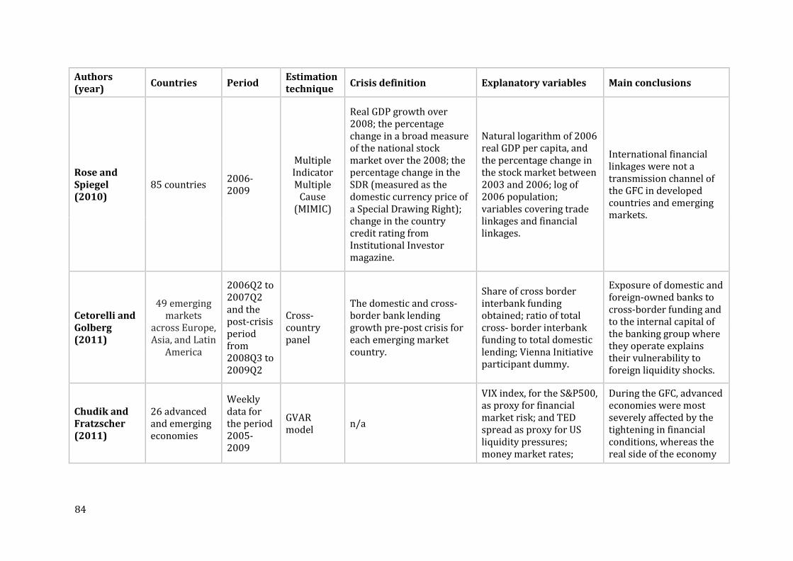
84
Authors (year)
Countries Period Estimation technique
Crisis definition Explanatory variables Main conclusions
Rose and Spiegel (2010)
85 countries 2006-2009
Multiple Indicator Multiple
Cause (MIMIC)
Real GDP growth over 2008; the percentage change in a broad measure of the national stock market over the 2008; the percentage change in the SDR (measured as the domestic currency price of a Special Drawing Right); change in the country credit rating from Institutional Investor magazine.
Natural logarithm of 2006 real GDP per capita, and the percentage change in the stock market between 2003 and 2006; log of 2006 population; variables covering trade linkages and financial linkages.
International financial linkages were not a transmission channel of the GFC in developed countries and emerging markets.
Cetorelli and Golberg (2011)
49 emerging markets
across Europe, Asia, and Latin
America
2006Q2 to 2007Q2 and the post-crisis period from 2008Q3 to 2009Q2
Cross-country panel
The domestic and cross-border bank lending growth pre-post crisis for each emerging market country.
Share of cross border interbank funding obtained; ratio of total cross- border interbank funding to total domestic lending; Vienna Initiative participant dummy.
Exposure of domestic and foreign-owned banks to cross-border funding and to the internal capital of the banking group where they operate explains their vulnerability to foreign liquidity shocks.
Chudik and Fratzscher (2011)
26 advanced and emerging economies
Weekly data for the period 2005-2009
GVAR model
n/a
VIX index, for the S&P500, as proxy for financial market risk; and TED spread as proxy for US liquidity pressures; money market rates;
During the GFC, advanced economies were most severely affected by the tightening in financial conditions, whereas the real side of the economy
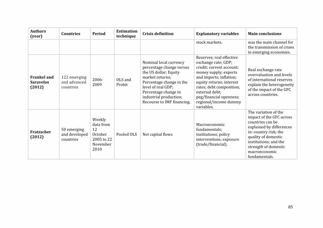
85
Authors (year)
Countries Period Estimation technique
Crisis definition Explanatory variables Main conclusions
stock markets. was the main channel for the transmission of crises in emerging economies.
Frankel and Saravelos (2012)
122 emerging and advanced countries
2006-2009
OLS and Probit
Nominal local currency percentage change versus the US dollar; Equity market returns; Percentage change in the level of real GDP; Percentage change in industrial production; Recourse to IMF financing.
Reserves; real effective exchange rate; GDP; credit; current account; money supply; exports and imports; inflation; equity returns; interest rates; debt composition; external debt; peg/financial openness; regional/income dummy variables.
Real exchange rate overvaluation and levels of international reserves explain the heterogeneity of the impact of the GFC across countries.
Fratzscher (2012)
50 emerging and developed countries
Weekly data from 12 October 2005 to 22 November 2010
Pooled OLS Net capital flows
Macroeconomic fundamentals; institutions; policy interventions; exposure (trade/financial).
The variation of the impact of the GFC across countries can be explained by differences in: country risk; the quality of domestic institutions; and the strength of domestic macroeconomic fundamentals.
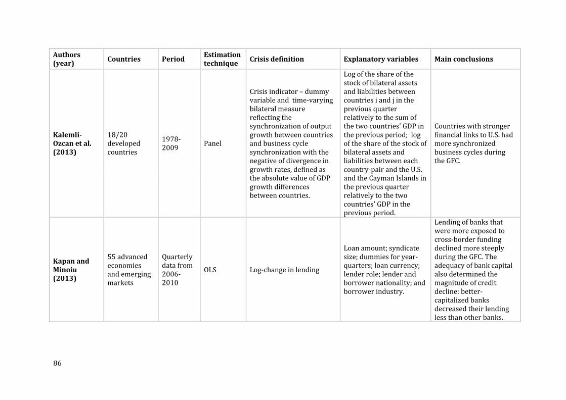
86
Authors (year)
Countries Period Estimation technique
Crisis definition Explanatory variables Main conclusions
Kalemli-Ozcan et al. (2013)
18/20 developed countries
1978-2009
Panel
Crisis indicator – dummy variable and time-varying bilateral measure reflecting the synchronization of output growth between countries and business cycle synchronization with the negative of divergence in growth rates, defined as the absolute value of GDP growth differences between countries.
Log of the share of the stock of bilateral assets and liabilities between countries i and j in the previous quarter relatively to the sum of the two countries' GDP in the previous period; log of the share of the stock of bilateral assets and liabilities between each country-pair and the U.S. and the Cayman Islands in the previous quarter relatively to the two countries' GDP in the previous period.
Countries with stronger financial links to U.S. had more synchronized business cycles during the GFC.
Kapan and Minoiu (2013)
55 advanced economies and emerging markets
Quarterly data from 2006-2010
OLS Log-change in lending
Loan amount; syndicate size; dummies for year-quarters; loan currency; lender role; lender and borrower nationality; and borrower industry.
Lending of banks that were more exposed to cross-border funding declined more steeply during the GFC. The adequacy of bank capital also determined the magnitude of credit decline: better-capitalized banks decreased their lending less than other banks.
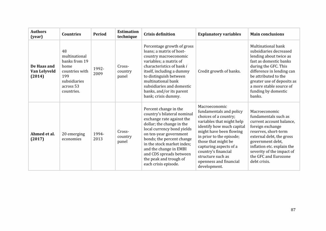
87
Authors (year)
Countries Period Estimation technique
Crisis definition Explanatory variables Main conclusions
De Haas and Van Lelyveld (2014)
48 multinational banks from 19 home countries with 199 subsidiaries across 53 countries.
1992-2009
Cross-country panel
Percentage growth of gross loans; a matrix of host-country macroeconomic variables; a matrix of characteristics of bank i itself, including a dummy to distinguish between multinational bank subsidiaries and domestic banks, and/or its parent bank; crisis dummy.
Credit growth of banks.
Multinational bank subsidiaries decreased lending about twice as fast as domestic banks during the GFC. This difference in lending can be attributed to the greater use of deposits as a more stable source of funding by domestic banks.
Ahmed et al. (2017)
20 emerging economies
1994-2013
Cross-country panel
Percent change in the country’s bilateral nominal exchange rate against the dollar; the change in the local currency bond yields on ten-year government bonds; the percent change in the stock market index; and the change in EMBI and CDS spreads between the peak and trough of each crisis episode.
Macroeconomic fundamentals and policy choices of a country; variables that might help identify how much capital might have been flowing in prior to the episode; those that might be capturing aspects of a country’s financial structure such as openness and financial development.
Macroeconomic fundamentals such as current account balance, foreign exchange reserves, short-term external debt, the gross government debt, inflation etc. explain the severity of the impact of the GFC and Eurozone debt crisis.
88
A number of empirical studies have investigated the impact of trade on the
international transmission of shocks. The results are mixed, some studies argue that
trade is a major important mechanism for transmission of the financial crises, while
other studies find no evidence for the importance of a trade channel in the
international transmission of the recent financial crises. Among the first studies
arguing that trade is an important channel for the international transmission of the
financial crisis is that of Eichengreen et al. (1996). The authors use panel data from
twenty countries during the period 1959-1993 and find that contagion spreads more
easily to countries with stronger trade linkages than to countries with similar
macroeconomic conditions. They conclude that trade links have been the dominant
channel for the international transmission of crises in the selected sample. Glick and
Rose (1999) further develop this framework by investigating five different currency
crises during the period 1971-1997 for 161 countries, many of which were not
directly involved in any of the five episodes and test whether trade linkages had an
impact in the probability of a country being affected by the crisis. They conclude that
trade linkages help explain cross-country correlations in exchange market pressure
during crisis episodes, even after controlling for macroeconomic factors. Similarly,
Forbes (2002) measures whether trade linkages are an important determinant of a
country’s vulnerability to crises that originate in other countries. The author shows
that trade can transmit crises through three different channels: a competitiveness
effect (when changes in relative prices affect a country’s ability to compete abroad);
an income effect (when a crisis affects income and imports); and cheap-import effect
(when crisis decreases import prices and acts as a positive supply shock). More
recently, Ozkan and Unsal (2012) investigate the transmission of the GFC to emerging
economies (Argentina, Brazil, Korea, Mexico and the Philippines). The authors
develop a two-country dynamic stochastic general equilibrium model with an explicit
treatment of both trade and financial linkages between the countries. They find that
the greater a country’s trade integration with the rest of the world, the greater the
response of its macroeconomic aggregates to a sudden stop in capital flows.
While the empirical studies reviewed above present convincing evidence that trade
linkages composed an important channel for the international transmission of recent
financial crises, several other studies disagree. Among the first of these studies was
89
Masson (1998), who based on a two-country simple balance of payments model
argues that trade was not important in the international transmission of the 1994
Mexican crisis and the 1997 Asian crisis. Baig and Goldfajn (1999) also argue that
trade was not an important international transmission channel for the Asian crisis.
Harrigan (2000) likewise concludes that trade did not compose a significant channel
of transmission of the Asian crisis to the United States. Van Rijckeghem and Weder
(2001) show that spillovers through bank lending, as opposed to trade linkages and
country characteristics can better explain contagion. They find that if either trade or
financial linkages are included in the model, they are highly significant. But if both of
them are included in the model, one of them becomes insignificant, reflecting the high
correlation between competition for funds and trade.
Trade linkages were the focus of the earlier research and helped explain contagion.
However, the researchers of the recent financial crises focused more on financial
linkages as an international channel of transmission of crises. Nevertheless, the
results of empirical studies focused on financial linkages are also diverse. A number
of empirical studies have found evidence that direct financial ties and competition for
funds from common bank lenders can forecast the impact of financial contagion and
crises, while others argue that financial linkages have played no role in international
transmission of recent financial crises.
Among the first studies arguing that financial linkages is an important channel for the
international transmission of financial crises was that of Fratzscher (2003), who
analyses the role of contagion in the currency crises in emerging markets during the
1990s. By using Markov-switching and panel data models, the author concludes that
financial crises can be explained and future transmission of financial crises can be
predicted by a high degree of economic integration through trade and financial
channels. Balakrishnan et al. (2011), using a new financial stress index for emerging
economies, investigate how financial stress is transmitted from advanced to
emerging countries. They find that the extent of pass-through of financial stress is
related to the depth of financial linkages between advanced and emerging economies.
Similarly, Milesi-Ferretti and Tille (2011) show that the magnitude of the decrease in
capital flows across countries is linked to the extent of international financial
integration, its specific nature (with countries relying on bank flows being the

90
hardest hit) as well as domestic macroeconomic conditions and their connection to
world trade flows. The authors argue that this diversity of experiences across
countries can be explained by the size of external exposures, reliance on debt
instruments and the importance of cross-border banking activity. Countries with
high degrees of financial integration through debt and banking were more affected,
and countries with large net liabilities in debt instruments suffered sharper declines
in capital inflows. Chudik and Fratzscher (2011) study 26 economies using weekly
data and find that a tightening of financial conditions was the key transmission
channel in advanced economies, whereas the real side of the economy was the main
channel in emerging economies. Another conclusion of their paper is that Europe
suffered a greater effect than other advanced economies from the shocks in the US, in
particular shocks to risk appetite (measured by VIX index for the S&P500 as a proxy
of financial market risk). Kalemli-Ozcan et al. (2013) also study the effect of financial
integration on the transmission of financial crises. They use a sample of 18/20
developed countries between 1978 and 2009 and find that financial crises induce co-
movement among more financially integrated countries. They also show that
countries with stronger financial links to the US had more synchronized business
cycles during the GFC.
A number of empirical studies that investigate the transmission of financial crises
have focused on the common creditor channel which links the probability of
experiencing a financial crisis with sharing the same lender with a country hit by a
crisis. Van Rijckeghem and Weder (2001) show that spillovers through bank lending
contributed to the transmission of currency crises during a number of episodes of
financial instability in emerging markets. They indicate that spillovers caused by
banks’ exposures to a crisis country help predict flows in third world countries after
the Mexican and Asian crisis. Moreover, they argue that countries might reduce
contagion risk by diversifying the sources of their financing and by carefully
monitoring borrowing from creditors exposed to potential crisis countries.
Caramazza et al. (2004) using panel probit regressions, examine the role of financial
linkages, especially through a common creditor, in the international transmission of
crisis to 41 emerging economies during the 1990s. They show that financial linkages
were important factors in explaining the spread of the Mexican, Asian, and Russian
crises. Similarly, Cetorelli and Goldberg (2011) demonstrate that the impact of
91
foreign liquidity shocks on domestic and foreign-owned banks depends on their
exposure to cross-border funding and to the internal capital of the banking group
where they operate. Likewise, Kapan and Minoiu (2013) show that banks that were
more dependent on cross-border funding reduced their lending more than other
banks during the GFC and that the adequacy of bank capital was important in
explaining the scale of credit decline: better capitalized banks decreased their
lending less than other banks. De Haas and Van Lelyveld (2014) investigate a large
group of multinational bank subsidiaries and stand-alone domestic banks and
conclude that multinational bank subsidiaries decreased lending about twice as fast
as domestic banks during the GFC. They argue that this difference in lending can be
attributed to the greater use of deposits, a more stable source of funding by domestic
banks.
In contrast to the evidence related to the role of financial linkages in international
transmission of crisis provided by the studies reviewed above, a number of other
studies find opposing empirical results. In particular Rose and Spiegel (2010) find no
role for international financial linkages in transmitting the GFC to developed
countries and emerging markets. Similarly, Lane and Milesi-Ferretti (2011) find no
evidence that higher financial integration contributed to the intensity of the GFC.
After controlling for the pre-crisis level of development, buoyancy of economic
activity and credit, external vulnerabilities and openness to trade, the authors find
that more financially integrated economies experienced smaller output declines
during the GFC. The lack of conclusive evidence of the relationship between financial
linkages and output decline during recent years has even led some researchers to
claim that financial linkages might not be an important factor in determining crisis
severity. The diversity of results might be due to variations across studies in terms of
samples, periods covered, methodologies and variables employed to account for
crisis severity.
Even though the literature on the international transmission of shocks focuses
extensively on trade and financial linkages as channels of contagion, the extent to
which the shocks get amplified also depends on the responses of policy-makers and
existing domestic vulnerabilities. During the years following the GFC there has been a
growing consensus on the importance of macroeconomic fundamentals in

92
determining the severity of the impact of crises across countries. Frankel and
Saravelos (2012) analyse the effects of the GFC by selecting variables from an
extensive review of the previous literature on early warning indicators. They find
that real exchange rate overvaluation and levels of international reserves can explain
the variation of the impact of GFC across countries. Fratzscher (2012) demonstrates
that the heterogeneity of the impact of the GFC across countries can be explained by
differences in country risk, quality of domestic institutions and the strength of
domestic macroeconomic fundamentals. More specifically, the author shows that
countries with high-quality institutions and strong macroeconomic fundamentals
were better able to protect their financial markets from adverse shocks during the
GFC. In addition, the author highlights that trade and financial linkages played a
minor role in explaining cross-country heterogeneities in the transmission of the
GFC. Ahmed et al. (2017) show that the financial markets in those emerging
economies with better macroeconomic fundamentals (current account balance;
foreign exchange reserves; short-term external debt; the gross government debt;
inflation etc.) were less severely affected by the GFC and the subsequent Eurozone
debt crisis. They also find that financial conditions worsened more in countries that
had previously experienced larger capital inflows and greater exchange rate
appreciation.
3.3 Benefits and costs associated with euroisation
The consequences of increasing dollarization/euroisation has been a subject of
controversial debates for a long time due to the costs associated with it (refer to
section 2.3) and the potentially greater financial instability it creates. One important
issue stressed in the literature is the increased vulnerability to exchange rate
fluctuations that increased euroisation creates with respect to financial distress and
limitations on monetary and exchange rate policies (Chitu, 2013). The role of
euroisation in amplifying the impact of financial crises has not been sufficiently
investigated by previous research. Nevertheless, a number of empirical studies have
investigated the relationship between financial dollarization and financial instability,
banking crises and inflation, but overall the evidence is inconclusive. Results of the
main studies investigating the impact of dollarization/euroisation on financial
stability/crisis severity are summarized in Table 3.3 below.

93
Table 3.3: Empirical studies investigating dollarization/euroisation and its impact on financial stability/crisis severity/inflation
Authors (year)
Sample Period Estimation technique
Dependent variable
Independent variables Main conclusions
Edwards and Magendzo (2001)
199 countries
1970-1998 Probit Binary variable (if country is dollarized)
GDP; population; degree of openness of the economy; dummy variable if the country is an island; dummy variable if the country has a common border with a nation whose currency is defined by the IMF as a convertible currency; variable that measures the country’s geographical location; dummy if the economy in question is an independent nation.
Inflation has been significantly lower in dollarized nations than in non-dollarized ones. Dollarized nations have had a lower rate of economic growth than non-dollarized ones. Macroeconomic volatility is not significantly different across dollarized and non-dollarized economies.
Honohan and Shi (2002)
58 emerging economies
1980-2000 Seemingly unrelated regression
The log of the consumer price
index
Log dollar exchange rate; real exchange rate.
A high level of dollarization increases banking spreads. A greater degree of dollarization is associated with a higher pass-through coefficient from exchange rate change to consumer prices.
Arteta (2003)
92 developing and transition economies
1975 - 1999
Probit, OLS, panel and instrumental-variable regression
Crisis-binary variable; currency crash - binary variable; GDP growth.
Deposit and credit dollarization; FDI/GDP; short term debt/total debt; international reserves; current account balance/GDP; real exchange rate overvaluation; domestic credit growth; GDP growth; M2 reserves; US interest rate; OECD growth rate.
The results show little evidence that dollarization increases the probability of banking crises or currency crashes. There is no evidence that banking crises and currency crashes are more costly in countries with high degree of dollarization.
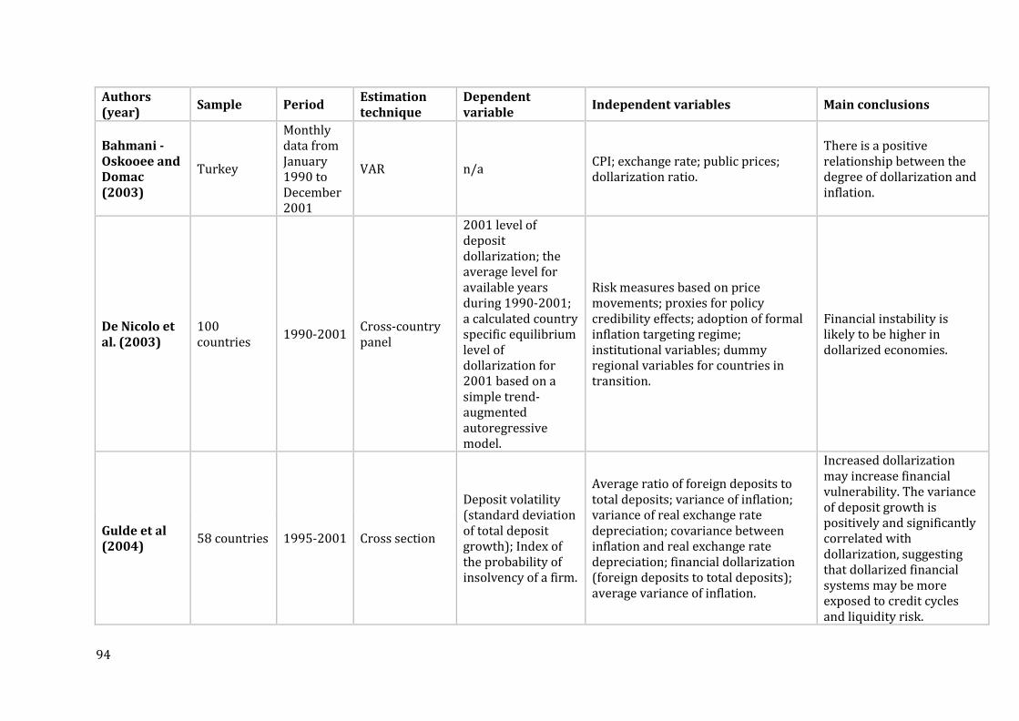
94
Authors (year)
Sample Period Estimation technique
Dependent variable
Independent variables Main conclusions
Bahmani - Oskooee and Domac (2003)
Turkey
Monthly data from January 1990 to December 2001
VAR n/a CPI; exchange rate; public prices; dollarization ratio.
There is a positive relationship between the degree of dollarization and inflation.
De Nicolo et al. (2003)
100 countries
1990-2001 Cross-country panel
2001 level of deposit dollarization; the average level for available years during 1990-2001; a calculated country specific equilibrium level of dollarization for 2001 based on a simple trend-augmented autoregressive model.
Risk measures based on price movements; proxies for policy credibility effects; adoption of formal inflation targeting regime; institutional variables; dummy regional variables for countries in transition.
Financial instability is likely to be higher in dollarized economies.
Gulde et al (2004)
58 countries 1995-2001 Cross section
Deposit volatility (standard deviation of total deposit growth); Index of the probability of insolvency of a firm.
Average ratio of foreign deposits to total deposits; variance of inflation; variance of real exchange rate depreciation; covariance between inflation and real exchange rate depreciation; financial dollarization (foreign deposits to total deposits); average variance of inflation.
Increased dollarization may increase financial vulnerability. The variance of deposit growth is positively and significantly correlated with dollarization, suggesting that dollarized financial systems may be more exposed to credit cycles and liquidity risk.

95
Authors (year)
Sample Period Estimation technique
Dependent variable
Independent variables Main conclusions
Bailey (2005)
Jamaica 1996-2004 VAR analysis n/a
Exchange rate; CPI; base money; an index of public sector prices (PSP) computed as government expenditure per capita and is deflated using 1995 values; the dollarization ratio; dummy variable for crisis years.
Shocks to financial dollarization reduce the monetary base, since investors switch to domestic currency from foreign currency. The high elasticity of substitution between domestic and foreign currency is also confirmed by the positive exchange rate response to an increase in foreign money holdings.
Calvo (2006) 161 countries
1990-2004 Panel OLS EMBI Index (Emerging Markets Bond Index Spread)
Volatility of EMBI; nominal exchange rate; exports; imports; capital flows proxy; exchange rate regime; sudden stop dummy; GDP; pre-crisis level of RES; Minimum level of RES during SS; maximum loss of Reserves during SS; pre-crisis level of EXR; maximum level of EXR during SS; maximum nominal depreciation; ratio reserves to external short-term debt; ratio reserves to M2.
Emerging market economies with greater degrees of euroisation face financial vulnerabilities that weaken the effectiveness of a domestic lender of last resort. As a result, monetary policy is linked to the state of the credit market. These conditions also impact on optimal monetary policy in normal but high-volatility periods.
Berkmen and Cavallo (2010)
145 countries
1970-2003 GMM Liability dollarization
Reserve volatility; exchange rate policy; volatility of Inflation; trade openness; capital account openness; country size.
Countries with high liability dollarization tend to stabilize their exchange rate. There is no causal effect going in the opposite
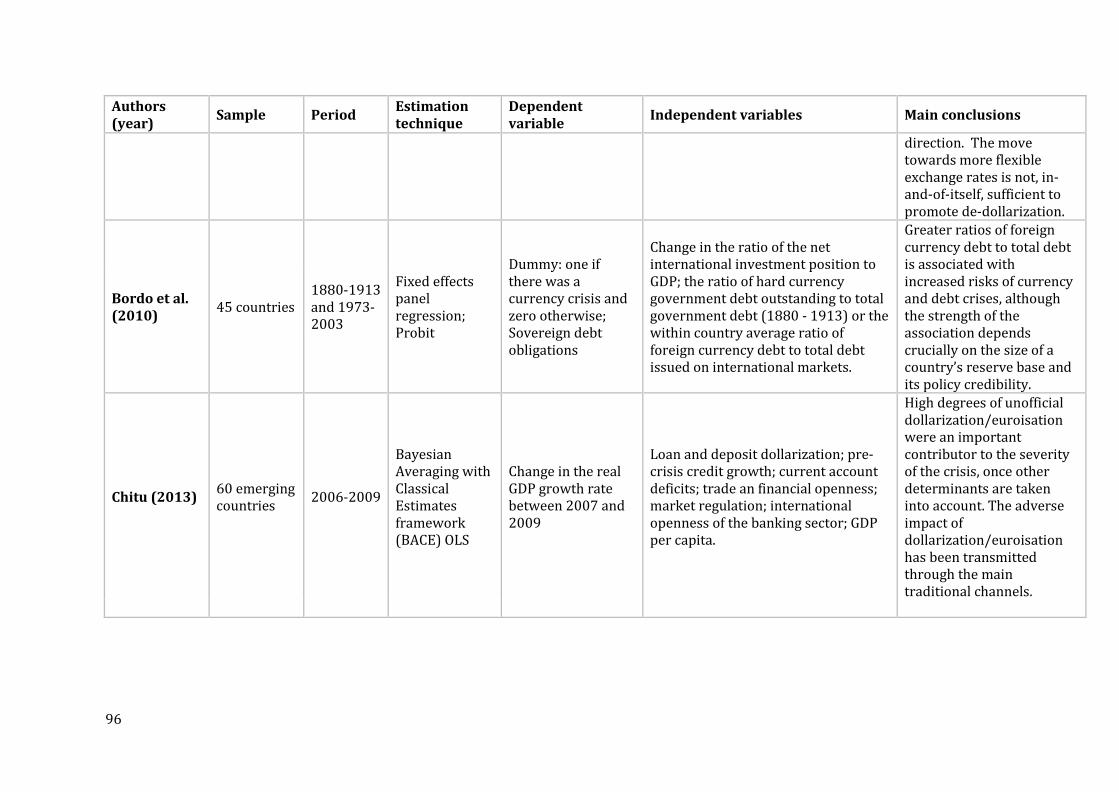
96
Authors (year)
Sample Period Estimation technique
Dependent variable
Independent variables Main conclusions
direction. The move towards more flexible exchange rates is not, in-and-of-itself, sufficient to promote de-dollarization.
Bordo et al. (2010)
45 countries 1880-1913 and 1973-2003
Fixed effects panel regression; Probit
Dummy: one if there was a currency crisis and zero otherwise; Sovereign debt obligations
Change in the ratio of the net international investment position to GDP; the ratio of hard currency government debt outstanding to total government debt (1880 - 1913) or the within country average ratio of foreign currency debt to total debt issued on international markets.
Greater ratios of foreign currency debt to total debt is associated with increased risks of currency and debt crises, although the strength of the association depends crucially on the size of a country’s reserve base and its policy credibility.
Chitu (2013) 60 emerging countries
2006-2009
Bayesian Averaging with Classical Estimates framework (BACE) OLS
Change in the real GDP growth rate between 2007 and 2009
Loan and deposit dollarization; pre-crisis credit growth; current account deficits; trade an financial openness; market regulation; international openness of the banking sector; GDP per capita.
High degrees of unofficial dollarization/euroisation were an important contributor to the severity of the crisis, once other determinants are taken into account. The adverse impact of dollarization/euroisation has been transmitted through the main traditional channels.

97
Authors (year)
Sample Period Estimation technique
Dependent variable
Independent variables Main conclusions
Reinhart, Rogoff and Savastano (2014)
1980-2001 and 1996-2001
2 samples: 90 and 48 non-industrial economies
Two-pronged methodology
Inflation rate, average GDP growth and revenues from seigniorage as a measure of monetary policy effectiveness.
The sum of the ratio of foreign currency deposits to broad money, the ratio of domestic government debt to total government debt and the ratio of external debt to GNP.
A high degree of dollarization does not seem to be an obstacle to monetary control or to disinflation. A high level of dollarization increases exchange rate pass-through.

98
Honohan and Shi (2002) show that that a high level of dollarization increases banking
spreads. A greater degree of dollarization is associated with a higher pass-through
coefficient from exchange rate change to consumer prices. Similarly, De Nicolo et al.
(2003) analyse the advantages and disadvantages of increased dollarization. The
authors show that dollarization is associated with higher financial instability. Similar
results are presented by Gulde et al. (2004), who investigate the solvency and liquidity
risks related to dollarization. The authors find that increased dollarization may increase
financial vulnerability. They also show that more dollarized economies are more prone
to credit cycles as well as liquidity and solvency risk. Levy Yeyati (2006) shows that
dollarized countries have a more unstable demand for money, higher inflation rates, a
greater propensity to suffer from banking crises after a depreciation of the local
currency and slower and more volatile output growth, without a significant positive
impact on financial depth.
On the other hand, very different results are provided by Arteta (2003). Using data on
deposit and credit dollarization for a large number of developing and developed
countries, the author finds little evidence that greater levels of dollarization increase the
probability of banking crises or currency crashes. Also, the author finds no evidence that
banking crises and currency crashes are more costly in countries with a high degree of
dollarization. Instead, macroeconomic and exchange rate policies are more significant in
determining such costs. Similarly, Honig (2006) investigate the potential variables that
could predict banking crises, focusing on the role played by unofficial dollarization.
Through a multivariate probit model, the author finds only weak evidence that the
degree of unofficial dollarization affects the probability of a banking crisis. Calvo (2006)
investigates the limitations faced by more dollarized countries to act as a lender of last
resort. Calvo argues that highly dollarized emerging market economies face greater
financial vulnerabilities that impair the function of the lender of last resort. An empirical
investigation of the relationship between dollarization and exchange rate policy choice
was conducted by Berkmen and Cavallo (2010). They find that countries with a high
share of foreign currency lending are likely to be more actively involved in exchange
99
rate stabilization operations, while they find no evidence that floating encourages de-
dollarization. Bordo et al. (2010) investigate the impact of foreign currency debt on
currency and debt crises and find a positive relationship between the two. However, the
authors show that the severity of the crises depends on the amount of reserves and
policy credibility. On the other hand, Reinhart et al. (2014), using a large sample of
developing countries, which they group according to their variety of dollarization
(degree and type), find that a high degree of dollarization does not impact the
effectiveness of monetary policy and that output fluctuations are similar in countries
with different levels of dollarization. However, they show that the average inflation rate
has been higher in more dollarized countries compared to those where the degree of
dollarization has been low. In addition, they show that the exchange rate pass-through
to prices has been different across countries with different levels of dollarization. They
conclude that the inflationary impact of exchange rate changes in the 1990s was higher
in more dollarized economies and lower in less dollarized economies. The relationship
between dollarization and inflation is also investigated by Bahmani-Oskooee and Domac
(2003). The authors investigate the role of dollarization in the dynamics of inflation in
Turkey. They find a positive relationship between the degree of dollarization and
inflation. Their results suggest that an increase in dollarization initially leads to a decline
in the monetary base as the public switches from domestic to foreign money holdings.
However, the monetary base increases later on to generate the required inflation tax for
a given budget deficit as fiscal authority tries to compensate for part of the decline in the
inflation tax through raising administered prices. As expected, the exchange rate
responds positively to increased dollarization owing to the high elasticity of substitution
between domestic and foreign currency. Likewise, Bailey (2005) analyses the
association between dollarization and inflation volatility in Jamaica. The author uses
VAR analysis and finds a positive relationship between dollarization and inflation. The
results show that shocks to financial dollarization reduce the monetary base, since
investors switch to domestic currency from foreign currency. The high elasticity of
substitution between domestic and foreign currency is also confirmed by the positive
exchange rate response to the increase in foreign money holdings. Very different results
are presented by Edwards and Magendzo (2001), who investigate whether dollarization

100
is associated with lower inflation and faster growth. They use a matching estimator
technique and conclude that inflation has been significantly lower in dollarized
countries. They also find that the rate of economic growth has been lower in more
dollarized economies. The authors show that dollarized and non-dollarized economies
experience similar levels of macroeconomic volatility.
None of the previous studies reviewed above consider the impact of
dollarization/euroisation on the amplification of financial crises. One study that
investigates the role of dollarization in amplification of the recent financial crises is that
of Chitu (2013). The author investigates whether the GFC had a more severe impact in
unofficially dollarized/euroised economies than in other economies. The author uses
OLS and Bayesian analysis for 60 emerging economies and shows that unofficial
dollarization/euroisation intensified the crisis, after controlling for other determinants
(fast pre-crisis credit growth; market regulation; international openness of the banking
sector; trade and financial openness; current account deficits; and GDP per capita).
Moreover, the author shows that the impact of dollarization was transmitted through
the three main traditional channels (currency mismatches, reduced monetary policy
autonomy and limited lender of last resort ability). However, as the author also
acknowledges, the data are not fully harmonised across countries.4 Furthermore, the
study employed a commonly used measure of currency mismatches: the difference
4The data on loan and deposit dollarization pertain to both advanced and emerging economies worldwide, from Europe, CIS, America, Africa, Middle East to Asia and Pacific. Data on the share of foreign currency loans to total loans are available for 76 economies worldwide, of which 60 are emerging economies, and those on the share of foreign currency deposits to total deposits for 75 economies worldwide, of which 55 are emerging economies. For the purpose of the empirical exercise, end-2006 was taken for data on foreign currency loans and deposit ratios. However, the data have been collected for an extended time horizon, which varies according to the countries considered. For example, data for loan dollarization for the period 1999 to 2008 for Albania, as opposed to Serbia where the ratio of foreign currency- denominated loans is available only since 2008. In addition, the change in the ratio of the private sector credit growth to GDP refers to the period between 2004 and 2007; the current account balance to GDP ratio is averaged out over 2005-2007; both (log) GDP per capita and trade openness are set at their 2007 values. As regards the transmission channels, the monetary policy channel is captured by the change in the key policy rate between July 2007 and April 2009, while the lender of last resort channel is captured by the changes in the central bank’s total assets (scaled by GDP in 2007) between July 2007 and April 2009.
101
between foreign currency loans and foreign currency deposits as a share of total loans,
which is an aggregate measure and cannot fully account for the potential currency
mismatches at the firm level
3.4 Integration with EU
Given the lack of empirical studies investigating the relationship between the degree of
integration with the EU and the international transmission of the GFC, this section
focuses on the empirical studies that have investigated the costs and benefits associated
with EU integration. The impact of European integration on countries and regions has
been a subject of controversial debates for a long time. From a theoretical point of view,
both positive and negative effects from increased economic integration are possible
(Badinger, 2005). When it comes to economic benefits that result from European
integration, although there is a general agreement that most of them are related to trade
liberalization, the single market and the common currency, it is widely recognised that
the most important effects are related to economic growth and productivity (Baldwin
and Seghezza, 1996; Badinger, 2005; Campos et al., 2014). Table 3.4 below summarizes
the results of the main studies related to the costs and benefits associated with a higher
degree of integration with the EU.
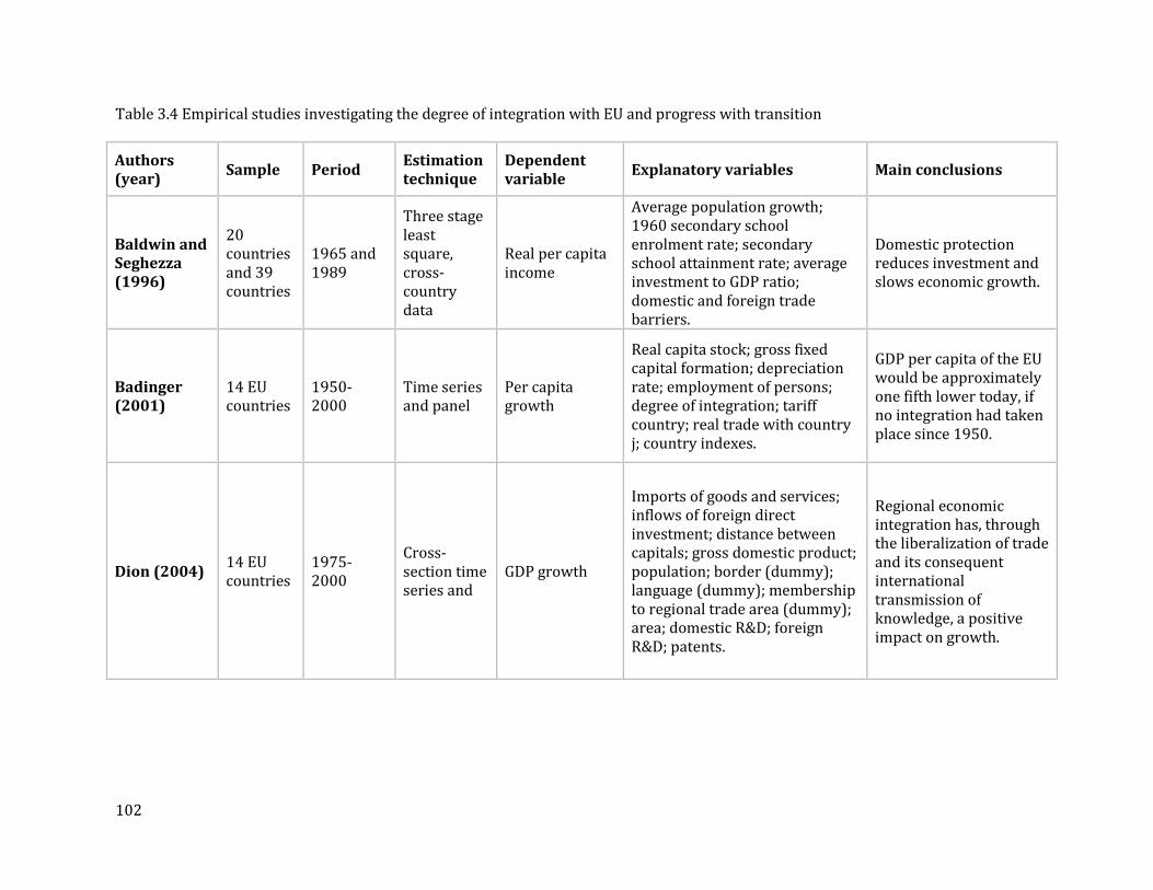
102
Table 3.4 Empirical studies investigating the degree of integration with EU and progress with transition
Authors (year)
Sample Period Estimation technique
Dependent variable
Explanatory variables Main conclusions
Baldwin and Seghezza (1996)
20 countries and 39 countries
1965 and 1989
Three stage least square, cross-country data
Real per capita income
Average population growth; 1960 secondary school enrolment rate; secondary school attainment rate; average investment to GDP ratio; domestic and foreign trade barriers.
Domestic protection reduces investment and slows economic growth.
Badinger (2001)
14 EU countries
1950-2000
Time series and panel
Per capita growth
Real capita stock; gross fixed capital formation; depreciation rate; employment of persons; degree of integration; tariff country; real trade with country j; country indexes.
GDP per capita of the EU would be approximately one fifth lower today, if no integration had taken place since 1950.
Dion (2004) 14 EU countries
1975-2000
Cross-section time series and
GDP growth
Imports of goods and services; inflows of foreign direct investment; distance between capitals; gross domestic product; population; border (dummy); language (dummy); membership to regional trade area (dummy); area; domestic R&D; foreign R&D; patents.
Regional economic integration has, through the liberalization of trade and its consequent international transmission of knowledge, a positive impact on growth.

103
Authors (year)
Sample Period Estimation technique
Dependent variable
Explanatory variables Main conclusions
Belke et al. (2009)
25 transition countries
1996-2008
Cross-country panel
Institutional quality measured by an index based on the World Bank Governance Indicators.
Dummy variable about Stabilization and Association Agreement; Dummy variable which equals 1 starting in the year a membership action plan was established; Dummy variable which equals 1 for all years following WTO or GATT accession; Official Development Assistance and Official Aid (Share of GDP), average over current and past two years; FDI net Inflows (share of GDP), average over current and past two years.
Pre-accession incentives provided by EU and NATO are important for the development of institutions.
Bartlett and Prica (2012)
12 SEE countries
2008-2009
Descriptive statistics and graphical analysis
Change in GDP growth
Exports; credit growth; FDI; remittances; integration with EU; quality of institutions; progress with transition.
Countries that were more integrated with the EU were more affected by the crisis, especially through credit and foreign investment channels. Countries that made more progress with transition were also more affected.

104
Authors (year)
Sample Period Estimation technique
Dependent variable
Explanatory variables Main conclusions
Campos et al. (2014)
17 EU countries
Country and regional level data from the 1973, 1980s, 1995 and 2004
Synthetic control methods for causal inference in comparative case studies
Percentage difference between the actual and estimated GDP per capita.
Real GDP per capita; labour productivity; trade openness; financial integration; EURO; political constraints; year of membership; country dummies, year dummies.
Growth and productivity effects from European Union accession vary across countries and over time, but without the EU, European incomes would be around 10 percent lower in 2013.
105
Baldwin and Seghezza (1996) investigate the relationship between trade
liberalization and investment-led growth. They find that domestic protection reduces
investment and slows economic growth. Badinger (2005) using a time series and
panel approach, study the permanent and temporary growth effects of integration
with EU. Even though the hypothesis of a permanent growth effect is rejected, the
author finds that GDP per capita of the EU would be approximately one fifth lower
today, if no integration had taken place since 1950. Dion (2004) contributes to the
empirical literature by providing a quantitative measurement of the influence of
regional trade integration on productivity. They address the link between trade and
productivity of EU countries through knowledge spillovers in a multi-country model.
They show that regional economic integration has, through the liberalization of trade
and its consequent international transmission of knowledge, a positive impact on
growth. Campos et al. (2014) also analyse the growth and productivity effects from
European Integration. The authors use country and regional level data from the
1973, 1980s, 1995 and 2004 enlargements for various measures of growth and
productivity and find significant and substantial positive growth and productivity
effects from European Union accession. They find that these effects vary across
countries and over time, but they conclude that without the EU, European incomes
would be around 10 percent lower in 2013. Additional benefits from integration with
the EU are the increased employment opportunities, cost reductions resulting from
the elimination of border formalities and national regulations, economies of scale
(Egger and Pfaffermayr, 2004; De Sousa et al., 2012).
Despite the overall positive effects associated with European integration, when it
comes to periods of crisis and shocks, it is still a debatable topic whether progress
with integration to EU equipped countries with the necessary tools to better deal
with them or whether it made them more vulnerable. A number of empirical studies
suggest that progress with EU integration has a positive effect on the quality of
institutions (Beck and Laeven, 2006; Di Tommaso et al., 2007; Belke et al. 2009). In
general, the institutional characteristics that may shape the impact of external shocks
are related to the quality of developed institutions, progress with transition to a
market economy and the quality of government policy-making (Bartlett and Prica,
2012). From the perspective of adjusting to external shocks, the institutional
106
development with respect to governance, including capacity for monetary and fiscal
policy/stabilization and well-functioning markets are unambiguously positive.
Likewise, during the periods of financial crises investors tend to withdraw from
those markets with weak macroeconomic fundamentals and poor institutions, thus
contributing to the transmission of crises (Bekaert et al., 2014).
Beck and Laeven (2006) show that EU membership has positive effects on
institutional change in ETEs. They measure institutional change using the World
Bank Governance Indicators. Di Tommaso et al. (2007) find similar results of the
positive impact of basic agreements between the EU and transition countries. They
measure institutional change by using EBRD indicators; however, they focus only on
economic institutions, ignoring political and legal institutions. Belke et al. (2009)
using a panel of 25 transition countries for the period 1996-2008 show that pre-
accession incentives provided by EU and NATO are important for the development of
institutions. They provide similar results for a positive relationship between
progress with EU integration and institutional quality measured by the World Bank
Governance Indicators.
The empirical studies reviewed above suggest that there is a positive relationship
between increased integration with the EU and the quality of institutions. However,
there is a lack of empirical studies that investigate the impact of integration with the
EU on the sensitivity of economies to exposure to external shocks. One paper that
considers integration with the EU and progress with transition in assessing the
impact of the GFC on economic activities of transition countries is that of Bartlett and
Prica (2012). The authors conclude that countries that were more integrated with
the EU were more affected by the crisis, mainly through credit and FDI channels.
Countries that made more progress with transition were also more affected, possibly
because this has led to deeper structural and institutional integration with the EU.
The authors argue that progress in adopting market-friendly institutions has made
these countries more vulnerable to external shocks by creating new channels of
contagion. However, this conclusion relies excessively on descriptive statistics and
graphical analysis and the authors consider only the South East European countries.
Nevertheless, as shown in section 1.2, despite the well-known benefits of economic
integration, it also appears to have made the countries more vulnerable to the effects
107
of the GFC by creating and/or strengthening potential channels for contagion
through trade, foreign banks, FDI, remittances and cross-border bank flows. On the
other hand, countries that made more progress with EU integration and institutional
reforms may have been better able to deal with external shocks, since their higher
quality institutions may be expected to contribute to output stability (Balavac and
Pugh, 2016).
3.5 Empirical work for European transition economies
Even though previous research contains numerous empirical studies on the
transmission of the GFC to developed and developing countries, there is still a lack
of empirical studies regarding transmission to the Central and Eastern European
countries. Given the relatively low level of financial market development in ETEs, the
empirical studies investigating the transmission of the GFC to these countries have
generally employed the second method of testing for contagion, which focuses on
individual channels of transmission of shocks. The following part of this section
reviews the main studies that have included ETEs in investigating the impact of the
GFC. It starts with studies that have focused on financial linkages and then continues
with those that focused on trade linkages as an international channel of transmission
of crises. The empirical studies which include ETEs in the investigation of the
determinants of the GFC are summarized in Table 3.5 below.

108
Table 3.5 Empirical studies investigating ETEs
Authors (year) Countries Period Estimation technique
Crisis definition
Main explanatory variables
Main conclusions
Árvai et al. (2009)
CEE and Western European countries
2002-2008
N/A Contagion index
Cross-border exposures
Most of Central, Eastern and Southern European countries are highly dependent on cross-border credit flows from Western European banks. Even in the cases where exposures of CESE countries are diversified, interdependencies between each other could trigger a regional contagion if one of the countries were to face a shock.
Milesi-Ferretti and Tille (2011)
75 countries from Emerging Europe, CIS, Emerging Asia, Western Hem. Carib. Africa, Industrial countries, Middle East
2008-2009
Panel, OLS estimation
Change in output growth
between 2008-2009 and 2005-
2007
GDP per capita, CA/GDP is the ratio of the 2007 current account balance to GDP, Private credit growth, Financial openness and Growth gap.
Trade openness and the manufacturing share in GDP are positively correlated with the output and demand declines; also, fast private credit growth and current account deficits are correlated with the decline in the growth rate of output and especially domestic demand during the crisis. The nature of the crisis in advanced economies is highlighted by the negative
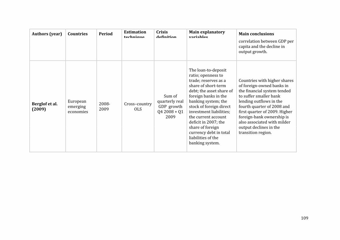
109
Authors (year) Countries Period Estimation technique
Crisis definition
Main explanatory variables
Main conclusions
correlation between GDP per capita and the decline in output growth.
Berglof et al. (2009)
European emerging economies
2008-2009
Cross–country OLS
Sum of quarterly real GDP growth
Q4 2008 + Q1 2009
The loan-to-deposit ratio; openness to trade; reserves as a share of short-term debt; the asset share of foreign banks in the banking system; the stock of foreign direct investment liabilities; the current account deficit in 2007; the share of foreign currency debt in total liabilities of the banking system.
Countries with higher shares of foreign-owned banks in the financial system tended to suffer smaller bank lending outflows in the fourth quarter of 2008 and first quarter of 2009. Higher foreign-bank ownership is also associated with milder output declines in the transition region.

110
Authors (year) Countries Period Estimation technique
Crisis definition
Main explanatory variables
Main conclusions
Balakrishnan et al. (2011)
26 advanced and emerging countries
1998-2003 2003-2009
Two stage econometric
analysis; cross-section
panel
Financial stress
Industrial production growth; commodity price growth; libor (3-month); bank linkages; portfolio linkages; direct investment linkages; trade linkages; US and Canada dummy; Western Europe dummy; trade openness; financial openness; current account; fiscal balance; foreign reserves.
Financial stress passes through rapidly to emerging economies. Financial links are the main channel of transmission of crisis. Emerging economies with higher levels of foreign liabilities to advanced economies have been more affected by the crisis that originated in advanced economies than emerging economies with lower foreign liabilities.
Jovičić (2010) Western Balkan countries
2009 VAR N/A Domestic production; exports
Countries with stronger trade ties with the EU experienced the crisis sooner. However, the countries with weaker trade ties with the EU had a larger decrease in production.

111
Authors (year) Countries Period Estimation technique
Crisis definition
Main explanatory variables
Main conclusions
Brezigar-Masten et al. (2011)
31 European countries
1996-2004
Cross-country panel
Real GDP per capita growth
Lagged GDP per capita growth; depth of national financial markets; inflation.
A high degree of financial integration did not increase the degree of financial fragility of transition countries and did not intensify the effects of the financial crises. They conclude that countries with a higher degree of financial openness had less of a credit decline during the GFC.
Berkmen et al. (2012)
40 emerging market economies
2009 Cross-country
OLS
Changes in the consensus forecast for 2009 between the averages of January–June 2009 and January–June 2008
Trade openness; Leverage; exchange rate peg dummy; EU accession dummy; cumulative credit growth.
Degree of leverage and cumulative credit growth and exchange rate policy explain a large share of the variation in the growth forecast revisions across these countries. Also the effect of leverage appears to have been stronger in the EU accession countries and there is weak evidence suggesting that a strong fiscal position helped shield countries from the effect of the GFC.

112
Authors (year) Countries Period Estimation technique
Crisis definition
Main explanatory variables
Main conclusions
De Hass et al. (2012)
1,294 banks in emerging Europe
1999-2009
Cross-section panel
Annual gross nominal credit growth
Vienna participation dummy variables; dummy for crisis;
Both domestic and foreign banks sharply reduced credit during the crisis, but foreign banks that participated in the Vienna Initiative were relatively more stable lenders.
dummy variables for private domestic, state or foreign banks.
Popov and Udell (2012)
16 emerging European countries
Survey data from 2005 and 2008 on 10,701 firms
Cross-section
A dummy variable equal to 1 if firm i in city j in country k
A matrix of firm characteristics; index of average bank balance sheet conditions; a matrix of country dummies; a matrix of industry dummies.
Firms' access to credit was affected by changes in the financial conditions of their parent banks.
in industry l is credit constrained in fiscal year 2007
113
Authors (year) Countries Period Estimation technique
Crisis definition
Main explanatory variables
Main conclusions
Ongena et al. (2015)
14 transition countries in Eastern Europe and Central Asia
2009 Cross-country Loan Growth
Internationally-borrowing domestic bank that equals one if the domestic bank borrowed at least once from the international wholesale market between 2004 and 2007 and equals zero otherwise; dummy foreign bank that equals one if the bank was foreign-owned in 2007 and equals zero otherwise.
Internationally borrowing domestic and foreign-owned banks contracted their credit more during the crisis than domestic banks that are funded only locally. Firms that are dependent on credit and at the same time have a relationship with an internationally borrowing domestic or a foreign bank suffer more in their financing and real performance.
Bonin and Louie (2015)
256 European bank subsidies in 8 ETEs
2004-2010
Cross-country panel
Real loan growth
GDP growth; assets, equity rationing; loans. deposits; ROAA; Inflation; Depreciation.
The 6 biggest European banks did not change their behavior in 8 ETEs under investigation during the GFC and the Eurozone debt crisis, whereas other foreign banks, in addition to contributing to credit boom prior to the GFC, also reduced their lending during the crises.
114
Authors (year) Countries Period Estimation technique
Crisis definition
Main explanatory variables
Main conclusions
Fadejeva et al. (2017)
41 emerging countries from Asia, the CESEE region including the Baltics, the CIS region, Latin America and EU.
Quarterly data from 1995Q1 to 2013Q4
GVAR N/A
Real GDP; change in prices; the real exchange rate; short term interest rates; and government bond yield; total credit to the private sector.
All shocks originating in the US and EU affect output and credit internationally, but with a different intensity. The study also finds that European emerging countries are more severely affected by these shocks than other emerging countries included in the sample.
Allen et al. (2017)
400 banks in CEE countries
1994-2010
Cross-section panel
Real growth in total loans
Deposit growth; liquidity (liquid assets to total assets); profitability (return on average assets); solvency (equity to asset); total bank assets to a country’s GDP as a measure of Size; parent bank-specific measures.
Lending behavior of foreign banks depended on the type of crisis; it remained constant during the domestic crises, while foreign crises were associated with decreased lending by foreign bank subsidies.
115
An important international transmission mechanism of the GFC highlighted in the
literature has been the restriction of credit, which, as discussed in section 1.2, has
particularly affected transition countries with a high degree of foreign bank
ownership. The EBRD (2009) claims that prior to the crisis, foreign financing, often
disproportionately funded by foreign banks, contributed to credit booms in these
countries. Moreover, most of this debt was denominated in foreign currency, which
increased the vulnerability of the region to external shocks. Milesi-Ferretti and Tille,
(2011) analyse capital flows in 75 countries (including ETEs) at a quarterly
frequency. They show that the global restriction of credit during the GFC in particular
affected those transition economies with a deeper international financial integration.
Similarly, Árvai et al. (2009) explore financial contagion focusing on financial
linkages. This study also draws attention to the important role of external financing
as a source of funding domestic credit growth. The authors explore the cross-border
exposures between emerging and advanced European countries. They present
indicators of contagion exposure which help identify the key points and spillover
effects and propagation channels of a shock that starts in a certain country. The
findings of this research highlight the relevance of financial interlinkages within
Europe and the high dependence of most of t h e Central, Eastern and Southern
European countries on Western European banks. The authors point out that even in
cases where exposures of CESE countries are diversified, interdependencies between
each other could trigger a regional contagion if one of the countries faces a shock.
However, their conclusions are mostly based on an interpretation of stylized facts,
without employing econometric techniques. Balakrishnan et al. (2011) develop a
new financial stress index for emerging economies to investigate how financial
stress is transmitted during crises, including the GFC. Based on a two- s t a g e
estimation, the authors assess the factors and intensity of transmission of stress
between advanced and emerging economies. In the first stage the degree of the
transmission of stress is estimated, while in the second stage differences and the
factors of co-movement are assessed. An annual panel data model employing
structural variables and policy variables is also used. The main results suggest
that financial stress passes rapidly to emerging economies. They suggest that
financial links are the main channel of transmission of crisis. They show that
emerging economies with a higher level of foreign liabilities to advanced economies
116
have been more affected by a crisis that originated in advanced economies than
emerging economies with lower foreign liabilities.
The determinants of credit growth during the GFC are analysed by De Hass et al.
(2012). By using data on 1,294 banks, the authors find that foreign banks reduced
lending earlier and deeper than did domestic banks in the 30 transition economies
they investigate. However, they show that countries that were part of the Vienna
Initiative were more stable sources of credit than those that did not participate in
this scheme. Similarly, Popov and Udell (2012), using survey data on 10,701 firms in
16 ETEs, find that firms’ credit access during the GFC was affected by the balance
sheet conditions of parent banks. Ongena et al. (2015) also find that banks that had
international funding sources as well as foreign-owned banks contracted lending
more during the GFC than did banks that had mainly domestic funding sources. Their
investigation employs bank-firm level data from Eastern Europe and Central Asia.
They also show that firms that relied on external funding were more severely
affected by the GFC. Another similar investigation assessing the lending behavior of
foreign banks during the GFC and the Eurozone debt crisis conducted by Bonin and
Louie (2015) provides additional insights. They show that the 6 biggest European
banks did not change their behavior in 8 ETEs under investigation during the GFC
and the Eurozone debt crisis, whereas other foreign banks, in addition to
contributing to credit boom prior to the GFC, also reduced their lending during the
crisis. Allen et al. (2017), using a panel data for 400 banks, also investigate the impact
of foreign bank ownership on lending behavior in Central and Eastern European
countries during the period 1994-2010. They find that the lending behavior of
foreign banks depended on the type of crisis; it remained constant during the crises
originating domestically, while crises that originated in foreign countries were
associated with decreased lending by foreign bank subsidies. A study that employs
the global vector auto-regression (GVAR) approach to investigate the international
transmission of aggregate demand, loan supply and loan demand shocks originating
in the USA and EU was conducted by Fadejeva et al. (2017). The findings of this
research revealed that all shocks originating in the US and EU affect output and credit
internationally, but with a different intensity. While aggregate demand and loan
demand shocks significantly affect output internationally, there is no evidence of
117
spillovers from loan supply shocks. The study also finds that European emerging
countries were more severely affected by these shocks due to their deep economic
integration with the EU, which exposed these countries to both EU and US shocks.
Consequently, the studies reviewed above provide evidence of the international
transmission of the crisis to the transition countries through financial linkages. These
studies point out the importance of foreign banks in international transmission of
shocks to these countries. However, this finding is not completely confirmed by
Berglöf et al. (2009); Lane and Milesi-Ferretti, (2011); Brezigar-Masten et al. (2011)
and Berkmen et al. (2012). These authors find no evidence that the presence of
foreign banks in transition countries have amplified the effects of the GFC.
Berkmen et al. (2012) employs cross-country regressions to try to explain the
differences in the severity of the GFC across developing and emerging economies. As a
proxy for the financial crisis impact on output, the authors focus on revisions of
projections for GDP growth, comparing the forecasts prior to and after the crisis in
September 2008. The authors use several explanatory variables in order to
capture the transmission of crisis through financial and trade channels. Another
group of variables such as current account deficit, level of reserves, level of
debt, credit growth etc, are used to capture the principal vulnerabilities and
financial structure and pre-existing conditions. For the basic regression, the authors
use the changes in the forecast between the averages of January–June 2009 and
January–June 2008 for 40 emerging economies. They find that the degree of
leverage and cumulative credit growth, as well as exchange rate policy, can
explain a high share of projected output decline in emerging countries. Moreover,
their results suggest that countries with a larger number of foreign banks experienced
less banking outflows in the fourth quarter of 2008 and the first quarter of 2009.
Similarly, they find that those emerging economies with a higher share of foreign-
owned banking assets suffered a softer output decline. The authors conclude that, in
general, the increasing level of financial integration has had a mixed effect in emerging
economies, since the foreign banks contributed to credit booms and external debts
but helped to stabilise the economies during the crisis. Similar results are reported by
Berglöf et al. (2009) who analyse the effects of the GFC on growth in emerging
Europe. They show that countries with higher shares of foreign-owned banking

118
assets experienced smaller bank lending outflows and milder output declines during
the GFC; whereas countries with larger pre-crisis credit booms, higher external debt
and hard pegs experienced larger output declines. The authors also argue that,
considering that foreign-owned banks have contributed to credit booms and external
debt accumulation, the effect of financial integration on the crisis in ETEs has been
mixed.
Lane and Milesi-Ferretti (2011) analyse whether the severity of the GFC depended on
pre-crisis macroeconomic and financial conditions, especially focusing on financial
linkages for a global sample of countries, including ETEs. They include
macroeconomic variables for 2008 and 2009 (though the 2009 data are based on
October 2009 projections) and they also include total domestic demand and
consumption. Their results suggest that pre-crisis factors such as a higher
development level, increasing economic activity and higher credit and trade
openness significantly increased the intensity of the crisis. On the other hand, they do
not find any evidence supporting the view that a higher level of financial integration
intensified the crisis. Brezigar-Masten et al. (2011) also investigate the role of
financial integration in transition countries’ growth, differentiating periods of
financial crisis from normal times. The authors conclude that a high degree of
financial integration did not increase the degree of financial fragility of transition
countries and did not intensify the effects of the financial crises. They conclude that
countries with a higher degree of financial openness had less of a credit decline
during the GFC. The final group of studies reviewed above find no evidence of the
importance of financial linkages in the international transmission of the GFC to
transition countries.
Trade appears to have been another important transmission channel of the crisis for
ETEs, considering that increasing trade deepening and rising trade integration with
the EU has made these countries more vulnerable to a reduction in export demand
(EBRD, 2009; Bartlett and Prica, 2012). A few studies have empirically investigated
this relationship and found a positive relationship between the impact of greater
trade linkages and the severity of the impact of the GFCC in transition countries (IMF,
2010; Jovicic, 2010; Blanchard, 2010; Lane and Milesi-Ferreti, 2011). Jovcic (2010)
using VAR modelling investigated the relationship between the strength of trade

119
linkages with the EU and the speed of contagion and the intensity of the crisis in
Western Balkan countries. The author shows that those countries with stronger
trade ties with the EU experienced the crisis sooner. However, the countries with
weaker trade ties with the EU had a larger decrease in production. On the other hand,
the IMF (2010) finds that, amongst other factors (higher pre-crisis vulnerabilities,
including pre-crisis credit booms), countries with a higher degree of trade
integration with the global economy were more severely affected by the crisis.
Blanchard et al. (2010) also show that trade and financial linkages as well as different
growth performances of partners in trade explain a large portion of the variability of
growth performance across transition countries during the GFC. Similarly, Lane and
Milesi-Ferretti (2011) show that international trade variables mattered during the
crisis. They find that countries more open to international trade and countries whose
main trading partners’ growth declined further during the crisis suffered larger
declines in capital inflows.
The review of the empirical studies presented above has shown that the majority of
the investigations have concentrated on financial linkages/financial integration as an
international channel of transmission of shocks, while less attention has been given
to trade linkages. More specifically, most of the studies reviewed above focus on the
degree of foreign-bank ownership and credit restriction during the GFC. However,
there is no consensus as to whether increased financial integration and foreign bank
ownership intensified the impact of the GFC on ETEs. While a number of the studies
reviewed above report a positive relationship between foreign-bank ownership and
the restriction of credit during the GFC, other studies claim that a higher degree of
foreign bank-ownership contributed to the resilience of the transition region.
Nevertheless, the latter group of studies acknowledge the contribution of foreign-
bank ownership in fuelling credit booms prior to the GFC. A potential explanation for
this difference in the results of the relationship between financial integration/foreign
bank ownership and crisis severity is the difference in sample/period coverage,
estimation technique adopted and measurement of the crisis severity.
A common weakness of most of the studies reviewed above, but also of other
empirical studies addressing the determinants of the severity of the GFC which can
lead to biased estimates, is the employment of inappropriate variables to measure

120
the impact of the GFC and define the crisis. The most commonly used measures have
been based on GDP growth/change in GDP growth or difference between forecast
and actual GDP growth and binary definition of the crisis presence during a certain
year/country. These might not be the most appropriate measures, given that using a
binary definition of the presence of a crisis does not provide a measure of the
intensity of the crisis nor does it take into account situations that do not completely
fit into a full-scale crisis, even though they might have a certain level of
macroeconomic impact. Likewise, using the difference between forecast and actual
GDP growth might lead to distorted results, given that forecasts for GDP growth for
2009 were made during 2008 when the initial effects of the crisis were already
present in most of these countries. Hence, the forecast GDP growth for 2009 already
took into consideration some of the effects of the crisis. Also, employing simply GDP
growth as a measure of the impact of the crisis might not provide accurate estimates,
considering that factors other than the crisis affect GDP growth and that these
studies have generally not controlled for such factors. Other measures of crisis
severity such as credit growth and financial stress indexes have also been
considered, which makes it difficult to reach conclusions regarding the severity of the
crisis.
An additional weakness of many of the studies reviewed above is that they have not
reported diagnostic tests regarding model specification, therefore the conclusions
reached regarding the determinants of the crisis severity should be interpreted with
some caution. With regards to estimation techniques, the majority of the studies
reviewed above adopted cross-country panel methods. However, other estimation
techniques such as VAR and GVAR have been adopted by some studies. It should be
pointed out that even though panel analysis is a well-established method,
nonetheless it is, normally, a single equations method with one endogenous variable
and other exogenous variables. Given the ambiguity of defining and measuring crisis
severity, other modelling approaches such as VAR and GVAR might be more
appropriate to model the transmission of financial crises as they treat all variables as
endogenous and provide full-system estimation where everything is allowed to
depend on everything else. In addition, the GVAR modelling approach allows for
interdependencies at international level and for long-run and short-run relationships

121
consistent with the theory and data. Overall GVAR provides a coherent and theory-
consistent solution to the issue of dimensionality in global modelling (Smith and
Galessi, 2014).
The limited number of studies that have investigated the transmission of the GFC to
ETEs have not considered certain factors such as the degree of integration with the
EU, and, in particular, the high but differing degrees of euroisation, although both are
key characteristics of ETEs. Furthermore, the majority of the studies reviewed above
have been carried out at country level, while there is a lack of studies that investigate
the transmission of the GFC to ETEs based on firm-level analysis. As Claessens and
Forbes (2004) point out, trade and financial linkages between countries are often
highly correlated; therefore, a firm-level investigation could provide additional
insights into the specific channels for the international transmission of crisis.
3.6 Conclusion
This chapter has provided an overview of the main empirical studies that have
investigated the international transmission of shocks through different channels
(cross-market asset correlations and individual channels of transmission of shocks)
before focusing on the determinants of the severity of GFC on ETEs. Although there
are a large number of empirical studies that have investigated the international
transmission of financial crises, the literature is still unable to provide conclusive
results on the determinants of crisis severity across countries. The studies reviewed
in this chapter provide a wide range of results, which are sometimes not in line with
the expectations suggested by orthodox theory. The analysis presented in this
chapter showed that the empirical results on the transmission of financial crises
based on cross-market correlation coefficients are inconclusive. More specifically,
when contagion was defined as a significant increase in cross-country asset
correlations following a crisis, without taking into account heteroscedasticity, the
authors found evidence of contagion, whereas when heteroscedasticity was
accounted for, no evidence of contagion was found. It was argued that the second
approach of testing for contagion, which is based on individual channels of
transmission of shocks, might provide more intuition on how exactly crisis has been
transmitted, as it distinguishes between different channels and propagation
122
mechanisms (e.g. trade and financial linkages, macroeconomic fundamentals).
However, in spite of the large number of empirical studies that have investigated the
transmission of financial crises based on individual channels of contagion, the results
remain inconclusive. To a large extent, the lack of conclusive results has been
attributed to measurement and misspecification errors of crisis severity. With
respect to crisis definition, the recent literature has most commonly focused on the
decline of GDP growth, cross-market correlation coefficients, financial stress indexes,
changes in capital flows and exchange rate tensions, which makes it difficult to reach
overall conclusions regarding the severity of the crisis.
The empirical studies investigating the transmission of the GFC to ETEs have
generally employed the second method of testing for contagion. The lack of studies
employing the first method of testing for contagion (based on cross-market
correlation confidents) has been attributed to the relatively low level of financial
market development in ETEs. The majority of the investigations have concentrated
on financial linkages/financial integration as an international channel of
transmission of shocks, while less attention has been given to trade linkages. As yet
there is no consensus as to whether the strengthening of financial linkages
intensified the impact of the GFC on ETEs. As for the estimation techniques, the
majority of the studies reviewed in this chapter have adopted cross-country panel
methods, while some studies also considered other methods such as GVAR and VAR.
Given the measurement and misspecification errors of crisis severity, it was argued
that panel analysis might not be the most appropriate method to test for
transmission of the GFC, since it is a single equation approach, with one endogenous
variable and other exogenous variables, which requires researchers to define and
measure crisis severity as a dependent variable. On the other hand, an approach such
as GVAR treats all variables as endogenous and is a full system approach to
estimation in which everything is allowed to depend on everything else. Therefore,
GVAR is considered a more appropriate approach to model interdependencies
between countries and international transmission of shocks.
The empirical review also disclosed that the limited number of studies that have
investigated the transmission of the GFC to ETEs have ignored factors such as
differing levels of integration with the EU, and, in particular, variations in the degree
123
of euroisation. In addition, it was shown that there is a complete lack of studies that
investigate the transmission of the GFC to ETEs based on firm-level analysis, which is
an important gap given (i) the argued correlations between trade and financial
linkages and (ii) the possibility that a firm-level investigation would provide more
insights into the specific channels of international transmission of crisis to ETEs. The
gaps identified in this chapter will be addressed empirically in Chapters 4 and 5. The
following chapter will investigate the international transmission of GDP and financial
shocks from 15 European advanced countries to 17 ETEs using the recently
developed GVAR approach, while Chapter 5 will investigate the transmission of the
GFC to 6 ETEs by employing firm-level data.

124
CHAPTER 4
EXPLAINING THE IMPACT OF THE GLOBAL FINANCIAL CRISIS ON EUROPEAN TRANSITION COUNTRIES: A GVAR APPROACH
Contents
4.1 Introduction ............................................................................................................................................. 125
4.2 The GVAR approach .............................................................................................................................. 126
4.3 Specification of data and variables ................................................................................................. 129
4.4 Empirical Approach .............................................................................................................................. 131
4.4.1 Specification and estimation of the country-specific models .......................................... 131
4.4.2 GVAR model specification ............................................................................................................... 137
4.4.3 Dynamic analysis using generalized impulse response functions and generalized forecast error variance decomposition ................................................................................................ 148
Impulse response functions of one standard error shock to GDP in EU ................................ 149
Generalized forecast error variance decomposition ...................................................................... 153
4.4.4 Robustness analysis .......................................................................................................................... 154
Impulse response functions of a one standard error shock to GDP in the EU ..................... 155
4.4.5 The effects of increased financial stress in the EU15 .......................................................... 164
Impulse response functions of a one standard error shock to CISS in EU ............................. 165
4.5 Conclusion ................................................................................................................................................. 167
125
4.1 Introduction
Chapter 2 of this thesis provided an overview of the theoretical framework within
which the international channels of transmission of the GFC are investigated. The
review presented in Chapter 3 showed that although there are a large number of
empirical studies that have investigated the international transmission of crises, the
literature is still unable to provide conclusive results of the determinants of crisis
severity across transition countries. To a large extent, the lack of conclusive results
has been attributed to measurement and misspecification errors of crisis severity.
With respect to crisis definition, the recent literature has most commonly focused on
the decline of GDP growth, cross-market correlation coefficients, financial stress
indexes, changes in capital flows and exchange rate tensions, which makes it difficult
to reach overall conclusions regarding the severity of the crisis. In addition, previous
studies have generally not reported diagnostic tests regarding model specification.
Furthermore, these studies have generally neglected to address the degree of
integration with the EU, and, in particular, the level of euroisation, even though these
are common characteristics of ETEs.
Understanding how external shocks transmit into domestic economies in ETEs is
important for policy makers. In order to investigate the interdependencies among
countries and to understand how shocks are transmitted internationally, a model
that accounts for these interdependencies and looks at them from a global
perspective is needed. Given the measurement and misspecification errors of crisis
severity presented in Chapter 3, it was argued that panel analysis might not be the
most appropriate method to test for transmission of the GFC, since it is a single
equation approach, with one endogenous variable and other exogenous variables,
which requires researchers to define and measure crisis severity as a dependent
variable. On the other hand, an approach such as GVAR treats all variables as
endogenous and, as such, is a full system approach to estimation in which everything
is allowed to depend on everything else. The main thing about the GVAR
methodology is time series depth. Single equation methods, whether they are cross
sectional or panel, are rooted in microeconomics, whereas in macroeconomic
analysis it is very difficult to distinguish between dependent and independent
variables and, potentially, everything is endogenous. That is why time series analysis
126
has developed a range of tools, most of which are in the platform of VAR and GVAR,
precisely to analyse interdependences. GVAR provides an effective way of modelling
interactions in a complex high-dimensional system such as the global economy.
Consequently, this chapter presents analyses of the international transmission of the
GFC in a global context. More specifically, by employing the global vector auto-
regression (GVAR) approach developed by Pesaran et al. (2004) and Dees et al.
(2007), this chapter investigates the international transmission of financial shocks to
ETEs.
The rest of this chapter is organized as follows. Section 4.2 provides an overview of
the GVAR modelling framework, its structure and applications. Section 4.3 specifies
the variables and data to be used in this investigation. Section 4.4 provides details of
the estimation technique adopted, specifying each step and presents the empirical
findings and diagnostic tests. The last section provides conclusions.
4.2 The GVAR approach
As reviewed in Chapter 2, there are many channels through which the international
transmission of shocks takes place. Transmission could be a result of the common
observed global shocks or other unobserved factors, but even when all common
factors are taken into account, there is likely to be important residual
interdependence that remains to be explained (Di Mauro and Pesaran, 2013).
Therefore, a global framework is needed to investigate the importance of sources of
international transmission of crises. In order to investigate the international
transmission of the global financial shocks to ETEs, in this chapter we use the Global
Vector Auto-Regression (GVAR) modelling framework. The GVAR approach,
developed by Pesaran et al. (2004) and further extended by Dées et al. (2007) and
Dées et al. (2009), can be used to investigate the international interdependencies
among countries and international channels of transmission of shocks (Dovern and
Roye, 2013). The main advantages of the GVAR modelling approach are that it allows:
(i) for interdependence at different levels (national or international) in a transparent
way that can be empirically evaluated; and (ii) for long-run relationships consistent
with theory together with short-run relationships consistent with the data and
provides a coherent, theory-consistent solution to the “curse of dimensionality” in

127
global modelling (Smith and Galesi, 2014). For a detailed description of the
methodology, this chapter refers to Di Mauro and Pesaran (2013).
GVAR combines separately estimated country-specific VARs into a global model. In
this model, domestic variables are linked to country-specific foreign variables, such
as foreign GDP or foreign exports. The latter are constructed from the domestic
variables based on certain weights in order to account for the international trade,
international finance or other interdependencies between countries. The country-
specific foreign variables serve as a proxy for common unobserved factors, such as
the diffusion of technological progress, or investors’ behaviour during times of
financial crisis or other determinants that we may not be able to measure, but it is
known that they are present and affect all the countries. However, even when all
these commonalities are accounted for, there might still be some residual
interdependencies due to policy or trade spillover effects. Therefore, in the GVAR
model the weighted combinations of observable factors are assumed to take into
account the unobservable factors. All country-specific variables are treated as
endogenous variables. Country-specific foreign variables are calculated and allowed
to directly influence domestic variables in the model. The foreign variables and
global variables are assumed to be weakly exogenous, assuming that every individual
country is a small economy compared to the rest of the world. More specifically, the
weak exogeneity of foreign variables means that domestic variables do not affect
foreign variables in the long run, while they are affected by them. This is the key
assumption of the GVAR modelling strategy since it allows country models to be
estimated individually and only at a later stage to be combined together (Di Mauro
and Pesaran, 2013). For every country, the standard VAR augmented with foreign
variables is estimated. The augmentation takes place at the country level, but once
the system as a whole is solved, we end up with a simple VAR. The general
specification of a country specific VARX* model is described below:
Suppose there are 𝑁 + 1 countries in the global economy, indexed by 𝑖 = 0,1,2, … ,𝑁,
where 𝑁 = 18 and country 0 is treated as the reference country (EU15 in our case) .
For each country 𝑖 an augmented 𝑉𝐴𝑅𝑋∗(𝑞𝑖, 𝑞𝑖∗) model, where 𝑞𝑖 and 𝑞𝑖
∗ are the lag
orders of the domestic and foreign variables respectively, can be written as follows:
128
𝑥𝑖𝑡 = a𝑖,0 + a𝑖,1𝑡 + ∑ 𝛼𝑖,𝑗𝑥𝑖,𝑡−𝑗 𝑞𝑖𝑗=1 + ∑ 𝛽𝑖,𝑗𝑥
∗𝑖,𝑡−𝑗
𝑞𝑖∗
𝑗=0 + ∑ 𝛾𝑖,𝑗𝑑𝑡−𝑗 𝑞𝑖𝑗=0 + 𝑢𝑖,𝑡, (4.1)
for 𝑡 = 0,1,2, … , 𝑇, and 𝑁 = 0,1,2, … ,𝑁, where 𝑥𝑖𝑡 is the 𝑘𝑖X 1 vector of country-
specific domestic or endogenous variables, 𝑥𝑖𝑡∗ is the 𝑘𝑖
∗𝑋 1 vector of country-specific
foreign variables (weakly exogenous), 𝑑𝑡a vector of global exogenous variable (here,
oil prices) that exist in every country VARX*, 𝑎𝑖0 is a constant, t is a linear trend, and
𝑢𝑖,𝑡 is the 𝑘𝑖X 1 vector of idiosyncratic, serially uncorrelated, country-specific shocks.
Foreign-specific variables are constructed as weighted averages across the domestic
variables of all countries, with the weights also being country-specific:
𝑥𝑖𝑡∗ = ∑ 𝑤𝑖𝑗
𝑁𝑗=0 𝑥𝑗𝑡 (4.2)
where 𝑤𝑖𝑗are a set of weights such that 𝑤𝑖𝑖 = 0 and the sum of all weights equals to 1.
The weights are determined to capture the importance of country j in the economy of
country i. The country specific VAR models can be transformed into error correction
forms (VECMX*) which allows a distinction between short-run and long-run
relationships and treatment of the long-run relationships as co-integrating. Even
though the VECMX* models are separately estimated on a country-by-country basis
taking potential cointegration between 𝑥𝑖𝑡 and 𝑥𝑖𝑡∗ x into account (Smith and Galesi,
2014), the GVAR model is solved for the whole system in which all variables are
endogenous. The GVAR model can allow interactions between countries through
three different channels: dependence of the domestic variables on foreign specific
variables and their lags; dependence of the domestic variables on global exogenous
variables such as oil prices; and dependence of shocks in country i on shocks in
country j (Di Mauro and Pesaran, 2013).
The GVAR model is a suitable tool for policy analysis, but it can be used more broadly.
For example, previously it has been used for analysing the transmission of shocks
(Galesi and Sgherri, 2009; Chudik and Fratszcher, 2011); credit risk (Pesaran et. al.,
2006); for forecasting purposes (Pesaran et. al. 2009); dynamics of global trade flows
(Bussière et al., 2009); and the role of oil prices in a global context (Rebucci and
Spatafora, 2006).
Galesi and Sgherri (2009) use a GVAR model to investigate the international
spillovers following slowdowns in U.S. equity prices. Their model contains 27
129
countries, including the United States, 17 European advanced economies, and 9
European emerging economies. They find that asset prices are the main channel
through which shocks are transmitted across countries in the short run, while the
cost and quantity of credit are important channels of transmission of shocks in the
long run. Chudik and Fratzscher (2011) through a GVAR model investigate the
importance of a tightening in liquidity conditions and collapse in risk appetite in the
international transmission of the GFC. They find that the tightening of financial
conditions was the most important transmission channel in advanced economies,
while the emerging market economies were more affected by the decline in risk
appetite. Bussière et al. (2009) use a GVAR model for a panel of 21 emerging market
and advanced economies to investigate the factors that influence the dynamics of
global trade flows. They model exports-imports response to three possible shocks: a
shock to U.S. output; a shock to the US real exchange rate; and a shock to German
output. They find that global exports are more affected by a shock to US output than
by a real effective depreciation of the dollar. Rebucci and Spatafora (2006) use a
GVAR model to investigate the role of oil prices in a global context. They find that
positive oil price shocks have a negative effect on the current account balance of non-
oil exporter countries including the US.
GVAR has not previously been used to model the transmission of financial shocks to
ETEs. Hence, in using the GVAR model to investigate the transmission of the GFC to
ETEs, this chapter will fill this gap in the literature.
4.3 Specification of data and variables
The first GVAR model will be estimated for 32 countries, including 17 ETEs5 and 15
European advanced economies (EU15)6, and using quarterly data for the period
2003Q1–2014Q4. Two types of variables are used to capture the main channels of
international financial contagion: trade and financial. The variable used to capture
the trade channel is exports. Since a major part of the theoretical and empirical
5 Albania, Bosnia and Herzegovina, Bulgaria, Croatia, the Czech Republic, Estonia, Hungary, Kosovo, Latvia, Lithuania, Macedonia, Montenegro, Poland, Romania, Serbia, Slovak Republic and Slovenia. 6 Austria, Belgium, Denmark, Finland, France, Germany, Greece, Ireland, Italy, Luxemburg, Netherlands, Portugal, Spain, Sweden and the United Kingdom.
130
review in previous chapters implies that exports are one of the main channels of
international transmission of shocks (Eichengreen et al., 1996; Glick and Rose, 1999;
Forbes, 2002; Ozgan and Unsal, 2012) the shocks in European advanced countries
are expected to affect more severely the ETEs with stronger trade links with them.
Quarterly data on exports are obtained from EUROSTAT, the World Bank and central
banks. The second group of variables will capture the international transmission of
the global financial shocks through financial linkages. A financial crisis in one country
can lead to direct financial effects, including reductions in foreign direct investment
and other capital flows abroad (Dornbusch et al, 2000; Cetorelli and Goldberg, 2011;
Milesi-Ferretti and Tille, 2011; Fratzscher, 2012). Since the GFC affected the EU15
financial sectors, transition countries with strong financial links with these advanced
economies are expected to have been more severely affected by the crisis. Therefore,
based on the overview of the impact of the GFC presented in Chapter 1 and literature
on the transmission of GFC presented in Chapters 2 and 3, the following variables are
used to capture the effect of transmission of crisis through the financial channel:
foreign credit flows; credit flows in foreign currencies; inward foreign direct
investment flows; and remittances. All these variables are expected to influence the
international transmission of the global financial shocks. Data on foreign direct
investment is obtained from the OECD, EUROSTAT and the European Commission;
and on foreign credit flows and credit flows in foreign currencies from the Bank of
International Settlements’ International Banking Statistics (BIS IBS). This analysis is
based on locational data, since these data are residence-based, therefore they are
expected to reflect whether conditions in specific ‘financial centre’ countries affect
flows to other countries, including flows to local subsidiaries. Data on remittances
are obtained from the World Bank database.
The third group of variables will capture the factors that might have amplified the
effects of the crisis on ETEs. They include: the degree of euroisation, namely, the
extent to which a country has assets and liabilities denominated in foreign currencies;
and the degree of integration with the EU. The degree of euroisation is measured by
the average of the share of foreign currency loans in total loans and of foreign
currency deposits in total deposits. Data on foreign currency loans and foreign
currency deposits are obtained from the EBRD, the ECB, the Bank for International

131
Settlements and national central banks. The degree of integration with the EU, is
captured by EU membership7 and partially by the trade and financial linkages
described in the previous paragraphs. Data from most of the sources are reported in
real terms. In cases when data were available only in nominal terms, they were
transformed into real terms by dividing the nominal time series with CPI.
4.4 Empirical Approach
The methodology proceeds through the following stages. First, the variables that
enter each country model are selected and the VAR model is extended with the
addition of a set of country-specific foreign variables. Second, the weights for
constructing the country-specific foreign variables are computed. In the third stage,
each variable in the model is tested for stationarity. Next, the VECM is specified for
each country, which means determining the lag order of the underlying VAR models
and testing for cointegration and the cointegrating ranks. Subsequently, different
diagnostic tests are checked and the global GVAR is solved. Accordingly, after
estimating the individual country VECMX* models as described, the corresponding
VARX* models are recovered as the platform for impulse-response analysis and
forecast error variance decomposition.
4.4.1 Specification and estimation of the country-specific models
The foreign country-specific variables are constructed as weighted averages of the
corresponding variables of other countries based on certain schemes of weights. In
theory, we could employ different weighting schemes for each country and variable,
but considering the relatively large number of countries, variables and schemes of
weights, this would result in an uncontrollable number of possible schemes. In
addition, the choice of weighting scheme depends on data availability. However, it is
important to know that using a bilateral weight based on a certain type of exposure,
i.e. trade or financial exposure, does not imply that the transmission channel
associated with the chosen type of exposure will be the only one captured by the
7 In section 4.4.2 the transmission of shocks from advanced EU countries to ETEs is analysed in sub-samples, which are defined by various country features, one of which is EU membership. Consequently, we address one of the main aims of the thesis, i.e. to analyse whether the degree of integration with the EU influenced the transmission of the global financial crisis to ETEs.
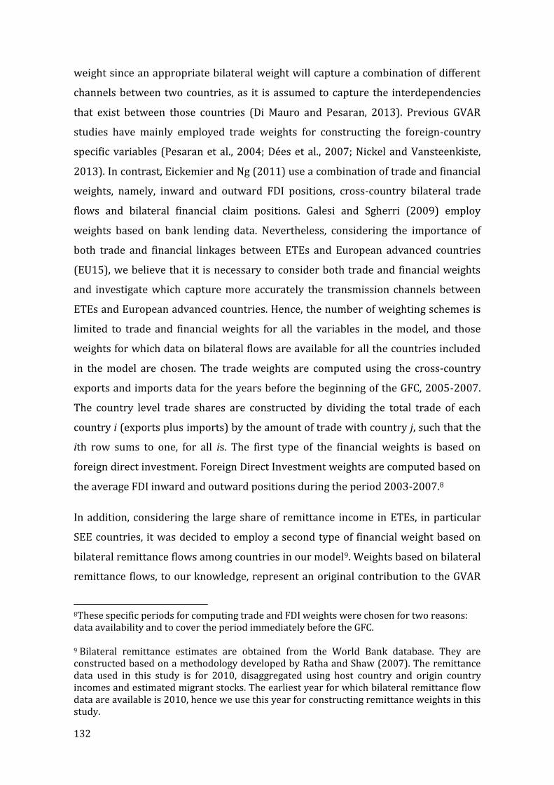
132
weight since an appropriate bilateral weight will capture a combination of different
channels between two countries, as it is assumed to capture the interdependencies
that exist between those countries (Di Mauro and Pesaran, 2013). Previous GVAR
studies have mainly employed trade weights for constructing the foreign-country
specific variables (Pesaran et al., 2004; Dées et al., 2007; Nickel and Vansteenkiste,
2013). In contrast, Eickemier and Ng (2011) use a combination of trade and financial
weights, namely, inward and outward FDI positions, cross-country bilateral trade
flows and bilateral financial claim positions. Galesi and Sgherri (2009) employ
weights based on bank lending data. Nevertheless, considering the importance of
both trade and financial linkages between ETEs and European advanced countries
(EU15), we believe that it is necessary to consider both trade and financial weights
and investigate which capture more accurately the transmission channels between
ETEs and European advanced countries. Hence, the number of weighting schemes is
limited to trade and financial weights for all the variables in the model, and those
weights for which data on bilateral flows are available for all the countries included
in the model are chosen. The trade weights are computed using the cross-country
exports and imports data for the years before the beginning of the GFC, 2005-2007.
The country level trade shares are constructed by dividing the total trade of each
country i (exports plus imports) by the amount of trade with country j, such that the
ith row sums to one, for all is. The first type of the financial weights is based on
foreign direct investment. Foreign Direct Investment weights are computed based on
the average FDI inward and outward positions during the period 2003-2007.8
In addition, considering the large share of remittance income in ETEs, in particular
SEE countries, it was decided to employ a second type of financial weight based on
bilateral remittance flows among countries in our model9. Weights based on bilateral
remittance flows, to our knowledge, represent an original contribution to the GVAR
8These specific periods for computing trade and FDI weights were chosen for two reasons: data availability and to cover the period immediately before the GFC. 9 Bilateral remittance estimates are obtained from the World Bank database. They are constructed based on a methodology developed by Ratha and Shaw (2007). The remittance data used in this study is for 2010, disaggregated using host country and origin country incomes and estimated migrant stocks. The earliest year for which bilateral remittance flow data are available is 2010, hence we use this year for constructing remittance weights in this study.

133
modelling framework. Trade, FDI and remittance weights are presented in tables
4.1a, 4.1b and 4.1c below.

134
Table 4.1a Trade weights used for computing foreign country-specific variables
Note: Bilateral weights are shown in columns and sum up to one. There is one column for each country in the sample; across the columns row totals have no meaning. Weights are calculated based on average trade flows (sum of exports and imports) among countries for the period 2005-2007. Rows represent the origin country and columns the partner countries; i.e. if we look at Albania, we can see that Bosnia and Herzegovina accounted for 0.4% of the total trade (exports + imports) of Albania during the period 2005-2007, Bulgaria 2.8%, and Croatia 1.3% (the same interpretation applies to all other countries).
Countries Alb bosn Bulg croat czeck esto Hung koso Latv Lithu maced monte pola roma Serbi slovak sloven EU15
alb 0 0.0013 0.0036 0.0013 0.0001 0.0000 0.0004 0.0361 0.0000 0.0000 0.0135 0.0064 0.0001 0.0006 0.0036 0.0001 0.0009 0.0142
bosn 0.0038 0 0.0041 0.0865 0.0011 0.0001 0.0039 0.0250 0.0001 0.0001 0.0215 0.0390 0.0008 0.0030 0.0744 0.0009 0.0297 0.0083
bulg 0.0278 0.0123 0 0.0110 0.0031 0.0006 0.0061 0.0507 0.0013 0.0020 0.0897 0.0035 0.0032 0.0257 0.0387 0.0030 0.0072 0.0718
croat 0.0134 0.2548 0.0113 0 0.0037 0.0003 0.0112 0.0299 0.0008 0.0008 0.0473 0.0405 0.0024 0.0043 0.0406 0.0035 0.0760 0.0368
czeck 0.0104 0.0228 0.0215 0.0255 0 0.0097 0.0435 0.0100 0.0172 0.0186 0.0111 0.0156 0.0589 0.0280 0.0206 0.1963 0.0281 0.2253
esto 0.0000 0.0002 0.0005 0.0004 0.0013 0 0.0018 0.0000 0.1269 0.0685 0.0001 0.0001 0.0039 0.0003 0.0004 0.0008 0.0006 0.0702
hung 0.0097 0.0588 0.0264 0.0361 0.0343 0.0151 0 0.0193 0.0111 0.0108 0.0108 0.0384 0.0325 0.0715 0.0545 0.0761 0.0387 0.1830
koso 0.0000 0.0000 0.0007 0.0000 0.0000 0.0000 0.0001 0 0.0000 0.0000 0.0000 0.0013 0.0000 0.0001 0.0000 0.0000 0.0023 0.0012
latv 0.0000 0.0001 0.0009 0.0003 0.0016 0.1053 0.0013 0.0000 0 0.1193 0.0001 0.0000 0.0060 0.0004 0.0006 0.0018 0.0007 0.0322
lithu 0.0000 0.0002 0.0018 0.0009 0.0027 0.0815 0.0021 0.0000 0.1806 0 0.0003 0.0000 0.0137 0.0010 0.0010 0.0021 0.0017 0.0372
maced 0.0236 0.0120 0.0220 0.0117 0.0003 0.0000 0.0010 0.2343 0.0000 0.0001 0 0.0104 0.0006 0.0015 0.0350 0.0003 0.0056 0.0185
monte 0.0009 0.0000 0.0001 0.0024 0.0001 0.0000 0.0006 0.0141 0.0000 0.0000 0.0022 0 0.0001 0.0001 0.0519 0.0000 0.0035 0.0035
pola 0.0070 0.0176 0.0284 0.0215 0.0705 0.0391 0.0515 0.0133 0.0759 0.1261 0.0295 0.0123 0 0.0377 0.0223 0.0679 0.0268 0.0200
roma 0.0107 0.0227 0.0689 0.0122 0.0098 0.0009 0.0424 0.0135 0.0010 0.0024 0.0216 0.0097 0.0109 0 0.0366 0.0128 0.0127 0.1134
serbi 0.0040 0.0000 0.0250 0.0147 0.0019 0.0003 0.0079 0.1914 0.0006 0.0002 0.0818 0.2718 0.0013 0.0042 0 0.0032 0.0266 0.0196
slovak 0.0020 0.0086 0.0112 0.0117 0.0893 0.0026 0.0420 0.0028 0.0069 0.0053 0.0049 0.0024 0.0257 0.0146 0.0200 0 0.0181 0.0858
sloven 0.0086 0.1534 0.0131 0.0949 0.0069 0.0015 0.0118 0.0572 0.0019 0.0029 0.0413 0.0595 0.0058 0.0086 0.0619 0.0088 0 0.0590
EU15 0.8779 0.4353 0.7605 0.6690 0.7734 0.7430 0.7724 0.3024 0.5756 0.6430 0.6244 0.4891 0.8342 0.7984 0.5380 0.6224 0.7208 0
135
Table 4.1b FDI weights
Note: Bilateral weights are shown in columns and sum up to one. FDI weights are computed based on the average FDI inflows from each country in the sample during the period 2003-2007.
Countries alb bosn bulg croat Czeck esto hung koso latv lithu maced monte pola roma serbi slovak sloven EU15
alb 0 0.0000 0.0000 0.0000 0.0041 0.0000 0.0000 0.0000 0.0000 0.0000 0.0197 0.0000 0.0000 0.0000 0.0000 0.0000 0.0000 0.0659
bosn 0.0000 0 0.0000 0.0167 0.0000 0.0000 0.0000 0.0000 0.0000 0.0000 0.0001 0.0000 0.0000 0.0000 0.0000 0.0000 0.0003 0.0000
bulg 0.0000 0.0000 0 0.0000 0.0000 0.0000 0.0000 0.0000 0.0000 0.0000 0.0000 0.0000 0.0000 0.0000 0.0000 0.0000 0.0000 0.0000
croat 0.0000 0.4184 0.0000 0 0.0000 0.0000 0.0000 0.0000 0.0000 0.0000 0.0394 0.0000 0.0000 0.0000 0.0000 0.0000 0.2567 0.0363
czeck 0.0001 0.0012 0.0100 0.0030 0 0.0010 0.0243 0.0000 0.0014 0.0006 0.0018 0.0000 0.0127 0.0052 0.0000 0.6296 0.0026 0.0929
esto 0.0000 0.0000 0.0000 0.0000 0.0000 0 0.0000 0.0000 0.0321 0.0056 0.0000 0.0000 0.0000 0.0000 0.0000 0.0000 0.0000 0.0017
hung 0.0001 0.0001 0.0034 0.0015 0.0021 0.0011 0 0.0000 0.0006 0.0002 0.0001 0.0246 0.0018 0.0797 0.0000 0.0063 0.0010 0.1488
koso 0.0000 0.0000 0.0000 0.0000 0.0000 0.0000 0.0000 0 0.0000 0.0000 0.0000 0.0000 0.0000 0.0000 0.0000 0.0000 0.0000 0.0000
latv 0.0000 0.0000 0.0000 0.0000 0.0000 0.0563 0.0000 0.0000 0 0.0391 0.0000 0.0000 0.0004 0.0000 0.0000 0.0000 0.0000 0.0087
lithu 0.0000 0.0000 0.0000 0.0000 0.0001 0.0111 0.0003 0.0000 0.0538 0 0.0000 0.0000 0.0012 0.0000 0.0000 0.0000 0.0000 0.0043
maced 0.0602 0.0022 0.0000 0.0000 0.0000 0.0000 0.0000 0.0000 0.0000 0.0000 0 0.0000 0.0000 0.0000 0.0338 0.0000 0.0000 0.0000
monte 0.0000 0.0000 0.0000 0.0000 0.0000 0.0000 0.0000 0.0000 0.0000 0.0000 0.0000 0 0.0000 0.0000 0.0000 0.0000 0.0000 0.0000
pola 0.0000 0.0028 0.0043 0.0016 0.0255 0.0049 0.0055 0.0000 0.0250 0.3116 0.0008 0.0000 0 0.0015 0.0000 0.0037 0.0015 0.5729
roma 0.0000 0.0000 0.0392 0.0026 0.0000 0.0000 0.0217 0.0000 0.0000 0.0000 0.0000 0.0000 0.0000 0 0.0000 0.0000 0.0000 0.0127
serbi 0.0000 0.0000 0.0000 0.0000 0.0000 0.0000 0.0000 0.0000 0.0000 0.0000 0.0000 0.0000 0.0000 0.0000 0 0.0000 0.0000 0.0000
slovak 0.0000 0.0003 0.0023 0.0009 0.2567 0.0002 0.0545 0.0000 0.0005 0.0001 0.0097 0.0000 0.0023 0.0012 0.0000 0 0.0015 0.0436
sloven 0.0001 0.0687 0.0004 0.0469 0.0011 0.0000 0.0009 0.0629 0.0000 0.0000 0.0538 0.0000 0.0001 0.0002 0.0000 0.0000 0 0.0122
EU15 0.9393 0.5063 0.9404 0.9268 0.7105 0.9254 0.8928 0.9370 0.8867 0.6428 0.8747 0.9754 0.9816 0.9123 0.9662 0.3603 0.7363 0

136
Table 4.1c Remittance weights
Note: Bilateral weights are shown in columns and sum up to one. The remittance weights are constructed based on the sum of incoming remittances from each country in the sample in 2010.
Countries Alb bosn bulg croat czeck esto hung koso latv lithu maced monte pola roma Serbi slovak sloven EU15
alb 0 0.0000 0.0008 0.0003 0.0003 0.0000 0.0000 0.0624 0.0000 0.0000 0.0095 0.0002 0.0000 0.0000 0.0000 0.0000 0.0003 0.0049
bosn 0.0000 0 0.0000 0.0224 0.0000 0.0000 0.0000 0.0017 0.0000 0.0028 0.0015 0.0117 0.0000 0.0004 0.0070 0.0005 0.0448 0.0042
bulg 0.0179 0.0001 0 0.0001 0.0056 0.0014 0.0118 0.0252 0.0006 0.0049 0.0342 -
0.0002 0.0003 0.0041 0.0077 0.0001 0.0018 0.0292
croat 0.0045 0.2124 0.0003 0 0.0000 0.0009 0.0290 0.0090 0.0002 0.0001 0.0233 0.0298 0.0003 0.0001 0.0308 0.0001 0.1405 0.0320
czeck 0.0032 0.0012 0.0207 0.0017 0 0.0003 0.0037 0.0017 0.0013 0.0019 0.0006 0.0038 0.0022 0.0145 0.0013 0.1012 0.0106 0.1980
esto 0.0000 0.0000 0.0026 0.0000 0.0000 0 0.0000 0.0000 0.1709 0.0926 0.0009 0.0061 0.0005 0.0000 0.0004 0.0001 0.0000 0.0219
hung 0.0010 0.0064 0.0373 0.0871 0.0038 0.0002 0 0.0000 0.0001 0.0010 0.1799 0.1064 0.0051 0.0204 0.0167 0.0624 0.0056 0.2108
koso 0.0000 0.0000 0.0000 0.0000 0.0000 0.0000 0.0000 0 0.0000 0.0000 0.0000 0.0000 0.0000 0.0000 0.0000 0.0000 0.0000 0.0006
latv 0.0000 0.0000 0.0049 0.0000 0.0000 0.0902 0.0000 0.0000 0 0.0726 0.0000 0.0113 0.0003 0.0000 0.0011 0.0002 0.0002 0.0099
lithu 0.0000 0.0020 0.0063 0.0001 0.0000 0.0955 0.0001 0.0000 0.0595 0 0.0000 0.0065 0.0081 0.0002 0.0016 0.0002 0.0000 0.0151
maced 0.0000 0.0000 0.0020 0.0013 0.0000 0.0000 0.0073 0.0093 0.0000 0.0000 0 0.0033 0.0000 0.0000 0.0032 0.0000 0.0193 0.0025
monte 0.0000 0.0017 0.0003 0.0018 0.0000 0.0000 0.0022 0.0000 0.0007 0.0000 0.0007 0 0.0000 0.0000 0.0113 0.0000 0.0088 0.0014
pola 0.0000 0.0044 0.0033 0.0040 0.0170 0.0045 0.0061 0.0000 0.0050 0.1444 0.0009 0.0056 0 0.0037 0.0018 0.0035 0.0095 0.2792
roma 0.0001 0.0001 0.0091 0.0006 0.0050 0.0022 0.0193 0.0000 0.0001 0.0022 0.0003 0.0003 0.0022 0 0.0057 0.0000 0.0030 0.0841
serbi 0.0000 0.1814 0.0031 0.0145 0.0000 0.0000 0.0047 0.0065 0.0000 0.0024 0.0340 0.1363 0.0002 0.0031 0 -0.0003 0.0887 0.0168
slovak 0.0000 0.0068 0.0006 0.0004 0.0415 0.0006 0.0369 0.0003 0.0013 0.0016 0.0000 0.0006 0.0020 0.0004 -0.0009 0 0.0032 0.0658
sloven 0.0001 0.1136 0.0019 0.0603 0.0015 0.0000 0.0011 0.1552 0.0001 0.0000 0.1120 0.0603 0.0011 0.0005 0.0719 0.0007 0 0.0232
EU15 0.9732 0.4698 0.9067 0.8054 0.9251 0.8042 0.8778 0.7287 0.7603 0.6735 0.6022 0.6181 0.9777 0.9526 0.8404 0.8313 0.6636 0

137
4.4.2 GVAR model specification
We use the GVAR Toolbox 2.0 developed by Smith and Galesi (2014) to estimate the
model. At the onset of the analysis, following the literature review in previous
chapters, the EU15 countries are aggregated into a region in order to be able to treat
it as the base ‘country’ and so capture its impact on the ETEs.
With the exception of the EU15 model, all country models include the same set of
variables, when data are available. The following domestic variables enter each
country model: GDP, gdp; exports, exp; foreign direct investment inward flows, FDI;
foreign credit flows, fcf; remittances, rem; and the foreign credit flows in foreign
currency, eur. The global variable price of oil, poil, enters as a weakly exogenous
variable in all country models. Considering the importance of the EU15 variables for
the other countries and the EU15's size compared to the transition countries and its
dominance in the region, it is not expected that other transition countries' variables
will significantly affect the EU variables, therefore, following the practice adopted in
the GVAR literature, the foreign country-specific variables are not included in the EU
model. Other country models include all the foreign country-specific variables. GDP,
exports, FDI, foreign credit flows, credit flows in foreign currencies and remittances
are measured in real terms and transformed to logs. In addition, the cubic spline
interpolation was used to convert annual data into quarterly data for several
variables and countries for earlier years where data were not available on a quarterly
basis. It has to be noted that this technique can only provide estimates of data
between known data points; it cannot create new “unknown” data. The variable
specifications are presented in Table 4.2 below.

Table 4.2 Variable specification of country VARX*10 models
Variable Description Expected impact
Source Units of measurement
Frequency EU model
Non-EU Model
Foreign Variables
EU model
Non-EU Model
gdp Gross Domestic Product
n/a EUROSTAT, World Bank log quarterly gdp*
exp Exports Negative EUROSTAT, World Bank, central banks
log quarterly exp*
fdi Foreign Direct Investment
Negative OECD, EUROSTAT, European Commission
log quarterly fdi*
fcf Foreign Credit Flows
Negative Bank of International Settlements
log quarterly fcf*
rem Remittances Negative World Bank log quarterly rem*
eur
Euroisation - foreign credit flows in foreign currencies
Negative OECD, EUROSTAT, European Commission
log quarterly eur*
poil Price of oil n/a World Bank log quarterly
10 * represents the foreign country-specific variables included in the model.

139
Before proceeding with the next stage of GVAR estimation, different information
criteria are checked and, based on their results, the benchmark model with respect to
weighting schemes is selected. More specifically, the performance of the GVAR model
in terms of stability (related to its eigenvalues) persistence profiles and impulse
response functions is compared under different weighting schemes. These three
indicators are crucial with regards to overall stability and performance of the GVAR
model (Pesaran et al., 2004; Eickemeier and Ng, 2011; Smith and Galesi, 2014). In the
case of I(1) cointegrated variables, the eigenvalues should lie on or inside the unit
circle, i.e. no eigenvalue should be above 1. The persistence profiles refer to the time
profiles of the effects of system or variable-specific shocks on the cointegrating
relations in the GVAR model (Pesaran and Shin, 1996, 1998) and they have a value of
unity on impact, while they should tend to zero as n→∞. It was observed that the
GVAR model that uses only trade weights provides the best performance in terms of
these indicators (no eigenvalues that lie above the unit circle, persistence profiles
converge to zero, while the impulse responses, which will be discussed latter, are
statistically and economically more significant, hence, it was selected as the
benchmark model. The next section presents the diagnostic tests for the benchmark
model.
Unit root tests
The standard Dickey-Fuller unit-root tests and weighted symmetric (WS) ADF tests
(Park and Fuller, 1995) are estimated11. Leybourne et al. (2005) provide evidence of
the superior performance of the weighted symmetric test statistic compared to the
standard ADF test or the GLS-ADF test proposed by Elliot et al. (1996). The lag length
employed in the ADF and WS unit root tests is selected to be 1 for all countries (see
the next section for further details). Results of the ADF and WS statistics are provided
for the level, first differences and second differences of all the country and region-
specific domestic and foreign, as well as for the global variables. The results at the
5% significance level suggest that for the majority of the variables the null of non-
stationarity cannot be rejected (refer to Table 4.3 below for the number of rejections
of the null hypothesis of non-stationarity, while for the complete set of results, refer
11 The current version of the GVAR toolbox used for estimation of the model does not allow control for structural breaks.

to tables A4.6 and A4.7 in appendix A4). The test results show that GDP is mostly I(1)
or borderline I(1) - I(2) (e.g. for Bosnia and Herzegovina, Kosovo, Montenegro and
the Slovak Republic). Exports are I(1) variables for all countries, except for Poland
where they appear to be I(2). FDI is mostly I(1), except for Bulgaria and Croatia,
where it appears to be I(2). Remittances appear to be I(0) variables in Estonia, Latvia,
Lithuania and the Slovak Republic, while in all other countries they are I(1). Foreign
credit flows is I(0) in Albania and I(2) in Bulgaria, Croatia, Latvia, Lithuania and
Romania. Euroisation is mostly I(1), except for Albania, where it is I(0) and Bulgaria
and Latvia, where it is I(2).
Since GDP, exports, FDI and remittances are usually considered as I(1) variables in
the literature, and taking into account that Dickey-Fuller unit-root tests and weighted
symmetric ADF tests do not perform well when the number of observations is
relatively small, after looking at the data plots, we assume these variables to be I(1)
for all the countries, which allows for long-run cointegration among them. It is
important to note that GVAR can be estimated in the presence of I(0) variables.
However, cointegration exists only between I(1) variables. The estimation of the
model continues under the assumptions of the weak exogeneity of the country-
specific foreign variables and stability of the parameters, which are both needed for
the GVAR estimation and will be tested at a later stage.

141
Table 4.3 Number of rejection of the null hypothesis of non-stationarity12
Selecting lag length and cointegration rank
In the next stage, the specifications for individual country models are selected.
Initially, the order of the individual country VARX models, pi and qi is determined,
corresponding to the lag orders of domestic and foreign variables, respectively. The
lag orders are selected according to the Akaike information criterion under the
constraints imposed by data limitations, where the maximum lag order of domestic
variables was selected to be 2, while the maximum lag order of foreign variables was
selected to be 1. However, considering the small number of observations, whilst
taking into account the results of the serial correlation diagnostics, eigenvalues of the
model and persistence profiles, and following the practice adopted in the GVAR
literature, the number of lags is reduced to 1 for both domestic and foreign variables
in all countries.
The choice of cointegration rank is a crucial step in the empirical analysis,
considering that a misspecification of the long-run relationships can destabilise the
GVAR model and distort the results and impulse response functions (Bussière et al.,
2009). The VARX* can manage within and between country cointegration, and as a
result country-specific foreign variables also need to be considered for the long-run
relationships (Pesaran and Smith, 2006), as there are many international long-run
relationships, e.g. the relationship between remittances and remittance-sending
12 Again, we note that the current version of the GVAR toolbox used for estimation of the model does not allow control for structural breaks.
Variables
Number of countries with I(0) variables
Number of countries with I(2) variables
Number of countries with I(1) variables (from 18)
Gdp 0 4 14
exp 0 1 17
FDI 0 2 16
fcf 1 5 12
rem 4 0 14
eur 1 2 15
countries' economic performance / GDP. It should be noted that when the sample is
small, the asymptotic distributions are generally poor approximations to the true
distributions and can result in substantial size and power distortions (Juselius,
2006). However, the definition of a "small" or "big" sample is not straightforward,
being based on the number of observations and also on the amount of information in
the data. When the data are very informative about a hypothetical long-run relation,
we might have good test properties even if the sample period is relatively short
(Juselius, 2006). It is also important to note that the cointegration rank is not in
general equivalent to the number of theoretical equilibrium relations derived from
an economic model. Namely, cointegration between variables is a statistical property
of the data that only exceptionally can be given a direct interpretation as an economic
equilibrium relation. The reason for this is that a theoretically meaningful relation
can be a linear combination of several ‘irreducible’ cointegration relations (Davidson,
2002). The rank orders of the VARX models are estimated based on Johansen’s trace
statistic, as set out in Pesaran et al. (2000) for models with weakly exogenous I(1)
regressors. The critical values for models including weakly exogenous variables are
obtained from Mackinnon et al. (1999). However, considering that the GVAR model
with the reported integrating relations (table 4.4) was not stable, i.e. there were a
number of eigenvalues lying above the unit circle and the persistent profiles did not
converge to zero even after 40 periods, then following Smith and Galesi (2014), the
number of cointegrating relations was decreased in the countries where the
persistence profiles did not converge to zero after 40 periods, or where they did
converge to zero in a manner that clearly indicated a problem in the underlying
vector. Table 4.4 below reports the final order of the VARX* models and the number
of cointegration relations. The persistence profiles under the final number of
cointegrating vectors are presented in Figure A4.8 in appendix A4.

143
Testing for weak exogeneity
The main assumption of the GVAR methodology is the weak exogeneity of foreign
variables. After estimating each country model, the weak exogeneity hypothesis of
country-specific foreign variables and global variables (oil prices) has to be tested.
The weak exogeneity assumption is verified by employing a test developed by
Johansen (1992) and Harbo et al. (1998) which checks the joint significance of the
estimated error correction terms in auxiliary equations for the country-specific
foreign variables. In particular, for each 𝑙𝑡ℎelement of 𝑋𝑖𝑡∗ the following regression is
carried out:
∆𝑥𝑖𝑡,𝑙 = a𝑖,𝑙 + ∑ 𝛿𝑖𝑗,𝑙𝑟𝑖𝑗=1 𝐸𝐶𝑀𝑖𝑗,𝑡−1 + ∑ 𝛷𝑖𝑘,𝑙
𝑞𝑖𝑘=1 ∆𝑥𝑖,𝑡−𝑘 +∑ ¥𝑖𝑚,𝑙∆𝑥 𝑖,𝑡−𝑚
∗ + ɳ𝑖𝑡,𝑙𝑞𝑖∗𝑚=1 (4.3)
Table 4.4 Chosen lag length and cointegration rank
Country p q
Number of cointegrating
relations based on Johansen
trace statistics
Final number of
cointegrating relations
ALBANIA 1 1 5 2 BOSNIA 1 1 3 2 BULGARIA 1 1 4 4 CROATIA 1 1 3 3 CZECK REPUBLIC
1 1 4 4
ESTONIA 1 1 3 3 EURO 1 1 0 0 HUNGARY 1 1 2 2 KOSOVO 1 1 2 2 LATVIA 1 1 4 4 LITHUANIA 1 1 3 3 MACEDONIA 1 1 3 3 MONTENEGRO 1 1 4 1 POLAND 1 1 3 3
ROMANIA 1 1 3 3 SERBIA 1 1 2 2 SLOVAK REPUBLIC
1 1 3 3
SLOVENIA 1 1 4 4

where 𝐸𝐶𝑀𝑖𝑗,𝑡−1, 𝑗 = 1, 2,…, 𝑟𝑖, are the estimated error-correction terms corresponding
to the 𝑟𝑖 cointegrating relations found for the ith country model, 𝑥𝑖𝑡∗ is the 𝑘𝑖
∗𝑋 1
vector of country-specific foreign variables that have to be weakly exogenous, 𝑞𝑖 and
𝑞𝑖∗ are the lag orders of the domestic and foreign variables respectively, 𝑎𝑖,𝑙 is a
constant, t is a linear trend, and ɳ𝑖𝑡,𝑙 is the 𝑘𝑖X 1 vector of idiosyncratic, serially
uncorrelated, country-specific shocks. For the weak exogeneity assumption to hold,
the ECM of the above equation must not be statistically significant. The test for weak
exogeneity is a F-test of the joint hypothesis that
𝛿𝑖𝑗,𝑙 = 0, j= 1,2,…, 𝑟𝑖 in the above regression.
A weakly exogenous variable can be defined as a variable whose value does not
depend on the contemporaneous values of the endogenous variables, but may
depend on lagged values of these variables. Formally, the weak exogeneity of foreign
variables means that domestic variables do not affect foreign variables in the long-
run, while they are affected by them. This assumption allows proper identification of
the co-integration relation as noted in Johansen (1992). The results of the test are
reported in Table 4.5 below. These suggest that the weak exogeneity assumption is
not rejected for most of the variables. Nevertheless, the weak exogeneity assumption
is rejected at the 5% significance level for the following two variables: exports from
Macedonia and foreign credit flows to Montenegro. Even though, based on the results
of the test, weak exogeneity holds for all variables of the EU15 region, we decided to
exclude all the foreign variables in the EU15 model, since EU15 is considered as the
dominant ‘country’ in our model and we would not expect other smaller countries to
significantly affect its variables.
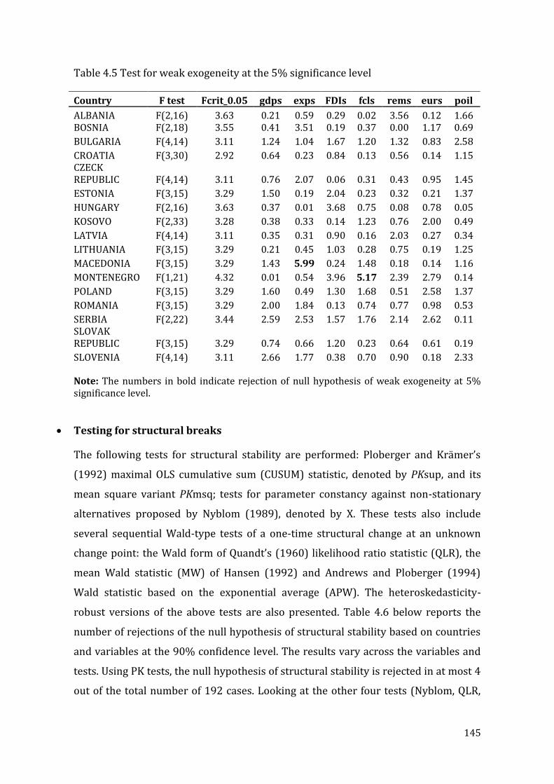
145
Table 4.5 Test for weak exogeneity at the 5% significance level
Note: The numbers in bold indicate rejection of null hypothesis of weak exogeneity at 5% significance level.
Testing for structural breaks
The following tests for structural stability are performed: Ploberger and Krämer’s
(1992) maximal OLS cumulative sum (CUSUM) statistic, denoted by PKsup, and its
mean square variant PKmsq; tests for parameter constancy against non-stationary
alternatives proposed by Nyblom (1989), denoted by X. These tests also include
several sequential Wald-type tests of a one-time structural change at an unknown
change point: the Wald form of Quandt’s (1960) likelihood ratio statistic (QLR), the
mean Wald statistic (MW) of Hansen (1992) and Andrews and Ploberger (1994)
Wald statistic based on the exponential average (APW). The heteroskedasticity-
robust versions of the above tests are also presented. Table 4.6 below reports the
number of rejections of the null hypothesis of structural stability based on countries
and variables at the 90% confidence level. The results vary across the variables and
tests. Using PK tests, the null hypothesis of structural stability is rejected in at most 4
out of the total number of 192 cases. Looking at the other four tests (Nyblom, QLR,
Country F test Fcrit_0.05 gdps exps FDIs fcls rems eurs poil
ALBANIA F(2,16) 3.63 0.21 0.59 0.29 0.02 3.56 0.12 1.66 BOSNIA F(2,18) 3.55 0.41 3.51 0.19 0.37 0.00 1.17 0.69
BULGARIA F(4,14) 3.11 1.24 1.04 1.67 1.20 1.32 0.83 2.58
CROATIA F(3,30) 2.92 0.64 0.23 0.84 0.13 0.56 0.14 1.15 CZECK REPUBLIC F(4,14) 3.11 0.76 2.07 0.06 0.31 0.43 0.95 1.45
ESTONIA F(3,15) 3.29 1.50 0.19 2.04 0.23 0.32 0.21 1.37
HUNGARY F(2,16) 3.63 0.37 0.01 3.68 0.75 0.08 0.78 0.05
KOSOVO F(2,33) 3.28 0.38 0.33 0.14 1.23 0.76 2.00 0.49
LATVIA F(4,14) 3.11 0.35 0.31 0.90 0.16 2.03 0.27 0.34
LITHUANIA F(3,15) 3.29 0.21 0.45 1.03 0.28 0.75 0.19 1.25
MACEDONIA F(3,15) 3.29 1.43 5.99 0.24 1.48 0.18 0.14 1.16
MONTENEGRO F(1,21) 4.32 0.01 0.54 3.96 5.17 2.39 2.79 0.14
POLAND F(3,15) 3.29 1.60 0.49 1.30 1.68 0.51 2.58 1.37
ROMANIA F(3,15) 3.29 2.00 1.84 0.13 0.74 0.77 0.98 0.53
SERBIA F(2,22) 3.44 2.59 2.53 1.57 1.76 2.14 2.62 0.11 SLOVAK REPUBLIC F(3,15) 3.29 0.74 0.66 1.20 0.23 0.64 0.61 0.19
SLOVENIA F(4,14) 3.11 2.66 1.77 0.38 0.70 0.90 0.18 2.33
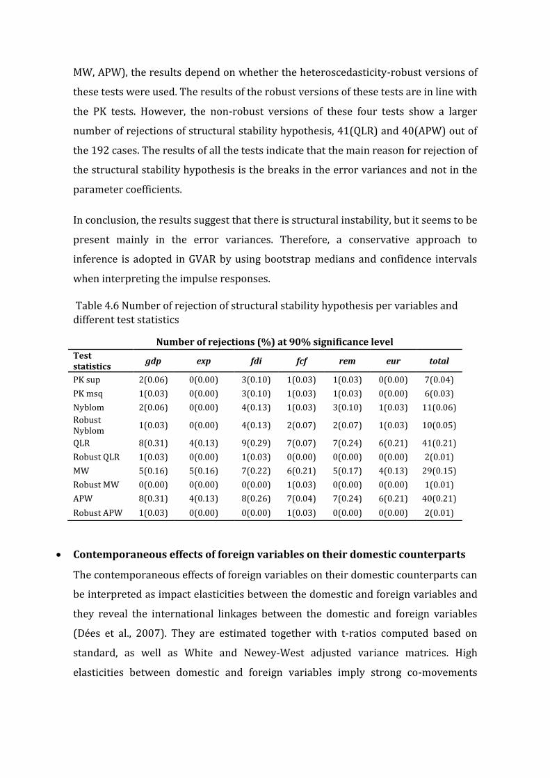
MW, APW), the results depend on whether the heteroscedasticity-robust versions of
these tests were used. The results of the robust versions of these tests are in line with
the PK tests. However, the non-robust versions of these four tests show a larger
number of rejections of structural stability hypothesis, 41(QLR) and 40(APW) out of
the 192 cases. The results of all the tests indicate that the main reason for rejection of
the structural stability hypothesis is the breaks in the error variances and not in the
parameter coefficients.
In conclusion, the results suggest that there is structural instability, but it seems to be
present mainly in the error variances. Therefore, a conservative approach to
inference is adopted in GVAR by using bootstrap medians and confidence intervals
when interpreting the impulse responses.
Table 4.6 Number of rejection of structural stability hypothesis per variables and
different test statistics
Contemporaneous effects of foreign variables on their domestic counterparts
The contemporaneous effects of foreign variables on their domestic counterparts can
be interpreted as impact elasticities between the domestic and foreign variables and
they reveal the international linkages between the domestic and foreign variables
(Dées et al., 2007). They are estimated together with t-ratios computed based on
standard, as well as White and Newey-West adjusted variance matrices. High
elasticities between domestic and foreign variables imply strong co-movements
Number of rejections (%) at 90% significance level
Test statistics
gdp exp fdi fcf rem eur total
PK sup 2(0.06) 0(0.00) 3(0.10) 1(0.03) 1(0.03) 0(0.00) 7(0.04)
PK msq 1(0.03) 0(0.00) 3(0.10) 1(0.03) 1(0.03) 0(0.00) 6(0.03)
Nyblom 2(0.06) 0(0.00) 4(0.13) 1(0.03) 3(0.10) 1(0.03) 11(0.06)
Robust Nyblom
1(0.03) 0(0.00) 4(0.13) 2(0.07) 2(0.07) 1(0.03) 10(0.05)
QLR 8(0.31) 4(0.13) 9(0.29) 7(0.07) 7(0.24) 6(0.21) 41(0.21)
Robust QLR 1(0.03) 0(0.00) 1(0.03) 0(0.00) 0(0.00) 0(0.00) 2(0.01)
MW 5(0.16) 5(0.16) 7(0.22) 6(0.21) 5(0.17) 4(0.13) 29(0.15)
Robust MW 0(0.00) 0(0.00) 0(0.00) 1(0.03) 0(0.00) 0(0.00) 1(0.01)
APW 8(0.31) 4(0.13) 8(0.26) 7(0.04) 7(0.24) 6(0.21) 40(0.21)
Robust APW 1(0.03) 0(0.00) 0(0.00) 1(0.03) 0(0.00) 0(0.00) 2(0.01)
147
between these variables (Smith and Galesi, 2014). Table A4.9 in appendix A4 reports
these coefficients as well as their Newey-West t-ratios.
We observe a significant elasticity between the foreign and the domestic exports,
indicating that trade linkages are likely to be strong among countries in our model.
For example, for Kosovo, the results suggest that a 1% increase in foreign exports in
a given quarter leads to a 0.75% increase in domestic exports in the same quarter.
We also observe a significant elasticity between domestic and foreign variables of
GDP, indicating close co-movements of this variable in the countries included in the
model. In contrast, we find fewer statistically significant elasticities for FDI,
suggesting that in the short run the domestic FDI in most countries is not affected
significantly by changes in foreign FDI.
Pair-wise cross-country correlations: variables and residuals
One of the basic assumptions of the GVAR modelling approach is that the country-
specific shocks are cross-sectionally ‘weakly correlated’ so that the weak exogeneity
of the foreign variables is ensured (Dées et al., 2007; Smith and Galesi, 2014).13 We
follow Dées et al. (2007) in checking this assumption by calculating pairwise cross-
section correlations for the levels and first differences of the endogenous variables of
the model, as well as those of the associated residuals over the selected estimation
period. These are computed as follows: for every country for each given variable, the
pairwise correlation of that country with each of the remaining countries is
computed, and averaged across countries. In Table A4.10 in appendix A4 we report
the average cross section correlations. The results differ across variables and
countries. However, they are generally higher for the level and fall in the first
differences. Trade levels show the highest degree of cross section correlations of
around 43%-90%. The FDI levels also show a high degree of cross section correlation
with an average across countries of 71%, which is followed by the levels of
remittances, with an average of 45%, and EU integration variable, with an average
cross section correlation of 30%. In contrast, very small correlation coefficients are
13 Ideally, we would specify our model with period dummies to attenuate cross-country error correlation. Unfortunately, the current version of the GVAR toolbox does not allow for this.
found for the residuals from the VECM models, which is an indication that the model
has been successful in capturing the unobserved global common effects.14
4.4.3 Dynamic analysis using generalized impulse response functions and generalized forecast error variance decomposition
This section investigates the dynamic properties of the GVAR model based on
generalized impulse response functions (GIRFs) and generalized forecast error
variance decomposition. Impulse responses, proposed by Koop et al. (1996) for non-
linear models and developed further in Pesaran and Shin (1998) and Pesaran and
Smith (1998) for vector error correcting models, refer to the time profile of the
effects of variable-specific shocks or identified shocks on the future states of a
dynamic system and thus on all the variables in the model (Smith and Galesi, 2014).
Identification of shocks in a GVAR is difficult, as in standard VARs, but is further
complicated due to the cross-country interactions and the high dimensionality of the
model (Chudik and Pesaran, 2016). Hence, in the absence of strong a priori beliefs on
the ordering of the variables and countries in the GVAR model, although the GIRFs
cannot identify the origins of shocks they do provide useful information about the
dynamics of the transmission of shocks. In this study, the EU region is considered as
the possible source of shocks. The GIRFs are provided for a period of 40 quarters.
However, only the impulse responses of the first 8-10 quarters are considered for
interpretation. Due to the relatively large number of countries included in the model,
in order to simplify discussion of the impulse responses and focus the interpretation
on the common patterns of responses based on specific regions, the ETEs are
aggregated into these sub-regions:15 Baltic countries, which include Estonia, Latvia
and Lithuania; Balkan countries, which include Albania, Bosnia and Herzegovina,
Macedonia, Montenegro, Kosovo and Serbia; the rest of the ETEs, which include the
Czech Republic, Bulgaria, Hungary, Poland, Romania, the Slovak Republic, Slovenia
and Croatia; and the previously aggregated EU countries.
14 By conditioning the country-specific models on weakly exogenous foreign variables, viewed as proxies for the “common” global factors, it is reasonable to expect that the degree of correlation of the remaining shocks across countries/regions will be modest. 15 This procedure yields similar results to individual country estimation. However, it is easier to interpret our findings in groups compared to individual countries.

149
The generalized forecast error-variance decomposition (GFEVD) is also employed to
investigate the international linkages between EU and ETEs. GFEVD provides useful
information about the international transmission channels through which shocks are
propagated (Galesi and Sgherri, 2009). GFEVD allocates the forecast error variance of
the shock to its respective variables and regions, where the relative contributions
measure the importance of the innovation to a given region’s variable to the rest of
the regions’ variables (Di Mauro and Pesaran, 2013). In the results presented in
figures 4.1 and 4.2, the impulse responses stabilise relatively quickly, suggesting that
the estimated GVAR model is stable. This is confirmed by the eigenvalues of the GVAR
model, which are all within the unit circle and by the persistence profiles, which
converge to zero relatively quickly. However, the bootstrap simulation provides
rapidly widening confidence bands around the impulse responses, which is most
likely a result of the short time series included in the model.
Impulse response functions of one standard error shock to GDP in EU
This subsection reports the effects of a one standard error negative shock in the
EU15 GDP, (which corresponds to a 0.3% decline) on five variables of interest: GDP;
exports; FDI; foreign credit flows and remittances.
Figure 4.1 reports the regional impulse response functions (in order to simplify the
comparison, only point estimates are presented without the standard error bands) of
GDP to a shock in EU's GDP using trade weights, FDI weights and remittance weights.
These show the effect in each quarter, not the cumulative effect. The graphs indicate
that the effect of the shock to GDP is stronger in all regions when using trade weights
to construct the foreign country-specific variables, indicating that trade represents
the strongest linkage between ETEs and European advanced countries. In addition,
as discussed in sub-section 4.2.2, it is observed that the GVAR model using only trade
weights provides the best performance in terms of persistence profiles and
eigenvalues, hence we selected it as the benchmark model.
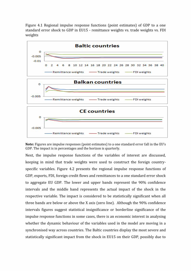
Figure 4.1 Regional impulse response functions (point estimates) of GDP to a one
standard error shock to GDP in EU15 - remittance weights vs. trade weights vs. FDI
weights
Note: Figures are impulse responses (point estimates) to a one standard error fall in the EU’s GDP. The impact is in percentages and the horizon is quarterly.
Next, the impulse response functions of the variables of interest are discussed,
keeping in mind that trade weights were used to construct the foreign country-
specific variables. Figure 4.2 presents the regional impulse response functions of
GDP, exports, FDI, foreign credit flows and remittances to a one standard error shock
to aggregate EU GDP. The lower and upper bands represent the 90% confidence
intervals and the middle band represents the actual impact of the shock in the
respective variable. The impact is considered to be statistically significant when all
three bands are below or above the X axis (zero line). Although the 90% confidence
intervals figures suggest statistical insignificance or borderline significance of the
impulse response functions in some cases, there is an economic interest in analysing
whether the dynamic behaviour of the variables used in the model are moving in a
synchronised way across countries. The Baltic countries display the most severe and
statistically significant impact from the shock in EU15 on their GDP, possibly due to
151
their stronger trade links with the EU15 countries.16 They experience a decline of
0.3% on impact, which then rises by the seventh quarter to 0.7% and dissipates in
the following periods. The Balkan transition countries also display a severe impact
from the shock to the EU15's GDP, with a decline of their GDP by 0.3% on impact,
which increases to 0.5% and stabilises by the eighth quarter. In the other CE
countries, the GDP falls by 0.15% on impact and stabilises in the eighth quarter at
about 0.3% (see Figure 4.2).
As expected, exports are also negatively affected by a GDP shock in EU15. From the
regional perspective, exports from the Balkan countries appear to be most severely
affected by the shock in the EU15, even though the impact is at the borderline of the
10% level of statistical significance. The CE transition countries also display a severe
and statistically significant impact from a shock to EU15 GDP on their exports which
stabilises at a 0.6% decline by the eighth quarter. Contrary to the strong and
synchronized regional GDP and exports responses to the EU15 GDP shock, the
generalized impulse responses of FDI to the GDP shock are statistically insignificant
or close to borderline significance at the 10% level, indicating that economic shocks
in the EU15 may not have a severe impact on FDI flows. The Balkan transition
countries display the most severe and statistically significant impact from the shock
in the EU15's GDP with a decline of their FDI by 0.5% on impact, which then rises by
the fifth quarter to 1% and stabilises in the following periods.
On average, all regions experience a fall in foreign credit flows of 1%-5% following a
negative shock to GDP in EU15. The impulse response functions stabilise after about
8 quarters. The effect is strongest in the Balkan countries; however, it appears to be
statistically insignificant, though close to the 10% borderline of statistical
significance across all regions.
All regions experience a fall in remittances of 1%-5% following a negative shock to
GDP in EU15. The impulse response functions stabilise after about 8 quarters.
However, the affect appears to be statistically insignificant across all regions except
16 The average share of exports of the Baltic countries to the EU15 during the period 2005-2007 was 65% of their total exports.

for the Baltic countries, where it appears to be at the 10% borderline of statistical
significance.
Figure 4.2 Regional impulse response functions of GDP, exports, FDI, foreign credit
flows and remittances to a one standard error shock to GDP in EU with their 90%
confidence bands
Note: Figures are median generalized impulse responses to a one standard error fall in the EU’s GDP, together with the 10 percent confidence bands. The impact is in percentages and the horizon is quarterly.
-0.02
-0.01
0
0 4 8 1216202428323640
Baltic GDP
-0.02
-0.01
0
0.01
0 4 8 1216202428323640
Balkan GDP
-0.01
-0.005
0
0 4 8 1216202428323640
CE GDP
-0.02
-0.01
0
0.01
0.02
0 4 8 1216202428323640
Baltic exports
-0.04
-0.02
0
0.02
0 4 8 1216202428323640
Balkan exports
-0.02
-0.01
0
0 4 8 1216202428323640
CE exports
-0.06
-0.04
-0.02
0
0.02
0 4 8 1216202428323640
Baltic FDI
-0.06
-0.04
-0.02
0
0.02
0 4 8 1216202428323640
Balkan FDI
-0.06
-0.04
-0.02
0
0.02
0 4 8 1216202428323640
CE FDI
-0.2
-0.1
0
0.1
0 4 8 12 16 20 24 28 32 36 40
Baltic remittances
-0.2
-0.1
0
0.1
0 4 8 1216202428323640
Balkan remittances
-0.1
-0.05
0
0.05
0 4 8 1216202428323640
CE remittances
-0.1
-0.05
0
0.05
0 4 8 1216202428323640
Baltic foreign credit flow
-0.4
-0.2
0
0.2
0 4 8 1216202428323640
Balkan foreign credit flow
-0.1
-0.05
0
0.05
0 4 8 1216202428323640
CE foreign credit flow
153
Generalized forecast error variance decomposition
Shock to GDP in the Balkan Countries
Following a historical shock to GDP in the Balkan countries, we analyse which of the
variables and regions explain most of the forecast error variance decomposition in
the short run. More specifically, the forecast error variance of the simulated shock is
allocated into respective variables and regions and the importance of innovations in
all the variables is checked. Results are presented in Table A4.11 in appendix A4. We
observe that among Balkan countries' variables, in the short run, on impact the GDP
explains most of the forecast error variance decomposition, it contributes 12% of the
variance of the historical shock. On the other hand, exports contribute to the variance
in the GDP shock with 10%, remittances with 3%, foreign credit flows with 4%, FDI
with 3% and foreign currency credit flows with 2%. The average relative importance
of all the variables that explain the shock increases over time. In addition, we also
look at the contribution of each region to the explanation of the forecast error
variance, since this illustrates how important are the international linkages in the
international transmission of shocks. As expected, the foreign regions that contribute
mostly to the variance in the shock to the GDP in the Balkan countries are: the EU
which, on impact, contributes to the shock with 38%; other ETEs contribute to the
shock with 19%; while the Baltic countries contribute 8% to the shock. The average
relative importance of all the variables of other regions that explain the shock
decreases over time.
Shock to GDP in the Baltic countries
Following a historical shock to GDP in the Baltic countries, we now assess which of
the following Baltic countries' variables explain most of the forecast error variance
decomposition in the short run. The results are presented in Table A4.12 in appendix
A4. Similar to the EU and the Balkan region, GDP explains most of the variance of the
shock in the GDP (7%); foreign credit flows explain 5% of the variance of the shock;
credit flows in foreign currency explains 5% of the variation; FDI explains 1%;
remittances 0.3% and exports 0.1%. The average relative importance of the variables
in the Baltic region that explain the shock decreases over time. In addition, we also
look at the contribution of each region to the explanation of the forecast error
variance. As expected, the foreign regions that contribute most to the variance in the
shock to GDP in the Baltic countries are: the EU, which, on impact, contributes to the
shock with 57%; other ETEs contribute 10%; while the Balkan countries contribute
14%.
Shock to GDP in CE transition countries
After a historical shock to GDP in CE transition countries, we observe that, among
other EU variables, in the short run, remittances explain most of the forecast error
variance decomposition. It contributes 10% to the variance of the historical shock,
while foreign credit flows contribute to the shock with 3%, credit flows in foreign
currency 3%, FDI 2% and exports 1%. As expected, the foreign regions that
contribute mostly to the variance in the shock to GDP in CE countries are: the EU,
which, on impact, contributes to the shock with 50%; the Balkan countries contribute
19%; while the Baltic countries contribute to the shock with 9%. The complete set of
results is presented in Table A4.13 in appendix A4.
4.4.4 Robustness analysis
In this section we modify the baseline model in two ways. Firstly, given the relatively
small number of observations and large number of variables included in the baseline
model, which reduces the degrees of freedom available to estimate the parameters'
variability, we investigate whether the statistical significance of the impulse
responses of the main variables changes when reducing the number of variables in
the model. Namely, we estimate the GVAR model with these core variables
representing the main transmission channels: exports, FDI, foreign credit flows and
GDP. Secondly, we analyse the transmission of shocks from advanced EU countries to
ETEs in sub-samples, which are defined by various country features. Consequently,
we address one of the main aims of the thesis, i.e. to analyse whether country
structural characteristics influence the transmission of the GFC. In addition, splitting
the sample in various ways also enables us to deal with country heterogeneity in a
more careful manner, since sub-samples analysed here consist of more homogenous
groups than the entire sample of 15 transition countries.
In the results presented in the figures, we can see that the impulse responses
stabilise relatively quickly, suggesting that the estimated GVAR model is stable. This
is confirmed by the eigenvalues of the GVAR model, which are all within the unit

155
circle and by the persistence profiles, which converge to zero relatively quickly. We
observe that the impulse response results are similar in terms of shape, signs and
magnitudes, suggesting that the estimated impulse responses do not differ
significantly; however, the confidence bands are generally below zero, which
indicates more statistical significance. Persistence profiles and other diagnostic tests
are presented in appendix A4.
Impulse response functions of a one standard error shock to GDP in the EU
This subsection reports the effects of a one standard error negative shock to the GDP
of the EU region (around a 0.3% GDP decline) on four variables of interest: GDP;
exports; FDI; and foreign credit flows. Although the 90% confidence intervals suggest
only borderline statistical significance of the impulse response functions in some
cases, there is nonetheless economic interest in analysing whether the dynamic
behaviour of the variables used in our model are moving in a synchronised way
across countries. Figure 4.3 presents the regional impulse response functions
together with their 10% confidence bands. As can be seen in this Figure, the negative
shock to the GDP in the EU15 region results in decreases in the GDP of all regions in
the model. The impulse responses in general follow the same pattern: in the first
quarters there is an immediate decline in GDP, but the impact stabilizes after 6-10
quarters. The Baltic countries display the most severe and statistically significant
impact from the shock in their GDP with a decline of 0.01% on impact, which then
rises by the seventh quarter to 0.6% and dissipates in the following periods. Across
other regions, the GDP falls by similar amounts (around 0.2%-0.3%). The Balkan
transition countries also display a severe impact from the shock to the EU's GDP, with
a decline of their GDP by 0.15% on impact increasing to 0.3% by the eighth quarter
and then stabilising. In CE countries, the GDP falls by 0.1% on impact and stabilises in
the sixth quarter at a decline of about 0.2% compared to the pre-shock level. As
expected, exports are also negatively affected by the GDP shock in EU, varying
between 0.5% and 1%. The exports impulse response pattern is similar across all
regions, showing an initial decline of 0.5% during the first two quarters following the
shock, and then oscillating and dissipating in about 5-8 quarters. From the regional
perspective, the exports from Balkan countries appear to be the most severely
affected by a shock to EU GDP, even though the impact is at the borderline of the 10%
statistical significance level. The CE transition countries also display a severe and
statistically significant impact from a shock to EU GDP on their exports, which
stabilises at a 0.59% decline by the eighth quarter. Similar behaviour is observed also
across the Baltic countries, even though the effect is statistically significant only in
the third quarter. The effect of the shock to EU GDP on foreign credit flows is the
strongest in the Baltic countries; the foreign credit flows decline by 2% by the eighth
quarter. The generalized impulse responses of foreign credit flows are weaker and
clearly statistically insignificant for Balkan countries. CE transition countries also
show a negative decline in foreign credit flows following a shock to the EU GDP. The
generalized impulse responses of FDI to the GDP shock are both small and borderline
at the 10% significance level. The Baltic countries display the most severe and
statistically significant impact from the shock in the EU GDP with a decline of 1% on
impact, which then rises by the eighth quarter to 2.2% and dissipates in the following
periods.
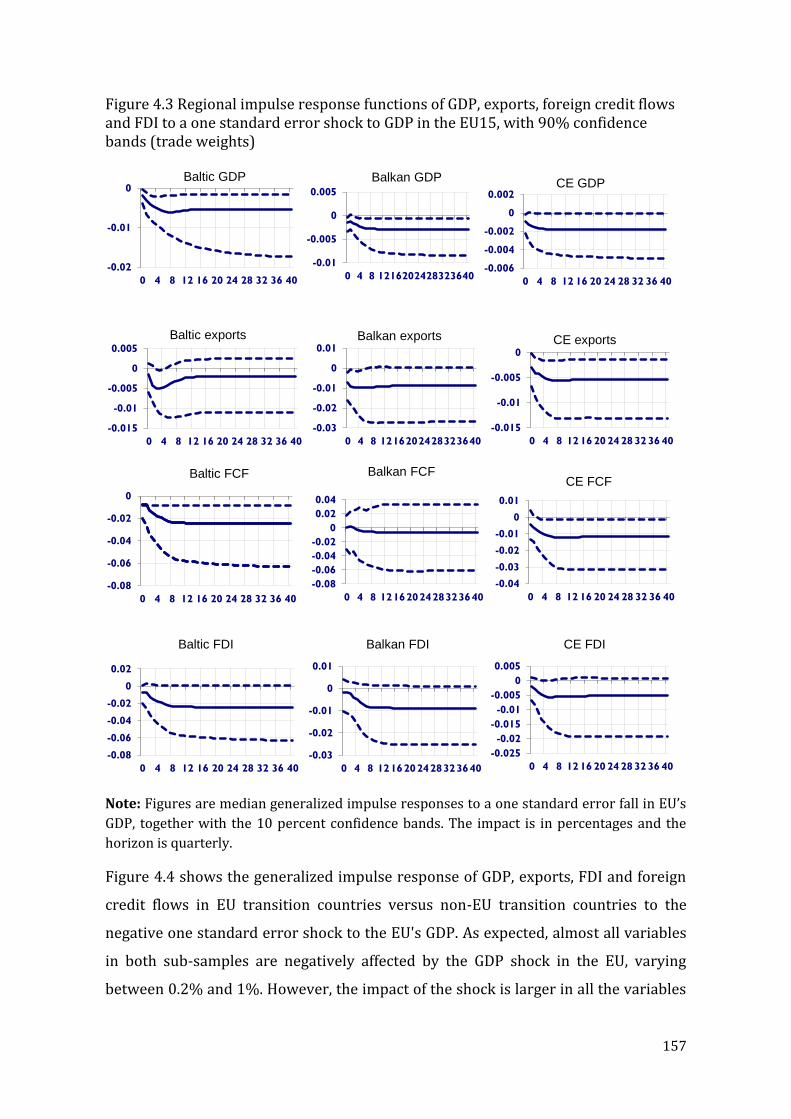
157
Figure 4.3 Regional impulse response functions of GDP, exports, foreign credit flows and FDI to a one standard error shock to GDP in the EU15, with 90% confidence bands (trade weights)
Note: Figures are median generalized impulse responses to a one standard error fall in EU’s
GDP, together with the 10 percent confidence bands. The impact is in percentages and the
horizon is quarterly.
Figure 4.4 shows the generalized impulse response of GDP, exports, FDI and foreign
credit flows in EU transition countries versus non-EU transition countries to the
negative one standard error shock to the EU's GDP. As expected, almost all variables
in both sub-samples are negatively affected by the GDP shock in the EU, varying
between 0.2% and 1%. However, the impact of the shock is larger in all the variables
-0.02
-0.01
0
0 4 8 12 16 20 24 28 32 36 40
Baltic GDP
-0.01
-0.005
0
0.005
0 4 8 1216202428323640
Balkan GDP
-0.006
-0.004
-0.002
0
0.002
0 4 8 12 16 20 24 28 32 36 40
CE GDP
-0.015
-0.01
-0.005
0
0.005
0 4 8 12 16 20 24 28 32 36 40
Baltic exports
-0.03
-0.02
-0.01
0
0.01
0 4 8 1216202428323640
Balkan exports
-0.015
-0.01
-0.005
0
0 4 8 1216202428323640
CE exports
-0.08
-0.06
-0.04
-0.02
0
0 4 8 12 16 20 24 28 32 36 40
Baltic FCF
-0.08
-0.06
-0.04
-0.02
0
0.02
0.04
0 4 8 1216202428323640
Balkan FCF
-0.04
-0.03
-0.02
-0.01
0
0.01
0 4 8 12 16 20 24 28 32 36 40
CE FCF
-0.08
-0.06
-0.04
-0.02
0
0.02
0 4 8 12 16 20 24 28 32 36 40
Baltic FDI
-0.03
-0.02
-0.01
0
0.01
0 4 8 1216202428323640
Balkan FDI
-0.025
-0.02
-0.015
-0.01
-0.005
0
0.005
0 4 8 1216202428323640
CE FDI

of the non-EU transition countries. The GDPs impulse response pattern is similar in
both sub-samples, showing an initial decline of 0.2% during the first four quarters
following the shock and stabilising by the fourth quarter at 0.2% decline in the EU
transition countries and 0.3% decline in the non-EU transition countries. The
impulse response function of exports in non-EU transition countries show a decline
which stabilises at 1% by the second quarter, while in the EU transition countries the
impulse response stabilises at a 0.55% decline by the eighth quarter. Nevertheless, it
should be pointed out that the impact has a higher statistical significance in non-EU
transition countries, while it is at the borderline of the 10% significance level in EU
transition countries. Similarly, the effects of the shock to EU GDP on foreign credit
flows and FDI are the strongest in the non-EU transition countries; the foreign credit
flows decline by 1.2% by the eighth quarter and FDI declines by 0.9% by the eighth
quarter. For EU transition countries, the generalized impulse responses of foreign
credit flows and FDI are weaker and statistically insignificant, or at the borderline of
the 10% statistical significance in the case of FDI.

159
Figure 4.4 Impulse response functions to a one standard error shock to GDP in EU15 with their 90% confidence bands (EU transition countries vs. NON-EU transition countries)
Note: Figures are median generalized impulse responses to a one standard error fall in EU’s
GDP, together with the 10 percent confidence bands. The impact is in percentages and the
horizon is quarterly.
-0.007
-0.006
-0.005
-0.004
-0.003
-0.002
-0.001
0
0 4 8 12 16 20 24 28 32 36 40
EU GDP
-0.01
-0.008
-0.006
-0.004
-0.002
0
0.002
0 4 8 12 16 20 24 28 32 36 40
Non-EU GDP
-0.014
-0.012
-0.01
-0.008
-0.006
-0.004
-0.002
0
0 4 8 12 16 20 24 28 32 36 40
EU exports
-0.03
-0.025
-0.02
-0.015
-0.01
-0.005
0
0.005
0 4 8 12 16 20 24 28 32 36 40
Non-EU exports
-0.08
-0.06
-0.04
-0.02
0
0.02
0.04
0 4 8 12 16 20 24 28 32 36 40
EU FCF
-0.04
-0.035
-0.03
-0.025
-0.02
-0.015
-0.01
-0.005
0
0.005
0.01
0 4 8 12 16 20 24 28 32 36 40
Non-EU FCF
-0.025
-0.02
-0.015
-0.01
-0.005
0
0.005
0 4 8 12 16 20 24 28 32 36 40
EU FDI
-0.03
-0.025
-0.02
-0.015
-0.01
-0.005
0
0.005
0.01
0 4 8 12 16 20 24 28 32 36 40
Non-EU FDI
Figure 4.5 shows the generalized impulse response of GDP, exports, FDI and foreign
credit flows in countries with a high degree of euroisation versus countries with a
low degree of euroisation to a negative one standard error shock to the EU's GDP. All
variables are negatively affected by the EU GDP shock in both sub-samples, varying
between 0.1% and 2%. The impact of the shock is larger and statistically more
significant in highly euroised countries' GDPs. The impulse response functions of GDP
show a decline which stabilises by the fifth quarter at -0.3% for highly euroised
countries and -0.1% for countries with a lower degree of euroisation. Other variables
impulse response patterns are similar between both sub-samples, showing an initial
decline of 0.2%-2% during the first four quarters following the shock and stabilising
by the eighth quarter.
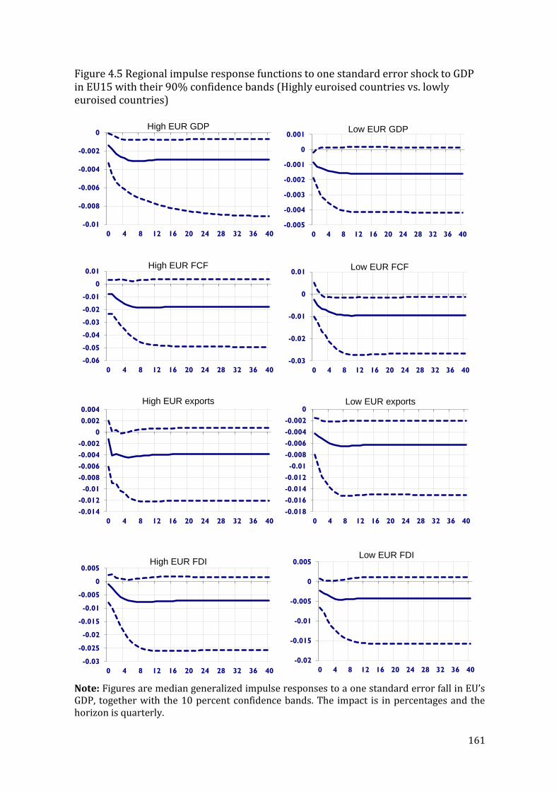
161
Figure 4.5 Regional impulse response functions to one standard error shock to GDP in EU15 with their 90% confidence bands (Highly euroised countries vs. lowly euroised countries)
Note: Figures are median generalized impulse responses to a one standard error fall in EU’s GDP, together with the 10 percent confidence bands. The impact is in percentages and the horizon is quarterly.
-0.01
-0.008
-0.006
-0.004
-0.002
0
0 4 8 12 16 20 24 28 32 36 40
High EUR GDP
-0.005
-0.004
-0.003
-0.002
-0.001
0
0.001
0 4 8 12 16 20 24 28 32 36 40
Low EUR GDP
-0.06
-0.05
-0.04
-0.03
-0.02
-0.01
0
0.01
0 4 8 12 16 20 24 28 32 36 40
High EUR FCF
-0.03
-0.02
-0.01
0
0.01
0 4 8 12 16 20 24 28 32 36 40
Low EUR FCF
-0.014
-0.012
-0.01
-0.008
-0.006
-0.004
-0.002
0
0.002
0.004
0 4 8 12 16 20 24 28 32 36 40
High EUR exports
-0.018
-0.016
-0.014
-0.012
-0.01
-0.008
-0.006
-0.004
-0.002
0
0 4 8 12 16 20 24 28 32 36 40
Low EUR exports
-0.03
-0.025
-0.02
-0.015
-0.01
-0.005
0
0.005
0 4 8 12 16 20 24 28 32 36 40
High EUR FDI
-0.02
-0.015
-0.01
-0.005
0
0.005
0 4 8 12 16 20 24 28 32 36 40
Low EUR FDI
Figure 4.6 shows the generalized impulse response of GDP, exports, FDI and foreign
credit flows in more open transition countries versus less open transition countries
to a negative one standard error shock to the EU's GDP. As expected, almost all
variables are negatively affected by the EU GDP shock in both sub-samples, varying
between 0.2% and 1%. The impact of the shock is larger on the GDP and the exports
of the more open economies compared to the less open economies and it is slightly
smaller for foreign credit flows and FDI in more open economies. The GDP impulse
response functions show a decline which stabilises at 0.2% by the eighth quarter in
both sub-samples; however, the effect is statistically more significant in more open
economies. The impulse response function of exports in more open economies shows
an initial decline of 0.7%, which stabilises at 0.6% by the eighth quarter, while in the
less open transition countries the impulse response stabilises at a 0.5% decline by
the eighth quarter. The effect of the shock to EU GDP on foreign credit flows and FDI
is stronger and more statistically significant in less open transition countries.

163
Figure 4.6 Regional impulse response functions to one standard error shock to GDP in EU15 with their 90% confidence bands (highly open countries vs. lowly open countries)
Note: Figures are median generalized impulse responses to a one standard error fall in EU’s
GDP, together with the 10 percent confidence bands. The impact is in percentages and the
horizon is quarterly.
-0.007
-0.006
-0.005
-0.004
-0.003
-0.002
-0.001
0
0 4 8 12 16 20 24 28 32 36 40
High trade openness GDP
-0.007
-0.006
-0.005
-0.004
-0.003
-0.002
-0.001
0
0.001
0 4 8 12 16 20 24 28 32 36 40
Low trade openness GDP
-0.02
-0.015
-0.01
-0.005
0
0 4 8 12 16 20 24 28 32 36 40
High trade openness exports
-0.016
-0.014
-0.012
-0.01
-0.008
-0.006
-0.004
-0.002
0
0.002
0 4 8 12 16 20 24 28 32 36 40
Low trade openness exports
-0.04
-0.035
-0.03
-0.025
-0.02
-0.015
-0.01
-0.005
0
0.005
0.01
0 4 8 12 16 20 24 28 32 36 40
High trade openness FCF
-0.04
-0.035
-0.03
-0.025
-0.02
-0.015
-0.01
-0.005
0
0.005
0.01
0 4 8 12 16 20 24 28 32 36 40
Low trade openness FCF
-0.015
-0.01
-0.005
0
0.005
0.01
0 4 8 12 16 20 24 28 32 36 40
High trade openness FDI
-0.025
-0.02
-0.015
-0.01
-0.005
0
0.005
0 4 8 12 16 20 24 28 32 36 40
Low trade openness FDI
4.4.5 The effects of increased financial stress in the EU15
In this section the baseline model is modified in two ways. Firstly, given the relatively
small number of observations included in the baseline model, the dataset is extended
by using observations from the first quarter of 1999 to the fourth quarter of 2014 to
estimate the 16 country/region-specific VARX* models. However, due to data
availability, two countries were dropped from estimation (Kosovo and Montenegro).
Secondly, given this study’s objective to analyse the macroeconomic effects of
increased global financial market volatility, we include an indicator to measure the
systemic stress in advanced economies in our framework. This indicator for
advanced economies is the composite indicator of systemic stress (CISS), constructed
by Holló et al. (2012), which measures the contemporaneous state of instability in
the financial system. The CISS can be interpreted as a measure of the systemic risk
that has materialised already (Holló et al., 2012). The CISS is composed of 15 mostly
market-based financial stress measures17 equally split into five categories, namely
the financial intermediaries’ sector, money markets, equity markets, bond markets
and foreign exchange markets, which represent the most important segments of an
economy’s financial system. In the results presented in the figures, we can see that
the impulse responses stabilise relatively quickly, suggesting that the estimated
GVAR model is stable. This is confirmed by the eigenvalues of the GVAR model, which
are all within the unit circle and by the persistence profiles, which converge to zero
relatively quickly. Persistence profiles and other diagnostic tests are presented in
appendix A4. However, here as well it should be pointed out that the bootstrap
simulation provides rapidly widening confidence bands around the impulse
17 Realised volatility of the 3-month Euribor rate; interest rate spread between 3-month
Euribor and 3-month French T-bills; Monetary Financial Institution’s (MFI) emergency
lending at Eurosystem central banks; realised volatility of the German 10-year benchmark
government bond index; yield spread between A-rated non-financial corporations and
government bonds; 10-year interest rate swap spread; realised volatility of the DataStream
non-financial sector stock market index: CMAX for the DataStream non-financial sector stock
market index; stock-bond correlation; realised volatility of the idiosyncratic equity return of
the DataStream bank sector stock market index over the total market index; yield spread
between A-rated financial and non-financial corporations (7-year maturity); CMAX as
defined above interacted with the inverse price-book ratio (book-price ratio) for the financial
sector equity market index; and realised volatility of the euro exchange rate vis-à-vis the US
dollar, the Japanese Yen and the British Pound, respectively.
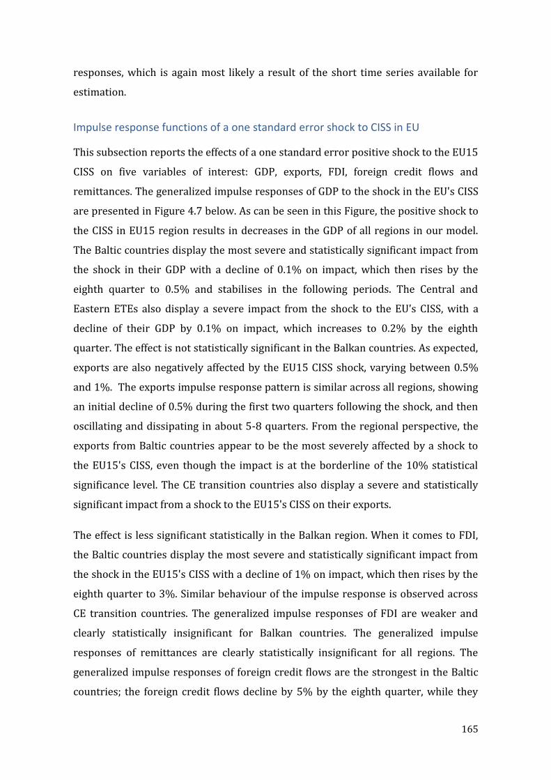
165
responses, which is again most likely a result of the short time series available for
estimation.
Impulse response functions of a one standard error shock to CISS in EU
This subsection reports the effects of a one standard error positive shock to the EU15
CISS on five variables of interest: GDP, exports, FDI, foreign credit flows and
remittances. The generalized impulse responses of GDP to the shock in the EU's CISS
are presented in Figure 4.7 below. As can be seen in this Figure, the positive shock to
the CISS in EU15 region results in decreases in the GDP of all regions in our model.
The Baltic countries display the most severe and statistically significant impact from
the shock in their GDP with a decline of 0.1% on impact, which then rises by the
eighth quarter to 0.5% and stabilises in the following periods. The Central and
Eastern ETEs also display a severe impact from the shock to the EU's CISS, with a
decline of their GDP by 0.1% on impact, which increases to 0.2% by the eighth
quarter. The effect is not statistically significant in the Balkan countries. As expected,
exports are also negatively affected by the EU15 CISS shock, varying between 0.5%
and 1%. The exports impulse response pattern is similar across all regions, showing
an initial decline of 0.5% during the first two quarters following the shock, and then
oscillating and dissipating in about 5-8 quarters. From the regional perspective, the
exports from Baltic countries appear to be the most severely affected by a shock to
the EU15's CISS, even though the impact is at the borderline of the 10% statistical
significance level. The CE transition countries also display a severe and statistically
significant impact from a shock to the EU15's CISS on their exports.
The effect is less significant statistically in the Balkan region. When it comes to FDI,
the Baltic countries display the most severe and statistically significant impact from
the shock in the EU15's CISS with a decline of 1% on impact, which then rises by the
eighth quarter to 3%. Similar behaviour of the impulse response is observed across
CE transition countries. The generalized impulse responses of FDI are weaker and
clearly statistically insignificant for Balkan countries. The generalized impulse
responses of remittances are clearly statistically insignificant for all regions. The
generalized impulse responses of foreign credit flows are the strongest in the Baltic
countries; the foreign credit flows decline by 5% by the eighth quarter, while they
are weaker and clearly statistically insignificant for Balkan countries. Other CE
transition countries also show a negative decline in foreign credit flows following a
shock in the CISS of the EU15.
Figure 4.7 Regional impulse response functions of GDP, exports, FDI, foreign credit
flows and remittances to a one standard error shock to the EU15 CISS with their 90%
confidence bands
Note: Figures are median generalized impulse responses to a one standard error fall in EU15 CISS together with the 10 percent confidence bands. The impact is in percentages and the horizon is quarterly.
-0.03
-0.02
-0.01
0
0.01
0 4 8 12 16 20 24 28 32 36 40
Baltic GDP
-0.1
-0.05
0
0.05
0 4 8 1216202428323640
Balkan GDP
-0.02
-0.01
0
0.01
0 4 8 1216202428323640
CE GDP
-0.06
-0.04
-0.02
0
0.02
0 4 8 1216202428323640
Baltic exports
-0.05
0
0.05
0 4 8 1216202428323640
Balkan exports
-0.04
-0.02
0
0.02
0 4 8 12 16 20 24 28 32 36 40
CE exports
-0.2
-0.15
-0.1
-0.05
0
0 4 8 12 16 20 24 28 32 36 40
Baltic FDI
-0.3
-0.2
-0.1
0
0.1
0 4 8 1216202428323640
Balkan FDI
-0.2
-0.15
-0.1
-0.05
0
0.05
0 4 8 12 16 20 24 28 32 36 40
CE FDI
-0.3
-0.2
-0.1
0
0.1
0 4 8 1216202428323640
Baltic remittances
-0.15-0.1-0.050
0.050.1
0 4 8 1216202428 323640
Balkan remittances
-0.2
-0.1
0
0.1
0 4 8 12 16 20 24 28 32 36 40
CE remittances
-0.3
-0.2
-0.1
0
0.1
0 4 8 12 16 20 24 28 32 36 40
Baltic FCF
-0.2
-0.1
0
0.1
0.2
0 4 8 1216202428323640
Balkan FCF
-0.15
-0.1
-0.05
0
0.05
0 4 8 12 16 20 24 28 32 36 40
CE FCF

167
4.5 Conclusion
Although there are a number of empirical studies that have investigated the
international transmission of crisis, the literature is still unable to provide conclusive
results on the determinants of crisis severity across transition countries. This study
contributes to knowledge in this area by providing analyses of the international
transmission of the global financial crises in a global context, employing the global
vector auto-regression (GVAR) approach.
The study begins with a discussion of the modelling framework, its structure and
applications. The discussion also relates the choice of the methodology to the
objective of the thesis. The methodology proceeds through four stages. Firstly, the
weights for constructing the country-specific foreign variables are computed.
Considering the importance of both trade and financial linkages between ETEs and
European advanced countries (EU15), trade, FDI and remittance weights are
computed and considered for the model. Second, for each country the VAR model is
extended with the addition of a set of country-specific foreign variables. These
foreign variables are computed as weighted averages of the respective domestic
variables, using the weights constructed during the first stage. In the third stage, each
variable in the model is tested for stationarity. Next, the VECM is specified for each
country. Particular attention has been paid to diagnostic tests and stability to ensure
the model is statistically well specified and thus produces valid estimates. In the final
stage, the global GVAR is solved and results from the estimated model are
interpreted by means of impulse responses and forecast error variance
decomposition.
By using GVAR, we extend the limited and quite recent body of literature that uses
this modelling framework in several key aspects. First, this is the first study that uses
the GVAR to model the transmission of shocks to ETEs. Second, weights based on
bilateral remittance flows, to our knowledge, represent an original contribution to
the GVAR modelling framework. Thirdly, unlike several other GVAR studies on the
transmission of crises, this method is applied in an extensive manner to deal with
country heterogeneity, by dividing the countries in sub-samples based on several
country characteristics (the level of country openness, the degree of euroisation, and
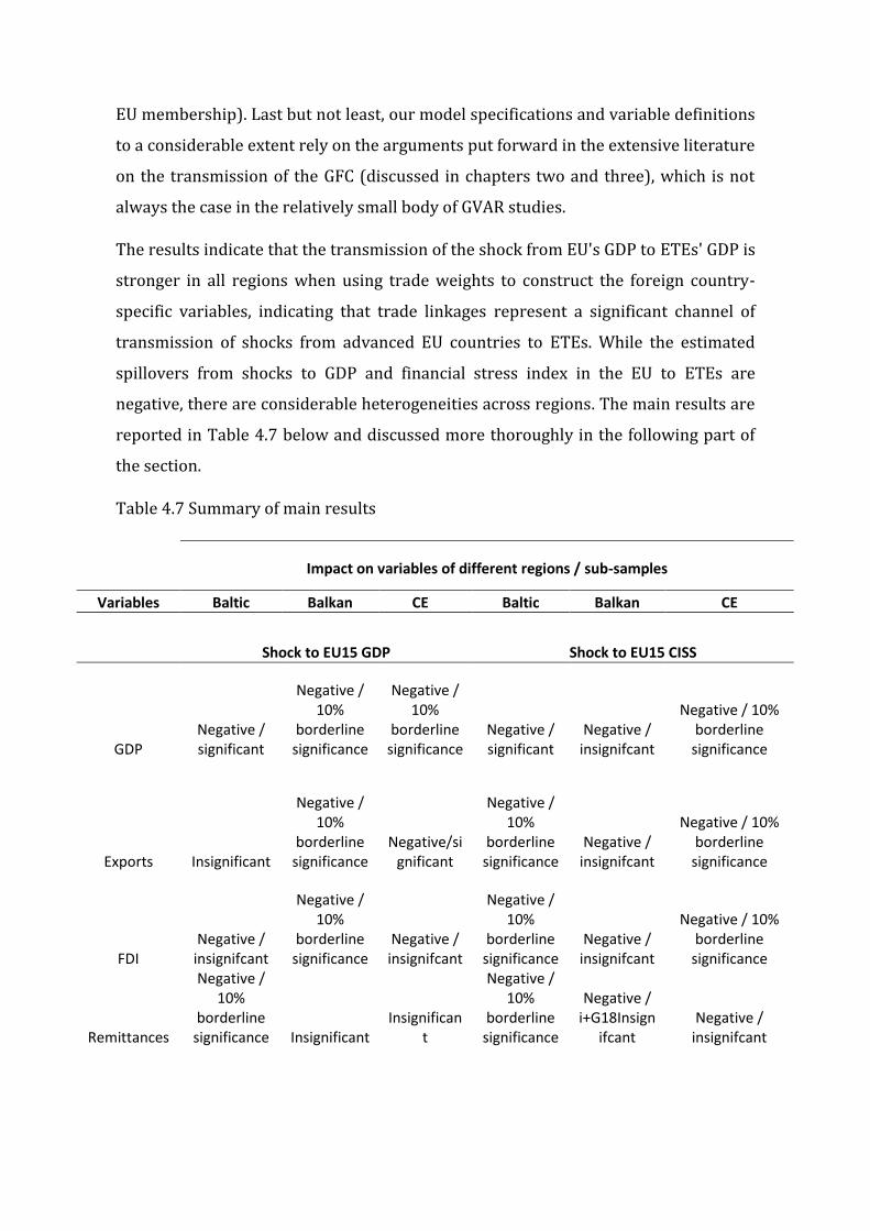
EU membership). Last but not least, our model specifications and variable definitions
to a considerable extent rely on the arguments put forward in the extensive literature
on the transmission of the GFC (discussed in chapters two and three), which is not
always the case in the relatively small body of GVAR studies.
The results indicate that the transmission of the shock from EU's GDP to ETEs' GDP is
stronger in all regions when using trade weights to construct the foreign country-
specific variables, indicating that trade linkages represent a significant channel of
transmission of shocks from advanced EU countries to ETEs. While the estimated
spillovers from shocks to GDP and financial stress index in the EU to ETEs are
negative, there are considerable heterogeneities across regions. The main results are
reported in Table 4.7 below and discussed more thoroughly in the following part of
the section.
Table 4.7 Summary of main results
Impact on variables of different regions / sub-samples
Variables Baltic Balkan CE Baltic Balkan CE
Shock to EU15 GDP Shock to EU15 CISS
GDP Negative / significant
Negative / 10%
borderline significance
Negative / 10%
borderline significance
Negative / significant
Negative / insignifcant
Negative / 10% borderline
significance
Exports Insignificant
Negative / 10%
borderline significance
Negative/significant
Negative / 10%
borderline significance
Negative / insignifcant
Negative / 10% borderline
significance
FDI Negative /
insignifcant
Negative / 10%
borderline significance
Negative / insignifcant
Negative / 10%
borderline significance
Negative / insignifcant
Negative / 10% borderline
significance
Remittances
Negative / 10%
borderline significance Insignificant
Insignificant
Negative / 10%
borderline significance
Negative / i+G18Insign
ifcant Negative /
insignifcant
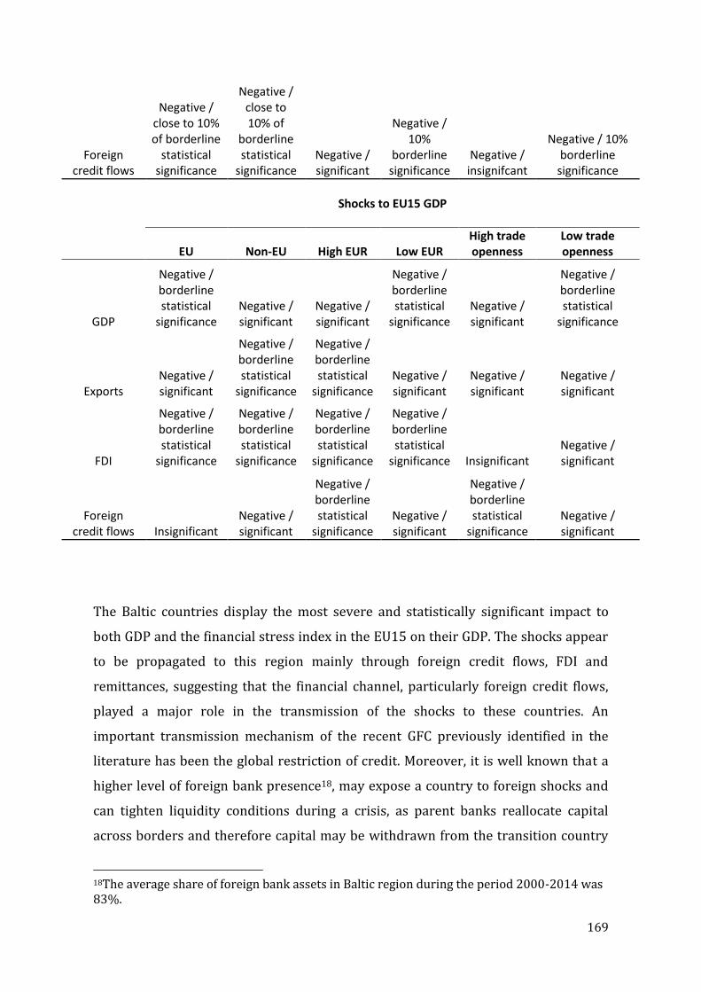
169
The Baltic countries display the most severe and statistically significant impact to
both GDP and the financial stress index in the EU15 on their GDP. The shocks appear
to be propagated to this region mainly through foreign credit flows, FDI and
remittances, suggesting that the financial channel, particularly foreign credit flows,
played a major role in the transmission of the shocks to these countries. An
important transmission mechanism of the recent GFC previously identified in the
literature has been the global restriction of credit. Moreover, it is well known that a
higher level of foreign bank presence18, may expose a country to foreign shocks and
can tighten liquidity conditions during a crisis, as parent banks reallocate capital
across borders and therefore capital may be withdrawn from the transition country
18The average share of foreign bank assets in Baltic region during the period 2000-2014 was 83%.
Foreign credit flows
Negative / close to 10% of borderline
statistical significance
Negative / close to 10% of
borderline statistical
significance Negative / significant
Negative / 10%
borderline significance
Negative / insignifcant
Negative / 10% borderline
significance
Shocks to EU15 GDP
EU Non-EU High EUR Low EUR
High trade openness
Low trade openness
GDP
Negative / borderline statistical
significance Negative / significant
Negative / significant
Negative / borderline statistical
significance Negative / significant
Negative / borderline statistical
significance
Exports Negative / significant
Negative / borderline statistical
significance
Negative / borderline statistical
significance Negative / significant
Negative / significant
Negative / significant
FDI
Negative / borderline statistical
significance
Negative / borderline statistical
significance
Negative / borderline statistical
significance
Negative / borderline statistical
significance Insignificant Negative / significant
Foreign credit flows Insignificant
Negative / significant
Negative / borderline statistical
significance Negative / significant
Negative / borderline statistical
significance Negative / significant
when it is needed in the bank’s home country (in line with the findings of Cetorelli
and Goldberg, 2011). In addition, recent empirical studies (Popov and Udell, 2012;
Ongena et al., 2015; by Bonin and Louie, 2015; Allen et al., 2017) have shown that
foreign bank subsidiaries in emerging Europe reduced lending earlier and faster than
domestic banks.
The Balkan transition countries also display a severe impact from the shock to the
EU15 GDP, with a decline of their GDP by 0.3% on impact, which increases to 0.6%
and stabilises by the eighth quarter. The shock in this region is propagated mainly
through exports, FDI and foreign credit flows. However, the region does not appear
to be affected by a shock to the EU15’s CISS; the impulse response functions are
clearly statistically insignificant for all the variables, possibly due to their relative
lack of development of the financial sector, which has not been affected by risky and
unsafe financial instruments.
The other CE transition countries are less severely affected by the shock to the EU's
GDP, possibly because they represent more advanced transition countries. Belke et
al. (2009) have shown that the level of development has a positive effect on
institutional quality as measured by the World Bank Governance Indicators, hence
making these countries more able to deal with external shocks. In general, the
institutional characteristics that may shape the impact of external shocks are related
to the quality of developed institutions, progress with transition to a market
economy and the quality of government policy making. Therefore, it seems that these
countries are more able to offset crisis effects and thus contribute to the resilience of
the region. The shock in this region is mainly propagated through the export channel,
probably due to their stronger trade linkages with the EU15.
In addition, through general forecast error variance decomposition, it was observed
that the variables of the EU region can explain most of the shock on other regions’
GDP, confirming the importance of linkages between the EU15 and ETEs in the
transmission of shocks. The baseline analysis is followed by robustness checks,
which in general confirm the results of the baseline model for the core variables
representing the main transmission channels: exports; FDI; foreign credit flows; and
GDP.
171
The chapter proceeds to analyse the transmission of shocks in various subsamples,
which are defined by various country characteristics: the degree of euroisation; EU
membership; and level of openness. The results suggest that the impact of the shock
is larger and statistically more significant on the GDPs of highly euroised countries.
Chapter 2 highlights various costs associated with euoisation, which may become
more visible during periods of severe financial crisis. First, there is the
inability/ineffectiveness to act as a lender of last resort. In a situation where there is
a general loss of confidence in the banking system, the central banks in these
countries are unable to fully back bank deposits. Considering that the central banks
do not have the ability to print foreign currencies, their function as a lender of last
resort is impaired. The second cost of euroisation relates to adverse currency
mismatches. During the recent GFC, the depreciation of the domestic currencies in
these countries prevented some unhedged borrowers from servicing their loans in
foreign currencies. The third cost of euroisation is related to a reduction in monetary
policy autonomy. A common view among economists is that euroisation makes
monetary policy less effective, since it can increase the volatility of demand for
domestic currency due to reduced costs of switching from local to foreign currency in
order to avoid the impact of inflation (Alvares-Plata and García-Herrero, 2007).
However, currency substitution also increases exchange rate volatility. In an
economy with high currency substitution, a policy of devaluation is less effective in
changing the real exchange rate because of significant pass-through effects to
domestic prices (Berg and Borensztein, 2000).
With regards to country openness, as expected, the impact of the shock is larger on
the GDPs of the more open economies compared to the less open economies. This
finding is in line with our expectations, as the literature on financial contagion
identifies exports as one of the main channels of the transmission of shocks. In
addition, impulse responses show that the shock is amplified in these countries
mainly through exports. Moreover, dividing the sample into more/less open
economies delivers a general gain in the statistical significance of the results,
suggesting an important heterogeneity that should be controlled for any modelling of
transmission effects.

When it comes to EU membership, it was observed that the impact of the shock in EU
GDP is larger on all the variables of the non-EU transition countries compared to the
EU transition countries. Although in the Balkan context, as argued above, there may
have been some advantages to lack of financial development, our findings for the EU
transition countries and the other CE transition countries suggest the advantages of
greater institutional development. This contrast may suggest that while institutional
development with respect to governance, including capacity for monetary and fiscal
policy/stabilization, and well-functioning markets are unambiguously positive from
the perspective of adjusting to external shocks, financial development may bring
both benefits and costs (i.e. a “mixed blessing”).
173
CHAPTER 5
EXPLAINING THE IMPACT OF THE GLOBAL FINANCIAL CRISIS ON EUROPEAN TRANSITION COUNTRIES: IMPACT ON FIRMS' SALES
Contents
5.1 Introduction ............................................................................................................................................. 172
5.2 Research design and data description........................................................................................... 174
5.3 Estimation technique ........................................................................................................................... 180
5.4 Diagnostic tests ....................................................................................................................................... 185
5.5 Empirical results .................................................................................................................................... 187
5.6 Discussion and interpretation .......................................................................................................... 204
5.7 Conclusion ................................................................................................................................................. 210
5.1 Introduction
Chapter 4 of this thesis presented an analysis of the international transmission of
shocks to ETEs. The results from the GVAR approach suggested the importance of
financial and trade interdependencies across countries in the international
transmission of shocks. Even though the GVAR model is very effective in dealing with
interdependencies and international co-movements of business cycles (Di Mauro and
Pesaran, 2013), the analysis faces difficulties when attempting to identify real shocks.
In addition, the use of macro data has been argued to be a weakness of GVAR models
when investigating the transmission of crisis, since, as Claessens and Forbes (2004)
point out, the aggregate proxies for trade and financial links are often correlated and
it is difficult to quantify the specific channels. For instance, firms' performance can be
worsened by both a decline in exports and a reversal of capital flows. Furthermore,
macro data often do not account for all the underlying channels of transmission of
crises, such as consumption and investment behaviour. On the other hand, using
firm-level data allows the different exposures of firms to the GFC to be distinguished
(e.g. firms that were more exposed to exports and those firms that were more
dependent on external financing). Therefore, a firm-level investigation could provide
more insights into the specific channels for the international transmission of crisis
and complement the study at macro level. Consequently, this chapter investigates the
transmission of the GFC by employing firm-level data. This is the first study that
comprehensively investigates the transmission of the GFC to ETEs using firm-level
data.
The rest of this chapter is organized as follows. Section 5.2 examines the research
design and specifies the variables and data to be used in the model. Section 5.3
provides the details of the estimation technique adopted. Section 5.4 provides
diagnostic tests. Section 5.5 reports and discusses the results, and section 5.6
provides conclusions.
5.2 Research design and data description
Firm-level analysis of the 2007-2009 GFC is relatively scarce, partly because firm-
level data for many countries are released only with a long lag. The closest study to
the one presented in this chapter is Claessens et al. (2012), who investigate how the
175
2007-2009 crisis affected firm performance and how various linkages propagated
shocks across borders by using accounting data for 7,722 non-financial firms in 42
countries. They find that the crisis had a bigger negative impact on firms with a
greater sensitivity to demand and trade (constructed as the elasticity of firm-specific
sales and exports to the country’s GDP in the six years before the crisis, i.e. 2000-
2006), particularly in those countries more open to trade. Other studies that used
firm or sector-level data to investigate the 2007-2009 GFC can be classified into two
main groups: the first group focus on the financial channel and credit constraints as
the main source of transmission and amplification of shocks (Ongena et al., 2015;
Iyer et al., 2014 and Laeven and Valencia, 2013); while the second group focus on the
drivers of the decline in trade (Levchenko et al., 2010; Alessandria et al., 2010 and
Duchin et al., 2010).
In this chapter firm-level data is used from the World Bank's Financial Crisis Survey
conducted in 2010 and the World Bank/EBRD's Business Environment and Enterprise
Performance Survey (BEEPS) conducted in 2009. BEEPS is a firm-level survey of a
representative sample of an economy’s private sector whose objective is to gain an
understanding of firms’ perception of the environment in which they operate. BEEPS
covers a broad range of business environment topics including access to finance,
corruption, infrastructure, crime, competition, and performance measures. There are
five rounds of surveys: 1999-2000; 2002; 2005; 2009; and 2012-2013. This study
uses data from the fourth round of BEEPS carried out in 2008-2009 but referring to
fiscal year 2007. The survey covered almost 12,000 enterprises in 29 countries.
The World Bank conducted three rounds of the Enterprise Financial Crisis Survey in
six countries of the Europe and Central Asia region (Bulgaria, Hungary, Latvia,
Lithuania, Romania and Kazakhstan). The range and variety of the countries included
makes them informative about transition countries as a whole, given that Hungary is
included as one of the Visegrad Group of the more advanced transition countries,
Bulgaria and Romania as representatives of less advanced ETEs, Latvia and Lithuania
as representative of the Baltic states, and Kazakhstan as a representative of Central
Asian transition countries. The surveys aimed to assess the effect of the GFC on each
country's private sector. The first round took place in June/July 2009, covering 1,686
firms, the second one in February/March 2010 covered 1,892 firms, and the last one
in June 2010, covered 1,393 firms in both the manufacturing and service sectors. For
these surveys, the World Bank contacted the same companies interviewed in BEEPS 2009.
The main idea was to use the previous round of surveys of the BEEPS as a baseline to
quantify the effect of the recent financial crisis on the private sector. Efforts were made to
contact all respondents of the baseline survey (BEEPS 2009) to determine which of the
companies were still operating and which were not. The original data also served as a
baseline for comparisons, because it referred mostly to fiscal year 2007, thus measuring
the pre-crisis scenario. The data from the BEEPS survey of 2009 mostly refers to the
fiscal year 2007, which suits this investigation as these data are used to account for the
pre-crisis conditions. Regarding the Financial Crisis Survey, given the profound impact of
the crisis in the countries of interest in 2009 (refer to Chapter 1), it was decided to use the
second survey, as it refers also to the fiscal year 2009 (hereafter Financial Crisis Survey
2009). Accordingly, the variables that are employed to measure the severity of the crisis
across these six countries are obtained from the Financial Crisis Survey 2009, while the
variables that account for the pre-crisis conditions as well as general information about the
firms are obtained from the BEEPS 2009. Data from the two surveys is linked together
through the common firm ID appearing in both surveys. Most of the companies surveyed
for BEEPS 2009 appear also in the Financial Crisis Survey 2009.
This empirical analysis investigates whether the initial conditions from 2007 had an
impact on the firms' sales during the GFC in 2009. In order to do so, the relationship
between firms' sales growth and different initial conditions is examined. More
specifically, the determinants of sales growth are estimated using a basic Cobb-
Douglas production function augmented with some additional variables of interest.
The dependent variable, which also proxies the severity of the crisis, is the
percentage change in sales from 2008 to 2009. Sales data are often used as proxies for
output in production functions. Moreover, the sales growth enables the investigation
of both price and output responses to the GFC and it reflects changes in demand
generally better than output growth, which includes inventory changes. In addition,
as a robustness check, the variable capacity utilization rate in 2009 is employed as a
dependent variable, which proxies for firms' performance during the GFC, where
firms that were able to cope better with the crisis are expected to have a higher
capacity utilization rate. This approach allows examining the underlying economic
factors, which have driven any observed changes in the potential output. The
177
percentage change in employment and capital purchased are also included as basic
variables of the Cobb-Douglas production function. Further, other variables are
employed that might have affected the firms' sales during the GFC. This study's
intention is to distinguish between two main channels of transmission as suggested
by theory and confirmed by the previous investigation in this thesis, namely the
trade and financial channels. In order to do that, the following approach is pursued. If
the trade channel was important for the impact of the severity of the crisis on firms,
it would be expected that exporting firms would have been more affected by the GFC.
Consequently, the dummy variable exports is employed to capture the trade channel.
In terms of the financial channel, several indicators are employed to capture its
importance. Namely, if the financial channel was important, this would have been
reflected in firms that relied more on external finances for working capital being
more affected by the GFC; hence, the variable share of working capital financed by
banks is employed to account for this channel. In addition, following the literature
review presented in section 2.3 and based on the results from the previous empirical
chapter, it would be expected that firms with a larger share of foreign currency loans
would have been more severely affected by the GFC. The firms with larger amounts
of foreign currency loans in their balance sheets are expected to face stronger
financial difficulties if their domestic currencies depreciate. Therefore, the variable
share of firm's foreign currency loans in total loans is employed. Finally, given the
potential importance of the FDI channel in the transmission of the GFC discussed in
Chapters 1 and 2, this study also investigates whether the share of foreign ownership
affected firms' performance during the crisis. Previous empirical studies suggest that
the nationality of a firm’s owner has an important influence on its financial
vulnerability, and foreign-owned firms generally have broader access to financial
support, especially during periods of crisis and in countries with weak financial
institutions (Desai et al., 2004; Desai et al., 2008). Since foreign ownership potentially
represents a financial advantage, it is expected that foreign-owned firms will suffer
less from the financial crisis, in particular from the tightening of liquidity conditions.
Next, a number of control variables are employed to account for various aspects of
sales change during the GFC. Considering that the managers' decisions before and
during the crisis will have affected firms' sales during the crisis, the number of years
of top managers' experiences are used as a proxy for the otherwise unobserved top
manager’s ability. We would expect managerial ability to influence a firm’s response
to change in demand conditions, since the firm cannot be considered as just a passive
recipient but also should be considered as an active agent. In addition, in production
function models managerial ability is typically acknowledged as an input, in
particular in cross-section analysis, otherwise the unobserved managerial ability
would go into the error term. Given that the managerial ability affects directly the use
of labour and capital to generate output, then we would have an error term
correlated with the independent variables. Further, the variable firm age is employed
to account for the years of experience of the firms and to investigate whether older or
newer firms performed better during the crisis. On the one hand, due to their
experience, it can be argued that older firms might be more able to adjust to difficult
circumstances than younger firms and are less likely to fail because they have
acquired a reputation in the market and therefore face a smaller liquidation risk
(Görg and Strobl, 2002). On the other hand, younger firms may be more likely to use
advanced technologies, which boost productivity and product quality, hence, they
may cope better with the crisis (Van Dijk, 2002). In terms of access to finance and the
liquidity of the firms, it is also investigated whether the firms that received subsidies
in the last three years had a better performance during the GFC. Given the common
difficulties in accessing finance during the GFC due to tightened financial conditions,
the firms that received subsidies before the crisis are expected to have performed
better during the crisis. The level of innovativeness of the firms is also included as a
control variable, which is proxied by a dummy variable for whether the firm had
introduced any new products during the last three years. To account for the firm’s
perceptions of the environment in which it operates, political instability is also
controlled for by a dummy that shows whether or not a firm considered political
instability as a main obstacle to its operations. In addition, the categorical variables
industry and firm size are employed to investigate whether particular industries and
firm sizes were more severely affected by the crisis. Finally, country dummies are
employed to account for heterogeneity of the crisis impact across countries.
Table 5.1 presents the list of variables together with their description, expected
impact on sales growth (derived from the literature review), data sources and
179
descriptive statistics of the variables. The summary of descriptive statistics reveals
that, on average, firms' sales decreased by 19% from 2008 to 2009. The maximum
increase in sales was 106% and the maximum decrease was 100%, while 69% of the
firms reported a decrease, 18% reported an increase and 13% no change in their
sales, suggesting that the majority of the firms were severely affected by the crisis.
The standard deviation for the change in firms' sales is relatively low, implying that
data are spread relatively tightly around the mean. Similarly, the standard deviations
of explanatory variables are generally relatively low. The number of employees, on
average decreased by 17% from 2008 to 2009. The average proportion of working
capital financed by banks was 36%. On average the proportion of foreign currency
loans in the total loans of these firms was 13%, while the average level of foreign
ownership of the firms was 12%. The average experience of the top managers was 15
years and the average age of the firms was 14 years. When it comes to dummy
variables, it is worth mentioning that the percentage of exporting firms is relatively
low in the sample; only 18 percent of the firms exported more 10% of their sales in
2007. In addition, only 12 percent of the firms reported having received subsidies in
the three years before 2007. The data for industries, firm size and country dummies
are more or less proportionally distributed within each category of the respective
variable. The statistics from the table below also show that some data are missing for
a number of variables. However, the absence of these data seems to be random,
therefore this is not expected to affect the accuracy of the results.

Table 5.1 Summary of variables
CONTINUES VARIABLES
Variable (as it
appears in equa. 1) Description
Expected
sign Source
Units of
measurement Obs. Mean
Std.
dev. Min
Max
salesgrowth
Percentage change in sales
from 2008 to 2009 n/a
Financial
Crisis Survey,
2009
% change (in
decimal form) 1186 -0.19 0.31 -1.00 1.06
emplgrowth
Percentage change in
employment from 2008 to
2009 Positive
Financial
Crisis Survey,
2009
% change (in
decimal form) 1186 -0.17 0.48 -1.00 2.75
capitalpurch
Capital purchased during
2007 (i.e. investment) Positive BEEPS, 2009
Additions to the
capital stock 1186 2.93 2.42 0.00 9.13
wcbanks
Proportion of working
capital financed by banks
in 2007 Negative
Financial
Crisis Survey,
2009 Proportion 1155 0.36 0.41 0.00 1.00
foreigncurr
Proportion of foreign
currency loans in total
loans on the firm in 2009 Negative
Financial
Crisis Survey,
2009 Proportion 1049 0.13 0.27 0.00 1.00
foreignown
Proportion of the firm’s
equity owned by foreign
individuals, companies or
organizations in 2007 Positive BEEPS, 2009 Proportion 1186 0.12 0.31 0.00 1.00
topmanagerexp
Years of experience of the
top manager Positive BEEPS, 2009 Years 1186 15.57 10.11 2.00 53.00
181
firmage
Number of years since the
firm started operating Ambiguous BEEPS, 2009 Years 1166 14.20 11.60 1.00 144.00
DUMMY VARIABLES
Variable (as it
appears in equ. 1) Description
Expected
sign Source Obs. Yes No
%
(Yes)
%
(No)
directexp A dummy variable equal to
one if the firms' direct
exports as a percentage of total sales is greater than
10% and zero otherwise Negative BEEPS, 2009 1186 208 978 18% 82%
subsidies A dummy variable with the
value of one if the firm has
received subsidies in the
last three years (before
2007); otherwise zero Positive BEEPS, 2009 1173 140 1033 12% 88%
newproduct3years A dummy variable with the
value of one if the firm has
introduced any new
products during the last
three years (before the
crisis) and zero otherwise Positive BEEPS, 2009 1178 544 634 46% 54%
politicalinstability A dummy variable equal to
one if firm considered
political instability as a
major obstacle to its
operations in 2007 and
zero otherwise Negative BEEPS, 2009 1140 724 416 64% 36%
19 Firm size as defined in BEEPS based on the number of employees: very small - less than 5; small >=5<=19; medium >=20<=99; large >=100.
currdep A dummy variable
equal to one if there
was currency
depreciation in
2009 and zero
otherwise Ambiguous
EUROSTAT,
World Bank 1186 638 548 54% 46%
Variable (as it
appears in equ. 1) Description
Expected
sign Source Obs. 1 2 3 4 5 6
industry 1 - manufacturing; 2 -
retail; 3 - wholesale; 4 -
services Ambiguous BEEPS, 2009 1186 432 366 93 295
firmsize
1 - very small; 2 - small; 3 -
medium; 4 - large19 Ambiguous BEEPS, 2009 1186 38 382 404 362
country 1-Bulgaria; 2-Hungary; 3-
Kazakhstan; 4-Latvia; 5-
Lithuania, 6-Romania Ambiguous BEEPS, 2009 1186 133 147 218 208 207 273
183
5.3 Estimation technique
This study employs a Cobb-Douglas production function augmented with
additional variables of interest and controls. The augmentation enables the
estimation of the determinants of changes in sales other than changes in inputs of
capital and labour. Due to data limitations, only labour and capital are employed as
inputs in the production function. The one-step production function has been
widely used to determine the impact of a various number of variables. An
alternative approach would be to use a two-step procedure, in which case during
the first step the total factor productivity (TFP) would be obtained from the error
term of the basic Cobb-Douglas production function which, during the second step,
would be regressed on the other variables which might have impacted on sales
during the GFC (Levinsohn and Petrin, 2003). However, considering that the data
for changes in other inputs from 2008 to 2009 (materials, electricity, fuel etc.) are
not available, the one-step production function is used in this study. The basic
function is specified as follows:
%∆𝑠𝑎𝑙𝑒𝑠𝑖 = 𝛽0 + 𝛽1%∆𝑒𝑚𝑝𝑙𝑜𝑦𝑚𝑒𝑛𝑡𝑖 + 𝛽2∆𝑐𝑎𝑝𝑖𝑡𝑎𝑙𝑝𝑢𝑟𝑐ℎ𝑖 + 𝛽3𝑤𝑐𝑏𝑎𝑛𝑘𝑠𝑖 +
𝛽4𝑓𝑜𝑟𝑒𝑖𝑔𝑛𝑐𝑢𝑟𝑟𝑖 + 𝛽5𝑓𝑜𝑟𝑒𝑖𝑔𝑛𝑜𝑤𝑛𝑖 + 𝛽6𝑡𝑜𝑝𝑚𝑎𝑛𝑎𝑔𝑒𝑟𝑒𝑥𝑝𝑖 + 𝛽7𝑓𝑖𝑟𝑚𝑎𝑔𝑒𝑖 +
𝛽8𝑑𝑖𝑟𝑒𝑐𝑡𝑒𝑥𝑝𝑑𝑢𝑚𝑚𝑖 + 𝛽9𝑠𝑢𝑏𝑠𝑖𝑑𝑖𝑒𝑠𝑖 + 𝛽10𝑛𝑒𝑤𝑝𝑟𝑜𝑑𝑢𝑐𝑡3𝑦𝑒𝑎𝑟𝑠𝑖 +
𝛽11𝑝𝑜𝑙𝑖𝑡𝑖𝑐𝑎𝑙𝑖𝑛𝑠𝑡𝑎𝑏𝑖𝑙𝑖𝑡𝑦𝑖 + 𝛽12𝐶𝑖 + 휀 (5.1)
where 휀 is the usual white noise error term. Assuming that the model (5.1)
satisfies the assumptions of the classical linear regression model, the OLS
methodology is used to estimate it. Given the assumptions of the classical linear
regression model, the least-squares estimates possess some ideal or optimum
properties. These properties are contained in the well-known Gauss–Markov
theorem: "Given the assumptions of the classical linear regression model, the
least-squares estimators, in the class of unbiased linear estimators, have minimum
variance, that is, they are BLUE" (Gujarati, 2003, p.79).
Before proceeding with the model estimation, two potential problems related to
the empirical strategy employed are acknowledged. Firstly, the potential
simultaneity between input choices is mentioned in most production function
models. Marschak and Andrews (1944) were among the first who raised the
problem of the potential correlation between input levels and the unobserved
firm-specific productivity shocks in the estimation of a production function. The
simultaneity can arise with firm-level data when input choices respond to shocks,
such as the GFC, which would cause some reductions in firms’ prices, output and
profitability below the levels anticipated and, if this shock is perceived as a
permanent one, then input choices are likely to be lowered. However, it has been
previously argued that capital and employment adjust only slowly with respect to
shocks. Consequently, in the face of shocks, sales fluctuate more than labour and
capital input changes (Smolny, 1998). In addition, the capital variable is lagged, so
any contemporaneous feedback from changes in sales is broken. Therefore, the
change in sales from 2008 to 2009 are not expected to alter the capital input in
2007; whereas it might reasonably be expected that contemporaneous changes in
labour will affect sales, the feedback effect takes time. As an additional robustness
check, we investigate whether the same variables that affected the firms' sales
during the GFC also affected the employment change and we find no significant
results (see Table 5.11), which is reassuring and implies that the model does not
suffer from simultaneity.
Secondly, a common concern when using survey data is the potential perception
bias, since it is common that responses of firms based on surveys are likely to be
biased by the general perceptions of firms (Kaufman and Wei, 1999). Depending
on their general perception of the environment where they operate, some firms
may consistently provide positive or negative answers. In cross-country surveys,
such as the BEEPS, the group within which the bias is typically correlated is the
particular country in which respondents operate (Godart and Görg, 2013). Fries et
al. (2003) check for such perception bias in the BEEPS 2002 and find no significant
perception biases across the countries in the sample. Therefore, since the BEEPS
2009 follows a similar methodology, it is not suspected that perception bias will
affect the results of this analysis. However, as a further control, the empirical
model in equation (5.1) includes industry and country level fixed effects.
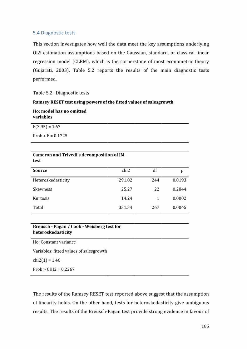
185
5.4 Diagnostic tests
This section investigates how well the data meet the key assumptions underlying
OLS estimation assumptions based on the Gaussian, standard, or classical linear
regression model (CLRM), which is the cornerstone of most econometric theory
(Gujarati, 2003). Table 5.2 reports the results of the main diagnostic tests
performed.
Table 5.2. Diagnostic tests
The results of the Ramsey RESET test reported above suggest that the assumption
of linearity holds. On the other hand, tests for heteroskedasticity give ambiguous
results. The results of the Breusch-Pagan test provide strong evidence in favour of
Ramsey RESET test using powers of the fitted values of salesgrowth
Ho: model has no omitted
variables
F(3,95) = 1.67
Prob > F = 0.1725
Cameron and Trivedi's decomposition of IM-
test
Source chi2 df p
Heteroskedasticity 291.82 244 0.0193
Skewness 25.27 22 0.2844
Kurtosis 14.24 1 0.0002
Total 331.34 267 0.0045
Breusch - Pagan / Cook - Weisberg test for
heteroskedasticity
Ho: Constant variance
Variables: fitted values of salesgrowth
chi2(1) = 1.46
Prob > CHI2 = 0.2267
homoscedastic variance, while the results of Cameron & Trivedi's test reject the
assumption of homoscedasticity. Although the null hypothesis of no excessive
skewness is clearly rejected, evidence of kurtosis suggests some departure from a
normal distribution of the residuals. However, this evidence of non-normality does
not invalidate statistical inference (F- and t-tests) in a sample of the size used in
the present study (Spanos, 1986). Therefore, a conservative approach to inference
is adopted by reporting robust standard errors, as these can address concerns
about failure to meet assumptions, such as minor problems about normality
(Spanos, 1986), heteroscedasticity, or some observations that exhibit large
residuals, leverage or influence (Wooldridge, 2015).
In each case we have investigated the statistical characteristics of the data with
further graphic checks, which are reported in appendix A5 (figures A5.1 – A5.4). In
terms of the linearity assumption, in line with the results of the Ramsey RESET
test, the plots of residuals versus predictor variables and augmented plus residual
plots presented in figures A5.1 and A5.2 in appendix A5 do not indicate that the
assumption is violated. These plots are evenly distributed vertically, and they do
not have outliers, or a clear shape to them. Further, the plot of kernel density
(kdensity) and the plots of quantiles of a variable against the quantiles of a normal
distribution (qnorm) are presented in figures A5.3 and A5.4 in appendix A5 to
check whether the residuals are normally distributed. The plots' appearance is in
line with the results of the Cameron and Trivedi's test. Pnorm (representing
skewness) shows no indications of non-normality, while the qnorm plot (kurtosis)
shows a slight deviation from normality at the upper tail, as can be seen in
the kdensity plot as well. Nevertheless, this seems to be a minor deviation from
normality and, as argued above, robust standard errors are used for inference.
In the next step we check for multicollinearity by using the variance inflation
factor (VIF). As a rule of thumb, if a VIF of a variable is greater than 10, it might
require further investigation, as the variable could be considered as a linear
combination of other independent variables. Both the individual VIFs and the
mean VIF reported in Table 5.3 below satisfy the most conservative thresholds
typically used by researchers.
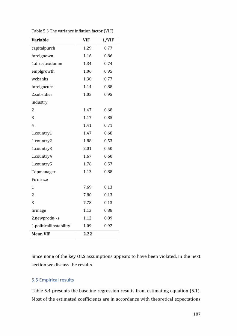
187
Table 5.3 The variance inflation factor (VIF)
Since none of the key OLS assumptions appears to have been violated, in the next
section we discuss the results.
5.5 Empirical results
Table 5.4 presents the baseline regression results from estimating equation (5.1).
Most of the estimated coefficients are in accordance with theoretical expectations
Variable VIF 1/VIF
capitalpurch 1.29 0.77
foreignown 1.16 0.86
1.directexdumm 1.34 0.74
emplgrowth 1.06 0.95
wcbanks 1.30 0.77
foreigncurr 1.14 0.88
2.subsidies 1.05 0.95
industry
2 1.47 0.68
3 1.17 0.85
4 1.41 0.71
1.country1 1.47 0.68
1.country2 1.88 0.53
1.country3 2.01 0.50
1.country4 1.67 0.60
1.country5 1.76 0.57
Topmanager 1.13 0.88
Firmsize
1 7.69 0.13
2 7.80 0.13
3 7.78 0.13
firmage 1.13 0.88
2.newprodu~s 1.12 0.89
1.politicallinstability 1.09 0.92
Mean VIF 2.22

and previous research. The estimates suggest that the financial variables are the
most economically influential and statistically significant. The relationship
between foreign currency loans and sales growth rate is negative and significant at
the 1% level. An increase of the share of foreign currency loans in total loans of the
firm by one percentage point, leads to a decrease in the growth rate of sales by
0.13 percentage points in 2009. This is a large effect relative to the mean growth of
sales of -0.19 (i.e. a mean decline of 19 percentage points). The relationship
between the variable working capital financed by banks (wcbanks) and the growth
rate of sales from 2008 to 2009 (salesgrowth) is also negative and significant at the
5% significance level. An increase in the proportion of the working capital of firms
financed by banks by 1 percentage point decreased the growth rate of sales by
0.06 percentage points. In addition, the dummy variable subsidies is also
statistically significant at the 5% significance level. The firms that received
subsidies during the previous 3 years (before 2007), compared to those firms
which did not receive subsidies, had an increase in the growth rate of sales of 7
percentage points. The relationship between foreignown and salesgrowth is
positive and significant at the 5% level. An increase in the foreign ownership of the
firm by one percentage points results in an increase of the growth rate of sales of
0.06 percentage points.
Results for most of the control variables appear to be statistically significant and
their signs are in accordance with theoretical predictions and previous empirical
findings. The relationship between the top manager's experience and the growth
rate of sales is positive and significant at the 5% level. An increase in the
experience of the top manager by one year leads to an increase in the growth rate
of sales by 0.3 percentage points. The variable newproduct3years is also significant
at the 5% level. Firms that introduced new products in the last 3 years (prior to
2007) experienced a growth rate of sales by 5 percentage points more than those
that did not introduce new products. The dummy variable politicalinstability is
also significant at the 5% level and has a negative relationship with the growth
rate of sales. Firms that perceived political instability to be a main obstacle to their
operations in 2007 had a decline in the growth rate of sales in 2009 of 5
percentage points more than firms that did not. The remaining dummy variable,

189
directexp, does not appear as statistically significant; moreover, it has very small
coefficients across all of our estimated models.
Table 5.4 OLS estimates of baseline regression (5.1) and extended models (5.2)
and (5.3)
Variables
Dependent Variable: %∆Sales Model (5.1) Model (5.2) Model (5.3)
Constant -0.0383 0.3325 0.3312
[0.0617] [0.1007] [0.1060]
%∆Employment 0.1251*** 0.1264*** 0.1282***
[0.0253] [0.0252] [0.0253]
∆Capital -0.0043 -0.005 -0.005
[0.0045] [0.0045] [0.0045]
Working Capital financed by Banks
-0.0660** -0.0622** -0.0522
[0.0259] [0.0253] [0.1276]
Foreign Currency Loans -0.1384*** -0.1403*** -0.1395***
[0.0355] [0.0354] [0.0356]
Foreign Ownership 0.0576** 0.0602** 0.0582**
[0.0274] [0.0274] [0.0275]
Top Manager Experience 0.0028** 0.0028*** 0.0028**
[0.0011] [0.0011] [0.0011]
Firm Age -0.0013 -0.0013 -0.0013
[0.0009] [0.0009] [0.0009]
Direct Exports Dummy 0.008 0.0057 -0.0912
[0.0290] [0.0288] [0.0863]
Subsidies 0.0690** 0.0728** 0.0715**
[0.0290] [0.0292] [0.0294]
New Product 3 years 0.0494** 0.0481** 0.0462**
[0.0207] [0.0203] [0.0203]
Political Instability -0.0528** -0.0477** -0.0470**
[0.0213] [0.0206] [0.0206]
Firm Size Dummy1 -0.0516 -0.0496 -0.0501
[0.0412] [0.0417] [0.0424]
Firm Size Dummy2 -0.0326 -0.0281 -0.0276
[0.0423] [0.0429] [0.0435]
Firm Size Dummy3 0.0226 0.0297 0.0296
[0.0456] [0.0448] [0.0456]
Foreign Bank Ownership
-0.3311*** -0.2996***
[0.0576] [0.0729] Aggregate Foreign Currency Loans
-0.1889*** -0.2025**
[0.0686] [0.0792]
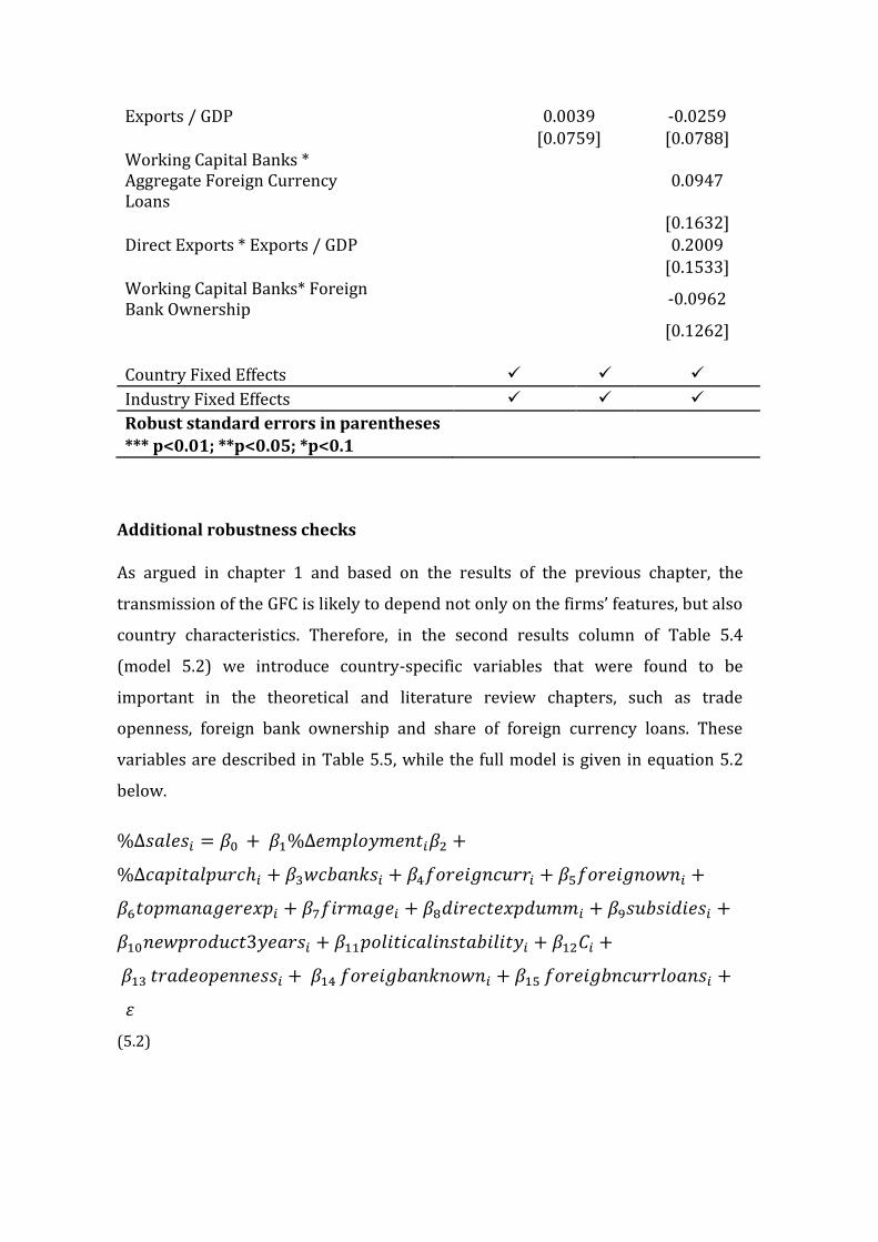
Exports / GDP
0.0039 -0.0259
[0.0759] [0.0788] Working Capital Banks * Aggregate Foreign Currency Loans
0.0947
[0.1632] Direct Exports * Exports / GDP
0.2009
[0.1533] Working Capital Banks* Foreign Bank Ownership
-0.0962
[0.1262]
Country Fixed Effects
Industry Fixed Effects
Robust standard errors in parentheses
*** p<0.01; **p<0.05; *p<0.1
Additional robustness checks
As argued in chapter 1 and based on the results of the previous chapter, the
transmission of the GFC is likely to depend not only on the firms’ features, but also
country characteristics. Therefore, in the second results column of Table 5.4
(model 5.2) we introduce country-specific variables that were found to be
important in the theoretical and literature review chapters, such as trade
openness, foreign bank ownership and share of foreign currency loans. These
variables are described in Table 5.5, while the full model is given in equation 5.2
below.
%∆𝑠𝑎𝑙𝑒𝑠𝑖 = 𝛽0 + 𝛽1%∆𝑒𝑚𝑝𝑙𝑜𝑦𝑚𝑒𝑛𝑡𝑖𝛽2 +
%∆𝑐𝑎𝑝𝑖𝑡𝑎𝑙𝑝𝑢𝑟𝑐ℎ𝑖 + 𝛽3𝑤𝑐𝑏𝑎𝑛𝑘𝑠𝑖 + 𝛽4𝑓𝑜𝑟𝑒𝑖𝑔𝑛𝑐𝑢𝑟𝑟𝑖 + 𝛽5𝑓𝑜𝑟𝑒𝑖𝑔𝑛𝑜𝑤𝑛𝑖 +
𝛽6𝑡𝑜𝑝𝑚𝑎𝑛𝑎𝑔𝑒𝑟𝑒𝑥𝑝𝑖 + 𝛽7𝑓𝑖𝑟𝑚𝑎𝑔𝑒𝑖 + 𝛽8𝑑𝑖𝑟𝑒𝑐𝑡𝑒𝑥𝑝𝑑𝑢𝑚𝑚𝑖 + 𝛽9𝑠𝑢𝑏𝑠𝑖𝑑𝑖𝑒𝑠𝑖 +
𝛽10𝑛𝑒𝑤𝑝𝑟𝑜𝑑𝑢𝑐𝑡3𝑦𝑒𝑎𝑟𝑠𝑖 + 𝛽11𝑝𝑜𝑙𝑖𝑡𝑖𝑐𝑎𝑙𝑖𝑛𝑠𝑡𝑎𝑏𝑖𝑙𝑖𝑡𝑦𝑖 + 𝛽12𝐶𝑖 +
𝛽13 𝑡𝑟𝑎𝑑𝑒𝑜𝑝𝑒𝑛𝑛𝑒𝑠𝑠𝑖 + 𝛽14 𝑓𝑜𝑟𝑒𝑖𝑔𝑏𝑎𝑛𝑘𝑛𝑜𝑤𝑛𝑖 + 𝛽15 𝑓𝑜𝑟𝑒𝑖𝑔𝑏𝑛𝑐𝑢𝑟𝑟𝑙𝑜𝑎𝑛𝑠𝑖 +
휀
(5.2)
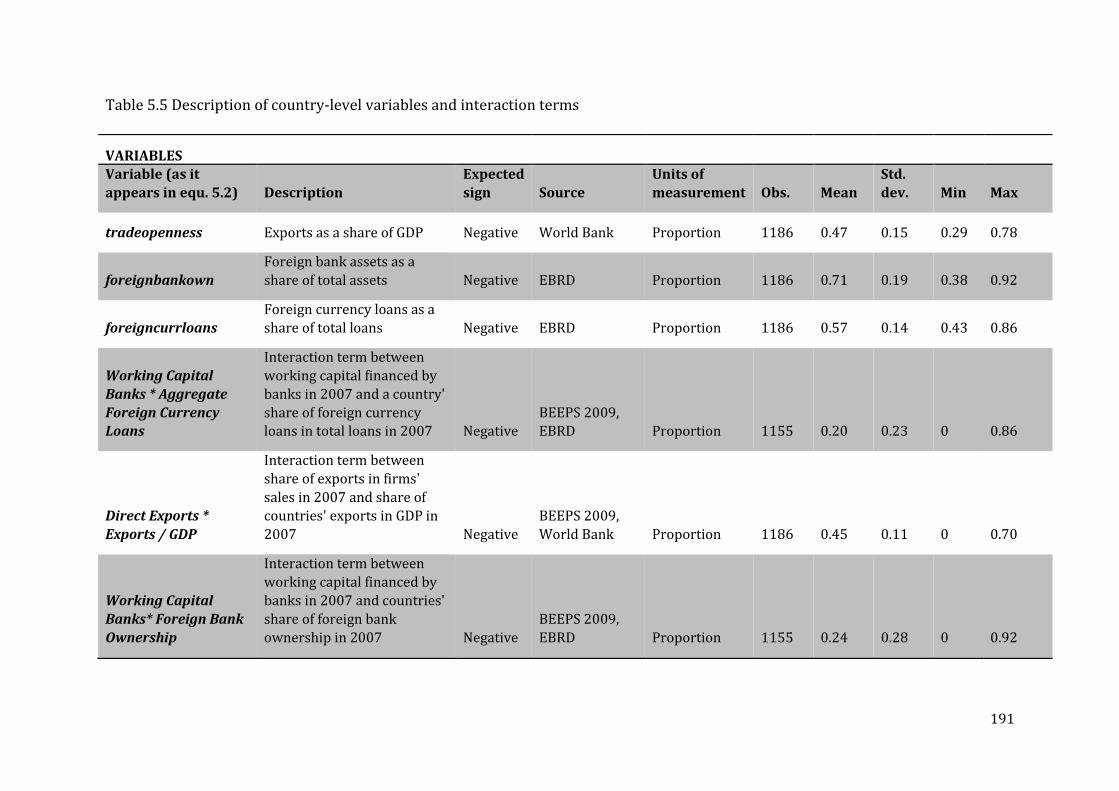
191
Table 5.5 Description of country-level variables and interaction terms
VARIABLES
Variable (as it
appears in equ. 5.2) Description
Expected
sign Source
Units of
measurement Obs. Mean
Std.
dev. Min Max
tradeopenness Exports as a share of GDP Negative World Bank Proportion 1186 0.47 0.15 0.29 0.78
foreignbankown
Foreign bank assets as a
share of total assets Negative EBRD Proportion 1186 0.71 0.19 0.38 0.92
foreigncurrloans
Foreign currency loans as a
share of total loans Negative EBRD Proportion 1186 0.57 0.14 0.43 0.86
Working Capital
Banks * Aggregate
Foreign Currency Loans
Interaction term between
working capital financed by
banks in 2007 and a country'
share of foreign currency loans in total loans in 2007 Negative
BEEPS 2009, EBRD Proportion 1155 0.20 0.23 0 0.86
Direct Exports *
Exports / GDP
Interaction term between
share of exports in firms'
sales in 2007 and share of
countries' exports in GDP in
2007 Negative
BEEPS 2009,
World Bank Proportion 1186 0.45 0.11 0 0.70
Working Capital
Banks* Foreign Bank
Ownership
Interaction term between
working capital financed by
banks in 2007 and countries'
share of foreign bank
ownership in 2007 Negative
BEEPS 2009,
EBRD Proportion 1155 0.24 0.28 0 0.92

Adding these country-specific variables does not significantly change the results of
the previously discussed variables from the baseline regression; indeed, it
strengthens them in some cases. The results of the aggregate variables are in line
with the results of their corresponding firm-level variables (where applicable)
presented in the second column of results in Table 5.4 (model 5.2). The relationship
between the aggregate share of foreign currency loans and sales growth is negative
and highly significant. An increase in the share of foreign currency loans in total loans
of a country by 1 percentage point leads to a decrease in the growth rate of sales of
the firms by 0.2 percentage points. The relationship between foreign bank ownership
and sales growth is also negative and highly significant. A one percentage point
increase in foreign bank ownership leads to a decrease in growth rate of sales by
around one third of a percentage point. A similar relationship to the firm-level
between exports as a share of total sales of the firm and growth rate of sales is
observed between the country-level exports as a share of GDP and sales growth; the
exports/GDP variable does not appear to be statistically significant and has a very
small coefficient.
Next, the country-level variables are interacted with the firm-level features and the
results are reported in the last column of Table 5.4 (model 5.3). For example, in order
to investigate whether foreign bank ownership in a country affected firms’ sales by
affecting access to finance during the GFC, the variable working capital financed by
banks is interacted with the level of the country's foreign bank ownership. Further, in
order to examine whether the firms that financed their working capital by banks in
countries with higher shares of foreign currency loans were more severely affected
by the crisis, the variable working capital financed by banks is interacted with the
country's level of foreign bank ownership. Finally, to test whether exporting firms in
countries more open to trade were affected differently during the GFC, the direct
exports dummy is interacted with the country's exports as a share of GDP variable.
Again, adding these interaction terms to the baseline regression does not change
significantly the results, indicating that the results of the main variables are robust to
different model specifications. We cannot infer whether there is any significant effect
of the interaction terms based solely on the results reported in the last column of
Table 5.3, given that the interaction coefficients show only the average effect of the
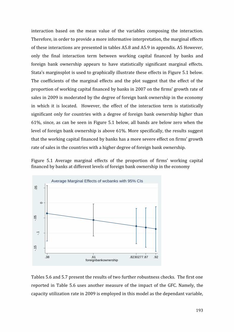
193
interaction based on the mean value of the variables composing the interaction.
Therefore, in order to provide a more informative interpretation, the marginal effects
of these interactions are presented in tables A5.8 and A5.9 in appendix. A5 However,
only the final interaction term between working capital financed by banks and
foreign bank ownership appears to have statistically significant marginal effects.
Stata’s marginsplot is used to graphically illustrate these effects in Figure 5.1 below.
The coefficients of the marginal effects and the plot suggest that the effect of the
proportion of working capital financed by banks in 2007 on the firms' growth rate of
sales in 2009 is moderated by the degree of foreign bank ownership in the economy
in which it is located. However, the effect of the interaction term is statistically
significant only for countries with a degree of foreign bank ownership higher than
61%, since, as can be seen in Figure 5.1 below, all bands are below zero when the
level of foreign bank ownership is above 61%. More specifically, the results suggest
that the working capital financed by banks has a more severe effect on firms’ growth
rate of sales in the countries with a higher degree of foreign bank ownership.
Figure 5.1 Average marginal effects of the proportion of firms’ working capital
financed by banks at different levels of foreign bank ownership in the economy
Tables 5.6 and 5.7 present the results of two further robustness checks. The first one
reported in Table 5.6 uses another measure of the impact of the GFC. Namely, the
capacity utilization rate in 2009 is employed in this model as the dependant variable,
-.15
-.1
-.05
0
.05
Effe
cts
on
Lin
ea
r P
redic
tion
.38 .61 .8230277.87 .92foreignbankownership
Average Marginal Effects of wcbanks with 95% CIs
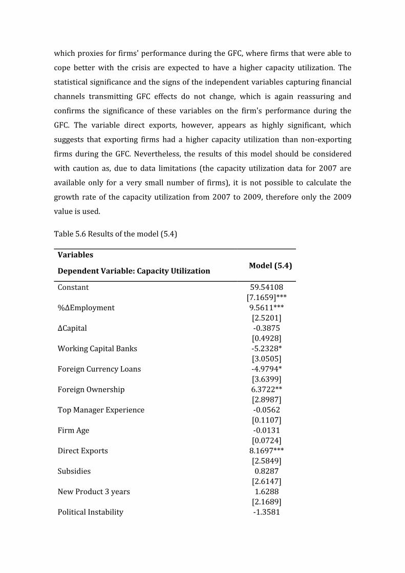
which proxies for firms' performance during the GFC, where firms that were able to
cope better with the crisis are expected to have a higher capacity utilization. The
statistical significance and the signs of the independent variables capturing financial
channels transmitting GFC effects do not change, which is again reassuring and
confirms the significance of these variables on the firm's performance during the
GFC. The variable direct exports, however, appears as highly significant, which
suggests that exporting firms had a higher capacity utilization than non-exporting
firms during the GFC. Nevertheless, the results of this model should be considered
with caution as, due to data limitations (the capacity utilization data for 2007 are
available only for a very small number of firms), it is not possible to calculate the
growth rate of the capacity utilization from 2007 to 2009, therefore only the 2009
value is used.
Table 5.6 Results of the model (5.4)
Variables
Model (5.4) Dependent Variable: Capacity Utilization
Constant 59.54108
[7.1659]***
%∆Employment 9.5611***
[2.5201]
∆Capital -0.3875
[0.4928]
Working Capital Banks -5.2328*
[3.0505]
Foreign Currency Loans -4.9794*
[3.6399]
Foreign Ownership 6.3722**
[2.8987]
Top Manager Experience -0.0562
[0.1107]
Firm Age -0.0131
[0.0724]
Direct Exports 8.1697***
[2.5849]
Subsidies 0.8287
[2.6147]
New Product 3 years 1.6288
[2.1689]
Political Instability -1.3581

195
[2.2097]
Firm Size Dummy1 4.6828
[5.9677]
Firm Size Dummy2 7.576
[5.9874]
Firm Size Dummy3 13.8414**
[6.2026]
Country Fixed Effects
Industry Fixed Effects
Robust standard errors in parentheses
*** p<0.01; **p<0.05; *p<0.1
As an additional robustness check, we investigate whether the same variables that
affected firms' sales during the GFC also affected their employment change. As
explained above, employment growth is potentially endogenous. However, as argued
in section 5.3, the independent variables of the baseline regression are not expected
to affect employment change; employment and output change do not change
simultaneously, because employment and output have very different adjustment
speeds. Therefore, we do not expect to find significant results from the latest
regression. The results are reported in Table 5.7 below and, as expected, none of the
independent variables appear to be significant influences on employment change
within the sample period. This is reassuring as it reduces concerns regarding both
simultaneity and common determinants, which could cause output and employment
to be correlated even if they stood in no causal relationship to one another. However,
we cannot demonstrate that output change and employment change have no
unobserved influences in common.
Table 5.7 Robustness check (dependent variable %∆Employment, model (5.5))
Variables Model (5.5)
Dependent Variable: %∆Employment
Constant -0.0046
[0.1360]
Working Capital Banks -0.0623
[0.0437]
Foreign Currency Loans 0.098
[0.0634]
Foreign Ownership 0.0266

[0.0405]
Top Manager Experience -0.0004
[0.0014]
Firm Age 0.0014
[0.0010]
Direct Exports 0.0337
[0.0403]
Subsidies 0.0529
[0.0437]
New Product 3 years 0.0286
[0.0304]
Political Instability -0.0225
[0.0317]
Firm Size Dummy1 -0.1355
[0.1242]
Firm Size Dummy2 -0.196
[0.1240]
Firm Size Dummy3 -0.2064
[0.1245]
Country Fixed Effects
Industry Fixed Effects
Robust standard errors in parentheses *** p<0.01; **p<0.05;
*p<0.1
Finally, a few more robustness checks are conducted to further investigate the
statistical insignificance of the dummy variable directexp in model 5.1. Firstly, it
should be noted that the lack of significance of this variable does not suggest that
exporting firms have not been affected by the crisis, nor that the crisis was not
transmitted through the exports channel; it simply suggests that exporting firms
have not been affected by the crisis significantly differently from non-exporting
firms. Table 5.8 reports the average predicted percentage change in sales when the
export dummy is set to zero and the average predicted percentage change in sales
when the export dummy is set to one in model 5.1 and shows that both types of firms
have been significantly affected by the crisis. However, the relative sizes of the
estimated effects suggest that the effect was slightly higher for non-exporting firms,
even though the difference in not statistically significant.

197
Table 5.8 Predictive margins of directexdumm
A growing body of literature has found that exporting firms are substantially and
significantly different from non-exporting firms. Numerous authors have
documented the superior performance of exporting firms compared to non-exporting
firms even in the same industry and region (Chen and Tang, 1987; Clerides et al.,
1998; Bernard and Jansen, 1999. Bernard and Jensen (1999) find that exporters are
larger, more productive, more technology and capital intensive, use more skilled
workers and pay higher wages than non-exporting firms. Other authors, Melitz
(2003), Melitz and Ottaviano (2003), and Bernard et al. (2003) claim that high-
productivity firms self-select themselves into export markets. Consequently, due to
their superior performance, it can be argued that the exporting-firms might be more
able to adjust to difficult circumstances; hence, they are more flexible when it comes
to reallocating to a different market (foreign or domestic market) due to a decline in
exports as a result of the crisis. In order to test whether this applies to the firms
included in this study, the variable directexp is interacted with the variable
changenatsales - a new variable computed as the percentage change in proportion of
sales to the domestic market from 2007 to 2009. Based on the arguments provided
above, it is expected that directly exporting firms able to reallocate a higher
percentage of their sales to domestic market have been less severely affected by the
crisis.20 It has to be noted that when using the actual percentage of sales that are
exports instead of the dummy variable directexp, we obtain similar results. However,
20 Due to lack of data, it cannot be identified whether the firms that reallocated their sales to other foreign markets / new countries, were less severely affected by the crisis. Therefore, it is only tested if those exporting firms that switched to domestic markets were less severely affected by the crisis.
directexp Margin Std. Err. t-value P>t [95% Conf. Interval]
Non-exporters - 0 - 0.203 0.011 - 19.170 0.000 - 0.224 - 0.183
Exporters - 1 - 0.196 0.026 - 7.480 0.000 - 0.247 - 0.144
we decided to use the dummy variable as it illustrates better the differences between
exporting and non-exporting firms through the marginsplot. The results of the
regression are presented in the first results column in Table 5.9 (model 5.6). Even
though the interaction term is statistically insignificant, it cannot be inferred whether
it has any relevant and significant effect on crisis severity given that the interaction
coefficient shows only the average effect of the interaction based on the mean value
of the variable changenatsales. Therefore, in order to provide a more informative
interpretation, the marginal effect of direct exports across different values of changes
in proportion of sales to domestic market is presented in Figure 5.2 below and the
marginsplot is used to graphically illustrate the effect. The marginal effect appears as
statistically significant under different values of changenatsales (appendix A5, Table
A5.17). However, the contrasts between exporting firms and non-exporting firms21
presented in Table 5.10 below do not appear to be statistically significant.
Nevertheless, the overall statistical significance of the contrasts increases with the
increase of the variable changenatsales. Even though these contrasts are not
significant at conventional levels, when combined with marginsplot presented in
Figure 5.2, they are suggestive that exporting firms which have been able to
reallocate higher proportions of their sales to domestic markets have been slightly
less affected by the crisis. It should be noted that 52% of the exporting firms in the
sample increased their proportion of sales to domestic markets in 2009, 50% of
which had an increase of 50% or higher. As for the rest of the exporting firms, 35%
decreased their proportion of sales to domestic markets, which suggest that their
sales to foreign markets increased and for the remaining 13% of the exporting firms
the proportion of sales to domestic markets did not change from 2007 to 2009.
Model 5.7 in Table 5.9 includes the interaction between directexp and foreigncurr, which
fits a separate slope for the relationship between foreigncurr and salesgrowth for
exporting firms versus non-exporting firms. Model 5.8 includes the interaction term
between directexdumm and foreignown, which fits a separate slope for the relationship
between the share of firms' foreign ownership and the rate of sales growth for exporting
21 As explained in Table 5.1, exporting firms refer to firms that export more than 10% of their sales, implying that the category of non-exporting firms includes low-intensity exporters, i.e. the firms that export less than 10% of their sales.
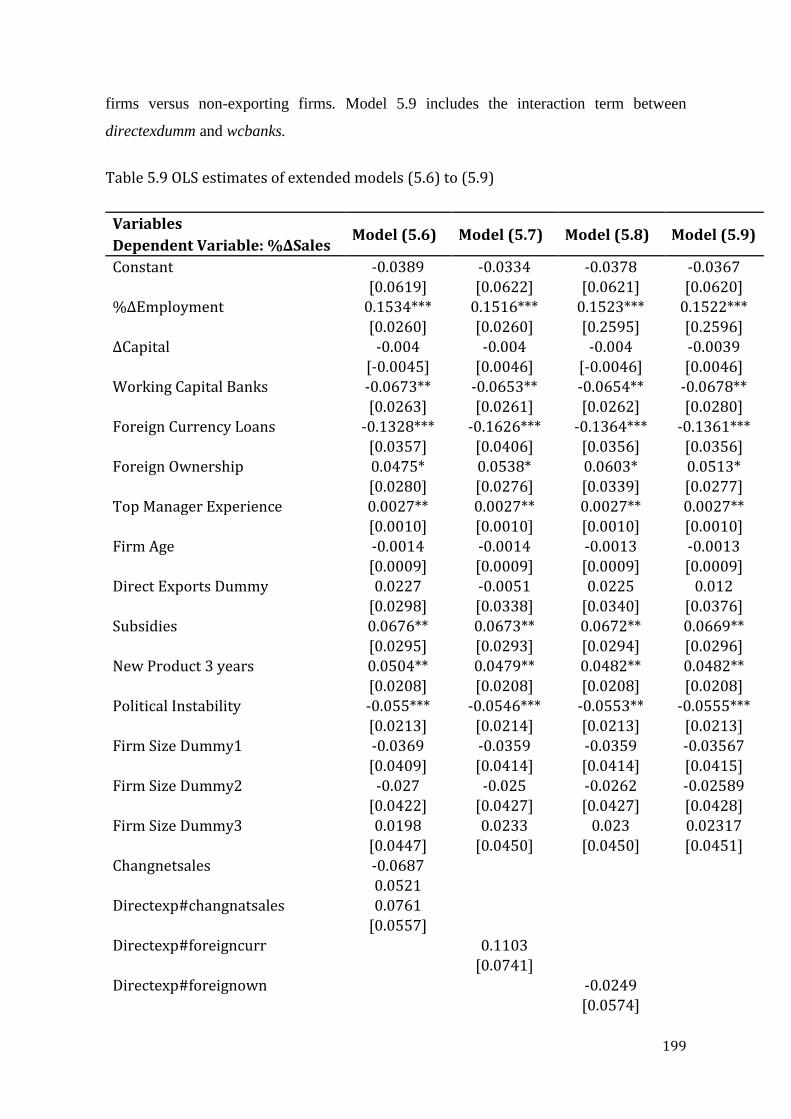
199
firms versus non-exporting firms. Model 5.9 includes the interaction term between
directexdumm and wcbanks.
Table 5.9 OLS estimates of extended models (5.6) to (5.9)
Variables Model (5.6) Model (5.7) Model (5.8) Model (5.9)
Dependent Variable: %∆Sales
Constant -0.0389 -0.0334 -0.0378 -0.0367
[0.0619] [0.0622] [0.0621] [0.0620]
%∆Employment 0.1534*** 0.1516*** 0.1523*** 0.1522***
[0.0260] [0.0260] [0.2595] [0.2596]
∆Capital -0.004 -0.004 -0.004 -0.0039
[-0.0045] [0.0046] [-0.0046] [0.0046]
Working Capital Banks -0.0673** -0.0653** -0.0654** -0.0678**
[0.0263] [0.0261] [0.0262] [0.0280]
Foreign Currency Loans -0.1328*** -0.1626*** -0.1364*** -0.1361***
[0.0357] [0.0406] [0.0356] [0.0356]
Foreign Ownership 0.0475* 0.0538* 0.0603* 0.0513*
[0.0280] [0.0276] [0.0339] [0.0277]
Top Manager Experience 0.0027** 0.0027** 0.0027** 0.0027**
[0.0010] [0.0010] [0.0010] [0.0010]
Firm Age -0.0014 -0.0014 -0.0013 -0.0013
[0.0009] [0.0009] [0.0009] [0.0009]
Direct Exports Dummy 0.0227 -0.0051 0.0225 0.012
[0.0298] [0.0338] [0.0340] [0.0376]
Subsidies 0.0676** 0.0673** 0.0672** 0.0669**
[0.0295] [0.0293] [0.0294] [0.0296]
New Product 3 years 0.0504** 0.0479** 0.0482** 0.0482**
[0.0208] [0.0208] [0.0208] [0.0208]
Political Instability -0.055*** -0.0546*** -0.0553** -0.0555***
[0.0213] [0.0214] [0.0213] [0.0213]
Firm Size Dummy1 -0.0369 -0.0359 -0.0359 -0.03567
[0.0409] [0.0414] [0.0414] [0.0415]
Firm Size Dummy2 -0.027 -0.025 -0.0262 -0.02589
[0.0422] [0.0427] [0.0427] [0.0428]
Firm Size Dummy3 0.0198 0.0233 0.023 0.02317
[0.0447] [0.0450] [0.0450] [0.0451]
Changnetsales -0.0687
0.0521 Directexp#changnatsales 0.0761
[0.0557] Directexp#foreigncurr
0.1103
[0.0741] Directexp#foreignown
-0.0249
[0.0574]
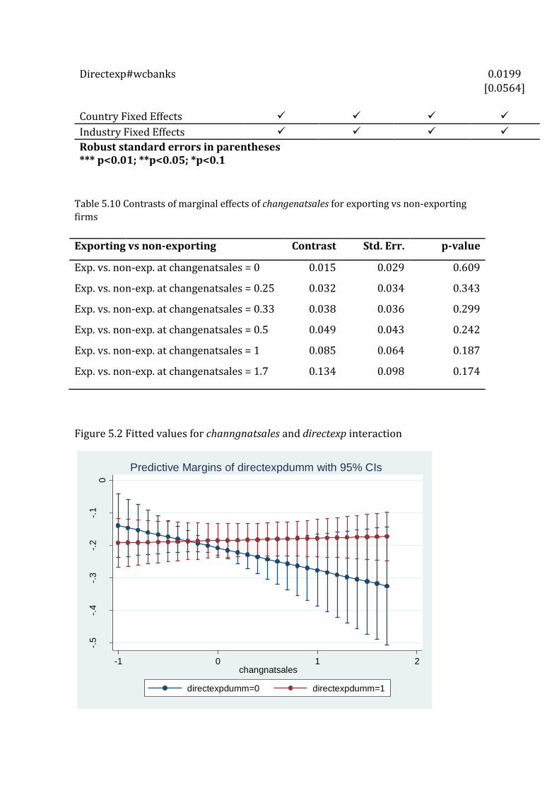
Directexp#wcbanks
0.0199
[0.0564]
Country Fixed Effects
Industry Fixed Effects
Robust standard errors in parentheses *** p<0.01; **p<0.05; *p<0.1
Table 5.10 Contrasts of marginal effects of changenatsales for exporting vs non-exporting
firms
Figure 5.2 Fitted values for channgnatsales and directexp interaction
-.5
-.4
-.3
-.2
-.1
0
Lin
ea
r P
redic
tion
-1 0 1 2changnatsales
directexpdumm=0 directexpdumm=1
Predictive Margins of directexpdumm with 95% CIs
Exporting vs non-exporting Contrast Std. Err. p-value
Exp. vs. non-exp. at changenatsales = 0 0.015 0.029 0.609
Exp. vs. non-exp. at changenatsales = 0.25 0.032 0.034 0.343
Exp. vs. non-exp. at changenatsales = 0.33 0.038 0.036 0.299
Exp. vs. non-exp. at changenatsales = 0.5 0.049 0.043 0.242
Exp. vs. non-exp. at changenatsales = 1 0.085 0.064 0.187
Exp. vs. non-exp. at changenatsales = 1.7 0.134 0.098 0.174

201
Further, as reported in Table 5.9, a number of other factors that might have
influenced the impact of exports on crisis severity are investigated. Given the overall
significance of the variables comprising the financial channel, it is explored whether
they might have affected differently exporting and non-exporting firms. Model 5.7
includes the interaction between directexp and foreigncurr, which fits a separate
slope for the relationship between foreigncurr and salesgrowth for exporting firms
versus non-exporting firms. The results of the regression are reported in the second
column of results in Table 5.9. The margins command is used to compute the
adjusted means for foreigncurr separately for exporting firms and non-exporting
firms. Then the marginsplot command is used to graph these adjusted means, which
are presented in Figure 5.3. This shows the adjusted mean for salesgrowth as a
function of foreigncurr (on the x axis) and with separate lines for exporting and non-
exporting firms. Although the marginal effects presented in Figure 5.3 for both
exporters and non-exports are all significantly different from zero, the contrasts
between each pair of marginal effects are uniformly non-significant at conventional
levels, although their significance increases as the share of foreigncurr increases
(table 5.11 below). Therefore, the results are suggestive that as the share of foreign
currency loans increases, the sales of non-exporting firms are more severely affected.
Again, we have some (albeit slight) evidence consistent with the interpretation that
exporting firms are more resistant to the pressures of the GFC. It should be pointed
out that 46% of the exporting firms and 26% of the non-exporting firms have loans in
foreign currencies. In addition, for around 25% of exporting firms and 15% of non-
exporting firms the proportion of loans in foreign currency is higher than 50%.
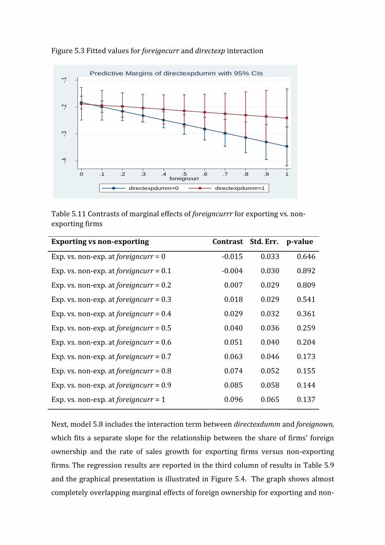
Figure 5.3 Fitted values for foreigncurr and directexp interaction
Table 5.11 Contrasts of marginal effects of foreigncurrr for exporting vs. non-
exporting firms
Next, model 5.8 includes the interaction term between directexdumm and foreignown,
which fits a separate slope for the relationship between the share of firms' foreign
ownership and the rate of sales growth for exporting firms versus non-exporting
firms. The regression results are reported in the third column of results in Table 5.9
and the graphical presentation is illustrated in Figure 5.4. The graph shows almost
completely overlapping marginal effects of foreign ownership for exporting and non-
-.4-.3
-.2-.1
Line
ar P
redi
ctio
n
0 .1 .2 .3 .4 .5 .6 .7 .8 .9 1foreigncurr
directexpdumm=0 directexpdumm=1
Predictive Margins of directexpdumm with 95% CIs
Exporting vs non-exporting Contrast Std. Err. p-value
Exp. vs. non-exp. at foreigncurr = 0 -0.015 0.033 0.646
Exp. vs. non-exp. at foreigncurr = 0.1 -0.004 0.030 0.892
Exp. vs. non-exp. at foreigncurr = 0.2 0.007 0.029 0.809
Exp. vs. non-exp. at foreigncurr = 0.3 0.018 0.029 0.541
Exp. vs. non-exp. at foreigncurr = 0.4 0.029 0.032 0.361
Exp. vs. non-exp. at foreigncurr = 0.5 0.040 0.036 0.259
Exp. vs. non-exp. at foreigncurr = 0.6 0.051 0.040 0.204
Exp. vs. non-exp. at foreigncurr = 0.7 0.063 0.046 0.173
Exp. vs. non-exp. at foreigncurr = 0.8 0.074 0.052 0.155
Exp. vs. non-exp. at foreigncurr = 0.9 0.085 0.058 0.144
Exp. vs. non-exp. at foreigncurr = 1 0.096 0.065 0.137
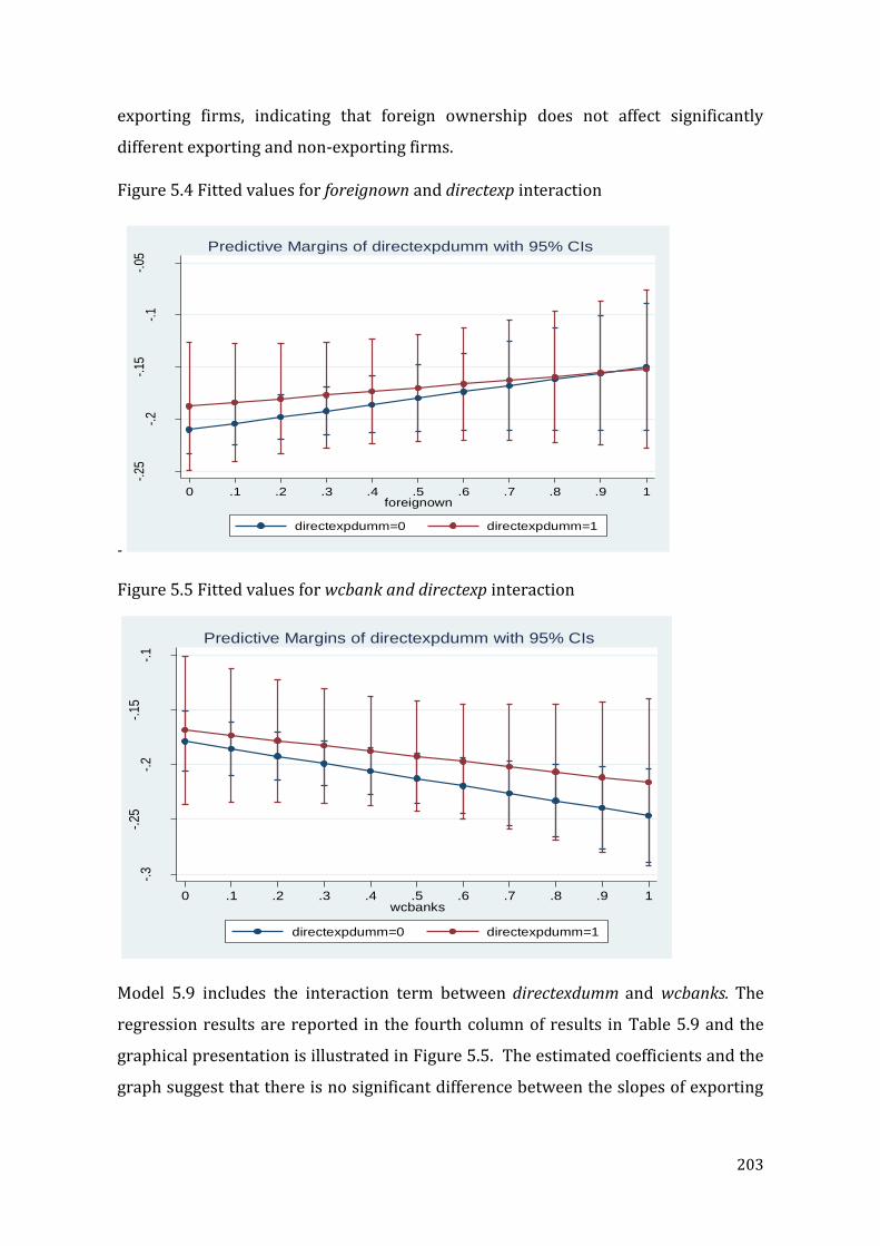
203
exporting firms, indicating that foreign ownership does not affect significantly
different exporting and non-exporting firms.
Figure 5.4 Fitted values for foreignown and directexp interaction
-
Figure 5.5 Fitted values for wcbank and directexp interaction
Model 5.9 includes the interaction term between directexdumm and wcbanks. The
regression results are reported in the fourth column of results in Table 5.9 and the
graphical presentation is illustrated in Figure 5.5. The estimated coefficients and the
graph suggest that there is no significant difference between the slopes of exporting
-.25
-.2
-.15
-.1
-.05
Lin
ear
Pre
dict
ion
0 .1 .2 .3 .4 .5 .6 .7 .8 .9 1foreignown
directexpdumm=0 directexpdumm=1
Predictive Margins of directexpdumm with 95% CIs
-.3
-.25
-.2
-.15
-.1
Lin
ear
Pre
dict
ion
0 .1 .2 .3 .4 .5 .6 .7 .8 .9 1wcbanks
directexpdumm=0 directexpdumm=1
Predictive Margins of directexpdumm with 95% CIs
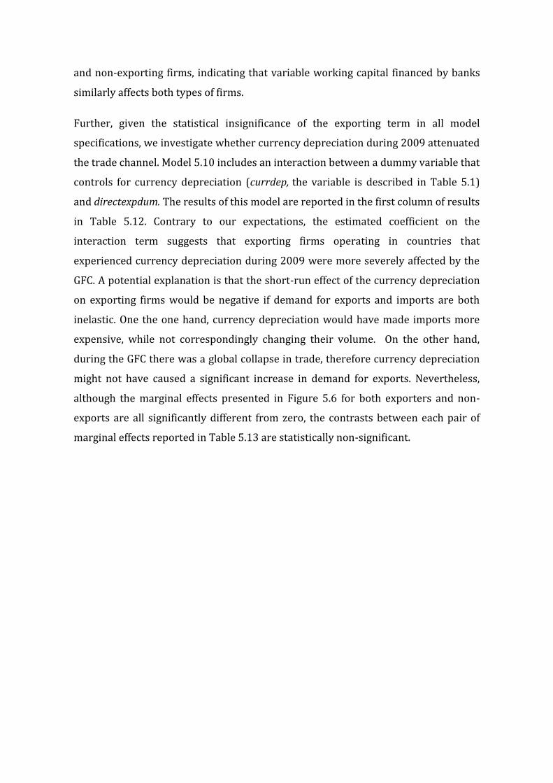
and non-exporting firms, indicating that variable working capital financed by banks
similarly affects both types of firms.
Further, given the statistical insignificance of the exporting term in all model
specifications, we investigate whether currency depreciation during 2009 attenuated
the trade channel. Model 5.10 includes an interaction between a dummy variable that
controls for currency depreciation (currdep, the variable is described in Table 5.1)
and directexpdum. The results of this model are reported in the first column of results
in Table 5.12. Contrary to our expectations, the estimated coefficient on the
interaction term suggests that exporting firms operating in countries that
experienced currency depreciation during 2009 were more severely affected by the
GFC. A potential explanation is that the short-run effect of the currency depreciation
on exporting firms would be negative if demand for exports and imports are both
inelastic. One the one hand, currency depreciation would have made imports more
expensive, while not correspondingly changing their volume. On the other hand,
during the GFC there was a global collapse in trade, therefore currency depreciation
might not have caused a significant increase in demand for exports. Nevertheless,
although the marginal effects presented in Figure 5.6 for both exporters and non-
exports are all significantly different from zero, the contrasts between each pair of
marginal effects reported in Table 5.13 are statistically non-significant.

205
Table 5.12 Results of the models (5.10) and (5.11)
Model (5.10) Model (5.11)
Dependent Variable: %∆Sales
Constant -0.0727 -0.071
[0.0549] [0.0551]
%∆Employment 0.1330*** 0.1361***
[0.0523] [0.0254]
∆Capital -0.005 -0.0048
[-0.0047] [0.0046]
Working Capital Banks -0.0326 -0.0409*
[0.0238] [0.0356]
Foreign Currency Loans -0.1695*** -0.748**
[0.0345] [0.0380]
Foreign Ownership 0.0608** 0.0561**
[0.0275] [0.0267]
Top Manager Experience 0.0029*** 0.0029***
[0.0011] [0.0011]
Firm Age -0.0019* -0.0020**
[0.0009] [0.0009]
Direct Exports Dummy 0.0428 -0.0069
[0.0336] [0.0289]
Subsidies 0.0547* 0.0504*
[0.0282] [0.02830]
New Product 3 years 0.0480** 0.0471**
[0.0206] [0.0205]
Political Instability -0.0685*** -0.0702***
[0.0209] [0.0209]
Currency Depreciation 0.1139*** 0.1249***
[0.0230] [0.0227]
Firm Size Dummy1 -0.0469 -0.0521
[0.0387] [0.0397]
Firm Size Dummy2 -0.022 -0.0273
[0.0398] [0.0404]
Firm Size Dummy3 0.0418 0.0325
[0.0426] [0.0435]
Directexp#currdep -0.1153**
[0.0542] Foreigncurr#currdep
-0.2356***
[0.0748]
Country Fixed Effects
Industry Fixed Effects
Robust standard errors in parentheses *** p<0.01; **p<0.05; *p<0.1
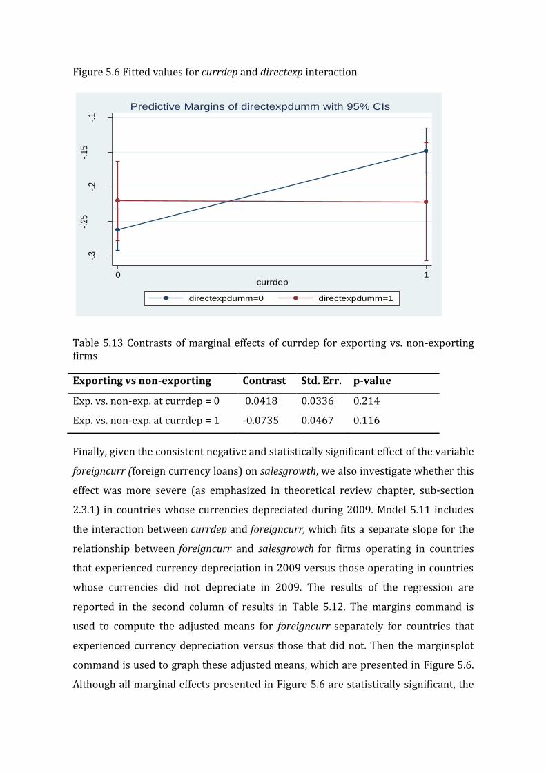
Figure 5.6 Fitted values for currdep and directexp interaction
Table 5.13 Contrasts of marginal effects of currdep for exporting vs. non-exporting firms
Finally, given the consistent negative and statistically significant effect of the variable
foreigncurr (foreign currency loans) on salesgrowth, we also investigate whether this
effect was more severe (as emphasized in theoretical review chapter, sub-section
2.3.1) in countries whose currencies depreciated during 2009. Model 5.11 includes
the interaction between currdep and foreigncurr, which fits a separate slope for the
relationship between foreigncurr and salesgrowth for firms operating in countries
that experienced currency depreciation in 2009 versus those operating in countries
whose currencies did not depreciate in 2009. The results of the regression are
reported in the second column of results in Table 5.12. The margins command is
used to compute the adjusted means for foreigncurr separately for countries that
experienced currency depreciation versus those that did not. Then the marginsplot
command is used to graph these adjusted means, which are presented in Figure 5.6.
Although all marginal effects presented in Figure 5.6 are statistically significant, the
-.3
-.25
-.2
-.15
-.1
Lin
ear
Pre
dict
ion
0 1currdep
directexpdumm=0 directexpdumm=1
Predictive Margins of directexpdumm with 95% CIs
Exporting vs non-exporting Contrast Std. Err. p-value
Exp. vs. non-exp. at currdep = 0 0.0418 0.0336 0.214
Exp. vs. non-exp. at currdep = 1 -0.0735 0.0467 0.116

207
contrasts between each pair of marginal effects reported in Table 5.14 are
statistically significant for only lower levels of foreign currency loans and they
approach borderline levels of statistical significance at the highest levels of foreign
currency loans. Nevertheless, the estimated coefficient and the marginal effects
presented in Figure 5.7 reinforce the general finding that foreign currency loans had
a negative effect on firms during the crisis. These results are also suggestive that
firms with higher levels of foreign currency loans operating in countries that
experienced currency depreciation in 2009 were more severely affected by the crisis.
Figure 5.7 Fitted values for foreigncurr and currdep interaction
-.6
-.5
-.4
-.3
-.2
-.1
Lin
ea
r P
redic
tion
0 .1 .2 .3 .4 .5 .6 .7 .8 .9 1foreigncurr
currdep=0 currdep=1
Predictive Margins of currdep with 95% CIs
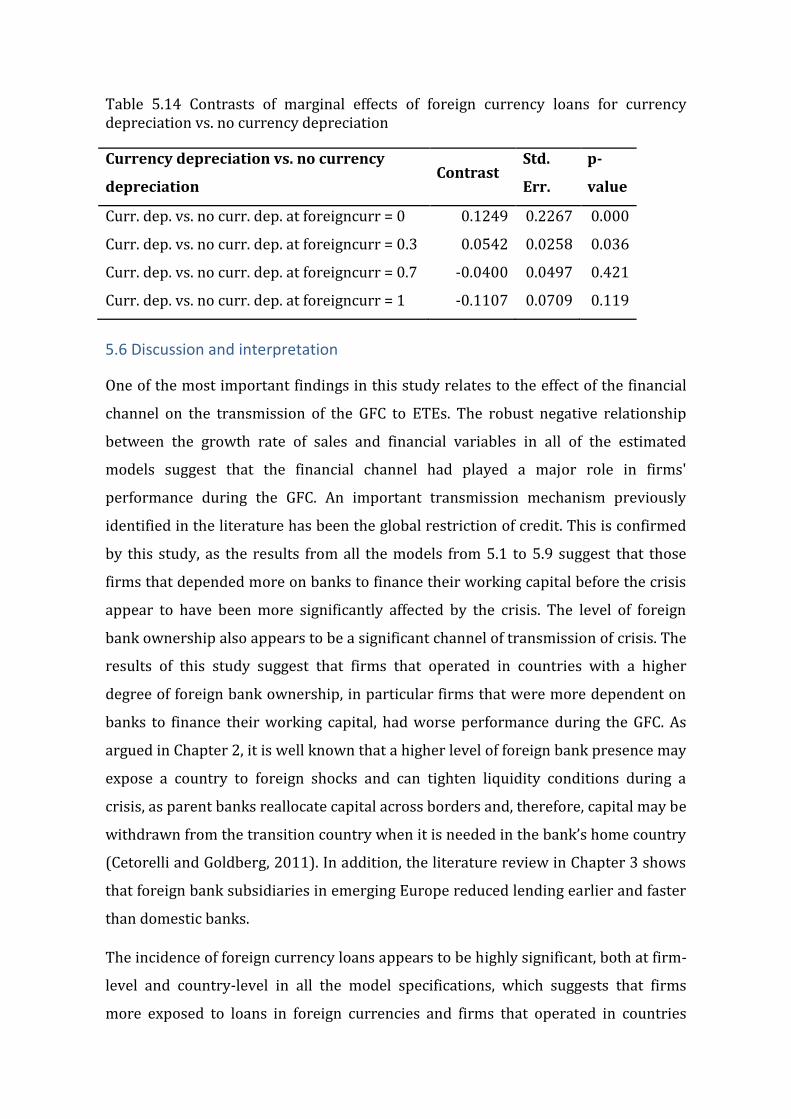
Table 5.14 Contrasts of marginal effects of foreign currency loans for currency depreciation vs. no currency depreciation
5.6 Discussion and interpretation
One of the most important findings in this study relates to the effect of the financial
channel on the transmission of the GFC to ETEs. The robust negative relationship
between the growth rate of sales and financial variables in all of the estimated
models suggest that the financial channel had played a major role in firms'
performance during the GFC. An important transmission mechanism previously
identified in the literature has been the global restriction of credit. This is confirmed
by this study, as the results from all the models from 5.1 to 5.9 suggest that those
firms that depended more on banks to finance their working capital before the crisis
appear to have been more significantly affected by the crisis. The level of foreign
bank ownership also appears to be a significant channel of transmission of crisis. The
results of this study suggest that firms that operated in countries with a higher
degree of foreign bank ownership, in particular firms that were more dependent on
banks to finance their working capital, had worse performance during the GFC. As
argued in Chapter 2, it is well known that a higher level of foreign bank presence may
expose a country to foreign shocks and can tighten liquidity conditions during a
crisis, as parent banks reallocate capital across borders and, therefore, capital may be
withdrawn from the transition country when it is needed in the bank’s home country
(Cetorelli and Goldberg, 2011). In addition, the literature review in Chapter 3 shows
that foreign bank subsidiaries in emerging Europe reduced lending earlier and faster
than domestic banks.
The incidence of foreign currency loans appears to be highly significant, both at firm-
level and country-level in all the model specifications, which suggests that firms
more exposed to loans in foreign currencies and firms that operated in countries
Currency depreciation vs. no currency
depreciation Contrast
Std.
Err.
p-
value
Curr. dep. vs. no curr. dep. at foreigncurr = 0 0.1249 0.2267 0.000
Curr. dep. vs. no curr. dep. at foreigncurr = 0.3 0.0542 0.0258 0.036
Curr. dep. vs. no curr. dep. at foreigncurr = 0.7 -0.0400 0.0497 0.421
Curr. dep. vs. no curr. dep. at foreigncurr = 1 -0.1107 0.0709 0.119
209
with higher levels of foreign currency loans were more severely affected by the GFC.
As argued in chapter 2, during the GFC, the depreciation of the domestic currencies
prevented some unhedged borrowers from servicing their loans in foreign
currencies. Further investigation revealed evidence consistent with this conjecture.
The margins and the marginsplot of the interaction term between foreigncurr and
currdep are suggestive that the firms more exposed to loans in foreign currencies
operating in countries whose currencies depreciated during 2009 have been more
severely affected by the crisis.
The overall size of the coefficients and their level of statistical significance enforces
the general finding in the literature that the financial channel does matter in
accounting for transmission of the global financial crises and its inclusion in models
for transition economies is crucial.
Another finding of this study suggests that the ownership structure of the firms was
also important in weathering the GFC. A positive relationship is found between the
level of foreign ownership and sales growth during the GFC, which suggest that,
ceteris paribus, the foreign-owned firms have been less severely affected by the
crisis.
Finally, no significant relationship is found between the dummy variable directexp
and salesgrowth. However, this does not suggest that the trade did not serve as a
transmission channel for the GFC for these six countries that participated in this
study, it simply suggests that exporting firms have not been affected by the crisis
significantly different than non-exporting firms. In addition, the non-significance of
the exporting term most probably also reflects the cross-sectional nature of the data
and corresponding estimation from between-firm variation only, which enabled a
better examination of the relative performance of exporting and non-exporting firms
than the performance of exporting firms as such. Moreover, previous empirical
studies have documented a superior performance of exporting firms compared to
non-exporting firms, which would suggest that exporting firms are more capable of
adjusting to difficult circumstances and more flexible when it comes to reallocating
output to a different market. Further investigation revealed evidence consistent with
this conjecture. The margins and the marginsplot of the interaction term between
directexpm and changnatsales, even though not significant at conventional levels, are
suggestive that the exporting firms that have been able to reallocate a higher
proportion of their sales to their domestic market have been less severely affected by
the crisis. Furthermore, the variable directexp appears as highly significant in the
model 5.4, which suggests that exporting firms had a higher capacity utilization
compared to non-exporting firms during the GFC. The superior performance of
exporting firms during the GFC is also indicated by the interaction term between the
directexp and foreigncurr.
5.7 Conclusion
In spite of a number of studies on transmission of the GFC to ETEs, there is a lack of
empirical evidence at firm-level. This study contributes to knowledge in this area by
providing firm-level evidence from a cross-country investigation of transmission of
the GFC to six transition countries. The measure of sales growth from 2008 to 2009 is
used to proxy the impact of the GFC on firms. The Cobb-Douglas production function
augmented with additional variables of interest was employed to estimate the
determinants of changes in sales, which are not explained by changes in inputs. The
model was estimated by OLS. Particular attention has been paid to diagnostic tests to
ensure the model is statistically well specified and thus produces valid estimates. The
major finding of this study is the importance of the financial channel in transmission
of the GFC to ETEs: a higher share of working capital financed by banks, a higher
share of foreign currency loans and a higher share of foreign bank ownership each
increased the impact of the GFC on the firms operating in these countries. With
regards to the exports channel, it was found that both exporting and non-exporting
firms operating in the six countries covered in this study were significantly affected
by the crisis. On the one hand, this finding does not completely confirm the
expectation deriving from the theoretical review that exports are one of the main
channels of transmission of crisis, as the results suggest that non-exporting firms
were slightly more affected by the crisis than exporting firms. On the other hand, the
theory also suggests that exporting firms have an overall superior performance
compared to non-exporting firms, which is further confirmed in this study by
investigating interaction terms. The results of the interaction term between the
variables directexp and changnatsales are suggestive that exporting-firms able to

211
reallocate a higher proportion of their sales to domestic markets were less severely
affected by the crisis. In addition, the interaction terms, although not significant at
conventional levels, are suggestive that the financial variables, which negatively
affect the dependant variable in models 5.1 - 5.6, appear to have affected slightly
more severely the non-exporting firms. The superior performance of exporting firms
is also confirmed by model 5.4, which shows that exporting firms had a higher rate of
capacity utilization during the GFC. In the light of all the evidence presented in this
study, the non-significance of the exporting term does not suggest that trade did not
serve as a transmission channel of the GFC, but that there were are also other
channels which affected the non-exporting firms, particularly the financial channel.
Secondly, although there is a trade channel, the exporting firms were able to cope
with the crisis better than non-exporting firms due to their overall superior
performance. So exports, or more precisely, exporting firms constitute a
transmission channel for the impact of GFC. Yet, exporting firms are also more able to
offset crisis effects and thus contribute to the resilience of transitional economies.
This study contributes to the empirical literature on transmission of the GFC by
investigating the firm-level determinants of the severity of the GFC and by
introducing new variables that have affected the firms' performance during that
period. However, this chapter is subject to two main limitations. The first limitation
is the lack of data for capital growth from 2008 to 2009 and the consequent inclusion
in the model of the logarithm of capital purchased in 2007. However, it is not
expected that firms purchased significant amounts of capital during a period of
tightened liquidity conditions and, even when excluding the variable capital
altogether from the model, the results do not change, especially those concerning the
variables of interest. The second limitation is the cross-sectional nature of the data,
which can only reflect between-firm differences and enabled a better examination of
the relative performance of exporting and non-exporting firms than the performance
of exporting firms as such. Therefore, the non-significance of the exporting term
does not suggest that the trade did not serve as a transmission channel for the GFC
for these six countries that participated in this study, it simply suggests that
exporting firms have not been affected by the crisis significantly different than non-
exporting firms. Nevertheless, within-firm variation over time might have revealed
the impact of the GFC on exporting firms as it would shed light on the performance of
the exporting firms before and after the GFC. It should be noted that BEEPS has
recently introduced a panel dataset and even though it was initially considered to be
used in this thesis, it was later deemed as unsuitable for the analysis of the
transmission of the GFC, since only a small fraction of firms were included in it and
even a smaller fraction of those firms were included in the Financial Crisis Survey.
Therefore, a panel covering a longer time span would be worth assessing in the
future to provide insights into the impact of the GFC on exporting firms as well as the
factors that affected the firms’ speed of recovery from the GFC.
213
CHAPTER 6
CONCLUSIONS
Contents
6.1 Introduction ............................................................................................................................................. 214
6.2 Findings of the thesis ............................................................................................................................ 215
6.3 Contributions to knowledge .............................................................................................................. 224
6.4 Policy implications ................................................................................................................................ 226
6.5 Limitations and recommendations for future research ......................................................... 230
6.1 Introduction
The aim of this thesis was to investigate the transmission of the GFC to ETEs. One
particular feature of the recent GFC has been the speed and synchronicity with which
it has spread around the world. Even though it originated in the US, it spread not only
to countries that shared similar vulnerabilities, but also to most emerging and
advanced countries. Although there have been a few studies that have investigated
the transmission of the GFC to ETEs, they have neglected factors such as: the degree
of euroisation; integration with the EU; remittances; bank ownership; and foreign
credit flows. This thesis fills this gap by exploring the impact of those influences on
the transmission of the GFC to ETEs and the nature and the severity of the spillovers.
More specifically, it addressed the following research questions:
1) What are the relevant models and empirical evidence on the international
transmission of financial crises? What are the gaps in knowledge?
2) Which were the most significant channels of international transmission of shocks
to ETEs?
3) Did the degree of euroisation, integration with the EU, remittance inflows, bank
ownership and foreign credit flows significantly modify the propagation of the GFC to
ETEs?
The objective of this chapter is to: present the key findings of the thesis; establish
their contribution to knowledge; examine their policy implications; identify the main
limitations of the research and provide recommendations for future research. The
rest of this chapter is organized as follows. Section 6.2 summarises and discusses the
main findings of the thesis. The main contributions to knowledge of this thesis are
discussed in section 6.3. Section 6.4 elaborates the main policy implications
emerging from this thesis and suggests a range of policy interventions to reduce the
vulnerability of ETEs to future negative global shocks. Section 6.5 summarizes the
main limitations that have arisen while conducting the empirical analyses and
provides recommendations for future research.
215
6.2 Findings of the thesis
Chapter 1 provided the context of the research conducted in this thesis. It initially
presented an overview of the transition process in the Central and Eastern European
countries, focusing on the key areas relevant to the research questions of this thesis.
Namely, it started by describing the process of transition from centrally planned
economies towards open, market-oriented economies, examined the output, trade,
FDI and remittance fluctuations throughout the period and described financial
developments and the progress towards integration with the EU during this period.
It then continued with an overview of the recent GFC and its impact on the ETEs.
Stylized facts showed that the ETEs were severely affected by the GFC with an
average GDP decline of around 7 percent in 2009, though the impact of the crisis on
economic activity varied extensively across countries in transition.
Having established the importance of an empirical exploration of the influences of
exports, euroisation, bank ownership, foreign credit flows, FDI, remittances and EU
integration in the transmission of the GFC to ETEs in Chapter 1, the thesis proceeded
with a critical review of the theoretical and empirical literature on the transmission
of the GFC to transition countries (the first research question). The literature review
in Chapters 2 and 3 provided the base for developing the models that were used to
explore the international transmission of GFC in the empirical chapters. The
literature review disclosed that although there were a large number of studies that
have investigated the international transmission of crisis, the literature was still
unable to provide conclusive results regarding the determinants of crisis severity
across transition countries. A common weakness of empirical studies investigating
the impact of the GFC has been argued to be the employment of inappropriate
variables to measure the impact of the GFC and the definition of a ‘crisis’. The most
commonly used measures have been based on a binary definition of the presence of a
crisis during a certain year/country or the difference between forecasted and actual
GDP growth. It was argued in section 3.6 that the former might not be the most
appropriate measure, given that if using binary definition of crisis presence, the
classification of the crisis presence in a certain year/country would be subjective.
Such variables do not provide a measure of the intensity of the crisis and do not take
into account the situations that do not completely fit into a full-scale crisis, even

though they might have a certain level of macroeconomic impact. Likewise, using the
difference between forecasted and actual GDP growth might lead to distorted results,
given that forecasts for GDP growth for 2009 were made during 2008 when the crisis
was already present in most of these countries, in which case the forecasted GDP
growths for 2009 might have already taken into consideration the effect of crisis. In
addition, previous studies have generally not reported diagnostic tests regarding
model specification. Furthermore, these studies have generally neglected to address
the degree of integration with the EU, bank ownership and, in particular, the level of
euroisation and size of foreign credit flows, albeit they are each a common
characteristic of ETEs.
Given the severity of the GFC and its impact on ETEs, it is important for policy
makers in these countries to understand the international channels of transmission
of the crisis in order to reduce their vulnerability to future negative global shocks.
Therefore, in an attempt to address research questions 2 and 3, the international
transmission of shocks was investigated empirically in chapter 4 and 5. In order to
investigate the interdependencies among countries and to understand how shocks
were transmitted internationally, a model that accounted for these
interdependencies and looked at them from a global perspective was needed.
Consequently, Chapter 4 presented analysis of the international transmission of GFC
in a global context. More specifically, by employing the recently developed global
vector auto-regression (GVAR), Chapter 4 investigated the transmission of the GFC
and propagation mechanisms to ETEs. Two samples were employed over the period
2003Q1-2014Q4 and 1999Q1-2014Q4. The first sample encompassed 32 countries
(17 ETEs and 15 advanced EU countries) and the second sample encompassed 30
countries (15 ETEs and 15 advanced EU countries).
The methodology proceeded through four stages. First, the variables that entered
each country model were selected and the VAR model was extended with the
addition of a set of country-specific foreign variables. Guided by the underlying
theory presented in Chapters 2 and 3, two types of variables were used to capture
the main channels of international financial contagion: trade and financial. The
variable used to capture the trade channel was exports. Following the literature on
the transmission of the GFC, the following variables were used to capture the effect of

217
transmission of crisis through the financial channel: foreign direct investment inward
flows; foreign credit flows; credit flows in foreign currencies; and remittances. In the
second stage, the weights for constructing the country-specific foreign variables were
computed. Considering the importance of trade and financial linkages between ETEs
and European advanced countries highlighted in section 1.2, both trade and financial
(FDI and remittances) weights were computed and considered for the estimations. In
the third stage, each variable in the model was tested for stationarity and the VECM
was specified for each country. Subsequently, different diagnostic tests were checked
and the global VAR was solved.
The results suggested that, while trade appeared to be the strongest linkage between
EU15 and ETEs, the shocks were propagated by both trade and financial channels.
While the estimated spillovers from the GDP and financial shocks in the EU to ETEs
were all negative, there were considerable heterogeneities across regions. The Baltic
countries displayed the most severe and statistically significant impact from the GDP
and financial shocks in the EU15 on their own GDP. The shocks appeared to be
transmitted to this region mainly through foreign credit flows, FDI and remittances,
suggesting that the financial channel, particularly foreign credit flows, played a major
role in the transmission of the shocks to these countries. The Balkan transition
countries also displayed a severe impact from the shock to the EU15 GDP. The shock
in this region was mainly propagated through exports, FDI and foreign credit flows.
However, the region did not appear to be affected by a financial shock in the EU15,
possibly due to the relative lack of development of their financial sectors, which in
general have not been significantly affected by risky and unsafe financial
instruments. The other CE transition countries were less severely affected by the
GDP and financial shocks in the EU15, possibly because they represent more
advanced transition countries. In general, the institutional characteristics that may
help to shape the impact of external shocks are related to the quality of institutions,
progress with transition to a market economy and the quality of government policy
making. The shock in this region was mainly propagated through the exports
channel, probably due to stronger trade linkages with the EU15. In addition, through
general forecast error variance decomposition, it was observed that the variables of
the EU15 can explain most of the shock on other regions’ GDPs, confirming the
importance of linkages between the EU15 and ETEs in the transmission of shocks.
The baseline analysis was followed by robustness checks, which in general confirm
the results of the baseline model for the core variables representing the main
transmission channels: exports; FDI; foreign credit flows; and GDP. The chapter
proceeded to analyse the transmission of shocks in various subsamples, which were
defined by various country characteristics: degree of euroisation, EU membership
and level of openness. The results suggested that the impact of the shock is larger
and statistically more significant on the GDPs of highly euroised countries. This
finding is in line with the expectations derived from the theoretical review in Chapter
2, which highlighted various costs associated with euoisation that may become more
visible during periods of severe financial crisis, such as: inability/ineffectiveness to
act as a lender of last resort; adverse currency mismatches and reduction in
monetary policy autonomy/effectiveness. Together these factors can increase the
vulnerability of the banking system, increase interest spreads and reduce credit
supply (Honohan and Shi, 2002; Winkler, et al., 2004; Click, 2007; Honohan, 2007;
Chitu, 2013).
The importance of the trade channel in the transmission of the GFC to ETEs was
confirmed by a subsequent investigation of sub-samples defined by the level of
country openness. The findings suggested that the impact of the shock was larger on
the GDPs of the more open economies compared to the less open economies. When it
comes to EU membership, it was observed that the impact of the shock in EU GDP is
larger on all the variables of the non-EU transition countries compared to the EU
transition countries, which suggested the advantages of EU-induced institutional
development. In general, the institutional characteristics that may shape the impact
of external shocks are related to the quality of developed institutions, progress with
transition to a market economy and the quality of government policy-making.
Therefore, it seemed that these countries were more able to offset crisis effects and
thus contributed to the resilience of the region. This contrast with the Balkan
countries, where there may have been some advantages of a lack of financial
development, may suggest that while institutional development with respect to
governance, including the capacity for monetary and fiscal policy/stabilization, and

219
well-functioning markets are unambiguously positive, from the perspective of
adjusting to external shocks financial development may bring both benefits and
costs.
Even though the GVAR model is very effective in dealing with interdependencies and
international co-movements of business cycles, the use of macro data has often been
argued to have some drawbacks when investigating the international transmission of
crises. In particular, aggregate proxies for trade and financial links are often
correlated and it is difficult to quantify the specific channels. For instance, firms'
performance can be worsened by both a decline in exports and a reversal of capital
flows. Furthermore, macro data often do not account for all the underlying channels
of transmission of crises, such as consumption and investment behaviour. On the
other hand, using firm-level data allows the different exposures of firms to the GFC to
be distinguished (e.g. firms that were more exposed to exports and those firms that
were more dependent on external financing). Therefore, in Chapter 5, the
investigation of the international transmission of the GFC to ETEs was complemented
by an additional analysis employing firm-level data. The use of both approaches
helped overcome weaknesses that this thesis would face if only one approach were
to be used.
The firm-level analysis investigated whether their pre-crisis position (from 2007)
had an impact on firms’ sales during the GFC. The measure of sales growth from 2008
to 2009 was used to proxy the impact of the GFC on firms. A Cobb-Douglas
production function augmented with additional variables of interest was employed
to estimate the determinants of changes in sales that were not explained by changes
in inputs. The data was obtained from the World Bank's Financial Crisis Survey
conducted in 2010 and the World Bank/EBRD's Business Environment and Enterprise
Performance Survey (BEEPS) conducted in 2009. The study covered six countries of
the Europe and Central Asia region (Bulgaria, Hungary, Latvia, Lithuania, Romania
and Kazakhstan). The data from the BEEPS survey of 2009 mostly refers to the fiscal
year 2007, which suited this investigation as these data were used to account for the
pre-crisis conditions. Accordingly, the variables that were employed to measure the
severity of the crisis across these six countries were obtained from the Financial
Crisis Survey 2010, while the variables that account for the pre-crisis conditions as
well as general information about the firms were obtained from the BEEPS 2009.
Data from the two surveys was linked together through the common firm ID. This
study's intention was to distinguish between the two main channels of transmission
as suggested by theory and confirmed by the analysis presented in Chapter 4, namely
the trade and financial channels. In order to do that, the following approach was
pursued. If the trade channel was important in the severity of the crisis’s impact on
firms, it would be expected that exporting firms would have been more affected by
the GFC. Consequently, a dummy variable for those firms who exported was
employed to capture the trade channel. In terms of the financial channel, several
indicators were employed to capture its importance. Namely, if the financial channel
was important, this would be partly reflected in firms that relied more on external
finances for working capital being more affected by the GFC; hence, the variable
share of working capital financed by banks was employed to account for this channel.
In addition, following the literature review presented in section 2.3 and based on the
results from the previous empirical chapter, it was expected that firms with a larger
share of foreign currency loans would have been more severely affected by the GFC.
Therefore, the variable share of firm's foreign currency loans in total loans was
employed. Finally, given the potential importance of the FDI channel in the
transmission of the GFC discussed in Chapter 2, this study also investigated whether
the share of foreign ownership affected firms' performance during the crisis. In
addition, a number of control variables were employed to account for various aspects
of sales change during the GFC: the years of top managers' experiences were used as
a proxy for the otherwise unobserved top manager’s ability. A variable firm age was
employed to account for the years of experience of the firms and to investigate
whether older or newer firms performed better during the crisis. A variable
subsidies was used to investigate whether the firms that received subsidies in the
previous three years had better performance during the GFC. The level of
innovativeness of the firms was also included as a control variable, which was
proxied by a dummy variable for whether the firm had introduced any new products
during the last three years. Political instability was captured by a dummy that showed
whether or not a firm considered political instability as a main obstacle to its
operations. The categorical variables industry and firm size were employed to
investigate whether particular industries and firm sizes were more severely affected
221
by the crisis. Finally, country dummies were employed to account for possible
heterogeneity of the crisis impact across countries. The model was estimated by OLS.
Particular attention was paid to diagnostic tests to ensure the model is statistically
well specified and thus produces valid estimates.
One of the most important findings in this study was related to the effect of the
financial channel on the transmission of the GFC to ETEs. The robust negative
relationship between the growth rate of sales and financial variables in all of the
estimated models suggested that the financial channel had played a major role in
determining firms' performance during the GFC. An important transmission
mechanism previously identified in the literature has been the global restriction of
credit. This was confirmed by this study, as the results from all the models suggested
that the firms who appeared to have been more significantly affected by the crisis
were those firms who before the crisis were more dependent on banks to finance
their working capital. The degree of foreign bank ownership also appeared to be a
significant channel of transmission of crisis. The results of this study suggested that
firms which operated in countries with a higher degree of foreign bank ownership, in
particular firms that were more dependent on banks to finance their working capital,
had worse performance during the GFC. As argued in Chapter 2, it is well known that
a higher level of foreign bank presence may expose a country to foreign shocks and
can tighten liquidity conditions during a crisis, as parent banks reallocate capital
across borders and therefore capital may be withdrawn from the transition country
when it is needed in the bank’s home country (Cetorelli and Goldberg, 2011). In
addition, the literature review in Chapter 3 showed that foreign bank subsidiaries in
emerging Europe typically reduced lending earlier and faster than did domestic
banks.
The incidence of foreign currency loans appeared to be highly significant, both at
firm-level and country-level, in all the model specifications, which suggested that
firms more exposed to loans in foreign currencies and firms that operated in
countries with higher levels of foreign currency loans were more severely affected by
the GFC. As argued in Chapter 2, during the GFC, the depreciation of the domestic
currencies prevented some unhedged borrowers from servicing their loans in foreign
currencies. Further investigation revealed that firms more exposed to loans in

foreign currencies operating in countries whose currencies depreciated during 2009
had been more severely affected by the crisis.
Another finding of this study suggests that the ownership structure of the firm was
also important in weathering the GFC. A positive relationship was found between the
level of foreign ownership and sales growth during the GFC, which suggested that,
ceteris paribus, the foreign-owned firms have been less severely affected by the
crisis. Results for most of the control variables appeared to be statistically significant
and their signs were in accordance with theoretical predictions and previous
empirical findings. The relationship between the top manager's experience and the
growth rate of sales was positive and significant at the 5% level. The level of
innovativeness of the firms appeared to be statistically significant as well. Firms that
had not introduced new products in the previous 3 years (prior to 2007) experienced
more decline in their growth rate of sales than those that had introduced new
products. The dummy variable politicalinstability was also significant at the 5% level
and had a negative relationship with the growth rate of sales. Firms that perceived
political instability to be a main obstacle to their operations in 2007 had a more
severe decline in the growth rate of sales in 2009 than firms that did not.
Finally, no significant relationship was found between the dummy variable exports
and firms’ sales. However, this does not suggest that the trade did not serve as a
transmission channel for the GFC for these six countries that participated in this
study, it simply suggests that exporting firms have not been affected by the crisis
significantly different than non-exporting firms. Moreover, previous empirical
studies have documented the superior performance of exporting firms compared to
non-exporting firms, which would suggest that exporting firms are more capable of
adjusting to difficult circumstances and more flexible when it comes to reallocating
output to a different market. Further investigation revealed evidence suggesting that
exporting firms that had been able to reallocate a higher proportion of their sales to
their domestic market were less severely affected by the crisis. In addition, findings
suggested that exporting firms had a higher rate of capacity utilization compared to
non-exporting firms during the GFC.

223
In the light of all the evidence presented in this thesis, both trade and financial
channels appear to have mattered in the transmission of GFC to ETEs. Nevertheless,
the major finding of this thesis is the greater importance of the financial channel in
transmission of the GFC to these countries, which was confirmed by both the macro
and micro-level studies. The overall size of the coefficients of financial variables and
their level of statistical significance reinforces the general finding in the literature
that the financial channel does matter when accounting for the transmission of the
GFC and its inclusion in models for transition economies is crucial. The results from
the macro-level study suggested that foreign credit flows were one of the main
channels of the transmission of shocks from the EU15 to ETEs, particularly to
countries with a higher degree of foreign bank ownership. Foreign bank ownership
was also found to be a significant channel for the transmission of the crisis in the
micro-level analysis. The results of the micro-level study suggested that firms which
operated in countries with a higher degree of foreign bank ownership, in particular
firms that were more dependent on banks to finance their working capital, had worse
performance during the GFC. The degree of euroisation appeared as a significant
amplification mechanism of the GFC in both empirical studies.
Finally, the results from the macro-level study suggest that exports were a significant
channel for the transmission of the crisis, though the exporting term appeared to be
insignificant in the firm-level analysis. However, this latter finding does not suggest
that trade did not serve as a transmission channel of the GFC, but that there were
also other channels affecting the non-exporting firms, particularly the financial
channel. In addition, the non-significance of the exporting term most probably also
reflects the cross-sectional nature of the data and corresponding estimation from
between-firm variation only, which enabled a better examination of the relative
performance of exporting and non-exporting firms than the performance of
exporting firms as such. Secondly, although there was a trade channel, the exporting
firms were able to cope with the crisis better than non-exporting firms due to their
overall superior performance. So exports, or more precisely, exporting firms
constituted a transmission channel of the GFC. Yet, exporting firms were also more
able to offset crisis effects and thus contribute to the resilience of ETEs.

6.3 Contributions to knowledge
In spite of a large number of studies on the international transmission of crises,
research is still unable to quantify the determinants of crisis severity across
countries. On the one hand, the vast majority of research studies investigating the
international transmission of crisis to ETEs at macro level have generally neglected
factors such as the degree of euroisation, integration with the EU, remittances, bank
ownership and foreign credit flows. On the other hand, there is still a lack of
empirical evidence at firm-level. This thesis contributed to knowledge in this area by
investigating the impact of the GFC on ETEs at both the macro and micro level. In
analysing the transmission of the GFC to these countries and the nature and severity
of the spillovers, both trade and financial channels were examined. Particular
emphasis was placed on exports, the degree of euroisation, integration with the EU,
FDI, remittances, bank ownership and foreign credit flows at either macro level,
micro level or both.
This thesis contributes to the literature on the transmission of the GFC to ETEs by
being, to the best of our knowledge, the first study that comprehensively investigates
the international transmission of shocks from European advanced countries to ETEs
using a model that looks at interdependencies among these countries. The thesis
explores two main channels of international transmission of shocks, trade and
financial, and finds evidence of the importance of both of these channels in the
transmission of shocks to ETEs. An additional contribution of this thesis is the
investigation of the influence of the degree of euroisation on the crisis severity across
transition countries, considering that the previous empirical research on ETEs has
neglected this impact. This thesis addressed this gap and confirmed the negative
impact of the degree of euroisation on the severity of the impact of the crisis at both,
macro and micro level. Furthermore, this thesis explored the importance of foreign
credit flows and found evidence that they served as a channel of propagation of
crisis, particularly in countries with higher share of foreign bank ownership. A
negative impact of the foreign bank ownership on the severity of the crisis across
transition countries was also found in the second empirical analysis.

225
The second empirical analysis contributes to the empirical literature on transmission
of the GFC by being, to the best of our knowledge, the first analysis to
comprehensively investigate the firm-level determinants of the severity of the GFC
and by introducing new variables that have affected the firms' performance during
the crisis in 6 transition countries. It investigated whether the initial conditions from
2007 had an impact on the firms' sales during the GFC in 2009 and found evidence of
the importance of the financial channel in transmission of the GFC to ETEs: a higher
share of working capital financed by banks, a higher share of foreign currency loans
and a higher share of foreign bank ownership each increased the impact of the GFC
on the firms operating in these countries. With regards to the exports channel, it was
found that both exporting and non-exporting firms operating in the countries
covered in this study were significantly affected by the crisis. This finding suggests
that, although there is a trade channel, the exporting firms were able to cope with the
crisis better than non-exporting firms due to their overall superior performance and
consequently contribute to the resilience of transitional economies. The cross-
sectional nature of the data enabled a better examination of the relative performance
of exporting and non-exporting firms than the performance of exporting firms as
such.
In terms of modelling framework, the thesis conducted extensive research for the
most appropriate empirical approaches to investigate the interdependencies among
countries and to understand how shocks are transmitted internationally. Given that
we needed a model accounting for these interdependencies and examining them
from a global perspective, in this thesis the GVAR modelling approach was used. This
modelling framework allows for interdependencies at international level and for
long-run and short-run relationships consistent with the theory and data, and
provides a coherent and theory-consistent solution to the “curse of dimensionality”
in global modelling (Smith and Galessi, 2011). By using GVAR, the limited and quite
recent body of literature that uses this modelling framework is extended in several
key aspects. Firstly, to the best of our knowledge, this is the first study that uses the
GVAR to model the transmission of financial shocks to ETEs. Secondly, this study uses
bilateral remittance flows to construct the weights needed for computing the foreign-
country specific variables, which, to the best of our knowledge, represents an original

contribution to the GVAR modelling framework. Thirdly, this method is applied to
deal with country heterogeneity by dividing the countries in sub-samples based on
several country characteristics (the level of country openness, the degree of
euroisation and EU membership). Last but not least, unlike several other GVAR
studies investigating the international transmission of shocks, the model
specifications follow the arguments suggested by the literature on financial
contagion and international transmission of the GFC to ETEs.
6.4 Policy implications
This thesis has investigated the international transmission of the GFC to ETEs. The
findings have several policy implications for ETEs seeking to reduce their
vulnerability to future negative global shocks.
The major finding of this thesis is the importance of the financial channel in the
transmission of the GFC to ETEs. First, this thesis showed that foreign credit flows in
ETEs have increased dramatically since 2000s, which resulted in a credit boom in the
transition region that boosted investment and output growth, but also led to large
external imbalances financed by cross-border capital flows. As shown in section 1.2,
during the GFC and the subsequent eurozone debt crisis, cross-border bank flows
declined sharply in the region, contracting by an average of 13% by the first quarter
of 2009. The results from the macro-level study suggested that the foreign credit
flows were one of the main channels of the transmission of shocks from the EU15 to
ETEs, particularly to the Baltic and Balkan countries. Second, an important
transmission mechanism previously identified in the literature has been the global
restriction of credit. This was confirmed by the micro-level study, as the results from
the estimated models suggested that those firms that depended more on banks to
finance their working capital before the crisis appeared to have been more
significantly affected by the crisis. Third, the level of foreign bank ownership also
appears to have been a significant channel of transmission of crisis. Section 1.2
showed the dominance of foreign bank ownership in ETEs. The results of the micro-
level study suggested that firms which operated in countries with a higher degree of
foreign bank ownership, in particular firms that were more dependent on banks to
finance their working capital, had worse performance during the GFC. Fourth, this
227
thesis has shown that a high degree of euroisation is a common characteristic of
ETEs. Section 1.2 showed that high levels of credit euroisation (the share of foreign
currency loans in total loans) and deposit euroisation (the share of foreign currency
deposits in total deposits) are prevalent in all transition countries, particularly in SEE
countries. Further, section 2.3 highlighted the main costs associated with euroisation
and argued that these might become more evident during periods of severe financial
crisis. The findings from the macro-level study in Chapter 4 suggested that the impact
of the shocks was larger and statistically more significant on the GDPs of highly
euroised countries.
Additionally, the incidence of foreign currency loans appeared to be highly
significant, both at firm-level and country-level in all the model specifications in the
micro-level study, which suggested that firms more exposed to loans in foreign
currencies and firms operating in countries with higher shares of foreign currency
loans as well as firms operating in countries that experienced currency depreciation
during 2009 were more severely affected by the GFC.
The recent financial crisis reflected weaknesses in previous economic policies at both
national and supra-national level. There is still much to be done regarding the policy
and reform agenda. Given the importance of financial development in terms of
economic growth in ETEs, policymakers in these countries are faced with additional
challenges to reform their financial system in order to mitigate the risk of
international transmission of global shocks through the financial channel in the
future. They have to be cautious of the impact of such reforms and policies on
exchange rates and the wider financial sector development. The thesis has shown
that international financial flows can grow very rapidly and then suddenly reverse,
having a potential severe impact on economic activity in these countries.
Policymakers in transition countries are still faced with the challenge of handling
surges in cross-border bank flows in order to make these countries less vulnerable to
future negative global shocks. In the aftermath of the GFC, capital controls have been
receiving increasing attention as a tool to manage the surge in financial flows. Of
course, given the importance of the cross-border financial flows to ETEs, the
potential benefits of capital controls should be assessed against their costs before
introducing/strengthening them. In addition to capital controls, macroprudential
policies such as additional capital requirements and limits on foreign exchange
lending to unhedged borrowers should be used to manage the volume, maturity and
currency composition of cross-border bank flows. Besides policies at national level,
additional collective policies at supra-national level and their implications for global
liquidity, leverage, and exposures, and the appropriateness of joint money and credit
policies from the point of view of financial stability should also be considered
carefully. For example, during the GFC the Vienna Initiative helped to ensure that an
immediate large-scale withdrawal of foreign banks from the ETEs did not occur, thus
it stabilised lending temporarily by the 17 banks that signed commitment letters.
Finally, greater reliance on local savings would make these countries less vulnerable
to future negative global shocks and subsequent reversals of cross-border bank
flows. One approach to incentivize local savings would be through increasing interest
rates and/or reducing tax on interest income. Moreover, deposit insurance schemes
could be introduced and/or strengthened to protect depositors from loss in case of
closure of a bank. Additionally, given the prevalence of high levels of euroisation in
ETEs, policymakers should undertake actions to reduce the degree of euroisation in
these countries. Most importantly, given that, as discussed in section 2.3, euroization
weakens central bank’s ability to act as a lender of last resort and reduces monetary
policy’s autonomy/effectiveness, substituting foreign currency lending with the local
currency lending, particularly to unhedged borrowers, would make these countries
less vulnerable to sudden exchange rate depreciations. Again, this thesis suggests
using/strengthening macroprudential policy instruments (i.e. limits on net open
currency position; caps on foreign currency lending; limits on foreign currency
lending etc.) as a tool to reduce the levels of euroization in ETEs.
Lastly, policymakers in ETEs should carefully consider the financial implications of
any further increases in the market share of foreign banks. Of course, given the
importance of the foreign banks financial flows to ETEs, the potential benefits of
capital controls should be assessed against their costs before As argued in Chapter 2,
it is well known that a higher level of foreign bank presence may increase the
exposure of a country to foreign shocks and can tighten liquidity conditions during a
crisis, as parent banks reallocate capital across borders and therefore capital may be
withdrawn from the transition country when it is needed in the bank’s home country.

229
Taking this into consideration, and given the significance of the empirical results
related to foreign bank ownership and firms’ dependence on banks to finance their
working capital presented in Chapter 5, enhanced supervisory and regulatory
frameworks are required to reduce the vulnerability of banking sector in transition
countries to future negative global shocks. One approach would be to introduce
the countercyclical capital buffer which requires banks to add capital at times when
credit is growing rapidly so that the buffer can be reduced when the financial cycle
turns and it could protect the banking sector against losses that could be caused by
cyclical systemic risks. In combination with other measures, these regulations are
likely to help produce a more stable financial system. In turn, greater financial
stability will help produce steady economic growth, with less risk for crisis
fuelled recessions such as the GFC.
The somewhat mixed evidence on the importance of the trade channel in the
transmission of the GFC makes it trickier to suggest related policy interventions. On
the one hand, the results from the macro-level study suggested that trade is the
strongest linkage between EU15 and ETEs and, in line with theoretical expectations,
the results suggested that trade served as a channel of international transmission of
GDP and financial shocks, particularly in countries with stronger trade linkages with
the EU15. The importance of the trade channel in the transmission of the GFC to ETEs
was confirmed by a subsequent investigation is sub-samples defined by the level of
country openness (exports to GDP ratio). The findings suggested that the impact of
the shocks was larger on the GDPs of the more open economies compared to the less
open economies.
On the other hand, the findings of the micro-level study provided contrary evidence
which suggested that exporting and non-exporting firms were affected similarly by
the GFC. It has been argued that exporting firms have an overall superior
performance compared to non-exporting firms, which was further confirmed in the
micro-level study with interaction terms. The results suggested that exporting-firms
were able to reallocate a higher proportion of their sales to domestic markets were
less severely affected by the crisis, which implies that exporting firms are more
capable of adjusting to difficult circumstances and more flexible when it comes to
reallocating output to a different market. In addition, findings suggested that

exporting firms had a higher rate of capacity utilization compared to non-exporting
firms during the GFC. So, even though exports constituted an international
transmission channel of the GFC, exporting firms were more able to offset crisis
effects and thus contribute to the resilience of ETEs. Therefore, assuming that ETEs
will most probably continue relying on an increase in exports as a major source of
growth, policy measures will be necessary to sustain export growth. A survey of the
literature on successful measures for promoting exports in developing countries is
provided by Belloc and Di Maio (2012). The authors highlight the following
measures: creating a more favourable environment for exporters by stimulating
institutional development, reducing corruption and improving the rule of law and
customs procedures; entering into regional trade agreements; encouraging strategic
collaboration between private and public actors and cooperation among producers,
exporters and the policy makers; incentivizing innovation; and promoting the
country in foreign markets.
This thesis has showed that ETEs have strong trade ties with the EU15, which makes
these countries more vulnerable to the future negative shocks in the EU15. Taking
this into consideration and given the growing consensus on the role of export
diversification as a mechanism for protection against crises and shocks (Karahan,
2017), policymakers in these countries should consider promoting export
diversification through negotiations for a favourable international environment and
by lowering non-tariff trade barriers (e.g. quotas, embargoes, sanctions, customs
delays, technical barriers, voluntary export restraints etc.) that impede new export
markets.
6.5 Limitations and recommendations for future research
The limitations of this thesis are mainly related to the length, the frequency and the
quality of the data available. Due to the lack of quarterly data for earlier years, this
thesis used data from 1999Q1-2014Q4. The relatively small number of observations
and large number of variables included in the baseline model reduced the degrees of
freedom available to estimate the parameters’, which might have led to statistical
insignificance or borderline significance of the impulse response functions in some
cases. Nevertheless, it was shown that the statistical significance of the impulse

231
responses of the main variables did not change significantly when the number of
variables in the model was reduced. Yet, GVAR is known for providing more efficient
estimates when using longer time series and higher frequency data. In addition, as
explained in section 4.4, data for several variables and countries were not available
on quarterly basis for some of the earlier years, therefore, the cubic spline
interpolation was used to convert annual data into quarterly data in these cases. As
noted in section 4.4, this technique can only provide estimates of data between know
data points, it cannot create new “unknown” data. Enriching the dataset in the years
to come most probably could produce more efficient estimates with less statistical
problems. In addition, as more years of data become available and countries continue
to recover from the recent Eurozone debt crisis, more investigation will provide
further insights into the channels of transmission of shocks to ETEs, as well as the
effect of policy responses and other factors on the duration of recessions and the
speed and shape of recovery.
Another important limitation of the investigation presented in Chapter 4 is related to
the period under analysis, which includes the GFC. The implicit assumption in the
GVAR analysis is that there are no structural breaks. However, the results of the tests
suggested that there was structural instability, but it seemed to be present mainly in
the error variances. GVAR is a relatively new empirical application and it relies
mostly on user-written codes. The code used in this thesis, while fairly
comprehensive, still does not have the ability to model intercept and/or trend breaks
to account for the otherwise un-modelled impact of the GFC. Therefore, a
conservative approach to inference was adopted using bootstrap medians and
confidence intervals when interpreting the impulse responses. This was argued to
account for structural instability in the error variances. If, however, this approach
was unable to fully address the issue of structural instability, then the use of the
GVAR would not be entirely appropriate, and consequently the validity of the results
would be impaired. Although the ability to overcome this problem is currently
limited, this opens up opportunities for future research.
The analysis presented in Chapter 5 is also subject to a couple of limitations. The first
limitation relates to the lack of data for capital growth from 2008 to 2009 and the
consequent inclusion in the model of capital purchased in 2007. However, it was not

expected that firms purchased significant amounts of capital during a period of
tightened liquidity conditions and, even when excluding the variable capital
altogether from the model, the results did not change, especially those concerning
the variables of interest. The second limitation relates to the lack of data available for
capacity utilization for 2007 when this variable was employed as a dependent
variable to run a robustness check. Section 5.5 pointed out that the results of that
model should be considered with caution due to data limitations (the capacity
utilization data for 2007 were available only for a very small number of firms). It was
not possible to calculate the growth rate of the capacity utilization from 2007 to
2009, therefore only the 2009 value was used. Another limitation of the data
analysed in Chapter 5 is its cross sectional nature, which can only reflect between-
firm differences. This might have resulted in the non-significance of the exporting
term, suggesting that exporting firms have not been affected by the crisis more
severely than non-exporting firms. Cross-section data allowed for a better
examination of the relative performance of exporting and non-exporting firms than
the performance of exporting firms as such. However, within-firm variation over
time might have revealed the impact of the GFC on exporting firms. It should be
noted that BEEPS has recently introduced a panel dataset and even though it was
initially considered to be used in this thesis, it was later deemed as unsuitable for the
analysis of the transmission of the GFC, since only a small fraction of firms were
included in it and even a smaller fraction of those firms were included in the
Financial Crisis Survey. Therefore, a panel covering a longer time span would be
worth assessing in the future to provide insights into the impact of the GFC on
exporting firms as well as the factors that affected the firms’ speed of recovery from
the GFC.
Finally, this thesis focused on the transmission of the GFC, which was a unique crisis
and we are uncertain how general these findings are to the other crises.
Nevertheless, the research programme reported in this thesis has shown the
importance of the financial channel in the transmission of the GFC to ETEs, which
was confirmed by both the macro and micro-level studies. The results presented in
this thesis reinforce a general finding in the literature that the financial channel does
matter when accounting for the international transmission of shocks and its

233
inclusion in models for transition economies is crucial. In regard to the trade channel,
this thesis has shown that while exports constituted a transmission channel of the
GFC, exporting firms were also more able to offset the crisis effects and thus
contribute to the resilience of ETEs.
References
Abrams, R.K., and Beato P., 1998. The Prudential Regulation and Management of
Foreign Exchange Risk. International Monetary Fund Working Paper No. 98/37.
Ahmed, S., Coulibaly, B. and Zlate, A., 2017. International financial spillovers to
emerging market economies: How important are economic fundamentals? Journal of
International Money and Finance, 76, pp. 133-152.
Ahrend, R. and Goujard, A., 2013. Foreign bank presence: Helping or hurting when
financial contagion strikes? Economics Letters, 120(2), pp. 314-317.
Aizenman J., Binici M. and Hutchison M.M., 2014. The Transmission of Federal
Reserve Tapering News to Emerging Financial Markets. International Journal of
Central Banking, 12(2), pp. 317-356.
Alessandria, G., Kaboski, J.P. and Midrigan, V., 2010. The Great Trade Collapse of
2008–09: An Inventory Adjustment? IMF Economic Review, 58(2), pp. 254-294.
Allen, F. and Gale, D., 2000. Financial contagion. Journal of Political Economy, 108(1),
pp. 1-33.
Allen, F., Jackowicz, K., Kowalewski, O. and Kozlowski L., 2017. Bank lending, crises,
and changing ownership structure in Central and Eastern European countries.
Journal of Corporate Finance, 42, pp. 494-515.
Alvares-Plata, P., and Garcia Herrera, A., 2007. To Dollarize or to De-dollarize:
Consequences for Monetary Policy. Bank for International Settlements Publication
and Research. Accessed at: http://www.bis.org/author/patricia_alvarez-plata.htm
Andersen, T.G., Bollerslev, T., Diebold, F.X. and Labys, P., 2001. The distribution of
realized exchange rate volatility. Journal of the American Statistical Association,
96(453), pp. 42-55.
Anderson, C.J. and Reichert, M.S., 1995. Economic benefits and support for
membership in the EU: A cross-national analysis. Journal of Public Policy, 15(3), pp.
231-249.

235
Andrews, D.W. and Ploberger, W., 1994. Optimal tests when a nuisance parameter is
present only under the alternative. Econometrica, 62, pp. 1383-1414.
Arghyrou, M.G. and Kontonikas, A., 2012. The EMU sovereign-debt crisis:
Fundamentals, expectations and contagion. Journal of International Financial
Markets, Institutions and Money, 22(4), pp. 658-677.
Arteta, C. 2003. Are financially dollarized countries more prone to costly crises?
International Finance Discussion Papers, No. 763, Board of Governors of the Federal
Reserve System.
Árvai, Z., Ötker, I. and Driessen, K. 2009. Regional financial interlinkages and financial
contagion within Europe. International Monetary Fund Working Paper No. 09/6.
Badinger, H., 2005. Growth effects of economic integration: evidence from the EU
member states. Review of World Economics, 141(1), pp. 50-78.
Badinger, H. and Breuss, F., 2011. 14 The Quantitative Effects of European Post-war
Economic Integration. In: Jovanovic, M. (ed.). International Handbook on the
Economics of Integration: General Issues and Regional Groups. Cheltenham: Edward
Elgar.
Bahmani-Oskooee, M. and Domac, I., 2003. On the Link between Dollarization and
Inflation: Evidence from Turkey. Comparative Economic Studies, 45(3), pp. 306-328.
Baig, T. and Goldfajn I. 1999. Financial Market Contagion in the Asian Crisis. IMF Staff
Papers 46: pp. 167-95.
Bailey, S.A., 2005. Investigating the link between financial dollarization and inflation:
evidence from Jamaica. Kingston: The Bank of Jamaica.
Balakrishnan, R., Danninger, S., Elekdag, S. and Tytell, I., 2011. The transmission of
financial stress from advanced to emerging economies. Emerging Markets Finance
and Trade, 47(sup2), pp. 40-68.
Balavac, M. and Pugh, G., 2016. The link between trade openness, export
diversification, institutions and output volatility in transition countries. Economic
Systems, 40(2), pp. 273-287.
Baldwin, R., 1989. The growth effects of 1992. Economic Policy, 4(9), pp. 247-281.
Baldwin, R. and Seghezza, E., 1996. Trade-induced investment-led growth. National
Bureau of Economic Research Working Paper No. w5582.
Balino, T., Bennett, A., and Borensztein, E., 1999. Monetary Policy in Dollarized
Economies. International Monetary Fund Occasional Paper No. 171.
Bartlett, W. and Prica, I., 2012. The variable impact of the global economic crisis in
South East Europe. Economic Annals, 56(191), pp. 7-34.
Bartlett, W. and Uvalic M., 2013. Social Consequences of the Global Economic Crisis in
South East Europe, London: London School of Economics and Political Science, LSEE -
Research on South Eastern Europe.
Beck, T. and Laeven, L., 2006. Institution Building and Growth in Transition
Economies. Journal of Economic Growth, 11(2), pp. 157-186.
Bekaert, G., Ehrmann, M., Fratzscher, M. and Mehl, A., 2014. The global crisis and
equity market contagion. The Journal of Finance, 69(6), pp. 2597-2649.
Belke, A., Bordon, I., Melnykovska, I. and Schweickert, R., 2009. Prospective
membership and institutional change in transition countries. Kiel Institute for World
Economy Working Paper No. 1562.
Belloc, M., and Di Maio, M., 2012. Survey of the literature on successful strategies and
practices for export promotion by developing countries (Working Paper 11/0248).
London, UK: International Growth Centre, London School of Economics.
Berg, A. and Borensztein, E., 2000. The pros and cons of full dollarization. IMF
Working Paper No. 50.
Berglof, E. and Bolton, P., 2002. The great divide and beyond: Financial architecture
in transition. Journal of Economic Perspectives, 16(1), pp. 77-100.
237
Berglöf, E., Korniyenko Y., Zettelmeyer J. and Plekhanov A., 2009. Understanding the
crisis in emerging Europe. EBRD Working Paper No. 108.
Berkmen, S.P. and Cavallo, E., 2010. Exchange rate policy and liability dollarization:
what do the data reveal about causality?. Review of International Economics, 18(5),
pp. 781-795.
Berkmen, S.P., Gelos, G., Rennhack, R. and Walsh, J.P., 2012. The GFC: Explaining
cross-country differences in the output impact. Journal of International Money and
Finance, 31(1), pp. 42-59.
Bernanke, B., 2010. What the Fed did and why: supporting the recovery and
sustaining price stability. Washington Post, No. 4. Accessed at:
http://www.washingtonpost.com/wpdyn/content/article/2010/11/03/AR2010110
307372.html
Bernanke, B.S. and Blinder, A., 1988. Credit, money, and aggregate demand. American
Economic Review, 78(2), 435-439.
Bernanke, B and Gertler, M., 1995. Inside the Black Box: The Credit Channel of
Monetary Policy Transmission. Journal of Economic Perspectives, 9(4), pp. 27-48.
Bernard, A., Eaton, J., Jensen, J. and Kortum, S., 2003. Plants and productivity in
international trade. American Economic Review, 93(4), pp. 1268-1290.
Bernard, A. and Jensen, J., 1999. Exceptional exporter performance: cause, effect, or
both?, Journal of International Economics, 47(1), pp. 1-25.
Blanchard, O. J., Das, M., and Faruqee, H., 2010. The initial impact of the crisis on
emerging market countries. Brookings Papers on Economic Activity, 2010 (1). pp.
263-307.
Blot, C., Le Bayon, S., Lemoine, M. and Levasseur, S., 2009. Quantifying the impact of
the financial crisis on the real sphere for France and the United States. Center for
Economic Research-Sciences Working Paper No. 113.

Bonin, J. and Louie, D., 2015. Did Foreign Banks "Cut and Run" or Stay Committed to
Emerging Europe During the Crises? BOFIT Discussion Papers No. 31/2015.
Boorman, J., 2009. The impact of the financial crisis on emerging market economies:
The transmission mechanism, policy response and lessons. Paper presented at the
Global Meeting of the emerging Markets Forum, June 2009, Washington D.C.
Bordo, M.D., Meissner, C.M. and Stuckler, D., 2010. Foreign currency debt, financial
crises and economic growth: A long-run view. Journal of international Money and
Finance, 29(4), pp. 642-665.
Boschi, M., 2005. International financial contagion: evidence from the Argentine
crisis of 2001–2002. Applied Financial Economics, 15(3), pp.153-163.
Boschi, M. and Goenka, A., 2012. Relative risk aversion and the transmission of
financial crises. Journal of Economic Dynamics and Control, 36(1), pp. 85-99.
Brezigar-Masten, A., Coricelli, F. and Masten, I., 2011. Financial integration and
financial development in transition economies: What happens during financial
crises?. Economic and Business Review for Central and South-Eastern Europe, 13(1/2),
pp. 119-132.
Broda, C. and Yeyati, E. L., 2006. Endogenous deposit dollarization. Journal of Money,
Credit and Banking, 38(4), pp. 963-988.
Broner, F.A., Gelos, R.G. and Reinhart, C.M., 2006. When in peril, retrench: Testing the
portfolio channel of contagion. Journal of International Economics, 69(1), pp.203-230.
Brunnermeier, M. K., 2008. Deciphering the Liquidity and Credit Crunch 2007-2008.
Journal of. Economic Perspectives, 23(1), pp. 77-110.
Bussière, M., Chudik, A., and Sestieri, G., 2009. Modelling global trade flows: results
from a GVAR model. European Central Bank Working Paper No. 1087.
Calvo, G., 2006. Monetary policy challenges in emerging markets: sudden stop,
liability dollarization, and lender of last resort. National Bureau of Economic Research
Working Paper No. 12788.
239
Calvo, G., 1998. Capital market contagion and recession: an explanation of the
Russian virus. Maryland: University of Maryland.
Calvo, G. and Mendoza, E., 2000. Capital-markets crises and economic collapse in
emerging markets: An informational-frictions approach. The American Economic
Review, 90(2), pp. 59-64.
Calvo, G., and Veigh, C., 1992. Currency Substitution in Developing Countries – An
Introduction. International Monetary Fund Working Paper No. 40.
Campos, N. F., Coricelli, F. and Moretti L., 2014. Economic Growth and Political
Integration: Estimating the Benefits from Membership in the European Union Using
the Synthetic Counterfactuals Method. IZA Discussion Paper No. 8162.
Caramazza, F., Ricci, L. and Salgado, R., 2004. International financial contagion in
currency crises. Journal of International Money and Finance, 23(1), pp. 51-70.
Cardarelli, R., Elekdag, S. and Lall, S., 2011. Financial stress and economic
contractions. Journal of Financial Stability, 7(2), pp. 78-97.
Carius, A., Homeyer, I. V. and Bar, S., 1999. Eastern Enlargement of the European
Union and Environmental Policy: Challenges, Expectations, Multiple Speeds and
Flexibility. Paper presented at the European Community Studies Association (ECSA)
Sixth Biennial International Conference, Pittsburgh, Pennsylvania June 2-5 1999.
Carmin, J. and Vandeveer, S. D., 2004. Enlarging EU environments: Central and
Eastern Europe from transition to accession. Environmental Politics, 13(1), pp. 3-24.
Catrinescu, N., Leon-Ledesma, M., Piracha, M. and Quillin, B., 2009. Remittances,
institutions, and economic growth. World Development, 37(1), pp. 81-92.
Cetorelli, N. and Goldberg, L.S., 2011. Global banks and international shock
transmission: Evidence from the crisis. IMF Economic Review, 59(1), pp. 41-76.
Chen, T.J. and Tang, D.P., 1987. Comparing technical efficiency between import-
substitution-oriented and export-oriented foreign firms in a developing economy.
Journal of Development Economics, 26(2), pp.277-289.

Chiang, T.C., Jeon, B.N. and Li, H., 2007. Dynamic correlation analysis of financial
contagion: Evidence from Asian markets. Journal of International Money and Finance,
26(7), pp. 1206-1228.
Chitu, L., 2013. Was Unofficial Dollarisation/Euroisation an Amplifier of the ‘Great
Recession’of 2007–2009 in Emerging Economies?. Comparative Economic Studies,
55(2), pp. 233-265
Choe, K.I., Choi, P., Nam, K. and Vahid, F., 2012. Testing financial contagion on
heteroskedastic asset returns in time-varying conditional correlation. Pacific-Basin
Finance Journal, 20(2), pp. 271-291.
Chudik, A. and Fratzscher, M. 2011. Identifying the global transmission of the 2007–
2009 financial crisis in a GVAR model. European Economic Review, 55(3), pp. 325-
339.
Chudik, A. and Pesaran, M.H., 2016. Theory and practice of GVAR modelling. Journal
of Economic Surveys, 30(1), pp.165-197;
Chui, M., Hall, S. and Taylor, A., 2004. Crisis Spillovers in Emerging Market
Economies: Interlinkages, Vulnerabilities and Investor Behaviour. Bank of England
Working Paper No. 212.
Claessens, S., Dell’Ariccia, G., Igan, D. and Laeven, L., 2010. Cross-country experiences
and policy implications from the global financial crisis. Economic Policy, 25(62), pp.
267-293.
Claessens, S. and Forbes K., 2004. International Financial Contagion: The Theory,
Evidence and Policy Implications. Paper presented at World Economic
Forum/Reinventing Bretton Woods Committee Conference on The IMF´s Role in
Emerging Market Economies: Reassessing the Adequacy of its Resources, pp. 1-34,
organized by RBWC, DNB and WEF in Amsterdam.
Claessens, S. and Kose, M. A., 2013. Financial crises explanations, types, and
implications. International Monetary Fund Working Paper No. 13-28.

241
Claessens, S., Tong, H. and Wei, S.J., 2012. From the financial crisis to the real
economy: Using firm-level data to identify transmission channels. Journal of
International Economics, 88(2), pp. 375-387.
Clerides, S.K., Lach, S. and Tybout, J.R., 1998. Is learning by exporting important?
Micro-dynamic evidence from Colombia, Mexico, and Morocco. The Quarterly Journal
of Economics, 113(3), pp. 903-947.
Click, R., 2007. The Latin American Dollar Standard in the post-crises era. George
Washington University. Accessed at: http://www.ssrn.com.
Coricelli, F. and Maurel, M., 2011. Growth and crisis in transition: A comparative
perspective. Review of International Economics, 19(1), pp. 49-64.
Corsetti, G., Pesenti, P. and Tille, C., 2000. Competitive Devaluations: Toward a
Welfare-Based Approach. Journal of International Economics, 51(1), pp. 217-241.
Court, E., Ozsoz, E., and Rengifo, E., 2010. Deposit Dollarization and Its Impact on
Financial Deepening in the Developing World. Fordham University Department of
Economics Discussion Paper Series No. 8.
Crotty, J., 2009. Structural causes of the global financial crisis: a critical assessment of
the ‘new financial architecture’. Cambridge Journal of Economics, 33(4), pp. 563-580.
Davidson, J., 2002. A model of fractional cointegration, and tests for cointegration
using the bootstrap. Journal of Econometrics, 110(2), pp. 187-212.
De Haas, R., Korniyenko, M.Y., Pivovarsky, M.A. and Loukoianova, E., 2012. Foreign
banks and the Vienna Initiative: Turning sinners into saints? International Monetary
Fund No. 12-117.
De Haas, R., Korniyenko, Y., Pivovarsky, A. and Tsankova, T., 2015. Taming the herd?
Foreign banks, the Vienna Initiative and crisis transmission. Journal of Financial
Intermediation, 24(3), pp. 325-355.

De Haas, R. and Van Lelyveld, I., 2006. Foreign banks and credit stability in Central
and Eastern Europe. A panel data analysis. Journal of Banking & Finance, 30(7), pp.
1927-1952.
De Haas, R. and Van Lelyveld, I., 2014. Multinational banks and the GFC: Weathering
the perfect storm? Journal of Money, Credit and Banking, 46(s1), pp. 333-364.
De Melo, M., Denizer, C. and Gelb, A., 1996. From plan to market: Patterns of
Transition. World Bank Policy Research Working Paper No. 1564.
De Melo, M., Denizer, C., Gelb, A. and Tenev, S., 2001. Circumstance and choice: The
role of initial conditions and policies in transition economies. The World Bank
Economic Review, 15(1), pp. 1-31.
De Nicolo, G., Honohan, P. and Ize, A., 2003. Dollarization of the banking system: good
or bad? International Monetary Fund Working Paper No. 3-146.
De Nicolo, G., Honhan, P. and Ize, A., 2005. Dollarization of bank deposits: Causes and
consequences. Journal of Banking and Finance, 29(7), pp. 1697-1727.
De Sousa, J., Mayer, T. and Zignago, S., 2012. Market access in global and regional
trade. Regional Science and Urban Economics, 42(6), pp. 1037-1052.
Dées S., Di Mauro F. and Pesaran M. H, Smith LV., 2007. Exploring the international
linkages of the Euro area: a global VAR analysis. Journal of Applied Econometrics,
22(32) pp.1–38.
Dées, S., Pesaran, M. H., Smith, L. V., and Smith, R. P., 2009. Identification of new
Keynesian Phillips curves from a global perspective. Journal of Money, Credit and
Banking, 41(7), pp. 1481-1502.
Derado, D., 2013. Determinants of FDI in transition countries and estimation of the
potential level of Croatian FDI. Financial Theory and Practice, 37(3), pp. 227-258.
Desai, M.A., Foley, C.F. and Hines, J.R., 2004. A multinational perspective on capital
structure choice and internal capital markets. The Journal of Finance, 59(6), pp. 2451-
2487.
243
Desai, M.A., Foley, C.F. and Hines Jr, J.R., 2008. Capital structure with risky foreign
investment. Journal of financial economics, 88(3), pp. 534-553.
Di Mauro, F. and Pesaran, M.H. eds., 2013. The GVAR handbook: structure and
applications of a macro model of the global economy for policy analysis. Oxford: Oxford
University Press.
Di Tommaso, M.L., Raiser, M. and Weeks, M., 2007. Home grown or imported? Initial
conditions, external anchors and the determinants of institutional reform in the
transition economies. The Economic Journal, 117(520), pp. 858-881.
Diamond, D.W. and Dybvig, P.H., 1983. Bank runs, deposit insurance, and liquidity.
Journal of Political Economy, 91(3), pp. 401-419.
Dion, D.P., 2004. Regional integration and economic development: A theoretical
approach. Governance and Efficiency of Economic System Discussion Paper No 20.
Dornbusch, R., Park, Y. C. and Claessens, S., 2000. Contagion: How it spreads and how
it can be stopped. World Bank Research Observer, 15(2), pp. 177-197.
Dovern, J., and Van Roye, B., 2013. International transmission of financial stress:
evidence from a GVAR. Kiel Working Paper No. 1844.
Duchin, R., Ozbas, O. and Sensoy, B.A., 2010. Costly external finance, corporate
investment, and the subprime mortgage credit crisis. Journal of Financial
Economics, 97(3), pp. 418-435.
EBRD, 2003. Transition report 2003: Integration and regional cooperation. London:
European Bank for Reconstruction and Development.
EBRD, 2004. Transition report 2004: Infrastructure. London: European Bank for
Reconstruction and Development.
EBRD, 2009. Transition report 2009: Transition in crisis? London: European Bank for
Reconstruction and Development.
EBRD, 2011. Transition report 2011: Crisis and Transition: The People’s Perspective.
London: European Bank for Reconstruction and Development.
EBRD, 2012. Transition report 2012: Integration across borders. London: European
Bank for Reconstruction and Development.
EBRD, 2015. Transition report 2015: Rebalancing finance. London: European Bank for
Reconstruction and Development.
Economou, F., Kostakis, A. and Philippas, N., 2011. Cross-country effects in herding
behaviour: Evidence from four south European markets. Journal of International
Financial Markets, Institutions and Money, 21(3), pp. 443-460.
Edwards, S. and Magendzo, I.I., 2001. Dollarization, inflation and growth. National
Bureau of Economic Research Working Paper No. w8671.
Egger, P. and Pfaffermayr, M., 2004. The impact of bilateral investment treaties on
foreign direct investment. Journal of Comparative Economics, 32(4), pp. 788-804.
Eichengreen B. and Gupta P., 2015. Tapering Talk: The impact of expectations of
reduced Federal Reserve security purchases on emerging markets. Emerging Markets
Review, 25(2015), pp. 1-15.
Eichengreen, B, Hausmann, R. and Panizza B., 2003. Currency mismatches, debt
intolerance and original sin: why they are not the same and why it matters. National
Bureau of Economic Research Working Paper No. 10036.
Eichengreen, B., Rose A. and Wyplosz Ch., 1996. Contagious Currency Crises.
Scandinavian Economic Review, 98(4) pp. 463-484.
Eickmeier, S. and Ng, T. (2011). How do credit supply shocks propagate
internationally? A GVAR approach. European Economic Review, 64(8), pp. 13-36.
Elliot, B.E., Rothenberg, T.J. and Stock, J.H., 1996. Efficient tests of the unit root
hypothesis. Econometrica, 64(8), pp.13-36.
Fadejeva, L., Feldkircher, M. and Reininger, T., 2017. International spillovers from
Euro area and US credit and demand shocks: A focus on emerging Europe. Journal of
International Money and Finance, 70(2017), pp. 1-25.
245
Falcetti, E., Lysenko, T. and Sanfey, P., 2006. Reforms and growth in transition: Re-
examining the evidence. Journal of Comparative Economics, 34(3), pp. 421-445.
Feldkircher, M., 2014. The determinants of vulnerability to the global financial crisis
2008 to 2009: Credit growth and other sources of risk. Journal of International Money
and Finance, 43(1), pp.19-49.
Fischer, S. and Sahay, R. 2000. The transition economies after ten years. National
Bureau of Economic Research Working Paper No. 7664.
Foglia, A., Hancock, D., Alessandri, P., Bayliss, T., Boissay, F., Christensen, I. and Lago,
R., 2011. The transmission channels between the financial and real sectors: a critical
survey of the literature. Basel Committee on Banking Supervision Working Paper No.
18.
Forbes, K.J., 2002. Are trade linkages important determinants of country
vulnerability to crises?. In Sebastian Edwards and Jeffrey Frankel, (eds.) Preventing
currency crises in emerging markets, pp.77-124. Chicago: University of Chicago Press.
Forbes, K.J., and Rigobon, R., 2001. Measuring Contagion: Conceptual and Empirical
Issues. In S. Claessens and K. Forbes (eds), International Financial Contagion. Boston:
Kluwer Academic, pp. 43 – 66.
Forbes, K.J. and Rigobon, R., 2002. No contagion, only interdependence: measuring
stock market comovements. The Journal of Finance, 57(5), pp. 2223-2261.
Frankel, J., 2010. The Estimated Trade Effects of the Euro: Why Are They Below
Those from Historical Monetary Unions among Smaller Countries?. In Alesina, A.,
Giavazzi, F. (Eds.), Europe and the Euro, pp. 169-212. Chicago: University of Chicago
Press.
Frankel, J. and Saravelos, G., 2012. Can leading indicators assess country
vulnerability? Evidence from the 2008–09 global financial crisis. Journal of
International Economics, 87(2), pp. 216-231.
Fratzscher, M., 2003. On currency crises and contagion. International Journal of
Finance & Economics, 8(2), pp. 109-129.

Fratzscher, M., 2012. Capital flows, push versus pull factors and the global financial
crisis. Journal of International Economics, 88(2), pp. 341-356.
Friedrich, C., Schnabel, I. and Zettelmeyer, J., 2013. Financial integration and
growth—Why is Emerging Europe different?. Journal of International Economics,
89(2), pp. 522-538.
Fries, S., Lysenko, T. and Polanec, S., 2003. The 2002 business environment and
enterprise performance survey: Results from a survey of 6,100 firms. EBRD Working
Paper No. 84.
Galariotis, E.C., Krokida, S.I. and Spyrou, S.I., 2016. Bond market investor herding:
Evidence from the European financial crisis. International Review of Financial
Analysis, 48(2), pp. 367-375.
Galesi, A. and Sgherri, S., 2009. Regional financial spillovers across Europe: a global
VAR analysis. International Monetary Fund Working Paper No. 9-23.
Galindo, A., and Leiderman, L., 2006. Living with Dollarization and the route to
Dedollarization. Inter-American Development Bank, Research Department, Working
Paper No. 4397.
Gerlach, S. and Smets, F., 1995. Contagious speculative attacks. European Journal of
Political Economy, 11(1), pp. 45-63.
Glick, R. and Rose A., 1999. Contagion and Trade: Why are Currency Crises Regional?
Journal of International Money and Finance, 18(4), pp. 603-617.
Godart, O.N. and Görg, H., 2013. Suppliers of multinationals and the forced linkage
effect: Evidence from firm level data. Journal of Economic Behavior and
Organization, 94, pp. 393-404.
Goldfajn, I. and Valdés R., 1997. Capital Flows and Twin Crises: The Role of Liquidity.
International Monetary Fund Working Paper No. 97/87.
Goodhart, C. and Hofmann, B., 2008. House prices, money, credit, and the
macroeconomy. Oxford Review of Economic Policy, 24(1), pp. 180-205.
247
Görg, H. and Strobl, E., 2002. Multinational companies and indigenous development:
An empirical analysis. European Economic Review, 46(7), pp. 1305-1322.
Gorton, G. and Metrick, A., 2012. Securitized banking and the run on repo. Journal of
Financial Economics, 104(3), pp. 425-451.
Greenlaw, D., Hatzius, J., Kashyap, A.K. and Shin, H.S., 2008. Leveraged losses: lessons
from the mortgage market meltdown. U.S. Monetary Policy Forum Report No. 2,
Rosenberg Institute, Brandeis International Business School and Initiative on Global
Markets, University of Chicago Graduate School of Business.
Greenwood, R., Landier, A. and Thesmar, D., 2015. Vulnerable banks. Journal of
Financial Economics, 115(3), pp. 471-485.
Grün, C. and Klasen, S., 2001. Growth, income distribution and well‐being in
transition countries. Economics of Transition, 9(2), pp. 359-394.
Gujarati, D.N., 2003. Basic Econometrics. 4th. Ed., New York: McGraw-Hill.
Gulde, A.M., Hoelscher, D., Ize, A., Marston, D. and De Nicoló, G., 2004. Financial
stability in dollarized economies. Washington, DC: International Monetary Fund.
Guo, F., Chen, C.R. and Huang, Y.S., 2011. Markets contagion during financial crisis: A
regime-switching approach. International Review of Economics & Finance, 20(1), pp.
95-109.
Harbo, I., Johansen, S., Nielsen, B. and Rahbek, A., 1998. Asymptotic inference on
cointegrating rank in partial systems. Journal of Business & Economic Statistics, 16(4),
pp.388-399.
Harrigan, J., 2000. International trade and American wages in general equilibrium,
1967-1995. In Feenstra, R.C., eds. The impact of international trade on wages (pp.
171-196). Chicago: University of Chicago Press.
Hollo, D., Kremer, M. and Lo Duca, M., 2012. CISS-a composite indicator of systemic
stress in the financial system. ECB Working Paper Series No. 1426.
Honig, A., 2006. Is there a link between dollarization and banking crises?. Journal of
International Development, 18(8), pp. 1123-1135.
Honohan, P., 2007. Dollarization and Exchange Rate Fluctuations. World Bank Policy
Research Working Paper No. 4172.
Honohan, P. and Shi A., 2002. Deposit dollarization and the financial sector in
emerging economies. World Bank Policy Research Working Paper No. 2748.
Iyer, R., Peydró, J.L., da-Rocha-Lopes, S. and Schoar, A., 2014. Interbank liquidity
crunch and the firm credit crunch: Evidence from the 2007–2009 crisis. Review of
Financial studies, 27(1), pp. 347-372.
Ize, A., and Levy Yeyati, E., 2003. Financial dollarization. Journal of International
Economics. 59(2), pp. 323-347.
Johansen, S., 1992. Cointegration in partial systems and the efficiency of single-
equation analysis. Journal of Econometrics, 52(3), pp. 389-402.
Jovicic, M., 2010. Export dependence and the economic crisis in the West Balkans.
International Journal of Sustainable Economy, 2(4), pp. 462-477.
Juvenal, L. and Monteiro, P.S., 2017. Trade and synchronization in a multi-country
economy. European Economic Review, 92, pp. 385-415.
Juselius, K., 2006, The cointegrated VAR model: Econometric Methodology and
Empirical Applications. Oxford: Oxford University Press.
Kalemli-Ozcan, S., Papaioannou, E. and Perri, F., 2013. Global banks and crisis
transmission. Journal of international Economics, 89(2), pp. 495-510.
Kaminsky, G., Lyons, R. and Schmukler, S., 2001. Mutual fund investment in emerging
markets: An overview. In Claessens S. and Forbes K., eds. International financial
contagion, pp. 157-185. Boston: Kluwer Academic Publishers.
Kapan, M.T. and Minoiu, C., 2013. Balance sheet strength and bank lending during the
GFC. International Monetary Fund Working Paper No. 13-102.
249
Karahan, H., 2017. Export Diversification in Emerging Economies. In Hacioglu U. and
Dincer H. eds. Global Financial Crisis and Its Ramifications on Capital Markets, pp.
287-296. Istanbul: Springer International Publishing.
Karolyi, G. A., 2003. Does international financial contagion really exist? International
Finance, 6(2), pp. 179-199.
Kaufmann, D. and Wei, S.J., 1999. Does" grease money" speed up the wheels of
commerce? National Bureau of Economic Research Working Paper No. w7093.
Kenourgios, D., Samitas, A. and Paltalidis, N., 2011. Financial crises and stock market
contagion in a multivariate time-varying asymmetric framework. Journal of
International Financial Markets, Institutions and Money, 21(1), pp. 92-106.
Keys, B. J., Mukherjee, T., Seru, A., and Vig, V., 2010. Did securitization lead to lax
screening? Evidence from subprime loans. The Quarterly Journal of Economics,
125(1), pp. 307-362.
King, M.A. and Wadhwani, S., 1990. Transmission of volatility between stock markets.
The Review of Financial Studies, 3(1), pp. 5-33.
Kolodko, G.W., 1999. Transition to a market economy and sustained growth.
Implications for the post-Washington consensus. Communist and Post-Communist
Studies, 32(3), pp. 233-261.
Komarek, L., and Melecky, M., 2003. Currency Substitution in a Transitional Economy
with an Application to the Czech Republic. Eastern European Economics, 41(4), pp.
72-79.
Koop, G., Pesaran, M.H. and Potter, S.M., 1996. Impulse response analysis in nonlinear
multivariate models. Journal of econometrics, 74(1), pp.119-147.
Laeven, L. and Valencia, F., 2013. The real effects of financial sector interventions
during crises. Journal of Money, Credit and Banking, 45(1), pp. 147-177.
Laeven, L. and Valencia, F., 2013. Systemic Banking Crises Database. IMF Economic
Review. 61(2), pp. 225-270.

Lane, P.R. and Milesi-Ferretti, G.M., 2011. The cross-country incidence of the global
crisis. IMF Economic Review, 59(1), pp. 77-110.
León‐Ledesma, M. and Piracha, M., 2004. International migration and the role of
remittances in Eastern Europe. International Migration, 42(4), pp. 65-83.
Levchenko, A.A., Lewis, L.T. and Tesar, L.L., 2010. The collapse of international trade
during the 2008–09 crisis: in search of the smoking gun. IMF Economic Review, 58(2),
pp.214-253.
Levinsohn, J. and Petrin, A., 2003. Estimating production functions using inputs to
control for unobservables. The Review of Economic Studies, 70(2), pp. 317-341.
Levy Yeyati, E., 2006. Financial Dollarisation: Evaluating the Consequences. Economic
Policy. 21(45), pp. 63-118.
Levy Yeyati, E., and Sturzenegger, F., 2001. Dollarization: A Primer. Cambridge and
London: MIT Press.
Leybourne, S., Kim, T.H. and Newbold, P., 2005. Examination of some more powerful
modifications of the Dickey–Fuller test. Journal of Time Series Analysis, 26(3), pp.
355-369.
Lupu, I., 2012. From the Financial Crisis to the Real Economy: the main channels of
transmission through a theoretical perspective. Euro Economica, 2012(28), pp. 45-
50.
MacKinnon, J.G., Haug, A.A. and Michelis, L., 1999. Numerical distribution functions of
likelihood ratio tests for cointegration. Journal of Applied Econometrics, pp. 563-577.
Marschak, J. and Andrews, W.H., 1944. Random simultaneous equations and the
theory of production. Econometrica, Journal of the Econometric Society, 12(3/4) pp.
143-205.
Masson, P. R., 1998. Contagion-Monsoonal Effects, Spillovers and Jumps Between
Multiple Equilibria. International Monetary Fund Working Paper No. 98/142.
251
Melitz, M.J., 2003. The impact of trade on intra‐industry reallocations and aggregate
industry productivity. Econometrica, 71(6), pp. 1695-1725.
Melitz, M.J. and Ottaviano, G.I., 2008. Market size, trade, and productivity. The Review
of Economic Studies, 75(1), pp. 295-316.
Milesi-Ferretti, G.M. and Tille, C., 2011. The great retrenchment: international capital
flows during the GFC. Economic Policy, 26(66), pp. 289-346.
Mishkin, F.S., 1995. Symposium on the Monetary Transmission Mechanism. The
Journal of Economic Perspectives, 9(4), pp. 3-10.
Mishkin, F.S., 2007. Housing and the monetary transmission mechanism. National
Bureau of Economic Research Working Paper No. 13518.
Moravcsik, A., 1993. Preferences and power in the European Community: a liberal
intergovernmentalist approach. Journal of Common Market Studies, 31(4), pp. 473-
524.
Nickel, C. and Vansteenkiste, I., 2013. The international spillover of fiscal spending on
financial variables. In Di Mauro, F. and Pesaran, M.H., eds. The GVAR Handbook:
Structure and Applications of a Macro Model of the Global Economy for Policy Analysis,
p.182. Oxford: Oxford University Press.
Nyblom, J., 1989. Testing for the constancy of parameters over time. Journal of the
American Statistical Association, 84(405), pp.223-230.
Ongena, S., Peydró, J.L. and Van Horen, N., 2015. Shocks Abroad, Pain at Home? Bank-
Firm-Level Evidence on the International Transmission of Financial Shocks. IMF
Economic Review, 63(4), pp. 698-750.
Ozkan, F.G. and Unsal D.F., 2012. Global financial crisis, financial contagion and
emerging markets. International Monetary Fund Working Paper No. 12/293.
Papell, D. H. and Prodan R., 2012. The statistical behavior of GDP after financial crises
and severe recessions. The B.E. Journal of Macroeconomics, 12(3), 1–31.

Park, C.Y. and Mercado, R.V., 2014. Determinants of financial stress in emerging
market economies. Journal of Banking & Finance, 45(c), pp. 199-224.
Park, H.J. and Fuller, W.A., 1995. Alternative estimators and unit root tests for the
autoregressive process. Journal of Time Series Analysis, 16(4), pp.415-429.
Peek, J. and Rosengren, E., 1995. Bank regulation and the credit crunch. Journal of
Banking and Finance, 19(3), pp. 679-692.
Pesaran, M. H., Schuermann, T., and Smith, L. V., 2009. Forecasting economic and
financial variables with global VARs. International Journal of Forecasting, 25(4), pp.
642-675.
Pesaran, M. H., Schuermann, T., Treutler, B. J., and Weiner, S. M., 2006.
Macroeconomic dynamics and credit risk: a global perspective. Journal of Money,
Credit and Banking, 38(5), pp. 1211-1261.
Pesaran, M. H., Schuermann, T., and Weiner, S. M., 2004. Modeling regional
interdependencies using a global error-correcting macroeconometric model. Journal
of Business and Economic Statistics, 22(2), pp. 129-162.
Pesaran, M.H. and Shin, Y., 1996. Cointegration and speed of convergence to
equilibrium. Journal of Econometrics, 71(1), pp.117-143.
Pesaran, M. H. and Shin, Y., 1998. Generalized impulse response analysis in linear
multivariate models. Economics Letters, 58(1), pp.17-29.
Pesaran, M.H., Shin, Y. and Smith, R.J., 2000. Structural analysis of vector error
correction models with exogenous I (1) variables. Journal of Econometrics, 97(2), pp.
293-343.
Pesaran, M.H. and Smith, R.P., 1998. Structural analysis of cointegrating VARs. Journal
of Economic Surveys, 12(5), pp.471-505.
Pesaran, M. H., and Smith, R., 2006. Macroeconometric Modelling with a Global
Perspective. The Manchester School, 74(1), pp. 24-49.
253
Piazolo, D., 2000. EU integration of transition countries: Overlap of requisites and
remaining tasks. Intereconomics, 35(6), pp. 264-273.
Piccotti, L.R., 2017. Financial contagion risk and the stochastic discount
factor. Journal of Banking & Finance, 77(1), pp. 230-248.
Ploberger, W. and Krämer, W., 1992. The CUSUM test with OLS
residuals. Econometrica: Journal of the Econometric Society, pp. 271-285.
Popov, A. and Udell, G.F., 2012. Cross-border banking, credit access, and the financial
crisis. Journal of International Economics, 87(1), pp. 147-161.
Puchala, D. J., 1999. Institutionalism, intergovernmentalism and European
integration: A review article. Journal of Common Market Studies, 37(2), pp. 317-331.
Quandt, R.E., 1960. Tests of the hypothesis that a linear regression system obeys two
separate regimes. Journal of the American Statistical Association, 55(290), pp.324-
330.
Quispe-Agnoli, M., 2002. Costs and Benefits of Dollarization. In LACC conference on
Dollarization and Latin America, Miami, Florida.
Rebucci, A. and Spatafora, N., 2006. Oil prices and global imbalances. IMF World
Economic Outlook, 4(2006), pp. 71-96.
Reinhart, C. M. and Rogoff, K. S., 2008a. Is the 2007 US sub-prime financial crisis so
different? An international historical comparison. American Economic Review, 98(2),
pp. 339-344.
Reinhart, C. M. and Rogoff, K. S., 2008b. This time is different: A panoramic view of
eight centuries of financial crises. Annals of Economics and Finance, 15(2), pp. 1065-
1188.
Reinhart, C. M. and Rogoff, K. S., 2009. The aftermath of financial crises. American
Economic Review, 92(2), pp. 466-472.
Reinhart, C., Rogoff, K., and Savastano, M., 2014. Addicted to dollars. Annala of
Economics and Finance, 15(1), pp. 1-50.
Roaf, J., Atoyan, R., Joshi, B., Krogulski, K. and an IMF Staff Team, 2014. 25 Years of
Transition: Post-Communist Europe and the IMF. Washington, DC: International
Monetary Fund.
Rosamond, B., 2000. Theories of European Integration. London: Macmillan.
Rose, A.K. and Spiegel, M.M., 2009a. Cross country causes and consequences of the
2008 crisis: International linkages and American exposure. Pacific Economic
Review, 15(3), pp. 340-363.
Rose, A.K. and Spiegel, M.M., 2009b. International financial remoteness and
macroeconomic volatility. Journal of Development Economics, 89(2), pp.250-257.
Rose, A.K. and Spiegel, M.M., 2010. Cross‐country causes and consequences of the
2008 crisis: International linkages and American exposure. Pacific Economic Review,
15(3), pp. 340-363.
Rose, A.K. and Spiegel, M.M., 2011. Cross-country causes and consequences of the
crisis: An update. European Economic Review, 55(3), pp. 309-324.
Sachs, J., Tornell, A. and Velasco, A., 1996. Financial crises in emerging markets: the
lessons from 1995. National Bureau of Economic Research No. w5576.
Sanchez, A., 2006. Financial dollarization, the portfolio approach and expectation:
Evidence for Latin America (1995-2005). Central Bank of Peru and University of
Oxford Working Paper No. 10.
Savastano, M.A., 1996. Dollarization in Latin America: recent evidence and some
policy issues. IMF Working Paper No. 96/4.
Schularick, M. and Taylor, A. M., 2009. Credit booms gone bust: monetary policy,
leverage cycles and financial crises, 1870–2008. National Bureau of Economic
Research Working Paper No. w15512.
Simkovic, M., 2013. Competition and crisis in mortgage securitization. Indiana Law
Journal, 88(1), pp. 214-271.
255
Smith, D.L. and Wanke, J., 1993. Completing the single European market: An analysis
of the impact on the member states. American Journal of Political Science, 37(2) pp.
529-554.
Smith, L.V. and Galesi A., 2014. GVAR Toolbox 2.0, available at
https://sites.google.com/site/gvarmodelling/gvar-toolbox.
Smolny, W., 1998. Innovations, prices and employment: A theoretical model and an
empirical application for West German manufacturing firms. The Journal of Industrial
Economics, 46(3), pp. 359-381.
Spanos, A., 1986. Statistical Foundations of Econometric Modelling. Cambridge:
Cambridge University Press.
Stiglitz, J.E. and Weiss, A., 1981. Credit rationing in markets with imperfect
information. The American Economic Review, 71(3), pp. 393-410.
Taylor, J. B., 2009. The financial crisis and the policy responses: An empirical analysis
of what went wrong. National Bureau of Economic Research Working Paper No.
w14631.
Tirole, J., 2011. Illiquidity and all its friends. Journal of Economic Literature, 49(2), pp.
287-325.
Van Dijk, M., 2002. The Determinants of Export Performance in Developing
Countries: the Case of Indonesian Manufacturing. Eindhoven Centre for Innovation
Studies Working Paper No. 02/01.
Van Rijckeghem, C. and Weder, B., 2001. Sources of contagion: is it finance or trade?.
Journal of international Economics, 54(2), pp. 293-308.
Vetter S., 2013. The Single European Market 20 years on. Achievements, unfulilled
expectations & further potential, „EU Monitor”, Deutsche Bank, DB Research, 31
October 2013.

Vousinas, G. L., 2013. The Transmission Channels between Financial Sector and Real
Economy in the Light of the Current Financial Crisis a Critical Survey of the
Literature. Modern Economy. 4(52), pp. 248-271.
Winkler, A., Mazzaferro, F., Nerlich, C. and Thimann, C., 2004. Official
dollarisation/euroisation: motives, features and policy implications of current
cases. ECB Occasional Paper No. 11.
Wooldridge, J.M., 2015. Introductory econometrics: A modern approach. Scarborough:
Nelson Education.
World Bank, 1996. World Development Report 1996: From Plan to Market. New York:
Oxford University Press.
World Bank, 2017. World Development Indicators Database. Washington: World
Bank.
Zettelmeyer, J., Nagy, P.M. and Jeffrey, S., 2010. Addressing private sector currency
mismatches in emerging Europe. London: European Bank for Reconstruction and
Development.

257
Appendix to Chapter 4 Table A4.6 Unit root tests for the domestic variables at 5% significance level Note: The results at the 5% significance level suggest that the majority of the variables are unable to reject the null of non-stationarity. WS statistics are weighted symmetric estimations of ADF type regressions introduced by Park and Fuller (1995).
Domestic Variables Statistic
Critical Value
ALBANIA
BOSNIA
BULGARIA
CROATIA
CZECK REPUBLIC
ESTONIA
EURO
HUNGARY
KOSOVO
LATVIA
LITHUANIA
MACEDONIA
MONTENEGRO
POLAND
ROMANIA
SERBIA
SLOVAK REPUBLIC
SLOVENIA
gdp (with trend) ADF -3.45 -0.93 -0.88 -1.75 -1.90 -2.12 -1.88 -2.21 -2.46 -2.66 -2.22 -2.04 -4.23 -0.85 -0.89 -2.04 -1.20 -4.28 -2.35
gdp (with trend) WS -3.24 -1.03 -1.29 -0.58 -0.67 -1.38 -1.60 -1.62 -1.54 -1.81 -1.80 -1.65 -4.36 -1.22 -0.72 -1.42 -0.21 -4.20 -1.95
gdp (no trend) ADF -2.89 -2.17 -1.60 -3.22 -1.98 -2.60 -1.82 -2.15 -2.49 0.24 -2.28 -1.99 -1.24 -1.74 -2.02 -1.98 -3.13 -1.92 -2.60
gdp (no trend) WS -2.55 0.77 0.48 1.04 -0.57 0.01 -0.51 0.00 -0.73 0.75 -1.06 -0.06 -0.03 0.45 1.43 0.41 1.02 -0.77 -1.24
Dgdp ADF -2.89 -6.27 -6.05 -3.25 -2.90 -2.65 -2.70 -2.72 -3.47 -7.02 -2.19 -3.18 -7.59 -5.91 -3.52 -3.86 -4.29 -12.50 -2.86
Dgdp WS -2.55 -6.50 -6.29 -3.50 -3.07 -2.88 -2.91 -2.98 -3.62 -7.30 -2.38 -3.38 -7.90 -6.15 -3.35 -4.06 -4.55 -12.82 -3.12
DDgdp ADF -2.89 -7.84 -7.84 -8.30 -6.17 -5.80 -8.15 -6.01 -6.74 -7.84 -6.75 -7.33 -7.38 -7.84 -10.07 -6.59 -10.38 -10.96 -5.32
DDgdp WS -2.55 -8.18 -8.18 -8.61 -6.46 -6.09 -8.48 -5.94 -7.06 -8.18 -7.04 -7.65 -7.71 -8.18 -9.99 -6.83 -10.75 -11.32 -5.57
exp (with trend) ADF -3.45 -3.32
-3.14 -1.86 -2.23 -1.98 -2.55 -1.84 -1.58 -2.27 -2.76 -2.44 -3.98 -2.47 -3.54 -2.04 -2.17 -2.67
exp (with trend) WS -3.24 -3.37
-3.39 -1.82 -1.88 -2.00 -2.47 -0.85 -1.40 -2.44 -3.03 -1.54 -4.25 -0.75 -3.07 -2.42 -2.30 -2.16
exp (no trend) ADF -2.89 -0.98
-1.37 -1.90 -1.98 -1.74 -2.14 -2.73 -2.05 -0.43 -1.28 -1.90 -2.46 -2.55 -1.36 -1.41 -1.44 -2.45
exp (no trend) WS -2.55 -0.52
-0.78 -1.81 0.48 -0.44 -0.70 0.71 0.24 0.79 -0.22 0.82 -2.33 1.16 0.98 -0.67 0.04 -0.35
Dexp ADF -2.89 -5.56
-6.62 -5.67 -4.19 -3.53 -3.99 -2.94 -5.49 -5.64 -5.45 -5.25 -11.36 -4.56 -5.84 -4.34 -3.92 -3.79
Dexp WS -2.55 -5.79
-6.92 -6.04 -4.45 -3.77 -4.23 -3.00 -5.72 -5.88 -5.66 -5.51 -10.26 -3.53 -5.69 -4.17 -4.12 -4.05
DDexp ADF -2.89 -8.72
-10.96 -9.29 -7.01 -7.31 -7.49 -6.09 -8.13 -9.33 -8.09 -11.18 -10.76 -6.81 -8.29 -7.41 -7.00 -5.82
DDexp WS -2.55 -9.00
-11.31 -8.69 -7.28 -7.61 -7.59 -6.28 -8.48 -9.70 -8.19 -11.61 -10.02 -7.09 -8.37 -7.72 -7.20 -6.07
FDI (with trend) ADF -3.45 -1.99 -1.45 -1.48 -1.48 -2.32 -3.25 -1.54 -3.32
-1.27 -2.03 -6.12 -4.62 -2.21 -1.56 -4.45 -0.16 -0.95
FDI (with trend) WS -3.24 -2.15 -0.23 0.27 -0.85 0.69 -0.62 -1.74 -1.77
-1.41 -1.71 1.84 1.25 -0.06 -0.62 1.57 -0.23 -1.25
FDI (no trend) ADF -2.89 -1.90 -3.43 -4.19 -2.27 -4.92 -3.21 -1.64 -3.39
-1.48 -2.16 -6.05 -5.96 -3.26 -3.35 -5.83 -3.16 -1.63
FDI (no trend) WS -2.55 -1.15 1.01 1.35 -0.02 1.75 1.05 0.78 -0.44
0.70 -0.34 2.74 2.32 1.50 0.43 2.69 0.36 -0.10
DFDI ADF -2.89 -6.65 -2.99 -2.96 -2.35 -3.32 -3.56 -4.39 -5.25
-2.90 -3.46 -4.08 -6.36 -4.11 -2.85 -6.30 -2.36 -3.22
DFDI WS -2.55 -6.91 -3.16 -2.52 -2.62 -2.57 -2.89 -4.65 -5.52
-3.16 -3.65 1.79 3.79 -3.66 -3.11 3.75 -2.60 -3.48
DDFDI ADF -2.89 -10.07 -7.12 -9.24 -5.98 -8.72 -5.52 -8.79 -7.91
-6.44 -5.52 -5.31 -7.15 -7.77 -7.91 -6.92 -6.89 -6.80
DDFDI WS -2.55 -10.45 -7.44 -9.37 -6.24 -9.08 -5.73 -9.16 -7.84
-6.68 -5.79 -5.14 -0.44 -8.07 -8.21 -0.08 -7.12 -7.08
rem (with trend) ADF -3.45 -3.33 -2.79 -5.40
-2.10 -3.02 -2.39 -4.09 -3.75 -1.93 -2.44 -1.47 -1.95 -4.34 -2.14
-2.25 -2.24
rem (with trend) WS -3.24 -3.57 -3.01 -5.66
-1.59 -1.95 -2.68 -1.33 -4.01 -1.72 -1.57 -1.86 -2.19 -2.56 -1.74
-2.36 -2.27
rem (no trend) ADF -2.89 -2.69 -2.76 -3.95
-2.47 -3.15 -2.30 -4.54 -3.11 -2.31 -2.79 -1.74 -1.33 -4.66 -2.26
-2.02 -0.90
rem (no trend) WS -2.55 -2.90 -3.01 -4.14
-0.66 -1.85 -1.70 -0.48 -3.26 -0.85 -0.23 -1.93 -1.30 -1.93 -1.68
-1.15 -1.14
Drem ADF -2.89 -6.38 -6.82 -11.36
-4.61 -5.17 -4.17 -4.65 -8.44 -4.62 -6.90 -5.53 -6.18 -5.70 -4.52
-6.07 -7.86
Drem WS -2.55 -6.66 -7.09 -11.70
-4.87 -5.43 -4.44 -4.92 -8.67 -4.86 -7.18 -5.71 -6.45 -5.65 -4.77
-6.36 -8.19
DDrem ADF -2.89 -8.90 -9.29 -12.40
-7.84 -6.52 -6.88 -7.84 -9.54 -7.84 -9.84 -8.18 -9.38 -8.07 -6.86
-9.20 -12.14
DDrem WS -2.55 -9.27 -9.61 -12.70
-8.19 -6.81 -7.19 -8.19 -9.92 -8.16 -10.24 -8.49 -9.76 -7.90 -7.16
-9.58 -12.61
fbo (with trend) ADF -3.45 -2.24 -1.41 -0.55 -2.94 -2.27 -2.72 -2.80 -4.00
-0.85 -3.71 -1.42
-2.02 -1.67 -3.01 -2.48 -2.14
fbo (with trend) WS -3.24 -1.50 -0.84 -0.87 -3.18 -2.21 -2.98 -2.80 -3.36
-1.00 -3.09 -1.71
-1.51 -1.82 -1.17 -2.70 -1.87
fbo (no trend) ADF -2.89 -2.64 -2.37 -0.76 -2.59 -2.42 -2.23 -2.49 -3.67
-1.60 -3.73 -1.73
-0.66 -1.82 -3.39 -1.85 -1.92
fbo (no trend) WS -2.55 -1.08 -0.54 -0.90 -2.79 -1.37 -2.43 -1.72 -2.24
-0.88 -2.79 -0.71
-1.16 -1.62 -0.26 -1.98 0.03
Dfbo ADF -2.89 -4.83 -4.61 -3.60 -4.31 -4.48 -4.40 -4.84 -4.93
-3.96 -5.03 -4.83
-3.89 -2.79 -4.97 -3.66 -4.48
Dfbo WS -2.55 -5.09 -4.87 -3.86 -4.57 -4.74 -4.67 -5.11 -5.20
-4.21 -5.30 -5.09
-4.15 -3.06 -5.23 -3.91 -4.73
DDfbo ADF -2.89 -8.08 -7.63 -7.73 -6.96 -7.42 -7.04 -7.62 -6.88
-7.71 -7.24 -7.81
-7.00 -5.61 -7.72 -6.30 -7.13
DDfbo WS -2.55 -8.42 -7.97 -8.07 -7.28 -7.75 -7.35 -7.95 -7.20
-8.05 -7.57 -8.16
-7.31 -5.90 -8.06 -6.60 -7.45
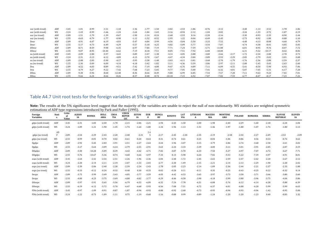
Table A4.7 Unit root tests for the foreign variables at 5% significance level Note: The results at the 5% significance level suggest that the majority of the variables are unable to reject the null of non-stationarity. WS statistics are weighted symmetric estimations of ADF type regressions introduced by Park and Fuller (1995).
eur (with trend) ADF -3.45 -1.01 -0.99 -1.51 -1.18 -1.36 -1.77 -1.50 -3.02 -2.53 -1.86 -0.76 -3.12
-3.48 -1.13 -3.52 -1.78 -1.86
eur (with trend) WS -3.24 -1.43 -0.99 -1.66 -1.24 -1.64 -1.84 -1.65 -3.16 -0.94 -2.12 -1.04 -3.02
-3.34 -1.33 -3.72 -1.87 -2.19
eur (no trend) ADF -2.89 -1.51 -1.79 -1.39 -0.67 -1.90 -1.14 -0.24 -2.68 -2.53 0.16 -2.20 -2.16
-3.30 -0.93 -2.35 -0.90 -1.44
eur (no trend) WS -2.55 -0.63 -0.79 -1.77 -0.98 -1.12 -1.52 -0.52 -2.95 1.22 -0.04 -0.49 -2.45
-2.73 -0.92 -1.80 -0.88 -1.10
Deur ADF -2.89 -4.91 -4.47 -6.19 -4.03 -5.47 -4.84 -3.99 -4.56 -5.04 -5.50 -3.33 -7.52
-4.48 -4.13 -8.08 -4.60 -4.79
Deur WS -2.55 -5.17 -4.73 -6.49 -4.29 -5.57 -5.10 -4.25 -4.82 -5.09 -5.77 -3.54 -7.07
-4.74 -4.38 -8.41 -4.85 -5.05
DDeur ADF -2.89 -8.71 -8.59 -9.98 -6.35 -6.97 -7.84 -7.19 -7.71 -7.24 -7.59 -5.71 -11.08
-6.01 -8.95 -9.76 -8.07 -7.72
DDeur WS -2.55 -9.07 -8.95 -10.40 -6.62 -7.19 -8.18 -7.51 -8.05 -7.51 -7.92 -6.00 -10.08
-6.31 -9.32 -10.17 -8.42 -8.06
eu (with trend) ADF -3.45 -2.09 -2.88 -5.97 -4.65 -3.89 -3.47 -1.38 -4.14 -4.05 -3.88 -3.80 -2.66 -2.17 -1.72 -2.54 -2.80 -2.78 -3.73
eu (with trend) WS -3.24 -2.31 -3.13 -6.12 -4.89 -4.15 -3.70 -1.67 -4.47 -4.34 -3.84 -3.89 -2.93 -2.29 -2.05 -2.79 -3.02 -3.01 -3.68
eu (no trend) ADF -2.89 -2.08 -2.83 -5.90 -4.17 -3.95 -3.38 -1.48 -3.03 -4.11 -3.81 -3.68 -2.70 -1.79 -1.76 -2.36 -2.80 -2.59 -2.37
eu (no trend) WS -2.55 -2.36 -3.09 -6.09 -4.14 -4.18 -3.42 -1.82 -3.11 -4.36 -3.39 -3.86 -2.97 -2.11 -2.08 -2.45 -3.05 -2.63 -2.60
Deu ADF -2.89 -4.52 -4.03 -8.89 -9.51 -7.42 -7.19 -4.88 -9.47 -6.76 -4.89 -7.11 -6.09 -4.55 -5.41 -8.50 -5.90 -6.93 -7.06
Deu WS -2.55 -4.79 -4.27 -9.22 -7.42 -7.68 -7.23 -5.05 -9.77 -7.05 -5.00 -7.41 -6.32 -4.81 -5.07 -7.05 -5.31 -6.17 -7.28
DDeu ADF -2.89 -9.30 -5.96 -8.60 -12.48 -8.36 -8.66 -8.49 -9.80 -6.99 -6.85 -7.54 -7.57 -7.28 -7.11 -9.63 -9.23 -7.02 -7.01
DDeu WS -2.55 -9.66 -6.24 -8.66 -8.26 -8.37 -8.48 -8.74 -10.18 -7.15 -6.92 -7.87 -7.82 -7.59 -6.77 -8.47 -8.17 -7.23 -7.26
Foreign Variables
Statis.
Critical
Value
ALBANIA
BOSNIA BULGARIA
CROATIA
CZECK REPUB
LIC
ESTONIA
EURO
HUNGARY
KOSOVO LATVIA
LITHUANIA
MACEDONIA
MONTENEGRO
POLAND ROMANIA SERBIA SLOVAK
REPUBLIC SLOVEN
IA
gdps (with trend) ADF -3.45 -2.31 -1.83 -2.30 -1.78 -2.15 -2.06 -2.21 -1.94 -2.43 -1.50 -2.00 -1.98 -2.40 -2.29 -1.60 -2.18 -2.24 -1.84
gdps (with trend) WS -3.24 -1.89 -1.21 -1.90 -1.35 -1.74 -1.64 -1.80 -1.34 -1.96 -1.13 -1.51 -1.46 -1.97 -1.88 -1.07 -1.74 -1.80 -1.13
gdps (no trend)
ADF -2.89 -2.54 -2.29 -2.43 -2.20 -2.48 -2.31
-2.4
5 -2.17 -2.45 -2.34 -2.35 -2.19 -2.58 -2.54 -2.27 -2.49 -2.53 -2.09
gdps (no trend) WS -2.55 -0.99 -0.01 -0.70 0.02 -0.61 -0.20 -0.64 0.31 -0.74 0.61 -0.25 -0.04 -1.06 -0.86 0.56 -0.53 -0.76 0.62
Dgdps ADF -2.89 -2.92 -5.45 -2.83 -3.91 -2.51 -2.27 -2.64 -3.44 -1.96 -3.07 -3.15 -3.79 -2.86 -2.74 -3.68 -2.58 -2.61 -3.02
Dgdps WS -2.55 -3.17 -5.64 -3.09 -4.14 -2.79 -2.55 -2.91 -3.63 -2.24 -3.33 -3.39 -4.00 -3.11 -3.01 -3.91 -2.85 -2.87 -3.19
DDgdps ADF -2.89 -5.50 -10.28 -5.09 -8.39 -4.43 -4.42 -4.71 -7.02 -3.87 -5.70 -6.33 -7.50 -5.27 -4.97 -7.07 -4.72 -4.67 -7.71
DDgdps WS -2.55 -5.76 -10.67 -5.36 -8.74 -4.68 -4.66 -4.97 -7.33 -4.13 -5.98 -6.64 -7.82 -5.53 -5.22 -7.39 -4.97 -4.91 -8.01
exps (with trend) ADF -3.45 -2.64 -2.42 -2.54 -2.51 -2.26 -1.96 -2.36 -2.84 -2.48 -1.72 -2.45 -2.65 -2.59 -2.47 -2.62 -2.20 -2.67 -2.12
exps (with trend) WS -3.24 -2.20 -2.14 -2.11 -2.19 -2.07 -1.53 -2.03 -2.77 -2.30 -1.49 -2.15 -2.21 -2.14 -2.13 -2.29 -1.90 -2.28 -2.02
exps (no trend) ADF -2.89 -2.39 -2.06 -2.40 -2.30 -2.39 -2.24 -2.43 -1.78 -2.05 -2.23 -2.14 -1.89 -2.36 -2.44 -2.21 -2.37 -2.33 -1.88
exps (no trend) WS -2.55 -0.33 -0.12 -0.24 -0.32 -0.48 0.30 -0.33 -0.02 -0.28 0.11 -0.11 0.35 -0.25 -0.43 -0.25 -0.22 -0.32 0.14
Dexps ADF -2.89 -3.75 -3.99 -3.49 -3.43 -4.05 -3.77 -3.59 -4.03 -4.42 -4.53 -3.65 -3.97 -3.73 -3.58 -3.71 -3.66 -3.80 -3.60
Dexps WS -2.55 -4.00 -4.23 -3.75 -3.69 -4.08 -4.02 -3.77 -4.29 -4.46 -4.58 -3.90 -4.18 -3.99 -3.80 -3.96 -3.75 -4.04 -3.86
DDexps ADF -2.89 -5.97 -5.91 -5.65 -5.56 -6.79 -6.53 -6.09 -6.32 -7.24 -7.78 -6.51 -6.08 -5.76 -6.12 -6.14 -6.38 -5.88 -6.39
DDexps WS -2.55 -6.19 -6.12 -5.72 -5.70 -6.47 -6.68 -5.93 -6.56 -7.08 -7.51 -6.72 -6.37 -6.01 -6.08 -6.28 -5.99 -5.99 -6.63
FDIs (with trend) ADF -3.45 -0.97 -1.09 -0.91 -0.87 -1.87 -0.94 -0.93 -0.88 -0.92 -2.68 -0.73 -0.95 -0.94 -0.93 -0.96 -1.42 -0.95 -5.08
FDIs (with trend) WS -3.24 -1.22 -0.73 -1.09 -1.11 0.75 -1.19 -0.68 -1.16 -0.88 0.99 -0.89 -1.24 -1.20 -1.20 -1.23 0.40 -0.83 1.32

259
FDIs (no trend) ADF -2.89 -1.69 -2.22 -1.78 -1.75 -3.43 -1.68 -2.13 -1.70 -1.98 -4.48 -1.96 -1.63 -1.67 -1.67 -1.66 -4.22 -2.09 -6.23
FDIs (no trend) WS -2.55 -0.02 0.26 0.16 0.08 1.99 0.02 0.67 -0.01 0.52 2.02 0.27 -0.08 -0.03 0.02 -0.05 1.47 0.24 2.24
DFDIs ADF -2.89 -3.17 -2.36 -3.13 -3.09 -3.79 -3.19 -3.13 -3.13 -3.06 -3.93 -2.89 -3.20 -3.20 -3.15 -3.19 -2.75 -2.71 -5.46
DFDIs WS -2.55 -3.43 -2.63 -3.37 -3.34 -0.56 -3.44 -3.09 -3.39 -3.20 1.10 -3.14 -3.46 -3.45 -3.40 -3.45 -2.12 -2.96 2.56
DDFDIs ADF -2.89 -6.65 -6.64 -6.72 -6.81 -6.39 -6.78 -6.72 -6.84 -6.69 -6.52 -6.86 -6.76 -6.79 -6.67 -6.72 -8.41 -6.84 -6.83
DDFDIs WS -2.55 -6.94 -6.95 -6.99 -7.10 -5.35 -7.06 -6.89 -7.12 -6.91 -4.51 -7.15 -7.05 -7.08 -6.95 -7.01 -8.72 -7.15 -4.04
rems (with trend) ADF -3.45 -2.25 -2.26 -2.29 -2.36 -2.28 -2.44 -2.28 -2.45 -2.45 -2.78 -2.47 -2.35 -2.26 -2.27 -2.38 -2.35 -2.38 -1.47
rems (with trend) WS -3.24 -2.28 -2.48 -2.36 -2.46 -2.30 -2.50 -2.36 -2.59 -2.72 -2.93 -2.67 -2.63 -2.29 -2.31 -2.44 -2.45 -2.62 -1.35
rems (no trend) ADF -2.89 -0.92 -1.59 -0.91 -0.94 -0.90 -0.85 -0.93 -0.91 -1.31 -1.02 -1.09 -1.31 -0.90 -0.91 -0.92 -0.93 -1.17 -2.32
rems (no trend) WS -2.55 -1.16 -0.88 -1.08 -1.03 -1.13 -0.94 -1.11 -0.90 -1.07 -0.91 -0.93 -0.88 -1.13 -1.13 -1.05 -1.01 -1.01 -0.25
Drems ADF -2.89 -7.86 -6.99 -7.88 -7.85 -7.87 -8.14 -7.85 -7.47 -7.27 -7.80 -7.72 -7.49 -7.87 -7.87 -7.84 -7.89 -7.52 -5.56
Drems WS -2.55 -8.20 -7.29 -8.21 -8.18 -8.21 -8.46 -8.18 -7.79 -7.58 -8.11 -8.04 -7.81 -8.20 -8.21 -8.17 -8.22 -7.84 -5.75
DDrems ADF -2.89 -12.11 -11.06 -12.16 -
12.18 -
12.12 -13.16 -12.04 -11.33 -10.72 -12.11 -11.84 -11.83 -12.14 -12.13 -12.04 -12.11 -11.82 -8.16
DDrems WS -2.55 -12.58 -11.51 -12.63 -
12.66 -
12.59 -13.67 -12.51 -11.78 -11.15 -12.59 -12.31 -12.29 -12.61 -12.60 -12.50 -12.58 -12.29 -8.45
fbos (with trend) ADF -3.45 -2.00 -2.20 -2.00 -1.90 -2.35 -1.87 -2.14 -1.37 -1.49 -2.06 -1.61 -1.47 -2.11 -2.03 -1.65 -2.02 -1.97 -1.93
fbos (with trend) WS -3.24 -1.74 -2.01 -1.63 -1.52 -1.34 -1.55 -1.54 -1.52 -1.22 -1.76 -1.37 -1.39 -1.63 -1.61 -1.27 -1.85 -1.51 -0.92
fbos (no trend) ADF -2.89 -2.00 -2.22 -2.15 -2.24 -2.56 -2.10 -2.29 -1.85 -2.23 -2.01 -2.12 -1.93 -2.13 -2.11 -2.35 -1.86 -2.20 -1.86
fbos (no trend) WS -2.55 -0.08 -1.21 -0.24 -0.29 0.41 0.07 0.03 -1.21 -0.15 -0.05 -0.42 -0.71 0.12 0.12 -0.13 -0.20 0.06 -0.91
Dfbos ADF -2.89 -4.37 -4.17 -4.48 -4.31 -5.11 -4.56 -4.74 -2.93 -4.42 -4.43 -3.93 -3.72 -4.68 -4.57 -3.87 -4.41 -4.57 -4.02
Dfbos WS -2.55 -4.61 -4.42 -4.72 -4.55 -5.36 -4.80 -4.99 -3.19 -4.67 -4.67 -4.17 -3.97 -4.93 -4.81 -4.11 -4.66 -4.81 -4.28
DDfbos ADF -2.89 -7.07 -6.91 -7.17 -7.02 -7.50 -7.23 -7.29 -6.16 -7.41 -7.15 -6.90 -6.83 -7.25 -7.21 -6.88 -7.07 -7.22 -7.30
DDfbos WS -2.55 -7.39 -7.22 -7.50 -7.34 -7.83 -7.55 -7.62 -6.46 -7.74 -7.48 -7.22 -7.14 -7.58 -7.53 -7.19 -7.39 -7.54 -7.62
eurs (with trend) ADF -3.45 -1.89 -1.62 -1.93 -1.97 -1.91 -1.86 -1.85 -3.06 -2.09 -2.00 -1.93 -2.08 -1.89 -1.96 -2.05 -1.94 -1.89 -1.40
eurs (with trend) WS -3.24 -2.22 -1.97 -2.25 -2.28 -2.23 -2.19 -2.18 -3.26 -2.39 -2.31 -2.25 -2.39 -2.21 -2.27 -2.35 -2.26 -2.22 -1.56
eurs (no trend) ADF -2.89 -1.44 -1.46 -1.43 -1.36 -1.41 -1.45 -1.44 -2.08 -1.39 -1.38 -1.48 -1.49 -1.42 -1.39 -1.36 -1.36 -1.45 -0.28
eurs (no trend) WS -2.55 -1.11 -1.03 -1.09 -1.03 -1.08 -1.10 -1.10 -2.23 -1.08 -1.04 -1.13 -1.14 -1.06 -1.02 -1.05 -0.97 -1.11 -0.62
Deurs ADF -2.89 -4.80 -4.59 -4.80 -4.83 -4.76 -4.80 -4.76 -5.19 -4.84 -4.81 -4.77 -4.88 -4.79 -4.81 -4.82 -4.80 -4.76 -4.11
Deurs WS -2.55 -5.06 -4.85 -5.06 -5.09 -5.02 -5.06 -5.02 -5.46 -5.11 -5.07 -5.04 -5.14 -5.05 -5.07 -5.08 -5.06 -5.02 -4.37
DDeurs ADF -2.89 -7.73 -7.77 -7.72 -7.78 -7.75 -7.73 -7.73 -7.61 -7.68 -7.69 -7.65 -7.66 -7.73 -7.74 -7.88 -7.75 -7.76 -6.83
DDeurs WS -2.55 -8.06 -8.11 -8.06 -8.12 -8.09 -8.07 -8.07 -7.95 -8.01 -8.03 -7.99 -8.00 -8.07 -8.08 -8.22 -8.09 -8.10 -7.14
eus (with trend) ADF -3.45 -3.81 -3.99 -3.74 -3.62 -3.44 -3.72 -3.61 -3.98 -3.80 -3.74 -3.52 -3.09 -3.75 -3.67 -3.80 -3.76 -3.74 -2.47
eus (with trend) WS -3.24 -3.78 -3.96 -3.69 -3.56 -3.35 -3.72 -3.53 -4.23 -3.93 -3.66 -3.51 -3.08 -3.70 -3.61 -3.79 -3.69 -3.68 -2.77
eus (no trend) ADF -2.89 -2.44 -2.58 -2.40 -2.43 -2.10 -2.23 -2.26 -3.98 -2.07 -2.17 -2.49 -2.71 -2.36 -2.27 -2.52 -2.30 -2.32 -2.58
eus (no trend) WS -2.55 -2.67 -2.82 -2.63 -2.64 -2.33 -2.48 -2.49 -4.22 -2.32 -2.43 -2.72 -2.86 -2.59 -2.50 -2.75 -2.54 -2.55 -2.79
Deus ADF -2.89 -7.00 -7.30 -6.98 -6.98 -6.96 -7.10 -7.00 -7.02 -6.72 -7.33 -6.85 -7.02 -7.05 -7.00 -6.90 -7.10 -7.05 -6.13
Deus WS -2.55 -7.22 -7.53 -7.19 -7.19 -7.18 -7.33 -7.22 -7.16 -6.95 -7.58 -7.09 -7.12 -7.27 -7.22 -7.13 -7.33 -7.28 -6.40
DDeus ADF -2.89 -6.89 -6.79 -6.87 -6.86 -6.95 -7.02 -6.92 -6.69 -6.87 -7.15 -6.74 -7.02 -6.96 -6.92 -6.70 -6.87 -6.92 -7.76
DDeus WS -2.55 -7.14 -6.99 -7.12 -7.12 -7.20 -7.28 -7.17 -6.97 -7.11 -7.42 -7.01 -7.29 -7.21 -7.17 -6.96 -7.13 -7.17 -7.82

Table A4.8 Tests of residual serial correlation for country-specific VARX* models
Note: The numbers in bold indicate the rejection of null hypothesis of no serial correlation at
5% significance level.
Figure A4.8 Persistence profiles for the baseline model
Note: Persistence profiles refer to the time profiles of the effects of system or variable-specific shocks on the cointegrating relations in the GVAR model and they have a value of unity on impact, while they should tend to zero as n→∞. The Figure above shows that all
persistence profiles converge to zero by the 15th quarter.
0
0.2
0.4
0.6
0.8
1
1.2
1.4
1.6
1.8
1 3 5 7 9 11 13 15 17 19 21 23 25 27 29 31 33 35 37 39 41
CV1
CV2
CV1
CV2
CV1
CV2
CV3
CV4
CV1
Countries Fcrit_0.05 gdp exp FDI fcl rem eur
ALBANIA F(4,33) 2.66 0.49 2.86 4.23 2.86 1.57 4.38
BOSNIA F(4,33) 2.66 7.53
2.33 1.34 1.03 1.35
BULGARIA F(4,31) 2.68 2.18 3.60 1.64 0.66 1.31 0.66
CROATIA F(4,32) 2.67 0.76 0.99 1.36 1.32
1.31
CZECK REPUBLIC F(4,31) 2.68 4.10 0.17 0.77 2.65 0.43 2.91
ESTONIA F(4,32) 2.67 2.18 2.51 1.58 1.17 0.82 1.17
EURO F(4,41) 2.60 2.99 0.41 0.03 3.87 0.03 0.49
HUNGARY F(4,33) 2.66 1.47 0.57 0.48 0.85 0.12 0.63
KOSOVO F(4,33) 2.66 1.40 0.78
0.55 LATVIA F(4,31) 2.68 0.50 1.61 1.13 2.51 0.07 2.35
LITHUANIA F(4,32) 2.67 0.82 3.63 2.39 0.45 1.59 0.52
MACEDONIA F(4,32) 2.67 5.08 1.55 1.72 0.38 1.62 0.36
MONTENEGRO F(4,34) 2.65 10.57 7.85 1.52
2.17 POLAND F(4,32) 2.67 2.08 3.07 0.82 0.66 1.16 0.67
ROMANIA F(4,32) 2.67 0.51 1.63 1.85 1.33 1.07 1.31
SERBIA F(4,33) 2.66 2.49 5.99 1.12 SLOVAK REPUBLIC F(4,32) 2.67 10.61 1.76 1.16 0.40 2.60 0.40
SLOVENIA F(4,31) 2.68 0.99 0.63 0.29 3.38 4.18 1.56

261
Table A4.9 Contemporaneous effects of foreign variables on domestic counterparts
Country Coefficient gdp exp FDI fcl rem eur
ALBANIA Newey-West's adjusted SE 0.04 0.38 1.08 3.11 0.23 1.85
t-ratio_NeweyWest 5.23 2.10 1.17 0.16 1.01 0.20
BOSNIA Newey-West's adjusted SE 0.07
0.09 0.80 0.33 0.74
t-ratio_NeweyWest 2.98
0.43 -1.24 2.30 2.13
BULGARIA Newey-West's adjusted SE 0.20 0.91 0.36 0.37 0.18 0.28
t-ratio_NeweyWest 4.56 1.04 2.48 1.42 3.66 4.64
CROATIA Newey-West's adjusted SE 0.12 0.23 0.22 0.26
0.23
t-ratio_NeweyWest 1.87 5.55 5.26 2.01
3.54
CZECK REPUBLIC Newey-West's adjusted SE 0.06 0.20 0.20 0.30 0.10 0.28
t-ratio_NeweyWest 9.01 2.06 2.18 1.68 1.82 1.28
ESTONIA Newey-West's adjusted SE 0.23 0.15 0.42 0.33 0.26 0.25
t-ratio_NeweyWest -0.19 4.26 2.47 3.43 2.91 1.14
EURO Newey-West's adjusted SE
t-ratio_NeweyWest
HUNGARY Newey-West's adjusted SE 0.04 0.13 0.25 0.23 0.53 0.18
t-ratio_NeweyWest 11.27 6.33 4.23 2.91 2.64 5.11
KOSOVO Newey-West's adjusted SE 0.12 0.75
0.07
t-ratio_NeweyWest -0.11 2.76
-3.27
LATVIA Newey-West's adjusted SE 0.20 0.11 0.05 0.34 0.26 0.36
t-ratio_NeweyWest 5.24 0.23 0.97 0.75 2.53 2.67
LITHUANIA Newey-West's adjusted SE 0.21 0.20 0.19 0.33 0.19 0.37
t-ratio_NeweyWest 3.57 3.14 6.51 3.83 2.42 1.24
MACEDONIA Newey-West's adjusted SE 0.88 0.46 0.10 0.80 0.31 0.61
t-ratio_NeweyWest 4.82 1.27 0.52 -0.22 -0.13 2.32
MONTENEGRO Newey-West's adjusted SE 1.02 1.29 0.19
0.10
t-ratio_NeweyWest 3.41 -0.82 -0.71
0.78
POLAND Newey-West's adjusted SE 0.11 0.12 0.22 0.33 0.22 0.29
t-ratio_NeweyWest 0.05 6.56 4.03 2.65 1.90 1.83
ROMANIA Newey-West's adjusted SE 0.11 0.32 0.23 0.35 0.09 0.22
t-ratio_NeweyWest 3.53 2.39 9.70 2.37 -2.53 4.04
SERBIA Newey-West's adjusted SE 0.27 0.20 0.09
t-ratio_NeweyWest -0.37 3.58 -1.59
SLOVAK REPUBLIC Newey-West's adjusted SE 0.63 0.21 0.04 0.62 0.09 0.54
t-ratio_NeweyWest 8.32 3.64 1.61 2.13 -0.78 0.84
SLOVENIA Newey-West's adjusted SE 0.13 0.10 0.14 0.19 0.13 0.18
t-ratio_NeweyWest 4.96 4.94 6.35 0.72 9.43 6.95
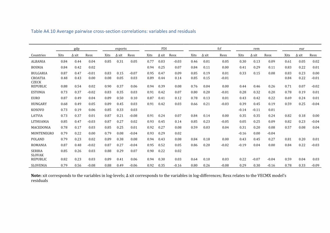
Table A4.10 Average pairwise cross-section correlations: variables and residuals
Note: xit corresponds to the variables in log-levels; Δ xit corresponds to the variables in log-differences; Resx relates to the VECMX model’s residuals
gdp
exports
FDI
fcf
rem
eur
Countries Xits Δ xit Resx Xits Δ xit Resx Xits Δ xit Resx Xits Δ xit
Resx Xits Δ xit Resx Xits Δ xit Resx
ALBANIA 0.84 0.44 0.04
0.85 0.31 0.05
0.77 0.03 -0.03
0.46 0.01 0.05
0.30 0.13 0.09
0.61 0.05 0.02
BOSNIA 0.84 0.42 0.02
0.94 0.25 0.07
0.84 0.11 0.00
0.41 0.29 0.11
0.83 0.22 0.01
BULGARIA 0.87 0.47 -0.01
0.83 0.15 -0.07
0.95 0.47 0.09
0.85 0.19 0.01
0.33 0.15 0.08
0.83 0.23 0.00
CROATIA 0.48 0.43 0.00
0.08 0.05 0.03
0.89 0.44 0.14
0.85 0.15 -0.01
0.84 0.22 -0.01 CZECK REPUBLIC 0.88 0.54 0.02
0.90 0.37 0.06
0.94 0.39 0.08
0.76 0.04
0.00
0.44 0.46 0.26
0.71 0.07 -0.02
ESTONIA 0.73 0.37 -0.02
0.83 0.35 0.03
0.91 0.42 0.07
0.80 0.20 -0.01
0.28 0.32 0.20
0.78 0.19 0.01
EURO 0.87 0.49 0.04
0.89 0.50 0.10
0.87 0.41 0.12
0.78 0.13 0.01
0.43 0.42 0.22
0.69 0.24 0.01
HUNGARY 0.68 0.49 0.05
0.89 0.45 0.03
0.91 0.42 0.03
0.66 0.21 -0.03
0.39 0.45 0.19
0.59 0.25 -0.04
KOSOVO 0.73 0.19 0.06
0.85 0.33 0.03
-0.14 -0.11 0.01
LATVIA 0.73 0.37 0.01
0.87 0.21 -0.08
0.91 0.24 0.07
0.84 0.14 0.00
0.35 0.35 0.24
0.82 0.18 0.00
LITHUANIA 0.85 0.47 -0.03
0.87 0.27 0.02
0.93 0.45 0.14
0.85 0.23 -0.05
0.05 0.25 0.09
0.82 0.23 -0.04
MACEDONIA 0.78 0.17 0.03
0.85 0.25 0.01
0.92 0.27 0.08
0.59 0.03 0.04
0.31 0.20 0.08
0.57 0.08 0.04
MONTENEGRO 0.79 0.22 0.00
0.79 0.08 -0.04
0.93 0.29 0.02
-0.16 0.00 -0.04
POLAND 0.79 0.23 0.02
0.89 0.38 0.08
0.94 0.43 0.08
0.84 0.18 0.00
0.43 0.45 0.27
0.81 0.20 0.01
ROMANIA 0.87 0.48 -0.02
0.87 0.27 -0.04
0.95 0.52 0.05
0.86 0.20 -0.02
-0.19 0.04 0.00
0.84 0.22 -0.03
SERBIA 0.85 0.26 0.03
0.88 0.29 0.07
0.90 0.22 0.02
SLOVAK REPUBLIC 0.82 0.23 0.03
0.89 0.41 0.06
0.94 0.30 0.03
0.64 0.10
0.03
0.22 -0.07 -0.04
0.59 0.04 0.03
SLOVENIA 0.79 0.56 -0.08 0.88 0.49 -0.06 0.92 0.35 -0.16 0.80 0.26
-0.08 0.29 0.30 -0.16 0.78 0.33 -0.09

263
Table A4.11 Proportion of the N-step ahead forecast error variance of Balkan GDP explained by conditioning on contemporaneous and future innovations of the country equations
Quarters
0 1 2 4 6 8 12 24 40
Regions Variables
Balkan region gdp 12% 14% 14% 14% 13% 13% 13% 12% 12%
exp 10% 12% 13% 13% 13% 13% 13% 12% 12%
fdi 3% 4% 5% 5% 5% 5% 5% 4% 4%
fcl 4% 6% 6% 7% 8% 8% 8% 7% 7%
rem 3% 3% 3% 3% 3% 3% 2% 2% 2%
eur 2% 4% 4% 5% 5% 5% 5% 5% 5%
Total Balkan region
35% 43% 45% 47% 47% 46% 45% 43% 43%
Baltic region gdp 0% 0% 0% 0% 0% 0% 0% 0% 0%
exp 1% 1% 1% 1% 1% 1% 1% 1% 1%
fdi 1% 1% 1% 0% 0% 0% 1% 1% 1%
fcl 1% 2% 1% 1% 1% 1% 1% 2% 2%
rem 5% 4% 3% 3% 3% 3% 3% 3% 3%
eur 1% 1% 1% 1% 1% 1% 1% 2% 2%
Total Baltic region
8% 9% 8% 7% 7% 7% 7% 8% 8%
CE region gdp 1% 1% 1% 1% 1% 1% 1% 1% 1%
exp 0% 1% 1% 1% 1% 1% 1% 2% 2%
fdi 1% 2% 1% 1% 1% 1% 2% 2% 2%
fcl 4% 3% 4% 3% 3% 2% 2% 2% 2%
rem 7% 6% 6% 5% 5% 5% 4% 4% 4%
eur 4% 3% 4% 3% 3% 2% 2% 2% 2%
Total CE region
19% 17% 16% 15% 14% 13% 13% 13% 13%
Euro region gdp 8% 6% 7% 9% 11% 11% 12% 13% 14%
exp 5% 5% 5% 8% 9% 10% 11% 12% 12%
fdi 0% 1% 1% 1% 0% 0% 0% 0% 0%
fcl 1% 3% 2% 2% 3% 3% 3% 3% 3%
rem 18% 12% 12% 10% 9% 8% 8% 8% 7%
eur 6% 5% 4% 2% 1% 1% 1% 0% 0%
Total Euro region 38% 31% 31% 31% 32% 34% 35% 36% 36%
Total 100% 100% 100% 100% 100% 100% 100% 100% 100%
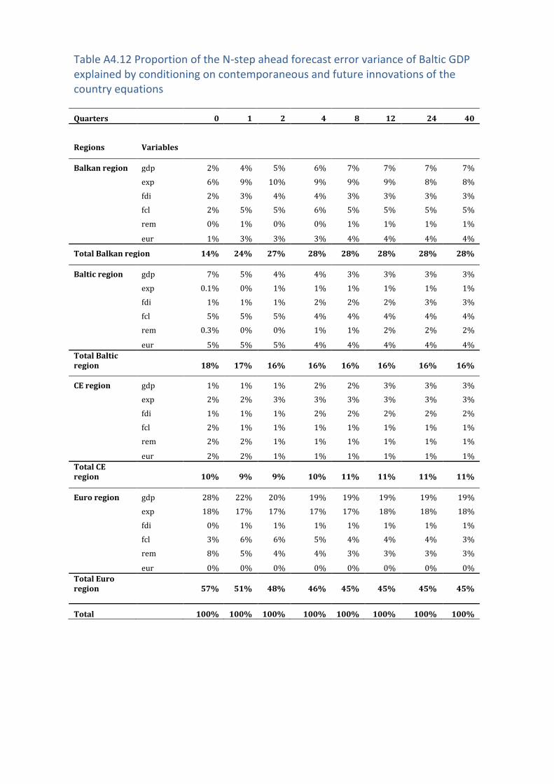
Table A4.12 Proportion of the N-step ahead forecast error variance of Baltic GDP explained by conditioning on contemporaneous and future innovations of the country equations
Quarters 0 1 2 4 8 12 24 40
Regions Variables
Balkan region gdp 2% 4% 5% 6% 7% 7% 7% 7%
exp 6% 9% 10% 9% 9% 9% 8% 8%
fdi 2% 3% 4% 4% 3% 3% 3% 3%
fcl 2% 5% 5% 6% 5% 5% 5% 5%
rem 0% 1% 0% 0% 1% 1% 1% 1%
eur 1% 3% 3% 3% 4% 4% 4% 4%
Total Balkan region 14% 24% 27% 28% 28% 28% 28% 28%
Baltic region gdp 7% 5% 4% 4% 3% 3% 3% 3%
exp 0.1% 0% 1% 1% 1% 1% 1% 1%
fdi 1% 1% 1% 2% 2% 2% 3% 3%
fcl 5% 5% 5% 4% 4% 4% 4% 4%
rem 0.3% 0% 0% 1% 1% 2% 2% 2%
eur 5% 5% 5% 4% 4% 4% 4% 4%
Total Baltic region
18% 17% 16% 16% 16% 16% 16% 16%
CE region gdp 1% 1% 1% 2% 2% 3% 3% 3%
exp 2% 2% 3% 3% 3% 3% 3% 3%
fdi 1% 1% 1% 2% 2% 2% 2% 2%
fcl 2% 1% 1% 1% 1% 1% 1% 1%
rem 2% 2% 1% 1% 1% 1% 1% 1%
eur 2% 2% 1% 1% 1% 1% 1% 1%
Total CE region
10% 9% 9% 10% 11% 11% 11% 11%
Euro region gdp 28% 22% 20% 19% 19% 19% 19% 19%
exp 18% 17% 17% 17% 17% 18% 18% 18%
fdi 0% 1% 1% 1% 1% 1% 1% 1%
fcl 3% 6% 6% 5% 4% 4% 4% 3%
rem 8% 5% 4% 4% 3% 3% 3% 3%
eur 0% 0% 0% 0% 0% 0% 0% 0%
Total Euro region 57% 51% 48% 46% 45% 45% 45% 45%
Total 100% 100% 100% 100% 100% 100% 100% 100%
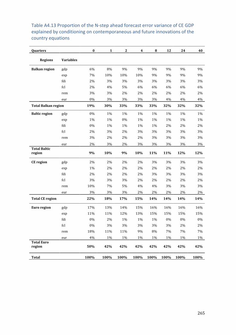
265
Table A4.13 Proportion of the N-step ahead forecast error variance of CE GDP explained by conditioning on contemporaneous and future innovations of the country equations
Quarters 0 1 2 4 8 12 24 40
Regions Variables
Balkan region gdp 6% 8% 9% 9% 9% 9% 9% 9%
exp 7% 10% 10% 10% 9% 9% 9% 9%
fdi 2% 3% 3% 3% 3% 3% 3% 3%
fcl 2% 4% 5% 6% 6% 6% 6% 6%
rem 3% 3% 2% 2% 2% 2% 2% 2%
eur 0% 3% 3% 3% 3% 4% 4% 4%
Total Balkan region 19% 30% 33% 33% 33% 32% 32% 32%
Baltic region gdp 0% 1% 1% 1% 1% 1% 1% 1%
exp 1% 1% 0% 1% 1% 1% 1% 1%
fdi 0% 1% 1% 1% 1% 2% 2% 2%
fcl 2% 3% 2% 3% 3% 3% 3% 3%
rem 3% 2% 2% 2% 3% 3% 3% 3%
eur 2% 3% 2% 3% 3% 3% 3% 3%
Total Baltic region
9% 10% 9% 10% 11% 11% 12% 12%
CE region gdp 2% 2% 2% 2% 3% 3% 3% 3%
exp 1% 2% 2% 2% 2% 2% 2% 2%
fdi 2% 2% 2% 2% 3% 3% 3% 3%
fcl 3% 3% 3% 2% 2% 2% 2% 2%
rem 10% 7% 5% 4% 4% 3% 3% 3%
eur 3% 3% 3% 2% 2% 2% 2% 2%
Total CE region
22% 18% 17% 15% 14% 14% 14% 14%
Euro region gdp 17% 13% 14% 15% 16% 16% 16% 16%
exp 11% 11% 12% 13% 15% 15% 15% 15%
fdi 0% 2% 1% 1% 1% 0% 0% 0%
fcl 0% 3% 3% 3% 3% 3% 2% 2%
rem 18% 11% 11% 9% 8% 7% 7% 7%
eur 4% 1% 1% 1% 1% 1% 1% 1%
Total Euro region 50% 42% 42% 42% 42% 42% 42% 42%
Total 100% 100% 100% 100% 100% 100% 100% 100%
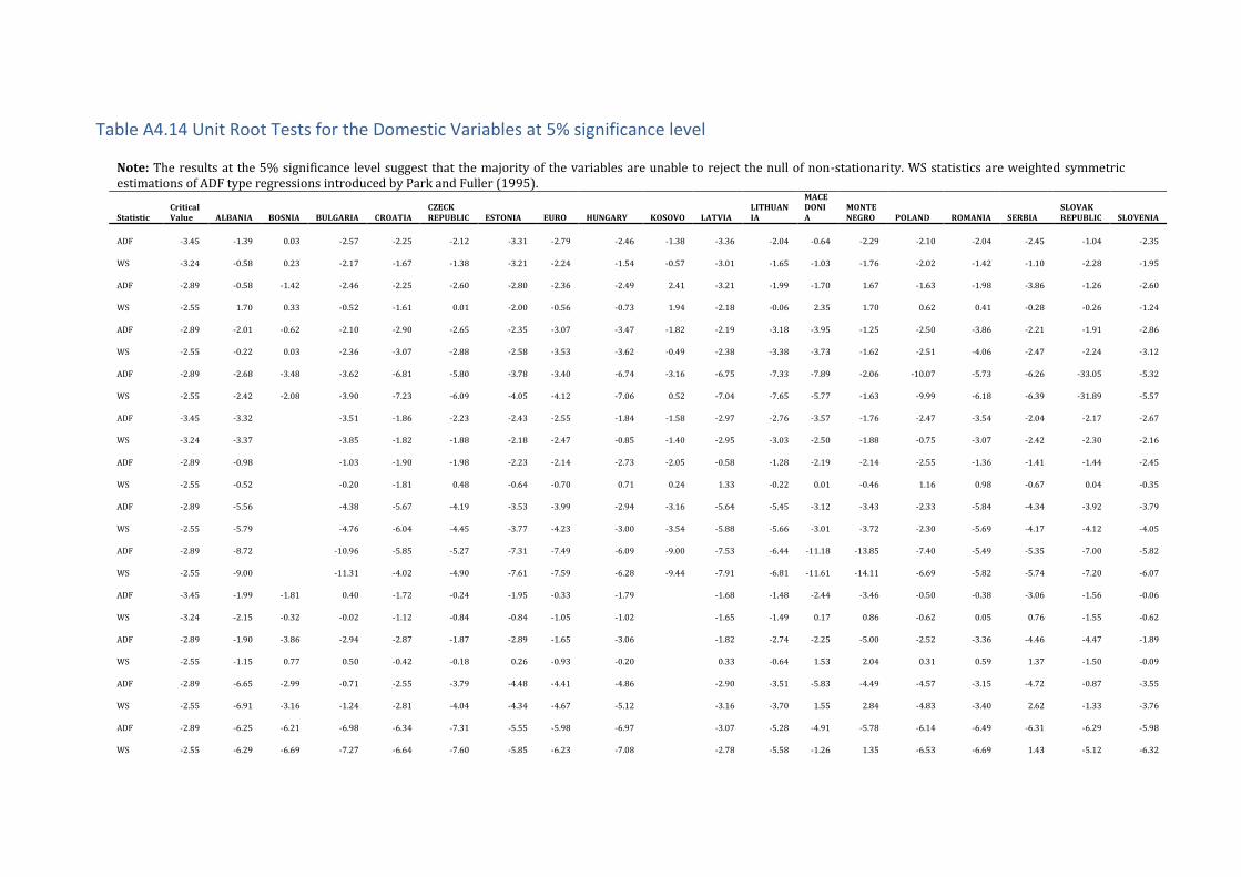
Table A4.14 Unit Root Tests for the Domestic Variables at 5% significance level Note: The results at the 5% significance level suggest that the majority of the variables are unable to reject the null of non-stationarity. WS statistics are weighted symmetric estimations of ADF type regressions introduced by Park and Fuller (1995).
Statistic Critical Value ALBANIA BOSNIA BULGARIA CROATIA
CZECK REPUBLIC ESTONIA EURO HUNGARY KOSOVO LATVIA
LITHUANIA
MACEDONIA
MONTENEGRO POLAND ROMANIA SERBIA
SLOVAK REPUBLIC SLOVENIA
ADF -3.45 -1.39 0.03 -2.57 -2.25 -2.12 -3.31 -2.79 -2.46 -1.38 -3.36 -2.04 -0.64 -2.29 -2.10 -2.04 -2.45 -1.04 -2.35
WS -3.24 -0.58 0.23 -2.17 -1.67 -1.38 -3.21 -2.24 -1.54 -0.57 -3.01 -1.65 -1.03 -1.76 -2.02 -1.42 -1.10 -2.28 -1.95
ADF -2.89 -0.58 -1.42 -2.46 -2.25 -2.60 -2.80 -2.36 -2.49 2.41 -3.21 -1.99 -1.70 1.67 -1.63 -1.98 -3.86 -1.26 -2.60
WS -2.55 1.70 0.33 -0.52 -1.61 0.01 -2.00 -0.56 -0.73 1.94 -2.18 -0.06 2.35 1.70 0.62 0.41 -0.28 -0.26 -1.24
ADF -2.89 -2.01 -0.62 -2.10 -2.90 -2.65 -2.35 -3.07 -3.47 -1.82 -2.19 -3.18 -3.95 -1.25 -2.50 -3.86 -2.21 -1.91 -2.86
WS -2.55 -0.22 0.03 -2.36 -3.07 -2.88 -2.58 -3.53 -3.62 -0.49 -2.38 -3.38 -3.73 -1.62 -2.51 -4.06 -2.47 -2.24 -3.12
ADF -2.89 -2.68 -3.48 -3.62 -6.81 -5.80 -3.78 -3.40 -6.74 -3.16 -6.75 -7.33 -7.89 -2.06 -10.07 -5.73 -6.26 -33.05 -5.32
WS -2.55 -2.42 -2.08 -3.90 -7.23 -6.09 -4.05 -4.12 -7.06 0.52 -7.04 -7.65 -5.77 -1.63 -9.99 -6.18 -6.39 -31.89 -5.57
ADF -3.45 -3.32
-3.51 -1.86 -2.23 -2.43 -2.55 -1.84 -1.58 -2.97 -2.76 -3.57 -1.76 -2.47 -3.54 -2.04 -2.17 -2.67
WS -3.24 -3.37
-3.85 -1.82 -1.88 -2.18 -2.47 -0.85 -1.40 -2.95 -3.03 -2.50 -1.88 -0.75 -3.07 -2.42 -2.30 -2.16
ADF -2.89 -0.98
-1.03 -1.90 -1.98 -2.23 -2.14 -2.73 -2.05 -0.58 -1.28 -2.19 -2.14 -2.55 -1.36 -1.41 -1.44 -2.45
WS -2.55 -0.52
-0.20 -1.81 0.48 -0.64 -0.70 0.71 0.24 1.33 -0.22 0.01 -0.46 1.16 0.98 -0.67 0.04 -0.35
ADF -2.89 -5.56
-4.38 -5.67 -4.19 -3.53 -3.99 -2.94 -3.16 -5.64 -5.45 -3.12 -3.43 -2.33 -5.84 -4.34 -3.92 -3.79
WS -2.55 -5.79
-4.76 -6.04 -4.45 -3.77 -4.23 -3.00 -3.54 -5.88 -5.66 -3.01 -3.72 -2.30 -5.69 -4.17 -4.12 -4.05
ADF -2.89 -8.72
-10.96 -5.85 -5.27 -7.31 -7.49 -6.09 -9.00 -7.53 -6.44 -11.18 -13.85 -7.40 -5.49 -5.35 -7.00 -5.82
WS -2.55 -9.00
-11.31 -4.02 -4.90 -7.61 -7.59 -6.28 -9.44 -7.91 -6.81 -11.61 -14.11 -6.69 -5.82 -5.74 -7.20 -6.07
ADF -3.45 -1.99 -1.81 0.40 -1.72 -0.24 -1.95 -0.33 -1.79
-1.68 -1.48 -2.44 -3.46 -0.50 -0.38 -3.06 -1.56 -0.06
WS -3.24 -2.15 -0.32 -0.02 -1.12 -0.84 -0.84 -1.05 -1.02
-1.65 -1.49 0.17 0.86 -0.62 0.05 0.76 -1.55 -0.62
ADF -2.89 -1.90 -3.86 -2.94 -2.87 -1.87 -2.89 -1.65 -3.06
-1.82 -2.74 -2.25 -5.00 -2.52 -3.36 -4.46 -4.47 -1.89
WS -2.55 -1.15 0.77 0.50 -0.42 -0.18 0.26 -0.93 -0.20
0.33 -0.64 1.53 2.04 0.31 0.59 1.37 -1.50 -0.09
ADF -2.89 -6.65 -2.99 -0.71 -2.55 -3.79 -4.48 -4.41 -4.86
-2.90 -3.51 -5.83 -4.49 -4.57 -3.15 -4.72 -0.87 -3.55
WS -2.55 -6.91 -3.16 -1.24 -2.81 -4.04 -4.34 -4.67 -5.12
-3.16 -3.70 1.55 2.84 -4.83 -3.40 2.62 -1.33 -3.76
ADF -2.89 -6.25 -6.21 -6.98 -6.34 -7.31 -5.55 -5.98 -6.97
-3.07 -5.28 -4.91 -5.78 -6.14 -6.49 -6.31 -6.29 -5.98
WS -2.55 -6.29 -6.69 -7.27 -6.64 -7.60 -5.85 -6.23 -7.08
-2.78 -5.58 -1.26 1.35 -6.53 -6.69 1.43 -5.12 -6.32

267
ADF -3.45 -5.11 -1.64 -1.86 -0.79 -1.80 -1.95 -2.75 -1.05
-1.36 -1.22 -1.33
-0.85 -1.76
-3.36 -0.54
WS -3.24 -5.38 0.22 -1.73 -0.89 -1.87 -0.43 -1.62 -0.08
0.34 -1.15 -1.41
-0.65 -1.43
-2.67 0.04
ADF -2.89 -3.29 -3.43 -3.27 -1.95 -1.77 -3.01 -3.03 -1.56
-2.00 -2.04 -1.02
-2.57 -2.98
-2.65 -2.25
WS -2.55 -3.22 0.84 -1.08 -0.45 -0.55 -1.16 -0.98 -0.98
-0.56 -1.13 -0.59
0.32 -0.85
-0.53 -0.95
ADF -2.89 -5.44 -5.29 -2.02 -1.90 -4.09 -2.08 -2.01 -1.66
-1.72 -1.10 -5.20
-4.72 -0.96
-7.21 -2.61
WS -2.55 -5.82 -5.09 -2.37 -2.01 -3.82 -2.40 -1.81 -1.78
-1.25 -1.45 -5.42
-4.98 -1.51
-7.45 -2.85
ADF -2.89 -5.58 -5.52 -4.52 -9.77 -6.88 -9.54 -11.67 -7.00
-3.98 -8.01 -7.94
-7.69 -5.47
-6.62 -8.14
WS -2.55 -6.21 -5.92 -2.85 -10.26 -7.34 -9.59 -11.62 -7.21 -3.22 -7.95 -6.41 -8.01 -5.58 -7.06 -8.47
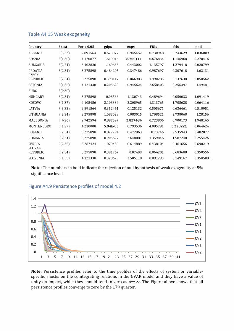
Table A4.15 Weak exogeneity
Note: The numbers in bold indicate the rejection of null hypothesis of weak exogeneity at 5%
significance level
Figure A4.9 Persistence profiles of model 4.2
Note: Persistence profiles refer to the time profiles of the effects of system or variable-specific shocks on the cointegrating relations in the GVAR model and they have a value of unity on impact, while they should tend to zero as n→∞. The Figure above shows that all persistence profiles converge to zero by the 17th quarter.
0
0.2
0.4
0.6
0.8
1
1.2
1.4
1 3 5 7 9 11 13 15 17 19 21 23 25 27 29 31 33 35 37 39 41
CV1
CV2
CV3
CV1
CV1
CV2
CV1
CV2
Country F test Fcrit_0.05 gdps exps FDIs fcls poil
ALBANIA F(3,33) 2.891564 0.673077 0.945452 0.730948 0.743629 1.836009
BOSNIA F(1,30) 4.170877 1.619016 8.700111 0.676834 1.146968 0.270416
BULGARIA F(2,24) 3.402826 1.169638 0.443002 1.135797 1.279418 0.020799
CROATIA F(2,34) 3.275898 0.484295 0.347486 0.987697 0.307618 1.62131 CZECK REPUBLIC F(2,34) 3.275898 0.398117 0.066983 1.990285 0.137638 0.050562
ESTONIA F(1,35) 4.121338 0.205629 0.945624 2.658403 0.256397 1.49481
EURO F(0,30) HUNGARY F(2,34) 3.275898 0.08568 1.130743 0.489694 0.050032 1.091419
KOSOVO F(1,37) 4.105456 2.103334 2.208965 1.313765 1.705628 0.064116
LATVIA F(3,33) 2.891564 0.352461 0.125132 0.505671 0.636461 0.510951
LITHUANIA F(2,34) 3.275898 1.083029 0.083015 1.798521 2.738068 1.28156
MACEDONIA F(4,26) 2.742594 0.897597 2.827484 0.723806 0.900173 1.948165
MONTENEGRO F(1,27) 4.210008 5.94E-05 0.793536 4.085791 5.228221 0.064624
POLAND F(2,34) 3.275898 0.877794 0.472863 0.73746 2.535943 0.402877
ROMANIA F(2,34) 3.275898 0.905627 2.648081 1.359846 1.587248 0.255426
SERBIA F(2,35) 3.267424 1.079459 0.614889 0.438104 0.461656 0.690219 SLOVAK REPUBLIC F(2,34) 3.275898 0.391767 0.07409 0.064201 0.683688 0.350556
SLOVENIA F(1,35) 4.121338 0.328679 3.505118 0.091293 0.149167 0.358508
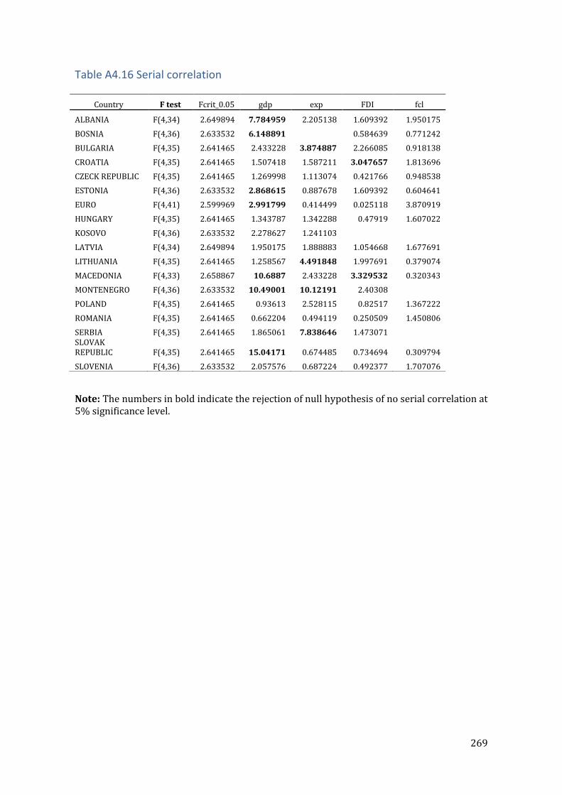
269
Table A4.16 Serial correlation
Note: The numbers in bold indicate the rejection of null hypothesis of no serial correlation at 5% significance level.
Country F test Fcrit_0.05 gdp exp FDI fcl
ALBANIA F(4,34) 2.649894 7.784959 2.205138 1.609392 1.950175
BOSNIA F(4,36) 2.633532 6.148891
0.584639 0.771242
BULGARIA F(4,35) 2.641465 2.433228 3.874887 2.266085 0.918138
CROATIA F(4,35) 2.641465 1.507418 1.587211 3.047657 1.813696
CZECK REPUBLIC F(4,35) 2.641465 1.269998 1.113074 0.421766 0.948538
ESTONIA F(4,36) 2.633532 2.868615 0.887678 1.609392 0.604641
EURO F(4,41) 2.599969 2.991799 0.414499 0.025118 3.870919
HUNGARY F(4,35) 2.641465 1.343787 1.342288 0.47919 1.607022
KOSOVO F(4,36) 2.633532 2.278627 1.241103 LATVIA F(4,34) 2.649894 1.950175 1.888883 1.054668 1.677691
LITHUANIA F(4,35) 2.641465 1.258567 4.491848 1.997691 0.379074
MACEDONIA F(4,33) 2.658867 10.6887 2.433228 3.329532 0.320343
MONTENEGRO F(4,36) 2.633532 10.49001 10.12191 2.40308 POLAND F(4,35) 2.641465 0.93613 2.528115 0.82517 1.367222
ROMANIA F(4,35) 2.641465 0.662204 0.494119 0.250509 1.450806
SERBIA F(4,35) 2.641465 1.865061 7.838646 1.473071 SLOVAK
REPUBLIC F(4,35) 2.641465 15.04171 0.674485 0.734694 0.309794
SLOVENIA F(4,36) 2.633532 2.057576 0.687224 0.492377 1.707076
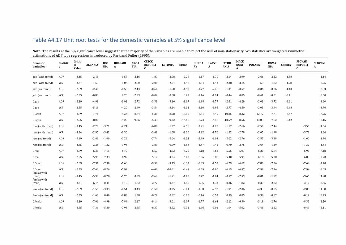
Table A4.17 Unit root tests for the domestic variables at 5% significance level Note: The results at the 5% significance level suggest that the majority of the variables are unable to reject the null of non-stationarity. WS statistics are weighted symmetric estimations of ADF type regressions introduced by Park and Fuller (1995).
Domestic Variables
Statistic
Critical Value
ALBANIA BOSNIA
BULGARIA
CROATIA
CZECK REPUBLIC
ESTONIA EURO HUNGARY
LATVIA
LITHUANIA
MACEDONIA
POLAND ROMANIA
SERBIA SLOVAK REPUBLIC
SLOVENIA
gdp (with trend) ADF -3.45 -2.18
-0.57 -2.16 -1.87 -2.08 -2.26 -1.17 -1.70 -2.14 -2.99 -2.66 -2.22 -1.38
-1.14
gdp (with trend) WS -3.24 -1.53
-1.06 -2.50 -2.00 -2.04 -1.96 -1.34 -1.43 -2.38 -3.15 -1.69 -1.82 -1.78
-0.96
gdp (no trend) ADF -2.89 -2.48
-0.53 -2.13 -0.64 -1.50 -1.97 -1.77 -2.46 -1.31 -0.57 -0.06 -0.26 -1.40
-2.33
gdp (no trend) WS -2.55 -0.83
0.20 -2.33 -0.04 0.08 0.27 -1.16 -1.14 -0.44 0.85 -0.41 -0.21 -0.41
0.50
Dgdp ADF -2.89 -4.99
-3.98 -2.72 -3.33 -3.16 -3.07 -1.98 -3.77 -2.61 -4.29 -2.03 -3.72 -6.61
-3.60
Dgdp WS -2.55 -5.19
-4.20 -2.99 -3.54 -3.24 -3.33 -2.16 -3.95 -2.77 -4.50 -2.05 -3.94 -6.48
-3.76
DDgdp ADF -2.89 -7.71
-9.36 -8.74 -5.30 -8.98 -15.95 -6.31 -6.40 -10.85 -8.32 -12.72 -7.71 -6.57
-7.95
DDgdp WS -2.55 -8.00
-9.20 -9.06 -5.43 -9.22 -16.46 -6.73 -6.48 -10.59 -8.56 -13.03 -7.62 -6.42
-8.15
rem (with trend) ADF -3.45 -2.70 -3.21 -2.24
-6.80 -1.37 -2.56 -3.21 -1.77 -1.57 -2.66 -2.50 -2.44
-3.50 -1.54
rem (with trend) WS -3.24 -2.95 -3.42 -2.30
-3.42 -1.68 -2.30 -3.22 -1.76 -1.82 -2.78 -2.65 -1.98
-3.72 -1.84
rem (no trend) ADF -2.89 -2.41 -1.60 -2.29
-7.74 -2.04 -1.54 -2.99 -2.03 -2.02 -2.76 -2.57 -3.28
-1.60 -1.74
rem (no trend) WS -2.55 -2.25 -1.32 -1.93
-2.89 -0.99 -1.86 -2.57 -0.41 -0.70 -2.76 -2.64 -1.49
-1.32 -1.54
Drem ADF -2.89 -6.38 -7.11 -6.79
-6.57 -4.02 -6.29 -6.18 -8.62 -5.55 -5.97 -6.20 -5.64
-5.91 -7.48
Drem WS -2.55 -5.95 -7.33 -6.92
-5.12 -4.04 -6.03 -6.36 -8.86 -5.40 -5.91 -6.18 -5.38
-6.09 -7.70
DDrem ADF -2.89 -7.37 -7.90 -7.68
-9.58 -9.73 -8.37 -8.39 -7.55 -6.29 -6.62 -7.80 -7.26
-7.64 -7.70
DDrem WS -2.55 -7.60 -8.26 -7.92
-4.40 -10.01 -8.41 -8.69 -7.90 -6.15 -6.87 -7.98 -7.34
-7.94 -8.05 forcla (with trend) ADF -3.45 -5.98 -0.28 -1.75 0.39 -2.69 -1.91 -1.75 0.72 -1.04 -0.57 -2.53 -0.01 -1.92
-3.65 1.28
forcla (with trend) WS -3.24 -6.14 -0.41 -1.10 1.02 -2.77 -0.27 -1.55 0.55 -1.33 -0.36 -1.82 -0.39 -2.02
-3.10 0.36
forcla (no trend) ADF -2.89 -1.55 -3.33 -0.51 -3.43 -1.50 -3.35 -3.41 -1.88 -2.92 -1.91 -2.06 -4.33 -0.85
-2.08 -1.88
forcla (no trend) WS -2.55 -1.60 0.40 -0.83 1.58 -0.22 0.82 -0.12 -0.14 -0.53 0.39 0.85 0.38 -0.67
-0.12 0.75
Dforcla ADF -2.89 -7.01 -4.99 -7.84 -2.87 -8.14 -3.01 -2.07 -1.77 -1.64 -2.12 -6.30 -3.19 -2.76
-8.32 -2.50
Dforcla WS -2.55 -7.36 -5.30 -7.94 -2.55 -8.37 -2.52 -2.31 -1.86 -2.01 -1.04 -5.02 -3.48 -2.82
-8.49 -2.11

271
DDforcla ADF -2.89 -7.80 -9.73 -7.29 -7.72 -7.34 -7.16 -15.49 -7.40 -7.51 -8.03 -9.64 -8.96 -6.98
-8.43 -5.87
DDforcla WS -2.55 -8.21 -8.90 -7.60 -7.98 -9.27 -4.79 -15.70 -8.09 -5.29 -8.34 -8.38 -8.37 -7.29
-8.79 -4.23
FDI (with trend) ADF -3.45 -2.95 -1.04 0.61 -1.33 -0.58 -1.26 -1.22 -2.99 -2.10 -2.17 -4.30 -1.04 -0.84 -1.56 0.08 -1.04
FDI (with trend) WS -3.24 -3.14 0.16 -0.50 -0.47 -1.82 1.36 0.81 2.00 1.32 1.80 -4.47 0.20 -1.39 -1.89 -0.73 0.76
FDI (no trend) ADF -2.89 -2.00 -1.58 -1.32 -2.07 -2.80 -3.87 -3.29 -5.19 -2.28 -4.46 -2.77 -3.63 -1.48 -0.71 -3.37 -2.63
FDI (no trend) WS -2.55 -2.14 1.58 0.41 1.22 -1.18 2.13 2.19 2.74 1.80 2.38 -2.06 1.27 -0.40 0.04 -0.39 1.77
DFDI ADF -2.89 -6.22 -6.03 -2.34 -4.52 -3.89 -4.81 -15.11 -3.40 -7.25 -4.40 -5.99 -3.13 -4.08 -5.14 -3.86 -4.85
DFDI WS -2.55 -6.21 -0.06 0.09 -0.50 -3.09 -3.12 -0.33 -1.06 0.06 -2.04 -5.50 -3.34 -4.25 -3.02 -3.43 -0.64
DDFDI ADF -2.89 -7.89 -6.68 -8.21 -8.31 -8.81 -6.82 -7.78 -7.19 -7.41 -6.53 -7.93 -7.61 -7.66 -5.84 -6.87 -6.31
DDFDI WS -2.55 -8.20 -1.44 -8.41 -8.29 -9.02 -6.47 -2.12 -7.29 -1.38 -6.07 -5.65 -7.78 -7.90 -5.00 -6.61 -4.74
exp (with trend) ADF -3.45 -2.44
-3.40 -1.51 -1.62 -3.74 -2.93 -2.15 -3.20 -3.60 -1.91 -2.71 -2.84 -2.73 -1.68 -2.29
exp (with trend) WS -3.24 -2.43
-3.59 -1.82 -1.77 -3.09 -2.39 -1.32 -3.32 -3.71 -2.19 -2.86 -2.87 -3.03 -1.97 -2.52
exp (no trend) ADF -2.89 -2.69
-0.82 -0.82 -1.60 -1.91 -1.89 -2.22 -0.91 -0.97 -1.93 -1.36 -0.29 -1.20 -1.39 -1.20
exp (no trend) WS -2.55 -2.98
0.08 0.31 0.79 1.03 0.53 1.03 0.82 0.69 -2.17 0.62 0.90 0.41 0.50 0.36
Dexp ADF -2.89 -4.53
-6.96 -5.67 -4.92 -4.21 -4.28 -3.81 -4.67 -5.38 -5.85 -5.48 -5.74 -5.55 -3.84 -4.18
Dexp WS -2.55 -4.42
-7.18 -5.86 -5.11 -4.40 -4.48 -3.88 -4.63 -5.56 -6.05 -5.55 -5.92 -5.77 -3.91 -4.38
DDexp ADF -2.89 -9.32
-6.93 -10.06 -7.58 -8.11 -7.82 -7.03 -6.38 -9.33 -6.25 -7.05 -9.53 -7.11 -7.17 -6.57
DDexp WS -2.55 -9.56
-7.24 -10.33 -7.82 -8.26 -7.96 -7.11 -6.69 -9.57 -6.56 -7.11 -9.79 -7.45 -7.38 -6.70
eur (with trend) ADF -3.45 -5.58 -0.87 -1.92 -0.98 -3.39 -2.64 -2.33 -0.27 -1.56 -1.25 -2.61 -2.59 -1.39
-4.59 -0.30
eur (with trend) WS -3.24 -5.77 -0.64 -1.61 0.86 -2.78 -0.53 -0.47 0.48 -1.31 0.00 -1.58 -0.64 -1.73
-3.22 0.57
eur (no trend) ADF -2.89 -1.70 -3.30 -0.64 -3.58 -2.05 -3.52 -3.51 -3.21 -3.24 -2.65 -2.29 -4.51 -0.87
-2.51 -2.87
eur (no trend) WS -2.55 -1.54 0.32 -0.75 1.84 -0.27 0.76 1.03 0.83 -0.21 0.94 0.89 0.85 -0.28
0.03 1.38
Deur ADF -2.89 -7.10 -4.94 -7.88 -6.48 -7.50 -3.24 -3.31 -2.73 -2.42 -2.56 -6.03 -3.31 -3.49
-5.13 -3.75
Deur WS -2.55 -7.45 -5.22 -8.01 -5.35 -7.72 -2.68 -3.43 -2.64 -2.66 -1.36 -4.73 -3.49 -3.52
-4.48 -2.99
DDeur ADF -2.89 -7.79 -9.44 -7.24 -7.60 -7.50 -6.66 -7.06 -7.65 -7.09 -7.86 -9.48 -8.85 -8.03
-8.09 -8.67
DDeur WS -2.55 -8.32 -8.56 -7.57 -7.89 -7.64 -4.92 -7.27 -8.33 -5.33 -8.21 -8.20 -8.27 -8.30 -8.43 -8.19

Table A4.18 Weak exogeneity
Note: The numbers in bold indicate the rejection of null hypothesis of weak exogeneity at 5% significance level.
Figure A4.10 Persistence profiles of model 4.3
Note: Persistence profiles refer to the time profiles of the effects of system or variable-specific shocks on the cointegrating relations in the GVAR model and they have a value of unity on impact, while they should tend to zero as n→∞. The Figure above shows that all persistence profiles converge to zero by the 17th quarter.
0
0.5
1
1.5
2
1 3 5 7 9 11 13 15 17 19 21 23 25 27 29 31 33 35 37 39 41
CV1CV2CV3CV4CV1CV2CV1CV2CV3CV1CV2CV3CV4
Country F test Fcri_0.05 gdps rems forclas FDIs exps eurs poil ciss
ALBANIA F(4,55) 2.54 0.80 0.52 0.28
0.78 1.29
0.40
0.98 0.11
BOSNIA F(2,59) 3.15 0.28 0.98 0.39
0.03 0.76
0.10
0.13 0.59
BULGARIA F(3,56) 2.77 1.35 0.83 0.75
1.10 1.05
0.67
0.51 0.52
CROATIA F(4,56) 2.54 0.43 1.61 1.87
0.78 0.71
1.94
0.38 0.59
CZECK REPUBLIC F(5,45) 2.42
0.60 0.32 0.88
3.21 0.61
0.61
0.51 1.61
ESTONIA F(2,57) 3.16 0.45 0.93 0.33
0.08 0.28
0.14
0.21 0.53
EURO F(3,41) 2.83
1.83 0.26
HUNGARY F(4,55) 2.54 1.02 0.12 1.06
0.21 0.52
0.45
0.72 0.40
LATVIA F(3,56) 2.77 1.26 1.24 0.34
0.51 1.73
0.83
0.38 0.44
LITHUANIA F(3,47) 2.80 1.68 1.97 1.73
0.41 0.80
3.31
1.01 1.62
MACEDONIA F(4,55) 2.54 1.58 0.26 0.16
1.20 1.23
0.37
1.57 1.93
POLAND F(3,56) 2.77 0.97 0.21 1.07
0.22 0.14
0.94
0.04 0.47
ROMANIA F(3,56) 2.77 0.15 0.46 0.40
0.19 0.79
0.09
0.69 2.12
SERBIA F(1,61) 4.00 1.16 1.17 4.16
2.85 0.62
1.74
1.17 1.44
SLOVAK REPUBLIC F(3,57) 2.77
0.56 0.75 0.57
1.16 0.21
1.85
0.04 0.77
SLOVENIA F(3,56) 2.77 2.20 0.27 1.38
1.51 1.38
0.53
1.93 1.15
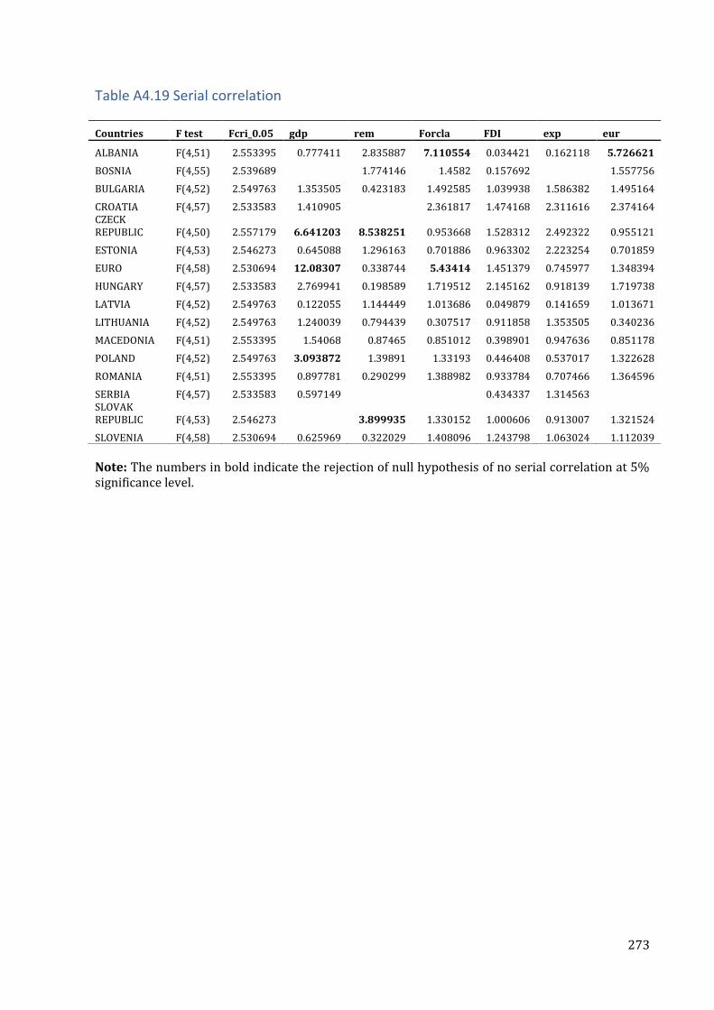
273
Table A4.19 Serial correlation
Note: The numbers in bold indicate the rejection of null hypothesis of no serial correlation at 5% significance level.
Countries F test Fcri_0.05 gdp rem Forcla FDI exp eur
ALBANIA F(4,51) 2.553395 0.777411 2.835887 7.110554 0.034421 0.162118 5.726621
BOSNIA F(4,55) 2.539689
1.774146 1.4582 0.157692
1.557756
BULGARIA F(4,52) 2.549763 1.353505 0.423183 1.492585 1.039938 1.586382 1.495164
CROATIA F(4,57) 2.533583 1.410905
2.361817 1.474168 2.311616 2.374164 CZECK REPUBLIC F(4,50) 2.557179 6.641203 8.538251 0.953668 1.528312 2.492322 0.955121
ESTONIA F(4,53) 2.546273 0.645088 1.296163 0.701886 0.963302 2.223254 0.701859
EURO F(4,58) 2.530694 12.08307 0.338744 5.43414 1.451379 0.745977 1.348394
HUNGARY F(4,57) 2.533583 2.769941 0.198589 1.719512 2.145162 0.918139 1.719738
LATVIA F(4,52) 2.549763 0.122055 1.144449 1.013686 0.049879 0.141659 1.013671
LITHUANIA F(4,52) 2.549763 1.240039 0.794439 0.307517 0.911858 1.353505 0.340236
MACEDONIA F(4,51) 2.553395 1.54068 0.87465 0.851012 0.398901 0.947636 0.851178
POLAND F(4,52) 2.549763 3.093872 1.39891 1.33193 0.446408 0.537017 1.322628
ROMANIA F(4,51) 2.553395 0.897781 0.290299 1.388982 0.933784 0.707466 1.364596
SERBIA F(4,57) 2.533583 0.597149
0.434337 1.314563 SLOVAK
REPUBLIC F(4,53) 2.546273
3.899935 1.330152 1.000606 0.913007 1.321524
SLOVENIA F(4,58) 2.530694 0.625969 0.322029 1.408096 1.243798 1.063024 1.112039

Appendix to Chapter 5 A5.1 Model 5.1 - estimated results
regress salesgrowth c.capitalpurch c.foreignown i.directexp c.emplgrowth c.wcbanks c.foreigncurr
i.subsidies i.industry i.country1 i.country2 i.country3 i.country4 i.country5i.country6
topmanagerexp i.firmsize c.firmage i.newproduct3years i.politicalinstability
Note: 1.country6 omitted because of collinearity
Source | SS df MS Number of obs = 972
-------------+------------------------------ F( 22, 949) = 8.61
Model | 16.8699296 22 .766814982 Prob > F = 0.0000
Residual | 84.5148194 949 .089056712 R-squared = 0.1664
-------------+------------------------------ Adj R-squared = 0.1471
Total | 101.384749 971 .104412718 Root MSE = .29842
----------------------------------------------------------------------------------------
salesgrowth | Coef. Std. Err. t P>|t| [95% Conf. Interval]
-----------------------+----------------------------------------------------------------
capitalpurch | -.0042864 .00458 -0.94 0.350 -.0132746 .0047017
foreignown | .057633 .0332814 1.73 0.084 -.0076807 .1229466
1.directexp | .0079668 .0291411 0.27 0.785 -.0492216 .0651553
emplgrowth | .125113 .0208496 6.00 0.000 .0841964 .1660297
wcbanks | -.0660177 .0264821 -2.49 0.013 -.117988 -.0140474
foreigncurr | -.1384894 .0366834 -3.78 0.000 -.2104793 -.0664995
1.subsidies | .0690813 .0306606 2.25 0.024 .1292518 .0089108
|
industry |
2 | -.0113732 .0251791 -0.45 0.652 -.0607863 .0380399
3 | -.0696036 .037962 -1.83 0.067 -.1441028 .0048955
4 | -.0279327 .0262101 -1.07 0.287 -.0793692 .0235038
|
1.country1 | -.0145911 .0376917 -0.39 0.699 -.0885599 .0593776
1.country2 | .0971389 .0401735 2.42 0.016 .0182997 .1759782
1.country3 | .1662858 .0337377 4.93 0.000 .1000767 .2324948
1.country4 | -.0030422 .0313422 -0.10 0.923 -.0645502 .0584658
1.country5 | -.040266 .0329422 -1.22 0.222 -.104914 .0243819
1.country6 | 0 (omitted)
topmanagerexp | .0027655 .0010157 2.72 0.007 .0007722 .0047588
|
firmsize |
1 | -.0515798 .0560603 -0.92 0.358 -.1615962 .0584366
2 | -.0326018 .0565542 -0.58 0.564 -.1435877 .078384
3 | .0225969 .0588348 0.38 0.701 -.0928644 .1380581
|
firmage | -.0013193 .0008479 -1.56 0.120 -.0029833 .0003446
1.newproduct3years | .0494467 .020317 2.43 0.015 .0893181 .0095753
1.politicalinstability | -.0528234 .0207232 -2.55 0.011 -.0934919 -.0121548
_cons | -.0383325 .0701684 -0.55 0.585 -.1760356 .0993706
----------------------------------------------------------------------------------------
A5.2 Model 5.1 – diagnostic tests Check for multicollinearity - VIF command - Model 5.1
. vif
Variable | VIF 1/VIF
-------------+----------------------
capitalpurch | 1.29 0.773039
foreignown | 1.16 0.859329
1.directex~m | 1.34 0.744205
emplgrowth | 1.06 0.946527
wcbanks | 1.30 0.767505
foreigncurr | 1.14 0.875153
2.subsidies | 1.05 0.948634

275
industry |
2 | 1.47 0.678528
3 | 1.17 0.851445
4 | 1.41 0.707447
1.country1 | 1.47 0.680744
1.country2 | 1.88 0.532247
1.country3 | 2.01 0.498121
1.country4 | 1.67 0.600293
1.country5 | 1.76 0.569381
topmanager~p | 1.13 0.883798
firmsize |
1 | 7.69 0.130009
2 | 7.80 0.128128
3 | 7.78 0.128519
firmage | 1.13 0.884307
2.newprodu~s | 1.12 0.894536
1.politica~y | 1.09 0.918072
-------------+----------------------
Mean VIF | 2.22
Tests for homoscedasticity - Model 5.1
. estat imtest
Cameron & Trivedi's decomposition of IM-test
---------------------------------------------------
Source | chi2 df p
---------------------+-----------------------------
Heteroskedasticity | 294.37 244 0.0150
Skewness | 25.14 22 0.2903
Kurtosis | 14.08 1 0.0002
---------------------+-----------------------------
Total | 333.59 267 0.0035
---------------------------------------------------
. estat hettest
Breusch-Pagan / Cook-Weisberg test for heteroskedasticity
Ho: Constant variance
Variables: fitted values of salesgrowth
chi2(1) = 1.26
Prob > chi2 = 0.2621
Tests for model specification - Model 5.1
. linktest
Source | SS df MS Number of obs = 972
-------------+------------------------------ F( 2, 969) = 97.15
Model | 16.9340105 2 8.46700523 Prob > F = 0.0000
Residual | 84.4507385 969 .087152465 R-squared = 0.1670
-------------+------------------------------ Adj R-squared = 0.1653
Total | 101.384749 971 .104412718 Root MSE = .29522
------------------------------------------------------------------------------
salesgrowth | Coef. Std. Err. t P>|t| [95% Conf. Interval]
-------------+----------------------------------------------------------------
_hat | .8812726 .1560048 5.65 0.000 .5751265 1.187419
_hatsq | -.3266976 .380997 -0.86 0.391 -1.074372 .4209767
_cons | -.0049804 .018289 -0.27 0.785 -.0408711 .0309103
------------------------------------------------------------------------------
. ovtest
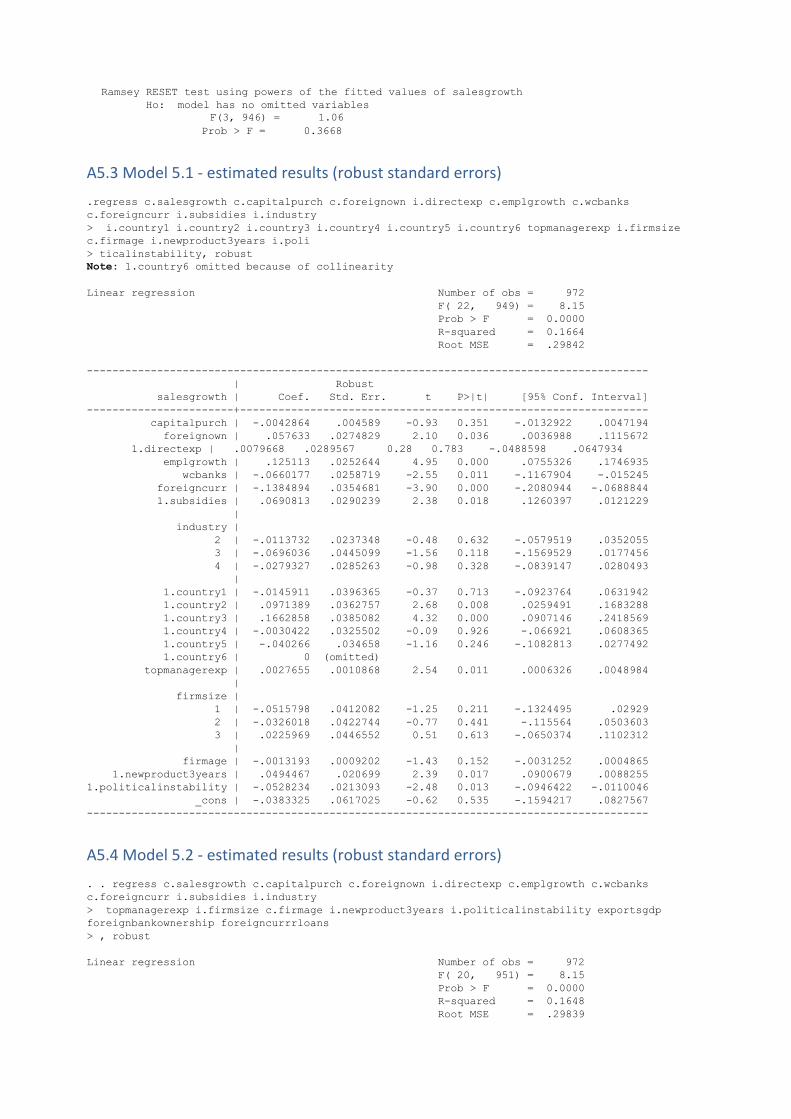
Prob > F = 0.3668
A5.3 Model 5.1 - estimated results (robust standard errors)
.regress c.salesgrowth c.capitalpurch c.foreignown i.directexp c.emplgrowth c.wcbanks
c.foreigncurr i.subsidies i.industry
> i.country1 i.country2 i.country3 i.country4 i.country5 i.country6 topmanagerexp i.firmsize
c.firmage i.newproduct3years i.poli
> ticalinstability, robust
Note: 1.country6 omitted because of collinearity
Linear regression Number of obs = 972
F( 22, 949) = 8.15
Prob > F = 0.0000
R-squared = 0.1664
Root MSE = .29842
----------------------------------------------------------------------------------------
| Robust
salesgrowth | Coef. Std. Err. t P>|t| [95% Conf. Interval]
-----------------------+----------------------------------------------------------------
capitalpurch | -.0042864 .004589 -0.93 0.351 -.0132922 .0047194
foreignown | .057633 .0274829 2.10 0.036 .0036988 .1115672
1.directexp | .0079668 .0289567 0.28 0.783 -.0488598 .0647934
emplgrowth | .125113 .0252644 4.95 0.000 .0755326 .1746935
wcbanks | -.0660177 .0258719 -2.55 0.011 -.1167904 -.015245
foreigncurr | -.1384894 .0354681 -3.90 0.000 -.2080944 -.0688844
1.subsidies | .0690813 .0290239 2.38 0.018 .1260397 .0121229
|
industry |
2 | -.0113732 .0237348 -0.48 0.632 -.0579519 .0352055
3 | -.0696036 .0445099 -1.56 0.118 -.1569529 .0177456
4 | -.0279327 .0285263 -0.98 0.328 -.0839147 .0280493
|
1.country1 | -.0145911 .0396365 -0.37 0.713 -.0923764 .0631942
1.country2 | .0971389 .0362757 2.68 0.008 .0259491 .1683288
1.country3 | .1662858 .0385082 4.32 0.000 .0907146 .2418569
1.country4 | -.0030422 .0325502 -0.09 0.926 -.066921 .0608365
1.country5 | -.040266 .034658 -1.16 0.246 -.1082813 .0277492
1.country6 | 0 (omitted)
topmanagerexp | .0027655 .0010868 2.54 0.011 .0006326 .0048984
|
firmsize |
1 | -.0515798 .0412082 -1.25 0.211 -.1324495 .02929
2 | -.0326018 .0422744 -0.77 0.441 -.115564 .0503603
3 | .0225969 .0446552 0.51 0.613 -.0650374 .1102312
|
firmage | -.0013193 .0009202 -1.43 0.152 -.0031252 .0004865
1.newproduct3years | .0494467 .020699 2.39 0.017 .0900679 .0088255
1.politicalinstability | -.0528234 .0213093 -2.48 0.013 -.0946422 -.0110046
_cons | -.0383325 .0617025 -0.62 0.535 -.1594217 .0827567
----------------------------------------------------------------------------------------
A5.4 Model 5.2 - estimated results (robust standard errors)
. . regress c.salesgrowth c.capitalpurch c.foreignown i.directexp c.emplgrowth c.wcbanks
c.foreigncurr i.subsidies i.industry
> topmanagerexp i.firmsize c.firmage i.newproduct3years i.politicalinstability exportsgdp
foreignbankownership foreigncurrrloans
> , robust
Linear regression Number of obs = 972
F( 20, 951) = 8.15
Prob > F = 0.0000
R-squared = 0.1648
Root MSE = .29839
Ramsey RESET test using powers of the fitted values of salesgrowth
Ho: model has no omitted variables
F(3, 946) = 1.06
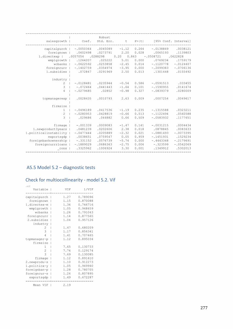
277
----------------------------------------------------------------------------------------
| Robust
salesgrowth | Coef. Std. Err. t P>|t| [95% Conf. Interval]
-----------------------+----------------------------------------------------------------
capitalpurch | -.0050364 .0045089 -1.12 0.264 -.0138849 .0038121
foreignown | .0602498 .0273791 2.20 0.028 .0065193 .1139803
1.directexp | .0057054 .0288298 0.20 0.843 -.0508721 .0622828
emplgrowth | .1264207 .025222 5.01 0.000 .0769234 .1759179
wcbanks | -.0622592 .0253858 -2.45 0.014 -.1120778 -.0124407
foreigncurr | -.1402759 .0354974 -3.95 0.000 -.2099383 -.0706136
1.subsidies | .072847 .0291969 2.50 0.013 .1301448 .0155492
|
industry |
2 | -.0128481 .0235944 -0.54 0.586 -.0591513 .033455
3 | -.072464 .0441443 -1.64 0.101 -.1590955 .0141674
4 | -.0279685 .02852 -0.98 0.327 -.0839379 .0280009
|
topmanagerexp | .0028435 .0010793 2.63 0.009 .0007254 .0049617
|
firmsize |
1 | -.0496189 .0417536 -1.19 0.235 -.1315588 .0323211
2 | -.0280953 .0428819 -0.66 0.513 -.1122494 .0560588
3 | .029686 .044882 0.66 0.509 -.0583932 .1177651
|
firmage | -.001339 .0009083 -1.47 0.141 -.0031215 .0004434
1.newproduct3years | .0481239 .0202606 2.38 0.018 .0878845 .0083633
1.politicalinstability | -.0477444 .0205889 -2.32 0.021 -.0881493 -.0073395
exportsgdp | .0038651 .0759547 0.05 0.959 -.1451931 .1529234
foreignbankownership | -.331152 .0576739 -5.74 0.000 -.4443348 -.2179691
foreigncurrrloans | -.1889029 .0686363 -2.75 0.006 -.323599 -.0542069
_cons | .3325962 .1006924 3.30 0.001 .1349912 .5302013
----------------------------------------------------------------------------------------
A5.5 Model 5.2 – diagnostic tests Check for multiocollinearity - model 5.2. Vif
.vif
Variable | VIF 1/VIF
-------------+----------------------
capitalpurch | 1.27 0.789096
foreignown | 1.15 0.870088
1.directex~m | 1.34 0.746716
emplgrowth | 1.05 0.948659
wcbanks | 1.26 0.791043
foreigncurr | 1.14 0.877565
2.subsidies | 1.04 0.957126
industry |
2 | 1.47 0.680209
3 | 1.17 0.856341
4 | 1.41 0.707465
topmanager~p | 1.12 0.895034
firmsize |
1 | 7.65 0.130733
2 | 7.74 0.129174
3 | 7.69 0.130085
firmage | 1.12 0.891610
2.newprodu~s | 1.10 0.912273
1.politica~y | 1.05 0.949940
foreignban~p | 1.28 0.780705
foreigncur~s | 1.24 0.807895
exportsgdp | 1.49 0.672287
-------------+----------------------
Mean VIF | 2.19
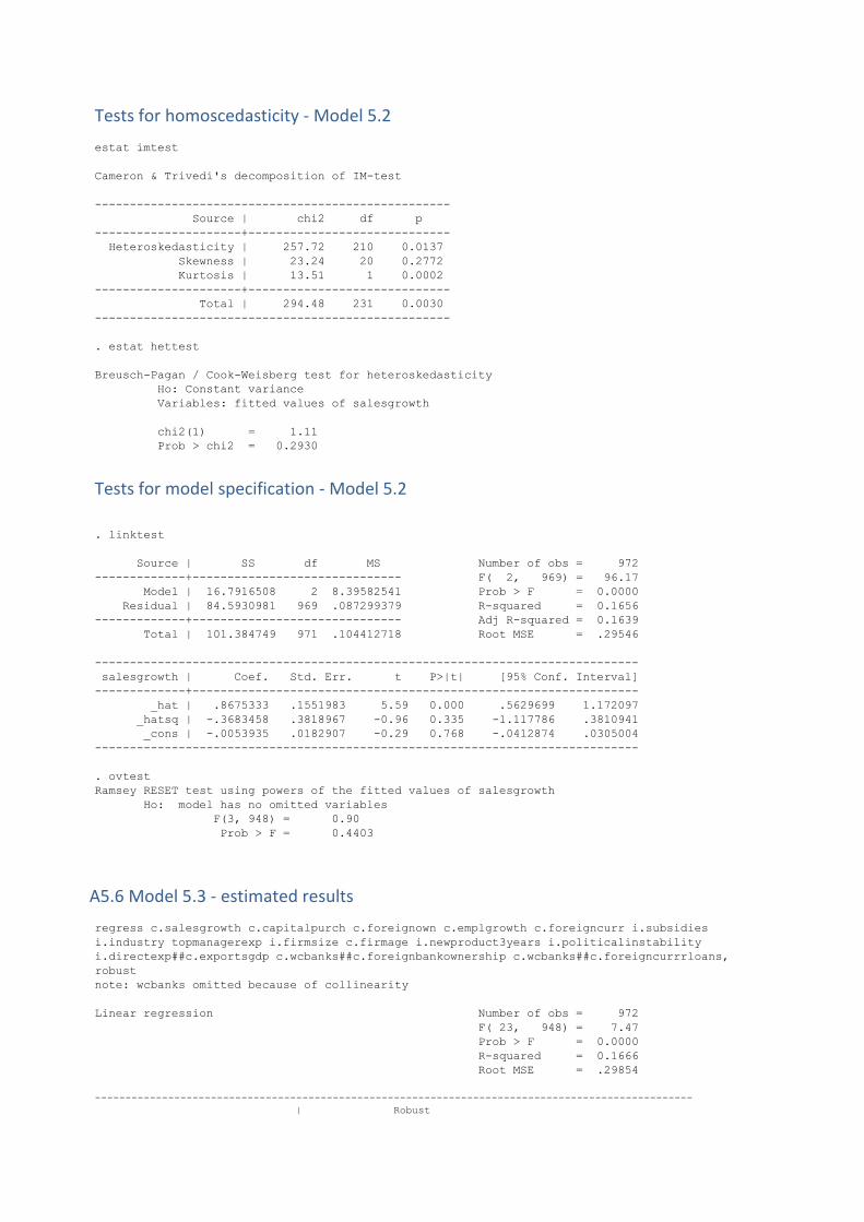
Tests for homoscedasticity - Model 5.2
estat imtest
Cameron & Trivedi's decomposition of IM-test
---------------------------------------------------
Source | chi2 df p
---------------------+-----------------------------
Heteroskedasticity | 257.72 210 0.0137
Skewness | 23.24 20 0.2772
Kurtosis | 13.51 1 0.0002
---------------------+-----------------------------
Total | 294.48 231 0.0030
---------------------------------------------------
. estat hettest
Breusch-Pagan / Cook-Weisberg test for heteroskedasticity
Ho: Constant variance
Variables: fitted values of salesgrowth
chi2(1) = 1.11
Prob > chi2 = 0.2930
Tests for model specification - Model 5.2
. linktest
Source | SS df MS Number of obs = 972
-------------+------------------------------ F( 2, 969) = 96.17
Model | 16.7916508 2 8.39582541 Prob > F = 0.0000
Residual | 84.5930981 969 .087299379 R-squared = 0.1656
-------------+------------------------------ Adj R-squared = 0.1639
Total | 101.384749 971 .104412718 Root MSE = .29546
------------------------------------------------------------------------------
salesgrowth | Coef. Std. Err. t P>|t| [95% Conf. Interval]
-------------+----------------------------------------------------------------
_hat | .8675333 .1551983 5.59 0.000 .5629699 1.172097
_hatsq | -.3683458 .3818967 -0.96 0.335 -1.117786 .3810941
_cons | -.0053935 .0182907 -0.29 0.768 -.0412874 .0305004
------------------------------------------------------------------------------
. ovtest
Ramsey RESET test using powers of the fitted values of salesgrowth
Ho: model has no omitted variables
F(3, 948) = 0.90
Prob > F = 0.4403
A5.6 Model 5.3 - estimated results
regress c.salesgrowth c.capitalpurch c.foreignown c.emplgrowth c.foreigncurr i.subsidies
i.industry topmanagerexp i.firmsize c.firmage i.newproduct3years i.politicalinstability
i.directexp##c.exportsgdp c.wcbanks##c.foreignbankownership c.wcbanks##c.foreigncurrrloans,
robust
note: wcbanks omitted because of collinearity
Linear regression Number of obs = 972
F( 23, 948) = 7.47
Prob > F = 0.0000
R-squared = 0.1666
Root MSE = .29854
--------------------------------------------------------------------------------------------------
| Robust
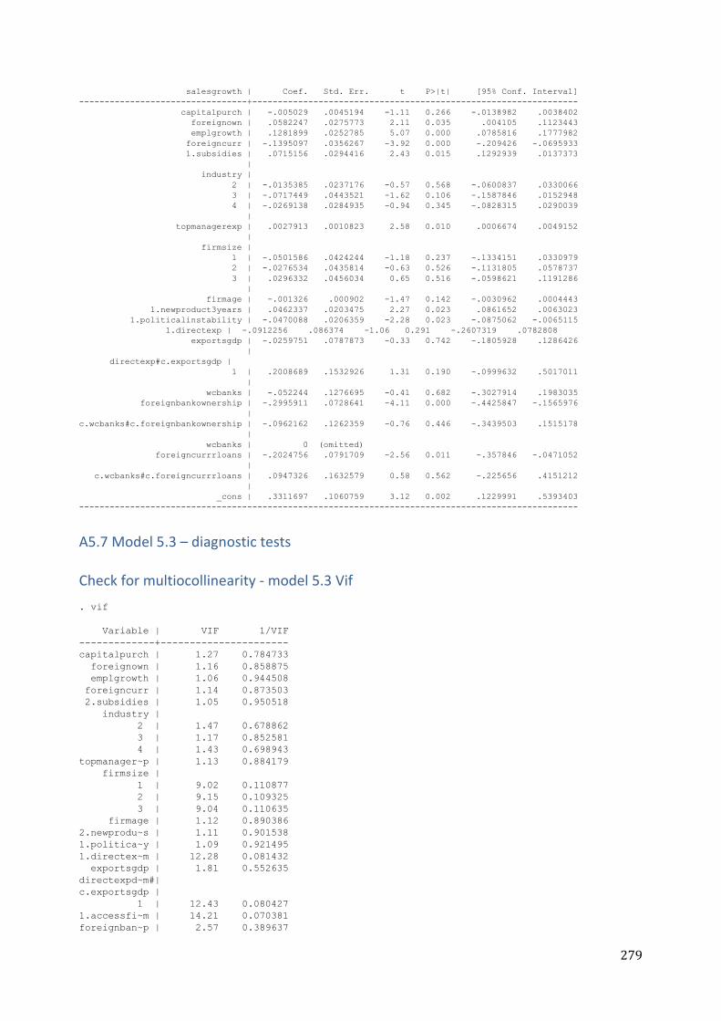
279
salesgrowth | Coef. Std. Err. t P>|t| [95% Conf. Interval]
---------------------------------+----------------------------------------------------------------
capitalpurch | -.005029 .0045194 -1.11 0.266 -.0138982 .0038402
foreignown | .0582247 .0275773 2.11 0.035 .004105 .1123443
emplgrowth | .1281899 .0252785 5.07 0.000 .0785816 .1777982
foreigncurr | -.1395097 .0356267 -3.92 0.000 -.209426 -.0695933
1.subsidies | .0715156 .0294416 2.43 0.015 .1292939 .0137373
|
industry |
2 | -.0135385 .0237176 -0.57 0.568 -.0600837 .0330066
3 | -.0717449 .0443521 -1.62 0.106 -.1587846 .0152948
4 | -.0269138 .0284935 -0.94 0.345 -.0828315 .0290039
|
topmanagerexp | .0027913 .0010823 2.58 0.010 .0006674 .0049152
|
firmsize |
1 | -.0501586 .0424244 -1.18 0.237 -.1334151 .0330979
2 | -.0276534 .0435814 -0.63 0.526 -.1131805 .0578737
3 | .0296332 .0456034 0.65 0.516 -.0598621 .1191286
|
firmage | -.001326 .000902 -1.47 0.142 -.0030962 .0004443
1.newproduct3years | .0462337 .0203475 2.27 0.023 .0861652 .0063023
1.politicalinstability | -.0470088 .0206359 -2.28 0.023 -.0875062 -.0065115
1.directexp | -.0912256 .086374 -1.06 0.291 -.2607319 .0782808
exportsgdp | -.0259751 .0787873 -0.33 0.742 -.1805928 .1286426
|
directexp#c.exportsgdp |
1 | .2008689 .1532926 1.31 0.190 -.0999632 .5017011
|
wcbanks | -.052244 .1276695 -0.41 0.682 -.3027914 .1983035
foreignbankownership | -.2995911 .0728641 -4.11 0.000 -.4425847 -.1565976
|
c.wcbanks#c.foreignbankownership | -.0962162 .1262359 -0.76 0.446 -.3439503 .1515178
|
wcbanks | 0 (omitted)
foreigncurrrloans | -.2024756 .0791709 -2.56 0.011 -.357846 -.0471052
|
c.wcbanks#c.foreigncurrrloans | .0947326 .1632579 0.58 0.562 -.225656 .4151212
|
_cons | .3311697 .1060759 3.12 0.002 .1229991 .5393403
--------------------------------------------------------------------------------------------------
A5.7 Model 5.3 – diagnostic tests Check for multiocollinearity - model 5.3 Vif
. vif
Variable | VIF 1/VIF
-------------+----------------------
capitalpurch | 1.27 0.784733
foreignown | 1.16 0.858875
emplgrowth | 1.06 0.944508
foreigncurr | 1.14 0.873503
2.subsidies | 1.05 0.950518
industry |
2 | 1.47 0.678862
3 | 1.17 0.852581
4 | 1.43 0.698943
topmanager~p | 1.13 0.884179
firmsize |
1 | 9.02 0.110877
2 | 9.15 0.109325
3 | 9.04 0.110635
firmage | 1.12 0.890386
2.newprodu~s | 1.11 0.901538
1.politica~y | 1.09 0.921495
1.directex~m | 12.28 0.081432
exportsgdp | 1.81 0.552635
directexpd~m#|
c.exportsgdp |
1 | 12.43 0.080427
1.accessfi~m | 14.21 0.070381
foreignban~p | 2.57 0.389637
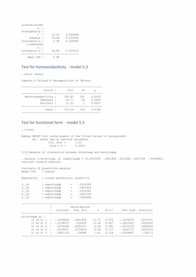
accessfind~m#|
c. |
foreignban~p |
1 | 15.61 0.064046
wcbanks | 19.98 0.050056
foreigncur~s | 1.90 0.526890
c.wcbanks#|
c. |
foreigncur~s | 18.86 0.053015
-------------+----------------------
Mean VIF | 5.88
Test for homoscedasticity - model 5.3
. estat imtest
Cameron & Trivedi's decomposition of IM-test
---------------------------------------------------
Source | chi2 df p
---------------------+-----------------------------
Heteroskedasticity | 335.87 291 0.0360
Skewness | 25.77 24 0.3649
Kurtosis | 11.52 1 0.0007
---------------------+-----------------------------
Total | 373.16 316 0.0148
--------------------------------------------------
Test for functional form - model 5.3
. ovtest
Ramsey RESET test using powers of the fitted values of salesgrowth
Ho: model has no omitted variables
F(3, 914) = 1.53
Prob > F = 0.2049
5.14 Margins of interaction between directexp and exoirtsgdp
. margins r.directexp, at (exportsgdp = (0.2914506 .3851856 .4931282 .5041728 .7832868))
contrast (nowald effects)
Contrasts of predictive margins
Model VCE : Robust
Expression : Linear prediction, predict()
1._at : exportsgdp = .2914506
2._at : exportsgdp = .3851856
3._at : exportsgdp = .4931282
4._at : exportsgdp = .5041728
5._at : exportsgdp = .7832868
-----------------------------------------------------------------------------------
| Delta-method
| Contrast Std. Err. t P>|t| [95% Conf. Interval]
------------------+----------------------------------------------------------------
directexp@_at |
(1 vs 0) 1 | -.0326822 .0461935 -0.71 0.479 -.1233355 .0579711
(1 vs 0) 2 | -.0138537 .035625 -0.39 0.697 -.0837667 .0560592
(1 vs 0) 3 | .0078286 .0280167 0.28 0.780 -.0471533 .0628104
(1 vs 0) 4 | .0100471 .0276816 0.36 0.717 -.0442772 .0643714
(1 vs 0) 5 | .0661124 .04688 1.41 0.159 -.0258881 .158113
-----------------------------------------------------------------------------------

281
A5.8 Margins of interaction between wcbanks and foreigncurrloans
. margins, dydx(wcbanks) at (foreigncurrrloans = (.427089 .497385 .5314689 .5421005
.547776.8648633 ))
Average marginal effects Number of obs = 972
Model VCE : Robust
Expression : Linear prediction, predict()
dy/dx w.r.t. : wcbanks
1._at : foreigncur~s = .427089
2._at : foreigncur~s = .497385
3._at : foreigncur~s = .5314689
4._at : foreigncur~s = .5421005
5._at : foreigncur~s = .547776
6._at : foreigncur~s = .8648633
------------------------------------------------------------------------------
| Delta-method
| dy/dx Std. Err. t P>|t| [95% Conf. Interval]
-------------+----------------------------------------------------------------
wcbanks |
_at |
1 | -.0279687 .0380694 -0.73 0.463 -.1026785 .0467412
2 | -.036642 .0303324 -1.21 0.227 -.0961682 .0228842
3 | -.0408474 .0276105 -1.48 0.139 -.095032 .0133373
4 | -.0421591 .0269511 -1.56 0.118 -.0950497 .0107315
5 | -.0428594 .0266407 -1.61 0.108 -.0951408 .0094221
6 | -.0819824 .0512363 -1.60 0.110 -.1825317 .0185669
------------------------------------------------------------------------------
A5.9 Margins of interaction between wcbanks and foreignabnkownership
. margins, dydx(wcbanks) at (foreignbankownership = (0.38 0.61 0.8230277 0.87 0.92))
Average marginal effects Number of obs = 972
Model VCE : Robust
Expression : Linear prediction, predict()
dy/dx w.r.t. : wcbanks
1._at : foreignban~p = .38
2._at : foreignban~p = .61
3._at : foreignban~p = .8230277
4._at : foreignban~p = .87
5._at : foreignban~p = .92
------------------------------------------------------------------------------
| Delta-method
| dy/dx Std. Err. t P>|t| [95% Conf. Interval]
-------------+----------------------------------------------------------------
wcbanks |
_at |
1 | -.0342511 .046867 -0.73 0.465 -.1262261 .0577239
2 | -.0563808 .0271482 -2.08 0.038 -.1096584 -.0031033
3 | -.0768776 .0298192 -2.58 0.010 -.1353968 -.0183583
4 | -.0813971 .0334268 -2.44 0.015 -.1469962 -.015798
5 | -.0862079 .0379143 -2.27 0.023 -.1606135 -.0118023
------------------------------------------------------------------------------
A5.10 Model 5.4 - estimated results
. regress c.utilcapacity c.capitalpurch c.foreignown i.directexp c.emplgrowth c.wcbanks
c.foreigncurr i.subsidies i.industry i.country1 i.
> country2 i.country3 i.country4 i.country5 i.country6 topmanagerexp i.firmsize c.firmage
i.newproduct3years i.politicalinstability, robust
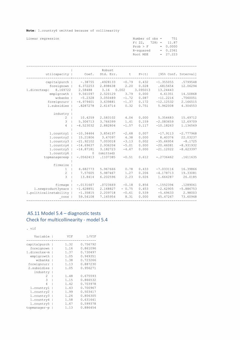
Note: 1.country6 omitted because of collinearity
Linear regression Number of obs = 751
F( 22, 728) = 11.87
Prob > F = 0.0000
R-squared = 0.2361
Root MSE = 27.223
----------------------------------------------------------------------------------------
| Robust
utilcapacity | Coef. Std. Err. t P>|t| [95% Conf. Interval]
-----------------------+----------------------------------------------------------------
capitalpurch | -.38755 .4928133 -0.79 0.432 -1.355055 .5799548
foreignown | 6.372253 2.898638 2.20 0.028 .6815654 12.06294
1.directexp| 8.169722 2.58488 3.16 0.002 3.095013 13.24443
emplgrowth | 9.561097 2.520129 3.79 0.000 4.61351 14.50868
wcbanks | -5.2328 3.050489 -1.72 0.087 -11.2216 .7560051
foreigncurr | -4.979401 3.639881 -1.37 0.172 -12.12532 2.166515
1.subsidies | .8287278 2.614714 0.32 0.751 5.962008 4.304553
|
industry |
2 | 10.4259 2.583102 4.04 0.000 5.354683 15.49712
3 | 5.306713 3.764399 1.41 0.159 -2.083659 12.69709
4 | -4.523032 2.882804 -1.57 0.117 -10.18263 1.136569
|
1.country1 | -10.34464 3.854197 -2.68 0.007 -17.9113 -2.777968
1.country2 | 15.21806 3.47097 4.38 0.000 8.40376 22.03237
1.country3 | -21.92102 7.003018 -3.13 0.002 -35.66954 -8.1725
1.country4 | -14.69637 2.936204 -5.01 0.000 -20.46081 -8.931932
1.country5 | -14.87181 3.182723 -4.67 0.000 -21.12022 -8.623397
1.country6 | 0 (omitted)
topmanagerexp | -.0562413 .1107385 -0.51 0.612 -.2736462 .1611635
|
firmsize |
1 | 4.682773 5.967666 0.78 0.433 -7.033116 16.39866
2 | 7.57605 5.987467 1.27 0.206 -4.178713 19.33081
3 | 13.8414 6.202596 2.23 0.026 1.664287 26.0185
|
firmage | -.0131667 .0723669 -0.18 0.856 -.1552394 .1289061
1.newproduct3years | -1.628851 2.168827 - 0.75 0.453 -2.62905 -5.886753
1.politicalinstability | -1.35815 2.209718 -0.61 0.539 -5.69633 2.98003
_cons | 59.54108 7.165954 8.31 0.000 45.47267 73.60948
----------------------------------------------------------------------------------------
A5.11 Model 5.4 – diagnostic tests Check for multicollinearity - model 5.4
. vif
Variable | VIF 1/VIF
-------------+----------------------
capitalpurch | 1.32 0.756792
foreignown | 1.16 0.861096
1.directex~m | 1.37 0.730497
emplgrowth | 1.05 0.949351
wcbanks | 1.38 0.723266
foreigncurr | 1.13 0.887230
2.subsidies | 1.05 0.956271
industry |
2 | 1.48 0.675593
3 | 1.15 0.866532
4 | 1.42 0.703978
1.country1 | 1.43 0.700967
1.country2 | 1.99 0.503417
1.country3 | 1.24 0.806305
1.country4 | 1.58 0.631641
1.country5 | 1.67 0.599378
topmanager~p | 1.13 0.886454

283
firmsize |
1 | 7.09 0.140949
2 | 6.89 0.145185
3 | 6.92 0.144541
firmage | 1.11 0.897101
2.newprodu~s | 1.12 0.891890
1.politica~y | 1.08 0.927139
-------------+----------------------
Mean VIF | 2.08
Test for homoscedasticity - model 5.4
. estat imtest
Cameron & Trivedi's decomposition of IM-test
---------------------------------------------------
Source | chi2 df p
---------------------+-----------------------------
Heteroskedasticity | 272.85 243 0.0914
Skewness | 82.12 22 0.0000
Kurtosis | 10.06 1 0.0015
---------------------+-----------------------------
Total | 365.03 266 0.0001
---------------------------------------------------
. estat hettest
Breusch-Pagan / Cook-Weisberg test for heteroskedasticity
Ho: Constant variance
Variables: fitted values of utilcapacity
chi2(1) = 30.52
Prob > chi2 = 0.0000
Test for functional form - model 5.4
. ovtest
Ramsey RESET test using powers of the fitted values of utilcapacity
Ho: model has no omitted variables
F(3, 725) = 5.34
Prob > F = 0.05
A5.12 Model 5.5 - estimated results
. regress c.emplgrowth c.foreignown i.directexp c.wcbanks c.foreigncurr i.subsidies i.industry
i.country1 i.country2 i.country3 i.country4 i.country5 i.country6 topmanagerexp i.firmsize
c.firmage i.newproduct3years i.politicalinstability, robust
Note: 1.country6 omitted because of collinearity
Linear regression Number of obs = 972
F( 20, 951) = 2.44
Prob > F = 0.0004
R-squared = 0.0535
Root MSE = .46414
----------------------------------------------------------------------------------------
| Robust
emplgrowth | Coef. Std. Err. t P>|t| [95% Conf. Interval]
-----------------------+----------------------------------------------------------------
foreignown | .0265615 .0404732 0.66 0.512 -.0528656 .1059885
1.directexp | .0336926 .0403484 0.84 0.404 -.0454896 .1128748
wcbanks | -.0623493 .0437451 -1.43 0.154 -.1481973 .0234988
foreigncurr | .0979953 .0634533 1.54 0.123 -.0265294 .22252
1.subsidies | .0529026 .0436689 1.21 0.226 .1386012 -.032796
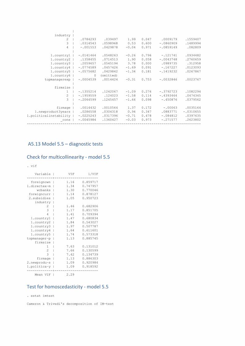
|
industry |
2 | .0784293 .039497 1.99 0.047 .0009179 .1559407
3 | .0314543 .0598968 0.53 0.600 -.0860909 .1489994
4 | -.001553 .0429878 -0.04 0.971 -.0859149 .082809
|
1.country1 | -.0141464 .0548263 -0.26 0.796 -.121741 .0934482
1.country2 | .1358455 .0714513 1.90 0.058 -.0043748 .2760659
1.country3 | .2059657 .0545194 3.78 0.000 .0989735 .312958
1.country4 | -.0774589 .0457426 -1.69 0.091 -.167227 .0123093
1.country5 | -.0575682 .0429842 -1.34 0.181 -.1419232 .0267867
1.country6 | 0 (omitted)
topmanagerexp | -.0004539 .0014424 -0.31 0.753 -.0032846 .0023767
|
firmsize |
1 | -.1355214 .1242067 -1.09 0.276 -.3792723 .1082294
2 | -.1959559 .124023 -1.58 0.114 -.4393464 .0474345
3 | -.2064599 .1245457 -1.66 0.098 -.450876 .0379562
|
firmage | .0014432 .0010564 1.37 0.172 -.00063 .0035164
1.newproduct3years | .0286558 .0304318 0.94 0.347 .0883771 -.0310655
1.politicalinstability | -.0225243 .0317396 -0.71 0.478 -.084812 .0397635
_cons | -.0045984 .1360427 -0.03 0.973 -.271577 .2623802
----------------------------------------------------------------------------------------
A5.13 Model 5.5 – diagnostic tests Check for multicollinearity - model 5.5
. vif
Variable | VIF 1/VIF
-------------+----------------------
foreignown | 1.16 0.859717
1.directex~m | 1.34 0.747957
wcbanks | 1.30 0.770046
foreigncurr | 1.14 0.878127
2.subsidies | 1.05 0.950723
industry |
2 | 1.46 0.682906
3 | 1.17 0.851705
4 | 1.41 0.709394
1.country1 | 1.47 0.680834
1.country2 | 1.84 0.543027
1.country3 | 1.97 0.507787
1.country4 | 1.64 0.611601
1.country5 | 1.74 0.573318
topmanager~p | 1.13 0.885745
firmsize |
1 | 7.63 0.131012
2 | 7.66 0.130599
3 | 7.42 0.134739
firmage | 1.13 0.886303
2.newprodu~s | 1.09 0.920984
1.politica~y | 1.09 0.918592
-------------+----------------------
Mean VIF | 2.29
Test for homoscedasticity - model 5.5
. estat imtest
Cameron & Trivedi's decomposition of IM-test

285
Source chi2 df p
Heteroskedasticity 239.90 199 0.0252
Skewness 46.46 20 0.0007
Kurtosis 14.29 1 0.0002
Total 300.65 220 0.0002
. estat hettest
Breusch-Pagan / Cook-Weisberg test for heteroskedasticity
Ho: Constant variance
Variables: fitted values of emplgrowth
chi2(1) = 47.06
Prob > chi2 = 0.0000
Test for functional form - model 5.5
. ovtest
Ramsey RESET test using powers of the fitted values of emplgrowth
Ho: model has no omitted variables
F(3, 948) = 1.23
Prob > F = 0.2967
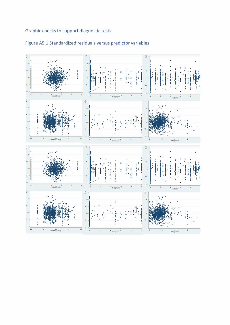
Graphic checks to support diagnostic tests Figure A5.1 Standardized residuals versus predictor variables
-1-.
50
.51
1.5
Re
sid
ua
ls
0 2 4 6 8 10capitalpurch
-1-.
5
0.5
1
1.5
Re
sid
ua
ls
0 .2 .4 .6 .8 1foreignown
-1-.
50
.51
1.5
Re
sid
ua
ls
-20 0 20 40 60topmanagerexp
-1-.
50
.51
1.5
Re
sid
ua
ls
-1 0 1 2 3emplgrowth
-1-.
50
.51
1.5
Re
sid
ua
ls
0 .2 .4 .6 .8 1wcbanks
-1-.
50
.51
1.5
Re
sid
ua
ls
0 .2 .4 .6 .8 1foreigncurr
-1-.
50
.51
1.5
Re
sid
ua
ls
0 2 4 6 8 10capitalpurch
-1-.
5
0.5
1
1.5
Re
sid
ua
ls
0 .2 .4 .6 .8 1foreignown
-1-.
50
.51
1.5
Re
sid
ua
ls
-20 0 20 40 60topmanagerexp
-1-.
50
.51
1.5
Re
sid
ua
ls
-1 0 1 2 3emplgrowth
-1-.
50
.51
1.5
Re
sid
ua
ls
0 .2 .4 .6 .8 1wcbanks
-1-.
50
.51
1.5
Re
sid
ua
ls
0 .2 .4 .6 .8 1foreigncurr

287
Figure A5.2 Augmented plus residual plot
Figure A5.3 Kemel density plot
-1
-.5
0.5
11
.5
Au
gm
en
ted
co
mp
on
en
t p
lus r
esid
ua
l
0 .2 .4 .6 .8 1foreignown
-1
-.5
0.5
11
.5
Au
gm
en
ted
co
mp
on
en
t p
lus r
esid
ua
l
-20 0 20 40 60topmanagerexp
-1
-.5
0.5
1
Au
gm
en
ted
co
mp
on
en
t p
lus
re
sid
ua
l
0 .2 .4 .6 .8 1wcbanks
-1
-.5
0.5
1
Au
gm
en
ted
co
mp
on
en
t p
lus r
esid
ua
l
0 .2 .4 .6 .8 1foreigncurr
-1
-.5
0.5
11
.5
Au
gm
en
ted
co
mp
on
en
t p
lus r
esid
ua
l
0 50 100 150firmage
-1
-.5
0
.5
1
0 2 4 6 8 10capitalpurch
-1
-.5
0
.5
1
1.5
-1 0 1 2 3emplgrowth
0.5
11
.52
Den
sity
-1 -.5 0 .5 1 1.5Residuals
Kernel density estimate
Normal density
kernel = epanechnikov, bandwidth = 0.0544
Kernel density estimate
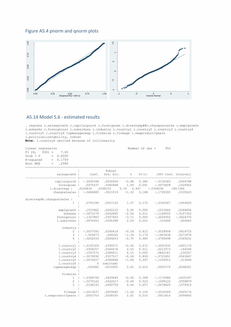
Figure A5.4 pnorm and qnorm plots
A5.14 Model 5.6 - estimated results
. regress c.salesgrowth c.capitalpurch c.foreignown i.directexp##c.changnatsales c.emplgrowth
c.wcbanks c.foreigncurr i.subsidies i.industry i.country1 i.country2 i.country3 i.country4
i.country5 i.country6 topmanagerexp i.firmsize c.firmage i.newproduct3years
i.politicalinstability, robust
Note: 1.country6 omitted because of collinearity
Linear regression Number of obs = 955
F( 24, 930) = 7.65
Prob > F = 0.0000
R-squared = 0.1759
Root MSE = .2966
-----------------------------+----------------------------------------------------------------
| Robust
salesgrowth | Coef. Std. Err. t P>|t| [95% Conf. Interval]
----------------------------- +----------------------------------------------------------------
capitalpurch | -.0040398 .0045954 -0.88 0.380 -.0130583 .0049788
foreignown | .0475537 .0280948 1.69 0.091 -.0075828 .1026902
1.directexp | .0226834 .0298153 0.76 0.447 -.0358296 .0811964
changnatsales | -.0686885 .0521019 -1.32 0.188 -.1709393 .0335623
|
directexp#c.changnatsales |
1 | .0761294 .0557122 1.37 0.172 -.0332067 .1854655
|
emplgrowth | .1533962 .0260123 5.90 0.000 .1023466 .2044458
wcbanks | -.0673179 .0262865 -2.56 0.011 -.1189055 -.0157302
foreigncurr | -.1327863 .0357443 -3.71 0.000 -.2029352 -.0626375
1.subsidies | .0676355 .0295398 2.29 0.022 .125608 .009663
|
industry |
2 | -.0057092 .0240414 -0.24 0.812 -.0528908 .0414725
3 | -.059473 .044265 -1.34 0.179 -.1463438 .0273978
4 | -.0202033 .0289253 -0.70 0.485 -.0769698 .0365631
|
1.country1 | -.0165329 .0390571 -0.42 0.672 -.0931832 .0601174
1.country2 | .0928257 .0364676 2.55 0.011 .0212573 .164394
1.country3 | .1597575 .0384911 4.15 0.000 .0842181 .235297
1.country4 | -.0079092 .0327517 -0.24 0.809 -.0721851 .0563667
1.country5 | -.0576227 .0346844 -1.66 0.097 -.1256915 .010446
1.country6 | 0 (omitted)
topmanagerexp | .002682 .0010925 2.45 0.014 .0005379 .0048261
|
firmsize |
1 | -.0368749 .0409645 -0.90 0.368 -.1172684 .0435187
2 | -.0270122 .0422417 -0.64 0.523 -.1099122 .0558879
3 | .0198143 .0446759 0.44 0.657 -.0678629 .1074915
|
firmage | -.0013637 .0009585 -1.42 0.155 -.0032449 .0005174
1.newproduct3years | .0503753 .0208335 2.42 0.016 .0912614 .0094892
0.0
00
.25
0.5
00
.75
1.0
0
Norm
al F
[(r-
m)/
s]
0.00 0.25 0.50 0.75 1.00Empirical P[i] = i/(N+1)
-1-.
50
.51
1.5
Resid
uals
-1 -.5 0 .5 1Inverse Normal
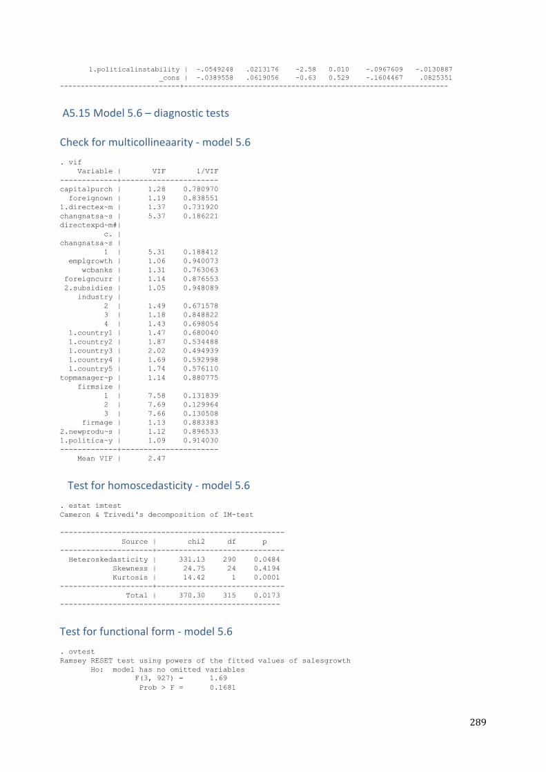
289
1.politicalinstability | -.0549248 .0213176 -2.58 0.010 -.0967609 -.0130887
_cons | -.0389558 .0619056 -0.63 0.529 -.1604467 .0825351
-----------------------------+----------------------------------------------------------------
A5.15 Model 5.6 – diagnostic tests Check for multicollineaarity - model 5.6
. vif
Variable | VIF 1/VIF
-------------+----------------------
capitalpurch | 1.28 0.780970
foreignown | 1.19 0.838551
1.directex~m | 1.37 0.731920
changnatsa~s | 5.37 0.186221
directexpd~m#|
c. |
changnatsa~s |
1 | 5.31 0.188412
emplgrowth | 1.06 0.940073
wcbanks | 1.31 0.763063
foreigncurr | 1.14 0.876553
2.subsidies | 1.05 0.948089
industry |
2 | 1.49 0.671578
3 | 1.18 0.848822
4 | 1.43 0.698054
1.country1 | 1.47 0.680040
1.country2 | 1.87 0.534488
1.country3 | 2.02 0.494939
1.country4 | 1.69 0.592998
1.country5 | 1.74 0.576110
topmanager~p | 1.14 0.880775
firmsize |
1 | 7.58 0.131839
2 | 7.69 0.129964
3 | 7.66 0.130508
firmage | 1.13 0.883383
2.newprodu~s | 1.12 0.896533
1.politica~y | 1.09 0.914030
-------------+----------------------
Mean VIF | 2.47
Test for homoscedasticity - model 5.6
. estat imtest
Cameron & Trivedi's decomposition of IM-test
---------------------------------------------------
Source | chi2 df p
---------------------+-----------------------------
Heteroskedasticity | 331.13 290 0.0484
Skewness | 24.75 24 0.4194
Kurtosis | 14.42 1 0.0001
---------------------+-----------------------------
Total | 370.30 315 0.0173
--------------------------------------------------
Test for functional form - model 5.6
Prob > F = 0.1681
. ovtest
Ramsey RESET test using powers of the fitted values of salesgrowth
Ho: model has no omitted variables
F(3, 927) = 1.69

A5.16 Predictive margins - model 5.6
. margins directexp, at (changnatsales=( -1(0.1) 1.777778))
Predictive margins Number of obs = 955
Model VCE : Robust
Expression : Linear prediction, predict()
1._at : changnatsa~s = -1
2._at : changnatsa~s = -.9
3._at : changnatsa~s = -.8
4._at : changnatsa~s = -.7
5._at : changnatsa~s = -.6
6._at : changnatsa~s = -.5
7._at : changnatsa~s = -.4
8._at : changnatsa~s = -.3
9._at : changnatsa~s = -.2
10._at : changnatsa~s = -.1
11._at : changnatsa~s = 0
12._at : changnatsa~s = .1
13._at : changnatsa~s = .2
14._at : changnatsa~s = .3
15._at : changnatsa~s = .4
16._at : changnatsa~s = .5
17._at : changnatsa~s = .6
18._at : changnatsa~s = .7
19._at : changnatsa~s = .8
20._at : changnatsa~s = .9
21._at : changnatsa~s = 1
22._at : changnatsa~s = 1.1
23._at : changnatsa~s = 1.2
24._at : changnatsa~s = 1.3
25._at : changnatsa~s = 1.4
26._at : changnatsa~s = 1.5
27._at : changnatsa~s = 1.6
28._at : changnatsa~s = 1.7
Delta-method
Margin Std. Err. t P>t [95% Conf. Interval]
_at#directexp
1 0 -.1390261 .0498704 -2.79 0.005 -.2368977 -.0411544
1 1 -.1924721 .0384684 -5.00 0.000 -.267967 -.1169772
2 0 -.1458949 .0447927 -3.26 0.001 -.2338014 -.0579884
2 1 -.191728 .0369257 -5.19 0.000 -.2641954 -.1192607
3 0 -.1527638 .0397493 -3.84 0.000 -.2307725 -.074755
3 1 -.1909839 .0354413 -5.39 0.000 -.2605381 -.1214297
4 0 -.1596326 .0347551 -4.59 0.000 -.2278402 -.0914251
4 1 -.1902398 .0340228 -5.59 0.000 -.2570102 -.1234695
5 0 -.1665015 .0298349 -5.58 0.000 -.225053 -.1079499
5 1 -.1894957 .0326788 -5.80 0.000 -.2536284 -.1253631
6 0 -.1733703 .0250323 -6.93 0.000 -.2224967 -.1242439
6 1 -.1887516 .0314188 -6.01 0.000 -.2504116 -.1270917
7 0 -.1802392 .0204305 -8.82 0.000 -.2203344 -.140144
7 1 -.1880076 .0302533 -6.21 0.000 -.2473803 -.1286348
8 0 -.187108 .0162014 -11.55 0.000 -.2189035 -.1553125
8 1 -.1872635 .0291938 -6.41 0.000 -.2445568 -.1299702
9 0 -.1939769 .0127223 -15.25 0.000 -.2189446 -.1690091
9 1 -.1865194 .028252 -6.60 0.000 -.2419644 -.1310743
10 0 -.2008457 .0107481 -18.69 0.000 -.221939 -.1797525
10 1 -.1857753 .0274401 -6.77 0.000 -.239627 -.1319236
11 0 -.2077146 .011112 -18.69 0.000 -.2295221 -.1859071
11 1 -.1850312 .02677 -6.91 0.000 -.2375677 -.1324947
12 0 -.2145834 .0136281 -15.75 0.000 -.2413288 -.1878381
12 1 -.1842871 .0262524 -7.02 0.000 -.2358079 -.1327663
13 0 -.2214523 .0173858 -12.74 0.000 -.2555722 -.1873324
13 1 -.183543 .0258966 -7.09 0.000 -.2343655 -.1327205
14 0 -.2283211 .0217508 -10.50 0.000 -.2710075 -.1856348

291
14 1 -.1827989 .0257092 -7.11 0.000 -.2332537 -.1323441
15 0 -.23519 .0264239 -8.90 0.000 -.2870473 -.1833326
15 1 -.1820548 .025694 -7.09 0.000 -.2324798 -.1316298
16 0 -.2420588 .0312672 -7.74 0.000 -.3034213 -.1806964
16 1 -.1813107 .0258513 -7.01 0.000 -.2320443 -.1305772
17 0 -.2489277 .0362125 -6.87 0.000 -.3199954 -.17786
17 1 -.1805666 .0261778 -6.90 0.000 -.2319411 -.1291922
18 0 -.2557965 .0412231 -6.21 0.000 -.3366977 -.1748954
18 1 -.1798225 .0266675 -6.74 0.000 -.232158 -.1274871
19 0 -.2626654 .0462778 -5.68 0.000 -.3534865 -.1718443
19 1 -.1790785 .0273116 -6.56 0.000 -.2326779 -.125479
20 0 -.2695342 .0513636 -5.25 0.000 -.3703363 -.1687322
20 1 -.1783344 .0280993 -6.35 0.000 -.2334798 -.1231889
21 0 -.2764031 .0564721 -4.89 0.000 -.3872306 -.1655755
21 1 -.1775903 .0290191 -6.12 0.000 -.2345408 -.1206397
22 0 -.2832719 .0615976 -4.60 0.000 -.4041584 -.1623855
22 1 -.1768462 .0300588 -5.88 0.000 -.2358372 -.1178551
23 0 -.2901408 .0667363 -4.35 0.000 -.4211119 -.1591696
23 1 -.1761021 .0312065 -5.64 0.000 -.2373454 -.1148588
24 0 -.2970096 .0718852 -4.13 0.000 -.4380856 -.1559336
24 1 -.175358 .0324506 -5.40 0.000 -.2390429 -.1116731
25 0 -.3038785 .0770424 -3.94 0.000 -.4550755 -.1526814
25 1 -.1746139 .0337806 -5.17 0.000 -.2409089 -.1083189
26 0 -.3107473 .0822062 -3.78 0.000 -.4720786 -.1494161
26 1 -.1738698 .0351866 -4.94 0.000 -.2429242 -.1048154
27 0 -.3176162 .0873756 -3.64 0.000 -.4890924 -.14614
27 1 -.1731257 .03666 -4.72 0.000 -.2450717 -.1011798
28 0 -.324485 .0925495 -3.51 0.000 -.5061152 -.1428549
28 1 -.1723816 .0381929 -4.51 0.000 -.247336 -.0974273
A5.17 Margins of interaction between directexodumm and changnatsales
. margins r.directexp, at (changnatsales =(-1 (0.1) 1)) contrast (nowald effects)
Contrasts of predictive margins
Model VCE : Robust
Expression : Linear prediction, predict()
1._at : changnatsa~s = -1
2._at : changnatsa~s = -.9
3._at : changnatsa~s = -.8
4._at : changnatsa~s = -.7
5._at : changnatsa~s = -.6
6._at : changnatsa~s = -.5
7._at : changnatsa~s = -.4
8._at : changnatsa~s = -.3
9._at : changnatsa~s = -.2
10._at : changnatsa~s = -.1
11._at : changnatsa~s = 0
12._at : changnatsa~s = .1
13._at : changnatsa~s = .2
14._at : changnatsa~s = .3
15._at : changnatsa~s = .4
16._at : changnatsa~s = .5
17._at : changnatsa~s = .6
18._at : changnatsa~s = .7
19._at : changnatsa~s = .8
20._at : changnatsa~s = .9
21._at : changnatsa~s = 1
-----------------------------------------------------------------------------------
| Delta-method
| Contrast Std. Err. t P>|t| [95% Conf. Interval]
------------------+----------------------------------------------------------------
directexp@_at |
(1 vs 0) 1 | -.0547827 .0551698 -0.99 0.321 -.1630525 .0534871
(1 vs 0) 2 | -.0478041 .0507956 -0.94 0.347 -.1474897 .0518814
(1 vs 0) 3 | -.0408256 .0465961 -0.88 0.381 -.1322696 .0506184
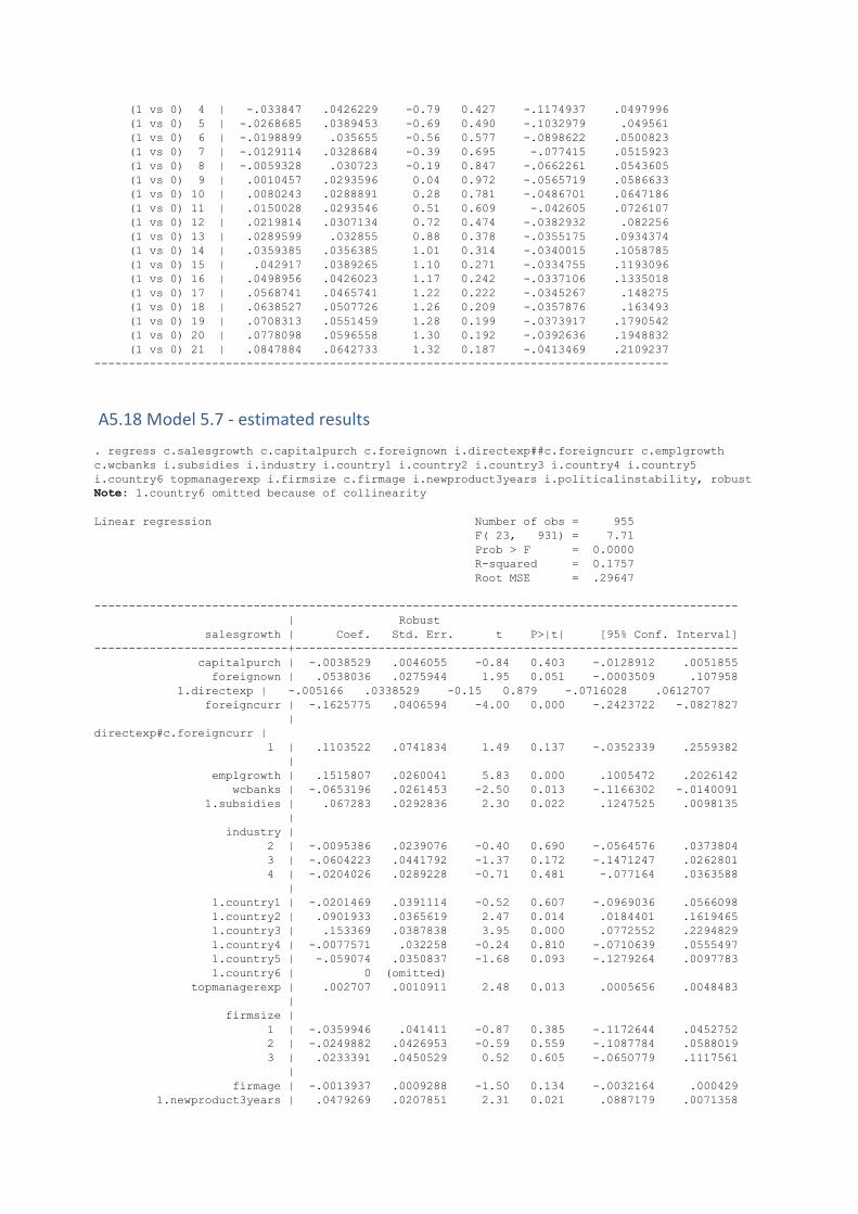
(1 vs 0) 4 | -.033847 .0426229 -0.79 0.427 -.1174937 .0497996
(1 vs 0) 5 | -.0268685 .0389453 -0.69 0.490 -.1032979 .049561
(1 vs 0) 6 | -.0198899 .035655 -0.56 0.577 -.0898622 .0500823
(1 vs 0) 7 | -.0129114 .0328684 -0.39 0.695 -.077415 .0515923
(1 vs 0) 8 | -.0059328 .030723 -0.19 0.847 -.0662261 .0543605
(1 vs 0) 9 | .0010457 .0293596 0.04 0.972 -.0565719 .0586633
(1 vs 0) 10 | .0080243 .0288891 0.28 0.781 -.0486701 .0647186
(1 vs 0) 11 | .0150028 .0293546 0.51 0.609 -.042605 .0726107
(1 vs 0) 12 | .0219814 .0307134 0.72 0.474 -.0382932 .082256
(1 vs 0) 13 | .0289599 .032855 0.88 0.378 -.0355175 .0934374
(1 vs 0) 14 | .0359385 .0356385 1.01 0.314 -.0340015 .1058785
(1 vs 0) 15 | .042917 .0389265 1.10 0.271 -.0334755 .1193096
(1 vs 0) 16 | .0498956 .0426023 1.17 0.242 -.0337106 .1335018
(1 vs 0) 17 | .0568741 .0465741 1.22 0.222 -.0345267 .148275
(1 vs 0) 18 | .0638527 .0507726 1.26 0.209 -.0357876 .163493
(1 vs 0) 19 | .0708313 .0551459 1.28 0.199 -.0373917 .1790542
(1 vs 0) 20 | .0778098 .0596558 1.30 0.192 -.0392636 .1948832
(1 vs 0) 21 | .0847884 .0642733 1.32 0.187 -.0413469 .2109237
-----------------------------------------------------------------------------------
A5.18 Model 5.7 - estimated results
. regress c.salesgrowth c.capitalpurch c.foreignown i.directexp##c.foreigncurr c.emplgrowth
c.wcbanks i.subsidies i.industry i.country1 i.country2 i.country3 i.country4 i.country5
i.country6 topmanagerexp i.firmsize c.firmage i.newproduct3years i.politicalinstability, robust
Note: 1.country6 omitted because of collinearity
Linear regression Number of obs = 955
F( 23, 931) = 7.71
Prob > F = 0.0000
R-squared = 0.1757
Root MSE = .29647
---------------------------------------------------------------------------------------------
| Robust
salesgrowth | Coef. Std. Err. t P>|t| [95% Conf. Interval]
----------------------------+----------------------------------------------------------------
capitalpurch | -.0038529 .0046055 -0.84 0.403 -.0128912 .0051855
foreignown | .0538036 .0275944 1.95 0.051 -.0003509 .107958
1.directexp | -.005166 .0338529 -0.15 0.879 -.0716028 .0612707
foreigncurr | -.1625775 .0406594 -4.00 0.000 -.2423722 -.0827827
|
directexp#c.foreigncurr |
1 | .1103522 .0741834 1.49 0.137 -.0352339 .2559382
|
emplgrowth | .1515807 .0260041 5.83 0.000 .1005472 .2026142
wcbanks | -.0653196 .0261453 -2.50 0.013 -.1166302 -.0140091
1.subsidies | .067283 .0292836 2.30 0.022 .1247525 .0098135
|
industry |
2 | -.0095386 .0239076 -0.40 0.690 -.0564576 .0373804
3 | -.0604223 .0441792 -1.37 0.172 -.1471247 .0262801
4 | -.0204026 .0289228 -0.71 0.481 -.077164 .0363588
|
1.country1 | -.0201469 .0391114 -0.52 0.607 -.0969036 .0566098
1.country2 | .0901933 .0365619 2.47 0.014 .0184401 .1619465
1.country3 | .153369 .0387838 3.95 0.000 .0772552 .2294829
1.country4 | -.0077571 .032258 -0.24 0.810 -.0710639 .0555497
1.country5 | -.059074 .0350837 -1.68 0.093 -.1279264 .0097783
1.country6 | 0 (omitted)
topmanagerexp | .002707 .0010911 2.48 0.013 .0005656 .0048483
|
firmsize |
1 | -.0359946 .041411 -0.87 0.385 -.1172644 .0452752
2 | -.0249882 .0426953 -0.59 0.559 -.1087784 .0588019
3 | .0233391 .0450529 0.52 0.605 -.0650779 .1117561
|
firmage | -.0013937 .0009288 -1.50 0.134 -.0032164 .000429
1.newproduct3years | .0479269 .0207851 2.31 0.021 .0887179 .0071358

293
1.politicalinstability | -.0546395 .0214081 -2.55 0.011 -.0966532 -.0126259
_cons | -.0333938 .0622046 -0.54 0.592 -.1554711 .0886836
capitalpurch | -.0038529 .0046055 -0.84 0.403 -.0128912 .0051855
foreignown | .0538036 .0275944 1.95 0.051 -.0003509 .107958
1.directexp | -.005166 .0338529 -0.15 0.879 -.0716028 .0612707
foreigncurr | -.1625775 .0406594 -4.00 0.000 -.2423722 -.0827827
|
directexp#c.foreigncurr |
1 | .1103522 .0741834 1.49 0.137 -.0352339 .2559382
|
emplgrowth | .1515807 .0260041 5.83 0.000 .1005472 .2026142
wcbanks | -.0653196 .0261453 -2.50 0.013 -.1166302 -.0140091
1.subsidies | .067283 .0292836 2.30 0.022 .1247525 .0098135
|
industry |
2 | -.0095386 .0239076 -0.40 0.690 -.0564576 .0373804
3 | -.0604223 .0441792 -1.37 0.172 -.1471247 .0262801
4 | -.0204026 .0289228 -0.71 0.481 -.077164 .0363588
|
1.country1 | -.0201469 .0391114 -0.52 0.607 -.0969036 .0566098
1.country2 | .0901933 .0365619 2.47 0.014 .0184401 .1619465
1.country3 | .153369 .0387838 3.95 0.000 .0772552 .2294829
1.country4 | -.0077571 .032258 -0.24 0.810 -.0710639 .0555497
1.country5 | -.059074 .0350837 -1.68 0.093 -.1279264 .0097783
1.country6 | 0 (omitted)
topmanagerexp | .002707 .0010911 2.48 0.013 .0005656 .0048483
|
firmsize |
1 | -.0359946 .041411 -0.87 0.385 -.1172644 .0452752
2 | -.0249882 .0426953 -0.59 0.559 -.1087784 .0588019
3 | .0233391 .0450529 0.52 0.605 -.0650779 .1117561
|
firmage | -.0013937 .0009288 -1.50 0.134 -.0032164 .000429
1.newproduct3years | .0479269 .0207851 2.31 0.021 .0887179 .0071358
1.politicalinstability | -.0546395 .0214081 -2.55 0.011 -.0966532 -.0126259
_cons | -.0333938 .0622046 -0.54 0.592 -.1554711 .0886836
---------------------------------------------------------------------------------------------
A5.19 Model 5.7 – diagnostic tests Test for homosecdasticity - model 5.7
. estat imtest
Cameron & Trivedi's decomposition of IM-test
---------------------------------------------------
Source | chi2 df p
---------------------+-----------------------------
Heteroskedasticity | 305.63 265 0.0436
Skewness | 25.09 23 0.3456
Kurtosis | 14.68 1 0.0001
---------------------+-----------------------------
Total | 345.40 289 0.0127
---------------------------------------------------
Test for functional form - model 5.7
. estat ovtest
Ramsey RESET test using powers of the fitted values of salesgrowth
Ho: model has no omitted variables
F(3, 928) = 2.52
Prob > F = 0.0564
. estat linktest
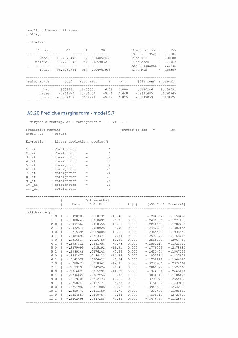
invalid subcommand linktest
r(321);
. linktest
Source | SS df MS Number of obs = 955
-------------+------------------------------ F( 2, 952) = 101.84
Model | 17.4970492 2 8.74852461 Prob > F = 0.0000
Residual | 81.7799292 952 .085903287 R-squared = 0.1762
-------------+------------------------------ Adj R-squared = 0.1745
Total | 99.2769784 954 .104063919 Root MSE = .29309
------------------------------------------------------------------------------
salesgrowth | Coef. Std. Err. t P>|t| [95% Conf. Interval]
-------------+----------------------------------------------------------------
_hat | .9032781 .1453551 6.21 0.000 .6180246 1.188531
_hatsq | -.264777 .3484769 -0.76 0.448 -.9486485 .4190945
_cons | -.0039115 .0177297 -0.22 0.825 -.0387053 .0308824
------------------------------------------------------------------------------
A5.20 Predicive margins form - model 5.7
. margins directexp, at ( foreigncurr = ( 0(0.1) 1))
Predictive margins Number of obs = 955
Model VCE : Robust
Expression : Linear prediction, predict()
1._at : foreigncurr = 0
2._at : foreigncurr = .1
3._at : foreigncurr = .2
4._at : foreigncurr = .3
5._at : foreigncurr = .4
6._at : foreigncurr = .5
7._at : foreigncurr = .6
8._at : foreigncurr = .7
9._at : foreigncurr = .8
10._at : foreigncurr = .9
11._at : foreigncurr = 1
-----------------------------------------------------------------------------------
| Delta-method
| Margin Std. Err. t P>|t| [95% Conf. Interval]
------------------+----------------------------------------------------------------
_at#directexp |
1 0 | -.1828785 .0118132 -15.48 0.000 -.206062 -.159695
1 1 | -.1880445 .0310092 -6.06 0.000 -.2489006 -.1271885
2 0 | -.1991362 .010655 -18.69 0.000 -.2200468 -.1782256
2 1 | -.1932671 .028026 -6.90 0.000 -.2482686 -.1382655
3 0 | -.215394 .0109805 -19.62 0.000 -.2369433 -.1938446
3 1 | -.1984896 .0263377 -7.54 0.000 -.2501777 -.1468014
4 0 | -.2316517 .0126758 -18.28 0.000 -.2565282 -.2067752
4 1 | -.2037121 .0261958 -7.78 0.000 -.2551217 -.1523025
5 0 | -.2479095 .015292 -16.21 0.000 -.2779203 -.2178987
5 1 | -.2089346 .0276241 -7.56 0.000 -.2631474 -.1547219
6 0 | -.2641672 .0184412 -14.32 0.000 -.3003584 -.227976
6 1 | -.2141572 .0304022 -7.04 0.000 -.2738219 -.1544925
7 0 | -.280425 .0218947 -12.81 0.000 -.3233936 -.2374564
7 1 | -.2193797 .0342026 -6.41 0.000 -.2865029 -.1522565
8 0 | -.2966827 .0255291 -11.62 0.000 -.346784 -.2465814
8 1 | -.2246022 .0387256 -5.80 0.000 -.3006019 -.1486026
9 0 | -.3129405 .0292773 -10.69 0.000 -.3703976 -.2554833
9 1 | -.2298248 .0437477 -5.25 0.000 -.3156802 -.1439693
10 0 | -.3291982 .0331006 -9.95 0.000 -.3941586 -.2642378
10 1 | -.2350473 .0491159 -4.79 0.000 -.331438 -.1386566
11 0 | -.3454559 .0369757 -9.34 0.000 -.4180213 -.2728906
11 1 | -.2402698 .0547285 -4.39 0.000 -.3476754 -.1328642
-----------------------------------------------------------------------------------
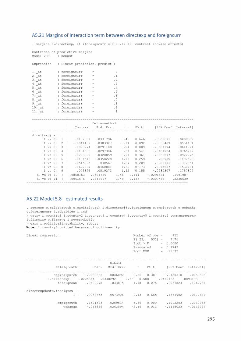
295
(1 vs 0) 10 | .0850163 .0581789 1.46 0.144 -.0291581 .1991907
(1 vs 0) 11 | .0961576 .0646667 1.49 0.137 -.0307488 .2230639
-----------------------------------------------------------------------------------
A5.22 Model 5.8 - estimated results
. regress c.salesgrowth c.capitalpurch i.directexp##c.foreignown c.emplgrowth c.wcbanks
c.foreigncurr i.subsidies i.ind
> ustry i.country1 i.country2 i.country3 i.country4 i.country5 i.country6 topmanagerexp
i.firmsize c.firmage i.newproduct3y
> ears i.politicalinstability, robust
Note: 1.country6 omitted because of collinearity
Linear regression Number of obs = 955
F( 23, 931) = 7.76
Prob > F = 0.0000
R-squared = 0.1743
Root MSE = .29672
--------------------------------------------------------------------------------------------
| Robust
salesgrowth | Coef. Std. Err. t P>|t| [95% Conf. Interval]
---------------------------+----------------------------------------------------------------
capitalpurch | -.0039863 .0046092 -0.86 0.387 -.0130318 .0050593
1.directexp | .0225364 .0340292 0.66 0.508 -.0442465 .0893193
foreignown | .0602978 .033875 1.78 0.075 -.0061824 .1267781
|
directexpdum#c.foreignow |
1 | -.0248653 .0573906 -0.43 0.665 -.1374952 .0877647
|
emplgrowth | .1521593 .0259534 5.86 0.000 .1012253 .2030933
wcbanks | -.065366 .0262094 -2.49 0.013 -.1168023 -.0139297
A5.21 Margins of interaction term between directexp and foreigncurr
. margins r.directexp, at (foreigncurr =(0 (0.1) 1)) contrast (nowald effects)
Contrasts of predictive margins
Model VCE : Robust
Expression : Linear prediction, predict()
1._at : foreigncurr = 0
2._at : foreigncurr = .1
3._at : foreigncurr = .2
4._at : foreigncurr = .3
5._at : foreigncurr = .4
6._at : foreigncurr = .5
7._at : foreigncurr = .6
8._at : foreigncurr = .7
9._at : foreigncurr = .8
10._at : foreigncurr = .9
11._at : foreigncurr = 1
-----------------------------------------------------------------------------------
| Delta-method
| Contrast Std. Err. t P>|t| [95% Conf. Interval]
------------------+----------------------------------------------------------------
directexp@_at |
(1 vs 0) 1 | -.0152552 .0331796 -0.46 0.646 -.0803691 .0498587
(1 vs 0) 2 | -.0041139 .0303327 -0.14 0.892 -.0636409 .0554131
(1 vs 0) 3 | .0070274 .0291188 0.24 0.809 -.0501174 .0641721
(1 vs 0) 4 | .0181686 .0297386 0.61 0.541 -.0401924 .0765297
(1 vs 0) 5 | .0293099 .0320859 0.91 0.361 -.0336577 .0922775
(1 vs 0) 6 | .0404512 .0358228 1.13 0.259 -.02985 .1107523
(1 vs 0) 7 | .0515925 .040567 1.27 0.204 -.0280191 .1312041
(1 vs 0) 8 | .0627337 .0460081 1.36 0.173 -.0275557 .1530231
(1 vs 0) 9 | .073875 .0519273 1.42 0.155 -.0280307 .1757807
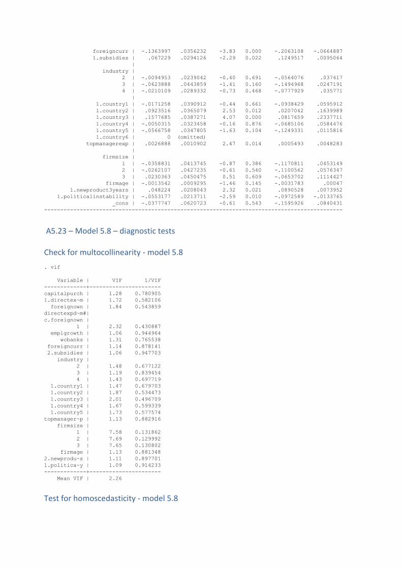
foreigncurr | -.1363997 .0356232 -3.83 0.000 -.2063108 -.0664887
1.subsidies | .067229 .0294126 -2.29 0.022 .1249517 .0095064
|
industry |
2 | -.0094953 .0239042 -0.40 0.691 -.0564076 .037417
3 | -.0623888 .0443859 -1.41 0.160 -.1494968 .0247191
4 | -.0210109 .0289332 -0.73 0.468 -.0777929 .035771
|
1.country1 | -.0171258 .0390912 -0.44 0.661 -.0938429 .0595912
1.country2 | .0923516 .0365079 2.53 0.012 .0207042 .1639989
1.country3 | .1577685 .0387271 4.07 0.000 .0817659 .2337711
1.country4 | -.0050315 .0323458 -0.16 0.876 -.0685106 .0584476
1.country5 | -.0566758 .0347805 -1.63 0.104 -.1249331 .0115816
1.country6 | 0 (omitted)
topmanagerexp | .0026888 .0010902 2.47 0.014 .0005493 .0048283
|
firmsize |
1 | -.0358831 .0413745 -0.87 0.386 -.1170811 .0453149
2 | -.0262107 .0427235 -0.61 0.540 -.1100562 .0576347
3 | .0230363 .0450475 0.51 0.609 -.0653702 .1114427
firmage | -.0013542 .0009295 -1.46 0.145 -.0031783 .00047
1.newproduct3years | .048224 .0208043 2.32 0.021 .0890528 .0073952
1.politicalinstability | -.0553177 .0213711 -2.59 0.010 -.0972589 -.0133765
_cons | -.0377747 .0620723 -0.61 0.543 -.1595926 .0840431
--------------------------------------------------------------------------------------------
A5.23 – Model 5.8 – diagnostic tests Check for multocollinearity - model 5.8
. vif
Variable | VIF 1/VIF
-------------+----------------------
capitalpurch | 1.28 0.780905
1.directex~m | 1.72 0.582106
foreignown | 1.84 0.543859
directexpd~m#|
c.foreignown |
1 | 2.32 0.430887
emplgrowth | 1.06 0.944964
wcbanks | 1.31 0.765538
foreigncurr | 1.14 0.878141
2.subsidies | 1.06 0.947703
industry |
2 | 1.48 0.677122
3 | 1.19 0.839454
4 | 1.43 0.697719
1.country1 | 1.47 0.679703
1.country2 | 1.87 0.534473
1.country3 | 2.01 0.496709
1.country4 | 1.67 0.599339
1.country5 | 1.73 0.577574
topmanager~p | 1.13 0.882916
firmsize |
1 | 7.58 0.131862
2 | 7.69 0.129992
3 | 7.65 0.130802
firmage | 1.13 0.881348
2.newprodu~s | 1.11 0.897701
1.politica~y | 1.09 0.914233
-------------+----------------------
Mean VIF | 2.26
Test for homoscedasticity - model 5.8
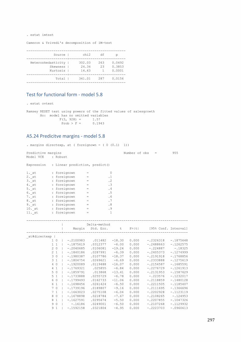
297
. estat imtest
Cameron & Trivedi's decomposition of IM-test
---------------------------------------------------
Source | chi2 df p
---------------------+-----------------------------
Heteroskedasticity | 302.03 263 0.0492
Skewness | 24.34 23 0.3853
Kurtosis | 14.63 1 0.0001
---------------------+-----------------------------
Total | 341.01 287 0.0156
---------------------------------------------------
Test for functional form - model 5.8
. estat ovtest
Ramsey RESET test using powers of the fitted values of salesgrowth
Ho: model has no omitted variables
F(3, 928) = 1.57
Prob > F = 0.1943
A5.24 Predicitve margins - model 5.8
. margins directexp, at ( foreignown = ( 0 (0.1) 1))
Predictive margins Number of obs = 955
Model VCE : Robust
Expression : Linear prediction, predict()
1._at : foreignown = 0
2._at : foreignown = .1
3._at : foreignown = .2
4._at : foreignown = .3
5._at : foreignown = .4
6._at : foreignown = .5
7._at : foreignown = .6
8._at : foreignown = .7
9._at : foreignown = .8
10._at : foreignown = .9
11._at : foreignown = 1
-----------------------------------------------------------------------------------
| Delta-method
| Margin Std. Err. t P>|t| [95% Conf. Interval]
------------------+----------------------------------------------------------------
_at#directexp |
1 0 | -.2100983 .011482 -18.30 0.000 -.2326318 -.1875648
1 1 | -.1875619 .0312377 -6.00 0.000 -.2488663 -.1262575
2 0 | -.2040685 .0106081 -19.24 0.000 -.224887 -.18325
2 1 | -.1840186 .0287991 -6.39 0.000 -.2405373 -.1274999
3 0 | -.1980387 .0107786 -18.37 0.000 -.2191918 -.1768856
3 1 | -.1804754 .0269621 -6.69 0.000 -.2333888 -.1275619
4 0 | -.1920089 .0119488 -16.07 0.000 -.2154587 -.1685591
4 1 | -.1769321 .025855 -6.84 0.000 -.2276729 -.1261913
5 0 | -.1859791 .013868 -13.41 0.000 -.2131953 -.1587629
5 1 | -.1733888 .0255729 -6.78 0.000 -.223576 -.1232017
6 0 | -.1799493 .0162733 -11.06 0.000 -.2118859 -.1480128
6 1 | -.1698456 .0261424 -6.50 0.000 -.2211505 -.1185407
7 0 | -.1739196 .0189807 -9.16 0.000 -.2111695 -.1366696
7 1 | -.1663023 .0275108 -6.04 0.000 -.2202928 -.1123119
8 0 | -.1678898 .0218784 -7.67 0.000 -.2108265 -.124953
8 1 | -.1627591 .0295674 -5.50 0.000 -.2207855 -.1047326
9 0 | -.16186 .0249001 -6.50 0.000 -.2107268 -.1129932
9 1 | -.1592158 .0321804 -4.95 0.000 -.2223703 -.0960613
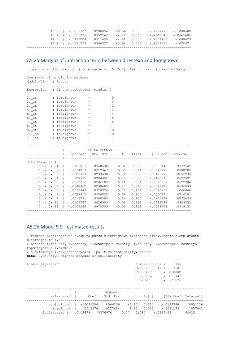
10 0 | -.1558302 .0280056 -5.56 0.000 -.2107916 -.1008688
10 1 | -.1556726 .0352263 -4.42 0.000 -.2248046 -.0865405
11 0 | -.1498004 .0311699 -4.81 0.000 -.2109718 -.088629
11 1 | -.1521293 .0386027 -3.94 0.000 -.2278876 -.076371
-----------------------------------------------------------------------------------
A5.25 Margins of interaction term between directexp and foreignown
. margins r.directexp, at ( foreignown = ( 0 (0.1) 1)) contrast (nowald effects)
Contrasts of predictive margins
Model VCE : Robust
Expression : Linear prediction, predict()
1._at : foreignown = 0
2._at : foreignown = .1
3._at : foreignown = .2
4._at : foreignown = .3
5._at : foreignown = .4
6._at : foreignown = .5
7._at : foreignown = .6
8._at : foreignown = .7
9._at : foreignown = .8
10._at : foreignown = .9
11._at : foreignown = 1
-----------------------------------------------------------------------------------
| Delta-method
| Contrast Std. Err. t P>|t| [95% Conf. Interval]
------------------+----------------------------------------------------------------
directexp@_at |
(1 vs 0) 1 | .0105051 .0340638 0.31 0.758 -.0563441 .0773542
(1 vs 0) 2 | .0094017 .0312967 0.30 0.764 -.0520171 .0708205
(1 vs 0) 3 | .0082983 .0293638 0.28 0.778 -.0493272 .0659239
(1 vs 0) 4 | .007195 .0284357 0.25 0.800 -.0486091 .0629991
(1 vs 0) 5 | .0060916 .0286103 0.21 0.831 -.0500552 .0622384
(1 vs 0) 6 | .0049882 .0298683 0.17 0.867 -.0536275 .0636039
(1 vs 0) 7 | .0038849 .0320826 0.12 0.904 -.0590763 .066846
(1 vs 0) 8 | .0027815 .0350725 0.08 0.937 -.0660471 .0716101
(1 vs 0) 9 | .0016781 .0386583 0.04 0.965 -.0741877 .0775439
(1 vs 0) 10 | .0005747 .0426903 0.01 0.989 -.0832037 .0843532
(1 vs 0) 11 | -.0005286 .0470539 -0.01 0.991 -.0928704 .0918131
-----------------------------------------------------------------------------------
A5.26 Model 5.9 - estimated results
. regress c.salesgrowth c.capitalpurch c.foreignown i.directexp##c.wcbanks c.emplgrowth
c.foreigncurr i.su
> bsidies i.industry i.country1 i.country2 i.country3 i.country4 i.country5 i.country6
topmanagerexp i.firmsiz
> e c.firmage i.newproduct3years i.politicalinstability, robust
Note: 1.country6 omitted because of collinearity
Linear regression Number of obs = 955
F( 23, 931) = 7.81
Prob > F = 0.0000
R-squared = 0.1743
Root MSE = .29673
-----------------------------------------------------------------------------------------
| Robust
salesgrowth | Coef. Std. Err. t P>|t| [95% Conf. Interval]
------------------------+----------------------------------------------------------------
capitalpurch | -.0039254 .0046109 -0.85 0.395 -.0129744 .0051236
foreignown | .0513374 .0277484 1.85 0.065 -.0031193 .1057941
1.directexp | .0102679 .0376976 0.27 0.785 -.0637142 .08425
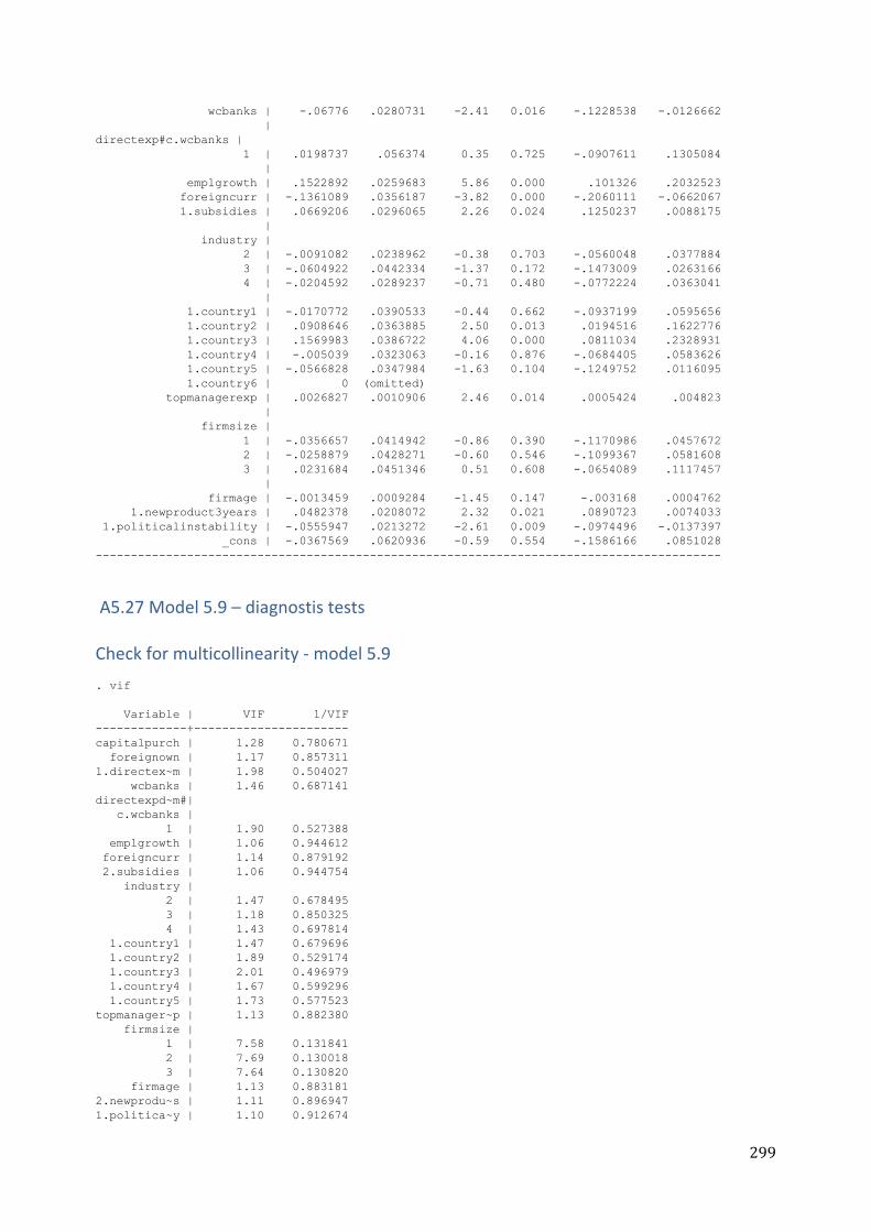
299
wcbanks | -.06776 .0280731 -2.41 0.016 -.1228538 -.0126662
|
directexp#c.wcbanks |
1 | .0198737 .056374 0.35 0.725 -.0907611 .1305084
|
emplgrowth | .1522892 .0259683 5.86 0.000 .101326 .2032523
foreigncurr | -.1361089 .0356187 -3.82 0.000 -.2060111 -.0662067
1.subsidies | .0669206 .0296065 2.26 0.024 .1250237 .0088175
|
industry |
2 | -.0091082 .0238962 -0.38 0.703 -.0560048 .0377884
3 | -.0604922 .0442334 -1.37 0.172 -.1473009 .0263166
4 | -.0204592 .0289237 -0.71 0.480 -.0772224 .0363041
|
1.country1 | -.0170772 .0390533 -0.44 0.662 -.0937199 .0595656
1.country2 | .0908646 .0363885 2.50 0.013 .0194516 .1622776
1.country3 | .1569983 .0386722 4.06 0.000 .0811034 .2328931
1.country4 | -.005039 .0323063 -0.16 0.876 -.0684405 .0583626
1.country5 | -.0566828 .0347984 -1.63 0.104 -.1249752 .0116095
1.country6 | 0 (omitted)
topmanagerexp | .0026827 .0010906 2.46 0.014 .0005424 .004823
|
firmsize |
1 | -.0356657 .0414942 -0.86 0.390 -.1170986 .0457672
2 | -.0258879 .0428271 -0.60 0.546 -.1099367 .0581608
3 | .0231684 .0451346 0.51 0.608 -.0654089 .1117457
|
firmage | -.0013459 .0009284 -1.45 0.147 -.003168 .0004762
1.newproduct3years | .0482378 .0208072 2.32 0.021 .0890723 .0074033
1.politicalinstability | -.0555947 .0213272 -2.61 0.009 -.0974496 -.0137397
_cons | -.0367569 .0620936 -0.59 0.554 -.1586166 .0851028
-----------------------------------------------------------------------------------------
A5.27 Model 5.9 – diagnostis tests Check for multicollinearity - model 5.9
. vif
Variable | VIF 1/VIF
-------------+----------------------
capitalpurch | 1.28 0.780671
foreignown | 1.17 0.857311
1.directex~m | 1.98 0.504027
wcbanks | 1.46 0.687141
directexpd~m#|
c.wcbanks |
1 | 1.90 0.527388
emplgrowth | 1.06 0.944612
foreigncurr | 1.14 0.879192
2.subsidies | 1.06 0.944754
industry |
2 | 1.47 0.678495
3 | 1.18 0.850325
4 | 1.43 0.697814
1.country1 | 1.47 0.679696
1.country2 | 1.89 0.529174
1.country3 | 2.01 0.496979
1.country4 | 1.67 0.599296
1.country5 | 1.73 0.577523
topmanager~p | 1.13 0.882380
firmsize |
1 | 7.58 0.131841
2 | 7.69 0.130018
3 | 7.64 0.130820
firmage | 1.13 0.883181
2.newprodu~s | 1.11 0.896947
1.politica~y | 1.10 0.912674
-------------+----------------------
Mean VIF | 2.23
Test for homoscedasticity - model 5.9
. estat imtest
Cameron & Trivedi's decomposition of IM-test
---------------------------------------------------
Source | chi2 df p
---------------------+-----------------------------
Heteroskedasticity | 302.77 264 0.0505
Skewness | 24.34 23 0.3853
Kurtosis | 14.50 1 0.0001
---------------------+-----------------------------
Total | 341.61 288 0.0163
---------------------------------------------------
Prob > F = 0.1765
A5.28 Predictive margins - model 5.9
. margins directexp, at (wcbanks = ( 0 (0.1) 1))
Predictive margins Number of obs = 955
Model VCE : Robust
Expression : Linear prediction, predict()
1._at : wcbanks = 0
2._at : wcbanks = .1
3._at : wcbanks = .2
4._at : wcbanks = .3
5._at : wcbanks = .4
6._at : wcbanks = .5
7._at : wcbanks = .6
8._at : wcbanks = .7
9._at : wcbanks = .8
10._at : wcbanks = .9
11._at : wcbanks = 1
-----------------------------------------------------------------------------------
| Delta-method
| Margin Std. Err. t P>|t| [95% Conf. Interval]
------------------+----------------------------------------------------------------
_at#directexp |
1 0 | -.1784528 .0139911 -12.75 0.000 -.2059106 -.1509951
1 1 | -.1681849 .0345579 -4.87 0.000 -.2360054 -.1003645
2 0 | -.1852288 .0123285 -15.02 0.000 -.2094238 -.1610339
2 1 | -.1729736 .0312384 -5.54 0.000 -.2342794 -.1116678
3 0 | -.1920048 .0111354 -17.24 0.000 -.2138582 -.1701515
3 1 | -.1777622 .028514 -6.23 0.000 -.2337214 -.121803
4 0 | -.1987808 .0105717 -18.80 0.000 -.2195281 -.1780336
4 1 | -.1825509 .0265685 -6.87 0.000 -.2346919 -.1304098
5 0 | -.2055568 .0107373 -19.14 0.000 -.2266289 -.1844848
Test for functional form - model 5.9
. estat ovtest
Ramsey RESET test using powers of the fitted values of salesgrowth
Ho: model has no omitted variables
F(3, 928) = 1.65

301
5 1 | -.1873395 .0255802 -7.32 0.000 -.237541 -.137138
6 0 | -.2123328 .0116008 -18.30 0.000 -.2350996 -.1895661
6 1 | -.1921281 .0256599 -7.49 0.000 -.2424861 -.1417701
7 0 | -.2191089 .0130242 -16.82 0.000 -.2446691 -.1935486
7 1 | -.1969168 .0267982 -7.35 0.000 -.2495086 -.1443249
8 0 | -.2258849 .0148473 -15.21 0.000 -.255023 -.1967467
8 1 | -.2017054 .02887 -6.99 0.000 -.2583632 -.1450475
9 0 | -.2326609 .0169416 -13.73 0.000 -.265909 -.1994127
9 1 | -.206494 .0316929 -6.52 0.000 -.2686918 -.1442963
10 0 | -.2394369 .0192186 -12.46 0.000 -.2771537 -.20172
10 1 | -.2112827 .0350859 -6.02 0.000 -.2801393 -.142426
11 0 | -.2462129 .0216207 -11.39 0.000 -.2886438 -.2037819
11 1 | -.2160713 .0389003 -5.55 0.000 -.2924137 -.1397289
-----------------------------------------------------------------------------------
A5.29 Model 5.10 - estimated results
. regress c.salesgrowth c.capitalpurch c.foreignown i.directexp##i.currdep c.emplgrowth c.wcban
> ks c.foreigncurr i.subsidies i.industry topmanagerexp i.firmsize c.firmage i.newproduct3years
i.
> politicalinstability, robust
Linear regression Number of obs = 972
F( 19, 952) = 7.93
Prob > F = 0.0000
R-squared = 0.1473
Root MSE = .30135
----------------------------------------------------------------------------------------
| Robust
salesgrowth | Coef. Std. Err. t P>|t| [95% Conf. Interval]
-----------------------+----------------------------------------------------------------
capitalpurch | -.0050224 .0046333 -1.08 0.279 -.0141149 .0040702
foreignown | .0607811 .0274819 2.21 0.027 .006849 .1147133
1.directexp | .0417837 .0335941 1.24 0.214 -.0241433 .1077107
1.currdep | .1138799 .0230122 4.95 0.000 .0687194 .1590404
|
directexp#currdep |
1 1 | -.1152724 .0542334 -2.13 0.034 -.2217033 -.0088414
|
emplgrowth | .1330162 .0252287 5.27 0.000 .083506 .1825264
wcbanks | -.0326326 .0237992 -1.37 0.171 -.0793376 .0140725
foreigncurr | -.1695198 .0344748 -4.92 0.000 -.2371753 -.1018643
2.subsidies | -.0547278 .0281932 -1.94 0.053 -.1100558 .0006003
|
industry |
2 | -.0094258 .023792 -0.40 0.692 -.0561166 .0372649
3 | -.0623808 .0442772 -1.41 0.159 -.1492729 .0245113
4 | -.0361624 .0287096 -1.26 0.208 -.0925038 .020179
|
topmanagerexp | .0028864 .0010822 2.67 0.008 .0007626 .0050102
|
firmsize |
1 | -.0469063 .0387442 -1.21 0.226 -.1229402 .0291276
2 | -.021989 .0397773 -0.55 0.581 -.1000503 .0560722
3 | .0418536 .0426451 0.98 0.327 -.0418357 .1255429
|
firmage | -.0018555 .000982 -1.89 0.059 -.0037826 .0000715
2.newproduct3years | -.0480434 .0206118 -2.33 0.020 -.0884931 -.0075936
1.politicalinstability | -.0685419 .0209023 -3.28 0.001 -.1095618 -.027522
_cons | -.0726648 .0548628 -1.32 0.186 -.1803308 .0350012
----------------------------------------------------------------------------------------
A5.30 Predictive margins - model 5.10
. margins directexpdum, at ( currdep = (0 1))
Predictive margins Number of obs = 972
Model VCE : Robust
Expression : Linear prediction, predict()
1._at : currdep = 0
2._at : currdep = 1
-----------------------------------------------------------------------------------
| Delta-method
| Margin Std. Err. t P>|t| [95% Conf. Interval]
------------------+----------------------------------------------------------------
_at#directexp |
1 0 | -.2615397 .015032 -17.40 0.000 -.2910394 -.2320401
1 1 | -.219756 .0292098 -7.52 0.000 -.2770792 -.1624329
2 0 | -.1476598 .0164529 -8.97 0.000 -.1799479 -.1153718
2 1 | -.2211485 .0435707 -5.08 0.000 -.3066541 -.1356429
-----------------------------------------------------------------------------------
. margins r.directexpdum, at ( currdep = (0, 1)) contrast (nowald effects)
Contrasts of predictive margins
Model VCE : Robust
Expression : Linear prediction, predict()
1._at : currdep = 0
2._at : currdep = 1
-----------------------------------------------------------------------------------
| Delta-method
| Contrast Std. Err. t P>|t| [95% Conf. Interval]
------------------+----------------------------------------------------------------
directexp@_at |
(1 vs 0) 1 | .0417837 .0335941 1.24 0.214 -.0241433 .1077107
(1 vs 0) 2 | -.0734886 .0466959 -1.57 0.116 -.1651273 .01815
-----------------------------------------------------------------------------------
A5.31 Model 5.11 – estimated results
. regress c.salesgrowth c.capitalpurch c.foreignown i.directexp c.emplgrowth c.wcbanks c.foreig
> ncurr##i.currdep i.subsidies i.industry topmanagerexp i.firmsize c.firmage i.newproduct3years
i.
> politicalinstability, robust
Linear regression Number of obs = 972
F( 19, 952) = 7.84
Prob > F = 0.0000
R-squared = 0.1524
Root MSE = .30045
----------------------------------------------------------------------------------------
| Robust
salesgrowth | Coef. Std. Err. t P>|t| [95% Conf. Interval]
-----------------------+----------------------------------------------------------------
capitalpurch | -.004843 .0046304 -1.05 0.296 -.01393 .004244
foreignown | .0560996 .0266605 2.10 0.036 .0037795 .1084197
1.directexp | -.0069599 .0289549 -0.24 0.810 -.0637827 .0498629
emplgrowth | .136109 .0254355 5.35 0.000 .0861928 .1860251
wcbanks | -.0409122 .0235562 -1.74 0.083 -.0871404 .005316
foreigncurr | -.0747667 .0379746 -1.97 0.049 -.1492904 -.0002431
1.currdep | .1248714 .0226701 5.51 0.000 .0803823 .1693605
|
currdep#c.foreigncurr |
1 | -.2355602 .0757979 -3.11 0.002 -.3843104 -.08681
|
303
2.subsidies | -.0503977 .0283037 -1.78 0.075 -.1059426 .0051472
|
industry |
2 | -.0092563 .0237212 -0.39 0.696 -.0558082 .0372956
3 | -.0557798 .044686 -1.25 0.212 -.1434743 .0319147
4 | -.0351359 .0285071 -1.23 0.218 -.0910799 .020808
|
topmanagerexp | .0028904 .0010748 2.69 0.007 .0007811 .0049997
|
firmsize |
1 | -.0521443 .0397585 -1.31 0.190 -.1301687 .0258801
2 | -.0273189 .0404228 -0.68 0.499 -.1066469 .0520091
3 | .0324703 .043467 0.75 0.455 -.0528319 .1177724
|
firmage | -.0019632 .0009582 -2.05 0.041 -.0038436 -.0000829
2.newproduct3years | -.0471344 .0205404 -2.29 0.022 -.087444 -.0068247
1.politicalinstability | -.070163 .0208762 -3.36 0.001 -.1111317 -.0291943
_cons | -.0710323 .0551443 -1.29 0.198 -.1792507 .037186
----------------------------------------------------------------------------------------
A5.32 Predictive margins - model 5.11
margins currdep, at ( foreigncurr = (0 (0.1) 1))
Predictive margins Number of obs = 972
Model VCE : Robust
Expression : Linear prediction, predict()
1._at : foreigncurr = 0
2._at : foreigncurr = .1
3._at : foreigncurr = .2
4._at : foreigncurr = .3
5._at : foreigncurr = .4
6._at : foreigncurr = .5
7._at : foreigncurr = .6
8._at : foreigncurr = .7
9._at : foreigncurr = .8
10._at : foreigncurr = .9
11._at : foreigncurr = 1
------------------------------------------------------------------------------
| Delta-method
| Margin Std. Err. t P>|t| [95% Conf. Interval]
-------------+----------------------------------------------------------------
_at#currdep |
1 0 | -.2461149 .0147452 -16.69 0.000 -.2750518 -.217178
1 1 | -.1212435 .0162337 -7.47 0.000 -.1531015 -.0893855
2 0 | -.2535916 .0133574 -18.99 0.000 -.2798049 -.2273782
2 1 | -.1522762 .0153672 -9.91 0.000 -.1824337 -.1221187
3 0 | -.2610683 .0129715 -20.13 0.000 -.2865243 -.2356122
3 1 | -.1833089 .0172787 -10.61 0.000 -.2172176 -.1494001
4 0 | -.2685449 .0136727 -19.64 0.000 -.295377 -.2417129
4 1 | -.2143416 .0212307 -10.10 0.000 -.2560059 -.1726772
5 0 | -.2760216 .0153122 -18.03 0.000 -.3060712 -.245972
5 1 | -.2453743 .0263195 -9.32 0.000 -.2970252 -.1937233
6 0 | -.2834983 .0176303 -16.08 0.000 -.3180971 -.2488994
6 1 | -.276407 .0320074 -8.64 0.000 -.3392202 -.2135937
7 0 | -.2909749 .0203969 -14.27 0.000 -.3310031 -.2509468
7 1 | -.3074397 .0380266 -8.08 0.000 -.3820652 -.2328141
8 0 | -.2984516 .0234538 -12.73 0.000 -.3444788 -.2524244
8 1 | -.3384723 .044242 -7.65 0.000 -.4252954 -.2516493
9 0 | -.3059283 .0267015 -11.46 0.000 -.3583289 -.2535277
9 1 | -.369505 .0505813 -7.31 0.000 -.4687688 -.2702413
10 0 | -.313405 .0300782 -10.42 0.000 -.3724323 -.2543776
10 1 | -.4005377 .0570032 -7.03 0.000 -.5124042 -.2886712
11 0 | -.3208816 .0335451 -9.57 0.000 -.3867125 -.2550508
11 1 | -.4315704 .0634827 -6.80 0.000 -.5561527 -.3069882
------------------------------------------------------------------------------
margins r.currdep, at ( foreigncurr = (0, 0.3, 0.7, 1)) contrast (nowald effects)
Contrasts of predictive margins
Model VCE : Robust
Expression : Linear prediction, predict()
1._at : foreigncurr = 0
2._at : foreigncurr = .3
3._at : foreigncurr = .7
4._at : foreigncurr = 1
------------------------------------------------------------------------------
| Delta-method
| Contrast Std. Err. t P>|t| [95% Conf. Interval]
-------------+----------------------------------------------------------------
currdep@_at |
(1 vs 0) 1 | .1248714 .0226701 5.51 0.000 .0803823 .1693605
(1 vs 0) 2 | .0542033 .0257602 2.10 0.036 .00365 .1047567
(1 vs 0) 3 | -.0400207 .0497174 -0.80 0.421 -.1375891 .0575476
(1 vs 0) 4 | -.1106888 .0709543 -1.56 0.119 -.2499337 .0285561