DNB Working PaperConsumption behaviour and financial crisis in the Netherlands

Federica Teppa

No. 453 / December 2019

De Nederlandsche Bank NV P.O. Box 98 1000 AB AMSTERDAM The Netherlands

Working Paper No. 453

December 2014

Consumption behaviour and financial crisis in the Netherlands Federica Teppa * * Views expressed are those of the author and do not necessarily reflect official positions of De Nederlandsche Bank.

Consumption behaviour and financial crisis in the Netherlands *

Federica Teppa

De Nederlandsche Bank (DNB) and Netspar

15 December 2014

Abstract The focus of this paper in on the effect that changes in income and financial assets have on household consumption in the Netherlands over the period 2009-2012. The empirical evidence is based on the LISS panel, a longitudinal survey representative of the Dutch-speaking population conducted and administrated by CentERdata at Tilburg University. We find a point estimate of the marginal propensity to consume (MPC) of 0.21 out of household income, that is in line with the international microeconomic evidence. We also find that less fragile households display a double MPC out of income than those more fragile (0.44 vs 0.21, respectively). The point estimate of the MPC out of total financial assets equals 0.04. We also find support of the fact that the MPC out of wealth is smaller for richer households. Keywords: Marginal propensities to consume, consumption behavior, survey data. JEL classification: E21, D12, D91.

* Corresponding author: Federica Teppa - De Nederlandsche Bank, Economics and Research Division - Westeinde 1 1017ZN Amsterdam Netherlands. Phone: +31 20 5245841; Fax: +31 20 5142506. Acknowledgments: We thank CentERdata at Tilburg University for supplying the data of the LISS panel. The paper has benefited from useful comments from Dimitris Christelis, Dimitris Georgarakos and at DNB seminars. The views expressed in this paper are those of the author and do not necessarily reflect those of the institutions she belongs to. Any remaining errors are the author's own responsibility.

1 Introduction

Households’ final consumption expenditure (also known as private consumption),

defined as the market value of all goods and services, including durable products and

excluding purchases of dwellings, is often considered a good measure for individual

living standards.

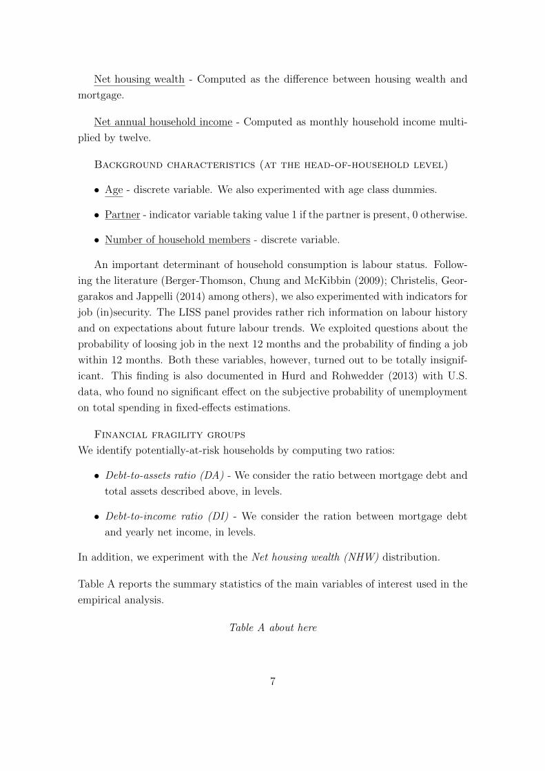
Figure 1 (top panel) shows that household private consumption represents more

than half of GDP in most European countries, and in the United States and the

United Kingdom as well, since the mid Sixties (see also Muellbauer and Lattimore,

1994). Although the level of consumption displays some degree of heterogeneity

across countries, overall a rather stable component of GDP can be observed over

the years.1 As a result private consumption has found comparatively little academic

and policy attention.

However, since the onset of the recent financial crisis consumption has dropped

markedly in many countries. Figure 1 (bottom panel) shows the development of per

capita annual changes in private consumption for the same set of countries. Hurd

and Rowhedder (2010) report that almost 30 percent of households aged 50 or older

in the US reduced their spending between 2007 and 2009, with an average decline of

8 percentage points. In addition, according to Petev, Pistaferri and Saporta (2011)

the fall in consumption in the same years was greater in magnitude at the top

bottom of the wealth distribution than at the bottom of the distribution. Overall,

since the wake of the Great Recession household consumption has experienced a

renewed interest among academic researchers and policy makers.

The possible determinants of the aggregate consumption function have been an-

alyzed extensively in the economic literature. Different consumption theories exist,

but it is hard to find a single theory of consumption that can possibly explain con-

sumption behavior in all economies. Prior to Keynes (1936), consumption had been

viewed as a passive residual, namely the amount of income remaining after saving.

The Keynesian consumption function is based on the “fundamental psychological law

... is that men are disposed, as a rule and on the average, to increase their consump-

1 The Netherlands is characterized by a lower level of private consumption if compared to

other economies mainly due to the different role of health-related spending. As of January 2006

the Dutch health insurance system substantially changed, and some statistics in terms of income,

prices, consumption and the National Accounts were affected by this reform. In particular, the

new basic insurance (that includes the previously privately insured expenditure on medical care)

has become mandatory, and consequently this component is no longer considered as household

consumption, but as government spending. Only the supplementary health care insurance that is

not included in the basic package is defined as household consumption. The introduction of the

new health care system is therefore responsible for the drop in household consumption observed in

the Netherlands in 2006.2

tion as their income increases, but not by as much as the increase in their income”

(Keynes, 1936). According to this static relationship households increase their utility

by consuming more as their income increases. The Keynesian consumption func-

tion, estimated on time series national account data, explains a large fraction of

the variance of consumption. On macro data, however, the marginal propensity to

consume is lower in the short run than in the long run (Kuznets paradox). On micro

data, saving rates change systematically with income (Friedman, 1957)2, and with

changes in income (Katona, 1949)3. Modigliani and Brumberg (1954) and Friedman

(1957) developed models of intertemporal allocation of consumption that could ex-

plain these stylized facts. In both models, consumption is a function of available

resources over a long time horizon (life-cycle wealth or permanent income). Ac-

cording to the Life Cycle-Permanent Income model consumers have concave utility

functions and therefore prefer smooth paths of consumption (over time and across

states of the world) over variable ones. Only unanticipated changes in income that

are perceived as permanent induce substantive changes in consumption. Expected

and temporary changes to income should not induce a strong change in consump-

tion. The explanation of the stylized facts above boils down to the observation that

a large fraction of the changes in income considered are temporary.

This paper focuses on the effect that changes in income and financial assets have

on household consumption in the Netherlands over the period 2009-2012 for about

4,600 households. The literature distinguishes two main approaches to the analysis

of the annual marginal propensity to consume (henceforth, “MPC”) out of income

and wealth. On the one hand, theoretical macroeconomic studies such as Zeldes

(1989) have studied life cycle models in which agents face permanent and transitory

shocks. The complexity of these models has probably restricted their applicability in

a dynamic general equilibrium context like that of Krusell and Smith (1998), which

would answer questions like how the MPC changes over the business cycle. On the

other hand, microeconomic studies have provided empirical estimates for MPCs by

using household-level datasets for different countries, based on alternative measures

of consumption. Poterba (2000) presents a review of empirical studies about the

wealth effect on consumption based on both aggregate and disaggregate data.

When reading the two strands of literature jointly, we see that most estimates of

the aggregate MPC coming from survey data range between 0.2 and 0.6, considerably

exceeding the low values implied by representative agent models or the standard

2 Groups of individuals with, on average, lower level of income (such as blacks) had higher

saving rates than other groups with higher levels of average income (such as whites) at any income

level.3 People whose income has increased save more than people whose income has decreased.

3

framework of Krusell and Smith (1998), yielding MPCs typically around 0.02-0.04.

Carroll, Slacalek and Tokuoka (2013) argue that heterogeneity is key. Models that

are able to match heterogeneity have much higher MPCs than representative agent

models.

Our methodology falls into the latter strand of the literature as we rely on survey

microeconomic household data. The empirical evidence is based on the LISS panel,

a longitudinal survey representative of the Dutch-speaking population conducted

and administrated by CentERdata at Tilburg University. We find a point estimate

of the marginal propensity to consume (MPC) of 0.21 out of household income, that

is in line with the international microeconomic evidence. This means that a one euro

increase in household income raises consumer spending by 21 cents. We also find

that less fragile households display a double MPC out of income than those more

fragile (0.44 vs 0.21, respectively). The point estimate for the MPC out of total

financial assets equals 0.04, in line with the early work of Modigliani (1971). The

economic interpretation is that for an extra unit of total financial assets, household

consumption increases by 4 cents. We also find support for the fact that the MPC

out of wealth is smaller for richer households.

The rest of the paper is organized as follows. Section 2 describes the data

used in the empirical analysis. Particular emphasis is devoted to the consumption

expenditure measure. Section 3 describes the empirical model and reports and

discusses the empirical results. Section 4 concludes.

2 The data

Measuring consumption empirically at the microeconomic level is not an easy task.

Almost all the main household surveys collect information about household spend-

ing, but there is considerable variety of methods. Consumer Expenditure Surveys

(CEX) have been developed for this specific purpose, but they all suffer from severe

measurement errors. There is substantial evidence that by aggregating CEX data it

is not easy to obtain figures corresponding closely to those from National Accounts.

In addition, for very few countries longitudinal studies are available. On the one

hand consumption and expenditures are typically much easier to be collected from

poor households than from wealthy households. On the other hand, for poor house-

holds it is more difficult to come up with a good measure of income and earnings, due

to the presence of informal income sources (e.g. intra-household members support).

The Panel Study of Income Dynamics (PSID) and the Household Finance and

Consumption Survey (HFCS) ask for food consumption, consumed at home and

outside home. The Survey of Health, Ageing and Retirement in Europe (SHARE)4

collects a few questions on consumption. Hurd and Rohwedder (2012) designed

a spending module administered as part of the Financial Crisis Surveys that was

conducted in early 2009 in the RAND American Life Panel. The US Consumer

Expenditure Survey contains a very extensive battery of questions about spending.

In absence of high-frequency elicitation of spending, in this paper we rely on the

information available in the LISS panel, an on-line longitudinal survey representative

of the Dutch-speaking population conducted and administrated by CentERdata at

Tilburg University since October 2007. It consists of about 5,000 households, com-

prising about 8,000 individuals. The panel is based on a true probability sample of

households drawn from the population register by Statistics Netherlands. House-

holds that could not otherwise participate are provided with a computer and Internet

connection. A special Immigrant panel is available since October 2010 in addition

to the LISS panel. It consists of about 1,600 households (about 2,400 individuals)

of which 1,100 households (1,700 individuals) are of non-Dutch origin.

Panel members complete questionnaires on a monthly basis of about 15 to 30

minutes in total. They are paid for each completed questionnaire. One member in

the household provides the household data and updates this information at regular

time intervals.

Part of the interview time available in both the LISS and the Immigrant panel

is reserved for the LISS Core Study. This longitudinal study is repeated yearly and

is designed to follow changes in the life course and living conditions of the panel

members. In addition to the LISS Core Study there is ample room to collect data

for different research purposes.4

For the purpose of this paper we use three waves of the LISS panel for which

information on household spending is available. In particular we use three waves of

the “Time Use and Consumption” module collected between 2009 and 2012. For

each wave respondents are asked to report the total average amount of money spent

per month at the household level. We then merge this module with the “Assets”

and the “Housing” modules belonging to the LISS Core Study.

In this paper we select the following variables.

Financial variables (at the household level)

Total annual household spending - The variable is computed as the self-reported

monthly household spending multiplied by twelve. The monthly expenditures come

from the following set of questions.

4A full description of the LISS panel, including sample weights and recruitment procedures, is

provided on: http://www.lissdata.nl/lissdata/Home.

5

The following questions are about the expenditure pattern of your household. Can

you indicate for each type of expenditure how many euros your household spends on

this on average, per month? Consider as reference period the past 12 months.

(-) mortgage: interest plus amortization (what matters is the gross amount, so be-

fore tax deduction);

(-) rent (NOT including costs of gas and electricity)

(-) general utilities (heating, electricity, water, telephone, Internet, etc; but NO in-

surances);

(-) transport and means of transport (public transport; own car: gasoline/diesel and

maintenance, but NOT insurances or the purchase of e.g. a car or [motor] bike);

(-) insurances (home insurance, car insurance, health insurance, etc.);

(-) childrens daycare (day care center, out-of-school supervision, guest parents, home-

work guidance, etc.)

(-) alimony and financial support for children not (or no longer) living at home;

(-) debts and loans (but NOT the mortgage);

(-) day trips and holidays with the whole family or part of the family (flight tickets,

hotel, restaurant bills for the family, etc.)

(-) expenditure on cleaning the house or maintaining the garden;

(-) eating at home (food, drinks, candy, etc.);

(-) other.

Total household assets - Computed as the sum of balance of the household’s

current accounts, savings accounts, term deposit accounts, savings bonds or savings

certificates; total sum of the guaranteed minimum payout of your single-premium

or life annuity insurances, or the total savings amount of your endowment insur-

ance; total value of your investments (growth funds, share funds, bonds, debentures,

stocks, options, warrants); value set by the most recent municipal property appraisal

(Dutch: Wet Waardering Onroerende Zaken, WOZ).

Total household financial assets - This is a subcomponent of total household as-

sets above, from which housing wealth is excluded.

Housing wealth - This is a subcomponent of total household assets above, namely

the value set by the most recent municipal property appraisal (Dutch: Wet Waarder-

ing Onroerende Zaken, WOZ). This wealth component is also self-reported by the

household.

Mortgage - remaining debt of all mortgage(s) or loan(s) at the end of the year.

6

Net housing wealth - Computed as the difference between housing wealth and

mortgage.

Net annual household income - Computed as monthly household income multi-

plied by twelve.

Background characteristics (at the head-of-household level)

• Age - discrete variable. We also experimented with age class dummies.

• Partner - indicator variable taking value 1 if the partner is present, 0 otherwise.

• Number of household members - discrete variable.

An important determinant of household consumption is labour status. Follow-

ing the literature (Berger-Thomson, Chung and McKibbin (2009); Christelis, Geor-

garakos and Jappelli (2014) among others), we also experimented with indicators for

job (in)security. The LISS panel provides rather rich information on labour history

and on expectations about future labour trends. We exploited questions about the

probability of loosing job in the next 12 months and the probability of finding a job

within 12 months. Both these variables, however, turned out to be totally insignif-

icant. This finding is also documented in Hurd and Rohwedder (2013) with U.S.

data, who found no significant effect on the subjective probability of unemployment

on total spending in fixed-effects estimations.

Financial fragility groups

We identify potentially-at-risk households by computing two ratios:

• Debt-to-assets ratio (DA) - We consider the ratio between mortgage debt and

total assets described above, in levels.

• Debt-to-income ratio (DI) - We consider the ration between mortgage debt

and yearly net income, in levels.

In addition, we experiment with the Net housing wealth (NHW) distribution.

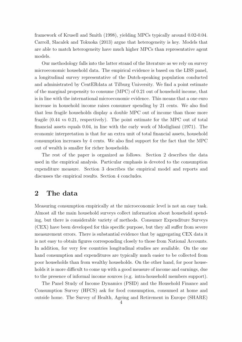
Table A reports the summary statistics of the main variables of interest used in the

empirical analysis.

Table A about here

7

3 Empirical models and results

The focus of this paper is to quantify the effect that changes in financial assets

and income have on household consumption in the Netherlands. We strictly follow

Christelis, Georgarakos and Jappelli (2014) as we use a linear specification, in which

the percentage change in consumption is regressed over the percentage changes in the

value of total financial wealth and in household income. We also control for several

changes over time in a vector of demographic characteristics. The corresponding

equation reads as follows:

∆ lnCht = αh + β∆ lnFAht + γ∆ lnHHIht + η∆ lnZht + εht (1)

where Cht represents total household spending, αh is the household fixed effect

capturing time-invariant unobserved heterogeneous characteristics such as house-

hold preferences, FAht represents household total financial assets, HHIht represents

household annual net income and Zht is a vector of the head of household’s back-

ground characteristics (namely age, number of children, presence of a partner). All

variables are observed at the household level h and at time t. The error term is

denoted by ε. We estimate equation (1) with fixed effects. We are particularly in-

terested in the parameters β and γ, representing the elasticity of consumption with

respect to total financial assets and to income, respectively. From those estimated

parameters we can then easily compute the corresponding marginal propensities to

consume.

3.1 Total financial assets and income

Table 1 reports the results for the whole sample (specification (1)) and by debt-to-

assets ratio (specification (2) and (3)). Total financial assets and income are esti-

mated significantly (at the 5-percent and at the 1-percent level, respectively) and

with the expected positive sign for the total sample. The implied computed MPCs

are 0.04 for total financial assets and 0.21 for household income. This means that

for an extra unit of total financial assets, household consumption increases by 4

cents; similarly, a one euro increase in household income raises consumer spend-

ing by 21 cents. These findings are in line with the international microeconomic

evidence. Christelis, Georgarakos and Jappelli (2014) find a MPC out of financial

wealth equal to 3.3 percentage points experienced by the US households aged 50 or

older in the years immediately after the collapse of Lehman Brothers. A number of

other studies based on U.S. data show that the range of the MPC out of the stock

8

market is between 0.01 and 0.06 (see Poterba (2000), Morris and Palumbo (2001),

Lettau and Ludvingson (2004), Carrol, Otsuka and Slacalek (2011) among others).

Most estimates of the aggregate MPC out of income coming from survey data range

between 0.2 and 0.6 (see Jappelli and Pistaferri (2006), Jappelli and Pistaferri (2011)

among others).

When splitting the sample by debt-to assets ratio, we see from Table 1, columns

(2) and (3), that less fragile households (defined as those who have a debt-to-assets

ratio less than 0.10) display a MPC which is double of the MPC of more fragile

households (defined as those who have a debt-to-assets ratio greater than 0.10).

The MPC out of household income of the former group is 0.44 whereas that of the

latter groups is 0.21. Home ownership does not seem to have any significant impact

on the consumption behaviour (specification (4)).

Table 1 about here

Table 2 reports the results for the whole sample and by debt-to-income ratio. We

distinguish debt-to-income ratio less than 1.9 (specification (2)) from debt-to-income

ratio greater than 1.9 (specification (3)). We then also consider more extreme cases

with debt-to-income ratio greater than 5 (specification (3)).

We find that higher levels of fragility are associated to relatively higher levels of

MPCs out of household income. The trend for MPCs out of total financial assets is

rather stable across fragility groups.

Table 2 about here

3.2 Housing wealth

The literature based on data from Anglo-Saxon countries shows that MPCs out of

financial wealth is usually lower than MPCs out of housing wealth, in an order of

magnitude of 4 percent versus 9 percent, respectively (see Case, Quigley, and Shiller

(2005), Carrol, Otsuka and Slacalek (2011) among others). Tang (2006) claims that

in Australia a permanent dollar increase in housing wealth leads to a six percent

rise in consumption, three times the effect of financial wealth. The estimates from

the euro area are rather different. Skudelny (2008) shows that, for the euro area,

the marginal propensity to consume out of financial wealth ranges between 1.3 to

3.5 cents per euro, while housing wealth effects do not seem to be significant. Guiso,

Paiella and Visco (2006) find that in Italy home owners have a positive wealth

elasticity, while renters have it negative and it counteracts the housing wealth effect

at the aggregate level. Paiella (2007) uses data from Italy again and finds 4.2 percent

9

for total wealth, 9.2 percent for financial wealth and 2.4 percent for housing

wealth. These findings for Italy are supported also by Bassanetti and Zollino (2010)

who estimate the size of the marginal propensity to consume out of housing wealth

about 1.5-2 cents, against values of 4-6 cents for the propensity to consume out of

each euro increase in financial wealth.

Our data do not allow to measure the MPC out of housing wealth directly due

to massive measurement errors. However we perform some analysis by splitting the

sample on the basis of housing wealth as follows. Table 3 reports the results for

the whole sample and by net housing wealth, defined as the self-reported WOZ-

value and the remaining mortgage on that property. We first consider households

with both negative and positive net housing wealth, within the range of -300,000

and +300,000 euros (specification (2)). We then consider households with negative

(and zero) net housing wealth (specification (3)) and those with strictly positive net

housing wealth (specification (4)).

It turns out that households with non-positive net housing wealth have much

higher MPCs than those with positive net housing wealth (0.35 vs. 0.06 respec-

tively), even if for the latter sub-group the elasticity is not estimated significantly

different from zero. Consistently with other fragility indicators the pattern for MPCs

out of total financial assets is rather flat across the net housing wealth distribution.

Table 3 about here

3.3 Household heterogeneity

Economic theory, empirical evidence, and common sense support the proposition

that the marginal propensity to consume out of wealth is smaller for richer house-

holds. One potential explanation is the different role of liquidity constraints across

the wealth distribution. The rationale behind this is the pivotal role of individual

heterogeneity in asset accumulation. Heterogeneity, both ex-ante (consumers differ

with respect to their degree of impatience) and ex-post (consumers are hit by differ-

ent idiosyncratic shocks), leads households to hold different wealth positions which

are associated with different MPCs.

In order to test this hypothesis for the Netherlands, we estimate an alternative

model where we dig into the role of financial wealth by considering financial assets

in quintiles. In this framework estimates cannot be interpreted as elasticities any

longer, and as a consequence MPCs cannot be computed. Nevertheless the flexibility

of this model formulation allows to better understand how consumption behaviour

changes along the distribution of percentage changes in financial wealth.

10

We observe from Table 4 that for lower quintiles the consumption response is

significant and larger in magnitude than for higher quintiles of financial assets.

Therefore, our data overall support the international evidence on the role of (finan-

cial) wealth. Johnson, Parker and Souleles (2006) study the effect of the 2001 tax

rebates in the US on consumption at the time households receive additional income

and find that households with low income or low assets spent a significantly greater

share of their rebates. This result is found also in Berger-Thomson, Chung and

McKibbin (2009), in their analysis of the effect of two policy changes (to income tax

rates and lump-sum transfers) in Australia.

In addition, we observe that higher percentage changes in the value of financial

assets are positively associated with percentage changes of consumption, and that

the relationship is not strictly monotonic. We see that pooling the data produces

more interesting results.

Table 4 about here

In order to further investigate the role of the net housing wealth on household

consumption, we run a slightly different version of this alternative model by splitting

the sample among households reporting negative net housing wealth and households

reporting positive net housing wealth. Table 5 reports the results.

We notice that for so-called “under water” households (specification (2)) the

consumption response is significant at the 5-percent level and much smaller in mag-

nitude than for household who report a positive net housing wealth (specification

(3)).

Table 5 about here

4 Concluding remarks

Household private consumption is a rather stable component of GDP representing

more than half of GDP in most European countries. However, since the onset of the

recent financial crisis consumption has dropped markedly in many countries, includ-

ing the Netherlands. Since the wake of the Great Recession household consumption

has seen a renewed interest among researchers and policy makers.

This paper focuses on the effect of changes in income and financial assets on

household consumption in the Netherlands over the period 2009-2012 for about

4,600 households. Our methodology falls into the microeconomic literature as we

use survey household data.

11

The empirical evidence is based on the LISS panel, an on-line longitudinal survey

representative of the Dutch-speaking population conducted and administrated by

CentERdata at Tilburg University since October 2007. For the purpose of this

paper we use three waves of the LISS panel for which information on household

spending is available. In particular, we use three waves of the “Time Use and

Consumption” module collected between 2009 and 2012. For each wave respondents

are asked to report the total average amount of money spent per month at the

household level. We then merge this module with the assets and the housing modules

belonging to the LISS Core Study. We follow Christelis, Georgarakos and Jappelli

(2014) as we use a linear specification with fixed effects, in which the percentage

change in consumption is regressed over the percentage changes in the value of

total financial wealth and in household income. We can produce the elasticities of

consumption with respect to total financial assets and to income, from which we

can easily compute the corresponding marginal propensities to consume.

We find a point estimate of the marginal propensity to consume of 0.21 out of

household income, that is in line with the international microeconomic evidence. We

also find that less fragile households (defined as those with debt-to-assets ratio below

0.10) display a MPC which is double of the MPC of more fragile households (0.44

vs 0.21, respectively). The point estimate for the MPC out of total financial assets

equals 0.04, in line with the early work of Modigliani (1971). The economic inter-

pretation is that for an extra unit of total financial assets, household consumption

increases by 4 cents.

We also find that households with non-positive net housing wealth have much

higher MPCs than those with positive net housing wealth (0.35 vs. 0.06 respec-

tively), even if for the latter sub-group the elasticity is not estimated significantly

different than zero. Consistently with other fragility indicators the pattern for MPCs

out of total financial assets is rather flat across the net housing wealth distribution.

In order to test the hypothesis that the MPC out of wealth is smaller for richer

households for the Netherlands, we estimate an alternative model where financial

assets are considered in quintiles. We find that for lower quintiles the consumption

response is significant and larger in magnitude than for higher quintiles of financial

assets. This indicates that the hypothesis is confirmed by Dutch data as well.

This paper seems to suggest that policies aiming at sustaining pre-crisis private

consumption levels, and aggregate demand at last, should take household hetero-

geneity (both cross-sectional and over time) into serious consideration. The house-

hold sector is unlikely to respond homogeneously across the wealth distribution,

highlighting the role of liquidity constraints and access to credit in household con-

sumption behaviour.

12

References

[1] Attanasio, O., L. Blow, R. Hamilton, and A. Leicester (2009), “Booms and

Busts: Consumption, House Prices and Expectations” Economica 76(301), 20-

50.

[2] Berger-Thomson, L., E. Chung and R. McKibbin (2009), “Estimating Marginal

Propensities to Consume in Australia using Micro Data” Reserve Bank of Aus-

tralia RDP 2009-07.

[3] Bostic, R., S. Gabriel, and G. Painter (2009), “Housing wealth, financial wealth,

and consumption: New evidence from micro data” Regional Science and Urban

Economics 39(1), 79-89.

[4] Bover, O. (2005), “Wealth effects on consumption: microeconometric estimates

from the Spanish survey of household finances” Banco de Espana Working

Paper 0522, Banco de Espana.

[5] Campbell, J. and J. Cocco (2007), “How do house prices affect consumption?

Evidence from micro data” Journal of Monetary Economics 54(3), 591-621.

[6] Carroll, C., J. Slacalek and K. Tokuoka (2013), “The Distribution of Wealth

and the Marginal Propensity to Consume” mimeo.

[7] Case K., R. Shiller, and J. Quigley (2005), “Comparing wealth effects: The

stock market versus the housing market” Advances in Macroeconomics 5(1),

1-32.

[8] Christelis, D., D. Georgarakos and T. Jappelli (2014), “Wealth Shocks, Unem-

ployment Shocks and Consumption in the Wake of the Great Recession” CEPR

Discussion Paper 10196.

[9] Disney, R., J. Gathergood and A. Henley (2010), “House price shocks, negative

equity and household consumption in the United Kingdom” Journal of the

European Economic Association 8, 1179-1207.

[10] European Central Bank (2013), “The Eurosystem Household Finance and Con-

sumption Survey - Results from the First Wave” ECB Statistics Paper Series

n. 2.

[11] Friedman, M. (1957), “A Theory of the Consumption Function” Princeton and

Oxford: Princeton University Press.

13

[12] Gan, J. (2010), “Housing wealth and consumption growth: Evidence from a

large panel of households” Review of Financial Studies 23(6), 2229-2267.

[13] Guiso, L., M. Paiella and I. Visco (2006), “Do Capital Gains Affect Consump-

tion? Estimates of Wealth Effects from Italian Households Behavior” in: L.

Klein (ed.), Long Run Growth and Short Run Stabilization: Essays in Memory

of Albert Ando (1929-2002), Elgar publisher.

[14] Hurd, M. and S. Rohwedder (2010), “The Effects of the Economic Crisis on

the Older Population” Michigan Retirement Research Center Working Paper

2010-231.

[15] Hurd, M. and S. Rohwedder (2012), “Measuring Total Household Spending in

a Monthly Internet Survey: Evidence from the American Life Panel” NBER

Working Papers 17974, National Bureau of Economic Research, Inc.

[16] Hurd, M. and S. Rohwedder (2013), “Expectations and Household Spend-

ing” Manuscript presented at the NETSPAR International Pension Workshop,

mimeo.

[17] Jappelli, T. and L. Pistaferri (2006), “Intertemporal Choice and Consumption

Mobility” Journal of European Economic Association 4, 75115.

[18] Jappelli, T. and L. Pistaferri (2011), “Financial Integration and Consumption

Smoothing” Economic Journal 121, 768706.

[19] Johnson, D.N., J.A. Parker and N.S. Souleles (2006), “Household Expendi-

ture and the Income Tax Rebates of 2001” American Economic Review 96(5),

15891610.

[20] Krusell, P. and A. Smith (1998), “Income and Wealth Heterogeneity in the

Macroeconomy” Journal of Political Economy 106(5), 867-896.

[21] Modigliani, F. (1971), “Consumer Spending and Monetary Policy: The Link-

ages” Federal Reserve Bank of Boston Conference Series 5.

[22] Muellbauer, J. N. and R. Lattimore (1994), “The Consumption Function: A

Theoretical and Empirical Overview” in Pesaran, H. and Wickens, M.R. (eds)

Handbook of Applied Econometrics.

[23] Paiella, M. (2007), “Does Wealth Affect Consumption? Evidence for Italy”

Journal of Macroeconomics 29(1), 189-205.

14

[24] Petev, I., L. Pistaferri and I. Saporta (2011), “Consumption and the Great

Recession” in Grusky, D., B. Western and C. Wimer (Eds.) Analyses of the

Great Recession, Russel Sage Foundation (forthcoming).

[25] Poterba, J. (2000), “Stock Market Wealth and Consumption” Journal of Eco-

nomic Perspectives 13, 91-118.

[26] Sousa, R. (2010), “Wealth effects on consumption: Evidence from the Euro

area” Banks and Bank Systems 5(2), 70-78.

[27] Zeldes, S. (1989), “Optimal Consumption with Stochastic Income: Deviations

from Certainty Equivalence” Quarterly Journal of Economics 104(2), 275-298.

15

Table A: Summary statistics - LISS panel

Statistics Mean Std.Dev. Min. Max. N.Obs

Financial variables (at the household level)

Total spending (in euros) 1,476 1,910 0 80,937 16,385

Total assets 201,397 309,693 1 8,608,035 7,773

Total financial assets (TFA) 20,535 140,257 -11,000 8,135,049 16,385

Housing value (WOZ) 75,007 172,122 0 8,470,000 16,385

Mortgages 31,129 97,151 0 5,100,000 16,385

Net housing wealth 43,879 160,330 -4,817,500 8,470,000 16,385

Annual net income (HHI) 2,991 5,255 0 295,195 15,057

Background characteristics (at the head-of-household level)

Age in years 49 17 16 97 16,385

Partner (indicator variable) 0.75 0.43 0 1 16,385

Number of household members 2.65 1.34 1 8 16,385

Fragility indicators

Debt-to-asset (DA) ratio 2.09 19.18 0 600 34,171

Debt-to-income (DI) ratio 4.17 6.70 0 277 3,469

16

Table 1: MPCs out of TFA and Income - total and by DA ratios

(1) (2) (3) (4)

Total DA1 DA2 DA3

Total fin. assets (logs) 0.025∗∗ 0.007 0.027∗∗ 0.026∗

(2.22) (0.16) (2.28) (1.69)

Annual net income (logs) 0.363∗∗∗ 0.770∗ 0.366∗∗∗ 0.139

(3.48) (1.69) (3.38) (1.01)

Age 0.005 -0.062∗∗ 0.007 0.012

(0.77) (-2.18) (0.90) (1.19)

N. household members 0.042 0.042 0.041

(0.85) (0.83) (0.74)

Partner -0.020 -0.024 0.117

(-0.21) (-0.24) (0.58)

Constant 5.487∗∗∗ 5.721 5.389∗∗∗ 7.477∗∗∗

(5.02) (1.32) (4.77) (5.37)

Implied MPC out of TFA 0.04∗∗ 0.01 0.05∗∗ 0.04∗

Implied MPC out of HHI 0.21∗∗∗ 0.44∗ 0.21∗∗∗ 0.08

N.Obs. 3696 118 3578 1787

DA1 represents debt-to-assets ratio ≤ 0.10

DA2 represents debt-to-assets ratio > 0.10

DA3 represents debt-to-assets ratio > 0.10 and home ownership

t statistics in parentheses

∗ p < 0.10, ∗∗ p < 0.05, ∗∗∗ p < 0.01

17

Table 2: MPCs out of TFA and Income - total and by DI ratios

(1) (2) (3) (4)

Total DI1 DI2 DI3

Total fin. assets (logs) 0.025∗∗ 0.082 0.023∗ 0.031∗∗

(2.22) (1.62) (1.95) (2.17)

Annual net income (logs) 0.363∗∗∗ 0.204 0.410∗∗∗ 0.593∗∗∗

(3.48) (0.51) (3.59) (3.81)

Age 0.005 0.001 0.005 -0.001

(0.77) (0.05) (0.69) (-0.15)

N. household members 0.042 -0.427 0.058 0.053

(0.85) (-0.98) (1.06) (0.75)

Partner -0.020 -0.046 -0.089

(-0.21) (-0.47) (-0.81)

Constant 5.487∗∗∗ 7.887∗∗ 5.026∗∗∗ 3.357∗∗

(5.02) (2.02) (4.18) (1.98)

Implied MPC out of TFA 0.04∗∗ 0.14 0.04∗ 0.05∗∗

Implied MPC out of HHI 0.21∗∗∗ 0.12 0.24∗∗∗ 0.34∗∗∗

N.Obs. 3696 327 3369 2643

DI1 represents debt-to-income ratio ≤ 1.9

DI2 represents debt-to-income ratio > 1.9

DI3 represents debt-to-income ratio > 5

t statistics in parentheses

∗ p < 0.10, ∗∗ p < 0.05, ∗∗∗ p < 0.01

18

Table 3: MPCs out of TFA and Income - total and by net housing wealth

(1) (2) (3) (4)

Total NHW1 NHW2 NHW3

Total fin. assets (logs) 0.025∗∗ 0.024∗∗ 0.031∗ 0.014

(2.22) (2.00) (1.87) (0.81)

Annual net income (logs) 0.363∗∗∗ 0.387∗∗∗ 0.605∗∗∗ 0.108

(3.48) (3.75) (3.73) (0.70)

Age 0.005 0.006 0.005 0.009

(0.77) (0.91) (0.48) (0.88)

N. household members 0.042 0.044 0.038 0.051

(0.85) (0.92) (0.54) (1.08)

Partner -0.020 -0.017 -0.005 0.196∗

(-0.21) (-0.30) (-0.06) (1.73)

Constant 5.487∗∗∗ 5.200∗∗∗ 2.860 7.977∗∗∗

(5.02) (4.86) (1.62) (5.47)

Implied MPC out of TFA 0.04∗∗ 0.04∗∗ 0.05∗ 0.02

Implied MPC out of HHI 0.21∗∗∗ 0.22∗∗∗ 0.35∗∗∗ 0.06

N.Obs. 3696 3391 2187 1204

NHW1 represents net housing wealth -300,000 < +300,000 euros

NHW2 represents net housing wealth ≤ 0

NHW3 represents net housing wealth > 0

t statistics in parentheses

∗ p < 0.10, ∗∗ p < 0.05, ∗∗∗ p < 0.01

19

Table 4: Consumption behaviour across changes in TFA quintiles - total and by

wave

(1) (2) (3)

Total Wave1 Wave2

Total fin. assets 2nd quintile (logs) 0.520∗∗∗ 1.002∗∗∗ 0.055

(2.88) (2.79) (0.78)

Total fin. assets 3rd quintile (logs) 0.424∗∗ 0.311 0.481∗∗

(2.39) (1.20) (1.99)

Total fin. assets 4th quintile (logs) 0.478∗∗ 0.327 0.605∗

(2.26) (1.33) (1.83)

Total fin. assets 5th quintile (logs) 0.242 0.349 0.144

(1.40) (1.31) (0.63)

Housing value (logs) -0.029 0.012 -0.082

(-0.53) (0.16) (-0.80)

Annual net income (logs) 0.034 0.140 -0.146

(0.14) (0.44) (-0.40)

Age -0.007 0.247

(-0.05) (0.73)

N. household members -0.027 -0.076 0.033

(-0.20) (-0.35) (0.18)

Partner 0.352∗∗ 0.378∗

(2.21) (1.68)

Constant -0.057 -0.170∗∗∗ -0.486

(-0.26) (-3.31) (-0.72)

N 545 242 303

t statistics in parentheses

∗ p < 0.10, ∗∗ p < 0.05, ∗∗∗ p < 0.01

20

Table 5: Consumption behaviour across changes in TFA - total and and by net

housing wealth

(1) (2) (3)

Total Negative NHW Positive NHW

Total fin. assets (logs) 0.067 0.030 0.001

(1.53) (0.68) (0.02)

Annual net income (logs) 0.124 0.562∗∗ 1.370∗

(1.53) (1.97) (1.90)

Age -0.047 -0.160 -0.337∗

(-0.46) (-1.59) (-1.88)

N. household members 0.005 0.008 -0.023

(0.07) (0.04) (-0.09)

Partner -0.026 -0.070 -0.450

(-0.20) (-0.16) (-0.62)

Constant 0.358∗ 0.740∗∗∗ 1.188∗∗∗

(1.77) (4.06) (3.72)

N 495 1368 742

t statistics in parentheses

∗ p < 0.10, ∗∗ p < 0.05, ∗∗∗ p < 0.01

21

Household final consumption expenditure (in % of GDP)

Household final consumption expenditure per capita growth (annual %)

Data Source: World Development Indicators

40

45

50

55

60

65

70

751

96

5

19

67

19

69

19

71

19

73

19

75

19

77

19

79

19

81

19

83

19

85

19

87

19

89

19

91

19

93

19

95

19

97

19

99

20

01

20

03

20

05

20

07

20

09

20

11

20

13

United Kingdom

Spain

France

Italy

Netherlands

United States

Euro area

-5

-4

-3

-2

-1

0

1

2

3

4

2002 2003 2004 2005 2006 2007 2008 2009 2010 2011 2012 2013

Euro area

Spain

France

United Kingdom

Italy

Netherlands

United States

Figure 1: Household final consumption, as % of GDP (top chart) and per capita

growth (bottom chart).

22

Previous DNB Working Papers in 2014 No. 406 Raymond Chaudron and Jakob de Haan, Identifying and dating systemic banking crises using

incidence and size of bank failures No. 407 Ayako Saiki and Sunghyun Henry Kim, Business cycle synchronization and vertical trade

integration: A case study of the Eurozone and East Asia No. 408 Emmanuel de Veirman and Andrew Levin, Cyclical changes in firm volatility No. 409 Carlos Arango, Yassine Bouhdaoui, David Bounie, Martina Eschelbach and Lola Hernández, Cash

management and payment choices: A simulation model with international comparisons No. 410 Dennis Veltrop and Jakob de Haan, I just cannot get you out of my head: Regulatory capture of

financial sector supervisors No. 411 Agnieszka Markiewicz and Andreas Pick, Adaptive learning and survey data No. 412 Michael Ehrmann and David-Jan Jansen, It hurts (stock prices) when your team is about to lose a

soccer match No. 413 Richhild Moessner, Jakob de Haan and David-Jan Jansen, The effect of the zero lower bound,

forward guidance and unconventional monetary policy on interest rate sensitivity to economic news in Sweden

No. 414 Dirk Broeders, An Chen and Birgit Koos, Utility-equivalence of pension security mechanisms No. 415 Irma Hindrayanto, Siem Jan Koopman and Jasper de Winter, Nowcasting and forecasting economic

growth in the euro area using principal components No. 416 Richhild Moessner, Effects of ECB balance sheet policy announcements on inflation expectations No. 417 Irma Hindrayanto, Jan Jacobs and Denise Osborn, On trend-cycle-seasonal interactions No. 418 Ronald Heijmans, Richard Heuver, Clement Levallois, Iman van Lelyveld, Dynamic visualization of

large transaction networks: the daily Dutch overnight money market No. 419 Ekaterina Neretina, Cenkhan Sahin and Jakob de Haan, Banking stress test effects on returns and

risks No. 420 Thorsten Beck, Andrea Colciago and Damjan Pfajfar, The role of financial intermediaries in

monetary policy transmission No. 421 Carin van der Cruijsen, David-Jan Jansen and Maarten van Rooij, The rose-colored glasses of

homeowners No. 422 John Bagnall, David Bounie, Kim Huynh, Anneke Kosse, Tobias Schmidt, Scott Schuh and Helmut

Stix, Consumer cash usage: A cross-country comparison with payment diary survey data No. 423 Ayako Saiki and Jon Frost, How does unconventional monetary policy affect inequality? Evidence

from Japan No. 424 Dirk van der Wal, The measurement of international pension obligations – Have we harmonised

enough? No. 425 Ivo Arnold and Saskia van Ewijk, The impact of sovereign and credit risk on interest rate

convergence in the euro area No. 426 Niels Vermeer, Maarten van Rooij and Daniel van Vuuren, Social interactions and the retirement

age No. 427 Richhild Moessner, International spillovers from US forward guidance to equity markets No. 428 Julia Le Blanc, Alessandro Porpiglia, Federica Teppa, Junyi Zhu and

Michael Ziegelmeyer, Household saving behaviour and credit constraints in the Euro area No. 429 Lola Hernandez, Nicole Jonker and Anneke Kosse, Cash versus debit card: the role of budget

control No. 430 Natalya Martynova, Lev Ratnovski and Razvan Vlahu, Franchise value and risk-taking in modern

banks No. 431 Thorsten Beck, Hans Degryse, Ralph de Haas and Neeltje van Horen, When arm’s length is too far.

Relationship banking over the business cycle No. 432 Tim de Vries and Jakob de Haan, Credit ratings and bond spreads of the GIIPS No. 433 Clemens Bonner, Preferential regulatory treatment and banks’ demand for government bonds No. 434 Tigran Poghosyan, Charlotte Werger and Jakob de Haan, Size and support ratings of US banks No. 435 Beata Javorcik and Steven Poelhekke, Former foreign affiliates: Cast out and outperformed? No. 436 Job Boerma, Openness and the (inverted) aggregate demand logic No. 437 Philip Wilms, Job Swank and Jakob de Haan, Determinants of the real impact of banking crises: A

review and new evidence No. 438 Jacob Bikker and Adelina Popescu, Efficiency and competition in the Dutch non-life insurance

industry: Effects of the 2006 health care reform

- 2 -

Previous DNB Working Papers in 2014 (continued) No. 439 Aleš Bulíř, Martin Číhak and David-Jan Jansen, Does the clarity of inflation reports affect volatility

in financial markets? No. 440 Gabriele Galati and Richhild Moessner, What do we know about the effects of macroprudential

policy? No. 441 Jon Frost and Ruben van Tilburg, Financial globalization or great financial expansion? The impact

of capital flows on credit and banking crises No. 442 Maarten van Oordt and Chen Zhou, Systemic risk and bank business models No. 443 Mariarosaria Comunale and Jeroen Hessel, Current account imbalances in the Euro area:

Competitiveness or financial cycle? No. 444 Jan Willem van den End and Marco Hoeberichts, Low real rates as driver of secular stagnation:

empirical assessment No. 445 Sebastiaan Pool, Leo de Haan and Jan Jacobs, Loan loss provisioning, bank credit and the real

economy No. 446 Jakob de Haan, Jeroen Hessel and Niels Gilbert, Reforming the architecture of EMU: Ensuring

stability in Europe No. 447 Marc Francke, Alex van de Minne and Johan Verbruggen, The effect of credit conditions on the

Dutch housing market No. 448 Niels Vermeer, Mauro Mastrogiacomo and Arthur van Soest, Demanding occupations and the

retirement age in the Netherlands No. 449 Raun van Ooijen and Maarten van Rooij, Mortgage risks, debt literacy and financial advice No. 450 Wilko Bolt, Maria Demertzis, Cees Diks, Cars Hommes and Marco van der Leij, Identifying booms

and busts in house prices under heterogeneous expectations No. 451 Niels Gilbert and Jasper de Jong, Does the Stability and Growth Pact induce a bias in the EC’s fiscal

forecasts? No. 452 Tom Boot and Andreas Pick, Optimal forecasts from Markov switching models