IFUM-956-FT

The impact of PDF and αs uncertainties on

Higgs Production in gluon–fusion at hadron colliders

Federico Demartina, Stefano Fortea,b, Elisa Mariania,Juan Rojob and Alessandro Vicinia,b

aDipartimento di Fisica, Universita di Milano, andbINFN, Sezione di Milano,

Via Celoria 16, I–20133 Milano, Italy

Abstract

We present a systematic study of uncertainties due to parton distributions and thestrong coupling on the gluon–fusion production cross section of the Standard ModelHiggs at the Tevatron and LHC colliders. We compare procedures and results whenthree recent sets of PDFs are used, CTEQ6.6, MSTW08 and NNPDF1.2, and we discussspecifically the way PDF and strong coupling uncertainties are combined. We find thatresults obtained from different PDF sets are in reasonable agreement if a common valueof the strong coupling is adopted. We show that the addition in quadrature of PDFand αs uncertainties provides an adequate approximation to the full result with exacterror propagation. We discuss a simple recipe to determine a conservative PDF+αsuncertainty from available global parton sets, and we use it to estimate this uncertaintyon the given process to be about 10% at the Tevatron and 5% at the LHC for a lightHiggs.ar

Xiv

:100

4.09

62v1

[he

p-ph

] 6

Apr

201

0

Contents

1 Introduction 2

2 The Higgs boson production cross section 42.1 The hadron–level cross section . . . . . . . . . . . . . . . . . . . . . . . . . . . 42.2 The strong coupling αs . . . . . . . . . . . . . . . . . . . . . . . . . . . . . . . 5

3 Parton sets with variable strong coupling 73.1 PDFs and αs in a Hessian approach . . . . . . . . . . . . . . . . . . . . . . . . 73.2 PDFs and αs in a Monte Carlo approach . . . . . . . . . . . . . . . . . . . . . 73.3 Comparison of global PDF sets with variable αs . . . . . . . . . . . . . . . . . 103.4 Correlation between PDFs and αs . . . . . . . . . . . . . . . . . . . . . . . . . 12

4 The cross section: PDF uncertainties 134.1 Comparison of cross sections and uncertainties . . . . . . . . . . . . . . . . . . 134.2 The uncertainty of the PDF uncertainty bands . . . . . . . . . . . . . . . . . . 14

5 The cross section: αs uncertainties 175.1 The cross section with a common αs value . . . . . . . . . . . . . . . . . . . . 175.2 Uncertainty due to the choice of αs . . . . . . . . . . . . . . . . . . . . . . . . 175.3 Impact of αs on uncertainties . . . . . . . . . . . . . . . . . . . . . . . . . . . 19

6 The cross section: final results 22

7 Conclusions 26

1

1 Introduction

At the dawn of experimentation of LHC it is important to assess carefully the expectedaccuracy of standard candle signal and background measurements. Standard model Higgsproduction is clearly one such process. The main production mechanism for a scalar Higgsboson at the LHC is the gluon–fusion process (pp → H + X) [1]. This process is also anespecially interesting test case to study QCD uncertainties: on the one hand, it starts atO(α2

s) and it undergoes large O(α3s) corrections which almost double the cross section [2,

3]. On the other hand, it is driven by the gluon distribution, which is only determinedstarting at O(αs) (unlike quark distributions which can be determined from parton–modelprocesses). Therefore, this process is quite sensitive both to parton distributions (PDFs) andαs uncertainties, and also on their interplay.

Our knowledge of PDFs (see Refs. [4, 5]) and of αs (see Refs. [6, 7]) have considerablyimproved in the last several years. However, they remain the main source of phenomenologicaluncertainty related to the treatment of the strong interaction: they limit the accuracy in away which cannot be improved upon by increasing the theoretical accuracy. It is the purposeof this work to explore this uncertainty using Higgs production in gluon–fusion as a test case.Our goal is fivefold:

• We would like to compare the procedure recommended by various groups to combinePDF uncertainties and αs uncertainties (and specifically Hessian–based approaches withMonte Carlo approaches) both in terms of procedure and in terms of results.

• We would like to assess the impact of the correlation between the value of αs and thePDFs both when determining central values and uncertainty bands, and specificallyunderstand how much results change when this correlation is taken into account incomparison to the case in which αs and PDF variations are done independently withresults added in quadrature.

• We would like to assess how much of the difference in results found when using differentPDF sets (both for central values and uncertainty bands) is due to the PDFs, and howmuch is due to the choice of value of αs.

• We would like to compare how much of the total uncertainty is due to αs and how muchis due to PDFs.

• We would like to arrive at an assessment of the value and PDF+αs uncertainty for thiscross section and more in general at a procedure to estimate them.

For each of these issues Higgs production through gluon–fusion is an interesting test case inthat it is likely to provide a worst–case scenario: differences between results obtained usingdifferent PDF sets or following different procedures for the combination of uncertainties arelikely to be smaller for many other relevant processes. For instance, in processes involvingquark PDFs the correlation between PDFs and the value of αs is likely to be weaker, andthus the results found adding uncertainties in quadrature are likely to differ less from thoseobtained when the correlation between PDFs and αs is fully accounted for.

The studies performed here will be done using PDF sets from the CTEQ, MSTW andNNPDF Collaborations, specifically the PDF sets CTEQ6.6 [8], MSTW08 [9] and NNPDF1.2 [10,11]. In order to account for the αs dependence, we will use PDF sets with varying αs which

2

have been published by CTEQ [8] and MSTW [12], as well as NNPDF1.2 sets with vary-ing αs [13] which will be presented here for the first time. Comparison between CTEQ andMSTW on one side and NNPDF on the other side will enable us to contrast results obtainedin the Hessian approach of the former with those found in the Monte Carlo approach of thelatter. Computations will be performed at next-to-leading order (NLO) in the strong cou-pling αs, because, even though NNLO results for the process we study are available [14],global parton fits with a full treatment of both DIS and hadronic data only exist at NLO (forinstance, the MSTW08 set [9] only treats DIS fully at NNLO, while Drell-Yan is describedusing K–factors, and jets using NLO theory). There are of course several other sources ofuncertainty on standard candles at colliders, such as electroweak uncertainties and furtherQCD uncertainties unrelated to PDFs, but their study goes beyond the scope of this work:here we concentrate on PDF uncertainties, and on the αs uncertainty which is tangled withthem.

The outline of the paper is as follows: in Sect. 2 we summarize the computation of theHiggs production cross section and the choice of value of αs. In Sect. 3 we discuss and comparePDF sets with varying αs, and specifically present the NNPDF1.2 sets with varying αs, whichallow for a direct computation of the correlation between αs and the gluon. We then turn toa comparison of predictions obtained using different PDF sets: first, in Sect. 4 we study PDFuncertainties and compare predictions for the cross section and the PDF uncertainty on itobtained using different sets; then in Sect. 5 we discuss αs uncertainties and their combinationwith PDF uncertainties; finally in Sect. 6 we compare final results and discuss a procedure toconstruct a combined prediction from the available sets. Conclusions are drawn in Sect. 7.

3

2 The Higgs boson production cross section

2.1 The hadron–level cross section

The hadronic total cross section for the production of a Standard Model Higgs of mass mH

via gluon–fusion at center-of-mass energy√s is

σ(h1 + h2 → H +X) =∑a,b

∫ 1

0

dx1dx2 fa,h1(x1, µ2F ) fb,h2(x2, µ

2F )

×∫ 1

0

dz δ

(z − τH

x1x2

)σab(z) , (1)

where τH = m2H/s, µF is the factorization scale, fa,hi(x, µ

2F ) are the PDFs for parton a, (a =

g, q, q) of hadron hi, and σab is the cross section for the partonic subprocess ab→ H + X atthe center-of-mass energy s = x1x2s = m2

H/z. The latter can be written as

σab(z, µ2R) = σ(0)

(µ2R

)z Gab(z, µ

2R) , (2)

where the Born cross section is

σ(0)(µ2R

)=Gµα

2s(µ

2R)

512√

2π

∣∣∣∣∣∑q

G(1l)q

∣∣∣∣∣2

(3)

and the sum runs over all quark flavors that appear in the amplitude G(1l), with

G(1l)q = −4yq [2− (1− 4yq) H(0, 0, xq)] . (4)

In Eq. (4) we have defined

yq ≡m2q

m2H

, xq ≡√

1− 4yq − 1√1− 4yq + 1

, H(0, 0, z) =1

2log2(z) , (5)

with the standard notation for Harmonic Polylogarithms (HPLs).Up to NLO,

Gab(z) = G(0)ab (z) +

αs(µ2R)

πG

(1)ab (z) (6)

where a, b stand for any allowed parton. Exact analytic results, with the full dependence onthe masses of the quarks running in the loop, have been obtained for the NLO coefficientfunction G

(1)ab in [3] and more recently in terms of HPLs in [15].

All numerical results presented in this paper have been obtained using a code based onthe expressions of Ref. [15]. We will consider only the gluon–gluon channel, and evaluate thetotal cross section at NLO-QCD, with the running of the strong coupling constant αs(µ

2R)

implemented as discussed in Sect. 2.2 below. The default choice for the renormalization scaleis µR = mH . The cross sections have been computed including the contributions due to thetop and the bottom quark running in the fermion loop, with masses mt = 172 GeV andmb = 4.6 GeV; the value of the Fermi constant is Gµ = 1.16637 10−5 GeV−2. The top masshas been renormalized in the on–shell scheme [3,15].

4

2.2 The strong coupling αs

Even though the strong coupling αs can be determined by a parton fit [12], its most accuratedetermination is arrived at by combining results from many high–energy processes, most ofwhich do not depend on PDFs at all. A recent combined determination [7] is

αs(MZ) = 0.1184± 0.0007, (7)

while the currently published1 PDG average [6] has a rather more conservative assessment ofthe uncertainty:

αs(MZ) = 0.1176± 0.002. (8)

Both these uncertainties should be understood as one–σ, i.e. 68% confidence levels.Because it starts at order α2

s and it undergoes sizable O(α3s) corrections, the Higgs cross

section is very sensitive to the central value of the strong coupling and it is thus importantto compare results obtained using the same value of αs. However, different values of αs areadopted by various parton fitting groups. Specifically, for the PDF sets we are interested in,the reference values are

αs(MZ) = 0.118 for CTEQ6.6,

αs(MZ) = 0.119 for NNPDF1.2, (9)

αs(MZ) = 0.12018 for MSTW08.

Therefore, in order to obtain a meaningful comparison, we must study the dependence ofresults obtained with different sets when the value of αs is varied about the central values ofEq. (9).

For comparison of relative uncertainties, which are less sensitive to central value of αs,but of course very sensitive to the range in which αs is varied, we will assume that the one–σand 90% confidence level variations of αs are respectively given by

∆(68)αs = 0.0012 = 0.002/c90 (10)

∆(90)αs = 0.002, (11)

where c90 = 1.64485... is the number of standard deviations for a gaussian distribution thatcorrespond to a 90% C.L. interval. Our choice Eqs. (10-11) is thus intermediate between thechoices in Eqs. (8–7). A reassessment of the value αs and and its uncertainty go beyond thescope of this work: these values are chosen as a reasonable reference, and ensure that ourresults will also be valid for other reasonable choices in the same ballpark.

An important subtlety is the number of active flavours in the running of the strong cou-pling, as implemented by various PDF analyses. Indeed, QCD calculations are usually per-formed in a decoupling scheme [17], in which heavy flavours decouple at scales much lowerthan their mass. When studying a process like Higgs production for a wide range of the Higgsmass one must then specify what to do above top threshold, and specifically fix the scale atwhich heavy quarks decouple, which amounts to a choice of renormalization scheme. Thischoice should be used consistently in the running of αs, the evolution equations for PDFs, andthe computation of hard matrix elements. In Refs. [3, 15], a scheme in which the number ofactive flavours becomes nf = 6 at Q2 = m2

t is adopted; this scheme is also used by NNPDF.

1The 2009 web PDG update [16] no longer provides a combined determination of αs, and refers to Ref. [7].

5

0.99

0.995

1

1.005

1.01

1.015

1.02

1.025

1.03

100 200 300 400 500 600 700 800 900 1000

R

Q (GeV)

R = αnf=6s (Q)/α

nf=5s (Q)

Figure 1: Ratio of the strong coupling determined with a number of flavours that varies fromnf = 5 to nf = 6 at Q > mt to that with nf = 5 at all scales.

However, CTEQ and MSTW instead use a scheme in which nf = 5 even when Q2 > m2t both

in the running of the strong coupling and in PDF evolution.The effect of this on the running of αs is small but non–negligible: in Fig. 1 we plot

the ratio of the variable–flavor αs to the fixed–flavor one, and show that for Q = 2mt thediscrepancy is already of order of 1%, and thus the effect on a quantity which depends onhigher powers of αs accordingly larger. Of course, this scheme dependence cancels to a largeextent once PDFs and hard cross sections are consistently combined, and a fully consistentcomparison would require the use of the same scheme everywhere. This is difficult in practicebecause of the different choices adopted by NNPDF on the one hand, and CTEQ and MSTWon the other hand. For the sake of comparisons below, we will use the NLO Higgs crosssection from Refs. [3,15] and, consistently αs which runs with nf that varies at Q = mt: thisis then also consistent with the evolution equations used to construct the NNPDF set, butnot with those used to construct the CTEQ and MSTW set. It should be born in mind thatthis incomplete cancellation of the scheme dependence above the top threshold may lead toa spurious difference between central values at the percent level between NNPDF and othergroups.

6

x0.1 0.2 0.3 0.4 0.5 0.6 0.7 0.8 0.9

) 02xg

(x, Q

0

0.5

1

1.5

2

2.5

3(mz) = 0.119s!(mz) = 0.113s!(mz) = 0.116s!(mz) = 0.121s!(mz) = 0.123s!(mz) = 0.125s!(mz) = 0.128s!

x-510 -410 -310 -210 -110

) 02xg

(x, Q

0

0.5

1

1.5

2

2.5

3(mz) = 0.119s!(mz) = 0.113s!(mz) = 0.116s!(mz) = 0.121s!(mz) = 0.123s!(mz) = 0.125s!(mz) = 0.128s!

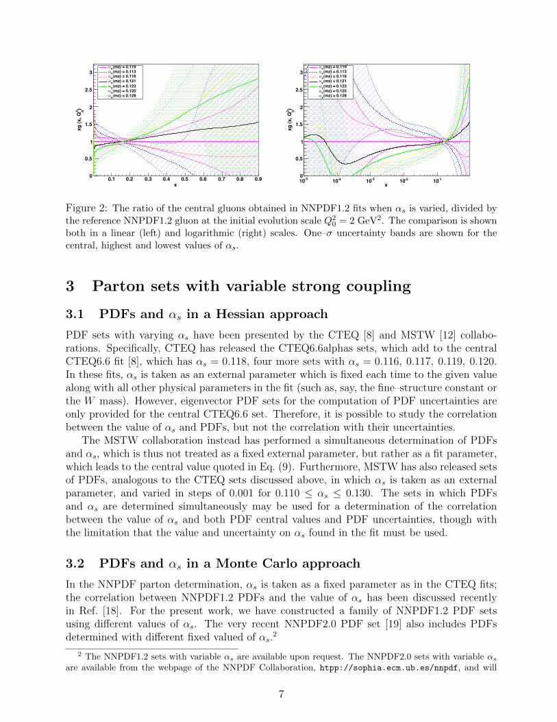
Figure 2: The ratio of the central gluons obtained in NNPDF1.2 fits when αs is varied, divided bythe reference NNPDF1.2 gluon at the initial evolution scale Q2

0 = 2 GeV2. The comparison is shownboth in a linear (left) and logarithmic (right) scales. One–σ uncertainty bands are shown for thecentral, highest and lowest values of αs.

3 Parton sets with variable strong coupling

3.1 PDFs and αs in a Hessian approach

PDF sets with varying αs have been presented by the CTEQ [8] and MSTW [12] collabo-rations. Specifically, CTEQ has released the CTEQ6.6alphas sets, which add to the centralCTEQ6.6 fit [8], which has αs = 0.118, four more sets with αs = 0.116, 0.117, 0.119, 0.120.In these fits, αs is taken as an external parameter which is fixed each time to the given valuealong with all other physical parameters in the fit (such as, say, the fine–structure constant orthe W mass). However, eigenvector PDF sets for the computation of PDF uncertainties areonly provided for the central CTEQ6.6 set. Therefore, it is possible to study the correlationbetween the value of αs and PDFs, but not the correlation with their uncertainties.

The MSTW collaboration instead has performed a simultaneous determination of PDFsand αs, which is thus not treated as a fixed external parameter, but rather as a fit parameter,which leads to the central value quoted in Eq. (9). Furthermore, MSTW has also released setsof PDFs, analogous to the CTEQ sets discussed above, in which αs is taken as an externalparameter, and varied in steps of 0.001 for 0.110 ≤ αs ≤ 0.130. The sets in which PDFsand αs are determined simultaneously may be used for a determination of the correlationbetween the value of αs and both PDF central values and PDF uncertainties, though withthe limitation that the value and uncertainty on αs found in the fit must be used.

3.2 PDFs and αs in a Monte Carlo approach

In the NNPDF parton determination, αs is taken as a fixed parameter as in the CTEQ fits;the correlation between NNPDF1.2 PDFs and the value of αs has been discussed recentlyin Ref. [18]. For the present work, we have constructed a family of NNPDF1.2 PDF setsusing different values of αs. The very recent NNPDF2.0 PDF set [19] also includes PDFsdetermined with different fixed valued of αs.

2

2 The NNPDF1.2 sets with variable αs are available upon request. The NNPDF2.0 sets with variable αs

are available from the webpage of the NNPDF Collaboration, htpp://sophia.ecm.ub.es/nnpdf, and will

7

We have repeated the NNPDF1.2 PDF determination with αs varied in the range 0.113 ≤αs ≤ 0.128 and all other aspects of the parton determination unchanged: for each value of αswe have produced a set of 100 PDF replicas. In Fig. 2 we show the ratios of the central gluonsobtained in these fits compared to the reference NNPDF1.2 gluon with αs (MZ) = 0.119,together with the PDF uncertainty band which corresponds to the reference value.

The qualitative behaviour of the gluon in Fig. 2 can be understood as follows. In NNPDF1.2,the gluon is determined by scaling violations of deep–inelastic structure functions, i.e. mostlyfrom medium and small x HERA data, with the large x gluon constrained by the momentumsum rule. With a given amount of scale dependence seen in the data, smaller values of αsrequire a larger small x gluon, and thus because of the sum rule a smaller large x gluon.In global fits [8, 12, 19] the behaviour is essentially the same, up to the fact that some extraconstraint on the large x gluon is provided by Tevatron jet data, as quantified in [19].

The size of this correlation of the gluon with the value of αs shown in Fig. 2 is clearlystatistically significant; however, when αs is varied within its uncertainty range, Eq. (10), thechange in gluon distribution is generally smaller than the uncertainty on the gluon itself. Itis interesting to note that the size of the uncertainty for values of αs which are away from thebest fit is often larger than the uncertainty when αs is at or close to its best fit value: thisis to be contrasted to what happens in a Hessian approach, where linear error propagationinevitably implies that the PDF uncertainty shrinks when αs moves away from its best–fitvalue [12].

Given sets of replicas determined with different values of αs, it is possible to performstatistics in which αs is varied, by assuming a distribution of values for αs. For instance, theaverage over Monte Carlo replicas of a general quantity which depends on both αs and thePDFs, F (PDF, αs) can be computed as

〈F〉rep =1

Nrep

Nα∑j=1

Nα(j)s

rep∑kj=1

F(

PDF(kj ,j), α(j)s

), (12)

where PDF(kj ,j) stands for the kj–th replica of the PDF fit with αs = α(j)s , and the numbers

Nα(j)s

rep of replicas for each value of αs in the total sample are determined by the probabilitydistribution of values of αs, with the constraint

Nrep =

Nαs∑j=1

Nα(j)s

rep . (13)

Specifically, assuming that global fit values of αs (such as Eqs. (7-8)) are gaussianly dis-tributed, the number of replicas is

Nα(j)s

rep ∝ exp

−(α(j)s − α(0)

s

)22(δ(68)αs

)2 . (14)

with the normalization condition Eq. (13).

also be available through the LHAPDF interface.

8

0.5

1

1.5

2

1e-05 0.0001 0.001 0.01 0.1 1

g(x)/g b

est(x)

x

MSTW

Q0 = 2 GeV

pdf unc. αs = 0.120αs = 0.110αs = 0.113αs = 0.116αs = 0.119αs = 0.121αs = 0.123αs = 0.125αs = 0.128αs = 0.130

0.9

0.95

1

1.05

1.1

1.15

1.2

1.25

1.3

1e-05 0.0001 0.001 0.01 0.1 1

g(x)/g b

est(x)

x

MSTW

Q0 = 100 GeV

pdf unc. αs = 0.120αs = 0.110αs = 0.113αs = 0.116αs = 0.119αs = 0.121αs = 0.123αs = 0.125αs = 0.128αs = 0.130

0.6

0.8

1

1.2

1.4

1.6

1.8

2

1e-05 0.0001 0.001 0.01 0.1 1

g(x)/g b

est(x)

x

CTEQ6.6alphas

Q0 = 2 GeV

pdf unc. αs = 0.118αs = 0.116αs = 0.117αs = 0.118αs = 0.119αs = 0.120

0.9

0.95

1

1.05

1.1

1.15

1.2

1.25

1e-05 0.0001 0.001 0.01 0.1 1

g(x)/g b

est(x)

x

CTEQ6.6alphas

Q0 = 100 GeV

pdf unc. αs = 0.118αs = 0.116αs = 0.117αs = 0.118αs = 0.119αs = 0.120

0.5

1

1.5

2

1e-05 0.0001 0.001 0.01 0.1 1

g(x)/g b

est(x)

x

NNPDF1.2Q0 = 2 GeV

pdf unc. αs = 0.119αs = 0.110αs = 0.113αs = 0.116αs = 0.119αs = 0.121αs = 0.123αs = 0.125αs = 0.128αs = 0.130

0.9

0.95

1

1.05

1.1

1.15

1.2

1.25

1.3

1e-05 0.0001 0.001 0.01 0.1 1

g(x)/g b

est(x)

x

NNPDF1.2

Q0 = 100 GeV

pdf unc. αs = 0.119αs = 0.110αs = 0.113αs = 0.116αs = 0.119αs = 0.121αs = 0.123αs = 0.125αs = 0.128αs = 0.130

Figure 3: Comparison of the gluon PDFs from MSTW08 (top), CTEQ6.6 (center) and NNPDF1.2(bottom) at the scales Q2 = 4 GeV2 and Q2 = 104 GeV2 as αs is varied, normalized to thecorresponding central sets, determined with the value of αs listed in Eq. (9). The one–σ uncertaintyband for the central set is also shown in each case.

9

x0.1 0.2 0.3 0.4 0.5 0.6 0.7 0.8 0.9

) 02xg

(x, Q

0.6

0.8

1

1.2

1.4

1.6

1.8

2

2 = 4 GeV2Q

MSTW2008

CTEQ6.6

NNPDF1.2

2 = 4 GeV2Q

x-510 -410 -310 -210 -110

) 02xg

(x, Q

0.6

0.8

1

1.2

1.4

1.6

1.8

2

2 = 4 GeV2Q

MSTW2008

CTEQ6.6

NNPDF1.2

2 = 4 GeV2Q

x0.1 0.2 0.3 0.4 0.5 0.6 0.7 0.8 0.9

) 02xg

(x, Q

0.6

0.8

1

1.2

1.4

1.6

1.8

2

2 GeV4 = 102Q

MSTW2008

CTEQ6.6

NNPDF1.2

2 GeV4 = 102Q

x-510 -410 -310 -210 -110

) 02xg

(x, Q

0.6

0.8

1

1.2

1.4

1.6

1.8

2

2 GeV4 = 102Q

MSTW2008

CTEQ6.6

NNPDF1.2

2 GeV4 = 102Q

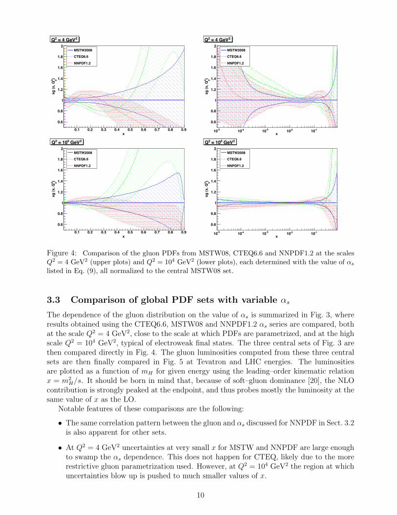
Figure 4: Comparison of the gluon PDFs from MSTW08, CTEQ6.6 and NNPDF1.2 at the scalesQ2 = 4 GeV2 (upper plots) and Q2 = 104 GeV2 (lower plots), each determined with the value of αslisted in Eq. (9), all normalized to the central MSTW08 set.

3.3 Comparison of global PDF sets with variable αs

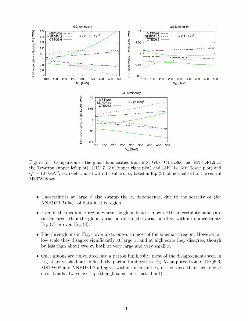
The dependence of the gluon distribution on the value of αs is summarized in Fig. 3, whereresults obtained using the CTEQ6.6, MSTW08 and NNPDF1.2 αs series are compared, bothat the scale Q2 = 4 GeV2, close to the scale at which PDFs are parametrized, and at the highscale Q2 = 104 GeV2, typical of electroweak final states. The three central sets of Fig. 3 arethen compared directly in Fig. 4. The gluon luminosities computed from these three centralsets are then finally compared in Fig. 5 at Tevatron and LHC energies. The luminositiesare plotted as a function of mH for given energy using the leading–order kinematic relationx = m2

H/s. It should be born in mind that, because of soft–gluon dominance [20], the NLOcontribution is strongly peaked at the endpoint, and thus probes mostly the luminosity at thesame value of x as the LO.

Notable features of these comparisons are the following:

• The same correlation pattern between the gluon and αs discussed for NNPDF in Sect. 3.2is also apparent for other sets.

• At Q2 = 4 GeV2 uncertainties at very small x for MSTW and NNPDF are large enoughto swamp the αs dependence. This does not happen for CTEQ, likely due to the morerestrictive gluon parametrization used. However, at Q2 = 104 GeV2 the region at whichuncertainties blow up is pushed to much smaller values of x.

10

0.7

0.8

0.9

1

1.1

1.2

1.3

1.4

1.5

100 150 200 250 300 350 400 450 500

PDF

unce

rtain

ty -

Ratio

to M

STW

08

MH [GeV]

GG luminosity

S = (1.96 TeV)2MSTW08

NNPDF1.2CTEQ6.6

0.9

0.95

1

1.05

1.1

100 150 200 250 300 350 400 450 500

PDF

unce

rtain

ty -

Ratio

to M

STW

08

MH [GeV]

GG luminosity

S = (14 TeV)2MSTW08

NNPDF1.2CTEQ6.6

0.9

0.95

1

1.05

1.1

100 150 200 250 300 350 400 450 500

PDF

unce

rtain

ty -

Ratio

to M

STW

08

MH [GeV]

GG luminosity

S = (7 TeV)2MSTW08

NNPDF1.2CTEQ6.6

Figure 5: Comparison of the gluon luminosities from MSTW08, CTEQ6.6 and NNPDF1.2 atthe Tevatron (upper left plot), LHC 7 TeV (upper right plot) and LHC 14 TeV (lower plot) andQ2 = 104 GeV2, each determined with the value of αs listed in Eq. (9), all normalized to the centralMSTW08 set

• Uncertainties at large x also swamp the αs dependence, due to the scarcity or (forNNPDF1.2) lack of data in this region.

• Even in the medium x region where the gluon is best known PDF uncertainty bands arerather larger than the gluon variation due to the variation of αs within its uncertaintyEq. (7) or even Eq. (8).

• The three gluons in Fig. 4 overlap to one–σ in most of the kinematic region. However, atlow scale they disagree significantly at large x, and at high scale they disagree, thoughby less than about two σ, both at very large and very small x.

• Once gluons are convoluted into a parton luminosity, most of the disagreements seen inFig. 4 are washed out: indeed, the parton luminosities Fig. 5 computed from CTEQ6.6,MSTW08 and NNPDF1.2 all agree within uncertainties, in the sense that their one–σerror bands always overlap (though sometimes just about).

11

-1

-0.5

0

0.5

1

1e-05 0.0001 0.001 0.01 0.1 1

Corre

latio

n co

effic

ient

x

NNPDF1.2 - Correlation of g(x,Q2) and !(MZ2)

g, Q2 = 2 GeV2

g, Q2 = 10000 GeV2

-1

-0.5

0

0.5

1

0.001 0.01 0.1 1

Corre

latio

n co

effic

ient

x

NNPDF1.2 - Correlation of PDFs(x,Q2) and !(MZ2)

Total Valence V, Q2 = 2 GeV2

Singlet ", Q2 = 2 GeV2Triplet T3, Q2 = 2 GeV2

Figure 6: The correlation Eq. (15) between PDFs and αs(MZ) as a function of x. Left: gluon PDFat Q2 = 2 GeV2 and Q2 = 104 GeV2; right: singlet, triplet and total valence PDFs for Q2 = 2 GeV2.

3.4 Correlation between PDFs and αs

Correlations between different PDFs, or between PDFs and physical observables, have beencomputed by CTEQ using a Hessian approach [8], and by NNPDF using a Monte Carloapproach [10]. Within a Monte Carlo approach it is in fact easy to estimate the correlationbetween any pair of quantities by computing their covariance over the Monte Carlo sample.Statistics involving the value of αs can then be performed provided only replicas with differentvalues of αs are available, as discussed in Sect. 3.2 above, Eq. (12).

Indeed, in a Monte Carlo approach the correlation between the strong coupling and thegluon (or any other PDF) is given by

ρ[αs(M2

Z

), g(x,Q2

)]=〈αs (M2

Z) g (x,Q2)〉rep − 〈αs (M2Z)〉rep 〈g (x,Q2)〉rep

σαs(M2Z)σg(x,Q2)

, (15)

where the distribution of values of αs is automatically reproduced if one picks Nα(j)s

rep of replicasfor each value of αs according to Eqs. (13-14) above.

Our results for the correlation coefficient between the gluon and αs(MZ) as a function ofx, computed using Eq. (15), with the NNPDF1.2 PDFs of Sect. 3.2 and Eq. (10) for αs, bothat a low scale Q2 = 2 GeV2 and at a typical LHC scale Q2 = 104 GeV2, are shown in Fig. 6.It is interesting to note how evolution decorrelates the gluon from the strong coupling. Wealso show in Fig. 6 the correlation coefficient for other PDFs: as expected for the triplet andvalence PDFs it is essentially zero, that is, in NNPDF1.2 these PDFs show essentially nosensitivity to αs. The correlation coefficient Fig. 6 quantifies the qualitative observations ofFig. 2.

12

0

0.2

0.4

0.6

0.8

1

1.2

1.4

100 150 200 250 300 350 400 450 500

σtot(pb)

mH (GeV)

TeVatron

68% C.L.

only pdf

NNPDF1.2CTEQ6.6

MSTW2008nlo

0.8

0.85

0.9

0.95

1

1.05

1.1

1.15

1.2

100 150 200 250 300 350 400 450 500

R

mH (GeV)

Tevatrononly pdf 68% C.L.

NNPDF1.2CTEQ6.6

MSTW2008nlo

-0.3

-0.2

-0.1

0

0.1

0.2

0.3

100 150 200 250 300 350 400 450 500

∆σ/σ

mH (GeV)

TeVatron68% C.L.only pdf

NNPDF1.2CTEQ6.6

MSTW2008nlo

0

2

4

6

8

10

12

14

16

18

100 150 200 250 300 350 400 450 500

σtot(pb)

mH (GeV)

LHC 7 TeV

68% C.L.

only pdf

NNPDF1.2CTEQ6.6

MSTW2008nlo

0.9

0.92

0.94

0.96

0.98

1

1.02

1.04

1.06

1.08

100 150 200 250 300 350 400 450 500

R

mH (GeV)

LHC 7 TeV

only pdf 68% C.L.

NNPDF1.2CTEQ6.6

MSTW2008nlo

-0.06

-0.04

-0.02

0

0.02

0.04

0.06

100 150 200 250 300 350 400 450 500

∆σ/σ

mH (GeV)

LHC 7 TeV68% C.L.only pdf

NNPDF1.2CTEQ6.6

MSTW2008nlo

0

5

10

15

20

25

30

35

40

45

50

55

100 150 200 250 300 350 400 450 500

σtot(pb)

mH (GeV)

LHC 14 TeV

68% C.L.

only pdf

NNPDF1.2CTEQ6.6

MSTW2008nlo

0.9

0.92

0.94

0.96

0.98

1

1.02

1.04

1.06

1.08

100 150 200 250 300 350 400 450 500

R

mH (GeV)

LHC 14 TeVonly pdf 68% C.L.

NNPDF1.2CTEQ6.6

MSTW2008nlo

-0.06

-0.04

-0.02

0

0.02

0.04

0.06

100 150 200 250 300 350 400 450 500

∆σ/σ

mH (GeV)

LHC 14 TeV68% C.L.only pdf

NNPDF1.2CTEQ6.6

MSTW2008nlo

Figure 7: Cross sections for Higgs production from gluon–fusion the Tevatron (top),LHC 7 TeV (center) and LHC 14 TeV (bottom). All uncertainty bands are one–σ PDFuncertainties, with αs fixed according to Eq. (9). The left column shows absolute results,the central column results normalized to the MSTW08 result, and the right column resultsnormalized to each group’s central result.

4 The cross section: PDF uncertainties

We now turn to the computation of the Higgs production cross section and associate un-certainty band due to PDF variation, with αs kept fixed at each group’s preferred value,as given by Eq. (9), and uncertainties consistently determined as one–σ intervals using eachgroups recommended method, hence in particular Hessian methods for CTEQ and MSTWand Monte Carlo methods for NNPDF. We will not address here the issue of comparison ofthe various methods, and we will simply take each group’s results at face value, in particularby taking as a 68% confidence level the interval determined as such by each group. Whencomparing results it should be born in mind that, as discussed in Sect. 3.3 the cross sectionsprobe the gluon luminosity at an essentially fixed value of x = m2

H/s.

4.1 Comparison of cross sections and uncertainties

In Fig. 7 we compare the cross sections at Tevatron and LHC (7 TeV and 14 TeV) energies asa function of the Higgs mass; each cross section is calculated using the best PDF set of eachgroup and the corresponding value of αs of Eq. (9) in the determination of the hard cross

13

section. Central values can differ by a sizable amount. Discrepancies are due to three distinctreasons: the fact that the hard cross sections (independent of the PDF) are different becauseof the different values of αs; the fact that the PDFs are different because they depend onαs as shown in Figs. 3; lastly the fact that even when the same value of αs is adopted PDFdetermination from different groups do not coincide.

As discussed in Sect. 3, the first two effects tend to compensate each other at small xbecause of the anticorrelation between the gluon and αs (see Fig. 6), while at large x they goin the same direction. As we shall see in Sect. 5.2, the transition between anticorrelation tocorrelation happens for LHC 7 TeV for intermediate values of the Higgs mass.

The relative impact the first effect (which affects the hard cross section) and of the secondtwo combined (which affect the parton luminosity) can be assessed by comparing the crosssections of Fig. 7 with the luminosities of Fig. 5: for instance, for mH = 150 GeV at theLHC (7 TeV), the MSTW08 cross section is seen in Fig. 7 to be by about 7% higher thanthe CTEQ6.6. Of this, Fig. 5 shows that about 3% is due to the different parton luminosity,hence about 4% must be due to the choice of αs in the hard matrix element. In Sect. 5.2 wewill determine this variation directly (Fig. 10) and see that this is indeed the case.

Because the cross section starts at order α2s(mH), with a NLO K–factor of order one, we

expect a percentage change ∆αs in αs to change the cross section by about 2.5∆αs, whichindeed suggests a 4% change of the hard cross section when αs is changed from the MSTW08to the CTEQ6.6 value. In fact, comparison of Fig. 7 to Fig. 5 shows that this simple estimateworks generally quite well: the difference in hard matrix elements is 2.5∆αs so 4% whenmoving from the MSTW08 to the CTEQ6.6 value, with the rest of the differences seen in thecross sections in Fig. 7 due to the gluon luminosities displayed in Fig. 5. Because the latterare compatible to one–σ, this is already sufficient to show that nominal uncertainties on PDFsets are sufficient to accommodate the different central values of NNPDF1.2, CTEQ6.6 andMSTW08 once a common value of αs is adopted.

Uncertainties turn out to be quite similar for all groups and of order of a few percent,with uncertainties largest at the Tevatron for large Higgs mass. The growth of uncertaintiesas the Higgs mass is raised or the energy is lowered is due to the fact that larger x values arethen probed, where knowledge of the gluon is less accurate, as shown in Fig. 4.

4.2 The uncertainty of the PDF uncertainty bands

In order to answer the question of the compatibility of different determinations of PDFs or ofphysical observables extracted from them it is important that the uncertainties are providedon the quantities which are being compared. Whereas this is standard for central values, itis less frequently done for uncertainties themselves. A systematic way of doing so in a MonteCarlo approach has been introduced in Refs. [10, 19] (see in particular Appendix A of [19]):the difference between two determinations of a central value or an uncertainty is comparedto the sum in quadrature of the uncertainty on each of the two quantities. Only when thisratio is significantly larger than one is the difference significant.

It is important to observe that when addressing the compatibility of two determinationstwo inequivalent questions can be asked: whether the two determination come from sta-tistically indistinguishable underlying distributions, or whether they come from statisticallydistinguishable distributions, but are nevertheless compatible. To elucidate the difference,consider two different determinations of the same quantities based on two independent setsof data. If the data sets are compatible, the two determinations will be consistent within

14

0.02

0.025

0.03

0.035

0.04

0.045

0.05

0.055

0.06

100 150 200 250 300 350 400 450 500

∆σ/σtot

mH (GeV)

NNPDF1.2

LHC 14 TeV

68% C.L.

αs = 0.113αs = 0.125αs = 0.119

Figure 8: The uncertainty on the Higgs cross section determined using NNPDF1.2 with differentvalues of αs. The width of the band shown denotes the statistical uncertainty on the mean uncer-tainty of the sample, σ[σ2], Eq. (17). Note that the uncertainty on the uncertainty of the PDFs is√Nrep = 10 times larger.

uncertainties in the sense that the central values are compatible within uncertainties (i.e. thecentral values will be distributed compatibly to the given uncertainty if many determinationsare compared). However, the underlying distribution of results will in general be different: forexample, if one of the two datasets is more accurate than the other, the two distributions willcertainly be statistically inequivalent (they will have different width), yet they may well becompatible. We expect complete statistical equivalence of two different PDF determinationsonly if they are based on the same data and methodology: for example, NNPDF verifies thatits PDF determination is statistically independent of the architecture of the neural networkswhich are used in the analysis. However, when comparing determinations which use differ-ent datasets, PDF parametrization, minimization algorithm etc. we only expect them to becompatibile, but not statistically indistinguishable.

The determination of the of the uncertainty on the uncertainty appears to be nontrivialin a Hessian approach, and it has not been addressed so far in the context of Hessian PDFdetermination to the best of our knowledge. We will thus only discuss it within a MonteCarlo framework. It seems plausible then to assume that uncertainties on uncertainties areof similar size in existing parton fits, so that a difference in uncertainties between two givenfits is only significant if it is rather larger than about

√2σ[σ2], where σ[σ2] is the typical

uncertainty which we will now determine in the Monte Carlo framework using NNPDF1.2PDFs.

In a Monte Carlo approach, the uncertainty which should be used when assessing statisti-cal equivalence of two quantities determined from two sets of Nrep replicas is the uncertainty ofthe mean of the replica sample, while the uncertainty to be used when assessing compatibilityis the uncertainty of the sample itself, which is larger than the former by a factor Nrep [10,19].The former vanishes in the limit Nrep, while the latter does not: indeed, if the two replica setscome from the same underlying distributions all quantities computed from them should coin-cide in the infinite–sample size limit, while if they merely come from compatible distributions

15

even for very large sample quantities computed from them should remain different.Given a set of Nrep replicas, the variance of the variance can be determined as [6]

σ2[σ2] =1

Nrep

[m4[q]−

Nrep − 3

Nrep − 1

(σ2)2]

, (16)

where σ2 and m4 are respectively the variance and fourth moment of the replica sample.Equivalently, we may determine σ2[σ2] by the jackknife method (see e.g. Ref. [21]), i.e.removing one of the replicas from the sample and determining the Nrep variances

σ2i (x) =

1

Nrep − 2

Nrep∑j=1,j 6=i

(xj − µi(x))2; i = 1, . . . , Nrep. (17)

The variance of the variance is then given by

σ2[σ2] =

Nrep∑i=1

[(σ2

i )2 − σ4

i

], (18)

where σ2i is given by Eq. (17) and

σ4i =

1

Nrep

σ4i . (19)

The quantity σ[σ2] estimated using Eq. (16) or equivalently Eq. (18) provides the uncer-tainty of the sample, and indeed it vanishes in the limit Nrep → ∞: it should thus be usedto assess statistical equivalence. The quantity which should be used to assess consistency is√Nrepσ[σ2].In Fig. 8 we plot σ[σ2] determined using Eq. (18) using the NNPDF1.2 sets with different

values of αs. We can immediately conclude from this figure that the uncertainties on thecross sections does not change in a statistically significant way when αs is varied within itsuncertainty Eq. (7) or even Eq. (8): αs has to be be varied by about three times the uncertaintyEq. (8) for the uncertainty on the cross section to change in a statistically significant way.Incidentally, this plot also shows that uncertainties are not necessarily smaller (and in factare mostly larger) when αs is varied away from its preferred value, as already seen in Sect. 3.2and Fig. 2.

When assessing compatibility (as opposed to statistical equivalence), the size of the un-certainty bands shown in Fig. 8 must be rescaled by a factor

√Nrep = 10. This rescaled

uncertainties on the uncertainty are then more then half of the uncertainty itself. This meansthat all uncertainties shown in Fig. 7 for the three PDF fits under investigation are in factcompatible with each other at the one–σ level, since they differ at most by a factor two(NNPDF vs. MSTW at LHC 14 TeV and the lowest values of mH), and in fact usually ratherless than that.

16

5 The cross section: αs uncertainties

We have seen in the previous Section (see Fig. 7) that once differences in hard matrix elementsdue to the different choice of αs are accounted for, cross sections computed using differentparton sets agree to one–σ because parton luminosities do. However, parton luminositiescompared in Fig. 5 were determined using the different values of αs Eq. (9).

For a fully consistent comparison, we must determine central parton luminosities (andthus cross sections) with a common value of αs, thereby isolating the differences which aregenuinely due to PDFs. The uncertainty related to the choice of αs must be then determinedby variation around the central value. This then raises the question of the correlation betweenthis αs variation and the values of the PDFs and their uncertainties. We now address all theseissues in turn.

5.1 The cross section with a common αs value

The cross sections obtained from the three PDF sets under investigation at the same value ofαs are compared in Fig. 9, where the ratios of cross sections computed using in the numer-ator and denominator two different PDF sets (NNPDF1.2 vs. MSTW08 and CTEQ6.6 vs.MSTW08) are shown for different choices of αs.

Comparison of these ratios to the PDF uncertainties shown in Fig. 7 show that they aretypically of a similar size: namely, two–three percent at the LHC, while at the Tevatronthey are about twice as large for light Higgs mass, rapidly growing more or less linearly,up to around 10% around the top threshold. The largest discrepancy in comparison to thePDF uncertainties is found at the lowest Higgs masses at the Tevatron between the CTEQand MSTW sets, whose uncertainty bands barely overlap there. This can be traced to thebehaviour of the gluon luminosities of Fig. 5.

Hence, the spread of central values obtained using the PDF sets under investigation isconsistent with their uncertainties, which are thus unlikely to be incorrectly estimated. Ofcourse, it should be born in mind that these uncertainties are in turn estimated with a finiteaccuracy, unlikely to be much better than 50%, as seen in Sect. 4.2.

5.2 Uncertainty due to the choice of αs

The simplest way to estimate the uncertainty due to αs is to take it as uncorrelated to thePDF uncertainty, and determine the variation of the cross section as αs is varied. This, inturn, can be done either by simply keeping the PDFs fixed, or else by also taking into accounttheir correlation to the value of αs discussed in Sect. 3, i.e. by using for each value of αs thecorresponding best–fit PDF set. In either case, the uncertainty on the cross section due tothe variation of αs is

(∆σ)±αs = σ(αs ±∆αs)− σ(αs), (20)

with, in the two cases, the cross section computed either with a fixed set of PDF, or with thesets of PDFs corresponding to the three values αs ±∆αs.

We have determined (∆σ)±αs Eq. (20) using the central value of αs of Eq. (10) and ∆αs =0.002, which would correspond to a 90% C.L. variation of αs according to Eq. (11), and itis (almost exactly) equal to the difference between the preferred values of αs for CTEQ6.6and MSTW08, Eq. (9). For NNPDF1.2 a PDF set with αs = 0.117 is not available, hence

17

0.9

0.95

1

1.05

1.1

1.15

1.2

1.25

1.3

1.35

100 150 200 250 300 350 400 450 500

R

mH (GeV)

R=CTEQ6.6alphas/MSTW2008nlo

Tevatron

αs = 0.116αs = 0.117αs = 0.118αs = 0.119αs = 0.120

0.9

0.95

1

1.05

1.1

1.15

1.2

1.25

1.3

1.35

100 150 200 250 300 350 400 450 500

R

mH (GeV)

R=NNPDF1.2/MSTW2008nlo

Tevatron

αs = 0.110αs = 0.113αs = 0.116αs = 0.119αs = 0.121αs = 0.123αs = 0.125αs = 0.128

0.95

0.96

0.97

0.98

0.99

1

1.01

1.02

1.03

100 150 200 250 300 350 400 450 500

R

mH (GeV)

R=CTEQ6.6alphas/MSTW2008nlo

LHC 7 TeV

αs = 0.116αs = 0.117αs = 0.118αs = 0.119αs = 0.120

0.95

0.96

0.97

0.98

0.99

1

1.01

1.02

1.03

100 150 200 250 300 350 400 450 500

R

mH (GeV)

R=NNPDF1.2/MSTW2008nlo

LHC 7 TeV

αs = 0.110αs = 0.113αs = 0.116αs = 0.119αs = 0.121αs = 0.123αs = 0.125αs = 0.128

0.95

0.96

0.97

0.98

0.99

1

1.01

1.02

1.03

100 150 200 250 300 350 400 450 500

R

mH (GeV)

R=CTEQ6.6alphas/MSTW2008nloLHC 14 TeV

αs = 0.116αs = 0.117αs = 0.118αs = 0.119αs = 0.120

0.95

0.96

0.97

0.98

0.99

1

1.01

1.02

1.03

100 150 200 250 300 350 400 450 500

R

mH (GeV)

R=NNPDF1.2/MSTW2008nlo

LHC14 TeV

αs = 0.110αs = 0.113αs = 0.116αs = 0.119αs = 0.121αs = 0.123αs = 0.125αs = 0.128

Figure 9: Ratio of the Higgs production cross sections determined using PDFs from different groups,but obtained with the same value of αs: CTEQ6.6/MSTW08 (left) and NNPDF1.2/MSTW08(right). Results are shown for different values of αs, and for the Tevatron (top), LHC 7 TeV(center) and LHC 14 TeV (bottom).

18

-0.06

-0.04

-0.02

0

0.02

0.04

0.06

100 150 200 250 300 350 400 450 500

(∆σtot)α

s

mH (GeV)

MSTW2008nloLHC 7 TeV

∆αs = 0.002

different pdfsfixed pdfs

-0.06

-0.04

-0.02

0

0.02

0.04

0.06

100 150 200 250 300 350 400 450 500

(∆σtot)α

s

mH (GeV)

CTEQ6.6alphasLHC 7 TeV

∆αs = 0.002

different pdfsfixed pdfs

-0.06

-0.04

-0.02

0

0.02

0.04

0.06

100 150 200 250 300 350 400 450 500

(∆σtot)α

s

mH (GeV)

NNPDF1.2

LHC 7 TeV

∆αs = 0.002

different pdfsfixed pdfs

Figure 10: Relative variation ∆σ/σ Eq. (20) of the cross section due a variation ∆αs = 0.002about the preferred value Eq. (10) adopted by each PDF set. Results are shown both withPDFs kept fixed (dashed bands), or with the best–fit PDF set corresponding to each value ofαs (solid bands).

the lower cross section in the case in which the PDFs are varied has been determined by asuitable rescaling of that which corresponds to αs = 0.116.

Results for LHC 7 TeV are shown in Fig. 10: upper and lower cross sections correspondto the upper and lower values of αs, but the variation turns out to be symmetric about thecentral value to good approximation. If the PDF is kept fixed, we find (∆σ)±αs/σ ≈ 1.04 when∆αs = 0.002, i.e. a variation of about 4%, in excellent agreement with the simple estimateof Sect. 4.1. If the PDFs are also varied, the width of the uncertainty band on the crosssection for light Higgs becomes smaller, because of the anticorrelation of the small x gluon toαs discussed in Sect. 3 (see Fig. 6), but it becomes wider as the the Higgs mass is raised andlarger x values are probed, for which the correlation of gluon to αs is positive.

5.3 Impact of αs on uncertainties

So far we have considered the uncertainties due to PDFs and due to the value of αs separately.However, as seen in Sect. 3, when αs changes, not only the central values but also the uncer-tainties on PDF change, and this leads to a correlation between PDF and αs uncertainties.The effects of this correlation on the determination of combined PDF+αs uncertainties is

19

-0.08

-0.06

-0.04

-0.02

0

0.02

0.04

0.06

0.08

100 150 200 250 300 350 400 450 500

∆σ/σ

mH (GeV)

NNPDF1.2LHC 7 TeV68% C.L.

exactquadrature

fixed pdf +∆αs

-0.06

-0.04

-0.02

0

0.02

0.04

0.06

0.08

100 150 200 250 300 350 400 450 500

∆σ/σ

mH (GeV)

MSTW2008nlo

LHC 7 TeV

68% C.L.

exactquadrature

fixed pdf+∆αs

Figure 11: The combined PDF+αs relative one–σ uncertainty on the Higgs cross section withNNPDF1.2 (left) and MSTW08 (right). The three bands correspond to results obtained keeping intoaccount the full correlation between αs and PDF uncertainties (exact), by adding in quadrature PDFuncertainties and αs uncertainties in turn determined by keeping into account the correlation betweenαs and PDF central values (quadrature), and finally by adding in quadrature PDF uncertainties andαs uncertainties determined with PDFs fixed at their central value (fixed PDF+∆αs). The centralvalues of αs are given by Eq. (9), and its one–σ range is in Eq. (10) in all cases except the MSTW08exact for which it is given in Eq. (22).

likely to be moderate: it is a higher order effect, and the dependence of uncertainties on αsis weak, especially if compared to the their own uncertainty, see Fig. 8.

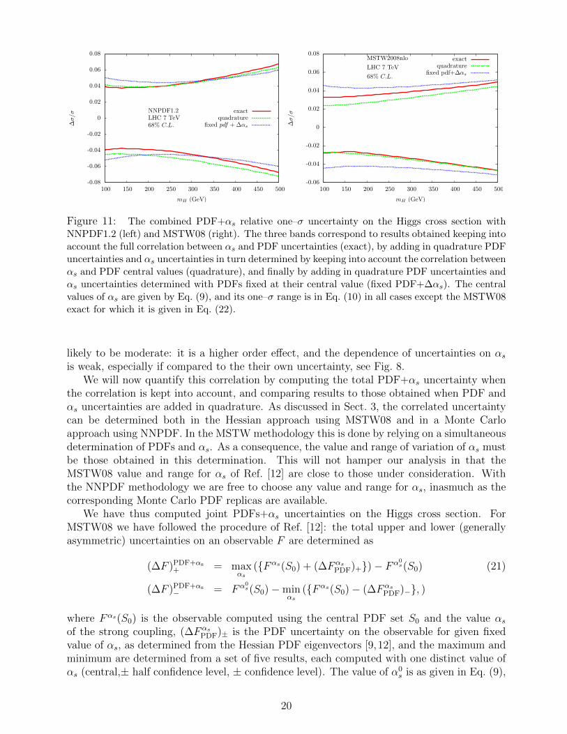
We will now quantify this correlation by computing the total PDF+αs uncertainty whenthe correlation is kept into account, and comparing results to those obtained when PDF andαs uncertainties are added in quadrature. As discussed in Sect. 3, the correlated uncertaintycan be determined both in the Hessian approach using MSTW08 and in a Monte Carloapproach using NNPDF. In the MSTW methodology this is done by relying on a simultaneousdetermination of PDFs and αs. As a consequence, the value and range of variation of αs mustbe those obtained in this determination. This will not hamper our analysis in that theMSTW08 value and range for αs of Ref. [12] are close to those under consideration. Withthe NNPDF methodology we are free to choose any value and range for αs, inasmuch as thecorresponding Monte Carlo PDF replicas are available.

We have thus computed joint PDFs+αs uncertainties on the Higgs cross section. ForMSTW08 we have followed the procedure of Ref. [12]: the total upper and lower (generallyasymmetric) uncertainties on an observable F are determined as

(∆F )PDF+αs+ = max

αs({Fαs(S0) + (∆Fαs

PDF)+})− Fα0s(S0) (21)

(∆F )PDF+αs− = Fα0

s(S0)−minαs

({Fαs(S0)− (∆FαsPDF)−}, )

where Fαs(S0) is the observable computed using the central PDF set S0 and the value αsof the strong coupling, (∆Fαs

PDF)± is the PDF uncertainty on the observable for given fixedvalue of αs, as determined from the Hessian PDF eigenvectors [9,12], and the maximum andminimum are determined from a set of five results, each computed with one distinct value ofαs (central,± half confidence level, ± confidence level). The value of α0

s is as given in Eq. (9),

20

while its one–σ upper and lower variations are

∆(68)αs =+0.0012−0.0015 . (22)

For NNPDF, the uncertainty is simply given by the standard deviation of the joint distri-bution of PDF replicas and αs values

∆FPDF+αs = σF ≡

1

Nrep − 1

Nα∑j=1

Nα(j)s

rep∑kj=1

(F [{q(kj ,j)}]− F [{q0}])2

1/2

(23)

where the number of replicas Nα(j)s

rep for each value α(j)s of the strong coupling is determined in

the gaussian case by Eq. (14). In this case, we have taken as central value and uncertaintyon αs those given in Eqs. (9-10) respectively.

The results for the uncertainty obtained in this way are shown in Fig. 11, each normalizedto the corresponding central cross section. They are compared to results obtained addingin quadrature the PDF uncertainties displayed in Fig. 7 and the αs uncertainties Eq. (20)displayed in Fig. 10, in turn obtained either with fixed PDFs, or by taking the PDF set thatcorresponds to each value of αs. Note that the range of αs variation for the MSTW08 curvewith full correlation kept into account, given in Eq. (22), differs slightly from that, Eq. (10),used in all other cases. The effect of the correlation between αs and PDF uncertainties isindeed quite small: as one might expect, it is in fact smaller than the effect of the correlationbetween αs and PDF central values shown in Fig. 10, and much smaller than the uncertaintyon the uncertainty discussed in Sect. 4.2.

21

6 The cross section: final results

Our final results for the Higgs cross section are collected in Fig. 12: the cross sections are thesame of Fig. 7, but now with the total PDF+αs uncertainty. This is computed taking fullyinto account the correlation between αs, PDF central values and uncertainties for NNPDFand MSTW (as discussed in Sect. 5.3 and shown in Fig. 10). For CTEQ, which does notprovide error sets for each value of αs, the PDF uncertainties (Fig. 7) and αs uncertainties(Sect. 5.2 and Fig. 10) are added in quadrature; however, as seen in Sect. 5.3, this makes littledifference.

The main features of these final results are the following:

• The total uncertainty on the cross section found by various groups are in reasonableagreement, especially if one recalls that they are typically affected by an uncertainty oforder of about half their size, as seen in Sect. 4.2. This follows from the fact that thetotal uncertainty is close to the sum in quadrature of the PDF and αs uncertainties,with the αs uncertainty essentially the same for all PDF sets, and PDF uncertaintieson the input parton luminosity quite close to each other,

• The predictions obtained using the three given sets all agree within the total PDF+αsone–σ uncertainty. This is a consequence of the fact that the central values of the crosssection computed using the same value of αs for all sets agree within PDF uncertainties,and that the spread of central values of αs used by the three groups Eq. (9) is essentiallythe same as the αs uncertainty under consideration.

The results shown in Fig. 12 can be combined into a determination of the cross sectionand its combined PDF+αs uncertainty. We have seen that there is reasonably good agree-ment between the parton sets under investigation: apparent disagreement is only found ifone compares results obtained with values of αs which differ more than the uncertainty onαs. However, in some cases (for example at the Tevatron for light Higgs) the agreement ismarginal: the one–σ uncertainty bands just about overlap. Ideally, this situation should beresolved by the PDF fitting groups by investigating the origin of the underlying imperfectagreement of parton luminosity. However, until this is done, a common determination ofthe cross section with a more conservative estimate of the uncertainty may be obtained bysuitably inflating the PDF uncertainty.

We have considered two different procedures which lead to such a common determination,based on the idea of combining a common αs uncertainty together with a PDF uncertaintysuitably enlarged in order to keep into account the spread of PDF central values obtainedusing different PDF sets.

Procedure A: This procedure is based on the observation that the change in PDFs anduncertainties when αs is varied by ∆αs ∼ 0.001 is small, as shown in Fig. 3, andimplicitly demonstrated by the weak effect of the keeping it into account when evaluatingαs and PDF uncertainties, Figs. 10-11. Therefore, we can obtain a prediction with acommon value of αs for all groups by simply using the common intermediate value ofαs = 0.119 in the computation of the hard cross section Eq. (2), and then using eachgroup’s PDFs and full PDF+αs uncertainties, despite the fact that strictly speaking theycorrespond to the slightly different values of αs listed in Eq. (9). Because all predictionsare given at the same value of αs, their spread reflects differences in underlying PDFs.Hence, we can take as a conservative estimate of the one–σ total PDF+αs uncertainty

22

0.7

0.8

0.9

1

1.1

1.2

1.3

100 150 200 250 300 350 400 450 500

R

mH (GeV)

Tevatron

normalized to MSTW2008

pdf+αs 68% C.L.

NNPDF1.2CTEQ6.6

MSTW2008nlo

-0.3

-0.2

-0.1

0

0.1

0.2

0.3

100 150 200 250 300 350 400 450 500

∆σ/σ

mH (GeV)

(αs + pdf) 68%

Tevatron

MSTW2008nloNNPDF1.2CTEQ6.6

0.85

0.9

0.95

1

1.05

1.1

100 150 200 250 300 350 400 450 500

R

mH (GeV)

LHC 7 TeVnormalized to MSTW2008pdf+αs 68% C.L.

NNPDF1.2CTEQ6.6

MSTW2008nlo

-0.1

-0.05

0

0.05

0.1

100 150 200 250 300 350 400 450 500

∆σ/σ

mH (GeV)

(αs + pdf) 68%

LHC 7 TeV

MSTW2008nloNNPDF1.2CTEQ6.6

0.85

0.9

0.95

1

1.05

1.1

100 150 200 250 300 350 400 450 500

R

mH (GeV)

LHC 14 TeVnormalized to MSTW2008pdf+αs 68% C.L.

NNPDF1.2CTEQ6.6

MSTW2008nlo

-0.1

-0.05

0

0.05

0.1

100 150 200 250 300 350 400 450 500

∆σ/σ

mH (GeV)

(αs + pdf) 68%

LHC 14 TeVMSTW2008nlo

CTEQ6.6NNPDF1.2

Figure 12: Cross sections for Higgs production from gluon–fusion the Tevatron (top), LHC 7 TeV(center) and LHC 14 TeV (bottom). All uncertainty bands are one–σ combined PDF+αs uncertain-ties, as in Fig. 11 (exact) for MSTW and NNPDF, and as in Fig. 10 for CTEQ, with the centralvalue of αs of Eq. (9). The left column shows results normalized to the MSTW08 result, and theright column results normalized to each group’s central result (relative uncertainty).

23

0.7

0.8

0.9

1

1.1

1.2

1.3

100 150 200 250 300 350 400 450 500

∆σ/σ

mH (GeV)

Tevatronnormalized to MSTW2008

CTEQ6.6 pdf + αs

MSTW2008nlo pdf + αs

NNPDF1.2 pdf + αs

only pdf envelope

0.85

0.9

0.95

1

1.05

1.1

100 150 200 250 300 350 400 450 500

∆σ/σ

mH (GeV)

LHC 7 TeVnormalized to MSTW2008

CTEQ6.6 pdf + αs

MSTW2008nlo pdf + αs

NNPDF1.2 pdf + αs

envelope only pdf

0.85

0.9

0.95

1

1.05

1.1

100 150 200 250 300 350 400 450 500

∆σ/σ

mH (GeV)

LHC 14 TeVnormalized to MSTW2008

CTEQ6.6 pdf + αs

MSTW2008nlo pdf + αs

NNPDF1.2 pdf + αs

envelope only pdf

Figure 13: The CTEQ, MSTW and NNPDF curves obtained using the common value αs = 0.119in the cross section Eq. (2), but with the PDF sets and uncertainties corresponding to each group’svalue of αs Eq. (9). All curves are normalized to the central MSTW curve obtained in this way.The common prediction can be taken as the envelope of these curves (Procedure A). The envelopecurve shown (Procedure B) is instead the envelope of the CTEQ, MSTW and NNPDF predictionsshowed in Fig. 7, obtained including PDF uncertainties only, but with each group’s value of αs usedboth in the PDFs and cross section, also normalized as the other curves.

on this process the envelope of these predictions, i.e. the band between the highestand the lowest prediction. This procedure would be easiest to implement if all PDFgroups were to provide PDFs with a common αs value and uncertainty. It is still viableprovided the central αs values are not too different, and the αs uncertainty can be takenas the same or almost the same for all groups.

Procedure B: This procedure is based on the observation that in fact the spread of centralvalues of αs Eq. (9) is essentially the same as the width as the one–σ error band Eq. (10).Because the total uncertainty is well approximated by the combination of αs and PDFuncertainties, this suggests that we can simply substitute the αs uncertainty by thespread of values obtained with the three sets. Hence, a conservative estimate of theone–σ total PDF+αs is obtained by taking the envelope of the PDF–only uncertaintybands obtained using each of the three sets, each at its preferred value of αs Eq. (9),i.e. the envelope of the bands shown in Fig. 7.

These two conservative estimates are shown in Fig. 13, where we display the uncertainty

24

bands obtained from the three MSTW, CTEQ and NNPDF sets whose envelope correspondsto the first method, as well as the envelope of the bands of Fig. 7, corresponding to the secondmethod. The results turn out to be in near–perfect agreement, and we can take them as aconservative estimate of the PDF+αs uncertainty. Note that if any of the three sets werediscarded, the prediction would change in a not insignificant way.

Typical uncertainties are, for light Higgs, of order of 10% at the Tevatron and 5% at theLHC. Very large uncertainties are only found for very heavy Higgs at the Tevatron, which issensitive to the poorly known large x gluon. As a central prediction one may take the midpointbetween the upper and lower bands: in practice, this turns out to be extremely close to theMSTW08 prediction found adopting the previous method, i.e. using the MSTW08 PDFs butwith αs = 0.119 in the matrix element.

These results for the combined PDF+αs uncertainties should be relevant for Higgs searchesboth at the Tevatron and at the LHC. For instance, the latest combined Tevatron analysis onHiggs production via gluon–fusion [22], which excludes a SM Higgs in the mass range 162-166GeV at 95% C.L., quotes a 11% systematic uncertainty from PDF uncertainties and higherorder variations. It would be interesting to reassess the above exclusion limits if the combinedPDF+αs uncertainties are estimated as discussed in this work.

25

7 Conclusions

We have presented a systematic study of the impact of PDF and αs uncertainties in the totalNLO cross section for the production of standard model Higgs in gluon–fusion. Whereas afull estimate of the uncertainty on this process would also require a discussion of other sourcesof uncertainty, such as electroweak corrections and the uncertainties related to higher orderQCD corrections (NNLO, soft gluon resummation etc.) our investigation has focussed onPDF uncertainties, which are likely to be dominant for many or most LHC standard candles,and the αs uncertainty which is tangled with them. The process considered here is one forwhich these uncertainties are especially large, and thus it provides a useful test case.

Our main findings can be summarized as follows:

• Parton distributions are correlated to the value of αs in a way which is visible, but ofmoderate significance. In particular, if αs is varied within a reasonable range, not muchlarger than the current global uncertainty, uncertainties due to PDFs and the variationof αs can be considered to good approximation independent and the total uncertaintycan be found adding them in quadrature.

• The gluon luminosities determined from MSTW08, CTEQ6.6 and NNPDF1.2 agree toone σ in the sense that their uncertainty bands always overlap (though just so for lightHiggs at the Tevatron). As a consequence, the Higgs cross sections determined usingthese PDF sets agree provided only the same value of αs is used in the computation ofthe hard cross section. The spread of central values between sets is of the order of thePDF uncertainty.

• The PDF uncertainties determined using these sets are in reasonable agreement andalways differ by a factor less than two, while being affected by an uncertainty which islikely to be about half their size. The αs uncertainties are essentially independent ofthe PDF set, and provide more than half of the combined uncertainty. The combineduncertainties determined using the sets under investigation are in thus in good agreementwith each other.

• A conservative estimate of the total uncertainty can be obtained from the envelope of thePDF+αs uncertainties obtained from each set, all evaluated with a common central αsvalue. Equivalently, it can be obtained from the envelope of the PDF–only uncertaintiesof sets evaluated each at different value of αs, within a range of values which covers theaccepted αs uncertainty.

• A typical conservative PDF+αs uncertainty is, for light Higgs, of order 10% at theTevatron and 5% at the LHC. This is at most a factor two larger than the PDF+αsuncertainty obtained using each individual parton set. Exclusion of any of the threesets considered here would lead to a total uncertainty which is rather closer to that ofindividual parton sets.

Further improvements in accuracy could be obtained by accurate benchmarking and cross–checking of PDF determinations in order to isolate and understand the origin of existingdisagreements. However, the overall agreement of existing sets appear to be satisfactory evenfor this worst–case scenario.

26

Acknowledgements: We thank all the members of the NNPDF collaboration, which hasdeveloped the PDF fitting methodology and code which has been used to produce the MonteCarlo varying–αs PDF sets used in this study. S.F. thanks the members of the PDF4LHCworkshop for various discussions on PDF uncertainties and their impact on LHC observ-ables, in particular Joey Huston and Robert Thorne. This work was partly supported by theEuropean network HEPTOOLS under contract MRTN-CT-2006-035505.

Note added: As this paper was being finalized, a study [23] of uncertainties on Higgs pro-duction has appeared. This paper presents detailed investigations of uncertainties which arenot being discussed by us, specifically electroweak and scale (higher order QCD) uncertain-ties, while it addresses only marginally the issue on which we have concentrated, namely theinterplay of αs and PDF uncertainties.

References

[1] H. M. Georgi, S. L. Glashow, M. E. Machacek and D. V. Nanopoulos, Phys. Rev. Lett.40 (1978) 692.

[2] S. Dawson, Nucl. Phys. B 359 (1991) 283.A. Djouadi, M. Spira and P. M. Zerwas, Phys. Lett. B 264 (1991) 440.

[3] M. Spira, A. Djouadi, D. Graudenz and P. M. Zerwas, Nucl. Phys. B 453 (1995) 17[arXiv:hep-ph/9504378].R. Harlander and P. Kant, JHEP 0512 (2005) 015 [arXiv:hep-ph/0509189].

[4] M. Dittmar et al., arXiv:hep-ph/0511119.

[5] M. Dittmar et al., arXiv:0901.2504 [hep-ph].

[6] C. Amsler et al. [Particle Data Group], Phys. Lett. B 667, 1 (2008).

[7] S. Bethke, Eur. Phys. J. C 64, 689 (2009) [arXiv:0908.1135 [hep-ph]].

[8] P. M. Nadolsky et al., Phys. Rev. D 78 (2008) 013004 [arXiv:0802.0007 [hep-ph]].

[9] A. D. Martin, W. J. Stirling, R. S. Thorne and G. Watt, Eur. Phys. J. C 63 (2009) 189[arXiv:0901.0002 [hep-ph]].

[10] R. D. Ball et al. [NNPDF Collaboration], Nucl. Phys. B 809 (2009) 1 [Erratum-ibid. B816 (2009) 293] [arXiv:0808.1231 [hep-ph]].

[11] R. D. Ball et al. [The NNPDF Collaboration], Nucl. Phys. B 823 (2009) 195[arXiv:0906.1958 [hep-ph]].

[12] A. D. Martin, W. J. Stirling, R. S. Thorne and G. Watt, Eur. Phys. J. C 64, 653 (2009)[arXiv:0905.3531 [hep-ph]].

[13] E. Mariani, “Determination of the strong coupling from an unbiased parton fit” Under-graduate Thesis, Milan University, 2009.

27

[14] R. V. Harlander, Phys. Lett. B 492 (2000) 74. [arXiv:hep-ph/0007289].S. Catani, D. de Florian and M. Grazzini, JHEP 0105 (2001) 025 [arXiv:hep-ph/0102227].R. V. Harlander and W. B. Kilgore, Phys. Rev. D 64 (2001) 013015 [arXiv:hep-ph/0102241].R. V. Harlander and W. B. Kilgore, Phys. Rev. Lett. 88 (2002) 201801 [arXiv:hep-ph/0201206].C. Anastasiou and K. Melnikov, Nucl. Phys. B 646 (2002) 220 [arXiv:hep-ph/0207004].V. Ravindran, J. Smith and W. L. van Neerven, Nucl. Phys. B 665 (2003) 325 [arXiv:hep-ph/0302135].

[15] R. Bonciani, G. Degrassi and A. Vicini, JHEP 0711 (2007) 095 [arXiv:0709.4227 [hep-ph]].U. Aglietti, R. Bonciani, G. Degrassi and A. Vicini, JHEP 0701 (2007) 021 [arXiv:hep-ph/0611266].U. Aglietti, R. Bonciani, G. Degrassi and A. Vicini, Phys. Lett. B 595 (2004) 432[arXiv:hep-ph/0404071].U. Aglietti, R. Bonciani, G. Degrassi and A. Vicini, –¿ H Phys. Lett. B 600 (2004) 57[arXiv:hep-ph/0407162].G. Degrassi and F. Maltoni, Nucl. Phys. B 724, 183 (2005) [arXiv:hep-ph/0504137].G. Degrassi and F. Maltoni, Phys. Lett. B 600, 255 (2004) [arXiv:hep-ph/0407249].

[16] “Review of particle physics”, 2009 partial update, Quantum Chromodynamics review,http://pdg.lbl.gov/2009/reviews/rpp2009-rev-qcd.pdf

[17] J. C. Collins, F. Wilczek and A. Zee, Phys. Rev. D 18 (1978) 242.

[18] R. D. Ball et al., Sect. II/21 in T. Binoth et al. (eds.) arXiv:1003.1241 [hep-ph].

[19] R. D. Ball, L. Del Debbio, S. Forte, A. Guffanti, J. I. Latorre, J. Rojo and M. Ubiali,arXiv:1002.4407 [hep-ph].

[20] M. Kramer, E. Laenen and M. Spira, Nucl. Phys. B 511, 523 (1998) [arXiv:hep-ph/9611272].

[21] B. Efron, SIAM Review, 21 (1979) 460

[22] T. Aaltonen et al. [CDF and D0 Collaborations], Phys. Rev. Lett. 104 (2010) 061802[arXiv:1001.4162 [hep-ex]].

[23] J. Baglio and A. Djouadi, arXiv:1003.4266 [hep-ph].

28