THE HOUSTON TOAD IN CONTEXT 2000-2004 - Allen Press

THE HOUSTON TOAD IN CONTEXT 2000-2004

EDITORS:

MICHAEL R.J. FORSTNER1 AND TODD M. SWANNACK2

1DEPARTMENT OF BIOLOGY, TEXAS STATE UNIVERSITY, SAN MARCOS, TX 78666 2DEPARTMENT OF WILDLIFE AND FISHERIES SCIENCES, TEXAS A&M UNIVERSITY, COLLEGE

STATION, TX 77843-2258

AUGUST 1, 2004

Dow

nloaded from http://m

eridian.allenpress.com/jfw

m/article-supplem

ent/203441/pdf/10_3996_062011-jfwm

-037_s1 by guest on 28 January 2022

TABLE OF CONTENTS Preface to Report……………...……………………………………………. i Introduction to the Houston toad…………..……………………………….. iii Executive Summary………………………………………………………… xv CHAPTER 1- ADULT HOUSTON TOAD ECOLOGY

• Activity patterns of the Dominant Herpetofauna of the Griffith League Ranch with emphasis on the Houston toad, Todd M. Swannack, Susannah R. Morris, Jacob T. Jackson, Angela D. Rainer, and Michael R. J. Forstner ……………………………………………... 1:1 • Spatial Distribution And Habitat Associations of Adult Houston Toads, Todd M. Swannack and Michael R. J. Forstner……………………. 1:22 • Population dynamics of Adult Houston Toads, Todd M. Swannack and Michael R. J. Forstner………………………………………………. 1:31 • A Possible Cause for the Disparity in the Sex Ratio of the Explosively Breeding Houston Toad, Todd M. Swannack and Michael R. J. Forstner 1:37

CHAPTER 2- JUVENILE HOUSTON TOAD ECOLOGY

• The Importance of Juvenile Ecology in the Conservation and Management of the Houston Toad, Bufo houstonensis, Kensley L. Greuter and Michael R. J. Forstner..………………………………… 2:1 • Field Techniques that aid in the Determination of Houston Toad, Bufo

houstonensis, Juvenile Survivorship, Kensley L. Greuter and Michael R. J. Forstner ………………………………………………………… 2:11 • Postmetamorphic Bioecology of the Juvenile Houston Toad, Bufo houstonensis, Kensley L. Greuter and Michael R. J. Forstner .…….. 2:29 • Conservation Implications of Survivorship Techniques and Juvenile Ecology in the Houston Toad, Bufo houstonensis, Kensley L. Greuter and Michael R. J. Forstner …………………………………………. 2:71 • Juvenile spatial distribution based on fluorescent tracking, Todd M. Swannack and Michael R. J. Forstner …………………………….. 2:81

CHAPTER 3- LARVAL HOUSTON TOAD ECOLOGY

• Effects of Various Levels of Predation and Abiotic Factors on the Survivorship of Bufonid Tadpoles, Jacob T. Jackson, Susannah R.

Morris, and Michael R.J. Forstner ………………………………… 3:1 CHAPTER 4- VERTEBRATE PREDATION ON ENDANGERED SPECIES

• Active Predation of Pitfall Traps at a Study Site for the Endangered Houston Toad, Adam W. Ferguson and Michael R. J. Forstner……….. 4:1

Dow



m/article-supplem

ent/203441/pdf/10_3996_062011-jfwm


CHAPTER 5- WILDLIFE AND VEGETATIVE ANALYSIS OF THE LOST PINES

• Habitat Affinities for White-Tailed Deer and Rio Grande Wild Turkey at the Griffith League Ranch, Bastrop County, Texas, Shane J. Kiefer and John T. Baccus………………………………………………….. 5:1 • Avian Habitat Affinity in the Lost Pines Region of Texas, Clayton J. White and Thomas R. Simpson………………………………………. 5:30

CHAPTER 6- TAXONOMY OF AN ENDEMIC LOST PINES’ SHREW

• Systematics of Locally Endemic Populations of Short-Tailed Shrews, Blarina (Insectivora: Soricidae), in Bastrop and Aransas Counties, Texas, Susannah R. Morris and Michael R. J. Forstner…………….. 6:1

CHAPTER 7- LITERATURE CITED…………………………………………… 7:1 APPENDICES A-D

• Technical Reports…………………………………………………… A:1 • Publications from the GLR………………………………………….. B:1 • Abstracts from Presentations…………………………………….….. C:1 • Presentations

o Status assessment, reproduction, habitat use, and survivorship of Houston toads using new techniques and integrated experimental design…………………………………………. D:1 o Lessons from the Houston Toad ……………………………. D:61 o Distribution of the Houston Toad (Bufo houstonensis) in Heterogeneous Habitats…………………………….………. D:79 o A Possible Cause of the Disparity in the Sex Ratio of Adult Houston Toads …………………………………………….. D:105 o Houston, we have a problem: Early Molecular Identification of the Endangered Bufo houstonensis ……………………… D:125 o Post-Emergent Behavior in the Juvenile Houston Toad, Bufo houstonensis ………………………………………….. D:169 o Postmetamorphic Dispersal Patterns in the Juvenile Houston Toad (Bufo houstonensis) …………………………………. D:193 o Early Juvenile Ecology of the Endangered Houston Toad, Bufo

houstonensis (Anura: Bufonidae) ………………………….. D:219 o Effects of Pond Slope and Predators on Larval Houston Toads (Bufo houstonensis) ………………………………………... D:275 o Active Predation of Pitfall Traps at a Study Site for the Endangered Houston Toad (Bufo houstonensis) ………….. D:293 o Habitat Affinities for White-Tailed Deer and Rio Grande Wild o Turkey at the Griffith League Ranch, Bastrop County, Texas, Shane J. Kiefer and John T. Baccus………………………… D:313

Dow



m/article-supplem

ent/203441/pdf/10_3996_062011-jfwm


o Systematics of Locally Endemic Short-tailed Shrews, Blarina (Insectivora: Soricidae), in Bastrop and Aransas Counties, Texas Susannah R. Morris, R.W.Manning, and Michael R.J. Forstner D:355 o Systematics of Locally Endemic Short-tailed Shrews, Blarina (Insectivora: Soricidae), in Bastrop and Aransas Counties, Texas

Susannah R. Morris ………………………………………… D:379 o Threats to the Houston Toad and Research Efforts for its Conservation. On-line Presentation and Study Guide for National Wildlife Federation – Wildlife University…………………… D:425

Dow



m/article-supplem

ent/203441/pdf/10_3996_062011-jfwm


Introduction to the Houston toad and its sympatric fauna and flora with a description of the Study Area (Griffith League Ranch, Bastrop Co., TX)

Phil Koepp1, Michael R.J. Forstner2, and James R. Dixon3

14805 Fieldstone Dr, Austin, TX, 78735; 2Department of Biology, Texas State University at San Marcos, San Marcos, TX 78666; 3Department of Wildlife and Fisheries Sciences, Texas A & M University, College Station, Texas 77843

1.1 Endangered and threatened species on the Griffith League Ranch The Houston toad is currently the only species in Bastrop County on the federal endangered species list. The State of Texas (Texas Parks and Wildlife Department) also lists the species as endangered. The bald eagle (Haliaeetus leucocephalus) is listed as threatened both by the Service and the State of Texas. The Service considers the reddish egret (Egretta rufescens), white-faced ibis (Plegadis chihi), Audubon’s oriole (Icterus graduacauda audubonii), loggerhead shrike (Lanius ludovicianus) and Texas horned lizard to be “species of concern”. Currently, available data do not support federal listing of any of these species. The State of Texas recognizes the reddish egret, white-faced ibis, Texas horned lizard and the canebrake (timber) rattlesnake as threatened. Other than the Houston toad, the canebrake rattlesnake is only state-listed species known to occur on the Griffith League Ranch. In Bastrop County, it has been found only on the Griffith League Ranch and in Bastrop State Park (pers. obs. Forstner, 2002). No federal or state-listed plants are known to occur on the Griffith League Ranch or in Bastrop County at the current time.

1.1.1 The Houston Toad The Houston toad is endemic to south-central Texas. John C. Wottring first noted the toad near Houston, Texas in the late 1940’s. In 1953 Ottys Sanders described it as a distinct species. On-going habitat destruction and a severe drought in the 1950’s raised concerns for the future of the species (Seal, 1994). The Houston toad was first listed as endangered in 1970 under the Endangered Species Conservation Act of 1969 (35 FR 16047). The endangered classification was continued with passage of the Endangered Species Act of 1973. The Service designated critical habitat for the Houston toad in Bastrop and Burleson counties in 1978 (43 FR 4022). The southern half of the Griffith League Ranch lies within federally designated critical habitat.

The species is currently known to occur in only nine Texas counties: Austin, Bastrop, Burleson, Colorado, Lavaca, Lee, Leon, Milam and Robertson. The Bastrop County population is considered to be the most robust and sustainable of the remaining populations (Seal, 1994; U.S. Fish and Wildlife Service, 1995). The Houston toad has been extirpated from Fort Bend, Harris and Liberty counties (Price, 1990a). Primary threats to survival of the Houston toad include habitat destruction and degradation, fragmentation of habitat, predation, inter-specific competition and hybridization, contamination by chemical herbicides, pesticides and fertilizers and prolonged drought.

iii

Dow



m/article-supplem

ent/203441/pdf/10_3996_062011-jfwm


There is a high correlation between the occurrence of the Houston toad and outcrops of the Eocene epoch Sparta Sand, Weches, Queen City Sand, Reklaw and Carrizo Sand formations (Seal, 1994). A large area of eastern Bastrop County is underlain by these formations. The Carrizo Sand and Reklaw formations underlie the eastern 73 percent of the Griffith League Ranch. The Calvert Bluff formation of the Wilcox Group underlies 27 percent of the property on its western side (Procter, et al, 1974).

Houston toads are usually associated with deep friable sandy soils. Ninety-eight percent of the Griffith League Ranch is covered with Patilo-Demona-Silstid and Axtell-Tabor soils, both series being characterized by deep sands with relatively shallow perched water tables. Sayers soils, on another 2 percent of the tract, are a deep fine sandy loam (Baker, 1979). The Houston toad is thought to burrow into all of these sandy soils to escape winter cold (hibernation) and summer heat and drought (aestivation).

The typical adult Houston toad is two to three inches long, with females being larger and bulkier than males. Coloration is generally speckled, light brown varying to black, sometimes with yellow patches. Some individuals may appear to have a slightly reddish, yellowish or grayish hue overall. Small dark spots are often found on the pale undersides. There may be a variable white stripe down the back and irregular white streaks along the sides. Dark bands extend from each eye to the mouth and also occur on the legs. Males have a dark throat that appears bluish when distended. The species’ mating call is a high-pitched ululating trill lasting for four to eleven seconds (U.S. Fish and Wildlife Service, 1984).

Life expectancy of the Houston toad is about four years (Price, 1992). Males can reach sexual maturity in captivity at about one year, females at two years (Quinn, 1981). The toads are generally active between January 15 and June 1, but may emerge as early as late December and remain active until late June, depending upon environmental conditions. Rainfall and warm nighttime temperatures initiate breeding activity, usually in February and March (Hillis, Hillis and Martin, 1984; Dixon, 1982; Dixon, Dronen, Godwin and Simmons, 1990; Price, 1990; Price and Yantiss, 1993). Dark phases of the moon influence nighttime activity (Price, 1990b).

For breeding and maturation of tadpoles, the species requires shallow, non-flowing ephemeral (lasting 30 to 60 days) pools, or permanent bodies of water with shallow, slow-flowing pools or eddies. Successful breeding and survival of tadpoles requires good water quality, availability of food and protection from predators. Female toads lay 500 to 6,000 eggs (Kennedy, 1962; Quinn and Mengden, 1984; Quinn and Mays, 1987). Less than one percent of the eggs survive to maturity (Seal, 1994).

Houston toad activity has been observed on warm, wet, humid nights during both its breeding and non-breeding season. However, little is known about its life history during the non-breeding season. On the Griffith League Ranch, native loblolly pine-oak woodland-savannah covers most (88 percent) of the tract. Native forbs and grasses provide shelter and insects for forage. Ground cover allows the Houston toad easy travel in this vegetation type. Individuals have previously been documented to travel up to 0.95 of a mile between breeding ponds (Price, 1992). The species is known to seek protection under rocks, logs, leaf litter, refuse piles, and in small animal burrows during daytime hours. While preferring deep sandy soils and woodlands, the toad will also breed and

iv

Dow



m/article-supplem

ent/203441/pdf/10_3996_062011-jfwm


travel in open areas and on non-sandy soils provided there are woodlands and sandy soils nearby.

In 1993, Dr. Andrew Price of Texas Parks and Wildlife Department (TPWD) documented Houston toads at three ponds on the Griffith League Ranch (Price, 1993). Between February 7, 2000 and the spring of 2004, Dr. Michael Forstner has conducted a presence/absence survey for Houston toads on the tract. He documented the species at 15 of 19 existing ponds, two of seven drainage systems (below Pond 12 and Alum Creek) and at one location northwest of Pond 8. In addition to his presence/absence surveys, grant funding provided for studies of the Houston toad during its non-breeding season from March 2001 through August 2004. In reporting the results from the study, he and his coauthors document dispersal, mortality and relevant ecology of juvenile Houston toads, population studies of the adult Houston toads on the Griffith League Ranch, the sympatric vertebrate fauna, and under the direction of Drs. Randy Simpson and John Baccus respectively, characterized floral, avian, and game animal components of the Houston toad’s habitat on the ranch.

1.1.2 State-Listed Species on the Griffith League Ranch The canebrake rattlesnake, listed as threatened by the State of Texas, is the only state-listed species other than the Houston toad that occurs on the Griffith League Ranch. It has been found only on the Griffith League Ranch and within Bastrop State Park in Bastrop County (pers. obs. Forstner, 2002). This seldom-seen snake occupies moist lowland and hilly pine and mixed hardwood forest. It is normally found less than a mile from permanent water sources (Werler and Dixon, 2000). State law prohibits take (injury, killing, capturing), possession, transportation or sale of any state-listed species. Texas law does not protect habitat of state-listed threatened and endangered species.

1.2 WILDLIFE Invertebrate fauna on the property have not been systematically inventoried. However, eight species of tiger beetle (Cicindela spp.) that are geographically separated from their east Texas pineywoods populations are known to occur in the vicinity and some of these have now been recognized at the species level (Taber and Fleenor, 2003). Numerous mounds of leaf-cutter ants (Atta sp.) have been observed in wooded areas and the red imported fire ant (Solenopsis invicta) has been noted in all large pastures and along roadways inside the property.

Many migratory bird species common to the central flyway are found in the area. Birds observed on the tract include the black vulture (Coragyps atratus), turkey vulture (Cathartes aura), red-shouldered hawk (Buteo lineatus), red-tailed hawk (B. jamaicensis), wild turkey (Meleagris gallopavo), barred owl (Strix varia), blue jay (Cyanocitta cristata), Carolina chickadee (Parus carolinensis), northern mockingbird (Mimus polyglottos) and northern cardinal (Cardinalis cardinalis). Other common birds likely to occur include the eastern screech owl (Otus asio), ruby-throated hummingbird (Archilochus colubris), red-bellied woodpecker (Melanerpes carolinus), tufted titmouse (Parus bicolor), Carolina wren (Thyrothorus ludovicianus), white-eyed vireo (Vireo griseus), northern parula (Parula americana), summer tanager (Piranga rubra), indigo bunting (Passerina cyanea), painted bunting (P. ciris), lark sparrow (Chondestes

v

Dow



m/article-supplem

ent/203441/pdf/10_3996_062011-jfwm


grammacus) and white-throated sparrow (Zonotrichia albicollis) (Freeman, 1996; Scott, 1987). The southwestern-most range of the pileated woodpecker (Dryocopus pileatus) and pine warbler (Dendroica pinus) and the western range extension of the Kentucky warbler (Oporornis formosus), hooded warbler (Wilsonia citrina) and Swainson’s warbler (Limnothlypis swainsonii) occur in Bastrop County (Bastrop County Environmental Network, undated).

Mammals observed on the Griffith League Ranch include the white-tailed deer (Odocoileus virginianus), raccoon (Procyon lotor), striped skunk (Mephitis mephitis), jackrabbit (Lepus californicus), coyote (Canis latrans), red fox (Vulpes vulpes), gray fox (Urocyon cinereoargenteus), bobcat (Lynx rufus), ringtail cat (Bassaricus astutus), opossum (Didelphus virginiana), fox squirrel (Sciurus niger), eastern cottontail (Sylvilagus floridanus) and nine-banded armadillo (Dasypus novemcinctus). The red bat (Lasiurus borealis), eastern mole (Scalopus aquaticus), plains pocket gopher (Geomys bursarius), Attwater’s pocket gopher (G. attwateri), hispid pocket mouse (Perognathus hispidus), white-footed mouse (Peromyscus leucopus), northern pygmy mouse (Baiomys taylori), hispid cotton rat (Sigmodon hispidus) and eastern woodrat (Neotoma floridana) are known to occur in the area and may occur on the tract. A disjunct population of short-tailed shrew (Blarina sp.), found in an area of sandy soils, new growth loblolly pine and old fallen logs within Bastrop State Park, also occurs on the Griffith League Ranch (Dixon, Dronen, Jr. and Schmidly, 1989; Dixon, Dronen, Jr., Godwin and Simmons, 1990; Dixon, 1987; Davis, 1960). The previous ambiguity in taxonomic identification for the Bastrop County shrew population is another aspect that is now resolved based on work completed during this study (see Chapter 6 below)

Amphibians documented on the property during the study period include the tiger salamander (Ambystoma tigrinum), southern leopard frog (Rana sphenocephala), bullfrog (R. catsbeiana), cricket frog (Acris crepitans), gray treefrog (Hyla versicolor), green treefrog (Hyla cinerea) two narrowmouth toads (Gastrophryne olivacea and G. carolinensis), spadefoot toad (Scaphiopus hurteri), Gulf Coast toad (Bufo valliceps), Woodhouse’s toad (B. woodhousei) and Houston toad (B. houstonensis). The Texas toad (Bufo speciosus), Rio Grande leopard frog (Rana berlandieri) and chorus frogs (Pseudacris streckeri and clarki) might be found on the tract.

Reptiles observed include turtles, lizards, and snakes. Two turtles have been found on the ranch, the common snapping turtle (Chelydra serpintina) and three-toed box turtles (Terepene carolina). Numerous lizards including the ground skink (Scincella lateralis), the green anole (Anolis carolinensis), the Texas spiney lizard (Scleroporus olivaceaous), eastern fence lizard (S. undulatus), and six-lined racerunner (Cnemidophorus sexlineatus). Snakes found on the site include the blind snake (Leptotyphlops dulcius), ground snake (Storeria dekayi), Ribbon snake (Thamnophis proximus), blotched water snake (Nerodia erythrogaster), broadbanded water snake (Nerodia fasciata) coachwhip (Masticophis flagellum), flat-headed snake (Tantilla gracilus), Eastern hognose (Heterodon platirhinos), Texas rat snake (Elaphe obsoleta lindheimeri) broad-banded copperhead (Agkistodon contortrix), western cottonmouth (A. piscivorus leucostoma), Texas coral snake (Micrurus fulvius tenere) and canebrake rattlesnake (Crotalus horridus atricaudatus) (Forstner pers.comm.. 2002,). Other reptiles could include the mud turtles (Kinosternon flavescens and subrubrum), soft-shelled turtle (Trionyx sp.), large skinks

vi

Dow



m/article-supplem

ent/203441/pdf/10_3996_062011-jfwm


(Eumeces sp.), Glass lizards (Ophiosaurus attentuatus), Texas horned lizard (Phrynosoma cornutum), Mediterranean gecko (Hemidactylus turcicus), Texas glossy snake (Arizona elegans), Eastern racer (Coluber constrictor), Corn snake (Elaphe guttata), Prairie kingsnake (Lampropeltis calligaster), speckled kingsnake (Lampropeltis getula), Louisiana milksnake (Lampropeltis triangulum), rough green snake (Opheodrys aestivus), Texas lined snake (Tropidoclonion lineatum), and rough earth snake (Virginia striatula) (Ahlbrandt and Forstner, 2002; Dixon et al., 1989, Dixon et al., 1990; Dixon, 1987)

1.2.1 Species of Concern potentially occurring on the Griffith League Ranch Species of concern are species for which there are indications of vulnerability, but for which there is insufficient information to support their listing as threatened or endangered. Species in this category receive no protection under the Endangered Species Act of 1973. Of the species of concern noted for Bastrop County, the Audubon’s oriole is an uncommon tropical resident in south Texas. It is not likely to occur on the Griffith League Ranch. Neither the reddish egret (except as a transient) nor the white-faced ibis are likely to occur on the tract as suitable habitat is lacking. Suitable habitat does exist for the loggerhead shrike and it is possible that this species could be recorded on the property in the future. The Texas horned lizard is not known to occur on the Griffith League Ranch. Given its association with sandy soils, however, it could potentially occur on the tract.

1.3 Vegetation on the Griffith League Ranch Vegetation on the Griffith League Ranch is typical of the Lost Pines area of Bastrop County: a loblolly pine (Pinus taeda) and mixed deciduous woodland interspersed with open, grassy areas. This loblolly pine woodland is disjunct from the “pineywoods” region of east Texas, being separated geographically by over 100 miles. Although rainfall in the Bastrop area averages 8 to 20 inches per year less than in the pine forests of east Texas, loblolly pines occur in Bastrop County because of high humidity, the timing and amount of rainfall, occurrence of deep sandy acid soils and the ability of the species to efficiently utilize available water. The loblolly pine and several associated plant and animal species reach their westernmost range extensions in this area. This loblolly pine-post oak-savannah ecosystem is an outstanding example of a fire-adapted, fire-climax community (Baker, 1979; Gould, 1962). It offers excellent opportunities for studies and discussions related to biogeography and plant and animal dispersal.

The dominant overstory on the Griffith League Ranch is composed of loblolly pine, post oak (Quercus stellata), blackjack oak (Q. marilandica) and eastern red cedar (Juniperus virginiana). Some sandjack oak (Q. incana) can also be found. Typically the pines are found in drainages and the oaks on ridge tops. However, they are components of mixed forests in many locations on this particular tract. American elm (Ulmus americana), cedar elm (U. crassifolia), hackberry (Celtis spp.) and hickory (Carya spp.) are found along drainages. Cottonwood (Populus deltoides) occurs in wetter drainages such as Alum Creek and the unnamed tributary of Piney Creek on the west side of the property.

Understory vegetation contains yaupon (Ilex vomitoria), possumhaw (I. decidua), southern wax-myrtle (Myrica cerifera), American beautyberry (Callicarpa americana),

vii

Dow



m/article-supplem

ent/203441/pdf/10_3996_062011-jfwm


and farkleberry (Vaccinium arboreum). Grapevine (Vitus spp.), greenbrier (Smilax spp.) and poison ivy (Rhus radicans) are also common in the understory.

Coarse bunchgrasses such as little bluestem (Schizachyrium scoparium), broomsedge bluestem (Andropogon virginicus), pineywoods dropseed (Sporobolus junceus), hairyawn muhly (Muhlenbergia capillaris), Indiangrass (Sorgastrum nutans), purpletop (Tridens flavus), beaked panicum (Panicum anceps), switchgrass (P. virgatum) and curly threeawn (Aristida desmantha) are common ground cover. Other common ground cover includes cactus (Opuntia spp.), yucca (Yucca spp.) and a variety of forbs, ferns, lichens and mosses, especially in openings of the woodland canopy.

Several sedges (Carex spp.) occur around permanent ponds and in wetter areas. Ponds no longer utilized by livestock now support a diverse aquatic flora. A charophycean alga (probably Nitella sp.) was noted in two small clear ponds in the pines. The American lotus (Nelumbo lutea) occurs in Pond 4 and Pond 12.

About 577 acres (12 percent) of the property have been cleared and planted with grasses, primarily coastal Bermuda (Cynodon dactylon). Livestock has historically grazed these pastures. Where not maintained, the pastures are being encroached upon by weedy species such as honey mesquite (Prosopis glandulosa), yankeeweed (Eupatorium compositifolium) and sesbania (Sesbania sp.). Many of these historical pastures are also being actively colonized by volunteer Loblolly pines and edge effect dispersal by native hardwoods.

2 Description of the Griffith League Ranch The environmental components and resources of the Griffith League Ranch are described in the following sections. These descriptions provide baseline information on key physical and biological components of the Griffith League Ranch.

2.1 Geology Underlying the Griffith League Ranch are three Eocene epoch geologic formations (Procter, Brown and Waechter, 1974). The deep billowy sands found on much of the tract generally cover geologic outcrops except in a few deep cuts in drainages and on exposed ridge tops.

The oldest geologic formation found on the Griffith League Ranch is the Calvert Bluff Formation of the Wilcox Group. Occurring on the west side of the ranch, it underlies about 27 percent of the property. The formation has a total thickness of about 1,000 feet. The Calvert Bluff is a massive to thin-bedded mudstone, locally glauconitic in its upper part, with varying amounts of sandstone, lignite, and ironstone concretions. The mudstone is silty with very fine laminae and weathers yellowish brown. The medium to fine-grained sandstone of the formation is moderately well sorted, cross-bedded and lenticular, with thin beds that may be locally burrowed. It weathers to various shades of brown. A brownish black lignite in the lower part of the formation occurs in seams one to 20 feet thick.

viii

Dow



m/article-supplem

ent/203441/pdf/10_3996_062011-jfwm


Overlying and to the east of the Calvert Bluff is the Carrizo Sand with a thickness of about 100 feet. It underlies over 59 percent of the property. The Carrizo Sand is a fine to coarse-grained poorly sorted friable non-calcareous thickly bedded sandstone. In its upper part is a carbonaceous black clay and portions of silty clay. It weathers yellowish brown to dark reddish brown. Some beds of ironstone are dark brownish red.

The Reklaw Formation underlies about 14 percent of the easternmost part of the tract. This sand and clay formation, which forms a deep red soil, has a thickness of about 80 feet. The upper part of the Reklaw is a silty carbonaceous clay with lentils of glauconitic clay ironstone. It is brownish black to reddish brown and weathers light brown to light gray. The lower part of the formation is a fine to medium-grained glauconitic greenish gray quartz sand and clay that weathers moderate brown and dark yellowish orange with some clay ironstone ledges and rubble.

Sands and coarse gravels are the most likely extractable minerals found on the Griffith League Ranch. There is some potential for oil, gas and lignite (Baker, 1979). BSA/CAC owns one-half the mineral rights and the estate of Mary Lavinia Griffith Sanders owns an undivided one-half. The United States reserves the rights to fissionable materials (uranium, etc.) on the tract (Paschall, 2000). Because BSA/CAC is the sole owner of surface rights on the Griffith League Ranch, development of mineral rights by other mineral rights owners would require the consent of BSA/CAC.

2.2 Soils Patilo-Demona-Silstid Association soils cover 91 percent of the Griffith League Ranch. Most common on the tract are Patilo soils (63 percent), followed by Silstid (22 percent) and Demona soils (6 percent). A small component (about 7 percent) of Axtell-Tabor Association soils can be found in the eastern and western corners of the property, with a few patches occurring along the east-west axis and in the southern corner. Within any given mapping unit of these five soil series, smaller areas of the other four may be found, so that there is some intermixing among the series. Sayers Series soils (80 acres, or less than 2 percent) occur in the Alum Creek drainage on the eastern corner of the property. Five very small outcrops (42 acres, or less than 1 percent) of Jedd Series soils are scattered about the ranch.

Patilo Series soils are deep, gently to strongly sloping (1 to 8 percent, ranging to 12 percent), moderately well-drained sandy soils. They formed in thick sandy and loamy material that appears to have been reworked by wind. The upper zone is a thin (5 inch) layer of loose, billowy fine sand above a thicker layer (47 inches) of fine loose sand. Below this is a thick layer (70 inches) of sandy clay loam. Permeability is moderately slow, runoff is slow and available water capacity is low. Patilo soils can have a perched water table at 48 to 72 inches after short periods of heavy rain. These soils are found mostly on upland ridge tops and side slopes. Erosion hazard for this soil is slight. Vegetation commonly associated with Patilo soils is wooded range with post oak, blackjack oak and coarse bunchgrass. These soils are typically utilized for pasture, range and wildlife habitat (Baker, 1979).

Silstid soils are deep, gently sloping (1 to 5 percent) well-drained sandy soils. They are found mostly on foot slopes and in drainages across uplands. These soils appear to have been formed from weathered sandy and loamy sediment interbedded with sandstone. The

ix

Dow



m/article-supplem

ent/203441/pdf/10_3996_062011-jfwm


surface is a loose loamy fine sand about 10 inches thick. Below the surface layer is about 18 inches of loamy fine sand over a thicker layer (40 inches) of sandy clay loam. Below the sandy clay loam is a 70-inch thick layer of clay loam, 40 inches of sandy clay loam and 80 inches of a fine sandy loam. Permeability is moderate, runoff is slow and available water capacity is medium. Erosion hazard is moderate. Silstid soils commonly support blackjack oak, post oak and yaupon with an understory of mid- and tall grasses. These soils are useful for recreation and wildlife habitat (Baker, 1979).

Demona Series soils occur mostly on foot slopes and in drainages across uplands, but can also be found on ridge tops. These are deep, gently sloping (1 to 5 percent) moderately well-drained sandy soils. The surface is typically a 5-inch layer of loamy fine sand overlying a thicker layer (23 inches) of loamy fine sand. Permeability is slow and runoff is slow to medium. After heavy rains, Demona sands can have a perched water table at 24 to 36 inches. Erosion hazard is moderate. Blackjack oak, post oak and bunchgrass are typically associated with Demona soils, providing range and wildlife habitat (Baker, 1979).

Three Axtell series phases occur on the property: Axtell fine sandy loam (1 to 5 percent slopes), Axtell fine sandy loam (2 to 5 percent slopes) and Axtell-Tabor Complex (1 to 8 percent slopes). These well-drained to moderately well-drained soils occur on nearly level to strongly sloping side slopes, eroded ridge tops and in drainages. A 5 to 14 inch surface layer of fine sandy to gravelly sandy loam characterizes Axtell soils. Lower layers are slowly permeable, runoff is slow to rapid and available water capacity is high. Permeability, corrosivity and shrink-swell potential limit development on Axtell soils. Erosion hazard is moderate to severe and widely spaced gullies are typical. Axtell soils support post oak, blackjack oak and bunchgrass. These soils are often are associated with native grass pastures, crops and woodland range (Baker, 1979).

Tabor fine sandy loams comprise only a small percentage (about 2 percent) of the soil found on the ranch. These deep, nearly level to sloping (1 to 3 percent) moderately well-drained loamy soils occur on ridge tops, foot slopes and in drainages. The surface is a 6-inch layer of sandy loam over a 9-inch layer of fine sandy loam and a thicker layer (38 inches) of clay. Permeability is very slow, runoff is slow to medium and available water capacity is high. Erosion hazard is moderate. Associated vegetation is post oak, blackjack oak, elm, hackberry and bunchgrass. These soils are normally used for range and pasture (Baker, 1979).

Sayers series soils are deep and nearly level (less than 1 percent slopes) excessively drained sandy soils that occur on floodplains and bottomlands that are subjected to frequent flooding. They formed in recent sandy alluvium and can occur in areas 100 to 500 feet wide and several miles long. The surface is a fine sandy loam about 10 inches thick, with some areas having a surface layer of loam, loamy fine sand or fine sand. Beneath the surface layer is up to 24 inches of slightly stratified loamy fine sand and about 60 inches of fine sand. Permeability is rapid, runoff slow, and available water capacity is low. A perched water table can be found at 60 to 120 inches during spring and fall. Erosion hazard is slight. Native vegetation on Sayers soils includes tall grasses, elm and cottonwood. These soils will support a few crops and are used as wooded and improved pasture and hayfields, native wildlife and livestock range and wildlife habitat (Baker, 1979).

x

Dow



m/article-supplem

ent/203441/pdf/10_3996_062011-jfwm


Only five small areas (42 acres) of Jedd Series soils occur on the property. These are moderately deep, sloping to moderately steep (5 to 20 percent), well-drained stony loamy soils found on small narrow ridge tops and short hilly side slopes in uplands. A 4-inch surface layer ranges from a gravelly sandy loam to a gravelly loamy sand. This layer is composed of 30 to 70 percent small siliceous pebbles and as much as 35 percent platy sandstone cobbles and stones. It can contain about 5 to 10 percent sandstone outcrops. A gravelly sandy loam about 8 inches thick with cemented sandstone fragments above a clay and sandy clay is found below the surface layer. Permeability is moderately slow and available water capacity is medium. Erosion hazard is severe. Associated vegetation is typically post oak and blackjack oak with an understory of yaupon, mulberry and bunchgrass supporting woodland and wildlife habitat (Baker, 1979).

2.3 Critical Habitat on the Griffith League Ranch Approximately 2,712 acres (56 percent) of the Griffith League Ranch are included in federally designated critical habitat for the Houston toad. The Service designated critical habitat for the species in Bastrop and Burleson counties in 1978 (43 FR 4022). Critical habitat in Bastrop County is delineated on the west by State Highway 95 and on the south by the Colorado River. The eastern limit, 97 degrees 7 minutes 30 seconds west longitude, is over four miles from the eastern corner of the Griffith League Ranch. The northern limit, latitude 30 degrees 12 minutes 00 seconds north, bisects the Griffith League Ranch so that its northern half is excluded from critical habitat while the southern half is within federally designated critical habitat.

Determination of critical habitat for the Houston toad pre-dates the Service’s 1984 regulations and procedures for designating critical habitat. Therefore, the primary elements of the species’ habitat were not detailed at the time critical habitat was listed. Primary elements of critical habitat for the Houston toad would likely include: shallow, non-flowing ephemeral pools or permanent water bodies with slow flowing pools or eddies for breeding and development of tadpoles; good water quality; cover of grasses and forbs that provide for availability of food and protection from predators; deep, friable, sandy soils for burrowing and aestivation or hibernation; and native pine and post oak woodlands-savannah (Seal, 1994; U.S. Fish and Wildlife Service, 1995). There is also a high correlation between occurrence of the Houston toad and outcrops of the Eocene Reklaw and Carrizo Sand formations (Seal, 1994). These elements are all present on the Griffith League Ranch.

No federal critical habitat has been designated for the bald eagle in Bastrop County. Texas law does not provide for protected habitat for state-listed species.

2.4 Wetlands on the Griffith League Ranch Nineteen ponds are known to occur on the Griffith League Ranch. Thirteen ponds and the headwaters of one creek are noted on the 1993 U.S. Department of the Interior Fish and Wildlife Service’s National Wetlands Inventory maps (U.S. Fish and Wildlife Service, 1993). One of the thirteen ponds, classified as palustrine, open water and permanently flooded, was not located. It appears that this site was either mapped in error or has been lost due to changes of a meandering stream channel. The head of the unnamed creek that flows directly into Lake Bastrop from the southern corner of the tract

xi

Dow



m/article-supplem

ent/203441/pdf/10_3996_062011-jfwm


is designated as riverine, intermittent, streambed and seasonally flooded. The portion of this drainage on the Griffith League Ranch does not meet these criteria and probably should not be listed as a wetland.

Four of the thirteen listed ponds are classified as palustrine, open water and permanently flooded. Three of these are one acre or less in size; the fourth is approximately three acres. Seven of the thirteen ponds are classed as palustrine, open water, permanently flooded and diked. Of these seven, one is about three acres in size, another about two acres and the other five are one acre or less. Two ponds of one acre or less are listed as palustrine, emergent, persistent, temporarily flooded and diked. All 13 ponds mapped as wetlands appear to be constructed stock ponds, possibly natural depressions that were scooped out to enlarge them. It was not possible to determine if any of the ponds are related to naturally occurring seeps or springs.

Two streams on the Griffith League Ranch are not listed on the National Wetlands Inventory, but probably should be. Alum Creek, in the eastern corner of the tract, has year-round water flowing along its length within the property boundaries. This stretch of Alum Creek is impacted by livestock activity upstream of the ranch. The area where Alum Creek flows off the property is a low-lying, marshy area. The streambed downstream of the Finger Pond (Pond 12) appears to meet wetland criteria as it has permanent pools along more than a mile of its reach toward the northwestern boundary of the property. The water source for this stream appears to be one or more natural seeps or small springs. Some of the pools along its run contain persistent perennial aquatic and semi-aquatic vegetation (Forstner, 2000). Likewise both of these locations have supported Houston toad chorusing during the study period.

During the wet winter of 2002, it was noted that almost all of the drainages on the ranch flow for some time after periods of heavy or extended rainfall. Also, shallow depressions in uplands appear to hold water after heavy or extended rainfall. Shallow pools along the intermittent drainages and the upland depressions, while not considered wetlands, could serve as breeding sites for the Houston toad provided that steep banks do not present a barrier for the species or the pools do not dry too fast.

2.5 WATER RESOURCES AND WATER QUALITY A north-south trending ridge with elevations of 600 to 650 feet divides the Griffith League Ranch hydrologically. The western and northwestern portions of the ranch are drained by intermittent tributaries of Piney Creek, which empties into the Colorado River upstream of Bastrop. Spicer Creek and an unnamed creek drain the southwestern portion of the property. These two creeks are intermittent, head on the property and drain into Lake Bastrop about 1.5 miles to the southwest. Spicer Creek continues below the dam on Lake Bastrop and empties into Piney Creek. Alum Creek, a short segment of which passes through the easternmost corner of the tract, is the major drainage east of the Griffith League Ranch. Several unnamed intermittent branches of Alum Creek head on the property, as does Price Creek, the only named tributary on the tract’s east side. Alum Creek empties into the Colorado River below Bastrop. Water flows year-round in this stretch of Alum Creek. While its quality has not been determined, it appeared eutrophic in 2000, probably due to livestock grazing on and upstream of the tract. Despite removal of all livestock from the property in 2001, the creek has remained eutrophic in character.

xii

Dow



m/article-supplem

ent/203441/pdf/10_3996_062011-jfwm


Of the 19 known ponds on the ranch, many appear to hold water year-round. Most of the ponds appear to be diked ponds, probably constructed to provide water for livestock. Judging from the size of pine trees growing in the dikes, most of the ponds appear to be old construction. In 2000, those ponds having heavy stock use were eutrophic, devoid of vegetation on their perimeters and had little evidence of diverse aquatic life. Water quality in the ponds ranged from excellent to poor during the 2000 season, depending on the amount of stock use each received. With heavier rainfall and removal of livestock during the 2001 season, water quality in all the ponds improved and vegetation covered their banks. In addition to the ponds, several dry upland depressions were noted in 2000. Vegetation associated with these dry depressions indicated that they might hold water for some time after precipitation events, particularly during wet periods. This was, in fact, observed during the winter of 2001, summer of 2002, and spring of 2003. At least one of these depressions served as a breeding site for the Houston toad. However, it dried before the tadpoles emerged (Forstner 2001).

Griffith League Ranch is underlain by two major aquifers of the region: the Wilcox Group and the Carrizo Sand. Only one well, State Well No. 58-55-402, has been recorded on the property. This well, drilled in 1952 for domestic and stock use, taps the Wilcox Group. Water from this well, which was apparently never used, was described as “soft” by the driller. Quality of the water from this well is unknown (Palafox, 1996). Several other wells, probably used to water livestock, are known to exist on the tract but no information related to them has been located. A hand-dug, stone-line well was reported by a Boy Scout Troop in January 2000. Its exact location is unknown and quality and quantity of its water is undetermined.

2.6 Land use and Ranch history The present Griffith League Ranch was originally granted to Jacob Large by the Board of Land Commissioners, Sabine County, Republic of Texas, in 1838. Jacob Large, upon being certified as “a married man...and the head of a family” and “being a resident citizen of Texas at the date of the Declaration of Independence” was granted “one league and labour of land in said Republic” (one league equals 4,428.4 acres; one labour equals 177.1 acres). Survey notes dated June 28, 1838 describe the property as “containing eight labours of temporal land and eighteen labours of pasture land” (Board of Land Commissioners, Republic of Texas, 1838).

In 1846, Jacob Large sold the tract to Alfred Griffith, a “native of the state of Maryland” (Bastrop County, Deed Record E, 1846). Additional adjacent acreage may have been purchased and some of the ranch was evidently sold and later reclaimed in the early 1900’s. The ranch passed to Mary Lavinia Griffith Sanders, a direct descendent of Alfred Griffith, in 1950. At about the same time that Mrs. Sanders received title to the ranch, she purchased an additional 50.5 acres from Mrs. Ella Fleming of Travis County. This 50-acre addition provided access to the Griffith League Ranch from Oak Hill Cemetery Road. Knox’s 1950 survey recorded the ranch at “4,847.5 acres, more or less”(Knox, 1950). The Griffith family owned the property until 1993 when Mrs. Sanders bequeathed it to BSA/CAC.

Griffith League Ranch remained predominantly vacant and undeveloped since the time of the original grant to Jacob Large in 1838. Aerial photographs dated 1974, 1981, 1991

xiii

Dow



m/article-supplem

ent/203441/pdf/10_3996_062011-jfwm


and 1999 show little change on the property. Topographic maps indicate that the tract has been heavily wooded for at least the past 50 years (Palafox, 1996; Texas Natural Resource Information System, 2000). Approximately 565 acres (about 12 percent) were in improved pastureland in 1999 and at least 17 constructed stock ponds were associated with these pastures. The pastures and adjacent woodlands were used for grazing cattle through 1999. Small areas of the ranch could have been farmed in past years. Fire scars on trees indicate that at least one widespread wildfire occurred on the ranch at some time in the past. A small sawmill operated in the southern corner of the property during the 1960’s. Several unimproved roads, skidder trails and the remains of the sawmill evidence past logging activity on much of the ranch (Palafox, 1996; Texas Natural Resource Information System, 2000).

During World War II and the Korean War (prior to 1955), the U.S. Army utilized most of the land between Elgin, Texas and Bastrop (State Highway 21) as a military training camp, Camp Swift. The eastern portion of the Griffith League Ranch was used as an artillery range impact zone. Knox noted military roads in his 1950 survey of the ranch (Knox, 1950). Some of the old military roads now provide access to various sections of the ranch. Archeologists surveying the tract have found evidence of military activities on the tract (Parkhill, 2000). The two existing ranch houses were moved from Camp Swift to the ranch’s central pasture in the late 1950’s (Palafox, 1996). The larger main residence was refinished with a stone facade and the smaller was used as a ranch worker’s residence. Several outbuildings and sheds were built adjacent to the houses.

Adjacent lands to the north of the Griffith League Ranch are heavily wooded. Land to the east and northeast and to the west and northwest appear to be used for agricultural purposes at the present time. To the southeast, south and southwest lands are platted for residential development and are rapidly being converted to that use.

xiv

Dow



m/article-supplem

ent/203441/pdf/10_3996_062011-jfwm


PREFACE

This volume is a compilation of the results from an integrated research design conducted on the Griffith League Ranch, Bastrop County, Texas during the period from 2001-2004. That research program sought novel field and laboratory data on the Houston toad, its sympatric flora and fauna, and factors affecting toad occupancy across the system within which the toad persists today. That ecosystem, the Lost Pines, represents a unique region of Texas and one containing a significant number of endemic and/or unique taxa in addition to the Houston toad. As a consequence, while our focus was Bufo houstonensis, we developed an integrated, but broadly focused program seeking data on the toad in context with the landscape in which it survives today.

The chapters that follow are primarily investigations with specific attention on the Houston toad (Chapters 1-3), but also include chapters on the wildlife and vegetation (5-6). We sought to provide all of these data in one volume, in a user-friendly format containing all of the information we gathered. To achieve part of this goal, we have included a comprehensive literature cited and substantial appendices. The appendices include data tables, the current group of peer reviewed publications resulting from this project thus far, the annual technical reports for the project, and the public presentations made by the researchers during this project. The scope of the project was large and several graduate students were able to gather enough data to write their respective theses. Where possible these form chapters contributed to this compilation. Our goal was to provide a single resource documenting our current research being carried out in the Lost Pines Ecosystem as the final report for the project. Obviously the work and the analyses continue and these future publications are also a direct result of the collaborative efforts of the management and funding agencies, collaborative partners, and the researchers themselves.

Timely peer reviewed publication of the results from scientific endeavors is an important and necessary part of academic life, and the format of this document reflects those needs. Each section was written with the intent of submitting it to a peer-reviewed journal, so the format among chapter sections will vary, according to the requirements of the target journal.

Each graduate student employed by the funds from the Section 6 grant were required to present their research at scientific meetings. Those presentations, plus any other presentation resulting from this research, are included at the end of the document, as they provide succinct summaries of each individual project. In one case the work has contributed to an on-line course, sponsored by the National Wildlife Federation, and the relevant world wide web address and title is provided for it, as well.

The scope of this project was larger than a handful of hard-working graduate students and professors could handle by themselves. Many people donated considerable amounts of time, and deserve special thanks: Jim and Mary Dixon, Josephine Duvall, Phil

i

Dow



m/article-supplem

ent/203441/pdf/10_3996_062011-jfwm


Koepp, Ruth Forstner, Chris Nice, Dan Morris, and especially the members, candidates and Elangomats in the Tonkawa Lodge of the Order of the Arrow. This project would not have been as successful if these folks had not been so dedicated to the conservation of the Houston toad and its habitat.

We would not have been able to accomplish as much as we did without the generous support from the Boy Scouts of America, Capitol Area Council. Their dedication to the conservation of both the Houston toad and Lost Pines ecosystem is unparalleled. The United States Fish and Wildlife Service, ALCOA, Texas Parks and Wildlife, and the United States Geological Survey were also critical partners and funding sources throughout this study. Michael R. J. Forstner, Ph.D. Todd M. Swannack, M.Sc. August 1, 2004

ii

Dow



m/article-supplem

ent/203441/pdf/10_3996_062011-jfwm


Executive Summary from the Research conducted on the Griffith League Ranch, Bastrop County, Texas from 2000-2004.

1. Extensive research in Bastrop County and on the Griffith League Ranch has re-emphasized the uniqueness of the Lost Pines ecosystem and its endemic fauna.

2. Unfortunately, our work has also revealed an extensively fire suppressed forest system with negative impacts to the Houston toad and the system as a whole. Indeed, we feel that the current environment on the Griffith League Ranch has a very high potential for catastrophic fire should a wildfire occur.

3. Extensive trapping results and habitat sampling strongly statistically support toads avoiding pastures, indeed relatively small openings or pastures (>15m) may pose significant barriers. Likewise reproduction occurring in ponds within, or even adjacent to, pastures is nearly always wasted, as all juveniles emerging into that environment perish.

4. Houston toad chorusing does not indicate successful reproduction, nor even the presence of female toads, much less actual emergence of juveniles from a pond.

5. Houston toad activity is correlated with both moon phase (toads are active only during ‘dark of the moon’ periods) and rainfall (Houston toad activity was correlated with rainfall events of at least 10 mm).

6. Competition between the Houston toad and the Gulf Coast toad, Bufo valliceps (its numerically dominant congener at the GLR) is reduced consequent of temporal isolation, decreasing the probability of hybridization as a significant factor.

7. Houston toads have a significantly skewed sex ratio as a natural consequence of their life history. Females are, at minimum, three times more rare than males, with consequent negative effects on population recruitment, growth, and effective size.

8. Successful reproduction (eggs deposited and hatched) and even more importantly juvenile emergence (recruitment) occur with success in ponds within mature forests with significant canopy. Even under perceived ‘perfect’ conditions juvenile survivorship may be as low as 0.0001 and thus potentially two orders of magnitude less than that used in the latest Houston toad modeling study (1% was required in that model in order to prevent extinction in less than ten years).

9. Extensive upland buffer zones surrounding breeding ponds are not just important, but absolutely critical during the first 8 weeks of the terrestrial stage for juvenile toads. The same area may well be as critical for adults during at least half of the annual cycle.

xv

Dow



m/article-supplem

ent/203441/pdf/10_3996_062011-jfwm


10. Based on 4 years of work on the GLR the number of toads captured over the past four years has a negative slope. After a peak in 2002, the total number of adult toads captured is decreasing. Each year a significant number of recaptures occur, supporting the idea of a fairly small overall population size localized to the GLR.

11. Survivorship estimates from the capture – recapture data from the GLR were lower than the estimates made from field data collected at Bastrop State Park.

12. Radio telemetry and fluorescent pigment tracking methods indicated both male and female Houston toads remain within 150 m of the edges of chorusing ponds during the active season (March – May). Likewise, during the same time period, toads do not burrow more than 3 cm from the surface of the soil. Houston toads use hollows beneath fallen logs as hibernacula.

13. Houston toads were not typically found in areas with dense stands of regrowth forest, nor were they found to occur outside of forests. The majority of Houston toads captured during this study were captured in areas reflecting a native mixed hardwood and loblolly pine forest with significant canopy and low duff layers.

14. Creating a more natural environment through fire management or manual clearing of trees and removal of heavy duff on the GLR, would not only increase the quality of habitat for the Houston toad, but also for game species such as White-tail deer and wild turkey.

15. Modern forest management methods that include considerations for the specific life history timing of the Houston toad would positively impact the remaining populations of this species while also benefiting the health of the ecosystem and its components alongside diminishing risks of catastrophic fire.

xvi

Dow



m/article-supplem

ent/203441/pdf/10_3996_062011-jfwm


1: 1

ACTIVITY PATTERNS OF THE DOMINANT HERPETOFAUNA OF THE GRIFFITH LEAGUE RANCH WITH EMPHASIS ON THE HOUSTON TOAD

Todd M. Swannack1*, Susannah R. Morris2, Jacob T. Jackson2, Angela D. Rainer2, and

Michael R. J. Forstner2*1Department of Wildlife and Fisheries Sciences, Texas A & M University, College Station, Texas 77843;

*E-mail: [email protected] 2Department of Biology, Texas State University at San Marcos, San Marcos, TX 78666;

*E-mail: [email protected]

From fairly low density populations of the late 1980s and early 1990s, the

Houston toad Bufo houstonensis crashed to its current extremely low densities (Price,

2003). Given the present state of human-mediated development and population growth

in Bastrop County, conservation efforts must be both comprehensive and cohesive in

order to save the species. Even with a plan for recovery, efforts must be accelerated and

reemphasized if the species is to be kept from extinction in the wild. Although the

Houston toad has received substantial media attention consequent of its endangered

status, there are still several aspects of its biology that remain unknown, and

unfortunately most of those factors are critical to effective management decisions.

Most of the studies have focused on the breeding behavior and reproductive

ecology of Bufo houstonensis when the toads are most active (Hillis et al., 1984; Price,

2003); however, most of the individuals were captured at breeding ponds while males

were in chorus. This manuscript is meant to supplement the current knowledge regarding

the activity patterns of the Houston toad both within and outside of its breeding season

based on the results from a four-year study, beginning on 12 March 2001 and ending on

01 August 2004. The work included both breeding pond surveys and an extensive system

of drift fence – pitfall traps allowing the presentation of these data in correlation with

other sympatric herpetofaunal species captured in the traps.

Dow



m/article-supplem

ent/203441/pdf/10_3996_062011-jfwm


1: 2

MATERIALS AND METHODS Study system

The Griffith League Ranch (GLR) is a 1951 ha property owned by the Boy Scouts

of America (BSA) in Bastrop County, 91% of the property is underlain by deep sandy

soils of the Patilo, Demona, or Silstid series, and the GLR was historically a pine and

mixed hardwood forest. Three large tracts of approximately 200 ha each were cleared for

cattle grazing early in the 20th century; however, cattle were removed from the property

in 2001. Bufo houstonensis was originally detected on the property during the early

1980s (A. Price, pers comm., 2002), but no program of monitoring was established until

the BSA acquired the property in 2000. Audio surveys were conducted each year from

2001 – 2004 to determine the distribution of Houston toads on the GLR. B. houstonensis

choruses were heard at 12 of the 17 ponds on the property.

Trap design and data collection

Based on the results of the 2000 call survey a trapping design was conceived to

both maximize the number of toads captured and to determine how B. houstonensis

utilized the landscape by evaluating 5 treatment groups (Table 1). This design had to be

implemented over time, and from the first installation to the last these were: March 2001

– 5 linear drift fences (two 121 m, three 153 m), with 1.9 liter pitfalls every 30 m, were

placed along the border of the forest and pasture to determine if toads utilized pasture

habitats (henceforth referred to as treatment 5); in addition to the pasture traps, three Y-

shaped drift fence arrays were placed in 3 habitats (one trap per habitat): 30 m from a

breeding pond (Pond 2) in pine forest, in mixed oak woodland, and in a small (~2 ha)

natural clearing. In February 2002, the remaining traps from the original conceptual

Dow



m/article-supplem

ent/203441/pdf/10_3996_062011-jfwm


1: 3

design were added – seven additional Y-shaped arrays and pitfalls, completing the

following trapping design: 4 traps surrounding Pond 2, one at each cardinal point, at

randomly chosen distances from the pond’s edge (10m, 30m, and 2 at 50m) (henceforth

referred to as treatment 1); two treatments of 3 traps placed 150 m apart, with the first

traps in each treatment being equidistant from a known B. houstonensis breeding pond

(treatments 2 & 3, placed at ponds 5 and 6, respectively). Additional funding allowed us

to add another treatment (treatment 4) identical to treatments 2 & 3, at another pond

(Pond 12) with known B. houstonensis chorusing (Figure 1).

Traps were checked every morning beginning on 12 March 2001 and ending 31

July 2004, with the exception of 1 August 2003 through 9 August 2003, and 20 August

2003 through 1 September 2003 when the traps were closed due to excessive

temperatures (greater than 37o C) in order to prevent trap mortalities. Snout-urostyle

length (SUL), head width (HW), and weight were recorded for all anurans. Standard

measurements were taken for all other vertebrate taxa. Each adult B. houstonensis

received a passive integrated transponder (PIT) tag. Juvenile Bufo sp. and all other

vertebrate taxa were toe-clipped. All organisms were released near their capture site

shortly after collection. Any dead specimens were cataloged; a tissue sample was

retained in the Forstner tissue collection, and when relevant, vouchers were deposited in

either the Texas Co-operative Wildlife Collection at Texas A & M University, College

Station Texas, or the Museum at Texas Tech University.

Nightly surveys were conducted at each of the 17 ponds at the GLR during the

breeding seasons of 2001 – 2004. Any B. houstonensis captured were measured and

marked accordingly, and released at the spot of capture within 10 minutes. Other anuran

vocalizations were noted.

Dow



m/article-supplem

ent/203441/pdf/10_3996_062011-jfwm


1: 4

Outdoor min-max thermometers and rain gauges accurate to .01 inches were

added in October of 2001. Climatic data were recorded daily, and missing data were

taken from the National Climatic Data Center’s weather station in Elgin, Texas (station

number: 412820), located approximately 10 miles west of the GLR. The daily moon

phase was taken from the Naval observatory’s online database.

The calendar year was divided into 7-day increments (weeks), with the first

increment being Julian days 1 – 7 (January 1st – 7th, regardless of day of week). In order

to seek trends within toad activity across years, the number of toads captured during each

7-day time period from January through June was summed across years then graphed in

order to determine peak activity; precipitation was summed across years and averaged for

each week and summed toad activity was plotted with it; finally, the daily moon phase

was plotted against the sum of the number of toads across years captured during that

phase, regardless of method (breeding pond captures or caught in pitfall traps).

RESULTS

Between 12 March 2001 and 31 July 2004, 156 adult B. houstonensis (132 M:

24F) were captured at either breeding ponds (or near the pond during walking surveys) or

in the drift fence / pitfall traps, refer to table 1 for a breakdown of the captures based on

treatment groups. Fifteen Houston toads were captured at treatment 5, this maybe

misleading, however as treatment 5 is primarily in open pastures. All of the individuals

captured in this treatment were either within a canopied drainage leading to a known

chorusing pond, or in the terminal buckets of the entire treatment group, which bordered

on the forests no farther than 15 meters from the forest edge. There were not any mid-

pasture captures, indeed, no captures occurred outside of 15 meters from the forest’s edge

for this treatment group.

Dow



m/article-supplem

ent/203441/pdf/10_3996_062011-jfwm


1: 5

The number of Houston toads captured increased from 2001, when 13 toads were

captured, to 2002, when 77 toads were captured, and decreased in both 2003 (40

individuals) and 2004 (29 individuals) (Figure 2). Several other species of anurans were

captured at the GLR during the study with enough data accumulated on 4 other species

(Bufo valliceps, Scaphiopus hurteri, Rana sphenocephala, and Gastrophryne olivacea) to

allow comparisons to B. houstonensis. Abundances of B. houstonensis and B. valliceps

peaked in 2002 and decreased each subsequent year; other anuran species either increased

in numbers captured (R. sphenocephala and S. hurteri) or remained constant (G.

olivacea) (Figure 3).

Five lizard species were captured in the drift fence arrays; two highly abundant

species (Cnemidophorus sexlineatus and Sceloporus undulatus) and the other three

species were captured infrequently (Figure 4); lizard densities increased until 2004 when

fewer lizards were captured; however, the active period for lizards, based on weekly

captures from 2001 – 2003, is late summer, and this would be after the trapping array was

beginning to be closed during 2004 (Figure 5). Sixteen species of snakes (157 total

individuals) were captured; the abundance of each species varied across years (Figures 6

& 7). In 2002, a timber rattlesnake Crotalus horridus, a state-threatened species was

captured in a funnel trap near pond 6. This was a county record, and a photograph of the

individual was placed in the University of Texas at Arlington’s Natural History Archive.

Male Bufo houstonensis activity began in January and extended through May,

peaking in March; female activity began in late February and extended through May, also

peaking in March (Figure 8). The Julian-week activity of B. houstonensis peaked at week

10, with continued activity during week 11, which is March 5th – 19th; a second bout of

activity occurred during weeks 13 and 14, which is March 26th – April 8th (Figure 9). Six

Dow



m/article-supplem

ent/203441/pdf/10_3996_062011-jfwm


1: 6

B. houstonensis were captured outside of the breeding season (June – December)

throughout the entire 4-year study.

Few Houston toads were captured when the moon was full, or when there was

over 50% lunation; most B. houstonensis were captured during the ‘dark of the moon’

(Figure 10).

Bufo valliceps activity did not begin until week 14, at the tail end of B.

houstonensis activity; there was very little temporal overlap between the two species, and

B. valliceps activity did not begin until after the peak of B. houstonensis (Figure 11).

Both bufonid species were active after significant rainfall; however, B. houstonensis did

not exhibit much activity after week 14, while B. valliceps showed bursts of active after

rainfall events over 0.5 inches (Figure 11).

DISCUSSION

The initial pitfall traps were opened on 12 March 2001, which is in the middle of

the peak activity for Houston toads, which could explain the low number of toads (13

individuals) captured in 2001; this is supported in part by significantly more B. valliceps,

which is active later in the year (Figure 11), collected in 2001 than B. houstonensis

(Figure 3). This was the only year in which these two species differed dramatically in

their respective number of captures. The number of Houston toads peaked in 2002 and

decreased every year thereafter (Figure 2), in correlation with the trends seen in B.

valliceps. The trapping effort remained consistent during the study. Traps were checked

every day and, in addition, when Houston toads are most active, during the spring

months, nightly surveys were performed at each pond on the GLR.

Other species of anurans increased in abundance during the study (Figure 3);

however, as mentioned above, B. valliceps, like B. houstonensis, peaked in 2002 and

Dow



m/article-supplem

ent/203441/pdf/10_3996_062011-jfwm


1: 7

decreased each year after that. The dearth of bufonids captured in 2003 and 2004

indicate a biological shift in the number of toads utilizing the GLR. This can be

interpreted in a variety of ways. We may be seeing a normal flucuation in mean

population activity across these years. It is also possible that inherently low population

numbers could explain the decreasing trend. Price (2003) also reported decreasing

numbers of Houston toads throughout his 12-year study at Bastrop State Park. Other

species did not generally show a decreasing trend across these years at the GLR.

The lizard fauna was dominated by two species (C. sexlineatus, and S. undulatus).

Cnemidophorus sexlineatus increased in abundance each year until 2004, when a sharp

decline resulted from closing the traps midway through the year. Anolis carolinensis and

both S. undulatus and S. olivaceous were probably under-represented in this sample as

those species have arboreal tendencies and would not be caught in terrestrial drift fences

as often. Scincella lateralis were captured frequently, but several individuals were

observed escaping through the holes in the bottom of the pitfall traps, so they were

probably also under-represented.

While the number of snake species captured at the GLR is representative of the

snake fauna of the county, the actual densities are probably under-represented. Our

trapping system was certainly able to capture snakes, including rare species (Ahlbrandt et

al., 2002); however, the trapping design was intended for Houston toads, which may

exclude some snakes.

Male B. houstonensis activity began in late January and extended through May

(Figure 6). Females were active in February, and peaked in March. Examining Houston

toad activity per month (Figure 6) indicates a decreasing slope of activity from March

through April; however, when Houston toad activity is plotted against weeks, there is a

Dow



m/article-supplem

ent/203441/pdf/10_3996_062011-jfwm


1: 8

dramatic decrease in activity during the middle of March (Figure 7), which is associated

with the phase of the moon (Figure 8). This second peak of activity is not as strong as the

first and most likely represents a small bout of reproductive activity and post breeding

foraging. The B. houstonensis captured outside of the breeding season were all captured

after rainfall events greater than 20 mm; and were probably active because they were

flooded out of their hibernacula.

Houston toad activity at the GLR was correlated on both the phase of the moon

(Figure 8) and rainfall (Figure 9). Houston toads were most active in March after

substantial rainfall in February (Figure 11). In 2003, which had a wet winter (16 inches

from December 2002 – March 2003) – based on the rain gauges stationed at the GLR),

toad activity increased throughout Bastrop County, and activity decreased in 2004 – a

drier year (10 inches during the same time period); however, even with increased activity

throughout the county, fewer toads were captured on the GLR in 2003 than 2002.

Likewise, the density of Houston toads appears to be decreasing at Bastrop State Park.

(Price, 2003).

Bufo valliceps activity began after the peak in B. houstonensis activity (Figure

11). This reduces competition between the two sympatric congeners; however, unlike B.

valliceps, which is active throughout the year, B. houstonensis breeds during a six-week

period, limiting recruitment to a small temporal window. Based on rainfall data from the

GLR, Houston toads require late winter rainfall (Figure 11), and if the appropriate

weather conditions are not present during consecutive breeding periods (years) then toad

densities will dramatically decrease. If Houston toad populations are allowed to drop

below threshold levels during bad years, then the remnant individuals may reach densities

so low that the population may not be able to rebound or recover during good years.

Dow



m/article-supplem

ent/203441/pdf/10_3996_062011-jfwm


1: 9

It has long been known that Houston toad chorusing at a given location, can

"wink out" for a period of years and then restart at that location after a period of absence.

This cycling of breeding locations is undoubtedly tied to expansions and contractions of

these populations over time. This is very likely to have been part of the normal ecology

of this species and potentially many amphibian species on boom or bust cycles.

Unfortunately, such life history strategies are reliant upon reservoirs of individuals

enabling the boom portion of the cycle in good years. For the Houston toad, it is possible

that as the population reaches a trough during one of these cycles, its continuing decline

may prevent the population from being capable of rebound even when environmental

conditions would otherwise allow it. Indeed this seems a particularly obvious depiction

of how extinction happens.

Dow



m/article-supplem

ent/203441/pdf/10_3996_062011-jfwm


Figure 1. Map of the trapping design on the Griffith League Ranch. Stars represent ponds where Houston toads have either chorused or bred. Boxes represent Y-shape drift fence arrays. Lines represent linear drift fence arrays. The circle represents an array of 24 artificial ponds. Numbers represent the numbers used for the treatment groups of the traps.

1: 10

Dow



m/article-supplem

ent/203441/pdf/10_3996_062011-jfwm


1: 11

Table 1. Number of toads captured per treatment group (refer to Figure 1 for the treatment groupings) and at breeding ponds at the Griffith League Ranch from 12 March 2001 through 31 July 2004. Type of traps refers to drift fence design. Installation date refers to when traps were placed into the ground. GLR Reference Pond indicates the closest pond(s) near the treatment group. The Ponds treatment group refers to the ponds at the GLR.

Treatment

group Habitat type Type of

traps Installation

Date GLR

Reference Pond

Number of toads

Captured 1 Oak – Pine

woodland 4 Y-shape arrays

Mar. 2001 (1) Jan. 2002 (3)

2 21

2 Oak woodland

3 Y arrays

Mar. 2001 (1) Jan 2002 (2)

5 9

3 Oak woodland

3 Y arrays

Mar. 2001 (1) Jan 2002 (2)

6 & 7 9

4 Oak – Pine woodland

3 Y arrays

Mar. 2001 (5) 12 2

5 Pasture 5 linear arrays

Mar. 2001 9 – 11 15

Ponds Ponds NA NA NA 97

Dow



m/article-supplem

ent/203441/pdf/10_3996_062011-jfwm


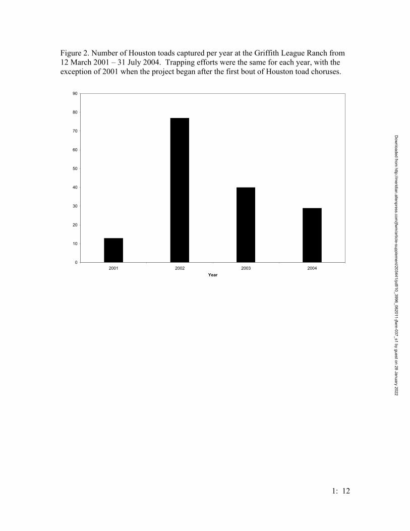
Figure 2. Number of Houston toads captured per year at the Griffith League Ranch from 12 March 2001 – 31 July 2004. Trapping efforts were the same for each year, with the exception of 2001 when the project began after the first bout of Houston toad choruses.

0

10

20

30

40

50

60

70

80

90

2001 2002 2003 2004Year

1: 12

Dow



m/article-supplem

ent/203441/pdf/10_3996_062011-jfwm


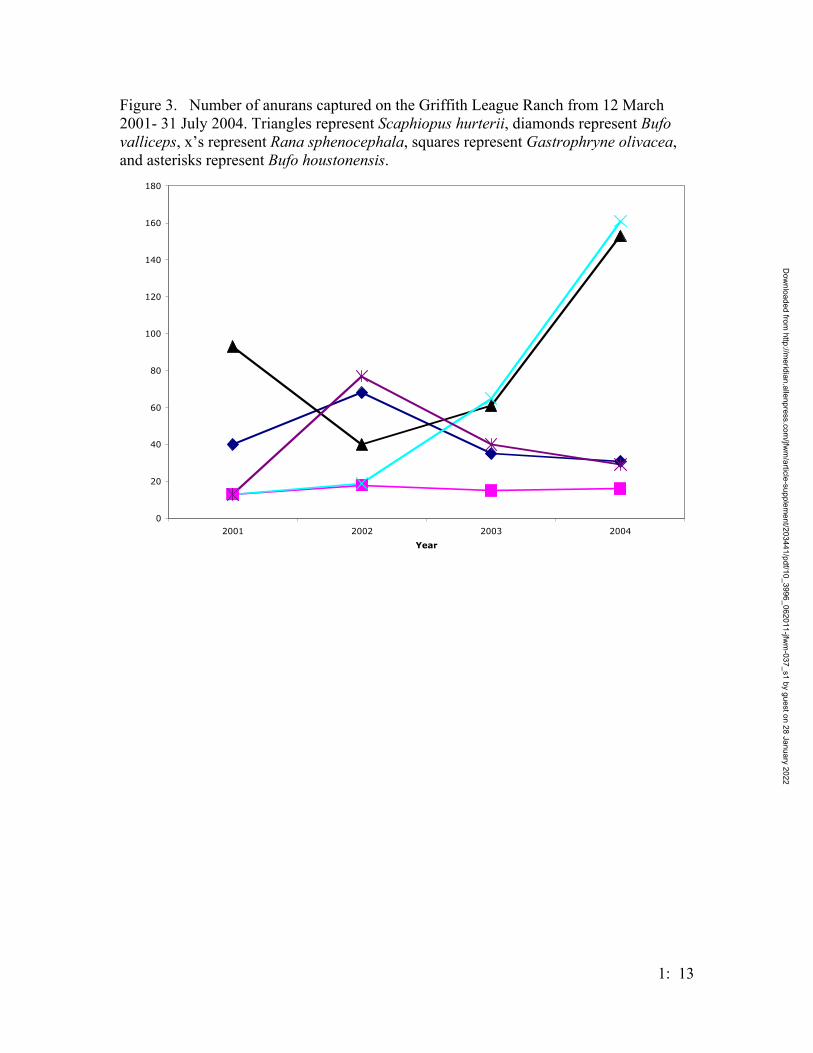
Figure 3. Number of anurans captured on the Griffith League Ranch from 12 March 2001- 31 July 2004. Triangles represent Scaphiopus hurterii, diamonds represent Bufo valliceps, x’s represent Rana sphenocephala, squares represent Gastrophryne olivacea, and asterisks represent Bufo houstonensis.

0

20

40

60

80

100

120

140

160

180

2001 2002 2003 2004

Year

1: 13

Dow



m/article-supplem

ent/203441/pdf/10_3996_062011-jfwm


Figure 4. Number of lizards captured at the Griffith League Ranch from 12 March 2001 – 31 July 2004. Triangles represent Sceloporus olivaceous, diamonds represent Cnemidophorus sexlineatus, X’s represent Anolis carolinensis, squares represent Sceloporus undulatus, and asterisks represent Scincella lateralis.

0

50

100

150

200

250

300

350

2001 2002 2003 2004

year

1: 14

Dow



m/article-supplem

ent/203441/pdf/10_3996_062011-jfwm


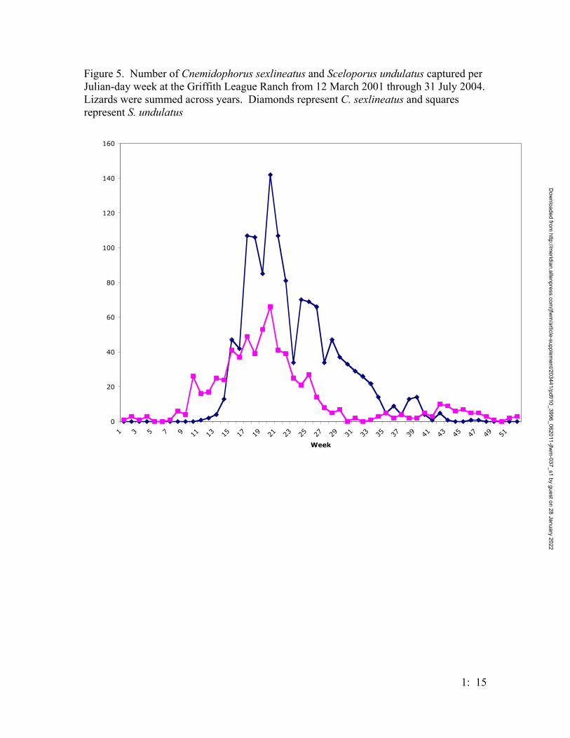
Figure 5. Number of Cnemidophorus sexlineatus and Sceloporus undulatus captured per Julian-day week at the Griffith League Ranch from 12 March 2001 through 31 July 2004. Lizards were summed across years. Diamonds represent C. sexlineatus and squares represent S. undulatus

0

20

40

60

80

100

120

140

160

1 3 5 7 9 11 13 15 17 19 21 23 25 27 29 31 33 35 37 39 41 43 45 47 49 51

Week

1: 15

Dow



m/article-supplem

ent/203441/pdf/10_3996_062011-jfwm


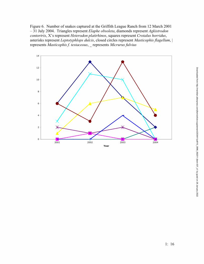
Figure 6. Number of snakes captured at the Griffith League Ranch from 12 March 2001 – 31 July 2004. Triangles represent Elaphe obsoleta, diamonds represent Agkistrodon contortrix, X’s represent Heterodon platirhinos, squares represent Crotalus horridus, asterisks represent Leptotyphlops dulcis, closed circles represent Masticophis flagellum, | represents Masticophis f. testaceous, _ represents Micrurus fulvius

0

2

4

6

8

10

12

14

2001 2002 2003 2004

Year

1: 16

Dow



m/article-supplem

ent/203441/pdf/10_3996_062011-jfwm


Figure 7. Number of snakes captured at the Griffith League Ranch from 12 March 2001 – 31 July 2004. Triangles represent Nerodia fasciata confluens, diamonds represent Nerodia erythrogaster, X’s represent Storeria dekayi, squares represent Nerodia rhombifer, asterisks represent Tantilla gracilis, closed circles represent Tantilla nigriceps, | represent Thamnophis proximus, _ represent Virginia striatula

0

2

4

6

8

10

12

2001 2002 2003 2004

Year

1: 17

Dow



m/article-supplem

ent/203441/pdf/10_3996_062011-jfwm


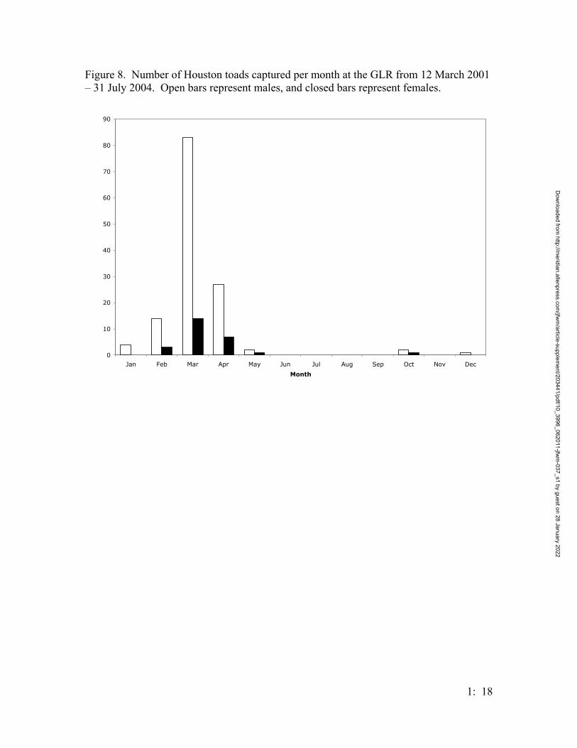
Figure 8. Number of Houston toads captured per month at the GLR from 12 March 2001 – 31 July 2004. Open bars represent males, and closed bars represent females.

0

10

20

30

40

50

60

70

80

90

Jan Feb Mar Apr May Jun Jul Aug Sep Oct Nov Dec

Month

1: 18

Dow



m/article-supplem

ent/203441/pdf/10_3996_062011-jfwm


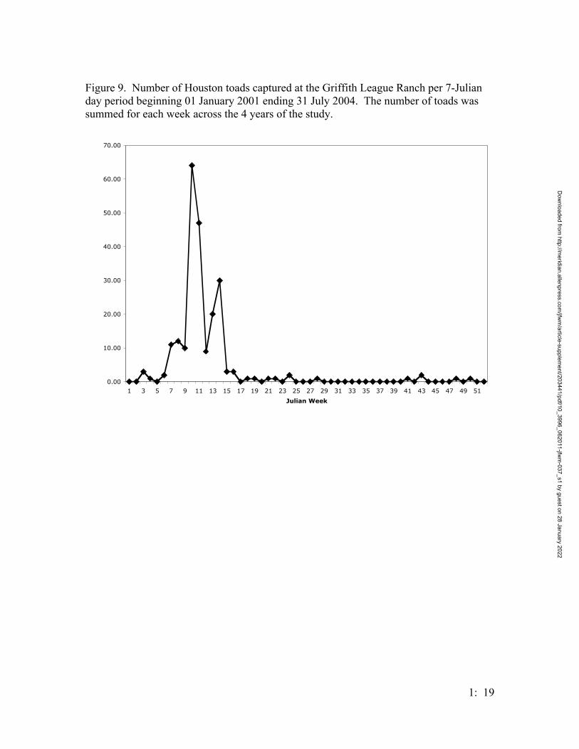
Figure 9. Number of Houston toads captured at the Griffith League Ranch per 7-Julian day period beginning 01 January 2001 ending 31 July 2004. The number of toads was summed for each week across the 4 years of the study.

0.00

10.00

20.00

30.00

40.00

50.00

60.00

70.00

1 3 5 7 9 11 13 15 17 19 21 23 25 27 29 31 33 35 37 39 41 43 45 47 49 51

Julian Week

1: 19

Dow



m/article-supplem

ent/203441/pdf/10_3996_062011-jfwm


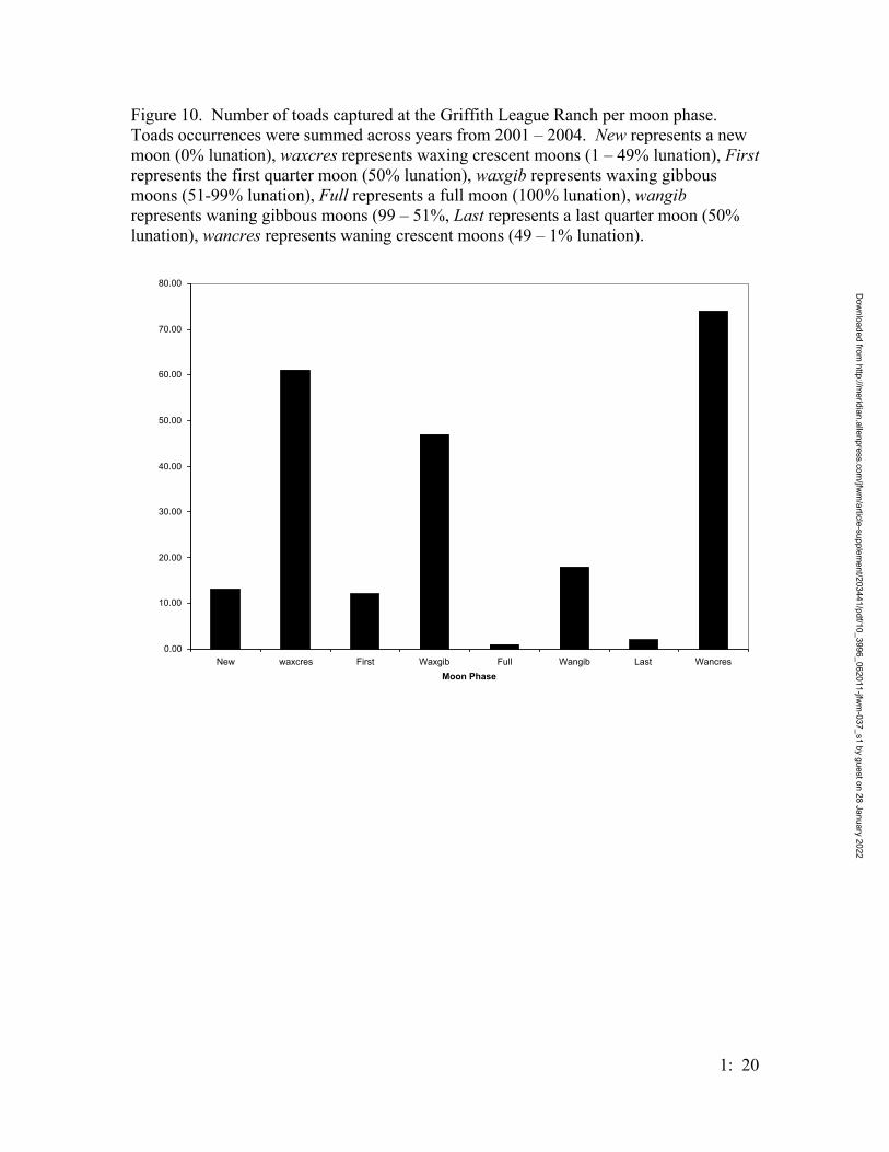
Figure 10. Number of toads captured at the Griffith League Ranch per moon phase. Toads occurrences were summed across years from 2001 – 2004. New represents a new moon (0% lunation), waxcres represents waxing crescent moons (1 – 49% lunation), First represents the first quarter moon (50% lunation), waxgib represents waxing gibbous moons (51-99% lunation), Full represents a full moon (100% lunation), wangib represents waning gibbous moons (99 – 51%, Last represents a last quarter moon (50% lunation), wancres represents waning crescent moons (49 – 1% lunation).

0.00

10.00

20.00

30.00

40.00

50.00

60.00

70.00

80.00

New waxcres First Waxgib Full Wangib Last WancresMoon Phase

1: 20

Dow



m/article-supplem

ent/203441/pdf/10_3996_062011-jfwm


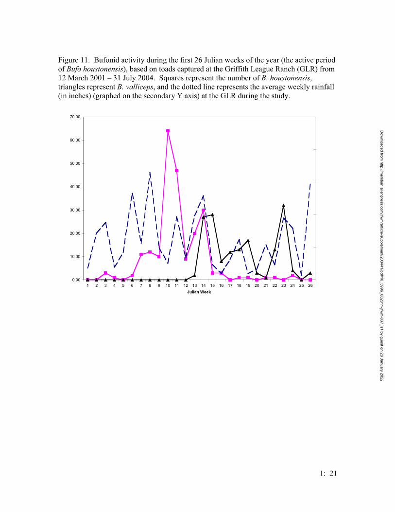
Figure 11. Bufonid activity during the first 26 Julian weeks of the year (the active period of Bufo houstonensis), based on toads captured at the Griffith League Ranch (GLR) from 12 March 2001 – 31 July 2004. Squares represent the number of B. houstonensis, triangles represent B. valliceps, and the dotted line represents the average weekly rainfall (in inches) (graphed on the secondary Y axis) at the GLR during the study.

0.00

10.00

20.00

30.00

40.00

50.00

60.00

70.00

1 2 3 4 5 6 7 8 9 10 11 12 13 14 15 16 17 18 19 20 21 22 23 24 25 26Julian Week

1: 21

Dow



m/article-supplem

ent/203441/pdf/10_3996_062011-jfwm


1: 22

SPATIAL DISTRIBUTION AND HABITAT ASSOCIATIONS OF ADULT HOUSTON TOADS

Todd M. Swannack1 and Michael R. J. Forstner21Department of Wildlife and Fisheries Sciences, Texas A & M University, College Station, Texas 77843;

E-mail: [email protected] 2Department of Biology, Texas State University at San Marcos, San Marcos, TX 78666;

E-mail: [email protected] INTRODUCTION One of the goals of conservation biology is to maintain native biodiversity,

regardless of taxonomic affiliation. Amphibians are currently the focus of concern

because of the perceived worldwide decline of the group (Barinaga, 1990). Amphibians

are important not only on a biodiversity scale, but also because they can be used as “bio-

indicator” species that help judge the integrity and health of an entire ecosystem.

As the human population continues to grow exponentially, encroaching and

fragmenting the remaining natural areas of the planet, natural resource managers and

conservation biologists are faced with an increasingly difficult task to develop

management strategies that both maximize biodiversity and provide some sustainable

value, economic or aesthetic, to the area of concern (Semlitsch, 2000). This is an

especially difficult task in areas with high levels of development, and is further

compounded if the area is within the distribution of an endangered species. Conservation

tools, such as buffer zones, can help protect native habitat for species; however, since

most organisms differ ontogenetically as to how they utilize their habitat, it is necessarily

important to understand the natural history of the different life stages of the target species

before restricting development to certain areas.

The Lost Pines region of Central Texas is the westernmost remnant of the

southern pine forests of the United States, and is a unique ecosystem due to its isolation

from the East Texas pineywoods (approx. 130 km separates the two regions). The Lost

Pines is home to several Texas endemics (Elliot’s short-tailed Shrew, Texas long-lipped

Dow



m/article-supplem

ent/203441/pdf/10_3996_062011-jfwm


1: 23

beetle, and the endangered Houston toad, to name a few); human-mediated development

and urban sprawl has fragmented the pine forests, leaving only patches of suitable habitat

within which these species thrive. In Bastrop County, the heart of the Lost Pines, two

large patches (over 1900 ha each), exist – Bastrop State Park (BSP) and the Griffith

League Ranch (GLR); there are currently no plans to significantly fragment either area.

While both BSP and GLR are large enough to provide suitable habitat for these

endemics, neither are pristine. Fire suppression and poor management have created

habitats with increased tree density and thick leaf-duff layers that do not represent the

natural condition of the region, and to which native species would be poorly adapted.

The Houston toad Bufo houstonensis is an endemic to South Central-East Texas,

and currently found in only 9 counties, with the largest known group being within the

Lost Pines region of Bastrop County. Due to its limited distribution, the toad was listed

as endangered in 1970 (Honegger, 1970). While B. houstonensis has received

considerable media attention, several critical aspects of its biology remain unknown, and

in order for conservation efforts to move forward, these components of the toad’s natural

history must be addressed.

Within Bastrop County, the Houston toad is currently being threatened by

encroaching development, yet only the chorus pond behavior of B. houstonensis has been

documented (Hillis et al., 1984; Price, 2003). Not only must the post-breeding movement

patterns of the toad must be documented, including how toads utilize their upland habitat,

where they go after the breeding season, but a quantitative characterization of their

habitat must be completed in order to determine the types of habitats B. houstonensis

utilize.

Dow



m/article-supplem

ent/203441/pdf/10_3996_062011-jfwm


1: 24

The purpose of this manuscript is to detail how the toad utilizes its habitat both

during and after the breeding season using radio telemetry and fluorescent powder, and to

also compare the habitat around known breeding ponds to determine if toads utilize

certain areas / habitat types more than others.

MATERIALS AND METHODS

This study took place at the Griffith League Ranch (GLR), which is within the

Lost Pines eco-region, located in Bastrop County, Texas (refer to Ch. 1 – Activity

Patterns for a complete description of the GLR).

Radio telemetry and fluorescent powder

Houston toads were captured for radio telemetry in 2003 & 2004. Toads were

either captured in the drift fence / pitfall array (refer to Ch. 1 – Activity Patterns for a

description of the trapping design) or at ponds during choruses. All individuals were

marked with PITs and radio telemeters (BD-2; 1.8g; Holohil Systems, Ontario Canada)

were placed on the individual within 30 minutes after capture. Only toads weighing

above 20 g received telemeters to stay within the 10% rule (White and Garrott, 1990). In

2003, spandex jackets (Figure 1A) were used to attach the telemeter to the toad; each

jacket weighed 0.5 grams. In 2004, a stainless steel beaded chain “belt” was created

(Rathburn and Murphey, 1996); the telemeter was attached to the belt with epoxy resin

and allowed to set overnight; the belts were made with extra beads and tailored (beads

were cut off) for individual toads. Males were generally collected while chorusing, and

females were collected in the pitfall traps; only non-gravid females were fitted with

telemeters.

Dow



m/article-supplem

ent/203441/pdf/10_3996_062011-jfwm


1: 25

Toads were located at least once every two days and locations were marked using

red marking flags. GPS coordinates were taken weekly using a Garmin GPS V. The

habitat immediately surrounding the radio-telemetered toad was recorded.

A black spandex jacket was placed on a single non-gravid female, captured on 2

May 2004. Inert fluorescent pigment (T1 series pigment, Radiant Color, Richmond, CA)

was placed underneath the jacket, against the dorsum of the toad. The female was

tracked each subsequent night until the jacket fell off, 48 hours from initial release.

Vegetation analysis

Woody vegetative cover was assessed using the line intercept method (Higgins et

al., 1996). The habitat immediately surrounding the drift fence / pitfall arrays (refer to

Ch. 1 – Activity Patterns) was measured in June 2004. Two 50 m intercepts were spaced

at each trap array. A randomly chosen bucket was used for the starting point; buckets

were assigned a number and a 4-sided die was rolled to determine the buckets used for

the analysis. Percent cover was calculated by summing canopy cover for the two

intercepts. Kiefer & Baccus (Ch. 5) and White & Simpson (Ch. 5) assessed the

vegetative cover for the rest of the GLR, using 25 additional reference points. A

principal component analysis was used to examine the habitat types of the traps and the

rest of the ranch to determine what type of canopy cover B. houstonensis utilized.

RESULTS AND DISCUSSION

Radio telemetry

Between 2003 and 2004 twelve B. houstonensis (7M, 5F) were fitted with radio

telemeters and 63 total observations were recorded. While the jackets were lightweight,

they did not stay on the toad for more than 4 days. The shortest monitoring period for an

individual was two days before the toad removed the jacket. The beaded chain belt

Dow



m/article-supplem

ent/203441/pdf/10_3996_062011-jfwm


1: 26

method (Rathburn and Murphey, 1996) worked better; the longest period of observation

was 6 weeks. Both males and females were released at the edge of a pond. Two of the 7

males stayed within 15 meters of the ponds edge, while the other 5 moved between 20 –

50 meters away from the pond. Females did not stay at the pond’s edge. Within two

days after release, all females had moved at least 50 m away from the ponds edge. Both

sexes chose hibernacula under fallen trees, generally oak stumps, and remained there.

Houston toads did not burrow more than 3 cm. Two females captured in 2004 were

observed in hibernacula, then observed foraging within two meters of their hibernacula,

and were re-located in the same hibernacula the following day. Foraging did not occur

every night; two toads were monitored every hour during a night of high anuran activity

(10 April 2004) and did not leave their hibernacula throughout the night. Toads did not

make any long excursions and generally remained in the same place for several

consecutive days. One individual, a female, moved from one hibernacula to another less

than 1 meter away and throughout the life of the telemeter (40 days), moved exclusively

between those two spots. While there are not enough data to determine a home range,

these data are valuable for qualitative descriptions of the post-breeding behaviors of the

females, and to a lesser degree males.

The fluorescent powder method provided a different type of result than the radio

telemetry. The female moved 3.2 m (straight line distance) from the release point, and

situated herself underneath a fallen oak tree. She did not move in a straight line,

however. The powder marks on the ground indicated she moved from the release point to

the tree and moved along the tree, paused (indicated by a higher concentration of

fluorescent powder), and then moved further down the length of the tree until she found a

Dow



m/article-supplem

ent/203441/pdf/10_3996_062011-jfwm


1: 27

hollow spot large enough to fit in. The female remained in the hollow for 48 hours after

release (confirmed visually), and then left, leaving the jacket, and all the powder.

Each of the telemetered individuals, regardless of sex, were found underneath

fallen logs; we assumed B. houstonensis uses the dead-fall for hibernacula. Several of the

hibernacula were lifted in order to determine if the toad was still present. Toads were not

buried more than 3 cm below the ground, and could usually be seen once the log was

removed. Most of the tree-fall utilized by toads were oak species; however, this may be

because the majority of toads were found in oak dominated habitat.

The woody vegetation was dominated by two species of oak: Quercus stellata,

and Quercus marilandica, loblolly pine Pinus taeda, Eastern red cedar Juniperus

virginiana, and yaupon Ilex vomitoria. The principal component analysis yielded three

distinct groupings, essentially, a grouping with dense canopy cover (dense pine stands

and yaupon), a grouping with moderate canopy cover (mostly oak), and a grouping zero

canopy cover (pasture land) (Figure 2). The majority of Houston toads were captured in

moderate canopy forest (all but 18 of the 159 individuals were captured in oak-pine

woodlands with low density of trees). During the study three individual males were

heard chorus, albeit infrequently, in areas with dense canopy; however, no egg strands or

post metamorphic juveniles were detected. The toads captured (15 individuals) in the

pastoral areas were only captured in at the border of the pasture and woodlands in

buckets no more than 15 meters away from moderate canopy forest, and near a drainage

that led to a pond, which has had B. houstonensis choruses every year since 2000.

While the system (the GLR) we have is one of the best remaining areas to study

the ecology of B. houstonensis within its historical distribution, it is very artificial. The

dense pine forest at the Southeastern edge of the ranch (refer to Figure 1 – Activity

Dow



m/article-supplem

ent/203441/pdf/10_3996_062011-jfwm


1: 28

Patterns) represents a 23 yr old clear cut (A. Sanson, pers. comm. to MRJF), which was

allowed to grow back without any management. The best habitat on the ranch for

Houston toads, based on the PCA (Figure 2) is a moderate canopy oak woodland. This

may be a consequence of oak duff decomposing quicker than pine duff. The pine duff at

the Southeastern edge is dense (Kiefer, Ch. 5) and even fire management would not

remove the duff layer quickly. If the GLR is going to be used as a refuge for the last

remaining Houston toad populations, then the property must be returned to its natural,

historical state. Both fire management and manual removal of the duff are recommended

in order recompose the natural integrity of the forest habitat on the GLR.

Dow



m/article-supplem

ent/203441/pdf/10_3996_062011-jfwm


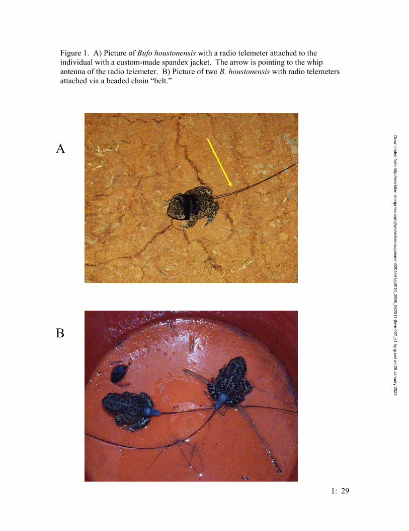
Figure 1. A) Picture of Bufo houstonensis with a radio telemeter attached to the individual with a custom-made spandex jacket. The arrow is pointing to the whip antenna of the radio telemeter. B) Picture of two B. houstonensis with radio telemeters attached via a beaded chain “belt.”

A

B

1: 29

Dow



m/article-supplem

ent/203441/pdf/10_3996_062011-jfwm


Figure 2. Results from a principal component analysis on the dominant vegetation of the GLR. Component 1 is canopy cover dominated by oak and pine; component 2 is canopy cover dominated by oak and negatively correlated with pine. The PCA yielded 3 separations, an area with 0% canopy cover (blue), an area with moderate canopy cover (orange) and an area with dense canopy cover (gray). The majority of Houston toads (greater than 90%) captured during this study were captured in areas with moderate canopy cover. Pita represents canopy cover (CC) from Pinus taeda, Quma represents CC from Quercus marilandica, Qust represents CC from Quercus stellata, Qusum represents CC from the sum of the oak component, Ilvo represents CC from Ilex vomitoria, and Juvi represents CC from Juniperus virginiana. Numbers represent either vegetation from the trap lines (1 – 18) or transects (19 – 43)

y

Com

p.2

-0.2

0.0

0.2

0.4

1

2

3

4

5

67

8

910111213

14

15

16

17

18

19

20

21 22

23

24

25

2627 29

31

34

35

3637

38

4041

42

-100 -50 0 50 100

-50

050

100

Ilvo

JuviQuma

Qust

QuSum

Moderate canopy

Dense canopy

Incr

easi

ng O

ak a

nd D

ecre

asin

g Pi

ne C

anop

y

Dow



m/article-supplem

ent/203441/pdf/10_3996_062011-jfwm

-037_s1 by guest on 28 Janua
0% canop
Comp.1

-0.2 0.0 0.2 0.4

2830

3233

39

43 -100Pita

Increasing Oak and Pine Canopy

1: 30

ry 2022

1: 31

POPULATION DYNAMICS OF ADULT HOUSTON TOADS

Todd M. Swannack1 and Michael R. J. Forstner2

1Department of Wildlife and Fisheries Sciences, Texas A & M University, College Station, Texas 77843; E-mail: [email protected]

2Department of Biology, Texas State University at San Marcos, San Marcos, TX 78666; E-mail: [email protected]

INTRODUCTION

While congeneric species may have similar life history strategies (Frazer et al.,

1990), detailed studies of the population dynamics of individual species remain

important, especially in the case of threatened or endangered species, as each species

possesses unique life history attributes, which affect its demographic dynamics. The

current concern over the decline of the amphibian populations (Barinaga, 1990;

Pechmann et al., 1991) re-emphasizes this importance – as amphibian species become

more rare, it becomes more important to fill in the knowledge gaps about the remaining

populations as quickly as possible.

The population dynamics of several species of Bufonid toads have been

thoroughly studied including the Gulf Coast toad Bufo valliceps, (Blair, 1961); the

American toad B. americanus (Christein and Taylor, 1978); Fowler’s toad B. woodhousei

foweleri, (Clarke, 1974) and the Common toad B. bufo (Gittins et al., 1985); however,

such data do not exist for most species of toads, including the highly endangered Houston

toad Bufo houstonensis. The purpose of this manuscript is to examine the dynamics of

the B. houstonensis population at the Griffith League Ranch in Bastrop County, Texas.

We further sought to place the annual dynamics of B. houstonensis in context with other

species of herpetofauna on the site for the same period in order to demonstrate the

different population trends occurring among herptile species on the GLR.

Dow



m/article-supplem

ent/203441/pdf/10_3996_062011-jfwm


1: 32


Trap design and data collection

Refer to Ch 1. Activity Patterns for a detailed description of the trapping regime at the GLR. Population dynamics

In order to examine the population dynamics of the Houston toad alongside other

amphibian and reptile species at the GLR, captured individuals were divided into two

categories: initial captures and recaptures. The time period for the mark-recapture

analyses was year, individuals were only counted once per year, either as an initial

capture or recapture. The percentage recapture per year was calculated for the

numerically dominant species collected during this study. Enough data were gathered for

Bufo houstonensis, B. valliceps, Scaphiopus hurteri, Cnemidophorus sexlineatus, and

Sceloporus undulatus to allow analyses.

In addition to the above analyses the B. houstonensis mark-recapture data was

examined using a full Jolly-Seber model (Krebs, 1999) in POPAN (Arnason et al., 1998).

The assumptions of the Jolly-Seber model include an open population (populations that

constantly change size because of differential rates of birth, death, immigration, and

emigration), equal catchability of marked and unmarked individuals, individuals are

clearly marked, and marks are not overlooked. An open population was assumed since B.

houstonensis are known to occur on several adjacent properties (e.g., B. houstonensis

were heard calling at a pond at the property bordering the Northern corner of the GLR),

both marked and unmarked individuals had an equal probability of being captured on any

given sample night; throughout the study we did not notice a difference among these

categories, and finally, for this analysis only adults with PITs (113 individuals) were

Dow



m/article-supplem

ent/203441/pdf/10_3996_062011-jfwm


1: 33

used, and since all B. houstonensis were scanned with a PIT reader, it was highly unlikely

that marks were overlooked.

RESULTS

From 2001 – 2004, 159 individual adult Houston toads were captured. Fourteen

toads, all males, were recaptured during subsequent years, an overall recapture rate of

8%. Females were not recaptured during this study. The percent recapture varied among

years, and other herpetofauna were not recaptured as frequently as B. houstonensis (Table

1). The recaptured Houston toads were distributed temporally as follows: two toads were

originally captured in 2001, and recaptured in 2002; six toads were initially captured in

2002 and recaptured in 2003; five toads initially captured in 2002 were recaptured in

2004. One individual was initially captured in 2002, and recaptured in 2003 and again in

2004.

The results from the Jolly-Seber model predicted adult B. houstonensis

survivorship at 12.47% from 2001 – 2002 and 12.19% from 2002 – 2003. Estimates

from 2003 – 2004 were unavailable due to the time period being too close to the end of

the sample chain. The population size estimate from the model for 2002 was 2373

individuals, and 2764 individuals for 2003, although these are obviously larger than the

actual population size. Estimates of abundance were unavailable for the first and last

time step.

DISCUSSION

Bufo houstonensis had the highest recapture rate among the herpetofaunal species

collected at the GLR during the 4-year study. This result maybe misleading, as this study

was specifically designed to capture B. houstonensis, so more effort went into collecting

Houston toads than any other species. Individuals initially captured in 2001 had a higher

Dow



m/article-supplem

ent/203441/pdf/10_3996_062011-jfwm


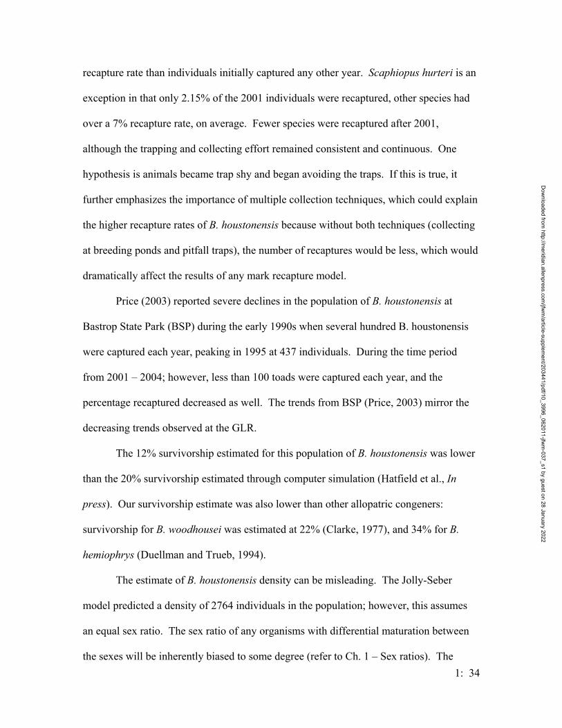
1: 34

recapture rate than individuals initially captured any other year. Scaphiopus hurteri is an

exception in that only 2.15% of the 2001 individuals were recaptured, other species had

over a 7% recapture rate, on average. Fewer species were recaptured after 2001,

although the trapping and collecting effort remained consistent and continuous. One

hypothesis is animals became trap shy and began avoiding the traps. If this is true, it

further emphasizes the importance of multiple collection techniques, which could explain

the higher recapture rates of B. houstonensis because without both techniques (collecting

at breeding ponds and pitfall traps), the number of recaptures would be less, which would

dramatically affect the results of any mark recapture model.

Price (2003) reported severe declines in the population of B. houstonensis at

Bastrop State Park (BSP) during the early 1990s when several hundred B. houstonensis

were captured each year, peaking in 1995 at 437 individuals. During the time period

from 2001 – 2004; however, less than 100 toads were captured each year, and the

percentage recaptured decreased as well. The trends from BSP (Price, 2003) mirror the

decreasing trends observed at the GLR.

The 12% survivorship estimated for this population of B. houstonensis was lower

than the 20% survivorship estimated through computer simulation (Hatfield et al., In

press). Our survivorship estimate was also lower than other allopatric congeners:

survivorship for B. woodhousei was estimated at 22% (Clarke, 1977), and 34% for B.

hemiophrys (Duellman and Trueb, 1994).

The estimate of B. houstonensis density can be misleading. The Jolly-Seber

model predicted a density of 2764 individuals in the population; however, this assumes

an equal sex ratio. The sex ratio of any organisms with differential maturation between

the sexes will be inherently biased to some degree (refer to Ch. 1 – Sex ratios). The

Dow



m/article-supplem

ent/203441/pdf/10_3996_062011-jfwm


1: 35

effective population size (Ne) quantifies breeding population sizes for populations with

biased sex ratios (Freeman and Herron, 1998), and from the data gathered at the GLR,

assuming a 4M : 1F sex ratio, Ne is 1769 individuals in the population. While this

estimate is significantly lower than what the Jolly-Seber model predicted, it is more

accurate, as the sex ratio in B. houstonensis is significantly male-biased. These results

indicate that toad densities at the GLR are incredibly low, and conservation strategy that

increase the number of toads, especially adult females, are vitally important to the

survival of the Houston toad.

Dow



m/article-supplem

ent/203441/pdf/10_3996_062011-jfwm


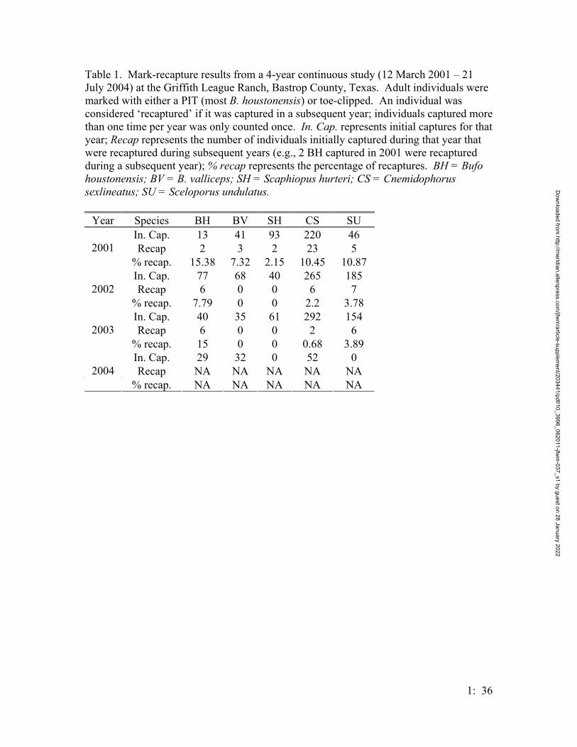
1: 36

Table 1. Mark-recapture results from a 4-year continuous study (12 March 2001 – 21 July 2004) at the Griffith League Ranch, Bastrop County, Texas. Adult individuals were marked with either a PIT (most B. houstonensis) or toe-clipped. An individual was considered ‘recaptured’ if it was captured in a subsequent year; individuals captured more than one time per year was only counted once. In. Cap. represents initial captures for that year; Recap represents the number of individuals initially captured during that year that were recaptured during subsequent years (e.g., 2 BH captured in 2001 were recaptured during a subsequent year); % recap represents the percentage of recaptures. BH = Bufo houstonensis; BV = B. valliceps; SH = Scaphiopus hurteri; CS = Cnemidophorus sexlineatus; SU = Sceloporus undulatus.

Year Species BH BV SH CS SU In. Cap. 13 41 93 220 46 Recap 2 3 2 23 5 2001

% recap. 15.38 7.32 2.15 10.45 10.87 In. Cap. 77 68 40 265 185 Recap 6 0 0 6 7 2002

% recap. 7.79 0 0 2.2 3.78 In. Cap. 40 35 61 292 154 Recap 6 0 0 2 6 2003

% recap. 15 0 0 0.68 3.89 In. Cap. 29 32 0 52 0 Recap NA NA NA NA NA 2004

% recap. NA NA NA NA NA

Dow



m/article-supplem

ent/203441/pdf/10_3996_062011-jfwm


1: 37

A POSSIBLE CAUSE FOR THE DISPARITY IN THE SEX RATIO OF THE EXPLOSIVELY BREEDING HOUSTON TOAD

Todd M. Swannack1 and Michael R. J. Forstner2

1Department of Wildlife and Fisheries Sciences, Texas A & M University, College Station, Texas 77843-2258; [email protected]

2Department of Biology, Texas State University at San Marcos, San Marcos, Texas 78666; E-mail: [email protected]

INTRODUCTION

Anurans exhibit several different temporal breeding strategies, from continuous

year-long breeding (prolonged) to short, seasonal breeding (explosive) that last from a

few days to a few weeks (Wells, 1977). Several species on the explosive end of the

breeding strategy continuum may have a breeding season lasting for several months, but

even then breeding activity actually occurs in intermittent bursts, termed breeding

periods, throughout the season, usually depending on favorable climatic conditions

(Wells, 1977; Zug, 1993; Duellman & Treub, 1994).

Most male anurans congregate and vocalize to attract females to a breeding area.

This breeding strategy most resembles a lek, where males are displaying to attract

females (Emlen, 1976). Males are concentrated at the breeding ponds and chorusing;

females do not visit the ponds simultaneously, but rather as individuals become receptive.

The adult sex ratio at any given instant at a breeding pond will most likely be male-biased

as a result of this breeding strategy. The breeding individuals function under an

operational sex ratio (OSR), which is the ratio of potentially mating males to receptive

females at any instant (Emlen, 1976). While the OSR is a valuable tool for examining

reproductive dynamics, it is not a good indicator of the population structure.

Unfortunately, accurate sex ratio estimates are difficult to obtain for explosively breeding

anurans, especially those species that retreat to hibernacula as soon as the breeding

Dow



m/article-supplem

ent/203441/pdf/10_3996_062011-jfwm


1: 38

season is over. An accurate sex ratio estimate of a population is an important

demographic measurement because of the potential influence each gender has on the

population dynamics (Gibbons, 1990). An intrinsically biased sex ratio lowers the

effective population size (Ne) (Freeman and Herron, 1998), which is the number of

individuals that actually contribute to reproduction in the population (Wilson, 1975).

Accurate sex ratio estimates are necessary to examine the population and genetical

dynamics of any species, and given the current concern for declining amphibian

populations (Barinaga, 1990; Blaustein and Wake, 1990) these data are especially

important in the cases of threatened or endangered amphibbians where they may provide

valuable direction for conservation and management efforts.

The Houston toad Bufo houstonensis is a relict descendant of the narrow-skulled

Bufo americanus species group, diverging from southernmost populations of ancestral B.

americanus within the last 10,000 years (Blair, 1972). Sanders (1953) first described B.

houstonensis, and its specific identity was reconfirmed genetically by Hillis et al. (1984).

Bufo houstonensis is an endemic Texas amphibian, historically distributed in South-

central Texas in areas underlain with deep, sandy soils associated with pine – mixed-oak

woodlands (Brown, 1971). The paucity of these habitats and the destruction of these

habitat types associated with urban expansion during the last half of the 20th century have

decreased the geographic distribution of B. houstonensis to 9 Texas counties. The largest

remaining group occurs in the Lost Pines region of Bastrop county; smaller, further

isolated groups are still found in adjacent Burleson and Lee counties (Dixon, 2000;

Gaston et al., 2001). This limited distribution alongside perceived declines caused B.

houstonensis to be listed on both national and international endangered species lists

(Gottschalk, 1970; Honegger, 1970). Although the Houston toad has received

Dow



m/article-supplem

ent/203441/pdf/10_3996_062011-jfwm


1: 39

considerable media attention due to its endangered status, the majority of previous studies

mainly focused on the toad’s reproductive biology (Hillis et al., 1984; Price, 2003).

The breeding strategy of the Houston toad falls onto the explosive side of the

anuran breeding continuum. The breeding season extends from late January through

early May (Hillis et al., 1984); however, B. houstonensis does not breed continuously

throughout the season, instead breeding activity and chorusing occurs intermittently in 3

– 5 day spurts, correlated in part with the dark of the moon (Price, 2003; pers. obs.). Bufo

houstonensis is an excellent model for examining the sex ratio of an explosive breeding

anuran not only because both Hillis et al., (1984) and Price (2003) reported male-biased

sex ratios (from data gathered from breeding locations), but also because the Houston

toad has been the focus of an extensive 3-year study encompassing both breeding pond

surveys and drift fences placed throughout Houston toad habitat (Forstner and Ahlbrandt,

2003). The objectives of this study were: 1) to establish an accurate sex ratio of B.

houstonensis captured at the Griffith League Ranch and to determine if the sex ratio was

the result of sampling error or a natural phenomenon, and 2) to explore, through

computer simulation, possibilities as to what could cause the sex ratio to be naturally

biased.


Study System and Field Research

The Griffith League Ranch (GLR) is a 1951 ha property owned by the Boy Scouts

of America (BSA) in Bastrop County, 91% of the property is underlain by deep sandy

soils of the Patilo, Demona, or Silstid series, and the GLR was historically a pine and

mixed hardwood forest. Three large tracts of approximately 200 ha each were cleared for

cattle grazing early in the 20th century. B. houstonensis were originally detected on the

Dow



m/article-supplem

ent/203441/pdf/10_3996_062011-jfwm


1: 40

property during the early 1980s (A. Price, pers comm). Beginning in 2000, audio surveys

were conducted to determine the current distribution of Houston toads on the GLR. B.

houstonensis choruses were heard at 12 of the 17 ponds on the property.

In March 2001, 5 linear drift fences (two 121 m, three 153 m), with 5-gallon

pitfalls every 30 m, were placed along the border of the forest and pasture to determine if

toads utilized pasture habitats. In addition to the pasture traps, three Y-shaped drift

fence arrays were placed in 3 habitats (one trap per habitat): 30 m from a breeding pond

(Pond 2) in pine forest, in mixed oak woodland, and in a small (~2 ha) natural clearing.

In February 2002, seven additional Y-shaped arrays and pitfalls were added, creating the

following trapping design: 4 traps surrounding Pond 2, one at each cardinal point, at

randomly chosen distances from the pond’s edge (10m, 30m, and 2 at 50m); 2 treatments

of 3 traps placed 150 m apart, with the first traps in each treatment being equidistant from

a known B. houstonensis breeding pond (FIG. 1).

Traps were checked every morning throughout the study period. Snout-urostyle

length (SUL), head width (HW), and weight were recorded for all anurans. Standard

measurements were taken for all other vertebrate taxa. Each adult B. houstonensis

received a passive integrated transponder (PIT) tag. Juvenile Bufo sp. and all other

vertebrate taxa were toe-clipped. All organisms were released near their capture site

shortly after collection.

Nightly surveys were conducted at each of the 17 ponds at the GLR during the

breeding seasons of 2001 and 2002. Any B. houstonensis captured were measured and

marked accordingly, and released at the spot of capture within 10 minutes.

Sex ratios were established for the total sample, pitfall traps, and breeding ponds.

Each observed ratio was tested for differences from parity using a χ2 test corrected for

Dow



m/article-supplem

ent/203441/pdf/10_3996_062011-jfwm


1: 41

continuity, and a minimum sex ratio that was not significantly different from the data was

established for each sample. The sex ratios established from the trapping data and

breeding pond data were tested for differences between each other. Critical statistical

values were taken from Draper and Smith (1998).

Simulation model

According to data gathered from a captive study (Quinn and Mengden, 1984),

male B. houstonensis mature in 1 year while females mature in 2 years. We were

interested to quantitatively determine how the adult sex ratio was affected by delayed

maturation and the associated differential mortality of the 1-year age class. One-year old

males are sexually mature and exhibit behaviors associated with reproduction, while one-

year old females are still juveniles and do not exhibit reproductive behavior and would

therefore experience a different mortality regime. In order to examine the hypothesis that

the bias in the adult sex ratio is, at least in part, a result of delayed maturation, a

simulation model was created using STELLA® v7 (High Performance Systems, 2001).

The model was represented mathematically as a discrete-time compartment model with a

1-year time step. Recruitment (R) into the terrestrial population was the driving variable

(see Grant et al., 1997 for specific definitions of variable types) of the model and was

parameterized as constant, adding the same number of new individuals to the system at

the beginning of each time step; eggs and tadpoles were included together. The sex ratio

was assumed equal at birth since gender is determined genetically in toads (Duellman and

Trueb, 1994), and mortality was not calculated as immature individuals are not thought to

possess behavioral differences which would significantly alter the adult sex ratio

(Gibbons, 1990). The state variables were the four terrestrial life stages of B.

houstonensis: post-metamorphic juveniles (PMJ), sexually mature adult males (AM),

Dow



m/article-supplem

ent/203441/pdf/10_3996_062011-jfwm


immature females (IF), and sexually mature adult females (AF). Mortality for PMJ was

once again assumed not to affect the adult sex ratio and not parameterized for the

metamorphs. After the first time step, 50% of the individuals in the PMJ state variable

were transferred to the AM state variable and the other half went into IF; assuming an

equal sex ratio at parturition, within a given cohort half of the individuals will be males

and mature in a single time step, the remaining individuals will be the immature females.

A conservative assumption of this model was that the adult mortality was constant

between the genders. Male B. houstonensis have a higher predation risk during the active

period (breeding season) since they will return to a breeding site multiple times in a

season, while females visit a breeding location once per season. Our data indicate a

significant male-biased sex ratio, which cannot be explained by higher predation on

males. IF mortality (ζ) was a constant, which was re-parameterized for each simulation –

ζ was calculated and immature females were removed for each time step. The state

variables were calculated as follows:

1) PMJt+1 = PMJt + R −PMJt( )∆t

2) AM t+1 = AM t + .5PMJt( )∆t

3) IFt+1 = IFt + .5PMJt −ζIFt − (IFt −ζIFt )( )∆t

4) AFt+1 = AFt + IFt −ζIFt( )∆t

Five simulations were executed based on maturation data from a captive

population with males maturing in 1 year and females maturing in 2 (Quinn and

Mengden, 1984); ζ was set at either 0.01, 0.1, 0.25, 0.5 or 0.75 for each simulation.

Another 5 simulations were executed, delaying female maturation by another time step

1: 42

Dow



m/article-supplem

ent/203441/pdf/10_3996_062011-jfwm


1: 43

(males matured in 1 year, females in 3) to simulate the effects of an extended growing

season (i.e., harsh environmental conditions preventing maturation within two years).

The same values for ζ were used for the second set of trials. Each simulation was run for

10 years to allow ample time for the model to stabilize. Adult sex ratios were established

as the proportion of AM : AF and expressed as the proportion of during each time step.

The resulting sex ratios were tested for differences from parity using χ2 test corrected for

continuity.

RESULTS

Between 5 March 2001 and 30 November 2003, a total of 129 (116M : 13F)

individual adult B. houstonensis was captured at the GLR; collection at the breeding

ponds yielded 84 (79M : 5F) toads, and the drift fence / pitfall traps captured 45 (37M :

8F). The sex ratios for the total sample and the two different collection methods (hand

collection at the ponds and toads captured in traps) were all male biased and significantly

different from parity (P > .05) (Table 1). Minimum sex ratios were established for which

the data were not significantly different, e.g., the actual sex ratio for the total sample was

8.92M : 1F, which is not significantly different from 5M : 1F; however, it is significantly

different from 4M : 1F (Table 1). The actual sex ratio established from the trapping

results (4.6M : 1F) was significantly different from the sex ratio of toads captured at

breeding ponds (15.8M: 1F) (χ2 = 8.33, P = .003)

The results of the 10 simulations are shown in Figure 1. The model stabilized two

time steps after female maturation. When females matured in 2 years, adult sex ratio

was not significantly different from parity at the three lowest values of ζ (0.01, 0.1, and

0.25) (P > .15); at higher values of ζ (0.5 & 0.75), the adult sex ratio was significantly

Dow



m/article-supplem

ent/203441/pdf/10_3996_062011-jfwm


1: 44

biased (P < .001). When females matured in 3 years the sex ratios were not significantly

different from 1: 1 at the two lower values of ζ (0.01, 0.1); the three higher values of ζ

(0.25, 0.5, & 0.75) produced significantly biased sex ratios (P < .006). An interesting

property of the model emerged – the sex ratio increased exponentially between the two

models. The final sex ratio at ζ = 0.5 and females maturing in 2 years and was 2M : 1F,

and 4M : 1F at females maturing in 3 years. This pattern holds when comparing each

pair of ζ values across the two maturation times.

DISCUSSION

The sex ratio for the overall sample of B. houstonensis at the GLR was

significantly male-biased. Previous studies on B. houstonensis reported male-biased sex

ratios as well (Hillis et al., 1984; Price, 2003); however, in those studies toads were only

collected at chorusing ponds, which could artificially bias the sample as the mating

system of B. houstonensis involves multiple males congregating and chorusing at ponds

to attract females. While previous studies (Hillis et al., 1984; Price, 2003), and the

chorusing pond capture data from this study were only initial captures, males are more

conspicuous and therefore easier to capture at breeding sites. The sex ratio of B.

houstonensis captured at the drift fence / pitfall arrays should more accurately reflect the

true sex ratio of the population as the traps were placed to capture toads as they moved

across the landscape, regardless of gender, minimizing collection site-mediated error.

The sex ratio of toads captured in traps was less biased, but still significantly different

from parity; the minimum sex ratio for this sample was 3M : 1F, and was significantly

different from the pond data. This indicated that the bias in the sex ratios from both

previous studies is indeed better explained by an operational sex ratio (Emlen, 1976).

Dow



m/article-supplem

ent/203441/pdf/10_3996_062011-jfwm


1: 45

Survivorship for juvenile toads is low ( Zug and Zug, 1979; Greuter, 2004;). The

results from the simulation model (FIG. 1) show that higher mortalities associated with

the IF life stage would result in a male biased sex ratio. Female B. houstonensis raised in

captivity matured in 2 years (Quinn and Mengden, 1984). If a female arrived at the

breeding site and deposited eggs early in the breeding season, then her female offspring

would be mature by their second year; however, if a female deposited eggs late in the

season, her female offspring would not be mature for 3 years. The simulations show that

there is a large difference in the adult sex ratio at higher mortalities between 2 and 3

years. The longer it takes for females to reach maturity, the more male biased the adult

sex ratio will be.

Females can achieve a larger size by delaying maturation, and since fecundity is

positively correlated with size in toads (Reading, 1986), longer maturation times result in

larger clutch sizes. The trade-off, however, results in fewer females reaching sexual

maturity, especially if the mortality of juvenile females is high. A male-biased sex ratio

results in a lower effective population size (Freeman and Herron, 1998), which will

decrease genetic variation more rapidly than a population with sex ratio at parity.

The results from this study indicate the bias in the adult sex ratio of B.

houstonensis can at least, in part, be explained by differential mortality experienced as a

result of delayed maturation by females, which would dramatically lower the effective

population size. Using the numbers from this study, Ne at parity would be 129

individuals, 82.56 individuals at the 4M : 1F sex ratio from the trapping data, 46.76 from

the 8M : 1F sex ratio from the overall sample, and 29.76 from the 15M : 1F sex ratio

established from the chorusing pond data (Ne was calculated from Ne = 4(NmalesNfemales) /

(Nmales + Nfemales) from Freeman and Herron (1998)). This is further exacerbated for

Dow



m/article-supplem

ent/203441/pdf/10_3996_062011-jfwm


1: 46

species with fragmented habitats. In the case of the Houston toad, where migration

among patches is incredibly limited, and in the majority of instances almost impossible

due to development, a male-biased sex ratio will be a natural, intrinsic property of the

dynamics of increasingly smaller and more isolated populations, increasing the

importance of each individual female. This dramatically affects management

applications as strategies that maximize female toad survival are likely to have significant

effects on Houston toad recovery.

Dow



m/article-supplem

ent/203441/pdf/10_3996_062011-jfwm


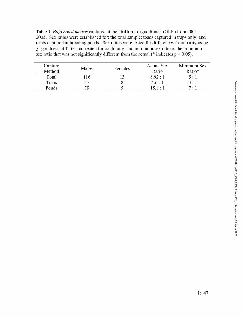
1: 47

Table 1. Bufo houstonensis captured at the Griffith League Ranch (GLR) from 2001 – 2003. Sex ratios were established for: the total sample; toads captured in traps only; and toads captured at breeding ponds. Sex ratios were tested for differences from parity using χ2 goodness of fit test corrected for continuity, and minimum sex ratio is the minimum sex ratio that was not significantly different from the actual (* indicates p > 0.05).

Capture Method Males Females Actual Sex

Ratio Minimum Sex

Ratio* Total 116 13 8.92 : 1 5 : 1 Traps 37 8 4.6 : 1 3 : 1 Ponds 79 5 15.8 : 1 7 : 1

Dow



m/article-supplem

ent/203441/pdf/10_3996_062011-jfwm


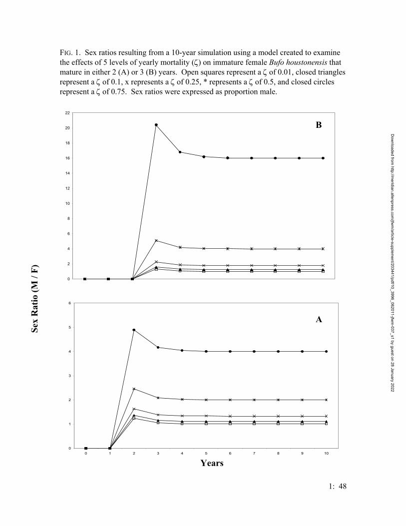
FIG. 1. Sex ratios resulting from a 10-year simulation using a model created to examine the effects of 5 levels of yearly mortality (ζ) on immature female Bufo houstonensis that mature in either 2 (A) or 3 (B) years. Open squares represent a ζ of 0.01, closed triangles represent a ζ of 0.1, x represents a ζ of 0.25, * represents a ζ of 0.5, and closed circles represent a ζ of 0.75. Sex ratios were expressed as proportion male.

0

2

4

6

8

10

12

14

16

18

20

22

B

Sex

Rat

io (M

/ F)

0

1

2

3

4

5

6

0 1 2 3 4 5 6 7 8 9 10

A

Years

1: 48

Dow



m/article-supplem

ent/203441/pdf/10_3996_062011-jfwm


THE IMPORTANCE OF JUVENILE ECOLOGY IN THE CONSERVATION AND MANAGEMENT

OF THE ENDANGERED HOUSTON TOAD, BUFO HOUSTONENSIS (ANURA: BUFONIDAE)

KENSLEY L. GREUTER AND MICHAEL R. J. FORSTNER

The Houston toad, Bufo houstonensis, is an endangered species that, despite

efforts to obtain life history information, retains many unknowns about of its ecology.

These ecological unknowns have inhibited management practices to the extent where

only practices to benefit the adult population have been applied (Hatfield 2002). To

determine the best management practices for any endangered species, data from all stages

of the life cycle are optimal. Data from the juvenile stage are particularly important, as

this stage is subject to higher vulnerability because of rapid desiccation (Werner 1986).

Anuran juveniles depend on wetlands and the surrounding upland habitat for their

survival (Semlitsch 2000a). To document this habitat dependence in B. houstonensis

juveniles, base line data on survivorship from egg to metamorph are necessary. Once this

is achieved, the development of techniques for determining juvenile growth, dispersal,

and morphological identification can be made. These techniques will allow more

efficient data collection and aid in management practices, including the definition of

appropriate buffer zones, for conservation of the species.

THE HOUSTON TOAD

The Houston toad was federally listed as an endangered species in 1970 (Peters

1968 found in Quinn and Mengden 1981). The listing was based primarily on strict

habitat requirements, its scarcity in perceived, and since realized, habitat destruction

2: 1

Dow



m/article-supplem

ent/203441/pdf/10_3996_062011-jfwm


(Brown 1975). Destruction of habitat has been linked mainly to agricultural use and

urban expansion and peripherally to watershed alteration. The decline of the species was

also resulted from failure in reproduction and survival during droughts (U. S. Fish and

Wildlife Service 1992). Hybridization with sympatric congeners has had an impact on

the species as well (Kennedy 1961, Brown 1971, Hillis et al. 1984).

Bufo houstonensis is a Texas endemic species with distribution in Bastrop,

Burleson, and Lee counties with scarce subpopulations located in 6 other counties

including Austin, Colorado, Lavaca, Leon, Milam, and Robertson counties (Jacobson

1989). Historically, the Houston toad occurred in Fort Bend, Harris, and Liberty counties

(U. S. Fish and Wildlife Service 1992); however, no recent records exist for those areas.

The preferred B. houstonensis habitat is deep, carrizo sand often in or near pines

of the Post Oak Savannah Region of Texas (Kennedy 1962, Brown 1971, Brown and

Thomas 1982). Because adult Houston toads are poor burrowers and have difficulty

digging into compacted soil (Bragg 1960), they select the soft, pliable sand of central

Texas. However, juveniles may not necessarily be confined to this soil type as they

might seek moist shelter under leaf litter (Clarke 1974).

Bufo houstonensis is a small toad 5.0 - 8.5 cm long and is similar in appearance to

the American toad, Bufo americanus. In fact, B. houstonensis is a relict descendant of the

narrow skulled B. americanus group (Hillis et al. 1984). General coloration varies from

light brown to gray or purplish gray, sometimes with green patches. They have pale

ventral surfaces, which often have small, dark spots. Males have a dark throat coloration

(U. S. Fish and Wildlife Service 1992). Figure 1 depicts an adult Houston toad (B.

houstonensis) with the characteristic mottled coloration and size.

2: 2

Dow



m/article-supplem

ent/203441/pdf/10_3996_062011-jfwm


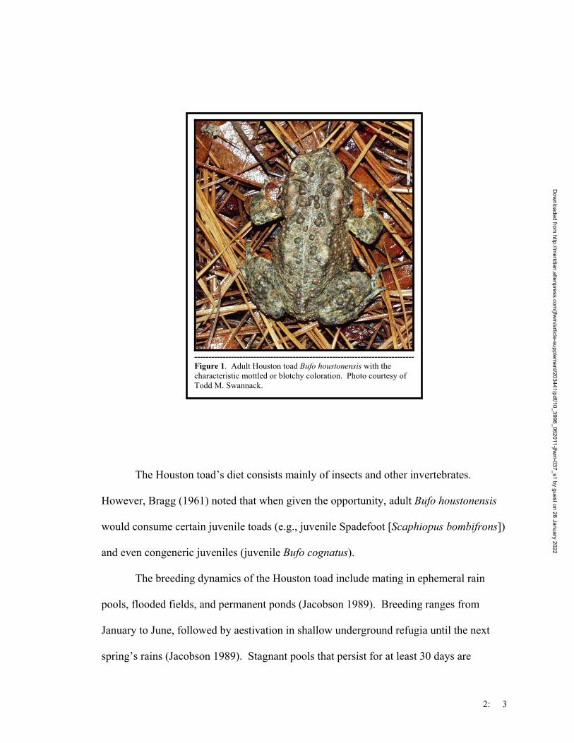
------------------------------------------------------------------------------ Figure 1. Adult Houston toad Bufo houstonensis with the characteristic mottled or blotchy coloration. Photo courtesy of Todd M. Swannack.

The Houston toad’s diet consists mainly of insects and other invertebrates.

However, Bragg (1961) noted that when given the opportunity, adult Bufo houstonensis

would consume certain juvenile toads (e.g., juvenile Spadefoot [Scaphiopus bombifrons])

and even congeneric juveniles (juvenile Bufo cognatus).

The breeding dynamics of the Houston toad include mating in ephemeral rain

pools, flooded fields, and permanent ponds (Jacobson 1989). Breeding ranges from

January to June, followed by aestivation in shallow underground refugia until the next

spring’s rains (Jacobson 1989). Stagnant pools that persist for at least 30 days are

2: 3

Dow



m/article-supplem

ent/203441/pdf/10_3996_062011-jfwm


required for breeding and for the aquatic larval life stage to develop (Jacobson 1989).

Males vocalize from shallow water or from habitat near the breeding pond and can call

up to a 100 m radius around the breeding pond. However, pairs have arrived to the

breeding sites already in amplexus (Jacobson 1989), indicating terrestrial amalgamation.

Adult toads emerge to breed only when conditions are optimal, but can emerge

outside the breeding season if habitat disturbance occurs. Adults do not appear to be

faithful to particular breeding ponds. This lack of site fidelity allows genetic exchange to

occur, alleviating isolated sink populations from the possibility of inbreeding or

bottlenecking (Lacy and Seal 1994). However, Houston toads in Bastrop County are part

of a metapopulation where two subpopulations are locally spread out (Semlitsch 2000b)

and separated by a four-lane highway. This separation has been a cause of concern for

the species as it inhibits the crucial genetic exchange that eventually could lead to

extinction.

These problems along with several other factors required a population and habitat

viability assessment (PHVA) for B. houstonensis to assist with recovery efforts. PHVA

is a conclusive assessment of the potential interacting risk factors of a population (Shaffer

1990). PHVA attempts to predict future events using present data. The viability of

Houston toad metapopulations is dependent on the size of populations, the rate of

exchange among individuals, and threats that affect each small population (Lacy and Seal

1994).

Several recommendations were made from examination of the initial Houston

toad population and habitat viability assessment (Lacy and Seal 1994). A geographic

information system database was proposed to incorporate annual surveys of the adult

2: 4

Dow



m/article-supplem

ent/203441/pdf/10_3996_062011-jfwm


population, soil maps, road maps, known Houston toad population locations, and habitat

type. This database would have determined areas of suitable habitat as well as the

amount of isolation and continuity among population localities (Lacy and Seal 1994).

However, this has not happened.

In the 1994 PHVA analysis, the Conservation Breeding Specialist Group (1994)

provided recommendations to improve habitat for the Houston toad, described threats and

land use activities, gave management guidelines, and encouraged public outreach. For

habitat improvement, the preferred toad habitat used outside of the breeding season must

be characterized. In addition, pond construction and restorative techniques must be

investigated. The role of travel corridors between and among breeding ponds must also

be explored (Lacy and Seal 1994).

Identifying possible threats such as oil run-off, imported fire ants (Solenopsis

invicta), and UV radiation will contribute to the limited information available for this

species. Likewise, identifying water and land use activities such as fish stocking,

agricultural practices, cropland/orchard operations, prescribed burning, and planned

grazing systems are essential in evaluating the natural history of the toad. Previously,

recommendations for management guidelines include minimizing the soil disturbance,

pesticide use, and habitat fragmentation, and maximizing the restoration of corridors and

potential habitat (Lacy and Seal 1994).

Since the publication of the PHVA in 1994, some recommendations have been

implemented. However, all recommendations were based on adult populations. To date,

the aquatic and juvenile life stages have not been addressed and therefore, are imperative

for inclusion in management plans. A closer inspection of interactions between B.

2: 5

Dow



m/article-supplem

ent/203441/pdf/10_3996_062011-jfwm


houstonensis life stages and the local environment might increase the support for a

greater protection.

HOUSTON TOAD ENVIRONMENT

Adult Houston toads use pond environments for breeding, while tadpoles use

ponds for growth and development. Once metamorphosed, emergent anuran juveniles

migrate to a terrestrial habitat, where they grow to sexual maturity (Semlitsch 1998) and

disperse. Terrestrial habitats are essential for juvenile dispersion and growth. Therefore,

both aquatic and terrestrial habitats are crucial to the Houston toad’s life history pattern.

These habitats tend to be located around small, fragmented wetland ponds, as

anthropogenic development has damaged much of the required habitat (Brown 1975).

Protection for small wetlands is not explicitly provided by the federal government

for tracts less than 0.4 ha (1 acre) as they are considered insignificant (Snodgrass et al.

2000). Combined, these small wetlands make up a large percentage of total wetland

habitat. Figure 2 illustrates the distribution of natural depression wetland sizes (n = 371)

from the Savannah River Site on the upper coastal plain of South Carolina where the

smallest wetland was 0.2 ha. Three hundred twenty-five of 371 wetland ponds were

smaller than 0.4 ha, which indicates that, although presumably insignificant, these

wetlands should not be overlooked as each can represent an entire ecosystem to a myriad

of species (Snogdrass et al. 2000). This example is just one of many that illustrate the

importance of all wetlands, regardless of size.

2: 6

Dow



m/article-supplem

ent/203441/pdf/10_3996_062011-jfwm


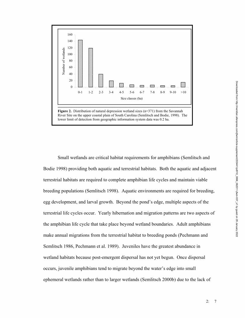
0

20

40

60

80

100

120

140

160

0-1 1-2 2-3 3-4 4-5 5-6 6-7 7-8 8-9 9-10 >10

Size classes (ha)

Num

ber o

f wet

land

s

--------------------------------------------------------------------------------------------------------------- Figure 2. Distribution of natural depression wetland sizes (n=371) from the Savannah River Site on the upper coastal plain of South Carolina (Semlitsch and Bodie, 1998). The lower limit of detection from geographic information system data was 0.2 ha.

Small wetlands are critical habitat requirements for amphibians (Semlitsch and

Bodie 1998) providing both aquatic and terrestrial habitats. Both the aquatic and adjacent

terrestrial habitats are required to complete amphibian life cycles and maintain viable

breeding populations (Semlitsch 1998). Aquatic environments are required for breeding,

egg development, and larval growth. Beyond the pond’s edge, multiple aspects of the

terrestrial life cycles occur. Yearly hibernation and migration patterns are two aspects of

the amphibian life cycle that take place beyond wetland boundaries. Adult amphibians

make annual migrations from the terrestrial habitat to breeding ponds (Pechmann and

Semlitsch 1986, Pechmann et al. 1989). Juveniles have the greatest abundance in

wetland habitats because post-emergent dispersal has not yet begun. Once dispersal

occurs, juvenile amphibians tend to migrate beyond the water’s edge into small

ephemeral wetlands rather than to larger wetlands (Semlitsch 2000b) due to the lack of

2: 7

Dow



m/article-supplem

ent/203441/pdf/10_3996_062011-jfwm


aquatic predators (Dayton and Fitzgerald 2001). Therefore, to complete their life cycles,

the majority of amphibian species require use of not only wetlands, but also lands

adjacent to them.

Protection is needed for wetland ponds and the habitat surrounding ponds. Often

characterized as buffer zones, these protected areas are important because they not only

allow amphibians and various other species the space required for reproduction and

survival, but they also minimize human interactions and harmful impacts to these species

(Clark et al. 1994). Buffer zones can increase the chances for survival of delicate species

that depend on small wetlands and increase the connectivity of each small wetland

section to ensure migration and aestivation are successful.

Often insufficient biological information is available for terrestrial habitats

surrounding these small isolated wetlands and for the area immediately adjacent to the

water’s edge, both of which are required for the survival of these species (Semlitsch

1998). This is especially true in the case of the Houston toad. The use of the adjacent

terrestrial habitats, the identification of relevant distances for both communities and

species, and the area required for the life cycle stages can be inconsistent but necessary in

the accurate determination of buffer zones (Burke and Gibbons 1995). Each of those

factors will have a direct effect on guiding basic principles for managing the remaining

Houston toad habitat.

Adult life stage dynamics are well known as studies have been done on

hybridization (Kennedy 1961, Brown 1971, Hillis et al 1984), reproductive ecology

(Hillis et al. 1984, Jacobson 1989, Price, pers. comm.) including captive breeding (Quinn

et al. 1987), feeding, (Bragg 1960), and conservation (Brown 1975, Brown and Thomas

2: 8

Dow



m/article-supplem

ent/203441/pdf/10_3996_062011-jfwm


1982). However, the post-emergent ecology of the Houston toad is poorly characterized.

Little research has exclusively focused on juvenile toad dispersal, developmental

patterns, and survivorship. Hillis et al. (1984) addressed tadpole development and only

briefly mentioned the dispersal of postmetamorphic B. houstonensis from the pond site.

Thomas and Allen (1997) observed a small number (n = 25) of juveniles over a short

sampling period (about 1 month) at a native pond. Quinn and Mengden (1983) evaluated

captive raised adults from chemically induced egg strands and observed all subsequent

life stages. Developmental growth was recorded, but dispersal of juveniles was not

addressed. In all of these studies, dispersal or growth were the only two aspects of

juvenile ecology addressed. Survivorship and morphological identification are also

needed to better address population survival estimates and field identification. Yet, data

on either topic have not been published.

Therefore, the current knowledge of Houston toad juvenile ecology remains

incomplete. An investigation is needed to classify and clarify the importance of

developmental growth, juvenile dispersal patterns, morphology, and survivorship. Such

data are useful for their contribution to survivorship calculations. These data also support

the need for buffer zone implementation and better management practices compatible

with the toad.

With little preexisting data and current information being neither extensive nor

complete, this study was designed to assemble biological and ecological characteristics of

the juvenile Houston toad. This research has included developmental growth, dispersal

patterns, morphological distinctions and the determination of survivorship from egg to

metamorph. The results are an evaluation for the Houston toad juvenile habitat and

2: 9

Dow



m/article-supplem

ent/203441/pdf/10_3996_062011-jfwm


developmental requirements, the justification for buffer zone enforcement, and the

calculation of survivorship and methods for making those assessments.

The objectives of this research were: (1) to test multiple methods of estimating

egg numbers in Bufonid egg strands and apply the successful technique to B.

houstonensis egg strands in calculating survivorship, (2) to study juvenile ecology

including dispersal, growth, habitat choice, and other important factors affecting

successful data collection including interspecific morphological characters, and (3) to

apply this information in guidelines for management and conservation plans for this

species.

2: 10

Dow



m/article-supplem

ent/203441/pdf/10_3996_062011-jfwm


FIELD TECHNIQUES WHICH AID IN THE DETERMINATION OF

HOUSTON TOAD BUFO HOUSTONENSIS

(ANURA: BUFONIDAE) JUVENILE ECOLOGY


To define ecological parameters needed in designing a management plan for an

endangered species, baseline data should be collected for all life history stages (Semlitsch

2000a). This has yet to happen for the endangered Houston toad, B. houstonensis, where

valuable larval and juvenile ecological data are scarce. The focus of this study is to

define Houston toad juvenile ecology, which will aid in better management practices

(Chapter 1). Before this can be done, basic life history parameters such as survivorship

calculations from egg to metamorph must be available. Once the number of survivors

from a cohort is established, characteristics of the juvenile ecology, such as growth,

movement, and morphology can be examined to determine which influences juvenile

survival to adulthood (Chapter 3).

Survivorship calculations range from simple in nature (number of individuals

survived/total number initial individuals) (Shirose and Brooks 1995) to highly complex

as those found in MARK (White and Burnham 1999), but the techniques used to

determine the raw data for these calculations (i.e., the actual number of individuals) have

rarely been explored. Published data on egg and tadpole counting techniques are limited

to 3 areas of estimation: counting the number of gravid females, total masses, or

individual eggs.

Dow



m/article-supplem

ent/203441/pdf/10_3996_062011-jfwm


Information on manipulation of females, masses, or eggs exists, but detailed

descriptions of methodologies are scarce. Berven and Chadra (1988) and Semlitsch and

Gibbons (1990) collected wood frog, Rana sylvatica, egg masses. They did not count

the eggs, but grouped the masses into categories based on their weight ranges. Crouch

and Paton (2000) only counted the total number of wood frog egg masses in a pond to

determine female/male population estimate. Reading (1986) determined how many eggs

were in an egg mass by subtracting the weight of a female common toad, Bufo bufo, (post

egg laying) from her gravid weight and dividing the remaining number by the average

weight of 1 egg. Light (1974) also used this method with the red-legged frog, Rana

aurora aurora, and the spotted frog, Rana pretiosa pretiosa. He modified the method to

include the chemical inducement of ovulation using Rugh’s (1941) pituitary method. In

other studies, eggs were counted individually, but the methodology was not described

(Anderson et al. 1971, Walls and Altig 1986, Semlitsch and Gibbons 1990).

Few techniques avoid handling eggs during counting. Because of clear, shallow

water, large eggs, and small masses, Anderson et al. (1971) counted eastern tiger

salamander ( Ambystoma t. tigrinum) eggs without removing masses from the

environment and with a minimum of handling. Biologists have used a technique that

avoided manipulation of amphibian eggs by using an estimation technique where the

number of eggs was counted in multiples of 10 (The Ministry of Environment, Lands,

and Parks 1998).

When dealing with an endangered species, such as the Houston toad,

manipulation of any part of the embryonic stage could contribute to mortality (Anderson

et al. 1971) and, therefore, is generally avoided. However, little research has addressed

2: 12

Dow



m/article-supplem

ent/203441/pdf/10_3996_062011-jfwm


egg counts without manipulation or displacement. Therefore, I: (1) designed 4 estimation

techniques, (2) tested these techniques on bufonid egg strands (Bufo valliceps) so that

unnecessary harm to B. houstonensis egg strands can be avoided, (3) determined the best

technique and apply that technique to future B. houstonensis egg strands, and (4) used

estimation techniques to determine survivorship calculations from egg to metamorph in

B. houstonensis.

METHODS

STUDY AREA

The Griffith League Ranch (1,963-ha; 4,848-acres) is located in Bastrop County

and is owned by the Boy Scouts of America. This ranch is an ideal site for observing

Houston toads due to its numerous ponds, favorable habitat conditions, and known

Houston toad populations.

Seventeen ponds on the Griffith Ranch have had Houston toad chorusing and 7 of

these are known breeding sites. One pond in particular was chosen for this experiment

(pond 2). Its abundance of Houston toads, characteristic habitat of carrizo sand and

mixed hardwood/pine forest, and easy access made pond 2 an optimal research site.

Eclosures were built for the experiment in pond 2. Two, 2-m radius aluminum

flashing enclosures were built along the eastward pond’s edge (0.5 m into the water).

These enclosures were used to house adult toads overnight to prevent escape and to

provide opportunity for breeding. As only 2 enclosures were made, multiple trials had to

be performed in each one. Therefore, multiple cohorts were contained in the enclosures

over time.

2: 13

Dow



m/article-supplem

ent/203441/pdf/10_3996_062011-jfwm


INVOLVED SPECIES

Only 2 B. houstonensis egg strands were found in the breeding pond (pond 2).

Half of each egg strand was moved and divided equally into 24 artificial ponds for a

separate experiment. Once the egg strand from the artificial arrays hatched, tadpoles

were individually counted to determine the number of eggs hatching from that half of the

strand. This additional counting was performed to determine the precision of my

estimates.

Gulf coast toad egg strands were also counted later in summer due to the small

number of B. houstonensis strands and the need to practice multiple times. Because B.

valliceps has analogous egg strands to B. houstonensis, is not endangered, and readily

available, the Gulf coast toad was an appropriate substitution. Eight B. valliceps egg

strands were estimated. The actual number of eggs in each egg strand was determined

by displacing each egg strand into a 5 gallon bucket until the tadpoles hatched. Once

hatched, the tadpoles were individually counted and placed back into the holding

enclosure until metamorphosis.

When working on B. valliceps strands, 3 strands died after initial development

and before hatching (before stage 13, Werner, 1986) due to a lack of fertilization or some

other natural cause. One B. houstonensis egg strand died in the pond before the eggs

could hatch (before stage 13, Werner, 1986) in early March due to extreme cold weather.

All 4 bufonid strands were estimated, but were not included in the data due to their

incomplete nature where completed survivorship calculations could not be made.

2: 14

Dow



m/article-supplem

ent/203441/pdf/10_3996_062011-jfwm


EGG STRAND ESTIMATION TECHNIQUES

The number of eggs in egg strands were estimated using 4 techniques. Each of

these techniques was performed 3 times to determine an average and to examine

precision over time. Each technique and trial was timed. A description of each

technique follows.

Full Wire Technique

Green craft wire was used to visually model the egg strand. The wire was

molded into the shape of the egg strand and then straightened out and measured. This

number was compared to a measured number of eggs (the average length of 10 eggs) to

determine the total number of eggs from the model. An egg strand was modeled 3 times

and then an average of the 3 attempts was taken.

Wire Section Technique

The wire section technique is similar to the full wire technique; but broken into

sections, instead of modeling the entire strand. Fifty eggs were measured 3 times.

These 3 measurements were averaged. This length became the wire length used to

measure the whole strand. The wire section was then held near the egg strand. I

counted the number of wire sections it took to estimate an entire egg strand. This

method was repeated 3 times and an average number of eggs was recorded.

2: 15

Dow



m/article-supplem

ent/203441/pdf/10_3996_062011-jfwm


Spherical Technique

The spherical technique uses the geometric equation for the volume of a sphere to

determine the approximate egg strand size. The number of eggs within a cm3 (e) was

recorded 3 times and averaged. The egg strand was estimated 3 times by visually

condensing the strand into a solid sphere of eggs and measuring the diameter (d). This

number was then used in the equation for the volume of a sphere, Vsphere = 4/3Πr2 where r

= the radius (cm). This estimation is particularly variable, as the equation tends to

increase by orders of magnitude. Therefore, precision is imperative. With the above

information, the following calculations can be performed:

1 e = # eggs/cm3 2 Vsphere = 4/3 Πr3 where r is the radius in cm 3 r = d/2 where d is the diameter of the estimated egg sphere

in cm so that 4 E = V*e where E is the total number of eggs

Individual Counting Technique

This technique is self-explanatory. Three attempts are made to count all the eggs

in an egg strand. This is by far the most variable as counting ability, memory, and vision

are crucial. However, I sought to test the difference between total counting and the other

techniques as so many studies have reported counting eggs one by one. This method

was not initiated until the third B. valliceps egg strand.

SURVIVORSHIP CALCULATIONS

2: 16

Dow



m/article-supplem

ent/203441/pdf/10_3996_062011-jfwm


Once multiple estimation of the egg strands occurred, the number of juveniles

emerging could be used in survivorship calculations from egg to metamorph. A simple

survivorship formula was used (Krebs, 1999) where the number of metamorphs to

emerge is divided by the estimated or actual number of eggs and multiplied by 100 to

obtain a percentage (metamorphosis survivorship). The equation is:

whe

The

estim

This

from

RES

EGG

com

devi

wire

indiv

Dow

nloade

Nt Ŝ0 = x 100
N0
re Ŝ0 = finite survival rate Nt = number of individuals alive at end of time period N0 = number individuals alive at start of time period

Survivorship from emergence to juvenile aged 13 weeks was calculated similarly.

Schnabel-Schumacher method (Krebs 1999) was used to determine the population

ate using mark-recapture data after juveniles emerged (data used in Chapter 3).

estimate was then similarly used in the above equation to determine survivorship

egg to 13-week old postmetamorphic juveniles.

ULTS

STRAND ESTIMATION TECHNIQUES

Results for the 4 egg strand techniques can be found in Figure 1, which is a

parison among all of the estimation techniques to the actual egg count. The standard

ation (σ2) for each technique was: (1) wire section technique, σ2 = 1279 eggs, (2) full

technique, σ2 = 1536 eggs, (3) spherical model technique, σ2 = 2098 eggs, and (4)

idual counting technique, σ2 = 1494 eggs.

2: 17

d from http://m


m/article-supplem

ent/203441/pdf/10_3996_062011-jfwm


Figure 2 individually compares each technique with the actual number of eggs.

Statistical analyses (Table 1) via analysis of variance (ANOVA) indicated no significant

difference overall among techniques (P = 0.27, α = 0.05). However, when testing each

technique on the individual level against the actual number using Student’s T-test, the full

wire model had a significant difference (P = 0.03) (Fig. 2-A). Comparison of the actual

number and the other 3 techniques are shown in Figures 2-B to 2-D.

Some techniques were difficult to perform. Multiple hours were spent on each

egg strand. If these techniques are to be used in a realistic situation, they must be

practical in nature. The degree of difficulty and the amount of time each technique took

on average is explained in Table 2.

SURVIVORSHIP CALCULATIONS

Survivorship for these 7 egg strands was difficult to determine due to the lack of

individual enclosures. The close proximity of the two B. houstonensis egg strands in the

open pond (wild) prevented individual traps. There was no way to determine how many

B. valliceps egg strands there were going to be in the summer of 2003. Therefore, only

two enclosures were made. Table 3 illustrates the estimated and actual percent survival

from all 7 cohorts . Survival of B. houstonensis metamorphs was overestimated using

the estimation techniques (5.29%) when compared to the actual number of juvenile

survival (4.73%). When averaged together, the estimation techniques provided a 1.36%

and 0.76% survival of B. valliceps metamorphs as compared to the actual number which

determined to be 1.20% and 0.64%. The estimated percentage was not significantly

2: 18

Dow



m/article-supplem

ent/203441/pdf/10_3996_062011-jfwm


different from the actual percentage (P = 0.89). Percent survival for each individual

estimation technique ranged from 0.49% to 15.09%.

Survivorship from egg to juvenile aged at 13-weeks is even lower than that of

metamorphic survivorship. The Schnabel-Schumacher method revealed an estimated

population size of a 15% decline in population from 332 individuals to 281 over the

course of 13 weeks. By the age of maturity (1 year for males), the survival rate, if

continuously declining, would decline to 2.9%. Survivorship would be near 0 if the 15%

decline was continuous for females who mature at an even later date (2 years post-

emergence).

2: 19

Dow



m/article-supplem

ent/203441/pdf/10_3996_062011-jfwm


0

1000

2000

3000

4000

5000

6000

7000

8000

9000

BH1 BH2 BV3 BV4 BV5 BV6 BV7

Egg Strand

Num

ber o

f Egg

s

Actual Number Wire Section Model Full Wire Model Spherical Model Individual Count

------------------------------------------------------------------------------------------------------------------------------ Figure 1. Average Houston and Gulf coast toad egg strand number comparison between four estimation techniques and the actual number counted. BH=Bufo houstonensis. BV=Bufo valliceps.

2: 20

Dow



m/article-supplem

ent/203441/pdf/10_3996_062011-jfwm


0

2000

4000

6000

8000

10000


Egg Strand

Num

ber o

f Egg

s

Actual Number Full Wire Model

0

2000

4000

6000

8000

10000


Egg Strand

Num

ber o

f Egg

s

Actual Number Wire Section Model

0

2000

4000

6000

8000

10000


Egg Strand

Actual Number Spherical Model

Eggs

0

2000

4000

6000

8000

10000


Egg Strand

Num

ber o

f Egg

s

Actual Number Individual Count

Num

ber o

f

Figure 2a. Average Houston and Gulf Coast toad egg number (No. egg/strand) estimated by the full wire model and compared to the actual egg number of each strand. BH1 and BH2 are Bufo houstonensis egg strands. BV3 through BV7 are Bufo valliceps egg strands. P = 0.03, Significant difference between actual number and full wire model number.

Dow



m/article-supplem

Figure 2b. Average Houston and Gulf Coast toad egg number (No. egg/strand) estimated by the wire section model and compared to the actual egg number of each strand. BH1 and BH2 are Bufo houstonensis egg strands. BV3 through BV7 are Bufo valliceps egg strands. P = 0.55, No significant difference between actual number and wire section model number.

ent/203441/pdf/10_3996_062011-jfwm

-037_s1 by guest o

Figure 2c. Average Houston and Gulf Coast toad egg number (No. egg/strand) estimated by the spherical model and compared to the actual egg number of each strand. BH1 and BH2 are Bufo houstonensis egg strands. BV3 through BV7 are Bufo valliceps egg strands. P = 0.68, No significant difference between actual number and spherical model number.

n 28 January 2022

Figure 2d. Average Houston and Gulf Coast toad egg number (No. egg/strand) estimated by the individual count method and compared to the actual egg number of each strand. BH1 and BH2 are Bufo houstonensis egg strands. BV3 through BV7 are Bufo valliceps egg strands. This method was not used on the Houston toad strands. P = 0.76, No significant difference between actual number and individual count number.

2: 21

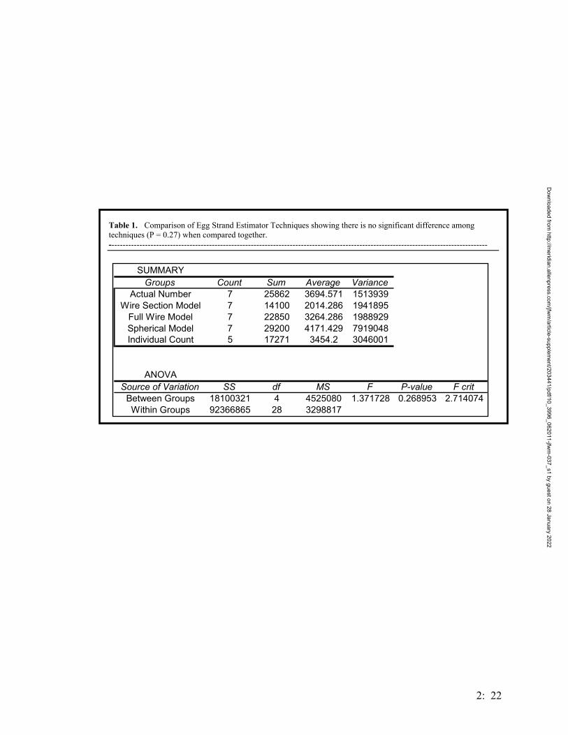
Table 1. Comparison of Egg Strand Estimator Techniques showing there is no significant difference among techniques (P = 0.27) when compared together. ----------------------------------------------------------------------------------------------------------------------------------------

SUMMARY

Groups Count Sum Average VarianceActual Number 7 25862 3694.571 1513939

Wire Section Model 7 14100 2014.286 1941895Full Wire Model 7 22850 3264.286 1988929Spherical Model 7 29200 4171.429 7919048Individual Count 5 17271 3454.2 3046001

ANOVASource of Variation SS df MS F P-value F crit

Between Groups 18100321 4 4525080 1.371728 0.268953 2.714074Within Groups 92366865 28 3298817

2: 22

Dow



m/article-supplem

ent/203441/pdf/10_3996_062011-jfwm


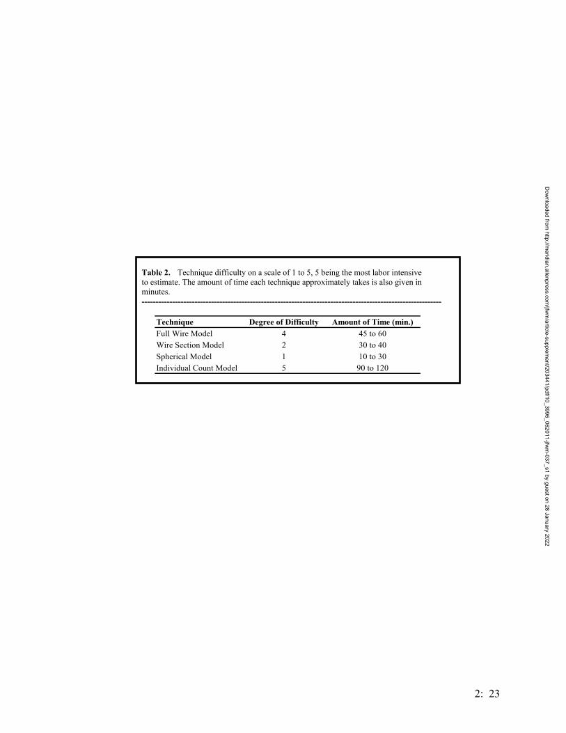
Table 2. Technique difficulty on a scale of 1 to 5, 5 being the most labor intensive to estimate. The amount of time each technique approximately takes is also given in minutes. ------------------------------------------------------------------------------------------------------------

Technique Degree of Difficulty Amount of Time (min.)Full Wire Model 4 45 to 60Wire Section Model 2 30 to 40Spherical Model 1 10 to 30Individual Count Model 5 90 to 120

2: 23

Dow



m/article-supplem

ent/203441/pdf/10_3996_062011-jfwm


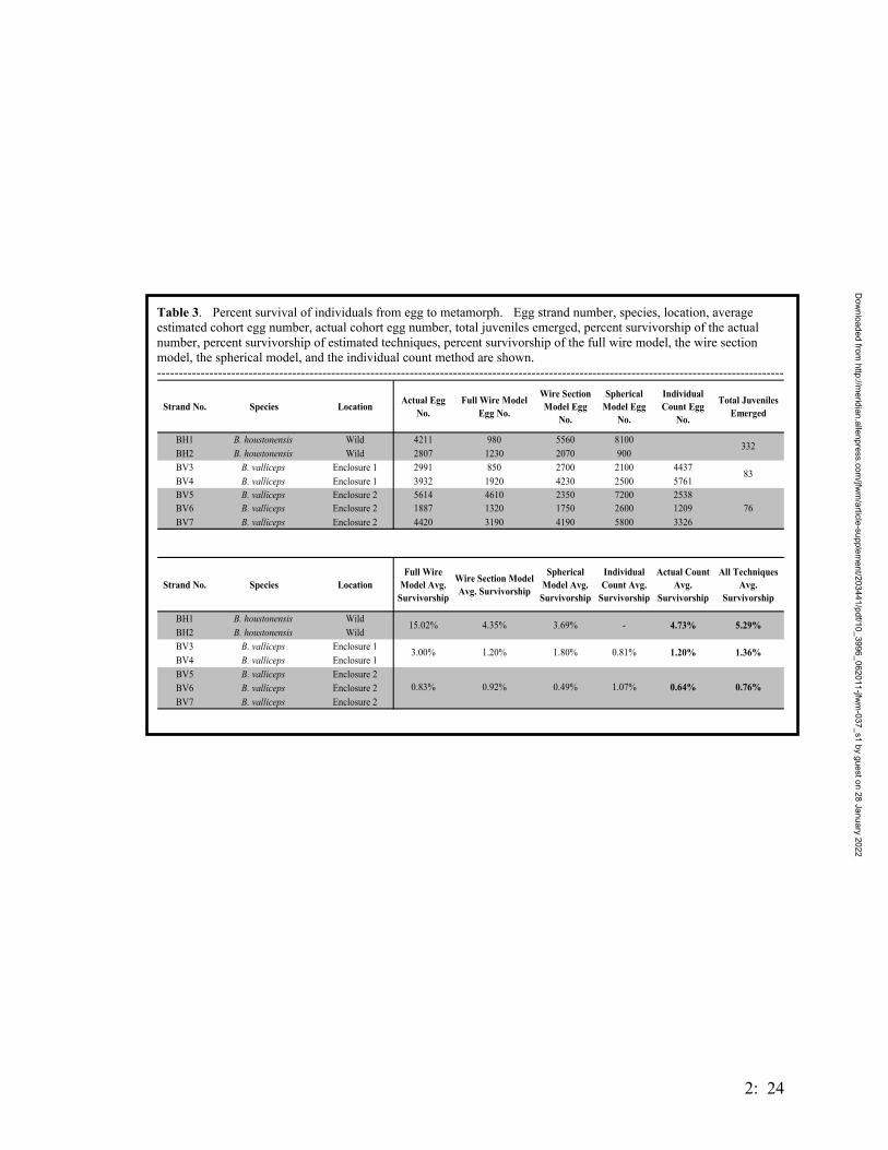
Table 3. Percent survival of individuals from egg to metamorph. Egg strand number, species, location, average estimated cohort egg number, actual cohort egg number, total juveniles emerged, percent survivorship of the actual number, percent survivorship of estimated techniques, percent survivorship of the full wire model, the wire section model, the spherical model, and the individual count method are shown. ------------------------------------------------------------------------------------------------------------------------------------------------

Strand No. Species Location Actual Egg No.

Full Wire Model Egg No.

Wire Section Model Egg

No.

Spherical Model Egg

No.

Individual Count Egg

No.

Total Juveniles Emerged

BH1 B. houstonensis Wild 4211 980 5560 8100BH2 B. houstonensis Wild 2807 1230 2070 900BV3 B. valliceps Enclosure 1 2991 850 2700 2100 4437BV4 B. valliceps Enclosure 1 3932 1920 4230 2500 5761BV5 B. valliceps Enclosure 2 5614 4610 2350 7200 2538BV6 B. valliceps Enclosure 2 1887 1320 1750 2600 1209BV7 B. valliceps Enclosure 2 4420 3190 4190 5800 3326

Strand No. Species LocationFull Wire

Model Avg. Survivorship

Wire Section Model Avg. Survivorship

Spherical Model Avg.

Survivorship

Individual Count Avg.

Survivorship

Actual Count Avg.

Survivorship

All Techniques Avg.

Survivorship

BH1 B. houstonensis WildBH2 B. houstonensis WildBV3 B. valliceps Enclosure 1BV4 B. valliceps Enclosure 1BV5 B. valliceps Enclosure 2BV6 B. valliceps Enclosure 2BV7 B. valliceps Enclosure 2

0.81%

1.07%

5.29%

1.36%

0.76%

1.20%

0.92%

3.69%

1.80%

0.49%

3.00%

0.83%

4.73%

1.20%

0.64%

332

83

76

15.02% 4.35% -

2: 24

Dow



m/article-supplem

ent/203441/pdf/10_3996_062011-jfwm


DISCUSSION

Given the importance of maintaining the integrity of fragile eggs for endangered

taxa, these estimation techniques prove vital in avoiding physical displacement or

manipulation. Precision was increased after several egg strand trials. Precision, not

accuracy, is needed for these techniques to work, as accuracy is unrealistic.

Choosing the best estimation technique requires the evaluation of several factors.

In terms of practical use and application of these techniques, it is best to have a smaller

modeling time and lower degree of difficulty. However, difficulty and time varied

among the 4 techniques.

Even though the spherical model was the fastest to estimate and the degree of

difficulty was very low, the deviation in estimation was extremely high (σ2 = 2098).

Individually counting the eggs was extremely difficult and time consuming; therefore, it

is not recommended. The full wire technique had a moderate time period and was more

strenuous to model. The complications associated with modeling an entire egg strand all

at one time make this technique not an optimal one.

The wire section technique had a moderate degree of difficulty and lower time

consumption. This technique had the lowest deviation from the actual number of eggs

(σ2=1279). Due to the model’s flexibility in technique and realistic time consumption,

the wire section model is most likely the technique to be used in a realistic application.

The technique allows for quick maneuverability and is simple in concept. The spherical

model could be used as an extremely fast technique; however, precision is not easily

obtained.

2: 25

Dow



m/article-supplem

ent/203441/pdf/10_3996_062011-jfwm


The survivorship numbers for B. houstonensis egg to metamorph were

surprisingly high in both the estimated and actual percent survivorship as juvenile

survivorship has been estimated to be between 1% and 2% (Hatfield et al. 2002) for

Houston toads during PVA simulations. This is extremely positive as survival was

better than expected. B. valliceps estimation and actual percentages were very close to

that prediction made by Hatfield et al. (2002).

There are two obvious explanations: (1) the 2 B. houstonensis cohorts were in

optimal conditions for survival and the 5 B. valliceps were not. Shade and confinement

could have played a role in B. valliceps survivorship as it is well documented that lower

pond temperature (Wilbur and Collins 1973, Semlitsch 2000) and increased density

(Smith 1983, Petranka and Sih 1986, Petranka 1989, Scott 1990, Van Buskirk and Smith

1991, Scott 1994) in larval populations not only decrease body size upon emergence, but

survivorship as well (Wilbur 1972, Wilbur and Collins 1973, Wilbur 1976, 1977a, b,

Smith-Gill and Gill 1978, Smith-Gill and Berven 1979, Pough and Kamel 1984, Goater et

al. 1993); and/or (2) accuracy of estimation increased over time and the five B. valliceps

cohort estimations are more representative of realistic survivorship numbers for

successful egg strands in the wild.

The latter is most likely to occur, as even though shade was present for the 5 B.

valliceps strands and could have affected survivorship, all 7 strands were in the same

pond at relatively the same time. This large difference in survivorship percentages is not

as likely to occur. B. houstonensis survivorship is overestimated. Because B.

houstonensis estimation received little practice, B. valliceps’ survivorship is relatively

low, but still has a thriving population, it can be assumed that the endangered B.

2: 26

Dow



m/article-supplem

ent/203441/pdf/10_3996_062011-jfwm


houstonensis survivorship is closer to that of B. valliceps’ survivorship. However, It is

not known how close.

Regardless of when estimation techniques were perfected and which species

benefited from better precision, there was a decrease in B. houstonensis survivorship over

the course of 13 weeks. This decline is indicative of serious problems for the species

given current PVA models. More research is needed to determine the last missing link

in the survivorship chain: survival of older juvenile (> 13 weeks) to adult.

By identifying these techniques and making them applicable for realistic

situations, more precise survivorship numbers can be calculated. Monitors of Houston

toad populations can use these methods to aid data collection related to population

dynamics. The survivorship of the remaining population is a better estimate of current

population trends for endangered species and future population trends.

2: 27

Dow



m/article-supplem

ent/203441/pdf/10_3996_062011-jfwm


2: 28

Dow



m/article-supplem

ent/203441/pdf/10_3996_062011-jfwm


POSTMETAMORPHIC BIOECOLOGY ON THE JUVENILE HOUSTON TOAD,

BUFO HOUSTONENSIS (ANURA: BUFONIDAE)


Buffer zones provide protection when anthropogenic activities conducted in

surrounding habitat impact wetlands. These areas are not just a buffer; they are core

habitat for many semi-aquatic species. Buffer zones are, therefore, essential for the

survival of a number of species and for the preservation of biological diversity (Semlitsch

2001). Biologists who study semi-aquatic species have long understood the importance

of uplands immediately adjacent to wetlands for the survival of myriad species of toads,

turtles, salamanders, and other organisms (Semlitsch 1998).

The endangered species, Bufo houstonensis, also requires upland habitat adjacent

to its wetland ponds for survival. Anthropogenic activities around vital breeding ponds

and core habitat appear to play an important role in the trend toward extinction (Brown

1975). These activities would be greatly reduced with the enforced protection of buffer

zones around native ponds. Information from all stages of the toad’s life cycle, especially

the juvenile stage, could help define Houston toad core habitat for buffer zone

enforcement. Once buffer zones are enforced, better management practices for all life

stages of the Houston toad could be implemented.

The habitat areas used by the juvenile stage can contribute to the definition of

“core habitat” for a species and hence, juvenile dispersal can help determine the

2: 29

Dow



m/article-supplem

ent/203441/pdf/10_3996_062011-jfwm


configuration of a buffer zone. Juvenile dispersal is among the most important life-

history movements as it connects populations and can thus mitigate against the

deleterious effects of genetic isolation (Gill 1978, Berven and Grudzien 1990,

DeMaynadier and Hunter 1999). When migrating towards other ponds, juveniles tend to

travel further distances than adults (Breden 1987), sometimes extending to 200 m or

beyond (Semlitsch 1998). Therefore, juveniles can actually use more of the upland

habitat surrounding wetland ponds than adults and can be better indicators of required

habitat.

While juvenile dispersal is well recognized for some species of amphibians,

relatively little is known concerning individual movements of the Bufonid

postmetamorphic stage (Daugherty and Sheldon 1982), especially the Houston toad. This

lack of knowledge has spurred interest in postmetamorphic behavior that has a direct

impact on the survivorship of adult populations. Breden (1987) observed dispersal in

juvenile B. woodhousei fowleri and found juvenile migrations to surrounding ponds serve

an important resource in maintaining genetic flow, a concept throughout all terrestrial

amphibians. Examining postmetamorphic behaviors such as dispersal and movement are

not only crucial to the genetic flow of a population, but can serve as a measurement tool

in the design of buffer zones. Therefore, monitoring juvenile dispersal helps determine

the core habitat for the majority of individuals.

Buffer zones are especially important to juvenile amphibians as this protected

habitat allows their development, ultimately resulting in the survival and reproductive

success of the species (Goater 1994). Juvenile growth analysis is essential because it can

contribute to an understanding of the population processes of the species (Clarke 1974).

2: 30

Dow



m/article-supplem

ent/203441/pdf/10_3996_062011-jfwm


This stage is particularly significant for those in the genus Bufo, which metamorphose at

an extremely small size relative to ranid and hylid frogs (Werner 1986). One

physiological advantage of this small size is that juveniles minimize the risk of mortality

due to desiccation (Boone et al. 2001). Clarke (1974) demonstrated Bufo juveniles grew

6 times as fast in the first year of life as those individuals in four ranid species. Werner

(1986) suggested that this selection for a high postmetamorphic growth rate and small

body size upon emergence occurs when the mortality and growth is relatively high in the

larval environment and low in the adult environment, a pattern found in R-selected

species. Therefore, this stage includes not only the most rapid growth (Breckenridge and

Tester 1961, Labanick and Schlueter 1976), but also the highest mortality (Pechmann et

al. 1991).

Contradictory to the rapidness of juvenile growth, morphological characteristics

develop over time. In fact, juveniles of the genus Bufo are reported to be

morphologically indistinguishable until maturity (Blair 1972). This ambiguity has caused

concern as B. houstonensis can be confused with B. valliceps, B. woodhousei, and other

congeners at this stage. In terms of conservation, detection of species’ differentiation

earlier than maturity would be beneficial. Identification of juvenile toads would provide

an opportunity to ensure their survival through better estimation measures. This earlier

detection could effectively enhance Houston toad population surveys if male audio calls,

amplexus, or egg strands were not directly observed. Therefore, it is beneficial to

investigate at what point morphological differentiation among congeneric bufonids

occurs.

2: 31

Dow



m/article-supplem

ent/203441/pdf/10_3996_062011-jfwm


Since development in congeneric species of B. houstonensis have been

moderately studied, the lack of juvenile B. houstonensis research is astonishing. Hillis et

al. (1984) only briefly mentioned the movement of postmetamorphic B. houstonensis

from their natural pond. Thomas and Allen (1997) observed only a few juveniles from a

natural population (maximum of 25 individuals at 1 time) in Bastrop State Park for only 1

month. Quinn and Mengden (1984) studied captive-raised adults from chemically-

induced egg strands and, hence, briefly studied the developmental growth of B.

houstonensis juveniles. Houston toad postmetamorphic development has never been

examined in natural populations while juvenile morphology has been overlooked

completely.

Examining these aspects of B. houstonensis juvenile ecology is essential for

understanding of not only Houston toad population dynamics, but for guiding

conservation practices. Studying juvenile dispersal would aid in measuring core habitat

used for buffer zone implementation. Analyzing juvenile growth would contribute to the

overall population dynamics of a species. Identifying morphological characteristics that

distinguish B. houstonensis would allow for quicker identification of juveniles for correct

conservation practices.

Therefore, the objectives of this study were: (1) to determine postmetamorphic

growth and development for multiple years and in various cohorts of toads in Bastrop

County, (2) to determine when morphological characters become differentiated among

bufonid species, and (3) to determine dispersal patterns and compare habitats of a natural

pond and an artificially cleared field.

2: 32

Dow



m/article-supplem

ent/203441/pdf/10_3996_062011-jfwm


METHODS

STUDY SYSTEM

The study site is located on the Griffith League Ranch (1,1963-ha; 4,848-acre) in

Bastrop County owned by the Boy Scouts of America. The Griffith League Ranch

(GLR) serves as an ideal site for the study of juvenile Houston toads due to its numerous

ponds, favorable habitat conditions, and known Houston toad populations.

Audio surveys began on the Griffith Ranch in 2000. Site-wide sampling Houston

toad research began on 12 March 2001. Permanent pitfall arrays were used to capture

herpetofauna throughout the Griffith Ranch. Three 23.6 m linear pitfall arrays and two

18.9 m linear pitfall arrays were installed in a cleared, open field (101-ha; 250-acre) on

the property near B.houstonensis breeding ponds. Fourteen Y-shaped aluminum pitfall

arrays were arranged in various habitats also adjacent to B.houstonensis breeding sites.

One 94.4 m linear pitfall array was placed in marshland habitat. Plant communities

associated with the arrays included: loblolly pine forest, pine-oak forest, mixed

hardwood-juniper forest, and a small natural clearing.

The permanent traps were checked at dawn each day. Five-gallon buckets flush

with the ground were used with bucket lids tilted over the openings to create shade and

shelter. These arrays had previously collected juvenile toads.

2: 33

Dow



m/article-supplem

ent/203441/pdf/10_3996_062011-jfwm


PROJECT DESIGN

Collection Dates

Data were collected from 26 May 2001 – 17 June 2001, 18 April 2002 – 25 June

2002, and 23 April 2003 – 15 August 2003. The 2001 data were used from a previous

collection by M. Gaston on the GLR.

Research Site –– Native Pond

Seventeen ponds on the GLR have had Houston toad chorusing and 7 of these are

known Houston toad breeding sites. One pond in particular was used for this project

(Pond 2). Abundance of Houston toads, characteristic habitat of carrizo sand and mixed

hardwood/pine forest, and easy access made it an optimal research site.

Pitfall traps were positioned around the natural pond to capture juveniles for

marking as they emerged and traveled throughout the habitat. Traps were 2.5-quart paint

mixing buckets with aluminum shading placed over each bucket to prevent desiccation.

Aluminum flashing (0.3 m x 15.24 m) was used as a guide to pitfall traps.

Pitfall traps were positioned in groups of concentric ellipses around the natural

pond (Figure 1). Egg mass surveys were conducted to determine how many egg masses

were in the pond. Sets of ellipses were arranged at the pond’s edge around B.

houstonensis egg strings. The ellipses were placed 2 m, 5 m, and 8 m from the egg

strings. Each end of the aluminum flashing was placed 3 m away from the previous end

and 1 m into the water. This layout helped determine in what direction and at what rate

2: 34

Dow



m/article-supplem

ent/203441/pdf/10_3996_062011-jfwm


the juveniles emerged from the natural pond. Emerging juveniles caught by the first

aluminum drift fence were marked and released on the opposite side of the flashing.

Houston toad juveniles were individually/cohort marked with toe clips (Ferner

1979). Standard measurement techniques of Houston toads caught in pitfall traps were

body mass (BM), head width (HW), and snout-to-urostyle length (SUL). A maximum of

5 to 10 min. were used in handling toads. An Acculab portable scale (model # PP2060D)

was used for weighing to the nearest 0.001 g. A 20 cm vernier caliper was used for

obtaining the length and head width to the nearest 0.01 mm.

In 2003, improvements of previous capture methods were attempted. Fluon AD-1

(Asahi Glass Fluoropolymers USA, Inc.), a non-toxic (when dry) “paintable Teflon,” had

been used in several studies to prevent invertebrates (Petren and Case, 1996; Fagan,

1997; Wirth et al., 1997; Cerda et al., 1998; Losey and Denno, 1998; Lucas et al., 1998),

and vertebrates such as geckos (Petren et al. 1993) from escaping pitfall traps. Fluon

AD-1 could be a potential method to prevent the escape of juvenile B. houstonensis from

buckets. Because of possible adverse effects of this product on B. houstonensis juveniles,

a short experiment was performed. B. houstonensis juveniles had adverse affects from

recently coated pitfalls. B. valliceps juveniles escaped from aged fluon-coated rims of

several buckets. Fluon AD-1 did not prove suitable for retaining juvenile amphibian

species in pitfalls as it is ineffective in preventing escape and may cause adverse effects

in some species.

I used quadrat plots in 2002 to randomly sample for B. houstonensis juveniles

throughout the adjacent upland habitat surrounding Pond 2. PVC pipes were cut to form

2: 35

Dow



m/article-supplem

ent/203441/pdf/10_3996_062011-jfwm


A

A

-----------------------------------------------------------------------------------

8 m 5 m

2 m

B

Figure 1. Elliptical aluminum arrays in (A) 2002 where the arrays cuhoustonensis egg strands, and (B) an illustration of these arrays. Theelliptical aluminum arrays around an egg strand (shown in black). Th5 m, and 8 m away from the water’s edge and in 3 m intervals away fside. Distances are shown in red.

Dow


eridian.allenpress.com/jf

pitfall trap drift fence

----------------------------------- rve around two B.

semicircles represent the e arrays were placed at 2 m, rom the egg strand on each

2: 36

wm

/article-supplement/203441/pdf/10_3996_062011-jfw

m-037_s1 by guest on 28 January 2022

a 5-m2 plot. The plots were randomly sampled in a flagged grid encircling the pond and

extending 50 m into the surrounding upland habitat. A 1-m2 plot was used to sample

only the pond’s immediate edge in 2002.

Five small moist refuges were constructed in 2002 at random distances around the

natural pond. Figure 2 illustrates the 3 stages of construction of local refugia around the

natural habitat. These refugia were dug 15 cm into the ground, lined with 3m x 3m

rubber liner (65 ml EPDM—Anjon Building Products), and filled with leaf litter, water,

and sand. They were flush with the ground surface to simulate the juveniles’

environment. Every 3 days the refugia were sprayed with 7.5 l of water to ensure

moisture. They were checked every 3 days to determine distances juveniles moved from

the pond beyond ellipses and the abundance of juveniles at a distance.

In 2003, a combination of quadrat plots and refugia was used. Fifty 1-m2 refugia

were randomly dug into the flagged grid, which now extended 250 m into the upland

habitat. Because refugia were randomly placed, they took the place of the previous

quadrat plots and large refugia.

Sampling for juveniles covered a variety of habitat conditions. Five categories

were used to determine habitat preference: (1) habitat type: forest vs. pasture; (2)

vegetation type: loblolly pine vs. mixed hardwood-juniper vegetation; (3) soil type:

carrizo sand vs. red clay subsoil; (4) soil moisture: moist vs. dry; and (5) sun exposure:

shade vs. sunlight. At the time of capture, habitat condition was recorded.

2: 37

Dow



m/article-supplem

ent/203441/pdf/10_3996_062011-jfwm


------------------------------------------------------------------------------------------------------------------------- Figure 2. Three stages of construction of local refugia found around the natural habitat. They are made from (A) pond liner, then covered with (B) moist, carrizo sand, and then layered with (C) pine needles. The refugia were checked every 3 days and sprayed with water to determine if juveniles tend to gather only near moistened areas.

A B C

2: 38

Dow



m/article-supplem

ent/203441/pdf/10_3996_062011-jfwm


Research Site — Artificial Ponds

Twenty-four artificial ponds were constructed in February 2002 in a large, cleared

field for a separate project. These ponds were in a pattern consisting of 4 rows with 6

ponds per row. The ponds were used to rear cohorts of Houston toads, thus providing

data for comparison with results from natural ponds.

For all 3 years, pitfall traps positioned around artificial ponds captured juveniles

as they emerged from ponds. I marked juveniles and followed their movement

throughout the habitat. There were 2 sets of traps: (1) around each individual pond, and

(2) around the perimeter of the entire 24-pond array.

Aluminum flashing was placed around each pond as a 1-m border. Two 2.5-quart

paint buckets were positioned as pitfall traps around each pond’s border. The outer

perimeter of pitfall traps was placed 10 m on the north and south sides and 20 m on the

east and west sides away from the outer ponds. These traps consisted of two 30.5 m and

two 45.7 m linear pitfall arrays. Additional traps were 5-gallon buckets. The buckets

were buried in the ground so they were flush with the surface. Once a juvenile was

captured in a trap, it was released outside of the 24-pond array to determine the time of

arrival at the outer perimeter. All juvenile Houston toads were marked with the method

used at the natural pond site.

Additional Pond Sampling

Ponds in Bastrop County were sampled in 2003 in addition to the main research

sites. Two privately owned ponds with dispersing juveniles were surveyed. Pond 11 on

2: 39

Dow



m/article-supplem

ent/203441/pdf/10_3996_062011-jfwm


the GLR had juveniles dispersing in early summer and was counted as a third additional

pond. At least 15 measurements and tissue samples were taken from each of the 3

locations. These samples were collected to compare juvenile mass from the natural pond

site to those in the surrounding area and to determine if there was a significant difference

in growth patterns.

STATISTICAL ANALYSIS

I used an analysis of variance (ANOVA) to compare the 3 years (2001-2003) to

determine if there was a difference in juvenile mass. ANOVA was also used to compare

the initial capture masses of all five ponds (2 research sites and 3 additional ponds in

2003). A 2-factor ANOVA was used to compare initial and recapture data with the

different years (2002 and 2003 only). T-tests were performed on comparisons between

previous data and this study’s data, between initial and recapture data, and between the 2

research sites (natural vs. artificial ponds). Pearson and Spearman Correlation

Coefficients were used to determine a correlation between mass and time.

MOLECULAR IDENTIFICATION

Bufo sp. juveniles are phenotypically indistinguishable at the species level.

Several sympatric species of Bufo inhabit the GLR, including B. valliceps, B.

woodhouseii, and B. houstonensis. A polymerase chain reaction (PCR) marker system

was used to distinguish the different species. This test positively identified juvenile B.

houstonensis by using species-specific primers designed in our laboratory. A positive

band identified Houston toads to the exclusivity of other taxa. A sample of the cohort

2: 40

Dow



m/article-supplem

ent/203441/pdf/10_3996_062011-jfwm


was tissue sequenced. DNA was extracted from tissue obtained by clipping toes of

captured juveniles using the DNeasy protocol for Animal Tissues (Quiagen #69506).

The DNA was amplified by PCR using the primers BHCB primers sequence and

BHDLR2 primers sequence. The PCR product was analyzed using agarose gel

electrophoresis to determine the species of the tissue donor. This identified species by

the presence and relative size of the resolved PCR product on the electrophoresed gel.

RESULTS

GROWTH & DEVELOPMENT

Evaluation of 2001, 2002, & 2003 Data

General information about all ponds sampled, the abundance of initial juvenile

captures, and the number of days sampled can be found in Table 1. The number of pond

sites increased over the 3-year period. Sites were not consistent in the number of

juveniles caught and number of days of observation. A t-test indicated a significant

difference in abundance and days observed (P = 0.040), confirming that multiple

juveniles were captured some days and few on others. For a detailed description of the

mark/recapture data, refer to APPENDICES 3 - 5.

Molecular identification confirmed that juveniles used in this research were

indeed B. houstonensis. There were several juvenile tissue samples taken later in the

summer when cohort marking was already completed that were not expected to be B.

houstonensis. These specimens were confirmed to be the genus Bufo. These juveniles

were most likely B. valliceps as this species’ breeding season is later than B.

houstonensis. B. valliceps juveniles emerged later but grew more quickly than B.

2: 41

Dow



m/article-supplem

ent/203441/pdf/10_3996_062011-jfwm


houstonensis juveniles and could look similar to B. houstonensis juveniles. Figure 3

shows PCR results of Bufo tissue samples taken. For a complete record of PCR results

from Bufo tissue, refer to APPENDIX 1. For a detailed description of each sample taken,

refer to APPENDIX 2. Two PCR analyses were performed on the inconclusive samples

(white labels).

Initial Bufo juvenile mass for all 3 years is illustrated in Figure 4 where mass

gradually increased more rapidly in 2003 than in preceding years. This analysis excluded

recapture data for 2001. There was no significant difference (Table 2) in juvenile mass

(P = 0.663) for the three years. This was surprising as collection numbers and patterns

were variable throughout the 3-year period.

Evaluation of 2002 & 2003 Data

I compared juvenile mass data for this study to the mass data reported in the

captive study of Quinn and Mengden (1984). The 2003 data was consistent with Quinn

and Mengden’s (1984) captive SUL data because Quinn and Mengden’s (1984)

regression line (R2 = 0.99) was not significantly different (P = 0.36) from this study’s

2003 SUL data regression line (R2 = 0.81) (Figure 5). The regression lines explained >

80% of the variation in both datasets.

However, when the regression line for 2002 (R2 = 0.34) was compared to the 2

other years (1984 and 2003), a significant difference was found (P = 0.040). When

comparing the raw data among all 3 years (1984, 2002, & 2003), a significant difference

was also found (P = 2.51E-05). A post hoc test, Tukey’s procedure, was performed and

the

2: 42

Dow



m/article-supplem

ent/203441/pdf/10_3996_062011-jfwm


Table 1. Description of pond site abundance of initially captured bufonid juveniles and number of days observed at each pond per year. Pond 2, the artificial arrays, pond 11, various sites on the Griffith League Ranch (GLR), and 2 privately owned (PO) ponds from Bastrop County were sampled. --------------------------------------------------------------------------------------

Year Site Abundance Days Observed 2001* 15 7Pond 2

2002 325 37Pond 2118 13Artificial Arrays

2003 332 43Pond 257 29Artificial Arrays

GLR 14 762 6Pond 11

PO #1 67 5PO #2 16 1

*2001 data were used from a previous collection

2: 43

Dow



m/article-supplem

ent/203441/pdf/10_3996_062011-jfwm


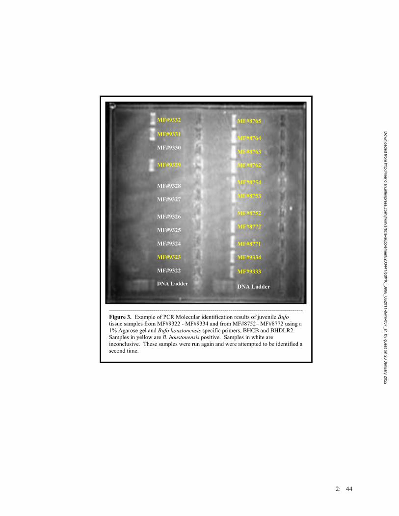
MF#9332

MF#9331 MF#9330

MF#9329

MF#9328 MF#9327

MF#9326 MF#9325 MF#9324 MF#9323 MF#9322 DNA Ladder

MF#8765

MF#8764 MF#8763 MF#8762

MF#8754 MF#8753

MF#8752 MF#8772

MF#8771 MF#9334

MF#9333

DNA Ladder

--------------------------------------------------------------------------------------------------- Figure 3. Example of PCR Molecular identification results of juvenile Bufo tissue samples from MF#9322 - MF#9334 and from MF#8752– MF#8772 using a 1% Agarose gel and Bufo houstonensis specific primers, BHCB and BHDLR2. Samples in yellow are B. houstonensis positive. Samples in white are inconclusive. These samples were run again and were attempted to be identified a second time.

2: 44

Dow



m/article-supplem

ent/203441/pdf/10_3996_062011-jfwm


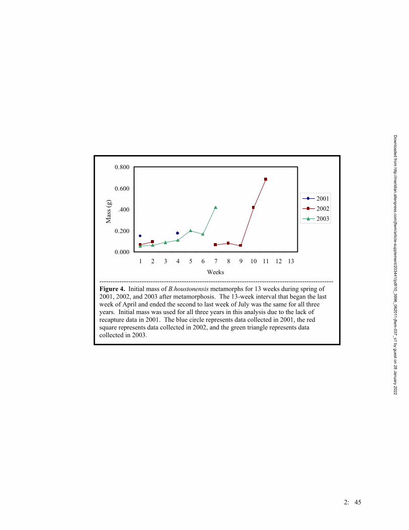
0.000

0.200

0.400

0.600

0.800

1 2 3 4 5 6 7 8 9 10 11 12 13

Weeks

Wei

ght (

g) 200120022003

Mas

s (g)

--------------------------------------------------------------------------------------------------------- Figure 4. Initial mass of B.houstonensis metamorphs for 13 weeks during spring of 2001, 2002, and 2003 after metamorphosis. The 13-week interval that began the last week of April and ended the second to last week of July was the same for all three years. Initial mass was used for all three years in this analysis due to the lack of recapture data in 2001. The blue circle represents data collected in 2001, the red square represents data collected in 2002, and the green triangle represents data collected in 2003.

2: 45

Dow



m/article-supplem

ent/203441/pdf/10_3996_062011-jfwm


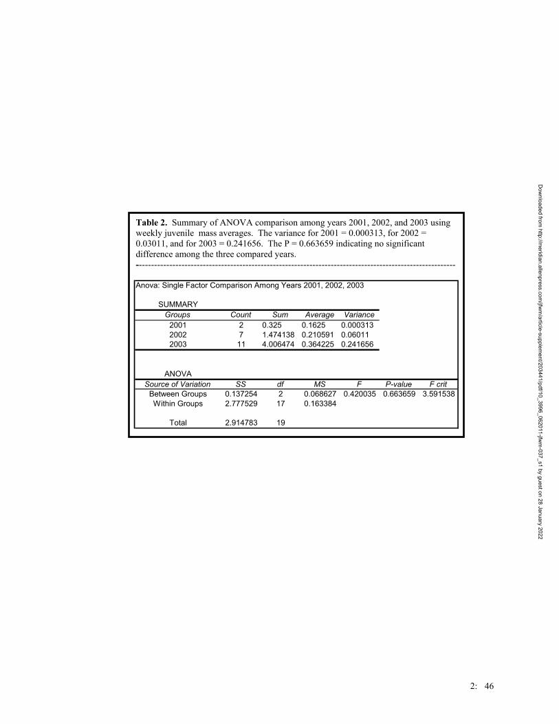
Table 2. Summary of ANOVA comparison among years 2001, 2002, and 2003 using weekly juvenile mass averages. The variance for 2001 = 0.000313, for 2002 = 0.03011, and for 2003 = 0.241656. The P = 0.663659 indicating no significant difference among the three compared years. ---------------------------------------------------------------------------------------------------------

Anova: Single Factor Comparison Among Years 2001, 2002, 2003

SUMMARYGroups Count Sum Average Variance

2001 2 0.325 0.1625 0.0003132002 7 1.474138 0.210591 0.060112003 11 4.006474 0.364225 0.241656


Between Groups 0.137254 2 0.068627 0.420035 0.663659 3.591538Within Groups 2.777529 17 0.163384

Total 2.914783 19

2: 46

Dow



m/article-supplem

ent/203441/pdf/10_3996_062011-jfwm


significant difference was found within the 2002 SUL data (P = 0.031) confirming the

regression line analysis conclusion.

There was a significant correlation between mass and snout-to-urostyle length as

was expected in both 2002 and 2003. This 2003 correlation is shown by the Pearson

Correlation Coefficient (r = 0.93) and the Spearman Correlation Coefficient (rs = 0.66).

The Spearman coefficient is more conservative than the Pearson coefficient, but it still

indicates a positive correlation. Figure 6 depicts the correlation of SUL and mass in

2003. The linear equation is y=9.7027x=8.2814.

Figures 7 and 8 both depict weekly mass averages of juveniles captured in the

natural pond (Pond 2) for the 11-week period of emergence in 2002 and 2003. The t-test

was used for comparison. For the 2002 data shown in Figure 7, there was no significant

difference between initial and recapture data (P=0.41). For the 2003 data shown in

Figure 8, there was no significant difference between initial and recapture data (P=0.45).

A two-factor ANOVA was used to compare differences between initial/recapture

data and years (2002 & 2003). There was no significant difference between 2002 and

2003 (P = 0.43), initial and recapture data (P = 0.26), or the interactions among the four

variables (P = 0.08).

Two sites, the natural and artificial settings, were compared for 2002 and 2003.

No juveniles were recaptured in the artificial pond setting in both years. In 2002, there

was not a significant difference (P = 0.12) between Pond 2 and the artificial pond (Figure

9) initial masses. However, in 2003, there was a significant difference (P = 0.03) in the

data between Pond 2 and the artificial pond (Figure 10) initial masses. In 2003, ponds

were covered by a mesh lining that lowered water temperature and caused a very

2: 47

Dow



m/article-supplem

ent/203441/pdf/10_3996_062011-jfwm


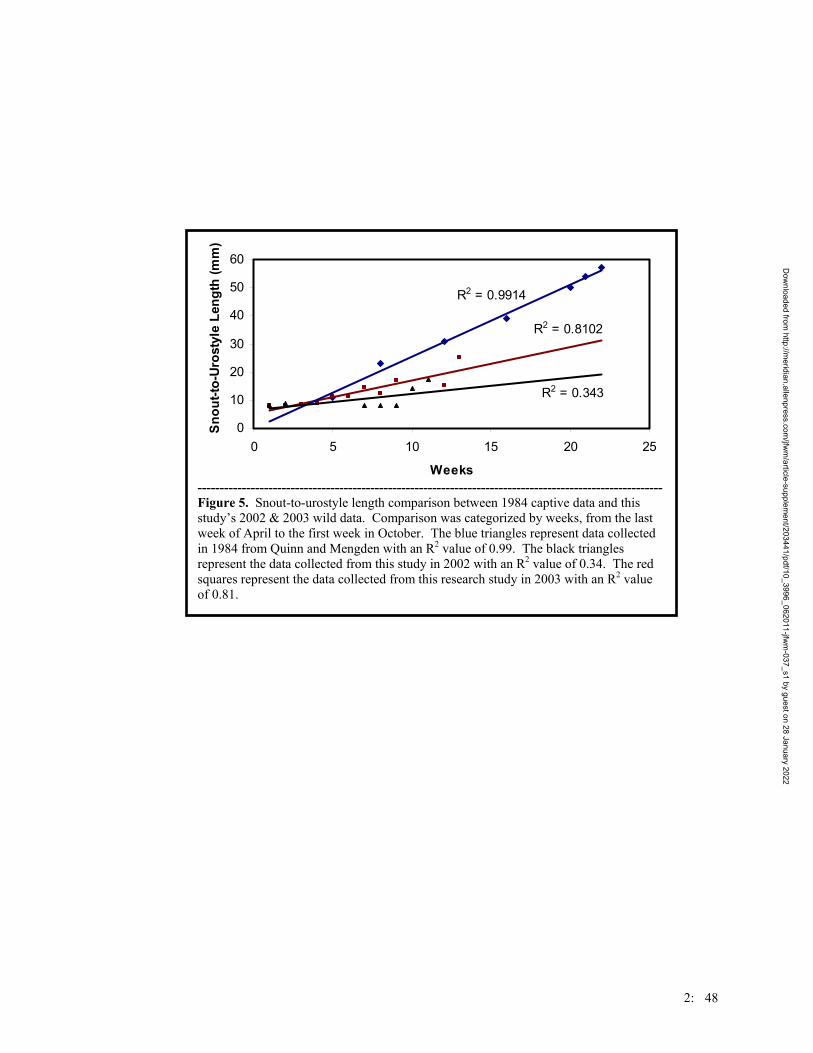
R2 = 0.8102

R2 = 0.9914

R2 = 0.343

0

10

20

30

40

50

60

0 5 10 15 20 25

Weeks

Sno

ut-to

-Uro

styl

e Le

ngth

(mm

)

--------------------------------------------------------------------------------------------------------- Figure 5. Snout-to-urostyle length comparison between 1984 captive data and this study’s 2002 & 2003 wild data. Comparison was categorized by weeks, from the last week of April to the first week in October. The blue triangles represent data collected in 1984 from Quinn and Mengden with an R2 value of 0.99. The black triangles represent the data collected from this study in 2002 with an R2 value of 0.34. The red squares represent the data collected from this research study in 2003 with an R2 value of 0.81.

2: 48

Dow



m/article-supplem

ent/203441/pdf/10_3996_062011-jfwm


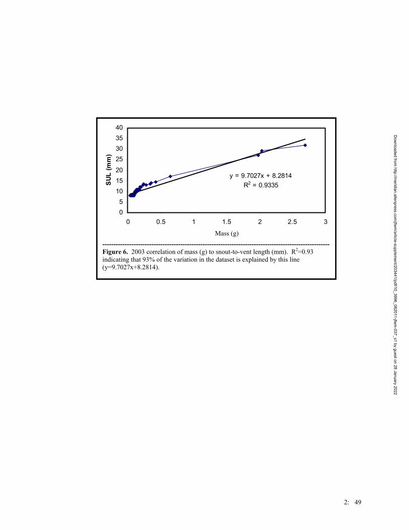
y = 9.7027x + 8.2814R2 = 0.9335

05

101520

25303540

0 0.5 1 1.5 2 2.5 3

Weight (g)

SUL

(mm

)

------------------------------------------------------------------------------------------------------

Mass (g)

Figure 6. 2003 correlation of mass (g) to snout-to-vent length (mm). R2=0.93 indicating that 93% of the variation in the dataset is explained by this line (y=9.7027x+8.2814).

2: 49

Dow



m/article-supplem

ent/203441/pdf/10_3996_062011-jfwm


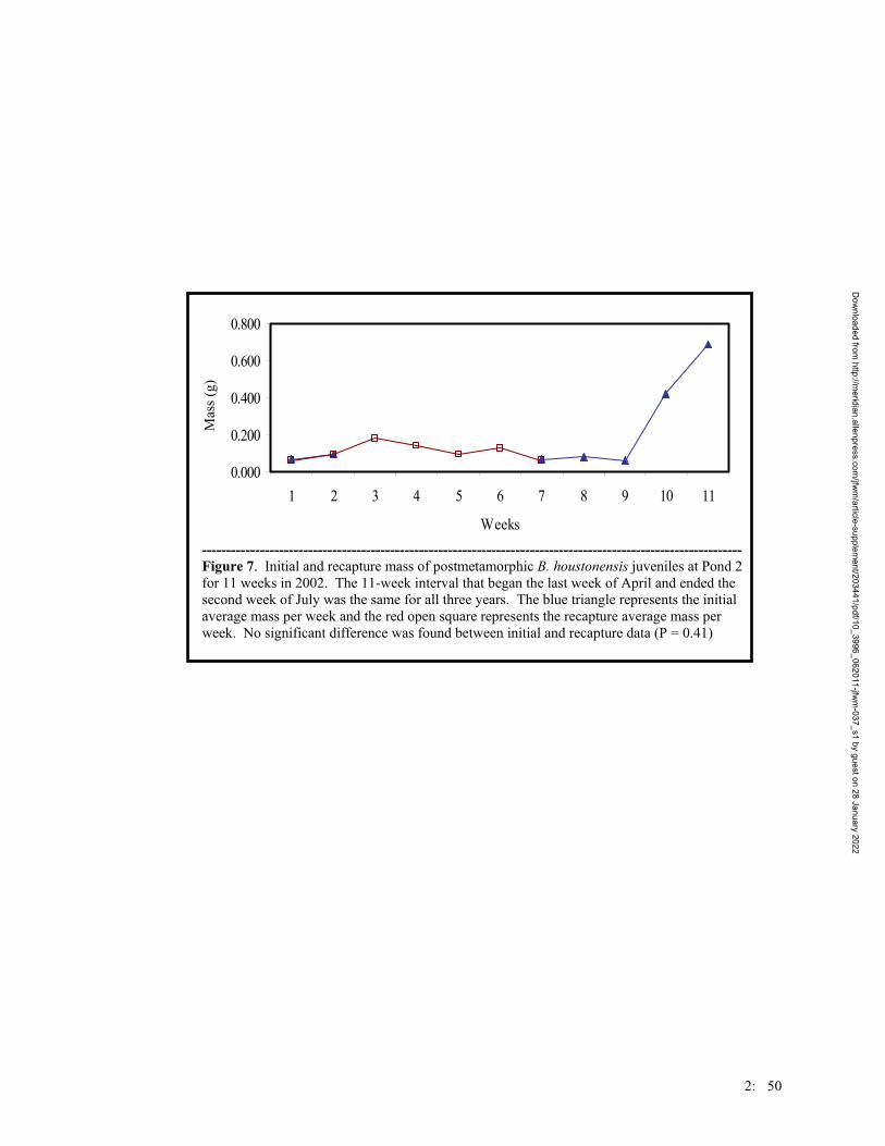
0.000

0.200

0.400

0.600

0.800

1 2 3 4 5 6 7 8 9 10 11

Weeks

Wei

ght (

g)

Mas

s (g)

---------------------------------------------------------------------------------------------------------------- Figure 7. Initial and recapture mass of postmetamorphic B. houstonensis juveniles at Pond 2 for 11 weeks in 2002. The 11-week interval that began the last week of April and ended the second week of July was the same for all three years. The blue triangle represents the initial average mass per week and the red open square represents the recapture average mass per week. No significant difference was found between initial and recapture data (P = 0.41)

2: 50

Dow



m/article-supplem

ent/203441/pdf/10_3996_062011-jfwm


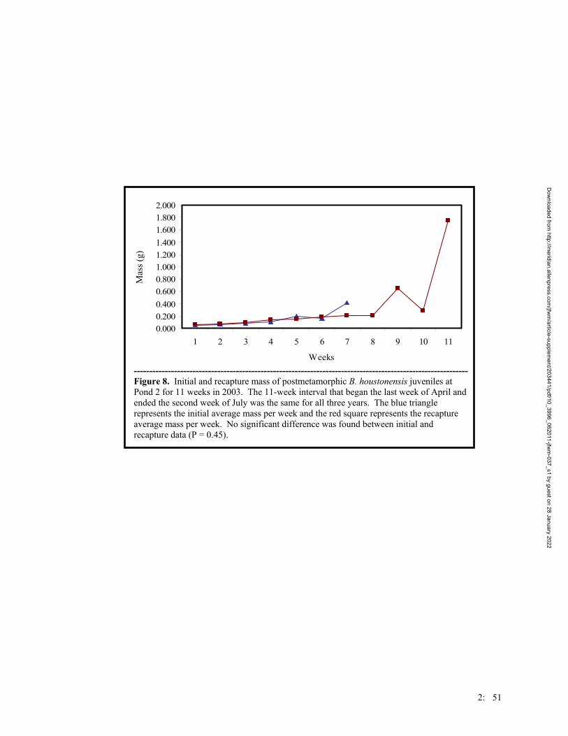
0.0000.2000.4000.6000.8001.0001.2001.4001.6001.8002.000

1 2 3 4 5 6 7 8 9 10 11

Weeks

Wei

ght (

g)

Mas

s (g)

------------------------------------------------------------------------------------------------------------ Figure 8. Initial and recapture mass of postmetamorphic B. houstonensis juveniles at Pond 2 for 11 weeks in 2003. The 11-week interval that began the last week of April and ended the second week of July was the same for all three years. The blue triangle represents the initial average mass per week and the red square represents the recapture average mass per week. No significant difference was found between initial and recapture data (P = 0.45).

2: 51

Dow



m/article-supplem

ent/203441/pdf/10_3996_062011-jfwm


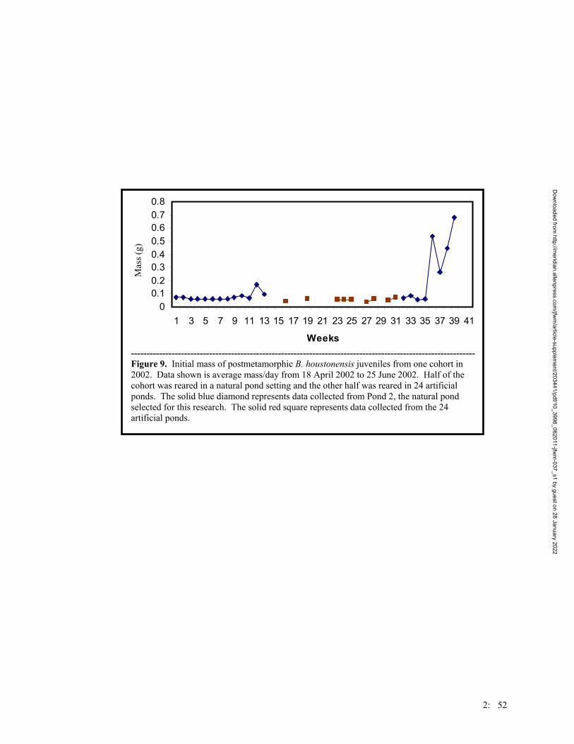
00.10.20.30.40.50.60.70.8

1 3 5 7 9 11 13 15 17 19 21 23 25 27 29 31 33 35 37 39 41

Weeks

Wei

ght (

g)

Mas

s (g)

-------------------------------------------------------------------------------------------------------------- Figure 9. Initial mass of postmetamorphic B. houstonensis juveniles from one cohort in 2002. Data shown is average mass/day from 18 April 2002 to 25 June 2002. Half of the cohort was reared in a natural pond setting and the other half was reared in 24 artificial ponds. The solid blue diamond represents data collected from Pond 2, the natural pond selected for this research. The solid red square represents data collected from the 24 artificial ponds.

2: 52

Dow



m/article-supplem

ent/203441/pdf/10_3996_062011-jfwm


0

0.5

1

1.5

2

1 4 7

Wei

ght (

g)M

ass (

g)

--------------------------Figure 10. Initial ma2003. Data shown is cohort was reared in aponds. Juveniles weregrowth was stagnant. natural pond selected the 24 artificial ponds

Dow

nloaded from http:/

Delayed emergence in Artificial Ponds.

10 13 16 19 22 25 28 31 34 37 40 43 46

Days ----------------------------------------------------------------------------------- ss of postmetamorphic B. houstonensis juveniles from one cohort in average mass/day from 23 April 2003 to 20 July 2003. Half of the natural pond setting and the other half was reared in 24 artificial still found emerging by week 11 in the artificial pond; however,

The solid blue diamond represents data collected from Pond 2, the for this research. The solid red square represents data collected from .

2: 53

/meridian.allenpress.com

/jfwm

/article-supplement/203441/pdf/10_3996_062011-jfw

m-037_s1 by guest on 28 January 2022

different effect. Emergence out of the artificial array did not begin until almost 3 weeks

after those in the natural pond in 2003. In 2002, juveniles emerged from artificial ponds

almost a week and a half after Pond 2 juveniles ceased to be found.

The difference in mass between a juvenile from the natural pond and a juvenile

from the artificial pond is illustrated in Figure 11. At the time the picture was taken, both

juveniles were 99 days old (from egg to postmetamorph) and weighed 0.450 g (juvenile

on left) and 0.079 g, respectively. The juveniles had the same age, but different emerging

times. The juvenile that emerged from the natural pond was almost five and a half times

larger, which was a significant difference (P < 0.01).

Evaluation of 2003 Data

Various ponds were surveyed for B. houstonensis juveniles in addition to the 2

main research sites (natural and artificial ponds). One privately owned pond (Ponderosa

Dr., Bastrop County) had over 500 juveniles dispersing from a recently excavated pond.

Sixty-nine measurements and tissue samples were taken from this site. Another privately

owned pond near HWY 290 in Bastrop County was inspected. This pond yielded 18

juvenile tissue samples and measurements. Pond 11 on the GLR also had dispersing

juveniles. Sixteen samples were taken from this site. The samples were determined to be

B. houstonensis tissue (APPENDIX 1) and a detailed description of each sample can be

found in APPENDIX 2.

2: 54

Dow



m/article-supplem

ent/203
441/pdf/10_3996_062011-jfwm

--------------------------------------------------------------------------------- Figure 11. Differences in mass between a juvenile from the natural pond setting (left) and a juvenile from the artificial pond setting (right). Both are 99 days old (from egg to postmetamorph). The masses were 0.450 g (left) and 0.079 g (right).

2: 55

Dow



m/article-supplem

ent/203441/pdf/10_3996_062011-jfwm


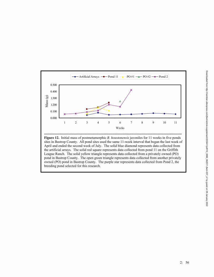
0.000

0.100

0.200

0.300

0.400

0.500

1 2 3 4 5 6 7 8 9 10 11

Weeks

Wei

ght (

g)

Artificial Arrays Pond 11 PO #1 PO #2 Pond 2

Mas

s (g)

---------------------------------------------------------------------------------------------------------------------- Figure 12. Initial mass of postmetamorphic B. houstonensis juveniles for 11 weeks in five ponds sites in Bastrop County. All pond sites used the same 11-week interval that began the last week of April and ended the second week of July. The solid blue diamond represents data collected from the artificial arrays. The solid red square represents data collected from pond 11 on the Griffith League Ranch. The solid yellow triangle represents data collected from a privately owned (PO) pond in Bastrop County. The open green triangle represents data collected from another privately owned (PO) pond in Bastrop County. The purple star represents data collected from Pond 2, the breeding pond selected for this research.

2: 56

Dow



m/article-supplem

ent/203441/pdf/10_3996_062011-jfwm


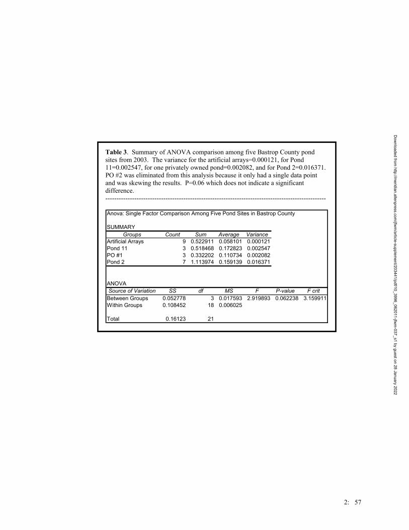
Table 3. Summary of ANOVA comparison among five Bastrop County pond sites from 2003. The variance for the artificial arrays=0.000121, for Pond 11=0.002547, for one privately owned pond=0.002082, and for Pond 2=0.016371. PO #2 was eliminated from this analysis because it only had a single data point and was skewing the results. P=0.06 which does not indicate a significant difference. --------------------------------------------------------------------------------------------------- Anova: Single Factor Comparison Among Five Pond Sites in Bastrop County

SUMMARYGroups Count Sum Average Variance

Artificial Arrays 9 0.522911 0.058101 0.000121Pond 11 3 0.518468 0.172823 0.002547PO #1 3 0.332202 0.110734 0.002082Pond 2 7 1.113974 0.159139 0.016371


Between Groups 0.052778 3 0.017593 2.919893 0.062238 3.159911Within Groups 0.108452 18 0.006025

Total 0.16123 21

2: 57

Dow



m/article-supplem

ent/203441/pdf/10_3996_062011-jfwm


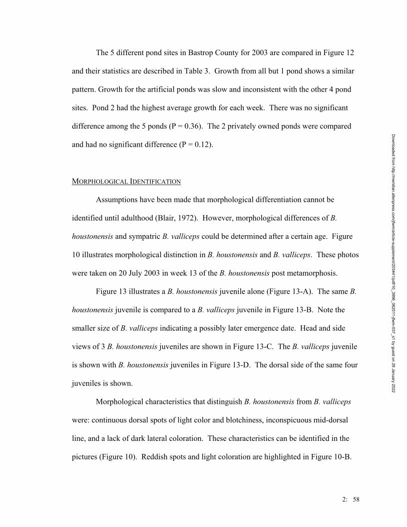
The 5 different pond sites in Bastrop County for 2003 are compared in Figure 12

and their statistics are described in Table 3. Growth from all but 1 pond shows a similar

pattern. Growth for the artificial ponds was slow and inconsistent with the other 4 pond

sites. Pond 2 had the highest average growth for each week. There was no significant

difference among the 5 ponds (P = 0.36). The 2 privately owned ponds were compared

and had no significant difference (P = 0.12).

MORPHOLOGICAL IDENTIFICATION

Assumptions have been made that morphological differentiation cannot be

identified until adulthood (Blair, 1972). However, morphological differences of B.

houstonensis and sympatric B. valliceps could be determined after a certain age. Figure

10 illustrates morphological distinction in B. houstonensis and B. valliceps. These photos

were taken on 20 July 2003 in week 13 of the B. houstonensis post metamorphosis.

Figure 13 illustrates a B. houstonensis juvenile alone (Figure 13-A). The same B.

houstonensis juvenile is compared to a B. valliceps juvenile in Figure 13-B. Note the

smaller size of B. valliceps indicating a possibly later emergence date. Head and side

views of 3 B. houstonensis juveniles are shown in Figure 13-C. The B. valliceps juvenile

is shown with B. houstonensis juveniles in Figure 13-D. The dorsal side of the same four

juveniles is shown.

Morphological characteristics that distinguish B. houstonensis from B. valliceps

were: continuous dorsal spots of light color and blotchiness, inconspicuous mid-dorsal

line, and a lack of dark lateral coloration. These characteristics can be identified in the

pictures (Figure 10). Reddish spots and light coloration are highlighted in Figure 10-B.

2: 58

Dow



m/article-supplem

ent/203441/pdf/10_3996_062011-jfwm


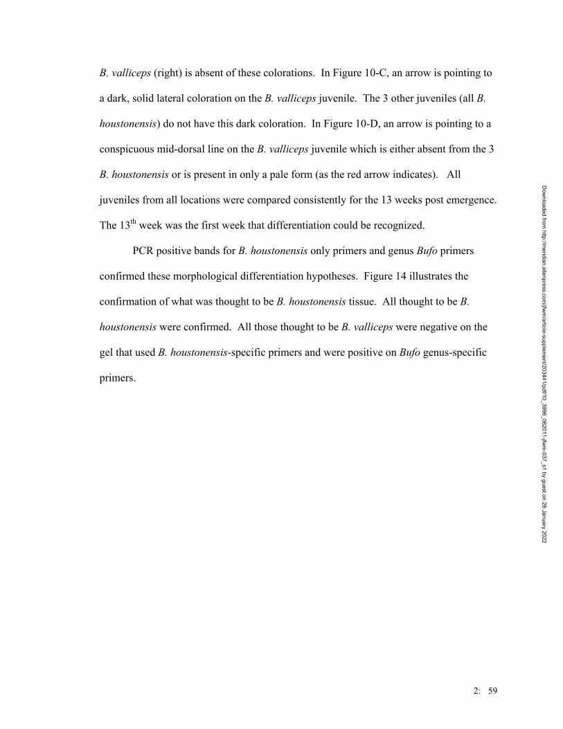
B. valliceps (right) is absent of these colorations. In Figure 10-C, an arrow is pointing to

a dark, solid lateral coloration on the B. valliceps juvenile. The 3 other juveniles (all B.

houstonensis) do not have this dark coloration. In Figure 10-D, an arrow is pointing to a

conspicuous mid-dorsal line on the B. valliceps juvenile which is either absent from the 3

B. houstonensis or is present in only a pale form (as the red arrow indicates). All

juveniles from all locations were compared consistently for the 13 weeks post emergence.

The 13th week was the first week that differentiation could be recognized.

PCR positive bands for B. houstonensis only primers and genus Bufo primers

confirmed these morphological differentiation hypotheses. Figure 14 illustrates the

confirmation of what was thought to be B. houstonensis tissue. All thought to be B.

houstonensis were confirmed. All those thought to be B. valliceps were negative on the

gel that used B. houstonensis-specific primers and were positive on Bufo genus-specific

primers.

2: 59

Dow



m/article-supplem

ent/203441/pdf/10_3996_062011-jfwm


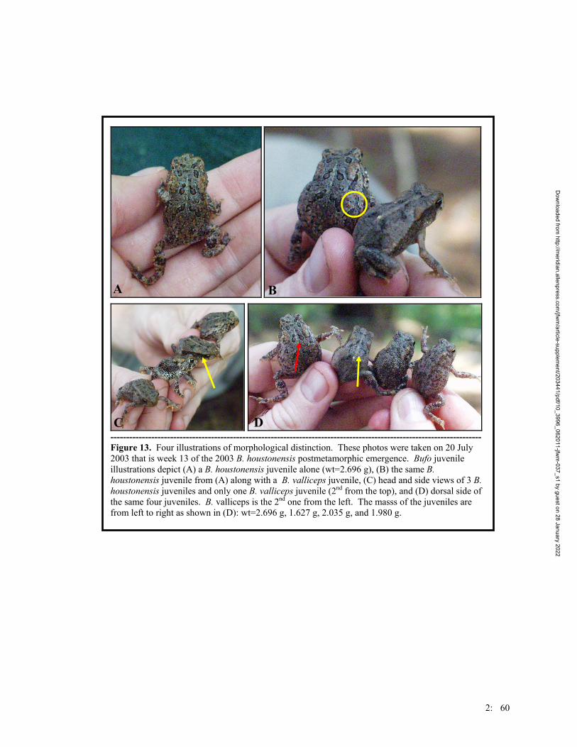
A B

-------------------------------------------- --------------------------------------------------------------------- C

Figure 13. Four illustrations of mor2003 that is week 13 of the 2003 B. hillustrations depict (A) a B. houstonehoustonensis juvenile from (A) alonghoustonensis juveniles and only one the same four juveniles. B. vallicepsfrom left to right as shown in (D): w

Dow



m/article-supplem

ent/203441/pdf/10_3996_062011

-----D

phological distinction. These photos were taken on 20 July oustonensis postmetamorphic emergence. Bufo juvenile nsis juvenile alone (wt=2.696 g), (B) the same B. with a B. valliceps juvenile, (C) head and side views of 3 B. B. valliceps juvenile (2nd from the top), and (D) dorsal side of is the 2nd one from the left. The masss of the juveniles are t=2.696 g, 1.627 g, 2.035 g, and 1.980 g.

2: 60

-jfwm


----------------------------------------------------------------------------------------------------------------------

Molecular Confirmation

BH BV BH BV BH BV BV BH BV Morphological Prediction

Figure 14. PCR results on a 1% Agarose gel using primers BHCB and BHDLR2. The row of morphological predictions represents the field assessment of morphological differences and the educated deduction as to which species the juvenile was. The molecular confirmation represents which tissue donor was B. houstonensis (BH). Those that were thought to be B. houstonensis were indeed confirmed to be. Those that were thought to be B. valliceps (BV) were negative on this gel. These five Bufo tissue donors were tested with the Bufo genus primers and those came out positive, indicating that these samples were not degraded, just not B. houstonensis.

2: 61

Dow



m/article-supplem

ent/203441/pdf/10_3996_062011-jfwm


2: 62

DISPERSAL PATTERNS

Dispersal was observed only at the natural pond. No recapture data was collected

in the habitat surrounding the artificial arrays in 2002 and 2003. During late April

through mid July, many young, recently metamorphosed Houston toads left the breeding

pond and invaded Pond 2’s upland habitat a week or more elapsing after emergence.

Using the elliptical arrays at Pond 2, juveniles reached the 8 m aluminum barrier

by week 2 in both years. In 2002, juveniles reached the last elliptical array on day 19

post emergence. In 2003, juveniles reached the last array on day 13 post emergence.

Juveniles stayed close to the water’s immediate edge for the first 3 weeks and then

gradually started migrating towards the upland habitat adjacent to the pond.

Five Bufo juveniles were found using the large refugia 20 m - 35 m away from the

pond in 2002. Four juveniles were found using the small refugia up to 50 m away from

Pond 2 in 2003. Eighteen Bufo juveniles were found throughout the GLR in 2003, but

only after precipitation occurred.

A correlation was found when comparing distance dispersed to juvenile mass. A

greater correlation was recognized in 2002 (r = 0.67) than in 2003 (r = 0.51). However,

both years indicated a positive correlation. This positive relationship signified that larger

juveniles disperse farther away from breeding ponds.

Because all sampling covered a large array of habitat, moist vs. dry, shade vs.

sunlit, sand vs. clay, and pine vs. mixed oak-juniper, habitat preference could be deduced.

Dow



m/article-supplem

ent/203441/pdf/10_3996_062011-jfwm


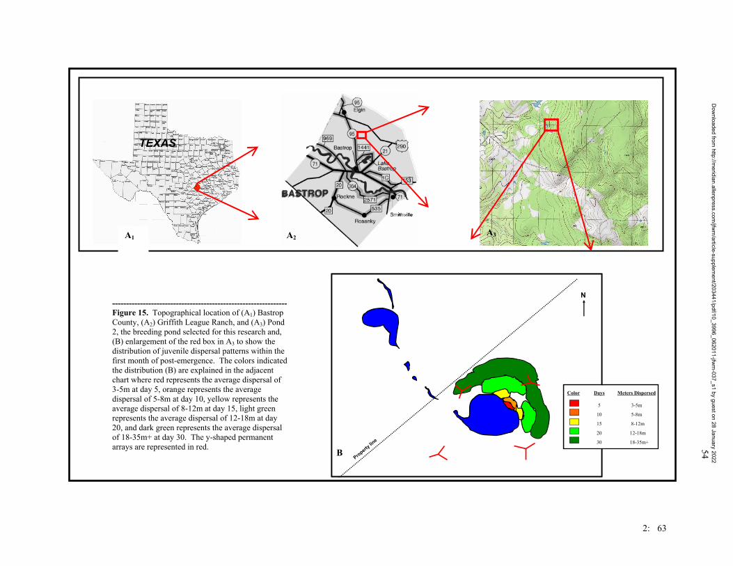
54

2: 63

N

Property lin

e

N

Property lin

e

5 3-5m

10 5-8m

15 8-12m

20 12-18m

30 18-35m+

Color Days Meters Dispersed

5 3-5m

10 5-8m

15 8-12m

20 12-18m

30 18-35m+

Color Days Meters Dispersed

A3

B

A2

--------------------------------------------------------------- Figure 15. Topographical location of (A1) Bastrop County, (A2) Griffith League Ranch, and (A3) Pond 2, the breeding pond selected for this research and, (B) enlargement of the red box in A3 to show the distribution of juvenile dispersal patterns within the first month of post-emergence. The colors indicated the distribution (B) are explained in the adjacent chart where red represents the average dispersal of 3-5m at day 5, orange represents the average dispersal of 5-8m at day 10, yellow represents the average dispersal of 8-12m at day 15, light green represents the average dispersal of 12-18m at day 20, and dark green represents the average dispersal of 18-35m+ at day 30. The y-shaped permanent arrays are represented in red.

TEXAS

A1

Dow



m/article-supplem

ent/203441/pdf/10_3996_062011-jfwm


Juveniles were only found in moist, shady areas. Juveniles were found in both

soils and vegetation types. Therefore, soil and vegetation type were not necessarily

factors in habitat choice.

Figure 15 provides a topographical location of Pond 2, the breeding pond selected

for this research and, the distribution of juvenile dispersal patterns within the first month

of post emergence. Color is used to demonstrate correlation between time and the

maximum scale of dispersal distance over which Bufo juveniles were found.

DISCUSSION

GROWTH & DEVELOPMENT

Bufo houstonensis postmetamorphic development was inconsistent, at least in

part, with previously documented juvenile growth data (Quinn and Mengden, 1984). The

significant difference found among the 2002 and 2003 research SUL data and Quinn and

Mengden’s SUL data (1984) was not surprising as captive studies tend to rear healthier

cohorts than those found in the wild where consumption, predatorial, and desiccation

factors are a constant threat. However, it was important to note the relationships within

each dataset, especially the high R2 value in Quinn and Mengden where mass/time was

almost 100% correlated. Perhaps juveniles in the lab, with consistent food availability

and absence of survivorship stresses, are more uniform in development. Another

advantage of captive-raising toads is that toads can be measured for a longer time than in

the wild because wild-caught juveniles tend to disappear after 13-15 weeks and will not

appear until the following breeding season.

2: 64

Dow



m/article-supplem

ent/203441/pdf/10_3996_062011-jfwm


As expected, there was a high significant correlation between mass and snout-to-

urostyle length in both 2002 and 2003. This correlation was important because the

relationship indicates proportionality in growth. In some cases, when only mass or SUL

can be measured, this high correlation allows assumption for the missing measurement by

using the simple linear equation, y = 9.7x+8.3, where x = mass (g) and y = SUL (mm).

This equation may vary from year to year and has only been applied to juveniles.

Therefore, adult correlations would need development.

In 2003, collections at 5 different ponds in Bastrop County showed a consistent

pattern up until week 5 (late May) when either collections ceased or juveniles became

rare. It is important to note the lack of a significant difference in the timing of juvenile

abundance and elevated densities among the Bastrop County pond cohorts. Juvenile

bufonid growth was consistent throughout the county for at least the first 6 weeks post

emergence.

The juveniles from Pond 11 on the GLR were larger in size than those found at

pond 2 in 2003. Juveniles in Pond 2 were larger in size than those found at artificial

ponds. Pond 11 juveniles emerged earlier than those in Pond 2 just as juveniles in Pond 2

emerged and were larger than those found at artificial arrays.

The comparison of initial and recapture measurements for 2002 and 2003 did not

indicate a significant difference. This result should not be surprising as these data are

from the same individuals of a cohort. The 2 figures (Figure 6, Figure 7) show that there

were small inconsistencies with these data collections indicating precision in

measurements.

2: 65

Dow



m/article-supplem

ent/203441/pdf/10_3996_062011-jfwm


Growth was rapid in the first weeks of life. Development can be inconsistent at

this time, even among individuals from the same cohort. When 2 halves of the same

cohort were divided into natural and artificial pond settings, results were not as expected

(Figure 8). In 2002, mass from juveniles emerging from the artificial ponds was

comparable to the natural pond and showed no significant difference (P = 0.12).

However, 2003 was unpredictable as there was a significant difference in the mass of

juveniles emerging from artificial ponds to the natural pond (P = 0.03). In 2003, black

mesh screens were made to cover ponds and prevent non-experimental individuals from

breeding. The temperature was reduced from these dark screens and development of

larval B. houstonensis was delayed. This delay persisted for 3 weeks after juveniles

emerged from the natural pond. Emergence was slow; only 1 or 2 juveniles were

captured a day. In fact, emergence continued for at least 5 weeks after most individuals

finished metamorphosis in the natural pond. This slow process was most likely caused

by the decreased temperature and light, deregulating normal metamorphosis. Another

factor involved in delayed metamorphosis could be the lack of required resources (i.e.,

food and protection).

Individuals from these artificial ponds not only encountered delayed

metamorphosis, but were never recaptured again. This absence was most likely related to

unfavorable habitat conditions. The artificial ponds were in an open field and received

no shade, allowing no protection for juveniles against the sunlight. This lack of protection

increased chances for dessication. In addition, Solenopsis invicta, the imported fire ant,

was a known predator present in large numbers in this pasture. Ant mounds were

observed daily around artificial arrays and ants were observed surrounding the water’s

2: 66

Dow



m/article-supplem

ent/203441/pdf/10_3996_062011-jfwm


edge when juveniles were metamorphosing and emerging. This absence is supported by

the 2002 and 2003 natural pond site data where no juvenile was found in a sunlit and /or

dry environment. This is extremely important because the 100% mortality of juveniles in

the artificial arrays and the 100% absence of capture indicate B. houstonensis

postmetamorphs will not likely be found in open fields or pastures. This is consistent

with the fact that adult Houston toads have yet to be caught in the middle of an open field

on the GLR. Adults were caught along the perimeter of several open fields, but none

were found in the center of an unshaded open field (Forstner, M.R.J. and Swannack, T.,

pers. comm.).

Pastures or grasslands could act as populations sinks because of decreased

juvenile survival during emigration (Rothermel, in press). The implication that open

fields are injurious to B. houstonensis juveniles and adults could lend support to

conservation efforts, perhaps in the conservation/restoration of Houston toad corridors.

Habitat alteration resulting in continuous open grassy areas with no canopy cover should

be considered detrimental to Houston toad juvenile dispersal and ultimately, its survival.

MORPHOLOGICAL IDENTIFICATION

Bufo juvenile species can be correctly identified using morphology at 13 weeks of

age. However, this distinction has only been observed in 2 sympatric species, B.

houstonensis and B. valliceps. Comparisons of B. houstonensis with other juveniles of

congeners, such as B. woodhousei and B. americanus, should be explored due to their

potentially less distinct juvenile morphological appearances. Therefore, more

information must be gathered before this early differentiation can become reliable.

2: 67

Dow



m/article-supplem

ent/203441/pdf/10_3996_062011-jfwm


However, these data are immediately useful in monitoring in Bastrop County and can be

supplemented by DNA identification.

To distinguish Bufo juveniles at the earliest age possible (aside from molecular

analyses) would be extremely valuable for individuals with properties containing

Houston toad habitat. Proper implementation of Houston toad regulations can occur at an

earlier date for Bastrop County landowners and an effective conservation plan can be

established or sustained more quickly. In addition, distinguishing the species

morphologically at such an early age would aid surveyors of multiple Houston toad

populations. This early detection, in addition to typical surveying procedures, might

increase the accuracy in estimating populations and improve yearly survival estimates.

Earlier detection of juvenile Houston toads could improve population surveys.

Emerging juveniles have been determined to linger near the pond’s edge for the first 3

weeks. Therefore, there are 3 weeks to determine whether a pond has compatible

Houston toad habitat and if adults return in subsequent breeding seasons. Surveyors

performing night surveys may not get the chance to detect Houston toad chorusing for a

pond due to a variety of circumstances (weather conditions, time of night, the presence of

a predator near a pond), but finding emerging juveniles documents the toad’s presence.

By 13 weeks, species differences can be determined and can aid in proper identification

of Houston toad, and viable habitats.

DISPERSAL PATTERNS

Results from monitoring dispersal and movement patterns are demonstrative of

the positive correlation to the presence of moisture. Juveniles immediately sought shade

2: 68

Dow



m/article-supplem

ent/203441/pdf/10_3996_062011-jfwm


and cover and were most abundant in thick leaf litter. Either juveniles had a preference

towards shadier, moist areas or they simply died in areas lacking in these qualities. Soil

and vegetation type were neither preferred nor avoided as juveniles occurred in all 4

types (carrizo sand, red clay subsoil, pine, or oak-juniper forests). A preference for forest

habitat (Semlitsch 2000a) is found in many amphibians and thus, supports these

observations.

After metamorphosis, juveniles remained by the immediate water’s edge for 3

weeks. It was observed that juveniles did not move nearly as quickly the first few days of

metamorphosis as they did weeks later. Therefore, initial movement was gradual as

juveniles were particularly dependent on the moisture from the saturated sands

immediately bordering the water’s edge. Clarke (1974) observed this dependency in

bufonid juveniles where the postmetamorphs lived in wet litter on the shore of the pond

for approximately a week.

Juveniles remained in the adjacent upland habitat for at least 13 weeks, where

juveniles were still caught within a 50 m radius surrounding the pond of emergence.

Refugia were useful in demonstrating that juveniles could be found in moist habitats.

This environment may also be a suitable habitat for a more permanent refuge throughout

the year and could be used as a potential habitat supplement for the conservation of

isolated subpopulations.

The small numbers of individuals that were found in these refugia may seem

inconsequential, but compared to the absence of juveniles found when doing the quadrat

surveys, these data are invaluable. Less than 1% of bufonid juveniles survive to

adulthood. The majority fall victim to predators or desiccation. Therefore, it is of the

2: 69

Dow



m/article-supplem

ent/203441/pdf/10_3996_062011-jfwm


utmost importance when juveniles are found utilizing moisture or a safe haven, which

could possibly increase their chance for survival. These data show that the few survivors

found and used damp, protected areas.

The correlation of mass and distance is vital in understanding dispersal patterns of

B. houstonensis juveniles. This information provides support for the contention that

juveniles disperse widely yet stay within at least a 50 m range of the pond of emergence

for approximately 11 weeks.

Knowing the estimated distance from a breeding pond that the majority of

juveniles stay within can be valuable information (Bellis, 1965) for the conservation of

Houston toad populations. This known radius (30 m) around the breeding pond can aid

in the implementation of a buffer zone, where little to no human interaction in that zone

is permitted. The buffer zone should be enforced while B. houstonensis juveniles are still

highly concentrated around the pond and have yet to disperse fully. Buffer zones are

preferred to have little to no human interaction including hunting, fishing, or allowing

cattle near Houston toad breeding ponds. Reduction in these interactions this would

reduce exploitation of habitat juveniles’ use as shelter and protection.

By using juvenile dispersal to define buffer zone requirements, a layer of

protection will hopefully be afforded to future generations. Consequently, juvenile

growth, development, and morphological differentiation can then be given a better

chance at functioning properly in an ever-threatening environment.

2: 70

Dow



m/article-supplem

ent/203441/pdf/10_3996_062011-jfwm


CONSERVATION IMPLICATIONS OF JUVENILE ECOLOGY AND SURVIVORSHIP

TECHNIQUES IN THE HOUSTON TOAD

BUFO HOUSTONENSIS (ANURA: BUFONIDAE)


To assist the recovery of an endangered species, conservation management

options attempt to increase the size of populations and achieve a self-sustaining level in

the wild (Maxwell and Jamieson 1997). In accomplishing these requires consideration of

several factors in any management plan; one of which includes local population dynamics

or in the case of the Houston toad, the number/density of individuals dispersing from

individual wetlands.

For local population dynamics in the toad, metamorphosis from the aquatic

habitat to the terrestrial environment is the critical step by which individuals are

potentially recruited into the breeding population (Semlitsch 2000a). When migrating

toward other ponds, juveniles tend to travel greater distances than adults (Breden 1987),

sometimes up to 200 m (Semlitsch 1998). This extensive travel makes the

metamorphosing juveniles the primary dispersal stage (Gill 1978) and hence, better

indicators of required habitat. If success rates of metamorphosis are high, juveniles can

help maintain local populations, and will likely supply dispersers to new or extirpated

populations. Therefore, management plans that include actions to ensure a high

probability of juvenile survival (e.g., protection of critical habitat adjacent to the pond or

2: 71

Dow



m/article-supplem

ent/203441/pdf/10_3996_062011-jfwm


wetland), will help maintain local species populations and provide dispersers for

recolonization (Semlitsch 2000b).

Unfortunately, current management of the Houston toad, Bufo houstonensis,

seldom includes aspects of juvenile ecology. As stated in Chapter 1, early PHVA

management recommendations included minimizing the disturbance of soil, pesticide

use, and habitat fragmentation. Maximizing the restoration of corridors and potential

habitat (Lacy and Seal 1994) were also included. However, in this PHVA, juvenile

ecology failed to be incorporated in recommendations.

Hatfield et al. (2002) conducted several Population Viability Analysis (PVA)

computer simulations for B. houstonensis in 2002 to estimate survival rates under

variable circumstances. This study acknowledged that upon simulating multiple

scenarios, juvenile survival is obviously important. If juvenile survival is 1%, single

populations usually have a high probability of extinction. If juvenile survival is 2%,

single populations usually have a low probability of extinction. Hatfield et al.

recommended that to determine whether the simulations performed were closer to low or

high juvenile survival scenarios, actual estimation of the number of eggs laid, estimation

of the number of metamorphs, and marking/recapturing juveniles should be done. With

these recommendations, the significance of juvenile data is finally recognized.

The estimation techniques used to determine survivorship data are a vital addition

in censusing Houston toad populations. The Wire Section model is the technique

recommended for realistic application. This technique allows for quick maneuverability

and is simple in concept. The model uses wires that are cut to the average known length

of 50 eggs to estimate the number of eggs in a cohort. Estimation time is 40 to 60

2: 72

Dow



m/article-supplem

ent/203441/pdf/10_3996_062011-jfwm


minutes. Conservationists and/or endangered species surveyors can use this method to

estimate egg numbers without displacement or manipulation that could cause detrimental

effects, such as abnormalities or even mortality.

From Chapter 2, B. houstonensis survival from egg to metamorph was 4.7%. This

survivorship percentage was based on recently emerged metamorphs, not juveniles

surviving beyond a few weeks in the terrestrial environment. There were 15% fewer

juveniles estimated to be living by week 13 (4.0% survivorship). It is estimated that by

the first year of adulthood, 1 out of every 200 (0.05%) Houston toads survive (Forstner,

M.R.J. and Swannack, T., pers. comm.). This percentage is greatly reduced from the

estimated 1% survival rate where populations have a high probability of extinction

(Hatfield et al. 2002) indicating an even higher extinction probability. If 15% of

juveniles die every 13 weeks, juveniles from the 2003 egg strand will be almost

completely eradicated by year 2 with an estimated survivorship of 0.0001%. This paired

with the fact that juvenile survivorship at 13 weeks (4.0%) is overestimated, it is

concluded that the population is serious risk of extinction. Survivorship data from older

juvenile (> 13 weeks) to adult is greatly needed to fill the gap in survivorship estimation.

With this study’s juvenile data, a more detailed indication of the Houston toad’s survival

rate can be considered and the immanency of the situation can be addressed. With the

knowledge that this endangered species is quickly moving towards extinction, thorough

management efforts should continue, if not increase in intensity.

The multiple aspects of juvenile ecology explained in Chapter 3 will certainly

change the way we look at managing the Houston toad. Analysis of juvenile growth and

developmental patterns are essential because it can contribute to an understanding of the

2: 73

Dow



m/article-supplem

ent/203441/pdf/10_3996_062011-jfwm


population processes of the species (Clarke, 1974). Juvenile growth in the Houston toad

was found to be rapid and variable. When comparing this study’s wild-caught data to

that of previously published captive-bred data, it was not surprising that the wild-caught

data would show lower growth rates. However, what could be beneficial to Houston toad

management is not that growth rates were lower; it is that wild-caught data 2003 was not

significantly different from that of captive-bred data. Therefore, wild-caught juveniles, at

least the ones that survive, are growing as well as can be expected considering multiple

stressors involved.

It is important to note the correlation between SUL and mass because with such a

high correlation, measurement assumptions can be made when there are constraints on

time in the field. By using the simple linear equation, y = 9.7x+8.3, where y = SUL

(mm) and x = mass (g), field biologists can then use just 1 measurement and calculate the

other.

Juveniles were not found in areas without shade and leaf litter. Therefore, it is

recommended that conservation efforts should focus on preventing large areas of open

fields near and/or around Houston toad habitat or breeding ponds. If open areas are

already present near and/or around Houston toad habitat or breeding ponds, then

vegetative reconstruction of native flora for canopy cover should be implemented when

possible.

The presence of shade in the terrestrial habitat is a necessity for juvenile survival.

However, tadpoles require the exactly the opposite. In 2003, delayed growth of a cohort

was discovered when tarps were placed over artificial ponds and juveniles emerging from

these ponds took 3 weeks longer to metamorphose. The constant shade decreased the

2: 74

Dow



m/article-supplem

ent/203441/pdf/10_3996_062011-jfwm


light exposure and pond temperature and, consequently, delayed emergence. The lack of

required resources such as food or shelter could also influence the delay of

metamorphosis. This along with temperature decrease created an inhospitable

environment which ultimately caused metamorphosis to slow.

Due to the relative density of water and the presence of aquatic vegetation, a

longer amount of time is needed to heat up a pond than a terrestrial environment.

Tadpoles need an optimum aquatic environment for normal metamorphosis to occur

(Breven and Chadra 1988). Sun exposure above a pond will allow the pond to warm and

speed up metamorphosis. Once tadpoles metamorphose into the harsh terrestrial

environment, shade is required for protection. Therefore, there should be little to no

shade above the pond, but rather around the pond. Relatively dense ground vegetation

should either be planted or retained around the pond to prevent desiccation upon

emergence.

Morphology, although thought to be slow in development (Blair 1972), can be

distinguishable down to the species level at 13 weeks post emergence for B. houstonensis

using these characteristics: continuous dorsal spots of light color and blotchiness,

inconspicuous mid-dorsal line, and a lack of dark lateral coloration. Molecular

identification can also be used to distinguish bufonid juveniles from one another using

the PCR method. A polymerase chain reaction (PCR) marker system was used to

distinguish the different species. This test positively identified juvenile B. houstonensis

by using species-specific primers designed in our laboratory. A positive band identified

Houston toads to the exclusivity of other taxa. Both identification methods have their

advantages and disadvantages. Table 1 explains the pros and cons of each method.

2: 75

Dow



m/article-supplem

ent/203441/pdf/10_3996_062011-jfwm


This study focused on morphological identification as it was lacking in research.

To distinguish Bufo juveniles at the earliest age possible (save molecular analyses) would

be extremely valuable for those parties whose properties are concerned with Houston

toad habitat. Proper implementation can then occur at an earlier date for landowners and

an effective conservation plan can be established or sustained more efficiently. In

addition, morphological distinction between species at such an early age would aid

surveyors in distinguishing B. houstonensis from other bufonid species. This early

detection, in addition to typical surveying procedures, might increase the accuracy of

estimating population numbers and the estimate of yearly survival.

Juvenile dispersal is one of the key factors in determining species range in the

critical metamorphosing period. By establishing the radius around a breeding pond

which most juveniles (> 75%) inhabit, one can apply this known distance to management

practices. The radius around a breeding pond can act as a guide for the implementation

of a buffer zone, where little to no human interaction is permitted. This implementation

does not have to be permanent. However, it is preferable that this buffer zone is enforced

throughout the duration of the time juveniles are concentrated around the breeding pond.

This would significantly decrease anthropogenic activities such as hunting and fishing.

The reduction of cattle around breeding ponds would also be a major improvement as

Houston toad breeding ponds are associated with water tanks used for cattle, more so

than ponds used for anthropogenic recreation (pers. obs.). The decrease of human

interaction with Houston toad breeding ponds during the time of juvenile

2: 76

Dow



m/article-supplem

ent/203441/pdf/10_3996_062011-jfwm


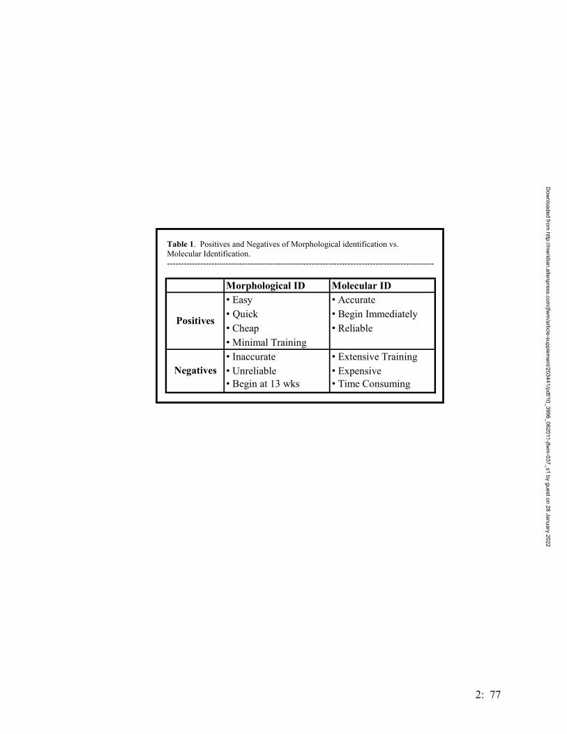
Table 1. Positives and Negatives of Morphological identification vs. Molecular Identification. ------------------------------------------------------------------------------------------------

Morphological ID Molecular ID• Easy • Accurate• Quick • Begin Immediately• Cheap • Reliable• Minimal Training• Inaccurate • Extensive Training• Unreliable • Expensive• Begin at 13 wks • Time Consuming

Positives

Negatives

2: 77

Dow



m/article-supplem

ent/203441/pdf/10_3996_062011-jfwm


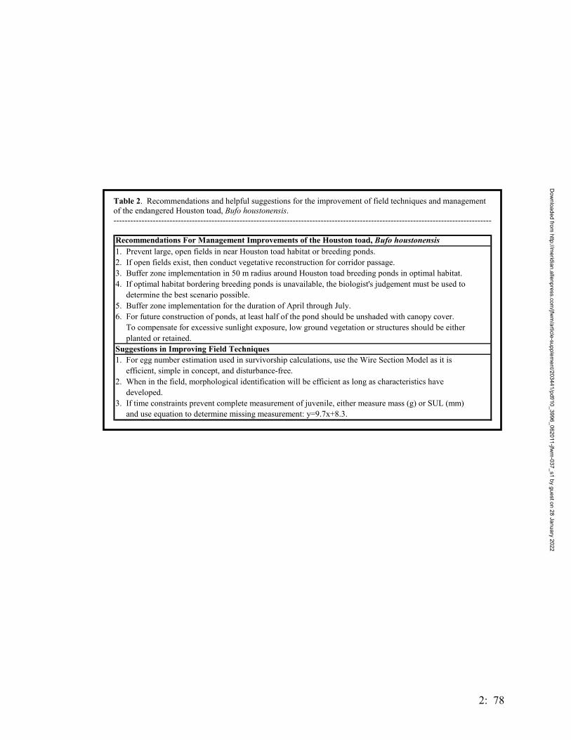
Table 2. Recommendations and helpful suggestions for the improvement of field techniques and management of the endangered Houston toad, Bufo houstonensis. --------------------------------------------------------------------------------------------------------------------------------------- Recommendations For Management Improvements of the Houston toad, Bufo houstonensis1. Prevent large, open fields in near Houston toad habitat or breeding ponds.2. If open fields exist, then conduct vegetative reconstruction for corridor passage.3. Buffer zone implementation in 50 m radius around Houston toad breeding ponds in optimal habitat.4. If optimal habitat bordering breeding ponds is unavailable, the biologist's judgement must be used to determine the best scenario possible.5. Buffer zone implementation for the duration of April through July.6. For future construction of ponds, at least half of the pond should be unshaded with canopy cover. To compensate for excessive sunlight exposure, low ground vegetation or structures should be either planted or retained.Suggestions in Improving Field Techniques1. For egg number estimation used in survivorship calculations, use the Wire Section Model as it is efficient, simple in concept, and disturbance-free.2. When in the field, morphological identification will be efficient as long as characteristics have developed.3. If time constraints prevent complete measurement of juvenile, either measure mass (g) or SUL (mm) and use equation to determine missing measurement: y=9.7x+8.3.

2: 78

Dow



m/article-supplem

ent/203441/pdf/10_3996_062011-jfwm


emergence and early dispersal would prevent habitat damage and simply prevent

unnecessary mortality. Therefore, based on the results of this study, it is recommended

that a buffer zone be implemented around known Houston toad breeding ponds at least 50

m in radius when in suitable Houston toad habitat between March and July. When

incompatible habitat happens to border Houston toad breeding ponds, the biologist’s

judgement must be used to determine appropriate measures for the best scenario possible.

The length of time and distance in radius are conservative in being less than ideal in both

size and duration, but allow for variation among breeding seasons.

The results of this research demonstrate the significance of the juvenile ecology in

proper management techniques. Aspects of the juvenile ecology such as growth and

development, morphological and molecular identification, and dispersal patterns are all

equally important and ultimately help define population survivorship. These

recommendations and helpful tips described in Table 2 will enhance Houston toad

conservation and management practices in efficiency and productivity. However, more

information can and should always be gathered to improve these statements.

2: 79

Dow



m/article-supplem

ent/203441/pdf/10_3996_062011-jfwm


2: 80

Dow



m/article-supplem

ent/203441/pdf/10_3996_062011-jfwm


BUFO HOUSTONENSIS (Houston Toad) JUVENILE DISPERSAL. Bufo houstonensis is an endangered anuran endemic to Central-East Texas. While its breeding behavior has been well documented (Hillis et al 1984. J. Herp. 18:56-72), very little published information exists concerning the juvenile life stages, and those studies focused on predation (Freed and Neitman 1988. Tex. J. Sci. 40:454-456), coloration (Mays and Freed 1985. Herpetol. Rev. 16:108-109), and growth (Greuter and Forstner. 2003. Herpetol. Rev. 34:355-356, Quinn and Mengden 1984 Southwest. Nat. 29:189-195). A Houston toad egg string was surrounded with an aluminum flashing enclosure during the spring of 2004 at the Griffith League Ranch (GLR) in Bastrop County, Texas, in order to monitor post-metamorphic behavior. Upon emergence, 993 individuals were captured and toe-clipped to identify the cohort. The flashing was carefully removed and 100 individuals were dusted with inert fluorescent powder (Radiant Color, T1 pigment) and released at the point of emergence as a single group. Fluorescent pigment was used with success to track Pelobates fuscus (Eggert 2002. Herpetol. J. 12:69-74) and the same technique was applied here. Toadlets were monitored immediately following release in order to determine if the pigment caused any malaise. Metamorphs were located with a UV light for two consecutive nights and observed during the early morning hours of the day following their pigment marked release. Metamorph locations were marked with marking flags; the area was left as undisturbed as possible, and the dispersal pattern was not analyzed until after the metamorphs left the pond’s edge. It was our intention to follow the juveniles for a longer period, but in the afternoon of the third day, the GLR received over 25 mm of rain. We believe this resulted in the pigment powder washing off of the toads, as well as, washing away all previous trackways. Within two days after emergence, at least a few (n=4) of the B. houstonensis metamorphs had dispersed from the pond’s edge up to 4m. We released the pigment marked individuals in one location causing a large amount of powder to be deposited in a small (~0.5m) area. One consequence of this was the tracks from individual metamorphs were not distinguishable within 0.5 m of the release site, but could be easily distinguished beyond that initial confused area of powder marks. When dispersing from the pond edge metamorphs did not move in a straight line, but a seeming random pattern may have been foraging or shade seeking behavior. The furthest distance an individual moved was 4 meters from the pond’s edge. However, the vast majority of individuals stayed between 2 – 3 meters from the edge, buried under grass or sedge tussocks. The dispersal pattern did not increase in diameter from 24 – 48 hours after marking. After the rainfall event, no metamorphs with pigments were relocated; however, toe-clipped individuals were found. Based on this information we assume the pigment washed off the pigment marked metamorphs’ bodies. During this study, metamorphs did not show any ill effects due to the powder. Using this method was an easy, efficient and cost effective way to track post-metamorphic juveniles. Nighttime observations of the movements of juveniles marked with the pigment were easily monitored using UV light. Metamorphs were also observable during the day as the powder is highly visible, allowing us to observe toadlets without disrupting the point of emergence. We could visually track the individuals during day or night using either naked eye or binoculars from a distance of 3m without difficulty. This is particularly relevant given the concentration of individuals at the pond’s edge during the emergence period and the consequent care required to prevent

2: 81

Dow



m/article-supplem

ent/203441/pdf/10_3996_062011-jfwm


accidental mortalities when trying to observe the behavior of these juveniles. We did not observe direct foraging during our observation of these individuals during day or night surveys. When moving individuals appeared to be simply moving between shaded cover (daylight) or moving from one resting area to the next (night time). The technique does have an inherent weakness in very wet or rainy areas. Rainfall, in particular, appears to be detrimental to this type of study, as it washes the powder off of the body, limiting the observation time to periods between pigment marking and the first rain. Submitted by TODD M. SWANNACK, Department of Wildlife and Fisheries, Texas A & M University, College Station, Texas 78743, USA; e-mail: [email protected], JAKE JACKSON and MICHAEL R. J. FORSTNER, Department of Biology, Texas State University, San Marcos, Texas 78666, USA; e-mail: [email protected]

2: 82

Dow



m/article-supplem

ent/203441/pdf/10_3996_062011-jfwm


EFFECTS OF VARIOUS LEVELS OF PREDATION AND ABIOTIC FACTORS ON THE

SURVIVORSHIP OF BUFONID TADPOLES

JACOB T. JACKSON, SUSANNAH R. MORRIS, AND MICHAEL R. J. FORSTNER

Predation is an important factor affecting the survival of larval anurans (Manteifel

and Reshetnikov 2002). Toads breed in both permanent and temporary water sources,

which have differentially structured predator assemblages (Werner and McPeek 1994).

Hydroperiod has significant effects on the structure of amphibian populations (Skelly et

al 1999). It is not clear in which case predation has the greatest effect on Bufo tadpoles,

or if the effect is significantly different among different habitat types. It has been found

that the presence of fish is beneficial to bullfrog tadpoles, while detrimental to green frog

tadpoles (Werner and McPeek 1994). It has also been observed that fish and other

predators show preference for some tadpoles over others as prey items (Werner and

McPeek 1994). Manteifel and Reshetnikov (2002) found fish not only preferred to

consume Rana tadpoles over Bufo, but that fish would actually reject a Bufo tadpole if

they took one into their mouth. The authors also observed that the defense of the Bufo

tadpoles was not as effective against invertebrate predators.

Both the endangered Houston Toad (Bufo houstonensis) and Gulf Coast toad

(Bufo valliceps)are R selected species, or species whose reproductive strategy consists of

the production of large quantities of offspring. Very few of these offspring will survive

to maturity. This produces a node in the life history of these organisms that might be an

opportune one from a management perspective. One potential aspect of that management

would be to understand whether or not ephemeral ponds (which by default could not have

fish as predators) actually represent more suitable habitats for Houston toads than do

3: 1

Dow



m/article-supplem

ent/203441/pdf/10_3996_062011-jfwm


permanent ponds. The environment of the Bastrop Co., Texas area has experienced

radical change since its settlement. Agriculture and development have resulted in a shift

from ephemeral ponds to permanent ponds constructed for livestock and other

agricultural uses. Many of these ponds have been stocked with introduced gamefish

species, which are potential tadpole predators. These species were not present in

ephemeral water sources. A counter argument can also be made that the presence of the

fish may be beneficial for the tadpoles due to the ability of the piscine vertebrate

predators to lower aquatic invertebrate predator densities. We conducted experiments to

empirically determine in which type of habitat toad tadpole survival was greatest.


Experiments were conducted over three consecutive years in an experimental

pond array on the Griffith League Ranch in Bastrop Co., TX to investigate the relative

effects of various abiotic and predator combinations on tadpole survival. To accomplish

this required the collection of tadpoles for the Houston toad. Obviously reproduction in

this endangered species is not common, hence relatively few total eggs could be safely

collected for use in any given year. Consequently, Bufo houstonensis tadpoles were

used in 2002 and 2003. However, 2004 experiment was conducted to determine the

effects of the three different predation regimes on Bufo valliceps tadpoles, a species

sympatric with the endangered Bufo houstonensis and, as a congener, an effective

substitute for the endangered species. Tadpoles were introduced into artificial ponds that

contained vertebrate and invertebrate predators, established invertebrate populations, or

3: 2

Dow



m/article-supplem

ent/203441/pdf/10_3996_062011-jfwm


invertebrate populations in the process of establishing through migration as would occur

in ephemeral pond habitats.

On the Griffith League Ranch in Bastrop County, Texas, 24 artificial ponds were

constructed in 2001. These ponds measure 1.5 m x 1.8 m x 76 cm, and have a volume of

approximately 1703 liters. Twelve of the ponds had a bank slope of 10 degrees, the other

twelve had a slope of 45 degrees. Each pond is surrounded by an aluminum flashing

enclosure to keep amphibians from escaping. Three treatments were originally

distributed randomly among the ponds. Fire ants were treated with Amdro inside the

array beginning in early April of each year. As mentioned previously, the final year of

the study differed from the first two years the experiment was conducted.

2002/2003

Twenty-four man-made experimental ponds on the Griffith League Ranch in

Bastrop County, TX were monitored in 2002 and 2003 from approximately March 23

through July 19. Prior to the spring breeding season, in late winter, the water in each

pond was drained, filtered to remove macroinvertebrates and then used to refill the pond.

Pond sediments were dredged to the banks and dried to facilitate removal of any

remaining macro-organisms. The ponds were subsequently stocked with 100 non-Bufo

tadpoles; these were primarily Rana tadpoles although some Hyla tadpoles were also

included. Predators were stocked according to Figure 1. Predator treatments were

assigned randomly to ponds within the two slope treatments. All ponds that required fish

were stocked with one bass and one perch, or one bass and four juvenile perch

approximately 3 cm in length. The insect treatment ponds each received 24 Odonate

3: 3

Dow



m/article-supplem

ent/203441/pdf/10_3996_062011-jfwm


larvae. All fish, insects, and tadpoles were obtained from other ponds on the Griffith

League Ranch, as was the case for all biological materials used in these experiments.

In 2003 screens were constructed and used to cover the ponds throughout the

season. They were in use soon after the ponds were stocked and used to prevent

invertebrate colonization of the experimental pond array. On March 23, each pond was

stocked with 183 Bufo houstonensis tadpoles from 1.5 egg strands (one half of each of

three egg strands) that were taken from Pond 2. The tadpoles from each egg strand were

divided equally among the 24 ponds; they were counted out in groups of 30 using small

buckets and a plastic eyedropper. The experimental pond array was treated as necessary

with Amdro throughout the summer to kill fire ants within the flashing.

2004

In a modification of the previous two years of treatments, bank slope was ignored.

Three treatments were then conceived in order to evaluate tadpole survival under

different predation regimes. The first treatment was designed to simulate emphemerality.

The ponds assigned to this treatment were drained on 8 April 2004. The intake on the

pump was fitted with a paint-straining screen, to ensure removal of all vertebrate and

invertebrate organisms, and the water was transferred to another pond. Each pond was

drained to a level of approximately six inches, and then fine mesh nets were repeatedly

swept through the water until no more invertebrates were found. All aquatic vegetation

and sediment were rinsed in a net to remove any predators hiding in them. Sediment and

vegetation were removed from the rubber pond liners with a shovel, and allowed to dry

on the bank for two weeks before being returned to the water. All invertebrate predators

3: 4

Dow



m/article-supplem

ent/203441/pdf/10_3996_062011-jfwm


removed from these ponds were kept in alcohol, quantified, and taxonomically identified.

All ponds were left uncovered to allow insects to migrate among ponds, facilitating

natural invertebrate colonization. This was the only treatment in which the ponds were

drained.

The second treatment was designed to simulate a permanent habitat with an

established invertebrate community. Invertebrate communities that had become

established over the previous years were therefore left intact.

The third treatment included vertebrate predators. One Micropterus salmoides

(Largemouth bass) mean length 27.53 cm and three Lepomis megalotis (longeared

sunfish) mean length 7.93 cm were added to each of these ponds on April 28th, before any

Bufo tadpoles were added. The established invertebrate communities were left intact as

with treatment two.

Difficulties were encountered globally in obtaining sufficient numbers of tadpoles

in all three years. The use of B. valliceps in the third year was in a direct attempt to

enable placing many more tadpoles into each pond. Unfortunately even with the

substitution of B. valliceps, in 2004 a total of 200 Bufo tadpoles per pond was established.

The ponds were checked daily for emergent toads from May through July 2004.

Dissolved oxygen and pH were checked weekly in the morning. 2004 protocol changes

included diurnal pH and DO measurements were recorded on 01 and 07 at 11 pm and 11

am the next morning. A data logger was placed in one pond receiving the second

treatment to record temperature through June 28th. Invertebrate surveys were conducted

on 17 April, 15 June, and 8 July using a six-inch diameter pipe thrust into the sediment

on the bottom of the pond (Werner and McPeek 1994). The depth was recorded using

3: 5

Dow



m/article-supplem

ent/203441/pdf/10_3996_062011-jfwm


graduations on the side of the pipe, and all invertebrates were netted out of the pipe with

a small aquarium net. The volume of water contained by the pipe was calculated for

each sample, allowing the density of invertebrates to be calculated, and population size of

each pond to be estimated.

RESULTS

2002

Twenty-seven post-emergent metamorphs were recovered from the 1200 (50 per

pond) initially stocked. Of those twenty-seven, all but one came from a pond containing

only fish and tadpoles. The other emerged from a pond only containing tadpoles.

2003

The first Houston toadlet emerged on May 12 from Experimental Pond (EP) 3,

and the last toadlet emerged on July 4 from EP-3. In total, 57 toadlets emerged from EP-

3. The ponds where emergence occurred were EP 3, 5, 12,13, and 18. These ponds

represent all treatments with the exception of that with only insect predators.

The low number of toadlets emerging may be attributed to several factors. The

toadlets emerged much later than their cohort that was left in the natural pond, probably

due to lower water temperature attributed to shading by the new screens. In 2002, the

pond temperatures varied from 81.6- 96.6 degrees F; in 2003, the temperature varied

from 79-80 degrees F on July 9. The lower temperature prolonged the larval stage thus

increasing the opportunity for predation by fish and insects. The Rana stocked in the

ponds could have been predators; since Rana were stocked early in the season, the

tadpoles were in their second year of development and therefore quite large. Although

checking ponds every 24 hours should ensure that toadlets remain near the water after

3: 6

Dow



m/article-supplem

ent/203441/pdf/10_3996_062011-jfwm


emerging, increased vegetation around the ponds may hide toadlets. Additionally, this

vegetation harbors potential predators such as wolf spiders, fishing spiders, and lizards.

Statistical analysis shows that there is no difference between 10 and 45-degree

angle ponds (F = 0.92, p= 0.35), no difference among predator treatments (F= 1.02, p=

0.41), and no interaction between factors (F= 0.93, p=0.45). However, the amount of

zeros (ponds with no emergence) in the data set could skew results; the majority of

emergence occurred from one pond, EP-3, which was not stocked with fish (tadpoles

only). Additional analyses may extract more meaningful results from the data.

2004

On June 15th, two juveniles (metamorphs) were recovered from pond 21. On June

16th, another was recovered from pond 21, as well as three from pond one. These six

were the only metamorphs recovered.

Shannon-Weiner indices were calculated from the invertebrate data collected

from the eight ponds drained at the beginning of the experiment are shown in Table 1.

Table 2 shows the average densities and population sizes for the four most common

predatory invertebrates, from both the drained ponds and the pipe samples conducted

over the course of the experiment.

The diurnal pH and DO data from both sampling events for all ponds included in

the experiment showed some fluctuation (Fig. 2). Mean a.m. pH ranged from 6.58 to

7.22, while p.m. readings had a range of 7.18 to 7.52. Mean DO had and a.m. range of

5.77 to 6.89, and a p.m. range of 7.08 to 7.25 for the experimental ponds in the array.

The pH and DO data recorded weekly in the mornings was averaged over the course of

the experiment. Figure three illustrates the pond/treatment layout.

3: 7

Dow



m/article-supplem

ent/203441/pdf/10_3996_062011-jfwm


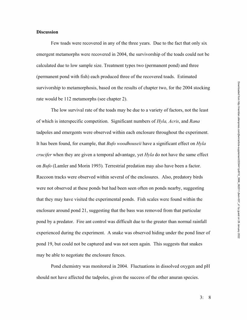
Discussion

Few toads were recovered in any of the three years. Due to the fact that only six

emergent metamorphs were recovered in 2004, the survivorship of the toads could not be

calculated due to low sample size. Treatment types two (permanent pond) and three

(permanent pond with fish) each produced three of the recovered toads. Estimated

survivorship to metamorphosis, based on the results of chapter two, for the 2004 stocking

rate would be 112 metamorphs (see chapter 2).

The low survival rate of the toads may be due to a variety of factors, not the least

of which is interspecific competition. Significant numbers of Hyla, Acris, and Rana

tadpoles and emergents were observed within each enclosure throughout the experiment.

It has been found, for example, that Bufo woodhouseii have a significant effect on Hyla

crucifer when they are given a temporal advantage, yet Hyla do not have the same effect

on Bufo (Lamler and Morin 1993). Terrestrial predation may also have been a factor.

Raccoon tracks were observed within several of the enclosures. Also, predatory birds

were not observed at these ponds but had been seen often on ponds nearby, suggesting

that they may have visited the experimental ponds. Fish scales were found within the

enclosure around pond 21, suggesting that the bass was removed from that particular

pond by a predator. Fire ant control was difficult due to the greater than normal rainfall

experienced during the experiment. A snake was observed hiding under the pond liner of

pond 19, but could not be captured and was not seen again. This suggests that snakes

may be able to negotiate the enclosure fences.

Pond chemistry was monitored in 2004. Fluctuations in dissolved oxygen and pH

should not have affected the tadpoles, given the success of the other anuran species.

3: 8

Dow



m/article-supplem

ent/203441/pdf/10_3996_062011-jfwm


Rosenberg and Pierce (1995), noted that while acidic conditions resulted in considerable

mortality in Pseudacris clarkii, it did not cause significant mortality in B. valliceps. The

authors did note, however that growth of B. valliceps tadpoles at pH 4 was significantly

less than at a neutral pH. The success or survivorship of the other species is hard to

determine, since the numbers of eggs or tadpoles that they originated from could not be

quantified. Other anuran species were not controlled in the experiment because they

were considered to be a standard factor present in all natural toad habitats, emphemeral or

permanent. It can be concluded that the number of tadpoles added was not enough to

produce sufficient power in the analyses, suggesting that Bufo tadpoles naturally

experience a very high rate of mortality.

The Shannon-Weiner indices suggest that the invertebrate predator communities

are not very diverse (Table 1). This index reveals nothing about the size of any given

population, however, only how evenly the number of individuals is distributed across all

species. The average estimated population sizes calculated from the pipe sampling data

are much larger than the average population sizes from the actual count data from the

drained ponds. There are two possible interpretations of this difference. The first would

be that the pipe sampling method applied here was susceptible to underestimation. This

is particularly notable, in the case of the Notonectidae and Dytiscidae, which are much

more agile swimmers than the Odonate larvae. This may have given them an advantage

in avoiding capture by avoiding the sampling apparatus itself. In a few cases, many of

them were observed, but none were captured. However, enough were captured for

sampling to be useful qualitatively if not quantitatively. The second, and more likely

explanation for the differences is that the invertebrate communities were maturing in both

3: 9

Dow



m/article-supplem

ent/203441/pdf/10_3996_062011-jfwm


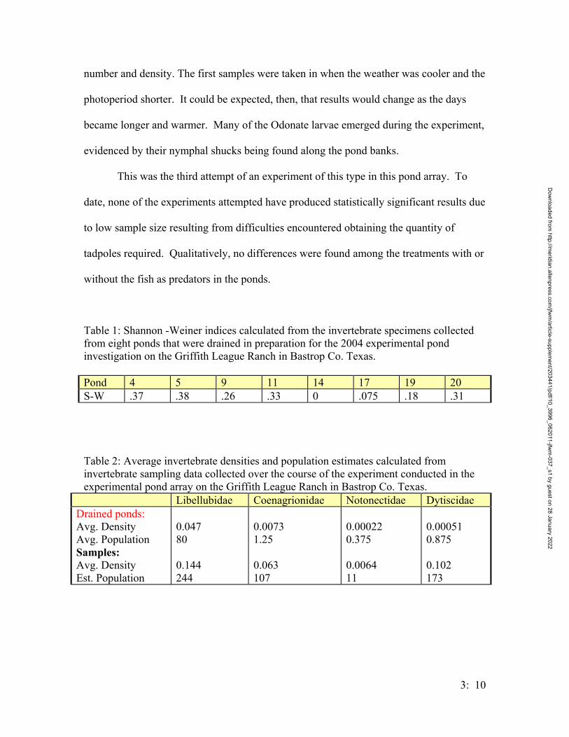
3: 10

number and density. The first samples were taken in when the weather was cooler and the

photoperiod shorter. It could be expected, then, that results would change as the days

became longer and warmer. Many of the Odonate larvae emerged during the experiment,

evidenced by their nymphal shucks being found along the pond banks.

This was the third attempt of an experiment of this type in this pond array. To

date, none of the experiments attempted have produced statistically significant results due

to low sample size resulting from difficulties encountered obtaining the quantity of

tadpoles required. Qualitatively, no differences were found among the treatments with or

without the fish as predators in the ponds.

Table 1: Shannon -Weiner indices calculated from the invertebrate specimens collected from eight ponds that were drained in preparation for the 2004 experimental pond investigation on the Griffith League Ranch in Bastrop Co. Texas. Pond 4 5 9 11 14 17 19 20 S-W .37 .38 .26 .33 0 .075 .18 .31

Table 2: Average invertebrate densities and population estimates calculated from invertebrate sampling data collected over the course of the experiment conducted in the experimental pond array on the Griffith League Ranch in Bastrop Co. Texas.

Libellubidae Coenagrionidae Notonectidae Dytiscidae Drained ponds: Avg. Density Avg. Population Samples: Avg. Density Est. Population

0.047 80 0.144 244

0.0073 1.25 0.063 107

0.00022 0.375 0.0064 11

0.00051 0.875 0.102 173

Dow



m/article-supplem

ent/203441/pdf/10_3996_062011-jfwm


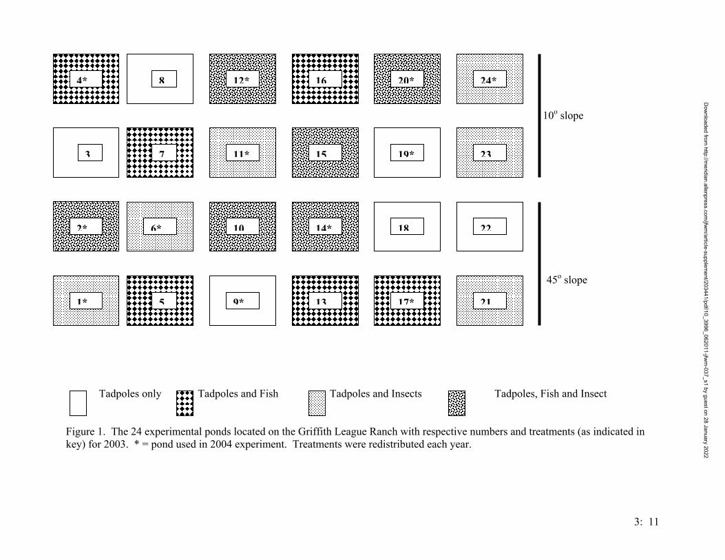
3:

11

10o slope

45o slope

Tadpoles only Tadpoles and Fish Tadpoles and Insects Tadpoles, Fish and Insect

Figure 1. The 24 experimental ponds located on the Griffith League Ranch with respective numbers and treatments (as indicated in key) for 2003. * = pond used in 2004 experiment. Treatments were redistributed each year.

21

22

23

24*

19*

18

139*51*

2*

3 11* 157

14*106*

17*

20*1612*84*

Dow



m/article-supplem

ent/203441/pdf/10_3996_062011-jfwm


Diurnal pH and DO (7/7/04)

0

1

2

3

4

5

6

7

8

9

24 23 21 19 16 14 13 11 8 6Pond

0

1

2

3

4

5

6

7

8

9

DO

pH pmpH amDO pmDO am

Figure 2: Diurnal fluctuations in pH and dissolved oxygen for the ponds used in the 2004 experiment. Day and night readings were taken 12 hours apart (11 p.m. and 11 a.m.) in the experimental pond array on the Griffith League Ranch.

3: 12

Dow



m/article-supplem

ent/203441/pdf/10_3996_062011-jfwm


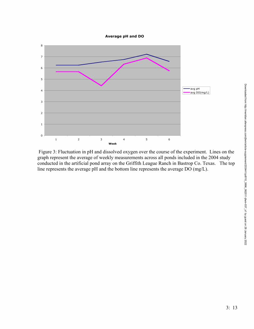
Average pH and DO

0

1

2

3

4

5

6

7

8

1 2 3 4 5 6

Week

avg pHavg DO(mg/L)

Figure 3: Fluctuation in pH and dissolved oxygen over the course of the experiment. Lines on the graph represent the average of weekly measurements across all ponds included in the 2004 study conducted in the artificial pond array on the Griffith League Ranch in Bastrop Co. Texas. The top line represents the average pH and the bottom line represents the average DO (mg/L).

3: 13

Dow



m/article-supplem

ent/203441/pdf/10_3996_062011-jfwm


Active Predation of Pitfall Traps at a Study Site for the Endangered Houston toad

(Bufo houstonensis)

Adam W. Ferguson and Michael R. J. Forstner

Pitfall traps with or without associated terrestrial drift fences remain a commonly

applied technique in the sampling of small vertebrate animals (Jenkins et al., 2003;

Shoop, 1965; Stenhouse, 1985; Sutton et al., 1999). This field technique is utilized

throughout the world and several studies have evaluated their effectiveness and reported

on problems with the methods (Brown, 1997; Crosswhite et al., 1999). Drawbacks of

pitfall traps with terrestrial drift fences have been covered in the literature and include

topics such as the escape of captured animals (Mazerolle, 2003), pitfall avoidance by

certain species such as terrestrial turtles (Christiansen and Vandewalle, 2000), and the

ability of animals to trespass or circumvent the fences themselves (Dodd, 1991). Another

problem in the use of drift fence arrays is the indirect mortality of trapped animals (Enge,

2001; Yunger et al., 1992).

Several other studies have addressed some of the many mortality factors

associated with pitfall trapping (Karraker, 2001; Kogut and Padley, 1997; Padget-Flohr

and Jennings, 2001). Those factors include desiccation (Jenkins et al., 2003), drowning

(Aubry and Stringer, 2000), starvation (Yunger et al., 1992), exposure (Padget-Flohr and

Jennings, 2001), and predation among species within the pitfall buckets (Dodd and Scott,

1994). However, the act of direct predation upon drift fence arrays by foraging vertebrate

predators is rarely mentioned and most studies have attempted to correct or calculate the

4: 1

Dow



m/article-supplem

ent/203441/pdf/10_3996_062011-jfwm


effects of only the aforementioned suite of problems. In fact, no previously published

study to our knowledge directly addresses the effects potential vertebrate predators might

have on drift fence sampling. Most direct predation events mentioned in the literature are

anecdotal and deal mainly with predation within the buckets themselves especially by

trapped mammals such as shrews (Jenkins et al., 2003) or minor disturbances to pitfall

covers by meso-mammals such as the raccoon (Sutton et al., 1999). Predation of drift

fence arrays by larger carnivores or other potential vertebrate predators is rarely

discussed and has not been studied quantitatively in any of the publications we located.

Our objective was to quantify the amount, rates, and variety of predators visiting

and potentially predating upon the animals captured in a grid of terrestrial drift fence

arrays established to monitor the dynamics of the endangered Houston toad (Bufo

houstonensis). In addressing such predatory activities we hope to provide insight into the

consequences vertebrate predators might engender in drift fence sampling and provide

solutions to curtail the problems associated with such behaviors.

Materials and Methods

This study was conducted on the Boy Scouts of America’s Griffith League Ranch

– a 2012 hectare ranch located in Bastrop County within the Lost Pines ecological region

of Texas. Vegetation communities consisted of mixed conifer hardwoods made up of

loblolly pine (Pinus taeda), blackjack oak (Quercus marilandica) and post oak (Quercus

stellata), mature pine stands of loblolly pines, several open pasture lands and mixed

deciduous hardwoods made up of oaks (Quercus spp.) with an under story of yaupon

4: 2

Dow



m/article-supplem

ent/203441/pdf/10_3996_062011-jfwm


(Ilex vomitoria), American beauty berry (Callicarpa americana), and farkleberry

(Vaccinium arboreum). Soil is composed of 91% sandy loam as illustrated by the

enclosed soil map.

Eighteen drift fence arrays were constructed to begin monitoring the local

herptofauna including the endangered Houston toad (Bufo houstonensis). Five treatment

groups were installed. Treatment group one consisted of four Y-shaped drift fence arrays

surrounding a known Houston toad breeding pond set various distances from the pond

edge. Three other Y-shaped drift fence arrays were placed in a deciduous-evergreen

mixed forest intercepting another known breeding pond, these three arrays were

designated treatment group two. Treatment group three also possessed three Y-shaped

drift fence arrays set to intercept a third known breeding pond found in a similar habitat

as treatment group two but more dominated by loblolly pines. Treatment group four

contained three Y-shaped arrays set in a line that began near a two ha lake and extended

outward east to west through a mixed deciduous-evergreen forest. Five straight line drift

fence arrays, two with four pitfall buckets and three with five pitfall buckets, made up

treatment group five. Y-shaped arrays were made up of three radiating arms of 18 cm by

15 m aluminum flashing buried five cm into the ground with four buckets; three terminal

and one central. Straight lined drift fences found in treatment group five were built of the

same aluminum flashing in the same manner as the Y-shaped arrays.

Each of the Y-shaped arrays had 6 funnel traps (2 on each arm) supplementing the

pitfall traps. Traps were checked daily from March 2001 through August 2004 for

trapped taxa which were subsequently measured, marked either by toe clippings, PIT

tags, with or ventral scale clips, gendered and then released >20 m from the array.

4: 3

Dow



m/article-supplem

ent/203441/pdf/10_3996_062011-jfwm


The predation study was initiated in 2003 in response to a perceived increase in

potential predator activity around the arrays (scat, tracks, disturbances, etc.). The study

involved a two-pronged approach using both track monitoring stations and motion sensor

cameras to document predator activity around the arrays.

Track Monitoring Stations

Track monitoring stations consisted of a two m diameter circle of cleared earth

with the bucket as the circles center point. Y-shaped arrays had two buckets, one central

and one randomly chosen terminal bucket, surrounded by the two m diameter circles of

tracking sand taken from the ranch. In areas where the substrate was inadequate as a

tracking media sand was imported from suitable sands on the ranch. The pasture lines in

treatment group five had alternating buckets fitted with the track monitoring stations. To

prevent grass re-growth, a 13 cm deep hole of two m diameter was dug out around the

bucket and then lined with artificial pond liner and filled with appropriate sand substrate

from the pasture. Once completed a total of 38 track monitoring stations were set in place

in addition to five controls of two m circles placed >100 m from the nearest track

monitoring station in each treatment group totaling 43 track monitoring stations.

Each track monitoring station was raked four times a month to clear the trap of

any previous tracks and prepare the sand for new track detection. Each was checked the

following morning for the occurrence, pattern, and kinds of animal tracks present. Tracks

were identified to species when possible and recorded as unknowns when this was not

possible. The presence or absence of animals in the pitfall buckets was also recorded.

4: 4

Dow



m/article-supplem

ent/203441/pdf/10_3996_062011-jfwm


CAMERA TRAPS

Ten Deer Cam® Model DC-100 cameras were set up in addition to the track

monitoring stations with two cameras in each treatment group. The buckets with the

cameras were randomly chosen; cameras were either placed near a terminal bucket or

over a central bucket. Central cameras were found on the Y-shaped arrays and were

supported 2.43 m over the central bucket by t-posts made into a H. Date and time were

recorded by the cameras to capture multiple visitors versus repeat visitors.

Results

Track monitoring stations

The track monitoring stations were operational from the 21 of October 2003

through 17 of June 2004. A total of 1236 observations were recorded. Of those 1236

observations, 443 of them had tracks present when checked (35.8%). Fifteen categories

of visitors were documented with 10 species identified and 5 general categories noted.

Predatory species observed included the raccoon (Procyon lotor), gray fox (Urocyon

cinereoargentius), Virginia opossum (Didelphis virginiana), striped skunk (Mephitis

mephitis), coyote (Canis latrans), domestic dog (Canis familiaris), and the American

crow (Corvus brachyrhynchos). Non-predatory tracks present were the white-tailed deer

(Odocoileus virginianus), wild turkey (Meleagaris gallopovo), and the armadillo

(Dasypus novemcinctus). General categories documented included unknown tracks, snake

drags, multiple visitors (tracks of more than one animal in the same trap night), bird

4: 5

Dow



m/article-supplem

ent/203441/pdf/10_3996_062011-jfwm


tracks, and rodent tracks. Such tracks were unidentifiable to the species specific level.

The distribution of visits by each species is depicted in Figure 1.

Each bucket affixed with a track monitoring station was visited at least once by

potential predators during the study. On 14 separate occasions, a combination of potential

predators visited the same station in a single night. There were combinations of nocturnal

(gray fox, opossum, raccoon) and diurnal predators (American crow), as well as

combinations of strictly nocturnal meso-mammals i.e., gray fox and opossum.

292

5431 25 20 13 11 10 10 6 5 2 2 1 10

20406080

100120140160180200220240260280300

Tota

l Num

ber o

f Vis

its

RC

CW UK GF

MV

SSpp

.

OP

SK RO

WTD

BSp

p. TY AD

CO

DG

Species

Species Visitation Rates

Figure. 1. Species specific visitation rates out of the 443 track observations recorded at a series of 43 track monitoring stations on drift fence/pitfall arrays in Bastrop County, Texas. The yellow numbers represent the individual times that the species was observed entering the track monitoring station area after a raking event. RC=raccoon, CW=American crow, UK=Unknown, GF=gray fox, MV=multiple visitors, SSpp.=snake species, OP=Virginia opossum, SK=striped skunk, RO=rodent spp., WTD=white-tailed deer, BSpp.=bird species, TY=wild turkey, AD=armadillo, CO=coyote, DG=domestic dog.

4: 6

Dow



m/article-supplem

ent/203441/pdf/10_3996_062011-jfwm


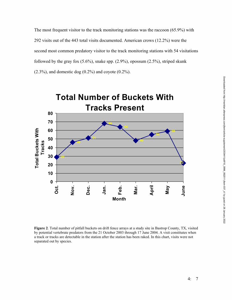
The most frequent visitor to the track monitoring stations was the raccoon (65.9%) with

292 visits out of the 443 total visits documented. American crows (12.2%) were the

second most common predatory visitor to the track monitoring stations with 54 visitations

followed by the gray fox (5.6%), snake spp. (2.9%), opossum (2.5%), striped skunk

(2.3%), and domestic dog (0.2%) and coyote (0.2%).

Total Number of Buckets With Tracks Present

29

4651

6864

48

5559

22

0

10

20

30

40

50

60

70

80

Oct

.

Nov

.

Dec

.

Jan.

Feb.

Mar

.

Apr

il

May

June

Month

Tota

l Buc

kets

With

Tr

acks

Figure 2. Total number of pitfall buckets on drift fence arrays at a study site in Bastrop County, TX, visited by potential vertebrate predators from the 21 October 2003 through 17 June 2004. A visit constitutes when a track or tracks are detectable in the station after the station has been raked. In this chart, visits were not separated out by species.

4: 7

Dow



m/article-supplem

ent/203441/pdf/10_3996_062011-jfwm


The total number of buckets was lowest with 29 visits in the month of October

and peaked at 68 in the month of January. Visits declined in the months of February and

March and then increased in April and May. June had the lowest visitation rate out of all

the months in the study with only 22 buckets visited.

Camera Results

The 10 motion sensor Deer Cam® cameras were operational for 168 days

beginning 11 of February 2004 through 29 July 2004. Since their installation the cameras

have detected all of the predator species whose tracks appeared in the track monitoring

stations and additional three species of animals whose tracks were not positively

identified or had not been detected. The three species only documented by the cameras

include the bobcat (Lynx rufus), the greater roadrunner (Geococcyx californianus), and

the fox squirrel (Sciurus niger). Two individual bobcats were recorded by cameras in

treatment group 2 and 3 and a single greater roadrunner was recorded from treatment

group 3.

The cameras were also able to document the actual behavior of the putative

predators at the buckets themselves. Pictures were taken of raccoons entering the buckets

as well as removing bucket lids from temporarily closed buckets. One of the fox squirrel

pictures was of an adult leaning over the edge of the bucket and looking into the center.

In addition to verifying the predators present, the cameras also captured times when more

than one carnivore was present. Several pictures were taken of multiple raccoons visiting

the same bucket at the same time, or of multiple visitors occurring at different times

during the night.

4: 8

Dow



m/article-supplem

ent/203441/pdf/10_3996_062011-jfwm


Discussion

The variety, abundance, and frequency of potential predators recorded at the track

monitoring stations obviously poses a threat to animals captured in drift fence arrays. The

high visitation rates of the raccoon, 292 out of 443, is a particular concern given the

dexterity of raccoons and their ability to procure as well as consume a wide variety of

prey items. Consistent visits by such carnivores (Figure 1) indicate that predation on drift

fence arrays is a serious concern often overlooked from the literature addressing

problems with drift fence sampling. In our research, in which an endangered species is

being monitored through drift fence sampling, concern about predation is particularly

significant. The presence of such known toad predators as the raccoons (Jones et. al,

1999; Schaaf and Garton, 1970) and skunks (Groves, 1980) could potentially pose a

serious threat to Houston toads captured in the buckets. Although no direct Houston toad

predation events were recorded from drift fence arrays during this study, there was

anecdotal evidence of other amphibians experiencing predation along the fences. Six

Hurter’s Spadefoot toads (Scaphiopus hurteri) and one Gulf Coast toad (Bufo valliceps)

were found partially consumed alongside the buckets. The partial consumption of the

toads is consistent with other studies documenting toad predation, in which the toxins of

the toads eventually deter or force the predator to selectively consume the prey item

(Groves, 1980; Jones et al., 1999). The Gulf Coast toad was found in a track monitoring

station that had raccoon prints all around the carcass; this was the same case for two of

the Hurter’s spadefoot toads. The presence of the fresh tracks alongside these carcasses

4: 9

Dow



m/article-supplem

ent/203441/pdf/10_3996_062011-jfwm


indicates that a raccoon was the predator involved. Another instance involved the

disappearance of a dead northern pygmy mouse (Baiomys taylori) from one of our

buckets. While raking one evening I found a dead pygmy mouse in one of our traps

which I subsequently moved to another trap with known visitation rates. Arriving early

the next morning to check the track monitoring stations I found the mouse was missing.

There was no sign of disturbance except for the presence of clearly visible gray fox tracks

up to and across the bucket. The pattern of the tracks would have forced the fox to go

over the top of the flashing and the bucket itself after venturing to the very edge of the

bucket itself.

Very few previous publications mention the problem of direct predation on drift

fence arrays. Often the concept of predation on captured animals is completely omitted

when considering the use of drift fence arrays for monitoring animal populations. Our

results disclose regular visitation of drift fence arrays by known predators such as

raccoons and gray fox. Both of these animals are more than capable of entering and

removing animals from a 19 L bucket. Regional considerations, such as the taxa targeted

by the drift fence arrays with pitfall traps as well as the specific predators found in the

study area need to be taken into account before implementing a drift fence array study.

For example, areas such as the Pacific Northwest where drift fences are commonly used

(Aubry and Stringer, 2000), agile predators such as pine martens (Martes americana) and

minks (Mustela vison) might pose additional threats to captured species. The results of

this paper illustrate the need to consider predation as a problem when using drift fences to

sample animals, especially in the case of rare or endangered animals such as the Houston

toad. Measures need to be taken to prevent known predators from entering and obtaining

4: 10

Dow



m/article-supplem

ent/203441/pdf/10_3996_062011-jfwm


animals from buckets used in drift fence array surveys in order to reduce unwanted

mortalities.

As illustrated by the continued visitation of predators throughout the study period,

some form of predator prevention might be necessary when implementing drift fence

sampling. In order to reduce the risk of predation of Houston toads, we implemented

predatory exclusion devices, or PEDs made out of plywood and built similarly to the

shade covers often used in drift fence studies. We are in the process of determining if

these devices successfully reduce the risk of predation to animals confined in the buckets.

Future studies on the success of predators in procuring prey items from drift fence arrays

as well as the initiation, habituation periods, and correlation with trapping frequency,

along drift fences by such carnivores need are now being addressed by our continuing

work.

4: 11

Dow



m/article-supplem

ent/203441/pdf/10_3996_062011-jfwm


5: 1

HABITAT AFFINITY FOR WHITE-TAILED DEER AND RIO GRANDE WILD TURKEY AT THE GRIFFITH LEAGUE RANCH, BASTROP COUNTY, TEXAS

SHANE J. KIEFER AND JOHN T. BACCUS

Game animal research throughout the range of southern pine forests is extensive, but the reasons for low populations of white-tailed deer and Rio Grande wild turkey in the isolated Lost Pines region of Bastrop County, Texas were not well understood. I characterized the vegetative communities on a 2012 ha ranch in the Lost Pines and related white-tailed deer and wild turkey abundance and distribution to available habitats. I measured woody plant cover and density in summer 2002 and assessed herbaceous cover, horizontal obscurity, duff depth, and percent canopy cover once per calendar season from summer 2002 to spring 2003. I estimated white-tailed deer abundance using a non-linear spotlight transect method and used GPS locations of sightings of both deer and wild turkeys to assess distribution and habitat affinity within a geographic information system. I found three major habitat types: pine forest, oak-juniper woodland, and grassland (improved pasture). Loblolly pine with an understory of yaupon dominated pine forests, which had higher woody plant density (7257 plants/ha), greater duff accumulation (60.2 mm), higher canopy coverage (87.1%), and lower visibility based on VPB measurements than oak-juniper woodlands (4419 plants/ha, 40.2 mm duff, 74.4% canopy). Post oak and blackjack oak mixed with eastern red cedar characterized oak-juniper woodlands. Pine and oak habitats showed sparse herbaceous plant cover (1.2% and 5.0%, respectively). Distance analysis estimated deer density at 0.010 deer/ha (20 deer on the ranch). Wild turkey abundance was approximately 20-30 individuals based on incidental sightings. Both species were associated with grassland habitat more than expected based on availability. Wild turkeys also appeared to favor oak-juniper woodlands over pine forests, while deer showed no preference for either. Long-term lack of management on the ranch has produced forest habitat that produces little food available to white-tailed deer and wild turkeys so they must utilize the grasslands for foraging. A combination of thinning and prescribed fire is recommended to increase forage quantity and quality. Future research should address the effectiveness of management practices in the Lost Pines compared to more mesic southern pine forests to the east.

Management of white-tailed deer (Odocoileus virginianus) and wild turkey

(Meleagris gallopavo) in southern pine forests has been studied extensively (Lay 1956,

Lay 1967a, Halls 1973, Blair et al. 1977, Melchiors et al. 1985, Thill et al. 1987, Bidwell

et al. 1989, Campo et al. 1989, Miller et al. 2000). Generally these studies addressed

game management within the silvicultural practices of pine forests for production of

lumber in the southeastern United States. Collectively, they suggested integrating

management practices that initiate early stage succession and encourage plant diversity,

Dow



m/article-supplem

ent/203441/pdf/10_3996_062011-jfwm


5: 2

particularly enhancing palatable herbaceous growth. Prescribed burning (Hodgkins 1958,

Moore 1982, Thill et al. 1987, Miller et al. 2000), thinning (Patton and McGinnes 1964,

Halls 1970, 1973), grazing (Thill 1984), and clear-cutting to produce openings (Campo et

al. 1989, Thill et al. 1990, Johnson et al. 1995) are common suggestions for habitat

improvement.

White-tailed deer prefer diverse habitat with a variety of forage sources and cover

(Allen et al. 1996). Many studies consider browse the principal food source and stress

increasing browse production, availability, and quality, while noting the importance of

herbaceous growth (Wolters and Schmidtling 1975, Blair and Feduccia 1977, Blair et al.

1977, Thill et al. 1990, Johnson et al. 1995). However, Lay (1964) suggests browse may

not be as dominant in the diet as indicated by the literature. Fungi may also be a highly

used resource when available (Johnson et al. 1995).

Wild turkeys prefer older, mixed pine-hardwood stands with an open understory

and scattered clearings (Bidwell et al. 1989, Campo et al. 1989, Allen et al. 1996, Miller

et al. 2000). Turkeys need herbaceous cover for nesting (Allen et al. 1996), and well-

forested riparian corridors for travel lanes (Miller et al. 2000).

Density estimates for deer in Bastrop County range from 0.016-0.042 deer/ha,

depending on year and location in the county (Len Polasek, Texas Parks and Wildlife

Department, personal communication). County estimates from 1998-2002 were lowest in

1999 (0.023 deer/ha) and highest in 2002 (0.037 deer/ha) (Wolf 2003). Reasons for low

deer populations are not well understood, because there are very little data for the species

in Bastrop County. The Post Oak Savannah ecoregion harvest data for wild turkey

indicate lower hunter participation and success than in other ecoregions with higher wild

turkey populations (Texas Parks and Wildlife Department 2003). Information is needed

Dow



m/article-supplem

ent/203441/pdf/10_3996_062011-jfwm


5: 3

about this unique and isolated ecoregion to elucidate why it does not support higher

populations of game species.

No research exists regarding management for game species in the Lost Pines,

where important differences from typical southern pine forests exist. Consequently,

current management guidelines applied to eastern Texas and United States forests may be

unsuitable.

The objectives of my study were to describe the composition and distribution of

habitats on Griffith League Ranch including horizontal and vertical coverage of

herbaceous and woody plants and woody plant density, and to provide baseline data

about white-tailed deer and Rio Grande wild turkey populations and corresponding

habitat affinities on the ranch. In addition, management recommendations for the ranch

were developed in accordance with my findings.

STUDY AREA

The Lost Pines in Central Texas are the westernmost extension of southern pine

forest in the United States. Separated from the Pineywoods of East Texas by about 130

km, the Lost Pines region receives substantially less rainfall than other southern forests.

There is disagreement about the Lost Pines ecological status, both as an island and a

remnant of a larger contiguous forest to the east. Descriptions range from island or

archipelago (because separate stands occur in 5 counties) to fractured peninsula (Taber

and Fleenor 2003). However, pollen records indicate no change in the distribution of

pines in the last 10-12,000 years (Larson et al. 1972).

The Lost Pines are maintained naturally by local adaptations by vegetation for

water conservation and coarse, sandy soils that act as water reservoirs (Taber and Fleenor

Dow



m/article-supplem

ent/203441/pdf/10_3996_062011-jfwm


5: 4

2003). Annual evapotranspiration is ≤ 25 mm higher in the Lost Pines than in similar

communities endemic to the western edge of the Pineywoods (Schultz 1997). The amount

of water available to plants after surface evaporation declines by ≤ 381 mm from the

Pineywoods to the Lost Pines (Taber and Fleenor 2003). The climate is humid subtropical

receiving about 889 mm of annual precipitation with peaks in spring and early fall (Taber

and Fleenor 2003).

The Griffith League Ranch (GLR) owned by the Capitol Area Council of the Boy

Scouts of America is located about 13 km north of Bastrop, Texas in Bastrop County. It

has a total area of 2012 ha composed of mixed pine-oak forest (1778 ha) that is typical of

the Lost Pines and improved pastures (234 ha). Principal overstory vegetation is loblolly

pine (Pinus taeda), blackjack oak (Quercus marilandica), post oak (Q. stellata), and

eastern red cedar (Juniperus virginiana) with an understory of yaupon (Ilex vomitoria),

farkleberry (Vaccinum arboreum) and beautyberry (Callicarpa americana) (Koepp 2001,

Taber and Fleenor 2003). Improved pastures are dominated by coastal Bermudagrass

(Cynodon dactylon) and bahia grass (Paspalum notatum).

The topography is rolling, with elevations ranging from 136 m above sea level in

the western part of the ranch to 202 m in the east. Contrary to the eastern portion of

Texas where bottomlands are occupied by hardwood species, this unique area supports

pines along creeks and drainages (Taber and Fleenor 2003). Soils are sandy, with Patilo

(63%), Silstid (22%), and Demona (6%) loamy fine sands dominating the ranch (Baker

1979, Koepp 2001). At least 20 ponds occur on the property. Ponds range in surface area

from about 0.5 ha to 1.5 ha. Nine ponds hold water intermittently (Koepp 2001). Alum

Creek flows through the extreme eastern part of the ranch.

Dow



m/article-supplem

ent/203441/pdf/10_3996_062011-jfwm


5: 5

METHODS

Vegetation Analysis

I initially determined habitat types using 1-m Digital Orthophoto Quarter

Quadrangles (DOQQ). I chose and ground-truthed 25 points to confirm the initial

selection of 4 different habitat types (Fig. 1). The 4 habitat types were designated as

grasslands composed of open areas of improved pasture, oak-juniper woodlands

dominated by post and blackjack oak with eastern red cedar, pine forests dominated by

loblolly pine, and pond habitats containing a permanent water source. I performed

vegetational analysis in conjunction with another study (White 2003), but excluded pond

habitats in my study, because water was not considered a limiting factor for highly

mobile game animals on the ranch. Pond locations were assigned to grassland, oak-

juniper woodland, or pine forest based on the surrounding habitat type, which was

confirmed by PCA analysis (White 2003).

I assessed woody cover during summer 2002 using line intercept methodology

(Higgins et al. 1996). Using each of the 25 sample points as a focus, I spaced 3 100-m

transects at 120 degree angles. I used a random compass heading for placement of the

initial transect at each point. I measured the vertical projection for all woody vegetation

crossing the tape, summed distances by species, and calculated the mean across all 3

transects at each point to determine percent cover. I measured density of woody

vegetation using 3 100-m2 quadrats at each point. I spaced quadrats 120 degrees apart and

placed them 15 m from the sample point to avoid overlapping measurements. I counted

the number of individuals of each species within the quadrat boundary and calculated a

Dow



m/article-supplem

ent/203441/pdf/10_3996_062011-jfwm


5: 6

mean across all 3 quadrats at each point. I discarded quadrats intersecting water at pond

habitat sites to avoid biasing density estimates of the surrounding habitat. I measured

both line intercepts and woody density only once at each site, because I presumed that

conditions during summer were representative of the year. I used a total of 75 100-m line

intercept transects and 75 100-m2 quadrats.

I determined herbaceous cover at each of the same 25 points using 0.1-m2

quadrats and 5 cover classes (Daubenmire 1959). I identified plants to species and later

grouped them into forbs, grasses, and sedges, as well as native and introduced species. At

each sample point I placed 10 quadrats randomly within 10-m intervals at random

distances from the line along a single 100-m transect placed at a random compass

heading. I measured litter or duff depth in the center of each quadrat. I measured percent

canopy cover at 5 quadrats on each line using a spherical densiometer (Higgins et al.

1996). I took 5 measurements of horizontal obscurity on each line using a 2.5-m

vegetation profile board (VPB) divided into 5 0.5-m segments placed 15 m from the

transect (Nudds 1977). Measurements represented percent cover (obscurity) at each

segment grouped in 5 equal classes from 0-100%. I used the midpoint of each class to

calculate means. I took herbaceous cover, duff depth, densiometer readings, and VPB

measures once per calendar season. I used a total of 250 0.1-m2 quadrats and took 125

canopy and horizontal obscurity measurements per season (1000 quadrats and 500

canopy and obscurity readings over the course of one year).

I analyzed differences in vegetative variables by habitat and season. Because of

an absence of woody vegetation in grasslands, I compared only oak-juniper and pine

habitats. I transformed variables if necessary to meet assumptions of homoscedasticity

and normality. I used t-tests to compare coverage of pine, oak, eastern red cedar, woody

Dow



m/article-supplem

ent/203441/pdf/10_3996_062011-jfwm


5: 7

plant density, and square-root transformed yaupon between oak-juniper and pine habitats.

I compared forb cover, grass cover, and total herbaceous cover (all log transformed)

between all habitats and seasons using analysis of variance (ANOVA) and Tukey’s

honestly significant differenced (HSD) test (Quinn and Keough 2002). I analyzed duff by

habitat, and duff and percent canopy by season and seasonally within habitats using

ANOVA. I compared only the lowest VPB level (0.0 - 0.5 m) across all 3 habitat types

because of heteroscedasticity resulting from absence of variance in the upper levels of

grassland VPB data, which I anticipated because I found no coverage in any season

above about 1 m and the majority below 0.5 m. All measurements above 1 m received the

lowest value, resulting in minimal variance at low obscurity readings. I analyzed changes

in obscurity by height within habitats, and among both habitats and seasons within each

level. All statistical analyses were performed in S-PLUS 6.1 (Insightful Corporation,

Seattle, Washington).

Wildlife Abundance and Distribution

Sighting data have been used to assess habitat use and predict distributions of

species in relation to habitat (Agee et al. 1989, Stoms et al. 1993, Knick and Dyer 1997,

Ortega-Huerta and Medley 1999). These analyses covered large geographic areas and

used existing data in creating regression models. However, the same technique should be

applicable to smaller areas using fine-scale data.

I conducted 12 spotlight surveys totaling > 192 km traveled during late summer and early

fall of 2002 (4) and 2003 (8) and estimated white-tailed deer density using a non-linear

spotlight transect method (Pierce 2000). I conducted surveys on nonconsecutive nights

within about 30 days. Line transect methodology eliminated the need to conduct an

unfeasible complete census (Buckland et al. 2001) and bias associated with calculating

Dow



m/article-supplem

ent/203441/pdf/10_3996_062011-jfwm


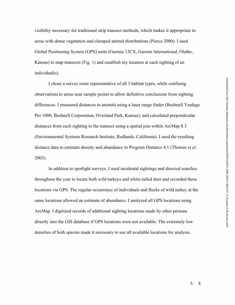
5: 8

visibility necessary for traditional strip transect methods, which makes it appropriate in

areas with dense vegetation and clumped animal distributions (Pierce 2000). I used

Global Positioning System (GPS) units (Garmin 12CX, Garmin International, Olathe,

Kansas) to map transects (Fig. 1) and establish my location at each sighting of an

individual(s).

I chose a survey route representative of all 3 habitat types, while confining

observations to areas near sample points to allow definitive conclusions from sighting

differences. I measured distances to animals using a laser range finder (Bushnell Yardage

Pro 1000, Bushnell Corporation, Overland Park, Kansas), and calculated perpendicular

distances from each sighting to the transect using a spatial join within ArcMap 8.3

(Environmental Systems Research Institute, Redlands, California). I used the resulting

distance data to estimate density and abundance in Program Distance 4.1 (Thomas et al.

2003).

In addition to spotlight surveys, I used incidental sightings and directed searches

throughout the year to locate both wild turkeys and white-tailed deer and recorded these

locations via GPS. The regular occurrence of individuals and flocks of wild turkey at the

same locations allowed an estimate of abundance. I analyzed all GPS locations using

ArcMap. I digitized records of additional sighting locations made by other persons

directly into the GIS database if GPS locations were not available. The extremely low

densities of both species made it necessary to use all available locations for analysis.

Dow



m/article-supplem

ent/203441/pdf/10_3996_062011-jfwm


Figure 1. Vegetation sample points and spotlight survey transect route on Griffith League Ranch, Bastrop County, Texas.

5: 9

Dow



m/article-supplem

ent/203441/pdf/10_3996_062011-jfwm


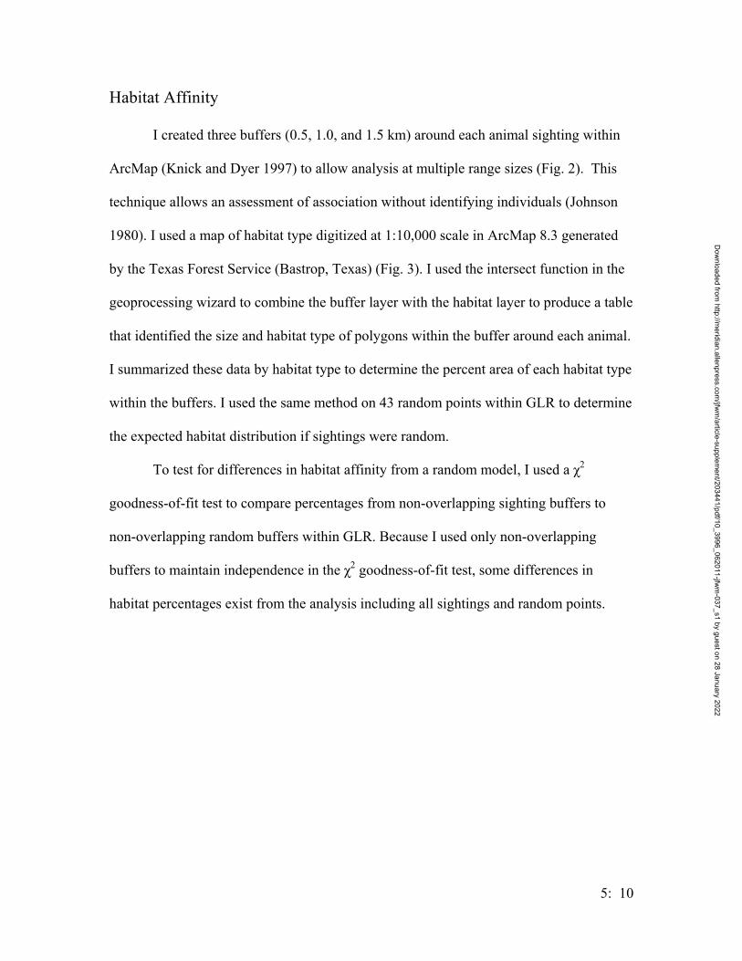
5: 10

Habitat Affinity

I created three buffers (0.5, 1.0, and 1.5 km) around each animal sighting within

ArcMap (Knick and Dyer 1997) to allow analysis at multiple range sizes (Fig. 2). This

technique allows an assessment of association without identifying individuals (Johnson

1980). I used a map of habitat type digitized at 1:10,000 scale in ArcMap 8.3 generated

by the Texas Forest Service (Bastrop, Texas) (Fig. 3). I used the intersect function in the

geoprocessing wizard to combine the buffer layer with the habitat layer to produce a table

that identified the size and habitat type of polygons within the buffer around each animal.

I summarized these data by habitat type to determine the percent area of each habitat type

within the buffers. I used the same method on 43 random points within GLR to determine

the expected habitat distribution if sightings were random.

To test for differences in habitat affinity from a random model, I used a χ2

goodness-of-fit test to compare percentages from non-overlapping sighting buffers to

non-overlapping random buffers within GLR. Because I used only non-overlapping

buffers to maintain independence in the χ2 goodness-of-fit test, some differences in

habitat percentages exist from the analysis including all sightings and random points.

Dow



m/article-supplem

ent/203441/pdf/10_3996_062011-jfwm


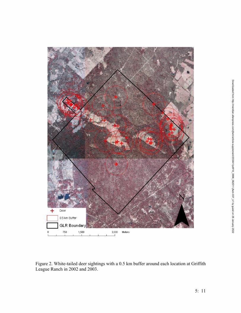
Figure 2. White-tailed deer sightings with a 0.5 km buffer around each location at Griffith League Ranch in 2002 and 2003.

5: 11

Dow



m/article-supplem

ent/203441/pdf/10_3996_062011-jfwm


Figure 3. Digitized habitat types on Griffith League Ranch and surrounding properties.

5: 12

Dow



m/article-supplem

ent/203441/pdf/10_3996_062011-jfwm


5: 13

RESULTS

Vegetation

Pine habitats had significantly greater coverage of loblolly pine (t = -7.43, P <

0.01) and yaupon (t = -3.12, P < 0.01), and oak-juniper habitats had greater coverage of

oak species (t = 5.03, P < 0.01) and eastern red cedar (t = 4.23, P < 0.01) (Table 1). The

only other woody plant with > 1% of cover in both habitats was farkleberry, which was

not different between habitats (t = -0.470, P = 0.64). American beautyberry was relatively

prominent, although variable in distribution, in pine forest habitat with a mean (± SE)

coverage of 4.03 m/100m ± 1.15, but made only a minor appearance in oak-juniper

woodlands with a total coverage of only 1.9 m from all 7 points. Seventeen other woody

species were encountered, but none constituted more than 20 m across all 25 sites (Table

2).

Table 1. Mean coverage (m/100 m of intercept length) of 5 dominant woody species and mean density (plants/ha) of all woody plants at 25 sampling sites in oak-juniper woodland, pine forest, and grassland habitat types on Griffith League Ranch (Summer 2002).

Habitat Loblolly Pine Post Oak Blackjack Oak Yaupon E. Red Cedar Density

Oak-Juniper 28.0 43.7 19.9 12.2 30.8 4419 (1467-6834)

Pine 64.1 26.8 7.6 30.7 13.8 7257 (3600-10450)

Grassland 5.5 0.9 1.5 0.7 0.4 n/a

Dow



m/article-supplem

ent/203441/pdf/10_3996_062011-jfwm


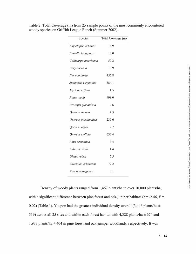
5: 14

Table 2. Total Coverage (m) from 25 sample points of the most commonly encountered woody species on Griffith League Ranch (Summer 2002).

Species Total Coverage (m)

Ampelopsis arborea 16.9

Bumelia lanuginosa 10.0

Callicarpa americana 50.2

Carya texana 19.9

Ilex vomitoria 457.8

Juniperus virginiana 384.1

Myrica cerifera 1.5

Pinus taeda 998.0

Prosopis glandulosa 2.6

Quercus incana 4.3

Quercus marilandica 239.6

Quercus nigra 2.7

Quercus stellata 632.4

Rhus aromatica 3.4

Rubus trivialis 1.4

Ulmus rubra 5.5

Vaccinum arboreum 72.2

Vitis mustangensis 3.1

Density of woody plants ranged from 1,467 plants/ha to over 10,000 plants/ha,

with a significant difference between pine forest and oak-juniper habitats (t = -2.46, P =

0.02) (Table 1). Yaupon had the greatest individual density overall (3,446 plants/ha ±

519) across all 25 sites and within each forest habitat with 4,328 plants/ha ± 674 and

1,933 plants/ha ± 404 in pine forest and oak-juniper woodlands, respectively. It was

Dow



m/article-supplem

ent/203441/pdf/10_3996_062011-jfwm


5: 15

followed by post oak with 720 plants/ha ± 136 in both habitats, 854 plants/ha ± 186 in the

pine forest, and 490 plants/ha ± 165 in oak-juniper woodland. Eastern red cedar (587

plants/ha ± 105) and farkleberry (259 plants/ha ± 78) were also prominent with respect to

overall density across both habitats.

Forb cover did not differ by season when blocking by habitat type (F (3, 88) =

1.42, P = 0.242) however, it was different between habitats (F (2, 88) = 99.5, P < 0.01)

with grasslands having the highest coverage of 14.3% ± 1.54 (Table 3). Both grass cover

and total herbaceous cover showed habitat by season interactions (F (6, 88) = 3.59, P <

0.01 and F (6, 88) = 4.10, P < 0.01, respectively). When analyzed only by season, there

was no difference for grass cover (F (3, 96) = 0.938, P = 0.426) or total herbaceous cover

(F (3, 96) = 2.03, P = 0.113).

Forest duff depths showed differences by both season (F (3, 68) = 6.03, P < 0.01)

and habitat type (F (1, 68) = 32.7, P < 0.01). Summer duff levels (65.9 mm ± 5.24) were

significantly higher than both winter and spring levels (45.9 mm ± 3.70 and 47.1 mm ±

3.28, respectively). Duff depth did not differ between all other seasons. Pine forests

showed more duff accumulation (60.2 mm ± 2.53) than oak-juniper woodlands (40.2 mm

± 2.67). Duff depths changed seasonally within the pine forest (F (3, 44) = 6.29, P <

0.01), but not in oak-juniper woodlands (F (3, 24) = 1.62, P = 0.211). Pine forest summer

duff levels (75.9 mm ± 5.79) were higher than in all other seasons. Percent canopy cover

in forest habitats averaged 74.4 % ± 3.26 and 87.1 % ± 1.27 in oak-juniper and pine

habitats, respectively. Canopy cover changed seasonally within the oak-juniper

woodlands (F (3, 24) = 3.24, P = 0.040) with a difference between summer (83% ± 3.47)

and winter (59% ± 7.03).

Dow



m/article-supplem

ent/203441/pdf/10_3996_062011-jfwm


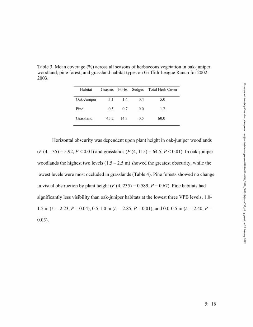
5: 16

Table 3. Mean coverage (%) across all seasons of herbaceous vegetation in oak-juniper woodland, pine forest, and grassland habitat types on Griffith League Ranch for 2002-2003.

Habitat Grasses Forbs Sedges Total Herb Cover

Oak-Juniper 3.1 1.4 0.4 5.0

Pine 0.5 0.7 0.0 1.2

Grassland 45.2 14.3 0.5 60.0

Horizontal obscurity was dependent upon plant height in oak-juniper woodlands

(F (4, 135) = 5.92, P < 0.01) and grasslands (F (4, 115) = 64.5, P < 0.01). In oak-juniper

woodlands the highest two levels (1.5 – 2.5 m) showed the greatest obscurity, while the

lowest levels were most occluded in grasslands (Table 4). Pine forests showed no change

in visual obstruction by plant height (F (4, 235) = 0.589, P = 0.67). Pine habitats had

significantly less visibility than oak-juniper habitats at the lowest three VPB levels, 1.0-

1.5 m (t = -2.23, P = 0.04), 0.5-1.0 m (t = -2.85, P = 0.01), and 0.0-0.5 m (t = -2.40, P =

0.03).

Dow



m/article-supplem

ent/203441/pdf/10_3996_062011-jfwm


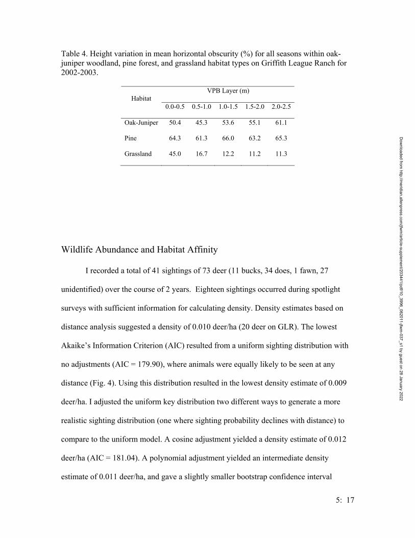
5: 17

Table 4. Height variation in mean horizontal obscurity (%) for all seasons within oak-juniper woodland, pine forest, and grassland habitat types on Griffith League Ranch for 2002-2003.

VPB Layer (m) Habitat

0.0-0.5 0.5-1.0 1.0-1.5 1.5-2.0 2.0-2.5

Oak-Juniper 50.4 45.3 53.6 55.1 61.1

Pine 64.3 61.3 66.0 63.2 65.3

Grassland 45.0 16.7 12.2 11.2 11.3

Wildlife Abundance and Habitat Affinity

I recorded a total of 41 sightings of 73 deer (11 bucks, 34 does, 1 fawn, 27

unidentified) over the course of 2 years. Eighteen sightings occurred during spotlight

surveys with sufficient information for calculating density. Density estimates based on

distance analysis suggested a density of 0.010 deer/ha (20 deer on GLR). The lowest

Akaike’s Information Criterion (AIC) resulted from a uniform sighting distribution with

no adjustments (AIC = 179.90), where animals were equally likely to be seen at any

distance (Fig. 4). Using this distribution resulted in the lowest density estimate of 0.009

deer/ha. I adjusted the uniform key distribution two different ways to generate a more

realistic sighting distribution (one where sighting probability declines with distance) to

compare to the uniform model. A cosine adjustment yielded a density estimate of 0.012

deer/ha (AIC = 181.04). A polynomial adjustment yielded an intermediate density

estimate of 0.011 deer/ha, and gave a slightly smaller bootstrap confidence interval

Dow



m/article-supplem

ent/203441/pdf/10_3996_062011-jfwm


5: 18

(0.006 – 0.018 deer/ha) than the cosine adjusted model (0.006 – 0.021 deer/ha). The data

fit both the uniform/cosine and the uniform/polynomial models better than the unadjusted

uniform model based on quantile-quantile plots (Fig. 5).

The percentage of grassland habitat within the sighting buffers showed a decrease

from 41.4% to 31.2% as distance increased (Table 5). As random buffer size increased

the percentage of grassland habitat only increased from 13.6% to 16.7%. Pine forest

made up the largest percentage of habitat within the sighting buffers at all distances

except 1.5 km, where oak-juniper woodlands were slightly higher. Within the random

buffers, pine forest made up the highest percentage of habitat at all distances.

The χ2 values indicate that habitat around white-tailed deer sightings at 0.5 km

was not in proportion to that available at random (χ2 = 42.3, P < 0.01). If deer were using

habitat at levels available, the χ2 values would be near null. Pine forest (35%) and oak-

juniper woodland (37%) were equally represented within 8 non-overlapping, 0.5 km

buffers around deer sightings. Grassland constituted 28% of habitat within non-

overlapping sighting buffers. Within 13 random, non-overlapping, 0.5 km buffers

grassland only accounted for 9% of habitat, while percentages of pine forest (47%) and

oak-juniper woodland (44%) both increased while remaining similar to each other.

Dow



m/article-supplem

ent/203441/pdf/10_3996_062011-jfwm


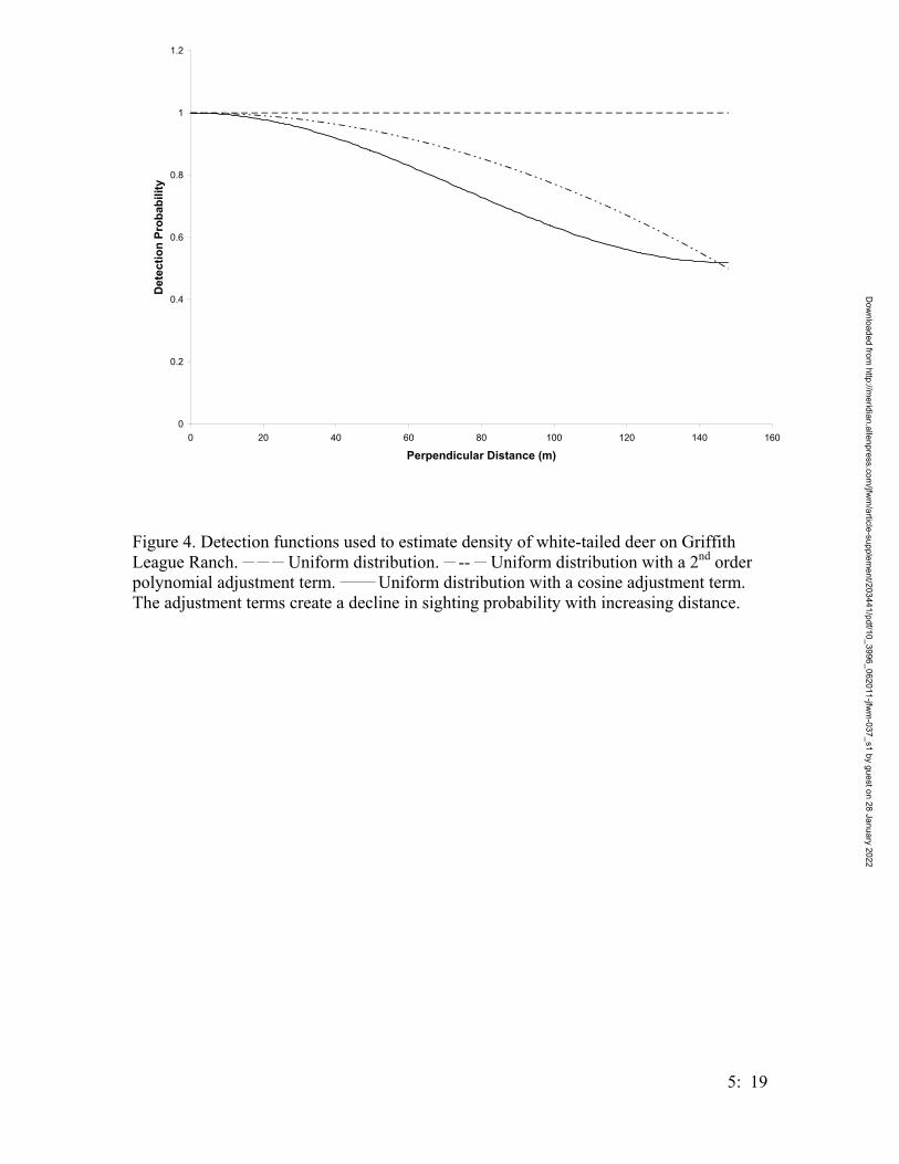
0

0.2

0.4

0.6

0.8

1

1.2

0 20 40 60 80 100 120 140 160

Perpendicular Distance (m)

Det

ectio

n Pr

obab

ility

Figure 4. Detection functions used to estimate density of white-tailed deer on Griffith League Ranch. __ __ __ Uniform distribution. __ -- __ Uniform distribution with a 2nd order polynomial adjustment term. ______ Uniform distribution with a cosine adjustment term. The adjustment terms create a decline in sighting probability with increasing distance.

5: 19

Dow



m/article-supplem

ent/203441/pdf/10_3996_062011-jfwm


A)

0

0.2

0.4

0.6

0.8

1

0 0.2 0.4 0.6 0.8 1

Empirical distribution function

Fitte

d cu

mul

ativ

e di

strib

utio

n fu

nctio

n B)

0

0.2

0.4

0.6

0.8

1

0 0.2 0.4 0.6 0.8 1


Fitte

d cu

mul

ativ

e di

strib

utio

n fu

nctio

n

C)

0

0.2

0.4

0.6

0.8

1

0 0.2 0.4 0.6 0.8 1


Fitte

d cu

mul

ativ

e di

strib

utio

n fu

nctio

n Figure 5. Quantile-quantile (qq) plots of fitted distribution function versus distribution of data used to assess how well the data fit the model. A) Qq plot for unadjusted uniform model showing deviation at medium distances. B) Qq plot for cosine adjusted model. C) Qq plot for polynomial adjusted model. Both B and C show only minor spikes just beyond zero distance.

5: 20

Dow



m/article-supplem

ent/203441/pdf/10_3996_062011-jfwm


5: 21

Table 5. Comparison of habitat coverage within buffers around sightings of white-tailed deer and around random locations on Griffith League Ranch.

Buffer Distance (km) Habitat Percent Area*

(Sightings)

Percent Area*

(Random Points)

Pine 33.3 44.2

Grassland 31.2 16.7

1.5

Oak-Juniper 35.5 39.1

Pine 34.9 45.2

Grassland 33.1 14.6

1.0


Pine 32.2 45.1

Grassland 41.4 13.6

0.5


*All sightings and random locations are included in calculation of percent area. Only non-overlapping buffers were used to calculate percent area for goodness-of-fit tests and differences do exist.

I recorded 24 sightings of 119 Rio Grande turkeys (8 males, 63 hens, 25 poults,

23 unidentified) during the study. Maximum group size was 16 with a mean of 5.

Turkeys showed more affinity for forested habitats than deer (Table 6). Oak-juniper

habitat was most prominent at all distances around sightings. Percentage of grassland

habitat within sighting buffers decreased from 33.6% to 21.1% and only exceeded pine

habitat at 0.5 km. Pine forests accounted for about 45% of habitat within random buffers

but did not exceed 35% at any distance around sightings. Oak-juniper woodlands were

present in similar quantities around both sightings and random locations. Based on

sightings, wild turkey abundance was estimated at between 20-30 individuals. A single

large flock concentrated on a main drainage in the central portion of the ranch.

Dow



m/article-supplem

ent/203441/pdf/10_3996_062011-jfwm


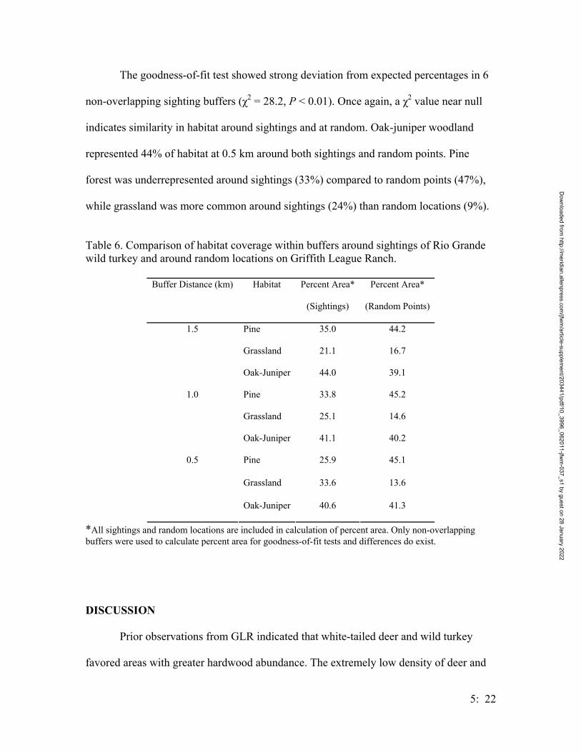
5: 22

The goodness-of-fit test showed strong deviation from expected percentages in 6

non-overlapping sighting buffers (χ2 = 28.2, P < 0.01). Once again, a χ2 value near null

indicates similarity in habitat around sightings and at random. Oak-juniper woodland

represented 44% of habitat at 0.5 km around both sightings and random points. Pine

forest was underrepresented around sightings (33%) compared to random points (47%),

while grassland was more common around sightings (24%) than random locations (9%).

Table 6. Comparison of habitat coverage within buffers around sightings of Rio Grande wild turkey and around random locations on Griffith League Ranch.

Buffer Distance (km) Habitat Percent Area*

(Sightings)

Percent Area*

(Random Points)

Pine 35.0 44.2

Grassland 21.1 16.7

1.5


Pine 33.8 45.2

Grassland 25.1 14.6

1.0


Pine 25.9 45.1

Grassland 33.6 13.6

0.5


*All sightings and random locations are included in calculation of percent area. Only non-overlapping buffers were used to calculate percent area for goodness-of-fit tests and differences do exist.

DISCUSSION

Prior observations from GLR indicated that white-tailed deer and wild turkey

favored areas with greater hardwood abundance. The extremely low density of deer and

Dow



m/article-supplem

ent/203441/pdf/10_3996_062011-jfwm


5: 23

their affinity for grassland areas (the only areas to produce any quantity of herbaceous

forage) suggested that deer were using the small amount of edge habitat available,

regardless of surrounding habitat type. Habitats occurring within 0.5 km, 1.0 km, and 1.5

km of deer sightings showed more grassland area than either pine forest or oak-juniper.

Grassland habitat was least available and changed little with distance in random buffers

(Table 5). The 1.0 km and 1.5 km sighting buffers showed an almost even distribution of

habitats, despite the uneven distribution seen in random buffers. Non-overlapping buffers

used for the goodness-of-fit tests showed a similar pattern of high grassland use.

Unmanaged pine forests slowly decrease in quality and quantity of forage

because fire suppression allows litter to accumulate while browse grows out of reach and

density and basal area increase (Halls 1973, Conroy et al. 1982, Scanlon and Sharik

1986, Thill et al. 1990). However, they may eventually become oak dominated

communities (Allen et al. 1996) important for mast and fungi production (Johnson et al.

1995). On intensively managed plantations, deer may not favor edge areas in stands up to

276 ha if there is sufficient production of forage in the forest (Melchiors et al. 1985).

High yaupon production in GLR pine forests (30.7 % canopy cover and 4,328 plants/ha)

should provide plenty of favored forage (Lay 1956, 1967a, 1967b). Some of this may be

out of reach, or the deer may not be willing to utilize large tracts of forest for a single

food item. The forest on GLR is largely unbroken by openings except for a line of central

pastures. The large stand sizes, lack of management, and low forage production on GLR

may force deer to use edges to subsist.

The decreasing percentage of grassland habitat with increasing buffer distance

indicates that Rio Grande wild turkeys on GLR were more associated with forest habitat

than deer. I observed them using openings to forage on insects and seeds and for

Dow



m/article-supplem

ent/203441/pdf/10_3996_062011-jfwm


5: 24

reproductive displays on several occasions. They primarily roosted in the center of the

ranch at the head of a large drainage. Miller et al. (2000) suggested that riparian corridors

are important for female movement and reproduction. Improvement of habitat

surrounding other drainages on the ranch and creation of small openings for herbaceous

forage production may increase use of the ranch by wild turkeys.

Vegetative density (Halls 1973), canopy cover (Conroy et al. 1982), and duff

(Thill et al. 1987) negatively impact forage production. Despite lower levels of litter

accumulation in oak-juniper woodlands (40.2 mm annually) than pine forests (60.1 mm

annually), canopy cover remained high (74% annually) and forb production remained low

(1.4%), making both pine and hardwood habitats marginal wildlife habitat. One pine

forest sample point (Point 12) averaged 116 mm of duff in summer, and is likely

responsible for the apparent seasonal change in duff depth. The unusually high

measurement probably resulted from random placement of quadrats near tree bases where

duff can build up substantially. Scanlon and Sharik (1986) found that forage production

in hardwood stands in a low mast year was similar to that of 17-year-old pine stands with

< 30 kg/ha, so low production of both on GLR is predictable. Oak mast may make up

large portions of white-tailed deer diets (Harlow et al. 1975), but almost no mast

production by oaks was observed on GLR, negating its influence on deer distribution on

the ranch.

Similar to white-tailed deer, wild turkeys tend to favor pine-hardwood mixtures

with low shrub densities, an open understory, and high herbaceous production (Bidwell et

al. 1989, Campo et al. 1989). The high woody plant density and decreased visibility at

low VPB levels in the pine forest on GLR may explain the apparent lack of affinity for

this habitat by wild turkeys (Allen et al. 1996). Campo et al. (1989) found that turkeys in

Dow



m/article-supplem

ent/203441/pdf/10_3996_062011-jfwm


5: 25

eastern Texas tended to inhabit stands associated with openings. The results of my study

supported that finding, because I recorded only 2 locations > 400 m from open areas and

18 of 24 sightings were < 100 m. The combination of lower woody plant density,

decreased low-level visual obscurity in the surrounding oak-juniper woodlands, and

access to the central pastures probably accounted for observed centralized locations of

most turkey sightings.

Some of the apparent selection for grassland habitats by both species may result

from differential sighting ability. However, wide scale use of the forested areas is

unlikely since there was a lack of sightings and sign (tracks, droppings) in forested areas.

The concentration of many deer sightings near the eastern and western boundaries of the

ranch, where surrounding ranches are mostly pasture, suggested selection for open areas

and edge despite differences in sighting probability.

Woody vegetation in forested areas was dense and dominated by few species in

both the overstory and understory. Herbaceous production was essentially nonexistent.

Unusually low measurements for herbaceous coverage in the fall for both oak-juniper and

pine habitats, which may be a result of the patchy nature of herbaceous cover in the

forest, explains the habitat by season interactions seen in grass and total herbaceous cover

measures. This complicates analysis of these data, but it is doubtful that any biologically

significant differences exist.

Bidwell et al. (1989) reported green herbaceous cover > 20% in 5 to 7-year-old

pine plantations, and even the oldest stands (11 to 13-years-old) had around 10%

coverage. Loblolly forests tend to have lower herbaceous species richness and higher

midstory and overstory densities than other southern pine forest types, but they can

contain herbaceous communities similar to longleaf forests, which are known for high

Dow



m/article-supplem

ent/203441/pdf/10_3996_062011-jfwm


5: 26

levels of herbaceous production (Hedman et al. 2000). The forest on GLR had a long

time for litter accumulation, midstory development, and canopy closure, all of which

inhibited forage production. In older stands, midstory browse tends to grow out of reach

of white-tailed deer (Halls 1973, Thill et al. 1990). In oak-juniper woodlands on GLR

horizontal obscurity was highest at higher VPB levels (Table 4), suggesting an elevated

midstory.

I found no differences in visual obscurity at the highest VPB levels between oak

and pine habitats. Spotlighting occurs from an elevated position and is probably

influenced most by these upper levels, but differences in sighting angle can change

visibility and an animal’s distance from the vehicle and position (bedded or standing)

may make lower levels important in sighting bias as well. Visibility in oak-juniper

woodlands was higher along the survey route but did not result in a substantial increase in

sightings. Only one spotlight sighting of a deer occurred in forest habitat. Increased

sampling of forest habitats would most likely increase numbers of deer sighted; however,

restrictions on available access precluded this option.

About 36% (5.9 km) of the transect route was in grassland habitat, and much of

this ran along edges, where two habitats were sampled simultaneously. The better

precision and lower AIC of the uniform sighting distribution probably resulted from the

high number of observations from grassland habitats where a uniform distribution is more

likely. All models pointed to an extremely low number of white-tailed deer on GLR.

Based on the confidence limits, the maximum density estimated is no more than the

lowest countywide estimates of 0.023 deer/ha.

Management Implications

Dow



m/article-supplem

ent/203441/pdf/10_3996_062011-jfwm


5: 27

This study provided baseline data for two important game species in an area

largely ignored in the published literature. The current focal species in the Lost Pines is

the Houston toad (Bufo houstonensis), a federally listed endangered species. Its presence

means that management activities on GLR have to consider potentially negative impacts

to this species (US Code, Title 16, Ch. 35; State of Texas Parks and Wildlife Code, Title

5, Ch. 68). Greuter (2004) recommended a 75-m buffer around ponds from March to July

to protect juvenile toads. Even if a more generous 500-m buffer is used year-round and

all known ponds are protected, 64% (1,295 ha) of the ranch area is still available for other

wildlife management activities. Much of this area is pine forest habitat, which is in the

most serious need of management.

Fire is an important tool for maintaining loblolly pine forests. Prescribed burning

reduces and lowers the woody understory and encourages herbaceous growth by

improving light penetration and removing litter (Hodgkins 1958, Moore 1982, Thill et al.

1987, Miller et al. 2000) as well as reducing the possibility of destructive fires (Hunter

1990). Burning too frequently can negatively impact hardwoods, but longer cycles

increase the risk of hotter fires which destroy old growth individuals (Schultz 1997).

Burning on 3 to 5-year intervals is recommended (Lay 1967a, Halls 1973, Miller et al.

2000). The large litter accumulations in some areas, patchy fuel loads, and lack of fire

breaks may make burning difficult on GLR. Caution must also be used to avoid

destroying large snags (Hunter 1990). An initial tree thinning followed by an early winter

burn to avoid active toads should promote increased forage production and diversity on

the ranch.

Tree thinning stimulates sprouting by woody browse plants and reduces

competition for herbaceous plants (Patton and McGinnes 1964; Halls 1970, 1973). Old,

Dow



m/article-supplem

ent/203441/pdf/10_3996_062011-jfwm


5: 28

unthinned pine forests support fewer plant species and produce less forage for herbivores

(Hunter 1990). Patton and McGinnes (1964) reported a 200% increase in browse

production following a 30% thinning in a Virginia forest, and Patton (1974) noted that

harvest of an Arizona forest increased forage and use of the area by deer. Blair and

Feduccia (1977) found an 81% increase in browse after burning in Louisiana. Removing

the midstory increased herb production as well. White (2003) made similar

recommendations for GLR to improve avian habitat. An increase in forage production

and diversity should benefit all wildlife on the ranch by reinstating previously naturally

occurring cycles and enhancing productivity.

To further improve forage production and use of GLR by white-tailed deer and

Rio Grande wild turkeys, small openings or clear-cuts can be made throughout the forest.

Clear-cutting produces openings to increase foraging opportunities and edge (Campo et

al. 1989, Thill et al. 1990) and may increase use because of increases in quality of forage

available (Johnson et al. 1995). Sweeney et al. (1984) found similar use of all distances

from the edge in young, open cuts < 25 ha in size. Seeding these openings could help

speed up forage production in these often poor soils. Many ponds on the ranch are located

close to existing roads. Careful placement of long, narrow clearings may allow their

simultaneous use as firebreaks when widening roads is not an option because of nearby

ponds.

The large size and relatively undeveloped conditions which exist at GLR hold potential

for quality habitat enhancement for game and nongame communities in the Lost Pines.

The presence of the Houston toad and several endemic and newly discovered species of

insects (Taber and Fleenor 2003) make the Lost Pines a unique and important ecosystem.

Future research should concentrate on specific needs of game animals that are or are not

Dow



m/article-supplem

ent/203441/pdf/10_3996_062011-jfwm


5: 29

being met in largely unmanaged pine forests in the area. Current management should

focus on immediate increases in forage availability. While most southern pine forests

suffer from a lack of quality forage because of high rainfall levels (Lay 1956), animals on

GLR are likely more heavily impacted by a lack of quantity. Future changes can be

compared to the current research to assess the effectiveness of traditional pine forest

management activities in improving habitat and abundance of species in the Lost Pines.

Increased game populations in Bastrop County may provide more recreational

opportunities for residents as well as increasing the awareness of proper management and

conservation of the Lost Pines. This is contingent on the prudent use of applied ecology

in maintaining the health of the ecosystem and the communities it supports.

Dow



m/article-supplem

ent/203441/pdf/10_3996_062011-jfwm


5: 30

Avian Habitat Affinity in the Lost Pines Region of Texas

Clayton J. White and Thomas R. Simpson

Department of Biology, Texas State University, San Marcos TX 78666

Avian diversity and habitat association has been investigated by many workers

(MacArthur and MacArthur 1961, MacArthur 1964, Rice et al. 1983, McCollin 1998).

Rice et al. (1983) found that avian communities can be used as an indicator of habitat

type, while Todt (1989) showed that avian diversity corresponds to differences observed

in the habitat. Diversity may also be used as an indicator of habitat quality. High quality

habitat is assumed to support a more diverse avian community which could include both

specialists and generalists (Gabbe et al. 2002). This could also indicate that low species

richness or the absence of common bird species may indicate poor habitat quality.

Among terrestrial vertebrate groups, birds are the most numerous and easiest to detect

making them the logical choice for the evaluation of habitat quality.

Single species or specific group studies focusing on habitat selection and habitat

attributes are also common, (Bertin 1977, Conner and Adkisson 1977, Martinez and

Jaksic 1996, Ritter and Savidge 1999). McClelland and McClelland (1999) reported that

Pileated Woodpeckers (Dryocopus pileatus) indicate a healthy old growth forest. Single

species studies are useful, but somewhat limited in overall conclusions that can be drawn

for an avian community. While these studies are necessary, especially when dealing with

endangered species, community based approaches must be used to conduct sound

ecosystem management. A community based approach would consider all species

present within the community, and any potential interactions among those species.

Dow



m/article-supplem

ent/203441/pdf/10_3996_062011-jfwm


5: 31

Avian Habitat Use

Habitat use by avifauna varies among species, seasons, and possibly broad-scale

location. Use of habitat is a well studied field with many proposed hypotheses on how

and why birds choose one or more habitat types. Boulinier et al. (2001) suggests that

landscape structure may influence forest bird communities at regional scales through its

effects on the total number of species and also on the temporal rates of change in

community composition. Reduction of nest predation pressure (Sieving and Wilson

1998), foliage profile characteristics (MacArthur and MacArthur 1961), latitude (Tramer

1969), heterogeneity and patchiness (Franzreb and Ohmart 1978), edge density (Howell

et al. 2000), plant species (Tomoff 1974), guild structure (Rice et al. 1983), interaction

and competition avoidance, microclimate modification, and vegetation structure

(McCollin 1998) all have been suggested as possible factors influencing habitat use. Not

only do these factors vary among species, but also among other taxonomic groupings and

seasonal groups (breeders, winter residents, permanent residents) as well. Flather and

Sauer (1996) reported Neotropical migrants show a more sensitive response than

temperate migrants or permanent residents to changes in landscape structure and utilize

large contiguous habitats with continuous canopy cover. Permanent residents in the same

study showed less affinity with landscape structure while temperate migrants were

correlated with habitat diversity and edge attributes rather than with the amount, size, and

dispersion of forest habitats.

Prior to any understanding of potential relationships between avian communities

and habitat, thorough descriptions of all possible factors influencing that relationship

must be investigated. Vegetation is the major component of most terrestrial habitats and

quantifying measurements of vegetation are useful in identifying any relationship

Dow



m/article-supplem

ent/203441/pdf/10_3996_062011-jfwm


5: 32

between avian diversity and habitat. Vegetation does not account for other influential

factors (avoidance of nest predation, guild structure, competition avoidance) that may

also affect avian diversity associations with habitat types. In addition to vegetation, avian

communities must be surveyed to estimate current populations. This data may also be

used to establish trends and evaluate progress following application of management

techniques.

The Lost Pines is a well known part of Texas, but little research has been

conducted that quantify the plant and animal communities associated with the region

(Taber and Fleenor 2003). Many scientists propose that this isolated pocket of pines is a

remnant of a greater forest that once covered the eastern half of the state. Correll (1966)

described the Lost Pines as a fractured, western peninsula that currently is a distant island

or archipelago of pine. Tabor and Fleenor (2003) proposed that the pines possibly arose

independently of the pines to the east but offered no support for this hypothesis. Pollen

analysis has suggested that loblolly pines have been in the area for nearly twenty

thousand years (Bryant 1977) and no significant change or expansion of the Lost Pines

has occurred during the last sixteen thousand years (Larson et al. 1972). Regardless of

origin, habitat fragmentation from recent urban sprawl has made its impact on the land

and will continue to do so over time. The best chance for conservation of the Lost Pines

is its strong hold for the endangered Houston Toad (Bufo houstonensis). Research on the

larger unfragmented areas of forest is necessary in order to identify habitats that support

the greatest diversity and the factors within those habitats that are most critical. In

addition to conservations efforts, baseline plant and animal populations will establish a

starting point for analyzing the effects of forest fragmentation in the Lost Pines Region.

Dow



m/article-supplem

ent/203441/pdf/10_3996_062011-jfwm


5: 33

Population decline among Neotropical migrants is a well documented occurrence

(Robbins et al. 1989). With this current trend, identification of diverse habitats and key

habitat components must be found within the Lost Pines for proper management of bird

populations. Among the problems contributing to the decline are habitat fragmentation,

urban sprawl, loss of old growth forest, loss of large scale contiguous forest, nest

parasitism and others. Habitat fragmentation coupled with Brown-headed Cowbird

(Molothrus ater) nest parasitism may multiply the detrimental effects on declining

populations. Fragments of habitat create more edge, which is utilized by the cowbirds,

and offer more hosts to parasitize (Robinson et al. 1995). Other combinations of causes

likely are having similar affects. With modern progress (urbanization, forest

fragmentation) and declining bird populations, application of sound ecosystem

management practices must focus on habitat types and factors that are most influential

across all seasons for the avian communities present.

Like many studies dealing with habitat use, components of the habitat that best

describe avian diversity may be site specific. Factors influencing a species may not differ

greatly by site but factors affecting diversity could and probably do vary by site. This

potential variation may be explained by vegetation, guild structure and microclimate

differences found within each habitat.

Research Objectives

In this paper I will present findings which 1) establish a baseline inventory of the

avian community found on Griffith League Ranch, 2) establish a vegetation profile of the

plant community including canopy coverage, vertical structure, woody species density,

herbaceous plant coverage, and duff depths, 3) identify habitats of higher diversity by

Dow



m/article-supplem

ent/203441/pdf/10_3996_062011-jfwm


5: 34

season and 4) identify primary vegetative components that are associated with avian

community diversity by season.


Study Site

The Griffith League Ranch (hereafter GLR) occupies 1,961 ha of the Lost Pines

Region of south central Texas (Fig.1). GLR lies in an isolated loblolly pine (Pinus taeda)

forest geographically separated from the Piney Woods region of east Texas by

approximately 160 km. GLR is approximately thirteen km northeast o f Bastrop, Texas

in Bastrop County.

Forested areas (1,728 ha) of GLR are a mix of loblolly pine, post oak (Quercus

stellata), blackjack oak (Q. marilandica) and eastern red cedar (Juniperus virginianus).

Cleared pasture lands (233 ha) consisting of costal Bermuda (Cynodon dactylon) and

Bahia grass (Paspalum notatum) formerly were grazed by livestock. Within the forested

areas, the understory includes American beautyberry (Callicarpa americana), yaupon

(Ilex vomitoria) and farkleberry (Vaccinium arboreum). Herbaceous vegetation under the

forest canopy is sparse, but does include Texas bull-nettle (Cnidoscolus texanus), panic

grasses (Dicanthelium spp,) and flowering spurge (Euphorbia corolata).

Rolling hills of sandy soils make up the topography of GLR. Demona loamy fine

sand, Patilo and Silstid loamy fine sand of the sand range site cover more than 90% of

GLR (USDA Soil Conservation Service 1979). Elevations range from 137 m to 198 m

with Alum Creek on the eastern edge of the ranch and Piney Creek and Spicer Creek

drainages to the west and southwest, respectively. Nineteen known ponds exist on the

ranch varying in size from less than 0.5 ha to just under 1.5 ha, eleven of which hold

water permanently (Koepp 2001).

Dow



m/article-supplem

ent/203441/pdf/10_3996_062011-jfwm


5: 35

Figure 1. Location of Griffith League Ranch within Bastrop County, Texas

(1,728 ha). Habitats Associated with Griffith League Ranch

Delineation of habitats was determined by the use of digital orthophoto quarter

quadrangles (DOQQ). Points within selected habitat types were selected and ground

truthed to verify habitat type identification. At each point one t-post was driven into the

ground to serve as a center point of that habitat. Twenty-five points within four habitat

types were chosen and measured to quantify habitat type assignments (Fig. 2). Habitat

types were grasslands with reduced woody species canopy cover, oak/cedar habitats with

greatest amounts of post and blackjack oaks and eastern red cedar, pine habitats with a

dominant overstory of loblolly pine, and pond habitats containing a permanent pond

Dow



m/article-supplem

ent/203441/pdf/10_3996_062011-jfwm


5: 36

within a 100 m radius of the point center (Fig. 2). Points were treated as independent

samples and spaced > 250 m apart to prevent violation of independence by overlapping

points.

Sampling Methods

Avian Surveys – Point counts were used to identify avifaunal communities at each point

within habitat types. Point counts are used to monitor trends of bird populations over

time, but are also useful in bird-habitat relationship studies (Dettmers et al. 1999) and less

time consuming than line-transect surveys (Robel et al. 2000). Detection of birds varies

among species (Mayfield 1981, Lynch 1995), seasons (Best 1981, Best and Peterson

1985), habitat types (Reynolds et al. 1980, Schiek 1997), and time of day (Fuller and

Langslow 1984, Gates 1995).

Dow



m/article-supplem

ent/203441/pdf/10_3996_062011-jfwm


Figure 2. Point count locations in the four habitat types surveyed on Griffith League Ranch, Bastrop County, Texas.

To reduce potential bias from samples, each point count site was surveyed three

times in each season, starting in the summer of 2002, with sampling occurring in four

assigned habitat types. Calendar dates were used to estimate seasonal changes (Winter,

Dec. 22 – Mar. 20; Spring, Mar. 21 – Jun. 20; Summer, Jun. 21 – Sept. 22; Fall Sept. 23 –

Dec. 22). Dettmers et al. (1999) reported that sampling twice is sufficient with little to no

improvement on the third sample. However, when studying bird-habitat associations,

more counts may be necessary (Petit et al. 1995, Thompson and Schwalbach 1995).

Point counts lasted for ten minutes (Ralph et al. 1993, Brooks et al. 2001) and all birds

counted were confined within a 100 m radius of the point count site center. All point

counts were conducted from 6:00 am to 9:00 am (Lynch 1995) with the earliest count

occurring no more than thirty minutes before sunrise.

5: 37

Dow



m/article-supplem

ent/203441/pdf/10_3996_062011-jfwm


5: 38

In addition to point counts, mist netting results and incidental observations were

recorded to supplement a list of birds recorded on GLR. These observations were not

used in the statistical analysis of point count data. Mist netting was conducted under

authority of Texas State University IACUC permit (N2E772) as well as a federal bird

marking and salvage permit (22280-P).

Vegetation Sampling – To understand avian diversity-habitat associations,

vegetation variables were measured at each point count site. Percent canopy cover of

each tree species sampled, density of trees sampled, duff depth (decaying leaves and

branches), vertical obscurity and herbaceous vegetation cover were measured to identify

potential associations between avian diversity and habitats. Many of the variables

measured at each point count site were discarded prior to analysis of the data due to an

infrequency of measurements among sites. These variables included uncommon woody

species present in small amounts at only a few locations. Woody vegetation variables

were measured only one time assuming that no change among seasons within a year

would occur while all other variables (herbaceous and structure composition) were

measured each season.

Line-intercepts method was used to measure the canopy cover of each woody

species. Three 100 m transects separated 120 degrees were stretched from center point to

perimeter of the point count circle. Woody vegetation crossing the tape was recorded by

site. Line-intercept data was summed by species to yield a percent canopy cover for each

species observed. In addition to line-intercepts, woody stems/ha were measured for each

species using a 10 X 10 m quadrat. Three quadrat measurements were taken within each

point count site to determine the density of each woody species. This technique also

measured the number of standing dead trees/ha. Woody species/ha were calculated from

Dow



m/article-supplem

ent/203441/pdf/10_3996_062011-jfwm


5: 39

the pooled quadrat samples measured at each point count site. Both line-intercept and

woody stems/ha were measured only once per site.

Horizontal visual obscurity below 2.5 m was measured using a vegetation profile

board (VPB) (Nudds 1977). Five VPB measures were taken at all points in each season.

Canopy cover of woody structure was measured using a spherical densiometer (model A)

(Lemmon 1957). Five readings using the densiometer were recorded per point in each

season. Means by point count sites were calculated for VPB and canopy cover measures

for each season.

Daubenmire frames (25 cm X 100 cm) were used in quantifying the herbaceous

vegetation at each site (Daubenmire 1959). Ten frame samples were used at each point

count site to determine herbaceous vegetation composition by season. Each plant was

identified and then classified as grass, forb or sedge. Plants again were classified into

groups of native and introduced herbaceous vegetation. Total percent cover by point for

each season was then determined for each of the five classifications.

Duff measures were recorded within each Daubenmire frame sample. Ten duff

measures were averaged and used to assess duff depth by point each season.

Canopy coverage, woody species density, VPB, herbaceous vegetation coverage

and duff measures are only representative of point count sites and may not adequately

describe the entire ranch on a broader scale.

Statistical Methods and Diversity Indices

Habitat assignments delineated through DOQQ's and ground truthing were

verified using the percent canopy cover measures of the common woody species in a

Principal Component Analysis using the covariance matrix (S-Plus). Principal

component loadings were then graphed on a biplot to examine the predetermined habitat

Dow



m/article-supplem

ent/203441/pdf/10_3996_062011-jfwm


5: 40

assignments. The biplot is a graphical representation of the first two component scores in

relation to the data set with the arrows representing the loadings of the two components.

Avian diversity was calculated using the observations from three point counts

performed at each point count site, within each season. This resulted in 100 diversity

values for the 25 point count sites. Diversity for habitats within each season was then

determined by taking the mean of diversity values for points in their respective habitat

types. Avian diversity was measured using Brillouin’s Index (H’) (Exeter Software

2000). This index is more appropriate because the total number of species within the

point count area is unknown (Krebs 1989). This conservative index is prone to

underestimate the diversity however, with sample sizes often exceeding thirty

observations the potential bias is reduced (Zar 1996).

A single factor Analysis of Variance (ANOVA) was performed on the diversity

indices to evaluate possible differences among habitats within seasons. Contrasts (3, -1,-

1,-1) were performed on the seasons showing differences among habitats to identify those

differences (S-Plus).

A fully factorial ANOVA with three fixed factors was used to identify differences

among seasons, habitats and half meter height increments for VBP measures. Line-

Intercept data was summed by species to yield a percent canopy cover for each species

observed.

To identify possible factors that influence avian diversity all possible subsets regression

was used (Montgomery et al. 2001). Data transformation (ln(1+value)) and variable

reduction procedures preceded the multiple linear regression analysis. Variables that

contained more that five zero values were first excluded from the data set leaving only

the variables with ample observations. Correlation matrices of all independent variables

Dow



m/article-supplem

ent/203441/pdf/10_3996_062011-jfwm


5: 41

that may be related were then constructed to reduce variable multicollinearity in the

model. The remaining variables were examined choosing the best three to five variables

to use in the complete model. All possible subsets multiple linear regression (MLR) was

then used to identify the best model from all possible combinations of the selected

variables. Selection of the best model was based on a combination of lowest Mallow’s

Cp, highest r2 value and lowest residual standard error (Montgomery et al. 2001).

Mallow’s Cp is a measure of bias within each subset model, assuming that the complete

model has no bias. The p value represents the results from an ANOVA test on the

selected model.

RESULTS

Habitat Identification

Habitat classification based on visual interpretation of DOQQ and ground truthing

first produced five habitat types (grassland, oak, cedar, pine, and pond) with five point

count sites in each habitat. Principal Component Analysis (PCA) was selected to verify

habitat classification of the 25 point count sites. Principal Component I explained 60.4%

of the variation among variables and Principal component II explained 20.9% of the

variation. Pine was highly correlated (0.81) with Principal Component I while both post

oak and eastern red cedar were moderately correlated with Component II (0.61, 0.54

respectively).

From the principal component loadings (Table 1) and biplot (Fig. 3) five grassland

habitats (point count sites 1, 8, 9, 13, 17), six oak/cedar habitats (2, 3, 4, 5, 6, 23), and

nine pine habitats (10, 11, 12, 15, 16, 19, 20, 21, 24) were identified (Fig. 2), reducing the

prior habitat designations to three habitat types. PCA designations for pond habitats were

disregarded based on the previous designation of permanent water, which was not a

Dow



m/article-supplem

ent/203441/pdf/10_3996_062011-jfwm


5: 42

variable considered in this analysis. Pond habitats, the fourth designated habitat,

occurred in both grassland (18) and oak/cedar (22) habitats one time each and pine

habitats (7, 14, 25) three times.

Table 1. Principal component loadings of yaupon, eastern red cedar, loblolly pine, blackjack oak and post oak canopy coverage of PC I and II for 25 point count sites on Griffith League Ranch, Bastrop Co. Texas. Principal Component I Principal Component II Yaupon 0.4623 -0.3413 Cedar 0.1794 0.5418 Pine 0.8060 -0.1879 Blackjack 0.0350 0.4213 Post 0.3213 0.6114

Dow



m/article-supplem

ent/203441/pdf/10_3996_062011-jfwm


5: 43

Avian Diversity

3,487 detections of 75 avian species were recorded from 300 point counts on the

Griffith League Ranch. Mist netting and incidental observations increased the total

number of species to 110. One hundred hours of mist netting accounted for five of the

species not detected in point counts.

Fall had the highest number of observations with 1,156 and the fewest number of

species at 39. Summer had the fewest observations with 749 and spring had the highest

number of species recorded totaling 74 (Table 2). Fall also had the lowest mean diversity

(H’= 2.02), while spring had the highest mean diversity (H’= 2.43). Pond habitats for

combined seasons had the highest mean diversity (H’= 2.59) and open habitats had the

lowest mean diversity (H’= 1.64). ANOVA and contrast results showed diversity by

habitat within each season to be fairly consistent yielding similar results for winter,

spring and summer. For each of these three seasons the ANOVA resulted in a significant

difference (p< 0.001) and the contrast identified pond habitats, oak habitats and pine

habitats as similar groups. Grassland habitats were dissimilar from all others in winter,

spring and summer. Fall diversity values had no significant differences among habitats

(Table 3).

Dow



m/article-supplem

ent/203441/pdf/10_3996_062011-jfwm


5: 44

Table 2. Mean number of observations, number of species and mean Brillouin’s Index (H’) of diversity for birds counted on the Griffith League Ranch from 300 point counts by season and habitat type.

Mean Number

of Number

of Mean Habitat type n Observations Species H'

Winter Grassland 5 17.4 17 1.43 Pond 5 49.0 30 2.77 Oak/Cedar 6 31.2 23 2.67 Pine 9 26.3 25 2.41

Spring Grassland 5 12.2 18 1.44 Pond 5 41.2 30 2.76 Oak/Cedar 6 37.2 22 2.64 Pine 9 37.2 28 2.63 Summer Grassland 5 17.0 16 1.63 Pond 5 39.2 29 2.42 Oak/Cedar 6 29.7 18 2.63 Pine 9 32.2 24 2.46 Fall Grassland 5 26.2 20 1.81 Pond 5 40.8 19 2.48 Oak/Cedar 6 81.5 16 1.84 Pine 9 37.9 18 1.99

Table 3. ANOVA results comparing Brillouin’s Index of diversity values for grassland, oak/cedar, pond and pine habitats within seasons. Source dfnumerator dfdenominator F p Winter 3 21 12.32 < 0.001 Spring 3 21 10.23 < 0.001 Summer 3 21 13.74 < 0.001 Fall 3 21 1.59 > 0.5

Dow



m/article-supplem

ent/203441/pdf/10_3996_062011-jfwm


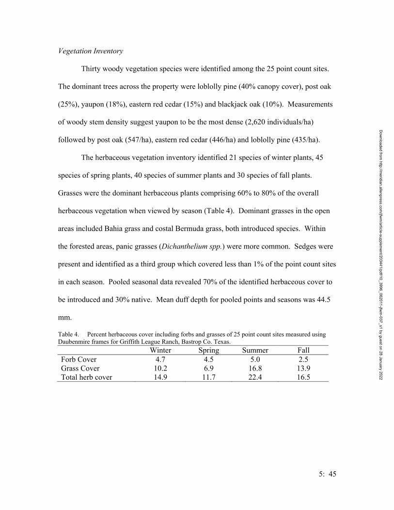
5: 45

Vegetation Inventory

Thirty woody vegetation species were identified among the 25 point count sites.

The dominant trees across the property were loblolly pine (40% canopy cover), post oak

(25%), yaupon (18%), eastern red cedar (15%) and blackjack oak (10%). Measurements

of woody stem density suggest yaupon to be the most dense (2,620 individuals/ha)

followed by post oak (547/ha), eastern red cedar (446/ha) and loblolly pine (435/ha).

The herbaceous vegetation inventory identified 21 species of winter plants, 45

species of spring plants, 40 species of summer plants and 30 species of fall plants.

Grasses were the dominant herbaceous plants comprising 60% to 80% of the overall

herbaceous vegetation when viewed by season (Table 4). Dominant grasses in the open

areas included Bahia grass and costal Bermuda grass, both introduced species. Within

the forested areas, panic grasses (Dichanthelium spp.) were more common. Sedges were

present and identified as a third group which covered less than 1% of the point count sites

in each season. Pooled seasonal data revealed 70% of the identified herbaceous cover to

be introduced and 30% native. Mean duff depth for pooled points and seasons was 44.5

mm.

Table 4. Percent herbaceous cover including forbs and grasses of 25 point count sites measured using Daubenmire frames for Griffith League Ranch, Bastrop Co. Texas. Winter Spring Summer Fall Forb Cover 4.7 4.5 5.0 2.5 Grass Cover 10.2 6.9 16.8 13.9 Total herb cover 14.9 11.7 22.4 16.5

Dow



m/article-supplem

ent/203441/pdf/10_3996_062011-jfwm


5: 46

VPB measures had a grand mean of 57.83% horizontal obscurity with means for

GLR reported in Table 5. No interaction was found among the main effects (p >0.05)

and habitat was the only main effect to show a significant difference.

Table 5. Mean Vegetation Profile Board measures of horizontal obscurity for five half meter height increments by habitat type within seasons for 25 points on Griffith League Ranch, Bastrop Co, Texas.

Habitat VPB1

(2-2.5 m) VPB2

(1.5-2 m) VPB3

(1-1.5 m) VPB4

(0.5-1m) VPB5

(0-0.5m) Winter Grassland 20.0 20.0 20.0 20.8 41.6 Oak/Cedar 60.7 58.0 60.0 53.3 58.0 Pond 66.8 64.6 67.4 77.6 75.6 Pine 72.0 74.7 74.7 73.8 72.9 Spring Grassland 20.0 20.0 23.2 24.8 62.4 Oak/Cedar 72.7 67.3 62.0 55.3 59.3 Pond 65.6 65.6 64.8 64.8 71.2 Pine 71.1 68.0 76.9 71.6 77.3 Summer Grassland 23.2 22.4 22.4 29.6 68.0 Oak/Cedar 82.7 69.3 69.3 56.0 66.0 Pond 72.8 68.0 64.8 60.0 73.6 Pine 72.9 66.7 74.7 62.2 70.2 Fall Grassland 20.0 20.0 20.8 28.0 48.8 Oak/Cedar 72.0 68.0 63.3 51.3 50.7 Pond 69.8 69.0 66.0 63.4 73.0 Pine 72.9 70.7 72.4 66.7 68.4

Factors Influencing Diversity

Factors affecting diversity within seasons varied greatly when compared across all

habitats. Multiple linear regression (MLR) models each season showed diversity

correlated with one to four variables. The MLR model for winter was represented by a

Mallow’s Cp of 4.579, r2 =0.61 and p <0.001. For the winter model, positive correlations

Dow



m/article-supplem

ent/203441/pdf/10_3996_062011-jfwm


5: 47

were found between diversity and both yaupon and post oak canopy covers. An inverse

correlation existed with duff depth.

H’ = 2.651 + 0.203 (yaupon canopy cover)

+ 0.233 (post oak canopy cover)

– 0.402 (duff depth)

The MLR model for spring had a Mallow’s Cp of 4.904, r2 = 0.646 and p < 0.001. Like

the winter model, the spring model shows a positive correlation between diversity and

yaupon canopy cover. A positive correlation with pine canopy coverage is also present in

the spring. The spring model also had an inverse correlation with horizontal obscurity

measures from 0.0 – 0.5 m.


+ 0.274 (pine canopy cover)

– 1.273 (VPB 0.0 – 0.5 m height increment)

The model for summer was represented by a Mallow’s Cp of 1.7, r2 = 0.699 and p <

0.001. This model was the simplest with only one factor needed to describe diversity,

post oak canopy cover with which a positive correlation was found.

H’ = 1.629 + 0.258 (post oak canopy cover)

The MLR model for fall was represented by a Mallow’s Cp of 8.244, r2 = 0.323 and p =

0.086. Of the four seasons, fall had the lowest desirable selection criteria (Cp, r2, p).

This model shows a positive correlation between diversity and both yaupon and eastern

red cedar canopy cover. Inverse correlations were shown with vertical obscurity

measures at 0.0 – 0.5 m and post oak canopy cover.


+ 0.481 (eastern red cedar canopy cover)

Dow



m/article-supplem

ent/203441/pdf/10_3996_062011-jfwm


5: 48

– 1.340 (VPB 0.0 – 0.5 m height increment)

– 0.702 (post oak canopy)

I. DISCUSSION

Avian Diversity

I documented the presence of 110 species of birds representing fifteen orders on

the Griffith League Ranch. Order Passeriformes, as expected, dominated the total

number of species detected with 62 detections through point counts, incidental

observation and mist netting. Other orders with modest representations include both

Orders Ciconiiformes and Piciformes, each with eight species. Two members of the

Order Ciconiiformes, White Ibis (Eudocimus albus) and White-faced Ibis (Plegadis

chihi), were unexpected birds for GLR due to the lack of suitable habitat. The White-

faced Ibis is currently listed as Threatened by the State of Texas.

Most species observed were expected, however, some common birds never were found or

were present in low numbers. One such group was ducks. Freeman (1996) notes 23

possible species for the area; only five species were recorded on GLR. Also missing

were Eastern Screech Owl (Megascops asio), Ruby-throated Hummingbird (Archilochus

colubris), Dickcissel (Spiza americana), Red-winged Blackbird (Ageliaus phoeniceus)

and Pine Siskin (Carduelis pinus). The only species of woodpecker (Piciformes) not

observed that could potentially occur on GLR was the Red- headed Woodpecker

(Melanerpes erthrocephalus). With an abundance of snags (75/ha) on GLR this diversity

of woodpeckers was expected, since woodpeckers show a positive correlation with snag

abundance (Lohr et al. 2002, Showalter and Whitmore 2002). While the species richness

for GLR is moderate at best, no introduced birds were observed.

Dow



m/article-supplem

ent/203441/pdf/10_3996_062011-jfwm


5: 49

Diversity values did not vary significantly among seasons but were different

among habitat types within three of the four seasons. Because diversity values did not

change across seasons, avian community variation may best explain the differences seen

among seasons, habitat use, and factors influencing avian diversity.

Birds common during all seasons (permanent residents) through point count

detections were Red-shouldered Hawk (Buteo lineatus), Red-bellied Woodpecker

(Melanerpes carolinus), Tufted-titmouse (Baeolophus bicolor), Carolina Wren

(Thryothorus ludovicianus), Pine Warbler (Dendroica pinus), and Northern Cardinal

(Cardinalis cardinalis). Winter birds common to GLR were Ruby-crowned Kinglet

(Regulus calendula), American Robin (Turdus migratorius), Cedar Waxwing

(Bombycilla cedrorum), Yellow-rumped Warbler (Dendroica coronata), American

Goldfinch (Carduelis psaltria) and Chipping Sparrow (Spizella passerine). Birds

common in the summer season were Yellow-billed Cuckoo (Coccyzus americanus),

White-eyed Vireo (Vireo griseus), Summer Tanager (Piranga flava) and Painted Bunting

(Passerina ciris).

Winter and summer had a similar number of species, 49 and 51 respectively.

Twenty-six species were present both seasons and can be classified as permanent

residents. Spring observations totaled 74 species, the most of any season. Twenty-six

species were seen only in the spring season, seventeen of these were migrants. Fall had

the fewest number of species, 39, with thirteen percent of the avian community being

sparrows of the Family Emberizidae. The low number of species in the fall may be a

reflection of the point count method as birds did not appear to vocalize as often or as late

into the morning when compared to the spring or summer. Fall did have the highest

Dow



m/article-supplem

ent/203441/pdf/10_3996_062011-jfwm


5: 50

number of observations but they commonly were visual detections of large groups of

American Robins and Cedar Waxwings.

From the results of the ANOVA and contrasts comparing habitats within season,

winter had similar diversity values for oak/cedar habitats, pond habitats and pine habitats.

Grassland habitats were less diverse and dissimilar from the other habitat types. Eastern

Phoebe (Sayornis phoebe), Vesper Sparrow (Poecetes gramineus) and Lincoln Sparrow

(Melospiza lincolnii) were common in winter grassland habitats. Mallard (Anas

platyrhynchos), Ring-necked Duck (Aythya collaris) and Purple Gallinule (Porphyrio

martinica) were found in pond habitats. Oak/cedar habitats and Pine habitats were

similar in avian composition.

Spring had similar results as winter for diversity among habitats. Mourning Dove

(Zenaida macroura), Scissor-tailed Flycatcher (Tyrannus forficatus) and Northern

Mockingbird (Mimus polyglottos) were commonly found in grassland habitats during the

spring. All spring migrants, excluding the Common Snipe (Gallinago gallinago) and

Northern Harrier (Ciris cyaneus), were found in the three other habitat types but appeared

more common (13 of 17) in the pond habitats.

Summer also had habitat diversities similar to winter and spring. Summer

breeders were commonly found in the three similar habitat types, but the late summer

migrant, Blue-gray Gnatcatcher (Polioptila caerulea), was most common in the oak/cedar

habitat. This may contribute to the slightly higher, though not significant, diversity value

found in the oak/cedar habitat.

Fall had the fewest number of species and no difference in diversity among

habitat types. The avian communities differed with sparrows common in the grasslands

Dow



m/article-supplem

ent/203441/pdf/10_3996_062011-jfwm


5: 51

while both kinglets, American Robins and Carolina Chickadees (Parus bicolor) were

common in the other habitats.

Vegetation Inventory

The USDA Soil Conservation Service, SCS (1979) lists an historical, stable plant

community most like that of a post oak savannah habitat with a mix of perennial grasses

and deciduous oaks. Little bluestem (Schizachyrium scoparium), indiangrass

(Sorghastrum nutans), brownseed paspalum (Paspalum plicatulum) and switchgrass

(Panicum virgatum) should be the dominant grass species and post oak, blackjack oak,

elm (Ulmus sp.), hackberry (Celtis sp.) and yaupon are listed as the dominant trees.

Interestingly, loblolly pine and eastern red cedar are not part of the historical plant

community according to the SCS but pollen records from nearby bogs document their

presence in the region for the last twenty-thousand years (Bryant 1977) and should be

included in any description of the vegetation.

Current vegetation conditions for GLR yield different results with the absence of

almost all dominant native grasses. In the northern corner of GLR little bluestem appears

to be holding strong, however brownseed paspalum and switchgrass are rare and

Indiangrass was never observed on GLR. Increased forest canopy, grazing history of the

property, and introduction of non-native grasses are possible explanations for the

reduction in these native grasses.

Dominant trees have increased from their historical proportion and contributed to

the lack of herbaceous vegetation by shading and excess deposits of duff. Post oak and

blackjack oak were the dominant woody species and have continued to increase along

with other tree species. Hackberry was not a common tree on the property, nor were elm

species except in the riparian habitats. One tree species quickly becoming abundant in

Dow



m/article-supplem

ent/203441/pdf/10_3996_062011-jfwm


5: 52

some parts of GLR is honey mesquite (Prosopus glandulosa). Chinaberry (Melia

azedarach) also is becoming abundant in some areas, but this tree was not noted at any of

the 25 point count sites. Fire suppression and grazing are the most likely causes for the

change in woody vegetation composition (Smeins and Diamond 1984).

VPB measures suggest that grassland habitats consistently have lower percent

horizontal obscurity in four or five height levels for the grassland habitat. All other

habitats are similar. This shows possible correlations with avian diversity and should

influence habitat use.

According to measures of herbaceous vegetation using Daubenmire frames 70%

of the herbaceous plant cover is composed of introduced species. The majority of this is

attributed to the cleared pastures of Bahia grass and costal Bermuda found across the

property. Habitat restoration of the grasslands as well as the woodlands must be

considered and are further discussed in the Management Implications section.

Factors Influencing Diversity

Avian communities may vary greatly among seasons at a given location (Rice et

al. 1980). If those communities vary, factors that best describe avian communities also

may vary from season to season. Rotenberry et al. (1979) found this variation of factors

among seasons, but also found that some factors were common in multiple seasons.

Factors of the habitat that best describe the association found between avian diversity and

habitats for my study are similar to that of Rotenberry et al., except post oak showed both

positive and inverse correlations to bird diversity among seasons. Also as previously

noted, there were similar results from ANOVA of VPB measures and avian diversity.

Both tests showed no difference among seasons, but were different among habitats.

Vertical structure has been reported in other studies as a factor relating to avian diversity

Dow



m/article-supplem

ent/203441/pdf/10_3996_062011-jfwm


5: 53

(MacArthur and MacArthur 1961, MacArthur 1964, Recher 1969). These factors

associated with avian diversity are simply the first step in understanding how diversity

relates to habitat components. How and why birds use these components were not

investigated in this study but possible explanations are offered.

Winter – American Robins and Cedar Waxwings, both known frugivores, were

abundant in the winter. Fruit produced by yaupon in the fall that persists throughout

much of the winter probably account for much of the positive

Dow



m/article-supplem

ent/203441/pdf/10_3996_062011-jfwm


SYSTEMATICS OF LOCALLY ENDEMIC POPULATIONS OF SHORT-TAILED

SHREWS, BLARINA (INSECTIVORA: SORICIDAE), IN BASTROP AND

ARANSAS COUNTIES, TEXAS

SUSANNAH R. MORRIS AND MICHAEL R. J. FORSTNER

Two isolated populations of short-tailed shrews exist in Texas; one in the Lost Pines region including Bastrop County and one at Aransas National Wildlife Refuge on the Gulf Coast. Fossil evidence suggests that two species of short-tailed shrew once were widespread in central Texas; Blarina hylophaga now inhabits Nebraska, Kansas, Oklahoma and Montague County, Texas, and Blarina carolinensis inhabits the Southeastern United States through the eastern third of Texas. Molecular and morphological methods were used to determine the systematic status of the two disjunct Texas populations. In morphological analyses, nine cranial measurements were analyzed using principal components analysis (PCA), and it was determined that Texas specimens were intermediate between the smaller B. carolinensis and larger B. hylophaga. Multivariate analysis of variance (MANOVA) determined that the nine cranial measures could be used to differentiate among three groups: B. carolinensis, B. hylophaga, and Texas Blarina (Pillai’s Trace= 1.23, P< 0.001). Phylogenetic analyses of the mitochondrial cytochrome b gene for three specimens from Aransas County and 20 specimens from Bastrop County revealed that the Texas groups are sister to B. hylophaga from Kansas and Nebraska. Based on the available evidence, subspecies status is warranted for the Texas short-tailed shrews. Because the Aransas population previously had been designated Blarina hylophaga plumbea, it is recommended that this subspecies now include the Bastrop County population as well. Biogeographic hypotheses are examined with respect to Texas as a Pleistocene refugium and these disjunct populations as relictual isolates. Areas in Texas inhabited by short-tailed shrews may harbor other locally endemic taxa; these areas should be examined closely as they may represent high value habitat for conservation efforts.

During the Late Pleistocene glacial maximum, approximately 18,000 years ago,

glaciers covered northern North America (Pielou 1991). Fossil evidence suggests that

the southern United States were much colder at that time and supported boreal flora and

fauna (e.g. Larson et al. 1972). The southern states provided refugia from the extreme

cold of periglacial environments, but as the climate warmed and the ice sheets in northern

North America receded, many animals and plants expanded their ranges northward.

6: 1

Dow



m/article-supplem

ent/203441/pdf/10_3996_062011-jfwm


These former refugia still harbor relictual populations of species that have shifted their

ranges northward. For example, Neotoma floridana smalli in the Florida Keys (Hayes

and Harrison 1992) and Microtus pinetorum in Texas (Lundelius 1967) are considered to

be relictual populations because they are small isolated populations that remain in the

Pleistocene refugium that is no longer a primary part of the species’ range. Both of these

states also harbor unique populations of short-tailed shrews (Blarina); in Florida, the now

extirpated subspecies Blarina carolinensis shermani is hypothesized to have been a

relictual isolate of the northernmost species of short-tailed shrew, B. brevicauda

(Genoways and Choate 1998). In Texas, one isolated population of short-tailed shrew in

Aransas County has been classified as B. hylophaga plumbea, also belonging to a species

whose distribution is further north.

Short-tailed shrews in the genus Blarina are endemic to eastern North America.

Three species have been described using morphological and molecular characters:

Blarina brevicauda is the northern short-tailed shrew, Blarina hylophaga is Elliot’s short-

tailed shrew, and Blarina carolinensis is the southern short-tailed shrew (Nowak 1999).

Blarina brevicauda is the largest of the short-tailed shrews, and can be found from the

Plains States through New England and southeastern Canada. Blarina carolinensis

inhabits the southeastern United States. Blarina hylophaga is found in the south-central

section of the country in Oklahoma, Nebraska, Missouri, and Arkansas and on the

Oklahoma border in Montague County in Texas (Figure 1). These shrews are known for

their voracious appetites and venomous saliva; Blarina is one of four genera of mammals

known to be venomous, three of which are members of Order Insectivora (Vaughan et al.

2000). These small mammals may be found in diverse habitats, including grasslands,

6: 2

Dow



m/article-supplem

ent/203441/pdf/10_3996_062011-jfwm


bottomland forest, and upland woods; their diet includes invertebrates, small vertebrates,

and some plant matter (Schmidly 1983).

Systematics and taxonomy of Blarina has been primarily based on morphology.

Initially, only one species was recognized in the genus, Blarina brevicauda, with the

subspecies B. b. carolinensis and B. b. hylophaga elevated to specific status in the early

1970s (Genoways and Choate 1972; Handley 1971) and 1980s (George et al. 1981),

respectively. Karyotypes (George et al. 1982) and molecular analyses have redefined the

systematics of this taxon (Brant and Ortí 2002, 2003). However, questions remain

regarding the isolated populations of Blarina found in central and coastal Texas.

In 1941, two short-tailed shrews were discovered at the Aransas National

Wildlife Refuge, Aransas County, Texas. The shrews were 400 kilometers southwest of

the known range of any congeners, and morphologically unique enough to warrant

recognition as a new subspecies, Blarina hylophaga plumbea (Davis 1941). A later

study using seven shrews collected at Aransas NWR reported that these individuals were

morphologically distinct from Blarina carolinensis in East Texas, but no comparison was

made to B. hylophaga (Schmidly and Brown 1979). Later it was found that shrews from

Aransas NWR were more similar to B. hylophaga from Oklahoma than B. carolinensis

from East Texas (George et al. 1981). In 1994, B. hylophaga plumbea was evaluated as a

candidate for listing as a federally endangered subspecies, but it subsequently was

rejected due in part to a lack of taxonomic clarity (Beattie 1994).

6: 3

Dow



m/article-supplem

ent/203441/pdf/10_3996_062011-jfwm


FIGURE 1. Distribution of three species of short-tailed shrew, Blarina, in the eastern United States (modified from George et al. 1982). Stars represent two isolated populations of Blarina in Texas. Blarina brevicauda is in grey, B. hylophaga is patterned, and the range of B. carolinensis is below the dotted line.

6: 4

Dow



m/article-supplem

ent/203441/pdf/10_3996_062011-jfwm


In 1989, another isolated population of Blarina was discovered at Bastrop State

Park, Bastrop County, Texas (Dixon et al. 1989; Dixon et al. 1990). Of four specimens

collected, three were identified as B. hylophaga and one as B. carolinensis based on a

suite of cranial measurements (Baumgardner et al. 1992). This population exists within

the Lost Pines region, approximately 130 kilometers west of the range of B. carolinensis.

This region is characterized by stands of loblolly pine (Pinus taeda) on sandy soils, and is

the westernmost outpost of these pines in Texas. Although Bastrop County is located in

the Blackland Prairie region of Texas (Diamond et al. 1987), it bears more resemblance

to the Piney Woods of East Texas.

The two Texas populations are separated by large geographic distances. There

are no museum records that would indicate any continuity between them, nor connecting

either to other populations of Blarina. It is difficult to assess the factors that limit species

ranges, and short-tailed shrews present a particularly challenging case because they are

found in a variety of habitats. Although they are habitat generalists, Blarina do prefer

areas that are mesic but not saturated (Genoways and Choate 1998). These shrews are

semi-fossorial and inhabit areas with pliable soil or ground cover, allowing construction

of burrows and runways (Genoways and Choate 1998). Bastrop and Aransas counties

both have sandy soils and considerable ground cover in unburned areas. While mammal-

trapping efforts are largely undocumented, major universities in Texas consistently

engage in widespread trapping that would likely have uncovered evidence of a

continuous, contemporary Texas Blarina population.

The Bastrop and Aransas populations of Blarina are limited to small areas of a

once extensive range in Texas. Based on fossil evidence, short-tailed shrews were

6: 5

Dow



m/article-supplem

ent/203441/pdf/10_3996_062011-jfwm


widespread in Texas for several thousand years. In Travis County, central Texas, the

most recent record is a specimen dated at approximately 1,015 years before present and

tentatively identified as B. carolinensis (Table 1 and Figure 2) (Jones et al. 1984;

Lundelius 1967). Lundelius (1986) also noted a possible B. carolinensis from Mac’s

Cave in Travis County dated at 600 years before present. The changes in habitat

associated with post-Pleistocene warming may have caused the short-tailed shrews to

shift their ranges to the east and north to stay within more mesic habitats (Graham 1987;

Lundelius 1967). The two disjunct populations that remain in Texas may be relictual

isolates, although it also has been hypothesized that shrews may have arrived at Aransas

via dispersal rather than being Pleistocene inhabitants of the area (Schmidly and Brown

1979).

Based on the fossil evidence (Table 1), it is possible that the isolation of these

populations occurred between 1,000 and 5,000 years ago. Species-level identification

based on morphological characters is not necessarily straightforward. These two species

are remarkably similar, and in fact clinal variation in size may result in overlap between

small B. hylophaga from the southern portion of their range with large B. carolinensis

from their northern range; where the ranges of the two species overlap, however, they are

morphologically distinct (George et al. 1981). In fact, Schmidly and Brown (1979) stated

that shrews from what is now delineated as B. carolinensis were “a southward extension

of the cline {B. hylophaga},” and Stangl and Carr (1997) stated that range limits

established by previous studies enabled “workers in Texas and Oklahoma to assign their

specimens of Blarina to one species or the other based solely on geographic grounds.”

Thus, identification of Blarina within their respective ranges is possible, but isolated

6: 6

Dow



m/article-supplem

ent/203441/pdf/10_3996_062011-jfwm


populations present a problem in that they may overlap morphologically with both B.

hylophaga and B. carolinensis. Additionally, due to clinal variation in size, disjunct

populations may be smaller or larger than the typical population. Because morphological

characters used in previous studies of Blarina are size-related (e.g., Choate 1972), this

overlap in size is a confounding factor when identifying isolated populations of either

taxon.

6: 7

Dow



m/article-supplem

ent/203441/pdf/10_3996_062011-jfwm


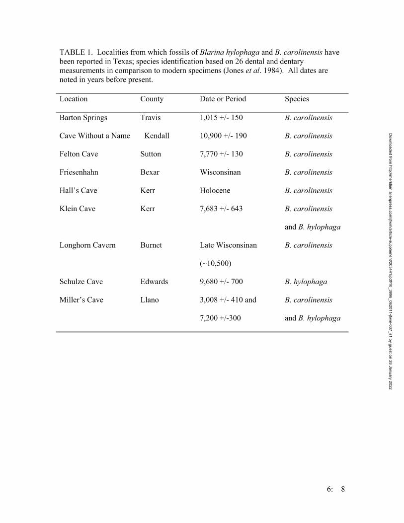
TABLE 1. Localities from which fossils of Blarina hylophaga and B. carolinensis have been reported in Texas; species identification based on 26 dental and dentary measurements in comparison to modern specimens (Jones et al. 1984). All dates are noted in years before present. Location County Date or Period Species

Barton Springs Travis 1,015 +/- 150 B. carolinensis

Cave Without a Name Kendall 10,900 +/- 190 B. carolinensis

Felton Cave Sutton 7,770 +/- 130 B. carolinensis

Friesenhahn Bexar Wisconsinan B. carolinensis

Hall’s Cave Kerr Holocene B. carolinensis

Klein Cave Kerr 7,683 +/- 643 B. carolinensis

and B. hylophaga

Longhorn Cavern Burnet Late Wisconsinan

(~10,500)

B. carolinensis

Schulze Cave Edwards 9,680 +/- 700 B. hylophaga

Miller’s Cave Llano 3,008 +/- 410 and

7,200 +/-300

B. carolinensis

and B. hylophaga

6: 8

Dow



m/article-supplem

ent/203441/pdf/10_3996_062011-jfwm


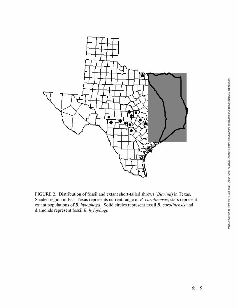
FIGURE 2. Distribution of fossil and extant short-tailed shrews (Blarina) in Texas. Shaded region in East Texas represents current range of B. carolinensis; stars represent extant populations of B. hylophaga. Solid circles represent fossil B. carolinensis and diamonds represent fossil B. hylophaga.

6: 9

Dow



m/article-supplem

ent/203441/pdf/10_3996_062011-jfwm


A technique that offered a potential solution to the shrew identification problem

was karyotyping. Blarina exhibit considerable polymorphism with respect to

chromosome fusions, and evidence for Robertsonian fans has been noted in B.

carolinensis (Qumsiyeh et al. 1999; Qumsiyeh et al. 1997). Fundamental numbers (FN)

for each species are distinct, with the largest variation within B. carolinensis (FN= 44, 45,

or 52); B. hylophaga has a fundamental number of 60 or 61 for the one locality sampled

(George et al. 1982). Another technique useful in identifying morphologically indistinct

organisms is DNA sequencing, which is becoming more readily available. Whereas

karyotyping requires tissue from live specimens, DNA sequencing can be performed on

stored tissue or even museum skins. DNA also provides more information for

phylogenetic analyses as well as population genetics and individual identification,

obviating the need for karyotyping for identification purposes. Studies contrasting

chromosomal and mitochondrial DNA evolution in the Sorex araneus group, which

exhibits considerable intraspecific variation in chromosome arrangements, have shown

that homoplasy in karyologic data can obscure evolutionary relationships (Taberlet et al.

1994).

Taxonomic revisions of the genus Blarina and particularly B. hylophaga, which

was recognized as a species only recently (George et al. 1981), have caused confusion in

the literature over the identity of Texas short-tailed shrews. Studies performed to date on

short-tailed shrews in Bastrop and Aransas counties, Texas, have utilized cranial and

external morphological characters that are ambiguous due to size overlap between B.

hylophaga and B. carolinensis. The study by George et al. (1981) reaffirmed the

6: 10

Dow



m/article-supplem

ent/203441/pdf/10_3996_062011-jfwm


taxonomic status of the Aransas subspecies Blarina hylophaga plumbea, but the tentative

identification of both B. hylophaga and B. carolinensis in Bastrop County by

Baumgardner et al. (1992) cast doubt on the classification of Texas Blarina. It seems that

in this case, additional characters are necessary to support or refute morphological data.

Brant and Ortí (2002) used mitochondrial DNA sequences to resolve evolutionary

relationships among the three species of Blarina. The sequences from their study were

available on the GenBank database, providing baseline Blarina sequences for comparison

of novel Texas Blarina sequences.

Phylogenetic analyses of mitochondrial DNA and quantitative morphological

techniques were chosen to resolve this taxonomic problem. Both Davis (1941) and

Dixon et al. (1989) recognized that the respective isolated populations differed from B.

carolinensis in East Texas. However, the taxonomic status remains unresolved for these

populations. With the availability of museum specimens for morphological analyses and

the recent publication of a molecular phylogeny for Blarina, the data were available to

help resolve questions regarding the two disjunct Texas populations.

The objective of this study was to resolve the systematic status of the two isolated

populations of short-tailed shrew in Texas using morphological and molecular

techniques. Additionally, biogeographical hypotheses were explored in an attempt to

explain the current distribution of short-tailed shrews in Texas.

6: 11

Dow



m/article-supplem

ent/203441/pdf/10_3996_062011-jfwm



SPECIMEN COLLECTION

Specimens were handled according to directives of TSU IACUC permit

#KUMJTX_02.

Trapping for the Bastrop County population occurred in conjunction with

concurrent herpetofaunal survey work on the Griffith League Ranch, which comprises

approximately 5,000 acres, under Texas Parks and Wildlife permit SPR-0102-191 and

U.S. Fish and Wildlife Service permit TE039544-1. Over 100 pitfall traps were placed

along 23 drift fence arrays in grasslands, pine-oak woodlands, and oak-juniper woodlands

and checked daily from 2001 through 2003. Thirteen Y-shaped arrays were created using

three lines of drift fence 50 feet in length radiating from a central point, with 5-gallon

buckets buried at the center and each terminus. Five linear arrays were set in grassland

with buckets every 100 feet; two lines were 400 feet and three lines were 500 feet in

length. One linear array in a pine forest was 100 feet in length with two terminal buckets

and two internal buckets spaced 25 feet apart. Four linear arrays were placed in a

grassland in a rectangular formation, two 100 feet in length with two terminal buckets

and one central bucket, and two 150 feet in length with four evenly spaced buckets. Six

arrays were added in the spring of 2003 that lacked drift fence; each consisted of four

buckets arranged linearly along a 150 foot transect. These traps were checked daily from

June 26 through July 31, 2003. Trapping in Aransas County took place at the Aransas

National Wildlife Refuge (ANWR), comprising approximately 54,000 acres, under

permit number 03-013. Twelve pitfall traps were placed along three 100-foot drift fence

arrays located in or near oak mottes. Four 50-meter lines, each with two terminal pitfall

6: 12

Dow



m/article-supplem

ent/203441/pdf/10_3996_062011-jfwm


traps, in use for an ANWR herpetofauna survey were monitored for shrews ten days of

every month during 2003.

Voucher specimens were taken as necessary, prepared by Richard W. Manning

and deposited at the Texas Tech University collection. Skeletal muscle, organs, and/or

blood were catalogued and stored at –80º C.

Specimens collected and prepared by previous researchers also were utilized in

this analysis. Jim Yantis collected several specimens in Houston and Anderson counties

in east Texas. Texas Cooperative Wildlife Collection (TCWC) housed several specimens

and allowed us access to them (Appendix I), including the removal of skin samples from

museum study skins. Samples from museum skins were taken with utmost care to

preserve the integrity of the skin and to prevent contamination among specimens. Skin

samples were approximately 5 mm2 taken from the area around the incision made during

the preparation of the skin. Scissors were flame-sterilized and gloves were changed

before each skin clip.

MORPHOLOGICAL ANALYSES

External measurements were taken when the condition of the specimen allowed;

these included total length, tail length, hind foot length, and ear length. Cranial

measurements, as established by Choate (1972) included, as seen in Figure 3:

• Occipitopremaxillary length

• Length P4-M3

• Cranial breadth

• Breadth of zygomatic plate

• Maxillary breadth

• Interorbital breadth

6: 13

Dow



m/article-supplem

ent/203441/pdf/10_3996_062011-jfwm


• Length of mandible

• Height of mandible

• Articular breadth

Principal Components Analysis (PCA) (Quinn and Keough 2002) using a covariance

matrix was used to determine whether statistical differences exist between these

populations of Blarina and specimens from other parts of the United States. Multivariate

analysis of variance (MANOVA) (Quinn and Keough 2002) was performed using species

as the independent variable and the nine cranial characters as response variables to

determine if there were differences between species. After performing MANOVA,

individual analysis of variance (ANOVA) tests (Quinn and Keough 2002) were

performed for each cranial measure using the same a priori groups as in the MANOVA.

Because of the increase in Type I error associated with multiple tests, the Bonferroni

procedure was used to adjust the significance level (Quinn and Keough 2002). The

resulting alpha level, adjusted for nine tests, was 0.0055.

S-Plus 6.1TM software was used for all morphological analyses.

6: 14

Dow



m/article-supplem

ent/203441/pdf/10_3996_062011-jfwm


IGURE 3. NINE CRANIAL MEASUREMENTS USED IN THIS STUDY, AS IN CHOATE (1972). OCCIPITO-PREMAXILLARY LENGTH (A), P4-M3 (B), CRANIAL BREADTH (C), BREADTH OF

F

ZYGOMATIC PLATE (D), MAXILLARY BREADTH (E), INTERORBITAL BREADTH (F), LENGTH OFMANDIBLE (G), HEIGHT OF MANDIBLE (H), AND ARTICULAR BREADTH (I).

6: 15

Dow



m/article-supplem

ent/203441/pdf/10_3996_062011-jfwm


DNA SEQUENCING Cytochrome b from the mitochondrial genome was used in all analyses because

baseline data for large-scale sampling of United States Blarina exclusive of Texas were

readily available from GenBank. Although 500 bases from the 16S gene also were

available for Blarina, that gene was excluded from these analyses because of perceived

ambiguities regarding its alignment and phylogenetic analysis (Springer and Douzery

1996). The cytochrome b gene encodes a protein which spans the inner matrix, inner

membrane, and outer intermembrane area in the mitochondrion, and acts as a component

of complex III of the mitochondrial oxidative phosphorylation system (Griffiths 1997;

Irwin et al. 1991). This gene has been widely utilized in systematic studies (e.g. Bradley

and Baker 2001; Johns and Avise 1998; Voelker and Edwards 1998; Yoder et al. 1996).

Although cytochrome b is useful in assessing phylogenies, potential pitfalls include

differential evolutionary pressures based on location in the membrane (Griffiths 1997),

insertions of the gene into the nuclear genome (Mirol et al. 2000; Mundy et al. 2000), and

rate heterogeneity among taxa (Spradling et al. 2001).

The QiagenTM DNeasy kit was used to extract genomic DNA from skeletal

muscle samples. The polymerase chain reaction (PCR) was used to amplify fragments of

the mitochondrial genome. Amplification of the cytochrome b gene was in a 50 µl

reaction using 10 µl Taq buffer (0.3 M TRIS, 0.0175 M MgCl2, and 0.075 M (NH4)2SO4,

pH 8.5), 0.5 µl DMSO, 0.5 µl dNTP’s (2.5 mM dATP, dCTP, dGTP, and dTTP), 0.5 µl

(10 mM) of each primer, 0.25 µl Taq polymerase, and 0.5 µl tDNA. The cytochrome b

gene was sequenced for all samples. The following primers were used in PCR and

sequencing: cytochrome b, L14724: 5’-CGAAGCTTGATAGAAAAACCATCGTTG-3’

and H15915: 5’-AACTGCAGTCATCTCCGGTTTACAAGAC-3’ (Irwin et al. 1991);

6: 16

Dow



m/article-supplem

ent/203441/pdf/10_3996_062011-jfwm


plus an internal sequencing primer, cytbR1: 5’-GCTTCGTTGTTTGGAGGT-3’ (Brant

and Ortí 2002), and novel internal sequencing primers shrewCBF1: 5’-

YTATTTTCTCCAGACTTACTAGGAGACCC-3’ (where Y is C or T), and

shrewCBR3: 5’-CCTCATGGAAGGACATACCCTATAAAGGCAGT-3’. The

GeneAmp ® PCR System 9700 performed denaturation at 94º C for 1 min followed by

35 cycles of 94º C (for 1 min), 50º C (for 30 s), and 72º C (for 1 min), and then a final

extension of 72º C for 5 minutes. Results of PCR were visualized on a 1% agarose gel.

The MarligenTM Rapid PCR Purification System was used for PCR cleanup. Clean PCR

product was cycle sequenced in a 9 µl reaction using 0.5 µl primer, 3 µl Big Dye version

3.0, 2- 4 µl clean PCR product (depending on concentration) and 1.5- 3.5 µl water

(depending on concentration of PCR product). GeneAmp® PCR System 9700 was used

to perform 25 cycles of 96º C for 30 s, 50º C for 1 min, and 60º C for 4 min. Cycle

sequence products were cleaned using 700 µl Sephadex solution (0.0625 g/ml) in a

Centri-sep column (Princeton Separations). The ABI Prism 377 XL DNA sequencer

assayed clean cycle sequence products using a 6% polyacrylamide gel.

Precautions were taken to avoid contamination when extracting, amplifying, and

sequencing DNA from TCWC museum skins. Protocols for ancient DNA extraction

included bleaching all laboratory bench surfaces, flame sterilizing metal utensils, UV

sterilizing consumables such as tubes and micropipettor tips as well as pipettors, and

including a negative control reaction for the extraction and subsequent PCR reactions.

Extraction was performed using standard phenol-chloroform protocols rather than a kit.

Tissue was incubated for 48 hours at 55 ºC after adding 500 µl STE buffer, 25 µl

20%SDS, and 25 µl of 20 mg/ml proteinase K. After two purifications in 500 µl of PCI

6: 17

Dow



m/article-supplem

ent/203441/pdf/10_3996_062011-jfwm


solution (25 phenol: 24 chloroform: 1 isoamyl alcohol) and two purifications in 500 µl

chloroform, tDNA was precipitated in 0.1 volume of 2M NaCl and 2.5 volumes of 99%

ethanol. The tDNA pellet was dried 24 hours later and re-suspended in ddH2O.

Amplification was performed using primers cytbL as the forward primer and shrewCBR3

as the reverse primer for a total of 395 bases. Cycle sequencing was performed as

previously described with ancient DNA protocols enforced.

Sequences were aligned using SequencherTM 4.1. Sequences were compared with

38 previously aligned sequences obtained from GenBank, as published in Brant and Ortí

(2002).

PHYLOGENETIC ANALYSES

Thirty-four Blarina, two Cryptotis parva and two Sorex cinereus cytochrome b

sequences from GenBank (accession numbers AF395449-86) were aligned with 23

Bastrop/Aransas sequences and exported as a NEXUS file to PAUP* 4.0b10 (Swofford

1999). Sorex cinereus and Cryptotis parva were designated as paraphyletic outgroups.

Individuals were coded according to geographic location and GenBank accession number

(Figure 4, Table 2). Morphological characters were excluded from phylogenetic analyses

because of continuous variation in cranial measurements that could not be coded for

analysis in an objective manner; see Poe and Wiens (2000) and Zelditch et al. (2000) for

a full review.

Saturation was estimated by graphing the uncorrected-p distance on the x-axis as

a measure of time since divergence against absolute number of transitions and

6: 18

Dow



m/article-supplem

ent/203441/pdf/10_3996_062011-jfwm


TABLE 2. Collection localities and abbreviations for Blarina specimens from Brant and Ortí (2002). Map codes correspond to locations in Figure 4. Individual abbreviations are noted as used in all phylogenetic analyses. Two-letter abbreviations used for all U.S. states. B.bre= Blarina brevicauda, B.car= Blarina carolinensis, B.hyl= Blarina hylophaga. Species County and State Map Code Individual Number B. BREVICAUDA Lancaster, NB 8 64.B.bre.NB Dixon, NB 9 65.B.bre.NB Valley, NB 1 61.B.bre.NB Wooster, OH 10 69.B.bre.OH Wooster, OH 10 72.B.bre.OH Manitoba, Canada 12 62.B.bre.Manitoba Manitoba, Canada 12 63.B.bre.Manitoba Allamakee, IA 11 66.B.bre.IA Trigg, KY 14 67.B.bre.KY Trigg, KY 14 68.B.bre.KY Grafton, NH 13 70.B.bre.NH Grafton, NH 13 71.B.bre.NH James City, VA 15 73.B.bre.VA James City, VA 15 74.B.bre.VA B. HYLOPHAGA Nuckolls, NB 3 75.B.hyl.NB Nuckolls, NB 3 80.B.hyl.NB Lincoln, NB 2 81.B.hyl.NB Lincoln, NB 2 78.B.hyl.NB Richardson, NB 4 79.B.hyl.NB Richardson, NB 4 76.B.hyl.NB McPherson, KS 5 77.B.hyl.KS Montgomery, KS 6 82.B.hyl.KS B. CAROLINENSIS GA 22 50.B.car.GA GA 22 49.B.car.GA Vernon, LA 18 57.B.car.LA Webster, LA 17 55.B.car.LA Polk, AR 19 59.B.car.AR Polk, AR 19 56.B.car.AR Highlands, FL 20 53.B.car.FL Highlands, FL 20 54.B.car.FL Lancaster, VA 23 51.B.car.VA Lancaster, VA 23 52.B.car.VA Jackson, IL 21 60.B.car.IL Jackson, IL 21 58.B.car.IL

6: 19

Dow



m/article-supplem

ent/203441/pdf/10_3996_062011-jfwm


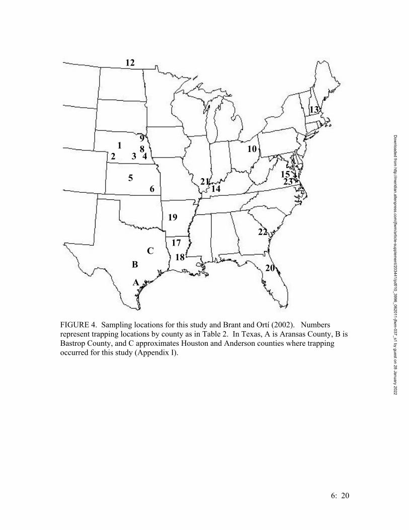
B

A

C

19

56

21

3 489

2114

10

221718

13

2315

12

20

FIGURE 4. Sampling locations for this study and Brant and Ortí (2002). Numbers represent trapping locations by county as in Table 2. In Texas, A is Aransas County, B is Bastrop County, and C approximates Houston and Anderson counties where trapping occurred for this study (Appendix I).

6: 20

Dow



m/article-supplem

ent/203441/pdf/10_3996_062011-jfwm


transversions separately on the y-axis (Griffiths 1997). Saturation curves were created

for the entire gene as well as for each codon position within the intermembrane, matrix,

and transmembrane regions as in Griffiths (1997). Additionally, a partition homogeneity

test with 100 repetitions was conducted to ensure that the three regions were suitable for

uniform analyses. Neighbor joining (NJ) analysis was performed using HKY distances

and bootstrapped using 1,000 pseudoreplicates. Maximum parsimony (MP) analysis was

performed using a heuristic search with tree-bisection reconnection (TBR) branch

swapping; gaps were treated as missing. The dataset was bootstrapped using 1,000

pseudoreplicates each with 5 random addition replicates. Weighted parsimony was

performed similarly, but with transversions (TV) and transitions (TI) weighted based on

estimation of the TI/TV ratio using maximum likelihood and codon positions weighted

based on number of changes at each position. A bootstrap similar to that of MP analysis

was performed on the weighted dataset.

Modeltest 3.06 (Posada and Crandall 1998) was used to determine the nucleotide

substitution model that best fit the data. This model with the parameters given by

Modeltest was used in a maximum likelihood (ML) analysis using a full heuristic search.

Bayesian analyses were performed using MrBayes (v. 3.0, Huelsenbeck and Ronquist

2001) with 1,000,000 generations of four Monte Carlo Markov chains (MCMC) sampled

every 1,000 generations. Only one outgroup is allowed by the software, so Sorex

cinereus AF395485 was specified as the outgroup; however, Cryptotis parva was

retained in the analysis.

6: 21

Dow



m/article-supplem

ent/203441/pdf/10_3996_062011-jfwm


The “Evaluate Random Trees” option in PAUP* (Swofford 1999) was used to

create a frequency distribution of random trees and generate the g1 statistic. This statistic

is a measure of skewness that indicates the amount of phylogenetic signal in a dataset

(Huelsenbeck 1991). A random dataset would have a normal distribution of random trees

and a positive g1 statistic, whereas a dataset with signal will produce a left-skewed

distribution of random trees with a negative value for g1 (Huelsenbeck 1991).

Each novel sequence and the compiled data set was examined thoroughly,

including translation to amino acid sequence and substitution pattern, to ensure the

integrity of subsequent analyses. Likewise such scrutiny ensured that any erroneous

sequence contaminant whether exogenous (PCR contamination) or endogenous (nuclear

introns) was exposed prior to the final analyses.

RESULTS

SPECIMEN COLLECTION

Three fresh specimens were collected from traps placed on the Aransas Wildlife

Refuge (Appendix I). Twenty-seven specimens were collected on Griffith League Ranch

in Bastrop County, and one (MF8057) was collected at Schulz Ranch in southern Bastrop

County (Appendix I). Additional morphological and molecular data were obtained from

preserved specimens at the Texas Cooperative Wildlife Collection (Appendix I).

Morphological Analyses

Most cranial measures were linearly correlated, with Pearson’s correlation

coefficient (r) ranging from 0.29 to 0.84 (Table 3). PCA (n= 52) recovered nine principal

6: 22

Dow



m/article-supplem

ent/203441/pdf/10_3996_062011-jfwm


components, the first of which (PC1) explained 77.7% of the variance and had an

eigenvalue of 0.97. The second component (PC2) was retained for use in the ordinal plot

(Figure 5) but only explained 7.9% of the variation and had an eigenvalue of 0.31. All

cranial characters had positive loadings on PC1, the largest being occipito-premaxillary

length which had a loading of 0.708. Remaining principal components were not included

in further analyses; all had eigenvalues less than 0.25 and explained less than 5% of the

variation. On PC1, B. carolinensis and B. hylophaga were distinguishable with B.

carolinensis having lower scores on that component. Specimens from Texas were

intermediate between the two species on PC1, although there was overlap between two

Bastrop specimens and B. carolinensis.

MANOVA was used to differentiate among three groups: TCWC B. carolinensis

and TCWC 51797 (previously identified as B. carolinensis), B. hylophaga from Kansas,

and Texas Blarina; the Pillai’s trace test statistic was 1.22837 (P<0.001). In univariate

tests of the nine cranial measures, two were non-significant: zygomatic plate breadth (P=

0.792) and interorbital breadth (P= 0.009).

6: 23

Dow



m/article-supplem

ent/203441/pdf/10_3996_062011-jfwm


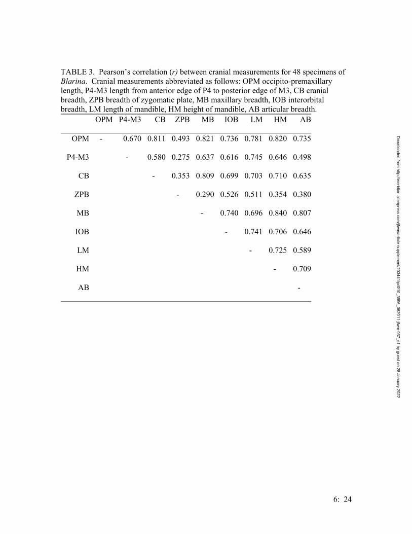
TABLE 3. Pearson’s correlation (r) between cranial measurements for 48 specimens of Blarina. Cranial measurements abbreviated as follows: OPM occipito-premaxillary length, P4-M3 length from anterior edge of P4 to posterior edge of M3, CB cranial breadth, ZPB breadth of zygomatic plate, MB maxillary breadth, IOB interorbital breadth, LM length of mandible, HM height of mandible, AB articular breadth.

OPM P4-M3 CB ZPB MB IOB LM HM AB

OPM - 0.670 0.811 0.493 0.821 0.736 0.781 0.820 0.735

P4-M3 - 0.580 0.275 0.637 0.616 0.745 0.646 0.498

CB - 0.353 0.809 0.699 0.703 0.710 0.635

ZPB - 0.290 0.526 0.511 0.354 0.380

MB - 0.740 0.696 0.840 0.807

IOB - 0.741 0.706 0.646

LM - 0.725 0.589

HM - 0.709

AB -

6: 24

Dow



m/article-supplem

ent/203441/pdf/10_3996_062011-jfwm


PC1

PC2

-0.2 0.0 0.2 0.4

-0.2

0.0

0.2

0.4

1

4

6

7

13

-4 -2 0 2 4

-4-2

02

4

Houston and Anderson counties, TexasBastrop County, Texas

Blarina carolinensis East Texas

Aransas County, TexasBlarina hylophaga from Kansas

FIGURE 5. Ordinal plot of the first two principal components in the analysis of nine cranial measurements for Blarina (n= 52). All nine cranial characters, as used in Choate (1972), were positively correlated with PC1. Symbols differ for geographic regions as indicated in key.

6: 25

Dow



m/article-supplem

ent/203441/pdf/10_3996_062011-jfwm


DNA SEQUENCING

Cytochrome b sequences 1140 nucleotides in length were obtained for three

Blarina specimens from Aransas NWR and 20 specimens from Bastrop County. The

Texas populations do not share any haplotypes with Blarina hylophaga from Kansas and

Nebraska (Brant and Ortí 2002). Four distinct haplotypes were present, one unique to

Aransas NWR (Haplotype A) and three in the Bastrop population (Haplotypes B1, B2,

and B3). Haplotype A was unique to the three Aransas individuals. Haplotype B1 was

the predominant haplotype in Bastrop County (n= 14) and Haplotype B2 was less

common (n= 4). Haplotype B3 was present in only one individual, MF 9158, and

differed from Haplotype B2 by only one nucleotide (see Appendix 2). Non-synonymous

mutations resulted in differing proteins, with changes at amino acid positions 23, 25, 189,

and 327 (Table 4). Amino acid 25 is located in the matrix domain of the cytochrome b

protein, which normally includes mostly polar amino acids; amino acid 189 is located in

the transmembrane domain in Helix D, which usually contains hydrophobic amino acids

(Griffiths 1997). Partial cytochrome b sequence was obtained for the paratype of B.

hylophaga plumbea, TCWC#1542; the first 400 bases of cytochrome b were sequenced

successfully and found to be identical to Haplotype B1.

The sequences obtained are assumed to be mtDNA rather than nuclear

pseudogenes from mtDNA sequence (also known as numts) based on the following

characteristics as outlined by Zhang and Hewitt (1996): 1) PCR amplification

consistently produced only one band, 2) No sequence ambiguities or background bands

persisted, 3) No unexpected insertions, deletions, or stop codons occurred, 4) Nucleotide

6: 26

Dow



m/article-supplem

ent/203441/pdf/10_3996_062011-jfwm


sequences were not radically different from those expected, and 5) Phylogenetic analyses

did not yield an unusual or contradictory tree topology.

Phylogenetic Analyses

The complete alignment consisted of 1140 nucleotides of cytochrome b for 38

taxa from GenBank, three Aransas specimens, and 20 Bastrop specimens. The treelength

distribution for 10,000 randomly generated trees was skewed left (Figure 6) with a g1 of

-0.389, therefore these data are significantly more structured than random data (P<0.01)

(Hillis and Huelsenbeck 1992). There was no significant difference found among the

intermembrane, matrix, and transmembrane regions of the gene in the partition

homogeneity test (P=0.50). Base frequencies were equivalent at first positions (χ2= 1.5,

P>0.5) but did not conform to a 1:1:1:1 ratio for position 2 (χ2 =65.64, P<0.01) or

position 3 (χ2 = 240.6, P<0.01) (Table 5).

Saturation of base substitutions does occur in the cytochrome b data set between

ingroup and outgroup (Figure 7). Saturation curves produced for each codon position

within the three domains of the membrane protein showed that saturation does not occur

at any codon position in any protein region within ingroup taxa, but ingroup-outgroup

saturation is present in third position transitions of all three regions of the protein as well

as first codon position transitions of the transmembrane region (Appendix 3). There is

0.5-0.6% divergence in cytochrome b between the two Texas lineages and 1.2-2.2%

between Texas and other populations of B. hylophaga (Table 6).

6: 27

Dow



m/article-supplem

ent/203441/pdf/10_3996_062011-jfwm


TABLE 4. Amino acids for five haplotypes in two isolated populations of Blarina in Texas compared to GenBank sequences from all three species of Blarina (see Table 2) from Brant and Ortí (2002). Haplotype B1 was the predominant haplotype in samples from Bastrop County (n= 14), with Haplotype B2 (n= 4) less common, and Haplotype B3 found in only one individual. Haplotype A is the only haplotype found in the Aransas County samples. Haplotype S was only present in the individual from southern Bastrop County. A.A. 23 A.A. 25 A.A. 189 A.A. 327

Haplotype B1 Alanine Serine Isoleucine Isoleucine

Haplotypes B2, B3 Alanine Alanine Isoleucine Isoleucine

Haplotype A Alanine Serine Valine Isoleucine

Haplotype S Threonine Serine Isoleucine Valine

BLARINA HYLOPHAGA Alanine Serine Isoleucine Isoleucine

BLARINA CAROLINENSIS Alanine Serine Isoleucine Isoleucine

BLARINA BREVICAUDA Alanine Serine Isoleucine Isoleucine

TABLE 5. Mean base frequencies for all Blarina individuals in this study as well as outgroups for each codon position over the entire cytochrome b gene. A C G T

Codon Position 1 0.26596 0.26096 0.22433 0.24875

Codon Position 2 0.19741 0.23756 0.14467 0.42036

Codon Position 3 0.38871 0.35490 0.04418 0.21221

6: 28

Dow



m/article-supplem

ent/203441/pdf/10_3996_062011-jfwm


TABLE 6. Percent difference between and within species of Blarina, calculated over all 1140 bases of cytochrome b. Blarina carolinensis, B. hylophaga, and B. brevicauda sequences from Brant and Ortí (2002), Texas Blarina sequences from Bastrop and Aransas counties. B. carolinensis B. hylophaga Texas Blarina B. brevicauda B. carolinensis 0.09- 3.9%

B. hylophaga 6.1- 11.1% 0.1- 0.97%

Texas Blarina 5.7- 6.6% 1.2-2.5% 0.1- 0.6%

B. brevicauda 6.5- 8.2% 8.6- 10% 8.3-9.0% 0.1- 2.9%

6: 29

Dow



m/article-supplem

ent/203441/pdf/10_3996_062011-jfwm


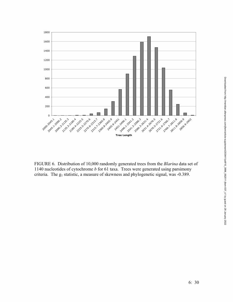
0

200

400

600

800

1000

1200

1400

1600

1800

2000

-204

5.1

2045

.1-2

090.

2

2090

.2-2

135.

3

2135

.3-2

180.

4

2180

.4-2

225.

5

2225

.5-2

270.

6

2270

.6-2

315.

7

2315

.7-2

360.

8

2360

.8-2

405.

9

2405

.9-2

451

2451

-249

6.1

2496

.1-2

541.

2

2541

.2-2

586.

3

2586

.3-2

631.

4

2631

.4-2

676.

5

2676

.5-2

721.

6

2721

.6-2

766.

7

2766

.7-2

811.

8

2811

.8-2

856.

9

2856

.9-2

902

Tree Length

FIGURE 6. Distribution of 10,000 randomly generated trees from the Blarina data set of 1140 nucleotides of cytochrome b for 61 taxa. Trees were generated using parsimony criteria. The g1 statistic, a measure of skewness and phylogenetic signal, was -0.389.

6: 30

Dow



m/article-supplem

ent/203441/pdf/10_3996_062011-jfwm


0

20

40

60

80

100

120

140

160

0 0.02 0.04 0.06 0.08 0.1 0.12 0.14 0.16 0.18 0.2

Uncorrected p Divergence

TransversionsTransitionsTransversions (outgroup)Transitions (outgroup)

FIGURE 7. Saturation curve for the complete cytochrome b gene for the Blarina data set, constructed using uncorrected p distance as a measure of time on the X-axis and absolute number of transitions and transversion on the Y-axis. Transitions and transversions labeled separately for ingroup and outgroup. Saturation does not occur within the ingroup but does occur between ingroup and outgroup transitions.

6: 31

Dow



m/article-supplem

ent/203441/pdf/10_3996_062011-jfwm


Parsimony analyses of the full data set with all characters equally weighted

resulted in 18 equally parsimonious trees with tree length 565, retention index (RI) of

0.941 and consistency index (CI) of 0.724 (Figure 8). Of the molecular characters, 801

were constant and 322 of the variable sites were parsimony informative. The MP

topology supports three monophyletic species of Blarina with B. brevicauda basal within

the genus, and Texas Blarina sister to B. hylophaga. The NJ bootstrap topology agrees

with MP at the interspecific level; the Texas clade is sister to Kansas/Nebraska B.

hylophaga (Figure 9). Weighted parsimony was performed with differential weights for

each codon position based on the number of changes for each position in the unweighted

MP topology (Figure 8): codon position 1= 0.1125, position 2= 1, and position 3= 0.019,

transversions were weighted at 5 times the transversion weight based on the TI/TV ratio

from the ModelTest 3.06 analysis. The resulting topology had a polytomy at the

interspecific level and a sister relationship between Texas Blarina and Kansas/Nebraska

B. hylophaga (Figure 10).

Maximum likelihood analysis was performed using the parameters given by

Modeltest 3.06, which were nucleotide frequencies of A=0.3118, C= 0.2912, T= 0.2779,

and G= 0.1191; TI/TV ratio of 5.2241; proportion of invariable sites equal to zero; and a

gamma distribution parameter of 0.1813, which cumulatively indicated a high number of

practically invariable sites (Nei and Kumar 2000). The resulting topology supported a

monophyletic B. hylophaga within the Texas Blarina, and B. hylophaga basal within the

genus (Figure 11).

The 50% majority-rule consensus tree for Bayesian analysis was calculated using

500 trees (Figure 12), and the resulting topology supported a sister relationship between

6: 32

Dow



m/article-supplem

ent/203441/pdf/10_3996_062011-jfwm


B. brevicauda and B. carolinensis. Also, the Texas clade was sister to B. hylophaga with

97% posterior probability. The proportion of trees supporting a particular clade is

considered to be the Bayesian posterior probability for that clade (Wilcox et al. 2002).

Bayesian support values are considered less conservative than bootstrap and possibly

closer estimates of phylogenetic accuracy, given that the correct model of evolution is in

use (Wilcox et al. 2002).

6: 33

Dow



m/article-supplem

ent/203441/pdf/10_3996_062011-jfwm


MF4745MF4859MF5356MF5376MF6156MF6397MF7497MF7498MF8049MF8054MF8803MF9158MF8050MF8051MF8052MF8053MF8055MF8224MF8802.AMF8231.AMF8801.AMF9157MF805775.B.hyl.NB76.B.hyl.NB78.B.hyl.NB80.B.hyl.NB79.B.hyl.NB77.B.hyl.KS81.B.hyl.NB82.B.hyl.KS55.B.car.LA56.B.car.Ark57.B.car.LA58.B.car.IL59.B.car.Ark60.B.car.IL53.B.car.FL54.B.car.FL49.B.car.GA50.B.car.GA51.B.car.VA52.B.car.VA70.B.bre.NH71.B.bre.NH73.B.bre.VA74.B.bre.VA72.B.bre.OH67.B.bre.KY68.B.bre.KY69.B.bre.OH61.B.bre.NB62.B.bre.Manitoba63.B.bre.Manitoba64.B.bre.NB65.B.bre.NB66.B.bre.IA85.Sorex86.Sorex84.Cryptotis83.Cryptotis

99

58

100

82

62

99

8374

66 87

85

87

99

60

82100

100

100

72

87 96

84 96

10066

52

100

100

FIGURE 8. Bootstrap consensus tree for cytochrome b in three species of Blarina and Texas specimens using unweighted parsimony with bootstrap support values on respective branches. Three species of Blarina abbreviated as in Table 2, MF numbers are assigned to all Bastrop and Aransas county specimens, the latter with an “A” appended. Cryptotis and Sorex were used as outgroups.

6: 34

Dow



m/article-supplem

ent/203441/pdf/10_3996_062011-jfwm


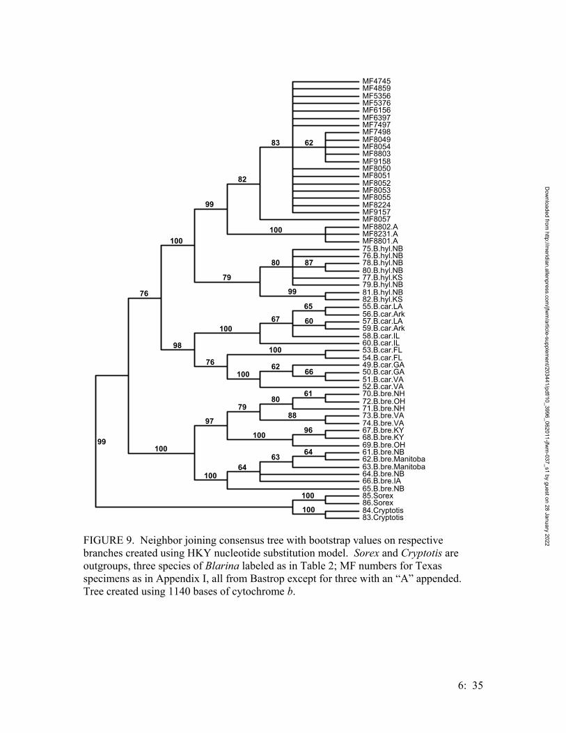
MF4745MF4859MF5356MF5376MF6156MF6397MF7497MF7498MF8049MF8054MF8803MF9158MF8050MF8051MF8052MF8053MF8055MF8224MF9157MF8057MF8802.AMF8231.AMF8801.A75.B.hyl.NB76.B.hyl.NB78.B.hyl.NB80.B.hyl.NB77.B.hyl.KS79.B.hyl.NB81.B.hyl.NB82.B.hyl.KS55.B.car.LA56.B.car.Ark57.B.car.LA59.B.car.Ark58.B.car.IL60.B.car.IL53.B.car.FL54.B.car.FL49.B.car.GA50.B.car.GA51.B.car.VA52.B.car.VA70.B.bre.NH72.B.bre.OH71.B.bre.NH73.B.bre.VA74.B.bre.VA67.B.bre.KY68.B.bre.KY69.B.bre.OH61.B.bre.NB62.B.bre.Manitoba63.B.bre.Manitoba64.B.bre.NB66.B.bre.IA65.B.bre.NB85.Sorex86.Sorex84.Cryptotis83.Cryptotis

99

76

100

99

82

83 62

100

79

80 87

99

98

10067

65

60

76100

10062 66

100

97

7980

61

88

100 96

10064

63 64

100

100

FIGURE 9. Neighbor joining consensus tree with bootstrap values on respective branches created using HKY nucleotide substitution model. Sorex and Cryptotis are outgroups, three species of Blarina labeled as in Table 2; MF numbers for Texas specimens as in Appendix I, all from Bastrop except for three with an “A” appended. Tree created using 1140 bases of cytochrome b.

6: 35

Dow



m/article-supplem

ent/203441/pdf/10_3996_062011-jfwm


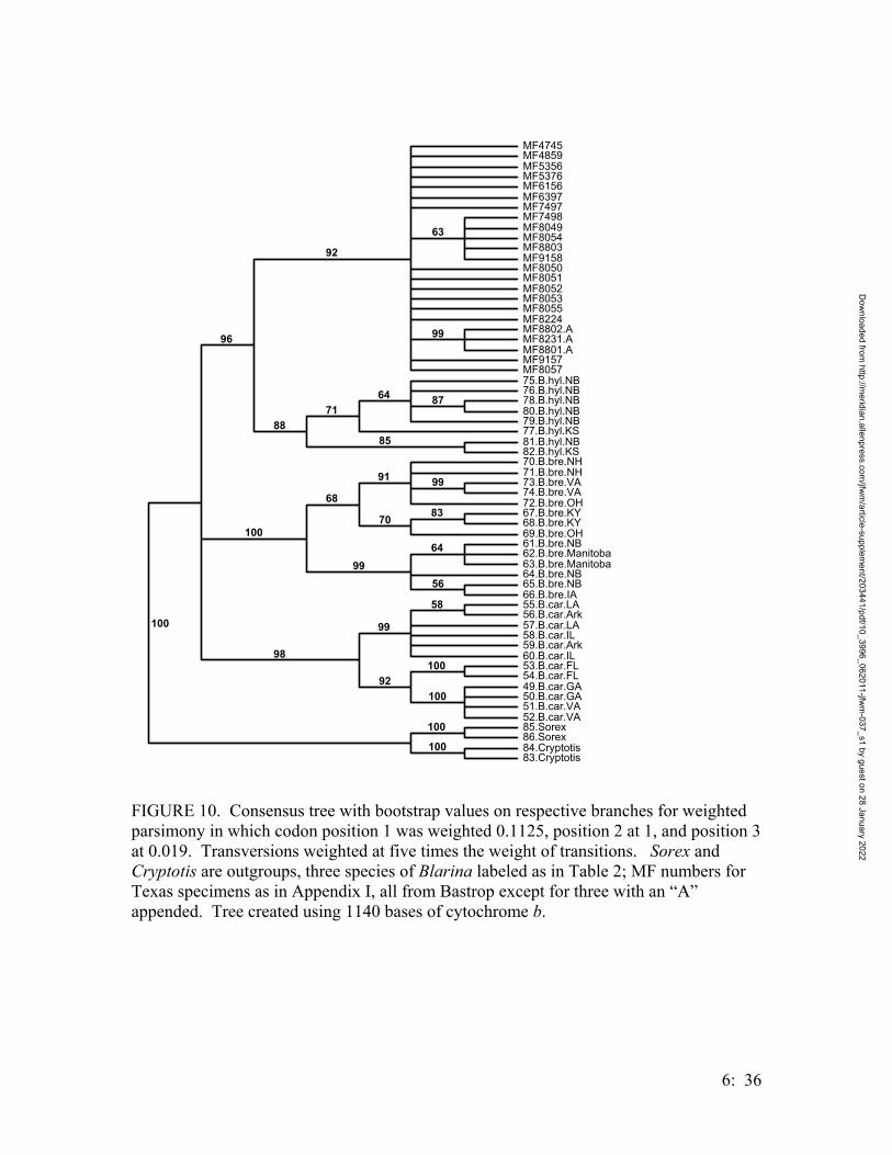
MF4745MF4859MF5356MF5376MF6156MF6397MF7497MF7498MF8049MF8054MF8803MF9158MF8050MF8051MF8052MF8053MF8055MF8224MF8802.AMF8231.AMF8801.AMF9157MF805775.B.hyl.NB76.B.hyl.NB78.B.hyl.NB80.B.hyl.NB79.B.hyl.NB77.B.hyl.KS81.B.hyl.NB82.B.hyl.KS70.B.bre.NH71.B.bre.NH73.B.bre.VA74.B.bre.VA72.B.bre.OH67.B.bre.KY68.B.bre.KY69.B.bre.OH61.B.bre.NB62.B.bre.Manitoba63.B.bre.Manitoba64.B.bre.NB65.B.bre.NB66.B.bre.IA55.B.car.LA56.B.car.Ark57.B.car.LA58.B.car.IL59.B.car.Ark60.B.car.IL53.B.car.FL54.B.car.FL49.B.car.GA50.B.car.GA51.B.car.VA52.B.car.VA85.Sorex86.Sorex84.Cryptotis83.Cryptotis

100

96

92

63

99

8871

64 87

85

100

68

91 99

70 83

9964

56

98

99

58

92100

100

100

100

FIGURE 10. Consensus tree with bootstrap values on respective branches for weighted parsimony in which codon position 1 was weighted 0.1125, position 2 at 1, and position 3 at 0.019. Transversions weighted at five times the weight of transitions. Sorex and Cryptotis are outgroups, three species of Blarina labeled as in Table 2; MF numbers for Texas specimens as in Appendix I, all from Bastrop except for three with an “A” appended. Tree created using 1140 bases of cytochrome b.

6: 36

Dow



m/article-supplem

ent/203441/pdf/10_3996_062011-jfwm


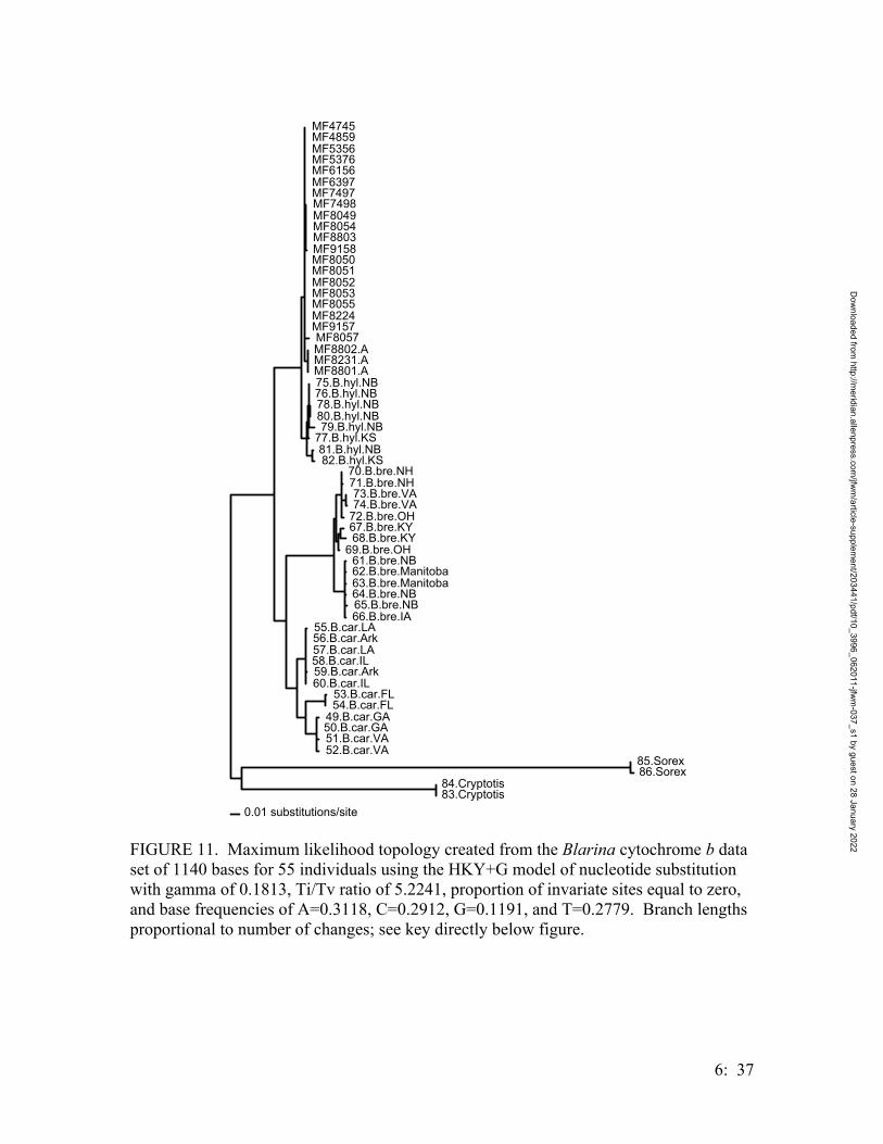
MF4745MF4859MF5356MF5376MF6156MF6397MF7497MF7498MF8049MF8054MF8803MF9158MF8050MF8051MF8052MF8053MF8055MF8224MF9157MF8057MF8802.AMF8231.AMF8801.A75.B.hyl.NB76.B.hyl.NB78.B.hyl.NB80.B.hyl.NB79.B.hyl.NB

77.B.hyl.KS81.B.hyl.NB82.B.hyl.KS

70.B.bre.NH71.B.bre.NH73.B.bre.VA74.B.bre.VA

72.B.bre.OH67.B.bre.KY68.B.bre.KY

69.B.bre.OH61.B.bre.NB62.B.bre.Manitoba63.B.bre.Manitoba64.B.bre.NB65.B.bre.NB66.B.bre.IA

55.B.car.LA56.B.car.Ark57.B.car.LA58.B.car.IL59.B.car.Ark60.B.car.IL

53.B.car.FL54.B.car.FL

49.B.car.GA50.B.car.GA51.B.car.VA52.B.car.VA

85.Sorex86.Sorex

84.Cryptotis83.Cryptotis

0.01 substitutions/site

FIGURE 11. Maximum likelihood topology created from the Blarina cytochrome b data set of 1140 bases for 55 individuals using the HKY+G model of nucleotide substitution with gamma of 0.1813, Ti/Tv ratio of 5.2241, proportion of invariate sites equal to zero, and base frequencies of A=0.3118, C=0.2912, G=0.1191, and T=0.2779. Branch lengths proportional to number of changes; see key directly below figure.

6: 37

Dow



m/article-supplem

ent/203441/pdf/10_3996_062011-jfwm


MF4745MF4859MF5356MF5376MF6156MF6397MF7497MF7498MF8049MF8054MF8803MF9158MF8050MF8051MF8052MF8053MF8055MF8224MF8802.AMF8231.AMF8801.AMF9157MF805775.B.hyl.NB76.B.hyl.NB78.B.hyl.NB80.B.hyl.NB79.B.hyl.NB77.B.hyl.KS81.B.hyl.NB82.B.hyl.KS70.B.bre.NH71.B.bre.NH73.B.bre.VA74.B.bre.VA72.B.bre.OH67.B.bre.KY68.B.bre.KY69.B.bre.OH61.B.bre.NB62.B.bre.Manitoba63.B.bre.Manitoba64.B.bre.NB65.B.bre.NB66.B.bre.IA55.B.car.LA56.B.car.Ark57.B.car.LA58.B.car.IL59.B.car.Ark60.B.car.IL53.B.car.FL54.B.car.FL49.B.car.GA50.B.car.GA51.B.car.VA52.B.car.VA85.Sorex86.Sorex84.Cryptotis83.Cryptotis

88

97

73

100

100

9970

88 100

100

74

100

78

100 100

89 100

10089

80

96

100

96

96100

100

100

100

FIGURE 12. 50% Majority-rule consensus tree from 500 trees produced after 1,000,000 generations of four Monte Carlo Markov Chains in MrBayes v.3.0. Bayesian posterior probabilities are noted on respective branches. Sorex and Cryptotis are outgroups; abbreviations for individuals follows Table 2 except for Texas specimens designated by MF numbers, Aransas specimens with an “A” appended.

6: 38

Dow



m/article-supplem

ent/203441/pdf/10_3996_062011-jfwm


DISCUSSION

MORPHOLOGY

Analyses performed here support the two Texas populations being intermediate in

size between B. hylophaga and B. carolinensis. Because all of the cranial measures were

positively correlated, PC1 can be considered a size component in the PCA (Flessa and

Bray 1977; Rohlf and Bookstein 1987), and PC 2 and subsequent principal components

can be considered size-free shape components (Humphries et al. 1981). Thus, these

shrews vary in size with B. carolinensis being the smallest, Texas B. hylophaga

intermediate and B. hylophaga the largest of the groups in the analysis. The shape

component PC2 accounts for little variation (7.9%) in cranial morphology and the three

groups in this comparison have considerable overlap on that axis (Figure 5). This is

congruent with previous studies using PCA to differentiate species of Blarina (Genoways

and Choate 1972).

One individual short-tailed shrew (TCWC# 51209) captured in Bastrop County

previously had been identified as B. carolinensis, and indeed fit with that species in the

morphological analyses. However, as previously mentioned, the characters used to

identify these shrews are purely size-based, and this individual most likely was a young

adult based on degree of ankylosis and lack of tooth wear. This example illustrates the

pitfalls of using size-based characters to identify animals; individuals that are not fully

grown will be classified as the smaller of the species. Another example can be found in

the East Texas specimens from Houston and Anderson counties, one of which fits in with

the Texas B. hylophaga on the ordinal plot (Figure 5). Although B. hylophaga has not

6: 39

Dow



m/article-supplem

ent/203441/pdf/10_3996_062011-jfwm


previously been reported from these counties, it is difficult to say if these specimens are

unusually large B. carolinensis or an additional population of B. hylophaga.

Clinal variation in size has been documented in previous studies of Blarina (e.g.

George et al. 1981; Jones and Findley 1954), and the Texas shrews being smaller than

northern populations of B. hylophaga supports those studies. This clinal variation

correlates with Bergmann’s Rule, which states that within a taxon, animals at higher

latitudes are larger than those closer to the equator (Brown and Lomolino 1998).

However, factors other than latitude also affect body size. Because the Blarina in Central

Texas inhabit an island-like fragment of pine forest and the coastal population is equally

insular by analogy, it is possible that their body sizes have changed due to differences in

predators, competitors, or other niche factors from the main population. Vertebrate

species that colonize islands often exhibit size differences from their mainland ancestors

(Case 1978). There is no consistent trend for insectivores to be larger or smaller on

islands (Lomolino 1985), so there is no prediction for these shrews to be larger or smaller

than the analogous “mainland” shrew population means.

Because morphological differences among species of Blarina are primarily size-

based, however, island effects should be a consideration when observing trends in body

size. Additionally, as there is no size-free shape component to differentiate between

species of Blarina, morphology is not useful to identify shrews in geographically isolated

populations. For example, one key to the identification of soricids differentiates between

B. hylophaga and B. carolinensis based on size, stating that animals less than 100

millimeters (mm) in total length, with condylobasal length of less than 20 mm and

weighing less than 10 grams are B. carolinensis (Choate et al. 1994). Few of the Texas

6: 40

Dow



m/article-supplem

ent/203441/pdf/10_3996_062011-jfwm


B. hylophaga would be correctly identified using this key, as they are small enough to be

incorrectly identified as B. carolinensis.

MOLECULAR PHYLOGENETICS

The use of mitochondrial DNA in phylogenetic studies is widespread and, despite

controversy, been well established as an effective tool to examine evolutionary histories

of taxa. Because the mitochondrial genome is uniparentally inherited and haploid, its

effective population size (Ne) is 1/4 that of nuclear markers (Moore 1995). While this

may enable early detection of speciation, ancestral polymorphisms in incipient species

may result in misleading patterns in gene trees (Neigel and Avise 1986). Conversely,

speciation may be detected early based on phenotypic differences between incipient

species in which mtDNA divergence cannot be detected (Nice and Shapiro 1999). It is

essential to be aware of these possibilities and to be cautious when making conclusions

based primarily on mtDNA.

Cytochrome b frequently is used in studies of molecular phylogenetics of animals

(Adachi and Hasegawa 1996). Evolutionary pressures differ within this gene by

membrane region, codon position, and amino acid. Based on the saturation curves

produced for the codon positions within each transmembrane region (Appendix 3), down-

weighting third positions throughout the gene will result in a loss of significant amounts

of unsaturated positions that could otherwise be informative. Hence, weighted parsimony

may result in a loss of phylogenetic signal in this gene. Additionally, when creating

saturation curves it is essential to consider saturation within the ingroup and between the

ingroup and outgroup separately.

6: 41

Dow



m/article-supplem

ent/203441/pdf/10_3996_062011-jfwm


DNA was successfully extracted and sequenced from two museum skins, one of

which was the paratype for the subspecies B. hylophaga plumbea. This individual was

collected at the Aransas NWR in 1941 by Davis (1941). The 400 bases of cytochrome b

sequenced for this individual are identical to Haplotype B1, the predominant haplotype in

Bastrop County. Phylogenetic analyses using cytochrome b unambiguously place the

paratype of Blarina hylophaga plumbea in the B. hylophaga clade. These analyses

should allay any doubts regarding the phylogenetic placement of this isolated population.

The Texas populations of short-tailed shrews form a monophyletic sister group to

other U.S. populations of Blarina hylophaga; within Texas, Bastrop and Aransas harbor

unique clades. Many of the molecular analyses were in agreement in the placement of

the Texas clade as a sister group to B. hylophaga. Maximum likelihood supported an

alternate hypothesis of a sister relationship between Aransas and the Kansas/Nebraska B.

hylophaga, with the remainder of Texas Blarina sister to that group; this topology is

probably an artifact of anomalies in the Kansas/Nebraska GenBank sequences, and is in

fact unsupported by any synapomorphies. This can be assessed by observing the length

of the terminal branches of B. hylophaga in comparison to B. carolinensis. There was no

overlap in haplotypes between Texas and Kansas/Nebraska B. hylophaga. Because

sampling was limited at Aransas NWR, it is possible that other haplotypes are present in

the population but were not found in this study.

Results differed among analyses with respect to the relationships of the three

species of Blarina. Previous morphological studies have supported the (B. brevicauda

(B. carolinensis, B. hylophaga)) topology (Jones et al. 1984; Stangl and Carr 1997), but

the recent molecular phylogeny by Brant and Ortí (2002) supports a (B. hylophaga (B.

6: 42

Dow



m/article-supplem

ent/203441/pdf/10_3996_062011-jfwm


brevicauda, B. carolinensis)) topology. In this study, the former relationship was

supported in neighbor joining and parsimony analysis, and the latter in Bayesian and ML

analyses. Weighted parsimony did not resolve the interspecific relationship. Support for

either of the resolved relationships was generally low and consisted of synonymous third

and first codon position changes, many of which had low CI values for the topology in

question, indicating homoplasy. Other genes may be successful in recovering any

interspecific structure, or morphology can be used as additional evidence to confirm B.

brevicauda as a basal species within Blarina.

BIOGEOGRAPHY AND AREAS OF ENDEMISM

These shrews may represent relictual isolates of B. hylophaga’s Pleistocene range

in Texas. Aransas and Bastrop counties do not have similar floras, but must share some

characteristics that make them hospitable to short-tailed shrews. Similarities between

Aransas and Bastrop counties that could make both suitable as shrew habitat include deep

sandy soils, ancient trees, deep leaf litter, abundance of prey, and suitable thermal

climate. While other areas of sandy soil exist in Texas, such as the coastal sand plain in

South Texas, lack of leaf litter or other factors may prohibit shrews from inhabiting the

area. It also is possible that Blarina do not occupy all suitable habitats in Texas, and

other circumstances have narrowed their distribution. Examining patterns of distribution

in other species may aid in understanding the pattern of short-tailed shrew distributions in

Texas.

6: 43

Dow



m/article-supplem

ent/203441/pdf/10_3996_062011-jfwm


Many small mammals inhabited Texas in the Pleistocene and may aid in

understanding the pattern of distribution in Blarina hylophaga in Texas. Other small

mammals with ranges extending southward from the midwest include the thirteen-lined

ground squirrel (Spermophilus tridecemlineatus) and the woodland vole (Microtus

pinetorum), both of which were reported at Aransas NWR by Davis (1941). Small

mammals having Pleistocene-era fossils in Texas whose current ranges no longer include

Texas or include only relictual populations include two additional species of vole

(Microtus pennsylvanicus and M. ochrogaster), the southern bog lemming Synaptomys

cooperi, the ermine Mustela erminea, and the cinereus shrew Sorex cinereus (Lundelius

1967). The common pattern among these animals is a northward-shifting range, probably

a consequence of warming temperatures over time. Some of these taxa, such as

Microtus, may be more tolerant of warm weather and therefore able to maintain isolated

populations in Texas, especially in favorable habitats.

The Lost Pines area in Central Texas is an area characterized by stands of loblolly

pine (Pinus taeda) on sandy soils. This area is superficially similar to the Piney Woods

of East Texas, also an area containing loblolly pines on sandy soils. The Lost Pines hosts

the westernmost distribution of these pines in Texas, as well as the fauna associated with

them. Animals such as flying squirrels (Glaucomys volans), pileated woodpecker

(Dryocopus pileatus), and pine warbler (Dendroica pinus) have presumably disjunct

populations in the Lost Pines. The endangered Houston toad (Bufo houstonensis) now is

effectively restricted to the Lost Pines, although its distribution once included a much

larger area. An endemic insect, the Texas long-lipped beetle (Telegeusis texensis),

6: 44

Dow



m/article-supplem

ent/203441/pdf/10_3996_062011-jfwm


recently was described from specimens collected in the Lost Pines (Taber and Fleenor

2003).

These animals inhabit a unique ecosystem that may be a relictual isolate or an

outpost of pines created by dispersal. Fossil pollen evidence confirms that Bastrop

County was the westernmost limit of the range of pine forests in Texas in late glacial and

postglacial times (Larson et al. 1972), and that pines have been present for nearly 20,000

years (Bryant 1977). This evidence strongly suggests that the Lost Pines region is a

remnant of a more widespread pine forest.

Aransas National Wildlife Refuge also harbors unique fauna; it is most well

known as the wintering grounds for the endangered whooping crane (Grus americana).

The rare Texas scarlet snake, Cemophora lineri, also has been found on the refuge. Both

the Lost Pines and Aransas NWR may represent areas of local endemism for many taxa.

Both areas have been scrutinized as endangered species habitat, but also should be

examined at the ecosystem level because of their unique nature.

TAXONOMY

While the debate over species concepts continues, some model must be applied in

order to define species taxonomically. Often a combinatorial approach is necessary,

using several data types to confirm the status of a taxon; for example, Wiens and Penkrot

(2002) proposed an approach using DNA and morphological data to delimit species. In

the case of these isolated populations of Blarina, however, morphological characters can

be nebulous or even misleading. Characters such as nuclear DNA or a karyotype may be

useful to support mtDNA phylogenies in this case. In an instance involving isolated

6: 45

Dow



m/article-supplem

ent/203441/pdf/10_3996_062011-jfwm


populations of pocket gophers which only had mtDNA evidence available, a “molecular-

phenetics species concept” was implemented, using known differences of closely related

taxa to create a standard to identify potential species-level differences (Demastes et al.

2002). This model is similar to the “cytochrome-b species concept” (Bradley and Baker

2001), but with the caveat that other types of evidence should be applied as well.

The Biological Species Concept (BSC) (Mayr 1942), Genealogical Species

Concept (GSC) (Mishler and Donoghue 1982), and Phylogenetic Species Concept (PSC)

(Cracraft 1983; Nelson and Platnick 1981) have been discussed philosophically to a

tremendous extent. It is difficult to decide which concept is appropriate to apply, so it is

necessary to consider the applicability of each concept to this research, which involves

two allopatric populations of morphologically indistinguishable animals with differences

in molecular traits.

The BSC defines species as “groups of interbreeding natural populations that are

reproductively isolated from other such groups” (Mayr 1969). Observations of

interbreeding are difficult to obtain for many if not most species, and for allopatric

populations these observations could only take place in captive organisms. For Texas

Blarina, it is unknown whether breeding with Oklahoma, Kansas, or Nebraska Blarina

would be successful; therefore, no evidence is available to support or refute classification

of Texas Blarina under this concept.

Employment of the phenetic measure of percent divergence as a criterion to

define species may be misleading when considering the differential rate of evolution

among taxa (Spradling et al. 2001) that may be affected by body size, thermal habit, and

metabolic rate (Martin and Palumbi 1993; Rand 1994). Oxygen radicals cause damage to

6: 46

Dow



m/article-supplem

ent/203441/pdf/10_3996_062011-jfwm


mtDNA, increasing rate of evolution in the mitochondrial genome (Richter et al. 1988);

shrews exhibit extremely high oxygen consumption per gram body mass, Blarina

brevicauda basal metabolic rates being over 150% of the expected value (Churchfield

1990). Therefore intra- and inter-species sequence divergences cannot be standardized

among taxa; however, it remains reasonable to use a within-taxon standard to gauge

differences in that taxon. Both B. carolinensis and B. brevicauda have intraspecific

divisions that are attributable to the Mississippi River; distances between those east-west

clades average 3.3% and 2.5%, respectively (Table 6). The genetic distance between

Texas B. hylophaga and the northern population of that species ranges from 1.2-2.2%,

and the genetic distance between the Aransas and Bastrop populations is 0.5%. This

evidence along with the monophyly of this group is sufficient evidence to classify the

Texas B. hylophaga as a subspecies, Blarina hylophaga plumbea (Davis 1941) under the

GSC.

The PSC defines species as “the smallest aggregation of … populations…

diagnosable by a unique combination of character states” (Wheeler and Platnick 2000).

Under the strictest interpretation of this concept, every haplotype in this study would

constitute a separate species; there is no room for intraspecific classification under the

PSC. Certainly both Aransas and Bastrop populations would warrant species status, since

each population does have a unique combination of character states. Widespread use of

the PSC by taxonomists would undoubtedly lead to significant increase in the number of

recognized species, if only by elevating subspecies to species.

The designation of subspecies is a taxonomic tradition that has been brought into

question under several species concepts. A subspecies can be defined as “a recognizably

6: 47

Dow



m/article-supplem

ent/203441/pdf/10_3996_062011-jfwm


different population…that occupies a different geographic area from other populations of

the same species” (Futuyma 1998); however, problems arise when attempting to

differentiate between a subspecies and a population, which is “a group of conspecific

organisms that occupy a…well defined geographic region and exhibit reproductive

continuity from generation to generation” (Futuyma 1998). Many subspecies are

recognized as morphologically different ecotypes; this use is perpetuated in field guides.

It has been noted that recognition of a subspecies requires as much evidence as for a

species, with the additional assumptions that the lineage may reconnect and interbreed

with the main lineage; although it is convenient to designate subspecies in collections and

field guides, it is difficult to justify a subspecies concept (Frost et al. 1992). One potential

utility of subspecies lies in conservation of locally endemic subspecies which may be

protected under the Endangered Species Act; such geographic variants of a species are

important components of biodiversity (O'Brien and Mayr 1991). From the perspective of

traditional recognition of subspecies as geographic variants or “a genetically distinct set

of populations with a discrete range” (Brown and Lomolino 1998), the short-tailed

shrews in Aransas and Bastrop counties can be recognized as a subspecies.

The two isolated populations of Blarina in Texas certainly warrant subspecies

recognition, and possibly species recognition under strict interpretation of the PSC

(Cracraft 1983). The Texas populations appear to be monophyletic (sensu Hennig 1966)

in that they are more closely related to each other than to other lineages and they appear

to have descended from a common ancestor. Therefore, based on geographic isolation

and genetic similarity, it is justifiable to separate them into a single Texas endemic

subspecies: Blarina hylophaga plumbea.

6: 48

Dow



m/article-supplem

ent/203441/pdf/10_3996_062011-jfwm


Parallels can be drawn between the Texas and Florida subspecies of short-tailed

shrews. Two subspecies inhabit Florida: Blarina carolinensis peninsulae and B.

carolinensis shermani. Despite several concerted efforts, the latter has not been captured

at the type locality in Ft. Myers since the initial type series was collected in 1955 (Layne

1992). Specimens collected in the 1980s are smaller than those in the series collected by

Hamilton (1955), and are postulated intergrades between B. c. shermani and B. c.

peninsulae. Again, because size-based morphological characters are the basis of

classification for these subspecies, clinal variation in size as well as other factors make it

difficult to determine if this subspecies is a relictual isolate of B. brevicauda or a

population of large B. carolinensis. Additionally, because material available for B. c.

shermani is limited to museum specimens, karyotyping is not possible and DNA analyses

have not yet been attempted. This subspecies was extirpated before it could be described;

whether it was a relictual isolate of B. brevicauda or a unique population of B.

carolinensis may be determined using DNA, but the opportunity to conserve this unique

population was lost.

The description of the endemic Texas subspecies Blarina hylophaga plumbea

should be followed with population estimates and characterization of the ecology of these

populations. The isolated populations in Aransas and Bastrop counties, Texas, should be

monitored so that they do not meet the same fate as B. c. shermani.

6: 49

Dow



m/article-supplem

ent/203441/pdf/10_3996_062011-jfwm


LITERATURE CITED

ADACHI, J., AND M. HASEGAWA. 1996. MOLPHY Version 2.3: Programs for Molecular

Phylogenetics Based on Maximum Likelihood.

AGEE, J. K., S. C. F. STITT, M. NYQUIST, AND R. ROOT. 1989. A geographic analysis of

historical grizzly bear sightings in the North Cascades. Photogrammetric Engineering and

Remote Sensing 55:1637-1642.

AHLBRANDT, L., K. JONES AND M.R.J. FORSTNER. 2002. Geographic distribution.

Crotalus horridus (Timber Rattlesnake). Herpetological Review. 33(3):227.

ALLEN, A. W., Y. K. BERNAL, AND R. J. MOULTON. 1996. Pine plantations and wildlife in

the southeastern United States: and assessment of impacts and opportunities. U. S. Department of

the Interior, National Biological Service Information and Technology Report 3.

ANDERSON, J. D., D. D. HASSINGER, AND G. H. DALRYMBLE. 1971. Natural mortality of

eggs and larvae of Ambystoma t. tigrinum. Ecology 52:1107-1112.

ARNASON, A. N., C. J. SCHWARZ, AND G. BOYER. 1998. POPAN-5: A data maintenance

and analysis system for mark-recapture data. Department of Computer Science, University of

Manitoba, Winnipeg, 265 pp.

BAKER, F. E. 1979. Soil survey of Bastrop County, Texas. U. S. Department of Agriculture,

Soil Conservation Service. Washington, D. C.

BANKS, RICHARD C., CARLA CICERO, JON L. DUNN, ANDREW W. KRATTER,

PAMELA C. RASMUSSEN, J. V. REMSEN, JR., JAMES D. RISING, AND DOUGLAS F.

STOTZ. 2003. Forty-fourth supplement to the American Ornithologists’ Union Check-list of

North American Birds. Auk 120(3):923-931.

BARINAGA, M. 1990. Where Have All the Froggies Gone? Science 247:1033-1034.

BASTROP COUNTY, Deed Record E. 1846. Bastrop County Deed Records, Vol. E. Bastrop

County, Texas.

BAUMGARDNER, G. D., N. O. DRONEN, AND D. J. SCHMIDLY. 1992. Distributional status

of short-tailed shrews (genus Blarina) in Texas. Southwestern Naturalist 37:326-328.

BEATTIE, M. H. 1994. Endangered and Threatened Wildlife and Plants; Animal Candidate

Review for Listing as Endangered or Threatened Speciesin Federal Register 59 (November 15,

1994): 58982. Environmental Protection Agency.

7: 1

Dow



m/article-supplem

ent/203441/pdf/10_3996_062011-jfwm


BEIER, P. AND S. LOE. 1992. A Checklist for Evaluating Impacts to Wildlife Movement

BEIER, P., AND R. F. NOSS. 1998. Do habitat corridors really provide connectivity?

Conservation Biology 12:1241-1252.

BERTIN R. I. 1977. Breeding habits of the Wood Thrush and Veery. Condor 79:303-311.

BERVEN, K. A., AND B. G. CHADRA. 1988. The relationship among egg size, density, and

food level on larval

development in the wood frog (Rana sylvatica). Oecologia 75:67-72.

BERVEN, K. A., AND T. A. GRUDZIEN. 1990. Dispersal in the wood frog (Rana sylvatica):

implications for genetic population structure. Evolution 44:2047-2256.

BEST L. B. AND K. L. PETERSEN. 1985. Seasonal changes in detectability of sage and

Brewer’s sparrow. Condor 87:556-558.

BEST, L. B. 1981. Seasonal changes in detection of individual bird species. Studies in Avian

Biology 6:252-261.

BIDWELL, T. G., S. D. SHALAWAY, O. E. MAUGHAN, AND L. G. TALENT. 1989. Habitat

use by female eastern wild turkeys in southeastern Oklahoma. Journal of Wildlife Management

53:34-39.

BLAIR, R. M., AND D. P. FEDDUCCIA. 1977. Midstory hardwoods inhibit deer forage in

loblolly pine plantations. Journal of Wildlife Management 41:677-684.

BLAIR, R. M., H. L. SHORT, AND E. A. EPPS, JR. 1977. Seasonal nutrient yield and

digestibility of deer forage from a young pine plantation. Journal of Wildlife Management

41:667-676.

BLAIR, W. F. 1961. Calling and spawning seasons in a mixed population of anurans. Ecology

42:99-110.

BLAIR, W. F. 1972. Evolution of the Genus Bufo. University of Texas

BLAIR, W. F. 1972. Bufo of North and Central America. Pages 93-101 in Evolution in the

Genus Bufo (W. F. Blair, ed.) University of Texas Press, Austin.

BLAUSTEIN, A. R., AND D. B. WAKE. 1990. Declining amphibian populations - a global

phenomenon. Trends in Ecology & Evolution 5:203-204.

BOARD OF LAND COMMISSIONERS, Republic of Texas. 1838. Certificate No. 37,

certificate with survey field notes (Abstract Number 224, Bastrop County, Texas.) Bastrop,

Texas.

7: 2

Dow



m/article-supplem

ent/203441/pdf/10_3996_062011-jfwm


BOONE, M. D., C. M. BRIDGES, AND B. B. ROTHERMEL. 2001. Growth and development

of larval green frogs (Rana clamitans) exposed to multiple doses of an insecticide. Oecologia

129:518-524.

BOULINIER, THIERRY, JAMES D. NICHOLS, JAMES E. HINES, JOHN R. SAUER,

CURTIS H. FLATHER, AND KENNETH H POLLOCK. 2001. Higher temporal variability of

forest breeding bird communities in fragmented landscapes. Proceedings of the National

Academy of Sciences (USA) 95 (13) 7497-7501.

BRADLEY, R. D., AND R. J. BAKER. 2001. A test of the genetic species concept: cytochrome

b sequences and

mammals. Journal of Mammalogy 82:960-973.

BRAGG, A. N. 1960. Feeding in the Houston toad. Southwestern Naturalist 5:106.

BRANT, S. V., AND G. ORTÍ. 2002. Molecular phylogeny of short-tailed shrews, Blarina

(Insectivora: Soricidae).

Molecular Phylogenetics and Evolution 22:163-173.

BRANT, S. V., AND G. ORTÍ. 2003. Phylogeography of the Northern short-tailed shrew,

Blarina brevicauda

(Insectivora: Soricidae): past fragmentation and postglacial recolonization. Molecular Ecology

12:1435-1449.

BRECKENRIDGE, W. J., AND J. R. TESTER. 1961. Growth, local movements, and

hibernation of the Manitoba toad, Bufo hemiophrys. Ecology 42:637-646.

BREDEN, F. 1987. The effect of post-metamorphic dispersal on the population genetic structure

of Fowler's toad, Bufo woodhousii fowleri. Copeia 1987:386-395.

BROOKS, MARSHALL A., BRENNA C. HARRIGAN, KAREN M. JOHNSON, DAVID E.

LOWE, JUSTEN P. LOWERY, JOEL W. MCGLOTHLIN, MICHELLE M. SASSO, SARAH

A. SMITH, AND DANIEL A. CRISTOL. 2001. Revisit schedule does not affect result of point

counts. Journal of Field Ornithology 72(3):404-411.

BROWN, J. H., AND M. V. LOMOLINO. 1998. Biogeography, Second ed. Sinauer Associates,

Inc., Sunderland, Mass.

BROWN, L. E. 1971. Natural hybridization and reproductive ecology of two toad species in a

disturbed environment. American Midland Naturalist 86:78-85.

7: 3

Dow



m/article-supplem

ent/203441/pdf/10_3996_062011-jfwm


BROWN, L. E. 1975. The status of the near-extinct Houston toad (Bufo houstonensis) with

recommendations for its conservation. Herpetological Review 6:37-40.

BROWN, L. E., AND R. A. THOMAS. 1982. Misconceptions about the endangered Houston

toad (Bufo houstonensis). Herpetological Review 13(2):37.

BRYANT V. M. JR. 1977. A 16,000 year old pollen record of vegetational change in central

Texas. Palynology I:43-156.

BUCKLAND, S. T., D. R. ANDERSON, K. P. BURNHAM, J. L. LAAKE, D. L. BORCHERS,

AND L. THOMAS. 2001. Introduction to distance sampling. Oxford University Press, New

York, New York.

BURKE, V. J. AND J. W. GIBBONS. 1995. Terrestrial buffer zones and wetland conservation:

A case study of

freshwater turtles in a Carolina Bay. Conservation Biology 9:1365-1369.

CAMPO, J. J., W. G. SWANK, AND C. R. HOPKINS. 1989. Brood habitat use by eastern wild

turkeys in eastern

Texas. Journal of Wildlife Management 53:479-482.

CASE, T. J. 1978. A general explanation for insular body size trends in terrestrial vertebrates.

Ecology 59:1-18.

CHOATE, J. R. 1972. Variation within and among populations of the short-tailed shrew in

Conneticut. Journal of

Mammalogy 53:116-128.

CHOATE, J. R., J. K. JONES, JR., AND C. JONES. 1994. Handbook of Mammals of the South-

Central States.

Louisiana State University Press, Baton Rouge.

CHRISTEIN, D., AND D. H. TAYLOR. 1978. Population-Dynamics in Breeding Aggregations

of American Toad, Bufo-americanus (Amphibia, Anura, Bufonidae). Journal of Herpetology

12:17-24.

CHURCHFIELD, S. 1990. The Natural History of Shrews. Cornell University Press, Ithaca,

N.Y.

CLARK, T. W., R. P. READING, AND A. L. CLARKE. 1994. Endangered Species Recovery:

Finding the Lessons, Improving the Process. Island Press, Washington, D.C.

7: 4

Dow



m/article-supplem

ent/203441/pdf/10_3996_062011-jfwm


CLARKE, R. D. 1974. Activity and movement patterns in a population of Fowler's toad, Bufo

woodhousei fowleri.

American Midland Naturalist 92:257-274.

CLARKE, R. D. 1977. Postmetamorphic survivorship of Fowler's toad, Bufo woodhousei

fowerli. Copeia:594-597.

CONNER, R. N. AND C. S. ADKISSON. 1977. Principal Component Analysis of woodpecker

nesting habitat. Wilson Bulletin 89:122-129.

CONROY, M. J., R. G. ODERWALD, AND T. L. SHARIK. 1982. Forage production and

nutrient concentrations in thinned loblolly pine plantations. Journal of Wildlife Management

46:719-727.

CORRELL, D. S. 1966. Pinaceae. In C. L. Lundell, Floral of Texas I. Renner: Texas Research

Foundation.

Corridors. Wildlife Society Bulletin 20.

CRACRAFT, J. 1983. Species concepts and speciation analysis. Current Ornithology 1:159-187.

CROUCH, W. B. AND P. W. C. PATON. 2000. Using egg-mass counts to monitor wood frog

populations. Wildlife Society Bulletin 28(4):895-901.

DAUBENMIRE, R. F. 1959. A canopy-coverage method of vegetational analysis. Northwest

Science 33:43-64.

DAUGHERTY, C. H., AND A. L. SHELDON. 1982. Age-specific movement patterns of the

frog Ascaphus truei.

Herpetologica 38:468-474.

DAVIS, W. B. 1941. A new shrew (genus Blarina) from Texas. Journal of Mammalogy 22:317-

318.

DAVIS, W. B. 1960. The mammals of Texas. Bulletin no. 41. Texas Game and Fish

Commission (Texas Parks and Wildlife). Austin. 252 pp: ill., maps

DAYTON, G. H. AND L. A. FITZGERALD. 2001. Competition, predation, and the

distributions of four desert anurans. Oecologia 129: 430-435.

DEMASTES, J. W., T. A. SPRADLING, M. S. HAFNER, D. J. HAFNER, AND D. L. REED.

2002. Systematics and phylogeography of pocket gophers in the genera Cratogeomys and

Pappogeomys. Molecular Phylogenetics and

Evolution 22:144-154.

7: 5

Dow



m/article-supplem

ent/203441/pdf/10_3996_062011-jfwm


DEMAYNADIER, P. G., AND M. L. HUNTER. 1999. Forest canopy closure and juvenile

emigration by pool-breeding amphibians in Maine. Journal of Wildlife Management 63:441-450.

DETTERMERS, RANDY, DAVID A. BUEHLER, JOHN G. BARTLETT, AND NATHAN A.

KLAUS. 1999. Influence of point count length and repeated visits on habitat model

performance. Journal of Wildlife Management 63(3):815-823.

DIAMOND, D. D., D. H. RISKIND, AND S. L. ORZELL. 1987. A framework for plant

community classification and conservation in Texas. Texas Journal of Science 39:203-221.

DIXON, J. R. 1982. The distribution and habitats of the Houston toad in the vicinity of Camp

Swift Military reservation. Final Report prepared for JRB Associates, Virginia.

DIXON, J. R. 1987. Amphibians and Reptiles of Texas, with keys, taxonomic synopsis,

bibliography, and distribution maps. College Station, Texas.

DIXON, J. R. 2000. Amphibians and Reptiles of Texas, 2nd edition. Texas A & M University

Press, College Station.

DIXON, J. R., N. D. DRONEN, AND D. J. SCHMIDLY. 1989. The amphibians, reptiles, and

mammals of Bastrop and Buescher State Parks. Texas Parks and Wildlife Department.

DIXON, J. R., N. O. DRONEN, J. C. GODWIN, AND M. A. SIMMONS. 1990. The

amphibians, reptiles, and

mammals of Bastrop and Buescher State Parks: with emphasis on the Houston toad (Bufo

houstonensis) and the

short-tailed shrew (Blarina sp.). Texas Parks and Wildlife Department.

DRAPER, N. R. AND SMITH, H. 1998. Applied Regression Analysis. 3rd edition. John Wiley

and Sons, New York.

DUELLMAN, W. E., AND L. TRUEB. 1994. Biology of Amphibians, 2nd edition. Johns

Hopkins University Press, Baltimore.

EMLEN, S. T. 1976. Lek organization and mating strategies in the bullfrog. Behavioral Ecology

and Sociobiology 1:283-313.

FERNER, J.W. 1979. A review of marking techniques for amphibians and reptiles. Society for

the Study of Amphibians and Reptiles, Herpetological Circular No.9.

FLATHER, C. H. AND J. R. SAUER. 1996. Using landscape ecology to test hypotheses about

large-scale abundance patterns in migratory bird. Ecology 77(1):28-35.

7: 6

Dow



m/article-supplem

ent/203441/pdf/10_3996_062011-jfwm


FLESSA, K. W., AND R. G. BRAY. 1977. On the measurement of size-independent

morphological variability: an

example using successive populations of a Devonian spiriferid brachiopod. Paleobiology 3:350-

359.

FORSTNER, M. R. J. 2000. Final Report, Griffith League Ranch Houston Toad Survey 2000,

Bastrop County, Texas prepared for the Capitol Area Council, Boy Scouts of America. Austin,

Texas. Unpublished.

FORSTNER, M. R. J. 2001. Final Report, Griffith League Ranch Houston Toad Survey 2001,

Bastrop County, Texas prepared for the Capitol Area Council, Boy Scouts of America. Austin,

Texas. Unpublished.

FORSTNER, M. R. J. 2002. pers. comm. Telephone conversation with Phil Koepp on June 19,

2002.

FORSTNER, M.R.J. 2002. Houston toad research and surveys: 2003 data and final report for the

CAC-Griffith League Ranch, Bastrop County, Texas. 21pgs.

FORSTNER, M. R. J., AND T. L. AHLBRANDT. 2003. Abiotic pond characteristics potentially

influencing breeding of Houston toads (Bufo houstonensis). Texas Journal of Science 55:315-

322.

FRANZREB, K. E. AND R. D. OHMART. 1978. The effects of timber harvesting on breeding

birds in mixed coniferous forest. Condor 80:431-441.

FRAZER, N. B., J. W. GIBBONS, AND J. L. GREENE. 1990. Life tables of a slider turtle.

Pages 183 - 200 in The Life History and Ecology of the Slider Turtle (J. W. Gibbons, ed.)

Smithsonian Institution Press, Washington D. C.

FREEMAN, BRUSH. 1996. Birds of Bastrop and Buescher State Parks, including Lake

Bastrop: A Field Checklist. Natural Resource Program, Texas Parks and Wildlife, Austin,

Texas. 16 pp.

FREEMAN, S., AND J. C. HERRON. 1998. Evolutionary Analysis. Prentice Hall, Upper Saddle

River, New Jersey.

FROST, D. R., A. G. KLUGE, AND D. M. HILLIS. 1992. Species in contemporary herpetology:

comments on

phylogenetic inference and taxonomy. Herpetological Review 23:46-54.

7: 7

Dow



m/article-supplem

ent/203441/pdf/10_3996_062011-jfwm


FULLER, R. J. AND D. R. LANGSLOW. 1984. Estimating numbers of birds by point counts:

how long should counts last? Bird Study 31:195-202.

FUTUYMA, D. J. 1998. Evolutionary Biology, Third ed. Sinauer Associates, Inc., Sunderland,

Mass.

GABBE, AARON, P., SCOTT K. ROBINSON, AND JEFFERY D. BROWN. 2002. Tree-

species preference of foraging insectivorous birds: Implications for floodplain restoration.

Conservation Biology 16(2):462-470.

GASTON, M., J. R. DIXON, AND M. R. J. FORSTNER. 2001. Geographic distribution: Bufo

houstonensis.

Herpetological Review 32:187-188.

GATES, J. E. 1995. Point count modifications and breeding bird abundances in central

Appalachian forests. Pages 135-144 in C. J. Ralph, J. R. Sauer, and S. Droege. Monitoring Bird

Populations by Point Counts. U.S. Forest Service General Technical Report PSW-GTR-149.

GENOWAYS, H. H., AND J. R. CHOATE. 1972. A multivariate analysis of systematic

relationships among populations of the short-tailed shrew (genus Blarina) in Nebraska.

Systematic Zoology 21:106-116.

GENOWAYS, H. H., AND J. R. CHOATE. 1998. Natural history of the Southern short-tailed

shrew, Blarina

carolinensis. Occasional Papers of the Museum of Southwestern Biology 8:1-43.

GEORGE, S. B., H. H. GENOWAYS, J. R. CHOATE, AND R. J. BAKER. 1982. Karyotypic

relationships within the short-tailed shrews, genus Blarina. Journal of Mammalogy 63:639-645.

GEORGE, S. B., J. R. CHOATE, AND H. H. GENOWAYS. 1981. Distribution and taxonomic

status of Blarina

hylophaga Elliot (Insectivora: Soricidae). Annals of Carnegie Museum 50:493-513.

GIBBONS, J. W. 1990. Sex ratios and their significance among turtle populations. Pages 171-

182 in The Life History and Ecology of the Slider Turtle (J. W. Gibbons, ed.) Smithsonian

Institution Press, Washington, D.C.

GILL, D. E. 1978. The metapopulation ecology of the red-spotted newt, Notophthalmus

viridescens (Rafinesque).

Ecological Monographs 48:145-166.

7: 8

Dow



m/article-supplem

ent/203441/pdf/10_3996_062011-jfwm


GITTINS, S. P., R. I. KENNEDY, AND R. WILLIAMS. 1985. Aspects of the Population Age-

Structure of the Common Toad (Bufo bufo) at Llandrindod Wells Lake, Mid-Wales. British

Journal of Herpetology 6:447-449.

GOATER, C. P. 1994. Growth and survival of postmetamorphic toads: interactions among larval

history, density, and parasitism. Ecology 75:2264-2274.

GOATER, C.P., R. D. SEMLITSCH, AND M. V. BERNASCONI. 1993. Effects of body size

and parasite infection on the locomotory performance of juvenile toads, Bufo bufo. Oikos

66:129-136.

GOTTSCHALK, J. S. 1970. United States list of endangered native fish and wildlife. Federal

Register 35:16047-16048.

GOULD, F. W. 1962. Texas plants—a checklist and ecological summary. The Agricultural and

Mechanical College of Texas, Texas. Agricultural Experiment Station. College Station. 112

pages.

GRAHAM, R. W. 1987. Late Quaternary mammalian faunas and paleoenvironments of the

southwestern plains of the United States, Pp. 24-86 in Scientific Papers, Volume 22 (R. W.

Graham, H. A. Semken and M. A. Graham,

eds.). Illinois State Museum, Springfield.

GRANT, W. E., E. K. PEDERSEN, AND S. L. MARIN. 1997. Ecology and Natural Resource

Management: systems analysis and simulation. John Wiley & Sons, New York.

GREUTER, K. L. and M.R.J. Forstner. 2003. Growth in Juvenile Houston toads. Herpetological

Review. In press.

GREUTER, K. L. 2004. Early Juvenile Ecology of the Endangered Houston Toad, Bufo

houstonensis (Anura: Bufonidae). Unpublished M.S. Thesis Texas State University, San Marcos,

Texas.

GRIFFITHS, C. S. 1997. Correlation of functional domains and rates of nucleotide substitution

in cytochrome b.

Molecular Phylogenetics and Evolution 7:352-365.

HALLS, L. K. 1970. Growing deer food amidst southern timber. Journal of Range Management

23:213-215.

HALLS, L. K. 1973. Managing deer habitat in loblolly-shortleaf pine forest. Journal of Forestry

71:752-757.

7: 9

Dow



m/article-supplem

ent/203441/pdf/10_3996_062011-jfwm


HAMILTON, W. J., JR. 1955. A new subspecies of Blarina brevicauda from Florida.

Proceedings of the Biological

Society of Washington 68:37-40.

HANDLEY, C. O., JR. 1971. Appalachian mammalian geography--Recent Epochin The

Distributional History of the Biota of the Southern Appalachians. Part III: Vertebrates (P. C.

Holt, R. A. Paterson and J. P. Hubbard, eds.).

Virginia Polytechnic Institute and State University, Blacksburg, Virginia.

HARLOW, R. F., J. B. WHELEN, H. S. CRAWFORD, AND J. E. SKEEN. 1975. Deer foods

during years of oak mast abundance and scarcity. Journal of Wildlife Management 39: 330-336.

HATFIELD, J. S., A. H. PRICE, D. D. DIAMOND, AND C..D. TRUE. (In Press) Houston Toad

Bufo houstonensis in Bastrop County, Texas. In: Akçakaya et al. (eds.) Species Conservation and

Management: Case Studies. Oxford

University Press.

HAYES, J. P., AND R. G. HARRISON. 1992. Variation in mitochondrial DNA and the

biogeographic history of

woodrats (Neotoma) of the eastern United States. Systematic Biology 41:331-344.

HEDMAN, C. W., S. L. GRACE, AND S. E. KING. 2000. Vegetation composition and structure

of southern coastal plain pine forests: an ecological comparison. Forest Ecology and

Management 134:233-247.

HENNIG, W. 1966. Phylogenetic systematics. University of Illinois Press, Urbana.

HIGGINS, K. F., J. L. OLDEMEYER, K. J. JENKINS, G. K. CLAMBEY, AND R. F.

HARLOW. 1996. Vegetation sampling and measurement, Pages 567-591 in T. A. Bookhout,

editor. Research and management techniques for wildlife and habitats. The Wildlife Society,

Bethesda, Maryland.

HIGH PERFORMANCE SYSTEMS. 2001. STELLA Research. High Performance Systems.

HILLIS, D. M., A. M. HILLIS, AND R. F. MARTIN. 1984. Reproductive ecology and

hybridization of the endangered Houston toad (Bufo houstonensis). Journal of Herpetology

18(1):56-72.

HILLIS, D. M., AND J. P. HUELSENBECK. 1992. Signal, noise, and reliability in molecular

phylogenetic analyses. Journal of Heredity 83:189-195.

7: 10

Dow



m/article-supplem

ent/203441/pdf/10_3996_062011-jfwm


HODGKINS, E. J. 1958. Effects of fire on undergrowth vegetation in upland southern pine

forests. Ecology 39:36-46.

HONEGGER, R. E. 1970. Red Data Book. Vol. 3. Amphibia and Reptilia. Union for

Conservation of Nature and Natural Resources. Unpaged., Survival Service Commission,

Switzerland.

HOWELL, CHRISTINE A., STEVEN C. LATTA, THERESE M. DONOVAN, PAUL A.

PORNELUZI, GEOFFREY R. PARKS, AND JOHN FAABORG. 2000. Landscape effects

mediate breeding bird abundance in Midwestern forests. Landscape Ecology 15(6):547-562.

HUELSENBECK, J. P. 1991. Tree-length distribution skewness: an indicator of phylogenetic

information. Systematic Zoology 40:257-270.

HUELSENBECK, J. P., AND F. RONQUIST. 2001. MRBAYES: Bayesian inference of

phylogenetic trees.

Bioinformatics 17:754-755.

HUMPHRIES, J. M., F. L. BOOKSTEIN, B. CHERNOFF, G. R. SMITH, R. L. ELDER, AND

S. G. POSS. 1981.

Multivariate discrimination by shape in relation to size. Systematic Zoology 30:291-308.

HUNTER, M. L., JR. 1990. Wildlife, forests, and forestry. Prentice Hall, Englewood Cliffs, New

Jersey.

IRWIN, D. M., T. D. KOCHER, AND A. C. WILSON. 1991. Evolution of the cytochrome b

gene of mammals. Journal of Molecular Evolution 32:128-144.

JACOBSON, N. L. 1989. Breeding dynamics of the Houston toad. Southwestern Naturalist

34(3):374-380.

JOHNS, G. C., AND J. C. AVISE. 1998. A comparative summary of genetic distances in the

vertebrates from the

mitochondrial cytochrome b gene. Molecular Biology and Evolution 15:1481-1490.

JOHNSON, A. S., P. E. HALE, W. M. FORD, J. M. WENTWORTH, J. R. FRENCH, O. F.

ANDERSON, AND G. B. PULLEN. 1995. White-tailed deer foraging in relation to successional

stage, overstory type and management of

southern Appalachian forests. American Midland Naturalist 133:18-35.

JOHNSON, D. H. 1980. The comparison of usage and availability measurements for evaluating

resource preference. Ecology 61:65.71.

7: 11

Dow



m/article-supplem

ent/203441/pdf/10_3996_062011-jfwm


JONES, C. A., J. R. CHOATE, AND H. H. GENOWAYS. 1984. Phylogeny and

paleobiogeography of short-tailed

shrews (genus Blarina), Pp. 56-148 in Contributions in Quaternary Vertebrate Paelontology: A

Volume in

Memorial to John E. Guilday (H. H. Genoways and M. R. Dawson, eds.). Carnegie Museum of

Natural History,

Pittsburgh.

JONES, J. K., JR., AND J. S. FINDLEY. 1954. Geographic distribution of the short-tailed

shrew, Blarina brevicauda, in the Great Plains. Transactions of the Kansas Academy of Science

57:208-211.

KENNEDY, J. P. 1962. Spawning season and experimental hybridization of the Houston toad,

Bufo houstonensis.


KNICK, S. T. AND D. L. DYER. 1997. Distribution of black-tailed jackrabbit habitat

determined by GIS in southwestern Idaho. Journal of Wildlife Management 61:75-85.

KNOX, J. 1950. Field notes of the Jacob Large League and Labor survey. Bastrop County

Deed Records, vol. 134, page 402. Bastrop County, Texas.

KOEPP, W. P. 2001. Environmental assessment/habitat conservation plan for an endangered

species section 10(a)(1)(B) permit for incidental take of the Houston toad (Bufo houstonensis) on

Griffith League Ranch in Bastrop County, Texas. U.S. Fish and Wildlife Service, Austin, Texas.

KREBS, C. J. 2000. Ecological Methodology software.

KREBS, C. J. 1999. Ecological Methodology 2nd ed. Addison-Wesley, Menlo Park.

LABANICK, G. M., AND R. A. SCHLUETER. 1976. Growth rates of recently transformed

Bufo woodhousei fowleri. Copeia 1976:824-826.

LACY, J. AND J. D. SEAL. 1994. Conservation Breeding Specialist Group: Houston toad:

population and habitat

viability assessment. Austin, TX. Information found at web site:

http://www.cbsg.org/reports/exec_sum/houston_toad_phva.pdf

LARSON, D. A, V. M. BRYANT, AND T. S. PATTY. 1972. Pollen analysis of a central Texas

bog. American Midland Naturalist 88:358-367.

7: 12

Dow



m/article-supplem

ent/203441/pdf/10_3996_062011-jfwm


Lawler, S.P. and P.J. Morin. 1993. Temporal overlap, competition, and priority affects in larval

anurans. Ecology 74: 174-182.

LAY, D. W. 1956. Some nutrition problems of deer in the southern pine type. Proceedings of the

Annual Conference Southeastern Association of Game and Fish Commissioners 10:53-58.

Lay, D. W. 1964. The importance of variety to southern deer. Proceedings of the Annual

Conference Southeastern

Association of Game and Fish Commissioners 18:57-62.

LAY, D. W. 1967a. Browse palatability and the effects of prescribed burning in southern pine

forests. Journal of Forestry 65:826-828.

LAY, D. W. 1967b. Deer range appraisal in eastern Texas. Journal of Wildlife Management

31:426-432.

LAYNE, J. N. 1992. Sherman's short-tailed shrew, Blarina carolinensis shermani, Pp. 328-334

in Rare and Endangered Biota of Florida (S. R. Humphrey, ed.). University Press of Florida,

Gainesville.

LEMMONS, P. E. 1957. A new instrument for measuring forest overstory density. Journal of

Forestry 55:667-669.

LICHT, L. E. 1974. Survival of embryos, tadpoles, and adults of the frogs Rana aurora aurora

and Rana pretiosa

pretiosa sympatric in southwestern British Columbia. Canadian Journal of Zoology 52:613-627.

LOHR, STEVEN M., SIDNEY A. GAUTHREAUX, AND JOHN C. KILGO. 2002.

Importance of coarse woody debris to avian communities in loblolly pine forests. Conservation-

Biology.16(3):767-777.

LOMOLINO, M. V. 1985. Body size of mammals on islands: the island rule reexamined.

American Naturalist 125:310-316.

LUNDELIUS, E. L., JR. 1967. Late-Pleistocene and early Holocene faunal history of central

Texas, Pp. 287-319 in Pleistocene Extinctions: the Search for a Cause (P. S. Martin and H. E.

Wright, Jr., eds.). Yale University Press, New Haven.

LUNDELIUS, E. L., JR. 1986. Vertebrate paleontology of the Balcones fault trend, Pp. 41-50 in

The Balcones Escarpment: Geology, Hydrology, Ecology and Social Development in Central

Texas (P. L. Abbott and C. M. Woodruff, Jr., eds.).

7: 13

Dow



m/article-supplem

ent/203441/pdf/10_3996_062011-jfwm


LYNCH, JAMES F. 1995. Effects of point count duration, time of day, and aural stimuli on

detectability of migratory and resident birds species in Quintana Roo, Mexico. Pages 1-6 in C. J.

Ralph, J. R. Sauer, and S. Droege. Monitoring Bird Populations by Point Counts. U.S. Forest

Service General Technical Report PSW-GTR-149.

MACARTHUR R. H. 1964. Environmental factors affecting bird species diversity. American

Naturalist 98:387-396.

MACARTHUR R. H. AND J. W. MACARTHUR. 1961. On bird species diversity. Ecology

42:594-598.

Manteifel, Y.B. and A. N. Reshetnikov. 2002. Avoidance of noxious tadpole prey by fish and

invertebrate predators: adaptivity of a chemical defence may depend on predator feeding habits.

Archiv-fuer-Hydrobiologie 153:657-668.

MARTIN, A. P., AND S. R. PALUMBI. 1993. Body size, metabolic rate, generation time, and

the molecular clock. Proceedings of the National Academy of Sciences of the United States of

America 90:4087-4091.

MARTINEZ, DAVID R. AND FABIAN M. JAKSIC. 1996. Habitat, relative abundance, and

diet of roufous-legged owls (Strix rufipes King) in temperate forest remnants of southern Chile.

Ecoscience 3(3):259-263.

MAXWELL, J. M., AND I. G. JAMIESON. 1997. Survival and recruitment of captive-reared

and wild-reared Takehe in Fiordland, New Zealand. Conservation Biology 11:683-691.

MAYFIELD H. F. 1981. Problems in estimating population size through counts of singing

males. Studies in Avian Biology 6:200-224.

MAYR, E. 1942. Systematics and the Origin of Species. Columbia University Press, New York.

MAYR, E. 1969. Principles of Systematic Zoology. McGraw-Hill, New York.

MCCLELLAND, RILEY B. AND PATRICIA T. MCCLELLAND. 1999. Pileated woodpecker

nest and roost trees in Montana: links with old-growth and forest “health”. Wildlife Society

Bulletin 27(3):846-857.

MCCOLLIN, DUNCAN. 1998. Forest edge habitat selection in birds: a functional approach.

Ecography 21(3):247-260.

MELCHIORS, M. A., T. H. SILKER, AND J. E. REEB. 1985. Deer use of young pine

plantations in southeastern Oklahoma. Journal of Wildlife Management 49:958-962.

7: 14

Dow



m/article-supplem

ent/203441/pdf/10_3996_062011-jfwm


MILLER, D. A., B. D. LEOPOLD, G. A. HURST, AND P. D. GERARD. 2000. Habitat

selection models for eastern wild turkeys in central Mississippi. Journal of Wildlife Management

64:765-776.

MINISTRY OF ENVIRONMENT, LANDS, AND PARKS (MELP). 1998. Standardized

inventory methodologies for components of British Columbia's biodiversity: pond-breeding

amphibians and painted turtle In Standards for

components of British Columbia's biodiversity 37:1-10. Vancouver, BC.

MIROL, P. M., S. MASCHERETTI, AND J. B. SEARLE. 2000. Multiple nuclear pseudogenes

of mitochondrial

cytochrome b in Ctenomys (Caviomorpha, Rodentia) with either great similarity to or high

divergence from the true mitochondrial sequence. Heredity 84:538-547.

MISHLER, B. D., AND M. J. DONOGHUE. 1982. Species concepts: a case for pluralism.

Systematic Zoology 31:491-503.

MONTGOMERY, DOUGLAS C., ELIZABETH A PECK, AND G. GEOFFREY VINING.

2001. Introduction to Linear Regression Analysis. John Wiley and Sons Inc. New York. pp.

641.

MOORE, W. H., B. F. SWINDEL, AND W. S. TERRY. 1982. Vegetative response to prescribed

fire in a north Florida flatwoods forest. Journal of Range Management 35:386-389.

MOORE, W. S. 1995. Inferring phylogenies from mtDNA variation: mitochondrial-gene trees

versus nuclear-gene trees. Evolution 49:718-726.

MUNDY, N. I., A. PISSINATTI, AND D. S. WOODRUFF. 2000. Multiple nuclear insertions of

mitochondrial

cytochrome b sequences in callitrichine primates. Molecular Biology and Evolution 17:1075-

1080.

NEI, M., AND S. KUMAR. 2000. Molecular Evolution and Phylogenetics. Oxford University

Press, New York.

NEIGEL, J. E., AND J. C. AVISE. 1986. Phylogenetic relationships of mitochondrial DNA

under various demographic models of speciation, Pp. 515-534 in Evolutionary Processes and

Theory (S. Karlin and E. Nevo, eds.). Academic Press, Inc., Orlando.

NELSON, K. C., AND N. I. PLATNICK. 1981. Systematics and Biogeography: Cladistics and

Vicariance. Columbia University Press, New York.

7: 15

Dow



m/article-supplem

ent/203441/pdf/10_3996_062011-jfwm


NICE, C. C., AND A. M. SHAPIRO. 1999. Molecular and morphological divergence in the

butterfly genus Lycaeides (Lepidoptera: Lycaenidae) in North America: evidence of recent

speciation. Journal of Evolutionary Biology 12:936-950.

NOWAK, R. M. 1999. Walker's Mammals of the World. Vol. 2, sixth ed. Johns Hopkins

University Press, Baltimore.

NUDDS, T. D. 1977. Quantifying the vegetative structure of wildlife cover. Wildlife Society

Bulletin 5:113-117.

O'BRIEN, S. J., AND E. MAYR. 1991. Bureaucratic mischief: recognizing endangered species

and subspecies. Science 251:1187-1188.

ORTEGA-HUERTA, M. A. AND K. E. MEDLEY. 1999. Landscape analysis of jaguar

(Panthera onca) habitat using sighting records in the Sierra de Tamaulipas, Mexico.

Environmental Conservation 26:257-269.

PALAFOX, D. 1996. Phase 1 Environmental site assessment, threatened/endangered species

evaluation & feasibility study for pond construction for Boy Scouts of America or BSA Capitol

Area Council No. 564. RMT/Jones & Neuse, Inc. 41 pp.

PARKHILL, D. T. 2000. The Griffith League Ranch Survey. An unpublished report on the

archeological survey of Griffith League Ranch prepared for the Capitol Area Council, Boy

Scouts of America. Austin, Texas.

PATTON, D. R. 1974. Patch cutting increases deer and elk use of a pine forest in Arizona.

Journal of Forestry 72:764-766.

PATTON, D. R., AND B. S. MCGINNES. 1964. Deer browse relative to age and intensity of

timber harvest. Journal of Wildlife Management 28:458-463.

PECHMAN, J. H. AND R. D. SEMLITSCH. 1986. Diel activity patterns in the breeding

migrations of winter-breeding anurans. Canadian Journal of Zoology 64:1116-1120.

PECHMAN, J. H., D. E. SCOTT, R. D. SEMLITSCH, J. P. CALDWELL, L. J. VITT, AND J.

W. GIBBONS. 1991. Declining amphibian populations: the problem of separating human

impacts from natural fluctuations. Science 253:892-895.

PECHMANN, J. H. K., D. E. SCOTT, J. W. GIBBONS, AND R. D. SEMLITSCH. 1989.

Influence of wetland

hydroperiod on diversity and abundance of metamorphising juvenile amphibians. Wetlands

Ecology and Management 1:3-11.

7: 16

Dow



m/article-supplem

ent/203441/pdf/10_3996_062011-jfwm


PETERS, J. A. 1968. Houston toad - Bufo houstonensis Sanders (endangered). Sheet RA-10, in

Rare and Endangered Fish and Wildlife of the United States. U. S. Dept. of the Interior/Bureau

of Sport Fisheries and Wildlife. (Resource Pub. 34).

PETIT, D. R., L. J. PETIT, V. A. SAAB, AND T. E. MARTIN. 1995. Fixed radius point counts

in forests: factors influencing effectiveness and efficiency. Pages 49-56 in C. J. Ralph, J. R.

Sauer, and S. Droege. Monitoring Bird Populations by Point Counts. U.S. Forest Service

General Technical Report PSW-GTR-149.

PETRANKA, J. W. 1989. Density-dependent growth and survival of larval Ambystoma:

evidence from whole-pond manipulations. Ecology 70:1752-1767.

PETRANKA, J. W. and A. Sih. 1987. Habitat duration, length of larval period, and the evolution

of a complex life cycle of a salamander, Ambystoma texanum. Evolution 50:1351-1358.

PIELOU, E. C. 1991. After the Ice Age: the Return of Life to Glaciated North America.

University of Chicago Press, Chicago.

PIERCE, B. L. 2000. A non-linear spotlight line transect method for estimating white-tailed deer

population densities. Unpublished M.S. Thesis Texas State University, San Marcos, Texas.

POE, S., AND J. J. WIENS. 2000. Character selection and the methodology of morphological

phylogenetics, Pp. 20-36 in Phylogenetic Analysis of Morphological Data (J. J. Wiens, ed.).

Smithsonian Institution Press, Washington, D.C.

POSADA, D., AND K. A. CRANDALL. 1998. Modeltest: Testing the model of DNA

substitution. Bioinformatics

14:817-818.

POUGH, F. H., AND S. KAMEL. 1984. Post-metamorphic change in activity metabolism of

anurans in relation to life history. Oecologia 65:138-144.

PRICE, A. 1990. Status of the Houston toad (Bufo houstonensis) along State Highway 21,

Bastrop County, Texas. Submitted to the Texas Department of Highways and Public

Transportation in fulfillment of Interagency Contract (90-91) 0860 330-0568. Texas Parks and

Wildlife Department. Austin, Texas.

PRICE, A. H. 1990. Houston Toad (Bufo houstonensis) status survey, performance report, Job

No. 8. Texas Parks and Wildlife Department. Austin, Texas.

PRICE, A. 1992. Houston Toad (Bufo houstonensis) status survey, performance report, Job No.

8. Texas Parks and Wildlife Department. Austin, Texas.

7: 17

Dow



m/article-supplem

ent/203441/pdf/10_3996_062011-jfwm


PRICE, A. H. 1993. Memorandum of results from a single day site visit of Lost Pines B. S.

Reserve. To Ray Smith CAC-BSA.

PRICE, A. H. AND J. H. YANTISS. 1993. Houston Toad (Bufo houstonensis) status survey,

final report, Job No. 8. Texas Parks and Wildlife Department. Austin, Texas.

PRICE, A. 2003. The Houston toad in Bastrop State Park 1990 - 2002: a narrative. Open-file

report 03-0401, Texas Parks & Wildlife Department.

PROCTER, JR. C. V., T. E. BROWN, N. B. WAECHTER. 1974. Geologic atlas of Texas,

Austin Sheet. The University of Texas at Austin, Bureau of Economic Geology. 8 pages and

map.

QUINN, H. R. 1981. Final Report: Captive propagation/release program of the Houston toad,

Bufo houstonensis. Submitted to U. S. Fish and Wildlife Service-EOS, Albuquerque, New

Mexico.

QUINN, H. R. AND G. MENGDEN. 1984. Reproduction and growth of Bufo houstonensis

(Bufonidae). Southwestern Naturalist, 29(2): 189-195.

QUINN, H. R. AND S. MAYS. 1987. Captive propagation/release and relocation program for

the endangered Houston toad Bufo houstonensis. Progress report to TPWD. 13 pages.

QUINN G. P., AND M. J. KEOUGH. 2002. Experimental Design and Data Analysis for

Biologists. Cambridge

University Press, New York, New York.

QUINN, H. R. AND G. MENGDEN. 1984. Reproduction and growth of Bufo houstonensis

(Bufonidae). The

Southwestern Naturalist 29:189-195.

QUINN, H. R., G. FERGUSON, AND S. R. MAYS. 1987. Captive propagation/release and

relocation program for the endangered Houston toad, Bufo houstonensis. Progress Report

Presented to The Texas Parks and Wildlife

Department and the US Department of Interior, Fish and WildlifeService, Office of Endangered

Species.

QUMSIYEH, M. B., J. L. COATE, J. A. PEPPERS, P. K. KENNEDY, AND M. L. KENNEDY.

1997. Robertsonian chromosomal rearrangements in the short-tailed shrew, Blarina carolinensis,

in western Tennessee. Cytogenetics and Cell Genetics 76:153-158.

7: 18

Dow



m/article-supplem

ent/203441/pdf/10_3996_062011-jfwm


QUMSIYEH, M. B., S. BARKER, S. DOVER, P. K. KENNEDY, AND M. P. KENNEDY.

1999. A potential model for early stages of chromosomal evolution via concentric Robertsonian

fans: a large area of polymorphism in southern short-tailed shrews (Blarina carolinensis).

Cytogenetics and Cell Genetics 87:27-31.

RALPH C. J., G. R. GEUPEL, P. PYLE, T. E. MARTIN, AND D. F. DESANTE. 1993.

Handbook of Field Methods for Monitoring Landbirds. US Forest Service General Technical

Report PSW-GTR-144.

RAND, D. M. 1994. Thermal habit, metabolic rate and the evolution of mitochondrial DNA.

Trends in Ecology and

Evolution 9:125-131.

RATHBURN, G. B., and T. G. MURPHEY. 1996. Evaluation of a radio-belt for ranid frogs.


READING, C. J. 1986. Egg production in the common toad, Bufo bufo. Journal of Zoology,

London 208:99-107.

RECHER, H. F. 1969. Species diversity and habitat diversity in Australia and North America.

American Naturalist 103:75-80.

REYNOLDS, R. T., J. M. SCOTT, AND R. A. NUSSBAUM. 1980. A variable circular-plot

method for estimating bird numbers. Condor 82:309-313.

RICE, JAKE, B. W. ANDERSON, AND R. D. OHMART. 1980. Seasonal habitat selection by

birds in the lower Colorado River valley. Ecology 61:1402-1411.

RICE, JAKE, ROBERT D. OHMART, AND ANDERSON W. BERTIN. 1983. Habitat

selection attributes of an avian community: a discriminant analysis investigation. Ecological

Monographs 53(3):263-290.

RICHTER, C., J.-W. PARK, AND B. N. AMES. 1988. Normal oxidative damage to

mitochondrial and nuclear DNA is extensive. Proceedings of the National Academy of Sciences

of the United States of America 85:6465-6467.

RITTER, MICHAEL W. AND JULIE A. SAVIDGE. 1999. A predictive model of wetland

habitat use on Guam by endangered Mariana Common Moorhens. Condor 101(2):282-287.

ROBEL, ROBERT J., SHANE J. ANTHOLZ, KENNETH E. KEMP, AND CHAD B. RUNCO.

2000. Assessment of avian populations in Kansas tallgrass prairie landscape: Two survey

methods compared. Transactions of the Kansas Academy of Science 103(3-4):139-149.

7: 19

Dow



m/article-supplem

ent/203441/pdf/10_3996_062011-jfwm


ROBINS, C. S., J. R. SAUER, R. GREENBERG, AND S. DROEGE. 1989. Population

declines in North American birds that migrate to the Neotropics. Proceedings of the National

Academy of Science (USA) 86:7658-7662.

ROBINSON, S. K., F. R. THOMPSON, T. M. DONOVAN, D. R. WHITEHEAD, AND J.

FAABORG. 1995. Regional forest fragmentation and the nesting success of migratory birds.

Science. 267(5206).

ROHLF, F. J., AND F. L. BOOKSTEIN. 1987. A comment on shearing as a method for "size

correction". Systematic Zoology 36:356-367.

ROSENBERG, E.A. and B. A. PIERCE. 1995. Effects of initial mass on growth and mortality

at low pH in tadpoles of Pseudacris clarkii and Bufo valliceps. Journal of Herpetology 29:181-

185.

ROSENBERG, K. V., R. D. OHMART, W. C. HUNTER, AND B. W. ANDERSON. 1991.

Birds of the lower Colorado River valley. University of Arizona Press.

ROTENBERRY, J. T., R. E. FITZNER, AND W. H. RICKARD. 1979. Seasonal variation in

avian community structure: differences in mechanisms regulating diversity. Auk 96:499-505.

ROTHERMEL, B. B. (in press) Migratory success of juveniles: a potential constraint on

connectivity for pond-breeding amphibians. Ecological Applications.

ROTHERMEL, B. B., AND R. D. SEMLITSCH. 2002. An experimental investigation of

landscape resistance of forest versus old-field habitats to emigrating juvenile amphibians.

Conservation Biology 16(5):1324-1332.

RUGH, R. 1941. Experimental embryology: a manual of techniques and procedures. New York,

New York University.

SCANLON, J. J., AND T. L. SHARIK. 1986. Forage energy for white-tailed deer in loblolly

pine plantations. Journal of Wildlife Management 50:301-306.

SCHIEK, J. 1997. Biased detection of bird vocalizations affects comparisons of bird abundance

among forested habitats. Condor 99:179-190.

SCHMIDLY, D. J. 1983. Texas Mammals East of the Balcones Fault Zone. Texas A & M

University Press, College

Station.

SCHMIDLY, D. J., AND W. A. BROWN. 1979. Systematics of short-tailed shrews (genus

Blarina) in Texas.

7: 20

Dow



m/article-supplem

ent/203441/pdf/10_3996_062011-jfwm


Southwestern Naturalist 24:39-48.

SCOTT, D. E. 1990. Effects of larval density in Ambystoma opacum: an experiment in large

scale field enclosures.

Ecology 71:296-306.

SCOTT, D. E. 1994. The effect of larval density on adult demographic traits in Ambystoma

opacum. Ecology 75:1383-1396.

SCOTT, S. L., editor. 1987. A Field Guide to the Birds of North America, Second Edition. The

National Geographic Society. Washington, D.C. 464 pages.

SEAL, U. S., editor. 1994. Population and Habitat Viability Assessment for the Houston Toad

(Bufo houstonensis). Report of workshop conducted by the IUCN Conservation Breeding

Specialist Group in partial fulfillment of U. S. Fish and Wildlife Service Contract #94-172.

Austin, Texas. 125 pages.

SEMLITSCH, R. D. 1998. Biological delineation of terrestrial buffer zones for pond-breeding

salamanders. Conservation Biology 12(5): 1113-1119.

SEMLITSCH, R. D. 2000a. Principles for management of aquatic-breeding amphibians.

Journal of Wildlife Management 64(3):615-631.

SEMLITSCH, R. D. 2000b. Size does matter: the value of small isolated wetlands. National

Wetlands Newsletter

January-February Issue: 5-13.

SEMLITSCH, R. D., AND J. B. JENSEN. 2001. Core habitat, not buffer zone. National

Wetlands Newsletter 23:5-11.

SEMLITSCH, R. D., AND J. R. BODIE. 1998. Are small, isolated wetlands expendable?

Conservation Biology 12(5): 1129-1133.

SEMLITSCH, R. D., AND J. W. GIBBONS. 1990. Effects of egg size on success of larval

salamanders in complex

aquatic environments. Ecology 71:1789-1795.

SHAFFER, M. L. 1990. Population viability analysis. Conservation Biology 4:39-40.

SHIROSE, L. J. AND R. J. BROOKS. 1995. Age structure, mortality, and longevity in syntopic

populations of three species of ranid frogs in central Ontario. Canadian Journal of Zoology

73:1878-1886.

7: 21

Dow



m/article-supplem

ent/203441/pdf/10_3996_062011-jfwm


SHOWALTER, CHRISTOPHER R. AND ROBERT C. WHITMORE. 2002. The effect of

gypsy moth defoliation on cavity-nesting bird communities. Forest Science 48(2)273-281.

SHULTZ, R. P. 1997. Loblolly pine: the ecology and culture of loblolly pine (Pinus taeda L.).

Agricultural Handbook 713. U.S. Department of Agriculture Forest Service, Washington, D.C.

SIEVING, KATHRYN E. AND MARY F. WILSON. 1998. Nest predation and avian species

diversity in northwester forest understory. Ecology 79(7):2391-2402.

SKELLY, D.K., E. E. WERNER and S.A. CORTWRIGHT. 1999. Long-term distributional

dynamics of a Michigan amphibian assemblage. Ecology 80:2326-2337.

SLATER, F. M. 1993. A population of Turlough toads. British Herpetological Society Bulletin

46:3-4.

SMEINS, FRED E. AND DAVID D. DIAMOND. 1984. Grasslands and savannahs of east

central Texas: Ecology, preservation status and management problems. In D. L. Kulhavy and R.

C. Conner. Wilderness and Natural areas in the Eastern United States: A Management Concern.

Stephen F. Austin University. Nacogdoches.

SMITH, D. C. 1983. Factors controlling tadpole populations of the chorus frog (Pseudacris

triseriata) on Isle Royale, Michigan. Ecology 64:501-510.

SMITH-GILL, S. J. AND D. E. GILL. 1978. Curvilinearity in the competition equations: an

experiment with ranid frogs. American Naturalist 112:557-570.

SMITH-GILL, S. J. AND K. A. BERVEN. 1979. Predicting amphibian metamorphosis. The

American Midland

Naturalist 113:563-585.

SNODGRASS, J. W., M. J. KOMOROSKI, A. L. Bryan, and J. Burger. 2000. Relationships

among isolated wetland size, hydroperiod, and amphibian species richness: implications for

wetlands regulations. The Journal of the Society for Conservation Biology 14:1-10.

S-PLUS 2001. Version 6.1 for Windows. Statistical software.

SPRADLING, T. A., M. S. HAFNER, AND J. W. DEMASTES. 2001. Differences in rate of

cytochrome b evolution among species of rodents. Journal of Mammalogy 82:65-80.

SPRINGER, M. S., AND E. DOUZERY. 1996. Secondary structure and patterns of evolution

among mammalian

mitochondrial 12S rRNA molecules. Journal of Molecular Evolution 43:357-373.

7: 22

Dow



m/article-supplem

ent/203441/pdf/10_3996_062011-jfwm


STANGL, F. B., AND C. B. CARR. 1997. Status of Blarina hylophaga (Insectivora: Soricidae)

in North Texas and

southern Oklahoma. Texas Journal of Science 49:159-162.

STOMS, D. M., F. W. DAVIS, C. B. COGAN, M. O. PAINHO, B. W. DUNCAN, J. SCEPAN

AND J. M. SCOTT. 1993. Geographic analysis of California condor sighting data. Conservation

Biology 7:148-159.

SWEENEY, J. M., M. E. GARNER, AND R. P. BURKERT. 1984. Analysis of white-tailed deer

use of forest clear-cuts. Journal of Wildlife Management 48:652-655.

SWOFFORD, D. L. 1999. PAUP*: Phylogenetic analysis using parsimony (* and other

methods). Sinauer Associates, Sunderland, MA.

TABER, S. W., AND S. B. FLEENOR. 2003. Insects of the Lost Pines. Texas A&M University

Press, College Station, Texas.

TABERLET, P., L. FUMAGALLI, AND J. HAUSSER. 1994. Chromosomal versus

mitochondrial DNA evolution:

tracking the evolutionary history of the southwestern European populations of the Sorex araneus

group

(Mammalia, Insectivora). Evolution 48:623-636.

TEXAS NATURAL RESOURCES INFORMATION SYSTEM. 2000. Texas Digital

Orthophoto Quadrangle, Lake Bastrop. Austin, Texas.

TEXAS PARKS AND WILDLIFE DEPARTMENT. 2003. Small game harvest survey results

1986-87 thru 2002-03. Texas Parks and Wildlife Department, Austin, Texas.

THILL, R. E. 1984. Deer and cattle diets on Louisiana pine-hardwood sites. Journal of Wildlife

Management 48:788-798.

THILL, R. E., A. MARTIN, JR., H. F. MORRIS, JR., AND E. D. MCCUNE. 1987. Grazing and

burning impacts on deer diets on Louisiana pine-bluestem range. Journal of Wildlife

Management 51: 873-880.

THILL, R. E., H. F. MORRIS, JR., AND A. T. HARREL. 1990. Nutritional quality of deer diets

from southern pine-hardwood forests. American Midland Naturalist 124:413-417.

THOMAS, L. A., AND J. ALLEN. 1997. Bufo houstonensis (Houston toad) behavior.


7: 23

Dow



m/article-supplem

ent/203441/pdf/10_3996_062011-jfwm


THOMAS, L., J.L LAAKE., S. STRINDBERG, F.F.C. MARQUES, S.T. BUCKLAND, D.L.

BORCHERS, D.R.

ANDERSON, K.P. BURNHAM, S.L. HEDLEY, J.H. POLLARD, AND J.R.B BISHOP. 2003.

Distance 4.1. Release 2. Research Unit for Wildlife Population Assessment, University of St.

Andrews, United Kingdom.

THOMPSON, F. R. AND SCHWALBACH. 1995. Analysis of sample size, count time, and

plot size from an avian point count survey on Hoosier National Forest, Indiana. Pages 45-48 in

C. J. Ralph, J. R. Sauer, and S. Droege. Monitoring Bird Populations by Point Counts. U.S.

Forest Service General Technical Report PSW-GTR-149.

TODT, D. 1989. Birds in the Ohio River Valley: Possible indicators of environmental quality.

Ohio Journal of Science 89(5):192-195.

TOMOFF, C. S. 1974. Avian species diversity in desert scrub. Ecology 55:396-403.

TRAMER, E. J. 1969. Bird species diversity: component of Shannon’s formula. Ecology

50:927-929.

U. S. FISH AND WILDLIFE SERVICE. 1984. Houston Toad Recovery Plan. U.S. Fish and

Wildlife Service, Albuquerque, New Mexico. 73 pages + iii.

U.S. FISH AND WILDLIFE SERVICE. August 1992. Threatened and Endangered Species of

Texas. Endangered

Species Office, Albuquerque, New Mexico.

U. S. FISH AND WILDLIFE SERVICE. 1993. National Wetlands Inventory - Smithville, NW,

Texas. Washington, D.C. 1 page map.

U. S. FISH AND WILDLIFE SERVICE. 1995. Letter from Sam D. Hamilton, Texas State

Administrator, U. S. Fish and Wildlife Service to Richard Niemeyer, National Park Service,

External Programs Division regarding the review of a proposed action to fund the expansion of

the Lost Pines Golf Course at Bastrop State Park, Texas. Austin, Texas. 18 pages.

USDA Soil Conservation Service. 1979. Soil Survey of Bastrop County. United States

Department of Agriculture in cooperation with the Texas Agriculture Experiment Station. U. S.

Government Printing Office.

VAN BUSKIRK, J., AND D. C. SMITH. 1991. Density-dependent population regulation in a

salamander. Ecology

72:1747-1756.

7: 24

Dow



m/article-supplem

ent/203441/pdf/10_3996_062011-jfwm


VAUGHAN, T. A., J. M. RYAN, AND N. J. CZAPLEWSKI. 2000. Mammalogy, Fourth ed.

Harcourt College

Publishers, Fort Worth.

VOELKER, G., AND S. V. EDWARDS. 1998. Can weighting improve bushy trees? Models of

cytochrome b evolution and the molecular systematics of pipits and wagtails (Aves:

Motacillidae). Systematic Biology 47:589-603.

WALLS, S. C., AND R. ALTIG. 1986. Female reproductive biology and larval life history of

Ambystoma salamanders: a comparison of egg size, hatchling size, and larval growth.


WELLS, K. D. 1977. The social behaviour of anuran amphibians. Animal Behaviour 25:666-

693.

WERLER, J. E. AND J. R. DIXON. 2000. Texas Snakes. University of Texas Press. Austin,

Tx. 437 pp.

WERNER, E. E. 1986. Amphibian metamorphosis: growth rate, predation risk, and the optimal

size at transformation. American Naturalist 128:319-341.

WERNER, E.E. and M.A. McPEEK. 1994. Direct and indirect effects of predators on two

anuran species along an

environmental gradient. Ecology 75:1368-1382.

WHEELER, Q. D., AND N. I. PLATNICK. 2000. The phylogenetic species concept (sensu

Wheeler and Platnick), Pp. 55-69 in Species Concepts and Phylogenetic Theory: a Debate (R.

Meier, ed.). Columbia University Press, New York.

WHITE, G. C., AND K. P. BURNHAM. 1999. Program MARK: survival estimation from

populations of marked

animals. Bird Study 46 Supplement:120-138.

WHITE, G. C., and R. A. GARROTT. 1990. Analysis of Wildlife Radio-Tracking Data.

Academic Press, San Diego.

WIENS, J. J., AND T. A. PENKROT. 2002. Delimiting species using DNA and morphological

variation and discordant species limits in spiny lizards (Sceloporus). Systematic Biology 51:69-

91.

WILBUR, H. M. 1972. Competition, predation, and the structure of the Ambystoma-Rana

sylvatica community. Ecology 53:3-21.

7: 25

Dow



m/article-supplem

ent/203441/pdf/10_3996_062011-jfwm


WILBUR, H. M. 1976. Density-dependent aspects of metamorphosis in Ambystoma and Rana

sylvatica. Ecology

57:1289-1296.

WILBUR, H. M. 1977b. Interactions of food level and population density in Rana sylvatica.

Ecology 58: 206-209.

WILBUR, H. M., AND J. P. COLLINS. 1973. Ecological aspects of amphibian metamorphosis.

Science 182:1305-1314.

WILCOX, T. P., D. J. ZWICKL, T. A. HEATH, AND D. M. HILLIS. 2002. Phylogenetic

relationships of the dwarf boas and a comparison of Bayesian and bootstrap measures of

phylogenetic support. Molecular Phylogenetics and Evolution 25:361-371.

WILSON, E. O. 1975. Sociobiology: the new synthesis. Harvard University Press, Cambridge.

WOLF, C. R. 2003. Performance report as required by Federal Aid in Wildlife Restoration Act,

Texas, Federal Aid Project No. W-127-R-11, big game research and surveys, project no. 1:

white-tailed deer population trends. Texas Parks and Wildlife Department, Austin, Texas.

WOLTERS, G. L., AND R. C. SCHMIDTLING. 1975. Browse and herbage in intensively

managed pine plantations. Journal of Wildlife Management 39: 557-562.

YODER, A. D., R. VILGALYS, AND M. RUVOLO. 1996. Molecular evolutionary dynamics of

cytochrome b in

Strepsirrhine primates: The phylogenetic significance of third-position transversions. Molecular

Biology and

Evolution 13:1339-1350.

ZAR, J. H. 1996. Biostatistical Analysis. Prentice Hall, Upper Saddle River, New Jersey. 662

pp.

ZELDITCH, M. L., D. L. SWIDERSKI, AND W. L. FINK. 2000. Discovery of phylogenetic

characters in morphometric data, Pp. 37-83 in Phylogenetic Analysis of Morphological Data (J.

J. Wiens, ed.). Smithsonian Institution Press, Washington, D.C.

ZHANG, D.-X., AND G. M. HEWITT. 1996. Nuclear integrations: challenges for mitochondrial

DNA markers. Trends in Ecology and Evolution 11:247-251.

ZUG, G. R., AND P. P. ZUG. 1979. The marine toad, Bufo marinus, a natural history resume of

native populations.

Smithsonian Contributions to Zoology 284:1-58.

7: 26

Dow



m/article-supplem

ent/203441/pdf/10_3996_062011-jfwm


7: 27

Dow



m/article-supplem

ent/203441/pdf/10_3996_062011-jfwm


THE HOUSTON TOAD IN CONTEXT 2000-2004 - Allen Press

Documents

Transcript of THE HOUSTON TOAD IN CONTEXT 2000-2004 - Allen Press