Utah State University Utah State University

DigitalCommons@USU DigitalCommons@USU

Reports Utah Water Research Laboratory

January 1972

The Great Salt Lake and Utah's Water Resources The Great Salt Lake and Utah's Water Resources

Utah Water Research Laboratory

Follow this and additional works at: https://digitalcommons.usu.edu/water_rep

Part of the Civil and Environmental Engineering Commons, and the Water Resource Management

Commons

Recommended Citation Recommended Citation Utah Water Research Laboratory, "The Great Salt Lake and Utah's Water Resources " (1972). Reports. Paper 37. https://digitalcommons.usu.edu/water_rep/37

This Report is brought to you for free and open access by the Utah Water Research Laboratory at DigitalCommons@USU. It has been accepted for inclusion in Reports by an authorized administrator of DigitalCommons@USU. For more information, please contact digitalcommons@usu.edu.

aeoe AMERICAN WATER RESOURCES ASSOCIATION

Utah Section

THE GREAT SALT LAKE AND UTAH'S. WATER RESOURCES

Proceedings of

The First Annual Conference of the Utah Section

of the American Water Resources Association

Held at the Hotel Utah, Salt Lake City, Utah

November 30, 1972

Sponsored in cooperation with Utah Water Research laboratory at Utah State

University and Utah Division of Water Resources

Utah Section

THE GREAT SALT LAKE

AND UTAH'S WATER RESOURCES

of

The First Annual Conference of the Utah Section

of the American Water Resources Association

Held at the Hotel Utah, Salt Lake City, Utah

November 30, 1972

Sponsored in coopE:oration '..vith Utah Water Research Laboratory at Utah State

University and Utah Division of Water Resources

ACKNOWLEDGMENTS

The success of the First Annual Conference of the Utah Section, American Water Resources Association (AWRA) was dependent upon the efforts of many people. We were gratefuL for the presence of Dr. Thad G. McLaughlin, Director of the Mountain District, .and who als'o represented the National Office of A WRA. In his opening remarks to the more than one hundred people who attended the Conference, Dr. McLaughlin outlined briefly the goals and objec­tives of AWRA, and thus set the stage for the interdisciplinary nature of the Conference. Later in the ConfereJ;lce during a brief business ses sion, he introduced and inducted the new officers of the Section for the corning year.

Sincere appreciation is expressed to the directors of the sponsoring agencies for the direct support which they provided -- Dr. Jay M. Bagley, Director of the Utah Water Research Laboratory, and Dr. Daniel F. Lawrence, Director of the Utah Division of Water Resources. Gratitude is also expressed to the Governor of the State, Governor Calvin L. Rampton, who took time from his busy schedule. to present a very timely and relevant keynote address to the Conference on the subject of making policy de.cisions regarding the water resources of the Great Salt Lake.

Gratitude is expressed to those who acted as chairmen of sessions, and to those who presented papers on the program. As indicated by these pro­ceedings, the papers were of a high quality and much thoughtful discussion was stirn.ulated. Special thanks is accorded to those who se.rved on va:dous committees, particularly to Dr. A. Bruce Bishop. who served as Chairrn.an of the Program Cornrnittee and who also assisted in many other ways. in­cluding taking much of the initiative in the publishing of these proceedings.

During the first year of operation the Utah Section, AWRA, adopted a set of bylaws, membership increased from about ten to nearly thirty rn.embers, and a succes sful annual conference was held. At elections conducted during the Annual Conference, new section officers were elected for the coming year, with Daniel F. Lawrence as President, George B. Coltharp as Vice-President, and Robert S. Johnston as Secretary-Treasurer. We wish these new.officers every success in the corning year, and hope thaf'the Conference of the Utah Section on November 30, 1972, will be the forerunner of many successful Annual Conferences in the future.

J. PAUL RILEY, President Uta.h Section, America.n Water Resources Association, 1971-1972

iii

GEORGE B. COLTHARP Secretary-Treasurer Utah Section, American Water Resources Association 1971-1972

CONFERENCE COMMITTEES

Representing the National AWRA Office: Thad G. McLaughlin, Director, Mountain District, AWRA

President of the Utah Section: J. Paul Riley

Secretary of the Utah Section: George B. Coltharp

Program Committee:

A. Bruce Bishop, Chairman; Richard H. Hawkins, Jay M. Bagley, Robert Gearheart

Dean K. Fuhriman, Richard H. Hawkins, Jay M. Bagley

Publicity and Local Arrangements: A. Bruce Bishop, J. Paul Riley, Donna :S:alkenborg; Lobby Displars: Jerry C. Stephens and Ted Arnow; Registra­~: George B. Coltharp, Bert Page; Induction of New Officers: Thad G. McLaughlin; Proceedings Editor: Donna Falkenborg; Trpists: Linda Fields, Mardene Matthews

iv

LIST OF PARTICIPANTS

First Annual Conference of the Utah Section, AWRA

"The Great Salt Lake and Utah's Water Resources"

Name

Adams, D. Briane Arnow, Ted Bagley, Jay M. Benson, Haldor T.

Bingham, Robert Bishop, Bruce BoIke, Ed Bouck, Ronald L.

Busby, Frank E. Christiansen, J. E. Clyde, Calvin G. Cohenour, Robert E.

Colladay, F. G. Collett, Glen C. Colurrn, Alan Cruff, Russel W. Dickson, Don R. Doty, Robert D. Eckoff, David Elmer. Stan

Farmer, Eugene E. Felix, James I. Fletcher, Joel E. French, Darrel L. Fuchs, R. J. Fuhriman Gillispie, D. M. Glassett, Joseph M. Glenne, B. Goode, Harry Grey, Donald Griffin, I. J. Hanks, R. J. Hansen, Keith

Affiliation (If Known)

U.S.G.S.

Utah State U. VanCott, Bagley, Cornwall &: Me­Carthy Univ; of Utah Utah State U. U.S.G.S. SLC Chamber of Commerce Utah State U.

II

Sachem Prospects Corp. Morton Salt Co.

Univ. of Utah U.S.F.S. Univ. of Utah Utah Dept. of Nat­ural Resources U. S. F;S. U.S.B.R. Utah State U. W. Adrian Wright Hardy Salt Co. Brigham Young U.

Austral-Erwin Eng. Univ. of Utah

Morton Salt Co. Utah State U. K. H. Associates

v

Hansen, Richard C.

Harmston, Gordon E.

Hawkins, Richard Herrera, Flay Hinshaw, Russell N.

Hoggan, Daniel Holman, J. Anne H;:"rst, Howard M.

lsraelsen, Eugene K. Jensen, Leon J. Jibson, Wallace N. Johnston, Robert S. Jurinak, Jerome J. Kad, S. K. Katzenburger, W. M. Keith, John Kennedy, Richard Knowlton, Clark S. Larson, Rex Lin, A. Magnuson, M. D. McCormick, W. R. McGreevy, Lawrence McLaughlen, Thad Mundorff, Jim Mutmansky, Jan M. Murdock. Bob

Newby, Jack

Nielson, Carolyn J. Nicholes, Paul S. Noyes, Stephen J.

Affiliation (If Known)

Utah Bur. of EnviI'orunental Health Utah Dept. of Natural Res. Utah State U.

Utah Div. Wildlife Res. Utah State U.

tI

Water Users Association Utah State U. U.S.G.S.

U.S.F.S. U~ah State U. Univ. of Utah Utah G&MS Utah State U. Univ. of Utah

"

Univ. of Utah ESSA

U.S.G.S.

U.S.G.S. Univ. of Utah Utah Div. of Water Res. VanCott, Bagley, Cornwall &: Mc­Carthy Univ. of Utah

U.S.B.R.

Olson, Ferron A. Osmond, John Pashley, E. Fred Porcella, Donald B. Raetz, William Rawley, Ed Rees, Don Regenthal, Albert

Richards, A. Z.

Richardson, Bland Richardson, Ray Riley, J. Paul Samuelson, J. A. Saunders, Barry

Sha, Paul Y. Sheffer, Dean Spa<rke, Earl A.

Stauffer, Norman

Stephen, Jerry C. Stephens, Doyle Stowe, Carlton Stutz, C. N.

Univ, of Utah

Utah State U.

Univ. of Utah Utah Div. of Natural Res. Caldwell, Rich­ards &; Sorenson U.S.F.S. ESSA Utah State U. Morton Salt Co. Div. of Water Resources

Utah Div. of Wildlife Res. Div. of Water Resources U,S.G.S. Univ. of Utah U.S.G.S. Brigham Young U.

vi

Sutton, M. L. Talbot, Sheldon Thompson, Dennis Vander Meide, John Villas, Elen Waddell, Kidd M. Wang, Phone-Wan Wang, Po Warner, O. R. Westnedge, David Whiting, Duane Williams, Geralc Williams, Gregory Williamson, Harry

Winget, Robert N. Wiser, Wendall H. Yates, G. S. Zdunkowski, Wilford Zenger, Ray H.

Zimmerman, A. L.

Morton Salt Co. U.S.B.R.

Univ. of Utah

U.S.G.S. Univ. of Utah

ESSA Van Cott, et al. So. Pacific Trans portation Co.

Univ. of Utah Morton Salt Co. Univ. of Utah Div. of Water Resources ESSA Portland

TABLE OF CONTENTS

INTRODUCTION J. Paul Riley

A PRELIMINARY LIMNOLOGICAL HISTORY OF GREAT SALT LAKE Donald C. Grey and Richmond Bennett

WATER BUDGET OF THE GREAT SALT LAKE J. N. Steed and B. Glenne .

SURFACE INFLOW TO GREAT SALT LAKE, UTAH Ted Arnow and J. C. Mundorff

FLUCTUATIONS OF THE SURFACE <ELEVATION OF GREAT SALT LAKE, UTAH Leon J. Jensen and Ted Arnow

SOME PHYSIO-CHEMICAL CHARACTERISTICS OF THE GREAT SALT LAKE Anching Lin, Po-cheng Chang, and Paul Sha .

COMMUNITY STRUCTURE AND ECOSYSTEM ANALYSIS OF THE GREAT SALT LAKE D. W. Stephens and D. M. Gillespie .

AN INDEX APPROACH TO FORECASTING THE SPRING PEAK LEVEL OF THE GREAT SALT LAKE A. L. Zimmerman .

FORECASTING THE LEVEL OF GREAT SALT LAKE FROM SCS S NOW SURVEY DATA Joel E. Fletcher.

THE HYDROLOGIC EFFECT OF CONTOUR TRENCHING Robert D. Doty

POLLUTION INPUT FROM THE LOWER JORDAN BASIN TO ANTELOPE ISLAND ESTUARY Alan A. Coburn and David W. Eckhoff

A STUDY OF THE DISTRIBUTION OF COLIFORM BACTERIA IN THE FARMINGTON BAY ESTUARY OF THE GREAT SALT LAKE John Vander Meide and Paul S. Nicholes

A HELE-SHAW MODEL STUDY OF SEEPAGE FLOW THROUGH THE CAUSEWAY OF THE GREAT SALT LAKE Anching Lin and Sang-Myung Lee

NUTRIENTS, ALGAL GROWTH, AND CULTURE OF BRINE SHRIMP IN THE SOUTHERN GREAT SALT LAKE Donald B. Porcella and J. Anne Holman

INSECT PROBLEMS ASSOCIATED WITH WATER RESOURCES DEVELOPMENT OF GREAT SALT LAKE VALLEY Robert N. Winget, Don M. Rees, and Glen C. Collett

vii

Page

3

19

29

41

49

66

73

87

97

104

121

134

142

156

T ABLE OF CONTENTS (Continued)

RECREATION ON THE GREAT SALT LAKE, UTAH W. M. Katzenberger .•

JORDAN RIVER BASIN WATER RESOURCE ALLOCATIONS: A SYSTEMS ANALYSIS APPROACH John E. Keith and J. C. Andersen

REVIEW OF STUDIES OF THE EAST EMBAYMENT AS A FRESH WATER RESERVOIR A. Z. Richards, Jr.

GREAT SALT LAKE -- KEY TO UTAH'S FUTURE INDUSTRIAL DEVELOPMENT? Joseph M. Glassett

POLITICAL RESTRAINTS ON RESOURCE MANAGEMENT OF GREAT SALT LAKE Dennis L. Thompson

viii

Page

167

169

180

190

203 I

INTRODUCTION

J. Paul Rileyl

It is appropriate to introduce these proceedings with a brief description of

the history and objectives of the American Water Resources Association

(AWRA). Quoting from a recent information brochure published by the A WRA, \

it is a non-profit, scientific organization that was incorporated in the State of

Illinois in March, 1964, with headquarters in Urbana, Illinois. A major factor

in the establishment of A WRA was the need for an organization to encourage

and foster interdisciplinary communication between professionals of diverse

backgrounds working on all aspects of water resources problems.

The principal objectives of A WRA are stated briefly as follows:

1. The advancement of water resources research, planning, develop­

ment, management, and education.

2. The establishment of a common meeting ground for engineers,

and physical, biological, and social scientists concerned with

water resources.

3. The collection, organization, and dissemination of ideas and

information in the field of water resources science and tech-

nology.

Approximately two years ago the directors of the A WRA, in an attempt to

promote increased participation and multi-disciplinary invohement at the local

level, divided the area of the United States into districts, each of which contain"

$everal states. Districts were further divided into state sections. The Utah

Section lies within the Mountain District, which also contains the state sections

of Montana, Wyoming, Colorado, and New Mexico.

At a business meeting of the Utah Section which was held on Noyember 17,

1971, bylaws were adopted. A primary objective of the Utah Section as set ont

by the bylaws isto provide a common forum in which professionals in water

resources and related areas can meet to discuss and exchange ideas pe rtaining

to all aspects of water resources research and management, specifically as

they related to problems in Utah. In selecting the Great Salt Lake and Utah's

water resources as the theme of the First Annual Conference of the Utah

1professor, Utah Water Research Laboratory, Utah State University, Logan, Utah, and President, Utah Section, American Water Resources Asso .. ciation, 1971-72.

Section, the program con:unittee very adequately fulfilled a requirement

necessary to meeting the terms of the objectives set out above. In his key­

note address, Governor Calvin L. Rampton pointed out that the Great Salt Lake

has had a history of public interest from much concern to apathy, but that now

the State is being faced with some crucial policy questions. Typical of these

policy questions are: Should oil drilling in the lake be permitted?' and Should

the railway causeway be opened to allow equalization of salinity within the

waters of the lake? It is hoped that this First Annual Conference of the Utah

Section, AWRA, will be the first of many succes sful conferences of this Section

which bring together people with widely varied backgrounds but all with a cOm­

mOn COnCern for particular water resource problems within the State of Utah.

2

A PRELIMINARY LIMNOLOGlCAL HISTORY OF

GREAT SALT LAKE

Donald C. Greyl and Richmond Bennett2

Great Salt Lake and its pluvial ancestors have responded in dramatic

fashion to the climatic changes of the late Quaternary. Lake Bonneville's

shorelines are prominent features of its basin and are world famous. They

inspired the first monograph of the U. S. GeOlogical Survey (Gilbert, 1890).

While many observations and interpretations of the sedim.ents (e. g., Eardley,

1967; Eardley, Gvosdetsky, and Marsell, 1957; Eardley and Gvosdetsky, 1960)

have been made, the chronology (Broecker and Orr, 1958; Broecker and Kauf­

mann, 1965) and details of the variations are still poorly known.

Lake Bonneville has been a thousand feet deeper than the present Great

Salt Lake. Elevated <erraces point to nun'lerous stillstands during rises or

falls (Morrison, 1965) of the lake. These terraces are, in large part, topo­

graphically controlled, but the rises and falls of the lake are controlled by the

water budget.

There is as yet no agreement as to the intensity or nature of the climatic

changes which define and characterize the Pleistocene Epoch, nor as to the

causes of the changes. It is not yet possible to predict future fluctuations of

Great Salt Lake. However, the lake is no doubt very sensitive to changes in

climate, and it would be of great interest to know the climatological history

contained in its sediments, and to try to estimate the likelihood that it will

rise again.

The highest levels of the lake appear to have been reached at intervals of

thousands of years, although Broecker and Kaufmatm (1965) hypothesize that

the lake went from maximum to near dessication and back to maximum in a

period less than 2500 years. Langbein ('1961), in his study of closed lakes,

points out the short response time of Great Salt Lake, which is entirelv in

accord with such a concept, though one cannot say yet whether such a change

1Laboratory of Isotope Geology of the University of Utah,. Salt Lake City, Utah.

2Chemistry Department of Montana State University, Bozeman, Montana.

3

actually took place until better time scales are established. It does appear

that lesser fluctuations of the lake take place in much shorter time periods.

The nature and time-scale of the climatic variations of glacial and post­

glacial times in the Bonneville Basin are but poorly known, despite the great

volume of literature on the subject. The reasons are two: First. there are

very few solidly established dates related to observed features, and second,

the evidence for climatic change has been mainly subjective.

Evidence of past lake conditions has been mainly from two sources _ the

shoreline geomorphological features and the lake sediments. Shoreline fea­

tures are hard to date, and sediments, while easier to date, are harder to

relate to :Lake depths and climatic conditions.

Cores taken from the deepest part of Great Salt Lake (Schreiber, 1958;

Mehringer, Nash and Fuller, in press) show no evidence of complete dessica­

tion in post-glacial times. Thus there seems to be a complete record contain­

ed in the sediments, to the extent that this record ca n be read and interpreted.

The data are in many forms, including the physical and chemical nature of the

sediment material, the microfossils, the stable- and radioactive-isotope data

and the paleomagnetic variations (Eardley et al., 1 ')73). The paleomagnetic

variations and the radiometric data provide a chronological framework, aided

by layers of volcanic ash which are chemically identified and correlated with

radiometrically dated deposits elsewhere (Mehringer et al., in press).

Many of the aforementioned types of data are quite familiar to hydrologists.

Perhaps the applications of stable-isotope data to p,tleolimnological studies are

not so familiar. Indeed, the detailed application of stable -isotope studies is

new and developing rapidly, and much of the work rcported in this paper is new

research. It is, therefore, the lnain purpose of this paper to present mainly

the stable-isotope research, with such data front other fields as necessary for

amplification and explanation.

Many elements have more than one isotope. The three elements of greatest

significance in limnological studies are sulfur, carbon and oxygen. Sulfur has

isotopes of masses 32, 33, 34, and.36 atomic-mass units, with 32 the most

abundant and 34 the next most abundant. Carbon has isotopes of mass 12 (the

most abundant) and mass 13 a. m. u. Oxygen has isotopes of masses 16, 17,

4

and 18 a. m. u., with 16 the most abundant and 18 next. Because of the different

masses of the isotopes, the reaction kinetics of the isotopes are different, with

the result that the end products of a physical or chemical reaction may have

slightly different ratios of isotopic abundances. This change of composition is

called isotopic fractionation.

The isotopic composition of an element is usually expressed in terms of

the ratio of the abundance of a lesser isotope to the abundance of the principal

isotope. For sulfur, the isotopic character is expressed by the ratio S34/ S32; 18 16 . 13 12

for oxygen, 0 /0 ,and for carbon, C IC • However, it is easier to use

such values if they'are expressed by comparison with a standard than simply as

absolute values. Conventionally, a difference (delta) notation is employed,

which expresses the relative amount by which the isotopic composition of a

sample varies from that of an accepted standard. Thus, one defines for

carbon the IS C 13 value to be

The subscript "x" refers to the sample. while the subscript "s" refers to the

standard. The factor of 1 03

converts the relative difference to a per ~ille (abbreviated permil or symbolized 0/00 ) departure from the standard. Occasion­

ally, 5 values will be expressed as a percent departure, using, of course, a'

factor of 102

•

For carbon,. the most generally used standard, and the one used'in this

report, is a marine fossil known as the Peedee Belenmite, or PDB for short,

which was introduced by the University of Chicago group many years ag£>o For

sulfur, the international standard is a sample of troilite from the Canyon Diablo

meteorite. For oxygen, two standards are in cornmon use; one is the oxygen

from the PDB carbonate, which is the one used in this report, and the other is

the oxygen from Standard Mean Ocean Water (SMOW). SMOW measures about

29.6 permil with respect to PDB.

Kinetic theory suggests that the reaction rates of isotopes will vary in­

versely as the square root of their masses, so that one expects C 12 to react

about 4 percent faster than CD. The differences for 016

and 018

are sO.me­

what less, and for sulfur still less. However, the thepretical reaction rates

are not always accurate guides to the actual rates in nature, because equilibrium

5

may not always be obtained. Kinetic theory also predicts that the amount of

fractionation in a reaction will decrease as the temperature of the reaction

increases, and this is generally true. Biological fractionation, which takes

place at relatively low temperatures, is usually strongly fractionating, al­

though the total fractionation may vary considerably with nutrient availability

and other factors.

Isotope Fractionation in Closed Lakes

The isotopic cornposition of elements in a closed lake, Or even an open

lake, will generally be different from that of the affluent elements, because of

the fractionating proces ses in the lake. Evaporation of water will selectively

remove the lighter isotopes of oxygen and hydrogen, leaving the lake water

isotopically heavier than the affluent stream water. Evolution of CO2

, with

the precipitation of carbonates, will tend to leave the lake water heavier in

carbon isotopes than the stream water. The reduction of dissolved sulfates by

anaerobic bacteria, such as Desulfovibrio desulfuricans, will tend to release

isotopically light sulfides (Grey and Jensen, 1972), leaving the sulfates iso­

topically heavier. The processes of carbonate or sulfate precipitation are not

strongly fractionating, but they contribute to increasing isotopic mass in

solution.

Generally speaking, the processes of dessication lead to heavier isotopes

in the lake, with light isotopes being introduced through the inflow. Thus a

rising lake tends toward lighter isotopes, while a falling lake tends toward

heavier isotopes. The amount of change depends upon the rate at which fraction­

ation occurs, the rate of inflow, and the time which the element spends in the lake.

Characteristic Times

There are several characteristic time quantities which must be considered

in connection with the amount of variability to be expected from the stable iso­

topes in a lake. Among these are the residence time of the element in the lake,

the time required for isotopic equilibration, and the. time required for a signifi­

cant change in lake leveL If the time required for isotopic equilibration is

longer than the mean residence time in the lake, the element will not become

equilibrated before removal, and hence will not reflect the lake conditions

completely.

6

The mean residence time for oxygen (or hydrogen) in the present Great

Salt Lake is easily determined. The present lake has an average depth of about

17 feet, and the annual evaporation appears to be about 40 inches. 17 divided

by 3.33 gives about 5. I years. From the amount of annual input of inorganic

carbon and the amount of inorganic carbon in the lake, the residence time for

carbon is about 9 years based on data published by the Utah Geological and

Mineralogical Survey (1963, 1964, 1968). For sulfur, the residence time is

more nearly a thousand years. It is to be expected that carbon and oxygen

would show much greater variability in their isotopes than would sulfur. It is

also to be expected that carbon and oxygen would be able to respond to much

shorter changes in the water budget than would sulfur.

The isotopic equilibration time is harder to measure. It is defined as

follows: Assume the lake has 'had a steady rate of inflow and evaporation, and

hence a constant depth, for some time, and that the isotopic values have

reached constant conditions. Then imagine that a sudden change of inflow occurs,

resulting in a new rate of inflow and a new lake level which are then maintained

constant until the isotopic values once again become constant. The time re­

quired for the isotopic values to accomplish all but lIe times the total change

is the equilibration time. This time would be different for each element.

Since nature does not often provide such an experiment for our observation,

the equilibration time must be estimated from mathematical models of the

systelll and the observed behavior.

The effects of a climatic change, and a concomitant change in water budget,

on the isotopic composition of the lake will depend on the time scale of the

change. A given change spread over a 500-year time period will have different

results from those produced by the same change in a 50-year period.

Clearly, the above-defined times are inter-related insofar as the expres­

sion in terms of stable isotopes is concerned. These relationships are best

understood in terms of the systems-analysis model of the lake and its input

system, which will be published in detail elsewhere. While informative, these

details are not es sential to the present discussion, which may be regarded

simply as an empirical observation that the isotope values change with the

water budget of the lake, and hence can be used as paleolimnological indicators.

It should be pointed out that the oxygen in the dissolved carbonates exchange

freely and rapidly with that in the water, so that the oxygen isotopes in

7

carbonate sediments have the same abundance as those in the water. On the

other hand, the oxygen in sulfate does not exchange rapidly with that in the

water, So that the oxygen isotopes in the sulfate sediments do not reflect those

in the water.

Changes in Residence Time

When the volume of a lake changes, it is to be expected that the residence

times of the various elements will also change. The residence time for oxygen

is given by

(I)

where To is the residence time, in years, V L is the volume of water in the lake,

in cubic feet, and I is the annual inflow in cubic feet per year. As the inflow

increases, so does the volume. The manner of the increase in volume is de-

termined mainly by topography, but the two increases tend to offset each other

to a degree, so the change in residence time for oxygen is not as great as for

some of the other elements.

For carbon,

T = C V IC I c L L I

(2)

where CL

is the concentration of carbon in the lake water, and C1

is the concen­

tration of carbon in the affluent water. CI

probably does not change greatly

with increasing I, but CL

will probably increase som.cwhat with volume of the

lake because of the generally increased solubility of inorganic carbon in water

of lower salinity. Thus the residence time for carbon will tend to increase

with increasing water budget.

For sulfur, the situation is rather different from those for carbon and

oxygen. The present lake is nearly saturated with sulfate, which probably

represents the result of concentrating a large volume of fresh water. Thus,

if the lake were to fill again, the total amount of sulfate in the lake would

probably not be drastically greater than it is at the present time. Assuming

that the concentration of sulfate in the affluent streams did not change greatly

with increased water budget, the residence time of sulfur can be expected to

decrease somewhat as the lake becomes deeper. In no case is it likely that

the residence time for any of the three elements under consideration would

8

change by as much as an order of magnitude.

Because of the changing residence times, it seems likely that carbon iso­

topes will show slightly lower variability when the lake is high, oxygen will

change but little, and sulfur will change almost not at all.

There have oeen numerous attempts (e. g., Emiliani, 1966) to use the fact

that isotopic fractionation is a temperature-dependent process to calculate the

temperature of ancient waters from the isotopic composition of oxygen in

carbonate sediments. The amount of fractionation of oxygen in going from

water to carbonate as a function of temperature can be measured in the labora­

tory, and results in the relation

The subscripts "c" and "w" refer to carbonate and water, respectively, and

a and b are empirical coefficients. The difficulty lies in the fact that both the

temperature and composition of the water are unknown. In the oceans, it is

possible to assume that the isotopic composition of the water is nearly constant

for small changesin volume, but this is clearly not so in lakes, nor is it true

in the ocean for large variations such as occur between glacial and non-glacial

times. The situation is further complicated by the fact that fractionation in

biogenic carbonates is often subject to variations from causes other than tem­

perature, such as those due to nutrient availability.

Theoretically, it would be possible to determine paleotemperatures if two

oxygen-obearing sediment phases, both precipitated in equilibrium with the water,

were measured and the water value eliminated between the equations. Unfor­

tunately, such pairs are generally not available. The sulfates and carbonates

.. in Great Salt Lake are very likely not both in equilibrium with the water at the

same time because of the enormous difference in exchange times between the

radicals and the water, and the very different residence times for tho;, carbon

and sulfur.

In order to evaluate the potential of stable-isotope data for paleolimnology,

a number of studies were done at the Laboratory of Isotope Geology. In addition

9

to a number of studies in related areas, which provided a considerable volume

of inferential data, samples of Great Salt Lake water and sediment cores were

analyzed for isotopic content. A deep, land-based core obtained near Saltair

was analyzed for carbon and oxygen isotopes in carbonates, and the results

compared with the inferred lake conditions which Eardley and Gvosdetsky

(1960) obtained from the lithologic and microfossil data. This study established

that the carbon and oxygen isotopes did indeed vary appreciably and in an

apparently systematic manner with lake conditions. A second series of mea­

surements of sulfur isotopes in another deep core from the Burmester area

showed that the gypsum layers in the evaporite sequences in this core did

indeed reflect the expected heavy isotope values expected of a dessicated lake

(Eardley, et al., 1973).

When the preliminary studies gave encouraging results, it was decided to

make more detailed studies of two cores relating to late-glacial and post­

glacial times which had been obtained by Dr. Mehringer (Washington State

University) for palynological studies. These were a land-based core obtained

from the marsh at Hogup Spring on the west side of Great Salt Lake, and a

second core which came from the deepest part of Great Salt Lake, about five

miles north of Bird Island.

The Hogup Spring core bottomed about four meters below the surface in

oolitic sand. Above the sand were nearly two meters of clays and silts which

appeared to have been deposited in deep water. These contained appreciable

carbonate, except at the very top, where humic acids had removed the carbon­

ate. Over the clays, there was a depositional hiatus followed by the depositio~

of organic materials from the vegetation mat that grew over the area ,after the

retreat of the lake and the emergence of the spring marsh. The organic

material was interrupted by three small bands of clay. which suggested short­

term rises of the lake to above the level of Hogup Spring, which is about 50

feet above present lake level. Radiocarbon measurements suggest that the

oolitic sand was deposited about 25,000 years ago, the lower organic material

at around 4500 years ago, and the three small clay bands around 2700 years

ago (Mehringer, personal communication).

The core from Great Salt Lake consisted of clays throughout, except for a

l-cm layer of volcanic ash near the bottom of the core at 1. 69 meters, and a

3-cm layer salt crust at the top. This ash was analyzed by electron microprobe

10

(Mehringer, Nash and Fuller, in press) and appears to be Mazama ash, which

is radiocarbon dated at about 7000 years old. The upper 16 cm of the core was

disturbed due to the crushing of the salt crust which has recently started to

form on the lake bottom, probably as a result of the construction of the rail­

road causeway. The crust fragments were pushed into the sediments by the

core barrel and disturbed the upper material.

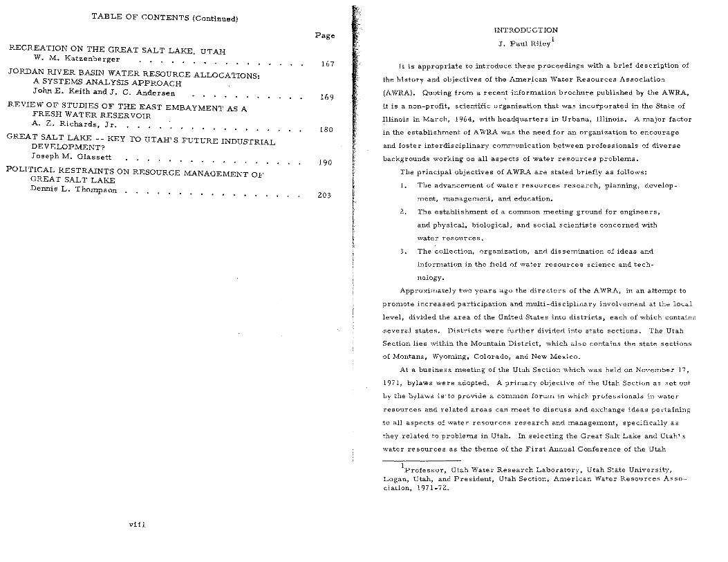
The Hogup Spring core was analyzed throughout the c§trbonate zone at

intervals of 2 cm. The carbon and oxygen isotopes were measured, and the

results are shown in Figure 1. The isotopes are relatively heavy near the

bottom of the core, then assume lighter values, suggesting a rise in the lake

level after about 25,000 years ago. After rising, the isotopes began to return

toward heavier values. The pollen studied by Mehringer showed increased

boreal forest elements when the isotopes were light. The obvious inference

is that the Hogup Spring cOre contains a record of the beginning of the pluvial

episode associated with the Late Wisconsin glaciation. A complete report on

the site is in preparation.

The Great Salt Lake core was analyzed for oxygen, carbon, and sulfur

isotopes. Total carbonates, and many types of pollen were also measured.

The microbiological data will be published elsewhere, but are consistent

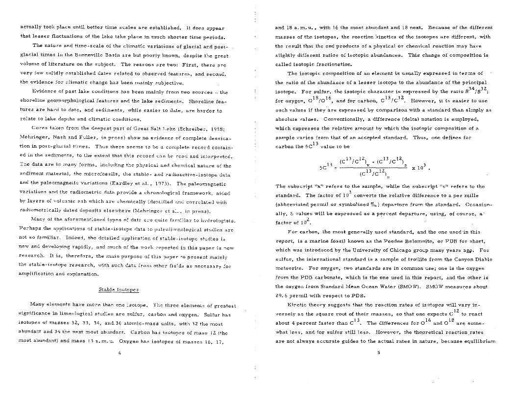
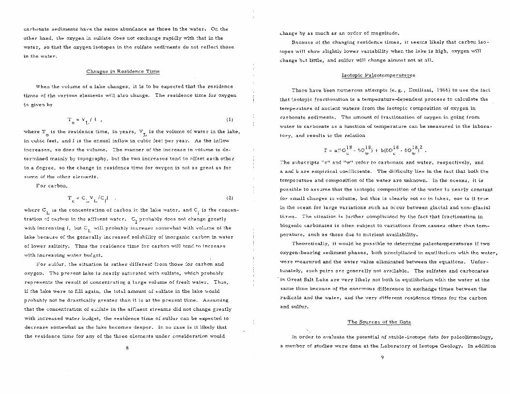
with the isotope-data interpretations given here. It can be seen from Figure 2

that the three stable isotopes show excellent correlation in the direction of their

variations. There is also good agreement with the total carbonate content.

The carbon and oxygen, as expected, show more variability than the sulfur.

The concomitant variations of the tsotopes and the carbonate content of the

core materials gives considerable credence to the belief that these variables

are reflecting the hydrologic water budget of the lake. The shifts toward lighter

isotopes and lower carbonates signify freshening water conditions, while the

opposite shifts signify dessication. Because of the good correlation between

the various indicators, it is possible to combine them into a single variable.

This was done by first normalizing the curves to have a common average value

and common standard deviation, and then averaging the data together. The

result was the qualitative "water budget" curve in Figure 2. The curve could

be made quantitative if several points on the curve could be calibrated against

11

'"'J o'Q' c .... (I)

:-

Cil() ;; II> ~, .... ;l ()

(lQ 0 ;l

n , 0 >'j II> (1) ;l

!l. C :<

'<. (lQ (I)

;l I .... f"'

N '" 0

0' 'U (I)

<: e:. c (I)

'" .... !:I

s: (I)

:r: 0

IJQ

C 'U

Ii' "-0 a ~

'" ,---------. ,

.c." ~ w w w w w w W N 0 \0 OJ ""-J 0' +' (....; N o 00 0' 4:'" N C co .?- P

~.:~ "t=== ~

'" I:j •

'"

-~~~.- -~---~-----~----- ' .. "':> , .0",,;4 -4" .44V;;YQQUUWIl.

.... '"

0

20

40

60

80

100

120

I l140

160

Depth, em

o %0 PDB

OS34 %0 eDT

T f

10

Figure 2. Isotope and lithologic data for Great Salt Lake Core, with qualitative water-budget and water-volume curves. The 169-cm level is Mazama ash, with an age of 7000 years. of core damaged. Present sulfur-isotope values in lake water shown at top of 5

known lake conditions.

The general trend of the curve is towards dessication during most of the

7000-year period, with appreciable variability. Between 150 cm and 104 cm

depth in the core, the sediments show that the lake was relatively steady,

followed by values indicating rises between l04 cm and 72 cm in the core,

with generally dessicating, but rather variable, conditions toward the present time.

By integrating the water-bUdget curve, one obtains a qualitative record

of the lake volume, approximately. The final curve in Figure 2 is the water­

volume curve. The peak at about 44 cm depth in the core represents the

highest rise of the lake in the 7000-year record. This probably corresponds

to the clay bands in the Hogup Spring core. Mehringer (personal communica_

tion) has obtained several radiocarbon measurements on the Great Salt Lake

core material, and finds that the foregOing interpretation is quite consistent with the radiocarbon data.

If the calculated peak at 44 cm depth in the core does indeed represent the

flooding of the Hogup Spring level, then some bounds can be placed on the water

depth because, while Hogup Spring appears to have been drowned, Danger Cave

was not flooded at this time (Jennings, 1957). Since Danger Cave is about 125

feet above the present lake level, the rise indicated in the volume curve must

have taken the lake to a depth between 50 and 125 feet above present lake level.

Hydrologic Equilibrium in Closed Lakes

Langbein (1961) has published a brief but very useful summary of the

theoretical hydrology of closed lakes, which will not be repeated here, but it

is worthwhile to make a few observations. First, it should be pointed out that

the area of the lake, rather than its depth, is the important parameter in

describing the water budget. The inflow to the lake is a result of direct

precipitation into the lake, groundwater inflow (or outflow), and runoff in the

drainage basin. The only outlet, except for some groundwater outflow at high

levels, is evaporation, which is a function of area. The inflow is expressed by

14

R . the :mean annual precipitation ' "fl" cubic feet per year, b 1S where I 1S the 1n ow 1n f t' onal runoff in the basin,

. other than the lake, f is the average rac 1 over the basl-n, d R is the annual

. A is the area of the lake, an L A is the area of the basl-n, L

p;eciPitation over the lake, measured in feet per year •.

The evaporation fro:m the lake is given by the relatlOn

(4)

" ) 'n cubic feet per year, and EL is the 0 " the outflow (by evaporahon , 1 where 1S It Effect

. the lake (taking into account the Raou mean annual evaporatlon over

" "h' h) :measured in feet per year. when brine concentrahon 1S 19 , . 1 _ 0

. tOll tand the inflow equals the evaporatlon, so - , When the lake 1S at a 5 1 s ,

and

G + Rbf ~

AL'" EL + Rbf (5)

a nd G prObably no more than a few that with f and A constant, It can be seen, b f th's

runoff term (see estimates of the present i:mportance 0 1 .

percent of the ti and rainfall are the controlhng te rm elsewhere in this volu:me), the evapora on

For a simple b t not of the depth or volu:me, per se. factors of the area, u . t be

rainfall over the lake and over the baSln 0 expression, assume the average h surface

"fl b bout 8 percent of t e d let the groundwater ln ow e a the same, an 'd l' t

for the present ar1 c lma e. inflow, let f be about 0.20, as would be cornmon

Then equation (5) simplifies to

or

1. 08 f R Ab

AL '" E - R (l - f) L

(6)

(7) AL'" E fR (1 - f)

L cli:mati-Now evaporation and precipitation are not independent quantities, d

anied by decrease P recipitation is usually accomp cally speaking, because more .

ti . the arid western states, an appro=­For a number of sta ons ln evaporation.

:mate formula is

E = 10.83 - 7 R (8)

15

The numbers 10.83 and 7 are not very accurate, and, of course, if high levels

of rainfall are sustained for an appreciable time, vegetative cover changes, as.

do other factors, and the arid-land equation no longer applies. Substituting

equation (8) into equation (7) gives

0.028 Ab

1. 39 _ I R

(9)

The equation, while not to be taken as numerically accurate, serves to point

up the possibility that a critical amount of rainfall exists such that, as the

rainfall in the basin increases toward this critical value (1. 39 feet in the

example), the lake is capable of extending its area almost indefinitely. The

relationship may have a bearing on Langbein's (1961) corrunent that Russ-en

had noted closed lakes only exist in areas where the rainfall is less than about 20 to 25 inches.

For a given basin, there is a simple relationship, determined by the top­

ography of the basin, between the depth and the area and volume. Since the

area is the controlling factor in closed lakes, one should perhaps treat it as

the independent variable. If one plots depth as a function of area for the

Bonneville Basin, he finds several levels which a slight increase in depth

results in a large increase in area. One such level is around 4197 feet. The

lake almost doubles its area in rising from 4195 to 4200 feet.

The lake levels at which a small increase in: depth causes large changes in

area tend to be levels of stability. When the lake is at one of these levels, an

increase in water budget will produce a large change in area, and hence in

evaporation, which will tend to offset the increase in water budget. Similarly,

a decrease in budget will cause a large decrease in evaporation, resulting in a stabilizing countereffect.

Equation (9) can be solved for R to find the amount of rainfall needed to support a given area of lake:

It can thus be seen that when topographic conditions dictate a large change in

area for a small increase in depth, there must be a relatively large change in

rainfall to get past such a stability barrier. While the above equations are far

16

too simple to provide quantitative estimates of the changes neces sar:, they

a qualitative picture of the action of stability (or stlllstand) serve to provide

levels.

A close-interval study of stable-isotope values and Hthologic data, par-

b " d with information from other disciplines, appears to ticularly when com lne

of producing detailed information about the hydrologic history of a be capable

The method might quite possibly be of use in open lakes, also, closed lake.

but has not been tried in such a setting yet.

It is not possible to recover actual tempera res tu from isotopic studies

. l't is possible to recover detailed water-budget of sediments in most cases, but

data, which has certain general climatic significance.

study seem to suggest that Great Salt Lake rose Data from the present

more than fifty, but less than 125, feet above its present level within the

during one of the so-called "Little Ice-Age" events. last three thousand years,

The present level seems to represent about the lowest level reached by the

lake in the last 7000 years, and is an unusual condition.

l'ttl time at such a Based solely on the fact that the lake has spent very 1 e

h I k will most probably rise again. low level in the past, one might infer that tea e

Acknowledgments

The experimental work reported ere1n was h' supported by, and performed

f Ut h Portions of the t he Laboratory of Isotope Geology, University 0 a. ~ dl . 1 d t d by the late Professor Armand Ear ey. Saltair core were graclous y ona e ,

The Hogup Spnng core an r a " d Get Salt Lake core materials were supphed by

Professor P. J. Mehringer.

Bro~ck~r; W. S., and A. Kaufmann. 'Lahoptan and Lake Bonneville II, pp"'. 5~7 -566.

1965. Radiocarbon Chronology of Lake Great Basin. Geo!. Soc. Am. Bull. 76,

Broecker, W. S., and P. C. Orr. Lahontan and Lake Bonneville.

1958. Radiocarbon Chronology of Lake Bull. Geol. Soc. Am. 69, pp. 1009-1032.

17

Eardley, A. J. 1967. Bonneville Chronolo. . . Exposed Stratigraphic Record d th gy. CorrelatlOn Between the Geol. Soc. Am Bull 78 7 an 9 e Subsurface Sedimentary Succession

. '" pp. 07-910. . Eardley A J d V ' • ., an • Gvosdetsky 1960 A .

Great Salt Lake Utah B 11 G' 1 • nalyslS of Pleistocene Core from , . u. eo. Soc. Am 71 132

Eardley A J V G • ,pp. 3-1344. , . ., . vosdetsky and REM

~ake 6Bu,.l1eville and Sedim~nts and' So~ls :t:t:ll~ 1.957. Hydrology of m. R, pp. 1141-1201. aSIn. Bull. Geol. Soc.

Eardley A J R T , . ., . • Shuey, V. Gvosdetsk W D. ~. Grey, and G. J. Kukla. 1973. y, • P. Nash, M. D. Picard, BaSIn, Utah. Geol. Soc. Am. BUll. Lake Cycles in the Bonneville

84, pp. 211-216. Gilbert, G. K. 1890 L k B .

. a e onneVllle U S G 1 U. S. Gov't Printing Office. ,.. eo. Surv. Monograph No.1,

Grey, D. C., and M. L. Jensen. Science 177, 1099.

1972. Bacteriogenic Sulfur in Air Pollut'o 1 n.

Jennings, J. D. 1957. D anger Cave. A th

Press, Salt Lake City. n roo Papers No. 27, Univ. of Utah

Langbein, W. B. 1961. Salinit and Sun'. Prnf. Paper No. 412 Y Hydrology. of Closed Lakes. U.S. Geol. . ' U. S. Gov't PrInting Office

Mehnnger P J W P , Washington. , . ., . . Nash and R H F 11

VOlcanic Ash from Northw ' t .. u er. In Press. A Holocene Letters. es ern Utah. Proc. Utah Acad Sci A t . ., r s,

Morrison, R. B. 1964. Quaternary Geology Press.

Quaternary Geology of th G . f h' e reat BasIn In Th

o t e Umted States, pp. 265-286 P . . e. , nnceton UnIv.

Schreiber, J. J., Jr. 1958. Sedimentar R . Ph. D. Dissertation Uni f Ut h y ecord In Great Salt Lake Utah.

, v. 0 a, Salt Lake City. Utah Geological and Mineralogical Sur

No.3, Part 1. Salt Lake City. vey. 1963. Water Resources Bulletin

Utah Geological and Mineralogical Survey 1964. ( No.3, Part II. Salt Lake City.' Water Resources Bulletin

Utah Geological and Mineralogical Surve 1968. No.3, Part III. Salt Lake City. y. Water Resources Bulletin

18

WATER BUDGET OF THE GREAT SALT LAKEI

J. N. Steed2

and B. Glenne3

Abstract

Thi~ paper is a summary of an investigation conducted of the monthly and annual water budget of Great Salt Lake in the period 1944-1970. The main factors of surface inflows, precipitation, groundwater, evaporation, transpiration and storage changes are e"aluated and balanced with an error term. Possible sources of error and inaccuracies are discussed. The purpose of the paper is to furnish data for rational development and conservation of Great Salt Lake's resources.

KEY WORDS: Water budget, Inflows, Outflows, Storage change, Streamflow, Precipitation, Groundwater, Evapor­at ion, T ranspi ration.

In! roduction

Great Salt Lake, the largest terminal lake in the United States, has re-

ceh'ed little attention as a tentative comprehensive water resource. Histori-

cally it has been exploited mainly for mineral extraction, limited recreation,

and as a sink for man's waste products.

Recent qUalitative and quantita:tive changes in Great Salt Lake caused by

man's inteden,nce with its circulation and inflow quantities have underlined

the delicate balance existing in the lake, Madison (1970), United States

Geological Survey (1970). Environmental fragility as well as a growing com­

petition for water in the Western United States have drawn attention to the

relatively large volumes of water in our terminal lakes, i. e., Great Salt Lake,

Salton Sea, Mono Lake, Pyramid Lake, Goose Lake, Walker Lake, etc.

Along the Wasatch Front Range in Utah an expanding population is in­

creasing its demands for municipal and industrial waters and has created an

IThis paper is a summary of James N. Steed's Master of Science thesis submitted in August 1972. James N. Steed passed away on October 14, 1972. May this paper honor his talents and memory.

2Formerly Research Assistant, Civil Engineering Department, University of Utah, Salt Lake City, Utah 84112.

3 Associate PrOfessor, Civil Engineering Department, University of Utah, Salt Lake City, Utah 84112.

19

earnest search for more water (Bear River Plan, Central Utah Project).

Whether Great Salt Lake is to be used as a water resource or as a waste sink,

it is inlportant that we understand the ramifications of our plans and activities.

This paper attempts to furnish SOITle of the basic data regarding the water

balance in Great Salt Lake so that we may better anticipate environITlental lake

changes and optimize de\'elopment and conservation of this important natural

resource.

Steed (1972.1 wrote the general equation for Great Salt Lake's water

budget as:

Inflows - Outflows i Storage Change = Error

in which, Inflows equal P recipitatiol1 plus Groundwater Inflows and Surface

Water Inflows lStreamflows); Outflows equal Evaporation plus Transpiration

Losses (no surface outflows since Great Salt Lake is a terminal lake). Time

Increment equals one month or one year, and Rate of Storage Change equals

change of lake volume during tinle increment. Error is the measure of in­

accuracy involved in the evaluation procedure. Units employed are acre-feet

per month or year.

The terms outlined above were evaluated for Great Salt Lake for a 27-

year period from 1944 to 1970. A scheITlatic representation of the specific

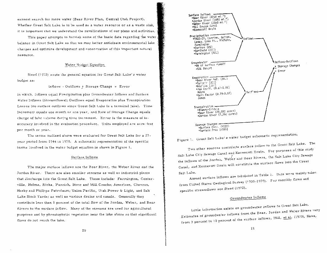
terms involved in the water budget equation is shown in Figure 1.

Surface Inflows

The major surface inflows are the Bear River, the Weber River and the

Jordan River. There are also smaller streams as well as industrial plants

that discharge into the Great Salt Lake. These include: Farmington, Center­

ville, Holms, Ricks, Parrish, Stone and Mill Creeks; American, Chevron,

Husky and Phillips PetroleuITl; Union Pacific, Utah Power & Light, and Salt

Lake Stock Yards; as well as various drains and canals. Generally they

contribute less than 5 percent of the total flow of the Jordan, Weber, and Bear

Rivers to the surface inflow. Many of the streaTI1S are used for agricultural

purposes and by phreatophytic vegetation near the lake shore so that significant

flows do not reach the lake.

20

Surface Inf1o"~ , . 'J oBear Ri ... ~r '.68,,0 ml '. ') oJordan RivCf (3490 ~1. oWeber River (2060 "'1. ') 0SLC Scv,age C;;~~l oKennecott Dram

Precipitation -.......... \ '1920-29, corrlne,,/e~t~n, ~lnfl0~JS\ Lemay, lake Pt., . ,ld a e.

Farmingtor oCorinn;, (8%) 'Garfle1d (3q::L OFal'1llir,gton i O<.,)

Ground~la ter Inn QvIS-OU tn 0'15

'6% of surface runoff + Storage Changes oGSL Oe5~rt

Transpiration .------~ ol\lanev-CriC:d1e , I 0Bear R i v~r (25 ,000 ,~:rtS 1 0Jordan Rilier (7,50:.. "eres

Storage Ch3~§es rUe"s' .surface uev. , J~ )

'Surface Acea (USGS)

Figure 1. Great Salt Lake' s"water

budget schematic representation.

l'nflow to the Great Salt Lake. The

t 'bute surface T wo other sources con 1."1 d

For purpose s of this stu Y

Lake City Sewage Canal and Kennecott Drain.

Salt f the Salt Lake City Sewage of the Jordan, Weber and Bear Rivers,

the inflows the surface flows into the Great tt Drain will constitute

Canal, and Kenneco

Salt Lake. 1 1. Annual surface inflows are tabulated in Tab e

Data we re mainly taken

For monthly flowS and . 1 S ey (1900-1970).

from United States GeologIca u rv

specific streamflows see Steed (1972.).

Groundwater Inflows

. flows to Great Salt Lake. Little information exists on groundwater in .

J dan and Weber RIvers vary . flows from the Bear. or

Estimates of groundwater In (1970), Haws, f th surface inflows. Hill,

from 3 percent to 10 percent 0 e

2.1

H <11 OJ >--­..., OJ OJ

4-< , OJ H U <11

o o o ..-<

.S

..., -;; [/j

+' <11 OJ H

a

OJ

;:0 <11

E-<

I­o l­I­

u.J

'" CH" ",,0 I-C 0'" "".c: Vl u

C o ~'" ...,'" ",,0 I-~ 0 .... 0.""

'" " >0 u.J

C o :;:;'" "'''' 1-0

"' .... "'..., C:o "'00 l-I-

C o ..., "'I to ;: . ..., 0'

0.4-C u_

'" I-"-

"'''' u", "'0 4-~ 1- .... :>C "'~

I­"'I­...,,,, «I'" ~ >- .

M ('1")00 r-..(""') r-...Lnwr-...~r­NN M~.....­

I I + I + I

a:;JCOC:OLnOo:::r Mq-Q'O a ...-.....-..-I.D o:::t-+ -r + + .+

MI.Do:::t-!.Do::::t M· 0'1 t."') 0) C\J.....- .-­M --r o::::t Ln r-...I.C NNNNNN

OJOMr-...,.....Ol o:::t-C'-II"QCOQ"'\'c) r-..r-..l.C'COI"Qr-..

\O('I")U'lCOMN O'IONN("'):..n .-NNNNN

LnOI.OLnC':)l.C") I.OOJLn 0'1 CJM oo:::tU'lOlr-..OQ .....- ............. r-NN

o:::t- Ln 1.0 r-.. co 0'1 oo:::t '<:;/" q-"'1'" "7 "<:i" 0'1 0'10'1 OlC"lOI ....--r--..-.....-_,......

a 1.00 LnI.OU'l o:::t-('I")r-...Ol OIM c..o\.C'lr-...r--N a Mr-­r-- M _M.....­+ 1++ I + + + + +

I.ON 0'1 0'10 0 lOQr-...\O r-..o:::t-O'I..-OOOO;O Mr--r-...r-...r--!.OLnl.Doo:::t Nr-... + +,...... 1.-- I I I I + ,

-':::-MI.OOLOOl..--OOlN co ...:- l."") r-... ;.n OJ L."') o;:!" 0'1..­r-..,-...--M(""')LnI.D«::t"I"QM NMMMMNNNNN

CCNOoo:::tLOOlI.OOOl('l") o:::t- L"') U'l Ln t.n ...:- Ln I.(') t.n U'l r--_ ...... r-r-..-r--r-r--r--

1.0 co Mr-...O-o:::t-I.OLnC!'l .--....-r-...I.OI.OI.ONlOU'lOJ ::0 co M..-....-..-I.Or-...r-... 0 NNMN ...... ,........-,..........-..-

O..-NMo:::t-LnI.Or-...OOOl U'lU'lLnU'llOU'llJ,"'):",&"')Lnl.{") Ol 0'1 C'l C. 0'1 0'1 C"I Ol 0'1 cr, .--..-r--....-r-....-r--.-- ..... ,.....

22

r-...r-...,......l.Oo:::t-OlMU'lOlr-...CC 1.Or-...1.01.O~\.!:IO;,oo:;;rr-...L."') Mr-a,OlCCOOo::::tO'lr--o::::t~ NC\Jr-.---r_.-C\J..--NC\JN

+

<0-<0-<D

::ri::ri5;~~~~::ri~~~1 ;;; - .......... ,.......-.--r--.--.--,...... ..... '" <D

r-...OlOlO ...... ('I")MMCOLnM I.D o:::t-NI..::;LnOlNOlOlOlU'lN 0 r-r--r-- ...... ,.....N ............ ..--NN N

\OMNNNI.DLnOo::::t.--M'Ln U'lU'lNOCO.-NC".JG"ILn::'.Ji Ln

o r-... oo:::t .- L."') 0'\ \,Q 1.0 I.C N ; ...... 1· ~ - --"-"-..--..--.---N...-

~~~[ci~~~~~~~! ; ~~~~~~~~~~~l ~

N o o

..­'"

.... C 00 . ..., "- '" ~.~

'" I-0", U >

et al. (1970), and Rely, et al. (1971). After considerable contemplation it was

decided upon to use 6 percent of the respective monthly surface inflows as the

groundwater contributions from the Bear, Weber, Jorda'n and other significant

surface inflows.

The groundwater inflows from the Great Salt Lake Desert most recently

have been investigated by Foote, et al. (1971). Their work was used to esti­

mate the Great Salt Lake Desert's contribution to groundwater inflows.

Annual groundwater inflows are tabulated in Table 1. For monthly in­

flows and further details see Steed (1972).

Precipitation Inflows

The records of precipitation, U. S. Weather Bureau (1915-1970), for the

study period (1944-1970) show only stations on the east side of the lake. These

locations are poorly located in terms of trying to obtain a representative value

for precipitation.

During the 1920' s the U. S. Weather Bureau collected records from

stations around the entire Great Salt Lake. For this reason, the 10-year

time period from 1920-1929 provides the basis for estimating the average

precipitation distribution over the lake. Six strategically located stations

have 10 years of data upon which a Thiessen Diagram can be made. These

stations arc Corinne, Kelton, Lemay, Lake Point, Farmington, and Midlake.

The results obtained were correlated to the records from the stations at

Corinne, Garfield (used as Lake Point) and Farmington, which are the three

stations with records common to both time periods. Average weighting

factors of 8. 15 percent for Corinne, 61. 6 percent for Garfield and 30.25 per­

cent for Farmington were used with precipitation records at these stations to

obtain average lake precipitation data.

To calculate the monthly water volume that is added to the lake by pre­

cipitation, the monthly precipitation was multiplied by the surface area

corresponding to the particular water stage. The surface area was read off

a set of curves prepared by the United States Geological Survey showing water

stage - surface area and<water stage - volume relationships.

Annual precipitation inflows are tabulated in Table 1. For monthly in­

flows and further details see Steed (1972).

23

Evaporation outflows were calculated using Class A pan evaporation data

from three stations; nam.ely, Saltair, Midlake, and Bear River Refuge (U.S.

Weather Bureau, 1915 -1970). The data had to be correlated with other stations

and wind-tem.perature data to com.plete the records. The records were then

weighted and m.uItiplied by a pan coefficient and a salt factor to obtain repre­

sentative lake evaporation in inches per m.onth. This figure was then multi­

plied by the appropriate surface area to give the m.onthly evaporation in acre­feet.

The pan coefficient problem. for the Salt Lake area has been studied by

Adam.s (l934) and Peck and Dickson (1965). Adams found values of 0.61 _

0.66 to be representative. In this study a value of 0.61 was used in for the

spring m.onths, a value of 0.66 for the fall m.onths, and a value of 0.65 for

the rest of the year.

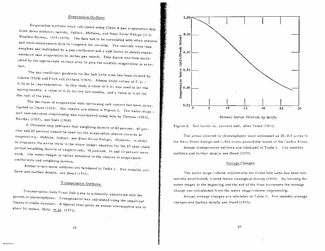
The decrease of evaporation with salt content has been inves-

tigated by Jones (1933). His results are shown in Figure 2. The water stage _

salt concentration relationship was established using data by Thomas (1914),

Eardley (1957), and Hahl (l969).

A Thiessen map indicates that factors of 40 percent, 40 per-

cent and 20 percent should be used for the evaporation station records at

respectively, Midlake, Saltair, and Bear River Refuge. However, in order

to m.inim.ize the error term. in the water budget equation for the 27-year study

period weighting factors of respectively, 35 percent, 35 and 30 percent were

used. The water budget is rather sensitive to the choices of evaporation

coefficients and Weighting factors.

Annual e\-aporation outflows are tabulated in Table 1. For monthly out­

flows and further details, see Steed (1972).

Transpiration from. Great Salt Lake is as sociated with the

growth of phreatophytes. Transpiration was calculated using the empirical

Blaney-Criddle equation. A typical year gives an annual consumptive use of

about 56 inches, Hely, et al. (1971).

24

1.(10

0.-<)5 -;; ~, ..,

?1 ~

r- 90

[

~ 0.85 .., III II:!

s:1 _0

~O'8°L i L

0.75 0 5 "-.i--~-=---~-----;;Z-----:JO

Percent Sodium Chloride by ~Jeight

Figure 2. Salt factor vs. percent salt, after Jones (1933).

The areas t " t d as 25,000 acres in covered by phreatophytes were es lma e

the Bear River Refuge d the m.outh of the Jordan River. and 7,500 acreS aroun

Annual transpiration outflows are tabulated in Table

outflows and further details see Steed (1972).

1. For monthly

The water stage -volume relationship for Great Salt Lake has been ten­

tativelyestablished, United States Geological Survey (1970). By knowing the

water stages at the beginning and the end of the tim.e increment the storage

change was established froIn the water stage-voluIne rel,ationship.

Annual storage changes are tabulated in Table

changes and further details see Steed (1972).

25

1. For monthly storage

Results

Table 1 indicates that evaporation and surface inflows are the largest

terms in Great Salt Lake's water budget equation while transpiration and

groundwater inflows are relatively unimportant. While the mean error has

been reduced to essentially nil by adjusting the evaporation station weighting

factors it is interesting to observe that the standard deviation of the error

term is only about 7.4 percent of the mean evaporation term. Without ex­

tensive further study it is difficult to distinguish between predictable and

random error,

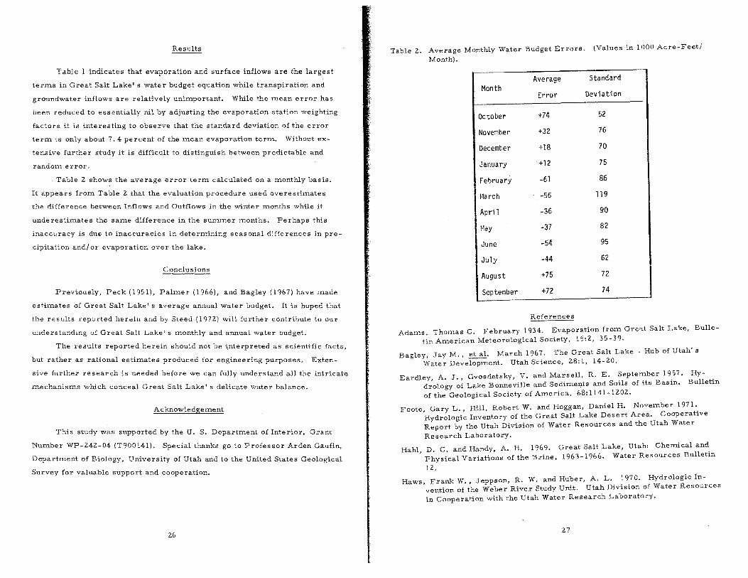
Table 2 shows the average error term calculated on a monthly basis.

It appears from Table 2 that the evaluation procedure used overestimates

the difference between Inflows and Outflows in the winter months while it

underestimates the same difference in the summer months. Perhaps this

inaccuracy is due to inaccuracies in determining seasonal differences in pre­

cipitation and/ or evaporation over the lake.

Previously, Peck (1951), Palmer (1966), and Bagley (1967) have made

estimates of Great Salt Lake's average annual water budget. It is hoped that

the results "epurted herein and by Steed (1972) will further contribute to our

understanding uf Great Salt Lake's monthly and annual water budget.

The results reported herein should not be interpreted as scientific facts,

but rather as rational estimates produced for engineering purposes. Exten­

sive further research is needed before we can fully understand all the intricate

mechanisms which conceal Great Salt Lake's delicate water balance.

Acknowledgement

This study was supported by the U. S. Department of Interior, Grant

Number WP-242-04 (T900141). Special thanks go to Professor Arden Gaufin,

Department of Biology, University of Utah and to the United States Geological

Survey for valuable support and cooperation.

26

Table 2. Average Monthly Water Budget Errors. (Values in 1000 Acre-Feet/

Monthl.

'---"" Standard Average Month

Deviation Error

October +74 52

November +32 76

December +18 70

January +12 75

February -61 86

~'arch -56 119

April -36 90

May -37 82

June -54 95

July -44 62

August +75 72

September +72 74

Adams, Thomas C. February 1934. Evaporation from Great Salt Lake, Bulle­tin American Meteorological Society, 15:2, 35-39.

Bagley, Jay M., March 1967. The Great Salt Lake Hub of Utah's Water Development. Utah Science, 28:1, 14-20.

Eardley, A. J., Gvosdetsky, V. and Marsell. R. E. ~epten:ber 19,57. drology of Lake Bonneville and Sedirnellts and SOlIs of lts BaSln. of the Geological Society of America, &8: 1141 1202.

Hy­Bulletin

Foote, Gary L., Hill, Robert W. and Hoggan, Daniel H. November 1971., Hydrologic Inventory of the Great Salt Lake Desert Area. Cooperahve Report by the Utah Division of Water Resources and the Utah Water

Research Laboratory.

Hahl, D. C. and Handy, A. H. 1969. Great Salt Lake, Utah: Chemical and, Physical Variations of the Brine, 1963-1966. Water Resources Bulletm

12.

Haws, Frank W., Jeppson, R. W. and Huber, A. L. 1970. Hydrologic In­vention of the Weber River Study Unit. Utah Division of Water Resources in Cooperation with the Utah Water Research Laboratory.

27

Hely, A. G., Mower, R. W. and Harr C A 1971 W t R L k C ' .• • a er esources of Salt

a e ounty, Utah. U. S. Geological Survey in cooperation with the Utah Department of Natural Resources, Technical Publication No.3!.

Hill, Robert W., et al. 1970. A HydrologiC Model of the Bea R' B' U h -- r 1ver aSln.

ta Water Research Laboratory. '

Jones, Douglas K. 1933. A Study of the Evaporation of the Water of Great Salt Lake. Unpublished M. S. Thesis, University of Utah.

Madison, R. J. 1970 Eff t f . ec s a a Causeway on the of the Brine in Great Salt ~ake., Water Resources Bulletin 14, U.S. Geological Surve m cooperahon wlth the Utah Geological and Mineralogical Survey. y

Palmer, Roland. 1966. Hydrologic Study of the Great Salt Lake Report prepared for the Utah Water and Power Board. .

Peck, Eugene L. 1951. H d Y :O!neteorological Study of the Great Salt Lake. Unpublished M. S. Thesls, University of Utah.

Peck, Eugene L. and Dickson, D. P. 1965. Evaporation Studies _ Great Salt LS ake. Water Resources Bulletin 6, Utah Geological and Mineralogy urvey.

Steed, James N. 1972. W t B d a ~r u. get of the Great Salt Lake, Utah, 1944-1970.

Unpublished M. S. Th C '1 E Utah.

eS1S, lVl ngineering Department, University of

Thomas, M. D. 1914. A Study of the Waters of Great Salt Lake B S Th Unpublished .. esis, University of Utah. .

United States Geological Survey, 1900-1970. W ater Resources Data for Utah,

Part 1, Surface Water Records.

United States Geological Survey, November 1970. Salt Lake Inflow, Outflow and Lake Levels. Survey Seminar.

Lake Bonneville and Great Presented at Utah Geological

United States Weather Bureau (now National Oceanl'c d 't . an rHrn""" •• o 1S ratlOn) 1915-1970. Environmental Data Service, Annual Sumnlaries, 1915-1970. Data,

28

SURFACE INFLOW TO GREAT SALT LAKE, UTAH1

Ted Arnow and J. C, Mundorff2

During 1960, 1961, and 1964 the Bear, Weber, and Jordan River systems contributed about 90 percent of the surface dis­charge and about 80 percent of the surficial dissolved-solids load that entered Great Salt Lake, Utah. During years of average streamflow, a total of more than 500,000 acre-feet of water suitable for public supply and more than 1,350, 000 acre-feet of water suitable for irrigation discharges in the Bear River past Corinne, the Weber River past Plain City, and the Jordan River past Cudahy Lane. During January­October 1972, water from the Weber River system generally had dissolved-solids concentrations of less than 500 mgt 1 (milligrams per liter) as determined at four sites in the Ogden Bird Refuge. The outflow from Farmington Bay, which in­cludes Jordan River discharge, had concentrations ranging from about 8,700 to 97, 000 mgtl, and water entering the lake from the Bear River at the Great Salt Lake Minerals and Chemicals Corp. bridge had concentrations ranging from about 1,900 to 13,000 mgtl. Except for Lee Creek, which had observed concentrations ranging from about 39,000 to 121,000 mgtI, the minor tributaries to Great Salt Lake had concentrations of less than 5,000 mgtl.

KEY WORDS: Great Salt Lake, Lake inflow, Saline lakes, Lakes.

The major surface inflow to Great Salt Lake is from the Bear, Weber,

and Jordan River drainage systems. The U. S. Geological Survey has oper­

ated gaging stations upstream from the lake on the main sterns of these streams

in cooperation with the Utah State Engineer for many years; but in 1960, 1961,

and 1964 the Geological Survey, in cooperation with the University of Utah and

the Utah Geological and Mineralogical Survey, made a special study to deter­

mine the actual amount of water that was entering the lake from these streams

and other surface sources around the lake. The information from this study

was summarized in a report by Hahl (1968).

IPublication authorized by the Director, U. S. Geological Survey.

2U. S. Geological Survey, Salt Lake City, Utah.

29

In the preparation of a State water plan, consideration has been given

to the concept of diverting som.e of the water that now enters the lake for use

upstream. Starting in 1971, in cooperation with the Utah Division of Water

Resources, the Geological Survey has been m.easuring the m.ajor surface in­

flow to the lake as close to the lake as feasible.

In the following discussion we use the term "surface inflow" to include

two things: surface discharge (quantity of water) and the surficial disso1ved­

solids load that enters the lake in stream.s, canals, drains, and springs that

are near the water's edge.

Inflow During 1960, 1961, and 1964

Distribution of inflow by percentage

Our study in 1960, 1961, and 1964 indicated that the Bear, Weber, and

Jordan Riv-ers carried about 85 percent of the surface discharge to the lake and

about 60 percent of the dissolved-solids load. (See Table 1.)

The Bear River carried more than half of the water and alm.ost 40 per­

cent of the load. The Weber River carried about 17 percent of the water but

only about 6 percent of the load. The Jordan River carried about 15 percent

of the water and 15 percent of the load. The sources of surface inflow exclud­

ing the three main-stem rivers carried only about 15 percent of the water, but

they carried about 40 percent of the load.

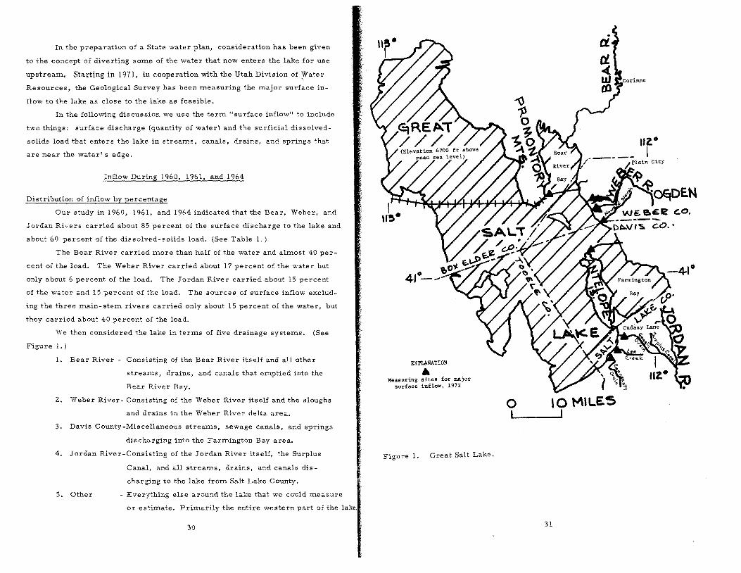
We then considered the lake in term.s of five drainage system.s. (See

Figure 1.)

1. Bear River - Consisting of the Bear River itself and all other

stream.s, drains, and canals that emptied into the

Bear River Bay.

2. Weber River- Consisting of the Weber River itself and the sloughs

and drains in the Weber River delta area.

3. Davis County-Miscellaneous stream.s, sewage Canals, and springs

discharging into the Farmington Bay area.

4. Jordan River-Consisting of the Jordan River itself, the Surplus

Canal, and all stream.s, drains, and canals dis-

charging to the lake from. Salt Lake County.

5. Other - Everything else around the lake that we could m.easure

or estim.ate. Prim.arily the entire western part of the lake. ;

30

EXPLANATION .. Measuring sites for major

.urface inflow, 1972

Figure 1. Great Salt Lake.

a I

10 M\LES I

31

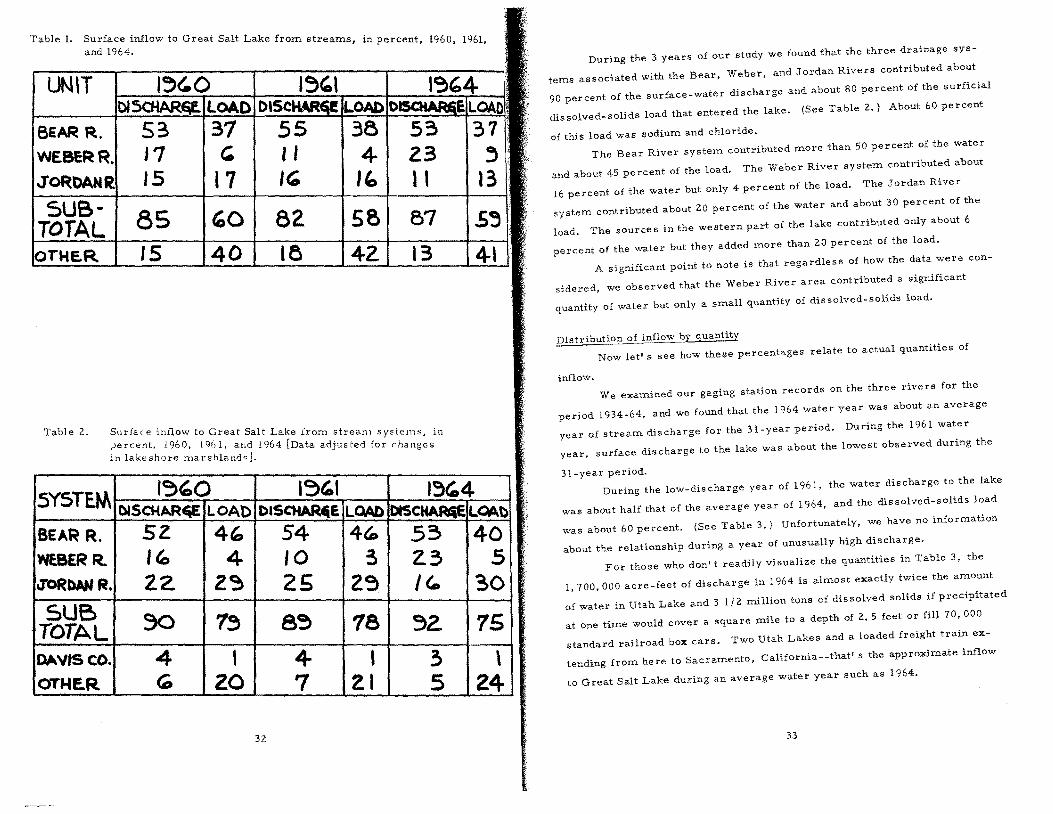
Table 1. Surface inflow to Great Salt Lake from str and 1964. earns, in percent, 1960, 1961,

UNIT

WEBER JoRDAN

5US-TOTAL

ER.

TabJe 2.

55 I , It;.

85 '0 82 58 87

15 40 10 42 13

Surface inflow to Great Salt Lake percent, 1960, ICl61. and 1964

from stream systems, in adjusted for rhanges

in lakeshore marshlandoJ.

4-'

BEAR R. SZ 4'- 54 4~ 53 40 WE8ERR. I~ 4 10 3 2.3 5 JORDAN R. 2.2. Z~ 25 29 1(. '?>o SUB

TOTAL ~v,sco.

OTHE.R

, 20

32

4 7

18 , ZI

.3 5

15 \

24

During the 3 years of our study we found that the three drainage sys­

tems associated with the Bear, Weber, and Jordan Rivers contributed about

90 percent of the surface-water discharge and about 80 percent of the surficial

dissolved-solids load that entered the lake. (See Table 2.) About 60 percent

of this load was sodium and chloride.

The Bear ·River system contributed more than 50 percent of the water

and about 45 percent of the load. The Weber River system contributed about

16 percent of the water but only 4 percent of the load. The Jordan River

system contributed about 20 percent of the water and about 30 percent of the

load. The sources in the western part of the lake contributed only about 6

percent of the water but they added tnore than 20 percent of the load.

A significant point to note is that regardless of how the data were con­

sidered, we observed that the Weber River area contributed a significant

quantity of water but only a small quantity of dissolved-solids load.

Distribution of inflow by quantity

Now let's see how these percentages relate to actual quantities of

inflow. We examined our gaging station records on the three rivers for the

period 1934-64, and we found that the 1964 water year was about an average

year of stream discharge for the 31-year period. During the 1961 water

year, surface discharge to the lake was about the lowest observed during the

31 - year pe riod. During the low-discharge year of 1961, the water discharge to the lake

was about half that of the average year of 1964, and the dissolved-solids load

was about 60 percent. (See Table 3.) Unfortunately, we have no information

about the relationship during a year of unusually high discharge.

For those who don't readily visualize the quantities in Table 3, the

l, 700, 000 acre -feet of discharge in 1964 is almost exactly twice the amount

of water in Utah Lake and 3 1/2 million tons of dissolved solids if precipitated

at one time would cover a square mile to a depth of 2.5 feet or fill 70, 000

standard railroad box cars. Two Utah Lakes and a loaded freight train ex­

tending from here to Sacramento, California--that's the approximate inflow

to Great Salt Lake during an average water year such as 1964.

33

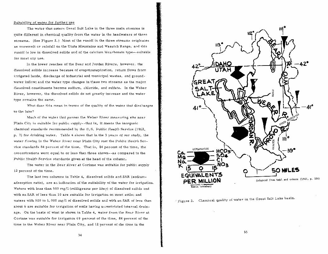
Suitability of water for further use

The water that enters Great Salt Lake in the three main streams is

quite different in chemical quality from the water in the headwaters of these

streams. (See Figure 2.) Most of the runoff in the three streams originates

as snowmelt or rainfall on the Uinta Mountains and Wasatch Range, and this

runoff is low in dissolved solids and of the calcium bicarbonate type--suitable

for most any use.

In the lower reaches of the Bear and Jordan Rivers, however, the

dissolved solids increase because of evapotranspiration, return flows from

irrigated lands, discharge of industrial and municipal wastes, and ground­

water inflow; and the water type changes in these two streams as the major

dis solved constituents become sodium, chloride, and sulfate. In the Weber

River, however, the dissolved solids do not greatly increase and the water

type remains the same.

What does this mean in terms of the quality of the water that discharges

to the lake?

Much of the water that passes the Weber River measuring site near

Plain City is suitable for public supp1y--that is, it meets the inorganic

chemical standards recommended by the U. S. Public Health Service (1962,

p. 7) for drinking water. Table 4 shows that in the 3 years of our study, the

water flowing in the Weber River near Plain City met the Public Health Ser­

vice standards 84 percent of the time. That is, 84 percent of the time, the

concentrations were equal to or less than those shown--as compared to the

Public Health Service standards given at the head of the column.

The water in the Bear River at Corinne was suitable for public supply

12 percent of the time.

The last two columns in Table 4, dissolved solids and SAR (sodium-

adsorption ratio), are an indication of the suitability of the water for irrigation.

Waters with less than 500 mg!l (milligrams per lite~) of dissolved solids and

with an SAR of less than 10 are suitable for irrigation on most soils; and

waters with 500 to 1, 000 mg/l of dissolved solids and with an SAR of less than

about 6 are suitable for irrigation of soils having unrestricted internal drain­

age. On the basis of what is shown in Table 4, water from the Bear River at

Corinne was suitable for irrigation 69 percent of the time, 84 percent of the

time in the Weber River near Plain City, and 12 percent of the time in the

34

\ REA" '\' 5AL T LA~E.

'-=.:" \

410-"" -41,°

\ « f

I

to. Co.. """"",00 Hd;}. MQ 504 \.f-) N" C, -- NO . ~ Irs 9 If> a ". _ EQU\VALcNT,5 9'-_' __ ....... PER NULl'ON (Adapted from Rah1 and others (1965, p. 184)

-.~---Bas in boundary

, Figure 2. Chemical qllality of water in the Great Salt Lake basin.

35

Table 3. Surface inflow to Great Salt Lake from major stream systems in thousands of acre- feet and thousands of tons, 1961 and 1964.

SYSTEM 19~1 (LOW) 19b4-~VERAG.E.) DISCHAR"E LOAt) DlSCWAA" LOAD

BEAR R. 43~ 1,010 ~13 1,368 WEBERR. 80 75 3~8 ZOO JORDAN R. 204 '-SO Z61 1,072. DAVIS co. 35 Z4 ~~ 40 OTHER COO 480 8'- 84Z TOT~L 810 2,2.00 1,70 0 ~500

Table 4. Inflow to Great Salt Lake from major streams and durations for selected chemical parameters, 1960, 1961, and 1964.

Percentage of time: The percentage of time that the concentrations were less than or equal to those shown. [Numbers in parentheses are standards recommenced b the U. S. Public Health Service (1962, p. 7) for drinking warer. J

PERCE NT- Mg/lite.r SOURCE AqE.OF S04- CI NO~ SOL\DS

TIME (250) i/2sOl (4S} (500)

~EAR R.. 69 "3 2eo 3.9 8<,;Z 9~.9 2~1 't~50 1.8 4,04-0 12 51 1i.8 .2 505

WEaER R. I Z4- 2C. 2.3 200 84- 3' ~8 17 500

~OR[)AN R. IZ 289 ZOO .3 897 9~ 74-2 350 7.8 1,8Z0

3 95 11 2.5 407

36

5AR

4.<; 23 2.9

." 1.5 3.1 3.1 1.4-

Jordan Rlver at Cudahy Lane.

In a year of average streamflow such as 1964, the combined flow of

the three rivers that had a dissolved-solids concentration of less than

1, 000 mg/l and thus is regarded as suitable for irrigation of m.any soils, was

at least 1. 35 million acre-feet, which is about one-third of the present total

quantity of water diverted each year for irrigation in the entire State. The

combined flow of the Bear and Weber Rivers that is suitable for public supply,

from the standpoint of inorganic chemical quality, is about 1/2 million acre­

feet. That is more than 1 1/2 times the present quantity of water diverted for

public supply in the entire State of Utah.

At its worst, none of the water in the three rivers could be considered

highly mineralized, as compared to ocean water which contains about 36, 000

mg/l and the Great Salt Lake itself which now contains about 150, 000 mg/l in

the upper layer in its south part and about 330, 000 mg/l in its north part.

Inflow During 1972

The detailed water-quality data collected during the period January­

October 1972 confirm our past knowledge that the surface streams supply the

lake with water that contains an extremely wide range in concentrations of

dissolved solids. The data also support the earlier finding that the surface

source of the water of best chemical quality entering the lake is the Weber

River.

Weber River

Water from the Weber River had dissolved-solids concentrations of a

maximum of 514 mg/l and generally less than 500 mg/l as determined at the

four sites in the Ogden Bird Refuge. On Figure 3, representative samples for

the Weber River are shown by the solid circles. The total dissolved-solids

concentrations of the waters represented by these circles are proportional to

the radii of the circles as indicated by t,he scale on the illustration. Fluctu­

ations in percentages of the major cations (lower left) are appreciablY greater

than fluctuations in percentages of major anions (lower right) and the water

type is generally either calcium magnesium bicarbonate or calcium sodium

bicarbonate.

37

• WEBER R1VE.R. o BE.A.I<. R.IVe. Q. o FARMINGTON

BAY OU'fLET

08 0 0 0 0°0'" o!\

Olf) °0 U'l_ " I I

Disaolved sOlids) in milligrams per liter

'0 0 Co..

CATIONS

I

CI AN\OJlJS

Figure 3. . . composition of anions and cations (equivalents per m11hon) for the Weber and Bear Rivers and Farmington Bay outlet.

38

Farmington Bay

Water from the Jordan River, together with other inflow to Farmington

Bay, moves through Farmington Bay and into Great Salt Lake at the bridge on

the Antelope Island-Syracuse causeway. Concentrations ranged from a minimum

of about 8,700 mg/l to about 97, 000 ITlg/l. The large open circles at the right

side of each part of Figure 3 show the wide range and high concentrations rep­

resentative of water flowing into the lake at this Antelope Island causeway

station. The water is definitely sodium chloride in type. Magnesium and

sulfate are present in significant concentrations but are ITlinor relative to

sodium and chloride. CalciuITl and bicarbonate are relatively very low and

are present in concentrations COITlITlon in ITlany norITlal stream waters.

Two-directional flow is COITlITlon at this site, and a dense lower layer

of brine COITlITlonly is observed as underflow at the bridge. This lower­

stratum water flowing southward from Great Salt Lake into FarITlington Bay

had dissolved-solids concentrations ranging froITl 136,000 to 152,000 ITlg/l.

This water is also sodiuITl chloride in type. This southward-flowing brine

mixes with the water in Farmington Bay near the causeway and undoubtedly

causes the water flowing north from the bay at the Antelope Island bridge

to have an appreciably higher salinity than the water entering the bay from

the Jordan River and other sources.

Water froITl the Bear River ITloves into the lake at the Great Salt Lake

Minerals and Chemical Corp. bridge. Dissolved-solids concentrations ranged

froITl a minimum of about 1,900 ITlg/1 to a maximum of about 13,000 mg/l for

southward-flowing water from the Bear River system. As is apparent from

the data in Figure 3 that represent water from the Bear River, these waters

are not greatly different cheITlically from those observed entering Great Salt

Lake from Farmington Bay, but the range in dissolved-solids concentrations

is much less.

COITlplex ITlultidirectional flow to and froITl the Great Salt Lake also

occurs at this site, but the quantity of water moving out of the lake is ITluch

lee s than at the Antelope Island causeway. The very slowly northward-ITloving

or stagnant bottoITllayer of water at this site had dissolved-solids concentra­

tions ranging froITl about 20,000 to 291,000 ITlg/l.

39

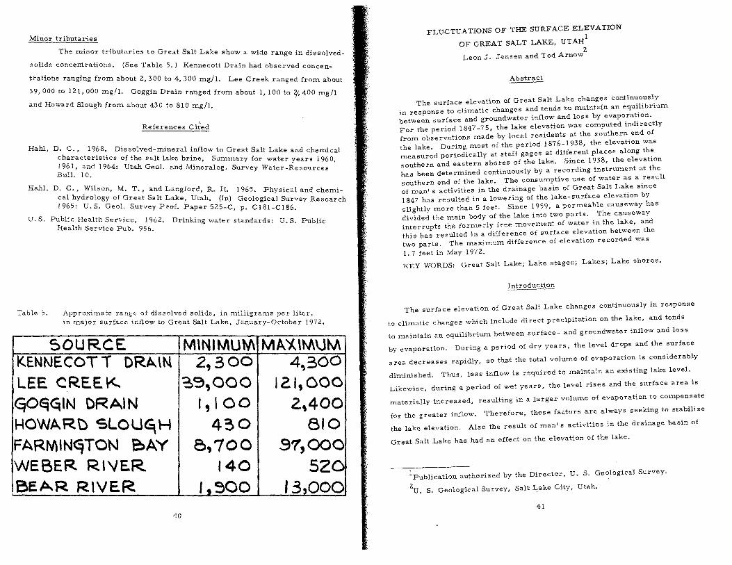
Minor tributaries

The minor tributaries to Great Salt Lake h s ow a wide range in dissolved-

solids concentrations. (S T bl ee a e 5.) Kennecott Drain had observed concen-

trations ranging from about 2,300 to 4,300 mgtl. Lee Creek ranged from about

39,000 to 121,000 mgtl. Goggin Drain ranged from about 1,100 to ~ 400 mgtl

and Howard Slough from about 430 to 810 mg/l.

References Cited

Hahl, D. C., 1968, Dis solved-mineral inilow to Great S It L k ' characteristics of the salt lake brine S f a a e and chemIcal 1961, and 1964: Utah Geol and M" ummary or water years 1960, Bull. 10. ,Ineralog. Survey Water-Resources

D. C., Wilson, M. T., and Langford, R. H. 1965. cal hydrology of Great Salt Lake Ut h ( :hysical and chemi-1965' U S GIS ' a. In) GeologIcal Survey Research

, •. eo, urvey Prof. Paper 525-C, p. C 181-C 186.

Hahl,

U.S. Public Health Service, 1962. D ' k rln ing water standards: U.S. Publl'C Health Service Pub. 956.

Table 5. Appro.ximate range; of dissolved solids, in milligrams per liter, In maJor surface mflow to Great Salt Lake, January-October 1972.

SOURCE M\NIMUtl\ MA~\t~\JM KENNECCT T DRA.\N 2,300 4,300 LEE CREE. \<.. ~9,OOO 121,000 ~OEiqIN DRA1N I, 100 2,400 HOWARt> SLOUGtH 430 810 FARM'N~TON e>AY 8,700 9'7,000 WEBER R'''E.R 140 520 BEAR RIVER '!) 900 , :3,000

40

FLUCTUATIONS OF THE SURFACE ELEVATION

OF GREAT SALT LAKE, UTAHI

Leon J. Jensen and Ted Arnow2

The surface elevation of Great Salt Lake changes continuously in response to climatic changes and tends to maintain an equilibrium between surface and groundwater inflow and loss by evaporation. For the period 1847-75, the lake elevation was computed indirectly from observations made by local residents at the southern end of the lake. During most of the period 1876 -1938, the elevation waS measured periodically at staff gages at different places along the southern and eastern shores of the lake. Since 1938, the elevation has been determined continuously by a recording instrument at the southern end of the lake. The consumptive use of water as a result of man's activities in the drainage basin of Great Salt Lake since 1847 has resulted in a lowering of the lake-surface elevation by slightly more than 5 feet. Since 1959, a permeable causeway has divided the main body of the lake into two parts, The causeway interrupts the formerly free movement of water in the lake, and this has resulted in a difference of surface elevation between the two parts. The maximum difference of elevation recorded was

1.7 feet in May 1972.

KEY WORDS: Great Salt Lake; Lake stages; Lakes; Lake shores.

The surface elevation of Great Salt Lake changes continuously in response

to climatic changes which include direct precipitation on the lake, and tends

to maintain an equilibrium between surface- and groundwater inflow and loss

by evaporation. During a period of dry years, the level drops and the surface

area decreases rapidly, so that the total volume of evaporation is considerably

diminished. Thus, less inflow is required to maintain an existing lake level.

Likewise, during a period of wet years, the level rises and the surface area is

materially increased, resulting in a larger volume of evaporation to compensate

for the greater inflow. Therefore, these factors are always seeking to stabilize

the lake elevation. Also the result of man's activities in the drainage basin of

Great Salt Lake has had an effect on the elevation of the lake.

authorized by the Director, U. S. Geological Survey.

2U. S. Geological Survey, Salt Lake City, Utah.

41

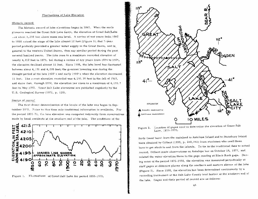
Fluctuations of Lake Elevation

The historic record of lake elevations began in 1847. When the early

pioneers reached the Great Salt Lake basin, the elevation of Great Salt/Lake

.. <is abouL .. ,200 feel above mean sea level. A series of wet years from 1862

to 1868 raised the stage of the lake almost 12 feet (Figure 1); that 7-year

period probably provided a greater water supply to the Great Basin, and in>

general to the western United States, than any similar period during the past

several hun"dred years. The lake rose to a maximum recorded elevation of

nearly 4,212 feet in 1873, but during a series of dry years from 1874 to 1905,

the elevation declined almost 16 feet. Since 1905,the lake level has fluctuated

between about 4,191 and 4,205 feet; the greatest lowering was during the

drought period of the late 1920' s and early 1930' s when the elevation decreased

11 feeL. Ihe luwest elevation recorded was 4, 191. 35 feet in the fall of 1963,

and since then, through 1972, the elevation has risen to a maximum of 4, 199.7

feet in May 1972. Great Salt Lake elevations are published regularly by the

U.S. Geological Survey (1971, p. 125).

The first direct determination of the levels of the lake was begun in Sep­

tember 1875. Prior to thIS time only traditional information is available. For

the period 1850 - 75, the lake elevation was computed indirectly from observations

made by local residents at the southern end of the lake. The conditions of the

- -Figure 1. Fluctuations of Great Salt Lake for period 1850-1972.

41~

eXPLANATION

.. periodic me.aBuremtJnu.l

.. Continuous meaSurements

o 10 MILE.S , I

Figure 2. f used to dete rmine the elevation of Great Salt Location 0 gages Lake, 1875-1972.

fords (sand bars) from the mainland to Antelope Island and to Stansbury Island

were obtained by Gilbert (1890, p. 240,241) from stockmen who used these

bars to get stock to and from the islands. To tie in the traditional data to actual

record, Gilbert made observations On Antelope bar on October 19, 1877, and

related the water elevation there to the gage reading at Black Rock gage. Dur­

ing most of the period 1876-1938, the elevation was measured periodically at

staff gages at different places along the southern and eastern shores of the lake

(Figure 2). Since 1938, the elevation has been determ.ined continuously by a

recording instrument at the Salt Lake County boat harbor at the southern end of

the lake. Gages and their period of record are as follows:

43

Gage

Black Rock Farmington Lakeshore Garfield Mid1ake Saltair Boat Harbor

Period of Record

1875-1876 1876-1879 1879-1881 1881-1901 1902-1903 1903-1938 1939-1972

Effect of Man's Activities on the Lake Elevation

Consumptive use of water

Although the major fluctuations of lake elevation are caused by climatic

variations, the consumptive use of water as a result of man's activities in the

drainage basin of Great Salt Lake since 1847 has resulted in a lowering o! the

lake surface. An evaluation of this effect was made in 1969 by the U. S. Geo­

logical Survey and the Utah Department of Natural Resources (Whitaker, 1971).

The elevation in 1965 would have been about 5 feet higher than the observed

elevation had there been no consumptive use of water because of man's activities

in the basin.

Figure 3 shows the effect of consutnptive use of water, resulting from man's

activities, on historic elevations of Great Salt Lake, 1850-1965. The difference

in 1965 was 5.28 feet. That is, the lake surface was 5.28 feet lower than it

would have been if man had not caused evapotranspiration of water by impound­

ing it in reservoirs and diverting some of it for irrigation and other uses.

The railroad causeway

During 1957 -59, the Southern Pacific Co. constructed a causeway to carry

its railroad lines across Great Salt Lake. The causeway is constructed of

permeable quarry-run rockfill capped with boulder-sized riprap. The cause­

way is breached by two culverts, each 15 feet wide, which allows brine to flow

through the causeway. The causeway divides the lake into two sections. About

one-third of the lake lies to the north of the causeway, but more than 95 per-

, cent of the fresh-water surface inflow enters the lake south of the causeway.

The inflow for each part is the sum of surfacewater inflow, groundwater in­

flow, precipitation, and inflow through the causeway. The outflow for each

part is the sum of evaporation and outflow through the causeway to the other

part. Because of the complex interrelationships among variable inflow

44

Figure 3.

Dashed line shows approximate elevation

-Effects of consumptive use of water, resulting from man's activities, on historic elevations of Great Salt Lake, 1850-1965.

4Z00

Figure 4.

50UT H PA.R T '\

\ ~ORTH PART

\970 t972 . of the north and south parts

Relationship between the elevations of Great Salt Lake, 1966- 1972.

45

relative to volumes and areas, evaporation, and two-way flows through the

causeway affected by salinity differences, a difference of water-surface ele-

. vation has developed between the two parts of the lake. The maximum dif­

ference of elevation recorded was 1. 7 feet in May 1972. (See Figure 4.)

Effect of Storms on the Lake Elevation

Figure 5 shows a continuous recording of the elevation of the lake at the

boat harbor. This period covers 8 days and shows the effects of storms on

the lake. To compensate for wind effect and seiches, elevations given for the

gage were taken from a mean slope line defined by several days gage-height

graph preceding and following the 1 st and 15th of each month. Wind effects

may cause substantial changes in elevation which are not shown in the publish­

ed elevations.

Relations of Lake Elevation, Volume, and Surface Area

Figure 6 shows relations among elevation, area, and volume of Great Salt

Lake prior to 1957 (Hahl and Handy, 1969, p. 10). These parameters are

greatly affected by evaporation from the lake surface. The rate of evaporation

varies inversely with the concentration of dissolved solids in the water, and

the concentration of dissolved solids varies inversely with the volume of water

in the lake. In addition, the volume of water evaporated is directly proportion­

al to the surface area, which varies directly with lake stage. It is obvious, for

example, that because of the greater surface area the amount of water evapo­

rated at the maximum recorded elevation of 4,212 feet (6 million acre-feet)

was much greater than that evaporated at the minimum elevation of 4, 191. 35

feet (apprOximately 1. 9 million acre-feet).

Gilbert, G. K. 1890. Lake Bonneville: U. S. Geol. Survey Mon. 1.

Hahl, D. C., and Handy, A. H. 1969. Great Salt Lake Utah: Chemical and physical variations of the brine, 1963-1966: Utah Geol. and Mineralog. Survey Water-Resources Bull. 12.

Madison, R. J. 1969. Hydrology and chemistry of Great Salt Lake, in Guide­book of northern Utah: Utah Geol. and Mineralog. Survey Bull. 82, 140-157.

46 47

"" o 't:l ,.. o u <ll ,.. III oj

g ~ 'ti ~ o U

U. S. Geological Surv 1971 W S f ey.. ater-resources data for Utah 1971 P ur ace water records: Water Resources Div. " art 1,

Whitaker, G. L. 1971. Changes in the elev t' f lllan's activities in the drainage b . .a ~n 0 ~reat Salt Lake caused by

U.S. Geol. Survey Prof. Paper 7;;~;;, ~18;~~lg;~~1 Survey Research 1971:

VOLUME, IN THoUSANDS OF ACRE .. FE:..ET

4214 0 10,000 20,000 30,OCO sr v. ,z.

4210 '873

4190 LOWEST E.LE.V. 1~1 .. ~s

(Adapted from Hani and Handy, 1969,

417°0 .500 p. 10)

1000 SURFACE AREA,IN THOUSANDs

1500 OF ACRES

Figure 6. Relations among elevation, area, and volume f Lake prior to 1957. 0 Great Salt

48

SOME PHYSICAL CHEMICAL CHARACTERISTICS

OF THE GREAT SALT LAKE

Anching Lin 1 2

Po-cheng Chang, and Paul

Results of SOllle work done on the Great Salt Lake during the SUllllller 1ll0nths of 1972 are presented. The detailed vertical profiles of temperature, dissolved oxygen, conductivity and pH values were llleasured alllong 17 buoy stations installed at the south end of the lake. Several phenolllena related to the deep brines of the lake seem to indicate some clues for the source of deep brines of the Great Salt Lake. Comparative study between the Great Salt Lake and the Dead Sea has proven to be very inforInative both in the mineral and the hydrological aspects of the two similar bodies of water.

The Great Salt Lake has recently received considerable public attention

as a result of the conflicts in development alllong existing mineral industries

and other future prospects for oil and gas exploration.

The abundance of mineral wealth of the lake has naturally directed people's

interest in the chemical and mineralogical investigations in the past as evi-

denced by the many theses on the chemical analysis of the lake water done in

the universities and the considerable amount of invaluable inforlllation collected

by the lake-related industries. However, the lake has received very little

attention as far as the study of its physical environlllent is concerned. The

bottom topography has never been defined in enough detail and a navigation

chart is not yet available. The nature of the lake's circulation and the trans­

port mechanisms are practically unknown. The precise definition of the effect

of the causeway still relllains to be determined.

The lack of such information virtually mystifies the outlook of the lake and

accordingly, controversies prevail. It is impossible at the moment to provide

a proper management program for a desirable future development of the lake.

Professor, Civil Engineering Department, University of Utah.

Professor, Civil Engineering Departlllent, UniverSity of Utah.

raml.aT:e Research Assistant, Civil Engineering Department, University of Utah.

49

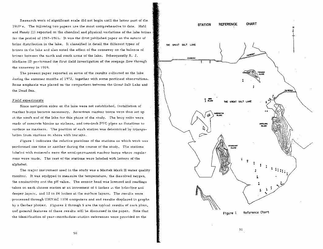
Research work of significant scale did not begin until the latter part of the

1960' s. The following two papers are the most comprehensive to date. Hahl

and Handy (l) reported on the chemical and physical variations of the lake brines

for the period of 1963-1966. It was the first published paper on the nature of

brine distribution in the lake. It classified in detail the different types of

brines in the lake and also noted the effect of the causeway on the balance of

brines between the north and south arms of the lake. Subsequently R. J.

Madison (2) performed the first field investigation of the seepage flow through

the causeway in 1969.

The present paper reported on some of the results collected on the lake

during the summer months of 1972, together with some pertinent observations.

Some emphasis was placed on the comparison between the Great Salt Lake and

the Dead Sea.

Field experiments

Since navigation aides on the lake were not established, installation of

marker buoys became necessary. Seventeen marker buoys were thus set up

at the south end of the lake for this phase of the study. The buoy units were

made of concrete blocks as sinkers, and two-inch PVC pipes as flotations to

surface as markers. The position of each station was determined by triangu­

lation from stations on shore with transits.

Figure 1 indicates the relative positions of the stations 011 which work was

performed one time or another during the course of the study. The stations

labeled with numerals were the semi-permanent marker buoys where regular

runs were made. The rest of the stations were labeled with letters of the

alphabet.

The major instrument used in the study was a Martek Mark II water quality

monitor. It was equipped to measure the temperature, the dissolved oxygen,

the conductivity and the pH value. The sensor head WaS lowered and readings

taken on each chosen station at an increment of 6 inches at the halocline and

deeper layers, and 12 to 24 inches at the surface layers. The results were

processed through UNIVAC 1108 computers and end results displayed in graphs

by a Gerber plotter. Figures 2 through 5 are the typical results of such plots,

and general features of these results will be discussed in the paper. Note that

the identification of year-month-date-station references were provided on the

50

STATION

il£ GREAT SALT LAKE

REFERENCE CHART

. ,

Tl£ GREAT SALT LAKE

Figure 1 Reference Chart

51

. ,

N

t

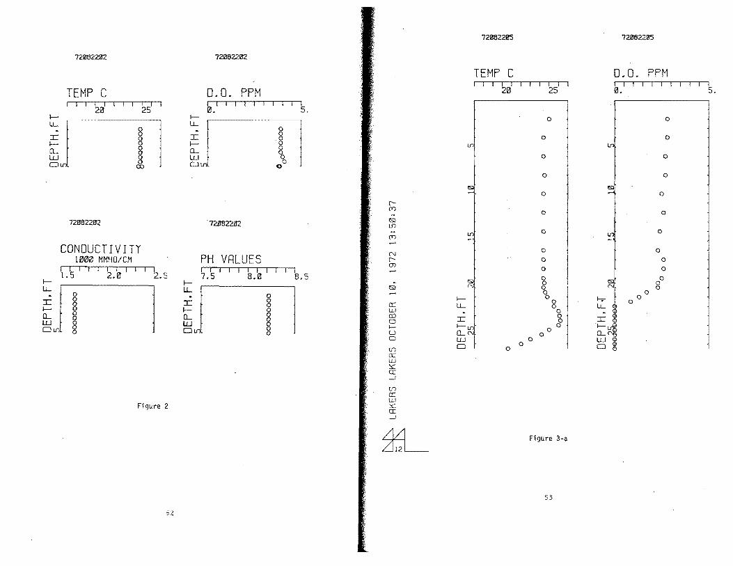
7211182202

TEMP C

f-

~J 7211182202

g 8 g g co

CONDUCTIVITY 1000 MMHO/CM

I J I I J ~ I I I I I 1.5 .0 2.5

f-LL . 0 :r: 0

0 f- 0 CL 0

0 w 0 0 o If) 0

Figure 2

52

f-LL . :r: f-CL w o If)

72082202

0.0. PPM I I I I I I 0.

. 721J82202

PH VALUES I I I I I I I 7.5 8.0

0 0 0 0 0 0 0 0 0

I I I I 5.

I 8.5

r-(T) .. 'Sl if) .. (T) ..... 0J r-CD ..... .

'Sl ..... a: LLJ t:D 0 I-u 0

If)

cc w ~ a: -1

7211182205 72082205

TEMP C 0.0. PPM I I I I I I I I I II I I I I

20 25 0. 5.

0 0

0 0

0 0

0 0

0 0

0 0

0 0

0 0

0 0

0 0

0 0 0 0 a 0 0 0 a I-;- a

0 0 0 LL

f-LL

0 a :r: 0 :r: 0 f-a CL 0

f-lf) CL

0 W 0 0 0

W 0

Figure 3-a

53

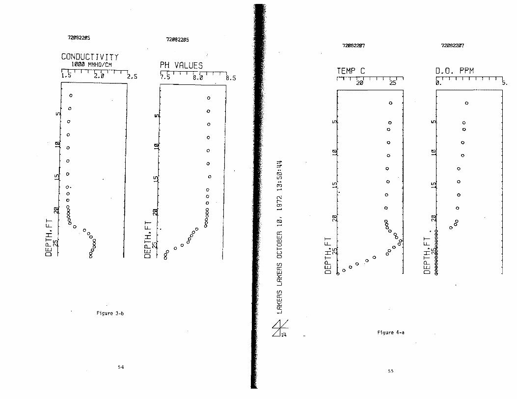
72082285 72082205 72082207 72082207

CONDUCTIVITY PH VALUES OrO. PPM

100" MMHO/CM TEMP C I ~ I I I I I I I I I I I I I I I I r I r

I I I I I I I I I I I i 2.0 2.5 7.5 8.0 8.5 r I I 0. 5.

1. 20 25

0 0 0 0

0 0

0 0 0 0

0 0 0

0 0 0

0 0

0 0

0 ::1'

0

0 ::1' 0 .. C'Sl 0 0 Lf'J

0 0 .. iii (T1 -' o· 0 ......

0 0 0 0 ("J

0 0 t-

O en

0

~ 8 ..... . cs;)

0 N 0 8 C'Sl

80

0 f- f- .....

0 u... 0 u...

00

0 0 a:: 'b

.. 0 .. :r: 00 :r: 0 LLI f-8 CO u... 0

f- 8 f- a 0 0.... (L- 0 I- • iii 0 0 <...) IN 0

W 8 w gO a f- 0 0 0

0 0.... 0 (f') w 0 a:: 0 0 LLI

.::s::: a:: ...J

(f')

a:: I.LJ .::s::: a::

Figure 3-b ...J

*- Figure 4-a

54 55

72.082207

CONDUCTIVITY 1000 MMHO/CM

ill I I I I I I I I L5 2.13 2.5

0

LI1 0

0

0

ISl 0

0

LI1 0 .....

0

0

ISl N 0

8 0

0 I- L

0 0

~ LI1[ a a

IN 0 0

t- . 0 (L

; 0 0

W 0 0 0

0

Figure 4-b

72082207

PH VALUES I I I I I I I ( I 7.5 8.13 8.5

o

o o

o

o

o

o

o

o

8 o o

72082212

TEMP C I I I I I

20

m LJ"'l .. (S;l LJ"'l .. en ..... ('\I e-m .....

(S;l :c ..... I-a: (L

\.tJ W en 0 0 l--U 0

LJ"'l a: \.tJ ~ a: ~

LJ"'l a: \.tJ ~ a: ~

~

I I 1 25

0

0

0

0

o

o o o o o o

80

0

0

o

Figure 5-a

57

72082212

D.O. PPM I I I I I I I I

0. 5.

0

0

0

0

0

0

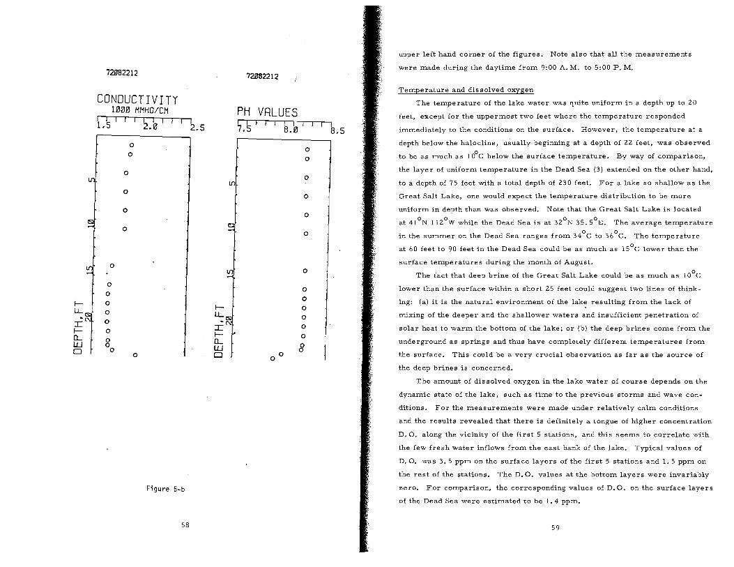
f-LL

I( f-0... W 0

72982212

CONDUCTIVITY 1000 MMHO/CM

I I I 1.5

0

0

0

0

0

0

0

0 0

0

o o

o

o

o

o

0

I I I 2.0

Figure 5-b

58

I 2.5

i-LLISI :iN f-0... w 0

72082212

PH VRLUES I I I I 7.5 8.0

0

0

0

0

0

0

0

0

0

0

0

0

0

00

8

I 8.5

upper left hand corner of the figures. Note also that all the measurements

were made during the daytime from 9:00 A. M. to S:OO P. M.

Temperature and dissolved oxygen

The temperature of the lake water was quite uniform in a depth up to 20

feet, except for the uppermost two feet where the temperature responded

immediately to the conditions on the surface. However, the temperature at a

depth below the haloc1ine, usually beginning at a depth of 22 feet, was observed

to be as much as 100

e below the surface temperature. By way of comparison,

the layer of uniform temperature in the Dead Sea (3) extended on the other hand,

to a depth of 75 feet with a total depth of 230 feet. For a lake so shallow as the

Great Salt Lake, one would expect the temperature distribution to be more

uniform in depth than was observed. Note that the Great Salt Lake is located

at 410

N 1120

W while the Dead Sea is at 320

N 3S. SOE. The average temperature

in the summer on the Dead Sea ranges from 340

e to 360e. The temperature

at 60 feet to 90 feet in the Dead Sea could be as much as lSoe lower than the

surface temperatures during the month of August.

The fact that deep brine of the Great Salt Lake could be as much as 100e

lower than the surface within a short 25 feet could suggest two lines of think­

ing: (a) it is the natural environment of the lake resulting from the lack of

mixing of the deeper and the shallower waters and insufficient penetration of

solar heat to warm the bottom of the lake; or (b) the deep brines come from the

underground as springs and thus have completely different temperatures from

the surface. This could be a very crucial observation as far as the source of

the deep brines is concerned.

The amount of dis solved oxygen in the lake water of course depends on the

dynamic state of the lake, such as time to the previous storms and wave con­

ditions. For the measurements were made under relatively calm conditions

and the results revealed that there is definitely a tongue of higher concentration

D. O. along the vicinity of the first S stations, and this seems to correlate with

the few fresh water inflows from the east bank of the lake. Typical values of

D. O. was 3. S ppm on the surface layers of the first S stations and 1. S ppm on

the rest of the stations. The D. O. values at the bottom layers were invariably

zero. For comparison, the corresponding values of D. O. on the surface layers

of the Dead Sea were estimated to be 1.4 ppm.

59

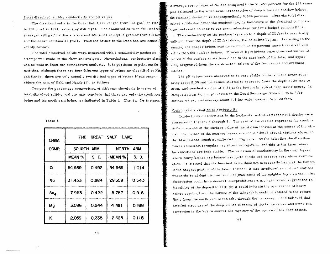
Total dissolved solids, conductivity and pH values

The dissolved salts in the Great Salt Lake ranged from 324 gm/l

to 170 gm/l in 1971, averaging 230 mg/I. The dissolved salts in the Dead

averaged 290 gm/l at the surface and 326 grn/l at depths greater than 300

and the ocean contains 35 gm/l. Thus the brines in the Dead Sea are consid­

erably denser.

The total dissolved solids were measured with a conductivity probe; no

attempt was made on the chemical analysis. Nevertheless, conductivity

can be used at least for comparative analysis. It is pertinent to point out the:

fact that, although there are four different types of brines as clas sHied by

and Handy, the re are only actually two distinct types of brines if one recon­

siders the data of Hahl and Handy (1), as follows:

Compute the percentage composition of different chemicals in terms of

total dissolved solids, and one may conclude that there are only the south arm,

brine and the north arm brine, as indicated in Table 1. That is, for instance,

Table L

CHEM. THE GREAT SALT LAKE

COMPo SOURTH ARM NORTH ARM

MEAN % S. D. MEAN % S. D.

CI 54.939 0.492 54.569 1.014

No 31.453 0.684 29.558 0.543

S04 7.963 0.422 8.757 0.916

Mg 3.586 0.244 4.491 0.168

K 2.059 0.235 2.625 0.118

60

if average percentages of Na are computed to be 31.453 percent for the 155 sam­

ples collected in the south arm, irrespective of deep brines or shallow brines,

the standard deviation is correspondingly 0.684 percent. Thus the total dis

solved solids and hence the conductivity, is indicative of the chemical composi­

tions and could be used to our great advantage for ionic budget computations.

The conductivity on the surface laye r up to a depth of 22 feet is practically

uniform; from the depth of 22 feet down, the halo cline begins. According to the

results, the deeper brines contain as much as 50 percent more total dissolved

solids thaI) the surface brines. Traces of light brines were observed within 12

inches of the surface at stations close to the east bank of the lake, and appar­

ently originated from the fresh water inflows of the few creeks and drainage

ditches.

The pH values were observed to .be very stable on the surface layer aver-

aging about 8.30 and the values started to decrease from the depth of 20 feet on

down, and reached a value of 7.65 at the bottom in typical deep water zones. In

comparison again, the pH values in the Dead Sea range from 6. 1 to 6.7 for

surface water, and average about 6.2 for water deeper than 120 feet.

Conductivity distributions in the horizontal extent at pres cribed depths were

presented in Figures 6 through 8. The area of the circles represent the conduc­

tivity in excess of the surface value at the station located at the center of the cir­

cle. The brines of the surface layers are more diluted around stations closer to

the Silver Sands Beach as indicated in Figure 5. At the ha10cline th.e distribu­

tion is somewhat irregular, as shown in Figure 6, and this is the layer where

the conditions are less stable. The variation of conductivity in the deep layers

where heavy brines are located are quite subtle and deserve very close examin­

ation. It is found that the heaviest brine does not necessarily berth at the bottom

of the deepest portion of the lake. Instead, it was monitored around two stations

where the total depth is two feet les s than some of the neighboring stations. This

observation could have several interpretations; e. g., (a) it could suggest the re­

dissolving of the deposited salt; (b) it could indicate the occurrence of heavy

brines seeping from the bottom of the lake; (cl it could be related to the return

flows from the north arm of the lake through the causeway. It is believed that

detailed structure of the deep brines in terms of the temperature and brine con­

centration is the key to answer the mystery of the source of the deep brines.

61

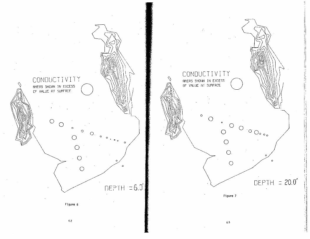
CONDUCTIVITY AREAS SHOWN IN EXCESS 0 OF VALUE RT SURFRCE

Figure 6

62

DEPTH· 6.0'

CONDUCTIVITY

o

DEPTH = 20.0'

Figure 7

63

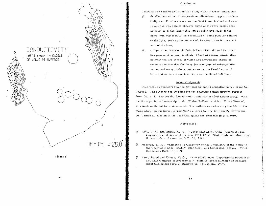
CONDUCTIVITY RRERS SHOWN IN EXCESS OF VRLUE RT SURFRCE

Figure 8

64

o

o

o

o PTH 25.0'

There are two major points in this study which warrant emphasis:

(1) detailed structure of temperature, dissolved oxygen. conduc­

tivity and pH values were for the first time obtained and as a

result one was able to observe some of the very subtle char­

acteristics of the lake water; more extensive study of the

same kind will lead to the revelation of some puzzles related

to the lake, such as the source of the deep brine in the south

arm of the lake;

(2) comparative study of the lake between the lake and the Dead

Sea proved to be very fruitful. There are many similarities

between the two bodies of water and advantages should be

taken of the fact that the Dead Sea was studied substantially

more, and many of the experiences on the Dead Sea could

be useful to the research workers on the Great Salt Lake.

Acknowledgments

This work is sponsored by the National Science Foundation under grant No.

GA3086. The authors are indebted for the abundant administrative support

from Dr. J. E. Fitzgerald, Department Chairman of Civil Engineering. With­

out the superb craftsmanship of Mr. Blaine Fullmer and Mr. Toney Howard,

this work would not ha\'e succeeded. The authors are also very thankful to the

many useful dis cussions and comments offered by Dr. William P. Hewitt and

Dr. James A. Whelan of the Utah Geological and Mineralogical Survey.

(1 )

References

Hah!, D. C. and Handy, A. H., "Great Salt Lake, Utah - Chemical and Physical Variations of the Brine, 1963-1966". Utah GeoI. and Mineralog. Survey, Water Resources Bull. 12. 1969.

(2) Madison. R. J., "Effects of a Causeway on the Chemistry of the Brine in the Great Salt Lake, Utah. II Utah Geo!. and Mineralog. Survey, Water Resources Bull. 14, 1970.

(3) Neev, David and Emery, K. 0., "The DEAD SEA: Depositional Processes and Environments of Evaporites," State of Israel Ministry of Develop ment Geological Survey, Bulletin 41, Jerusalem, 1967.

65

COMMUNITY STRUCTURE AND ECOSYSTEM ANALYSIS OF THE GREAT SALT LAKE

D. W. Stephens and D. M. Gillespie l

Abstract

Salt L T;e construc~ion of an earthfill cau·seway across the Great Th a e resulted m development of two basins within the lake

,e no~thern basin supports a depauperate biota consistin . ~rlma~11Y of an alga, Dunaliella salina, several protozoa g and ~ctena. The southern basin exhibits two energy flow 't

,,:'th only minor interactions: The planktonic system wi:~sa ems sIngle phytoplankter, (Dunaliella viridis) and a singl plankter, (Artemia,salina); and a ~c' system of bl::

oo-

alga (Coccochloris ~s), detritis, and brine fly larv~!reen (Ephydra). The only outflow from either t ' b' d sys em occurs when Ir .5 feed upon the shrimp or fly larvae. The Dunaliella 0

ulatlOn seems ,to be limited early in the calendar year by t~x!.=

f:~~l:O~i/~I:~~dxhf;lili~~~~~e~~r~::~~Sit:e~~~~i:!t:oPI::: ~~~~lation x Iter OCcurs in May d J . an une as a consequence of the

rapidly e~andin~ Artemia salina pOpulation. Theavailabilit of the nutnents nitrogen and phosphorous d t y

l ' 't' oes no seem to be a Iml lng factor for Dunaliella.

KEY WORDS: Ecosystem; Brine shrimp; Artemia salina' Dunaliella; Energy flow; Plankton. ---'

The Great Salt Lake is a prime example of an extremely rigorous environ_ ment. Due to its shallownes s « 9 ) h om, t e temperature ranges from· freezing to

near 40 C over a yea I t' . r s Ime Interval. Coupled with thO . th

IS 1S e topography of the surrounding area which drains most waters

in the Bonneville Basin into the

lake. Anything soluble in water or capable of transport by water is carried to

the lake, including partially treated sewage

ties from Spanish Fork to Logan. and industrial wastes of communi_

The more hostile and demanding the environ­ment, the fewer are the types of organisms which are

capable of inhabiting it. In fact, the existance of relatively few types

of organisms but large numbers of them in a body of water is . currently used by some as an indicator of a special_

Ized or a polluted system. The lake superficially appears as a grossly polluted

system but one relativel bl f '. Y capa e 0 self perpetuation because of the adaptations

of the blOta Within it.

of Biology, University of Utah, Salt Lake City, 84112.

66

It is very fortunate for the communities bordering the lake that three

large sewage lagoons exist to partially stabilize the wastes which are discharged

into the lake. These lagoons, Bear River Bay and Ogden Bay, which receive

drainage waters fr0D?- the northern section of the Bonneville Basin, and Farming­

ton Bay, receiving southern basin waters, effectively oxidize much of the

organic material produced by the human communities along the Wasatch Front

and thereby reduce the loading that would be placed on the Great Salt Lake.

The lake is very susceptible to changes brought about by man because it

is such a simple ecosystem. The construction of the railroad causeway in 1957

resulted in the division of Great Salt Lake into north ,:-nd south basins, creating

ecologically two separate lakes due to salinity imbalance. Due to inflow and

evaporation characteristics, there is a net migration of water and salts to the

northern basin where the brine remains at or near saturation most of the time.

The salinity problem was first reported by T. C. Adams in 1964.

The extremely harsh environment of the north end results in a very simple

ecosystem consisting basically of the alga, Dunaliella Teodoresco, several

protozoa, and bacteria. Visual comparisons of the north versus the south end

show the pink color of northern basin waters to be due to the large number of the

alga. Q. salina which possesses a red pigment.

The southern portion of the lake is slightly less saline and therefore is not

quite as rigorous an environment as the north. This fact is evident in looking

at the ecosystem which has developed. There are two basic biotic systems

operating in the southern portion: a planktonic system consisting of the alga

Dunaliella Teodoresco, brine shrimp Artemia salina (L.), and several

protozoa and bacte ria (Figure 1); and a benthic sequence consisting of the blue­

green alga Coccochloris elebans Drout and Daily, detritis, and the brine flies

Ephydra spp. (Figure 2). The two systems are linked in that brine fly larvae

will feed on detritis consisting of dead Dunaliella and Artemia, and Artemia

will feed on the blue-green alga and shrimp fec;!.l pellets when Dunaliella pop­

ulations decline. The only outflow from either system occurs when birds (pri­

marily gulls, Larus spp.) feed upon the brine shrimp or brine flies and when the

brine flies emerge and leave the lake.

In any balanced ecosystem, there must be factors which limit the excess

growth of constituent populations. In most systems the availability of nutrients

acts as the controlling device. Our work with the large populations of Dunaliella

67

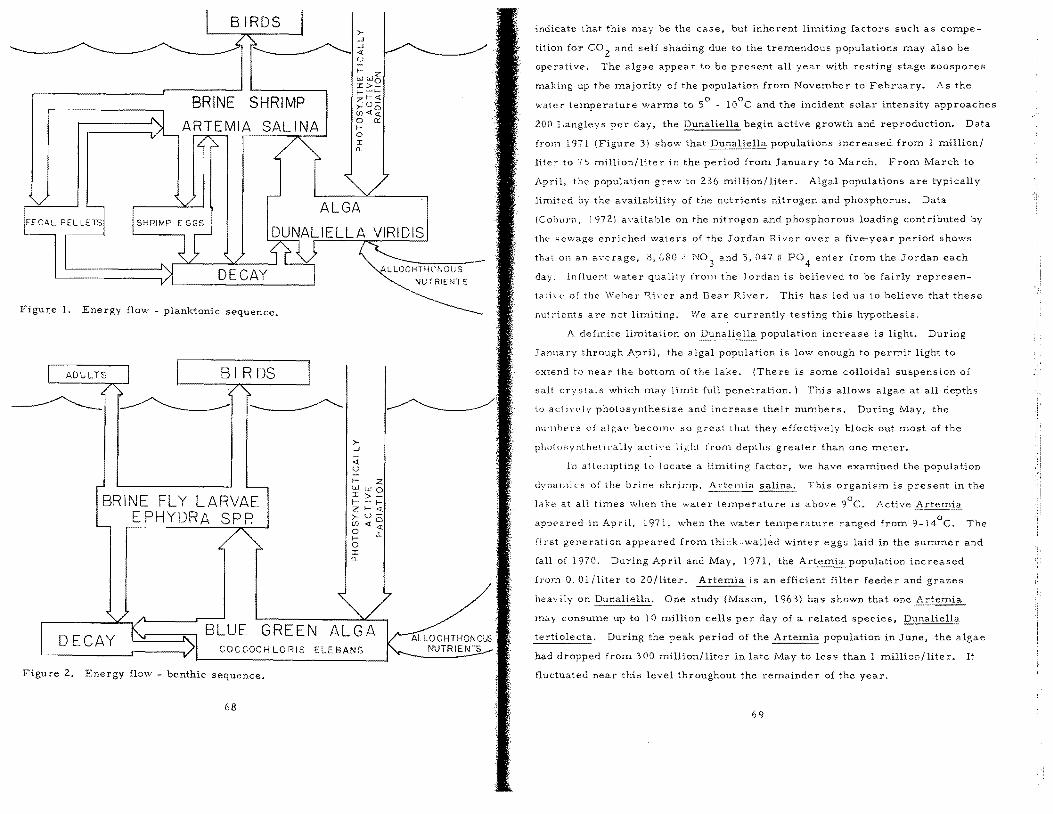
BRINE SHRIMP

SALINA

Figure 1. Energy flow - planktonic sequence.

BRINE FLY LARVAE E PHYDRA SP P.

BLUE GREEN COCCOC H LO RIS

Figure 2. Energy flow benthic sequence.

68

>­-' -' <l: ()

>­-' ..J « U

ALLOCHTHCNOUS NUTRIENT S

I- Z

indicate that this may be the case, but inherent limiting factors such as compe­

tition for eo 2 and self shading due to the tremendous populations may also be

operative. The algae appear to be present all year with resting stage zoospores

making up the majority of the population from November to February. As the

water temperature warms to - lOoe and the incident solar intensity approaches

200 Langleys per day, the Dunaliella begin active growth and reproduction. Data

from 1971 (Figure 3) show that Dunaliella populations increased from 1 million/

liter to 75 million/liter in the period from January to March. From March to

April. the population grew to 236 million/liter. Algal populations are typically

limited by the availability of the nutrients nitrogen and phosphorus. Data

(Coburn, J 972i available on the nitrogen and phosphorous loading contributed by

the sewage enriched waters of the Jordan River over a five-year period shows

that 011 an aycrage, is, (,80 ,; N03

and 3,047 Ii PO 4 enler [rom the Jordan each

day. Influent water quality from the .J orclan is believed to be fairly represen­

lathe of the' Weber Rher and l3ear River. This has led us to believe that these

nutrients are not limiting. We are currently testing this hypothesis.

A definite limitation on Dunaliella population increase is light. During

January through April, the algal population is low enough to permit light to

extend to near the bottom of the lake. (There is some colloidal suspension of

salt crystals which may limit full penetration.) This allows algae at all depths

to a<:th"c']y photosynthesize and increase their numbers. During May, the

numbers of algal' become so great that they effectively block out most of the

photo"ynthe(il"ally acti,·" lighl ["1'0111 depths greater than one meter.

In alt"mpting to locate a limiting [actor, we have examined the population

dynamics of the brine shrimp, ATtemia salina. This organism is present in the

lake at all times when the water temperature is above 90

C. Active Artemia

appeared in Ap ril. 1971, when the water temperature ranged from 9- 140

C. The

first generation appeared from thick-wall~d winter eggs laid in the summer and

fall of 1970. During April and May, 1971. the =c...:...::.;:.:.;.=population increased

from O. Ol/liter to 20/liter. _.:.-'-'-.-'.--- is an efficient filter feeder and grazes

heavily on ____ _ One study (Mason, 1963) has shown that one Artemia

may consume up to 10 million cells per day of a related species, Dunaliella

tertiolecta. During the peak period of the =::..;;.;:== population in June, the algae

had dropped from 300 million/liter in late May to less than 1 million/liter. It

fluctuated near this level throughout the remainder of the year.

69

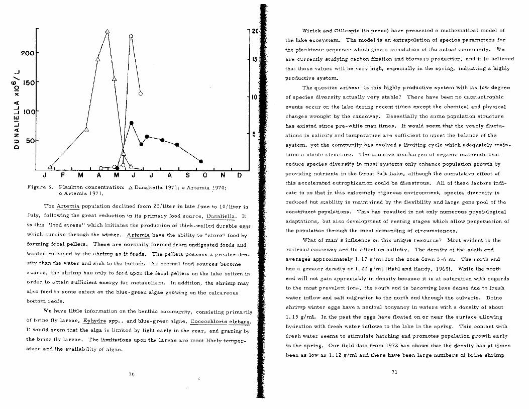
200

...J ........

150 CD 52 )(

« ...J ...J 100 IJJ ..J « z ::> 50 o

J F M o N

Figure 3. Plankton concentration: t:;. Dunaliella 1971; 0 Artemia 1970; o Artemia 1971.

o

The Artemia population declined from 20/liter in late June to la/liter in

July, following the great reduction in its primary food source, Dunaliella. It

is this "food stress" which initiates the production of thick-walled durable eggs

which survive through the winter. Artemia have the ability to "store" food by

forming fecal pellets. These are normally formed from undige~ted foods and

wastes released by the shrimp as it feeds. The pellets pos ses s a greate r den­

sity than the water and sink to the bottom. As normal food sources become

scarce, the shrimp has only to feed upon the fecal pellets on the lake bottom in

order to obtain sufficient energy for metabolism. In addition, the shrimp may

also feed to some extent On the blue-green algae growing on the calcareous

bottom reefs.

We have little information on the benthic community, consisting primarily

of brine fly larvae, Ephydra spp., and blue-green algae, Coccochloris ---'-.;....c...;....c..~ "

It would seem that the alga is limited by light early in the year, and grazing by

the brine fly larvae. The limitations upon the larvae are most likely temper­

ature and the availability of algae.

70

15

5

Wirick and Gillespie (in press) have presented a mathematical model of

the lake ecosystem. The model is an extrapolation of species parameters for

the planktonic sequence which give a simulation of the actual community. We

are currently studying carbon fixation and biomass production, and it is believed

that these values will be very high, especially in the spring, indicating a highly

productive system .

The question arises: Is this highly productive system with its low degree

of species diversity actually very stable? There have been no catatastrophic

events occur on the lake during recent times except the chemical and physical

changes wrought by the causeway. Essentially the same population structure

has existed since pre-white man times. It would seem that the yeady fluctu­

ations in salinity and temperature are sufficient to upset the balance of the

system, yet the community has evolved a limiting cycle which adequately main­

tains a stable structure. The massive discharges of organic materials that

reduce species diversity in most systems only enhance population growth by

providing nutrients in the Great Salt Lake, although the cumulative effect of

this accelerated eutrophication could be disastrous. All of these factors indi­

cate to us that in this extremely rigorous environment, species diversity is

reduced but stability is maintained by the flexibility and large gene pool of the

constituent populations. This has resulted in not only numerous physiological

adaptations, but also development of resting stages which allow perpetuation of

the population through the most demanding of circumstances.

What of man's influence On this unique resource? Most evident is the

railroad causeway and its effect on salinity. The density of the south end

averages approximately 1. 17 g/ml for the zone down 5-6 m. The north end

has a greater density of 1. 22 g/ml (Hah1 and Handy, 1969). While the north

end will not gain appreciably in density because it is at saturation with regards

to the most prevalent ions, the south end is becoming less dense due to fresh

water inflow and salt migration to the north end through the culverts. Brine

shrimp winter eggs have a neutral bouyancy in waters with a density of about

1.15 g/ml. In the past the eggs have floated on or near the surface allowing

hydration with fresh water inflows to the lake in the spring. This contact with

fresh water seems to stimulate hatching and promotes population growth early

in the spring. Our field data from 1972 has shown that the density has at times

been as low as 1. 12 g/rnl and there have been large numbers of brine shrimp

71

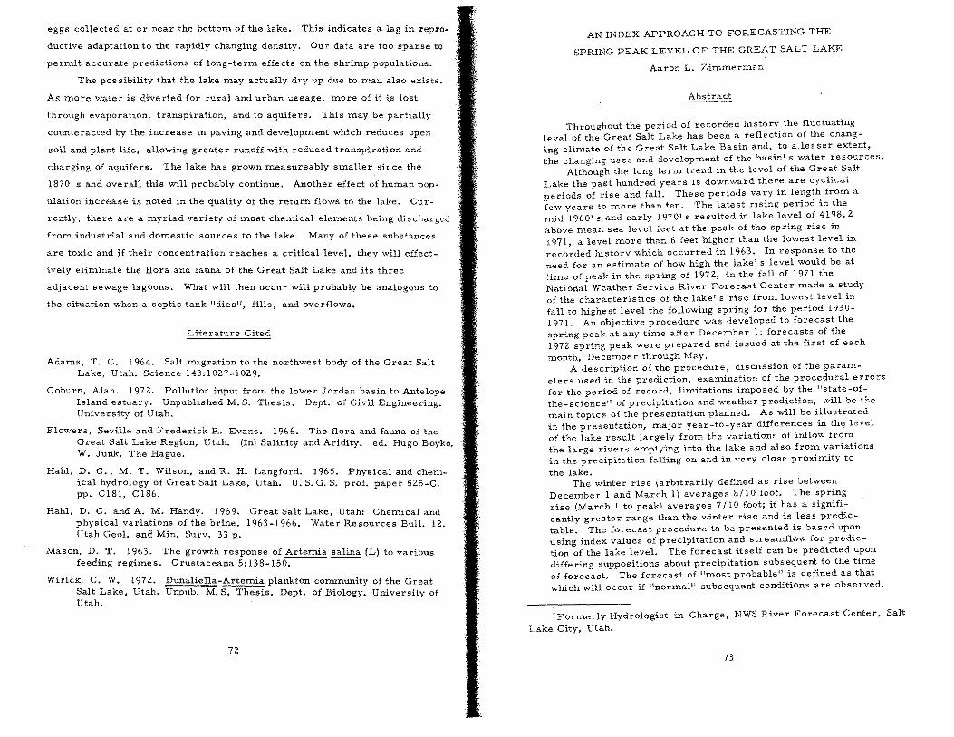
eggs collected at or near the bottom of the lake. This indicates a lag in repro­

ductive adaptation to the rapidly changing density. Our data are too sparse to

permit accurate predictions of long-term effects on the shrimp populations.

The possibility that the lake may actually dry up due to man also exists.

As more water is diverted for rural and urban ,useage, more of it is lost

through evaporation, transpiration, and to aquifers. This may be partially

counteracted by the increase in paving and development which reduces open

soil and plant life, allowing greater runoff with reduced transpiration and

charging of aquifers. The lake has grown measureably smaller since the

1870' s and overall this will probably continue. Another effect of human pop­

ulation increase is noted in the quality of the return flows to the lake. Cur­

rently, there are a myriad variety of most chemical elements being discharged

from industrial and domestic sources to the lake. Many of these substances

are toxic and if their concentration reaches a critical level, they will effect­

ively eliminate the flora and fauna of the Great Salt Lake and its three

adjacent sewage lagoons. What will then occur will probably be analogous to

the situation when a septic tank "dies", fills, and overflows.

Adams, T. C. 1964. Salt migration to the northwest body of the Great Salt Lake, Utah. Science 143:1027-1029.

Coburn, Alan. 1972. Pollution input from the lower Jordan basin to Antelope Island estuary. Unpublished M. S. Thesis. Dept. of Civil Engineering. University of Utah.

Flowers, Seville and Frederick R. Evans. 1966. The flora and fauna of the Great Salt Lake Region, Utah. (In) Salinity and Aridity. ed. Hugo Boyko, W. Junk, The Hague.

Hahl, D. C., M. T. Wilson, and R. H. Langford. 1965. Physical and chem­ical hydrology of Great Salt Lake, Utah. U. S. G. S. prof. paper 525-C. pp. C181, C186.

Hahl, D. C. and A. M. Handy. 1969. physical variations of the brine, Utah Geol. and Min. Surv. 33 p.

Great Salt Lake, Utah: Chemical and 1963-1966. Water Resources Bull. 12.

Mason, D. T. 1963. The growth response of Artemia salina (L) to various feeding regimes. Crustaceana 5:138-150.

Wirick, C. W. 1972. Dunaliella-Artemia plankton corrununity of the Great Salt Lake, Utah. Unpub. M. S. Thesis. Dept. of Biology. University of Utah.

72

AN INDEX APPROACH TO FORECASTING THE

SPRING PEAK LEVEL OF THE GREAT SALT LAKE 1

Aaron L. Zimmerman

Abstract

Throughout the period of recorded history the fluctuating level of the Great Salt Lake has been a reflection of the chang-ing climate of the Great Salt Lake Basin and, to a,les ser extent, the changing uses and development of the basin's water resources.

Although the long term trend in the level of the Great Salt Lake the past hundred years is downward there are cyclical periods of rise and fall. These periods vary in length from a few years to more than ten. The latest rising period in the mid 1960' s and early 1970' s re suIted in lake level of 4198. Z above mean sea level feet at the peak of the spring rise in 1 97 1, a level more than 6 fe et highe r than the lowe st level in recorded history which occurred in 1963. In response to the need for an estimate of how high the lake's level would be at time of peak in the spring of 1972., in the fall of 1971 the National Weather Service River Forecast Center made a study of the characteristics of the lake's rise from lowest level in fall to highest level the following spring for the period 1930-1971. An objective procedure was developed to forecast the spring peak at any time after December 1; forecasts of the 1972 spring peak were prepared and issued at the first of each month, December through May.

A description of the procedure, discussion of the param­eters used in the prediction, examination of the procedural errors for the period of record, limitations imposed by the "state-of­the-science" of precipitation and weather prediction, will be the main topics of the presentation planned. As will be illustrated in the presentation, major year-to-year differences in the level of the lake result largely from the variations of inflow from the large rivers emptyi.ng into the lake and also from variations in the precipitation falling on and in very close proximity to

the lake. The winter rise (arbitrarily defined as rise between

December 1 and March 1) averages 8/10 foot. The spring rise (March 1 to peak) averages 7/10 foot; it has a signifi-cantly greater range than the winter rise and is less prediC­table. The forecast procedure to be presented is based upon using index values of precipitation and streamflow for predic­tion of the lake level. The forecast itself can be predicted upon differing suppositions about precipitation subsequent to the time of forecast. The forecast of "most probable" is defined as that which will occur if "normal" subsequent conditions are observed.

IFOrmerly Hydrologist-in-Charge, NWS River Forecast Center, Salt

Lake City, Utah.

73

The fluctuations in the level of the Great Salt Lake from year to year are

in a large measure a reflection of the varying annual precipitation falling in

the Great Salt Lake Basin (Peck and Richardson, 1966). The cyclical char~

acteristics of the past rising and falling trends in the lake level have provided

a continuing source of speculation about the future. However, past weather~

related cyclical variations, unfortunately, are too unreliable to be of much

value in predicting when the cycle will change. Since 1969, when a major

seasonal rise of 2.9 feet brought the lake level up to 4197 feet above mean

sea level for the first time since 1958, there has been an increasing interest

in the present upward rise which began in the early 1960' 6. In mid~May 1972

the lake level reached 4199. 7 feet, highest since 1953. The recent high levels

of the lake are affecting lakeshore resort owners, the maintenance of the

Antelope Island road, and the efficient operation of evaporation ponds along

the lake's periphery.

While weather prediction in the time frame of the next several months is

presently beyond the state of the science of meteorology, a large part of the

inflow to the Great Salt Lake lags behind the precipitation occurrence. This

allows some predictive time in anticipating the magnitude of the seasonal (low

point in fall to high point in spring) rise.

Methods for predicting the peak spring lake level have been developed in

the past, but to the author's knowledge have been used very little (Peck, 1954).

The procedure outlined in this paper can be best described as an "index"

approach to prediction. There is no reason to believe that the method repre~

sents the best index, because only limited exploration of all the past available

data was made. But, the obvious relationships between precipitation on and

near the lake and lake level, and between surface inflow to the lake and lake

level are treated in time intervals which allow prediction of the high spring

lake level, with reasonable accuracy, by December 1. The take~off point for

the prediction of a following spring's high lake level is the low point the pre~

ceding fall. The rise from low point in fall, usually about November 1, to

high in spring, usually around June 1, is arbitrarily divided into three periods:

(1) the fall rise (lowpoint to December 1), (2) the winter rise (December 1 to

March 1), and (3) the spring rise (March 1 to high point). The period of study

for the predictive procedure is from 1931~1971. The procedure was used to

predict the spring high level in 1972, with good results.

74

The fall change in the lake level is quite highly correlated with fall precipi­

tation (September through November) on the lake and in its immediate vicinity

(Figure 2). The fall change averages less than. 2 foot rise for the 42-year

period (1931-71); it has equalled or exceeded. 3 foot in twelve of these years,

with the maximum fall rise of • 6 foot in 1971, or wate r year 1972.

The winter rise, December 1 to March 1, has averaged. 8 foot in the 42-

year period, ranging from a low of .3 foot in 1933 and 1955 to 1.5 feet in 1969.

The winter rise has equalled or exceeded 1.0 foot in ten years and has been

less than. 5 foot in only six years. The average winter rise in the three-month

pe riod December 1 to March 1 represents almost one -half of the average total

seasonal rise of 1. 7 feet. The winter rise is quite highly correlated with fall

and winter precipitation in the lake area, and the lower limits of the winter

rise are highly correlated with the fall streamflow on the lower Bear River,

the major winter contributor to river inflow to the lake. Figures 3 and 4 illus­

trate these correlations.

The spring rise, March 1 to peak, has averaged. 7 foot in the 42-year

period and it is quite highly correlated with the March-June runoff from the

major rivers feeding the lake and with spring precipitation. The range of the

spring rise is large, from zero in two years (no rise after March 1) to 2.1

feet in 1964, and 1. 0 foot or more in twelve years. During June 1964 and 1967

a rise of .7 foot occurred. These were the wettest Junes in weather history in

the vicinity of the lake, indicating the major effect from excessive rains in late

spring. Figures 5 and 6 illustrate the spring rise correlation with both March­

June runoff into the lake from the major rivers and spring precipitation, March­

June.

Perhaps the most valuable index tool for forecasting the winter rise in the

Great Salt Lake stems from the hydrologic characteristics of the Lower Bear

River Basin. The Bear contributes, on the average, about 75 percent of the

surface runoff into Great Salt Lake during the winter season. Unlike most of

the rivers flowing into Great Salt Lake it has a relatively high winter flow.

For example, at Colliston the four-month November~February average flow

for the 42-year (1931-71) period is 305,000 acre-feet, which is about 70 per­

cent of the total which occurs in the four-month spring runoff period, March­

June. By contrast on the Weber near Plain City the November-February flow

is only 33 percent of the March~June flow and in the Six Creeks near Salt Lake

75

..... .....

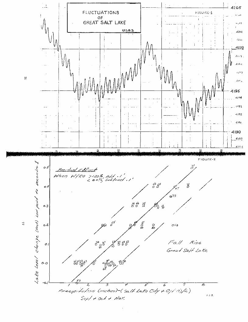
..... 0'

\'i t ~

?,., '\ ~J

~ { \.. '~

'\ \ ~

~ ~ ~ ~)

~ 0;:-~

'~ I:;

"-~ ~

~ ~ ~

l-----;-,---------'---­FLUCTUATIONS FiGVi~E'l

~A I L"l v v ~ l I: . , ._j 1/ \ I . .

. -I

!

OF GREAT SALT LAKE

U.S.G.S.

~. I )jWfll ., 1/\ '~i --~~I~Hli~IH--Ir'+H 'G

--- ._, IH''' II H +l+jV _ : u

0.5

0.1

0·3

0.2..

a./

0·0

I I

I

-~ <>

fie~N!oo/EM."c/

I

o ,'.'"

#'3en j1/YRo »/zoJ{..1 /9c/c/ • / / . ..( e $'.d.6 "?"t".:Zc/ . / '

/ / :3'1I/b 3$ 6' (£) Q

~

/ /

/'

~z /;1

ijll

<> .-.--~ ,~.

FIGU!<.E-2.

7/ 0/

/. / /

0

73/ ./

/ /f ;5"

Q

(£)~ )f 311J3 5t-

ly oh3

ra// 8/5e

G,...e::z -/ Slz// A""e

/ ~4itJ'~b' (;0 0j?r:-

.' ,0 :" 0/6)() o 4~01iJP.jOO ~

b~ 5f) '?;1..-

, / ~3 / -0./ I 0 Z 3 ;;; .5" 6- --7-----:8---

~r-e.cfO/~A~I,? (//1C-7e5)-{ So..// /a.~~ C;,f- r- 0-1/"?)fl)

S~jC/ ~ Oc/ y //0/':" ;. 1..1..

~

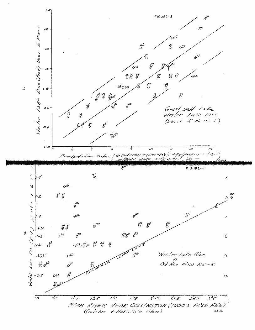
...... CfJ

......

'"

~

" " .~ , .' \

\i .:, '\

(! ". 'I.

... ~

'" ~

/.6

"-~ I.~ :s: ~ ~

t..!!

"-\J

~ '0, ~ 1.0

~ ~ ~ ~ o.a

~ ~ a6

~ ~ at'

,0, .e. 5

,,1 Q

.6O,'35

of k~ -bQ

bZ­Q

FIGURE-3 J9

/"'1 /' . // /eP f

./ tJ c:PZ

/'

/

d.:2- .// f! /

~ 0 f/ 5bf"} .

CJbb 3t>~:,2...-50 fgGJ (') / 1/~1: b~

/ #0':- 0

. '?f 59 (,0 o

4t!1 (j).

/,

.If] ~1

1;.3 (7) 61

~4 Il / / 6~"'>"J

(l)o

?.....-ec-30/h k~-? ..L . .-?cye~-::::

1/ (,)

Qb6

l' J/-f . G)

.j2J Ii)

(,)5h (l)if7

#tJ 1/-8 010 50

0@ E)

(,)tf5 GJB ~ IS

0 51 rJ35q f!~ ~ ~ ,(f'

'" 0/;,"J ~'-' I/e-,n (,)

I/lI B

Y '],,1 f)

U3 (9

C /-'<::0/ Sc?-// ,-C,,;{ d"-e Yll//;1k,'" L 4' ,I::." /:?s::-

(Dec, / /7,.: ..... - ,~; /')

/,z 13

.c//:~,,) A

FIGVRE-4

/

7)0" j" ~

~:/' .

'0//'

5.2-(,)

(:)/ ./'/ /

c

W//7/C"r &se o P':F

a:/-:;4Iop ..6i'c.J,~ R:

0..( I!)bf 0,

,--.-.. -'"'""T.-----c', £50 ,275 .

8EA/f'R/,YE/f' Al'F,4£" Cou./.lVSro# (/000 IS 4(1££ ~[:f:!T. (Ock~-:'r -/ . .I'Ior.".·~'£;·:'" ",.c/orv) A.Li',

2..0

'.8

1.6

1.4

.?- c "I

/'

0 .,

SPRING LAKE RISE VS.

~;; f'vlAR-J'\JNE RUNOFF

(BEAR .. vJEBER)

0",'1

r.

o <-4 /0.0

0 43

FIGURE-5

CO 0 51 1Z. lib

!.;; °'70 '% Iv1AR.-JCNE R.C. (51-7oMe) BEAR R.i' \..J£BtOR R.

</0 [',0 12e I?o 2.(.(.> 24D 280 _' ..

80

z 0

t> ..., 0'" ."" l-

e:( "" 0

() 'n ~ 0

U.

... ~

-0:: UJ > UJ (f)

a: Ul ~ .q: .J

(J)

Z ex:: Q.. (j)

1..

t-- '" Q'" o'l-

<:l"- "-... '" 0 0

~ ";l-

0

'" ..!}

o~ •

1:)

"" '" '" ci~'" 0'"

81

;:.. 0

:;, N

'" ....

.... 00 I '" ;;, ....

0' ~ ;; .... ;; ~

<ll II!

E ..... II!

0

E f.<

""' 0 01) f.< .... l': ....

M 01)

l': l': 'Q, <Ii

.::: ... oj Ul ... II! ..... Ul <)

] ... .... 0

<)

0- Il!

'"'" ..... .0 ... ::l

<Ii 0 q q

"'''' "'-" <*

• 0 ~

o 0""

o ....

t\I IU ......: u)

oc <.!) z c::: a. c: <.r) ....

Q UJ

& w III

8 (J

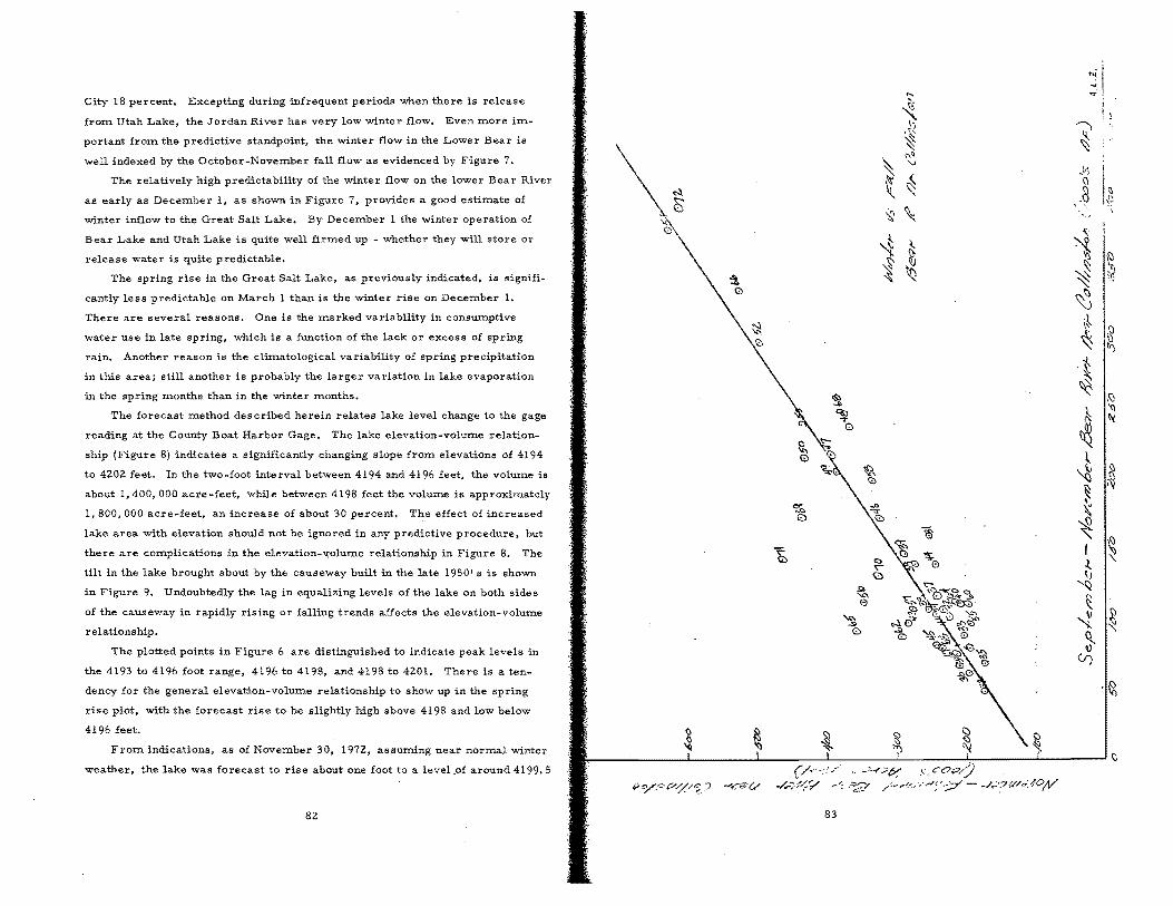
City 18 percent. Excepting during infrequent periods when there is re.1ease

from Utah Lake, the Jordan River has very low winter flow. Even mOre im­

portant from the predictive standpoint, the. winter flow in the Lower Bear is

well indexed by the October-November fall flow as evidenced by Figure 7.

The relatively high predictability of the winter flow on the lower Bear River

as early as December 1, as shown in Figure 7, provides a good estimate of

winter inflow to the Great Salt Lake. By December 1 the winter operation of

Bear Lake and Utah Lake is quite well firmed up - whether they will store or

release water is quite predictable.

The spring rise in the Great Salt Lake, as previously indicated, is signifi­

cantly less predictable on March 1 than is the winter rise on December 1.

There are several reasons. One is the marked variability in consumptive

water use in late spring, which is a function of the lack or excess of spring

rain. Another reason is the climatological variability of spring precipitation

in this area; still another is probably the larger variation in lake evaporation

in the spring months than in the winter months.

The forecast method described herein relates lake level change to the gage

reading at the County Boat Harbor Gage. The lake elevation-volume relation­

ship (Figure 8) indicates a significantly changing slope from elevations of 4194

to 4202 feet. In the two-foot interval between 4194 and 4196 feet, the volume is

about 1,400,000 acre -feet, while between 4198 feet the volume is approxirnately

1,800,000 acre-feet, an increase of about 30 percent. The effect of increased

lake area with elevation should not be ignored in any predictive procedure, but

there are complications in the elevation-v;olume relationship in Figure B. The

tilt in the lake brought about by the causeway built in the late 1950 1 s is shown

in Figure 9. Undoubtedly the lag in equalizing levels of the lake on both sides

of the causeway in rapidly rising or falling trends affects the elevation-volume

relationship.

The plotted points in Figure 6 are distinguished to indicate peak levels in

the 4193 to 4196 foot range, 4196 to 4198, and 4198 to 4201. There is a ten­

dency for the general elevation-volume relationship to show up in the spring

rise plot, with the forecast rise to be slightly high above 4198 and low below

4196 feet.

From indications, as of November 30, 1972, assuming near normal winter

weather, the lake was forecast to rise about one foot to a level.of around 4199. 5

82

\s <2)

:.'t. <;)

~ \:')

" -{ \)

.}:: ~

\ f\~

'" ~ ~

~

~ \

~ ~ ~ ~

83

jj I

!, ~ ~

~ I ... V'I

() I~ .a I ~~. \ '.,

-<:,

~ ~ '<'i

~ t,j '\:

~ & iI)

VOLU>!E, 1M THOUSAHi>S OF ACRE-FEET

g <> <> :5 :5 <> <> <> <> <> <> <> g .., '" '0 ~ <> <> <> <> '" ~ e; <> 0 <> c <::. 0 0 'C '" ~ ci ,; ..; ., <> N ,; '" <II <>

". ., N N N '" N ., nlq

4212 EXPLMIATIOII o Are., from map prepared by A. J. Eardley,

UnIverSIty of Utan. Apr; I 1961 4210 <> Area from Army Map Service maps, scale 1:250,000 6 From figures determined by Thomas C. Adams

4208 o From University of Utah 8ultetin No. 63

t Volume 1+5,

Humber 8, by E. L. Pee •• U. S. Weather Bureau + Stansbury' ~\Jrvey. 1850 U206 x C. King's Survey. 1869

4204

4202l

"" [ w > w 4198 , ~

'" 4196 ~

t:. A + w

~

:2 I..:.J

4194 w ,. '" ~ 4192 "" ,... w w ~ 4190

"" w 4188

~ -------- SALT LAKE COUNTY eOAT HARBOR GAGE DATUN ,...

"186 ::;f

4184

q 172

4170 Compiled by G. L. Wn it".r, 0

~ <> 0 0 <> <> <> 8 0 '" :5 <> 0 0 ~ Ii? :; 0 0 0 g 0 ~ 0 <> <> '" '" ... '" !:! N '" ". '" SURFACE AREA. '" THOUSANDS Of ACRES

FIG. 8 - Relations among surface altitude, surface area, and volume of Grcat Salt Lake prior to 1957.

84

1961

<>

~ <> ~

"-N (!) '" .~ 'l'l

~ N :(i\ ..J

~ "<C ,I W '0: ;'J ,~

.J) 'IJ-»i

~ ,

W 11'\0

~ ~ 12 c:(

t9 0

~ uJ :J-

Z Ul

r:::. <ll «

.J fX)

0\ « I ....... c.:'

J?U:> 0 (0 !It: u.1/) <C

"'-'::> ::t

R -I '3 I-;§ ~ w :2: > ro

OC IJJ wit l-e:{ <:: -.I lu (!) ....... :r: >-lIJ ~ >-0 O'l ~ 0

~ <t .q::r ---J a::: ~ \-

Z 0 j CO Z a 0:: 0 lu

W <:( ..J CO 0

,,, ~ :r: <C

Z a: -.; Lu I-ex:: c:( ~ w 0 '2

u.. CO ~ !'-. U. >-- -...9 - I- '-'"

~ 0 z ::> 0 \.)

-.\) -..l)

G'l <> 55

.13.3':: NI 3::)N3'd1:f:lIQ

85

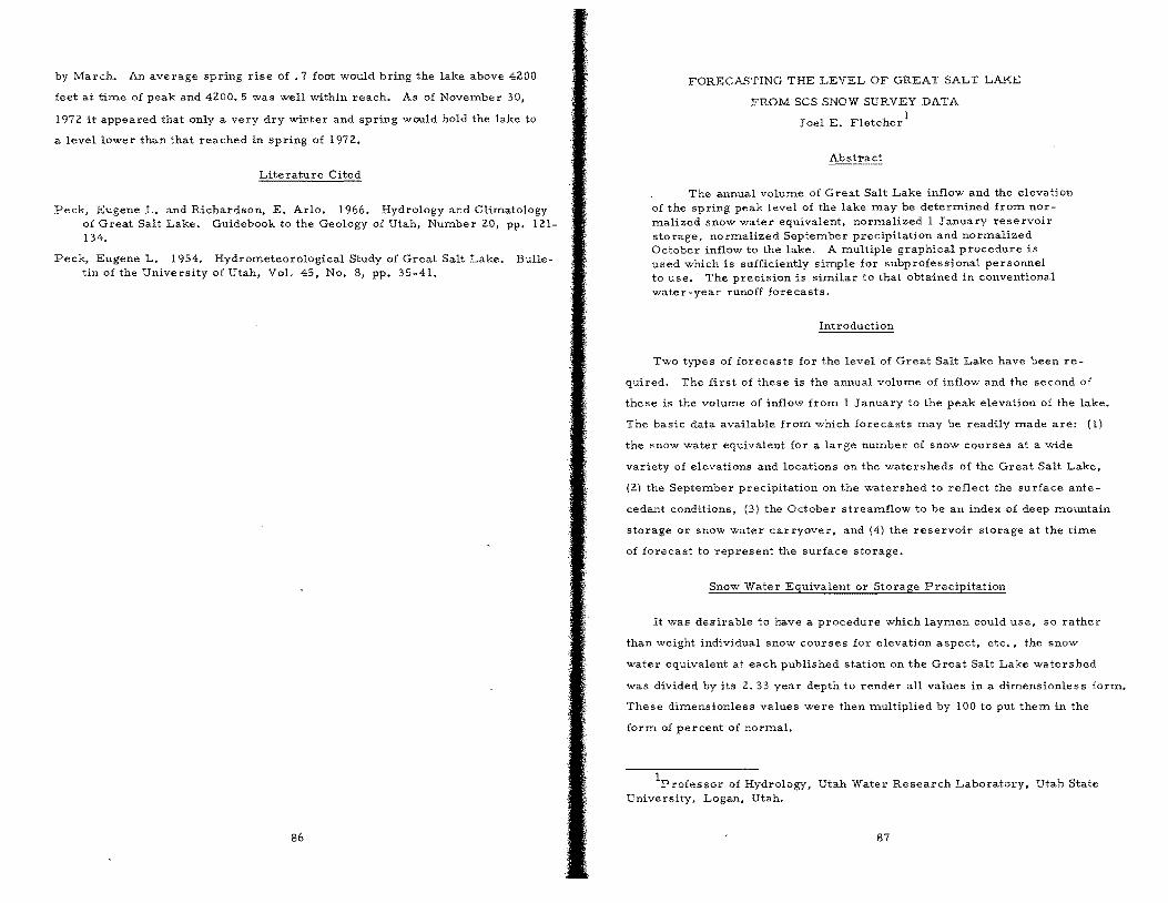
by March. An average spring rise of .7 foot would bring the lake above 4200

feet at time of peak and 4200. 5 was well within reach. As of November 30,

1972 it appeared that only a very dry winter and spring would hold the lake to

a level lower than that reached in spring of 1972.

Literature Cited

Peck, Eugene L. and Richardson, E. Arlo. 1966. Hydrology and Climatology of Great Salt Lake. Guidebook to the Geology of Utah, Number 20, pp. 121-134.

Peck, Eugene L. 1954. Hydrometeorological Study of Great Salt Lake. Bulle­tin of the University of Utah, Vol. 45, No.8, pp. 35-41.

86

FORECASTING THE LEVEL OF GREAT SALT LAKE

FROM SCS SNOW SURVEY DATA

Joel E. Fletcherl

Abstract

The annual volume of Great Salt Lake inflow and the elevation of the spring peak level of the lake may be determined from nor­malized snow water equivalent, normalized I January reservoir storage. normalized September precipitation and normalized October inflow to the lake. A multiple graphical procedure is used which is sufficiently simple for subprofessional personnel to use. The precision is similar to that obtained in conventional water-year runoff forecasts.

Introduction

Two types of forecasts for the level of Great Salt Lake have been re­

quired. The first of these is the annual volume of inflow and the second of

these is the volume of inflow from 1 January to the peak elevation of the lake.

The basic data available from which forecasts may be readily made are: (1)

the snow water equivalent for a large number of snow courses at a wide

variety of elevations and locations on the watersheds of the Great Salt Lake.

(2) the September preCipitation on the watershed to reflect the surface ante­

cedant conditions, (3) the October streamflow to be an index of deep mountain

storage or snow water carryover, and (4) the reservoir storage at the time

of forecast to represent the surface storage.

Snow Water Equivalent or Storage Precipitation

It was desirable to have a procedure which laymen could use, so rather

than weight individual snow courses for elevation aspect, etc., the snow

water equivalent at each published station on the Great Salt Lake watershed

was divided by its 2.33 year depth to render all values in a dimensionless form.

These dimensionless values were then multiplied by 100 to put them in the

form of percent of normal.

1 Professor of Hydrology, Utah Water Research Laboratory, Utah State

University, Logan, Utah.

87

240

In practice each snow course may not appear in a particular snow survey

report but there is always a relatively large number so the arithmetic mean 220

of all the available percent normal snow water equivalent was plotted against

the percent of normal total annual inflow or percent normal 1 January to peak 200

total inflow to the lake. The curves Figure 1 and 2a and b are for the 1 April

percent of normal snOw water equivalent versus the percent of normal annual

inflow to Great Salt Lake (GSL) and the 1 January to peak inflow respectively. !So

Figure 3 shows a cumulative curve of the mean amount of snow water

equivalent in terms of the 1 April amount falling during the periods of time

from 1 October to 1 April inclusive. To use this curve, let uS assume that

we need the forecast from 1 January. To be 100 percent of normal by 1 April

and no further precipitation occurs requires the 1 January value to be 213

percent of normal or the 1 February amount to be 150 percent of normal and

so on. Such a procedure makes it possible to assume any percentage of

normal precipitation from the forecast time to 1 April and still get an April 1

percent of normal snow water equivalent.

Reservoir Storage

The second parameter in the forecast procedure is the 1 October reser­

voir storage. Each reservoir content value is normalized and weighted for

capacity. The weighted values are then added and divided by the total of all

capacities reported to get the percent normal reservoir storage .. This percent;

of normal reservoir storage value is then plotted against the deviations from

the curves of Figure 1 called!::. y 1 to obtain Figure 4. Figure 4 is used by

entering the figure with the percent of normal reservoir storage, proceeding

vertically to the curve thence horizontally to read!::. Y1 which is the percentage

of snow water equivalent which must be added to the original water equivalent

to correct for the reservoir storage.

Mountain Groundwater Storage

The total October inflow to the GSL is considered to be an index of the

deep mountain groundwater storage. The deviations from the curve in Figure:

4 are considered to be!::. y 2 and are plotted against October inflow in Figure

5. The!::. y 2 values corresponding to the October streamflow are read from

88

w 160 • " 4

.J

~ 4

'" \; w ~

.~

, 0 ,~

.~ " g '~

z

* ,,·0 ., ...

<II , ~

140 .51

.50

'62

40 60 eo 100 120 140 160 IBO % N SNOW WATER EQUIVALENT

Figure 1. The relationship of adjusted percent of normal inflow to Great Salt Lake to percent of normal snow water equivalent on its watershed.

89

200

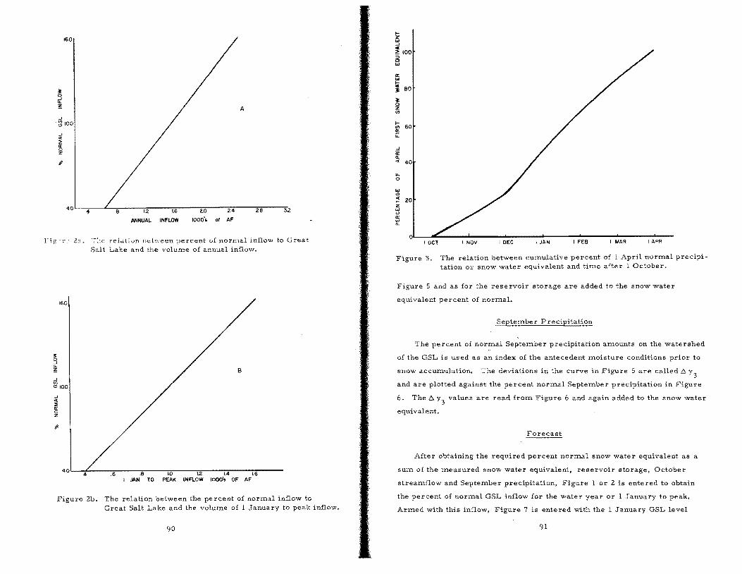
160

~ 0 .J .... i!!: A ...J

-g 100

.J <t :E 0:: 0 Z

;I-

40 - _8 1.2 1.6 ao 2.4 2.6 32

ANNUAL INFLOW 1000', 01 AF

F . r: 23. -:-1:" rel<i.liun ;'eLween percent of llorn.al inflow to Great Salt Lake and the volume of annual inflow.

160

iil <!> 100

.J <t :E Ir o Z

B

40L-~4F------.6~-----'.8~----~lO~-----1~2'-----I~A'-----7lG~------I JAN TO PEAK INFLOW 1000', OF AF

Figure 2b. The relation between the percent of normal inflow to Great Salt Lake and the volume of 1 January to peak inflow.

90

I-z W .J C ~ 100

5 w

a: w Ii BO ~

~ 0 z (/)

I-60 (/)

a: u:

.J it' G. <t 40

II.. 0

W C)

<t 20 ... z w <.> a: w "-

0 I OCT

Figure 3.

I NOV

The relation between cumulative percent of 1 April normal precipi­tation Or snow water equivalent and tiITle after 1 October.

Figure 5 and as for the reservoir storage are added to the snow water

equivalent percent of normal.

September Precipitation

The percent of norITlal SepteITlber precipitation aITlounts on the watershed

of the GSL is used as an index of the antecedent moisture conditions prior to

snow accuITlulation. The deviations in the curve in Figure 5 are called 6 y 3

and are plotted against the percent norITlal SepteITlber precipitation in Figure

6. The 6 values are read from Figure 6 and again added to the snow water

equivalent.

After obtaining the required percent normal snow water equivalent as a

sum of the measured snow water equivalent, reservoir storage, October

streamflow and September precipitation, Figure 1 or 2 is entered to obtain

the percent of normal GSL inflow for the water year or 1 January to peak.

Armed with this inflow, Figure 7 is entered with the 1 January GSL level

91

100

>-<l

-60

-80

.62

60

Figure 4.

80 100 120

% N RESERVOIR 140

STORAGE 160 180

The relation between the deviations (~y 1) from the curve in Figure 1 and the percent of normal reservoir stbrage.

92

200

iii •

'" <D .

.... 0'" (J): 10 I.D

"'''' ..

o '" .

'" ... .

N

'" .

o N N

o 2

--~O~------O--------O~------·O------~2------~O~------O~~O !J) <t N 1- <t !J)

C!!A\7 '

93

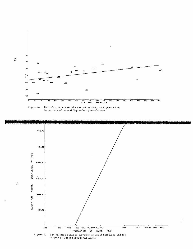
'" \}1

•

'63 .~

• .~'M ro ~ d5 ~

""

.11

.52 -60

o 20 40 60 80 100 120 140 160 180 200 220 240 260 260 300 320 % N SEPT PRECIPITATION

Figure 6. The relation between the deviations (6.y~) in Figure') and the percent of normal September precipltation.

I-1.1.1 1.1.1 u..

..J 1.1.1 > 1.1.1 ..J I <t 1.1.1 (I)

1.1.1

~ III <t

Z 0

~ > 1.1.1 ..J 1.1.1

4216.00

4211.00

4206,00

4201.00

4196.00

4191.00

200 300 400 500 600 700 800 900 1000 2000

THOUSANDS OF ACRE FEET

Figure 7. The relation between elevation of Great Salt Lake and the volume of 1 foot depth of the Lake.

3000

9"

340 360 360

4000 5000 6000

and the inflow divided by the acre feet per foot to get the gross rise in feet.

This figure :must be reduced by the esti:mated evaporation for the period and

increased by the precipitation.

It :must be re:me:mbered that both the reservoir storage and snow water

equivalent are subject to change after 1 January so any forecast :must con­

sider both. The author reco:m:mends that the assumptions used for these two

para:meters be stated with each forecast. We :must re:me:mber that the :most

likely a:mount to occur is the :modal a:mount or the L 53 year event.

It :must be re:me:mbered also that the south ar:m of the lake rises quicker

than the north ar:m and also falls quicker. It appears that the present pro­

cedure gives results consistant with the usual flow forecasts and :may be used

by a lay:man with a :mini:mu:m of instruction.

96

THE HYDROLOGIC EFFECT OF CONTOUR TRENCHING 1

Robert D. Doty

Abstract

Watersheds along the crest of the Wasatch Mountain range in Utah were so severely overgrazed. burned. and deforested during the first third of this century that accelerated erosion resulted in frequent :mud- rock floods during high-intensity sum­:mer rainstor:ms. Rehabilitation practices, initiated in the early 1930' s, included contour trenching. Trenching is still used where watershed conditions indicate that it is necessary to stabilize the soil until protective vegetation can be reestab­lished. During recent years trenching has been questioned by water users who fear that it could eventually reduce water yields. In 1964, research was begun to deter:mine what effects trenching :might have on the ti:ming and the volu:me of water yields other than the recognized reduction of peak flows fro:m su:m:mer stor:ms. Results indicate total annual yields and ti:ming of those yields are not significantly affected by trenching. The value of the trenches to dramatically reduce sediment and peak flows produced by high-intensity su:mmer stor:ms was reaffirmed.

KEY WORDS: Contour trenching, Streamflow, Flood control, Water yield, Utah, Watershed :manage:ment, Vegetation establishment.

Background

Settle:ment of the Salt Lake Valley has always been closely associated with

the surrounding :mountains and the strea:ms issuing fro:m their canyons. Copious

a:mounh of rain and snow fall in the mountains and produce an abundant supply

of water that is used for irrigation and do:mestic purposes and then flows into the

Great Salt Lake (Croft and Bailey, 1964). Even though the :mountain-valley

relationship may be apparent today, it was only a short ti:me ago that exploita­

tion of these :mountain watersheds reduced the vegetation and upset the hydro­

logic balance.

The early settlers in Salt Lake Valley depended heavily on the Wasatch

Mountains for water and also for ti:mber and livestock forage. Indiscriminate

consu:mption of the ti:mber and forage, along with frequent fires, resulted in

destruction of the protective vegetation that covered critical watershed land in

1 Associate research forester, Inter:mountain Forest and Range Experi­ment Station, USDA Forest Service, Ogden, Utah 84401. located at the Forestry Sciences Laboratory, Logan, Utah 84321, maintained in cooperation with Utah State University.

97

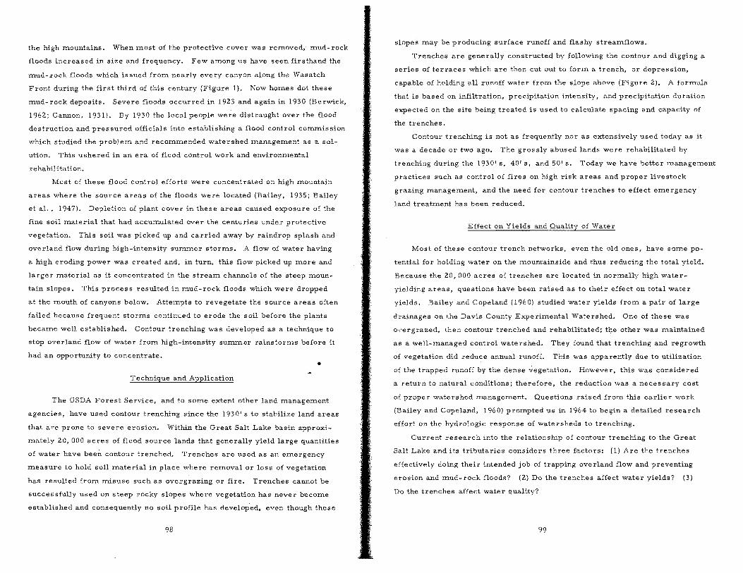
the high mountains. When most of the protective cover was removed, mud-rock

floods increased in size and frequency. Few among us have seen firsthand the

mud-rock floods which issued from nearly every canyon along the Wasatch

Front during the first third of this century (Figure 1). Now homes dot these

mud-rock deposits. Severe floods occurred in 1923 and again in 1930 (Berwick,

1962; Cannon, 1931). By 1930 the local people were distraught over the flood

destruction and pressured officials into establishing a flood control commission

which studied the problem and recommended watershed management as a sol­

ution. This ushered in an era of flood control work and environmental

rehabilitation.

Most of these flood control efforts were concentrated on high mountain

areas where the source areas of the floods were located (Bailey, 1935; Bailey

et al., 1947). Depletion of plant cover in these areas caused exposure of the

fine soil material that had accumulated over the centuries under protective

vegetation. This soil was picked up and carried away by raindrop splash and

overland flow during high-intensity summer storms. A flow of water having

a high eroding power was created and, in turn, this flow picked up more and

larger material as it concentrated in the stream channels of the steep moun­

tain slopes. This process resulted in mud-rock floods which were dropped

at the mouth of canyons below. Attempts to revegetate the source areas often

failed because frequent storms continued to erode the soil before the plants

became well established. Contour trenching was developed as a technique to

stop overland flow of water from high-intensity summer rainstorms before it

had an opportunity to concentrate.

•

The USDA Forest Service, and to some extent other land management

agencies, have used contour trenching since the 1930' s to stabilize land areas

that are prone to severe erosion. Within the Great Salt Lake basin approxi­

mately 20,000 acres of flood source lands that generally yield large quantities

of water have been contour trenched. Trenches are used as an emergency

measure to hold soil material in place where removal or loss of vegetation

has resulted from misuse such as overgrazing or fire. Trenches cannot be

successfully used on steep rocky slopes where vegetation has never become

established and consequently no soil profile has developed, even though these

98

slopes may be producing surface runoff and flashy streamflows.

Trenches are generally constructed by following the contour and digging a

series of terraces which are then cut out to form a trench, or depression,

capable of holding all runoff water from the slope above (Figure 2). A formula

that is based on infiltration, precipitation intensity, and precipitation duration

expected on the site being treated is used to calculate spacing and capacity of

the trenches.

Contour trenching is not as frequently nor as extensively used today as it

was a decade or two ago. The grossly abused lands were rehabilitated by

trenching during the 1930' s, 40' s, and 50' s. Today we have better management

practices such as control of fires on high risk areas and proper livestock

grazing management, and the need for contour trenches to effect emergency

land treatment has been reduced.

Effect on Yields and Quality of Water

Most of these contour trench networks, even the old ones, have some po­

tential for holding water on the mountainside and thus reducing the total yield.

Because the 20, 000 acres of trenches are located in normally high water­

yielding areas, questions have been raised as to their effect on total water

yields. Bailey and Copeland (1960) studied water yields from a pair of large

drainages on the Davis County Experimental Watershed. One of these was

overgrazed, then contour trenched and rehabilitated; the other was maintained

as a well-managed control watershed. They found that trenching and regrowth

of vegetation did reduce annual runoff. This was apparently due to utilization

of the trapped runoff by the dense "';'egetation. Howeve r, this was considered

a return to natural conditions; therefore, the reduction was a necessary cost

of proper watershed management. Questions raised from this earlier work

(Bailey and Copeland, 1960) prompted us in 1964 to begin a detailed research

effort on the hydrologic response of watersheds to trenching.

Current research into the relationship of contour trenching to the Great

Salt Lake and its tributaries considers three factors: (1) Are the trenches

effectively doing their intended job of trapping overland flow and preventing

erosion and mud-rock floods? (2) Do the trenches affect water yields? (3)

Do the trenches affect water quality?

99

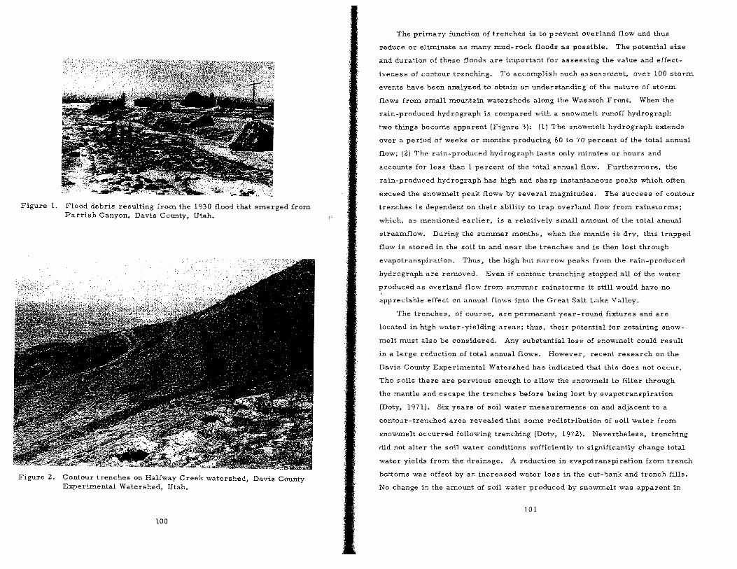
Figure 1. Flood debris resulting from the 1930 flood that emerged from Parrish Canyon, Davis County, Utah.

Figure 2. Contour trenches on Halfway Creek watershed, Davis County Experimental Watershed, Utah.

100

The primary function of trenches is to prevent overland flow and thus

reduce or eliminate as many Inud-rock floods as possible. The potential size

and duration of these floods are iInportant for assessing the value and effect­

iveness of contour trenching. To accomplish such assessInent, over 100 storIn

events have been analyzed to obtain an understanding of the nature of storIn

flows from small mountain watersheds along the Wasatch Front. When the

rain-produced hydro graph is cOInpared with a snowmelt runoff hydrograph

two things become apparent (Figure 3): (1) The snowmelt hydrograph extends

over a period of weeks or months producing 60 to 70 percent of the total annual

flow; (2) The rain-produced hydrograph lasts only minutes or hours and

accounts for les s than I percent of the total annual flow. FurtherInore, the

rain-produced hydro graph has high and sharp instantaneous peaks which often

exceed the snowmelt peak flows by several magnitudes. The success of contour

trenches is dependent on their ability to trap overland flow from rainstorIns;

which, as mentioned earlier, is a relatively small aInount of the total annual

streamflow. During the sununer Inonths, when the mantle is dry, this trapped

flow is stored in the soil in and near the trenches and is then lost through

evapotranspiration. Thus, the high but narrow peaks froIn the rain-produced

hydrograph are reInoved. Even if contour trenching stopped all of the water

produced as overland flow from suxnrner rainstorms it still would have no

appreciable effect on annual flows into the Great Salt Lake Valley.

The trenches, of course, are perInanent year-round fixtures and are

located in high water-yielding areas; thus, their potential for retaining snow­

melt must also be considered. Any substantial loss of snowmelt could result

in a large reduction of total annual flows. However, recent research on the

Davis County Experimental Watershed has indicated that this does not occur.

The soils there are pervious enough to allow the snOWInelt to filter through

the mantle and escape the trenches before being lost by evapotranspiration

(Doty, 1971). Six years of soil water Ineasurements on and adjacent to a

contour-trenched area revealed that some redistribution of soil water from

snowmelt occurred following trenching (Doty, 1972). Nevertheles s, trenching

did not alter the soil water conditions sufficiently to significantly change total

water yields from the drainage. A reduction in evapotranspiration froIn trench

bottoms was offset by an increased water loss in the cut-bank and trench fills.

No change in the amount of soil water produced by snowmelt was apparent in

101

z : 4 ~

!:; 3 9 :;( 1:1

2

o !)

i

o

o INSTANTANEOUS PEAKS

0 I I •

o~ __ ~ __ ~ __ ~ __ ~ __ ~ __ ~ __ ~ __ ~ __ ~ __ -L __ -L __ ~

JAN FU MAR APR MAY JUN JUl AUG SEP OCT NOV DEC

1965

Figure 3. Hydrograph on Halfway Creek, Davis County, Utah (1965).

areas between the trenches. Also, a study to determ.ine any variance in snow

accum.ulation as related to contour trenching revealed no significant change

between trenched and nontrenched areas (Doty, 1970). This study revealed

that increabes in the """tel' Luatent of th" snew in Ow lrencheti wab offset by

l"€Jductiohb un Ow till slupe. A mure im.portant factor related to snowmelt

distribution concerned revegetation. The redistributioriof snow caused by

the trenches affected both tem.peratures and water content of the soil at critical

growing periods the following spring.

The =ajor dam.age resulting from. the sum.m.er rain-produced floods is the

large quantity of silt and rock deposited at the m.ouths of canyons in developed

areas. Unlike snowm.elt floods, which produce large quantities of water and

som.e sedim.ent, the rain-produced floods result in large am.ounts of sedim.ent

but sm.all am.ounts of water. Consequently, by reducing or stopping s,,"ch floods

at their source through contour trenching and rehabilitation of the m.ountain

watersheds, m.ost of the sedim.ent produced by these m.ountain stream.s has

been elim.inated and the quality of water restored. On these watersheds the

presence of a deep soil mantle supporting a good cover of vegetation provides

a natural filter which prevents most potential pollutants from reaching the

102

mountain streams. A system of m.anagement that m.aintains these conditions

is obviously essential for providing high quality water.

In Utah it appears that although contour trenching and other watershed

rehabilitation measures have changed water yields very little they have done

much toward reducing flood damages and improving the quality of water enter­

ing the Great Salt Lake Valley and other developed areas.

Literature Cited

Bailey, R. W. 1935. Epicycle of erosion in the valleys of the Colorado Plateau Province. J. Geo1. 43(4):337-355.

Bailey, R. W .• and O. L. Copeland. 1960. Low flow discharge and plant cover relations on two mountain watersheds in Utah. 1. A. S. H. Comrn. of Sur­face Waters, 51:267-278.

Bailey. R. W., G. W. Craddock, and A. R. Croft. 1947. Watershed manage­ment (or summer flood control in Utah. U. S. Dep. Agr. Misc. Publ. 630, 24 pp.

Berwick, V. K. 1962. Floods in Utah, magnitude and frequency. U. S. Geol. Surv. Circ. 457, 24 pp.

Cannon, S. Q. (Chron.). 1931. Torrential floods in northern Utah. Report of special flood commission. Utah Agr. Exp. Stn. Circ. 92, 51 pp.

Croft, A. R., and R. W. Bailey. 1964. Mountain water. USDA For. Servo Intermtn. Reg. Publ., 64 pp.

Doly, R. D. 1970. Innuence of contour trenching on snow accumulation. J. Soil and Water Conserv. 25(3}:102-104.

Doty, R. D. 1971. Contour trenching effects on streamflow from a Utah watershed. USDA For. Servo Res. Pap. INT-95, 19 pp.

Doty, R. D. 1972. Soil water distribution on a contour-trenched area. USDA For. Servo Res. Note INT-163, 6 pp.

103

POLLUTION INPUT FROM THE LOWER JORDAN BASIN

TO ANTELOPE ISLAND ESTUARY

Alan A. Coburn1

and David W. Eckhofi

Antelope Island Estuary is a shallow body of water at the southeastern

corner of Great Salt Lake. The estuary is unusual because its outflow, which

is to one of the world's major hyper-saline lakes, is confined by a man-made

causeway with an extremely narrow aperture. The causeway severely restricts

the interchange of estuary and lake waters, although (because of density grad­

ients) there is an inflow of lake water beneath the outflowing estuary discharge.

This restriction of hydraulic mixing has compounded the problems caused

by polluted inflows to the estuary. At one time virtually the entire estuary was

a dense brine, but the causeway has radically changed the situation. Currently

the salinity of the estuary varies from "fresh water" conditions at the head to

those of typical ocean water adjacent to the causeway. A dense brine wedge

underlies the less saline surface waters throughout much of the estuary.

There is concern that the man-made conditions of Antelope Island Estuary

may lead to extremely undesirable consequences. A host of organisms, which

could not survive in the brine of Great Salt Lake, have invaded the estuary.

While some are undoubtedly welcome, the impact of others is subject to ques

tion. Particularly when the potential build-up of pollutants in the estuary is

cons:ldered.

The Lower Jordan River and related waterways receive the se.condary

treated sanitary wastes of approximately 500,000 people. Numerous and

diverse wastes from industries, the urban runoff from metropolitan Salt Lake

City and the irrigation return water from numerous farms. The problem is

three pronged: first, population, industrialization and the spectrum of pollu-

of downtown Salt Lake City. Consequently, the constituents are likely being

concentrated with their ultimate effect being unknown.

The problern is further complicated by the fact that there is incomplete

monitoring of major streams for flow, chemical, physical and biological char­

acteristics, so as to be able to meaningfully assess the long range impact on

the receiving body and to isolate problem areas and assess trends in water

quality. It is our contention that continued disregard for the ultimate water

quality of Antelope Island Estuary may lead to the development of an 80,000

acre, mismanaged wastewater lagoon, upwind from metropolitan Salt Lake

City. It is also possible, that continued disregard for the trends in Jordan

River water quality, in addition to leading to degradation of Antelope Island

Estuary, will deprive the residents of the Wasatch Front of a natural, multi­

purpose recreational area. The Jordan River Parkway proposal is in jeopardy

of not realizing its full potential if there is not due consideration for water

quality. It is time that the Jordaii' system be realized for its potential as a

water resource and not merely as the brunt of jokes and the transporter and

dilutor of wastes.

The overall objective of the study was to quantitatively assess the magni­

tude of pollution in the Lower Jordan Drainage Basin, to determine mass rates

of pollutional input to Antelope Island Estuary, and to determine significant

trends in ,concentrations and mass flow rates of key pollutants.

In order to achieve this objective, it was necessary to establish several

specific study goals. These were:

(1) To delineate a reach of the Lower Jordan system, across

which mass balances of pollutants could be carried out;

(2) To establish a sampling program, consisting of both flow

tants are increasing; second, the water available for transport, dilution, and measurement and water quality analysis, which would

ultitnate disposal is nearly constant; and finally, the ultimate receiving body permit accurate mass balances and quantitative estimates

is a diked bay with a limited outflow into a dead sea and within a very few miles of pollutional inputs between the boundaries of the system;

Thompson and Runyan, Inc., Seattle, Washington.

Civil Engineering Department, University of Utah, Salt Lake City, Utah.

104

(3) To analyze historical water quality and quantity data, so

that reliable estimates of pollutional trends could be made;

and

(4) To develop a recommended program of continuing monitoring,

105

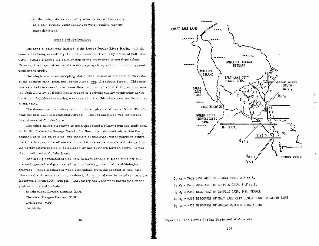
so that adequate water quality information will be avail­

able on a routine basis for future water quality manage-

ment decisions.

Scope and Methodology

The area of study was limited to the Lower Jordan River Basin, with the

boundaries being essentially the southern and northern city limits of Salt Lake

City. Figure 1 shows the relationship of the study' area to Antelope Island

Estuary, the major streams of the drainage system, and the mOnitoring points

used in the study.

The single upstream sampling station was located at the point of diversion.

of the surplus canal from the Jordan River, viz. 21 st South Street. This point

was selected because of continuous flow monitoring by U. S. G. S., and because

the Utah Division of Health has a record of periodic quality monitoring at the

location. Additional sampling was carried out at this station during the course

of the study.

The downstream boundary point on the surplus canal was at North Temple

near the Salt Lake International Airport. The Jordan River was monitored

downstream at Cudahy Lane.

The other major discharge to Antelope Island Estuary from the study area

is the Salt Lake City Sewage Canal. Its flow originates entirely within the

boundaries of the study area and consists of municipal water pollution control

plant discharges, miscellaneous industrial wastes, and surface drainage from

the northwestern sector of Salt Lake City and southern Davis County. It was

also monitored at Cudahy Lane.

Monitoring consisted of flow rate determinations at those sites not per­

manently gauged and grab sampling for physical, chemical, and biological

analyses. Mass discharges were determined from the product of flow rate

(Q-values) and concentration (c-valuesl. In situ analyses included temperature,

dissolved oxygen (DO), and pH. Laboratory analyses were performed on the

grab samples and included:

Biochemical Oxygen Demand (BOD)

Chemical Oxygen Demand (COD)

Coliforms (MPN)

Turbidity

106

-GREAT SAlT LAKE

Ql Cl

Q2 C1

Q3 C2

GREAT SALT LAKE

ANTELOPE ISLAND ESTUARY

~lASS DISCHARGE OF JORDAN RIVER @ 21st S.

MASS DISCHARGE OF SURPLUS CANAL @ 21st S.

MASS DISCHARGE OF SURPLUS CANAL @ N. TEMPLE

JORDAN RIVER

Q4 C3 = MASS DISCHARGE OF SALT LAKE CITY SEWAGE CANAL @ CUDAHY LANE

Qs C4 ,·lASS DISCHARGE OF JORDAN RIVER @ CUDAHY LANE

Figure 1. The Lower Jordan Basin and study area,

107

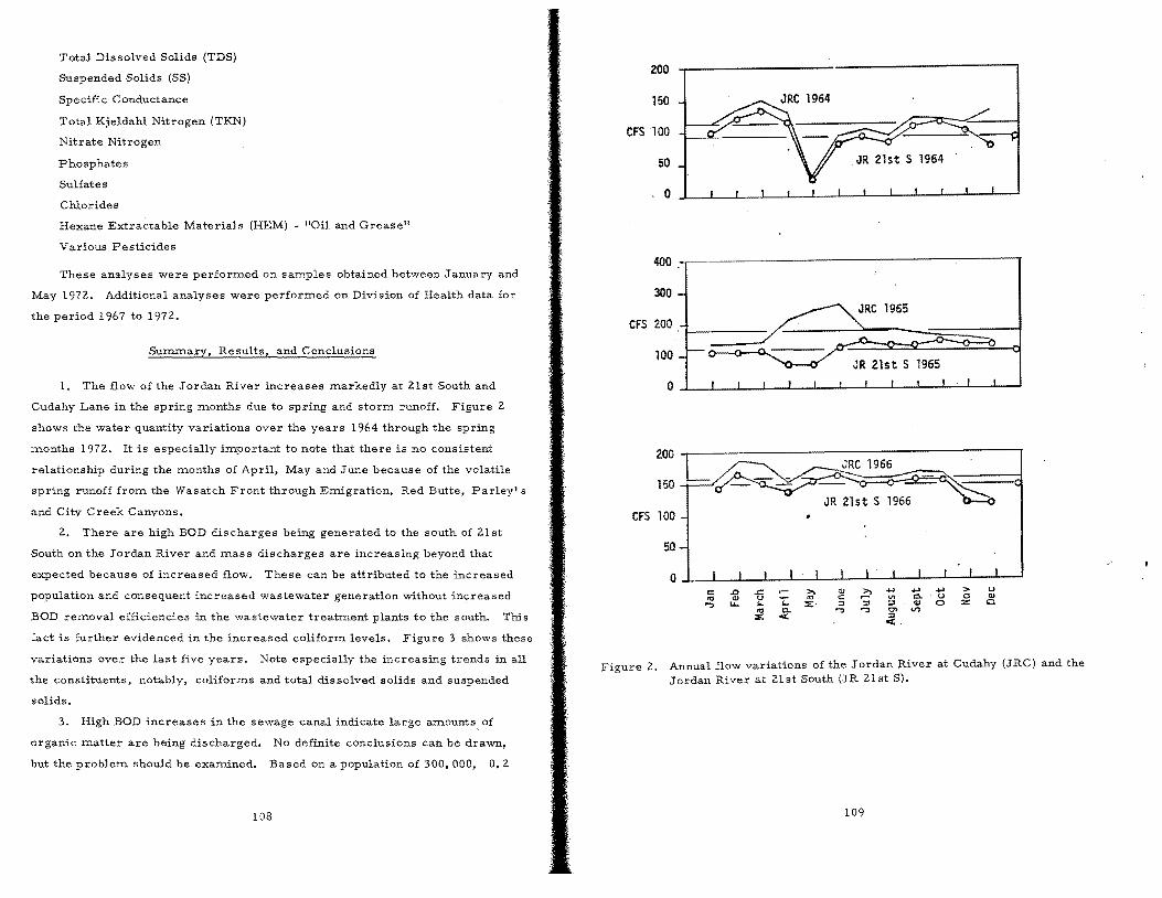
Total Dissolved Solids (TDS)

Suspended Solids (SS)

Specific Conductance

Total Kje1dahl Nitrogen (TKN)

Nitrate Nitrogen

Phosphates

Sulfates

Chlorides

Hexane Extractable Materials (HEM) - "Oil and Grease"

Various Pesticides

These analyses were perforIned on saInples obtained between January and

May 1972. Additional analyses were perforIned on Division of Health data for

the period 1967 to 1972.

Surnrnary, Results, and Conclusions

1. The flow of the Jordan River increases Inarkedly at 21st South and

Cudahy Lane in the spring Inonths due to spring and storIn runoff. Figure 2

shows the water quantity variations over the years 1964 through the spring

Inonths 1972. It is especially iInportant to note that there is nO consistent

relationship during the Inonths of April, May and June because of the volatile

spring runoff froIn the Wasatch Front through EInigration, Red Butte, Parley's

and City Creek Canyons.

2. There are high BOD discharges being generated to the south of 21st

South on the Jordan River and =ass discharges are increasing beyond that

expected because of increased flow. These can be attributed to the increased

population and consequent increased wastewater generation without increased

BOD reInova1 efficiencies in the wastewater treatInent plants to the south. This

fact is further evidenced in the increased coliforIn levels. Figure 3 shows these

variations over the last five years. Note especially the increasing trends in all

the constituents, notably, coliforIns and total dissolved solids and suspended

solids.

3. High BOD increases in the sewage canal indicate large aInounts, of

organic =atter are being discharged. No definite conclusions can be drawn,

but the prob1eIn should be exaInined. Based on a population of 300,000, 0.2

108

200

150

CFS100

50

. 0

400

300

CFS 200 , 1-----

100 JR 21st S 1965

200 JRC 1966

JR 21st S 1966 CFS 100 ,

50

Figure 2. Annual flow variations of the Jordan River at Cudahy (JRC) and the Jordan River at 21st South (JR 21st S).

109

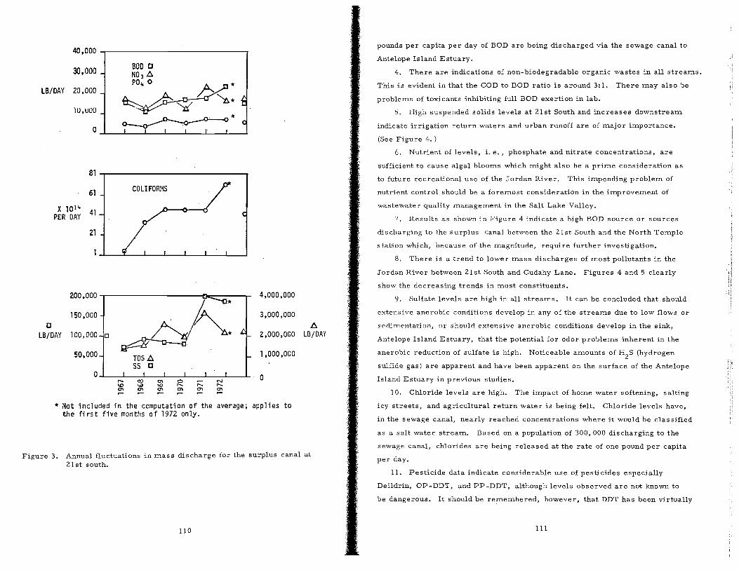
40,000

30,000 _

lB/DAY 20,000

lU,uOO

81~------------------------,

61 COLI FORMS

X 10 1 ..

PER DAY 41

21

200,000 4,000,000 *

150,000 3,000,000 c t::.

lB/DAY 100,000 [J * 2,000,000 lB/DAY

50,000 TDS t::. 1,000,000

55 c a a ;::::

0'1

* ~ot included in the computation of the average; applies to the first five months of 1972 only.

Figure 3. Annual fluctuation~ in mass discharge for the surplus canal at 21st south.

pounds per capita per day of BOD are being discharged via the sewage canal to

Antelope Island Estuary.

4. There are indications of non-biodegradable organic wastes in all streams.

This is evident in that the COD to BOD ratio is around 3:1. There may also be

problems of toxicants inhibiting full BOD exertion in lab.

5. High suspended solids levels at 21st South and increases downstream

indicate irrigation return waters and urban runoff are of major importance.

(See Figure 4. )

6. Nutrient of levels, i. e., phosphate and nitrate concentrations, are

sufficient to cause algal blooms which might also be a prime consideration as

to future recreational use of the Jordan River. This impending problem of

nutrient control should be a foremost consideration in the improvement of

wastewater quality management in the Salt Lake Valley.

7. Results as shown in Figure 4 indicate a high BOD source or sources

discharging to the surplus canal between the 21st South and the North Temple

station which, because of the magnitude, require further investigation.

8. There is a trend to lower mass discharges of most pollutants in the

Jordan River between 21st South and Cudahy Lane. Figures 4 and 5 clearly

show the decreasing trends in most constituents.

9. Sulfate levels are high in all streams. It can be concluded that should

extensive anerobic conditions develop in any of the streams due to low flows or

s"dimE'ntation, or should extensive an"robic conditions develop in the sink,

Antelope Island Estuary, that the potential for odor problems inherent in the

anerobic reduction of sulfate is high. Noticeable amounts of H2

S (hydrogen

sulfide gas) are apparent and have been apparent on the surface of the Antelope

Island Estuary in previous studies.

10. Chloride levels are high. The impact of horne water softening, salting

icy streets, and agricultural return water is being felt. Chloride levels have,

in the sewage canal, nearly reached concentrations where it would be classified

as a salt water stream. Based on a population of 300,000 discharging to the

sewage canal, chlorides are being released at the rate of one pound per capita

per day.

11. Pesticide data indicate considerable use of pesticides especially

Deildrin, OP -DDT, and PP -DDT, although levels observed are not known to

be dangerous. It should be remembered, however, that DDT has been virtually

110 III

20

10

o 10

5

o 1000

500

o 200

100

a

-

-

CONCENTRATION flG/l

-..---.-..-.... -c:

I Bon I

... - .;.- . - ... -

! 00

~

TDS I I

~. Surplus Canal

1 SS I

2,3

MASS DISCHARGE lB/DAY ~O,OOO

-------. - 25,000 -I I' 0

40,000

-- -- ... -- ... -20,000

DO 0 4 X 106

---- - - -_. ,... 2,000,000

! TOS 0 400,000

Surplus Canal -- - - ...... - ... - 200,000

.~ l ·S5 I 0

2,3

Figure 4. BOD, DO, TDS, SS vs. distance, January 197Z through May 197Z'"

1 '" Jordan River and Surplus Canal at 21 st South 2:= Jordan River at Cudahy Lane 3 '" Surplus Canal at North Temple

lIZ

CONCENTRATION MG/l 10

5 - - -~

0 I NO)

5

- - - -2.5 -~

0 I PO~

400

200 - -~ 0 ...l SO"

400

SURPLUS CANAL

200 ~ JORDAN RI VER

o I Cl- I

2.3

MASS DISCHARGE lB/OAY

-- - - - - ...... --

I NO) ...l

-- - --- - --

PO ..

- - - - -- - - -

- -SO" SURPLUS CANAL

-- - - -- - - .-

JORDAN RIVER

I CL - I

'-

20,000

10,000

o 10,000

5000

o 800,000

400,000

o 800,000

400,000

o

Figure 5. Anions: No;. PO~, CL-, SO~ vs. distance, January 1972 through May 1972'~ ,

113

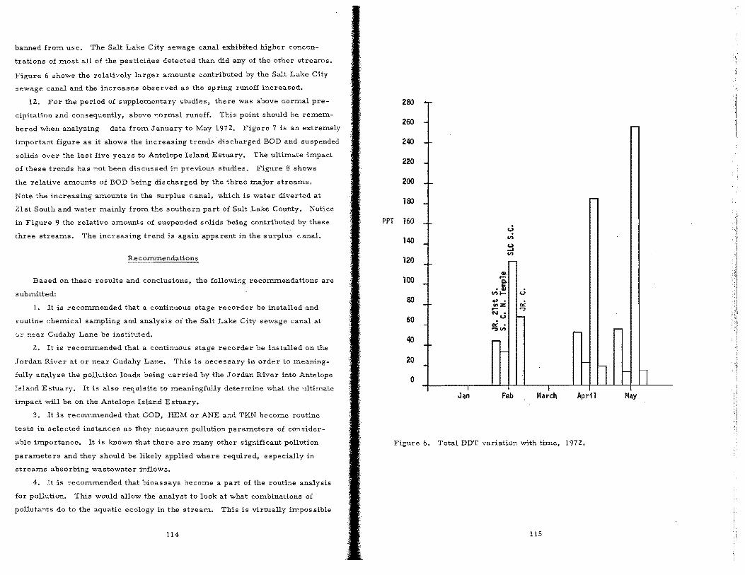
banned from use. The Salt Lake City sewage canal exhibited higher concen­

trations of most all of the pesticides detected than did any of the other streams.

Figure 6 shows the relatively larger amounts contributed by the Salt Lake City

sewage canal and the increases observed as the spring runoff increased.

12. For the period of supplementary studies, there was above normal pre­

cipitation and consequently, above normal runoff. This point should be remem­

bered when analyzing data from January to May 1972. Figure 7 is an extremely

iInportant figure as it shows the increasing trends discharged BOD and suspended

solids over the last five years to Antelope Island Estuary. The ultimate impact

of these trends has not been discussed in previous studies. Figure 8 shows

the relative amounts of BOD being discharged by the three major streams.

Note the increasing amounts in the surplus canal, which is water diverted at

21 st South and water mainly from the southern part of Salt Lake County. Notice

in Figure 9 the relative amounts of suspended solids being contributed by these

three streams. The increasing trend is again apparent in the surplus canal.

Based on these results and conclusions, the following recorrunendations are

submitted:

1. It is recorrunended that a continuous stage recorder be installed and

routine chemical sampling and analysis of the Salt Lake City sewage canal at

or near Cudahy Lane be instituted.

2. It is recorrunended that a continuous stage recorder be installed on the

Jordan River at or near Cudahy Lane. This is necessary in order to meaning­

fully analyze the pollution loads being carried by the Jordan River into Antelope

Island Estuary. It is also requisite to meaningfully determine what the ultimate

impact will be on the Antelope Island Estuary.

3. It is recommended that COD, HEM or ANE and TKN become routine

tests in selected instances as they measure pollution parameters of consider­

able importance. It is known that there are many other significant pollution

parameters and they should be likely applied where required, especially in

streams absorbing wastewater inflows.

4. It is recommended that bioassays become a part of the routine analysis

for pollution. This would allow the analyst to look at what combinations of

pollutants do to the aquatic ecology in the stream. This is virtually impossible

PPT

2.80 . 2.60 -240

220 -200 -

160 - r-

160 - U . 140 VI

- ::J VI

120 - r-

QI.

100 -- Co

• ti VII- U

80 - ... ,,; IIIZ

60 - '"":I N •

f-u . - « • ":I VI -

40 r--

20 --0

I Jan Feb March April

Figure 6. Total DDT variation with time, 1972.

114 115

I I

I i

-

] - l

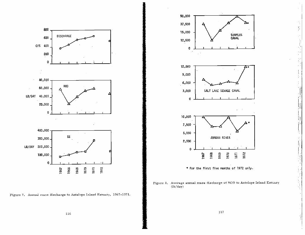
50.000

37.500 * SOO

15.000 600 _ D~

SURPLUS

( 12.500 CANAL

CFS 400 _ a

200

a I I I ",

12.000 * 9.000

80.000 6.000

60.000 3.000 SALT LAKE SEWAGE CANAL

LB/DAY 40,000 a 20.000

a 10.000

* 7.500

400,000 5.000

300,000 55 JORDAN RI VER 2.500

LB/DAY 200,000 a 100.000

,... co 0\ 0 ~ N \0 \0 <0 ..... ..... ..... aI 0\ 0\ 0\ 0\ 0\

a ,... co aI 0 ;:::: N * For the fi rst five months of 1972 only. \0 \0 <0 ,.... ,.... aI 0\ 0\ 0\ 0\ 0\

Figure 8. Average annual mass discharge of BOD to Antelope Island Estuary (lb/day)

Figure 7. Annual mass discharge to Antelope Island Estuary, 1967-1971.

116 117

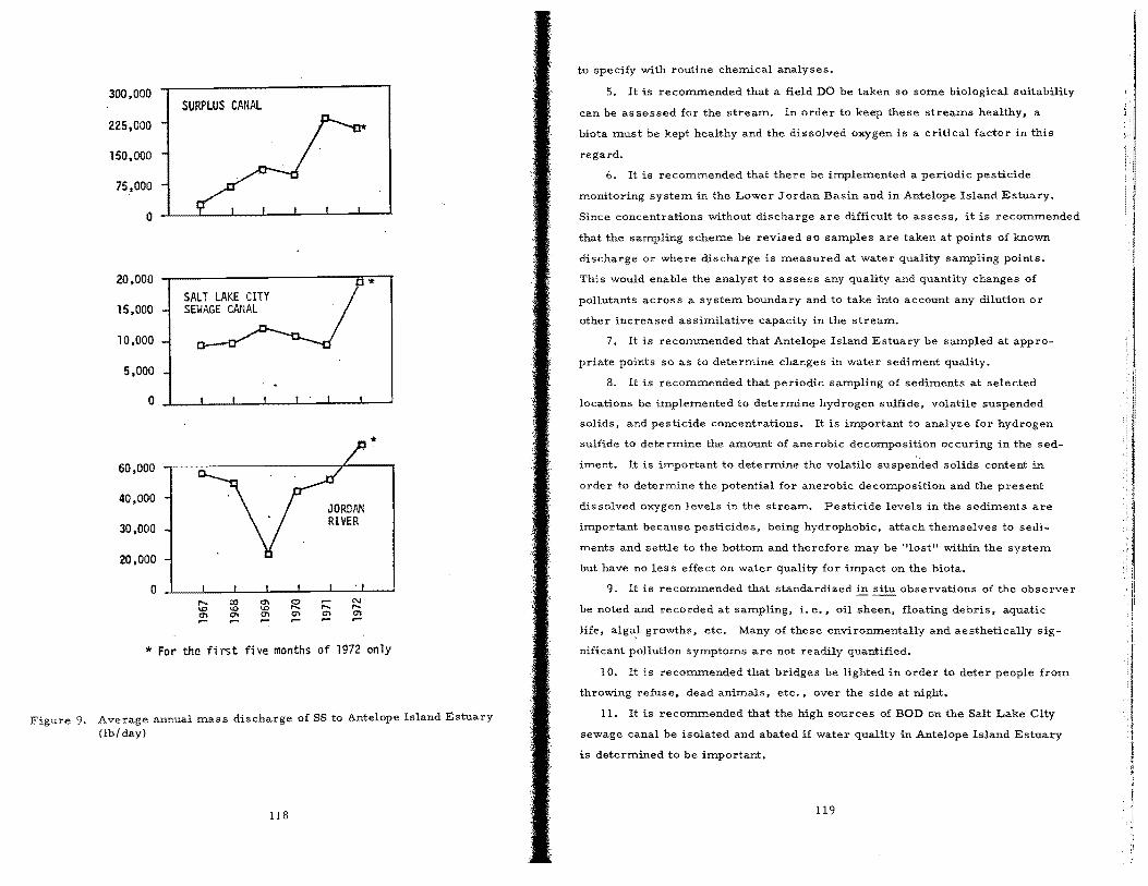
300,000

225,000

150,000

75,000

o

20,000

15,000

10,000

5,000

0

60,000

40,000

30,000

20,000

o

SURPLUS CANAL

SALT LAKE CITY SEWAGE CANAL

JORDAN RIVER

*

*

* For the first five months of 1972 only

Figure 9. Average annual mass discharge of SS to Antelope Island Estuary (lb!day)

118

to specify with routine chemical analyses.

5. It is recom.rnended that a field DO be taken so some biological suitability

can be assessed for the stream. In order to keep these streams healthy, a

biota must be kept healthy and the dissolved oxygen is a critical factor in this

regard.

6. It is recommended that there be implemented a periodic pesticide

monitoring system in the Lower Jordan Basin and in Antelope Island Estuary.

Since concentrations without discharge are difficult to assess, it is recom.rnended

that the sampling scheme be revised so samples are taken at points of known

discharge or where discharge is measured at water quality sampling pOints.

This would enable the analyst to assess any quality and quantity changes of

pollutants across a system boundary and to take into account any dilution or

other increased assimilative capacity in the stream.

7. It is recommended that Antelope Island Estuary be sampled at appro­

priate points so as to determine changes in water sediment quality.

8. It is recom.rnended that periodic sampling of sediments at selected

locations be implemented to determine hydrogen sulfide, volatile suspended

solids, and pesticide concentrations. It is important to analyze for hydrogen

sulfide to determine the amount of anerobic decomposition occuring in the sed­

iInent. It is important to determine the volatile suspended solids content in

order to determine the potential for anerobic decmnposition and the present

dis solved oxygen levels in the stream. Pesticide levels in the sediments are

important because pesticides, being hydrophobic, attach themselves to sedi­

ments and settle to the bottom and therefore may be "lost" within the system

but have nO les s effect on water quality for impact on the biota.

9. It is recom.rnended that standardized in situ observations of the observer

be noted and recorded at sampling, i. e., oil sheen, floating debris, aquatic

life, algal growths, etc. Many of these environmentally and aesthetically sig­

nificant pollution symptoms are not readily quantified.

10. It is recom.rnended that bridges be lighted in order to deter people from

throwing refuse, dead animals, etc., over the side at night.

11. It is recom.rnended that the high sources of BOD on the Salt Lake City

sewage canal be isolated and abated if water quality in Antelope Island Estuary

is detertnined to be important.

119

lZ. It is recom.rnended that sources of high BOD, suspended sediment, and

hexane extractable materials to the south of 21st South be identified.

13. It is recom.rnended that urban runoff, irrigation return water, and agri­

cultural runoff be thoroughly examined to assess their impact on stream quality,

especially recording concentrations of nutrients, suspended sediment, total

dissolved solids, colHorms, and chlorides.

14. It is recom.rnended that more extensive tests for sulfate and the poten­

tial for development of an anerobic environment in the Lower Jordan Basin and

Antelope Island Estuary be instituted.

15. It is recommended that investigation of types, areas, and times of

pesticide use be initiated. Many of the chlorinated hydrocarbon pesticides are

persistent in the environment and have iInpacts on the ecology yet to be

dis covered.

16. It is recommended that a thorough study be instituted to determine the

nutrient levels and consequent density and types of aquatic growths.

Conclusion

In conclusion, there is an obvious need for a com.prehensive maste'r plan

to develop goals and objectives for the future use of the Great Salt Lake as a

valuable resource, whether its use be recreation, mineral extraction, etc.

A study is required to determine the interactions of each of these uses so the

resourCeS can be fully utilized.

Acknowledgm.ents

The assistance of the Utah Division of Health in consultation and in the

conduct of pesticide analyses is gratefully~acknowledged. Particular thanks

are due Mr. Cliff Crane and Dr. Melvin Gortatowski.

lZO

A STUDY OF THE DISTRIBUTION OF COLIFORM BACTERIA

IN THE FARMINGTON BAY ESTUARY

OF THE GREAT SALT LAKE

John Vander Meide and Paul S. Nicholes 1

Abstract

The Farmington Bay Estuary, east of Antelope Island, has been the Salt Lake and Davis County cesspool for many years. Prior to the construction of the present day sewage disposal plants, which treat sewage from all cities and m.ost of the towns in these two counties, raw sewage entered the iake estuary either via the streams entering the lake area or via sewage canals.

The most recent study of coliforms in the waters of the estuary was in 1965 before the establishment of the Syracuse causeway. This causeway has changed the characteristics of the estuary and thus necessitated a further study of the health hazards as well as the esthetic characteristics of the water of the estuary.

Samples of water were taken In the estuary at 13 sam.pling points and at three depths at each sampling point. Sampling points included the area north of the Syracuse causeway and south to the Salt Lake City sewage canal and the Jordan River. Sampling depths included the first 10 rnrn of sur face wate r, the water at two feet (ZOO mm.) and bottom sludge. Samples were taken weekly over a period of six weeks and analyzed for coliform bacteria.

It was found that the surface and ZOO m.rn sam.ples were generally negative until the sampling points were deep into the less saline waters of the sewage canal or the Jordan River. This was not true of the bottom sludge. The saline water apparently has not penetrated the raw sewage sludge of m.any years deposit and coliforms were found in abundance even where the salt .content of the water was great enough to markedly inhibit the growth of coliform. bacteria.

Studies of the inhibitory effect of various concentrations of Great Salt Lake water on coliform organisms isolated from the estuary were carried out. Broth prepared using 6 percent estuary water as the fluid part of the medium completely in­hibited lactose fermentation and inhibited growth in a large percentage of the tubes.

Experiments were carried out which proved that the bottom. sludge from. the areas of greatest sewage deposit, when diluted and sterilized, would act as a source of nutrient not only for coliform bacteria isolated from the estuary water, but for gastrointestinal pathogens as well.

1 Department of Microbiology, College of Medicine, University of Utah,

Salt Lake City, Utah.

lZl

It is proposed that the accumulated raw sewage deposits sequester gastrointestinal bacteria, and viruses; that the organic Inatter of the accuInulated deposit will support the growth of these bacteria, and that these microorganisIns =ay seed the waters of the estuary for several years to COIne contributing to pos sible health hazards and certainly detract­ing from the esthetic quality of the area.

The Great Salt Lake holds for Inany of us a great deal of interest. It is

an extremely hostile environInent for many forIns of life, yet there are a few

creatures which have adapted theInselves to this environment. A study by a

group of students during the SUInIner of 1971 produced some very interesting

data on the biological forIns associated with the lake. This study atteInpted to

measure and predict the impact which the hUInan population surrounding the

lake has had. and Inight have in the future, on one specifically defined area of

the Great Salt Lake. The material of this sp('cific presentation is one part of

this student study, naInely, the coliforIn content of the lake at different depth

levels including bottOIn Inuds and sand in the Farmington Bay Estuary.,

For =any years --ever since Salt Lake City has become large enough to

force public collection and disposal of sewage--the liquid refuse of the city

has been dumped into the FarInington Bay. Until very recently, this refuse

",as gathered by the Salt Lake City sewage systeIn and lead by a canal to a spot

ne'lr the mo,,-" of th", Jordan Ri·:er and allowcd to flow untreated into the brine

of Farmington Bay. Also, until recently, the entire liquid sewage refuse of the

Wasatch Front towns and cities froIn Layton on the north to the towns of the

Southern Utah Valley, where collection systems existed, ended up untreated,

except for dilution, in the estuary. This practice has resulted in a sewage

delta of rather large proportions in a very localized area.

Man's further iInpact on the lake, and one which =ay produce ecological

changes of SaIne Inagnitude, has been the construction of the causeway from

S} racuse acros S the intervening span of water to the southern tip of Antelope

Island ",here the Great Salt Lake State Park has been established and is being

developed. The construction of the causeway has, of course, introduced a

possible barrier to natural exchange of water froIn the estuary to the Inain

body of the lake. It was proposed, therefore, that the general fluid flow would

be through the one opening into the lake and that the Farmington Bay Estuary

12.2.

would ultiInately become a fresh water body. One of the largest flows of fresh,

non-saline water into the lake is into the estuary. This is the Inain drainage of

the Wasatch Front Inountains froIn Layton and Farmington on the north to the

Southern Utah Valley. Even though the waters of the streaInS along the front

are used extensively for irrigation and culinary purposes, except for that lost

by evaporation, it must all end up in the estuary, and we Inight add, at the same

tiIne carry much of the liquid refuse of the large hUInan population now dwelling

along the front.

It should also be pointed out that additional water other than the natural

streaIn drainage is added to the estuary now that reclamation projects have

diverted large amounts of water from other drainage areas. Projects such as

the Strawberry Reservoir and the Deer Creek Project, to name the two larger

ones, are good exaInples.

We were curious as to the possible contribution of the large deposits of

"unspoiled" sewage to a fresh water lake in the estuary, and whether or not

this Inaterial would increase the coliforIn index with an accompanying hazard

of fecal pathogens, should the salinity of the water drop below a level detri­

mental to nonhalophilic or salt tolerant InicroorganisIns. It was possible that

a health hazard existed, and surely that there would be an esthetic impact

upon the estuary when storms stirred up the sewage deposits and sent them

floating in fresh water to the bathing beaches of the estuary, should the latter

be established.

The microflora of the lake has been studied in the past. Studies of micro­

biological iInportance have been few. Elfriede Frederick prepared a masters

thesis in 192.4 which presented a description of a few strains of halophilic

bacteria which she was able to culture froIn the lake. In 1936, W. W. SInith

reported on the "Evidence of a Bacterial Flora Indigenous to the Great Salt

Lake." In this thesis, he pointed out that the high salinity of the lake was very

detrimental to becteria of soil or human origin, whether in sewage or froIn the

bathers in the lake. This cOInment, though, did not take into consideration the

large deposition potential of the raw sewage entering the lake in a single sIna11

area.

Other publications discus sing the pollution of the lake have appeared over

the years, but tiIne and space are inadequate to discuss them. One report,

though, should be Inentioned, and this is one entitled !fA Preliminary

12.3

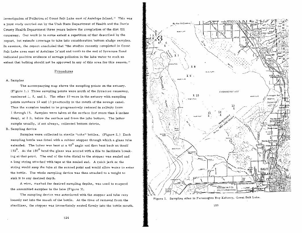
Investigation of Pollution of Great Salt Lake east of Antelope Island." This was

a jOint study carried out by the Utah State Department of Health and the Davis

County Health Department three years before the completion of the dirt fill

causeway. Our work is to some extent a repetition of that described by the

report, but extends coverage to take into consideration bottom sludge samples.

In essence, the report concluded that "the studies recently completed in Great

Salt Lake area east of Antelope Island and north to the end of Syracuse Road

indicated positive evidence of sewage pollution in the lake water to such an

extent that bathing shoUld not be approved in any of this area for this season."

Procedures

A. Samples

The accompanying map shows the sampling points on the estuary.

(Figure 1.) Three sampling points were north of the Syracuse causeway,

numbered 1, 2, and 3. The other 10 were in the estuary with sampling

points numbers 12 and 13 practically in the mouth of the sewage canal.

Thus the samples tended to be progressively reduced in salinity from

1 through 13. Samples were taken at the surface (not more than 2 inches

deep), at 2 ft. below the surface and from the lake bottom. The latter

sample usually, if not always, collected bottom debris.

B. Sampling device

Samples were collected in sterile "coke" bottles. (Figure 2.) Each

sampling bottle was fitted with a rubber stopper through which a glass tube

extended. The latter was bent at a 900

angle and then bent back on itself

1800

• At the 1800

bend the glass was scored with a file to facilitate break­

ing at that point. The end of the tube distal to the stopper was sealed and

a long string attached with tape at the sealed end. A quick jerk on the

string would snap the tube at the scored point and would allow water to enter

the bottle. The whole sampling device was then attached to a weight to

sink it to any desired depth.

A wire, marked for desired sampling depths, was used to suspend

the assembled samples in the lake (Figure 3).

The sampling device was autoclaved with the stopper and tube very

loosely set into the mouth of the bottle. At the tirue of removal from the

sterilizer, the stopper was immediately seated firmly into the bottle mouth.

124

'.' \~

'. \

X 9 MUD H.A'

X 8

X 10

MVO "I..AT

MUD rt",A1

11 i2 X ·X

13 X

MUD f-I.I\T

Figure 1. Sampling sites in Farmington Bay Estuary, Great Salt Lake.

125

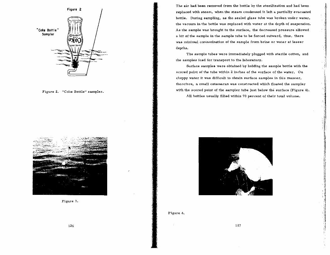
"Coke Bottle" Sampler

Figure 2

Figure Z. "Coke Bottle" sampler.

Figure 3.

lZ6

The air had been removed fro:m the bottle by the sterilization and had been

replaced with steam, when the stea:m condensed it left a partially evacuated

bottle. During sa:mpling, as the sealed glass tube was broken under water,

the vacuum in the bottle was replaced with water at the depth of suspension.

As the sample was brought to the surface, the decreased pressure allowed

a bit of the sa:mple in the sample tube to be forced outward, thus, there

was :minimal contamination of the sample fro:m brine or water at lesser

depths.

The sa:mple tubes were immediately plugged with sterile cotton, and

the samples iced for transport to the laboratory.

Surface sa:mples were obtained by holding the sa:mple bottle with the

scored point of the tube within Z inches of the surface of the water. On

choppy water it was difficult to obtain surface samples in this manner,

therefore, a small catamaran was constructed which floated the sa:mpler

with the scored point of the sa:mpler tube just below the surface (Figure 4).

All bottles usually filled within 70 percent of their total volume.

Figure 4.

127

C. Determination of MPN

The MPN was determined by the multiple tube method described in

the "Standard Methods for Examination of Water and Waste Water." U.S.

Public Health Association, Inc. 12th Ed., 1965.

Millipore counts were attempted, but found to be impractical because

the pores plugged after the first few ml of brine were filtered. This was

were used in these experiments.

F. Tributary Samples

One set of samples from 28 different streams and canals flowing into

the estuary were taken during the week of 25 July 1971. The MPN for this

set of samples was determined.

Results ----

especially true of the bottom samples. The most effort of the summer's work went into the sampling and deter-

There was some concern as to the toxicity of the brine for the coli­

forms, especially in the 10 ml samples. It was determined that there was

adequate dilution with the double strength lactose broth to allow growth of

the organisms.

All positive gas producing organisms were subjected to confirmation

tests for E. coli with final identification confirmed with the use of TSI agar

and IMViC tests.

D. Effect of Brine Concentration on Growth of ColHorms (Kill Tests)

Two samples of lake brine were used to test the bactericidal effect

of the lake water; one contained 96,900 ppm NaCl, the other 91,700 ppm.

A series of tubes was set up using from 0 to 10 ml of lake water. The

total volume of each tube was then brought to lO ml with sterile distilled

water. Lactose was then added to each tube to a concentration of 13 grn/

liter. Actively growing cultures of§.. coli isolated from the lake or from

the U. of U. Department of Microbiology stock cultures were used as

inoculum for the brine lactose tubes. Twenty-four sets were tested, each

with a different confirmed coliform.

E. Growth Curves of Various Microorganisms Utilizing Bottom Debris as the

Sole Source of Nutriments.

Flasks containing sterilized bottom debris collected at station 13

were inoculated with the following microorganisms:

Coliform No. 2.

(U. of U. stock culture) (U. of U. stock culture) (U. of U. stock culture) (U. of U. stock culture) (Isolate from lake) (Isolate from lake)

Plate counts of viable organisms were made from these cultures at

0, 6, and 18 hours in order to determine a growth rate, if any, of each of

the species of microorganisms. It is to be noted that 3 human pathogens

12.8

mination of the coliform MPN at each of the 13 sampling stations. Table 1

presents the mean MPN for each station as determined for the surface, at a

depth of 2 feet and at the bottom of the lake. Invariably, the bottom saInple

included debris from the lake bottoIn Inud or sand. As was expected the

greatest number of colHorms was found in the area nearest the mouth of the

sewage canal, and the greatest concentration was found in bottom sludge.

As may be noted in the table, coliforms were isolated from bottom material

at station No. 2 which was north of the causeway.

We had anticipated finding larger numbers of coliforms in surface samples,

as suming that the surface waters were lower in saline content. Except at

stations II, 12, and 13, this was not the case.

The results of the tests for the toxicity of lake water for 24 different strains

of confirmed colHorms (Table 2) showed that concentrations of NaCl above 6.78

percent allowed no growth. At the latter concentration only 3 of the 24 grew to

show increased turbidity in the tubes. At a NaCl concentration of 5.81 percent,

9 of the strains failed to grow while 15 grew but produced no gas. At 4.95 per­

cent NaCl, 4 strains failed to grow, 11 grew but produced no gas, while 9 grew

and produced gas. At 3.88 percent NaCI only 1 organism failed to grow, 6

grew without gas production and 17 grew and did produce gas. Most of the

strains grew and produced gas at concentrations below 3. 88 percent. Strain

17 appeared to be les s salt tolerant than the other strains and failed to grow at

all at 2,91 percent NaCl, but did show growth at 1. 94 and 0.97 percent. Strain

24 produced no gas at any concentration of NaCl, and failed to grow in NaCl

concentration above 4.95 percent.

Table 3 presents the results of the experiment to demonstrate the ability

of coliform organisms to grow in a broth where sole nutriment was obtained

from the bottom sludge collected at sampling station No. 13. Of all the

129

Table 1. Average M. P. N. coliforlns at each salnpling station (five salnplings).

2

3

4

5

6

7

S

9

10

11

12

13

o

o

o

o

o

o

o

o

2.5c

357

a. 2 of 4 samples + b. 1 of 5 samples +

o

o

o

o

o

o

o

o

0.4b

0.4b

0.4b

2.5d

lS8

o

o

28.5

8.1

330

717

132S

c. 2 or 5 samples + d. 3 of 5 samples +

130

Table 2. Growth of 24 strains of coliforlns in Great Salt Lake water with added lactose.

9.69 -

S.72 - -

7.69

t>.78 - o - o - 0

5.S] 0 o 0 0 0 0 0 0 - - - - 0 - - 0 0 0 0 0 0 -

4.95 0 0 e 0 @ e e e e 00- 0 e e - e 0 000 0 -

1.94 e e e e e e e e e e e e e e e e 0 e e e e e e 0

0.97 e e e e e e e e $ e e e e e e e e e e e e e e 0

0.00' e e e e e e e e e e e e e e e e e e e e e e e 0 1 2 3 4 5 6 7 8 9 10 11 12 13 14 15 16 17 IS 19 20 21 22 23 24

o Indicates growth in lactose broth e Indicates growth with gas production within 24 hrs. - Indicates no growth

Table 3. Growth of various lnicroorganislns with sterile bottoln sludge as sole nutriment.

Time Org8nisms Q 6 !-Irs. IS !-Irs.

7 341 greater than 10,000

£. typhimurium 9 74 greater than 10,000

18 19 420

Shig. dysenteriae no growth

Coliform #1 31 290 greater than 10,000

5 78 greater than 10,000

131

;1

organism.s tested, which included stock cultures of hum.an pathogens as well as

2 strains isolated from lake brine, Shigella dysenteriae was the only organism.

which failed to reproduce.

The MPN determinations of the various "tributaries" of the "stuary are

not presented in tabular form. Suffice it to say that of som.e 28 stream.s and

canals flowing into the estuary, every single one was found to be polluted with

!;.. coli, the lowe"t MPN being 70 per 100 rnl of H20 and the highest> 1,600, 000.

Many streams showed counts greater than 1,600. This was but a single sam.pl­

ing, and dilutions were not prepared to determine m.ore accurately the numbers

of coliforms present. Many of these streams could have been, and possibly

were, polluted with sewage, and the MPN of coliforms was more than likely

f 06 . in excess 0 1 organIsms.

Discussion and Conclusions

It was found by this student group that there is a flow of brine from the

main part of the lake through the causeway bridge into the estuary. Also that

the water has a greater saline content now than it did in 1965 when the State

Department of Health and the Davis County Departm.ent ran their survey of the

area. This m.ay account for the lower MPN counts of coliforms generally found

in the present survey--at least in the surface sam.ples.

There is nO doubt that the sewage deposits contain large numbers of coli­

forms, and that should the inflow of fresh water be adequate to make a fresh

water lake of the estuary, then these and possibly sequestered human pathogens

could conceivably make the estuary a dangerous and certainly non-esthetic

recreation area for years to corne. It was shown by these experiments that the

coliforms there have become quite salt tolerant, and that there are adequate

nutrients in the bottom sludge to maintain the multiplication of sequestered

coliforms and organisms generally conceded to be human pathogens. This is

true also for new coliforms and pathogens being continually deposited in the

lake from the streams and drainage canals feeding the estuary.

Bibliography

Frederick, Elfriede, The Bacterial Flora of Salt Lake and the Viability of other Microorganisms in Great Salt Lake Water. M. S. Thesis, 1924, University of Utah.

132

Smith, W. W.. Evidence of a Bacterial Flora Indigenous to the Great Salt Lake in Utah. M. S. Thesis, 1936, University of Utah.

Utah State Department of Health; Davis County Health Departm.ent. Prelim­inary Investigation of Pollution of Great Salt Lake East of Antelope Island. Utah DepartInent of Health, July 9, 1965 (revised) SOH-San-7/65.

U. S. Public Health As soc. Inc.. Standard Methods for Examination of Water and Waste Water. 12th Edition.

133

A HELE-SHAW MODEL STUDY OF SEEPAGE FLOW

THROUGH THE CAUSEWAY OF THE GREAT SALT LAKE

Anching Lin 1

and Sang-Myung Lee 2

Abstract

The hydrodynamic nature of the seepage flow through the causeway is described. The method of viscous flow analogy (or the Hele-Shaw model study) was introduced and applied to the investigation of the exchange of brines through the cause­way. The model study provides an independent method that can develop all the necessary information concerning the effect of the causeway. Coupled with field investigations, the Hele-Shaw model study offers a most effective and economical approach for the development of pertinent data for the manage­ment of the Great Salt Lake. The study of seepage movement was was documented in 16= movie films.

Introduction

Ever since the construction of the Southern Pacific Railroad causeway

on the Great Salt Lake in 1957, the balance of brines in the lake has undergone

a drastic change as first noted by T. C. Adams (Adams, 1964).

The brines in the north arm of the lake (relative to the causeway) have

been obse rved to stay steadily at a state of near saturation, while those in the

south were near saturation during the early 1960 1 s and were very much diluted

in the last three years. The dilution of urines in the south obviously resulted

from the increased amount of fresh water inflows to the lake.

The cyclic recurrence of wet and dry hydrologic conditions will continue

to influence the physical environment of the lake. The precise e£fect of the

causeway on the balance of brines in relation to the cyclic hydrologic event

will have to be defined in order that the developable mineral resources on the

lake may be assessed and future plans for mineral exploration may be established.

Madison of the U. S. Geological Survey conducted a field investigation on the

effect of the causeway in 1969 (Madison, 1970). The study pointed out the many

problems associated with the causeway, yet precise effects of the causeway

were not defined.

Professor, Civil Engineering Departtnent, University of Utah.

U]"a(lliiUe Research Assistant, Civil Engineering Department, University of Utah.

134

This paper introduces a Hele-Shaw model study in order to investigate in

detail the mechanism that governs the seepage flow through the causeway.

The Hele-Shaw Model

Hele-Shaw, in 1898, suggested the use of viscous flow analogy to study the

potential flows to which the seepage through the causeway belongs. The analogy

is made possible by comparing the dynamic equations of motion between the flow

through porous media and the flow in a very thin gap, called Hele-Shaw cell.

That is, if one builds a Hele-Shaw model which is geometrically sitnilar to a

prototype, e. g., the shape of the cross-section of the causeway, the flows

through the model and the prototype are' similar and conditions in the tnodel can

be interpreted and utilized in the prototype if the proper tnodelling laws are

acknowledged (DeWiest, 1965),

where }"K' >--L' >--T are the ratios of permeability, length and time between the

model and the prototype. Here the permeability of the model is defined as a 2

Km '" ~ a being the thickness of the Hele-Shaw cell and v the viscosity of

liquid used in the model. See attached bibliography for the theory and typical

applications of Hele-Shaw model study.

The Causeway and the Model Study

The Southern Pacific Railroad causeway is a rock-filled structure; over

the years, new materials have been added to the original structure to stabilize

the slope. Thus the causeway mainly cotnposed of two parts, (a) the core

portion consisting of more compact materials, and (b) the cover portion on the

slope resulting from newly added material and through which water flows with

little resistance. It is the cOre portion that is responsible for the dynamic

consequence of the causeway and thus the tnodelling is focused on the core

portion.

A Hele-Shaw cell was built to the estitnated proportions of the core portion

of the causeway with a side slope of 1. 5 units in horizontal direction versus

1. 0 unit in the vertical. The overall base ditnension of the model is about 24

inches and the working thickness of the Hele-Shaw cell was chosen to be 1/8

135

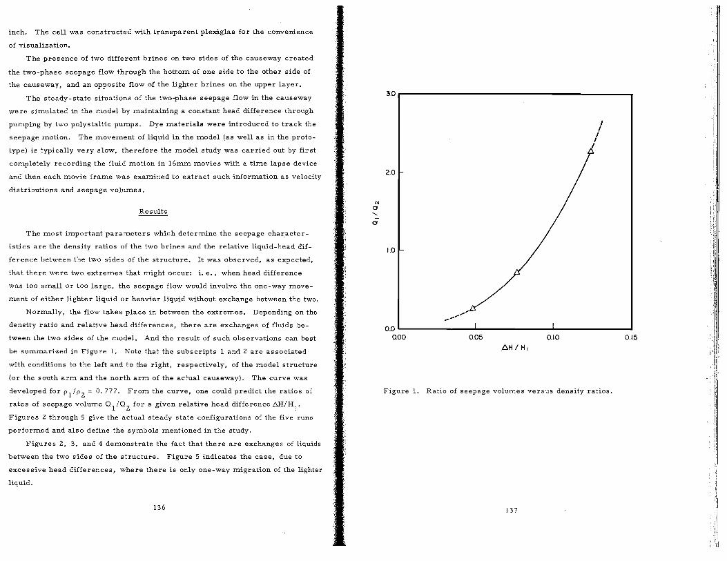
inch. The cell was constructed with transparent plexiglas for the convenience

of visualization.

The presence of two different brines on two sides of the causeway created

the two-phase seepage flow through the bottom of one side to the other side of

the causeway, and an opposite flow of the lighter brines on the upper layer.

The steady-state situations of the two-phase seepage flow in the causeway

were simulated in the model by maintaining a constant head difference through

pumping by two polystaltic pumps. Dye materials were introduced to track the

seepage motion. The movement of liquid in the model (as well as in the proto­

type) is typically very slow, therefore the model study was carried out by first

completely recording the fluid motion in l6mm movies with a time lapse device

and then each movie frame was examined to extract such information as velocity

distributions and seepage volumes.

Results

The most important parameters which determine the seepage character­

istics are the density ratios of the two brines and the relative liquid-head dif­

ference between the two sides of the structure. It was observed, as expected,

that there were two extremes that might occur: i. e., when head difference

was too small or too large, the seepage flow would involve the one-way move­

ment of either lighter liquid or heavier liquid without exchange between the two.

Normally, the flow takes place in between the extremes. Depending on the

density ratio and relative head differences, there are exchanges of fluids be­

tween the two sides of the model. And the result of such observations can best

be summarized in Figure 1. Note that the subscripts 1 and 2 are associated

with conditions to the left and to the right, respectively, of the model structure

(or the south arm and the north arm of the actual causeway). The curve was

developed for p 11 P 2 = 0.777. From the curve, one could predict the ratios of

rates of seepage volume Q l/Q2

for a given relative head difference ~/H1.

Figures 2 through 5 give the actual steady state configurations of the five runs

performed and also define the symbols mentioned in the study.

Figures 2, 3, and 4 demonstrate the fact that there are exchanges of liquids

between the two sides of the structure. Figure 5 indicates the case, due to

excessive head differences, where there is only one-way migration of the lighter

liquid.

136

N 0

" 0

3.0

I I

I I

I

2.0

1.0

0.0 L..-______ "--______ .l...-_____ ----'

0.00 0.05 0.10 0.15

Figure 1. Ratio of seepage volumes versus density ratios.

137

I I

i I

i II

I ]

1

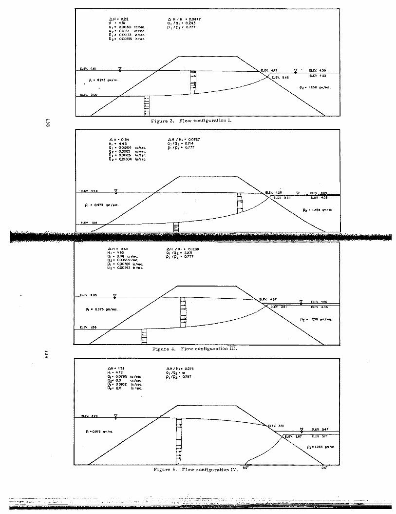
.... w 00

.... W '>0

ELEV. 4.61

e..H. O.ZZ H • 4.51 Q I· 0.00391 echK. 02' 0016! «1,0", il,. 0.00!73 in" ... O2 • 000785 In/sec.

Pt ,. 0.973 um/ct.

ELEV. 2.00

e..H • 0.34 HI • 4.43 01 • 0.01304 02' 0.0203 0, • 0.00615 O2 , 0.0!304

cc.lseC. cc/sec. In/s,c. In/sec.

PI • 0.973 QI'ft/"c,

aH· 0.60 HI:It 4,85 01 • 0.118 cc/see. QZ' 0.=<:0/50<. QI • 000386 In/HC. U 2. 000292 In 'sec.

e..Ho 1.31 H.' 4.78

0.0785 eel .... 0.0 ce/_ 0.0102 In/""" 0.0 In ISK

e.. H I H • 0.0477 01 10.' 0.243 PI IP.· 0.777

Figure Z. Flow configuration I.

e..H I H •• 0.0767 Q, IQ2' 0.714 PI I P2' 0.777

~H IH, • 0.12:3:5 Q, IQ2 • 2.271 PI Ip • • 0.777

Figure 4. Flow configuration III.

e..H I HI" 0.275 01 /Q2.. Q)

PI IPZ' 0.797

Figure 5. Flow configuration IV. $.0'

383

4S7

. :->: . ':-.~ . -'-.:..= _ ... i'-":'.:-= .. -o; ,.'-'--::ff-_" __ f.,.--;:.. .--::~ .. --"-~ -;,~; ~.,~-' ':1-'"'; I " -i,:.,,,,-" -"--";;;:':'--'--"-~'-~-'!!i i ;t:, +, nnnnn~

ELEV .•. 39

£LEY. 422

pz.. 1.,256 om/Me.

PZ • LZ$$ ""I ....

El.E\! ll47

EI..EV. 117

0.0·

The velocity vectors shown are the results of study on movie films taken.

The integration of the velocity profiles then gives the rates of seepage volume.

The results presented in dimensionless form such as 0l/OZ' t"H/Hl

, etc.,

are readily applicable to the prototype without having to consider the modelling

laws.

One may consider the year 197Z as an illustration. The head difference

between the south arm and the north arm of the lake has been quoted as 1. 8

feet and the water depth at the south side of the causeway averages, say, Z5

feet. Then, the relative head difference t"H/Hl is estimated to be 0.07 (or 7

percent). If the density ratio were 0.777, then the ratio of exchange volume

01/0Z would have been about 0.50 (from Figure 1). Or equivalently, if the

density of the brines in the south were diluted to 78 percent of that in the

north, then relative head difference 0.07 would have indicated that heavier

brines were migrating two times as much from the north to the south than the

much diluted brines from the south to the north. Of course, the actual density

ratio is about 0.90 and the ratio of seepage volumes will be higher than 0.50.

From a consideration similar to Ghyben-Herzberg' s (De Wiest, 1965),

and working from Figure 1 the ratio of seepage volume should be close to One.

That is, the volumes of brines migrated from the south are almost balanced

by those from the north.

Future extension of the work will have to include more density ratios and

wave effects. However, before the actual parameters of the field environment

including physical and hydrological are developed and incorporated to the model

study, any unplanned extensive study may prove to be only a futile academic

exercise.

Conclusion

The model study offers a simple and direct approach to the investigation of

the dynamic behavior of seepage flow through the causeway. It is by far the

most effective and economical way for the treatment of seepage flows involving

the exchange of two-phase fluids.

Coupled with field investigations, the model study should provide all the

information that is needed to assess the ir;npact of the causeway.

The advantages of the model study can be summarized as follows:

(1) The model study prOvides comprehensive details of the seepage

140

parameters, such as velocity distributions, exchange of

seepage volumes, location of interface, etc.;

(2) The execution of the experiment and the interpretation

of the results are simple and straightforward. The

movies made on the fluid movement can be accepted

readily as results;

(3) It is possible to incorporate the wave effects to the study

with little additional work.

It is suggested then that future model study be designed to relate the actual

field environment including all the possible head and density differences re­

sulting from cyclic hydrological conditions, and the wave effects should also be

investigated.

Acknowledgement

This work is partially supported by National Science Foundation under

grant No. GA 3086. The authors are grateful for the critical comments of

Dr. P. C. Chang and appreciate the technical advice on movie making offered

by Mr. Mike Milochik.

Adams, T. C. Salt migration to the northwest body of Great Salt Lake, Utah, March 1964.

Bear, J. Scales of viscous analogy models for groundwater studies, of Hydr. Div., February 1960.

DeJosselin, deJong, G. Singularity distributions for the analysis multiple fluid flow through porous media, J. of Geophysical Res. , November 1960.

DeWiest, R. J. M. Geohydrology, John Wiley, New York 1965.

Madison, R. J. Effect of a causeway on the chemistry of the brine in Great Salt Lake, Utah: Utah Geological and Mineralogical Survey Water Resources Bulletin, 1970

P01ubarinova-Kochina, P. Ya. The Theory of Groundwater Movement, trans­lated by R. J. M. DeWiest, Princeton University Press 196Z.

Santing, G. A horizontal scale model, based on the viscous flow in an acquifer having storage, lASH, General Assembly, Toronto, 1957.

Todd, D. K. Unsteady flow in porous media by means of a Hele-Shaw viscous fluid model, , 35(6), 1954.

Yen, B. C. and Hsie, C. H. Viscous flow model for groundwater movement, Water Resources, Res., .§.(5), lZ99-1306, 197Z.

141

,!

NUTRIENTS, ALGAL GROWTH, AND CULTURE OF BRINE SHRIMP

IN THE SOUTHERN GREAT SALT LAKEI

2 3 Donald B. Porcella and J. Anne Holman

Abstract

'T'he overall objective of this study was to measure nutrients in Great Salt Lake waters and to determine how the alga, Dunaliella .!1E. responds to nutrients. The relationship between food supply (algae) and the growth and reproduction of brine shrimp Artemia.!1E' was also studied.

Based on chemical analyses inorganic nitrogen is app~rently the limiting factor for growth in the samples of Great Salt Lake water. Carbon may also be limiting. Phosphorus, iron and other trace elements seem to be in abundant supply. These observations were confirmed by algal bioassays.

Brine shrimp we re fed on several concentrations of Dunaliella as well as on yeast cells. Growth and reproduction of the brine

on aJgae alone was superior to yeast alone. The optimum utilization by the brine shrimp was about I, 000 algal cells per brine shrimp per day. Different concentrations and ages of added algae had no apparent effect on whether the mature brine shrimp pro­duced live young (nauplii) or resistant cysts.

It can be concluded that a feasible aquaculture based on ~~~~~.!1E. and Artemia~. can be developed for brine shrimp isolated from the Great Salt Lake. Production of algae and brine shrimp in lake enclosures may be increased by add'ition of specific nutrients.

KEY WORDS; Great Salt Lake, Productivity, Nutrients, Aqua­culture, Carbon, Nitrogen, Phosphorus, Dunaliel1a .!1E. , .!1E' (Brine Shrimp).

Because of the high salt content of the Great Salt Lake waters, it is con­

sidered a harsh environment for most mi·croorganisms and higher plants and

animals (Brock, 1969). A harsh environment actually could be defined as one

where the environment has not existed as a permanent entity long enough to

lThis work supported by funds provided by NL Industries, Inc. New Ven­tures Division, Mr. Robert Ade, Project Officer. The help of Peter A. Cowan, R. David Johann, and M. Virmani in the analysis of samples and data is gratefully acknowledged.

2 . ASSocIate Professor of Civil and Environmental Engineering and the Utah

Water Research Laboratory, Utah State University, Logan, Utah.

3 Assistant Professor of Wildlife Science, Utah State University, Logan, Utah:.

142

allow the evolution of a wide variety of organisms. Thus in harsh environments

very simple and specific food chains exist which have little or no competition

with other species for resources in short supply. The Great Salt Lake environ­

ment is one of these environments and appears to be ideally suited for maximi­

zing flow of energy and production in a food chain.

There are a few species which have been selected for, and which domin­

ate and compete for energy and nutrients, and carry out their full life-cycle

in the waters of the lake. These include various kin~s of "salt-loving" bac­

teria and algae and the brine shrimp, Artemia~. At present the economic

potential of the Great Salt Lake for aquaculture depends On methods for

growing brine shrimp and selling them to the large market of tropical fish

fanciers. Feasible aquaculture is based on the proposition that increased

concentrations of nutrients would lead to higher bacterial and algal popula­

tions and therefore higher production of brine shrimp. As a whole the Great

Salt Lake is relatively nutrient poor and does not receive large influxes of

nutrients from. pollution. Thus, the opposite side of the increas ed nutrient

question, eutrophication or increased nutrient concentrations with the resul­

tant overproductivity problems, apparently dOes not occur in the lake.

The complicating factor in the Great Salt Lake is that the availability

of nutrients which are required by algal populations is also affected by the

high concentration of salts. There is not only the possibility of salt con­

centration affecting the activity of specific nutrients needed for growth of micro­

organisms, but the biological fixation of various kinds of nutrients is probably

affected by the lack of species of sufficient variety to fix nutrients. Therefore,

to develop a feasible aquaculture it is necessary to understand the inputs and

cycling of various nutrients, to understand how they are utilized by the pro­

ducer forms of the food chain (algae), and finally to determine the role of

producers in supporting the brine shrimp. Only in this way can a viable brine

shrimp proces sing industry be developed. Because brine shrimp feed on any

particle within the appropriate size range, bacteria and detritus are foods

also. These usually depend On producers for their growth.

The overall objective of this study then was to measure nutrients in Great

Salt Lake waters and determ.ine how the algal species of interest respond to

nutrients. Then the relationships between food supply (as algae) and growth

of brine shrimp were to be estimated.

143

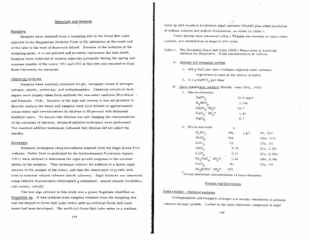
Materials and Methods

Sampling

Samples were obtained from a sampling site in the Great Salt Lake

adjacent to the Magnesium Division Plant of NL Industries at the south end

of the lake to the west of Stansbury Island. Because of the isolation of the

sampling point, it is not polluted and probably represents the lake itself.

Samples were collected at various intervals primarily during the spring and

summer months of the years 1971 and 197Z at this site and returned to Utah

State University for analysis.

Chemical analyses

Samples were routinely analyzed for pH, inorganic forms of nitrogen

(nitrate, nitrite, ammonia), and orthophosphate. Chemical analytical tech­

niques were largely taken from methods for sea-water analysis (Strickland

and Parsons, 1968). Because of the high salt content it was not possible to

directly analyze the water and samples were first diluted to approximately

ocean-water salt concentrations by dilution to 20 percent with deionized

distilled water. To ensure that dilution was not changing the concentrations

of the nutrients of interest, standard addition techniques were performed.

The standard addition techniques indicated that dilution did not affect the

results.

Bioassays

Bioassay techniques using procedures adapted from the AI~al Assay Pro­

cedures: Bottle Test as published by the Environmental Protectio'n Agency

(1971) were utilized to determine the algal growth response to the nutrient

milieu in the samples. This technique utilized the addition of a known

species to the sample of the water, and then the observance of growth With

time in constant volume cultures (batch cultures). Algal biomass was measured

using relative fluorescence (chlorophyll3! estimates), optical density (turbidity),

cell counts, and pH.

The test alga utilized in this study was a green flagellate identified as

Dunaliella!E.' It was isolated from samples obtained from the sampling site

and maintained in Great Salt Lake water until an artificial Great Salt Lake

water had been developed. The artificial Great Salt Lake water is a medium

144

...!.,.,-

made up with'standard freshwater algal nutrients (NAAM) plus added quantities

of sodium chloride and sodium bicarbonate, as shown in Table l.

Brine shrimp were nleasured using a Whipple micronleter or clear ruler,

counted, and identified as to stage in life-cycle.

Table 1. The Simulated Great Salt Lake (SGSL) Water.used as artificial nledium for Dunaliella. Final concentrations in culture.

A. Salinity and inorganic carbon

B.

I. ZOO g NaCl per liter (Culligan supplied water softener

regenerant is used as the source of NaCI)

Z. 0.5 g NaHC03

per liter

~~"--.f~~!@:I~....!!:~~!!:(NAAM, refer EPA, 1971)

3. Macro-elenlents

NaN03

KZHP0

4 MgS0,47H

ZO

CaClZ' ZHZO

MgClz

4. Micro-elements

*

COCIZ

CuClZ

NaZMo04

' ZHZO

FeCl3

" 186.

264.

33.

25.5 mgll

L 044

14.7

4.41

5.7

fl gIl

0.78

0.01

7.Z6

96.

300.

(B, 33)':'

(Mn, 114)

(Zn, 15)

(Co, 0.35)

(Cu, 0.003)

(Mo, Z.88)

(Fe, 33)

Actual elemental concentrations of trace' elements

Results and Discussion

Field studies! chenlical analyses

OrthOphosphate and inorganic nitrogen are usually considered of prinlary

interest in algal growth. Carbon is the nlost important component of algal

145

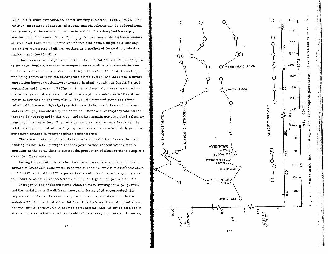
cells, but in most environments is not limiting (Goldman. et al.. 1972). The

relative importance of carbon, nitrogen, and phosphorus can be deduced from

the following estimate of composition by weight of marine plankton (e. g.,

see Stumm and Morgan, 1970), C 41 N7

, 2 P. Because of the high salt content

of Great Salt Lake water, it was considered that carbon might be a limiting

factor and monitoring of pH was utilized as a method of determining whether

carbon was indeed limiting.

The measurement of pH to indicate carbon limitation in the water samples

is the only simple alternative to comprehensive studies of carbon utilization

in the natural water (e. g., Verduin, 1956). Rises in pH indicated that CO2

was being removed from the bicarbonate buffer system and there was a direct

correlation between qualitative increases in algal (not always Dunaliella.§ll..)

population and increased pH (Figure 1). Simultaneously, there was a reduc­

tion in inorganic nitrogen concentration when pH increased, indicating utili­

zation of nitrogen by growing algae. Thus, the expected cause and effect

relationship between high algal populations and chang.es in inorganic nitrogen

and carbon (pH) was shown by the samples. However, orthophosphate concen­

trations do not respond in this way, and in fact remain quite high and relatively

constant for all samples. The low algal requirement for phosphorus and the

relatively high concentrations of phosphorus in the water would likely preclude

noticeable changes in orthophosphate concentration.

These observations indicate that there is a possibility of more than one

limiting factor, i. e., nitrogen and inorganic carbon concentrations may be

operating at the same time to control the production of algae in these samples of

Great Salt Lake waters.

During the period of time when these observations were made, the salt

content of Great Salt Lake water in terms of specific gravity varied' from about

1. 11 in 1971 to 1. lOin 1972 ; apparently the reduction in spe cHic gravity was

the result of an influx of fresh water during the high runoff periods of 1972.

Nitrogen is one of the nutrients which is most limiting for algal growth,

and the variations in the different inorganic forms of nitrogen reflect this

requirement. As can be seen in Figure 2, the most abundant form in the

samples was ammonia nitrogen, followed by nitrate and then nitrite nitrogen,

Because nitrite is unstable in aerated environments and quickly is oxidized to

nitrate, it is expected that nitrite would not be at very high levels. However.

146

UJ

!;t ::c a.. trl 0 ::c a. 0 ::c I-[l:

0

~ ......

'" =(

z UJ (!) 0 0::

!: z U

z <t (!) 0:: 0 ~

0 0

1- 10 z UJ

u.::E oUJ

..J UJ

>-I-:> <t 0:: (!)

u u. u

::c UJ

a. a.. trl

'\11131l'lfNOa AN'\1V>J

3'\191\1 M3:::!

\11131l'lfNna AN\1V'l

'lf1131l\1Nna AN'lfW

3'1f91'1f M3:::!

!2>-!:!:I-

::c u-a.. UJ:?i

0..0::: trll.!)

147

.; d3S '" .....

0 ~ 0 N '" 9f\'If k

'" ..., 01 ~

1f\r '" 0 ~

':!1 01 ..:1

NM ..., ";;l trl

N ..., t- 01

'" 0 A'lfV>J-~ k

Q 0 ,~

!:Id'lf '" ;:! k 0

.<: p.

0 !:I'lfV>J '" 0 10 .<:

p.

'" 83:1 ..., <II

.<: trl p. ::c '" 0

0 N'If I- .<: z p.

<I) 0 0 >- ::E ..q <t ..,

k 0 0

~J.:)O UJ '0

s:: ::E 01

i= l- s::' 0 '" 10 b1l N 0

d3S k ..., ';:1 u

0 9f\'If '§

0 b1l N k

0 s::

' ....

1f\r-~ i 0'> P.

0 ,!1 ':!1 '" NOr '" b1l

s:: 01

cil .<: u ' ,

A'lfV>J ,iii 0

i/ Q

'" k

~ Ii ..... I,!

!:Id'lf ~

; I~!

I'll .,

Ilt\

~, I

,1,[

'~I Ii

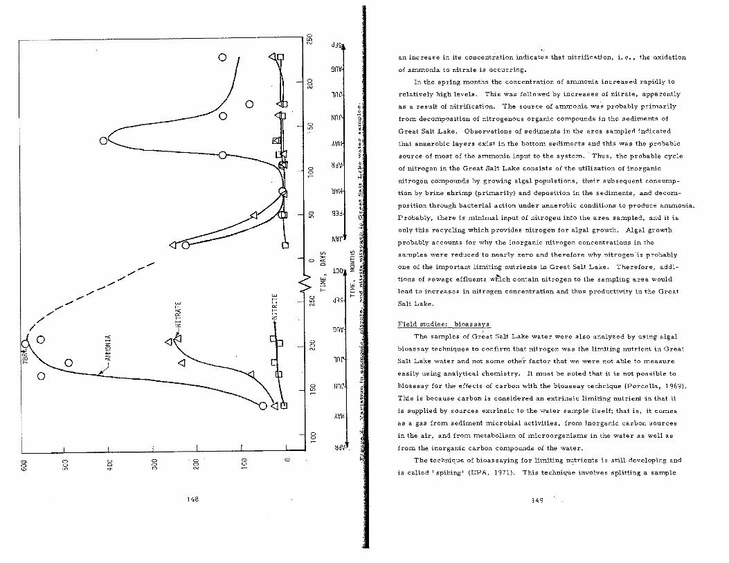
0-o \0

o

"" en

o o

"" o o M

<l

o o N

148

o

o o

1

o

a UC> N

0 0 N

0 UC>

0 a

a UC>

0 In N

0 0 N

-0 In

0 0

d3S

gmf

lnr

Nne

A'IM

~d\i

~\f

93d

N'fJf

Vl >-..; c

DO w ;:s I-

d3S

~Jn\f

lnr

t,lnr

A'tfH

~d\f .

.; ~

~-• · -"i · '-"-,\.

~

• ,;:

" ~.

::: • U)

" 0, . -k:"

0 ,~~'

~: 0,

Vl :t: f-z 0 :iF:

~ ::;: ~

f-

; " i!I

" +'

'a i!I

l 0 g. a

;,,-

an increase in its concentration indicates that nitrification, 1. e., the oxidation

of arnrnonia to nitrate is occurring,

In the spring months the concentration of arnrnonia increased rapidly to

relatively high levels. This was followed by increases of nitrate, apparently

as a result of nitrification. The source of ammonia wa~ probably primarily

from decomposition of nitrogenous organic compounds in the sediments of

Great Salt Lake. Observations of seditnents in the area sampled indicated

that anaerobic layers exist in the bottom sediments and this was the probable

source of tnost of the atntnonia input to the system. Thus, the probable cycle

of nitrogen in the Great Salt Lake consists of the utilization of inorganic

nitrogen compounds by growing algal populations, their subsequent consUITlp­

tion by brine shrimp (prim.arily) and deposition in the seditnepts, and decotn­

position through bacterial action under anaerobic conditions to produce amtnonia •

Probably, there is minimal input of nitrogen into the area sampled, and it is

only this recycling which provides nitrogen for algal growth. Algal growth

probably accounts for why the inorganiC nitrogen concentrations in the

samples were reduced to nearly zero and therefore why nitrogen -is probably

one of the important litniting nutrients in Great Salt Lake. Therefore, addi­

tions of sewage effluents wlrich contain nitrogen to the satnpling area would

lead to increases in nitrogen concentration and thus productivity in the Great

Salt Lake.

Field studies: bioassays

The samples of Great Salt Lake water were also analyzed by using algal

bioassay techniques to confirtn that nitrogen was the lim.iting nutrient in Great

Salt Lake water and not some othe'r factor that we were not able to measure

easily using analytical chemistry. It must be noted that it is not possible to

bioassay for the effects of carbon with the bioassay technique (Porcella, 1969).

This is because carbon is considered an extrinsic limiting nutrient in that it

is supplied by sources extrinsic to the water sam.ple itself; that is, it co:mes

as a gas from sediment microbial activities, from inorganic carbon sources

in the air, and from metabolism of microorganisms in the water as well as

from the inorganic carbon compounds of the water.

The technique of bioas saying for limiting n'7trients is stin developing and

is called I spiking' (EPA, 1971). This technique involves splitting a sample

149

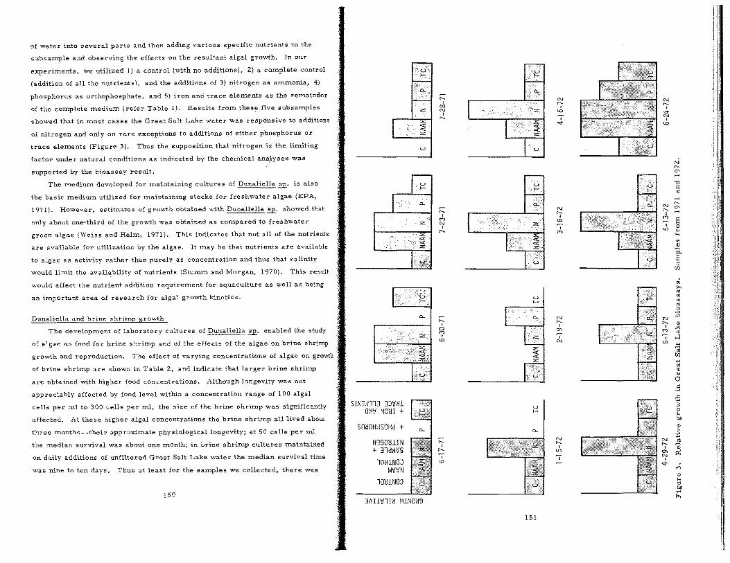
of water into several parts and then adding various specific nutrients to the

subsample and observing the effects on the resultant algal growth. In our

experiments, we utilized 1) a control (with no additions), 2.) a complete control

(addition of all the nutrients), and the additions of 3) nitrogen as ammonia, 4)

phosphorus as orthophosphate, and 5) iron and trace elements as the reInainder

of the complete Inedium (refer Table 1). Results from these five subsamples

showed that in most cases the Great Salt Lake water was responsive to additions

of nitrogen and only on rare exceptions to additions of either phosphorus or

trace elements (Figure 3). Thus the supposition that nitrogen is the limiting

factor under natural conditions as indicated by the cheInical analyses was

supported by the bioassay result.

The Inedium developed for maintaining cultures of Dunaliella.!E' is also

the basic mediUIn utilized for Inaintaining stocks for freshwater algae (EPA,

1971). However, estiInates of growth obtained with Dunaliella.!E' showed that

only about one-third of the growth waS obtained as compared to freshwater

green algae (Weiss and Helm, 1971). This indicates that not all of the nutrients

are available for utilization by the algae. It Inay be that nutrients are available

to algae as activity rather than purely as concentration and thus that salinity

would liInit the availability of nutrients (StUInIn and Morgan, 1970). This result

would affect the nutrient addition requirement for aquaculture as well as being

an iInportant area of research for algal growth kinetics.

Dunaliella and brine shriInp growth

The development of laboratory cultures of Dunaliella.!E' enabled the study

of algae as food for brine shriInp and of the effects of the algae on brine shrimp

growth and reproduction. The effect of varying concentrations of algae on growth;

of brine shrimp are shown in Table 2, and indicate that larger brine shriInp

are obta ined with higher food concentrations. Although longevity was not

appreciably affected by food level within a concentration range of 100 algal

cells per Inl to 300 cells per Inl, the size of the brine shrimp was significantly

affected. At these higher algal concentrations the brine shdmp all lived about

three months--their approxiInate physiological longevity; at 50 cells per m1

the median survival was about one month; in bdne shrimp cultures maintained

on daily additions of unfiltered Great Salt Lake water the median survival time

was .nine to ten days. Thus at least for the samples we collected, there was

150

SlN3~\IJ13 3Jifell mJ'd NOl:lI +

SnliOHdSOHd +

N390'CIlIN + 31dWVS

lOlilNOJ WWN

lOl:lHlOJ

3AIlif13el Hl110l:l9

;:::: N I "" eo ,

N 1.0 I ..... 'I

"'"

;:::: N ..... , M

, N

<D

I 'I "" M

u I-

;:::: N ..... I I

C> '" M I ,.

1.0 N

u I-

0-

.- N

"" "" I I

"" II) .-

I 'I '"

151

N ..... , "'" N

I

'"

N t-O'

'tl 1'1 rd

N t-

"" 0'

I M S ~ • 0 Ln k .....

'" <1l ......

~ rd

(J)

;, ~ rd

'" '" rd 0 .....

N ,.0

"" I M

<1l .;; oj

~

I ....:l U)

;t; <II

(J)

+' <II <1l k U

1'1 ..... ,.0

~ 0

'" bll

<1l :> ..... +'

N

"" I

'" N I

<II I ...... <1l iii P: 'I

"'" ,..; " <1l

k :;! bll f .....

I ~

I 'Ii "

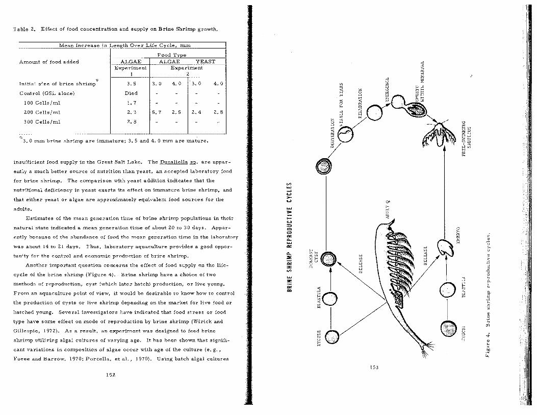
Table 2. Effect of food concentration and supply on Brine Shrimp growth.

Mean Increase in Le?g!h Over Life Cycle, mm

Food Type A=ount of food added ALGAE ALGAE YEAST

Experi=ent Experi=ent 1 2

'" Initial size of brine shrimp 3.5 3.0 4.0 3.0 4.0

Control (GSL alone) Died - - - -

100 Cells/=l 1.7 - - -200 Cells/=l 2.3 5.7 2.5 2.4 2.8

300 Cells/=l 2.8 -

* 3.0 In= brine shrimp are immature; 3.5 and 4.0 mm are mature.

insufficient food supply in the Great Salt Lake. The Dunaliella.§J2. are appar­

ently a tnuch better source of nutrition than yeast, an accepted laboratory food

for brine shrimp. The comparison with yeast addition indicates that the

nutritional deficiency in yeast exerts its effect on immature brine shritnp. and

that either yeast Or algae are approximately equivalent food sources for the

adults.

Estitnates of the mean generation time of brine shritnp populations in their

natural state indicated a mean generation time of about 20 to 30 days. Appar­

ently because of the abundance of food the =ean generation time in the laboratory

was about 14 to 21 days. Thus, laboratory aquaculture provides a good oppor­

tunity for the control and economic production of brine shrimp.

Another itnportant question concerns the effect of food supply on the life­

cycle of the brine shritnp {Figure 4}. Brine shrimp have a choice of two

tnethods of reproduction, cyst (which later hatch) production, or live young.

Frotn an aquaculture point of view, it would be desirable to know how to control

the production of cysts or live shrimp depending on the market for live food or

hatched young. Several investigators have indicated that food stress or food

type have some effect on tnode of reproduction by brine shrimp (Wirick and

Gillespie, 1972). As a result, an experiment was designed to feed brine

shrimp utilizing algal cultures of varying age. It has been shown that signifi­

cant variations in composition of algae occur with age of the culture (e. g .•

Foree and Barrow, 1970; Porcella, et al., 1970). Using batch algal cultures

152

...., > I­c..:t

= CI

= 0:: 0-...., 0::

0-:::E 0::

= en ...., z:: co: co

153

'" ", ::i ...J W

'"

~

0 >< '"

~ ~ '"

0 , ,

I e

<r.

" .-< V

'" v

" ~ V ;:l

'1:l c

j '" ~ ;:J ~ f-'

'" u,

"'" .§ co

" .c (I) ., .~

" CQ

5 '.!> .¢ -" .,

'" :; btl

&:

of age 7, 14, 21, and 28 days, adult brine shriIllp were fed during their repro­

ductive life to deterIlline the effect of Illode of reproduction and nU1l1bers of

young produced. There was no apparent effect of algal culture age on either

paraIlleter. Varying food level concentrations of the different aged algal

cultures produced no effect on Illode of production either.

Conclusions

1. Both cheIllical and bioassay results indicated that inorganic nitrogen is

apparently the limiting factor for growth in the saIllples studied.

2. Phosphorus and iron and other Illetals seeIll to be in abundant supply

relative to nitrogen.

3. Analyses of field saIllples by pH indicate that carbon Illay also be liIlliting

in the Great Salt Lake itself.

4. Growth and reproduction of brine shriIllp on Dunaliella~. alone was

superior to yeast alone. Thus the algae can be used for brine shriIllp

aquaculture.

5. The relationships between optiIlluIll algal additions to cultures of brine

shriIllp and rates of brine shriIllp population increase indicated that

optiIllUIll utilization of algae was about 1,000 algal cells per brine shriIllp

per day, but greater growth of brine shriIllp occurred at additions of

2,000 and 3,000 algal cells per brine shriIllp per day.

6. However, different concentrations and ages of added algae had no apparent

effect on the Illode of brine shriIllp reproduction.

7. It can be concluded that a feasible aquaculture based on algae and brine

shriIllp can be developed for brine shriIllp isolated froIll the Great Salt

Lake. Addition of the specific liIlliting nutrients to the Great Salt Lake or

to enclosures of Great Salt Lake water would probably increase the pro­

duction of brine shriIllp under natural lake conditions.

References Cited

Brock, T. D. 1969. "Microbial growth under extreIlle conditions". In Microbial Growth, 19th SyIllposiuIll of the Society for General Micro­biology. Call1bridge Univ. Press. pp 15-42.

Environmental Protection Agency. 1971. "Algal assay procedures: bottle test". National EnvironIllental Research Center, Corvallis, Oregon, 97330. 82 pp.

Foree, E. G., and R. L. Barrow. 1970. "Algal growth and decoIllposition: effect on water quality, Phase II". Univ. of Kentucky Water Resources Institute Report. Project No. A-023-KY. 89 pp.

GoldIllan, J. C., D. B. Porcella, E. J. Middlebrooks, and D. F. Toerien. 1972. "The effect of carbon on algal growth--its relationship to eutrophi­cation". Water Research, ~: 637-679.

Porcella, D. B. 1969. "Continuous-flow (cheIllostat) assays". In Proceed­ings of the Eutrophication-BiostiIllulation AssessIllent Workshop (E. J. Middlebrooks, et al., Editors). Univ. of Calif., Berkeley. pp 7-22.

Porcella, D. B., P. Grau, C. R. Huang, J. RadiIllsky, D. F. Toerien, and E. A. Pearson. 1970. "Provisional algal assay procedures". First Annual Report, SERL Rept. No. 70-8. Univ. of Calif., Berkeley. 180 p.

Strickland, J. D. H. andT. R. Parsons. 1968. "A practical handbook of seawater analysis". Bull. No. 167, Fisheries Research Board of Canada, Ottawa. 311 pp.

StuIllm, W. and J. J. Morgan. 1970. "Aquatic CheIllistry". Wiley Inter­science, N. Y. 583 pp.

Venluin, J. 1956. "PriIllary production in lakes". LiIllnol. Oceanog., 1: 85-9l.

Weiss, C. M. and R. W. He1Ill. 1971. "Interlaboratory precision test". National Eutrophication F(esearch PrograIll. EPA. Corvallis, Oregon, 97330. 70 pp.

Wirick, C. D. and D. M. Gillespie. 1972. "The Great Salt Lake plankton cOIllIllunity: dynaIllics and preliIllinary Illodel". Rough draft Illanuscript. Univ. of Utah, Salt Lake City.

155

INSECT PROBLEMS ASSOCIATED WITH WATER RESOURCES

DEVELOPMENT OF GREAT SALT LAKE VALLEY

Robert N. Winget 1

, Don M. Rees2

, and Glen C. Collett3

Abstract

Insect pests and/ or vectors are already numerous in many areas in the Salt Lake Valley at certain times each year. Their numbers will probably increase with increased water resource development unless an integrated control program including water management, habitat modifications and use of chemicals is in­cluded in plans for future water development for the Salt Lake Valley.

KEY WORDS: Brine flies, Habitat modification, Integrated control, Leptoconops kerteszi Kieffer, Mosquito production, Water management.

rut i uuuc tian

Problems caused by insects associated with the Great Salt Lake, especially

those related to mosquitoes, biting gnats and brine flies, have received a great

deal of publicity. Numerous species of insects and related arthropods which

are pests, potential vectors or pathogens are associated with the development

and use of the Great Salt Lake and its tributaries. Some of the most import­

ant ones are mosquitoes, midges, biting gnats, brine flies, blackflies or

buffalo gnats, deerflies, and horseflies. These insects are dependent on water

and their numbers are related to kinds and amounts of water available which

is determined largely by water use and management. This report deals mainly

with problems associated with mosquitoes, biting gnats and brine flies, with a

brief treatise on the rnidges, deerflies and horseflies.

As the human population of Salt Lake Valley increases, there is a propor­

tionate increase in the use and development of our water resources. Housing

developments are now situated in areas which were primarily agricultural,

marsh, and desert areas. Parks and other recreational facilities are being

l Ret ('arch Associate, Center for Health and Environmental Studies, 786 WIDB, Brigham Young Uni\-ersity, Provo, Utah 84601.

2professor Emeritus, Department of Biology, 201 South Biology Building, University of Utah, Salt Lake City, Utah 84112.

3Manager, Salt Lake City Mosquito Abatement District, 463 North Redwood Road, Salt Lake City, Utah 84116.

156

developed along the Jordan River, mountain streams and canyons, and fresh­

water marshes on the shores of the Great Salt Lake. Industries have been

established throughout the Salt Lake Valley. All of these add to the rate of

population increase in this area.

Related to development of water resources and increase in population

density are two aspects of insect problems which need to be understood and

included in the development program: (1) as water resources are developed,

the number of insects associated with aquatic environments such as mosquitoes,

midges and blackflies usually increases, as well as the numbers of biting gnats,

d'eerflies and horseflies; and (2) with an increase in the population in a given

area, there is an increase in the number of people who are exposed to the

insect pests and/or vectors.

Tipton and Saunders (1971) reviewed the arthropod-borne diseases endemic

in the state. They pointed out the potential dangers of exposure to plague,

tularemia and several types of encephalitides in several counties in northern

Utah. Suitable vectors for these diseases are present in most counties

surrounding the Great Salt Lake. With an increase in the number of people

visiting these areas, an increase in the incidence of these diseases in man and

other animals is possible.

Extensive fresh water marshes border the Great Salt Lake On the south,

east, and north, with the western shore of the lake being largely desert with

few streams or marshy ground. The marshes comprise a strip of ground

varying in width from 2 to 18 miles wide extending along the shores for

approximately 100 miles. The water creating these marshes is run-off from

precipitation, drainage from irrigation, industrial and municipal facilities.

This water has been impounded by dikes to sustain existing and create additional

marsh land.

These extensive man-made marshes have been developed by sportsmen as

habitat for wildlife and other recreational activities, by ranchers for livestock

grazing, harvesting of salt grass and storage of irrigation water. Within this

area are five water management refuges operated by the Utah State Division of

Wildlife Resources, one federal migratory bird refuge, numerous privately

owned and operated gun, fur and reclamation clubs, and one Bureau of Recla­

mation water storage project.

157

Mosquitoes - -Diptera: Culicidae

Rees (1964) commented on water resource development and use and mos­

quito control, and stated that mosquito production in Utah is largely dependent

upon and attributed to water development and use by man. Fifty to eighty per­

cent of the mosquitoes produced in th,,-se parts of Utah inhabited by man are the

result of man-made situations which are created 'Irom the development and use

of water. He further stated that if mosquito prevention measures were better

understood and incorporated into water development plans, the mosquito problem

could not only be reduced, but could be eliminated in many areas with little ad­

ditional expense and without curtailment of water development.

Gartrell et al. (1972). of the Tennessee Valley Authority, reported that in­

creased potential for production of mosquitoes is an undesirable consequence of

many types of water resource management projects. Control is required in

many cases to safeguard public health and prevent nuisances that would inter­

fere with full realization of the purposes for which the projects are undertaken.

Rees and Collett (1959) reported an epidemic of Western Equine Encephalitis

in northern Utah and concluded that 1) in Utah in 1958 a recognized outbreak of

WEE occurred in man; 2) it was accompanied by a tremendous increase in the

number of Culex tarsalis mosquitoes; 3) Culex tarsalis mosquitoes avidly fed on

man in conSiderable numbers during this period; and 4) some C. ====mos-quitoes harbored the WEE strain of virus.

Smart et al. (19721 isolated Western Equine Encephalitis virus from pools

of Culex tar salis and Aedes dorsalis, and the California group virus from fl. ==== and inornata mosquitoes. Most of these mosquitoes were

from Skull and Tooele Valleys south and southwest of the Great Salt Lake.

Tipton and Saunders (1971) reported other arboviruses which have been iso­

lated from mosquitoes in Utah. They include Hart Park-like virus isolates from

Culex tarsalia, California encephalitis group virus isolates from Anopheles free­

borni, Culiseta inornata, Aedes fl. nigromaculus, Culex erythrothorax,

and Culex tarsalis, and Cache Valley virus isolates from Culiseta inornata and

Anopheles freeborni.

All of the forementioned mosquitoes are COmmon in the Salt Lake Valley, and

all readily feed on human hosts except Culiseta which only occasionally

feeds on humans.

It is evident from the forementioned references that development of the

water resources in the Salt Lake Valley could result in an increase in mosquito

158

problems with an increase also in the danger from encephalitis infections. This

could be a serious obstacle to the full development of these water resources.

With proper planning and water management the problems a,ssociated with

mosquito production can be largely reduced or eliminated. '

Biting Gnats - -Diptera: Ceratopogonidae

Leptoconops kerteszi Kieffer is a species of mihute, biting gnat present in

abundance in the western United States and other parts of the world where

suitable habitats exist. Common names such as "midges," "punkie s" and "no-

see-ums" reflect the small size of these gnats. In Utah they are produced in

many diverse habitats but most commonly and in countless numbers in the moist

oolitic sand along the shores of the Great Salt Lake. In these areas, particu­

larly in the spring of the year, the adult gnats become extremely numerous

and annoying, and the f<'ll1ales inflict painful bites on man and other animals.

Consequently, sonle recreational areas along the shore of the lake are rendered

undesirable during periods of peak emergence.

Rees and Smith (1950, 1952) and Rees et al. (1969) reported that at the

Salt Lake Refining Company north of Salt Lake City, and the Marquardt facility

at Little Mountain west of Ogden, biting gnats were so numerous as to be

responsible for a 20 percent loss of efficiency of outside workmen.

At the construction site of National Lead's magnesium extraction facilities

on the western shore of the Great Salt Lake at Lake Side during 1970 and 1971,

workmen threatened to walk off the job if some control measures for these biting

gnats were not put into operation.

Hansen (1969) reported On these biting gnats at the solar pond complex on

the eastern shore of the Great Salt Lake, owned and operated by the Great Salt

Lake Minerals and Chemicals Corporation. He stated that these gnats are

despised because of their blood-sucking bite. He reported that they are not

j'epelled by' chemical repellants and will quickly drive away anyone who is not

protected by nets, clothing, or other protective devices. An Ogden salvage

firm found it difficult to hold employees much over a few days while they worked

at Promontory Point. Visitors to that area during May. June and July are

usually driven away. Tourists have been heard to refer to these gnats as

"teeth with wings. "

159

Rees et al. (1969) reported that adult Leptoconops kerteszi are widespread

throughout the state of Utah, and the annoyance caused by these gnats is more

extensive and severe than previously suspected. The flight range apparently

exceeds ten miles in certain areas. In some study areas, adults have been

present from May through September, but the peak adult gnat population in most

localities o('curs in a six to eight week period from early May through,)une. If

soil moisture remains high, the length of the adult season may be lengthened.

Lawyer (1971) reported a broad distribution of Leptoconops kerteszi in

Utah collections of adults from valleys, near streams, lakes and reservoirs,

but most commonly in large numbers in the vicinity of the Great Salt Lake.

Rees et aJ. (1970) reported that these gnats have not been collected at eleva­

tions over 7.000 feeL

Control of these gnats is possible but requires extensive surveys, and

control1Yieasu1'('~" d~(' (iftf'"n (I~-:pel1S1Se \\rith variable 1(>,,"('15 of success (Rees

et aI., 19(0),

Brine FliesuDiptera: Ephydridae

Jorgenson (1956) reported that 69 species representing 24 genera of the

family Ephydridae Occur in Utah. Aldrich (1912) recognized two species of the

genus Ephydra in the Great Salt Lake; E. gracilis Packard is the most abun­

dant and smaller species, and~ .. 1,:i:,ns Say, the larger species is less abUll­

(1:;l1t but widely dift rib,,, ed.

The early reports of Fremont (1845), Captain Stansbury (1852) and others

indicate that these flies have always been abundant in the Great Salt Lake. The

present increase in their numbers may be the result of a cyclic increase,

increased wate l' level resulting in a dilution of the salt water, increased organic

pollution entpring the lal:e, or an increased awareness of the fly population due

to a recent increase in the number of people exposed to these insects.

Mr. Jobn Silvers, proprietor of Silver Sands Beach. reported, liMy sons

and I have boated and roamed the Great Salt Lake and all the islands many

tir:1C~. Or; svn'( 0(~ ::::ir::ns '\\-e did encounter the brine fly but never in lTIass

on the south shores of Great Salt Lake. Now we have noticed the hatch steadily

increasing from year to year. This hatch must be appreciably reduced before

shoreline resorts, such as Silver Sands Beach, can justify development and

continued facility improvement. Almost without exception during the

160

heart of the tourist season, which is June, July and August, the brine fly is

multitudinous and ther.e are times when the entire beach and picnic areas are

vacated by our patrons because of this obnoxious insect. . . Not only do the

bodies of the fallen insects we kill blacken our entire beach by the water's edge.

but likewise the ve ry much alive brine flies COver the Great Salt Lake waters

for a good block or so out from the shore and oftentimes sweep over the higher

beach areas and spread out like a huge brown blanket for miles around the

south end of the Lake. On numerous occasions the air has been so thick with

these insidious creatures that many of our patrons in their cars refused to

open their windows or doors and often leave our beach resort saying that they

will never return (Hansen, 1969)."

The rnanagernent of Great Salt Lake Minerals and Chemicals Corporation,

in a letter to Utah Industrial Services Agency, University of Utah, stated:

"We presently have two problems with the insects at our solar pond complex.

One is caused by the super abundance of flies that plug up the radiators of

vehicle cooling systems, and the cooling systems at the pump stations and

motor control stations. On occasion these flies are so dense that the truck

radiator can becorn€ plugged in less than a day. These flies have caused

damage to this equipment which has resulted in down time. While these par­

ticular flies do not bite, they occur in such abundance that they are occasionally

inhaled, caught in the eyes, or crawl into the ear channel (Hansen, 1969}."

To better understand the biology of the brine fly and the extent of the

problem caused by these flies, a study was conducted during 1969 and 197 o.

Results of this study were reported by Winget, Rees and Collett (1969, 1970).

Some of the important findings of this study are as follows: (I) Larvae and

pupae of Ephydra have been found widely distributed in the Great Salt Lake

wherever algal bioherms Or reefs are present On the bottom. These algal

reefs, according to Cohenour (1966). covered approximately 10 percent of

the lake bottom or 100 square miles in 1966. (2) The brine flies have an

important role in the ecological balance of the Great Salt Lake. The la rvae

are responsible for consuming vast quantities of algae and decaying organic

matter. The pupae and adult flies are an·important part of the overall food

web of many animals associated with the Great Salt Lake including birds,

rodents, lizards, snakes and many species of insects and other arthropods.

(3) This dependence on the brine flies of so many animals should be taken into

161 Ii I

:1 " i

:1 i

i

consideration whenever a control program is planned. It is impossible to fully

comprehend the long-range effects that eradication or widespread reduction in

the numbers of brine flies would have on the ecology of the lake.

In direct opposition to this idea of preserving e'cological balance in the

Great Salt Lake is the attitude that the brine fiies should be eradicated at any

cost.

Jorgensen (1969) stated that the position of the Utah Travel Council is that

this (the brine fly) and other insects must be eradicated or the lake, One of the

state's greatest tourist attractions, must be closed.

Winget. Rees and Collett (1970) recomm.ended that it is not practical or

desirable at this time to destroy the brine flies over a large area. This would

be expensive, and the results would be temporary unless a major portion of

the lake was treated at regular intervals for several seasons. Control' is possi­

ble and practical in limited areas. A limited experimental control program

funded by several governn:u:~p.tal and private sources and directed by Larry

Nielsen of the Magna Mosquito Abatement District was fairly successful during

the summ.er of 1972. It appears advisable to continue this program on an ex­

panded scale next year.

Midges - -Diptera: Chironomidae

Nabrotzky (1968) stated that members of the family Chironomidae are

becoming a serious pest in and adjoining marshes in Utah and other parts of

North America. These gnats are a nuisance merely because of their great

abundance. At times they appear in swarms of hundreds of thousands and may

persist for several weeks. These adult gnats alight On animals present, and

during popuLation peaks are extremely annoying. Defacement of property may

also take place by means of the egg masses deposited on walls, ~indows, and

other objects where lights are present. This problem creates a nuisance as

well as an expense to property owners.

Gaufin and Tarzwell (1952) reported that the Chironomidae are important

as indicators of organic pollution and as pests.

Nabrotzky (1968) reported that larval abundance in Utah marshes and

shallow ponds was related to water depth and bottom materials, and the

majority of the larvae occur in water 18 inches in depth Or less, with very

few in water deeper than 36 inches.

162

Midge control should be included in water-use plans where dwellings are

in the immediate vicinity of shallow ponds, ,reservoirs Or marshes. Control

may include biological methods, water management, habitat modifications or

chemical control.

Deerflies and Horseflies--Diptera: Tabanidae

Hansen (1952} reported that in some recreational areas deerflies and

horseflies are considered second only to mosquitoes as biting pests of man.

Bishop and Phillip (1952) described deerflies and horseflies as aggressive

bloodsuckers attacking bathers, picnickers, and outdoorsmen, rendering many

recreational areas unde sir able during the period of the flies seasonal occur­

rence. They also reported that in 1935 on the salt marshes near Bear Lake,

Utah Civilian Conservation Corpsmen working on a game refuge project found

the deerflies annoying, and thirty men contracted tularemia in two weeks. As

a result the camp was closed.

Francis and Mayne (1921) demonstrated experimentally that Chrysops

discalis Williston is a vector of the tularemia causative organism in Utah and

other western states.

Knudsen (1970) reported that on July 8, 1968, Franciscella tularensis, the

causative organism of tularemia, was isolated from two pools of 100 deerflies

collected from a fresh-water marsh on the southeastern shore of the Great

Salt Lake. During that same month, an employee of the Salt Lake City Mos-

quito Abatement District contracted tularemia near this marsh. Transmission

from the bite of an infected deerfly, Chrysops , is suspected.

Rees et a1. (1969) reported that as long as the marshes along the Great

Salt Lake are utilized as they are at present, the deerfly and horsefly popula­

tions will probably remain abundant and continue to constitute an important

annoyance, and remain as potential vectors of tularemia organisms to suscept­

able hosts inhabiting or visiting the area. He went on to state that it is evident

that an appreciable reduction in the number of tabanids on these marshes can be

attained by proper water management and a limited use of insecticides.

Knudsen (1970) reported that development of areas along the southeastern

shore of the Great Salt Lake, which were formerly inundated by the lake but are

now utilized for limited agricultural purposes and as developed marshlands,

has resulted in an increase in the production of noxious insects such as

163

mosquitoes, gnats, deerflies and horseflies.

Water management techniques appear to be more successful in controlling

deerflies and horseflies than biological or chemical control.

Surrunary

Insect pests and! or vectors dependent on water are already nu,:t:nerous in

many areas in the Salt Lake Valley at certain times each year. Their nuxnbers

will probably increase with increased water resource development'unless an

integrated control program including water management, habitat modifications

and use of chemicals is included in plans for future water development in the

Salt Lake Valley.

Literature Cited

Aldrich, J. M. 1912. The biology of some western species dipteran, genus Ephydra. N. Y. Ent. Soc. Jour. 20:77 -79. .

Bishop, F. C. and C. B. Phillip. 1952. Carriers of human disease. Insects-­the 1952 Yearbook of Agriculture. U. S. Dept. of Agr., Washington, D. C. p. 151-152.

Cohenour, R. E. 1966. Great Salt Lake, Utah and its environment. Symp. on Salt: Geol., Geochem., and Mining. Northern Ohio Geol. Soc. Cleveland, Ohio. 1:201-214.

Ecodynamics Inc. 1972. Ecology studies in western Utah. Ecodynamic Series 72-1, Annual Report. 82 West Louise Avenue, Salt Lake City, Utah. May 31, 1972. 112 pp.

Francis, E. and B. Mayne. 1921. The occurrence of tularemia in nature as a disease of man. Public Health Reports 36:1731-1745.

Fremont, J. C. 1845. Report of the exploring expedition to the RockY Moun­tains in the year 1842. U. S. Senate; Gales and Seaton, Washington, D. C. pp. 148-157.

Gartrell, F. E., W. W. Barnes and G. S. Christopher. 1972. Environmental impact and mosquito control water resource management projects. Mosq. News 32(3):337-343.

Gaufin, A. R. and C. M. Tarzwell. 1952. Aquatic invertebrates as indicators of stream pollution. Public Health Report 67:57-67.

Hansen, E. J. 1952. Some observations on the abundance of salt marsh green­heads. N. J. Mosq. Exterm. Assoc. Proc. 39:93-98.

Hansen, Gene. 1969. Utah's economic future--a fly in the ointment. Utah Mosq. Abate. Assoc. Proc. 22:18-20.

Jorgensen, Lee. 1969. Brine fly problem on Great Salt Lake and proposed action. Utah Mosq. Abate. Assoc. Proc. 22:20-24.

164

Jorgenson, E. C. 1956. The Ephydridae of Utah. Unpublished M. S. thesis. Dept. of Biology, Univ. of Utah. 62 pp.

Knudsen, A. B. 1970. The biology and control of the deerfly, Chrysops Williston, and other tabanids in marshlands near the Great Salt

=::,=::=:, Unpublished Ph. D. thesis, Dept. of Biology, Univ. of Utah, June 197 O. xvi + 115 pp.

Lawyer, P. G. 1971. Colonization and biology of the biting gnat, Leptoconops kerteszi Kieffer (Diptera: Ceratopogonidae.) Unpublished M. S. thesis, Dept. of Biology, Univ. of Utah, June 1971. ix + 79 pp.

Nabrotzky, F. V. 1968. Biology, behavior and control of some Utah gnats with special reference to Tendipes utahensis Malloch. Unpublished M. S. thesis. Dept. of Biology, Univ. of Utah, June 1968. 63 pp.

Rees, D. M. 1964. Comments on water resource development and use and mosquito control in Utah. Utah Mosq. Abate. Assoc. Proc. 17:13-14.

Rees, D. M. and G. C. Collett. 1959. F;.ctors influencing the encephalitis outbreak in Utah in 1958. Calif. Mosq. Control Assoc. Proc. 27:88-97.

Rees, D. M., G. C. Collett and R. M. Winget. 1969. The Leptoconops problem in Utah. Utah Mosq. Abate. Assoc. Proc. 22:29-30.

Rees, D. M. and A. B. Knudsen. 1969. The biology and control of tabanids in marshlands along the southeastern shore of the Great Salt Lake, Utah. Univ. of Utah. Center for Enviromnental BioI. Terminal Report. VIII-90 p.

Rees, D. M. and J. V. Smith. 1950. Effective control methods used on biting gnats in Utah (Diptera; Ceratopogonidae). Mosq. News 100):9-15.

Rees, D. M. and J. V. Smith. 1952. Control of biting gnats in north Salt Lake City, Utah (Diptera: He1eidae). Mosq. News 12(2):49-52.

Rees, D. M. and R. N. Winget. 1970. biting gnat Leptoconops kerteszi.

Current investigations in Utah of the Mosq. News 30(2):121-127.

Rees, D. M., R. N. Winget andP. G. Lawyer. 1970. Studies in Utah of the biting gnat Leptoconops kerteszi Kieffer (Diptera: Ceratopogonidae). Printed Report, U. S. Army Medical Research and Development Command, Washington, D. C. 20315, Contract No. DADA 17-69-C-905-P003, also available from Center of Environmental Biology, Univ. of Utah, Salt Lake City, Utah 84112. 40 pp.

Smart, K. L., R. E. Elbel, R. F. N. Woo, E. R. Kern, G. T. Crane, G. L. Bales and D. W. Hill. 1972. California and western encephalitis viruses from Bonneville Basin, Utah in 1965. Mosq. News 32(3):382-389.

Stansbury, H. 1852. Exploration and survey of the valley of the Great Salt Lake, including a reconnaisance of a new route thJ:ough the Rocky Moun­tains. U.S. Senate, Lippincott, Branbo and Co., Phila.

Tipton, V. J. and R. C. Saunders. 1971. A list of arthropods of medical importance which occur in Utah with a review of arthropod-borne diseases endemic in the state. Brigham Young University Science Bulletin, Biologi­cal Series XV(2):1-31.

165

:l "

Winget, R. N., D. M. Rees and G. C. Collett. 1969. Preliminary investi~ gation of the brine flies in the Great Salt Lake, Utah. Utah Mosq. Abate. Assoc. Proe. 22: 16-18.

Winget, R. N., D. M. Rees and G. C. Collett. 1970. Brine fly control studies on Great Salt Lake State Park. Utah Mosq. Abate. Assoc. Proc. 23:31-34.

166

RECREATION ON THE GREAT SALT LAKE, UTAH 1

W.' 'M. Katzenberger

Abstract

Potentiai for tourism based on the Great Salt Lake is largely unrealized. The greatest problems are overcoming misconceptions and misinformation about the lake and making it attractive and accessible to visitors.

KEY WORDS: Great Salt Lake, Tourism

The Great Salt Lake has potential in tourism and the recreational field

which has not been realized. As a tourist attraction, it is one of the natural

wonders of our state and an object of curiosity for the vacationer to include

in his itinerary.

To stretch out on the waters of the Great Salt Lake in complete relaxation

is somethinp: few of us have experienced. It amazes me a health spa has not

filled a pool with the waters of the Great Salt Lake for relaxation purposes.

The state's interest in development of the southern half of the Great Salt

Lake should swing into action rather than remain dormant. Lack of control of

the brine flies and lack of development of a clean beach area costs us, the

taxpayer, untold dollars per year. We could and would hold tourists in our

ctrea for longer periods if we were to develop the Great Salt Lake as a tourist

attraction and have lnotels Ihotels ther" to give the tourists something to stay

for. Cruising upon the lake itself has potential as evidenced by the number

utilizing the only ope rating cruise boat at this time.

Once the railway causeway is opened and the entire approximate 1200

square miles of the lake is available for navigation purposes, boating potential

on the lake will be doubled. The old Salt Lake Yacht Club Charter has been

reestablished by an active group of sail-boaters. I'm sure they would all

verify that the beauty, peace, and serenity of sailing on the Great Salt Lake

is beyond comprehension unless experienced. The modern day sailing craft is

constructed from fiber-glass and stainless steel, materials impervious to the

effects of the salt. The nearnes s of the beautiful body of water to Our capital

city and surrounding communities, geographically adds to its potent~al for

lChief of Operations, Utah Geological and Mineralogical Survey, Great Salt Lake Research, Salt Lake City, Utah.

167

II

II'

'I, "

I I I I,

development. Its southern shore touching upon one of Our main highway arter­

ies, US-40, for east - west traffic is certainly no detriment.

Granted, the Great Salt Lake will never equal a fresh water lake of propor­

tionate size for water sports such as skiing, etc. The salt is irritating to the

eyes, but for a relaxing day of cruising to the power boater, the lake has much

to offer. The hazard of the brine to the power boat is minimized if extra care

is taken to clean and flush the craft upon removal from the water. Should one

intend to operate a power driven craft regularly in the Great Salt Lake as I do,

it can be outfitted with a heat exchanger at a relatively small cost.

Due to the extreme buoyancy of the water the strong possibility of the

utilization of the lake for the establishment of water speeds records certainly

merits inquiry. Utah could become the speed capital of the world for several

kinds of water craft, as for land vehicles on the salt flats.

The water of the lake has the clarity during summer months to allow visi­

bility to a depth of 25 feet, which certainly is indicative that the water is much

less turbid than imagined by those who have never been upon the lake.

Simply having fresh water readily available for boaters and vacationers

would help. All it would take would be just a bit more planning. Imagine the

Bear River and the Great Salt Lake as one, and this is not a dream but a very

real p os sibility.

The largest problem to overcome is educating the people that the hardness

of the water is not such that a broken neck will be suffered from divIng in, and

that the lake is not a cesspool. Granted that a gallon of Great Salt Lake water

is heavier than fresh water, approximately 30 oz. at a density of 1. 190 specific

gravity. 1'm sure the effect of this is noted only in the effect of the large waves

striking the shores. With the Great Salt Lake containing a present day value of

$170,000,000,000 worth of minerals, this in itself should want to make people

look at it. Can you imagine a hotel overlooking the lake with a sign stating

"room overlooking $170, 000, 000, 000."

The potential is there, it need only be developed and this I hope will be in

a very near future for the benefit of us all.

168

JORDAN RIVER BASIN WATER RESOURCE. ALLOCATIONS:

A SYSTEMS ANALYSIS APPROACH

John E. Keith and Jay C. Andersenl

Abstract

The study is a mathematical programming model which is used to determine optimal allocations of water in Utah. D;emand schedules for agricultural water are derived from the value of the productivity of marginal, or additional, units of water in agricultural applica­tions. Supply schedules are developed from the costs of providing marginal, or additional, units of water to agriculture from local sources and by interbasin transfers. Supply and demand curves are compared for· given levels of inflows to the Great Salt Lake to determine economically efficient allocations, with particular reference to the Bonneville Unit of the Central Utah Project. Inflows to Great Salt Lake and water salvage potentials are shown to be critical to the timing of interbasin transfers of water for agricultural purposes.

KEY WORDS: Mathematical programming, -Demand, Supply, Economically efficient allocations, Inflows to Great Salt Lake, Interbasin transfers of water

The Problem

Extt.nsive debate has been carried On concerning various programs for

developing and allocating water in the Jordan River Basin, as well as other

drainages in Utah. The dialogues 'often contain emotional arguments for or

against various alternative developments and allocations, but hard looks at

the social costs and benefits to all of Utah forthcoming from various projects

have ·not been so frequently observed. This paper arises from a study which

has attempted to analyze, at least in part, the economic aspects of social

welfare which accrue from various alternative water allocation policies and

st ructure s .

The Methodological Approach

The method used for this analysiS is mathematical programming which

provides for maximization (or minimization) of a specified objective function,

subject to a series of constraining equations (Hadley, 1962). By manipulating

lRes.earch Economist, Utah Water Research Laboratory, and Assoc. Professor of Economics, Utah State University, Logan, Utah.

169

- ~ :1 'J

.:.:

.. , !, ;1 Ii ii Ii Ii :i

1 I

I

I I

I I \

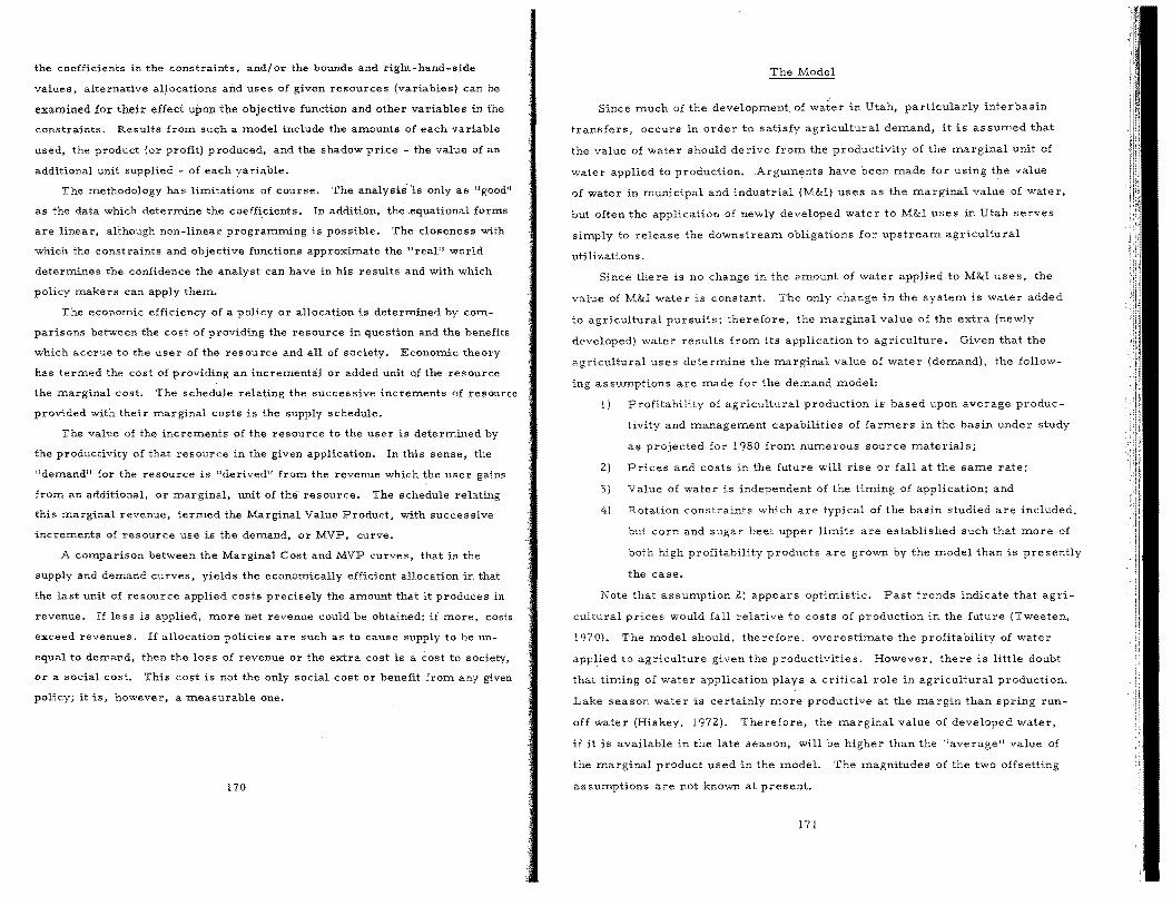
the coefficients in the constraints, and/or the bounds and right-hand-side

values, alternative altocations and uses of given resources (variables) can be

examined for their effect upon the objective functioll and other variables in the

constraints. Results from such a model include the amounts of each variable

used, the product (or profit) produced, and the shadow price - the value of an

additional unit supplied - of each variable.

The methodology has limitations of course. The analysis"is only as "good"

as the data which determine the coefficients. In addition, the, equational forms

are linear, although non-linear programming is possible. The closeness with

which the constraints and objective functions approximate the "real" world

determines the confidence the analyst can have in his results and with which

policy makers can apply them.

The econoITlic efficiency of a policy or allocation is determined by com­

parisons between the cost of providing the resource in question and the benefits

which accrue to the user of the resource and all of society. Economic theory

has termed the cost of providing an incremental or added unit oJ the resource

the marginal cost. The schedule relating the successive increments of resource

provided with their marginal costs is the supply schedule.

The value of the increments of the reSource to the user is determined by

the productivity of that resource in the given application. In this sense, the

"demand" for the reSOurce is "derived" from the revenue which the user gains

from an additional. or marginal, unit of the resource. The schedule relating

this marginal revenue, terITled the Marginal Value Product, with successive

increments of resource use is the demand, or MVP, curve.

A comparison between the Marginal Cost and MVP curves, that is the

supply and demand curves, yields the economically efficient allocation in that

the last unit of resource applied costs predsely the amount that it produces in

revenue. If less is applied, more net revenue could be obtained; if more. costs

exceed revenues. If allocation policies are such as to cause supply to be un­

equal to demand, then the loss of revenUe or the extra cost is a cost to SOciety,

or a social cost. This cost is not the only social cost or benefit from any given

policy; it is, however, a measurable one.

170

The Model

Since rrlUch of the developmen( of in Utah, particularly interbasin

transfers, occurs in order to satisfy agricultural demand, it is assumed that

the value of water should derive from the productivity of the marginal unit of

water applied to production. Arguments have been made for using the value

of water in ITlunicipal and industrial (M&I) uses as the marginal value of water.

but often the application of newly developed wate r to M&I uses in Utah serves

simply to release the downstream obligations for upstream agricultural

utilizations.

Since there is no change in the aITlount of water applied to M&I uses, the

value of M&I water is constant. The only change in the system is water added

to agricultural pursuits; therefore, the marginal value of the extra (newly

d€'veloped) water results from its application to agriculture. Given that the

agricultural uses determine the ITlarginal value of water (demand), the follow­

ing assumptions are ITlade for the demand model:

1) Profitability of agricultural production is based upon average produc­

tivity and management capabilities of farmers in the basin under study

as projected for 1980 froITl numerous source ITlaterials;

Z} Prices and costs in the future will rise Or fall at the same rate;

3) Value of water is independent of the timing of application; and

4} Rotation constraints which are typical of the basin studied are included,

but corn and sugar beet upper limits are established such that ITlore of

both high profitability products are grown by the ITlodel than is presently

the case.

Note that assumption 2) appears optiITlistic. Past trends indicate that agri­

cultural prices would fall relative to costs of production in the future (Tweeten,

1970). The ITlodel should, therefore, overestimate the profitability of water

applied to agriculture given the productivities. However, there is little doubt

that tiITling of water application plays a critical role in agricultural production.

Lake season water is certainly ITlore productive at the margin than spring run­

off water (Hiskey. 1972). Therefore, the marginal value of developed water,

if it is available in the late season, will be higher than the "average" value of

the ITlarginal product used in the mode1. The magnitudes of the two offsetting

as sumptions are not known at present.

171

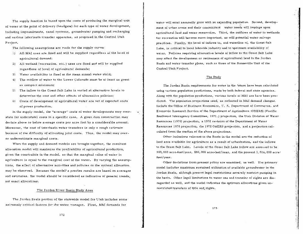
The supply function is based upon the costs of producing the lnarginal unit

of water at the point of delivery (headgate) for each type of water developlnent,

including ilnpoundrrlents, canal systerrls, groundwater pumping and recharging

and various interbasin transfer apparatus, as proposed in the Central Utah

Project.

The following assulnptions are rrlade for the supply curve:

1) All M&I uses are fixed and will be supplied regardless of the level of

agricultural demand;

2) All wetland (recreation, etc.) uses are fixed and will be supplied

regardless of level of agricultural derrlands;

3) Water availability is fixed at the mean annual water yield;

4) The outflow of water to the Lower Colorado must be at least as great

5)

as cOrrlpact minimum;

The inflow to the Great Salt Lake is varied at alternative levels to

detertnine the cost and other effects of alternative policies;

6) Costs of development of agricultural water are net of expected costs

of power production.

In the supply model, the "average" costs of water developments may over­

state (or understate) costs in a specific case. A given dam construction may

deviate above or below average costs per acre foot by a considerable amount.

Moreover, the cost of interbasin water transfers is only a rough estimate

because of the difficulty of allocating joint costs. Thus, the model may over­

or underestirrlate marginal costs.

When the supply and demand lnodels are brought together, the resultant

allocation nlOdel will maximize the profitability of agricultural production,

given the constraints in the lnodel, so that the marginal value of water in

agriculture is equal to the rrlarginal cost of the water. By varying the assump­

tions, the effect of alternative activities and policies on the optimal allocation

may be observed. Because the rrlodel' s precise results are based on averages

and estirrlates, the rrlodel should be considered as indicative of general trends,

not exact allocations.

The Jordan River Basin Study Area

The Jordan Basin portion of the statewide model for Utah includes SOrrle

extremely critical factors for the water manager. First, M&I derrlands for

172

water will most assuredly grow with an expanding population. Second, develop-e,

ment of urban areas and their concomitant water needs will impinge upon

agricultural land and water reservoirs. Third, the outflows of water to wetlands

for recreation will b.ecome more important, as will potential water salvage

practices. Finally, the level of inflows to, and waterline of, the Great Salt

Lake, is critical to local lakeside industryand to upstream availability of

water. Policies requiring alternative levels of inflow to the Great Salt Lake

may affect the development or retirement of agricultural land in the Jordan

Basin and water transfer plane, such as those of the Bonneville Unit of the

Central Utah Project.

The Study

The Jordan Basin requirements for water in the future have been calculated

using various population predictions, made by both federal and state agencies.

Along with the population predictions, various levels of M&l use have been pre­

dicted. The population projections used, as reflected in M&l demand changes,

include the Office of Business Econotni,cs, U. S. Department of Commerce, and

Econotnic Research Service of the Department of Agriculture (OBERS) (Pacific

Southwest Interagency Committee, 1971.) projection, the Utah Division of Water

Resources (1970) projection, a 1972 revision of the Department of Water

Resources 1970 projection, the 1972 OBERS projection, and a projection cal­

culated from the median of the above projections.

Other inclusions relevant to the Basin in the model are the reduction of

land area available for agriculture as a result of urbanization, and the inflows

to the Great Salt Lake. Levels of the Great Salt Lake inflow are assumed to be

500, 000 acre-feet/year, 850, 000 acre-feet/year, and the present 1, 014, 000 acre­

feet/year.

Other deviations from present policy are examined, as well. The primary

model includes maximum sustained utilization of available groundwater in the

Jordan Basin, although present legal restrictions severely restrict pumping in

the basin. Other legal limitations to water use and transfer of rights are dis­

regarded as well, and the model indicates the optimum allocations given un­

restricted transfers of title and, rights.

173

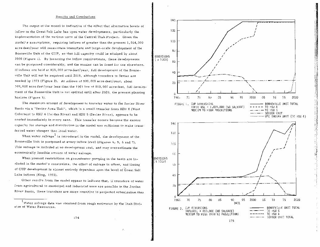
Results and Conclusions

The output of the model is indicative of the effect that alte rnative levels of

inflow to the Great Salt Lake has upon water developments, particularly the

implementation of the various units of the Central Utah Project. Given the

model's assumptions, requiring inflows of greater than the present 1,014,000

acre-feet/year will necessitate immediate and large-scale

Bonneville Unit of the CUP, so that full capacity could be attaiped by about

2000 (Figure 1). By lessening the inflow requirements, these developments

can be postponed considerably, and the monies can be freed for use elsewhere.

If inflows are held at 850, 000 acre-feet/year, full development of the Bonne­

ville Unit will not be required until 2015, although transfers to Sevier are

needed by 1973 (Figure 2). At inflows of 500,000 acre-feet/year, about

300, 000 acre-ieet/year less than the 1963 low of 800, 000 acre-feet, full develop­

ment of the Bonneville Unit is not optimal until after 2020, the present planning

horizon (Figure 3).

The maximum amount of development to transfer water to the Sevier River

Basin via a "Sevier Area Unit", which is a small transfer from HSu 8 (West

Colorado) to HSU 4 (Jordan River) and HSU 5 (Sevier River). appears to be

needed immediately in every case. This transfer occurs because the excess

capacity for storage and distribution in the model was sufficient to make trans

ferred water cheaper than local water.

When water salvage I is introduced in the model, the development of the

Bonneville Unit is postponed at every inflow level (Figures 4" 5, 6 and 7).

This salvage is included at no development cost, and may overestimate the

econoTnically feasible amount of water salvage.

When present restrictions on groundwater pumping in the basin are in­

cluded in the model's constraints, the effect of salvage is offset, and timing

of CUP development is almost entirely dependent upon the level of Salt

Lake inflows (King, 1972).

Other results from the model appear to indicate that, if transfers of water

from agricultural to municipal and industrial uses are possible in the Jordan

River Basin, these transfers are more sensitive to projected urbanization than

Water salvage data was obtained from rough estimates by the Utah Divi­sion of Water Resources.

174

DlVERSlONS ( x 1000)

140

120

1 00

8U

60 I I

I I

I

/' I

I

".. ,;

,;

,; "..

--,,-

40 I L..,...",===",_ _~~"'-.-.-.-~-._

'-' I "

I I ---

r­I I

20 .. - .. _ .. _ .. "-_.- ..

I /

.'""<;;." "

I ". / .... , OL-__ ~~~ __ -L __ ~ __ -L __ -L __ ~~~ __ ~ __ ~~~

196~ 70 75 80 85 90 95

FIGUK~ 1. CUP DIVERSIONS

140

120

100

i;()

Lv

-

IIIFLO GSL ~ 1,014,000 (NO SALVAGE) NEDIU~l TO HIGH PROJECTIONS

2000 05 10 15 2020

BONNEVILLE UNIT TOTAL - - - - - TO HSU 4

TO HSU 5 SEVIER UNIT

............. UTE INDIAN UNIT (TO HSU 4)

I I

I

I

I I

I

I I

-..I r-

I I

r I

I

40 .-.---~---~-......... ..."..::.-. -' -i'--·-".

20

0 1965 70 75 80 85 90

DATE 95

I "'. .. _,._ .. _ .. --'\"._ .. _ .. I "

". -. 2000 05 10 15 2020

FIGURE 2. CUP DIVERSIONS INFLOGSL = 850,000 (NO SALVAGE) MEDIUM TO HIGH (HSU 5) PROJECTIONS

BONNEVILLE UNIT TOTAL TO HSU 5 TO HSU 4 SEVIER UNIT TOTAL

175

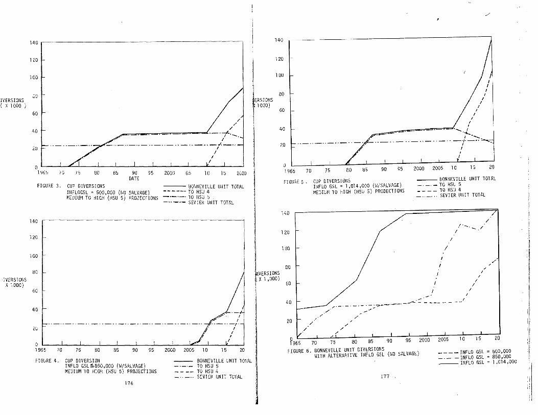
IVERS IONS ( X 1000 )

IVERS IONS X 1000)

140~·--------------------------------------------~

120

100

GO

60

40

20

o

/ /

/

·-·T"-. I

._ .. _ .. _ .. - .. _ .. _ .. - .. -- •. _.1._ ..

90 95 DATE

2000 05

I

10

I /

I

15 2020

FIGURE 3. CUP DIVERSIONS ---- BONNEVILLE ulin TOTAL INFLOGSL 500,000 (NO SALVAGE) ------ TO HSU 4 MEDIU~1 TO HIGH (HSU 5) PROJECTIONS -._.-. TO HSU 5

_ •• _ •• - SEVIER UNIT TOTAL

140

120

100

80

60

40

i96~5~-;~--~--~~--~--~L---9~5---2-00~0---2-00W5~-1~0---1~5~~20 FIGURE 4. CUP DIVERSION

INFLO GSL S850 ,000 (I.J/SALVAGE) MEDIUM TO HIGH (HSU 5) PROJECTIONS

176

---- BONNEVILLE UNIT TOTAL -'-'- TO HSU 5 - - -- TO HSU 4 _ .. _ .• SEVIER UNIT TOTAL

140

120

100

80 ERSIONS ( 1000)

60

40

20

0 1965 70 75 80 85

I /

I

__ =.....,.....,-="s=,......"""=="'~.__ / ~.~.- "

I

I I

I

/

I I

I

/ '-"-"- .. - .. _ .. -.- --/._ .. :....... .. I •

90 95 2000 2005 10

I I

/

15 20

FIGURE 5. CUP DIVERSIONS mFLO GSL = 1,014,000 (W/SALVAGE) MEDIUM TO HIGH (HSU 5) PROJECTIONS

___ BONI~EVILLE UNIT TOTAL ___ . - TO HSU 5

. lVERSIONS I X 1 ,000)

____ TO HSU 4 __ ._ .. SEVIER UNIT TOTAL

140 /

/"-. / 120 I

/

100 I

/"

80 I .-.-I

I

60 I

I I .-

40 ,/._._. _. -' - ;..?'~-'--'-'-"""- - - ---/' ...... ..,..

/" 20 /

10 15 20

FIGURE 6. BONNEVILLE UNIT DIVERSIONS WITH ALTERNATIVE INFLO GSL (NO SALVAGE)

____ INFLO GSL = 500,000 _____ INFLO GSL = 850,000 ___ INFLG GSL = 1,014,000

177

140

120

100

I·· :~ 1000)

I

I /

,0

r 1 G~ hE . ;';:tEVl~li:. U:HT CU DIVERSIOtlS \dTH ALTERNATIVE INFLO GSL (WSALVAGE)

_. _._ INFLU GSLs 850, --- INFLO GSL=1014,

to the levels of Great Salt Lake inflows. Prior to 2010 little reduction in

preO'ently irrigated acres is indicated at any level of inflow, with or without

salvage. The dc\'eJopITlent of ~ agricultural land in the Jordan, Great Salt

Lake Desert, and Weber River Basins is, however. depe~dent upon the inflows.

At 500,000 acre-feet/year or less, as znuch as 250,000 acres of cropland are

developed prior to 1975. Population increases erode the water availability for

development frozn that date until 2000 at which time no new land is developed.

At inflows of 1,014,000 acre-feet/year, however, developznent of new agricul­

tural land is Hznited to about 114,000 acres with water salvage or 40,000 acres

'Without salvage in the three HSU! s. The level of Gre at Salt Lake inflow is also

criti<;al to the amount of water available to recharge groundwater aquifers. At

low Je,ds of inflv,', the :naxiznuzn low cost recharge in the Jordan River and

Bear River Basins is reached by 1995-2000. At the 1,014,000 acre-feet inflow,

znaximum recharge is not reached until 2015.

The model indicates that the level of inflow to Great Salt Lake is a critical

factor in making economically optimal decisions concerning wat~.r importation

through the Bonneville Unit facilities. As such, the costs Of immediate

178

development of the Bonneville Unit znust be weighed against the costs of lower­

ing the level of the Great Salt Lake considerably. Models such as this one

should help to emphasize the trade-offs which occur in policy decisions about a

specific resource, such as the Great Salt Lake.

Literature Cited

Hadley, G. 1962. Linear programming. Addison-Wesley Publishing Co. , Inc.

520 pp.

Hiskey, Harold H. 1972. Optiznal allocation of irrigation water: the Sevier River Basin. Ph. D. dissertation. Utah State University, 163 pp.

King, Alton B. et a1. 1972. Development of regional supply functions and a least-cost model for allocating water resources in Utah: a parametric linear programming approach. Utah Water Research Laboratory Publi­cationPRWGI00-2, Utah State University, Logan, Utah. 162 pp.

Pacific Southwest Interagency Coznmittee. 1971. Economic base and projec­tions. Appendix II. Great Basin Region comprehensive framework study. Salt Lake City, Utah. 181 pp.

Tweeten, Luther. 1970. Foundations of farm policy. University of Nebraska Press. 540 pp.

Utah Division of Water Resources. 1970. Interim report on state water plan. Staff Report No.6, Salt Lake City, Utah. 44 pp.

179

i I, ,

I .1

REVIEW OF PAST STUDIES OF THE EAST EMBAYMENT

AS A FRESH WATER RESERVOIR

A. Z. Richards, Jr.l

Abstract

From the years 1930 to 1935 there was considerable interest in the inter-islands diking project for creating a fresh water reser­voir. Such men as Louis E. Fox, Theodore L. Keller, Sumner G. Margetts, Dr. Dorsey A. Lyon, J. J. Lillie, R. E. Van Liew, R. A. Hart, N. E. McLaughlan, Jacob L. Crane, Dr. Thomas C. Adams, and others made studies and wrote papers on the intrigu­ing pos sibilities and problems of such a project. From. 1936 to 1954 - - the war years there appears to be little documented interest, but in 1955 the Utah Legislature commissioned the State 'Road Comm.is sion to initiate studies of the advisability of con­structing the inter-island dikes. An Advisory Comm.ittee was appointed and local consulting engineers were selected. They prepared two important reports under this assignment. In 1962 Douglas R. Mabey prepared an im.portant treatise on the diking project, suggesting the use of Kennecott tailings m.aterial. In 1965 a Prelim.inary Master Plan was prepared by the Great Salt Lake Authority, and in 1966 the Tailings Feasibility Project was undertaken on the shore of the lake near Saltair. Harry S. Suekawa studied the Tailings Project and prepared a university thesis On the results of the test. Final com.m.ents by the writer consist of emphasizing the im.portance of the fresh water aspects of the East Em.baym.ent Reservoir Project and its potential for saving much of the water now running to waste into the Great Salt Lake.

Under date of May 15, 1930, Louis E. Fox and Theodore L_ Keller, then

in the Civil Engineering Department at the University of Utah, prepared a

thesis entitled "Putting Great Salt Lake to Work." They proposed a three-part

dike extending westerly from the mainland to the south end of Antelope Island,

and northerly from. the north end of Antelope Island to the south end of Frem.ont

Island, and from the north end of Fremont Island to the Prom.ontory Point

mainland; the lake to be enclosed on the east side of these islands by the dike

chain and the east shore mainland would be fed by the three principal water

sources for the Great Salt Lake--the Bear, Weber, and Jordan Rivers. This

subsequently becam.e known as the "large project. "

1 Consulting Civil Engineer, President of Caldwell, Richards &, Sorensen,

Inc., Salt Lake City, Utah.

180

'In March, 1932, SumnerG. Margette, a consulting engineer from Salt

Lake City issued a paper titled "Report on Proposed Fresh Water Lake. II He

recom.mended that a smaller fresh water lake be developed in Farmington Bay

by damm.ing the 146 square mile area between the m.ainland and the south end

of Antelope Island and between the 'north end of Antelope Island and the m.ain-

1and at Syracuse. Mr. Margetts, to supplement the water supply from the

Jordan River and all of the small stream.s running into Farmington Bay, diverted

water from the Weber River into the proposed reservoir by means of an 11. 5

mile long canal along the mainland from the outlet of the Weber River to

Syracuse, Utah. This proposed project was referred to as the Farmington

Bay Reservoir, or the "small project. "

By July, 1933, a great deal of public interest had developed in the pro­

posed diking project. Advisory co'mrnittees and subcommittees were formed

and some state and industrial sponsored general engineering studies were

undertaken. Dr. Dorsey A. Lyon, at that time Director of the Utah Engineering

Experiment Station, summarized these studies in his report entitled "Report

of Sub-Committee Appointed to Investigate Technical Problems that Present

Themselves in Connection with the Proposed Diking of the Great Salt Lake for

the Purpose of Creating a Body of Fresh Water." Discussed in Dr. Lyon's

report were the following items: (a) Dike Studies by J. J. Lillie which were

directed to the "large project"; (b) Hydraulic Studies by R. E. Van Liew; (cl

A review of all reports, and the COncern of a technical subcommittee on the

problems to be encountered in constructing a dike from Fremont Island to

Promontory Point, as required by the "large project." Borings drilled by

Lillie indicated a "very soft mud" to a m.aximum depth of exploration of 13

feet below the bottom. of the lake at this dike location. It is interesting to

note, however, that this committee recommended excavation by dredging.

By hydraulic methods the lake bed material was to be deposited to form a dike

with side slopes of 20 to 1 to solve a construction problem and to withstand the

wave action of the lake.

In June, 1933 appeared a significant joint authorship paper by Mr. R. A.

Hart, a Civil Engineer who, at that time, was Industrial Secretary of the

Chamber of Com.merce of Salt Lake City, and Mr. N. E. MCLaughlan, City

Chemist, entitled "Abstract of Report on Laboratory Tests of Feasibility of

Freshening the Proposed Diked-off Portion of the Great Salt Lake." Mr. Hart

181

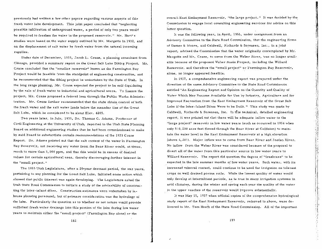
previously had written a few other papers regarding variousaspe.cts of this

fresh water lake development. This joint paper concluded that "neglecting

possible infiltration of underground water, a period of only two years would

be required to freshen the water in the proposed reservoir." Mr. Hart's

studies were based on the water supply outlined by Mr. Margetts in 193Z, and

on the displacement of salt water by fresh water from the natural incoming

supplies.

Under date of December, 1933, Jacob L. Crane, a plannin~ consultant from

Chicago, provided a summary report On the Great Salt Lake Diking Project. Mr.

Crane concluded that the "smaller reservoir" known as the Farmington Bay

Project would be feasible from the standpoint of engineering construction, and

he recommended that the diking project be undertaken by the State of Utah. In

the long range planning, Mr. Crane expected the project to be self-liquidating

by the sale of fresh water to industrial and agricultural users. To finance the

project, Mr. Crane proposed a federal loan through the Public Works Adminis­

tration. Mr. Crane further recommended that the state obtain control of both

the fresh water and the salt water lands below the meander line of the Great

Salt Lake, which he considered to be about Elev. 4Z05.

Two years later, in July, 1935, Dr. Thomas C. Adams, Professor of

Civil Engineering at the University of Utah, reported to the Utah State Planning

Board on additional engineering studies that he had been 'commis sioned to make

by said Board to substantiate certain recommendations of the 1933 Crane

Report. Dr. Adams pointed out that the salt content of the water in Farmington

Bay Reservoir, not receiving any water from the Bear River would, at times,

reach to more than 5,000 ppm, and that this would be in excess ';f d~'sired values for certain agricultural uses, thereby discouraging further interest in

the "small project."

The 1955 Utah Legislature, after a ZO-year dormant period, the war years,

pertaining to any planning for the Great Salt Lake, initiated some action which

showed that public interest was again developing. The Legislature asked the

Utah State Road Commis sion to initiate a study of the advisability of construc­

ting the inter-island dikes. Construction estimates were undertaken by in­

house planning personnel, but of primary consideration was the hydrology of

the lake. Particularly the question as to whether or not nature would prOvide

sufficient fresh water drainage into this portion of the lake during low water

years to maintain either the "small project" (Farmington Bay alone) or the

182

overall East Embayment Reservoir, "the large project. 11 It was decided by

Commission to engage local consulting engineering services for advice On this

latter question.

It was the following year, in April, 1956, under as signment from an

Advisory Committee to the State Road Commission, that the engineering firms

of Dames & Moore, and Caldwell, Richards &, Sorensen, Inc., in a joint

report, advised the Commission that the water originally contemplated by Mr.

Margetts and Mr. Crane, to come from the Weber River, was nO longer avail­

able because of the proposed Weber Basin Project, including the Willard

ReserVOir, and therefore the " small project" or Farmington Bay Reservoir,

alone, no longer appeared feasible.

In 1957, a comprehensive engineering report was prepared under the

direction of the same Advisory Committee to the State Road Commission

entitled "An Engineering Report and Opinion on the Q1.lantity and Quality of

Water Which May Become Available for Use by Industry, Agriculture and for

Improved Recreation from the East Embayment Reservoir of the Great Salt

Lake if the Inter-Island Dikes Were to be Built." This study was made by

Caldwell, Richards & Sorensen, Inc. In ttis technical, detailed engineering

report, it was pointed out that there will be adequate inflow water to the

"large project" reservoir in low water years (such as occurred in 1954 when

only 510,200 acre feet flowed through the Bear River at Colliston) to main­

tain the water level in the East Embayment Reservoir at a high elevation

(above 4,201). Major inflow was to come from Bear River and Jordan River.

No inflow from the Weber River was considered because of the proposal to

divert all of the water from this particular source in low water years to

Willard Reservoir. The report did question the degree, of "freshness" to be

expected in the late summer months of low water years. Such water, with its

increased mineral content, could continue to be ,used for irrigation on tolerant

crops on well drained porous soils. While the lowest quality of water would

only develop at intermittent periods, as is true in many irrigation systems in

arid climates, during the winter and spring each year the quality of the water

in the upper reaches of the reservoir would improve substantially.

It was May 15, 1957 when official copies of the comprehensive hydrological

study report of the East Embayment Reservoir, referred to above, were de­

livered to Mr. Tom Heath of the State Road Cornmissiol" All of the important

183

-/.-

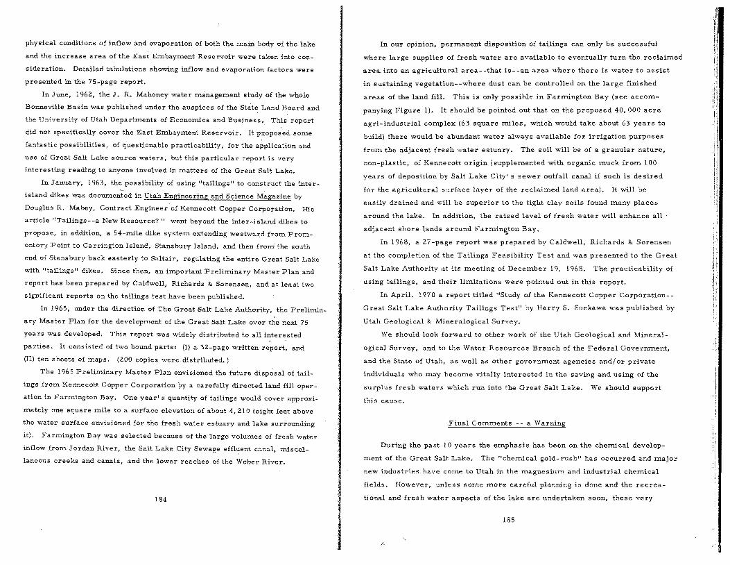
physical conditions of inflow and evaporation of both the main body of the lake

and the increase area of the East Embayment Reservoir were taken into con­

sideration. Detailed tabulations showing inflow and evaporation factors were

presented in the 7S-page report.

In June, 1962, the J. R. Mahoney water management study of the whole

Bonneville Basin was published under the auspices of the State Land Board and

the University of Utah Departments of Economics and Business" This report

did not specifically cover the East Embayment Reservoir. It p:.;:oposed some

fantastic possibilities, of questionable practicability, for the application and

use of Great Salt Lake source waters, but this particular report is very

interesting reading to anyone involved in matters of the Great Salt Lake.

In January, 1963, the possibility of using "tailings" to construct the inter­

island dikes was documented in Utah Engineering and Science Magazine by

Douglas R. Mabey, Contract Engineer 'of Kennecott Copper Corporation. His

article "Tailings--a New Resource?" went beyond the inter-island dikes to

propose, in addition, a 54-mile dike system extending westward from P rom­

ontory Point to Carrington Island, Stansbury Island, and then irorri:" the south

end of Stansbury back easterly to Saltair, regulating the entire Great Salt Lake

with "tailings" dikes. Since then, an important Preliminary Master Plan and

report has been prepared by Caldwell, Richards &: Sorensen, and at least two

significant reports on the tailings test have been published.

In 1965, under the direction of The Great Salt Lake Authority, the Prelimin­

ary Master Plan for the development of the Great SaIt Lake over the next 75

years was developed. This report was Widely distributed to all interested

parties. It consisted of two bound parts: (I) a 32-page written report, and

(II) ten sheets of maps. (200 copies were distributed. )

The 196 5 Preliminary Maste r Plan envisioned the future disp~sal of tail­

ings from Kennecott Copper Corporation by a carefully directed land fill oper­

ation in Farmington Bay. One year's quantity of tailings would cover approxi­

mately one square mile to a surface elevation of about 4,210 (eight feet above

the water surface envisioned for the fresh water estuary and lake surrounding

it). Farmington Bay was selected because of the large volumes of fresh water

inflow from Jordan River, the Salt Lake City Sewage effluent canal, miscel­

laneous creeks and canals, and the lower reaches of the Weber River.

184

In our opinion, permanent disposition of tailings can only be successful

where large supplies of fresh water are available to eventually turn the reclaimed

area into an agricultural area--that iso-an area where there is water to assist

in sustaining vegetation--where dust can be controlled on the large finished

areas of the land fill. This is only possible in Farmington Bay (see accom­

panying Figure 1). It should be pointed out that on the proposed 40, 000 acre

agri-industrial complex (63 square miles, which would take about 63 years to

build) there would be abundant water always available for irrigation purposes

from the adjacent fresh water estuary. The soil will be of a granular nature,

non-plastic, of Kennecott origin (supplemented with organic muck from 100

years of deposition by Salt Lake City's sewer outfall canal if such is desired

for the agricultural surface layer of the reclaimed land area). It will be

easily drained and win be superior to the tight clay soils found many places

around the lake. In addition, the raised level of fresh water win enhance all

adjacent shore lands around Farmin~ton Bay.

In 1968, a 27 -page report was prepared by Caldwell, Richards &: Sorensen

at the completion of the Tailings Feasibility Test and was presented to the Great

Salt Lake Authority at its meeting of December 19, 1968. The practicability of

using tailings, and their limitations were pointed out in this report.

In April, 1970 a report titled "Study of the Kennecott Copper Corporation­

Great Salt Lake Authority Tailings Test" by Harry S. Suekawa was published by

Utah Geological & Mineralogical Survey.

We should look forward to other work of the Utah Geological and Mineral­

ogical Survey, and to the Water Resources Branch of the Federal Government,

and the State of Utah, as well as other government agencies and/or private

individuals who may become vitally interested in the saving and using of the

surplus fresh waters which run into the Great Salt Lake. We should support

this cause.

Final Comments n a Warning

During the past 10 years the emphasis has been on the chemical develop­

ment of the Great Salt Lake. The "chemical gold- rush" has occurred and major

neW industries have come to Utah in the magnesium and industrial chemical

fields. However, unless some more careful planning is done and the recrea­

tional and fresh water aspects of the lake are undertaken soon, these very

185

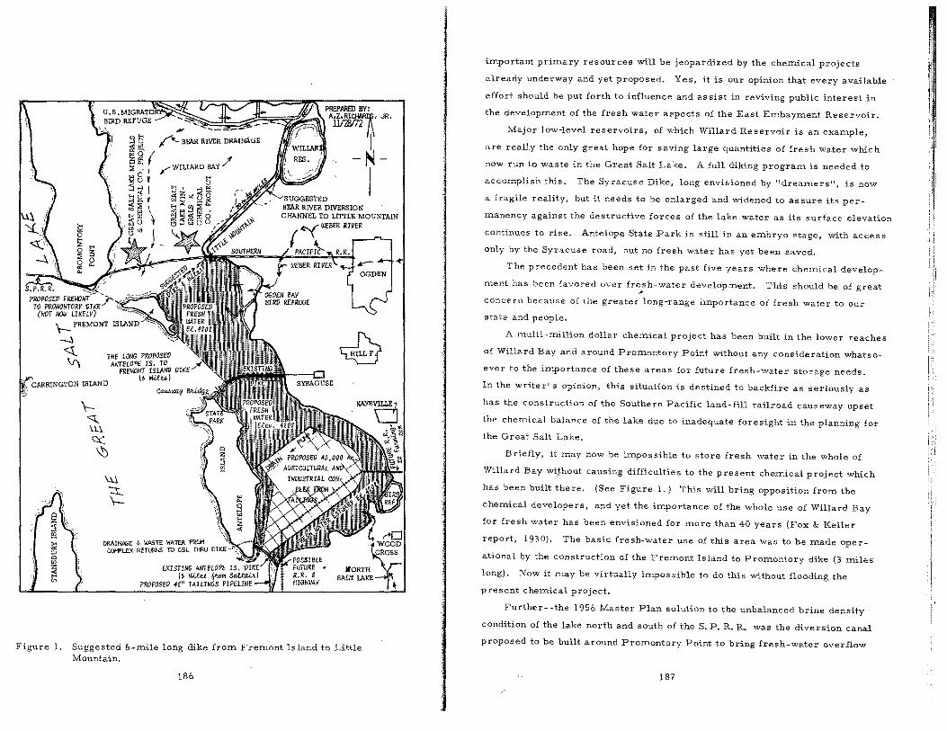
PROPOSEl1 TO PROMOIITORY VI K€

(NOT NOW LIKELY)

\-- FREMONT

--.\ <t. V\

CARRINGTON ISLAND

DRAINAGE & WASTE WATER FR<l'1 COWLEX RETURNS TO GSL THRU DIKE

Figure 1. Suggested 6-:mile long dike from Fremont Island to Little Mountain.

186

important primary resources will be jeopardized by the chemical projects

already underway and yet proposed. Yes, it is our opinion that every available

effort should be put forth to influence and assist in reviving public interest in

the development of the fresh water aspects of the East Embay:ment Reservoir.

Major low-level reservoirs, of which Willard Reservoir is an exa:mple,

are really the only great hope for saving large quantities of fresh water which

now run to waste in the Great Salt Lake. A full diking program is needed to

acco:mplish this. The Syracuse Dike, long envisioned by "dreamers", is now

a fragile reality, but it needs to be enlarged and widened to assure its per­

manency against the destructive forces of the lake water as its surface elevation

continues to rise. Antelope State Park is still in an embryo stage, with access

only by the Syracuse road, but no fresh water has yet been saved.

The precedent has been set in the past five years where che:mical develop­

ment has been favored over fresh-water development. This should be of great .. concern because of the greater long-range importance of fresh water to Our

state and people.

A multi-million dollar chemical project has been built in the lower reaches

of Willard Bay and around Promontory Point without any consideration whatso­

ever to the importance of these areas for future fresh-water storage needs.

In the writer's opinion, this situation is destined to backfire as seriously as

has the construction of the Southern Pacific land-fill railroad causeway upset

the chemical balance of the lake due to inadequate foresight in the planning for

the Great Salt Lake.

Briefly, it :may nOW be impossible to store fresh water in the whole of

Willard Bay wi,thout causing difficulties to the present chemical project which

has been built the reo (See Figure 1.) This will bring opposition fro:m the

chemical developers, and yet the importance of the whole use of Willard Bay

for fresh water has been envisioned for more than 40 years (Fox & Keller

report, 1930). The basic fresh-water use of this area was to be made oper­

ational by the Construction of the Frem,ont Island to Promontory dike (3 :miles

long). Now it may be virtually im,possible to do this without flooding the

present chemical project.

Further- -the 1956 Master Plan solution to the unbalanced brine density

condition of the lake north and south of the S. P. R. R. was the diversion canal

proposed to be built around Promontory Point to bring fresh-water overflow

187

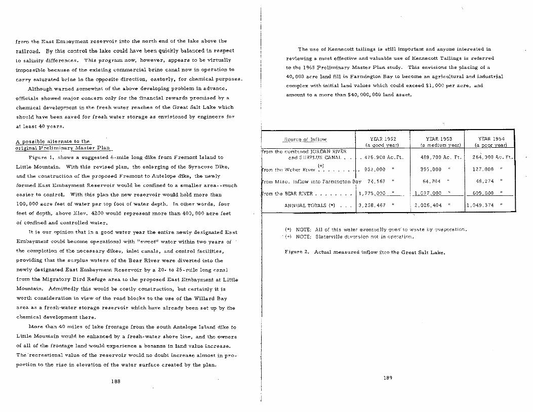
frorn the East Embayment reservoir into the north end of the lake above the

railroad. By this control the lake could have been quickly balanced in respect

to salinity differences. This progra= now, however, appears to be virtually

impossible because of the existing com.xnercial brine canal now in operation to

carry saturated brine in the opposite direction, easterly, for chemical purposes.

Although warned somewhat of the above developing problem in advance,

officials showed major concern only for the financial rewards promised by a

chemical development in the fresh water reaches of the Great Salt Lake which

should have been saved for fresh water storage as envisioned by engineers for

at least 40 years.

A possible alternate to the original Preliminary Master Plan

Figure 1. shows a suggested 6 -mile long dike from Fremont Island to

Little Mountain. With this revised plan, the enlarging of the Syracuse Dike,

and the construction of the proposed Fremont to Antelope dike, the newly

formed East Embayment Reservoir would be confined to a smaller area-;..much

easier to control. With this plan the new reservoir would hold more than

100,000 acre feet of water per top foot of water depth. In other words, four

feet of depth, above Elev. 42.00 would represent more than 400, 000 acre feet

of confined and controlled water.

It is our opinion that in a good water year the entire newly designated East

Embayment could become operational with "sweet" water within two years of

the completion of the necessary dikes, inlet canals, and control facilities,

providing that the surplus waters of the Bear River were diverted into the

newly designated East Embayment Reservoir by a 2.0- to 2.5-mile long canal

froIn the Migratory Bird Refuge area to the proposed East Embayment at Little

Mountain. AdInittedly this would be costly construction, but certainly it is

worth consideration in view of the road blocks to the use of the Willard Bay

area as a fresh-water storage reservoir which have already been set up by the

chemical developInent there.

More than 40 miles of lake frontage from the south Antelope Island dike to

Little Mountain would be enhanced by a fresh-water shore line, and the owners

of all of the frontage land would experience a bonanza in land value increase.

The "recreational value of the reservoir would no doubt increase alInost in pro­

portion to the rise in elevation of the water surface created by the plan.

188

The use of Kennecott tailings is still important and anyone interested in

reviewing a most effective and valuable use of Kennecott Tailings is referred

to the 1965 Preliminary Master Plan study. This envisions the placing of a

40, 000 acre land fill in Farmington Bay to become an agricultural and industrial

complex with initial land values which could exceed $1,000 per acre, and

amount to a more than $40, 000,000 land asset.

Source of Inflow YEAR 1952 YEAR 1953 (a good year) (a medium year)

From the combined JORDAN RIVER and SURPLUS CANAL. 476,900 Ac. Ft. 489,700 Ac. Ft.

; (+) iFrom the Weber River. 932,000 " 395,000 "

From Misc. Inflow into Farmington Bay 74,567 " 64,704 "

From the BEAR RIVER . ~S,OOO " L077 ,000 "

ANNUAL TOTALS (*) 3,258,467 " 2,026,404 "

(*) NOTE: All of this water eventually goe5'to waste by evaporation. (+) NOTE: Slaterville diversion not in operation.

Figure 2. Actual measured inflow into the Great Salt Lake.

189

YEAR 1954 (a poor year>

264,300 Ac. Ft.

127,000 "

4B,274 "

609,BOO "

1,049,374 "

GREAT SALT LAKE -

KEY TO UTAH'S FUTURE INDUSTRIAL DEVELOPMENT? 1

Joseph M. Glas sett

Two ~l'mp''l::ies 1'18:: to prOd\lCe Jarge annual ton'1.ages of Inagnesium. l1'Z'gnesiu", chloride. chlorine, potassium sulfate, sodium sulfate. gypsum, lithium chloride, and bromine from Great Salt Lake. The production of these chemicals, and other pos sible chemicals. in conjunction with Utah mineral resources already well developed, may be the key to Utah's future indus­trial development. A feasibility study is needed to determine which of many suggested chemical products will provide the largest profil margin for future Utah enterprises.

KEY WORDS: Great Salt Lake; Industrial development; Mineral recovery; Utah minerals

L adie sana gentlenl.:cn.

A sanitation engineer visited one of the Great Salt Lake resorts and asked

the manager what he did to make the water safe to drink.

"First we filter the water," replied the manager.

"That's good, " said the engineer.

"Then we chlorinate it. "

"Excellent!" exclaimed the engineer.

"And then." said the manager, "just for safety's sake. we drink soda pop. It

College professors have a reputation for asking their students questions and

(hen answering themselves. I would now like to proceed with my effort to answer

the question posed by the title of this paper.

Introduction

During the past century Utah has gained prominence as a mineral commodity

producing state. Among the states in our country, Utah ranks second in produc­

tlOn of copper, gold, molybdenum, and asphalt; third in production of iron and

uramum. Tabje 1 presents the values of the principal mineral commodities

mined in Utah during the period 1865 through 1961.

1 Associate Professor of Chemical Engineering, Brigham Young Unive rsity, Provo, Utah.

190

TABLE I (1)

VALUE OF UTAI! mNERAL CONt,lODITIES

Copper Coal Lead Silver Cold Petroleum Zinc Iron

Commodi ty

Uranium, vanadium and radium ~!olybdenum and other metals Sand and grtlvl' I Solid hydrocarhon,; StOlle Common salt Clay I'otash ~Ii sce II uneous

3311 914 688 blO 476 461 283 282 234 233 99 91 63 34 ~8

26 200

Each of the mineral commodities listed in Table I has been responsible for

the growth of satellite commodities which are hidden in the "Miscellaneous"

category. For example, United States Steel Co., Geneva Works, at Orem,

Utah is the state's largest producer of iron. Geneva consumes large tonnages

of coal to make coke for their iron producing blast furnaces. They also pro­

duce oxygen to enrich the air to the blast furnaces. By-products resulting from

these two processes have resulted in the production of'liquid air, oxygen,

nitrogen, hydrogen, ammonia, sulfuric acid, nitric acid, ammonium sulfate,

ammonium nitrate, benzene, toluene, and other hydrocarbons.

It is anticipated that production rates of the mineral commodities listed in

Table I will increase with time. Significant reserves of other mineral com­

modities are known and are being developed. Some of these are beryllium,

manganese, mercury, thorium and the rare earths, titanium, tungsten, arsenic,

antimony, bismuth, cadmium, selenium, and tellurium.

191

Future Utilization of Great Salt Lake Minerals

One of Utah's great ore bodies which has not been fully utHized is Great

Salt Lake. This remnant of ancient Lake Bonneville contains m.ore than 4

billion tons (2) of dissolved salts. Hahl and Langford (3) tell us that the lake

contains the following concentration of ions in parts per million: 147, 000

chloride, 85,700 sodium, 17,400 sulfate, 8,050 m.agnesium, 4,55.0 potassium,

327 bicarbonate, 319 calcium., 82 nitrate, 42 lithium., 28 boron, 6-fluoride,

and 6 silica. According to Stokes (4) stream. flow into Great Salt Lake is

building the solids content of the lake at the rate of two million tons per year.

At least two companies are presently processing Great Salt Lake water to

recover chemicals other than com.m.on salt (sodium. chloride). N. L. Industries

plans to produce (5) 45, 000 tons per year of m.agnesium metal, 81,000 tons per

year of liquified chlorine, and 48, 000 tons per year of gypsum. Great Salt Lake

Minerals and Chemicals Corporation (6) expects an annual production of 300, 000

tons of magnesium chloride, 200, 000 tons of potash (primarily potassium sul­

fate), 100, 000 tons of sodiunl sulfate, 5, 000 tons of lithium chloride, and 2,500

tons of bromine.

It may beconle econonlical to produce other chemicals from Great Salt Lake

water other than those already mentioned. A few likely prospects are mag­

nesiunl oxide, m.agnesiunl hydroxide, magnesium carbonate, potassium chloride,

sodiUnl sulfide, elenlental sulfur, and calcium chloride. These chemicals are

used as raw nlaterials in many industries. The industrial development of Utah

can be enhanced by attracting companies to Utah which can utilize thes"e chem.i­

cal raw materials in conjunction with Utah l s other chemical resources such as:

coal, oil, steel, copper, sulfuric acid, etc. A feasibility study is needed to

deternline the chemical products which will provide the largest profit margin.

A campaign can then be launched to attract cOnlpanies to Utah to produce these

profitable chemical products.

The possible production of sodium sulfide from Utah resources' serves as

an example of how a chemical obtained from Great Salt Lake can teanl up "'ith

other mineral resources to obtain a chenlical product. Shreve (7) tells us that

sodium sulfide is made by reducing sodium sulfate with powdered coal in a

reverbatory furnace at a temperature above 8500C. Utah coal reserves are

readily available for use. An economic study of this process may reveal that

the furnaces should be heated with natural gas from. Utah's gas reserves.

192

Great Salt Lake Minerals and Chemicals Corporation plans to produce large

tonnages of sodium. sulfate from Great Salt Lake. Alternatively, Larsen (8)

and Glassett (9, 10). have suggested chemical processes for winning sodium.

sulfate from Great Salt Lake. This example indicates how three Utah re­

sources can be used to produce a fourth product using an accepted commercial

process.

Many other suggestions similar to the production of sodium sulfide may be

generated by making a study of the uses and methods of manufacture of possible

chem.ical products obtainable fronl Great Salt Lake in combination with other

Utah resources. After an economic feasibility study of each suggestion is

made a campaign can be launched to attract companies to Utah to produce the

more profitable chemical products.

Initial efforts which have been made to lay the groundwork for the needed

feasibility study include the preparation of Tables II, III and IV in this paper.

Table II is a preliminary listing of chemical products which can be obtained

directly from Great Salt Lake water processing and SOnle uses of these chemi­

cals. Table III is a preliminary listing of secondary products which nlay be

produced by utilizing the primary chem.ical products of Table II in conjunction

with other Utah resources and some uses of these products. Table IV is a

list of prospective Utah products prepared by one of my students at BYU, Mr.

Robert McKee (11).

1. Utah has gained prominence as a mineral comm.odity producing state

but a concerted effort by her peopi~ is needed to accelerate the industrial devel­

opment of Utah.

2. The industrial developm.ent of Great Salt Lake appears to be the key to

the future development of Utah's mineral resources.

3. Two lists of chemical products obtainable from Great Salt Lake water

processing are presented.

4. A third and longer list of prospective Utah products from all Utah re­

sources is presented.

5. A feasibility study is needed to generate possible chem.ical processing

routes and to determine what chemical industries could flourish in Utah by

utilizing as raw m.aterial minerals from Great Salt Lake and other Utah resources.

193

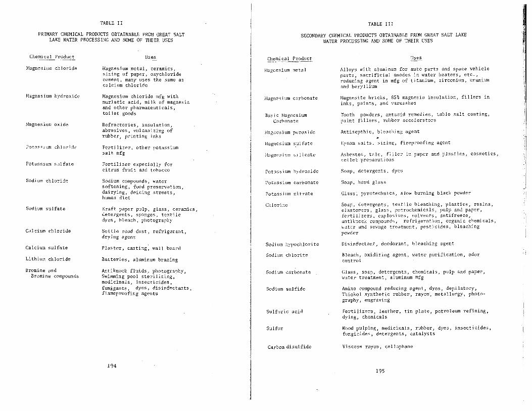
TABLE II

PRIMARY CHEMICAL PRODUCTS OBTAINABLE FROM GREAT SALT LAKE WATER PROCESSING AND SOME OF THEIR USES

~!agnesium chloride

Magnesium hydroxide

Magnesium oxide

PQt{!~<::;jum chlorine

Potassium sulfate

Sodium chloride

Sodium sulfate

Calcium chloride

Calcium sulfate

Lithium chloride

Bromine and Bromine compounds

Uses

~Iagnesium metal, ceramics, sizing of paper, oxychloride cement, many uses the same as calcium chloride

Magnesium chloride mfg with muriatic acid, milk of magnesia and other pharmaceuticals, to il e t goods

Refractories, inSUlation, abrasives, vulcanizing of rubber, printing inks

Fertilizer, other potassium salt mfg

Fertilizer expecially for citrus fruit and tobacco

Sodium compounds, water softening,- food preservation, dairying, deicing streets, human diet

Kraft paper pulp, glass, ceramics, detergents, sponges, textile dyes, bleach, photography

Settle road dust, refrigerant, drying agent

Plaster, casting, wall board

Batteries, aluminum brazing

Antiknock fluids, photography, Swimming pool sterilizing, medicinals, insecticides, fumigants, dyes, disinfectants, flameproofing agents

194

TABLE III

SECONDARY CHEMICAL PRODUCTS OBTAINABLE FRO~1 GREAT SALT LAKE WATER PROCESSING AND SO~1E OF THEIR USES

~lagnesium metal

"'agncsium carbonate

Basic Magnesium Carbonate

Magnesium peroxide

~lagl1es ium sui fate

Potassium hydroxide

Potassium carbonate

Potassium nitrate

Chlorine

Sodium hypochlori.te

Sodium ell lori te

Sodium carbonate

Sodium sulfide

Sulfuric acid

Sulfur

Carbon disulfide

Uses

Alloys with aluminum for auto parts and space vehicle parts, sacrificial anodes in water heaters, etc., reducing agent in mfg of titanium, zirconium, uranium and beryllium

Magnesite bricks, 85% magnesia insulation, fillers in inks, paints, and varnishes

Tooth pm,ders, antacid remedies, table salt coating, paint fillers, rubber accelerators

Antisepthic, bleaching agent

"l'som salts, sizing, fireproofing agent

Asbestos, talc, fi !ler in paper and plastics, cosmetics, toilet preparations

Soap, detergents, dyes

Soap, hard glass

Glass; pyrotechnics, s 101< burning b lack powder

Soap. detergents, textile bleaching, plastics, resins, elastomers, glass, pctrochemica1s, pulp and paper, fertilizers, cxplosives, solvents, antifreeze, antiknock compounds. refrigeration, organic chemicals, \,atcr and sewage treatment, pesticides, bleaching powder

Disinfectant, deodorant, bleaching agent

Bleach, oxidizing agent, \Vater purification, odor control

Class, soap, detergents, chemicals, pulp and paper, \vater treatment, al uminum mfg

Amino compound reducing agent, dyes, depilatory, Thiokol synthetic rubber, rayon, metallurgy, photo­graphy, engraving

Fertilizers, leather, tin plate, petroleum refining, dying, chemicals

Wood pulping, medicinals, rubber, dyes, insecticides, fungicides, detergents, catalysts

Viscose rayon, cellophane

195

TABLE IV

PROSPECTIVE UTAH PRODUCTS

Ammonium Sulfate Anhydrite

Storage Lithium Hydroxide

Battery Boxes Gilsonite

Dry Cells Zinc, Zinc Chloride, Carbon ,Cardboard, Ammonium Chloride, -Magnesium Dioxide, Copper Sulfate, Lead Sulfate

Edison Potassium Hydroxide, Lithium Hydroxide, Iron

Lead Storate Lead, Lead Oxide, Sulfuric Acid

Low Temperature Lithium Bromide

Nickel-Cadmium Cadmium, Cadmium Hydroxide, Potassium Hydroxide

Sil ver-Cadmium Silver, Cadmium

Storage Devices Barium Titanate

Beryllium Recovery Sodium Chloride

Bleaching Agents Magnesium, Chlorine, Calcium OXide, Chlorine Dioxide, Barium, PeroxIde, Lithium Hypochlorite, Sodium Silicates, Sodium Hypochlorite, Sodium Chlorite

Scouring Powders - Wools Chlorine, Calcium Hydroxide, Steel Sodium Silicates

Bromine Recovery Sodium Chlorate

, Gilsonite Catalyst

Sodium Nitrate, Silica Gel, Molybdenum, Vanadium, Sulfur Molybdate Alum~num H~droxide,Activated Alumina, Aluminum Phosphate, Aluminum' BromIde, LIthIum Molybdate, Ammonium Molybdate

Acrylonitrile Uranium

Corrosion Inhibitor Sodium Molybdate, Sodium Silicates

Ethylene to Ethanol Vanadium Trioxide, Vanadium Tetroxide

Ion Exchange Resins Uranium, Vanadium

Organic Oxidation Reactions Vanadium

Polymerization Vanadium, Sulfur Molybdate

Reactor Fuel Uranium

Stabilizer Phosphorus Pentasulfide, Lead Sulfate

196

Sulfur Dioxide to Sulfur Trioxide Vanadium

Sulfuric Acid Vanadium

fellophane Carbon Disulfide

Gypsum, Anhydrite, Limestone

Aluminum Phospilate, Beryllium, Magnesium, Molybdenum Trioxide, Uranium Dioxide, Aluminum HydrOXide, Calcium Carbonate, Gypsum, Barium Carbonate, Vanadium Pentoxide, Barium, Titanate

Detergents Chlorine, Sodium Polyphosphates, Potassium Polyphosphates, Sodium Silicates, Potassium Silicate, Hagnesium Silicate, Sodium Sulfate, Benzene, Olevin

Liquid Potassium Phosphate

Drilling Bits (Wells) Diamonds, Steel, Steel Alloys

Dri 11 ing ~luds

,

Barite, Calcium Chloride, Bentonite Deflocculant Agent

Sodium Tripolyphosphates

Cal cium ~Iagncsi urn Ch loride, Molybdenum, Calcium Acetate, Calcium Olromate, Barium Thiosulfate

Electrical Equipment Lithium, Barite, fluorine

Digital Calculators Bari urn Ti tanate

Dielectric Amplifier Barium Titanate

Electrical Porcelain ller)"llium, Calcined Alumina, Barium Titanate

Electronic Tubes Gla~s, Barium, Fluorine, Argon

Fluorescent Compounds Vi trcous Silica

High Voltage Equipment Beryllium, Calcined Alumina, Copper, Steel

Insulation Gilsonite, Ozokerite, Magnesium, Beryllium, Calcined Alumina

Printed Circuits Gold, Silver, Calcined Alumina, Copper

RectHiers Selenium

Resistors Beryllium Oxide

Semi Conductors Silicon Carbide, Selenium

Solar Space Generators Beryllium

Space Antennas Beryllium, Steel

Sparking Alloys & Carbon Arcs Carbon, Rare Earths

Switches Beryllium, Copper, Steel

197

TV Picture Tube Barium Carbonate

Ultraviolet Inhibitor Vanadium Pentoxide

X-ray Tube Windows Beryllium

Explosives Barium Chlorate, Ammonium Nitrate, Sodium Nitrate, Potash, Ammonium P"rchlorate, Sodium Chloride, Sodium Perchlorate, Ni tric Acid, 5111 fUrlc Acid, Potassium Sulfate

.Jato Fuel Ammonium Perchlorate

Incendiary Bombs & Shells Phosphorus

Rodet Fuel Ni tric Acid, SuI furi c Acid

Oxidizer Ammonium Nitrate, Ammonium Perchlorate

Safety Matches Cedar Trees, Barium Chromate, Potassium Nitrate, Phosphorus Trisulfide, Phosphorus, Sodium Chlorate, Aluminum Sodium Sulfate, Barium Nitrate

Signal Flares ,:,dciam Phosphlde, Barium Sitrate

Smoke Columns & Screens Phosphorus

Tear Gas Barium Acetone

Fertilizer Magnesium, Calcium Nitrate, Phosphate Rock, Phosphoric Acid, Ammonium Nitrate, Potassium Nitrate, Potassium Chloride, Potassium Sulfate

Liquid Calcium Ammonium Nitrate, Ammonium Sulfate Fluoride, Gypsum

Trace Element Carries Sodium ~'lolybdate

Fi h('rl"'("::~'(l --, ... , --Cedar' frees, -:~i1sonite

Filter Medium Calcium Carbonate, Silica

Fire Retardants Aluminum Sulfate, Sodium Bicarbonate, Magnesium, Bromine, ~1onoammonium Phosphate, Magnesium Sulfate, Sodium Phosphate

Asbestos ~Iagnesium Si licate, Barite

Fabrics & Wood ~Iagnesium

Pyrotechnics Calcium Nitrate," Ce llulose Phosphates

\\allboard Calcium Alginate, Gypsum (Calcium Sulfate)

Phosphoric Acid, Calcium Chlorate, Saccharin, Calcium Hydroxide, Calcium Chloride, Calcium Phosphate

Preservatives Calcium Bromide, Potassium Bisulfate

198

Foundary Core Compounds Barium Carbonate

Gas Mantles

Glass Magnesium, Thorium

Silican Oxide, Aluminum Oxide, Calcium Oxide, Magnesium Oxide, Sodium'Oxide, Calcium Phosphate, Potassium Oxide, Iron Oxide, Beryllium, Barium Peroxide, Aluminum Phosphate, Calcined Alumina, Barite, Sodium Nitrate

Plate Glass Gypsum

Polishing Rare Earths

Etching Fluorine

Flash Bulbs Magnesium

fiber Glass Light.Bulbs

Copper Flux

Lithium Lead Glass - decorative, optical effects, tableware Optical ~1irrors

Magnesium, Silver X-Ray Tube Windows

Beryllium Sealed Beam Headlights

Lithium High Stress Windows

Lithium Incandescent Mantles

Beryllium Optical Alloys

Beryllium Pigments

Vanadyl Sulfate, Lead ~lolybdate TV Tubes

Lithium, Barium Carbonate Milk Glass

Sodium Aluminate Neon Sign Tubing

Lithium Glues --Adhesives

Cellulose Phosphates, Sodium Silicates Casein Glues

Sodium Molybdate Epoxy Fi 11 er

Alumina Epoxy Resin for Stones

Magnesium Hydroxide, Magnesium Chloride Grinding Wheels

Calcined Alumina, Synthetic Diamonds, Silicon Carbide, Sodium Silica Oxide, Sodium Tetrasilicate

Heat Exchanger Medium Lithium Chloride, Sodium, Lithium Fluoride

Refrigerants Chlorine, Fluorine, Lithium Nitrate, Calcium Chloride, Sodium Nitrate

199

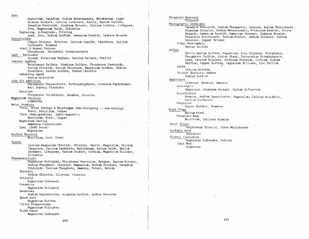
Inks Magnesium, Vanadium, Sodium Metavanadate, Molybdenum, Light Alumina Hydrate, Calcium Carbonate, Barite, Barium Sulfate, Vanadium Pentoxide, Aluminum Nitrate, Calcium Acetate, Lithopone, Zinc, Magnesium Oxide, Gilsonite

Engraving, Lithography, Printing Lead, Zinc, Sodium Sulfide, Ammonium Bromide, Cadmium Bromide

Insecticides

Lath

Copper Nitrate, Chlorine, Calcium Cyanide, Parathoin, Calcium Carbonate, Bromine

Roach & Rodent Poisons Phosphorus, Tetraethyl Pyrophosphates

Wallboard Gypsum, Potassium Sulfate, Calcium Sulfate, Perlite

Leather Tanning . Molybdenum Sulfate, Aluminum Sulfate, Phosphorus Pentoxld~, Barium Chloride, Sodium Phosphate, Magnesium Sulfate, SodIum Bisulfate, Sodium Sulfate, Sodium Chlorite

Dehairing Agent Barium Hydroxide

Lube Oil Additives Phosphorus Pentasulfate, Dithiophosphates, Aluminum Naphthenate Aryl Sufonyl Fluorides

Gasoline Phosphorus Trichloride, Bromine, Chlorine

Magnesium Recovery Limestone

Metal Products Tools, Metal Springs & Diaphragms (Non~fatiguing -- non-rusting)

Steel, Beryllium, Copper Tools (Non-sparking) (Anti-magnetic)

Beryllium, Steel, Copper Magnesium Casting

Ammonium Fluosilicate Cans (Soft Drink)

Magnesium Nuclear

Lead, Steel Paints

Calcium Magnesium Chloride, Chlorine, Barite, Magnesium, Calcium Tungstate, Calcium Carbo~ate, Molybdenum,.Barium OXi?e, B~r~um Chromate, Lithopone, BarIum Sulfate, LIthIum, MagneSIum SIlIcate, Gilsonite

Pharmaceuticals Magnesium HydrOXide, Phosphorus Pentoxlde, Bromine, Barium Nitrate, Sodium Phosphate, Chlorine, Magnesium, Sodium Chlorate, Vanadium Pentoxide, Calcium Phosphate, Ammonia, Potash, Helium

Aerosols Sodium Chlorite, Chlorine, Fluorine

Antiacid Magnesium Carbonate

Cosmetics Magnesium Silicates

Deodorant Sodium Hypochlorite, Aluminum Sulfate, Sodium Peroxide

Epsom Salt Magnesium Sulfate

Toilet Preparations Magnesium Silicates

Tooth Paste Magnesium Carbonate

zoo

Phosphate Recovery Fluorine

Photographic Chemicals . . . Vanadium Pentoxide, Sodium Phosphates, UranIum, BarIum ThIocyanate, Aluminum Chloride, Sodium Metavanadate, Potassium Bromide, Silver Bromide Ammonium Bromide, Ammonium Chromate, Cadmium Bromide, Potassi~m Perchlorate, Sodium Sulfide, Sodium Sulfates, Sodium Selenite, Copper Nitrate

X-Ray Development Barium Sulfate

Barite ,Barium Sulfate, Magnesium, Zinc Chloride, Phosphorus, Phosphoric Sulfide, Carbon Black, Tetrasodium Pyrophosphate, Lead, Calcium Silicate, Aluminum Chloride, Lithium, Sodium Sulfide, Copper SuI fate, ~!agnesium Silicate, Zinc Sulfide

Latex Calcium Nitrate

Thiokol Synthetic Rubber Sodium Sulfide

, Bromine, Ammonia Antiseptic

~lagnesium, Aluminum Acetate, Sodium Bifluoride Disinfect:lJlt

Bromjne, Sodium lIypochlorite, ~!agnesium, Calcium Bisulfite, Calcium Carhonate

Fungicide Copper Sulfate, Bromine

Steel Porcelain Body

Beryllium, Calcined Alumina

Steel Alloys - ~!olybdenum Trioxide, Ferro Molybdenate Sulfuric Acid

Anl1ydri te ·!1\erm3l Insulation

Magnesium Carbonate, Perlite Rock Wool

Limestone

ZOI

6. A campaign can then be launched to try to attract companies with know­

:lOW to Utah to produce these profitable chemical products.

Literature Cited

1. Mineral and Water Resources of Utah. Report of the U. S. Geological Survey in cooperation with Utah Geological and Mineralogical Survey and the Utah Water and Power Board. 1969. p. 13.

2. Cohenour, R. E., "Great Salt Lake, Utah, and its Environment", Utah Geological Survey, Salt Lake City, Utah, p. 211. (Date not given but probably about 1966)

3. Hahl and Langford, Dissolved-Mineral Inflow to Great Salt Lake, Water­Resources Bulletin No.3, 1963.

4. W. L. Stokes, Guidebook to the Geology of Utah No. 20, Utah Geological Survey,pp. 153 155.

5. Ash, A., Director of The Magnesium Project, Testimony given in Public Se rvice COlnmission - -Raft River hearing, January, 1968.

6. Johnson, B., Utah's Dead Sea Alive with Action, Intermountain Industry, pp. 6-120, August 1967.

7. Shreve, R. N., Chemical Process Industries, 3rd ed., McGraw-Hill, 1967, p. 2017.

8. Larsen, K. G., "Optimum Design of an Anhydrous Sodium Sulfate Plant", Brigham Young University M.S. Thesis, Chern. Eng. Dept., August 1965.

9. Glassett, J. M., and B. J. Anderson, "Recovery of Salts from the Waters of Great Salt Lake", Univ. of Utah Eng. Experiment Station Bulletin No. 128, May 1964.

lfl. {~lass('tt. '. 1\1.. ""("c-''''pry 0f Minerals from Concentrated Brines," Office of Saline 'Water Research and Development Progress Report No. 593, Decem­ber 1970.

11. McKee, R. H., "Applications for Utah's Che=ical and Mineral Resources," B. S. Thesis, Chemical Engineering Department, Brigham Young University, Provo, Utah, May 1970.

20020

POLITICAL RESTRAINTS ON RESOURCE MANAGEMENT

OF GREAT SALT LAKE

Dennis L. Thompson 1

Abstract

Great Salt Lake is a victim of incredible bad luck in its physical characteristics, environmental setting, and political management. One must understand the policy process to see where and how politics has failed to deal with the lake's problems. The policy determinants which affect the lake can be categorized as systemic (institutional), situational, and psychological (behavioral). In breakin~ each of these cate­gories down, we see the tremendous complexity of looking at a single policy problem, and Great Salt Lake abounds in a multitude of problems.

The most important factor to consider is that first of all Great Salt Lake is a body of water and it must be dealt with comprehensively as a body of water. There are then many other sub-problems such as pollution, desalinization, diking, recreation, mineral production, and reliction lands.

The comprehensive planning effort put into other Western water basins has not been put into Great Salt Lake. The responsibility should be the state's; but in th-e vacuu= the local governments have done little and the federal government has at times been a hindrance. The policy on the direction which the lake's development should take is a result of non­decisions. The state should be the moving force and it should be focused by the state water agency.

KEY WORDS: Policy process; Federal government; Local government; Policy determinants; State govern­ment; Non-decisions; Planning

Great Salt Lake is a victim of incredible bad luck. It began as an immense

inland sea, but is now a perpetually diminishing vestige of its former self.

This decrease in size is due to its bad luck of being located in an area of

extreme aridity where it cannot even count on regular replenishment. In

modern times its relatively limited sources of supply have also been diminished

because of upstream demands that have been placed on the streams. Great

Salt Lake is at the end of the hydrologic syste= which means it gets what is

left over after all other uses have been allocated. Being at the end of the

drainage systems has meant that the quality of water delivered to it is not

Professor, Department of Political Science, University of Utah. I acknowledge the use of the files of the Utah State Historical Society.

2003

:1

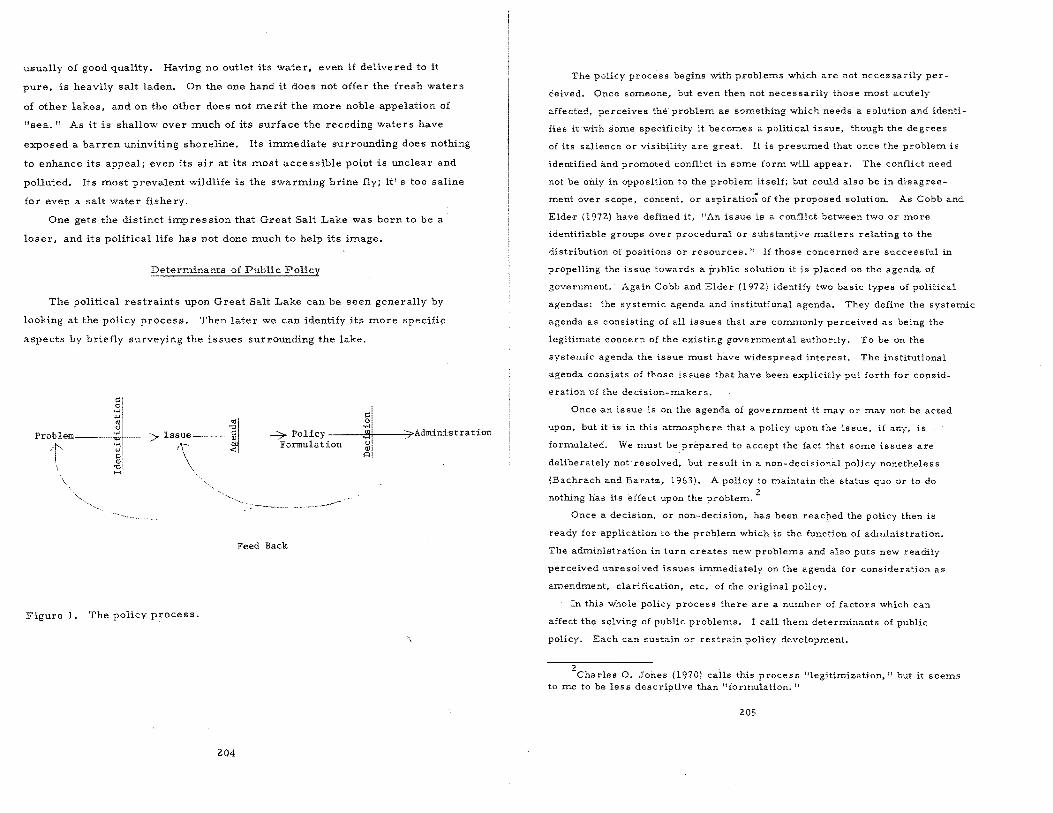
usually of good quality. Having no outlet its water, even if delivered to it

pure, is heavily salt laden. On the one hand it does not offer the fresh waters

of other lakes, and on the other does not rn.erit the rn.ore noble appelation of

"sea. II As it is shallow over much of its surface the receding waters have

exposed a barren uninviting shoreline. Its immediate surrounding does nothing

to enhance its appeal; even its air at its most accessible point is unclear and

polluted. Its most prevalent wildlife is the swarrn.ing brine fly; it's too saline

for even a salt water fishery.

One gets the distinct impression that Great Salt Lake was born to be a

loser, and its political life has not done much to help its irn.age.

Deterrn.inants of Public Policy

The political restraints upon Great Salt Lake can be seen generally by

looking at the policy process. Then later we can identify its rn.ore specific

aspects by briefly surveying the issues surrounding the lake.

"OJ... +0 Issue------#"'i+-----7-- Policy :,-j " Administration 'I;- Formulation ~

'\ A

Feed Back

Figure 1. The policy proces s.

\

204

The policy process begins with problems which are not necessarily per­

ceived. Once someone, but even then not necessarily those most acutely

affected, perceives the problem as something which needs a sQlution and identi­

fie's it with some specificity it becomes a political issue, though the degrees

of its salience or visibility are great. It is presumed that once the problem is

identified and promoted conflict in some form will appear, The conflict need

not be only in opposition to the problem itself; but could also be in disagree-

ment over scope, content, or aspiratio,;' of the proposed solution. As Cobb and

Elder (1972,} have defined it, "An issue is a conflict between two or more

identifiable groups over procedural or substantive matters relating to the

distribution of positions or resources." If those concerned are successful in

propelling the issue towards a public solution it is placed on the agenda of

government. Again Cobb and Elder (l972} identify two basic types of political

agendas: the systeInic agenda and institutional agenda. They define the systemic

agenda as consisting of all issues that are commonly perceived as being the

legitimate concern of the existing governmental authority. To be on the

systemic agenda the issue must have widespread interest. The institutional

agenda consists of those issues that have been explicitly put forth for consid­

eration 'of the decision-makers.

Once an issue is on the agenda of government it mayor may not be acted

upon, but it is in this atmosphere that a policy upon the issue, if any, is

formulated. We must beprepared to accept the fact that SOIne issues are

deliberately not resolved, but result in a non-decisional policy nonetheless

(Bachrach and Baratz, 1963). A policy to maintain the status quo or to do

nothing has its effect upon the probleIn. 2

Once a decision, or non-decision, has been reacl'ed the policy then is

ready for application to the problem which is the function of administration.

The administration in turn creates new problems and also puts new readily

perceived unresolved issuesirnrnediately on the agenda for consideration as

amendment, clarification, etc, of the original policy.

In this whole policy process there are a nUInber of factors which can

affect the solving of public problems. I call them determinants of public

policy. Each can sustain or restrain policy development.

2Charles O. Joues (1970) calls this process "legitimization," but it seems to me to be less descriptive than "formulation. "

20S

The policy determinants seem to logically fall into three categories:

systemic, situational, and psychological (or behavioral). Systemic determin­

ants are those which are inherent in the political system. The nature of the

legislature; the executive focus; the possibility of independent judicial review;

the strength and competence of the bureaucracy; the kinds and sources of

support mustered by the administrative agencies; and the organizational re­

lationships of all of these are all systemic determinants. Dror (l96-8) has

indicated the significance of analyzing what we know about the policy-making

process, what he calls metapolicy knowledge. This kind of information is. also

systemic as it relates to all potential policy issues in a given political system.

In the United States when dealing with a problem at the state level the

systemic determinants could be those related to the state system of government

as well. But in most cases there is involvement or interest on the part of

both national and state or local governments, thus the nature of American fed­

eralism also becomes significant; the legal and political relationship of the

state and federal governments. This is crucial in looking at Great Salt Lake.

Situational determinants are those which have to do with any given policy

issue. The interests and values involved in the policy issue at hand must be

traded off against a multitude of other events and iSBues which compete for

time, attention and resources (Bauer, 1968). One could list indefinitely events

and issues which could be remotely connected to the policy problem at hand.

There are antecedants and consequences which must be considered; but there

should also be some logical division between those which have, can or will

affect the policy and those which are tendential to the problem at hand. Bauer

(1968) uses the phrase "the envelope of events and issues" to denote the context

within which a given problem should be analyzed. Much of this envelope will

be concerned with the state of affairs--the criticality of the problem, the

pressures and counter pressures extant, and the major events and issues to

which the policy-makers are giving their time. Other situational determinants

must be considered as well. The level of public concern, whether well­

founded or not, will have important bearing on issue resolution. Interested

organizations become part of the situation because they do not have a general

interest in all issues, but pick and choose the cauSes for their involvement,

Also included here is the extent to which a problem is understood, the infor­

mational aspect. This mayor may not include the state of technology. If that

206

technology is not available to properly analyze the problem or collect the needed

data, the information level will not be adequate. It tnay -be just a matter of

transferral of technology from some other policy area, but this is not always

evident nor is it always done (Furash, 1968). Resource supply is also partic­

ular to each issue, including the level and availability of trained personnel,

money, and time. In this same vein, and particularly with natural resources

issues, the state of nature is a significant situational}actor. Access, pollution

level, water level, and salinity are examples relevant to the Great Salt Lake.

Finally, psychological determinants are those which relate directly to the

people involved. After all, policy issues are not resolved by institutions or in

situations, but by people. We must always be aware of what factors affect their

behavior and participation on a policy issue. These factors are much more

difficult to identify or analyze than the systemic and situational ones. But by

being aware of their existence and recognizing their effect, we can at least know

where the secrets lie if our political understanding is incomplete after all other

data has been collected. The base of psychOlogical determinants is the values

which the participants bring to political situations. A person's value judgments

color his attitude toward all other factors (Davies, 1963). Also of critical im­

portance are the capabilities which those involved possess. The political cul­

ture, which as a whole could be either systemic or situational,comes to bear

on a policy issue as it effects the individuals--as they feel its demands and re­

straints. Akin to this latter concept is the extent to which a person has been

socialized, into a political culture generally, but, more spec_ifically, into a

peculiar situation. The above, and other, factors will in turn determine how a

participant perceives a problem, its alternative solutions, and their consequen­

ces. The policy participant also has a relationship to interested institutions

and organizations which colors his perceptions and actions, Finally, the inde­

pendent factor of communication has its effect on the individual. The level of

infortnation (situational) may be high, but there may be a lack in communication.

This can result in turn from a lack of effort to communicate, an inability to

understand (which often happens when technical data is transmitted). or a lack of

opportunity (inadequate means of communication). The results are the same;

those who are, should or could be concerned don't get the word. This tneans

they act on partial information, are delayed, or do not act at all.

207

These determinants are not intended to constitute a complete list of factors

affecting public policy formulation. But they are the more important ones, and

do give an idea of the complexity of all the factors involved. All of these' deter­

minants may not necessarily be involved in any specific policy issue; but before

taking heart, I would warn that most of them are factors to be considered to

some extent in every policy determination.

With the problems of managing Great Salt Lake peppered with a profusion

of policy determinants, the lake is also salted by an equally perplexing number

of issues.

Great Salt Lake is first of all a body of water, though this fact has often

been of secondary importance as other issues have captured greater interest.

Its inflow, water level, quality, distribution, and utilization are primarily and

pre imminently water factors which affect all other uses of the lake and its sUr­

rounding area. Yet its problems are not usually treated as water problems

and thus the institutional determinants are often not water related institutions.

This in turn Ineans that the people involved are not water related people; thus

the psychological deterIninants will not be wetted by water either. This has

Inade uncoInfortable decisional situations, because the situational determinants

reInain true to reality.

The problems which have remained as water issues have not had the atten­

tion of many of the other problems. As with Inost of oUr inland bodies of ~ater,

pollution was an ongoing and unheralded fact of lake life for years. And the

eutrophication of Great Salt Lake was less noticeable than in fresh water lakes.

But the lake had its defenders who warned of the damage being done. From the

early 60' s, when it was called one of the biggest open ended cesspools in the

country, to the late 60' s, when much of its wastewater was put through treat­

ment plants, its pollution input declined. Yet the pollution grows worse as it

is cmTlulative, and the input of waste from the drainage systems continues.

Diking the lake to p'roduce fresh water reservoirs, long discussed, is now

a reality as a result of the Willard Bay development of the Weber Basin Project.

But there are still other proposals for diking parts of the lake. The Lucin cut­

off causeway built by the Southern Pacific Railroad was not intended to create

a fresh water lake, but has made the southern end less saline than the northern

208

end. Desalinization fOr the production of sweet water and power production are

still other potential uses of lake water which would bring additional interests

and issues into play.

Traditionally, and probably most evident in the public eye, the lake has

been used for recreation. Nostalgic reminiscences of the glorious days of

Saltair provided historical and pictorial evidence that the lake was there for

recreation. For decades dreams, proposals, "lind even some plans for the

further development of the lake's boatery, swimming and beach potentials have

been put forth; but alas little has been done. The interest has been mostly

private, but the hindrances are public. Brine flies, pollution, receding shore--L

line, and the need for fresh water are problems beyond the capability of private

developers.

The state, of course, did finally set aside the Great Salt Lake State Park

on the north shore of Antelope Island in the face of another attempt to create a

national monument on the island. This is an amazingly sparse political record

of accomplishment given the almost universal agreement that recreational de­

velopment of the lake should proceed. The Legislative Council, the Governor,

the State Park and Recreation Commission, The Salt Lake Tribune, The Deseret

News, The Standard Examiner, the chambers of commerce of Salt Lake City

and Ogden, and county governments have not proved an adequate base for the

development of a meaningful recreational development policy.

Minerals have been the most widely used resOUrce oi Great Salt Lake.

Beginning with salt the trend of mineral production is constantly on the increase

and now includes potash, lithium, magnesium, sodium sulphate, potassium

chloride, and chlorine. And there are constant proposals for drilling for oil

and some minute production at the north end of the lake shore. As with recrea­

tional proposals there are a lot of private interests which want to Inaintain Or

gain accesS to an eventual wealth and are ready to promise huge development

to protect their interests. And some companies have built extraction plants

and are producing to the extent that the state is encouraged to manage the lake

for its mineral content as well as anything else.

Probably the most critical issue in the past decade has been the contra­

dictory problem of lake land. The general problem of ownership of the lake

(which to me was a non-issue issue) and specifically the reliction lands Or that

land which has been exposed by the receding shoreline of the lake. The owner-

209

ship of the lake has been clarified by the Supreme Court in favor of the state; and

the relicted lands has been settled, unsatisfactorily for the state, by Congress

and awaits another Court decision.

It is evident that the planning effort and resultant political bargaining and

adjustments which have been put in to most other drainage basins in the West

have not been put in to the Great Salt Lake Basin. Its tributary river basins

have each in turn been considered but as river basins, not as part of a larger

entity. The type of research reported here today is necessary. The lake must

be looked at as a whole, rather than in its parts. The lake must be looked at

as a body of water rather than as a mine, or a beach, or a dumping ground.

As a water entity it will tie all of its component interests together.

The lake in the past has been the victim of bad government. If governments

did not want to do anything to enhance the lake, they at least should have done

nothing to damage it. The problems created by federalism are especially evi­

dent in this context. On the one hand while the collective governments, federal,

state, and numerOUs local entities have not sought to develop the potentials of

the lake in concert SO that the collective interests of all might be served; neither

have they separately acted in good faith toward a public good for the lake.

Local governments often remind me of the parable of the talents. We do in

fact give them the least authority and opportunity for broad action. But the ex­

pectation is that what is given should be used. The purpose of local government

is to provide for local needs. Their talent cannot be hidden, otherwise as the

parable ends (Matthew 25:28-30)

Take therefore the talent from him, and give it unto him which hath ten talents. For unto everyone that hath shall be given, and he shall have abundance: but from him that hath not shall be taken away even that which he hath.

And cast ye the unprofitable servant into outer darkness: there shall be weeping and gnashing of teeth.

Need I explain.

The State of Utah comes off the best of the lot, but not unscathed. While

claiming sovereignty over the lake it has not undertaken the broad-based com­

prehensive planning program that the basin so desperately needs. If, as I have

contended here. it is primarily a water issue, the State Board of Water Re­

sources should be the responsible governmental entity. But it did not undertake

to direct, guide or participate though it was authorized to study. investigate

and plan for the "full development, and utilization and promotion of the water

210

resources of the state .... " Four of the seven members of the board could be

from the Great Salt Lake drainage basin. It appears that comprehensive plan­

ning and management is a victim of psychological determinants. It is difficult

to get people to face conflictual situations. They do not want to deal with, let

alone create it. It is easier to let sleeping dogs and dormant lakes lie.

The creation of the Great Salt Lake Authority is an example of the state's

attitude. The initial legislation recognized the need for some overall look at

the problems of Great Salt Lake and provided for something more than had been

completely negotiated amongst the state interests or even that the authority was

prepared to do. As a result the GSLA did little more than develop the Great

Salt Lake Park; and it even had difficulty in doing that because of an insistent

recognition in some places that the lake should be looked at in a broader con-

text. As it became evident that the creation of a park was all that the GSLA

was to be allowed or even wished to do, it also became evident that the Division

of Parks and Recreation should probably be doing that. The subsequent amend­

ment to the GSLA legislation, four years after its creation, more clearly defined

its authority in line with what it was in fact doing. That is hardly decisive leader­

ship on the part of the state. Finally the state 'transferred the authority to the

Division of Parks and Recreation and gave it the overall duty for "planning and

developing uses of the Great Salt Lake" including the "mainland, peninsula,

islands, and water within the ... meander line" (Utah State Code [65)). This

ignores the fact that Great Salt Lake is a water resource with multiple uses.

On the other hand the state was forced to put much of its available energy

which could be allotted to Great Salt Lake to deal with the obtuseness of the fed­

eral. government. When the state attempted to take affirmative action on some

of the lake's problems in 1961 it was stymied by a federal contention of owner­

ship, not only of reliction lands but of the lake itself. As Max C. Gardiner,

then Director of the State Land Board, said in July, 1962,

"The federal government should not put the state to the expense and burden of litigation to confirm such a well known fact (as the na vigability of the lake). "

Furthermore, the attempts of the state at that time to clear this nonsensical

hurdle by introducing legislation in Congress through its Congressional delegation

were insistently fought by Secretary of the Interior Udall who wanted the state to

exhaust administrative remedies before seeking legislative relief, as though the

211

pattern of federal action to that point had implied any administrative remedy

was available.

A number of years ago, Morton Grodzins, a perceptive writer on American

federalism, wrote (Grodzins, 1961)

The rhetoric of state and national power becomes easily and falsely a rhetoric of conflict. It erroneously conceives states and localities, on one side, and the central government, on the other, as adversaries. There are undoubtedly occasions when the advantage of a locality, state or region is a disadvantage to the nation as a whole. But in most circumstances at most times compatibility rather than conflict of interests is characteristic. . .. Federal, state, and local officials and not adversaries. They are cOlleagues. The sharing of functions and powers is impossible without a whole. The American system is best conceived as one government serving one people.

Scientific and technical personnel often act in harmony, but somehow,

federal, state, and local officials didn't get the word. All governments must

be involved and we should expect them to work as one government serving one

people. Among them one group has to take the lead- -1 suggest that it is logi­

cally the role of the state on Great Salt Lake. Surely the management and de-

velopment of Great Salt Lake can be of advantage to all Americans. Since when

is a Utah advantage not an American advantage? To ask for state leadership by

the water board is not to be prejudicial to any current or projected uses; but

seeks comprehensive management and planning.

In the terms of Gilbert White's excellent analysis of Strategies of Ameri­

="-'-':':"'::=~==:::.J>;="""'=( 196 9), where he identifies six types of strategy in

light of purpose, means, and management agency, it is evident that Great Salt

Lake calls for application of his sixth and most complicated strategy: ".... a

merging of multiple purposes, and multiple means, including research, ... II

As I have said, I can find no evidence that the decision-making elements of

Utah state government have decided what should be done with Great Salt Lake;

yet the state insists it should be the one to make the decision. Decisions to

lease land for ponds or drilling, to build a road or causeway, or to create a

park show no pattern of a conscious decision as to what the expectations of lake

use are. There is no state agency with overall planning and management re­

sponsibility for the lake, nor is there a state plan. The complex problems of

the lake have pushed the decision-makers into partial solutions. But neither

is there widespread public concern over the future of the lake, which means

the special interests have clearer sailing to maintain their status quo or

212

presumed future benefits. And there is some lack of information on the lake;

but who wants to dig up data which has little prospect of being used.

It is amazing how many studies have been made and how much data has

been collected, but how few decisions have been made. I have made no attempt

to ascertain the psychological determinants which are most basically involved

in the state policy process on Great Salt Lake, but Without doubt many of the .. restraints upon the development of a state policy can be found in the make-up

of a handful of individuals who either have had no interest Or have had specific

interests which promote non-decisions. Yes, we have an overall policy on

Great Salt Lake created mostly by non-decisions and partial decisions.

References

Bachrach, Peter and Morton S. Baratz. 1963. Decisions and Non-Decisions. American Political Science Review 57: 532-542.

Bauer, Raymond A. 1968. The Study of Policy Formation: An Introduction, in Raym.ond A. Bauer and Kenneth J. Gergen (eds.). The Study of Policy Formation. The Free Press. 392 pp.

Butrico, F. A. et al. D. C. Heath &. Co.

1971. Resource Management in the Great Lakes Basin. 190 pp.

Cobb, Roger W. and Charles D. Elder. 1972. Participation in American Politics: The Dynamics of Agenda-Building. Allyn and Bacon, Inc. 182 pp.

Davies, James C. 1963. Human Nature in Politics. John Wiley &: Sons.

Dror, Yehezkel. 1968. Public Policymaking Reexamined. Chandler Publishing Co. 370 pp.

Dworsky, Leonard B. et al. Resources Development. 245 pp.

1971. Social and Economic Aspects of Water The American Water Resources Association.

Furash, Edward E. 1968. The Problem of Technology Transfer, in Raymond A. Bauer and Kenneth J. Gergen (eds.). The Study of Policy Formation. The Free Press. 392 pp.

Gadd, John D. C. 1967. Recreational Development of the Great Salt Lake. Unpublished thesis. University of Utah. 128 pp.

Grodzins, Morton. 1961. Centralization and Decentralization in the American Federal System, in Robert A. Goldwin. A Nation of States: Essays on the American Federal System. Rand McNally &. Co. 148 pp.

Jones, Charle's O. 1970. An Introduction to the Study of Public Policy. Wads­worth Publishing Co. 170 pp.

Teal, John and Mildred Teal. 1969. Life and Death of the Salt Marsh. Little, Brown &. Co. 278 pp.

213

Utah State Code 65-8-4 (5) and 65-8-2.

Utah State Code 73-10-4 (I).

White, Gilbert. 1969. Strategies of American Water Management. The Uni­versity of Michigan Press. ISS pp.

214