Utah State UniversityDigitalCommons@USU

Reports Utah Water Research Laboratory

January 1994

The Great Salt Lake: A Barometer of LowFrequency Climate VariabilityUpmanu Lall

Michael Mann

Follow this and additional works at: http://digitalcommons.usu.edu/water_rep

Part of the Civil and Environmental Engineering Commons, and the Water ResourceManagement Commons

This Report is brought to you for free and open access by the Utah WaterResearch Laboratory at DigitalCommons@USU. It has been accepted forinclusion in Reports by an authorized administrator ofDigitalCommons@USU. For more information, please contactdylan.burns@usu.edu.

Recommended CitationLall, Upmanu and Mann, Michael, "The Great Salt Lake: A Barometer of Low Frequency Climate Variability" (1994). Reports. Paper244.http://digitalcommons.usu.edu/water_rep/244

THE GREAT SALT LAKE:

A BAROMETER OF LOW FREQUENCY

CLIMATE VARIABILITY

Upmanu Lall and Michael Mann

Working Paper WP-94-HWR-UL/005

October 1994

Utah Water Research Laboratory Utah State University

Logan, ur 84322-8200 (801) 797-3155

Fax (801) 797-3663

The Great Salt Lake: A Barometer of Low Frequency Clhnatic Variability

Upmanu Lall1t and Michael Mann2

Low frequency (interannual or longer period) climatic variability is of interest because of its

significance for the understanding and prediction of protracted climatic anomalies. Closed basin

lakes are sensitive to long term climatic fluctuations and integrate out high frequency variability. It

is thus natural to examine the records of such lakes to better understand long term climate

dynamics. Here we use Singular Spectral Analysis (SSA) and Multi-Taper Spectral Analysis

(MTM) to analyze the time series of Great Salt Lake (GSL) monthly volume change from 1848-

1992, and monthly precipitation, temperature and streamflow for nearby stations with 74 or more

years of data. This analysis reveals high fractional variance in 15-18, 10-12, 3-7 and 2 year

frequency bands, which seem to be consistent across time series. The putative decadal and

interdecadal signals appear to be related to large scale climate signals discussed recently. The

interannual signals are consistent with EI Nino Southern Oscillation (ENSO) and quasi-biennial

variability identified by others. Prospects for improved prediction of the GSL volume and of

protracted wet/dry periods in the Western United States are discussed.

lUtah Water Research Laboratory, Utah State University, UMC82, Logan UT 84322-8200

2Department of Geology and Geophysics, Yale University, P.O. Box 208109, New Haven CT 06520-8109

Introduction

Our fascination with climatic cycles goes back as far as recorded history. Almost every

possible periodicity between 2 and 200 years has been observed with some certainty (Burroughs,

1992, p. 60). Burroughs also observes that "the history of meteorology is littered with the

whitened bones of claims to have demonstrated the existence of reliable cycles in the weather".

Often, the "cycle" is wont to disappe~ soon after its discovery-, and may spontaneously reappear

later. The existence and understanding of all but the diurnal and the annual cycle is polemical.

The search for hidden order is one of science's aspirations. Moreover, given the socio-eco­

geo-political implications of successful long term climatic forecasts, interest in the identification

and explanation of recurrent climatic patterns is natural. Recently (see Diaz and Pulwarty (1994),

Mann and Park (1993, 1994) (hereafter, MP93, MP94), Houghton and Tourre (1992), Currie and

O'Brien (1992), Ghil and Vautard (1991) (hereafter, GV), Dettinger and Ghil (1991), Trenberth

(1990), and Levitus (1989» interest has focused on the possibility of decadal/interdecadal climatic

variability that may be due to internal (e.g., ocean-atmosphere interaction) or external (e.g.,

sunspot cycles or lunar tides) factors. Indeed, GV and MP94 argue that a large part of the recent

global warming may be explained as the superposition of distinct quasiperiodic climatic patterns

with different frequencies. Can one explain droughts and other protracted anomalies similarly?

Recognition of low frequency variability leads to changes in the interpretation (e.g., of water

quality trends) and utility of hydro-climatic records. Traditional hydrologic models formulated at

monthly or annual time scales assume stationarity of the statistics of the underlying process.

Interannual structure in these time series invalidates such assumptions. The identification of

coherent, low frequency patterns is also relevant to interpretation of long range persistence or the

Hurst effect.

Draft U. Lall October 11,1994 2

A purpose of the work presented here is to develop an empirical understanding of the role of

climatic variability in the dynamics of the Great Salt Lake (GSL) of Utah - a closed lake in the arid

Western U.S.A. Our findings are also directly relevant to the ongoing debate on interdecadal

climatic variability. A long record (1848-1992) was available. The GSL "samples" precipitation in

the Great Basin, an area where most of the precipitation occurs at high elevations and runoff is

largely from snow melt. Worldwide, very few long record, high elevation, precipitation gages are

available. Barnston and van den Dool (1993) suggest that regions with low interannual variance in

atmospheric circulation are favorable sites for studying low frequency climatic behavior. In their

analysis of 700 mb atmospheric pressure surface data, the GSL basin is such a region. Insights

from spectral analyses using "modern" methods such as Singular Spectral Analysis (SSA)

(Vautard et al (1992», and the Multi-taper spectral analysis method (MTM) (Thomson (1982» of

GSL volume changes and precipitation, temperature, and streamflow time series at nearby stations

are presented here (see Figure 1 for a site map, and Table 1 for site information). Of interest is

evidence for structured low frequency variability in these time series, and insight into the relative

sensitivity of the GSL to low frequency precipitation and temperature variability.

In the next section we develop a perspective for the analysis of climatic variability - is it

random; is it deterministic but chaotic and unpredictable; are cycles sustainable; do they represent

quasi-periodic transitions between different climatic regimes~ or are they episodic damped

oscillations triggered by external events? What are the implications for the analysis of a finite,

noisy time series? Are some types of data (e.g., spatially gridded or averaged data vs. point time

series) more useful than others? What are some desirable attributes of the analysis methodology?

Background information on the Great Salt Lake and its environs comes next. A section describing

the methods used follows. This leads to the results from the analysis of the selected time series.

Draft U. Lall October 11,1994 3

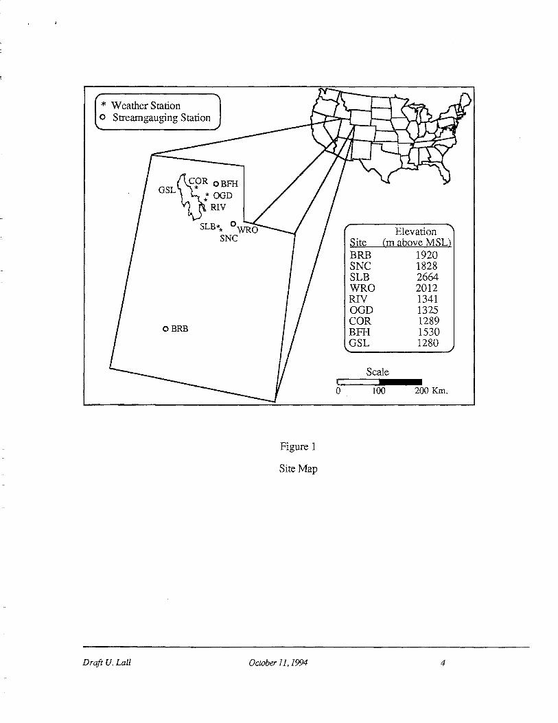
* Weather Station ° Streamgauging Station

GSL~PR OBFH : OGD

RIV

SLB** °WRO SNC

OBRB

Figure 1

Site Map

Draft U. Lall October 11.1994

o

Elevation Site (m above MSL) BRB 1920 SNC 1828 SLB 2664 WRO 2012 RIV 1341 OOD 1325 COR 1289 BFH 1530 OSL 1280

Scale

100 200 Km.

4

Table 1

Data Sets Analyzed

Elevation Latitude Longitude (m. above MSL) Record Length

Great Salt Lake (GSL) 40' 20' to Ill' 52' to 1280 1848-1991 Monthly Volume Change 41' 40' N 113' 06' W

Snake Creek 40' 33' N Ill' 30' W 1828 1916-1989 (SNC)

Silver Lake/Brighton 40' 36' N 111' 35' W 2664 1916-1989 (SLB) (Highest station)

Riverdale 41' 09' N 112' 00' W 1341 1916-1989 (RlV)

Ogden 41' 15' N Ill' 51' W 1325 1916-1989 (OGD)

Corinne 41' 33' N 112' 01' W 1289 1902-1989 (COR) (Closest to GSL) (Lowest Station)

BeaverRivernr. Beaver 38' 17' N 112' 34' W 1920 1915-1988 (BRB) (South ofGSL drainage and does not flow into GSL)

Weber River nr Oakley (WRO)

40' 44' N 111'15' W

Blacksmith Fork nr Hyrum 41' 37' N Ill' 44' W (BFH)

2012

1530

Draft U. Lall October 1J, 1994

1905-1988

1919-1988

Source/Comments

U.S.G.S./Sangoyomi(1993)

Fan and Duffy (1993) Monthly Temperature/Precipitation

Fan and Duffy (1993) Monthly Precipitation

Fan and Duffy (1993) Monthly Temperature/Precipitation

Fan and Duffy (1993) Monthly Precipitation

Fan and Duffy (1993) Monthly Temperature/Precipitation

U.S.G.S., Slack et al (1992) Monthly Streamflow

U.S.G.S., Slack et al (1992) Monthly Streamflow

U.S.G.S., Slack et al (1992) Monthly Streamflow

5

Notions about Climatic Fluctuations and Data Analysis Issues

During 1983-86, the Great Salt Lake rose rapidly to its highest level in a hundred years, and

then declined quickly just as a $60 million pumping project to control its level was implemented.

The previous decade had seen concern that the GSL might be drying up. The persistent rain and

floods in the Mississippi River basin in 1993, were equally noteworthy. Such extremes are

fascinating because they occur at every time scale, and in human memory, with some regularity.

Let us examine some postulates regarding such behavior.

(I) The climatic time series is the outcome of a random process (perhaps one with some

memory) and the diurnal and annual cycles.

The observed extremes occur randomly in accordance with such a process. This is a rather

unsatisfying postulate, not in the least because it provides little physical intuition or understanding

of the climatic process.

Pragmatically, it is known that a number of deterministic and chaotic systems (Abarbanel et

ai, 1993) have generally broadband spectra that can be easily misclassified as "white" or "red"

noise systems. The underlying dynamics may have well defined regimes with nearly periodic

transitions between them at some preferred range of time scales. Predictability is lost only by

passage through some unstable state(s). Palmer(1993) exemplifies this perspective using the

Lorenz equations. Consequently, there are no sharp spectral peaks, but possibly high power in

some frequency bands that will be overlooked in a traditional periodogram analysis. Since it calls

for an explanation, evidence of such frequency structure in the spectrum of climatic time series is

important, even if no sharp spectral peaks are apparent. There is a growing recognition (e.g.,

Kahya and Dracup (1993), Guetter and Georgakokas (1993), Cayan and Webb (1992), Cayan and

Peterson (1989), Ropelewski and Halpert (l986)} of the importance of the nearly periodic (over a

Draft U. Lall October 11, 1994 6

2 to 3 and 4 to 6 year frequency bands) EI Nifio Southern Oscillation (ENSO) on temperature,

precipitation and streamflow variability over large regions. Philander (1990) presents a treatise on

the observational aspects of ENS 0 as well as several physical/dynamical explanations.

(II) The climate system is deterministic, with positive and negative feedbacks that lead to

recurrent patterns in time and space.

Such "oscillations" may be described by linear or nonlinear dynamics associated with the

amplifying (positive) and restoring (negative) forces. The governing equations (see Lorenz

(1976), or Saltzman (1983» of the climate system are nonlinear with a variety of feedbacks. Ghil

et al (1992) review recent work on understanding climate through a nonlinear dynamics

perspective. What are some implications of nonlinearity that are of interest in analyzing climatic

time series?

1. Harmonic Generation. Burroughs (1992), p.147, indicates that in a nonlinear system, (a)

higher harmonics (e.g., 2f, 3f etc.) of an external forcing at frequency f, may be generated, and (b)

if there are two or more forcing frequencies, periodicities at integer combinations of these

frequencies may show up in the response. In the latter case (often called a quasi-periodic

system)l, low frequency responses (e.g., through the combination f1-f2) may be generated.

Typically, the amplitude of the higher harmonics is smaller than that of the lower harmonics. Once

again, such a response could easily be misclassified as "red" noise upon periodogram analysis.

Burroughs offers the example of the 11 year (f1 =1/11) sunspot cycle, which if relevant to climate,

may lead to harmonics at 5.5 (2f1) and 3.7 (3f1) years; and its combination with the purported

lunar tide cycle of 18.6 (f2=1/18.6) years could produce periodicities of 6.9 (n +f2), and 120.3

(4f2-2f1) years. Sangoyomi and Lall (1993) analyzed the spectra of the biweekly 1848-1992 GSL

volume using classical periodogram analysis following a recipe for peak identification suggested

lSome authors use the tenn quasi-periodic to mean periodic behavior that is slowly frequency or amplitude

modulated. Such behavior is tenned nearly rather than quasi periodic here, to distinguish it from the fonnal

defmition of quasi-periodicity used by physicists and mathematicians.

Draft U. Lall October 11.1994 7

by MacDonald(1989), and found that there were 15 peaks that were significant at the 0.1 level.

However •. all these peaks could be resolved as integer combinations of four base frequencies

corresponding to periods of 36.07, 14.23, 11.10 and 1 years. This is an interesting preamble for

this work since it naturally raises the question of whether this quasi-periodicity (if real) is generated

by the dynamics of the lake and its drainage or by climatic variability. Jin et al (1994) developed a

paradigm for ENSO along these lines.

2. Entrainment. Burroughs (1992), p.148 describes entrainment as a situation in which a system

with a natural self-excitation frequency f l' if stimulated by a forcing at frequency f 2, may respond

at f2 if f2 is close to f1, or asynchronously, at a new frequency f3. Transient oscillations in one

part of the system (e.g., the ocean) may consequently lead to a synchronous or asynchronous

response in other parts of the system. Energetic perturbations, such as volcanoes, may lead to a

chain reaction of oscillations in the system. The effected subsystem may respond with a damped

oscillation at its natural frequency. Interacting subsystems may respond synchronously or

asynchronously, and may also have positive feedbacks. In a dissipative system, eventually such a

chain of events would damp out. Vautard et al (1992) point out that the behavior of a chaotic

system is usually not totally random. Near periodicities may contribute a large part of the system

variability. Weakly unstable periodic orbits (corresponding to internal or natural response

frequencies) may attract trajectories intermittently and lead to spells of periodic activity. Such

cycles may show up in one segment of the data, but may be missing in another.2 Thus the

response of the system to particular forcings (e.g. volcanic disturbances) that occur at roughly the

same state of the system may have short term predictability. This observation may account for Lall

et al's (1994) success in predicting the GSL for up to 4 years in the future using a nonlinear

dynamics based forecasting model.

brhis ties in with what we called nearly periodic behavior earlier. Such variability will typically show up in a

spectrum as an elevated narrow band rather than a sharp peale ENSO is often assigned this interpretation.

Draft U. Lall October 11.1994 8

3. Phase Shift. Phase shifts relate to the previous discussion on entrainment. Burroughs (1992),

p. 149, points out that for systems that are forced by a combination of frequencies that slowly

move in and out of phase (e.g., 8.65 and 18.6 years, that have a 165 year overtone), the response

of the climate at the higher frequency may suddenly switch its phase by 1t radians. This leads to a

loss of predictability and identifiability unless such a phase shift can be anticipated or described. It

also implies that the associated signal will most likely fail significance tests for phase coherence

upon data analysis, unless appropriately chosen data segments are looked at.

Research into interannual and interdecadal climatic mechanisms has received renewed

impetus recently as it has become clear that (a) such features exist, (b) the amplitude of low

frequency oscillations is high, and (c) they are important to understand in the context of not only

the global warming debate, but also the nature of climate in general. Of course, considerable

controversy surrounds the data, the analysis and the proposed mechanisms at this point. Typical

cycles identified most often are 2.1, 3.1, 3.4, 3.7, 5.2, 6.9, 10, 11, 15, 18,22, and 25 years

(Burroughs (1992) ). In light of the discussion thus far, it is useful to think of such variability as

organized by characteristic frequency bands rather than sharp peaks. We refer the reader to

Burroughs (1992) and Ohil et al (1992) for discussion of the features and suspected mechanisms

associated with these cycles.

Clearly, nonlinearity imparts complexity, and by itself, the analysis of a finite data set is

unlikely to resolve most of the features we list above. We hope to isolate at least some frequency

bands where there is evidence of activity, as well as intermittent oscillations. It will also be

instructive to see if the differences in the analyses of precipitation, temperature, streamflow and

OSL time series are consistent with one's expectations regarding the evolution of these processes.

Specifically, do we see a relative filtering of the higher frequency phenomena as we move through

this sequence of series. Are there any new features introduced that may highlight the role of

hydrologic processes?

Draft U. Lall October 11.1994 9

L<?!lg records are clearly essential for investigations into intermittent oscillations, phase

shifts, and important frequency bands. What kind of records are most useful? Clearly, one must

guard against making far reaching conclusions from data at a single location, lest the feature may

be an artifact of the local circulation, or systematic biases (e.g., due to man's activity or

instrumental errors). On the other hand, MP93 show that the use of regionally or globally averaged

data can lead to a cancellation of a spatially evolving pattern. Since the spatial distribution of

recording stations is highly nonuniform over the earth, working with the spatial data set may also

implicitly introduce poorly quantifiable biases into the analysis. Carefully selected hydrologic

records (streams, closed basin lakes) offer an opportunity to use "natural" averaging of the climatic

signal. However, they may introduce artifacts (at the high frequency range) that are peculiar to

drainage basin hydrology, and also suffer from non stationarity induced by man's activity. Here,

we use a number of local hydro-climatic records as a check for the self-consistency of the

local/regional signal identified. Connections between the signals identified here and large scale

atmospheric circulation are explored further in Mann et al (1994).

The Great Salt Lake And Data Used

Closed lakes occur in arid regions of the world, where there is a delicate hydrologic balance

between the long term average lake evaporation, precipitation and runoff from the drainage basin.

The average lake evaporation rate (volume/(time*area)), usually exceeds the average precipitation

rate, and the difference is balanced by basin runoff. The drainage basin of the lake is

topographically closed. The only outlet for water is evaporation, which is determined by

temperature, relative humidity, lake area, wind and salinity. Precipitation on the lake and runoff

(induced by precipitation in the drainage basin) constitute lake inputs. Such lakes are of interest

Draft U. Lall October 11.1994 10

because (1) they are very sensitive to climatic variability, (2) their volumetric fluctuation represents

a natural space and time average of regional climatic variability, and (3) they can highlight longer

term fluctuations through a natural damping of high frequency components.

The GSL is the fourth largest (average surface area 4350 Km2), first or second saltiest (salt

15 to 28% by weight), and shallowest (average depth 5 m.) perennial closed lake in the world. The

large surface area and shallow depth make the lake very sensitive to fluctuations in long term

evaporation and precipitation. The topographic relief in the basin ranges from the GSL elevation of

1280 m. above Mean Sea Level (MSL) to 3960 m. above MSL. The principal mountain ranges as

well as the primary influent rivers are east of the lake. The drainage area of the lake is

approximately 90,000 Km2, of which approximately 40% does not contribute flow to the lake

except under very wet conditions (e.g., 1983-86). Low levels of the GSL correspond to regional

drought. High levels of the GSL in the 1980's led to extensive flooding and damage. A volumetric

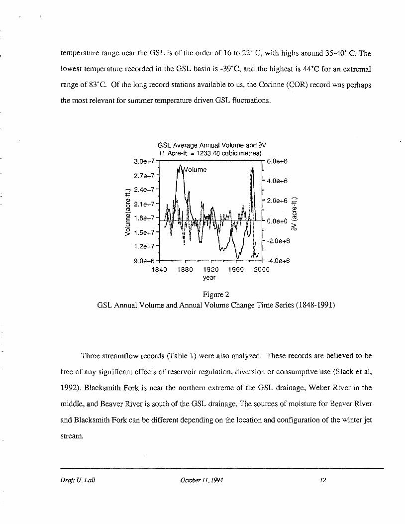
record (Figure 2) from 1848-1992 developed by Sangoyomi (1993) is used here. The variables

analyzed are the monthly and annual GSL average volume change. We choose the differenced

volume, rather than the volume itself, to allow an easier comparison with the precipitation,

temperature and streamflow records. While such differencing could introduce noise at frequencies

near the monthly sampling, it does not significantly alter the attributes of low frequency periodic

structure.

Monthly temperature and precipitation records (see Fan and Duffy, 1993) for five sites

(Silver Lake-Brighton (SLB), Corinne, Ogden, Riverdale, and Snake Creek) in the GSL drainage

were analyzed. Most of the precipitation in the GSL basin occurs in Winter/Spring. Precipitation

increases with elevation. SLB, the highest available long term precipitation station, is

approximately at the elevation of the 700 mb pressure surface. The SLB precipitation should be

well correlated with precipitation driven GSL fluctuations as well as larger scale atmospheric

fluctuations. Most of the GSL evaporation takes place in Summer/FalL The summer diurnal

Draft U. Lall October 11.1994 11

temperature range near the GSL is of the order of 16 to 22° C, with highs around 35-40· C. The

lowest temperature recorded in the GSL basin is -39°C, and the highest is 44°C for an extremal

range of 83°C. Of the long record stations available to us, the Corinne (COR) record was perhaps

the most relevant for summer temperature driven GSL fluctuations.

GSL Average Annual Volume and av (1 Acre-ft. = 1233.48 cubic metres)

3.0e+7 ..,..--------.....-----,- 6.0e+6

2.7e+7

--.:- 2.4e+7 ;;;= t5 2.1e+7 2.0e+6 ~ ~ ~ ~ 1.8e+7 J....S.IH4-~H-:-\l~~~~....;.;:4R.;.I_,1_ 16 :J O.Oe+O ;-

g 1.5e+7 t\',)

1.2e+7

9.0e+6 -t---r-,---.,..-,---,---,--......--t- -4.0e+6

1840 1880 1920 1960 2000 year

Figure 2 GSL Annual Volume and Annual Volume Change Time Series (1848-1991)

Three streamflow records (Table 1) were also analyzed. These records are believed to be

free of any significant effects of reservoir regulation, diversion or consumptive use (Slack et aI,

1992). Blacksmith Fork is near the northern extreme of the GSL drainage, Weber River in the

middle, and Beaver River is south of the GSL drainage. The sources of moisture for Beaver River

and Blacksmith Fork can be different depending on the location and configuration of the winter jet

stream.

Draft U. Lall October 11.1994 12

Willet and Prohaska (198S) speculate that three major circulation patterns influence the

weather iii the basin. These are: (1) a high latitude (SOON), moderate jet stream, corresponding to a

dry climate; (2) a lower latitude split jet stream, with a primary storm track that borders the

northern extreme of the OSL drainage, and a secondary storm track that borders the southern part

of the drainage; and (3) a cellular blocking pattern with large, alternating north and south strong

jets, and a breakdown of the westerly flow. The split jet stream is very active and corresponds to a

rapid rise of the GSL. The cellular blocking pattern leads to hot, dry summers and a falling GSL.

In their investigation of the relationship between North Pacific atmospheric circulation and

streamflow in the Western United States, Cayan and Peterson (1989) noted a strong association

(correlation=0,43) between positive Weber River streamflow anomalies and a positive Sea Level

Pressure (SLP) anomaly centered over N. Pacific and with a negative SLP anomaly locally. This

implies a southerly displaced storm track across the Eastern North Pacific and into the West with

increased activity from Canadian and Alaskan storms that dip in east of the Cascades. An

anomalous northeasterly to southeasterly flow with precipitation associated with a local trough

corresponds to this pattern. Enhanced winter precipitation is accompanied by positive minimum

daily temperature anomalies. Cayan and Peterson (1989) found a positive association between the

Southern Oscillation Index (SOl) (defined as the difference between normalized SLP anomalies

between Darwin and Tahiti), and two indices of pressure anomalies over the North Pacific - the

Pacific North American (PNA) Index (defined in terms of 700 mb height H, as PNA= H(170·W,

200 N)-H(16soW,45"N) +H(115"W,S8°N) -H(90·W,300N), and the Central North Pacific (CNP)

Index (defined as CNP = average SLP over 35" -SsoN and 1700E -IS00W). These indices reflect

characteristic pressure systems that determine atmospheric flow and hence precipitation in the OSL

area. The SOl has nearly periodic behavior (Keppenne and Ohil, 1992) with high (2-3 yr) and low

frequency (4-7 year) bands corresponding to ENSO, which is best understood as an internal self­

sustained equatorial oscillation in the coupled ocean-atmosphere system (see Philander, 1990).

Draft U. Lall October 11.1994 13

Streamflow relates to PNA and CNP which are measures of the strength of the winter Aleutian

Low (see also Barnston and van den Dool (1993) who identify the GSL area as one with a maxima

in interannual N. Hemisphere 700 mb height standard deviation). One should thus expect some

organized inter-annual variability at least in the ENSO band for the hydro-climatic variables in this

area.

Spectral Analysis Methods

The limited length of instrumental records, the sensitivity of the variable analyzed to local as

well as global factors, the intermittence of oscillatory patterns, and issues (see MP93) related to the

interpretation of space and time averaged data make the identification of a coherent long period

signal difficult. Spectral analysis methods tailored to the identification of coherent variability in

specific frequency bands where the underlying spectrum may have line (Le. sharp peaks

corresponding to periodic behavior) as well as broad band (due to stochastic, chaotic or nearly

periodic factors) features are needed.

We tested Windowed Periodograms, Maximum Entropy Spectral Estimates, SSA and

MTM, on a variety of synthetic data sets with these factors in mind. Of these, MTM and SSA were

the most successful in terms of the criteria listed above. Our goal here is to present evidence of low

frequency climatic variability, rather than a comparative evaluation of methods of spectral

estimation. We shall limit ourselves to a brief description of the relevant attributes of SSA and

MTM. We use SSA to identify anharmonic oscillations, and MTM for identification of peaks and

frequency band structure.

Singular Spectral Analysis(SSA):

An excellent exposition of SSA, complete with guidance for interpretation of results, tests

Draft U. Lall October 11, 1994 14

and properties is provided by Vautard et al (1992). Recall that the traditional periodogram

constructs the spectrum as a Fourier decomposition of the variance of the time series. This can be

done equivalently through appropriate Fourier transforms of the time series or the autocovariance

function. Likewise, the windowing or smoothing operation can be done in the frequency, time or

autocovariance domain. SSA is similar in that it operates on the autocovariance structure of the time

series. It differs in using data driven, empirical, orthogonal basis functions, rather than Fourier

(Le. sin or cos) basis functions for the decomposition. Ohil and Le Treut (1981), discuss and

model saw tooth shaped variations in the Quaternary climate record, that could be captured better

by SSA than the Fourier basis.

SSA considers the eigen decomposition (Principal Component Analysis - PCA) of the

autocorrelation matrix of a time series formed to some lag M. The resulting eigenvectors are the

basis functions. The corresponding eigenvalues indicate the fraction of overall variance explained

by an eigenvector, and projections of the time series on to the eigenvector provide a representation

of that component of the time series. Eigenvectors with the same shape and nearly equal

eigenvalues are called oscillatory pairs and jointly represent the amplitude and phase of a cyclic

pattern. SSA can potentially resolve signal and noise and works well in situations where there is a

distinct signal-noise separation. The data driven basis functions can potentially resolve the signal in

terms of a smaller set of basis functions than the Fourier basis. SSA can have problems

identifying underlying signals if a long memory stochastic process constitutes the noise, or if the

underlying signals have periods that are close, but long relative to reasonable choices of the

windowing parameter (lag M). Its strength is the recovery of dominant, arbitrarily shaped, data

adaptive recurrent patterns from a finite sample, and their corresponding time history. A

decomposition of the time series into orthogonal variance components, and their associated time

patterns is provided. Thus one can identify the timing and amplitude of oscillations, as well as the

nature of trends. The statistical machinery associated with PCA is readily invoked by SSA. A

Draft U. Lall October 11.1994 15

synopsis of the algorithm (based on Vautard et al (1992» for a scalar time series follows. While

some results are referenced in this section, they are formally discussed later.

1. Given a time series {xi' i=l,n},translated to have zero expectation, and rescaled to unit standard

deviation, form the Toeplitz matrix Tx. with element ~j=c(k), where k=li-jl, k=O ... M-1, and c(k) n-k

=(l/(n-k) ~>iXi+k is an estimate of the lag k covariance. Here the dimension of T x is M*M, and i=l

M has the role of a smoothing window. The longest period recoverable is thus M. Vautard et al

(1992) recommend M s: 0/3 for stability of the computed c(k). They also suggest that SSA is

successful in analyzing periods in the range (Ml5, M). The spectral resolution is 11M since the

frequencies that can be resolved are 1, 1/2, ... 11k, .. lIM. As M decreases, neighboring peaks in the

spectrum may coalesce, while as M increases, a peak may split into components at adjacent

frequencies (the Gibbs effect). Varying M over a coarse grid during the analysis is consequently

desirable to screen out spurious frequencies and to focus on signals in different frequency bands.

II. Now an eigen decomposition of T x yields a decomposition of the total variance into

components in a manner analogous to Fourier analysis.

(1)

where A is a diagonal matrix of eigenvalues (generally positive) sorted in descending order, and E

is a corresponding matrix of eigenvectors, such that ETE =1.

Each eigenvector ei of length M represents a data pattern, or empirical orthogonal basis

function. The corresponding eigenvalue Ai provides a measure of the variance associated with this

pattern. The leading eigenvectors consequently provide information on the dominant patterns in the

data. All eigenvalues for a white noise series are equal in expectation. A plot of Ai vs i, is termed

an SSA eigenspectrum (see Figure 3 for some of our data sets). Eigenvectors i and i+ 1 are termed

an oscillatory pair if Aj""Aj+ 1. and the coefficients el and el+ 1 exhibit a similar temporal pattern

for j=l...M. Preisendorfer (1988), p.247 reports that standard deviation aAj of Aj is asymptotically

Draft U. Lall October 11, 1994 16

A.i(2/n)1!2. Thus if (A.rA.i+1) is of the same size or smaller than OA.i' the eigenvalues may be

considered to be equal. One can think of this oscillatory pair (see Figure 4 for an example) as a sine

and cosine pair that carries the frequency and phase information. Energetic intermittent oscillations

with lifetime less than the window length can be identified through the eigencoefficient pattern.

A number of strategies for selecting the "statistically significant" eigenvectors for PCA are

described by Preisendorfer (1988). These are applicable here as well. GV, Vautard et al (1992) and

Allen and Smith (1994) review some of these techniques as well as Monte Carlo strategies for

testing for significance against white and red noise. For the results presented here, we considered

(a) only the first 8 eigenvectors in any case, (b) dropped eigenvectors if the corresponding

eigenvalue dropped below 11M, and (c) considered paired eigenvectors only as described above,

where the patterns were distinct, meaningful and similar. Finally, we satisfied ourselves that our

choices were conservative relative to those from the significance criteria against the white noise

hypothesis (using Rule N, described in Preisendorfer (1988), p.199-206, based on a Monte Carlo

Analysis of Gaussian data, with consideration of serial correlation). Coherent patterns that have

low contribution to the time series variance are thus missed. Our primary purpose for using SSA

was to identify prominent recurrent patterns and their time projection, with a view to comparing the

leading patterns in local precipitation, temperature and the OSL. Formal significance testing of

peaks was done as part of the MTM procedure.

Draft U. Lall October 11.1994 17

SSA Eigenvalues, m=25 0.12 -r--------.,....----------_

"0 0.10 (I) c '(6

~ 0.08 (I)

(I)

§ 0.06 ·c «l > '0 0&04 c o

~ 0.02 -

o weber flow 1915-88 • SLB Precip, 1916·89 a GSL eN 1848-1991, m=50

Corinne Temp 1902-89, m=30

:::::::::::::::::::::::::::::::::::::::::::::::~:::::::::::::~:::: .. :::."".--~-........ .~. d 0.00 -f---~----r---_-----'r---_----I

o 5 . Eigenvector

10 15

Figure 3 Eigenvalue Spectrum from SSA for Selected Sites.

The window length m =25 years unless noted otherwise.

The three horizontal lines (.02,.033,.04) correspond to the average eigenvalues for (WRO, SLB), COR-T, and GSL respectively. Only the first 15 eigenvectors are shown in each case. Note the near equality of some pairs of leading eigenvalues (especially GSL). Typically, these pairs correspond to eigenvectors that are periodic and in quadrature as shown in Figure, 4. Such a relation was not clear cut for COR-T, where the first 4 eigenvalues are nearly equal and only the flrst and fourth eigenvector look "similar".

Draft U. Lall October 11.1994 18

0.2 en ~ 0.1 '0 :;:: Q) 0.0 o (.) c: (J.) -0.1 OJ iii

-0.2

GSL Annual av (1848-1991) EOF's 1 & 2, m=50

-0.3 -I--.,......r--.,~--.--t-__ +-~i--r-+--.--i-__ +-.,......+--r--l

o 5 10 15 20 25 30 35 40 45 50 Lag

GSL Annual av (1848-1991) EOF's 3 & 4, m=50 0.3 -r-----,.----r------,.----r-----,

0.2

en C 0.1 (J.)

'0 ~ 0.0 o (.)

5.5-0.1 OJ iii

-0.2

-0.3 -I---r---f--r--I--r----t--r-...;--r---I

o 10 20 30 40 50 Lag

Figure 4 Eigenvectors 1-4 for annual GSL av

Each set is seen to form an oscillatory pair (near 11 years for 1-2, and near 15 years for 3-4).

Not all eigenvectors whose eigenvalues are nearly equal are so obviously in quadrature.

Draft U. Lail October 11. 1994 19

> rc

SSA Reconstruction of GSL av using 11 and 15 year cycles (1848-1991) m=50

6e+6~------------------------------------------~

2e+6

Oe+O

y -2e+6

-4e+6~~--~~--r-~-'--~~~~~----~~--r-~~

1840 1860 1880 1900 1920 1940 1960 1980 2000

Year

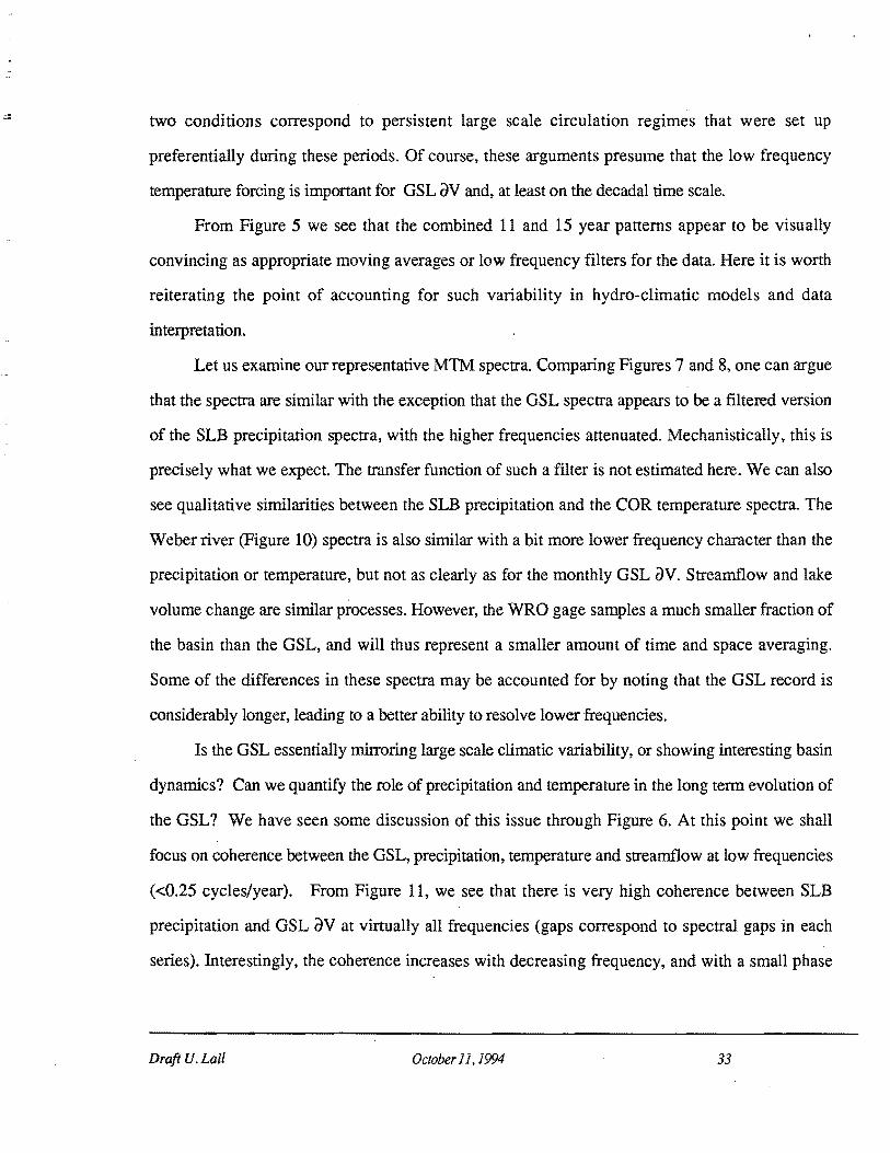
Figure 5 Reconstruction of annual GSL av time series using the 11 and 15 year cycles shown in Figure 4.

Nearly 40% of the variance is accounted for.

Draft U. Lall October 11.1994 22

~ 2.5 r::: 8. E 1.5

8 "C 0.5 (J)

U 2 -0.5 1i) r::: 8 -1.5 (J)

a:

15 year Reconstructed Component

i

I · · · -g -2.5 •••••••• SLB-P.RCl,2

COR-T, RCl,4

GSL, m=50, RC3-5 BFH, RCl,2

N

~ lU -3.5 ~ lU U5 -4.5 -tI--_-...--..... -.,........-\r--"'r-""I--r--r~__r-r_;

1900 1910 1920 1930 1940 1950 1960 1970 1980 1990

year

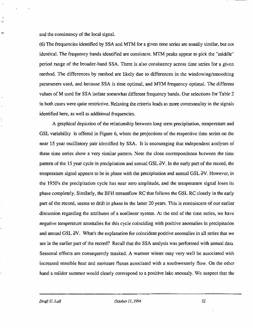
Figure 6 Comparison of 15 yr Reconstructed Component Pair (RCP) of annual GSL av, SLB-P, and

COR-To

To ease plotting, each RCP is standardized by removing its mean and dividing by its standard deviation. In each case, the full record described in Table I was used. Results are plotted only for the overlapping time period. Each RCP has an approximately 14-15 year period. Note how the GSL and precipitation (SLB-P) are nearly coherent throughout, while the temperature (COR-T) signal is nearly in phase with the other two to begin with and then drifts completely out of phase around 1950. The COR-T eigenvectors corresponding to this RCP were not as clearly periodic as the others, and this Rep may represent a mixture of two nearby interdecadal frequencies, resulting in a "frequency" drift. The streamflow BFH is also coherent with GSL and SLB-P. Evidence of a small phase shift between GSL and BFH in the 1960-1989 period is also evident. However, this drift may be due to the estimated periods being slightly different.

Draft U. Lall October 11. 1994 23

Multitaper Method of Spectral Analysis (MTM):

Thomson (1982) provides the following motivation for the MTM algorithm. He points out

that (a) the classical periodogram is an inconsistent estimator of the spectrum, (b) without a taper

window, it may be too biased to be useful, (c) usual tapers can reduce variance efficiency, (d)

smoothing the periodogram is unsatisfactory for spectra with large range and line and broadband

components, since the true spectrum is not smooth, and (e) since the periodogram based spectral

estimator does not directly use phase information, line detection is poor. He sets his sights on

developing an estimator (MTM) that (a) is consistent, (b) has good small sample performance in

terms of variance efficiency, (c) is data adaptive, (d) is nonparametric, i.e. locally approximates the

spectrum using information only from neighboring frequencies, (e) works well with spectra with a

high dynamic range, (f) is computationally easy, and (g) whose statistics can be estimated, and

hence significance tests for line components and coherence can be provided. We outline the aspects

of the MTM algorithm relevant to our presentation and refer the reader to Thomson (1982) and

Percival and Walden (1993), Chapter 7, for details.

The fmite discrete fourier transform (OFf) of the data, x(O), .x(t), .. x(n-l) is given by ,...1

y(f)= Le-i2l1f(Hn-1)f2)x(t) (4) t=0

For a finite data set, the DFf is related to the spectrum as: 1/2 • 1/2

y(f)= J sl~n1t(f -v) dZ(v) = J G(n,f,v)dZ(v) (5) -1{2 sm1t(f -v) -112

where the spectrum S(f) is defined through {Set) df = E[ldZ(f)12]}, where E[.] denotes

expectation.

Note that the periodogram estimate Sp(t) is simply ly(f)12, whose properties will not

correspond to those of Set), since the term G(n,f,v) in (5) poorly approximates a Dirac delta

function. This term is a consequence of a rectangular window of width n placed on the underlying

process. Given the estimate y(t), one can seek a solution for dZ(fo) in (5) in some locale (fo-W,

Draft U. Lall October 11,1994 24

fo+W) of a frequency fo' This is an inverse problem parameterized by G(n,f,v). Thomson pursues

a least squares solution, by considering a weighted eigenfunction expansion in this locale, and then

an appropriate combination of the resulting estimates. Consider the K term (k=O ... K-l)

eigenfunction expansion: w

1lA;(n,W),UA;(n,W;f)= J G(n,j,v)U(n,W;v)dv (6) -w

where Uk(n,W;f) is the kth eigenfunction centered at f, with window width W, and Ak(n,W) is the

corresponding eigenvalue.

The eigenfunctions (called discrete prolate spheroidal wave functions) are ordered by

decreasing eigenvalue, with the first nW eigenvalues close to 1. Consequently, of all functions that

are DFT's of some discrete sequence, these leading eigenfunctions have a maximum energy

concentration in the interval (fo-W, fo+W). This implies that the tapers are leakage resistant. The

window width W is O<W<l/2, and is usually of order liN to retain high resolution of the resulting

estimate. The idea here is that if the K term approximation in (6) is "good", then a good solution to

the estimation of S(f) is available. Thomson derives such a solution by first considering K spectral

estimates corresponding to each of the eigenfunctions and then combining them using an optimality

criteria derived from estimates of the mean square error of estimate of the spectrum in the locale of

interest. The K eigenspectra Sk(f), k==O, ... K-l, are defined through:

YA;(f)= I,X(t) vt,A;(n,W) e-i21f/(I-(II-I)/2)

t=O E;; (7)

Sk(f) = IYk(f)12 (8)

where Ek is 1 for k even, and i for k odd; and vt,k(n,W), the kth discrete prolate spheroidal

sequence (DPSS) is defined such that its Fourier transform gives Uk(n,W;f-fo)'

The MTM estimate is obtained as:

Draft U. Lall October 11.1994 25

K-l

SMCf)= LWk (f)Sk Cf) (9) k=O

and wkCt) is a weight associated with the kth eigenspectrum estimate at frequency f.

The windows Uk(') are positive everywhere, and hence the problem of getting negative

estimates of S(f) resulting from traditional higher order spectral windows is averted. The combined

estimate from K orthogonal tapers also circumvents the loss of resolution and variance efficiency

problems endemic to periodograms smoothed with a single taper. The orthogonality of the

eigenfunctions leads the Sk to be approximately uncorrelated. MTM recovers information lost by

using a single taper and by ignoring the phase information in the periodogram. A number of

strategies for choosing the weights wk(f) at each frequency f are indicated by Thomson. These

range from a simple average, to weights proportional to the eigenvalues Ak, to a fully data adaptive

and recursive procedure that internally estimates the bias and variance of the local estimate. We

used the last two strategies in our work. The latter allows improved separation of the line and

broad band spectral components. We refer the reader to Thomson for details of the DPSS and the

wk' and discuss the choice of W and K, the user selected parameters of the model.

The half bandwidth W is usually specified in terms of the Rayleigh frequency fR = (ru1tr 1,

where At is the sampling frequency, as pfR' where p is usually a small integer. The corresponding

DPSS is called a p1t taper. The corresponding spectral estimate averages in the frequency band

f±pfR' For example, a 21t taper, for a 100 year annual data set would average over f±0.02

cycles/year. Note that this would correspond to periods of 1.92 to 2.08 years for a band centered at

f=0.5, and 14.28 to 33.33 years for a band centered at f=0.05. We see from this example that it is

desirable to use a small value of p to get higher resolution in the low frequency range. On the other

hand a small value of p can lead to peak splitting in the high frequency range. Comparing estimates

obtained by varying p over a small range is consequently desirable. As K increases, the variance of

Draft U. Lall October 11,1994 26

SM decreases, however, the broad band bias can increase. SM is distributed as X22K' rather than

as X22 for the periodogram, and the increased degrees of freedom correspond to reduced variance.

The first (2p-1) tapers are leakage resistant, so K is usually taken to be 2p-1. As p increases, the

number of leakage resistant tapers increases. Note that, as n increases, one can increase p while

retaining the same spectral resolution. The estimate SM(f) is unbiased, but its local features

(amplitude) will depend on p and K. Consequently, it is desirable to also look at a significance test

for line components based on the ratio of variance explained by a peak at fo to unexplained

variance in a band centered at fo'

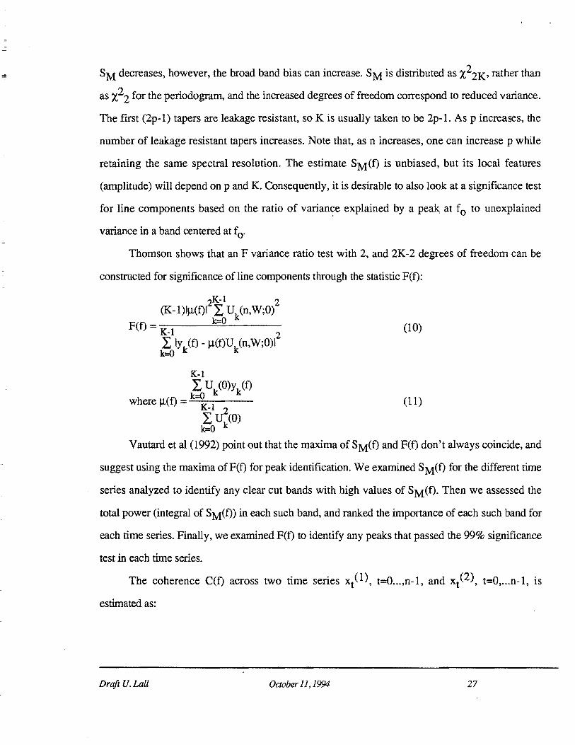
Thomson shows that an F variance ratio test with 2, and 2K-2 degrees of freedom can be

constructed for significance of line components through the statistic F(f):

K-l l: Uk(O)Yk(f)

where !l(f) = .;;.;..k=O"';;K-_-l---

l: U~(O) k=O

(10)

(11)

Vautard et al (1992) point out that the maxima of SM(f) and F(f) don't always coincide, and

suggest using the maxima ofF(f) for peak identification. We examined SM(f) for the different time

series analyzed to identify any clear cut bands with high values of SM(f). Then we assessed the

total power (integral of SM(f) in each such band, and ranked the importance of each such band for

each time series. Finally, we examined F(f) to identify any peaks that passed the 99% significance

test in each time series.

The coherence C(f) across two time series xt (1), t=0 ... ,n-1, and xt (2), t=0, ... n-1, is

estimated as:

Draft U. Lall October 11, 1994 27

11 y~I)* (t)y~2\t) C(t) = k=O

(11 y~I)* (t)y~I)(t)~1 /2)* (t)/2\t) Ifl k=O J=O J J

(12)

where * represents a complex conjugate.

A confidence test (see Brillinger (1981» similar to the F variance ratio test is used to test for

the significance of the coherence amplitude.

Our experience with synthetic data suggested that the MTM procedures were very reliable

and were not as sensitive to signal to noise ratio, or to the memory in the broadband noise process

as SSA or MESA or periodogram estimates. We did not see a need to prefilter the data via SSA and

then apply MTM, as done by Vautard et al (1992). The reader may have noted that SSA uses an

eigenexpansion of the autocovariance function, while MTM does something similar in the

frequency domain. Consequently, SSA may be more useful for showing time patterns. MTM is

generally superior for identifying phase coherent frequency structure. One could subject the SSA

RC's to frequency analysis by MTM, or use the MTM estimates in the frequency domain to

bandpass the time series at desired frequencies. We prefer to examine the SSA time optimal

decompositions and the MTM frequency optimal decomposition independently and seek

consistency across the analyses. Confirmation of "patterns" by independent analyses by different

methods and across data sets is in our view more valuable than statistical confidence limits for a

single analysis of a particular data set. A comparative discussion of the two methods is offered by

Thomson (1982) and Vautard et al (1992).

Draft U. Lall October 11.1994 28

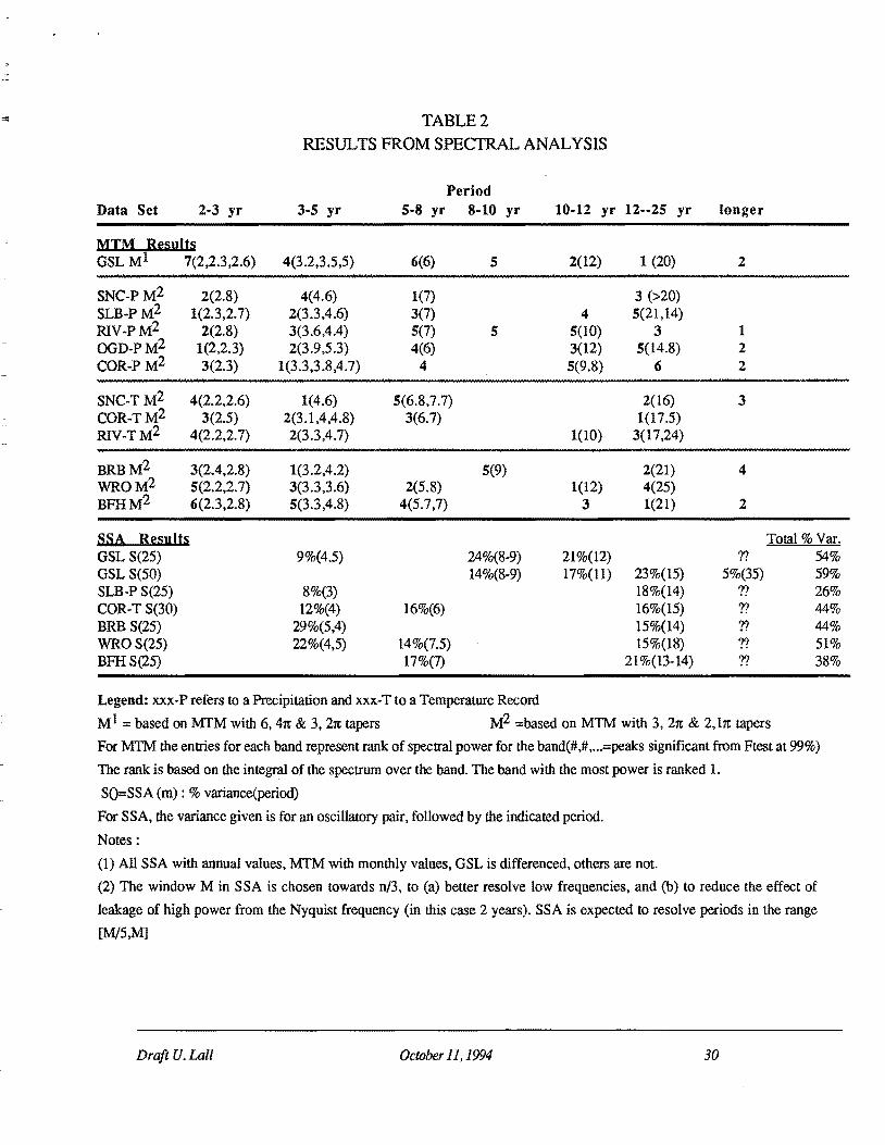
Spectral Analysis Results

For brevity we shall focus on the main points through an examination of some key spectra,

and through the summary of the individual time series analyses presented in Table 2. After a

preliminary screening of the spectral output, it was clear that one could designate bands in which

there was power. The bands are larger in the time domain near the lower frequencies recognizing

the increasing effect of the fixed averaging window in frequency space. The approximate spectral

power in each band was ranked for each time series, and any spectral peak in that band that met the

F variance ratio test for significance at the 0.99 level, for MTM was also r~corded. For a confident

interpretation of a periodic signal, it is desirable to have sizeable power as well as a significant F­

test. Features that are resistant to the indicated variations in MTM parameters are reported in Table

2. We summarize results for the GSL, all precipitation series, all temperature series and then all

streamflow series. In each subset, sites are arranged from South to North. The SSA results report

the fractional variance explained by the oscillatory pairs of eigenvectors and the corresponding

period of the variation. Only the readily interpretable eigenvectors, with dominant eigenvalues are

used. The last column for the SSA results gives the total variance explained by the selected

eigenvectors.

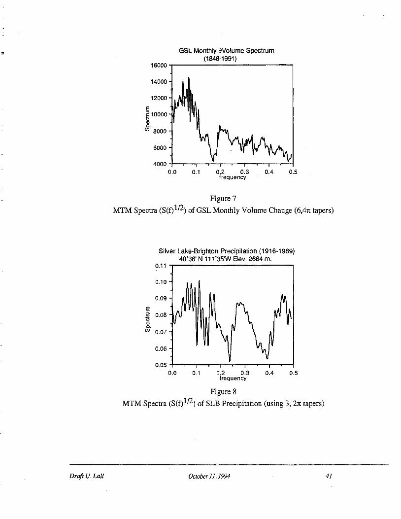
Representative MTM spectra for each hydro-climatic process are presented in Figures 7

through 10. MTM estimates of coherence across selected time series are presented in Figures 11

through 13.

Draft U. Lall October 11,1994 29

Data Set 2·3 yr

MTM B~~nll~ GSLMI 7(2,2.3,2.6)

SNC-P M2 2(2.8) SLB-PM2 1(2.3,2.7) RIV.PM2 2(2.8) OGD-PM2 1(2,2.3) COR-PM2 3(2.3)

SNC-T M2 4(2.2,2.6) COR-TM2 3(2.5) RIV-TM2 4(2.2,2.7)

BRBM2 3(2.4,2.8) WROM2 5(2.2,2.7) BFHM2 6(2.3,2.8)

SSA Resnlts GSL S(25) GSL S(50) SLB-P S(25) COR-T S(30) BRB S(25) WROS(25) BFHS(25)

TABLE 2

RESULTS FROM SPECfRAL ANALYSIS

3·5 yr

4(3.2,3.5,5)

4(4.6) 2(3.3,4.6) 3(3.6,4.4) 2(3.9,5.3)

1(3.3,3.8,4.7)

1(4.6) 2(3.1,4,4.8) 2(3.3,4.7)

1(3.2,4.2) 3(3.3,3.6) 5(3.3,4.8)

9%(4.5)

8%(3) 12%(4)

29%(5,4) 22%(4,5)

Period 5·8 yr 8-10 yr

6(6)

1(7) 3(7) 5(7) 4(6)

4

5(6.8,7.7) 3(6.7)

2(5.8) 4(5.7,7)

16%(6)

14%(7.5) 17%(7)

5

5

5(9)

24%(8-9) 14%(8-9)

10·12 yr 12--25 yr longer

2(12)

4 5(10) 3(12) 5(9.8)

1(10)

1(12) 3

21%(12) 17%(11)

1 (20)

3 (>20) 5(21,14)

3 5(14.8)

6

2(16) 1(17.5)

3(17,24)

2(21) 4(25) 1(21)

23%(15) 18%(14) 16%(15) 15%(14) 15%(18)

21%(13-14)

2

1 2 2

3

4

2

n 5%(35)

n n n n n

Legend: xxx-P refers to a Precipitation and xxx-T to a Temperature Record

Total % Var. 54% 59% 26% 44% 44% 51% 38%

M 1 = based on MTM with 6, 41t & 3, 21t tapers M2 =based on MTM with 3, 21t & 2,11t tapers

For MTM the entries for each band represent rank of spectral power for the band(#,#, ... =peaks significant from Ftest at 99%)

The rank is based on the integral of the spectrum over the band. The band with the most power is ranked 1.

SO=SSA (m) : % variance(period)

For SSA, the variance given is for an oscillatory pair, followed by the indicated period.

Notes:

(1) All SSA with annual values, MTM with monthly values, GSL is differenced, others are not.

(2) The window M in SSA is chosen towards n/3, to (a) better resolve low frequencies, and (b) to reduce the effect of

leakage of high power from the Nyquist frequency (in this case 2 years). SSA is expected to resolve periods in the range

[M/5,M]

Draft U. Lall October 11.1994 30

We offer the following observations:

(1) There is significant power in these series at selected bands. There are also clear gaps in the

spectrum at some frequency bands (e.g., 8-10 years). Such features are generally consistent across

sites for the same type of series, in particular for sites at similar elevation and latitude.

(2) Coherent cyclic activity with periods around 2.2, 2.6, 2.8, 3.3, 3.6, 3.9, 4.5, 5, 6, 7, 10, 14,

17, and 21 years shows up in the MTM analysis of virtually all the series. These cycles are

consistent with the summary presented in our motivational section. These frequencies are best

interpreted as representing activity in the bands shown in Table 2. Support for the 14-15 year

cycle, and the lower frequency end of the ENSO band also comes from the SSA analysis of each

time series. We report fewer cycles from SSA because we were rather deliberate about excluding

eigenvectors with low variance even if they showed coherent patterns.

(3) A small set of low frequency recurrent patterns explains a relatively large fraction of the

observed variability for some time series. As an example, see figure 5 for a reconstruction of the

GSL series using only the 11 and 15 year cycles that account for 40% of the variance in the series.

It is worth noting that significant modes of spatio-temporal variance in global surface temperature

are observed on each of these time scales in MP94. GV report 15 and 20 year cycles in global

average temperature, while MP94 identify a broader-band 16-20 year oscillation in gridded surface

temperature records.

(4) The relative amplitude of these cycles varies across the series, with the GSL series favoring the

lower frequencies as expected. A closer examination of these series (e.g., Figure 6) reveals that the

amplitude of each cycle is variable over each record as well.

(5) The MTM spectra for precipitation and temperature data from Corinne, Ogden and Riverdale

(only Corinne is shown here) are very similar, reflecting the proximity of these sites to each other,

Draft U. Lall October 11.1994 31

and the consistency of the local signal.

(6) The frequencies identified by SSA and MTM for a given time series are usually similar, but not

identical. The frequency bands identified are consistent. MTM peaks appear to pick the "middle"

period range of the broader-band SSA. There is also consistency across time series for a given

method. The differences by method are likely due to differences in the windowing/smoothing

parameters used, and because SSA is time optimal, and MTM frequency optimal. The different

values ofM used for SSA isolate somewhat different frequency bands. Our selections for Table 2

in both cases were quite restrictive. Relaxing the criteria leads to more commonality in the signals

identified here, as well as additional frequencies.

A graphical depiction of the relationship between long term precipitation, temperature and

GSL variability is offered in Figure 6, where the projections of the respective time series on the

near 15 year oscillatory pair identified by SSA. It is encouraging that independent analyses of

these time series show a very similar pattern. Note the close correspondence between the time

pattern of the 15 year cycle in precipitation and annual GSL avo In the early part of the record, the

temperature signal appears to be in phase with the precipitation and annual GSL avo However, in

the 1950's the precipitation cycle has near zero amplitude, and the temperature signal loses its

phase completely. Similarly, the BFH streamflow RC that follows the GSL RC closely in the early

part of the record, seems to drift in phase in the latter 20 years. This is reminiscent of our earlier

discussion regarding the attributes of a nonlinear system. At the end of the time series, we have

negative temperature anomalies for this cycle coinciding with positive anomalies in precipitation

and annual GSL avo What's the explanation for coincident positive anomalies in all series that we

see in the earlier part of the record? Recall that the SSA analysis was performed with annual data.

Seasonal effects are consequently masked. A warmer winter may very well be associated with

increased sensible heat and moisture fluxes associated with a southwesterly flow. On the other

hand a milder summer would clearly correspond to a positive lake anomaly. We suspect that the

Draft U. Lall October 11, 1994 32

two conditions correspond to persistent large scale circulation regimes that were set up

preferentially during these periods. Of course, these arguments presume that the low frequency

temperature forcing is important for GSL av and, at least on the decadal time scale.

From Figure 5 we see that the combined 11 and 15 year patterns appear to be visually

convincing as appropriate moving averages or low frequency filters for the data. Here it is worth

reiterating the point of accounting for such variability in hydro-climatic models and data

interpretation.

Let us examine our representative MTM spectra. Comparing Figures 7 and 8, one can argue

that the spectra are similar with the exception that the GSL spectra appears to be a filtered version

of the SLB precipitation spectra, with the higher frequencies attenuated. Mechanistically, this is

precisely what we expect. The transfer function of such a filter is not estimated here. We can also

see qualitative similarities between the SLB precipitation and the COR temperature spectra. The

Weber river (Figure 10) spectra is also similar with a bit more lower frequency character than the

precipitation or temperature, but not as clearly as for the monthly GSL avo Streamflow and lake

volume change are similar processes. However, the WRO gage samples a much smaller fraction of

the basin than the GSL, and will thus represent a smaller amount of time and space averaging.

Some of the differences in these spectra may be accounted for by noting that the GSL record is

considerably longer, leading to a better ability to resolve lower frequencies.

Is the GSL essentially mirroring large scale climatic variability, or showing interesting basin

dynamics? Can we quantify the role of precipitation and temperature in the long term evolution of

the GSL? We have seen some discussion of this issue through Figure 6. At this point we shall

focus on coherence between the GSL, precipitation, temperature and streamflow at low frequencies

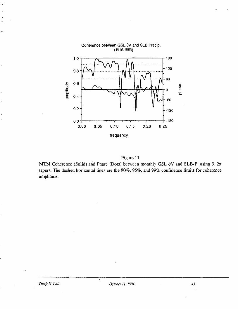
«0.25 cycles/year), From Figure 11, we see that there is very high coherence between SLB

precipitation and GSL av at virtually all frequencies (gaps correspond to spectral gaps in each

series), Interestingly, the coherence increases with decreasing frequency, and with a small phase

Draft U. Lall October 11.1994 33

lag. This suggests that low frequency precipitation variability largely drives the GSL. From Figure

12, we observe that coherence between COR temperature and monthly GSL av is high for three

frequency bands ( >40 years or secular, "" 10 years or decadal, =5 years or interannual). It is worth

noting that these are precisely the three low frequency bands where consistent climate signals

impacting on the U.S are noted through a spatiotemporal analysis of global surface temperatures

and North American surface Sea Level Pressures (Mann et al, 1994). Temperature is nearly 1800

out of phase with the GSL aV. Recall that the COR-T MTM spectra does not show much power at

the 10 year period. A weak (in terms of variance) 10 year pattern in temperature nevertheless

appears to be coherent with the 10 year GSL variability. From Table 2, we see that the COR-P

precipitation does show a peak (that passes the F-test) near 10 years in the MTM spectra. The

story is confirmed in Figure 13, where COR-T and SLB-P show a similar relationship to COR-T

and monthly GSL avo Given the analyses of global and U.S. data reported in Mann et al (1994),

and the results in Table 2, and Figures 11 through 13, we believe that the lake is largely

precipitation driven, with temperature forcing important at a few selected frequencies. The

temperature signals are consistent with the precipitation signals. A consistent climatic signal driving

the long term evolution of the GSL is thus apparent.

A better understanding of the mechanisms responsible for this low frequency climate

variability is important for improved management of regional, anomalous wet periods and

droughts, and the rise and fall of the GSL. Work on linking these analyses with analyses of large

scale atmospheric circulation is reported in Mann et al (1994). Explanations for the apparent phase

lag at low frequencies between temperature, precipitation and GSL (figures 12,13) are developed

in Mann et al (1994) in terms of the large scale circulation. However, it is clear that the near O·

phase lag between SLB-P and monthly GSL av, together with statistically significant coherence at

some frequencies is consistent with precipitative forcing of the GSL. Likewise, a 180· phase and

significant coherence between monthly GSL av and COR-T at certain frequencies may imply

Draft U. Lall October 11, 1994 34

temperature forcing of GSL evaporation. The relationship with precipitation is present over a much

larger fraction of the frequency range than the one between temperature and the GSL. Precipitative

forcing may consequently account for far more of the low frequency variability, and some of this

variability appears to have periodic or quasiperiodic structure

Closure

We find consistent evidence for structured low frequency variability from an analysis of a

number of hydro-climatic time series in the Great Salt Lake basin. The implications of such a

finding were stressed earlier. Given the richness of the behavior seen, it is hard to accept simple

explanations of external forcing at 11 and 18.6 year periods corresponding to the sunspot or lunar

tide cycles, as advanced by some researchers (e.g., Willet and Prohaska, and Currie and O'Brien).

The climatic behavior observed seems more consistent with the signature of a nonlinear

dynamical system as discussed earlier - general broadband structure, with preferred frequency

bands; with a variety of harmonics with power in a finite record; with lower frequencies being

more important; with phase degeneracy of some signals; with amplitude of the harmonic variable

dependant on position in the cycle; and the hint of persistent low frequency regimes marked by

different joint characteristics of precipitation and temperature. Of course, this is a speculative

argument, and in this manuscript we report no evidence of formal tests of nonlinearity (e.g., higher

order spectra, or dimensionality or predictability). However, such evidence is forthcoming in

Sangoyomi and Lall (1993) for the GSL time series.

The suggestion that low frequency behavior accounts for a large part of the GSL variability

and that this low frequency signature is closely coupled to precipitation and temperature variability

is also interesting. Recall that SLB, our index precipitation station is a high elevation station, and is

believed to be minimally affected by local factors such as lake effect precipitation. The high

Draft U. Lall October 11. 1994 35

coherence between SLB-P and GSL av at interannual and interdecadal periods has directed our

efforts into seeking an understanding of the large scale atmospheric circulation and its relation to

low frequency local precipitation and temperature variability (see Mann et al (1994)). Preliminary

analyses suggest strong coherence between decadal and secular variations in spatial pressure and

temperature fields and the GSL. This gives us hope that we can develop a cogent explanation for

long term GSL variability in terms of recurrent atmospheric circulation described regimes.

Mechanistic investigations to develop a physical explanation for the observed low frequency

hydroclimatic variability should be fruitful, and are being pursued.

Draft U. Lall October 11. 1994 36

ACKNOWLEDGEMENTS

We thank Barry Saltzman and David Tarboton for helpful comments regarding the

manuscript. U. Lall is grateful for support under NSF Grant # EAR-9205727 and USGS Grant #

1434-92-G-226, and to BSA, USGS, Reston, V A, for partial support of his sabbatical leave. M.

Mann was supported by NASA grant NAG5-2316.

REFERENCES

Abarbanel, H.D.I., M. I. Rabinovich and M. M. Sushchik, (1993). " Introduction to Nonlinear

Dynamics for Physicists", World Scientific.

Brillinger, D. R. (1981). "Time Series, Data Analysis and Theory" Holden-Day.

Burroughs, W. J., (1992) "Weather Cycles: Real or Imaginary?" Cambridge University Press, 201 pgs.

Cay an, D. R. and D. H. Peterson, (1989) "The Influence of North Pacific Atmospheric Circulation on Streamflow in the West. Aspects of Climate Variability in the Pacific and the Western Americas,"

Amer. Geophys. Union Geophys. Monogr. No. 55, pp. 375-397.

Cayan, D. and R. Webb, (1992), "EI Nino/Southern Oscillation and Streamflow in the Western United

States" in EI Nino: historical and paleoclimatic aspects of the Southern Oscillation, edited by H. F.

Diaz, and V. Markgraf. Cambridge University Press.pp. 29-68.

Currie, R. G., and D. P. O'Brien, (1992), "Deterministic Signals in USA Precipitation Records Part

II.", International Journal of Climatology, 12, pp. 181-304

Dettinger, M. D., and M. Ghi!, (1991) "Interannual and interdecadal Variability of Surface-Air

Temperatures in the United States", in Proc. XVIth Annual Climate Diagnostics Workshop, U.S. Department of Commerce, NOAA, Los Angeles, CA pp.209-214.

Diaz, H.F., and R.S. Pulwarty, (1994), "An Analysis of the Time Scales of Variability in Centuries-

Draft V.Lall October 11. 1994 37

Long ENSO-Sensitive Records in the Last 100 Years", Climate Change, 26, pp. 317-342.

Fan, Y. and C.J. Duffy, (1993), "Monthly temperature and precipitation fields on a storm-facing mountain front: Statistical structure and empirical parameterization", Water Resources Research, 29(12) pp. 4157-4166.

Ghil, M. and H. Le Treut, (1981), "Climate Model with Cryodynamics and Geodynamics", J. Geophys. Res., 86, pp. 5262-5670.

Ghil, M. and R. Vautard, (1991), "Interdecadal Oscillations and the Warming Trend in Global Temperature Time Series," Nature 350, pp. 324-327.

Ghil M., M. Kimoto, and J. D. Neelin, (1992), "Nonlinear Dynamics and Predictability in the Atmospheric Sciences", Rev. Geophys.

Guetter, A. K., and K. P. Georgakokas, (1993). "River Outflow of the Conterminous United States, 1939-1988. Bulletin of the American Meteorological Society, 74, pp. 1873-1891.

Houghton, R. W., and Y. M. Tourre, (1992) "Characteristics of Low-Frequency Sea Surface Temperature Fluctuations in the Tropical Atlantic." Journal of Climate, V.5(7), pp. 765-771.

Jin, F-F., J. D. Neelin, M. Ghil, (1994), tiEl Nino on the Devil's Staircase: Annual Subharmonic Steps to Chaos", Science, 264, #5155, pp. 70-72.

Kahya, E., and J. A. Dracup, (1993) "U.S. Streamflow Patterns in Relation to the EI Nino/Southern Oscillation," Water Resources Research 29(8), pp. 2491-2503.

Keppenne, C.L., and M. Ghil, (1992) ... Adaptive filtering and prediction of the Southern Oscillation index." 1. Geophys. Res., 97, pp. 20449--20454.

Lall U., T. Sangoyomi and H. D. I. Abarbanel (1994), "Nonlinear Dynamics of the Great Salt Lake: Nonparametric Short Term Forecasting" submitted to Water Resources Research.

Levitus, S. (1989), "Interpentatal Variability of Temperature and Salinity at Intermediate Depths of the North Atlantic Ocean, 1970-74 versus 1955-59". J. Geophys Res. 94. pp. 6091-6131.

Lorenz, E. N., (1976), "Nondeterministic Theories of Climatic Change," Quart. Res., 6 pp. 496-506.

Draft U. Lall October 11. 1994 38

MacDonald,G. I. , (1989), "Spectral Analysis of Time Series Generated by Nonlinear Processes", Rev. Geophys., 27, pp. 449-469.

Mann, M. E., and J. Park, (1993). "Spatial Correlations of Interdecadal Variation in Global Surface Temperatures", Geophys. Res. Lett., 20, 1055-1058.

Mann, M.E. and I.,Park (1994). "Global modes of surface temperature variability on interannual to century time scales." J. Geophys. Res., in press.

Mann, M.E., U. Lall and B. Saltzman, (1994), "Decadal and Secular Climate Variability: Understanding the Rise and Fall of the Great Salt Lake", submitted to Nature.

Palmer, T. N., (1993), "Extended-Range Atmospheric Prediction and the Lorenz Model," Bulletin of the American Meteorological Society., VoL 74, (1) pp. 49-65.

Philander, S.G., (1990), "EI Nino, La Nina and the Southern Oscillation", Academic Press.

Preisendorfer,R. W. (1988) "Principal Component Analysis in Meteorology and Oceanography", Elsevier Science Publishers, New York. 401 pgs.

Ropelewski, C. E, and M. S. Halpert, (1987), "Global and Regional Scale Precipitation Patterns Associated with the EI Nino/Southern Oscillation. Monthly Weather Review. 115, pp. 1606-1626.

Saltzman, B., (1983). "Climatic Systems Analysis." Advances in Geophysics 25, pp. 173-233.

Sangoyomi, T. and U. Lall, (1993), "Nonlinear Dynamics of the Great Salt Lake: Insights from the 1848-1992 Time Series." UWRL Report RR-93-HWR-UL/002.

Sangoyomi, Taiye B., (1993), "Climatic Variability and Dynamics of Great Salt Lake Hydrology," Ph.D. dissertation Utah State University, Logan, Utah, 247 pgs.

Slack, I.R., I. M. Landwehr and A. Lumb, (1992), !lA. U.S. Geological Survey Streamflow Data Set for the United States for the Study of Climate Variations, 1874-1988, U.S.G.S. Open File Report, 92-129, 1992.

Allen, M. R., and L. A. Smith (1994) "Investigating the Origins and Significance of Low-Frequency

Draft U. Lall October 11. 1994 39

Modes of Climate Variability." Geophysical Research Letters, Vol 21, No. 10. pgs 883-886.

Thomson, D. J., (1982) "Spectrum Estimation and Harmonic Analysis." IEEE Proceedings, 70, pp. 1055-1096.

Trenberth, K. E. (1990), "Recent Observed Interdecadal Climate Changes in the Northern Hemisphere." Bulletin of the American Meteorological Society, 71, pp. 988-993.

Vautard R., P. Yiou and M. GhU, (1992), "Singular Spectrum Analysis: A Toolkit for Short, Noisy and Chaotic Series." Physica D, 58, pp. 95-126.

Draft U. Lall October 11. 1994 40

Draft U. Lall

GSl Monthly aVolume Spectrum (184&1991)

16000...,....-------------""'"1

14000

12000

E .E 10000

~ en 8000

6000

4000~~-~~_r~--~~_.r_~~

0.0 0.1 0.2 0.3 0.4 0.5 frequency

Figure 7

MTM Spectra (S(f) 1/2) of GSL Monthly Volume Change (6,41t tapers)

E

Silver lake-Brighton Precipitation (1916-1989) 40·36' N 111·3S'W Elev. 2664 m.

0.11 -r-------------""'"I 0.10

0.09

2 0.08 g 0.. en 0.07

0.06

0.05 +-~......,r__........___r"~-.,..__...____,r__...__-I 0.0 0.1 0.2 0.3 0.4 0.5

frequency

Figure 8

MTM Spectra (S(f)l/2) of SLB Precipitation (using 3, 21t tapers)

October 11.1994 41

Draft U. Lall

E 2 t> Ql Q. 1/1

Corinne UT Temperature (1902-1989) 41°33'N 112'OTW Elev. 1289 m.

0.4 -r-------------_

0.3

0.2

0.1

0.0 +-__ ---,r---y-__r_---.-..,.-__r_--.-.,..--!

0.0 0.1 0.2 0.3 0.4 0.5 frequency

Figure 9

MTM Spectra (S(f)l/2) of COR Temperature (using 3, 21t tapers)

E ::l .... t> Ql Q. (/I

14

12

10

8

6

4

2 0.0

Weber River nr Oakley (1915-88) 40· 44'N 111 0 15'W Elev. 2012 m.

0.1 0.2 0.3 0.4 frequency

Figure 10

0.5

MTM Spectra (S(f)1/2) of WRO (3, 21t tapers)

October 11.1994 42

Q)

"C ::::I .-= 0.. E co

Coherence between GSL av and SLB Precip. (1916-1989)

1.0 .....---~-------------r 180

0.8 120

60 0.6

0

0.4 -60

0.2 -120

0.0 -180 0.00 0.05 0.10 0.15 0.20 0.25

frequency

Figure 11

Q) (/)

co ..c: c.

MTM Coherence (Solid) and Phase (Dots) between monthly GSL av and SLB-P. using 3, 21t tapers. The dashed horizontal lines are the 90%, 95%, and 99% confidence limits for coherence amplitude.

Draft U. Lall October 11,1994 43

Q) "C :::J

.t:: 'B. E «I

Coherence between Corinne Temperature & GSL av (1902-1989)

1.0 180

0.8 120

60 0.6

0

0.4 -60

0.2 -120

0.0 -180 0.00 0.05 0.10 0.15 0.20 0.25

frequency

Figure 12

Q) (I) «I

.r::::. c.

MTM Coherence (Solid) and Phase (Dots) between GSLdV and COR-To using 3, 21t tapers. The dashed horizontal lines are the 90%, 95%, and 99% confidence limits for coherence amplitude. Note that phase lags of 1800 and -1800 are the same, and switching between them may not be significant. The phase difference at 0.01< f<0.05 has temperature leading GSL.

Draft U. Lall October 11.1994 44

Q) "0 ::I =: 0.. E a:s

1.0

0.8

0.6

0.4

0.2

Coherence between SLB-Precip. & COR-Temp. (1916-1989)

~ ., ...... ~ .. • t-c\/! : --,---.-! -~.-.'- ----··1-! i Ii • -·--i-- _.- ........ _--t.:.\:

: : § ~ .... _ •• -.- . -to.,.. .... _- c··· .. ·.. ·· ...... -i.;

1 ~il ~ I 1\

180

120

60

0

-60

-120

o. 0 -I---r--.-'.:....!..,r----.--,.....a~-..,......!:........,...---1rrr___+_ -180

0.00 0.05 0.10 0.15 0.20 0.25

frequency

Figure 13

Q) en a:s

.s:::. a.

MTM Coherence (Solid) and Phase (Dots) between SLB-P and COR-T, using 3, 21t tapers. The dashed horizontal lines are the 90%, 95%, and 99% confidence limits for coherence

amplitude.

Note that phase lags of 180· and -180· are the same, and switching between them may not be significant. The phase difference at 0.01< f<0.05 has temperature leading SLB-P, as was the case with GSL.

Draft U. Lall OClober 11.1994 45