The great observatories origins deep survey. VLT/VIMOS spectroscopy in the GOODS-south field
18
A&A 494, 443–460 (2009) DOI: 10.1051/0004-6361:200809617 c ESO 2009 Astronomy & Astrophysics The great observatories origins deep survey VLT/VIMOS spectroscopy in the GOODS-south field P. Popesso 1 , M. Dickinson 4 , M. Nonino 3 , E. Vanzella 2,3 , E. Daddi 8 , R. A. E. Fosbury 5 , H. Kuntschner 5 , V. Mainieri 7 , S. Cristiani 3 , C. Cesarsky 7 , M. Giavalisco 6 , A. Renzini 2 , and the GOODS Team 1 Max-Planck-Institut fur extraterrestrische Physik„ Giessenbachstrasse 2, 85748 Garching, Germany e-mail: [email protected] 2 Dipartimento di Astronomia dell’Università di Padova, Vicolo dell’Osservatorio 2, 35122 Padova, Italy 3 INAF – Osservatorio Astronomico di Trieste, Via G.B. Tiepolo 11, 40131 Trieste, Italy 4 National Optical Astronomy Obs., PO Box 26732, Tucson, AZ 85726, USA 5 ST-ECF, Karl-Schwarzschild Str. 2, 85748 Garching, Germany 6 Space Telescope Science Institute, 3700 San Martin Drive, Baltimore, MD 21218, USA 7 European Southern Observatory, Karl-Schwarzschild-Strasse 2, Garching, 85748, Germany 8 Université Paris-Sud 11, 15 rue Georges Clemenceau, 91405 Orsay, France Received 20 February 2008 / Accepted 14 November 2008 ABSTRACT Aims. We present the first results from the VIsible Multiobject Spectrograph (VIMOS) ESO/GOODS program of spectroscopy for faint galaxies in the Chandra Deep Field South (CDF-S). This program complements the FORS2 ESO/GOODS campaign. Methods. All 3312 spectra were obtained in service mode with VIMOS at the ESO/VLT UT3. The VIMOS LR-Blue and MR grisms were used to cover different redshift ranges. Galaxies at 1.8 < z < 3.5 were observed in the GOODS VIMOS-LR-Blue campaign. Galaxies at z < 1 and Lyman Break Galaxies at z > 3.5 were observed in the VIMOS MR survey. Results. Here we report results for the first 12 masks (out of 20 total). We extracted 2344 from 6 LR-Blue masks and 968 from 6 MR masks. A large percentage, 33% of the LR-Blue and 18% of the MR spectra, are serendipitous observations. We obtained 1481 and 656 redshifts in the LR-Blue and MR campaign, respectively, for a total success rate of 70% and 75%, respectively, which decrease to 63% and 68% when also the serendipitous targets are considered. The typical redshift accuracy is σ z = 0.001. The reliability of the redshift estimate varies with the quality flag. The LR-Blue quality flag A redshifts are reliable at ∼95% confidence level, flag B redshifs at ∼70% and quality C et ∼40%. The MR redshift reliability is somewhat higher: 100% for quality flag A, ∼90% for quality flag B and ∼70% for flag C. By complementing our VIMOS spectroscopic catalog with all existing spectroscopic redshifts publicly available in the CDF-S, we created a redshift master catalog. By comparing this redshift compilation with di fferent photometric redshift catalogs we estimate the completeness level of the CDF-S spectroscopic coverage in several redshift bins. Conclusions. The completeness level is very high, >60%, at z < 3.5, and it is very uncertain at higher redshift. The master catalog was used also to estimate completeness and contamination levels of different galaxy photometric selection techniques. The BzK selection method leads to a ∼86% complete sample of z > 1.4 galaxies at i AB < 25 mag and with a contamination ∼23% of lower redshift objects. The so-called “sub”-U-dropout and the U-dropout methods lead to an 80% complete galaxy sample at z > 1.4 and i AB < 25 mag, with ∼24% low redshift contaminants. Key words. cosmology: observations – cosmology: large-scale structure of Universe – galaxies: evolution 1. Introduction The Great Observatories Origins Deep Survey (GOODS) is a public, multi-facility project that aims at answering some of the most profound questions in cosmology: how did galaxies form and assemble their stellar mass? When was the morphological differentiation of galaxies established and how did the Hubble sequence form? How did AGN form and evolve, and what role do they play in galaxy evolution? How much do galaxies and AGN contribute to the extragalactic background light? A project of this scope requires large and coordinated efforts from many facilities, pushed to their limits, to collect a database with suf- ficient quality and size for the task at hand. It also requires that Based on observations made at the European Southern Observatory, Paranal, Chile (ESO program 171.A-3045 The Great Observatories Origins Deep Survey: ESO Public Observations of the SIRTF Legacy/HST Treasury/Chandra Deep Field South.) the data be readily available to the worldwide community for independent analysis, verification, and follow-up. The program targets two carefully selected fields, the Hubble Deep Field North (HDF-N) and the Chandra Deep Field South (CDF-S), with three NASA Great Observatories (HST, Spitzer and Chandra), ESA’s XMM-Newton, and a wide variety of ground-based facilities. The area common to all the observing programs is 320 arcmin 2 , equally divided between the North and South fields. For an overview of GOODS, see Dickinson et al. (2003), Renzini et al. (2003) and Giavalisco et al. (2004). Spectroscopy is essential to reach the scientific goals of GOODS. Reliable redshifts provide the time coordinate needed to delineate the evolution of galaxy masses, morphologies, clus- tering, and star formation. They calibrate the photometric red- shifts that can be derived from the imaging data at 0.36-8 μm. Spectroscopy will measure physical diagnostics for galaxies in the GOODS field (e.g., emission line strengths and ratios to trace Article published by EDP Sciences
-
Upload
independent -
Category
Documents
-
view
3 -
download
0
Transcript of The great observatories origins deep survey. VLT/VIMOS spectroscopy in the GOODS-south field

A&A 494, 443–460 (2009)DOI: 10.1051/0004-6361:200809617c! ESO 2009
Astronomy&
Astrophysics
The great observatories origins deep survey
VLT/VIMOS spectroscopy in the GOODS-south field
P. Popesso1, M. Dickinson4, M. Nonino3, E. Vanzella2,3, E. Daddi8, R. A. E. Fosbury5, H. Kuntschner5,V. Mainieri7, S. Cristiani3, C. Cesarsky7, M. Giavalisco6, A. Renzini2, and the GOODS Team
1 Max-Planck-Institut fur extraterrestrische Physik„ Giessenbachstrasse 2, 85748 Garching, Germanye-mail: [email protected]
2 Dipartimento di Astronomia dell’Università di Padova, Vicolo dell’Osservatorio 2, 35122 Padova, Italy3 INAF – Osservatorio Astronomico di Trieste, Via G.B. Tiepolo 11, 40131 Trieste, Italy4 National Optical Astronomy Obs., PO Box 26732, Tucson, AZ 85726, USA5 ST-ECF, Karl-Schwarzschild Str. 2, 85748 Garching, Germany6 Space Telescope Science Institute, 3700 San Martin Drive, Baltimore, MD 21218, USA7 European Southern Observatory, Karl-Schwarzschild-Strasse 2, Garching, 85748, Germany8 Université Paris-Sud 11, 15 rue Georges Clemenceau, 91405 Orsay, France!
Received 20 February 2008 / Accepted 14 November 2008
ABSTRACT
Aims. We present the first results from the VIsible Multiobject Spectrograph (VIMOS) ESO/GOODS program of spectroscopy forfaint galaxies in the Chandra Deep Field South (CDF-S). This program complements the FORS2 ESO/GOODS campaign.Methods. All 3312 spectra were obtained in service mode with VIMOS at the ESO/VLT UT3. The VIMOS LR-Blue and MR grismswere used to cover di!erent redshift ranges. Galaxies at 1.8 < z < 3.5 were observed in the GOODS VIMOS-LR-Blue campaign.Galaxies at z < 1 and Lyman Break Galaxies at z > 3.5 were observed in the VIMOS MR survey.Results. Here we report results for the first 12 masks (out of 20 total). We extracted 2344 from 6 LR-Blue masks and 968 from6 MR masks. A large percentage, 33% of the LR-Blue and 18% of the MR spectra, are serendipitous observations. We obtained1481 and 656 redshifts in the LR-Blue and MR campaign, respectively, for a total success rate of 70% and 75%, respectively, whichdecrease to 63% and 68% when also the serendipitous targets are considered. The typical redshift accuracy is "z = 0.001. Thereliability of the redshift estimate varies with the quality flag. The LR-Blue quality flag A redshifts are reliable at "95% confidencelevel, flag B redshifs at "70% and quality C et "40%. The MR redshift reliability is somewhat higher: 100% for quality flag A,"90% for quality flag B and "70% for flag C. By complementing our VIMOS spectroscopic catalog with all existing spectroscopicredshifts publicly available in the CDF-S, we created a redshift master catalog. By comparing this redshift compilation with di!erentphotometric redshift catalogs we estimate the completeness level of the CDF-S spectroscopic coverage in several redshift bins.Conclusions. The completeness level is very high, >60%, at z < 3.5, and it is very uncertain at higher redshift. The master catalog wasused also to estimate completeness and contamination levels of di!erent galaxy photometric selection techniques. The BzK selectionmethod leads to a "86% complete sample of z > 1.4 galaxies at iAB < 25 mag and with a contamination "23% of lower redshift objects.The so-called “sub”-U-dropout and the U-dropout methods lead to an 80% complete galaxy sample at z > 1.4 and iAB < 25 mag, with"24% low redshift contaminants.
Key words. cosmology: observations – cosmology: large-scale structure of Universe – galaxies: evolution
1. Introduction
The Great Observatories Origins Deep Survey (GOODS) is apublic, multi-facility project that aims at answering some of themost profound questions in cosmology: how did galaxies formand assemble their stellar mass? When was the morphologicaldi!erentiation of galaxies established and how did the Hubblesequence form? How did AGN form and evolve, and what roledo they play in galaxy evolution? How much do galaxies andAGN contribute to the extragalactic background light? A projectof this scope requires large and coordinated e!orts from manyfacilities, pushed to their limits, to collect a database with suf-ficient quality and size for the task at hand. It also requires that
! Based on observations made at the European Southern Observatory,Paranal, Chile (ESO program 171.A-3045 The Great ObservatoriesOrigins Deep Survey: ESO Public Observations of the SIRTFLegacy/HST Treasury/Chandra Deep Field South.)
the data be readily available to the worldwide community forindependent analysis, verification, and follow-up.
The program targets two carefully selected fields, the HubbleDeep Field North (HDF-N) and the Chandra Deep Field South(CDF-S), with three NASA Great Observatories (HST, Spitzerand Chandra), ESA’s XMM-Newton, and a wide variety ofground-based facilities. The area common to all the observingprograms is 320 arcmin2, equally divided between the North andSouth fields. For an overview of GOODS, see Dickinson et al.(2003), Renzini et al. (2003) and Giavalisco et al. (2004).
Spectroscopy is essential to reach the scientific goals ofGOODS. Reliable redshifts provide the time coordinate neededto delineate the evolution of galaxy masses, morphologies, clus-tering, and star formation. They calibrate the photometric red-shifts that can be derived from the imaging data at 0.36#8 µm.Spectroscopy will measure physical diagnostics for galaxies inthe GOODS field (e.g., emission line strengths and ratios to trace
Article published by EDP Sciences

444 P. Popesso et al.: The great observatories origins deep survey
star formation, AGN activity, ionization, and chemical abun-dance; absorption lines and break amplitudes that are relatedto the stellar population ages). Precise redshifts are also indis-pensable to properly plan for future follow-up at higher disper-sion, e.g., to study galaxy kinematics or detailed spectral-lineproperties.
The ESO/GOODS spectroscopic program is designed to ob-serve all galaxies in the CDF-S field for which VLT opticalspectroscopy is likely to yield useful data. The program is or-ganized in two campaigns, carried out at VLT/FORS2 at UT1and VLT/VIMOS at UT3. The program makes full use of theVLT instrument capabilities, matching targets to instrument anddisperser combinations in order to maximize the e!ectiveness ofthe observations.
The FORS2 campaign is now completed (Vanzella et al.2005, 2006, 2008). 1715 spectra of 1225 individual targets havebeen observed and 887 redshifts have determined as a result.Galaxies have been selected adopting three di!erent color crite-ria and using photometric redshifts. The resulting redshift dis-tribution typically spans two redshift domains: from z = 0.5to 2 and z = 3 to 6.5. The reduced spectra and the derivedredshifts have been released to the community through theESO web pages http://archive.eso.org/cms/eso-data/data-packages. The typical redshift uncertainty is estimatedto be "z " 0.001.
We have carried out the VIMOS ESO/GOODS spectroscopicsurvey to complement the observations done with the FORS2 in-strument, in order to ensure optimal completeness and sky cov-erage. The FORS2 campaign was designed to take advantage ofthat instrument’s very high throughput at red wavelengths. Thiswas particularly important for detecting rest-frame optical andnear-ultraviolet spectral features (such as the [OII]3727 Å emis-sion line) out to z $ 1.6, and rest-frame UV emission and ab-sorption lines at z > 4. The GOODS VIMOS campaign, in turn,takes advantage of that instrument’s very large field of view andmultiplexing capability, and its good instrumental throughput atroughly 360#900 nm. This enables us to measure large num-bers of redshifts at z < 1.4 from the [OII]3727 Å emission lineand other optical and near-UV features, as well as redshifts at1.5 < z < 3.5 from Lyman # emission and rest-frame UV ab-sorption lines. The cumulative source counts on the CDF-S fieldtaken from the deep public FORS1 data (Szokoly et al. 2004),show that down to VAB = 25 mag there are "6000 objects overthe 160 arcmin2 of the GOODS field. The high multiplexing ca-pabilities of VIMOS at VLT make it possible to reach the desiredredshift completeness in a reasonable amount of observing time.
The GOODS VIMOS program used two di!erent observa-tional configurations, with di!erent object selection criteria foreach. Observations with the Medium Resolution (MR) orangegrism target galaxies in the redshift ranges 0.5 < z < 1.3 (pri-marily from [OII]) and z > 3.5 (from Ly #). Observations withthe low resolution blue (LR-Blue) grism cover the wavelengthsof Ly # and UV rest-frame absorption lines at 1.8 < z < 3.5,a range not covered by the FORS2 spectroscopy. On average,"330 objects at a time have been observed with the low resolu-tion (R " 250) blue grism and "140 with the medium resolu-tion (R " 1000) orange grism. The overall goal of the GOODSspectroscopic campaign was to reach signal-to-noise ratios ade-quate for measuring redshifts for galaxies with AB magnitudesin the range "24#25, in the B-band for objects observed with theVIMOS LR-Blue grism, in the R-band for objects observed withthe VIMOS MR grism, and in the z-band for objects observedwith FORS2.
In this paper we report on the first 60% of the VIMOSspectroscopic follow-up campaign in the Chandra Deep FieldSouth (CDF-S), carried out with the VIMOS instrument atthe VLT from ESO observing periods P74 through P78 (mid-2004 through early 2007). 10 masks have been observed in theLR-Blue grism and 10 with the MR grism. Here we report re-sults for the first 6 masks that have been analyzed from each ofthe LR-Blue and MR grisms.
The paper is organized as follows: in Sect. 2 we describe thesurvey strategy and in Sect. 3 the observations and the data re-duction. The details of the redshift determination is presentedin Sect. 4. In Sect. 5 we discuss the data and in Sect. 6 thereliability of the photometric techniques used to identify thehigh redshift targets. In Sect. 7 we present our the conclu-sions. Throughout this paper the magnitudes are given in theAB system (AB % 31.4#2.5 log& f$/nJy'), and the ACS F435W,F606W, F775W, and F850LP filters are denoted hereafter asB435, V606, i775 and z850, respectively. We assume a cosmologywith "tot,"M,"# = 1.0, 0.3, 0.7 and H0 = 70 km s#1 Mpc#1.
2. The survey strategy
2.1. The VIMOS instrument
The VIsible MultiObject Spectrograph (VIMOS) is installed onthe ESO/VLT, at the Nasmyth focus of the VLT/UT3 “Melipal”(Le Fevre et al. 2003). VIMOS is a 4-channel imaging spectro-graph, each channel (a “quadrant”) covering"7(8 arcmin2 for atotal field of view (a “pointing”) of "218 arcmin2. Each channelis a complete spectrograph, using either broad band filters fordirect imaging, or "30 ( 30 cm2 slit masks at the entrance focalplane and grisms to disperse spectra onto 2048 ( 4096 pixels2
EEV CCDs.The pixel scale is 0.205 arcsec/pixel, providing excellent
sampling of the Paranal mean image quality and Nyquist sam-pling for a slit width of 0.5 arcsec. The spectra resolution rangesfrom "200 to "5000. Because of the large field of view of theinstrument (16) ( 18)) and the lack of an atmospheric disper-sion compensator, observations are restricted to 1.1 airmasses tominimize the loss of light due to atmospheric refractions.
In the MOS mode of observations, short “pre-images” aretaken ahead of the observing run. Sources from a user-suppliedcatalog of targets are identified with objects in the pre-images inorder to map the celestial coordinates of the observer’s targetsto the instrumental coordinate system. The slit masks are thenprepared using the VMMPS tool, provided by ESO, with an au-tomated optimization of slit number and position (see Bottiniet al. 2005).
2.2. The field coverage: VIMOS pointing layout
The VIMOS geometry (16) ( 18), with a cross gap of 2) be-tween the quadrants) is such that only 50% of its instantaneousfield of view can overlap with the 10) ( 16) region that roughlydefines the GOODS-CDFS field. At least 3 VIMOS pointingsare required to cover the whole GOODS area (see Fig. 1), fill-ing the gaps between the spectrograph quadrants, and somefraction of the VIMOS coverage will fall outside the nominalGOODS area. The VIMOS multiplex allows observations to tar-get an average of "360 objects per pointing in the case of theLow Resolution (LR) grism and "150 objects in the case of theMedium Resolution (MR) grism. Before the program began, weestimated that 10 Low Resolution and 10 Medium Resolutionmasks (on average 3 LR and 3 MR masks per pointing) would
P. Popesso et al.: The great observatories origins deep survey 445
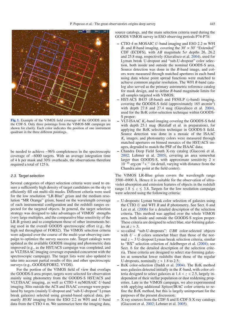
Fig. 1. Example of the VIMOS field coverage of the GOODS area inthe CDF-S. Only three pointings from the VIMOS-MR campaign areshown for clarity. Each color indicates the position of one instrumentquadrant in the three di!erent pointings.
be needed to achieve "96% completeness in the spectroscopiccoverage of "6000 targets. With an average integration timeof 4 h per mask and 30% overheads, the observations thereforerequired a total of 125 h.
2.3. Target selection
Several categories of object selection criteria were used to en-sure a su$ciently high density of target candidates on the sky toe$ciently fill out multi-slit masks. Di!erent criteria were usedfor the low resolution “LR-Blue” grism and the medium reso-lution “MR Orange” grism, based on the wavelength coverageof each instrumental configuration and the redshift ranges ex-pected for the targeted objects. In general, the target selectionstrategy was designed to take advantages of VIMOS’ strengths(very large multiplex, and the comparative blue sensitivity of theLR-B grism) and to complement those of other instruments be-ing used in the overall GOODS spectroscopic e!ort (e.g., thehigh red throughput of FORS2). The VIMOS selection criteriawere adjusted over the course of the multi-year observing cam-paign to optimize the survey success rate. Target catalogs wereupdated as the available GOODS imaging and photometric dataimproved (e.g., as the HST/ACS campaign was completed, andas VLT/ISAAC imaging coverage expanded concurrent with thespectroscopic campaign). The target lists were also updated totake into account partial results of this and other spectroscopicsurveys (e.g., GOODS/FORS2, VVDS).
For the portion of the VIMOS field of view that overlapsthe GOODS-S area proper, targets were selected for observationmainly using photometry from the GOODS-S HST/ACS andVLT/ISAAC imaging, as well as CTIO 4 m/MOSAIC U-bandimaging. Slits outside the ACS and ISAAC coverage were popu-lated by targets (mainly U-dropout and “sub-U-dropout” Lymanbreak galaxies) selected using ground-based optical data, pri-marily BVRI imaging from the ESO 2.2 m WFI and U-banddata from the CTIO 4 m. We summarize here the imaging data,
source catalogs, and the main selection criteria used during theGOODS VIMOS survey in ESO observing periods P74-P78:
– CTIO 4 m MOSAIC U-band imaging and ESO 2.2 m WFIB- and R-band imaging, covering the 30) ( 30) “Extended”CDF (ECDFS), with AB magnitude 5" depths 26, 26.2and 25.8 mag, respectively (Giavalisco et al. 2004), used forLyman break U-dropout and “sub-U-dropout” color selec-tion, both inside and outside the nominal GOODS-S area.Source detection was done in the R-band image, and col-ors were measured through matched apertures in each bandusing data whose point spread functions were matched toachieve common angular resolution. The WFI R-band cata-log also served as the primary astrometric reference catalogfor mask design, and to define R-band magnitude limits forall samples targeted with VIMOS;
– HST-ACS B435 (B-band) and F850LP (z-band) imaging,covering the GOODS-S field (approximately 165 arcmin2)with depth 27.8 and 27.4 mag (Giavalisco et al. 2004),used for the BzK color-selection technique within GOODS-S proper;
– VLT-ISAAC Ks-band imaging covering the GOODS-S fieldwith depth 25.1 mag (Retzla! et al. in preparation), forapplying the BzK selection technique in GOODS-S field.Source detection was done in a mosaic of the ISAACKs images, and photometry colors were measured throughmatched apertures on binned mosaics of the HST/ACS im-ages, degraded to match the PSF of the ISAAC data;
– Chandra Deep Field South X-ray catalog (Giacconi et al.2002; Lehmer et al. 2005), covering an area somewhatlarger than GOODS-S, with approximate sensitivity 2 (10#16 erg cm#2 s#1 (in detail, varying with distance from theChandra aim point at the field center).
The VIMOS LR-Blue grism covers the wavelength range3500#6900 Å. Hence it is suitable for the observation of ultra-violet absorption and emission features of objects in the redshiftrange 1.8 * z * 3.8. Targets for the low resolution campaignwere selected using the following criteria:
– U-dropouts: Lyman break color selection of galaxies usingthe CTIO U and WFI B and R photometry. See Sect. 6 andLee et al. (2006) for a detailed description of the selectioncriteria. This method was applied over the whole VIMOSarea, both inside and outside the GOODS-S region proper.These criteria are designed to select blue, star-forming galax-ies at z $ 3;
– so-called “sub-U-dropouts”: UBR color-selected objectswith U # B colors somewhat bluer than those of the nor-mal z " 3 U-dropout Lyman break selection criteria, similarto “BX” selection criterion of Adelberger et al. (2004); seeSect. 6 for the detailed description of the selection crite-ria. These criteria are designed to select star-forming galax-ies at somewhat lower redshifts than those of the regularU-dropouts, nominally z $ 1.8 to 2.5;
– BzK color-selection (Daddi et al. 2004). The BzK methoduses galaxies detected initially in the K-band, with color cri-teria designed to select galaxies at 1.4 < z < 2.5, largely in-dependent of their stellar population or dust reddening prop-erties. Late in the VIMOS campaign, we also experimentedwith applying additional Spitzer/IRAC color criteria to re-fine the BzK method, but this is largely unimportant for thepurposes of the present discussion;
– X-ray sources from the CDF-S and E-CDF-S X-ray catalogs(Giacconi et al. 2002; Lehmer et al. 2005).
446 P. Popesso et al.: The great observatories origins deep survey
No low redshift galaxies were intentionally targeted for theLR-Blue masks, although as we will see in Sect. 6, some fore-ground interlopers do “contaminate” the color-selected sam-ples, particularly the sub-U-dropouts. A magnitude cut at B <24.5 mag was applied to all target catalogs listed above.
The wavelength range of the VIMOS MR grism is4000#10 000 Å, similarly to that of FORS2. However, the fring-ing at red wavelength (% + 7000 Å) is somewhat stronger thanin FORS2, and the VIMOS red throughput is lower. Hence, op-tical rest-frame spectral features for galaxies at z > 1, and theultraviolet rest-frame spectral features of Lyman break galaxies(LBGs) at z >" 4.8,which would appear at very red optical wave-lengths, are harder to detect with VIMOS than with FORS2.Therefore, our VIMOS target selection was limited to brightergalaxies (mainly expected to be at z < 1.2), and to color-selectedLBGs in the redshift range 2.8 < z < 4.8. As for the LR-Bluecampaign, target selection used the available imaging data andphotometry catalogs according to the following criteria:
1. galaxies with R < 24.5, with no other color pre-selection,excluding VIMOS LR-Blue targets and objects already ob-served in other spectroscopic programs. In the later VIMOScampaigns, some preference was given to galaxies detectedat 24 µm from the GOODS Spitzer MIPS data (Dickinsonet al. in preparation; Chary et al. in preparation), meeting thesame R < 24.5 mag limit. We do not consider the MIPS-detected sources as a separate category for the purposes ofthis paper;
2. relatively bright Lyman break galaxies at i775 < 25, selectedas B435, V606 dropouts (nominally, redshifts z $ 4 and 5,respectively), according to the same color criteria describedin Vanzella et al. (2005, 2006, 2008).
We did not use photometric redshifts, nor did we apply sur-face brightness selection when selecting galaxies for observa-tions. When designing the masks, we avoided (as much as possi-ble) observing targets that had already been observed in otherredshift surveys of the GOODS-S and CDFS region, namely,the K20 survey of Cimatti (2002), the spectroscopic survey ofX-ray sources by Szokoly et al. (2004), the VIMOS VLT DeepSurvey (Le Fevre et al. 2005) and the ESO/GOODS FORS2 sur-vey (Vanzella et al. 2005, 2006).
3. Observations and data reduction
The VLT/VIMOS spectroscopic observations were carried out inservice mode during ESO observing periods P74-P78.
3.1. Preparation of VIMOS observations
For each pointing a short V-band image was taken with VIMOSin advance of the spectroscopic observations. We used this pre-imaging, together with the GOODS WFI R band image, to de-rive the transformation matrix from the (#, &) celestial refer-ence frame of the target catalogs to the (XCCD, YCCD) VIMOSinstrumental coordinate system. This procedure was carried outusing the routines geomap and geoxytran in the IRAF environ-ment. The rms of the residuals from these transformations were"0.05 arcsec, ten times better than the accuracy of the matchingprocedure implemented in the VIMOS mask preparation soft-ware (VMMPS, Bottini et al. 2005). This is due to the choice ofa higher order polynomial of the fitting procedure, which is notallowed in VMMPS.
Once the target catalog was expressed in the (XCCD,YCCD)VIMOS instrumental coordinate system, the next steps in theslit mask design were conducted with the VMMPS tool. Afterplacing two reference apertures on bright stars for each point-ing quadrant, slits were assigned to sources drawn from the tar-get catalog. The automated SPOC (Slit Positioning OptimizationCode, Bottini et al. 2005) algorithm was run to maximize thenumber of slits assigned, given the geometrical and optical con-straints of the VIMOS set-up. We designed masks with slitwidths of one arcsec, and required that a minimum of 1.8 arc-sec of sky is left on each side of a targeted object to allow foraccurate sky background fitting and removal during later spec-troscopic data processing. The spectral range of the VIMOSLR-Blue masks, projected onto the VIMOS CCDs, is shortenough that it is possible to have several “layers” of slits whosespectra do not overlap in the dispersion axis. Because of thisspectral multiplexing, each GOODS LR-Blue mask could in-clude up to 360 slits in the combined four quadrants. Masks forthe VIMOS MR grism were designed with no multiplexing inthe dispersion axis to avoid the superposition of zero and nega-tive orders. The combined four quadrants of a GOODS MR maskcontained 150 slits on average. The observations were ditheredto move targets along the axis of the slits in order to improvethe sky subtraction and the removal of CCD cosmetic defects.In the LR-Blue survey, the dithering pattern consisted of threeposition separated by a step of 1.4 arcsec. In the MR survey, thedithering pattern consisted of five position separated by a step of1.5 arcsec, in order to provide enough independent pointings toconstruct and apply a correction for fringing at red wavelengths(see Sect. 3.2).
In the LR-Blue campaign, we used the LR-Blue grism to-gether with the OS-Blue cuto! filter, which limits the bandpassand order overlap. With 1 arcsec slits, the spectral resolutionis "28 Å and the dispersion is 5.7 Å/pixel. 10 exposures of24 min each were taken for a total exposure time of 4 h per mask.In the MR campaign, the MR grism was used together with theGG475 filter. With 1 arcsec slits, the resolution is "13 Å and thedispersion is 2.55 Å/pixel. 12 exposures of 20 min each weretaken for a total exposure time of 4 h per mask. We requestednightly arc-lamp calibrations to measure the wavelength solutionof the spectra and reduce problems due to instrument flexure.
3.2. Data reduction
The pipeline processing of the VIMOS-GOODS data is carriedout using the VIMOS Interactive Pipeline Graphical Interface(VIPGI, see Scodeggio et al. 2005, for a full description). Thedata reduction is performed in several interactive steps: locatingthe spectra in the individual spectroscopic frames, wavelengthcalibration, sky subtraction and fringing correction, combina-tion of the 2D spectra of dithered observations, extraction ofthe 1D spectra, and flux calibration. The location of the slits isknown from the mask design process, hence, knowing the grismzero deviation wavelength and the dispersion curve, the approx-imate location of each spectrum on the detectors is known a pri-ori. However, small shifts from the predicted positions are pos-sible. From the predicted position, the location of the spectra areidentified accurately on the 4 detectors and an extraction win-dow is defined for each slit. The wavelength calibration is se-cured by the observation of nightly arc-lamps through each slitmask. Wavelength calibration spectra are extracted at the samelocation as the object spectra and calibration lines are identi-fied to derive the pixel to wavelength mapping for each slit. The
P. Popesso et al.: The great observatories origins deep survey 447
wavelength to detector pixel transformation is fit using a thirdorder polynomial, resulting in a median rms residual of "0.7 Åacross the wavelength range in the LR-Blue masks and "0.36 Åin the MR masks. A low order polynomial (second order) is fitalong the slit, modeling the sky background contribution at eachwavelength position, and subtracted from the 2D spectrum. Forthe LR-Blue data, fringing is not present, and all 10 exposures ofa sequence are directly combined by shifting the 2D spectra fol-lowing the o!set pattern to register the object at the same posi-tion. The individual frames are combined with a median, sigma-clipping algorithm to produce the final summed, sky subtracted2D spectrum. In the case of the Medium Resolution spectra, thefringing is significant at % > 7000 Å and needs to be removed.Therefore, a fringing correction is applied before combining thedithered exposures. As the object is moved to di!erent positionsalong the slit following the dithering pattern, the median of the2D sky subtracted spectra produces a frame from which the ob-ject is eliminated, but that includes all residuals not corrected bysky subtraction, in particular the fringing pattern varying withposition across the slit and wavelength. This sky/fringing resid-ual image is then subtracted from each individual 2D sky sub-tracted frame. The fringing corrected frames are then shifted andcombined as in the case of the LR-Blue spectra.
The last step done automatically by VIPGI is to extract a1D spectrum from the summed 2D spectrum, using an optimalextraction following the slit profile measured in each slit (Horne1986). The 1D spectrum is flux calibrated using a transforma-tion computed from observations of spectrophotometric standardstars.
Final, we checked each 1D calibrated spectra individually,and removed the most discrepant features manually, cleaningeach spectrum of zero order contamination, strong sky linesresiduals and negative unphysical features.
3.3. The VIMOS LR-Blue wiggles
Spurious wiggles with amplitude of about 3 to 8% are found inVIMOS MOS spectra taken with the combination of LR_Bluegrism and OS_Blue Order Sorting (OS) filter. The position of thewiggles in the spectrum compares well with the wiggles in theresponse curve of the OS_Blue filter (see also the ESO VIMOSUser Manual, Fig. A.3). This clearly indicates that the wigglesoriginate in the OS filter. The e!ect of the wiggles should there-fore be multiplicative. In principle, spectroscopic screen flat-fields, even taken during the day, would be su$cient to correctthe wiggles. However, several aspects make this correction verydi$cult. The position and amplitude of the wiggles are found todepend on the spectral resolution, which in turn depends on slitwidth and object size. The wiggle pattern and the overall shapeof the flat field spectra depend significantly on the position of theslit in the field of view. In addition, the normalization of flat fieldspectra is made problematic by the possible overlap of 0th-orderspectra from neighboring slits. For these reasons we prefer notto correct the wiggles observed in the LR-Blue spectra.
3.4. Target coordinates
The rotation angle of the VIMOS GOODS pointings (#20 deg)is di!erent from the default values accepted by VIPGI(0 and 90 deg). Therefore, VIPGI does not provide the astrom-etry of the extracted spectra. The only information provided byVIPGI are the coordinates in mm on the focal plane stored in theVIPGI object table. To overcome this problem, we transform the
-0.4 -0.2 0 0.2 0.40
200
400
600
-0.4 -0.2 0 0.2 0.40
100
200
300
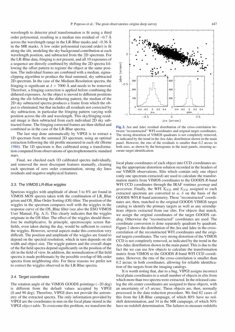
Fig. 2. %ra and %dec residual distribution of the cross-correlation be-tween “reconstructed” WFI coordinates and original target coordinates.The strong distortion of VIMOS quadrants is not completely removed,as indicated by the trend in the %ra-%dec distribution shown in the mainpanel. However, the rms of the residuals is smaller than 0.2 arcsec inboth axes, as shown by the histograms in the inset panels, ensuring ac-curate target identification.
focal plane coordinates of each object into CCD coordinates us-ing the appropriate distortion solution recorded in the headers ofour VIMOS observations. Slits which contain only one object(only one spectrum extracted) are used to calculate the transfor-mation matrix from VIMOS coordinates to the GOODS R-bandWFI CCD coordinates through the IRAF routines geomap andgeoxytran. Finally, the WFI XCCD and YCCD assigned to eachextracted spectrum are converted to #, & on the basis of theGOODS WFI R-band astrometry. These “reconstructed” coordi-nates are, then, matched to the original GOODS VIMOS targetcatalog to identify the primary targets as well as any serendip-itous objects extracted from our slits. For objects that match,we assign the original coordinates of the target GOODS cat-alog. Otherwise the “reconstructed” coordinates are used. Thecoordinate conversion is done separately quadrant by quadrant.Figure 2 shows the distribution of the %ra and %dec in the cross-correlation of the reconstructed WFI coordinates and the origi-nal targets coordinates. The very strong distortion of the VIMOSCCD is not completely removed, as indicated by the trend in the%ra-%dec distribution shown in the main panel. This is due to thefact the we can use few objects to calculate the transformationmatrix from VIMOS to the GOODS R-band WFI CCD coordi-nates. However, the rms of the cross-correlation is smaller than0.2 arcsec in both coordinates, allowing for reliable identifica-tion of the targets from the imaging catalogs.
It is worth noting that, due to a bug, VIPGI assigns incorrectfocal plane coordinates to a small number of objects in slits fromwhich more than two spectra were extracted. In the released cata-log the slit center coordinates are assigned to these objects, withan uncertainty of ±5 arcsec. These objects are, then, normallyprocessed in the data reduction procedure. We find 82 cases ofthis from the LR-Blue campaign, of which 80% have no red-shift determination, and 34 in the MR campaign, of which 50%have no redshift determination. The failures to measure redshifts
448 P. Popesso et al.: The great observatories origins deep survey
are simply due to the low S/N in these spectra. Those objectsare given focal plane coordinates xfp = 0.0, yfp = 0. Moreover,on the basis of the reconstructed WFI coordinates, these objectswould be located completely out of the slits where they shouldbe. The complete list of those objects is available at http://archive.eso.org/cms/eso-data/data-packages.
4. Redshift determination
2344 spectra have been extracted from the 6 LR-Blue masks and968 have been extracted from 6 MR masks. From these, we havebeen able to determine 1481 redshifts in the LR-Blue campaignand 656 in the MR campaign. 33% of the LR-Blue slits and 18%of the MR slits contain more than one spectrum. Most of thesecondary spectra obtained provide additional observations ofknown targets. We have identified 2235 unique LR-Blue objectsand 886 unique MR objects.
Redshift estimation has been performed by cross-correlatingthe individual observed spectra with templates of di!erent spec-tral types. Templates for ordinary S0, Sa, Sb, Sc, and ellipticalgalaxies were used to measure redshifts of relatively low redshiftgalaxies. At higher redshifts, where the VIMOS observationsmainly sample the ultraviolet rest frame, several di!erent spec-tral templates for Lyman break galaxies, BzK-selected galaxies,and AGN were used. The cross-correlation is carried out usingthe rvsao package (xcsao routine, Kurtz & Ming 1998) in theIRAF environment. In particular, a trial-and-error approach isused for the z > 1.8 galaxies, whose redshift determination ismade di$cult by the low S/N ratio of the spectral absorptionfeatures and the wiggles in the LR-Blue spectrum.
In the large majority of the cases the redshift has been deter-mined through the identification of prominent features of galaxyspectra:
– at low redshift the absorption features: the 4000 Å break,Ca H and K, H& and H' in absorption, g-band, MgII 2798;
– and the emission features: [O !!]3727, [O !!!]4959,5007, H',H#;
– at high redshift: Ly#, in emission and absorption, ultra-violet absorption features such as [Si !!]1260, [O !]1302,[C !!]1335, [Si !"]1393,1402, [S !!]1526, [C !"]1548,1550,[Fe !!]1608 and [Al !!!]1670 (see also Fig. B.1 of theappendix).
In analogy to the complementary GOODS-FORS2 redshift cam-paign (Vanzella et al. 2005, 2006, 2008), we use four flag valuesto indicate the quality of each redshift estimate. The determina-tion of the quality flag is done in two steps. As a first step, the as-signment of the quality flag is done during the cross-correlationof the spectrum with the templates on the basis of the cross-correlation coe$cient provided by the routine xcsao in the IRAFenvironment. The quality flags are assigned according to the fol-lowing criteria (see also the appendix for several examples):
– flag A: high quality, values of the xcsao correlation coe$-cient R + 5; emission lines and strong absorption featuresare well identified;
– flag B: intermediate quality, values of the xcsao correlationcoe$cient 3 * R < 5; one emission line plus few absorptionfeatures are well identified;
– flag C: low quality, values of the xcsao correlation coe$-cient R < 3, features of the continuum not well identified.
– flag X: no redshift estimated, no features identified.
As a second step, each spectrum, with superposed labels indi-cating the main spectral features, is checked by eye by several
di!erent people, who refine the redshift determination and thequality flag assignment. A good agreement of the di!erent red-shift estimates has been found for nearly all of the flag A spec-tra, "80% of original quality B cases, and "60% of originalC cases. In case of disagreement the object is assigned a lowerquality flag. On average, each spectrum is checked more thenthree times.
In "15% of the cases the redshift is based only on one emis-sion line, usually identified with [O !!]3727 or Ly#. In thesecases, the continuum shape, the presence of breaks, the absenceof other spectral features in the observed spectral range, and thebroad band photometry are considered in the redshift evalua-tion. In general these solo-emission line redshifts are classifiedas “likely” (B) or “tentative” (C) if no other information is pro-vided by the continuum. In a few cases, the quality flag is set toA if the photometry or the availability of photometric redshiftshelp in distinguishing between high and low redshift sources (seeKirby et al. 2007, for the DEEP2 survey).
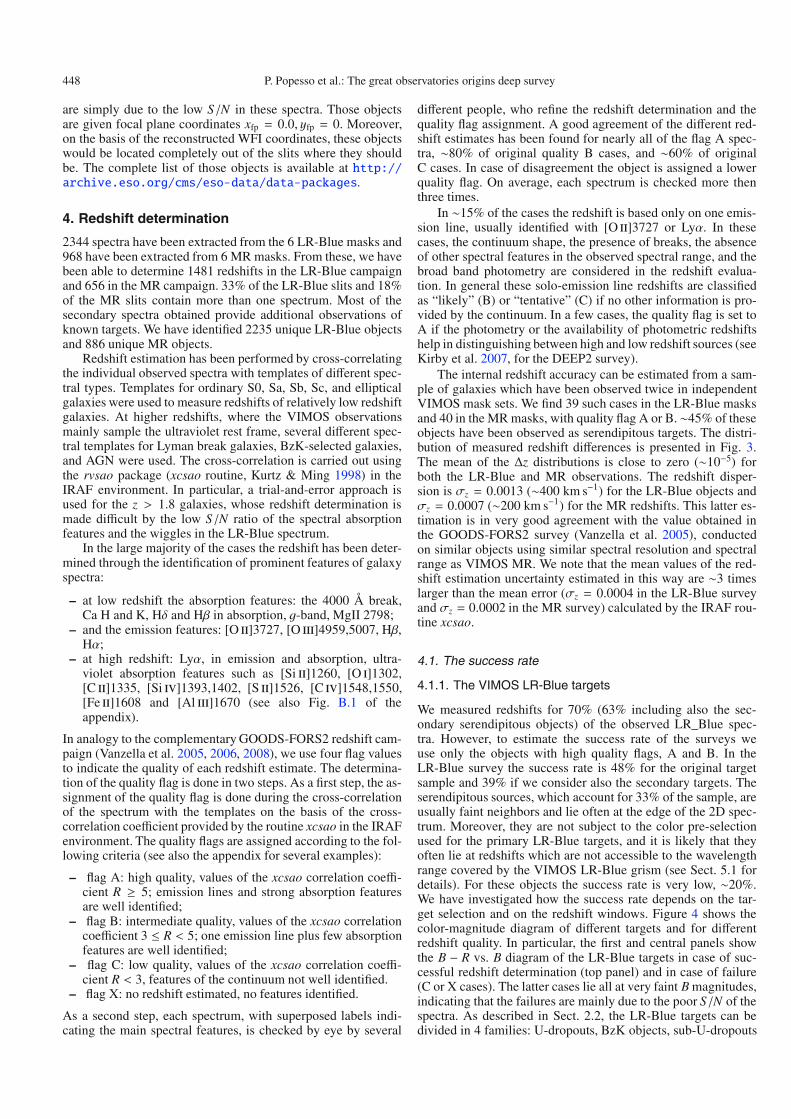
The internal redshift accuracy can be estimated from a sam-ple of galaxies which have been observed twice in independentVIMOS mask sets. We find 39 such cases in the LR-Blue masksand 40 in the MR masks, with quality flag A or B. "45% of theseobjects have been observed as serendipitous targets. The distri-bution of measured redshift di!erences is presented in Fig. 3.The mean of the %z distributions is close to zero ("10#5) forboth the LR-Blue and MR observations. The redshift disper-sion is "z = 0.0013 ("400 km s#1) for the LR-Blue objects and"z = 0.0007 ("200 km s#1) for the MR redshifts. This latter es-timation is in very good agreement with the value obtained inthe GOODS-FORS2 survey (Vanzella et al. 2005), conductedon similar objects using similar spectral resolution and spectralrange as VIMOS MR. We note that the mean values of the red-shift estimation uncertainty estimated in this way are "3 timeslarger than the mean error ("z = 0.0004 in the LR-Blue surveyand "z = 0.0002 in the MR survey) calculated by the IRAF rou-tine xcsao.
4.1. The success rate
4.1.1. The VIMOS LR-Blue targets
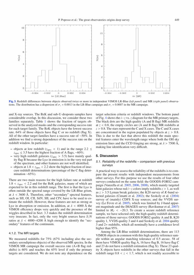
We measured redshifts for 70% (63% including also the sec-ondary serendipitous objects) of the observed LR_Blue spec-tra. However, to estimate the success rate of the surveys weuse only the objects with high quality flags, A and B. In theLR-Blue survey the success rate is 48% for the original targetsample and 39% if we consider also the secondary targets. Theserendipitous sources, which account for 33% of the sample, areusually faint neighbors and lie often at the edge of the 2D spec-trum. Moreover, they are not subject to the color pre-selectionused for the primary LR-Blue targets, and it is likely that theyoften lie at redshifts which are not accessible to the wavelengthrange covered by the VIMOS LR-Blue grism (see Sect. 5.1 fordetails). For these objects the success rate is very low, "20%.We have investigated how the success rate depends on the tar-get selection and on the redshift windows. Figure 4 shows thecolor-magnitude diagram of di!erent targets and for di!erentredshift quality. In particular, the first and central panels showthe B # R vs. B diagram of the LR-Blue targets in case of suc-cessful redshift determination (top panel) and in case of failure(C or X cases). The latter cases lie all at very faint B magnitudes,indicating that the failures are mainly due to the poor S/N of thespectra. As described in Sect. 2.2, the LR-Blue targets can bedivided in 4 families: U-dropouts, BzK objects, sub-U-dropouts
P. Popesso et al.: The great observatories origins deep survey 449
Fig. 3. Redshift di!erences between objects observed twice or more in independent VIMOS LR-Blue (left panel) and MR (right panel) observa-tions. The distribution has a dispersion of "z = 0.0013 in the LR-Blue campaign and "z = 0.0007 in the MR campaign.
and X-ray sources. The BzK and sub-U-dropouts samples haveconsiderable overlap. In this discussion, we consider these twofamilies separately. Table 1 shows the fraction of targets ob-served in the analyzed masks and the corresponding success ratefor each target family. The BzK objects have the lowest successrate. 64% of those objects have flag C or no redshift (flag X).All of the other target families have a success rate of "50%. Inaddition we find a strong dependence of the success rate on theredshift window. In particular:
– objects at low redshift (zspec < 1) and in the range 2.2 *zspec * 3.5 have the highest fraction of A flags, "60%;
– very high redshift galaxies (zspec > 3.5) have mainly qual-ity flag B because the Ly# in emission is in the very red partof the spectrum, and other features are not well identified;
– objects at 1.8 < zspec < 2.2 show the highest fraction of inse-cure redshift determinations (percentage of the C flag deter-mination "65%).
There are two main reasons for the high failure rate at redshift1.8 < zspec < 2.2 and for the BzK galaxies, many of which areexpected to lie in this redshift range. The first is that the Ly# isoften outside the spectral range covered by the LR-Blue grism,at % < 3600 Å. Therefore, other “secondary” spectral features,such as SII, OI, CII, SiIV, SII, and CIV, have to be used to es-timate the redshift. However, these features are not as strong asLy# in absorption or emission. In addition, at % < 4000 Å theVIMOS e$ciency drops very quickly and the presence of thewiggles described in Sect. 3.3 makes the redshift determinationvery insecure. In fact, only the very bright sources have S/Nratios at % < 4000#4200 Å high enough to identify the “sec-ondary” features of the continuum.
4.1.2. The MR targets
We measured redshifts for 75% (67% including also the sec-ondary serendipitous objects) of the observed MR spectra. In theVIMOS MR campaign the overall success rate (A+B flag red-shifts) is 60% and reaches the 65% level if only the primarytargets are considered. We do not note any dependence on the
target selection criteria or redshift windows. The bottom panelof Fig. 4 shows the i#z vs. z diagram for the MR primary targets.The black dots are the high quality (A and B flag) MR redshiftsat z < 0.8, the empty circles are (A and B flag) MR redshifts atz > 0.8. The stars represent the C and X cases. The C and X casesare concentrated in the region populated by objects at z > 0.8.This is due to the fact that above this redshift the main spec-tral features enter the wavelength range where both the OH skyemission lines and the CCD fringing are strong, at % > 7500 Å,making line identification very di$cult.
5. Discussion
5.1. Reliability of the redshifts – comparison with previoussurveys
A practical way to assess the reliability of the redshifts is to com-pare the present results with independent measurements fromother surveys. For this purpose we use the results of four othersurveys conducted on the same field: the GOODS-FORS2 cam-paign (Vanzella et al. 2005, 2006, 2008), which mainly targetedfaint galaxies whose red i#z colors imply redshifts z > 1, as wellas z > 3.5 Lyman break galaxies; the K20 survey of K-band se-lected galaxies (Cimatti et al. 2002); the Szokoly et al. (2004)survey of (mainly) CDFS X-ray sources; and the VVDS sur-vey (Le Fevre et al. 2005), which was limited by I-band appar-ent magnitude and the IMAGES survey (Ravikumar et al. 2007)limited to MJ < #20.3. To create a secure redshift referencesample, we have selected only the high quality redshift determi-nations of those surveys: GOODS FORS2 quality A and B, K20quality 1, VVDS quality 3 and 4 and Szokoly et al. 2004 quality3 and 2+ redshifts, which all nominally have a confidence levelhigher than 95%.
Among the LR-Blue redshift determinations, there are 113VIMOS objects in common with this high quality reference sam-ple within an angular matching tolerance of 0.5 arcsec. 58 ofthem have VIMOS quality flag A, 16 have flag B, 16 have flag Cand 23 do not have a redshift estimation (flag X). These 23 qual-ity X objects have redshifts in the other surveys that fall in theredshift range 0.8 < z < 1.7, which is not readily accessible to
450 P. Popesso et al.: The great observatories origins deep survey
Fig. 4. Color#magnitude diagram of the LR-Blue and MR primary tar-gets. The first panel shows the B # R vs. B diagram for A and B highquality LR-Blue redshifts. Low quality LR-Blue redshifts (C flag, dots)and failure (X flag, stars) are shown in the central panel. The bottompanel shows the i # z vs. z diagram for the MR primary targets. Theblack dots are the high quality (A and B flag) MR redshifts at z < 0.8,the empty circles are high quality (A and B flag) MR redshifts at z > 0.8.The stars represent the C and X cases.
the VIMOS LR_Blue observations given their wavelength cov-erage. 27 cases of the A, B and C quality redshifts show “catas-trophic” discrepancies (|zVIMOS # zFORS2/K20/CDF/VVDS| > 0.015).
Table 1. Success rate of the GOODS VIMOS LR-Blue campaign. Thefirst column lists the name of the target family, the second column liststhe fraction of the target catalog due to the corresponding color selection(BzK and sub-dropout family overlap largely but they are considered asseparated family in the table). The third column lists the success rate(fraction A+B flag objects) of each target family. The last four columnslist the percentage of A, B, C and X flag redshift determinations, re-spectively.
Target Fraction s.r. A B C XU-dropouts 16% 49% 35% 14% 15% 36%
BzK 51% 36% 24% 12% 21% 43%sub-U-dropouts 66% 51% 35% 16% 16% 33%
X-ray 5% 51% 37% 14% 14% 35%
These account for 5 of the VIMOS flag A objects, 8 of the flag Bsources, and 11 of the flag C sources.
After visual comparison of the VIMOS andFORS2/K20/CDF/VVDS spectra we find that 3 of the 5VIMOS quality A spectra with “catastrophic” discrepancies arelikely to be incorrect GOODS/VIMOS redshift determinations:
– VIMOS GOODS_LRb_001_q2_1_1 versus FORS2GDS_J033217.78-274823.8 (flag A): the [OIII] in emissionis identified in the FORS2 spectrum and it is hidden by astrong sky line residual in the VIMOS spectrum. Thus, the[OII] in the VIMOS spectrum is misclassified as Ly# due tothe absence of H' and [OIII] emissions.
– VIMOS GOODS_LRb_001_1_q1_51_1 versus FORS2GDS_J033226.67-274013.4 (flag A): the [OII] in the FORS2spectrum is identified at z = 1.612, a redshift window not ac-cessible to VIMOS LR-Blue. No emission lines are visible inthe VIMOS spectrum and the low S/N UV absorption fea-tures are misclassified.
– VIMOS GOODS_LRb_001_q2_35_1 versus VVDS VVDS32126 (flag 3, observed with the VIMOS LR-Red grism): thestrong UV absorption features identified in our VIMOS LR-Blue spectrum provide a xcsao correlation coe$cient similarto that of the FeII and NeV absorption features identified inthe VVDS LR-Red spectrum. We have combined the twospectra and re-performed the cross correlation. The highestcorrelation peak corresponds to the VVDS redshift value
– VIMOS GOODS_LRb_001_q3_71_2 versus VIMOS LR-Red VVDS 16975 (flag 24): the VIMOS LR-Blue sourceis an emission line galaxy and the reference VVDS spec-trum is clearly an early type galaxy without any emissionline. The two spectra can not refer to the same object. Since16975 is a secondary object and not a primary target, we sus-pect that the coordinates provided by VIPGI (used to reducethe VVDS data) could be wrong as explained in Sect. 3.4.Thus, we consider our VIMOS redshift estimation correct,although the object identification may be incorrect.
– VIMOS GOODS_LRb_002_q2_55_1 versus FORS2GDS_J033221.94-274338.8 (flag A): the strong emissionline in the VIMOS spectrum is identified as a Ly# due to theabsence of H' and [OIII] emission and due to the photometry(the target was selected to be a U-dropout). The emissionline could be classified as a [OII] at much lower redshift(z = 0.166) with a much lower xcsao correlation coe$cient.In either case, the FORS2 redshift is not in agreement. Wehave combined the two spectra and re-measured the redshift.The correlation gives a good result only with a Ly# emittertemplate at z = 2.576. No match is found for the emissionseen in the FORS2 spectrum, which has a very low S/N. We
P. Popesso et al.: The great observatories origins deep survey 451
think that the line identified as [OII] in the FORS2 spectrumis instead due to a fringing residual since it is sitting on a skyline. Thus, we believe that the VIMOS redshift estimation islikely to be correct.
The resulting confidence level for the flag A redshift deter-minations is 95% (3 mistakes out of 58 redshift determina-tions). Among the flag B spectra showing “catastrophic” dis-crepancies, 6 VIMOS redshift determinations are wrong, mainlydue to the presence of sky residuals and 0th order contam-ination from neighboring spectra, and only 2 are more con-vincing than the FORS2/K20/CDF/VVDS determinations. Theresulting confidence level is 62% (6 mistakes out of 16 red-shift determinations). For all of the Flag C discrepancies, theFORS2/K20/CDF/VVDS redshift determinations are more con-vincing than the ultraviolet features identified in the LR-Bluespectra. The resulting confidence level is 31%. However, it isimportant to note that in most cases, the VIMOS flag C is as-signed to redshifts in the range 1.8 < z < 2.2, as explained inSect. 4.1. The surveys considered in this comparison (FORS2,K20, CDF and VVDS) were not optimized (mainly, in termsof wavelength coverage) to measure redshifts in this range.Thus, such comparisons can only reveal the mistakes in theGOODS/VIMOS redshift sample, and cannot provide confir-mations to our estimates. In conclusion, 19 redshift determi-nations out of 90 are wrong, resulting in an overall confidencelevel of 78% in the LR-Blue VIMOS redshifts. For the 71 casesout of 90 which show good agreement, we find a mean di!er-ence &zLR#Blue#VIMOS#zFORS2/k20/VVDS' = 0.0018±0.0019, whichconfirms the mean uncertainty %z found in Sect. 4.
The comparison between the VIMOS MR redshift determi-nations and FORS2/K20/CDF/VVDS measurements is simpli-fied by the fact that our MR observations cover a similar wave-length range to those observed in the other surveys. There are 94VIMOS objects in common with the high quality reference sam-ple within a positional tolerance of 0.5 arcsec. 69 of them haveVIMOS quality flag A, 17 have quality flag B and 8 have qual-ity flag C. We find 5 “catastrophic” discrepancies: 1 has flag A,1 has flag B and 3 have flag C:
– flag A case GOODS_MR_new_1_d_q3_22_1 versusFORS2 GDS_J033243.19-275034.9 (flag A): an accurateanalysis is provided by Vanzella et al. (2006, see their Fig. 2).The continuum shows increasing bumps/bands in the red,very similar to typical cold stars. After visual inspection ofthe ACS color image Vanzella et al. (2006) concluded thatGDS_J033243.19-275034.9 is a simultaneous spectrum oftwo very close sources: a star and a possible high-z galaxy;
– B flag case VIMOS GOODS_MR_new_1_d_q2_21_2 ver-sus FORS2 GDS_J033249.04-2705015.5 (flag A): the spec-tral features used to identify the VIMOS redshift are all at% > 7500, where the fringing is very strong. The correspond-ing FORS2 spectra, which su!er less of fringing, show moreconvincing spectral features.
In the 3 flag C cases, the FORS2/K20/CDF/VVDS redshift esti-mates seem to be more robust than the VIMOS redshifts. In allthree cases the spectral features used to identify the redshift arein the region strongly a!ected by fringing.
Thus, we obtain a confidence level of 98% for the qual-ity A MR redshifts (1 mistake out of 69 redshifts), 94% forthe quality B redshifts (1 mistakes out of 17 determinations)and 62% for the quality C cases (3 mistakes out of 8 deter-minations). The overall confidence level of the redshift deter-minations of the MR redshift survey is 95%. For the 89 cases
-0.4 -0.2 0 0.2 0.4
0
100
200
300
400
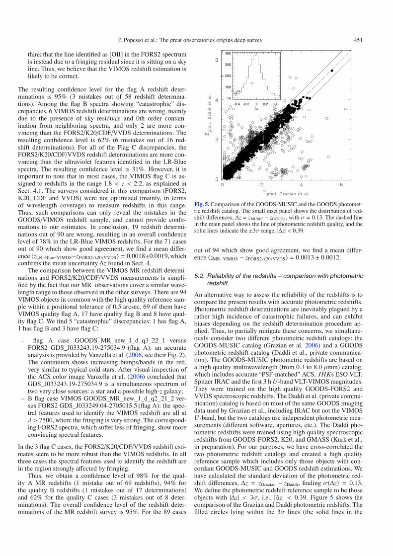
Fig. 5. Comparison of the GOODS-MUSIC and the GOODS photomet-ric redshift catalog. The small inset panel shows the distribution of red-shift di!erences, %z = zMUSIC # zGOODS, with " = 0.13. The dashed linein the main panel shows the line of photometric redshift quality, and thesolid lines indicate the ±3" range, |%z| < 0.39.
out of 94 which show good agreement, we find a mean di!er-ence &zMR#VIMOS # zFORS2/k20/VVDS' = 0.0013 ± 0.0012.
5.2. Reliability of the redshifts – comparison with photometricredshift
An alternative way to assess the reliability of the redshifts is tocompare the present results with accurate photometric redshifts.Photometric redshift determinations are inevitably plagued by arather high incidence of catastrophic failures, and can exhibitbiases depending on the redshift determination procedure ap-plied. Thus, to partially mitigate these concerns, we simultane-ously consider two di!erent photometric redshift catalogs: theGOODS-MUSIC catalog (Grazian et al. 2006) and a GOODSphotometric redshift catalog (Daddi et al., private communica-tion). The GOODS-MUSIC photometric redshifts are based ona high quality multiwavelength (from 0.3 to 8.0 µmm) catalog,which includes accurate “PSF-matched” ACS, JHKs ESO VLT,Spitzer IRAC and the first 3 h U-band VLT-VIMOS magnitudes.They were trained on the high quality GOODS-FORS2 andVVDS spectroscopic redshifts. The Daddi et al. (private commu-nication) catalog is based on most of the same GOODS imagingdata used by Grazian et al., including IRAC but not the VIMOSU-band, but the two catalogs use independent photometric mea-surements (di!erent software, apertures, etc.). The Daddi pho-tometric redshifts were trained using high quality spectroscopicredshifts from GOODS-FORS2, K20, and GMASS (Kurk et al.,in preparation). For our purposes, we have cross-correlated thetwo photometric redshift catalogs and created a high qualityreference sample which includes only those objects with con-cordant GOODS-MUSIC and GOODS redshift estimations. Wehave calculated the standard deviation of the photometric red-shift di!erences, %z = zGrazian # zDaddi, finding "(%z) = 0.13,We define the photometric redshift reference sample to be thoseobjects with |%z| < 3", i.e., |%z| < 0.39. Figure 5 shows thecomparison of the Grazian and Daddi photometric redshifts. Thefilled circles lying within the 3" lines (the solid lines in the
452 P. Popesso et al.: The great observatories origins deep survey
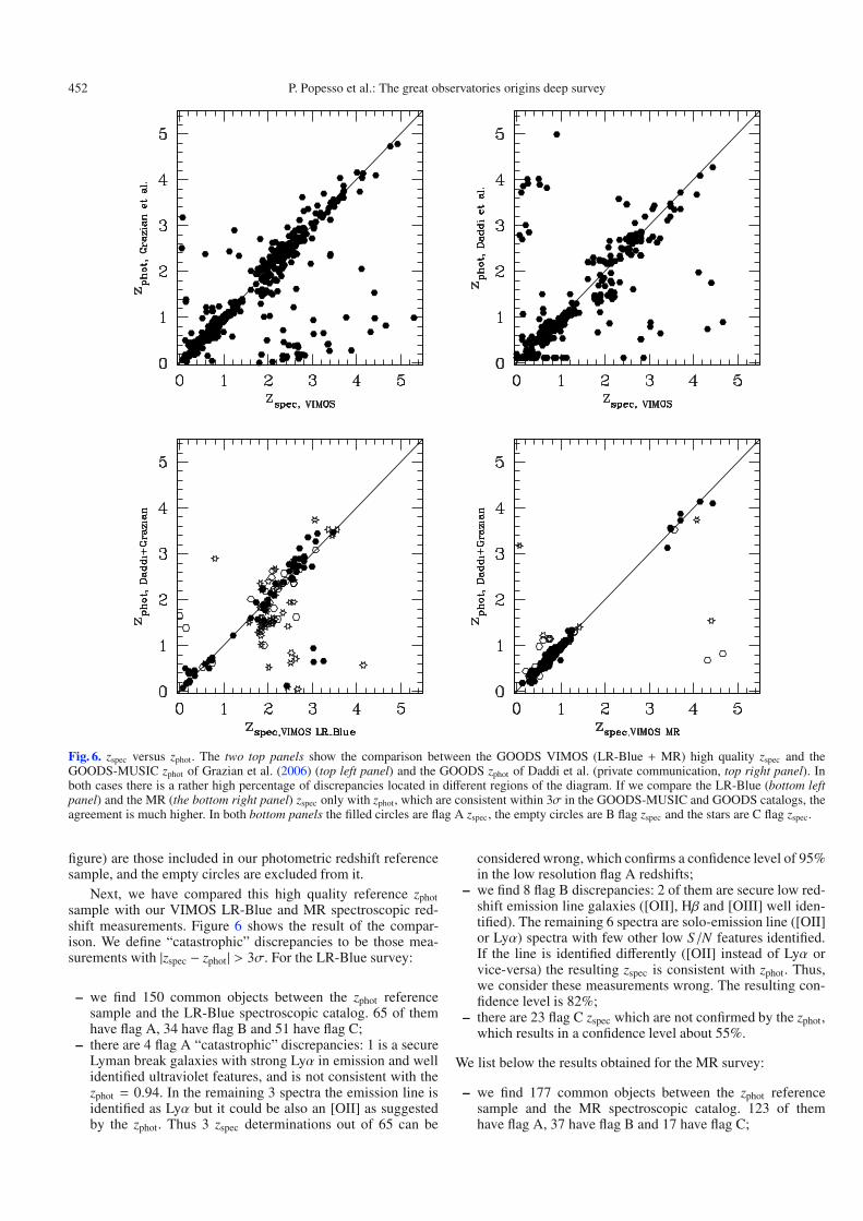
Fig. 6. zspec versus zphot. The two top panels show the comparison between the GOODS VIMOS (LR-Blue + MR) high quality zspec and theGOODS-MUSIC zphot of Grazian et al. (2006) (top left panel) and the GOODS zphot of Daddi et al. (private communication, top right panel). Inboth cases there is a rather high percentage of discrepancies located in di!erent regions of the diagram. If we compare the LR-Blue (bottom leftpanel) and the MR (the bottom right panel) zspec only with zphot, which are consistent within 3" in the GOODS-MUSIC and GOODS catalogs, theagreement is much higher. In both bottom panels the filled circles are flag A zspec, the empty circles are B flag zspec and the stars are C flag zspec.
figure) are those included in our photometric redshift referencesample, and the empty circles are excluded from it.
Next, we have compared this high quality reference zphotsample with our VIMOS LR-Blue and MR spectroscopic red-shift measurements. Figure 6 shows the result of the compar-ison. We define “catastrophic” discrepancies to be those mea-surements with |zspec # zphot| > 3". For the LR-Blue survey:
– we find 150 common objects between the zphot referencesample and the LR-Blue spectroscopic catalog. 65 of themhave flag A, 34 have flag B and 51 have flag C;
– there are 4 flag A “catastrophic” discrepancies: 1 is a secureLyman break galaxies with strong Ly# in emission and wellidentified ultraviolet features, and is not consistent with thezphot = 0.94. In the remaining 3 spectra the emission line isidentified as Ly# but it could be also an [OII] as suggestedby the zphot. Thus 3 zspec determinations out of 65 can be
considered wrong, which confirms a confidence level of 95%in the low resolution flag A redshifts;
– we find 8 flag B discrepancies: 2 of them are secure low red-shift emission line galaxies ([OII], H' and [OIII] well iden-tified). The remaining 6 spectra are solo-emission line ([OII]or Ly#) spectra with few other low S/N features identified.If the line is identified di!erently ([OII] instead of Ly# orvice-versa) the resulting zspec is consistent with zphot. Thus,we consider these measurements wrong. The resulting con-fidence level is 82%;
– there are 23 flag C zspec which are not confirmed by the zphot,which results in a confidence level about 55%.
We list below the results obtained for the MR survey:
– we find 177 common objects between the zphot referencesample and the MR spectroscopic catalog. 123 of themhave flag A, 37 have flag B and 17 have flag C;
P. Popesso et al.: The great observatories origins deep survey 453
18 20 22 240
0.2
0.4
0.6
0.8
1
18 20 220
0.2
0.4
0.6
0.8
1
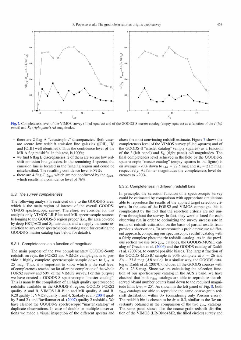
Fig. 7. Completeness level of the VIMOS survey (filled squares) and of the GOODS-S master catalog (empty squares) as a function of the I (leftpanel) and KS (right panel) AB magnitudes.
– there are 2 flag A “catastrophic” discrepancies. Both casesare secure low redshift emission line galaxies ([OII], H'and [OIII] well identified). Thus the confidence level of theMR A flag redshifts, in this test, is 100%;
– we find 6 flag B discrepancies: 2 of them are secure low red-shift emission line galaxies. In the remaining 4 spectra, theemission line is located in the fringing region and could bemisclassified. The resulting confidence level is 89%;
– there are 4 flag C zspec which are not confirmed by the zphot,which results in a confidence level of 76%.
5.3. The survey completeness
The following analysis is restricted only to the GOODS-S area,which is the main region of interest of the overall GOODS-VIMOS spectroscopic survey. Therefore, we consider for thisanalysis only VIMOS LR-Blue and MR spectroscopic sourcesbelonging to the GOODS-S region proper (i.e., the area coveredby deep HST/ACS and Spitzer data), and we apply the same re-striction to any other spectroscopic catalog used for creating theGOODS-S master catalog (see below for details).
5.3.1. Completeness as a function of magnitude
The main purpose of the two complementary GOODS-Southredshift surveys, the FORS2 and VIMOS campaigns, is to pro-vide a highly complete spectroscopic sample down to i775 =25 mag. Thus, it is important to know which is the real levelof completeness reached so far after the completion of the wholeFORS2 survey and 60% of the VIMOS survey. For this purposewe have created a GOODS-S spectroscopic “master catalog”.This is namely the compilation of all high quality spectroscopicredshifts available in the GOODS-S region: GOODS FORS2quality A and B, VIMOS LR-Blue and MR quality A and B,K20 quality 1, VVDS quality 3 and 4, Szokoly et al. (2004) qual-ity 3 and 2+ and Ravikumar et al. (2007) quality 2 redshifts. Wehave cleaned the GOODS-S spectroscopic “master catalog” ofduplicate observations. In case of double or multiple observa-tions we made a visual inspection of the di!erent spectra and
chose the most convincing redshift estimate. Figure 7 shows thecompleteness level of the VIMOS survey (filled squares) and ofthe GOODS-S “master catalog” (empty squares) as a functionof the I (left panel) and KS (right panel) AB magnitudes. Thefinal completeness level achieved in the field by the GOODS-Sspectroscopic “master catalog” (empty squares in the figure) ison average "70% down to iAB = 22.5 mag and Ks = 21.5 mag,respectively. At fainter magnitudes the completeness level de-creases to "20%.
5.3.2. Completeness in different redshift bins
In principle, the selection function of a spectroscopic surveycould be estimated by comparison with appropriate simulationsable to reproduce the results of the applied target selection cri-teria. In the case of the FORS2 and VIMOS campaigns this iscomplicated by the fact that the selection criteria are not uni-form throughout the survey. In fact, they were tailored for eachobserving run in order to optimizing the survey success rate interms of redshift estimation on the basis of partial results fromprevious observations. To overcome this problem we use a di!er-ent approach, comparing our spectroscopic redshift catalog witha fairly complete photometric redshift catalog. As in the previ-ous section we use two zphot catalogs, the GOODS-MUSIC cat-alog of Grazian et al. (2006) and the GOODS catalog of Daddiet al. (2007b), to control possible biases. The largest fraction ofthe GOODS-MUSIC sample is 90% complete at z " 26 andKs " 23.8 mag (AB scale). In a similar way, the GOODS cata-log of Daddi et al. (2007b) includes all the GOODS sources withKs < 23.8 mag. Since we are calculating the selection func-tion of our spectroscopic catalog in the ACS i band, we havechecked that both zphot catalogs are able to reproduce the ob-served i-band number counts band down to the required magni-tude limit (i775 = 25). As shown in the left panel of Fig. 8, bothzphot catalogs are able to reproduce the same coarse-grain red-shift distribution within 3" (considering only Poisson errors).The redshift bin is chosen to be &z = 0.3, similar to the 3" un-certainty obtained in the comparison of the two zphot catalogs.The same panel shows also the coarse-grain redshift distribu-tion of the VIMOS (LR-Blue+MR, the filled circles) survey and
454 P. Popesso et al.: The great observatories origins deep survey
0 1 2 3 4 5
0
0.2
0.4
0.6
0.8
1
0 1 2 3 4 5
0
0.2
0.4
0.6
0.8
1
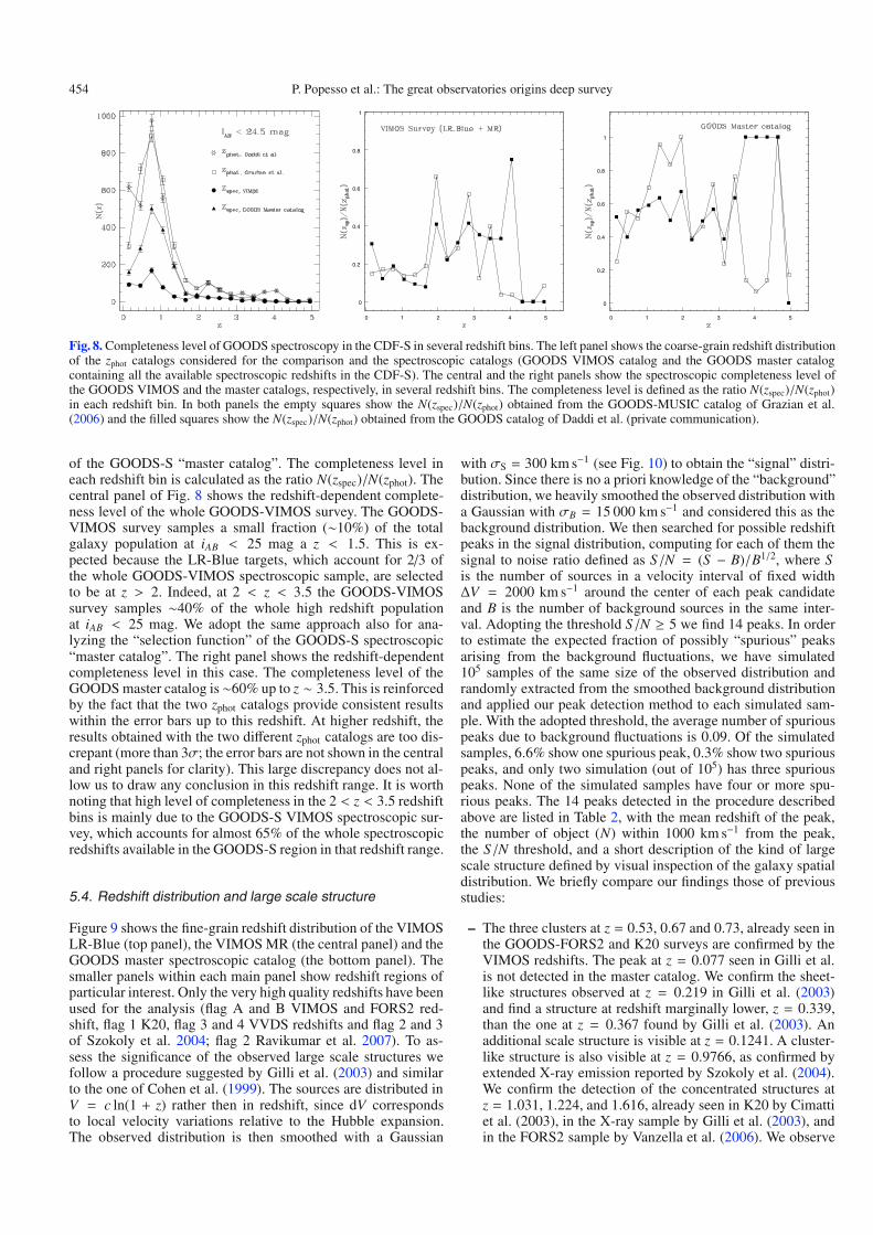
Fig. 8. Completeness level of GOODS spectroscopy in the CDF-S in several redshift bins. The left panel shows the coarse-grain redshift distributionof the zphot catalogs considered for the comparison and the spectroscopic catalogs (GOODS VIMOS catalog and the GOODS master catalogcontaining all the available spectroscopic redshifts in the CDF-S). The central and the right panels show the spectroscopic completeness level ofthe GOODS VIMOS and the master catalogs, respectively, in several redshift bins. The completeness level is defined as the ratio N(zspec)/N(zphot)in each redshift bin. In both panels the empty squares show the N(zspec)/N(zphot) obtained from the GOODS-MUSIC catalog of Grazian et al.(2006) and the filled squares show the N(zspec)/N(zphot) obtained from the GOODS catalog of Daddi et al. (private communication).
of the GOODS-S “master catalog”. The completeness level ineach redshift bin is calculated as the ratio N(zspec)/N(zphot). Thecentral panel of Fig. 8 shows the redshift-dependent complete-ness level of the whole GOODS-VIMOS survey. The GOODS-VIMOS survey samples a small fraction ("10%) of the totalgalaxy population at iAB < 25 mag a z < 1.5. This is ex-pected because the LR-Blue targets, which account for 2/3 ofthe whole GOODS-VIMOS spectroscopic sample, are selectedto be at z > 2. Indeed, at 2 < z < 3.5 the GOODS-VIMOSsurvey samples "40% of the whole high redshift populationat iAB < 25 mag. We adopt the same approach also for ana-lyzing the “selection function” of the GOODS-S spectroscopic“master catalog”. The right panel shows the redshift-dependentcompleteness level in this case. The completeness level of theGOODS master catalog is "60% up to z " 3.5. This is reinforcedby the fact that the two zphot catalogs provide consistent resultswithin the error bars up to this redshift. At higher redshift, theresults obtained with the two di!erent zphot catalogs are too dis-crepant (more than 3"; the error bars are not shown in the centraland right panels for clarity). This large discrepancy does not al-low us to draw any conclusion in this redshift range. It is worthnoting that high level of completeness in the 2 < z < 3.5 redshiftbins is mainly due to the GOODS-S VIMOS spectroscopic sur-vey, which accounts for almost 65% of the whole spectroscopicredshifts available in the GOODS-S region in that redshift range.
5.4. Redshift distribution and large scale structure
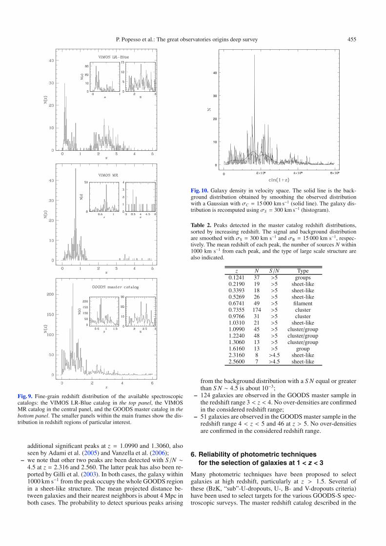
Figure 9 shows the fine-grain redshift distribution of the VIMOSLR-Blue (top panel), the VIMOS MR (the central panel) and theGOODS master spectroscopic catalog (the bottom panel). Thesmaller panels within each main panel show redshift regions ofparticular interest. Only the very high quality redshifts have beenused for the analysis (flag A and B VIMOS and FORS2 red-shift, flag 1 K20, flag 3 and 4 VVDS redshifts and flag 2 and 3of Szokoly et al. 2004; flag 2 Ravikumar et al. 2007). To as-sess the significance of the observed large scale structures wefollow a procedure suggested by Gilli et al. (2003) and similarto the one of Cohen et al. (1999). The sources are distributed inV = c ln(1 + z) rather then in redshift, since dV correspondsto local velocity variations relative to the Hubble expansion.The observed distribution is then smoothed with a Gaussian
with "S = 300 km s#1 (see Fig. 10) to obtain the “signal” distri-bution. Since there is no a priori knowledge of the “background”distribution, we heavily smoothed the observed distribution witha Gaussian with "B = 15 000 km s#1 and considered this as thebackground distribution. We then searched for possible redshiftpeaks in the signal distribution, computing for each of them thesignal to noise ratio defined as S/N = (S # B)/B1/2, where Sis the number of sources in a velocity interval of fixed width%V = 2000 km s#1 around the center of each peak candidateand B is the number of background sources in the same inter-val. Adopting the threshold S/N + 5 we find 14 peaks. In orderto estimate the expected fraction of possibly “spurious” peaksarising from the background fluctuations, we have simulated105 samples of the same size of the observed distribution andrandomly extracted from the smoothed background distributionand applied our peak detection method to each simulated sam-ple. With the adopted threshold, the average number of spuriouspeaks due to background fluctuations is 0.09. Of the simulatedsamples, 6.6% show one spurious peak, 0.3% show two spuriouspeaks, and only two simulation (out of 105) has three spuriouspeaks. None of the simulated samples have four or more spu-rious peaks. The 14 peaks detected in the procedure describedabove are listed in Table 2, with the mean redshift of the peak,the number of object (N) within 1000 km s#1 from the peak,the S/N threshold, and a short description of the kind of largescale structure defined by visual inspection of the galaxy spatialdistribution. We briefly compare our findings those of previousstudies:
– The three clusters at z = 0.53, 0.67 and 0.73, already seen inthe GOODS-FORS2 and K20 surveys are confirmed by theVIMOS redshifts. The peak at z = 0.077 seen in Gilli et al.is not detected in the master catalog. We confirm the sheet-like structures observed at z = 0.219 in Gilli et al. (2003)and find a structure at redshift marginally lower, z = 0.339,than the one at z = 0.367 found by Gilli et al. (2003). Anadditional scale structure is visible at z = 0.1241. A cluster-like structure is also visible at z = 0.9766, as confirmed byextended X-ray emission reported by Szokoly et al. (2004).We confirm the detection of the concentrated structures atz = 1.031, 1.224, and 1.616, already seen in K20 by Cimattiet al. (2003), in the X-ray sample by Gilli et al. (2003), andin the FORS2 sample by Vanzella et al. (2006). We observe
P. Popesso et al.: The great observatories origins deep survey 455
Fig. 9. Fine-grain redshift distribution of the available spectroscopiccatalogs: the VIMOS LR-Blue catalog in the top panel, the VIMOSMR catalog in the central panel, and the GOODS master catalog in thebottom panel. The smaller panels within the main frames show the dis-tribution in redshift regions of particular interest.
additional significant peaks at z = 1.0990 and 1.3060, alsoseen by Adami et al. (2005) and Vanzella et al. (2006);
– we note that other two peaks are been detected with S/N "4.5 at z = 2.316 and 2.560. The latter peak has also been re-ported by Gilli et al. (2003). In both cases, the galaxy within1000 km s#1 from the peak occupy the whole GOODS regionin a sheet-like structure. The mean projected distance be-tween galaxies and their nearest neighbors is about 4 Mpc inboth cases. The probability to detect spurious peaks arising
0
0
10
20
30
40
Fig. 10. Galaxy density in velocity space. The solid line is the back-ground distribution obtained by smoothing the observed distributionwith a Gaussian with "C = 15 000 km s#1 (solid line). The galaxy dis-tribution is recomputed using "S = 300 km s#1 (histogram).
Table 2. Peaks detected in the master catalog redshift distributions,sorted by increasing redshift. The signal and background distributionare smoothed with "S = 300 km s#1 and "B = 15 000 km s#1, respec-tively. The mean redshift of each peak, the number of sources N within1000 km s#1 from each peak, and the type of large scale structure arealso indicated.
z N S/N Type0.1241 37 >5 groups0.2190 19 >5 sheet-like0.3393 18 >5 sheet-like0.5269 26 >5 sheet-like0.6741 49 >5 filament0.7355 174 >5 cluster0.9766 31 >5 cluster1.0310 21 >5 sheet-like1.0990 45 >5 cluster/group1.2240 48 >5 cluster/group1.3060 13 >5 cluster/group1.6160 13 >5 group2.3160 8 >4.5 sheet-like2.5600 7 >4.5 sheet-like
from the background distribution with a S N equal or greaterthan S N " 4.5 is about 10#3;
– 124 galaxies are observed in the GOODS master sample inthe redshift range 3 < z < 4. No over-densities are confirmedin the considered redshift range;
– 51 galaxies are observed in the GOODS master sample in theredshift range 4 < z < 5 and 46 at z > 5. No over-densitiesare confirmed in the considered redshift range.
6. Reliability of photometric techniquesfor the selection of galaxies at 1 < z < 3
Many photometric techniques have been proposed to selectgalaxies at high redshift, particularly at z > 1.5. Several ofthese (BzK, “sub”-U-dropouts, U-, B- and V-dropouts criteria)have been used to select targets for the various GOODS-S spec-troscopic surveys. The master redshift catalog described in the
456 P. Popesso et al.: The great observatories origins deep survey
0 2 4 6-2
0
2
4
0 2 4 6-2
0
2
4
0 2 4 6-2
0
2
4
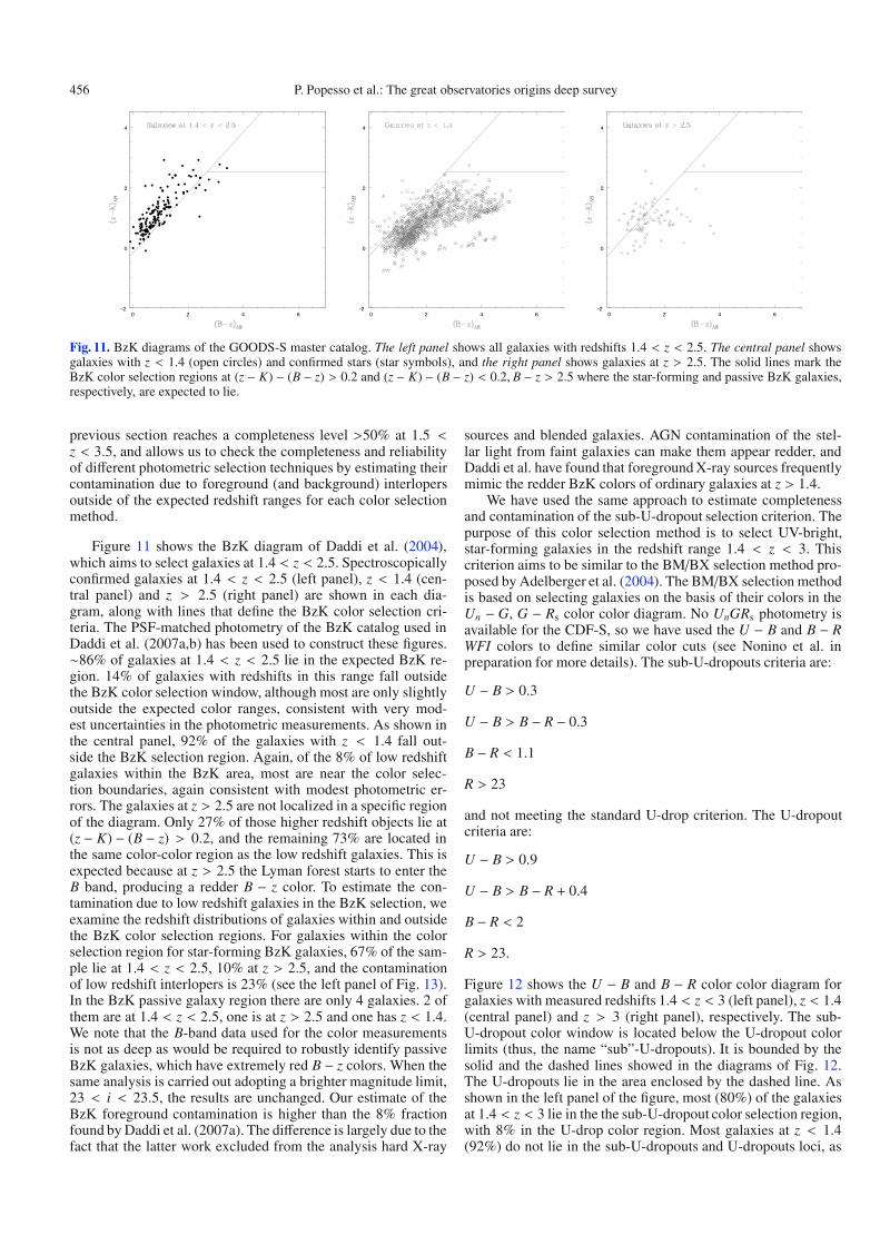
Fig. 11. BzK diagrams of the GOODS-S master catalog. The left panel shows all galaxies with redshifts 1.4 < z < 2.5. The central panel showsgalaxies with z < 1.4 (open circles) and confirmed stars (star symbols), and the right panel shows galaxies at z > 2.5. The solid lines mark theBzK color selection regions at (z # K) # (B # z) > 0.2 and (z # K) # (B # z) < 0.2, B # z > 2.5 where the star-forming and passive BzK galaxies,respectively, are expected to lie.
previous section reaches a completeness level >50% at 1.5 <z < 3.5, and allows us to check the completeness and reliabilityof di!erent photometric selection techniques by estimating theircontamination due to foreground (and background) interlopersoutside of the expected redshift ranges for each color selectionmethod.
Figure 11 shows the BzK diagram of Daddi et al. (2004),which aims to select galaxies at 1.4 < z < 2.5. Spectroscopicallyconfirmed galaxies at 1.4 < z < 2.5 (left panel), z < 1.4 (cen-tral panel) and z > 2.5 (right panel) are shown in each dia-gram, along with lines that define the BzK color selection cri-teria. The PSF-matched photometry of the BzK catalog used inDaddi et al. (2007a,b) has been used to construct these figures."86% of galaxies at 1.4 < z < 2.5 lie in the expected BzK re-gion. 14% of galaxies with redshifts in this range fall outsidethe BzK color selection window, although most are only slightlyoutside the expected color ranges, consistent with very mod-est uncertainties in the photometric measurements. As shown inthe central panel, 92% of the galaxies with z < 1.4 fall out-side the BzK selection region. Again, of the 8% of low redshiftgalaxies within the BzK area, most are near the color selec-tion boundaries, again consistent with modest photometric er-rors. The galaxies at z > 2.5 are not localized in a specific regionof the diagram. Only 27% of those higher redshift objects lie at(z # K) # (B # z) > 0.2, and the remaining 73% are located inthe same color-color region as the low redshift galaxies. This isexpected because at z > 2.5 the Lyman forest starts to enter theB band, producing a redder B # z color. To estimate the con-tamination due to low redshift galaxies in the BzK selection, weexamine the redshift distributions of galaxies within and outsidethe BzK color selection regions. For galaxies within the colorselection region for star-forming BzK galaxies, 67% of the sam-ple lie at 1.4 < z < 2.5, 10% at z > 2.5, and the contaminationof low redshift interlopers is 23% (see the left panel of Fig. 13).In the BzK passive galaxy region there are only 4 galaxies. 2 ofthem are at 1.4 < z < 2.5, one is at z > 2.5 and one has z < 1.4.We note that the B-band data used for the color measurementsis not as deep as would be required to robustly identify passiveBzK galaxies, which have extremely red B # z colors. When thesame analysis is carried out adopting a brighter magnitude limit,23 < i < 23.5, the results are unchanged. Our estimate of theBzK foreground contamination is higher than the 8% fractionfound by Daddi et al. (2007a). The di!erence is largely due to thefact that the latter work excluded from the analysis hard X-ray
sources and blended galaxies. AGN contamination of the stel-lar light from faint galaxies can make them appear redder, andDaddi et al. have found that foreground X-ray sources frequentlymimic the redder BzK colors of ordinary galaxies at z > 1.4.
We have used the same approach to estimate completenessand contamination of the sub-U-dropout selection criterion. Thepurpose of this color selection method is to select UV-bright,star-forming galaxies in the redshift range 1.4 < z < 3. Thiscriterion aims to be similar to the BM/BX selection method pro-posed by Adelberger et al. (2004). The BM/BX selection methodis based on selecting galaxies on the basis of their colors in theUn # G, G # Rs color color diagram. No UnGRs photometry isavailable for the CDF-S, so we have used the U # B and B # RWFI colors to define similar color cuts (see Nonino et al. inpreparation for more details). The sub-U-dropouts criteria are:
U # B > 0.3
U # B > B # R # 0.3
B # R < 1.1
R > 23
and not meeting the standard U-drop criterion. The U-dropoutcriteria are:
U # B > 0.9
U # B > B # R + 0.4
B # R < 2
R > 23.
Figure 12 shows the U # B and B # R color color diagram forgalaxies with measured redshifts 1.4 < z < 3 (left panel), z < 1.4(central panel) and z > 3 (right panel), respectively. The sub-U-dropout color window is located below the U-dropout colorlimits (thus, the name “sub”-U-dropouts). It is bounded by thesolid and the dashed lines showed in the diagrams of Fig. 12.The U-dropouts lie in the area enclosed by the dashed line. Asshown in the left panel of the figure, most (80%) of the galaxiesat 1.4 < z < 3 lie in the the sub-U-dropout color selection region,with 8% in the U-drop color region. Most galaxies at z < 1.4(92%) do not lie in the sub-U-dropouts and U-dropouts loci, as
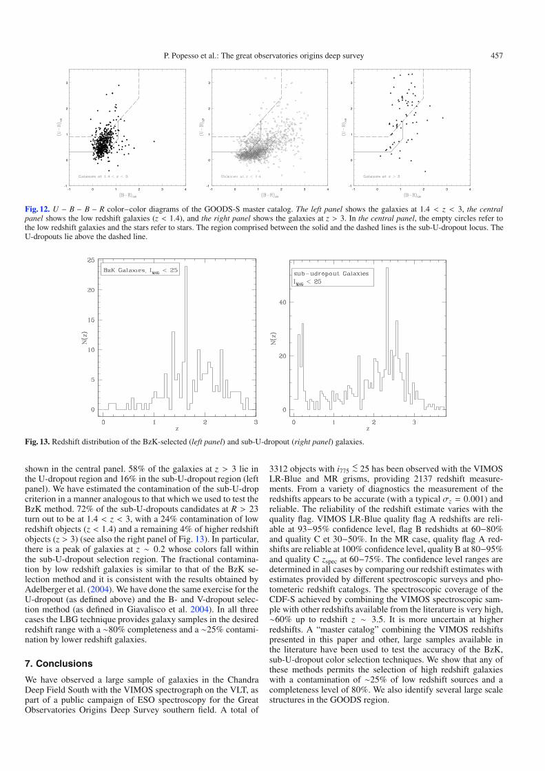
P. Popesso et al.: The great observatories origins deep survey 457
-1 0 1 2 3 4-1
0
1
2
3
-1 0 1 2 3 4-1
0
1
2
3
-1 0 1 2 3 4-1
0
1
2
3
Fig. 12. U # B # B # R color#color diagrams of the GOODS-S master catalog. The left panel shows the galaxies at 1.4 < z < 3, the centralpanel shows the low redshift galaxies (z < 1.4), and the right panel shows the galaxies at z > 3. In the central panel, the empty circles refer tothe low redshift galaxies and the stars refer to stars. The region comprised between the solid and the dashed lines is the sub-U-dropout locus. TheU-dropouts lie above the dashed line.
Fig. 13. Redshift distribution of the BzK-selected (left panel) and sub-U-dropout (right panel) galaxies.
shown in the central panel. 58% of the galaxies at z > 3 lie inthe U-dropout region and 16% in the sub-U-dropout region (leftpanel). We have estimated the contamination of the sub-U-dropcriterion in a manner analogous to that which we used to test theBzK method. 72% of the sub-U-dropouts candidates at R > 23turn out to be at 1.4 < z < 3, with a 24% contamination of lowredshift objects (z < 1.4) and a remaining 4% of higher redshiftobjects (z > 3) (see also the right panel of Fig. 13). In particular,there is a peak of galaxies at z " 0.2 whose colors fall withinthe sub-U-dropout selection region. The fractional contamina-tion by low redshift galaxies is similar to that of the BzK se-lection method and it is consistent with the results obtained byAdelberger et al. (2004). We have done the same exercise for theU-dropout (as defined above) and the B- and V-dropout selec-tion method (as defined in Giavalisco et al. 2004). In all threecases the LBG technique provides galaxy samples in the desiredredshift range with a "80% completeness and a "25% contami-nation by lower redshift galaxies.
7. Conclusions
We have observed a large sample of galaxies in the ChandraDeep Field South with the VIMOS spectrograph on the VLT, aspart of a public campaign of ESO spectroscopy for the GreatObservatories Origins Deep Survey southern field. A total of
3312 objects with i775 "< 25 has been observed with the VIMOSLR-Blue and MR grisms, providing 2137 redshift measure-ments. From a variety of diagnostics the measurement of theredshifts appears to be accurate (with a typical "z = 0.001) andreliable. The reliability of the redshift estimate varies with thequality flag. VIMOS LR-Blue quality flag A redshifts are reli-able at 93#95% confidence level, flag B redshidts at 60#80%and quality C et 30#50%. In the MR case, quality flag A red-shifts are reliable at 100% confidence level, quality B at 80#95%and quality C zspec at 60#75%. The confidence level ranges aredetermined in all cases by comparing our redshift estimates withestimates provided by di!erent spectroscopic surveys and pho-tometeric redshift catalogs. The spectroscopic coverage of theCDF-S achieved by combining the VIMOS spectroscopic sam-ple with other redshifts available from the literature is very high,"60% up to redshift z " 3.5. It is more uncertain at higherredshifts. A “master catalog” combining the VIMOS redshiftspresented in this paper and other, large samples available inthe literature have been used to test the accuracy of the BzK,sub-U-dropout color selection techniques. We show that any ofthese methods permits the selection of high redshift galaxieswith a contamination of "25% of low redshift sources and acompleteness level of 80%. We also identify several large scalestructures in the GOODS region.
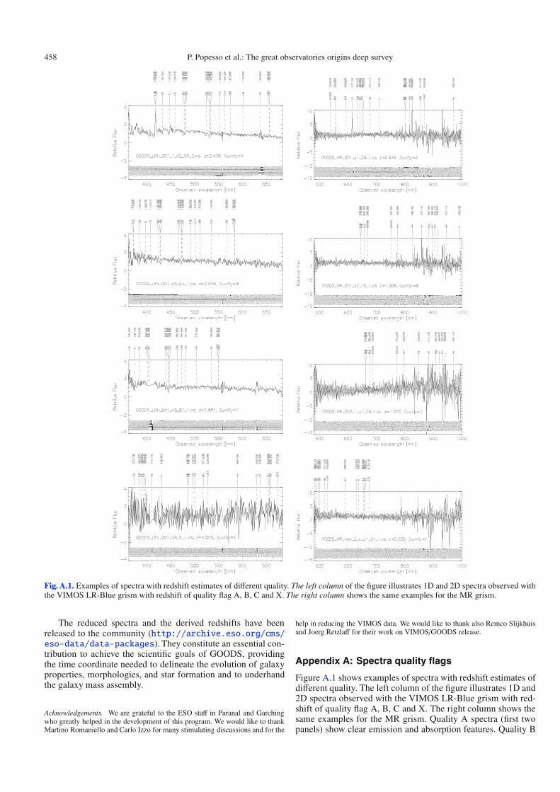
458 P. Popesso et al.: The great observatories origins deep survey
Fig. A.1. Examples of spectra with redshift estimates of di!erent quality. The left column of the figure illustrates 1D and 2D spectra observed withthe VIMOS LR-Blue grism with redshift of quality flag A, B, C and X. The right column shows the same examples for the MR grism.
The reduced spectra and the derived redshifts have beenreleased to the community (http://archive.eso.org/cms/eso-data/data-packages). They constitute an essential con-tribution to achieve the scientific goals of GOODS, providingthe time coordinate needed to delineate the evolution of galaxyproperties, morphologies, and star formation and to underhandthe galaxy mass assembly.
Acknowledgements. We are grateful to the ESO sta! in Paranal and Garchingwho greatly helped in the development of this program. We would like to thankMartino Romaniello and Carlo Izzo for many stimulating discussions and for the
help in reducing the VIMOS data. We would like to thank also Remco Slijkhuisand Joerg Retzla! for their work on VIMOS/GOODS release.
Appendix A: Spectra quality flags
Figure A.1 shows examples of spectra with redshift estimates ofdi!erent quality. The left column of the figure illustrates 1D and2D spectra observed with the VIMOS LR-Blue grism with red-shift of quality flag A, B, C and X. The right column shows thesame examples for the MR grism. Quality A spectra (first twopanels) show clear emission and absorption features. Quality B
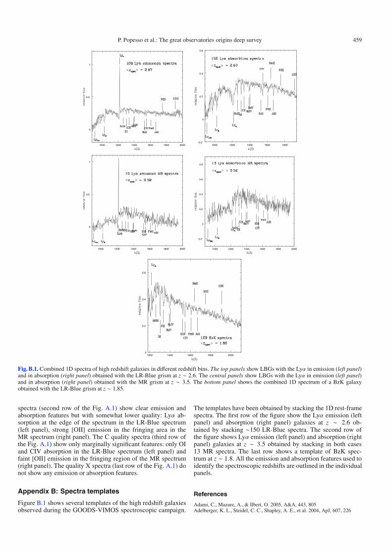
P. Popesso et al.: The great observatories origins deep survey 459
1000 1200 1400 1600 1800 2000
0
0.5
1
1000 1200 1400 1600 1800-0.2
0
0.2
0.4
0.6
1000 1200 1400 1600 1800 2000
0
0.5
1
1000 1200 1400 1600 1800 2000
-0.2
0
0.2
0.4
0.6
0.8
1200 1400 1600 1800 20000
0.2
0.4
0.6
Fig. B.1. Combined 1D spectra of high redshift galaxies in di!erent redshift bins. The top panels show LBGs with the Ly# in emission (left panel)and in absorption (right panel) obtained with the LR-Blue grism at z " 2.6. The central panels show LBGs with the Ly# in emission (left panel)and in absorption (right panel) obtained with the MR grism at z " 3.5. The bottom panel shows the combined 1D spectrum of a BzK galaxyobtained with the LR-Blue grism at z " 1.85.
spectra (second row of the Fig. A.1) show clear emission andabsorption features but with somewhat lower quality: Ly# ab-sorption at the edge of the spectrum in the LR-Blue spectrum(left panel), strong [OII] emission in the fringing area in theMR spectrum (right panel). The C quality spectra (third row ofthe Fig. A.1) show only marginally significant features: only OIand CIV absorption in the LR-Blue spectrum (left panel) andfaint [OII] emission in the fringing region of the MR spectrum(right panel). The quality X spectra (last row of the Fig. A.1) donot show any emission or absorption features.
Appendix B: Spectra templates
Figure B.1 shows several templates of the high redshift galaxiesobserved during the GOODS-VIMOS spectroscopic campaign.
The templates have been obtained by stacking the 1D rest-framespectra. The first row of the figure show the Ly# emission (leftpanel) and absorption (right panel) galaxies at z " 2.6 ob-tained by stacking "150 LR-Blue spectra. The second row ofthe figure shows Ly# emission (left panel) and absorption (rightpanel) galaxies at z " 3.5 obtained by stacking in both cases13 MR spectra. The last row shows a template of BzK spec-trum at z " 1.8. All the emission and absorption features used toidentify the spectroscopic redshifts are outlined in the individualpanels.
References
Adami, C., Mazure, A., & Ilbert, O. 2005, A&A, 443, 805Adelberger, K. L., Steidel, C. C., Shapley, A. E., et al. 2004, ApJ, 607, 226
460 P. Popesso et al.: The great observatories origins deep survey
Bottini, D., Garilli, B., Maccagni, D., et al. 2005, PASP, 117, 996Cimatti, A., Mignoli, M., Daddi, E., et al. 2002, A&A, 392, 395Cohen, J. G., Blandford, R., Hogg, D. W., et al. 1999, ApJ, 512,30Daddi, E., Cimatti, A., Renzini, A., et al. 2004, ApJ, 617, 746Daddi, E., Alexander, D. M., Dickinson, M., et al. 2007a, ApJ, 670, 173Daddi, E., Dickinson, M., Morrison, G., et al. 2007b, ApJ, 670, 156Dickinson, M., Giavalisco, M., & The Goods Team 2003, in The Mass of
Galaxies at Low and High Redshift: Proc. of the ESO/USM Workshop(Venice, Italy, October 2001), ed. R. Bender, & A. Renzini, 324
Giacconi, R., Zirm, A., Wang, J., et al. 2002, ApJS, 139, 369Giavalisco, M., Ferguson, H. C., Koekemoer, A. M., et al. 2004, ApJ, 600, L93Gilli, R., Cimatti, A., Daddi, E., et al. 2003, ApJ, 592, 721Grazian, A., Fontana, A., de Santis, C., et al. 2006, A&A, 449, 951Horne, K. 1986, PASP, 98, 609Kirby, E. N., Guhathakurta, P., Faber, S. M., et al. 2007, ApJ, 660, 62Kurtz, M. J., & Mink, D. J. 1998, PASP, 110, 934
Lee, K. S., Giavalisco, M., Gnedin, O. Y., et al. 2006, ApJ, 642, 63Le Fevre, O., Vettolani, G., Maccagni, D., et al. 2003, SPIE, 4834, 173Le Fevre, O., Vettolani, G., Paltani, S., et al. 2005, A&A, 428, 1043Lehmer, B. D., Brandt, W. N., Alexander, D. M., et al. 2005, ApJS, 161, 21Ravikumar, C. D., Puech, M., Flores, H., et al. 2007, A&A, 465, 1099Renzini, A., Cesarsky, C., Cristiani, S., et al. 2003, in The Mass of Galaxies
at Low and High Redshift: Proc. of the ESO/USM Workshop (Venice, Italy,October 2001), ed. R. Bender, & A. Renzini, 332
Scodeggio, M., Franzetti, P., Garilli, B., et al. 2005, PASP, 117, 1284Szokoly, G. P., Bergeron, J., Hasinger, G., et al. 2004, ApJS, 155, 271Vanzella, E., Cristiani, S., Dickinson, M., et al. 2005, A&A, 434, 53Vanzella, E., Cristiani, S., Dickinson, M., et al. 2006, A&A, 454, 423Vanzella, E., Cristiani, S., Dickinson, M., et al. 2008, A&A, 478, 83Warmels, R. H. 1991, The ESO-MIDAS System, in Astronomical Data Analysis
Software and Systems I, PASP Conf. Ser., 25, 115