The Genetic Lottery - VU Research Portal

VU Research Portal

The Genetic Lottery

Burik, Casper Adrianus Pieter

2021

document versionPublisher's PDF, also known as Version of record

Link to publication in VU Research Portal

citation for published version (APA)Burik, C. A. P. (2021). The Genetic Lottery: Essays on Genetics, Income and Inequality. Rozenberg Publishers.

General rightsCopyright and moral rights for the publications made accessible in the public portal are retained by the authors and/or other copyright ownersand it is a condition of accessing publications that users recognise and abide by the legal requirements associated with these rights.

• Users may download and print one copy of any publication from the public portal for the purpose of private study or research. • You may not further distribute the material or use it for any profit-making activity or commercial gain • You may freely distribute the URL identifying the publication in the public portal ?

Take down policyIf you believe that this document breaches copyright please contact us providing details, and we will remove access to the work immediatelyand investigate your claim.

E-mail address:[email protected]

Download date: 14. Mar. 2022

https://research.vu.nl/en/publications/44c35033-5177-45b7-bd05-3fe0e640835a

This dissertation develops statistical methods in genetics and with their application answers both old and new questions related to genetics, income and inequality. Chapter 2 develops a new method to support identification of causal effects in nonexperimental data. Additionally, a new method for estimating heritability using two polygenic indices (PGI) from independent genome-wide association studies (GWAS) is developed. In Chapter 3 this new heritability method is explored further and compared to the established and widely used method, genome-based restricted maximum likelihood (GREML). Chapter 4 aims to remove several barriers for researchers wanting to use PGI in their study. In this chapter a broad array of PGI are constructed, covering a wide range of phenotypes for a number of datasets used by social scientists. Furthermore, in this chapter a theoretical framework is introduced for interpreting associations with PGI. In Chapter 5, the first large scale GWAS on personal income is conducted, using data from the UK Biobank. It is shown that a higher PGI is linked to higher education and better health. Chapter 6 builds upon the results of the previous chapter and further investigates the genetic and environmental factors underlying socioeconomic and health inequality. A lower bound is estimated for the relevance of genetic factors and early-childhood environment for differences in education, income and body mass index. Chapter 7 presents the first results of an ongoing research project where the first large-scale GWAS meta-analysis on personal income is performed. The meta-analysis has a total sample size of 1,161,574 observations from approximately 756,000 individuals.

Casper Burik holds a BSc in Economics and Business from the University of Amsterdam, a BSc in Econometrics and Operations Research from the University of Amsterdam, and an MPhil in Econometrics from Tinbergen Institute. His research has been published in leading peer-reviewed journals such as Nature Communications, Nature Human Behaviour, Molecular Psychiatry and Proceedings of the National Academy of Sciences of the United States of America.

Vrije Universiteit Amsterdam

The Genetic Lottery Casper Adrianus Pieter Burik

Casper Adrianus Pieter Burik

790

The Genetic LotteryEssays on Genetics, Income and Inequality

The Genetic Lottery

Essays on Genetics, Income and Inequality


Vrije Universiteit Amsterdam and Tinbergen Institute

ISBN: 978-90-361-0671-9 Cover design: Crasborn Graphic Designers bno, Valkenburg a.d. Geul Illustration: Casper Burik © Casper Burik, 2021

This book is no. 790 of the Tinbergen Institute Research Series, established through cooperation between Rozenberg Publishers and the Tinbergen Institute. A list of books which already appeared in the series can be found in the back.

VRIJE UNIVERSITEIT

THE GENETIC LOTTERY

Essays on Genetics, Income and Inequality

ACADEMISCH PROEFSCHRIFT

ter verkrijging van de graad Doctor aan de Vrije Universiteit Amsterdam, op gezag van de rector magnificus

prof.dr. C.M. van Praag, in het openbaar te verdedigen

ten overstaan van de promotiecommissie van de School of Business and Economics

op woensdag 15 december 2021 om 15.45 uur in een bijeenkomst van de universiteit,

De Boelelaan 1105

door


geboren te Capelle aan Den IJssel

promotoren: prof.dr. P.D. Koellinger

prof.dr. M. Lindeboom

copromotoren: dr. A. Okbay

dr. R. de Vlaming

promotiecommissie: prof.dr. B. van der Klaauw

prof.dr. M.C. Keller prof.dr. J.L.W. van Kippersluis dr. N.M. Davies prof.dr. D.I. Boomsma dr. W.D. Hill

To Mayra

Contents

Chapter 1 Introduction

p. 1

Chapter 2 Genetic instrumental variable regression: Explaining socioeconomic and

health outcomes in nonexperimental data

p. 19

Supplementary Information

p. 53

Chapter 3 A comparison of heritability estimates from GIV regression and GREML

p. 117

Chapter 4 Resource Profile and User Guide of the Polygenic Index Repository

p. 129

Chapter 5 Genetic Fortune: Winning or Losing Education, Income, and Health

p. 181


p. 229

Chapter 6 Disparities in socio-economic status and BMI in the UK are partly due to

genetic and environmental luck

p. 299


p. 325

Chapter 7 A large-scale meta-analysis of genome-wide association studies on income

p. 337

Acknowledgements p. 387

1

Chapter 1 Introduction

Chapter 1

2

“The disposition to admire, and almost to worship, the rich and the powerful, and to despise, or, at least,

to neglect persons of poor and mean condition is the great and most universal cause of the corruption of

our moral sentiments.”

Adam Smith (1759), The Theory of Moral Sentiments

1.1 Why integrate genetics into economics?

Economics is a social science that studies production, consumption and trades of goods and services.

Usually, economics is split into two parts. Macroeconomics focusses on aggregate markets, studying the

factors that affect production and consumption levels, as well as savings and investments.

Microeconomics analyses individual economic agents: firms, households or individuals, and how they

interact on markets. They are traditionally modelled as rational agents, who optimize their choices to

maximize their profits or utility. Simple or complex models can be made to describe their behaviour.

So why should economists care about genetics? At the end of the day, these economic agents are people

making choices based on their personal preferences. While these choices and preferences may be put into

consumption and utility functions, they remain a description of human behaviour and human traits.

Moreover, half a century of twin studies have shown that every single human trait is heritable to a degree

(Polderman et al., 2015). This observation, that all human traits are heritable, has also been coined “the

first law of behaviour genetics” (Turkheimer, 2000). Of course, the researched traits includes

economically relevant outcomes and descriptors like income (Benjamin, Cesarini, Chabris, et al., 2012;

Hill et al., 2019; Taubman, 1976), educational attainment (de Vlaming et al., 2017; Lee et al., 2018;

Okbay et al., 2016; Rietveld et al., 2013) and risk preferences (Karlsson Linnér et al., 2019).

Many potential uses of genetic data in economics and other social sciences have been described in the

literature (Beauchamp et al., 2011; Benjamin et al., 2012; Freese, 2018; Harden & Koellinger, 2020). I

will summarise several of them below. Following this summary, I will describe the tools and methods

available to include genetic data in social sciences. Next, I will describe the contributions this thesis

makes to the literature, based on the research conducted in the following chapters. I will end with a

statement of my personal contributions to each chapter.

First, genetic research in economics provides an opportunity to measure otherwise unobserved

differences between individuals. As genetic factors may be descriptive of differences between people,

Introduction

3

they provide economists a chance to measure heterogeneity in economic agents. Economists may

describe people as economic agents optimizing their utility based on how they value outcomes and costs.

The differences in choices individual agents make, may be attributed to differences in individual

preferences. However, measures of these preferences remain elusive as self-reported preferences are often

mistrusted. The preferred option is to rely on revealed preferences (Samuelson, 1948). Genetic

heterogeneity in economic agents may give alternative measures for individual preferences. For example,

one could use the results of a recently published genome-wide association study (GWAS) of risk

tolerance and risky behaviours (Karlsson Linnér et al., 2019) to create measures of individual risk

preferences. While such GWAS-based measures are noisy and currently cannot be used for individual

level predictions, they may be useful for analyses on the group level.

Furthermore, as genetic factors may be descriptive of individual differences, they can serve as a measure

to study the influences of policy measures in practice. Through gene–by–environment studies (i.e.,

considering interaction effects between genetic factors and environment), we can start to account for

potential heterogeneity in the effects of policy measures. Such efforts may shine a light on who is

benefiting most from certain policy measures, and who is benefitting least. For example, in a recent

study, Barcellos, Carvalho and Turley (2018) analysed the effects of an increase in compulsory schooling

on health and found that increased education leads to better health outcomes and those effects were

stronger among people with a high genetic risk for obesity, thus mitigating (in part) the genetic risk

factors. The uses of gene–by–environment studies are not limited to studying policy measures; such

studies can also be used to investigate interactions between other environmental measures and genetic

factors, as I show in Chapter 2.

Second, measures of genetic factors may be used as control variables. One could simply include these

variables to reduce variance in statistical models (Benjamin, Cesarini, Chabris, et al., 2012). More

importantly though, when studying a relation between explanatory variable and outcome in non-

experimental data, confounding is always a serious concern. When genetic factors between explanatory

variables and outcome are shared or correlated, not controlling for it would lead to biased estimation

results. For example, a labour economist, interested in estimating the returns to schooling while

controlling for confounding factors such as cognitive ability, may create a proxy for ability using the

results from a genetic study on cognitive performance (Davies et al., 2018) or educational attainment

Chapter 1

4

(Lee et al., 2018). In Chapter 2, I extensively explore such research designs using genetic factors as

control variables.

Third, as genotypes can be seen as random draws from parental genotypes, they are a good candidate for

instrumental variable regression. The use of genotypes as instruments is called Mendelian

Randomisation (MR; Davey Smith & Ebrahim, 2004). While MR is a promising concept and it could be

used for medical outcomes that are only affected by a handful of genes, the use for social sciences is

severely limited by several factors. First, socioeconomic outcomes and behavioural traits are generally

genetically complex, meaning that they are affected by a large number of genes that individually have

small effects (Chabris et al., 2015). Such genetic complexity could lead to the well-known problem of

weak instruments (Hahn & Hausman, 2003), although the large increases in sample sizes of genotyped

individuals in the last decade may abate this issue to some degree. Second, there is the possibility of genes

affecting multiple outcomes, a phenomenon known as pleiotropy. As a result of pleiotropy, the genes

that are used as instruments may affect both the explanatory variable and the outcome (Chen et al.,

2016), violating the basic assumptions of instrumental variable regression. Third, while genotypes are

random draws of parental genotypes, the possibility exists that parental genotypes indirectly influence

the outcomes of their offspring (Kong et al., 2018). This possibility might be especially true for

socioeconomic outcomes. There are multiple promising augmentations of MR to address some of these

issues (Bowden, Davey Smith, & Burgess, 2015; Verbanck, Chen, Neale, & Do, 2018; Zhu et al., 2018).

However, these approaches are all dependent on varying sets of assumptions that may fail to hold in

practice.

Finally, the wealth of data and methods that genetics brings to economics not only helps us to re-

examine the answers to old questions, but also enables us to answer questions that we could not answer

at all before. For example, in Chapters 5–7 we estimate the effects of genetic factors on inequality in

income, education and health. We show, using random genetic differences between siblings, that these

effects are partially causal. This result raises new questions about the underlying mechanisms that cause

disparities in such important life outcomes. Moreover, the same result also raises questions about

fairness, as these disparities are not caused by people themselves, but rather through a genetic lottery at

conception. However, nothing in our research implies that the effects of genetic factors on

socioeconomic outcomes are biologically predetermined. The channels through which genetic factors

operate could be purely environmental. As mentioned above Barcellos, Carvalho and Turley (2018)

Introduction

5

show that the genetic risk factors for obesity can (in part) be mitigated through additional education.

Similarly, the genetic factors driving part of inequalities in income may be mitigated with policy changes.

1.2 Methods in social-science genetics

Twin studies have been a central tool in genetics since the 70s. A large meta-analysis of 2,748

publications on twin studies has shown that all studied traits are heritable to some degree (Polderman et

al., 2015). In twin studies, one compares the correlation of phenotypes between monozygotic (MZ)

twins, also known as identical twins, with the correlation between dizygotic (DZ) twins, also known as

fraternal twins. MZ twins share all of their DNA and DZ twins share the same amount of DNA as

regular siblings. By studying differences in correlations between MZ twin pairs and DZ twin pairs, you

can estimate the heritability of a trait (the proportion of phenotypic variance that may be attributed to

genetic effects). Twin models can be extended to estimate more than just heritability. However, using

only twin models constrains the range of possible studies that can be done as the underlying genetic

markers are not measured in classical twin models and the models typically need constraining

assumptions on the environments of twins.

Fortunately, technological advances made way for many new opportunities to study genetics. Two

decades ago, the International Human Genome Project published sequences of the human genome

(Lander et al., 2001; Venter et al., 2001). The human genome consists of 23 pairs of chromosomes, each

chromosome is a sequence of DNA molecules. They can be denoted by a chain of four letters, ‘G’, ‘C’,

‘T’ and ‘A’, representing the four different possible nucleobases of the nucleotides forming the sequence

(guanine, cytosine, thymine and adenine). Most of the sequence is identical for all human beings (The

1000 Genomes Project Consortium, 2015). However, since there are approximately 3 billion nucleotide

pairs in the human DNA sequence, there is still a plethora of variation to study. The most common

variation comes in the form of single nucleotide polymorphisms (SNPs), these are variations in a single

base-pairs creating two possible alleles. Where one person may have a ‘C’ in the sequence, another may

have a ‘T’. As one inherits one copy of each chromosome from each parent (excluding the sex

chromosomes), this can be summarized in simple count variables where one individual can have 0, 1, or 2

of the reference alleles.

Chapter 1

6

Since the International Human Genome Project, many more advances have been made and with cheap

commercial genotyping arrays (chips that allow measurement of hundreds of thousands of markers at

the same time) now available, the cost of genotyping has gone down substantially. This decrease in costs

made it possible to genotype individuals on an increasingly larger scale and led to the creation of large

scale Biobanks, like the UK Biobank which contains the genotypes of approximately half a million Brits

(Fry et al., 2017; Sudlow et al., 2015).

The availability of all this data has made it possible for researchers to test the associations of SNPs with

various human traits on a much larger scale than ever before. The standard approach is to do hypothesis-

free testing in the form of genome-wide association studies (GWAS). In a GWAS all available SNPs are

tested in separate regression models on their association with the phenotype. Here, the statistical

significance thresholds are set very stringent to account for the testing of millions of SNPs. GWAS are

typically done in samples of individuals with similar ancestries and the leading principal components

from the genetic data are added as control variables to account for population structure (Price et al.,

2006), which limits the possibility of spurious findings due to unobserved variable bias where

environments are correlated to individual markers due to ancestry being correlated to both environments

and individual markers. Finally, GWAS studies often include replication in a sample that is independent

from their discovery sample to further reduce the possibility of spurious findings.

The results of GWAS studies allow for many follow-up analyses. For instance, bioinformatics tools

allowed Lee et al. (2018) to find that the genes that lie close to the SNPs most strongly associated with

educational attainment are overwhelmingly expressed in tissues related to the brain and central nervous

system. Furthermore, by analysing the results of GWAS for multiple phenotypes, it is possible to

calculate genetic correlations directly from the GWAS results (Bulik-Sullivan et al., 2015a; Bulik-Sullivan

et al., 2015b), which can lead to new insights on how phenotypes are related to each other as well as aid

in the discovery of the channels through which SNPs affect the studied phenotypes. This is even possible

when two phenotypes have never been measured in the same sample. The creation of LD Hub (Zheng et

al., 2017), an online repository to calculate genetic correlations, has made it especially convenient to

include this in follow-up analyses to GWAS.

Introduction

7

Finally, one of the most valuable tools for economists and social-scientists, who want to do genetically

informed analyses, is the use of polygenic indices (PGI)1. The results of various GWAS of social-science

outcomes show that those traits are usually genetically complex (Chabris et al., 2015), meaning that the

effects of individual SNPs are very small, yet all SNPs combined can explain a substantial amount of

variance. Of course, it’s impractical or impossible to include thousands or potentially millions of markers

into a single regression model. A convenient work-around is to create a single index for every individual,

wherein the effects of the individual SNPs are summed up. This can be as simple as a weighted sum of all

genotypes, where the weights are the estimated GWAS effect sizes. However, more elegant solutions are

advised to account for the correlation structure between SNPs (Vilhjálmsson et al., 2015). These PGI

have proven to be very valuable in social-science genetics and play a crucial role throughout this thesis.

The use of PGI to study within-sibling differences may be especially powerful as it provides the

opportunity to control for family-specific environments while studying the effects of genetic factors on

your outcome of interest.

1.3 Contributions of this thesis

The contributions of this thesis can be divided in two main categories. The first is providing fellow

scientists with new tools to do research with. These tools come in the form of new statistical methods

and the production of new variables and data made available for others to use (i.e., PGI and GWAS

summary statistics). The second category of contributions is the applications of these new methods

together with existing methods in answering both old and new questions related to genetics, income and

inequality. The rest of this section will summarize the findings and contributions of each chapter.

In Chapter 2 we develop a new method to support identification of causal effects in nonexperimental

data. While some experiments may be done in economics and other social sciences, often ethical and legal

considerations constrain them. Therefore, many analyses will be done using nonexperimental data,

which often limits the causal interpretation of the findings.

An often-used technique to circumvent this problem is using instrumental variable methods. One of the

methods suggested by the literature is Mendelian Randomisation, discussed earlier in this chapter. Yet its

1 Here I use the relatively new term PGI instead of the commonly used polygenic score (PGS) or polygenic risk score (PRS), which was suggested by members of the scientific community to make it less likely to be wrongly interpreted as a value judgement.

Chapter 1

8

usefulness is limited due to SNPs possibly affecting multiple outcomes (pleiotropy). As socio-economic

outcomes are often biologically distal and genetically complex, the channels through which SNPs

operate are often unknown. This prohibits their use as instruments as they may violate the exclusion

restriction for instrumental variables. Moreover, the SNPs themselves may cause bias due to pleiotropy

by possibly confounding relations when they are not controlled for.

In this chapter we develop Genetic Instrumental Variables regression (GIV) to deal with the possible

biases due to pleiotropic effects between an exposure and outcome. Naïvely using PGI as control

variables is not sufficient in this case, because PGI are only noisy estimates of the underlying genetic

architecture. This creates a problem equivalent to the classic econometric problem of errors-in-variables.

This problem can be solved using instrumental variable methods if a suitable instrument can be found.

We make use of the fact that multiple PGI can be constructed using GWAS results from independent

samples. If the estimation error in both PGI is independent from each other, then one can be used as an

instrument for the other. We use this idea to design two estimators (GIV-C and GIV-U), which provide

upper and lower bounds for the effect of the exposure on the outcome. We test our method using

simulations for a wide array of scenarios. Our estimator works in most scenarios, except when there is a

strong environmental bias. In an empirical example we use GIV to show how the estimated effects of

body height on education are biased due to pleiotropic effects.

Additionally, during the development of this method, we found that two PGI from independent GWAS

samples for the same trait can be used to estimate heritability. Using PGI for educational attainment we

show that our estimates are close to the heritability estimates obtained using an established and widely-

used method, Genome-based restricted maximum likelihood (GREML; Yang et al., 2010).

We further explored this method for estimating heritability in Chapter 3. While the project was shelved

before a manuscript was written, a summary of the results is included in this thesis. In this project, we

compare heritability estimates of our GIV method to GREML. While GIV requires the availability of

two independent samples for GWAS, it does not require the same assumptions as GREML on trait

architecture, because in this regard it is completely agnostic. Thus, GIV potentially provides better

heritability estimates when the GREML assumptions on trait architecture are not met. We test both our

method and GREML in various scenarios, where some scenarios violate the GREML assumptions.

However, the GREML estimator proved surprisingly resilient to these violations and was proven to be a

Introduction

9

more efficient estimator in all our simulation scenarios. Yet, there may still be applications for which

GIV can be used. It may be possible, with some tweaking, to disentangle genetic nurture and heritability

estimates using within-family GWAS. However, since large scale within-family GWASs are not yet

available, we shelved further development of this method for the time being.

Chapter 4 aims to remove several barriers for researchers wanting to use PGI in their study. First,

creating PGI is a time-consuming process and requires knowledge of the specific software tools used.

Second, to create the most accurate PGI possible one needs to use summary statistics from the largest

GWAS sample possible. However, GWAS summary statistics are not always publicly available, adding

additional hurdles. Third, publicly available GWAS summary statistics often includes the dataset in

which the researcher wants to do their analyses. Such sample overlap may cause biases due to overfitting.

Fourth, comparison of results between studies is often difficult due to different methodologies used by

different researchers.

To address the first hurdle, we construct a broad array of PGI covering a wide range of phenotypes for a

number of datasets used by social scientists. These PGI will be made available for download through the

providers of the datasets. For the second problem, the PGI are constructed from GWAS results from a

meta-analysis for the largest GWAS sample size possible. These meta-analyses include novel GWAS

results and GWAS summary statistics available to us that are not easily obtainable for most researchers.

The third problem is solved by making sure that for each dataset, the provided PGI are constructed from

summary statistics that exclude that dataset. Finally, the PGI are constructed using a uniform

methodology across all phenotypes and datasets, so that results across studies are comparable.

Furthermore, in this chapter a theoretical framework is introduced for interpreting associations with

PGIs. Here, PGIs are shown to be noisy, but unbiased estimators of the additive SNP factor, a term that

is introduced to describe the best linear predictor of the phenotype from the measured genetic variants.

Within this theoretical framework we derive an estimator that corrects for the errors–in–variables bias

that is encountered when using noisy variables in an ordinary least squares framework. This estimator

tackles the same problem described in Chapter 2, but using a different methodology. In Chapter 2, an

instrumental variables approach using multiple PGIs is introduced to derive a consistent estimator. Here,

the errors–in–variables bias is corrected for using a newly derived estimator based on parameters that can

be estimated in the sample where the estimator is implemented.

Chapter 1

10

The last three chapters are about the effects of genetic factors on income and inequalities in income,

education and health. It has long been recognized that parental socioeconomic status is a strong

predictor for children’s health, educational attainment and income. As these traits are all heritable to

some degree (Benjamin et al., 2012; De Vlaming et al., 2017; Polderman et al., 2015; Taubman, 1976),

parents provide both the environment in which their children grow up as well as pass on their genes. In a

way, one has already participated in two lotteries at birth: a social lottery that determines who your

parents are and which environment you grow up in and a genetic lottery that determines which part of

your parent’s genome you have inherited. The results of these two lotteries potentially provide inequal

opportunities in life, through which they may affect disparities in education, income and health.

Moreover, the results of these two lotteries could be correlated, which further exacerbates the resulting

inequalities. Moreover, it provides a major challenge to distinguish different channels through which

economic prosperity is passed on through generations. A better understanding of these channels would

provide an important contribution to the study of causes of socioeconomic disparities and the

mechanisms through which they affect health.

In Chapter 5, we conduct the first large scale GWAS on personal income, using data from the UK

Biobank. We find that approximately 10% of the variation in occupational wages is captured by common

genetic variants. Our findings are validated in two US samples using PGI constructed from our GWAS

results. These PGI capture approximately 1 percent of the variation in these US samples and

approximately 3 percent using a holdout sample in the UK Biobank. A one–standard–deviation increase

in the PGI is associated with a 6 to 8 percent increase in self-reported hourly wages. Using within-sibling

differences in PGI in the UK Biobank we show that part of the covariance between the PGI and income

is causal. Furthermore, we find that a higher PGI is linked to higher education and better health. The

relation between the genetic endowment and health is in part mediated by education. Finally, we show

using GIV regression, that even after controlling for genetic confounding the returns–to–schooling is

strong, suggesting that education may alleviate the inequalities caused by genetic endowments.

In Chapter 6 we build upon the results of Chapter 5 and further investigate the genetic and

environmental factors underlying socioeconomic and health inequality. Here, we estimate a lower

bound for the relevance of genetic factors and early-childhood environment for differences in education,

income and body mass index in a sample of 38,698 siblings in the UK Biobank. Our estimates are based

on models that combine family-fixed effects with gene-by-environment interactions. We find that the

Introduction

11

random differences between siblings in their genetic endowments clearly contribute towards inequalities

in the outcomes we study. Our rough proxy of the environment people grew up in, which we derived

from their place of birth, are also predictive of the studied outcomes, but not beyond the relevance of

family environment. Overall, our estimates suggest that at least 13 to 17 percent of the inequalities in

education, wages and BMI in the UK are due to inequalities in opportunity that arise from the outcomes

of the social and the genetic lottery.

In Chapter 7 we conduct the first large-scale GWAS meta-analysis on personal income. While this large

project is still ongoing, this chapter presents the first phase of the project. The meta-analysis has a total

sample size of 1,161,574 observations from approximately 756,000 individuals using four different

measures of income: personal income, household income, occupational wages and parental income. In

this chapter I present the first phase of the project by summarising the data collection process, the quality

control protocol and presenting the first set of results of this project. The genetic variants underlying

income capture between 4 and 7 percent of the variation in our measures of income. Combining the

results of all four measures of income, we identify 160 independent genome–wide–significant SNPs that

are associated with income. Furthermore, we find a very high genetic correlation with other

socioeconomic variables like educational attainment. Finally, we find evidence of genetic heterogeneity

between men and women.

1.4 Statement of contributions

Chapters 2–7 are all based on collaborative work with many colleagues, who all contributed in various

ways. In this section I will state my personal contributions as well as possible and highlight the work of

the main contributors to each chapter.

Chapter 2 was the first project I worked on and it was an extension of my master’s thesis. All authors

contributed to the development of the method. DiPrete extended the mathematical derivations to the

final method. I conducted the simulations and the empirical analyses. All authors were involved in

writing and editing the manuscript.

For Chapter 3 De Vlaming, Koellinger and I designed the study. De Vlaming focussed on the theory and

I focussed on the simulations. I wrote the manuscript, incorporating comments and notes from De

Vlaming.

Chapter 1

12

For Chapter 4, I was one of the analysts. The design and supervision of the study was done by Benjamin,

Cesarini, Okbay and Turley. Okbay supervised the analyses and led the writing of the manuscript.

Becker was responsible for the GWAS and MTAG analyses, quality control of the GWAS summary

statistics and did the validation analyses for the PGI. I was involved in cleaning the genetic data and

creating harmonized datasets, creating the UK Biobank phenotypes and constructing PGI and genetic

principal components. Goldman conducted the illustrative application and wrote the Python code.

Turley derived the measurement-error-correction estimator. Benjamin, Cesarini, Okbay and Turley

wrote the manuscript.

For Chapter 5, I was one of the analysts. Koellinger designed, lead and oversaw the study. Kweon was the

lead analyst. He developed the method for imputing income in the UK Biobank and conducted many of

the analyses. I mainly conducted analyses in the Health and Retirement Study. I contributed to the

writing and editing of the manuscript, but Koellinger and Kweon made especially major contributions to

the writing and editing.

I was the lead analyst for Chapter 6 and lead the writing of the manuscript. Koellinger, Kweon and I

designed the project. I conducted the MTAG analyses, created the PGI and conducted the analyses

presented in the chapter. Kweon conducted the GWAS in UK Biobank, linked the neighbourhood data

and prepared the phenotypic data. Koellinger supervised the study.

Chapter 7 is the start of a very large collaborative study involving many researchers. I am the lead analyst

for this project. Next to the many cohort analysts who conducted GWAS, Kweon and I conducted

several GWAS. I was responsible for the quality control of the summary statistics. Kweon and I also

implemented the imputation algorithm from chapter four to studies from other countries. I was

specifically responsible for the implementation in Dutch datasets. I also conducted the meta-analyses and

LDSC analyses. Karlsson Linnér created the Manhattan plots of the results. Koellinger lead and oversaw

the study. I wrote the chapter presenting first phase of this project included in this thesis, incorporating

previous texts from Koellinger and Kweon.

Introduction

13

During my PhD I also contributed to the following publications not included in this thesis:

Bansal, V., Mitjans, M. et al. (2018) Genome-wide association study results for educational attainment

aid in identifying genetic heterogeneity of schizophrenia. Nature Communications, 9(1), 1-12. [3078].

Meddens, S.F.W. et al. (2020). Genomic analysis of diet composition finds novel loci and associations

with health and lifestyle. Molecular Psychiatry, 1-14.

1.4 References

Barcellos, S. H., Carvalho, L. S., & Turley, P. (2018). Education can reduce health differences related to

genetic risk of obesity. Proceedings of the National Academy of Sciences, 115(42), E9765 LP-

E9772. https://doi.org/10.1073/pnas.1802909115

Beauchamp, J. P., Cesarini, D., Johannesson, M., Van Der Loos, M. . H. M., Koellinger, P. D., Patrick J.

F. Groenen, … Christakis, N. A. (2011). Molecular genetics and economics. Journal of Economic

Perspectives, 25(4). https://doi.org/10.1257jep.25.4.57

Benjamin, D. J., Cesarini, D., Chabris, C. F., Glaeser, E. L., Laibson, D. I., Gudnason, V., …

Lichtenstein, P. (2012). The promises and pitfalls of genoeconomics. Annual Review of

Economics, 4(4), 627–662. https://doi.org/10.1146/annurev-economics-080511-110939

Benjamin, D. J., Cesarini, D., van der Loos, M. J. H. M., Dawes, C. T., Koellinger, P. D., Magnusson, P.

K. E., … Visscher, P. M. (2012). The genetic architecture of economic and political preferences.

Proceedings of the National Academy of Sciences, 109(21), 8026–8031.

https://doi.org/10.1073/pnas.1120666109

Bowden, J., Davey Smith, G., & Burgess, S. (2015). Mendelian randomization with invalid instruments:

Effect estimation and bias detection through Egger regression. International Journal of

Epidemiology, 44(2), 512–525. https://doi.org/10.1093/ije/dyv080

Bulik-Sullivan, B., Finucane, H. K., Anttila, V., Gusev, A., Day, F. R., Consortium, R., … Neale, B. M.

(2015). An atlas of genetic correlations across human diseases and traits. Nature Genetics, 47(11),

1236–1241.

Bulik-Sullivan, B. K., Loh, P.-R., Finucane, H., Ripke, S., Yang, J., Psychiatric Genomics Consortium, S.

Chapter 1

14

W. G., … Neale, B. M. (2015). LD score regression distinguishes confounding from polygenicity in

genome-wide association studies. Nature Genetics, 47, 291–295.

https://doi.org/doi:10.1038/ng.3211

Chabris, C. F., Lee, J. J., Cesarini, D., Benjamin, D. J., & Laibson, D. I. (2015). The Fourth Law of

Behavior Genetics. Current Directions in Psychological Science, 24(4), 304–312.

https://doi.org/10.1177/0963721415580430

Chen, B. H., Marioni, R. E., Colicino, E., Peters, M. J., Ward-Caviness, C. K., Tsai, P. C., … Horvath, S.

(2016). DNA methylation-based measures of biological age: Meta-analysis predicting time to

death. Aging, 8(9), 1844–1865. https://doi.org/10.18632/aging.101020

Davey Smith, G., & Ebrahim, S. (2004). Mendelian randomization: prospects, potentials, and

limitations. International Journal of Epidemiology, 33(1), 30–42.

https://doi.org/10.1093/ije/dyh132

Davies, G., Lam, M., Harris, S. E., Trampush, J. W., Luciano, M., Hill, W. D., … Deary, I. J. (2018).

Study of 300,486 individuals identifies 148 independent genetic loci influencing general cognitive

function. Nature Communications, 9(1), 2098. https://doi.org/10.1038/s41467-018-04362-x

de Vlaming, R., Okbay, A., Rietveld, C. A., Johannesson, M., Magnusson, P. K. E., Uitterlinden, A. G.,

… Koellinger, P. D. (2017). Meta-GWAS Accuracy and Power (MetaGAP) Calculator Shows that

Hiding Heritability Is Partially Due to Imperfect Genetic Correlations across Studies. PLoS

Genetics, 13(1), e1006495. https://doi.org/10.1371/journal.pgen.1006495

Freese, J. (2018). The Arrival of Social Science Genomics. Contemporary Sociology, 47(5), 524–536.

https://doi.org/10.1177/0094306118792214a

Fry, A., Littlejohns, T. J., Sudlow, C., Doherty, N., Adamska, L., Sprosen, T., … Allen, N. E. (2017).

Comparison of Sociodemographic and Health-Related Characteristics of UK Biobank Participants

With Those of the General Population. American Journal of Epidemiology, 186(9), 1026–1034.

https://doi.org/10.1093/aje/kwx246

Hahn, J., & Hausman, J. (2003). Weak instruments: Diagnosis and cures in empirical econometrics. The

American Economic Review, 93(2), 118–125. https://doi.org/10.2307/3132211

Harden, K. P., & Koellinger, P. D. (2020). Using genetics for social science. Nature Human Behaviour.

Introduction

15

Hill, W. D., Davies, N. M., Ritchie, S. J., Skene, N. G., Bryois, J., Bell, S., … Deary, I. J. (2019). Genome-

wide analysis identifies molecular systems and 149 genetic loci associated with income. Nature

Communications, 10(1), 5741. https://doi.org/10.1038/s41467-019-13585-5

Karlsson Linnér, R., Biroli, P., Kong, E., Meddens, S. F. W., Wedow, R., Fontana, M. A., …

Consortium, S. S. G. A. (2019). Genome-wide association analyses of risk tolerance and risky

behaviors in over 1 million individuals identify hundreds of loci and shared genetic influences.

Nature Genetics, 51(2), 245–257. https://doi.org/10.1038/s41588-018-0309-3

Kong, A., Thorleifsson, G., Frigge, M. L., Vilhjalmsson, B. J., Young, A. I., Thorgeirsson, T. E., …

Stefansson, K. (2018). The nature of nurture: Effects of parental genotypes. Science, 359(6374),

424–428. https://doi.org/10.1126/science.aan6877

Lander, E. S., Linton, L. M., Birren, B., Nusbaum, C., Zody, M. C., Baldwin, J., … International Human

Genome Sequencing, C. (2001). Initial sequencing and analysis of the human genome. Nature,

409(6822), 860–921. https://doi.org/10.1038/35057062

Lee, J. J., Wedow, R., Okbay, A., Kong, E., Maghzian, O., Zacher, M., … others. (2018). Gene discovery

and polygenic prediction from a 1.1-million-person GWAS of educational attainment. Nature

Genetics, 50(8), 1112.

Okbay, A., Beauchamp, J. P., Fontana, M. A., Lee, J. J., Pers, T. H., Rietveld, C. A., … Benjamin, D. J.

(2016). Genome-wide association study identifies 74 loci associated with educational attainment.

Nature, 533, 539–542. https://doi.org/10.1038/nature17671

Polderman, T. J. C., Benyamin, B., de Leeuw, C. A., Sullivan, P. F., van Bochoven, A., Visscher, P. M.,

& Posthuma, D. (2015). Meta-analysis of the heritability of human traits based on fifty years of

twin studies. Nature Genetics, advance on. https://doi.org/10.1038/ng.3285

Price, A. L., Patterson, N. J., Plenge, R. M., Weinblatt, M. E., Shadick, N. A., & Reich, D. (2006).

Principal components analysis corrects for stratification in genome-wide association studies.

Nature Genetics, 38(8), 904–909. https://doi.org/10.1038/ng1847

Rietveld, C. A. C. A., Medland, S. E. S. E., Derringer, J., Yang, J., Esko, T., Martin, N. G. N. W. N. W.

N. G., … Koellinger, P. D. P. D. (2013). GWAS of 126,559 individuals identifies genetic variants

Chapter 1

16

associated with educational attainment. Science, 340(6139), 1467–1471.

https://doi.org/10.1126/science.1235488

Samuelson, P. A. (1948). Consumption Theory in Terms of Revealed Preference. Economica, 15(60),

243–253. https://doi.org/10.2307/2549561

Sudlow, C., Gallacher, J., Allen, N., Beral, V., Burton, P., Danesh, J., … Collins, R. (2015). UK Biobank:

An open access resource for identifying the causes of a wide range of complex diseases of middle

and old age. PLoS Medicine, 12(3), e1001779. https://doi.org/10.1371/journal.pmed.1001779

Taubman, P. (1976). The determinants of earnings: Genetics, family, and other environments: A study

of white male twins. The American Economic Review, 66(5), 858–870. Retrieved from

http://www.jstor.org/stable/1827497

The 1000 Genomes Project Consortium. (2015). A global reference for human genetic variation.

Nature, 526, 68.

https://doi.org/10.1038/nature15393https://www.nature.com/articles/nature15393#supplement

ary-information

Turkheimer, E. (2000). Three laws of behavior genetics and what they mean. Current Directions in

Psychological Science, 9(5), 160–164. https://doi.org/10.1111/1467-8721.00084

Venter, J. C., Adams, M. D., Myers, E. W., Li, P. W., Mural, R. J., Sutton, G. C., … Al, E. (2001). The

sequence of the human genome. Science, 291(5507), 1304–1351.

Verbanck, M., Chen, C.-Y., Neale, B., & Do, R. (2018). Detection of widespread horizontal pleiotropy

in causal relationships inferred from Mendelian randomization between complex traits and

diseases. Nature Genetics, 50(5), 693–698. https://doi.org/10.1038/s41588-018-0099-7

Vilhjálmsson, B. J., Jian Yang, H. K. F., Alexander Gusev, S. L., Stephan Ripke, G. G., Po-Ru Loh,

Gaurav Bhatia, R. Do, Tristan Hayeck, H.-H. W., … Price, A. L. (2015). Modeling Linkage

Disequilibrium Increases Accuracy of Polygenic Risk Scores. The American Journal of Human

Genetics, 97(4), 576–592. https://doi.org/10.1016/j.ajhg.2015.09.001

Yang, J., Benyamin, B., McEvoy, B. P., Gordon, S., Henders, A. K., Nyholt, D. R., … Dale, R. (2010).

Common SNPs explain a large proportion of the heritability for human height. Nature Genetics,

42(7), 565–569. https://doi.org/10.1038/ng.608

Introduction

17

Zheng, J., Erzurumluoglu, A. M., Elsworth, B. L., Kemp, J. P., Howe, L., Haycock, P. C., … Neale, B. M.

(2017). LD Hub: a centralized database and web interface to perform LD score regression that

maximizes the potential of summary level GWAS data for SNP heritability and genetic correlation

analysis. Bioinformatics, 33(2), 272–279. https://doi.org/10.1093/bioinformatics/btw613

Zhu, Z., Zheng, Z., Zhang, F., Wu, Y., Trzaskowski, M., Maier, R., … Yang, J. (2018). Causal

associations between risk factors and common diseases inferred from GWAS summary data.

Nature Communications, 9(224). https://doi.org/10.1038/s41467-017-02317-2

19

Chapter 2 Genetic instrumental variable regression: Explaining socioeconomic and health outcomes in nonexperimental data

Published as:

DiPrete, T. A., Burik, C. A. P., & Koellinger, P. D. (2018). Genetic instrumental variable regression: Explaining socioeconomic and health outcomes in nonexperimental data. Proceedings of the National Academy of Sciences of the United States of America, 115(22).

Chapter 2

20

Abstract

Identifying causal effects in nonexperimental data is an enduring challenge. One proposed solution that

recently gained popularity is the idea to use genes as instrumental variables [i.e., Mendelian

randomization (MR)]. However, this approach is problematic because many variables of interest are

genetically correlated, which implies the possibility that many genes could affect both the exposure and

the outcome directly or via unobserved confounding factors. Thus, pleiotropic effects of genes are

themselves a source of bias in nonexperimental data that would also undermine the ability of MR to

correct for endogeneity bias from nongenetic sources. Here, we propose an alternative approach, genetic

instrumental variable (GIV) regression, that provides estimates for the effect of an exposure on an

outcome in the presence of pleiotropy. As a valuable by product, GIV regression also provides accurate

estimates of the chip heritability of the outcome variable. GIV regression uses polygenic scores (PGSs)

for the outcome of interest which can be constructed from genome-wide association study (GWAS)

results. By splitting the GWAS sample for the outcome into nonoverlapping subsamples, we obtain

multiple indicators of the outcome PGSs that can be used as instruments for each other and, in

combination with other methods such as sibling fixed effects, can address endogeneity bias from both

pleiotropy and the environment. In two empirical applications, we demonstrate that our approach

produces reasonable estimates of the chip heritability of educational attainment (EA) and show that

standard regression and MR provide upwardly biased estimates of the effect of body height on EA

2.1 Introduction

A major challenge in the social sciences and in epidemiology is the identification of causal effects in

nonexperimental data. In these disciplines, ethical and legal considerations along with practical

constraints often preclude the use of experiments to randomize the assignment of observations between

treatment and control groups or to carry out such experiments in samples that represent the relevant

population (McNeill, 1993). Instead, many important questions are studied in field data which make it

difficult to discern between causal effects and (spurious) correlations that are induced by unobserved

factors (Stigler, 2005). Obviously, confusing correlation with causation is not only a conceptual error; it

can also lead to ineffective or even harmful recommendations, treatments, and policies, as well as a

significant waste of resources (e.g., as in (Lawlor, Smith, & Ebrahim, 2004)).

Genetic instrumental variable regression: Explaining socioeconomic and health outcomes in nonexperimental data

21

One important source of bias in field data stems from genetic effects: Twin studies (Plomin, 1999) as

well as methods based on molecular genetic data (Yang et al., 2010; Yang, Lee, Goddard, & Visscher,

2011) allow estimation of the proportion of variance in a trait that is due to linear genetic effects (so-

called narrow-sense heritability). Using these and related methods, an overwhelming body of literature

demonstrates that almost all important human characteristics, behaviors, and health outcomes are

influenced both by genetic predisposition and by environmental factors (Turkheimer, Haley, Waldron,

D’Onofrio, & Gottesman, 2003; Polderman et al., 2015; Conley, 2016). Most of these traits are

“genetically complex”, which means that the observed heritability is due to the accumulation of effects

from a very large number of genes that each have a small, often statistically insignificant, influence

(Chabris, Lee, Cesarini, Benjamin, & Laibson, 2015).

Furthermore, genes often influence several seemingly unrelated traits, a phenomenon called direct or

vertical pleiotropy (Paaby & Rockman, 2013; Solovieff, Cotsapas, Lee, Purcell, & Smoller, 2013). For

example, a mutation of a single gene that causes the disease phenylketonuria is responsible for mental

retardation and also for abnormally light hair and skin color (Low, 2001). Pleiotropy is not restricted to

diseases. All genes involved in healthy cell metabolism and cell division can be expected to directly

influence a broad range of traits such as body height, cognitive ability, and longevity, even if the effect on

each of these traits may be tiny. Similarly, any gene involved in neurodevelopment and brain function is

likely to contribute to human behavior and mental health in some way (Boyle, Li, & Pritchard, 2017).

In addition to direct pleiotropic effects, genes can also have indirect or horizontal pleiotropic effects,

where a genetic variant influences one trait, which in turn influences another trait (Paaby & Rockman,

2013). The similarity of the genetic architecture of two traits is estimated by their genetic correlation

(i.e., the correlation of the “true” effect sizes of all genetic variants on both traits) (Okbay, Beauchamp, et

al., 2016), which captures both direct and indirect pleiotropic effects (Lynch & Walsh, 1998; S. H. Lee,

Yang, Goddard, Visscher, & Wray, 2012; B. Bulik-Sullivan et al., 2015). Genetic correlations exist

between many traits and often exceed their phenotypic correlations (Zheng et al., 2017), giving rise to

the concern that direct pleiotropy may substantially bias studies that do not control for genetic effects

(D’Onofrio et al., 2010).

Chapter 2

22

If an experimental design is not possible, the gold standard in the presence of genetic confounds is to

compare outcomes for monozygotic (MZ) twins (Asbury, Dunn, Pike, & Plomin, 2003; Caspi et al.,

2004), who are by definition genetically (almost) identical (Ehli et al., 2012). In addition, this approach

also controls for effects that arise from shared parental environment. However, the practical challenge is

that such studies require very large sample sizes of MZ twin pairs because differences within MZ twin

pairs tend to be small or non-existent. Furthermore, unobserved environmental differences between the

twins or reverse causation can still lead to wrong conclusions in this study design.

Another popular strategy to isolate causal effects in nonexperimental data is to use instrumental variables

(IVs) (Wooldridge, 2002). Valid IVs are conceptually similar to natural experiments: They provide an

exogenous “shock” on the exposure of interest to isolate the effect of that exposure on an outcome. Valid

IVs need to satisfy two important conditions.1 First, they need to be correlated with the exposure

conditional on the other control variables in the regression (i.e., IVs need to be “relevant”). Second, they

need to be independent of the error term of the regression conditional on the other control variables and

produce their correlation with the outcome solely through their effect on the exposure (the so-called

exclusion restriction). In practice, finding valid IVs that satisfy both requirements is difficult. In

particular, satisfying the exclusion restriction is challenging.

Epidemiologists have proposed to use genetic information to construct IVs and termed this approach

Mendelian randomization (MR) (Smith & Ebrahim, 2003; Davey Smith & Hemani, 2014; Pickrell,

2015; Davey Smith, 2015). The idea is in principle appealing because genotypes are randomized in the

production of gametes by the process of meiosis. Thus, conditional on the genotype of the parents, the

genotype of the offspring is the result of a random draw. So if it could be known which genes affect the

exposure, it may be possible to use them as IVs to identify the causal influence of the exposure on some

outcome of interest. However, there are four challenges to this idea. First, we need to know which genes

affect the exposure and isolate true genetic effects from environmental confounds that are correlated

with ancestry. Second, if the exposure is a genetically complex trait, any gene by itself will capture only a

very small part of the variance in the trait, which leads to the well-known problem of weak instruments

(Hahn & Hausman, 2003; Murray, 2006). Third, genotypes are randomly assigned only conditional on

1 Two other conditions that valid IVs need to satisfy are monotonicity (everyone who is affected by the IV is affected in the same direction) and the stable unit treatment value assumption (SUTVA): the “treatment” of one unit does not affect the outcome variable for other units.


23

the genotype of the parents. Unless it is possible to control for the genotype of the parents, the genotype

of the offspring is not random and correlates with everything that the genotypes of the parents correlate

with (e.g., parental environment, personality, and habits) (Hamer & Sirota, 2000). Fourth, if direct

pleiotropic effects of genes are the source of the confound, these genes could obviously not be used as

IVs. One could try to isolate a subset of genes that influence only the exposure, but such attempts are still

hindered by our limited knowledge of the function of most genes (Bowden, Davey Smith, & Burgess,

2015; Pickrell, 2015; Verbanck, Chen, Neale, & Do, 2017).

Recent advances in complex trait genetics make it possible to address the first two challenges of MR.

Array-based genotyping technologies have made the collection of genetic data fast and cheap. As a result,

very large datasets are now available to study the genetic architecture of many human traits and a

plethora of robust, replicable genetic associations have recently been reported in large-scale genome-wide

association studies (GWASs) (Welter et al., 2014). These results begin to shed light on the genetic

architecture that is driving the heritability of traits such as body height (Wood et al., 2014), body mass

index (BMI) (Locke et al., 2015), schizophrenia (Ripke et al., 2014), Alzheimer’s disease (Lambert et al.,

2013), depression (Okbay, Baselmans, et al., 2016), and educational attainment (EA) (Okbay,

Beauchamp, et al., 2016).

High-quality GWASs use several strategies to control for genetic structure in the population, and

empirical evidence suggests that the vast majority of the reported genetic associations for many traits is

not confounded by ancestry (Price et al., 2006; Rietveld et al., 2014; B. K. Bulik-Sullivan et al., 2015; Loh

et al., 2015). Polygenic scores (PGSs) have become the favored tool for summarizing the genetic

predispositions for genetically complex traits (Purcell et al., 2009; Dudbridge, 2013; Okbay, Baselmans,

et al., 2016; Okbay, Beauchamp, et al., 2016). PGSs are linear indexes that aggregate the estimated effects

of all currently measured genetic variants (typically single nucleotide polymorphisms (SNPs)). The

effects of each SNP on an outcome are estimated in large-scale GWASs that exclude the prediction

sample. Recent studies demonstrate that this approach yields PGSs that begin to predict genetically

complex outcomes such as height, BMI, schizophrenia, and EA (Rietveld et al., 2013; Wood et al., 2014;

Locke et al., 2015; Ripke et al., 2014; Okbay, Baselmans, et al., 2016). Although PGSs still capture

substantially less of the variation in traits than suggested by their heritability (Witte, Visscher, & Wray,

2014) (an issue we return to below), PGSs capture a much larger share of the variance of genetically

Chapter 2

24

complex traits than individual genetic markers. The third challenge to MR in the above list could in

principle be addressed if the genotypes of the parents and the offspring are observed (e.g., in a large

sample of parent–offspring trios) or by using large samples of siblings or dizygotic twins where the

genetic differences between siblings are random draws from the parent’s genotypes. However, the fourth

challenge (i.e., pleiotropy) remains a serious obstacle despite recent efforts to relax the exogeneity

assumptions in MR (Bowden, Davey Smith, & Burgess, 2015; van Kippersluis & Rietveld, 2017; Zhu et

al., 2018).

Here, we address the implications of pleiotropy for modeling causal relationships using nonexperimental

data. We demonstrate that pleiotropy is a serious source of bias in ordinary least-squares regression

(OLS) and MR. We propose alternative estimation strategies that use PGSs for the outcome of interest

to reduce bias arising from pleiotropy. In particular, we propose an approach that we call genetic

instrumental variables (GIV) regression that can be implemented using widely available statistical

software. GIV regression estimates practically useful upper and lower bounds for the causal effect of an

exposure on an outcome even in the presence of substantial direct pleiotropy.

We begin by providing intuition and laying out the assumptions of our approach. We go on to show that

GIV regression produces accurate estimates for the effect of the PGSs on the outcome variable when the

other covariates in the model are exogenous, when the true PGS is uncorrelated with the error term net

of the included covariates, and when the GWAS sample sizes are sufficiently large relative to the number

of SNPs. We then turn to the more complex case of when a regressor of interest (T)is potentially

correlated with unobserved variables in the error term because of pleiotropy, and we show with evidence

from a comprehensive set of simulations that the bias under these assumptions with GIV regression is

generally smaller than with OLS, MR, or what we term an enhanced version of MR (EMR).

Next, we demonstrate the practical usefulness of our approach in empirical applications using the

publicly available Health and Retirement Study (HRS) (Sonnega et al., 2014). First, we demonstrate that

a consistent estimate of the so-called chip heritability (Witte et al., 2014) of EA can be obtained with our


25

method. Then, we estimate the effects of body height on EA. As a “negative control,” we check whether

our method finds a causal effect of EA on body height (it should not).2

Formal derivations and technical details are contained in Supplementary Information (SI), sections

S2.1–S2.5.

2.2 Theory

2.2.1 Intuition

To build intuition for our approach, we introduce the concept of the true PGS for ywhich would be

constructed using the true effects of each SNP on y. In theory, the true SNP effects could be estimated in

a GWAS on yin an infinitely large sample that is drawn from the same population as the prediction

sample. The true PGS would capture the narrow-sense heritability of y. Of course, the true PGS is

unknown. All one can practically obtain is a PGS from a finite GWAS sample that will capture a part,

but not all, of the genetic influence on ybecause the effect of each SNP is estimated with noise. The

attenuated predictive accuracy of practically available PGSs (Daetwyler, Villanueva, & Woolliams, 2008;

Dudbridge, 2013; Witte et al., 2014) is conceptually similar to the well-known problem of measurement

error in regression analysis. It has long been understood that multiple indicators can, under certain

conditions, provide a strategy to correct regression estimates for attenuation from measurement error

(Bielby, Hauser, & Featherman, 1977; Bollen, 2002; Angrist & Pischke, 2009). We show below that by

splitting the GWAS sample into independent subsamples, one can obtain several PGSs (i.e., multiple

indicators) in the prediction sample. Each will have even lower predictive accuracy than the original

score due to the smaller GWAS subsamples used in their construction, but these multiple indicators can

be used as instrumental variables for each other, and the instruments will satisfy the assumptions of IV

regression to the extent that the measurement errors (the difference between the true and calculated

PGSs) are uncorrelated. Standard two-stage least-squares (2SLS) regression (Wooldridge, 2002) (readily

available in statistics software packages) using at least one valid IV for the PGS of ycan then be used to

back out an unbiased estimate of the heritability of y.

2 Note that a clean experimental design which randomizes people into groups based on body height or EA is not possible. Thus, any attempt to study the causal relationship between the two variables must rely on observational data and naturally occurring experiments like the genetic endowment of individuals, which we exploit here.

Chapter 2

26

Next, presume the matter of interest is not heritability, but the causal effect of some treatment Ton y,

where Tis also heritable and some genes have direct pleiotropic effects on both. If these genes are not

known and not controlled for, regressing yon Twould result in omitted variable bias.3 Suppose the

effects of all genes that influence ythrough channels other than Tcould be known. Theoretically, one

could estimate these effects in a GWAS on ythat controls for Tin an infinitely large sample. That

information could be used to construct a “true conditional” PGS in a prediction sample. Adding the true

conditional PGS to a regression of yon Tin the prediction sample would effectively eliminate bias

arising from direct pleiotropy. However, the true conditional PGS is also unknown and all we can

practically obtain is a noisy proxy of it from a finite GWAS sample. While it is not guaranteed, the

general conclusion of the literature is that the use of proxy variables is an improvement over omitting the

variable being proxied (Wickens, 1972; Aigner, 1974). Furthermore, having a valid IV for the conditional

score would potentially correct for its noise and get us closer to estimating the true causal effect of Ton

y. As before, a valid IV can be practically obtained by splitting the GWAS sample into independent parts

and standard IV estimation techniques such as two-stage least squares can be used. We refer to this

approach as conditional genetic IV regression (GIV-C).

If conditional GWAS results are not available, one can still add the unconditional PGS for yas a control

variable and use IV regression with multiple indicators for this score to correct for measurement error.

We refer to this as unconditional GIV regression (GIV-U). GIV-U still corrects for bias arising from

direct pleiotropy, but this strategy will overcontrol and result in estimates for Tthat are biased toward

zero because the unconditional PGS also includes indirect pleiotropic effects of genes that affect yonly

because they affect T. However, extensive simulations show that the combination of GIV-C and GIV-U

turns out to produce reasonable upper and lower bounds for the effect of Ton yacross a broad range of

scenarios if the only sources of bias are pleiotropic genes.

The GIV strategy starts to break down when bias arises from unobserved nongenetic factors as well as

from pleiotropic effects. We show below that both GIV and MR produce biased estimates in this case.

However, we demonstrate that the combination of GIV-C and GIV-U still outperforms OLS and MR.

Furthermore, the GIV approach has additional utility because it can be combined with other strategies to

3 Unfortunately, that is the reality in most social scientific and epidemiological studies that use nonexperimental data


27

reduce the effects of environmental endogeneity (e.g., additional control variables or family fixed

effects). We demonstrate that these combined strategies can potentially provide accurate information

about the effects of an exposure in situations with both genetic and nongenetic sources of endogeneity.

In contrast, the problems for MR that are produced by pleiotropy bias are not fixable in a similar

manner.

2.2.2 Assumptions

GIV regression builds on the standard identifying assumptions of IV regression (Wooldridge, 2002). In

the context of our approach, this implies six specific conditions:

i) Polygenicity: The outcome is a genetically complex trait that is influenced by many genetic

variants, each with a very small effect.

ii) Complete genetic information: The available genetic data include all variants that influence the

variable(s) of interest.

iii) Genetic effects are linear: All genetic variants influence the variable(s) of interest via additive

linear effects. Thus, there are no genetic interactions (i.e., epistasis) or dominant alleles.

iv) Unbiased GWAS results: The available GWAS results are not systematically biased by omitted

environmental variables. For example, failure to control for population structure can lead to spurious

genetic associations (Hamer & Sirota, 2000).

v) Nonoverlapping samples: It is possible to divide GWAS samples into nonoverlapping

subsamples drawn from the same population.

vi) The genetic effects on yare the same in the GWAS and the prediction samples; i.e., the genetic

correlation between samples is one.

2.2.3 Estimating Narrow-Sense SNP Heritability from Polygenic Scores

Under these assumptions, consistent estimates of the chip heritability of a trait (i.e., the proportion of

variance in a trait that is due to linear effects of currently measurable SNPs) can be obtained from

polygenic scores (for full details, see Supplementary Information, section S2.2). If yis the outcome

variable, Xis a vector of exogenous control variables, and 𝑆!|#∗ is a summary measure of genetic tendency

for yin the presence of controls for X, then one can write

𝑦 = 𝛼 + 𝑋𝛽 + 𝛾𝑆!|#∗ + 𝜖 (2.1)

Chapter 2

28

= 𝛼 + 𝑋𝛽 + 𝛾(𝐺𝜁!|#) + 𝜖,

where Gis an n×mmatrix of genetic markers, and 𝜁!|#is the m×1vector of SNP effect sizes, where the

number of SNPs is typically in the millions. If the true effects of each SNP on the outcome were known,

the entire genetic tendency for ywould be captured by the true unconditional score Sy∗|X, and the

marginal R2of 𝑆!|#∗ in Eq. 2.1 would be the chip heritability of the trait. We refer to the estimate of the

PGS from actually available GWAS data in the presence of controls for Xas Sy|X, where

𝑆!|# = 𝑆!|#∗ +𝑣% = 𝐺𝜁!|# + 𝐺𝑢!|# (2.2)

and 𝑢!|#is the estimation error in 𝜁!|#and 𝑆!|#is substituted for 𝑆!|#∗ in Eq. 2.1. The variance of a trait

that is captured by its available PGS increases with the available GWAS sample size to estimate 𝜁!|# and

converges to the SNP-based narrow-sense heritability of the trait at the limit if all relevant genetic

markers were included in the GWAS and if the GWAS sample size were sufficiently large (Daetwyler et

al., 2008; Dudbridge, 2013; Witte et al., 2014).

Eq. 2.1 contains what is called in econometrics a “generated regressor” in that 𝑆∗ is a function of a set of

variables (G)and coefficients (𝜁!|#) from another model. As previous work (Pagan, 1984; Murphy &

Topel, 2002) has established, OLS will provide consistent estimates of the parameters of Eq. 2.1

(although corrections for standard errors are needed) if Sis substituted for 𝑆∗ under a set of reasonable

assumptions that include convergence in probability of 𝜁1!|# to 𝜁!|# as the sample size grows larger.

However, the practical utility of this mathematical result is questionable in the current context, when the

number of variables in Gis in the millions while the number of cases available to estimate 𝑆∗ is far smaller

than that. The imposed ratio of coefficients to cases requires nonconventional estimation methods that

use a combination of statistical assumptions to obtain estimates of S. Empirical studies using PGSs for a

variety of traits have consistently demonstrated substantial attenuation in the estimate of γ(Daetwyler et

al., 2008; Dudbridge, 2013; Witte et al., 2014), and, while the bias diminishes with GWAS sample size,

we are a long time away from having large enough sample sizes to bring this attenuation down to

ignorable levels. This situation, therefore, calls for alternative strategies to address important questions

with the datasets currently available.

The most straightforward solution to the problem of attenuation bias is to obtain multiple indicators of

the PGS by splitting the GWAS discovery sample for yinto two mutually exclusive subsamples with at

least partially overlapping sets of SNPs. This produces noisier estimates of 𝑆!|#∗ ,with lower predictive


29

accuracy, but the multiple indicators can be used as IVs for each other. The 2SLS regression using 𝑆!%|#

as an instrument for 𝑆!&|# will then recover a consistent estimate of γin Eq. 2.1 under standard IV

assumptions (Angrist & Pischke, 2009; Burgess, Small, & Thompson, 2015).

As discussed more technically in SI, section S2.1, an additional important assumption for 𝑆!%|# to be a

valid instrument for 𝑆!&|# is that ybe a complex trait, meaning that it is influenced by a large number of

genetic markers, each of which has a very small effect. If yis primarily influenced by a relatively small

number of markers, then the method proposed here would not work well. However, there would also be

no need for the proposed method, because the markers with large effects could be easily identified and

their effects estimated with reasonable precision using discovery sample sizes that are already obtainable.

Another required assumption is that the genetic markers are independent of each other. In general,

genetic markers are correlated if they are located close to each other on the same chromosome. However,

it is currently possible to isolate several hundred thousand markers from the total set of millions of SNPs

that have sufficient spatial separation in the DNA to be essentially mutually independent, which means

that this assumption can be satisfied to a sufficient level of accuracy.

Assuming that the variables in Eq. 2.1 are standardized to have mean zero and a SD of one, and further

assuming that the variables contained in Xcontrol for population stratification or are not correlated with

genotype G, a consistent estimate of the chip heritability of ycan now be obtained from

ℎ!2! = 𝛾"2𝜌(𝑆𝑦1|𝑋, 𝑆𝑦2|𝑋), where ρis the correlation coefficient. The heritability estimate ℎ!

2!is not

equal to 𝛾5& simply because we regressed on 𝑆!|# = 𝑆!|#∗ + 𝑣instead of 𝑆!|#∗ . Thus, we stan-

dardize with respect to the variance of 𝑆!|# instead of 𝑆!|#∗ , which leads to a bias equal to 1/𝑉𝑎𝑟(𝑆!|#∗ ).

Multiplying 𝛾5& with the correlation between 𝑆!%|# and 𝑆!&|# recovers a consistent estimate for 𝛾5& (SI,

section SI 2.2.1).4

4 For an alternative approach to correcting attenuation bias based on the use of multiple indicators in a structural equation modeling framework, see ref. Tucker-Drob, 2017.

Chapter 2

30

2.3 Reducing bias arising from genetic correlation

between exposure and outcome

Polygenic scores also play a potentially important role in situations where the question of interest is not

the chip heritability of yper se, but rather the effect of some nonrandomized exposure on y(e.g., a

behavioral or environmental variable or a nonrandomized treatment due to policy or medical

interventions). We can rewrite Eq. 2.1 by adding a treatment variable of interest T, such that

𝑦 = 𝛿𝑇 + 𝑋𝛽! + 𝛾𝑆!|#+∗ + 𝜖! (2.3)

= 𝛿𝑇 + 𝑋𝛽! + 𝐺𝜁!|#+ + 𝜖!

where

𝑇 = 𝛼𝑆+|#∗ + 𝑋𝛽+ + 𝜖+ (2.4)

= 𝐺𝜉+|# + 𝑋𝛽+ + 𝜖+,

We assume that the disturbance term is uncorrelated with genetic variables.5 We now use the true

conditional score 𝑆!|#+∗rather than 𝑆!|#∗ in the equation. Given that Tis in the model, the effect of

individual SNPs on ywill generally involve a direct net effect of T(ζ)and an indirect effect stemming

from the combination of their effect on T(ξ)and the effect of Ton y.Having 𝑆!|#+∗ in the equation

would effectively control for pleiotropic effects on Tand y.

In standard MR, a measure of genetic tendency (𝑆+|#) for a behavior of interest (Tin Eq. 2.3) is used as

an IV in an effort to purge 𝛿1 of bias that arises from correlation between Tand unobservable variables in

the disturbance term under the assumption that 𝑆+|# is exogenous (Burgess, Butterworth, Malarstig, &

Thompson, 2012; Burgess et al., 2015). One such example would be the use of a PGS for height as an

instrument for height in a regression of EA on height. The problem with this approach is that the PGS

for height will fail to satisfy the exclusion restriction if (some of) the genes affecting height also have a

direct effect on EA (e.g., via healthy cell growth and metabolism) or if they are correlated with

unmeasured environmental factors that affect EA. (Classic MR typically does not use PGSs as

5 We drop this assumption later. Also, we drop the subscript on the coefficients for the exogenous control variables Xbelow when it would not lead to confusion.


31

instruments. Instead, the idea is to use single genetic variants that are known to affect the exposure via

well-understood biological mechanisms that make it unlikely to violate the exclusion restriction. In

practice, limited knowledge about the biological function of most genes makes it difficult to argue that

direct pleiotropic effects of the gene on the exposure and the outcome of interest exist.)

If the true conditional (net of T) genetic propensity for ycould be directly controlled in the regression,

pleiotropy would not bias coefficient estimates. For example, fixed-effects regression where the same

individual is observed multiple times would effectively control for pleiotropy (which does not vary over

time), but this strategy is often not available (e.g., in a study of the effect of height on EA).6 Direct

control for the conditional genetic propensity for yis, of course, not possible, because 𝑆!|#+∗ (more

specifically, the coefficients 𝜁!|#+in Eq. 2.3) is not known. What is obtainable instead is a proxy 𝑆!|#+∗ ,

namely 𝑆!|#+, which contains measurement error due to finite GWAS sample size and potential bias in

the estimate of Tin the GWAS.

We refer to the combined use of 𝑆!|#+ as a control and 𝑆+|# as an IV for Tas EMR. However,

controlling for 𝑆!|#+ as a proxy for 𝑆!|#+∗ is not a perfect solution to pleiotropy because it leaves a

component of 𝑆!|#+∗ in the error term which is correlated with STdue to pleiotropy. As a result, the

EMR estimate for δwill be biased. The practical question, then, is whether alternative strategies that

split the GWAS sample for Yto obtain multiple indicators of 𝑆!|#+ that can be used as IVs for each other

(e.g., 𝑆!%|#+ and 𝑆!&|#+) are sufficient to rescue 𝑆+ as a practically useful IV for T.7This is a practical

question beyond the reach of formal mathematics and best answered by simulation analyses.

Unfortunately, and as we show in SI, section S2.2, the pleiotropy-induced violation of the exclusion

restriction when using genetic IVs for Tis sufficient to produce serious bias in the estimated effect of T

even if one attempts to control for pleiotropy using such strategies. The magnitude of bias clearly

6 Fixed-effects estimation with panel data would also preclude MR-type strategies because the IV does not vary over time, and genetic indicators for T would generally have a weak relationship to changes in T over time. Fixed-effects regressions based on other strategies (e.g., sibling or neighborhood fixed-effects models) would not control for pleiotropy. We discuss these strategies at greater length below. 7 An earlier version of our paper pursued this approach and called it GIV regression. However, we later found that controlling for T in a GWAS for y induces a correlation of 𝑆!"|$% with ST that invalidates the latter as an IV. The version of GIV-U and GIV-C regression we describe below does not have this problem because it does not use a genetic instrument for T anymore. Instead, GIV-U and GIV-C both rely on a proxy-control strategy that uses only an instrument for 𝑆!"|$% or 𝑆!"|$ to correct for measurement error in these proxies for 𝑆!|$%∗

and 𝑆!|$%∗ .

Chapter 2

32

depends on the quality of the proxies for 𝑆!|#+∗ . However, we find that pleiotropy leads to considerable

bias in MR in virtually all scenarios we investigated (SI sections S2.2 – S2.4 and Tables S2.2–S2.15).

The problems posed by pleiotropy cannot be completely eliminated without knowledge of 𝑆!|#+∗ (SI,

section S2.2). However, this situation does not mean that the estimation problems introduced by

pleiotropy are intractable. When endogeneity bias is driven by genetic correlation, the PGS for ycan still

be used to obtain more accurate estimates of the effect of Tthan can be obtained with MR or, for that

matter, with OLS that lacks controls for the direct effect of genetic markers on y. To gain insight into the

best strategy, we consider the reasons for the pleiotropy bias. Regardless of whether the estimation

strategy is OLS or the second stage of IV regression involving OLS on predicted variables from the first

stage, the coefficient bias comes from the extent to which the expected estimate of the OLS coefficients

differs from the true coefficients;8 namely,

𝐸?𝛽1@𝑋A = 𝛽 + 𝐸[(𝑋,𝑋)-%𝑋,𝜖|𝑋] (2.5)

In other words, the coefficient bias from OLS is the expected regression coefficient of the error on the

included variables in the regression. If is the sum of an omitted variable, z, which is correlated with the

regressors, and additional variables that are uncorrelated with the regressors, then the bias for each

coefficient βkin Eq. 2.5 becomes the product of the regression coefficient for xkin the regression of zon

all of the omitted variables multiplied by the effect of zon the outcome. For simplicity, we assume that

the only variables in the regression are Tand a potential proxy for 𝑆!|#+∗ , which we call 𝑆E!|#+. For any

given proxy𝑆E!|#+, the bias in the estimate of 𝛿1(the coefficient for Tin Eq. 2.3) comes from the expected

coefficient of Tfrom a regression of 𝛾𝑆!|#+∗ − 𝛾G𝑆E!|#+ on Tand 𝑆E!|#+. We consider three alternative

approaches for the proxy 𝑆E!|#+, which we call simple OLS, GIV-C, and GIV-U. First, we use 𝑆!|#+ as a

proxy for 𝑆!|#+∗in a simple OLS regression. Second, we observe that 𝑆!|#+ is correlated with T; its

inclusion in the error (by virtue of its being controlled) may affect the bias in δˆ. So we construct an

estimate for 𝑆!%|#+, namely 𝑆1!%|#+, by using 𝑆!&|# (the unconditional PGS from the second GWAS

sample) as its IV. We call this approach, where 𝑆1!%|#+ is used as the regressor in the second stage, GIV-C.

8 It is possible to have finite-sample bias that disappears asymptotically, in which case the estimator is consistent. We use the expectation formula instead because it is arguably more straightforward to understand.


33

We also use a third estimator that uses the same IV as in GIV-C (i.e., 𝑆!&|#), but that substitutes the

unconditional PGS for y(i.e., substitutes Sy1|Xfor the conditional PGS Sy1|XT) in the structural model in

Eq. 2.3. We then use Sy2|Xto predict Sy1|X, obtaining 𝑆1!%|# as the regressor in the second stage. We call

this third approach GIV-U.

We generally expect the use of GIV-C to perform better than the use of the proxy Sy|XTin simple OLS. If

the true effect of Ton yis positive and positive pleiotropy is present, the estimated effect of Ton ywill

have positive bias. This follows from the positive correlation between Sy∗|XTand Tand from the positive

effect of 𝑆!|#+∗on y. The presence of the proxy Sy|XTin the first approach (simple OLS) adds a partially

offsetting negative bias, because the correlation between Sy|XTand Tis positive and the effect 𝛾G./0 is also

positive, but 𝛾5./0𝑆!|#+ is being subtracted, which causes the offsetting bias to be negative. The net bias

is expected to be positive, but we would expect it to be smaller with the inclusion of the proxy than with

no proxy at all, both because the correlation between Tand Sy|XTwould be lower than between Tand

Sy∗|XTand because we expect 𝛾5./0 to be attenuated relative to γ. When GIV-C is used instead, the term in

the error becomes

𝛾𝑆!|#+∗ − 𝛾5123𝑆1!%|#+. The presence in the first stage of GIV-C of T, which is correlated with 𝑆!|#+∗ ,

prevents the IV strategy from obtaining a consistent estimate of γ. Nonetheless, we would generally

expect 𝛾5123 >𝛾5./0, and therefore we expect the positive bias for the estimate of δto be smaller when

using GIV-C than when estimating δusing OLS and the proxy Sy1|X. We confirm this in the simulations

in SI, Tables S2.2–S2.7.

With GIV-U, the problem term in the error is 𝛾𝑆!|#+∗ − 𝛾5124𝑆1!%|#. As before, the presence of the first

term produces a positive bias in the estimate of δ, while the second term produces an offsetting negative

bias. The offset will be stronger when the unconditional PGS for yis the regressor in the structural

model, because the coefficients of the genetic markers in Sy1are 𝛿1𝜉1 + 𝜁1, where ξis the effect of the

genetic marker on T. The presence of 𝛿1(𝐺𝜉1) in the second endogenous term in the error (i.e., the second

term in 𝛾𝑆!|#+∗ − 𝛾G𝑆E!|#+) produces a stronger downward bias. This downward bias is made still stronger

by the use of 𝛾5124 instead of 𝛾5./0 as the coefficient, because we expect the first-stage regression to reduce

the downward bias of 𝛾5./0. In other words, we expect these three proxies to behave differently in the

simulations, and, as we will see, this expectation is met in practice. We establish via a comprehensive set

Chapter 2

34

of simulations that GIV-C and GIV-U provide upper and lower bounds for the effect of Tacross a range

of plausible scenarios for pleiotropy and for heritability (SI, Tables S2–S7). We further establish through

simulation analyses that GIV-C and GIV-U perform similarly in the case when endogeneity arises from

pleiotropy and when it arises from pleiotropy in combination with genetic confounds for reasons other

than pleiotropy (epistasis, effects from rare alleles, or genetic nurturing effects, where the environment of

ego is shaped by genetically related individuals to ego (Kong et al., 2017)) (SI, section S2.3 and Tables

S2.8–S2.10).

2.4 Simulations

We explored the performance of GIV regression in finite sample sizes using three sets of simulation

scenarios (SI, sections S2.2–S2.4). The simulations generated genetic and phenotypic data at the

individual level from a set of known models in a training sample and a holdout sample using parameters

that are realistic for genetically complex traits. We then estimated genetic effects on Tand yusing GWAS

in the training sample and constructed polygenic scores with the estimated parameters for each SNP in

the holdout sample. Thus, the polygenic scores in our simulations have the realistic property that their

predictive accuracy increases with the size of the training (i.e., GWAS) sample and the average effect size

of each SNP (Daetwyler et al., 2008; Dudbridge, 2013). Finally, we analyzed the extent to which various

estimation strategies recover the effect of the PGS for yon yand the effect of Ton yin the holdout

sample. We produced these estimates using OLS, MR, EMR, proxy OLS, GIV-C, and GIV-U

regression, and we compared these results with the true answer across a range of parameter values. We

ran 20 simulations with different random seeds for each set of parameters to obtain a distribution of

estimated effects.9

The simulations specify that the true PGS scores for yand Tcovary as a result of genetic correlation. We

made the conservative assumption that the entire genetic correlation between yand Tis due to direct

pleiotropy; i.e., all genes that are associated with both phenotypes have direct effects on both. In practice,

this is unlikely to be the case, but it is equally unlikely that one can put a credible upper bound on (or

completely rule out) direct pleiotropy.

9 The computer code for these simulations is available at https://github.com/cburik/GIVsim.


35

In the first set of simulations, we assumed that the entire endogeneity problem arises from genetic

confounds (SI, section S2.2).

In the second set of simulations, we allowed endogeneity to arise from sources that are both correlated

with genes and that cause the disturbance term in the structural equation for yto be correlated with the

disturbance term in the structural model for Teven if the true conditional PGS for ywere included in

the structural equation (SI, section S2.3). This situation would occur if rare alleles were missing from the

true PGS for Tand the true conditional PGS for ybased on known SNPs and if the effect of these alleles

was correlated with the true PGS scores for Tand y. It would also occur under conditions of epistasis

where nonlinear effects of genes were in the error and were correlated with the linear effects of genes in

the PGS for Tand the conditional PGS for y.Third, this situation would occur if the genetic factors that

affect Tare correlated with the environmental factors in the disturbance term for ythat are caused or

selected by parental genes, which are correlated with the genes of sample members and therefore also

with variables (like T) that are affected by the genes of sample members, i.e., by genetic nurturing (Kong

et al., 2017).

In the third set of simulations, we specified the presence of a correlation between the error terms in the

models for yand Tthat was not itself correlated with genetic variables (SI, section S2.4). This would

occur in a situation where some environmental or behavioral factor that is unrelated to genetics produces

both an effect on Tand an effect on y.

A summary of these results is in Table 2.1 for the case where the effect of Tis set to 1.0 (see SI, Table

S2.16 for details on the standardized effect size). Scenarios A–D in Table 2.1 refer to situations where

pleiotropy is the only source of bias, scenario E contains pleiotropy plus other sources of genetic

confounds, while scenarios F and G also include endogeneity from nongenetic (i.e., environmental)

sources. The results provide considerable reason to be skeptical of estimates from MR. When pleiotropy

is present, the MR strategy is undermined by the violation of the exclusion restriction for genetic IVs.

Our results find that MR performs poorly even when nongenetic endogeneity is present along with

pleiotropy. In contrast, GIV regression provides reasonable upper and lower bounds of the true effect of

Ton yif the source of endogeneity is only from pleiotropy or other genetic confounds (i.e., unobserved

genetic variants, epistasis, or genetic nurturing) and the heritability of Tand yis not extreme. GIV-C

Chapter 2

36

generally overestimates the effect of Tbut the overestimation is modest at low to moderate levels of

pleiotropy and heritability and is more accurate than OLS without proxies, MR, or EMR. GIV-U

generally underestimates the effect of Ton ybut provides an estimate that is reasonably close to the true

answer under conditions of low to moderate levels of pleiotropy and heritability. Even at higher levels of

pleiotropy and heritability, the combination of GIV-C and GIVU provides useful information about

whether Tactually has a causal effect on yand what the upper bound of this effect is likely to be.

In the case where the true value of Tis zero (i.e., where the true model is Eq. 2.1), we expect that GIV-U

will produce an estimate that is close to zero as long as the endogeneity comes either from pleiotropy or

from other genetic confounds (see SI, sections SI 2.2–2.4, for details). The simulations in SI section S2.2

show that when the endogeneity is only from genetic sources, GIV-U estimates the effect of Tto be close

to zero regardless of the level of pleiotropy or inheritance that is specified in the simulations.

When the source of endogeneity is nongenetic in origin, we find that neither MR nor proxy controls for

pleiotropy provide a satisfactory method for determining the effect of Ton y. In this scenario, the

pleiotropy creates endogeneity bias for genetic IVs that defeats the ability of MR to solve the problem of

nongenetic endogeneity via an IV strategy. Nongenetic endogeneity can cause even GIV-U to

overpredict the effect of Ton y,although in our simulations it is clearly the most accurate of all of the

estimators that we have surveyed when the effect of Tis zero. Indeed, GIV-U always provides the most

conservative estimate across the entire range of scenarios that we have surveyed, both for the case where

an effect of Ton yexists and when the effect of Tis zero.

Inference with the GIV can be further strengthened in cases where nongenetic endogeneity can be

controlled either through observable variables or through strategies such as family fixed effects that

reduce or eliminate the impact of nongenetic forms of environmental endogeneity. Indeed,

environmental endogeneity is a concern in most applied-research questions that use nonexperimental

data. Reassuringly, our simulations show that GIV regression is a good estimation strategy in the

presence of both direct pleiotropy and environmental endogeneity if control variables are available that

manage to absorb a substantial share of the nongenetic confounds (SI, Tables S2.13– S2.15). Therefore,

we recommend using GIV regression always in combination with control variables the capture possible

environmental confounds, ideally in datasets that allow controlling for family fixed effects (e.g., using


37

siblings or dizygotic twins). In SI, section S2.6, we provide additional practical guidelines for GIV

regression.

The simulations described in this paper certainly do not cover all conceivable data-generating processes,

but they are nonetheless of considerable utility.

2.5 Empirical Applications

We illustrate the practical use of GIV regression in two empirical applications using data from the

Health and Retirement Survey (HRS) for 2,751 unrelated individuals of northwest European descent

who were born between 1935 and 1945 (SI, section S2.5).

2.5.1 The Narrow-Sense SNP Heritability of EA

First, we demonstrate that GIV regression can recover the unbiased genomic– relatedness-matrix

restricted maximum-likelihood (GREML) estimate of the chip heritability of EA. Specifically, we follow

the common practice in GREML estimates of heritability and analyse the residual of EA from a

regression of EA on birth year, birth year squared, gender, and the first 20 principal components from

the genetic data (de Vlaming et al., 2017). Next, we standardize the residual and regress it on a

standardized PGS for EA using OLS or GIV. The results are displayed in Table 2.2. The OLS estimate of

the PGS accounts for 6.8% of the variance in EA (β2= ∆R2= 6.8%), which is substantially lower than the

17.3% (95% CI ±4%) estimate of chip heritability reported by ref. 64 in the same data using GREML.10

Instead, the GIV regression results in columns 2 and 3 of Table 2.2 imply a chip heritability of 13.4% (CI

±3.9%) and 13.8% (±4.0%), respectively. Thus, the 95% CIs of the GREML mate and the two GIV

estimates overlap, demonstrating that GIV regression can recover the chip heritability of EA from

polygenic scores.

2.5.2 The Relationship Between Body Height and Educational Attainment

Previous studies using both OLS and sibling or twin fixed-effects methods have found that taller people

generally have higher levels of EA (Silventoinen, Kaprio, & Lahelma, 2000; Case, Paxson, & Islam, 2009;

Anne Case & Christina Paxson, 2008). They are also more likely to perform well in various other life

10 GREML yields unbiased estimates of SNP based heritability that are not affected by attenuation (Yang et al., 2015).

Chapter 2

38

domains, including earnings, higher marriage rates for men (although with higher probabilities of

divorce), and higher fertility (Heineck, 2005, 2009; Schick & Steckel, 2015; Weitzman & Conley, 2014;

Kanazawa, 2005; Cinnirella, Piopiunik, & Winter, 2011). The question is what drives these results. Can

they be attributed to genetic effects that jointly influence these outcomes? Are there social mechanisms

that systematically favor taller or penalize shorter individuals? Or are there nongenetic factors (e.g., the

uterine and postbirth environments especially related to nutrition or disease) that affect both height and

these life-course outcomes? The literature on the relationship between height and EA has found

evidence that the association arises largely through the relationship between height and cognitive ability,

which may suggest that the height–EA association is driven largely by genetic association between height

and cognitive ability. We use GIV regression with individual-level data from the HRS to clarify the

influence of height on EA, and we compare these results with those obtained from OLS and from MR.

In addition, we conduct a negative control experiment that estimates the causal effect of EA on body

height (which should be zero). A complete description of the materials and methods is available in SI,

section 2.5.

GWAS summary statistics for height were obtained from the Genetic Investigation of Anthropometric

Traits (GIANT) consortium (Wood et al., 2014) and by running a GWAS on height (conditional on EA

and unconditional on EA) in the UKB (Marchini et al., 2015). The UKB was not part of the GIANT

sample. GWAS summary statistics for EA were obtained from the Social Science Genetic Association

Consortium (SSGAC) for the unconditional PGSs. The most recent study of the SSGAC on EA used a

meta-analysis of 64 cohorts for genetic discovery (Okbay, Beauchamp, et al., 2016). We obtained meta-

analysis results from this study with the HRS, UKB, and 23andMe cohorts excluded and we refer to the

PGS constructed from these results as EA SSGAC. Furthermore, we obtained GWAS estimates for EA

in the full UKB release (N=442,183) from Lee et al. (2018). We refer to this PGS as PGS EA unc. UKB.

We also created a PGS for EA conditional on height by running a GWAS on EA in the same UKB

sample (PGS EA cond. UKB). There is sample overlap between Height GIANT and EA SSGAC.

Therefore, whenever one of the two was used as regressor, we excluded the other as instrument and used

a PGS from UK Biobank data instead to ensure independence of measurement errors in the PGS.

In Table 2.3 we report the estimated standardized effect of height on EA. The OLS results show that

height appears to have a strong positive effect on EA, with 2.5 additional centimeters in height


39

generating one additional month of schooling. MR appears to confirm the causal interpretation of the

OLS result; indeed, the point estimate from MR is even slightly larger than from OLS. As discussed

above, MR suffers from probable violations of the exclusion restriction due to pleiotropy. These

violations could stem from the possibility that some genes have direct effects on both height and EA.11

They could also stem from the possibility that the PGS for height by itself is correlated with the genetic

tendency for parents to have higher EA and income, which enables higher parental investments into

their children who may therefore be more likely to reach their full cognitive potential and have higher

EA. Controlling for the PGS is an imperfect strategy for eliminating this source of endogeneity because

the bias in the estimated effect of the PGS score also biases the estimated effect of height.

If all of the bias in EA came from positive pleiotropy, then we would expect GIV-C and GIV-U to

provide upper and lower bounds for the true effect of height on EA, respectively. Thus, if the only

source of endogeneity is pleiotropy, the results in Table 2.3 would suggest that the true standardized

effect is between 0.11 (from GIV-U) and 0.17 (from GIV-C).

However, the negative control regression results in Table 2.4 provide substantial evidence of endogeneity

bias from environmental sources. Given that the true effect of EA on height should be zero, then GIV-U

would accurately estimate this effect to be zero in the absence of environmental endogeneity. Instead,

GIV-U reports a significant positive effect of EA on height. MR also reports a positive and statistically

significant effect of EA on height. This upward bias in the MR estimate is strong evidence of pleiotropy

bias that invalidates the IV in MR. The guidance from the simulations points to a true estimate of the

effect of height on EA that is as small or smaller than the GIV-U estimate, which is 25% smaller than the

estimate from MR. The extent of upward bias in the GIV-U estimate depends on the strength of

environmental variables that simultaneously affected the height of HRS respondents and also affected

their EA.

These results also point toward a productive strategy for learning more about the true effect of height on

EA. The demonstration that pleiotropy as well as environmental bias is affecting the estimates in Table

2.3 implies that there is no effective fix for MR; its genetic instruments are contaminated by pleiotropy

and therefore cannot be used to adjust for environmental endogeneity. Comparisons between

11 Results from B. Bulik-Sullivan et al. (2015) and Okbay, Beauchamp, et al. (2016) suggest a genetic correlation between height and EA of about 0.15.

Chapter 2

40

monozygotic twins would effectively control for pleiotropy, but unobserved environmental factors

affecting height and EA could still bias the results from MZ twin data. The most productive strategy is

arguably to use GIV-U and GIV-C as proxy strategies to address bias from pleiotropy while also

correcting for environmental confounds either by controlling for the relevant environmental factors

directly or by using data on siblings that allow controlling for shared environmental variables via family

fixed-effects. With such data, the estimates from GIV-C and GIV-U would provide approximate bounds

as long as the GIV-U estimate of the effect of EA on height was close to zero. If the negative control

regression suggests bias from environmental sources, the GIV-U estimate will be more conservative than

all of the other estimators considered in this paper, and it will underpredict the true effect unless positive

bias from both pleiotropy and genetic-unrelated endogeneity is quite strong.

These results do not provide as clean and neat a conclusion as might be desired, although uncertainty is

inevitable in the absence of experimental data or a valid IV. At the same time, the empirical example

provides considerable insight into the implications of the available estimates. Our results strongly imply

that OLS provides an upwardly biased estimate of the effect of height on EA. They also strongly imply

that the MR estimate suffers from pleiotropy bias and that MR is not an effective strategy for

determining whether and to what extent height affects EA. Other studies suggest that pleiotropy

between EA and height is not extremely high (B. Bulik-Sullivan et al., 2015). Our simulation results

therefore suggest that GIV-U either is a plausible estimate for the effect of height on EA if genetic-

unrelated endogeneity is relatively strong or underpredicts this effect if the endogeneity is weaker. If the

estimate of GIV-U continued to be positive and statistically significant in a sibling fixed-effects analysis,

we would be rather confident that the effect is real and not an artifact of bias either from pleiotropy or

from genetic-unrelated endogeneity. In other words, these results represent progress toward the goal of

understanding how large the social advantage provided by height is in the process of EA given the

existence of genetic confounds.12

2.6 Conclusion

Accurate estimation of causal relationships with observational data is one of the biggest and most

important challenges in epidemiology and the social sciences—two fields of inquiry where many

12 Obviously, none of the estimation strategies we discussed here address possible bias from nonrandom selection into samples.


41

questions of interest cannot be adequately addressed with properly designed experiments due to practical

or ethical constraints. One important confound in nonexperimental data comes from direct pleiotropic

effects of genes on the exposure and the outcome of interest. Both OLS and MR yield biased results in

this case. We proposed GIV regression as an empirical strategy that controls for such pleiotropic effects

using polygenic scores. GIV regression uses standard IV estimation algorithms such as two-stage least

squares that are widely available in existing statistical software packages. Our approach provides

reasonable upper and lower bounds of causal effects in situations when pleiotropic effects of genes are

the only source of bias. We showed that OLS, MR, and GIV regression yield biased estimates if both

genetic and environmental sources of endogeneity are present. However, GIV regression still

outperforms OLS and MR in this scenario. Furthermore, GIV regression can (and should) be combined

with additional strategies that allow controlling for bias from purely environmental or behavioral factors,

such as using covariates or family-fixed effects. Together, these approaches can provide reasonable

estimates of causal effects across a broad range of scenarios.

GIV regression is called for whenever an experimental design, a valid IV strategy, or a large-enough

sample of MZ twins is not available and when pleiotropy is a potential problem—a situation that is

frequently encountered in practice. The main requirements for GIV regression are a prediction sample

that has been comprehensively genotyped and large-scale GWAS results for the outcome of interest from

two nonoverlapping samples. Due to rapidly falling genotyping costs that enable a growing availability of

genetic data and large GWAS samples for many traits, these requirements have become increasingly

feasible for many applications. Indeed, the combination of new estimation tools and continued rapid

advancements in genetics should provide a significant improvement in our understanding of the effects

of behavioral and environmental variables on important socioeconomic and medical outcomes.

2.7 References

Aigner, D. J. (1974). MSE dominance of least squares with errors-of-observation. Journal of

Econometrics, 2(4), 365–372.

Angrist, J., & Pischke, J.-S. (2009). Mostly harmless econometrics: an empiricist’s companion. Princeton

University Press, NJ, USA.

Chapter 2

42

Anne Case, & Christina Paxson. (2008). Stature and status: Height, ability, and labor market outcomes.

Journal of Political Economy, 116(3), 499-532. doi: 10.1086/589524

Asbury, K., Dunn, J. F., Pike, A., & Plomin, R. (2003). Nonshared environmental influences on

individual differences in early behavioral development: A monozygotic twin differences study.

Child development, 74(3), 933–943.

Bielby, W. T., Hauser, R. M., & Featherman, D. L. (1977). Response errors of nonblack males in models

of the stratification process. Journal of the American Statistical Association, 72(360a), 723–735.

Bollen, K. A. (2002). Latent variables in psychology and the social sciences. Annual Review of

Psychology, 53(1), 605–634.

Bowden, J., Davey Smith, G., & Burgess, S. (2015). Mendelian randomization with invalid instruments:

effect estimation and bias detection through Egger regression. International journal of

epidemiology, 44(2), 512–525.

Boyle, E. A., Li, Y. I., & Pritchard, J. K. (2017). An Expanded View of Complex Traits: From Polygenic

to Omnigenic. Cell, 169(7), 1177–1186. doi: 10.1016/j.cell.2017.05.038


(2015). An atlas of genetic correlations across human diseases and traits. Nature genetics, 47(11),

1236–1241.

Bulik-Sullivan, B. K., Loh, P.-R., Finucane, H. K., Ripke, S., Yang, J., Patterson, N., … Neale, B. M.

(2015). LD Score regression distinguishes confounding from polygenicity in genome-wide

association studies. Nature genetics, 47(3), 291–295.

Burgess, S., Butterworth, A., Malarstig, A., & Thompson, S. G. (2012). Use of Mendelian randomisation

to assess potential benefit of clinical intervention. BMJ, 345:e7325

Burgess, S., Small, D. S., & Thompson, S. G. (2015). A review of instrumental variable estimators for

mendelian randomization. Statistical methods in medical research, 26, 2333–2355

Case, A., Paxson, C., & Islam, M. (2009). Making sense of the labor market height premium: Evidence

from the British Household Panel Survey. Economics letters, 102(3), 174–176.


43

Caspi, A., Moffitt, T. E., Morgan, J., Rutter, M., Taylor, A., Arseneault, L., … Polo-Tomas, M. (2004).

Maternal expressed emotion predicts children’s antisocial behavior problems: using monozygotic-

twin differences to identify environmental effects on behavioral development. Developmental

psychology, 40(2), 149.

Chabris, C. F., Lee, J. J., Cesarini, D., Benjamin, D. J., & Laibson, D. I. (2015). The fourth law of

behavior genetics. Curr. Dir. Psychol. Sci., 24(4), 304–312. doi: 10.1177/0963721415580430

Cinnirella, F., Piopiunik, M., & Winter, J. (2011). Why does height matter for educational attainment?

Wvidence from German children. Economics & Human Biology, 9(4), 407–418.

Conley, D. (2016, July). Socio-Genomic Research Using Genome-Wide Molecular Data. Annual

Review of Sociology, 42(1), 275–299.

Daetwyler, H. D., Villanueva, B., & Woolliams, J. A. (2008). Accuracy of predicting the genetic risk of

disease using a genome-wide approach. PLoS One, 3(10), e3395.

Davey Smith, G. (2015). Mendelian randomization: a premature burial? bioRxiv, 021386.

Davey Smith, G., & Hemani, G. (2014). Mendelian randomization: Genetic anchors for causal inference

in epidemiological studies. Hum. Mol. Genet., 23(R1), R89–98.

De Vlaming, R., Okbay, A., Rietveld, C. A., Johannesson, M., Magnusson, P. K. E., Uitterlinden, A. G.,

… Koellinger, P. D. (2017). Meta-gwas accuracy and power (metagap) calculator shows that hiding

heritability is partially due to imperfect genetic correlations across studies. PLOS Genetics, 13(1),

1-23.

D’Onofrio, B. M., Singh, A. L., Iliadou, A., Lambe, M., Hultman, C. M., Neiderhiser, J. M., …

Lichtenstein, P. (2010). A Quasi-Experimental Study of Maternal Smoking During Pregnancy and

Offspring Academic Achievement. Child development, 81(1), 80–100.

Dudbridge, F. (2013). Power and predictive accuracy of polygenic risk scores. PLoS Genet., 9(3),

e1003348.

Chapter 2

44

Ehli, E. A., Abdellaoui, A., Hu, Y., Hottenga, J. J., Kattenberg, M., Van Beijsterveldt, T., … Scheet, P.

(2012). De novo and inherited CNVs in MZ twin pairs selected for discordance and concordance

on Attention Problems. European Journal of Human Genetics, 20(10), 1037–1043.

Hahn, J., & Hausman, J. (2003). Weak instruments: Diagnosis and cures in empirical econometrics. The

American Economic Review, 93(2), 118–125.

Hamer, D., & Sirota, L. (2000). Beware the chopsticks gene. Mol. Psychiatry, 5(1), 11–13.

Heineck, G. (2005). Up in the skies? The relationship between body height and earnings in Germany.

Labour, 19(3), 469–489.

Heineck, G. (2009). Too tall to be smart? The relationship between height and cognitive abilities.

Economics Letters, 105(1), 78–80.

Kanazawa, S. (2005). Big and tall parents have more sons: further generalizations of the Trivers–Willard

hypothesis. Journal of Theoretical Biology, 235(4), 583–590.

Kong, A., Thorleifsson, G., Frigge, M. L., Vilhjalmsson, B., Young, A. I., Thorgeirsson, T. E., … Masson,

G. (2017). The nature of nurture: effects of parental genotypes. bioRxiv, 219261.

Lambert, J.-C., Ibrahim-Verbaas, C. A., Harold, D., Naj, A. C., Sims, R., Bellenguez, C., … Amouyel, P.

(2013, October). Meta-analysis of 74,046 individuals identifies 11 new susceptibility loci for

Alzheimer’s disease. Nature Genetics, 45(12), 1452–1458.

Lawlor, D. A., Smith, G. D., & Ebrahim, S. (2004). Commentary: The hormone replacement–coronary

heart disease conundrum: is this the death of observational epidemiology? International Journal of

Epidemiology, 33(3), 464–467.

Lee, J. J., Wedow, R., Okbay, A., Kong, E., Benjamin, D. J., & Cesarini, D. (2018). Gene discovery and

polygenic prediction from a 1.1-million-person gwas of educational attainment. in press.

Lee, S. H., Yang, J., Goddard, M. E., Visscher, P. M., & Wray, N. R. (2012). Estimation of pleiotropy

between complex diseases using SNP-derived genomic relationships and restricted maximum

likelihood. Bioinformatics, 2–3. doi: 10.1093/bioinformatics/bts474


45

Locke, A. E., Kahali, B., Berndt, S. I., Justice, A. E., Pers, T. H., Day, F. R., … Speliotes, E. K. (2015).

Genetic studies of body mass index yield new insights for obesity biology. Nature, 518(7538), 197–

206.

Loh, P.-R., Tucker, G., Bulik-Sullivan, B. K., Vilhjálmsson, B. J., Finucane, H. K., Salem, R. M., … Price,

A. L. (2015, feb). Efficient Bayesian mixed-model analysis increases association power in large

cohorts. Nature Genetics, 47(3), 284–290.

Low, K. B. (2001). Pleiotropy. In S. Brenner & J. H. Miller (Eds.), Encyclopedia of Genetics (pp. 1490–

1491). New York: Academic Press.

Lynch, M., & Walsh, B. (1998). Chapter 21. correlations between Characters. In Genetics and analysis of

quantitative traits (pp. 629–656). MA: Sinauer Sunderland.

Marchini, J., O’Connell, J., Delaneau, O., Sharp, K., Kretzschmar, W., Band, G., … Donnelly, P. (2015).

Genotype Imputation and Genetic Association Studies of Uk Biobank: Interim Data Release

(Tech. Rep.).

McNeill, P. M. (1993). The ethics and politics of human experimentation. New York, NY, USA:

Cambridge University Press.

Murphy, K. M., & Topel, R. H. (2002). Estimation and inference in two-step econometric models.

Journal of Business & Economic Statistics, 20(1), 88–97.

Murray, M. P. (2006). Avoiding invalid instruments and coping with weak instruments. The journal of

economic perspectives, 20(4), 111–132.

Okbay, A., Baselmans, B. M. L., Neve, J.-E. D., Turley, P., Nivard, M. G., Fontana, M. A., … Cesarini,

D. (2016). Genetic variants associated with subjective well-being, depressive symptoms, and

neuroticism identified through genome-wide analyses. Nat. Genet. doi: 10.1038/ng.3552



Nature. doi: 10.1038/nature17671

Chapter 2

46

Paaby, A. B., & Rockman, M. V. (2013). The many faces of pleiotropy. Trends in Genetics, 29(2), 66–

73.

Pagan, A. (1984). Econometric issues in the analysis of regressions with generated regressors.

International Economic Review, 221–247.

Pickrell, J. (2015). Fulfilling the promise of Mendelian randomization. bioRxiv, 018150.

Plomin, R. (1999). Genetics and general cognitive ability. Nature, 402(Supplement), 25–29.

Polderman, T. J. C., Benyamin, B., de Leeuw, C. A., Sullivan, P. F., van Bochoven, A., Visscher, P. M.,

& Posthuma, D. (2015, may). Meta-analysis of the heritability of human traits based on fifty years

of twin studies. Nat. Genet., 47, 702–709. doi: 10.1038/ng.3285

Price, A. L., Patterson, N. J., Plenge, R. M., Weinblatt, M. E., Shadick, N. A., & Reich, D. (2006).

Principal components analysis corrects for stratification in genome-wide association studies. Nat.

Genet., 38(8), 904–909. doi: 10.1038/ng1847

Purcell, S. M., Wray, N. R., Stone, J. L., Visscher, P. M., O’Donovan, M. C., Sullivan, P. F., …

Consortium, T. I. S. (2009). Common polygenic variation contributes to risk of schizophrenia and

bipolar disorder. Nature, 460(7256), 748–752. doi: 10.1038/nature08185

Rietveld, C. A., Conley, D., Eriksson, N., Esko, T., Medland, S. E., Vinkhuyzen, A. A., … Koellinger, P.

D. (2014). Replicability and robustness of GWAS for behavioral traits. Psychol. Sci., 25(11),

1975–1986.

Rietveld, C. A., Medland, S. E., Derringer, J., Yang, J., Esko, T., Martin, N. W., … Koellinger, P. D.

(2013). GWAS of 126,559 individuals identifies genetic variants associated with educational

attainment. Science, 340(6139), 1467–1471.

Ripke, S., Neale, B. M., Corvin, A., Walters, J. T. R., Farh, K.-H., Holmans, P. A., … O’Donovan, M. C.

(2014). Biological insights from 108 schizophrenia-associated genetic loci. Nature, 511(7510),

421–427. doi: 10.1038/nature13595

Schick, A., & Steckel, R. H. (2015). Height, Human Capital, and Earnings: The Contributions of

Cognitive and Noncognitive Ability. Journal of Human Capital, 9(1), 94–115.


47

Silventoinen, K., Kaprio, J., & Lahelma, E. (2000). Genetic and environmental contributions to the

association between body height and educational attainment: a study of adult Finnish twins.

Behavior genetics, 30(6), 477–485.

Smith, G. D., & Ebrahim, S. (2003). ’mendelian randomization’: Can genetic epidemiology contribute

to understanding environmental determinants of disease? International Journal of Epidemiology,

32(1), 1-22.

Solovieff, N., Cotsapas, C., Lee, P. H., Purcell, S. M., & Smoller, J. W. (2013). Pleiotropy in complex

traits: challenges and strategies. Nature Reviews Genetics, 14(7), 483-495.

Sonnega, A., Faul, J. D., Ofstedal, M. B., Langa, K. M., Phillips, J. W., & Weir, D. R. (2014). Cohort

profile: the Health and Retirement Study (HRS). Int. J. Epidemiol., 43(2), 576–585.

Stigler, S. M. (2005). Correlation and causation: A comment. Perspectives in Biology and Medicine, 48(1

Supplement), 88-S94.

Tucker-Drob, E. M. (2017). Measurement Error Correction of Genome-Wide Polygenic Scores in

Prediction Samples [working paper]. bioRxiv.

Turkheimer, E., Haley, A., Waldron, M., D’Onofrio, B., & Gottesman, I. I. (2003). Socioeconomic

status modifies heritability of IQ in young children. Psychological science, 14(6), 623–628.

van Kippersluis, H., & Rietveld, C. A. (2017). Pleiotropy-robust mendelian randomization.

International Journal of Epidemiology. 10.1093/ije/dyx002.

Verbanck, M., Chen, C.-Y., Neale, B., & Do, R. (2017). Widespread pleiotropy confounds causal

relationships between complex traits and diseases inferred from Mendelian randomization.

bioRxiv, 157552.

Weitzman, A., & Conley, D. (2014, August). From assortative to ashortative coupling: Men’s height,

height heterogamy, and relationship dynamics in the united states (Working Paper No. 20402).

Cambridge, MA, USA: National Bureau of Economic Research.

Chapter 2

48

Welter, D., MacArthur, J., Morales, J., Burdett, T., Hall, P., Junkins, H., … Parkinson, H. (2014, jan).

The NHGRI GWAS Catalog, a curated resource of SNP-trait associations. Nucleic Acids Res.,

42(Database issue), D1001–1006.

Wickens, M. R. (1972). A note on the use of proxy variables. Econometrica: Journal of the Econometric

Society, 759–761.

Witte, J. S., Visscher, P. M., & Wray, N. R. (2014, sep). The contribution of genetic variants to disease

depends on the ruler. Nat. Rev. Genet., 15(11), 765–776. doi: 10.1038/nrg3786

Wood, A. R., Esko, T., Yang, J., Vedantam, S., Pers, T. H., ..., … Frayling, T. M. (2014). Defining the

role of common variation in the genomic and biological architecture of adult human height. Nat.

Genet., 46(11), 1173–1186.

Wooldridge, J. M. (2002). Econometric Analysis of Cross Section and Panel Data. (p. 83-113).

Cambridge, MA: Massachusetts Institute of Technology.

Yang, J., Bakshi, A., Zhu, Z., Hemani, G., Vinkhuyzen, A. A. E., Lee, S. H., … Visscher, P. M. (2015).

Genetic variance estimation with imputed variants finds negligible missing heritability for human

height and body mass index. Nat. Genet., 47(10), 1114–20. doi: 10.1038/ng.3390

Yang, J., Benyamin, B., McEvoy, B. P., Gordon, S., Henders, A. K., Nyholt, D. R., … Visscher, P. M.

(2010). Common SNPs explain a large proportion of the heritability for human height. Nat.

Genet., 42(7), 565–569.

Yang, J., Lee, S. H., Goddard, M. E., & Visscher, P. M. (2011). GCTA: a tool for genome-wide complex

trait analysis. Am. J. Hum. Genet., 88(1), 76–82.

Zheng, J., Erzurumluoglu, A. M., Elsworth, B. L., Kemp, J. P., Howe, L., Haycock, P. C., … Pourcain, B.

S. (2017). LD Hub: a centralized database and web interface to perform LD score regression that

maximizes the potential of summary level GWAS data for SNP heritability and genetic correlation

analysis. Bioinformatics, 33(2), 272–279.

Zhu, Z., Zheng, Z., Zhang, F., Wu, Y., Trzaskowski, M., Maier, R., … Yang, J. (2018). Causal

associations between risk factors and common diseases inferred from GWAS summary data.

Nature Communications, 9(1).


49

2.8 Tables

Shown are mean estimated coefficient for T and SE within parentheses of 20 simulations using different estimation methods for several models. For all models the genetic correlation (ρ) was 0.5 and the coefficient for T (δ) was 1. h2

y and h2T are the heritability parameters of y and T. ρνy is the correlation

between y and the genetic confound for y. ρνT is the correlation between T and the genetic confound for T. ρe =0.4 is the correlation between the nongenetic confound and y. s is the share of the confound that is controlled for in terms of variance of the confound. These results are a selection from SI, Tables S2.2–S2.4, S2.7, S2.9, S2.11, and S2.14; see SI, sections S2.2–S2.4 for all results. A, Table S2.2; B, Table S2.3; C, Table S2.4; D, Table S2.7; E, Table S2.9; F, Table S2.11; and G, Table S2.14. See row 2 of each table. See SI, Table S2.6 for more details on the parameters, variance, and standardized effect size.

Table 2.1 Illustrative results from simulations, estimated coefficient for T Model Parameter OLS MR GIV-C GIV-U A Pleiotropy only 1.1004 1.5040 1.0131 0.9419 ℎ!& = ℎ+& = 0.2 (0.0001) (0.0012) (0.0001) (0.0001) B Pleiotropy only 1.2011 1.5024 1.0604 0.8575 ℎ!& = ℎ+& = 0.4 (0.0001) (0.0004) (0.0001) (0.0001) C Pleiotropy only 1.3016 1.5020 1.1573 0.7263 ℎ!& = ℎ+& = 0.6 (0.0001) (0.0002) (0.0001) (0.0002) D Pleiotropy only 1.5004 3.4922 1.0776 0.8689 ℎ!& = 0.8, ℎ+& = 0.2 (0.0005) (0.0093) (0.0002) (0.0002) E Genetic Confounds 1.3106 1.4609 1.1922 0.6422 ℎ!& = ℎ+& = 0.5,

𝜌5! = 𝜌5+ = 0.5 (0.0001) (0.0002) (0.0001) (0.0002)

F Nongenetic confounds 1.4520 1.5032 1.4259 1.1193 ℎ!& = ℎ+& = 0.5,

𝜌6 = 0.4 (0.0001) (0.0002) (0.0001) (0.0001)

G Non genetic confounds with control ℎ!& = ℎ+& = 0.5,𝜌6 = 0.4, 𝑠 = 0.5

1.3643 (0.0001)

1.5064 (0.0002)

1.3346 (0.0001)

0.9587 (0.0001)

Chapter 2

50

Table 2.2 Effects of the polygenic score for educational attainment (PGS EA) on (residualized) educational attainment in the Health and Retirement Study (HRS)

Variables (1) OLS

(2) IV1

(3) IV2

PGS EA Unc. UKB 0.259 *** (0.0183 )

0.523 *** (0.0385)

PGS EA SSGAC

0.530 *** (0.0389 )

ℎ&Q n.a. n.a.

0.134 (0.0197)

0.138 (0.0202)

N 2,751 2,751 2,751 *P <0.05, **P <0.01, ***P <0.001. We regress the residual of EA on the different PGSs and calculate the implied heritability estimates. SEs are in parentheses. All variables have been standardized. EA is measured in years of schooling needed to obtain the highest achieved educational degree according to International Standard Classification of Education (ISCED) classifications. We use the residual of EA after a regression on birth year, birth year squared, gender, and the first 20 principal components in the genetic data. PGS EA SSGAC: PGS for EA using meta-analysis from Okbay, Beauchamp, et al. (2016), excluding data from 23andMe, UK Biobank (UKB), and HRS; PGS EA UKB, PGS for EA using UKB data. IV1 uses PGS EA SSGAC as instrument and IV2 uses PGS EA UKB as instrument. NA, not applicable.

Table 2.3 Estimates of the effect of height on educational attainment (EA) Variables OLS MR GIV-C GIV-U Height 0.136***

(0.0262) 0.160*** (0.0481)

0.168*** (0.0264)

0.110*** (0.0262)

PGS EA cond. UKB

0.396*** (0.0367)

PGS EA uncond. UKB

0.384*** (0.0354)

N 2,751 2,751 2,751 2,751 *P <0.05, **P <0.01, ***P <0.001. Standardized effect sizes and SEs are in parentheses. Birth year, birth year squared, gender, EA mother, EA father, and the first 20 principal components are included as control variables. For MR, a PGS for height from UK Biobank (UKB) data was used as instrument for height. For GIV-C and GIV-U PGS EA SSGAC was used as an instrument.


51

Table 2.4 Estimates of the effect of height on educational attainment (EA) Variables OLS MR GIV-C GIV-U EA 0.072***

(0.0138) 0.179** (0.0543)

0.050*** (0.0119)

0.040*** (0.0120)

PGS height cond. UKB

0.448*** (0.0174)

PGS height uncond. UKB

0.446*** (0.0175)

N 2,751 2,751 2,751 2,751 *P <0.05, **P <0.01, ***P <0.001. Standardized effect sizes and SEs are in parentheses. Birth year, birth year squared, gender, EA mother, EA father, and the first 20 principal components are included as control variables. For MR, a PGS for EA from UK Biobank (UKB) data was used as an instrument for EA. For GIV-C and GIV-U PGS height GIANT was used as an instrument.

53

Chapter 2 Supplementary Information

Chapter 2

54

The Supporting Information (SI) for this article consists of six sections. In section 1, we provide

technical details of the method for estimating narrow-sense SNP heritability from polygenic scores. In

section 2, we discuss the details of GIV regression and why it provides more accurate estimates than OLS

or MR for the case where measured SNPs have direct pleiotropic effects on the exposure and the

outcome. In section 3, we discuss estimating the effects of an exposure in the presence of pleiotropy

combined with other sources of endogeneity that are related to the observed genotypes (e.g. unobserved

genetic variants, epistasis, genetic nurturing). Section 4 extends the possible sources of endogeneity

further to cases that are unrelated to genetics (e.g. purely environmental unobserved confounds).

For each of these sections, we provide evidence from detailed simulations under a varying set of

assumptions that cover a range of empirically-likely situations. Each of these simulations is generated at

the level of individual SNPs. The SNP level simulations are used to generate data for the exposure and

outcome variable in both the simulated GWAS samples and the replication sample and the simulated

data are then used to estimate the parameters of interest using alternative methods.

Section 5 describes the data and methods used for our empirical examples, and we provide additional

information about the empirical examples described in the article. The last section of the SI provides

some practical guidelines for the usage of GIV regression.

S2.1 Estimating narrow-sense SNP heritability from

polygenic scores

S2.1.1 Technical details

We begin by showing that consistent estimates of the chip heritability of a trait (i.e. the proportion of

variance in a trait that is due to linear effects of currently measurable SNPs) can be obtained from

polygenic scores. If yis the outcome variable, Xis a vector of control variables including a constant, and

𝑆!|#∗ is a summary measure of genetic tendency for yin the presence of controls for X, then one can write

𝑦 = 𝑋𝛽 + 𝛾𝑆!|#∗ + 𝜖 (S2.1)


55

where, for example, 𝑦 is educational attainment. Typical variables in 𝑋 would be age, gender, and the

first twenty principal components in the genetic data as controls for population structure. If the

heritability of 𝑦 is caused by a large number of genetic loci, each with a very small effect (Chabris, Lee,

Cesarini, Benjamin, & Laibson, 2015), we call 𝑦 a “genetically complex trait.” In this situation, the

genetic liability for y cannot be adequately represented by just one gene. Rather, it is preferable to

approximate the genetic liability with a polygenic score (PGS). The weights of each SNP that are

summed up in the PGS are obtained from a GWAS on y in an independent sample (Dudbridge, 2013;

McCarthy et al., 2008). In a GWAS, yis regressed on each SNP separately, typically including a set of

control variables such age, sex, and the first few principal components of the genetic data to control for

population structure (Price et al., 2006). Thus, the obtained estimates for each SNP do not account for

correlation between SNPs (a.k.a. linkage disequilibrium LD), which may bias the PGS. In practice,

several solutions are available to deal with this challenge, including pruning SNPs for LD prior to

constructing the score (Abdellaoui & Al., 2013) or using a method that explicitly takes the LD structure

between SNPs into account (e.g. LDpred, see (Vilhjælmsson et al., 2015)). The scores themselves (𝑆!|#)

are linear combination of the elements in Gweighted by the estimated coefficients, 𝜁!|# obtained from

𝑦 = 𝑋𝛽 + 𝐺𝜁+!|# + 𝜖 (S2.2)

where Gis an n×mmatrix of genetic markers, and ζ+!|# is the m×1vector of LD-adjusted estimated

effect sizes, where the number of SNPs (the size of min equation S2.2) is typically in the millions. If the

true effects of each SNP on the outcome were known, the true genetic tendency (𝑆!|#∗ ) would be

expressed by the PGS for y, and the marginal 𝑅% of 𝑆!|#∗ in equation S2.1 would be the chip heritability

of the trait. In practice, GWAS results are obtained from finite sample sizes that only yield noisy

estimates of the true effects of each SNP. Thus, a PGS constructed from GWAS results typically

captures far less of the variation in ythan suggested by the chip heritability of the trait (Dudbridge, 2013;

Daetwyler, Villanueva, & Woolliams, 2008; Witte, Visscher, & Wray, 2014). We refer to the estimate of

the PGS from available GWAS data as 𝑆!|#, and substitute 𝑆!|# for 𝑆!|#∗ in equation S2.1. The variance

Chapter 2

56

of a trait that is captured by its available PGS increases with the available GWAS sample size to estimate ζ

and converges to the true narrow-sense heritability of the trait at the limit if all relevant genetic markers

were included in the GWAS and if the GWAS sample size were sufficiently large (Witte et al., 2014).

As reported in Dudbridge (2013) and Rietveld et al. (2013), the explained variance in a regression of a

phenotype on its PGS can be expressed as

𝑅!,'!% =

.𝑛𝑚1ℎ(

.𝑛𝑚1ℎ% + 1

(S2.3)

where 𝑦 is standardized, 𝜎)% is the genetic variance of 𝑦 (i.e., the proportion of the variance in 𝑦 explained

by G), n is the sample size, and m is the number of genetic markers. For example, a PGS for EA based on

a GWAS sample of 100,000 individuals would be expected to explain about 4% of the variance of EA in a

hold-out sample (assuming there are 70,000 effective loci, all of them included in the GWAS, and a chip

heritability of 20% (Rietveld et al., 2013)), even though the estimated total heritability of EA in family

studies is roughly 40% (Branigan, McCallum, & Freese, 2013).

It has long been understood that multiple indicators can, under certain conditions, provide a strategy to

correct regression estimates for attenuation from measurement error (Bielby, Hauser, & Featherman,

1977; Bollen, 2002). Instrumental variables (IV) regression using estimation strategies such as two stage

least squares (2SLS) and limited information maximum likelihood (LIML) will provide a consistent

estimate for the regression coefficient of a variable that is measured with error if certain assumptions are

satisfied (Angrist & Pischke, 2009; Burgess, Small, & Thompson, 2015): (1) The IV is correlated with the

problem regressor, and (2) conditional on the variables included in the regression, the IV does not

directly cause the outcome variable, and it is not correlated with any of the unobserved variables that

cause the outcome variable [13]. In general, these assumptions are difficult to satisfy. In the present case,

however, GWAS summary statistics can be used in a way that comes close enough to meeting these

conditions to measurably improve results obtainable from standard OLS regression and from standard

Mendelian Randomization (MR) (Davey Smith & Hemani, 2014).


57

Multiple indicators of the PGS provide a theoretical solution to the problem of attenuation bias, and, we

argue, a practical solution as well. The most straightforward solution to the problem is to split the

GWAS discovery sample for yinto two mutually exclusive subsamples. This produces noisier estimates

of 𝑆!|#∗ ,with lower predictive accuracy. However, it also produces an IV for 𝑆!|#∗ that has desirable

properties. Formally, we let 𝜁+!"|# be the estimated coefficient vector for 𝜁!|#in equation S2.2 from the

first training sample, and 𝜁+!#|# be the coefficient vector estimated from the second training sample. It

follows then that

𝜁+!"$|# = 𝜁!$|# + 𝑢!"$|#

𝜁+!#$|# = 𝜁!$|# + 𝑢!#$|#

for the j-th genetic marker, where 𝑢!"|# and 𝑢!#|# are asymptotically normally distributed errors with

𝐸 .𝑢!"$|#1 = 𝐸 .𝑢!#$|#1 and 𝑉 .𝑢!"$|#1 = 𝑉 .𝑢!#$|#1 = 𝜎*%𝑛+,/𝑣𝑎𝑟(𝑥-),and where 𝑥- is the

observed number of reference alleles for location j. In practice, the SNPs in 𝜁+!"|# and 𝜁+!#|# do not need

to be exactly identical. Our derivations and results hold if the SNPs in both scores capture a sufficiently

large amount of the SNP heritability of y, even if they are not the same SNPs. This is feasible because

SNPs that are close to each on the same chromosome are often correlated with each other (a

phenomenon referred to as linkage disequilibrium or LD), but the coefficient vectors 𝜁+!"|# and 𝜁+!#|#

typically come from GWAS analyses that regress the outcome on one SNP at a time, ignoring the

correlation structure between SNPs. Thus, neighboring SNPs that are correlated typically carry similar

information about their contribution to yvia 𝜁+!"|# and 𝜁+!#|# and can therefore we substituted with

each other in the construction of the PGS.

Because the two discovery samples are non-overlapping, 𝑢!"|# and 𝑢!#|# would be independent of each

other if the PGS model is correctly specified (we return to this point below). By applying the two vectors

of estimated coefficients, we obtain two PGS,

𝑆!"|# = 𝑆!∗ + 𝑣, = 𝐺𝜁!|# + 𝐺𝑢!"|# = 𝑆!∗ + 𝐺𝑢!"|# (S2.4)

𝑆!#|# = 𝑆!∗ + 𝑣% = 𝐺𝜁!|# + 𝐺𝑢!#|# = 𝑆!∗ + 𝐺𝑢!#|#


59

+JJ𝐸@𝑔-𝑔1B𝐸@𝑢!,-|#)𝐸(𝑢!%-|#B/

12-

/

-0,

= 0

where the third row follows because the coefficient errors for any given genetic marker from one sample

will be independent of their value in a second independent sample. Now IV regression will be valid if the

IV 𝑆!#|# is uncorrelated with the error term in equation S2.5,

i.e., if

𝑝𝑙𝑖𝑚1𝑛J@𝑆!%|#B3(𝜖3 − @𝐺𝑢!,|#B33

= 𝑝𝑙𝑖𝑚1𝑛J@𝑆!|#∗ + 𝐺𝑢!#|#B3(𝜖3 − @𝐺𝑢!,|#B33

= 𝑝𝑙𝑖𝑚1𝑛JF(𝑆!|#∗ B

3𝜖3 + @𝑆!|#∗ B

3@𝐺𝑢!"|#B3 + @𝐺𝑢!#|#B3𝜖3 + @𝐺𝑢!"|#B3@𝐺𝑢!#|#B3]

3

= 𝑝𝑙𝑖𝑚1𝑛J@𝐺𝑢!"|#B3@𝐺𝑢!#|#B33

= 0

(S2.7)

A complexity in the present situation is that the condition in equation S2.7 does not automatically

follow from equation S2.6, because the correlation in the sample is computed on the given coefficient

errors that were generated via the regressions in the two GWAS samples. This is readily appreciated if the

number of markers was very small. If this number mequaled one, for example, then clearly the sample

average of the square of each person’s genetic marker multiplied by two given coefficient errors would

not be zero even though the coefficient errors themselves were independent random draws from a

distribution with mean zero.

However, as we show through SNP-level simulations below, this condition will generally hold for

genetically complex traits that have been investigated in large-scale GWAS. In particular, assuming that

all measured SNPs are causal and independent and their effect sizes are drawn from a normal

Chapter 2

60

distribution, we find that even when the GWAS sample is smaller than is the number of SNPs, IV

estimation with 𝑆!%|#as the instrument for 𝑆!,|# does a very good job of recovering the true coefficient

for 𝑆!∗ across a range of scenarios. In practice, SNPs are not independent because of linkage

disequilibrium. However, there are more than 1,000,000 approximately independent loci (i.e. groups of

SNPs that vary together) in 1000 Genomes imputed data that might potentially affect traits (Auton et

al., 2015).. And even after stringent quality control and filtering of GWAS summary statistics, typically

at least 200,000 LD-independent loci remain (Bansal et al., 2017). If only independent loci are used in

the construction of the PGS, it is reasonable to assume that the independence assumption holds so long

as the polygenic score is not dominated by a relatively small number of loci. If we then assume that

genetic effects on ystem from both correlated and uncorrelated markers, the situation becomes only

slightly more complicated. As mentioned above, the practical challenge is that the coefficient vector ζy|X

typically comes from GWAS analyses that regress the outcome on one SNP at a time, ignoring the

correlation structure between SNPs. The statistical dependence among SNPs in the construction of PGS

is then dealt with in one of various ways. One obviously suboptimal solution is to ignore LD structure

entirely and to construct the PGS using all available SNPs and their univariate coefficients. In practice,

this naive solution often performs relatively well, although not as good as more sophisticated approaches.

A second solution is to use LD-pruning. In this approach, only the most strongly associated SNP in each

independent locus is used to construct the score, and the score consists of tens or even hundreds of

thousands of approximately independent SNPs (Wray et al., 2014). Finally, there are algorithm such as

LDpred (Vilhjælmsson et al., 2015) that infer the LD-corrected, multivariate coefficients of each SNP

from the original GWAS results taking all SNPs and their actual correlation structure into account.

LDpred is the current best practice solution to construct PGS because it yields slightly better predictive

performance than ignoring LD-structure or LD-pruning.

Our formal derivations until now assumed that the true coefficients of the genetic markers in Gdo not

vary in the population. More generally, we might assume that the population consists of a finite number

of (possibly latent) groups, k=1,...,Kwith the kthgroup having the polygenic score 𝑆!1|#∗ . Absent

information about the specific number of groups and the group memberships of individuals in any

specific population, the polygenic score that would be estimated from a sufficiently large sample from


61

that population would be a weighted average of the scores for each group, with the weights dependent

on the proportion each group is of the total population (Angrist & Pischke, 2009). Any population P

therefore can be characterized in terms of its group composition, p1,p2,...,pK. The above results apply

straightforwardly when the PGS are estimated and analyzed using samples from a single group. When

they are instead estimated on a population that is a mixture of groups, the situation is more complicated.

The true PGS for any individual who is in group kcan be expressed as

𝑆!1|#∗ = 𝑆!̅4|#∗ + Δ!1|#

where P={p1,p2,...,pK}is the group composition that defines population Pand ∆yk|Xis the deviation

between the group kspecific PGS for trait yand the population average (for population P). Under this

elaboration, equation S2.5 can be written as

𝑦31 = 𝑋3β + γS!31|#∗ + 𝜖3

= 𝑋3β + γ@𝑆!̅4|#∗ + Δ!1|#B + 𝜖3

= 𝑋3β + γ𝑆!̅,34|# + @𝜖3 + 𝛾Δ!1|# − 𝛾𝑣,3B

Where the S!31|#∗ is the true PGS for trait yfor individual 𝑖 in group 𝑘, and where 𝑆!̅,34|# is the first

the first polygenic score estimated using coefficients from the GWAS sample drawn from population P.

Variation in true PGS by group creates the possibility that the exclusion restriction will be violated. If

𝑆!̅%4|# is the IV, then 𝑆!̅%4|# is correlated with Δ!1|#to the extent that the true PGS differs by group

and to the extent that the weighted average deviation of the true PGS estimated from each individual’s

group and the true PGS estimated from the other groups correlates with the PGS for the population P. If

the two PGS scores were estimated on one pure group and the analysis sample was for a second pure

group, then the deviation between the two PGS would of course correlate with the PGS for one of the

groups, and the exclusion restriction would be violated unless the SNP coefficients of the PGS for the

one group were the same as the beta coefficients of the PGS for the other group. If the analysis sample

and the GWAS samples are drawn from the same population (i.e., the same mixture of groups), we

would expect the correlation between the deviations for analysis sample members (drawn from each of

Chapter 2

62

the groups in the same proportion as the GWAS sample) and the true PGS for the GWAS sample to be

very small. If the population consists only of a single group or, equivalently, if all groups have the same

SNP coefficients in their PGS for trait y, then the issue of group-specific heterogeneity in PGS

disappears.1

When PGS for yare used that were constructed with a different set of control variables than are used in

the regression, the above results need to be modified. Let us assume that variables χwere controlled in

the GWAS and variables Xare controlled in the regression model. Then

𝑦 = 𝑋𝛽 + 𝛾𝑆!|5∗ + W𝑆!|#∗ − 𝑆!|5∗ + 𝜖X

= 𝑋𝛽 + 𝛾𝑆!|5∗ + W𝐺𝑑!#5 + 𝜖X

where 𝑑!#5 is the vector of differences in the effects of genetic markers on ywhen Xis controlled and

when χis controlled. If a finite sample PGS of yis constructed using χas controls, i.e., 𝑆!,|5, and this

finite sample PGS is used in place of 𝑆!,|# as a proxy for 𝑆!|#∗ in model 1, one obtains

𝑦 = 𝑋𝛽 + 𝛾𝑆!,|5 + @𝐺𝑑!#5 − 𝐺𝑢!,|5 + 𝜖B

where

𝑆!,|5 = 𝑆!|5∗ + 𝐺𝑑!#5 + 𝐺𝑢!,|5

The problem now is that using 𝑆!%|5 as an IV would violate the exclusion restriction to the extent that

𝑑!#5 differs from zero, because 𝐺𝑑!#5 is both in S𝑆!%|5 and in the error, and because 𝑆!|5∗ would

generally be correlated with 𝐺𝑑!#5. The extent of bias would depend on the extent to which the effects

of the genetic markers on ydiffer when Xand when χare controlled.

Once a consistent estimate for 𝛾Z has been obtained, it is possible to derive an estimate of the narrow-

sense SNP (or chip) heritability of y. In a univariate linear regression model with standardized variables,

1 This issue is similar to the attenuation of predictive accuracy of a PGS that results from an imperfect genetic correlation between the GWAS summary statistics in the hold-out sample and the GWAS summary statistics in the discovery sample (de Vlaming et al., 2017).


63

the squared regression coefficient is equal to 𝑅%. This follows directly from the definition of 𝑅% as the

variance of yexplained by Xas a fraction of total variance of y. Thus, 𝛾% in 1 can be thought of as the

narrow-sense chip heritability of yif both yand 𝑆!|#∗ are standardized variables with mean zero and a

standard deviation of one (assuming the controls included in Xare not correlated with genotype G). In

practice, however, the estimate 𝛾Z% originates from a regression on a PGS that contain measurement error

(𝑆!,|# or 𝑆!%|#) rather than on the true PGS 𝑆!|#∗ . In particular, the obtained regression coefficient 𝛾Z

will be standardized using the variance of 𝑆!,|# or 𝑆!%|# instead of the variance of 𝑆!|#∗ .2 It turns out

that this implies that the heritability estimate 𝛾Z% is biased by a factor equal to 𝑣𝑎𝑟(𝑆!|#)/𝑣𝑎𝑟(𝑆!|#∗ ),

which simplifies to 1/𝑣𝑎𝑟(𝑆!|#∗ ) if the observed score was standardized.2 However, it is possible to

derive a simple error correction because one can estimate the variance of 𝑆!|#∗ by estimating the

covariance of 𝑆!,|# and 𝑆!%|#:

𝑐𝑜𝑣@𝑆!,|# , 𝑆!%|#B = 𝑐𝑜𝑣@𝑆!|#∗ + 𝑒!,, 𝑆!|#∗ + 𝑒!%B = 𝜌@𝑆!,|# , 𝑆!%|#B = 𝑣𝑎𝑟@𝑆!|#∗ B.

With an estimate of 𝑣𝑎𝑟@𝑆!|#∗ B. at hand, we can back out an unbiased heritability estimate:

ℎ!% = 𝛾Z%𝑣𝑎𝑟(𝑆!|#∗ )/𝑣𝑎𝑟(𝑦).

When yis standardized, var(y)=1, the error correction simplifies to

ℎ!% = 𝛾Z%𝜌@𝑆!,|# , 𝑆!%|#B.

An estimate of the standard error of h2ycan be obtained using the Delta method (Davidson &

MacKinnon, 2004).3

S2.1.2 Simulations

Our first set of simulations are based on the following model for y:

𝑦 = 𝛾, + 𝛾%𝑆∗(𝑦) + 𝜖

2 We thank Elliot Tucker-Drob for pointing this out to us. 3 See Tucker-Drob (2017) for an alternative correction method.

Chapter 2

64

We generate 𝑆∗ using varying numbers of independently drawn genetic markers from 1,000 to 300,000 –

up to the memory limits of our processor nodes (512 GB) – with a minor allele frequency of 0.5 and

coefficients for these genetic markers.4 The constant γ1is set to zero and the coefficients for the genetic

markers are drawn from a normal distribution. We also draw from a normal distribution. The variance

of the distributions for and the coefficients of the genetic markers are set such that the heritability is

correct and the variance of yis equal to 1 (i.e. yis standardized). We use this data generating process to

produce two independent samples, which together constitute the GWAS sample. We specify varying

sizes of the total GWAS sample from 50,000 to 500,000 observations. We generate these data under

three different assumptions about the SNP heritability of y, namely that h2is alternately set to 0.1, 0.3,

and 0.5. We then use the two independent GWAS samples to estimate the effect of each marker twice,

using bivariate regressions of yon each of the individual markers. In a third independent sample (N=

10,000) we construct the PGS for y, which we designate as S(y1)and S(y2),using the two GWAS

estimates.

We then estimate the effect 𝛾Z% of the PGS for yon y. We do this using an IV regression with S(y2)as the

IV for S(y1). In other words, we use OLS to estimate the second stage model

𝑦 = 𝛾, + 𝛾%𝑆+(𝑦,) + 𝜖

where the predicted value of S(y1)is obtained via estimates from a first stage regression of

S(y1) on S(y2), i.e.,

𝑆+(𝑦,) = 𝛽+, + 𝛽+%𝑆(𝑦%)

The standardized coefficient estimate 𝛾Z% from the second stage regression is used to obtain an estimate

for ℎ% via the equation

ℎ% = 𝛾Z%% .𝑐𝑜𝑟𝑟@𝑆(𝑦,), 𝑆(𝑦%)B1.

4 Assuming a MAF of 0.5 for all markers is unlikely to affect our results beyond statistical power.


65

Table S2.1 shows the results of these simulations where we do 20 simulations for each condition and

report average results in the table. Panel (a) presents simulations where the SNP heritability is set to 0.1.

As can be seen in panel (a), the estimated heritability is very close to the true heritability so long as the

GWAS sample size is as large or larger than the number of SNPs that are included in the computation of

the PGS. Also, for all simulations where the GWAS sample exceeds the number of SNPs, the standard

errors are small relative to the estimate. In panel (b), we simulate using a heritability of 0.3 and we obtain

an accurate estimate with a relatively small standard error when the GWAS sample is as large or larger

than the number of SNPs. The same result is obtained when the data are generated with a heritability of

0.5. Generally speaking, we observe that the sample size needed for an accurate estimate of heritability

has an inverse relationship with the size of the heritability. Thus, 50,000 cases is not sufficient to estimate

heritability precisely when the true SNP heritability is 0.1 and the number of SNPs is 100,000, and

100,000 cases produces an accurate estimate but a fairly large standard error. The precision of the

estimates increases considerably for both of these cases, however, when the true SNP heritability is 0.3,

and even 50,000 cases is sufficient to produce a precise and accurate estimate of heritability when the

true SNP heritability is 0.5 and the number of SNPs is 100,000 or fewer. As mentioned above, most

practical applications will be based on more than 100,000 independent SNPs, although many of them

may actually have a true effect of zero. Hence, the remaining causal loci for y will tend to have slightly

larger true effects than we simulated here under the assumption that all SNPs are causal. Slightly larger

SNP effects imply better statistical power in GWAS analyses and a more favorable ratio of estimated

effect sizes to their standard errors. Thus, our simulation results are likely to be conservative lower

bounds for the accuracy that our method can achieve for estimating heritability in real data.

S2.2 Reducing bias due to direct pleiotropic effects on

exposure and outcome

We next address situations where the question of interest is not the SNP heritability of yper se, but

rather the influence of some non-randomized exposure Ton y(e.g. a behavioral or environmental

Chapter 2

66

variable, or a non-randomized treatment due to policy or medical interventions). We rewrite equation

S2.1 such that

𝑦 = 𝛿𝑇 + 𝑋𝛽! + 𝛾𝑆!|#6∗ + 𝜖!

= 𝛿𝑇 + 𝑋𝛽! + 𝐺𝜁!|#6 + 𝜖!

(S2.8)

Where

𝑇 = 𝛼𝑆6|#∗ + 𝑋𝛽6 + 𝜖6

= 𝐺𝜉6|# + 𝑋𝛽6 + 𝜖6

(S2.9)

where, for example, ycould be educational attainment and Tcould be body height and where we assume

that the disturbance term is uncorrelated with genetic variables. We drop the subscript on the

coefficients on the exogenous control variables Xbelow when it would not lead to confusion. In each

case, it is presumed that the outcome variable is to some extent caused by genetic factors, and the

concern is that the genetic propensity for the outcome variable is also correlated with the treatment

represented by Tin equation S2.8. We now use 𝑆!|#6∗ rather than 𝑆!|#∗ in the equation, where𝑆!|#6∗ is

the linear combination of the effects of SNPs on ywhen Tis controlled. Given that Tis in the model, the

effect of individual SNPs on ywill generally involve a direct effect net of T(ζ)and an indirect effect

stemming from the combination of their effect on T(ξ)and the effect of Ton y.

Adding the true conditional score (𝑆6|#∗ ) as a control variable to a regression of Yon Twould eliminate

bias arising from direct pleiotropy. Pleiotropy leads to omitted variable bias from the failure to control

for the (possibly tens of thousands of) individual SNPs in the structural model that influence both Yand

Tdirectly. So imagine a model that contained tens of thousands of variables for the SNPs and a sample

large enough and computers capable enough of estimating the coefficients of this model using OLS.

Aside from the enormous number of regressors, this is a standard regression problem. Under standard

conditions and if uncontrolled pleiotropy is the only source of bias, then the the coefficients of the SNPs

converge in probability to the true coefficients while the coefficient on Tconverges in probability to its

true value. In other words, the sum of the SNPs multiplied by their coefficients converges in probability


67

to the true conditional PGS 𝑆!|#6∗ . Thus, controlling for tens of thousands of SNP variables in the

structural model becomes closer and closer to controlling for the true conditional PGS in sufficiently

large samples. Of course, in sample sizes that are currently available or that might be available in the

foreseeable future, we are very far from being able to use direct controls for the individual SNPs in order

to address the pleiotropy problem. However, proxies for 𝑆!|#6∗ are already available.

If the true 𝑆!|#6∗ is not observed and cannot be explicitly controlled in equation S2.8, it is part of the

disturbance term. If so-called Type 1 pleiotropy is present (Davey Smith & Hemani, 2014), then Titself

is a function of the same genetic markers that have other effects on ythat do not operate through T, and

the coefficients of these markers on T(ξ), which represent the indirect effects of the markers on ythat

operate through T, are correlated with the direct effects of the markers on

y(ζ)when Tis controlled in equation S2.8. Because of the correlation between Tand 𝑆!|#6∗ (which

along with 𝜖! is in the disturbance term in equation S2.8), 𝛿+ will be a biased estimate of the effects of T.

While the true 𝑆!|#6∗ is unknown, we may be able to obtain a proxy 𝑆!|#6 for it from GWAS in finite

sample sizes. While it is not guaranteed, the general conclusion of the literature is that the use of proxy

variables such as 𝑆!|#6 is an improvement over omitting the variable being proxied (Wickens, 1972;

Aigner, 1974). However, if the proxy is measured with error, some bias will remain. More specifically, if

𝑆!|#6 is used instead of 𝑆!|#6∗ in equation S2.8, we get

𝑆!|#6 = 𝑆!|#6∗ + 𝐺𝑢!|#6 = 𝑆!|#6∗ + 𝑣

which yields

𝑦 = 𝛿𝑇 + 𝑋𝛽 + 𝛾𝑆!|#6 + (𝜖! − 𝛾𝑣)

(10)

The problem now is that 𝑆!|#6 is constructed from a large number of regressions of one genetic marker

at a time along with the control variable T.The presence of Tin the GWAS regressions for yproduces

Chapter 2

68

estimated coefficients for the markers, G, that are functions of T. The error in the conditional PGS for y

is a function of the coefficient estimates for the individual genetic markers and therefore is correlated

with T. The estimation error plus pleiotropy produces a correlation between Tand v, which still induces

bias in OLS estimates of δ. Thus, while the use of a proxy control such as 𝑆!|#6 will generally reduce bias

in the estimated effect of δ, some bias will remain as long as 𝑆!|#6 is measured with error.

Because of its relevance later on, we also note that the problem cannot be solved by constructing a PGS

for ythat is unconditional on T, i.e., Sy|X. The use of Sy|Xinstead of Sy|XTproduces an over-control, where

an estimate of the total effect of each genetic marker is controlled instead of just the direct effect. This

over-control would produce a severe downward bias in the estimate of δ. To see this, imagine that there

are only two genetic markers, g1and g2, where

𝑇 = 𝜉,𝑔, + 𝜉%𝑔% + 𝑒6

and therefore, where

𝑦 = 𝛿(𝜉,𝑔, + 𝜉%𝑔% + 𝑒6) + 𝜁,𝑔, + 𝜁%𝑔% + 𝑒!

= (𝛿𝜉, + 𝜁,)𝑔, + (𝛿𝜉% + 𝜁%)𝑔% + 𝛿𝑒6 + 𝑒!

= (0𝑆6∗ + 𝛿𝑒6) + 𝛾𝑆!∗ + 𝑒!

(S2.11)

Note that the effects 𝛿𝜉1 + 𝜁1 represent the total effect of gkon yand provide the reduced form for the

structural model in equation S2.8 if Tis omitted from the model. As can be seen in equation S2.11, a

control for the true unconditional PGS for 𝑦𝑆!∗) would be expected to produce an estimated effect of T

that biased towards zero. Substituting the proxy 𝑆! for 𝑆!∗ would not eliminate the downward bias

entirely.

In standard MR, a measure of genetic tendency (𝑆6|#) for a behavior of interest (Tin equation S2.8) is

used as an IV in an effort to purge 𝛿+ of bias that arises from correlation between Tand unobservable

variables in the disturbance term under the argument that the genetic tendency variable, e.g., the


69

measured PGS 𝑆6|#, is exogenous (Burgess et al., 2015; Burgess, Butterworth, Malarstig, & Thompson,

2012). This approach would generally be successful if the endogeneity in the error term is from

nongenetic sources and, consequently, if the genetic information in the IV for Tis uncorrelated with the

error term. In the absence of pleiotropy and other forms of genetic endogeneity (e.g., genetic nurturing),

MR should be an effective strategy if the IV is strong enough to provide reasonable precision in the

estimator.

However, MR becomes problematic when genetic variables in the error term are affecting ynet of T

while at the same time are correlated with the genetic variables in the equation for T, in other words,

when ξis correlated with ζin equations S2.8 and S2.9. An example of this situation would be the use of a

PGS for height as an instrument for height in a regression of the effect of height on educational

attainment. The second stage regression in MR, then, takes the form

𝑦 = 𝛿𝑇c + 𝑋𝛽 + {𝜖! + 𝛾𝑆!|#6∗ + 𝛿@𝑇 − 𝑇cB}

(S2.12)

The problem with this approach is that the PGS for height will typically fail to satisfy the exclusion

restriction because of pleiotropy: the genetic variants that predispose individuals to be tall may also

directly increase the predisposition for higher educational attainment (Bulik-Sullivan et al., 2015; Okbay,

Beauchamp, et al., 2016) (e.g. via healthy cell growth and metabolism). Because ξis correlated with 𝜁,

𝑆6|#∗ is correlated with 𝑆!|#6∗ . This problem is not solved even if we could use the true PGS 𝑆6∗ as the IV,

because the genetic effects in 𝑆6∗ are correlated with the genetic effects in

𝑆!|#6∗ . Whether the endogeneity bias from pleiotropy is big enough to offset MR’s potential advantages

for addressing the endogeneity from non-genetic sources is an empirical question that depends on the

specific situation. The problems that pleiotropy creates for MR could be solved if the true genetic

Chapter 2

70

propensity for y, net of Tcould be directly controlled in the regression.5 Unfortunately, this is not

possible because the best we can do is to use 𝑆!|#6 as a proxy for 𝑆!|#6∗ .

Endogeneity bias that stems purely from non-genetic sources can sometimes be addressed through the

use of non-genetic IVs that are available from randomized clinical trials (RCTs) or from natural

experiments. It can also sometimes be addressed through the use of fixed effects strategies when data on

siblings or dizygotic twins is available. It can also often be reduced by controlling for observable variables

that affect both the “assignment” to Tand also the outcome variable. However, in the absence of data

from RCTs, endogeneity bias from genetic sources is a difficult problem, and certainly one that MR

does not directly address. We therefore first discuss the cases where all the endogeneity bias is from

genetic sources, whether pleiotropy alone or pleiotropy in combination with other genetic confounds.

We subsequently address the implications of endogeneity bias that emerge from both genetic and non-

genetic sources.

S2.2.1 Reducing bias from pleiotropy

First, we assume that the only source of endogeneity in equation S2.8 is pleiotropy, and we examine the

performance of a set of estimators intended to reduce its impact. The first strategy is to reduce the

correlation between the instrument STin MR and the error by controlling for a proxy of𝑆!|#6∗ , namely

𝑆!,|#6. We refer to the combined use of 𝑆!|#6 as a control and 𝑆6|# as an IV as “enhanced Mendelian

Randomization” (EMR). Controlling for Sy|XTas a proxy for is not fully adequate because the

error in 𝑆!|#6 (i.e., 𝑆!|#6∗ − 𝑆!|#6) is correlated with 𝑆6|#. As noted previously, the use of a proxy

control should improve the quality of the estimate for δ. However, as we show below, the pleiotropy bias

at levels that would be expected to occur for real-world applications creates serious problems for MR as

an effective strategy for obtaining accurate estimates of δeven if 𝑆!|#6 is included as a control variable.

5 Note that this approach would not solve problems caused by other sources of genetic endogeneity such as environmental effects in the error term that were correlated with parental genes, which themselves are correlated with the genetic information in ST|X.


71

The second set of strategies drop the use of STas an instrument because it is not a valid instrument in the

presence of pleiotropy and is not of practical utility in this situation either, as we show below. Instead,

we start with the well-known formula for endogeneity bias for a generic OLS with dependent variable y,

included covariates X, and coefficients of these covariates contained in the vector β, namely

𝛽+ = (𝑋7𝑋)+,𝑋7𝑦

= (𝑋7𝑋)+,𝑋7(𝑋𝛽 + 𝜖)

= 𝛽 + (𝑋7𝑋)+,𝑋7𝜖

So

𝐸F𝛽+f𝑋G = 𝛽 + 𝐸[(𝑋7𝑋)+,𝑋′𝑒|𝑋] (S2.13)

In other words, the coefficient bias from OLS is the expected regression coefficient of the error on the

included variables in the regression. If is the sum of an omitted variable that we can label as z, which is

correlated with the regressors and additional variables that are uncorrelated with the regressors, then the

bias for each coefficient βkin the vector βin equation S2.13 becomes the product of the regression

coefficient for xkin the regression of zon all the omitted variables multiplied by the effect of zon the

outcome.

For simplicity, we assume that the only variables in the regression are Tand a potential proxy for 𝑆!|#6∗ ,

which we call 𝑆!|#6 . For any given proxy, 𝑆!|#6, the bias in the estimate of δ(the coefficient for Tin

equation S2.8) comes from the expected coefficient on Tin the regression of 𝛾𝑆!|#6∗ − 𝛾j𝑆!|#6 and Ton

𝑆!|#6. We consider three alternatives as proxies for 𝑆!|#6∗ . First, we use 𝑆!|#6, i.e. the conditional PGS

for yfrom the full GWAS sample, in a simple OLS regression.6 Second, we attempt to adjust for

measurement error in 𝑆!|#6 by constructing the predicted conditional PGS for y, called 𝑆+!,|#6,by using

𝑆!%|# (the unconditional PGS for y) as an IV for 𝑆!,|#6 where GWAS coefficients for 𝑆+!,|#6,and 𝑆!%|#

6 We also estimate versions of this model using only the first half of the GWAS sample to be able to compare results across methods while holding GWAS sample size constant. We call the resulting score Sy1|XT and we present both sets of estimates in our simulation results.

Chapter 2

72

are obtained from non-overlapping GWAS samples of the same population. We call this approach,

where 𝑆+!,|#6 (the predicted conditional PGS for y) is used as the regressor in the second stage,

“conditional GIV regression” (GIV-C).

We generally expect the use of GIV-C to perform better than the use of the proxy 𝑆!|#6 in simple OLS.

Recall that where the true effect of Ton yis positive and in the presence of positive pleiotropy, the

estimated effect of Ton ywill have positive bias. This follows from the positive correlation between

𝑆!|#6∗ and Tand from the positive effect of 𝑆!|#6∗ (which is a component of the error) on y. The presence

of the proxy 𝑆!|#6 with simple OLS adds a partially offsetting negative bias, because the correlation

between 𝑆!|#6 and Tis positive and the effect 𝛾j89' is also positive, but 𝛾Z89'𝑆!,|#6 is being subtracted,

which causes the offsetting bias to be negative. The net bias is expected to be smaller with the inclusion

of the proxy than with no proxy at all, but we still expect it to be positive both because the correlation

between Tand Sy|XTwould be lower than between Tand 𝑆!|#6∗ , and because we expect 𝛾Z89' to be

attenuated relative to γ.

When GIV-C is used instead of simple OLS, the term in the error becomes

𝛾𝑆!|#6∗ − 𝛾Z:;<𝑆+!,|#6 (S2.14)

The presence of Tas a regressor in the first and second stages of GIV-C, which is correlated with

𝑆!|#6∗ , prevents the IV strategy from obtaining a consistent estimate of γ. Nonetheless, we would

generally expect 𝛾Z:;< > 𝛾Z89' and therefore we expect the positive bias for the estimate of δto be smaller

when using GIV-C than when estimating δusing simple OLS with the proxy 𝑆!|#6.

We also employ a third estimator that substitutes the unconditional PGS for y(i.e., substitutes 𝑆!,|# for

the conditional PGS 𝑆!,|#6) as the proxy control in the structural model in equation S2.8. We then use

𝑆!%|# (the same IV as with GIV-C) to predict 𝑆!,|#, obtaining 𝑆+!,|# as the regressor in the second stage.

We call this third approach “unconditional GIV regression” (GIV-U). With GIV-U, the problem term in

the error is

𝛾𝑆!|#6∗ − 𝛾Z:;=𝑆+!,|# (S2.15)


73

As before, the presence of the first term produces a positive bias in the estimate of δ, while the second

term produces an offsetting negative bias. The offset will be stronger when 𝑆!,|# is used as the covariate

in the structural model than when 𝑆!,|#6 is used because the coefficients of the genetic markers in 𝑆!,|#

are𝛿+𝜉+ + 𝜁+, where ξis the effect of the genetic marker on T. The presence of 𝛿+𝐺𝜉+in the second term in

the error produces a stronger downward bias. This downward bias is made still stronger by the use of

𝛾Z:;= instead of 𝛾Z89' as the coefficient, because we expect the first stage regression to reduce the

downward bias of 𝛾Z89'.

To summarize, we expect these three proxies to behave differently in the simulations, and, as we will see,

this expectation is met in practice. It turns out to be the case that GIV-C and GIV-U provide upper and

lower bounds for the effect of Tacross a range of plausible scenarios for pleiotropy and for heritability.

S2.2.2 Evidence from simulations

To address the utility of these estimators, we conducted a set of simulations. We first discuss simulations

under various assumptions about endogeneity and heritability for the case where the data generation

model includes an effect of Ton y. After discussing each of the relevant scenarios, we will then revisit

each of these scenarios and examine the performance of the alternative estimators using a data generation

process in which there is no effect of Ton y.

We simulated data for two independent GWAS samples and for an independent prediction sample. The

data generating process for the pleiotropy analysis is as follows:

𝑇 = 𝛼𝑆6∗ + 𝜖6 , 𝜖6 ∼ 𝑁(0, 𝜎>%)

𝑦 = 𝛾𝑆!|6∗ + 𝛿𝑇 + 𝜖! , 𝜖! ∼ 𝑁(0, 𝜎*%)

𝑆!|6∗ and 𝑆6∗ were constructed from the simulation of 10,000 independent genetic markers and

coefficients for these genetic markers. The coefficients for these markers are drawn from a joint

multivariate normal distribution, where the correlation between the 𝜁3 for 𝑆!|6∗ and the 𝜉3 for 𝑆6∗ (see

Chapter 2

74

equations S2.8 and S2.9) is varied in order to simulate varying degrees of pleiotropy (this genetic

correlation is labelled as ρin Tables S2.2- S2.14). Each simulation is based on a GWAS combined sample

of 100,000 with 10,000 SNPs, a third independent prediction sample of 10,000 and twenty repetitions.

We use these values because they are large enough to reveal the essential properties of the estimators

under the alternative conditions considered in the tables.

Tis standardized and has a mean of 0 and a variance of 1. The variance of the true polygenic scores (𝑆!|6∗

and 𝑆6∗ ) are simulated to match the heritability of the two traits. Furthermore, yis standardized when T

has no causal effect (δ=0) and in absence of pleiotropy. When δis 1 and in the absence of pleiotropy,

the variance of yis equal to 2. When pleiotropy increases, the scale of the coefficients of the markers is

kept constant to minimize the parameter changes across simulations and thus the variance of yincreases.

See table S2.16 for a list of parameters with the matching variance and heritability of y, and the

standardized effect size of T. We do not include any Xvariables in the simulations, because they are not

needed in order to analyze the essential issues.

In these simulations, we vary the amount of genetic correlation as well as the heritability for both yand

T.7 In the tables below, we report average coefficient estimates and standard errors across 20 repetitions

for each model. We also limit the simulations below to the case of positive pleiotropy. In practice, this

corresponds to a state of knowledge where the analyst either knows the sign of the pleiotropy correlation,

or knows that it is weak but is uncertain whether it is weak positive or weak negative.

Tables S2.2, S2.3, S2.4, and S2.5 show the results of this set of simulations where we vary both the extent

of heritability (h2) for Tand for yand the strength of the genetic correlation (ρ) between the effects of

SNPs on Tand their effect on y, net of T(i.e., between ζand ξ). Each of these columns has four panels

across the columns:

7 There is a logical relationship between the level of heritability for T and y , the strength of the correlation between the effects of genetic markers on T and on y, the size of the effect of T on y in the structural model for y, and the error variance in the equations for T and y. These logical relationships make some combinations of heritability and genetic correlation impossible, but we explore a wide range of the possible values in the simulations below.


75

• The first panel reports the OLS estimates of yon Twith no additional controls.

• The second panel reports estimates that are based on MR, i.e., that use 𝑆6 as an instrument

for T. The column labelled MR only includes Tas the regressor and uses 𝑆6 as the as the IV.

Column EMR-1 is a version of enhanced MR that uses STas an IV along with a control for

𝑆!, in an effort to reduce pleiotropy. Column EMR-2 uses 𝑆!,|6 as the control and uses

two IVs, namely 𝑆6 and 𝑆!%.

• The third panel, which is labelled “Conditional Proxy PGS”, uses versions of the

conditional PGS for yas a proxy control for 𝑆!|6∗ . The column labelled as “OLS S(y|T)”

uses the conditional PGS for yfrom the entire GWAS sample as the proxy control. The

column labelled as “OLS S(y1|T)” uses the conditional PGS for yfrom the first half of the

split GWAS sample as the proxy control. The column labelled as GIV-C uses the

conditional PGS for yfrom the first GWAS sample as the proxy control but it uses 𝑆!% as

the IV. 𝑆6 is not used as an IV in any of these models.

• The fourth panel, which is labelled “Unconditional Proxy PGS,” uses versions of the

unconditional PGS for yas a proxy control. The first column (OLS S(y)) uses the

unconditional PGS from the full GWAS sample (Sy) as the proxy control. The second

column, which is labelled as “OLS S(y1)” uses the unconditional PGS for yfrom the first

half of the split GWAS sample (Sy1) as the proxy control. The column labelled as GIV-U

uses the unconditional PGS for yfrom the first GWAS sample (𝑆!,) as the proxy control

but it uses 𝑆!% as its IV. 𝑆6 is not used as an IV in any of these models.

Each of the tables has six sets of rows. The first three panels down the rows present simulations where the

true effect of Ton yis 1.0. These rows show the ability of the various estimators to recover an accurate

estimate of Twhen Tactually has an effect on y. The second three panels present simulations where Tis

specified to have no effect on y. It is worth pointing out that Tcan be correlated with y(e.g., via a

pleiotropic correlation between ξand ζ) without it necessarily being the case that Thas a causal effect on

Chapter 2

76

y. It could be the case that Tand yare correlated (partly) because yis a cause of T. It could also be the

case that Tand yare correlated with neither variable causing the other. These rows show the extent to

which an estimator will erroneously report that Taffects ywhen in reality it has no effect.

Table S2.2 shows the results under the conditions of modest heritability for both yand T, where we vary

the genetic correlation (ρ) between ζand ξ(i.e., between the effect of SNPs on Tand on y, net of T)

between 0.2 and 0.8. As can be seen in the first three row panels for Table S2.2, the MR estimate for Tis

upwardly biased, and the bias gets worse as the pleiotropy gets stronger. Indeed, MR seriously

underperforms simple OLS (i.e., with no proxy control) in obtaining an accurate estimate for the effect

of Ton ywhen Tis specified to have an actual effect. In the presence of positive pleiotropy, OLS of

course overestimates the effect of T; it attributes the direct effect of SNPs on yto the indirect effect

through T.The amount of over-estimation also, as expected, grows with the size of the genetic

correlation between the effect of markers on Tand their effect on y, net of T. GIV-C, in contrast,

provides highly accurate estimates of the effect of Ton yeven in the case of very strong pleiotropy.

Interestingly, GIV-U also produces rather accurate estimates of the effect of Ton y, though at a

heritability of 0.2, GIV-U underestimates the size of δ. We note that GIV-C and GIV-U are together

providing bounds for the true answer at these specifications for the simulation. The use of an

unconditional or a conditional proxy in OLS also performs well; it is only slightly less accurate than GIV-

C, but sometimes it underestimates and sometimes it overestimates the true answer.

The bottom panels of Table S2.2 show the performance of the estimators when Thas no true effect. MR

erroneously finds that Thas a significant effect on yand the size of this estimated effect grows with the

strength of the pleiotropy. Simple OLS is more accurate, and both GIV-C and GIV-U are more accurate

still. They both estimate a very small effect of Ton y. This makes sense, because if the true effect of Ton

yis zero, this means that Tshould have a very weak relationship in a finite sample with the coefficient

errors for the genetic markers in the unconditional PGS for y(i..e, 𝐺@𝜁 − 𝜁+,B = 𝑣,) hence with the PGS

error that is part of the error term in 10. Similarly, Sy2will also have a very weak correlation with v1.

Therefore, Tand Sy2are valid instruments for the case where δ=0 and where there is no non-genetic

endogeneity, and the GIV-U estimates are very close to the true answer in this case.


77

Table S2.3 has the same layout as Table S2.2, but in Table S2.3 the heritability for both Tand for yis

increased from 0.2 to 0.4. Higher heritability slightly increases the positive bias of GIV-C, and it also

increases the negative bias of GIV-U. Even though GIV-C has positive bias, it is always more accurate

than MR and also more accurate than simple OLS. Greater heritability increases the positive bias of

GIV-C when there is no true effect of T, and the over-prediction is larger when the pleiotropy is stronger.

Nevertheless, GIV-C is clearly more accurate than either simple OLS or MR-based estimators. When the

true effect of Ton yis zero, GIV-U provides clear evidence of this fact. As before, GIV-C and GIV-U are

bounding the true answer when it is specified to be 1.0. When the true answer is zero, GIV-U is very

close to the true answer.

Table S2.4 has the same layout as Tables S2.2 and S2.3, but in Table S2.4, the heritability for both Tand

for yis increased to 0.6. Higher heritability slightly increases the positive bias of GIV-C when Tis

specified to have an actual effect on y, and it also increases the negative bias of GIV-U. Even though

GIV-C has positive bias, it is always more accurate than MR and also more accurate than simple OLS.

GIV-U continues to under-predict the true answer, and GIV-C and GIV-U together continue to provide

bounds on the correct answer, though these bounds become gradually wider as we increase the amount

of heritability of Tand yin the simulations. When the true effect of Ton yis zero, GIV-U provides clear

evidence of this fact.

Table S2.5 shows simulations where the heritability of Tand yis specified to be 0.8. Higher heritability

further increases the positive bias of GIV-C though it remains more accurate than simple OLS or MR.

Very high heritability also increases the negative bias of GIV-U and further widens the gap between GIV-

C and GIV-U, though they continue to bound the true answer. When the true effect of Ton yis zero,

GIV-C is positively biased though not as much as simple OLS or MR. GIV-U remains very accurate in

estimating the true effect of Ton ywhen this effect is actually zero.

Next we consider in Table S2.6 the case where Thas a high heritability of 0.8 while yhas a low

heritability of 0.2 (this is empirically possible because yhas other causes than Tand these other causes

Chapter 2

78

can be largely non-genetic). The pattern of estimates in Table S2.6 resembles those of Table S2.4 where

heritability is 0.6 for both Tand for y.

Table S2.7, then shows the case where Thas a low heritability of 0.2 while yhas a high heritability of 0.8.

In this case, GIV-C and GIV-U are giving more accurate answers, and GIV-C is giving a much better

answer than simple OLS or MR when the true answer is zero. By comparing Table S2.6 and Table S2.7,

we see that the size of the upward bias of GIV-C depends on how strong is the relative heritability of T

and yas well as on how strong is the pleiotropy. But in all of these cases, GIV-C and GIV-U are

bracketing the true effect of Twhen the true effect is non-zero, and GIV-U gives accurate answers

relative to all other methods when the true effect is zero.

2.3 Estimating exposure effects in the presence of

both pleiotropy and genetic related endogeneity

Pleiotropy, of course, is not the only potential problem that challenges efforts to estimate the effect of T

on ywith accuracy, and, indeed, it was not the problem that MR was developed to solve. So now we

elaborate the structural model to be as follows:

𝑦 = 𝛿𝑇 + 𝑋𝛽! + 𝛾𝑆!|6∗ + 𝑣! + 𝜖! (S2.16)

𝑇 = 𝛼𝑆6∗ + 𝑋𝛽6 + 𝑣6 + 𝜖6 (S2.17)

Now the disturbance for both equations has two terms, 𝑣 and 𝜖. We assume that 𝜖6 and 𝜖! are

uncorrelated, but that 𝑣6 and 𝑣! are correlated with each other (with correlation ρν), which produces

endogeneity in the structural model. We also assume that 𝑣6 and 𝑣! are correlated with the genetic

markers in 𝑆6∗ and 𝑆!|6∗ (ρνT and ρνy, respectively). There are three principal substantive conditions that

could alone or in combination produce this correlation. The first condition is epistasis, meaning that

SNPs have nonlinear or interactive effects that are correlated with the linear effects in the PGS. The

second condition is when rare alleles have effects on yand on Tand when these alleles are correlated with

observed alleles. The third condition is “genetic nurturing.” Genetic nurturing (Kong et al., 2017) is the

condition where the environment of ego is shaped by genetically related individuals to ego. For example,

children live in an environment that is partly created and selected by their parents. If environmental


79

characteristics are related to parents’ genes, which of course are correlated with ego’s genes, and if the

environment affects ywhile also being correlated with T, then the environment is endogenous to Twhile

also being correlated with ego’s genes. The model for height on educational attainment provides a useful

example. Taller children could be taller partly for genetic reasons, but also because they grew up in an

environment that provided better nutrition. Children who grew up in a better nutritional environment

would also be expected to go further in school. Parents who provide a better nutritional environment for

their children may have done so in part based on genetic advantages, or on behavioral consequences of

genetic advantages (e.g., when a taller parent is rewarded for being tall in school or the workplace and

therefore has more money to spend on their children).

While recognizing that the substantive reasons for this form of endogeneity can vary, we will refer to it

below as genetic nurturing for ease of exposition.

In order to evaluate alternative estimation strategies in the presence of both pleiotropy and genetic

nurturing, we elaborated the simulations to include the additional error terms 𝑣6 and 𝑣!, assuming both

to have a variance of 0.1 and assuming correlations of 0.4 between 𝑣6 and 𝑣!

(ρν=0.4). We assumed varying genetic correlations between ST∗and νT(ρνT), and between and νy

(ρνy). We further assumed that the correlation between νTand 𝑆!|6∗ is 0.4 as large as is the correlations set

between 𝑆6∗ and νT, and that the correlation between νyand 𝑆6∗ is 0.4 as large as is the correlation between

𝑆!|6∗ and νyfor that particular set of simulations.

Table S2.8 shows the results from a set of simulations where the correlation between yand νyand also

between Tand νT(i.e., ρνyand ρνT) is set at 0.2 and where the heritability for both yand Tis set at 0.5. As

for the simpler simulations that only included pleiotropy, we find that GIV-C consistently outperforms

both OLS and MR. In all these cases, GIV-C is positively biased in its estimate of δ, and these biases are

comparable to those that we found for the case of pleiotropy alone when the heritability of yand Twas

of comparable magnitude. As with the simpler case of pleiotropy without genetic nurturing, we find that

GIV-U consistently underestimates the effect of Ton y, and that GIV-C and GIV-U bracket the correct

Chapter 2

80

answer. The pattern of results for the case of a zero effect are also similar to what we saw in the case of

moderate heritability without the additional genetic confounding; GIV-C over-predicts but not as much

as for OLS and MR, and GIV-U provides a very accurate answer. This pattern is actually similar to what

we find when we increase the extent of genetic confounding (i.e., increase ρνyand ρνT), as shown in

Table S2.9, where ρνy=ρνT=0.5, and in Table S2.10, where ρνy=ρνT=0.8. If the reasons for the

additional endogeneity do arise from genetic nurturing, and if these genetic nurturing effects are the

same for siblings or for dizygotic twins, then the inclusion of family fixed effects are a good strategy that

can be used in combination with GIV-C and GIV-U, because in these cases the fixed effects estimator

will control for the unobserved but common family effect. Note that a fixed effects model among

siblings or dizygotic twins does not solve the problem of endogeneity due to pleiotropy, and GIV-C and

GIV-U can be used in combination to address that issue. At the same time, we note that family fixed

effects models usually are only possible with smaller samples and they use up many degrees of freedom.

Given the simulation results in Tables S2.8- S2.10, it may be that the greater statistical power available in

using GIV-C and GIV-U alone offsets any additional advantage from the fixed effects estimator.

S2.4 Estimating exposure effects in the presence of

both pleiotropy and genetic-unrelated endogeneity

Next we use simulated data to estimate the effects of Tin the presence of both pleiotropy and genetic-

unrelated endogeneity. Table S2.11 shows simulations where the heritability is 0.5 for both yand Tand

where there is also pleiotropy but where the error terms in equations S2.8 and S2.9 have a 0.4 correlation

(ρe) with each other and are uncorrelated with the genetic variables 𝑆6|#6 and 𝑆!|#6 . As Table S2.11

shows, this is the most challenging of all the simulation results obtained so far. Neither OLS or MR

provide accurate answers at any level of genetic correlation, and the results for GIV-C are not an

improvement. Moreover, GIV-U in this case also has a positive bias, and so GIV-C and GIV-U no longer

provide bounds for the true answer. The table has a simple message: when the endogeneity problem

stems from non-genetic sources, genetic information will not by itself provide a solution to the

estimation strategy. Of course, the validity of this message depends on the extent of the endogeneity

problem, as can readily be seen in Table S2.12. The simulations in Table S2.12 differ from those in Table


81

S2.11 only in that the non-genetic endogeneity is much weaker; instead of a 0.4 correlation between the

errors in equations S2.8 and S2.9, we assume a -0.1 correlation. The consequence of weakening the non-

genetic endogeneity is that GIV-C produces very accurate estimates of the effect of T, estimates which

are more accurate than those of either OLS or MR. Finally, and consistent with the earlier simulations,

the use of 𝑆!,|6 as a proxy control in OLS provides an estimate that is more sensitive to the extent of

pleiotropy than is GIV-C, being smaller at low levels of genetic correlation and larger at higher levels.

However, it is not as consistent in the sign of its bias and therefore is less useful for the purpose of

establishing bounds.

While we do not wish to minimize the challenges posed by non-genetic endogeneity, we also note that

this situation provides grounds for optimism. Non-genetic sources of endogeneity can often be

measured and included in the model as control variables. Once this is done, the endogeneity problem is

reduced in severity. We show this illustratively in Tables S2.13, S2.14, and S2.15. In the simulations

reported in these tables, the non-genetic endogeneity correlation (ρe) is again 0.4, but we specify it

explicitly as the consequence of two unmeasured variables. We then assume that one of these

environmental confounds can be measured, and so we include it explicitly in the regression and re-

estimate the models. In Table S2.13, we assume that the measurable environmental variable accounts for

20% of the variance of the original error term, such that the remaining correlation between the error

terms is 0.27. In Table S2.14, we assume instead that the measurable environmental variable accounts for

50%, implying a remaining correlation of 0.20. In Table S2.15, we assume that it accounts for 80% of the

non-genetic endogeneity, implying a remaining correlation of 0.13. Perhaps not surprisingly, the

performance of both GIV-C and GIV-U improve and the level of improvement depends upon the

amount of the environmental confounding variables that can be controlled. It’s notable that even if 80%

of the confounding effects of nongenetic environmental variables were controlled, GIV-C still shows

considerable upward bias, though generally not as much as MR. GIV-U, on the other hand, performs

reasonably well when most of the environmental confounds are controlled.

Chapter 2

82

We also note that GIV-U does not consistently under-predict the effect of Ton ywhen there are

positive-biasing environmental confounds as well as pleiotropy. On the other hand, it does reliably give

the most conservative answer of all the estimators we have considered. If the pleiotropy is not extreme

and if the amount of uncontrolled environmental endogeneity is not too large, then estimates from GIV-

U are in the neighborhood of the true answer.

Another strategy for addressing the environmental confounds problem is to use fixed effects models

where the clustered cases (e.g., siblings) have similar values on the environmental variables that are

producing the non-genetic environmental endogeneity. In general, we conclude that non-genetic

endogeneity causes potentially large problems for estimating causal effects when pleiotropy is moderate

to large in size. Fixed effects models with monozygotic twins will solve pleiotropy problems but it is

difficult to obtain monozygotic twin data at sufficient scale to address most problems of interest in the

social and behavioral sciences. Well-designed experiments using randomized assignment to treatment

would address all the problems considered here, though experiments are frequently infeasible to conduct

for well-known reasons. Valid non-genetic environmental IVs would similarly address both the problems

of environmental endogeneity and pleiotropy, though these variables are often unavailable. In such cases,

the strategy of addressing as much non-genetic endogeneity as possible either with explicit control

variables or with fixed-effects models and then calculating both the GIV-C and the GIV-U estimates

provides more information about the true effect of Tthan any of the other strategies considered here.

SI 2.5 Empirical application

We used data from the Health and Retirement Survey (HRS) for our empirical example [28]. The HRS

is a longitudinal survey on health, retirement and aging which is presentative for the US population aged

50 years or older. The survey consists of eleven waves from 1992 to 2012. We used phenotypic data that

has been cleaned and harmonized by the RAND cooperation.8

8 RAND HRS Data, Version O. Produced by the RAND Center for the Study of Aging, with funding from the National Institute on Aging and the Social Security Administration. Santa Monica, CA (August 2016). See http://www.rand.org/labor/aging/dataprod/hrs-data.html for additional information.


83

Since 2006, data collection has expanded to include biomarkers and a subset of the participants has been

genotyped.9 Autosomal SNPs were imputed using the worldwide reference panel from phase I of the

1000 Genomes project (v3, released March 2012) (The 1000 Genomes Project Consortium, 2012). If the

uncertainty about the genotype of an individual was greater than 10 percent, the SNP was removed.

Furthermore, SNPs were removed from the entire sample if the imputation quality was below 70

percent, if the minor allele frequency was smaller than 1 percent, or if the SNP was missing in over 5

percent of the sample. Our analyses were restricted to unrelated participants of European descent

according to the standard HRS protocol. Specifically, HRS filtered out parent-offspring pairs, siblings

and half-siblings. Selection on European descent was done based on self-reported race and principal

component analysis (Weir, 2012). The PGS for educational attainment is negatively correlated with

birth year (r= -0.06; p< 0.0001) and educational attainment has been shown to affect longevity (van

Kippersluis, O’Donnell, & van Doorslaer, 2011; Cutler & Lleras-Muney, 2008). Thus, age-related

sample selection is likely to be correlated with educational attainment and its PGS, which could

potentially bias our results. Since the HRS is a sample of an older population spanning across many birth

years, we further restricted our analysis sample to a a relatively younger group of people born between

1935 and 1945. This subsample is still large enough to for our analyses (N=2,839), yet less likely to be

affected by age-related sample selection.

We constructed polygenic scores starting with a set of 2,224,079 SNPs that were either directly

genotyped in HRS or present in the HapMap3 reference panel (The International HapMap

Consortium, 2010) providing us with a high-resolution coverage of common genetic variants. To

control for linkage disequilibrium (LD) between SNPs, we constructed all polygenic scores using

LDpred (Vilhjælmsson et al., 2015) with the default LD window (total number of SNPs divided by

3000) and assuming that all of the SNPs are causal.

The first unconditional polygenic score for educational attainment was constructed by using GWAS

results provided by the Social Science Genetic Association Consortium (SSGAC) (Okbay, Beauchamp,

9 See https://hrs.isr.umich.edu/data-products/genetic-data

Chapter 2

84

et al. 2016), excluding HRS, UK Biobank and the 23andMe cohort from the meta-analysis. The

remaining SSGAC sample consists of several cohorts from around the world (n=207,605, see

Supplementary Table S2.18). We included all SNPs that overlapped with our initial set in LDpred. After

LDpred filtered out ambiguous SNPs and SNPs with minor allele frequency smaller than 0.01;

1,849,602 autosomal SNPs remained.

The second unconditional polygenic score for educational attainment was constructed by using results

from a GWAS in the UK Biobank, also provided by the SSGAC (Lee et al., 2018) (n=442,183;

1,870,853 SNPs).

The first unconditional polygenic score for height was constructed using the publicly available GWAS

summary results from the GIANT consortium (n=253,288) (Wood et al., 2014),10 which are based on

≈2.5million autosomal SNPs that were imputed using the HapMap 2 CEU reference panel (The

International HapMap Consortium, 2007) (See Supplementary Table S2.19). Merging this set with the

directly genotyped and HapMap 3 SNPs resulted in 1,264,571 SNPs that were included in the score by

LDpred.

We conducted three GWASs in the UK Biobank (UKB) to obtain the other required polygenic scores.

The UKB is a publicly available population-based prospective study of individuals aged 40-69 years

during recruitment in 2006-2010 (Sudlow et al., 2015). We restricted the analysis to unrelated Brits of

European descent (Marchini et al., 2015) that were available in the full release of the genetic data (n=

441,298). Autosomal SNPs were imputed using the UK10K reference panel. Details on genotyping,

pre-imputation quality control, and imputation have been documented extensively elsewhere (Marchini

et al., 2015).

To obtain a second unconditional polygenic score for height, the GWAS analysis included as control

variables dummies for genotyping batches and sex. We also included a third order polynomial of age and

it’s interaction terms with sex. Furthermore, the first 20 principal components of the genetic data were

10 http://portals.broadinstitute.org/collaboration/giant/index.php/GIANT_consortium_data_files #GWAS_Anthropometric_2014_Height


85

also included to control for subtle population structure. The obtained GWAS results underwent quality

control following an extended version of the EasyQC protocol (Winkler et al., 2014) described in detail

elsewhere (Okbay, Baselmans, et al., 2016). Two loci had SNPs with p-values that were numerically

equal to 0, these could not be entered into LDpred. From each of the two loci one SNP was included

into the score after LDpred was done. This yielded a score consisting of 1,861,847 autosomal SNPs.

For the conditional polygenic score for educational attainment, we included as control variables height,

genotyping batches, sex, age, age and height squared and cubed, the interaction terms between the terms

for age and height, as well as their interaction terms with sex. Furthermore, the first 20 principal

components of the genetic data were included as controls for population stratification and the GWAS

results underwent quality control, yielding 1,861,878 autosomal SNPs.

For the conditional polygenic score for height, an identical GWAS analysis was conducted where we

controlled for educational attainment instead (including squared, cubic and interaction terms). This

yielded a score based on 1,861,847 autosomal SNPs (including the same two SNPs that were manually

added, as described above).

There is an overlap in the cohorts used by the GIANT consortium in the GWAS on height and by the

SSGAC GWAS on educational attainment (Okbay, Beauchamp, et al., 2016). To ensure independence

of measurement errors in the PGS, whenever the GIANT height PGS was used, we excluded the other as

an instrument and used a PGS constructed from the UK Biobank GWAS results instead.

Using these data, we demonstrate the value of the GIV regression approach in several important

empirical applications. First, we estimated the chip heritability of educational attainment (EA) in the

HRS data from a PGS for EA. We use the residual of EA after regressing it on control variables. The

results are shown in Table 2.1 of the main text. All reported coefficients are standardized. Since the

squared standardized coefficient in OLS equals 𝑅%, our OLS result in column 1 of Table 2.1 implies that

the PGS for EA currently captures 6.8% of the variance in EA.

Chapter 2

86

Using the GIV regression results reported in columns 2 and 3 of Table 2.1 and the error correction

described above 1.1, we obtain chip heritability estimates of 13.4% (95% CI +/3.9%) and 13.8% (+/-

4.0%), respectively.

Second, we estimated the (causal) effect of body height on EA. Earlier studies have reported a positive

relationship between these variables (Silventoinen, Kaprio, & Lahelma, 2000; Case, Paxson, & Islam,

2009; Anne Case & Christina Paxson, 2008). Third, we present results from a negative control that

estimates the (causal) effect of EA on body height (which should be zero). We estimated these effects

using OLS, MR, GIV-C, and GIVU regression. In each regression, we included birth year, birth year

squared, educational attainment of both parents and (in pooled models) sex as control variables. We

included PGS of EA or height depending on the method. All variables have been standardized. The

results are shown and discussed in main text (see Tables 2.3 and 2.4).

SI 2.6 Practical recommendations

We discussed two main sources of bias in this paper – direct pleiotropy and unobserved environmental

confounds that may or may not covary with genetic effects. These sources of bias are relevant in almost

all research questions in the social sciences and epidemiology when experimental data is not available.

The existing literature addresses these challenges with various strategies. All of them have their

advantages and disadvantages. For example, panel data that contain repeated measures for each

individual over time can be used for individual fixed-effects models that control for all unobserved

heterogeneity among people, including genetic and environmental factors. Unfortunately, individual

fixed-effects models do not allow investigating variables that do not vary over time for a particular

person, such as the relationship between educational attainment and body height.

The gold standard to address potential bias arising from genetic and family-specific environmental

confounds is a comparison among MZ twin pairs. These pairs are (almost) genetically identical and share

the same family environment. However, very large samples of MZ twin pairs are necessary for this

approach because within MZ twin pair variation tends to be very small or non-existent. Also, this


87

approach does by itself not control for unobserved environmental confounds that are individual-

specific.

Probably the most popular approach to identify causal effects in non-experimental data are instrumental

variable techniques. Yet, convincing environmental instruments are rare and they limit the scope of

research questions to scenarios to which the instruments apply. Furthermore, as discussed earlier, genetic

instruments are invalid when they have direct pleiotropic effects on the exposure and the outcome or if

they are correlated with other unobserved confounds.

This leaves a broad class of important applied research questions for which GIV regression offers a new

approach to obtain more precise estimates than ordinary multiple regression techniques or approaches

that use invalid instruments. Table S2.17 provides an overview of different types of applied research

questions and our recommended estimation strategy in cross-sectional population samples that lack an

experimental design, or valid non-genetic instruments, or relevant natural experiments. We differentiate

these research questions based on the expected degree of pleiotropic confounds and whether

environmental sources of endogeneity may also exist or not. Unfortunately, environmental endogeneity

is hard to rule out in almost all non-experimental research scenarios.

Mendelian Randomization is in principle a great idea for addressing environmental endogeneity, but its

application is limited to scenarios where direct pleiotropy between the exposure and the outcome is of

no concern. An example may be the influence of number of cigarettes smoked per day on the number of

biological offspring – smoking intensity seems to be regulated by a relatively limited number of genes

with strong effects and clear biological functions that are unlikely to have direct pleiotropic effects on

reproductive success (The Tobacco and Genetics Consortium, 2010). Yet, even in this situation, genes

related to smoking may still violate the exclusion restriction via LD with other genes or via their

correlation with unobserved environmental confounds, such as parental socioeconomic status. In short,

it is difficult to argue convincingly that the assumptions of MR are actually satisfied. The assumptions of

MR are less likely to hold the more genetically complex the investigated traits are, the higher their genetic

Chapter 2

88

correlation is, and the more likely it is that the genes associated with these traits work via unobserved

environmental channels.

We argue that GIV regression is a reasonable estimation strategy whenever pleiotropic confounds are a

possible concern. If genetic and environmental confounds are both likely to exist, we recommend the

combination of GIV regression with control variables that correct for non-genetic endogeneity as far as

possible, ideally in samples that also allow controls for family-fixed effects (e.g. siblings or DZ twins).

Examples of research questions with both sources of endogeneity are plentiful, e.g. the relationships

between body height and educational attainment (low pleiotropy), diet and body mass (probably with a

medium degree of direct pleiotropy), and the returns to schooling (probably with a high degree of direct

pleiotropy on educational attainment and personal income, and quite likely mediated by factors such as

cognitive ability and personality). GIV regression in combination with environmental controls is a

reasonable estimation strategy in all of these cases.

An important practical question is data availability for GIV regression. In addition to a genotyped

prediction sample, the researcher will need GWAS summary statistics from nonoverlapping samples to

construct the conditional and unconditional scores. Unconditional scores for many traits can often be

constructed using publicly available GWAS results from consortia such as GIANT11, SSGAC12, PGC13,

or CHARGE14. Most of these consortia did not include data from the UKB in their earlier publications.

Thus, the publicly available UKB data can often be used to obtain a second score from an independent

sample. Unconditional GWAS results for virtually all traits in the UKB are publicly available from the

Broad Institute15. The UKB, or any other large, publicly available biobank, can also be considered as a

source for obtaining conditional GWAS results. If the researcher does not have access to these data or

lacks the resources for large-scale GWAS analyses, it is always possible to team up with one of the many

11 https://portals.broadinstitute.org/collaboration/giant/index.php/GIANT_consortium_data_files 12 https://www.thessgac.org 13 https://www.med.unc.edu/pgc/results-and-downloads 14 http://www.chargeconsortium.com/main/results 15 http://www.nealelab.is/blog/2017/7/19/rapid-gwas-of-thousands-of-phenotypes-for-337000-samplesin-the-uk-biobank


89

research groups around the world that have the necessary data and resources. Running a conditional

GWAS in a large sample like the UKB can often be done in a matter of hours by experienced research

teams. Importantly, GIV regression only requires one conditional score which can be instrumented by

an unconditional score from a non-overlapping sample. Thus, data access or computational resources

should not be a serious practical limitation for GIV regression.

Furthermore, the UKB is large enough to be split into three sub-samples for GIV regression. One

particularly appealing approach would be to use the subsample of siblings in the UKB as a prediction

sample that allows the researcher to control for family fixed-effects. The remaining unrelated individuals

can be split into two, still very large, subsamples to conduct conditional and unconditional GWAS

analyses. Because all participants in the UKB have been recruited at about the same time and in the same

country, the genetic correlations for a given trait are likely to be perfect for randomly chosen subsets of

the data.

An important practical issue is that the prediction sample should not be included in any of the GWAS

samples used to construct the scores to avoid overfitting. Reassuringly, this is not a problem either

because most GWAS consortia provide meta-analysis results excluding specific samples upon request. If

this is not possible, an alternative strategy is to conduct the GWAS on yin the prediction sample and to

subtract the effect of each SNP in this cohort from the publicly available results using the meta-analysis

formula that the consortium used to aggregate effects. For example, if the meta-analysis used sample size

weights to obtain the z-scores of each SNP, the corrected z-scores excluding the prediction sample could

be obtained by simply subtracting the z-score in the prediction sample using the appropriate weight

(Willer, Li, & Abecasis, 2010). Furthermore, many samples have only recently been genotyped and are

therefore not included yet in published GWAS studies. These samples could be readily employed for

GIV regression using the approaches described above.

Overall, we believe that GIV regression has substantial practical utility for many researchers and across a

wide range of important applied research questions. The usefulness of GIV regression will increase

Chapter 2

90

further in the future as a result of the growing availability of accurate, cheap genetic data and GWAS

results on many traits from ever growing sample sizes.

S2.7 References

Abdellaoui, A. et al. (2013). Population structure, migration, and diversifying selection in the Netherlands. Eur. J. Hum. Genet., 21(11), 1277 1285.

Aigner, D. J. (1974). MSE dominance of least squares with errors-of-observation. Journal of Econometrics, 2(4), 365 372. 2

Allen, H. L., Estrada, K., Lettre, G., Berndt, S. I., Weedon, M. N., Rivadeneira, F., ... Hirschhorn, J. N. (2010, sep). Hundreds of variants clustered in genomic loci and biological pathways affect human height. Nature, 467(7317), 832 838.

Angrist, J., & Pischke, J.-S. (2009). Mostly harmless econometrics: an empiricist’s companion. Princeton University Press, NJ, USA. 1.1, 1.1

Anne Case, & Christina Paxson. (2008). Stature and status: Height, ability, and labor market outcomes. Journal of Political Economy, 116(3), 499-532.

Auton, A., Abecasis, G. R., Altshuler, D. M., Durbin, R. M., Bentley, D. R., Chakravarti, A., ... Schloss, J. A. (2015). A global reference for human genetic variation. Nature, 526(7571), 68 74.

Bansal, V., Mitjans, M., Burik, C. A. P., Karlsson Linner, R., Okbay, A., Rietveld, C. A., ...

Koellinger, P. D. (2017). Gwas results for educational attainment aid in identifying genetic heterogeneity of schizophrenia. bioRxiv

Bielby, W. T., Hauser, R. M., & Featherman, D. L. (1977). Response errors of nonblack males in models of the strati cation process. Journal of the American Statistical Association, 72(360a), 723 735. 1.1

Bollen, K. A. (2002). Latent variables in psychology and the social sciences. Annual Review of Psychology, 53(1), 605 634. 1.1

Branigan, A. R., McCallum, K. J., & Freese, J. (2013, jun). Variation in the Heritability of Educational Attainment: An International Meta-Analysis. Soc. Forces, 92(1), 109 140. doi: 10.1093/sf/sot076 1.1

Bulik-Sullivan, B., Finucane, H. K., Anttila, V., Gusev, A., Day, F. R., Consortium, R., ... Neale, B. M. (2015, sep). An atlas of genetic correlations across human diseases and traits. Nature genetics, 47(11), 1236 1241.

Burgess, S., Butterworth, A., Malarstig, A., & Thompson, S. G. (2012). Use of Mendelian randomisation to assess potential benefit of clinical intervention. BMJ, 345:e7325


91

Burgess, S., Small, D. S., & Thompson, S. G. (2015). A review of instrumental variable estimators for mendelian randomization. Statistical methods in medical research, 26, 2333–2355

Case, A., Paxson, C., & Islam, M. (2009). Making sense of the labor market height premium: Evidence from the British Household Panel Survey. Economics letters, 102(3), 174–176.Chabris, C. F., Lee, J. J., Cesarini, D., Benjamin, D. J., & Laibson, D. I. (2015, jul). The fourth law of behavior genetics. Curr. Dir. Psychol. Sci., 24(4), 304 312. doi: 10.1177/0963721415580430 1.1

Consortium, T. I. H. (2007). A second generation human haplotype map of over 3.1 million SNPs. Nature, 449(7164), 851 861.

Consortium, T. I. H. . (2010). Integrating common and rare genetic variation in diverse human populations. Nature, 467, 52-58. doi: doi:10.1038/nature09298 5

Cutler, D. M., & Lleras-Muney, A. (2008). Education and health: Evaluating theories and evidence. In J. House, R. Schoeni, G. Kaplan, & H. Pollack (Eds.), New York: Russell Sage Foundation.

Daetwyler, H. D., Villanueva, B., & Woolliams, J. A. (2008). Accuracy of predicting the genetic risk of disease using a genome-wide approach. PLoS One, 3(10), e3395. 1.1

Davey Smith, G., & Hemani, G. (2014). Mendelian randomization: Genetic anchors for causal inference in epidemiological studies. Hum. Mol. Genet., 23(R1), R89 98.

Davidson, R., & MacKinnon, J. G. (2004). Econometric theory and methods. (p. 177 - 212). Oxford

University Press. 1.1

de Vlaming, R., Okbay, A., Rietveld, C. A., Johannesson, M., Magnusson, P. K. E., Uitterlinden, A. G., ... Koellinger, P. D. (2017). Meta-gwas accuracy and power (metagap) calculator shows that hiding heritability is partially due to imperfect genetic correlations across studies. PLOS Genetics, 13(1), 1-23.

Dudbridge, F. (2013). Power and predictive accuracy of polygenic risk scores. PLoS Genet., 9(3), e1003348.

Kong, A., Thorleifsson, G., Frigge, M. L., Vilhjalmsson, B., Young, A. I., Thorgeirsson, T. E., ... Masson, G. (2017). The nature of nurture: effects of parental genotypes. bioRxiv, 219261. 3

Lee, J. J., Wedow, R., Okbay, A., Kong, E., Benjamin, D. J., & Cesarini, D. (2018). Gene discovery and polygenic prediction from a 1.1-million-person GWAS of educational attainment. in press.

Marchini, J., O’Connell, J., Delaneau, O., Sharp, K., Kretzschmar, W., Band, G., ... Freeman (WTCHG), P. P. D. W. (2015). Genotype imputation and genetic association studies of UK Biobank.

Chapter 2

92

McCarthy, M. I., Abecasis, G. R., Cardon, L. R., Goldstein, D. B., Little, J., Ioannidis, J. P. A., & Hirschhorn, J. N. (2008). Genome-wide association studies for complex traits: Consensus, uncertainty and challenges. Nat. Rev. Genet., 9(5), 356 369. 1.1

Okbay, A., Baselmans, B. M. L., Neve, J.-E. D., Turley, P., Nivard, M. G., Fontana, M. A., ... Cesarini, D. (2016). Genetic variants associated with subjective well-being, depressive symptoms, and neuroticism identified through genome-wide analyses. Nat. Genet.. doi: 10.1038/ng.3552 5

Okbay, A., Beauchamp, J. P., Fontana, M. A., Lee, J. J., Pers, T. H., Rietveld, C. A., ... Benjamin, D. J. (2016). Genome-wide association study identifies 74 loci associated with educational attainment. Nature. doi: 10.1038/nature17671 2, 5, 18

Price, A. L., Patterson, N. J., Plenge, R. M., Weinblatt, M. E., Shadick, N. A., & Reich, D. (2006). Principal components analysis corrects for strati cation in genome-wide association studies. Nat. Genet., 38(8), 904-909. doi: 10.1038/ng1847 1.1

Rietveld, C. A., Medland, S. E., Derringer, J., Yang, J., Esko, T., Martin, N. W., ... Koellinger, P. D. (2013). GWAS of 126,559 individuals identifies genetic variants associated with educational attainment. Science, 340(6139), 1467-1471. doi: 10.1126/science.1235488 1.1, 1.1

Silventoinen, K., Kaprio, J., & Lahelma, E. (2000). Genetic and environmental contributions to the association between body height and educational attainment: a study of adult Finnish twins. Behavior genetics, 30(6), 477-485.

Sonnega, A., Faul, J. D., Ofstedal, M. B., Langa, K. M., Phillips, J. W., & Weir, D. R. (2014). Cohort pro le: the Health and Retirement Study (HRS). Int. J. Epidemiol., 43(2), 576 585. doi: 10.1093/ije/dyu067-5

Sudlow, C., Gallacher, J., Allen, N., Beral, V., Burton, P., Danesh, J., ... Collins, R. (2015). UK Biobank: An open access resource for identifying the causes of a wide range of complex diseases of middle and old age. PLoS Med., 12(3), e1001779.

The 1000 Genomes Project Consortium. (2012). An integrated map of genetic variation from 1,092 human genomes. Nature, 491, 56-65. 5

The Tobacco and Genetics Consortium. (2010). Genome-wide meta-analyses identify multiple loci associated with smoking behavior. Nat. Genet., 42(5), 441 7. doi: 10.1038/ng.571-6

Tucker-Drob, E. M. (2017). Measurement Error Correction of Genome-Wide Polygenic Scores in Prediction Samples [working paper]. bioRxiv.

van Kippersluis, H., O’Donnell, O., & van Doorslaer, E. (2011). Long-run returns to education. Journal of Human Resources, 46(4), 695-721.

Vilhjælmsson, B. J., Jian Yang, H. K. F., Alexander Gusev, S. L., Stephan Ripke, G. G., Po-Ru Loh, Gaurav Bhatia, R. D., Tristan Hayeck, H.-H. W., ... Price, A. L. (2015). Modeling linkage disequilibrium increases accuracy of polygenic risk scores. Am. J. Hum. Genet., 97(4), 576-592.


93

Weir, D. (2012). Quality control report for genotypic data. http://hrsonline.isr .umich.edu/sitedocs/genetics/HRS_QC_REPORT_MAR2012.pdf. (Accessed: 201704-06)

Wickens, M. R. (1972). A note on the use of proxy variables. Econometrica: Journal of the Econometric Society, 759-761.

Willer, C. J., Li, Y., & Abecasis, G. R. (2010). METAL: Fast and efficient meta-analysis of genome-wide association scans. Bioinformatics, 26(17), 2190-2191. doi: 10.1093/ bioinformatics/btq340 6

Winkler, T. W., Day, F. R., Croteau-Chonka, D. C., Wood, A. R., Locke, A. E., M gi, R., ... Loos, R. J. F.

(2014). Quality control and conduct of genome-wide association meta-analyses. Nat. Protoc., 9(5), 1192-1212.

Witte, J. S., Visscher, P. M., & Wray, N. R. (2014). The contribution of genetic variants to disease depends on the ruler. Nat. Rev. Genet., 15(11), 765-776. doi: 10.1038/nrg3786 1.1

Wood, A. R., Esko, T., Yang, J., Vedantam, S., Pers, T. H., ..., ... Frayling, T. M. (2014). Defining the role of common variation in the genomic and biological architecture of adult human height. Nat. Genet., 46(11), 1173-1186. 5, 19

Wray, N. R., Lee, S. H., Mehta, D., Vinkhuyzen, A. A., Dudbridge, F., & Middeldorp, C. M. (2014). Research Review: Polygenic methods and their application to psychiatric traits. Journal of Child Psychology and Psychiatry, 55(10), 1068 1087. doi: 10.1111/jcpp.12295

Chapter 2

94

S2.8 Tables

Table S2.1: Estimating the SNP heritability of y Number

of SNPs Total GWAS sample size

50,000 100,000 300,000 500,000 h2= 0.1 1000 0.1002 0.1008 0.0999 0.1016

(0.00725) (0.00666) (0.00621) (0.00618) 10000 0.1039 0.0969 0.0988 0.0995 (0.0165) (0.0112) (0.0080) (0.0073) 100000 0.1247 0.0964 0.0972 x (0.1343) (0.0475) (0.0215) 300000 0.1822 0.09197∗ x x (8.3243) (0.1512)

h2= 0.3 1000 0.2937 0.2968 0.2961 0.2952 (0.0100) (0.0095) (0.0093) (0.0092) 10000 0.2999 0.3016 0.2976 0.2982 (0.0175) (0.0134) (0.0106) (0.0100) 100000 0.2873 0.3087 0.2999 x (0.0889) (0.0522) (0.0232) 300000 0.2811 0.3558 x x (0.2586) (0.1713)

h2= 0.5 1000 0.4969 0.4951 0.5001 0.5103 (0.0108) (0.0103) (0.0101) (0.0102) 10000 0.5039 0.4991 0.5008 0.4974 (0.0181) (0.0140) (0.0114) (0.0107) 100000 0.5167 0.5110 0.5024 x (0.0988) (0.0519) (0.0234) 300000 0.6080 0.5460 x x (0.4702) (0.1536)

Mean of heritability estimates of twenty simulations for several GWAS sample sizes, varying the number of SNPs and the heritability (h2) of y. Standard errors (in parentheses) are calculated via the delta method. The size of the replication sample is 10,000. * Mean of nineteen simulations, due to one extreme outlier. x Unable to simulate due to memory constraints on the high memory nodes of the high performance computer.


95

Table S2.2: Endogeneity between yand Tdue to Pleiotropic Effects, h2=0.2for both yand T

OLS MR-based Conditional Proxy PGS Unconditional Proxy PGS

MR EMR-1 EMR-2

OLS S(y|T) OLS S(y1|T) GIV-C OLS S(y) OLS S(y1) GIV-U

δ=1,ρ=0.2 1.0405 1.2018 0.8247 1.0522 1.0190 1.0249 1.0081 0.9525 0.9744 0.9100 (0.0001) (0.0010) (0.0017) (0.0011) (0.0001) (0.0001) (0.0001) (0.0001) (0.0001) (0.0001)

δ=1,ρ=0.5 1.1004 1.5040 1.1240 1.1155 1.0473 1.0617 1.0131 0.9891 1.0150 0.9419 (0.0001) (0.0012) (0.0023) (0.0015) (0.0001) (0.0001) (0.0001) (0.0001) (0.0001) (0.0001)

δ=1,ρ=0.8 1.1602 1.8058 1.5649 1.1880 1.0764 1.1011 1.0094 1.0275 1.0567 0.9761 (0.0001) (0.0014) (0.0040) (0.0051) (0.0001) (0.0001) (0.0001) (0.0001) (0.0001) (0.0001)

δ=0,ρ=0.2 0.0405 0.2018 0.1083 0.0522 0.0190 0.0249 0.0092 0.0139 0.0127 0.0015 (0.0001) (0.0010) (0.0009) (0.0011) (0.0001) (0.0001) (0.0001) (0.0001) (0.0001) (0.0001)

δ=0,ρ=0.5 0.1004 0.5040 0.2922 0.1155 0.0473 0.0617 0.0180 0.0349 0.0519 0.0016 (0.0001) (0.0012) (0.0012) (0.0015) (0.0001) (0.0001) (0.0001) (0.0001) (0.0001) (0.0001)

δ=0,ρ=0.8 0.1602 0.8058 0.5956 0.1880 0.0764 0.1011 0.0164 0.0585 0.0857 0.0015 (0.0001) (0.0014) (0.0021) (0.0051) (0.0001) (0.0001) (0.0001) (0.0001) (0.0001) (0.0001)

Mean of estimated effect for T and its standard error (within parenthesis) of twenty simulations for several methods (columns) and different parameters (rows). The effect for T (δ) is equal to either 1 or 0. The correlation between the true polygenic scores (ρ) varies. See the supplementary text for details.



MR EMR-1 EMR-2 OLS S(y|T) OLS S(y1|T) GIV-C OLS S(y) OLS S(y1) GIV-U δ=1, ρ=0.2 1.0810 1.2002 0.6374 1.0874 1.0425 1.0497 1.0313 0.8563 0.8983 0.7900

(0.0001) (0.0004) (0.0007) (0.0003) (0.0001) (0.0001) (0.0001) (0.0001) (0.0001) (0.0001)

δ=1, ρ=0.5 1.2011 1.5024 0.9270 1.2086 1.1044 1.1230 1.0604 0.9337 0.9825 0.8575 (0.0001) (0.0004) (0.0009) (0.0004) (0.0001) (0.0001) (0.0001) (0.0001) (0.0001) (0.0001)

δ=1, ρ=0.8 1.3210 1.8040 1.4201 1.3322 1.1640 1.2016 1.0533 1.0228 1.0773 0.9376 (0.0001) (0.0004) (0.0015) (0.0008) (0.0001) (0.0001) (0.0001) (0.0001) (0.0001) (0.0001)

δ=0, ρ=0.2 0.0810 0.2002 0.0738 0.0874 0.0425 0.0497 0.0336 0.0176 0.0288 0.0025 (0.0001) (0.0004) (0.0003) (0.0003) (0.0001) (0.0001) (0.0001) (0.0001) (0.0001) (0.0001)

δ=0, ρ=0.5 0.2011 0.5024 0.2053 0.2086 0.1044 0.1230 0.0736 0.0447 0.0729 0.0024 (0.0001) (0.0004) (0.0004) (0.0004) (0.0001) (0.0001) (0.0001) (0.0001) (0.0001) (0.0001)

δ=0, ρ=0.8 0.3210 0.8040 0.4707 0.3322 0.1640 0.2016 0.0800 0.0813 0.1295 0.0018 (0.0001) (0.0004) (0.0007) (0.0008) (0.0001) (0.0001) (0.0001) (0.0001) (0.0001) (0.0001)

Mean of estimated effect for T and its standard error (within parentheses) of twenty simulations for several methods (columns) and different parameters (rows). The effect for T (δ) is equal to either 1 or 0. The correlation between the true polygenic scores (ρ) varies. See the supplementary text for details.

Chapter 2

96




(0.0001) (0.0002) (0.0004) (0.0001) (<0.0001) (0.0001) (0.0001) (0.0001) (0.0001) (0.0001)

δ=1, ρ=0.5 1.3016 1.5020 0.8074 1.3056 1.1979 1.2134 1.1573 0.8469 0.9255 0.7263 (0.0001) (0.0002) (0.0005) (0.0001) (0.0001) (0.0001) (0.0001) (0.0001) (0.0001) (0.0002)

δ=1, ρ=0.8 1.4816 1.8033 1.3247 1.4868 1.3136 1.3470 1.1774 1.0101 1.0985 0.8685 (0.0001) (0.0002) (0.0007) (0.0002) (0.0001) (0.0001) (0.0001) (0.0001) (0.0001) (0.0002)

δ=0, ρ=0.2 0.1213 0.1999 0.0562 0.1249 0.0798 0.0860 0.0737 0.0196 0.0331 0.0031 (0.0001) (0.0002) (0.0001) (0.0001) (<0.0001) (0.0001) (0.0001) (<0.0001) (0.0001) (0.0001)

δ=0, ρ=0.5 0.3016 0.5020 0.1586 0.3056 0.1979 0.2134 0.1733 0.0511 0.0867 0.0028 (0.0001) (0.0002) (0.0002) (0.0001) (0.0001) (0.0001) (0.0001) (0.0001) (0.0001) (0.0001)

δ=0, ρ=0.8 0.4816 0.8033 0.3896 0.4868 0.3136 0.3470 0.2267 0.1036 0.1701 0.0019 (0.0001) (0.0002) (0.0003) (0.0002) (0.0001) (0.0001) (0.0001) (0.0001) (0.0001) (0.0001)


Table S2.5: Endogeneity between y and T due to Pleiotropic Effects, h2 = 0.8 for both y and T

OLS MR-based Conditional Proxy PGS Unconditional Proxy PGS MR EMR-1 EMR-2 OLS S(y|T) OLS S(y1|T) GIV-C OLS S(y) OLS S(y1) GIV-U

δ=1, ρ=0.2 1.1613 1.1998 0.4528 1.1629 1.1323 1.1359 1.1283 0.5309 0.6309 0.3819 (0.0001) (0.0002) (0.0002) (0.0001) (<0.0001) (<0.0001) (<0.0001) (0.0001) (0.0001) (0.0001)

δ=1, ρ=0.5 1.4020 1.5018 0.7269 1.4036 1.3303 1.3389 1.3098 0.7034 0.8323 0.4962 (0.0001) (0.0001) (0.0003) (0.0001) (<0.0001) (<0.0001) (<0.0001) (0.0001) (0.0001) (0.0002)

δ=1, ρ=0.8 1.6421 1.8030 1.2567 1.6440 1.5292 1.5461 1.4440 0.9822 1.1310 0.7094 (0.0001) (0.0001) (0.0004) (0.0001) (<0.0001) (<0.0001) (0.0001) (0.0001) (0.0001) (0.0003)

δ=0, ρ=0.2 0.1613 0.1998 0.0454 0.1629 0.1323 0.1359 0.1293 0.0208 0.0357 0.0033 (0.0001) (0.0002) (0.0001) (0.0001) (<0.0001) (<0.0001) (<0.0001) (<0.0001) (<0.0001) (<0.0001)

δ=0, ρ=0.5 0.4020 0.5018 0.1292 0.4036 0.3303 0.3389 0.3179 0.0565 0.0978 0.0028 (0.0001) (0.0001) (0.0001) (0.0001) (<0.0001) (<0.0001) (<0.0001) (<0.0001) (<0.0001) (0.0001)

δ=0, ρ=0.8 0.6421 0.8030 0.3323 0.6440 0.5292 0.5461 0.4807 0.1325 0.2188 0.0016 (0.0001) (0.0001) (0.0001) (0.0001) (<0.0001) (<0.0001) (0.0001) (0.0001) (0.0001) (0.0001)

Mean of estimated effect for T and its standard error of twenty simulations for several methods (columns) and different parameters (rows). The effect for T (δ) is equal to either 1 or 0. The correlation between the true polygenic scores (ρ) varies. See the supplementary text for details.


97

Table S2.6: Endogeneity between yand Tdue to Pleiotropic Effects, h2=0.2for yand h2=0.8for T



(0.0004) (0.0006) (0.0013) (0.0007) (0.0004) (0.0004) (0.0005) (0.0007) (0.0006) (0.0036)

δ=1, ρ=0.5 1.2048 1.2541 1.0996 1.2088 1.1940 1.1988 1.1588 0.9961 1.0686 0.7259 (0.0004) (0.0006) (0.0015) (0.0008) (0.0004) (0.0004) (0.0005) (0.0008) (0.0007) (0.0043)

δ=1, ρ=0.8 1.3244 1.4042 1.3181 1.3321 1.3145 1.3188 1.2156 1.1385 1.2037 0.8799 (0.0004) (0.0006) (0.0018) (0.0013) (0.0004) (0.0004) (0.0012) (0.0009) (0.0007) (0.0057)

δ=0, ρ=0.2 0.0822 0.1012 0.0539 0.0837 0.0715 0.0749 0.0673 0.0301 0.0438 0.0048 (0.0001) (0.0002) (0.0001) (0.0002) (0.0001) (0.0001) (0.0001) (0.0001) (0.0001) (0.0001)

δ=0, ρ=0.5 0.2025 0.2521 0.1457 0.2044 0.1777 0.1852 0.1619 0.0801 0.1140 0.0059 (0.0001) (0.0002) (0.0002) (0.0002) (0.0001) (0.0001) (0.0001) (0.0001) (0.0001) (0.0002)

δ=0, ρ=0.8 0.3224 0.4025 0.2968 0.3257 0.2923 0.3032 0.2442 0.1656 0.2175 0.0087 (0.0001) (0.0001) (0.0002) (0.0002) (0.0001) (0.0001) (0.0001) (0.0001) (0.0001) (0.0004)

Mean of estimated effect for T and its standard error(within parenthesis) of twenty simulations for several methods (columns) and different parameters (rows). The effect for T (δ) is equal to either 1 or 0. The correlation between the true polygenic scores (ρ) varies. See the supplementary text for details.

Table S2.7: Endogeneity between yand Tdue to Pleiotropic Effects, h2=0.8for yand h2=0.2for T



(0.0005) (0.0061) (0.0022) (0.0017) (0.0001) (0.0001) (0.0002) (0.0001) (0.0002) (0.0002)

δ=1, ρ=0.5 1.5004 3.4922 1.0200 1.5280 1.1304 1.1664 1.0776 0.9427 1.0010 0.8689 (0.0005) (0.0093) (0.0029) (0.0024) (0.0001) (0.0001) (0.0002) (0.0001) (0.0002) (0.0002)

δ=1, ρ=0.8 1.8001 5.0029 2.3902 1.8300 1.1725 1.2414 1.0647 1.0432 1.1262 0.9365 (0.0005) (0.0153) (0.0125) (0.0074) (0.0001) (0.0002) (0.0002) (0.0001) (0.0002) (0.0002)

δ=0, ρ=0.2 0.0898 0.4412 0.1173 0.1048 0.0274 0.0353 0.0187 0.0125 0.0220 0.0015 (0.0001) (0.0016) (0.0008) (0.0008) (0.0001) (0.0001) (0.0001) (0.0001) (0.0001) (0.0001)

δ=0, ρ=0.5 0.2240 1.1174 0.3304 0.2400 0.0648 0.0850 0.0377 0.0310 0.0544 0.0010 (0.0001) (0.0023) (0.0011) (0.0012) (0.0001) (0.0001) (0.0001) (0.0001) (0.0001) (0.0001)

δ=0, ρ=0.8 0.3579 1.7928 0.8247 0.3782 0.0906 0.1290 0.0335 0.0524 0.0917 0.0000 (0.0001) (0.0035) (0.0036) (0.0034) (0.0001) (0.0001) (0.0001) (0.0001) (0.0001) (0.0001)


Chapter 2

98

Table S2.8: Genetic-Related Endogeneity, with a Correlation of 0.2 between the Polygenic Score and the Genetically-Related Confounder (ρνy=ρνT=0.2)



(0.0001) (0.0002) (0.0004) (0.0001) (<0.0001) (0.0001) (0.0001) (0.0001) (0.0001) (0.0001)

δ=1, ρ=0.5 1.3005 1.4781 0.7704 1.3021 1.2043 1.2176 1.1692 0.8158 0.8996 0.6877 (0.0001) (0.0002) (0.0004) (0.0001) (<0.0001) (0.0001) (0.0001) (0.0001) (0.0001) (0.0002)

δ=1, ρ=0.8 1.4390 1.6917 1.0739 1.4361 1.2993 1.3203 1.2130 0.9371 1.0284 0.7906 (0.0001) (0.0002) (0.0005) (0.0001) (0.0001) (0.0001) (0.0001) (0.0001) (0.0001) (0.0002)

δ=0, ρ=0.2 0.1664 0.2621 0.0668 0.1649 0.1141 0.1201 0.1042 0.0250 0.0422 0.0011 (0.0001) (0.0002) (0.0001) (0.0001) (<0.0001) (0.0001) (0.0001) (<0.0001) (0.0001) (0.0001)

δ=0, ρ=0.5 0.3005 0.4781 0.1400 0.3021 0.2043 0.2176 0.1829 0.0457 0.0806 -0.0003 (0.0001) (0.0002) (0.0001) (0.0001) (<0.0001) (0.0001) (0.0001) (0.0001) (0.0001) (0.0001)

δ=0, ρ=0.8 0.4390 0.6917 0.2590 0.4361 0.2993 0.3203 0.2467 0.0817 0.1366 -0.0004 (0.0001) (0.0002) (0.0002) (0.0001) (0.0001) (0.0001) (0.0001) (0.0001) (0.0001) (0.0001)

Mean of estimated effect for T and its standard error (within parentheses) of twenty simulations for several methods (columns) and different parameters (rows). The effect for T (δ) is equal to either 1 or 0. The correlation between the true polygenic scores (ρ) varies. The heritability for both yand Tis 0.5. The variance of both νyand νTequals 0.1. Correlation of νyand νTis 0.4. See the supplementary text for details.

Table S2.9: Genetic-Related Endogeneity, with a Correlation of 0.5 between the Polygenic Score and the Genetically-Related Confounder (ρνy=ρνT=0.5



(0.0001) (0.0002) (0.0003) (0.0001) (<0.0001) (<0.0001) (0.0001) (0.0001) (0.0001) (0.0002)

δ=1, ρ=0.5 1.3106 1.4609 0.7257 1.3101 1.2235 1.2334 1.1922 0.7825 0.8726 0.6422 (0.0001) (0.0002) (0.0004) (0.0001) (<0.0001) (<0.0001) (0.0001) (0.0001) (0.0001) (0.0002)

δ=1, ρ=0.8 1.4359 1.6493 0.9807 1.4336 1.3111 1.3285 1.2449 0.8918 0.9910 0.7334 (0.0001) (0.0002) (0.0004) (0.0001) (<0.0001) (0.0001) (0.0001) (0.0001) (0.0001) (0.0002)

δ=0, ρ=0.2 0.1878 0.2789 0.0675 0.1878 0.1357 0.1411 0.1259 0.0265 0.0449 0.0002 (0.0001) (0.0002) (0.0001) (0.0001) (<0.0001) (<0.0001) (0.0001) (<0.0001) (<0.0001) (0.0001)

δ=0, ρ=0.5 0.3106 0.4609 0.1252 0.3101 0.2235 0.2334 0.2037 0.0466 0.0797 -0.0002 (0.0001) (0.0002) (0.0001) (0.0001) (<0.0001) (<0.0001) (0.0001) (<0.0001) (0.0001) (0.0001)

δ=0, ρ=0.8 0.4359 0.6493 0.2186 0.4336 0.3111 0.3285 0.2717 0.0747 0.1274 0.0003 (0.0001) (0.0002) (0.0001) (0.0001) (<0.0001) (0.0001) (0.0001) (0.0001) (0.0001) (0.0001)

Mean of estimated effect for T and its standard error (within parentheses) of twenty simulations for several methods (columns) and different parameters (rows). The effect for T (δ) is equal to either 1 or 0. The correlation between the true polygenic scores (ρ) varies. The heritability for both yand Tis 0.5. The variance of both νyand νTequals 0.1. Correlation of νyand νTis 0.4. See the supplementary text for details.


99

Table S2.10: Genetic-Related Endogeneity, with a Correlation of 0.8 between the Polygenic Score and the Genetically-Related Confounder (ρνy=ρνT=0.8)



(0.0001) (0.0002) (0.0003) (0.0001) (<0.0001) (<0.0001) (0.0001) (0.0001) (0.0001) (0.0002)

δ=1, ρ=0.5 1.3193 1.4520 0.7034 1.3192 1.2383 1.2471 1.2109 0.7540 0.8510 0.6031 (0.0001) (0.0002) (0.0003) (0.0001) (<0.0001) (<0.0001) (0.0001) (0.0001) (0.0001) (0.0002)

δ=1, ρ=0.8

δ=0, ρ=0.2 0.2084 0.2951 0.0697 0.2087 0.1559 0.1612 0.1465 0.0283 0.0484 0.0005 (0.0001) (0.0002) (0.0001) (0.0001) (<0.0001) (<0.0001) (0.0001) (<0.0001) (<0.0001) (0.0001)

δ=1, ρ=0.5 0.3193 0.4520 0.1181 0.3192 0.2383 0.2471 0.2209 0.0462 0.0793 0.0000 (0.0001) (0.0002) (0.0001) (0.0001) (<0.0001) (<0.0001) (0.0001) (<0.0001) (<0.0001) (0.0001)

δ=0, ρ=0.8

Mean of estimated effect for T and its standard error (within parentheses) of twenty simulations for several methods (columns) and different parameters (rows). The effect for T (δ) is equal to either 1 or 0. The correlation between the true polygenic scores (ρ) varies. The heritability for both yand Tis 0.5. The variance of both νyand νTequals 0.1. Correlation of νyand νTis 0.4. The empty lines were unobtainable parameter combinations. See the supplementary text for details.

Table S2.11: Genetic-Unrelated Endogeneity, with a Correlation of 0.4 between the Error

Terms (ρe)



(0.0001) (0.0003) (0.0006) (0.0002) (0.0001) (0.0001) (0.0001) (0.0001) (0.0001) (0.0001)

δ=1, ρ=0.5 1.4520 1.5032 0.9145 1.4545 1.4306 1.4346 1.4259 1.1992 1.2481 1.1193 (0.0001) (0.0002) (0.0006) (0.0002) (<0.0001) (0.0001) (0.0001) (0.0001) (0.0001) (0.0001)

δ=1, ρ=0.8 1.6019 1.8051 1.4138 1.6055 1.5225 1.5391 1.4684 1.3539 1.4032 1.2721 (0.0001) (0.0002) (0.0007) (0.0002) (0.0001) (0.0001) (0.0001) (0.0001) (0.0001) (0.0001)

δ=0, ρ=0.2 0.3017 0.2004 0.0618 0.3040 0.3436 0.3385 0.3517 0.2222 0.2342 0.2064 (0.0001) (0.0003) (0.0002) (0.0002) (0.0001) (0.0001) (0.0001) (0.0001) (0.0001) (0.0001)

δ=0, ρ=0.5 0.4520 0.5032 0.1778 0.4545 0.4306 0.4346 0.4267 0.2713 0.3002 0.2302 (0.0001) (0.0002) (0.0002) (0.0002) (<0.0001) (0.0001) (0.0001) (0.0001) (0.0001) (0.0001)

δ=0, ρ=0.8 0.6019 0.8051 0.4271 0.6055 0.5225 0.5391 0.4838 0.3648 0.4093 0.2949 (0.0001) (0.0002) (0.0003) (0.0002) (0.0001) (0.0001) (0.0001) (0.0001) (0.0001) (0.0001)

Mean of estimated effect for T and its standard error (within parentheses) of twenty simulations for several methods (columns) and different parameters (rows). The effect for T (δ) is equal to either 1 or 0. The correlation between the true polygenic scores (ρ) varies. The heritability for both yand Tis 0.5. See the supplementary text for details.

Chapter 2

100

Table S2.12: Genetic-Unrelated Endogeneity, with a Correlation of -0.1 between the Error Terms (ρe)



(0.0001) (0.0003) (0.0005) (0.0002) (0.0001) (0.0001) (0.0001) (0.0001) (0.0001) (0.0001)

δ=1, ρ=0.5 1.2012 1.4988 0.8404 1.2047 1.0741 1.0950 1.0174 0.8188 0.8832 0.7200 (0.0001) (0.0003) (0.0006) (0.0002) (0.0001) (0.0001) (0.0001) (0.0001) (0.0001) (0.0001)

δ=1, ρ=0.8 1.3512 1.8003 1.3490 1.3537 1.1531 1.1962 1.0074 0.9331 1.0066 0.8179 (0.0001) (0.0003) (0.0011) (0.0005) (0.0001) (0.0001) (0.0001) (0.0001) (0.0001) (0.0002)

δ=0, ρ=0.2 0.0509 0.1968 0.0625 0.0546 -0.0114 -0.0020 -0.0240 -0.0314 -0.0192 -0.0479 (0.0001) (0.0003) (0.0002) (0.0002) (0.0001) (0.0001) (0.0001) (0.0001) (0.0001) (0.0001)

δ=0, ρ=0.5 0.2012 0.4988 0.1773 0.2047 0.0741 0.0950 0.0386 -0.0068 0.0258 -0.0544 (0.0001) (0.0003) (0.0002) (0.0002) (0.0001) (0.0001) (0.0001) (0.0001) (0.0001) (0.0001)

δ=0, ρ=0.8 0.3512 0.8003 0.4234 0.3537 0.1531 0.1962 0.0520 0.0249 0.0852 -0.0718 (0.0001) (0.0003) (0.0005) (0.0005) (0.0001) (0.0001) (0.0001) (0.0001) (0.0001) (0.0001)

Mean of estimated effect for T and its standard error (within parentheses) of twenty simulations for several methods (columns) and different parameters (rows). The effect for T (δ) is equal to either 1 or 0. The correlation between the true polygenic scores (ρ) varies. The heritability for both yand Tis 0.5. See the supplementary text for details.

Table S2.13: Genetic-Unrelated Endogeneity, Partially Controlling for 20% of the Confounds.



(0.0001) (0.0002) (0.0005) (0.0002) (<0.0001) (0.0001) (0.0001) (0.0001) (0.0001) (0.0001)

δ=1, ρ=0.5 1.4008 1.5056 0.9103 1.4456 1.3792 1.3828 1.3720 1.1078 1.1646 1.0154 (0.0001) (0.0002) (0.0005) (0.0002) (<0.0001) (0.0001) (0.0001) (0.0001) (0.0001) (0.0001)

δ=1, ρ=0.8 1.5582 1.8046 1.4053 1.5961 1.4735 1.4908 1.4046 1.2638 1.3226 1.1667 (0.0001) (0.0002) (0.0007) (0.0002) (<0.0001) (0.0001) (0.0001) (0.0001) (0.0001) (0.0001)

δ=0, ρ=0.2 0.2433 0.2051 0.0552 0.2948 0.2878 0.2822 0.2968 0.1590 0.1717 0.1429 (0.0001) (0.0002) (0.0002) (0.0002) (<0.0001) (0.0001) (0.0001) (<0.0001) (0.0001) (0.0001)

δ=0, ρ=0.5 0.4008 0.5056 0.1704 0.4456 0.3792 0.3828 0.3742 0.2053 0.2361 0.1617 (0.0001) (0.0002) (0.0002) (0.0002) (<0.0001) (0.0001) (0.0001) (0.0001) (0.0001) (0.0001)

δ=0, ρ=0.8 0.5582 0.8046 0.4178 0.5961 0.4735 0.4908 0.4267 0.2904 0.3403 0.2121 (0.0001) (0.0002) (0.0003) (0.0002) (<0.0001) (0.0001) (0.0001) (0.0001) (0.0001) (0.0001)

Mean of estimated effect for T and its standard error (within parentheses) of twenty simulations for several methods (columns) and different parameters (rows). The effect for T (δ) is equal to either 1 or 0. The correlation between the true polygenic scores (ρ) varies. The heritability for both yand Tis 0.5. Controlling for 20% of the original endogeneity. Remaining correlation between error terms is 0.27. See the supplementary text for details.


101




(0.0001) (0.0002) (0.0004) (0.0001) (<0.0001) (<0.0001) (<0.0001) (0.0001) (0.0001) (0.0001)

δ=1, ρ=0.5 1.3643 1.5064 0.9110 1.4469 1.3431 1.3467 1.3346 1.0555 1.1151 0.9587 (0.0001) (0.0002) (0.0004) (0.0001) (<0.0001) (<0.0001) (0.0001) (0.0001) (0.0001) (0.0001)

δ=1, ρ=0.8 1.5210 1.8054 1.4062 1.5973 1.4355 1.4530 1.3563 1.2042 1.2673 1.1002 (0.0001) (0.0002) (0.0005) (0.0001) (<0.0001) (<0.0001) (0.0001) (0.0001) (0.0001) (0.0001)

δ=0, ρ=0.2 0.2075 0.2057 0.0562 0.2962 0.2521 0.2466 0.2617 0.1233 0.1360 0.1073 (0.0001) (0.0002) (0.0001) (0.0001) (<0.0001) (<0.0001) (<0.0001) (<0.0001) (<0.0001) (<0.0001)

δ=0, ρ=0.5 0.3643 0.5064 0.1712 0.4469 0.3431 0.3467 0.3378 0.1656 0.1969 0.1215 (0.0001) (0.0002) (0.0001) (0.0001) (<0.0001) (<0.0001) (<0.0001) (<0.0001) (<0.0001) (0.0001)

δ=0, ρ=0.8 0.5210 0.8054 0.4183 0.5973 0.4355 0.4530 0.3839 0.2407 0.2928 0.1591 (0.0001) (0.0002) (0.0002) (0.0001) (<0.0001) (<0.0001) (0.0001) (<0.0001) (<0.0001) (0.0001)


Chapter 2

102




(0.0001) (0.0002) (0.0003) (0.0001) (<0.0001) (<0.0001) (<0.0001) (<0.0001) (0.0001) (0.0001)

δ=1, ρ=0.5 1.3312 1.5074 0.9121 1.4487 1.3102 1.3138 1.3003 1.0040 1.0672 0.9012 (0.0001) (0.0001) (0.0003) (0.0001) (<0.0001) (<0.0001) (<0.0001) (<0.0001) (<0.0001) (0.0001)

δ=1, ρ=0.8 1.4887 1.8065 1.4079 1.5989 1.4017 1.4195 1.3121 1.1477 1.2157 1.0353 (<0.0001) (0.0001) (0.0003) (0.0001) (<0.0001) (<0.0001) (0.0001) (<0.0001) (<0.0001) (0.0001)

δ=0, ρ=0.2 0.1736 0.2067 0.0577 0.2981 0.2187 0.2132 0.2291 0.0888 0.1016 0.0728 (0.0001) (0.0002) (0.0001) (0.0001) (<0.0001) (<0.0001) (<0.0001) (<0.0001) (<0.0001) (<0.0001)

δ=0, ρ=0.5 0.3312 0.5074 0.1725 0.4487 0.3102 0.3138 0.3045 0.1276 0.1596 0.0825 (0.0001) (0.0001) (0.0001) (0.0001) (<0.0001) (<0.0001) (<0.0001) (<0.0001) (<0.0001) (<0.0001)

δ=0, ρ=0.8 0.4887 0.8065 0.4195 0.5989 0.4017 0.4195 0.3450 0.1940 0.2488 0.1082 (<0.0001) (0.0001) (0.0001) (0.0001) (<0.0001) (<0.0001) (<0.0001) (<0.0001) (<0.0001) (<0.0001)



103

Table S2.16: List of Parameters, Variances and Heritability

Name 𝛿 ℎ!% ℎ!% 𝜌 𝜌M!/6 𝜌O var(𝑦) True ℎ!%

std. 𝛿

Pleiotropic 1 0.2 0.2 0.2 0 0 2.08 0.23 0.48 Endogeneity 1 0.2 0.2 0.5 0 0 2.2 0.27 0.45

1 0.2 0.2 0.8 0 0 2.32 0.31 0.43

0 0.2 0.2 0.2 0 0 1 0.2 0

0 0.2 0.2 0.5 0 0 1 0.2 0 0 0.2 0.2 0.8 0 0 1 0.2 0

1 0.4 0.4 0.2 0 0 2.16 0.44 0.46 1 0.4 0.4 0.5 0 0 2.4 0.5 0.42 1 0.4 0.4 0.8 0 0 2.64 0.55 0.38

0 0.4 0.4 0.2 0 0 1 0.4 0 0 0.4 0.4 0.5 0 0 1 0.4 0

0 0.4 0.4 0.8 0 0 1 0.4 0

1 0.6 0.6 0.2 0 0 2.24 0.64 0.45

1 0.6 0.6 0.5 0 0 2.6 0.69 0.38 1 0.6 0.6 0.8 0 0 2.96 0.73 0.34

0 0.6 0.6 0.2 0 0 1 0.6 0 0 0.6 0.6 0.5 0 0 1 0.6 0 0 0.6 0.6 0.8 0 0 1 0.6 0

1 0.8 0.8 0.2 0 0 2.32 0.83 0.43 1 0.8 0.8 0.5 0 0 2.8 0.86 0.36

1 0.8 0.8 0.8 0 0 3.28 0.88 0.3

0 0.8 0.8 0.2 0 0 1 0.8 0

0 0.8 0.8 0.5 0 0 1 0.8 0 0 0.8 0.8 0.8 0 0 1 0.8 0

1 0.2 0.8 0.2 0 0 5.76 0.2 0.17 1 0.2 0.8 0.5 0 0 6 0.23 0.17 1 0.2 0.8 0.8 0 0 6.24 0.26 0.16

0 0.2 0.8 0.2 0 0 1 0.2 0 0 0.2 0.8 0.5 0 0 1 0.2 0

0 0.2 0.8 0.8 0 0 1 0.2 0

1 0.8 0.2 0.2 0 0 7.9 0.91 0.13

1 0.8 0.2 0.5 0 0 10.9 0.94 0.09 1 0.8 0.2 0.8 0 0 13.9 0.95 0.07

0 0.8 0.2 0.2 0 0 1 0.8 0 0 0.8 0.2 0.5 0 0 1 0.8 0 0 0.8 0.2 0.8 0 0 1 0.8 0

Chapter 2

104

Table S2.16 - continued

Name 𝛿 ℎ!% ℎ!% 𝜌 𝜌M!/6 𝜌O var(𝑦) True ℎ!%

std. 𝛿

Genetic- 1 0.5 0.5 0.2 0.2 0 2.53 0.47 0.4 Related 1 0.5 0.5 0.5 0.2 0 2.83 0.53 0.35 Endogeneity 1 0.5 0.5 0.8 0.2 0 3.13 0.57 0.32

0 0.5 0.5 0.2 0.2 0 1.09 0.46 0 0 0.5 0.5 0.5 0.2 0 1.09 0.46 0

0 0.5 0.5 0.8 0.2 0 1.09 0.46 0

1 0.5 0.5 0.2 0.5 0 2.91 0.41 0.34

1 0.5 0.5 0.5 0.5 0 3.21 0.47 0.31 1 0.5 0.5 0.8 0.5 0 3.51 0.51 0.29

0 0.5 0.5 0.2 0.5 0 1.22 0.41 0 0 0.5 0.5 0.5 0.5 0 1.22 0.41 0 0 0.5 0.5 0.8 0.5 0 1.22 0.41 0

1 0.5 0.5 0.2 0.8 0 3.28 0.37 0.3 1 0.5 0.5 0.5 0.8 0 3.58 0.42 0.28

1 0.5 0.5 0.8 0.8 0 3.88 0.46 0.26

0 0.5 0.5 0.2 0.8 0 1.36 0.37 0

0 0.5 0.5 0.5 0.8 0 1.36 0.37 0 0 0.5 0.5 0.8 0.8 0 1.36 0.37 0

Genetic- 1 0.5 0.5 0.2 0 0.4 2.6 0.46 0.38 Unrelated 1 0.5 0.5 0.5 0 0.4 2.9 0.52 0.34 Endogeneity 1 0.5 0.5 0.8 0 0.4 3.2 0.56 0.31

0 0.5 0.5 0.2 0 0.4 1 0.5 0 0 0.5 0.5 0.5 0 0.4 1 0.5 0

0 0.5 0.5 0.8 0 0.4 1 0.5 0

1 0.5 0.5 0.2 0 -0.1 2.1 0.57 0.48

1 0.5 0.5 0.5 0 -0.1 2.4 0.63 0.42 1 0.5 0.5 0.8 0 -0.1 2.7 0.67 0.37

0 0.5 0.5 0.2 0 -0.1 1 0.5 0 0 0.5 0.5 0.5 0 -0.1 1 0.5 0 0 0.5 0.5 0.8 0 -0.1 1 0.5 0

List of parameters and the corresponding variance of y. The variance of Tis always equal to 1. The effect sizes of the genetic markers are kept constant in each table, so there is no compensation for an increase in genetic correlation or for the correlation with the confounds. Hence the true heritability of ychanges. δis the effect of T, ρis the genetic correlation, ρeis the correlation between the error terms in y and T (to create environmental confounds) and ρνyis the correlation between the genetic confounds for yand polygenic score for y. In all simulations ρνy= ρνT. The last two columns show the actual heritability for yand the standardized effect size for T.


105

Table S2.17: Guidance for applications

Direct pleiotropy Environment endogeneity

Recommended Example

method

No / very low

Yes MR Smoking intensity on number of children

No OLS Randomized controlled trials

Low

Yes GIV + FFE + Controls*

Body height on educational attainment

No GIV x

Medium


Diet on body mass

No GIV x

High


Returns to schooling

No GIV x

MR – Mendelian Randomization, OLS – Ordinary Least Squares, GIV – Genetic Instrumental Variable regression, FFE – Family fixed-effects, ideally estimated in pairs of dizygotic twins. *How well this strategy works depends on the strength of the residual environmental endogeneity after adjusting for controls and FFE; more residual environmental endogeneity will lead to more bias in the estimates of treatment T and outcome y. x No good example is known to us.

Chapter 2

106

Table S2.18: Cohort List for Educational Attainment Score from SSGAC

Study Full name Sampling Country Sample

size

ACPRC Manchester Studies of Cognitive Ageing

Population-based England 1713

AGES Age, Gene / Environment Susceptibility-Reykjavik Study

Population-based Iceland 3212

ALSPAC Avon Longitudinal Study of Parents and Children

Population-based birth cohort

England 2877

ASPS Austrian Stroke Prevention Study Population-based Austria 777

BASE-II Berlin Aging Study II Population-based Germany 1619 CoLaus Cohorte Lausannoise Population-based Switzerland 3269

COPSAC2000 Copenhagen Studies on Asthma in Childhood 2000

Case-control birth cohort

Germany 318

CROATIA- Korčula

Croatia Korčula Population-based (Isolate)

Croatia 842

deCODE deCODE genetics Population-based Iceland 46758 DHS Dortmund Health Study Population-based Germany 953

DIL Wellcome Trust Diabetes and Inflammation Laboratory


EGCUT1 Estonian Genome Center, University of Tartu

Population-based Estonia 5597





ERF Erasmus Rucphen Family Study Family-based Netherlands 2433

FamHS Family Heart Study Family-based USA 3483

FINRISK The National FINRISK Study Case-control (Cardiovascular health)

Finland 1685

FTC Finnish Twin Cohort Family-based Finland 2418

GOYA Genetics of Overweight Young Adults

Case-control (Obesity)

Denmark 1459

107

GRAPHIC Genetic Regulation of Arterial Pressure in Humans


GS Generation Scotland Population-based Scotland 8776

H2000 Cases Health 2000 Case-control (Metabolic syndrome)

Finland 797

H2000 Controls

Same as above Case-control (Metabolic syndrome)

Finland 819

HBCS Helsinki Birth Cohort Study Population-based birth cohort

Finland 1617

HCS Hunter Community Study Population-based Australia 1946 HNRS (CorexB)

Heinz Nixdorf Recall Study Population-based Germany 1401

HNRS (Oexpr)

Same as above Same as above Germany 1347

HNRS (Omni1)

Same as above Same as above Germany 778

Hypergenes Hypergenes Case-control Italy/ UK/ Belgium

815

INGI-CARL Italian Network of Genetic Isolates - Carlantino

Population-based (Isolate)

Italy 947

INGI-FVG Italian Network of Genetic Isolates - Friuli Venezia Giulia

Population-based (Isolate)

Italy 943

KORA S3 Kooperative Gesundheitsforschung in der Region Augsburg

Population-based Germany 2655

KORA S4 Same as above Population-based Germany 2721

LBC1921 Lothian Birth Cohort 1921 Population-based birth cohort

Scotland 515

LBC1936 Lothian Birth Cohort 1936 Population-based birth cohort

Scotland 1003

LifeLines The LifeLines Cohort Study Population-based Netherlands 12539

MCTFR Minnesota Center for Twin and Family Research

Family-based, but only founders used. USA 3819

MGS Molecular Genetics of Schizophrenia

Population-based USA 2313

MoBa Mother and Child Cohort of NIPH

Population-based (Nested case-control) Norway 622

NBS Nijmegen Biomedical Study Population-based Netherlands 1808

Chapter 2

108

NESDA Netherlands Study of Depression and Anxiety

Case-control (Mental health)

Netherlands 1820

NFBC66 Northern Finland Birth Cohort 1966

Population-based Finland 5297

NTR Netherlands Twin Register Family-based Netherlands 5246

OGP Ogliastra Genetic Park Population-based Italy 370

OGP-Talana Ogliastra Genetic Park-Talana Population-based

(Isolate) Italy 544

ORCADES Orkney Complex Disease Study Population-based

(Isolate) Scotland 1828

PREVEND Prevention of Renal and Vascular End-stage Disease

Population-based Netherlands

3578

QIMR Queensland Institute of Medical Research

Family-based Australia 8006

RS-I Rotterdam Study Baseline Population-based Netherlands 6108

RS-II Rotterdam Study Extension of Baseline

Population-based Netherlands

1667

RS-III Rotterdam Study Young Population-based Netherlands 3040

Rush-MAP Rush University Medical Center - Memory and Aging Project

Community based USA 887

Rush-ROS Rush University Medical Center - Religious Orders Study

Community based USA 808

SardiNIA SardiNIA Study of Aging Family-based Italy 5616 SHIP Study of Health in Pomerania Population-based Germany 3556 SHIP-TREND Study of Health in Pomerania Population-based Germany 901 STR - Salty Swedish Twin Registry Family-based Sweden 4832 STR - Twingene

Swedish Twin Registry Family-based Sweden 9553

THISEAS

The Hellenic Study of Interactions between SNPs & Eating in Atherosclerosis Susceptibility

Case-control Greece 829

TwinsUK St Thomas UK Adult Twin Registry


WTCCC58C 1958 British Birth Cohort Population-based England 2804


109

YFS The Cardiovascular Risk in Young Finns Study


This table contains the list of cohorts used in the GWAS of Educational Attainment of (Okbay, Beauchamp, et al., 2016), excluding the Health and Retirement Study and 23andMe cohorts. A more detailed list and description can be found in the supplementary materials of (Okbay, Beauchamp, et al., 2016)

Chapter 2

110

Table S2.19: Cohort List for Height Score from GIANT

Study Full name Sampling Country Sample

size

ACTG The AIDS Clinical Trials Group

Population-based International

1055

ADVANCE Atherosclerotic Disease, VAscular FunctioN, and GenetiC Epidemiology

Population-based case-control

USA 584

AE Athero-Express Biobank Study patient-cohort The Netherlands 686

AGES Age, Gene/Environment SusceptibilityReykjavik Study

Population-based Iceland 3219

Amish HAPI Heart Study

Amish Heredity and Phenotype Intervention Heart Study

Founder population USA 907

ARIC Atherosclerosis Risk in Communities Study


ASCOT AngloScandinavian Cardiac Outcome Trial

"Randomised control clinical trial"

UK, Ireland and Nordic Regions 3802

B58C-T1DGC British 1958 birth cohort (Type 1 Diabetes Genetic Consortium controls)

Populationbased birth cohort

UK 2591

B58C- WTCCC

British 1958 birth cohort (Wellcome Trust Case Control Consortium controls)

Populationbased birth cohort

UK 1479

BHS Busselton Health Study Population-based Australia 1328

BLSA Baltimore Longitudinal Study on Aging


B-PROOF Baltimore Longitudinal Study on Aging

"Randomised control clinical trial" Netherlands 2669

BRIGHT British Genetic of Hypertension (BRIGHT) study Hypertension cases UK 1806

CAD-WTCCC WTCCC Coronary Arteryt Disease cases

Case series UK 1879


111

CAPS1 cases Cancer Prostate in Sweden 1 Case-control Sweden 489

CAPS1 controls

Cancer Prostate in Sweden 1 Case-control Sweden 491

CAPS2 cases Cancer Prostate in Sweden 2 Case-control Sweden 1483

CAPS2 controls

Cancer Prostate in Sweden 2 Case-control Sweden 519

CHS Cardiovascular Health Study Population-based USA 3228

CoLaus Cohorte Lausannoise Population-based Switserland 5409

Corogene

Genetic Predisposition of Coronary Heart Disease in Patients Veri ed with Coronary Angiogram


deCODE deCODE genetics sample set Population-based Iceland 26799

DESIR Data from an Epidemiological Study on the Insulin Resistance syndrome

Population-based France 716

DGI cases Diabetes Genetics Initiative Case-control Scandinavia 1317

DGI controls Diabetes Genetics Initiative Case-control Scandinavia 1090

DNBC Danish National Birth Cohort - Preterm Delivery Study

Case-control Denmark 1802

EGCUT Estonian Genome Center, University of Tartu


EGCUT-370 Estonian Genome Center, University of Tartu


EGCUTOMNI Estonian Genome Center, University of Tartu


EPIC-Obesity Study

European Prospective Investigation into Cancer and Nutrition - Obesity Study

Population-based UK 3552

ERF Erasmus Rucphen Family Study

Family-based Netherlands

2726

FamHS Family Heart Study Population-based USA 1463

Fenland Fenland Study Population-based UK 1402

FINGESTURE cases

Finnish Genetic Study of Arrhythmic Events

Disease cohort (MI cases only)

Finland 943

Chapter 2

112

FRAM Framingham Heart Study Population-based, multigenerational USA 8089

FTC Finnish Twin Cohort Monozygotic twins

Finland 125

FUSION cases Finland-United States Investigation of NIDDM Genetics

Case-control Finland 1082

FUSION controls

Finland-United States Investigation of NIDDM Genetics

Case-control Finland 1167

GENMETS cases

Health 2000 / GENMETS substudy of Metabolic syndrome Case-control Finland 824

GENMETS controls

Health 2000 / GENMETS substudy of Metabolic syndrome Case-control Finland 823

GerMiFSI (cases only)

German Myocard Infarct Family Study I

Case-control Germany 600

GerMiFSII (cases only)

German Myocard Infarct Family Study II

Case-control Germany 1124

GOOD Gothenburg Osteoporosis and Obesity Determinants Study

Population-based Sweden 938

HBCS Helsinki Birth Cohort Study Birth cohort study

Finland 1726

Health ABC Health, Aging, and Body Composition Study

longitudinal cohort study

USA 1655

HERITAGE Family Study

Health, Risk Factors, Training and Genetics (HERITAGE) Family Study

Family Study, baseline data from an exercise training intervention

USA 500

HYPER- GENES Cases

HYPERGENES Case-control Italy/ UK/ Belgium

1841

HYPER- GENES Controls

HYPERGENES Case-control Italy/ UK/ Belgium

1900

InCHIANTI Invecchiare in Chianti Population-based Italy 1138


113

IPM Mount Sinai BioMe

The Charles Bronfman Institute for Personalized Medicine BioMe Biobank Program

Hospital-based USA 2867

KORA S3

Cooperative Health Research in the Region of Augsburg, Kooperative Gesundheitsforschu ng in der Region Augsburg


KORA S4

Cooperative Health Research in the Region of Augsburg, KOoperative Gesundheitsforschu ng in der Region Augsburg


LifeLines LifeLines Cohort study Population-based Netherlands

8118

LLS Leiden Longevity Study Family based Netherlands

1903

LOLIPOP _EW610

London Life Sciences Prospective Population Study


LOLIPOP _EWA

London Life Sciences Prospective Population Study

Population-based with some enrichment

UK 513

LOLIPOP _EWP London Life Sciences Prospective Population Study

Population-based with some enrichment

UK 651

MGS Molecular Genetics of Schizophrenia/NIMH Repository Control Sample

Population-based (survey research method)

USA 2597

MICROS MICROS (EUROSPAN) Population-based Italy 1079

MIGEN Myocardial Infarction Genetics Consortium

Case-control

USA / Finland / Italy / Spain / Sweden

2652

NBS-WTCCC WTCCC National Blood Service donors


NELSON Dutch and Belgian Lung Cancer Screening Trial

Netherlands and Belgium 2668

Chapter 2

114

NFBC1966 Northern Finland Birth Cohort 1966


NHS The Nurses’ Health Study Nested case-control

USA 3217

NSPHS Northern Sweden Population Health Study (EUROSPAN)

Population-based Sweden 652

NTRNESDA Netherlands Twin Register & the Netherlands Study of Depression and Anxiety

Case-control Netherlands 3522

ORCADES Orkney Complex Disease Study (part of EUROSPAN)

Population-based Scotland 695

PLCO The Prostate, Lung Colorectal and Ovarian Cancer Screening Trial

Case-control USA 2244

PLCO2 controls Prostate, Lung, Colorectal, and Ovarian Cancer Screening Trial

Population-based case-control

USA 1193

PREVEND Prevention of REnal and Vascular ENdstage Disease (PREVEND) Study

Population-based Netherlands 3624

PROCARDIS Precocious Coronary Artery Disease


PROSPER/ PHASE

The PROspective study of Pravastatin in the Elderly at Risk for vascular disease

Randomized controlled trial

Netherlands, Scotland and Ireland

5244

QFS Quebec Family Study Family-based??? Canada 860

QIMR Twin study at Queensland Institute of Medical Research

Population-based Australia 3627

RISC Relationship between Insulin Sensitivity and Cardiovascular disease Study

Population-based Europe 1031

RS-I Rotterdam Study I Population-based Netherlands

5744

RS-II Rotterdam Study II Population-based Netherlands

2124

RS-III Rotterdam Study III Population-based Netherlands

2009


115

RUNMC

Nijmegen Bladder Cancer Study (NBCS) & Nijmegen Biomedical Study (NBS), Radboud University Nijmegen Medical Centre

Population-based Netherlands 2873

SardiNIA SARDINIA Population-based Italy 4298

SASBAC cases Swedish And Singapore Breast Association Consortium

Case-control Sweden 794

SASBAC controls

Swedish And Singapore Breast Association Consortium

Case-control Sweden 758

SEARCH / UKOPS

Studies of Epidemiology and Risk factors in Cancer Heredity / UK Ovarian Cancer Population Study


SHIP Study of Health in Pomerania Population-based Germany 4092

SHIP-TREND Study of Health in Pomerania - TREND


Sorbs Sorbs are selfcontained population from Eastern Germany, European Descent


T2D-WTCCC WTCCC Type 2 Diabetes cases

case series UK 1903

TRAILS Tracking Adolescents’ Individual Lives Survey

Population-based (measured at 18yrs of age)

Netherlands 1139

TWINGENE TWINGENE Population-based Sweden 9380

TwinsUK TwinsUK Twins pairs UK 1479

VIS VIS (EUROSPAN) and KORCULA

Population-based Croatia 784

WGHS Women’s Genome Health Study


YFS The Cardiovascular Risk in Young Finns Study

Population-based cohort

Finland 1995

This table contains the list of cohorts used in the GWAS of height from (Wood et al., 2014). A more detailed list and description can be found in the supplementary materials of (Wood et al., 2014) and (Allen et al., 2010)

117

Chapter 3 A comparison of heritability estimates from GIV regression and GREML

Based on unpublished work by C.A.P. Burik, R. de Vlaming and P.D. Koellinger

Chapter 3

118

Abstract

We compare heritability estimates from genetic instrumental variables (GIV) regression and genome-

based restricted maximum likelihood (GREML) in various simulated scenarios. We simulate phenotypes

using real genotypes from the UK Biobank (N = 408,741). We simulate phenotypes using three different

models, a baseline model adhering to the GREML assumptions and two models that deviate from the

GREML assumptions. GIV regression and GREML perform well in all scenarios. GREML performs

well even when the simulation model strongly deviates from the assumptions of GREML.

3.1 Introduction

Heritability is one of the core concepts of quantitative genetics, as it describes the proportion of

phenotypic variance that may be attributed to genetic effects. Traditionally, heritability is estimated

within families, with particular emphasis on twin studies, which have been utilized since the 1970s. Over

the last two decades, technological advancements have made it possible to estimate heritability using

different methods from molecular genetic data and in the last decade, three main classes of methods have

emerged. Here, we provide a short summary of the most used methods from each class.

The first class of methods uses individual-level genotype and phenotype data directly (Yang et al., 2010).

This class contains the well-established method genome-based restricted maximum likelihood

(GREML). GREML is a method that uses a mixed-effects model, where the phenotypic variance is

explained by a genetic component and an idiosyncratic noise component. The genetic variance

component is built around a genomic-relatedness matrix (GRM), which reflects genetic similarity

between individuals. The two variance components are estimated using restricted maximum likelihood

estimation. The heritability then equals the share of the total variance explained by the genetic

component. GREML assumes a model where all SNPs are causal and the SNP effects are normally

distributed with an inverse relation between effect size and minor allele frequency (MAF). GREML is

usually performed in a sample of unrelated individuals using common single nucleotide polymorphisms

(SNPs) with a MAF above 1 percent.

The second class of methods, which includes LD-score (LDSC) regression, uses genome-wide association

study (GWAS) summary statistics (Bulik-Sullivan et al., 2015). While LDSC was not originally designed

to estimate heritability, it is often used for this purpose, as one only needs GWAS summary statistics and

A comparison of heritability estimates from GIV regression and GREML

119

can thus be done without direct access to the genotypes or phenotypes. Bulik-Sullivan et al. (2015) show

that the heritability of a trait can be estimated by regressing GWAS 𝜒!-statistics on the linkage-

disequilibrium (LD) score of a SNP, which measures the degree to which a SNP is correlated to

neighboring SNPs. LDSC and other methods in this category all rely on LD being present in the data.

For reasons discussed below, we will use genetic data that is heavily pruned on LD and thus methods in

this category cannot be included in the comparison. A detailed comparison of LDSC and other methods

has been done by Evans et al. (2018).

The third and final class uses a polygenic index (PGI) constructed from summary statistics. The only

method in this class is the recently developed genetic instrumental-variable (GIV) regression (DiPrete,

Burik, & Koellinger, 2018). The starting point for GIV regression is the following observation: if it

would be possible to construct a perfect PGI without any estimation error, then heritability of a

phenotype could be estimated by regressing the phenotype on that PGI and taking the share of explained

variance from that regression. When using PGIs in practice, the estimates are attenuated by estimation

error in the PGI. This can be compensated by creating two PGIs using GWAS summary statistics from

independent GWAS samples and regressing the phenotype on one PGI using two-stage least squares

estimation, where the second PGI is used as an instrument for the first PGI.

When the estimation errors in the two PGIs are independent, this methodology corrects the attenuation

found in a regular regression of the phenotype on the PGI. From this instrumental-variables approach, a

heritability estimate can then be recovered. The key assumption here is that the estimation errors in the

two PGI are independent from each other. Any violations (e.g., by not accounting for LD structure or

sample overlap) from independence may bias the estimator. A big advantage of GIV regression is the

absence of assumptions on the distribution of SNP effects that are required for most estimators in the

first two classes.

In this paper, we compare the newly developed GIV regression to the long-established GREML

estimation. First, we compare the methods in a baseline scenario where both methods should provide

unbiased estimates. Next, we consider scenarios where GIV regression may be preferred over GREML, as

those scenarios violate the assumptions of GREML. Specifically, scenarios where very few SNPs are

causal and scenarios where the relation between effect size and MAF deviates from the GREML

Chapter 3

120

assumptions. The simulations are carried out using real genetic data from the UK Biobank (Fry et al.,

2017; Sudlow et al., 2015) with simulated SNP effects and phenotypes.

3.2 Materials and Methods

3.2.1 Genetic Data

We use genetic data from the UK Biobank participants. The UK Biobank is a large population-based

longitudinal study, designed to study health in middle aged and older UK citizens (Fry et al., 2017;

Sudlow et al., 2015).

To avoid spurious associations in our simulations we perform quality control (QC) on the genetic data.

We remove individuals that are related, using relatedness estimates provided by the UK Biobank. We

restrict our analyses to individuals of European descent, to simplify the simulations. We filter SNPs

based on low MAF (i.e., below 1%), high missingness (i.e., above 1%), and deviations from Hardy-

Weinberg equilibrium (p-values below 10−6). We also remove long-range LD regions.

As correcting for LD (e.g., using LDpred; Vilhjálmsson et al., 2015) is computationally intensive we

perform LD pruning on SNPs, using an r2 threshold of 0.03. To further simplify the simulations, we fill

missing SNP observations by drawing randomly from a binomial distribution with 2 draws and

probability of ‘success’ equal to the empirical MAF of the given SNP. After these QC steps, we are left

with 54,280 SNPs for 408,741 individuals. QC is carried out using Plink 1.9 (Chang et al., 2015; Purcell

et al., 2007).

The genetic data is divided into three subsamples, two GWAS samples consisting of 90 percent of the

total sample, creating samples of 183,933 individuals each, and a hold-out sample of the remaining 10

percent of the sample—40,875 individuals. The GWAS samples are used to perform two separate

GWASs. The estimated effects from these GWAS are then used to construct two PGIs in the hold-out

sample. The hold-out sample is used for heritability estimation using both GREML estimation and GIV

regression, where the former uses individual-level genotypes and phenotypes in the hold-out sample,

whereas the latter only makes use of the two aforementioned PGIs and the phenotype in the hold-out

sample.

We also construct twenty leading principal components (PCs) from the genetic data that we use in our

simulations to account for further population structure in the data. The PCs are created from all SNPs


121

after the QC steps, as long-range LD regions are removed and SNPs pruned on LD during the QC steps.

The PCs are created separately for each subsample. The PCs are calculated using FlashPCA2 (Abraham,

Qiu, & Inouye, 2017).

For GREML we also calculate a GRM in the hold-out sample. This GRM is used in the simulations.

The GRM is created using Plink 1.9, also using the full set of SNPs after QC.

3.2.2 Simulations

We compare the heritability estimates from GREML and GIV regression using simulations. We use

genotypes from the UK Biobank and simulate phenotypes by drawing SNP effects from a normal

distribution when the SNP is causal. Effect sizes increase or decrease with MAF depending on parameter

settings. The distribution of SNP effects can be given as follows:

𝛽"~$0, withprobability1 − 𝜋,

𝒩(0, 𝜎"!), withprobability𝜋, (3.1)

𝜎"! = ;2𝑓">1 − 𝑓"?@#, (3.2)

where 𝛽" is the effect of SNP 𝑗, 𝜋 is the probability for each SNP being causal, 𝑓" is the MAF of SNP 𝑗, 𝛼

is the parameter that determines the relationship between MAF and effect size. Note that

𝛼 = −1 corresponds to standard GREML assumptions, where standardized SNPs have homoscedastic

effects.

The phenotype is then created from the drawn effect sizes by post-multiplying the matrix of SNP data by

the column vector of SNP effects. Next, we set our outcome, y, as a linear combination of the genetic

term, g, and the error term, 𝛆, such that the proportion of variance of y accounted for by g equals the

desired heritability, ℎ!. More specifically, we set

𝐲 = $ !"#$%(𝐠)𝐠 + 𝛜, (3.3)

𝐠 = 𝐗𝛃,and (3.4)

𝛜~𝒩(0, (1 − ℎ!)𝐈), (3.5)

where 𝐲 is the vector of phenotypes, ℎ! is the heritability, 𝐗 is the matrix of SNPs, I the identity matrix,

and 𝛜 is the error term. Furthermore, we orthogonalize the phenotype from the first twenty principal

components of the genetic data to remove population structure.

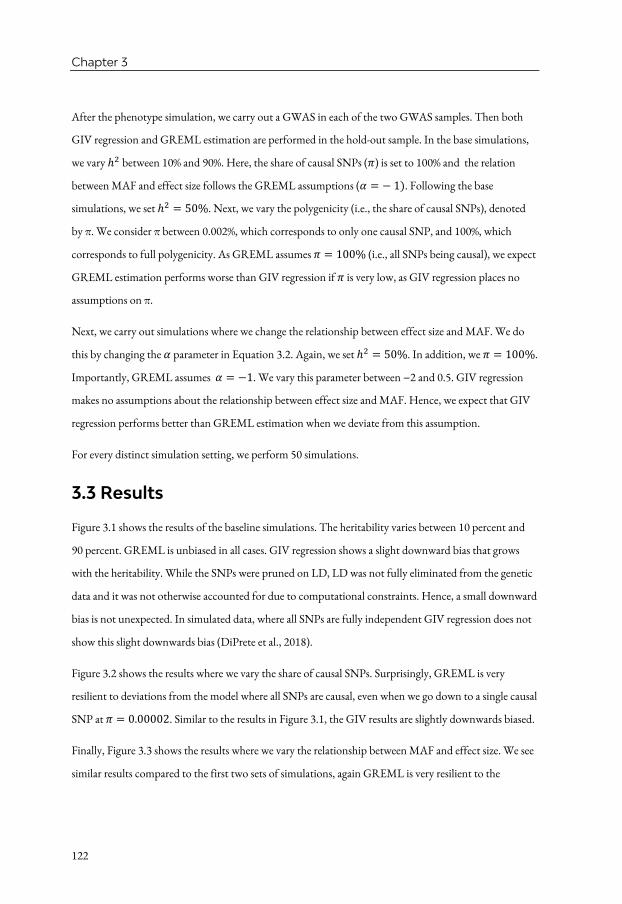
Chapter 3

122

After the phenotype simulation, we carry out a GWAS in each of the two GWAS samples. Then both

GIV regression and GREML estimation are performed in the hold-out sample. In the base simulations,

we vary ℎ! between 10% and 90%. Here, the share of causal SNPs (𝜋) is set to 100% and the relation

between MAF and effect size follows the GREML assumptions (𝛼 = −1). Following the base

simulations, we set ℎ! = 50%. Next, we vary the polygenicity (i.e., the share of causal SNPs), denoted

by π. We consider π between 0.002%, which corresponds to only one causal SNP, and 100%, which

corresponds to full polygenicity. As GREML assumes 𝜋 = 100% (i.e., all SNPs being causal), we expect

GREML estimation performs worse than GIV regression if 𝜋 is very low, as GIV regression places no

assumptions on π.

Next, we carry out simulations where we change the relationship between effect size and MAF. We do

this by changing the 𝛼 parameter in Equation 3.2. Again, we set ℎ! = 50%. In addition, we 𝜋 = 100%.

Importantly, GREML assumes 𝛼 = −1. We vary this parameter between −2 and 0.5. GIV regression

makes no assumptions about the relationship between effect size and MAF. Hence, we expect that GIV

regression performs better than GREML estimation when we deviate from this assumption.

For every distinct simulation setting, we perform 50 simulations.

3.3 Results

Figure 3.1 shows the results of the baseline simulations. The heritability varies between 10 percent and

90 percent. GREML is unbiased in all cases. GIV regression shows a slight downward bias that grows

with the heritability. While the SNPs were pruned on LD, LD was not fully eliminated from the genetic

data and it was not otherwise accounted for due to computational constraints. Hence, a small downward

bias is not unexpected. In simulated data, where all SNPs are fully independent GIV regression does not

show this slight downwards bias (DiPrete et al., 2018).

Figure 3.2 shows the results where we vary the share of causal SNPs. Surprisingly, GREML is very

resilient to deviations from the model where all SNPs are causal, even when we go down to a single causal

SNP at 𝜋 = 0.00002. Similar to the results in Figure 3.1, the GIV results are slightly downwards biased.

Finally, Figure 3.3 shows the results where we vary the relationship between MAF and effect size. We see

similar results compared to the first two sets of simulations, again GREML is very resilient to the


123

deviations of its assumptions across all simulations considered. The GIV results are again slightly biased

downwards.

3.4 Discussion

Our results show that GREML is a reliable method which is very resilient to the deviations from the

assumptions that we considered (i.e., polygenicity, π, and the relationship between MAF and effect size,

𝛼). GIV regression also works as expected in these simulations. It has a slight bias downwards due to LD

not being fully accounted for. In practice, it can be combined with methods like LDpred (Vilhjálmsson

et al., 2015) to create PGIs. Such an approach, however, is computationally infeasible in our simulation

study.

The advantage of GREML is that it can be applied without performing any GWAS prior to the analysis.

It also has smaller standard errors in each of the scenarios we simulated. Therefore, it remains the

recommended method to estimate heritability here. However, as GIV regression does not require many

assumptions it remains a very flexible method that might have advantages when applied elsewhere. One

possibility is extending the method so it can be applied to within-family GWAS to estimate both

heritability and genetic nurture (Kong et al., 2018). Currently, however, the within-family samples sizes

are not big enough yet to conduct the type of large-scale within-family GWASs needed to potentially

extend the GIV regression method further.

3.5 References

Abraham, G., Qiu, Y., & Inouye, M. (2017). FlashPCA2: principal component analysis of Biobank-scale

genotype datasets. Bioinformatics, 33(17), 2776–2778.



association studies. Nature Genetics, 47(3), 291–295. https://doi.org/10.1038/ng.3211

Chang, C. C., Chow, C. C., Tellier, L. C., Vattikuti, S., Purcell, S. M., & Lee, J. J. (2015). Second-

generation PLINK: rising to the challenge of larger and richer datasets. GigaScience, 4(1), 7.

https://doi.org/10.1186/s13742-015-0047-8

Chapter 3

124

DiPrete, T. A., Burik, C. A. P., & Koellinger, P. D. (2018). Genetic instrumental variable regression:

Explaining socioeconomic and health outcomes in nonexperimental data. Proceedings of the

National Academy of Sciences of the United States of America, 115(22).


Evans, L. M., Tahmasbi, R., Vrieze, S. I., Abecasis, G. R., Das, S., Gazal, S., … others. (2018).

Comparison of methods that use whole genome data to estimate the heritability and genetic

architecture of complex traits. Nature Genetics, 50(5), 737–745.

Fry, A., Littlejohns, T. J., Sudlow, C., Doherty, N., Adamska, L., Sprosen, T., … Allen, N. E. (2017).

Comparison of Sociodemographic and Health-Related Characteristics of UK Biobank Participants

With Those of the General Population. American Journal of Epidemiology, 186(9), 1026–1034.

https://doi.org/10.1093/aje/kwx246

Kong, A., Thorleifsson, G., Frigge, M. L., Vilhjalmsson, B. J., Young, A. I., Thorgeirsson, T. E., …

Stefansson, K. (2018). The nature of nurture: Effects of parental genotypes. Science, 359(6374),

424–428. https://doi.org/10.1126/science.aan6877

Purcell, S., Neale, B., Todd-Brown, K., Thomas, L., Ferreira, M. a R., Bender, D., … Sham, P. C. (2007).

PLINK: A tool set for whole-genome association and population-based linkage analyses. American

Journal of Human Genetics, 81(3), 559–575. https://doi.org/10.1086/519795










42(7), 565–569. https://doi.org/10.1038/ng.608


125

3.6 Figures

Figure 3.1. Baseline simulations

This figure shows the results of the baseline simulations, as described by equations (3.1) to (3.5). The results are based on 50 simulations for each parameter setting. GIV and GREML are estimated in a hold-out sample from the UK Biobank using simulated phenotypes. The GWASs for GIV are run in two independent subsamples of the UK Biobank.

Chapter 3

126

Figure 3.2. Simulations with varied share of causal SNPs

This figure shows the results of simulations where the share of causal SNPs is varied between 0.002 percent (i.e., one causal SNP) and 100 percent. The simulations are described by equations (3.1) to (3.5). In this set of simulations, the results are based on 50 simulations for each parameter setting. GIV and GREML are estimated in a hold-out sample from the UK Biobank using simulated phenotypes. The GWASs for GIV are run in two independent subsamples of the UK Biobank.

Figure 3.3. Simulations with varied scaling parameter

This figure shows the results of simulations where the relationship between SNP effect size and minor allele frequency is varied. The simulations are described by equations (3.1) to (3.5). The results are based on 50 simulations for each parameter setting. GIV and GREML are estimated in a hold-out sample from the UK Biobank using simulated phenotypes. The GWASs for GIV are run in two independent subsamples of the UK Biobank.


127

129

Chapter 4 Resource Profile and User Guide of the Polygenic Index Repository

Published as:

Becker, J., Burik, C. A. P., Goldman, G.,. . ., Cesarini, D., Benjamin, D.J., Turley, P. & Okbay, A. (2021). Resource profile and user guide of the Polygenic Index Repository. Nature Human Behaviour.

This publication contains online supplements not included in this chapter

Chapter 4

130

Abstract

Polygenic indexes (PGIs) are DNA-based predictors. Their value for research in many scientific

disciplines is rapidly growing. As a resource for researchers, we used a consistent methodology to

construct PGIs for 47 phenotypes in 11 datasets. To maximize the PGIs’ prediction accuracies, we

constructed them using genome-wide association studies—some not previously published—from

multiple data sources, including 23andMe and UK Biobank. We present a theoretical framework to help

interpret analyses involving PGIs. A key insight is that a PGI can be understood as an unbiased but noisy

measure of a latent variable we call the “additive SNP factor.” Regressions in which the true regressor is

the additive SNP factor but the PGI is used as its proxy therefore suffer from errors-in-variables bias. We

derive an estimator that corrects for the bias, illustrate the correction, and make a Python tool for

implementing it publicly available.

4.1 Main

The ability to predict complex outcomes from genotype data alone is rapidly increasing. The main

catalyst behind the increases is the success of genome-wide association studies (Visscher et al., 2017)

(GWAS). GWAS estimate the relationship between a trait, called a “phenotype,” and each of millions of

genetic variants. The “summary statistics” (coefficients and standard errors) from GWAS can be used to

construct a DNA-based predictor of the phenotype, calculated essentially as a coefficient-weighted sum

of allele counts (Purcell et al., 2009; Wray, Goddard, & Visscher, 2007). There are a variety of terms used

for such DNA-based predictors. In this paper, we will refer to them as “polygenic indexes”1.

As GWAS sample sizes have grown, coefficients are estimated more precisely, enabling the construction

of more predictive PGIs. One example is the PGI for educational attainment. The original PGI was

constructed from a GWAS of ~100,000 individuals and predicted ~2% of the variance in years of

schooling across individuals (C. A. Rietveld et al., 2013). The third and most recent PGI for educational

attainment (EA) predicts ~12% of the variance (Lee et al., 2018). Qualitatively similar patterns have been

1 In this paper, we use the term “polygenic index” instead of the commonly used terms “polygenic score” and “polygenic risk score.” Most of us prefer the term polygenic index because we are persuaded by the argument that it is less likely to give the impression of a value judgment where one is not intended. The term polygenic index was first proposed by Martha Minow at a meeting of the Trustees of the Russell Sage Foundation.

Resource Profile and User Guide of the Polygenic Index Repository

131

observed in PGIs for other complex-trait phenotypes (Cesarini & Visscher, 2017; Visscher et al., 2017),

including height, fertility, personality traits, and risk of many common diseases.

PGIs became mainstream in human genetics remarkably quickly. While predictive genetic indexes have a

long history in plant and animal genetics (Wray, Kemper, Hayes, Goddard, & Visscher, 2019), the idea

of using GWAS summary statistics to generate a PGI for humans was first proposed in 2007 (Wray et al.,

2007). The first study to empirically construct and validate a PGI was a GWAS of bipolar disorder and

schizophrenia published in 2009 (Purcell et al., 2009). Soon thereafter, command of methods used to

construct PGIs became a standard part of the skill repertoire of analysts specializing in genome-wide

data.

Today, PGIs are profoundly impacting research across the disciplinary spectrum. In medicine, much of

the discussion revolves around their potential use as tools for identifying individuals who could benefit

from enhanced screening and preventive therapies (Green & Guyer, 2011). Though much uncertainty

remains about their ultimate clinical utility (Wray et al., 2013), one recent study of polygenic risk for five

common diseases concluded that the science is sufficiently far along to contemplate incorporating

polygenic prediction into clinical care (Khera et al., 2018). Researchers working at the intersection of the

social and natural sciences have articulated visions of how PGIs could be productively leveraged in a

number of ways to advance knowledge about important questions (Belsky & Harden, 2019; Benjamin et

al., 2012; Freese, 2018). Already, the various iterations of the EA PGI have been used, among other

things, to trace out pathways for genetic influences that develop with age (Belsky et al., 2016) and

through school (Harden et al., 2020), study assortative mating (Robinson et al., 2017; Yengo, Robinson,

et al., 2018), trace recent migration patterns (Abdellaoui et al., 2019; Domingue, Rehkopf, Conley, &

Boardman, 2018), and improve analyses of the relationship between education and earnings (Papageorge

& Thom, 2020). As PGIs become more predictive and available for more phenotypes, potential

applications will multiply, and novel areas of research are likely to open up.

To depict the rapid growth in research using PGIs, Figure 4.1 shows the percentage of PGI-related

papers presented at the annual meetings of the Behavior Genetics Association. The percentage increased

from zero in 2009 to 20% in 2019. The figure also shows how the percentages of papers classified as

candidate-gene studies and twin/family/adoption studies—two other commonly used approaches—

have evolved over time. The declining fraction of candidate-gene studies in the figure is consistent with

Chapter 4

132

the hypothesis of a paradigm shift, with candidate-gene-based approaches gradually being displaced by

PGI-based approaches (Freese, 2018). This shift occurred, at least in part, because PGIs are not subject to

some well-known methodological limitations of candidate-gene studies (Duncan & Keller, 2011; Hewitt,

2012; C. A. Rietveld et al., 2014).

In this paper, we hope to promote productive behaviour-genetic research using PGIs in three ways. First

and most centrally, we make a broad array of PGIs available via a Polygenic Index Repository, covering a

number of datasets that may be useful to social scientists. By constructing the PGIs ourselves and making

them available as variables downloadable from the data providers, our resource eliminates a number of

roadblocks for researchers who would like to use PGIs in their research, as we detail below. The

Repository contains PGIs for 47 phenotypes. To maximize prediction accuracy of the PGIs, we meta-

analysed summary statistics from multiple sources, including several large-scale GWASs conducted in

UK Biobank and the personal genomics company 23andMe. 23andMe shared summary statistics from

37 separate association analyses, 9 of which have not been reported previously. Therefore, almost all

PGIs in our initial release perform at least as well as currently available PGIs in terms of prediction

accuracy. We will update the Repository regularly with additional PGIs and datasets.

Second, we present a theoretical framework for interpreting associations with a PGI. Using this

framework, we show that a PGI can be understood as an unbiased but noisy measure of what we call the

“additive SNP factor,” which is the best linear predictor of the phenotype from the measured genetic

variants. Because the PGI is a noisy measure, regressions that use the PGI as an explanatory variable

suffer from errors-in-variables bias. Since different papers use different versions of a PGI, the magnitude

of this bias varies. We hope that the theoretical framework helps establish a common language for

discussions about the interpretation of PGIs and their effect sizes.

Third, we propose an approach that improves the interpretability and comparability of research results

based on PGIs: to use in place of ordinary least squares (OLS) regression, we derive an estimator that

corrects for the errors-in-variables bias. (We are aware of four papers to date that have implemented a

measurement-error correction along the lines we propose here (Beauchamp, 2016; DiPrete, Burik, &

Koellinger, 2018; Kong et al., 2017; Tucker-Drob, 2017). Our approach is most similar to that of ref.

(Tucker-Drob, 2017), who develops a nearly identical framework using a psychometrics modeling

approach but focuses on the univariate case.) The estimator produces coefficients in units of the

standardized additive SNP factor, which has a more meaningful interpretation than units of some


133

particular PGI. We illustrate by applying the estimator to multivariate and gene-by-environment

regressions from a recently published paper (Papageorge & Thom, 2020). We make a Python command-

line tool publicly available for implementing the estimator.

4.2 Results

4.2.1. The Polygenic Index Repository

The Polygenic Index Repository is a resource that addresses several practical obstacles that researchers

interested in using PGIs must often confront. These include:

1. Constructing PGIs from individual genotype data can be a time-consuming process, even for

researchers trained to work with large datasets.

2. Since the prediction accuracy of a PGI is increasing in the sample size of the underlying GWAS,

it is generally desirable to generate PGI weights from GWAS summary statistics based on the

largest available samples. However, privacy and IRB restrictions often create administrative

hurdles that limit access to summary statistics and force researchers to trade off the benefit of

summary statistics from a larger sample against the costs of overcoming the hurdles. In practice,

researchers often end up constructing PGIs using only publicly available summary statistics.

3. Publicly available GWAS summary statistics are sometimes based on a discovery sample that

includes the target cohort (or close relatives of cohort members) in which the researcher wishes

to produce the PGI. Such sample overlap causes overfitting, which can lead to highly misleading

results (Wray et al., 2013). (Sometimes, when GWAS consortia provide summary statistics upon

request from a GWAS that is restricted so as to exclude the cohort, this barrier is surmounted at

low cost.)

4. Because different researchers construct PGIs from GWAS summary statistics using different

methodologies, it is hard to compare and interpret results from different studies.

We overcome #1 by constructing the PGIs ourselves and releasing them to the data providers, who in

turn will make them available to researchers. This simultaneously addresses #2 because we use all the data

available to us that may not be easily available to other researchers or to the data providers, including

genome-wide summary statistics from 23andMe. Using these genome-wide summary statistics from

Chapter 4

134

23andMe is what primarily distinguishes our Repository from existing efforts by data providers to

construct PGIs and make them available, such as the effort by the Health and Retirement Study

(https://hrs.isr.umich.edu/data-products/genetic-data/products#pgs). It also distinguishes our

Repository from efforts to make publicly available PGI weights directly available for download (Lambert

et al., 2020) (although we also do that, for weights constructed without 23andMe data). To deal with #3,

for each phenotype and each dataset, we construct a PGI from GWAS summary statistics that excludes

that dataset. We overcome #4 by using a uniform methodology across the phenotypes. In Methods, we

detail how the Repository disseminates the PGIs, as well as the principal components of the genetic data

in each dataset (which often should be used as controls for ancestry; see Supplementary Methods).

Figure 4.2 depicts the algorithm that determined which PGIs we constructed. In a preliminary step, we

obtained GWAS summary statistics for a comprehensive list of 53 candidate phenotypes (see

Supplementary Tables 1 and 2, meta-analysed the summary statistics for each candidate phenotype, and

calculated the expected 𝑅! for an out-of-sample regression of each candidate phenotype on a PGI

derived from its GWAS summary statistics. We calculated this expected 𝑅! from the GWAS summary

statistics (see Methods for details). If it exceeded 𝑅! = 0.01, then we used the meta-analysis output to

construct a PGI for the phenotype. We call these the “single-trait PGIs.” For each candidate phenotype,

we also identified a list of supplementary phenotypes: any other phenotype whose pairwise genetic

correlation with the candidate exceeds 0.6 in absolute value. For each candidate with at least one

supplementary phenotype, we then calculated the out-of-sample expected 𝑅! of a PGI derived from a

joint analysis of the candidate and supplementary phenotype summary statistics. If the expected 𝑅!

exceeded 0.01, then we used the joint-analysis output to construct a “multi-trait PGI” for the phenotype.

When both single-trait and multi-trait PGIs are available, the multi-trait PGI generally has greater

predictive power, but the single-trait PGI may be better suited for some applications (see Supplementary

Methods).

For each of the 47 phenotypes for which we constructed a single-trait and/or multi-trait PGI, Table 4.1

lists the total sample size included in the GWAS summary statistics (Total 𝑁), followed by the sample-

size contributions from three separate sources. For comparison, we also report the sample size of the

largest GWAS whose summary statistics are in the public domain (Public 𝑁). With three exceptions,

Total 𝑁 exceeds Public 𝑁. Two exceptions are height and BMI, where our UKB sample inclusion filters

lead to a slightly smaller sample size than the Public 𝑁. The remaining exception is cognitive


135

performance, where the sample size of our GWAS is smaller due to overlap between the discovery sample

in the largest GWAS with publicly available summary statistics and some of our Repository cohorts. For

the remaining phenotypes, the gains in sample size relative to the public 𝑁 are often substantial, and

driven by our inclusion of summary statistics from large-scale GWASs conducted in 23andMe, UKB, or

both. Table 4.1 also shows the 36 and 35 phenotypes for which we created single-trait and multi-trait

PGIs, respectively.

We created PGIs for these phenotypes in 11 Repository cohorts that shared their individual-level genetic

data with us (regardless of whether the phenotype itself is measured in the cohort). Table 4.2 lists the

datasets and some of their basic characteristics. Each data provider will make these PGIs available to

researchers through their own data access procedures (see Supplementary Note).

The UK Biobank is among the 11 cohorts included in the Polygenic Index Repository. Because of its

large sample size (see Table 4.2), the UK Biobank contributes substantially to the available sample for the

GWAS for many phenotypes. We therefore did not want to exclude the entire UK Biobank from the

GWASs used to create the PGIs. Instead, we split the UK Biobank sample into three equal-sized

partitions. We ran three 1/3-sample GWASs for each phenotype. To create the PGI for each partition,

we included results from the other two partitions in the meta-analysis. Consequently, researchers can

conduct analyses of a PGI in any one of the partitions and obtain unbiased results. However, we caution

researchers against conducting analyses in two or three of the partitions and meta-analyzing across

partitions; because the other partitions are used to create the PGI, the results obtained across different

partitions (although individually unbiased) will be correlated. Meta-analysis standard errors will

therefore be anticonservative, and this bias can be substantial (see Methods). Therefore, to maximize the

usefulness of our PGIs for research involving related individuals or brain-scan data, we assigned to the

same partition all pairs of individuals that are related up to second degree (and some pairs of third

degree), as well as all individuals with brain-scan data.

For validating the predictive power of the PGIs, we used five cohorts for which we had access to

individual-level genetic and phenotypic data: the Health and Retirement Study, a representative sample

of Americans over the age of 50; the Wisconsin Longitudinal Study, a sample of individuals who

graduated from high school in Wisconsin in 1957; the Dunedin Multidisciplinary Health and

Development Study, a sample of residents of Dunedin, New Zealand, born in 1972-1973; the

Chapter 4

136

Environmental Risk (E-Risk) Longitudinal Twin Study, a birth cohort of twins born in England and

Wales in 1994-1995; and the UKB (our third partition). The top panel of Figure 4.3 shows the observed

𝑅! and 95% confidence intervals for the single-trait PGIs in one or more validation cohorts, depending

on which had a measure of the phenotype. Height, BMI, and educational attainment are shown

separately because the y-axis scale is different. The bottom panel of Figure 4.3 shows the difference

between the 𝑅! of the single-trait Repository PGI and that of a PGI we constructed using the largest

non-overlapping GWAS whose summary statistics are in the public domain. The Repository PGIs are

almost always at least as predictive as the PGIs based on publicly available GWAS results. For the

corresponding results for the multi-trait PGIs, see Supplementary Figure 1. The multi-trait PGIs are

usually at least as predictive as the single-trait PGIs (Supplementary Figure 1C and Supplementary Table

3).

We have written a User Guide (reproduced in the Supplementary Methods) that will be distributed by

participating cohorts along with the Repository PGIs. It discusses interpretational issues, including those

relevant for whether researchers should use the single-trait or multi-trait PGIs when both are available.

4.2.2 Theoretical Framework for Polygenic Indexes

To help interpret PGIs, we lay out a theoretical framework. Denote individual 𝑖’s phenotype value by

𝑦"⋆. Denote individual 𝑖’s allele count at genetic variant 𝑗 by 𝑥"$⋆ ∈ {0,1,2}. Without loss of generality, we

use a mean-centred transformation of the phenotype and allele counts, such that 𝑦" ≡ 𝑦"⋆ − 𝐸(𝑦"⋆)and

𝑥"$ ≡ 𝑥"$⋆ − 𝐸6𝑥"$⋆ 7 for each SNP 𝑗. We denote the vector of mean-centered allele counts at 𝐽 genetic

variants by 𝒙" = 6𝑥"%, 𝑥"!, … , 𝑥"&7'. As a benchmark, consider the standardized best linear predictor of

the phenotype based on the allele counts:

𝑔" ≡𝒙"'𝜸

𝑠𝑑6𝒙"'𝜸7,

where

𝜸 = argmin𝜸)𝐸[(𝑦" − 𝒙"'𝜸F)!].

That is, the optimal weight vector 𝜸 is the vector of coefficients from the population regression of 𝑦" on

𝒙". This population regression may also include control variables; we omit them here to avoid cluttering

notation, but in the Supplementary Methods we extend the framework to include them and explain why


137

they do not affect the results in this paper. In the User Guide (also in the Supplementary Methods), we

explain how control variables do matter for the interpretation of a PGI.

When the set of genetic variants in 𝒙" is all variants in the genome, 𝑔" is referred to as the “standardized

additive genetic factor.” The variance in the phenotype explained by 𝑔" is called the “(narrow-sense)

heritability,” often the object of interest in twin, family, and adoption studies that draw inferences

without access to molecular genetic data.

In studies with molecular genetic data—our focus here—the set of genetic variants in 𝒙" is restricted to

those measured or imputed from the single-nucleotide polymorphisms (SNPs) assayed by standard

genotyping platforms (and which pass quality-control filters). In that case, the variance in the phenotype

explained by 𝑔" is called the “SNP heritability” (Yang et al., 2010), which we denote ℎ*+,! . We will refer

to 𝑔" as the standardized “additive SNP factor.”

Since the population regression cannot be run, the vector 𝜸 is unknown, so 𝑔" cannot be constructed

empirically. What can be constructed empirically is a “polygenic index (PGI),” 𝑔I", which is a

standardized, weighted sum of allele counts using some other weight vector 𝜸J calculated from GWAS

summary statistics:

𝑔I" ≡𝒙"'𝜸J

𝑠𝑑6𝒙"'𝜸J7.

In general, 𝜸J will not be equal to 𝜸 because 𝜸J is calculated from GWAS summary statistics that are

estimated in a finite sample. The key observation for our framework is that when 𝜸J is calculated using

standard methods (that include all the SNPs in 𝒙"), such as LDpred (Vilhjálmsson et al., 2015) and PRS-

CS (Ge, Chen, Ni, Feng, & Smoller, 2019), the resulting PGI can be expressed as

𝑔I" =(𝑔" + 𝑒")

𝜌,

where 𝑒" is mean-zero estimation error that is uncorrelated with 𝑔", and 𝜌 ≡ 𝑠𝑑(𝒙"'𝜸J)/𝑠𝑑(𝒙"'𝜸) is a

scaling factor that standardizes 𝑔I". In words, the PGI is a standardized, noisy measure of the additive

SNP factor, where the noise is classical measurement error.

One way to characterize the amount of measurement error is the value 𝜌. In Methods, we show that

Chapter 4

138

𝜌! = 1 + 𝑉𝑎𝑟(𝑒") =ℎ*+,!

𝑅!≥ 1,

where ℎ*+,! is the SNP heritability (the predictive power of 𝑔") and 𝑅! is the fraction of variance

explained in a regression of the phenotype 𝑦" on the PGI 𝑔I" (the predictive power of 𝑔I"). The ratio

ℎ*+,! /𝑅! is greater than or equal to one because the weights that define 𝑔" maximize the variance

explained in 𝑦", and therefore any other weights—including those used to construct the PGI—explain at

most ℎ*+,! of the variation. Furthermore, the amount of measurement error 𝜌 would achieve its

minimum value of one only if the PGI weights were based on GWAS summary statistics from an infinite

sample. Across studies, 𝜌! varies. For example, 𝑅! depends on the sample size of the GWAS underlying

the PGI weights and the method of constructing PGI weights (e.g., LDpred vs. PRS-CS). However, 𝜌!

can usually be estimated using estimates of ℎ*+,! and 𝑅! from the sample at hand or other samples that

are sufficiently similar.

4.2.3 Measurement-Error-Corrected Estimator for PGI Regressions

Typical research with a PGI involves running a regression with the PGI as an explanatory variable and

reporting results in units of standard deviations of the PGI. This approach, however, has two

shortcomings. First, it is often unclear how to interpret these units, which depend on the amount of

measurement error. Second and relatedly, the effect sizes are not comparable across PGIs that differ in

their amount of measurement error.

We argue that such a regression should be interpreted as aiming to approximate a regression with the

standardized additive SNP factor as the explanatory factor. The PGI serves as an empirically feasible

proxy for the standardized additive SNP factor. An analysis of the standardized additive SNP factor has a

clearer interpretation than an analysis of the PGI and puts results in comparable units, regardless of

which specific PGI was used in the analysis. Here we extend known results from errors-in-variables

models to derive a consistent estimator for the coefficients from a regression with the standardized

additive SNP factor as an explanatory variable.

The “theoretical regression” is what we call a regression with the (unobserved) standardized additive SNP

factor as an explanatory variable. Consider an OLS regression of a phenotype 𝜙" on the standardized

additive SNP factor 𝑔", a vector of covariates 𝒛", and a vector 𝒘" of interactions between 𝑔" and a subset

of the regressors in 𝒛" (possibly all of them):


139

𝜙" = 𝑔"𝛽- + 𝒛"𝜻- +𝒘"𝜹- + 𝜖-," , (4.1)

where the 𝑔 subscripts indicate that these are parameters from the theoretical regression. (Note that the

phenotype 𝜙" need not be the same phenotype 𝑦" for which the standardized additive SNP factor is the

best linear predictor. For example, some papers have studied the relationship between the PGI for

educational attainment and test scores at younger ages (Belsky et al., 2016). Note also that the covariates

in 𝒛" may be measured with error; equation (4.1) represents whatever regression is run by a researcher

except that 𝑔" is measured without error.) The “feasible regression” is what we call the regression using

the PGI 𝑔I" in place of 𝑔":

𝜙" = 𝑔I"𝛽-/ + 𝒛"𝜻-/ +𝒘J "𝜹-/ + 𝜖-/," , (4.2)

where 𝒘" ! is the vector of interactions with 𝑔I" in place of 𝑔". We denote the vectors of coefficients from

the theoretical and feasible regressions by 𝜶- ≡ 6𝜷-, 𝜻-, 𝜹-7' and 𝜶-/ ≡ 6𝜷-/ , 𝜻-/ , 𝜹-/7

', respectively.

In what follows, we sketch the derivation of an estimator for 𝜶- (for details, see the Supplementary

Methods). The derivation assumes that the error in the PGI, 𝑒", is uncorrelated with 𝒛" and 𝒘". In the

Supplementary Methods, we show that this condition holds exactly if the PGI weights 𝜸J are unbiased

estimates of 𝜸. We also show that if the PGI weights 𝜸J are estimated using LDpred-inf—as is true for the

Repository PGIs—then the bias in our estimator due to plausible violations of this condition will

typically be negligible.

Extending the standard formula for errors-in-variables bias (Spearman, 1904) in a multivariate regression

to this setting, and under the assumption that 𝑒" is uncorrelated with 𝒛" and 𝒘", the feasible-regression

coefficients can be shown to be biased:

𝜶-/ = 𝜬6𝑽- +𝜴70%𝑽-𝜶- ≠ 𝜶-, (4.3)

where𝜬 ≡ `𝜌𝑰%1|𝒘| 00 𝑰|𝒛|

b, 𝑰|𝒙| is the identity matrix with the dimensionality of 𝒙, 𝑽- is the variance-

covariance matrix of (𝑔" , 𝒘" , 𝒛")', and 𝜴 is the component of the variance-covariance matrix of

(𝑔I" , 𝒘J " , 𝒛")' that is due to error (see Supplementary Methods). In the special case of a univariate

regression, in which the only covariate is a constant term, equation (4.3) implies that the regression slope

coefficient 𝛽-/ converges to %6

𝛽-. This is a familiar form of attenuation bias, in which the degree of

attenuation toward zero is greater the larger the amount of measurement error. In the multivariate case,

however, the amount of attenuation bias for 𝛽-/ will also depend on the covariance matrix of 𝑔" with 𝒛".

Chapter 4

140

Moreover, the other coefficients, 𝜻-/ and 𝜹-/ , will be biased as well, not necessarily toward zero. For

example, a covariate whose coefficient in equation (4.1) is zero can have a coefficient in equation (4.2)

that is non-zero, leading to an incorrect rejection of the null hypothesis (Abel (2017), unpublished

manuscript).

The idea underlying our “corrected” estimator follows immediately from equation (4.3) by inverting the

bias term:

𝜶7899 = 𝑽-0%6𝑽- +𝜴7𝜬0%𝜶-/ = 𝜶-. (4.4)

This expression is called a regression-disattenuation estimator. It cannot be implemented directly,

however, because 𝑽- involves the variance and covariances of the unobserved standardized additive SNP

factor 𝑔". However, the variance and covariances involving 𝑔" differ from analogous terms involving 𝑔I"

only due to measurement error, and the amount of measurement error is given by 𝜌. Therefore, the

variance and covariances involving 𝑔" can be inferred from estimable quantities. In the Supplementary

Methods, we derive an expression for 𝜶7899 in terms of 𝜌 and population parameters that can be

estimated consistently using the observed data. That expression is stated in Methods. We implement that

version of the estimator. In the Supplementary Methods, we also derive standard errors for the regression

coefficients, under the assumption that 𝜌 is known.

If the PGI is uncorrelated with the covariates, then the estimator will inflate the naïve OLS estimate 𝛽c-

and its standard error by the factor 𝜌. If, in addition, the covariates are uncorrelated with each other,

then the estimator will also inflate 𝜹d- and its standard error by the factor 𝜌. Because the regression

coefficients and standard errors are inflated by the same factor, the 𝑡-statistics and 𝑝-values for the

corrected estimates will be identical to those for the uncorrected estimates. Correlation between the PGI

and the covariates and correlation among the covariates will lead to deviations from this “rule of thumb”

adjustment (and can lead to the adjustment being different across regression coefficients and standard

errors).

In the univariate case where 𝜌 is estimated within the same dataset as the PGI analysis is conducted, we

show that while uncertainty in 𝑅g! causes downward bias in the standard error, uncertainty inℎg*+,!

causes upward bias, and the net effect is likely to be standard errors that are slightly conservative. We

conjecture that the standard errors will also typically be conservative in multivariate settings. If the 𝜌

estimate is from a different dataset, then ignoring the uncertainty in 𝜌 will unambiguously cause the


141

standard errors to be anticonservative. In such settings and in settings when there is meaningful

uncertainty in the estimate of 𝜌, we recommend that users calculate bootstrapped standard errors. The

bootstrapped standard errors correctly account for uncertainty in 𝜌 and will be larger than the

unbootstrapped standard errors.

We provide a Python command-line tool that implements the measurement-error correction based on a

user-specified value of 𝜌. The package can also estimate 𝜌 by calculating estimates of ℎ*+,! (using the

GREML method(Yang et al., 2010; Yang, Lee, Goddard, & Visscher, 2011) or, for larger datasets,

BOLT-REML(P. R. Loh et al., 2015)) and 𝑅!. The package can calculate standard errors either treating

𝜌 as known or (at some computational cost) by bootstrapping. When possible, we recommend users

estimate 𝜌 within the dataset they use to analyse the PGI. If the dataset is too small to reliably estimate 𝜌

or lacks a measure of the phenotype corresponding to the PGI, an estimate of 𝜌 from another dataset can

be used under the assumption of perfect genetic correlation of the phenotype across datasets. In the

Polygenic Index Repository, we provide pre-specified estimates of 𝜌 for three participating datasets for

which we have access to the phenotypic data corresponding to the PGI: HRS, WLS, and the third

partition of UKB (see Supplementary Table 4). For many of the cohorts, the standard error on the ℎ*+,!

estimate is large, so we recommend a value of 𝜌 based on existing ℎ*+,! and 𝑅! estimates from a larger

sample.

Although our estimator is derived for an OLS estimation framework, it will be approximately correct for

logistic regression (Rosner, Spiegelman, & Willet, 1992) and survival models (Hughes, 1993) as long as

the coefficient on the standardized additive SNP factor, 𝛽-, is not too large. For example, applying a

measurement-error correction that would be correct for OLS will be a very accurate approximation for

the coefficient in a survival model when the hazard ratio associated with a one-standard deviation

difference in the variable measured without error is 1.11 (Hughes, 1993). However, the correction is

roughly 20% too small when the hazard ratio is 1.65 (Hughes, 1993).

4.2.4 Illustrative Application

To illustrate our proposed measurement-error correction, we apply it to several analyses reported in a

recent paper relating educational attainment (and labour market outcomes) to a PGI for educational

attainment (Papageorge & Thom, 2020). The paper uses data from the HRS, one of our validation

cohorts (N = 8,537; 58.3% female; median age = 83). As a preliminary analysis, the paper reports some

Chapter 4

142

straightforward tests of the relationship between educational attainment (EA) and the EA PGI. In Panel

A of Table 4.3, we reproduce their univariate regression of EA on the PGI and their multivariate

regression that additionally includes controls for mother’s and father’s EA. In the univariate regression,

shown in column (1), a 1-standard-deviation increase in the PGI is associated with 0.844 (95%

confidence interval = [0.793, 0.895]) additional years of schooling. This association is reduced to 0.619

(95% confidence interval = [0.572, 0.666]) years in column (2), once the controls are included.

The measurement-error-corrected univariate regression is shown in column (3) of Panel A. We estimate

that a 1-standard-deviation increase in the additive SNP factor is associated with 1.318 (95% confidence

interval = [1.238, 1.398]) additional years of schooling. Relative to the PGI coefficient in column (1),

this coefficient is larger by a factor of 1.318 / 0.844 = 1.56. In the regression with controls for parental

education, shown in column (4), we estimate a corrected coefficient of 1.104 (95% confidence interval =

[1.022, 1.186]) additional years. Relative to column (2), this is an increase by a factor of 1.104 / 0.619 =

1.78. Since for EA in the HRS, ℎg*+,! ≈ 0.25 and 𝑅g! ≈ 0.10, according to the rule of thumb mentioned

above, both coefficients should be expected to have increased by a factor of 1.58 (≈ j0.25/0.10). The

increase is larger than that from column (2) to (4) due to the positive correlations between the PGI, the

controls, and the dependent variable.

The results in Panel A illustrate a general implication of the measurement-error correction for mediation

analyses: the correction deflates estimates of how much covariates mediate the effect of the PGI. There

have been several mediation analyses in which researchers study how much the coefficient on a PGI is

reduced when control variables—which are usually positively correlated with both the PGI and the

dependent variable—are added to the regression (Elliott et al., 2018; Okbay, Beauchamp, et al., 2016;

Stergiakouli et al., 2016). Going from column (1) to (2), the drop in the coefficient on the PGI would

lead a researcher to conclude that parental education mediates (0.844 – 0.619) / 0.844 = 27% of the

effect of the PGI. Going from column (3) to (4) shows the corrected estimate of mediation is only (1.318

– 1.104) / 1.318 = 16%. The drop is larger for the uncorrected regressions because in those regressions,

the control variables are proxying for part of the additive SNP factor that is not well captured by the

PGI. Therefore, studies that do not correct for measurement error will tend to overestimate the extent to

which the control variables mediate the effect of the PGI.

The results in Panel B illustrate a fairly general implication of the measurement-error correction for PGI-

by-environment interaction analyses: in contrast to how it affects mediation estimates, the correction


143

tends to increase the magnitude of PGI-by-environment interaction estimates. A main result of

Papageorge and Thom is about two such interactions: a higher PGI is associated with a weaker

relationship between childhood SES and high school completion but a stronger relationship between

childhood SES and college completion (Papageorge & Thom, 2020). Columns (1) and (2) reproduce

two specifications that show this result: a regression of high school completion on the PGI, self-reported

childhood SES, their interaction, and controls; and the analogous regression for college completion. The

key finding is that the interaction term is negative in column (1) but positive in column (2). As shown in

columns (3) and (4), once the additive SNP factor is considered instead of the PGI, the interaction

coefficients for both the high school and college regressions move farther away from zero, strengthening

the main result of the paper. In general, PGI-by-environment interaction studies that do not correct for

measurement error will tend to underestimate the magnitude of the interaction because the interaction

term will tend to be attenuated by the measurement error. Note, however, that this conclusion may not

hold if other regressors are correlated with the interaction term.

4.3 Discussion

We described the initial release of the Polygenic Index Repository, which contains PGIs for 47

phenotypes. A major goal of this effort is to disseminate PGIs with greater predictive power than the

PGIs typically used. To maximize prediction accuracy of the PGIs, we meta-analysed data from multiple

sources, including 23andMe and the UK Biobank.

We also derived a measurement-error-corrected estimator that can be used instead of OLS regressions

where the independent variables include a PGI or a PGI and its interactions. While some lack of

comparability of results across studies is inevitable (e.g., due to differences across samples in SNP

heritabilities), one goal of both the Repository and the proposed estimator is to increase comparability.

For example, when constructing the PGIs, we applied to each cohort uniform sets of inclusion criteria

for individuals and markers in the genotype data. The estimator contributes to improving comparability

by putting regression coefficients in units of the additive SNP factor, regardless of the predictive power

of the particular PGI available to the researchers.

Because genetic associations are easily misinterpreted, researchers who use PGIs should be especially

careful to understand and convey the appropriate interpretation of their findings. For example, it is

Chapter 4

144

important to keep in mind that PGI associations may be mediated by environmental factors, and these

factors may be modifiable. To facilitate understanding of these and other interpretational issues, we have

written a User Guide that cohorts will distribute to users of the Repository PGIs (see Supplementary

Methods).

As more GWAS summary statistics become available in the years ahead, and better methods for

constructing PGIs are developed, we plan to update the Repository regularly with more predictive PGIs

that leverage these advances. For example, future releases will incorporate PGIs of novel phenotypes for

which it is not currently feasible to construct PGIs with meaningful predictive power. We emphasize,

however, that although PGIs have attained levels of predictive power that can be useful to researchers,

the limited heritability of behavioural phenotypes such as those in the Repository implies that the PGIs

will never be able to predict any individual’s phenotype with much precision. Additionally, since GWAS

summary statistics have only been available in large samples of individuals from European ancestries,

currently available PGIs have limited portability to individuals of non-European ancestries (Martin et al.,

2017). In future releases of the Repository, once sufficient data becomes available to create PGIs that

have non-negligible predictive power for other ancestry groups, we will update the Repository to contain

such PGIs.

4.4 Methods

The polygenic indexes (PGIs) shared through the Repository are based on summary statistics from three

types of sources: GWASs conducted in UK Biobank (UKB), GWASs conducted in samples of volunteer

research participants from 23andMe, and other published genome-wide association studies (GWAS). In

Section 4.4.1 below, we begin by detailing how the Repository facilitates researchers’ access to the PGIs.

In Section 4.4.2, we describe how the summary statistics used in our main analyses were generated,

quality-controlled and meta-analysed to generate a set of files used as inputs into construction of the

single-trait and multi-trait PGIs. In Section 4.4.3, we define and justify the 𝑅! criterion we used to

determine which PGIs to include in the first release of the Repository. We then describe quality-control

filters applied to the individual-level genotype data supplied by each Repository cohort. We conclude by

describing the methods used to construct the cohort PGIs. In Section 4.4.4 we state our measurement-

error-corrected estimator and its standard error in terms of estimable quantities. Section 4.4.5 describes

our estimation of 𝜌 in the HRS, WLS and UKB. Section 4.4.6 describes the data underlying Figure 4.1.


145

4.4.1 PGI Dissemination Strategies

Recall from the main text that the PGI Repository aims to overcome four obstacles: (1) Constructing

PGIs can be time-consuming and requires specialized knowledge; (2) Researchers face administrative

hurdles in accessing all the genome-wide summary statistics for constructing PGIs; (3) Publicly available

summary statistics may include the target dataset (which should be omitted when constructing the PGI);

and (4) PGIs are often constructed with a variety of methods and idiosyncratic analysis decisions.

Disseminating PGSIs through participating datasets

As described in the main text, we overcome all four obstacles by constructing PGIs that include both

publicly available data and restricted data (including genome-wide summary statistics from 23andMe)

and releasing them to the data providers, who in turn will make them available to researchers. We omit

the participating dataset from the summary statistics used to construct that dataset’s PGIs, and we

construct all the PGIs using a uniform methodology. We similarly construct principal components

(PCs) of the genome-wide data using a uniform methodology and release them to the data providers to

make available. Our methodology is described below in Sections 4.4.2 and 4.4.3. Upon publication, we

will post the code we used for constructing the PGIs and PCs on the SSGAC website

(https://www.thessgac.org/data).

To access the PGIs and PCs in a dataset, researchers will need to follow the usual data access procedures

for that dataset (typically including a Data Use Agreement and approval from an IRB). The current

procedures for each dataset are in the Supplementary Note, and up-to-date procedures will be

maintained on the SSGAC website.

Data providers can join the Repository if: (i) they share their individual-level genetic data with the

SSGAC so that we can construct the PGIs and PCs on our secure servers; and (ii) they have procedures

by which external researchers can gain access to the dataset.

Disseminating PGI weights based on public data

For datasets not participating in the Repository, we cannot overcome obstacles (1)-(4). However, for

researchers who wish to construct the PGIs in a non-participating dataset, we will facilitate this effort by

posting on the SSGAC website (www.thessgac.org/data) the weights underlying the PGIs constructed

from publicly available data (i.e., that have no 23andMe data). As mentioned above, we will also post the

code we used for constructing the PGIs and PCs. In addition, we refer researchers to 23andMe’s

Chapter 4

146

“Publication Dataset Access Request Form” (https://research.23andme.com/dataset-access/#how-to),

which allows researchers to gain access to GWAS results used in published papers (after signing a Data

Use Agreement with 23andMe). In this way, researchers can gain access to the same 23andMe data that

we used, and use it to construct the PGIs that are wholly or partly based on data from 23andMe.

4.4.2 Summary Statistics

UKB GWAS

Supplementary Table 5 lists all UKB phenotypes for which we ran GWASs. Before running the GWASs,

we filtered out poor-quality genotypes: (i) samples identified as putatively carrying sex-chromosome

configurations that are neither XX nor XY, (ii) samples identified as outliers in heterozygosity and

missingness rates, (iii) samples whose sex inferred from sex chromosomes does not match self-reported

gender, and (iv) samples with missing sex, birth year, genotyping batch, or PC information. We also

restricted the sample to individuals we will refer to as of “European ancestries,” defined as the first

genetic PC provided by UKB being greater than 0 and individual self-reporting to be of “British”,

“Irish”, or “Any other white background.”

In order to make PGIs for the UK Biobank (UKB) without having to exclude the entire UKB from the

discovery GWAS, we split the UK Biobank sample into three equal-sized partitions and, for each

partition, used the summary statistics from the other two partitions when generating its PGI. The first

partition (UKB1) is composed of UKB participants with brain-scan data (as indicated by data field

12188), all pairs of UKB participants related up to second degree, and the pairs of relatives of third-

degree relatedness with greatest relatedness. Pairs of individuals of third-degree relatedness were ordered

based on the maximum relatedness coefficient they have with another participant and assigned to the

first partition in decreasing relatedness order until the partition was full. Remaining individuals with

third-degree relatives were assigned to the second partition. Finally, individuals with no third degree or

closer relatives were randomly assigned to the second (UKB2) or third (UKB3) partition.

For all phenotypes in Supplementary Table 5, we ran three separate GWASs, one for each partition.

Briefly, each GWAS in UKB was conducted using mixed-linear models implemented by the software

BOLT-LMM (P.-R. Loh et al., 2015). The dependent variable in each analysis is a phenotype that has

been residualized on sex, a third-degree polynomial in birth year (defined as (𝑏𝑖𝑟𝑡ℎ𝑦𝑒𝑎𝑟– 1900)/10),

their interactions, 106 genotyping batch dummies, and the first 40 of the PCs released by the UK

Biobank. Details on how each phenotype is coded are provided in Supplementary Table 5. For the


147

variance-component estimation in BOLT-LMM (but not the association analyses), we restricted the set

of markers to the set of 622,788 hard-called SNP genotypes that remained after filtering for 1% minor

allele frequency and 60% imputation accuracy and pruning with an 𝑟! threshold of 0.3. Our subsequent

association analyses were performed on imputed SNP dosages provided by UKB.

Using the UK Biobank split-sample PGI

Splitting the UKB into thirds as described above increases the predictive power of the PGI within each

third (relative to omitting the UKB from the GWAS sample). Researchers may desire to conduct

analyses that simultaneously include individuals from different partitions of the data or to meta-analyse

results across different partitions. Such analyses will produce estimates that are unbiased, but the

standard errors will be incorrectly calibrated. To see why, consider a linear model

𝑌" = 𝑿"𝜷 + 𝜀" ,

where 𝑿" is a vector of covariates that includes a PGI. Imagine that the data (𝒀, 𝑿) include individuals

from different partitions of the data. As a result of the sample-splitting procedure above, Cov(𝑿" , 𝜀") =

0, which implies that the OLS estimator for 𝜷 will be unbiased. However, because some of the

individuals in the data were used to generate the PGI for other individuals in the data, Cov6𝑿" , 𝜀$7 ≠ 0

whenever individuals 𝑖 and 𝑗 are in different partitions. As a result,

Var6𝜷d7 = Var[(𝑿'𝑿)0%𝑿'𝒀]

= Var[(𝑿'𝑿)0%𝑿'𝜺] (5)

≠ (𝑿'𝑿)0%𝑿'Var(𝜺)𝑿(𝑿'𝑿)0%. (4.6)

The expression (6) is the standard general formula for the sampling variance of OLS estimates. It is not

equal to (5) due to the correlation between (𝑿'𝑿)0%𝑿' and 𝜺. If we knew the correlation between these

two vectors, we could calculate correct standard errors in this setting, but the correlation structure is

complex, and we are unaware of any current method that produces correct standard errors. For this

reason, we recommend that researchers only do analyses on sets of individuals within a partition. If

researchers choose to do analyses with individuals across different partitions, they should include the

strong caveat that their standard errors may be poorly calibrated.

Chapter 4

148

23andMe GWAS

Our analyses use summary statistics from GWASs conducted by 23andMe in samples of European-

ancestry volunteer research participants for 37 different phenotypes. Supplementary Table 6 provides an

overview of these summary statistics. 28 out of the 37 are from previously published studies (Day et al.,

2015; Demontis et al., 2019; Ferreira et al., 2017; Hinds et al., 2013; Hu et al., 2016; Hyde et al., 2016;

Karlsson Linnér et al., 2019; Lee et al., 2018; Liu et al., 2019; Lo et al., 2016; Pasman et al., 2018; Pickrell

et al., 2016; Sanchez-Roige et al., 2017, 2018; Warrier et al., 2018). For these, we cite the original study in

the column labelled “Citation”. The remaining 9 are based on previously unreported GWASs. Two of

these GWASs are for phenotypes (Subjective Well-Being and Risk) for which GWASs had been

previously published by 23andMe but with a smaller sample. The remaining summary statistics have not

been previously published by 23andMe. Supplementary Table 6 describes the details of the association

model used for each phenotype. For details on 23andMe’s genotyping and imputation, see

Supplementary Tables 17 and 18 in Lee et al.(Lee et al., 2018)

Quality control of summary statistics

We applied a uniform set of quality-control filters to each original file with summary statistics (both

those from previously unpublished and previously published GWASs). We closely followed the quality-

control pipeline detailed in section 1.5.1 of Okbay, Beauchamp, et al. (2016) and implemented in the

software EasyQC (Winkler et al., 2014). Our QC protocol departed from Okbay, Beauchamp, et al.

(2016) in the following steps:

- We used data from the Haplotype Reference Consortium reference panel (r1.1) (McCarthy et

al., 2016) to check for strand misalignment, allele mismatch, chromosome and base pair position

concordance, and allele frequency discrepancies (instead of using data from the 1000 Genomes

Phase 1 (Abecasis et al., 2010)). (Mapping file and allele frequency data were downloaded from

the EasyQC website, from the following urls, respectively: https://homepages.uni-

regensburg.de/~wit59712/easyqc/HRC/HRC.r1-1.GRCh37.wgs.mac5.sites.tab.rsid_map.gz ,

https://homepages.uni-regensburg.de/~wit59712/easyqc/HRC/HRC.r1-

1.GRCh37.wgs.mac5.sites.tab.cptid.maf001.gz .)

- For simplicity and uniformity, we applied a more conservative imputation accuracy filter of 0.7

to all input files irrespective of the software that was used for imputation.


149

- We applied a uniform minor allele frequency filter of 0.01 to all input files. Stricter filters

varying by sample size were not necessary because the studies that we analysed were much larger

than some of those in Okbay, Beauchamp, et al. (2016)

- We filtered out standard-error outliers. To do so, we first estimated the standard deviation (𝜎I:)

of the phenotype in each input file by regressing the reported standard errors on the following

approximation to the standard error of a coefficient estimated by OLS when the phenotype is

standardized:

𝑆𝐸;9<=,$ =1√𝑁

×1

{2 ×𝑀𝐴𝐹$ × 61 −𝑀𝐴𝐹$7,

where 𝑀𝐴𝐹$ is the minor allele frequency of SNP 𝑗 and 𝑁 is the GWAS sample size. We filtered

out markers with *>!"#$,&*>&

< ?@'!

or *>!"#$,&*>&

> 2𝜎I:. This filter allowed us to identify and remove

markers for which the reported GWAS sample size deviated considerably from the sample size

implied by the marker’s standard error. This filter was particularly relevant for publicly available

summary statistics, where marker-specific sample sizes were typically not reported. (Having an

accurate number for the sample size is important for LDpred (Vilhjálmsson et al., 2015).)

Before each filtered file was cleared for subsequent meta-analyses, we also prepared and visually inspected

a number of diagnostic plots, as described in Okbay et al. Our final analyses are limited to files whose

diagnostic plots did not suggest any anomalies. Finally, we examined the genetic correlation between

input files (estimated using the LDSC software package (Bulik-Sullivan et al., 2015)) for each phenotype

to make sure phenotype coding was in the same direction across 23andMe, UKB, and published studies.

Supplementary Table 7 summarizes the number of SNPs dropped in each filtering step in the files that

passed all diagnostic checks.

Single-Trait Input GWAS

In this section, we describe the construction of single-trait input GWASs used in several of our

downstream analyses, including as inputs for the single-trait and multi-trait PGIs. The single-trait input

GWAS for a phenotype is obtained by meta-analysing summary statistics from up to three sources of

information: analyses in UKB, analyses in 23andMe, and summary statistics from a previously published

study of the phenotype (Barban et al., 2016; Day et al., 2015; de Moor et al., 2012, 2015; Demontis et al.,

Chapter 4

150

2019; Doherty et al., 2018; Ferreira et al., 2017; Furberg et al., 2010; Kunkle et al., 2019; Lee et al., 2018;

Liu et al., 2019; Locke et al., 2015; Okbay, Baselmans, et al., 2016; Perry et al., 2014; Stringer et al., 2016;

Trampush et al., 2017; van den Berg et al., 2016; Wood et al., 2014; Wray et al., 2018). The input GWAS

for a phenotype is the same across most cohorts. However, when there is overlap between a Repository

cohort and cohorts that contributed to summary statistics from previously published studies, or in order

to construct a PGI for a UKB partition that is based on summary statistics including the rest of the UKB

sample, we restrict the meta-analyses to summary statistics based on non-overlapping data. Details on the

construction of single-trait input GWAS are in Supplementary Table 8.

To illustrate the general procedure, consider the single-trait input GWAS for neuroticism in ELSA and

EGCUT. Supplementary Table 8 shows that the largest meta-analysis of neuroticism (NEURO1)

yielded a final sample of 𝑁 = 484,560 individuals by combining data from UKB (𝑁 = 361,688),

23andMe (𝑁 = 59,206) and a previously published study (𝑁 = 63,666). Since the column does not

indicate any overlap with ELSA, the single-trait input GWAS for neuroticism in ELSA is the set of

summary statistics from this meta-analysis. EGCUT, however, is listed in Supplementary Table 8 as

overlapping with the NEURO1 meta-analysis. The reason is that EGCUT contributed to the summary

statistics of the previously published study (it is one of the cohorts in de Moor et al. (de Moor et al.,

2015)). To eliminate overlap, EGCUT’s single-trait input is therefore generated by meta-analysing the

summary statistics from UKB (𝑁 = 361,688) and 23andMe (𝑁 = 59,206) only. This restricted meta-

analysis is listed in the table as NEURO2. Similarly, the largest single-trait input GWAS for neuroticism

includes the UKB, so all three UKB partitions are listed as overlapping with it. To eliminate overlap, the

single-trait input for each UKB partition (which are labelled NEURO3, NEURO4, and NEURO5) is

generated by meta-analysing 23andMe, de Moor et al., and the remaining two UKB partitions.

Each input GWAS is conducted by meta-analysing the relevant input files in MTAG (Turley et al.,

2018). All analyses are conducted allowing for sample overlap and setting all genetic correlations equal to

unity. However, we allow the SNP-heritability parameter to vary across input files. Even though MTAG

produces a separate output file for each input file, the assumption of perfect genetic correlation ensures

that the SNP coefficients in each output file are a constant multiple of each other (hence the PGIs

generated by the output files are the same). In all analyses that follow, we adopt the convention of

designating the output file with the highest estimated SNP heritability as the input GWAS (this matters


151

for the expected 𝑅! calculation but nothing else). The details of the heritability estimation are described

below, in the subsection “Criterion for Inclusion in Repository” in Section III.

Multi-Trait Input GWAS

For several phenotypes in the first-wave release of the Repository, we provide multi-trait PGIs. Here, we

describe the multi-trait input GWAS used to generate each of these.

In a first step, we used LDSC (Bulik-Sullivan et al., 2015) to estimate genetic correlations between the

phenotypes in Supplementary Table 8. For phenotypes with multiple single-trait input GWAS files, we

used the version with the largest Total 𝑁. This restriction leaves 53 single-trait input GWAS files, each of

which is associated with a distinct phenotype. Because there may be sample overlap between the meta-

analysed summary statistics, we used GWAS-equivalent sample sizes as reported by MTAG when

estimating genetic correlations. (This was the case for Age First Birth, Number Ever Born (men),

Number Ever Born (women), and Asthma/Eczema/Rhinitis. For the first three phenotypes, we meta-

analysed the publicly available summary statistics from Barban et al. (Barban et al., 2016), which

included the first release of UKB, with UKB full release. Similarly, for Asthma/Eczema/Rhinitis, we

meta-analysed publicly available summary statistics from Ferreira et al., (2017), which included the first

release of UKB, with UKB full release.) The set of pairwise genetic correlations is reported in

Supplementary Table 9.

In a second step, we identified each Repository phenotype’s supplementary phenotypes. A phenotype is

supplementary to a target phenotype (and vice versa) if the pairwise genetic correlation between the

phenotypes exceeds 0.6 in absolute value. Under this definition, the estimates in Supplementary Table 9

identify each target phenotype’s supplementary phenotypes. These are listed in the column “Input files”

of Supplementary Table 10 (set to “No Supplementary Phenotypes” if the phenotype has genetic

correlation less than 0.6 with all other phenotypes). For 37 of the 53 Repository phenotypes, we

identified at least one supplementary phenotype.

In a final step, for each of these 37 phenotypes, and for each Repository cohort, we ran a multivariate

MTAG analysis on the target phenotype together with its supplementary phenotypes, using the version

of the target phenotype and each supplementary phenotype for which the cohort is listed in the column

“Repository Datasets Sumstats are Used For” in Supplementary Table 8. (In some cases, the same version

Chapter 4

152

of the target phenotype and each supplementary phenotype were used for more than one cohort; in

those cases, we ran the MTAG analysis only once for that group of cohorts.)

Each MTAG analysis produces multiple output files—one for the target phenotype and one for each of

the supplementary phenotypes—but we only retain the summary statistics for the target phenotype. In

what follows, we refer to each such file as a multi-trait input GWAS.

For multi-trait MTAG analyses, in order to understand which traits drive results from using multi-trait

PGIs, in Supplementary Table 10, we report the average weight that MTAG assigned to each input file

in the multi-trait MTAG analyses. These weights may vary by SNP when there is variation in the sample

size across SNPs, but the average weights summarize the relative contributions to predictive power.

4.4.3 Constructing Repository PGIs

Criterion for Inclusion in Repository

The previous section described how we generated single-trait and multi-trait input GWASs from which

it is straightforward to generate single-trait and multi-trait PGIs for a large number of phenotypes. We

now describe how we determined, for each candidate phenotype, whether to include neither the single-

nor multi-trait PGI, both PGIs, or one of the two in the initial release of the Repository. The structure of

our algorithm is outlined in Figure 4.2. This section provides the details.

For both single- and multi-trait PGIs, we limited the initial set of PGIs released to those with an out-of-

sample expected 𝑅! above 1%. While the threshold itself is arbitrary, the decision to have a threshold was

driven by two considerations: the value of a PGI for research is increasing in its predictive power, and we

worried that a PGI with low predictive power could cause more harm than good if researchers are

tempted to conduct underpowered studies.

We calculated the expected predictive power of each PGI (that might potentially be included in the

Repository) using the following formula from Daetwyler, Villanueva, & Woolliams (2008):

𝐸(𝑅!) =(ℎ*+,! )!

ℎ*+,! +𝑀𝑁,

where ℎ*+,! is the phenotype’s SNP heritability, 𝑀 is the effective number of independent SNPs which

we assume to be equal to 60,000 (Wray et al., 2013), and 𝑁 is the GWAS sample size for the phenotype.


153

We first used the formula above to project the expected predictive power of each potential single-trait

PGI. Our projections for the 53 potential PGIs and the underlying parameter values assumed are shown

in Supplementary Table 1. We set ℎ*+,! equal to the SNP heritability estimated by LDSC in the

summary statistics from the single-trait input GWAS file with the largest sample size for a phenotype.

We set 𝑁 equal to the GWAS-equivalent sample size reported in the MTAG output. For the 37

phenotypes with at least one supplementary phenotype, we generated similar projections for the multi-

trait PGIs, using the Multi-Trait Input GWAS files instead. The results of the 37 projections, and the

underlying parameter values assumed, are shown in Supplementary Table 2.

We find that our criterion results in 47 phenotypes with at least one PGI in the Repository (see Figure

4.2). For 12 phenotypes, our procedure results in the release of a single-trait PGI but no multi-trait PGI;

these are the phenotypes with no supplementary phenotypes. For 11 other phenotypes, our procedure

results in the release of a multi-trait PGI but no single-trait PGI; these are typically phenotypes without

large GWASs but for which we have multiple supplementary phenotypes with large GWASs. Finally,

our procedure yields 24 phenotypes with both single- and multi-trait PGIs that satisfy our inclusion

criterion (Table 4.1) and 6 phenotypes for which neither PGI qualifies.

Genotype Data QC in Repository Cohorts

We restricted the set of markers to the SNPs present in the third phase of the international HapMap

project (HapMap 3) (International HapMap 3 Consortium et al., 2010) in order to reduce

computational burden (relative to using all reported SNPs) while keeping a set of markers that covers

most of the common variation in individuals with European ancestries.

Subject-level QC in Repository Cohorts

We restricted the samples to individuals with European ancestries. Exclusion criteria were based on the

first four principal components of the genetic data. In order to obtain the principal components, for

each cohort, we first converted the imputed genotype dosages for HapMap3 SNPs into hard calls. We

then merged the data with all samples from the third phase of the 1000 Genomes Project, restricting to

SNPs that had a call rate greater than 99% and minor allele frequency greater than 1% in the merged

sample. We calculated the principal components (PCs) in the 1000 Genomes subsample and projected

these onto the remaining individuals in the merged data. In order to select European-ancestry samples,

Chapter 4

154

we plotted the first four PCs against each other and visually identified the individuals that cluster

together with the 1000 Genomes EUR sample.

Creation of PCs in Repository Cohorts

In the Repository cohorts, before constructing PCs, we removed markers with imputation accuracy less

than 70% or minor allele frequency less than 1%, as well as markers in long-range LD blocks (chr5:44mb-

51.5mb, chr6:25mb-33.5mb, chr8:8mb-12mb, chr11:45mb-57mb). Next, we restricted the sample to

individuals with European ancestries, as described immediately above. We further pruned the markers to

obtain a set of approximately independent markers, using a 1Mb rolling window (incremented in steps

of 5 variants) and an 𝑅! threshold of 0.1. We used this set of markers to estimate a genetic relatedness

matrix. We identified all pairs of individuals with a relatedness coefficient greater than 0.05 as calculated

by Plink1.9 (Chang et al., 2015). We excluded one individual from each pair, calculated the first 20 PCs

for the resulting sample of unrelated individuals using Plink 1.9, and projected the PCs onto the sample

of unrelated individuals. In HRS, we re-labeled the PCs in sets of five in order to address identifiability

concerns.

Constructing PGIs

All PGIs in the initial release of the Repository were constructed in Plink2 (Chang et al., 2015) using

imputed genotype probabilities. Prior to constructing the PGIs, we adjusted the SNP weights for linkage

disequilibrium (LD) using LDpred (Vilhjálmsson et al., 2015). We estimated the LD patterns using

genotype data from the public release of the HRC Reference Panel (version 1.1) after applying the

following quality-control filters. First, we limited the set of variants to HapMap3 SNPs and filtered out

variants with genotyping call rate <0.98 and individuals with genotype missingness rate >0.02. Next, we

calculated the genomic relatedness matrix and dropped one individual out of each pair with relatedness

coefficient >0.025. We clustered the remaining individuals based on their identity-by-state distances

using Plink1.9 and dropped an individual if the Z-score corresponding to their distance to their nearest

neighbour is less than -5. In the remaining sample that we fed into LDpred for LD estimation, there were

1,214,408 SNPs and 14,028 individuals. At the coordination step of LDpred, we used the option “--max-

freq-discrep” in order to exclude markers that have a frequency discrepancy greater than 0.1 between the

summary statistics and genotype data. We also used the “--z-from-se” option so that 𝑍 statistics were

obtained from the GWAS coefficient estimates and their standard errors rather than from 𝑃 values (the

default) because the latter led to issues in LDpred for markers with extremely small 𝑃 values. For each

PGI, we used the LD window recommended by Vilhjálmsson et al. (2015), i.e., the number of markers


155

common between the LD reference data, cohort genotype data and summary statistics left after the

remaining LDpred quality control filters (MAF > 0.01, no allele mismatch, no ambiguous alleles),

divided by 3,000. The fraction of causal markers was set to 1 for each phenotype to ensure consistency

across phenotypes.

Prediction Analyses

We conducted a validation exercise for our PGIs in the HRS (N = 10,978; 57% female; median age = 82),

WLS (N = 8,937; 52% female; median age = 82), Dunedin (N = 887; 49% female; 1972 birth cohort), E-

Risk (N = 1,968; 51% female; 1994 birth cohort), and UKB (third partition; N = 148,662; 54% female;

median age = 71) cohorts. The HRS sample used in our validation exercise (2006-2010) is smaller than

the HRS sample for which we are releasing PGIs (2006-2012) because we only had access to phenotype

data in the former. Supplementary Table 12 describes the phenotypes used as outcomes in these analyses

for all cohorts except UKB. The UKB phenotypes are described in Supplementary Table 5. (The UKB

phenotypes used in the prediction exercise differ slightly from the GWAS phenotypes described in

Supplementary Table 5 in that they were not residualized on the PCs and genotyping batch dummies.

Instead, we have controlled for these covariates in the regressions when calculating incremental 𝑅! as

described below.) As a general rule, if a single measurement in time was available, we residualized the

phenotype on a second-degree polynomial in age, sex, and their interactions. If multiple measurements

were available, we either did the same residualization in each wave and took the mean across waves or we

took the maximum across waves and then residualized on birth year, sex, and their interactions.

Supplementary Table 3 shows the results from the prediction analyses. The incremental 𝑅! was

calculated as the difference in explained variance when adding the PGI to a regression of the residualized

phenotype on the first 10 principal components of the genetic data. In the UKB prediction analyses, we

included an additional 10 principal components and 106 genotyping batch dummies. We obtained 95%

confidence intervals around the incremental 𝑅!’s by bootstrapping with 1000 repetitions.

Supplementary Table 3 also shows the predictive power of “public PGIs”, which are PGIs constructed

using our Repository pipeline based on the largest publicly available GWAS on the phenotype that does

not have sample overlap with the prediction cohort (Barban et al., 2016; Day et al., 2015; de Moor et al.,

2012, 2015; Demontis et al., 2019; Doherty et al., 2018; Ferreira et al., 2017; Furberg et al., 2010;

Howard et al., 2019; Jones et al., 2019; Karlsson Linnér et al., 2019; Lee et al., 2018; Liu et al., 2019;

Locke et al., 2015; Nagel et al., 2018; Okbay, Baselmans, et al., 2016; Okbay, Beauchamp, et al., 2016;

Chapter 4

156

Perry et al., 2014; C. A. C. A. Rietveld et al., 2013; Savage et al., 2018; Stringer et al., 2016; Trampush et

al., 2017; van den Berg et al., 2016; Wood et al., 2014; Wray et al., 2018; Yengo, Sidorenko, et al., 2018)

(we also use http://www.nealelab.is/uk-biobank/). The details of the input GWAS used for each

validation cohort for the construction of the “public PGIs” are in Supplementary Table 13.

4.4.4 Measurement-Error-Corrected Estimator

Equation (4.4) in the main text gives an expression for our measurement-error-corrected estimator, but it

cannot be implemented directly because 𝑽- and 𝛀 are based on unobserved variables. In the

Supplementary Methods we derive an equivalent expression in terms of variables that can all be

consistently estimated using sample analogues:

𝜶ABCC = 𝑷�1𝜌! 𝚺D 𝚺DE,F

𝚺F�

0%

𝑽-𝜶-/ , (4.7)

where

𝚺D ≡ �1 𝜌!Cov(𝒘J, 𝑔I")

𝜌!𝚺G@ − (𝜌! − 1)𝚺HIJ,F�,

𝚺DE,F ≡ Cov[(𝑔I" , 𝒘J "), 𝒛"], 𝚺F ≡ Var(𝒛"), 𝚺G@ ≡ Var(𝒘J "), 𝚺HIJ,F ≡ Var6𝒛HIJ,"7, and 𝒛HIJ," is the vector

of the covariates that are interacted with 𝑔" to form the vector 𝒘".

To obtain standard errors for 𝜶ABCC, we calculate

Var(𝜶ABCC) = 𝑪𝑨-/𝑪', (4.8)

where 𝑨-/ ≡ Var6𝜶-/7 and

𝑪 ≡ 𝑷�1𝜌! 𝚺D 𝚺DE,F

𝚺F�

0%

𝑽-. (4.9)

The standard errors are the square root of the diagonal of Var(𝜶ABCC). Note that equations (4.7) – (4.9)

are written in terms of population variance-covariance matrices, model coefficients, and the parameter 𝜌.

To implement this correction, we replace each of these terms with its sample counterpart.

4.4.5 Estimation of 𝝆 in HRS, WLS and UKB

We estimated the value of 𝜌 for all PGIs satisfying the criterion for inclusion in the Repository in three

of our validation datasets: HRS, WLS and UKB (partition 3). Recall from the main text that 𝜌 is defined

as


157

𝜌 = �ℎ*+,!

𝑅!,

where ℎ*+,! is the SNP heritability and 𝑅! is the fraction of variance explained in a regression of the

phenotype on the PGI.

In order to estimate ℎ*+,! and 𝑅!, we first took the residualized phenotypes described in section

“Prediction Analyses” and additionally residualized these on 20 PCs in HRS and WLS, and 40 PCs and

batch effects in UKB3. We did the same for the PGIs. In HRS and WLS, we estimated ℎ*+,! with

genomic-relatedness-matrix restricted maximum likelihood (GREML) implemented in GCTA

v1.93.0beta(Yang et al., 2010, 2011) using HapMap3 SNPs with MAF > 1%. Prior to the ℎ*+,!

estimation, we dropped one individual from each pair with a relatedness greater than 0.025. We

estimated 𝑅! as the explained variance in a simple regression of the residualized phenotype on the

residualized PGI. Standard errors for 𝑅!, ℎ*+,! , and 𝜌 were estimated with a 100-block jackknife

procedure.

In UKB3, because of the large sample size, we faced computational constraints. We therefore used the

REML implementation in BOLT v2.3(P. R. Loh et al., 2015) (with the --remlNoRefine option).

Moreover, we estimated standard errors only for three phenotypes: friend satisfaction, educational

attainment, and height. We chose these three phenotypes so as to have one each corresponding to a

single-trait PGI with low (friend satisfaction), medium (educational attainment) and high predictive

power (height).

Supplementary Table 4 lists the estimates of 𝜌 for HRS, WLS and UKB3, along with the underlying

ℎ*+,! and 𝑅! estimates and standard errors where available.

4.4.6 Categorization of BGA Annual Meeting Presentations

To obtain the data for Figure 4.1, we first created a dataset containing the titles, authors, and abstracts of

all presentations at the 2009-2019 Behavior Genetics Association Annual Meetings. The information

about the presentations is printed each year in issue six of the association journal Behavior Genetics.

There were 2,034 presentations in this initial dataset. Included in the initial dataset were 36 symposia and

5 papers that were submitted as a part of symposia; all 41 of these are omitted from the final dataset. The

final dataset contains a total of 1,993 presentations.

Chapter 4

158

After some trial-and-error and visual inspection of several dozen abstracts, we arrived at the algorithm

below for categorizing studies:

• We categorized a presentation as a “PGI study” if the title or the abstract contains at least one of

the following keywords: 'PGS', 'PRS', 'PGRS', 'polygenic score', 'polygenic risk score', 'genetic

risk score', 'GRS'.

• We categorized a presentation as a “twin, family, or adoption study” if it satisfies at least one of

the following conditions:

- The abstract contains 'twin' at least twice.

- The title contains the word 'twin'.

- The title or abstract contain at least one of the following keywords: 'twin registry', 'center

for twin research', 'twin project', 'twin panel', 'twin study at the', ‘twin study (LTS)',

'(RFAB) twin study', 'twin register', 'twin pairs', 'nonidentical twins', 'identical twins', 'pairs

of twins', 'twin sample', ' MZ', ' DZ', 'monozygotic', 'dizygotic', 'pairs of twins', 'adopted',

'adoptee', 'adoptive', 'adoption design', 'biological parent', 'adoptive parent', 'adoption-

sibling', 'genetically-unrelated', 'genetically-related', 'siblings reared together', 'siblings reared

apart', 'mother and child', 'father and child', 'parent and child', 'intergenerational',

'transracial', 'biometric', 'path analy', 'Cholesky', 'children-of-twins', 'children of twins',

'common environment', 'unique environment', 'ACE', 'ACDE'.

• We categorized a presentation as a “candidate-gene study” if it satisfies at least one of the

following conditions:

- The title contains ‘candidate gene’ or at least one of the following candidate gene keywords:

'HTR2', 'MAOA', '5-HTT', '5HTT', 'DRD', 'SLC6', 'BDNF', 'COMT', 'TPH',

'MTHFR', 'APOE', 'DTNBP1', 'DBH', 'ABCB1', 'VNTR', 'CRHR', 'AKT', 'NRG',

'AVP', 'rs0', 'rs1', 'rs2', 'rs3', 'rs4', 'rs5', 'rs6', 'rs7', 'rs8', 'rs9'.

- The abstract contains at least one of the above candidate-gene keywords.

- The abstract contains 'candidate' at least twice and 'candidate gene' at least once.

However, a presentation was removed from the candidate-gene study category if the abstract contains

GWAS keywords: 'wide association analysis', 'wide association study', 'GWAS'.

To quantify how accurately the algorithmic classifications predict categorizations based on human

evaluations, we asked two researchers with expertise in behaviour genetics to categorize 65 randomly


159

sampled presentations. The raters worked independently, without any external assistance, and based

their categorizations solely on information supplied about the title and abstract. Each rater assigned three

yes/no labels—representing candidate-gene study; twin, family or adoption study; or PGI study—to

each presentation. Raters sought to make labelling decisions consistent with the labels’ typical usage in

the literature. We defined “agreement” on a presentation as an identical judgment about each of the

three labels (i.e., if the raters disagreed about any of the three categories, they were considered as not

agreeing). Even under this strict definition, we found an interrater agreement of 94%. The agreement

between the algorithm’s and one rater’s categorizations was 86%, and that between the algorithm’s and

the other rater’s categorizations was 83%.

4.5 Data availability

For how to access the Repository PGIs and other data from each participating dataset, see

Supplementary Note; upon publication, an up-to-date list of participating datasets and data access

procedures will be maintained at https://www.thessgac.org/pgi-repository. For each phenotype that we

analyse, we report GWAS and MTAG summary statistics and PGI (LDpred) weights for all SNPs from

the largest discovery sample for that analysis, unless the sample includes 23andMe. SNP-level summary

statistics from analyses based entirely or in part on 23andMe data can only be reported for up to 10,000

SNPs. Therefore, if the largest GWAS or MTAG analysis for a phenotype includes 23andMe, we report

summary statistics for only the genome-wide significant SNPs from that analysis. In addition, we report

summary statistics for all SNPs from a version of the largest GWAS analysis that excludes 23andMe.

Finally, we also report summary statistics and PGI (LDpred) weights that the “public PGIs” are based

on. These summary statistics and PGI weights can be downloaded from https://www.thessgac.org/pgi-

repository upon publication. The data underlying Figure 4.1 will also be available at

https://www.thessgac.org/pgi-repository. Researchers at non-profit institutions can obtain access to the

genome-wide summary statistics from 23andMe used in this paper by completing the 23andMe

Publication Dataset Access Request Form, available at https://research.23andme.com/dataset-access/.

4.6 Code availability

Upon publication, the software used for the measurement-error correction will be

available at https://github.com/JonJala/pgi_correct. The code for constructing PGIs and principal

Chapter 4

160

components, the code for the illustrative application, and the code for analyzing the data displayed in

Figure 4.1 will be available at https://www.thessgac.org/pgi-repository.

4.7 References

Abdellaoui, A., Hugh-Jones, D., Kemper, K. E., Holtz, Y., Nivard, M. G., Veul, L., … Visscher, P. M.

(2019). Genetic correlates of social stratification in Great Britain. Nature Human Behaviour, 3,

1332–1342. https://doi.org/https://doi.org/10.1038/s41562-019-0757-5

Abecasis, G. R., Altshuler, D., Auton, A., Brooks, L. D., Durbin, R. M., Gibbs, R. a, … McVean, G. a.

(2010). A map of human genome variation from population-scale sequencing. Nature, 467(7319),

1061–1073. https://doi.org/10.1038/nature09534

Barban, N., Jansen, R., de Vlaming, R., Vaez, A., Mandemakers, J. J., Tropf, F. C., … Mills, M. C.

(2016). Genome-wide analysis identifies 12 loci influencing human reproductive behavior. Nature

Genetics, 48(12), 1462–1472. https://doi.org/10.1038/ng.3698

Beauchamp, J. P. (2016). Genetic evidence for natural selection in humans in the contemporary United

States. Proceedings of the National Academy of Sciences of the United States of America, 113(28),

7774–7779. https://doi.org/10.1073/pnas.1600398113

Belsky, D. W., & Harden, K. P. (2019). Phenotypic Annotation: Using Polygenic Scores to Translate

Discoveries From Genome-Wide Association Studies From the Top Down. Current Directions in

Psychological Science, 28(1), 82–90. https://doi.org/10.1177/0963721418807729

Belsky, D. W., Moffitt, T. E., Corcoran, D. L., Domingue, B., Harrington, H. L., Hogan, S., … Caspi, A.

(2016). The Genetics of Success: How Single-Nucleotide Polymorphisms Associated With

Educational Attainment Relate to Life-Course Development. Psychological Science, 27(7), 957–

972. https://doi.org/10.1177/0956797616643070

Benjamin, D. J., Cesarini, D., Chabris, C. F., Glaeser, E. L., Laibson, D. I., Gudnason, V., …

Lichtenstein, P. (2012). The promises and pitfalls of genoeconomics. Annual Review of

Economics, 4(1), 627–662. https://doi.org/10.1146/annurev-economics-080511-110939




161

1236–1241.

Cesarini, D., & Visscher, P. M. (2017). Genetics and educational attainment. Npj Science of Learning,

2(1), 4. https://doi.org/10.1038/s41539-017-0005-6



https://doi.org/10.1186/s13742-015-0047-8

Daetwyler, H. D., Villanueva, B., & Woolliams, J. a. (2008). Accuracy of predicting the genetic risk of

disease using a genome-wide approach. PLoS One, 3(10), e3395.

https://doi.org/10.1371/journal.pone.0003395

Day, F. R., Bulik-Sullivan, B., Hinds, D. A., Finucane, H. K., Murabito, J. M., Tung, J. Y., … Perry, J. R.

B. (2015). Shared genetic aetiology of puberty timing between sexes and with health-related

outcomes. Nature Communications. https://doi.org/10.1038/ncomms9842

de Moor, M. H. M., Costa, P. T., Terracciano, A., Krueger, R. F., de Geus, E. J. C., Toshiko, T., …

Boomsma, D. I. (2012). Meta-analysis of genome-wide association studies for personality.

Molecular Psychiatry, 17(3), 337–349. https://doi.org/10.1038/mp.2010.128

de Moor, M. H. M., van den Berg, S. M., Verweij, K. J. H., Krueger, R. F., Luciano, M., Arias Vasquez,

A., … Boomsma, D. I. (2015). Meta-analysis of genome-wide association studies for neuroticism,

and the polygenic association with Major Depressive Disorder. JAMA Psychiatry, 72(7), 642–650.

https://doi.org/10.1001/jamapsychiatry.2015.0554

Demontis, D., Walters, R. K., Martin, J., Mattheisen, M., Als, T. D., Agerbo, E., … Team, 23andMe

Research. (2019). Discovery of the first genome-wide significant risk loci for attention

deficit/hyperactivity disorder. Nature Genetics, 51(1), 63–75. https://doi.org/10.1038/s41588-

018-0269-7



National Academy of Sciences, 115(22), E4970–E4979.


Chapter 4

162

Doherty, A., Smith-Byrne, K., Ferreira, T., Holmes, M. V., Holmes, C., Pulit, S. L., & Lindgren, C. M.

(2018). GWAS identifies 14 loci for device-measured physical activity and sleep duration. Nature

Communications, 9(1), 1–8. https://doi.org/10.1038/s41467-018-07743-4

Domingue, B. W., Rehkopf, D. H., Conley, D., & Boardman, J. D. (2018). Geographic Clustering of

Polygenic Scores at Different Stages of the Life Course. RSF: The Russell Sage Foundation Journal

of the Social Sciences, 4(4), 137 LP – 149. https://doi.org/10.7758/RSF.2018.4.4.08

Duncan, L., & Keller, M. (2011). A critical review of the first 10 years of candidate gene-by-environment

interaction research in psychiatry. American Journal of Psychiatry, 168, 1041.

Elliott, M. L., Belsky, D. W., Anderson, K., Corcoran, D. L., Ge, T., Knodt, A., … Hariri, A. R. (2018).

A Polygenic Score for Higher Educational Attainment is Associated with Larger Brains. Cerebral

Cortex, 29(8), 3496–3504. https://doi.org/10.1093/cercor/bhy219

Ferreira, M. A., Vonk, J. M., Baurecht, H., Marenholz, I., Tian, C., Hoffman, J. D., … Paternoster, L.

(2017). Shared genetic origin of asthma, hay fever and eczema elucidates allergic disease biology.

Nature Genetics, 49(12), 1752–1757. https://doi.org/10.1038/ng.3985


https://doi.org/10.1177/0094306118792214a

Furberg, H., Kim, Y., Dackor, J., Boerwinkle, E., Franceschini, N., Ardissino, D., … Sullivan, P. F.

(2010). SI - Genome-wide meta-analyses identify multiple loci associated with smoking behavior.


Ge, T., Chen, C.-Y., Ni, Y., Feng, Y.-C. A., & Smoller, J. W. (2019). Polygenic prediction via Bayesian

regression and continuous shrinkage priors. Nature Communications, 10(1), 1776.

https://doi.org/10.1038/s41467-019-09718-5

Green, E. D., & Guyer, M. S. (2011, February). Charting a course for genomic medicine from base pairs

to bedside. Nature. https://doi.org/10.1038/nature09764

Harden, K. P., Domingue, B. W., Belsky, D. W., Boardman, J. D., Crosnoe, R., Malanchini, M., …

Harris, K. M. (2020). Genetic associations with mathematics tracking and persistence in secondary

school. Npj Science of Learning, 5(1), 1. https://doi.org/10.1038/s41539-020-0060-2


163

Hewitt, J. K. (2012). Editorial policy on candidate gene association and candidate gene-by-environment

interaction studies of complex traits. Behavior Genetics, 42(1), 1–2.

https://doi.org/10.1007/s10519-011-9504-z

Hinds, D. A., McMahon, G., Kiefer, A. K., Do, C. B., Eriksson, N., Evans, D. M., … Tung, J. Y. (2013).

A genome-wide association meta-analysis of self-reported allergy identifies shared and allergy-

specific susceptibility loci. Nature Genetics. https://doi.org/10.1038/ng.2686

Howard, D. M., Adams, M. J., Clarke, T.-K., Hafferty, J. D., Gibson, J., Shirali, M., … others. (2019).

Genome-wide meta-analysis of depression identifies 102 independent variants and highlights the

importance of the prefrontal brain regions. Nature Neuroscience, 22(3), 343.

Hu, Y., Shmygelska, A., Tran, D., Eriksson, N., Tung, J. Y., & Hinds, D. A. (2016). GWAS of 89,283

individuals identifies genetic variants associated with self-reporting of being a morning person.

Nature Communications, 7(1), 1–9. https://doi.org/10.1038/ncomms10448

Hughes, M. (1993). Regression dilution in the proportional hazards model. Biometrics, 49(4), 1056–

1066.

Hyde, C. L., Nagle, M. W., Tian, C., Chen, X., Paciga, S. A., Wendland, J. R., … Winslow, A. R. (2016).

Identification of 15 genetic loci associated with risk of major depression in individuals of European

descent. Nature Publishing Group, 48. https://doi.org/10.1038/ng.3623

International HapMap 3 Consortium, T. I. H. 3, Altshuler, D. M., Gibbs, R. A., Peltonen, L., Altshuler,

D. M., Gibbs, R. A., … McEwen, J. E. (2010). Integrating common and rare genetic variation in

diverse human populations. Nature, 467(7311), 52–58. https://doi.org/10.1038/nature09298

Jones, S. E., Lane, J. M., Wood, A. R., van Hees, V. T., Tyrrell, J., Beaumont, R. N., … Weedon, M. N.

(2019). Genome-wide association analyses of chronotype in 697,828 individuals provides insights

into circadian rhythms. Nature Communications, 10(1), 1–11. https://doi.org/10.1038/s41467-

018-08259-7




Chapter 4

164


Khera, A. V., Chaffin, M., Aragam, K. G., Haas, M. E., Roselli, C., Choi, S. H., … Kathiresan, S. (2018).

Genome-wide polygenic scores for common diseases identify individuals with risk equivalent to

monogenic mutations. Nature Genetics, 50(9), 1219–1224. https://doi.org/10.1038/s41588-018-

0183-z

Kong, A., Frigge, M. L., Thorleifsson, G., Stefansson, H., Young, A. I., Zink, F., … Stefansson, K. (2017).

Selection against variants in the genome associated with educational attainment. Proceedings of the

National Academy of Sciences, 114(5), E727–E732. https://doi.org/10.1073/pnas.1612113114

Kunkle, B. W., Grenier-Boley, B., Sims, R., Bis, J. C., Damotte, V., Naj, A. C., … Pericak-Vance, M. A.

(2019). Genetic meta-analysis of diagnosed Alzheimer’s disease identifies new risk loci and

implicates Aβ, tau, immunity and lipid processing. Nature Genetics, 51(3), 414–430.

https://doi.org/10.1038/s41588-019-0358-2

Lambert, S. A., Gil, L., Jupp, S., Ritchie, S., Xu, Y., Buniello, A., … Inouye, M. (2020, May). The

Polygenic Score Catalog: an open database for reproducibility and systematic evaluation.

MedRxiv. Cold Spring Harbor Laboratory Press. https://doi.org/10.1101/2020.05.20.20108217

Lee, J. J., Wedow, R., Okbay, A., Kong, E., Maghzian, O., Zacher, M., … Cesarini, D. (2018). Gene

discovery and polygenic prediction from a genome-wide association study of educational

attainment in 1.1 million individuals. Nature Genetics, 50(8), 1112–1121.

https://doi.org/10.1038/s41588-018-0147-3

Liu, M., Jiang, Y., Wedow, R., Li, Y., Brazel, D. M., Chen, F., … Psychiatry, H. A.-I. (2019). Association

studies of up to 1.2 million individuals yield new insights into the genetic etiology of tobacco and

alcohol use. Nature Genetics, 51(2), 237–244. https://doi.org/10.1038/s41588-018-0307-5

Lo, M.-T., Hinds, D. A., Tung, J. Y., Franz, C., Fan, C.-C., Wang, Y., … Chen, C.-H. (2016). Genome-

wide analyses for personality traits identify six genomic loci and show correlations with psychiatric

disorders. Nature Genetics, 49(1), 152–156. https://doi.org/10.1038/ng.3736

Locke, A. E., Kahali, B., Berndt, S. I., Justice, A. E., Pers, T. H., Day, F. R., … Speliotes, E. K. (2015).

Genetic studies of body mass index yield new insights for obesity biology. Nature, 518(7538), 197–

206. https://doi.org/10.1038/nature14177


165


A. L. (2015). Efficient Bayesian mixed-model analysis increases association power in large cohorts.


Loh, P. R., Bhatia, G., Gusev, A., Finucane, H. K., Bulik-Sullivan, B. K., Pollack, S. J., … Price, A. L.

(2015). Contrasting genetic architectures of schizophrenia and other complex diseases using fast

variance-components analysis. Nature Genetics, 47(12), 1385–1392.

https://doi.org/10.1038/ng.3431

Martin, A. R., Gignoux, C. R., Walters, R. K., Wojcik, G. L., Neale, B. M., Gravel, S., … Kenny, E. E.

(2017). Human Demographic History Impacts Genetic Risk Prediction across Diverse

Populations. American Journal of Human Genetics, 100(4), 635–649.

https://doi.org/10.1016/j.ajhg.2017.03.004

McCarthy, S., Das, S., Kretzschmar, W., Delaneau, O., Wood, A. R., Teumer, A., … Haplotype

Reference Consortium. (2016). A reference panel of 64,976 haplotypes for genotype imputation.


Nagel, M., Jansen, P. R., Stringer, S., Watanabe, K., Leeuw, C. A. De, Bryois, J., … Sullivan, P. F. (2018).

Meta-analysis of genome-wide association studies for neuroticism in 449,484 individuals identifies

novel genetic loci and pathways. Nature Genetics. https://doi.org/10.1038/s41588-018-0151-7

Okbay, A., Baselmans, B. M. L., De Neve, J.-E., Turley, P., Nivard, M. G., Fontana, M. A., … Cesarini,

D. (2016). Genetic variants associated with subjective well-being, depressive symptoms, and

neuroticism identified through genome-wide analyses. Nature Genetics, 48(6), 624–633.





Papageorge, N. W., & Thom, K. (2020). Genes, Education, and Labor Market Outcomes: Evidence

from the Health and Retirement Study. Journal of the European Economic Association, 18(3),

1351–1399. https://doi.org/10.1093/jeea/jvz072

Chapter 4

166

Pasman, J. A., Verweij, K. J. H., Gerring, Z., Stringer, S., Sanchez-Roige, S., Treur, J. L., … Vink, J. M.

(2018). GWAS of lifetime cannabis use reveals new risk loci, genetic overlap with psychiatric traits,

and a causal influence of schizophrenia. Nature Neuroscience, 21(9), 1161–1170.

https://doi.org/10.1038/s41593-018-0206-1

Perry, J. R. B., Day, F., Elks, C. E., Sulem, P., Thompson, D. J., Ferreira, T., … Ong, K. K. (2014).

Parent-of-origin-specific allelic associations among 106 genomic loci for age at menarche. Nature,

514(7520), 92–97. https://doi.org/10.1038/nature13545

Pickrell, J. K., Berisa, T., Liu, J. Z., Ségurel, L., Tung, J. Y., & Hinds, D. A. (2016). Detection and

interpretation of shared genetic influences on 42 human traits. Nature Genetics, 48(7), 709–717.


Purcell, S. M., Wray, N. R., Stone, J. L., Visscher, P. M., O’Donovan, M. C., Sullivan, P. F., …

Consortium, T. I. S. (2009). Common polygenic variation contributes to risk of schizophrenia and

bipolar disorder. Nature, 460(7256), 748–752. https://doi.org/10.1038/nature08185





Rietveld, C. A., Conley, D., Eriksson, N., Esko, T., Medland, S. E., Vinkhuyzen, A. A. E., … Koellinger,

P. D. (2014). Replicability and Robustness of Genome-Wide-Association Studies for Behavioral

Traits. Psychological Science, 25(11), 1975–1986. https://doi.org/10.1177/0956797614545132

Robinson, M. R., Kleinman, A., Graff, M., Vinkhuyzen, A. A. E., Couper, D., Miller, M. B., … Visscher,

P. M. (2017). Genetic evidence of assortative mating in humans. Nature Human Behaviour.

https://doi.org/10.1038/s41562-016-0016

Rosner, B., Spiegelman, D., & Willet, W. C. (1992). Correction of Logistic Regression Relative Risk

Estimates and Confidence Intervals for Random Within-Person Measurement Error. American

Journal of Epidemiology, 136(11), 1400–1403.

Sanchez-Roige, S., Fontanillas, P., Elson, S. L., Gray, J. C., de Wit, H., Davis, L. K., … Palmer, A. A.

(2017). Genome-wide association study of alcohol use disorder identification test (AUDIT) scores


167

in 20 328 research participants of European ancestry. Addiction Biology.

https://doi.org/10.1111/adb.12574

Sanchez-Roige, S., Fontanillas, P., Elson, S. L., Pandit, A., Schmidt, E. M., Foerster, J. R., … Davis, L. K.

(2018). Genome-wide association study of delay discounting in 23,217 adult research participants

of European ancestry. Nature Neuroscience, 21(1), 16.

Savage, J. E., Jansen, P. R., Stringer, S., Watanabe, K., Bryois, J., De Leeuw, C. A., … Posthuma, D.

(2018). Genome-wide association meta-analysis in 269,867 individuals identifies new genetic and

functional links to intelligence. Nature Genetics, 50(7), 912–919.

https://doi.org/10.1038/s41588-018-0152-6

Spearman, C. (1904). The Proof and Measurement of Association between Two Things. The American

Journal of Psychology, 15(1), 72–101. https://doi.org/10.2307/1412159

Stergiakouli, E., Martin, J., Hamshere, M. L., Heron, J., St Pourcain, B., Timpson, N. J., … Davey Smith,

G. (2016). Association between polygenic risk scores for attention-deficit hyperactivity disorder

and educational and cognitive outcomes in the general population. International Journal of

Epidemiology, 46(2), dyw216. https://doi.org/10.1093/ije/dyw216

Stringer, S., Minică, C. C., Verweij, K. J. H., Mbarek, H., Bernard, M., Derringer, J., … Vink, J. M.

(2016). Genome-wide association study of lifetime cannabis use based on a large meta-analytic

sample of 32 330 subjects from the International Cannabis Consortium. Translational Psychiatry,

6(December 2015), e769. https://doi.org/10.1038/tp.2016.36

Trampush, J. W., Yang, M. L. Z., Yu, J., Knowles, E., Davies, G., Liewald, D. C., … Lencz, T. (2017).

GWAS meta-analysis reveals novel loci and genetic correlates for general cognitive function: a

report from the COGENT consortium. Molecular Psychiatry, 22(3), 336–345.

https://doi.org/10.1038/mp.2016.244

Tucker-Drob, E. M. (2017). Measurement Error Correction of Genome-Wide Polygenic Scores in

Prediction Samples. BioRxiv, 165472. https://doi.org/10.1101/165472

Turley, P., Walters, R. K., Maghzian, O., Okbay, A., Lee, J. J., Fontana, M. A., … Benjamin, D. J. (2018).

Multi-trait analysis of genome-wide association summary statistics using MTAG. Nature Genetics,

Chapter 4

168

50(2), 229–237. https://doi.org/10.1038/s41588-017-0009-4

van den Berg, S. M., de Moor, M. H. M., Verweij, K. J. H., Krueger, R. F., Luciano, M., Arias Vasquez,

A., … Scotland, G. (2016). Meta-analysis of Genome-Wide Association Studies for Extraversion:

Findings from the Genetics of Personality Consortium. Behavior Genetics, 46(2), 170–182.

https://doi.org/10.1007/s10519-015-9735-5





Visscher, P. M., Wray, N. R., Zhang, Q., Sklar, P., McCarthy, M. I., Brown, M. A., & Yang, J. (2017). 10

Years of GWAS Discovery: Biology, Function, and Translation. American Journal of Human


Warrier, V., Toro, R., Chakrabarti, B., Børglum, A. D., Grove, J., Agee, M., … Baron-Cohen, S. (2018).

Genome-wide analyses of self-reported empathy: Correlations with autism, schizophrenia, and

anorexia nervosa. Translational Psychiatry, 8(1), 1–10. https://doi.org/10.1038/s41398-017-0082-

6

Winkler, T. W., Day, F. R., Croteau-Chonka, D. C., Wood, A. R., Locke, A. E., Mägi, R., … Loos, R. J.

F. (2014). Quality control and conduct of genome-wide association meta-analyses. Nature

Protocols, 9(5), 1192–1212.

Wood, A. R., Esko, T., Yang, J., Vedantam, S., Pers, T. H., Gustafsson, S., … Frayling, T. M. (2014).

Defining the role of common variation in the genomic and biological architecture of adult human

height. Nature Genetics, 46(11), 1173–1186. https://doi.org/10.1038/ng.3097

Wray, N. R., Goddard, M. E., & Visscher, P. M. (2007). Prediction of individual genetic risk to disease

from genome-wide association studies. Genome Research, 17(10), 1520–1528.

https://doi.org/10.1101/gr.6665407

Wray, N. R., Kemper, K. E., Hayes, B. J., Goddard, M. E., & Visscher, P. M. (2019). Complex trait

prediction from genome data: Contrasting EBV in livestock to PRS in humans. Genetics, 211(4),

1131–1141. https://doi.org/10.1534/genetics.119.301859


169

Wray, N. R., Ripke, S., Mattheisen, M., Trzaskowski, M., Byrne, E. M., Abdellaoui, A., … Sullivan, P. F.

(2018). Genome-wide association analyses identify 44 risk variants and refine the genetic

architecture of major depression. Nature Genetics, 50(5), 668–681.

https://doi.org/10.1038/s41588-018-0090-3

Wray, N. R., Yang, J., Hayes, B. J., Price, A. L., Goddard, M. E., & Visscher, P. M. (2013). Pitfalls of

predicting complex traits from SNPs. Nature Reviews. Genetics, 14(7), 507–515.

https://doi.org/10.1038/nrg3457



42(7), 565–569. https://doi.org/10.1038/ng.608

Yang, J., Lee, S. H., Goddard, M. E., & Visscher, P. M. (2011). GCTA: A tool for genome-wide complex

trait analysis. The American Journal of Human Genetics, 88(1), 76–82.


Yengo, L., Robinson, M. R., Keller, M. C., Kemper, K. E., Yang, Y., Trzaskowski, M., … Visscher, P. M.

(2018). Imprint of Assortative Mating on the Human Genome. Nature Human Behaviour, 2(12),

2, 948–954. https://doi.org/10.1038/s41562-018-0476-3

Yengo, L., Sidorenko, J., Kemper, K. E., Zheng, Z., Wood, A. R., Weedon, M. N., … GIANT

Consortium. (2018). Meta-analysis of genome-wide association studies for height and body mass

index in ∼700000 individuals of European ancestry. Human Molecular Genetics, 27(20), 3641–

3649. https://doi.org/10.1093/hmg/ddy271

Chapter 4

170

4.8 Figures

Figure 4.1: Type of study in presentations at Behavior Genetics Association Annual Meetings

Notes: For a description of the data underlying this figure, see Methods. Out of 1,993 presentations in total (over the 2009-2019 period), the percentages that are in exactly 0, 1, 2, or 3 categories are 26.76%, 67.56%, 5.5%, and 0.2%, respectively.


171

Figure 4.2: Algorithm determining which single-trait and multi-trait PGIs were generated for the Repository

Notes: See Table 4.1 for the 36 single-trait PGIs and 35 multi-trait PGIs included in the Repository.

Chapter 4

172

Figure 4.3: Predictive power of Repository single-trait PGIs

(a)


173

(b)

Notes: Error bars show 95% confidence intervals from bootstrapping with 1,000 repetitions. Panel (A): Incremental R2 from adding Repository’s single-trait PGI to a regression of the phenotype on 10 principal components of the genetic relatedness matrix for HRS, WLS, Dunedin and ERisk, and on 20 principal components and 106 genotyping batch dummies for UKB. Prior to the regression, phenotypes are residualized on a second-degree polynomial for age or birth year, sex, and their interactions (see

Supplementary Tables 5 and 12). For the sample sizes of the GWAS that the PGIs are based on, see Supplementary Table 478. Panel (B): Difference in incremental R2 between Repository single-trait PGI and PGI constructed from publicly available summary statistics using our Repository pipeline. (Note that the latter do not include PGI directly available from cohortdatasets, such as the ones accessible from the HRS website.) If no publicly available summary statistics are available for a phenotype, then the difference in incremental R2 is equal to the incremental R2 of the single-trait PGI and is represented by an open circle. “Cigarettes per Day” in Dunedin was omitted from the Figure because the confidence interval (-5.99% to 0.94%) around the point estimate (-2.38%) required extending the y-axis substantially, making the figure hard to read. For the GWAS sample sizes of the PGIs based on publicly available summary statistics, see Supplementary Table 13.

Chapter 4

174

4.9 Tables


175

Chapter 4

176


177

Table 4.2. Datasets participating in the Repository

Dataset 𝑁 Country Population- or Family-based

Dunedin Multidisciplinary Health and Development Study 887 New Zealand Population

English Longitudinal Study of Ageing (ELSA) 7,310 UK Population

Environmental Risk (E-Risk) Longitudinal Twin Study 2,316 UK Family

Estonian Genome Center, University of Tartu (EGCUT) 51,719 Estonia Population

Health and Retirement Study (HRS) 12,090 USA Population

Minnesota Center for Twin and Family Research (MCTFR) 7,654 USA Family National Longitudinal Study of Adolescent to Adult Health (Add Health)

5,689 USA Family

Swedish Twin Registry (STR) 38,072 Sweden Family

Texas Twin Project 556 USA Family

UK Biobank (UKB) 445,985 UK Population

Wisconsin Longitudinal Study (WLS) 8,949 USA Family

Notes: The “𝑁” column gives the number of participants in each dataset for whom the PGIs in Table 4.1 are supplied in the initial release of the Repository (i.e., those who passed the subject-level exclusion filters described in Methods). “Population- or Family-based” refers to how individuals were recruited to the dataset.

Chapter 4

178

Table 4.3. Application of measurement-error correction

Panel A. Association Between EA and the PGI, Without and With Controls for Parental EA Original Corrected (1) (2) (3) (4) EA PGI 0.844

(0.026) 0.619

(0.024) 1.318

(0.041) 1.104

(0.042) Father’s EA - 0.154

(0.010) - 0.112

(0.010) Mother’s EA - 0.176

(0.011) - 0.141

(0.012) # Obs. 8,537 8,537 8,537 8,537 Panel B. Interaction Between PGI and Family SES Predicting High School and College Completion (1) (2) (3) (4) High school College High school College EA PGI 0.095

(0.008) 0.055

(0.008) 0.166

(0.014) 0.103

(0.014) Family SES 0.069

(0.009)

0.031 (0.010)

0.063 (0.009)

0.034 (0.010)

EA PGI X Family SES -0.047 (0.009)

0.068 (0.010)

-0.084 (0.015)

0.101 (0.016)

# Obs. 8,387 8,387 8,387 8,387

Notes: Each column reports estimated regression coefficients, with standard errors in parentheses. Panel A: Columns (1) and (2) replicate results from Papageorge and Thom’s Table 2 columns 1 and 2. Panel B: Columns (1) and (2) replicate results from Papageorge and Thom’s Table B.2 panel B columns 2 and 4. Panels A and B: Columns (3) and (4) apply our measurement-error-corrected estimator to the feasible-regression results in Columns (1) and (2). A value of 𝜌 = 1.52 was used in the correction. All regressions include indicators for birth year, sex, interactions of birth year and sex, and 10 principal components of the genetic data (coefficients not reported). The regressions in Panel B also control for mother and father’s educational attainment and an indicator for whether these values are missing (these data are missing for 2000 individuals). Our panel B regressions differ from Papageorge and Thom as we do not include a cubic of the PGI as control variables. We omitted the cubic terms because our measurement-error-corrected estimator does not account for non-linear transformations of the PGI.


179

181

Chapter 5 Genetic Fortune: Winning or Losing Education, Income, and Health

Published as:

Kweon, H., Burik, C. A. P., Karlsson Linnér, R., de Vlaming, R., Okbay, A., Martschenko, D., Harden, K.P., DiPrete, T.A.,& Koellinger, P. D. (2020). Genetic Fortune: Winning or Losing Education, Income, and Health (Tinbergen Institute Discussion Papers No. 20- 053/V). Amsterdam.

Chapter 5

Abstract

We develop a polygenic index for individual income and examine random differences in this index with

lifetime outcomes in a sample of ~35,000 biological siblings. We find that genetic fortune for higher

income causes greater socio-economic status and better health, partly via intervenable environmental

pathways such as education. The positive returns to schooling remain substantial even after controlling

for now observable genetic confounds. Our findings illustrate that inequalities in education, income,

and health are partly due the outcomes of a genetic lottery. However, the consequences of different

genetic endowments are malleable, for example via policies that target education.

5.1 Introduction

The origins, extent, and consequences of income inequalities differ across nations, regions, time and

social systems (Chetty & Hendren, 2018; Corak, 2013; Kuznets, 1955; Piketty & Saez, 2003; Roine &

Waldenström, 2015). However, a universal fact is that parents influence the starting-points of their

children by providing them with family-specific environments and by passing down a part of their genes.

This phenomenon creates individual-specific social and genetic endowments that are due to luck in the

sense that they are exogenously given rather than the result of one's own actions. Thus, inequalities of

opportunity (Roemer & Trannoy, 2015) can partly arise from the outcomes of two family-specific

“lotteries” that take place during conception — a “social lottery” that determines who our parents are,

and a “genetic lottery” that determines which part of their genomes our parents pass on to us.

Inequalities in opportunity restrict the extent of intergenerational social mobility (Becker et al., 2018;

Belsky et al., 2018; Durlauf & Seshadri, 2018; Jäntti & Jenkins, 2015) and limit how much credit people

can claim for achievements such as their education or income (Rawls, 1999; Roemer, 1998). The relative

importance of social and genetic luck has policy relevance because the extent to which people are willing

to tolerate or endorse inequality partially depends on whether they perceive that disparity originates

from differences in effort and choice (e.g., working hard) or from differences in circumstances that are

outside of one’s control (e.g., luck in the social or genetic lotteries). The empirical results suggest that

inequality that can ultimately be traced back to luck may be perceived as unfair and people may favor

redistributive policies more strongly if inequality is the result of luck rather than agency (Alesina et al.,

2018; Alesina & La Ferrara, 2005; Almås et al., 2010; Cappelen et al., 2013; Clark & D’Ambrosio, 2015;

Gromet et al., 2015). It has even been suggested that GDP per capita as a measure of economic

Genetic Fortune: Winning or Losing Education, Income, and Health

183

development should be replaced with a measure of the degree to which opportunities for income

acquisition in a nation have been equalized (Roemer & Trannoy, 2016).

If the outcomes of the genetic or social lottery influence economic outcomes, it can challenge common

intuitions about the relative importance of luck and agency. For example, it is tempting to appraise good

performance at work due to conscientiousness as rooted in individual agency. However, if genetics partly

influence personality traits such as conscientiousness (Lo et al., 2016), luck and agency will be

intertwined, and genetic fortune could be expected to affect outcomes throughout the life course not

only via direct biological effects, but also through behavioral and environmental channels. It is

important for science and policy to understand the extent to which genetic and social fortune contribute

to inequality, the mechanisms that are at work, and whether and how the consequences of exogenously

given endowments can be altered.

The current paper makes progress in this regard by using large-scale molecular genetic and family data to

test the influence of genetic and family-specific endowments on income inequality and its consequences

for health. Specifically, we develop a new polygenic index for individual income and exploit random

differences between ~35,000 biological siblings in this index to estimate the consequences of the genetic

lottery for income on a range of life-time outcomes. We show that the well-known gradient between

socioeconomic status and health is partly rooted in exogenously given genetic and social endowments.

Furthermore, we demonstrate that a substantial part of genetic luck for income and its link with health

appears to operate via educational attainment and its accompaniments, i.e., environmental factors that

are in principle malleable through policy interventions. Finally, we show that the effects of schooling on

income remain strong and positive even when potential confounds from linear effects of common

genetic variants are explicitly controlled for. Our results demonstrate the relevance of exogenously given

genetic endowments for inequalities in income, education, and health. They also illustrate that the

implications of the genetic lottery are not immutable because they operate at least partly via behavioral

and environmental channels. Finally, our results emphasize the importance of education for inequality.

Our paper builds on recent work in social science genetics (Abdellaoui et al., 2019; Hill et al., 2016,

2019; Lee et al., 2018; Okbay et al., 2016; Rietveld et al., 2013) and applications of this work in

economics. For example, (Belsky et al., 2018) used family data to explore the links between a genetic

Chapter 5

184

index for educational attainment and various measures of social mobility. Furthermore, (Barth et al.,

2020) and (Papageorge & Thom, 2019) studied the associations between a genetic index for educational

attainment and a variety of economic decisions and outcomes, without, however, using a within-family

research design that would allow them to identify causal effects.

We accompany this article with a frequently asked questions (FAQ) document that explains in plain and

simple language what we have done, what we found, what our results mean, and — importantly — what

they do not mean (https://bit.ly/3f5TXoV). This FAQ document aims to address a wider audience of

nonexperts in an effort to responsibly communicate scientific results, which is especially important given

the dark history and abuses of social science genetics (Editors, 2013; Nuffield Council on Bioethics,

2002).

5.1.1 Background

One approach researchers have used to quantify the relevance of luck due to genetic and family-specific

endowments in the past are twin studies, which decompose observed differences in outcomes into

genetic, family-specific, and residual variance components, leveraging the insight that monozygotic (MZ)

twins are genetically (almost) completely identical, whereas dizygotic (DZ) twins have a genetic similarity

of ≈50% (Falconer & Mackay, 2009; Plomin et al., 2012). The identifying assumptions in classic twin

studies include that MZ and DZ twins are different from each other only because of genetic reasons and

not, for example, because parents treat MZ twin pairs systematically different from DZ twin pairs.

Furthermore, classic twin studies assume that all genetic influences are additively linear and that parents

are randomly matched rather than assorted based on similarity. Violations of these assumptions can lead

to either upward or downward bias in the estimated variance components and have consequently

sparked an extensive debate in the literature (Felson, 2014; Lerner, 2006; Purcell, 2002; Visscher et al.,

2008; Zuk et al., 2012). Additionally, the findings from twin studies are typically based on samples from

specific Western, educated, industrialized, rich, and democratic (WEIRD) populations (Henrich et al.,

2010), thereby missing the importance of factors such as policies, culture, attitudes, institutions or

economic development that do not vary much within the considered samples, but that can matter a great

deal for differences between groups and over time.

Keeping these limitations in mind, the main conclusion from twin studies is that genetic differences

account for a substantial part of the observed differences in income, educational attainment, or

occupational choice in the samples analyzed (Nicolaou & Shane, 2010; Polderman et al., 2015; Rietveld


185

et al., 2013; Rowe et al., 1998; Taubman, 1976). For example, according to a meta-analysis of 10 studies

based on 24,484 partly overlapping twin pairs, 52% (SE = 0.03) of the variance in educational attainment

can be attributed to genetic influences and 27% (SE = 0.03) to family-specific environments (Polderman

et al., 2015; Rietveld et al., 2013; Rowe et al., 1998). The first study of this kind in economics

(Taubman, 1976) found a large influence of genetic and family-specific effects on earnings and years of

schooling in a sample of white male twins who served in the U.S. Armed Forces during World War II.

The article described these findings as “disturbing” given the author’s inclination to accept

socioeconomic inequalities due to “hard work and effort” much more than those arising from the

contributions of one’s parents.

Studies that considered genetic factors as potential contributors to socioeconomic inequality tend to

trigger controversy, worry, and opposition (Comfort, 2018). These concerns have to be taken seriously

because misinterpretations of genetic influences and heritability estimates as measures of “purely

biological” and “immutable” factors have been abused to justify ideologies about “natural rank orders”

among individuals. This type of thinking has contributed to discrimination and some of the most

horrifying atrocities in human history, including the Holocaust, involuntary sterilization programs, and

state-sponsored violence targeting minorities and the poor (Kevles, 1995; Ladd-Taylor, 2020; Zimmer,

2018). Unfortunately, these ideologies and dangers still exist today.

Viewing genetic influences as immutable factors that are independent from the environment is not only

dangerous but also factually incorrect: the heritability of a trait puts no upper bound on the potential

relevance of the environment (Goldberger, 1978, 1979; Jencks, 1980). Indeed, the heritability of a trait

can even be entirely caused by environmental conditions.1 Furthermore, genetic influences on

socioeconomic outcomes are most likely indirect, working via social and behavioral pathways that

strongly depend on institutions, norms, policies, and incentives that are man-made and mutable (Jencks,

1980). Genetic influences that work via environmental pathways, for example by selection into

1 For example, a hypothetical society that discriminates against people with red hair in college admissions

would induce a heritability of educational attainment and a correlation between genes that influence hair

pigmentation and college attendance, even though hair pigmentation may be orthogonal to academic

aptitude (Jencks, 1972).

Chapter 5

186

particular surroundings such as colleges, may lead to substantial disparities in outcomes such as income

for environmental reasons that are everything but universal, perpetual, or “given by nature”. As a result,

genetic influences on socioeconomic outcomes can differ across divergent environments, making them

neither inalterable nor purely biological factors. Thus, heritability estimates or genetic associations by

themselves are uninformative about whether an environmental change such as a policy reform would

affect an outcome or not. Rather, they are snapshots of a particular moment in time, a particular

context, and most often of a particular ancestral population, one that is traditionally afforded higher

income and education.

In response to some of these challenges, it has been suggested that “economists might do well to abandon

the enterprise of determining the heritability of socioeconomic achievement measures” altogether

(Goldberger, 1978; Manski, 2011). Although interest in the potential contributions of genetic factors to

economic outcomes and behaviors has never entirely ceased (Bowles & Gintis, 2002; D. Cesarini et al.,

2009; David Cesarini et al., 2010; Sacerdote, 2002; Zax & Rees, 2002), most economists seem to have

largely followed Goldberger’s advice and turned their attention away from genetics and heritability

estimates in the past four decades.2

However, genetic influences do not disappear just because one chooses to ignore them. Instead, genetic

influences remain both a challenge and an opportunity for attempts to understand economic realities

such as the origins and consequences of inequalities in income. First, genetic influences are a challenge

because they may induce omitted variable bias in observational, nonexperimental studies. For example, a

central issue for understanding the origins of inequality is to grasp the effects of education on income.

One of the challenges in attempts to accurately estimate the returns to schooling are unobserved

2 This development away from genetics in economics is in stark contrast to what happened in

psychology, where estimating the heritability of traits and their co-heritability has been an active field of

research since the 1970s that produced an extensive body of empirical evidence that can be succinctly

summarized as “all human behavioral traits are heritable” (Turkheimer, 2000), with an average

heritability estimate of around 50% across all traits (Polderman et al., 2015).


187

differences in “ability” that may have a genetic component (J. J. Heckman et al., 2006).3 As a result,

unaccounted genetic factors that are related to both educational attainment and income may lead to false

conclusions about the extent to which differences in income can be attributed to schooling (DiPrete et

al., 2018). Second, ignoring any source of variability of an outcome and relegating it to the error term of

a regression necessarily leads to noisier, less precise estimates of the observed variables of interest. This

phenomenon also holds for genetic sources of variability. Obviously, both uncertainty and bias can be

serious obstacles in attempts to generate useful empirical insights.

Of course, these challenges are not new and economists already have potentially powerful tools to

address them. For example, natural experiments and instrumental variable techniques can be used to

identify causal effects, but they hinge on the availability of truly exogenous shocks that are relevant and

measurable. Another popular way to address potential bias from unobserved heterogeneity is individual

fixed-effects models. However, these models require panel data featuring both regressors and regressands

that vary among individuals over time, which restricts the type of questions one can ask. When genetic

differences among people and their correlations with economic outcomes are observed directly, it opens

up new opportunities to avoid unobserved variable bias and to obtain more accurate estimates of

nongenetic influences (Benjamin et al., 2012; Harden & Koellinger, 2020).

Furthermore, genetic data have two properties that make them particularly interesting for applied

empirical work (Mills et al., 2020). First, the genetic sequence of each person is fixed at conception and

does not change throughout one’s lifetime. Thus, reverse causality from behavior or environmental

exposures to the genome can be ruled out. Therefore, genetic data provide researchers with the potential

to construct noisy but exogenously given proxies for individual characteristics and outcomes that will

emerge and change over the life course, allowing us to trace development paths. Second, each child is the

3 “Ability” is often mentioned in economic studies on the returns to schooling, but it is also a

historically-burdened term that has been used to validate and carry out violent campaigns against the

poor and racially-defined minorities at different points in history (Tabery, 2015). This background

contributes to the discomfort and caution applied to current genetics research (Roberts, 2015). We use

quotation marks in our mention of the term “ability” to recognize this historical legacy and the

potentially misleading nature of this term.

Chapter 5

188

result of a natural experiment that randomly mixes the genetic sequences of her biological parents. Thus,

with the possible exception of monozygotic twins, all children who share the same biological parents

exhibit random genetic differences. These exogenous shocks of the “genetic lottery” are a natural

experiment that may be useful to identify causal relationships (Davies et al., 2019). Here, we provide an

example of how random differences between siblings in a genetic score for income lead to inequalities in

socioeconomic outcomes and health later in life and we begin to explore the possible mechanisms.

5.2 Data

5.2.1 Genetic data

The genome is encoded in a sequence of DNA (deoxyribonucleic acid) molecules. This sequence

contains hereditary information that provides building instructions for all living organisms. In humans,

the genome consists of 23 pairs of chromosomes, with one chromosome in each pair passed down by the

father and one by the mother. Each chromosome is composed of two connected DNA strands that

together resemble a twisted “ladder” (i.e., a double-helix). The “rails” of the “ladder” consist of a sugar-

phosphate backbone and a nitrogenous base (adenine [A], cytosine [C], thymine [T], or guanine [G]) is

attached to each sugar-phosphate group. Together, these components construct a “nucleotide”. The

nitrogenous bases bind to each other in a strictly complementary way such that A always binds with T

and G always binds with C, forming the “rungs” of the “ladder”. The bases of the two copies of each

chromosome may vary if father and mother passed down different variants.

Human DNA consists of ≈3 billion nucleotide pairs, the overwhelming majority of which are shared

across individuals. Here, we study variations in nucleotide pairs in which some people carry a different

base at a particular location (e.g., AT instead of GC). These so-called single nucleotide polymorphisms

(SNPs) are the most common form of genetic variation that exists. Relatively common SNPs that vary

among >1% of humans make up less than 2% of all ≈3 billion base pairs of human DNA (Auton et al.,

2015), rendering these SNPs both informative about common genetic differences between people as well


189

as relatively cheap4 and easy to measure (e.g., using saliva samples and high-throughput genotyping

arrays) (Mills et al., 2020).5

Because individuals have two copies of each chromosome, they typically have either two ATs, two GCs,

or one AT and one GC at each position in their DNA. Therefore, SNPs can be numerically represented

as count variables that indicate the number of copies of a chosen reference molecule (AT or GC), taking

the values 0, 1, or 2.

SNP data exhibit two types of correlations that must be taken into account. The first type consists of

SNP correlations among the rows in the data (i.e., individuals) which increase if two individuals are

related to each other and decrease with the number of generations that lie between them and their last

common ancestor. While relatedness among individuals in a dataset can occur simply due to sampling

multiple individuals from the same family, there can also be more subtle types of population structures

underlying SNP data that can be traced back to shared ancestors many generations ago. Subgroups of the

population that have different allele frequencies may also have different outcomes due to nongenetic

factors such as cultural norms, policies, geographic environments, or economic circumstances, which can

induce bias known as population stratification (Hamer & Sirota, 2000). Thus, many research questions

4 The collection of a saliva sample, DNA extraction, and genotyping using a machine-readable array can

currently be achieved for around $50 or less.

5 In addition to the common SNPs analyzed here, other types of genetic variation exist such as rare and

multiallelic SNPs or structural genetic variants including inversions, deletions, insertions, copy number

variants, or translocations (Auton et al. (2015)). To the extent that these unobserved genetic variants are

not or only weakly correlated with common SNPs, their influence cannot be detected well using SNP

data. Thus, methods that use these data tend to underestimate the extent of genetic influences (Witte,

Visscher, and Wray (2014)). To measure structural and rare genetic variants, full genome sequencing

would be required, which is much more expensive than the array-based scans of common SNPs that we

and the vast majority of all studies in human genetics rely on, and which would imply substantially

smaller sample sizes.

Chapter 5

190

that rely on genetic data need to control for unobserved variable bias due to population structure (Price

et al., 2006; Young et al., 2018, 2019).

Second, there is also a correlation structure among the SNPs themselves, i.e., the data columns. In

molecular genetics, this is called linkage disequilibrium (LD) and it refers to the fact that genetic variants

that are in close physical proximity to one another on a chromosome tend to be inherited together,

creating persistent correlational patterns. LD is driven by several factors including biological mechanisms

such as chromosomal crossover that happens during the formation of egg and sperm cells (i.e., meiosis),

but also by mating patterns, selection, or migration events (Mills et al., 2020). We detail below how we

addressed potential biases from population structure and how we adjusted for LD in the construction of

the genetic indices that are central for our applications.

5.2.2 UK Biobank (UKB)

The UKB is an ongoing population-based longitudinal study that was established to allow investigations

of genetic and nongenetic factors that influence health outcomes in middle and old age. The UKB

recruited 502,522 participants who were between 40-69 years old when they entered the study between

2006-2010 (Fry et al., 2017; Sudlow et al., 2015). All participants gave consent, answered questions, had

physical measurements taken and provided samples of blood, urine and saliva at a baseline assessment

center visit.

We use the molecular genetic data (see Appendix VI) and several available measures of SES of the UKB

participants (standardized occupation codes, household income, educational attainment, and regional

measures of socioeconomic status that were derived by the UKB from home locations and national

statistics). We also use the digital health records of all participants, which are provided by UKB via

continuously updated data linkage with the National Health Service (NHS). The NHS provides free

medical treatment to all UK residents and is funded through general taxation. Thus, in contrast to other

countries, access to medical treatment and the availability of digital health records in the UK is not a

function of income or SES. Specifically, digital health records for England are available from hospital

inpatient episodes (1996-2017), cancer registries (1971-2016), and death registries (2006-2018)6,

providing clinical diagnoses for all instances according to the International Classification of Diseases

6 See http://biobank.ndph.ox.ac.uk/showcase/exinfo.cgi?src=Data_providers_and_dates


191

(ICD; 9th or 10th revision), which defines the universe of diseases, disorders, injuries and other related

health conditions in a comprehensive, hierarchical fashion (World Health Organization, 2019). We

examined all available hospital inpatient records, cancer episodes, and deaths for different types of disease

using all major ICD chapters with a prevalence rate higher than 10% (16 in total). As an overall measure

of health, we aggregate the available digital health records to examine whether participants had ever been

hospitalized for any disease or diagnosed with any type of cancer. The available digital health records are

left-censored, which prevents us from observing disease episodes from earlier periods where the

participants were younger. It should therefore be kept in mind that our estimates with respect to disease

occurrence and hospitalization are likely to be underestimated.

In addition, we use four proxies for health that are not subject to left-censoring and that are

continuously distributed: body-mass-index (BMI), waist-to-hip ratio (WHR), blood pressure, and a

measure of lung function (Global Burden of Disease Obesity Collaborators et al., 2017; Huxley et al.,

2010; Srikanthan et al., 2009). Finally, we use a summary index of overall health that is a weighted sum of

all binary and continuously distributed health indicators mentioned above.7 Table S5.1 provides a list of

these variables and their definitions. In addition, Tables S5.2 and S5.3 show relevant descriptive statistics.

5.2.3 Health and Retirement Study (HRS)

The HRS is an ongoing longitudinal survey on health, retirement, and aging that is representative of the

US population aged 50 years or older (Sonnega et al., 2014). The survey contains a wide range of

socioeconomic outcomes, including income, educational attainment, working hours, and standardized

job codes. Since 2006, data collection has expanded to include biomarkers and a subset of the

participants has been genotyped (Weir, 2013). We use the second release of the HRS genetic data here

(see Appendix VI). Our primary outcome of interest in the HRS is hourly wages, which are constructed

from self-reports of income and hours worked. We use a cleaned and harmonized dataset produced by

7 The summary index of every health measure is constructed by following (Anderson, 2008). This

method takes a weighted average of standardized outcomes where weights are determined by the inverse

of the correlation matrix. Outcomes highly correlated with each other are assigned less weight, while

outcomes receive more weight if they are uncorrelated and therefore represent new information. The

weights we used in our study are reported in Table A4.

Chapter 5

192

the RAND corporation8, which includes twelve waves from 1992 to 2014. We convert nominal wages

into real wages using the consumer price index (base =1982-1984).

5.2.4 Polygenic indices

All heritable human behaviors are associated with very many genetic variants, each of which accounts for

a very small percentage of the behavioral variability. This stylized fact is known as the “Fourth Law of

Behavior Genetics” (Chabris et al., 2015). Due to the sheer number of SNPs that are potentially relevant

for human behavior and economic outcomes, it is difficult to incorporate them directly in an

econometric model. Instead, an efficient and well-established way of exploiting the SNP data is to

construct a polygenic index (PGI) that additively summarizes the effects of more than 1 million SNPs.

Formally, a PGI 𝑠! is a weighted sum of SNPs:

𝑠! =#"

#$%

𝛽%#𝑥!# (5.1)

where 𝑥!" is individual i’s genotype at SNP j. The weights 𝛽%" are estimated in a genome-wide association

study (GWAS) (see Appendix III) which scans all measured genetic variations among people for

associations with the outcome of interest. Since the number of SNPs J is typically orders of magnitude

greater than the number of individuals in the sample, it is impossible to fit all SNPs simultaneously in a

multiple regression. Instead, the outcome is regressed on each SNP separately, resulting in J regressions in

total. Importantly, in order to avoid overfitting, the GWAS estimation sample does not include

individuals for which a PGI is constructed.

PGI for several economic outcomes are already available, thanks to large-scale GWAS on traits such as

educational attainment (Lee et al., 2018; Okbay et al., 2016; Rietveld et al., 2013), risk tolerance

(Karlsson Linnér et al., 2019), subjective well-being (Turley et al., 2018), and household income (Hill et

al., 2016, 2019). However, no PGI for individual income exists until now, despite the fact that individual

income is one of the most central topics in economics and one of the most important proxies for well-

8 Health and Retirement Study, (RAND HRS Longitudinal File, version P) public use dataset.

Produced and distributed by the University of Michigan with funding from the National Institute on

Aging (grant number NIA U01AG009740). Ann Arbor, MI, 2017.

See https://www.rand.org/well-being/social-and-behavioral-policy/centers/aging/dataprod/hrs-data.html


193

being (Sacks et al., 2012; Stevenson & Wolfers, 2013) and health throughout the lifecourse (Adler et al.,

1994; Chetty et al., 2016; Wilkinson & Marmot, 2003). The primary reason for this deficiency is that

most datasets that contain genetic information have been collected for medical research purposes and

lack measures of individual income. The few existing genetic datasets that do contain high-quality

measures of income are, unfortunately, too small to allow conducting statistically well-powered GWAS

on individual income (e.g. the Health and Retirement Study and the Wisconsin Longitudinal Study).

We remedy this issue by conducting GWAS on a good proxy for individual income, occupational wages,

which we imputed from standardized occupation codes in the UKB, one of the largest existing

genotyped datasets in the world. In essence, our imputation algorithm reflects the typical log wage of

occupations in the UK, adjusted for demographic characteristics such as sex and age. Appendix I

describes the procedure in detail. The income PGI that we created here adds to the growing array of

polygenic indices that are useful for economists and other social scientists. Furthermore, a PGI for

individual income is crucial for several of the analyses we present below, including our estimates of the

returns to schooling.

Specifically, we follow a preregistered analysis plan (https://osf.io/rg8sh/) and conduct GWAS on

occupational wages using 252,958 individuals in the UKB, excluding siblings and their close relatives to

obtain an independent sample for follow-up analyses using the PGI. In Appendix III, we provide

detailed descriptions of the GWAS and discuss the results of the GWAS on occupational wages with the

full sample including the sibling sample (N=282,963). In short, our GWAS on occupational wages

identified 45 approximately independent genetic loci from 3,920 SNPs that are significant after

Bonferroni correction for multiple testing (p < 5×10-8).9 The estimated effect size of each individual

SNP is very small (𝑅# < 0.04%), which is consistent with previous GWAS results for socio-economic

outcomes (Chabris et al., 2015; Hill et al., 2019; Lee et al., 2018; Rietveld et al., 2013). The effects of

1,197,148 SNPs are then aggregated into a PGI in the sibling sample. We take the correlations between

9 The summary statistics of the genome-wide association study (GWAS) presented here can be

downloaded at https://osf.io/rg8sh/. These data are useful for many purposes such as constructing

genetic indices, computing genetic correlations (Bulik-Sullivan et al., 2015), and for genetically informed

study designs involving income (Harden & Koellinger, 2020).

Chapter 5

194

SNPs into account by using a Bayseian approach that adjusts the estimated GWAS weights 𝛽%" with

information about correlations between SNPs (Vilhjálmsson et al., 2015) (see Appendix IV). The

resulting PGI is then standardized to have zero mean and unit variance. This PGI captures

approximately 3% of the variation in occupational wages in the UKB sibling sample and 1% of self-

reported wages in holdout samples from the U.S. (Table S5.7).10 For simplicity, we refer to this polygenic

index as the “income PGI” below.

Our GWAS results for occupational wages are similar to those for educational attainment, which was

previously studied in GWAS sample size of N > 1,000,000 (Lee, Wedow, et al. (2018). The genetic

similarity between occupational wages and educational attainment can be quantified by the so-called

genetic correlation coefficient between both traits11, which is 0.923 (SE = 0.01). Thus, occupational

wages and educational attainment are genetically very similar but not identical traits (see Appendix III).

The genetic similarity between occupational wages and educational attainment can be exploited to

improve the accuracy of the income PGI by applying a multivariate statistical method called Multi-Trait

Analysis of Genome-wide association summary statistics (MTAG) (Turley et al., 2018). MTAG

increases the accuracy of a PGI by “borrowing” information from GWAS estimates of genetically similar

traits, which could also be obtained from partly or even completely overlapping GWAS samples. The

MTAG approach substantially boosts the accuracy of the income PGI. For instance, the R2 of the

income PGI increases in the UKB holdout sample of siblings from 2.77% to 4.47% for occupational

wages and from 0.66% to 1.40% for BMI when MTAG is used (Table S5.9).

10 The difference in R2 of the PGI across samples is likely due to differences in heritability and the true

genetic architecture of different measures of income (i.e. occupational wages versus self-reported wages)

across different environments (i.e. UK versus US), see (de Vlaming et al., 2017).

11 The genetic correlation between two traits quantifies the extent to which they share the same

molecular genetic architecture, ranging from -1 to 1 (Bulik-Sullivan et al., 2015; Harden & Koellinger,

2020; Okbay et al., 2016).


195

5.3 Statistical considerations

Our main analysis examines the consequence of the genetic lottery for income on socioeconomic and

health outcomes, taking advantage of the large sibling sample from the UKB. Consider the following

baseline specification for outcome y for individual i from family j:

𝑦!# = 𝛿𝑠!# + 𝑧′!#𝜃 + 𝛼# + 𝑒!# (5.2)

where 𝑠!" is the PGI for income, 𝑧!" a vector of covariates, and 𝛼" unobserved family-specific effects. In

what follows, we discuss two important sources of potential bias when estimating the effects of the

genetic lottery (𝛿) and how we address these issues.

5.3.1 Confounds due to family environment

Estimates of 𝛿 can be confounded due to the fact that the PGI only summarizes genetic associations,

which are not necessarily the same as the causal genetic effects. The causal genetic effect can be defined as

the average (counterfactual) change in an individual’s outcome that would occur as a result of a ceteris

paribus change of that individual’s genotype at conception. In practice, however, GWAS are typically

conducted in population samples and the obtained GWAS results and PGI can, and often do, contain

environmental confounds, for example due to the environment that parents provide for their children

(Kong et al. 2018).12 More generally, when 𝑐𝑜𝑣(𝑠!" , 𝛼") ≠ 0 and 𝛼" is not specifically controlled for,

estimates of 𝛿 will be inflated as a result of family-specific environmental conditions that influence 𝑦!" .

12 Another example is population stratification, i.e. environmental effects that correlate with more

distant genetic ancestry that subgroups of the population share with each other such as cultural norms,

policies, geographic environments, or economic circumstances (Hamer & Sirota, 2000). GWAS typically

try to address bias from population stratification by restricting samples to a relatively homogenous

population, e.g. by limiting the study sample to individuals of European descent, and second by

controlling for first 40 principal components from the SNP data. This is also the approach we followed

here. These strategies help to some extent, but they are typically not sufficient to eliminate bias due to

population stratification when socio-economic outcomes are studied in large GWAS samples

(Abdellaoui et al., 2019; Haworth et al., 2019).

Chapter 5

196

This bias is particularly relevant for socioeconomic outcomes (Kong et al., 2018; Lee et al., 2018; Young

et al., 2018).

To break the link between 𝑠!"and 𝛼" , the natural experiment of meiosis can be exploited in a sample of

siblings who share the same biological parents. During meiosis, the two copies of each parental

chromosome are randomly combined and then separated to create a set of two gametes (e.g., two eggs or

two sperm), each of which contains only one new, resampled copy of each chromosome. The resulting

genetic differences between full siblings and dizygotic twins are therefore random and independent from

family-specific ancestry and environmental factors that vary between families.

In a sample of siblings, the unobserved family-specific effects can simply be accounted for by including

family fixed effects. Hence, a within-family regression will yield estimates of the coefficient for the PGI

(δ) that are immune to parental genetic nurture and the uncontrolled population structure in GWAS

that cannot be traced back to causal genetic effects. For this purpose, our main analysis relies on a hold-

out sample of approximately 35,000 siblings from the UKB.

5.3.2 Measurement error in the PGI

Empirically estimated PGI are noisy proxies for “true” PGI that would capture the linear effects of all

genetic variants in their entirety. The differences between the “true” and the available PGI are primarily

due to two reasons. First, currently available genotyping technologies focus on common genetic variants,

but they miss rare or structural genetic variants that are not highly correlated with the observed common

variants (see footnote 7). For this reason, most empirical work in complex trait genetics is currently

limited to studying the effects of common genetic variants, including this study. Second, GWAS

estimates of the effect sizes of individual SNPs are noisy because they are obtained from finite sample

sizes. The noise in the estimated effects of SNPs translates into noise in the PGI that is akin to classic (i.e.

random) measurement error (Daetwyler et al., 2008; de Vlaming et al., 2017) which can be adjusted

using instrumental variable regression (DiPrete et al., 2018). In our concrete example, we estimate that a

PGI of all common genetic variants could potentially capture up to ≈10% of the variation in

occupational wages, which is the share of variance in occupational wages that can be attributed to the

combined linear effects of common genetic variants among UKB participants (See Appendix II). Thus,

noisy GWAS estimates attenuate the accuracy of the currently available income PGI by more than 50%.


197

To address attenuation bias due to measurement error, we use genetic instrument variable (GIV)

regression (DiPrete et al., 2018), which constructs an instrument for the noisy PGI by randomly splitting

the GWAS sample into two independent subsamples that allow for constructing two (even noisier)

indicators of the PGI. Under the reasonable assumption that the error terms of both indicators are

independent, one of them can be used as an instrument for the other to obtain coefficient estimates that

are corrected for measurement error.

More formally, define a PGI 𝑠! = 𝑠!∗ + 𝑢!, where 𝑠!∗ is the true PGI and 𝑢!is additive measurement

error. Because the PGI is a linear combination of SNP effects, we can write ui = x′i (b – 𝛃), where xi is the

vector of SNP data for individual i, 𝛃 is the vector of true SNP effects, and b is the vector of estimated

SNP effects. That is, the PGI can be decomposed into a true part and the contribution from the

estimation error in the GWAS (i.e., b – 𝛃).

Suppose that we generate two PGI, by randomly splitting the GWAS sample into two independent

subsamples to obtain two estimates of 𝛃, where 𝑠!(') is constructed using the estimate from one

subsample and 𝑠!(#) using the estimate from the other subsample, where the additive measurement error

in 𝑠!(#) is denoted by 𝑢!(#).

Now, if we are to use 𝑠!(#) = 𝑠!∗ + 𝑢!(#) as an instrument for 𝑠!('), 𝑠!(#) must capture the true PGI

term 𝑠!∗ only in the first stage regression. This implies that the noise terms 𝑢!(')and 𝑢!(#) of the two PGI

must be uncorrelated with each other. Thus, the estimation error of GWAS, b – 𝛃, cannot be correlated

across the two subsamples, so that Cov(𝑢!('), 𝑢!(#)) = 0. In practice, the two most important steps that

need to be taken are (1) excluding genetic relatives from all subsamples and (2) adding fairly rigorous

controls against population structure to the GWAS. To the extent that Cov(𝑢!('), 𝑢!(#)) = 0 holds,

using one PGI as an instrument for the PGI in a two-stage least squares regression will yield effect size

estimates for the PGI that are no longer attenuated by finite GWAS sample sizes (DiPrete et al., 2018).

However, even this correction of measurement error in PGI due to finite GWAS sample sizes does not

address the fact that the influence of rare and structural genetic variants that are not well tagged by

current genotyping arrays remain unobserved. Therefore, estimates of the effects of the genetic lottery

that we report below are lower bounds for the influences of all genetic variants.

Chapter 5

198

To obtain GWAS results for GIV analyses, we split the UKB GWAS estimation sample randomly into

two subsamples, each containing 126,478 individuals. The subsamples have the same male-female ratio

and the individuals in each sample are genetically related to those in the other sample with no more than

first degree cousins or great-grandparents. We re-conducted a GWAS of occupational wages on these

two subsamples and constructed two PGI for the sibling sample to use for GIV analyses. Note that these

GIV PGI are not augmented with the GWAS results of educational attainment using MTAG.

5.4 The SES-health gradient in the UK Biobank

It is well-known that people with high SES also tend to live longer and healthier lives than those with

lower SES (Chetty et al., 2016; Piotrowska et al., 2015; Stringhini et al., 2017b; Wilkinson & Marmot,

2003). Natural experiments show that higher education has a positive causal effect on health (Grossman,

2000, 2006). However, studies looking at income and health have produced mixed results about causal

effects and come with many methodological challenges (Kawachi et al., 2010; O’Donnell et al., 2015).

The UK Biobank offers a unique opportunity to gain additional insights into the relationship between

SES and health thanks to its broad coverage of the UK population; its large sample size, which includes

one of the largest samples of genotyped siblings in the world; as well as the availability of detailed health

records from assessment center visits and digital health records that are continuously updated and that

span the entire universe of medical diagnoses. In addition to descriptive analyses of the SES-health

gradient for a variety of health outcomes, this particular type of data also allows us to estimate the extent

to which exogenously given endowments from the social and the genetic lottery drive the relationships

between SES and health. As a first step, we conduct a family fixed-effects analysis in the sibling sample

that allows us to control for the outcomes of the social lottery (i.e., the parental environment that both

siblings share) and a part of the genetic lottery (i.e., the genetic similarity of siblings that is due to their

descent from the same biological parents). The remaining differences in SES and health outcomes

between siblings are the result of their random genetic differences as well as unique environmental

influences that are unrelated to their shared genetic endowments.

Table 5.1 shows the relationship between SES, approximated by having a college degree and

occupational wage, and health outcomes in the UKB. The first five rows of the table show estimates for

the gradient with continuous proxies of health that include the waist-to-hip ratio, BMI, blood pressure,

lung function, as well as the summary index for health. The results imply strong health advantages for


199

people with higher SES. For example, a ten percent increase in occupational wages is associated with ≈

0.12 decrease in BMI (95% CI: 0.09-0.34). The same picture emerges for the digital health records that

were grouped into specific disease categories: Individuals with higher occupational wages and a college

degree exhibit a lower tendency for severe disease outcomes that would require hospitalization (ever

hospitalized). High SES is also associated with a lower likelihood of being diagnosed with all major

disease categories, with the exception of neoplasms and cancers. The association between SES and health

outcomes is particularly strong for endocrine, nutritional, and metabolic diseases; mental, behavioral,

and nervous system disorders; and diseases of the circulatory and digestive systems. For example, having a

college degree decreases the risk of ever being hospitalized for diseases of the circulatory system by ≈ 8

percentage points (95% CI: 6.12-10.10). These estimates are a lower bound of the SES-health gradient

because the well-known healthy volunteer bias in the UK Biobank attenuates the estimates (Fry et al.,

2017).

The results in Table 5.1 also clearly demonstrate that exogenously given family-specific endowments are

responsible for the majority of the gradient between SES and health. In particular, when we control for

family fixed effects, all estimated coefficients between SES and health are closer to zero and only the

associations of SES with circulatory system disorders, waist-hip-ratio, lung function, and the summary

index across all health outcomes remain statistically distinguishable from zero. The substantial

contributions of family-specific genetic and environmental effects that are outside of one’s control

emphasize moral concerns about these observed health inequalities (Alesina et al., 2018; Alesina & La

Ferrara, 2005; Almås et al., 2010; Cappelen et al., 2013; Gromet et al., 2015).

5.5 Consequences of the genetic lottery for income

We now turn to the consequences of the genetic lottery based on the random differences between

siblings in their polygenic index for income. Our approach allows us to examine the causal impact of the

genetic lottery for income on lifetime outcomes in the present-day UK.

There are 18,807 genetic sibling groups in the UKB (38,698 individuals). Our analyses are restricted to

pairs that have the respective outcome variables available for both individuals,13 leading to varying sample

13 Only 1,003 sibling groups have more than 2 members. We dropped sibling groups if more than two siblings were available for a given outcome.

Chapter 5

200

sizes between 8,780 and 17,633 pairs per outcome. We regressed each of the SES and health outcomes on

the income PGI and covariates.14 For each outcome, we estimated the regression with and without family

fixed effects. In the OLS estimation, the MTAG income PGI is used, whereas GIV estimation uses the

ordinary income PGI estimated from the UKB subsamples.15 All PGIs are standardized to have zero

mean and unit variance. We adjusted for multiple hypothesis testing using Holm’s method (Holm,

1979) in each set of analyses.16

Figure S5.1 shows the distribution of the sibling difference in the MTAG income PGI in absolute value.

Most of the sibling pairs exhibit a very small difference.17 Half of the sibling pairs have a difference in

income PGI values smaller than 0.63, measured in standard deviations of PGI in the sibling sample. The

results of our within-family PGI analyses are presented in Table 5.2 and 5.3. The OLS estimates reported

in the first column of Table 5.2 and 5.3 demonstrate that the MTAG income PGI is associated with all

socioeconomic and almost all health-related outcomes we investigated. Furthermore, as reported in the

third column, GIV regression estimates, which correct for measurement error in the PGI are typically

twice as large as their corresponding OLS estimates.

Across the board, we find that a higher income PGI is associated with more favorable lifetime outcomes

including higher educational attainment, higher occupational wages, living in a better neighborhood, a

lower BMI and waist-to-hip ratio, lower blood pressure, a lower chance of having ever been hospitalized,

and a lower probability of being diagnosed with all disease categories in the digital health records that

that we investigated, again with the exception of cancer and neoplasms (Figure S5.2). When we correct

for the attenuation bias in our results due to the measurement error in the PGI using GIV regression

(but before we control for family fixed effects), our estimates show that a one-standard-deviation

increase in the genetic propensity for higher income is associated with a 15% increase in occupational

wages, a 7-percentage-point-increase in the likelihood of having a university education, an almost one-

14 See the note in Table 2 and 3 for the included covariates. 15 This is because the GWAS results for educational attainment are from a meta-analysis of many cohorts. 16 Holm’s method controls the familywise error rate like Bonferroni correction, while it offers a uniformly more powerful correction by sequentially adjusting rejection criteria. 17 22% of the variation in the MTAG income PGI comes from within-family differences, while 78% comes from between-family variation. The correlation of a genotype between two siblings is 0.5 in expectation, which implies that 25% of the variation in the PGI is due to within-family differences in expectation. However, in the presence of assortative mating, the PGI of siblings can be more similar to each other than in expectation, which can lower the share of the within-family variation to below 25%.


201

point-decrease in BMI, and a 4-percentage-point decrease in the likelihood of ever being hospitalized for

the given age. Thus, the phenotypic associations between SES and health are mirrored in the associations

between the PGI for income and health.

This pattern of results is consistent with the finding that measures of SES such as educational attainment

show pervasive and often substantial genetic correlations with health outcomes that range between -0.3

for Alzheimer’s disease, depressive symptoms, and body fat percentage to 0.6 with Mother’s age at death

(Bulik-Sullivan et al., 2015; Harden & Koellinger, 2020), illustrating that health and SES are also tightly

intertwined at a genetic level.

However, a substantial part of the correlations between PGI for socioeconomic outcomes and disease is

likely to be due to indirect genetic effects such as genetic nurture (Kong et al., 2018) or subtle forms of

population stratification such as correlations between gene frequencies and neighborhood characteristics

that are also correlated with SES and health outcomes (Abdellaoui et al., 2019; Haworth et al., 2019).

When comparing our OLS estimates of the coefficient for income PGI with and without family fixed-

effects, we observe that the within-family effects are typically halved (Figure S5.2). For instance, the

estimated effect of a one standard deviation increase in the PGI for log occupational wage per hour

decreases from 0.074 (95% CI: 0.07-0.08) to 0.046 (95% CI: 0.03-0.06) after controlling for family fixed-

effects. Likewise, the estimate of a one standard deviation increase in the income PGI with family fixed

effects implies a 0.29 reduction in BMI (95% CI: 0.16-0.41), while it is estimated to be a 0.52 reduction

without family fixed effects (95% CI: 0.51-0.62). However, even with the smaller point estimates and the

larger standard errors from within-family analyses, we still find statistically significant associations of the

income PGI with all socioeconomic outcomes we investigated as well as with BMI, waist-to-hip ratio,

and diseases of the musculoskeletal system and connective tissues. Thus, approximately one half of the

observed associations between our income PGI, socioeconomic attainment, and health outcomes in late

adulthood are due to random genetic differences between siblings.

Finally, combining the GIV regression with family fixed-effects allows us to estimate the combined linear

causal effects of common SNPs while adjusting the PGI for measurement error. Despite substantially

larger standard errors of the point estimates due to the two-stage least squares approach of the GIV

regression, we find effects of the genetic lottery for a number of outcomes that are statistically

Chapter 5

202

distinguishable from zero, including occupational wages, household income, regional income, years of

schooling, and having a college degree. For example, a one-standard-deviation increase in income PGI is

estimated to increase the chance of obtaining a college degree by 14.5 percentage points (95% CI: 10.4-

18.6) and an annual household income greater than £52,000 by 9.2 percentage points (95% CI: 4.3-

14.1). Although none of the health and disease measures is statistically significant in GIV fixed-effects

estimations due to lower estimation precision, the point estimates are very similar to the statistically

significant OLS estimates in the first column of Table 5.2 and 5.3.

We repeated these analyses with a PGI for income that was not augmented by using MTAG (Table

S5.13) and obtained qualitatively similar results, but with smaller point estimates in OLS regression due

to the larger measurement error in the non-augmented PGI. We also conducted these analysis using a

PGI for educational attainment (Table S5.13), with very similar results. Interesting, the PGI for

educational attainment remains associated with health outcomes even after we add controls for actually

achieved educational attainment, albeit with smaller effect sizes.

These results are inline with findings from Selzam et al. (2019) who compared PGI predictions within-

and between-family for standardized test scores, IQ, and health-related outcomes using the Twins Early

Development Study from the UK. They found that PGI are still predictive within-family while within-

family estimate sizes for the PGI are typically smaller than between-family estimates. The differences are

particularly large for standardized test scores, for which family background seems to play a more

important role. These differences tend to disappear once parental socioeconomic variables are controlled

for, suggesting that it is mainly the family’s socioeconomic status that confounds the PGI. Similar

findings for within-family estimates were also reported by Belsky et al. (2018).

5.6 Decomposition of the genetic lottery effects

The previous section demonstrated that the genetic lottery for income has incontrovertible

consequences for a broad range of life-time outcomes. However, as mentioned in section 5.1.1, these

genetic influences do not imply purely biological mechanisms, nor do they imply that policy

interventions are doomed to be unsuccessful (Goldberger 1979; Jencks 1980; Harden and Koellinger

2020). To illustrate these important points, consider an intervenable pathway 𝑚!" for individual i in

family j through which the genetic lottery for income may affect an outcome such as health (e.g. access to

favourable environmental conditions such as high-quality health care, healthy nutrition, or clean air and


203

water). This intervenable pathway 𝑚!" can be added to model (2) and an auxiliary regression can be

conducted, where 𝑚!" is the dependent variable:

𝑦!# = 𝛼/# + 𝛿0%𝑠!# + 𝛿0&𝑚!# + 𝑧′!#𝜃2 + �̃�!# (5.3)

𝑚!# = 𝛼'# + 𝛾𝑠!# + 𝑧′!#𝜃' + 𝑒'!# (5.4)

Then, the coefficient of the PGI 𝛿 from the model (2) can be written as:

𝛿 = 𝛿0%+𝛾 ⋅ 𝛿0& (5.5)

Therefore, the effect of genetic lottery 𝛿 can be decomposed into the effect working via pathway 𝑚!"

(𝛾 ⋅ 𝛿B#) and the residual effect that does not work via that pathway (𝛿B'). Estimates of each parameter

(𝛿B', 𝛿B#, 𝛾) can simply be obtained by estimating the equations (5.3) and (5.4) separately and the pathway

effect (𝛾 ⋅ 𝛿B#) can be estimated as the product of estimates of 𝛾 and 𝛿B#. The standard errors can be

computed by the delta method.

As an empirical illustration, we focus on having a college degree as an example of 𝑚!" . Colleges are social

institutions that have admission policies, procedures, and graduation requirements that are shaped by

their decision makers and that can be influenced by policy. In this sense, colleges are intervenable

institutions. They create value by giving their attendees access to potentially valuable assets (e.g.

knowledge and skills). They can also bestow advantages on their attendees by serving as a signalling

mechanism for potential employers that have imperfect information about job applicants (Arcidiacono

et al., 2010; Michael, 1973). Of note, colleges remain intervenable institutions independent from how

heritable it is to have a college degree and to which extent the genetic architecture of having a college

degree is shared with other lifetime outcomes such as income or health. In fact, policy interventions

could change both the heritability of having a college degree as well as it’s molecular genetic architecture

dramatically. For example, a policy that randomly assigns people to college could lower the heritability of

educational attainment substantially. Alternatively, a policy that forbids men to go to college would lead

to a perfect correlation between having a college degree and whether an individual has one or two X

chromosomes, without any meaningful biological mechanism that would stop men from going to

college in a different environment. And yet, as long as colleges grant some advantages to their attendees

that have health benefits, any genetic variant that is associated with college attendance would also have

an indirect health benefit, but these health effects of genes could in principle be intervened upon.

Chapter 5

204

To increase statistical power, we limit our empirical analyses to five lifetime outcomes that are

continuously distributed and available for many UKB participants (occupational wages, BMI, waist-to-

hip ratio, blood pressure, and lung function). The participants were at least aged 40, with the mean age

of 57, when they were assessed for these measures. This limits concerns about potential reverse causality

of these outcomes on college attendance.

While we can interpret the total effects of the genetic lottery as causal in the within-family model, this is

not the case for the decomposed effects. In order for the intervenable pathway 𝑚!" to be causal, it would

be required that the PGI is exogenous with respect to both the late-adulthood outcomes and college

education conditional on the covariates and, second, that having a college degree is exogenous with

respect to the outcomes later in life conditional both on the PGI and the covariates.18 Whereas the first

part of these assumptions is plausibly satisfied given the random distribution of the PGI between

siblings, the second part is likely to be violated in practice. In particular, this condition requires that there

is no unobserved variable that affects both the late-adulthood outcomes and college education, which is

clearly unrealistic. Having a college degree can be expected to affect many health-relevant circumstances,

including income, neighborhood quality, and lifestyle-related choices that could influence health (e.g.,

smoking, alcohol consumption, diet, and physical activity) despite conditioning on family fixed effects.

Therefore, the decomposed effects we estimate here do not illustrate the causal mechanism of the genetic

effect. Instead, the results reported in Table 5.4 illustrate that the genetic lottery for income affects

occupational wages and health partly via college education and its unobserved accompaniments —

videlicet pathways that can be environmentally intervened upon (Barcellos et al., 2018).

For occupational wages and all the objective health outcomes that we examined, we observe that the

effect of the MTAG income PGI that operates via college education and its accompaniments is

statistically significant after Bonferroni correction for multiple testing. A one-standard-deviation

increase in the PGI boosts the probability of attaining a college degree by up to 14.5 percentage points

(Table 5.2), and having a college degree is in turn associated with lower waist-to-hip ratio, BMI, and

blood pressure as well as better lung function and higher occupational wages. The intervenable pathway

18 This is the same logic as the sequential ignorability assumption in causal mediation analysis (J. Heckman & Pinto,

2015; Imai et al., 2010)


205

that is approximated by having a college degree accounts for almost 35% of the total effect of the income

PGI on occupational wages. For the health outcomes, 9% - 29% is accounted for by the indirect path,

with the lowest indirect effect for BMI and the highest for lung function. Obviously, these are lower

bound estimates for how much of the effect of the genetic lottery could be intervened upon because the

residual effects of the PGI could include other 𝑚!" that imperfectly correlated with having a college

degree. While the estimated residual effects of the PGI on the health outcomes in Table 5.4 are often too

noisy to draw a clear statistical inference, we find statistically significant effects of the 𝑚!" pathway that

is approximated by having a college degree in every case.

Thus, educational attainment and its accompaniments play a crucial role in the relationship between

genetic fortune for income and health outcomes in later life. Thus, the genetic associations we report

here clearly do not imply biological determinism.

5.7 Returns to schooling

The results above show a clear relationship between genetic predisposition (i.e., the results of genetic

lottery), educational attainment, and income. This reinvigorates the much-debated question in

economics of how sensitive estimates of the returns to schooling are to hitherto unobserved genetic

confounds. Could it be that the strong, positive relationship between schooling and income is biased

upwards by unobserved differences in family backgrounds and “ability”19 that are at least partially rooted

in genetic factors (Griliches, 1977; J. J. Heckman et al., 2006; Mincer, 1958)? We address this question

for the first time with an explicit control for potential confounds from common genetic variants that

may influence both education and income. Specifically, we use data from the HRS and our

(nonaugmented) PGI for income and apply GIV regression to correct for measurement error in the PGI

(DiPrete et al., 2018).

The coefficient we estimate is not the ex ante expected rate of return, which depends on psychic and

financial costs of education, expected tax rates, expected number of working years after completing

school, expected option values of additional years of education, and other information known to the

economic agent at the time schooling decisions are being made (J. J. Heckman et al., 2006). The

19 See footnote 5.

Chapter 5

206

approach we take here is much more humble. It addresses the question of whether the ex post average

growth rate of income with respect to schooling is potentially biased by hitherto unobserved linear

effects of common genetic variants. Nevertheless, we use the more well-known phrase “returns to

schooling” throughout the rest of the paper to improve understandability.

We pool individual observations in the HRS across the waves spanning from 1992 to 2014, which

provides us with a weighted average of cross-sectional estimates, and we estimate a standard Mincer

equation. We also consider a more flexible specification to capture potentially nonlinear returns to

higher education by including a dummy variable for college education as well as an interaction term for

having a college degree and years of schooling. As relevant proxies for family backgrounds, we also add

controls for years of schooling for both parents.

As a measure of genetic confounds, we would ideally want to have a PGI that captures only directly

pleiotropic effects on educational attainment and individual income (rather than genetic effects that are

mediated by educational attainment). Thus, a PGI for educational attainment cannot be used as a

control variable in this context because it would remove the covariation in years of schooling and income

that we intend to identify. However, it is possible to obtain reasonable upper and lower bounds of the

relationship between education and income conditional on genetic effects using GIV regression (DiPrete

et al., 2018).

More specifically, the GIV regressions of the returns to schooling estimate the following equations with

two-stage least squares:

𝑦! = 𝛽() + 𝛽%

)𝑒𝑑𝑢! + 𝛽&)𝑠*|,-.,!(%) + 𝑧′!𝛾) + 𝑒!) (5.6)

𝑠*|,-.,!(%) = 𝛿%)𝑠*,!(&) +𝛿&

)𝑒𝑑𝑢! + 𝑧′!𝜃) + 𝑢!) (5.7)

𝑦! = 𝛽(. + 𝛽%

.𝑒𝑑𝑢! + 𝛽&.𝑠*,!(%) + 𝑧′!𝛾. + 𝑒!. (5.8)

𝑠*,!(%) = 𝛿%.𝑠*,!(&) +𝛿&

.𝑒𝑑𝑢! + 𝑧′!𝜃. + 𝑢!. (5.9)

where GIV-C and GIV-U are described by equations (5.6) and (5.7) as well as (5.8) and (5.9),

respectively. 𝑦! denotes log hourly wages and 𝑒𝑑𝑢! the years of schooling for individual i. 𝑠),!(') is a PGI

summarizing the GWAS effects of outcome k estimated with the first subsample, where outcome k is log

hourly wage (y) for GIV-U while it is the log hourly wage conditional on years of schooling (𝑦|𝑒𝑑𝑢) for

GIV-C. 𝑠+,!(#) is a PGI constructed from a GWAS on hourly wage estimated with the second

subsample. 𝒛𝒊 is a vector of control variables and 𝑒! and 𝑢! are error terms.


207

Extensive simulations under a wide variety of conditions found the GIV-U estimate to be downwardly

biased and the GIV-C estimate to be upwardly biased as long as no environmental endogeneity was

present (DiPrete et al., 2018). Thus, when taken together, the use of GIV-U and GIV-C will generally

produce bounds on the true effect of T. Moreover, in the simulations performed by DiPrete, Burik, and

Koellinger (2018), the upward bias of GIV-C was always smaller than the upward bias in OLS.

Intuitively, GIV-U provides the lower bound for the relationship between education and income

conditional on the currently observed linear SNP effects because the PGI that is used as a control in this

regression also captures genetic effects on income that work via education. On the other hand, GIV-C

provides an upper bound because although it mimics a regression of income on education conditional

on all SNPs, it does so only imperfectly (see Table 1 in DiPrete et al. (2018)) and some of the bias due to

direct pleiotropic effects of SNPs on education and income may remain in the estimates.

When environmental sources of endogeneity are present, of course, the GIV-U + GIV-C bounding

strategy may fail, just as all other methods fail. As a practical matter, therefore, accurate estimates of the

effects of education on wages require strategies for identifying and reducing the impact of environmental

endogeneity. Therefore, the bounds reported here only reflect the extent of confounds due to the linear

effects of common genetic variants in the returns to schooling.

In addition to the two GIV models, we consider a baseline OLS model excluding PGI, as well as a naïve

model, where the PGI is included as a control variable without accounting for attenuation bias due to

estimation errors in the GWAS. Note that we do not use the MTAG income PGI here.

Table 5.5 presents our results. The estimate with the baseline controls for the pooled sample (Panel A,

column 1) suggests that one additional year of schooling is associated with an average increase in hourly

wages of 11% (95% CI: 9.7-12.4), which is slightly higher than earlier estimates from cross-sectional OLS

in other US samples (Card, 1999; Harmon et al., 2003; J. J. Heckman et al., 2006). However, the HRS is

a sample of elderly individuals who are approaching or who already are at the end of their professional

careers, which could contribute to the slightly higher returns to schooling we find here. Previous

attempts to uncover causal estimates of the returns to schooling have shown that the cross-sectional OLS

estimates tend to be lower than instrumental variable based approaches (Harmon et al., 2003). The

second column shows the results when the PGI is naïvely controlled for, i.e., by simply adding the

Chapter 5

208

income PGI as an additional control variable in an OLS regression. The estimated returns to schooling

decreases slightly to 10.7% (95% CI: 9.4-12.1) for each additional year of schooling. Notably, a one-

standard-deviation increase in the PGI in this model is associated with 3% higher hourly wages even after

adjusting for educational attainment (95% CI: 1.3-4.8). Due to the measurement error in the PGI for

income, this is a downward biased, lower-bound estimate of the relevance of genetic effects on income

after controlling for education.

The coefficient estimates for the returns to schooling decrease marginally (~0.5 percentage points) after

including controls for parental education, which is a proxy for both genetic and environmental

advantages that parents pass on to their children. Interestingly, the coefficient estimates of income PGI

are also slightly lower in models that include these controls (~0.2 percentage points), possibly because

parental education captures some of the indirect genetic effects that work via favorable environmental

conditions that highly educated parents tend to provide for their children (Kong et al., 2018).

Columns 3 and 4 in Panel 1 show the estimates that correct the measurement error in the income PGI

with GIV-C and GIV-U regression, providing upper and lower bounds, respectively, of the coefficients

for educational attainment conditional on observed genetic confounds. Our results suggest that the

average return for an additional year of schooling is between 10.3% and 10.4% even after adjusting for

the now observed linear common genetic confounds (95% CI: 8.7-11.8; 8.8-12.0). Furthermore, GIV

yields substantially larger estimates of the genetic effects, with a one-standard-deviation increase in the

PGI being associated with 8.4% to 15.8% higher hourly wages after adjusting for educational attainment

(95% CI: 2.9-13.9; 5.2-26.4). These results decrease slightly when controls for parental education are

included (7.9% and 14.8%).

Our sex-specific estimation results suggest that the returns to schooling are substantially higher for

women than for men in the HRS, which is in line with previous studies. The gender differential in

returns to schooling has been well documented and has previously been attributed to differences in

discrimination, tastes, and circumstances of highly educated women compared to less educated women

(Dougherty, 2005). In particular, the baseline OLS model estimates an average return of 7.8% (95% CI:

5.7-10) for an additional year for schooling for men (Panel B, column 1) but almost twice as much for

women (13.3%; 95% CI: 11.5-15.1) (Panel C, column 1). The estimated returns decrease by almost the

same small magnitude for both men and women when we adjust for potential genetic confounds (Panels

B and C, columns 2-4). Furthermore, having a college degree seems to yield an additional 10% (95% CI:


209

1-18) income advantage for women over and above the 12% (95% CI: 9-15) higher hourly wages for an

additional year of schooling in the GIV models (Panel C, column 3-4).

As a robustness check, the same analyses in the HRS are repeated with 3-year moving averages of wages,

which reduces measurement error and transitory variance in the wage distribution. As reported in Table

S5.10, the overall results are largely similar to the original results, while some statistical precision is lost

due to a smaller sample size.

Our results are comparable to the results of studies that used differences between monozygotic twins to

estimate the returns to schooling. For instance, Ashenfelter and Rouse (1998) report that including

family fixed effects reduces the returns to schooling from 11% (95% CI: 0.09-0.13) to 7% (95% CI: 0.03-

0.11) in the Princeton Twins survey data. Similarly, Behrman et al. (1994) show that the returns to

schooling decreases from 7% (95% CI: 0.07-0.07) to 3.5% (95% CI: 0.03-0.04) in the National Academy

of Science-National Research Council Twins and the Minnesota Twin Registry. Although some of these

estimates are noisy, controlling for family fixed-effects seems to reduce the returns to schooling more

sharply in MZ-twin designs than in our approach. This is not surprising given that our approach

controls only for currently observed linear genetic confounding effects and parental education as a

measure of family background, whereas the twin approach entirely eliminates the bias arising from all

family-specific environments and all linear genetic confounds.

Oster (2019) notes that coefficient stability alone cannot provide evidence against omitted variable

bias—it does so only if the additional controls are sufficiently important in explaining the outcome

variation. There is only a marginal increase in 𝑅# when we use the naïve control strategy. However, while

we cannot obtain 𝑅# from IV regression directly, the substantially larger coefficient estimate of the PGI

in GIV regressions may imply a nonnegligible change in 𝑅# when the measurement error in the PGI is

adequately corrected for.

In summary, controlling for now observable confounds from linear effects of common genetic variants

slightly decreases the estimated returns to schooling, but not by more than 0.8 percentage points. At the

same time, the estimated relationship between genetic predisposition and realized income remains

substantial even after we control for educational attainment. Even in regressions that explicitly control

Chapter 5

210

for one’s own and one’s parents’ education, a one-standard-deviation increase in the PGI is associated

with an 8-15% higher average wage in the pooled GIV-C and GIV-U models.

5.7 Discussion

Conceptually, genetic endowments are a form of luck — they are one-time, irreversible, exogenously

given, individual-specific endowments that result from the natural experiment of meiosis that randomly

mixes the genotypes of one's biological parents. We have shown here that genetic fortune for high

income, in the form of random genetic differences between siblings, contributes to inequalities

throughout the life course, influencing the education people attain, which occupations they pursue, how

much they earn, the quality of the neighborhoods they live in, and the type of health outcomes they will

tend to experience in late adulthood. Our results illustrate how tightly health, skills, work, achievements,

and genetic luck are coupled: the idea that human agency in the form of choices and effort could be

neatly separated from luck is unsubstantiated in light of the life-long consequences of the genetic lottery

that influence behavior and achievements. The inequalities due to genetic luck that we showed here

clearly violate the principle of equal opportunity. They also raise questions about how much credit and

responsibilities society can or should attribute to individual's socio-economic and health-related

outcomes in life (Rawls, 1999; Roemer, 1998). If inequalities partly result from a genetic lottery, the case

in favor of a social contract that provides insurance against unfavorable outcomes is strong (Alesina et al.,

2018; Alesina & La Ferrara, 2005; Cappelen et al., 2013; Gromet et al., 2015).

Specifically, our results show that the positive relationship between SES and health (Chetty et al., 2016;

Stringhini et al., 2017a; Wilkinson & Marmot, 2003) is due partly to family-specific genetic and

environmental endowments that affect both factors. Furthermore, siblings who “won” the genetic

lottery for income are more likely to have favorable health outcomes later in life (e.g., lower BMI), but

this genetic advantage is partly mediated by obtaining a college degree. Although our study design does

not allow us to identify the causal effect of education on health, our results strongly suggest that high

educational attainment and its accompaniments tend to bring about a lifestyle that has health benefits.

Furthermore, we have shown that genetic fortune for income also causes differences in educational

attainment. However, even when we control for the currently observed genetic confounds, the positive

relationship between income and educational attainment remains strong, with an average of 8-11%

higher hourly wages for each additional year of schooling. These results illustrate that the causal


211

pathways from genes to behavior, achievements, and health involve environmental and behavioral

pathways that can be intervened upon, such as education. Thus, genes contribute to inequality, but this

does not imply biological determinism or an irrelevance of policy.

Genetic predispositions, such as those we studied here, have relevance for all branches of economics that

are concerned with differences between individuals (Harden & Koellinger, 2020). The rapidly growing

availability of genetic data and improvements in computing power and statistical methods now allow us

to investigate links between genetic and environmental factors, human behaviour, and economic

outcomes directly. This new type of data now permits economists to use genetically-informed study

designs that enrich our empirical toolbox and that allow us to ask new questions and to gain new insights

on core questions of our discipline. Our results here are illustrations of this.

5.8 References

Abdellaoui, A., Hugh-Jones, D., Yengo, L., Kemper, K. E., Nivard, M. G., Veul, L., Holtz, Y., Zietsch, B. P., Frayling, T. M., Wray, N. R., Yang, J., Verweij, K. J. H., & Visscher, P. M. (2019). Genetic correlates of social stratification in Great Britain. Nature Human Behaviour, 3(12), 1332–1342.

Adler, N. E., Boyce, T., Chesney, M. A., Cohen, S., Folkman, S., Kahn, R. L., & Syme, S. L. (1994). Socioeconomic status and health. The challenge of the gradient. American Psychology, 49(1), 15–24.

Alesina, A., & La Ferrara, E. (2005). Preferences for redistribution in the land of opportunities. Journal of Public Economics, 89(5), 897–931.

Alesina, A., Stantcheva, S., & Teso, E. (2018). Intergenerational mobility and preferences for redistribution. The American Economic Review, 108(2), 521–554.

Almås, I., Cappelen, A. W., Sørensen, E. Ø., & Tungodden, B. (2010). Fairness and the development of inequality acceptance. Science, 328(5982), 1176–1178.

Anderson, M. L. (2008). Multiple Inference and Gender Differences in the Effects of Early Intervention: A Reevaluation of the Abecedarian, Perry Preschool, and Early Training Projects. In Journal of the American Statistical Association (Vol. 103, Issue 484, pp. 1481–1495). https://doi.org/10.1198/016214508000000841

Arcidiacono, P., Bayer, P., & Hizmo, A. (2010). Beyond Signaling and Human Capital: Education and the Revelation of Ability. American Economic Journal. Applied Economics, 2(4), 76–104.

Ashenfelter, O., & Rouse, C. (1998). Income, Schooling, and Ability: Evidence from a New Sample of Identical Twins. Quarterly Journal of Economics, 113, 253–284.

Chapter 5

212

Auton, A., Abecasis, G. R., Altshuler, D. M., Durbin, R. M., Bentley, D. R., Chakravarti, A., Clark, A. G., Donnelly, P., Eichler, E. E., Flicek, P., Gabriel, S. B., Gibbs, R. A., Green, E. D., Hurles, M. E., Knoppers, B. M., Korbel, J. O., Lander, E. S., Lee, C., Lehrach, H., … Schloss, J. A. (2015). Genetic variance estimation with imputed variants finds negligible missing heritability for human height and body mass index. Nature Genetics, 526(7571), 1114–1120. arXiv.

Barcellos, S. H., Carvalho, L. S., & Turley, P. (2018). Education can reduce health differences related to genetic risk of obesity. Proceedings of the National Academy of Sciences of the United States of America, 115(42), E9765–E9772.

Barth, D., Papageorge, N. W., & Thom, K. (2020). Genetic endowments and wealth inequality. The Journal of Political Economy, 24642. https://doi.org/10.3386/w24642

Becker, G. S., Kominers, S. D., Murphy, K. M., & Spenkuch, J. L. (2018). A Theory of Intergenerational Mobility. The Journal of Political Economy, 126(S1), S7–S25.

Behrman, J. R., Rosenzweig, M. R., & Taubman, P. (1994). Endowments and the Allocation of Schooling in the Family and in the Marriage Market: The Twins Experiment. In Journal of Political Economy (Vol. 102, Issue 6, pp. 1131–1174). https://doi.org/10.1086/261966

Belsky, D. W., Domingue, B. W., Wedow, R., Arseneault, L., Boardman, J. D., Caspi, A., Conley, D., Fletcher, J. M., Freese, J., Herd, P., Moffitt, T. E., Poulton, R., Sicinski, K., Wertz, J., & Harris, K. M. (2018). Genetic analysis of social-class mobility in five longitudinal studies. Proceedings of the National Academy of Sciences of the United States of America, 115(31), E7275–E7284.

Benjamin, D. J., Cesarini, D., Chabris, C. F., Glaeser, E. L., Laibson, D. I., Gudnason, V., Harris, T. B., Launer, L. J., Purcell, S., Smith, A. V., Johannesson, M., Magnusson, P. K. E., Beauchamp, J. P., Christakis, N. A., Atwood, C. S., Hebert, B., Freese, J., Hauser, R. M., Hauser, T. S., … Lichtenstein, P. (2012). The promises and pitfalls of genoeconomics. Annual Review of Economics, 4(1), 627–662.

Bowles, S., & Gintis, H. (2002). The Inheritance of Inequality. The Journal of Economic Perspectives: A Journal of the American Economic Association, 16(3), 3–30.

Bulik-Sullivan, B., Finucane, H. K., Anttila, V., Gusev, A., Day, F. R., Consortium, R., Genomics Consortium, P., of the Wellcome Trust Consortium, G. C. F. A., Perry, J. R. B. B., Patterson, N., Robinson, E. B., Daly, M. J., Price, A. L., Neale, B. M., ReproGen Consortium, Psychiatric Genomics Consortium of the Wellcome Trust Consortium, G. C. F. A., Perry, J. R. B. B., Patterson, N., Robinson, E. B., … Neale, B. M. (2015). An atlas of genetic correlations across human diseases and traits. Nature Genetics, 47(11), 1236–1241.

Cappelen, A. W., Konow, J., Sørensen, E. Ø., & Tungodden, B. (2013). Just luck: An experimental study of risk-taking and fairness. The American Economic Review, 103(4), 1398–1413.

Card, D. (1999). The Causal Effect of Education on Earnings. In Handbook of Labor Economics (pp. 1801–1863). https://doi.org/10.1016/s1573-4463(99)03011-4

Cesarini, D., Dawes, C. T., Johannesson, M., Lichtenstein, P., & Wallace, B. (2009). Genetic variation in preferences for giving and risk taking. The Quarterly Journal of Economics, 124(2), 809–842.

Cesarini, D., Johannesson, M., Lichtenstein, P., Sandewall, Ö., & Wallace, B. (2010). Genetic variation in financial decision-making. The Journal of Finance, 65(5), 1725–1754.


213

Chabris, C. F., Lee, J. J., Cesarini, D., Benjamin, D. J., & Laibson, D. I. (2015). The fourth law of behavior genetics. Current Directions in Psychological Science, 24(4), 304–312.

Chetty, R., & Hendren, N. (2018). The Impacts of Neighborhoods on Intergenerational Mobility II: County-Level Estimates. The Quarterly Journal of Economics, 133(3), 1163–1228.

Chetty, R., Stepner, M., Abraham, S., Lin, S., Scuderi, B., Turner, N., Bergeron, A., & Cutler, D. (2016). The association between income and life expectancy in the United States, 2001-2014. JAMA: The Journal of the American Medical Association, 315(16), 1750.

Clark, A. E., & D’Ambrosio, C. (2015). Chapter 13 - Attitudes to income inequality: Experimental and survey evidence. In A. B. Atkinson & F. Bourguignon (Eds.), Handbook of Income Distribution (Vol. 2, pp. 1147–1208). Elsevier.

Comfort, N. (2018). Genetic determinism rides again. Nature, 561(7724), 461–463.

Corak, M. (2013). Income Inequality, Equality of Opportunity, and Intergenerational Mobility. The Journal of Economic Perspectives: A Journal of the American Economic Association, 27(3), 79–102.

Daetwyler, H. D., Villanueva, B., & Woolliams, J. A. (2008). Accuracy of predicting the genetic risk of disease using a genome-wide approach. PloS One, 3(10), e3395.

Davies, N. M., Howe, L. J., Brumpton, B., Havdahl, A., Evans, D. M., & Davey Smith, G. (2019). Within family Mendelian randomization studies. Human Molecular Genetics, 28(R2), R170–R179.

de Vlaming, R., Okbay, A., Rietveld, C. A., Johannesson, M., Magnusson, P. K. E., Uitterlinden, A. G., van Rooij, F. J. A., Hofman, A., Groenen, P. J. F., Thurik, A. R., & Koellinger, P. D. (2017). Meta-GWAS accuracy and power (MetaGAP) calculator shows that hiding heritability is partially due to imperfect genetic correlations across studies. PLoS Genetics, 13(1). https://doi.org/10.1371/journal.pgen.1006495

DiPrete, T. A., Burik, C., & Koellinger, P. (2018). Genetic instrumental variable regression: Explaining socioeconomic and health outcomes in nonexperimental data. Proceedings of the National Academy of Sciences of the United States of America, 115(22), E4970–E4979.

Dougherty, C. (2005). Why Are the Returns to Schooling Higher for Women than for Men? In Journal of Human Resources: Vol. XL (Issue 4, pp. 969–988). https://doi.org/10.3368/jhr.xl.4.969

Durlauf, S. N., & Seshadri, A. (2018). Understanding the Great Gatsby Curve. NBER Macroeconomics Annual, 32, 333–393.

Editors, N. (2013). Dangerous work. Nature, 502(7469), 5–6.

Falconer, D. S., & Mackay, T. F. C. (2009). Introduction to Quantitative Genetics. Pearson.

Felson, J. (2014). What can we learn from twin studies? A comprehensive evaluation of the equal environments assumption. Social Science Research, 43, 184–199.

Fry, A., Littlejohns, T. J., Sudlow, C., Doherty, N., Adamska, L., Sprosen, T., Collins, R., & Allen, N. E.

Chapter 5

214

(2017). Comparison of Sociodemographic and Health-Related Characteristics of UK Biobank Participants With Those of the General Population. American Journal of Epidemiology, 186(9), 1026–1034.

Global Burden of Disease Obesity Collaborators, Afshin, A., Forouzanfar, M. H., Reitsma, M. B., Sur, P., Estep, K., Lee, A., Marczak, L., Mokdad, A. H., Moradi-Lakeh, M., Naghavi, M., Salama, J. S., Vos, T., Abate, K. H., Abbafati, C., Ahmed, M. B., Al-Aly, Z., Alkerwi, A., Al-Raddadi, R., … Murray, C. J. L. (2017). Health effects of overweight and obesity in 195 countries over 25 years. The New England Journal of Medicine, 377(1), 13–27.

Goldberger, A. S. (1978). The Genetic Determination of Income: Comment. The American Economic Review, 68(5), 960–969.

Goldberger, A. S. (1979). Heritability. Economica, 46(184), 327–347.

Griliches, Z. (1977). Estimating the returns to schooling: Some econometric problems. Econometrica: Journal of the Econometric Society, 45(1), 1–22.

Gromet, D. M., Hartson, K. A., & Sherman, D. K. (2015). The politics of luck: Political ideology and the perceived relationship between luck and success. Journal of Experimental Social Psychology, 59, 40–46.

Grossman, M. (2000). The human capital model. In Handbook of health economics (Vol. 1, pp. 347–408). Elsevier.

Grossman, M. (2006). Chapter 10 Education and Nonmarket Outcomes. In E. Hanushek & F. Welch (Eds.), Handbook of the Economics of Education (Vol. 1, pp. 577–633). Elsevier.

Hamer, D. H., & Sirota, L. (2000). Beware the chopsticks gene. Molecular Psychiatry, 5(1), 11–13.

Harden, K. P., & Koellinger, P. D. (2020). Using genetics for social science. Nature Human Behaviour. https://doi.org/10.1038/s41562-020-0862-5

Harmon, C., Oosterbeek, H., & Walker, I. (2003). The Returns to Education: Microeconomics. In Journal of Economic Surveys (Vol. 17, Issue 2, pp. 115–156). https://doi.org/10.1111/1467-6419.00191

Haworth, S., Mitchell, R., Corbin, L., Wade, K. H., Dudding, T., Budu-Aggrey, A., Carslake, D., Hemani, G., Paternoster, L., Smith, G. D., Davies, N., Lawson, D. J., & J Timpson, N. (2019). Apparent latent structure within the UK Biobank sample has implications for epidemiological analysis. Nature Communications, 10(1), 333.

Heckman, J. J., Lochner, L. J., & Todd, P. E. (2006). Chapter 7: Earnings functions, rates of return and treatment effects: The Mincer equation and beyond. In E. Hanushek & F. Welch (Eds.), Handbook of the Economics of Education, Volume 1 (Vol. 1, pp. 307–458). Elsevier.

Heckman, J., & Pinto, R. (2015). Econometric Mediation Analyses: Identifying the Sources of Treatment Effects from Experimentally Estimated Production Technologies with Unmeasured and Mismeasured Inputs. Econometric Reviews, 34(1-2), 6–31.

Henrich, J., Heine, S. J., & Norenzayan, A. (2010). The weirdest people in the world? The Behavioral and Brain Sciences, 33(2-3), 61–83; discussion 83–135.


215

Hill, W. D., Davies, N. M., Ritchie, S. J., Skene, N. G., Bryois, J., Bell, S., Di Angelantonio, E., Roberts, D. J., Xueyi, S., Davies, G., Liewald, D. C. M., Porteous, D. J., Hayward, C., Butterworth, A. S., McIntosh, A. M., Gale, C. R., & Deary, I. J. (2019). Genome-wide analysis identifies molecular systems and 149 genetic loci associated with income. Nature Communications, 10(1), 5741.

Hill, W. D., Hagenaars, S. P., Marioni, R. E., Harris, S. E., Liewald, D. C. M., Davies, G., Okbay, A., McIntosh, A. M., Gale, C. R., & Deary, I. J. (2016). Molecular genetic contributions to social deprivation and household income in UK Biobank. Current Biology: CB, 26(22), 3083–3089.

Holm, S. (1979). A simple sequentially rejective multiple test procedure. Scandinavian Journal of Statistics, Theory and Applications, 6(2), 65–70.

Huxley, R., Mendis, S., Zheleznyakov, E., Reddy, S., & Chan, J. (2010). Body mass index, waist circumference and waist:hip ratio as predictors of cardiovascular risk--a review of the literature. European Journal of Clinical Nutrition, 64(1), 16–22.

Imai, K., Keele, L., & Yamamoto, T. (2010). Identification, Inference and Sensitivity Analysis for Causal Mediation Effects. In Statistical Science (Vol. 25, Issue 1, pp. 51–71). https://doi.org/10.1214/10-sts321

Jäntti, M., & Jenkins, S. P. (2015). Chapter 10 - Income mobility. In A. B. Atkinson & F. Bourguignon (Eds.), Handbook of Income Distribution (Vol. 2, pp. 807–935). Elsevier.

Jencks, C. (1972). Inequality: A Reassessment of the Effect of Family and Schooling in America. Basic Books, Inc.

Jencks, C. (1980). Heredity, environment, and public policy reconsidered. American Sociological Review, 45(5), 723–736.

Karlsson Linnér, R., Biroli, P., Kong, E., Meddens, S. F. W., Wedow, R., Fontana, M. A., Lebreton, M., Tino, S. P., Abdellaoui, A., Hammerschlag, A. R., Nivard, M. G., Okbay, A., Rietveld, C. A., Timshel, P. N., Trzaskowski, M., Vlaming, R. de, Zünd, C. L., Bao, Y., Buzdugan, L., … Beauchamp, J. P. (2019). Genome-wide association analyses of risk tolerance and risky behaviors in over 1 million individuals identify hundreds of loci and shared genetic influences. Nature Genetics, 51, 245–257.

Kawachi, I., Adler, N. E., & Dow, W. H. (2010). Money, schooling, and health: Mechanisms and causal evidence. Annals of the New York Academy of Sciences, 1186, 56–68.

Kevles, D. J. (1995). In the Name of Eugenics: Genetics and the Uses of Human Heredity. Harvard University Press.

Kong, A., Thorleifsson, G., Frigge, M. L., Vilhjalmsson, B. J., Young, A. I., Thorgeirsson, T. E., Benonisdottir, S., Oddsson, A., Halldorsson, B. V., Masson, G., Gudbjartsson, D. F., Helgason, A., Bjornsdottir, G., Thorsteinsdottir, U., & Stefansson, K. (2018). The nature of nurture: Effects of parental genotypes. Science, 359(6374), 424–428.

Kuznets, S. (1955). Economic Growth and Income Inequality. The American Economic Review, 45(1), 1–28.

Chapter 5

216

Ladd-Taylor, M. (2020). Fixing the Poor. Johns Hopkins University Press.

Lee, J. J., Wedow, R., Okbay, A., Kong, E., Maghzian, O., Zacher, M., Nguyen-Viet, T. A., Bowers, P., Sidorenko, J., Karlsson Linnér, R., Fontana, M. A., Kundu, T., Lee, C., Li, H., Li, R., Royer, R., Timshel, P. N., Walters, R. K., Willoughby, E. A., … Cesarini, D. (2018). Gene discovery and polygenic prediction from a genome-wide association study of educational attainment in 1.1 million individuals. Nature Genetics, 50(8), 1112–1121.

Lerner, R. M. (2006). Another nine-inch nail for behavioral genetics! Human Development, 49(6), 336–342.

Lo, M.-T., Hinds, D. A., Tung, J. Y., Franz, C., Fan, C.-C., Wang, Y., Smeland, O. B., Schork, A., Holland, D., Kauppi, K., Sanyal, N., Escott-Price, V., Smith, D. J., O’Donovan, M., Stefansson, H., Bjornsdottir, G., Thorgeirsson, T. E., Stefansson, K., McEvoy, L. K., … Chen, C.-H. (2016). Genome-wide analyses for personality traits identify six genomic loci and show correlations with psychiatric disorders. Nature Genetics, 49(1), 152–156.

Manski, C. F. (2011). Genes, eyeglasses, and social policy. The Journal of Economic Perspectives: A Journal of the American Economic Association, 25(4), 83–94.

Michael, S. (1973). Job market signaling. The Quarterly Journal of Economics, 87(3), 355–374.

Mills, M. C., Barban, N., & Tropf, F. C. (2020). An Introduction to Statistical Genetic Data Analysis. The MIT Press.

Mincer, J. (1958). Investment in human capital and personal income distribution. The Journal of Political Economy, 66(4), 281–302.

Nicolaou, N., & Shane, S. (2010). Entrepreneurship and occupational choice: Genetic and environmental influences. Journal of Economic Behavior & Organization, 76(1), 3–14.

Nuffield Council on Bioethics. (2002). Genetics and human behaviour: the ethical context. Nuffield Council on Bioethics. http://nuffieldbioethics.org/wp-content/uploads/2014/07/Genetics-and-human-behaviour.pdf

O’Donnell, O., Van Doorslaer, E., & Van Ourti, T. (2015). Health and Inequality. In Handbook of Income Distribution (pp. 1419–1533). https://doi.org/10.1016/b978-0-444-59429-7.00018-2

Okbay, A., Beauchamp, J. P., Fontana, M. A., Lee, J. J., Pers, T. H., Rietveld, C. A., Turley, P., Visscher, P. M., Esko, T., Koellinger, P. D., Cesarini, D., & Benjamin, D. J. (2016). Genome-wide association study identifies 74 loci associated with educational attainment. Nature, 533, 539–542.

Oster, E. (2019). Unobservable Selection and Coefficient Stability: Theory and Evidence. In Journal of Business & Economic Statistics (Vol. 37, Issue 2, pp. 187–204). https://doi.org/10.1080/07350015.2016.1227711

Papageorge, N. W., & Thom, K. (2019). Genes, Education, and Labor Market Outcomes: Evidence from the Health and Retirement Study. Journal of the European Economic Association. https://doi.org/10.1093/jeea/jvz072

Piketty, T., & Saez, E. (2003). Income Inequality in the United States, 1913–1998. The Quarterly Journal of Economics, 118(1), 1–41.


217

Piotrowska, P. J., Stride, C. B., Croft, S. E., & Rowe, R. (2015). Socioeconomic status and antisocial behaviour among children and adolescents: A systematic review and meta-analysis. Clinical Psychology Review, 35, 47–55.

Plomin, R., DeFries, J., Knopik, V., & Neiderhiser, J. (2012). Behavioral Genetics (Vol. 6, p. 560). Worth Publishers.

Polderman, T. J. C., Benyamin, B., de Leeuw, C. A., Sullivan, P. F., van Bochoven, A., Visscher, P. M., & Posthuma, D. (2015). Meta-analysis of the heritability of human traits based on fifty years of twin studies. Nature Genetics, 47, 702–709.

Price, A. L., Patterson, N. J., Plenge, R. M., Weinblatt, M. E., Shadick, N. A., & Reich, D. (2006). Principal components analysis corrects for stratification in genome-wide association studies. Nature Genetics, 38(8), 904–909.

Purcell, S. (2002). Variance components models for gene–environment interaction in twin analysis. Twin Research and Human Genetics: The Official Journal of the International Society for Twin Studies, 5(6), 554–571.

Rawls, J. (1999). A theory of justice. Belknap Press of Harvard University Press.

Rietveld, C. A., Medland, S. E., Derringer, J., Yang, J., Esko, T., Martin, N. W., Westra, H.-J., Shakhbazov, K., Abdellaoui, A., Agrawal, A., Albrecht, E., Alizadeh, B. Z., Amin, N., Barnard, J., Baumeister, S. E., Benke, K. S., Bielak, L. F., Boatman, J. A., Boyle, P. A., … Koellinger, P. D. (2013). GWAS of 126,559 individuals identifies genetic variants associated with educational attainment. Science, 340(6139), 1467–1471.

Roberts, D. (2015). Can research on the genetics of intelligence be “socially neutral”? The Hastings Center Report, 45(1), S50–S53.

Roemer, J. E. (1998). Equality of Opportunity. Harvard University Press.

Roemer, J. E., & Trannoy, A. (2015). Chapter 4 - Equality of opportunity. In A. B. Atkinson & F. Bourguignon (Eds.), Handbook of Income Distribution (Vol. 2, pp. 217–300). Elsevier.

Roemer, J. E., & Trannoy, A. (2016). Equality of Opportunity: Theory and Measurement. Journal of Economic Literature, 54(4), 1288–1332.

Roine, J., & Waldenström, D. (2015). Chapter 7 - Long-run trends in the distribution of income and wealth. In A. B. Atkinson & F. Bourguignon (Eds.), Handbook of Income Distribution (Vol. 2, pp. 469–592). Elsevier.

Rowe, D. C., Vesterdal, W. J., & Rodgers, J. L. (1998). Herrnstein’s syllogism: genetic and shared environmental influences on IQ, education, and income. Intelligence, 26(4), 405–423.

Sacerdote, B. (2002). The nature and nurture of economic outcomes. The American Economic Review, 92(2), 344–348.

Sacks, D. W., Stevenson, B., & Wolfers, J. (2012). The new stylized facts about income and subjective well-being. Emotion , 12(6), 1181–1187.

Chapter 5

218

Selzam, S., Ritchie, S. J., Pingault, J.-B., Reynolds, C. A., O’Reilly, P. F., & Plomin, R. (2019). Comparing Within- and Between-Family Polygenic Score Prediction. American Journal of Human Genetics, 105(2), 351–363.

Sonnega, A., Faul, J. D., Ofstedal, M. B., Langa, K. M., Phillips, J. W., & Weir, D. R. (2014). Cohort Profile: the Health and Retirement Study (HRS). In International Journal of Epidemiology (Vol. 43, Issue 2, pp. 576–585). https://doi.org/10.1093/ije/dyu067

Srikanthan, P., Seeman, T. E., & Karlamangla, A. S. (2009). Waist-hip-ratio as a predictor of all-cause mortality in high-functioning older adults. Annals of Epidemiology, 19(10), 724–731.

Stevenson, B., & Wolfers, J. (2013). Subjective well-being and income: Is there any evidence of satiation? The American Economic Review, 103(3), 598–604.

Stringhini, S., Carmeli, C., Jokela, M., Avendaño, M., Muennig, P., Guida, F., Ricceri, F., d’Errico, A., Barros, H., Bochud, M., & Others. (2017a). Socioeconomic status and the 25×25 risk factors as determinants of premature mortality: a multicohort study and meta-analysis of 1.7 million men and women. The Lancet, 389(10075), 1229–1237.

Stringhini, S., Carmeli, C., Jokela, M., Avendaño, M., Muennig, P., Guida, F., Ricceri, F., d’Errico, A., Barros, H., Bochud, M., & Others. (2017b). Socioeconomic status and the 25× 25 risk factors as determinants of premature mortality: a multicohort study and meta-analysis of 1.7 million men and women. The Lancet, 389(10075), 1229–1237.

Sudlow, C., Gallacher, J., Allen, N., Beral, V., Burton, P., Danesh, J., Downey, P., Elliott, P., Green, J., Landray, M., Liu, B., Matthews, P., Ong, G., Pell, J., Silman, A., Young, A., Sprosen, T., Peakman, T., & Collins, R. (2015). UK Biobank: An open access resource for identifying the causes of a wide range of complex diseases of middle and old age. PLoS Medicine, 12(3), e1001779.

Tabery, J. (2015). Why is studying the genetics of intelligence so controversial? The Hastings Center Report, 45(5), S9–S14.

Taubman, P. (1976). The determinants of earnings: Genetics, family, and other environments: A study of white male twins. The American Economic Review, 66(5), 858–870.

Turkheimer, E. (2000). Three laws of behavior genetics and what they mean. Current Directions in Psychological Science, 9(5), 160–164.

Turley, P., Walters, R. K., Maghzian, O., Okbay, A., Lee, J. J., Fontana, M. A., Nguyen-Viet, T. A., Wedow, R., Zacher, M., Furlotte, N. A., Magnusson, P., Oskarsson, S., Johannesson, M., Visscher, P. M., Laibson, D., Cesarini, D., Neale, B. M., & Benjamin, D. J. (2018). Multi-trait analysis of genome-wide association summary statistics using MTAG. Nature Genetics, 50(2), 229–237.

Vilhjálmsson, B. J., Yang, J., Finucane, H. K., Gusev, A., Lindström, S., Ripke, S., Genovese, G., Loh, P.-R., Bhatia, G., Do, R., Hayeck, T., Won, H.-H., Schizophrenia Working Group of the Psychiatric Genomics Consortium, Discovery, Biology, and Risk of Inherited Variants in Breast Cancer (DRIVE) study, Kathiresan, S., Pato, M., Pato, C., Tamimi, R., Stahl, E., Zaitlen, N., … Price, A. L. (2015). Modeling Linkage Disequilibrium Increases Accuracy of Polygenic Risk Scores. American Journal of Human Genetics, 97(4), 576–592.

Visscher, P. M., Hill, W. G., & Wray, N. R. (2008). Heritability in the genomics era--concepts and misconceptions. Nature Reviews. Genetics, 9(4), 255–266.


219

Weir, D. (2013, September 4). Quality Control Report for Genotypic Data. http://hrsonline.isr.umich.edu/sitedocs/genetics/HRS2_qc_report_SEPT2013.pdf

Wilkinson, R. G., & Marmot, M. (2003). Social Determinants of Health: The Solid Facts. World Health Organization.

World Health Organization. (2019, October 11). International Classification of Diseases (ICD). International Classification of Diseases (ICD); World Health Organization. https://www.who.int/classifications/icd/en/

Young, A. I., Benonisdottir, S., Przeworski, M., & Kong, A. (2019). Deconstructing the sources of genotype-phenotype associations in humans. Science, 365(6460), 1396–1400.

Young, A. I., Frigge, M. L., Gudbjartsson, D. F., Thorleifsson, G., Bjornsdottir, G., Sulem, P., Masson, G., Thorsteinsdottir, U., Stefansson, K., & Kong, A. (2018). Relatedness disequilibrium regression estimates heritability without environmental bias. Nature Genetics, 50(9), 1304–1310.

Zax, J. S., & Rees, D. I. (2002). IQ, Academic Performance, Environment, and Earnings. The Review of Economics and Statistics, 84(4), 600–616.

Zimmer, C. (2018). She Has Her Mother’s Laugh The Powers, Perversions, and Potential of Heredity. Dutton.

Zuk, O., Hechter, E., Sunyaev, S. R., & Lander, E. S. (2012). The mystery of missing heritability: Genetic interactions create phantom heritability. Proceedings of the National Academy of Sciences of the United States of America, 109(4), 1193–1198.

Chapter 5

220

5.9 Tables

Table 5.1 Association between socioeconomic status (SES) measures and health outcomes in the UK Biobank

log occupational wage

per hour College education

OLS OLS-FE OLS OLS-FE summary index -0.126*** -0.049 -0.112*** -0.046*** (N = 13,862 | 26,550) (0.009) (0.018) (0.005) (0.011) waist-to-hip ratio -0.019*** -0.007 -0.017*** -0.007** (N = 17,658 | 35,028) (0.002) (0.003) (0.001) (0.002) BMI -1.248*** -0.103 -1.298*** -0.415** (N = 17,644 | 34,968) (0.108) (0.202) (0.055) (0.111) blood pressure -2.531*** -0.788 -1.885*** -1.185* (N = 15,818 | 31,372) (0.326) (0.663) (0.171) (0.371) lung function 0.279*** 0.097 0.188*** 0.082** (N = 15,506 | 29,844) (0.019) (0.040) (0.010) (0.022) ever hospitalized -0.061*** -0.019 -0.047*** -0.007 (N = 17,692 | 35,132) (0.009) (0.021) (0.005) (0.011) ever diagnosed with cancer 0.006 -0.008 0.002 0.004 (N = 17,692 | 35,132) (0.008) (0.018) (0.004) (0.011) infectious and parasitic diseases -0.030*** -0.017 -0.028*** -0.003 (N = 17,692 | 35,132) (0.006) (0.014) (0.003) (0.008) neoplasms 0.013 -0.007 0.006 0.005 (N = 17,692 | 35,132) (0.008) (0.017) (0.004) (0.010) diseases of blood organs and immune system -0.028** -0.006 -0.031*** -0.009 (N = 17,692 | 35,132) (0.009) (0.020) (0.005) (0.012) endocrine, nutritional, and metabolic diseases -0.054*** -0.011 -0.069*** -0.024 (N = 17,692 | 35,132) (0.008) (0.018) (0.004) (0.011) mental, behavioral, nervous system disorders -0.071*** -0.047 -0.059*** -0.026 (N = 17,692 | 35,132) (0.008) (0.019) (0.004) (0.010) diseases of the eye and adnexa -0.006 -0.009 -0.017*** -0.019 (N = 17,692 | 35,132) (0.006) (0.014) (0.004) (0.009) diseases of the circulatory system -0.081*** -0.017 -0.086*** -0.038* (N = 17,692 | 35,132) (0.010) (0.022) (0.005) (0.012) diseases of the respiratory system -0.051*** -0.027 -0.047*** -0.018 (N = 17,692 | 35,132) (0.008) (0.017) (0.004) (0.010) diseases of the digestive system -0.090*** -0.026 -0.075*** -0.010 (N = 17,692 | 35,132) (0.011) (0.024) (0.006) (0.014) diseases of the skin and subcutaneous tissue -0.014 -0.011 -0.023*** -0.018


221

log occupational wage

per hour College education

OLS OLS-FE OLS OLS-FE (N = 17,692 | 35,132) (0.007) (0.015) (0.004) (0.009) diseases of musculoskeletal system and connective tissue -0.065*** -0.026 -0.068*** -0.029

(N = 17,692 | 35,132) (0.010) (0.022) (0.005) (0.012) diseases of genitourinary system -0.063*** -0.014 -0.053*** -0.017 (N = 17,692 | 35,132) (0.010) (0.021) (0.005) (0.012) symptoms and signs not elsewhere classified -0.068*** -0.024 -0.066*** 0.000 (N = 17,692 | 35,132) (0.011) (0.024) (0.006) (0.013) injury, poisoning, and other consequences of external causes

-0.035*** -0.030 -0.015** -0.002

(N = 17,692 | 35,132) (0.008) (0.018) (0.004) (0.011) external causes of morbidity and mortality -0.045*** -0.043 -0.023*** -0.007 (N = 17,692 | 35,132) (0.008) (0.019) (0.004) (0.011) other health conditions -0.052*** -0.025 -0.067*** -0.026 (N = 17,692 | 35,132) (0.011) (0.025) (0.006) (0.014) Note: The table reports the coefficients from separate regressions of health outcomes on log occupational wages per hour and a dummy variable for college education, with or without family fixed effects (FE). Standard errors clustered by family are reported in parentheses. Significance at family-wise error rate 5% (*), 1% (**), 0.1% (***), where multiple hypothesis testing is corrected by Holm's method (Holm, 1979) for each set of analysis. For each outcome, the sample is restricted to sibling pairs for both of whom the outcome is observed. The summary index is a weighted average of all the health outcomes constructed according to Anderson (2008) such that lower values imply a better health. All regressions controlled for a sex dummy, year of birth, year of assessment, and the interaction terms between the sex dummy and all other covariates. Regressions on log hourly wages also included dummies for year and age of observation.

Chapter 5

222

Table 5.1 Associations between the polygenic index for income and measures of socioeconomic achievement and health in UK Biobank siblings OLS OLS-FE GIV GIV-FE Socioeconomic outcomes log hourly wage 0.074*** 0.046*** 0.147*** 0.084** (N=17,692) (0.002) (0.007) (0.008) (0.022) top household income 0.056*** 0.034*** 0.122*** 0.092** (N=27,412) (0.003) (0.007) (0.008) (0.025) log regional income 0.041*** 0.015*** 0.080*** 0.041* (N=31,692) (0.001) (0.003) (0.005) (0.012) neighborhood score 1.523*** 0.643* 2.869*** 1.598 (N=29,166) (0.088) (0.203) (0.284) (0.694) years of education 1.394*** 0.771*** 2.774*** 1.498*** (N=35,132) (0.026) (0.066) (0.095) (0.237) college degree 0.131*** 0.069*** 0.258*** 0.145*** (N=35,132) (0.002) (0.006) (0.009) (0.021)

health proxies

waist-to-hip ratio -0.007*** -0.004** -0.015*** -0.009 (N=35,498) (0.000) (0.001) (0.001) (0.003)

BMI -0.563*** -0.286*** -0.994*** -0.497 (N=35,432) (0.027) (0.063) (0.086) (0.223)

blood pressure -0.847*** -0.608 -1.678*** -0.795 (N=31,770) (0.078) (0.208) (0.250) (0.735)

lung function 0.055*** 0.017 0.112*** 0.052 (N=30,240) (0.005) (0.013) (0.015) (0.047) Note: The table reports the coefficient estimates for the standardized polygenic index for income (PGI). Standard errors clustered by family are reported in parentheses. Significance at family-wise error rate 5% (*), 1% (**), 0.1% (***), where multiple testing is controlled using Holm’s method (Holm, 1979) for each set of analysis. For each outcome, the sample is restricted to sibling pairs for both of whom the outcome is observed. FE: family fixed effects included. OLS regressions use MTAG PGI for income (i.e. a PGI for income that also takes information from a GWAS on educational attainment into account). GIV regressions use two (non-MTAG) income PGI estimated from two independent samples, where one PGI instruments the other. All analyses included dummy variables for the year of birth, male, and being the younger sibling as well as the first 20 genetic PCs. For economic outcomes, we use age dummies instead of the year of birth and add dummies for the year of survey. For health outcomes we also control for the age dummies instead but not for the year of survey. In every case, we also include the interaction terms between the male dummy and the rest of covariates.


223

Table 5.2 Associations between the polygenic index for income and disease diagnosis outcomes in UK Biobank siblings

OLS OLS-FE GIV GIV-FE

ever hospitalized -0.021*** -0.012 -0.036*** -0.028 (N=35,602) (0.002) (0.006) (0.006) (0.020) ever diagnosed with cancer -0.001 0.001 0.000 0.007 (N=35,602) (0.002) (0.006) (0.006) (0.021) infectious and parasitic diseases -0.013*** -0.005 -0.026*** 0.004 (N=35,602) (0.002) (0.005) (0.005) (0.017) neoplasms 0.000 0.001 0.002 0.007 (N=35,602) (0.002) (0.006) (0.006) (0.021) diseases of blood organs and immune system -0.012*** 0.001 -0.024** 0.002 (N=35,602) (0.002) (0.007) (0.007) (0.023) endocrine, nutritional, and metabolic diseases -0.026*** -0.011 -0.030*** 0.007 (N=35,602) (0.002) (0.006) (0.007) (0.022) mental, behavioral, nervous system disorders -0.027*** -0.009 -0.048*** 0.002 (N=35,602) (0.002) (0.006) (0.007) (0.021) diseases of the eye and adnexa -0.006*** -0.005 -0.016* -0.018 (N=35,602) (0.002) (0.005) (0.005) (0.017) diseases of the circulatory system -0.035*** -0.013 -0.066*** -0.035 (N=35,602) (0.003) (0.007) (0.008) (0.025) diseases of the respiratory system -0.022*** -0.010 -0.045*** -0.026 (N=35,602) (0.002) (0.006) (0.007) (0.021) diseases of the digestive system -0.033*** -0.013 -0.068*** -0.043 (N=35,602) (0.003) (0.008) (0.008) (0.027) diseases of the skin and subcutaneous tissue -0.008*** -0.005 -0.013* -0.013 (N=35,602) (0.002) (0.005) (0.006) (0.018) diseases of musculoskeletal system and connective tissue

-0.035*** -0.023* -0.065*** -0.037

Chapter 5

224

Table 5.2 Associations between the polygenic index for income and disease diagnosis outcomes in UK Biobank siblings

OLS OLS-FE GIV GIV-FE (N=35,602) (0.002) (0.007) (0.008) (0.025) diseases of genitourinary system -0.022*** -0.011 -0.051*** -0.006 (N=35,602) (0.002) (0.007) (0.008) (0.024) symptoms and signs not elsewhere classified -0.033*** -0.016 -0.064*** -0.032 (N=35,602) (0.003) (0.008) (0.008) (0.027) injury, poisoning, and other consequences of external causes

-0.009*** -0.004 -0.018* -0.023

(N=35,602) (0.002) (0.006) (0.006) (0.021) external causes of morbidity and mortality -0.011*** -0.004 -0.020* -0.027 (N=35,602) (0.002) (0.006) (0.007) (0.022) other health conditions -0.032*** -0.022 -0.056*** -0.039 (N=35,602) (0.003) (0.008) (0.009) (0.027) Note: The table reports the coefficient estimates for the standardized polygenic indice for income (PGI). Standard errors clustered by family are reported in parentheses. Significance at family-wise error rate 5% (*), 1% (**), 0.1% (***), where multiple testing is controlled using Holm’s method (Holm, 1979) for each set of analysis. For each outcome, the sample is restricted to sibling pairs for both of whom the outcome is observed. FE: family fixed effects included. OLS regressions use MTAG PGI for income (i.e. a PGI for income that also takes information from a GWAS on educational attainment into account). GIV regressions use two (non-MTAG) income PGI estimated from two independent samples, where one PGI instruments the other. All analyses included dummy variables for the year of birth, male, and being the younger sibling as well as the first 20 genetic PCs. For economic outcomes, we use age dummies instead of the year of birth and add dummies for the year of survey. For health outcomes we also control for the age dummies instead but not for the year of survey. In every case, we also include the interaction terms between the male dummy and the rest of covariates.


225

Table 5.3 Decomposition of the genetic lottery effects in the UK Biobank siblings

estimation effect via college

education residual effect total effect

effect via college education %

log occupational wage per hour OLS 0.014*** 0.031*** 0.046*** 31.7 (N=17,578) (0.002) (0.006) (0.007)

GIV 0.030*** 0.057* 0.087*** 34.7 (0.006) (0.021) (0.022)

waist-to-hip ratio OLS -0.0004** -0.003** -0.004*** 11 (N=35,028) (0.0001) (0.001) (0.001)

GIV -0.001* -0.008 -0.008 10.1 (0.000) (0.003) (0.003)

BMI OLS -0.025* -0.256*** -0.281*** 8.8 (N=34,968) (0.008) (0.064) (0.064)

GIV -0.052* -0.415 -0.467 11.2 (0.019) (0.228) (0.224)

blood pressure OLS -0.077* -0.546* -0.622* 12.3 (N=31,372) (0.027) (0.210) (0.209)

GIV -0.159* -0.596 -0.755 21 (0.060) (0.748) (0.735)

lung function OLS 0.005** 0.013 0.018 29.4 (N=29,844) (0.002) (0.014) (0.013)

GIV 0.011* 0.041 0.052 21.2 (0.004) (0.048) (0.047)

Note: * p<0.05, ** p<0.01, *** p<0.001 with Bonferroni correction for testing 5 outcomes. Standard errors clustered by family are reported in parentheses. The standard errors for the indirect effects are computed using the delta method. All regressions used family fixed effects. The table reports decomposition of the genetic lottery effects i for 4 health measures and occupational wages into the effect working via college education and the residual effect. "effect via college education %" reports the proportion of the effect via college education in the total effect. OLS regressions use MTAG PGI for income. GIV regressions use two income PGI estimated from two independent samples, where one PGI instruments the other. Covariates are the top 20 genetic PCs and dummy variables for the year of birth, male, the age at the time of assessment, and being a younger sibling, as well as the interaction terms between the male dummy and the rest of covariates. For occupational wages, we use age dummies instead of the year of birth and add dummies for the year of survey. For each outcome, the sample is restricted to sibling pairs for both of whom the outcome is observed.

Chapter 5

226


227

229


Chapter 5

230

S5.1 Imputing occupational wages from standardized

occupation codes

The UK Biobank (UKB) does not contain information about individual income. However, it provides

rich information directly relevant to labor earnings such as 4-digit standardized occupation codes (SOCs)

and working hours. We take advantage of this information to impute occupational wages in the UKB

data. We use three datasets to develop our imputation algorithm: the Labour Force Survey (LFS) for the

UK, the Annual Survey of Hours and Earnings (ASHE), and the British Household Panel Survey

(BHPS), which was collected independently from the LFS. In short, we fit a regression model on wages

in the LFS using mean and median wages for standardized job codes obtained from the ASHE. We then

assess the accuracy of our imputation algorithm in the BHPS. As a final step, we apply the imputation

algorithm in the UKB to obtain our measure of occupational wages.

S5.1.1 The Labour Force Survey (LFS)

The LFS data are collected by the Office for National Statistics (ONS) of the UK. With the intention to

be representative of the whole UK population, the LFS has selected samples every quarter by randomly

drawing residential addresses from the postcode database since 1973. The households of those drawn

addresses are followed for five consecutive quarters, where information on earnings is collected in the

first and last waves. Covering a long period of years, the LFS provides data with a large sample size along

with various sets of individual information relevant to labor earnings. We pool samples of wage-earning

individuals aged between 35 and 64 observed from 2002 to 2016, given that the UKB sample consists of

those aged 40-64. We include those aged 35-39 to increase the sample size of the LFS because these

individuals should not be too different from those aged over 40.

In addition to those with incomplete data, we excluded those who reported working hours less than one

hour per week as well as those who reported working part-time (full-time) but working for more than or

equal to (less than) 30 hours per week. We exclude these observations as they only introduce more noise

in the estimation. As a result, we obtain a sample size of 464,192.

S5.1.2 The Annual Survey of Hours and Earnings (ASHE)

The ASHE, also collected by the ONS, provides detailed labor statistics of the UK working population.

It is based on a 1% sample randomly drawn annually from employees recorded in the labor tax database


231

of the UK. It is therefore the best source available from which high-quality wage information of each

occupation can be obtained. The occupation groups are defined by the Standard Occupation

Classification (SOC) constructed by the ONS. The classifications define four levels of occupation

groups indexed by 4-digit codes. In the case of the 2000 version, the 4-digit SOC defines 353 occupation

groups.

S5.1.3 The British Household Panel Survey (BHPS)

Conducted by the Institute for Social and Economic Research at the University of Essex, the BHPS is an

annual survey that provides data on a nationally representative sample of more than 5,000 households

and their adult members, who were followed from 1991 to 2009, with additional subsamples added in

1997 and 1999. Similar to the LFS, the household samples were drawn randomly from the postcode

database. Despite its smaller sample size compared to that of the LFS, the BHPS has rich information on

working individuals, which can suitably be used to test the accuracy of wage imputation based on LFS

data. We pool working individuals aged 40-64 observed from 2002 to 2009, removing one extreme

outlier with a peculiarly high wage. As it is done for the LFS, we also exclude those who reported

working for less than one hour per week. A sample size of 32,947 is obtained as a result.

S5.1.4 Occupation composition

While the LFS and the BHPS consist of representative samples of the UK population, the participants of

the UKB data were not recruited in such a way that they can exactly represent the UK population. This

fact implies that using the BHPS to assess the imputation accuracy may lead to exceedingly optimistic

results of the imputation accuracy to the extent that the imputation error occurs due to the sample

difference between the LFS and the UKB. Therefore, it is important to first identify any distinctive

differences between the data sets. Since it is practically impossible to discuss every summary statistic for

all three data sets, we examine only the occupation composition of each data set.

Table S5.11 presents the mean wages of nine major occupation groups (defined by the 1-digit SOCs)

obtained from the ASHE and averaged over 2006-2010, the period during which the UKB participants

were surveyed. It shows that the top three major occupation groups are: “1. Managers and senior

officials”, “2. Professional occupations” and “3. Associate professional and technical occupations”. On

the other hand, the bottom three groups are: “7. Sales and customer service occupations”, “9. Elementary

occupations”, and “6. Personal service occupations”

Chapter 5

232

Figure S5.4 depicts the composition of these major occupation groups for each sample. Clearly,

compared to the LFS and the BHPS, a larger share of the individuals in the UKB had a job classified in

the top three occupation groups. It is also evident that there are relatively fewer individuals in the UKB

who had a job that belongs to the bottom three occupation groups. In contrast, there is only a subtle

difference between the LFS and the BHPS in their job composition, which is not a surprise as they are

meant to represent the UK population. Hence, it is important to keep in mind that the UKB sample

includes many individuals who had relatively high-paying jobs and their actual wage levels are likely to be

higher on average than those in the LFS and the BHPS.

S5.1.5 Imputation approach

Our imputation approach is fully parametric and conducted in two steps. We first fit a regression of log

wages in the LFS data. Based on the estimated coefficients, we then predict log-wages for samples in the

UKB. We impute both weekly and hourly wages because the latter demands less information while the

former can be imputed more precisely. This procedure requires that the two data sets contain the same

predictor variables. Additionally, the available predictor variables must be sufficiently correlated with the

wage distribution. Given these requirements, it is possible to use the following predictors: 4-digit

standardized occupation code (SOC), working hours, full/part-time status, age, sex, square, cube, and

interaction terms, as well as year-specific effects.

The pivotal information for predicting wages is the occupational information given by the 4-digit SOCs.

However, simply including dummy variables for the 4-digit SOCs in the prediction model (353

occupation groups in total for the 2000 SOC) in combination with other categorical characteristics (e.g.,

age, sex) can lead to cells with zero or too few observations, which in turn will result in failed or

inaccurate imputations for some of the sample. Therefore, instead of dummy variables, we include mean

and median wages for each individual’s occupation group by sex and full/part-time status obtained from

the ASHE.

This is the key feature of our imputation procedure that ensures both the efficiency and the accuracy of

the imputation. In particular, using wage data from the ASHE is useful in that it allows us to include

interaction terms between occupational profiles and other variables without substantially increasing the

number of parameters, which can efficiently capture any heterogeneity across occupational groups.

Another important reason is a change in the SOC system made in 2010, which updated the SOC from

its 2000 version to the 2010 version. As the job codes in the two SOC systems cannot straightforwardly


233

be converted into the other system, in essence, it is impossible to pool the LFS data for a long period that

covers both before and after 2010 if one wishes to make use of detailed occupational information.

Complementing the LFS with the ASHE data offers a convenient solution to this complication.

Specifically, the prediction model is specified as:

𝑙𝑜𝑔(𝑌!) = 𝛼 + 𝑋!𝛽 +𝑍!𝛾 + 𝑖𝑛𝑡𝑒𝑟𝑎𝑐𝑡𝑖𝑜𝑛!𝛿 + 𝜖! (S5.1)

where 𝑙𝑜𝑔(𝑌!) are log weekly gross wages from employment, standardized to the 2015 currency value by

the Consumer Price Index. 𝑋! is a vector of predictors including working hours per week (and its

square), and dummies for full/part-time status (full if working hours ≥30), age, sex, year of observation,

and 2-digit SOCs.1 𝑍! is a vector that contains log mean and log median weekly wages as well as their

interaction term for the 4-digit-level occupation group (by sex and full/part-time status) to which

individual i belongs. “𝑖𝑛𝑡𝑒𝑟𝑎𝑐𝑡𝑖𝑜𝑛!” includes interaction terms between sex, full/part-time status, the

remaining variables in 𝑋!, and the 𝑍! term.

The prediction model for hourly wages is identical except that the hours worked variable is used only to

construct hourly wages from the weekly wages and the dummy for full/part-time status as well as hours

worked are not included as predictors. Furthermore, occupational hourly wages are collected from the

ASHE only by sex.

The imputation is then conducted as follows: (i) estimate the prediction model in the LFS data using

mean and median wages of each SOC obtained from the ASHE; (ii) predict log wages in the UKB

sample based on the estimated coefficients from (i). To evaluate the imputation accuracy, we utilize the

BHPS data by comparing the predicted log-wages from step (i) for samples in the BHPS with their actual

log-wages. By regressing the imputed log-wages on the actual log wages of the BHPS, we obtain an 𝑅" of

approximately 0.75 for weekly wages and 0.50 for hourly wages. Figure S5.5 presents a scatter plot of the

actual log wages against the imputed log wages, which demonstrates that the wages are imputed with

1 While the variation over 4-digit level occupation groups is supposed to be captured by mean and median wages from the ASHE, including the dummies for occupational groups appears to still improve the model fit by correcting some group-level difference between the LHS and the ASHE data. The 2-digit level is chosen to have sufficient observations in each group. Additionally, the difference between the 2000 and 2010 SOC systems is not too problematic for the 2-digit level classifications.

Chapter 5

234

reasonable accuracy. Note that the distribution of reported log wages may contain transitory variance;

therefore, the reported imputation accuracy can be regarded as a conservative result.

S5.1.3 Imputing wages of the UKB

We impute both weekly and hourly wages for individuals in the UKB. For the former, only the current

job information is used since the information on hours worked is available only for the current job.

Additionally, only individuals younger than 65 are considered. For the latter, we use primarily

information on the current job, while we instead use the information on the most recent job held before

the age of 65 if it is not reported or if an individual is older than 64. Therefore, whereas we impute

weekly wages with more reliable information, we can obtain a larger sample size for hourly wages. As a

result, we impute weekly wages for 236,743 individuals and hourly wages for 282,963 individuals.

Since the two imputed wages are both available for 236,743 individuals, the first check is to compare the

two imputed wages as follows: we subtract the log of hours worked from the imputed log weekly wages,

which effectively produces the log hourly wage. 𝑅" between this computed term and the imputed hourly

wage is 0.92, which implies that both of the wages are imputed with reasonable accuracy.

We ran GWAS on both weekly and hourly wages imputed for the UKB. For the former, hours worked

and their polynomial terms are also controlled for. We then confirmed that the genetic correlation

between the two wage measures is not statistically distinguishable from one (0.993 with SE = 0.004),

which means that the distributions of the GWAS estimates are almost the same. Because imputing

hourly wages requires less information and allows us to have a larger sample size, we utilize only log

hourly wages in this paper.

S5.2 Estimating heritability from SNP data

S5.2.1 Heritability framework

Consider the following general framework for the outcome of interest, y, for some individual, i:

𝑦! = 𝑔! + 𝑒! (S5.2)

where 𝑦! is decomposed into a contribution from genes in the form of SNPs, denoted by 𝑔!, and the

environment, denoted by 𝑒!. Genetic effects are modeled as 𝑔! = xi′𝛃 where xi is the vector that

comprises data on J standardized SNPs for the given individual. Here, vector 𝛃 represents the vector of

causal SNP effects, which includes SNP effects that work indirectly e.g., via behavioral or environmental


235

pathways. Finally, e is a residual that can be interpreted as the nongenetic component of environmental

influences.

This linear model is a simplified version of how genetic factors can contribute to an outcome by making

two important assumptions. First, it abstracts from alleles that have dominant or recessive effects.2

Second, it does not include possible gene–gene or gene–environment interactions. However, the

weighted average effects of the alleles can be estimated with this linear model, which is a useful starting

point.

The challenge is that the true vector 𝛃 is unknown, and any estimate of 𝛃 is noisy and potentially biased

in finite population samples, especially if the genetic architecture of y is complex and driven by many

SNPs that each have very small effect sizes. However, one can still obtain an estimate of ℎ#$%" by

considering whether two randomly drawn individuals who are genetically slightly more similar to each

other than expected by chance, also tend to resemble each other slightly more in terms of the given

outcome.

More specifically, if we are able to compute genetic similarities between people, we can model the

covariance between individuals in terms of outcomes as a function of genetic similarity. This approach

enables us to decompose the total variance in y into the variance from the genetic and environment

components, denoted by 𝜎&" and 𝜎'" respectively, assuming that g and e are orthogonal (Visscher, 2010;

Yang et al., 2010).

Such a model can be extended to control for confounding factors, such as population structure, and can

thus be formulated as a so-called linear mixed model (LMM), where SNPs are assumed to have linear

random effects and the covariates are assumed to have linear, fixed effects.

Importantly, the term “fixed effects” has different meanings in different fields. In complex trait genetics

(i.e., the field that considers outcomes to which many genes contribute) fixed effects are simply

conceptualized as nonstochastic effects—they are parameters that have a fixed value in a population.

However, in panel econometrics, fixed effects often refer to firm-, country- or individual-specific means

that do not change over time. In the context of family data, fixed effects can be considered as family-

2 This assumption is often justified by pointing to existing data and theory that primarily suggest additive genetic effects for most genetically complex traits (W. G. Hill et al., 2008).

Chapter 5

236

specific means that do not change from one family member to the next. Here, we use the term fixed

effect interchangeably. That is to say, when we talk about fixed effects in an LMM, we simply mean non-

stochastic effects, and when we talk about fixed effects in a family study, we mean family-specific effects.

Under the formal derivations involved in such a SNP LMM, one typically assumes that the elements of 𝛃

(i.e., the vector of effects of the standardized SNPs) are independent and identically distributed draws

from a normal distribution with mean zero, and a variance equal to 𝜎(". This assumption should be

thought of as a mild prior on the SNP effects which implies that a trait is influenced by many, if not all,

SNPs, where, in turn, the contribution of each SNP separately is very small. Under this model, the true

ℎ#$%" is given by the total genetic variance, 𝜎&" = 𝐽𝜎(", over the total phenotypic variance, after correcting

for the covariates that are assumed to have fixed effects. That is, ℎ#$%" = 𝜎&"(𝜎&" + 𝜎'")–*.

S5.2.2 Genomic-relatedness-based restricted maximum likelihood

estimation

Under such an LMM, ℎ#$%" is typically estimated using restricted maximum likelihood estimation. This

approach is referred to as genomic-relatedness-based restricted maximum likelihood (GREML)

estimation (Daniel J. Benjamin et al., 2012).

A crucial and strong assumption of this framework is that the true linear combination of genetic effects

towards the outcome, g, is orthogonal to e. As long as this assumption is satisfied, GREML tends to yield

robust estimates of ℎ#$%" under many different types of genetic architectures, even if the effect sizes of

SNPs are not strictly drawn from a normal distribution. This result holds true as long as the set of SNPs

that are analyzed represent the true genetic architecture of the trait in terms of MAF and LD (Evans et

al., 2018; Lee & Chow, 2014).

GREML estimates of ℎ#$%" from population samples can be influenced by indirect genetic influences of

biological relatives (e.g., parents) that are not included in the sample, but that influence the observed

outcomes through their behavior and the environment they create or provide (Young et al., 2018).

Strictly speaking, such indirect genetic influences are not part of the standard definition of heritability.

Nevertheless, the ℎ#$%" GREML estimate that can be obtained from population samples reflects true

genetic effects that influence the outcomes of the observed individuals either via biological or

environmental channels or a combination of both.


237

We estimate the heritability of occupation wages in the UKB sample using GREML. We first estimate

ℎ#$%" with a single genetic variance parameter that uses all available unrelated individuals with data on

occupational wages (196,187 in total, including 93,666 males and 102,521 females). For this estimation,

we used SNPs that were included in the HapMap3 reference panel (Altshuler et al., 2010) because this

set of SNPs tends to be measured with high accuracy and provides good coverage of common genetic

variation among humans of European ancestries. For SNPs that contain mostly redundant information

(LD R2 > 0.9), we keep only the SNP with the highest MAF.3 Furthermore, we exclude rare SNPs with

MAF<1% because they cannot be measured with high accuracy, and each of them contributes only a

marginal share of the overall genetic variation in the sample (Auton et al., 2015). As covariates, we use

dummies for age and the year of observation; dummies that account for differences in the income

imputation procedure and genotyping and assessment processes; and the first 40 PCs from the genetic

data (Marchini et al., 2015). We also include a male dummy and interact it with the whole set of

covariates in the pooled analysis. To reduce the computational burden due to the large sample size, we

take advantage of an efficient algorithm developed by (Loh et al., 2015).

An additional feature of GREML is that it allows us to decompose the total SNP-based heritability for

different types of SNPs. Specifically, if the SNPs are partitioned into independent groups k = 1, …, K, the

total genetic variance 𝜎&" equals ∑+,-* 𝜎&," , where 𝜎&," = 𝐽,𝜎(," denotes the variance accounted for by

the Jk SNPs in group k. Thus, by parsing the total set of SNPs into categories of interest (e.g., by

chromosome, MAF, or LD), one can learn about the molecular genetic architecture of y without

needing to estimate the effects of each SNP directly.

Partitioning SNPs in this manner implicitly allows SNP effect sizes to be drawn from different

distributions for the various categories considered (e.g., rare SNPs may on average have considerably

larger effects than common SNPs), thereby reducing the scope for bias in GREML estimates (Evans et

al., 2018). Furthermore, as we indicated, one can easily correct for covariates in GREML, enabling us to

control for important sources of bias such as population structure.

3 This procedure is called LD-pruning, which was performed using Plink software (Purcell et al., 2007). In principle, LD-pruning is not necessary for GREML to work properly, although it might increase the estimate slightly. See (Yang et al., 2017) for an additional discussion.

Chapter 5

238

The multiple variance parameter models require the computation of many GRMs. Since this is the

computationally most intensive step of the procedure, we further reduce computational costs by

restricting the analyses to a subset of 24,000 randomly selected unrelated individuals. We explore two

cases: First, we allow the variance to differ across different groups of SNPs with different genetic

features. More specifically, we define four groups of SNPs depending on i) whether they are common

(MAF ≥ 0.05) or rare (0.01 < MAF < 0.05)4 and ii) whether they have a relatively high or low LD score,

using the median LD score as the cutoff.5 Since we are allowing for different variances of different

genetic features, we use all available SNPs except for low-frequency ones (MAF < 0.01). Second, we let

the variance differ across autosomes, which therefore gives 22 groups of SNPs. For computational

reasons, we limited analysis to SNPs included in the HapMap3 reference panel.

S5.2.3 Result

Table S5.5 reports the results. The ℎ#$%" estimates are 12.6% (SE = 0.5%) for females and 10.3% (SE =

0.5%) for males, suggesting a higher heritability of income for females. Thus, the heritability of

occupational wages is somewhat higher for females than for males in our sample. When both male and

female samples are analyzed together, the pooled h2SNP is estimated to be 10.3% (SE = 0.3%). Note that

the estimate for the pooled sample is not necessarily the weighted average between the two estimates for

males and females because additional covariates are included to control for male-female heterogeneity.

Figure S5.6 reports the heritability estimates of occupational wages from four different groups of SNPs,

clustering them by their minor allele frequencies and LD. These estimates can shed light on the

molecular genetic architecture of income by suggesting whether the observed heritability is primarily due

to common genetic variants, which are most likely to have small effects, or due to relatively rare variants

that may have stronger effects (Gibson, 2012). Furthermore, this “binning” of SNPs into groups avoids

potential bias in the GREML estimates which could stem from violations of the assumption that the

effect sizes of all SNPs in R2 are drawn from the same distribution, irrespective of their LD and MAF

(Evans et al., 2018). Our results imply that relatively common SNPs (MAF ≥ 5%) with above-median

4 Common SNPs mean that their minor alleles are frequently observed, which leads to larger variation at those SNP locations. If SNPs are rare, we do not find much variation at those locations across individuals of the given population. 5 The degree of LD between two SNPs can be measured by the Pearson correlation coefficient while the degree of LD for a given SNP can be measured by the LD score, which is the sum of the Pearson correlation coefficients with other SNPs.


239

LD scores contribute most to the total heritability of occupational wages (h2SNP = 4.6%, SE = 0.9%),

followed by relatively rare SNPs (1% < MAF < 5%) with below-median LD scores (h2SNP = 3.0%, SE =

1.9%). In contrast, rare SNPs with above-median LD scores seem to play at most a minor role. The sum

of these four point estimates in Figure S5.6 is 10.2% (SE = 2.2%), which is very close to the pooled h2SNP

estimate of 10.3% (SE = 0.3%). Notably, there are many rare genetic variants with low LD that are

currently not included in genotyping arrays and that are difficult or impossible to impute (Auton et al.,

2015; McCarthy et al., 2016). The effects of such rare, low-LD SNPs are unobserved here, which could

contribute to the gap between our h2SNP estimates and heritability estimates for income from twin

studies (Witte et al., 2014).

Figure S5.7 plots the heritability estimates of each chromosome against the number of effective loci per

chromosome.6 For a genetically highly complex trait that has a very large number of causal SNPs across

the genome, one would expect that each chromosome’s contribution to the total heritability is

approximately proportional to the number of independent loci on the chromosome (i.e., the amount of

information contained in the chromosome). Indeed, the results in Figure S5.7 show that chromosomes

with more effective loci contribute more to the heritability of income than chromosomes with fewer

effective loci. A naïve regression of the subheritability estimates of each chromosome on the number of

effective loci yields a standardized coefficient of 0.72 (95% CI: 0.41-1.02) and R2 = 0.5, suggesting a

robust positive relationship between the number of effective loci and contributions to the heritability of

occupational wage, which leaves room for some variation of the importance of each chromosome.

Overall, these results are consistent with the idea that occupational wage is a genetically highly complex

trait that is influenced by a large number of SNPs with small effects. Finally, the sum of h2SNP estimates

across chromosomes is 9.5% (SE = 1.5%), which is slightly lower than the pooled h2SNP estimate reported

in Table S5.5 (10.3%, SE = 0.3%), but the 95% confidence intervals of both point estimates overlap,

assuming asymptotic normality.

Our SNP-based heritability estimate of ≈10% for occupational wages is considerably lower than most

previously reported twin-study heritability estimates for income (Hyytinen et al., 2019; Taubman,

1976a, 1976b). While some of this divergence may be driven by imprecise point estimates, potential

6 Effective loci refer to the set of SNPs that can be considered statistically independent of each other. We obtained the number of effective loci for each chromosome from (Lee, Wedow, et al., 2018).

Chapter 5

240

upward bias in twin studies, or differences in the samples and measures of income used, our results are

consistent with many studies on other traits that find lower heritability estimates with SNP-based

methods compared to classic twin studies (Witte et al., 2014). Most likely, a part of the difference can be

attributed to a downward bias in h2SNP estimates due to unobserved genetic markers such as very rare

and structural genetic variants that are in low LD with the observed SNPs on current genotyping arrays.

Indeed, studies on BMI and height showed that much of this so-called “missing heritability” can be

recovered when rare and structural genetic variants are observed and taken into account (Auton et al.,

2015; Wainschtein et al., 2019).

However, since X is the result of both the genetic and the social lottery, h2SNP estimates based on X in

population samples such as the one we used here may also capture indirect genetics effects from

unobserved family members (e.g., parents and siblings) that influence the outcomes of the study

participants via their behavior and the environment they create (Kong et al., 2018; Young et al., 2018).

These so-called genetic nurturing effects violate the assumption of our estimation method that genetic

effects and exogenously given environmental effects are orthogonal to each other. Genetic nurture

effects are likely to be particularly relevant for socioeconomic outcomes such as income, and they are an

interesting source of inequality by themselves (Koellinger & Harden, 2018). Indirect genetic effects via

relatives induce an upward bias in the h2SNP estimate. Our within-family analyses using PGI shed some

light on whether such indirect effects exist and how important they are.

S5.3 Genome-wide association study (GWAS) on

occupational wages

We follow a preregistered analysis plan (https://osf.io/rg8sh/) and conduct GWAS on occupational

wages in the UKB. A GWAS systematically scans all measured genetic variations among people for

associations with outcomes of interest. Thanks to rapid decreases in genotyping costs and a

correspondingly rapid increase in the availability of genetic data, GWAS on thousands of traits have been

conducted, enabling a remarkable range of discoveries in population and complex-trait genetics as well as

epidemiology and the social sciences (Harden & Koellinger, 2020; Visscher et al., 2017).

Consider Equation S5.2 again. In medical research, interest in 𝛃 stems primarily from the hope of

gaining insights into the biological causes of diseases that could potentially be targeted by drugs or other

treatments (King et al., 2019; Visscher et al., 2017). In the context of socioeconomic differences,


241

however, estimates of 𝛃 are not only a useful starting point for biological investigations, but also may

help to better understand the influence of individual behavior and the environment (D. J. Benjamin et

al., 2012; Harden & Koellinger, 2020).

The statistical challenge is that the true vector 𝛃 is unknown and any estimate of 𝛃 (denoted b) is noisy

and potentially biased in finite population samples, especially if the genetic architecture of y is complex

and driven by many SNPs that each have very small effect sizes (Chabris et al., 2015). Moreover, the

number of SNPs J is typically orders of magnitude greater than the number of individuals in the sample

(N). Therefore, Equation S5.2 cannot be estimated by fitting all SNPs simultaneously in a multiple

regression. Instead, the outcome is regressed on each SNP separately, resulting in J regressions in total. As

a consequence, the LD-structure between SNPs (i.e., correlation between regressors) is ignored, and

GWAS estimates should be considered as pointers to LD-linked regions in the genome (so-called loci)

that are associated with the outcome rather than causal estimates.

More importantly, uncontrolled correlations between allele frequencies, environments, and ancestry

backgrounds violate the assumption that xi and e are orthogonal, making it challenging to interpret

GWAS estimates of b from population samples (Hamer & Sirota, 2000; Young et al., 2019). The

standard approach to tackle this challenge is (1) to restrict the sample to individuals of similar ancestries

(due to data availability, this typically means European ancestries7) and (2) to control for leading

principal components (PC) from genetic data in our GWAS. These lead PCs tend to capture differences

in genotypes across geographic regions and ancestries, provided they are constructed using a large set of

uncorrelated SNPs (Abdellaoui et al., 2013; Price et al., 2006). We follow this state-of-art approach here

and conduct a GWAS on the log of occupational wages, including 40 genetic PCs as control variables to

7 Between 2007 and 2017, 86% of GWAS discovery samples were of European ancestries (Mills & Rahal, 2019)

partly because the interest and investments in genetic research vary dramatically across countries and more than

50% of all GWAS participants until 2017 were recruited in the UK and Iceland alone — two countries that are

populated by a majority of people of European ancestries. However, factors such as distrust of the

medical/scientific community, poor access to primary medical care, the failure of researchers to actively recruit

non-Europeans, the alienation of minority health professionals, the lack of knowledge about clinical trials, as well as

language and cultural barriers were also identified as important impediments to more diverse genotyped research

samples (Shavers‐Hornaday et al., 1997).

Chapter 5

242

adjust for population stratification bias and modeling the error structure with random SNP effects to

account for relatedness. Appendix 1.III describes our GWAS estimation procedure in detail. (See FAQ

section “What is a GWAS? Are the genetic variants identified in a GWAS “causal”?)

It is crucial to understand that b is not a clean estimate of biological effects for two reasons. First, b

includes indirect effects of xi on 𝑦! that work via behavioral or environmental pathways (e.g., self-

selection of i into specific environments and feedback loops between the behavior of i and the responses

from those environments). Thus, b partly reflects social facts that depend on environmental conditions

and may vary across different environments and samples. In our context, technological progress, labor

market conditions, and social factors such as discrimination or racism may influence the b for income.

Thus, the effects of xi on 𝑦! that are captured by b are not universally true or simply “given by nature”.

Rather, b reflects social and economic realities that may be outside of the control of any given individual

i but are subject to change over time and could be malleable by collective human action, policy reforms

etc. Which specific environmental factors influence b is an empirical question of considerable interest

for the social sciences and policy.

Second, xi is the outcome of both the genetic and the social lottery in a population sample, which implies

that b captures both genetic and family-specific effects. To isolate the effects of the genetic and the social

lottery, it would be necessary to estimate b from random differences in xi between biological relatives

(e.g., siblings or parents and their children). However, doing so would sharply reduce the GWAS sample

size N and the variance in xi and 𝑦!, which would lead to a substantial loss of statistical power to estimate

b. In the absence of extremely large genotyped family samples, the best strategy to estimate b is arguably

to maximize the statistical power by maximizing N with population samples, followed by within-family

analyses that make use of polygenic indices that have been constructed from estimates of b in

independent samples (Chabris et al., 2015; Kong et al., 2018; Lee, Wedow, et al., 2018). We follow this

strategy in the current study.

Specifically, we conduct GWAS on occupational wages in the UKB population sample using a linear

mixed model (LMM). In our LMM, we assign a fixed effect to the SNP under consideration, while

treating the effects of all other SNPs as random (Yang et al., 2014). In addition, we control for the 40

leading PCs from the genetic data in our LMM.


243

For each SNP j = 1, ..., J, we consider a leave-one-chromosome-out (LOCO) LMM for our sample of N

individuals. That is, we examine

y=xjβj+Z𝛄+X(j)𝛃(j)+e (S5.3)

where y denotes the outcome vector and xj the N-by-1 vector of data on SNP j. The main parameter of

interest is 𝛽. , the effect of SNP j. In this model, Z denotes the N-by-K matrix of covariates, with effects

𝛄, and X(j) denotes the matrix of SNP data, excluding the SNP at hand as well as all other SNPs on the

same chromosome, with associated random effects 𝛃(j).

Effectively, under this LOCO LMM, we have an error structure that captures contributions from the

environment as well as SNPs located on other chromosomes. This error structure is fully characterized

by the two parameters 𝜎&" and 𝜎/". We estimate this LOCO LMM in two steps. First, the parameters 𝜎&"

and 𝜎/" are estimated using GREML (i.e., the same method that is also used for ℎ#$%" estimation).

Second, the effects, βj and 𝛄, are then estimated with generalized least squares. To reduce the

computational burden, we use an efficient approximation algorithm that converges after a small number

of iterations (Loh et al., 2015).

To account for the possibility that occupational wages are influenced by different sex-specific factors, we

estimate GWAS according to Equation S5.3 separately for males (N = 133,689) and females (N =

149,274) using the same set of covariates as in the heritability estimation described above. Next, we

combined the sex-specific results using a special case of the MTAG (multi-trait analysis of GWAS)

method.8 MTAG implements a generalized version of inverse-variance-weighted meta-analysis that takes

into account the relatedness between the male and female samples as well as potential bias due to an

uncontrolled population structure (Turley et al., 2018).9

Several quality control filters were applied to exclude SNPs that are problematic, implemented according

to the commonly applied procedure developed by (Winkler et al. (2014)). The main steps include

8 The similarity of the genetic architecture of income for males and females can be quantified by the genetic correlation coefficient. A robust estimate of this quantity can be obtained with bivariate LD score regression (Canela-Xandri et al., 2018; Lee, McGue, et al., 2018). Applying this method to our GWAS results on income in the UKB, we estimate a genetic correlation of 0.921 (SE=0.034) between males and females, which is very high but statistically indistinguishable from a perfect genetic correlation of 1 (Koellinger et al., 2018). 9 A measure of bias due to population stratification can be obtained from the intercept, a so-called LD score regression, which regresses the LD scores of all SNPs on their observed Chi-squared test statistic in a GWAS (B. K. Bulik-Sullivan et al., 2015).

Chapter 5

244

removing SNPs that have missing or incorrect numerical values for some variables (a p-value outside of

[0,1], for instance); have a MAF below 0.1%; have imputation accuracy below 0.7; have the effect-coded

allele or the other allele with values different from “A,” “C,” “G,” or “T”; are duplicate SNPs; and have

an allele frequency different from the allele frequency in the HRC reference panel by more than 0.2.

A systematic scan of all observed SNPs in a GWAS imposes a high multiple-testing burden, which led to

the adoption of a stringent p-value threshold of 5×10–8 for genome-wide significance, reflecting a

Bonferroni correction for one million independent tests (Shah et al. (2008)). Although the actual

number of SNPs in a GWAS is often higher than one million, many SNPs are correlated, and the p-value

threshold of 5×10–8 is the accepted benchmark for GWAS in European ancestry samples that rely

primarily on common SNPs.10

We follow this standard approach here. Of the 9,773,980 autosomal SNPs included in our GWAS on

occupational wages in the UKB (N = 282,963), we identified 3,920 genome-wide significant SNPs.

These 3,920 SNPs cluster across 45 approximately independent loci.11 We found one novel locus that has

never been reported for any other traits.12

The GWAS results are visually presented in a so-called Manhattan plot in Figure S5.8, where the p-values

of all SNPs are plotted on a −𝑙𝑜𝑔*0 scale against their chromosomal position. The SNPs with the lowest

p-value per locus are referred to as lead SNPs and are reported in Table S5.6. The effect sizes of the lead

SNPs in absolute terms range from 0.018 to 0.005 with a mean of 0.007, which corresponds to a 0.7%

change in occupational wage per allele.13 In terms of R2, the variance explained by each lead SNP ranges

from 0.011% to 0.037% with a mean of 0.014%, implying that each of the lead SNPs captures only a very

10 More stringent thresholds may be necessary for non-European ancestries that observe a higher degree of genetic variation and datasets that include very rare or structural genetic variants that are not in strong LD with common SNPs (Auton et al., 2015). 11 We define a locus using a clumping algorithm that begins by selecting the SNP with the lowest p-value as the lead SNP in the first clump and includes in the first clump all SNPs that have R2 greater than 0.1 with the lead SNP. Next, the SNP with the second-lowest p-value outside the first clump becomes the lead SNP of the second clump, and the second clump is created analogously but using only the SNPs outside of the first clump. This process continues until every genome-wide-significant SNP is either designated a lead SNP or is clumped to another lead SNP. The genomic proximity is not considered when forming clumps. The LD between the SNPs is calculated from a reference panel of the Haplotype Reference Consortium (HRC; (McCarthy et al., 2016)) 12 We looked up the previous GWAS results by using the GWAS Catalog data obtained on February 21 2020 (Buniello et al., 2019). 13 These effect size estimates are not LD-adjusted.


245

small proportion of the variation in occupational wages. Note that uncontrolled population structure

(Price et al., 2006), indirect genetic effects (Kong et al., 2018), and the statistical winner’s curse would

tend to bias these effect size estimates away from zero (Palmer & Pe’er, 2017), which implies that the true

causal effects may be even smaller. The genomic loci that are represented by our lead SNPs can be

positionally mapped to 184 protein-coding genes. An analysis of the set of genes that are potentially

tagged by our GWAS results shows that they are most strongly expressed in brain tissues.14

We compared our results to GWAS results for other SES measures by using the 45 lead SNPs as well as

the SNPs that are highly correlated with them (𝑅" > 0.6). Twenty-six of our loci were previously found

to be significantly associated with household income (W. D. Hill et al., 2019) and 31 loci with

educational attainment (Lee, Wedow, et al., 2018). The similarity of the distribution of SNP effects for

two different traits (𝛃1, 𝛃2) is given by the so-called genetic correlation coefficient (B. Bulik-Sullivan et

al., 2015; Okbay et al., 2016). The genetic correlation of occupational wages with educational attainment

is 0.923 (SE = 0.01) and 0.919 (SE = 0.02) with household income, which is statistically distinguishable

from one.15 Thus, the genetic architecture of these different measures of SES is very similar, but not

exactly identical.

Most of the genome-wide significant loci identified here were previously found to be associated with

health outcomes such as BMI, HDL cholesterol levels, diabetes, bipolar disorder, alcohol consumption,

Parkinson’s disease, and many others (Table S5.6). Thus, genetic factors linked to income also tend to

have relevance for health and vice versa. Several different mechanisms could lead to this relevance

(Hemani et al., 2018; Solovieff et al., 2013). First, it is possible that some genes affect both income and

health directly via the same biological mechanism. Second, health and income may act as mediating

variables for each other. For example, income could have causal downstream consequences on health or

health conditions, with early onset conditions (e.g., ADHD) possibly having causal effects on income.

Finally, the identified genes may also be associated with unobserved outcomes that influence both health

and income (e.g., neighborhood quality during childhood). GWAS results by themselves do not

14 Functional mapping and annotation of our GWAS results was conducted using the bioinformatic tool FUMA (Watanabe et al., 2017). 15 The genetic correlation is the correlation between two sets of standardized GWAS effect sizes. We estimated this by using LD score regression (B. Bulik-Sullivan et al., 2015). Testing whether these estimates are different from one yields p-values of 5.03×10-13 and 3.78×10-8 respectively for educational attainment and household income, which indicates that the genetic correlation is not perfect.

Chapter 5

246

illuminate causal pathways, but the identified genetic loci can serve as useful starting points for follow-

up studies that aim at elucidating mechanisms (Harden & Koellinger, 2020; Visscher et al., 2017). Thus,

although we do not know why our GWAS identifies these loci for income, it is clear that the genetic

architectures of income and health are related and no clear boundaries can be drawn between

socioeconomic and medical outcomes. This is not surprising, given the well-known relationships

between SES and health (Chetty et al., 2016; Piotrowska et al., 2015; Stringhini et al., 2017; Wilkinson &

Marmot, 2003).

Although previous GWAS on household income or neighborhood differences (W. D. Hill et al., 2016,

2019) uncovered many interesting findings, it is challenging to interpret genetic associations with such

aggregate measures of prosperity. Our approach that maps individual differences in income to

individual-specific genetic markers reduces this complexity to some extent and our results allow for the

formation of new types of genetically informed study designs on income inequality (e.g., to estimate the

returns to schooling while explicitly controlling for genetic confounds). Furthermore, although the most

recent GWAS on educational attainment (Lee, Wedow, et al., 2018) of more than 1.1 million individuals

was the largest GWAS on SES to date, a genetic risk score constructed from our results improves upon

the variance in individual income that can be captured by a risk score for educational attainment (see

A.IV. Polygenic indices).

Since our GWAS results are derived from a sample of elderly inhabitants of the UK who all have

European ancestries, there will be limits to the transferability of our results to other populations: The

genetic associations with income we report here are conditional on the social and economic context of

the White, educated, industrialized, rich, and democratic (Weird) sample we studied. Different contexts

(e.g. discrimination against some groups in society) may imply different genetic architectures that would

limit the external validity of our results (de Vlaming et al., 2017; Mostafavi et al., 2020). In addition,

genetic associations also depend on the frequencies of genetic variants and their correlations with each

other in the samples studied. This dependence generally limits the transferability of GWAS results and

polygenic indices across groups that differ in ancestries (Martin et al., 2019; Rosenberg et al., 2019) and

implies that our results cannot be used for comparison across groups. Our results cannot be used for

predicting individual outcomes for the same reasons and for the limited statistical accuracy of our

polygenic indice. (See FAQ sections “Can your polygenic score be used to predict how well someone


247

will do in life?” and “Can your polygenic score be used for research studies in non-European-ancestry

populations?”)

5.4 Polygenic indices

The tiny effect sizes of each individual SNP in our GWAS on occupational wages (R2 < 0.04%) prohibit

a statistically well-powered SNP-level replication of our results in the two available hold-out samples.16

As an alternative, holistic form of replication, we constructed PGI from our GWAS estimates on

occupational wages in the HRS and the WLS samples to test the associations with measures of self-

reported income.

Our PGI uses LDpred-adjusted GWAS estimates, based on the observed LD structure in the prediction

sample (Vilhjálmsson et al., 2015). Specifically, we construct PGI using all directly genotyped SNPs and

those included in the HapMap3 reference panel (Altshuler et al., 2010), yielding 2,547,062 SNPs in the

HRS, 1,519,416 SNPs in the WLS, and 1,685,746 SNPs in the UKB. This focus on common, high-

quality SNPs improves the signal-to-noise ratio in the PGI relative to methods that use all available SNPs

or only a small subset of them (e.g., only the SNPs that are genome-wide significant).17

The EA PGI are constructed from a publicly available version of the GWAS results reported in (Lee,

Wedow, et al., 2018), which are based on N≈760,000, after regenerating GWAS results excluding each

prediction sample.18

All PGIs are standardized to have zero mean and unit variance and tested in linear regressions on log

hourly wages. The main quantity of interest here is the contribution of the PGI to variation in log hourly

wages in a regression model with baseline controls. This contribution is measured by an increase in 𝑅"

(𝛥𝑅") in response to adding the PGI to a baseline model that controls e.g., for age, sex, the first 20

principal components of the genetic data. We also report partial 𝑅", the variance explained by the PGI

16 The combined number of individuals in HRS and WLS that have genetic data, information on income, and standard control variables is N = 13,558 (Table S5.2). This would yield only ≈50% statistical power to replicate a SNP with R2 = 0.04% at α = 0.05 and only ≈15% power for a SNP with R2 = 0.01%. 17 It is difficult to accurately measure and impute rare SNPs. Furthermore, the standard error of the estimated effect of rare SNPs is larger because SE(b) ≈ 2∙MAF∙(1-MAF);see (Rietveld et al., 2013). 18 Note that whenever constructing a PGI the GWAS summary statistics are regenerated to exclude a prediction sample, which prevents overfitting. Therefore, the actual sample size of EA GWAS used for PGI is slightly different for each prediction sample.

Chapter 5

248

when partialling out the control variables from both the log hourly wage and the PGI. For comparison,

we also constructed a PGI for educational attainment (EA) in HRS and WLS using the results from a

much larger GWAS sample (N ≈ 0.76 million) that excluded the prediction samples (Lee, Wedow, et al.,

2018). This PGI for EA has previously been shown to be correlated with labor market outcomes and

measures of financial wealth in the HRS (Barth et al., 2020; Papageorge & Thom, 2019). All PGIs are

standardized to have zero mean and unit variance.

The polygenic prediction results for the HRS can be found in Panel A of Table S5.7. The pooled

baseline model with all control variables but without the PGI captures 8.6% of the variance in log hourly

wages. When the PGI for income is added to the model, 𝑅" increases by 0.91%, giving a partial 𝑅" of

0.99% (p=6.2× 10120). This finding is in line with theoretical expectations that take the imprecision of

the SNP effect-size estimates due to the finite GWAS sample size into account.19 The coefficient estimate

for the income PGI implies that one-standard deviation-increase in the PGI is associated with an 8.0%

increase in hourly wages (95% CI: 6.2-9.7%).

The EA PGI is also associated with income in the HRS (ΔR2≈1.10% in the pooled model; p =

4.4× 10130). If both PGI are included simultaneously, both remain predictive and statistically highly

significant, jointly accounting for 1.29% of the variation in the hourly wage in the pooled HRS sample (p

= 2.8× 101*"; p = 1.6× 101""). Thus, the income PGI contributes information over and above the

information in the EA PGI, although income and EA are genetically very similar (W. D. Hill et al., 2019;

Koellinger et al., 2018) and the EA GWAS sample is substantially larger. This result likely occurred

because the estimation error for the SNP effects is still relatively large, but not identical for both GWAS

samples. Thus, having GWAS results for multiple indicators is a way to increase the combined predictive

accuracy that can be obtained from genetic data.20 Since the EA and income PGI are correlated with each

other (𝜌 ≈ 0.54), the increase in the explanatory power in the combined model is smaller than the sum

19 Using the MetaGAP calculator (de Vlaming et al., 2017) with a GWAS sample size of N = 282,963 (corresponding to the size of our UKB sample), 250,000 independent SNPs (a realistic number after GWAS quality control), and assuming h2

SNP = 0.1 with 20,000 independent causal SNPs as well as a perfect genetic correlation between the GWAS and the prediction sample, the expected R2 of a polygenic indice is 1%. 20 (Turley et al., 2018) developed a multivariate method to combine GWAS results from genetically strongly correlated traits that builds on a similar intuition. Indeed, adding several PGI as predictors in a multiple regression is a naïve way to mimic the increase in polygenic R2 that their approach yields.


249

of ΔR2’s from the models in which each PGI is added separately. Finally, both polygenic indices capture

similar shares in income variation for males and females in the HRS sample.

Panel B of Table S5.7 reports the results for self-reported wage rates observed in the WLS. While the

results are consistent with the HRS in that we find statistically significant associations between the log

hourly wage and the PGI in every case, the predictive power of the PGI is overall lower in the WLS.21

The pooled baseline model explains 19.2% of the variance and adding the income PGI increases the 𝑅"

by 0.57%. The coefficient estimate implies that an increase in the PGI of one standard deviation is

associated with an increase of approximately 5.8% (95% CI: 4.3-7.4) in the hourly wage rate. When using

the EA PGI instead, the increase in 𝑅" is again slightly higher compared to the income PGI (𝛥𝑅"= 0.62%

and partial 𝑅"= 0.76%). Similar to what we observed in HRS, both PGI remain individually predictive

and statistically highly significant (p = 1.6× 1014; p = 1.9× 1012) in a multiple regression that includes

both scores, whose correlation is again 𝜌 ≈ 0.54.

In contrast to the HRS sample, we observed considerable heterogeneity between males and females in

the WLS in terms of 𝛥𝑅" of the PGI. While the females’ wages observed in the WLS are as well predicted

by the PGI as those in the HRS, the predictive accuracy of both PGI is lower for males. This result may

be due to a lower SNP-based heritability of income for males in the WLS, but it may also be due to

technical effects such as differences in the genetic architecture of income between males and females

within and across the samples we studied.

In a similar vein, the predictive power of the PGI can also be underestimated due to the measurement

error and transitory variance in the cross-sectional distribution of income. Table S5.8 reports the same

set of analyses for the HRS but with 3-year moving averages of wages, which can alleviate such issues to

some extent. In the pooled sample, 14.83% of the variation can be additionally explained by the income

PGI. The income and educational attainment PGI together explain more than 2% of the variation. As

such, the predictive power of the PGI is expected to be higher for better measures of income or longer-

term income.

21 The lower delta R2 of the PGI in the WLS could be due to several factors, including a potentially lower h2 of income in the WLS sample, a lower genetic correlation for income between the WLS and the UKB than between HRS and the UKB (de Vlaming et al., 2017), or because of the sibling pairs included in the WLS (the OLS estimates in WLS reflect within-family estimates to some degree, which tend to be smaller than between-family estimates, as shown in the following section).

Chapter 5

250

Although both our income PGI and the PGI for educational attainment capture a small share of the

distribution of income in independent hold-out samples, they are not useful for individual-level

predictions for statistical as well as conceptual reasons. The statistical limitations of individual

predictions are illustrated in Figure S5.3. Even for PGI values that are relatively extreme outliers (e.g.,

those 2 standard deviations below or above the mean), an extremely wide range of incomes is observed.

More generally, no single variable with an 𝑅" ≈1% is useful for individual-level prediction. The 𝑅"of

PGI will increase in the future as GWAS sample sizes increase (Daetwyler et al., 2008), with an upper

bound given by h2SNP, which, according to our estimates, is in the range of approximately 10% with

current SNP data. However, even a variable with 𝑅" ≈10% would not be sufficiently accurate to make

reliable individual-level predictions (Harden & Koellinger, 2020). As we emphasized before, PGI should

not be considered as “objective” or “purely biological” measures. The GWAS results that are used to

construct PGI may capture many things that are associated with income, but are not due to directly

causal effects of genes (Haworth et al., 2019; Kong et al., 2018). To the extent that the income PGI

capture directly causal genetic effects, these effects will reflect the social realities of the samples used in

the study. For example, the environmental circumstances that matter in the context of income include

the relative supply of and demand for certain types of skills (Acemoglu, 2002); the presence or absence of

discrimination (Bertrand & Mullainathan, 2004; Reimers, 1983); the extent to which problems of

asymmetric information between employers, workers, and job candidates can or cannot be resolved

(Autor, 2001); existing regulations (Siebert, 1997); the opportunity costs of labor market participation

(Becker, 1965), labor market discrimination (Kaas & Manger, 2012) and many other features of

economic reality that are neither universal nor necessarily optimal from a welfare perspective. Thus, aside

from statistical considerations, the environmental context of the income distribution puts limits on the

potential transferability of the income PGI across samples (Mostafavi et al., 2020). If PGI are used for

individual prediction despite these limitations (e.g., in school entrance exams or job hires (Plomin,

2019)), it can exacerbate existing stigmas, discrimination, and inefficiencies, and create or amplify

economic and ethical dilemmas. Thus, while the PGI we constructed here can be a very useful tool for

research, its practical implications are very limited at best and feature many complications.


251

S5.5 Additional information on data

S5.5.1 Health and Retirement Study (HRS)

In 2006, the HRS started collecting biomarkers and DNA samples in a subset of the participants (Weir,

2013). Here we used the second release of the HRS genetic data,22 which covers genotyping phases 1 to

3. In phase 1, DNA samples were extracted from buccal swabs and in phase 2 and 3 this was done using

saliva samples. The DNA samples were genotyped at the Center for Inherited Disease Research (CIDR).

Phases 1 and 2 were genotyped together on the Illumina HumanOmni2.5-4v1 array and phase 3 was

genotyped on the Illumina HumanOmni2.5-8v1 array.

The two arrays have 2,365,472 overlapping SNPs. Those SNPs were then subjected to CIDR technical

filters and tests for duplicate sample discordance, Mendelian errors in trios, Hardy Weinberg equiibrium

testing, and tests on sex differences. In total, 2,075,208 SNPs passed these QC filters (Weir, 2013).

Autosomal SNPs were imputed using the worldwide reference panel from phase I of the 1000 Genomes

project (v3, released March 2012) (Consortium & The 1000 Genomes Project Consortium, 2012; HRS,

2013). 1,945,761 Genotyped SNPs were used as a basis for imputation. Imputation was performed using

IMPUTE2 software. The imputation output contains 22,378,417 autosomal SNPs. Before our analyses,

we filtered out SNPs that had an imputation quality below 0.7. SNPs were also removed if the SNP was

missing in over 5% of the sample or the MAF was smaller than 1%. Due to computational restraints in

constructing the PGI with LDpred, we further reduced the number of SNPs to those that were directly

genotyped or present in the HapMap3 imputation panel, providing us with a high-resolution coverage

of common genetic variants. This leaves 2,547,062 SNPs included in the construction of the PGI.

Our analyses were restricted to unrelated participants of European descent. Specifically, HRS filtered out

parent-offspring pairs, siblings and half-siblings. For participants present in version 1 of the HRS genetic

data, we selected European descent using a list provided by HRS that is based on self-reported race and

principal component analysis. For participants who were added to version 2 of the HRS genetic data, we

excluded those who self-identified as having non-European ancestry as well as those who fall outside of

the European ancestry cluster in our principal component analysis. The principal component analysis

was performed by plotting the first four principal components of HRS version 1, together with HRS

22 See https://hrs.isr.umich.edu/data-products/genetic-data/products#gdv2, for more information.

Chapter 5

252

version 2 and the 1000 Genomes project reference panel. We also excluded individuals who did not

satisfy HRS internal genotype quality control criteria.

S5.5.2 Wisconsin Longitudinal Study (WLS)

The WLS (Herd et al., 2014) is a longitudinal study of individuals who graduated from Wisconsin high

schools in 1957 as well as one randomly selected sibling. The original respondents and their selected

siblings were surveyed six times over the years. The WLS collected extensive information on family

backgrounds, schooling, and labor market experiences. In addition, genetic data was also collected for

approximately 9,800 individuals including both the original respondents and their siblings. We use

hourly wage rates surveyed in 1992-1994, which was the first wave during which information on wages

was collected and the last wave before most respondents reached retirement age. The nominal wages are

converted into real wages in the same way as in the HRS.

The WLS has two waves of genetic data, in our analyses we use the second wave of genetic data (Herd,

2016). Over the course of 2007 and 2008 the WLS began to collect saliva samples by mail. Additional

samples were added in 2010 during home interviews. A total of 9,027 panel members contributed saliva

samples for genetic analysis. The DNA was extracted and genotyped at the CIDR using the Illumina

HumanOmniExpress array (713,014 SNPs).

Similar to the HRS genetic data the SNPs were subjected to CIDR technical filters and tests for

duplicate sample discordance, Mendelian errors in trios, Hardy Weinberg Equiibrium testing, and tests

on sex differences (Herd, 2016).

In WLS, the autosomal SNPs were imputed using phase 3 from the 1000 Genomes project reference

panel and imputation was performed using IMPUTE2 software (WLS, 2016). This process resulted in

32,367,317 autosomal SNPs. In our PGI analyses, SNPs were selected in the same way as in the HRS

data, resulting in 1,519,416 SNPs.

Our analyses were restricted to unrelated participants of European descent. Selection on European

descent was done based on principal component analysis by plotting the first four principal components

together with those of the 1000 Genomes project reference panel. Self-reported ethnicity was not

considered here as it was surveyed only in a later wave, which led to too many missing outcomes.


253

S5.5.3 UK Biobank

The UK Biobank genetic data contain genotypes for 488,377 participants (Bycroft et al., 2018). DNA

was extracted from blood samples that were collected at a UK Biobank assessment center. A subset of

49,950 participants were genotyped using the UK BiLEVE Axiom Array by Affymetrix (807,411

markers). The remaining 438,427 participants were genotyped using the custom UK Biobank Axiom

Array (825,927 markers). The two arrays have a 95% overlap.

The markers were assessed on quality for batch, plate, array, or sex effects, tests on Hardy–Weinberg

equilibrium and discordance across control replicates. Autosomal SNPs were imputed using a custom

imputation panel based on the Haplotype Reference Consortium data and UK10K Panel using

IMPUTE4 software. This resulted in an imputation output of 93,095,623 autosomal SNPs.

For the sibling sample used as a hold-out sample for PGI analyses, SNPs were selected in the same way as

in the HRS data, resulting in 1,685,746 SNPs.

Our analyses were restricted to unrelated participants of European descent internally identified by the

UKB. The UKB identified them based on principal component analysis with the 1000 Genomes project

reference panel. The individuals were dropped if their reported ethnic background was not white.

S5.6 References

Abdellaoui, A., Hottenga, J.-J., de Knijff, P., Nivard, M. G., Xiao, X., Scheet, P., Brooks, A., Ehli, E. A., Hu, Y., Davies, G. E., Hudziak, J. J., Sullivan, P. F., van Beijsterveldt, T., Willemsen, G., de Geus, E. J., Penninx, B. W. J. H., & Boomsma, D. I. (2013). Population structure, migration, and diversifying selection in the Netherlands. European Journal of Human Genetics: EJHG, 21(11), 1277–1285.

Acemoglu, D. (2002). Technical Change, Inequality, and the Labor Market. Journal of Economic Literature, 40(1), 7–72.

Altshuler, D. M., Gibbs, R. A., & Peltonen, L. (2010). Integrating common and rare genetic variation in diverse human populations. Nature, 467(7311), 52–58.

Auton, A., Abecasis, G. R., Altshuler, D. M., Durbin, R. M., Bentley, D. R., Chakravarti, A., Clark, A. G., Donnelly, P., Eichler, E. E., Flicek, P., Gabriel, S. B., Gibbs, R. A., Green, E. D., Hurles, M. E., Knoppers, B. M., Korbel, J. O., Lander, E. S., Lee, C., Lehrach, H., … Schloss, J. A. (2015). Genetic variance estimation with imputed variants finds negligible missing heritability for human height and body mass index. Nature Genetics, 526(7571), 1114–1120. arXiv.

Autor, D. H. (2001). Wiring the Labor Market. The Journal of Economic Perspectives: A Journal of the

Chapter 5

254

American Economic Association, 15(1), 25–40. Barth, D., Papageorge, N. W., & Thom, K. (2020). Genetic endowments and wealth inequality. The

Journal of Political Economy, 24642. https://doi.org/10.3386/w24642 Becker, G. S. (1965). A theory of the allocation of time. The Economic Journal, 75(299), 493–517. Benjamin, D. J., Cesarini, D., Chabris, C. F., Glaeser, E. L., Laibson, D. I., Gudnason, V., Harris, T. B.,

Launer, L. J., Purcell, S., Smith, A. V., Johannesson, M., Magnusson, P. K. E., Beauchamp, J. P., Christakis, N. A., Atwood, C. S., Hebert, B., Freese, J., Hauser, R. M., Hauser, T. S., … Lichtenstein, P. (2012). The promises and pitfalls of genoeconomics. Annual Review of Economics, 4(1), 627–662.

Benjamin, D. J., Cesarini, D., van der Loos, M. J. H. M., Dawes, C. T., Koellinger, P. D., Magnusson, P. K. E., Chabris, C. F., Conley, D., Laibson, D., Johannesson, M., & Visscher, P. M. (2012). The genetic architecture of economic and political preferences. Proceedings of the National Academy of Sciences of the United States of America, 109(21), 8026–8031.

Bertrand, M., & Mullainathan, S. (2004). Are Emily and Greg more employable than Lakisha and Jamal? A field experiment on labor market discrimination. The American Economic Review, 94(4), 991–1013.

Bulik-Sullivan, B., Finucane, H. K., Anttila, V., Gusev, A., Day, F. R., Consortium, R., Genomics Consortium, P., of the Wellcome Trust Consortium, G. C. F. A., Perry, J. R. B. B., Patterson, N., Robinson, E. B., Daly, M. J., Price, A. L., Neale, B. M., ReproGen Consortium, Psychiatric Genomics Consortium of the Wellcome Trust Consortium, G. C. F. A., Perry, J. R. B. B., Patterson, N., Robinson, E. B., … Neale, B. M. (2015). An atlas of genetic correlations across human diseases and traits. Nature Genetics, 47(11), 1236–1241.

Bulik-Sullivan, B. K., Loh, P.-R., Finucane, H. K., Ripke, S., Yang, J., Schizophrenia Working Group of the Psychiatric Genomics Consortium, Patterson, N., Daly, M. J., Price, A. L., & Neale, B. M. (2015). LD Score regression distinguishes confounding from polygenicity in genome-wide association studies. Nature Genetics, 47(3), 291–295.

Buniello, A., MacArthur, J. A. L., Cerezo, M., Harris, L. W., Hayhurst, J., Malangone, C., McMahon, A., Morales, J., Mountjoy, E., Sollis, E., Suveges, D., Vrousgou, O., Whetzel, P. L., Amode, R., Guillen, J. A., Riat, H. S., Trevanion, S. J., Hall, P., Junkins, H., … Parkinson, H. (2019). The NHGRI-EBI GWAS Catalog of published genome-wide association studies, targeted arrays and summary statistics 2019. Nucleic Acids Research, 47(D1), D1005–D1012.

Bycroft, C., Freeman, C., Petkova, D., Band, G., Elliott, L. T., Sharp, K., Motyer, A., Vukcevic, D., Delaneau, O., O’Connell, J., Cortes, A., Welsh, S., Young, A., Effingham, M., McVean, G., Leslie, S., Allen, N., Donnelly, P., & Marchini, J. (2018). The UK Biobank resource with deep phenotyping and genomic data. Nature, 562(7726), 203–209.

Canela-Xandri, O., Rawlik, K., & Tenesa, A. (2018). An atlas of genetic associations in UK Biobank. Nature Genetics, 50(11), 1593–1599.

Chabris, C. F., Lee, J. J., Cesarini, D., Benjamin, D. J., & Laibson, D. I. (2015). The fourth law of behavior genetics. Current Directions in Psychological Science, 24(4), 304–312.

Chetty, R., Stepner, M., Abraham, S., Lin, S., Scuderi, B., Turner, N., Bergeron, A., & Cutler, D.


255

(2016). The association between income and life expectancy in the United States, 2001-2014. JAMA: The Journal of the American Medical Association, 315(16), 1750.

Consortium, T. 1000 G. P., & The 1000 Genomes Project Consortium. (2012). An integrated map of genetic variation from 1,092 human genomes. In Nature (Vol. 491, Issue 7422, pp. 56–65). https://doi.org/10.1038/nature11632

Daetwyler, H. D., Villanueva, B., & Woolliams, J. A. (2008). Accuracy of predicting the genetic risk of disease using a genome-wide approach. PloS One, 3(10), e3395.

de Vlaming, R., Okbay, A., Rietveld, C. A., Johannesson, M., Magnusson, P. K. E., Uitterlinden, A. G., van Rooij, F. J. A., Hofman, A., Groenen, P. J. F., Thurik, A. R., & Koellinger, P. D. (2017). Meta-GWAS accuracy and power (MetaGAP) calculator shows that hiding heritability is partially due to imperfect genetic correlations across studies. PLoS Genetics, 13(1). https://doi.org/10.1371/journal.pgen.1006495

Evans, L. M., Tahmasbi, R., Vrieze, S. I., Abecasis, G. R., Das, S., Gazal, S., Bjelland, D. W., de Candia, T. R., Haplotype Reference Consortium, Goddard, M. E., Neale, B. M., Yang, J., Visscher, P. M., & Keller, M. C. (2018). Comparison of methods that use whole genome data to estimate the heritability and genetic architecture of complex traits. Nature Genetics, 50(5), 737–745.

Gibson, G. (2012). Rare and common variants: twenty arguments. Nature Reviews. Genetics, 13(2), 135–145.

Hamer, D. H., & Sirota, L. (2000). Beware the chopsticks gene. Molecular Psychiatry, 5(1), 11–13. Harden, K. P., & Koellinger, P. D. (2020). Using genetics for social science. Nature Human Behaviour.

https://doi.org/10.1038/s41562-020-0862-5 Haworth, S., Mitchell, R., Corbin, L., Wade, K. H., Dudding, T., Budu-Aggrey, A., Carslake, D.,

Hemani, G., Paternoster, L., Smith, G. D., Davies, N., Lawson, D. J., & J Timpson, N. (2019). Apparent latent structure within the UK Biobank sample has implications for epidemiological analysis. Nature Communications, 10(1), 333.

Hemani, G., Bowden, J., & Davey Smith, G. (2018). Evaluating the potential role of pleiotropy in Mendelian randomization studies. Human Molecular Genetics, 27(R2), R195–R208.

Herd, P. (2016). Quality Control Report for Genotypic Data. University of Washington. https://www.ssc.wisc.edu/wlsresearch/documentation/GWAS/Herd_QC_report.pdf

Herd, P., Carr, D., & Roan, C. (2014). Cohort profile: Wisconsin longitudinal study (WLS). International Journal of Epidemiology, 43(1), 34–41.

Hill, W. D., Davies, N. M., Ritchie, S. J., Skene, N. G., Bryois, J., Bell, S., Di Angelantonio, E., Roberts, D. J., Xueyi, S., Davies, G., Liewald, D. C. M., Porteous, D. J., Hayward, C., Butterworth, A. S., McIntosh, A. M., Gale, C. R., & Deary, I. J. (2019). Genome-wide analysis identifies molecular systems and 149 genetic loci associated with income. Nature Communications, 10(1), 5741.

Hill, W. D., Hagenaars, S. P., Marioni, R. E., Harris, S. E., Liewald, D. C. M., Davies, G., Okbay, A., McIntosh, A. M., Gale, C. R., & Deary, I. J. (2016). Molecular genetic contributions to social deprivation and household income in UK Biobank. Current Biology: CB, 26(22), 3083–3089.

Hill, W. G., Goddard, M. E., & Visscher, P. M. (2008). Data and theory point to mainly additive genetic

Chapter 5

256

variance for complex traits. PLoS Genetics, 4(2), e1000008. HRS. (2013). Imputation Report - 1000 Genomes Project reference panel.

http://hrsonline.isr.umich.edu/sitedocs/genetics/1000G_IMPUTE2report_HRS2_2006_2008_2010.pdf

Hyytinen, A., Ilmakunnas, P., Johansson, E., & Toivanen, O. (2019). Heritability of lifetime earnings. Journal of Economic Inequality, 17(3), 319–335.

Kaas, L., & Manger, C. (2012). Ethnic discrimination in Germany’s labour market: a field experiment. German Economic Review, 13(1), 1–20.

King, E. A., Davis, J. W., & Degner, J. F. (2019). Are drug targets with genetic support twice as likely to be approved? Revised estimates of the impact of genetic support for drug mechanisms on the probability of drug approval. PLoS Genetics, 15(12), e1008489.

Koellinger, P. D., & Harden, K. P. (2018). Using nature to understand nurture: Genetic associations show how parenting matters for children’s education. Science, 359(6374). https://doi.org/10.1126/science.aar6429

Koellinger, P. D., Kweon, H., Burik, C., DiPrete, T., Karlsson Linnér, R., & Okbay, A. (2018). Genome-wide association study on income. Open Science Framework Registries. https://osf.io/rg8sh

Kong, A., Thorleifsson, G., Frigge, M. L., Vilhjalmsson, B. J., Young, A. I., Thorgeirsson, T. E., Benonisdottir, S., Oddsson, A., Halldorsson, B. V., Masson, G., Gudbjartsson, D. F., Helgason, A., Bjornsdottir, G., Thorsteinsdottir, U., & Stefansson, K. (2018). The nature of nurture: Effects of parental genotypes. Science, 359(6374), 424–428.

Lee, J. J., & Chow, C. C. (2014). Conditions for the validity of SNP-based heritability estimation. Human Genetics, 133(8), 1011–1022.

Lee, J. J., McGue, M., Iacono, W. G., & Chow, C. C. (2018). The accuracy of LD Score regression as an estimator of confounding and genetic correlations in genome-wide association studies. Genetic Epidemiology, 42(8), 783–795.

Lee, J. J., Wedow, R., Okbay, A., Kong, E., Maghzian, O., Zacher, M., Nguyen-Viet, T. A., Bowers, P., Sidorenko, J., Karlsson Linnér, R., Fontana, M. A., Kundu, T., Lee, C., Li, H., Li, R., Royer, R., Timshel, P. N., Walters, R. K., Willoughby, E. A., … Cesarini, D. (2018). Gene discovery and polygenic prediction from a genome-wide association study of educational attainment in 1.1 million individuals. Nature Genetics, 50(8), 1112–1121.

Loh, P.-R., Tucker, G., Bulik-Sullivan, B. K., Vilhjálmsson, B. J., Finucane, H. K., Salem, R. M., Chasman, D. I., Ridker, P. M., Neale, B. M., Berger, B., Patterson, N., & Price, A. L. (2015). Efficient Bayesian mixed-model analysis increases association power in large cohorts. Nature Genetics, 47(3), 284–290.

Marchini, J., O’Connel, J., Delaneau, O., Sharp, K., Kretzschmar, W., Band, G., McCarthy, S., Petkova, D., Bycroft, C., Freeman, C., & Donnelly, P. (2015). Genotype imputation and genetic association studies of UK Biobank (Interim Data Release). UK Biobank. http://www.ukbiobank.ac.uk/wp-content/uploads/2014/04/imputation_documentation_May2015-1.pdf

Martin, A. R., Kanai, M., Kamatani, Y., Okada, Y., Neale, B. M., & Daly, M. J. (2019). Clinical use of current polygenic risk scores may exacerbate health disparities. Nature Genetics, 51(4), 584–591.


257

McCarthy, S., Das, S., Kretzschmar, W., Delaneau, O., Wood, A. R., Teumer, A., Kang, H. M., Fuchsberger, C., Danecek, P., Sharp, K., Luo, Y., Sidore, C., Kwong, A., Timpson, N., Koskinen, S., Vrieze, S., Scott, L. J., Zhang, H., Mahajan, A., … Marchini, J. (2016). A reference panel of 64,976 haplotypes for genotype imputation. Nature Genetics, 48(10), 1279–1283.

Mills, M. C., & Rahal, C. (2019). A scientometric review of genome-wide association studies. Communications Biology, 2, 9.

Mostafavi, H., Harpak, A., Agarwal, I., Conley, D., Pritchard, J. K., & Przeworski, M. (2020). Variable prediction accuracy of polygenic scores within an ancestry group. eLife, 9. https://doi.org/10.7554/eLife.48376

Okbay, A., Beauchamp, J. P., Fontana, M. A., Lee, J. J., Pers, T. H., Rietveld, C. A., Turley, P., Visscher, P. M., Esko, T., Koellinger, P. D., Cesarini, D., & Benjamin, D. J. (2016). Genome-wide association study identifies 74 loci associated with educational attainment. Nature, 533, 539–542.

Palmer, C., & Pe’er, I. (2017). Statistical correction of the Winner’s Curse explains replication variability in quantitative trait genome-wide association studies. PLoS Genetics, 13(7), e1006916.

Papageorge, N. W., & Thom, K. (2019). Genes, Education, and Labor Market Outcomes: Evidence from the Health and Retirement Study. Journal of the European Economic Association. https://doi.org/10.1093/jeea/jvz072

Piotrowska, P. J., Stride, C. B., Croft, S. E., & Rowe, R. (2015). Socioeconomic status and antisocial behaviour among children and adolescents: A systematic review and meta-analysis. Clinical Psychology Review, 35, 47–55.

Plomin, R. (2019). Blueprint: How DNA Makes Us Who We Are. MIT Press. Price, A. L., Patterson, N. J., Plenge, R. M., Weinblatt, M. E., Shadick, N. A., & Reich, D. (2006).

Principal components analysis corrects for stratification in genome-wide association studies. Nature Genetics, 38(8), 904–909.

Purcell, S., Neale, B., Todd-Brown, K., Thomas, L., Ferreira, M. A. R., Bender, D., Maller, J., Sklar, P., de Bakker, P. I. W., Daly, M. J., & Sham, P. C. (2007). PLINK: A Tool Set for Whole-Genome Association and Population-Based Linkage Analyses. In The American Journal of Human Genetics (Vol. 81, Issue 3, pp. 559–575). https://doi.org/10.1086/519795

Reimers, C. W. (1983). Labor market discrimination against hispanic and black men. The Review of Economics and Statistics, 65(4), 570–579.

Rietveld, C. A., Medland, S. E., Derringer, J., Yang, J., Esko, T., Martin, N. W., Westra, H.-J., Shakhbazov, K., Abdellaoui, A., Agrawal, A., Albrecht, E., Alizadeh, B. Z., Amin, N., Barnard, J., Baumeister, S. E., Benke, K. S., Bielak, L. F., Boatman, J. A., Boyle, P. A., … Koellinger, P. D. (2013). GWAS of 126,559 individuals identifies genetic variants associated with educational attainment. Science, 340(6139), 1467–1471.

Rosenberg, N. A., Edge, M. D., Pritchard, J. K., & Feldman, M. W. (2019). Interpreting polygenic scores, polygenic adaptation, and human phenotypic differences. Evolution, Medicine, and Public Health, 2019(1), 26–34.

Shavers‐Hornaday, V. L., Lynch, C. F., Burmeister, L. F., & Torner, J. C. (1997). Why are African

Chapter 5

258

Americans under‐represented in medical research studies? Impediments to participation. Ethnicity & Health, 2(1-2), 31–45.

Siebert, H. (1997). Labor market rigidities: At the root of unemployment in Europe. The Journal of Economic Perspectives: A Journal of the American Economic Association, 11(3), 37–54.

Solovieff, N., Cotsapas, C., Lee, P. H., Purcell, S. M., & Smoller, J. W. (2013). Pleiotropy in complex traits: challenges and strategies. Nature Reviews. Genetics, 14(7), 483–495.

Stringhini, S., Carmeli, C., Jokela, M., Avendaño, M., Muennig, P., Guida, F., Ricceri, F., d’Errico, A., Barros, H., Bochud, M., & Others. (2017). Socioeconomic status and the 25× 25 risk factors as determinants of premature mortality: a multicohort study and meta-analysis of 1\textperiodcentered 7 million men and women. The Lancet, 389(10075), 1229–1237.

Taubman, P. (1976a). Earnings, education, genetics, and environment. The Journal of Human Resources, 11(4), 447–461.

Taubman, P. (1976b). The determinants of earnings: Genetics, family, and other environments: A study of white male twins. The American Economic Review, 66(5), 858–870.

Turley, P., Walters, R. K., Maghzian, O., Okbay, A., Lee, J. J., Fontana, M. A., Nguyen-Viet, T. A., Wedow, R., Zacher, M., Furlotte, N. A., Magnusson, P., Oskarsson, S., Johannesson, M., Visscher, P. M., Laibson, D., Cesarini, D., Neale, B. M., & Benjamin, D. J. (2018). Multi-trait analysis of genome-wide association summary statistics using MTAG. Nature Genetics, 50(2), 229–237.

Vilhjálmsson, B. J., Yang, J., Finucane, H. K., Gusev, A., Lindström, S., Ripke, S., Genovese, G., Loh, P.-R., Bhatia, G., Do, R., Hayeck, T., Won, H.-H., Schizophrenia Working Group of the Psychiatric Genomics Consortium, Discovery, Biology, and Risk of Inherited Variants in Breast Cancer (DRIVE) study, Kathiresan, S., Pato, M., Pato, C., Tamimi, R., Stahl, E., Zaitlen, N., … Price, A. L. (2015). Modeling Linkage Disequilibrium Increases Accuracy of Polygenic Risk Scores. American Journal of Human Genetics, 97(4), 576–592.

Visscher, P. M. (2010). A commentary on common SNPs explain a large proportion of the heritability for human height by Yang et al. Twin Research and Human Genetics: The Official Journal of the International Society for Twin Studies, 13(6), 517.

Visscher, P. M., Wray, N. R., Zhang, Q., Sklar, P., McCarthy, M. I., Brown, M. A., & Yang, J. (2017). 10 years of GWAS discovery: Biology, function, and translation. American Journal of Human Genetics, 101(1), 5–22.

Wainschtein, P., Jain, D. P., Yengo, L., Zheng, Z., TOPMed Anthropometry Working Group, Trans-Omics for Precision Medicine Consortium, Adrienne Cupples, L., Shadyab, A. H., McKnight, B., Shoemaker, B. M., Mitchell, B. D., Psaty, B. M., Kooperberg, C., Roden, D., Darbar, D., Arnett, D. K., Regan, E. A., Boerwinkle, E., Rotter, J. I., Allison, M. A., … Visscher, P. M. (2019). Recovery of trait heritability from whole genome sequence data. In bioRxiv (p. 588020). https://doi.org/10.1101/588020

Watanabe, K., Taskesen, E., van Bochoven, A., & Posthuma, D. (2017). Functional mapping and annotation of genetic associations with FUMA. Nature Communications, 8(1), 1826.

Weir, D. (2013, September 4). Quality Control Report for Genotypic Data. http://hrsonline.isr.umich.edu/sitedocs/genetics/HRS2_qc_report_SEPT2013.pdf


259


Witte, J. S., Visscher, P. M., & Wray, N. R. (2014). The contribution of genetic variants to disease depends on the ruler. Nature Reviews. Genetics, 15(11), 765–776.

WLS. (2016). Imputation Report. https://www.ssc.wisc.edu/wlsresearch/documentation/GWAS/Herd_1000G_IMPUTE2report.pdf

Yang, J., Benyamin, B., McEvoy, B. P., Gordon, S., Henders, A. K., Nyholt, D. R., Madden, P. A., Heath, A. C., Martin, N. G., Montgomery, G. W., Goddard, M. E., & Visscher, P. M. (2010). Common SNPs explain a large proportion of the heritability for human height. Nature Genetics, 42(7), 565–569.

Yang, J., Zaitlen, N. A., Goddard, M. E., Visscher, P. M., & Price, A. L. (2014). Advantages and pitfalls in the application of mixed-model association methods. Nature Genetics, 46(2), 100–106.

Yang, J., Zeng, J., Goddard, M. E., Wray, N. R., & Visscher, P. M. (2017). Concepts, estimation and interpretation of SNP-based heritability. Nature Genetics, 49(9), 1304–1310.

Young, A. I., Benonisdottir, S., Przeworski, M., & Kong, A. (2019). Deconstructing the sources of genotype-phenotype associations in humans. Science, 365(6460), 1396–1400.

Young, A. I., Frigge, M. L., Gudbjartsson, D. F., Thorleifsson, G., Bjornsdottir, G., Sulem, P., Masson, G., Thorsteinsdottir, U., Stefansson, K., & Kong, A. (2018). Relatedness disequilibrium regression estimates heritability without environmental bias. Nature Genetics, 50(9), 1304–1310.

Chapter 5

260

S5.7 Tables

Table S5.1 List of variables in the UK Biobank Variables Details

log hourly wage Imputed from standard occupation codes. See Appendix

top household income = 1 if the annual household income before tax is greater than £52,000.

log regional income Computed by matching home locations to Middle-layer Super Output Areas. Data from Official National Statistics (England and Wales only)

neighborhood score

Negative of index of multiple deprivation for Lower-layer Super Output Areas derived by the UK's Ministry of Housing, Communities & Local Government (England only)

years of education See Okbay et al. (2016)

college degree = 1 if having a college degree

waist-to-hip ratio Waist circumference divided by hip circumference

BMI Body mass index

blood pressure Average of systolic and diastolic measures

lung function Average of forced expiratory volume in the first second, forced vital capacity, and peak expiratory flow weighted by their covariance matrix. See Barcellos et al. (2019).

ever hospitalized = 1 if any record in in-patient data

ever diagnosed with cancer = 1 if any record in cancer registry

infectious and parasitic diseases = 1 if any record for disorders classified in ICD-10 chapter 1 and codes Z20-29

neoplasms = 1 if any record for disorders classified in ICD-10 chapter 2

diseases of blood organs and immune system

= 1 if any record for disorders classified in ICD-10 chapter 3

endocrine, nutritional, and metabolic diseases


mental, behavioral, nervous system disorders

= 1 if any record for disorders classified in ICD-10 chapter 5 and 6

diseases of the eye and adnexa = 1 if any record for disorders classified in ICD-10 chapter 7

diseases of the circulatory system = 1 if any record for disorders classified in ICD-10 chapter 9


261

diseases of the respiratory system = 1 if any record for disorders classified in ICD-10 chapter 10

diseases of the digestive system = 1 if any record for disorders classified in ICD-10 chapter 11

diseases of the skin and subcutaneous tissue


diseases of musculoskeletal system and connective tissue


diseases of genitourinary system = 1 if any record for disorders classified in ICD-10 chapter 14

symptoms and signs not elsewhere classified


injury, poisoning, and other consequences of external causes


external causes of morbidity and mortality


other health conditions = 1 if any record for the rest of disorders classified in ICD-10

Chapter 5

262

Table S5.2 Descriptive statistics

N Mean S.D Min Max

UK Biobank year of birth 38697 1951.045 7.347 1937 1969 male 38697 0.421 0.494 0 1 log hourly wage 25292 2.6 0.349 1.833 3.881 top household income 33477 0.233 0.423 0 1 regional income 35393 739.482 193.387 300 1730 neighborhood score 33276 -17.646 13.937 -82 -0.61 years of education 38424 14.627 5.135 7 20 college degree 38424 0.291 0.454 0 1 waist-to-hip ratio 38638 0.866 0.089 0.581 1.342 BMI 38596 27.267 4.706 13.789 63.809 blood pressure 36099 110.879 13.898 65.5 179 lung function 35357 0 0.849 -3.922 20.781 ever hospitalized 38697 0.831 0.375 0 1 ever diagnosed with cancer 38697 0.183 0.387 0 1 infectious and parasitic diseases 38697 0.098 0.297 0 1 neoplasms 38697 0.176 0.381 0 1 diseases of blood organs and immune system 38697 0.222 0.416 0 1 endocrine, nutritional, and metabolic diseases 38697 0.216 0.412 0 1 mental, behavioral, nervous system disorders 38697 0.186 0.389 0 1 diseases of the eye and adnexa 38697 0.117 0.322 0 1 diseases of the circulatory system 38697 0.359 0.48 0 1 diseases of the respiratory system 38697 0.172 0.378 0 1 diseases of the digestive system 38697 0.426 0.494 0 1 diseases of the skin and subcutaneous tissue 38697 0.118 0.323 0 1 diseases of musculoskeletal system and connective tissue

38697 0.316 0.465 0 1

diseases of genitourinary system 38697 0.283 0.45 0 1 symptoms and signs not elsewhere classified 38697 0.389 0.487 0 1 injury, poisoning, and other consequences of external causes

38697 0.171 0.376 0 1

external causes of morbidity and mortality 38697 0.181 0.385 0 1 other health conditions 38697 0.494 0.5 0 1


263

Health and Retirement Study number of survey responses 6171 3.605 2.047 1 12 year of birth 6171 1944.487 8.431 1928 1968 male 6171 0.451 0.498 0 1 hourly earnings 22247 11.622 15.908 0.002 1244.848 job experience 22180 36.37 5.531 7 57 years of education 6152 13.588 2.414 0 17 college degree 6152 0.307 0.461 0 1 father's years of education 5635 10.667 3.538 0 17 mother's yeras of education 5862 11.06 2.918 0 17 Wisconsin Longitudinal Study year of birth 7387 39.742 3.747 29 64 male 7387 0.494 0.5 0 1 sibling respondent 7387 0.319 0.466 0 1 hourly earnings 7387 18.261 33.418 0.04 1282.051 years of education 6902 13.905 2.423 7 21

Chapter 5

264


265

Table S5.4 Weights used to construct the summary index of health in the UK Biobank sample

Health measure Weight waist-to-hip ratio 0.070 BMI 0.055 blood pressure 0.113 lung function 0.079 ever hospitalized 0.001 ever diagnosed with cancer 0.049 infectious and parasitic diseases 0.050 neoplasms 0.037 diseases of blood organs and immune system 0.062 endocrine, nutritional, and metabolic diseases -0.003 mental, behavioral, nervous system disorders 0.050 diseases of the eye and adnexa 0.101 diseases of the circulatory system -0.026 diseases of the respiratory system 0.041 diseases of the digestive system 0.044 diseases of the skin and subcutaneous tissue 0.080 diseases of musculoskeletal system and connective tissue 0.042 diseases of genitourinary system 0.077 symptoms and signs not elsewhere classified 0.019 injury, poisoning, and other consequences of external causes 0.065 external causes of morbidity and mortality 0.010 other health conditions -0.016

Chapter 5

266

Table S5.5 Heritability estimation of occupational wages in the UK Biobank using a single variance genetic relatedness matrix restricted maximum likelihood (GREML)

Estimates N

Male+Female 0.103 (0.003) 196,187

Male 0.103 (0.005) 93,666

Female 0.126 (0.005) 102,521

Note: Standard errors in parentheses.


267

Table S5.6 Lead single nucleotide polymorphisms (SNPs) from a genome-wide association study (GWAS) on log occupational wages in the UK Biobank and overlap with other traits.

SNP ID Chrom

o -some

Effect-

coded allele

Effect allele

frequency

Beta 𝑹𝟐(%) Overlap with other traits

rs1487441 6 A 0.485 0.0097 0.037

Alcohol consumption (drinks per week), Autism and educational attainment, Bipolar disorder, Cognitive ability, Educational attainment, Extremely high intelligence, General risk tolerance, Highest math class taken, Household income, Intelligence, QT interval (drug interaction), Regular attendance at a pub or social club, Risk-taking tendency (4-domain principal component model), Self-reported math ability, Tourette syndrome

rs11130203 3 A 0.308 0.0100 0.033

Blood protein levels, Chronic inflammatory diseases (ankylosing spondylitis, Crohn's disease, psoriasis, primary sclerosing cholangitis, ulcerative colitis) (pleiotropy), Cognitive ability, Crohn's disease, Depressed affect, Educational attainment, Estimated glomerular filtration rate, Extremely high intelligence, Feeling fed-up, Glioblastoma, Glioma, Gut microbiota (functional units), Highest math class taken, Household income, Inflammatory bowel disease, Intelligence, Menarche (age at onset), Metabolite levels, Parental longevity (father's age at death or father's attained age), Pediatric autoimmune diseases, Primary sclerosing cholangitis, Regular attendance at a religious group, Self-reported math ability, Ulcerative colitis

rs7627910 3 C 0.462 -0.0078 0.024 BMI, Cognitive ability, Cognitive ability, years of educational attainment or schizophrenia (pleiotropy),

Chapter 5

268

Depressed affect, Educational attainment, Feeling miserable, Gastroesophageal reflux disease, HDL cholesterol, HDL cholesterol levels, HDL cholesterol levels in current drinkers, HDL cholesterol levels x alcohol consumption (drinkers vs non-drinkers) interaction (2df), HDL cholesterol levels x alcohol consumption (regular vs non-regular drinkers) interaction (2df), HDL cholesterol x physical activity interaction (2df test), Household income, Intelligence, Menarche (age at onset), Morning person, Morningness, Parental longevity (mother's age at death or mother's attained age), Predicted visceral adipose tissue, Regular attendance at a gym or sports club, White blood cell count

rs11678979 2 C 0.271 0.0078 0.019 Balding type 1, BMI, Cognitive ability, Household income, Intelligence, Male-pattern baldness

rs4977836 9 A 0.417 0.0069 0.018

Autism and educational attainment, Bipolar disorder, Cognitive ability, Depressed affect, Educational attainment, Extremely high intelligence, Feeling lonely, Highest math class taken, Household income, Insomnia symptoms (never/rarely vs. sometimes/usually), Insomnia symptoms (never/rarely vs. usually), Intelligence, Mental health study participation (completed survey), Remission after SSRI treatment in MDD or neuroticism, Self-reported math ability

rs185291 5 C 0.584 -0.0069 0.018

Cognitive ability, Depression, Educational attainment, Highest math class taken, Household income, Intelligence, Lung function (FVC), Major depressive disorder, Sedentary behaviour duration, Self-reported math ability

rs890546 18 T 0.638 0.0070 0.018 Cognitive ability, Cognitive ability, years of educational attainment or


269

schizophrenia (pleiotropy), Depressed affect, Depression, Depression (broad), Educational attainment, Experiencing mood swings, Feeling fed-up, Feeling hurt, General factor of neuroticism, Highest math class taken, Household income, Lifetime smoking index, Mood instability, Neuroticism, Neuroticism, Remission after SSRI treatment in MDD or neuroticism, Response to amphetamines, Subjective well-being, Well-being spectrum (multivariate analysis), Worry

rs199441 17 G 0.783 0.0076 0.016

Alcohol consumption (drinks per week), Alzheimer's disease in APOE e4- carriers, Balding type 1, Brain region volumes, Breast cancer, Celiac disease, Cognitive ability, Depressed affect, Epithelial ovarian cancer, Experiencing mood swings, Feeling fed-up, Feeling guilty, Feeling hurt, Feeling miserable, Feeling nervous, Feeling worry, General factor of neuroticism, Handedness (Left-handed vs. non-left-handed), Handedness (left-handed vs. right-handed), Handedness (non-right-handed vs right-handed), Intelligence, Intracranial volume, Intraocular pressure, Irritable mood, Lung function (FEV1), Lung function (FVC), Macular thickness, Male-pattern baldness, Multiple system atrophy, Neuroticism, Neuroticism, Ovarian cancer in BRCA1 mutation carriers, Parkinson's disease, Parkinson's disease or first degree relation to individual with Parkinson's disease, Post bronchodilator FEV1, Sense of smell, White matter microstructure (axial diusivities), White matter microstructure (fractional anisotropy), White matter microstructure (mean diusivities), White matter microstructure (radial diusivities), Worry

Chapter 5

270

rs3911063 3 C 0.323 0.0067 0.016

BMI, General risk tolerance, Household income, Predicted visceral adipose tissue, Risk-taking tendency (4-domain principal component model), Smoking initiation (ever regular vs never regular), Smoking status, Smoking status (ever vs never smokers), Waist circumference, Waist-hip ratio

rs35175818 16 C 0.372 -0.0065 0.016

Albumin-globulin ratio, Alcohol consumption (drinks per week), Allergic disease (asthma, hay fever or eczema), Bipolar disorder or body mass index, Blood protein levels, BMI, BMI (joint analysis main effects and physical activity interaction), BMI in physically active individuals, Body fat percentage, Childhood obesity, Chronic inflammatory diseases (ankylosing spondylitis, Crohn's disease, psoriasis, primary sclerosing cholangitis, ulcerative colitis) (pleiotropy), Chronic obstructive pulmonary disease, Cognitive ability, Crohn's disease, Eczema, Educational attainment, Estimated glomerular filtration rate, Extremely high intelligence, Hand grip strength, Hip circumference, Hip circumference adjusted for BMI, Household income, Inflammatory bowel disease, Inflammatory bowel disease (early onset), Intelligence, Offspring birth weight, Pediatric autoimmune diseases, Red blood cell count, Red cell distribution width, Type 1 diabetes, Ulcerative colitis, Waist circumference, Weight

rs34305371 1 A 0.102 0.0100 0.014

Alcohol consumption (drinks per week), Cognitive ability, Cognitive ability, years of educational attainment or schizophrenia (pleiotropy), Educational attainment, Household income, Insomnia, Intelligence

rs78871889 5 T 0.299 -0.0066 0.014 Educational attainment, Height, Highest math class taken, Household income


271

rs10053567 5 C 0.218 0.0072 0.014 Educational attainment

rs619466 18 G 0.906 -0.0101 0.014

Automobile speeding propensity, Depressed affect, Depressive symptoms, General factor of neuroticism, Household income, Life satisfaction, Neuroticism, Positive affect, Well-being spectrum (multivariate analysis)

rs62183028 2 T 0.312 -0.0063 0.013

Cognitive ability, Depressed affect, Educational attainment, Highest math class taken, Household income, Intelligence, Self-reported math ability

rs3847223 9 T 0.523 0.0057 0.013 Educational attainment, Household income

rs6928545 6 G 0.317 -0.0061 0.013 Cognitive ability, Household income, Intelligence

rs113011189 3 T 0.091 -0.0097 0.012 Educational attainment

rs59971723 4 A 0.381 -0.0057 0.012

Cognitive ability, Cognitive ability, years of educational attainment or schizophrenia (pleiotropy), Educational attainment, Height, Highest math class taken, Household income, Intelligence

rs56211325 2 T 0.024 0.0182 0.012 Cognitive ability, Household income, Intelligence

rs13107325 4 T 0.074 -0.0104 0.012

Adventurousness, Alcohol consumption, Alcohol consumption (drinks per week), Alcohol use disorder, Alcohol use disorder (consumption score), Alcohol use disorder (dependence and problematic use scores), Alcohol use disorder (total score), Autism spectrum disorder or schizophrenia, Balding type 1, Bitter alcoholic beverage consumption, Blood pressure, BMI, BMI (adjusted for smoking behaviour), BMI (joint analysis main effects and physical activity interaction), BMI (joint analysis main effects and smoking interaction), BMI in non-smokers, BMI in physically active individuals, Body fat percentage, Brain imaging

Chapter 5

272

measurements, Brain region volumes, Childhood body mass index, Cognitive ability, Cognitive ability, years of educational attainment or schizophrenia (pleiotropy), Diastolic blood pressure, Diastolic blood pressure x alcohol consumption interaction (2df test), Eczema, Educational attainment, Hand grip strength, HDL cholesterol, HDL cholesterol levels, HDL cholesterol levels in current drinkers, HDL cholesterol levels x alcohol consumption (drinkers vs non-drinkers) interaction (2df), HDL cholesterol levels x alcohol consumption (regular vs non-regular drinkers) interaction (2df), HDL cholesterol x physical activity interaction (2df test), Height, High density lipoprotein cholesterol levels, Hypertension, Insomnia, Intelligence, Low density lipoprotein cholesterol levels, Lung function (FVC), Male-pattern baldness, Mean arterial pressure, Mean arterial pressure x alcohol consumption interaction (2df test), Medication use (agents acting on the renin-angiotensin system), Multisite chronic pain, NT-proBNP levels in acute coronary syndrome, Obese vs. thin, Osteoarthritis, Predicted visceral adipose tissue, Red blood cell count, Risk-taking tendency (4-domain principal component model), Schizophrenia, Self-reported math ability, Sleep duration (short sleep), Systolic blood pressure, Systolic blood pressure x alcohol consumption interaction (2df test), Total cholesterol levels, Voxel-wise structural brain imaging measurements, vWF levels, Waist-hip ratio, Waist-to-hip ratio adjusted for BMI, White blood cell count


273

rs10818605 9 T 0.556 0.0055 0.012 Cognitive ability, Educational attainment, Highest math class taken, Household income

rs7715147 5 A 0.242 0.0063 0.012 Household income, Multiple system atrophy

rs6935954 6 G 0.576 0.0055 0.012

Age of smoking initiation, Birth weight, Chronotype, Educational attainment, Height, Lifetime smoking index, Mosquito bite size, Offspring birth weight, Parental longevity (father's age at death or father's attained age), Smoking cessation

rs10515086 5 T 0.171 -0.0072 0.012 Educational attainment, Household income

rs1455351 2 G 0.418 -0.0055 0.011

Cognitive ability, Educational attainment, Experiencing mood swings, Highest math class taken, Household income, Inflammatory bowel disease, Intelligence, Mood instability, Self-reported math ability, Smoking initiation (ever regular vs never regular), Smoking status, Ulcerative colitis

rs7556782 2 C 0.634 -0.0056 0.011

Carpal tunnel syndrome, Risk-taking tendency (4-domain principal component model), Smoking cessation, Waist-hip ratio

rs1254319 14 A 0.294 0.0059 0.011

Chronotype, Educational attainment, Glaucoma, Glaucoma (high intraocular pressure), Glaucoma (primary open-angle), Heel bone mineral density, Height, Highest math class taken, Hip circumference adjusted for BMI, Medication use (antiglaucoma preparations and miotics), Menarche (age at onset), Optic cup area, Optic disc area, Optic disc size, Optic nerve measurement (rim area), Refractive error, Self-reported math ability, Vertical cup-disc ratio, Waist-hip ratio

rs2535911 14 T 0.357 0.0056 0.011 Cognitive ability

Chapter 5

274

rs6561943 13 T 0.257 -0.0061 0.011

BMI, Cognitive ability, Cognitive ability, years of educational attainment or schizophrenia (pleiotropy), Educational attainment, Experiencing mood swings, Highest math class taken, Household income, Intelligence, Predicted visceral adipose tissue, Type 2 diabetes

rs10789336 1 A 0.597 0.0054 0.011

Allergic rhinitis, Asthma and major depressive disorder, BMI, BMI (adjusted for smoking behaviour), BMI (joint analysis main effects and physical activity interaction), BMI (joint analysis main effects and smoking interaction), BMI in non-smokers, BMI in physically active individuals, BMI in physically inactive individuals, BMI in smokers, Body fat percentage, Childhood body mass index, Cognitive ability, Depression, Depression (broad), Depressive symptoms, Hip circumference, Insomnia, Intelligence, Major depressive disorder, Menarche (age at onset), Obesity, Obesity (early onset extreme), Subcutaneous adipose tissue, Waist circumference, Weight

rs11168416 12 T 0.324 -0.0057 0.011 Educational attainment, Highest math class taken, Metabolite levels

rs7975227 12 G 0.371 -0.0055 0.011 Intelligence

rs4811076 20 G 0.511 0.0053 0.011

Cognitive ability, Educational attainment, Highest math class taken, Self-reported math ability, Vitiligo, White blood cell count

rs2726518 4 C 0.571 -0.0053 0.011

Adventurousness, Cognitive ability, Colorectal cancer or advanced adenoma, Educational attainment, Highest math class taken, Household income, Intelligence, Multiple sclerosis

rs9824386 3 A 0.865 0.0077 0.011

Chronotype, Cognitive ability, Educational attainment, Highest math class taken, Intelligence, Metabolite levels, Morningness

rs7940022 11 T 0.680 0.0056 0.011 Balding type 1, Cognitive ability, Cognitive ability, years of educational


275

attainment or schizophrenia (pleiotropy), Educational attainment, Highest math class taken, Household income, Intelligence, Male-pattern baldness

rs12204714 6 T 0.632 0.0054 0.011 Age at first birth, Educational attainment

rs2494995 1 C 0.217 -0.0063 0.011

Adventurousness, Attention deficit hyperactivity disorder or cannabis use, Balding type 1, Coffee consumption, Cognitive ability, Educational attainment, Household income, Intelligence, Number of sexual partners, Perceived intensity of sweet substances

rs4953097 2 T 0.663 -0.0055 0.011

Age at first sexual intercourse, Chronotype, Educational attainment, General risk tolerance, Height, Morning person

rs9729959 1 T 0.226 0.0062 0.011

Cognitive ability, Cognitive ability, years of educational attainment or schizophrenia (pleiotropy), Educational attainment, Glioma, Highest math class taken, Household income, Intelligence, Non-glioblastoma glioma, Regular attendance at a religious group, Self-reported math ability, Urinary sodium excretion

rs13240401 7 C 0.224 -0.0062 0.011 Cognitive ability, Educational attainment, Highest math class taken, Self-reported math ability

rs2282760 3 G 0.132 -0.0076 0.011

Age at voice drop, Coffee consumption, Depressive symptom (appetite changes) (binary trait), Depressive symptom (fatigue) (ordinal trait), Depressive symptoms (binary sum-score), Depressive symptoms (sum-score), Diastolic blood pressure, Eosinophil counts, Lung function (FVC), Morningness, Systolic blood pressure, Waist-to-hip ratio adjusted for BMI (additive genetic model)

Chapter 5

276

rs141349367 8 T 0.059 -0.0109 0.011

rs4408596 17 G 0.623 0.0053 0.011 Cognitive ability, Intelligence, Morning person

Note: Summary statistics were downloaded from the NHGRI-EBI GWAS Catalog (Buniello et al., 2019) on 21/02/2020. The association overlaps are checked for the lead SNPs as well as the SNPs in high LD with them (𝑅" > 0.6). The Beta estimates measure the effect sizes on log occupational wage per effective allele count, which are approximated as: 𝜎#𝑍[2𝑁(𝑀𝐴𝐹)(1 −𝑀𝐴𝐹)]$%.', where 𝑁 = 282,963 is the sample size, 𝑀𝐴𝐹 is a effectallele frequency, and 𝜎# = 0.351 is the standard deviation measured from the pooled sample of men and women of the UKB. Similarly, 𝑅", the variance explained by the SNP alone, is approximated as 𝑍"/𝑁.


277

Chapter 5

278


279

Table S5.9 Comparison of predictive power of polygenic indices in UK Biobank sibling sample.

Income PGI Δ𝑅" MTAG PGI Δ𝑅" N Log occupational wage per hour 2.77% 4.47% 17,690 Years of education 4.18% 7.26% 35,128 BMI 0.66% 1.40% 35,428 Note: The table reports the change in 𝑅" when a polygenic index is added to the model. As covariates, all analyses include dummy variables for the year of birth, male, and being the younger sibling as well as the first 20 genetic PCs. For occupational wages, we use age dummies instead of the year of birth and add dummies for the year of survey. For BMI ratios we also control for the age dummies instead but not for the year of survey. In every case, we also include the interaction terms between the male dummy and the rest of covariates.

Chapter 5

280


281

Chapter 5

282

Table S5.11 Average wages of major occupation groups in the UK (listed in order of highest wages)

Major occupation group Weekly wage averaged

over 2006-2010 (£)

1. Managers and Senior Officials 807.74

2. Professional Occupations 688.72

3. Associate Professional and Technical Occupations 526.3

5. Skilled Trades Occupations 451.32

8. Process, Plant and Machine Operatives 412.68

4. Administrative and Secretarial Occupations 322.38

6. Personal Service Occupations 246.9

9. Elementary Occupations 232.38

7. Sales and Customer Service Occupations 202.32

Source: The Annual Survey of Hours and Earnings


283

Table S5.12 Associations of polygenic index for income (without MTAG) in UK Biobank sibling pairs

Conditional on education OLS OLS-FE OLS OLS-FE

Socioeconomic outcomes log hourly wage 0.0581*** 0.0325*** 0.0158*** 0.0161 (N = 17,692 | 17,578) (0.003) (0.006) (0.002) (0.006) top household income 0.0459*** 0.0280** 0.0167*** 0.0181 (N = 27,412 | 27,296) (0.003) (0.007) (0.003) (0.007) log regional income 0.0315*** 0.0143*** 0.0143*** 0.0112* (N = 31,692 | 31,266) (0.001) (0.003) (0.001) (0.003) neighborhood score 1.1489*** 0.7167** 0.3561*** 0.5556 (N = 29,166 | 28,778) (0.088) (0.196) (0.088) (0.198) years of education 1.0508*** 0.5683*** (N = 35,132 | NA) (0.027) (0.065) college degree 0.0986*** 0.0500*** (N = 35,132 | NA) (0.002) (0.006) health proxies waist-to-hip ratio -0.0051*** -0.0029 -0.0028*** -0.0022 (N = 35,498 | 35,028) (0.000) (0.001) (0.000) (0.001) BMI -0.3844*** -0.1559 -0.2051*** -0.1132 (N = 35,432 | 34,968) (0.027) (0.062) (0.027) (0.062) blood pressure -0.6487*** -0.2545 -0.4445*** -0.1968 (N = 31,770 | 31,372) (0.078) (0.200) (0.081) (0.203) lung function 0.0453*** 0.0044 0.0168** -0.0032 (N = 30,240 | 29,844) (0.005) (0.012) (0.005) (0.012)

Chapter 5

284



disease diagnoses ever hospitalized -0.0141*** -0.0066 -0.0072** -0.0053 (N = 35,602 | 35,132) (0.002) (0.006) (0.002) (0.006) ever diagnosed with cancer 0.0001 0.0028 -0.0002 0.0017 (N = 35,602 | 35,132) (0.002) (0.006) (0.002) (0.006) infectious and parasitic diseases -0.0088*** 0.0007 -0.0045 0.0012 (N = 35,602 | 35,132) (0.002) (0.005) (0.002) (0.005) neoplasms 0.0004 0.0024 -0.0004 0.0014 (N = 35,602 | 35,132) (0.002) (0.006) (0.002) (0.006) diseases of blood organs and immune system

-0.0088*** -0.0007 -0.0039 0.0004

(N = 35,602 | 35,132) (0.002) (0.006) (0.002) (0.006) endocrine, nutritional, and metabolic diseases

-0.0152*** -0.0032 -0.0048 -0.0008

(N = 35,602 | 35,132) (0.002) (0.006) (0.002) (0.006) mental, behavioral, nervous system disorders

-0.0189*** -0.0042 -0.0105*** -0.0023

(N = 35,602 | 35,132) (0.002) (0.006) (0.002) (0.006) diseases of the eye and adnexa -0.0059** -0.0031 -0.0036 -0.0022 (N = 35,602 | 35,132) (0.002) (0.005) (0.002) (0.005) diseases of the circulatory system -0.0264*** -0.0128 -0.0149*** -0.0105 (N = 35,602 | 35,132) (0.002) (0.007) (0.003) (0.007) diseases of the respiratory system -0.0173*** -0.0075 -0.0109*** -0.0057 (N = 35,602 | 35,132) (0.002) (0.006) (0.002) (0.006)


285



diseases of the digestive system -0.0246*** -0.0076 -0.0133*** -0.0053 (N = 35,602 | 35,132) (0.003) (0.007) (0.003) (0.007) diseases of the skin and subcutaneous tissue -0.0047* -0.0014 -0.0011 0.0000 (N = 35,602 | 35,132) (0.002) (0.005) (0.002) (0.005) diseases of musculoskeletal system and connective tissue

-0.0237*** -0.0096 -0.0136*** -0.0070

(N = 35,602 | 35,132) (0.002) (0.007) (0.003) (0.007) diseases of genitourinary system -0.0162*** -0.0036 -0.0080* -0.0017 (N = 35,602 | 35,132) (0.002) (0.007) (0.002) (0.007) symptoms and signs not elsewhere classified -0.0252*** -0.0116 -0.0151*** -0.0107 (N = 35,602 | 35,132) (0.003) (0.007) (0.003) (0.007) injury, poisoning, and other consequences of external causes

-0.0073** -0.0027 -0.0042 -0.0028

(N = 35,602 | 35,132) (0.002) (0.006) (0.002) (0.006) external causes of morbidity and mortality -0.0082*** -0.0031 -0.0044 -0.0032 (N = 35,602 | 35,132) (0.002) (0.006) (0.002) (0.006) other health conditions -0.0222*** -0.0145 -0.0126*** -0.0129 (N = 35,602 | 35,132) (0.003) (0.008) (0.003) (0.008) Note: Significance at family-wise error rate 5% (*), 1% (**), 0.1% (***), where multiple hypothesis testing is corrected using Holm’s method (Holm, 1979) for each set of analysis. Standard errors clustered by family are reported in parentheses. The table reports the coefficient estimates for the standardized PGI for income (non-augmented). For each outcome, the sample is restricted to sibling pairs for both of whom the outcome is observed. FE indicates the models with family fixed effects included. The second column set reports the results where education is controlled for by including dummies for each qualification. As covariates we include dummy variables for the year of birth, male, and being a younger sibling as well as the top 20 genetic PCs. For the economic outcomes we control for the age dummies instead of the year of birth and add dummies for the year of survey. For BMI and waist-to-hip ratio we also control for the age dummies instead but not for the year of survey. In every case we also include the interaction terms between the male dummy and the rest of covariates.

Chapter 5

286

Table S5.13 Associations of polygenic index for educational attainment in UK Biobank sibling pairs


Socioeconomic outcomes log hourly wage 0.0717*** 0.0443*** 0.0174*** 0.0235** (N = 17,692 | 17,578) (0.002) (0.007) (0.002) (0.006) top household income 0.0547*** 0.0339*** 0.0171*** 0.0203* (N = 27,412 | 27,296) (0.003) (0.007) (0.003) (0.007) log regional income 0.0397*** 0.0132** 0.0185*** 0.0093* (N = 31,692 | 31,266) (0.001) (0.003) (0.002) (0.003) neighborhood score 1.5003*** 0.5229 0.5085*** 0.3163 (N = 29,166 | 28,778) (0.088) (0.200) (0.091) (0.203) years of education 1.3486*** 0.7235*** (N = 35,132 | NA) (0.026) (0.066) college degree 0.1281*** 0.0662*** (N = 35,132 | NA) (0.002) (0.006) health proxies waist-to-hip ratio -0.0063*** -0.0038** -0.0033*** -0.0029* (N = 35,498 | 35,028) (0.000) (0.001) (0.000) (0.001) BMI -0.5545*** -0.2903*** -0.3452*** -0.2425** (N = 35,432 | 34,968) (0.027) (0.063) (0.028) (0.064) blood pressure -0.8190*** -0.6570* -0.5865*** -0.5989* (N = 31,770 | 31,372) (0.078) (0.208) (0.083) (0.212) lung function 0.0521*** 0.0192 0.0156** 0.0102 (N = 30,240 | 29,844) (0.005) (0.013) (0.005) (0.013) disease diagnoses ever hospitalized -0.0206*** -0.0112 -0.0129*** -0.0102


287



(N = 35,602 | 35,132) (0.002) (0.006) (0.002) (0.006) ever diagnosed with cancer -0.0007 -0.0004 -0.0009** -0.0011 (N = 35,602 | 35,132) (0.002) (0.006) (0.002) (0.006) infectious and parasitic diseases -0.0125*** -0.0067 -0.0068*** -0.0057 (N = 35,602 | 35,132) (0.002) (0.005) (0.002) (0.005) neoplasms 0.0006 -0.0001 -0.0004 -0.0006 (N = 35,602 | 35,132) (0.002) (0.006) (0.002) (0.006) diseases of blood organs and immune system -0.0118*** 0.0001 -0.0062** 0.0008 (N = 35,602 | 35,132) (0.002) (0.007) (0.002) (0.007) endocrine, nutritional, and metabolic diseases

-0.0270*** -0.0136 -0.0152*** -0.0114

(N = 35,602 | 35,132) (0.002) (0.006) (0.002) (0.006) mental, behavioral, nervous system disorders -0.0275*** -0.0084 -0.0174*** -0.0055 (N = 35,602 | 35,132) (0.002) (0.006) (0.002) (0.006) diseases of the eye and adnexa -0.0060** -0.0062 -0.0031** -0.0053 (N = 35,602 | 35,132) (0.002) (0.005) (0.002) (0.005) diseases of the circulatory system -0.0348*** -0.0119 -0.0211*** -0.0098 (N = 35,602 | 35,132) (0.003) (0.007) (0.003) (0.007) diseases of the respiratory system -0.0209*** -0.0079 -0.0131*** -0.0062 (N = 35,602 | 35,132) (0.002) (0.006) (0.002) (0.006) diseases of the digestive system -0.0335*** -0.0143 -0.0202*** -0.0118 (N = 35,602 | 35,132) (0.003) (0.008) (0.003) (0.008) diseases of the skin and subcutaneous tissue -0.0082*** -0.0040 -0.0048** -0.0024

Chapter 5

288



(N = 35,602 | 35,132) (0.002) (0.005) (0.002) (0.005) diseases of musculoskeletal system and connective tissue

-0.0354*** -0.0256** -0.0241*** -0.0229*

(N = 35,602 | 35,132) (0.002) (0.007) (0.003) (0.007) diseases of genitourinary system -0.0220*** -0.0111 -0.0128*** -0.0099 (N = 35,602 | 35,132) (0.002) (0.007) (0.003) (0.007) symptoms and signs not elsewhere classified -0.0317*** -0.0136 -0.0200*** -0.0127 (N = 35,602 | 35,132) (0.003) (0.008) (0.003) (0.008) injury, poisoning, and other consequences of external causes

-0.0088*** -0.0035 -0.0051** -0.0023

(N = 35,602 | 35,132) (0.002) (0.006) (0.002) (0.006) external causes of morbidity and mortality -0.0106*** -0.0038 -0.0061** -0.0028 (N = 35,602 | 35,132) (0.002) (0.006) (0.002) (0.006) other health conditions -0.0325*** -0.0243* -0.0219*** -0.0224* (N = 35,602 | 35,132) (0.003) (0.008) (0.003) (0.008) Note: Significance at family-wise error rate 5% (*), 1% (**), 0.1% (***), where multiple hypothesis testing is corrected using Holm’s method (Holm, 1979) for each set of analysis. Standard errors clustered by family are reported in parentheses. The table reports the coefficient estimates for the standardized PGI for educational attainment. For each outcome, the sample is restricted to sibling pairs for both of whom the outcome is observed. FE indicates the models with family fixed effects included. The second column set reports the results where education is controlled for by including dummies for each qualification. As covariates we include dummy variables for the year of birth, male, and being a younger sibling as well as the top 20 genetic PCs. For the economic outcomes we control for the age dummies instead of the year of birth and add dummies for the year of survey. For BMI and waist-to-hip ratio we also control for the age dummies instead but not for the year of survey. In every case we also include the interaction terms between the male dummy and the rest of covariates.


289

S5.8 Figures

Figure S5.1 Distribution of the differences in MTAG polygenic indices (PGI) for income between siblings in the UK Biobank

Note: The figure plots the density distribution of the absolute difference in the standardized PGI between siblings with Gaussian kernel.

Chapter 5

290

Figure S5.1 Associations of MTAG polygenic index (PGI) for income in UK Biobank sibling pairs (OLS)

Note: The figure plots the regression coefficients for the standardized MTAG income PGI estimated by OLS with or without education controlled for. Error bars are 95% confidence intervals. The upper panel shows the estimates measured on percentage scale. The lower panel plots the standardized estimates (i.e., the outcomes and the PGI are both standardized). One asterisk indicates significance at the 5% family-wise error rate for the estimate with family fixed effects while two asterisks indicate the significance conditional on education. Multiple testing is corrected for using Holm’s method (Holm, 1979). See Table 5 and 6 for more details.


291

Chapter 5

292

Figure S5.2 The composition of major occupation groups in the UK

Note: see Table for the major occupation group reference.


293

Figure S5.5 Scatter plots of imputed and observed log-wages in the BHPS (N=32,947)

Chapter 5

294

Figure S5.6 Decomposition of the total heritability of occupational wages by different groups of single nucleotide polymorphisms (SNPs)

Note: GREML estimation in 24,000 unrelated individuals from the UK Biobank. Error bars are standard errors. SNPs are sorted into four groups by different genetic features. LD - linkage disequilibrium scores.


295

Figure S5.7 Decomposition of the total heritability of occupational wages by chromosomes

Note: GREML estimation in 24,000 unrelated individuals from the UK Biobank. Error bars are standard errors from GREML estimation. The standardized coefficient of a regression of chromosomal h2

SNP on the effective number of loci per chromosome is 0.72 (95% CI: 0.41 - 1.02).

Chapter 5

296

Figure S5.8 Manhattan plot for a genome-wide association study (GWAS) of occupational wages in the UK Biobank

Note: The GWAS is run on 282,963 individuals from the UK Biobank. The p-values are plotted on the -𝑙𝑜𝑔(% scale on the vertical axis. Chromosomal positions of each of 9,773,981 single nucleotide polymorphisms (SNPs) are plotted on the horizontal axis.


297

299

Chapter 6 Disparities in socio-economic status and BMI in the UK are partly due to genetic and environmental luck

Submitted as:

Burik, C.A.P., Kweon, H., & Koellinger, P.D. (2021) Disparities in socio-economic status and BMI in the UK are partly due to genetic and environmental luck.

Chapter 6

300

Abstract

Two family-specific lotteries take place during conception— a social lottery that determines who our

parents are and which environment we grow up in, and a genetic lottery that determines which part of

their genomes our parents pass on to us. The outcomes of these lotteries create inequalities of

opportunity that can translate into disparities in health and socioeconomic status. Here, we estimate a

lower bound for the relevance of these two lotteries for differences in education, income and body mass

index in a sample of 38,698 siblings in the UK who were born between 1937 and 1970. Our estimates

are based on models that combine family-specific effects with gene-by-environment interactions. We

find that the random differences between siblings in their genetic endowments clearly contribute

towards inequalities in the outcomes we study. Our rough proxy of the environment people grew up in,

which we derived from their place of birth, are also predictive of the studied outcomes, but not beyond

the relevance of family environment. Our estimates suggest that at least 13 to 17 percent of the

inequalities in education, wages and BMI in the UK are due to inequalities in opportunity that arise

from the outcomes of the social and the genetic lottery.

6.1 Introduction

It has long been recognized that parent’s health and socio-economic status (SES) are strong predictors for

their children’s health, educational attainment and income later in life. Furthermore, health, educational

attainment, and income are all heritable to some degree (Benjamin et al., 2012; de Vlaming et al., 2017;

Polderman et al., 2015; Taubman, 1976). Thus, parents do not only influence their children via the

rearing environment they provide for them, but also by the random combination of the genes they pass

on to their offspring. This creates two major sources of differences in opportunities at conception in the

form of exogenously determined environmental and genetic endowments. Disparities in important life

outcomes that arise from differences in opportunity are often viewed as unfair and less desirable than

inequality that is created by active choices and agency (e.g. due to hard work). This may have policy

implications because people tend to favour redistribution policies more when inequalities in

opportunity and luck are major drivers of inequality (Alesina & La Ferrara, 2005; Alesina, Stantcheva, &

Teso, 2018; Almås, Cappelen, Sørensen, & Tungodden, 2010; Cappelen, Konow, Sørensen, &

Tungodden, 2013; Clark & D’Ambrosio, 2015; Gromet, Hartson, & Sherman, 2015). Thus, studying

Disparities in socio-economic status and BMI in the UK are partly due to genetic and environmental luck

301

the relative importance of inequalities of opportunity for important life outcomes is of fundamental

importance to discussions about fairness and policy.

Genetic factors that are linked to socio-economic status are a reflection of social realities. For example,

societies that value high cognitive performance in schools and labour markets will tend to exhibit that

genetic factors that are linked with cognitive health are also related to socio-economic outcomes such as

educational attainment or income. Thus, genes do not operate in a vacuum – their effects are partially

contingent on environmental factors. Furthermore, specific environments and genes may also interact

with each other (Barcellos, Carvalho, & Turley, 2018, 2020; Schmitz & Conley, 2017a, 2017b),

potentially further exacerbating the importance of the genetic and the social lottery as a source of

inequality.

Recent advances in genetics have made it possible to measure genetic differences between people

comprehensively, providing researchers with new opportunities to study the potential relevance of

genetic luck and to investigate how exogenously given genetic and environmental endowments can

interact to cause inequalities (Harden & Koellinger, 2020). Moreover, increases in sample size have led to

publicly available summary statistics from large-scale genome-wide association studies (GWAS) for many

outcomes related to SES and health, such as educational attainment (Lee et al., 2018), household income

(Hill et al., 2019), occupational wages (Kweon et al., 2020), body fat percentage (Lu et al., 2016), and

body mass index (BMI) (Locke et al., 2015). The estimated effects of these GWAS can be summarized in

linear indices that are called polygenic indices (PGIa) (Daetwyler, Villanueva, & Woolliams, 2008;

Dudbridge, 2013). Although PGI capture only a part of the heritability of a trait because they are

measured with error (Daetwyler et al., 2008; DiPrete, Burik, & Koellinger, 2018; Dudbridge, 2013), they

nevertheless provide a valuable new tool to analyse genetic contributions to inequality and to study

potential interactions between genetic endowments and specific environmental conditions (Barcellos et

al., 2018; Harden & Koellinger, 2020).

The goal of this study is to estimate a lower bound for the relevance of environmental and genetic luck

and their interactions for important life outcomes. We employ data from the UK Biobank, which is

currently the largest publicly available sample of genotyped siblings in the world (38,698 individuals).

Genetic differences between biological siblings are due to the natural experiment of meiosis. During

a Here we follow the recent change proposed in Becker et al., (2021) from polygenic (risk) score to polygenic index to make it less likely to be wrongly interpreted as a value judgement.

Chapter 6

302

meiosis, the two copies of each parental chromosome are randomly combined and then separated to

create a set of two gametes (e.g., two eggs or two sperm), each of which contains only one new,

resampled copy of each chromosome. The resulting genetic differences between full siblings are

therefore random and independent from family-specific ancestry and environmental factors that vary

between families.

Our choice of outcome variables was specified in a pre-registered analysis planb and driven by

considerations about data availability and statistical power. In the socioeconomic domain, we focus on

educational attainment (EA) and hourly wages. Both are key components of socio-economic status, and

both are linked to happiness (Boyce, Brown, & Moore, 2010; Frijters, Haisken-DeNew, & Shields,

2004), health, and longevity (Adler & Rehkopf, 2008; Stringhini et al., 2017; Wilkinson & Marmot,

2003). In the health domain, we focus on BMI as a proxy for morbidity that is also linked to mortality

(Mokdad et al., 2003) and many other health outcomes. Importantly, for all three outcomes, large-scale

GWAS results are available that allow constructing PGI that capture a substantial part of the heritability

of these traits (Kweon et al., 2020; Lee et al., 2018; Locke et al., 2015).

We extracted measures of potentially relevant environmental factors during early childhood from

available information about place of birth. Chetty and Hendren (2018a, 2018b) show childhood

neighbourhood affects later-life outcomes like educational attainment and income. Amongst other

factors, they find that school quality has a positive effect. Furthermore, neighbourhood SES has been

shown to be related to infant health and infant mortality rate in the UK (Weightman et al., 2012). In this

study, we used the local average school leaving age and the district mortality rate at the place of birth as

measures of childhood environment.

Importantly, our genetic and environmental variables only capture a part of the ways in which the

outcomes of the genetic and the social lottery may influence outcomes later in life, and all our variables

are subject to substantial measurement error, which attenuates the estimated effects of these two lotteries

towards zero. Thus, our study estimates a conservative lower bound for the potential relevance of these

two sources of luck on lifetime outcomes.

In addition to the linear effects of PGI and childhood environments, we also investigate potential

interaction effects between them. Numerous studies have begun identifying relevant gene-by-

b Our pre-registered analysis plan can be accessed here: https://osf.io/wf56h/


303

environment interactions both on SES and health outcomes. One example of a study on inequality and

gene-by-environment interaction is Belsky et al. (2018), who study social mobility in several cohorts

using a PGI based on GWAS results for educational attainment (EA) from Lee et al. (2018). They find

that both parental SES and the genetic endowment of the child contribute to social mobility. In analyses

that control for family fixed effects, the sibling with the higher PGI for EA is found to be more likely to

have higher SES later in life, suggesting that random genetic differences between siblings contribute

towards social mobility. While Belsky et al. also investigate gene-by-environment interactions and

conduct analyses within-families, they do not combine the two approaches. This makes their results of

the gene-by-environment analyses more difficult to interpret because they may be confounded by

unobserved family-specific environments that correlated with genetic endowments (Harden &

Koellinger, 2020; Schmitz & Conley, 2017a).

Similar to the study of Belsky et al. (2018), many gene-by-environment studies are difficult to interpret

due to sensitivity to confounding from unobserved family-specific environments and population

structure that are correlated with both the environmental measure and the underlying genetic factors

(Harden & Koellinger, 2020; Schmitz & Conley, 2017a).

One of the solutions proposed in the literature is the use of natural experiments (Schmitz & Conley,

2017a), for instance using policy interventions (Schmitz & Conley, 2017b). Barcellos et al. (2018) take

this approach and study the effects of genes and education on health outcomes in the UK Biobank. They

make use of a well-known compulsory schooling age reform in the United Kingdom in in 1972 as a

quasi-experiment and find that an increase in education can reduce health differences related to genetic

risk of obesity. Furthermore, Barcellos et al. (2020) use a similar approach to Barcellos et al. (2018) to

investigate the effects of the same schooling reform on education and wages later in life as well as the

interaction between birth place effects and PGI. They found that the schooling reform reduced

differences in educational attainment across birth places, but benefitting those with high PGI for EA the

most. The effect of education on wage was twice as high in the top tercile of the PGI, compared to the

bottom and middle terciles. While policy reforms that induce as-good-as-random variation in education

are a common method to identify causal effects, the results are often specific to the policy and context

that is being studied (Rosenzweig & Wolpin, 2000).

Chapter 6

304

Our study investigates the effects of environmental and genetic luck and their possible interactions for

important life outcomes using a novel approach. We combine measures of early childhood environment

with random genetic differences between siblings in a within-family design. The random genetic

differences between siblings are by definition independent from shared environments that are not

captured by our early life exposures of interest, thereby circumventing the endogeneity problem that

most gene-environment studies suffer from. Furthermore, we investigate different gene-environment

interactions than those investigated in earlier work.

6.2 Materials

6.2.1 Sample

The UK Biobank is a large population-based longitudinal study, designed to study health in middle aged

and older UK citizens (Fry et al., 2017; Sudlow et al., 2015). The participants were between 40 and 69

years old when they entered the study between 2006 and 2010. Participants answered a wide array of

survey questions about their life and health and various physical measurements and biological samples

(saliva, blood and urine) were taken during an assessment centre visit. Almost all participants were

genotyped and all participants gave broad consent for research related to health and well-being. We

restrict our analyses to individuals of European descent to limit possible confounding due to population

structure. Identification of European ancestry was done by the UK Biobank based on principal

component analysis with the 1000 Genomes project reference panel (1000 Genomes Project

Consortium et al., 2015).

6.2.2 Early Childhood Environment

The UK Biobank does not contain direct measures of early childhood environment that are pertinent to

our research question. To obtain proxies of socio-economic environment during childhood, we used

birth place coordinates. We matched these coordinates to district-level early-childhood exposures that we

obtained from historical data made available by Vision of Britain (Southall, 2011)c. Specifically, we use

the local average school leaving age and the infant mortality rate at the district level (see Supplementary

Information (SI) Section S6.2 for details).

c www.visionofbritain.org.uk


305

6.2.3 Outcomes

Following prior literature, we measured educational attainment in years of schooling (see SI S6.5). To

obtain a proxy for individual income, we imputed occupational wages from standardized occupation

codes using an algorithm developed by Kweon et al. (2020). The imputed values reflect the logarithm of

the typical wage per hour for each occupation, adjusted for demographic characteristics such as sex and

age. The imputation algorithm utilizes wage data provided by the UK Office of National Statistics, using

the British Household Panel Survey to estimate model parameters and the Labour Force Survey for

external validation. This procedure primarily captures wage differences between occupations and

captures R2 ≈ 0.50 of the total variance of hourly wages. Finally, body mass index (BMI) -- our proxy for

health -- is based on physical measures taken in the UK Biobank assessment centre.

6.2.4 Polygenic Indices

We constructed PGI using the results of the largest GWAS publicly available for educational attainment,

occupational wages, and BMI, which are Lee et al. (2018), Kweon et al. (2020), and Locke et al. (2015)

respectively. Furthermore, we used multi-trait analysis of genome-wide association summary statistics

(MTAG; Turley et al., 2018) to increase the accuracy of the PGI by including summary statistics of

genetically correlated traits. To account for linkage-disequilibrium, we constructed PGI using LDpred

(Vilhjálmsson et al., 2015). SI Section S6.3 provides further detail.

6.3 Methods

First, we mapped the relationships of the outcomes in adulthood with early childhood environment and

genetic endowments. We divided the sample into different terciles of the early childhood environment

and PGI distributions. We then compared the means of our outcome variables across terciles to visualize

how SES and BMI differ based on place of birth and genetic endowments.

We then regressed our outcomes on the PGI, dummy variables for the district terciles, and interaction

terms between the two as well as other control variables:

𝑦! = 𝛽" + 𝛽#𝐺! +𝑫𝒊𝜷𝟐 + (𝐺! ×𝑫𝒊)𝜷𝟑 + 𝑷𝑪𝒊𝜸 + 𝒁𝒊𝜹 + 𝜖!

(6.1)

where 𝑦! is the outcome of individual 𝑖 (educational attainment, imputed log hourly wage or BMI), 𝐺! is

the PGI for the respective outcome, 𝑫𝒊 is a vector with two dummy variables for the middle and top

Chapter 6

306

terciles of the distribution of our environmental variable (local average school leaving age or local infant

mortality rate), 𝑷𝑪𝒊 is a vector of principle components of the genetic data to control for population

stratification, 𝒁𝒊 is a vector of other control variables (including year of birth, year of birth squared, year

of birth cubed, gender, gender interacted with the year of birth variables and genotyping batch), and 𝜖! is

the error term. It should be noted that while our primary interest lies in the estimates for 𝛽#, 𝜷𝟐 and 𝜷𝟑,

the covariates included in 𝒁𝒊 are also the result of luck in the sense that nobody has an influence of their

time and place of birth or their biological sex, either. Thus, all of the variance explained by model (6.1)

can be attributed to luck defined as exogenously given resources that are outside of one’s control.

Next, we re-estimate Equation (6.1) adding family fixed effects. By using family fixed effects, we utilize

the random genetic differences between siblings that are by definition independent from shared

environments that are not captured by our early life exposures of interest, thereby circumventing

endogeneity problems caused by inadequately controlling for unobserved gene-environment

correlations. Since our environmental exposures are local-level measures at the birth location, it is

plausible that these exposures are not dependent on own genetic effects but only on parental genetic

effects and pre-birth family characteristics, which are captured by the family fixed effects. Therefore,

these family fixed effects also adjust for potential biases in the estimates of 𝛽# that result from indirect

genetic effects such as genetic nurture (Kong et al., 2018) or any population stratification that is not

captured by the principal components of the genetic data.

While the family fixed effects capture many possible biases, it can fail to deliver a within-family estimator

for the interaction term, as the interaction term is not guaranteed to be independent of between-family

variation (Giesselmann & Schmidt-Catran, 2018, 2020). Therefore, we extend our analyses to control

for those sources of between-family variation by adding additional control variables for between-family

variation to a random effects model based on Mundlak’s work (Mundlak, 1978), extended to account

for interaction terms:

𝑦!" = 𝛽#𝐺!" + 𝛽$𝐸!" + 𝛽%(𝐺!" × 𝐸!") + 𝜃#𝐺&, + 𝜃$𝐸&, + 𝜃%-𝐺&, × 𝐸!". + 𝜃'-𝐺!" × 𝐸&,. + 𝒁!"( 𝜹𝟏

+ 𝒁,"(𝜹𝟐 + (𝑢" + 𝜀!")

(6.2)


307

where 𝑋'4 indicates the family-specific mean of the variable 𝑋!( and (𝑢( + 𝜀!() is the error component,

with 𝑢( as the family-level random effect. All other variables are defined as above. Every variable in this

regression was mean-centred, so that the estimated coefficients of the model provide the effect size at the

means of all variables.

Estimating this model as a random-effects framework gives within-family estimate for 𝛽# , 𝛽), and 𝛽*.

The key components of this model are 𝐺'4 , 𝐸'4 , 9𝐺'4 × 𝐸!(:, and 9𝐺!( × 𝐸'4: which control for the

unobserved between-family differences in the PGI, the environment measure, and the gene-environment

interaction; thereby yielding within-family estimates for 𝛽# , 𝛽), and 𝛽*. The within-family means are

designed to capture more dimensions of the between family variation than the family fixed effects model.

Therefore, a within-family estimate for the gene-environment interaction of this model will not

represent a spurious gene-environment interaction (Giesselmann & Schmidt-Catran, 2018, 2020). While

the model accounts for many possible sources of bias by including family specific effects and other

control variables, it cannot control for all possible sources of omitted variable bias, especially those due to

potential indirect genetic effects from siblings on each other, which may limit the causal interpretation

of our estimates. However, indirect genetic effects from siblings would lead to a bias towards zero for the

estimated effect of the PGI and the interaction term due to possible spill-over effects from the sibling

with the higher PGI to the sibling with the lower PGI, decreasing the within-sibling differences in

outcomes. Therefore, if sibling effects are present, our estimates are likely to underestimate the direct

genetic effects.

6.4 Results

Figure 6.1 shows the mean educational attainment of the UK Biobank participants, divided into terciles

of the distribution of mean local school leaving age in their neighborhood of birth (left panel) and the

terciles of the EA PGI distribution (right panel). Participants born in neighborhoods in the top

educational attainment terciles have on average 1.7 years more education compared to those in the

bottom tercile. Inequality reflected by genetic differences are even larger, with those in the top tercile of

the PGI distribution having on average 3.5 years more education than those in the bottom tercile.

Chapter 6

308

Figure 6.2 shows the results for imputed log hourly wages. Participants in the top local schooling terciles

have 1.07 pounds per hour higher wages than those in the bottom, and those born with a genetic

endowment in the top tercile have 2.49 pounds per hour higher wages than those in the bottom.

Finally, Figure 6.3 shows the results for BMI. Participants in the top local schooling tercile have a mean

BMI that is 0.53 lower than those in the bottom. The difference between the top and bottom BMI PGI

terciles is 3.58 BMI points. For a person that is 180 cm tall, a difference of 3.58 BMI points would be

equivalent to 11.6 kilograms.

SI Figure 6.1 shows the mean educational attainment, hourly wage and BMI by terciles of the infant

mortality rate distribution. Those results show a similar pattern where persons born in the top tercile

have more favorable outcomes than those in the bottom.

We illustrate the regression results from model (6.1) for EA in Figure 6.4. The panels show the

scatterplots of EA and the EA PGI for the bottom, middle, and top terciles of the local school leaving age

distribution, after residualizing both axis on control variables. The mean of both EA and the EA PGI

vary across environments, an ANOVA mean comparison test shows that they significantly differ from

each other (𝑝 ≤ 0.0001). The difference in means show that being born in a district in the top tercile of

the local school leaving age distribution is associated with approximately 1.1 years more education

compared to being born in the bottom tercile. There is also difference in the effect of the EA PGI on EA

between the three local school leaving age terciles, as indicated by a difference in slopes of the regression

line. The slope indicates that that a 1 standard deviation (SD) increase in the PGI is associated with an

increase in education of approximately 1.4 years in the bottom tercile and 1.51 or 1.74 for the middle or

top tercile. The effect of the PGI is stronger for individuals from districts with a higher average school

leaving age. Thus, the interaction between the PGI and the district of birth exacerbates the inequalities

from each of the two sources of luck. Finally, the mean PGI also varies by the district terciles and its

mean is 0.26 higher in the in the top tercile compared to the bottom (𝑝 ≤ 0.0001). Thus, the social and

genetic sources of luck that we investigated are positively correlated with each other, which further

increases inequalities that arise from them. The results of this regression are also reported in column (1)

of Table 6.1. Here, the effects of the EA PGI, the tercile dummies, as well as their interactions are all

statistically significant with 𝑝-values below 0.05.


309

Column (2) of Table 6.1 reports regression results including family fixed effects. The family fixed effects

absorb a substantial part of the signal from the other variables. The district terciles are designed to

capture early childhood environmental effects, but the results show that they are not predictive beyond

the family environment. It should be noted that the family-fixed effects may capture most of the

variation in the terciles and the variation in the local average school leaving age between siblings is

typically small, which decreases power. The coefficient for the PGI remains statistically significant (𝑝 ≤

0.001), but with a lower coefficient. This is in line with previous findings, and may be attributed to

genetic nurture effects (Kong et al., 2018; Lee et al., 2018), which are indirect effects from parental

genotypes on the offspring through the environment they provide. Parental genotypes are correlated

with the genotypes of their offspring, and may also be correlated to environment they provide for their

offspring. This induces an unobserved variable bias in the estimated effect of the PGI when there are no

controls for parental genotype or family fixed effects. Another possibility is that the PGI also captures

some population stratification (Hamer & Sirota, 2000), which is a term that describes the systematic

differences in allele frequencies between subpopulations. This could cause an inflation of the coefficient

for the PGI the coefficient before controlling for family-fixed effects, if there are environmental

differences between the subpopulations that are correlated with the PGI and the outcome, even though

twenty principal components of the genetic data were added as control variables (Price et al., 2006).

While these two potential sources of the decrease in PGI are not indicative of luck due to direct genetic

effects, both still refer to luck due to exogenously given endowments that our outside of one’s control

(i.e. parental environment and population effects). Nevertheless, our results indicate that direct genetic

luck still plays an important role in educational attainment, even when family fixed effects are controlled

for: A one standard deviation increase in the PGI implies an increase of 0.8 years of education.

Figure 6.5 shows the results for imputed log hourly wage and its respective PGI. The regression

coefficients are reported in column (3) of Table 6.1. When comparing the bottom to the middle tercile,

we see that being born into a middle tercile SES district does not affect hourly wages compared to the

bottom tercile. Being born in the top tercile does have an impact on hourly wages and the coefficient in

column (3) of Table 6.1 shows that it is associated with 5.0% higher wages. The coefficient for the PGI in

column (3) is significant (𝑝 ≤ 0.001) and indicates an increase in wages of approximately 7.2% per SD

of the PGI, which is in line with previous findings (Kweon et al., 2020). The relationship between the

PGI and mean log hourly wages is identical across terciles, which can be seen from the identical slope of

Chapter 6

310

the regression line across terciles in Figure 6.5 and interaction coefficients in column (3). Again, the

mean PGI is higher in the highest tercile (𝑝 ≤ 0.0001), indicating a positive correlation between genetic

and social luck.

When adding family-fixed effects to the model in column (4), the coefficient of the PGI decreases

compared to the model without family-fixed effects, but remains an important predictor of hourly

wages. A one standard deviation increase in the PGI is associated with a 5.1% increase in hourly wages.

Similar to the effects for EA, the district terciles are not predictive when controlling for family-fixed

effects.

The regression results for BMI are visualized in a similar fashion in Figure 6.6. The top tercile of the local

school leaving age distribution exhibits a substantially lower average BMI of 0.41 points (𝑝 ≤ 0.001).

Furthermore, the BMI PGI is associated with a 1.5 point increase in BMI per standard deviation of the

PGI (𝑝 ≤ 0.001). Similar to the results for hourly wages, the relationship between the PGI and BMI

does not vary by district tercile.

Comparing the results of column (5) to column (6) in Table 6.1, the coefficient of the BMI PGI barely

changes when family fixed-effects are controlled for, which indicates that genetic nurture is less

important for BMI than for socio-economic outcomes. This is consistent with the findings reported by

Kong et al. (2018) However, controlling for family-fixed effects again absorbs the effects of the local

school leaving age on BMI.

We obtained qualitatively similar results when we used the local infant mortality rate terciles as proxies of

early childhood environment (SI Table S6.3). One notable difference is that we observe an interaction

effect between the BMI PGI and the local infant mortality rate on BMI in adulthood: The BMI PGI is

more strongly associated with BMI in districts with low infant mortality rate. This interaction effect

remains even after family-fixed effects are controlled for, indicating that the infant mortality rate may

capture health-relevant environmental effects that are not captured by the local average schooling leaving

age.

Finally, the results of our random effects models (Equation 6.2) are shown in Table 6.2. The estimates

for EA, log hourly wage and BMI are shown in columns (1), (2), and (3), respectively. The results are

very similar to the models with family fixed effects in Table 6.1. We see that genetic luck, measured by

the respective PGI, remains an important factor even after controlling for non-genetic confounds such as


311

population stratification and environmentally mediated indirect genetic effects from parents on their

children. Thus, we find that genetic luck in the form of random genetic differences between siblings is an

important factor that contributes to inequalities in socio-economic outcomes and BMI. Specifically, a

one standard deviation increase in the PGI for EA is associated with a 0.8 year increase in EA. Similarly, a

one standard deviation increase in the PGI for hourly wage is associated with a 4.7% wage increase.

Finally, a one standard deviation increase in the PGI for BMI is associated with a 1.6 point increase in

BMI. Similar to the family-fixed effects models in Table 6.1, the local school leaving age and the

interaction terms lose their predictiveness when all the controls for between-family differences are added.

The overall variance explained in outcomes by our models in Table 6.2 can be interpreted as a lower

bound of the effects of luck because all covariates measure exogenously given endowments that are out

of the control of the individual. This includes the outcomes of the social lottery (i.e. the identity of one’s

parents, the family one is born into, the neighborhood the family lives in) as well the outcomes of the

genetic lottery (i.e. one’s biological sex and values of the polygenic indices).

Although one does not have any control over their year of birth, it could be argued that year of birth

effects should not be counted as luck, as our outcomes may partly be determined by the process of aging.

For instance, older employees may have more experience, which may increase their wages. Furthermore,

biological processes in our body change due to aging which may affect our BMI. As everyone will go

through the process of aging in their life, it could be argued that this should not be attributed to luck.

However, it should be noted that the UK Biobank participants are past the typical schooling age, as the

participants were between 40 and 69 when they entered the study. Thus, if birth year has an effect on

educational attainment, it could very well be due to the luck of the social circumstances one is born in, as

different schooling regulations were in place depending on the exact age of the participants.

To re-evaluate the amount of variance explained in our outcomes that can be attributed to sources of

luck, we re-estimate our models from Table 6.2 by first removing all birthyear effects. Here, we first

regress our outcomes and all covariates on birth year, birth year squared and birth year cubed and take

the residuals. In these models approximately 14 percent of educational attainment can be attributed to

luck, 17 percent of occupational wages and 13 percent of BMI. When comparing these numbers to the

overall 𝑅) measures in Table 6.2, we see that the change in the share of variation that can be attributed to

Chapter 6

312

luck does not change much. The largest change is for educational attainment, where the share of luck

drops by approximately 2 percent.

SI Table 6.4 shows the results of the random effects models using the local infant mortality rate as an

early life exposure. The results are very similar to those reported in Table 6.2. For each of the outcomes,

the PGI has a similar effect size to those reported in Table 6.2, and the local infant mortality rate and

interaction terms are not predictive of the outcomes.

6.5 Discussion

We investigated the effects of inequalities in opportunity that are due to social and genetic luck on

educational attainment, occupational wages and BMI. We tested potential interaction effects between

genes and environment in a novel within-family study design that uses the random genetic differences

between siblings to break the link between family-environments and genes. This approach allowed us to

obtain estimates of gene-environment interactions that do not suffer from endogeneity bias, which is a

common concern in gene-environment studies (Harden & Koellinger, 2020; Schmitz & Conley, 2017a).

Our results illustrate that both social and genetic luck contribute towards inequalities in socio-economic

status and BMI. Our estimates suggest that at least 13 to 17 percent of the inequalities in education,

wages and BMI in the UK are due to inequalities in opportunity that arise from the outcomes of the

social and the genetic lottery. This estimate is likely to be strongly attenuated by measure error both in

the polygenic indices and the proxies of childhood environment that we had available. Thus, the true

influence of social and genetic luck on inequalities in the UK is likely to be substantially higher in reality.

Future investigations on this would benefit from more precise polygenic indices as well as better

measures of relevant environments during childhood.

Our results also showed that social and genetic luck are correlated, which exacerbates their influence on

disparities on socioeconomic and health outcomes. This type of Matthew effect had previously been

identified in large-scale, genetically informed study designs. For example, children who grew up in high-

SES households also tended to have higher polygenic indices for educational attainment in Belsky et al.

(2018). In Abdellaoui et al. (2019), polygenic index values for educational attainment where on average

lower in regions of the UK that had overall lower SES (e.g. former coal mining areas). Furthermore, the

indirect genetic effects for educational attainment reported by Kong et al. (2018) are another example for

how tightly intertwined genetic and environmental factors are that contribute towards SES.


313

Our results further emphasize the importance of both social and genetic luck as drivers of inequalities in

socio-economic status and BMI. In particular, we found that genetic luck is a strong predictor for our

outcomes in all our model specifications, including those that rely on the random genetic differences

between siblings for identification (e.g. models in which genetic effects have a causal interpretation). In

contrast, we find that the early childhood environmental exposures lose their predictiveness when we

control for family-fixed effects. Similarly, we find some evidence for gene-by-environment interactions,

but not when controlling for family-specific effects.

However, this does not imply that social luck is less important than genetic luck. Rather, the

environmental exposures we studied are based on noisy neighbourhood proxies that are unlikely to

capture all facets of the environment that are relevant. Moreover, siblings are typically born in similar

socio-economic environments and are on average 50% genetically identical. This implies that the

differences between siblings tend to be smaller than differences between unrelated individuals, which

decreases statistical power to detect true effects in study designs such as ours that use the random

differences between siblings for identification. Even larger samples of genotyped siblings would be

desirable to identify relevant environment and gene-by-environment interactions in such study designs.

Thus, our study illustrates some of the challenges for identifying robust, non-endogenous gene-

environment interactions.

The relative importance of social and genetic luck that we studied here has policy relevance because the

extent to which people are willing to tolerate or endorse inequality partially depends on whether they

perceive that disparity originates from differences in effort and choice (e.g., working hard) or from

differences in circumstances that are outside of one’s control (e.g., luck in the social or genetic lotteries).

The existing empirical evidence suggests that inequality that can ultimately be traced back to luck may be

perceived as unfair and people may favor redistributive policies more strongly if inequality is the result of

luck rather than agency (Alesina & La Ferrara, 2005; Alesina et al., 2018; Almås et al., 2010; Cappelen et

al., 2013; Clark & D’Ambrosio, 2015; Gromet et al., 2015). Furthermore, policies that aim at providing

broad access to education and health care are desirable if policies aim at providing people with equal

opportunities. However, more equal opportunities do not necessarily translate into equalities in

outcomes. For example, previous studies have indicated that schooling reforms can reduce disparities in

education and health that are rooted in genetic effects, but these reforms may not decrease inequalities in

Chapter 6

314

wages (Barcellos et al., 2018, 2020). Thus, it is important for science and policy to better understand the

extent to which genetic and social luck contribute to inequality, the mechanisms that are at work, and

whether and how the consequences of exogenously given endowments can be altered.

6.6 Author Contributions

Conceived and designed the study: CAPB, HK, PDK. Prepared data: CAPB, HK. Analysed the data:

CAPB. Wrote and edited the manuscript: CAPB, PDK, HK.

6.7 Acknowledgments

This research was conducted using the UK Biobank Resource under applications 11425. We thank all

UKB cohort participants for making this study possible. This study was financially supported through a

European Research Council Consolidator Grant to PDK (647648 EdGe). Support for this research was

provided by the Office of the Vice Chancellor for Research and Graduate Education at the University of

Wisconsin –Madison with funding from the Wisconsin Alumni Research Foundation. These analyses

were made possible by the generous public sharing of summary statistics from published GWAS from

the Social Science Genetics Association Consortium (SSGAC) and the Genetic Investigation of

Anthropometrics Traits Consortium (GIANT). We would like to thank the many studies that made

these consortia possible, the researchers involved, and the participants in those studies, without whom

this effort would not be possible.

6.8 Data reporting

Access to the UK Biobank resource can be requested https://bbams.ndph.ox.ac.uk/ams/. We will share

the polygenic indices we created and the district information we obtained via the standard data sharing

mechanism of the UK Biobank.

6.9 References

1000 Genomes Project Consortium, T. 1000 G. P., Auton, A., Brooks, L. D., Durbin, R. M., Garrison, E. P., Kang, H. M., … Abecasis, G. R. (2015). A global reference for human genetic variation. Nature, 526(7571), 68–74. https://doi.org/10.1038/nature15393

Abdellaoui, A., Hugh-Jones, D., Kemper, K. E., Holtz, Y., Nivard, M. G., Veul, L., … Visscher, P. M. (2019). Genetic correlates of social stratification in Great Britain. Nature Human Behaviour, 3, 1332–1342. https://doi.org/https://doi.org/10.1038/s41562-019-0757-5


315

Adler, N. E., & Rehkopf, D. H. (2008). U.S. disparities in health: Descriptions, causes, and mechanisms. Annual Review of Public Health, 29(1), 235–252. https://doi.org/10.1146/annurev.publhealth.29.020907.090852

Alesina, A., & La Ferrara, E. (2005). Preferences for redistribution in the land of opportunities. Journal of Public Economics, 89(5), 897–931. https://doi.org/https://doi.org/10.1016/j.jpubeco.2004.05.009

Alesina, A., Stantcheva, S., & Teso, E. (2018). Intergenerational Mobility and Preferences for Redistribution. American Economic Review, 108(2), 521–554. https://doi.org/10.1257/aer.20162015

Almås, I., Cappelen, A. W., Sørensen, E. Ø., & Tungodden, B. (2010). Fairness and the development of inequality acceptance. Science (New York, N.Y.), 328(5982), 1176–1178. https://doi.org/10.1126/science.1187300

Barcellos, S. H., Carvalho, L. S., & Turley, P. (2018). Education can reduce health differences related to genetic risk of obesity. Proceedings of the National Academy of Sciences, 115(42), E9765 LP-E9772. https://doi.org/10.1073/pnas.1802909115

Barcellos, S. H., Carvalho, L. S., & Turley, P. (2020). Is Education the Great Equalizer? Retrieved from http://www2.nber.org/conferences/2020/SI subs/Equalizer_NBER1.pdf

Becker, J., Burik, C. A. P., Goldman, G., Wang, N., Jayashankar, H., Bennett, M., … Okbay, A. (2021). Resource Profile and User Guide of the Polygenic Index Repository. Nature Human Behaviour, Forthcomin.

Belsky, D. W., Domingue, B. W., Wedow, R., Arseneault, L., Boardman, J. D., Caspi, A., … Harris, K. M. (2018). Genetic analysis of social-class mobility in five longitudinal studies. Proc Natl Acad Sci U S A, 115(31), E7275–E7284. https://doi.org/10.1073/pnas.1801238115

Benjamin, D. J., Cesarini, D., van der Loos, M. J. H. M., Dawes, C. T., Koellinger, P. D., Magnusson, P. K. E., … Visscher, P. M. (2012). The genetic architecture of economic and political preferences. Proceedings of the National Academy of Sciences, 109(21), 8026–8031. https://doi.org/10.1073/pnas.1120666109

Boyce, C. J., Brown, G. D. A., & Moore, S. C. (2010). Money and happiness: Rank of income, not income, affects life satisfaction. Psychological Science. Boyce, Christopher J.: Department of Psychology, University of Warwick, Gibbet Hill Rd., Coventry, United Kingdom, CV4 7AL, [email protected]: Sage Publications. https://doi.org/10.1177/0956797610362671

Cappelen, A. W., Konow, J., Sørensen, E. Ø., & Tungodden, B. (2013). Just Luck: An Experimental Study of Risk-Taking and Fairness. American Economic Review, 103(4), 1398–1413. https://doi.org/10.1257/aer.103.4.1398

Chetty, R., & Hendren, N. (2018a). The Impacts of Neighborhoods on Intergenerational Mobility I: Childhood Exposure Effects. Quarterly Journal of Economics, 113(3). Retrieved from https://academic.oup.com/qje/article-abstract/133/3/1107/4850660

Chetty, R., & Hendren, N. (2018b). The Impacts of Neighborhoods on Intergenerational Mobility II:

Chapter 6

316

County-Level Estimates*. The Quarterly Journal of Economics, 133(3), 1163–1228. https://doi.org/10.1093/qje/qjy006

Clark, A., & D’Ambrosio, C. (2015). Attitudes to Income Inequality: Experimental and Survey Evidence. Handbook of Income Distribution, 2. https://doi.org/10.1016/B978-0-444-59428-0.00014-X

Daetwyler, H. D., Villanueva, B., & Woolliams, J. a. (2008). Accuracy of predicting the genetic risk of disease using a genome-wide approach. PLoS One, 3(10), e3395. https://doi.org/10.1371/journal.pone.0003395

de Vlaming, R., Okbay, A., Rietveld, C. A., Johannesson, M., Magnusson, P. K. E., Uitterlinden, A. G., … Koellinger, P. D. (2017). Meta-GWAS Accuracy and Power (MetaGAP) Calculator Shows that Hiding Heritability Is Partially Due to Imperfect Genetic Correlations across Studies. PLoS Genetics, 13(1), e1006495. https://doi.org/10.1371/journal.pgen.1006495

DiPrete, T. A., Burik, C. A. P., & Koellinger, P. D. (2018). Genetic instrumental variable regression: Explaining socioeconomic and health outcomes in nonexperimental data. Proceedings of the National Academy of Sciences of the United States of America, 115(22). https://doi.org/10.1073/pnas.1707388115

Dudbridge, F. (2013). Power and Predictive Accuracy of Polygenic Risk Scores. PLoS Genetics, 9(3). https://doi.org/10.1371/journal.pgen.1003348

Frijters, P., Haisken-DeNew, J. P., & Shields, M. A. (2004). Money Does Matter! Evidence from Increasing Real Income and Life Satisfaction in East Germany Following Reunification. American Economic Review, 94(3), 730–740. https://doi.org/10.1257/0002828041464551

Fry, A., Littlejohns, T. J., Sudlow, C., Doherty, N., Adamska, L., Sprosen, T., … Allen, N. E. (2017). Comparison of Sociodemographic and Health-Related Characteristics of UK Biobank Participants With Those of the General Population. American Journal of Epidemiology, 186(9), 1026–1034. https://doi.org/10.1093/aje/kwx246

Giesselmann, M., & Schmidt-Catran, A. W. (2018). Getting the Within Estimator of Cross-Level Interactions in Multilevel Models with Pooled Cross-Sections: Why Country Dummies (Sometimes) Do Not Do the Job. Sociological Methodology, 49(1), 190–219. https://doi.org/10.1177/0081175018809150

Giesselmann, M., & Schmidt-Catran, A. W. (2020). Interactions in Fixed Effects Regression Models. Sociological Methods & Research, 0049124120914934. https://doi.org/10.1177/0049124120914934

Gromet, D. M., Hartson, K. A., & Sherman, D. K. (2015). The politics of luck: Political ideology and the perceived relationship between luck and success. Journal of Experimental Social Psychology, 59, 40–46. https://doi.org/https://doi.org/10.1016/j.jesp.2015.03.002

Hamer, D. H., & Sirota, L. (2000). Beware the chopsticks gene. Molecular Psychiatry, 5(1), 11–13. https://doi.org/10.1038/sj.mp.4000662




317

wide analysis identifies molecular systems and 149 genetic loci associated with income. Nature Communications, 10(1), 5741. https://doi.org/10.1038/s41467-019-13585-5

Kong, A., Thorleifsson, G., Frigge, M. L., Vilhjalmsson, B. J., Young, A. I., Thorgeirsson, T. E., … Stefansson, K. (2018). The nature of nurture: Effects of parental genotypes. Science, 359(6374), 424–428. https://doi.org/10.1126/science.aan6877

Kweon, H., Burik, C. A. P., Karlsson Linnér, R., de Vlaming, R., Okbay, A., Martschenko, D., … Koellinger, P. D. (2020). Genetic Fortune: Winning or Losing Education, Income, and Health (Tinbergen Institute Discussion Papers No. 20- 053/V). Amsterdam.

Lee, J. J., Wedow, R., Okbay, A., Kong, E., Maghzian, O., Zacher, M., … others. (2018). Gene discovery and polygenic prediction from a 1.1-million-person GWAS of educational attainment. Nature Genetics, 50(8), 1112.

Locke, A. E., Kahali, B., Berndt, S. I., Justice, A. E., Pers, T. H., Day, F. R., … Speliotes, E. K. (2015). Genetic studies of body mass index yield new insights for obesity biology. Nature, 518(7538), 197–206. https://doi.org/10.1038/nature14177

Lu, Y., Day, F. R., Gustafsson, S., Buchkovich, M. L., Na, J., Bataille, V., … Loos, R. J. F. (2016). New loci for body fat percentage reveal link between adiposity and cardiometabolic disease risk. Nature Communications, 7, 10495. https://doi.org/10.1038/ncomms10495

Mokdad, A. H., Ford, E. S., Bowman, B. A., Dietz, W. H., Vinicor, F., Bales, V. S., & Marks, J. S. (2003). Prevalence of obesity, diabetes, and obesity-related health risk factors, 2001. JAMA, 289(1), 76–79. https://doi.org/10.1001/jama.289.1.76

Mundlak, Y. (1978). On the pooling of time series and cross section data. Econometrica, 46(1), 69. https://doi.org/10.2307/1913646

Polderman, T. J. C., Benyamin, B., de Leeuw, C. A., Sullivan, P. F., van Bochoven, A., Visscher, P. M., & Posthuma, D. (2015). Meta-analysis of the heritability of human traits based on fifty years of twin studies. Nature Genetics, advance on. https://doi.org/10.1038/ng.3285

Price, A. L., Patterson, N. J., Plenge, R. M., Weinblatt, M. E., Shadick, N. A., & Reich, D. (2006). Principal components analysis corrects for stratification in genome-wide association studies. Nature Genetics, 38(8), 904–909. https://doi.org/10.1038/ng1847

Rosenzweig, M. R., & Wolpin, K. I. (2000). Natural “Natural Experiments” in Economics. Journal of Economic Literature, 38(4), 827–874.

Schmitz, L. L., & Conley, D. (2017a). Modeling gene‐environment interactions with quasi‐natural experiments. Journal of Personality, 85(1), 10–21.

Schmitz, L. L., & Conley, D. (2017b). The effect of Vietnam-era conscription and genetic potential for educational attainment on schooling outcomes. Economics of Education Review, 61, 85–97. https://doi.org/https://doi.org/10.1016/j.econedurev.2017.10.001

Southall, H. (2011). Rebuilding the Great Britain Historical GIS, Part 1: Building an Indefinitely Scalable Statistical Database. Historical Methods: A Journal of Quantitative and Interdisciplinary History, 44(3), 149–159. https://doi.org/10.1080/01615440.2011.589774

Chapter 6

318

Stringhini, S., Carmeli, C., Jokela, M., Avendaño, M., Muennig, P., Guida, F., … Zins, M. (2017). Socioeconomic status and the 25 × 25 risk factors as determinants of premature mortality: a multicohort study and meta-analysis of 1·7 million men and women. The Lancet, 389(10075), 1229–1237. https://doi.org/10.1016/S0140-6736(16)32380-7

Sudlow, C., Gallacher, J., Allen, N., Beral, V., Burton, P., Danesh, J., … Collins, R. (2015). UK Biobank: An open access resource for identifying the causes of a wide range of complex diseases of middle and old age. PLoS Medicine, 12(3), e1001779. https://doi.org/10.1371/journal.pmed.1001779

Taubman, P. (1976). The determinants of earnings: Genetics, family, and other environments: A study of white male twins. The American Economic Review, 66(5), 858–870. Retrieved from http://www.jstor.org/stable/1827497

Turley, P., Walters, R. K., Maghzian, O., Okbay, A., Lee, J. J., Fontana, M. A., … Benjamin, D. J. (2018). Multi-trait analysis of genome-wide association summary statistics using MTAG. Nature Genetics, 50(2), 229–237. https://doi.org/10.1038/s41588-017-0009-4

Vilhjálmsson, B. J., Jian Yang, H. K. F., Alexander Gusev, S. L., Stephan Ripke, G. G., Po-Ru Loh, Gaurav Bhatia, R. Do, Tristan Hayeck, H.-H. W., … Price, A. L. (2015). Modeling Linkage Disequilibrium Increases Accuracy of Polygenic Risk Scores. The American Journal of Human Genetics, 97(4), 576–592. https://doi.org/10.1016/j.ajhg.2015.09.001

Weightman, A. L., Morgan, H. E., Shepherd, M. A., Kitcher, H., Roberts, C., & Dunstan, F. D. (2012). Social inequality and infant health in the UK: systematic review and meta-analyses. BMJ Open, 2(3), e000964. https://doi.org/10.1136/bmjopen-2012-000964



319

6.10 Figures

Figure 6.1 Mean of educational attainment for different terciles of the local school leaving age and PGI distribution

This figure shows the mean of educational attainment (EA), measured in years of schooling, by the different terciles of the average local school leaving age distribution (left panel) and the PGI for EA (right panel).

Figure 6.2 Mean hourly wage for different terciles of the local school leaving age and PGI distribution

This figure shows the mean of imputed occupational wages, measured in pounds per hour, by the different terciles of the average local school leaving age distribution (left panel) and the PGI for occupational wages (right panel).

Chapter 6

320

Figure 6.3 Mean BMI for different terciles of the local school leaving age and PGI distribution

This figure shows the mean body mass index (BMI), by the different terciles of the average local school leaving age distribution (left panel) and the PGI for BMI (right panel).

Figure 6.4 Educational attainment by terciles of the local school leaving age

This figure shows the effect of the EA PGI on educational attainment for different terciles of the local school leaving age distribution. We residualized educational attainment and the EA PGI by regressing them on year of birth, year of birth squared, year of birth cubed, gender, gender interacted with the year of birth variables, twenty principal components and genotyping batch.


321

Figure 6.5 Log hourly wage by terciles of the local school leaving age

This figure shows the effect of the PGI for log hourly wage on imputed log hourly wage for different terciles of the local school leaving age distribution. We residualized log hourly wages and the income PGI by regressing them on year of birth, year of birth squared, year of birth cubed, gender, gender interacted with the year of birth variables, twenty principal components and genotyping batch.

Figure 6.6 BMI by terciles of the local school leaving age

This figure shows the effect of the PGI for BMI on BMI for different terciles of the local school leaving age distribution. We residualized BMI and the BMI PGI by regressing them on year of birth, year of birth squared, year of birth cubed, gender, gender interacted with the year of birth variables, twenty principal components and genotyping batch.

Chapter 6

322

6.11 Tables

Table 6.1 Regression of the outcomes on PGI, local school leaving age terciles and interactions

EA Log Hourly

Wage BMI

(1) (2) (3) (4) (5) (6) Family Fixed Effects No Yes No Yes No Yes PGI 1.384 0.799 0.072 0.051 1.584 1.561 S.E. 0.043 0.068 0.004 0.008 0.040 0.066 p-value 0.000 0.000 0.000 0.000 0.000 0.000 Middle Tercile 0.190 -0.072 0.006 -0.018 -0.045 0.173 S.E. 0.062 0.139 0.006 0.016 0.060 0.154 p-value 0.002 0.606 0.375 0.272 0.453 0.261 Top Tercile 1.123 -0.139 0.050 -0.003 -0.412 0.074 S.E. 0.065 0.144 0.007 0.016 0.063 0.150 p-value 0.000 0.334 0.000 0.838 0.000 0.619 PGI x Middle Tercile 0.124 0.033 0.002 -0.009 0.057 0.126 S.E. 0.061 0.092 0.006 0.011 0.059 0.095 p-value 0.043 0.719 0.713 0.409 0.328 0.185 PGI x Top Tercile 0.360 0.060 0.003 -0.005 0.077 0.033 S.E. 0.061 0.092 0.006 0.010 0.059 0.091 p-value 0.000 0.511 0.573 0.654 0.191 0.717 𝑅) (Overall) 0.161 0.107 0.175 0.144 0.137 0.126 𝑅) (Between) 0.136 0.145 0.146 𝑅) (Within) 0.039 0.143 0.092 N 32474 32474 16175 16175 32942 32942 Sibling Groups 15787 7894 16013 This table shows Ordinary Least Squares (OLS) regression results for regressing each of the outcomes (Educational Attainment (EA), Imputed log hourly wages and Body Mass Index (BMI)), on their respective polygenic indices (PGI), local school leaving age terciles and interactions. Columns 1 and 2 show results for EA, columns 3 and 4 for log hourly wage, and columns 5 and 6 for BMI. Columns 2, 4 and 6 include family fixed effects. All regressions included the following control variables: age, age squared, age cubed, gender, gender interacted with age variables, twenty principal components of the genetic data and dummies for genotyping batches. In the family fixed effects models some control variables had to be dropped due to multi-collinearity.


323

Table 6.2 Random Effects Models

EA

Log Hourly Wage BMI

(1) (2) (3) PGI 0.823 0.047 1.612 S.E. 0.043 0.005 0.042 p-value 0.000 0.000 0.000 Local School Leaving Age -0.031 0.010 -0.065 S.E. 0.085 0.009 0.087 p-value 0.712 0.260 0.454 PGI x Local School Leaving Age -0.133 0.012 -0.018 S.E. 0.112 0.029 0.112 p-value 0.238 0.684 0.872 𝑅) (Overall) 0.163 0.168 0.132 𝑅) (Between) 0.216 0.188 0.156 𝑅) (Within) 0.036 0.140 0.090 N 32474 16175 32942 Sibling Groups 15787 7894 16013 This table shows the results of the random effects models based on a Mundlak formulation. Column (1) shows results for educational attainment (EA), column (2) for imputed log hourly wages, column (3) for body mass index (BMI). The outcomes were regressed on the PGI, Local School Leaving age, their interaction and control variables (gender, year of birth and year of birth squared). For each variable within-family means were added to control for between family variation. See equation 6.2 for the full model.

325


Chapter 6

326

S6.1 Measures of early-childhood environment

As early-childhood environmental exposures, we derived the local average school leaving age and the infant

mortality rate at the district level by exploiting the birth locations provided by the UKB. We obtained the

historical local-level data from Vision of Britain (www.visionofbritain.org.uk), which covers the period

from the early 20th century to the 1970s. Using boundary data for local government districts as of 1931,

1951, 1961, and 1971, we first coded the birth locations in terms of local government district. Based on this

information, we constructed childhood local environment measures by matching the birth places to the

local-level data.

We derived the local average school leaving age as of 1961 by using district-level data provided as fractions of

pupils in the district who left school at the age of under-15, 15, 16, 17 to 19, and above-20. To these

fractions, we multiplied the values of 10, 15, 16, 18, and 20, respectively, to compute the average school

leaving age of the district. This data was only available for 1961.1 We used the boundary data for local

government districts as of 1961 to match the local average school leaving age to each participant.

The local infant mortality rates were available at the district level annually. To reduce the noise in the data,

we smoothed the infant mortality rate time series for each district by using the Hodrick-Prescott filter with

the smoothing parameter of 100 (Hodrick & Prescott, 1997). We also dropped observations if the number

of births in the district was fewer than 50 in that year. The boundary data was only available for 1931, 1951,

1961, and 1971 while the local infant mortality data was available annually. Therefore, we used the

boundary data from the year nearest to the birth year for each participant.

S6.2 Polygenic indices

We constructed polygenic indices (PGI) using the results of the largest GWAS that are currently publicly

available for educational attainment (Lee et al., 2018), occupational wages (Kweon et al., 2020), and BMI

(Locke et al., 2015). We further improved the accuracy of these PGI with MTAG (Turley et al., 2018),

which is a multivariate statistical method that increases the statistical power of GWAS by including GWAS

summary statistics from genetically correlated phenotypes.

1 In 1951, this data was only available for men. Therefore, we only used the 1961 data.


327

MTAG analyses included GWAS summary statistics of phenotypes that pass the following criteria:

1. The phenotype belongs to the same scientific domain as the outcome variable of interest. This

limits the possibilities of spurious associations when covariates are genetically correlated to the

outcome. 2. The phenotype has been included in a previously published GWAS, as GWAS for novel

phenotypes would go beyond the scope of this paper.

3. Genetic correlation (r(G)) between the phenotypes is at least 0.6 Here we follow the genetic

correlation threshold of Becker et al. (2020) Where the authors conduct many MTAG analyses to construct a repository of PGI.

4. The heritability of the trait is significantly different from 0. Adding traits with little genetic signal

would only add noise to our PGI.

5. The GWAS had a sample size of at least 20,000. So that the phenotype contributes significantly to the predictiveness of the PGI.

SI Table 1 gives an overview of all included GWAS summary statistics that meet these criteria. These studies

were found via a systematic literature review and genetic correlations provided by LD Hub (Zheng et al.,

2017) and Becker et al. (2020) If the phenotype was available in the UK Biobank, we conducted GWAS on

a subsample of the UK Biobank that excluded siblings and their genetic relatives (see section 3). Genetic

relatives were identified using relatedness coefficients provided by the UK Biobank. We meta-analysed these

results with the publicly available GWAS summary statistics that excluded the UK Biobank. SI Table 1

provides an overview of the GWASs run in the UK Biobank.

SI Table 2 gives an overview of phenotypes that meet the above criteria, but had to be dropped during our

preliminary analyses. The table also provides the reason for their dismissal.

To adjust for linkage-disequilibrium, we constructed PGI using LDpred (Vilhjálmsson et al., 2015). The

Haplotype Reference Consortium (McCarthy et al., 2016) panel was used as LD reference and we

employed the recommended LD window, (number of SNPs divided by 3000) and set the fraction of causal

markers to 1. We limited the number of SNPs that we included in the PGI to those that are directly

genotyped or are present in the HapMap3 reference panel (International HapMap 3 Consortium et al.,

2010). This set of SNPs provides a good coverage of common genetic variants and it tends to yield PGI that

perform well empirically (Lee et al., 2018). The number of SNPs included in each PGI is further limited by

the fact that MTAG only considers SNPs that are present in all summary statistics. The remaining number

of SNPs are 1,209,700; 1,209,700; and 1,188,098 for EA, Occupational wages and BMI respectively.

Chapter 6

328

S6.3 GWAS in the UKB

For the phenotypes indicated with the UKB as the source in Table 1, we conducted GWAS on the UKB

participants of European ancestry excluding those in the sibling sample and their close relatives (up to the

third degree).

We followed the standard phenotype definitions in the literature except for the income outcomes. We

coded household income as the natural log of the midpoint income of each income bracket, where 3/4

times the upper bound and 4/3 times the lower bound were used as the midpoint respectively for the lowest

and highest brackets, which are open-ended. Regional income (local average weekly household income in

2011) was derived from home locations coded in Middle-layer Super Output Areas. We obtained the

income data from the UK’s Office for National Statistics, which was available for England and Wales only.

For the non-income outcomes, the control variables included dummy variables for sex, age, year of

observation, and assessment centre, and their interaction with sex dummy as well as genotyping arrays and

batches and 40 top genetic principal components. For the income outcomes, we conducted GWAS on male

and female samples separately and meta-analysed the male and female results of each measure by relying on

the meta-analysis version of MTAG to address possible sex heterogeneity in economic outcomes. In the

GWAS of the income outcomes, dummy variables for employment status were additionally included.

Each GWAS was run based on a linear mixed model, estimated with BOLT-LMM (Loh et al., 2015). We

then applied standard quality control filters to exclude SNPs that are problematic, which we implemented

with EasyQC (Winkler et al., 2014). These filters removed SNPs that had missing or incorrect numerical

values for output statistics (a p-value outside of [0,1], for example); duplicate SNPs; imputation accuracy

below 0.7; a minor allele frequency lower than 0.1%; an allele other than “A,” “C,” “G,” or “T”; or had an

allele frequency that deviates 0.2 or more from the allele frequency in the reference panel (Haplotype

Reference Consortium v1.1 (McCarthy et al., 2016)).

S6.4 Measuring educational attainment

We measured educational attainment in years of schooling, using a transformation from the highest

achieved diploma to a set number of years such that it retains the rank order of lowest to highest degree as

much as possible (see SI Table 3). Because the participants could report more than one qualifications, each

reported qualification was converted to years of schooling and the maximum value was retained.


329

S6.5 Results for infant mortality rate

This section shows the results when using infant mortality rate as early childhood environmental exposure.

SI Figure 1 shows the mean of EA, hourly wages and BMI of the UK Biobank participants when divided

into terciles of the infant mortality rate distribution. Infant mortality rate was reverse coded such that

higher numbers are better to ease the comparison to the results using local school leaving age, as discussed in

the main text. The results for EA and BMI are similar to the results using local school leaving age. For

hourly wages, we note the differences in sample sizes for the different terciles of the distribution. There are

many more missing observations for hourly wages in the bottom tercile of the distribution, indicating

attrition in our sample. Thus, the results for hourly wages cannot be interpreted in any meaningful way.

SI Table 3 shows the equivalent results of table 1 in the main text using local infant mortality rate terciles

instead of local school leaving age. The results are in line with those of table 1. One notable difference is the

interaction effects for BMI. There we do find that the PGI is more strongly associated with BMI in

neighbourhoods with low infant mortality rate. The interaction effect remains for the middle tercile, even

when controlling for family fixed effects. Again, due to attrition in the sample the results for hourly wages

cannot be interpreted in any meaningful way.

SI table 4 shows the results for the random effects models using the local infant mortality rate as an early life

exposure. The results are very similar to that of table 2 in the main text.

S6.6 References

Becker, J., Burik, C. A. P., Goldman, G., Wang, N., Jayashankar, H., & Karlsson Linnér, R. (2020). The Polygenic Index Repository: Resouce Profile and User Guide. Manuscript in Submission.

Berndt, S. I., Gustafsson, S., Mägi, R., Ganna, A., Wheeler, E., Feitosa, M. F., … Ingelsson, E. (2013). Genome-wide meta-analysis identifies 11 new loci for anthropometric traits and provides insights into genetic architecture. Nature Genetics, 45(5), 501–512. https://doi.org/10.1038/ng.2606

Dupuis, J. J., Langenberg, C., Prokopenko, I., Saxena, R., Soranzo, N., Jackson, A. U., … Serrano-Rios, M. (2010). New genetic loci implicated in fasting glucose homeostasis and their impact on type 2 diabetes risk. Nature Genetics, 42(2), 105–116. https://doi.org/10.1038/ng.520

Hodrick, R. J., & Prescott, E. C. (1997). Postwar U.S. Business Cycles: An Empirical Investigation. Journal of Money, Credit and Banking, 29(1), 1–16. https://doi.org/10.2307/2953682

International HapMap 3 Consortium, T. I. H. 3, Altshuler, D. M., Gibbs, R. A., Peltonen, L., Altshuler, D. M., Gibbs, R. A., … McEwen, J. E. (2010). Integrating common and rare genetic variation in diverse human populations. Nature, 467(7311), 52–58. https://doi.org/10.1038/nature09298

Chapter 6

330

Kilpeläinen, T. O., Carli, J. F. M., Skowronski, A. A., Sun, Q., Kriebel, J., Feitosa, M. F., … Loos, R. J. F. (2016). Genome-wide meta-analysis uncovers novel loci influencing circulating leptin levels. Nature Communications, 7, 10494. https://doi.org/10.1038/ncomms10494

Kweon, H., Burik, C. A. P., Karlsson Linnér, R., de Vlaming, R., Okbay, A., Martschenko, D., … Koellinger, P. D. (2020). Genetic Fortune: Winning or Losing Education, Income, and Health (Tinbergen Institute Discussion Papers No. 20- 053/V). Amsterdam.

Lee, J. J., Wedow, R., Okbay, A., Kong, E., Maghzian, O., Zacher, M., … others. (2018). Gene discovery and polygenic prediction from a 1.1-million-person GWAS of educational attainment. Nature Genetics, 50(8), 1112.

Locke, A. E., Kahali, B., Berndt, S. I., Justice, A. E., Pers, T. H., Day, F. R., … Speliotes, E. K. (2015). Genetic studies of body mass index yield new insights for obesity biology. Nature, 518(7538), 197–206. https://doi.org/10.1038/nature14177

Loh, P.-R., Tucker, G., Bulik-Sullivan, B. K., Vilhjálmsson, B. J., Finucane, H. K., Salem, R. M., … Price, A. L. (2015). Efficient Bayesian mixed-model analysis increases association power in large cohorts. Nature Genetics, 47(3), 284–290. https://doi.org/10.1038/ng.3190

Lu, Y., Day, F. R., Gustafsson, S., Buchkovich, M. L., Na, J., Bataille, V., … Loos, R. J. F. (2016). New loci for body fat percentage reveal link between adiposity and cardiometabolic disease risk. Nature Communications, 7, 10495. https://doi.org/10.1038/ncomms10495

McCarthy, S., Das, S., Kretzschmar, W., Delaneau, O., Wood, A. R., Teumer, A., … Haplotype Reference Consortium. (2016). A reference panel of 64,976 haplotypes for genotype imputation. Nature Genetics, 48(10), 1279–1283. https://doi.org/10.1038/ng.3643

Rietveld, C. A. C. A., Medland, S. E. S. E., Derringer, J., Yang, J., Esko, T., Martin, N. G. N. W. N. W. N. G., … Koellinger, P. D. P. D. (2013). GWAS of 126,559 individuals identifies genetic variants associated with educational attainment. Science, 340(6139), 1467–1471. https://doi.org/10.1126/science.1235488

Shungin, D., Winkler, T. W., Croteau-Chonka, D. C., Ferreira, T., Locke, A. E., Mägi, R., … Mohlke, K. L. (2015). New genetic loci link adipose and insulin biology to body fat distribution. Nature, 518(7538), 187–196. https://doi.org/10.1038/nature14132

Trampush, J. W., Yang, M. L. Z., Yu, J., Knowles, E., Davies, G., Liewald, D. C., … Lencz, T. (2017). GWAS meta-analysis reveals novel loci and genetic correlates for general cognitive function: a report from the COGENT consortium. Molecular Psychiatry, 22(3), 336–345. https://doi.org/10.1038/mp.2016.244

Turley, P., Walters, R. K., Maghzian, O., Okbay, A., Lee, J. J., Fontana, M. A., … Benjamin, D. J. (2018). Multi-trait analysis of genome-wide association summary statistics using MTAG. Nature Genetics, 50(2), 229–237. https://doi.org/10.1038/s41588-017-0009-4

Vilhjálmsson, B. J., Jian Yang, H. K. F., Alexander Gusev, S. L., Stephan Ripke, G. G., Po-Ru Loh, Gaurav Bhatia, R. Do, Tristan Hayeck, H.-H. W., … Price, A. L. (2015). Modeling Linkage Disequilibrium Increases Accuracy of Polygenic Risk Scores. The American Journal of Human Genetics, 97(4), 576–592. https://doi.org/10.1016/j.ajhg.2015.09.001

Winkler, T. W., Day, F. R., Croteau-Chonka, D. C., Wood, A. R., Locke, A. E., Mägi, R., … Loos, R. J. F. (2014). Quality control and conduct of genome-wide association meta-analyses. Nature Protocols,


331

9(5), 1192–1212.

Zheng, J., Erzurumluoglu, A. M., Elsworth, B. L., Kemp, J. P., Howe, L., Haycock, P. C., … Neale, B. M. (2017). LD Hub: a centralized database and web interface to perform LD score regression that maximizes the potential of summary level GWAS data for SNP heritability and genetic correlation analysis. Bioinformatics, 33(2), 272–279. https://doi.org/10.1093/bioinformatics/btw613

S6.7 Tables

Table S6.1 Overview of GWAS Summary Statistics

Phenotype Target r(G) N Source

Hardest Math Class EA, Occ. Wages 0.81, 0.78 430,439 (Lee et al., 2018)

Cognitive Performance EA, Occ. Wages 0.63, 0.67 35,298 (Trampush et al., 2017)

Cognitive Performance EA, Occ. Wages 0.63, 0.67 129,048 UKB Data Field: 20016

Cognitive Performance EA, Occ. Wages 0.63, 0.67 101,205 UKB Data Field: 20191

Household Income EA, Occ. Wages 0.74, 0.91 340,935 (Kweon et al., 2020)

Regional Income EA, Occ. Wages 0.81, 0.83 359,437 (Kweon et al., 2020)

Body fat percentage BMI 0.84 390,601 UKB Data Field: 23099

Hip Circumference BMI 0.87 224,459 (Shungin et al., 2015)

Hip Circumference BMI 0.87 397,156 UKB Data Field: 49

Waist Circumference BMI 0.90 224,459 (Shungin et al., 2015)

Waist Circumference BMI 0.90 397,197 UKB Data Field: 48

This table gives an overview of GWAS summary statistics from previous studies used to improve the accuracy of the PGI. The first column states the phenotype of the GWAS. The second column indicates for which outcome the summary statistics were used. The third column gives the genetic correlation between the phenotype and target outcome. The genetic correlation was calculated using the meta-analysed results if there were multiple sources for that phenotype. The reported correlation was calculated during our preliminary MTAG analyses. The fourth column gives the size of the GWAS. The fifth column gives a reference to the study where the GWAS was published or the UKB Data-Field.

Chapter 6

332

Table S6.3 Transformation Qualification to Years of Schooling

Qualification Years of schooling

College or University degree 20

A levels/AS levels or equivalent 13

O levels/GCSEs or equivalent 10

CSEs or equivalent 10

NVQ or HND or HNC or equivalent Age when left full-time education – 5

Other professional qualifications e.g.: nursing, teaching 15

None of the above 7

This table shows the conversion for each type of diploma to a set years of schooling

Table S6.2 Overview of Dismissed GWAS Summary Statistics

Phenotype Target Source Reason for dismissal

College Completion EA, Occ. Wages (Rietveld et al., 2013) A

Body fat percentage BMI (Lu et al., 2016) B

Obesity Class 1 BMI (Berndt et al., 2013) A



Overweight BMI (Berndt et al., 2013) A

Leptin BMI (Kilpeläinen et al., 2016) C

HOMA-IR BMI (Dupuis et al., 2010) D

This table gives an overview of GWAS summary statistics but were dropped in preliminary analyses. The first column states the phenotype of the GWAS. The second column indicates for which outcome the summary statistics were used. The third column gives a reference to the study where the GWAS was published. The fourth column gives the reason code for the dismissal. Where the codes are as follows: A: the phenotype is a binary measure of another included phenotype and the sample is completely overlapping with it. B: the results are from mixed ancestry. C: The phenotype greatly reduced the number of overlapping SNPs used by MTAG. D: the phenotype had no reported number of samples per SNP.


333

Table S6.4 Regression of the outcomes on PGI, infant mortality rate terciles and interactions

EA Log Hourly Wage BMI

(1) (2) (3) (4) (5) (6) Family Fixed Effects No Yes No Yes No Yes PGI 1.483 0789 0.082 0.071 1.461 1.512 S.E. 0.049 0.071 0.008 0.012 0.046 0.068 p-value 0.000 0.000 0.000 0.000 0.000 0.000 Middle Tercile 0.644 0.034 0.016 0.014 -0.082 0.122 S.E. 0.087 0.113 0.011 0.015 0.084 0.115 p-value 0.002 0.003 0.138 0.346 0.330 0.286 Top Tercile 0.706 -0.026 0.025 0.007 -0.504 0.029 S.E. 0.124 0.177 0.014 0.020 0.120 0.181 p-value 0.000 0.883 0.069 0.714 0.000 0.875 PGI x Middle Tercile 0.107 0.136 -0.014 -0.025 0.242 0.171 S.E. 0.067 0.084 0.009 0.013 0.065 0.087 p-value 0.117 0.105 0.121 0.042 0.000 0.049 PGI x Top Tercile 0.065 0.007 -0.006 -0.028 0.271 0.151 S.E. 0.068 0.092 0.009 0.013 0.065 0.095 p-value 0.340 0.936 0.468 0.028 0.000 0.113 𝑅! (Overall) 0.147 0.103 0.166 0.136 0.133 0.122 𝑅! (Between)

0.129

0.126

0.138

𝑅! (Within)

0.042

0.151

0.093 N 26612 26612 13102 13102 26898 27034 Sibling Groups

12933

6395

13136

This table shows Ordinary Least Squares (OLS) regression results for regressing each of the outcomes (Educational Attainment (EA), Imputed log hourly wages and Body Mass Index (BMI)), on their respective polygenic indices (PGI), infant mortality terciles and interactions. Infant mortality is reverse coded such that higher numbers are good. Columns 1 and 2 show results for EA, columns 3 and 4 for log hourly wage, and columns 5 and 6 for BMI. Columns 2, 4 and 6 include family fixed effects. All regressions included the following control variables: age, age squared, age cubed, gender, gender interacted with age variables, twenty principal components of the genetic data and dummies for genotyping batches. In the family fixed effects models some control variables had to be dropped due to multi-collinearity.

Chapter 6

334

Table S6.5 Random Effects Models

EA

Log Hourly Wage BMI

(1) (2) (3) PGI 0.833 0.048 1.612 S.E. 0.048 0.005 0.046 p-value 0.000 0.000 0.000 Infant mortality rate 6.413 -0.148 -6.207 S.E. 7.675 1.088 7.972 p-value 0.403 0.892 0.436 PGI x Infant mortality rate 1.267 -0.693 -8.231 S.E. 5.474 0.740 5.218 p-value 0.817 0.349 0.115 𝑅! (Overall) 0.147 0.157 0.132 𝑅! (Between) 0.194 0.165 0.157 𝑅! (Within) 0.037 0.145 0.090 N 26612 13102 27034 Sibling Groups 12933 6395 13136 This table shows the results of the random effects models based on a Mundlak formulation. Column (1) shows results for educational attainment (EA), column (2) for imputed log hourly wages, column (3) for body mass index (BMI). The outcomes were regressed on the PGI, infant mortality rate, their interaction and control variables (gender, year of birth and year of birth squared). Infant mortality rate is reverse coded such that higher numbers are good. For each variable within-family means were added to control for between family variation. See equation 6.2 for the full model.


335

S6.8 Figures

Figure S6.1 Outcomes by infant mortality rate terciles

This figure shows each of the outcomes plotted by the district infant mortality rate terciles. Infant mortality rate is reverse coded such that higher numbers are good. The left panel shows educational attainment, the middle hourly wages and the right BMI.

337

Chapter 7 A large-scale meta-analysis of genome-wide association studies on income

Based on forthcoming work by C.A.P. Burik, H. Kweon, A. Okbay, R. Karlsson Linnér, R. de Vlaming, P.D. Koellinger and many more. This work is part of an ongoing research effort with many collaborators. The work presented here also includes work done by many researchers affiliated with individual cohorts. Due to space constrains they are not mentioned here, but they will be credited in the eventual publication

Chapter 7

338

Abstract

We present results of a large-scale GWAS meta-analysis of 1,161,574 observations from approximately

756,000 individuals using four different measures of income: personal income, household income,

occupational wages and parental income. We identified 160 independent loci associated with income in

an MTAG meta-analysis of all four of these methods. We find 67 independent loci associated with

occupational wages, 48 for household income and 1 for parental income. We find no genome-wide

significant SNPs for individual income. Overall, 4.3 to 7.6 percent of the variance in the income

measures may be attributed to genetic factors. The four income measures show high genetic correlation

with each other, a high genetic correlation with educational attainment, a moderate genetic correlation

with cognitive performance and a moderate to high negative genetic correlation with the Townsend

index. Furthermore, we find evidence for genetic heterogeneity between men and women.

7.1 Introduction

We conducted a large-scale GWAS meta-analysis of 1,161,574 observations from approximately 756,000

individuals using four different measures of income: personal income, household income, occupational

wages and parental income. We meta-analyse GWAS results from 31 cohorts (Table 7.1 gives an

overview of all cohorts and the sample size contribution of each cohort). This study is the first part of an

ongoing research effort to generate a set of publicly available genome-wide association study (GWAS)

results on income that will provide researchers from various disciplines with new, better ways to study

the causes and consequences of inequality and social mobility – two matters that are of fundamental

importance for science and policy (Piketty, 1995). Differences in wealth and income are not only robust

predictors of subjective well-being (Sacks, Stevenson, & Wolfers, 2012; Stevenson & Wolfers, 2013), but

low socio-economic status (SES, i.e. the combination of education, occupation, and income) is also a

major risk factors for mental and physical diseases (Wilkinson & Marmot, 2003) as well as lower life

expectancy (Stringhini et al., 2017). Paying attention to these robust health-related consequences of SES

is particularly important and timely now because the income and wealth gap between the richest and

poorest people has been steadily rising in the past few decades in the US and many other countries

(Acemoglu, 2002; Piketty, 2014). Thus, understanding the structural causes of inequality, social

mobility, and their links with health is of fundamental importance both as a matter of science and for

interventions aiming to improve health outcomes, well-being, and longevity (Piketty, 1995).

A large-scale meta-analysis of genome-wide association studies on income

339

In the last few years several large-scale GWAS related to socioeconomic outcomes have produced

publicly available summary statistics, such as educational attainment (Lee et al., 2018; Okbay, et al.,

2016; Rietveld et al., 2013), household income (Hill et al., 2019, 2016) and occupational wages (Kweon

et al., 2020). These publicly available summary statistics provide many research opportunities in

economics and other social sciences (Beauchamp et al., 2011; Benjamin et al., 2012; Freese, 2018; Harden

& Koellinger, 2020).

While publicly available summary statistics for income exist, many of the potential follow-up analyses

will benefit from GWAS results based on larger sample sizes than currently available. For instance, the

increases in sample sizes of GWAS on educational attainment has led to a tremendous increase in

predictiveness of polygenic indexes (PGI) for educational attainment. Where a sample size of 101,069

yielded a PGI that predicts approximately 2 percent of the variation in educational attainment (Rietveld

et al., 2013), the latest GWAS on educational attainment of 1.1 million individuals lead to the PGI

predicting up to approximately 13 percent (Lee et al., 2018).

While it is possible to use a PGI for educational attainment to predict income due to the high genetic

correlation between the two (Hill et al., 2019; Kweon et al., 2020), Kweon et al. (2020) show that a PGI

for occupational wages, can predict wages beyond the PGI for educational attainment, even with a much

lower sample size. Furthermore, some analyses require separate GWAS summary statistics for income

and educational attainment (e.g. GIV regression (DiPrete, Burik, & Koellinger, 2018)).

Finally, by employing multivariate methods (e.g. MTAG (Turley et al., 2018) or GenomicSEM

(Grotzinger et al., 2019)) new GWAS results for income may further boost the statistical power of

GWAS results across the socioeconomic spectrum. Therefore, it is key to generate a set of publicly

available large-scale GWAS results for income that will provide researchers the necessary tools to conduct

genetically informed analyses on income and inequality.

7.1.1 Phenotype description

We think of individual income, household income, educational attainment, and occupation as related,

but not identical measures that capture different aspects an individual’s socioeconomic circumstances. In

this study, we use several measures of income and occupation to maximize the possible sample size.

These measures may be combined using various multivariate approaches (e.g. MTAG (Turley et al.,

Chapter 7

340

2018) or GenomicSEM (Grotzinger et al., 2019)). Furthermore, this allows for exploration of any

potential genetic heterogeneity between different income measures.

Preferably, income is measured using official registry data to obtain high-accuracy measures of income.

When official registry data is not available, self-reported income measures are used. We consider all

sources of income that are “earned” as income (e.g. salaries, income from self-employment, profits from

running one’s own business, bonuses, vacation benefits), but exclude non-earned monetary transfers

such as rental income, capital gains, dividends, and transfers from the government, family, or former

spouses.

Individual Income

Individual income is the most direct measure of the consumption and savings opportunities that a

person has. Individual income is the result of various factors including achieved qualifications (e.g.

education, learnt occupation, experience), personal characteristics (e.g. leadership, cognitive skills,

consciousness), the demand and supply for these qualifications and characteristics in the labour market,

and personal choices about labour supply (e.g. due to personal preferences, decisions about division of

labour among household members).

Household income

We consider household income as an alternative measure, when personal income is not available.

Household income shares many of the characteristics of individual income and shares some of the

underlying factors contributing to it. However, household income aggregates the individual incomes of

all household members (e.g. spouses and possibly even children or other relatives). Therefore, household

income captures not only factors that contribute towards individual income, but also other factors such

as the ability and desire to attract a spouse and the characteristics of that spouse

Occupational wages

A number of cohorts do not have any income data. Instead, those cohorts may use the available

information on the occupations of participants. Occupation encompasses income potential and typically

also reflects educational attainment, personal interests, social prestige and labour market opportunities.

Here, we follow the example of Kweon et al. (2020) by measuring the income potential of occupations

by imputing the expected wages for each occupation. The details on the imputation algorithms for each

of the cohorts are described in Appendix 1.


341

Parental income

In one cohort we ran a GWAS on parental income using their offspring’s genotype. In this cohort,

iPSYCH (Pedersen et al., 2018), the participants are too young and therefore their current income does

not accurately reflect their life-time earnings potential. Therefore, we opted to use the income of their

parents instead. We consider this a valid approach as parental income is typically predictive for their

offspring’s income. More importantly, through biological inheritance the offspring’s genotype is a draw

of their parental genotypes. Therefore the offspring’s genotype is also highly correlated with each of the

parental genotypes.

Pensioners

While pensioners typically do not have any directly “earned” income, their pension income is usually

reflective of their lifetime earnings. Cohorts can include pensioners when this is the case, with added

control variables for pension income. Alternatively, the last earned income before retirement may be

used, if available.

Categorical income

Many cohorts opt to use categorical responses to measure individual or household income. In these cases

we convert these categories to a semi-continuous measure by taking the natural logarithm of the

midpoint of the category. As the top and bottom category are often open-ended and do not have a

midpoint, we convert the top category by taking the logarithm of 4/3 times the lower bound of that

category. For the bottom category we take the logarithm of 3/4 times the upper bound of that category.

Table 7.2 gives an overview of the income measures for each cohort, as well as the survey question or a

short description of the measure.

7.2 Data and Methods

Cohorts were asked to carefully follow our preregistered analysis plan1 when conducting any analyses.

Cohorts were instructed to only include individuals of European ancestry to limit the possibility of

spurious findings. They were instructed to exclude individuals with missing covariates, individuals with a

call rate lower than 0.95, ancestry outliers and to follow their usual internal quality control for their

participants and genotypes. Cohorts were advised to exclude individuals that had not finished education,

1 The analysis plan can be accessed here: https://osf.io/rg8sh/

Chapter 7

342

or when education enrolment was not observed, to exclude individuals under the age of 30. Finally, we

asked cohorts to remove individuals with unusual answers for self-reported income measures (e.g. a

negative yearly income or a yearly income above 10 million euro’s). Imputation was conducted using a

reference panel from either the 1000 Genomes Project (Abecasis et al., 2012) or the Haplotype Reference

Consortium (HRC) (McCarthy et al., 2016). Some cohorts made use of a combined reference panel

using one of the two aforementioned reference panels in combination with a reference panel

representative of the local population (e.g. UK10K (Walter et al., 2015), GoNL (Deelen et al., 2014) or

an Estonian specific reference panel (Mitt et al., 2017)).

An overview of the genotyping platforms, cohort specific quality control thresholds and imputation

procedure is provided in Table 7.3.

7.2.1 GWAS models

Cohorts were encouraged to run analyses using mixed linear models that account for (cryptic)

relatedness (e.g. BOLT-LMM (Loh et al., 2015) or GCTA-MLMA (Yang, Zaitlen, Goddard, Visscher,

& Price, 2014)). This allows cohorts to included related individuals, which yields larger sample sizes and

greater statistical power. Therefore, it was especially recommended for family-based studies.

Furthermore, mixed linear models are more effective in dealing with potential confounds due to subtle

population structure than only using genetic PCs as control variables (Yang et al., 2014). As control

variables each cohort was asked to include the following covariates: at least 15 principal components

associated with the 15 (or more) largest eigenvalues of the variance-covariance matrix of the genotypic

data; dummy variables for year of observation (if this varied in the sample); dummy variables for each age

group, or age, age squared and age cubed if the sample is too small and there are too few observations in

each age group; cohort specific dummy variables related to genotyping (e.g. genotyping batch or

genotyping array); dummy variables for sources of income (e.g. self-employment), where wage

employment is the reference category; hours worked, hours worked squared and hours worked cubed,

unless the phenotype is household income; and if the phenotype is household income, the number of

adults in the household, when possible.

When multiple observations of the income measure per individual are available (i.e. panel data), cohorts

were advised to first regress the income measure on all control variables including time-fixed effects.

Then, the mean of the residuals for each person should be taken as the phenotype.


343

Analyses were run on male and female subsets of each cohort separately. Table 7.4 gives a detailed

overview of the specific analysis run by each cohort.

7.2.2 Meta-Analysis

Meta-analyses were carried out on the sets of cleaned summary statistics of each cohort after stringent

quality control (see Appendix 2). For each phenotype a sample weighted meta-analysis was carried out

for each gender using METAL (Willer, Li, & Abecasis, 2010). All meta-analyses were conducted using a

unique SNP ID format as the identifier of each SNP (e.g. 1:123456:C:T). All meta-analyses were

restricted to SNPs that were available in 80 percent of the maximum available sample size across all SNPs

for each phenotype. As parental income was only available in iPSYCH, these meta-analyses includes all

available SNPs that passed quality control filters.

After the meta-analysis for each phenotype for each gender, we meta-analysed the results for men and

women using MTAG (Turley et al., 2018). MTAG accounts for possible (cryptic) relatedness and

family-overlap between the male and female subsets of each cohort. For this analysis, we used meta-

analysis equivalent settings for MTAG where we assumed perfect genetic correlation and equal

heritability across gender.

Finally, we meta-analysed the MTAG output for each phenotype to conduct a meta-analysis across the

different measures of income. Here we consider a MTAG model where each of the phenotypes are

measuring the same underlying trait (i.e. perfect genetic correlation), with a different heritability for each

phenotype.

MTAG does not provide the output summary statistics with a sample size. For each of the output files,

we approximate a GWAS sample size equivalent for each SNP, which would be lower than the total

number of observations per SNP due to family overlap. We use the following formula:

𝑁! ≈1

𝑆𝐸!" ×𝑀𝐴𝐹! (1 − 𝑀𝐴𝐹!)

(7.1)

Where 𝑁! is the GWAS equivalent sample size for SNP 𝑗, 𝑆𝐸!" is the standard error of the coefficient

found for that SNP and 𝑀𝐴𝐹! is the minor allele frequency of that SNP.

Chapter 7

344

7.2.3 LD Score regression

Using the LDSC software package (Bulik-Sullivan, Finucane, et al., 2015; Bulik-Sullivan, Loh, et al.,

2015), we calculate the heritability of each phenotype after each meta-analysis. Thus, we estimate the

heritability for male and female subsets as well as for their meta-analysed results. Furthermore, we

calculated the genetic correlations between our main phenotypes to assess whether the genetic variants

associated with our phenotypes tend to be the same and tend to have similar effect sizes as each other. We

also calculated genetic correlations other traits in the socioeconomic spectrum that are possibly related

and genetic correlations between the male and female subsamples for each phenotype. To calculate the

genetic correlation we used bi-variate LD-score regression to estimate pairwise correlations. For both the

heritability estimates and the genetic correlation estimates, we use the LD scores included in the LDSC

software package, which are valid for European populations.

7.2.4 Approximately independent lead SNPs

We apply the clumping algorithm from the PLINK software package (Chang et al., 2015; Purcell et al.,

2007) to identify approximately independent genome-wide significant “lead SNPs” (SNPs with a p-value

below 5 × 10#$ are considered genome-wide significant). A lead SNP is a genome-wide significant SNP

with lowest p-value in an approximately independent clump of SNPs. The clumping algorithm uses four

input parameters: a primary p-value cut-off (set to 5 × 10#$), a secondary p-value cut-off (set to

1 × 10#%), an 𝑟" threshold (set to 0.1), and a SNP window (set to 1,000,000 kilobases). The clumping

algorithm starts by selecting the smallest p-value SNP as the lead SNP. Then all SNPs within the SNP

window (i.e. all SNPs within 1,000,000 kilobases of the lead SNP, which is effectively the entire

chromosome) with an 𝑟" with the lead SNP above the threshold and with a p-value below the secondary

cut-off are then assigned to belong in the same clump as the lead SNP. Afterwards, the next lead SNP is

selected by taking the SNP with the lowest p-value that does not belong to any clump yet. The algorithm

continues until all SNPs with a p-value below the primary cut-off are either selected as lead SNP or

assigned to belong to the same clump as a lead SNP. We use the same parameter settings as previous

studies in the field (Karlsson Linnér et al., 2019; Lee et al., 2018).

7.3 Results

Table 7.8 shows the results of the LDSC heritability estimates. Panel A shows the heritability estimates

of the pooled male and female results. The heritability estimates of our different income measures vary


345

between 4.3 percent (for individual income) 7.6 percent (for occupational wages). Many factors may

contribute to the differences in heritability between our phenotypes. First, there is the issue of

misreporting when self-reported income is used, which is the case with all the individual income and

household income cohorts. It could be the case that people are less likely to misreport their occupation

than their income. Second, aggregate income measures like household income are less sensitive to income

shocks as they are averaged out between household members. As occupational wages is an imputed

measure, it is not sensitive to temporary income shocks. Third, as occupational wages is imputed per

occupation code, it does not contain any within occupation variation. It could be that within

occupation variation of income, is less heritable than the between occupation variation of income.

Finally, in the case of parental income, an additional level of noise is added due to using parental

phenotypes and the offspring’s genotypes. Overall our heritability estimates are lower than what has

been found in some previous studies, where Kweon et al. (2020) found a heritability of 10.3 percent for

occupational wages in the UK Biobank and Hill et al. (2016) found a heritability of 11 percent for

household income in the UK Biobank. One possible explanation for this difference is the methods used

in these analyses. Here we present results from LDSC, while both Kweon et al. (2020) and Hill et al.

(2016) present results from GREML (Yang et al., 2010). Hill et al. (2019) find a heritability of 7.6

percent for household income in the UK Biobank using LDSC, which is closer to our estimates.

Furthermore, while these previous studies present heritability estimates for a single cohort, our estimates

come from a meta-analysis from several cohorts. These cohorts are samples from several different

countries where individuals and households face may face different environments. Therefore, our meta-

analysis can be seen as an average effect across these environments, which could result in a lower

heritability.

Panels B and C of Table 7.8 show the heritability estimates for men and women separately. We note that

there is a difference in the heritability for men and women most of the measures. The last column of

panel A of Table 7.8 shows the p-value for a test of equal heritability using the following𝑍-test:

𝑍 = ℎ#$%" −ℎ&'#$%"

√(𝑆𝐸#$%" + 𝑆𝐸&'#$%" )

(7.2)

Where 𝑍 is the test statistic, considered to follow a normal distribution, ℎ&" is the heritability estimate for

gender 𝑖, and 𝑆𝐸& is the standard error of that heritability estimate.

Chapter 7

346

The heritability for individual income and household income are significantly higher for men than for

women. The opposite holds true for occupational wages and for parental income the difference is not

statistically significant. Furthermore, Table 7.9 shows the genetic correlation between men and women.

While the genetic correlation is high for all our measures, it is significantly different from 1 for all of our

measures, except individual income. We note that the standard error of our estimate for individual

income is a lot higher than for the other measures due to the difference in sample size. The deviation

from unity for the genetic correlation implies there is some genetic heterogeneity between men and

women. This genetic heterogeneity may be attributed to the difference in environments men and

women face. There is an extensive literature on for differences in wages and occupations between men

and women and the factors that attribute to these difference, such as discrimination and differences in

preferences and circumstances (See for instance Blau & Kahn (2017) for a discussion). All these factors

may also play a role in the difference in genetic heterogeneity between and women, as genes do not

operate in a vacuum, but can act through differences in environments. Similar genetic heterogeneity

between men and women has been found in traits that may be related to income like risk tolerance

(Karlsson Linnér et al., 2019).

In Table 7.10 we present the genetic correlations between our different measures, with the meta-analysed

combination measure, as well as their genetic correlation with other socioeconomic traits to assess the

similarity in genetic architecture between them. The different measures are all highly correlated with

each other and the meta-analysed combination measure, with genetic correlation estimates varying

between 0.81 and 1.11. Thus, the different measures mostly share their genetic architecture. However, as

the genetic correlation between some of the measures significantly differ from 1, there is some genetic

heterogeneity between the different measures. Furthermore, we find that all measures have a high genetic

correlation with educational attainment; a moderate genetic correlation with cognitive performance; and

a moderate to high negative genetic correlation with the Townsend index. As educational attainment has

a direct effect on income (Card, 2001; Harmon, Oosterbeek, & Walker, 2003), this high correlation is

expected and it is similar to which has been found in previous studies (Hill et al., 2019; Kweon et al.,

2020). A similar argument can be made for the relation between cognitive performance and our different

measures of income. Hill et al. (2019) explore the potential link between cognitive performance and

income further. They identify intelligence as a likely causal phenotype that contributes to income.

Finally, as income has a direct effect on the housing budget of an individual, which contributes to the

quality of housing and neighbourhood. Which would contribute to a lower score on the Townsend


347

index. Therefore, a moderate to high genetic correlation between income and the Townsend index is

expected.

Figures 7.1 to 7.5 show Manhattan plots of the meta-analysis results of the different measures and the

meta-analysis of all measures combined. Using the clumping algorithm described above we find 160

approximately independent genome-wide significant lead SNPs for the meta-analysis of all the measures

combined, 67 for occupational wages, 48 for household income and 1 for parental income. We find no

genome-wide significant SNPs for individual income, which could be attributed to both low sample size

and lower heritability.

7.4 Discussion

We meta-analysed GWAS result from over a million observations using four different measures of

income (personal income, household income, occupational wages and parental income). We identified

160 independent loci associated with income. Overall, 4.3 to 7.6 percent of the variance of income may

be attributed to genetic factors.

Although the genetic correlation between the different measures, and between men and women is high,

we do find evidence of genetic heterogeneity both between the different measures of income, and

between men and women. Further research has to be done to pinpoint the underlying factors that affect

this genetic heterogeneity.

It is important to note, that these results are part of an ongoing research initiative and many follow-up

analyses are already planned. First and foremost, a replication study of these findings will be done using

data from the Swedish Twin Registry (STR) (Magnusson et al., 2013). In this cohort, data is available on

three of the income measures (personal income, household income and occupational wages) for

approximately 25,000 individuals (of which 3,500 complete monozygotic twin pairs and 5,500 complete

dizygotic twin pairs). This will allow us to replicate our findings using both a population based approach

and within families.

Multivariate analyses using MTAG (Turley et al., 2018) and GenomicSEM (Grotzinger et al., 2019) are

planned to analyse the full socioeconomic spectrum, where we can utilize GWAS results from related

traits such as educational attainment. These multivariate analyses may be used to study unobserved

genetic latent factors of the socioeconomic spectrum and boost statistical power for the GWAS results of

Chapter 7

348

income as well as all associated traits. The large sample size as well as the boosted power from these

multivariate approach might push as closer to create polygenic scores that approach the theoretical upper

limit of predictiveness. These polygenic scores will be used for well-powered within-family polygenic

prediction in several cohorts.

Finally, these results allow us to comprehensively study relationships between socioeconomic status and

health through genetic correlations, phenome-wide association studies and comprehensive bio-

annotation. A better understanding of the link between socioeconomic status and health and the

channels through which socioeconomic status may influence health is important to the discussion on

socioeconomic and health inequality.

This studies adds to the growing availability of publicly available GWAS results for socioeconomic

outcomes using increasingly large sample sizes. These GWAS results, made possible due to the rapidly

growing availability of genetic data, in combination with advances in statistical methods permit

researchers to study the causes socioeconomic inequality and consequences to inequalities in health and

well-being in a genetically informed study design. These advances may lead to new insights in various

disciplines.

7.5 References

Abecasis, G. R., Auton, A., Brooks, L. D., DePristo, M. A., Durbin, R. M., Handsaker, R. E., …

McVean, G. A. (2012). An integrated map of genetic variation from 1,092 human genomes.

Nature, 491(7422), 56–65. https://doi.org/10.1038/nature11632

Acemoglu, D. (2002). Technical change, inequality, and the labor market. Journal of Economic

Literature, 40(1), 7–72. Retrieved from http://www.jstor.org/stable/2698593

Beauchamp, J. P., Cesarini, D., Johannesson, M., Van Der Loos, M. . H. M., Koellinger, P. D., Patrick J.

F. Groenen, … Christakis, N. A. (2011). Molecular genetics and economics. Journal of Economic

Perspectives, 25(4). https://doi.org/10.1257jep.25.4.57

Benjamin, D. J., Cesarini, D., Chabris, C. F., Glaeser, E. L., Laibson, D. I., Guðnason, V., …

Lichtenstein, P. (2012). The Promises and Pitfalls of Genoeconomics. Annual Review Of

Economics, 1(4), 627–662.

Blau, F. D., & Kahn, L. M. (2017). The Gender Wage Gap: Extent, Trends, and Explanations. Journal of


349

Economic Literature, 55(3), 789–865. https://doi.org/10.1257/jel.20160995

Brieger, K., Zajac, G. J. M., Pandit, A., Foerster, J. R., Li, K. W., Annis, A. C., … Abecasis, G. R. (2019).

Genes for Good: Engaging the Public in Genetics Research via Social Media. The American

Journal of Human Genetics, 105(1), 65–77. https://doi.org/10.1016/j.ajhg.2019.05.006

Bulik-Sullivan, B. K., Finucane, H. K., Anttila, V., Gusev, A., Day, F. R., Loh, P. R., … Neale, B. M.


1236–1241. https://doi.org/10.1038/ng.3406



association studies. Nature Genetics, 47(3), 291–295. https://doi.org/10.1038/ng.3211

Bulik-Sullivan, B. K., Loh, P.-R., Finucane, H., Ripke, S., Yang, J., Psychiatric Genomics Consortium, S.

W. G., … Neale, B. M. (2015). LD score regression distinguishes confounding from polygenicity in

genome-wide association studies. Nature Genetics, 47, 291–295.

https://doi.org/doi:10.1038/ng.3211

Bycroft, C., Freeman, C., Petkova, D., Band, G., Elliott, L. T., Sharp, K., … Marchini, J. (2018). The UK

Biobank resource with deep phenotyping and genomic data. Nature, 562(7726), 203–209.

https://doi.org/10.1038/s41586-018-0579-z

Card, D. (2001). Estimating the Return to Schooling: Progress on Some Persistent Econometric

Problems. Econometrica, 69(5), 1127–1160. https://doi.org/https://doi.org/10.1111/1468-

0262.00237

Centraal Bureau voor Statistiek. (2014). Beroepenindeling ROA-CBS 2014. Retrieved from

https://www.cbs.nl/-/media/imported/onze-

diensten/methoden/classificaties/documents/2015/09/beroepenindeling-roacbs-2014.pdf

Centraal Bureau voor Statistiek. (2021). Enquête beroepsbevolking (EBB). Retrieved April 3, 2021, from

https://www.cbs.nl/nl-nl/onze-diensten/methoden/onderzoeksomschrijvingen/korte-

onderzoeksbeschrijvingen/enquete-beroepsbevolking--ebb--


Chapter 7

350


https://doi.org/10.1186/s13742-015-0047-8

de Mutsert, R., den Heijer, M., Rabelink, T. J., Smit, J. W. A., Romijn, J. A., Jukema, J. W., …

Rosendaal, F. R. (2013). The Netherlands Epidemiology of Obesity (NEO) study: study design

and data collection. European Journal of Epidemiology, 28(6), 513–523.

https://doi.org/10.1007/s10654-013-9801-3

Deelen, P., Menelaou, A., van Leeuwen, E. M., Kanterakis, A., van Dijk, F., Medina-Gomez, C., …

Swertz, M. a. (2014). Improved imputation quality of low-frequency and rare variants in European

samples using the “Genome of The Netherlands”. European Journal of Human Genetics : EJHG,

22(11), 1321–1326. https://doi.org/10.1038/ejhg.2014.19



National Academy of Sciences of the United States of America, 115(22).


Firmann, M., Mayor, V., Vidal, P., Bochud, M., Pecoud, A., Hayoz, D., … Vollenweider, P. (2008). The

CoLaus study: a population-based study to investigate the epidemiology and genetic determinants

of cardiovascular risk factors and metabolic syndrome. BMC Cardiovascular Disorders, 8(1), 6.

Retrieved from http://www.biomedcentral.com/1471-2261/8/6

Fraser, A., Macdonald-Wallis, C., Tilling, K., Boyd, A., Golding, J., Davey Smith, G., … Lawlor, D. A.

(2013). Cohort Profile: the Avon Longitudinal Study of Parents and Children: ALSPAC mothers

cohort. International Journal of Epidemiology, 42(1), 97–110. https://doi.org/10.1093/ije/dys066


https://doi.org/10.1177/0094306118792214a

Grotzinger, A. D., Rhemtulla, M., de Vlaming, R., Ritchie, S. J., Mallard, T. T., Hill, W. D., … Tucker-

Drob, E. M. (2019). Genomic structural equation modelling provides insights into the multivariate

genetic architecture of complex traits. Nature Human Behaviour, 3(5), 513–525.

https://doi.org/10.1038/s41562-019-0566-x



351

Harmon, C., Oosterbeek, H., & Walker, I. (2003). The Returns to Education: Microeconomics. Journal

of Economic Surveys, 17(2), 115–156. https://doi.org/https://doi.org/10.1111/1467-6419.00191

Harris, K. M., Halpern, C. T., Haberstick, B. C., & Smolen, A. (2013). The National Longitudinal

Study of Adolescent Health (Add Health) sibling pairs data. Twin Research and Human Genetics,

16(01), 391–398. https://doi.org/10.1017/thg.2012.137

Heath, A. C., Whitfield, J. B., Martin, N. G., Pergadia, M. L., Goate, A. M., Lind, P. A., … Montgomery,

G. W. (2011). A Quantitative-Trait Genome-Wide Association Study of Alcoholism Risk in the

Community: Findings and Implications. Biological Psychiatry, 70(6), 513–518.

https://doi.org/10.1016/j.biopsych.2011.02.028

Herd, P., Carr, D., & Roan, C. (2014). Cohort Profile: Wisconsin longitudinal study (WLS).

International Journal of Epidemiology, 43(1), 34–41. https://doi.org/10.1093/ije/dys194


wide analysis identifies molecular systems and 149 genetic loci associated with income. Nature

Communications, 10(1), 5741. https://doi.org/10.1038/s41467-019-13585-5

Hill, W. D., Hagenaars, S. P., Marioni, R. E., Harris, S. E., Liewald, D. C. M., Davies, G., … Deary, I. J.

(2016). Molecular genetic contributions to social deprivation and household income in UK

Biobank. Current Biology, 26(22), 3083–3089. https://doi.org/10.1016/J.CUB.2016.09.035

Ikram, M. A., Brusselle, G. G. O., Murad, S. D., van Duijn, C. M., Franco, O. H., Goedegebure, A., …

Hofman, A. (2017). The Rotterdam Study: 2018 update on objectives, design and main results.

European Journal of Epidemiology, 32(9), 807–850. https://doi.org/10.1007/s10654-017-0321-4

International Labour Office. (2012). INTERNATIONAL STANDARD CLASSIFICATION OF

OCCUPATIONS VOLUME 1: STRUCTURE, GROUP DEFINITIONS AND

CORRESPONDENCE TABLES. Retrieved from

http://www.ilo.org/public/english/bureau/stat/isco/docs/publication08.pdf

Kaprio, J. (2013). The Finnish Twin Cohort Study: an update. Twin Research and Human Genetics :

The Official Journal of the International Society for Twin Studies, 16(1), 157–162.

https://doi.org/10.1017/thg.2012.142

Chapter 7

352





Knopik, V. S., Heath, A. C., Madden, P. A. F., Bucholz, K. K., Slutske, W. S., Nelson, E. C., … Martin,

N. G. (2004). Genetic effects on alcohol dependence risk: re-evaluating the importance of

psychiatric and other heritable risk factors. Psychological Medicine, 34(8), 1519–1530.

https://doi.org/10.1017/s0033291704002922

Krokstad, S., Langhammer, A., Hveem, K., Holmen, T. L., Midthjell, K., Stene, T. R., … Holmen, J.

(2013). Cohort Profile: The HUNT Study, Norway. International Journal of Epidemiology,

42(4), 968–977. https://doi.org/10.1093/ije/dys095

Kweon, H., Burik, C. A. P., Karlsson Linnér, R., de Vlaming, R., Okbay, A., Martschenko, D., …

Koellinger, P. D. (2020). Genetic Fortune: Winning or Losing Education, Income, and Health

(Tinbergen Institute Discussion Papers No. 20- 053/V). Amsterdam.

Lee, J. J., Wedow, R., Okbay, A., Kong, E., Maghzian, O., Zacher, M., … others. (2018). Gene discovery

and polygenic prediction from a 1.1-million-person GWAS of educational attainment. Nature

Genetics, 50(8), 1112.

Ligthart, L., van Beijsterveldt, C. E. M., Kevenaar, S. T., de Zeeuw, E., van Bergen, E., Bruins, S., …

Boomsma, D. I. (2019). The Netherlands Twin Register: Longitudinal Research Based on Twin

and Twin-Family Designs. Twin Research and Human Genetics, 22(6), 623–636.

https://doi.org/DOI: 10.1017/thg.2019.93


A. L. (2015). Efficient Bayesian mixed-model analysis increases association power in large cohorts.


Magnus, P., Birke, C., Vejrup, K., Haugan, A., Alsaker, E., Daltveit, A. K., … Stoltenberg, C. (2016).

Cohort Profile Update: The Norwegian Mother and Child Cohort Study (MoBa). International

Journal of Epidemiology, 45(2), 382–388. https://doi.org/10.1093/ije/dyw029

Magnusson, P. K. E., Almqvist, C., Rahman, I., Ganna, A., Viktorin, A., Walum, H., … Lichtenstein, P.


353

(2013). The Swedish Twin Registry: Establishment of a Biobank and Other Recent Developments.

Twin Research and Human Genetics, 16(Special Issue 01), 317.

https://doi.org/10.1017/thg.2012.104

McCarthy, S., Das, S., Kretzschmar, W., Delaneau, O., Wood, A. R., Teumer, A., … Haplotype

Reference Consortium. (2016). A reference panel of 64,976 haplotypes for genotype imputation.


Medland, S. E., Nyholt, D. R., Painter, J. N., McEvoy, B. P., McRae, A. F., Zhu, G., … Martin, N. G.

(2009). Common variants in the trichohyalin gene are associated with straight hair in Europeans.

American Journal of Human Genetics, 85(5), 750–755.


Miller, M. B., Basu, S., Cunningham, J., Eskin, E., Malone, S. M., Oetting, W. S., … McGue, M. (2012).

The Minnesota Center for Twin and Family Research Genome-Wide Association Study. Twin

Research and Human Genetics, 15(06), 767. https://doi.org/10.1017/thg.2012.62

Mitt, M., Kals, M., Pärn, K., Gabriel, S. B., Lander, E. S., Palotie, A., … Palta, P. (2017). Improved

imputation accuracy of rare and low-frequency variants using population-specific high-coverage

WGS-based imputation reference panel. European Journal of Human Genetics, 25(7), 869–876.

https://doi.org/10.1038/ejhg.2017.51







Oldfield, Z., Rogers, N., Phelps, A., Blake, M., Steptoe, A., Oskala, A., … Banks, J. (2020). English

Longitudinal Study of Ageing: Waves 0-9, 1998-2019. UK Data Service.

https://doi.org/10.5255/UKDA-SN-5050-20

Pedersen, C. B., Bybjerg-Grauholm, J., Pedersen, M. G., Grove, J., Agerbo, E., Bækvad-Hansen, M., …

Chapter 7

354

Mortensen, P. B. (2018). The iPSYCH2012 case–cohort sample: new directions for unravelling

genetic and environmental architectures of severe mental disorders. Molecular Psychiatry, 23(1),

6–14. https://doi.org/10.1038/mp.2017.196

Piketty, T. (1995). Social Mobility and Redistributive Politics. The Quarterly Journal of Economics,

110(3), 551–584. https://doi.org/10.2307/2946692

Piketty, T. (2014). Capital in the 21st Century. Cambridge, MA: Harvard University Press.

Power, C., & Elliott, J. (2006). Cohort profile: 1958 British birth cohort (National Child Development

Study). International Journal of Epidemiology, 35(1), 34–41. https://doi.org/10.1093/ije/dyi183

Purcell, S., Neale, B., Todd-Brown, K., Thomas, L., Ferreira, M. a R., Bender, D., … Sham, P. C. (2007).

PLINK: A tool set for whole-genome association and population-based linkage analyses. American

Journal of Human Genetics, 81(3), 559–575. https://doi.org/10.1086/519795





Rudan, I. (2009). 10001 Dalmatians: Croatia launches its national biobank. Croatian Medical Journal,

50, 4.

Sacks, D. W., Stevenson, B., & Wolfers, J. (2012). The new stylized facts about income and subjective

well-being. Emotion, 12(6), 1181–1187. https://doi.org/10.1037/a0029873

Scholtens, S., Smidt, N., Swertz, M. A., Bakker, S. J. L., Dotinga, A., Vonk, J. M., … Stolk, R. P. (2015).

Cohort Profile: LifeLines, a three-generation cohort study and biobank. International Journal of

Epidemiology, 44(4), 1172–1180. https://doi.org/10.1093/ije/dyu229

Smith, B. H., Campbell, A., Linksted, P., Fitzpatrick, B., Jackson, C., Kerr, S. M., … Morris, A. D.

(2013). Cohort Profile: Generation Scotland: Scottish Family Health Study (GS:SFHS). The

study, its participants and their potential for genetic research on health and illness. International

Journal of Epidemiology, 42(3), 689–700. https://doi.org/10.1093/ije/dys084

Sonnega, A., Faul, J. D., Ofstedal, M. B., Langa, K. M., Phillips, J. W., & Weir, D. R. (2014). Cohort


355

Profile: the Health and Retirement Study (HRS). International Journal of Epidemiology, 43(2),

576–585. https://doi.org/10.1093/ije/dyu067

Statistics Estonia. (2012). Estonian Labour Force Survey. Retrieved from

https://www.stat.ee/sites/default/files/2021-01/Eesti tööjõ-uuring.pdf

Statistics Norway. (n.d.). Monthly earnings, by occupation, sector, sex and working hours 2015 - 2020.

Retrieved April 3, 2021, from https://www.ssb.no/en/statbank/table/11418/

Stevenson, B., & Wolfers, J. (2013). Subjective well-being and income: Is there any evidence of satiation?

American Economic Review, 103(3), 598–604. https://doi.org/10.1257/aer.103.3.598

Stringhini, S., Carmeli, C., Jokela, M., Avendaño, M., Muennig, P., Guida, F., … Zins, M. (2017).

Socioeconomic status and the 25 × 25 risk factors as determinants of premature mortality: a

multicohort study and meta-analysis of 1·7 million men and women. The Lancet, 389(10075),

1229–1237. https://doi.org/10.1016/S0140-6736(16)32380-7




Turley, P., Walters, R. K., Maghzian, O., Okbay, A., Lee, J. J., Fontana, M. A., … Benjamin, D. J. (2018).

Multi-trait analysis of genome-wide association summary statistics using MTAG. Nature Genetics,

50(2), 229–237. https://doi.org/10.1038/s41588-017-0009-4

University Of Essex, I. F. S. (2020). Understanding Society: Waves 1-10, 2009-2019 and Harmonised

BHPS: Waves 1-18, 1991-2009. UK Data Service. https://doi.org/10.5255/UKDA-SN-6614-14

Völzke, H., Alte, D., Schmidt, C. O., Radke, D., Lorbeer, R., Friedrich, N., … Hoffmann, W. (2011).

Cohort profile: The Study of Health in Pomerania. International Journal of Epidemiology, 40(2),

294–307. https://doi.org/10.1093/ije/dyp394

Walter, K., Min, J. L., Huang, J., Crooks, L., Memari, Y., McCarthy, S., … Zhang, W. (2015). The

UK10K project identifies rare variants in health and disease. Nature, 526(7571), 82–90.

https://doi.org/10.1038/nature14962

Wichmann, H.-E., Gieger, C., Illig, R., & Group, for the M. S. (2005). KORA-gen - Resource for

Chapter 7

356

population genetics, controls and a broad specturm of disease phenotypes. Gesundheitswesen, 67,

S26.

Wilkinson, R. G., & Marmot, M. (2003). Social Determinants of Health: The Solid Facts. World Health

Organization.

Willer, C. J., Li, Y., & Abecasis, G. R. (2010). METAL: fast and efficient meta-analysis of genomewide

association scans. Bioinformatics, 26(17), 2190–2191.

https://doi.org/10.1093/bioinformatics/btq340

Winkler, T. W., Day, F. R., Croteau-Chonka, D. C., Wood, A. R., Locke, A. E., Mägi, R., … Loos, R. J.

F. (2014). Quality control and conduct of genome-wide association meta-analyses. Nature

Protocols, 9(5), 1192–1212.



42(7), 565–569. https://doi.org/10.1038/ng.608

Yang, J., Zaitlen, N. A., Goddard, M. E., Visscher, P. M., & Price, A. L. (2014). Advantages and pitfalls

in the application of mixed-model association methods. Nature Genetics, 46(2), 100–106.


A7.1 Imputation of occupational wages

A7.1.1 British cohorts

In a recent study Kweon et al. (2020) developed an imputation algorithm to derive expected wages for

participants in the UK Biobank using standardized occupation codes (SOC). In their study, they fitted a

regression equation (See Equation A7.3) using a sample of 474,367 wage-earning individuals aged 35-64

from the British Labour Force Survey (LFS) to calibrate their model. The LFS is a nationally

representative survey that contains detailed information on individual income, occupations and other

variables related to income and occupation that can be used to impute income from . Instead of using

dummy variables for each SOC they included the mean and median wage for each occupation group, as

reported by the British Office of National Statistics and estimated in the Annual Survey of Hours and

Earnings.


357

The accuracy of their model was tested using data from the British Household Panel Survey, where they

found that a regression of actual wages on their imputed values yielded an 𝑅" of approximately 0.50.

The regression equation is as follows:

log(𝑌() = 𝛼 + 𝑋(𝛽 +𝑍(𝛾 + 𝑖𝑛𝑡𝑒𝑟𝑎𝑐𝑡𝑖𝑜𝑛(𝛿 + 𝜖( (A7.3)

where log(𝑌&) are logged hourly wages from employment, 𝑋& is a vector of predictors, which includes

dummies for age, sex, year of observation, and 2-digit SOCs. 𝑍& is a vector that contains log mean and log

median hourly wages as well as their interaction term for the 4-digit-level occupation group (by sex) to

which individual 𝑖 belongs. “𝑖𝑛𝑡𝑒𝑟𝑎𝑐𝑡𝑖𝑜𝑛&” includes interaction terms between sex and the remaining

variables in 𝑋&, and the 𝑍& term.

We use the imputed log hourly wages estimated by Kweon et al. (2020) as a phenotype in the UK

Biobank. Furthermore, we apply the same imputation algorithm to a subset of ALSPAC, a British family

cohort. While there is a self-reported income measure available for the children in ALSPAC, it is not

available for the mothers of ALSPAC. Therefore, we use the imputation algorithm to imputed

occupational wages for the subset containing mothers.

A7.1.2 Dutch cohorts

Following the imputation algorithm developed by Kweon et al. (2020) as closely as possible we

developed a similar algorithm for cohorts in the Netherlands. Here we use data from the Dutch labour

force survey, ‘Enquête Beroepsbevolking’ (EBB) (Centraal Bureau voor Statistiek, 2021). The EBB is a

national representative survey of the Dutch labour force, conducted by Statistics Netherlands (CBS). We

use data a merged dataset containing 479,893 individuals in yearly waves from 2012 to 2017, where we

exclude multiple observations per individual by taking the latest observation. The EBB uses standardized

occupation codes, BRC, developed by CBS based on the ISCO-08 standard to fit the Dutch labour

market (Centraal Bureau voor Statistiek, 2014). As the EBB is the only national representative survey

containing standardized occupation codes, we fit the regression model and calculate the mean and

median hourly wages per occupation group in the same sample. We standardize hourly wages to the year

2012 using the consumer price index calculated by CBS. We calculate the mean and median wage for

each 4 digit occupation code separately for each gender. If there are less than 10 people per occupation

code, we calculate the mean and median using a pooled sample of both genders. If there are less than 10

people per occupation code in the pooled sample, we use the 3 digit occupation code instead. If the 3

Chapter 7

358

digit occupation code still does not yield a sufficient sample size, we use the 2 digit occupation code. The

model specified in Equation A7.3 is then estimated.

Using this coefficients from this model, we imputed the log hourly wages in two Dutch cohorts: NTR

and LifeLines. The accuracy of the model was tested by taking the 2017 EBB subset as a hold-out sample

(N = 91,821) and re-estimating the regression model using the 2012 – 2016 subset, excluding those

present in both the 2017 and the 2012 – 2016 subset (N = 388,072). Regressing the log hourly wage on

the imputed log hourly wage in the 2017 EBB subset yielded an 𝑅" of 0.47.

A7.1.3 ECGUT

To impute expected wages in the Estonian cohort, ECGUT, we employed a simpler algorithm. Here, we

used the mean log wage of each occupation code. The mean log wage was calculated, for men and

women separately, using a representative sample of 369,247 individuals aged 25 to 64 from the 2011

labour market census published by Statistics Estonia (Statistics Estonia, 2012). ECGUT uses 3-digit

occupation codes based on the ISCO-88 standard and Statistics Estonia uses occupation codes based on

the ISCO-08 standard (International Labour Office, 2012). The mean log wages for each ISCO-08 code

were matched to the ISCO-88 codes based on the correspondence file published by the International

Labour Organisation (ILO). When multiple ISCO-08 corresponded to a single ISCO-88 code, the

average was taken.

A7.1.4 HUNT

In the Norwegian cohort HUNT, we used a similar algorithm to that of ECGUT. Here, we use mean

wage statistics for men and women in Norway from 2015 to 2019 from registry data, published by the

Statistics Norway (Statistics Norway, 2021). While, HUNT uses 3-digit occupation codes based on the

ISCO-88 standard, Statistics Norway uses occupation codes based on the ISCO-08. The two are

matched together in the same way as was done for ECGUT.

A7.2 Quality Control

We applied a stringent quality-control (QC) protocol to each set of GWAS results of each cohort

based on the EasyQC software package (version 9.2) developed by the GIANT consortium (Winkler et

al., 2014), as well as additional steps developed by the SSGAC (Karlsson Linnér et al., 2019; Lee et al.,

2018; Okbay, et al., 2016). All issues raised during the QC protocol described below were resolved

through iterations with cohort analysts, before the meta-analyses.


359

A7.2.1 Main Reference panel

For the main reference panel we used HRC v.1.1 as the reference panel for quality control of the GWAS

summary statistics and to determine the independence of significant SNPs. The quality control of this

reference panel has been described in the supplementary materials of Karlsson Linnér et al. (2019).

A7.2.2 Pre-QC inspection

All cohorts were asked to supply their GWAS summary statistics in a pre-specified format, together with

a document providing an overview of the descriptive statistics of their sample as pre-specified in the

analysis plan2. The completeness of this document and the summary statistics, as well as their formatting,

was assessed prior to QC.

A7.2.3 EasyQC protocol

The filters applied in the QC protocol are described below in chronological order. While the order of the

filters does not affect the set of SNPs in the cleaned summary statistics file, it does affect in which step a

given SNP is removed. An overview of the removed SNPs according to the QC steps is given in Table 5.

Step 1: Removal of inadmissible alleles. In the first step we remove all SNPs that have another value than

“A”, “T”, “C” or “G”. This step removes all structural variants (e.g. inserts and deletions).

Step 2: Variable Quality. In this step we remove all SNPs with missing values for one of the following

columns: SNP identifier, effect allele, other allele, p-value, beta coefficient, standard error, effect allele

frequency, N, imputed or genotyped, and when SNPs were imputed it also removed missing values

from the following columns: imputation accuracy, Hardy-Weinberg-Equilibrium p-value, call rate. This

step also removed non-sensical values: values outside of the interval [0,1] for p-values, negative values for

the standard error or imputation accuracy, infinite values for the beta coefficient or standard error, and

invalid values for the imputed or genotyped column.

Step 3: Removal of the X-chromosome. While cohorts were asked to only supply GWAS summary

statistics for the autosomes, some cohorts did provide results for the X-chromosome. These we removed

in this step.

2 The analysis plan can be accessed here: https://osf.io/rg8sh/

Chapter 7

360

Step 4: MAF and MAC filter. In this step SNPs were removed with a minor-allele frequency (MAF)

below 0.001 or a minor-allele count (MAC) below 200.

Step 5: Imputation Accuracy. In this step imputed SNPs with a low imputation accuracy were removed.

The thresholds for imputation accuracy were dependent on the imputation software that was used. We

set the following thresholds: 0.6 for MACH, 0.7 for IMPUTE, 0.8 for PLINK.

Step 6: HWE p-value. In this step we removed directly SNPs that deviated from Hardy-Weinberg

Equilibrium according to a direct test p-value. We removed SNPs below the p-value threshold. The

threshold was dependent on cohort sample size: 10#' if 𝑁 < 1000, 10#% if 1000 ≤ 𝑁 < 2000, 10#(

if 2000 ≤ 𝑁 < 10000. For cohort sample size above 10,000 we did not apply this filter.

Step 7: Duplicate chromosome and base-pair position. In this step we removed SNPs with identical

chromosome and base-pair position. This step was applied after harmonizing the chromosome and base-

pair positions with the main reference panel.

Step 8: Alignment to the reference panel. In this step we aligned SNPs to the reference panel. Here SNPs

that are not present in the main reference panel are removed. Also SNPs we removed if they had an allele

mismatch with the reference panel (e.g. SNPs that have the alleles “A” and “G” while the reference panel

as the alleles “A” and “T”).

Step 9: Allele frequency outliers. In this step we removed SNPs that had an allele frequency that deviates

from the reference panel. Here we used 0.2 in absolute value as a cut-off point.

After applying these steps, the resulting output was inspected to determine if an unusual number of

SNPs were removed during one of the steps and when necessary errors were resolved together with the

cohort analysts. Table 7.5 gives an overview of the SNPs removed in each step for set of summary

statistics from all cohorts.

A7.2.4 Quality control plots

After applying the SNP filters, several diagnostic plots were produced for each cohort to further assess

the presence of any issues or errors in the summary statistics. Most of these graphs are standard output

from EasyQC and are thoroughly discussed in Winkler et al. (2014). The other plots were developed by

the SSGAC (Karlsson Linnér et al., 2019; Lee et al., 2018; Okbay, et al., 2016). and were produced in R.


361

Allele frequency Plots: Here we plot the reported allele frequency in the summary statistics against the

allele frequency in the main reference panel. This plot was produces before Step 9 of the SNP filtering. If

the sample closely resembles the main reference panel, then the SNPs should be aligned around the

diagonal with a positive slope (bottom left to top right). This plot enables the analyst to detect deviations

in ancestry from the main reference panel as well as any errors in the coding of the effect allele or allele

frequency (e.g. if the effect allele and other allele are reversed, the SNPs would be plotted across the other

diagonal: top left to bottom right). Figure 7.6 shows two examples of these plots. In panel A, the allele

frequency plot of the UK Biobank is shown. As this cohort is imputed with both HRC and UK10k

reference panels, almost no SNPs fall outside the +-0.2 allele frequency band outside of the diagonal.

Panel B shows the same plot a cohort is imputed with the 1000 Genomes Project reference panel. Here

we see more SNPs outside of the band around the diagonal, but most still fall within the band, indicating

that they belong to the same population. None of these plots showed abnormal results for any of the

cohorts.

P-Z plots: This plot shows if the reported p-value is consistent with the reported coefficient estimates

and their reported standard error. The SNPs are plotted with the reported p-value on one axis and the

expected p-value calculated from the reported coefficient and standard error on the other axis. Figure 7.7

shows this plot for one set of results. As can be seen from this plot, all SNPs fall exactly on the diagonal,

as they should when the results are reported correctly. All cohorts showed exactly this result.

Q-Q plots: In the quantile-quantile plot the distribution of the observed p-values is plotted against the

expected p-values under the null hypothesis of no SNPs being associated with the phenotype. This plot

allows for visualization of any unaccounted-for stratification in the cohorts, which would deflate the p-

values. Figure 7.8 shows this plot for a cohort with a large sample size (panel A), a small sample size

(panel B) and a small cohort with abnormal results (panel C). In cohorts with a large sample size, one can

expect larger deviations from the 45 degree line. Panel B shows results that can be expected for small

cohorts, where SNPs should follow the distribution under the null hypothesis, due to a lack of power of

analysing results in a single small cohort. Panel C shows an abnormal strong deviation of the null

hypothesis in a small cohort, which indicates spurious associations. This particular cohort was dropped

from the meta-analysis. All other cohorts showed normal plots in their final set of results.

Chapter 7

362

SE-Expected SE plots: We plot the reported standard error against the expected standard error using the

following formula:

𝐸(𝑆𝐸) ≈𝜎D)

√(2𝑛! 𝑀𝐴𝐹! (1 − 𝑀𝐴𝐹!)).

Where SE is the standard error, 𝜎D) the estimated standard error of the phenotype, 𝑛! the sample size for a

given SNP and 𝑀𝐴𝐹! the minor allele frequency of a given SNP. This plot allows us to detect issues or

errors regarding the reported standard error, allele frequency and sample size. Panel A of figure 7.9 shows

this plot one of the cohorts, this plot is exactly as would be expected when the phenotype is standardized.

The reported standard error and predicted standard error are very close to each other for all SNPs. The

reported standard error is very slightly smaller, which can be attributed to the increased power due to the

use of mixed linear models. Panel B shows the same plot for preliminary results from a cohort that had

initially misreported the sample size per SNP, this issue was resolved for the final results.

SE Manhattan plot: Finally we plot the standard error ratio (reported standard error divided by the

expected standard error) of each SNP in order of their chromosome and base-pair position. This allows

for visualization of outliers and groups of outliers in terms of the reported standard errors. Figure 7.10

shows this plot for one cohort. As can be seen from this plot, there were no loci with large outliers. All

finalized sets of results showed similar plots.

All plots were inspected for each cohort and all issues were resolved together with the cohort analysts

before the meta-analysis. In one case, a cohort was dropped from the meta-analysis.

Finally, as part of our QC protocol we calculate the estimated heritability of the phenotype using LD

score regression (Bulik-Sullivan, Loh, et al., 2015) and calculate the genetic correlation with occupational

wages in the UK Biobank. As most individual cohorts are small we also estimated the heritability and

genetic correlation after meta-analysing the male and female results for each cohort. We meta-analysed

these results using METAL (Willer et al., 2010). The results of this meta-analysis were only used for QC

purposes, as there may be some family overlap between the male and female results of each cohort, which

is addressed in the overall meta-analysis by using MTAG (Turley et al., 2018). Table 7.6 gives an

overview the LDSC heritability estimates of the pooled meta-analysis and Table 7.7 gives an overview of

the genetic correlation estimates of the pooled meta-analysis, both with additional statistics from LDSC.

Any unusual results were discussed with the cohort analyst to solve potential issues.


363

A7.3 Tables

Chapter 7

364


365

Table 7.2 Phenotype Description

Study Phenotype Registry-based

or Self-reported

Single Observation,

Average or Panel Survey Question or Description

1958 Personal Self-reported Panel Total gross pay

AddHealth Personal Self-reported Single Observation

"Now think about your personal earnings. In {2006/2007/2008}, how much income did you receive from personal earnings before taxes—that is, wages or salaries, including tips, bonuses, and overtime pay, and income from self-employment? "

ALSPAC - Mothers Occupational Wages Self-reported Single Observation Derived variable - Occupational wage from standardized occupation codes

ALSPAC - Children Personal Self-reported Single Observation

What is your total take-home pay each month (after tax and national insurance are removed as appropriate)? If possible, please refer to a recent payslip. If this is not possible, please estimate. If irregular work, please give an average per month.

CoLaus Household Self-reported Single Observation

Quel est le montant total des revenus mensuels bruts de votre foyer? C’est-à-dire la somme des revenus des personnes de votre foyer ou vos propres revenus si vous vivez seul(e), quelle qu’en soit l’origine.

Croatia - Korcula Household Self-reported Single Observation Monthy Household Income using 6 categories

EGCUT Occupational Wages Self-reported Single Observation Derived variable - What is your current occupation?

ELSA Personal Self-reported Panel Derived variable - Individual earnings after tax and other deductions

FinnTwin Personal Self-reported Single Observation How much is Your monthly income, pretax?

GFG Household Self-reported Single Observation

What is your best estimate of the current total yearly income of all individuals living in your household (for example, family members) with whom you share finances?<br><br>Please include all sources of income, before taxes, in U.S. Dollars.

GS Household Self-reported Single Observation

Average total income before tax of your entire household? 1 - <10,000,2 - 10,000-30,000,3 - 30,000-50,000,4 - 50,000-70,000,5 - 70,000+,6 - prefer not-answer

HRS Personal Self-reported Panel

Derived variable - Individual earnings, the sum of wage/salary income, bonuses/overtime pay/commissions/tips, 2nd job or military reserve earnings, professional practice or trade income.

HUNT Occupational Wages Self-reported Single Observation Derived occupational wage from occupation codes

iPSYCH Parental Proxy Registry-based Average Average income of their mothers or fathers between age 30 and 55

KORA - S3 Household Self-reported Single Observation What is the monthly household income, i.e. the net income, that all of you have available after taxes and social contributions?

KORA - S4 Household Self-reported Single Observation

What is the total monthly net income of your household, i.e. the income of all household members after taxes and social contributions? Please indicate the corresponding number from the list.

LifeLines - Cyto Household Self-reported Single Observation

Hoeveel bedraagt het netto inkomen per maand. Dus wat contant en/of op uw bank/giro ontvangt. LET OP: als u het huishouden met iemand deelt, dan ook de inkomsten van uw partner(s) meetellen.

Occupational Wages Self-reported Single Observation What is your current or last occupation? (recoded into isco, recoded into income)

LifeLines - UGLI Household Self-reported Single Observation

Hoeveel bedraagt het netto inkomen per maand. Dus wat contant en/of op uw bank/giro ontvangt. LET OP: als u het huishouden met iemand deelt, dan ook de inkomsten van uw partner(s) meetellen.

Chapter 7

366

Occupational Wages Self-reported Single Observation What is your current or last occupation? (recoded into isco, recoded into income)

MCTFR - Children Personal Self-reported Single Observation "What is your annual income from salary before taxes?"

MCTFR - Family Household Self-reported Single Observation "What is the total gross income from all sources (before taxes but after business expenses) for your household."

MoBa Personal Self-reported Single Observation What was your gross income (before tax) last year? (using categories)

NEO Personal Self-reported Single Observation What is your net monthly income? (that is the amount paid into your account each month by your employer or benefits agency)

NTR Occupational Wages Self-reported Single Observation Derived income - Income derived from ISCO codes based on job description

QIMR Personal Self-reported Single Observation

(1) [older studies] "Thinking of the income you make from all sources -- salary, investments, pensions, and other sources - approximately how much did you earn before tax (gross) during the last financial year ?" [in 8 bins from 0 to AU$50000; the midrange income for the bin was used in analysis, or the low end of the bin if the highest bin]; or (2) [newer studies] "What is your current combined household gross income, that is before tax. Just give me the letter." followed by list of list of 12 bins from 0 to AU$150000;

RS Household Self-reported Single Observation

"Could you indicate on this map what income represents the current total monthly income of your household?" and "How many people, including you, have to live from this income?"

SHIP Household Self-reported Single Observation

Wie hoch ist etwa das monatliche Haushaltseinkommen, das heißt das Nettoeinkommen, das Ihnen allen zusammen nach Abzug der Steuern und Sozialabgaben zur Verfügung steht? Es würde uns helfen, wenn Sie die Einkommensgruppe nennen könnten, zu der Ihr Haushalt gehört.

UKB

Household Self-reported Single Observation What is the average total income before tax received by your HOUSEHOLD?

Occupational Wages Self-reported Single Observation Derived variable - Occupational wage from standardized occupation codes

Regional Income Self-reported Single Observation Derived from home location: Local average weekly household income in 2011, estiamted at Middle Layer Super Output Area

UKHLS Personal Self-reported Panel Derived variable - monthly gross labour income

Household Self-reported Panel Derived variable - gross household income, the month before interview

WLS Personal Self-reported Single Observation Base hourly wage rate at current/last job.

Household Self-reported Single Observation Total income for respondent's entire household in the last 12 months

Note: This table gives an overview of the phenotypes for each cohort


367

Chapter 7

368


369

Chapter 7

370


371

Table 7.4 Association Analyses Cohort Software Variables omitted Additional controls Familial adjustment

1958 GCTA-fastGWA v1.93.2b Linear Mixed Model

AddHealth GCTA-fastGWA v1.93.2b Linear Mixed Model

ALSPAC SNPTEST v2.5.4 None

CoLaus GCTA 1.92.1 Dummy variable for retirement benefits None

Croatia - Korcula RegScan v0.2 GenABEL

EGCUT SAIGE 0.29.4.2 Linear Mixed Model

ELSA GCTA v1.91.7 Linear Mixed Model

FinnTwin RVTESTS v2.0.9 Linear Mixed Model

GFG BOLT-LMM

Dummy variables for unemployment, materinity, stay at home parents, disabled and retired, and number of adults in the household

Linear Mixed Model

GS BOLT-LMM v2.3.2 Linear Mixed Model

HRS GCTA v1.91.7 Linear Mixed Model

HUNT BOLT-LMM v2.3.4 Dummy variables for genotyping batches Linear Mixed Model

iPSYCH BOLT-LMM v2.3.2 Dummy variables for disease status and survey wave, number of adults in the household (household income only)

Linear Mixed Model

KORA SNPTEST v2.5.4 None

LifeLines BOLT-LMM v2.3.4 Linear Mixed Model

MCTFR GCTA v1.92.2 Linear Mixed Model

MoBa BOLT-LMM v2.3.4 Dummy variables for genotyping batches Linear Mixed Model

NEO SNPTEST v2.5.4 None

NTR Saige v0.38 Dummy variables for genotyping platforms Linear Mixed Model

QIMR BOLT-LMM v2.3.2 Birth year variables Dummy variables for year of measurement and genotyping platforms

Linear Mixed Model

RS RVTESTS None

SHIP EPACTS 3.2.6 Number of adults in the household None

UKB BOLT-LMM v2.3.4

Dummy variables for assessment center (all) and Employment status (only for household income and regional income

Linear Mixed Model

UKHLS SNPTEST v2.5.2 None

WLS GCTA-fastGWA v1.93.2b Dummy variable for sibling respondents Linear Mixed Model

Note: This table gives an overview of the analyses run in each cohort

Chapter 7

372


373

Chapter 7

374


375

Table 7.6 Estimated heritability from LDSC

Cohort Phenotype h2 S.E. Z-score P-value λgc

mean χ2

LDSC interce

pt

LDSC intercept S.E.

Ratio Ratio S.E N

1958 Personal 0.134 0.100 1.34 1.8E-01 1.008 1.012 0.998 0.007 NA* NA* 4,748

AddHealth Personal 0.086 0.120 0.72 4.7E-01 1.026 1.015 1.007 0.008 0.472 0.549 4,301 ALSPAC - Mothers Occupational 0.089 0.069 1.30 1.9E-01 1.029 1.031 1.019 0.007 0.589 0.231 7,019 ALSPAC - Children Personal 0.054 0.198 0.28 7.8E-01 1.005 1.005 1.002 0.009 0.339 1.845 2,542

CoLaus Household 0.032 0.212 0.15 8.8E-01 1.035 1.033 1.031 0.009 0.941 0.283 2,716 Croatia - Korcula Household -0.029 0.202 -0.14 8.9E-01 1.008 1.007 1.008 0.009 1.237 1.322 2,716

EGCUT Occupational 0.038 0.008 4.83 1.3E-06 1.108 1.114 1.054 0.007 0.469 0.064 79,694

ELSA Personal 0.128 0.162 0.79 4.3E-01 1.005 1.001 0.993 0.008 NA* NA* 2,745

FinnTwin Personal -0.236 0.055 -4.27 2.0E-05 1.011 1.004 1.041 0.008 11.109 2.029 7,797

GFG Household 0.081 0.029 2.85 4.4E-03 1.047 1.052 1.018 0.008 0.344 0.157 20,659

GS Household 0.030 0.037 0.80 4.2E-01 1.077 1.072 1.064 0.006 0.891 0.090 13,367

HRS Personal 0.098 0.067 1.47 1.4E-01 1.011 1.006 0.993 0.007 NA* NA* 6,812

HUNT Occupational 0.063 0.014 4.56 5.1E-06 1.156 1.157 1.098 0.008 0.627 0.049 46,342

iPSYCH Parental 0.046 0.006 8.00 1.2E-15 1.102 1.108 1.000 0.008 0.003 0.074 105,667**

KORA - S3 Household -0.252 0.154 -1.64 1.0E-01 0.990 0.992 1.007 0.006 NA* NA* 3,460

KORA - S4 Household -0.083 0.127 -0.65 5.1E-01 1.002 1.002 1.008 0.007 4.409 3.890 2,715 LifeLines - Cyto Household 0.087 0.043 2.05 4.1E-02 1.038 1.038 1.019 0.007 0.501 0.177 10,949 LifeLines - Cyto Occupational 0.088 0.068 1.28 2.0E-01 1.041 1.038 1.026 0.008 0.689 0.200 6,822 LifeLines - UGLI Household 0.042 0.019 2.18 2.9E-02 1.062 1.059 1.040 0.007 0.681 0.116 23,514 LifeLines - UGLI Occupational 0.042 0.036 1.19 2.3E-01 1.044 1.045 1.034 0.007 0.756 0.154 13,528 MCTFR - Children Personal 0.235 0.242 0.97 3.3E-01 1.047 1.041 1.031 0.008 0.740 0.201 2,137 MCTFR - Family Household 0.169 0.122 1.39 1.6E-01 1.146 1.149 1.134 0.008 0.898 0.053 4,417

MoBa Personal 0.065 0.022 2.96 3.0E-03 1.029 1.027 1.002 0.007 0.053 0.243 20,428

NEO Personal 0.174 0.182 0.96 3.4E-01 1.008 1.012 0.999 0.010 NA* NA* 3,144

NTR Occupational -0.022 0.075 -0.30 7.7E-01 1.026 1.030 1.033 0.008 1.105 0.258 6,778

QIMRB Personal 0.170 0.114 1.49 1.4E-01 1.020 1.024 1.009 0.007 0.373 0.305 4,167

RS I Household 0.125 0.090 1.39 1.6E-01 1.041 1.039 1.026 0.007 0.669 0.177 4,999

RS II Household 0.356 0.279 1.27 2.0E-01 1.065 1.060 1.045 0.009 0.755 0.154 1,942

RS III Household 0.291 0.193 1.51 1.3E-01 1.038 1.042 1.025 0.008 0.598 0.196 2,739

SHIP Household 0.035 0.141 0.25 8.0E-01 1.011 1.012 1.009 0.007 0.794 0.631 3,228

UKB Household 0.066 0.003 20.59 3.1E-94 1.449 1.555 1.045 0.011 0.081 0.020 382,731

UKB Occupational 0.094 0.004 22.29 5E-110 1.453 1.581 1.035 0.011 0.060 0.018 282,963

UKB Regional 0.056 0.003 19.45 3.0E-84 1.540 1.624 1.161 0.011 0.259 0.017 401,856

UKHLS Household 0.090 0.054 1.67 9.5E-02 1.017 1.024 1.008 0.008 0.325 0.318 8,837

UKHLS Personal 0.116 0.072 1.62 1.1E-01 1.011 1.012 0.997 0.007 NA* NA* 6,288

Chapter 7

376

WLS Household 0.043 0.061 0.70 4.8E-01 1.008 0.994 0.987 0.007 NA* NA* 7,602

WLS Personal 0.011 0.057 0.19 8.5E-01 0.993 0.994 0.993 0.007 NA* NA* 7,493 Note: This table gives an overview of LDSC heritability estimates for each cohort *LDSC does not calculate the ratio when the mean χ2 or LDSC intercept is below 1 **Maximum of equivalent N


377

Table 7.7 Estimated genetic correlation with UKB Occupational Wages Cohort Phenotype

Gen Cov

S.E. Z-score

P-value rG S.E. Z-

score P-value N

1958 Individual 0.1033 0.0153 6.75 1.5E-11 0.97 0.48 2.03 4.2E-02 4,748

AddHealth Individual Could not be estimated* Could not be estimated* 4,301 ALSPAC - Mothers Occupational 0.123 0.013

9.63 0.0E+00 1.05 0.40 2.67 7.7E-03 7,019

ALSPAC - Children Individual Could not be estimated* Could not be estimated* 2,542

CoLaus Household Could not be estimated* Could not be estimated* 2,716 Croatia - Korcula Household 0.033 0.018 1.82 6.8E-02 Could not be estimated* 2,716

EGCUT Occupational 0.069 0.004 16.14 1.3E-58 1.12 0.10 11.63 2.8E-31 79,694

ELSA Individual 0.025 0.020 1.23 2.2E-01 0.18 0.17 1.07 2.9E-01 2,745

FinnTwin Individual 0.030 0.010 3.00 2.7E-03 Could not be estimated* 7,797

GFG Household 0.069 0.007 9.45 3.3E-21 0.78 0.13 6.11 9.9E-10 20,659

GS Household 0.071 0.009 8.16 3.3E-16 1.12 0.48 2.36 1.8E-02 13,367

HRS Individual 0.070 0.012 5.81 6.3E-09 0.67 0.22 2.98 2.8E-03 6,812

HUNT Occupational 0.062 0.005 11.83 2.8E-32 0.82 0.10 8.34 7.5E-17 46,342

iPSYCH Parental 0.057 0.004 14.30 2.2E-46 0.87 0.05 16.83 1.6E-63 105,667**

KORA - S3 Household 0.041 0.017 2.42 1.6E-02 Could not be estimated* 3,460

KORA - S4 Household -0.019 0.017 -1.10 2.7E-01 Could not be estimated* 2,715

LifeLines - Cyto Household 0.060 0.009 6.74 1.6E-11 0.69 0.21 3.27 1.1E-03 10,949

LifeLines - Cyto Occupational 0.076 0.012 6.34 2.3E-10 1.05 0.73 1.43 1.5E-01 6,822 LifeLines - UGLI Household 0.051 0.006 8.43 3.6E-17 0.89 0.24 3.68 2.3E-04 23,514 LifeLines - UGLI Occupational 0.064 0.008 7.86 3.7E-15 0.91 0.34 2.67 7.6E-03 13,528 MCTFR - Children Individual 0.052 0.021 2.47 1.3E-02 0.36 0.26 1.37 1.7E-01 2,137 MCTFR - Family Household 0.073 0.014 5.13 3.0E-07 0.60 0.26 2.34 1.9E-02 4,417

MoBa Household 0.056 0.007 8.37 5.6E-17 0.80 0.18 4.44 9.0E-06 20,428

NEO Individual 0.087 0.018 4.87 1.1E-06 0.68 0.41 1.68 9.3E-02 3,144

NTR Occupational 0.063 0.012 5.07 3.9E-07 Could not be estimated* 6,778

QIMRB Individual 0.061 0.014 4.30 1.7E-05 0.49 0.20 2.44 1.5E-02 4,167

RS I Household 0.037 0.012 3.07 2.2E-03 0.35 0.18 1.92 5.5E-02 4,999

RS II Household 0.021 0.023 0.92 3.6E-01 0.12 0.14 0.85 3.9E-01 1,942

RS III Household 0.090 0.020 4.61 4.1E-06 0.49 0.17 2.85 4.4E-03 2,739

SHIP Household Could not be estimated* Could not be estimated* 3,228

UKB Household 0.071 0.003 22.09 4E-108 0.90 0.01 66.93 0.0E+00 382,731

UKB Occupational Target phenotype Target phenotype 282,963

UKB Regional 0.060 0.003 21.54 7E-103 0.83 0.02 40.87 0.0E+00 401,856

UKHLS Household 0.086 0.011 7.93 2.3E-15 0.93 0.28 3.36 7.8E-04 8,837

UKHLS Individual Could not be estimated* Could not be estimated* 6,288

WLS Household Could not be estimated* Could not be estimated* 7,602

WLS Individual -0.004 0.011 -0.33 7.4E-01 Could not be estimated* 7,493 Note: This table gives an overview of LDSC correlation estimates for each cohort with occupational wages in the UK Biobank * LDSC can fail to deliver estimates when heritability is low and/or the number of observations is low, which is the case for most individual cohorts **Maximum of equivalent N

Chapter 7

378

Table 7.8 LDSC Heritability

(A)

Phenotype h2pooled S.E. Z-score P-value N pooled* P-value (h2

men = h2women)

Personal Income 0.043 0.0076 5.62 1.9E-08 72,175.1 6.0E-12 Household Income 0.059 0.0028 20.96 0.0E+00 474,266.3 0.0E+00 Occupational Wages 0.076 0.0031 24.55 0.0E+00 421,053.6 0.0E+00 Parental Income 0.046 0.0058 8.00 1.3E-15 105,667.0 0.0E+00

(B) Phenotype h2

men S.E. Z-score P-value N men Personal Income 0.054 0.016 3.39 7.0E-04 33,833 Household Income 0.066 0.004 17.42 0.0E+00 229,061 Occupational Wages 0.069 0.004 16.38 0.0E+00 193,466 Parental Income 0.048 0.010 4.71 2.4E-06 63,886

(C) h2

women S.E. Z-score P-value N women Personal Income 0.034 0.012 2.76 5.8E-03 38,781 Household Income 0.056 0.003 16.38 0.0E+00 267,347 Occupational Wages 0.089 0.004 20.63 0.0E+00 249,598 Parental Income 0.052 0.011 4.54 5.8E-06 64,838

Note: This table reports the estimated heritability for each income measure. Panel A shows pooled results, while panels B and C show the results for men and women respectively *Maximum of equivalent N

Table 7.9 Estimated genetic correlation between men and women

Phenotype rG S.E. Z-score

P-value (rG = 0)

P-value (rG = 1) N men N women

Personal Income 1.05 0.32 3.34 8.0E-04 1.0E+00 33,833 38,781 Household Income 0.94 0.028 33.02 4.5E-239 1.4E-02 229,061 267,347 Occupational Wages 0.91 0.027 33.83 8.2E-251 7.8E-04 193,466 249,598 Parental Income 0.78 0.111 7.07 1.6E-12 2.5E-02 63,886 64,838

Note: This table reports the genetic correlation between men and women for each of the cohorts


379

Table 7.10 Estimated genetic correlation main phenotypes with related phenotypes

Phenotype 1 Phenotype 2 rG S.E. Z-score P-value (rG = 0)

P-value (rG = 1) N1* N2*

Educational Attainment Personal Income 0.78 0.061 12.69 0.0E+00 1.2E-04 766,345 72,175 Educational Attainment Household Income 0.79 0.013 60.29 0.0E+00 0.0E+00 766,345 474,266 Educational Attainment Occupational Wages 0.93 0.010 92.97 0.0E+00 1.0E-12 766,345 421,054 Educational Attainment Parental Income 0.90 0.011 84.04 0.0E+00 0.0E+00 766,345 105,667 Educational Attainment Combined Measures 0.90 0.008 111.96 0.0E+00 0.0E+00 766,345 887,680 Cognitive Performance Personal Income 0.41 0.055 7.51 5.9E-14 0.0E+00 257,828 72,175 Cognitive Performance Household Income 0.59 0.018 33.08 0.0E+00 0.0E+00 257,828 474,266 Cognitive Performance Occupational Wages 0.67 0.015 46.17 0.0E+00 0.0E+00 257,828 421,054 Cognitive Performance Parental Income 0.52 0.044 11.95 0.0E+00 0.0E+00 257,828 105,667 Cognitive Performance Combined Measures 0.64 0.017 37.80 0.0E+00 0.0E+00 257,828 887,680 Townsend Index Personal Income -0.45 0.086 -5.26 1.5E-07 0.0E+00 423,218 72,175 Townsend Index Household Income -0.61 0.024 -25.43 0.0E+00 0.0E+00 423,218 474,266 Townsend Index Occupational Wages -0.47 0.028 -16.54 0.0E+00 0.0E+00 423,218 421,054 Townsend Index Parental Income -0.77 0.093 -8.32 0.0E+00 0.0E+00 423,218 105,667 Townsend Index Combined Measures -0.55 0.031 -17.99 0.0E+00 0.0E+00 423,218 887,680 Combined Measures Personal Income 0.93 0.078 11.83 0.0E+00 1.7E-01 887,680 72,175 Combined Measures Household Income 0.98 0.007 147.73 0.0E+00 7.6E-05 887,680 474,266 Combined Measures Occupational Wages 0.96 0.005 194.98 0.0E+00 0.0E+00 887,680 421,054 Combined Measures Parental Income 0.94 0.043 22.05 0.0E+00 7.8E-02 887,680 105,667 Personal Income Household Income 0.87 0.086 10.15 0.0E+00 6.4E-02 72,175 474,266 Personal Income Occupational Wages 0.81 0.075 10.74 0.0E+00 5.0E-03 72,175 421,054 Personal Income Parental Income 1.11 0.15 7.22 5.2E-13 2.4E-01 72,175 105,667 Household Income Occupational Wages 0.89 0.013 68.78 0.0E+00 0.0E+00 474,266 421,054 Household Income Parental Income 0.91 0.058 15.83 0.0E+00 7.0E-02 474,266 105,667 Occupational Wages Parental Income 0.86 0.049 17.56 0.0E+00 1.5E-03 421,054 105,667

Note: This table shows the results of LDSC genetic correlation estimates between income measures and with related phenotypes. Educational attainment results are obtained from the publicly available results of Lee et al. (2018). Cognitive performance results were obtained by running a GWAS in the UK Biobank using data fields 20016 and 20191 and meta-analyzing the results. Townsend Index results were obtained by running a GWAS in the UK Biobank using data field 189. *MTAG equivalent N for internally run GWAS.

Chapter 7

380

A7.4 Figures

Figure 7.1 Manhattan plot combined measures

Note: This figure shows a Manhattan plot for the meta-analysis combining all income measures. The log p-value is reported on the y-axis and the chromosome and base pair on the x-axis. The lead SNPs are calculated using a clumping algorithm described in the methods section. Figure 7.2 Manhattan plot household income

Note: This figure shows a Manhattan plot for household income. The log p-value is reported on the y-axis and the chromosome and base pair on the x-axis. The lead SNPs are calculated using a clumping algorithm described in the methods section.


381

Figure 7.3 Manhattan plot occupational wages

Note: This figure shows a Manhattan plot for occupational wages. The log p-value is reported on the y-axis and the chromosome and base pair on the x-axis. The lead SNPs are calculated using a clumping algorithm described in the methods section. Figure 7.4 Manhattan plot personal income

Note: This figure shows a Manhattan plot for personal income. The log p-value is reported on the y-axis and the chromosome and base pair on the x-axis. The lead SNPs are calculated using a clumping algorithm described in the methods section.

Chapter 7

382

Figure 7.5 Manhattan plot parental income

Note: This figure shows a Manhattan plot for parental income. The log p-value is reported on the y-axis and the chromosome and base pair on the x-axis. The lead SNPs are calculated using a clumping algorithm described in the methods section. Figure 7.6 Allele frequency plots

(A)

(B)

Note: This figure shows two allele frequency plots, where the allele frequency of the cohort (y-axis) is plotted against the allele frequency in the reference sample (x-axis). In panel A, the allele frequency plot of the UK Biobank is shown. As this cohort is imputed with both HRC and UK10k reference panels, almost no SNPs fall outside the +-0.2 allele frequency band outside of the diagonal. Panel B shows the same plot a cohort is imputed with the 1000 Genomes Project reference panel. Here we see more SNPs outside of the band around the diagonal, but most still fall within the band, indicating that they belong to the same population. For computational reasons the center band has not been plotted.


383

Figure 7.7 P-Z plot

Note: This figure shows an example of P-Z plot, where the p-value calculated from the z-statistic (y-axis) is plotted against the reported p-value (x-axis). Figure 7.8 Three QQ plots

(A)

(B)

(C)

Note: This figure shows three examples of QQ plots, where the distribution of the observed p-values (y-axis) is plotted against the expected p-value under the null-distribution (x-axis). Panel (A) shows the results for a large cohort. Panel (B) shows the results for a small cohort. Panel (C) shows the results for a small cohort with abnormal results. The results in panel (C) are a clear sign of spurious associations.

Chapter 7

384

Figure 7.9 SE-N plots

(A)

(B)

Note: This figure shows two examples of SE-N plots with the predicted standard error from the minor allele frequency and reported sample size on the y-axis and the reported standard error on the x-axis. Panel (A) shows results as one would expect, where the reported standard error is close to the predicted standard error. Panel (B) shows an example of a cohort where the reported sample size was misreported.


385

Figure 7.10 SE Manhattan plot

Note: This figure shows an example of a standard error Manhattan plot, where the standard error ratio (reported standard error divided by the predicted standard error) is plotted on the y-axis, against the base pair position on each chromosome on the x-axis for each chromosome. This figure shows an example for the first 11 chromosomes.

385

Acknowledgements

“True education is a kind of never-ending story — a matter of continual beginnings, of habitual

fresh starts, of persistent newness.”

J.R.R. Tolkien

Six and a half years ago my supervisor, Philipp, gave a presentation at Tinbergen Institute on the research

he did in the field of social science genetics. There was a promise of big data, interesting statistics, and a

new and quickly developing field. I was immediately excited about the opportunity to learn new things

outside of all the economics and econometrics I had been studying for some time. While I wasn’t quite

sure whether I wanted to pursue a PhD, I decided to send him a message about writing my MPhil thesis

in his field. Slowly but surely, the ball started rolling and my journey as an academic began.

I am writing this a month after starting a new job as a data science consultant, six months after handing

in my manuscript for review and five years after I started as a PhD candidate at the Vrije Universiteit.

Now, I’m reflecting and looking back on those years, and I am thankful for all the people who’ve helped

me get to where I am. It has been a journey with highs and lows. I had the opportunity to travel to many

conferences in Europe and the United States, learn so much, and meet so many new people. I even ended

up getting a 𝛽" tattoo from a classmate during a course in Santa Barbara. Thank you for all the fun! Sadly,

it has also been a journey with moments of getting stuck at dead-ends in research, deadlines and stress.

I’m also thankful for all the people who’ve helped me move passed those.

Now, I would like to thank several people in particular: First, my supervisors, thank you very much, I

have learned a lot from you. Philipp, thank you for your guidance, feedback and support, the Christmas

parties (including all the cocktails), and giving me the freedom to work from the other side of the globe.

Aysu, thank you for your advice and teaching me so much and of course, thank you for all the drinks at

conferences. Ronald, thank you for all your help and feedback. From the time you helped me recover my

work after I deleted everything in my project folder by accidently adding a space in “rm * .log” to

writing efficient python code for our simulations. I learned a great deal from working together.

My colleagues at the VU, I missed you while working from home. Fleur, thank you for all your advice.

I’ve missed having you around the office ever since you graduated. I loved our talks and discussions

386

about social and economic inequality and life in general. Richard, you’ve always been so chill. I can’t

remember ever seeing you stressed. Thanks for all chill talks, and thanks for the DJ sets at the Christmas

parties. Hermon, I’ve enjoyed working with you on our income projects. I hope you take good care of

them now that I’m outside of academia, and I hope to see your thesis soon! Dieter, thank you for having

all those cups of coffee at the VU and talking about research, econometrics, life after academia and

everything else.

My dearest friends and colleagues at the SSGAC and everyone I’ve met at conferences, workshops and

courses, you’ve made me feel right at home in this small field of social science genetics.

I want to thank all my family and friends for all their love and support. My paranymphs, Bas and Mick, I

thank you for all your support and much needed distraction during my PhD with dinners, drinks, parties

and festivals. Taking a tram with Bas to Pakistan and ending up in Thailand. Being festival buddies with

Mick and becoming colleagues. Thanks buddies. Evert, from nerdy kids in primary school to nerdy data

scientists as adults. From living together as flatmates to visiting each other while we live in different

countries. It’s always a blast, and we always have fun. Thank you for everything. Eline, we’ve been

through so much together and I am so grateful we always had each other. You have always been

incredibly kind to everyone around you which is something I greatly admire. I’m thankful we’re siblings

and close friends. Mayra, we’ve been together for over a decade now and you supported me in so many

ways that I could never thank you enough. I love all the adventures we’ve been on together. It has been

amazing so far and I can’t wait to get married soon and keep on adventuring.

Love,

Amsterdam, October 2021

387

The Tinbergen Institute is the Institute for Economic Research, which was founded in 1987 by the

Faculties of Economics and Econometrics of the Erasmus University Rotterdam, University of

Amsterdam and VU University Amsterdam. The Institute is named after the late Professor Jan

Tinbergen, Dutch Nobel Prize laureate in economics in 1969. The Tinbergen Institute is located in

Amsterdam and Rotterdam. The following books recently appeared in the Tinbergen Institute Research

Series:

740 E.S. ZWIERS, About Family and Fate: Childhood Circumstances and Human Capital Formation

741 Y.M. KUTLUAY, The Value of (Avoiding) Malaria 742 A. BOROWSKA, Methods for Accurate and Efficient Bayesian Analysis of Time Series 743 B. HU, The Amazon Business Model, the Platform Economy and Executive Compensation: Three Essays in Search Theory 744 R.C. SPERNA WEILAND, Essays on Macro-Financial Risks 745 P.M. GOLEC, Essays in Financial Economics 746 M.N. SOUVERIJN, Incentives at work 747 M.H. COVENEY, Modern Imperatives: Essays on Education and Health Policy 748 P. VAN BRUGGEN, On Measuring Preferences 749 M.H.C. NIENTKER, On the Stability of Stochastic Dynamic Systems and their use in

Econometrics 750 S. GARCIA MANDICÓ, Social Insurance, Labor Supply and Intra-Household Spillovers 751 Y. SUN, Consumer Search and Quality 752 I. KERKEMEZOS, On the Dynamics of (Anti) Competitive Behaviour in the Airline Industry 753 G.W. GOY, Modern Challenges to Monetary Policy 754 A.C. VAN VLODROP, Essays on Modeling Time-Varying Parameters 755 J. SUN, Tell Me How To Vote, Understanding the Role of Media in Modern Elections 756 J.H. THIEL, Competition, Dynamic Pricing and Advice in Frictional Markets: Theory and

Evidence from the Dutch Market for Mortgages 757 A. NEGRIU, On the Economics of Institutions and Technology: a Computational Approach 758 F. GRESNIGT, Identifying and Predicting Financial Earth Quakes using Hawkes Processes 759 A. EMIRMAHMUTOGLU, Misperceptions of Uncertainty and Their Applications to

Prevention 760 A. RUSU, Essays in Public Economics 761 M.A. COTOFAN, Essays in Applied Microeconomics: Non-Monetary Incentives, Skill

Formation, and Work Preferences 762 B.P.J. ANDRÉE, Theory and Application of Dynamic Spatial Time Series Models 763, P. PELZL, Macro Questions, Micro Data: The Effects of External Shocks on Firms 764 D.M. KUNST Essays on Technological Change, Skill Premia and Development 765 A.J. HUMMEL, Tax Policy in Imperfect Labor Markets

388

766 T. KLEIN, Essays in Competition Economics 767 M. VIGH, Climbing the Socioeconomic Ladder: Essays on Sanitation and Schooling 768 YAN XU, Eliciting Preferences and Private Information: Tell Me What You Like and What

You Think 769 S. RELLSTAB, Balancing Paid Work and Unpaid Care over the Life-Cycle 770 Z. DENG, Empirical Studies in Health and Development Economics 771 L. KONG, Identification Robust Testing in Linear Factor Models 772 I. NEAMŢU, Unintended Consequences of Post-Crisis Banking Reforms 773 B. KLEIN TEESELINK, From Mice to Men: Field Studies in Behavioral Economics 774 B. TEREICK, Making Crowds Wiser: The Role of Incentives, Individual Biases, and Improved

Aggregation 775 A. CASTELEIN, Models for Individual Responses 776 D. KOLESNYK, Consumer Disclosures on Social Media Platforms: A Global Investigation 777 M.A. ROLA-JANICKA, Essays on Financial Instability and Political Economy of Regulation 778 J.J. KLINGEN, Natural Experiments in Environmental and Transport Economics 779 E.M. ARTMANN, Educational Choices and Family Outcomes 780 F.J. OSTERMEIJER, Economic Analyses of Cars in the City 781 T. ÖZDEN, Adaptive Learning and Monetary Policy in DSGE Models 782 D. WANG, Empirical Studies in Financial Stability and Natural Capital 783 L.S. STEPHAN, Estimating Diffusion and Adoption Parameters in Networks New Estimation

Approaches for the Latent-Diffusion-Observed-Adoption Model 784 S.R. MAYER, Essays in Financial Economics 785 A.R.S. WOERNER, Behavioral and Financial Change – Essays in Market Design 786 M. WIEGAND, Essays in Development Economics 787 L.M. TREUREN, Essays in Industrial Economics - Labor market imperfections, cartel stability,

and public interest cartels 788 D.K. BRANDS, Economic Policies and Mobility Behaviour 789 H.T.T. NGUYỄN, Words Matter? Gender Disparities in Speeches, Evaluation and

Competitive Performance

This dissertation develops statistical methods in genetics and with their application answers both old and new questions related to genetics, income and inequality. Chapter 2 develops a new method to support identification of causal effects in nonexperimental data. Additionally, a new method for estimating heritability using two polygenic indices (PGI) from independent genome-wide association studies (GWAS) is developed. In Chapter 3 this new heritability method is explored further and compared to the established and widely used method, genome-based restricted maximum likelihood (GREML). Chapter 4 aims to remove several barriers for researchers wanting to use PGI in their study. In this chapter a broad array of PGI are constructed, covering a wide range of phenotypes for a number of datasets used by social scientists. Furthermore, in this chapter a theoretical framework is introduced for interpreting associations with PGI. In Chapter 5, the first large scale GWAS on personal income is conducted, using data from the UK Biobank. It is shown that a higher PGI is linked to higher education and better health. Chapter 6 builds upon the results of the previous chapter and further investigates the genetic and environmental factors underlying socioeconomic and health inequality. A lower bound is estimated for the relevance of genetic factors and early-childhood environment for differences in education, income and body mass index. Chapter 7 presents the first results of an ongoing research project where the first large-scale GWAS meta-analysis on personal income is performed. The meta-analysis has a total sample size of 1,161,574 observations from approximately 756,000 individuals.

Casper Burik holds a BSc in Economics and Business from the University of Amsterdam, a BSc in Econometrics and Operations Research from the University of Amsterdam, and an MPhil in Econometrics from Tinbergen Institute. His research has been published in leading peer-reviewed journals such as Nature Communications, Nature Human Behaviour, Molecular Psychiatry and Proceedings of the National Academy of Sciences of the United States of America.

Vrije Universiteit Amsterdam

The Genetic Lottery Casper Adrianus Pieter Burik


790

The Genetic LotteryEssays on Genetics, Income and Inequality

The Genetic Lottery - VU Research Portal

Documents

Transcript of The Genetic Lottery - VU Research Portal