The evolution of shipping emissions and the costs of ...

Atmos. Chem. Phys., 13, 11375–11389, 2013www.atmos-chem-phys.net/13/11375/2013/doi:10.5194/acp-13-11375-2013© Author(s) 2013. CC Attribution 3.0 License.

Atmospheric Chemistry

and PhysicsO

pen Access

The evolution of shipping emissions and the costs of regulationchanges in the northern EU area

L. Johansson1, J.-P. Jalkanen1, J. Kalli 2, and J. Kukkonen1

1Finnish Meteorological Institute, P.O. Box 503, 00101 Helsinki, Finland2University of Turku, Centre for Maritime Studies, P.O. Box 181, 28101 Pori, Finland

Correspondence to:L. Johansson ([email protected])

Received: 16 April 2013 – Published in Atmos. Chem. Phys. Discuss.: 14 June 2013Revised: 14 October 2013 – Accepted: 17 October 2013 – Published: 25 November 2013

Abstract. An extensive inventory of marine exhaust emis-sions is presented in the northern European emission controlarea (ECA) in 2009 and 2011. The emissions of SOx, NOx,CO2, CO and PM2.5 were evaluated using the Ship TrafficEmission Assessment Model (STEAM). We have combinedthe information on individual vessel characteristics and po-sition reports generated by the automatic identification sys-tem (AIS). The emission limitations from 2009 to 2011 havehad a significant impact on reducing the emissions of bothSOx and PM2.5. The predicted emissions of SOx originatedfrom IMO (International Maritime Organization)-registeredmarine traffic have been reduced by 29 %, from 320 kt to231 kt, in the ECA from 2009 to 2011. The correspondingpredicted reduction of PM2.5 emissions was 17 %, from 72 ktto 61 kt. The highest CO2 and PM2.5 emissions in 2011 werelocated in the vicinity of the coast of the Netherlands, in theEnglish Channel, near the south-eastern UK and along thebusiest shipping lines in the Danish Straits and the BalticSea. The changes of emissions and the financial costs causedby various regulative actions since 2005 were also evaluated,based on the increased direct fuel costs. We also simulatedthe effects and direct costs associated with the forthcomingswitch to low-sulfur distillate fuels in 2015. According to theprojections for the future, there will be a reduction of 87 %in SOx emissions and a reduction of 48 % in PM2.5 emis-sions in 2015, compared with the corresponding shippingemissions in 2011 in the ECA. The corresponding relativeincrease in fuel costs for all IMO-registered shipping variedbetween 13 % and 69 %, depending on the development ofthe prices of fuels and the use of the sulfur scrubber equip-ment.

1 Introduction

It has been estimated in the recent literature that the upcom-ing Marpol Annex VI agreement will be costly for the ship-ping industry. The financial costs will increase from 25 % to40 % within short sea-shipping lanes inside the northern Eu-ropean Sulfur Emission Control Area, due to the shift to ma-rine gas oil (MGO) (0.1 %) fuel in 2015 (Notteboom et al.,2010). This cost increase will probably lead to changes in themodes of transportation. Possible consequences may be thereduction of capacity for short sea services and an increasedcargo transfer by trucks; these changes may undermine theplanned benefits associated with reduced marine emissions.However, the estimates of these consequences have up to datetaken into account neither (i) the increases of fuel costs forindividual ships or ship categories nor (ii) spatially and tem-porally accurate activity data of ships.

Emission abatement strategies that specify reduced fuelsulfur content will result in lower emissions of both fine par-ticulate matter and SO2 from ships. This in turn tends todecrease adverse health effects in human populations, espe-cially within the riparian states and in coastal cities. Also,greenhouse gas emissions from shipping are an increasingconcern. Various cost effective mitigation plans have there-fore been suggested for CO2 originated from shipping, usingvarious policies and technological improvements. Corbett etal. (2009) estimated that fuel savings of up to 70 % per routecould be achieved by halving the cruising speed of containerships, which would cause an equally dramatic decrease inCO2 emissions from these vessels. However, the loading ca-pacity and overall fleet size would probably need to be cor-respondingly increased (Corbett et al., 2009).

Published by Copernicus Publications on behalf of the European Geosciences Union.

11376 L. Johansson et al.: The evolution of shipping emissions

The auxiliary engines are responsible for a significant por-tion of the total fuel consumption, and any reduction in cruis-ing speed will inevitably result in an increase in auxiliary fuelconsumption. Further, the engine load affects emission fac-tors and engine efficiency. Ultimately, in order to evaluate theoverall feasibility of slow-steaming scenarios, the increase intotal operational time for ships needs to be accounted andreflected on fuel consumption savings and the need for addi-tional ships.

This study addresses the shipping emissions of the north-ern European emission control area (ECA), which includesthe North Sea, the Baltic Sea and the English Channel, from2011 to 2015. In the following, we refer to the northern Eu-ropean ECA simply as “the ECA”. The first aim of this paperis to present an extensive inventory of shipping emissions inthe ECA in 2009 and 2011. We have presented the predictedemissions of CO, CO2, SOx, NOx and PM2.5 among differentflag states and ship types. The high-resolution geographicaldistribution of CO2 and PM2.5 emissions has also been pre-sented. The second aim of this paper is to present the resultsof model simulations for selected scenarios, assuming differ-ent regulations for the fuel sulfur limits, the reductions of thecruising speeds, and the installations of sulfur scrubbers. Foreach of these scenarios, we have evaluated the respective im-pacts on shipping emissions and fuel costs. In particular, thedirect fuel costs and emission reductions have been evaluatedfor the forthcoming Marpol Annex VI requirement, accord-ing to which there will be a shift to 0.1 % MGO fuel in 2015.

2 Methods

The emissions presented in this paper were evaluated usingthe Ship Traffic Emission Assessment Model (STEAM). Abrief overview of this model is presented in the following; fora more detailed description, the reader is referred to Jalkanenet al. (2009, 2012, 2013).

2.1 The STEAM model and its input values

This modelling approach uses as input values the position re-ports generated by the automatic identification system (AIS);this system is globally on-board every vessel that weighsmore than 300 t. The AIS system provides automatic updatesof the positions and instantaneous speeds of ships at inter-vals of a few seconds. For this paper, archived AIS messagesprovided by the North Sea and the Baltic Sea riparian statesin 2009 were combined, covering the entire ECA. In order toavoid the processing of an excessive amount of data, the AISmessage set used in this study has been down-sampled; thetemporal separation between messages is commonly 6 min.The combined data set for 2009 however, still contains morethan 552 million archived AIS messages. For the ECA in2011, AIS messages were extracted from a data set given

by the European Maritime Safety Agency (EMSA). This ex-tracted data set contains 607 million archived AIS messages.

The model requires as input also the detailed techni-cal specifications of all fuel consuming systems on-boardand other relevant technical details of the ships for all theships considered. Such technical specifications were there-fore collected and archived for over 50 000 ships from vari-ous sources of information; the data from IHS Fairplay (IHS,2012) was the most significant source.

The STEAM model is then used to combine the AIS-based information with the detailed technical knowledgeof the ships. The model predicts as output both the in-stantaneous fuel consumption and the emissions of selectedpollutants. The fuel consumption and emissions are com-puted separately for each vessel; by using archived regional-scale AIS data results in a regional emission inventory. TheSTEAM emission model allows for the influences of thehigh-resolution travel routes and ship speeds, engine load,fuel sulfur content, multiengine set-ups, abatement methodsand waves (Jalkanen et al., 2012).

2.2 Model performance and uncertainty considerations

The model has been able to predict aggregate annual fuelconsumption of a collection of large marine ships with amean prediction error of 9 % (Jalkanen et al., 2012). Large-scale comparisons to ship owner fuel reports have been con-strained by the availability of vessel fuel reports, but have sofar been done for a data set of 20 vessels. The capability ofthe model for estimating instantaneous power consumptionhas been evaluated to be moderately less accurate, comparedwith the corresponding accuracy for predicting the fuel con-sumption, with a mean prediction error of 15 % in a thor-ough case study (Jalkanen et al., 2012). The evaluated emis-sions agree fairly well with the results of several measure-ment campaigns presented in literature, for various engines,engine loads and pollutants. A more detailed description ofthe model evaluation studies have been presented in Jalkanenet al. (2009, 2012). Model uncertainties have been previouslyassessed in Jalkanen et al. (2013).

Accurate modelling of emissions with the presentedmethod requires that (i) the vessel routes and shipping ac-tivities are evaluated correctly, (ii) the instantaneous powerrequirements of ships are successfully evaluated and (iii) theresulting fuel consumption and emissions are accurately pre-dicted. Considering each of these three consecutive steps, thefollowing sources of uncertainty can be identified. These un-certainties correspond to regional scale emission inventories,as compiled in this study.

2.2.1 Ship routes and harbour activities

High geographic accuracy (tens of metres) of shipping routescan be expected, due to the GPS based location signaling.The temporal and spatial coverage of archived AIS messages

Atmos. Chem. Phys., 13, 11375–11389, 2013 www.atmos-chem-phys.net/13/11375/2013/

L. Johansson et al.: The evolution of shipping emissions 11377

was good in the ECA. Therefore there is only a very smallfraction of route segments that cross land masses, such aspeninsulas or islands.

Accurate modelling of maneuvering activities in harbourareas would require a data set with more frequent (severaltimes per minute) dynamic updates, as the speed of ves-sels can change frequently and rapidly. We applied in thisstudy down-sampled AIS messages on 6 min intervals. Fur-thermore, the use of auxiliary engines for ships at berth isdifficult to predict as, in contrast to main engines, detailedengine specifications of auxiliary engines are not commonlyavailable. In some, cases however, auxiliary engine informa-tion has been augmented with data from classification soci-eties. We estimate that moderate to high uncertainty can beassociated with harbour emissions within regional emissioninventories.

2.2.2 The characteristics of vessels and fuels

The ship characteristics database includes detailed informa-tion for more than 50 000 ships with a unique IMO (Interna-tional Maritime Organization) identification number. How-ever, the number of unidentified ships without an IMO num-ber has been increasing steadily. For instance, the unidenti-fied ships were the second largest ship type category in termsof the number of ships in the ECA in 2011. All unidentifiedships are presumed to be small vessels, and we have treatedthose in the modelling by assuming only generic specifica-tions (weighting 500 t with a single 1000 kW four-stroke en-gine). The emissions originated from unidentified vessels aretherefore known with a significantly lower accuracy.

The fuel type and especially the fuel sulfur content (FSC),affects significantly the SOx and PM2.5 emissions. We as-sume that all ships conform to ECA sulfur limits. Consid-ering that ship owners have economic incentive to use fuelgrades, which have the maximum allowed FSC, we can esti-mate that the uncertainty arising from fuel type evaluation isfairly small. However, some engines may use fuel with evenlower FSC than the allowed maximum, for technical reasons.This causes additional uncertainties in the evaluation of theemissions, especially for the estimation of fuel type used inauxiliary engines.

2.2.3 The emissions of various species

We evaluate that the estimated CO2 emissions have the low-est margin of error, compared with those of the other mod-elled species, as the amount of CO2 per fuel burned can beestimated fairly accurately. Also the NOx emission factor,which is almost unaffected by engine load and fuel type, canbe estimated with a relatively good accuracy. We use TierI and II NOx limits for vessels, depending on the year theywere built. There may therefore be some underestimation ofNOx for old ships that are not obliged to conform with Tier Irequirements.

The conversion rate of fuel sulfur to SO4, the main com-ponent of PM2.5 emissions, has been assumed to be indepen-dent of engine load. However, some recent studies suggestthat this conversion rate may be affected by engine load (Pet-zold et al., 2010). Numerical computations with the modelhave indicated that conversion rates for SO4 as presentedby Petzold et al. (2010) would significantly reduce the esti-mated emissions of SO4 (up to 50 % in mass). Furthermore,the emissions of organic and elemental carbon, as well asash particles, have been assumed to be unaffected by the fueltype; this assumption may prove to be inaccurate. The high-est margin of error is expected with estimated CO emissions,as the emission factor has been observed to be highly sensi-tive to engine load and its rapid changes.

2.3 Model extensions

The model refinements since the previous studies (Jalkanenet al., 2009, 2012, 2013) are presented in this section.

2.3.1 Evaluation of fuel sulfur content in case of fuelconversion and switching, and exhaust gascleaning systems

Clearly, the fuel sulfur content significantly affects the PM2.5and SOx emissions per amount of fuel burned. The emissionsof particulate sulfate (SO4) included in the PM2.5 emissionsare assumed to have a linear dependency with FSC. The othermodelled components (ash, elemental and organic carbonparticles) are unaffected by FSC (Buhaug et al., 2009; Jalka-nen et al., 2012). The remaining sulfur in the fuel, which hasnot been converted to sulfate, contributes to SOx emissions.In the ECA region, since the beginning of 2010, the maxi-mum allowed FSC in inland waterway vessels and for shipsat berth has been restricted to 0.1 %; however, the latter reg-ulation applies only to vessels which are berthing for morethan 2 h. Otherwise, the maximum FSC has been limited to1.0 % since July 2010.

Ship operators have several options for complying withFSC requirements, such as (i) fuel conversion, (ii) fuelswitching and (iii) exhaust gas cleaning systems (EGCS). Infuel conversion, all fuel storage tanks, piping systems andcombustion equipment are converted to be compatible withlow sulfur fuel, which is to be used in all situations. In fuelswitching, a secondary low sulfur fuel storage and pipingsystem is installed and low-sulfur fuel is switched on whenthe ship operates inside the ECA area. The switching pro-cess, however, may take a considerable amount of time as theswitched fuel needs to be warmed (heavy fuel oil, HFO) orcooled (MGO) before use. Hence the requirement for 0.1 %FSC for ships at berth is applied only for the ships that berthlonger than 2 h. For ships using EGCS instead of low sulfurfuel, the amount of exhausted SOx and particle matter is notallowed to exceed the amount that would be exhausted byburning fuel with acceptable FSC.

www.atmos-chem-phys.net/13/11375/2013/ Atmos. Chem. Phys., 13, 11375–11389, 2013


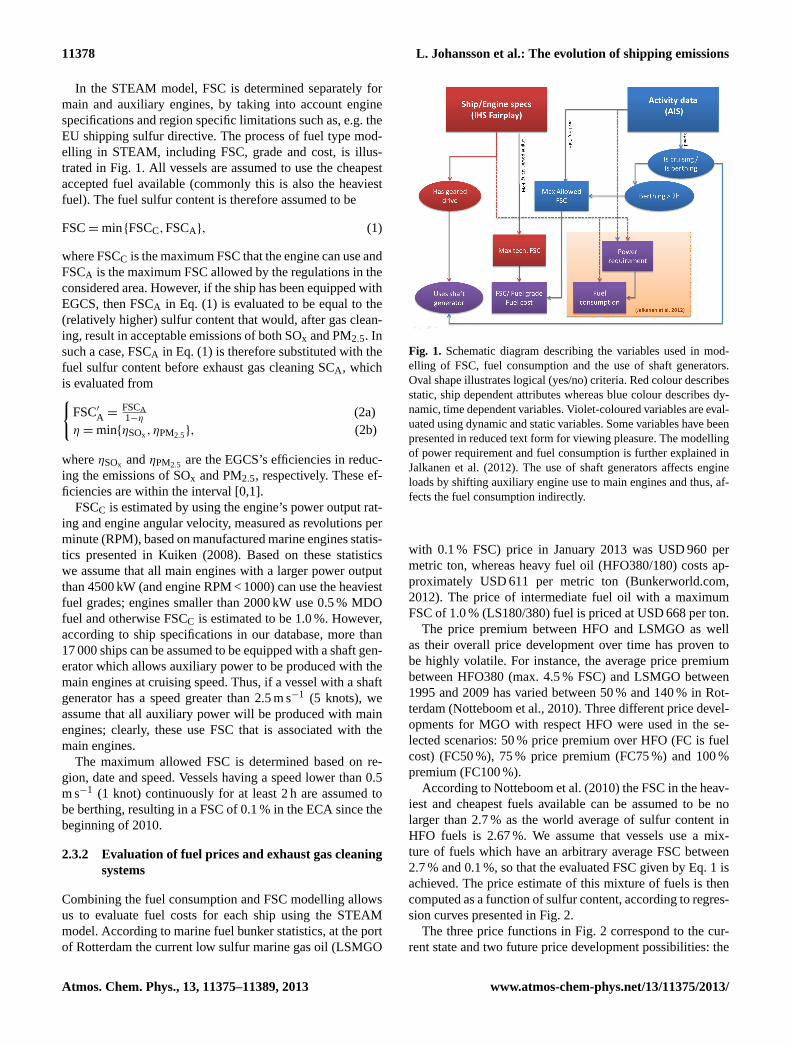
In the STEAM model, FSC is determined separately formain and auxiliary engines, by taking into account enginespecifications and region specific limitations such as, e.g. theEU shipping sulfur directive. The process of fuel type mod-elling in STEAM, including FSC, grade and cost, is illus-trated in Fig. 1. All vessels are assumed to use the cheapestaccepted fuel available (commonly this is also the heaviestfuel). The fuel sulfur content is therefore assumed to be

FSC= min{FSCC,FSCA}, (1)

where FSCC is the maximum FSC that the engine can use andFSCA is the maximum FSC allowed by the regulations in theconsidered area. However, if the ship has been equipped withEGCS, then FSCA in Eq. (1) is evaluated to be equal to the(relatively higher) sulfur content that would, after gas clean-ing, result in acceptable emissions of both SOx and PM2.5. Insuch a case, FSCA in Eq. (1) is therefore substituted with thefuel sulfur content before exhaust gas cleaning SCA , whichis evaluated from{

FSC′

A =FSCA1−η

(2a)η = min{ηSOx ,ηPM2.5}, (2b)

whereηSOx andηPM2.5 are the EGCS’s efficiencies in reduc-ing the emissions of SOx and PM2.5, respectively. These ef-ficiencies are within the interval [0,1].

FSCC is estimated by using the engine’s power output rat-ing and engine angular velocity, measured as revolutions perminute (RPM), based on manufactured marine engines statis-tics presented in Kuiken (2008). Based on these statisticswe assume that all main engines with a larger power outputthan 4500 kW (and engine RPM < 1000) can use the heaviestfuel grades; engines smaller than 2000 kW use 0.5 % MDOfuel and otherwise FSCC is estimated to be 1.0 %. However,according to ship specifications in our database, more than17 000 ships can be assumed to be equipped with a shaft gen-erator which allows auxiliary power to be produced with themain engines at cruising speed. Thus, if a vessel with a shaftgenerator has a speed greater than 2.5 m s−1 (5 knots), weassume that all auxiliary power will be produced with mainengines; clearly, these use FSC that is associated with themain engines.

The maximum allowed FSC is determined based on re-gion, date and speed. Vessels having a speed lower than 0.5m s−1 (1 knot) continuously for at least 2 h are assumed tobe berthing, resulting in a FSC of 0.1 % in the ECA since thebeginning of 2010.

2.3.2 Evaluation of fuel prices and exhaust gas cleaningsystems

Combining the fuel consumption and FSC modelling allowsus to evaluate fuel costs for each ship using the STEAMmodel. According to marine fuel bunker statistics, at the portof Rotterdam the current low sulfur marine gas oil (LSMGO

27

688

689

Figure 1: Schematic diagram describing the variables used in modelling of FSC, fuel consumption and 690 the use of shaft generators. Oval shape illustrates logical (yes/no) criteria. Red color describes static, 691 ship dependent attributes whereas blue color describes dynamic, time dependent variables. Violet-692 colored variables are evaluated using dynamic and static variables. Some variables have been 693 presented in reduced text-form for viewing pleasure. The modelling of power requirement and fuel 694 consumption is further explained in (Jalkanen et al, 2012). The use of shaft generators affects engine 695 loads by shifting auxiliary engine use to main engines and thus, affects the fuel consumption indirectly. 696

Fig. 1. Schematic diagram describing the variables used in mod-elling of FSC, fuel consumption and the use of shaft generators.Oval shape illustrates logical (yes/no) criteria. Red colour describesstatic, ship dependent attributes whereas blue colour describes dy-namic, time dependent variables. Violet-coloured variables are eval-uated using dynamic and static variables. Some variables have beenpresented in reduced text form for viewing pleasure. The modellingof power requirement and fuel consumption is further explained inJalkanen et al. (2012). The use of shaft generators affects engineloads by shifting auxiliary engine use to main engines and thus, af-fects the fuel consumption indirectly.

with 0.1 % FSC) price in January 2013 was USD 960 permetric ton, whereas heavy fuel oil (HFO380/180) costs ap-proximately USD 611 per metric ton (Bunkerworld.com,2012). The price of intermediate fuel oil with a maximumFSC of 1.0 % (LS180/380) fuel is priced at USD 668 per ton.

The price premium between HFO and LSMGO as wellas their overall price development over time has proven tobe highly volatile. For instance, the average price premiumbetween HFO380 (max. 4.5 % FSC) and LSMGO between1995 and 2009 has varied between 50 % and 140 % in Rot-terdam (Notteboom et al., 2010). Three different price devel-opments for MGO with respect HFO were used in the se-lected scenarios: 50 % price premium over HFO (FC is fuelcost) (FC50 %), 75 % price premium (FC75 %) and 100 %premium (FC100 %).

According to Notteboom et al. (2010) the FSC in the heav-iest and cheapest fuels available can be assumed to be nolarger than 2.7 % as the world average of sulfur content inHFO fuels is 2.67 %. We assume that vessels use a mix-ture of fuels which have an arbitrary average FSC between2.7 % and 0.1 %, so that the evaluated FSC given by Eq. 1 isachieved. The price estimate of this mixture of fuels is thencomputed as a function of sulfur content, according to regres-sion curves presented in Fig. 2.

The three price functions in Fig. 2 correspond to the cur-rent state and two future price development possibilities: the



28

697

Figure 2: Estimated fuel prices (USD/ton) as a function of the sulphur content of fuel, for 698

three different fuel cost (FC) scenarios. The scenarios correspond to the current state 699

(FC50%) and two future price (FC75 % and FC100 %) scenarios; these have been defined in 700

the text. The numerical equations of the fits have also been reported. 701

702

Figure 3: Seasonal variation of the predicted CO2 emissions in the ECA in 2009 and 2011, 703

presented separately for different ship types. Cargo ships include bulk carriers, general cargo 704

vessels and vehicle carriers. Passenger ships include RoPaX ships, ferries and passenger 705

cruisers. 706

Fig. 2. Estimated fuel prices (USD/ton) as a function of the sul-fur content of fuel, for three different fuel cost (FC) scenarios. Thescenarios correspond to the current state (FC50 %) and two futureprice (FC75 % and FC100 %) scenarios; these have been defined inthe text. The numerical equations of the fits have also been reported.

FC50 % curve corresponds to prices (HFO380, LS180 andLSMGO) as they were at the time of writing, in Rotterdam,FC75 % and FC100 % are the price estimates in case the pricepremium between LSMGO and HFO380 increases to 75 %and 100 % respectively. We apply these fuel prices for all pastand future scenarios presented in this paper; the derived fuelcosts (and thus the direct costs of regulations to ship owners)of each scenario are therefore comparable with each other.

The use of EGCSs offer potential fuel cost savings forships that operate in the ECA area, as IMO accepts EGCSsas alternatives to the use of low sulfur fuels. With a scrubberon-board, a ship can consume high FSC fuel and still complywith regulations. In Reynolds (2011) it was estimated thatany ship, which consumes annually more than 4000 metrictons of fuel in the ECA, should be a potential candidate foran EGCS installation. Assuming a 50 % price premium forLSMGO with respect to HFO and active use within the ECAfor at least 6 yr after 2015, the net financial value for EGCSscrubber installment should be positive.

Scrubbers can use wet or dry physical scrubbing or chem-ical adsorption to remove combustion products. In Corbett etal. (2010) it was concluded that the PM2.5 removal is likelyto be 75± 15 % with a scrubber on-board. Other studies haveindicated that the resulting reduction in PM mass can be be-tween 25 % and 98 %, depending on particle size distribu-tion, although the removal rates by species are more uncer-tain (Lack and Corbett, 2012). Also, a significant reductionin SOx output will occur. In Andreasen and Mayer (2007) itwas estimated that a sea water scrubber system can reduce66 % of SOx emissions.

2.3.3 Interpolation of shipping routes

In the STEAM model, the travel routes are evaluated in astepwise manner, by a linear interpolation of the geographi-cal coordinates, for each consecutive AIS message pair. Dueto this method of determining routes, it is useful to analyse inaddition the validity of each travel segment. The calibrationand use of AIS transmitters is also potentially susceptible tohuman errors. Especially as smaller ships without an IMOnumber behave erratically in some cases, based on the geo-graphic information included in their AIS messages. Further,in order to ensure a good accuracy of the method, at opensea fairly extensive spatial and temporal gaps can be allowed,whereas at harbours the possible AIS down-time of ships (i.e.the interval between an end of a berthing activity and the startof cruising) needs to be substantially shorter. The methodsfor the evaluation of route segments were therefore refinedfor this study.

The validity of each linear route segment has been eval-uated based on the average vessel speedva given by twoconsecutive AIS messages: the time duration1t , which iscomputed from message time stamps, and the distance1s,which is calculated from the two message coordinate pairs.In addition, two other evaluation measures are used: the so-called implied speed, defined asvI = 1s/1t , and implieddistance, defined as1sI = va1t . The emission is computedfor any route segment, if and only if the following three con-ditions are satisfied.

– The ship is physically able to travel the distance duringthe time interval in view of the specified design speedof the vessel. This criterion is confirmed ifva or vI isnot significantly greater than the vessel’s listed designspeed.

– The temporal or spatial separation of a route orberthing segment does not exceed pre-selected maxi-mum values. These maximum values have been spec-ified separately for harbour activities and open sea ac-tivities. For each segment in the ECA, we have usedthe maximum values of 600 km and 24 h for open seaoperations and 2 h for berthing activities.

– The vessel would not travel multiple times (or just afraction of) the distance1s within the givenva and1t . Thus,1sI must be close to1s.

2.3.4 Slow-steaming

Required propelling power for any marine vessel increasesstrongly as a function of its speed, due to the friction againstwater and the formation of waves. Even a minor reductionof vessel speed can therefore significantly reduce the mainengine’s fuel consumption. The concept of slow-steamingrefers to a situation, in which a marine vessel reduces itsspeed to achieve significant fuel savings. However, the fuel



savings and emission reductions are obviously obtained atthe expense of a longer cruising time.

In order to evaluate the net benefits in the selected slow-steaming scenario, the total travel time differential is calcu-lated for each route segment. We assume a fractional speedreduction with a factor ofa ∈ [0,1]. The increase in traveltime T+, the reduced slow-steaming speedviR and the in-creased duration1t iR are given by

T+ =∑i

(1tiR − 1ti) (3a)

viR = (1− a)vi (3b)1t iR = 1t i (1+ a), (3c)

where1ti is the duration of the travel of the ship during theith segment of a route (defined by two consecutive AIS mes-sages) andvi is the average speed ini-th segment of a routebefore applying speed reduction.1tiR is the increased du-ration of travel with the slow-steaming speed. The reducedspeedviR is used for instantaneous main engine power es-timation, which in turn is used for engine load, fuel con-sumption and subsequently for emission estimation. To ac-count for the fact that engines are being used longer witheach segment using the reduced speed, the duration1t iR isused instead of1t i in emission calculation. Besides the in-stantaneous speed, the main engine power requirement is af-fected by various ship attributes, such as hull dimensions andpropeller properties. This fairly complicated process was dis-cussed in more detail in Jalkanen et al. (2012).

2.3.5 Auxiliary fuel consumption of non-IMOregistered vessels

The number of unidentified vessels in AIS data has steadilyincreased during recent years. According to AIS data, a sub-stantial fraction of these vessels seem to be inactive; these aremostly berthing. Such vessel behaviour in the model wouldresult in an excessive amount of auxiliary fuel consumption,especially as the number of berthing small vessels increasesin time.

We have therefore added to the model a limiting rule forthe auxiliary fuel consumption of non-IMO-registered ves-sels. After 2 h (i.e. a reasonable time required for unload-ing the vessel) of continuous berthing, the rate of auxiliaryfuel consumption is assumed to start to decrease linearly as afunction of time. We have assumed that after 8 h of berthing,the rate of auxiliary fuel consumption has been decreased toone fifth (1/5) of the initial auxiliary fuel consumption rate.

2.4 Selected scenarios of the emissions and fuel costs

2.4.1 Scenarios in the past, since 2005, 2009 andJanuary of 2010

We have evaluated the emissions and fuel costs for three sep-arate scenarios in the past, all of which assume that no abate-ment of shipping emission had been done. (i) First, we have

evaluated the emissions and fuel cost differentials for a sce-nario in which we assumed that no FSC regulations had beenimposed in the ECA after 2005. We have therefore assignedFSCA = 2.7 % in Eq. (1), and compared the resulting SOxand PM2.5 emissions and fuel costs with the status quo emis-sion estimates in 2011.

Further, similar simulations are presented for scenarios as-suming that (ii) no further regulations had been introducedafter 2009, i.e. FSCA = 1.5 %, and (iii) no further regula-tions had been introduced after January of 2010, i.e. FSCA =

1.5 % and 0.1 % for berthing ships.

2.4.2 Scenarios for the future, in 2015

We have simulated the effects of the upcoming FSC require-ments in 2015, by using the archived AIS data for 2011 andassigning FSCA = 0.1 % for all ships and activities.

Another simulation for 2015 was performed, in whichEGCS installation candidate vessels were identified (cf.Sect. 2.3.2) and were assumed to be equipped with scrub-ber abatement equipment. Vessels which are equipped withabatement equipment may use cheaper and heavier fuel thanLSMGO, provided that the emissions do not exceed thosethat would be achieved with LSMGO without abatementequipment.

2.4.3 Slow steaming scenario

In the slow steaming scenario, we have evaluated the ship-ping emissions and statistics, as if each ship would have fared10 % and 30 % slower while cruising (a = 0.1 anda = 0.3 inEq. 3c). However, we assume that the speed reduction at slowspeeds would not be economically desirable for ship owners.The speed reduction is therefore applied only, if the instan-taneous speed exceeds 5.1 m s−1 (10 knots). As the enginepower needs to be continuous in time, any reduced speed willnot be reduced below this selected threshold value.

The increase in cruising time has been calculated accord-ing to Eq. (3a)–(3c), and the resulting emissions and fuel con-sumption with the reduced speed has been compared with thebaseline emission estimates and fuel consumption and costsfor 2011. Thus, we account for the increase in auxiliary fuelconsumption as well as the decrease in main engine loads.We have not taken into account however the potential needfor increasing the fleet size, due to the increase in cruisingtime.

3 Numerical results

The results were evaluated using the shipping emissionmodel STEAM, with the archived AIS and ship propertiesdata for the ECA region in 2009 and 2011. In the following,we first present an inventory of the emissions in 2009 and2011 in the ECA, second, we address the spatial concentra-tion distributions of the emissions in 2011, and third, present



Table 1.Predicted emissions and shipping statistics for the ECA in 2009. Shipping emission inventories by EMEP have also been presentedfor comparison purposes. Payload is the amount of transferred freight inside the ECA, which has been estimated based on ship’s deadweightand its type-specific fraction of payload reported in Buhaug et al. (2009).

ECA – CO2 NOx SOx PM2.5 CO Payload Ships Travel2009 [ton] [ton] [ton] [ton] [ton] [10^9 km*t] [10^6 km]

All ships EMEP 1 098 720 409 540 55 500 122 151

All ships STEAM 43 121 100 944 100 327 000 73 500 94 900 2699 23 973 325IMO-registered 41 848 800 923 400 319 900 71 600 89 300 2699 15 049 296non-IMO-registered 1 272 300 20 600 7100 1900 5600 0 8924 29Baltic Sea 15 545 400 321 100 117 600 26 400 32 300 765 – –North Sea 27 530 200 622 200 209 000 47 100 62 400 1933 – –

Top flags United Kingdom 3 826 900 82 100 28 200 6300 9000 184 2495 29Norway 3 600 500 72 800 23 900 5600 8000 136 2277 32Sweden 3 190 500 56 900 25 000 5500 6500 86 1693 23Netherlands 2 855 700 57 300 20 000 4600 6400 110 2164 32Liberia 2 472 000 63 600 20 400 4500 5400 267 1014 11Denmark 2 353 500 46 500 16 400 3800 6400 91 1241 21Bahamas 2 299 000 53 400 17 600 3900 4600 167 734 14Germany 2 091 400 46 200 16 600 3600 4800 122 1803 15Finland 1 990 700 38 200 16 800 3600 4100 66 496 13Malta 1 782 400 40 900 13 000 2900 3500 157 836 15Antigua and Barbuda 1 726 900 35 700 11 500 2600 3300 86 840 21Cyprus 1 571 500 35 400 11 600 2600 3300 113 467 12Marshall Islands 960 600 24 500 7700 1700 1900 118 522 5Greece 923 600 26 000 8500 1800 1700 165 316 3Gibraltar 836 500 18 500 5700 1300 1500 46 245 8Panama 698 200 18 400 6100 1300 1500 77 344 3Italy 623 400 14 800 5400 1100 1200 42 198 3Hong Kong 607 500 16 000 5300 1100 1300 80 334 2Russia 483 600 9400 2600 600 1000 17 711 6France 475 300 10 000 4000 800 1300 7 394 3

Ship types Passenger ships 7 785 700 147 200 64 200 13 900 18 200 54 863 39Cargo ships 11 283 500 246 900 83 500 18 800 21 900 844 5908 122Container ships 9 113 800 222 900 76 800 16 800 22 000 679 1868 39Tankers 9 267 700 228 200 73 700 16 400 17 400 1123 3284 61Other 4 397 800 78 000 21 400 5600 9600 0 3126 35

model predictions for the various assumed scenarios in thepast and for the future.

3.1 Emission budgets in 2009 and 2011

The predicted emission inventories and shipping statistics arepresented in Table 1 for the ECA in 2009. The maximumallowed FSC at the time was 1.5 %.

The corresponding shipping emission inventories accord-ing to EMEP have also been included in Table 1. However,there are some methodological differences between the cur-rent study and the methods used by EMEP. First, the STEAMmodel evaluated the PM2.5 emissions, including the mois-ture (SO4 + 6.5H2O) for sulfate particles (Jalkanen et al.,2012), whereas EMEP has used the dry weight of SO4. Sec-ondly, the EMEP estimates include neither harbour activi-ties nor non-IMO-registered ships, whereas those have been

included in the STEAM computations. The accounting ofharbour activities is a major methodological difference. Ac-cording to the predictions using the STEAM model, approx-imately 22 % of the total fuel was consumed at harbours inthe ECA in 2009. Despite this, the total shipping emissionspredicted using the STEAM model were 14 % smaller thanthe corresponding EMEP emissions in case of NOx, whilethe SOx emissions predicted using the STEAM model were20 % lower. There were also notable differences between thepredictions of these two modelling systems in case of PM2.5and CO.

In 2009, approximately 15.5 and 27.5 million tons ofCO2 were emitted at the Baltic Sea and at the North Sea(for simplicity, the latter is here interpreted to include alsothe English Channel), respectively. The most significant flagstates were the Scandinavian countries Norway, Sweden and



Table 2.Predicted emissions and shipping statistics for the ECA in 2011.

ECA – CO2 NOx SOx PM2.5 CO Payload Ships Travel2011 [ton] [ton] [ton] [ton] [ton] [10^9 km*t] [10^6 km]

All ships STEAM 48 029 900 1 010 400 239 300 63 800 110 900 2985 30 165 375

IMO-registered 45 570 700 970 900 231 100 60 900 101 000 2985 15 411 320non-IMO-registered 2 459 200 39 500 8200 2900 9900 0 14 754 55

Baltic Sea 17 614 600 356 100 87 400 23 200 37 400 890 – –North Sea 30 033 600 648 900 151 300 40 200 72 600 2091 – –

Top flags Netherlands 4 004 100 75 000 17 700 5000 9900 126 7295 52United Kingdom 3 931 500 82 200 19 400 5100 9400 209 1916 29Norway 3 332 500 65 200 15 100 4100 7600 98 1513 28Liberia 2 984 000 73 200 15 800 4100 7300 352 1117 13Sweden 2 898 600 50 600 15 900 4000 5500 70 936 19Germany 2 659 400 53 800 12 400 3400 7100 124 2730 23Denmark 2 652 700 52 400 12 600 3400 7100 118 1126 22Bahamas 2 281 100 52 000 12 000 3100 4700 171 698 14Antigua and Barbuda 2 233 900 44 900 10 800 2800 4500 115 825 26Malta 2 100 200 45 300 10 300 2700 4300 162 937 18Finland 2 051 500 38 100 11 300 2800 4300 66 507 13Cyprus 1 934 000 41 100 9400 2500 4300 135 484 15Marshall Islands 1 217 400 29 400 6400 1600 2700 155 681 6Hong Kong 985 600 24 100 5400 1400 2500 131 440 4Gibraltar 972 200 20 900 4700 1200 2000 55 248 11Italy 791 300 18 000 4500 1100 1600 56 237 4Greece 764 400 20 900 4500 1100 1700 150 250 3France 734 500 15 500 4100 1000 1900 25 944 6Russia 650 400 12 500 2200 700 1400 22 670 7Panama 643 900 15 800 3400 900 1500 69 336 3

Ship types Passenger ships 7 804 500 145 500 44 000 10 900 17 300 54 825 39Cargo ships 12 608 500 268 200 65 500 17 000 25 200 978 6183 133Container ships 10 377 300 242 400 55 300 14 500 27 800 857 1711 44Tankers 8 934 900 212 100 47 800 12 400 18 200 1096 3337 61Other 5 845 400 102 500 18 300 5900 12 300 0 3355 43

Denmark, the Netherlands and the United Kingdom. Thecargo ships were the single most significant ship type interms of the CO2 emissions.

The corresponding emission estimates in the ECA in 2011are presented in Table 2. In contrast to 2009, the maximumallowed FSC for ships at berthing was limited to 0.1 %, andotherwise to a maximum of 1.0 %. The contribution fromnon-IMO-registered ships in terms of CO2 has doubled since2009, but it is still only 5 % of the total estimated CO2;this increase has probably been caused by an increase of thenumber of small ships that have installed AIS transmitters.The number of non-IMO-registered ships has increased from8924 (in 2009) to 14754 (in 2011). However, this increasehas not necessarily been caused by an increase in fleet size.A larger fraction of smaller ships have installed AIS transmit-ters, partly as these have become more affordable. The tem-poral evolution of the emissions of CO2 has been presented

in Fig. 3 for different ship categories and non-IMO-registeredvessels both in 2009 and 2011.

The annual IMO-registered marine traffic has significantlyincreased from 2009 to 2011, in terms of both the CO2 emis-sions (+8.9 %) and the cargo payload amounts (+10.6 %),possibly caused by the recovery of the European economyduring the study period. There have been significant changesin the distribution of emissions for the various flag states aswell. For instance, the number of ships sailing under the flagof Norway has substantially decreased, while the fleet of theNetherlands has significantly increased. A geographical dif-ference map between the CO2 emissions in 2011 and 2009reveals a strong increase in the sea regions in the vicinity ofthe Netherlands, and a distinct decrease near the coasts ofNorway (the results not shown here). These changes couldbe caused either by changes in shipping activities or changesin the use of AIS equipment.



28

697

Figure 2: Estimated fuel prices (USD/ton) as a function of the sulphur content of fuel, for 698

three different fuel cost (FC) scenarios. The scenarios correspond to the current state 699

(FC50%) and two future price (FC75 % and FC100 %) scenarios; these have been defined in 700

the text. The numerical equations of the fits have also been reported. 701

702

Figure 3: Seasonal variation of the predicted CO2 emissions in the ECA in 2009 and 2011, 703

presented separately for different ship types. Cargo ships include bulk carriers, general cargo 704

vessels and vehicle carriers. Passenger ships include RoPaX ships, ferries and passenger 705

cruisers. 706

Fig. 3.Seasonal variation of the predicted CO2 emissions in the ECA in 2009 and 2011, presented separately for different ship types. Cargoships include bulk carriers, general cargo vessels and vehicle carriers. Passenger ships include RoPax ships, ferries and passenger cruisers.

The imposed emission limitations up to date have had asignificant impact on the emissions of SOx and PM2.5. Ac-cording to results in Tables 1 and 2, the SOx emissions origi-nated from IMO-registered marine traffic have been reducedfrom 2009 to 2011 from 320 kt to 231 kt. The correspond-ing predicted reduction for PM2.5 from 71.6 kt to 60.9 kt.The estimated NOx emissions from IMO-registered trafficare slightly larger in 2011 than in 2009 (+5.1 %). The in-crease of the emissions of NOx was smaller than the corre-sponding increase of emissions of CO2. The reason for thisis that after January 2011, the NOx emission factor was notallowed to exceed the IMO specified Tier II factor, which isslightly lower than the previous Tier I requirement for all en-gines. We have assumed that ships built after 2008 conformto the new Tier II limitations, as the engine manufactureshave been well prepared for those requirements. However,the effect of the implementation of Tier II for the emissionsof NOx from 2009 to 2011 seems minuscule, but will cer-tainly increase when the fleet is renewed in time.

Based on the modelled fuel consumption statistics forIMO-registered vessels, 33 % of the total fuel was consumedby auxiliary engines in 2011. However, the ratio of the aux-iliary fuel consumption and the total fuel consumption variessignificantly between ship types (18 % for passenger ships,30 % for cargo ships, 35 % for container ships, 31 % fortankers and 64 % for other ships). Approximately 17 000ships in the ship properties database have been associatedwith a shaft generator, which allows the main engine to pro-vide power to ship operating systems while cruising. Theo-retically, it can be shown by numerical computations that ifthere would have been no shaft generators available, the pre-dicted fuel consumption of the main and auxiliary engineswould have been almost equal in the ECA in 2011.

It has been predicted that the use of HFO significantly out-weights the use of distillate fuels. Commonly a ratio, such as85 % / 15 %, has been used to distinguish the use of distillatefuels and the heavier grades. However, according to resultsthis assumption seems to be biased. Assuming that fuels witha lower FSC than 1 % were distillate fuels (MDO or MGO),

the ratio of HFO and distillate fuel consumption of IMO-registered vessels was approximately 76 % / 24 % in 2009. In2011, this ratio changed to 70 % / 30 %. The high fraction ofthe distillate fuels is caused by two main factors. First, a ma-jor fraction of the fuel consumption originates from auxiliaryengines during harbour activities; most of the auxiliary en-gines cannot use HFO due to engine restrictions (e.g. enginesize, RPM and stroke type). Second, distillate fuel consump-tion for ships at berthing has increased significantly after theintroduction of the Marpol Annex VI regulation.

3.2 The geographical distribution of shipping emissionsin 2011

For 2011, the geographical distribution of CO2 and PM2.5emissions in the ECA has been presented in Figs. 4 and 5, re-spectively. The relative geographical distribution of the ship-ping emissions is similar also for the other modelled com-pounds, and those results have therefore not been presentedhere. The highest CO2 and PM2.5 emissions originated fromshipping are located near the coast of the Netherlands, in theEnglish Channel and along the busiest shipping lines in theDanish Straits and the Baltic Sea.

In particular, in the vicinity of the coast of the Netherlands,the predicted PM2.5 emissions per unit sea area are fromthree to five times higher, compared with the correspondingvalues in the major shipping lanes of the Baltic Sea. Nearseveral major ports (e.g. Antwerp, Rotterdam, Amsterdam,Hamburg, Riga, Tallinn, Helsinki and St Petersburg) thereare localized high amounts of PM2.5 emissions that exceedthe corresponding emissions even within the busiest shippinglanes in the ECA.

The geographic distribution of CO2 emissions varies sub-stantially between ship types, as illustrated in Fig. 6. Pas-senger ships operate relatively more at short distances, com-pared with the other presented ship categories. There is es-pecially intensive passenger ship traffic between the ports ofFrance and the UK, and there is busy traffic also between Ro-stock and Trelleborg, and between Helsinki and Tallinn. The



29

707

Figure 4: Predicted geographic distribution of shipping emissions of CO2 in the ECA in 2011. 708

The colour code indicates emissions in relative mass units per unit area. 709

710

Fig. 4. Predicted geographic distribution of shipping emissions ofCO2 in the ECA in 2011. The colour code indicates emissions inrelative mass units per unit area.

geographical distributions of CO2 emissions originated fromcontainer ships and cargo ships are similar with each other.However, the cargo ships were responsible for approximately21 % more CO2 emissions in 2011 than container ships. Asubstantial fraction of both container and cargo ships are lo-cated along the main shipping lanes from south-west (the En-glish Channel) to north-east (St Petersburg). Miscellaneousships operate intensively near the ports and the oil rigs on theNorth Sea. Almost 4 % of the fuel consumed on the NorthSea is used by service ships that operate between oil rigs andports.

3.3 Results for the selected scenarios of the emissionsand fuel costs

Since May of 2006, the maximum allowed FSC in the ECAhas been gradually lowered. In 2015, it will be reduced to0.1 % for all large marine vessels operating within the area.

3.3.1 Results for the scenarios in the past, since 2005,2009 and January of 2010

The relative SOx and PM2.5 emissions and fuel costs for theselected scenarios have been summarized in Fig. 7, in rela-tion to modelled emissions and fuel costs in 2011. The sim-ulations for the past assumed that there would have been noregulative actions since 2005, 2009 or January of 2010, andthen proceeded to evaluate the emissions and fuel costs forthe reference year of 2011. In the following, we call thesescenarios for simplicity the 2005, 2009 and 2010 scenarios.

For the 2005 scenario the SOx emissions in 2011 wouldhave been more than double (+127 %), compared with theactual situation in 2011. The emissions of SOx and PM2.5

30

711

Figure 5: Predicted geographic distribution of shipping emissions of PM2.5 in the ECA in 2011. 712 PM2.5 has been assumed to consist of organic and elemental carbon, ash and moist sulfate particles. 713 Fig. 5. Predicted geographic distribution of shipping emissions of

PM2.5 in the ECA in 2011. PM2.5 has been assumed to consist oforganic and elemental carbon, ash and moist sulfate particles.

31

714

Figures 6a-d: Predicted geographic distribution of the shipping emissions of for 715

passenger (a), container (b), cargo (c) and miscellaneous (d) ships in the ECA in 2011. 716

Passenger ships include RoPaX vessels, cruisers, ferries and other passenger ships. Cargo 717

ships include general cargo, RoRo, vehicle carriers and bulk carriers. Miscellaneous ships 718

include yachts, fishing boats, tugs, ice breakers, barges dredge ships, etc. 719

720

Fig. 6. Predicted geographic distribution of the shipping emissionsof CO2 for passenger(a), container(b), cargo(c) and miscellaneous(d) ships in the ECA in 2011. Passenger ships include RoPax ves-sels, cruisers, ferries and other passenger ships. Cargo ships includegeneral cargo, RoRo, vehicle carriers and bulk carriers. Miscella-neous ships include yachts, fishing boats, tugs, ice breakers, bargesdredge ships, etc.

for this scenario would have been 525 kt and to 104 kt, re-spectively. As expected, the direct fuel costs would have beenlower that for the actual situation in 2011, about USD 9.8 bil-lion, based on the current Rotterdam bunker fuel prices; thisis USD 1.0 billion less than the actual estimated fuel costs in2011.

In the 2009 scenario, there would be 337 kt and 76 kt ofSOx and PM2.5 emissions, respectively. These estimates areslightly larger than the presented values that were estimatedwith the actual data set for 2009. The total fuel costs for



32

721

Figure 7: Relative emissions of SOx and PM2.5, and direct fuel costs of IMO-registered marine 722

traffic in the ECA in 2011, for the various selected scenarios. The situation in 2011 has been 723

evaluated also using three different assumed options regarding the regulations of marine 724

emissions in the past (the three sets of columns on the left-hand side). The scenarios for the 725

future have been presented using three fuel cost (FC) options (the two sets of columns on the 726

right-hand side). 727

Fig. 7. Relative emissions of SOx and PM2.5, and direct fuel costsof IMO-registered marine traffic in the ECA in 2011, for the variousselected scenarios. The situation in 2011 has been evaluated alsousing three different assumed options regarding the regulations ofmarine emissions in the past (the three sets of columns on the left-hand side). The scenarios for the future have been presented usingthree fuel cost options (the two sets of columns on the right-handside).

all ships would be USD 10.4 billion, which is only USD 250million more than the costs in the 2005 scenario. The reasonis that the price of marine fuel with a FSC close to 1.5 % isonly slightly higher than the fuel price for 2.7 % HFO, whichwas accepted before May 2006 in the ECA.

In the 2010 scenario, in which FSC maximum was set to1.5 % and 0.1 % for ships at berth, ships would exhaust 309 ktof SOx and 72 kt of PM2.5, having fuel cost of USD 10.6billion, which is roughly USD 220 million less than the es-timated fuel costs for 2011 and 580 million more than inthe 2009 scenario. Thus, we estimate that the requirementto switch to low sulfur distillates while berthing decreasedthe SOx emissions in harbours only by 28.4 kt and the PM2.5emissions by 4.2 kt. The reduction of FSC to a maximumof 1.0 % starting from 1 July 2010, reduced SOx emissionsfurther by 77.9 kt and PM2.5 emissions by 11.3 kt; the com-bined direct fuel costs of these reductions is approximatelyUSD 0.8 billion.

3.3.2 Results for the scenarios of the future, in 2015

The 2015 scenario was simulated with the ECA 2011 datasets, i.e. by assuming that the shipping activities and theproperties of the ships will be the same in the future, andby setting a maximum allowed FSC to 0.1 % for all activ-ities. Three different fuel price scenarios were included, asthe evolution of the relative prices of these fuels is uncertain;these are denoted briefly by FC50 %, FC75 % and FC100 %.These fuel price scenarios correspond to the cases in whichthe fuel prices remain the same as in 2011, and MGO is 50 %,75 % or 100 % more expensive than HFO.

The SOx emissions in this scenario will be reduced to amere 29.2 kt and fine particle emissions will be reduced to31.4 kt. In comparison with the situation in 2011, the SOxemissions will be reduced by 87 % and the PM2.5 emissionswill be reduced by 46 %. The relative reduction of PM2.5emissions is smaller in comparison to those of SOx, as ma-rine engines produce significant amounts of carbon and ashparticles, regardless of FSC. The direct fuel costs will in-crease to USD 13.3, 15.7 or 18.3 billion, depending on thefuel price development, which corresponds to a cost increaseof 23–69 %.

Reynolds (2011) estimated that ships with an annual fuelconsumption of more than 4000 t would gain economic ben-efit from scrubber installation, instead of using 0.1 % MGOfuel in 2015, provided that MGO will be at least 50 % moreexpensive than HFO and each ship with an installed scrub-ber will be active for at least 5 yr after installation. Usingthe modelled fuel consumption statistics for the year 2011,the possible candidates for EGCS installment suggested byReynolds were identified; a total of 635 candidate ships werefound. While there was more than 30 000 different ships op-erating at the time, these 635 ships account for 21 % of thetotal fuel consumption in the ECA. These ships have beenlisted in Table 3 according to their ship category. Most ofthese candidate ships are either container ships or RoPax ves-sels.

Another simulation was performed with the 2015 regula-tions, in which a typical scrubber abatement method was as-sumed to be installed to each candidate ship. The fuel costs ofthis scenario were significantly lower compared with the cor-responding scenario without the scrubbers: USD 12.3, 14.2or 16.1 billion (a cost increase from 13 % to 49 %). Further,most of the economic benefits from the use of scrubbers (andfrom using cheaper fuel simultaneously) were in the BalticSea shipping. A major portion of the identified EGCS candi-date ships operates mainly in the Baltic Sea. The estimatedPM2.5 emissions in this scenario were slightly smaller thanin the 2015 scenario without scrubbers. The reason for this isthat the virtual scrubbers reduced 66 % from SOx emissionsand 75 % from PM2.5 emissions and, thus, FSCA in Eq. (2a)and (2b) results in a slightly lower FSC than would be re-quired in terms of a PM2.5 emission factor in 2015.

The economic benefits from the use of scrubbers in 2015are clear, based on these computations. However, the cost ofan EGCS installment per vessel can be from USD 5 to 9 mil-lion (Reynolds, 2011), and there are also maintenance costs.These installment and maintenance costs have not been takeninto account in the presented scenarios. Further, for techni-cal reasons not all ships can be equipped with such systemsand it might also not be economically viable, if the vessel isreaching the end of its lifespan.



Table 3. The numbers of candidate ships for the installment of theEGCS, and their fraction of the total fuel consumption, presentedseparately for each ship type. The values are based on the estimatedfuel consumption in the ECA in 2011. Ships with an annual fuelconsumption of at least 4000 t have been qualified as such candi-dates, according to Reynolds (2011).

Ship category The number of Fraction ofcandidate ships for the total fuel

installed EGCS consumption

All 635 21 %

Container 258 7.0 %RoPax 132 7.1 %RoRo 82 2.8 %Crude oil tanker 42 1.2 %Passenger cruiser 23 0.6 %Chemical tanker 21 0.5 %Bulk carrier 13 0.3 %Vehicle carrier 9 0.2 %Product tanker 8 0.2 %General cargo 6 0.2 %

3.4 Slow steaming

We have investigated the savings in fuel consumption andthe reduction of emissions, due to reducing vessel speeds.In evaluating the financial costs, we have not addressed theadditional costs associated with longer cruising times, suchas, e.g. increased personnel costs, costs related to the slowerdelivery of the cargo, and the potential need for increasingthe fleet size.

For simplicity, the amount of speed reduction was selectedto be proportional to actual speed, viz. 10 % or 30 %. How-ever, such speed reduction was imposed only if vessel speedwas higher than 5.1 m s−1 (10 knots), as it would be un-likely to achieve significant economic savings by reducingspeeds that are lower than this selected threshold value. Theestimated savings in the consumption and costs of fuel, andthe reductions in emissions have been presented in Table 4aand b.The results of these slow-steaming scenarios are shownseparately for those vessel categories, for which the fuel con-sumption is > 1.0 % of total fuel consumption in the ECA in2011. The presented ship types, except for the container shipcategory, are sub-classes of the vessel categories presented inTables 1 and 2.

Even a reduction of 10 % in cruising speed will effectivelyreduce the main fuel consumption of several ship categories.In total, CO2, NOx, SOx, and PM2.5 emissions are reducedby 9.4 %, 11.7 %, 13.2 % and 11.5 % respectively. The re-ductions of the NOx, SOx and PM2.5 emissions are largerthan those for CO2. The reason is that the main engines gen-erally use fuel with a higher FSC and large two-stroke mainengines are responsible for higher NOx emissions per pro-vided energy unit, compared with smaller auxiliary engines.

However, the CO emissions per provided energy unit tend toincrease for lower engine loads.

Depending on the ship type, the achieved reduction inmain fuel consumption ranges from 6.5 % to 18.3 %. The rel-ative change of the operational time (berthing, maneuveringand cruising) is significantly smaller. For instance, the fuelcosts of RoPax ships would be reduced by 13.6 %, while theoperational time increases by 3.2 %. RoRo and vehicle carri-ers would achieve the reductions in fuel costs of 14.3 % and12.5 %, while their operational time would increase by 5.0 %.Together, the categories of RoPax, RoRo and vehicle carrierscontribute 22.4 % of the total fuel consumption in the ECA.The container ship category, which is the largest vessel cate-gory in the ECA, would gain a more modest 8.6 % reductionin fuel costs, and an increase of operational time of+4.7 %.

For the scenario with a speed reduction of 30 %, the emis-sions of CO2, NOx, SOx and PM2.5 are reduced by 20.7 %,26.7 %, 29.6 % and 24.5 %, respectively. Due to the selectionof the above mentioned threshold speed (5.1 m s−1), only theships which are cruising faster than 7.4 m s−1 (approximately14.3 knots) are subject to a full 30 % reduction in speed. Sub-stantial reductions due to a reduced speed would be expectedfor RoPax ships, vehicle carriers, crude oil tankers and pas-senger cruisers.

Inter-comparing the results for these two speed reductionscenarios reveals that the savings of fuel costs with respect tothe increases of operational times are higher in the scenariowith a 10 % speed reduction. This is to be expected, as theslower cruising speed results in a higher fuel consumption ofauxiliary engines. A major increase in operational time alsoresults in a need for using additional ships.

4 Conclusions

The marine exhaust emissions were evaluated using theSTEAM model in the ECA in 2009 and 2011. The combinedemissions of CO2 from shipping sources in the ECA wereevaluated to have increased from 43 to 48 million tons from2009 to 2011 (+11 %, using 2009 as the base year), mostlycaused by the increase in cargo transport in the ECA regionduring the study period. Although the number of non-IMO-registered vessels strongly increased, the estimated contribu-tion of these presumably small vessels was only 5 % in termsof CO2 emissions in 2011.

The predicted SOx emissions originating from IMO-registered marine traffic have been reduced from 320 kt to231 kt from 2009 to 2011 (−29 %, using 2009 as the baseyear). The corresponding predicted reduction for PM2.5 wasfrom 71.6 kt to 60.9 kt (−17 %, using 2009 as the base year).The emission limitations from 2009 to 2011 have obviouslyhad a significant impact on reducing the emissions of bothSOx and PM2.5.



Table 4.The predictions for the slow-steaming scenarios, assuming speed reductions of 30 % (a) and 10 % (b). Speed reductions have beenapplied only for instantaneous speeds exceeding 10 knots. “Share of total FC 2011” refers to the estimated share of total fuel consumption inthe ECA in 2011. Operational time is the combined duration of berthing, maneuvering and cruising.

(a) Slow-steaming (30 %)

Share of total 1Main fuel 1Operational 1Fuel cost 1CO2 1NOx 1SOx 1PM2.5 1COShip category FC 2011 [%] cons. [%] time [%] [%] [%] [%] [%] [%] [%]

Vehicle carrier 2.8 % −45.4 % 15.6 % −29.8 % −31.4 % −40.3 % −39.9 % −34.3 % 28.8 %Refrigerated cargo 1.7 % −43.7 % 11.5 % −20.6 % −22.9 % −33.2 % −36.8 % −28.4 % 26.5 %RoRo 6.1 % −42.5 % 15.4 % −34.1 % −35.5 % −38.8 % −41.1 % −37.3 % 6.3 %RoPax 13.5 % −40.8 % 10.1 % −31.7 % −33.0 % −35.3 % −38.5 % −36.6 % −7.9 %Passenger cruiser 2.3 % −39.0 % 12.1 % −27.7 % −29.0 % −31.1 % −34.0 % −32.2 % −10.3 %Container ship 19.9 % −38.2 % 14.6 % −19.4 % −20.9 % −29.7 % −30.0 % −20.4 % 12.8 %Tanker, LPG 1.4 % −36.9 % 9.1 % −18.1 % −20.0 % −28.5 % −31.9 % −26.9 % 29.3 %Bulk cargo 6.5 % −33.6 % 8.8 % −18.2 % −19.8 % −27.5 % −29.3 % −25.7 % 29.4 %Tanker, crude 5.3 % −33.1 % 7.8 % −22.3 % −23.5 % −30.5 % −29.6 % −27.6 % 31.1 %Tanker, chem. 9.3 % −32.1 % 9.1 % −18.0 % −19.6 % −26.9 % −28.8 % −25.3 % 27.1 %Tanker, product 2.3 % −31.3 % 5.1 % −17.7 % −19.3 % −27.0 % −28.6 % −25.1 % 27.9 %General cargo 10.9 % −18.0 % 3.9 % −9.5 % −10.5 % −14.2 % −16.2 % −13.6 % 16.6 %Dredge 1.2 % −16.4 % 1.5 % −7.6 % −8.4 % −9.6 % −13.4 % −11.2 % 3.5 %Service ship 4.0 % −14.3 % 1.6 % −5.1 % −5.8 % −6.2 % −10.8 % −8.5 % 1.1 %Fishing boat 1.4 % −12.6 % 1.2 % −3.0 % −3.6 % −4.7 % −8.8 % −5.5 % 4.3 %Tug boat 2.3 % −11.8 % 0.5 % −2.6 % −3.1 % −3.7 % −8.7 % −5.5 % 3.3 %

(b) Slow-steaming (10 %)

Share of total 1Main fuel 1Operational 1Fuel cost 1CO2 1NOx 1SOx 1PM2.5 1COShip category FC 2011 [%] cons. [%] time [%] [%] [%] [%] [%] [%] [%]

Vehicle carrier 2.8 % −18.3 % 5.0 % −12.5 % −13.1 % −16.0 % −16.4 % −15.0 % 15.5 %RoRo 6.1 % −17.7 % 5.0 % −14.3 % −14.9 % −16.0 % −17.1 % −16.3 % 5.8 %Refrigerated cargo 1.7 % −17.5 % 3.8 % −8.7 % −9.6 % −13.2 % −14.9 % −12.6 % 14.4 %RoPax 13.5 % −17.4 % 3.2 % −13.6 % −14.2 % −15.0 % −16.5 % −15.7 % −2.7 %Passenger cruiser 2.3 % −16.6 % 3.9 % −12.1 % −12.7 % −13.4 % −14.8 % −14.1 % −5.3 %Tanker, LPG 1.4 % −16.4 % 3.5 % −8.4 % −9.2 % −12.3 % −14.3 % −12.4 % 14.5 %Bulk cargo 6.5 % −15.9 % 3.6 % −8.8 % −9.6 % −12.7 % −14.0 % −12.4 % 15.1 %Container ship 19.9 % −15.8 % 4.7 % −8.6 % −9.2 % −12.8 % −12.9 % −10.4 % 8.3 %Tanker, chem. 9.3 % −15.2 % 3.8 % −8.8 % −9.5 % −12.5 % −13.7 % −12.2 % 14.3 %Tanker, crude 5.3 % −15.0 % 3.1 % −10.3 % −10.9 % −13.5 % −13.6 % −12.7 % 15.8 %Tanker, product 2.3 % −14.0 % 2.1 % −8.1 % −8.8 % −11.8 % −12.9 % −11.4 % 14.3 %General cargo 10.9 % −9.7 % 2.0 % −5.3 % −5.8 % −7.4 % −8.8 % −7.6 % 9.6 %Service ship 4.0 % −8.2 % 0.9 % −2.9 % −3.3 % −3.5 % −6.2 % −4.9 % 0.6 %Dredge 1.2 % −7.7 % 0.7 % −3.6 % −3.9 % −4.5 % −6.3 % −5.2 % 2.7 %Fishing boat 1.4 % −7.1 % 0.7 % −1.7 % −2.1 % −2.6 % −4.9 % −3.3 % 2.6 %Tug boat 2.3 % −6.5 % 0.3 % −1.4 % −1.7 % −2.0 % −4.8 % −3.0 % 1.6 %

The highest CO2 and PM2.5 emissions originating fromshipping in 2011 were located in the vicinity of the coastof the Netherlands, in the English Channel, near the south-eastern UK and along the busiest shipping lines in the Dan-ish Straits and the Baltic Sea. Near several major ports(e.g. Antwerpen, Rotterdam, Amsterdam, Hamburg, Riga,Tallinn, Helsinki and St Petersburg), there were especiallyhigh PM2.5 emissions per square kilometre, which exceededthe corresponding emission values even within the busiestshipping lanes in the ECA. The geographic distribution ofemissions was substantially different for various ship types.Clearly, the emission inventories of this study could be usedas input values for evaluating the atmospheric dispersion,population exposure and health impacts caused by shipping.

A number of scenario computations for the past were per-formed to evaluate more extensively the effects of the grad-

ually decreasing maximum allowed FSC. As a result of therestrictions, the SOx and fine particle matter emissions origi-nated from IMO-registered shipping have steadily decreased.A model simulation was performed, in which we assumedthat the FSC regulations as they were issued in 2005 wouldhave been in effect until 2011, without any subsequent fuelsulfur content restrictions. The simulation showed that theSOx emissions in the ECA would have been 127 % higher(i.e. more than twice as high), compared with the predictedvalues in 2011, including all the implemented regulations.The corresponding PM2.5 emissions would have been 71 %higher. However, the direct fuel costs would have been 10 %lower, according to the predictions.

The potential impacts of the forthcoming reductions re-garding the maximum allowed FSC in 2015 were also stud-ied, with simulations using the archived data in 2011. It was



estimated that the emissions of SOx will be reduced by 87 %and those of PM2.5 by 48 %, with respect to the estimatedemissions in the ECA in 2011. The direct fuel costs were es-timated to increase by 23 % from 2011 to 2015, assumingthe contemporary bunker prizes. However, if the price pre-mium of MGO with respect to HFO by that time increases100 %, due to the increase in demand, then the direct fuelcosts would annually be 69 % higher.

Based on the estimated fuel consumption and current fuelprices, it was evaluated that more than 630 IMO-registeredships might benefit from a retrofit scrubber installation.These candidate ships were responsible for approximately21 % of the total fuel consumption in the ECA in 2011. As-suming that each of these ships would use sulfur scrubbersinstead of using 0.1 % sulfur content MGO in 2015, the esti-mated fuel cost would increase in 2015 either only by 13 %(using the contemporary bunker prizes) or by 49 % (assum-ing 100 % price premium between HFO and MGO). How-ever, we did not address in these computations the install-ment costs and running maintenance costs. It is also not tech-nically feasible to retrofit all of the candidate ships with suchan EGCS device.

The possibility to achieve emission reductions by decreas-ing vessel cruising speeds was also investigated. We numer-ically applied speed reductions of 10 % and 30 % to speedsexceeding 5.1 m s−1 (10 knots). Furthermore, we accountedfor the increases in auxiliary engine fuel consumption, de-creases in engine loads and computed the resulting fuel sav-ings and emission reductions for each pollutant and ship cat-egory individually. The resulting fuel savings were signifi-cant even with a 10 % reduction of cruising speed. The rel-ative reduction of NOx, SOx and PM2.5 emissions was esti-mated to be higher than the reduction in total fuel consump-tion. The effectiveness of speed reduction as a way to curbemissions varies substantially between ship types. EspeciallyRoPax, RoRo, tankers and vehicle carrier ships could sub-stantially save in fuel costs, while the increase in operationaltime would not be significantly increased. The ratio of fuelsavings and the increase in operational time was better usingthe smaller, 10 % speed reduction for all ship types. How-ever, the reduced cruising speeds may result in a need forlarger fleet sizes.

Acknowledgements.We gratefully acknowledge the support ofthe Finnish Transport Safety Agency (TraFi), the member statesof the Marine Environment Protection Committee of the BalticSea (Helcom) and the funding for Finnish Academy APTA projectin this work. We are thankful for the European Maritime SafetyAgency for providing the ship movement data for this research.The research leading to these results has received funding from theEuropean Regional Development Fund, Central Baltic INTERREGIV A Programme within the project SNOOP. The publicationhas been partly produced in co-operation with the BSR InnoShipproject (project no #051 in the Grant Contract). The project is partlyfinanced by the EU Baltic Sea Region Programme 2007–2013,

which supports transnational cooperation in the Baltic Sea region.The research leading to these results has also received fundingfrom the European Union’s Seventh Framework ProgrammeFP/2010-2013 within the TRANSPHORM project, grant agree-ment no. 243406. This publication reflects the author’s viewsand the Managing Authority of Central Baltic INTERREG IV Aprogramme 2007–2013 cannot be held liable for the informationpublished by project partners. This publication cannot be taken toreflect the views of the European Union.

Edited by: V.-M. Kerminen

References

Andreasen, A. and Mayer, S.: Use of Seawater Scrubbing for SO2Removal from Marine Engine Exhaust Gas, Energy Fuels 21,3274–3279, 2007.

BunkerWorld: http://www.bunkerworld.com, last access: 10 Jan-uary 2013.

Buhaug, Ø., Corbett, J. J., Endresen, Ø., Eyring, V., Faber, J.,Hanayama, S., Lee, D. S., Lee, D., Lindstad, H., Markowska, A.Z., Mjelde, A., Nelissen, D., Nilsen, J., Pålsson, C., Winebrake,J. J., Wu, W.-Q., and Yoshida, K.: Second IMO GHG study 2009,International Maritime Organization, London, UK, April 2009.

Corbett, J. J., Wang, H., and Winebrake, J. J.: The effectiveness andcosts of speed reductions on emissions from international ship-ping, Transportation Research D, Elsevier, 14, 593–598, 2009.

Corbett, J. J., Winebrake, J. J., and Green, E. H.: An Assessment ofTechnologies for reducing Regional Short-Lived Climate ForcersEmitted by Ships with Implications for Arctic Shipping, CarbonManagement, 1, 207–225, doi:10.4155/cmt.10.27, 2010.

IHS Fairplay, Lombard House, 3 Princess Way, Redhill, Surrey,RH1 1UP, UK, 2012.

Jalkanen, J.-P., Brink, A., Kalli, J., Pettersson, H., Kukkonen, J.,and Stipa, T.: A modelling system for the exhaust emissionsof marine traffic and its application in the Baltic Sea area, At-mos. Chem. Phys., 9, 9209–9223, doi:10.5194/acp-9-9209-2009,2009.

Jalkanen, J.-P., Johansson, L., Kukkonen, J., Brink, A., Kalli, J.,and Stipa, T.: Extension of an assessment model of ship trafficexhaust emissions for particulate matter and carbon monoxide,Atmos. Chem. Phys., 12, 2641–2659, doi:10.5194/acp-12-2641-2012, 2012.

Jalkanen, J.-P., Johansson, L., and Kukkonen, J.: A comprehen-sive inventory of the ship traffic exhaust emissions in the BalticSea from 2006 to 2009, Ambio, doi:10.1007/s13280-013-0389-3, 2013.

Kuiken, K.: Diesel engines II – for ship propulsion and powerplants, Target Global Energy Training, ISBN: 978-90-79104-02-4, Onnen, the Netherlands, 2008.

Lack, D. A. and Corbett, J. J.: Black carbon from ships: a review ofthe effects of ship speed, fuel quality and exhaust gas scrubbing,Atmos. Chem. Phys., 12, 3985–4000, doi:10.5194/acp-12-3985-2012, 2012.

Notteboom, T., Delhay, E., and Vanherle, K.: Analysis of theConsequences of Low Sulphur Fuel Requirements, ITMMA–Universiteit Antwerpen, 2010.


http://www.bunkerworld.com

http://dx.doi.org/10.4155/cmt.10.27

http://dx.doi.org/10.5194/acp-9-9209-2009



http://dx.doi.org/10.1007/s13280-013-0389-3

http://dx.doi.org/10.1007/s13280-013-0389-3




Petzold, A., Weingartner, E., Hasselbach, J., Lauer, P., Kurok, C.and Fleischer, F.: Physical Properties, Chemical Composition,and Cloud Forming Potential of Particulate Emissions from aMarine Diesel Engine at Various Load Conditions, Environ. Sci.Technol., 44, 3800–3805, doi:10.1021/es903681z, 2010.

Reynolds, K. J.: Exhaust gas cleaning systems selection guide, Shipoperations cooperative program, The Glosten Associates, USA,2011.


http://dx.doi.org/10.1021/es903681z

The evolution of shipping emissions and the costs of ...

Documents

Transcript of The evolution of shipping emissions and the costs of ...