Transport Infrastructure, Urbanization and Shipping Costs

FACULDADE DE ECONOMIA

PROGRAMA DE PÓS-GRADUAÇÃO EM ECONOMIA APLICADA

Transport Infrastructure, Urbanization and

Shipping Costs: An analysis of the effects of

an exogenous transport cost reduction on

regional development

Flávia Chein

Cristine C. de Xavier Pinto

TD. 005/2015

Programa de Pos-Graduação em Economia

Aplicada - FE/UFJF

Juiz de Fora

2015

Transport Infrastructure, Urbanization and Shipping Costs: An analysis of

the effects of an exogenous transport cost reduction on regional

development

⇤

Flávia Chein

†

Cristine C. de Xavier Pinto

‡

Abstract

This paper investigates the role of infrastructure improvements, especially those related to transport network,on regional development. It aims to verify that the greater proximity to markets, by reducing transportationcosts, provides greater regional development, causing urbanization and changes in local labor markets, thatleads to improvements in the living conditions of the population. We adopt an emprical strategy basedon a difference-in-difference approach, taking into account four different investments in Brazilian transportnetwork, the Belém-Teresina (BR 010/316); the Cuiabá-Porto Velho (BR 364); the Cuiabá-Santarém (BR163/230) and the Highway of Coffee (BR 376). Our analysis is carried on using data from Brazilian CensusDemographic (IBGE) for the years 1970 to 2000. The main results show that construction of new limitedaccess highways has contributed to the development of those municipalities directed and indirected benefitedby the highway, improving well-being of those living in the countryside.

Keywords: transport infrastructure;roads; shipping costs; regional development.

Este artigo investiga o papel de melhorias de infra-estrutura, especialmente relacionadas à rede de transportes,no desenvolvimento regional. O objetivo é verificar se a maior proximidade dos mercados, ao reduzir custos detransporte, proporciona maior desenvolvimento regional, com maior urbanização e mudanças nos mercadosde trabalho locais, que leva a melhorias nas condições de vida da população. A estratégia empírica adotadabaseia-se em uma abordagem de diferenças em diferenças, a partir de quatro diferentes investimentos emrede de transportes brasileira, a Belém-Teresina (BR 010/316); a Cuiabá-Porto Velho (BR 364); a Cuiabá-Santarém (BR 163/230) e a Rodovia do Café (BR 376). São utilizados dados do Censo Demográfico Brasileiro(IBGE) para os anos de 1970 a 2000. Os principais resultados mostram que a construção de novas estradasem áreas de acesso limitado propiciam a melhoria na qualidade de vida e mudanças no mercado de trabalhoem municípios afetados direta e indiretamente pela melhoria de infraestrutura.

⇤This project received funds from Swiss Program for Research on Global Issues for Development (r4d program)under the thematic research module “Employment in the context of sustainable development” and the research project“Trade and Labor Market Outcomes in Developing Countries”. We are also thankful to CNPq and Fapemig for financialsupport.

†Department of Economics, Federal University of Juiz de Fora. Fellow of CNPq research productivity (2013-2015). Address: Rua José Lourenço Kelmer, s/n, Juiz de Fora, Brazil, 36036-900. Tel.: +55-32-2102-3554. E-mail :[email protected].

‡Department of Economics, EESP-FGV/SP. Fellow of CNPq research productivity (2013-2015). Address:Rua Itapeva, 474, São Paulo, Brazil, 01332-000. Tel.: +55-11-3799-3578; fax : +55-11-3799-3350. E-mail :[email protected].

1

2

Palavras-Chave:: infraestrutura; rodovias; custos de transporte; desenvolvimento regional.JEL Classification: J31, O15, O18, R42.

Introduction

The history of regional economic is based on the existence of transport costs as an instrument toform economic agglomeration and improve trade, in particular exports and imports. The economicdecisions are built and limited by the transport costs of goods and commodities from one place toanother (Christaller, 1966; Lösch, 1954; Isard, 1960; Fujita et al.,1999; Glaeser & Kohlase, 2003).Many empirical works have pointed to a strong relationship between access to sea, percent of popu-lation living in coastal areas, urbanization and economic growth (Gallup, Sachs & Mellinger,1998).The development of areas far from the sea depends on the investments in infrastructure, despite theexistence of natural resources. These investments are related to specific production and trade pat-terns imposed by high transport costs. As documented recently, major roads affect the distributionof the population (Baum-Snow 2007a, 2007b; Duranton & Turner 2007) and labor markets (Michaels2008). Based on these evidences we propose to investigate the impacts of transport cost reductionon income or wages premium, human capital formation and labor markets.

In fact, our aim is to analyze the relationship between urbanization or urban growth and devel-opment by exploring the role of transport costs in the process of urbanization. The urbanizationprocess, or more generally, the creation of urban agglomeration, and its relation to economic growthhave been deeply discussed by the empirical and theoretical regional and urban economics literature(Lewis, 1954; Hoselitz, 1953; Christaller, 1966; Lösch, 1954; Pred, 1966; Jacobs, 1969; Henderson,1999; 2003; Glaeser et al., 1992; Glaeser, Scheinkman e Shleifer, 1995; Glaeser, 1999; Fujita & Thisse,2002; Fujita et al.,1999; Black & Henderson, 1999, and others). The urban economists and develop-ment economic literature recognize the positive relation between urbanization and income (Kuznets,1966; Jacobs, 1969; Bairoch, 1988; Glaeser & Maré, 2001; Acemoglu et al., 2002; Berry & Glaeser,2005).

Empirically, Acemoglu et al. (2002) show that a country with an urbanization rate of 10 percentpoints above the average presents a per capita income 43% higher. Glaeser & Maré (2001) foundan average urban wage premium that ranges from 24,9% to 10,9 % for those who lives in denselypopulated areas, controlling by individual characteristics.

Despite these empirical results, there are still few studies that deal with urbanization not onlyfrom the point of view of the change from agricultural sector to the industrial sector, but consider,in fact, the existence of cities, as in Henderson & Wang (2005). Actually there is still two main gapsin the literature: how to identify the relation between urbanization and economic growth and oncewe identify transport costs as one possible channel to urbanization, how to measure it.

According to Kuznets (1966), the population migration from countryside to the city, or from ruralto urban areas, is afforded by population growth and structural changes that generate productivitygains per worker and per capita income increase associated with economic development. Hence, asagricultural surplus are generated and the transport network are improved, it become possible totrade the surplus and consequently new urban centers are created (Bairoch, 1988).

Historically, taking the American example, in the eighteenth century, when transportation costswere very high, and goods transported, basically, by water, the structure and location of these citiesreflect high transportation costs. As roads and railways were expensive and rare, every major city

3

was located along waterways, such as Boston, Chicago, New York, New Orleans, among others. Smalltowns were inside the country and were specialized in the provision of basic services to those livingin production for self-consumption (Glaeser & Kohlhase, 2003).

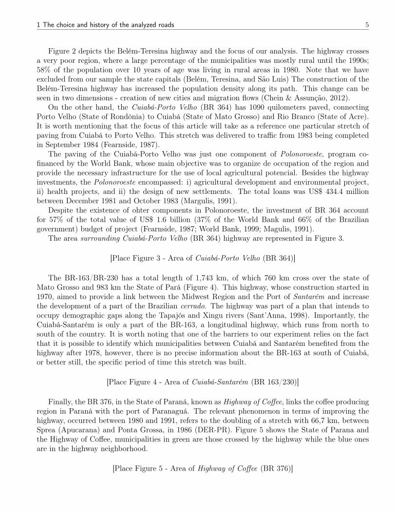
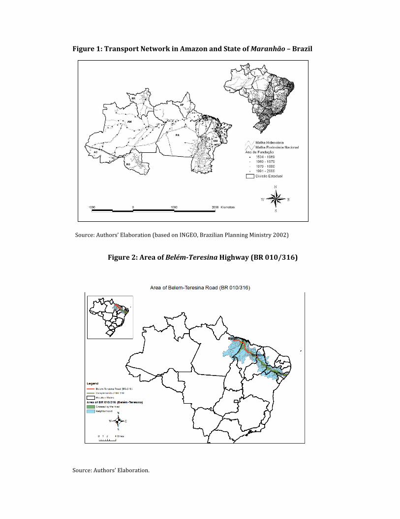
In Brazil, a large fraction of old municipalities are settled along the coastline or in riverbeds, whilethe more recent cities have their headquarters along the national highway network. Figure 1 showssome examples of this phenomenon.

[Place Figure 1 - Transport Network in Amazon and State of Maranhão – Brazil ]

The black points represent the oldest municipalities while the white points with black contourmark the newest ones. A quickly view point that the oldest municipalities in the Amazon Region aresettled along the riverside. In Maranhão, that has an earliest settlement process, the urbanizationbegins in the coastal and comes to interior following the implantation of highway network. In thelate 70’s, Brazilian Government introduces a regional policy based on the creation and developmentof a highway network that aimed to link the poorest country regions to the richest ones. Due to thisexperience, the majority of the cities in the Rondonia State, in the North region, were settled downjust along Porto Velho-Cuiabá highway (BR 364).

Chein et al. (2009) have already studied some effects of transport infrastructure developmentin Brazil. The authors investigate the relationship between urbanization and individual incomesby exploring the role of transport costs in the Brazilian process of urbanization. They find that,although this relationship exists, it is not, necessarily, direct. Productive structure and local labormarket are important channels which relate urbanization to individual income in emerging townsaround the roads. Their empirical results show that there is no statistically significant relationshipbetween the accumulation of human capital in those towns and the individual incomes, differentlyfrom the findings for large and medium-sized cities.

The idea behind our paper is very similar to the experiment designed in Chein et al. (2009), butwe will make some advances in the identification of the relation between urbanization and economicgrowth or development. In fact the results present in Chein et al. (2009) refer to a simple correlationbetween urbanization and income; we want to identify a cause relationship between urbanizationand some indicators of development using a reduction in transportation cost as an instrument tourbanization. Following Michaels (2008) and Baum-Snow (2007), instead of using a measure oftransportation costs we will associate the development of highway networks with a transportationcost reduction. But, contrary to Baum-Snow (2007) and differently from Michaels (2008) experimentwe are interested in identifying the impact of urbanization caused by the roads investments on labormarkets and income, that is, we use the highway improvement to identify urban growth and nota suburbanization (Baum-Snow, 2007) or necessarily and increase in international trade (Michaels,2008).

Our empirical framework will be built on the importance of the transport networks, especiallyroads, in increasing urbanization and changing regional economies. In this context, some emphasiswas given to the role of roads paving and expansion of transport network to increase agriculturalproductivity and consequently to induce the recent process of urbanization in the Center-west andNorth region.

The main idea is to implement an empirical exercise based on a difference-in-difference approachconsidering Brazilian municipalities, which the basic difference over the time relies on the developmentof a highway network that mainly reduces transport costs. We will compare the economic developmentin these municipalities before and after the improvement in a highway network. Our analysis will be

1 The choice and history of the analyzed roads 4

carried on based on Census Demographic Database (IBGE) and on secondary data concerning the dateof creation or improvement of roads infrastructure and their spatial information, which is providedby a geo-referenced database (Brazilian Ministery of Planning). We basically analyze the case ofinvestment in four different Brazilian roads: the Belém-Teresina (BR 010/316), in North/NortheastRegions, the Cuiabá-Porto Velho (BR-364), in Center-West/North Regions, the Cuiabá-Santarém(BR-163), also in Center West/North Regions and the Highway of Coffee (BR-376), in the SouthRegion.

Our main results point that construction of new limited access highways in Brazil has contributedto the development of those municipalities directed and indirected benefited by the highway, improvingwell-being of those living in the countryside. To illustrate, the estimate of the difference in populationgrowth comparing municipalities benefited by the Cuiabá-Santarém highway and the rest of thecountry reaches 62%. Concerning the human capital formation, those areas benfited by Cuiabá-Santarém highway and by Highway of Coffee had an increase of 1.8 years of education comparingto the others Brazilian municipalities. We also find positive effects of highways improvements onemployment rate, high-qualified occupation rates, service occupation rate, familar per capita incomeand others.

The remainder of the paper is organized as following. Section 1 presents the history of the fourroads analyzed. Section 2 describes the database and methodology. Section 3 presents the impactsestimates of the transport network investments on regional development. Section 4 discusses somelimitations and caveats. Section 5 concludes.

1 The choice and history of the analyzed roads

We must emphasize that there is no consolidated database with information about the implementationdates, paving or duplication of highways. Alternatively, the strategy adopted was the choice ofsome stretches of major highways, local, regional or national level, from the information of thenational highway network (Ministry of Transport). First, we identify highways located in differentregional areas in terms of stage / level of development. There were selected, preliminarily, about 30highway sections. The next step was to determine which of these had stretches deployment or sufferedsome significant improvements such as paving or duplication in one of three inter-census periodsconsidered. From the information available to state agencies for transportation, the internet addressof municipalities and documents on regional development (Sant’Anna, 1998; Margulis, 1991; GTI,2005), it was possible to identify four highway sections with works impact between 1970-2000, BR-163/BR-230 (Cuiabá-Santarém), BR-364 (Cuiabá-Porto Velho); BR-316/BR-010 (Belém-Teresina)and BR-376 (Highway of Coffee -PR).

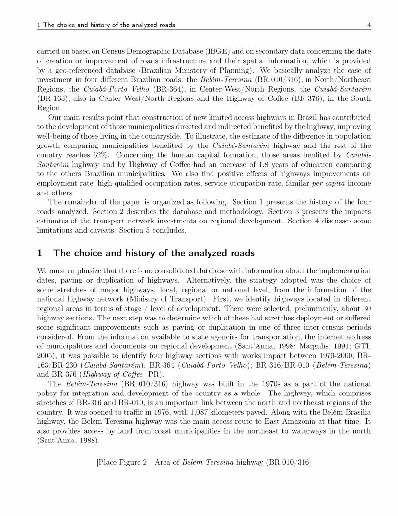
The Belém-Teresina (BR 010/316) highway was built in the 1970s as a part of the nationalpolicy for integration and development of the country as a whole. The highway, which comprisesstretches of BR-316 and BR-010, is an important link between the north and northeast regions of thecountry. It was opened to traffic in 1976, with 1,087 kilometers paved. Along with the Belém-Brasiliahighway, the Belém-Teresina highway was the main access route to East Amazônia at that time. Italso provides access by land from coast municipalities in the northeast to waterways in the north(Sant’Anna, 1988).

[Place Figure 2 - Area of Belém-Teresina highway (BR 010/316]

1 The choice and history of the analyzed roads 5

Figure 2 depicts the Belém-Teresina highway and the focus of our analysis. The highway crossesa very poor region, where a large percentage of the municipalities was mostly rural until the 1990s;58% of the population over 10 years of age was living in rural areas in 1980. Note that we haveexcluded from our sample the state capitals (Belém, Teresina, and São Luis) The construction of theBelém-Teresina highway has increased the population density along its path. This change can beseen in two dimensions - creation of new cities and migration flows (Chein & Assunção, 2012).

On the other hand, the Cuiabá-Porto Velho (BR 364) has 1090 quilometers paved, connectingPorto Velho (State of Rondônia) to Cuiabá (State of Mato Grosso) and Rio Branco (State of Acre).It is worth mentioning that the focus of this article will take as a reference one particular stretch ofpaving from Cuiabá to Porto Velho. This stretch was delivered to traffic from 1983 being completedin September 1984 (Fearnside, 1987).

The paving of the Cuiabá-Porto Velho was just one component of Polonoroeste, program co-financed by the World Bank, whose main objective was to organize de occupation of the region andprovide the necessary infrastructure for the use of local agricultural potencial. Besides the highwayinvestments, the Polonoroeste encompassed: i) agricultural development and environmental project,ii) health projects, and ii) the design of new settlements. The total loans was US$ 434.4 millionbetween December 1981 and October 1983 (Margulis, 1991).

Despite the existence of ohter components in Polonoroeste, the investment of BR 364 accountfor 57% of the total value of US$ 1.6 billion (37% of the World Bank and 66% of the Braziliangovernment) budget of project (Fearnside, 1987; World Bank, 1999; Magulis, 1991).

The area surrounding Cuiabá-Porto Velho (BR 364) highway are represented in Figure 3.

[Place Figure 3 - Area of Cuiabá-Porto Velho (BR 364)]

The BR-163/BR-230 has a total length of 1,743 km, of which 760 km cross over the state ofMato Grosso and 983 km the State of Pará (Figure 4). This highway, whose construction started in1970, aimed to provide a link between the Midwest Region and the Port of Santarém and increasethe development of a part of the Brazilian cerrado. The highway was part of a plan that intends tooccupy demographic gaps along the Tapajós and Xingu rivers (Sant’Anna, 1998). Importantly, theCuiabá-Santarém is only a part of the BR-163, a longitudinal highway, which runs from north tosouth of the country. It is worth noting that one of the barriers to our experiment relies on the factthat it is possible to identify which municipalities between Cuiabá and Santarém benefited from thehighway after 1978, however, there is no precise information about the BR-163 at south of Cuiabá,or better still, the specific period of time this stretch was built.

[Place Figure 4 - Area of Cuiabá-Santarém (BR 163/230)]

Finally, the BR 376, in the State of Paraná, known as Highway of Coffee, links the coffee producingregion in Paraná with the port of Paranaguá. The relevant phenomenon in terms of improving thehighway, occurred between 1980 and 1991, refers to the doubling of a stretch with 66,7 km, betweenSprea (Apucarana) and Ponta Grossa, in 1986 (DER-PR). Figure 5 shows the State of Parana andthe Highway of Coffee, municipalities in green are those crossed by the highway while the blue onesare in the highway neighborhood.

[Place Figure 5 - Area of Highway of Coffee (BR 376)]

2 Data and Methodology 6

2 Data and Methodology

We use data from the Demographic Censuses of 1970, 1980, 1991 and 2000, collected by the BrazilianInstitute of Geography and Statistics (IBGE). Along with the basic information collected for theCensus, IBGE also used an extended questionnaire to obtain more detailed socioeconomic information.This extended questionnaire is applied to a sample of 10 to 20% of the population of each municipality,depending on its size. Our data come from this longer survey. Table 1 brings some descriptivestatistics.

[Place Table 1- Descriptive Statistics]

The initial idea was to get some inferences about the impacts generated by improvements intransport infrastructure identified in the previous section on some municipal development indicators,specifically on the variables of income, education, occupational and productive structure. The firststep, therefore, was the definition of the coverage area of the highway to define the group of mu-nicipalities benefited. To that end, we made the intersection (spatial join line-point) between thenational highway network and the comparison areas grid, resulting from compatibility of existingmunicipalities in 1970 and 2000 (see Chein et al. 2007). Thus, there were defined the comparisonareas directly benefited by the construction of the highway, or those whose seats are closest to each ofthe stretches of highway, in almost all cases, municipalities crossed by the highway. Then, we definedthe direct and indirect neighbors of these areas in order to obtain the total area covered highway.

Importantly, in the case of municipalities in the North and some in the Midwest, the compatibilitygenerates comparison areas of large territory, which enlarges the area surrounding the highway. Then,the inclusion of all neighbors may overestimates indirect beneficiaries, while take into account onlythe direct neighbors can cause some sort of underestimation. The choice was to estimate a DID model(differences in difference) considering first neighbors and second neighbors, as follows:

Yi,t

�Yi,t�1 = ↵+ �C1 (D

364Ci,t

�D364Ci,t�1)+�C2 (D

163Ci,t

�D163Ci,t�1)+ �C3 (D

316Ci,t

�D316Ci,t�1)+�C4 (D

376Ci,t

�D376Ci,t�1)+

�FN

1 (D364FN

i,t

�D364FN

i,t�1 )+�FN

2 (D163FN

i,t

�D163FN

i,t�1 )+�FN

3 (D316FN

i,t

�D316FN

i,t�1 )+�FN

4 (D376FN

i,t

�D376FN

i,t�1 )+�SN1 (D364SN

i,t

�D364SNi,t�1 )+�SN2 (D163SN

i,t

�D163SNi,t�1 )+�SN3 (D316SN

i,t

�D316SNi,t�1 )+�SN4 (D376SN

i,t

�D376SNi,t�1 )+✏

i,t

where Yi,t

refers to a municipal development indicator, or the outcome variable, DC

i,t

is a dummyvariable that is equal to one if the observation refers to a municipality or comparison area that iscrossed by the highway at a time t after its construction or improvement; DFN

i,t

is a dummy variablethat is equal to one if the observation refers to a municipality or comparison area that is a direct (orfirst) neighbor of the highway at a time t after its construction or improvement; DSN

i,t

is a dummyvariable that is equal to one if the observation refers to a municipality or comparison area that is anindirect (or second) neighbor of the highway at a time t after its construction or improvement.

Thus, � coefficients give us the difference-in-difference estimator, that is �YTreat

� �YControl

,which means the difference between the change of the indicator occurred in the areas benefited by theopening or improvement of the highway and that of the control group, in these case, municipalitiesor comparison areas not benefited by highways improvement between 1970-2000.

3 Empirical Results

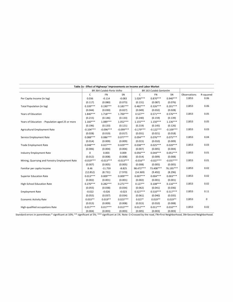
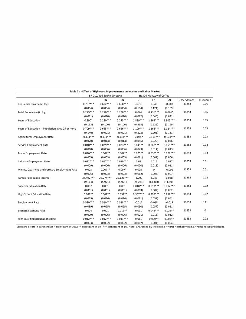
Tables 2a and 2b bring the estimate effects of highways improvements on development indicators.Generally, we find evidences of a positive impact of the highways on the area benefited by the

4 Caveats and Limitations 7

transport network investments. The results point to a positive and highly significant effect on percapita income in the case of Cuiabá-Santarém (179%)1 and Belém-Teresina (115%) highway. Interms of population growth, the effect was around 62%. This result could be understood as a positiveeffect on migration flows, that is, the new economic perspectives generated by the highway affect thepopulation distribution in the neighborhoods of highways as a consequence o lower migration costs.

We should also emphasize positive impacts of highways on human capital formation in all cases.The comparison areas benfited by Cuiabá-Santarém highway and by Highway of Coffee had an increaseof 1.8 years of education comparing to the others Brazilian municipalities. Moreover, the analysis ofmarket labor indicators shows that there was a change from an agricultural economy to an urban onein surrounding areas of the highways, or better, it is possible to observe an increase in the employmentrates in industry, trade and services as well as in high-qualified occupation rates.

[Place Table 2a and Table 2b - Effects of Highways’ Improvements on Income and Labor Market]

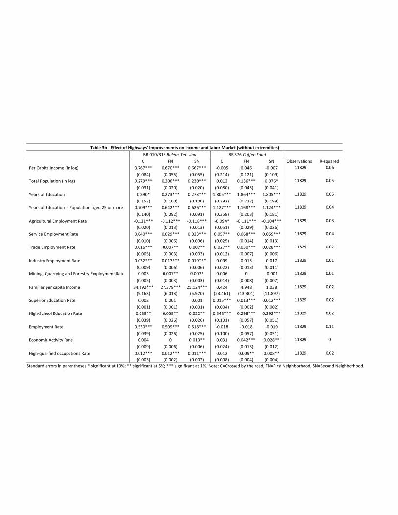
In spite of the positive effects of highways presented in Table 2a and Table 2b, it is important toremember that there is a few difficulties in measuring the impact of a reduction in shipping costs. Onone side, a good transport network allows access to less expensive markets, which corresponds to thebest business opportunities. On the other hand, it is the more developed regions and the richest onesthat can afford the high costs of construction and maintenance of transport infrastructure. Naturally,the construction of a road or highway is strongly influenced by the characteristics of the cities thatare at its ends. However, that link is much weaker for those that are located in more intermediatepositions. At first, the population of these cities experienced an exogenous reduction in shippingcosts.

In order to mitigate this identification problem (simultaneous correlation), i.e., to consider justthe first relation or the impact of transport network on new ecoomic perspectives, the models ofTable 2a and 2b were reestimate without the extremities of the highways and the capitals in theirneighborhoods. Table 3a and Table 3b report the new estimates. The results are very similar to thosefound on Table 2a and 2b.

[Place Table 3a and Table 3b - Effects of Highways’ Improvements on Income and Labor Marketwithout extremities]

In summary, we find some evidence that lower shipping costs changes the regional economy sur-rounding the highways and leads to a new distribution of humam and physical capital. In generally,it is possible to observe that investments in transport networks induce a change from rural to urbanactivities, an increase on wages or incomes and higher levels of human capital.

4 Caveats and Limitations

It is worth mentioning that our results are still very preliminary. The analysis of the previous sectionis based on the assumption that the investments in transport network were the only event that hasaffected differently comparison areas benefited by them.

In this sense, it is important to emphasize some of the underlying assumptions and characteristicsof the experiment designed here to test whether different highways improvements cause economicgrowth:

1 (exp(1.026)-1)*100

5 Conclusion 8

1. Characteristics of the cities not constant over time were not considered in our analysis, so thateffects of the construction of highways might be underestimated or overestimated, if there issomething besides the highway built that could affect the regional/local development.

2. The definition of highways’ beneficiaries has a margin of error, since it was not possible toclearly identify the date of construction of each sections of the national highway network,i.e.,in Cuiabá-Porto Velho area were also considered as beneficiaries, in 1980s, the municipalities atnorth of Porto Velho and south of Cuiabá. Similar problems were encountered in the definitionof the coverage area of the others highways.

3. Is is difficult to isolate the effect of the construction of highway, since the transport issue shouldbe considered in an integrated way, that is, the positive effect of a particular road can becanceled if it is built in the same period of the construction of a road with a lower cost or betterroute, connecting, for exemple, isolate areas to a more modern port. Moreover, in general,investments in network transport infrastructure are took together with others ones, like fiscalincentives, agricultural programs, cash transfers and more.

In order to mitigate such kind of limitations and make some robustness checks, the next steps of thisresearch include new definitions of the groups of beneficiaries and not beneficiaries, as the comparisonbetween the municipalities crossed by the road and the first and second neighbors. Besides, we intendto estimate similar models to the previous ones considering data at micro or individual instead ofmunicipal one.

5 Conclusion

This paper investigates the impact of improvements in the transport network on economic develop-ment. We have shown that investments in highways seem to changed the human and physical capitaldistribution - economies near the highways increases population, income and schooling as well as re-duces the participation of agricultural sector. Our results bring new evidence of the role of highwaysin promoting urbanization, better living conditions and economic expansion of new areas.

References

[1] ACEMOGLU, D., JOHNSON, S., ROBINSON, J. Reversal of fortune: geography andinstitution in the making of the modern world income distribution. The Quarterly Jour-nal of Economics. v.117, n.4, p.1231-1294, Nov. 2002.

[2] BAIROCH, P. Cities and economic development: from the down of history to the present.Chicago, IL: University of Chicago, 1988. 574p.

[3] BAUM-SNOW, Nathaniel. Did Highways cause suburbanization? The Quarterly Journalof Economics. v. 122, n. 2, p. 775-805, May 2007.

[4] BERRY, C., GLAESER, E. The divergence of human capital level across cities. Cam-bridge, Mass.: Harvard Institute of Economic Research, 2005. (Discussion papers, 2091).

[5] BLACK, D., HENDERSON, J.V. A theory of urban growth. Journal of Political Econ-omy. v.107, n.2, p.252-284, 1999.

5 Conclusion 9

[6] CHEIN, Flávia; ASSUNÇÃO, J.J. How does Emigration affect Labor Markets? Evidencefrom Road Construction in Brazil. manuscript. July, 2012.

[7] CHEIN, Flávia; ASSUNÇÃO, J.J.; LEMOS, M.B. Custos de Transporte, Urbanizaçãoe Desenvolvimento: evidências a partir da criação de Cidades. Revista Brasileira deEconomia. Vol. 63, n.3, p.249-275, July/Sept. 2009.

[8] CHEIN, Flávia; ASSUNÇÃO, J.J.; LEMOS, M.B. Desenvolvimento Desigual no Brasil:evidências a partir da criação de Cidades. Revista Brasileira de Economia. Vol. 61, n.3,p.301-330, July/Sept. 2007.

[9] CHRISTALLER, W. Central places in southern Germany. New Jersey: Prentice-Hall,1966. 230p.

[10] FEARNSIDE, P. M. Deflorestation and international economic development projects inbrazilian amazonia. Conservative Biology, vol. 1, n.3, p. 1523-1739. 1987.

[11] FUJITA, M., KRUGMAN, P., VENABLES, A. The spatial economy: cities, regions andinternational trade. Cambridge, Mass.: MIT. 1999. 367p.

[12] GALLUP, J., SACHS, J., MELLINGER, A.. Geography and economic growth. In:PLESKOVIC, B., STIGLITZ, J.E. Annual World Bank Conference on DevelopmentEconomics. Washington, D.C.: World Bank, 1998. p.127-178.

[13] GLAESER, E. Learning in cities. Journal of Urban Economics. v.46, n.2, p.254-277,Sept. 1999.

[14] GLAESER, E., KALLAL, H.D., SCHEINKMAN, J.A., SHLEIFER, A. Growth in cities.Journal of Political Economy. v.100, n.6, p.1126-1152, Dec.1992.

[15] GLAESER, E., KOHLHASE, J. Cities, regions and the decline of transport costs. Cam-bridge, Mass.: Harvard Institute of Economic Research, 2003. (Discussion papers, 2014)

[16] GLAESER, E., MARE, D. Cities and skills. Journal of Labor Economics. v.19, n.2,p-316-342, 2001.

[17] GLAESER, E., SAIZ, A. The rise of the skilled city. Cambridge, Mass.: Harvard Instituteof Economic Research, 2003. (Discussion papers, 2025)

[18] GLAESER, E., SCHEINKMAN, J.A., SHLEIFER, A. Economic growth in a cross-section of cities. Cambridge, Mass.: NBER, 1995. (Working papers, 5013).

[19] GREENWOOD, M. Research on internal migration in the United States: a survey.Journal of Economic Literature. v.13, n.2, p.397-433, 1975.

[20] GRUPO DE TRABALHO INTERMINISTERIAL (2005). Plano de DesenvolvimentoRegional Sustentável para a Área de Influência da Rodovia BR-163/Cuiabá-Santarém.Brasília: Casa Civil da Presidência da República.

5 Conclusion 10

[21] HENDERSON, J.V. Overcoming the adverse effects of geography: infraestructure,health, and agricultural policies. International Regional Science Review. v.22, n.2, p.233-237, Aug. 1999.

[22] HENDERSON, J.V. Urbanization and economic development. Annals of Economics andFinance. v.4, n.2, p.275-341, Nov. 2003.

[23] HENDERSON, J.V., WANG, H.G. Aspects of the rural-urban transformation of coun-tries. Journal of Economic Geography. v.5, n.1, p.23-42, Jan. 2005.

[24] HOSELITZ B.F. The role of cities in the economic growth of underdeveloped countries.Journal of Political Economy. v.61, n.3, p.195-208, 1953.

[25] ISARD, W., BRAMHALL, D.F. Methods of regional analysis: an introduction to re-gional science. Cambridge, Mass., M.I.T, 1960. 784p.

[26] JACOBS, J. The economy of cities. Middlesex: Penguin Books, 1969. 268p.

[27] KIRK, Dudley (1996). Demographic Transition Theory. Population Studies, 50(3),November,361-87.

[28] KUZNETS, S. Modern economic growth: rate structure and spread. New Haven: YaleUniversity, 1966. 529p.

[29] LEWIS, A. Economic development with unlimited supplies of labor. Manchester Schoolof Economic Social Studies. v.22, p139-191, May 1954.

[30] LÖSCH, A. The economics of location. New Haven: Yale University, 1954. 520p.

[31] MARGULIS, Sergio. O desempenho do governo brasileiro, dos órgãos contratantes, e doBanco Mundial em relação a questão ambiental do Polonoroeste. Texto para Discussãonº 227. Brasília: IPEA. 1991

[32] MICHAELS, Guy. The Effect of Trade on the Demand for Skill – Evidence from the In-terstate Highway System. Review of Economics and Statistics. Vol. 90, No. 4, p; 683–701,Nov. 2008.

[33] PRED, A.R. The spatial dynamics of U.S. urban-industrial growth, 1800-1914: inter-pretative and theoretical essays. Cambridge, Mass.: MIT, 1966. 225p.

[34] RADELET, S. and SACHS, J. Shipping Costs, Manufactured Exports, and EconomicGrowth. manuscript. 1998.

[35] SANT’ANNA, José Alex. 1988. Rede Básica de Transportes da Amazônia. Texto paraDiscussão n. 562. IPEA, Brasília, DF

[36] .WORLD BANK. Projeto Úmidas: um enfoque participatório para o desenvolvi-mento sustentável: o caso de Rondônia. Washington: World Bank, 1999. (BrazilCountry Management Unit. Latin America and Caribbean Region). Avaiable at:www.bancomundial.org.br/content/_downloadblob.php?cod_blob=287.

Figure'1:'Transport'Network'in'Amazon'and'State'of'Maranhão(–'Brazil'''

!!!Source:!Authors’!Elaboration!(based!on!INGEO,!Brazilian!Planning!Ministry!2002)!!!' Figure'2:'Area'of'Belém.Teresina'Highway'(BR'010/316)'

!

!Source:!Authors’!Elaboration.'' ' '

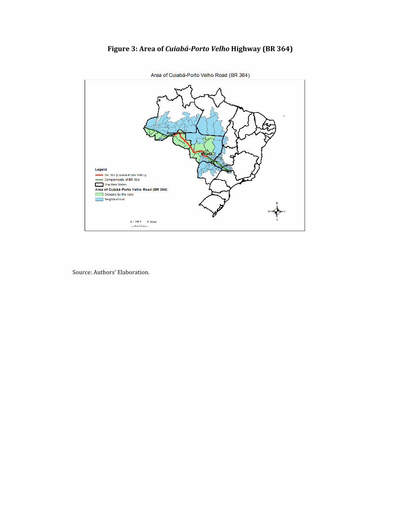
Figure'3:'Area'of'Cuiabá.Porto(Velho'Highway'(BR'364)'

!!Source:!Authors’!Elaboration.!!!' ' '''''''''''''''''''''

Figure'4:'Area'of'Cuiabá.Santarém''Highway'(BR'163)'!

!Source:!Authors’!Elaboration.!' '' '''''''''''''''''''''''

'Figure'5:'Area'of'Highway(of(Coffee((BR'376)'

!

!Source:!Authors’!Elaboration.!!!!!!!!!!!

Table&1:&Descriptive&Statistics&

!! Cuiabá'Porto,Velho,(BR,364), Cuiabá'Santarém,(BR,163), Belém'Teresina!(BR!010/316)! Highway,of,Coffee,(BR,376),!! 0! 1! Diff!

!0! 1! Diff! !! 0! 1! Diff!

!0! 1! Diff!

!Employment&Rate&! ! ! !

!!! !

!!! ! ! !

!!! ! !1970! 0.44! 0.45! 0.01! ***! 0.44! 0.46! 0.02! ***! 0.44! 0.46! 0.02! ***! 0.44! 0.46! 0.02! ***!

1980! 0.98! 0.98! 0.00!!

0.98! 0.98! 0.00! !! 0.98! 0.98! 0.00!!

0.98! 0.99! 0.01! ***!

1991! 0.96! 0.96! 0.00!!

0.96! 0.96! 0.00! *! 0.96! 0.95! '0.01! *! 0.96! 0.97! 0.01! ***!

2000! 0.89! 0.87! '0.01! ***! 0.88! 0.88! '0.01! *! 0.88! 0.90! 0.01! ***! 0.88! 0.88! 0.00!!Average&Familiar&Per&Capita&Income&

! ! ! !!!

! !!!

! ! ! !!!

! ! !1970! 45.23! 54.63! 9.40! ***! 45.37! 52.44! 7.07! ***! 47.18! 29.07! '18.11! ***! 45.39! 58.58! 13.19! ***!

1980! 114.03! 149.04! 35.01! ***! 114.93! 131.32! 16.39! ***! 120.99! 57.36! '63.63! ***! 115.28! 130.40! 15.12! **!

1991! 108.25! 142.11! 33.86! ***! 109.03! 127.48! 18.45! ***! 114.85! 54.87! '59.99! ***! 109.30! 132.31! 23.01! ***!

2000! 175.47! 213.50! 38.03! ***! 176.41! 195.52! 19.11! ***! 185.89! 83.22! '102.67! ***! 176.46! 212.80! 36.35! ***!

Years&of&Education&! ! ! !

!!! !

!!! ! ! !

!!! ! !1970! 1.39! 1.37! '0.02!

!1.40! 1.22! '0.17! ***! 1.46! 0.67! '0.78! ***! 1.38! 1.71! 0.32! ***!

1980! 1.88! 1.93! 0.05!!

1.89! 1.79! '0.10! **! 1.97! 0.96! '1.01! ***! 1.88! 2.22! 0.35! ***!

1991! 3.44! 3.66! 0.22! ***! 3.44! 3.61! 0.17! ***! 3.56! 2.24! '1.32! ***! 3.43! 4.05! 0.62! ***!

2000! 4.60! 4.82! 0.22! ***! 4.60! 4.79! 0.19! ***! 4.73! 3.33! '1.39! ***! 4.60! 5.29! 0.70! ***!

Earnings&per&Worker&! ! ! !

!!! !

!!! ! ! !

!!! ! !1970! 145.51! 177.43! 31.91! ***! 145.91! 172.18! 26.27! ***! 151.87! 93.76! '58.10! ***! 146.26! 181.06! 34.80! ***!

1980! 334.16! 443.35! 109.19! ***! 336.20! 407.96! 71.76! ***! 352.62! 192.27! '160.34! ***! 338.43! 365.61! 27.18! *!

1991! 286.60! 379.23! 92.62! ***! 287.99! 357.88! 69.89! ***! 301.20! 177.59! '123.61! ***! 289.84! 333.36! 43.51! ***!

2000! 441.64! 542.72! 101.08! ***! 443.58! 508.50! 64.92! ***! 464.44! 249.01! '215.42! ***! 444.70! 517.47! 72.77! ***!Agricultural&Employment&Rate&

! ! ! !!!

! !!!

! ! ! !!!

! ! !1970! 0.70! 0.63! '0.07! ***! 0.70! 0.69! '0.01! !! 0.69! 0.79! 0.10! ***! 0.70! 0.67! '0.03!!1980! 0.56! 0.51! '0.05! ***! 0.56! 0.56! 0.01! !! 0.55! 0.67! 0.12! ***! 0.56! 0.54! '0.01!!1991! 0.48! 0.41! '0.07! ***! 0.48! 0.44! '0.04! ***! 0.47! 0.62! 0.15! ***! 0.48! 0.44! '0.04!!2000! 0.38! 0.34! '0.04! ***! 0.38! 0.36! '0.02! **! 0.37! 0.51! 0.14! ***! 0.38! 0.33! '0.05! **!

Industry&Employment&Rate&! ! ! !

!!! !

!!! ! ! !

!!! ! !1970! 0.09! 0.06! '0.03! ***! 0.09! 0.06! '0.03! ***! 0.09! 0.05! '0.07! ***! 0.08! 0.10! 0.02!

!1980! 0.14! 0.10! '0.04! ***! 0.14! 0.10! '0.03! ***! 0.14! 0.07! '0.07! ***! 0.13! 0.15! 0.02!!

1991! 0.14! 0.11! '0.04! ***! 0.14! 0.10! '0.04! ***! 0.15! 0.07! '0.07! ***! 0.14! 0.17! 0.03! **!

2000! 0.14! 0.12! '0.02! ***! 0.14! 0.11! '0.03! ***! 0.15! 0.09! '0.06! ***! 0.14! 0.18! 0.04! ***!

Total&Income&! ! ! !

!!! !

!!! ! ! !

!!! ! !1970! 44.53! 55.68! 11.15! ***! 44.68! 53.55! 8.87! ***! 46.57! 28.39! '18.17! ***! 44.78! 57.51! 12.73! ***!

1980! 115.00! 152.10! 37.10! ***! 115.89! 135.12! 19.22! ***! 122.09! 58.05! '64.04! ***! 116.36! 130.61! 14.25! **!

1991! 108.40! 142.73! 34.32! ***! 109.17! 128.40! 19.23! ***! 115.03! 54.98! '60.05! ***! 109.48! 132.14! 22.66! ***!

2000! 175.40! 213.53! 38.13! ***! 176.32! 195.84! 19.52! ***! 185.81! 83.30! '102.51! ***! 176.38! 212.79! 36.41! ***!*!significant!at!10%;!**!significant!at!5%;!***!significant!at!1%.!Source:!Authors’!Elaboration!based!on!Demographic!Census!(IBGE)!

! !

Table&2a&E&Effect&of&Highways'&Improvements&on&Income&and&Labor&Market&&!! BR!364!Cuiabá'Porto,Velho! BR!163!Cuiabá'Santarém! !! !!

!C! FN! SN! C! FN! SN! Observations! R'squared!

Per!Capita!Income!(in!log)! 0.036! '0.114! '0.083! 1.026***! 0.870***! 0.940***! 11853! 0.06!

!(0.117)! (0.080)! (0.073)! (0.131)! (0.087)! (0.076)! ! !

Total!Population!(in!log)! 0.339***! 0.190***! 0.185***! 0.482***! 0.326***! 0.201***! 11853! 0.06!

!(0.044)! (0.030)! (0.027)! (0.049)! (0.032)! (0.028)! ! !

Years!of!Education! 1.840***! 1.718***! 1.700***! 0.527**! 0.571***! 0.576***! 11853! 0.05!

!(0.215)! (0.146)! (0.133)! (0.240)! (0.159)! (0.139)! ! !

Years!of!Education!!'!Population!aged!25!or!more! 1.160***! 1.089***! 1.052***! 1.155***! 1.150***! 1.136***! 11853! 0.05!

!(0.196)! (0.133)! (0.121)! (0.219)! (0.145)! (0.126)! ! !

Agricultural!Employment!Rate! '0.104***! '0.096***! '0.099***! '0.179***! '0.122***! '0.109***! 11853! 0.03!

!(0.028)! (0.019)! (0.017)! (0.031)! (0.021)! (0.018)! ! !

Service!Employment!Rate! 0.088***! 0.086***! 0.077***! 0.094***! 0.076***! 0.075***! 11853! 0.04!

!(0.014)! (0.009)! (0.009)! (0.015)! (0.010)! (0.009)! ! !

Trade!Employment!Rate! 0.048***! 0.027***! 0.029***! 0.038***! 0.025***! 0.020***! 11853! 0.03!

!(0.006)! (0.004)! (0.004)! (0.007)! (0.005)! (0.004)! ! !

Industry!Employment!Rate! 0! 0.003! 0.009! 0.056***! 0.044***! 0.051***! 11853! 0.01!

!(0.012)! (0.008)! (0.008)! (0.014)! (0.009)! (0.008)! ! !

Mining,!Quarrying!and!Forestry!Employment!Rate! '0.019***! '0.013***! '0.013***! '0.016**! '0.027***! '0.037***! 11853! 0.01!

!(0.007)! (0.005)! (0.005)! (0.008)! (0.005)! (0.005)! ! !

Familiar!per!capita!Income!! 8.46! '11.759! '8.825! 98.472***! 73.408***! 76.195***! 11853! 0.02!

!(12.852)! (8.731)! (7.970)! (14.369)! (9.492)! (8.296)! ! !

Superior!Education!Rate! 0.013***! 0.009***! 0.009***! 0.007***! 0.004***! 0.003***! 11853! 0.02!

!(0.002)! (0.001)! (0.001)! (0.002)! (0.001)! (0.001)! ! !

High'School!Education!Rate! 0.270***! 0.282***! 0.271***! 0.127**! 0.108***! 0.116***! 11853! 0.02!

!(0.055)! (0.038)! (0.034)! (0.062)! (0.041)! (0.036)! ! !

Employment!Rate! '0.022! '0.026! '0.023! 0.527***! 0.510***! 0.517***! 11853! 0.11!

!(0.055)! (0.037)! (0.034)! (0.061)! (0.040)! (0.035)! ! !

Economic!Activity!Rate! 0.033**! 0.019**! 0.023***! 0.027*! 0.019**! 0.019**! 11853! 0!

!(0.013)! (0.009)! (0.008)! (0.015)! (0.010)! (0.008)! ! !

High'qualified!occupations!Rate! 0.017***! 0.017***! 0.013***! 0.012***! 0.011***! 0.010***! 11853! 0.02!

!! (0.004)! (0.003)! (0.003)! (0.005)! (0.003)! (0.003)! !! !!Standard!errors!in!parentheses!*!significant!at!10%;!**!significant!at!5%;!***!significant!at!1%.!Note:!C=Crossed!by!the!road,!FN=First!Neighborhood,!SN=Second!Neighborhood.!

Table&2b&E&Effect&of&Highways'&Improvements&on&Income&and&Labor&Market&&!! BR!010/316!Belém'Teresina! BR!376!Highway!of!Coffee! !! !!


Per!Capita!Income!(in!log)! 0.767***! 0.672***! 0.668***! '0.019! 0.046! '0.007! 11853! 0.06!

!(0.084)! (0.054)! (0.054)! (0.194)! (0.121)! (0.109)! ! !

Total!Population!(in!log)! 0.279***! 0.210***! 0.230***! 0.046! 0.136***! 0.076*! 11853! 0.06!

!(0.031)! (0.020)! (0.020)! (0.072)! (0.045)! (0.041)! ! !

Years!of!Education! 0.290*! 0.280***! 0.273***! 1.839***! 1.864***! 1.805***! 11853! 0.05!

!(0.153)! (0.100)! (0.100)! (0.355)! (0.222)! (0.199)! ! !


!(0.140)! (0.091)! (0.091)! (0.323)! (0.203)! (0.181)! ! !

Agricultural!Employment!Rate! '0.131***! '0.111***! '0.118***! '0.085*! '0.111***! '0.104***! 11853! 0.03!

!(0.020)! (0.013)! (0.013)! (0.046)! (0.029)! (0.026)! ! !

Service!Employment!Rate! 0.040***! 0.029***! 0.023***! 0.049**! 0.068***! 0.059***! 11853! 0.04!

!(0.010)! (0.006)! (0.006)! (0.023)! (0.014)! (0.013)! ! !

Trade!Employment!Rate! 0.016***! 0.007**! 0.007**! 0.025**! 0.030***! 0.028***! 11853! 0.03!

!(0.005)! (0.003)! (0.003)! (0.011)! (0.007)! (0.006)! ! !

Industry!Employment!Rate! 0.032***! 0.017***! 0.019***! 0.01! 0.015! 0.017! 11853! 0.01!

!(0.009)! (0.006)! (0.006)! (0.020)! (0.013)! (0.011)! ! !

Mining,!Quarrying!and!Forestry!Employment!Rate! 0.003! 0.007**! 0.007*! 0.005! 0! '0.001! 11853! 0.01!

!(0.005)! (0.003)! (0.003)! (0.012)! (0.008)! (0.007)! ! !

Familiar!per!capita!Income!! 34.492***! 28.274***! 25.126***! '3.009! 4.948! 1.038! 11853! 0.02!

!(9.164)! (5.971)! (5.971)! (21.224)! (13.303)! (11.898)! ! !

Superior!Education!Rate! 0.002! 0.001! 0.001! 0.018***! 0.013***! 0.012***! 11853! 0.02!

!(0.001)! (0.001)! (0.001)! (0.003)! (0.002)! (0.002)! ! !

High'School!Education!Rate! 0.089**! 0.062**! 0.052**! 0.357***! 0.298***! 0.292***! 11853! 0.02!

!(0.039)! (0.026)! (0.026)! (0.091)! (0.057)! (0.051)! ! !

Employment!Rate! 0.530***! 0.510***! 0.518***! '0.017! '0.018! '0.019! 11853! 0.11!

!(0.039)! (0.025)! (0.025)! (0.090)! (0.057)! (0.051)! ! !

Economic!Activity!Rate! 0.004! 0.001! 0.013**! 0.031! 0.042***! 0.028**! 11853! 0!

!(0.009)! (0.006)! (0.006)! (0.021)! (0.013)! (0.012)! ! !

High'qualified!occupations!Rate! 0.012***! 0.012***! 0.011***! 0.011! 0.009**! 0.008**! 11853! 0.02!


Table&3a&E&Effect&of&Highways'&Improvements&on&Income&and&Labor&Market&(without&extremities)&!! BR!364!Cuiabá'Porto,Velho! BR!163!Cuiabá'Santarém! !! !!


Per!Capita!Income!(in!log)! 0.04! '0.114! '0.083! 1.029***! 0.870***! 0.947***! 11829! 0.06!

!(0.121)! (0.080)! (0.073)! (0.137)! (0.087)! (0.076)! ! !

Total!Population!(in!log)! 0.309***! 0.190***! 0.185***! 0.476***! 0.326***! 0.180***! 11829! 0.05!

!(0.045)! (0.030)! (0.027)! (0.051)! (0.032)! (0.028)! ! !

Years!of!Education! 1.804***! 1.718***! 1.700***! 0.532**! 0.571***! 0.582***! 11829! 0.05!

!(0.222)! (0.146)! (0.133)! (0.251)! (0.159)! (0.140)! ! !


!(0.203)! (0.133)! (0.121)! (0.229)! (0.145)! (0.127)! ! !

Agricultural!Employment!Rate! '0.105***! '0.096***! '0.099***! '0.182***! '0.122***! '0.114***! 11829! 0.03!

!(0.029)! (0.019)! (0.017)! (0.033)! (0.021)! (0.018)! ! !

Service!Employment!Rate! 0.090***! 0.086***! 0.077***! 0.095***! 0.076***! 0.076***! 11829! 0.04!

!(0.014)! (0.009)! (0.009)! (0.016)! (0.010)! (0.009)! ! !

Trade!Employment!Rate! 0.047***! 0.027***! 0.029***! 0.037***! 0.025***! 0.020***! 11829! 0.02!

!(0.007)! (0.004)! (0.004)! (0.007)! (0.005)! (0.004)! ! !

Industry!Employment!Rate! 0! 0.003! 0.009! 0.059***! 0.044***! 0.052***! 11829! 0.01!

!(0.013)! (0.008)! (0.008)! (0.014)! (0.009)! (0.008)! ! !

Mining,!Quarrying!and!Forestry!Employment!Rate! '0.020**! '0.013***! '0.013***! '0.018**! '0.027***! '0.036***! 11829! 0.01!

!(0.008)! (0.005)! (0.005)! (0.009)! (0.005)! (0.005)! ! !

Familiar!per!capita!Income!! 8.865! '11.759! '8.825! 97.347***! 73.408***! 76.485***! 11829! 0.02!

!(13.301)! (8.730)! (7.969)! (15.006)! (9.490)! (8.353)! ! !

Superior!Education!Rate! 0.013***! 0.009***! 0.009***! 0.006**! 0.004***! 0.003***! 11829! 0.02!

!(0.002)! (0.001)! (0.001)! (0.002)! (0.001)! (0.001)! ! !

High'School!Education!Rate! 0.261***! 0.282***! 0.271***! 0.120*! 0.108***! 0.117***! 11829! 0.02!

!(0.057)! (0.038)! (0.034)! (0.065)! (0.041)! (0.036)! ! !

Employment!Rate! '0.021! '0.026! '0.023! 0.524***! 0.510***! 0.517***! 11829! 0.11!

!(0.057)! (0.037)! (0.034)! (0.064)! (0.040)! (0.036)! ! !

Economic!Activity!Rate! 0.033**! 0.019**! 0.023***! 0.026*! 0.019**! 0.019**! 11829! 0!

!(0.013)! (0.009)! (0.008)! (0.015)! (0.010)! (0.008)! ! !

High'qualified!occupations!Rate! 0.017***! 0.017***! 0.013***! 0.012**! 0.011***! 0.010***! 11829! 0.02!


Table&3b&E&Effect&of&Highways'&Improvements&on&Income&and&Labor&Market&(without&extremities)&!! BR!010/316!Belém'Teresina! BR!376!Coffee,Road! !! !!


Per!Capita!Income!(in!log)! 0.767***! 0.670***! 0.667***! '0.005! 0.046! '0.007! 11829! 0.06!

!(0.084)! (0.055)! (0.055)! (0.214)! (0.121)! (0.109)! ! !

Total!Population!(in!log)! 0.279***! 0.206***! 0.230***! 0.012! 0.136***! 0.076*! 11829! 0.05!

!(0.031)! (0.020)! (0.020)! (0.080)! (0.045)! (0.041)! ! !

Years!of!Education! 0.290*! 0.273***! 0.273***! 1.805***! 1.864***! 1.805***! 11829! 0.05!

!(0.153)! (0.100)! (0.100)! (0.392)! (0.222)! (0.199)! ! !


!(0.140)! (0.092)! (0.091)! (0.358)! (0.203)! (0.181)! ! !

Agricultural!Employment!Rate! '0.131***! '0.112***! '0.118***! '0.094*! '0.111***! '0.104***! 11829! 0.03!

!(0.020)! (0.013)! (0.013)! (0.051)! (0.029)! (0.026)! ! !

Service!Employment!Rate! 0.040***! 0.029***! 0.023***! 0.057**! 0.068***! 0.059***! 11829! 0.04!

!(0.010)! (0.006)! (0.006)! (0.025)! (0.014)! (0.013)! ! !

Trade!Employment!Rate! 0.016***! 0.007**! 0.007**! 0.027**! 0.030***! 0.028***! 11829! 0.02!

!(0.005)! (0.003)! (0.003)! (0.012)! (0.007)! (0.006)! ! !

Industry!Employment!Rate! 0.032***! 0.017***! 0.019***! 0.009! 0.015! 0.017! 11829! 0.01!

!(0.009)! (0.006)! (0.006)! (0.022)! (0.013)! (0.011)! ! !

Mining,!Quarrying!and!Forestry!Employment!Rate! 0.003! 0.007**! 0.007*! 0.006! 0! '0.001! 11829! 0.01!

!(0.005)! (0.003)! (0.003)! (0.014)! (0.008)! (0.007)! ! !

Familiar!per!capita!Income!! 34.492***! 27.379***! 25.124***! 0.424! 4.948! 1.038! 11829! 0.02!

!(9.163)! (6.013)! (5.970)! (23.461)! (13.301)! (11.897)! ! !

Superior!Education!Rate! 0.002! 0.001! 0.001! 0.015***! 0.013***! 0.012***! 11829! 0.02!

!(0.001)! (0.001)! (0.001)! (0.004)! (0.002)! (0.002)! ! !

High'School!Education!Rate! 0.089**! 0.058**! 0.052**! 0.348***! 0.298***! 0.292***! 11829! 0.02!

!(0.039)! (0.026)! (0.026)! (0.101)! (0.057)! (0.051)! ! !

Employment!Rate! 0.530***! 0.509***! 0.518***! '0.018! '0.018! '0.019! 11829! 0.11!

!(0.039)! (0.026)! (0.025)! (0.100)! (0.057)! (0.051)! ! !

Economic!Activity!Rate! 0.004! 0! 0.013**! 0.031! 0.042***! 0.028**! 11829! 0!

!(0.009)! (0.006)! (0.006)! (0.024)! (0.013)! (0.012)! ! !

High'qualified!occupations!Rate! 0.012***! 0.012***! 0.011***! 0.012! 0.009**! 0.008**! 11829! 0.02!


Transport Infrastructure, Urbanization and Shipping Costs

Documents

Transcript of Transport Infrastructure, Urbanization and Shipping Costs