arX

iv:1

011.

5222

v1 [

astr

o-ph

.CO

] 23

Nov

201

0Mon. Not. R. Astron. Soc.000, 000–000 (0000) Printed 25 November 2010 (MN LATEX style file v2.2)

The evolution of AGN across cosmic time: what is downsizing?

N. Fanidakis,1 C. M. Baugh,1 A. J. Benson,2 R. G. Bower,1 S. Cole,1 C. Done,1

C. S. Frenk1, R. C. Hickox1, C. Lacey1, C. del P. Lagos11Institute for Computational Cosmology, Department of Physics, University of Durham,Science Laboratories, South Road, Durham DH1 3LE, United Kingdom2Mail Code 130-33, California Institute of Technology, Pasadena, CA 91125, USA

25 November 2010

ABSTRACT

We use a coupled model of the formation and evolution of galaxies and black holes (BH)to study the evolution of active galactic nuclei (AGN) in a cold dark matter universe. Themodel predicts the BH mass, spin and mass accretion history.BH mass grows via accretiontriggered by discs becoming dynamically unstable or galaxymergers (called the starburstmode) and accretion from quasi-hydrostatic hot gas haloes (called the hot-halo mode). Bytaking into account AGN obscuration, we obtain a very good fitto the observed luminosityfunctions (LF) of AGN (optical, soft and hard X-ray, and bolometric) for a wide range ofredshifts (0 < z < 6). The model predicts a hierarchical build up of BH mass, withthe typicalmass of actively growing BHs increasing with decreasing redshift. Remarkably, despite this,we find downsizing in the AGN population, in terms of the differential growth with redshiftof the space density of faint and bright AGN. This arises naturally from the interplay betweenthe starburst and hot-halo accretion modes. The faint end ofthe LF is dominated by massiveBHs experiencing quiescent accretion via a thick disc, primarily during the hot-halo mode.The bright end of the LF, on the other hand, is dominated by AGNwhich host BHs accretingclose to or in excess of the Eddington limit during the starburst mode. The model predictsthat the comoving space density of AGN peaks atz ≃ 3, similar to the star formation history.However, when taking into account obscuration, the space density of faint AGN peaks at lowerredshift (z . 2) than that of bright AGN (z ≃ 2 − 3). This implies that the cosmic evolutionof AGN is shaped in part by obscuration.

Key words: galaxies:nuclei – galaxies:active – quasars:general – methods:numerical

1 INTRODUCTION

Reproducing the evolution of active galactic nuclei (AGN) isa crucial test of galaxy formation models. Not only are AGNan important component of the Universe, they are also thoughtto play a key role in the evolution of their host galaxies andtheir environment. For example, feedback processes which ac-company the growth of black holes (BHs) during AGN ac-tivity are thought to influence star formation (SF) throughthe suppression of cooling flows in galaxy groups and clus-ters (Dalla Vecchia et al. 2004; Springel, Di Matteo, & Hernquist2005; Croton et al. 2006; Bower et al. 2006; Hopkins et al. 2006;Thacker, Scannapieco, & Couchman 2006; Somerville et al. 2008;Lagos, Cora, & Padilla 2008, see also Marulli et al. 2008). Sim-ilarly, energy feedback from AGN is a key ingredient indetermining the X-ray properties of the intracluster medium(Bower, McCarthy, & Benson 2008; McCarthy et al. 2010). Under-

standing these processes requires that the underlying galaxy forma-tion model is able to track and reproduce the evolution of AGN.

Early surveys demonstrated that quasi-stellar objects(QSOs) undergo significant evolution fromz ∼ 0 up toz ∼ 2 − 2.5 (Schmidt & Green 1983; Boyle, Shanks, & Peterson1988; Hewett, Foltz, & Chaffee 1993; Boyle et al. 2000). Be-yond z ∼ 2, the space density of QSOs starts to decline(Warren, Hewett, & Osmer 1994; Schmidt, Schneider, & Gunn1995; Fan et al. 2001; Wolf et al. 2003). Recently there has beenmuch progress in pinning down the evolution of faint AGN inthe optical. Using the 2-degree-field (2dF) QSO Redshift survey,the luminosity function (LF) was probed to around a magnitudefainter than the break toz ∼ 2 (2QZ Croom et al. 2001, 2004).This limit was extended by the 2dF-SDSS luminous red galaxyand QSO (2SLAQ) survey (Richards et al. 2005; Croom et al.2009a). The estimate of the LF from the final 2SLAQ cataloguereachedMbJ ≃ −19.8 at z = 0.4 (Croom et al. 2009b). With the2SLAQ LF, Croom et al. (2009b) demonstrated that in the optical,

c© 0000 RAS

2 Fanidakis et al.

faint quasars undergo mild evolution, with their number densitypeaking at lower redshifts than is the case for bright quasars (seealso Bongiorno et al. 2007).

Faint AGN can be selected robustly in X-rays (Hasinger et al.2001; Giacconi et al. 2002; Alexander et al. 2003; Barcons etal.2007, see also the review by Brandt & Hasinger 2005), whichmeans that a wider range of AGN luminosity can be probed in X-rays than is possible in the optical. This permits the study of theevolution of a wider variety of AGN in addition to QSOs (e.g.,Seyfert galaxies) and thus provides a more representative pictureof the various AGN populations. The evolution of the AGN LF inX-rays has been investigated by many authors by employing datafrom the Chandra, ASCA, ROSAT, HEAO-1 and XMM-Newtonsurveys (Miyaji, Hasinger, & Schmidt 2000; La Franca et al. 2002;Cowie et al. 2003; Fiore et al. 2003; Ueda et al. 2003; Barger et al.2005; Hasinger, Miyaji, & Schmidt 2005). These studies showthatin both soft (0.5−2keV) and hard (2−10keV) X-rays, faint AGNare found to evolve modestly with redshift. In contrast, bright AGNshow strong evolution, similar to that seen for quasars in the optical.In addition, observations in soft X-rays suggest that the comovingspace density of bright AGN peaks at higher redshifts (z ∼ 2) thanfaint AGN (z < 1, Hasinger, Miyaji, & Schmidt 2005).

The differential evolution of bright and faint AGN withredshift has been described asdownsizing (Barger et al. 2005;Hasinger, Miyaji, & Schmidt 2005). This implies that AGN ac-tivity in the low-z universe is dominated by either high-massBHs accreting at low rates or low-mass BHs growing rapidly.Hopkins et al. (2005b) proposed that the faint end of the LF iscomposed of high mass BHs experiencing quiescent accretion(seealso Hopkins et al. 2005a,c; Babic et al. 2007). The bright end, onthe other hand, in this picture corresponds to BHs accretingneartheir Eddington limit. In the Hopkins et al. model, quasar activ-ity is short-lived and is assumed to be driven by galaxy mergers(Di Matteo, Springel, & Hernquist 2005).

The mass of accreting BHs can be estimated using the spectraof the AGN. Quasars are ideal for this since they are detectedupto very high redshifts and hence can trace the evolution of activelygrowing BH mass back into the early Universe (Fan et al. 2001;Fan et al. 2003; Fontanot et al. 2007; Willott et al. 2010) . TheBH mass in quasars is calculated using empirical relations derivedfrom optical or UV spectroscopy. In particular, mass-scaling re-lations between the widths of different broad emission lines andcontinuum luminosities that have been calibrated against reverber-ation mapping results (Vestergaard 2002; Vestergaard & Peterson2006) have allowed BH mass estimates in several large, unobscured(type-1) quasar samples. When translating quasar luminosities intoBH masses using the width of broad lines, a similar downsizing isseen in BH mass (Vestergaard & Osmer 2009; Kelly et al. 2010),suggesting that the most massive BHs (MBH > 109 M⊙) were al-ready in place atz > 2, whereas the growth of the less massiveones is delayed to lower redshifts.

An important feature of AGN which should be taken into ac-count is that they exhibit evidence of obscuration at both optical andsoft X-ray wavelengths. The obscuration may be linked to theexis-tence of a geometrical torus around the accretion disc whosepres-ence is invoked in the AGN unification scheme (Antonucci 1993;Urry & Padovani 1995) or to intervening dust clouds related tophysical processes within the host galaxy (Martınez-Sansigre et al.2005), such as SF activity (Ballantyne, Everett, & Murray 2006,but also Goulding & Alexander 2009). As a consequence, a largefraction of AGN could be obscured and thus missing from opti-cal and soft X-ray surveys. Hence, when applying the scalingre-

lations to estimate the mass of accreting BHs, the absence ofob-scured (type-2) quasars from the AGN samples may introduce sig-nificant biases into the inferred evolution of BH mass. Only hardX-rays can directly probe the central engine by penetratingthe ob-scuring medium, therefore providing complete and unbiasedsam-ples of AGN (Ueda et al. 2003; La Franca et al. 2005; Barger et al.2005). However, even in hard X-rays, a population of Compton-thick sources, namely AGN with hydrogen column densities ex-ceedingNH ≃ 1024cm−2, would still be missing (Comastri 2004;Alexander et al. 2005, 2008; Goulding et al. 2010).

In this paper we present a study of AGN evolution using semi-analytic modelling (see Baugh 2006 for a review). Our aim is toprovide a robust framework for understanding the downsizing ofAGN within a self-consistent galaxy formation model. The paperis organized as follows. In Section 2 we present the galaxy forma-tion model upon which we build our AGN model. In Section 3 westudy the evolution of BH mass and explore the scaling relationspredicted between the BH mass and the mass of the host galaxymass and dark-matter (DM) halo. In Section 4 we present the es-sential ingredients of the AGN model and study the evolutionofthe physical properties which, together with the mass, provide acomplete description of accreting BHs. In Section 5 we presentour predictions for the evolution of the optical, soft/hardX-ray andbolometric LFs. Finally, in Section 6 we explore the downsizing ofAGN in our model.

2 THE GALAXY FORMATION MODEL

We use theGALFORM semi-analytical galaxy formation code(Cole et al. 1994, 2000, also Baugh et al. 2005; Bower et al. 2006;Font et al. 2008) and the extension to follow the evolution ofBHmass and spin introduced by Fanidakis et al. (2010).GALFORMsimulates the formation and evolution of galaxies and BHs inahierarchical cosmology by modelling a wide range of physical pro-cesses, including gas cooling, AGN heating, SF and supernovae(SN) feedback, chemical evolution, and galaxy mergers.

Our starting point is the Bower et al. (2006) galaxy forma-tion model. This model invokes AGN feedback to suppress thecooling of gas in DM haloes with quasi-static hot atmospheresand has been shown to reproduce many observables, such asgalaxy colours, stellar masses and LFs remarkably well. Themodel adopts a BH growth recipe based on that introduced byMalbon et al. (2007), and extended by Bower et al. (2006) andFanidakis et al. (2010). During starbursts triggered by a disc in-stability (Efstathiou, Lake & Negroponte 1982) or galaxy merger,the BH accretes a fixed fraction,fBH, of the cold gas that is turnedinto stars in the burst, after taking into account SN feedback andrecycling. The value offBH is chosen to fit the amplitude of thelocal observedMBH −Mbulge relation. In addition to the cold gaschannel, quiescent inflows of gas from the hot halo during AGNfeedback also contribute to the mass of the BH (see White & Frenk1991; Cole et al. 2000; Croton et al. 2006, for the cooling proper-ties of gas in haloes). To distinguish between these two accretionchannels, we refer to the accretion triggered by disc instabilities orgalaxy mergers as thestarburst mode and the accretion from quasi-hydrostatic hot haloes as thehot-halo mode. These correspond tothequasar andradio modes, respectively, in the terminology usedby Croton et al. (2006). Finally, mergers between BHs, whichoc-cur when the galaxies which host the BHs merge, redistributeBHmass and contribute to the build up of the most massive BHs in theuniverse (see Fanidakis et al. 2010).

c© 0000 RAS, MNRAS000, 000–000

The evolution of AGN across cosmic time 3

Table 1. Summary of the revised parameter values in the variants of theBower et al. model considered here.

Study fEdda ǫkin

b fBHc

Fan10b (this study) 0.039 0.016 0.005Fan10a (Fanidakis et al. 2010) 0.01 0.1 0.017

Notes.aFraction of the Eddington luminosity available for heatingthe gasin the host halo.bAverage kinetic efficiency during the hot-halo mode.cRatio of the mass of cold gas accreted onto the BH to the mass ofcoldgas used to form stars.

GALFORM calculates a plethora of properties for each galaxyincluding disc and bulge sizes, luminosities, colours and metallici-ties to list but a few. In this analysis, we are primarily interested inthe properties that describe the BHs. Specifically, we output the BHmass,MBH, the amount of gas accreted in a starburst or during thehot-halo mode,Macc, the time that has passed since the last burstof SF experienced by the host galaxy and the BH spin (discussedin more detail below). The time since the last burst is necessary todetermine the beginning of the active phase of BH growth in thestarburst mode.

Fanidakis et al. (2010) extended the model to trackthe evolution of BH spin, a. By predicting the spin wecan compute interesting properties such as the efficiency,ǫ,of converting matter into radiation during the accretion ofgas onto a BH and the mechanical energy of jets in theBlandford & Znajek (1977) and Blandford & Payne (1982) mech-anisms. To calculate the evolution ofa we use thechaotic accretionmodel (King, Pringle, & Hofmann 2008; Berti & Volonteri 2008;Fanidakis et al. 2010). In this model, during the active phase gasis accreted onto the BH via a series of randomly oriented accre-tion discs, whose mass is limited by their self-gravity (King et al.2005). We choose the chaotic model (over the alternativeprolongedmodel in the literature by Volonteri, Sikora, & Lasota 2007)sincein this case the predicted BH spin distributions, through their influ-ence on the strength of relativistic jets, reproduce betterthe pop-ulation of radio-loud AGN in the local Universe (Fanidakis et al.2010). A correction to the amount of gas that is accreted is ap-plied in order to account for the fraction of gas that turns into radi-ation during the accretion process. Finally, we note that wedo nottake into account BH ejection via gravitational-wave recoils duringgalaxy mergers (Merritt et al. 2004). This omission is not expectedto have a significant impact on the evolution of BH mass in ourmodel (Libeskind et al. 2006).

With this extension to the Bower et al. model, inFanidakis et al. we were able to reproduce the diversity ofnuclear activity seen in the local universe. Furthermore, wedemonstrated that the bulk of the phenomenology of AGN can benaturally explained in aΛCDM universe by the coeval evolution ofgalaxies and BHs, coupled by AGN feedback. In this paper we aimto extend the predictive power of the model to high redshiftsanddifferent wavelengths, to provide a complete and self-consistentframework for the formation and evolution of AGN in aΛCDMcosmology.

For completeness, we now list the model parameters whichhave an influence over the growth of BH mass:

(i) fBH, the fraction of the mass of stars produced in a star-burst, after taking into account SN feedback and the recycling ofgas, that is accreted onto the BH during the burst.

(ii) fEdd, the fraction of the Eddington luminosity of an ac-

Figure 1. Top: The cosmic history of the total SFR density (black lines) inthe Fan10b (solid line) and Fan10a (dashed line) models. Also shown is thecontribution from each SF activity mode, namely burst and quiescent SF(red and blue respectively), to the total SFR density. Bottom: The contri-bution of disc instabilities (green lines) and galaxy mergers (orange lines)to the cosmic history of SFR density in the burst SF activity mode for theFan10b (solid lines) and Fan10a (dashed lines) models.

creting BH that is available to heat the hot halo during an episodeof AGN feedback.

(iii) ǫkin, the average kinetic efficiency of the jet during thehot-halo mode.

The fiducial model in this paper is denoted as Fan10b. Weadopt the values for the above parameters that were used in theBower et al. (2006) model, as listed in Table 1 against the Fan10bmodel. Fanidakis et al. made some small changes to these param-eter values, which are given in the Fan10a entry in Table 1. Thesechanges resulted in a small change in the distribution of accretionrates in the hot-halo mode. By reverting to the original parametervalues used in the Bower et al. model, we note that there is a smalltail of objects accreting in the hot-halo mode, for which theac-cretion rate is higher than that typically associated with advectiondominated accretion via a thick disc (see Section 4.1 for furtherdiscussion).

A further difference between our fiducial model, Fan10b, andthe Fan10a model is the use of an improved SF law. FollowingLagos et al. (2010), who implemented a range of empirical andtheoretical SF laws intoGALFORM, we use the SF law of Blitz &Rosolowsky (2006, hereafter BR06). Lagos et al. found that thisSF law in particular improved the agreement between the modelpredictions and the observations for the mass function of atomichydrogen in galaxies and the hydrogen mass to luminosity ratio.The BR06 model has the attraction that it is more physical than theprevious parametric SF law used in Bower et al., and agrees withobservations of the surface density of gas and SF in galaxies. TheBR06 law distinguishes between molecular and atomic hydrogen,with only the molecular hydrogen taking part in SF. The fractionof hydrogen in molecular form depends on the pressure withinthegalactic disc, which in turn is derived from the mass of gas and

c© 0000 RAS, MNRAS000, 000–000

4 Fanidakis et al.

Figure 2. The fraction of baryons locked in BHs as a function of redshift(black lines) for the Fan10b (solid lines) and Fan10a (dashed lines) models.The plot also shows the contribution of each accretion channel, namely discinstabilities (orange), galaxy mergers (green) and quasi-hydrostatic halo ac-cretion (blue), to the total fraction of baryons in BHs.

stars and the radius of the disc; these quantities are predicted byGALFORM. The BR06 SF law contains no free parameters once ithas been calibrated against observations. We adopt a value for thenormalization of the surface density of SF that is two thirdsof thevalue used by Lagos et al., but which is still within the observa-tional uncertainty. We do this to improve the match to the observedquasar luminosity function.

As shown by Lagos et al., the adoption of the BR06 SF lawchanges the SF history predicted by the model. This is due to amuch weaker dependence of the effective SF timescale on redshiftwith the new SF law, compared with that displayed by the Boweret al. model. This leads to the build-up of larger gas reservoirs indiscs at high redshift, resulting in more SF in bursts. This is shownin the top panel of Fig. 1, which compares the predictions of theFan10b (solid lines) and Fan10a (dashed lines) models for the to-tal SFR density and the SFR density in the quiescent and burstSFmodes. Fig. 1 shows that the individual SF modes change substan-tially on using the BR06 SF law. The quiescent SF mode in theFan10b model is suppressed by almost an order of magnitude abovez ∼ 3 compared to the Fan10a model. This has an impact on thebuild up of BH mass, by changing the amount of mass brought inthrough the starburst mode. The enhancement of the burst mode isfurther demonstrated in the bottom panel of Fig. 1, where we showthe SFR density history in bursts distinguishing between those trig-gered by disc instabilities and galaxy mergers for the Fan10a andFan10b models. Both channels show a significant increase in SFRdensity in the Fan10b model. Since the BHs in our model grow inbursts of SF following disc instabilities and galaxy mergers we ex-pect this enhancement to have a significant impact on the evolutionof BH mass.

To evaluate the change in the BH mass when we use the BR06SF law, we plot in Fig. 2 the fraction of baryons locked up in BHsas a function of redshift. In this plot we have also distinguished

Table 2.Summary of the local BH mass densities found in this and previousstudies (assumingh = 0.7). Densities are shown for BHs in disc (S,S0) andelliptical (E) galaxies, and for the global BH population inour model (tot).

Study ρBH(S, S0)1 ρBH(E)2 ρBH(tot)3

This study 0.72 4.70 5.42Graham et al. (2007) 0.95+0.49

−0.49 3.46+1.16−1.16 4.41+1.67

−1.67

Shankar et al. (2004) 1.1+0.5−0.5 3.1+0.9

−0.8 4.2+1.1−1.1

Marconi et al. (2004) 1.3 3.3 4.6+1.9−1.4

Fukugita & Peebles (2004) 1.7+1.7−0.8 3.4+3.4

−1.7 5.1+3.8−1.9

Notes.1,2,3In units of105 M⊙Mpc−3.

between the different accretion channels: disc instabilities, galaxymergers and accretion from hot gas haloes in quasi-hydrostaticequilibrium. We note that in this plot it becomes clear that thegrowth of BHs is dominated by accretion of cold gas during discinstabilities. Therefore, secular processes in galaxies are responsi-ble for building most of the BH mass, while galaxy mergers be-come an important channel only when they occur between galaxiesof similar mass (i.e. major mergers).

The contribution of the starburst mode to the build up of BHmass increases significantly in the Fan10b model compared withthe Fan10a model. Both the disc instability and galaxy mergerchannels are enhanced by a significant factor, resulting in differ-ent evolution of the total BH mass. The Fan10b model also predictsdifferent hot-halo mode accretion. This can be attributed to the dif-ferent values of theǫkin andfEdd parameters used in Fan10a (notethat halo accretion is completely independent of SF in the galac-tic discs). It will become evident in later sections that allof theaforementioned changes induced to the BH mass are essentialforproviding a good fit to the evolution of the AGN LF.

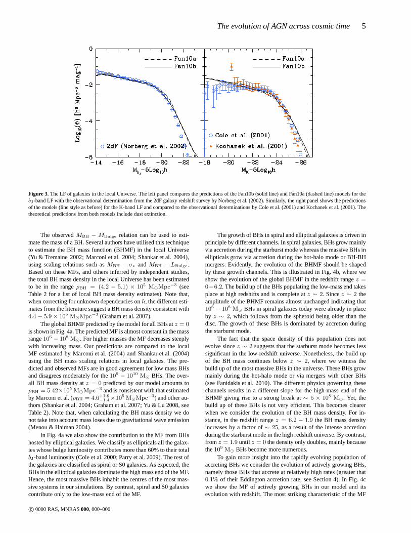
Finally we note that the total SFR density history in Fig. 1remains unchanged when using the BR06 SF law, as reported byLagos et al. This implies that properties such as stellar masses andgalaxy luminosities are fairly insensitive to the choice ofSF law.Indeed, Lagos et al. show that the predictions for thebJ andK-band LFs on using the BR06 SF law are very similar to those of theoriginal Bower et al. model and reproduce the observations veryclosely. Since we have changed the normalization of the SF surfacedensity, we recheck that our model still reproduces the observed LFof local galaxies, as shown in Fig. 3. Hence, we are confident thatwe are a building an AGN model within a realistic galaxy formationmodel.

3 THE EVOLUTION OF BH MASS

BH demographics have been the topic of many studies in the pastdecade mainly because of the tight correlations between theprop-erties of BHs and their host stellar spheroids. These correlationstake various forms, relating, for example, the mass of the BHto the mass of the galactic bulge (theMBH − MBulge relation:Magorrian et al. 1998; McLure & Dunlop 2002; Marconi & Hunt2003; Haring & Rix 2004), or to the stellar velocity dispersion (theMBH−σ relation: Ferrarese & Merritt 2000; Gebhardt et al. 2000;Tremaine et al. 2002). These remarkable and unexpected correla-tions suggest a natural link between the BH evolution and thefor-mation history of galaxies. The manifestation of this link could beassociated with AGN activity triggered during the build up of BHs.

c© 0000 RAS, MNRAS000, 000–000

The evolution of AGN across cosmic time 5

Figure 3. The LF of galaxies in the local Universe. The left panel compares the predictions of the Fan10b (solid line) and Fan10a (dashed line) models for thebJ-band LF with the observational determination from the 2dF galaxy redshift survey by Norberg et al. (2002). Similarly, the right panel shows the predictionsof the models (line style as before) for the K-band LF and compared to the observational determinations by Cole et al. (2001) and Kochanek et al. (2001). Thetheoretical predictions from both models include dust extinction.

The observedMBH − MBulge relation can be used to esti-mate the mass of a BH. Several authors have utilised this techniqueto estimate the BH mass function (BHMF) in the local Universe(Yu & Tremaine 2002; Marconi et al. 2004; Shankar et al. 2004),using scaling relations such asMBH − σ∗ andMBH − LBulge.Based on these MFs, and others inferred by independent studies,the total BH mass density in the local Universe has been estimatedto be in the rangeρBH = (4.2 − 5.1) × 105 M⊙Mpc−3 (seeTable 2 for a list of local BH mass density estimates). Note that,when correcting for unknown dependencies onh, the different esti-mates from the literature suggest a BH mass density consistent with4.4− 5.9× 105 M⊙Mpc−3 (Graham et al. 2007).

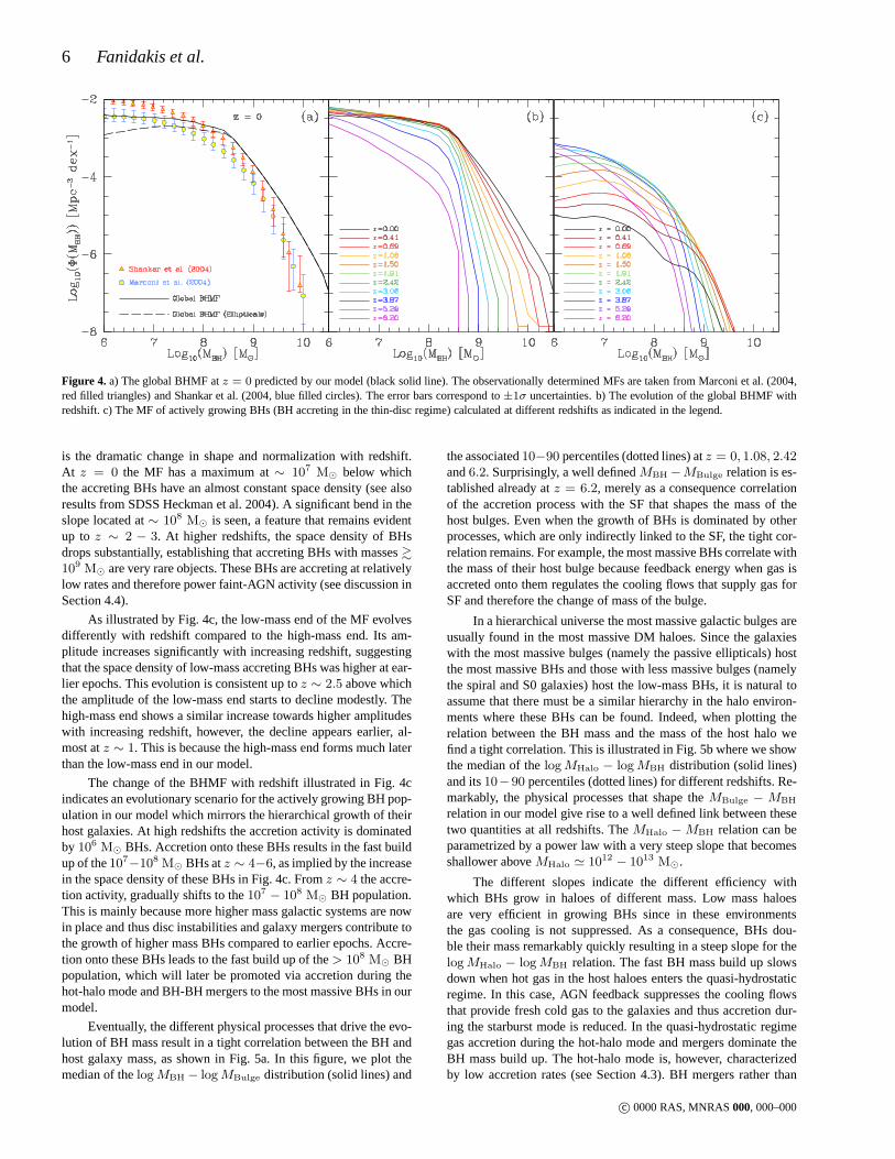
The global BHMF predicted by the model for all BHs atz = 0is shown in Fig. 4a. The predicted MF is almost constant in themassrange106 − 108 M⊙. For higher masses the MF decreases steeplywith increasing mass. Our predictions are compared to the localMF estimated by Marconi et al. (2004) and Shankar et al. (2004)using the BH mass scaling relations in local galaxies. The pre-dicted and observed MFs are in good agreement for low mass BHsand disagrees moderately for the109 − 1010 M⊙ BHs. The over-all BH mass density atz = 0 predicted by our model amounts toρBH = 5.42×105 M⊙Mpc−3 and is consistent with that estimatedby Marconi et al. (ρBH = 4.6+1.9

−1.4×105 M⊙Mpc−3) and other au-thors (Shankar et al. 2004; Graham et al. 2007; Yu & Lu 2008, seeTable 2). Note that, when calculating the BH mass density we donot take into account mass loses due to gravitational wave emission(Menou & Haiman 2004).

In Fig. 4a we also show the contribution to the MF from BHshosted by elliptical galaxies. We classify as ellipticals all the galax-ies whose bulge luminosity contributes more than 60% to their totalbJ-band luminosity (Cole et al. 2000; Parry et al. 2009). The rest ofthe galaxies are classified as spiral or S0 galaxies. As expected, theBHs in the elliptical galaxies dominate the high mass end of the MF.Hence, the most massive BHs inhabit the centres of the most mas-sive systems in our simulations. By contrast, spiral and S0 galaxiescontribute only to the low-mass end of the MF.

The growth of BHs in spiral and elliptical galaxies is driveninprinciple by different channels. In spiral galaxies, BHs grow mainlyvia accretion during the starburst mode whereas the massiveBHs inellipticals grow via accretion during the hot-halo mode or BH-BHmergers. Evidently, the evolution of the BHMF should be shapedby these growth channels. This is illustrated in Fig. 4b, where weshow the evolution of the global BHMF in the redshift rangez =0−6.2. The build up of the BHs populating the low-mass end takesplace at high redshifts and is complete atz ∼ 2. Sincez ∼ 2 theamplitude of the BHMF remains almost unchanged indicating that106 − 108 M⊙ BHs in spiral galaxies today were already in placeby z ∼ 2, which follows from the spheroid being older than thedisc. The growth of these BHs is dominated by accretion duringthe starburst mode.

The fact that the space density of this population does notevolve sincez ∼ 2 suggests that the starburst mode becomes lesssignificant in the low-redshift universe. Nonetheless, thebuild upof the BH mass continues belowz ∼ 2, where we witness thebuild up of the most massive BHs in the universe. These BHs growmainly during the hot-halo mode or via mergers with other BHs(see Fanidakis et al. 2010). The different physics governing thesechannels results in a different slope for the high-mass end of theBHMF giving rise to a strong break at∼ 5 × 108 M⊙. Yet, thebuild up of these BHs is not very efficient. This becomes clearerwhen we consider the evolution of the BH mass density. For in-stance, in the redshift rangez = 6.2 − 1.9 the BH mass densityincreases by a factor of∼ 25, as a result of the intense accretionduring the starburst mode in the high redshift universe. By contrast,from z = 1.9 until z = 0 the density only doubles, mainly becausethe109 M⊙ BHs become more numerous.

To gain more insight into the rapidly evolving population ofaccreting BHs we consider the evolution of actively growingBHs,namely those BHs that accrete at relatively high rates (greater that0.1% of their Eddington accretion rate, see Section 4). In Fig. 4cwe show the MF of actively growing BHs in our model and itsevolution with redshift. The most striking characteristicof the MF

c© 0000 RAS, MNRAS000, 000–000

6 Fanidakis et al.

Figure 4. a) The global BHMF atz = 0 predicted by our model (black solid line). The observationally determined MFs are taken from Marconi et al. (2004,red filled triangles) and Shankar et al. (2004, blue filled circles). The error bars correspond to±1σ uncertainties. b) The evolution of the global BHMF withredshift. c) The MF of actively growing BHs (BH accreting in the thin-disc regime) calculated at different redshifts as indicated in the legend.

is the dramatic change in shape and normalization with redshift.At z = 0 the MF has a maximum at∼ 107 M⊙ below whichthe accreting BHs have an almost constant space density (seealsoresults from SDSS Heckman et al. 2004). A significant bend in theslope located at∼ 108 M⊙ is seen, a feature that remains evidentup to z ∼ 2 − 3. At higher redshifts, the space density of BHsdrops substantially, establishing that accreting BHs withmasses&109 M⊙ are very rare objects. These BHs are accreting at relativelylow rates and therefore power faint-AGN activity (see discussion inSection 4.4).

As illustrated by Fig. 4c, the low-mass end of the MF evolvesdifferently with redshift compared to the high-mass end. Its am-plitude increases significantly with increasing redshift,suggestingthat the space density of low-mass accreting BHs was higher at ear-lier epochs. This evolution is consistent up toz ∼ 2.5 above whichthe amplitude of the low-mass end starts to decline modestly. Thehigh-mass end shows a similar increase towards higher amplitudeswith increasing redshift, however, the decline appears earlier, al-most atz ∼ 1. This is because the high-mass end forms much laterthan the low-mass end in our model.

The change of the BHMF with redshift illustrated in Fig. 4cindicates an evolutionary scenario for the actively growing BH pop-ulation in our model which mirrors the hierarchical growth of theirhost galaxies. At high redshifts the accretion activity is dominatedby 106 M⊙ BHs. Accretion onto these BHs results in the fast buildup of the107−108 M⊙ BHs atz ∼ 4−6, as implied by the increasein the space density of these BHs in Fig. 4c. Fromz ∼ 4 the accre-tion activity, gradually shifts to the107 − 108 M⊙ BH population.This is mainly because more higher mass galactic systems arenowin place and thus disc instabilities and galaxy mergers contribute tothe growth of higher mass BHs compared to earlier epochs. Accre-tion onto these BHs leads to the fast build up of the> 108 M⊙ BHpopulation, which will later be promoted via accretion during thehot-halo mode and BH-BH mergers to the most massive BHs in ourmodel.

Eventually, the different physical processes that drive the evo-lution of BH mass result in a tight correlation between the BHandhost galaxy mass, as shown in Fig. 5a. In this figure, we plot themedian of thelogMBH − logMBulge distribution (solid lines) and

the associated10−90 percentiles (dotted lines) atz = 0, 1.08, 2.42and6.2. Surprisingly, a well definedMBH −MBulge relation is es-tablished already atz = 6.2, merely as a consequence correlationof the accretion process with the SF that shapes the mass of thehost bulges. Even when the growth of BHs is dominated by otherprocesses, which are only indirectly linked to the SF, the tight cor-relation remains. For example, the most massive BHs correlate withthe mass of their host bulge because feedback energy when gasisaccreted onto them regulates the cooling flows that supply gas forSF and therefore the change of mass of the bulge.

In a hierarchical universe the most massive galactic bulgesareusually found in the most massive DM haloes. Since the galaxieswith the most massive bulges (namely the passive ellipticals) hostthe most massive BHs and those with less massive bulges (namelythe spiral and S0 galaxies) host the low-mass BHs, it is natural toassume that there must be a similar hierarchy in the halo environ-ments where these BHs can be found. Indeed, when plotting therelation between the BH mass and the mass of the host halo wefind a tight correlation. This is illustrated in Fig. 5b wherewe showthe median of thelogMHalo − logMBH distribution (solid lines)and its10−90 percentiles (dotted lines) for different redshifts. Re-markably, the physical processes that shape theMBulge − MBH

relation in our model give rise to a well defined link between thesetwo quantities at all redshifts. TheMHalo − MBH relation can beparametrized by a power law with a very steep slope that becomesshallower aboveMHalo ≃ 1012 − 1013 M⊙.

The different slopes indicate the different efficiency withwhich BHs grow in haloes of different mass. Low mass haloesare very efficient in growing BHs since in these environmentsthe gas cooling is not suppressed. As a consequence, BHs dou-ble their mass remarkably quickly resulting in a steep slopefor thelogMHalo − logMBH relation. The fast BH mass build up slowsdown when hot gas in the host haloes enters the quasi-hydrostaticregime. In this case, AGN feedback suppresses the cooling flowsthat provide fresh cold gas to the galaxies and thus accretion dur-ing the starburst mode is reduced. In the quasi-hydrostaticregimegas accretion during the hot-halo mode and mergers dominatetheBH mass build up. The hot-halo mode is, however, characterizedby low accretion rates (see Section 4.3). BH mergers rather than

c© 0000 RAS, MNRAS000, 000–000

The evolution of AGN across cosmic time 7

Figure 5. The median of theMBulge − MBH (a) andMHalo − MBH (b) distributions predicted by our model (solid lines). Predictions are shown forz = 0, 1.08, 2.42 and6.20 as indicated by the legend. The dotted lines indicate the10− 90 percentile ranges of the distributions.

adding new baryons to the BHs, only redistribute the BH mass.Therefore, the BH mass build up slows down establishing haloes ofMHalo ∼ 1013 − 1015 M⊙ as environments where BH growth isnot very efficient.

Given the efficiencies that characterize the two differentregimes in Fig. 5b we expect to find the brightest AGN in the1011 − 1013 M⊙ haloes. This perhaps is in contrast with the com-mon expectation that the brightest quasars should be found in themost massive haloes.

4 BH SPINS, ACCRETION EFFICIENCIES AND DISCLUMINOSITIES

AGN are unambiguously the most powerful astrophysical sourcesin the Universe. The ability of an accretion disc to produce elec-tromagnetic radiation is attributed to gravity yet its radiative effi-ciency is controlled primarily by the properties of the gas.Whenthe gas settles itself into a thin, cool, optically-thick accretion disc(Shakura & Sunyaev 1973), the efficiency of converting matter intoradiation can reach32% (Novikov & Thorne 1973). When the flowis characterized by very high, Eddington accretion rates, such ex-tremely luminous discs can power1047 − 1048erg s−1 quasars. Inthe next sections we describe how we model the physics of accre-tion flows and present predictions for the most fundamental prop-erties characterising the accreting BH systems in our model.

4.1 Calculation of the disc luminosity

The first important property that we can calculate in our model isthe physical accretion rate,M , onto a BH. This is defined as

M =Macc

tacc, (1)

whereMacc is the total accreted mass andtacc is the accretiontimescale. The accretion timescale is assumed to be directly linked

to the dynamical timescale of the host bulge,tBulge, through therelation

tacc = fqtBulge. (2)

fq is a free parameter and its value is fixed to 10. This is determinedby fitting the predictions of our model for the quasar LF to theobservations (see Section 5.2).

A second important quantity associated with every BH is theEddington luminosity,

LEdd =4πGMBHmpc

κ= 1.4× 1046

(

MBH

108 M⊙

)

erg s−1,

(3)whereκ ∼ 0.3 cm2g−1 is the electron scattering opacity andmp

is the proton mass. The Eddington luminosity has an associatedaccretion rate which is expressed as

MEdd = LEdd/ǫc2, (4)

whereǫ is the accretion efficiency andc is the speed of light. This isthe accretion rate at which the black hole radiates at the Eddingtonluminosity. The accretion efficiency is assumed to be determinedby the spin of the BH (Novikov & Thorne 1973) and its value iscalculated as in Fanidakis et al. (2010). It is convenient inour anal-ysis to express the physical accretion rate in units of the Eddingtonaccretion rate,m ≡ M/MEdd, in order to introduce a dependenceon the BH mass.

The accretion rate has a dramatic impact on the ge-ometry and radiative properties of the accretion disc (seeDone, Gierlinski, & Kubota 2007). In our model, we considertwodistinct accretion modes separated at a rate of1% of MEdd. In thefirst state, form > 0.01, we assume that the gas forms an accre-tion disc whose physics is adequately described by the radiativelyefficient thin-disc model of Shakura & Sunyaev (1973). The bolo-metric luminosity of a thin disc,Lbol, is linked toM through the

c© 0000 RAS, MNRAS000, 000–000

8 Fanidakis et al.

standard expression

Lbol = ǫMc2. (5)

When the accretion becomes substantially super-Eddington(Lbol > ηLEdd), the bolometric luminosity is limited toη[1 +ln(m/η)]LEdd (Shakura & Sunyaev 1973), whereη is an ad hocparameter equal to2 that allows a better modelling of bright end ofthe LF (see Section 5). However, we do not restrict the accretionrate if the flow becomes super-Eddington.

The second accretion state, withm < 0.01, is associatedwith sub-Eddington accretion flows with very low density. For suchlow accretion rates, the gas flow is unable to cool efficientlysinceradiative cooling does not balance the energy generated by vis-cosity. Thus, the viscous energy is trapped in the gas as entropyand ultimately advected into the hole. This type of accretion isknown as an advection dominated accretion flow (ADAF, Rees1982; Narayan & Yi 1994; Abramowicz et al. 1995). ADAFs havea number of distinct properties, some of which will be essentialfor the analysis in later sections (see Sections 5 and 6). Forex-ample, for an ADAF around a BH, only a fraction of the standardaccretion luminosity,L = ǫMc2, is emitted as radiation. The re-mainder of the viscously dissipated energy is stored in the gas asentropy, resulting in hot flows with almost virial temperatures. Wenote that, as shown by Ichimaru (1977), the ions and the electronsin an ADAF are not thermally coupled and, thus, reach differenttemperatures. This two-temperature virialized plasma flowis opti-cally thin and, for high viscosity parameters (α ∼ 0.1 − 0.3), itacquires a quasi-spherical geometry around the BH, which resem-bles spherical Bondi accretion. However, the accretion is entirelydue to dissipation via viscous forces rather than gravity. The bolo-metric luminosity of the flow in this case is equal to the luminosityemitted by the various cooling processes. Form . 10−3α2 it isonly due to Comptonisation, whereas form & 10−3α2 the coolingis split between Compton and synchrotron emission.

As the accretion rate increases, the emission of the energy pro-duced by the viscous processes in the gas becomes more efficient.Above some critical accretion rate,mc, the radiative efficiency ofthe gas is so high that the flow cools down to a thin disc. The crit-ical accretion is independent of the BH mass but depends stronglyon the viscosity,mc ≃ 1.3α2. Takingmc = 0.01 implicitly fixesthe value ofα to be0.087 for all the ADAFs in our model. Theluminosity of the flow for the two different regimes is then givenby Mahadevan (1997),

Lbol,ADAF =

{

ǫMc2[

0.4mβ/α2]

, m > 7.5 × 10−6

ǫMc2[

4×10−4(1−β)]

, m . 7.5× 10−6 (6)

whereβ is related to the Shakura-Sunyaev viscosity parameterαthrough the relationα ≈ 0.55(1−β) (Hawley, Gammie, & Balbus1995). The expressions in the square brackets in Eq. 6 shows howmuch less efficient the cooling is in an ADAF compared to the stan-dard efficiencyǫ of a thin disc. For example, atm = 0.01 an ADAFis characterized by an accretion efficiency of0.44ǫ, less than ap-proximately half as luminous as a thin disc.

4.2 BH spins and accretion efficiencies

In Fanidakis et al. (2010) we describe in detail how we model theevolution of BH spin. In brief, the spins of BHs change duringgas accretion (whenever a starburst is triggered by disc instabili-ties or galaxy mergers in the starburst mode or during the coolingof gas from the hydrostatic halo in the hot-halo mode) and merg-ers with other BHs. Fig. 6 shows the evolution with redshift of the

Figure 6. Top: The median BH spin weighted by BH mass as a functionof redshift for BHs in our model (solid black line). Bottom: The medianBH spin weighted by disc luminosity for all AGN accreting in the thin-discregime (solid black line). The values of the different percentiles (shadedregions) are indicated in both cases by the colour bars.

median of the BH spin distribution at a given redshift for twodiffer-ent cases. Firstly, we show the median spin weighted by BH mass(upper panel) for all the BHs withMBH > 106 M⊙. The medianshows an approximately constant trend fromz = 6 to z = 2 andhas a well defined value of∼ 0.25. In this redshift range BHs growpredominantly during disc instabilities (see Fig. 2) and thereforethe evolution of BH spin is governed by accretion. As shown byFanidakis et al., accretion of gas results in low spins with atyp-ical value ofa ∼ 0.2 (under the assumption that the gas is fedchaotically onto the BH). Hence, as indicated also by the differentpercentiles in the plot (shaded regions), the bulk of BHs acquirelow spins.

Below z = 2 BH mergers start to become an important chan-nel for growing the BH mass, especially when they are betweenBHs of similar mass, as expected following a major galaxy merger.However, this is a characteristic only of the most massive BHs inour model (MBH > 109 M⊙). Mergers between those BHs tend toincrease the spin of the final remnant to valuesa > 0.7 (see alsoBaker et al. 2007; Berti & Volonteri 2008; Fanidakis et al. 2010).Eventually, at low redshifts BH mergers give rise to a populationof rapidly rotating BHs. The appearance of these BHs, as indicatedalso by the different percentiles belowz = 2, increases the dynam-ical range of the predicted spins up to values of0.998 (the range ofspin values in the distribution of BHs in Fig. 6 is smaller becausewe show only up to the90th percentile of the data). The environ-mental dependence of BH spins is illustrated in Fig. 7, wherewe seethat the most rapidly-rotating BHs populate the centres of the mostmassive DM haloes. In contrast, slowly rotating BHs are found inlow mass halo environments. This is a consequence of the correla-tion between BH mass and spin in our model: rapidly rotating BHshave masses& 109 M⊙. These BHs are hosted by massive ellip-

c© 0000 RAS, MNRAS000, 000–000

The evolution of AGN across cosmic time 9

Figure 7. The distribution of rotating BHs atz = 0 in the Millennium simulation. The two panels show the same DMdistribution in a cube of comovinglength100 Mpc h−1 colour coded according to density (black represents the peaks of DM density). Over plotted with blue spheres in the left plot are galaxieswith rapidly rotating BHs (a > 0.7) predicted by the semi-analytic model. Similarly, in the right plot are shown a sample of galaxies with slowly rotatingBHs (a < 0.7) randomly chosen from our data and equal in number to thea > 0.7 BHs. The size of the spheres is proportional to the spin of theBH that thegalaxy hosts.

tical galaxies in our model which inhabit the centres of the mostmassive haloes.

In contrast, the median spin of actively growing BHs in ourmodel does not reveal the presence of rapidly spinning BHs. Thisis demonstrated in the lower panel of Fig. 6 where we have selectedthe actively growing BHs in our sample (m > 0.01) and plot themedian of their spin distribution weighted by disc luminosity. As il-lustrated in the plot, the predictions are consistent with low spins atall redshifts even atz ∼ 0. This is because in this sample we haveselected only the actively growing BHs; we find that almost exclu-sively these are. 109 M⊙ BH and thus have low spins. Hence,these BHs dominate the sample and determine the over all trend ofthe median.

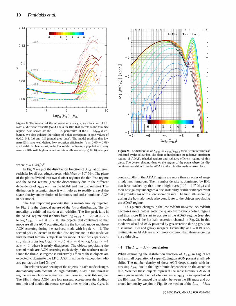
The a − MBH correlation can be further elucidated throughthe dependence of the accretion efficiency on the mass of activelygrowing BHs. This is illustrated in Fig. 8 where we show the me-dian of theǫ distribution for the sample of actively growing BHs(solid lines), again weighted by the disc luminosity. Atz = 0, themedian is approximately constant forMBH . 108, with a typicalvalue of∼ 0.07. As implied by the10 − 90 percentiles (dottedlines), the dynamical range of the typicalǫ values is very small andrestricted to the range0.06− 0.08 (a = 0.1− 0.5). For higher BHmasses the efficiency can reach significantly higher values.This isa manifestation of the fact that high mass BHs have high spinsandthus high accretion efficiencies when they accrete in the thin-discregime. Fig. 8 also demonstrates that the dependence of the effi-ciency on the BH mass does not change with redshift. Hence, atall redshifts BHs have very well determined accretion efficiencies.

It is therefore, only the accretion rate that regulates the luminosityoutput from an accreting BH.

Note that, BHs with higher efficiencies (ǫ & 0.15) are stillfound in our BH populations. However, they are usually very mas-sive (MBH > 5 × 108 M⊙) and do not undergo significant quasaractivity. These BHs can support the formation of very strongjets inthe presence of an ADAF and establish the host galaxy as a radio-loud AGN (high spins and BH mass are essential for high jet lumi-nosities; Fanidakis et al. 2010). In this case, a plot similar to the onein the top panel of Fig.6, weighted by jet instead of disc luminosity,will unveil a significant population of AGN with rapidly rotatingBHs. Hence, BH spins (and efficiencies) can display different dis-tributions depending on the AGN population we are probing.

4.3 The distribution of the λEdd parameter

Having explored the evolution of the BH mass and spin, and cal-culated the accretion efficiencies for the BHs accreting in the thin-disc regime, we now investigate the disc luminosities of theaccret-ing BHs predicted by the model. We calculate the bolometric discluminosity in the ADAF and thin-disc regime using the formula-tion described in Section 4.1. It is useful to scaleLbol, in units ofLEdd in order to remove the dependence of the luminosity on theBH mass. For this purpose we introduce the Eddington parameter,λEdd, defined as,

λEdd = Lbol/LEdd =

γm2, if m <0.01m, if m >0.01

η[1 + ln(m/η)], if Lbol > ηLEdd

(7)

c© 0000 RAS, MNRAS000, 000–000

10 Fanidakis et al.

Figure 8. The median of the accretion efficiency,ǫ, as a function of BHmass at different redshifts (solid lines) for BHs that accrete in the thin discregime. Also shown are the10 − 90 percentiles of theǫ − MBH distri-bution. We also indicate the values ofǫ that correspond to spin values of0, 0.2, 0.4, 0.6 and 0.8 (dotted grey lines). The model predicts that lowmass BHs have well defined low accretion efficiencies (ǫ ≃ 0.06 − 0.08)at all redshifts. In contrast, in the low redshift universe,a population of verymassive BHs with high radiative accretion efficiencies (ǫ & 0.08) emerges.

whereγ = 0.4β/α2 .In Fig. 9 we plot the distribution function ofλEdd at different

redshifts for all accreting sources withMBH > 106 M⊙. The planeof the plot is divided into two distinct regions: the thin-disc regimeand the ADAF regime (note the discontinuity due to the differentdependence ofλEdd onm in the ADAF and thin disc regime). Thisdistinction is essential since it will help us to readily unravel thespace density and evolution of luminous and under-luminousAGNin our model.

The first important property that is unambiguously depictedby Fig. 9 is the bimodal nature of theλEdd distribution. The bi-modality is exhibited nearly at all redshifts. The first peakfalls inthe ADAF regime and it shifts fromlog λEdd ≃ −2.5 at z ∼ 6to log λEdd ≃ −4 at z ∼ 0. The objects that contribute to thatmode are all the AGN accreting during the hot-halo mode and thoseAGN accreting during the starburst mode withlog m < −2. Thesecond peak is located in the thin-disc regime and in this mode wefind the most luminous objects in our model. Their peak space den-sity shifts from log λEdd ≃ −0.5 at z ∼ 6 to log λEdd ≃ −1at z ∼ 0, where it nearly disappears. The objects populating thesecond mode are AGN accreting exclusively in the starburst mode.Since the thin-disc regime is radiatively efficient these objects areexpected to dominate the LF of AGN in all bands (except the radioand perhaps the hard X-rays).

The relative space density of the objects in each mode changesdramatically with redshift. At high redshifts, AGN in the thin-discregime are much more numerous than those in the ADAF regime.The BHs in these AGN have low masses, accrete near the Edding-ton limit and double their mass several times within a few Gyrs. In

Figure 9.The distribution ofλEdd = Lbol/LEdd for different redshifts asindicated by the colour bar. The plane is divided into the radiative-inefficientregime of ADAFs (shaded region) and radiative-efficient regime of thindiscs. The denser shading denotes the region of the plane where the dis-continues transition from the ADAF to the thin-disc regime takes place.

contrast, BHs in the ADAF regime are more than an order of mag-nitude less numerous. Their number density is dominated by BHsthat have reached by that time a high mass (108 − 109 M⊙) andtheir host galaxy undergoes a disc instability or minor merger eventthat provides gas with a low accretion rate. The first BHs accretingduring the hot-halo mode also contribute to the objects populatingthe ADAF regime.

This picture changes in the low redshift universe. As redshiftdecreases more haloes enter the quasi-hydrostatic coolingregimeand thus more BHs start to accrete in the ADAF regime (see alsothe evolution of the hot-halo accretion channel in Fig. 2). In thismode we also find AGN powered by gas accretion during gas-poordisc instabilities and galaxy mergers. Eventually, atz = 0 BHs ac-creting via an ADAF are much more common than those accretingvia a thin disc.

4.4 TheLbol −MBH correlation

When examining the distribution function ofλEdd in Fig. 9 wefind a small population of super-Eddington AGN present at allred-shifts. The number density of these AGN drops sharply with in-creasingλEdd due to the logarithmic dependence on the accretionrate. Whether these objects represent the most luminous AGNatsome given redshift is not obvious sinceλEdd is independent ofthe BH mass. To unravel the relation between the BH mass and ac-creted luminosity we plot in Fig. 10 the median of theLbol−MBH

c© 0000 RAS, MNRAS000, 000–000

The evolution of AGN across cosmic time 11

distribution and its associated percentiles atz = 0.5, 1 and 2.We show predictions both for objects accreting in the thin-disc(lower panels) and ADAF (upper panels) regime. To guide thereader we also distinguish with different shading the region whereLbol > LEdd(MBH).

When we consider BHs accreting in the ADAF regime we findthat theLbol − MBH correlation is characterized by a floor at lu-minosities. 1042erg s−1. In this regime, BHs haveλEdd ≃ 10−4

and therefore they comprise the majority of accreting BHs inoursample (remember the location of the peak of theλEdd distributionfunction in Fig. 9). For example, atz = 0 we find that∼ 93% of theBHs produce luminosities fainter than1042erg s−1. For brighterluminosities, we find a strong correlation betweenMBH andLbol

which indicates that the most massive BHs must have higher ac-cretion rates compared to the lower mass ones. Indeed, when iden-tifying the accretion properties of the most massive BHs we findthat the& 108 M⊙ BHs haveλEdd & 10−3. Thus, these BHs areable to produce a significant luminosity even though they accretein the ADAF regime. In fact, in our sample we find∼ 1010 M⊙

BHs accreting atm ≃ 0.01 which produce luminosities as highas1046erg s−1. However, these BHs are very rare: atz = 0.5,where the space density of these BHs peaks, we find only a hand-ful of them (space densities lower than10−8 Mpc−3). For higherredshifts, their space density declines and as a consequence themaximum disc luminosity produced in the ADAF regime is alsoreduced.

In the thin-disc regime, we find that accreting BHs typicallyproduce luminosities greater than1042erg s−1. The logLbol −

logMBH correlation in this regime increases monotonically untilthe slope becomes significantly shallower near the highest lumi-nosities achieved at a given redshift. The nature of the break inthe slope is determined by the AGN feedback prescription in ourmodel. When massive haloes reach quasi-hydrostatic equilibriumthey become subject to AGN feedback that suppresses the coolingflows; some of the mass which would have been involved in thecooling flow is instead accreted onto the BH. In these haloes wefind the most massive BHs in our model (& 109 M⊙, see Fig 5b).Therefore, these BHs are expected to live in gas poor environmentsand when they accrete gas they usually do so via an ADAF disc. Inthis regime, the suppression of cooling flows forces theLbol−MBH

correlation to evolve only along theLbol axis since accretion via athin disc onto& 109 M⊙ BHs becomes very rare.

The correlation betweenLbol andMBH found atz = 0.5 re-mains approximately the same at higher redshifts. Only the rangesof BH mass corresponding to the bulk of the AGN shift modestlyto lower mass. This is due to the fact that in a hierarchical universeaccretion shifts to lower BH masses at higher redshifts (Section 3).In addition, the break in the slope at high luminosities becomes lessprominent since fewer haloes are in quasi-hydrostatic equilibriumat high redshifts.

The most luminous AGN (& 1046erg s−1) are exclusivelypowered by super-Eddington accretion onto∼ 108 − 109 M⊙

BHs. This implies that the most luminous quasars are expected tobe found in∼ 1012 − 1013 M⊙ DM haloes and not in the mostmassive ones (remember theMHalo −MBH in Fig. 5b). This is ingood agreement with the typical DM halo mass quasars are inferredto inhabit as suggested by several observational clustering analyses(daAngela et al. 2008; Shen et al. 2009; Ross et al. 2009). In con-trast, accretion characterized by lower luminosities spans the wholerange of BH masses (106 − 1010 M⊙).

5 THE EVOLUTION OF THE AGN LUMINOSITYFUNCTIONS

5.1 Bolometric corrections and obscuration

The LF is calculated in redshift ranges which are determinedbythe observations we are comparing with. The contribution ofeachAGN to the LF in a rangez = z1 − z2 is weighted by a factor,

wBH = tactive/∆tz1,z2 , (8)

where∆tz1,z2 is the time interval delineated by the redshift rangez1 − z2 and tactive is the time during which the AGN is “on” inthe∆tz1,z2 interval (in principletactive = tacc only if the wholeperiod of accretion falls withinz1 − z2). The bands for whichwe present predictions are theB-band (4400A), soft X-ray (SX:0.5 − 2 keV) and hard X-ray (HX:2 − 10 keV). The bolometriccorrections considered here are approximated by the following 3rd

degree polynomial relations (Marconi et al. 2004),

log(LHX/Lbol) = −1.65− 0.22L − 0.012L2 + 0.0015L3

log(LSX/Lbol) = −1.54− 0.24L − 0.012L2 + 0.0015L3

log(νBLνB/Lbol) = −0.80 + 0.067L − 0.017L2 + 0.0023L3

(9)

whereL = log(Lbol/L⊙)−12. Marconi et al. derive these correc-tion based on a spectral template where the spectrum atλ > 1µm istruncated in order to remove the IR bump. In this way, the spectrumcorresponds to the intrinsic luminosity of the AGN (optical, UV andX-ray emission from the disc and hot corona). We apply Eqs. 9 toboth thin discs and ADAFs, though we note that there is evidencefor a change in these corrections withλEdd (Vasudevan & Fabian2007).

There is evidence that the fraction of obscured AGN decreaseswith increasing X-ray luminosity (Ueda et al. 2003; Steffenet al.2003; Hasinger 2004; La Franca et al. 2005) a trend found alsoby Simpson (2005) in a sample of broad and narrow-line AGNfrom the SDSS. The question of whether the fraction of obscuredAGN depends also on redshift is more uncertain. If gas or dustin galaxies provide the obscuring medium then its abundanceshould evolve in a fashion similar to the SFR history. This willresult in a fraction of obscured AGN that is redshift dependent.In addition, a strongly evolving population of obscured AGNis required by AGN population synthesis models to reproducethe properties of the X-ray background (Comastri et al. 1995;Gilli, Risaliti, & Salvati 1999; Ballantyne, Everett, & Murray2006; Ballantyne et al. 2006; Gilli, Comastri, & Hasinger 2007).Ueda et al. (2003) and Steffen et al. (2003) suggest that suchatrend is not clear in AGN samples of deep X-ray surveys. However,the analysis by Treister & Urry (2006) on AGN samples of higheroptical spectroscopic completeness indicates that the relativefraction of obscured AGN does increase with redshift.

More recently, Hasinger (2008) showed, based on a sampleof X-ray selected AGN from ten independent samples with highredshift completeness, that the fraction of obscured AGN increasesstrongly with decreasing luminosity and increasing redshift. Ac-cording to Hasinger, the dependence of the obscured fraction ofAGN, fobsc, on LHX, can be approximated by a relation of theform,

fobsc = −0.281 log(LHX) + A(z), (10)

whereA(z) = 0.308(1+z)0.48 andLHX = 1042−1046erg s−1. Abroken power law can also be used to describeA(z)which providesa fit with modestly better statistical significance. The bestfit gives

c© 0000 RAS, MNRAS000, 000–000

12 Fanidakis et al.

Figure 10. The median of theMBH − Lbol distribution atz = 0.5, 1 and2 (black solid lines) for BHs accreting via a thin disc (lower panels) and ADAF(upper panels). The different percentiles of the distribution are colour-coded according to the bar on the right. The shaded regions represent the regime wherethe accretion becomes super-Eddington.

a power law of the formA(z) ∝ (1 + z)0.62 that saturates atz =2.06 and remains constant thereafter.

Hence, in order to determine the correct population of AGN ina luminosity bin of a given band we need to take into account theeffects of obscuration. To do so, we utilise the dependence of theobscured fraction on theLHX luminosity found in Hasinger (2008)as follows. We calculate the fraction of visible AGN,fvis = 1 −

fobsc, at a given luminosity bin in the2−10 keV band using Eq. 10and then we associate the value offvis with the corresponding B-band or soft X-ray luminosity bin using Eqs. 9. The LF can thenbeexpressed as,

dΦ

d log(LX)

∣

∣

∣

∣

vis

= fvis(LHX, z)dΦ

d log(LX). (11)

In our analysis, we choose the single instead of the broken powerlaw form of A(z) to allow for a comparison with previous work(e.g., La Franca et al. 2005). In this way we provide a simple,yetwell constrained, prescription for the effects of obscuration in theAGN of our model.

5.2 The optical LF

In Fig. 11 we present thebJ-band LF of quasars in 9 different red-shift bins between0.4 < z < 4.25. Our predictions are shown

before and after applying the obscuration effect (dashed and solidblack lines respectively). Absolute magnitudes are first calculatedin the B band using the standard expression

MB = −10.44− 2.5 log(LB/1040erg s−1), (12)

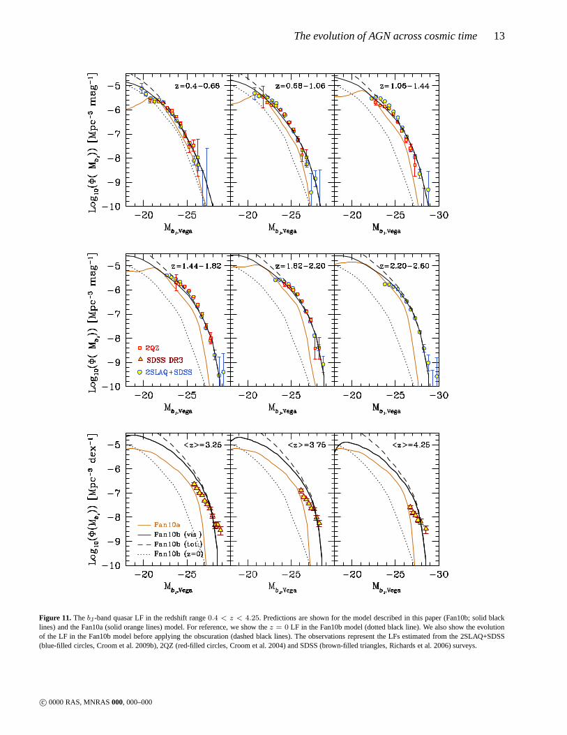
for magnitudes in the Vega system and then converted to thebJband using the correctionMbJ = MB − 0.072 (Croom et al.2009b). Predictions are shown for the Fan10b and for comparison,the predictions from the modified version of the Bower et al. (2006)model (solid orange lines) presented in Fanidakis et al. (2010,Fan10a). The Fanidakis et al. model was constrained to matchtheobserved LF of quasars atz ∼ 0.5. In brief, the model assumes aconstant obscuration fraction offvis = 0.6 and abJ-band bolomet-ric correction of0.2. Finally, our predictions for thez = 0 LF, af-ter applying the obscuration effect, are shown in every redshift bin(black dotted lines) to help us assess the evolution with redshift.

Our predictions are compared to the 2SLAQ+SDSS QSO LFs(Croom et al. 2009b). QSO magnitudes in the 2SLAQ sample wereobtained in theg-band and therefore need to be converted to thebJband considered here. We useMbJ = Mg + 0.455 (Croom et al.2009b) where the K-corrections for theg band have been normal-ized toz = 2. In addition, we plot the 2QZ LFs by Croom et al.(2004). The observed LFs agree very well with each other particu-larly at bright magnitudes (MbJ < −24). The modest disagreement

c© 0000 RAS, MNRAS000, 000–000

The evolution of AGN across cosmic time 13

Figure 11. ThebJ-band quasar LF in the redshift range0.4 < z < 4.25. Predictions are shown for the model described in this paper(Fan10b; solid blacklines) and the Fan10a (solid orange lines) model. For reference, we show thez = 0 LF in the Fan10b model (dotted black line). We also show the evolutionof the LF in the Fan10b model before applying the obscuration(dashed black lines). The observations represent the LFs estimated from the 2SLAQ+SDSS(blue-filled circles, Croom et al. 2009b), 2QZ (red-filled circles, Croom et al. 2004) and SDSS (brown-filled triangles, Richards et al. 2006) surveys.

c© 0000 RAS, MNRAS000, 000–000

14 Fanidakis et al.

Table 3. Typical values offvis in three magnitude bins and its evolutionwith redshift.

MbJ= −20 MbJ

= −24 MbJ= −28

z = 0.4 53.3% 84.3% 100%z = 0.68 49% 81% 100%z = 1.06 44.9% 76.9% 100%z = 1.44 42.2% 73.3% 100%z = 1.82 27.8% 69.9% 100%z = 2.20 24.7% 66.7% 98.7%

seen at the faintest magnitudes is due to the different K-correctionapplied to the 2QZ QSO sample by Croom et al. (2004). For higherredshifts, we include the LF derived from the SDSS Data Release3 sample (DR3, Richards et al. 2006). The SDSS DR3 LF is ob-tained in thei band, therefore we need to convert it to thebJ band.We useMbJ = Mi+0.71, assuming a spectral index ofaν = −0.5(Croom et al. 2009b).

The AGN model contains one free adjustable parameter thatmust be constrained by observational data. This is thefq parameterin Eq. 2 which sets the accretion timescale. We choose thebJ bandfor constraining the value offq because it is the most sensitive tothe modelling of AGN. Other free parameters are constrainedbythe galaxy formation model and are adjusted to reproduce theob-served galaxy LFs (Bower et al. 2006; Lagos et al. 2010, see alsoBower et al. 2010 for further discussion of our parameter fittingphilosophy). Sincefq is essentially the only free parameter in ourmodel, the predictions presented in these Sections are genuine pre-dictions of the underlying galaxy formation model. By fixingfq to10 we obtain an excellent overall match to the observed QSO LFsin the 0.4 < z < 2.6 redshift interval. For higher redshifts, ourmodel provides a good match, however, it predicts a much steeperslope for the bright end compared to the SDSS DR3 LF.

A comparison between the predictions for thez = 0.4− 4.25andz = 0 LFs in Fig. 11 shows that quasars undergo significantcosmic evolution. For example, quasars withMbJ = −25 increasein space density from∼ 10−8 to ∼ 10−6 Mpc−3 betweenz = 0andz = 2.2 − 2.6. This strong evolution in the space density ofquasars is due to the fact that disc instabilities and galaxymerg-ers, the two processes that trigger accretion during the starburstmode, become more frequent at higher redshifts (see Fig. 1).Yet,the strong evolution of quasars does not affect only their space den-sity. At a fixed space density of10−8 Mpc−3 the quasar LF bright-ens fromMbJ ≃ −25 at z = 0 to MbJ ≃ −28 at z = 2.2 − 2.6.This is attributed to the fact that the cold gas becomes more abun-dant with increasing redshift. This is equivalent to a strong increasein the gas reservoir available for feeding the central BHs since moregas is turned into stars when a starburst is triggered.

The processes that are responsible for driving the formationof stars in starbursts are also responsible for the cosmic evolutionof quasars. Qualitatively, the strong link between the formation ofstars and quasar activity (and therefore BH growth) can be illus-trated by considering the Fan10a model. In Fig.1 we can see that theSFR density in bursts in the Fan10a model shows a milder evolu-tion with redshift compared to the Fan10b model. Hence, the modelpredicts considerably that less gas is available for accretion whichthen results in more modest evolution of the quasar LF. As a con-sequence, the predictions of the model Fan10a provide an overallpoor match to the observed LFs.

The evolution of the SFR density with redshift does not im-

ply a proportional evolution of quasar luminosities on theMbJ −

Φ(MbJ ) plane. The space density of the brightest quasars increasewith redshift. However, the density of objects around the breakin the LF increases more quickly, leading to a steepening of theLF as illustrated by Fig.11. This differential evolution isdeter-mined exclusively by the accretion physics in our model. In the0.01 < m < 1 regime, the disc luminosity scales in propor-tion to m. However, when the flow becomes substantially super-Eddington, the luminosity instead grows asln(m) and thereforethe dynamical range of predicted luminosities decreases dramati-cally. The logarithmic dependence of luminosity on the accretionrate has a strong impact on the shape of the LF, resulting in a verysteep slope at the bright end. This becomes apparent in the highestredshift intervals (z > 1.44) where the relative number of super-Eddington accreting sources becomes significantly higher than inthe lower redshift intervals (because more gas is availablefor ac-cretion, see Fig. 9). Since these sources exclusively populate thebrightest magnitude bins, the bright end of the LF now becomessignificantly steeper.

Another factor that influences the evolution of the quasar LFisobscuration. Low luminosity quasars are heavily obscured accord-ing to our obscuration prescription, and thus remain well buriedin their host galactic nuclei. This is clear from Table 3 where wesummarize the evolution of thefvis value in the redshift range ofinterest. In the highest redshift intervals the obscuration becomesmore prominent affecting even the brightest sources. However, theintense accretion activity during the starburst mode dominates theevolution of the faint end, and therefore a strong cosmic evolutionin the space density of the faintest sources, similar to thatof thebrightest sources, is still observed. Nonetheless, the obscurationsignificantly influences the cosmic abundance of the quasar popu-lations dominating the faint end, something that will become moreevident in Section 5.5 where we will explore the cosmic evolutionof quasars of given intrinsic luminosity.

Finally, we point out that those AGN that are powered byan ADAF contribute significantly to the space density of AGNfainter thanMbJ ≃ −22 in the low redshift universe. In fact,in the range0.4 < z < 0.68, we find ADAF sources withm ≃ 0.001 − 0.01 contributing also to the knee of the LF. Thesesystems represent the rare& 109 M⊙ accreting BHs in Fig. 10.Identifying the ADAF systems with optically bright quasarsintro-duces a caveat for the model since quasars typically show high ex-citation spectra which indicate the presence of a bright, UVthindisc (see e.g., Marchesini, Celotti, & Ferrarese 2004). Nonetheless,these systems accrete where the transition to a thin disc takes place.Observations of stellar mass BH binary systems show that this tran-sition is complex, probably taking on a composite structurewiththe thin disc replacing the hot flow at progressively smallerradii(see e.g,. the review by Done, Gierlinski, & Kubota 2007). Such aconfiguration could possibly produce high excitation lineswhile re-taining also the ADAF characteristics. For a more comprehensiblerepresentation of the objects populating the LF, we refer the readerto Fig. 14 in Section 5.4 where we decompose the LF into the con-tribution from ADAF, thin-disc, and also super-Eddington sources.

5.3 The X-ray LFs

The good agreement between our model predictions for the opticalLF and the observations motivates us to study also the evolutionof X-ray AGN as a function of redshift and intrinsic luminosity.X-rays account for a considerable fraction of the bolometric lu-minosity of the accretion disc and therefore provide an ideal band

c© 0000 RAS, MNRAS000, 000–000

The evolution of AGN across cosmic time 15

Figure 12. The predictions of our model for evolution of the soft X-ray LF (solid black lines). Predictions are shown before (total:dashed lines) and after(visible: solid lines) we apply the effects of obscuration.In addition, we quote the total fraction of AGN withLSX > 1042erg s−1 that are visible in everyluminosity bin. Data are taken from Ueda et al. (2003).

Figure 13. The evolution of the hard X-ray LF in our model (solid black lines). Predictions are shown only forz < 1.6 and no obscuration correction isapplied. Observational data are taken from Hasinger, Miyaji, & Schmidt (2005).

c© 0000 RAS, MNRAS000, 000–000

16 Fanidakis et al.

for studying the cosmic evolution of AGN. The observed contin-uum spectra of AGN in the X-rays can be represented by a simplepower law in thehard part of the spectrum (2 − 10 keV) witha universal spectral index ofαX ∼ 0.7 which is independent ofthe luminosity over several decades. In thesoft part of the spec-trum (0.5−2 keV) the power law continuum is strongly attenuatedby absorption which is typically in excess of the Galactic valueand corresponds to a medium with hydrogen column densities ofNH ≃ 1020 − 1023 cm−1 (Reynolds 1997; George et al. 1998;Piconcelli et al. 2005).

The cosmic evolution of X-ray AGN has been in-vestigated by employing AGN selected both in the soft(Miyaji, Hasinger, & Schmidt 2000; Hasinger, Miyaji, & Schmidt2005) and hard part of the spectrum (Ueda et al. 2003;La Franca et al. 2005; Barger et al. 2005; Aird et al. 2010). Mir-roring the strong evolution of the optical LF, the LF of X-rayse-lected AGN also evolves strongly with cosmic time. The LFs insoft and hard X-rays have similar characteristics, evolving at thesame rate but differ significantly in normalization. For example,the Hasinger, Miyaji, & Schmidt (2005) soft X-ray sample hasap-proximately a 5 times smaller global LF normalization comparedto that of the hard X-ray LF estimated by Ueda et al. (2003). Thisdifference is most likely attributed to the fact that a largefraction ofAGN is obscured in the soft X-rays (type-2 AGN are by a factor of4 more numerous than type-1 AGN, Risaliti, Maiolino, & Salvati1999).

We present in this section our predictions for the X-rayLFs. We calculate the X-ray emission in the0.5 − 2 keV and2 − 10 keV bands using Eq. (9). Our predictions for the softand hard X-ray LFs are shown in Figs. 12 and 13 respectively(solid lines). The predictions are compared to the LFs estimatedby Hasinger, Miyaji, & Schmidt (2005) for the soft X-rays andUeda et al. (2003) for the hard X-rays. Note that we do not showes-timates from observations that consist only of upper limits(emptybins). The Hasinger, Miyaji, & Schmidt sample comprises unab-sorbed AGN and therefore we need to take this into account forthe sample in the soft X-rays the effect of obscuration. We doso byusing the Hasinger (2008) prescription as explained in the previoussection. To quantify the effect of absorption we also plot inthe softX-rays the total population of AGN (dashed lines).

Overall, our model provides a very good match to the observa-tions in both soft and hard X-rays. We find discrepancies betweenthe observations and the model predictions in the redshift rangez = 0.4 − 0.8, where the space density of the< 1043erg s−1 softX-ray AGN is under predicted. A similar disparity is also seen inthez = 0.8− 1.6 bin for the1043 − 1045erg s−1 AGN. However,it is important to bear in mind that our predictions in the soft X-rays depend strongly on our prescription for the obscuration. Sinceour predictions for the total AGN population are always wellabovethe observations, it is likely that these discrepancies areattributedto the modelling of the obscuration. We also find that the modelpredicts at high redshifts a somewhat steeper bright end comparedto the observations, although the very brightest point could be dueto beaming effects in a small fraction of the more numerous lowerluminosity sources (Ghisellini et al. 2010). Nonetheless,the verysteep slope in our predictions is again a manifestation of the Ed-dington limit applied to the super-Eddington sources, an effect thatbecomes more significant at higher redshifts as already explainedin the previous section.

As illustrated by the predictions for the soft X-ray LF inFig. 12, the space density of the faintest soft X-ray AGN in ourmodel is strongly affected by the obscuration. As illustrated by the

LFs in the soft X-rays, AGN withLSX ≃ 1042 − 1044erg s−1 areheavily obscured. In fact, in the redshift intervalz = 0.015 − 0.2only 19% of the total AGN population withLSX > 1042erg s−1

is visible in soft X-rays. Hence, the obscured AGN outnumberthevisible AGN by a factor of 4 (Risaliti, Maiolino, & Salvati 1999).This fraction of visible AGN becomes even smaller at higher red-shift because the obscuration becomes more prominent with red-shift. At z > 3.2 only a negligible fraction of the AGN are seen insoft X-rays. Based on these results we estimate that approximately10% of the total number of AGN withLSX > 1042erg s−1 are vis-ible in the soft X-rays in thez = 0.015 − 4.8 universe. We notethat these estimations are based on the obscuration model whichaccording to the AGN sample from Hasinger (2008) is evaluatedonly for luminosities1042erg s−1 < LHX < 1046erg s−1. Forluminosities lower than1042erg s−1 we assume thatfvis remainsconstant and equal tofvis(1042erg s−1). It is therefore likely thatwe underestimate the value offvis.

5.4 The bolometric LF

We have so far studied the LF of AGN and quasars in differentwavebands using the bolometric corrections in Eq. (9) and com-pared them to the available observations. We find that our predic-tions match reasonably well the observations, particularly in thebJ band. Further insight into the evolution of AGN can be gainedby calculating the bolometric LF and studying its evolutionwithredshift. This will provide an overall characterisation ofthe globalAGN population and might reveal additional trends which areper-haps unseen when exploring the LF in the other bands we studiedearlier.

To calculate the bolometric LF we consider all accreting ob-jects (in both the starburst and hot-halo mode) taking into accountthe regime these objects accrete in (ADAF or thin disc). Thistimewe probe a wider baseline in luminosity and thus we expect tosee clearly the contribution of the AGN powered by ADAFs. Wecalculate the bolometric LF at some redshiftz following the tech-nique described in the previous sections. AGN are sampled overa period equal to20% of the age of the universe at redshiftz.We need to stress that the resolution of the Millennium simula-tion has an impact on the gas properties of the. 1044erg s−1

objects at high redshifts. Therefore, we compare the N-bodyre-sults with high-resolution simulations using Monte-Carlo(MC)halo merger trees to test the limit of our predictions. The MCal-gorithm we use to generate the DM halo merger trees has beenpresented in Parkinson, Cole, & Helly (2008). The algorithmis amodification of the Extended Press-Schechter algorithm describedin Cole et al. (2000) and accurately reproduces the conditional MFspredicted by the Millennium N-body simulation. The comparisonshows that the calculation with N-body trees becomes incompletefor Lbol . 1044 − 1045erg s−1 AGN at z & 4. Therefore, at highredshifts we show predictions only down to the resolution limit ofthe Millennium simulation (the limit is indicated by the verticaldotted lines).

Our predictions for the bolometric LF are shown in Fig. 14(solid black lines) in the redshift rangez = 0.2 − 6. In addi-tion, we show independently the contribution to the LF from theADAF, thin-disc, andLbol > LEdd sources (dashed colouredlines). Our results are compared to the bolometric LF extractedfrom observations by Hopkins, Richards, & Hernquist (2007), us-ing a combination of a large set of observed LFs in the optical,X-ray, near- and mid-infrared wavebands. The authors are ableto reproduce the bolometric LF and the individual bands by em-

c© 0000 RAS, MNRAS000, 000–000

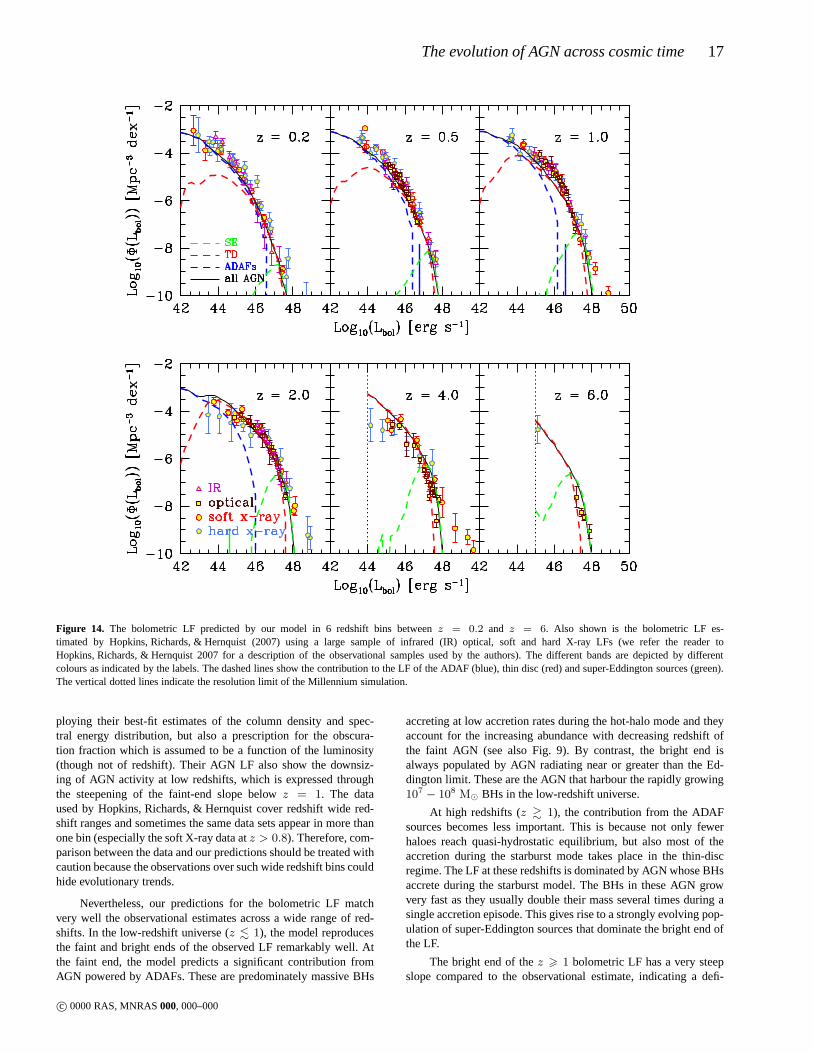
The evolution of AGN across cosmic time 17

Figure 14. The bolometric LF predicted by our model in 6 redshift bins between z = 0.2 and z = 6. Also shown is the bolometric LF es-timated by Hopkins, Richards, & Hernquist (2007) using a large sample of infrared (IR) optical, soft and hard X-ray LFs (we refer the reader toHopkins, Richards, & Hernquist 2007 for a description of theobservational samples used by the authors). The different bands are depicted by differentcolours as indicated by the labels. The dashed lines show thecontribution to the LF of the ADAF (blue), thin disc (red) andsuper-Eddington sources (green).The vertical dotted lines indicate the resolution limit of the Millennium simulation.

ploying their best-fit estimates of the column density and spec-tral energy distribution, but also a prescription for the obscura-tion fraction which is assumed to be a function of the luminosity(though not of redshift). Their AGN LF also show the downsiz-ing of AGN activity at low redshifts, which is expressed throughthe steepening of the faint-end slope belowz = 1. The dataused by Hopkins, Richards, & Hernquist cover redshift wide red-shift ranges and sometimes the same data sets appear in more thanone bin (especially the soft X-ray data atz > 0.8). Therefore, com-parison between the data and our predictions should be treated withcaution because the observations over such wide redshift bins couldhide evolutionary trends.

Nevertheless, our predictions for the bolometric LF matchvery well the observational estimates across a wide range ofred-shifts. In the low-redshift universe (z . 1), the model reproducesthe faint and bright ends of the observed LF remarkably well.Atthe faint end, the model predicts a significant contributionfromAGN powered by ADAFs. These are predominately massive BHs

accreting at low accretion rates during the hot-halo mode and theyaccount for the increasing abundance with decreasing redshift ofthe faint AGN (see also Fig. 9). By contrast, the bright end isalways populated by AGN radiating near or greater than the Ed-dington limit. These are the AGN that harbour the rapidly growing107 − 108 M⊙ BHs in the low-redshift universe.

At high redshifts (z & 1), the contribution from the ADAFsources becomes less important. This is because not only fewerhaloes reach quasi-hydrostatic equilibrium, but also mostof theaccretion during the starburst mode takes place in the thin-discregime. The LF at these redshifts is dominated by AGN whose BHsaccrete during the starburst model. The BHs in these AGN growvery fast as they usually double their mass several times during asingle accretion episode. This gives rise to a strongly evolving pop-ulation of super-Eddington sources that dominate the bright end ofthe LF.

The bright end of thez > 1 bolometric LF has a very steepslope compared to the observational estimate, indicating adefi-

c© 0000 RAS, MNRAS000, 000–000

18 Fanidakis et al.

Figure 15.Our predictions for the bolometric LF atz = 2 considering fourdifferent values of the accretion timescale parameter,fq , as indicated in thelegend. Data are taken from Hopkins, Richards, & Hernquist (2007).

ciency of very bright quasars (Lbol > 1048erg s−1). The inabil-ity of the model to predict the luminosities of the most luminousquasars is due to the fact that the accretion luminosity is constrainedby the Eddington limit. As discussed before, applying the Edding-ton limit to the accreting sources in our model results in a verysteep decline in the space density of the super-Eddington sources,an effect clearly seen earlier in the optical LF. The reader needsto keep in mind though that, as far as the observational estimatesare concerned, many of the brightest luminosity bins do not includeany objects and therefore, they constitute only upper limits.

To achieve higher quasar luminosities we need to increase theaccretion rates in the most massive BHs to values much higherthanthe Eddington rate1. This is necessary because even if we assumethat all our BHs accrete at the Eddington limit the maximum lu-minosity we can produce is∼ 1048erg s−1 (when we consider,for example, a1010 M⊙ BH) which is still lower than the highestluminosities observed. Note though that, AGN feedback preventsBHs more massive than109 M⊙ from accreting at or near supper-Eddington accretion rates in our model.

To increase the accretion rate of a BH we can either increasethe amount of gas that is fed into it or decrease the accretiontimescale. The former solution corresponds to increasing the valueof fBH (the parameter that determines the fraction of gas avail-able for accretion) which has already been tuned to provide agoodmatch to the local BH density and MF. The latter solution givesus the freedom to adjust the accretion rates without changing theBH mass properties. By decreasing the value offq in Eq. 2 wecan obtain higherm values and therefore boost the produced bolo-metric luminosities toLbol > 1048erg s−1. This is illustrated inFig. 15, where we show the bolometric LF atz = 2 assumingfq = 20, 10, 1 and 0.5. However, changing the value offq has

1 For comparison, a BH accreting atm ∼ 100 is only∼ 5 more luminousthat a BH accreting atm = 1.

a strong effect on the faint end of the LF since it decreases thespace density of the low accretion rate objects (the space densityof the. 1043erg s−1 AGN remains unchanged since that part ofthe LF is dominated by AGN in the hot-halo mode in which theaccretion timescale is derived directly from the cooling timescaleof the gas). In addition, it reduces significantly the duty cycle ofactively growing BHs by limiting the typical accretion timescale to∼ 105 − 106 yr if fq 6 1. Hence, having a constant value offqfor all the accreting BHs limits our ability to account for the entireLbol baseline. Perhaps this suggests that a more sophisticated treat-ment of the accretion timescale is therefore needed. However, thisis beyond the scope of the present analysis.

5.5 The evolution of cosmic AGN abundances: cosmicdownsizing?

Our predictions for the optical, X-ray and bolometric LFs, sug-gest that AGN undergo important cosmic evolution. Their spacedensity was significantly higher at earlier epochs, an evolution-ary trend which suggests that AGN activity in the past was muchmore intense. Interestingly, our predictions indicate that the effectsof the different physical processes considered here (the two accre-tion modes and the obscuration prescription) must have an impor-tant, and indeed variable, effect on the evolution of faint and brightAGN. Therefore, to gain more insight into the cosmic evolutionof AGN we study how the abundance of different luminosity pop-ulations of AGN evolves with redshift. This is shown in Fig. 16,where we show the cosmic evolution of optically selected AGNin11 magnitude bins (left panel) and soft X-ray selected AGN in8luminosity bins (right panel). We have depicted separatelythe evo-lution of the total number of AGN (before applying obscuration;dashed lines) and visible population of AGN (after applyingob-scuration; solid lines) in each bin. In this figure we also show thesum over all magnitudes withMbJ 6 −18 and luminosities withlogLSX > 1042erg s−1 (black solid lines for the visible and blackdashed lines for the total populations).

A feature immediately evident in both wavebands is that theevolution of the space density of AGN is shallower for faintersources. For example, in the optical waveband the increase in thespace density of theMbJ = −21 AGN is characterized in the red-shift interval z = 0 − 1 by a power law of the form(1 + z)β

with a very shallow slope ofβ ∼ 0.5. The slope becomes gradu-ally steeper reaching a value of∼ 2.3 for theMbJ = −26 AGN.The steepening of the slope is evident in both the total and visiblepopulations and it is driven primarily by the two distinct accretionchannels in our model as follows. The faintest sources depictedin the plots of Fig. 16 comprise a combination of objects accret-ing during the starburst and hot-halo mode. The hot-halo mode isresponsible for building up the majority of them in the low red-shift universe whereas the starburst mode accounts for themex-clusively in the high redshift universe (cf. Figs. 9 and 10, but alsoFig. 14). The slope of these populations changes very slowlysincethe transition from the hot-halo mode to starburst-mode domina-tion is not characterized by a strong change in the space density ofAGN (the decrease of hot-halo sources is compensated by the in-crease of starburst sources). However, when we consider brighterpopulations, the contribution of the hot-halo mode becomeslessimportant (or vanishes for the brightest populations). As aconse-quence, in the low redshift universe we find a much steeper slopefor the bright AGN since their evolution is driven primarilyby thestarburst mode.

A second noticeable feature is the strong reduction of the vis-

c© 0000 RAS, MNRAS000, 000–000

The evolution of AGN across cosmic time 19

Figure 16. The cosmic evolution of different magnitude and luminosityclasses of AGN selected in the opticalMbJ-band (left panel) and soft X-rays (right

panel) respectively. In addition, we show the cosmic evolution of the sum of all AGN withMbJ6 −18 in the optical andlogLSX > 1042erg s−1 in the

soft X-rays (black lines). In all cases we show with dashed and solid lines the evolution of the space density of AGN before(total) and after (visible) applyingthe effects of obscuration.

ible populations compared to the total AGN populations. Theef-fect is stronger in the faintest populations where we see a decreasein the space density of AGN sometimes greater than an order ofmagnitude. This has a significant effect on the redshift at whichthe space density of AGN peaks. For example, the space densityof the MbJ 6 −18 and logLSX > 1042erg s−1 AGN (dashedblack lines) peaks atz ≃ 3.5, which is the same redshift wherethe SF in bursts peaks (Fig.1). The same behaviour is seen also inthe individual luminosity AGN populations in both the optical andsoft X-rays. However, the visible population shows a different be-haviour. AGN activity, as observed in the soft X-rays for example,seems to peak atz ∼ 2−2.5, much later than that of the total AGNpopulation. More interestingly, when considering each luminositypopulation separately we notice that the brightest sourcespeak atz ∼ 3 whereas the faintest ones atz . 2. Similarly, although lessobviously, in the optical the space density of the faintest quasarspeaks atz ∼ 2 whereas that of the most luminous increases mono-tonically until z ≃ 3. This behaviour is ascribed to the fact thatfainter populations are subject to stronger obscuration. Thereforetheir abundance reaches a maximum at lower redshifts and beyondthat it declines faster. The strong obscuration also contributes to thefurther flattening of the slope making the evolution of theseAGNquite modest.

Trends similar to those seen in the cosmic evolution of AGNin our model have been reported in the literature. For exam-ple, Hopkins, Richards, & Hernquist (2007) find in their analysis

of the bolometric LF that faint AGN evolve much more slowlythan bright AGN (Fig. 9 in their analysis). The modest evolutionis evident also in the optical and soft/hard X-rays. In addition,Hasinger, Miyaji, & Schmidt (2005) report that in their sample ofsoft X-ray AGN, the redshift at which the space density of AGNpeaks changes significantly with luminosity: the peak of AGNwith1042erg s−1 < LSX < 1043erg s−1 is at z ≃ 0.7 but gradu-ally shifts to higher redshifts, reachingz ≃ 2 for 1045erg s−1 <LSX < 1046erg s−1. Similarly, Croom et al. (2009b) found thesame downsizing behaviour in the optical sample of quasars from2SLAQ+SDSS. The faintest quasars in their sample peak atz ∼

0.6 − 0.8 (−21.5 > Mg > −22.5) whereas the brightest sources(Mg 6 −25.5) seem to monotonically increase in density up toz ≃ 2.5. Further evidence that the redshift at which the space den-sity of quasar peaks is a strong function of luminosity form theanalysis of Croom et al. is the inability of pure luminosity evolu-tion models (PLE; models where only the luminosity of objectschanges) to provide an excellent fit to the data. Instead, luminosityand density evolution (LEDE; models where both the luminosityand density of objects change) are needed to provide the bestfit tothe data.

These predictions pose the following key question. Why doesAGN activity shift from high-luminosity objects in the high-z uni-verse to low-luminosity objects in the low-z universe? Is this clearevidence against hierarchical galaxy formation models as has beeninterpreted by many authors? In our model, the downsizing ofAGN

c© 0000 RAS, MNRAS000, 000–000

20 Fanidakis et al.

is expressed through the shallow slope that characterizes the evolu-tion of faint AGN and the dependence on luminosity of the redshiftat which the AGN density in a given luminosity range peaks. Theformer arises naturally from the interplay of the starburstand hot-halo mode, just as in the galaxy population (Bower et al. 2006).Therefore, the SF and cooling processes in a hierarchical cosmol-ogy can account consistently for the different evolution with red-shift of the individual luminosity populations. The latteris drivenlargely by obscuration biases rather than the nature of their hostgalaxies. The analysis presented earlier in this section shows clearlythat the cosmic evolution of the AGN space density is subjecttostrong obscuration which depends significantly on both luminos-ity and redshift. Therefore, AGN populations that are subject toobscuration could lead to misleading conclusions. For example, inboth the Croom et al. (2009b) QSO (these are only type-1 AGNCroom et al. (2009a)) and Hasinger, Miyaji, & Schmidt (2005)softX-ray AGN samples no correction for obscuration is adopted.Given that at low redshifts only unabsorbed AGN are detectedinsoft X-rays (La Franca et al. 2005), these samples can only tracethe evolution of a small fraction (and also a specific class) of thetotal AGN population.

Hence, to probe the intrinsic evolution of AGN one needs tocorrect for observational biases caused by obscuration (note alsothat incompleteness effects at low luminosities and high redshiftscould also influence observational results about the evolution ofAGN). Ueda et al. (2003) investigated the cosmological evolutionof hard X-ray AGN using a combination of surveys such as theHEAO 1, ASCA and Chandra. The sample of AGN constructed byUeda et al., which was compared to our predictions for the hardX-ray LF in Section 5.3, was corrected using an absorption dis-tribution function that depends on both the luminosity and red-shift. In a similar analysis, La Franca et al. (2005) used a sampleof AGN from the HELLAS2XMM survey to study the evolutionof the hard X-ray LF taking into account selection effects due toX-ray absorption. In both these studies, a careful examination ofthe “cosmic evolution” plots (Fig. 12 in Ueda et al. and Fig. 8inLa Franca et al.) reveals no evidence for downsizing in hard X-rays.

When accounting for these effects, our model suggests that thecosmic interplay between the starburst and hot-halo mode results incomplex evolution scheme for the AGN. In this scheme, low lumi-nosity AGN avoid the cosmic fate (namely becoming dramaticallyless numerous with time) of their bright counterparts, since accre-tion during the hot-halo mode provides gas for enabling modestAGN activity in the low-z universe. Note that, as already impliedby our analysis, modest activity implies low accretion rates ratherthan low BH masses. The AGN in the hot-halo mode show a widerange of BH masses, and therefore, in our model the AGN down-sizingdoes not imply that the growth of low-mass BHs is delayedto low redshifts. Averaged-sized BHs accreting at low ratesas aninterpretation of the reported AGN downsizing is also supportedby observations of X-ray selected AGN in the Chandra Deep FieldSouth atz < 1 (Babic et al. 2007).

6 CONCLUSIONS

In this paper we have made predictions for the evolution of AGNusing an extended version of the semi-analytic codeGALFORM.GALFORM simulates the formation and evolution of galaxies in aΛCDM cosmology. In Fanidakis et al. (2010), we introduced a cal-

culation of BH spin. The fiducial model in this paper uses an im-proved SF law, as implemented by Lagos et al. (2010).

Using this model we calculate the cosmic evolution of the fun-damental parameters that describe BHs in our model. These are theBH mass,MBH, BH spin,a, and accretion rate onto the BH,m(expressed in units of the the Eddington accretion rate through outthis paper). We find that at high redshifts (z ∼ 6) it is mainly the106−107 M⊙ BHs accreting atm ≃ 0.3 that are actively growing.This picture changes at lower redshifts where we find that theaccre-tion activity peaks for107 − 108 M⊙ BHs, accreting atm ≃ 0.05.Throughout the evolution of these BHs their spin is kept low be-cause of the chaotic fashion with which gas is consumed. However,when these BHs grow to masses of& 5 × 108 M⊙ they acquirehigh spins as a consequence of mergers with other BHs.

Knowledge of the values ofMBH, a andm allows us to cal-culate the luminosity produced during the accretion of gas.To doso, we assume that accretion takes place in two distinct regimes:the thin-disc (radiatively efficient) and ADAF (radiatively ineffi-cient) regime. Objects accreting in the thin-disc regime are lumi-nous enough to account for the observed luminosities of AGN.Us-ing the luminosities predicted for each AGN (formed when thecen-tral BH experiences an accretion episode) and a prescription fortaking into account the effects of obscuration (Hasinger 2008) wecalculate the LF of all accreting objects in the optical, soft and hardX-rays. We find an a very good agreement with the observations,particularly in the optical, by adjusting the value of thefq parame-ter, namely the proportionality factor that determines theaccretiontimescale in our model.

The presence of two distinct accretion channels naturallycauses a downsizing in the predicted AGN populations. Thesechannels shape the evolution of the faint AGN with cosmic time,indicating that the faint end of the LF is dominated by massive BHsexperiencing quiescent accretion. By contrast, the brightend is al-ways populated by AGN radiating near or greater than the Edding-ton limit. In addition, our model suggests that a significantfractionof AGN are obscured in optical and soft X-rays. In fact, we findthat∼ 90% of the total number of AGN in thez = 0.015 − 4.8 uni-verse are not visible in soft X rays. The implications of the obscura-tion are further revealed when we study the cosmological evolutionof AGN of different luminosity populations. As demonstrated byFig. 16, low luminosity AGN populations are strongly attenuatedby obscuration. As a result, their peak of AGN activity appearsshifted to lower redshifts.

This analysis explicitly demonstrates that hierarchical cosmo-logical models for galaxy formation and evolution are able to pro-vide a robust framework in which the evolution of AGN can bestudied. The ability of our galaxy formation model to reproducethe observed LFs and account for the mechanisms that shape theevolution of the faint and bright AGN populations strengthens thepowerful capabilities of semi-analytic modelling and shows that thelevel of AGN activity implied by AGN feedback is compatible withobservations. In future studies, we aim to further study thestatis-tical properties of AGN by exploring their spatial clustering andenvironmental dependence.

ACKNOWLEDGEMENTS

NF acknowledges receipt of a fellowship funded by the Euro-pean Commission’s Framework Programme 6, through the MarieCurie Early Stage Training project MEST-CT-2005-021074. AJBacknowledges the support of the Gordon & Betty Moore Founda-

c© 0000 RAS, MNRAS000, 000–000

The evolution of AGN across cosmic time 21

tion. SC acknowledges the support of a Leverhulme research fel-lowship. CSF acknowledges a Royal Society Wolfson ResearchMerit Award. This work was supported in part by an STFC RollingGrant to the Institute for Computational Cosmology.

REFERENCES

Abramowicz M. A., Chen X., Kato S., Lasota J.-P., Regev O.,1995, ApJ, 438, L37

Aird J., et al., 2010, MNRAS, 401, 2531Alexander D. M., et al., 2003, AJ, 126, 539Alexander D. M., Chartas G., Bauer F. E., Brandt W. N., SimpsonC., Vignali C., 2005, MNRAS, 357, L16

Alexander D. M., et al., 2008, ApJ, 687, 835Antonucci R., 1993, ARA&A, 31, 473Babic A., Miller L., Jarvis M. J., Turner T. J., Alexander D.M.,Croom S. M., 2007, A&A, 474, 755

Baker J. G., McWilliams S. T., van Meter J. R., Centrella J., ChoiD.-I., Kelly B. J., Koppitz M., 2007, PhRvD, 75, 124024

Ballantyne D. R., Everett J. E., Murray N., 2006, ApJ, 639, 740Ballantyne D. R., Shi Y., Rieke G. H., Donley J. L., Papovich C.,Rigby J. R., 2006, ApJ, 653, 1070

Barcons X., et al., 2007, A&A, 476, 1191Barger A. J., Cowie L. L., Mushotzky R. F., Yang Y., Wang W.-H.,Steffen A. T., Capak P., 2005, AJ, 129, 578

Baugh C. M., Lacey C. G., Frenk C. S., Granato G. L., Silva L.,Bressan A., Benson A. J., Cole S., 2005, MNRAS, 356, 1191

Baugh C. M., 2006, RPPh, 69, 3101Berti E., Volonteri M., 2008, ApJ, 684, 822Blandford R. D., Znajek R. L., 1977, MNRAS, 179, 433Blandford R. D., Payne D. G., 1982, MNRAS, 199, 883Blitz L., Rosolowsky E., 2006, ApJ, 650, 933Bongiorno A., et al., 2007, A&A, 472, 443Bonoli S., Marulli F., Springel V., White S. D. M., BranchiniE.,Moscardini L., 2009, MNRAS, 396, 423

Bower R. G., McCarthy I. G., Benson A. J., 2008, MNRAS, 390,1399

Boyle B. J., Shanks T., Peterson B. A., 1988, MNRAS, 235, 935Boyle B. J., Shanks T., Croom S. M., Smith R. J., Miller L., Loar-ing N., Heymans C., 2000, MNRAS, 317, 1014

Bower R. G., Benson A. J., Malbon R., Helly J. C., Frenk C. S.,Baugh C. M., Cole S., Lacey C. G., 2006, MNRAS, 370, 645

Bower R. G., Vernon I., Goldstein M., Benson A. J., Lacey C. G.,Baugh C. M., Cole S., Frenk C. S., 2010, MNRAS, 407, 2017

Brandt W. N., Hasinger G., 2005, ARA&A, 43, 827Cole S., Aragon-Salamanca A., Frenk C. S., Navarro J. F., ZepfS. E., 1994, MNRAS, 271, 781

Cole S., Lacey C. G., Baugh C. M., Frenk C. S., 2000, MNRAS,319, 168

Comastri A., Setti G., Zamorani G., Hasinger G., 1995, A&A,296, 1

Comastri A., 2004, ASSL, 308, 245Cowie L. L., Barger A. J., Bautz M. W., Brandt W. N., GarmireG. P., 2003, ApJ, 584, L57

Croom S. M., Smith R. J., Boyle B. J., Shanks T., Loaring N. S.,Miller L., Lewis I. J., 2001, MNRAS, 322, L29

Croom S. M., Smith R. J., Boyle B. J., Shanks T., Miller L., Out-ram P. J., Loaring N. S., 2004, MNRAS, 349, 1397

Croom S. M., et al., 2005, MNRAS, 356, 415Croom S. M., et al., 2009, MNRAS, 392, 19Croom S. M., et al., 2009, MNRAS, 399, 1755

Croton D. J., et al., 2006, MNRAS, 365, 11daAngela J., et al., 2008, MNRAS, 383, 565Dalla Vecchia C., Bower R. G., Theuns T., Balogh M. L., Maz-zotta P., Frenk C. S., 2004, MNRAS, 355, 995

Di Matteo T., Springel V., Hernquist L., 2005, Natur, 433, 604De Lucia G., Blaizot J., 2007, MNRAS, 375, 2Done C., Gierlinski M., Kubota A., 2007, A&ARv, 15, 1Efstathiou G., Lake G., Negroponte J. 1982, MNRAS, 199, 1069Fabian A. C., Vasudevan R. V., Gandhi P., 2008, MNRAS, 385,L43

Fan X., et al., 2001, AJ, 121, 54Fan X., et al., 2001, AJ, 122, 2833Fan X., et al., 2003, AJ, 125, 1649Fanidakis N., Baugh C. M., Benson A. J., Bower R. G., Cole S.,Done C., Frenk C. S., 2010, MNRAS, 1547

Ferrarese L., Merritt D., 2000, ApJ, 539, L9Fiore F., et al., 2003, A&A, 409, 79Font A. S., et al., 2008, MNRAS, 389, 1619Fontanot F., Cristiani S., Monaco P., Nonino M., Vanzella E.,Brandt W. N., Grazian A., Mao J., 2007, A&A, 461, 39

Fukugita M., Peebles P. J. E., 2004, ApJ, 616, 643Gebhardt K., et al., 2000, ApJ, 539, L13George I. M., Turner T. J., Netzer H., Nandra K., Mushotzky R.F.,Yaqoob T., 1998, ApJS, 114, 73

Ghisellini G., et al., 2010, MNRAS, 405, 387Giacconi R., et al., 2002, ApJS, 139, 369Gilli R., Risaliti G., Salvati M., 1999, A&A, 347, 424Gilli R., Comastri A., Hasinger G., 2007, A&A, 463, 79Graham A. W., Driver S. P., 2007, MNRAS, 380, L15Graham A. W., Driver S. P., Allen P. D., Liske J., 2007, MNRAS,378, 198

Goulding A. D., Alexander D. M., 2009, MNRAS, 398, 1165Goulding A., Alexander D., Mullaney J., Gelbord J., Hickox R.,Ward M., Watson M., 2010, arXiv, arXiv:1009.4929

Haring N., Rix H.-W., 2004, ApJ, 604, L89Hasinger G., et al., 2001, A&A, 365, L45Hasinger G., 2004, NuPhS, 132, 86Hasinger G., 2008, A&A, 490, 905Hasinger G., Miyaji T., Schmidt M., 2005, A&A, 441, 417Hawley J. F., Gammie C. F., Balbus S. A., 1995, ApJ, 440, 742Heckman T. M., Kauffmann G., Brinchmann J., Charlot S.,Tremonti C., White S. D. M., 2004, ApJ, 613, 109

Hewett P. C., Foltz C. B., Chaffee F. H., 1993, ApJ, 406, L43Hopkins P. F., Hernquist L., Martini P., Cox T. J., RobertsonB.,Di Matteo T., Springel V., 2005, ApJ, 625, L71

Hopkins P. F., Hernquist L., Cox T. J., Di Matteo T., RobertsonB., Springel V., 2005, ApJ, 630, 716

Hopkins P. F., Hernquist L., Cox T. J., Di Matteo T., RobertsonB., Springel V., 2005, ApJ, 632, 81

Hopkins P. F., Hernquist L., Cox T. J., Robertson B., Springel V.,2006, ApJS, 163, 50

Hopkins P. F., Richards G. T., Hernquist L., 2007, ApJ, 654, 731Ichimaru S., 1977, ApJ, 214, 840Kelly B. C., Vestergaard M., Fan X., Hopkins P., Hernquist L.,Siemiginowska A., 2010, ApJ, 719, 1315

Kennicutt R. C., Jr., 1998, ApJ, 498, 541King A. R., Lubow S. H., Ogilvie G. I., Pringle J. E., 2005, MN-RAS, 363, 49

King A. R., Pringle J. E., Hofmann J. A., 2008, MNRAS, 385,1621

Lagos C. D. P., Cora S. A., Padilla N. D., 2008, MNRAS, 388,587

c© 0000 RAS, MNRAS000, 000–000

22 Fanidakis et al.

Lagos C., Baugh C. M., Benson A. J., Bower R. G., Lacey C. S.,in prep.

Magorrian J., et al., 1998, AJ, 115, 2285Malbon R. K., Baugh C. M., Frenk C. S., Lacey C. G., 2007, MN-RAS, 382, 1394

Marconi A., Hunt L. K., 2003, ApJ, 589, L21McLure R. J., Dunlop J. S., 2002, MNRAS, 331, 795Lada E. A., 1992, ApJ, 393, L25La Franca F., et al., 2002, ApJ, 570, 100La Franca F., et al., 2005, ApJ, 635, 864Leroy A. K., Walter F., Brinks E., Bigiel F., de Blok W. J. G.,Madore B., Thornley M. D., 2008, AJ, 136, 2782

Lewis I. J., et al., 2002, MNRAS, 333, 279Libeskind N. I., Cole S., Frenk C. S., Helly J. C., 2006, MNRAS,368, 1381

Lynden-Bell D., 1969, Natur, 223, 690Mahadevan R., 1997, ApJ, 477, 585Marchesini D., Celotti A., Ferrarese L., 2004, MNRAS, 351, 733Marconi A., Hunt L. K., 2003, ApJ, 589, L21Marconi A., Risaliti G., Gilli R., Hunt L. K., Maiolino R., SalvatiM., 2004, MNRAS, 351, 169

Martınez-Sansigre A., Rawlings S., Lacy M., Fadda D., MarleauF. R., Simpson C., Willott C. J., Jarvis M. J., 2005, Natur, 436,666

Marulli F., Bonoli S., Branchini E., Moscardini L., Springel V.,2008, MNRAS, 385, 1846

McCarthy I. G., et al., 2010, MNRAS, 406, 822McKee C. F., Ostriker E. C., 2007, ARA&A, 45, 565Menou K., Haiman Z., 2004, ApJ, 615, 130Merloni A., Heinz S., 2008, MNRAS, 388, 1011Merritt D., Milosavljevic M., FavataMiyaji T., Hasinger G., Schmidt M., 2000, A&A, 353, 25 M.,Hughes S. A., Holz D. E., 2004, ApJ, 607, L9

Narayan R., Yi I., 1994, ApJ, 428, L13Parkinson H., Cole S., Helly J., 2008, MNRAS, 383, 557Parry O. H., Eke V. R., Frenk C. S., 2009, MNRAS, 396, 197Piconcelli E., Guainazzi M., Cappi M., Jimenez-Bailon E., Schar-tel N., 2005, A&A, 432, 835

Rees M. J., 1982, AIPC, 83, 166Reynolds C. S., 1997, MNRAS, 286, 513Richards G. T., et al., 2005, MNRAS, 360, 839Richards G. T., et al., 2006, AJ, 131, 2766Risaliti G., Maiolino R., Salvati M., 1999, ApJ, 522, 157Ross N. P., et al., 2009, ApJ, 697, 1634Schmidt M., Green R. F., 1983, ApJ, 269, 352Schmidt M., Schneider D. P., Gunn J. E., 1995, AJ, 110, 68Shakura N. I., Sunyaev R. A., 1973, A&A, 24, 337Shankar F., Salucci P., Granato G. L., De Zotti G., Danese L.,2004, MNRAS, 354, 1020

Shen Y., et al., 2009, ApJ, 697, 1656Simpson C., 2005, MNRAS, 360, 565Somerville R. S., Hopkins P. F., Cox T. J., Robertson B. E., Hern-quist L., 2008, MNRAS, 391, 481

Springel V., et al., 2005, Natur, 435, 629Springel V., Di Matteo T., Hernquist L., 2005, MNRAS, 361, 776Steffen A. T., Barger A. J., Cowie L. L., Mushotzky R. F., YangY., 2003, ApJ, 596, L23

Thacker R. J., Scannapieco E., Couchman H. M. P., 2006, ApJ,653, 86

Treister E., Urry C. M., 2006, ApJ, 652, L79Tremaine S., et al., 2002, ApJ, 574, 740Ueda Y., Akiyama M., Ohta K., Miyaji T., 2003, ApJ, 598, 886

Urry C. M., Padovani P., 1995, PASP, 107, 803Vasudevan R. V., Fabian A. C., 2007, MNRAS, 381, 1235Vestergaard M., 2002, ApJ, 571, 733Vestergaard M., Peterson B. M., 2006, ApJ, 641, 689Vestergaard M., Osmer P. S., 2009, ApJ, 699, 800Volonteri M., Sikora M., Lasota J.-P., 2007, ApJ, 667, 704Warren S. J., Hewett P. C., Osmer P. S., 1994, ApJ, 421, 412White S. D. M., Frenk C. S., 1991, ApJ, 379, 52Willott C. J., et al., 2010, AJ, 140, 546Wolf C., Wisotzki L., Borch A., Dye S., Kleinheinrich M.,Meisenheimer K., 2003, A&A, 408, 499

York D. G., et al., 2000, AJ, 120, 1579Yu Q., Tremaine S., 2002, MNRAS, 335, 965Yu Q., Lu Y., 2008, ApJ, 689, 732

c© 0000 RAS, MNRAS000, 000–000