The effects of integrating management judgement into intermittent demand forecasts

(International Journal of Production Economics)

Aris A. Syntetos∗, Salford Business School, University of Salford Konstantinos Nikolopoulos, Manchester Business School, University of Manchester John E. Boylan, School of Business and Management, Buckinghamshire Chilterns University College Robert Fildes, Lancaster University Management School Paul Goodwin, School of Management, University of Bath

Abstract Empirical research suggests that quantitatively derived forecasts are very frequently judgementally

adjusted. Nevertheless, little work has been conducted to evaluate the performance of these

judgemental adjustments in a practical demand/sales context. In addition, the relevant analysis

does not distinguish between slow and fast moving items. Currently, there are neither conceptual

developments nor empirical evidence on the issue of integrating judgements and statistical

forecasts for slow/intermittent demand items. Moreover, no results have ever been reported on the

stock control implications of these human judgements. Our work analyses monthly intermittent

demand forecasts for the UK branch of a major international pharmaceutical company. The

company relies upon a commercially available statistical forecasting system to produce forecasts

that are subsequently judgementally adjusted based on marketing intelligence gathered by the

company forecasters. The benefits of the intervention are evaluated by comparing the actual sales

to system and final forecasts using both forecast accuracy and inventory control (accuracy

implication) metrics. Our study allows insights to be gained on potential improvements to

intermittent demand forecasting processes and, subsequently, the design effectiveness of

Forecasting Support Systems.

Keywords: Forecasting Support Systems, Intermittent Demand, Judgemental Forecasts, Stock Control

∗ Corresponding author : Centre for OR and Applied Statistics, Salford Business School

University of Salford, Maxwell Building, Greater Manchester M5 4WT, UK Tel. No. +(44) (0) 161 295 5804, Fax no. +(44) (0) 161 295 5556 e-mail: a.syntetos@salford.ac.uk

1

1. Research background Forecasting at the Stock Keeping Unit (SKU) level in order to support operations management and

inventory decision making is a difficult task. The levels of accuracy achieved have major

consequences for companies at all levels of the supply chain. Empirical research suggests that

practitioners rely heavily on judgemental forecasting methods such as the direct use of managers’

expectations (e.g. Klassen and Flores, 2001; McCarthy et al., 2006). Further, when quantitative

forecasting methods are used, they are very frequently judgementally adjusted. According to

Sanders and Manrodt’s (1994) survey of forecasters at 96 US corporations, about 45% of the

respondents claimed that they always made judgemental adjustments to statistical forecasts, while

only 9% said that they never did.

Goodwin (2002) discusses a number of reasons for the prevalence of judgemental adjustment,

including a desire to reflect the effects of special events on the forecast and a need for a sense of

ownership of the forecasts. In the light of the widespread use of judgmental adjustments, Sanders

and Manrodt (op. cit: 100) and Armstrong and Collopy (1998: 289) have suggested that further

research should be carried out to investigate the effectiveness of these adjustments and how they

might be improved. Although this appeal for further work has been heeded, researchers have yet

to investigate the problem of integrating judgment and statistical methods when items have

intermittent demand. In addition, no results have ever been reported on the stock control

implications of judgementally adjusting statistical forecasts.

Intermittent demand appears at random with some time periods showing no demand at all.

Demand, when it occurs, may be for a single unit, a constant or a (highly) variable demand size.

Intermittent demand items may be spare parts (engineering spares, service parts kept at the

wholesaling/retailing level etc) or any SKU within the range of products offered by all companies

at any level of a given supply chain. The management of intermittent demand items has not

received as much academic attention as the implications of decision making in that area would

require. Despite the inherent infrequent demand occurrence associated with such items and the

consequent, comparatively low contribution to the total turnover of an organization, these slower

moving SKUs can constitute up to 60% of the total stock value (see, for example, Johnston et al.,

2003). Thus, small improvements regarding their management may be translated to substantial cost

savings.

2

Our work is based on data relating to the monthly intermittent demand forecasts for the UK branch

of a major international pharmaceutical company. The company relies upon commercially

available software to produce system forecasts (SFC) per SKU for each time period (i.e. month).

Final forecasts (FFC) are produced at a later stage through the superimposition of judgements

based on marketing intelligence gathered by the company forecasters. The aim of this paper is to

establish the benefits of the intervention, if any, by comparing the actual demand to the system and

final forecasts using both forecast accuracy and inventory control (accuracy implication) metrics.

Our study offers insights on potential improvements to the intermittent demand forecasting process

and, subsequently, the design effectiveness of Forecasting Support Systems.

2. Literature review In many organisations the size and complexity of the demand forecasting task at the individual

SKU level typically necessitates the use of statistical methods, such as exponential smoothing.

However, in many cases these statistical forecasts will be subject to judgmental adjustment by

managers (Sanders and Manrodt, 1994; Fildes and Goodwin, 2007). Research carried out into the

effectiveness of these adjustments suggests that they can improve accuracy when forecasters have

important information about the product they are forecasting that is not available to the statistical

method (e.g. knowledge of a forthcoming promotion campaign) (Mathews and Diamantopoulos,

1990; Turner, 1990; Mathews and Diamantopoulos, 1992; Lim and O’Connor, 1995; Goodwin and

Fildes, 1999; Sanders and Ritzman, 2001). The strongest evidence that judgemental interventions

can be effective when applied to SKU data comes from Mathews and Diamantopoulos (1986),

Diamantopoulos and Mathews (1989), Mathews and Diamantopoulos (1990) and Mathews and

Diamantopoulos (1992). These studies also found that larger adjustments were more effective in

improving accuracy. Similar results have been found in a recent study of demand forecasting in

four companies (Fildes et al., 2006a). Adjustments made in the absence of important information

may result from the forecaster reading false patterns in the noise associated with the time series

and these adjustments are likely to damage accuracy (O’Connor et al., 1993). None of the studies

carried out so far have considered the effectiveness of judgmental adjustments when products have

intermittent demand.

3

2.1 Forecasting intermittent demand

Some academic papers have been devoted to stock control issues for intermittent demand items.

Forecasting their requirements has been addressed to a far lesser extent (De Gooijer and Hyndman,

2006) and little research has been conducted in this area since Croston’s work (1972). Some

researchers have conducted empirical investigations on the performance of various statistical

intermittent demand forecasting approaches (Willemain et al., 2004; Syntetos and Boylan, 2005).

Finally, the accuracy measures that are generally used to compare methods do not address the

implications of that accuracy on inventory management (stock-holding costs and service levels

achieved). Boylan and Syntetos (2006: 42) recently noted that “no matter what inventory system is

in use, the accuracy-implication metrics of stock-holding costs and service-level should always be

used, since this is of prime importance to the organisation. These measures should be used not

only when it is difficult to assess forecast error directly. By keeping an inventory method fixed,

accuracy-implication metrics offer a direct comparison of the effects of using different forecasting

methods.” In this study both accuracy and accuracy implications metrics are used in order to

evaluate the performance of judgementally adjusted forecasts of intermittent demand.

3. Empirical data The database available for this research consists of the individual demand1 histories of 829 end-

product SKUs. Demand is intermittent, meaning that it occurs at random with some time periods

showing no demand at all2. Demand is recorded monthly and the history available covers 36

consecutive periods from January 2003 to December 2005 (three years in total). System forecasts

are available for all time periods. In addition, the judgemental adjustments (both positive and

negative) are also available. The system forecast (SFC) plus the judgemental adjustment (when

there is one) gives the final forecast (FFC, i.e. the one used for decision making purposes).

Not all series were considered for experimentation purposes. The following series were eliminated:

Series with missing demand data (i.e. blank cells in the spreadsheet – when that was the

case there was a series of blank cells) or invalid recording of data (e.g. decimals, text etc)

Series that consist only of zeros (most probably re-coded SKUs)

1 This is essentially sales rather than demand data, the former often being used, as in this research, as an approximation for the latter. The data represent sales of packs to wholesalers who will often buy in certain multiples. 2 Intermittence may be partly explained in terms of: i) the launch of a new product, e.g. a whole batch goes out at once and then subsequent demand for several periods is zero while this stock is used up by the purchaser, ii) SKU supplied according to a minimum order quantity; with the same subsequent effect as in i, and iii) marked seasonal effects, e.g. some goods, such as animal health products, only sell in particular seasons.

4

Series that consist of a streak of zeros followed by a streak of non-zero demands or the

other way around (new SKUs or re-coded ones respectively)

Series with only one zero observation; in that case no average inter-demand interval figures

can be obtained.

After the initial screening, individual attention was given to each of the remaining series in order

to identify potential ‘anomalies’. More details on this process can be found in Appendix A. This

screening process resulted in only 138 SKUs being considered in the analysis. This is disappointing

in terms of the final sample size (almost 74% of the files available in the beginning had to be

excluded) but important in terms of throwing light on an issue, the importance of which has been

rather understated in the past; that of the very selection of an empirical sample for experimentation

purposes. The demand data sample characteristics are summarised in the following table. The

descriptive statistics are rounded to two decimal places.

138

SKUs Demand Demand Size Inter-Demand Interval

Mean St. Dev. CV Mean St Dev. CV Mean St Dev. CV

Min. 0.19 0.62 0.50 1.75 0.55 0.17 1.06 0.00 0.00

25%ile 13.75 15.83 0.94 21.30 15.49 0.51 1.16 0.38 0.32

Median 60.60 92.66 1.23 110.49 88.06 0.67 1.40 0.65 0.48

75%ile 281.51 297.34 1.84 421.34 269.09 0.90 2.00 1.29 0.70

Max. 13275.94 10631.70 5.14 15931.13 10575.89 2.08 8.33 7.96 1.46

The squared coefficient of variation of demand sizes ranges from 0.03 to 4.31 (25%ile = 0.26, median = 0.45, 75%ile = 0.81).

Table 1. Demand data series characteristics

4. Research questions and details of empirical investigation

4.1 Research questions

The review of the literature on managerial adjustments of statistical forecasts suggests that

adjusted forecasts should, in general, be more accurate that system forecasts, assuming that the

adjustments are based on important information not available to the statistical method. This will

form the basis for our main research question:

Q1. Do judgemental adjustments of statistical forecasts improve accuracy when demand is

intermittent?

5

There is also some evidence that there is no learning effect in the forecasting function. Studies

have shown that forecasters in companies are not trained sufficiently over time (Klassen and

Flores, 2001). An investigation was recently conducted on the company that provided the data set

used for our research from an organizational learning as well as an individual learning perspective.

This study shows serious gaps in the learning loop within the company (Nikolopoulos et al., 2006);

neither the system forecasts nor the final ones were improving over time. This study was limited to

regular data series, i.e. non-intermittent. However this would be the closest example upon which

we may base our second research question:

Q2. Does the accuracy of judgemental adjustments improve over time when demand is

intermittent (i.e. is there any learning effect)?

Previous research on intermittent demand forecasting (Johnston and Boylan, 1996; Syntetos et al.,

2005) has indicated that forecast accuracy is closely related to specific demand characteristics.

These research projects were concerned with statistical methods for estimating demand

requirements. However, it may be beneficial to explore whether or not the performance of the

adjustments can be related to certain series characteristics:

Q3. Is there a relation between the intermittent data series characteristics and the forecast

accuracy of the adjustments?

The literature review discussed evidence that small adjustments (usually less than 10% relative to

the baseline forecast) are not worth making as these are merely response to noise; in fact these

adjustments seem not to account for any accuracy gain, at least for the case of Fast Moving

Consumer Goods (Nikolopoulos et al., 2005). Thus a reasonable assumption would be that the size

of the adjustments plays an important role in the accuracy of the revised forecasts. Similarly, we

decided to experiment with the effect of the sign of the adjustments (positive or negative) on

forecast accuracy.

Q4. Do small adjustments improve forecast accuracy when demand is intermittent?

Q5. Is there any difference in the effect on accuracy between positive and negative

adjustments when demand is intermittent?

Finally, we evaluate, for the first time, the stock control implications of judgementally adjusting

statistical forecasts. The forecast accuracy implications of judgementally adjusting statistical

forecasts may or may not be reflected in the stock control performance of such an integrated

procedure. Our last research question is:

6

Q6. Is there any improvement in the stock control performance by judgementally adjusting

statistical forecasts when demand is intermittent?

4.2 Experimental structure

We have generated Mean Absolute Errors (MAE) across time for each SKU, for both SFC and

FFC, i.e. ∑=

=n

ijien 1

,j1MAE for the jth SKU (where n = 36). We have synthesised the results across

series (SKUs) with a relative (numerator: FFC; denominator: SFC) arithmetic (RAMAE) and

relative geometric (RGMAE) summarisation. The latter error measure avoids scale dependencies

and it has been found to be a robust measure for intermittent demand series (Syntetos and Boylan,

2005)3. In order to evaluate the effect of the size and sign of the adjustments, we opted for a

different approach: each adjustment (for every forecast) is considered as an individual case and

results are summarised across time and SKUs.

In order to test whether or not there is improvement in the accuracy of judgemental adjustments

over time we worked as follows: each series was divided in two parts (18 consecutive periods

each) or three parts (12 consecutive periods each). RAMAE and RGMAE are then generated for

each sub-sample.

In order to evaluate the stock control implications of judgementally adjusting statistical forecasts, a

stock control model needs to be developed. Periodic review models are most commonly used for

intermittent demand SKUs (Sani and Kingsman, 1997). Our intermittent series consist of monthly

data, which cover the demand history of three years. The data is collected on a monthly basis so

that one month can be viewed as the inventory review period ( 1=T ). At the end of every period

both system and final forecasts are available and the stock status may be reviewed and

consequently compared against a control parameter, to decide how much to order. Stock control

follows a periodic order-up-to-level ( ) model (allowing for backorders to reflect the

company’s policy). Relatively simple techniques are recommended in the literature and applied by

practitioners to deal with intermittent demand items. The chosen model is simple, close to optimal

(Sani, 1995) and reflects, to a certain extent, real world practices.

ST ,

3 Syntetos and Boylan (2005) used the Relative Geometric Root Mean Square Error (RGRMSE) measure which, as Hyndman (2006) noted, is identical to the RGMAE.

7

The service measure used is the criterion (the probability of stock-out at the end of an arbitrary

period is (at most) ). In periodic stock control applications, forward estimations refer to the

lead time length (

P1

P−1 1

L ) plus review period (as opposed to continuous review systems where estimates

over the lead time only are required). The demand forecasts over lead time plus review period (L +

T) are obviously available. Regarding the variability of demand, the smoothed cumulative Mean

Squared Error (MSE) approach is adopted (Syntetos and Boylan, 2006a). Demand over lead time

plus review period is assumed to be normally distributed, following the approach of authors such

as Croston (1972) and Willemain et al. (2004).

The smoothing constant α used for MSE updating purposes has been assigned three values: 0.05,

0.1 and 0.15. The lead times associated with the SKUs available for this research are between 3 and

12 weeks. Consequently, for the purposes of the simulation experiment, the lead time (as a control

parameter) will be assigned three values: 1, 2 and 3 periods (months). Finally, the control

parameter has been assigned two values: 0.95 and 0.99, to reflect the high target service levels

used by the company concerned.

P1

The unit cost information is not available for any of the SKUs included in our empirical data

sample. Therefore, no inventory cost results could be generated in the simulation exercise. Volume

differences can be considered instead, regarding the number of units kept in stock for both the

system and final forecasts. Customer Service Level (CSL) results were also generated (100 – the

percentage of stock-out occasions for each of the real demand series) and they can be related

directly to performance differences as far as the number of units backordered is concerned.

5. Empirical results The RGMAE (across all SKUs) is 0.923, suggesting an improvement achieved by judgementally

adjusting the system forecasts. This is confirmed by the RAMAE results (0.804). In terms of

percentage improvement, the adjusted forecasts perform better than the system forecasts (across

time for a particular SKU) in approximately 61% of the series considered (84 series). There are 50

cases where the systems forecasts are more accurate than the final forecasts whereas there is no

difference in only 4 cases.

8

5.1 Performance over time

In order to assess whether or not there is any improvement in the accuracy of the judgemental

forecasts over time each of the demand series was divided in two and subsequently three sub-

samples (18 and 12 consecutive periods each, respectively). Relative error results were then

generated for each sub-sample across all SKUs. In the former case, 14 files had to be excluded

because the MAE equals zero in either the first or the second sub-sample (consequently no

geometric summary results can be obtained). As such, RGMAE results were generated only on 124

SKUs. Similarly, 28 files had to be excluded for the latter investigation, leaving us with 110 SKUs.

The results are summarised in the following tables.

Performance overtime: Series are divided in 2 sub-samples (18 consecutive periods each)

Periods 1 – 18 Periods 19 – 36

RAMAE

(all 138 files)

RAMAE

(124 files)

RGMAE

(124 files)

RAMAE

(all 138 files)

RAMAE

(124 files)

RGMAE

(124 files)

0.636 0.645 0.834 0.938 0.937 0.900

Evaluation on 124 files. Adjusted forecasts perform:

Evaluation on 124 files. Adjusted forecasts perform:

Better: 77 files Worse: 44 The same: 3 Better: 74 files Worse: 48 The same: 2

Evaluation on 138 files. Adjusted forecasts perform:

Evaluation on 138 files. Adjusted forecasts perform:

Better: 82 files Worse: 49 The same: 7 Better: 76 files Worse: 51 The same: 11

Table 2. Evaluation of performance over time (18 period blocks)

Performance overtime: Series are divided in 3 sub-samples (12 consecutive periods each)

Periods 1 – 12 Periods 13 – 24 Periods 25 – 36 RAMAE

138 files

RAMAE

110 files

RGMAE

110 files

RAMAE

138 files

RAMAE

110 files

RGMAE

110 files

RAMAE

110 files

RAMAE

110 files

RGMAE

110 files

0.606 0.580 0.827 0.804 0.816 0.852 0.974 0.978 0.973

110 files: Adjustments perform: 110 files: Adjustments perform: 110 files: Adjustments perform:

Better:70 Worse:35 Same: 5 Better:78 Worse:30 Same: 2 Better:53 Worse:51 Same: 6

138 files: Adjustments perform: 138 files: Adjustments perform: 138 files: Adjustments perform:

Better:78 Worse:48 Same: 12 Better:87 Worse:43 Same: 8 Better:60 Worse:57 Same: 21

Table 3. Evaluation of performance over time (12 period blocks)

9

The results indicate that the adjusted forecasts are more accurate than the system forecasts, though

they do not improve over time. In fact, the accuracy of the judgemental adjustments reduces over

time in contrast with what one might have expected as more information becomes available. The

results could obviously be interpreted in a different way; statistical forecasts are improving over

time whereas the quality of the judgemental interventions remains more or less the same, or it

certainly does not improve as much as that of the final forecasts. In fact a closer look at the results

indicates that this is the case. RGMAE results have been separately generated for the system and

final forecasts over time (numerator: performance on the most recent time block). When the data

series are divided in two sub-samples, the RGMAE equals 0.852 and 0.920 for the SFC and FFC

respectively. Similarly, for the case of three time blocks (12 periods each) the results indicate an

improvement in the performance of the SFC overtime (RGMAE = 0.923 - from time block 1 to 2 -

and 0.968 – from block 2 to 3). The corresponding results for the FFC are 0.951 and 1.10 indicating,

overall, a similar performance of the adjustments overtime.

5.2 Series characteristics

Johnston and Boylan (1996) offered for the first time an ‘operationalised’ definition of intermittent

demand for forecasting purposes (demand patterns associated with an average inter-demand

interval ( ) greater than 1.25 forecast revision periods). The contribution of their work lies on the

identification of the average inter-demand interval as a demand classification parameter rather than

the specification of an exact cut-off value. Syntetos et al. (2005) took this work forward by

developing a demand classification scheme that it relies upon both and the squared coefficient

of variation of demand sizes ( ). The resulting demand categories were termed as ‘fast’, ‘slow’,

‘erratic’ and ‘lumpy’. The recommended cut-off points were 1.32 and 0.49 respectively. Finally,

Boylan et al. (2007) showed empirically the insensitivity of the cut-off value, for demand

classification purposes, in the approximate range 1.18 – 1.86.

p

p

CV 2

p

We have attempted to relate the forecast performance to the demand data series characteristics.

The scheme developed in Syntetos et al. (2005) is used as a starting point for experimentation

purposes. Some other cut-off values have also been considered and the results are summarised in

Figure 1.

The RGMAE results indicate a better performance of the adjustments for the intermittent demand

series (‘fast’ and ‘erratic’), i.e. series with a value below the cut-off point. The RAMAE results p

10

confirm the overall superiority of the adjusted forecasts but they indicate a better performance in

the ‘slow’ and ‘erratic’ demand categories. Some considerable differences occur for slow and

erratic demand items, in absolute terms between the MAEs, mainly due to large positive

adjustments. For example the absolute difference in the MAEs can be as high as 4,880 units. Such

differences are obviously affecting the RAMAE results which are not scale independent.

cut-off value p

CV 2 cut-off value

Figure 2.a. = 1.32, = 0.49 Figure 2.b. = 1.25, CV = 0.49 p CV 2 p 2

Figure 2.c. = 1.50, = 0.49 Figure 2.d. = 1.75, CV = 0.49 p CV 2 p 2

Figure 2.e. = 1.32, = 0.30 Figure 2.f. = 1.32, = 0.70 p CV 2 p CV 2

CV cut-off value 2

Erratic 22 files

RAMAE = 0.638 RGMAE = 0.923

Fast 35 files

RAMAE = 0.934 RGMAE = 0.875

Lumpy 39 files

RAMAE = 0.959 RGMAE = 0.982

Slow 42 files

RAMAE = 0.596 RGMAE = 0.910

Erratic 26 files

RAMAE = 0.639 RGMAE = 0.881

Lumpy 35 files

RAMAE = 0.986 RGMAE = 1.024

Fast 36 files

RAMAE = 0.935 RGMAE = 0.879

Slow 41 files

RAMAE = 0.592 RGMAE = 0.907

Erratic 44 files

RAMAE = 0.710 RGMAE = 0.880

Fast 48 files

RAMAE = 0.932 RGMAE = 0.876

Lumpy 17 files

RAMAE = 1.111 RGMAE = 1.207

Slow 29 files

RAMAE = 0.535 RGMAE = 0.925

Erratic 38 files

RAMAE = 0.661 RGMAE = 0.851

Lumpy 23 files

RAMAE = 1.071 RGMAE = 1.173

Fast

40 files RAMAE = 0.933 RGMAE = 0.903

Erratic 21 files

RAMAE = 0.630 RGMAE = 0.889

Fast 41 files

RAMAE = 0.931 RGMAE = 0.875

Lumpy 24 files

RAMAE = 0.979 RGMAE = 1.078

Slow 52 files

RAMAE = 0.659 RGMAE = 0.909

Erratic 43 files

RAMAE = 0.703 RGMAE = 0.872

Lumpy 52 files

RAMAE = 0.947 RGMAE = 0.964

Fast 19 files

RAMAE = 0.928 RGMAE = 0.897

Slow 24 files

RAMAE = 0.483 RGMAE = 0.951

Slow 37 files

RAMAE = 0.538 RGMAE = 0.884

cut-off value p

Figure 1. Evaluation of performance in relation to series characteristics

11

5.3 Size and sign of adjustments

Recall that previous research conducted on fast moving items (Diamantopoulos and Mathews,

1989; Fildes et al., 2006a) has indicated that ‘small’ adjustments of less than 10% of the system

forecast may not be worth making. Experimentation with this hypothesis necessitates the

qualification of what is a ‘small’ adjustment. We started our investigation by considering the Mean

Absolute Adjustment performed in each one of the series (relative to the average System Forecast).

Nevertheless, we were not able to experiment with this approach because the percentage

adjustments across time per series are almost all ‘large’. That is to say, the range apart from two

small values is 21.9% - 6400%. As such, we have considered each adjustment as an individual case.

Such an approach also ensures that the effect of the sign of the adjustments can also be considered.

In total there 3,659 adjustments across all 138 demand histories. That is to say, adjustments are

performed in approximately 74% of the cases. (There are 4,968 cases = 36 periods x 138 series.)

There are 1,620 negative adjustments and 2,039 positive adjustments. Positive adjustments have

been found, overall, to be larger (in absolute terms) than the negative adjustments.

Relative arithmetic and relative geometric absolute error results have been generated in order to

isolate the effect of the sign of the adjustments to the forecast accuracy. The geometric

summarisation of the relative absolute errors necessitates the exclusion of zero absolute deviations

for either the system or adjusted forecasts (299 absolute errors needed to be excluded, i.e. the

RGMAE error results were therefore generated on 1,620 – 299 = 1321 adjustments). The RAMAE

equals 0.620 whereas the RGMAE is 0.635. Regarding the positive adjustments, results are

summarised in the following table where we also distinguish between the case of positive

adjustments to zero and non-zero forecasts. The number of observations that needed to be excluded

(error = 0) for RGMAE calculation purposes is also indicated.

All positive adjustments Positive adjustments on non-

zero forecasts Positive adjustments on zero

forecasts RAMAE RGMAE RAMAE RGMAE RAMAE RGMAE

0.913 1.071 0.914 1.180 0.894 0.639

No. of adjustments: 2039 Excluded: 504 No. used for RGMAE: 1535

No. of adjustments: 1435 Excluded: 144 No. used for RGMAE: 1291

No. of adjustments: 604 Excluded: 360 No. used for RGMAE: 244

Table 4. Performance of positive adjustments

12

The results indicate quite conclusively that negative adjustments perform better than the positive

ones. Positive adjustments seem to be beneficial only when they are superimposed on zero

forecasts in which case negative adjustments cannot be considered by definition.

In order to study the effect of the size of the adjustments we first related the RGMAE (across

observations, each adjustment is considered as an individual case) to relative absolute adjustments

(expressed in relation to the system forecast - distinguishing between positive and negative ones)

on positive forecasts. The results are summarised in the following table. There are 3,055

adjustments on positive forecasts. The observations where the absolute error associated with the

System and/or the Adjusted forecast equals zero needed to be excluded (443 in total). Those

observations have not been included in the results generation process since neither relative

adjustment can be calculated nor RGMAE results can be produced. In total we evaluate

performance on 2612 adjustments. In brackets we indicate the number of observations that each

result was produced upon.

RGMAE results

Relative adjustment All adjustments Positive Negative <10% 0.984 (255) 0.967 (105) 0.996 (150) [10% - 20%) 0.922 (295) 1.054 (137) 0.822 (158) [20% - 30%) 0.811 (260) 0.797 (110) 0.821 (150) [30% - 40%) 0.873 (236) 1.047 (94) 0.774 (142) [40% - 50%) 0.791 (183) 1.179 (67) 0.628 (116) [50% - 60%) 0.644 (224) 0.849 (74) 0.562 (150) [60% - 70%) 0.766 (169) 1.175 (65) 0.587 (104) [70% - 80%) 0.608 (137) 0.954 (58) 0.437 (79) [80% - 90%) 0.573 (118) 1.201 (46) 0.358 (72) [90% - 100%) 0.208 (92) 0.917 (33) 0.091 (59) [100% - 110%) 0.955 (199) 1.304 (58) 0.841 (141) [110% - 120%) 0.922 (26) 0.922 (26) [120% - 130%) 1.371 (26) 1.371 (26) [130% - 140%) 1.822 (21) 1.822 (21) [140% - 150%) 1.525 (17) 1.525 (17) >=150% 1.651 (354) 1.651 (354) 2,612 1291 1321

Table 5. Evaluation of performance on positive forecasts

Regarding the positive adjustments on the zero forecasts, we report the Relative Geometric Mean

Absolute Error as calculated for various ranges of adjustments in absolute terms, i.e. number of

units. We evaluate performance on 244 adjustments (604 in total minus – 360 where the error

equals zero in the System and/or the Adjusted Forecast).

13

Absolute adjustment RGMAE Absolute adjustment RGMAE 1-4 0.621 (58) 1-9 0.592 (86) 5-9 0.536 (28) 10-19 0.607 (32) 10-14 0.731 (24) 20-29 1.172 (15) 15-19 0.348 (8) 30-39 1.464 (7) 20-24 1.186 (13) 40-49 1.532 (14) 25-29 1.085 (2) 50-59 1.077 (7) 30-34 2.783 (3) 60-69 0.842 (6) 35-39 0.904 (4) 70-79 0.508 (7) 40-44 1.595 (12) 80-89 0.474 (5) 45-49 1.202 (2) 90-99 0.621 (3) 50-54 1.020 (5) >=100 0.455 (62) 55-59 1.235 (2) 60-64 0.648 (5) >=65 0.478 (78) 244 244

Table 6. Evaluation of performance on zero forecasts

Regarding the adjustments on positive forecasts, the results indicate that large negative

adjustments (between 50% and 100% of the corresponding system forecasts) perform very well and

increase considerably the forecast accuracy. Positive adjustments perform rather poorly

independently of their relative magnitude. When the zero forecasts have been considered, small

absolute adjustments (less than 20 units) offer a considerable benefit in terms of forecast accuracy

improvement. Larger adjustments, say above 60, units do also perform well although we would

have liked to be able to test this on more cases.

5.4 Stock control implications

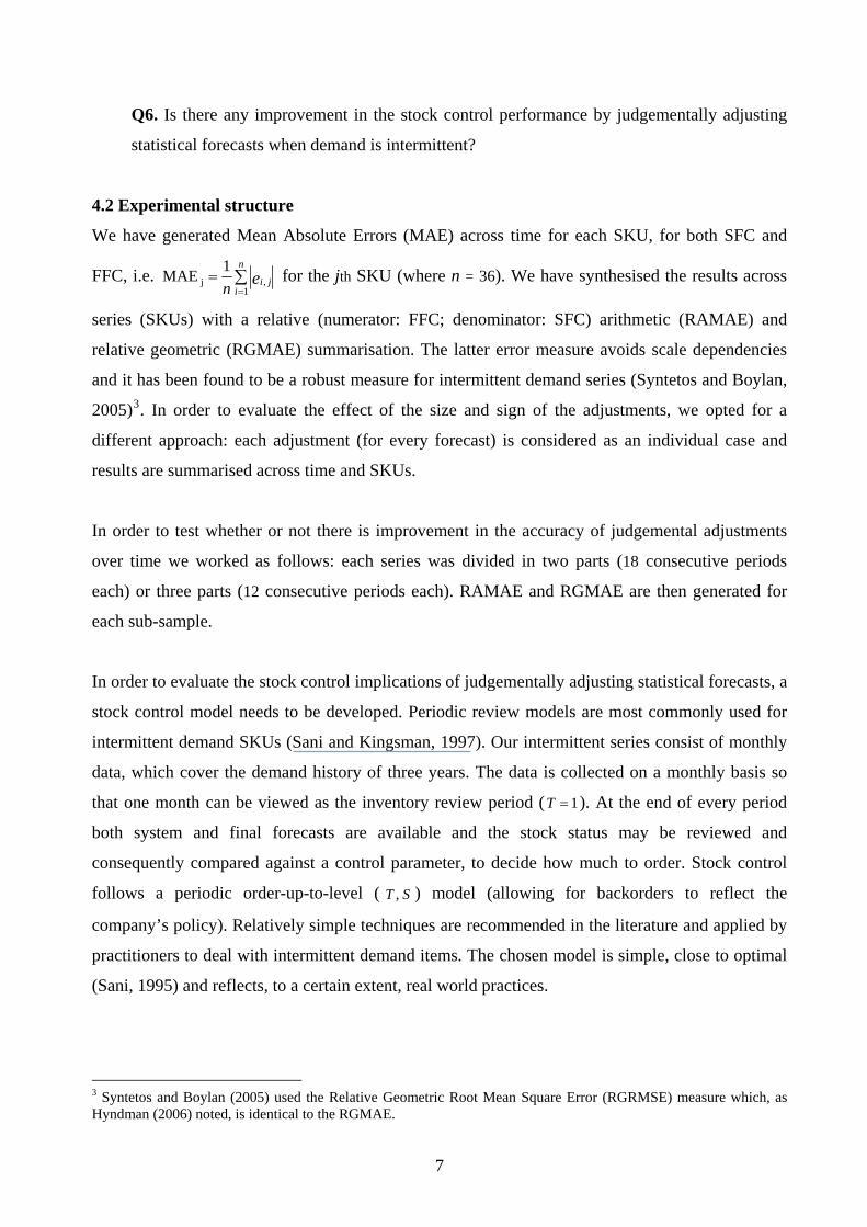
The summary stock control simulation results (across all 138 SKUs) are presented in Table 7.

‘Stock’ results indicate the average monthly amount of units kept in stock across all series. The

results have been rounded to the second decimal place. Customer Service Level (CSL) results

indicate the average service level achieved across all series and they have been rounded to the third

decimal place.

Overall, the results indicate the poor performance of the system forecasts for both target service

levels. Final forecasts perform very well for a service level equal to 95% but they result in an

under-achievement of the higher service level considered in our experiment (i.e. 99%). The

smoothing constant value used for MSE updating purposes appears to have little effect on the

performance of both system and final forecasts. Similar comments can be made on the sensitivity

of the results to the lead time length. Regarding the final forecasts, one would expect the

14

performance of the judgemental adjustments to deteriorate over time (i.e. a larger positive effect in

the short term and a smaller effect for the longer term). However, this is not the case.

System Forecasts Final Forecasts Summary stock control results

across all 138 SKUs Stock CSL Stock CSL

L = 1 1534.06 0.928 1525.22 0.954 L = 2 1721.10 0.928 1854.30 0.961

α = 0.05

L = 3 1773.39 0.928 1937.77 0.962 L = 1 1492.86 0.933 1437.51 0.957 L = 2 1723.35 0.929 1821.17 0.962

α = 0.10

L = 3 1835.67 0.931 1984.21 0.961 L = 1 1476.59 0.933 1391.23 0.957 L = 2 1729.37 0.929 1799.69 0.961 C

usto

mer

Ser

vice

Lev

el =

0.9

5

α = 0.15

L = 3 1871.18 0.933 2001.56 0.959 L = 1 2078.57 0.956 2046.18 0.973 L = 2 2323.99 0.954 2444.00 0.975

α = 0.05

L = 3 2338.36 0.959 2502.70 0.975 L = 1 2025.26 0.960 1924.97 0.976 L = 2 2332.92 0.959 2400.33 0.977

α = 0.10

L = 3 2439.88 0.960 2573.72 0.977 L = 1 2005.82 0.959 1864.25 0.976 L = 2 2346.38 0.961 2374.23 0.977 C

usto

mer

Ser

vice

Lev

el =

0.9

9

α = 0.15

L = 3 2499.07 0.960 2605.72 0.978

Table 7. Summary stock control results

Tables 8 and 9 summarise the simulation output for specific target values. For each smoothing

constant value simulated and lead time length results are summarised across all SKUs and the

remaining control parameter combinations.

P1

When system forecasts are utilised there is a considerable under-achievement of the service level

by 2.0% and 3.1%, for targets equal to 95% and 99% respectively. In both cases, the volume of

stock slightly increases with the smoothing constant value and the lead time length. The service

levels achieved using final forecasts exceed target levels of 95% by 0.9% on average. For the

higher target level simulated in our experiment there is an under-achievement of 1.4% on average.

Stock volume performance slightly improves with the smoothing constant value; the opposite is

the case, as expected, for the lead time length.

The inconsistency between target and achieved service levels is something that was both

theoretically and empirically expected. Various research projects have demonstrated that the

substitution of the true moments of the demand distribution with estimates lead to an inevitable

‘loss of performance’; that ‘loss’ is, most often, associated with an under-achievement of the target

15

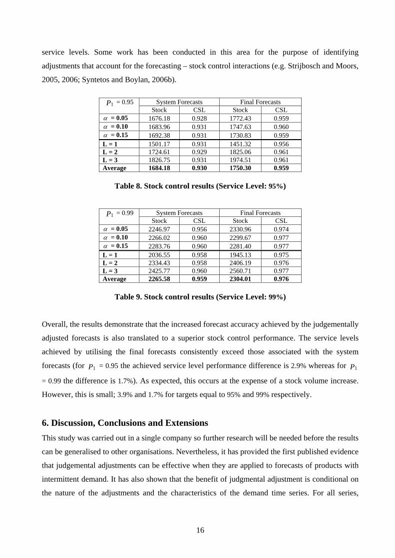
service levels. Some work has been conducted in this area for the purpose of identifying

adjustments that account for the forecasting – stock control interactions (e.g. Strijbosch and Moors,

2005, 2006; Syntetos and Boylan, 2006b).

System Forecasts Final Forecasts P1 = 0.95

Stock CSL Stock CSL α = 0.05 1676.18 0.928 1772.43 0.959 α = 0.10 1683.96 0.931 1747.63 0.960 α = 0.15 1692.38 0.931 1730.83 0.959 L = 1 1501.17 0.931 1451.32 0.956 L = 2 1724.61 0.929 1825.06 0.961 L = 3 1826.75 0.931 1974.51 0.961 Average 1684.18 0.930 1750.30 0.959

Table 8. Stock control results (Service Level: 95%)

System Forecasts Final Forecasts P1 = 0.99

Stock CSL Stock CSL α = 0.05 2246.97 0.956 2330.96 0.974 α = 0.10 2266.02 0.960 2299.67 0.977 α = 0.15 2283.76 0.960 2281.40 0.977 L = 1 2036.55 0.958 1945.13 0.975 L = 2 2334.43 0.958 2406.19 0.976 L = 3 2425.77 0.960 2560.71 0.977 Average 2265.58 0.959 2304.01 0.976

Table 9. Stock control results (Service Level: 99%)

Overall, the results demonstrate that the increased forecast accuracy achieved by the judgementally

adjusted forecasts is also translated to a superior stock control performance. The service levels

achieved by utilising the final forecasts consistently exceed those associated with the system

forecasts (for = 0.95 the achieved service level performance difference is 2.9% whereas for

= 0.99 the difference is 1.7%). As expected, this occurs at the expense of a stock volume increase.

However, this is small; 3.9% and 1.7% for targets equal to 95% and 99% respectively.

P1 P1

6. Discussion, Conclusions and Extensions This study was carried out in a single company so further research will be needed before the results

can be generalised to other organisations. Nevertheless, it has provided the first published evidence

that judgemental adjustments can be effective when they are applied to forecasts of products with

intermittent demand. It has also shown that the benefit of judgmental adjustment is conditional on

the nature of the adjustments and the characteristics of the demand time series. For all series,

16

negative adjustments are more effective than positive adjustments and large negative adjustments

lead to forecasts that are particularly accurate. These results are consistent with those found for

products that are not subject to intermittent demand (Nikolopoulos et al., 2005). The relatively

poor performance of positive adjustments may be a result of an optimism bias on the part of the

forecasters. Optimism bias would lead to positive adjustments being made in the absence of

reliable evidence that the forecasts need adjusting upwards or lead to over enthusiastic upward

adjustment when such evidence was available. Alternatively, unwarranted or excessive upward

adjustments may be motivated by political factors such as pressures from senior management. In

the case of this company, the forecasters indicated that the need to ensure that suppliers gave them

priority was occasionally a reason for producing forecasts that were ‘on the high side’.

The finding that there is no significant learning effect, in that the adjustments do not tend to

improve over time is also consistent with that found for products that are not subject to intermittent

demand (Nikolopoulos et al., 2006). As indicated earlier, this probably partly reflected the

improved accuracy of the statistical forecasts which thereby reduced the potential improvements

that could be obtained through adjustments. However, it might also reflect a defective feedback

system which prevents forecasters from learning from past errors. The irregularity of intermittent

demand would be likely to pose a challenge to anyone seeking to design a feedback system which

fosters learning. It is certainly notable that the adjustments perform better for fast intermittent

demand series where inter-demand periods are relatively short.

Interestingly, the results also suggest that when zero forecasts are considered, small absolute

adjustments are likely to be beneficial. This contrasts with results from research involving non-

intermittent demand goods where small adjustments tend to have limited value. A possible

explanation lies in the nature of the information being used by the forecaster to make the

adjustment. Finally, the results demonstrate that the improved forecast accuracy achieved by

judgementally adjusting forecasts is also reflected in the stock control performance of the estimates

under concern. Adjusted forecasts have been found to offer service levels closer to the target ones,

as compared with the system forecasts, at the expense of modest stock volume differences.

While this research has provided evidence of the benefits that can be achieved though judgemental

adjustments of system forecasts, there is scope for improvement in the way that judgemental

adjustments are applied. Some of these improvements may be achievable though the development

17

of facilities to support judgemental intervention within forecasting software as described in Fildes

et al. (2006b) and backed up by experimental evidence (Goodwin et al., 2006).

Given the frequency with which adjustments are applied to forecasts of intermittent demand and

given the value of judgemental intervention that this study has revealed, further research into the

design and effectiveness of these facilities would appear to be merited.

7. References Armstrong, J.S. and F. Collopy, 1998, Integration of statistical methods and judgement for time series

forecasting: Principles for empirical research, In (eds. Wright, G. and P. Goodwin) Forecasting with

Judgement, John Wiley & Sons, Inc., New York.

Boylan, J.E. and A.A. Syntetos, 2006, Accuracy and accuracy-implication metrics for intermittent demand

items, Foresight: International Journal of Applied Forecasting 4, 39 – 42.

Boylan, J.E., Syntetos, A.A. and G.C. Karakostas, 2007, Classification for forecasting and stock control: A

case study, Journal of the Operational Research Society, advance online publication doi: 10.1057/

palgrave.jors.2602312.

Croston, J.D., 1972, Forecasting and stock control for intermittent demands, Operational Research

Quarterly 23, 289 – 303.

De Gooijer, J.G. and R.J. Hyndman, 2006, 25 years of time series forecasting, International Journal of

Forecasting 22, 443 – 473.

Diamantopoulos, A. and B.P. Mathews, 1989, Factors affecting the nature and effectiveness of subjective

revision in sales forecasting: an empirical study, Managerial and Decision Economics 10, 51 – 59.

Fildes, R., Goodwin, P., Lawrence, M. and K. Nikolopoulos, 2006a, Producing more efficient demand

forecasts, Working paper 2006/054, Lancaster University Management School, UK.

Fildes, R., Goodwin, P. and M. Lawrence, 2006b, The design features of forecasting support systems and

their effectiveness, Decision Support Systems 42, 351 – 361.

Fildes, R. and P. Goodwin, 2007, Against your better judgment: How organizations can improve their use

of judgment in forecasting. Working paper 2007/01, Lancaster University Management School, UK.

Goodwin, P., 2002, Integrating management judgment with statistical methods to improve short-term

forecasts, Omega, International Journal of Management Science 30, 127 – 135.

Goodwin, P. and R. Fildes, 1999, Judgmental forecasts of time series affected by special events: does

prviding a statistical forecast improve accuracy? Journal of Behavioral Decision Making 12, 37 – 53.

Goodwin, P., Fildes, R., Lawrence, M. and K. Nikolopoulos, 2006, The process of using a forecast support

system, Working paper 2006/09, University of Bath, Management School, UK.

Hyndman, R.J., 2006, Another look at forecast-accuracy metrics for intermittent demand, Foresight:

International Journal of Applied Forecasting 4, 43 – 46.

18

Johnston, F.R. and J.E. Boylan, 1996, Forecasting for items with intermittent demand, Journal of the

Operational Research Society 47, 113 – 121.

Johnston, F.R., Boylan, J.E. and E.A. Shale, 2003, An examination of the size of orders from customers,

their characterization and the implications for inventory control of slow moving items, Journal of the

Operational Research Society 54, 833 – 837.

Klassen, R.D. and B.E. Flores, 2001, Forecasting practices of Canadian firms: survey results and

comparisons, International Journal of Production Economics 70, 163 – 174.

Lim, J.S. and M. O’Connor, 1995, Judgemental adjustment of initial forecasts: its effectiveness and biases,

Journal of Behavioral Decision Making 8, 149 – 168.

Mathews, B.P. and A. Diamantopoulos, 1986, Managerial intervention in forecasting: An empirical

investigation of forecast manipulation, International Journal of Research in Marketing 3, 3 – 10.

Mathews, B.P. and A. Diamantopoulos, 1990, Judgmental revision of sales forecasts - effectiveness of

forecast selection, Journal of Forecasting 9, 407 – 415.

Mathews, B.P. and A. Diamantopoulos, 1992, Judgmental revision of sales forecasts - the relative

performance of judgementally revised versus nonrevised forecasts, Journal of Forecasting 11, 569 – 576.

McCarthy, T.M., Davis, D.F., Golicic, S.L. and J.T. Mentzer, 2006, The evolution of sales forecasting

management: a 20 year longitudinal study of forecasting practices, Journal of Forecasting 24, 303 – 324.

Nikolopoulos, K., Fildes, R., Lawrence, M. and P. Goodwin, 2005, On the accuracy of judgmental

interventions on forecasting support systems, Working paper 2005/022, Lancaster University Management

School, UK.

Nikolopoulos, K., Stafylarakis, M., Goodwin, P. and R. Fildes, 2006, Why do companies not produce better

forecasts over time? An organizational learning approach, Proceedings of the 12th IFAC Symposium on

Information Control Problems in Manufacturing, Vol. 3, 167 – 172, Saint Etienne, France.

O’Connor, M., Remus, W. and K. Griggs, 1993, Judgemental forecasting in times of change, International

Journal of Forecasting 9, 163 – 172.

Sanders, N. and K.B. Manrodt, 1994, Forecasting practices in US corporations: Survey results, Interfaces

24, 92 – 100.

Sanders, N. and L. Ritzman, 2001, Judgmental adjustments of statistical forecasts, In (ed. Armstrong, J.S.)

Principles of Forecasting, Kluwer Academic Publishers, New York.

Sani, B., 1995, Periodic inventory control systems and demand forecasting methods for low demand items,

Unpublished Ph.D. thesis, Lancaster University, UK.

Sani, B. and B.G. Kingsman, 1997, Selecting the best periodic inventory control and demand forecasting

methods for low demand items, Journal of the Operational Research Society 48, 700-713.

Strijbosch, L.W.G. and J.J.A. Moors, 2005, The impact of unknown demand parameters on (R, S) -

inventory control performance, European Journal of Operational Research 162, 805 – 815.

Strijbosch, L.W.G and J.J.A. Moors, 2006, Modified Normal demand distributions in (R, S) - inventory

control, European Journal of Operational Research 172, 201 – 212.

19

Syntetos, A.A. and J.E. Boylan, 2005, The accuracy of intermittent demand estimates. International Journal

of Forecasting 21, 303 – 314.

Syntetos, A.A., Boylan, J.E. and J.D. Croston, 2005, On the categorization of demand patterns. Journal of

the Operational Research Society 56, 495 – 503.

Syntetos, A.A. and J.E. Boylan, 2006a, On the stock control performance of intermittent demand

estimators, International Journal of Production Economics 103, 36 – 47.

Syntetos, A.A. and J.E. Boylan, 2006b, Smoothing and adjustments of demand forecasting for inventory

control, Proceedings of the 12th IFAC Symposium on Information Control Problems in Manufacturing, Vol.

3, 173 – 178, Saint Etienne, France.

Turner, D.S., 1990, The role of judgment in macroeconomic forecasting, Journal of Forecasting 9, 315 –

345.

Willemain, T.R, Smart, C.N. and H.F. Schwarz, 2004, A new approach to forecasting intermittent demand

for service parts inventories, International Journal of Forecasting 20, 375-387.

APPENDIX A: Data selection When one of the following scenarios was the case, the corresponding series were excluded from

our empirical investigation. At this stage it is important to note that there were 24 intermittent

series containing some negative values (returns). It has been argued (Willemain et al., 2004) that a

conservative solution is to replace those negative values with zero. This solution was also adopted

for the purposes of this research.

Only positive demands

Only zero demands interspersed with negative demands (returns)

A number of positive demands (long stream) followed by a stream of zeros (and returns)

Some returns in the beginning (negative values - first 6 months) followed by zero demands

(not stocked anymore)

One - off (lumpy) delivery at the beginning followed by zero demands (launch of a new

product). Or few (3 or 4) lumpy deliveries in the beginning followed by zero demands

Some SKUs being intermittent for the first 18 months or so and then zeroes and/or returns

Zeros interspersed with only one demand occurrence

Only last 12 months history available

18 periods available - break - 12 periods available

12-14 months (start of series) intermittence, followed by zeroes.

20