The Effects of Household Income Volatility on Divorce

The Effects of Household Income Volatilityon Divorceajes_731 983..1010

By JOHN M. NUNLEY and ALAN SEALS*

ABSTRACT. We extend the literature on the effects of earnings shockson divorce by identifying separately the effects of transitory andpermanent household income shocks and by allowing the shocks tohave asymmetric effects across education and racial groups. Theeconometric evidence suggests negative (positive) transitory house-hold income shocks increase (decrease) the probability of divorce,while there is only weak evidence that positive (negative) permanenthousehold income shocks raise (lower) the probability of divorce.Some differences in the effects of household income shocks ondivorce propensities arise for subsamples selected by education andrace.

I

Introduction

THE THEORY DEVELOPED by Becker et al. (1977) contends that “sur-prises,” whether positive or negative, increase the probability ofdivorce. In Becker et al.’s framework, household income volatility is aproxy for these unexpected events. Their model predicts that house-hold income volatility increases the risk of divorce because unex-pected changes alter the couples’ expected returns from marriage.

*John M. Nunley is an Assistant Professor of Economics at University of Wisconsin–La

Crosse. Direct correspondence to: John M. Nunley, Department of Economics, Univer-

sity of Wisconsin–La Crosse, La Crosse, WI 54601, e-mail: [email protected]; and

Alan Seals is an Assistant Professor of Economics at Oklahoma City University. Direct

correspondence to: Alan Seals, Department of Economics, O326 Haley Center, Auburn

University, AL 36849-5049. The authors thank two anonymous referees, Brandeanna

Allen, Charles Baum, Taggert Brooks, E. Anthon Eff, Greg Givens, Duane Graddy,

Widdy Ho, Adam Hogan, Travis Minor, Pam Morris, James Murray, Mark Owens, Adam

Rennhoff, and Joachim Zietz for helpful assistance, comments, and suggestions.

American Journal of Economics and Sociology, Vol. 69, No. 3 (July, 2010).© 2010 American Journal of Economics and Sociology, Inc.

Negative shocks to household income could lower the returns frommarriage below a particular threshold level, which may lead todivorce. Positive earnings shocks could induce a self-reliance effect,which may also increase the risk of divorce.

Economists have begun to question whether the traditional modelof marriage and divorce (e.g., Becker 1973, 1974; Becker et al. 1977)remains valid in the presence of numerous changes to family life. Forexample, Stevenson and Wolfers (2007) suggest that labor-savingtechnologies, the ability to buy household services in the market, andthe rising opportunity costs of specializing in household work forwomen have altered the returns from marriage. Today, it appears thatmarriage and its benefits are based on shared interests, i.e., consump-tion and leisure, rather than the gains from specialization in marketand domestic spheres. In this context, negative earnings shocksreduce the gains from marriage, while positive earnings shocksincrease the gains from marriage. The former may increase the risk ofdivorce, while the latter may lower the risk of divorce.

A number of studies examine the effects of earnings shocks onhousehold consumption and other economic outcomes.1 However,there have been few studies that examine the effects of earningsshocks on divorce. Previous attempts to measure the effects of earn-ings shocks on divorce have used actual minus predicted earnings(Becker et al. 1977), changes in predicted earnings capacities (Weissand Willis 1997), and job displacement (Charles and Stephens 2004).

In this article, we investigate the effect of household income vola-tility on divorce by separating the household income shocks intotransitory and permanent components. We use panel data from the1979 cohort of the National Longitudinal Survey of Youth (NLSY79) toinvestigate this question. We also use a technique developed byMeghir and Pistaferri (2004), which is novel to this literature, toconstruct the transitory and permanent household income shocks. Theapproach developed by Meghir and Pistaferri (2004) emphasizes theimportance of allowing the household income shocks to be generatedby heterogeneous processes. Our analysis of household income fluc-tuations and divorce differs from previous work in three ways: (i)spousal incomes are jointly considered, (ii) transitory and permanenthousehold income shocks are identified separately, and (iii) the

984 The American Journal of Economics and Sociology

household income shocks are generated separately by SES, for whichindividual educational attainments proxy, and race.

We find that negative (positive) transitory household income shocksincrease (decrease) the probability of divorce, while there is weakevidence that positive (negative) permanent household incomeshocks increase (decrease) divorce propensities. The effects differsomewhat by SES and race. For example, the divorce propensitiesof high-school dropouts (low SES) are unaffected by transitoryhousehold income shocks but are affected positively by permanenthousehold income shocks. The effects differ for those who graduatefrom high school and/or attend some college (mid SES): their divorcepropensities are negatively affected by transitory household incomeshocks but are unaffected by permanent household income shocks.Neither the transitory nor permanent household income shocksaffect the divorce propensities of college graduates (high SES). Thedivorce propensities of nonblacks/non-Hispanics and Hispanics areaffected negatively by transitory household income shocks. Permanenthousehold income shocks are statistically insignificant for all racialgroups.

II

A Review of the Literature on Earnings Shocks and Divorce

IN HIS SEMINAL THEORY OF MARRIAGE, Becker (1973, 1974) posits thatindividuals marry those with like characteristics, otherwise known aspositive assortative mating. For example, individuals with similareducation levels, intelligence, social background, race, and religionare more likely to marry and to be better matches once wed. Bycontrast, negative assortative mating occurs with respect to earningsbecause spousal earnings are substitutes.2 Becker argues that marriageallows individual spouses to take advantage of the gains from trademade possible by the division of labor within the household. Thedivision of labor is determined in the marriage market where indi-viduals are matched, through the assortatitve mating process, so as togenerate the highest return from marriage.

Becker et al. (1977) extend Becker’s general theory of the familyto explain marital dissolution. The authors argue that because there

The Effects of Household Income Volatility on Divorce 985

is limited information in the marriage market, it is costly, at both theextensive (i.e., it is costly to search over the market) and intensive(i.e., it is costly to vet individual mates) margins, to search for theoptimal mate. At the outset of marriage, individuals form expecta-tions concerning the returns to marriage based on the quality ofthe initial match. A key aspect of Becker et al.’s (1977) theory isthat new information induces spouses to update their expectationsof the returns from marriage. The authors posit that unexpectedevents should unambiguously increase the probability of divorce,regardless of whether these surprises are negative or positive.3 Theunderpinning of the argument is that expected events deleterious tomarriage would inhibit the couple from marrying, whereas unex-pected events would cause them to reevaluate the relative returns tothe marriage.

A number of researchers have attempted to test this prediction.4

In Becker et al. (1977), unanticipated events or earnings shocks,measured as the actual earnings minus predicted earnings, tend toraise the probability of divorce for both men and women. Whetherthe measure of unexpected events is positive or negative has nobearing on the statistically significant, positive effect on divorce pro-pensities. However, Becker et al.’s (1977) analysis is limited to cross-sectional data and therefore cannot control for marriage-matchquality.

Weiss and Willis (1997) extend the work of Becker et al. (1977) byexamining the effects of unexpected changes in predicted earningscapacity on the likelihood of divorce using panel data, which allowsthem to control for the quality of the marriage match.5 They find thatan increase in predicted earnings capacity decreases the probabilityof divorce for men; however, the effect is positive for women. Weissand Willis (1997) attribute the positive effect of unexpected shocks towives’ income on divorce to the endogeneity of fertility and femalelabor supply. However, research by Sayer and Bianchi (2000) andNock (2001) attribute the positive relationship between wives’income and divorce to wives’ ability to exit bad marriages. Theauthors argue that husbands derive more social value from “beingmarried,” while wives place greater value on the marital relationship.Hence, failing to control for issues related to the quality of the


marriage relationship and changing gender roles in society couldintroduce omitted variable bias to an analysis of the effects of earn-ings shocks on divorce.

One limitation of the study by Weiss and Willis (1997), which ispointed out by Charles and Stephens (2004), is that the authors do notuse an explicit measure of earnings shocks. Charles and Stephens(2004) also use panel data to examine the effect of negative earningsshocks, measured as job loss, on divorce propensities. They examinethree types of job displacement: (i) layoffs, (ii) plant closings, and (iii)disability. They find no evidence that plant closings or disabilitiestranslate into a higher probability of divorce. However, layoffs affectdivorce propensities positively. Since plant closings, disabilities, andlayoffs have similar long-run earnings effects, this suggests that aspouse’s noneconomic suitability may play a more significant rolethan pecuniary matters in divorce decisions. While Charles andStephens (2004) do appear to identify negative, exogenous shocks toincome, they do not identify the effect of positive earnings shocks ondivorce propensities.

We extend these studies by using an alternative measure of earn-ings shocks developed by Meghir and Pistaferri (2004). In particular,we examine separately the effects of transitory and permanent house-hold income shocks on the probability of divorce. The transitoryshocks represent “surprises” (both positive and negative) in thecontext of Becker et al. (1977), which are predicted to unambiguouslyraise the probability of divorce. By contrast, Weiss and Willis (1997)suggest that permanent shocks should have no effect on divorcepropensities, as these shocks should be expected. Our approach alsoallows us to address the issues raised by Sayer and Bianchi (2000)and Nock (2001). Because the evolution of the marriage relationshipis likely a gradual process, by separating the slower moving perma-nent component from the transitory component of income shockswhile holding constant time-invariant factors related to the initialmatch quality of the couple, it is possible to identify the effect of ahousehold income “surprise” independent of overall marriage quality.In addition, our analysis extends the existing literature by allowingdifferent socioeconomic processes to generate the household incomeshocks.


III

Data

WE USE PANEL data from the 1979 National Longitudinal Survey of Youth(NLSY79) to examine the effects of household income volatility ondivorce. In 1979, the NLSY79 began surveying individuals between theages of 14 and 21. These data allow us to follow individuals well intoadulthood, at which point they are likely to have reached or would beapproaching the peak of their earnings potential. As such, the indi-viduals surveyed should experience substantial fluctuations in house-hold income over time (e.g., see Meghir and Pistaferri 2004). Theseindividuals are also likely candidates for marriage and divorce.

While data are available from 1979 to 2006, annual data are pro-vided only through 1994. Beginning in 1994, the survey was con-ducted on a biennial basis. Extending the analysis beyond 1994introduces potential confounds to the analysis. Specifically, marriageswhich end in divorce between survey years could bias the estimatedeffects of household income volatility on divorce propensities. As aresult, we examine annual data from 1979 to 1994.

The NLSY79 identifies never married, married, separated, widowed,and divorced individuals in each survey year. The sample we use isconstructed by identifying all married individuals. One limitation ofour data set is that we are unable to observe both spouses beforemarriage, which would be ideal because it would allow us to controlfor match quality. Individuals who are single during the entire sampleperiod are excluded. We also exclude observations from individualswho are widowed, who married before the survey began, and whohave been married more than once. We treat separated individuals asbeing married.

The divorce outcome variable is a zero-one indicator variable,which equals one if the individual is married and one if divorced. Forexample, an individual who marries in 1981 and divorces in 1989receives a zero for each year of marriage and a one for the year inwhich divorce occurs. Because second- and higher-order marriagesare excluded, individuals who divorce exit the sample the followingyear. After imposing all sample restrictions, our data consist of 10,580marriages, of which 11.5 percent end in divorce.


The NLSY79 also provides a family-income variable, which is usedto construct the household income volatility measures (See SectionIV.A). The family-income variable remains in nominal form.6 Thesurvey also provides consistent information on demographic, labor-market, and familial characteristics. We use these variables as controlsin the divorce equations to aid in parsing the effects of householdincome volatility on divorce propensities. In addition, the panel natureof the NLSY79 offers an opportunity to purge any individual-specificfixed effects from the divorce equations, which proxies for the qualityof the marriage match (Weiss and Willis 1997).

IV

Econometric Methodology

A. Constructing the Transitory and Permanent Household Income Shocks

We construct the transitory and permanent household income shocksusing the approach developed by Meghir and Pistaferri (2004).7 Thisapproach makes use of the residuals from a first-stage model:

log .hhincit it it( ) = + +δ δ ε0 1X (1)

The variable log(hhinc) represents the logarithm of nominal house-hold income; X is a vector of observable characteristics, including age,race, and education, whether the individual lives in an urban area,region-of-residence indicators, and a set of year-indicator variables;8

e is the disturbance term; and the dj are parameters to be estimated.The first difference of the residuals from Equation (1), i.e.,

Δε ε εit it it* * *= − −1, is used to construct the transitory and permanenthousehold income shocks. The following equations define the tran-sitory and permanent household income shocks, respectively:

Transitoryit it it= × +Δ Δε ε* * 1 (2)

Permanentit it it it it it it= × + + + +− − + +Δ Δ Δ Δ Δ Δε ε ε ε ε ε* ( * * * * * ).2 1 1 2 (3)


The variables Transitory and Permanent are included as right-hand-side variable in the divorce equations (discussed in Section IV.B),along with the variables in X from Equation (1).

The inclusion of asymmetric effects based upon educational attain-ment is a distinguishing feature of Meghir and Pistaferri’s (2004)approach to modeling income shocks. Following Meghir and Pistaferri(2004), we also estimate Equation (1) separately for three educationgroups and three racial groups: high-school dropouts, those whograduated from high school and/or attended some college, andcollege graduates and Hispanics, blacks, and nonblacks/non-Hispanics, respectively.

We estimate separate household-income regressions for each sub-sample to allow heterogeneous processes to generate the householdincome shocks. Tables 1 and 2 present summary statistics for thetransitory and permanent household income shocks by education andrace, respectively. These tables show that the magnitude and standarddeviations of the shocks vary substantially by education and race. As

Table 1

Sample Means and Standard Deviations for Permanent andTransitory Household Income Shocks by

Educational Attainment

VariableFull

SampleHigh School

DropoutsHigh School/Some College

CollegeGraduates

Transitory Shock -0.2492 -0.2853 -0.2406 -0.2492(1.535) (1.480) (1.535) (1.587)

Permanent Shock 0.1086 0.0856 0.1070 0.1376(1.110) (1.105) (1.076) (1.242)

Number ofObservations

67,883 10,847 45,846 11,190

Percentage of theSample

100% 16% 68% 16%

Notes: Standard deviations are in parentheses.


such, it is likely that the effects on divorce of the household incomeshocks will differ across these groups.

B. Empirical Strategy

Our baseline model takes the probit functional form and is specifiedas:

Divorce c Transitory Permanentit i it it it it= + + + +β β β η1 2 3 X . (4)

The variable Divorce is an indicator variable that equals one if theindividual is divorced and zero otherwise; c is an individual-specificfixed effect;9 Transitory and Permanent are defined above by Equa-tions (2) and (3); X is defined above;10 and h is the disturbance term.The primary coefficients of interest are b1 and b2.

A number of estimation issues arise when examining the effects ofhousehold income volatility on divorce propensities. In particular,measures of household income volatility and divorce may be jointlydetermined variables, and unobserved factors correlated with house-hold income volatility and related to the probability of divorce could

Table 2

Sample Means and Standard Deviations for Permanent andTransitory Household Income Shocks by Race

VariableFull

Sample Hispanics BlacksNon-Hispanics/

Nonblacks

Transitory Shock -0.2480 -0.2406 -0.2731 -0.2397(1.540) (1.457) (1.377) (1.623)

Permanent Shock 0.1169 0.1014 0.1019 0.1272(1.137) (0.943) (1.148) (1.180)

Number ofObservations

67,883 11,032 16,517 40,334

Percentage of theSample

100% 16% 24% 60%

Notes: Standard deviations are in parentheses.


bias estimates. In what follows, we discuss these complications inmore detail and how we address them empirically.

Individuals who anticipate divorce may alter their labor-supplybehavior. If individuals increase or decrease their labor supply whenthe probability of divorce rises, this implies that divorce and house-hold income are jointly determined variables. In fact, there isempirical support for this. For example, Parkman (1992), Gray(1998), and Stevenson (2008) examine the impact of unilateraldivorce laws, which make divorce easier by allowing either spouseto file for divorce without consent from their spouse, on women’slabor-force participation rates (LFPRs). For the most part, thesestudies find that unilateral divorce laws raise women’s LFPRs. Thesestudies rely on variation in the timing of divorce-law reforms as aproxy for divorce risk. Greene and Quester (1982) and Johnson andSkinner (1986) use more direct measures of divorce risk, and findthat women begin participating in the labor market at greater rateswhen the probability of divorce increases. Sen (2000) analyzes amore recent cohort (i.e., the NLSY79) and finds that the probabilityof divorce played a large role in determining women’s labor-supplybehavior in the older cohort, while the effects are modest for amore recent cohort.

A typical way to deal with the potential simultaneous relationshipbetween household income volatility and divorce is through the useof instrumental variables (IV). Unfortunately, few valid instrumentsexist in the present context. A valid instrument must be significantlycorrelated with the suspected endogenous variable on the right-handside of the regression model, i.e., the household income shocks, andit must be uncorrelated with the outcome variable, in this case, theprobability of divorce.11 We ran a number of models with a variety ofdifferent IVs for the household income volatility measures, includinga set of state-level economic variables (e.g., the unemployment rate,per capita income, etc.), occupation indicators as in Hess (2004), andlagged values of the transitory and permanent household incomeshocks as in Meghir and Pistaferri (2004). After investigating the powerof the IVs in the first-stage models and whether they are exogenousin the second-stage model, none of these IVs satisfied the criteria fora valid instrument.


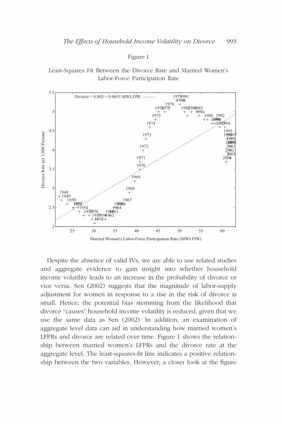
Despite the absence of valid IVs, we are able to use related studiesand aggregate evidence to gain insight into whether householdincome volatility leads to an increase in the probability of divorce orvice versa. Sen (2002) suggests that the magnitude of labor-supplyadjustment for women in response to a rise in the risk of divorce issmall. Hence, the potential bias stemming from the likelihood thatdivorce “causes” household income volatility is reduced, given that weuse the same data as Sen (2002). In addition, an examination ofaggregate level data can aid in understanding how married women’sLFPRs and divorce are related over time. Figure 1 shows the relation-ship between married women’s LFPRs and the divorce rate at theaggregate level. The least-squares-fit line indicates a positive relation-ship between the two variables. However, a closer look at the figure

Figure 1

Least-Squares Fit Between the Divorce Rate and Married Women’sLabor-Force Participation Rate

2

2.5

3

3.5

4

4.5

5

5.5

25 30 35 40 45 50 55 60

Div

orce

Rat

e pe

r 1,

000

Per

sons

Married Women's Labor-Force Participation Rate (MWLFPR)

19481949

195019511952

195419551956

19571958

195919611962

1963196419651966

1967

1968

1969

1970

1971

1972

1973

1974

1975

197619771978

19791980

1981

1982198419851986

198819901991

1992

19931994

199519961997

1998199920002001

20022003

2004

Divorce = 0.803 + 0.0655 MWLFPR


indicates two clear negative relationships between the two variables:one before the mid-1960s surge in the divorce rate, and the otherduring the fall in the divorce rate from 1980 onwards. Individual-leveland aggregate evidence suggest rather strongly that divorce risk doesnot appear to be a key determinant of married women’s LFPRs. Assuch, this should reduce the likelihood of simultaneous relationshipbetween divorce propensities and household income fluctuations.

Another issue that complicates estimation is the influence of unob-served variables correlated with the measures of household incomevolatility that are also related to the probability of divorce. Individualswho experience high income volatility could differ in unobservedways from those whose incomes are more stable. Unobserved vari-ables such as laziness or lack of motivation may lead to negativeearnings shocks, and these variables could also be related to divorce.Researchers in the divorce literature often term these unobservedfactors marriage-match quality. Attempts to account for the quality ofthe marriage match include controls for marital history and husbands’and wives’ educations, races, and religions (Charles and Stephens2004) and the inclusion of individual-specific fixed effects (Weiss andWillis 1997). We are able to account for the quality of the initialmarriage match by including individual-specific fixed effects. Theinclusion of individual-specific fixed effects eliminates time-invariantunobserved characteristics correlated with the household incomevolatility measures and related to the probability of divorce. Thisimplies the inclusion of the individual-specific fixed effects likelypurges the influence of religion and other marital-history variables.This approach is used by Weiss and Willis (1997), while Charles andStephens (2004) include controls for marital history and observablespousal characteristics to proxy for marriage-match quality. TheNLSY79 does not provide information on spouses’ educational attain-ments. However, we control for the educational attainments of theindividuals, which are likely correlated with their spouses’ educationalattainments due to high degree of positive assortative mating based oneducation observed in the literature (Lam 1988; Schwartz and Mare2005).

In terms of causal inference, previous work and aggregate evidenceminimize the potential for divorce and household income shocks to


be jointly determined, and our ability to control for marriage-matchquality by including individual-specific fixed effects reduces thechance that our results are driven by unobservables.

In addition, a closer examination of our data can provide additionalinsight about the direction of causality. Figures 2, 3, and 4 show thebehavior of the household income shocks across marital stages (nor-malized on the year of divorce) for the full sample, for partitionedsamples by SES, and for partitioned samples by race. Figure 2 presentsboth the transitory and permanent household income shocks for thefull sample. Figures 3 and 4 focus on transitory household incomeshocks, which represent surprises in the context of Becker et al.(1977), for the different SES and racial groups. Overall, Figures 2, 3,and 4 indicate that the variances of the household income shocks arerelatively small before divorce, become large in the year of divorce,and narrow following divorce. This suggests that it is unlikely thatthere is, for example, increases or decreases in labor supply as a resultof rising divorce expectations.

Figure 2

Permanent and Transitory Shocks

-20

02

04

06

0

Perm

anent

Shock

-6 -4 -2 0 2 4 6Divorce

Permanent Shocks Across Marital Stages

Before Divorce After Divorce

-10

0-5

00

50

Tra

nsitory

Shock

-6 -4 -2 0 2 4 6

Divorce

Transitory Shocks Across Marital Stages



Figures 3 and 4 also make clear the importance of allowing theprocesses that generate the household income shocks to vary by SESand race (as mentioned in Section IV.A) and of examining the effectsof household income shocks on divorce propensities separately bySES and race. It is apparent from Figures 3 and 4 that there aresubstantial differences in the variance of the transitory householdincome shocks before divorce across these groups. Figure 3 indicatesgreater variability in the transitory household income shocks beforedivorce for high-school dropouts (low SES) and college graduates(high SES). By contrast, in the years before divorce, the variance of thetransitory household income shocks for those who graduate from highschool and/or attend some college (mid SES) is relatively small. FromFigure 3, we might expect the low SES group to be unaffected by

Figure 3

Transitory Shocks by Education Group

-60

-40

-20

02

04

0

Tra

nsito

ry S

ho

ck

-6 -4 -2 0 2 4 6

Divorce

Transitory Shocks to College Graduates

Across Marital Stages

Before Divorce

-60

-40

-20

02

0

Tra

nsito

ry S

ho

ck

-6 -4 -2 0 2 4 6

Divorce

Transitory Shocks to High School Dropouts



-50

-40

-30

-20

-10

01

0

Tra

nsito

ry S

ho

ck

-6 -4 -2 0 2 4 6

Divorce

Transitory Shocks to High School Graduates


Before Divorce

After Divorce

After Divorce


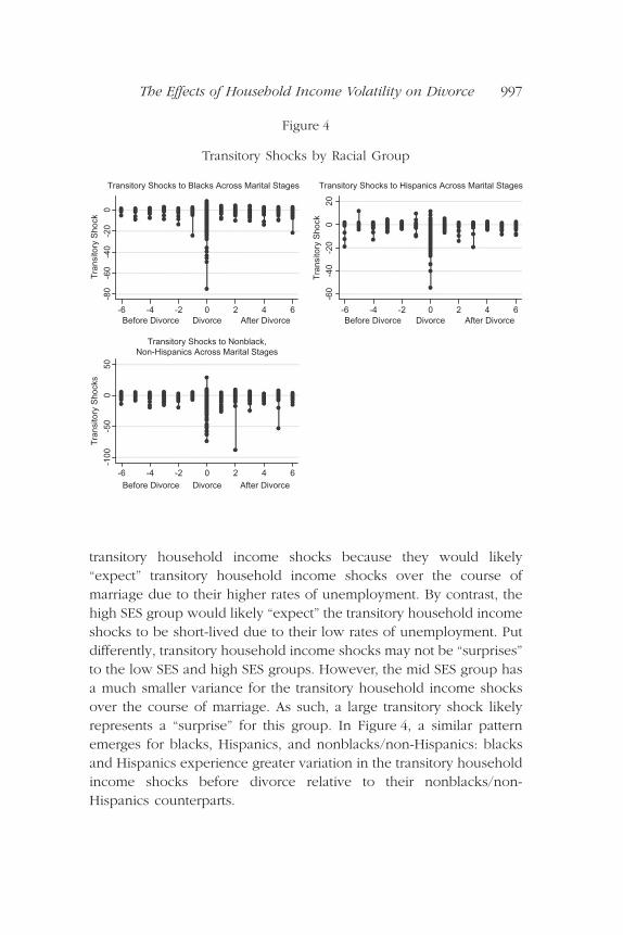
transitory household income shocks because they would likely“expect” transitory household income shocks over the course ofmarriage due to their higher rates of unemployment. By contrast, thehigh SES group would likely “expect” the transitory household incomeshocks to be short-lived due to their low rates of unemployment. Putdifferently, transitory household income shocks may not be “surprises”to the low SES and high SES groups. However, the mid SES group hasa much smaller variance for the transitory household income shocksover the course of marriage. As such, a large transitory shock likelyrepresents a “surprise” for this group. In Figure 4, a similar patternemerges for blacks, Hispanics, and nonblacks/non-Hispanics: blacksand Hispanics experience greater variation in the transitory householdincome shocks before divorce relative to their nonblacks/non-Hispanics counterparts.

Figure 4

Transitory Shocks by Racial Group

-80

-60

-40

-20

0

Tra

nsitory

Shock

-6 -4 -2 0 2 4 6

Divorce

Transitory Shocks to Blacks Across Marital Stages


DivorceBefore Divorce After Divorce

-60

-40

-20

020

Tra

nsitory

Shock

-6 -4 -2 0 2 4 6

Divorce

Transitory Shocks to Hispanics Across Marital Stages


-100

-50

050

Tra

nsitory

Shocks

-6 -4 -2 0 2 4 6

Transitory Shocks to Nonblack,

Non-Hispanics Across Marital Stages


V

Results

A. The Effects of Household Income Volatility on Divorce bySocioeconomic Status

Table 3 presents probit estimates for the effects of transitory andpermanent household income volatility on the probability of divorcefor the full sample and for subsamples partitioned by SES. Thesubsamples are divided into three groups: high-school dropouts (lowSES), individuals who graduated from high school and/or attendedsome college (mid SES), and college graduates (high SES). Model 1shows the results from the full sample. This specification suggests thatpositive (negative) transitory household income shocks lower (raise)

Table 3

Probit Estimates for the Effects of Permanent and TransitoryHousehold Income Shocks on the Probability of Divorce by

Educational Attainment

VariableFull Sample

High SchoolDropouts

High School/Some College

CollegeGraduates

Model 1 Model 2 Model 3 Model 4

Transitory Shock -0.0190*** -0.0167 -0.0205*** -0.0158(0.005) (0.012) (0.005) (0.011)

Permanent Shock 0.0139 0.0431* 0.0052 0.0306*(0.010) (0.027) (0.013) (0.019)

Number of Obs. 67,883 10,847 45,846 11,190Psuedo R-squared 0.0542 0.0735 0.0455 0.0648Log Likelihood -5,781 -960 -4,256 -543

Notes: Standard errors are in parentheses. *, **, and *** indicate statistical significance atthe 10, 5, and 1 percent levels, respectively. Each model includes controls for age, race,educational attainment (Model 1 only), family size, region of residence, and whether theindividual lives in an urban area. High School Dropouts represents individuals whoobtained less than 12 years of schooling; High School/Some College represents indi-viduals who completed 12 years of schooling and less than 16 years of schooling; andCollege Graduates are those who have completed 16 years or more of education.


the probability of divorce, while permanent household income shocksare statistically unrelated to the probability of divorce. A one standarddeviation increase (decrease) in the transitory household incomeshock lowers (increases) the probability of divorce by 7.35 percent.

The effects of household income shocks on divorce propensitiesdiffer for the subsamples based on the individual’s SES. For the lowSES group (Model 2), the transitory household income shocks arestatistically unrelated to the probability of divorce, while permanenthousehold income shocks increase the probability of divorce. For thelow SES group, a one standard deviation increase (decrease) in thepermanent household income shock raises (lowers) the probability ofdivorce by 12.6 percent; however, this effect is only statisticallysignificant at the 10 percent level. The estimates for the mid SES group(Model 3) are similar to the estimates for the full sample. The perma-nent household income shock is statistically unrelated to the prob-ability of divorce, while transitory household income shocks arenegative and statistically significant at the 1 percent level. For the midSES group, a one standard deviation increase (decrease) in the tran-sitory household income shock lowers (raises) the probability ofdivorce by 7.59 percent. The effects of the household income shockson the divorce propensities of the high SES group (Model 4) aresimilar to those found for the low SES group. A positive (negative)permanent household income shock raises (lowers) the probability ofdivorce. This effect translates into an 11.29 percent increase (decrease)in the probability of divorce when the permanent household incomeshock rises (declines) by one standard deviation; however, this esti-mate is only statistically significant at the 10 percent level. Thetransitory household income shock is not statistically different fromzero for the high SES group.

Table 4 is analogous to Table 2. The only difference is the inclusionof individual-specific fixed effects, which proxies for the quality of theinitial marriage match. We conduct an exclusion test on the individual-specific fixed effects for each model. The F-statistic and p-values forthese exclusion tests are shown at the bottom of Table 4. The joint-exclusion tests for the individual-specific fixed effects are statisticallydifferent from zero for all model specifications (Models 5, 7, and 8)except the one for the low SES group (Model 6). This implies that


including the individual-specific fixed effects improves the statistical fitof all models except Model 6.

The effects of the transitory and permanent household incomeshocks are largely robust to the inclusion of individual-specific fixedeffects for the full sample (Model 5). One difference that arises whenindividual-specific fixed effects are included is the permanent house-hold income shock remains positive but becomes statistically signifi-cant; however, the estimate is only marginally statistically significant(10 percent level). For the full sample, a one standard deviationincrease (decrease) in the transitory household income shock lowers(raises) the probability of divorce by 6.11 percent, while a one

Table 4


Educational Attainment (with Individual-Specific Fixed Effects)

VariableFull Sample

High SchoolDropouts

High School/Some College

CollegeGraduates


Transitory Shock -0.0150*** -0.0128 -0.0164*** -0.0134(0.005) (0.015) (0.006) (0.014)

Permanent Shock 0.0208* 0.0563* 0.0125 0.0363(0.012) (0.030) (0.014) (0.023)

Exclusion Tests forFixed Effects

74.47*** 8.94 17.15** 14.08**[0.000] [0.257] [0.016] [0.050]

Number of Obs. 67,883 10,847 45,846 11,190Psuedo R-squared 0.0602 0.0776 0.0475 0.0745Log Likelihood -5,743 -956 -4,248 -537

Notes: Standard errors are in parentheses. *, **, and *** indicate statistical significance atthe 10, 5, and 1 percent levels, respectively. Each model includes controls for age, race,educational attainment (Model 1 only), family size, region of residence, and whether theindividual lives in an urban area. High School Dropouts represents individuals whoobtained less than 12 years of schooling; High School/Some College represents indi-viduals who completed 12 years of schooling and less than 16 years of schooling; andCollege Graduates are those who have completed 16 years or more of education. Theexclusion test is an F-test for the joint statistical significant of the individual-specificfixed effects.


standard deviation increase (decrease) in the permanent householdincome shocks raises (lowers) the probability of divorce by sixpercent.

While the estimated effects for the transitory and permanent house-hold income shocks using the full sample (i.e., Model 6) are similar tothose shown in Table 3, this is not the case for the subsamplespartitioned by SES. For the low SES group (Model 6), transitoryhousehold income shocks are statistically unrelated to divorce pro-pensities, while permanent household income shocks raise the prob-ability of divorce. For example, a one standard deviation increase inthe permanent household income shocks increases the probability ofdivorce by 17.89 percent for the low SES group. By contrast, a onestandard deviation increase in the transitory household income shocklowers the probability of divorce by 5.77 percent for the mid SESgroup (Model 7), which is statistically significant at the 1 percent level.The divorce propensities of the mid SES group are unaffected statis-tically by permanent household income shocks. Neither transitory norpermanent household income shocks affect the divorce propensitiesof the high SES group (Model 8).

We find limited evidence that permanent household income shocksincrease the propensity to divorce, which is roughly consistent withthe predictions made by Becker et al. (1977). The results do not showa consistent relationship between unexpected household incomevolatility (i.e., transitory shocks) and divorce across SES groups, whichappears to support the findings of Sayer and Bianchi (2000) and Nock(2001). Stevenson and Wolfers (2007) also argue that specializationwithin the household has decreased due to increased female labor-force-participation rates, labor-saving technologies, the ability to buyhousehold services in the market, and increased longevity (whichmeans couples spend the majority of their married lives without ownchildren present in the household). Hence, couples may responddifferently to income shocks than in previous cohorts, i.e., couples inwhich both spouses work may view marriage as consumption insur-ance (Hess 2004). While we do find a negative, statistically significanteffect of the transitory shocks on divorce for the whole sample, theeffect appears to be driven by the mid SES group—the largest groupin our sample. Hence, our results could reflect sampling error. One


could also argue that the mid SES group is the most likely to expe-rience unexpected household income volatility. The spouses ofcollege graduates and high school dropouts would likely expectcertain fluctuations in income; for example, high school dropoutsgenerally have higher rates of unemployment, and the spouses ofthese individuals likely take this into account before marriage. Collegegraduates generally have lower rates of unemployment and theirspouses may build this into their expectations of the future returns tomarriage. Hence, the divorce propensities of college graduates maynot be as sensitive to adverse income shocks, as their respectivespouses may have the expectation that the income disruption is onlya temporary setback.12 The statistical insignificance of the transitoryhousehold income shocks on the divorce propensities of collegegraduates and high school dropouts suggests that there is not an issuewith reverse causality between divorce and our constructed measuresof household income shocks. If the relationship between divorce andthe transitory shocks was spurious, we would expect to find astatistically significant relationship between the two variables for allSES subsamples, not simply the mid SES group.

B. The Effects of Household Income Volatility on Divorce by Race

In this section, we allow the household income shocks generated fromEquation (1) to vary by race in lieu of SES. Table 5 shows the probitestimates for the effects of household income volatility on divorcepropensities for the full sample and for partitioned samples based onrace. The results for the full sample (Model 9) are largely consistentwith those from the models estimated by SES. Transitory householdincome shocks reduce the probability of divorce; however, permanenthousehold income shocks are statistically unrelated to divorcepropensities in all models. The probability of divorce declines(increases) by 7.53 percent following a one standard deviationincrease (decrease) in the transitory household income shock.

The effects of the transitory household income shocks differ acrossracial groups. However, the permanent household income shocksare statistically unrelated to the probability of divorce for all racialgroups. The transitory household income shocks are only statistically


significant for non-Hispanics/nonblacks (Model 12). For this group,the probability of divorce declines (increases) by 7.6 percent followinga one standard deviation increase (decrease) in the transitory house-hold income shock. The transitory household income shocks arestatistically unrelated to divorce propensities of Hispanics and blacks.

We reestimate the models presented in Table 5 by includingindividual-specific fixed effects. The results from these models areshown in Table 6. The joint-exclusion tests suggest that the individual-specific fixed effects improve the statistical fit of the models for the fullsample (Model 13) and for non-Hispanics/nonblacks (Model 16). InModels 14 and 15, the individual-specific fixed effects are not statis-tically different from zero. The results shown in Table 6 are largelyrobust to the inclusion of individual-specific fixed effects. However,the magnitudes of the effects become slightly smaller. For example, aone standard deviation increase (decrease) in the transitory householdincome shock lowers (raises) the probability of divorce by 6.1 percentfor the full sample. Similarly, for non-Hispanics/nonblacks, the

Table 5

Probit Estimates for the Effects of Permanent and TransitoryHousehold Income Shocks on the Probability of Divorce

by Race

Variable

FullSample Hispanics Blacks

Non-Hispanics/Nonblacks


Transitory Shock -0.0191*** -0.0210 -0.0087 -0.0205***(0.004) (0.014) (0.013) (0.005)

Permanent Shock 0.0107 0.0056 0.0061 0.0116(0.010) (0.038) (0.022) (0.012)

Number of Obs. 67,883 11,032 16,517 40,334Psuedo R-squared 0.0541 0.0493 0.0437 0.0624Log Likelihood -5,782 -962 -1,129 -3,661

Notes: Standard errors are in parentheses. *, **, and *** indicate statistical significance atthe 10, 5, and 1 percent levels, respectively. Each model includes controls for age, race(Model 9 only), educational attainment, family size, region of residence, and whetherthe individual lives in an urban area.


probability of divorce declines (rises) by 5.6 percent following a onestandard deviation increase (decrease) in the transitory householdincome shock. The only difference in the estimated effects arises forHispanics, whose probability of divorce is affected statistically bytransitory household income shocks once fixed effects enter themodel. Their probability of divorce declines (rises) by 10.79 percentfollowing a one standard deviation increase (decrease) in the transi-tory household income shock. For all racial groups, divorce propen-sities are statistically unrelated to permanent household incomeshocks once individual-specific fixed effects enter the model.

Our results indicate that household income shocks do not have aconsistent effect on blacks and Hispanics. It is likely that othersocioeconomic variables are more important in the decision to divorce

Table 6


Race (with Individual-Specific Fixed Effects)

Variable

FullSample Hispanics Blacks

Non-Hispanics/Nonblacks


Transitory Shock -0.0148*** -0.0310* -0.0042 -0.0142**(0.005) (0.017) (0.015) (0.006)

Permanent Shock 0.0183 0.0270 0.0144 0.0169(0.011) (0.046) (0.025) (0.013)

Exclusion Tests forFixed Effects

74.90*** 9.47 9.35 22.38***[0.000] [0.220] [0.229] [0.002]

Number of Obs. 67,883 11,032 16,517 40,334Psuedo R-squared 0.0602 0.0542 0.0479 0.0624Log Likelihood -5,744 -957 -1,124 -3,661

Notes: Standard errors are in parentheses. *, **, and *** indicate statistical significance atthe 10, 5, and 1 percent levels, respectively. Each model includes controls for age,educational attainment, family size, region of residence, and whether the individuallives in an urban area. The exclusion test is an F-test for the joint statistical significantof the individual-specific fixed effects.


for these groups. However, for non-Hispanics/nonblacks the resultsare more in line with the predictions made by Stevenson and Wolfers(2007) mentioned above.

VI

Conclusions

BECKER ET AL. (1977) contend that unexpected changes (either positiveor negative) in household income should unambiguously increase theprobability of divorce. However, sociological research on the familyindicates that the estimated effects of income volatility may be biasedif variables related to the quality of marital relationship are omitted(Sayer and Bianchi 2000; Nock 2001). Recent research on the eco-nomics of the family has also highlighted the need to reevaluatetraditional economic inquiry into marriage and divorce, as specializa-tion within marriage has fallen or has taken on a new meaning inrecent decades (Stevenson and Wolfers 2007).

In this article, we investigate the relationship between householdincome shocks and divorce. We extend previous research by using amethod developed by Meghir and Pistaferri (2004) to construct thehousehold income shocks. The approach allows us to examine sepa-rately the impact of transitory and permanent household incomeshocks on divorce propensities and allows the processes that generatethe shocks to vary by race and education.

We find no consistent evidence that permanent income volatilityaffects divorce propensities, which is consistent with Becker et al.’s(1977) argument that only “unexpected” volatility in income shouldaffect the divorce decision. However, our results differ from Beckeret al.’s (1977) predictions for the effect of household income volatilityon divorce. We find a negative, statistically significant effect of tran-sitory income shocks on the probability of divorce. However, thestatistical significance of transitory income shocks on divorce varies byrace and level of education. We find that high school graduates arenegatively affected by transitory income shocks, while college gradu-ates and high school dropouts are unaffected by transitory incomeshocks. We contend that the spouses of high school dropouts andcollege graduates would be less affected by transitory income shocks


because their respective spouses would likely have a more well-defined expectation of their lifetime earnings profile. Whereas, thespouses of individuals with a high school education who experiencea negative, transitory income shock may view the event as a harbingerof bad times to come.

We also find that the divorce decisions of blacks and Hispanics arelargely unaffected by unexpected (or transitory) income shocks, whilethere is a statistically significant negative effect for nonblacks/non-Hispanics. It is likely that these racial groups are subject to differentsociological/cultural constraints that determine the decision todivorce. Our results also reinforce the idea that different racial groups,on average, participate in labor markets that are subject to differentlevels of volatility. Hence, spouses of Hispanics and blacks may takeinto account that blacks and Hispanics have higher than averageunemployment rates and, as a result, short-term “unexpected” incomeshocks are to some extent “expected.”

Notes

1. For example, see Blundell and Preston (1998), Cullen and Gruber(2000), Stephens (2001), Pistaferri (2001), Blundell and Pistaferri (2003), andMeghir and Pistaferri (2004).

2. Earnings may be substitutable because one spouse may specialize inmarket work while the other spouse may specialize in home production.However, there is little empirical support for negative assortative mating basedon earnings (e.g., see Smith 1979; Nakosteen et al. 2004). Zhang and Liu(2003) is an exception. However, they only find weak statistical evidence ofnegative assortative mating with respect to wage rates. Lam (1998) developsa theoretical model that discusses potential reasons for the lack of empiricalsupport for negative assortative mating on wages.

3. The effects of household income volatility on divorce can also beanalyzed in the context of a divorce-threat bargaining model. Divorce-threatbargaining models imply that the incomes received by husbands and wivesshift bargaining power between spouses. For example, spouses who havehigher incomes exert greater bargaining power, as they possess more controlover family resources. Individuals who divorce value the outside option,which is the divorced state, more than remaining married. In a number ofmodels, the threat point is interpreted as the utility associated with thedivorced state; however, in others, the threat point is a noncooperativeequilibrium within marriage. See Lundberg and Pollak (1993, 1996) andBergstrom (1996) for a discussion of noncooperative marriage models.


4. In a related study, Hess (2004) examines whether couples use mar-riage as a hedge against income risk. Negative shocks to one spouse’sincome can be offset by the other spouse’s income. Hence, marriage offersspouses consumption insurance. Hess (2004) examines the impact of themean difference, correlations, and relative variances of spousal earnings onmarriage and divorce propensities. Using NLSY79 data, Hess finds thatincreases in relative spousal income variances increase the probability ofdivorce.

5. Weiss and Willis (1997) add to the literature by incorporating matchquality into the divorce equation. The authors suggest that match quality haspermanent and transitory components. If constant mean and covarianceassumptions hold, match quality can be accounted for by including fixedeffects in the divorce equation.

6. In the econometric models, we include year indicators as right-hand-side variables. The inclusion of these variables captures price-level changesand other macroeconomic variables that may be correlated with the measuresof household income volatility and related to divorce propensities.

7. Variations of this approach have been used widely (e.g., see Blundelland Preston 1998; Pistaferri 2001; Blundell and Pistaferri 2003).

8. The year-indicator variables capture price-level changes and the influ-ence of other macroeconomic factors.

9. In lieu of including individual-specific fixed effects, it may be prefer-able to control for a wide range of covariates. Because of data limitations,some necessary control variables are not available. Other research has shownthe importance of age at marriage, religious upbringing, cohabitation, and thepresence of children from previous marriages in divorce decisions (e.g.,Becker et al. 1977; Weiss and Willis 1997). Unfortunately, some of this infor-mation is not available in the NLSY79. However, many of these variables aretime-invariant. Therefore, the influence of these variables can be removedfrom the model by including individual-specific fixed effects. Estimating probitmodels with fixed effects is complicated by the “incidental parameters”problem (see Cameron and Trivedi 2005). However, Wooldridge (1995) andJäckle and Himmler (2007) develop a specification to avoid problems withincluding fixed effects in probit models.

10. The vector X also includes a control for family size in Equation (4) butnot Equation (1).

11. See Nelson and Startz (1990a, 1990b), Bound et al. (1995), and Staigerand Stock (1997) for discussions on the potential problems associated with IVestimation.

12. It could be other factors that affect the probability of divorce for thesegroups. For example, previous research suggests that the child-custody regimein place (Brinig and Allen 2000) is an important determinant of divorce, whileothers argue that the legal structure of child-support awards and payments


(Nixon 1997; Braver et al. 2008) and divorce laws (e.g., Méchoulan 2006) areimportant determinants of divorce.

References

Becker, G. S. (1973). “A Theory of Marriage: Part I.” Journal of PoliticalEconomy 81: 813–846.

——. (1974). “A Theory of Marriage: Part II.” Journal of Political Economy 82:S11–S26.

Becker, G. S., E. M. Landes, and R. T. Michael. (1977). “An Economic Analysisof Marital Instability.” Journal of Political Economy 85: 1141–1188.

Bergstrom, T. (1996). “Economics in a Family Way.” Journal of EconomicLiterature 34: 1903–1934.

Blundell, R., and L. Pistaferri. (2003). “Income Volatility and HouseholdConsumption: The Impact of Food Assistance Programs.” Journal ofHuman Resources 38: 1032–1051.

Blundell, R., and I. Preston. (1998). “Consumption Inequality and IncomeUncertainty.” Quarterly Journal of Economics 113: 603–640.

Bound, J., D. A. Baker, and R. M. Baker. (1995). “Problems with InstrumentalVariables Estimation when the Correlation Between the Instruments andthe Endogenous Explanatory Variable is Weak.” Journal of the AmericanStatistical Association 90: 433–450.

Braver, S. L., R. MacCoun, and I. M. Ellman. (2008). “Converting Sentiments toDollars: Scaling and Incommensurability Problems in the Evaluation ofChild Support Payments.” 3rd Annual Conference on Empirical LegalStudies Papers. Available at SSRN: http://ssrn.com/abstract=1121240.

Brinig, M., and D. W. Allen. (2000). “These Boots Are Made for Walking: WhyMost Divorce Filers Are Women.” American Law and Economics Review2: 126–169.

Cameron, A. C., and P. K. Trivedi. (2005). Microeconometrics: Methods andApplications. New York: Cambridge University Press.

Charles, K., and M. Stephens. (2004). “Job Displacement, Disability, andDivorce.” Journal of Labor Economics 22: 489–522.

Cullen, J., and J. Gruber. (2000). “Does Unemployment Insurance Crowd OutSpousal Labor Supply?” Journal of Labor Economics 18: 546–572.

Gray, J. (1998). “Divorce-Law Changes, Household Bargaining, and MarriedWomen’s Labor Supply.” American Economic Review 88(3): 628–642.

Greene, W. H., and A. O. Quester. (1982). “Divorce Risk and Wives’ LaborSupply Behavior.” Social Science Quarterly 63: 16–27.

Hess, G. D. (2004). “Marriage and Consumption Insurance: What’s Love Gotto Do with It?” Journal of Political Economy 112: 290–318.

Jäckle, R., and O. Himmler. (2007). “Health and Wages: Panel Data EstimatesConsidering Selection and Endogeneity.” Munich Personal RePEc ArchiveWorking Paper No. 11578.


Johnson, W., and J. Skinner. (1986). “Labor Supply and Marital Separation.”American Economic Review 76: 455–469.

Lam, D. (1988). “Marriage Markets and Assortative Mating with HouseholdPublic Goods: Theoretical Results and Empirical Implications.” Journal ofHuman Resources 23: 462–487.

Lundberg, S., and R. A. Pollak. (1993). “Separate Spheres Bargaining and theMarriage Market.” Journal of Political Economy 101: 988–1010.

——. (1996). “Bargaining and Distribution in Marriage.” Journal of EconomicPerspectives 10: 139–158.

Méchoulan, S. (2006). “Divorce Laws and the Structure of the AmericanFamily.” Journal of Legal Studies 35: 143–174.

Meghir, C., and L. Pistaferri. (2004). “Income Variance Dynamics and Hetero-geneity.” Econometrica 72: 1–32.

Nakosteen, R., O. Westerlund, and M. Zimmer. (2004). “Marital Matching andEarnings: Evidence from the Unmarried Population in Sweden.” Journalof Human Resources 39: 1033–1044.

Nelson, C. R., and R. Startz. (1990a). “Some Further Results on the Exact SmallSample Properties of the Instrumental Variables Estimator.” Econometrica58: 967–976.

——. (1990b). “The Distribution of the Instrumental Variables Estimator andIts T-Ratio when the Instrument is a Poor One.” Journal of Business 63:S125–S140.

Nixon, L. (1997). “The Effect of Child Support Enforcement on Marital Disso-lution.” Journal of Human Resources 32: 159–181.

Nock, S. L. (2001). “The Marriages of Equally Dependent Spouses.” Journal ofFamily Issues 22: 756–777.

Parkman, A. (1992). “Unilateral Divorce and the Labor-Force ParticipationRate of Married Women, Revisited.” American Economic Review 82:671–678.

Pistaferri, L. (2001). “Superior Information, Income Shocks, and the PermanentIncome Hypothesis.” Review of Economics and Statistics 83: 465–476.

Sayer, L. C., and S. M. Bianchi. (2000). “Women’s Economic Independence andthe Probability of Divorce: A Review and Reexamination.” Journal ofFamily Issues 21: 906–943.

Schwartz, C. R., and R. D. Mare. (2005). “Trends in Educational AssortativeMarriage from 1940 to 2003.” Demography 42: 621–646.

Sen, B. (2000). “How Important is Anticipation of Divorce in Married Women’sLabor Supply Decisions? An Intercohort Comparison Using NLS Data.”Economic Letters 67: 209–216.

Smith, J. (1979). “The Distribution of Family Earnings.” Journal of PoliticalEconomy 87: S163–S192.

Staiger, D., and J. H. Stock. (1997). “Instrumental Variables Regression withWeak Instruments.” Econometrica 65: 557–586.


Stephens, M. (2001). “The Long-Run Consumption Effects of Earnings Shocks.”Review of Economics and Statistics 83: 28–36.

——. (2003). “Job Loss Expectations, Realizations, and Household Consump-tion Behavior.” NBER Working Paper Series No. 9508.

Stevenson, B. (2008). “Divorce Law and Women’s Labor Supply.” Journal ofEmpirical Legal Studies 5: 853–873.

——., and J. Wolfers. (2007). “Marriage and Divorce: Changes and TheirDriving Forces.” Journal of Economic Perspectives 21: 27–52.

Weiss, Y., and R. J. Willis. (1997). “Match Quality, New Information, andMarital Dissolution.” Journal of Labor Economics 15: S293–S329.

Wooldridge, J. M. (1995). “Selection Correction for Panel Data Models UnderConditional Mean Independence Assumption.” Journal of Econometrics68: 115–132.

Zhang, J., and P. Liu. (2003). “Testing Becker’s Prediction on AssortativeMating on Spouses’ Wages.” Journal of Human Resources 38: 99–110.


The Effects of Household Income Volatility on Divorce

Documents

Transcript of The Effects of Household Income Volatility on Divorce