Research Memorandum

52 • August 2005

The Effects of Exchange Rate on the Trade Balance in Ghana:

Evidence from Cointegration Analysis

DR. KESHAB R. BHATTARAI AND MARK K. ARMAH

Centre for Economic Policy Business School, University of Hull

Cottingham Road, Hull HU6 7RX United Kingdom

E-mail: K.R.Bhattarai@hull.ac.uk M.K.Armah@hull.ac.uk

ISBN: 1-90203 448-1

© 2005 Keshab R. Bhattarai and Mark K. Armah All intellectual property rights, including copyright in this publication, except for those attributed to named sources, are owned by the author(s) of this research memorandum. No part of this publication may be copied or transmitted in any form without the prior written consent from the author(s) whose contact address is given on the title page of the research memorandum.

2

Abstract This paper examines the effects of exchange rates on the trade balance of Ghana. The paper first derives the real exchange rate as a function of preferences and technology of two trading economies and then applies small price taking economy assumption to the Ghanaian economy, using annual time series data from 1970-2000 to estimate trade balance as a function of the real exchange rate, domestic and foreign incomes. Cointegration analyses of both single equation models and VAR-Error correction models confirm a stable long-run relationship between both exports and imports and the real exchange rate. The short-run elasticities of imports and exports indicate contractionary effects of devaluation in terms of the Marshall-Lerner-Robinson conditions though these elasticities add up to almost 1 in the long-run estimates. The overall conclusion drawn from the study is that for improved balance of trade in Ghana, coordination between the exchange rate and demand management policies should be strengthened and be based on the long-run fundamentals of the economy.

Keywords Exchange rate; trade policy; Ghana; cointegration

3

4

1. INTRODUCTION Ghana had disastrous performance on economic growth in the last 20 years. Real per capita income fell by a factor of two during this period. This is reflected in a pattern of trade that continuously deteriorated from 1970 to 1990 in real terms, but started to pick up in recent years, only after it reformed and liberalised the economy and made the exchange rate regime responsive to market fundamentals. Despite these successive reforms and devaluations, the tendency for imbalances has widened even further. Why these reforms in the exchange rate system have not been effective is an interesting issue to investigate. The exchange rate has been used as a tool for regulating flows of trade and capital by many developing economies, which tend to have persistent deficits in the balance of payments because of a structural gap between the volumes of exports and imports. These economies tend to have inelastic demand for both exports and imports. In addition, the rate of growth of imports is often higher than the rate of growth of exports resulting in rising imbalances in trade. There have been many discussions in the literature about the determinants of real and nominal exchange rates and how these affect the trade and growth in an economy. Should an economy adopt a fixed or flexible exchange rate system? Should it target the real or the nominal exchange rate? Models of real exchange rates reflect the relative prices of one country in terms of reference of households, technology of firms and institutional arrangements as well as taxes and tariffs between two countries. The real exchange rate is, then, the outcome of general equilibrium in markets for goods and services, (See Singer, 1950; Meade, 1955; Armington, 1969; and Whalley, 1985). Financially, nominal exchange rates can be fixed by authorities or allowed to change according to the differences in the purchasing power parity and the differences in the interest rates (Johnson, 1954; Fleming, 1962; Dornbusch, 1976; Krugman, 1979; Krugman and Miller, 1992; and Taylor, 1995). Under a flexible exchange rate system both real and nominal exchange rates are aligned to each other through the market mechanism. Under the fixed exchange rate system these automatic adjustments are not guaranteed leaving room for appreciation or depreciation of currency, with its consequence for the relative competitive position of the economy. A correct exchange rate has been one of the most important factors for economic growth in the economies of Southeast Asia and volatility in exchange rates has been one of the major obstacles to economic growth of many African and Latin American economies. It is interesting therefore to investigate whether correcting the exchange rate system could solve some of the structural rigidities, imbalances in trade and slow growth performance of the Ghanaian economy. The fact that Ghana experienced economic crises partly reflects the breakdown of a stable exchange rate system and more importantly reflects imprudent policies adopted by governments in the past, which rendered it less competitive in the world. In many advanced economies as well as developing

5

economies the automatic adjustment in the exchange rate, guaranteed by the price-specie-flow mechanism under the gold standard, or dollar standards, that provided a stable exchange rate system were lost following the breakdown of the dollar standard in 1973. One after another economies started artificially adjusting exchange rates, aiming to correct the balance in international trade. These arrangements have destabilised the international payment system and led to exchange rate crises. These global phenomena are partly responsible for the Ghanaian crises. The Ghanaian problem illustrates how a free exchange rate system can destabilise an economy and why it is important to maintain the correct basic fundamentals in order to let an economy grow over time. Table 1. Exchange Rate Policy Episodes in Ghana 1957-2004

Episode Period Policy

1

2

3 4 5 6 7 8

1957-1966

1966-1982 1983-1986 1986-1987 1987-1988 1988-1989 1990-1992 1992-date

Fixed to the British Pound.

Fixed to the American Dollar. Multiple exchange rate system. Dual exchange rate system-auction determined, dual retail auction rate. Dutch auction system. Foreign exchange bureaux. Wholesale and inter-bank auction system. Inter-bank market. The Bank of Ghana (BoG) selling and buying rates were determined by the average daily retail rates of commercial banks.

Source: Bank of Ghana, IMF.

Evolution of Exchange Rate System in Ghana Ghana’s policies on the exchange rate have been influenced by the contrasting political regimes that have been in place since independence in 1957. Exchange rate management in Ghana is summarised in Table 1. From the table we can see that, from independence in 1957 to 1982, Ghana adopted a fixed exchange rate regime in the management of its exchange rate. During this period, the Ghanaian cedi was pegged to the main convertible currencies, notably the British pound and the American dollar. The fixed exchange rate was not maintained by active intervention in the foreign exchange market, as was standard in market economies in those days. Instead, the exchange rate was pegged more or less by decree and a series of administrative controls were instituted to deal with any possible excess demand for foreign currency. The issuing of import licenses was one such control.

6

With the launching of the economic recovery programme (ERP), the government made a series of devaluations of the cedi between 1983 and 1986. In particular, the cedi was devalued in stages from ¢2.75: US$1.00 in 1983 to ¢90.00: US$1.00 by the third quarter of 1986. The new foreign exchange policy was characterised by a scheme of bonuses on exchange receipts and surcharges on exchange payments. A multiple exchange rate system of two official rates of ¢23.38: US$1.00 and ¢30.00: US$1.00 was applied to specified payments and receipts. The two official rates were eventually unified at ¢30.00: US$1.00 in October 1983. A real exchange rate rule cost in the purchasing power parity (PPP) framework was introduced. This required a quarterly adjustment of exchange rates in accordance with the relative inflation rates of its major trading partners for the period 1983-1984. In December 1984, a policy of more periodic exchange rate devaluations was adopted in place of the quarterly adjustment mechanism because the real exchange rate was thought to be overvalued (Bank of Ghana). In September 1986, the government adopted an auction market approach in order to accelerate the adjustment of the exchange rate and to achieve the object of trade liberalisation, leaving it partially to market forces (demand and supply) to determine the cedi-dollar rates. This new arrangement was made up of a dual exchange rate comprising two windows. Window one was operated as a fixed exchange rate and pegged the cedi-dollar exchange rates at ¢90.00: US$ 1.00 and mainly used in relation to earnings from the export of cocoa and residual oil products. Window two, which catered for all other transactions, was determined by demand and supply in a weekly auction conducted by the Bank of Ghana. The two systems were however unified in February 1987. The Dual-Retail Auction was adopted and was based on the marginal pricing mechanism. It required successful bidders to pay the marginal price. A second auction - the Dutch auction - was introduced and under it, successful bidders were supposed to pay the bid price. The foreign exchange bureaux system was established in 1988 in an attempt to absorb the parallel market into the legal foreign exchange market. These “forex” bureaux were fully licensed entities operated by individuals, groups or institutions. Their operation alongside the auction meant that the foreign exchange market was characterised by two spot foreign exchange rates. (It must be noted that the forex bureaux were not allowed to bid for foreign exchange in the weekly- retail auction). In March 1990, the wholesale auction was introduced to replace the weekly retail auction. Under this system, a composite exchange rate system was operated, namely the inter-bank and a wholesale system. Under the wholesale system, eligible forex bureaux and authorised dealer banks were allowed to purchase foreign exchange from the Bank of Ghana for sale to their end-user customers and to meet their own foreign exchange needs. They could now sell the foreign exchange obtained to their customers subject to a margin determined by each authorised dealer. The wholesale auction system was abolished in April 1992 and replaced by the inter-bank market. Since then, both the commercial banks and the Forex

7

Bureaux have operated in a competitive environment. From Table 1, it is clear that since 1986 the exchange rate policy of the Bank of Ghana has been the managed floating exchange rate. The Bank of Ghana’s intervention in the foreign exchange market has been mainly to smooth fluctuations in the foreign exchange market (Bank of Ghana). The exchange rate system, as discussed above, has had profound influence on the flows of exports and imports in Ghana. The pattern of trade has changed significantly since the trade reforms were initiated. In particular, the export to GDP ratio was higher (between 32.1% and 49.2%) in 1996-2000 than in 1994-1995 where the export to GDP ratio actually fell from 25.3% to 24.5%. In the later period however, the import to GDP ratio also was higher (between 40.09% and 69.59%) than in 1994-1995 (between 32.56% and 32.93%). See Table A1 in Appendix 2. The nominal exchange rate is known not to be the only influencing variable on the real exchange rate, and the effect of the nominal exchange rate on the real exchange rate has not been clear. Moreover, the assertion that the nominal exchange rate contributes more to the movement of the real exchange rate has also not been made clear between the neo-Keynesian and the classical schools of thoughts in economics. Some classical economists hold the view that nominal exchange rate regimes are neutral, but that view is rejected by the neo-Keynesian group. The latter argue that the increased variability or otherwise of the real exchange rate is caused by a shift from either the fixed or flexible exchange rate regime that is adopted. The computed correlation coefficient between the nominal exchange rate and the real exchange rate in Ghana seems to confirm the view held by the neo-Keynesian economists (See Table A3 in Appendix 2). This result suggests that the variability of the real exchange rate is largely accounted for by the changes in the nominal exchange rate (Musila, 2002). One of the most important problems identified in developing economies, especially in Africa, is the deficit in the government budget and balance of payments. These countries have sought aid in the form of grants and loans from the IMF, the World Bank and other financial institutions to meet these deficits. More often than not this assistance is given on condition that the borrowing country implements specified reforms in policy. Since the 1970s, these policy reforms have changed considerably, gradually, leading the way toward a more liberal market mechanism. As a result, developing countries’ governments have been put under enormous pressure to abandon inward-oriented, export pessimism, import substitution industrialisation (ISI) development strategies and to stake the future of their people on increasingly ‘unprotected’ participation in the international market. The free-market adjustment programmes have advocated liberalisation of markets, allowing prices to be set through the free play of market forces, and promoting export-oriented growth. Accordingly, the free market adjustment packages have included greater incentives for export led activities, the switching of demand from imports to domestic products and ensuring that the exchange rate was set at a competitive level for exports. In most cases, developing countries

8

have devalued their currencies to reduce the deficit in the balance of payments. Ghana was successful in using the exchange rate as a tool for macroeconomic stability since its independence in 1957 to the 1980’s. However, since the mid 1980s trade and budget deficits have become larger and persistent.1 Various exchange rate policies, including policies under the Economic Recovery Programme (ERP) have been pursued for stabilisation. Nonetheless, there is still debate whether devaluation really improves a country’s trade balance. This paper examines whether changes in the real exchange rate and the domestic and foreign national income affect the trade balance in both the short and the long run. Section two reports on recent development issues and gives an overview of trade and exchange rate policies. It is followed by the theoretical justification of the study, in section three. Section four discusses model specification and estimation methods. Section five presents the data and an econometric analysis of the short and long-run impacts of exchange rates on imports and exports. Sections six and seven constitute summary, policy discussions and conclusions, respectively.

2. RECENT DEVELOPMENT ISSUES AND AN OVERVIEW OF EXCHANGE RATE POLICIES

Ghana adopted the fixed exchange rate system in the 1960s, immediately after independence. The Bretton Woods system supported the policy of fixed exchange rates. In particular, the Ghanaian cedi was pegged at two cedis to the British pound. Adjustments were only supposed to occur when there were fundamental balance of payments disequilibria. The choice of a fixed exchange regime in Ghana was therefore consistent with the thinking of the time. Due to the inheritance of huge foreign exchange reserves from the colonial era, Ghana exercised practically no control over the foreign exchange markets, which were in the hands of a few commercial houses and the commercial banks. Tavlas (2003) offers a review of issues of exchange rate particularly the types of exchange rate regimes, and also a critique of Goldstein (2002) and Corden (2002). There are other analyses and reviews of the real exchange rate, such as those by Mussa et al (2000) and Edwards (1999 and 2002) 2. In particular, Mussa et al (1994:2) pointed out that exchange rate misalignment issues figure prominently in the exchange rate regime literature. When fundamentals (including macroeconomic policies) change, the equilibrium real exchange rate changes and, if the nominal exchange rate remains fixed the result is misalignment between the real exchange rate and the new equilibrium rate. It 1 See trade balance in Table A1 and graph of trade balance ($million) and overall budget deficit (%GDP) in Figure A1 in Appendix 2. 2 Real exchange rate is also known as fundamental equilibrium exchange rate or the actual real exchange rate (Mussa et al, 1994).

9

follows that exchange rate misalignment can occur because of misaligned policy, because macroeconomic policies are included in the set of fundamentals. Various articles have sought to identify effective exchange rate regimes in a world increasingly characterised by high capital mobility. 3 According to Goldstein and Isard (1992:25), policy advice from official circles (e.g. IMF and World Bank) proposed that countries could choose among a broad spectrum of exchange rate arrangements and that exchange rate commitments should be tailored to the characteristics and circumstances of individual countries. Sowa and Acquaye (1998:10) have pointed out that the massive industrialisation and modernisation programme implemented by the government in the early 1960s depleted the country’s external reserves and Ghana began to see the signs of foreign exchange constraints. No doubt the first Exchange Control Act was passed to regulate the foreign exchange market. The scarcity of foreign exchange notwithstanding, the cedi remained fixed to the pound sterling and was thus highly overvalued. Ghana retained this policy until 1983 when it embarked on the donor support ERP. In September 1986, Ghana reformed its exchange rate policy with the support of the IMF and the World Bank under the ERP/SAP. Initially this was a two-tier system which was aimed particularly at an official fixed rate to take care of imports and exports of selected goods and a weekly auction rate for the remaining two thirds of Ghana’s external transactions. In February 1987, the two systems were unified with all transactions determined at weekly auction (Oduro and Harrigan 2000:156). In February 1988, the foreign exchange bureau was established to trade in currency freely. Wholesale auctions were introduced in 1990 and replaced by the inter-bank market in 1992. The authorities believed that these reforms would serve to balance Ghana’s international trade by making prices of traded goods and services flexible internationally. In spite of the increased flexibility in the exchange rate in the years after the reforms and in recent years, the trade deficit has increased and the balance of payments has continued to show strains (See Table A1 in Appendix 2). Recent trends in the overall balance of payments and its major components are depicted in Table A1. The table also shows the sources of financing, both domestic and foreign. The overall balance was in surplus by US$ 250.8m in 1995 and in a small deficit (US$20.4m) in 1996. In 1998 it registered a surplus and again declined again in 1999. In 2000 a large deficit of US$258.5m was registered. This deficit has been attributed in some quarters to the fact that 2000 was an election year and therefore government spending was high. This erratic behaviour of the economy has led to many questions being asked about the wisdom of implementing the ERP/SAP and has fuelled the already intense debate on the rationale of the reforms.

3 See Tavlas and Ulan (2002) for detailed discussions and references.

10

3. THEORETICAL JUSTIFICATIONS OF STUDY

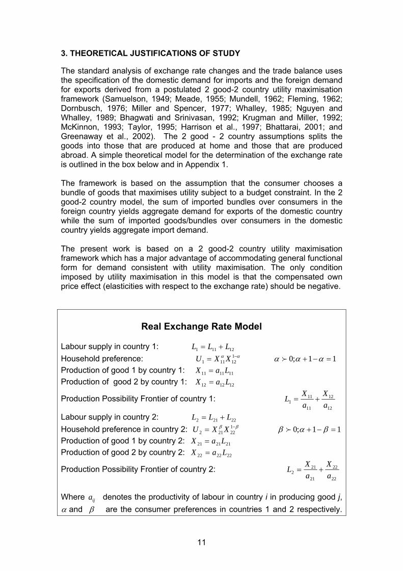
The standard analysis of exchange rate changes and the trade balance uses the specification of the domestic demand for imports and the foreign demand for exports derived from a postulated 2 good-2 country utility maximisation framework (Samuelson, 1949; Meade, 1955; Mundell, 1962; Fleming, 1962; Dornbusch, 1976; Miller and Spencer, 1977; Whalley, 1985; Nguyen and Whalley, 1989; Bhagwati and Srinivasan, 1992; Krugman and Miller, 1992; McKinnon, 1993; Taylor, 1995; Harrison et al., 1997; Bhattarai, 2001; and Greenaway et al., 2002). The 2 good - 2 country assumptions splits the goods into those that are produced at home and those that are produced abroad. A simple theoretical model for the determination of the exchange rate is outlined in the box below and in Appendix 1. The framework is based on the assumption that the consumer chooses a bundle of goods that maximises utility subject to a budget constraint. In the 2 good-2 country model, the sum of imported bundles over consumers in the foreign country yields aggregate demand for exports of the domestic country while the sum of imported goods/bundles over consumers in the domestic country yields aggregate import demand. The present work is based on a 2 good-2 country utility maximisation framework which has a major advantage of accommodating general functional form for demand consistent with utility maximisation. The only condition imposed by utility maximisation in this model is that the compensated own price effect (elasticities with respect to the exchange rate) should be negative.

Real Exchange Rate Model

Labour supply in country 1: 12111 LLL += Household preference: αα −= 1

12111 XXU 11;0 =−+ ααα f Production of good 1 by country 1: 111111 LaX = Production of good 2 by country 1: 121212 LaX =

Production Possibility Frontier of country 1: 12

12

11

111 a

XaXL +=

Labour supply in country 2: 22212 LLL += Household preference in country 2: ββ −= 1

22212 XXU 11;0 =−+ βαβ f

Production of good 1 by country 2: 212121 LaX = Production of good 2 by country 2: 222222 LaX =

Production Possibility Frontier of country 2: 22

22

21

212 a

XaXL +=

Where denotes the productivity of labour in country i in producing good j, ijaα and β are the consumer preferences in countries 1 and 2 respectively.

11

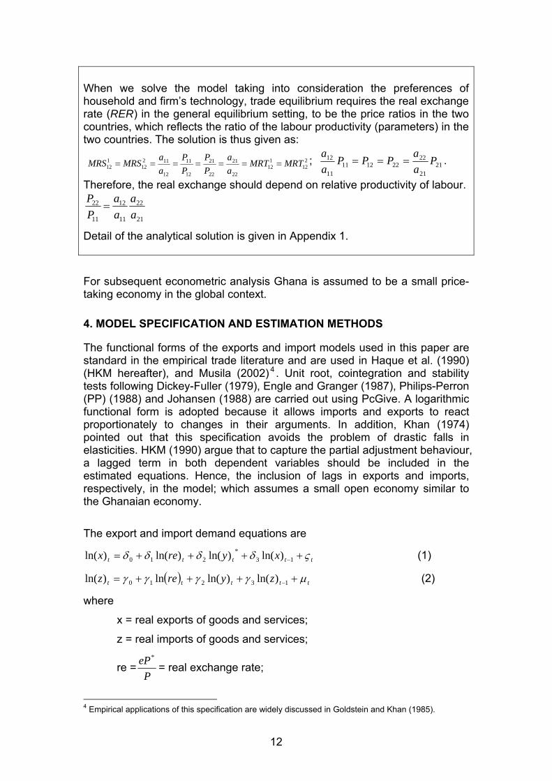
When we solve the model taking into consideration the preferences of household and firm’s technology, trade equilibrium requires the real exchange rate (RER) in the general equilibrium setting, to be the price ratios in the two countries, which reflects the ratio of the labour productivity (parameters) in the two countries. The solution is thus given as:

212

112

22

21

22

21

12

11

12

11212

112 MRTMRT

aa

PP

PP

aa

MRSMRS ======= ; 2121

22221211

11

12 PaaPPP

aa

=== .

Therefore, the real exchange should depend on relative productivity of labour.

Detail of the analytical solution is given in Appendix 1.

21

22

11

12

11

22

aa

aa

PP

=

For subsequent econometric analysis Ghana is assumed to be a small price-taking economy in the global context.

4. MODEL SPECIFICATION AND ESTIMATION METHODS

The functional forms of the exports and import models used in this paper are standard in the empirical trade literature and are used in Haque et al. (1990) (HKM hereafter), and Musila (2002) 4 . Unit root, cointegration and stability tests following Dickey-Fuller (1979), Engle and Granger (1987), Philips-Perron (PP) (1988) and Johansen (1988) are carried out using PcGive. A logarithmic functional form is adopted because it allows imports and exports to react proportionately to changes in their arguments. In addition, Khan (1974) pointed out that this specification avoids the problem of drastic falls in elasticities. HKM (1990) argue that to capture the partial adjustment behaviour, a lagged term in both dependent variables should be included in the estimated equations. Hence, the inclusion of lags in exports and imports, respectively, in the model; which assumes a small open economy similar to the Ghanaian economy.

The export and import demand equations are

ttttt xyrex ςδδδδ ++++= −13*

210 )ln()ln()ln()ln( (1)

( ) ttttt zyrez μγγγγ ++++= −13210 )ln()ln(ln)ln( (2)

where

x = real exports of goods and services;

z = real imports of goods and services;

re =P

eP*

= real exchange rate;

4 Empirical applications of this specification are widely discussed in Goldstein and Khan (1985).

12

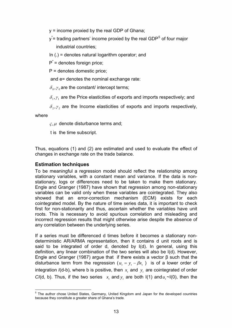
y = income proxied by the real GDP of Ghana;

y*= trading partners’ income proxied by the real GDP5 of four major

industrial countries;

ln (.) = denotes natural logarithm operator; and

P* = denotes foreign price;

P = denotes domestic price;

and e= denotes the nominal exchange rate:

00 ,γδ are the constant/ intercept terms;

11 ,γδ are the Price elasticities of exports and imports respectively; and

22 ,γδ are the Income elasticities of exports and imports respectively,

where

μς , denote disturbance terms and;

t is the time subscript.

Thus, equations (1) and (2) are estimated and used to evaluate the effect of changes in exchange rate on the trade balance.

Estimation techniques To be meaningful a regression model should reflect the relationship among stationary variables, with a constant mean and variance. If the data is non-stationary, logs or differences need to be taken to make them stationary. Engle and Granger (1987) have shown that regression among non-stationary variables can be valid only when these variables are cointegrated. They also showed that an error-correction mechanism (ECM) exists for each cointegrated model. By the nature of time series data, it is important to check first for non-stationarity and thus, ascertain whether the variables have unit roots. This is necessary to avoid spurious correlation and misleading and incorrect regression results that might otherwise arise despite the absence of any correlation between the underlying series. If a series must be differenced d times before it becomes a stationary non-deterministic AR/ARMA representation, then it contains d unit roots and is said to be integrated of order d, denoted by I(d). In general, using this definition, any linear combination of the two series will also be I(d). However, Engle and Granger (1987) argue that if there exists a vector β such that the disturbance term from the regression ( ttt xyu β−= ) is of a lower order of integration I(d-b), where b is positive, then and are cointegrated of order CI(d, b). Thus, if the two series and are both I(1) and ~I(0), then the

tx ty

tx ty tu

5 The author chose United States, Germany, United Kingdom and Japan for the developed countries because they constitute a greater share of Ghana’s trade.

13

two series would be cointegrated of order CI(1, 1). The cointegration of and also implies the existence of a restriction on the standard vector autoregressive (VAR) model and therefore, the estimates obtained from the VAR can be misleading (Engle and Granger (1987)). They further argue that when and are cointegrated then the relationship between them can be expressed as an error-correction model (ECM) and estimated correctly. With this context, a more appropriate simple dynamic representation of the ECM is of the form:

ty

tx

ty tx

( ) ( ) ( )[ ] tptpttt xyxLByLA ωββπμ +−−−−Δ+=Δ −− 10

ˆˆ1 (3)

where A (L) is the polynomial lag operator ; B(L) is the

lag polynomial operator ;

pp LLL ααα −−−− ...1 2

21

pp LLL γγγγ ++++ ...2

210 pαααπ +++= ...21 ; ∆ is

the first difference operator; is a vector in the cointegrating equation; β̂,,αμ and γ are coefficients; ω is the error term and ( )π−1 term provides

information on the speed of adjustment of the level variables. This is the preferred representation for estimation since it incorporates both short and long-run effects6. We start by checking the order of integration of the variables. This is reported in Table 2. The Augmented Dickey-Fuller test is used for this purpose, with sufficient lags to whiten the residuals. The results indicate a unit root in the original series but stationarity in the first difference in all of the series. Thus, the level variables are integrated to order one represented as I(1) (See Table 2). The lag length (the value of p) was set by the R2 approach. This approach uses the model selection procedure that tests to see if an additional lag is statistically significant. Harris (1995) argues that this procedure of selecting a lag length is consistent with the formula reported in Schwert (1989) i.e.

( ){ }4/112 100/12int Tl = and the Philips-Perron (PP) tests.7

5. DATA AND ECONOMETRIC ANALYSIS

The data used in this study was obtained from the World Bank CD-ROM (2000), IFS Yearbook 2001 and IMF Direction of Trade Statistics (DOTS). All the variables are real and in logs. The frequency of the data used is annual and runs from 1970 to 2000. The variables used as fundamentals were determined by three basic considerations, namely; the availability of data,

6 Harris (1985) has pointed out that using the dynamic modelling procedure results in a more powerful test for cointegration as well as giving generally unbiased estimates of the long-run relationship and the standard t statistics for conducting statistical hypothesis testing. He attributes it to the dynamic model not pushing the short-run dynamics into the residual term of the estimated OLS regression. 7 Indeed, in the estimation of the UK money demand, the DF test for interest rate R, was based on the significant lagged and found to be important for the test of unit root. Similar results were obtained when lag length was set by the l12 formula. See Harris, (1995).

14

theory, and the fact that the variable would fit well in the model in statistical terms. In most theoretical studies, the real exchange rate is defined as the ratio of the prices of tradable to non-tradable goods. The real exchange rate was

constructed as re =P

eP*

, where e is the official (nominal) exchange rate, P* is

proxied by the trading partners’ trade weighted GDP deflator, and P is approximated by Ghana’s GDP deflator. The definitions of exports and imports of goods and services are based on the national accounts and the definition as contained in the IMF Direction of Trade Statistics (DOTS), and the World Bank CD-ROM (2002). As has been established already, the variables are integrated of order I(1) at the 5% and 1% significance levels. A dummy variable D91 was used to account for the effect of reforms, notably in exchange rates and trade.8

A cointegration analysis using the Engle and Granger (1987) procedure to determine the long-run relationship between the variables was conducted. Having confirmed the variables were cointegrated, we then applied the error correction model to estimate equations (1) and (2) as set out in section 4. We used PcGive version 10.3 econometric software package for the estimation.

Table 2. Unit Root Test of Variables (level and first differenced): Annual Data, 1970-2000

Variable Lags DF/ADF Order of Integration

lnx ∆lnx

lnz ∆lnz

lnre ∆lnre

lnrei ∆lnrei

lny ∆lny

lny* ∆lny*

2 1

2 1

1 1

1 1

2 1

1 1

-0.533 -3.420*

-0.4706 -3.663*

-1.289 -3.868**

-1.289 -3.868**

-0.3890 -3.101*

-1.628 -5.978**

I(1) I(0)

I(1) I(0)

I(1) I(0)

I(1) I(0)

I(1) I(0)

I(1) I(0)

Notes: DF/ADF - Dickey Fuller/Augmented Dickey Fuller; **Significant at 1%; *Significant at 5%. y* is the real GDP of Ghana’s major trading partners in industrial countries.

8 Exchange rate and trade reforms included the gradual abolition of the controlled rate regime to a somewhat managed rate regime and the abolition of extra tariffs on importables.

15

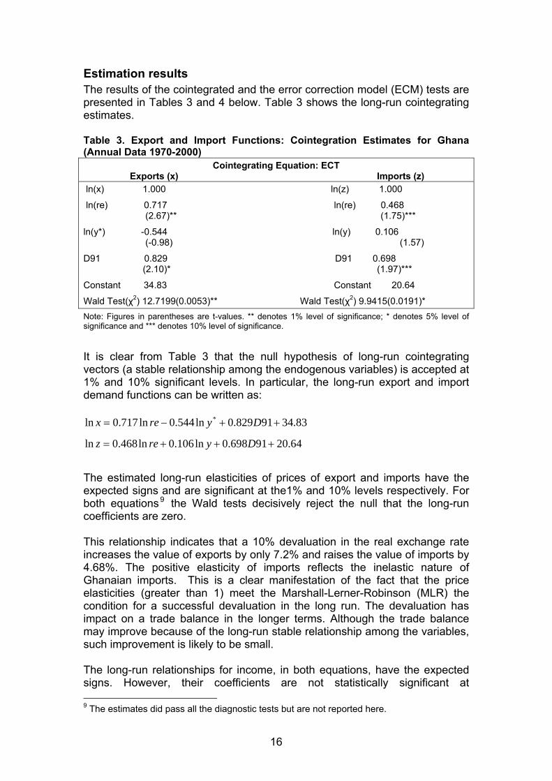
Estimation results The results of the cointegrated and the error correction model (ECM) tests are presented in Tables 3 and 4 below. Table 3 shows the long-run cointegrating estimates. Table 3. Export and Import Functions: Cointegration Estimates for Ghana (Annual Data 1970-2000)

Cointegrating Equation: ECT Exports (x) Imports (z) ln(x) 1.000 ln(z) 1.000

ln(re) 0.717 ln(re) 0.468 (2.67)** (1.75)***

ln(y*) -0.544 ln(y) 0.106 (-0.98) (1.57)

D91 0.829 D91 0.698 (2.10)* (1.97)***

Constant 34.83 Constant 20.64

Wald Test(χ2) 12.7199(0.0053)** Wald Test(χ2) 9.9415(0.0191)* Note: Figures in parentheses are t-values. ** denotes 1% level of significance; * denotes 5% level of significance and *** denotes 10% level of significance.

It is clear from Table 3 that the null hypothesis of long-run cointegrating vectors (a stable relationship among the endogenous variables) is accepted at 1% and 10% significant levels. In particular, the long-run export and import demand functions can be written as:

83.3491829.0ln544.0ln717.0ln * ++−= Dyrex

64.2091698.0ln106.0ln468.0ln +++= Dyrez

The estimated long-run elasticities of prices of export and imports have the expected signs and are significant at the1% and 10% levels respectively. For both equations9 the Wald tests decisively reject the null that the long-run coefficients are zero. This relationship indicates that a 10% devaluation in the real exchange rate increases the value of exports by only 7.2% and raises the value of imports by 4.68%. The positive elasticity of imports reflects the inelastic nature of Ghanaian imports. This is a clear manifestation of the fact that the price elasticities (greater than 1) meet the Marshall-Lerner-Robinson (MLR) the condition for a successful devaluation in the long run. The devaluation has impact on a trade balance in the longer terms. Although the trade balance may improve because of the long-run stable relationship among the variables, such improvement is likely to be small. The long-run relationships for income, in both equations, have the expected signs. However, their coefficients are not statistically significant at 9 The estimates did pass all the diagnostic tests but are not reported here.

16

conventional levels. The relationship indicates that a 10% increase in the real incomes of the major trading partners of Ghana (industrial countries) i.e. foreign income, would reduce the value of Ghana’s exports by about 5.44 percentage points while a 10% increase in the real income of Ghana also increases the value of its imports by just 1% (0.106) in the long run. The inclusion of the dummy (D91) to reflect the impact of the reforms is effective. In particular, the coefficients have the expected signs and are significant at conventional levels (See Table 3). This result shows the effect of the structural changes that have taken place in the Ghanaian economy as a result of the reforms. In a nutshell, the real exchange rate rather than the real incomes are important in the determination of the export and import demand for Ghana in the long run. It is also clear that the very high magnitude of the elasticities with respect to the exchange rate suggests that exchange rate policies somehow have been effective, but they alone would not improve the trade balance unless it is pursued with other policies notably, appropriate aggregate-demand policies. The unit root tests indicate that the short-run dynamic model must be specified in the differences of the relevant variables. The results of the estimated short-run export and import demand functions are presented in Table 4. Table 4. Short-Run Estimates: Error Correction Model (ECM) (Annual Data 1970-2000)

Error Correction Model :ECT Dependent variable =∆ln(x) Dependent variable=∆ln(z) ∆ln(re)-2 0.161 ∆lnre-2 0.192 (2.37) * (2.87)**

∆ln(y*)-2 - 0.019 ∆ln(y)-2 0.007 (-0.118) (0.04)

∆ln(x)-2 -0.171 ∆ln(z)-2 -0.254 (-1.09) (-1.51)

ECT -0.846 ECT -0.003 (-4.16)** (0.013)

D91 0.151 D91 0.139 (2.64) * (2.13)*

Notes: Figures in parentheses are t-values; ** denotes 1% level of significance;* denotes 5% level of significance.

Diagnostics Exports R2 =0.582; FPE =0.0194033; SE =0.126409; F (5, 22) =6.131[0.001]; Far (2, 20) =0.34181 [0.7146]; Farch (1, 20) =0.058094 [0.8120]; Fhet (9, 12) =1.2585 [0.3477]; RESET F (1, 21) =11.584 [0.0027]; Normality (2) =3.0523 [0.2174].

17

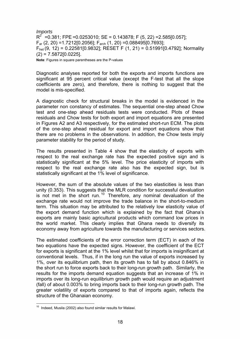
Imports R2 =0.381; FPE =0.0253010; SE = 0.143878; F (5, 22) =2.585[0.057]; Far (2, 20) =1.7212[0.2056]; Farch (1, 20) =0.088495[0.7693]; Fhet (9, 12) = 0.22581[0.9832]; RESET F (1, 21) = 0.51991[0.4792]; Normality (2) = 7.5872[0.0225]. Note: Figures in square parentheses are the P-values Diagnostic analyses reported for both the exports and imports functions are significant at 95 percent critical value (except the F-test that all the slope coefficients are zero), and therefore, there is nothing to suggest that the model is mis-specified. A diagnostic check for structural breaks in the model is evidenced in the parameter non constancy of estimates. The sequential one-step ahead Chow test and one-step ahead residuals tests were conducted. Plots of these residuals and Chow tests for both export and import equations are presented in Figures A2 and A3 respectively, for the estimated short-run ECM. The plots of the one-step ahead residual for export and import equations show that there are no problems in the observations. In addition, the Chow tests imply parameter stability for the period of study. The results presented in Table 4 show that the elasticity of exports with respect to the real exchange rate has the expected positive sign and is statistically significant at the 5% level. The price elasticity of imports with respect to the real exchange rate also has the expected sign, but is statistically significant at the 1% level of significance. However, the sum of the absolute values of the two elasticities is less than unity (0.353). This suggests that the MLR condition for successful devaluation is not met in the short run. 10 Therefore, any nominal devaluation of the exchange rate would not improve the trade balance in the short-to-medium term. This situation may be attributed to the relatively low elasticity value of the export demand function which is explained by the fact that Ghana’s exports are mainly basic agricultural products which command low prices in the world market. This clearly implies that Ghana needs to diversify its economy away from agriculture towards the manufacturing or services sectors. The estimated coefficients of the error correction term (ECT) in each of the two equations have the expected signs. However, the coefficient of the ECT for exports is significant at the 1% level whilst that for imports is insignificant at conventional levels. Thus, if in the long run the value of exports increased by 1%, over its equilibrium path, then its growth has to fall by about 0.846% in the short run to force exports back to their long-run growth path. Similarly, the results for the imports demand equation suggests that an increase of 1% in imports over its long-run equilibrium growth path would require an adjustment (fall) of about 0.003% to bring imports back to their long-run growth path. The greater volatility of exports compared to that of imports again, reflects the structure of the Ghanaian economy. 10 Indeed, Musila (2002) also found similar results for Malawi.

18

The results indicate that foreign income, though negatively related to Ghanaian exports, is not significantly different from zero and therefore, not an important determinant of export demands in the short run. The results further show that domestic income is also not an important determinant of import demand. It has the expected sign but is significantly not different from zero. One possible explanation might be that both exports and imports are inelastic relative to domestic and foreign income. These low income elasticities indicate that Ghanaian exports are an inferior commodity in the global market. The growth of income in the rest of the world does not transmit to Ghana. Ghana’s exports consist mostly of basic agricultural produce that is not processed and it is therefore subject to the dictates of its trading partners in the international market. Another possible explanation is that Ghana’s imports might not depend on its past income and therefore does not need to do more to strengthen its exports with its trading partners. Again, the result shows that the real exchange rate in the short run does affect the export and import demand. This might be explained by the rapid fluctuations in the nominal exchange rate (devaluations) that have occurred with its concomitant increases in price levels. As has been stated earlier, the dummy variable D91 is included to capture the impact of the economic reforms (exchange rates and trade policy reforms) through the implementation of the ERP/SAP. As expected, the overall impact of the reform was positive for exports, reflecting the significant structural change in the demand for exports. The implementation of the reforms also impacted positively on imports with a significant structural shift occurring in import demand as well (refer to coefficient of D91 in Table 4). Increased exports were accompanied by increased imports. Accordingly, the reforms embarked on by the government (trade and exchange rate) since 1983 did open up the economy in terms of trade (see Tables A2 and A4). However, the reforms did not improve the trade balance in the short run as expected (see Figure A1).

Impulse response analysis of Ghanaian trade: cointegrated VAR analysis Due to the likelihood of simultaneity bias in the use of the single equation procedure, we employed the multiple estimation method to correct it. In employing the (1995) procedure, to determine the number of cointegrating vectors, we first estimated the unrestricted VAR with sufficient lags to whiten the residuals. We started with a lag length of three and these were pared down after checking the significance levels of the coefficients. The F-test for reducing the number of lags from three to two is accepted.

We also checked the properties of the residual in the preferred VAR model. The diagnostic tests are presented in Table 5a. The table reports individual tests for exports and imports and also the system wide test. The test results show that they are all insignificant at the 5% level.

19

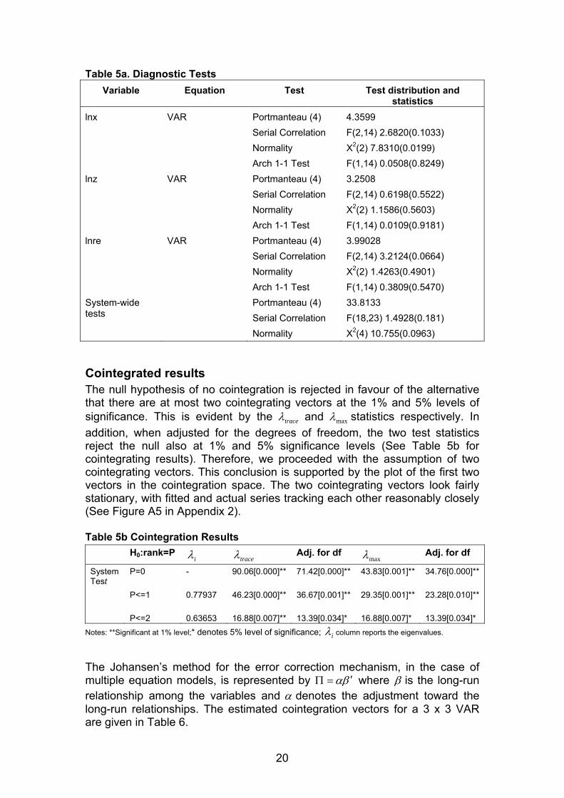
Table 5a. Diagnostic Tests Variable Equation Test Test distribution and

statistics lnx lnz lnre System-wide tests

VAR VAR VAR

Portmanteau (4) Serial Correlation Normality Arch 1-1 Test Portmanteau (4) Serial Correlation Normality Arch 1-1 Test Portmanteau (4) Serial Correlation Normality Arch 1-1 Test Portmanteau (4) Serial Correlation Normality

4.3599 F(2,14) 2.6820(0.1033) Χ2(2) 7.8310(0.0199) F(1,14) 0.0508(0.8249) 3.2508 F(2,14) 0.6198(0.5522) Χ2(2) 1.1586(0.5603) F(1,14) 0.0109(0.9181) 3.99028 F(2,14) 3.2124(0.0664) Χ2(2) 1.4263(0.4901) F(1,14) 0.3809(0.5470) 33.8133 F(18,23) 1.4928(0.181) Χ2(4) 10.755(0.0963)

Cointegrated results The null hypothesis of no cointegration is rejected in favour of the alternative that there are at most two cointegrating vectors at the 1% and 5% levels of significance. This is evident by the traceλ and maxλ statistics respectively. In addition, when adjusted for the degrees of freedom, the two test statistics reject the null also at 1% and 5% significance levels (See Table 5b for cointegrating results). Therefore, we proceeded with the assumption of two cointegrating vectors. This conclusion is supported by the plot of the first two vectors in the cointegration space. The two cointegrating vectors look fairly stationary, with fitted and actual series tracking each other reasonably closely (See Figure A5 in Appendix 2). Table 5b Cointegration Results H0:rank=P

iλ traceλ Adj. for df maxλ Adj. for df

System Test

P=0 P<=1 P<=2

- 0.77937 0.63653

90.06[0.000]** 46.23[0.000]** 16.88[0.007]**

71.42[0.000]** 36.67[0.001]** 13.39[0.034]*

43.83[0.001]** 29.35[0.001]** 16.88[0.007]*

34.76[0.000]** 23.28[0.010]** 13.39[0.034]*

Notes: **Significant at 1% level;* denotes 5% level of significance; iλ column reports the eigenvalues.

The Johansen’s method for the error correction mechanism, in the case of multiple equation models, is represented by βα ′=Π where β is the long-run relationship among the variables and α denotes the adjustment toward the long-run relationships. The estimated cointegration vectors for a 3 x 3 VAR are given in Table 6.

20

Table 6. Normalised (to diagonal) Cointegrating Vectors lnx lnz ln(re) ln(y)-1

ln(y)-2

L(y*)-1

L(y*)-2

D91 Trend

1.0000 -1.6080 -0.075171 0.84993 -0.0091221 0.026187 0.29997 -0.20073 0.24387

-0.84632 1.0000 -0.36554 0.93255 -0.89787 1.3107 0.44759 0.27205 -0.065084

-0.80383 -0.36484 1.0000 1.3207 1.3309 -0.66011 -0.95487 -0.35635 0.77065

The long-run general joint restriction that the lags of the explanatory variables are the same, and the hypothesis that there is no trend in the original series, is strongly rejected. The static long-run relationship for export and import demand functions respectively, as presented in Table 7 can be written as:

31.7058630.0910330.0*ln9875.1ln +++= TrendDyx

03.4652139.0911201.0ln0271.2ln ++−= TrendDyz

72.8710914.09133908.0*ln6748.3ln0347.0ln ++++= TrendDyyre Impulse response functions are presented in Figure A6 in Appendix 2. A shock to the export function largely reflects similar hump-shaped response in both the exports and imports. Although exports fall immediately, imports first rise by 75% and fall gradually. The real exchange rate falls sharply and then begins to rise (hump-shaped as well). Evidently, little similar dynamics can be observed between the response in the export and import functions as a result of a shock to the system. Table 7. Long-run Cointegrating Equations in VAR (Exports, Imports and Real Exchange Rate)

Export (x) Imports(z) Real Exchange Rate(re)

lny

lny*

D91

Trend

Constant

- 1.9875

(1.8014)

0.0330

(0.72117)

0.58630

(0.39232)

70.31

2.0271

(1.8014)

-

-0.1201

(0.45896)

0.52139

(0.24968)

46.03

0.03476

(1.1586)

3.6748

(1.4035)

0.33908

(0.56188)

-0.10914

(0.30567)

87.72 Notes: Figures in parentheses are the standard errors Indeed, an unanticipated increase in the real exchange rate shows export and imports behaved similarly (increase) while the real exchange rate decreases.

21

6. SUMMARY AND POLICY ISSUES

This paper set out to examine the effects of the exchange rate on the trade balance of Ghana. Cointegrating and error correction modelling techniques have been used to estimate the demand equations for exports and for imports. The data used is an annual observation obtained from the Direction of Trade Statistics (DOTS), various issues and the World Bank CD-ROM World Development Indicators, 2002. The study explored whether the devaluation of the country’s currency (cedi) would improve the trade balance. The results indicate that the price elasticities of the export demand and import demand equations in the long run are consistent with the theoretical predictions of utility maximisation based model which this study adopts. However, the elasticities of exports and imports relative to the real exchange rate in the short-run are very small suggesting supply- and demand-side rigidities in export and import demand flows of Ghana. In the short run, estimated export and import elasticities with respect to the real exchange rate do not satisfy the Marshall-Lerner-Robinson (MLR) condition for a successful devaluation. Therefore, any nominal devaluation of the cedi is bound to weaken the trade balance at least in the short-to-medium term. In the long run, the results show that a stable linear relationship exists among the exports, imports, and trade balance, domestic and foreign income. Ghana has no choice, other than to adhere to the fundamentals of the foreign exchange rate market to solve its perennial problems of deficit, by applying prudent fiscal and monetary policies and exchange rate policies based on purchasing power parity. These policy rules will also improve the confidence of consumers and investors in the economy and improve Ghana’s competitiveness in the global market.

7. CONCLUSION

The results from this study show that the trade balance of Ghana will not improve in the short run unless it adopts policy rules in the foreign exchange market, but it may be costly if such adjustment were to occur unaided, in the long run. The standard theoretical propositions in the trade and exchange rate literature for a small open economy such as Ghana are tested using results from time series based single equation, VAR and cointegration models. The results obtained are very similar to the findings of earlier studies on contractionary devaluation as reported in Khan (1974), Musila (2002), the IMF and the World Bank. However, the estimates for Ghana also show that even in the long run, the MLR condition for a successful devaluation is barely met and therefore, in Ghana’s case the gains would not be enough to offset the losses in the trade balance in the short run. The results also show that in the short-to-medium term, as well as in the long term, income levels are not important determinants either of the import demand or the export demand of Ghana. Imports are inelastic and the exports, being predominantly primary commodities, are an inferior commodity in the global market. The results show that it is the exchange rate that is the significant factor in the short term. In the long run however, the study reveals that only the real exchange rate significantly affects the trade balance.

22

In short, the econometric model shows that the policies that have been adopted by Ghana have not been effective when evaluated in terms of the MLR conditions for a successful devaluation. Furthermore, the model and associated results indicate that more effective policies may be founded on a sharper appreciation of the interaction and the interrelationships between the policy instruments (exchange rate and aggregate demand management) which have been considered here. It would be interesting to see how far these low elasticities relate to the preferences of households, the technology of firms, and policy instruments under consideration by the government, taking account of structural realities of the Ghanaian economy, in order to establish an incentive structure in Ghana that is conducive to macroeconomic stability and higher rate of growth. These issues will be taken up in subsequent work.

23

REFERENCES

Armington, P.S. (1969) A Theory of Demand for Products Distinguished by Place of Production. International Monetary Fund Staff Papers 16, 159-76

Bank of Ghana. (Various issues) Quarterly Journals, Accra Bhagwati, J.N. and Srinivasan, T.N. (1992) Lectures on International Trade.

Cambridge: MIT Press Bhattarai, K. (2001) Welfare Gains to UK from a Global Free Trade. The

European Research Studies IV, 3-4 Buiter, W.H. and Miller, M. (1992) Exchange Rate Economics 1, 233-65.

Aldershot. UK: International Library of Critical Writings in Economics (16) Corden, W.M. (2002) Too Sensational: On the Choice of Exchange Rate

Regimes. Cambridge, MA: MIT Press Dickey, D.A. and Fuller, W.A. (1976) Distribution of Estimators for

Autoregressive Time Series with a Unit Root. Journal of American Statistical Association 74, 427-431

Dornbusch, R. (1976) Expectations and Exchange Rate Dynamics. Journal of Political Economy 84, (6)

Edwards, S. (1999) How Effective are Capital Control? Journal of Economic Perspectives 13, 65-84

Edwards, S. (2002) Capital Mobility, Capital Controls, and Globalisation in the Twenty First Century. The Annals of the American Academy of Political and Social Science 579, 261-70

Engel, R.F. and Granger, C.W.J. (1987) Cointegration and Error Correction: Representation, Estimation and Testing. Econometrica 55, 251-76

Fleming, J.M. (1962) Domestic Financial Policies under Fixed and under Floating Exchange Rates. IMF staff paper 9, (November) 369-379

Goldstein, M. (2002) Managed Floating Plus. Policy Analyses in International Economics. Washington DC: Institute for International Economics

Goldstein, M. and Khan, M.S. (1985) Income and Price Effects in Foreign Trade. In Handbook of International Economics Vol. 2. R.W. Jones and P.B. Kenen (eds), Amsterdam: North-Holland

Goldstein, M. and Isard, P. (1992) Mechanisms for Promoting Global Monetary Stability. In Policy Issues in the Evolving International Monetary System. M. Goldstein, P. Isard, P. Mason and M. Taylor (eds) IMF Occasional Paper 26, Washington, D.C: International Monetary Fund

Greenaway, D., Morgan, W. and Wright, P. (2002) Trade Liberalisation and Growth in Developing Countries. Journal of Development Economics 67, 229-244

Harris, R.I.D. (1985) Interrelated Demand for Factors of Production in the UK Engineering Industry 1968-81. Economic Journal 95, 1049-68

Harris, R. (1995) Using Cointegration Analysis in Econometric Modelling, Harlow: Prentice Hall

Harrison, G.W., Rutherford, T.F. and Tarr, D.G. (1997) Quantifying the Uruguay Round. Economic Journal 107, (444) September, 1405-1430

24

Haque, N.U., Karjal, L. and Montiel, P. (1990) Estimation of Rational Expectations Macroeconomic Model for Developing Counties with Capital Controls. Unpublished; Washington: International Monetary Fund

IMF, Direction of Trade Statistics Reports, various issues, Washington D.C. IMF, International Financial Statistics Yearbook, various issues, Washington

D.C. Johnson H.G. (1954) Optimal Tariffs and Retaliation. Review of Economic

Studies 21, (2) 142-43 Johansen, S. (1988) Statistical Analysis of Cointegration and Statistics

Vectors. Journal of Economic Dynamics and Control 12, 231-54 Johansen, S. (1995) A Statistical Analysis of I(2) Variables. Econometric

Theory 11, 25-59 Khan, M.S. (1974) Imports and Export Demands in Developing Countries,

Staff Papers. International Monetary Fund (Washington) 21, 678-93 Krugman Paul (1979) A Model of Balance of Payment Crisis. Journal of

Money Credit and Banking 11, Aug Krugman, P. and Miller, M. (1992) Exchange Rate Targets and Currency

Bands. The Economic Journal 102, (415) 1548-1550 McKinnon, R.I. (1993) The Order of Economic Liberalization: Financial Control

in the Transition to a Market Economy. Baltimore: JHUP Meade, J.E. (1955) Problems of Economic Union. The American Economic

Review 45, (4) 700-704 Miller, M.H. and Spencer, J.E. (1977) The Static Economic Effects of the UK

Joining the EEC: A General Equilibrium Approach. Review of Economic Studies 44, (Feb. Issue 1) 71-93

Mundell, R.A. (1962) Capital Mobility and Stabilisation Policy under Fixed and Flexible Exchange Rates. Canadian Journal of Economic and Political Science 29, 475-85

Mussa, M. (1976) The Exchange Rate: The Balance of Payments and Monetary and Fiscal Policies under a Regime of Controlled Floating. Scandinavian Journal of Economics 78, (2) 229-248

Mussa, M., Masson, P., Swoboda, A., Jadrestic, E., Mauro, P. and Berg, A. (2000) Exchange Rate Regimes in an Increasingly Integrated World Economy. International Monetary Fund Occasional Paper 193. Washington DC: International Monetary Fund

Mussa, M., Goldstein, M., Clark, P.B., Mathieson, D. and Bayoumi, T. (1994) Improving the International Monetary System: Constraints and Possibilities. International Monetary Fund Occasional Paper 116, Washington DC: International Monetary Fund

Musila, J.W. (2002) Exchange Rate Changes and Trade Balance Adjustments in Malawi. Canadian Journal of Development Studies 23, (1) 69-85

Nguyen, T.T. and Whalley, J. (1989) General Equilibrium Analysis of Black and White Markets: A Computational Approach. Journal of Public Economics 40, 331-347

Oduro, A.D. and Harrigan, J. (2000) Exchange Rate Policy and the Balance of Payments 1972-96. In Economic Reforms in Ghana: The Miracle and the Mirage. E. Aryeetey, J. Harrigan, and M. Nissanke (eds) Oxford: James Currey Ltd

Philips, P.C.B. and Perron, P. (1988) Testing for the Unit Root in Time Series Regression. Biometrica 75, 335-46

25

Samuelson, P.A. (1949) International Factor Price Equalisation. Economic Journal (June) 181-197

Schwert, G.W. (1989) Tests for Unit Roots: A Monte Carlo Investigation. Journal of Business and Economic Statistics 7, 147-59

Singer, H.W. (1950) The Distribution of Trade between Investing and Borrowing Countries. American Economic Review 40, 472-485

Sowa, N.K. and Acquaye, I.K. (1998) Financial and Foreign Exchange Liberalisation in Ghana. Centre for Policy Analysis Research Papers No.10, Accra: CEPA

Tavlas, G.S. and Ulan, M. (eds) (2002) Exchange Rate Regimes and Capital Flows. Special Issue of The Annals of American Academy of Political and Social Science 579, Philadelphia

Tavlas, S. (2003) The Economics of Exchange Rate Regimes: A Review Essay. Oxford: Blackwell Publishing Ltd

Taylor, M. (1995) The Economics of Exchange Rates. Journal of Economic Literature 33, (March No. 1) 13-47

Whalley, J. (1985) Trade Liberalization among Major World Trading Areas. Cambridge: MIT Press

World Bank CD-ROM (2002) World Development Indicators. Washington D.C: World Bank

26

APPENDIX 1: Determination of Real Exchange Rate as a Function of Preferences, Technology and Endowments between two Countries Country 1 (Ghana) Country 2 (Rest of the World) By optimising using the Lagrangian procedure, we have:

⎥⎦

⎤⎢⎣

⎡−−+=∠ −

12

12

11

111

112111 a

XaX

LXX λαα

011

112

111

11

1 =−=∂∂∠ −−

aXX

Xλα αα (1a)

0)1(12

121112

1 =−−=∂∂∠ −

aXX

Xλα αα (1b)

(1a)/(1b)

11

12

11

12112

11

12112 1 P

PaaMRT

XXMRS ===⎟

⎠⎞

⎜⎝⎛−

=α

α

1111

1212

1 XaaX ⎟

⎠⎞

⎜⎝⎛ −

=αα (1c)

but,

111211

12

11

111

1 Xaa

aaXL ⎟

⎠⎞

⎜⎝⎛ −

+=αα

By substitution, we have

= ( ) a1X111

1111

111111 ⎟⎟

⎠

⎞⎜⎜⎝

⎛=⎟⎟

⎠

⎞⎜⎜⎝

⎛ −+

ααα

aaX

11111 LaX α= (1d) substituting (1d) into (1c), results

11111

1212

1 LaaaX α

αα⎟⎠⎞

⎜⎝⎛ −

=

( ) 11212 1 LaX α−= ( )

11

12

11

12 1PP

XX

αα−

=

11

12

11

12112 a

aPPMRS ==

Again, using the Lagrangian procedure, we have:

⎥⎦

⎤⎢⎣

⎡−−+=∠ −

22

22

21

212

122212 a

XaX

LXX λββ

021

122

121

21

2 =−=∂∂∠ −−

aXX

Xλβ ββ (2a)

0)1(22

222122

2 =−−=∂∂∠ −

aXX

Xλβ ββ (2b)

(2a)/(2b)

22

21212

21

22

21

22212 1 P

PMRTaa

XXMRS ===⎟⎟

⎠

⎞⎜⎜⎝

⎛−

=β

β

2121

2222

1 XaaX ⎟⎟

⎠

⎞⎜⎜⎝

⎛ −=

ββ (2c)

but,

22

22

21

212 a

XaXL +=

By substitution, we have

= ( )⎟⎟⎠

⎞⎜⎜⎝

⎛=⎟⎟

⎠

⎞⎜⎜⎝

⎛ −+

2121

212121

1111a

Xaa

Xββ

β

22121 LaX β= (2d) substituting (2d) into (2c), results

22121

2222

1 LaaaX β

ββ⎟⎟⎠

⎞⎜⎜⎝

⎛ −=

( ) 22222 1 LaX β−=

( ) 22

21

22

21

1 PP

XX

ββ−

=

22

21

22

21221 a

aPPMRS ==

Global market clearing: 12111 XXX =+ , 2111 PP =

212

112

22

21

22

21

12

11

12

11212

112 MRTMRT

aa

PP

PP

aaMRSMRS ======= ;

22212 XXX =+ , 2212 PP = 2121

22221211

11

12 PaaPPP

aa

=== 21

22

12

11

22

11

aa

aa

PP

=

27

APPENDIX 2: Tables and Figures Table A1. Balance of Payments of Ghana, 1994-2000 (US$m) 1994 1995 1996 1997 1998 1999 2000

current account

bal(incl. grant )

(%GDP)

exports (%GDP) of which: cocoa total (% contribution) minerals(incl.Gold) (% contribution) timber total (% contribution) other non traditional products (%contribution) Imports (% GDP) Trade Balance *(% GDP) Services Balance (% GDP) Capital account bal.(incl.errors & omissions) *(% GDP) overall Balance *(% GDP) GDP Financing domestic foreign

-254.6

4.68

1542.4 25.3

320.2 25.9

588.2 13.4

165.4 13.4

86.6 6.9

2022.2 32.56

-615.5

9.9

-273.3 4.4

1.0 0.016

172.1 2.77

6209.1

-26.7 -85.0

-144.7 2.24

1582.7

24.5

389.5 27.2

678.8 13.3

190.6 13.3

100 6.9

2126.2 32.93

-538.7

8.3

-282.1 4.38

1.0 0.015

250.8 3.88

6457.4

-27.7 -42.6

-324.7 4.68

2256.0

32.1

552.1 35.1

641.4 9.3

146.8 9.3

143.6

9.2

2777.3 40.09

-666.5

9.9

-299.6 4.4

1.0 0.015

-20.4 0.30

6754.6

531.1 -195.7

-549.7 7.98

2345.5

32.4

470.0 31.6

613.0 11.5

172.0 11.5

157.1 10.5

3823.8 52.99

-978.4 13.9

-340.1

4.8

1.0 0.014

26.7 0.38

7038.1

728.0 -430.3

-443.1 5.92

2596.3

33.9

617.4 34.1

717.8 9.4

171.0 9.4

228 12.6

4131.6 46.74

-104.1 1.41

-235.0

3.2

1.0 0.014

107.9 1.46

7368.9

672.6 -376.2

-932.5 11.9

2910.2

31.9

N/A N/A N/A N/A N/A N/A

N/A N/A

4583.8 49.21

-142.1 1.84

-198.1

2.6

1.0 0.013

-89.6 1.17

7693.6

N/A N/A

-412.6 7.94

2843.9

49.2

N/A N/A N/A N/A N/A N/A

N/A N/A

3790.8 69.59

-935.9 11.7

-93.0 1.2

1.0 0.013

-258.5 3.24

7978.3

N/A N/A

Source: World Bank CD Rom (2002) University of Hull; IFS Yearbook 2001. * Percentage figures calculated by author using GDP values obtained from the World Bank CD Rom, 2002.

28

Table A2. Ghana’s Trade Analysis (1994-2000) 1994 1995 1996 1997 1998 1999 2000

Exports (%)

Indust. countries of

which:

United States

United Kingdom

Germany

Japan

Develop. countries

of which:

Nigeria

Cote d’voire

Togo

Imports (%)

Indust. countries

of which:

United States

United Kingdom

Germany

Japan

Develop. countries

of which:

Nigeria

Cote d’voire

Togo

100

72.5

12.6 13.0

14.8 3..9

23.4

2.8 0.2 0.4

100

59.8

6.7 15.8

5.6 6.8

39.1

17 3.2 0.4

100

70.3

11.3 14.4

11.8 3..9

25.1

2.9 0.5 0.4

100

57.6

6.8 16.4

7.6 4.0

41.3

15.3 4.0 0.4

100

67.0

9.5 15.6

8.9 3.8

27.8

3.0 0.3 0.5

100

61.3

10.2 16.2

5.4 3.4

37.7

13.4 4.3 0.4

100

63.6

8.3 11.6

9.1 4.4

30.8

3.4 0.1 0.5

100

59.7

10.5 15.1

6.0 2.5

39.3

14.3 5.1 0.4

100

64.9

7.1 11.8

6.8 3.3

29.5

3.2 0.1 0.6

100

56.1

7.2 11.8

5.0 2.6

42.8

14.2 8.1 0.5

100

62.7

9.3 11.4

5.0 2.9

31.3

3.1 0.1 0.5

100

55.3

8.2 9.7

5.6 3.0

43.5

15.0 4.7 0.5

100

58.8

11.3 7.6

6.2 2.5

33.8

4.3 0.1 0.4

100

51.9

6.6 9.0

4.5 1.5

46.6

19.3 4.8 0.6

Percentage figures calculated by author using data from Direction of Trade Statistics (DOTS), various issues.

Table A3. Correlation Matrix for the Endogenous Variables

NER RE EXPORT IMPORT GDP

NER RE EXPORT IMPORT GDP

1

0.985652

0.759654

0.72921

0.873181

1

0.74217

0.680486

0.87579

1

0.909757

0.758854

1

0.747134

1

Notes: NER, RE and GDP denote nominal exchange rate, real exchange rate and gross domestic product respectively.

29

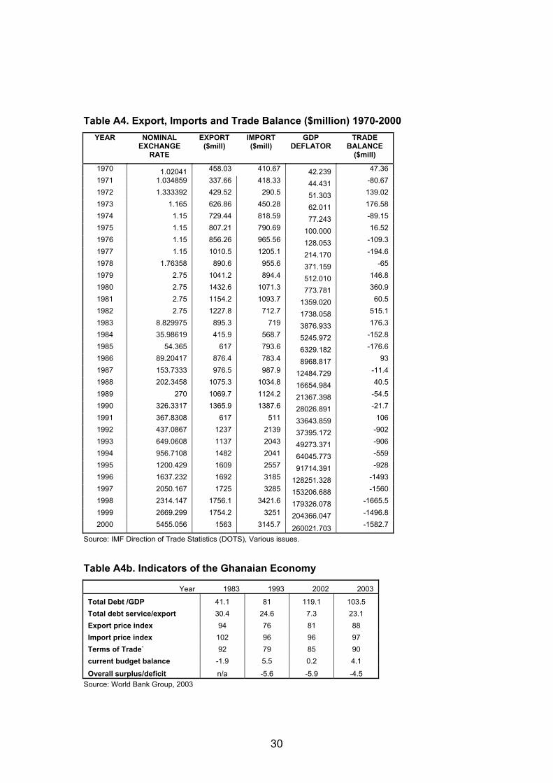
Table A4. Export, Imports and Trade Balance ($million) 1970-2000 YEAR NOMINAL

EXCHANGE RATE

EXPORT ($mill)

IMPORT ($mill)

GDP DEFLATOR

TRADE BALANCE

($mill)

1970 1.02041 458.03 410.67 42.239 47.36 1971 1.034859 337.66 418.33 44.431 -80.67 1972 1.333392 429.52 290.5 51.303 139.02 1973 1.165 626.86 450.28 62.011 176.58 1974 1.15 729.44 818.59 77.243 -89.15 1975 1.15 807.21 790.69 100.000 16.52 1976 1.15 856.26 965.56 128.053 -109.3 1977 1.15 1010.5 1205.1 214.170 -194.6 1978 1.76358 890.6 955.6 371.159 -65 1979 2.75 1041.2 894.4 512.010 146.8 1980 2.75 1432.6 1071.3 773.781 360.9 1981 2.75 1154.2 1093.7 1359.020 60.5 1982 2.75 1227.8 712.7 1738.058 515.1 1983 8.829975 895.3 719 3876.933 176.3 1984 35.98619 415.9 568.7 5245.972 -152.8 1985 54.365 617 793.6 6329.182 -176.6 1986 89.20417 876.4 783.4 8968.817 93 1987 153.7333 976.5 987.9 12484.729 -11.4 1988 202.3458 1075.3 1034.8 16654.984 40.5 1989 270 1069.7 1124.2 21367.398 -54.5 1990 326.3317 1365.9 1387.6 28026.891 -21.7 1991 367.8308 617 511 33643.859 106 1992 437.0867 1237 2139 37395.172 -902 1993 649.0608 1137 2043 49273.371 -906 1994 956.7108 1482 2041 64045.773 -559 1995 1200.429 1609 2557 91714.391 -928 1996 1637.232 1692 3185 128251.328 -1493 1997 2050.167 1725 3285 153206.688 -1560 1998 2314.147 1756.1 3421.6 179326.078 -1665.5 1999 2669.299 1754.2 3251 204366.047 -1496.8 2000 5455.056 1563 3145.7 260021.703 -1582.7

Source: IMF Direction of Trade Statistics (DOTS), Various issues.

Table A4b. Indicators of the Ghanaian Economy

Year 1983 1993 2002 2003

Total Debt /GDP 41.1 81 119.1 103.5 Total debt service/export 30.4 24.6 7.3 23.1 Export price index 94 76 81 88 Import price index 102 96 96 97 Terms of Trade` 92 79 85 90 current budget balance -1.9 5.5 0.2 4.1

Overall surplus/deficit n/a -5.6 -5.9 -4.5 Source: World Bank Group, 2003

30

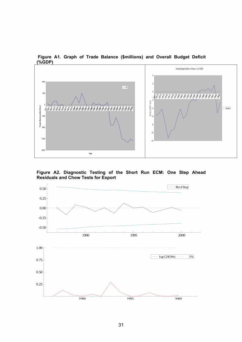
Figure A1. Graph of Trade Balance ($millions) and Overall Budget Deficit (%GDP)

-2000

-1500

-1000

-500

0

500

1000

1970

Year

Trad

e B

alan

ce($

mill

ion)

TB

Overall Budget Deficit in Ghana ( % of GDP)

-12

-10

-8

-6

-4

-2

0

2

4

1972

Def

icit

GD

P ra

tio

Series1

Figure A2. Diagnostic Testing of the Short Run ECM: One Step Ahead Residuals and Chow Tests for Export

1990 1995 2000

-0.50

-0.25

0.00

0.25

0.50 Res1Step

1990 1995 2000

0.25

0.50

0.75

1.00

1up CHOWs 5%

31

Figure A3. Diagnostic Testing of the Short Run ECM: One Step Ahead Residuals and Chow Tests for Imports

1990 1995 2000

-0.50

-0.25

0.00

0.25

0.50Res1Step

1990 1995 2000

0.25

0.50

0.75

1.00

1up CHOWs 5%

Figure A4. Graph of Export and Import Showing the Trade Gap ($millions)

0

500

1000

1500

2000

2500

3000

3500

4000

1970

1971

1972

1973

1974

1975

1976

1977

1978

1979

1980

1981

1982

1983

1984

1985

1986

1987

1988

1989

1990

1991

1992

1993

1994

1995

1996

1997

1998

1999

2000

Year

Expo

rts

and

Impo

rts

($m

illio

ns)

XZ

32

Figure A5. Graph of Cointegrating Vectors

1970 1980 1990 2000

-0.25

0.00

0.25

vector1

1970 1980 1990 2000

-0.50

-0.25

0.00

0.25

0.50vector2

1970 1980 1990 2000

-0.5

0.0

0.5

fitted Lx

1970 1980 1990 2000

-0.5

0.0

0.5

fitted Lz

Figure A6. Impulse Response Analysis from the Reduced Form VAR Model

0 20

-0.1

0.0

0.1 Lx (Lx eqn)

0 20

-0.05

0.00

0.05

0.10Lz (Lx eqn)

0 20-0.10

-0.05

0.00Lre (Lx eqn)

0 20

-0.05

0.00

0.05

0.10Lx (Lz eqn)

0 20

0.0

0.1 Lz (Lz eqn)

0 20

-0.050

-0.025

0.000Lre (Lz eqn)

0 20

1

2

3Lx (Lre eqn)

0 20

0.5

1.0

1.5

2.0Lz (Lre eqn)

0 20

0.0

0.2

0.4 Lre (Lre eqn)

33

The Business School Research Memorandum Series

Please note that some of these are available at:

http://www.hull.ac.uk/hubs/research/memoranda

52 K. R. Bhattarai and Mark K. Armah (2005) The Effects of Exchange Rate on the Trade Balance on Ghana: Evidence from Cointegration Analysis

51 A. Aritzeta, S. Swailes and B. Senior (2005) Team Roles: Psychometric Evidence, Construct Validity and Team Building

50 Giovan Francesco Lanzara and Michele Morner (2005) Making and Sharing Knowledge at Electronic Crossroads: The Evolutionary Ecology of Open Source

49 Wendy Robson and José Córdoba (2005) What Research Methodology Suits Collaborative Research

48 Keshab R. Bhattarai (2005) Economic Growth: Models and Global Evidence

47 Pat Mould and Tony Boczko (2004) Standard-setting and the Myth of Neutrality: Boundaries, Discourse and the Exercise of Power

46 Peter Murray (2005) ‘Learning’ with Complexity: Metaphors from the New Sciences

45 Hon. Dr. Diodorus Kamala (2004) The Voices of the Poor and Poverty Eradication Strategies in Tanzania

44 Michael R. Ryan (2003) Vertical Integration Results and Applications to the Regulation of Supermarket Activity

43 Michael A. Nolan and Felix R. Fitzroy (2003) Inactivity, Sickness and Unemployment in Great Britain: Early Analysis at the Level of Local Authorities

42 Keshab R Bhattarai (2003) An Analysis of Interest Rate Determination in the UK and Four Major Leading Economies

41 Keshab R Bhattarai (2004) Macroeconomic Impacts of Consumption and Income Taxes: A General Equilibrium Analysis

40 Juan Paez-Farrell (2003) Business Cycles in the United Kingdom: An Update on the Stylised Facts

39 Juan Paez-Farrell (2003) Endogenous Capital in New Keynesian Models 38 Philip Kitchen, Lynne Eagle, Lawrence Rose and Brendan Moyle (2003)

The Impact of Gray Marketing and Parallel Importing on Brand Equity and Brand Value

37 Marianne Afanassieva (2003) Managerial Responses to Transition in the Russian Defence Industry

36 José-Rodrigo Córdoba-Pachón and Gerald Midgley (2003) Addressing Organisational and Societal Concerns: An Application of Critical Systems Thinking to Information Systems Planning in Colombia

35 Joanne Evans and Richard Green (2003) Why Did British Electricity Prices Fall After 1998?

34

34 Christine Hemingway (2002). An Exploratory Analysis of Corporate Social Responsibility: Definitions, Motives and Values

33 Peter Murray (2002) Constructing Futures in New Attractors 32 Steven Armstrong, Christopher Allinson and John Hayes (2002). An

Investigation of Cognitive Style as a Determinant of Successful Mentor-Protégé Relationships in Formal Mentoring Systems

31 Norman O'Neill (2001) Education and the Local Labour Market 30 Ahmed Zakaria Zaki Osemy and Bimal Prodhan (2001) The Role of

Accounting Information Systems in Rationalising Investment Decisions in Manufacturing Companies in Egypt

29 Andrés Mejía (2001) The Problem of Knowledge Imposition: Paulo Freire and Critical Systems Thinking

28 Patrick Maclagan (2001) Reflections on the Integration of Ethics Teaching into the BA Management Degree Programme at The University of Hull

27 Norma Romm (2001) Considering Our Responsibilities as Systemic Thinkers: A Trusting Constructivist Argument

26 L. Hajek, J. Hynek, V. Janecek, F. Lefley, F. Wharton (2001) Manufacturing Investment in the Czech Republic: An International Comparison

25 Gerald Midgley, Jifa Gu, David Campbell (2001). Dealing with Human Relations in Chinese Systems Practice

24 Zhichang Zhu (2000). Dealing With a Differentiated Whole: The Philosophy of the WSR Approach

23 Wendy J. Gregory, Gerald Midgley (1999). Planning for Disaster: Developing a Multi-Agency Counselling Service

22 Luis Pinzón, Gerald Midgley (1999). Developing a Systemic Model for the Evaluation of Conflicts

21 Gerald Midgley, Alejandro E. Ochoa Arias (1999). Unfolding a Theory of Systemic Intervention

20 Mandy Brown, Roger Packham (1999). Organisational Learning, Critical Systems Thinking and Systemic Learning

19 Gerald Midgley (1999). Rethinking the Unity of Science 18 Paul Keys (1998). Creativity, Design and Style in MS/OR 17 Gerald Midgley, Alejandro E. Ochoa Arias (1998). Visions of Community

for Community OR 16 Gerald Midgley, Isaac Munlo, Mandy Brown (1998) The Theory and

Practice of Boundary Critique: Developing Housing Services for Older People

15 John Clayton, Wendy Gregory (1997) Total Systems Intervention or Total Systems Failure: Reflections of an Application of TSI in a Prison

14 Luis Pinzon, Nestor Valero-Silva (1996) A Proposal for a Critique of Contemporary Mediation Techniques - The Satisfaction Story

13 Robert L. Flood (1996) Total Systems Intervention: Local Systemic Intervention

12 Robert L. Flood (1996) Holism and Social Action ‘Problem Solving’

35

11 Peter Dudley, Simona Pustylnik (1996) Modern Systems Science: Variations on the Theme?

10 Werner Ulrich (1996) Critical Systems Thinking for Citizens: A Research Proposal

9 Gerald Midgley (1995) Mixing Methods: Developing Systems Intervention 8 Jane Thompson (1995) User Involvement in Mental Health Services: The

Limits of Consumerism, the Risks of Marginalisation and the Need for a Critical Systems Approach

7 Peter Dudley, Simona Pustylnik (1995) Reading the Tektology: Provisional Findings, Postulates and Research Directions

6 Wendy Gregory, Norma Romm (1994) Developing Multi-Agency Dialogue: The Role(s) of Facilitation

5 Norma Romm (1994) Continuing Tensions between Soft Systems Methodology and Critical Systems Heuristics

4 Peter Dudley (1994) Neon God: Systems Thinking and Signification 3 Mike Jackson (1993) Beyond the Fads: Systems Thinking for Managers 2 Steve M. Green (1993) Systems Thinking and the Management of a

Public Service Organisation 1 M.C. Jackson and R.L. Flood (1993) Opening of the Centre for Systems

Studies

36

Centre for Economic Policy Research Papers (prior to merging with the Business School in August 2002)

283 Naveed Naqvi, Tapan Biswas and Christer Ljungwall (2002). Evolution

of Wages and Technological Progress in China’s Industrial Sector 282 Tapan Biswas, Jolian P McHardy (2002). Productivity Changes with

Monopoly Trade Unions in a Duopoly Market 281 Christopher Tsoukis (2001). Productivity Externalities Tobin’s Q and

Endogenous Growth 280 Christopher J Hammond, Geraint Johnes and Terry Robinson (2000).

Technical Efficiency Under Alternative Regulatory Regimes: Evidence from the Inter-War British Gas Industry

279 Christopher J Hammond (2000). Efficiency in the Provision of Public Services: A Data Envelopment Analysis of UK Public Library Systems

278 Keshab Bhattarai (2000). Efficiency and Factor Reallocation Effects and Marginal Excess Burden of Taxes in the UK Economy

277 Keshab Bhattarai, Tomasz Wisniewski (2000). Determinants of Wages and Labour Supply in the UK

276 Taradas Bandyopadhay, Tapan Biswas (2000). The Relation Between Commodity Prices and Factor Rewards

275 Emmanuel V Pikoulakis (2000). A “Market Clearing” Model of the International Business Cycle that Explains the 1980’s

274 Jolian P McHardy (2000). Miscalculations of Monopoly and Oligopoly Welfare Losses with Linear Demand

273 Jolian P McHardy (2000). The Importance of Demand Complementarities in the Calculation of Dead-Weight Welfare Losses

272 Jolian P McHardy (2000). Complementary Monopoly and Welfare Loss 271 Christopher Tsoukis, Ahmed Alyousha (2000). A Re-Examination of

Saving – Investment Relationships: Cointegration, Causality and International Capital Mobility

270 Christopher Tsoukis, Nigel Miller (2000). A Dynamic Analysis of Endogenous Growth with Public Services

269 Keshab Bhattarai (1999). A Forward-Looking Dynamic Multisectoral General-Equilibrium Tax Model of the UK Economy

268 Peter Dawson, Stephen Dobson and Bill Gerrad (1999). Managerial Efficiency in English Soccer: A comparison of Stochastic Frontier Methods

267 Iona E Tarrant (1999). An Analysis of J S Mill’s Notion of Utility as a Hierarchical Utility Framework and the Implications for the Paretian Liberal Paradox

266 Simon Vicary (1999). Public Good Provision with an Individual Cost of Donations

265 Nigel Miller, Chris Tsoukis (1999). On the Optimality of Public Capital for Long-Run Economic Growth: Evidence from Panel data

264 Michael J Ryan (1999). Data Envelopment Analysis, Cost Efficiency and Performance Targetting

263 Michael J Ryan (1999). Missing Factors, Managerial Effort and the Allocation of Common Costs

37