arX

iv:a

stro

-ph/

0504

337v

1 1

5 A

pr 2

005

The Effective Temperature Scale of Galactic Red Supergiants:

Cool, But Not As Cool As We Thought

Emily M. Levesque1,2, and Philip Massey2

Lowell Observatory, 1400 W. Mars Hill Road, Flagstaff, AZ 86001

e levesq@space.mit.edu, Phil.Massey@lowell.edu

K. A. G. Olsen3

Cerro Tololo Inter-American Observatory, National Optical Astronomy Observatory,

Casilla 603, La Serena, Chile

kolsen@noao.edu

Bertrand Plez and Eric Josselin

GRAAL, Universite de Montpellier II, 34095 Montpellier Cedex 05, France

Bertrand.Plez@graal.univ-montp2.fr,Eric.Josselin@graal.univ-montp2.fr

Andre Maeder and Georges Meynet

Geneva Observatory, 1290 Sauverny, Switzerland

andre.maeder@obs.unige.ch,georges.meynet@obs.unige.ch

ABSTRACT

We use moderate-resolution optical spectrophometry and the new MARCS

stellar atmosphere models to determine the effective temperatures of 74 Galactic

1Participant, Research Experiences for Undergraduates program, Summer 2004; current address: Mas-

sachusetts Institute of Technology, 77 Massachusetts Avenue, Cambridge, MA 02139

2Visiting Astronomer, Kitt Peak National Observatory, National Optical Astronomy Observatory, which

is operated by the Association of Universities for Research in Astronomy, Inc., under cooperative agreement

with the National Science Foundation.

3Visiting Astronomer, Cerro Tololo Inter-American Observatory, National Optical Astronomy Observa-

tory, which is operated by the Association of Universities for Research in Astronomy, Inc., under cooperative

agreement with the National Science Foundation.

– 2 –

red supergiants (RSGs). The stars are mostly members of OB associations or

clusters with known distances, allowing a critical comparison with modern stellar

evolutionary tracks. We find we can achieve excellent matches between the ob-

servations and the reddened model fluxes and molecular transitions, although the

atomic lines Ca I λ4226 and Ca II H and K are found to be unrealistically strong

in the models. Our new effective temperature scale is significantly warmer than

those in the literature, with the differences amounting to 400 K for the latest-

type M supergiants (i.e., M5 I). We show that the newly derived temperatures

and bolometric corrections give much better agreement with stellar evolution-

ary tracks. This agreement provides a completely independent verification of our

new temperature scale. The combination of effective temperature and bolometric

luminosities allows us to calculate stellar radii; the coolest and most luminous

stars (KW Sgr, Case 75, KY Cyg, HD 206936=µ Cep) have radii of roughly

1500R⊙ (7 AU), in excellent accordance with the largest stellar radii predicted

from current evolutionary theory, although smaller than that found by others

for the binary VV Cep and for the peculiar star VY CMa. We find that similar

results are obtained for the effective temperatures and bolometric luminosities

using only the de-reddened V −K colors, providing a powerful demonstration of

the self-consistency of the MARCS models.

Subject headings: stars: atmospheres — stars: fundamental parameters — stars:

late-type — supergiants

1. Introduction

Red supergiants (RSGs) are an important but poorly characterized phase in the evolu-

tion of massive stars. As discussed recently by Massey (2003) and Massey & Olsen (2003),

stellar evolution models do not produce RSGs that are as cool or as luminous as those ob-

served. Such a discrepancy is not surprising, given the tremendous challenge RSGs present to

evolutionary calculations. The RSG opacities are uncertain because of possible deficiencies

in our knowledge of molecular opacities. The atmospheres of these stars are highly extended,

but in general the models assume plane-parallel geometry. In addition, the velocities of the

convective layers are nearly sonic, and even supersonic in the atmospheric layers, giving rise

to shocks (Freytag et al. 2002). This invalidates the mixing-length assumptions, making the

star’s photosphere very asymmetric and its radius poorly defined, as demonstrated by recent

high angular resolution observations of Betelgeuse (Young et al. 2000).

While considering these challenges, we must, however, recognize that the “observed”

– 3 –

location of RSGs in the H-R diagram is also highly uncertain, as it requires a sound knowledge

of the effective temperatures of these stars. For stars this cool (roughly 3000 to 4000 K), the

bolometric corrections (BCs) are quite significant (-4 to -1 mags), and these BCs are a steep

function of effective temperature. This makes an accurate effective temperature scale doubly

necessary, as a 10% error in Teff would lead to a factor of 2 error in bolometric luminosity

computed from V , according to the Kurucz (1992) model atmospheres as described by Massey

& Olsen (2003). While interferometric data has provided a good fundamental calibration of

red giants (see, for example, Dyck et al. 1996), there are not enough nearby red supergiants

to employ this method in determining an effective temperature scale. Instead, previous

scales have relied upon using broad-band colors to assign temperatures based on the few

red supergiants with measured diameters (Lee 1970, following Johnson 1964, 1966), or upon

“observed” bolometric corrections (from IR measurements) combined with the assumption

of a blackbody distribution for the continuum (see Flower 1975, 1977). However, (B−V )o is

highly sensitive to the surface gravity of the star due to the increased effects of line blanketing

with lower surface gravities; the effect is particularly pronounced at B due to the multitude

of weak metal lines in the region; see discussion in Massey (1998). In point of fact, the

true continuum at these temperatures (that produced by continuous absorption) is probably

never seen, as noted by Aller (1960). White & Wing (1978) attempt to get around this

problem by a novel scheme involving an 8-color narrow band filter set, which was fit by a

blackbody curve and iteratively corrected to determine uncontaminated continua. However,

in all such continuum fits there is always some degeneracy between changes in the effective

temperature and changes in the amount of reddening to be applied to the models; this is

particularly important for the RSGs, as they can be heavily reddened.

An alternative approach would be to make use of the incredibly rich TiO molecular

bands which dominate the optical spectra of M-type stars. Atmospheric models, however,

have not always included an accurate opacity, especially for molecular transitions. The

problem largely stems from the fact that any molecule found in a stellar atmosphere—even

that of an M-type star—must be considered “high temperature”, while most laboratory

data have been obtained at much lower temperatures and do not include high-excitation

transitions. The situation has decided improved in the past years, in large part due to the

great efforts by a few groups to compute ab initio line lists (e.g., Partridge & Schwenke 1997,

Harris et al. 2003), and it now seems quite satisfactory regarding oxygen-rich mixtures, such

as TiO (see reviews by Gustafsson & Jorgensen 1994 and Tsuji 1986).

The new generation of MARCS models (Gustafsson et al. 1975; Plez et al. 1992) now

includes a much-improved treatment of molecular opacity (see Plez 2003, Gustafsson et al.

2003). Using absolute spectrophotometry (both continuum fluxes and the strengths of the

G-band for K stars and the TiO bands for M stars), these models can now be used to make

– 4 –

a far more robust determination of Teff and the reddening. Since band strengths are used to

determine the spectral type of RSGs, these new models could serve as a definitive connection

between spectral type and Teff .

Here we present spectrophotometry of 74 Galactic K- and M-type supergiants (Sec. 2),

and use fits of the MARCS models to determine effective temperatures (Sec. 3)1. We begin

the analysis by reclassifying the stars (Sec. 3.1), and then construct a new Teff scale for

Galactic RSGs (Sec. 3.2). Most of these stars are members of associations and clusters with

known distances, allowing us to also place the stars on the H-R diagram for comparison

with the latest generation of stellar evolutionary models, which include the effects of stellar

rotation (Sec. 3.3). In Sec. 3.4, we compare the physical parameters of these stars derived

in the optical to those found from K-band photometry in order to test the self-consistency

of the MARCS models.

In future work, we will extend this study to the lower metallicity Magellanic Clouds,

where the distribution of spectral subtypes is considerably earlier than in the Milky Way

(Elias et al. 1985; Massey & Olsen 2003). The lower abundance of TiO may by itself lead to

a lower Teff for stars of the same spectral subtype, as suggested by Massey & Olsen (2003).

2. Observations

2.1. The Sample

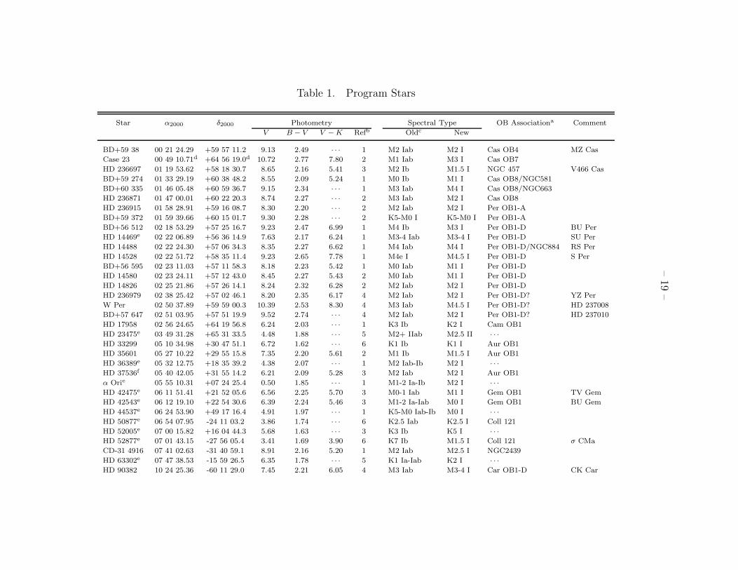
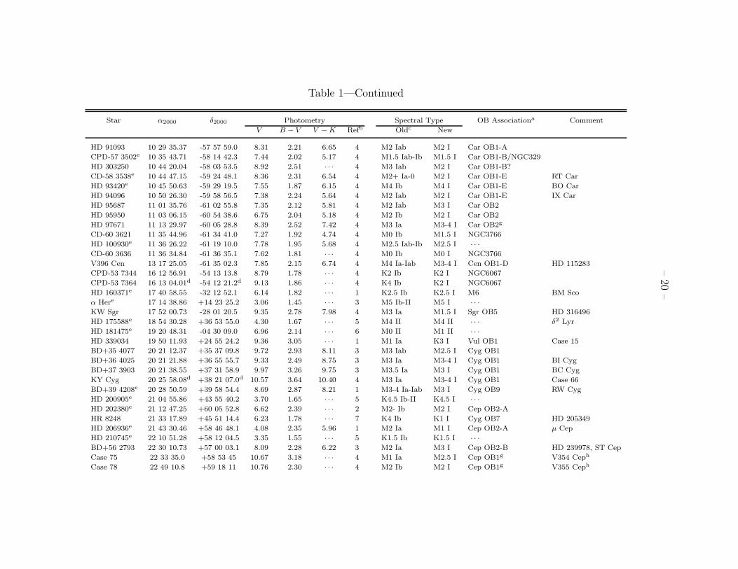
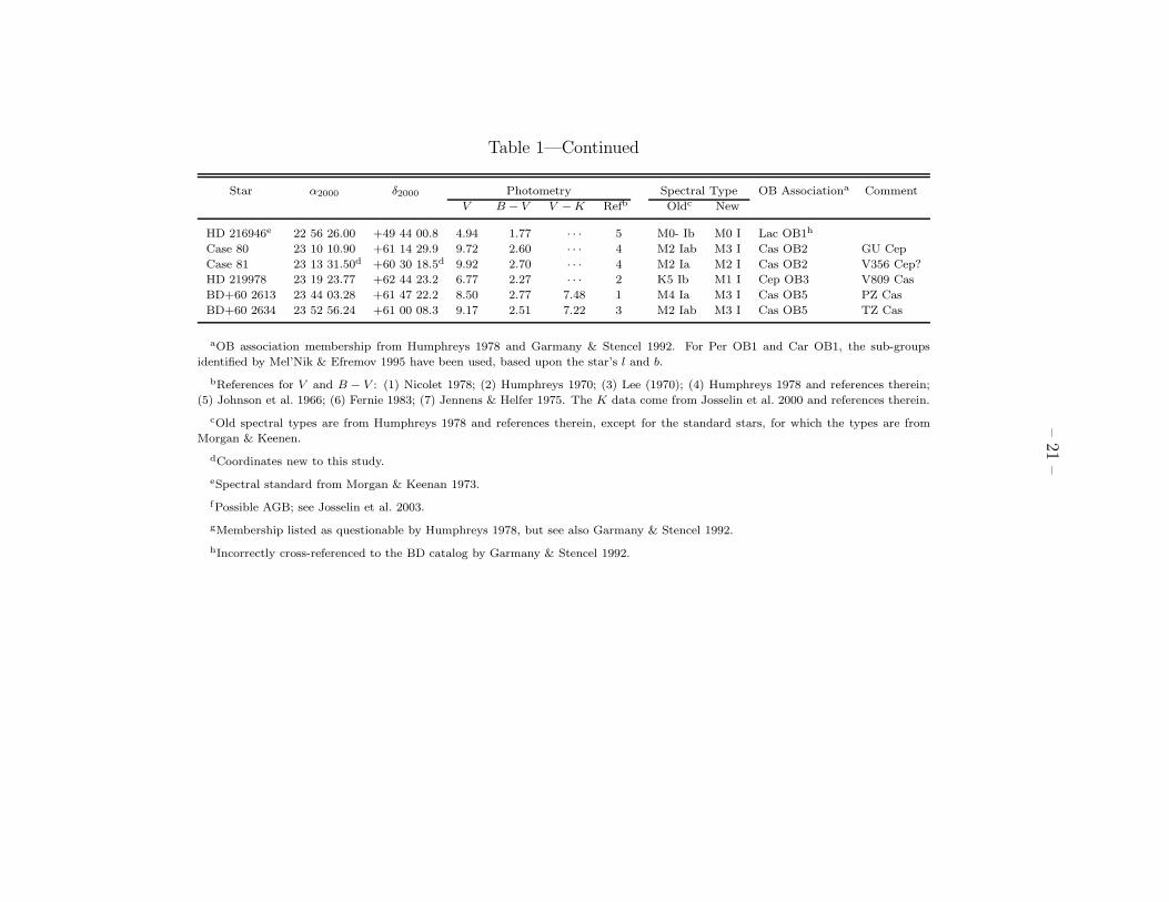
Our stars are listed in Table 1. The sample was selected in order to cover the full range of

spectral subtypes from early K through the latest M supergiants. The sample was originally

chosen to contain only stars with probable membership in OB associations and clusters with

known distances (Humphreys 1978, Garmany & Stencel 1992), but we supplemented this

list with spectral standards from the list of Morgan & Keenan (1973) in order to help refine

the spectral classification. We indicate both cluster membership and/or use as a spectral

standard in the table. The photometry comes from a variety of sources, as indicated; one

should keep in mind that most (if not all) of these stars are variable at the level of several

tenths or more in V . We have included the V − K colors as well, where the K comes from

Josselin et al. (2000) and references therein.

Distances of OB associations are notoriously uncertain, as most are far too distant for

1We are making both the observed spectra and models available to others via data files at the Centre de

Donnees Astronomiques de Strasbourg (CDS).

– 5 –

reliable trigonometric parallaxes; instead, spectral parallaxes need to be used, often resulting

in a large dispersion due to the large scatter in MV for a given spectral subtype (see Conti

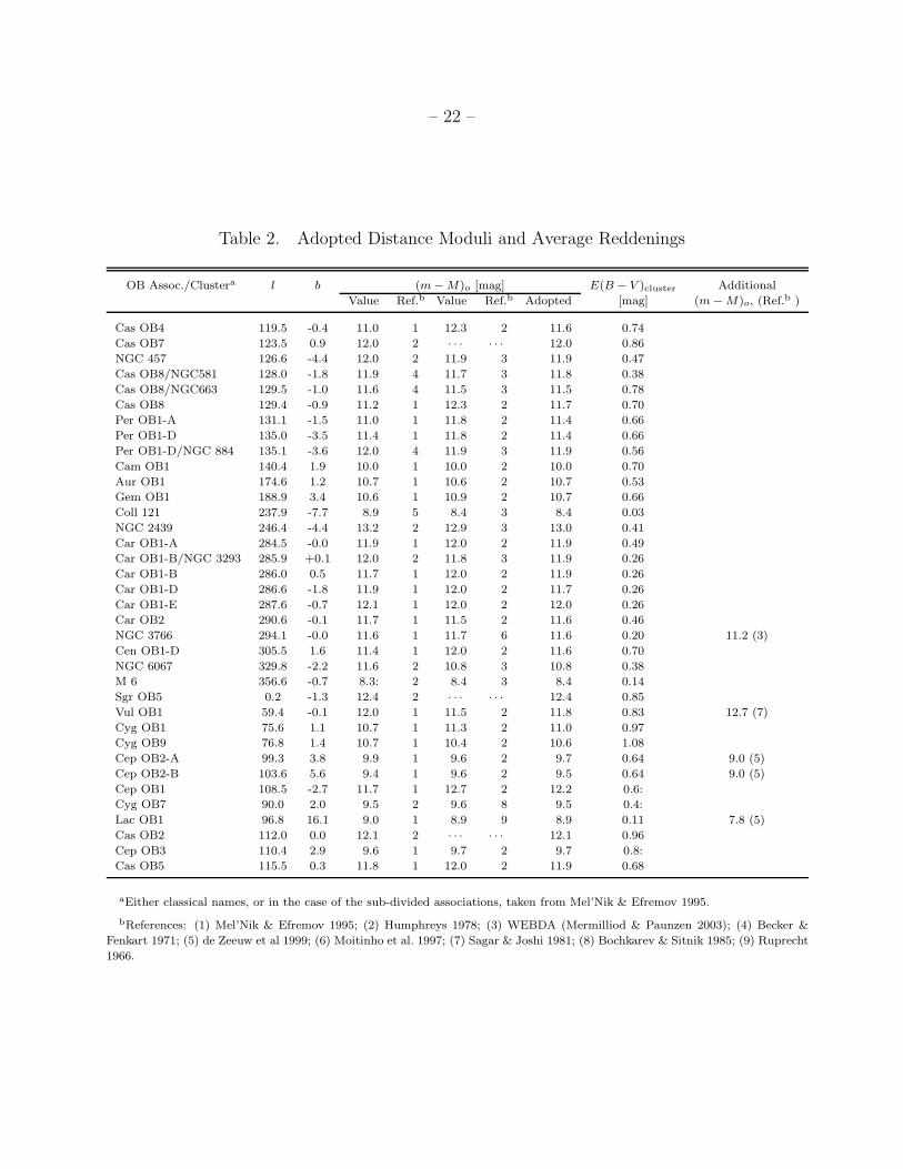
1988). In Table 2 we give the distances from several sources, when possible, for each OB

association or cluster in our sample; in general, the agreement is within a few tenths of a

magnitude. We also include in Table 2 the “average” reddenings determined from the values

for early-type members listed by Humphreys (1978) for the OB associations. For the clusters,

we list the average reddening values given by Mermilliod & Paunzen (2003). We note that in

general membership in an OB association is never perfectly well established, and therefore

there is an additional uncertainty connected with the distance of any particular star.

2.2. Spectrophotometry

The spectrophotometry data were obtained during three observing runs: two with the

KPNO 2.1-meter telescope and GoldCam Spectrograph (17-24 March 2004 and 28 May - 1

June 2004), and one with the CTIO 1.5-meter telescope and Cassegrain CCD spectrometer

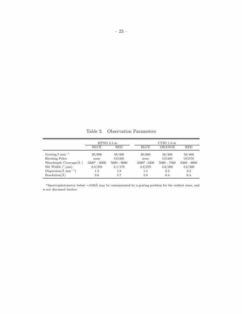
(7-12 March 2004). Similar resolutions and wavelength coverage were obtained in both

hemispheres. Detailed information on the observing parameters is given in Table 3.

The Kitt Peak observations were taken under sporadically cloudy conditions in March,

while all of the nights in May/June were photometric. Before observing each object, the

spectrograph was manually rotated so that the slit was aligned with the parallactic angle.

We aimed for a S/N of 50 per spectral resolution element (4 pixels) at the bluest end of

the spectrum, with care being taken not to saturate the detector at the reddest end. For

the brightest stars (V < 6), we employed a 5.0 mag or 7.5 mag neutral density filter.

Observations of the flat-field lamps were obtained both with and without these filters in

order to correct for the wavelength dependence of the transmission of these “neutral” filters.

Throughout each night we also observed a set of spectrophotometric standards. The seeing

for these observations was 1.2” to 3”, with a typical value of 2”. Exposures of both dome

flats and projector flats were obtained at the beginning of each night; for the red nights,

we also obtained projector flats throughout the night to monitor any shifting of the fringe

pattern that affects the CCD at longer wavelengths. Wavelength calibration exposures of a

He-Ne-Ar lamp were obtained at the beginning and end of each night.

At CTIO, it was not practical to always observe at the parallactic angle; instead, each

star was observed with a single exposure through a very wide slit (for good relative fluxes),

followed by a series of shorter exposures obtained through a narrow slit (for good resolu-

tion). Projector flats were obtained for all wavelength regions through both the wide and

narrow slits. The exposures were typically obtained in conjunction with a wavelength cal-

– 6 –

ibration exposure, although in practice we found there was little flexure. Observations of

spectrophotometric standards were obtained throughout the night.

We reduced the data using IRAF2 packages CCDRED, KPNOSLIT and CTIOSLIT. We

used dome flats to flatten the blue Kitt Peak data, and the projector lamps to flatten the

red Kitt Peak data. We found that the only shift in the fringe pattern in the red occurred

during the thirty minutes following a refill of the dewar with liquid nitrogen. After that the

fringe pattern was stable, so we simply combined these projector flats. The spectra were

all extracted using an optimal-extraction algorithm. When reducing the CTIO data the

narrow slit width observations were combined and divided into the wide slit observations.

The resulting division was fit with a low-order function and used to correct the fluxes of

the narrow-slit observations. In a few cases the wide-slit observations included the presence

of an additional star in the extraction aperture; these stars were eliminated from further

consideration, and do not appear in Table 1.

The observations of spectrophotometric standards were used to create sensitivity func-

tions; typically a grey-shift was applied to each night’s data, and the resulting scatter was

0.02 mag. In addition, the different wavelength regions were grey-shifted to agree in the

regions of overlap.

When we began our analysis we found significant discrepancies between the reddened

model atmospheres and the observed spectra in the near-UV region (<4000A for the reddest

stars. Careful investigations suggest that, despite the excellent agreement of the spectropho-

tometric standards, there could be contamination by a grating ghost in the near-UV, in which

a small fraction of the red light contaminates the data. The expected flux ratio Fλ7000/Fλ3500

is roughly 10,000 for the most reddened M supergiants, a regime seldom encountered in

astronomical spectrophotometry. We do not know if this contamination is a small fraction

of the near-UV light, or if it dominates, and we have therefore restricted our study to the

data longwards 4100A, where our tests show that the ghosting effect is negligible.

2IRAF is distributed by the National Optical Astronomy Observatories, which are operated by the As-

sociation of Universities for Research in Astronomy, Inc., under cooperative agreement with the National

Science Foundation.

– 7 –

3. Analysis

3.1. Reclassification of Spectral Type

We reclassified each of our stars by visually comparing each spectrum to the spectral

standards. In order to avoid questions of normalizing these rich and complicated spectra

(with uncertain continuum levels), we did this comparison in terms of log flux. Given that

many of these stars can be variable in spectral type, we were unsurprised to find that we

needed to reclassify a few of the spectral standards for consistency. For the late-K and all

M type stars, the classification was based upon the depths of the TiO bands, which are

increasingly strong with later spectral type. The reclassification of the early and mid K

supergiants was based primarily on the strengths of the G-band plus the strength of Ca I

λ4226. These features all get weaker with later spectral types (Jaschek & Jaschek 1987), a

temperature effect which we confirmed with the MARCS models. We list our revised spectral

types in Table 4.

3.2. Modeling the Stars: Effective Temperatures and Reddenings

We compared the observed spectral energy distribution (SED) of each star to a series of

MARCS stellar atmosphere models. The models used in our comparisons ranged from 3000 K

to 4300 K in increments of 100 K, with log g from +1.0 to -1.0 in increments of 0.5 dex.

The choice of surface gravity was derived iteratively; we began by adopting the log g = −0.5

models for all of the fits, as this surface gravity was generally what was expected with the

old effective temperature scale and the resulting placement in the HRD. However, our new

temperatures were a bit warmer than that predicted by the old scale, so we re-evaluated all of

the fits using log g = 0.0, as this was more consistent with the revised locations in the HRD.

The effective temperatures remained unchanged with the use of these higher surface gravities

(except for the occasional star), but the values of E(B − V ) increased slightly. Finally, we

used the revised temperature scale and bolometric luminosities with the evolutionary tracks

(Sec. 3.3) to compute log g star-by-star for the RSGs with distances. This confirmed that

our choice of the log g = 0.0 models was appropriate for most of the stars. We refit the stars

using the appropriate log g if the distance was known; otherwise, we adopted log g = 0.0. In

practice the choice of log g affected the derived values of E(B − V ) by < 0.1 mag, and had

no effect on the derived effective temperatures.

In making the fits, we reddened each model using a Cardelli et al. (1989) reddening

– 8 –

law with the standard ratio of total-to-selective extinction RV = 3.13. Our initial guess

for E(B − V ) was based upon the average value for the cluster, i.e., E(B − V )cluster from

Table 2. The temperature was determined primarily from the strengths of the TiO bands

(M supergiants) and the G-band (early-to-mid K supergiants), with E(B−V ) then adjusted

to produce the best fit to the continuum. In Fig. 1 we show a sample of spectra and fits,

covering a range of spectral types; the complete set is available in the electronic edition of

the journal. The fitting was all done in log units of flux in order to facilitate comparisons of

line intensities without the uncertain process of normalization, as mentioned previously.

As described in the previous section, our initial modeling revealed a significant discrep-

ancy between the models and the data in the near-UV region (3500-4000A) for the reddest

stars, which we first attributed to a peculiar reddening law, caused, we argued, by circum-

stellar dust. However, since we cannot exclude the possibility that the near-UV data are

affected by an instrumental problem, we will revisit this issue at a later time when we have

better data in the near-UV.

Otherwise, the agreement between the SEDs of the reddened models and the data

is extremely good, both in terms of the continua and molecular band depths. The only

significant problem we encountered was for the early-to-mid K stars, where we expected to

use both the Ca I λ4226 line as well as the G-band in modeling the stars, as these lines are

among the primary classification lines for the early K’s. However, we found that these Ca I

line was stronger in the MARCS models’ synthetic spectra than in our stars, usually by a

factor of 3 or so. The Ca I line show the same qualitative behavior with effective temperature

as expected (see above discussion), but the absolute line strengths in the models were too

strong. Since Ca has a very low ionization potential (6.11 eV), most of the Ca is in the form

of Ca II: ∼99% in the model at 4000 K and 98% in the model at 3600 K (at an optical

depth of 0.01 for the continuum). Thus, a small over-ionization will strongly impact the line

strength, due to either the effects of non-LTE or a slight error in the model’s temperature

structure. The occurrence of cool or hot spots on the stellar surface could also lead to regions

where the ionization equilibrium is strongly affected.

3RV is typically taken to be ∼ 3.6 for RSGs (Lee 1970), due to the increase of the effective wavelength of

broad-band filters with redder stars; see McCall (2004) for a recent discussion. Our own calculations from

the models suggest that RV ∼ 4.4 would be more appropriate for BV photometry of RSGs. Note, however,

that in the absence of a peculiar reddening law, RV = 3.1 is an appropriate choice for our study, since our

analysis is not based upon broad-band filter photometry, but rather upon moderate-resolution (5A) SEDs;

i.e., neither the B nor V filters were involved in our extinction determinations. In order to prevent confusion,

we use the equivalent AV values rather than E(B−V ), as our AV values will be directly comparable to those

of others, while our E(B − V ) values would be larger than those determined from broad-band photometry

for RSGs.

– 9 –

In addition to the problem with the Ca I line, the models also produce Ca II H and K

lines that are significantly stronger than those observed, even in those stars for which the

fluxes of the dereddened stars and the stars were in good agreement. This is not hard to

understand, as RSGs are expected to have chromospheric activity, and this is not accounted

for in the models. The presence of a chromosphere would lead to emission in the H and

K lines, resulting in weaker observed lines than would be the case if the lines were purely

photospheric in origin. This explanation could be further investigated by means of high-

dispersion spectroscopy.

We relied instead upon the G-band for the fitting of the early and mid-Ks. We substan-

tiated that we obtained similar temperatures using the G-band and the TiO bands for the

late Ks. The resulting temperature fits for the early and mid Ks are therefore less certain,

probably ±100 K.

We list the effective temperatures in Table 4. In general, we found that the data could

be matched very well by the models, both in line strength and in continuum shape, and

we expect that the effective temperatures of the M supergiants have been obtained to a

precision of 50 K. The AV values are determined to a precision of about 0.15 mag. We

note with interest that the derived AV values of about one-third our sample are significantly

higher than the average found from the OB stars in the same associations and clusters using

the data from Humphreys (1978); indeed, the same conclusion could have been drawn from

the older data given in that paper. A possible interpretation is that this extra extinction is

due to circumstellar dust. We include the ∆AV values in Table 4. We will revisit this issue

in a subsequent paper, once our analysis of the Magellanic Cloud data (where the foreground

reddening is low, and relatively uniform) is complete.

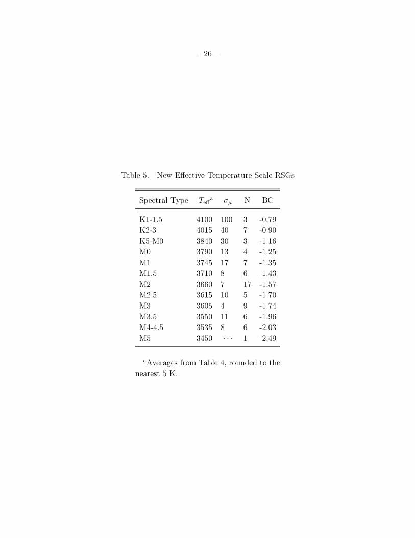
Our new effective temperature scale is given in Table 5, where we include the number of

stars and standard deviation of the mean (σµ) at each spectral type. We compare this scale

to that of Humphreys & McElroy (1984) and Massey & Olsen (2003) in Fig. 2. Both of the

latter are “averages” from the literature. We see that the new scale agrees well for the K

supergiants, but is progressively warmer than past scales for later spectral types, with the

differences amounting to 400 K by the latest M supergiants (M5 I). The overall progression

of the temperature with later spectral type is more gradual than in past studies.

We include in Table 5 the bolometric corrections to the V-band corresponding to the

new effective temperature scale; these values are the linear interpolations of the BCs from

the MARCS models given below. The values are for log g = 0.0, but there is little change

with surface gravity (< 0.05 mag over 0.5 dex in log g for 3500 ≤ Teff ≤ 4300). Note that we

have referenced the BCs to the system advocated by Bessell et al. (1998), i.e., that the Sun

has a BC of -0.07 mag. This results in values less luminous (by 0.12 mag) than the historical

– 10 –

one; on this system the Sun is defined to have an Mbol of 4.74.

3.3. Comparison to Evolutionary Models

In order to compare these stars to the evolutionary models, we must convert the absolute

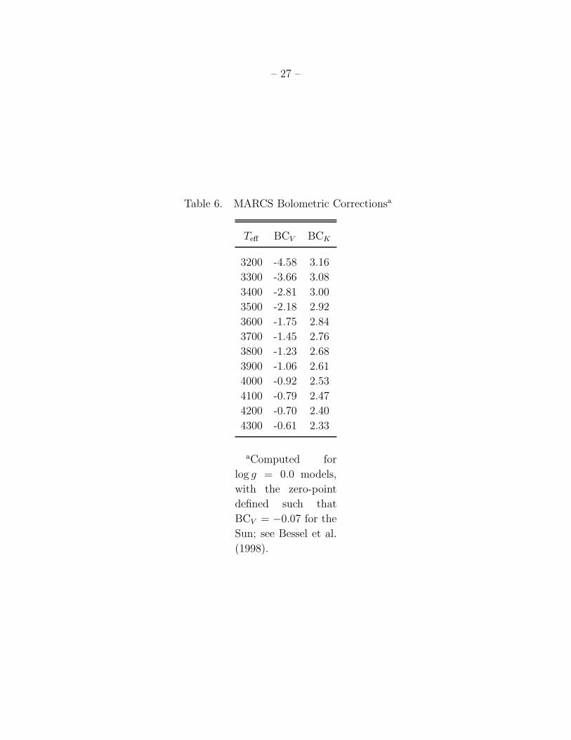
visual luminosities to bolometric luminosities. In Table 6 we give the bolometric corrections

(BCs) as a function of effective temperature determined from the MARCS models. We list

the bolometric magnitudes for each star with a known distance in Table 44.

In Fig. 3(a) we show the solar-metallicity evolutionary tracks of Meynet & Maeder

(2003) compared to the location of the Galactic RSGs taken from Humphreys (1978) using

the effective temperature and bolometric corrections of Humphreys & McElroy (1984). The

disagreement is not as bad as that shown by Massey (2003), as the new tracks extend further

to the right at higher luminosities than did the older tracks of Schaller et al. (1992). Nev-

ertheless, it is clear that there are significant differences between theory and “observation”.

In Fig. 3(b) we now compare the same tracks to the Galactic RSGs using the new effective

temperatures and bolometric models found by using the MARCS models. We have marked

with filled symbols those five stars for which the K-band data suggests that our Mbol values

are too luminous (Sec. 3.4), and in Fig. 3c show the location of these stars based upon the K-

band data. In (b) and (c) the disagreement between theory and location in the HRD has now

disappeared, giving us some confidence in the accuracy of our new calibration. A few stars

have luminosities significantly higher than the evolutionary tracks would predict (Fig. 3b),

but these are invariably the stars whose Mbol values derived from V are at odds with those

derived from K (Fig. 3c), presumably due to mistakes in the correction for reddening, and

hence their value must be considered poorly determined; Fig. 3c is the best determined.

The fact that we have both Mbol and Teff allows us to determine the stellar radii R/R⊙

from the formal definition of Teff ; i.e., (R/R⊙) = (L/L⊙)0.5(Teff/5781)2, where the numerical

quantity is the effective temperature of the sun (see discussion in Bessell et al. 1998), and

L/L⊙ = 10−(Mbol−4.74)/2.5. We include these values in Table 4. The stars with the largest

radii in our sample, KW Sgr, Case 75, KY Cyg, and HD 206936 (=µ Cep)5 all have radii

4We note that Josselin et al. (2003) have proposed that the star HD 37536 is an AGB based upon the

detection of Tc and Li. On the other hand, the star is seen projected against Aur OB1, and if membership

is assumed, a sensible MV is derived. In addition, the reddening is similar to that of the early-type members

of Aur OB1.

5Also known as Herschel’s “Garnet Star”, this star is often cited as the largest known normal star; see

http://www.astro.uiuc.edu/∼kaler/sow/garnet.html.

– 11 –

of roughly 1500R⊙ (7 AU), making these the largest normal stars known. For comparison,

Betelgeuse has a radius (measured by interferometry) of 645 R⊙ (Perrin et al. 2004). We

include in Fig. 3(c) lines of constant radii. These four large stars are right at what current

evolutionary theory predicts is the maximum radius for Galactic RSGs, as the largest radius

reached by the tracks is found at roughly Mbol = −9 and log Teff = 3.57 (3715 K).

Two peculiar RSGs are known with significantly larger radii. The M2 I primary in

the interacting binary VV Cep has a radius that has been variously estimated as 1200R⊙

(Hutchings & Wright 1971) to 1600R⊙ (Wright 1977) and beyond, with a reasonable upper

limit of 1900R⊙ determined by Saito et al. (1980); see discussion in Bauer & Bennett (2000).

VV Cep consists of a RSG primary and a hotter companion orbiting within a common

envelope. These estimates of the radii are complicated by the uncertainties in the orbital

inclination in Section 3 of Saito et al. 1980), with the “definition” of radius determined by

the eclipse method leading to a further ambiguity. In any event, gravitational interactions

are certainly taking place in this system (Hutchings & Wright 1971), and thus may not have

applications to normal, single stars.

The other star with a humongous radius is VY CMa. Using interferometry with Keck,

Monnier et al. (2004) find a photospheric radius of 14 AU (3020R⊙) for this star, where

the distance of 1.5 kpc appears fairly certain from maser proper motions (Richards et al.

1998; see discussion in Monnier et al. 1999). The properties of this intriguing object have

been recently discussed by Monnier et al. (1999) and Smith et al. (2001). With a luminosity

of 2 to 5 ×105L⊙ (Mbol = −8.5 to −9.5) well established from the IR (Monnier et al.

1999, Smith 2001), the star’s temperature would have to be extremely cool, (2225 K!) to

have such a large radius. Using K-band photometry and a simple model, Monnier et al.

(2004) suggest an effective temperature of 2600 K, similar to the 2800 K value found by Le

Sidaner & Le Bertre (1996); again, see discussion in Monnier et al. (1999, 2004). We note

that none of these stellar properties are in accord with stellar evolutionary theory (Fig. 3c),

and, indeed, based upon its inferred mass-loss history, Humphreys et al. (2005) describe

the star as “perplexing”, and argue that it may be in a “unique evolutionary state.” Such

an object may provide important insight into a previously unrecognized avenue of normal

stellar evolution, or its peculiarities may be the product of (for instance) binary evolution,

as is the case for VV Cep. Smith et al. (2001) state that any hot, massive companion in

VY CMa would have been previously detected spectroscopically, but we believe that further

searching, particularly in the UV, is warranted. This star was not included in our sample,

but we hope to perform an analysis in the near future.

– 12 –

3.4. Comparison with (V − K)o

In Sec. 3.2 we derived a precise relationship between spectral subtype and effective

temperature based primarily on the strengths of the TiO band strengths. One test of this

result’s accuracy is to check for consistency with other temperature indicators. Josselin

et al. (2000) have emphasized the usefulness of K-band photometry in deriving bolometric

luminosities of RSGs, as the bolometric correction to the K-band is relatively insensitive to

effective temperature and surface gravities, while RSGs themselves are less variable in the

K band than at V . In addition, correction for interstellar reddening is minor at K. At the

same time, the effective temperature is a very sensitive function of (V −K)o. Since over half

of our sample have K-band photometry (Table 1), we can perform some exacting tests of

the models to see if we obtained similar physical parameters by very different techniques.

We have derived synthetic (V − K)o colors for our models following the procedure and

assumptions of Bessell et al. (1998). The V bandpass comes from Bessell (1990), while

the K bandpass comes from Bessell & Brett (1988). Note that the latter is similar to the

“standard” K system of Elias et al. (1982) and Johnson (1965), and a good approximation

to the convolution of detector and filter used at UKIRT and with most ESO and NOAO

instrumentation; however, this differs considerably from the Ks filter employed in other

modern instruments, such as the 2Mass survey and the VLT ISAAC instruments, and the

transformations given below will not apply to Ks.

We found that we could approximate the relationship between (V −K)o color as a simple

power-law:

Teff = 7741.9 − 1831.83(V − K)o + 263.135(V − K)2o − 13.1943(V − K)3

o,

over the range 2.9 < (V − K)o < 8.0, (3200-4300 K) with a dispersion of 11K, where the

dispersion comes from considering the full range of appropriate surface gravities (log g = −1

to 1); see Fig. 4a. The bolometric correction at K is an almost linear relationship with

effective temperature over the range 3200 < Teff < 4300:

BCK = 5.574 − 0.7589(Teff/1000),

with a dispersion of 0.01 mag (Fig. 4). We have included these BCK values in Table 6.

We de-reddened the V − K colors in Table 1 using the extinction values derived from

the model fits, and assuming E(V − K) = 2.73E(B − V ), based on Schlegel et al. (1998);

this does not account for a modest change due to the shifts of the effective wavelenths of

the band-passes for very red stars. We compare the effective temperatures derived by this

method with those obtained from the spectral types in Fig. 5a. The scatter is large, as one

– 13 –

might expect given the strong functional dependence of Teff on (V − K)o, the variability

of V , and the fact that the effective temperatures now depend strongly upon the assumed

reddenings. Note that our uncertainty of 0.15 in AV translates to an uncertainty of 0.13 in

E(V − K), and hence 50 K in Teff . However, in general the agreement is good, with the

(V − K)o colors yielding a temperature whose median difference is 60 K warmer than our

adopted scale.

How well do the bolometric luminosities then agree? In Fig. 5b we show the relationship

between the bolometric luminosities derived from V and our Teff values (Table 4) and those

found purely from the de-reddened V −K colors. The agreement here is excellent, with only

one significant outlier, KY Cyg, the most luminous star shown.

What if instead we had derived bolometric luminosities without reference to the V −K

colors at all, but rather simply used the extinction values from the fits to derive the absolute

magnitude in the K-band [MK = K − 0.37E(B − V ) − (m − M)o], and then determined

the bolometric correction at K using the Teff of the models fits? We give that comparison in

Fig. 5c. Clearly there is excellent agreement.

In Fig. 5d we show the comparison between the bolometric magnitudes derived from

the K-band in the same manner as in (c) and the bolometric magnitudes derived from the

visible. This plot is similar to that of Fig. 5b, with excellent agreement in general. There

are five significant outliers, whose differences are greater than 1 mag using the two methods

(KY Cyg, CD-31 4916, BD+35 4077, BD+60 2613, and HD 14528), all in the sense that the

bolometric luminosity derived from V may be overly luminous. We flagged all five stars in

Fig. 3 as well as in Table 4.

The fact that these five outliers were all more luminous based upon V than upon K

raised the the question as to whether our method was systematically overestimating AV .

Recall that we did find that our AV values tend to be higher than that of OB stars in the

same clusters and associations. Following a suggestion offered by the referee, we derived the

bolometric luminosities at K based instead based upon the J −K colors alone, ignoring our

AV values. We used the effective temperatures derived from our model fits both to determine

the bolometric corrections, and to compute the intrinsic (J −K)o colors from a relationship

we found using the MARCS models:

(J − K)o = 3.10 − 0.547(Teff/1000).

We adopt the broad-band extinction terms suggested by Schlegel et al. (1998), i.e., AK =

0.70E(J − K). Again, the numerical factor here does not take into account the shift of

RK due to the change in the effective wavelengths of the broad-band filters, but it should

be good enough for the test we intend. The J − K photometry comes from Josselin et al.

– 14 –

(2000) and references therein. We show this comparison between the two ways of deriving

Mbol from K in Fig. 5e. There is excellent agreement between the two methods. Thus, there

cannot be anything systematically wrong with our AV values in general. Interestingly, the

two stars with the largest deviations in this figure are KY Cyg and KW Sgr. The J − K

correction suggests that if anything the Mbol values should be intermediate between what

we derive above from V and from K using our values for the extinction, and that perhaps

our extinction values for these two stars are too low, rather than too high. A comparison

between the lumionsities derived from K and E(J − K) and those derived from V and the

extinctions derived from our model fits is shown in Fig. 5f; this is very similar to what we

found in Fig. 5d.

We summarize the conclusions from these comparisons as follows. First, the MARCS

models yield consistent results (to within 100 K) both from the molecular band strengths

and from the V − K colors. Thus if one’s goal is simply to derive bolometric luminosities,

V and K band data will suffice for most purposes, if one has an estimate of the reddenings.

However, for accurate placement in the H-R diagram (requiring Teff) then there is as yet

no substitute for spectroscopy and the use of molecular bands. It is possible that other

colors, such as V −Rc, might prove more effective in determining the effective temperatures

than V − K, given the shorter baseline and therefore lower sensitivity to reddening, i.e.

E(V − Rc) = 0.64E(B − V ). We will explore this further when we consider the Magellanic

Cloud sample, as these stars have simultaneous V and R measures, and the reddenings are

low and uniform (Massey et al. 1995).

4. Conclusions and Summary

We have determined a new effective temperature scale for Galactic RSGs by fitting mod-

erate resolution (4-6A) spectrophotometry with the new MARCS stellar atmosphere models.

Our effective temperature scale is significantly warmer than previous scales, particularly for

the later M supergiants, where the differences amount to 400 K. However, our new results

give excellent agreement with the evolutionary tracks of Meynet & Maeder (2003), resolving

the issue posed by Massey (2003) that the evolutionary models do not produce RSGs as cool

and as luminous as “observed”.

Our fitting showed excellent agreement between the models and data for the majority

of the stars. The Ca I λ4226 and Ca II H and K atomic lines appear to be too strong in the

models, but the molecular transitions agree well at this dispersion. When we compare the

physical properties derived from the model fits to our optical spectrophotometry with those

found from the models using only the dereddened V − K colors, we find good agreement,

– 15 –

providing an exacting demonstration of the self-consistency of the MARCS models.

Extension of these studies to the Magellanic Clouds is underway, which should help us

understand the effect that metallicity has on the effective temperature scale of RSGs. In

addition, the fact that the reddenings are small and uniform and the distances are known

(van den Bergh 2000) will allow further investigation of colors as probes of the physical

properties of these interesting massive stars.

This work was supported by NSF Grant AST 00-093060 to PM, and and the NSF’s

Research Experience for Undergraduates program at Northern Arizona University (AST 99-

88007). We are very grateful for the excellent hospitality and support provided by the staff at

KPNO and CTIO, and also thank Nat White and Kathy Eastwood for their encouragement

and guidance. Hank Levesque pointed us towards some discussions of previous “record

holders” of the largest stars known, and we also had correspondence with Jim Kaler on

this topic. John Monnier kindly called his interesting results on VY CMa to our attention.

We also gratefully acknowledge correspondence with Geoff Clayton. Comments by an the

referee, Roberta Humphreys, led to improvements in the presentation of our arguments in

several places.

REFERENCES

Aller, L. H. 1960, in Stellar Atmospheres, ed. J. L. Greenstein (Chicago: Univ Chicago

Press), 232

Bauer, W. H., & Bennett, P. D. 2000, PASP, 112, 31

Becker, W., & Fenkart, R. 1971, A&AS, 4, 241

Bessell, M. S. 1990, PASP, 102, 1181

Bessell, M. S., & Brett, J. M. 1988, PASP, 100, 1134

Bessell, M. S., Castelli, F., & Plez, B. 1998, A&A, 3333, 231

Bochkarev, N. G., & Sitnik, T. G. 1985, Ap&SS, 108, 237

Cardelli, J. A., Clayton, G. C., & Mathis, J. S. 1989, ApJ, 345, 245

Conti, P.S. 1988, in O Stars and Wolf-Rayet Stars, ed. P. S. Conti & A. B. Underhill, NASA

SP-497

Danchi, W. C., Bester, M., Degiacomi, C. G., Greenhill, L. J., & Townes, C. H. 1994, AJ,

107, 1469

– 16 –

de Zeeuw, P. T., Hoogerwerf, R., de Bruijne, J. H. J., Brown, A. G. A., & Blaauw, A. 1999,

ApJ, 117, 354

Dyck, H. M., Benson, J. A., van Belle, G. T., & Ridgway, S. T. 1996, AJ, 111, 1705

Elias, J.H., Frogel, J. A., & Humphreys, R. M. 1985, ApJS, 57, 91

Elias, J. H., Frogel, J. A., Matthews, K., & Neugebauer, G. 1982, AJ, 87, 1029

Fernie, J. D. 1983, ApJS, 52, 7

Freytag, B. in The Future of Cool-Star Astrophysics: 12th Cambridge Workshop on Cool

Stars, Stellar Systems, and the Sun, ed. A. Brown, G. M. Harper, & T. R. Ayres

(Boulder: Univ of Colorado), 1024

Freytag, B., Steffen, M., & Dorch, B. 2002, Astron. Nach., 323, 213

Flower, P. J. 1975, A&A, 41, 391

Flower, P. J. 1977, A&A, 54, 31

Garmany, C. D., & Stencel, R. E. 1992, A&AS, 94, 221

Gustafsson, B., Bell, R. A., Eriksson, K., & Nordlund, A. 1975, A&A, 42, 407

Gustafsson, B., Edvardsson, B., Eriksson, K., Mizuno-Wiedner, M., Jorgensen, U. G., &

Plez, B. 2003, in Stellar Atmosphere Modeling, ed. I. Hubeny, D. Mihalas, & K.

Werner (San Francisco: ASP), 331

Gustafsson, B. & Jorgensen, U. G. 1994, A&ARv 6, 19

Harris, G. J., Polyansky, O. L., & Tennyson, J. 2002, ApJ, 578, 657

Humphreys, R. M. 1970, AJ, 75, 602

Humphreys, R. M. 1978, ApJS, 38, 309

Humphreys, R. M., Davidson, K., Ruch, G., & Wallerstein, G. 2005, AJ, 129, 492

Humphreys, R. M., & McElroy, D. B. 1984, ApJ 284, 565

Hutchings, J. B., & Wright, K. O. 1971, MNRAS, 155, 203

Jaschek, C. & Jaschek, M. 1987, The Classification of Stars (Cambridge: Univ Press)

Jennens, P. A., & Helfer, H. L. 1975, MNRAS, 172, 667

Johnson, H. L. 1964, Bol. Obs. Tonantzintla y Tacubaya 3, 305

Johnson, H. L. 1965, ApJ, 141, 923

Johnson, H. L. 1966, ARA&A, 4, 193

Johnson, H. L., Iriarte, B., Mitchell, R. I., Wisniewskj, W. Z. 1966, CoLPL, 4, 99

– 17 –

Josselin, E., Blommaert, J. A. D. L., Groenewegen, M. A. T., Omont, A., & Li, F. L. 2000,

A&A, 357, 225

Josselin, E., Plez, B., & Mauron, N. 2003, in Modelling of Stellar Atmospheres, ed. N.

Piskunov, W. W. Weiss, & D. F. Gray (San Francisco: ASP), F9

Kurucz, R. L. 1992, in IAU Symp. 149, The Stellar Populations of Galaxies, ed. B. Barbuy

& A. Renzini (Dordrecht: Kluwer), 225

Le Sidaner, P., & Le Bertre, T. 1996, A&A, 314, 896

Lee, T. A. 1970, ApJ, 162, 217

Mason, B. D., Wycoff, G. L., Hartkopf, W. I., Douglass, G. G., & Worley, C. E. 2001, AJ,

122, 3466

Massey, P. 1998, ApJ, 501, 153

Massey, P. 2003, ARA&A, 41, 15

Massey, P., Lang, C. C., DeGioia-Eastwood, K., & Garmany, C. D. 1995, ApJ, 438, 188

Massey, P., & Olsen, K. A. G. 2003, AJ, 126, 2867

McCall, M. L. 2004, AJ, 128, 2144

Mel’Nik, A. M., & Efremov, Yu. N. 1995 PAZh, 21, 13

Mermilliod, J.C., & Paunzen, E. 2003, A&A, 410, 511

Meynet, G., & Maeder, A. 2003, A&A, 404, 975

Moitinho, A., Emilio, J., Yun, J. L., & Phelps, R. L. 1997, AJ, 113, 1359

Monnier, J. D. et al. 2004, ApJ, 605, 436

Monnier, J. D., Tuthill, P. G., Lopez, B., Cruzalebes, P., Danchi, W. C., & Haniff, C. A.

1999, ApJ, 512, 351

Morgan, W. W., & Keenan, P. C. 1973, ARA&A, 11, 29

Nicolet, B. 1978, A&AS, 34, 1

Partridge, H. & Schwenke, D. W. 1997, JCP, 106, 4618

Perrin, G., Ridgway, S. T., Coude du Foresto, V., Mennesson, B., Traub, W. A., & Lacasse,

M. G. 2004, A&A, 418, 675

Plez, B. 2003, in GAIA Spectroscopy: Science, and Technology, ed. U. Munari (San Fran-

cisco, ASP), 189

Plez, B., Brett, J. M., & Nordlund, A. 1992, A&A, 256, 551

Richards, A. M. S., Yates, J. A., & Cohen, R. J. 1998, MNRAS, 299, 319

– 18 –

Ruprecht, J. 1966, Trans. IAU, 12B, 350

Sagar, R., & Joshi, U. C. 1981, Ap&SS, 75, 465

Saito, M., Sato, H., Saijo, K., & Hayasaka, T. 1980, PASJ, 32, 163

Schaller, G., Schaerer, D., Meynet, G., & Maeder, A. 1992, A&AS, 96, 269

Schlegel, D. J., Finkbeiner, D. P., & Davis, M. 1998, ApJ, 500, 525

Smith, N., Humphreys, R. M., Davidson, K., Gehrz, R. D., Schuster, M. T., & Krautter, J.

2001, AJ, 121, 1111

Tsuji, T. 1986, ARA&A, 24, 89

van den Bergh, S. 2000 The Galaxies of the Local Group (Cambridge, Cambridge University

Press)

White, N. M., & Wing, R. F. 1989, ApJ, 222, 209

Wright, K. O. 1977, JRASC, 71, 152

Young, J. S. et al. 2000, MNRAS, 315, 635

This preprint was prepared with the AAS LATEX macros v5.2.

–19

–

Table 1. Program Stars

Star α2000 δ2000 Photometry Spectral Type OB Associationa Comment

V B − V V − K Refb Oldc New

BD+59 38 00 21 24.29 +59 57 11.2 9.13 2.49 · · · 1 M2 Iab M2 I Cas OB4 MZ Cas

Case 23 00 49 10.71d +64 56 19.0d 10.72 2.77 7.80 2 M1 Iab M3 I Cas OB7

HD 236697 01 19 53.62 +58 18 30.7 8.65 2.16 5.41 3 M2 Ib M1.5 I NGC 457 V466 Cas

BD+59 274 01 33 29.19 +60 38 48.2 8.55 2.09 5.24 1 M0 Ib M1 I Cas OB8/NGC581

BD+60 335 01 46 05.48 +60 59 36.7 9.15 2.34 · · · 1 M3 Iab M4 I Cas OB8/NGC663

HD 236871 01 47 00.01 +60 22 20.3 8.74 2.27 · · · 2 M3 Iab M2 I Cas OB8

HD 236915 01 58 28.91 +59 16 08.7 8.30 2.20 · · · 2 M2 Iab M2 I Per OB1-A

BD+59 372 01 59 39.66 +60 15 01.7 9.30 2.28 · · · 2 K5-M0 I K5-M0 I Per OB1-A

BD+56 512 02 18 53.29 +57 25 16.7 9.23 2.47 6.99 1 M4 Ib M3 I Per OB1-D BU Per

HD 14469e 02 22 06.89 +56 36 14.9 7.63 2.17 6.24 1 M3-4 Iab M3-4 I Per OB1-D SU Per

HD 14488 02 22 24.30 +57 06 34.3 8.35 2.27 6.62 1 M4 Iab M4 I Per OB1-D/NGC884 RS Per

HD 14528 02 22 51.72 +58 35 11.4 9.23 2.65 7.78 1 M4e I M4.5 I Per OB1-D S Per

BD+56 595 02 23 11.03 +57 11 58.3 8.18 2.23 5.42 1 M0 Iab M1 I Per OB1-D

HD 14580 02 23 24.11 +57 12 43.0 8.45 2.27 5.43 2 M0 Iab M1 I Per OB1-D

HD 14826 02 25 21.86 +57 26 14.1 8.24 2.32 6.28 2 M2 Iab M2 I Per OB1-D

HD 236979 02 38 25.42 +57 02 46.1 8.20 2.35 6.17 4 M2 Iab M2 I Per OB1-D? YZ Per

W Per 02 50 37.89 +59 59 00.3 10.39 2.53 8.30 4 M3 Iab M4.5 I Per OB1-D? HD 237008

BD+57 647 02 51 03.95 +57 51 19.9 9.52 2.74 · · · 4 M2 Iab M2 I Per OB1-D? HD 237010

HD 17958 02 56 24.65 +64 19 56.8 6.24 2.03 · · · 1 K3 Ib K2 I Cam OB1

HD 23475e 03 49 31.28 +65 31 33.5 4.48 1.88 · · · 5 M2+ IIab M2.5 II · · ·

HD 33299 05 10 34.98 +30 47 51.1 6.72 1.62 · · · 6 K1 Ib K1 I Aur OB1

HD 35601 05 27 10.22 +29 55 15.8 7.35 2.20 5.61 2 M1 Ib M1.5 I Aur OB1

HD 36389e 05 32 12.75 +18 35 39.2 4.38 2.07 · · · 1 M2 Iab-Ib M2 I · · ·

HD 37536f 05 40 42.05 +31 55 14.2 6.21 2.09 5.28 3 M2 Iab M2 I Aur OB1

α Orie 05 55 10.31 +07 24 25.4 0.50 1.85 · · · 1 M1-2 Ia-Ib M2 I · · ·

HD 42475e 06 11 51.41 +21 52 05.6 6.56 2.25 5.70 3 M0-1 Iab M1 I Gem OB1 TV Gem

HD 42543e 06 12 19.10 +22 54 30.6 6.39 2.24 5.46 3 M1-2 Ia-Iab M0 I Gem OB1 BU Gem

HD 44537e 06 24 53.90 +49 17 16.4 4.91 1.97 · · · 1 K5-M0 Iab-Ib M0 I · · ·

HD 50877e 06 54 07.95 -24 11 03.2 3.86 1.74 · · · 6 K2.5 Iab K2.5 I Coll 121

HD 52005e 07 00 15.82 +16 04 44.3 5.68 1.63 · · · 3 K3 Ib K5 I · · ·

HD 52877e 07 01 43.15 -27 56 05.4 3.41 1.69 3.90 6 K7 Ib M1.5 I Coll 121 σ CMa

CD-31 4916 07 41 02.63 -31 40 59.1 8.91 2.16 5.20 1 M2 Iab M2.5 I NGC2439

HD 63302e 07 47 38.53 -15 59 26.5 6.35 1.78 · · · 5 K1 Ia-Iab K2 I · · ·

HD 90382 10 24 25.36 -60 11 29.0 7.45 2.21 6.05 4 M3 Iab M3-4 I Car OB1-D CK Car

–20

–

Table 1—Continued

Star α2000 δ2000 Photometry Spectral Type OB Associationa Comment

V B − V V − K Refb Oldc New

HD 91093 10 29 35.37 -57 57 59.0 8.31 2.21 6.65 4 M2 Iab M2 I Car OB1-A

CPD-57 3502e 10 35 43.71 -58 14 42.3 7.44 2.02 5.17 4 M1.5 Iab-Ib M1.5 I Car OB1-B/NGC329

HD 303250 10 44 20.04 -58 03 53.5 8.92 2.51 · · · 4 M3 Iab M2 I Car OB1-B?

CD-58 3538e 10 44 47.15 -59 24 48.1 8.36 2.31 6.54 4 M2+ Ia-0 M2 I Car OB1-E RT Car

HD 93420e 10 45 50.63 -59 29 19.5 7.55 1.87 6.15 4 M4 Ib M4 I Car OB1-E BO Car

HD 94096 10 50 26.30 -59 58 56.5 7.38 2.24 5.64 4 M2 Iab M2 I Car OB1-E IX Car

HD 95687 11 01 35.76 -61 02 55.8 7.35 2.12 5.81 4 M2 Iab M3 I Car OB2

HD 95950 11 03 06.15 -60 54 38.6 6.75 2.04 5.18 4 M2 Ib M2 I Car OB2

HD 97671 11 13 29.97 -60 05 28.8 8.39 2.52 7.42 4 M3 Ia M3-4 I Car OB2g

CD-60 3621 11 35 44.96 -61 34 41.0 7.27 1.92 4.74 4 M0 Ib M1.5 I NGC3766

HD 100930e 11 36 26.22 -61 19 10.0 7.78 1.95 5.68 4 M2.5 Iab-Ib M2.5 I · · ·

CD-60 3636 11 36 34.84 -61 36 35.1 7.62 1.81 · · · 4 M0 Ib M0 I NGC3766

V396 Cen 13 17 25.05 -61 35 02.3 7.85 2.15 6.74 4 M4 Ia-Iab M3-4 I Cen OB1-D HD 115283

CPD-53 7344 16 12 56.91 -54 13 13.8 8.79 1.78 · · · 4 K2 Ib K2 I NGC6067

CPD-53 7364 16 13 04.01d -54 12 21.2d 9.13 1.86 · · · 4 K4 Ib K2 I NGC6067

HD 160371e 17 40 58.55 -32 12 52.1 6.14 1.82 · · · 1 K2.5 Ib K2.5 I M6 BM Sco

α Here 17 14 38.86 +14 23 25.2 3.06 1.45 · · · 3 M5 Ib-II M5 I · · ·

KW Sgr 17 52 00.73 -28 01 20.5 9.35 2.78 7.98 4 M3 Ia M1.5 I Sgr OB5 HD 316496

HD 175588e 18 54 30.28 +36 53 55.0 4.30 1.67 · · · 5 M4 II M4 II · · · δ2 Lyr

HD 181475e 19 20 48.31 -04 30 09.0 6.96 2.14 · · · 6 M0 II M1 II · · ·

HD 339034 19 50 11.93 +24 55 24.2 9.36 3.05 · · · 1 M1 Ia K3 I Vul OB1 Case 15

BD+35 4077 20 21 12.37 +35 37 09.8 9.72 2.93 8.11 3 M3 Iab M2.5 I Cyg OB1

BD+36 4025 20 21 21.88 +36 55 55.7 9.33 2.49 8.75 3 M3 Ia M3-4 I Cyg OB1 BI Cyg

BD+37 3903 20 21 38.55 +37 31 58.9 9.97 3.26 9.75 3 M3.5 Ia M3 I Cyg OB1 BC Cyg

KY Cyg 20 25 58.08d +38 21 07.0d 10.57 3.64 10.40 4 M3 Ia M3-4 I Cyg OB1 Case 66

BD+39 4208e 20 28 50.59 +39 58 54.4 8.69 2.87 8.21 1 M3-4 Ia-Iab M3 I Cyg OB9 RW Cyg

HD 200905e 21 04 55.86 +43 55 40.2 3.70 1.65 · · · 5 K4.5 Ib-II K4.5 I · · ·

HD 202380e 21 12 47.25 +60 05 52.8 6.62 2.39 · · · 2 M2- Ib M2 I Cep OB2-A

HR 8248 21 33 17.89 +45 51 14.4 6.23 1.78 · · · 7 K4 Ib K1 I Cyg OB7 HD 205349

HD 206936e 21 43 30.46 +58 46 48.1 4.08 2.35 5.96 1 M2 Ia M1 I Cep OB2-A µ Cep

HD 210745e 22 10 51.28 +58 12 04.5 3.35 1.55 · · · 5 K1.5 Ib K1.5 I · · ·

BD+56 2793 22 30 10.73 +57 00 03.1 8.09 2.28 6.22 3 M2 Ia M3 I Cep OB2-B HD 239978, ST Cep

Case 75 22 33 35.0 +58 53 45 10.67 3.18 · · · 4 M1 Ia M2.5 I Cep OB1g V354 Ceph

Case 78 22 49 10.8 +59 18 11 10.76 2.30 · · · 4 M2 Ib M2 I Cep OB1g V355 Ceph

–21

–

Table 1—Continued

Star α2000 δ2000 Photometry Spectral Type OB Associationa Comment

V B − V V − K Refb Oldc New

HD 216946e 22 56 26.00 +49 44 00.8 4.94 1.77 · · · 5 M0- Ib M0 I Lac OB1h

Case 80 23 10 10.90 +61 14 29.9 9.72 2.60 · · · 4 M2 Iab M3 I Cas OB2 GU Cep

Case 81 23 13 31.50d +60 30 18.5d 9.92 2.70 · · · 4 M2 Ia M2 I Cas OB2 V356 Cep?

HD 219978 23 19 23.77 +62 44 23.2 6.77 2.27 · · · 2 K5 Ib M1 I Cep OB3 V809 Cas

BD+60 2613 23 44 03.28 +61 47 22.2 8.50 2.77 7.48 1 M4 Ia M3 I Cas OB5 PZ Cas

BD+60 2634 23 52 56.24 +61 00 08.3 9.17 2.51 7.22 3 M2 Iab M3 I Cas OB5 TZ Cas

aOB association membership from Humphreys 1978 and Garmany & Stencel 1992. For Per OB1 and Car OB1, the sub-groups

identified by Mel’Nik & Efremov 1995 have been used, based upon the star’s l and b.

bReferences for V and B − V : (1) Nicolet 1978; (2) Humphreys 1970; (3) Lee (1970); (4) Humphreys 1978 and references therein;

(5) Johnson et al. 1966; (6) Fernie 1983; (7) Jennens & Helfer 1975. The K data come from Josselin et al. 2000 and references therein.

cOld spectral types are from Humphreys 1978 and references therein, except for the standard stars, for which the types are from

Morgan & Keenen.

dCoordinates new to this study.

eSpectral standard from Morgan & Keenan 1973.

fPossible AGB; see Josselin et al. 2003.

gMembership listed as questionable by Humphreys 1978, but see also Garmany & Stencel 1992.

hIncorrectly cross-referenced to the BD catalog by Garmany & Stencel 1992.

– 22 –

Table 2. Adopted Distance Moduli and Average Reddenings

OB Assoc./Clustera l b (m − M)o [mag] E(B − V )cluster Additional

Value Ref.b Value Ref.b Adopted [mag] (m − M)o, (Ref.b )

Cas OB4 119.5 -0.4 11.0 1 12.3 2 11.6 0.74

Cas OB7 123.5 0.9 12.0 2 · · · · · · 12.0 0.86

NGC 457 126.6 -4.4 12.0 2 11.9 3 11.9 0.47

Cas OB8/NGC581 128.0 -1.8 11.9 4 11.7 3 11.8 0.38

Cas OB8/NGC663 129.5 -1.0 11.6 4 11.5 3 11.5 0.78

Cas OB8 129.4 -0.9 11.2 1 12.3 2 11.7 0.70

Per OB1-A 131.1 -1.5 11.0 1 11.8 2 11.4 0.66

Per OB1-D 135.0 -3.5 11.4 1 11.8 2 11.4 0.66

Per OB1-D/NGC 884 135.1 -3.6 12.0 4 11.9 3 11.9 0.56

Cam OB1 140.4 1.9 10.0 1 10.0 2 10.0 0.70

Aur OB1 174.6 1.2 10.7 1 10.6 2 10.7 0.53

Gem OB1 188.9 3.4 10.6 1 10.9 2 10.7 0.66

Coll 121 237.9 -7.7 8.9 5 8.4 3 8.4 0.03

NGC 2439 246.4 -4.4 13.2 2 12.9 3 13.0 0.41

Car OB1-A 284.5 -0.0 11.9 1 12.0 2 11.9 0.49

Car OB1-B/NGC 3293 285.9 +0.1 12.0 2 11.8 3 11.9 0.26

Car OB1-B 286.0 0.5 11.7 1 12.0 2 11.9 0.26

Car OB1-D 286.6 -1.8 11.9 1 12.0 2 11.7 0.26

Car OB1-E 287.6 -0.7 12.1 1 12.0 2 12.0 0.26

Car OB2 290.6 -0.1 11.7 1 11.5 2 11.6 0.46

NGC 3766 294.1 -0.0 11.6 1 11.7 6 11.6 0.20 11.2 (3)

Cen OB1-D 305.5 1.6 11.4 1 12.0 2 11.6 0.70

NGC 6067 329.8 -2.2 11.6 2 10.8 3 10.8 0.38

M 6 356.6 -0.7 8.3: 2 8.4 3 8.4 0.14

Sgr OB5 0.2 -1.3 12.4 2 · · · · · · 12.4 0.85

Vul OB1 59.4 -0.1 12.0 1 11.5 2 11.8 0.83 12.7 (7)

Cyg OB1 75.6 1.1 10.7 1 11.3 2 11.0 0.97

Cyg OB9 76.8 1.4 10.7 1 10.4 2 10.6 1.08

Cep OB2-A 99.3 3.8 9.9 1 9.6 2 9.7 0.64 9.0 (5)

Cep OB2-B 103.6 5.6 9.4 1 9.6 2 9.5 0.64 9.0 (5)

Cep OB1 108.5 -2.7 11.7 1 12.7 2 12.2 0.6:

Cyg OB7 90.0 2.0 9.5 2 9.6 8 9.5 0.4:

Lac OB1 96.8 16.1 9.0 1 8.9 9 8.9 0.11 7.8 (5)

Cas OB2 112.0 0.0 12.1 2 · · · · · · 12.1 0.96

Cep OB3 110.4 2.9 9.6 1 9.7 2 9.7 0.8:

Cas OB5 115.5 0.3 11.8 1 12.0 2 11.9 0.68

aEither classical names, or in the case of the sub-divided associations, taken from Mel’Nik & Efremov 1995.

bReferences: (1) Mel’Nik & Efremov 1995; (2) Humphreys 1978; (3) WEBDA (Mermilliod & Paunzen 2003); (4) Becker &

Fenkart 1971; (5) de Zeeuw et al 1999; (6) Moitinho et al. 1997; (7) Sagar & Joshi 1981; (8) Bochkarev & Sitnik 1985; (9) Ruprecht

1966.

– 23 –

Table 3. Observation Parameters

KPNO 2.1-m CTIO 1.5-m

BLUE RED BLUE ORANGE RED

Grating/l mm−1 26/600 58/400 26/600 58/400 58/400

Blocking Filter none GG495 none GG495 OG570

Wavelength Coverage(A ) 3200a - 6000 5000 - 9000 3500a -5200 5000 - 7500 6300 - 9000

Slit Width (”/µm) 3.0/250 2.1/170 4.9/270 3.6/200 3.6/200

Dispersion(A mm−1) 1.3 1.9 1.5 2.2 2.2

Resolution(A) 3.6 5.7 5.0 6.4 6.4

aSpectrophotometry below ∼4100A may be contaminated by a grating problem for the reddest stars, and

is not discussed further.

– 24 –

Table 4. Results of Model Fits

Star Spectral Teff AV log ga R/Roa,b MV

b Mbola,b ∆AV

c

Type Model Actuald

BD+59 38 M2 I 3650 3.10 0.0 0.1 600 -5.57 -7.17 0.81

Case 23 M3 I 3600 3.25 0.5 0.3 410 -4.53 -6.28 0.59

HD 236697 M1.5 I 3700 1.55 0.5 0.4 380 -4.80 -6.25 0.09

BD+59 274 M1 I 3750 1.55 0.5 0.4 360 -4.80 -6.14 0.37

BD+60 335 M4 I 3525 2.63 0.0 0.1 610 -4.99 -7.05 0.22

HD 236871 M2 I 3625 2.17 0.0 0.2 520 -5.13 -6.80 0.00

HD 236915 M2 I 3650 1.71 0.0 0.3 420 -4.80 -6.40 -0.34

BD+59 372 K5-M0 I 3825 2.48 0.5 0.6 290 -4.58 -5.77 0.43

BD+56 512 M3 I 3600 3.25 0.5 0.1 620 -5.42 -7.17 1.21

HD 14469 M3-4 I 3575 2.01 0.0 -0.1 780 -5.78 -7.64 -0.03

HD 14488 M4 I 3550 2.63 0.0 -0.3 1000 -6.18 -8.15 0.90

HD 14528 M4.5 I 3500 4.18 -0.5 -0.4/-0.1 1230/780 -6.36 -8.53/-7.53 2.14

BD+56 595 M1 I 3800 1.86 0.0 0.4 380 -5.08 -6.31 -0.19

HD 14580 M1 I 3800 2.17 0.5 0.4 380 -5.12 -6.35 0.12

HD 14826 M2 I 3625 2.48 0.0 0.0 650 -5.64 -7.31 0.43

HD 236979 M2 I 3700 2.32 0.0 0.2 540 -5.52 -6.97 0.28

W Per M4.5 I 3550 4.03 0.0 0.1 620 -5.13 -7.09 1.98

BD+57 647 M2 I 3650 4.03 0.0 0.0 710 -5.91 -7.51 1.98

HD 17958 K2 I 4200 2.17 0.5 0.5 360 -5.93 -6.63 0.00

HD 23475 M2.5 II 3625 1.08 0.0 · · · · · · · · · · · · · · ·

HD 33299 K1 I 4300 0.77 0.5 0.9 190 -4.76 -5.37 -0.87

HD 35601 M1.5 I 3700 2.01 0.0 0.2 500 -5.36 -6.81 0.37

HD 36389 M2 I 3650 1.24 0.0 · · · · · · · · · · · · · · ·

HD 37536 M2 I 3700 1.39 0.0 0.1 630 -5.88 -7.33 -0.25

α Ori M2 I 3650 0.62 0.0 · · · · · · · · · · · · · · ·

HD 42475 M1 I 3700 2.17 0.0 -0.1 770 -6.31 -7.76 0.12

HD 42543 M0 I 3800 2.01 0.0 0.0 670 -6.32 -7.55 -0.03

HD 44537 M0 I 3750 0.62 0.0 · · · · · · · · · · · · · · ·

HD 50877 K2.5 I 3900 0.16 0.5 0.6 280 -4.69 -5.75 0.06

HD 52005 K5 I 3900 0.00 0.0 · · · · · · · · · · · · · · ·

HD 52877 M1.5 I 3750 0.16 0.5 0.3 420 -5.14 -6.48 0.06

CD-31 4916 M2.5 I 3600 2.01 0.0 -0.1/0.2 850/500 -6.11 -7.85/-6.69 0.74

HD 63302 K2 I 4100 0.62 0.0 · · · · · · · · · · · · · · ·

HD 90382 M3-4 I 3550 1.86 0.0 -0.3 1060 -6.31 -8.27 1.05

HD 91093 M2 I 3625 2.01 0.0 0.0 640 -5.60 -7.28 0.50

CPD-57 3502 M1.5 I 3700 1.08 0.0 0.2 540 -5.54 -6.99 0.28

HD 303250 M2 I 3625 2.94 0.0 -0.1 750 -5.92 -7.60 2.14

CD-58 3538 M2 I 3625 3.10 0.0 -0.3 1090 -6.74 -8.41 2.29

HD 93420 M4 I 3525 1.08 0.0 -0.1 790 -5.53 -7.60 0.28

HD 94096 M2 I 3650 1.86 0.0 -0.2 920 -6.48 -8.08 1.05

HD 95687 M3 I 3625 1.71 0.0 -0.1 760 -5.96 -7.63 0.28

HD 95950 M2 I 3700 1.24 0.0 0.0 700 -6.09 -7.54 -0.19

HD 97671 M3-4 I 3550 2.63 0.0 -0.2 860 -5.85 -7.81 1.21

CD-60 3621 M1.5 I 3700 0.77 0.0 0.3 440 -5.11 -6.55 0.16

HD 100930 M2.5 I 3600 1.08 0.0 · · · · · · · · · · · · · · ·

– 25 –

Table 4—Continued

Star Spectral Teff AV log ga R/Roa,b MV

b Mbola,b ∆AV

c

Type Model Actuald

CD-60 3636 M0 I 3800 0.77 0.5 0.5 320 -4.76 -5.98 0.16

V396 Cen M3-4 I 3550 2.48 0.0 -0.3 1070 -6.33 -8.29 0.31

CPD-53 7344 K2 I 4000 0.77 1.0 1.3 100 -2.78 -3.70 -0.40

CPD-53 7364 K2 I 4000 1.08 1.0 1.3 100 -2.76 -3.67 -0.09

HD 160371 K2.5 I 3900 0.31 1.0 1.3 100 -2.57 -3.63 -0.12

α Here M5 I 3450 1.40 0.0 · · · · · · · · · · · · · · ·

KW Sgr M1.5 I 3700 4.65 -0.5 -0.5 1460 -7.70 -9.15 2.01

HD 175588 M4 II 3550 0.47 0.0 · · · · · · · · · · · · · · ·

HD 181475 M1 II 3700 1.39 0.0 · · · · · · · · · · · · · · ·

HD 339034 K3 I 4000 5.27 0.0 -0.2 980 -7.71 -8.63 2.70

BD+35 4077 M2.5 I 3600 5.27 0.0 -0.3/0.1 1040/620 -6.55 -8.30/-7.18 2.26

BD+36 4025 M3-4 I 3575 5.11 -0.5 -0.4 1240 -6.78 -8.64 2.11

BD+37 3903 M3 I 3575 5.58 -0.5 -0.3 1140 -6.61 -8.46 2.57

KY Cyg M3-4 I 3500 7.75 -1.0 -0.9/-0.5 2850/1420 -8.18 -10.36/-8.84 4.74

BD+39 4208 M3 I 3600 4.49 0.0 -0.2 980 -6.41 -8.15 1.15

HD 200905 K4.5 I 3800 0.00f 0.0f· · · · · · · · · · · · · · ·

HD 202380 M2 I 3700 2.63 0.0 0.1 590 -5.72 -7.16 0.65

HR 8248 K1 I 4000 0.93 1.0 0.9 200 -4.20 -5.12 -0.31

HD 206936 M1 I 3700 2.01 -0.5 -0.5 1420 -7.63 -9.08 0.03

HD 210745 K1.5 I 4000 0.00 0.0 · · · · · · · · · · · · · · ·

BD+56 2793 M3 I 3600 2.32 0.5 0.6 290 -3.73 -5.48 0.34

Case 75 M2.5 I 3650 6.05 -0.5 -0.5 1520 -7.57 -9.17 4.18

Case 78 M2 I 3650 4.65 0.0 -0.1 770 -6.09 -7.69 2.79

HD 216946 M0 I 3800 0.31 0.5 0.7 260 -4.27 -5.50 -0.03

Case 80 M3 I 3625 2.94 0.0 0.1 570 -5.32 -7.00 -0.03

Case 81 M2 I 3700 3.56 0.0 0.1 590 -5.74 -7.19 0.59

HD 219978 M1 I 3750 2.17 0.5 0.4 410 -5.10 -6.44 -0.31

BD+60 2613 M3 I 3600 4.49 -0.5 -0.7/-0.4 1940/1190 -7.89 -9.64/8.57 2.39

BD+60 2634 M3 I 3600 3.25 0.0 -0.1 800 -5.98 -7.73 1.15

aIn the case of the five stars whose Mbol found from K differ significantly from that found from V , we list

both values, with the V values first.

bGiven the 0.1 mag estimated error in E(B − V ), we expect that the MV and Mbol values are determined

to approximately 0.3 mag. Add to this the 50-100 K uncertainty in Teff , the uncertainty in R/R⊙ is roughly

20%.

c∆AV =AV (RSG)-3.1 E(B − V )cluster.

dBased upon adopting an approximate mass log(M/Mo) = 0.50 − .10Mbol.

– 26 –

Table 5. New Effective Temperature Scale RSGs

Spectral Type Teffa σµ N BC

K1-1.5 4100 100 3 -0.79

K2-3 4015 40 7 -0.90

K5-M0 3840 30 3 -1.16

M0 3790 13 4 -1.25

M1 3745 17 7 -1.35

M1.5 3710 8 6 -1.43

M2 3660 7 17 -1.57

M2.5 3615 10 5 -1.70

M3 3605 4 9 -1.74

M3.5 3550 11 6 -1.96

M4-4.5 3535 8 6 -2.03

M5 3450 · · · 1 -2.49

aAverages from Table 4, rounded to the

nearest 5 K.

– 27 –

Table 6. MARCS Bolometric Correctionsa

Teff BCV BCK

3200 -4.58 3.16

3300 -3.66 3.08

3400 -2.81 3.00

3500 -2.18 2.92

3600 -1.75 2.84

3700 -1.45 2.76

3800 -1.23 2.68

3900 -1.06 2.61

4000 -0.92 2.53

4100 -0.79 2.47

4200 -0.70 2.40

4300 -0.61 2.33

aComputed for

log g = 0.0 models,

with the zero-point

defined such that

BCV = −0.07 for the

Sun; see Bessel et al.

(1998).

– 28 –

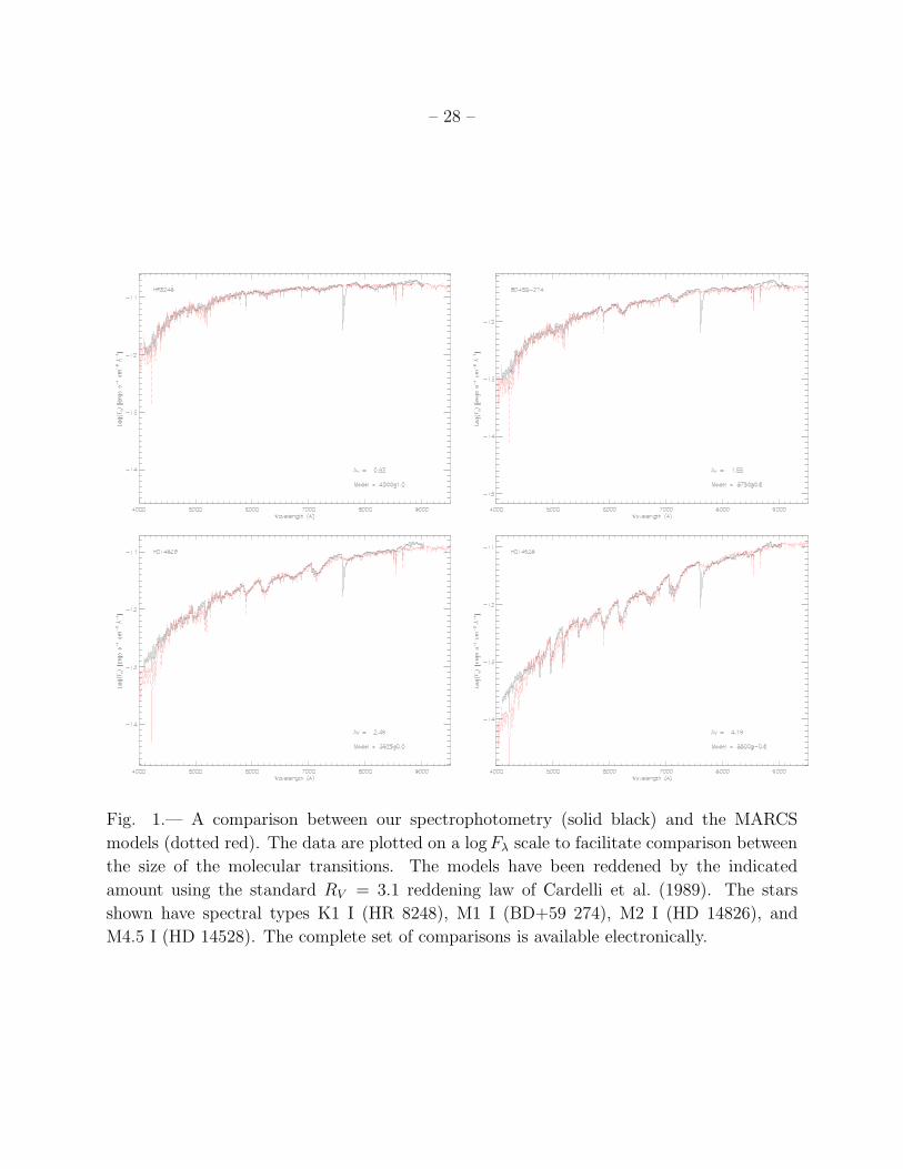
Fig. 1.— A comparison between our spectrophotometry (solid black) and the MARCS

models (dotted red). The data are plotted on a log Fλ scale to facilitate comparison between

the size of the molecular transitions. The models have been reddened by the indicated

amount using the standard RV = 3.1 reddening law of Cardelli et al. (1989). The stars

shown have spectral types K1 I (HR 8248), M1 I (BD+59 274), M2 I (HD 14826), and

M4.5 I (HD 14528). The complete set of comparisons is available electronically.

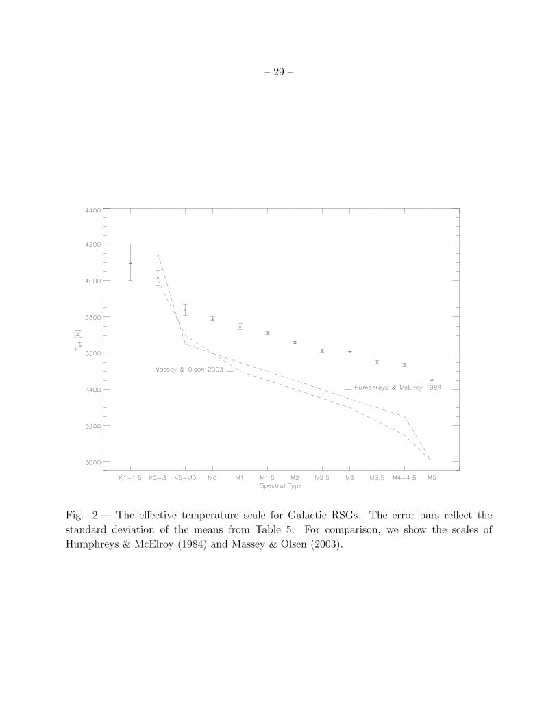
– 29 –

Fig. 2.— The effective temperature scale for Galactic RSGs. The error bars reflect the

standard deviation of the means from Table 5. For comparison, we show the scales of

Humphreys & McElroy (1984) and Massey & Olsen (2003).

– 30 –

Fig. 3.— Comparison with evolutionary tracks. The evolutionary tracks of Meynet & Maeder

(2003) are shown, along with the location of Galactic RSGs. The solid lines denote the no-

rotation models, while the dotted lines show the evolutionary tracks for an initial rotation

velocity of 300 km s−1. The tracks with rotation appear above the no-rotation tracks; the

one for 60 M⊙ does not extend this far to the right in the HRD. In (a) we show the location

of the RSGs taken from Humphreys (1978), using the effective temperature and bolometric

corrections of Humphreys & McElroy (1984). In (b) we show the location of the RSGs using

our new model fits (from Table 4). The filled circles in (b) denote those five stars whose

luminosities derived from V are significantly higher than those derived from K. In (c) we

show these same five stars with the luminosities derived from K. The diagonal lines at upper

right in this figure show lines of constant radii.

– 31 –

Fig. 4.— Derivation of (a) effective temperatures and (b) bolometric corrections at K based

on the (V − K)o colors. The points were computed from the models, while the curve shows

the smooth fits described in the text. The data extends from 3200 K to 4300 K with log g

values ranging from -1 to +1.

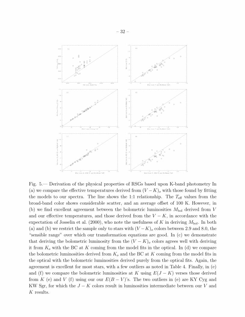
– 32 –

Fig. 5.— Derivation of the physical properties of RSGs based upon K-band photometry In

(a) we compare the effective temperatures derived from (V −K)o with those found by fitting

the models to our spectra. The line shows the 1:1 relationship. The Teff values from the

broad-band color shows considerable scatter, and an average offset of 100 K. However, in

(b) we find excellent agreement between the bolometric luminosities Mbol derived from V

and our effective temperatures, and those derived from the V − K, in accordance with the

expectation of Josselin et al. (2000), who note the usefulness of K in deriving Mbol. In both

(a) and (b) we restrict the sample only to stars with (V −K)o colors between 2.9 and 8.0, the

“sensible range” over which our transformation equations are good. In (c) we demonstrate

that deriving the bolometric luminosity from the (V − K)o colors agrees well with deriving

it from Ko with the BC at K coming from the model fits in the optical. In (d) we compare

the bolometric luminosities derived from Ko and the BC at K coming from the model fits in

the optical with the bolometric luminosities derived purely from the optical fits. Again, the

agreement is excellent for most stars, with a few outliers as noted in Table 4. Finally, in (e)

and (f) we compare the bolometric luminosities at K using E(J − K) verses those derived

from K (e) and V (f) using our our E(B − V )’s. The two outliers in (e) are KY Cyg and

KW Sgr, for which the J − K colors result in luminosities intermediate between our V and

K results.