at SciVerse ScienceDirect

Estuarine, Coastal and Shelf Science xxx (2012) 1e12

Contents lists available

Estuarine, Coastal and Shelf Science

journal homepage: www.elsevier .com/locate/ecss

The effect of physical drivers on ecosystem indices derived from ecologicalnetwork analysis: Comparison across estuarine ecosystems

Nathalie Niquil a,*, Eric Chaumillon a, Galen A. Johnson a,b, Xavier Bertin a, Boutheina Grami a,Valérie David a, Cédric Bacher c, Harald Asmus b, Daniel Baird d, Ragnhild Asmus b

a LIENSs, Littoral, Environnement et Sociétés, UMR 6250, Université de La Rochelle e CNRS, 2 rue Olympe de Gouges, La Rochelle 17000, FrancebAlfred Wegener Institut, Wattenmeerstation, Hafenstrasse 43, List 25992, Germanyc IFREMER, BP 70, 29280 Plouzané, FrancedDepartment of Botany & Zoology, University of Stellenbosch, Private Bag X1, Matieland, Stellenbosch, South Africa

a r t i c l e i n f o

Article history:Received 17 August 2011Accepted 28 December 2011Available online xxx

Keywords:mass-balance modelecological network analysisecosystem functioningphysical forcingestuaries comparisonsemi-enclosed systems

* Corresponding author.E-mail addresses: nniquil@univ-lr.fr, nathalie.n

echaumil@univ-lr.fr (E. Chaumillon), galen.a.johns@xavier.bertin@univ-lr.fr (X. Bertin), grami.boutheivalerie.david@univ-lr.fr (V. David), cbacher@ifremer.bremerhaven.de (H. Asmus), danbaird@sun.ac.za (awi.de (R. Asmus).

0272-7714/$ e see front matter � 2012 Published bydoi:10.1016/j.ecss.2011.12.031

Please cite this article in press as: Niquil, N.,Comparison across estuarine ecosystems, Es

a b s t r a c t

The structure and function of estuarine food webs change in response to both natural and anthropogenicstresses. The construction of quantitative food webs and their analysis by means of Ecological NetworkAnalysis provides outputs that have been used in many studies to assess system development, stress,robustness, resilience and maturity. Here we attempt to relate to the physical characteristics of theenvironment, ecosystem indices derived from Ecological Network Analysis. Ten models of food webswere gathered, across a selection of soft-bottom estuaries representative of a large morphological andhydrodynamic diversity, from wave-dominated to mixed energy tide-dominated systems. The selectionallowed the comparison of their derived Ecological Network Analysis indices, because of similarities ofaccuracy in the representation of detritus and bacteria, and because models took into account all trophiclevels up to top-predators. In order to obtain comparable physical characteristics, global models wereused for a homogeneous description of tide and tidal prisms. Spearman correlations, hierarchicalascendant clustering and Redundancy Analysis were applied to examine the relationship betweenEcological Network Analysis indices and physical characteristics. The set of four physical variablesselected (catchment area, tidal range at neap tide, index of tide-wave domination and latitude in absolutevalue) explained 67% of the structure of the Ecological Network Analysis indices. This implies that thephysical forcing related to climate, hydrodynamics and morphology is essential for determining theecological emergent properties of the food web. In the European policy context of determining the ‘goodecological status’ of coastal ecosystems, it implies that the use of Ecological Network Analysis indices forbasing the determination of operational indicators should be done, taking into account this context ofa strong influence of physical factors.

� 2012 Published by Elsevier Ltd.

1. Introduction

Recent developments in the management of coastal regionsshow an increasing interest in holistic approaches throughassessments of how ecosystems function. In Europe, the WaterFramework Directive (WFD; Directive 2000/60/EC) states the need

iquil@univ-lr.fr (N. Niquil),gmail.com (G.A. Johnson),na@gmail.com (B. Grami),fr (C. Bacher), hasmus@awi-D. Baird), Ragnhild.Asmus@

Elsevier Ltd.

et al., The effect of physical drtuarine, Coastal and Shelf Sc

to achieve a “good ecological status” by 2015 for all Europeanwaterbodies, including estuaries and other transitional waters (Uriarteand Borja, 2009). For coastal and offshore waters, the MarineStrategy Framework Directive (Directive 2008/56/EC) requires EUMember States to report on the environmental status of the seasunder their jurisdiction and to work to achieve a “good environ-mental status”, defined by 11 descriptors. One of those, calledGroup 4 descriptor, is defined as “All elements of the marine foodwebs, to the extent that they are known, occur at normal abun-dance and diversity and levels capable of ensuring the long-termabundance of the species and the retention of their full reproduc-tive capacity” (Rogers et al., 2010). Any management decisionshould thus be based on a precise description of how ecosystems,which are influenced by natural as well as human forcing, function.

ivers on ecosystem indices derived from ecological network analysis:ience (2012), doi:10.1016/j.ecss.2011.12.031

N. Niquil et al. / Estuarine, Coastal and Shelf Science xxx (2012) 1e122

It thus follows that an understanding of natural forcing on anecosystem is firstly necessary, before assessments can be made ofhow human impacts modify it. However, the ideal situation forstudying this natural forcing would be to compare pristine estu-aries, which is not possible, under temperate climates.

According to Pritchard (1967, in Elliott and McLusky, 2002) anestuary is “a semi-enclosed coastal body of water, which has a freeconnection with the open sea, and within which seawater ismeasurably diluted with fresh water derived from land drainage”.Estuaries are highly productive and harbour a high diversity ofplants and animals. They provide nursery grounds for marine fishand feeding grounds for migratory birds, while a multiplicity ofgoods and services are derived from them (McLusky and Elliott,2004). Estuarine ecosystems are subject to increasing anthropo-genic impacts including pollution, excess nutrient loading, habitatdestruction, and changes in biodiversity (Halpern et al., 2008).Estuaries are highly variable and considered as highly stressedsystems, while Elliott and Quintino (2007) also emphasized thedifficulty to delineate natural from human-induced stressors.However, despite natural and human-induced pressures, estuarieshave nevertheless maintained their attractiveness for wildlife,leading Elliott and McLusky (2002) to consider that they are someof the most resilient habitats on earth. Numerous recent publica-tions have highlighted the need and difficulty to define whatshould be considered as a “good ecological status” in these complexsystems (e.g. de Jonge, 2007; Christian et al., 2009; Dauvin andRuellet, 2009; Pinto et al., 2009; Lester et al., 2010).

Ecological Network Analysis (ENA) is essentially a set of algo-rithms to evaluate the flow and cycling of energy and materialthrough ecosystems from which a suite of system indices can bederived (Ulanowicz, 1986, 1997, 2009; Wulff et al., 1989; Kay et al.,1989). It has often been used to compare food web functioningspatially (e.g. Leguerrier et al., 2007), over time (e.g. Christian et al.,2009), and it has been often been applied to estuarine ecosystems(Christian et al., 2005). Based on such comparisons, attempts haveoften been made to link system indices derived from ENA to levelsof stress (Kay et al., 1989; Ulanowicz, 1996, 2009; Heymans et al.,2007), to stability (Vasconcellos et al., 1997; Heymans et al.,2002; Heymans, 2003), development (Ulanowicz, 1997) andmaturity (Christensen, 1995). Most of these indices has been alsoshown to be highly sensitive to the level of aggregation of the foodweb compartments (Baird, 2009; Johnson et al., 2009) and to thefact that detritus (Allesina et al., 2005) and bacteria (Abarca-Arenasand Ulanowicz, 2002; Johnson et al., 2009) had to be incorporatedin separate compartments in food webs. All these criteria (samelevel of aggregation, detritus and bacteria in their own compart-ments) have been taken into account in the present paper to set upa selection of comparable models.

The objectives of the present paper are firstly to examine andcompare ENA derived indices of several semi-enclosed and typicalestuarine systems with physical forcing variables, describing inparticular morphology and hydrodynamics. Secondly, we attemptto identify those physical variables, which could modify or influ-ence the ecological functioning of these systems.

Our working hypotheses are: (1) that the morphological clas-sification between wave- and tide-dominated systems willinfluence the shape of the estuary mouth that may act onwater exchanges with the ocean; (2) that the fluvial discharge,the catchment area and the surface of the estuary may act on thesalinity, the transparency, the nutrients concentration and thesuspended matter supplies; (3) that these first level consequenceswill in turn modify the community structure and the processes ofthe pelagos as well as of the benthos. The detail of the chain ofcauses and consequences will not be studied in the present articlethat constitutes a preliminary step. The demonstration is done here

Please cite this article in press as: Niquil, N., et al., The effect of physical drComparison across estuarine ecosystems, Estuarine, Coastal and Shelf Sc

that the physical variables are highly influential and a more preciseapproach will be necessary to better understand causes andconsequences that should be led at the scale of the habitat.

2. Material and methods

A set of 10 semi-enclosed and typical estuarine ecosystemswereselected for the purposes of this study whose characteristics aregiven in Table 1 and their geographical position in Fig. 1.

The selection of estuarine ecosystem models discussed in thispaper represent whole ecosystem food webs, taking into accountall compartments from primary producers to top-predators. Allsites selected for the ecosystem attribute comparison were semi-enclosed soft-bottom coastal environments. To take into accountthe full diversity of semi-enclosed coastal environments we usedestuaries classifications (Davies, 1964; Pritchard, 1967; Hayes, 1979;Nichol, 1991; Reinson, 1992; Boyd et al., 1992; Dalrymple et al.,1992), which refers to the morphology and the relative influenceof waves, tides and rivers. The selection of the semi-enclosedsystems in this paper was not exhaustive but represented a -diversity of estuaries in terms of hydrodynamics (from micro- tomacrotidal regimes, from wave-dominated to mixed energy tide-dominated systems) and morphology (from open estuaries dis-playing moderatly developed sand spits to barred estuaries).

2.1. Study sites

The 10 study sites are briefly described from the largestto the smallest. In this study, we defined arbitrarily largeestuaries with surface areas greater than 1000 km2, medium-sizeestuaries with surface areas between 100 and 1000 km2 andsmall estuaries with surface areas less than 100 km2. In terms ofoffshore wave climate, we considered it as energetic when offshoreyearly-mean significant wave height Hs is larger than 2 m, inter-mediate for yearly-mean Hs between 1.4 and 2m, andmoderate forthe yearly-mean Hs below 1.4 m. In terms of tidal range, weconsidered it as large when the median tide range (TR) of TR_50%(50th percentile of tidal ranges) is>3m, intermediate if the TR_50%is between 1.5 and 3 m and small for a TR_50% <1.5 m. In terms ofriver catchment area, we considered a large river catchment an area>100,000 km2, medium-size river catchments between 10,000 and100,000 km2, and small river catchments <10,000 km2 (Table 1).

The Chesapeake Bay, located on the north-east coast of USA, isthe largest estuary in the United States and one of the largest in theworld (320 km long). This semi-enclosed ria-type, mesotidalestuary is subject to a moderate offshore wave climate, and a smalltidal range. It has a large river catchment area (166,000 Km2) andthemesohaline region (5e18 psu) receives freshwater input mainlyfrom the Susquehanna River (long-term average discharge of about1099 m3 s�1) and from the Potomac River (long-term averagedischarge of about 310 m3 s�1). This estuary has been extensivelyexploited for its natural resources, while it has received largeamounts of pollutants and nutrients from the catchment area(Baird et al., 1991).

The Delaware Bay is a large semi-enclosed ria-type estuarylocated on the north-east coast of USA. This microtidal estuary issubject to amoderate offshorewave climate, has a small tidal range,with a medium-size river catchment. It mainly receives fresh waterfrom the Delaware River (58% of the total estimated discharge) andfrom the Schuylkill River (15% of the total estimated discharge(Sharp et al., 1986)). Dalrymple et al. (1992) labelled the Ches-apeake Bay and the Delaware Bay as mixed tide-and-wave domi-nated estuaries. Nevertheless, considering the relatively small ratiobetween the spit length and estuary mouth width, the Chesapeake

ivers on ecosystem indices derived from ecological network analysis:ience (2012), doi:10.1016/j.ecss.2011.12.031

N. Niquil et al. / Estuarine, Coastal and Shelf Science xxx (2012) 1e12 3

Bay can be more precisely qualified as a mixed-energy tide-domi-nated system following the terminology of Hayes (1979).

The Ems-river Estuary is a shallow back-barrier mesotidal,well-mixed estuary of medium-size, draining into the Wadden Sea.It has a medium-size river catchment and an intermediate offshorewave climate. The Ems-Dollard estuary receives fresh water fromthe river Ems (average discharge 120m3 s�1) and theWesterwoldseAa Rivers (average discharge 14 m3 s�1). Considering the presenceof barrier islands, the Ems-River Estuary can be qualified as a mixedenergy wave-dominated system. The large amount of nutrientsintroduced annually comes both from the catchment and from thesea (de Jonge, 1988; Baird et al., 1991).

The Narragansett Bay is a medium-size, open ria-type estuarylocated on the East coast of USA. Thismicrotidal estuary is subject toa moderate offshore wave climate, a small tidal range, with a small-size river catchment. Considering the absence of spits or barriers atthe mouths, which is partly the result of a low sediment supply, theNarraganset Bay can be qualified as a mixed energy tide-dominatedsystem. It receives fresh water from the Blackstone, Taunton, andPawtuxet Rivers, but the daily river fresh water input is less than 1%of the volume of Narragansett Bay. It has a long history of humanintensive use and high impacts (Vadeboncoeur et al., 2010).

The Sylt-Rømø Bight is a medium-size, mesotidal shallow,semi-enclosed back-barrier lagoon, located between the islands ofSylt in Germany and Rømø in Denmark (Backhaus et al., 1998) andis part of the greater Wadden Sea. The Bight receives little freshwater from the surrounding land and the nutrient load is very low(Baird et al., 2011). Considering the presence of barrier islands, theSylt-Rømø Bight can be qualified as a mixed energy wave-dominated system. Sand is the prevailing sediment type andcovers 72e90% of the total intertidal area (Bayerl et al., 1998). It wasdeclared a World Heritage Site by UNESCO in July 2009.

The Marennes-Oléron Bay is a medium-size, macrotidal,shallow, semi-enclosed back-barrier lagoonwith a large tidal range,and located on the Atlantic coast of France. This back-barrier lagoonis characterized by two connections with the open ocean and isbounded seaward by an island, which consists of both rocky andsedimentary coasts (Allard et al., 2008). The offshore wave climateis energetic offshore (Bertin et al., 2008), but moderate inside theestuary. The catchment basin is medium-sized. The Marennes-Oléron Bay receives fresh water from the Charente River. It hasextensive mudflats and mixed sand-and-mud flats (Sauriau et al.,1989). The presence of spits at its entrances (Chaumillon et al.,2004; Bertin et al., 2005) suggests the Marennes-Oléron Bay isa mixed energy system. It has a long history of human use mainlyrelated to land reclamation (Chaumillon et al., 2004), deforestation(Poirier et al., 2011) and more recently related to oyster farming(Bertin et al., 2005).

The Ythan estuary is a small, shallow, semi-enclosed estuarylocated in the north-east of Scotland. This mesotidal and well-mixed estuary, with a small-sized catchment area, is subjected toan intermediate offshore wave climate. The substrate consistsmainly of sand, with the rest being mud or mud-sand (Baird andUlanowicz, 1993). The presence of well-developed spit at themouth suggests the Ythan estuary is mixed energy wave-dominated system. The Ythan River flows into the estuary, whichdrains agricultural fields bringing high nutrient concentrations intothe Ythan River (Gillibrand and Balls, 1998).

Three small barred estuaries, located close to one another inSouth Africa and discharging into the Indian Ocean, are presentedbelow. These microtidal estuaries are exposed to a strong offshorewave climate, and a small tidal range. They are normally openbarred estuaries (Cooper, 2001) indicating they can all be consid-ered as wave-dominated at a world wide scale. At the scale of theSouth African estuaries where closed estuaries occur, those three

Please cite this article in press as: Niquil, N., et al., The effect of physical drComparison across estuarine ecosystems, Estuarine, Coastal and Shelf Sc

barred estuaries are more tide-dominated because their inlet ismaintained by the tidal prism (Cooper, 2001).

The Swartkops Estuary is a well-mixed estuary (Baird et al.,1991) with a small-size river catchment (Scharler and Baird,2005). It is located in a heavily populated area and subject toagricultural, urban and industrial pollution.

The Kromme Estuary is a seawater-dominated estuary, witha small-size river catchment area. Due to the construction ofstorage reservoirs in the catchment, it receives very little freshwater (Scharler and Baird, 2005). During summer, the upper rea-ches become hypersaline (salinity>35 psu). The sediment is mainlycomposed of sand of marine origin, but mud of fluvial origin is alsopresent in the middle and upper reaches of the estuary (Baird andUlanowicz, 1993).

The Sundays Estuary is longer than the two other estuariesfrom South Africa with a channel-like shape, and a small andnarrow intertidal area (Scharler and Baird, 2005). Its river catch-ment is medium-sized (Scharler and Baird, 2005) and it has a strongaxial salinity gradient (Whitfield, 1994). Its catchment area is sub-jected to less anthropogenic pressure than the two other SouthAfrican estuaries, and it receives a considerable amount of freshwater from an inter-basin water transfer scheme (Archibald, 1983).

From this short description, it appears that despite the lack oftypical tide-dominated and wave-dominated closed estuaries, theselected study sites offer a good gradient from mixed energy tide-dominated to wave-dominated estuaries.

2.2. Physical variables considered

Over the last five decades, several classifications have beenproposed in an attempt to link geomorphic properties of tidal inletsand estuaries with incident hydrodynamic conditions (Bruun,1978;Hayes, 1979; Oertel, 1988). Thus, Hayes (1979) proposed a classifi-cation, which related the observed tidal inlet morphologies(main channel cross-sectional area and dynamic, tidal deltas shapeand volume) to the ratio between yearly-mean wave height andtidal range. Nevertheless, probably due to its simplicity, this ratiowas shown to be insufficient to predict inlet morphologies (Nahonet al., 2012). For instance, if two tidal inlets are subjected to thesame wave and tidal regimes but have very different tidal prisms,they may exhibit large differences in their morphologies. Tocounteract this limitation, we propose a new index, based on theformula:

log10 ðUÞHs2

(1)

where U is the spring tidal prism and Hs is the offshore yearly-mean significant wave height. In order to perform a consistentcomparison between the various study sites, a time-series of Hsoriginating from the WaveWatchIII hindcast performed at NCEP/NOAA (Tolman et al., 2002) was extracted offshore for each sitebetween 2000 and 2010, and the mean value for each computedover this period. This 10-year time windowwas selected to smoothinter-annual variability of wave climate in the Atlantic Ocean, asevidenced by Dodet et al. (2010). A similar systematic procedurewas not possible for the tidal prism since its value depends onseveral parameters (the estuary bathymetry, the tidal rangeand distortion inside the estuary), some of which are unknownat several sites. Therefore, the values of tidal prism found in theliterature were used to apply formula (1). Nevertheless, due tothe use of a log10 function, an error of 100% on U would affect theproposed index (1) by 5% only.

The mean tidal range was also identified as a potential rele-vant physical parameter. Amplitude and phases of the 7 main

ivers on ecosystem indices derived from ecological network analysis:ience (2012), doi:10.1016/j.ecss.2011.12.031

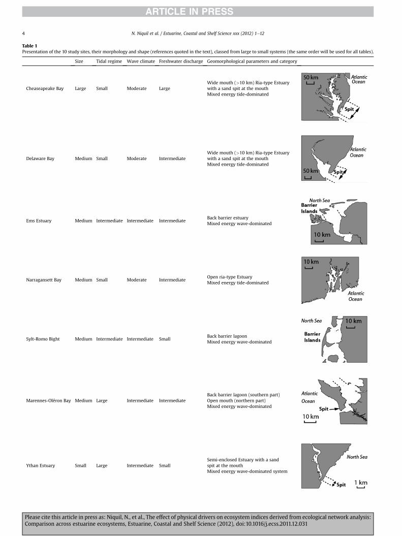
Table 1Presentation of the 10 study sites, their morphology and shape (references quoted in the text), classed from large to small systems (the same order will be used for all tables).

Size Tidal regime Wave climate Freshwater discharge Geomorphological parameters and category

Cheaseapeake Bay Large Small Moderate LargeWide mouth (>10 km) Ria-type Estuarywith a sand spit at the mouthMixed energy tide-dominated

Delaware Bay Medium Small Moderate IntermediateWide mouth (>10 km) Ria-type Estuarywith a sand spit at the mouthMixed energy tide-dominated

Ems Estuary Medium Intermediate Intermediate IntermediateBack barrier estuaryMixed energy wave-dominated

Narragansett Bay Medium Small Moderate IntermediateOpen ria-type EstuaryMixed energy tide-dominated

Sylt-Romo Bight Medium Intermediate Intermediate SmallBack barrier lagoonMixed energy wave-dominated

Marennes-Oléron Bay Medium Large Intermediate IntermediateBack barrier lagoon (southern part)Open mouth (northern part)Mixed energy wave-dominated

Ythan Estuary Small Large Intermediate SmallSemi-enclosed Estuary with a sandspit at the mouthMixed energy wave-dominated system

N. Niquil et al. / Estuarine, Coastal and Shelf Science xxx (2012) 1e124

Please cite this article in press as: Niquil, N., et al., The effect of physical drivers on ecosystem indices derived from ecological network analysis:Comparison across estuarine ecosystems, Estuarine, Coastal and Shelf Science (2012), doi:10.1016/j.ecss.2011.12.031

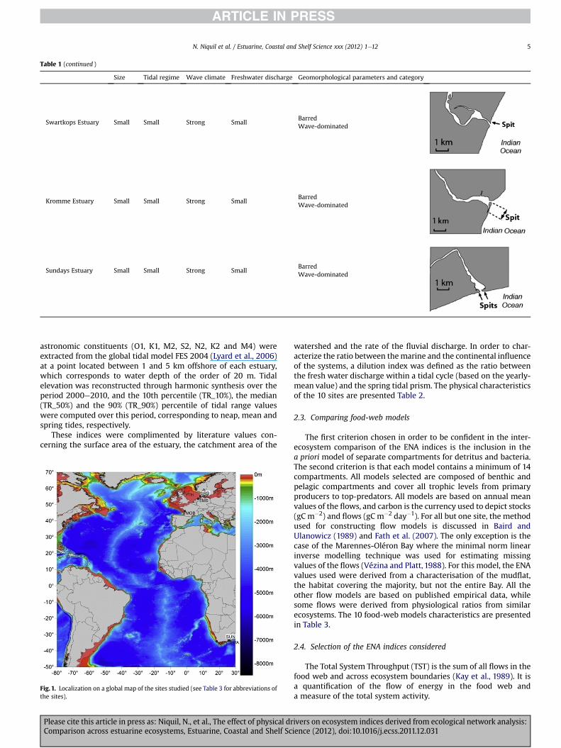
Table 1 (continued )

Size Tidal regime Wave climate Freshwater discharge Geomorphological parameters and category

Swartkops Estuary Small Small Strong SmallBarredWave-dominated

Kromme Estuary Small Small Strong SmallBarredWave-dominated

Sundays Estuary Small Small Strong SmallBarredWave-dominated

N. Niquil et al. / Estuarine, Coastal and Shelf Science xxx (2012) 1e12 5

astronomic constituents (O1, K1, M2, S2, N2, K2 and M4) wereextracted from the global tidal model FES 2004 (Lyard et al., 2006)at a point located between 1 and 5 km offshore of each estuary,which corresponds to water depth of the order of 20 m. Tidalelevation was reconstructed through harmonic synthesis over theperiod 2000e2010, and the 10th percentile (TR_10%), the median(TR_50%) and the 90% (TR_90%) percentile of tidal range valueswere computed over this period, corresponding to neap, mean andspring tides, respectively.

These indices were complimented by literature values con-cerning the surface area of the estuary, the catchment area of the

Fig. 1. Localization on a global map of the sites studied (see Table 3 for abbreviations ofthe sites).

Please cite this article in press as: Niquil, N., et al., The effect of physical drComparison across estuarine ecosystems, Estuarine, Coastal and Shelf Sc

watershed and the rate of the fluvial discharge. In order to char-acterize the ratio between themarine and the continental influenceof the systems, a dilution index was defined as the ratio betweenthe fresh water discharge within a tidal cycle (based on the yearly-mean value) and the spring tidal prism. The physical characteristicsof the 10 sites are presented Table 2.

2.3. Comparing food-web models

The first criterion chosen in order to be confident in the inter-ecosystem comparison of the ENA indices is the inclusion in thea priori model of separate compartments for detritus and bacteria.The second criterion is that each model contains a minimum of 14compartments. All models selected are composed of benthic andpelagic compartments and cover all trophic levels from primaryproducers to top-predators. All models are based on annual meanvalues of the flows, and carbon is the currency used to depict stocks(gC m�2) and flows (gC m�2 day�1). For all but one site, the methodused for constructing flow models is discussed in Baird andUlanowicz (1989) and Fath et al. (2007). The only exception is thecase of the Marennes-Oléron Bay where the minimal norm linearinverse modelling technique was used for estimating missingvalues of the flows (Vézina and Platt, 1988). For this model, the ENAvalues used were derived from a characterisation of the mudflat,the habitat covering the majority, but not the entire Bay. All theother flow models are based on published empirical data, whilesome flows were derived from physiological ratios from similarecosystems. The 10 food-web models characteristics are presentedin Table 3.

2.4. Selection of the ENA indices considered

The Total System Throughput (TST) is the sum of all flows in thefood web and across ecosystem boundaries (Kay et al., 1989). It isa quantification of the flow of energy in the food web anda measure of the total system activity.

ivers on ecosystem indices derived from ecological network analysis:ience (2012), doi:10.1016/j.ecss.2011.12.031

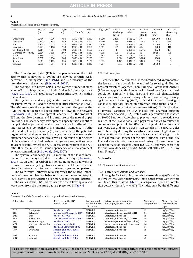
Table 2Physical characteristics of the 10 sites compared.

Site TR_10%(m)

TR_50%(m)

TR_90%(m)

U(*10^6 m3)

Mean Hs(m)

log(U)/Hs2 Fluvialdischarge(m3 s-1)

Dilutionindex

Absolutevalue oflatitude

Catchmentarea(km2)

Surface ofthe estuary(km2)

Chesapeake 0.744 1.096 1.450 1.25E þ 09 1.260 5.730 2280 8.15E-02 37 166,000 5470Delaware 0.842 1.193 1.552 7.39E þ 09 1.290 5.930 336 2.03E-03 39.42 17,378 2069Ems 1.806 2.425 3.022 9.00E þ 08 1.520 3.876 134 6.66E-03 53.7 12,600 500Narragansett 0.773 1.166 1.559 3.25E þ 08 1.260 5.361 105 1.44E-02 41.4 3489 416Sylt-Romo Bight 1.314 1.864 2.403 6.60E þ 07 1.560 3.213 14 9.48E-03 55.16 1828 404Marennes-Oléron Bay 2.224 3.565 4.867 8.00E þ 08 1.480 4.065 100 5.59E-03 46 10,855 190Ythan 1.585 3.093 4.170 3.42E þ 06 1.480 2.983 6.960 9.10E-02 57.34 548 71Swartkops 0.597 1.234 1.808 2.88E þ 06 2.220 1.311 0.600 9.31E-03 33.86 1360 4Kromme 0.649 1.165 1.655 1.87E þ 06 2.120 1.395 0.127 3.04E-03 34.23 936 3Sundays 0.628 1.251 1.819 2.20E þ 06 2.220 1.287 1.875 3.81E-02 34.5 20,990 3

N. Niquil et al. / Estuarine, Coastal and Shelf Science xxx (2012) 1e126

The Finn Cycling Index (FCI) is the percentage of the totalactivity that is devoted to cycling (i.e. flowing through cyclicpathways) in the system (Finn, 1976), and is a measure of theretentiveness of the system (Baird et al., 2004).

The Average Path Length (APL) is the average number of stepsa unit of fluxwill experiencewithin the foodweb, from entry to exit(Kay et al., 1989). It is another way of measuring retention withinthe food web.

The system Ascendency (A) is the product of the activity,measured by the TST, and the average mutual information (AMI).The AMI measures the organisation of the flows: the greater theAMI, the higher degree of specialization of flows in the network(Ulanowicz,1986). The Development Capacity (DC) is the product ofTST and the flow diversity and is a measure of the natural upperlimit of A. The Ascendency/Development Capacity ratio quantifiesthe potential organisation realised and is a useful attribute forinter-ecosystems comparison. The internal Ascendency (Ai)/theinternal development Capacity (Ci) ratio reflects on the potentialorganisation based on internal exchanges alone. Consequently, thedifference between A/C and Ai/Ci gives an indication of the degreeof dependence of a food web on exogenous connections withadjacent systems: where the Ai/Ci decreases in relation to the A/Cratio, then the system has some dependency on a few dominantexternal connections (Baird et al., 1991, 2007).

The system Redundancy (R) is a measure of the loss of infor-mation within the system, due to parallel pathways (Ulanowicz,1997), i.e. an atom of Carbon can follow numerous pathways ofequivalent probability to go from a compartment to another one.The R/DC ratio can also be used for inter-ecosystems comparisons.

The Detritivory/Herbivory ratio expresses the relative impor-tance of these two feeding behaviours within the second trophiclevel, namely as consumption of primary producers and detritus.

The values of the ENA indices used for the following analysiswere taken from the literature and are presented in Table 4.

Table 3Characteristics of the food-web models compared and associated references.

Abbreviation Site Reference for the ENAindices values

Program usfor ENA indcalculation

CHE Chesapeake Baird et al., 1991 NETWRKDEL Delaware Monaco and Ulanowicz, 1997 NETWRKEMS Ems Baird et al., 1991 NETWRKNAR Narragansett Monaco and Ulanowicz, 1997 NETWRKSRB Sylt-Romo Bight Baird et al., 2004 NETWRKMOB Marennes-Oléron Bay Leguerrier et al., 2004 NETWRKYTH Ythan Baird and Ulanowicz, 1993 NETWRKSWA Swartkops Scharler and Baird, 2005;

Baird, 2009NETWRK

KRO Kromme Scharler and Baird, 2005 NETWRKSUN Sundays Scharler and Baird, 2005 NETWRK

Please cite this article in press as: Niquil, N., et al., The effect of physical drComparison across estuarine ecosystems, Estuarine, Coastal and Shelf Sc

2.5. Data analyses

Because of the low number of models considered as comparable,the Spearman rank correlation was used for relating all ENA andphysical variables together. Then, Principal Component Analysis(PCA) was applied to the ENA variables, based on a Spearman rankcorrelation similarity index. ENA and physical characteristicsassociations were analysed using a hierarchical average linkageagglomerative clustering (HAC), analysed in R mode (looking atvariable associations, based on Spearman correlations) and in Qmode (in order to describe the site associations). Finally, the effectof physical variables on ENA indices was analysed applyingRedundancy Analysis (RDA), tested with a permutation test basedon 10,000 iterations. According to previous results, a selection wasrealised of the ENA variables and physical variables, to follow thecommonly accepted rule for RDA: more dependent than indepen-dent variables and more objects than variables. The ENA variableswere chosen by deleting the variables that showed highest corre-lation coefficients and conserving at least one structuring variable(high contribution) for each of the first 4 principal axes of the PCA.Physical characteristics were selected using a forward selection,using the ‘packfor’ package under R 2.12.2. All analyses, except thelast one, were done using XLSTAT (Addinsoft 2011.2.02 XLSTAT-Pro,Paris, France).

3. Results

3.1. Spearman rank correlation

3.1.1. Correlations among ENA variablesAmong the ENA variables, the relative Ascendency (A/C) and the

relative internal Ascendency (Ai/Ci) are related by the way they arecalculated. This resulted (Table 5) in a significant positive correla-tion between them (p ¼ 0.017). The index built by the difference

edices

Determination of unknownflow or physiological rates

Number ofcompartments

Model currencyin the referencepaper

Literature, efficiencies 15 mgC/m2/dayLiterature, efficiencies, ECOPATH 14 mgC/m2/yearLiterature, efficiencies 15 mgC/m2/dayLiterature, efficiencies, ECOPATH 14 mgC/m2/yearNone (complete set of flow values) 59 mgC/m2/dayLinear inverse method - least square 16 mgC/m2/dayLiterature, efficiencies 14 mgC/m2/dayLiterature, efficiencies 15 mgC/m2/day

Literature, efficiencies 16 mgC/m2/dayLiterature, efficiencies 25 mgC/m2/day

ivers on ecosystem indices derived from ecological network analysis:ience (2012), doi:10.1016/j.ecss.2011.12.031

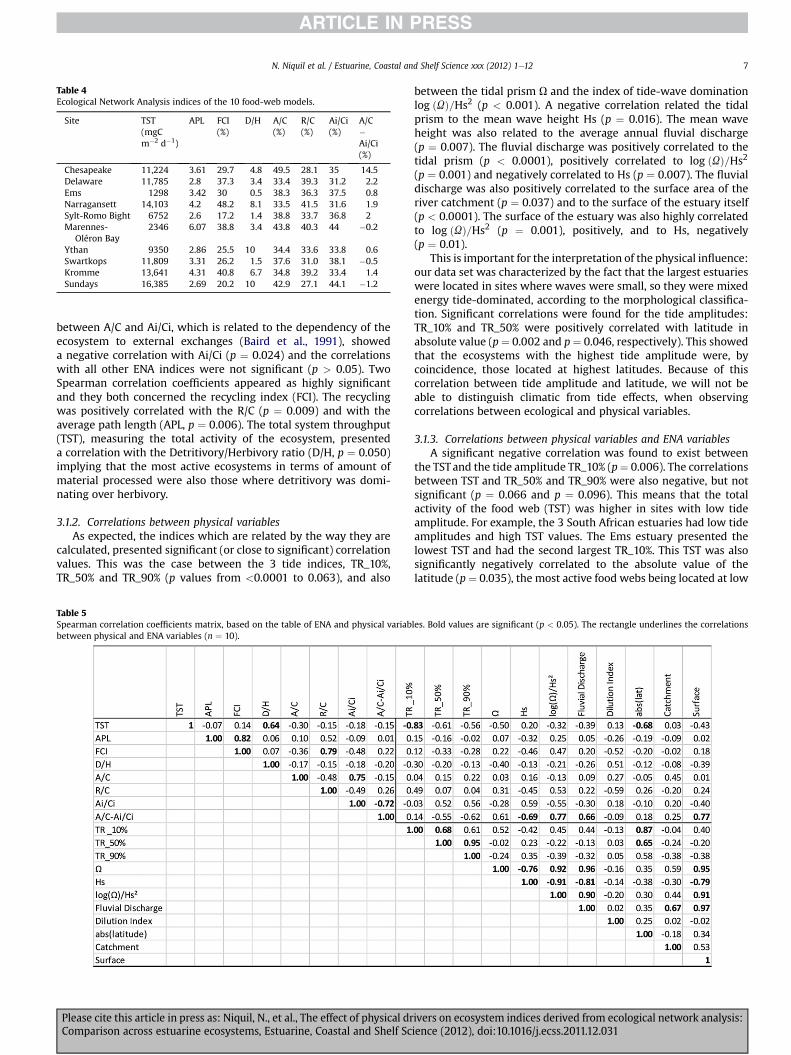
Table 4Ecological Network Analysis indices of the 10 food-web models.

Site TST(mgCm�2 d�1)

APL FCI(%)

D/H A/C(%)

R/C(%)

Ai/Ci(%)

A/C�Ai/Ci(%)

Chesapeake 11,224 3.61 29.7 4.8 49.5 28.1 35 14.5Delaware 11,785 2.8 37.3 3.4 33.4 39.3 31.2 2.2Ems 1298 3.42 30 0.5 38.3 36.3 37.5 0.8Narragansett 14,103 4.2 48.2 8.1 33.5 41.5 31.6 1.9Sylt-Romo Bight 6752 2.6 17.2 1.4 38.8 33.7 36.8 2Marennes-

Oléron Bay2346 6.07 38.8 3.4 43.8 40.3 44 �0.2

Ythan 9350 2.86 25.5 10 34.4 33.6 33.8 0.6Swartkops 11,809 3.31 26.2 1.5 37.6 31.0 38.1 �0.5Kromme 13,641 4.31 40.8 6.7 34.8 39.2 33.4 1.4Sundays 16,385 2.69 20.2 10 42.9 27.1 44.1 �1.2

N. Niquil et al. / Estuarine, Coastal and Shelf Science xxx (2012) 1e12 7

between A/C and Ai/Ci, which is related to the dependency of theecosystem to external exchanges (Baird et al., 1991), showeda negative correlation with Ai/Ci (p ¼ 0.024) and the correlationswith all other ENA indices were not significant (p > 0.05). TwoSpearman correlation coefficients appeared as highly significantand they both concerned the recycling index (FCI). The recyclingwas positively correlated with the R/C (p ¼ 0.009) and with theaverage path length (APL, p ¼ 0.006). The total system throughput(TST), measuring the total activity of the ecosystem, presenteda correlation with the Detritivory/Herbivory ratio (D/H, p ¼ 0.050)implying that the most active ecosystems in terms of amount ofmaterial processed were also those where detritivory was domi-nating over herbivory.

3.1.2. Correlations between physical variablesAs expected, the indices which are related by the way they are

calculated, presented significant (or close to significant) correlationvalues. This was the case between the 3 tide indices, TR_10%,TR_50% and TR_90% (p values from <0.0001 to 0.063), and also

Table 5Spearman correlation coefficients matrix, based on the table of ENA and physical variabbetween physical and ENA variables (n ¼ 10).

Please cite this article in press as: Niquil, N., et al., The effect of physical drComparison across estuarine ecosystems, Estuarine, Coastal and Shelf Sc

between the tidal prism U and the index of tide-wave dominationlog ðUÞ=Hs2 (p < 0.001). A negative correlation related the tidalprism to the mean wave height Hs (p ¼ 0.016). The mean waveheight was also related to the average annual fluvial discharge(p ¼ 0.007). The fluvial discharge was positively correlated to thetidal prism (p < 0.0001), positively correlated to log ðUÞ=Hs2(p ¼ 0.001) and negatively correlated to Hs (p ¼ 0.007). The fluvialdischarge was also positively correlated to the surface area of theriver catchment (p ¼ 0.037) and to the surface of the estuary itself(p < 0.0001). The surface of the estuary was also highly correlatedto log ðUÞ=Hs2 (p ¼ 0.001), positively, and to Hs, negatively(p ¼ 0.01).

This is important for the interpretation of the physical influence:our data set was characterized by the fact that the largest estuarieswere located in sites where waves were small, so they were mixedenergy tide-dominated, according to the morphological classifica-tion. Significant correlations were found for the tide amplitudes:TR_10% and TR_50% were positively correlated with latitude inabsolute value (p¼ 0.002 and p¼ 0.046, respectively). This showedthat the ecosystems with the highest tide amplitude were, bycoincidence, those located at highest latitudes. Because of thiscorrelation between tide amplitude and latitude, we will not beable to distinguish climatic from tide effects, when observingcorrelations between ecological and physical variables.

3.1.3. Correlations between physical variables and ENA variablesA significant negative correlation was found to exist between

the TSTand the tide amplitude TR_10% (p¼ 0.006). The correlationsbetween TST and TR_50% and TR_90% were also negative, but notsignificant (p ¼ 0.066 and p ¼ 0.096). This means that the totalactivity of the food web (TST) was higher in sites with low tideamplitude. For example, the 3 South African estuaries had low tideamplitudes and high TST values. The Ems estuary presented thelowest TST and had the second largest TR_10%. This TST was alsosignificantly negatively correlated to the absolute value of thelatitude (p¼ 0.035), the most active food webs being located at low

les. Bold values are significant (p < 0.05). The rectangle underlines the correlations

ivers on ecosystem indices derived from ecological network analysis:ience (2012), doi:10.1016/j.ecss.2011.12.031

N. Niquil et al. / Estuarine, Coastal and Shelf Science xxx (2012) 1e128

latitudes. The second ENA variable highly related to physical vari-ables is the A/C � Ai/Ci. It was significantly negatively correlatedwith Hs and positively with log ðUÞ=Hs2, fluvial discharge, andsurface area of the estuary (p values from 0.13 to 0.42).

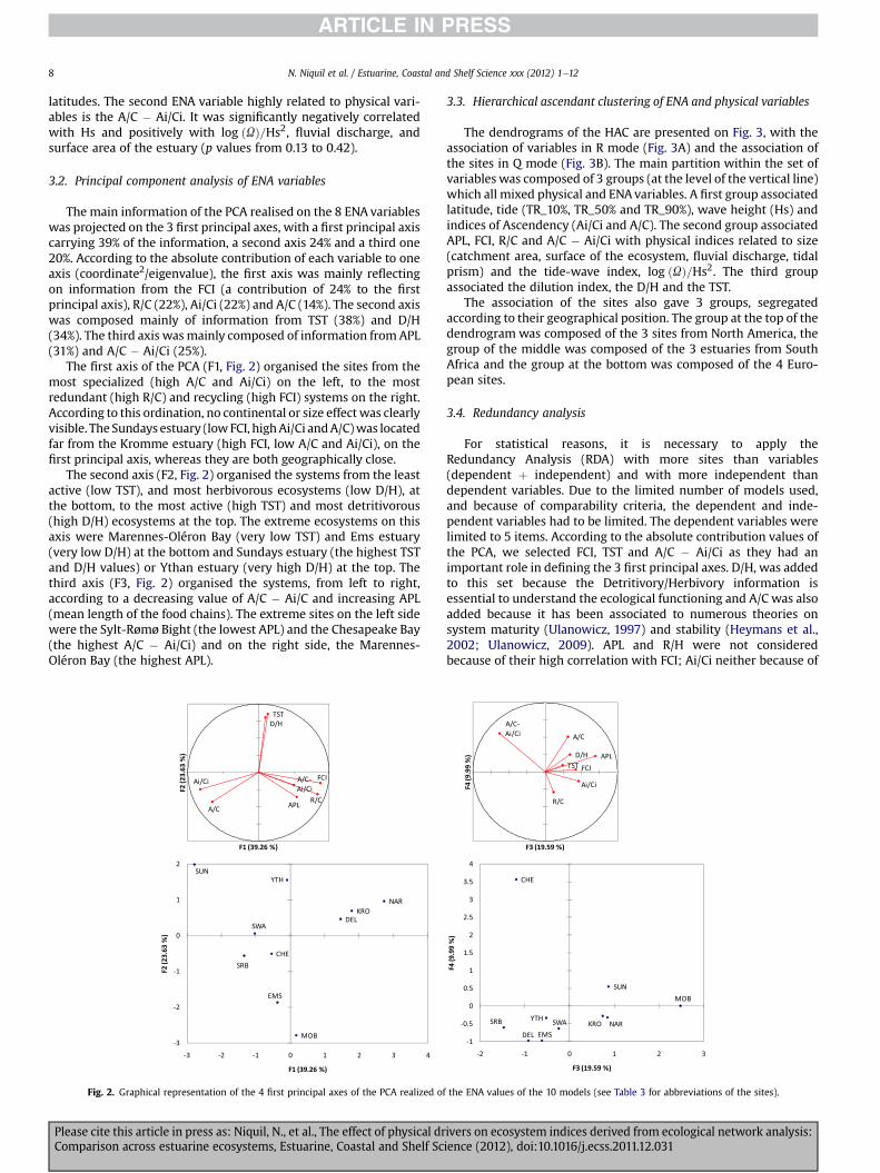
3.2. Principal component analysis of ENA variables

The main information of the PCA realised on the 8 ENA variableswas projected on the 3 first principal axes, with a first principal axiscarrying 39% of the information, a second axis 24% and a third one20%. According to the absolute contribution of each variable to oneaxis (coordinate2/eigenvalue), the first axis was mainly reflectingon information from the FCI (a contribution of 24% to the firstprincipal axis), R/C (22%), Ai/Ci (22%) and A/C (14%). The second axiswas composed mainly of information from TST (38%) and D/H(34%). The third axis wasmainly composed of information fromAPL(31%) and A/C � Ai/Ci (25%).

The first axis of the PCA (F1, Fig. 2) organised the sites from themost specialized (high A/C and Ai/Ci) on the left, to the mostredundant (high R/C) and recycling (high FCI) systems on the right.According to this ordination, no continental or size effectwas clearlyvisible. The Sundays estuary (lowFCI, highAi/Ci andA/C)was locatedfar from the Kromme estuary (high FCI, low A/C and Ai/Ci), on thefirst principal axis, whereas they are both geographically close.

The second axis (F2, Fig. 2) organised the systems from the leastactive (low TST), and most herbivorous ecosystems (low D/H), atthe bottom, to the most active (high TST) and most detritivorous(high D/H) ecosystems at the top. The extreme ecosystems on thisaxis were Marennes-Oléron Bay (very low TST) and Ems estuary(very low D/H) at the bottom and Sundays estuary (the highest TSTand D/H values) or Ythan estuary (very high D/H) at the top. Thethird axis (F3, Fig. 2) organised the systems, from left to right,according to a decreasing value of A/C � Ai/C and increasing APL(mean length of the food chains). The extreme sites on the left sidewere the Sylt-Rømø Bight (the lowest APL) and the Chesapeake Bay(the highest A/C � Ai/Ci) and on the right side, the Marennes-Oléron Bay (the highest APL).

Fig. 2. Graphical representation of the 4 first principal axes of the PCA realized o

Please cite this article in press as: Niquil, N., et al., The effect of physical drComparison across estuarine ecosystems, Estuarine, Coastal and Shelf Sc

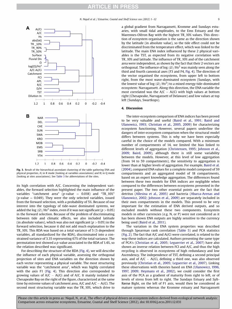
3.3. Hierarchical ascendant clustering of ENA and physical variables

The dendrograms of the HAC are presented on Fig. 3, with theassociation of variables in R mode (Fig. 3A) and the association ofthe sites in Q mode (Fig. 3B). The main partition within the set ofvariables was composed of 3 groups (at the level of the vertical line)which all mixed physical and ENAvariables. A first group associatedlatitude, tide (TR_10%, TR_50% and TR_90%), wave height (Hs) andindices of Ascendency (Ai/Ci and A/C). The second group associatedAPL, FCI, R/C and A/C � Ai/Ci with physical indices related to size(catchment area, surface of the ecosystem, fluvial discharge, tidalprism) and the tide-wave index, log ðUÞ=Hs2. The third groupassociated the dilution index, the D/H and the TST.

The association of the sites also gave 3 groups, segregatedaccording to their geographical position. The group at the top of thedendrogram was composed of the 3 sites from North America, thegroup of the middle was composed of the 3 estuaries from SouthAfrica and the group at the bottom was composed of the 4 Euro-pean sites.

3.4. Redundancy analysis

For statistical reasons, it is necessary to apply theRedundancy Analysis (RDA) with more sites than variables(dependent þ independent) and with more independent thandependent variables. Due to the limited number of models used,and because of comparability criteria, the dependent and inde-pendent variables had to be limited. The dependent variables werelimited to 5 items. According to the absolute contribution values ofthe PCA, we selected FCI, TST and A/C � Ai/Ci as they had animportant role in defining the 3 first principal axes. D/H, was addedto this set because the Detritivory/Herbivory information isessential to understand the ecological functioning and A/C was alsoadded because it has been associated to numerous theories onsystem maturity (Ulanowicz, 1997) and stability (Heymans et al.,2002; Ulanowicz, 2009). APL and R/H were not consideredbecause of their high correlation with FCI; Ai/Ci neither because of

f the ENA values of the 10 models (see Table 3 for abbreviations of the sites).

ivers on ecosystem indices derived from ecological network analysis:ience (2012), doi:10.1016/j.ecss.2011.12.031

A

B

Fig. 3. Result of the hierarchical ascendant clustering of the table gathering ENA andphysical properties, A) in R mode (looking at variables associations) and B) in Q mode(looking at sites associations). See Table 3 for abbreviations of the sites.

N. Niquil et al. / Estuarine, Coastal and Shelf Science xxx (2012) 1e12 9

its high correlation with A/C. Concerning the independent vari-ables, the forward selection highlighted the main influence of thevariables “catchment area” (p-value ¼ 0.018) and “TR_10%”(p-value ¼ 0.049). They were the only selected variables, issuedfrom the forward selection, with a probability of 5%. Because of ourinterest into the typology of tide-wave dominated systems, weadded the log ðUÞ=Hs2 index, even if it was not significant (p> 0.05)in the forward selection. Because of the problem of discriminatingbetween tide and climatic effects, we also included latitude(in absolute values), which was also not significant (p> 0.05) in theforward selection, because it did not add much explanation to theTR_10%. This RDA was based on a total variance of 5 (5 dependentvariables, all standardized for the RDA), discriminated into a con-strained variance of 3.35 representing 67% of the total variance. Thepermutation test showed a p-value associated to the RDA of 1.4%, sothe relation described was significant.

For describing the structure of the RDA (Fig. 4), we will describethe influence of each physical variable, assessing the orthogonalprojection of sites and ENA variables on the direction shown byeach vector representing a physical variable. The most structuringvariable was the “catchment area”, which was highly correlatedwith the axis F1 (Fig. 4). This direction also corresponded togrowing values of A/C � Ai/Ci and of A/C. It mainly isolated theChesapeake Bay on the right of the figure, characterized at the sametime by extreme values of catchment area, A/C and A/C � Ai/Ci. Thesecond most structuring variable was the TR_10%, which drive to

Please cite this article in press as: Niquil, N., et al., The effect of physical drComparison across estuarine ecosystems, Estuarine, Coastal and Shelf Sc

a global gradient from Narragansett, Kromme and Sundays estu-aries, with small tidal amplitudes, to the Ems Estuary and theMarennes-Oléron Bay with the highest TR_10% values. This direc-tion of ecosystem organisation is the same as the direction shownby the latitude (in absolute value), so the tide effect could not bediscriminated from the temperature effect, which was linked to thelatitude. The main ENA index influenced by these 2 physical vari-ables is the TST, as expected from its negative correlation withTR_10% and latitude. The influence of TR_10% and of the catchmentareawere independent, as shown by the fact that their 2 vectors areorthogonal. The influence of log ðUÞ=Hs2 was mainly seen along thethird and fourth canonical axes (F3 and F4, Fig. 4). The direction ofthe vector organised the ecosystems, from upper left to bottomright, from the most wave-dominated ecosystem (Sundays, withthe lowest value of log ðUÞ=Hs2) to a mixed energy tide-dominatedecosystem: Narragansett. Along this direction, the ENA variable themost correlated was the A/C � Ai/Ci with high values at bottomright (Chesapeake, Narragansett of Delaware) and low values at topleft (Sundays, Swartkops).

4. Discussion

The inter-ecosystem comparison of ENA indices has been provedto be very valuable and useful (Baird et al., 1991; Baird andUlanowicz, 1993; Christian et al., 2005, 2009) for characterizingecosystem functioning. However, several papers underline thedangers of inter-ecosystem comparison when the structural modeldiffers between systems. This is why we have been especiallycareful in the choice of the models compared. With a minimumnumber of compartments of 14, we limited the bias linked todifferent levels of aggregation (Christensen, 1995; Johnson et al.,2009; Baird, 2009), although there is still some variabilitybetween the models. However, at this level of low aggregation(from 14 to 59 compartments), the sensitivity to aggregation islower than at higher levels of aggregation. For example, Baird et al.(2004), compared ENAvalues for a completemodel composed of 59compartments and an aggregated model of 18 compartments,based on an expert knowledge aggregation. The differences foundbetween these two models for ENA indices are negligible whencompared to the differences between ecosystems presented in thepresent paper. The two other essential points are the fact thatdetritus (Allesina et al., 2005) and bacteria (Abarca-Arenas andUlanowicz, 2002; Johnson et al., 2009) are separately included intheir own compartments in the models. This proved to be veryimportant for the estimation of ENA derived outputs, and soexcluded models without these two components. Ecosystemmodels in other currencies (e.g. N, or P) were not considered as ithas been shown ENA outputs are highly sensitive to the currencybeing used (Baird et al., 2011).

The variation in the ENA system properties was describedthrough Spearman rank correlation (Table 5) and PCA statistics(Fig. 2). The fact that A/C and Ai/Ci were correlated, is related to theway these indices are calculated. Authors presenting the same typeof PCA’s (Christian et al., 2005; Leguerrier et al., 2007) have alsoshown an inverse relation between FCI and A/C, and thus the highrecycling is observed in ecosystems of high redundancy and lowAscendency. The independence of TST, defining a second principalaxis, and of A/C � Ai/Ci, defining a third one, was also observedpreviously (Christian et al., 2005; Leguerrier et al., 2007). Linkingthese observations with theories based on ENA (Ulanowicz, 1996,1997, 2009; Heymans et al., 2002), we could consider the firstaxis of the PCA as a gradient of maturity from right to left, or oflevels of stress from left to right. The Sundays Estuary and Sylt-Rømø Bight, on the left of F1 axis, would then be considered asmature systems whereas the Kromme estuary and Narragansett

ivers on ecosystem indices derived from ecological network analysis:ience (2012), doi:10.1016/j.ecss.2011.12.031

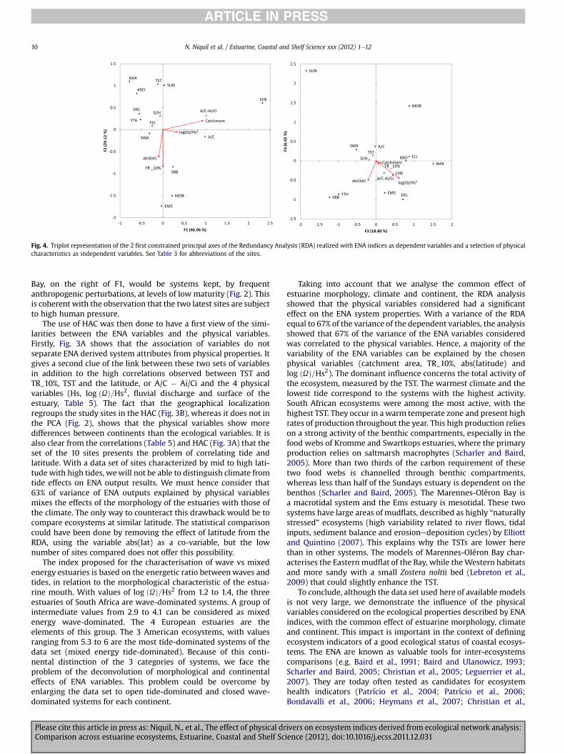
Fig. 4. Triplot representation of the 2 first constrained principal axes of the Redundancy Analysis (RDA) realized with ENA indices as dependent variables and a selection of physicalcharacteristics as independent variables. See Table 3 for abbreviations of the sites.

N. Niquil et al. / Estuarine, Coastal and Shelf Science xxx (2012) 1e1210

Bay, on the right of F1, would be systems kept, by frequentanthropogenic perturbations, at levels of lowmaturity (Fig. 2). Thisis coherent with the observation that the two latest sites are subjectto high human pressure.

The use of HAC was then done to have a first view of the simi-larities between the ENA variables and the physical variables.Firstly, Fig. 3A shows that the association of variables do notseparate ENA derived system attributes from physical properties. Itgives a second clue of the link between these two sets of variablesin addition to the high correlations observed between TST andTR_10%, TST and the latitude, or A/C � Ai/Ci and the 4 physicalvariables (Hs, log ðUÞ=Hs2, fluvial discharge and surface of theestuary, Table 5). The fact that the geographical localizationregroups the study sites in the HAC (Fig. 3B), whereas it does not inthe PCA (Fig. 2), shows that the physical variables show moredifferences between continents than the ecological variables. It isalso clear from the correlations (Table 5) and HAC (Fig. 3A) that theset of the 10 sites presents the problem of correlating tide andlatitude. With a data set of sites characterized by mid to high lati-tudewith high tides, wewill not be able to distinguish climate fromtide effects on ENA output results. We must hence consider that63% of variance of ENA outputs explained by physical variablesmixes the effects of the morphology of the estuaries with those ofthe climate. The only way to counteract this drawback would be tocompare ecosystems at similar latitude. The statistical comparisoncould have been done by removing the effect of latitude from theRDA, using the variable abs(lat) as a co-variable, but the lownumber of sites compared does not offer this possibility.

The index proposed for the characterisation of wave vs mixedenergy estuaries is based on the energetic ratio betweenwaves andtides, in relation to the morphological characteristic of the estua-rine mouth. With values of log ðUÞ=Hs2 from 1.2 to 1.4, the threeestuaries of South Africa are wave-dominated systems. A group ofintermediate values from 2.9 to 4.1 can be considered as mixedenergy wave-dominated. The 4 European estuaries are theelements of this group. The 3 American ecosystems, with valuesranging from 5.3 to 6 are the most tide-dominated systems of thedata set (mixed energy tide-dominated). Because of this conti-nental distinction of the 3 categories of systems, we face theproblem of the deconvolution of morphological and continentaleffects of ENA variables. This problem could be overcome byenlarging the data set to open tide-dominated and closed wave-dominated systems for each continent.

Please cite this article in press as: Niquil, N., et al., The effect of physical drComparison across estuarine ecosystems, Estuarine, Coastal and Shelf Sc

Taking into account that we analyse the common effect ofestuarine morphology, climate and continent, the RDA analysisshowed that the physical variables considered had a significanteffect on the ENA system properties. With a variance of the RDAequal to 67% of the variance of the dependent variables, the analysisshowed that 67% of the variance of the ENA variables consideredwas correlated to the physical variables. Hence, a majority of thevariability of the ENA variables can be explained by the chosenphysical variables (catchment area, TR_10%, abs(latitude) andlog ðUÞ=Hs2). The dominant influence concerns the total activity ofthe ecosystem, measured by the TST. The warmest climate and thelowest tide correspond to the systems with the highest activity.South African ecosystems were among the most active, with thehighest TST. They occur in awarm temperate zone and present highrates of production throughout the year. This high production relieson a strong activity of the benthic compartments, especially in thefood webs of Kromme and Swartkops estuaries, where the primaryproduction relies on saltmarsh macrophytes (Scharler and Baird,2005). More than two thirds of the carbon requirement of thesetwo food webs is channelled through benthic compartments,whereas less than half of the Sundays estuary is dependent on thebenthos (Scharler and Baird, 2005). The Marennes-Oléron Bay isa macrotidal system and the Ems estuary is mesotidal. These twosystems have large areas of mudflats, described as highly “naturallystressed” ecosystems (high variability related to river flows, tidalinputs, sediment balance and erosionedeposition cycles) by Elliottand Quintino (2007). This explains why the TSTs are lower herethan in other systems. The models of Marennes-Oléron Bay char-acterises the Easternmudflat of the Bay, while theWestern habitatsand more sandy with a small Zostera noltii bed (Lebreton et al.,2009) that could slightly enhance the TST.

To conclude, although the data set used here of available modelsis not very large, we demonstrate the influence of the physicalvariables considered on the ecological properties described by ENAindices, with the common effect of estuarine morphology, climateand continent. This impact is important in the context of definingecosystem indicators of a good ecological status of coastal ecosys-tems. The ENA are known as valuable tools for inter-ecosystemscomparisons (e.g. Baird et al., 1991; Baird and Ulanowicz, 1993;Scharler and Baird, 2005; Christian et al., 2005; Leguerrier et al.,2007). They are today often tested as candidates for ecosystemhealth indicators (Patrício et al., 2004; Patrício et al., 2006;Bondavalli et al., 2006; Heymans et al., 2007; Christian et al.,

ivers on ecosystem indices derived from ecological network analysis:ience (2012), doi:10.1016/j.ecss.2011.12.031

N. Niquil et al. / Estuarine, Coastal and Shelf Science xxx (2012) 1e12 11

2009). In the context of the present legal situation defined inEurope by the Marine Strategy Framework Directive, it is necessaryto define tendencies and thresholds values for these indicators inorder to define the good ecological status of coastal ecosystems.This definition must be done taking into account the physicalinfluence. It will be necessary to take into account the physicaltypology of estuarine ecosystems for defining sub-categories inwhich these thresholds will have to be defined.

Acknowledgements

The authors thank Prof J.A.G. Cooper and 2 anonymous refereesfor commenting on the manuscript. This study was supported byIFREMER, the Alfred Wegener Institut, Procope Hubert CurienProgramme and the French National Programme for Coastal Envi-ronment (PNEC/EC2CO) ‘COMPECO’ coordinated by Nathalie Niquil.The definition of physical parameters and indices was possible dueto the availability of the tidal constituent database FES 2004 (UMRLEGOS, France) and the WW3 wave hindcast (NOAA, USA). Themaps included in Table 1 were realised by the GIS platform ofLIENSS (Cécilia Pignon-Mussaud and Pascal Brunello).

References

Abarca-Arenas, L.G., Ulanowicz, R.E., 2002. The effects of taxonomic aggregation onnetwork analysis. Ecological Modelling 149, 285e296.

Allard, J., Chaumillon, E., Poirier, C., Sauriau, P.-G., Weber, O., 2008. Evidence offormer Holocene sea level in the Marennes-Oléron Bay (French Atlantic coast).Comptes Rendus Geosciences 340, 306e314.

Allesina, S., Bondavalli, C., Scharler, U.M., 2005. The consequences of the aggrega-tion of detritus pools in ecological networks. Ecological Modelling 189,221e232.

Archibald, R.E.M., 1983. The Diatoms of the Sundays and Great Fish Rivers in theEastern Cape Province of South Africa. A.R. Gantner Verlag Kommanditgesell-schaft, Vaduz.

Backhaus, J., Hartke, D., Hübner, U., Lohse, H., Müller, A., 1998. Hydrography andKlima im Lister Tidebecken. In: Gätje, C.H., Reise, K. (Eds.), Ökosystem Wat-tenmeer, pp. 39e54.

Baird, D., 2009. An assessment of the functional variability of selected coastalecosystems in the context of local environmental changes. ICES Journal ofMarine Science 66, 1520e1527.

Baird, D., Ulanowicz, R.E., 1989. The seasonal dynamics of the Chesapeake Bayecosystem. Ecological Monographs 59, 329e364.

Baird, D., Ulanowicz, R.E., 1993. Comparative study on the trophic structure, cyclingand ecosystem properties of four tidal estuaries. Marine Ecology Progress Series99, 221e237.

Baird, D., McGlade, J.M., Ulanowicz, R.E., 1991. The comparative ecology of sixmarine ecosystems. Philosophical Transactions of the Royal Society of London,Series B: Biological Sciences 333, 15e29.

Baird, D., Christian, R.R., Peterson, C.H., Johnson, G.A., 2004. Consequences ofhypoxia on estuarine ecosystem function: energy diversion from consumers tomicrobes. Ecological Applications 14, 805e822.

Baird, D., Asmus, H., Asmus, R., 2007. Trophic dynamics of eight intertidalcommunities of the Sylt-Rømø Bight ecosystem, northern Wadden Sea. MarineEcology Progress Series 351, 25e41.

Baird, D., Asmus, H., Asmus, R., 2011. Carbon, nitrogen and phosphorus dynamics innine sub-systems of the Sylt-Rømø Bight ecosystem, German Wadden Sea.Estuarine, Coastal and Shelf Science 91, 51e68.

Bayerl, K.-A., Köster, R., Murphy, D., 1998. Verteilung und Zusammensetzung derSedimente im Lister Tidebecken. In: Gätje, C.H., Reise, K. (Eds.), ÖkosystemWattenmeer, pp. 31e38.

Bertin, X., Chaumillon, E., Sottolichio, A., Pedreros, R., 2005. Tidal inlet response tosediment infilling of the associated bay and possible implications of humanactivities: the Marennes-Oléron Bay and Maumusson Inlet, France. ContinentalShelf Research 25, 115e1131.

Bertin, X., Castelle, B., Chaumillon, E., Butel, R., Quique, R., 2008. Estimation andinter-annual variability of the longshore transport at a high-energy dissipativebeach: the St Trojan beach, SW Oléron Island, France. Continental ShelfResearch 28, 1316e1332.

Bondavalli, C., Bodini, A., Rossetti, G., Allesina, S., 2006. Detecting stress at thewhole-ecosystem level: the case of a mountain lake (Lake Santo, Italy).Ecosystems 9, 768e787.

Boyd, R., Dalrymple, R.W., Zaitlin, B.A., 1992. Classification of clastic coastal depo-sitional environments. Sedimentary Geology 80, 139e150.

Bruun, P., 1978. Stability of Coastal Inlets: Theory and Engineering. Elsevier Sci. Publ.Co., Amsterdam, 509 pp.

Please cite this article in press as: Niquil, N., et al., The effect of physical drComparison across estuarine ecosystems, Estuarine, Coastal and Shelf Sc

Chaumillon, E., Tessier, B., Weber, N., Tesson, M., Bertin, X., 2004. Buried sandbodieswithin present-day estuaries (Atlantic coast of France) revealed by very highresolution seismic surveys. Marine Geology 211, 189e214.

Christensen, V., 1995. Ecosystem maturity e towards unification. EcologicalModelling 61, 169e185.

Christian, R.R., Baird, D., Luczkovich, J., Johnson, J.C., Scharler, U.M.,Ulanowicz, R.E., 2005. Role of network analysis in comparative ecosystemecology of estuaries. In: Belgrano, A., Scharler, U.M., Dunne, J.,Ulanowicz, R.E. (Eds.), Aquatic Food Webs: An Ecosystem Approach. OxfordUniversity Press, pp. 25e40.

Christian, R.R., Brinson, M.M., Dame, J.K., Johnson, G., Peterson, C.H., Baird, D., 2009.Ecological network analyses and their use for establishing reference domain infunctional assessment of an estuary. Ecological Modelling 220, 3113e3122.

Cooper, J.A.G., 2001. Geomorphological variability among microtidal estuaries fromthe wave-dominated South African coast. Geomorphology 40, 99e122.

Dalrymple, R.W., Zaitlin, B.A., Boyd, R., 1992. Estuarine facies models: conceptualbasis and stratigraphic implications. Journal of Sedimentary Petrology 62,1130e1146.

Dauvin, J.C., Ruellet, T., 2009. The estuarine quality paradox: is it possible to definean ecological quality status for specific modified and naturally stressed estua-rine ecosystems? Marine Pollution Bulletin 59, 38e47.

Davies Jr., R.A., 1964. A morphological approach to the word of shorelines. Zeits-chrift fur Geomorphologie 8, 127e142.

de Jonge, V.N., 1988. The abiotic environment. In: Baretta, J., Ruardij, P. (Eds.), TidalFlat Estuaries: Simulation and Analysis of the Eros Estuary. Springer, Berlin,pp. 14e27.

de Jonge, V.N., 2007. Toward the application of ecological concepts in EU coastalwater management. Marine Pollution Bulletin 55, 407e414.

Dodet, G., Bertin, X., Taborda, R., 2010. Wave climate variability in the North-EastAtlantic Ocean over the last six decades. Ocean Modelling 31, 120e131.

Elliott, M., McLusky, D.S., 2002. The need for definitions in understanding estuaries.Estuarine, Coastal and Shelf Science 55, 815e827.

Elliott, M., Quintino, V., 2007. The Estuarine quality paradox, environmentalhomeostasis and the difficulty of detecting anthropogenic stress in naturallystressed areas. Marine Pollution Bulletin 54, 640e645.

Fath, B.D., Scharler, U.M., Ulanowicz, R.E., Hannon, B., 2007. Ecological networkanalysis: network construction. Ecological Modelling 208, 49e55.

Finn, J.T., 1976. Measures of ecosystem structure and function derived from analysisof flows. Journal of Theoretical Biology 56, 363e380.

Gillibrand, P.A., Balls, P.W., 1998. Modelling salt intrusion and nitrate concentrationsin the Ythan Estuary. Estuarine, Coastal and Shelf Science 47, 695e706.

Halpern, B.S., McLeod, K.L., Rosenberg, A.A., Crowder, L.B., 2008. Managing forcumulative impacts in ecosystem-based management through ocean zoning.Ocean and Coastal Management 51, 203e211.

Hayes, M.O., 1979. Barrier island morphology as a function of tidal and wave regime.In: Leatherman, S.P. (Ed.), Barrier Island: From the Gulf of St. Lawrence to theGulf of Mexico. Academic Press, New York, pp. 1e28.

Heymans, J.J., 2003. Comparing the Newfoundland-Southern Labrador marineecosystem models using information theory. In: Heymans, J.J. (Ed.), EcosystemModels of Newfoundland and Southeastern Labrador (2J3KLNO): AdditionalInformation and Analyses for “Back to the Future”, vol. 11(5). Fisheries CentreResearch Reports, pp. 62e71.

Heymans, J.J., Ulanowicz, R.E., Bondavalli, C., 2002. Network analysis of the SouthFlorida Everglades graminoid marshes and comparison with nearby cypressecosystems. Ecological Modelling 149, 5e23.

Heymans, J.J., Christensen, V., Guénette, S., Christensen, V., 2007. Evaluatingnetwork analysis indicators of ecosystem status in the Gulf of Alaska. Ecosys-tems 10, 488e502.

Johnson, G.A., Niquil, N., Asmus, H., Bacher, C., Asmus, R., Baird, D., 2009. The effectsof aggregation on the performance of the inverse method and indicators ofnetwork analysis. Ecological Modelling 220, 3448e3464.

Kay, J., Graham, L.A., Ulanowicz, R.E., 1989. A detailed guide for network analysis. In:Wulff, F., Field, J.G., Mann, K.H. (Eds.), Network Analysis in Marine Ecology.Methods and Applications. Springer-Verlag, Berlin, pp. 15e61.

Lebreton, B., Richard, P., Radenac, G., Bordes, M., Bréret, M., Arnaud, C., Mornet, F.,Blanchard, G.F., 2009. Are epiphytes a significant component of intertidal Zos-tera noltii beds? Aquatic Botany 91, 82e90.

Leguerrier, D., Niquil, N., Petiau, A., Bodoy, A., 2004. Modeling the impact of oysterculture on a mudflat food web in Marennes-Oléron Bay (France). MarineEcology Progress Series 273, 147e162.

Leguerrier, D., Degre, D., Niquil, N., 2007. Network analysis and inter-ecosystemcomparison of two intertidal mudflat food webs (Brouage Mudflat andAiguillon Cove, SW France). Estuarine, Coastal and Shelf Science 74,403e418.

Lester, S.E., McLeod, K.L., Tallis, H., Ruckelshaus, M., Halpern, B.S., Levin, P.S.,Chavez, F.P., Pomeroy, C., McCay, B.J., Costello, C., Gaines, S.D., Mace, A.J.,Barth, J.A., Fluharty, D.L., Parrish, J.K., 2010. Science in support of ecosystem-based management for the US West Coast and beyond. Biological Conserva-tion 143, 576e587.

Lyard, F., Lefevre, F., Letellier, T., Francis, O., 2006. Modelling the global ocean tides:modern insights from Fes2004. Ocean Dynamics 56, 394e415.

McLusky, D.S., Elliott, M., 2004. The Estuarine Ecosystem: Ecology, Threats andManagement. OUP, Oxford, 214 pp.

Monaco, M.E., Ulanowicz, R.E., 1997. Comparative ecosystem trophic structure ofthree US mid-Atlantic estuaries. Marine Ecology Progress Series 161, 239e254.

ivers on ecosystem indices derived from ecological network analysis:ience (2012), doi:10.1016/j.ecss.2011.12.031

N. Niquil et al. / Estuarine, Coastal and Shelf Science xxx (2012) 1e1212

Nahon, A., Bertin, X., Fortunato, A.B., Oliveira, A., 2012. Process-based 2DH mor-phodynamic modeling of tidal inlets: a comparison with empirical classifica-tions and theories. Marine Geology 291e294, 1e11.

Nichol, S.L., 1991. Zonation and sedimentology of estuarine facies in an incisedvalley, wave-dominated, microtidal setting, New South Wales, Australia. ClasticTidal Sedimentology, 41e57.

Oertel, G.F., 1988. Processes of sediment exchange between tidal inlets and barrierislands. In: Aubrey, D.G., Weishar, L. (Eds.), Hydrodynamics and SedimentDynamics of Tidal Inlets. Springer, New York, pp. 186e225.

Patrício, J., Marques, J.C., 2006. Mass balanced models of the food web in three areasalong a gradient of eutrophication symptoms in the south arm of the Mondegoestuary (Portugal). Ecological Modelling 197, 21e34.

Patrício, J., Ulanowicz, R., Pardal, M.A., Marques, J.C., 2004. Ascendency as ecologicalindicator: a case study on estuarine pulse eutrophication. Estuarine, Coastal andShelf Science 60, 23e35.

Pinto, R., Patrício, J., Baeta, A., Fath, B.D., Neto, J.M., Marques, J.C., 2009. Review andevaluation of estuarine biotic indices to assess benthic condition. EcologicalIndicators 9, 1e25.

Poirier, C., Chaumillon, E., Arnaud, F., 2011. Siltation of river-influenced coastalenvironments: respective impact of late Holocene land use and high-frequencyclimate changes. Marine Geology 290, 51e62.

Pritchard, D.W., 1967. What is an estuary: physical viewpoint. In: Lauff, G.H. (Ed.),Estuaries. American Association for the Advancement of Science, Washington,D.C., pp. 3e5.

Reinson, G.E., 1992. Transgressive barrier island and estuarine systems. In:Walker, R.G., James, N.P. (Eds.), Facies Models e Response to Sea Level Change.Geological Association of Canada, pp. 179e194.

Rogers, S., Casini, M., Cury, P., Heath, M., Irigoien, X., Kuosa, H., Scheidat, M.,Skov, H., Stergiou, K., Trenkel, V., Wikner, J., Yunev, O., 2010. In: Piha, H.(Ed.), Marine Strategy Framework Directive Task Group 4 Report, FoodWebs. European Commission Joint Research Centre, ICES DOI: 10.2788/87659.

Sauriau, P.-G., Mouret, V., Rincé, P.-G., 1989. Organisation trophique de la mala-cofaune benthique non cultivée du bassin ostréicole de Marennes-Oléron.Oceanologica Acta 12, 193e204.

Please cite this article in press as: Niquil, N., et al., The effect of physical drComparison across estuarine ecosystems, Estuarine, Coastal and Shelf Sc

Scharler, U.M., Baird, D., 2005. A comparison of selected ecosystem attributes ofthree South African estuaries with different freshwater inflow regimes, usingnetwork analysis. Journal of Marine Systems 56, 283e308.

Sharp, J.H., Cifuentes, L.A., Coffin, R.B., Pennock, J.R., Wong, K.C., 1986. The influenceof river variability on the circulation, chemistry, and microbiology of theDelaware Estuary. Estuaries 9, 261e269.

Tolman, H.L., Balasubramaniyan, B., Burroughs, L.D., Chalikov, D.V., Chao, Y.Y.,Chen, H.S., Gerald, V.M., 2002. Development and implementation of windgenerated ocean surface wave models at NCEP. Weather and Forecasting 17,311e333.

Ulanowicz, R.E., 1986. Growth and Development: Ecosystems Phenomenology.Springer-Verlag, New York, 203 pp.

Ulanowicz, R.E., 1996. Trophic flow networks as indicators of ecosystem stress. In:Polis, G., Winemiller, K. (Eds.), Food Webs: Integration of Patterns andDynamics. Chapman-Hall, New York, pp. 358e368.

Ulanowicz, R.E., 1997. Ecology, the Ascendant Perspective. Columbia UniversityPress, NY, 201 pp.

Ulanowicz, R.E., 2009. The dual nature of ecosystem dynamics. Ecological Modelling220, 1886e1892.

Uriarte, A., Borja, A., 2009. Assessing fish quality status in transitional waters,within the European Water Framework directive: setting boundary classes andresponding to anthropogenic pressures. Estuarine, Coastal and Shelf Science 82,214e224.

Vadeboncoeur, M.A., Hamburg, S.P., Pryor, D., 2010. Modeled nitrogen loading toNarragansett Bay: 1850 to 2015. Estuaries and Coasts 33, 1113e1127.

Vasconcellos, M., Mackinson, S., Sloman, K., Pauly, D., 1997. The stability of trophicmass-balance model of marine ecosystems: a comparative analysis. EcologicalModelling 100, 125e134.

Vézina, A.F., Platt, T., 1988. Food web dynamics in the ocean. I. Best estimates usinginverse methods. Marine Ecology Progress Series 42, 269e287.

Whitfield, A.K., 1994. Abundance of larval and 0þ juvenile marine fishes in thelower reaches of the three southern African estuaries with differing freshwaterinputs. Marine Ecology Progress Series 3, 45e57.

Wulff, F., Field, J.G., Mann, K.H., 1989. Network Analysis in Marine Ecology. Methodsand Applications. Springer-Verlag, Berlin.

ivers on ecosystem indices derived from ecological network analysis:ience (2012), doi:10.1016/j.ecss.2011.12.031