Modeling drivers! speech under stress

Raul Fernandez *, Rosalind W. PicardMIT Media Laboratory, 20 Ames. Street, Cambridge, MA 02139, USA

Abstract

We explore the use of features derived from multiresolution analysis of speech and the Teager energy operator forclassification of drivers! speech under stressed conditions. We apply this set of features to a database of short speechutterances to create user-dependent discriminants of four stress categories. In addition we address the problem ofchoosing a suitable temporal scale for representing categorical di!erences in the data. This leads to two modelingapproaches. In the first approach, the dynamics of the feature set within the utterance are assumed to be important forthe classification task. These features are then classified using dynamic Bayesian network models as well as a modelconsisting of a mixture of hidden Markov models (M-HMM). In the second approach, we define an utterance-levelfeature set by taking the mean value of the features across the utterance. This feature set is then modeled with a supportvector machine and a multilayer perceptron classifier. We compare the performance on the sparser and full dynamicrepresentations against a chance-level performance of 25% and obtain the best performance with the speaker-dependentmixture model (96.4% on the training set, and 61.2% on a separate testing set). We also investigate how these modelsperform on the speaker-independent task. Although the performance of the speaker-independent models degrades withrespect to the models trained on individual speakers, the mixture model still outperforms the competing models andachieves significantly better than random recognition (80.4% on the training set, and 51.2% on a separate testing set).! 2002 Elsevier Science B.V. All rights reserved.

Zusammenfassung

In diesem Bericht untersuchen wir die Verwendung von Merkmalen der Sprachanalyse aufgrund mehrerer Zeitskalenzur Klassifikation der Sprache eines Fahrers unter Stress. Diese Merkmale wenden wir auf eine Datenbank kurzerSprachsequenzen an, um vier sprecherabh!aangige Stresskategorien zu erstellen. Zus!aatzlich besch!aaftigen wir uns mit derAuswahl der passenden Zeitskala f!uur die Repr!aasentation klassenspezifischer Unterschiede in der Datenmenge. Diesf!uuhrt zu zwei unterschiedlichen Modellierungsans!aatzen. Im ersten Ansatz wird vorausgesetzt, dass die dynamischeEntwicklung der Merkmale, die innerhalb der Sprachsequenzen vorhanden ist, wichtig f!uur die Klassifizierung ist. DieseMerkmale werden klassifiziert mit Hilfe von dynamischen Bayes Netzen bzw. mit einer Mischung von Hidden MarkovModellen. Im zweiten Ansatz definieren wir Merkmale auf Artikulationsebene, indem wir die Mittelwerte der Merk-male !uuber die Sprachsequenzen berechnen. Diese Merkmalsmenge wird dann mit einer Support Vector Maschine undeinem Multilayer-Perzeptron modelliert. Die Performanz der sp!aarlichen und der voll dynamischen Darstellung wirdverglichen mit dem zuf!aalligen Klassifikationsniveau von 25%. Das beste Ergebnis erhalten wir hierbei mit einemsprecherabh!aangigen Mischmodell (96,4% auf den Trainingsdaten und 61,2% auf unabh!aangigen Testdaten). Weiterhinuntersuchen wir, wie diese Modelle bei sprecherunabh!aangigen Aufgaben abschneiden. Obwohl die sprecher-unabh!aangigen Modelle schlechter abschneiden als die auf einzelne Sprecher justierten Modellen, !uubertri!t das

*Corresponding author.E-mail addresses: galt@media.mit.edu (R. Fernandez), picard@media.mit.edu (R.W. Picard).

0167-6393/02/$ - see front matter ! 2002 Elsevier Science B.V. All rights reserved.PII: S0167-6393 (02 )00080-8

Speech Communication 40 (2003) 145–159www.elsevier.com/locate/specom

Mischmodell die konkurrierenden Modelle immer noch und erzielt signifikant bessere Sprechererkennung als Zufalls-erkennung (80.4% auf den Trainingsdaten und 51.2% auf unabh!aangigen Testdaten).! 2002 Elsevier Science B.V. All rights reserved.

R"eesum"ee

Nous explorons l!utilisation de repr"eesentations d"eeriv"eees de l!analyse multir"eesolution de la parole et de l!op"eerateurd!"eenergie de Teager pour la classification de la parole de conducteurs en condition de stress. Nous appliquons cetteanalyse #aa corpus d!enonces courts pour creer des fonctions discriminantes dependantes du locuteur pour quatre cate-gories de stress. En outre nous adressons le probl#eeme du choix d!une "eechelle temporelle appropri"eee pour cat"eegoriser lesdonn"eees. Ceci m#eene #aa deux approches pour la mod"eelisation. Dans la premi#eere approche, la dynamique des variablesissues de l!analyse d!un "eenonc"ee donn"ee est suppos"eee pertinente pour la classification. Ces variables sont alors mod"eelis"eeesau moyen de r"eeseaux bay"eesiens dynamiques (DBN) ou par un m"eelange des mod#eeles de Markov cach"ees (M-HMM). Pourla seconde approche, nous ne gardons que les valeurs moyennes de ces variables pour chaque "eenonc"ee. Le vecteurr"eesultant est alors mod"eelis"ee au moyen d!une machine #aa support de vecteur et d!un perceptron multicouches. Nouscomparons les performances de ces deux approches #aa un tirage al"eeatoire (25%), les meilleurs r"eesultats "eetant obtenus avecle m"eelange de mod#eeles d"eependant du locuteur (96,44% sur les donn"eees d!apprentissage, et 61,20% sur un jeu de testdistinct). Nous "eetudions "eegalement les performances de mod#eeles ind"eependants du locuteur. Bien que les performances sed"eegradent par rapport des mod#eeles sp"eecifiques aux locuteurs, le m"eelange de mod#eeles surpasse encore les autres mod#eeleset obtient un taux de reconnaissance sensiblement meilleur qu!un tirage al"eeatoire (80,42 sur les donn"eees d!apprentissage,et 51,22% sur le jeu de test).! 2002 Elsevier Science B.V. All rights reserved.

Keywords: Stress in speech; Automatic recognition

1. Introduction

Much of the current e!ort on studying speechunder stress has been aimed at detecting stressconditions for improving the robustness of speechrecognizers; typical research of speech under stresshas targeted perceptual (e.g. Lombard e!ect),psychological (e.g. timed tasks), as well as physicalstressors (e.g. roller-coaster rides, high G forces)(Steeneken and Hansen, 1999). In this work we areinterested in modeling speech in the context ofdriving under varying conditions of cognitive loadhypothesized to induce a level of stress on thedriver. The results of this research may be relevantnot only to building recognition systems that aremore robust in the context described, but also toapplications that attempt to infer the underlyinga!ective state of an utterance. We have chosenthe scenario of driving while talking on the phoneas an application in which knowledge of the dri-ver!s state may provide benefits ranging from amore fluid interaction with a speech interface toimprovement of safety in the response of the ve-hicle.

The recent literature discussing the e!ects ofstress on speech applies the label of stress to dif-ferent phenomena. Some work views stress as anybroad deviations in the production of speech fromits normal production (Hansen and Womack,1996; Sarikaya and Gowdy, 1998). In discussingthe SUSAS database for the study of speech understress, Hansen et al. (1998) go on to describe var-ious types of stress in speech. These include thee!ects that speaking styles, noise, and G forceshave on the speaker!s output, as well as the e!ectof states that are often described under the label ofemotions elsewhere in the literature (e.g., anxiety,fear, or anger).

In an attempt to unify the often diverging viewsof stress that are being invoked by the research inthis field, Murray et al. (1996) have reviewed var-ious definitions of stress, and proposed a descrip-tion of this phenomenon based on the character ofthe stressors. They have hypothesized four levels ofstressors that can a!ect the speech productionprocess. At the lowest level, these include directchanges on the vocal apparatus (zero-order stres-sors), unconscious physiological changes (first-

146 R. Fernandez, R.W. Picard / Speech Communication 40 (2003) 145–159

order stressors), and conscious physiologicalchanges (second-order stressors). At the highestlevel, changes can also be brought about by stimulithat are external to the speech production process,by the speaker!s cognitive reinterpretation of thecontext in which the speech is being produced, aswell as by the speaker!s underlying a!ective con-ditions (third-order stressors). In this paper, wefollow this taxonomy and investigate whether it ispossible to discriminate between spoken utterancesthat have been produced under the influence ofthird-order stressors with a varying degree ofstress.

2. Speech corpus and data annotation

The speech data used in the research presentedin this paper was collected from subjects driving ina simulator at the Nissan!s Cambridge ResearchLab. Subjects were asked to drive through a coursewhile engaged in a simulated phone task: while thesubject drove, a speech synthesizer prompted thedriver with a math question consisting of addingup two numbers whose sum was less than 100. Wecontrolled for the number of additions with andwithout carry-ons in order to maintain an ap-proximately constant level of di"culty across tri-als.

The two independent variables in this experi-ment were the driving speed and the frequencywith which the driver was given math questions.Each variable had two conditions––slow andfast––resulting in four di!erent combinations.Subjects drove at 60 m.p.h. in the slow speedcondition and at 120 m.p.h. in the fast speedcondition (the perceptual speed in the simulator isapproximately half). One subject complained ofmotion sickness in the fast speed condition, so inthat case the speed was reduced to 100 m.p.h. Thefrequency at which drivers were prompted with amath question was once every 9 s (slow condition)or once every 4 s (fast condition). The driver!sanswers were captured by a head-mounted mi-crophone and recorded in VHS format. The cor-pus analyzed here consists of 598 utterances(154, 156, 137 and 151 for each subject, respec-tively). The answers varied from approximately

0.5–6 s, with the average length of an utterancebeing 1.6 s.

The objective of this work is to build automatedsystems that can discriminate between stress con-ditions that are categorically di!erent; conse-quently, it is necessary to devise an annotation ofthe data that groups categorically similar utter-ances together for the purposes of modeling thecommonalities. The issue of how to label the datais one that deserves particular attention since usingdi!erent criteria to label the data can (and prac-tically will) lead to di!erent ways to categoricallypartition the data set, possibly making it moreor less challenging to build systems that candiscriminate between the selected categories. It ispossible, for instance, to assign labels to the databased on the state of the speaker or, conversely,based on some measure which incorporates howlisteners perceive the utterances. No single ap-proach is correct, and it is important to bear inmind the application when deciding how to labelthe data. Cowie (2000) labels these two approachesas cause- and e!ect-type descriptions to distinguishwhether the aim is to capture information aboutthe speaker!s state at the time of encoding thespeech versus e!ects on the listener when decoding.

For this work, we have labeled the speech cor-pus by matching each experimental condition witha distinct category. We feel that this approach ismore relevant for stress detection than, for in-stance, the perceptual similarities and di!erences,if any, that might exist between the utterances ofthe corpus. Although we have not conducted anyformal perceptual studies on this corpus, the firstauthor has found that perceptual di!erences be-tween these utterances are not clearly marked;therefore, labeling rules based on experimentalconditions may be more suitable for this modelingproblem. This approach falls in line with a cause-type description of the data set since it aims tocapture the state of the speaker. However, it isimportant to recognize that even this goal may notbe fully achieved since a similar experimentalcondition may not always translate into the samecondition of stress. We have therefore labeled thespeech according to the stimulus condition usedduring the experiment, where each condition wasthe result of a 2! 2 factorial design involving the

R. Fernandez, R.W. Picard / Speech Communication 40 (2003) 145–159 147

driving speed (fast or slow) and the frequency withwhich the driver was prompted to solve the cog-nitive task (every 4 or 9 s).

It is important to bear in mind that we are in-vestigating whether an algorithm can be trained todetect di!erences in the level of stress, and that inorder to do this we have equated categoricallydistinct experimental conditions with categories ofstress. The reader should not interpret this to be astatement about the categorical di!erences (per-ceptual or otherwise) in the speech. At the onset ofthis investigation, it was not known whether suchdi!erences existed. However, by investigating towhat extent machine learning algorithms are ableto di!erentiate between labels established a priorion the basis of experimental conditions, we may beable to conclude something about whether theselabels actually correspond to di!erent categories ofstress, or which of them, if any, is categoricallydistinct from the rest.

3. Feature extraction

Non-linear features of the speech waveformhave received much attention in studies of speechunder stress; in particular, the Teager energy op-erator (TEO) has been proposed to be robust tonoisy environments and useful in stress classifica-tion (Zhou et al., 1998, 1999; Jabloun and Cetin,1999). Another useful approach for analysis ofspeech and stress has been subband decompositionor multiresolution analysis via wavelet transforms(Sarikaya and Gowdy, 1997, 1998). Multiresolu-tion analysis and TEO-based features have alsobeen combined for recognizing speech in thepresence of car noise and shown to yield superiorrates (Jabloun and Cetin, 1999). In this work we

investigate a feature set consisting of variants offeatures proposed in (Jabloun and Cetin, 1999)and in (Sarikaya and Gowdy, 1998) based on theTEO and multiresolution analysis and apply it tothe task of modeling categories of drivers! stress.

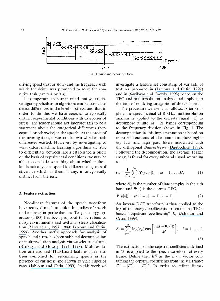
The procedure we use is as follows. After sam-pling the speech signal at 8 kHz, multiresolutionanalysis is applied to the discrete signal y"n# todecompose it into M $ 21 bands correspondingto the frequency division shown in Fig. 1. Thedecomposition in this implementation is based onrepeated iterations of the minimum-phase eight-tap low and high pass filters associated withthe orthogonal Daubechies-4 (Daubechies, 1992).Following the decomposition, the average Teagerenergy is found for every subband signal accordingto

em $ 1

Nm

XNm

n$1

jW%ym"n#&j; m $ 1; . . . ;M ; %1&

where Nm is the number of time samples in the mthband and W%'& is the discrete TEO,

W%y"n#& $ y2"n# ( y"n( 1#y"n) 1#: %2&

An inverse DCT transform is then applied to thelog of the energy coe"cients to obtain the TEO-based ‘‘cepstrum coe"cients’’ El (Jabloun andCetin, 1999),

El $XM

m$1

log%em& cosl%m( 0:5&p

M

! "; l $ 1; . . . ; L:

%3&

The extraction of the cepstral coe"cients definedin (3) is applied to the speech waveform at everyframe. Define then E"r# as the L! 1 vector con-taining the cepstral coe"cients from the rth frame:E "r# $ "E"r#

1 ; . . . ;E"r#L #

0. In order to reflect frame-

Fig. 1. Subband decomposition.

148 R. Fernandez, R.W. Picard / Speech Communication 40 (2003) 145–159

to-frame correlations within an energy subband,the following autocorrelation measure has beenproposed (Sarikaya and Gowdy, 1998):

ACE"r#l;s $

Pr)Tn$r E

"n#l E"n)s#

l

maxjPj)T

n$j E"n#l E"n)s#

l

# $ ; l $ 1; . . . ; L;

%4&

where s is the lag between frames, T is the numberof frames included in the autocorrelation window,and j is an index that spans all correlation coe"-cients within the same scale along all frames tonormalize the autocorrelation. Define the vectorcontaining the logarithm of the L autocorrela-tion coe"cients as ACE L"r#

s $ "log ACE"r#1;s; . . . ;

logACE"r#L;s#

T . We define the frame-based featurevector as the set of L cepstral coe"cients and thelog of the L autocorrelation coe"cients,

FS"r# $ E"r#

ACE L"r#s

! ": %5&

Taking the log of (4) is done to avoid modeling afinite support density distribution (which resultsfrom the normalization of (4)) with a single or asmall number of Gaussians in the learning stage.The number of subbands used in this implemen-tation was M $ 21, resulting from the five-leveldecomposition sketched in Fig. 1. The remainingconstants were adjusted empirically: s $ 1 and

T $ 2 (to capture pairwise correlations of adjacentsamples), and L $ 10 (to compress the originalinformation across 21 bands into 10). The result-ing feature vector after appending the correlationcoe"cients is therefore of dimensionality 20. Theframe features are derived from 24 ms of speechand are computed every 10 ms.

4. Modeling dynamics within the utterance

4.1. Graphical models

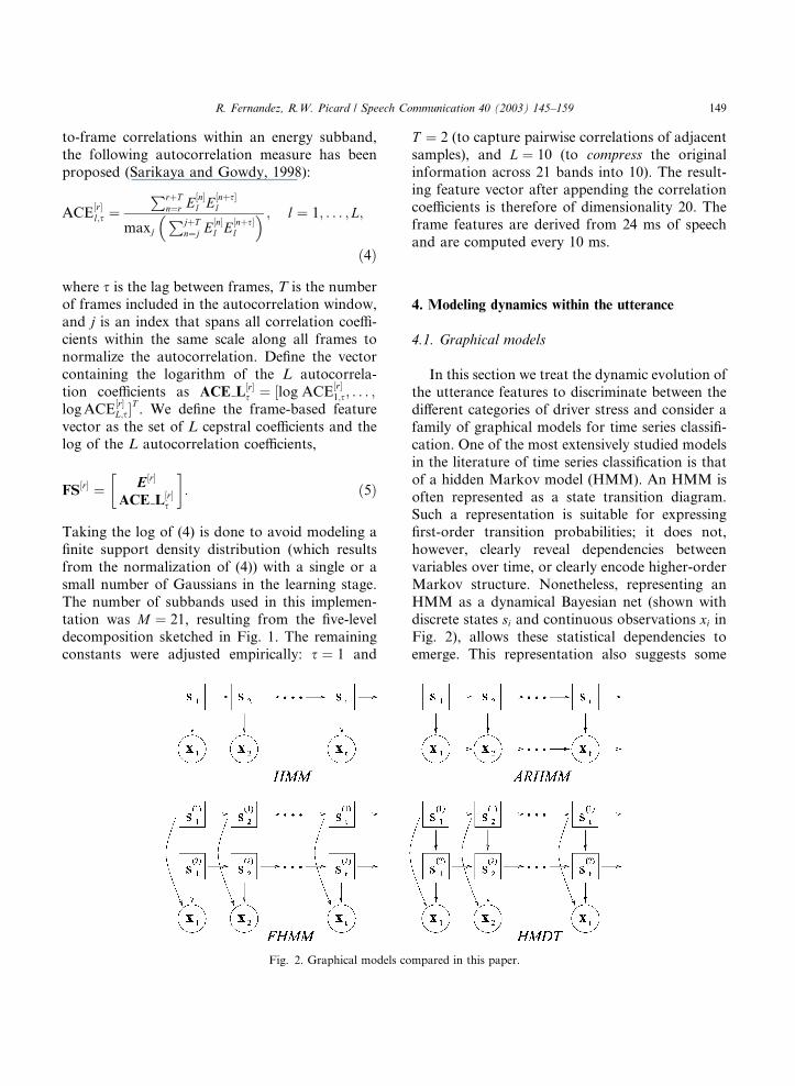
In this section we treat the dynamic evolution ofthe utterance features to discriminate between thedi!erent categories of driver stress and consider afamily of graphical models for time series classifi-cation. One of the most extensively studied modelsin the literature of time series classification is thatof a hidden Markov model (HMM). An HMM isoften represented as a state transition diagram.Such a representation is suitable for expressingfirst-order transition probabilities; it does not,however, clearly reveal dependencies betweenvariables over time, or clearly encode higher-orderMarkov structure. Nonetheless, representing anHMM as a dynamical Bayesian net (shown withdiscrete states si and continuous observations xi inFig. 2), allows these statistical dependencies toemerge. This representation also suggests some

Fig. 2. Graphical models compared in this paper.

R. Fernandez, R.W. Picard / Speech Communication 40 (2003) 145–159 149

natural extensions to the structure of the HMMmodel and aids in the development of general-purpose algorithms that may be used to dolearning and inference for a variety of structures.

An assumption behind the HMM, as shown bythe dependency diagram of Fig. 2, is that the ob-servations are independent of each other given thehidden state sequence. One may alleviate thislimitation by incorporating some dependency onpast observations. A simple way to do this isthrough a first-order recursion on the previousobservation. This yields the autoregressive hiddenMarkov model (ARHMM).

The representational capacity of an HMM isalso limited by how closely the number of hiddenstates approximates the state space of the dy-namics. Since the naive way to overcome thislimitation––namely, to increase the number ofstates of the hidden discrete node––yields an in-crease in the number of parameters to be esti-mated, distributed state representations whichmake use of fewer parameters have been proposed.One such structure is the factorial hidden Markov(FHMM) model. In an FHMM the state factorsinto multiple state variables, each modeled by anindependent chain evolving according to the sameMarkovian dynamics of the basic HMM (Ghahr-amani and Jordan, 1997).

One can also introduce dependencies betweenthe chains to impose structure while retainingparsimony. For instance, the di!erent state chainscan be arranged in a hierarchical structure suchthat, for any time slice, the state at any level of thehierarchy is dependent on the state at all levelsabove it. (See Fig. 2 for a model with two chains.)The result––a hidden decision tree evolving overtime with Markovian dynamics––is called a hiddenMarkov decision tree (HMDT) (Jordan et al.,1996).

The family of graphical models shown in Fig. 2has in common a set of unobserved discrete statesdistributed on a single or multiple chains, andcontinuous observation nodes. The following for-mulation of the learning algorithms can be appliedto any of the previous structures, as well as toextensions not described here. For instance, adistributed state representation may be combinedwith an ARHMM to obtain an autoregressive

factorial HMM. We will assume that every discretenode has only discrete parents––that is, theparameters associated with a discrete node consistof a conditional probability table––and that thecontinuous nodes have a conditional Gaussiandistribution. We represent the hidden state as avector st $ "s%1&t ; . . . ; s%m&t ; . . . ; s%M&

t #0 to generalize tothe case where the hidden state is distributed alongseveral chains, and the observations as the d-dimensional set fxgTt$1. In general, a continuousnode may have both continuous and discreteparents. Since the kind of dependency on contin-uous nodes we are interested in is first-orderautoregressive, a conditional Gaussian node hasdistribution

p%xtjxt(1; st $ i& * N%xt;Bixt(1;Ri&; %6&

where N%x; lx;Rx& is a multivariate Gaussian dis-tribution on the random variable x with meanvector lx and covariance matrix Rx. Letting xt(1 $I (the identity matrix) and Bi $ li in (6), we obtainthe distribution on Gaussian nodes with only dis-crete parents.

We can do learning on these structures by ap-plying the EM algorithm. First, we compute theexpected value of the complete data log likelihoodgiven the observations, and holding the currentparameters constant (E step), we then maximizethe expectation with respect to the parameters toobtain a new estimate (M step). The observation-dependent term of the complete log likelihood isgiven by

L $ E logYK

k

YTk

t

YjJ j

j

Pr%xkt jx

kt(1; st

"

$ j; fxtgTk1 &qjt

#

;

%7&

where qjt $: d%st $ j& is an indicator function.

Combining (6) and (7), and taking the derivativesof this expectation with respect to the parametersof the distribution, the following estimates areobtained (see (Murphy, 1998) for derivations):

eBBj $XK

k

XTk

t

ckt %j&xkt x

0kt(1

" #XK

k

XTk

t

ckt %j&xkt(1x

0kt(1

" #(1

;

%8&

150 R. Fernandez, R.W. Picard / Speech Communication 40 (2003) 145–159

eRRj $PK

k

PTkt ckt %j&xk

t x0ktPK

k

PTkt ckt %j&

(eBBj

PKk

PTkt ckt %j&xk

t(1x0ktPK

k

PTkt ckt %j&

: %9&

Eqs. (8) and (9) are written in terms of the ex-pectations

ckt %j& $ E"qjtjfxkt g

Tk1 # $ Pr%skt $ jjfxk

t gTk1 &: %10&

Letting xkt(1 $ I and eBBj $ ~llj in (8) and (9) yields

the estimation equations for the case when theobservation nodes are only dependent on thehidden discrete state.

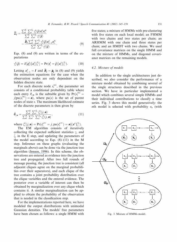
For each discrete node s%m&t , the parameter setconsists of a conditional probability table whereeach entry hj;n is the subtable given by Pr%s%m&t $jjpa%s%m&t & $ n&, where pa%s& is the set of parentnodes of state s. The maximum likelihood estimateof the discrete parameters is then given by

~hhj;n $PK

k

PTkt fkt %j; n&PK

k

PTkt

PJmj fkt %j; n&

; %11&

where fkt %j; n& $ Pr%sk%m&t $ j; pa%sk%m&t & $ njfxkgTk1 &.The EM algorithm consists of iteratively

collecting the expected su"cient statistics ct andft in the E step, and updating the parameters ofthe model according to Eqs. (8)–(11) in the Mstep. Inference on these graphs (evaluating themarginals above) can be done via the junction treealgorithm (Jensen, 1996). In this scheme, the ob-servations are entered as evidence into the junctiontree and propagated. After two full rounds ofmessage passing, the junction tree is consistent (alladjacent cliques agree on the marginal probabili-ties over their separators), and each clique of thetree contains a joint probability distribution overthe clique variables and the entered evidence. Theposterior over a variable of interest can then beobtained by marginalization over any clique whichcontains it. A similar marginalization can be ap-plied to obtain the probability of the observationthat is needed in the classification step.

For the implementations reported here, we havemodeled the output distributions with unimodalGaussian densities. The models! free parametershave been chosen as follows: a single HMM with

five states; a mixture of HMMs with pre-clusteringwith five states on each local model; an FHMMwith two chains and two states per chain; anARHMM with one chain and three states perchain; and an HMDT with two chains. We usedfull covariance matrices on the single HMM andon the mixture of HMMs, and diagonal covari-ance matrices on the remaining models.

4.2. Mixture of models

In addition to the single architectures just de-scribed, we also consider the performance of amixture model obtained by combining several ofthe single structures described in the previoussection. We have in particular implemented amodel which combines several simple HMMs andtheir individual contributions to classify a timeseries. Fig. 3 shows this model generatively: thenth model is selected with probability an (with

Fig. 3. Mixture of HMMs model.

R. Fernandez, R.W. Picard / Speech Communication 40 (2003) 145–159 151

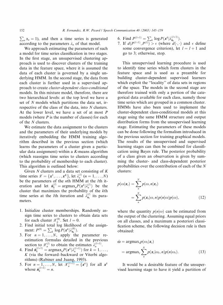
Pn an $ 1), and then a time series is generated

according to the parameters kn of that model.We approach estimating the parameters of such

a model for time series classification in two stages.In the first stage, an unsupervised clustering ap-proach is used to discover clusters of the trainingdata in the feature space, where it is assumed thedata of each cluster is governed by a single un-derlying HMM. In the second stage, the data fromeach cluster is further used in a supervised ap-proach to create cluster-dependent class-conditionalmodels. In this mixture model, therefore, there aretwo hierarchical levels: at the top level we have aset of N models which partitions the data set, ir-respective of the class of the data, into N clusters.At the lower level, we have a set of at most Pmodels (where P is the number of classes) for eachof the N clusters.

We estimate the data assignment to the clustersand the parameters of their underlying models byiteratively embedding the HMM training algo-rithm described in the previous section (whichlearns the parameters of a cluster given a partic-ular data assignment) within a K-means algorithm(which reassigns time series to clusters accordingto the probability of membership to each cluster).This algorithm is outlined below:

Given N clusters and a data set consisting of Ktime series X $ fx1; . . . ; xKg, let k%l&n (n $ 1; . . . ;N )be the parameters of the nth HMM at the lth it-eration and let nn%l&k $ argmaxnP %xkjk%l&n & be thecluster that maximizes the probability of the kthtime series at the lth iteration and k%l&nnk its para-meters.

1. Initialize cluster memberships. Randomly as-sign time series to clusters to obtain data setsfor each cluster X%0&

n . Set l $ 0.2. Find initial total log likelihood of the assign-

ment: P %0& $P

k log P %xkjk%0&nnk &.3. For n $ 1; . . . ;N , apply the parameter re-

estimation formulas detailed in the previoussection to X%l&

n to obtain the estimates k%l)1&n .

4. Find nn%l)1&k $ argmaxnP%xkjk%l)1&

n & for k $ 1; . . . ;K (via the forward–backward or Viterbi algo-rithms) (Rabiner and Juang, 1993).

5. For n $ 1; . . . ;N , let X%l)1&n $ fxkg for all xk

whose nn%l)1&k $ n.

6. Find P %l)1& $P

k log P %xkjk%l)1&nnk &.

7. If d%P %l)1&; P %l&& > ! (where d%'; '& and ! definesome convergence criterion), let l $ l) 1 andgo to 3; otherwise, stop.

This unsupervised learning procedure is usedto identify time series which form clusters in thefeature space and is used as a preamble forbuilding cluster-dependent supervised learnerswhich exploit the ‘‘locality’’ of data sets in regionsof the space. The models in the second stage aretherefore trained with only a portion of the cate-gorical data available for each class, namely thosetime series which are grouped in a common cluster.HMMs have also been used to implement thecluster-dependent class-conditional models at thisstage using the same HMM structure and outputdistribution forms from the unsupervised learningstage. Estimating the parameters of these modelscan be done following the formalism introduced inthe previous section for training graphical models.The results of the unsupervised and supervisedlearning stages can then be combined for classifi-cation using Bayes rule. The posterior probabilityof a class given an observation is given by sum-ming the cluster- and class-dependent posteriorprobabilities over the contribution of each of the Nclusters:

p%xjxt& $XN

n

p%x; njxt&

$XN

n

p%xtjx; n&p%njx&p%x&; %12&

where the quantity p%njx& can be estimated fromthe output of the clustering. Assuming equal priorson all classes, and a maximum a posteriori classi-fication scheme, the following decision rule is thenobtained:

xx $ argmaxlp%xljxt&

$ argmaxlXN

n

p%xtjxl; n&p%njxl&: %13&

It would be a desirable feature of the unsuper-vised learning stage to have it yield a partition of

152 R. Fernandez, R.W. Picard / Speech Communication 40 (2003) 145–159

the data which is as homogeneous as possible; thatis, we would like to obtain a partition which yieldsclusters with representatives from as few classes aspossible. We can diagnose the homogeneity of theclusters by considering the outcome of the unsu-pervised algorithm in terms of two multinomialvariables: the class of the kth data sequence xk

t (xk)and the cluster to which it is assigned (ck 2 n $1; . . . ;N ). The clustering algorithm may then beviewed as yielding a data set fxk; ckgKk$1 to whichwe want to apply a hypothesis test to determinewhether the set of labels and the set of clusterswere generated by di!erent multinomial distribu-tions or by the same multinomial. More formally,we would like to know the probability that the setsX $ fxgk and C $ fcgk were generated by thesame distribution:

p%sjX;C& $ p%X;Cjs&p%s&p%X;Cjs&p%s& ) p%X;Cjd&p%d&

$ 1

1) %p%X;Cjd&=p%X;Cjs&&%p%d&=p%s&&;

%14&

where the labels s and d indicate same or di!erentdistributions. The main quantity involved incomputing (14) is the ratio of evidence of thedata sets under di!erent and same distributionsp%X;Cjd&=p%X;Cjs&, a quantity which may bewritten in terms of factorized and joint evidence%p%X&p%C&&=p%X;C&. Let the class x take on one ofJ outcomes, and let the cluster c take on one of Noutcomes. Define the following partial counts:

Kj;n $XK

k$1

dwk ;jdck ;n;

Kj $XN

n$1

Kj;n;

Kn $XJ

j$1

Kj;n; j $ 1; . . . ; J ; n $ 1; . . . ;N :

It can be shown (Minka, 1999) that, under theassumption of multinomial distributions, the evi-dence ratio in (14) is given by

p%X&p%C&p%X;C& $ C%JN&

C%K ) JN&Y

j

C%Kj ) N&C%N&

!Y

n

C%Kn ) J&C%J&

Y

j;n

C%1&C%1) Kj;n&

: %15&

The quantity in (15) also has an interpretation asthe mutual information between the variables xand c (Minka, 1999). Eq. (14) may be used to de-termine whether the clustering procedure has in-troduced some dependencies between labels andclusters. Furthermore, it may be used togetherwith the clustering algorithm above to select thenumber of clusters which establishes the largestdependency between variables. For the results re-ported in this paper, we have considered mixturemodels with 2–6 components, and chosen thenumber of components which maximizes (14) onthe training set.

5. Modeling features at the utterance-level

Modeling of linguistic phenomena requires thatwe choose an adequate time scale to capture rele-vant details. For speech recognition, a suitabletime scale might be one that allows representingphonemes. For the supralinguistic phenomena weare interested in modeling, however, we wish toinvestigate whether a coarser time scale su"ces.The database used in this study consists of shortand simple utterances (with presumably sim-pler structures than those found in unconstrainedspeech), and hence, global utterance-level featuresmight provide stress discrimination. A simple wayto obtain an utterance-level representation of theoriginal dynamic feature set is to use a statistic ofeach feature time series defined along an utterance(e.g., its sample mean, median, etc.). For the sim-ulations here we have chosen the sample mean ofeach dynamic feature as the utterance-level featurevalue. Since the temporal dynamics are nowmissing, we use static classifiers to discriminate thefour categories.

We consider two classification schemes, a sup-port vector machine (SVM) and a neural network(ANN). An SVM implements an approximation tothe structural risk minimization principle in whichboth the empirical error and a bound related to the

R. Fernandez, R.W. Picard / Speech Communication 40 (2003) 145–159 153

generalization ability of the classifier are mini-mized. The SVM fits a hyperplane that achievesmaximum margin between two classes; its decisionboundary is determined by the discriminant

f %x& $X

i

yikiK%x; xi& ) b; %16&

where xi and yi 2 f(1; 1g are the input–outputpairs, K%x; y&$: /%x& ' /%y& is a kernel functionwhich computes inner products, and /%x& is atransformation from the input space to a higherdimensional space. In the linearly separable case,/%x& $ x. An SVM is generalizable to non-linearlyseparable cases by first applying the mapping /%'&to increase dimensionality and then applying alinear classifier in the higher-dimensional space.The parameters of this model are the values ki,non-negative constraints that determine the con-tribution of each data point to the decision sur-face, and b, an overall bias term. The data pointsfor which ki 6$ 0 are the only ones that contributeto (16) and are known as support vectors. Fittingan SVM consists of solving the quadratic program(Osuna et al., 1997):

max F %K& $ K ' 1( 12K ' DK;

subject to K ' y $ 0;

K6C1;

KP 0; %17&

where K $ "k1; . . . ; kl#0, D is a symmetric matrixwith elements Di;j $ yiyjK%xi; xj&, and C is a non-negative constant that bounds each ki, and whichis related to the width of the margin between theclasses. Having solved K from the equations in(17), the bias term can be found:

b $ (12

X

i

kiyi K%x(; xi&% ) K%x); xi&&; %18&

where x( and x) are any two correctly classifiedsupport vectors from classes (1 and )1, respec-tively (Gunn, 1998).

We also consider a two-layer ANN classifierproviding a mapping of the form

z $ f %x& $ g2%W2g1%W1x) b1& ) b2&; %19&

where gi, Wi and bi are the non-linear activationunit, weight matrix and bias vector respectively

associated with each layer. We have trained anANN to minimize the following error criterion:

E $ Ex ) Ew $ (X

i

ti ' ln%zi& ) jjwjj2; %20&

where ti is a k ! 1 vector of zero-one target valuesencoding the class of the xi data point, and w is avector containing all the parameters of the net-work (the entries of Wi and bi). The first error term(Ex) is the negative cross-entropy between thenetwork outputs and the desired target values.Minimizing this error function is equivalent tomaximizing the likelihood of the data set of targetvalues given the input patterns. The second term in(20) (Ew) is a weight decay regularizer that penal-izes larger sizes of network parameters (controllingsmoothness of the decision surface and regular-ization ability of the machine) (Bishop, 1995). Theweights of the network are updated according tothe rule

Dw $ (adEdw

$ (%H ) lI&(1%g ) w&; %21&

where g $P

i gi $

Pi%dEi

x=dw& is the gradient ofthe cross-entropy error function with respect to thenetwork weights and H $

Pi g

i%gi&T is the outerproduct approximation to the Hessian matrix. Theparameter l is a momentum parameter chosenadaptively to speed convergence. The derivativesneeded to compute (21) are calculated using stan-dard back-propagation.

For the simulations reported here, we have builtSVMs with a Gaussian kernel function havingwidth parameter r $ 5, and two-layer ANNs with10 and 4 hidden units, and sigmoid and softmaxactivation units on each layer, respectively.

6. Results and discussion

The speech data of four subjects was first di-vided into a training and testing set comprisingapproximately 80% and 20% of the data set, re-spectively. The following labels will be used todenote the four categories of data: FF, SF, FS, SS.The first letter denotes whether the data came froma fast (F) or slow (S) driving speed condition; thesecond indicates the frequency with which the

154 R. Fernandez, R.W. Picard / Speech Communication 40 (2003) 145–159

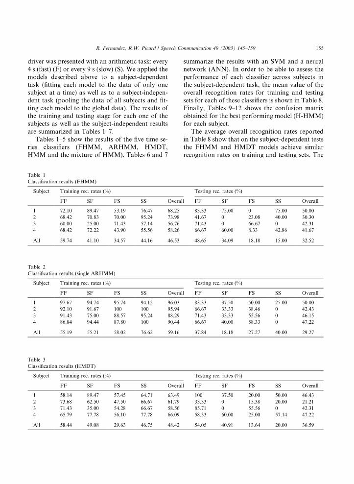
driver was presented with an arithmetic task: every4 s (fast) (F) or every 9 s (slow) (S). We applied themodels described above to a subject-dependenttask (fitting each model to the data of only onesubject at a time) as well as to a subject-indepen-dent task (pooling the data of all subjects and fit-ting each model to the global data). The results ofthe training and testing stage for each one of thesubjects as well as the subject-independent resultsare summarized in Tables 1–7.

Tables 1–5 show the results of the five time se-ries classifiers (FHMM, ARHMM, HMDT,HMM and the mixture of HMM). Tables 6 and 7

summarize the results with an SVM and a neuralnetwork (ANN). In order to be able to assess theperformance of each classifier across subjects inthe subject-dependent task, the mean value of theoverall recognition rates for training and testingsets for each of these classifiers is shown in Table 8.Finally, Tables 9–12 shows the confusion matrixobtained for the best performing model (H-HMM)for each subject.

The average overall recognition rates reportedin Table 8 show that on the subject-dependent teststhe FHMM and HMDT models achieve similarrecognition rates on training and testing sets. The

Table 2Classification results (single ARHMM)

Subject Training rec. rates (%) Testing rec. rates (%)

FF SF FS SS Overall FF SF FS SS Overall

1 97.67 94.74 95.74 94.12 96.03 83.33 37.50 50.00 25.00 50.002 92.10 91.67 100 100 95.94 66.67 33.33 38.46 0 42.433 91.43 75.00 88.57 95.24 88.29 71.43 33.33 55.56 0 46.154 86.84 94.44 87.80 100 90.44 66.67 40.00 58.33 0 47.22

All 55.19 55.21 58.02 76.62 59.16 37.84 18.18 27.27 40.00 29.27

Table 3Classification results (HMDT)

Subject Training rec. rates (%) Testing rec. rates (%)

FF SF FS SS Overall FF SF FS SS Overall

1 58.14 89.47 57.45 64.71 63.49 100 37.50 20.00 50.00 46.432 73.68 62.50 47.50 66.67 61.79 33.33 0 15.38 20.00 21.213 71.43 35.00 54.28 66.67 58.56 85.71 0 55.56 0 42.314 65.79 77.78 56.10 77.78 66.09 58.33 60.00 25.00 57.14 47.22

All 58.44 49.08 29.63 46.75 48.42 54.05 40.91 13.64 20.00 36.59

Table 1Classification results (FHMM)

Subject Training rec. rates (%) Testing rec. rates (%)

FF SF FS SS Overall FF SF FS SS Overall

1 72.10 89.47 53.19 76.47 68.25 83.33 75.00 0 75.00 50.002 68.42 70.83 70.00 95.24 73.98 41.67 0 23.08 40.00 30.303 60.00 25.00 71.43 57.14 56.76 71.43 0 66.67 0 42.314 68.42 72.22 43.90 55.56 58.26 66.67 60.00 8.33 42.86 41.67

All 59.74 41.10 34.57 44.16 46.53 48.65 34.09 18.18 15.00 32.52

R. Fernandez, R.W. Picard / Speech Communication 40 (2003) 145–159 155

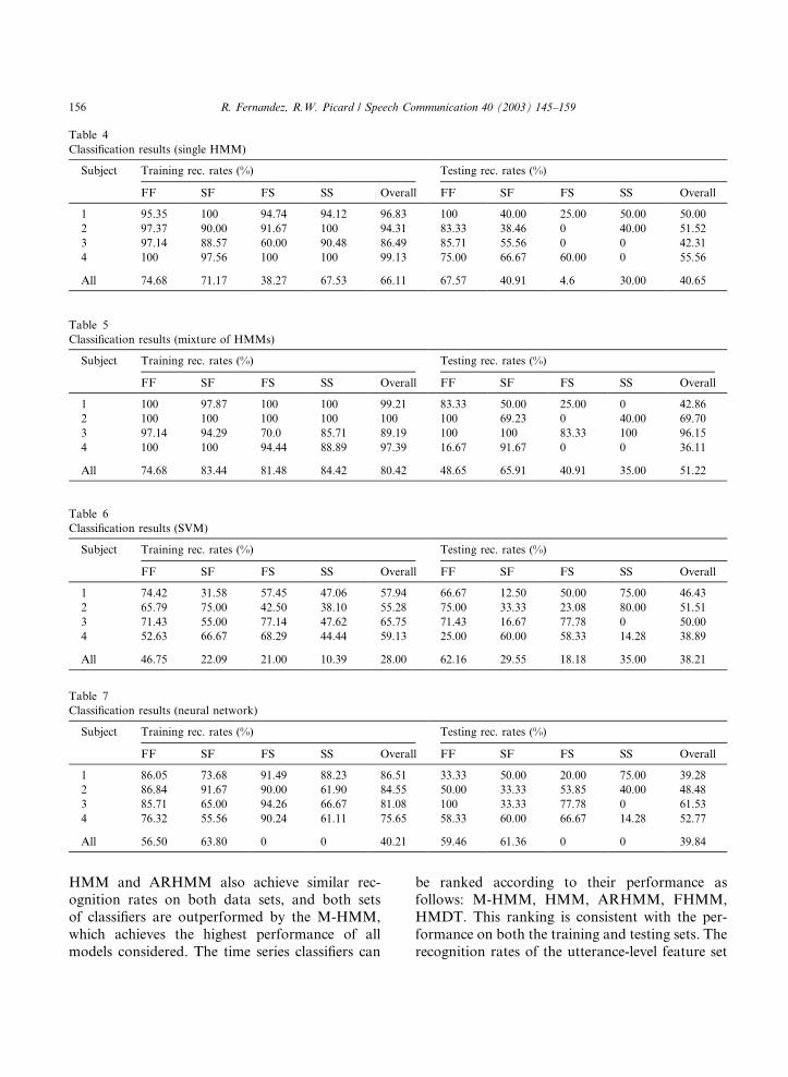
HMM and ARHMM also achieve similar rec-ognition rates on both data sets, and both setsof classifiers are outperformed by the M-HMM,which achieves the highest performance of allmodels considered. The time series classifiers can

be ranked according to their performance asfollows: M-HMM, HMM, ARHMM, FHMM,HMDT. This ranking is consistent with the per-formance on both the training and testing sets. Therecognition rates of the utterance-level feature set

Table 6Classification results (SVM)

Subject Training rec. rates (%) Testing rec. rates (%)

FF SF FS SS Overall FF SF FS SS Overall

1 74.42 31.58 57.45 47.06 57.94 66.67 12.50 50.00 75.00 46.432 65.79 75.00 42.50 38.10 55.28 75.00 33.33 23.08 80.00 51.513 71.43 55.00 77.14 47.62 65.75 71.43 16.67 77.78 0 50.004 52.63 66.67 68.29 44.44 59.13 25.00 60.00 58.33 14.28 38.89

All 46.75 22.09 21.00 10.39 28.00 62.16 29.55 18.18 35.00 38.21

Table 7Classification results (neural network)

Subject Training rec. rates (%) Testing rec. rates (%)

FF SF FS SS Overall FF SF FS SS Overall

1 86.05 73.68 91.49 88.23 86.51 33.33 50.00 20.00 75.00 39.282 86.84 91.67 90.00 61.90 84.55 50.00 33.33 53.85 40.00 48.483 85.71 65.00 94.26 66.67 81.08 100 33.33 77.78 0 61.534 76.32 55.56 90.24 61.11 75.65 58.33 60.00 66.67 14.28 52.77

All 56.50 63.80 0 0 40.21 59.46 61.36 0 0 39.84

Table 5Classification results (mixture of HMMs)

Subject Training rec. rates (%) Testing rec. rates (%)

FF SF FS SS Overall FF SF FS SS Overall

1 100 97.87 100 100 99.21 83.33 50.00 25.00 0 42.862 100 100 100 100 100 100 69.23 0 40.00 69.703 97.14 94.29 70.0 85.71 89.19 100 100 83.33 100 96.154 100 100 94.44 88.89 97.39 16.67 91.67 0 0 36.11

All 74.68 83.44 81.48 84.42 80.42 48.65 65.91 40.91 35.00 51.22

Table 4Classification results (single HMM)

Subject Training rec. rates (%) Testing rec. rates (%)

FF SF FS SS Overall FF SF FS SS Overall

1 95.35 100 94.74 94.12 96.83 100 40.00 25.00 50.00 50.002 97.37 90.00 91.67 100 94.31 83.33 38.46 0 40.00 51.523 97.14 88.57 60.00 90.48 86.49 85.71 55.56 0 0 42.314 100 97.56 100 100 99.13 75.00 66.67 60.00 0 55.56

All 74.68 71.17 38.27 67.53 66.11 67.57 40.91 4.6 30.00 40.65

156 R. Fernandez, R.W. Picard / Speech Communication 40 (2003) 145–159

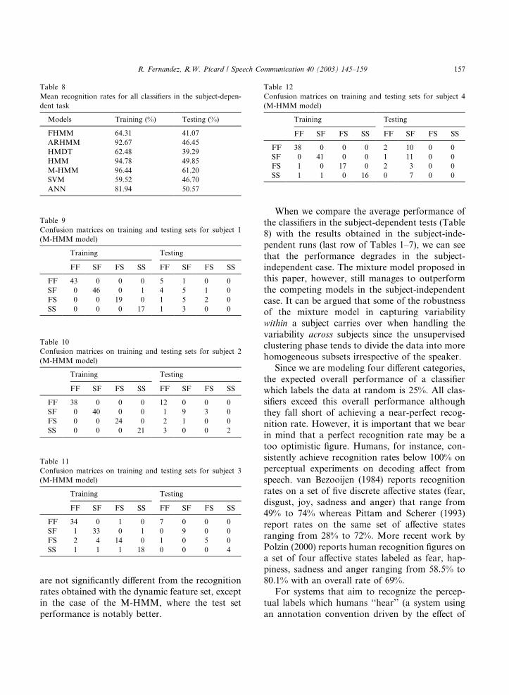
are not significantly di!erent from the recognitionrates obtained with the dynamic feature set, exceptin the case of the M-HMM, where the test setperformance is notably better.

When we compare the average performance ofthe classifiers in the subject-dependent tests (Table8) with the results obtained in the subject-inde-pendent runs (last row of Tables 1–7), we can seethat the performance degrades in the subject-independent case. The mixture model proposed inthis paper, however, still manages to outperformthe competing models in the subject-independentcase. It can be argued that some of the robustnessof the mixture model in capturing variabilitywithin a subject carries over when handling thevariability across subjects since the unsupervisedclustering phase tends to divide the data into morehomogeneous subsets irrespective of the speaker.

Since we are modeling four di!erent categories,the expected overall performance of a classifierwhich labels the data at random is 25%. All clas-sifiers exceed this overall performance althoughthey fall short of achieving a near-perfect recog-nition rate. However, it is important that we bearin mind that a perfect recognition rate may be atoo optimistic figure. Humans, for instance, con-sistently achieve recognition rates below 100% onperceptual experiments on decoding a!ect fromspeech. van Bezooijen (1984) reports recognitionrates on a set of five discrete a!ective states (fear,disgust, joy, sadness and anger) that range from49% to 74% whereas Pittam and Scherer (1993)report rates on the same set of a!ective statesranging from 28% to 72%. More recent work byPolzin (2000) reports human recognition figures ona set of four a!ective states labeled as fear, hap-piness, sadness and anger ranging from 58.5% to80.1% with an overall rate of 69%.

For systems that aim to recognize the percep-tual labels which humans ‘‘hear’’ (a system usingan annotation convention driven by the e!ect of

Table 12Confusion matrices on training and testing sets for subject 4(M-HMM model)

Training Testing

FF SF FS SS FF SF FS SS

FF 38 0 0 0 2 10 0 0SF 0 41 0 0 1 11 0 0FS 1 0 17 0 2 3 0 0SS 1 1 0 16 0 7 0 0

Table 8Mean recognition rates for all classifiers in the subject-depen-dent task

Models Training (%) Testing (%)

FHMM 64.31 41.07ARHMM 92.67 46.45HMDT 62.48 39.29HMM 94.78 49.85M-HMM 96.44 61.20SVM 59.52 46.70ANN 81.94 50.57

Table 10Confusion matrices on training and testing sets for subject 2(M-HMM model)

Training Testing

FF SF FS SS FF SF FS SS

FF 38 0 0 0 12 0 0 0SF 0 40 0 0 1 9 3 0FS 0 0 24 0 2 1 0 0SS 0 0 0 21 3 0 0 2

Table 9Confusion matrices on training and testing sets for subject 1(M-HMM model)

Training Testing

FF SF FS SS FF SF FS SS

FF 43 0 0 0 5 1 0 0SF 0 46 0 1 4 5 1 0FS 0 0 19 0 1 5 2 0SS 0 0 0 17 1 3 0 0

Table 11Confusion matrices on training and testing sets for subject 3(M-HMM model)

Training Testing

FF SF FS SS FF SF FS SS

FF 34 0 1 0 7 0 0 0SF 1 33 0 1 0 9 0 0FS 2 4 14 0 1 0 5 0SS 1 1 1 18 0 0 0 4

R. Fernandez, R.W. Picard / Speech Communication 40 (2003) 145–159 157

the utterances on the listeners, as we discussed inSection 2), the human performance figures o!er areasonable yardstick by which we should evaluatethe performance of an automated system. How-ever, for systems aiming to recognize labels gov-erned by the state of the speaker (cause-type ofannotation), establishing a benchmark is lessstraightforward. Comparison with other studiesthat use a similar labeling approach to build au-tomatic recognizers may be useful to obtain animpressionistic idea of what is accomplishable.However, as the context in which the utterancesare produced often varies significantly across thesestudies, it is important that we carry such com-parisons with due care. Even a!ective states thatare labeled with the same descriptor may corre-spond to very di!erent realities about the internalstate of the speaker. McGilloway et al. (2000) havecarried out a study in which they used emotivetexts to induce a!ect in speech. This study cantherefore be considered similar in so far as thelabels capture information about the state of thespeaker. They report recognition rates rangingfrom 50% to 64% for a set of five states (fear,happiness, neutral, sadness and anger). Bearingthe above mentioned caveats in mind, we can seethe performance that the M-HMM achieves onsome subjects as being competitive with some ofthe results published elsewhere in the literature.

There is variability, however, on how thesesystems perform across subjects. This result maybe due to the fact that subjects with the lowerrecognition rates do not show su"cient variabilityacross the categories we are modeling, but it mayalso be attributed to a limitation of the models orthe features in capturing the variability that thesubjects may have exhibited. This is an issue thatwould require further research in order to drawmore rigorous conclusions. It is also important tonote the variability of the classifiers in modelingeach of the categories considered independently.Whereas all the models provide an adequate fit tothe FF category, each of them fails to consistentlypredict above random the remaining categories forall subjects (see Tables 1–7). This may be due toone or more of several reasons: (i) the inherentmodeling capacity of the models considered, (ii)an underoptimized local solution found during

training, (iii) the discriminative capacity of thefeatures for the di!erent categories, or (iv) the in-herent noise in the ground truth of the categoriesof driver!s stress due to how accurately the ex-perimental procedure was able to e!ectively inducethe assigned labels. Since the FF category is themost ‘‘extreme’’ in terms of driving speed andcognitive load on the driver, it is tempting to as-sume that the better performance on this label maybe related to how reliably the driver becamestressed in these portions of the experiment. Wehave also included for completeness confusionmatrices that show the kinds of misclassificationsthat the best performer (mixture model) tends toproduce (Tables 9–12). There is no consistentpattern that emerges from inspecting these confu-sion matrices: no category is consistently mistakenfor another one when the results are evaluatedacross subjects. We have dealt with subject de-pendency by fitting a di!erent system to eachspeaker. One open question worth investigating iswhether this dependency can be reduced withouthaving to go to the extreme of fitting a di!erent setof parameters to each speaker. An alternative so-lution might be finding prototypes of speakers inthe space of speaker variability and fit a model toeach prototype rather than to each speaker. Weare advancing the hypothesis that the mixturemodel might o!er a good point of departure forthis kind of modeling (as well as modeling anycategories involving variability across speakers)because of how it proceeds in dividing the featurespace into similar clusters. A data set with a largernumber of speakers would be needed, however, inorder to evaluate this hypothesis.

7. Conclusions

In this paper we have investigated the use offeatures based on subband decompositions and theTEO for classification of stress categories in speechproduced in the context of driving at variablespeeds while engaged on mental tasks of variablecognitive load for a set of four subjects. We in-vestigated the performance of several classifiers ontwo representations of the speech waveforms:using a feature set representing intra-utterance

158 R. Fernandez, R.W. Picard / Speech Communication 40 (2003) 145–159

dynamics and a sparser set consisting of more glo-bal utterance-level features. The best performancewas obtained by using the dynamic feature set andby exploiting local models and then combiningthem in a weighted classification scheme. All clas-sifiers produced recognition rates above random forall subjects, but, with the exception of the fast-fastcategory, showed variability in consistently pre-dicting each of the remaining stress conditions.

Acknowledgements

The authors would like to thank Nissan!s CBRLab and Elias Vyzas for their help with data col-lection and Thomas Minka for valuable technicaldiscussions and for suggesting the significance test.

References

Bishop, C.M., 1995. Neural Networks for Pattern Recognition.Clarendon Press, Oxford.

Cowie, R., 2000. Describing the emotional states expressed inspeech. In: Proceedings of the ISCA ITRW on Speech andEmotion, 5–7 September 2000, Textflow, Belfast.

Daubechies, I., 1992. Ten Lectures on Wavelets. RegionalConference Series in Applied Mathematics, SIAM, Phila-delphia, PA, 1992.

Ghahramani, Z., Jordan, M.I., 1997. Factorial hidden Markovmodels. Machine Learning 29, 245–275.

Gunn, S., 1998. Support vector machines for classification andregression. Technical Report, Image, Speech and IntelligentSystems Group, University of Southampton.

Hansen, J.H.L., Womack, B.D., 1996. Feature analysis andneural network-based classification of speech under stress.IEEE Transactions on Speech and Audio Processing IV (4),307–313.

Hansen, J., Bou-Ghazale, S.E., Sarikaya, R., Pellom, B., 1998.Getting started with the SUSAS: Speech Under Simulatedand Actual Stress database. Technical Report, RobustSpeech Proc. Laboratory, Department of Electrical Engi-neering, Duke University.

Jabloun, F., Cetin, A.E., Yjhjnj, K., 1999. The Teager energybased feature parameters for robust speech recognition incar noise. In: Proceedings of the IEEE InternationalConference on Acoustics, Speech, and Signal Processing,Vol. 1, pp. 273–276.

Jensen, F.V., 1996. An Introduction to Bayesian Networks.Springer, New York.

Jordan, M.I., Ghahramani, Z., Saul, L.K., 1996. HiddenMarkov decision trees. In: Mozer, M.C., Jordan, M.I.,

Petsche, T. (Eds.), Advances in Neural Information Pro-cessing Systems, Vol. 9. MIT Press, Cambridge, MA, pp.501–507.

McGilloway, S., Cowie, R., Douglas-Cowie, E., Gielen, S.,Westerdijk, M., Stroeve, S., 2000. Automatic recognition ofemotion from voice: a rough benchmark. In: Proceedings ofthe ISCA ITRW on Speech and Emotion, 5–7 September2000, Textflow, Belfast, pp. 207–212.

Minka, T.P., 1999. Bayesian inference of a multinominaldistribution. Available from <http://www.media.mit.edu/*tpminka/papers/tutorial.html>.

Murphy, K., 1998. Fitting a constrained conditional Gaussian.Technical Report, Department of Computer Science, UCBerkeley.

Murray, I.R., Baber, C., South, A.J., 1996. Towards adefinition and working model of stress and its e!ects onspeech. Speech Communication 20, 1–12.

Osuna, E.E., Freund, R., Girosi, F., 1997. Support vectormachines: Training and applications. Technical Report, no.AI Memo 1602/CBCL, Paper 144, MIT.

Pittam, J., Scherer, K., 1993. Vocal expression and communi-cation of emotion. In: Lewis, M., Haviland, J.M. (Eds.),Handbook of Emotions. Guilford Press, New York, pp.185–197.

Polzin, T., 2000. Detecting verbal and non-verbal cues in thecommunication of emotions. Unpublished Doctoral Disser-tation, School of Computer Science, Carnegie MellonUniversity.

Rabiner, L., Juang, B.-H., 1993. Fundamentals of SpeechRecognition. Prentice Hall, Upper Saddle River, NJ.

Sarikaya, R., Gowdy, J.N., 1997. Wavelet based analysis ofspeech under stress. In: Proceedings of the Southeastcon !97,Engineering New Century, IEEE, pp. 92–96.

Sarikaya, R., Gowdy, J.N., 1998. Subband based classificationof speech under stress. In: Proceedings of the IEEEInternational Conference on Acoustics, Speech, and SignalProcessing, Vol. I, pp. 569–572.

Steeneken, H.J.M., Hansen, J.H.L., 1999. Speech under stressconditions: Overview of the e!ect on speech production andof system performance. In: Proceedings of the IEEEInternational Conference on Acoustics, Speech, and SignalProcessing, Vol. IV, pp. 2079–2082.

van Bezooijen, R., 1984. Characteristics and Recognizabilityof Vocal Expressions of Emotion. Foris Publications,Holland.

Zhou, G., Hansen, J., Kaiser, J., 1998. Classification of speechunder stress based on features derived from the nonlinearTeager energy operator. In: Proceedings of the IEEEInternational Conference on Acoustics, Speech, and SignalProcessing, Vol. I, pp. 549–552.

Zhou, G., Hansen, J.H.L., Kaiser, J.F., 1999. Methods forstress classification: Nonlinear TEO and linear speech basedfeatures. In: Proceedings of the IEEE International Con-ference on Acoustics, Speech, and Signal Processing, Vol.IV, pp. 2087–2090.

R. Fernandez, R.W. Picard / Speech Communication 40 (2003) 145–159 159