arX

iv:c

ond-

mat

/011

2033

v1 3

Dec

200

1

The effect of non-ideal market conditions on

option pricing

Josep Perello and Jaume Masoliver

Departament de Fısica Fonamental, Universitat de Barcelona, Diagonal, 647,

08028-Barcelona, Spain

Abstract

Option pricing is mainly based on ideal market conditions which are well representedby the Geometric Brownian Motion (GBM) as market model. We study the effectof non-ideal market conditions on the price of the option. We focus our attentionon two crucial aspects appearing in real markets: The influence of heavy tails andthe effect of colored noise. We will see that both effects have opposite consequenceson option pricing.

1 Introduction

Option pricing lies, from the very beginning, at the heart of mathematical fi-nance as scientific discipline. In 1900, Bachelier proposed the arithmetic Brow-nian motion for the dynamical evolution of stock prices as a first step towardsobtaining a price for options [1]. Since then and specially after the landmarkwork of Black and Scholes [2] and Merton [3], the underlying asset of anyoption is usually assumed to be driven by Brownian motion, being the mostubiquitous model the geometric Brownian motion (GBM):

S

S= µ+

1

2σ2 + σξ(t), (1)

where S(t) is the price of stock (or the value of an index) at time t, µ+ σ2/2is the drift, σ is the volatility and ξ(t) is Gaussian white noise with zero meanand correlation 〈ξ(t)ξ(t′)〉 = δ(t− t′). Associated with stock price S(t) there isanother random process: the return. In continuos-time finance this is definedby R(t) = lnS(t)/S(t0). For the GBM (1) one can see, after using Ito lemma[4], that the return obeys the following SDE

R = µ+ σξ(t), (2)

Preprint submitted to Elsevier Preprint 1 February 2008

from which we see that µ is the mean return rate. Since, by definition, theinitial return is zero, then in terms of the integral of ξ(t) which is taken in theIto sense, we can explicitly write the return as

R(t) = µ(t− t0) + σ

t∫

t0

ξ(t′)dt′, (3)

where the integral of ξ(t) appearing in the rhs of this equation is simply theWiener process W (t). Note that, independently of the stock price S(t0), thereturn at initial time t0 is always zero since R(t0) = lnS(t0)/S(t0) = ln 1 = 0.

However, the market model given by Eq. (1) or Eqs. (2)–(3) does not fullyaccount for all properties observed in real markets. Some of them are quitecrucial such as the existence of heavy tails and negative skewness in probabilitydistributions, evidence of self-scaling (at least for high frequency data) [5],leverage [6] and even the existence of mild correlations in the increments ofreturn [7]. All of this, undoubtedly has to affect option pricing. Therefore,the theoretical price for the option obtained through the assumption thatmarkets are governed by the GBM would not be adjusted to reality. Our mainobjective here is to elucidate how some of the above properties of real marketsmay affect the price of options. Specifically we will obtain an option price formarket models that present fat tails and self-scaling. After that, we will relaxthe so called efficient market hypothesis [8] and assume the existence of autocorrelations in stock prices. We restrict the analysis to European call options,although it can be easily generalized to the European put and other optionswith fixed exercise date. The extension to American options seems to be moreinvolved.

The starting point of this work is the martingale option price. As was shownin early eighties, the Black-Scholes (B-S) option price can also be obtainedusing martingale methods [9]. This is a shorter, although more abstract way,to derive an expression for the call price. The main advantage is that one onlyneeds to know the probability density function governing market evolution.The main inconvenience is that there is no known hedging strategy as in thecase of B-S theory.

The probability distribution of some of the more realistic market models wewill use is only known through its characteristic function. We will thereforederive a formula which will allow us to obtain, via martingale price, the op-tion price in terms of the characteristic function of the market model chosen.Having the necessary tools to address the problem, we will apply them to arecently presented market model which shows self-similarity, fat tails and fi-nite moments [10]. We will obtain an option price this model and compare itwith B-S price.

2

The second problem we want to address is the effect of colored noise in theprice of options. The GBM model supposes that prices are driven by Gaussianwhite noise, this implies that prices S(t), at different times, are uncorrelatedwhich, for certain times scales, does not seem to be completely adjusted toreality. We will thus assume that prices are driven by colored noise and obtainthe corresponding fair price for the European call.

The paper is organized as follows, after this introduction, in Sect. 2 we review,from a physicist’s point of view, the martingale price for the European call.In Section 3 we obtain the call price formula using Fourier analysis and applyit in Sect. 4 to heavy tail and self-similar processes. In Sect. 5 we study theeffect of colored noise on option pricing. Conclusions are drawn in Sect. 6.

2 The martingale option price

We start by recalling that an European call option is a derivative giving to itsowner the right but not the obligation to buy a share at a fixed date T (thematurity) for a certain price K (the strike or striking price). The call optioncontract is basically specified by its gain at maturity. If S = S(T ) is the shareprice at time T this gain, called payoff, is given by

(S −K)+ ≡ max[S −K, 0]. (4)

As was shown in the early eighties [9], the B-S option price can also be obtainedusing martingale methods. This is a shorter, although more abstract way, toderive an expression for the call price. The main advantage being that one onlyneeds to know the probability density function governing market evolution.

Before proceeding further let us briefly explain, in layman terms and withoutpretending to be rigorous, what a martingale is. Suppose X(t) is a well definedrandom process such that its previous history is perfectly known. That is, wekeep record, and hence know of, all values taken by X(t) before time t. Underthese conditions the process is a martingale if the conditional expected value〈X(t)|X(t0) = x0〉 for any t > t0 is given by

〈X(t)|X(t0) = x0〉 = x0, (t > t0). (5)

An example. Under quite general conditions any driftless process driven byzero-mean noise is a martingale [11]. If X(t) follows the SDE: X = F (t) where

3

F (t) is a zero-mean random process, then

X(t) = x0 +

t∫

t0

F (t′)dt′,

where x0 = X(t0) is known and F (t) is supposed to be integrable, at least inthe sense of generalized functions. Since 〈F (t)〉 = 0, we have 〈X(t)|x0〉 = x0.Hence X(t) is a martingale.

In what follows we generalize the GBM model (1)–(3) to include driving noisesother than the Wiener process and thus trying to account for some featuresof real markets such as fat tails, self-scaling and, eventually, correlations. Wetherefore proposed as market model the one whose return is given by (see Eq.(3))

R(t) = µ(t− t0) +

t∫

t0

F (t′)dt′, (6)

where µ is the (constant) mean return rate, F (t) is zero-mean noise and, ifneeded, the integral of F (t) should be interpreted in the sense of Ito. We definethe zero-mean return X(t) by

X(t) =

t∫

t0

F (t′)dt′. (7)

In generalizing the GBM for option pricing we have to assume that the zero-mean return X(t) does not allow for arbitrage opportunities. In other words, itmust avoid money profits for free without taking any risk. To this end, as wasproved by Harrison et al. [12], it suffices that X(t) be a noise of unboundedvariation. We will assume this condition in what follows.

One can easily show from Eq. (7) that

〈X(t2)|X(t1)〉 = X(t1)

for any t2 > t1. Hence, the zero-mean return is a martingale. Moreover, interms of X(t) the return is

R(t) = µ(t− t0) +X(t), (8)

in consequence, R(t) obeys the following SDE

R(t) = µ+ F (t), (9)

4

which is the generalization of SDE (2).

We now return to options. The equivalent martingale measure theory imposesthe condition that, in a “risk-neutral world”, the stock price S(t) evolves, onaverage, as a riskless security and discards any underlying process that allowsfor arbitrage opportunities. Thus if at time t we buy a European call on stockhaving price S, then in terms of the risk-neutral density p∗(R, t|t0) it is possibleto express the price for the European call option by defining its value as thediscounted expected gain due to holding the call. That is [9]

C(S, t) = e−r(T−t)

∞∫

ln(K/S)

(

SeR −K)

p∗(R, T |t)dR, (10)

where T and K are the maturity and strike of the option.

Let us define the risk-neutral density p∗(R, t|t0). This density, which is alsocalled the “equivalent martingale measure” associated with return R(t) under“risk-neutrality”, is the probability density function (pdf) of a process R∗(t)which we call risk-neutral return and such that

⟨

eR∗(t)|t0⟩

= er(t−t0), (11)

where r is the risk-free interest rate ratio. Since the stock price associated withR∗ is given by S∗(t) = S(t0)e

R∗(t), condition (11) imposes that risk-neutralprices S∗ must grow on average as a riskless security.

Note that we can easily prove that stock price S is always greater than callprice. In effect, from (10) we have

C(S, t) ≤ Se−r(T−t)

∞∫

−∞

eRp∗(R, T |t)dR = Se−r(T−t)⟨

eR∗(T )|t⟩

and, after using Eq. (11) we conclude that

C(S, t) ≤ S. (12)

We now assume that the market model for the evolution of the underlyingstock is given by Eq. (9). Then, analogously to Eq. (8) for the return R(t), weimpose that the risk-neutral return R∗(t) be written as

R∗(t) = m∗(t− t0) +X(t), (13)

5

where m∗(t) is a deterministic function and X(t) is given by Eq. (7). In orderto find the expression for m∗(t), observe that

⟨

eR∗(t)⟩

= em∗(t)⟨

eX(t)⟩

,

and from the risk neutrality condition (11) we see that

m∗(t− t0) = r(t− t0) − ln⟨

eX(t)⟩

.

The average 〈eX(t)〉 is obtained from the known probability distribution ofthe driving noise X(t). Indeed, let ϕX(ω, t|t0) be the characteristic functionof X(t),

ϕX(ω, t|t0) ≡⟨

eiωX(t)|t0⟩

, (14)

then

〈eX(t)〉 = ϕX(−i, t|t0) (15)

and

m∗(t− t0) = r(t− t0) − lnϕX(−i, t|t0). (16)

For the GBM, the zero-mean return X(t) is the Wiener process (cf. Eq. (2)).Thus

ϕX(ω, t|t0) = e−σ2ω2(t−t0)/2, (17)

consequently lnϕX(−i, t|t0) = σ2(t− t0)/2 is the spurious drift, and

m∗(t− t0) = (r − σ2/2)(t− t0). (18)

Finally, since R∗(t) and X(t) are related by the simple linear relation (13),the risk-neutral density p∗ can be written, in terms of the zero-mean returndensity pX , as

p∗(R, t|t0) = pX(R−m∗(t− t0), t|t0), (19)

and the price of the call is given by

C(S, t) = e−r(T−t)

∞∫

ln(K/S)

(

SeR −K)

pX(R−m∗(T − t), T |t)dR. (20)

6

3 Martingale option price by Fourier analysis

As we have said, the main advantage of martingale pricing is that one canobtain a fair option price when the market obeys a random dynamics differentthan the geometric Brownian motion. In this case one only has to know thereturn distribution of the underlying and then, using Eq. (20), one readily getsa fair price for the option. Nevertheless, knowing an analytical expression ofthe pdf pX(x, t|t0) may be, in practice, beyond our reach. There are howevermany situations in which we know the characteristic function of the modelalthough one is not able to invert the Fourier transform and obtain the densitypX(x, t|t0). This is the case of non-Gaussian models such as Levy processes [5]and some generalizations [10], the case of stochastic volatility models [13,14]among others. For these cases, we will develop an option pricing based on acombination of martingale methods and harmonic analysis.

We recall that the characteristic function (cf) of a random variable is theFourier transform of its probability density function. Thus the characteristicfunction of the return will be given by:

ϕ(ω, t|t0) =⟨

eiωR(t)|t0⟩

=

∞∫

−∞

eiωxp(R, t|t0)dx.

The starting point of our analysis is Eq. (10) that we write in the form

C(S, t) = e−r(T−t)

∞∫

−∞

(

SeR −K)

p∗(R, T |t)dR

−ln(K/S)∫

−∞

(

SeR −K)

p∗(R, T |t)dR

. (21)

The first integral on the right hand side (rhs) of this equation can be solvedin closed form with the result (see Eq. (11))

∞∫

−∞

(

SeR −K)

p∗(R, T |t)dR = S⟨

eR∗(T ) | t⟩

−K = Ser(T−t) −K.

As to the second integral on the rhs of Eq. (21), we have

I ≡ln(K/S)∫

−∞

(

SeR −K)

p∗(R, T |t)dR = K

∞∫

0

(

e−z − 1)

p∗(−z −RK , T |t)dR,

7

where

RK ≡ ln(S/K) (22)

can be considered as the return associated with moneyness 1 The inverseFourier transform of the characteristic function

p∗(R, T |t) =1

2π

∞∫

−∞

e−iωRϕ∗(ω, T |t)dω

allows us to write this second integral as

I =K

2π

∞∫

−∞

ϕ∗(ω, T |t)eiωRKdω

∞∫

0

eiωz(

e−z − 1)

dz. (23)

In the Appendix A we show that I can be written as

I = −K2

+K

2π

∞∫

−∞

ϕ∗(ω, T |t)eiωRKdω

1 − iω− i

∞∫

−∞

[

eiωRKϕ∗(ω, T |t)− 1]dω

ω.(24)

Collecting results into Eq. (21), we finally get

C(S, t) = S − K

2e−r(T−t) − K

2πe−r(T−t)

{ ∞∫

−∞

ϕ∗(ω, T |t)eiωRKdω

1 − iω

−i∞∫

0

[

eiωRKϕ∗(ω, T |t) − 1]dω

ω

}

. (25)

The representation (25) is indeed very useful when the risk-neutral density p∗

is unknown but its characteristic function ϕ∗ is known. This would be indeedthe case of more sophisticated market models such as those of next sections.A similar result has been given in [15] using a different but equivalent form ofEq. (25) in order to numerically perform the integration knowing ϕ∗(ω, T |t).It is asserted in [15] that these Fourier methods allow a fast computing of theoption price.

We close this section presenting an alternative price formula to that of Eq.(25) that is written in terms of the characteristic function of the zero-meanreturn instead of the risk-neutral cf ϕ∗. This price formula only involves real

1 The neologism “moneyness” refers to the ratio S/K.

8

quantities and it can be more convenient in a number of cases. From Eq. (19)we easily see that

ϕ∗(ω, T |t) = eiωm∗(T−t)ϕX(ω, T |t), (26)

where ϕX(ω, T |t) is the characteristic function of the zero-mean return X(t).Moreover, since 〈X(t)|t0〉 = 0, the distribution of X(t), pX(x, T |t), is symmet-ric around x = 0. Then its Fourier transform is a real and even function of ω[17],

ϕX(−ω, T |t) = ϕX(ω, T |t).These properties allow us to further simplify the integrals appearing in Eq. (25).In effect, in terms of ϕX(ω, T |t) given by Eq. (26), the first integral on the rhsof Eq. (25) (we call it I1) reads

I1 = 2

∞∫

0

ϕX(ω, T |t)cosωα(T − t) − ω sinωα(T − t)

1 + ω2dω,

where

α(t) ≡ RK +m∗(t). (27)

Following an analogous reasoning we obtain, for the second integral on the rhsof Eq. (25) the result

I2 = 2i

∞∫

0

ϕX(ω, T |t)sinωα(T − t)

ωdω.

The substitution of these two integrals into Eq. (25) yields our final result

C(S, t) = S − K

2e−r(T−t)

−Kπe−r(T−t)

∞∫

0

ϕX(ω, T |t)[

cosωα(T − t) +sinωα(T − t)

ω

]

dω

1 + ω2, (28)

where α is given by Eq. (27). Note that this expression only involves one realintegral and it is therefore simpler and faster to compute than Eq. (25).

Finally, for the GBM market model, the substitution of Eqs. (17)–(18) and(27) into Eq. (28) yields the Black-Scholes formula

CBS(S, t) = SN(d1) −Ke−rtN(d2), (29)

9

where

N(x) = (1/√

2π)

x∫

−∞

e−z2/2dz,

is the probability integral, and

d1 =rt+RK + σ2/2√

σ2t, (30)

d2 =rt+RK − σ2/2√

σ2t, (31)

In Fig. 1, we plot this classic option price using the volatility estimated fromStandard and Poors-500 tick by tick data (January 1986 - December 1996).Time to maturity is assumed to be 30 days and we compare the resulting callprice with the deterministic call price given by Eq. (55).

0

0.01

0.02

0.03

0.04

0.05

0.06

0.07

0.94 0.96 0.98 1 1.02 1.04

C/K

moneyness

Black-Scholes call -maturity 30 d.deterministic call -maturity 30 d.

Fig. 1. The B-S call price in terms of the moneyness. For this graph, we taker = 5% year−1 and the volatility estimated from the S&P-500. The B-S call priceformula is given by Eq. (29) and the deterministic price is given by Eq. (55).

4 Option pricing on heavy-tailed stocks

We will now apply the formalism developed hitherto to pricing options whoseunderlying assets have probability distributions showing fat tails. In suchcases, the ideal market conditions upon which the B-S theory is based are

10

no longer valid and B-S formula is not reliable. We want to elucidate whatthis implies on the price of the option.

The first market model incorporating heavy tails in a natural way was givenby Mandelbroth in the early sixties [18,19] who, based on Pareto-Levy stablelaws, obtained a Leptokurtic distribution. In that model, the zero-mean returndefined above has the following characteristic function

ϕX(ω, t) = exp(−ktωα), (32)

(1 < α < 2, k > 0). There is, however, a drawback in this model: no finite mo-ments exist beyond the first one. This certainly is a severe limitation speciallyfor the practitioner. Moreover, testing the Pareto-Levy distribution againstdata has always resulted with the same conclusion: the tails are far too heavycompared with actual data. Although, as Mantegna and Stanley have clearlyshown [5], the Levy distribution fits very well the center of empirical distribu-tions – much better than the Gaussian distribution of the GBM. Furthermore,Levy distributions show a feature recently observed in data, specially in intra-day data, and this is the self-scaling behavior of the probability distribution atdifferent times [5,20,22]. Nevertheless, and regardless these advantages, the ab-sence of finite moments seriously affects obtaining a price for options. Indeed,in this case the average 〈eX(t)〉 does not exist (see Eqs. (15)–(16)) and optionprice (20) is useless. Therefore, any attempt to price options through Levyprocesses has to be done by means of truncated Levy distributions [24] withthe added inconvenience that truncation is an ad hoc procedure introducinghigh degrees of arbitrariness.

In a recent work we have presented a market model that explains the appear-ance of fat tails and self-scaling but still keeping all moments finite [10,23]. Inthat model we assume that all random changes in the stock price are modelledby a continuos superposition of different shot-noise sources, each source cor-responding to the detailed arrival of information [10]. The zero-mean returnis given by

X(t) =

n(t)∫

−∞

Y (u, t)du, (33)

where n(t) represents the maximum “number” of noise sources taken up totime t and it is an increasing function of time to be determined by the self-scaling property (see below). For any fixed time t, Y (u, t) are independentrandom variables for different values of parameter u and for any fixed value oft, Y (u, t) is a white shot-noise process represented by a countable superposition

11

of Poisson pulses of rectangular shape:

Y (u, t) =∞∑

k=1

Ak(u)Θ [t− Tk(u)] , (34)

where Θ(t) is the Heaviside step function, Tk(u) marks the onset of the kthpulse, and Ak(u) is its amplitude. Both Tk(u) and Ak(u) are independent andidentically distributed random variables with probability density functionsgiven by h(x, u) and ψ(u, t), respectively.

We assume that the occurrence of jumps is a Poisson process, in this casethe shot-noise Y (u, t) is Markovian, and the pdf for the time interval betweenjumps, ψ(u, t)dt = P{t < Tk(u) − Tk−1(u) < t+ dt}, is exponential:

ψ(u, t) = λ(u)e−λ(u)t (t ≥ 0),

where λ(u) is the mean jump frequency. We recall that jump amplitudes Ak(u)are identically distributed (for all k = 1, 2, 3, · · ·) and independent randomvariables (for all k and u). In what follows we will assume that they have zeromean and a pdf, h(u, x)dx = P{x < Ak(u) < x + dx}, depending on a single“dimensional” parameter which, without loss of generality, we assume to be

the standard deviation of jumps σ(u) =√

〈A2k(u)〉. That is,

h(u, x) =1

σ(u)h

[

x

σ(u)

]

.

The function n(t) appearing in Eq. (33) is determined by imposing on X(t)self-scaling properties. It reads (see [10] for details)

n(t) =1

αln bt. (35)

Under these assumptions we have shown that the characteristic function ofthe zero mean return X(t) is [10]

ϕX(ω, t) = exp

−abt(bt)1/α∫

0

z−1−α[1 − h(ωz)]dz

, (36)

where h(ω) is the characteristic function of the jump distribution h(x). Wethus see that the model depends on three positive constants: a, b, and α < 2and an unknown distribution h(x) to be guessed from data.

Let us summarize the main results and consequences of the model. First, themodel contains the Levy process as a special case. Indeed if a→ 0 and b→ ∞

12

in such a way that ab is finite, Eq. (36) yields, for any jump distribution h(x),the Pareto-Levy distribution (32) with

k = ab

∞∫

0

z−1−α[1 − h(z)]dz.

Since the limit b → ∞ implies that n(t) → ∞ (cf. Eq. (35)) we see from Eq.(33) that Levy process are continuos an unbounded superposition of familiesof white Poissonian shot noises 2 .

Second, the volatility of the zero-mean return is given by

〈X2(t)〉 =a

2 − α(bt)2/α, (37)

which proves that α < 2 and that the volatility shows super-diffusion. Theanomalous diffusion behavior of the empirical data (at least at small timescales) was first shown by Mantegna and Stanley [25]. Third, kurtosis is con-stant and given by

γ2 =(2 − α)2h(iv)(0)

(4 − α)a. (38)

Thus γ2 > 0 for all t, in other words, we have a Leptokurtic distribution (i.e.,heavy tails) in all time scales. Fourth, the return probability distribution scalesas

ϕX(ω, t) = ϕX((bt)1/αω) (39)

and the model becomes self-similar [5,20,22].

As to the asymptotic behavior of our distribution. It can be shown fromEq. (36) that the center of the distribution, defined by |x| < (bt)1/α, is againapproximated by the Levy distribution defined above. On the other hand thetails of the distribution are solely determined by the jump pdf h(u) by meansof the expression

pX(x, t) ∼ abt

|x|1+α

∞∫

|x|/σm

uαh(u)du, (|x| ≫ (bt)1/α). (40)

2 We use the adjective “unbounded” in the sense that there is no maximum numberof shot-noise sources, i.e., n(t) = ∞ in Eq. (33).

13

−15 −10 −5 0 5 10 15x/Σ

10−2

100

102

104

p(x,

t)

Fig. 2. Probability density function p(x, t) for t = 1 min. Circles represent empiricaldata from S&P 500 cash index (January 1988 to December 1996). Σ is the standarddeviation of empirical data. Dotted line corresponds to the Guassian density. Dashedline is the Levy distribution and the solid line is the Fourier inversion of Eq. (36)with a gamma distribution of jumps.

Therefore, return distributions present fat tails and have finite moments ifjump distributions behave in the same way. This, in turn, allows us to makestatistical hypothesis on the form of h(u) based on the empirical form andmoments of the pdf.

In Fig. 2, we plot the probability density pX(x, t) of the S&P 500 cash indexreturns X(t) observed at time t = 1 min (circles). Σ = 1.87 × 10−4 is thestandard deviation of the empirical data. Dotted line corresponds to a Gaus-sian density with standard deviation given by Σ. Solid line shows the Fourierinversion of Eq. (36) with α = 1.30, σm = 9.07 × 10−4, and a = 2.97 × 10−3.We use the gamma distribution of the absolute value of jump amplitudes,

h(u) = µβ|u|β−1e−µ|u|/2Γ(β), (41)

with β = 2.39, and µ =√

β(β + 1) = 2.85. Dashed line represents a sym-metrical Levy stable distribution of index α = 1.30 and the scale factork = 4.31 × 10−6 [10]. We note that the values of σm and Σ predict thatthe Pareto-Levy distribution fails to be an accurate description of the empir-

14

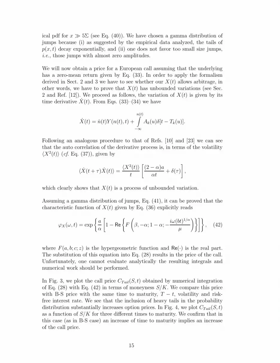
ical pdf for x ≫ 5Σ (see Eq. (40)). We have chosen a gamma distribution ofjumps because (i) as suggested by the empirical data analyzed, the tails ofp(x, t) decay exponentially, and (ii) one does not favor too small size jumps,i.e., those jumps with almost zero amplitudes.

We will now obtain a price for a European call assuming that the underlyinghas a zero-mean return given by Eq. (33). In order to apply the formalismderived in Sect. 2 and 3 we have to see whether our X(t) allows arbitrage, inother words, we have to prove that X(t) has unbounded variations (see Sec.2 and Ref. [12]). We proceed as follows, the variation of X(t) is given by itstime derivative X(t). From Eqs. (33)–(34) we have

X(t) = n(t)Y (n(t), t) +

n(t)∫

−∞

Ak(u)δ[t− Tk(u)].

Following an analogous procedure to that of Refs. [10] and [23] we can seethat the auto correlation of the derivative process is, in terms of the volatility〈X2(t)〉 (cf. Eq. (37)), given by

〈X(t+ τ)X(t)〉 =〈X2(t)〉

t

[

(2 − α)a

αt+ δ(τ)

]

,

which clearly shows that X(t) is a process of unbounded variation.

Assuming a gamma distribution of jumps, Eq. (41), it can be proved that thecharacteristic function of X(t) given by Eq. (36) explicitly reads

ϕX(ω, t) = exp

{

a

α

[

1 − Re

{

F

(

β,−α; 1 − α;−iω(bt)1/α

µ

)}]}

, (42)

where F (a, b; c; z) is the hypergeometric function and Re(·) is the real part.The substitution of this equation into Eq. (28) results in the price of the call.Unfortunately, one cannot evaluate analytically the resulting integrals andnumerical work should be performed.

In Fig. 3, we plot the call price CTail(S, t) obtained by numerical integrationof Eq. (28) with Eq. (42) in terms of moneyness S/K. We compare this pricewith B-S price with the same time to maturity, T − t, volatility and risk-free interest rate. We see that the inclusion of heavy tails in the probabilitydistribution substantially increases option prices. In Fig. 4, we plot CTail(S, t)as a function of S/K for three different times to maturity. We confirm that inthis case (as in B-S case) an increase of time to maturity implies an increaseof the call price.

15

0

0.01

0.02

0.03

0.04

0.05

0.06

0.07

0.94 0.96 0.98 1 1.02 1.04

C/K

moneyness

Black-Scholes call -maturity 30 d.heavy tail call -maturity 30 d.

deterministic call -maturity 30 d.

Fig. 3. The heavy tail and B-S call prices in terms of the moneyness when maturityis in 30 days. For this graph, we take r = 5% year−1 and the parameters estimatedfor the S&P-500 from January 1988 to December 1996 (σ = 3.54 × 10−3days−1/2).

0

0.02

0.04

0.06

0.08

0.1

0.12

0.14

0.96 0.98 1 1.02 1.04 1.06 1.08 1.1

C/K

moneyness

heavy tail call -maturity 15 d.-heavy tail call -maturity 30 d.-heavy tail call -maturity 60 d.-

Fig. 4. The heavy tail call price in terms of the moneyness. For this graph, we taker = 5% year−1 and the parameters estimated for the S&P-500.

16

0

0.1

0.2

0.3

0.4

0.5

0.6

0.7

0.8

0.9

1

0.96 0.98 1 1.02 1.04 1.06 1.08

call

pric

e di

ffere

nce

moneyness

heavy tail price difference -maturity 15 d.-heavy tail price difference -maturity 30 d.-heavy tail price difference -maturity 60 d.-

Fig. 5. The relative differences, ∆ = (CTail−CBS)/CTail, in terms of the moneynessS/K (r = 5% year−1, σ = 3.54 × 10−3days−1/2).

Finally in Fig. 5 we plot the relative difference

∆ = (CTail − CBS)/CTail

as a function of moneyness. We observe that for OTM, ATM, and some ITMoptions ∆ increases as T − t increases, while for options well in the money ∆becomes smaller with T−t. There is thus a “crossover” which, in our example,is located around S/K = 1.03. We also note that ∆ → 0 as S/K → ∞ veryslowly which implies the great persistence of the heavy-tail effect in the priceof the option.

5 Option pricing on correlated stocks

As we have mentioned in Section 1, the classical option formula of Black, Sc-holes and Merton is based on the “efficient market hypothesis” which meansthat the market incorporates instantaneously any information concerning fu-ture market evolution [8]. However, as empirical evidence shows, real marketsare not efficient, at least at short times [26]. Indeed, market efficiency is closelyrelated to the assumption of totally uncorrelated price variations (white noise).But white noise is only an idealization since, in practice, no actual randomprocess is completely white. For this reason, white processes are convenientmathematical objects valid only when the observation time is much larger than

17

the auto correlation time of the process. And, analogously, the efficient mar-ket hypothesis is again a convenient assumption when the observation time ismuch larger than time spans in which “inefficiencies” (i.e., correlations, delays,etc.) occur.

Note that auto correlation in the underlying driving noise is closely related tothe predictability of asset returns, of which there seems to be ample evidence[28,29]. Indeed, if for some particular stock the price variations are correlatedduring some time τ , then the price at time t2 will be related to the price at aprevious time t1 as long as the time span t2 − t1 is not too long compared tothe correlation time τ . Hence correlation implies partial predictability.

In Ref. [27], we have derived a nontrivial option price by relaxing the effi-cient market hypothesis and allowing for a finite, non-zero, correlation timeof the underlying noise process. As a model for the evolution of the marketwe chose the Ornstein-Uhlenbeck (O-U) process for essentially two: (a) O-Unoise is still a Gaussian random process with an arbitrary correlation timeτ and it has the property that when τ = 0 the process becomes Gaussianwhite noise, as in the original Black-Scholes option case. (b) The O-U processis, by virtue of Doob’s theorem, the only Gaussian random process which issimultaneously Markovian and stationary. In this sense the O-U process is thesimplest generalization of Gaussian white noise.

We thus assume that the underlying asset price is not driven by Gaussianwhite noise ξ(t) but by O-U noise V (t). In other words, instead of Eq. (2), wenow have the following singular two-dimensional diffusion process:

R(t) = µ+ V (t), (43)

V (t) =1

τ[−V (t) + σξ(t)] , (44)

where τ ≥ 0 is the correlation time. More precisely, V (t) is O-U noise inthe stationary regime, which is a Gaussian colored noise with zero mean andcorrelation function:

〈V (t1)V (t2)〉 =σ2

2τe−|t1−t2|/τ . (45)

Note that, when τ = 0, this correlation goes to σ2δ(t1−t2) and we thus recoverthe one-dimensional diffusion discussed above. Therefore, the case of positiveτ is a measure of the inefficiencies of the market. The combination of Eqs. (43)and (44) leads to a second-order stochastic differential equation for R(t)

τR(t) + R(t) = µ+ σξ(t). (46)

18

From this equation, we clearly see that when τ = 0 we recover the one-dimensional diffusion case (2). In the opposite case when τ = ∞, Eq. (44)shows that V (t) = 0. Thus, V (t) is constant which we may equal it to zero.Hence, R(t) = µt and the underlying price, S(t) = S0e

µt, evolves as a risklesssecurity. We also observe that the O-U process V (t) is the random part of thereturn velocity, and sometimes we refer to V (t) as the “velocity” of the returnprocess R(t).

One may argue that the O-U process (43)–(44) is an inadequate asset modelsince the return R(t) given by Eq. (43) is a continuous random process withbounded variations. As we have explained in Section 2, continuous processeswith bounded variations allow arbitrage opportunities and this is an undesir-able feature for obtaining a fair price. Thus, for instance, in this present casearbitrage would be possible within a portfolio containing bonds and stockwhose strategy at time t is buying (or selling) stock shares when µ + V (t) isgreater (or lower) than the risk-free bond rate [12]. However, the problem isthat in the practice the return velocity V (t) is non tradable and its evolutionis ignored. In other words, in real markets the observed asset dynamics doesnot show any trace of the velocity variable. Indeed, knowing V (t) would implyknowing the value of the return R(t) at two different times, since

V (t) = limǫ→0+

R(t) − R(t− ǫ)

ǫ− µ.

Obviously, this operation is not performed by traders who only manage port-folios at time t based on prices at t and not at any earlier time. This featureallows us to perform a projection of the two-dimensional diffusion process[R(t), V (t)] onto a one-dimensional equivalent process R(t) independent ofthe velocity V (t). We have shown elsewhere [27] the projected process R(t) isequal to the actual return R(t) in mean square sense, 〈[R(t)− R(t)]2〉 = 0 forany time t, and it obeys the following one-dimensional SDE 3

R(t) = µ+√

κ(T − t)ξ(t), (47)

where

κ(t) = σ2(

1 − e−t/τ)

. (48)

In this way, we have projected the two-dimensional O-U process (S, V ) ontoa one-dimensional price process which is a Wiener process with time varyingvolatility. Therefore, the return given by Eq. (47) is driven by a noise of un-bounded variation, the Wiener process, and the O-U projected process is still

3 Since R(t) and R(t) are equal in mean square sense we will drop the bar on R aslong as there is no confusion. Thus, we will use R for the projected process as well.

19

a suitable starting point for option pricing since it does not permit arbitrage.We also note that we need to specify the final condition of the process becausethe volatility

√κ is a function of the time to maturity T − t, and this implies

that the projected asset model depends on each particular contract.

The zero-mean return (7) associated with the projected process (47) followsthe SDE

X(t) =√

κ(T − t)ξ(t),

and its density, pX(x, T |t), satisfies the backward equation

∂pX

∂t= −1

2κ(T − t)

∂2pX

∂x2,

with final condition pX(x, T |T ) = δ(x). The solution to this problem reads

pX(x, T |t) =1

√

2πκ(T − t)exp

[

− x2

2κ(T − t)

]

, (49)

where (cf. Eq. (48))

κ(t) = σ2[

t− τ(

1 − et/τ)]

. (50)

The corresponding characteristic function reads

ϕX(ω, T |t) = exp[−κ(T − t)ω2/2],

and from Eq. (16) we get

m∗(T − t) = r(T − t) − κ(T − t)/2. (51)

In this case the price of the European option is obtained substituting Eqs.(49) and (51) into Eq. (20). We have

COU(S, t) = S N(dOU1 ) −Ke−r(T−t) N(dOU

2 ), (52)

where N(z) is the probability integral, and

dOU1 =

ln(S/K) + r(T − t) + κ(T − t)/2√

κ(T − t), (53)

dOU2 = dOU

1 −√

κ(T − t), (54)

with κ(t) given by Eq. (50).

20

0

0.005

0.01

0.015

0.02

0.025

0.97 0.98 0.99 1 1.01 1.02

C/K

moneyness

deterministic price -maturity 15 d.-correlated call -maturity 15 d.-

Black-Scholes call -maturity 15 d.-

Fig. 6. The correlated and B-S call prices in terms of the moneyness when maturityis in 15 days and correlation time is 2 days. For this graph, we take r = 5% year−1

and the parameters estimated for the S&P-500 (σ = 3.54 × 10−3days−1/2).

When τ = 0, the variance becomes κ(t) = σ2t and the price in Eq. (52) reducesto the Black-Scholes price given by Eq. (29). We observe that the O-U pricein Eq. (52) has the same functional form as B-S price in Eq. (29) when σ2t isreplaced by κ(t).

In the opposite case, τ = ∞, where there is no random noise but a determin-istic and constant driving force (in our case it is zero), Eq. (52) reduces to thedeterministic price (cf. Eqs. (4) and (10))

Cd(S, t) = max[S −Ke−r(T−t), 0]. (55)

We have proved elsewhere [27] that the O-U price is an intermediate pricebetween B-S price and the deterministic price (see Fig. 6)

Cd(S, t) ≤ COU(S, t) ≤ CBS(S, t), (56)

for all S and 0 ≤ t ≤ T .

In Fig. 7, we plot COU in terms of S/K for three different values of the time tomaturity. We see in the figure that, analogously to B-S and heavy tail cases,the O-U price increases with maturity. In any case, the assumption of uncor-related underlying assets (B-S case) overprices any call option. This confirms

21

0

0.02

0.04

0.06

0.08

0.1

0.12

0.96 0.98 1 1.02 1.04 1.06 1.08

C/K

moneyness

correlated call -maturity 15 d.-correlated call -maturity 30 d.-correlated call -maturity 60 d.-

Fig. 7. The correlated call prices in terms of the moneyness with correlation timeof 2 days. For this graph, we take r = 5% year−1 and the parameters estimated forthe S&P-500 (σ = 3.54 × 10−3days−1/2).

0

0.1

0.2

0.3

0.4

0.5

0.6

0.7

0.8

0.9

1

0.88 0.9 0.92 0.94 0.96 0.98 1 1.02

pric

e di

ffere

nce

moneyness

correlated price difference -maturity 15 d.correlated price difference -maturity 30d.correlated price difference -maturity 60d.

Fig. 8. Relative differences, D = (CBS − COU )/CBS , in terms of moneyness (τ = 2days, r = 5% year−1, and σ = 3.54 × 10−3days−1/2).

22

the intuition understanding that correlation implies more predictability andtherefore less risk and, finally, a lower price for the option.

In fact, one can quantify this overprice by evaluating the relative difference

D = (CBS − COU)/CBS.

Figure 8 shows the ratio D(S, t), for a fixed time to expiration, plotted as afunction of the moneyness, S/K. Note that the relative difference D increasesas T−t decreases. Moreover, contrary to the fat tail case, D quickly fades awaywith moneyness and it is negligible for ITM options showing no crossover.

6 Conclusions

We have performed an analytical study of option pricing on a more realisticsetting than that of Black and Scholes theory. Our starting point has beenthe martingale option price conveniently modified to become more practical toimplement by means of Fourier analysis. We have applied these analytical toolsto study the effect on option price of long tails in the underlying probabilitydistribution. For this, we have used a market model we recently developed[10] which combines fat tails, finite moments and self-similarity. The secondproblem we wanted to address is the effect of colored noise on option pricing,since there seems to be empirical evidence of mild auto correlation in stocks[7]. We have thus rederived, using the methods herein presented, our previousresult on option pricing on stocks driven by O-U noise.

One overall conclusion is that, taking the Black-Scholes price as a benchmark,heavy tails overprice by far options, while colored driving noise underprices it.The scheme is

S ≥ CTail ≥ CBS ≥ COU ≥ Cd,

where S is the underlying price when the option is bought and Cd is thedeterministic price given by Eq. (55). Moreover, the relative difference withB-S price is in both cases more important for OTM and ATM options thanfor ITM options. In any case, there is a great persistence of fat-tail effects onthe price of the options.

There are some open questions, one of which being the extension of the aboveformalism to other option classes (American, Asian, etc.). Another point is toinvestigate whether fat tails and correlations produce the “smile effect” in theimplied volatility. We believe that this is more likely to happen in the case ofheavy-tails. This point is under present investigation.

23

Acknowledgements

The authors acknowledge helpful discussions with Miquel Montero on the re-sults herein derived for the market model showing fat tails. This work hasbeen supported in part by Direccion General de Investigacion under contractNo. BFM2000-0795, by Generalitat de Catalunya under contract No. 2000SGR-00023 and by Societat Catalana de Fısica (Institut d’Estudis Catalans).

A Derivation of Eq. (24)

Let us derive Eq. (24). We start from Eq. (23)

I =K

2π

∞∫

−∞

ϕ∗(ω, T |t)eiωRKdω

∞∫

0

eiωz(

e−z − 1)

dz,

but∞∫

0

eiωz(

e−z − 1)

dz =1

1 − iω−

∞∫

0

eiωzdz,

and∞∫

0

eiωzdz = limε→0+

∞∫

0

e−(ε−iω)zdz = limε→0+

i

ω + iε=

i

ω + i0,

where this result has to be understood in the sense of generalized functions as[16]

1

ω ± i0= ∓iπδ(ω) + P

[

1

ω

]

,

where δ(ω) is the Dirac delta function, and P [1/ω] is the Cauchy principalvalue, i.e.,

P [1/ω] = 1/ω for ω 6= 0

and

P

∞∫

−∞

φ(ω)

ωdω

= limε→0+

−ε∫

−∞

φ(ω)

ωdω +

∞∫

ε

φ(ω)

ωdω

,

where φ(ω) is any regular function fast decaying at infinity. Therefore,

∞∫

0

eiωzdR = πδ(ω) + iP[

1

ω

]

.

Hence

I = −K2

+K

2π

∞∫

−∞

ϕ∗(ω, T |t)eiωRKdω

1 − iω− iP

∞∫

−∞

eiωRKϕ∗(ω, T |t)

ωdω

,

24

and using the following alternative expression for the Cauchy principal value[16]

P

∞∫

−∞

φ(ω)

ωdω

=

∞∫

−∞

φ(ω) − φ(0)

ωdω,

we obtain Eq. (24):

I = −K2

+K

2π

∞∫

−∞

ϕ∗(ω, T |t)eiωRKdω

1 − iω− i

∞∫

−∞

[

eiωRKϕ∗(ω, T |t) − 1]dω

ω.

References

[1] The Random Character of Stock Market Prices, P. H. Cootner ed. (MIT Press,Cambridge MA, 1964).

[2] F. Black, M. Scholes, J. Pol. Econ. 81 (1973) 637-659.

[3] R. C. Merton, Bell J. Econ. and Management Sci. 4 (1973) 141-183.

[4] J. Perello, J. M. Porra, M. Montero, and J. Masoliver, Physica A 278, 260-274(2000).

[5] R. N. Mantegna, and E.H. Stanley, Nature 376, 46-49 (1995).

[6] J.-P. Bouchaud, A. Matacz, and M. Potters, Phys. Rev. Lett. (to appear, 2002).

[7] A. W. Lo, and J. Wang, J. Finance 50, 87-129 (1995).

[8] E. F. Fama, J. Finance 25, 383-417 (1970).

[9] J. M. Harrison, and D. Kreps, J. Economics Theory 20, 381-408 (1979); J. M.Harrison, and S. Pliska, Stochastic Process. Appl. 11, 215-260 (1981).

[10] J. Masoliver, M. Montero, and J. M. Porra, Physica A 283, 559-567 (2000).

[11] M. Baxter and A. Rennie, Financial Calculus (Cambridge University Press,Cambridge, 1998).

[12] J. M. Harrison, R. Pitbladdo, and S. M. Schaefer, J. Business 57, 353-365(1984).

[13] R. Schobel and J. Zhu, European Finance Rev. 3, 23-46 (1999).

[14] J. Masoliver, and J. Perello, submitted for publication.

[15] L. O. Scott, Mathematical Finance 7, 413-424 (1997).

[16] V. S. Vladimirov, Equations of Mathematical Physics (Mir, Moscow, 1984).

[17] E. Lukacs, Characteristic Functions (Griffin, London 1970).

25

[18] B. Mandelbrot, J. Business 35, 394-419 (1963).

[19] E. Fama, J. Business 35, 420-429 (1963).

[20] E. Scalas, Physica A 253, 394-402 (1998).

[21] S. Gashghaie, W. Breymann, J. Peinke, P. Talkner, and Y. Dodge, Nature381, 767-770 (1996).

[22] S. Gallucio, G. Caldarelli, M. Marsili, and Y.-C. Zhang, Physica A 245, 423-436 (1997).

[23] J. Masoliver, M. Montero, and A. McKane, Phys. Rev. E 64, 011110 (2001).

[24] A. Matacz, Int. J. Theor. Appl. Finance 3, 143-160 (2000).

[25] R. N. Mantegna, and H. E. Stanley, Nature 383, 587-588 (1995).

[26] E. F. Fama, J. Finance 46, 1575-1617 (1991).

[27] J. Masoliver and J. Perello, submitted for publication.

[28] W. Breen, and R. Jagannathan, J. Political Economy 44, 1177-1189 (1989).

[29] J. Campbell, and Y. Hamao, J. Finance 47, 43-70 (1992).

26