The Performance of VIX Option Pricing Models - Dean Street

1

The Performance of VIX Option Pricing Models:

Empirical Evidence Beyond Simulation

Zhiguang Wang

Ph.D. Candidate

Florida International University

Robert T. Daigler

Knight Ridder Research Professor of Finance

Florida International University

JEL category: G13 Contingent Pricing

Keywords: VIX options, volatility options

Zhiguang Wang is a Ph.D. Candidate, Florida International University, Department of Economics DM 308A, Miami, FL 33199. Email: [email protected] Robert Daigler is Knight Ridder Research Professor of Finance, Florida International University, Department of Finance RB 206, College of Business, Miami FL 33199. Email: [email protected]. Phone: 305-348-3325 (or home 954-434-2412). An earlier version of this paper was presented at the 2008 Financial Management Meetings in Dallas. We wish to thank the referee for comments that helped clarify the presentation of this paper.

This version: April 30, 2009

2

The Performance of VIX Option Pricing Models:

Empirical Evidence Beyond Simulation

Abstract

We examine the pricing performance of VIX option models. Such models possess a wide-range of underlying characteristics regarding the behavior of both the S&P500 index and the underlying VIX. Our contention that “simpler is better” is supported by the empirical evidence using actual VIX option market data. Our tests employ three representative models for VIX options: Whaley (1993), Grunbichler and Longstaff (1996), and Carr and Lee (2007). We also compare our results to Lin and Chang (2009), who test four stochastic volatility models, as well as to previous simulation results of VIX option models. We find that no model has small pricing errors over the entire range of strike prices and times to expiration. In particular, out-of-the-money VIX options are difficult to price, with Grunbichler and Longstaff’s mean-reverting model producing the smallest dollar errors in this category. In general, Whaley’s Black-like option model produces the best overall results, supporting the “simpler is better” contention. However, the Whaley modeldoes under/overprice out-of-the-money call/put VIX options, which is opposite the behavior of stock index option pricing models.

1. Introduction

In February, 2006 the CBOE introduced a new instrument for speculating and hedging

volatility risk on the S&P 500 index, i.e. options on the VIX. The cash VIX measures the one

month forward implied volatility inherent in the S&P 500 index by using S&P500 option

premiums. The issue with employing option pricing models originally developed for stocks and

stock indexes without making any adjustments is that the underlying VIX characteristics differ

from stocks and stock indexes characteristics. These characteristics include mean-reversion of

the VIX, jumps in the VIX, stochastic volatility of the VIX, a lack of a cost of carry position, the

effect of net demand, and an unusual settlement procedure. Consequently, a variety of option

pricing models have emerged in the literature, prompting two relevant questions concerning VIX

option models are: how closely do model-based VIX option prices match market prices? Are

simple or complex option pricing models best for VIX options?

VIX options are third generation volatility products. Stock and stock index options are first

3

generation products. VIX futures (futures based on the behavior of the S&P500 index options)

are second generation products. VIX options (based on the VIX and VIX futures) are third

generation volatility products. Current models for VIX options differ primarily in how they treat

the behavior of changes in volatility. Three considerations concerning modeling volatility

options are: (1) the stochastic volatility process for the S&P500 index returns, including the

mean-reversion characteristic of volatility over longer time intervals; (2) the stochastic volatility

process for the VIX/VIX futures (the stochastic volatility of volatility); (3) jumps in the S&P500

index and the VIX/VIX futures. The distinction between (1) and (2) is critical. To date, VIX

option models have concentrated on the mean-reversion characteristic of the S&P500 volatility,

including jumps. No models include the stochastic volatility of VIX/VIX futures.

We categorize VIX option models into model-dependent and model-free approaches. The

model-dependent approach is adopted by Whaley (1993), Grunbichler and Longstaff (1996),

Detemple and Osakwe (2000) and Lin and Chang (2009). This type of model employs an

estimation procedure for some aspect of the underlying stochastic process. Whaley is based on

an estimated but constant volatility for the underlying VIX/VIX futures. Grunbichler and

Longstaff (1996) and Detemple and Osakwe (2000) model the mean-reversion process for the

VIX, with their mean-reverting processes assuming a constant volatility of volatility, as in

Heston (1993). Lin and Chang (2009) differ from the first three models by following the Eraker

et al. (2003,2004) approach by (1) modeling a jump-diffusion process for the S&P500 index; (2)

modeling the volatility of the S&P500 index by a correlated mean-reversion jump-diffusion

process. No model actually considers the stochastic volatility of the VIX (or volatility of

volatility). These model-dependent approaches must estimate the model parameters by

employing historical data (or by providing accurate forecasts of the inputs). The alternative

model-free approach is pioneered by Carr and Lee (2007). The Carr and Lee model does not

4

necessitate any estimation procedure, rather it employs inputs that are directly observable or

computable from current market data.

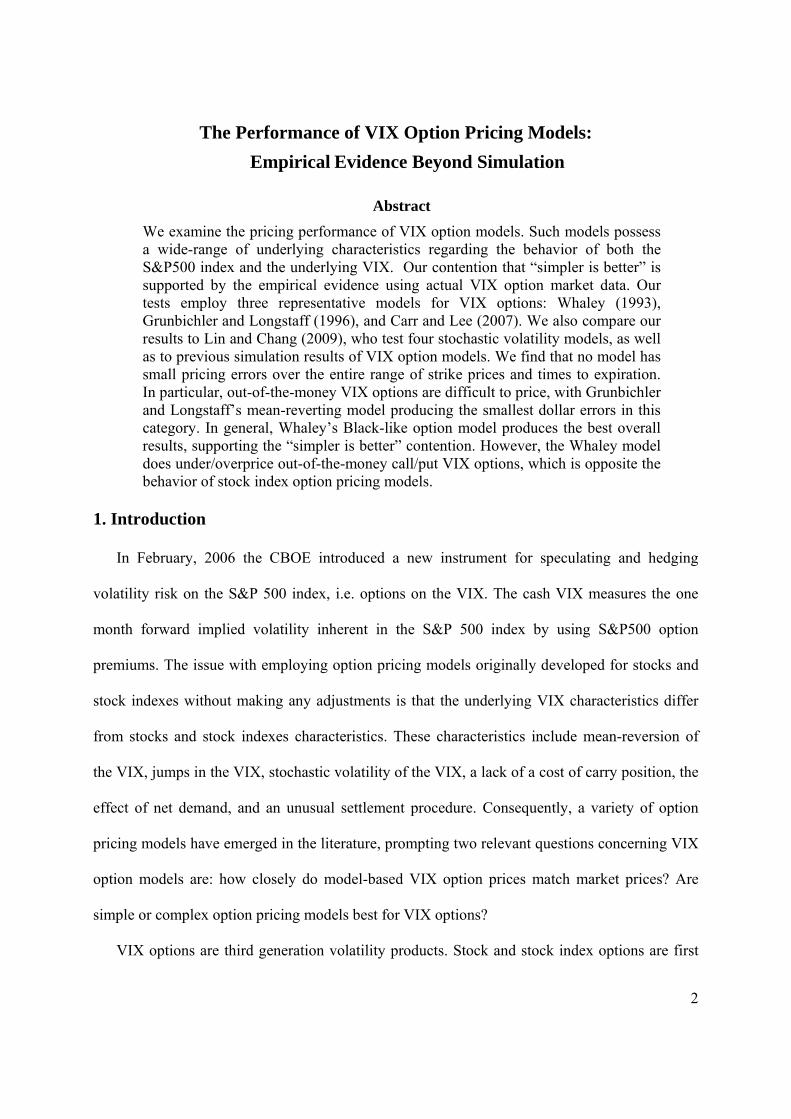
Our paper overcomes the paucity of empirical testing of the model-dependent and model-free

approaches to VIX option pricing by employing daily market VIX option prices. Previous

attempts to examine such models are limited to Monte Carlo-based simulations, except for Lin

and Chang (2009). In particular, Psychoyios and Skiadopoulos (2006) apply simulation to

examine possible pricing patterns and related hedging performance of the three model-dependent

approaches listed above. However, their simulations assume that the value of the VIX is

generated by an assumed mean-reverting square root process with arbitrarily predetermined

parameters. We also compare our results to the only other empirical results using actual market

data, namely Lin and Chang (2009); this comparison is useful since Lin and Chang examine

more complex models to price VIX options.

Our results for the market-based pricing errors reveal that the basic Whaley (1993) model

prices deep-in-the-money options well and in-the-money options comparatively well, both in

terms of percentage and dollar errors. However, out-of-the-money VIX options have large

percentage errors with this model, which contrasts with the simulation-based findings by

Psychoyios and Skiadopoulos (2006). Grunbichler and Longstaff’s (1996) mean-reverting model

provides less variable results across the sample and across option strikes, as well as having the

advantage of pricing out-of-the-money options with the smallest dollar errors relative to the other

models, which is also contrary to the simulation results. However, the Grunbichler and Longstaff

results create large absolute dollar error values as well as large percentage errors for near-the-

money and all in-the-money options for all times to option expiration categories. Carr and Lee’s

(2007) results resemble those from Whaley’s model in terms of their patterns of errors, although

the Carr and Lee results are inferior across almost all moneyness and time to expiration

5

categories in terms of both percentage and dollar errors. Comparison of our results of these three

models to the Lin and Chang (2009) results show that the models tested here clearly possess

smaller errors than the Lin and Chang models.

Overall, whereas none of these models price out-of-the-money options well based on

absolute percentage errors, Whaley (1993) (the simplest model) achieves the best overall

performance among the models. An interesting characteristic of the Whaley results is that it

underprices (overprices) out-of-the-money call (put) VIX options, which provides evidence for

an implied volatility skew of the volatility index that is opposite the skew for index options, i.e.

the VIX skew emphasizes the call option skew over the put option skew. Of course, all of the

model mispricings examined here can be caused either by imperfect models or by inefficient

market prices.

The organization of this paper is as follows. Section 2 describes the three models to be tested.

Section 3 details the data source, examines the validity of the data through the put-call parity

equation, and describes the estimation method and our criteria to compare the results. Section 4

discusses the empirical results and compares them to the simulation-based results by Psychoyios

and Skiadopoulos (2006) and the empirical results by Lin and Chang (2009). Section 5

concludes.

2. The Models

A number of factors reasonably affect the pricing of VIX options. Since no current model

includes all of these factors, we contend that the question of which VIX option model is best

remains an empirical question. The factors affecting VIX option pricing are as follows: mean-

reversion of volatility, jumps in the S&P500 index and in its volatility, stochastic volatility of the

VIX and potentially of the S&P500 index, the lack of a cost of carry formulation, the effect of

net demand, and an unusual settlement procedure. Let us briefly examine each of these factors.

6

The first factor is mean-reversion, which is a well known characteristic of volatility and is

more pronounced the longer the time to option expiration. The interest in the importance of

jumps has increased in recent years, as seen in Duffie, Pan and Singleton (2000), Pan (2002),

Eraker, Johannes and Polson (2003), and Eraker (2004). However, whether one should include

jumps in volatility as well as jumps in the underlying S&P500 index (and the form of a jump

parameter) is an unsettled question.1 More importantly, no paper has yet considered the

stochastic volatility of the VIX to price VIX options; alternatively models assume that the

volatility of volatility parameter in the mean-reversion process is constant. Unlike stock options,

VIX options do not have a tradable underlying asset, therefore the typical stock option cost of

carry Black-Scholes hedge formulation is not relevant for VIX options; a Black options on

futures approach is more appropriate. Bollen and Whaley (2004) show that net demand is a

factor affecting option prices; however, including net demand as an option parameter has not yet

been implemented in option modeling.2 Finally, VIX options settle to a value based on the

opening price of the underlying S&P500 options when there are 30 days left to the S&P500

option expirations (see Pavlova and Daigler (2008)). This settlement procedure is affected by the

supply and demand of the S&P500 options based on the closing positions of VIX option dealers

and arbitrageurs. No VIX option model considers the settlement procedure. As can be seen, a

number of complicated interrelated factors affect VIX option prices. Which model best

incorporates the relevant factors in relation to empirical VIX option market prices is the focus of

the rest of this paper.

Here we discuss the existing option models to price VIX options: Whaley (1993),

Grunbichler and Longstaff (1996), Carr and Lee (2007), and Lin and Chang (2009). These

1 As noted in the introduction, Lin and Chang (2009) follow Eraker’s approach by employing a jump-diffusion process to model the S&P500 index and by modeling the volatility of the S&P500 index by a correlated mean-reverting jump-diffusion process. 2 Net demand especially affects out-of-the-money put stock index options due to the demand for downside price protection. For VIX options out-of-the-money call options provide similar protection.

7

models represent three important and different approaches for VIX option pricing. The Whaley

model assumes that the underlying instrument follows the Geometric Brownian Motion given in

Black (1976), where the underlying instrument can be either the cash VIX index or the VIX

futures contract.3 Therefore, we call the Whaley model “the standard Black approach.”

Grunbichler and Longstaff model the underlying cash VIX by a mean-reverting square root

process and consequently is called the “mean reversion” approach, and follows the approach

proposed for stock index options by Heston (1993). Both the “standard Black” and “mean

reversion” approaches are model-dependent. Carr and Lee (2007) follow a model-free approach

that does not require estimation of the parameters to the underlying process; rather they compute

the inputs to their pricing formula directly from concurrent market information. We show and

discuss the general formulas for these three models of VIX call option prices in the following

sub-sections.4 Lin and Chang (2009) model the S&P500 index and the S&P500 volatility

simultaneously with correlated jump-diffusion processes. Therefore, their approach is also

model-dependent.

The implementation of the Whaley (1993) model includes two approaches to calculate VIX

option prices: the first uses historical volatility as a proxy for the current implied volatility,

whereas the second employs the previous day’s implied volatility to estimate today’s implied

volatility. The second approach is employed by Bakshi, Cao and Chen (1997), among others. For

the Grunbichler and Longstaff (1996) model we calibrate the parameters to the current market

price of all the VIX options from the previous day and then calculate the out-of-sample pricing

3 Whaley (1993) assumes that the cost of carrying the volatility index is zero. Therefore, there is no clear distinction between the cash VIX and the VIX futures in his model. 4 We do not include the Detemple and Osakwe (2000) model for two reasons: (1) their mean-reverting logarithm model is very similar to Grunbichler and Longstaff’s (1996) mean-reverting square root model; and (2) Psychoyios and Skiadopoulos (2006) document the inferior pricing and hedging performance of Detemple and Osakwe relative to Whaley’s (1993) model. Specifically, Psychoyious and Skiadopoulous show that the pricing errors from the Detemple and Osakwe model are often 15 to 40 times the size of Whaley’s (1993) errors across all strikes and times to expiration.

8

errors for the current day, i.e. the parameters for the model are determined based on the previous

price information and then the model is tested using the current day’s prices. Finally, for the Carr

and Lee (2007) model we directly calculate the VIX option prices using the derived variance and

volatility swap rates in order to determine the relevant model inputs. For each of the model-

implied results we compute percentage and dollar errors for various levels of moneyness and

times to expiration.

2.1 The Standard Black Approach: Whaley (1993)

Assuming that the underlying VIX follows a Geometric Brownian Motion, Whaley (1993)

utilizes the theoretic development of Black (1976) for options on futures. Given the underlying

VIX, the price of a VIX call option can be expressed as follows:

1 2

21

2 1

( , , ) ( ( ) ( ))

ln( / ) / 2

rTt t

t

C F K T e F N d KN d

d F K T

d d T

(1)

where , , ,tF K T N , and σ represents the current price for the VIX futures, the strike price, the

time to expiration, the cumulative normal probability, and the volatility of the cash VIX or VIX

futures, respectively.

2.2 Mean Reversion Approach: Grunbichler and Longstaff (1996)

Using the work by Cox, Ingersoll and Ross (1985) and Heston (1993) as a foundation,

Grunbichler and Longstaff (1996) derive a formula for volatility options by assuming that the

volatility index follows a mean-reverting square root process using risk neutrality. Solving a

partial differential equation, as in Cox, Ingersoll and Ross (1985), leads to the following pricing

formula:

2

2

2

( , , ) ( ( ; 4, ))

(1 ) ( ; 2, )

( ; , )

rT Tt t

T

C V K T e e V K

m e K

K K

(2)

9

where the associated risk-neutral process of the underlying VIX is defined by

( )t t t tdV m V dt V dW (3)

with β, m, and σ representing the speed of mean-reversion, the long-run mean, and the volatility

of the VIX, respectively. 2 (.; , ) is a non-central chi-square distribution with degrees of

freedom and non-centrality λ. The parameters of the option pricing formula in Equation (2)

and the parameters of the volatility process in Equation (3) are connected via the following

relation:

2

2

4

(1 )

4 /

T

Tt

e

m

e V

(4)

2.3 Model-free Approach: Carr and Lee (2007)

Carr and Lee (2007), and equivalently Carr and Wu (2006), provide a closed-form equation

for the valuation of VIX options, which is an application of their more generalized pricing

formula for options on realized volatility. Unlike the two model-dependent VIX option models

presented in previous sections, Carr and Lee replicate variance and volatility swaps on the S&P

500 index, using the associated variance and volatility swap rates as the inputs to the pricing

model, with these rates based on the S&P 500 option prices. Without having to calibrate

parameters based on historical VIX options data, this approach makes real-time pricing and the

implementation of hedging strategies more readily applicable.5

The Carr and Lee formula for a VIX call option is:

5 The replication of variance and volatility swaps is studied by various researchers. For example, see Neuberger (1990), Dupire (1993), Carr and Madan (1998), and Derman, Demeterfi, and Zou (1999).

10

1 2

1

2

1 2

22 1

1

2 1

( , , ) ( ( ) ( ))

2 ln 0.5ln

ln 2 ln

( ln ) /

rTt t

t

rTt

t

t

t t t

t

C F K T e F N d KN d

F

A e

m

s

d m K s s

d d s

(5)

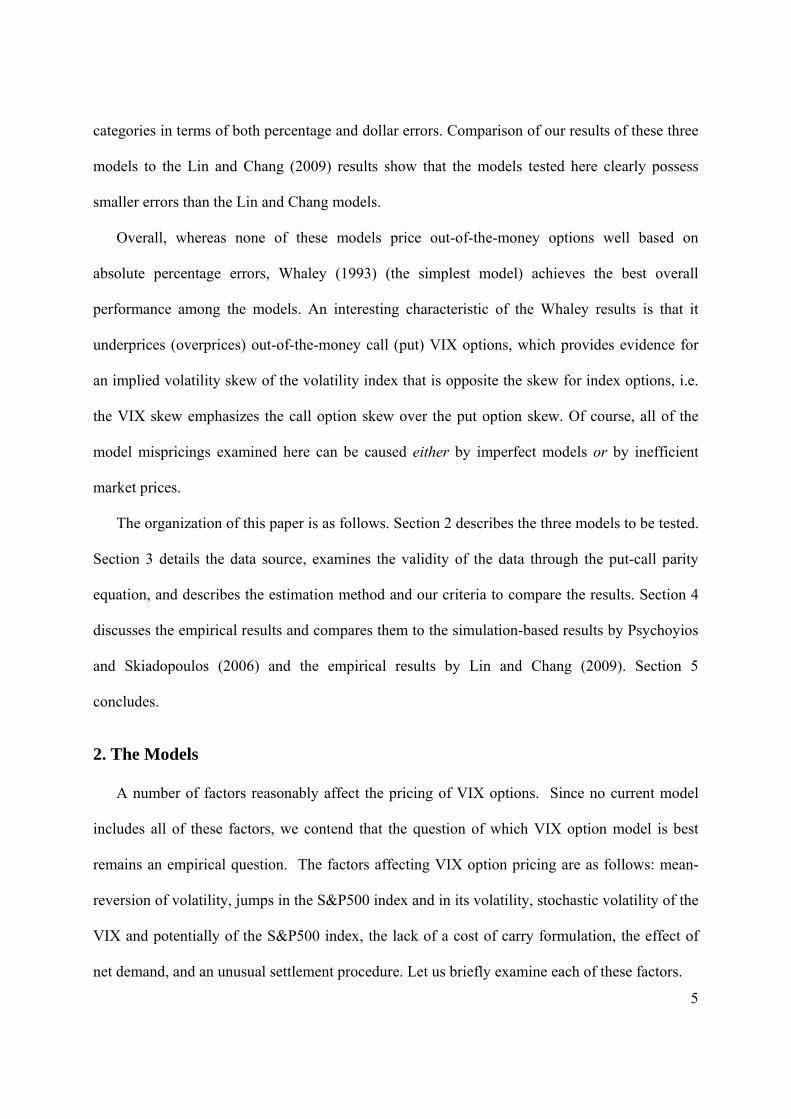
where , ,t t tA m s represent the variance swap rate, the time-t conditional mean, and the variance of

the log return of the VIX, respectively.

The difference between Equation (1) for Whaley (1993) and Equation (5) for Carr and Lee

(2007) lies in the inputs: the former uses a VIX cash or futures price and does not provide an

explicit way of calculating the constant volatility ( ), whereas Carr and Lee compute the

forward rate volatility ( ts ) of the underlying VIX. Based on the similarity of the two pricing

formulas, we can view both Whaley and Carr and Lee as “Black-type models.”

2.4 Lin and Chang (2009) Models

Lin and Chang derive a closed-form VIX option pricing model with jumps and with an

embedded stochastic volatility component for the S&P500 index which underlies the S&P500

options that make up the VIX. Lin and Chang employ four separate stochastic volatility

processes, although three of the processes are nested models of the main Eraker (2004) process.

The Eraker approach is unique in that it models jumps in both the S&P500 index and jumps in

the S&P500 stochastic volatility. The other three models in Lin and Chang assume different

characteristics of the S&P500 return process. Details of their VIX option model and stochastic

volatility processes used to test the pricing of the VIX options model can be found in Lin and

Chang (2009).

11

3. Data and Methodology

We employ daily VIX options data from DeltaNeutral for our analysis. The data set spans

January through September 2007, during which the monthly average VIX level covers a range of

11 to 25.1. The sample period reflects market environments for nonvolatile months (e.g.

January), intermediate volatility months (e.g. March), and relatively high volatile months (e.g.

August). The T-bill rate is used for the risk-free interest rate, and is obtained from the Federal

Reserve Bank of St. Louis. Daily spot and futures price data are obtained from Tradestation and

the CBOE, respectively. Due to the non-convergence of the VIX futures to the cash VIX, as

noted by Pavlova and Daigler (2008), we delete options within 6 days to expiration. There are a

total of 26,094 VIX option prices over the 184 days of the sample.

We compute pricing errors both in percentage and dollar terms in order to compare the

pricing performance of the three models. The percentage error is defined as the (theoretical

model price - market price)/market price, whereas the dollar error is the difference between the

theoretical price and the market price. We provide percentage and dollar errors for both the

unsigned and signed cases in order to determine both the absolute size and the distribution of

errors around the market price. The market price is determined as the average between the

closing bid and ask prices.

We implement two approaches for the Whaley model. The first approach computes the inputs

for the volatility variable by determining the 5-day Whaley(H5) and 30-day Whaley(H30)

historical volatilities using the daily average Garman and Klass’ (1980) volatility estimator, as

well as determining the future realized volatility for Whaley(FR) by calculating the daily

standard deviation during the remaining life of the option. The 5-day and 30-day volatilities are

employed as short and long measures of historical volatility. The future volatility uses the

volatility from the current trading day to the expiration day of the option, which is the

12

theoretically correct measure of volatility. This future volatility is computed to provide a

comparison to the historical volatilities, rather than for real-world pricing, since the future

volatility is not known at the time of pricing the options.

The second approach for the Whaley model calibrates the option prices for the entire range of

strikes for each day by determining the implied volatility from yesterday’s option prices to

employ as the volatility variable in today’s option prices; this approach is labeled Whaley(IV).

The implied volatility is estimated by minimizing the sum of the squared errors of the difference

between the market and derived model prices simultaneously for all of the option strikes for all

of the expiration months for each day, which follows the method in Bakshi, Cao and Chen

(1997).

For the Grunbichler and Longstaff model we calibrate the β, m, and σ parameters to the

market prices using the same method as employed for estimating the implied volatility for the

Whaley model. We then use these parameters to price the next day’s (out-of-sample) options

based on Equation (2). Finally, we implement the Carr and Lee (2007) model by computing the

volatility and variance swap rates from the S&P 500 option data together with the available VIX

futures data to price the VIX options based on Equation (5).

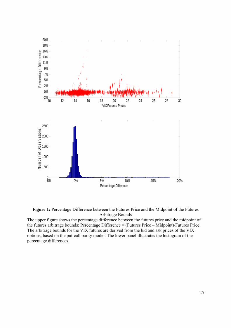
Since the end-of-day midpoint prices of the VIX options may not completely reflect the price

information from the end-of-day VIX futures prices (due to small size limit orders at away-from-

the-market prices and/or larger than normal bid-ask spreads for some VIX options), we examine

the validity of the VIX options dataset before evaluating the pricing performance of the three

VIX options models. In order to implement this evaluation we derive the arbitrage bounds for the

underlying VIX futures from the following put-call parity relation with the corresponding VIX

call and put option prices:

( ) ( )r T tt t tP C e F K (6)

13

The lower bound of the VIX futures price is formed from the bid price of the VIX call option and

the ask price from the VIX put option. The upper bound of the VIX futures price is obtained

from the ask price from the call and the bid price from the put. We find that 95.9% of the futures

prices fall within the arbitrage bound defined by the put-call parity relation. The mean, variance,

minimum, and maximum of the absolute difference between the futures prices and the mid-point

of the theoretical arbitrage bounds are 0.42%, 0.0052%, -3% and 16%, respectively. The

distribution of these differences is shown in Figure 1, which shows that these differences are

concentrated around zero, with only a few outliers > 2% from the midpoints of the arbitrage

bounds. These results provide confidence in the validity of the data and that the data corresponds

to expected basic financial economics pricing concepts.

4. Results and Discussion

Section 4.1 examines the pricing errors of the Whaley (1993), Grunbichler and Longstaff

(1996), and Carr and Lee (2007) models. Section 4.2 investigates the pricing errors across

models for both moneyness and time to expiration. Section 4.3 further examines the results for

the different measures of pricing errors, namely percentages vs. dollars and signed vs. unsigned

errors. Section 4.4 compares our results to the simulation results in Psychoyios and Skiadopoulos

(2006) and to the results from the Lin and Chang (2009) paper.

Moneyness is categorized in terms of the logarithm of the strike price divided by the current

cash (spot) VIX value. The categories are: deep-in-the-money (abbreviated DITM) call options

with moneyness smaller than -0.3; in-the-money (ITM) options with moneyness between -0.3

and -0.03; near-the-money (NTM) options with moneyness falling between -0.03 and 0.03; out-

of-the-money (OTM) options with a moneyness ranging from 0.03 to 0.3; and deep-out-of-the-

14

money (DOTM) options with moneyness larger than 0.3.6 Time to expiration is divided into

three groups: short (less than 30 days), intermediate (between 30 and 90 days) and long (over 90

days). We list the number of options for each combination of moneyness and time to expiration

in Table 1. The associated average pricing errors are computed for each combination.

4.1 Pricing Errors within Models

This section examines how a change in moneyness and time to expiration affects the pricing

errors of each model. Tables 1 and 2 report the mean pricing errors for five moneyness

categories and three time to expiration categories. Table 1 provides the absolute (unsigned)

magnitude of the pricing errors, whereas Table 2 examines the average (signed) size and

direction of the over/underpricing of the errors. Figures 2 to 5 show the related error distributions

across moneyness and Figures 6 to 9 show the error distributions across time to expiration.

(1) Errors across moneyness

The Whaley model: The first four panels of Tables 1 and 2 report the percentage and dollar

pricing errors for the Whaley model. Among the four versions of the Whaley model,

Whaley(H30) produces the smallest average errors for the short-term options across the

moneyness categories, whereas Whaley(IV) produces the smallest average errors for the longer-

term options. Going forward we concentrate on the Whaley(IV) results, and to a lesser extent the

Whaley(H30) results, as benchmarks for the Whaley model.

The first three columns of Table 1 show that the percentage errors increase as one goes down

the column from DITM to DOTM, whereas the last three columns show that the dollar errors

exhibit no systematic trend. Table 2 illustrates that the Whaley models typically underprice near-

term VIX options relative to market prices for all moneyness categories, and overprice far-term

6 We do not adopt the categorization used by Lin and Chang (2009), which follows the categories for stock index options by Bakshi, Cao and Chen (1997). On an average day (with 18 different strikes for VIX options) we have 3 (vs. 8), 5 (vs. 0), 1 (vs. 1), 5 (vs. 1), and 4 (vs. 8) VIX options falling in the DITM, ITM, NTM, OTM and DOTM categories based on our approach (vs. Lin and Chang’s (2009) approach). Thus, the strikes are more evenly allocated to the categories using our intervals.

15

options for all but the Whaley(FR) model.7 Across moneyness categories Whaley(IV) almost

exclusively underprices NTM and OTM call options, while ITM options have no particular

pattern. This pricing behavior resembles the findings in Rubinstein (1985) for 30 actively traded

short-maturity stock options, but contrasts with MacBeth and Merville’s (1980) findings

concerning stock options.8 More recently, Bakshi, Cao and Chen (1997) and Corrado and Su

(1998) examine the pricing behavior for stock index options, both concluding that the Black-

Scholes formula overprices (underprices) OTM (ITM) S&P 500 call options. Our results for VIX

options are opposite these studies for the Whaley(IV) and Whaley(FR) models with less than 90

days to expiration. This is consistent with our findings (not shown here) that the difference in the

sign of the pricing errors reveals that VIX options generate different implied volatility surfaces

from stock index options.

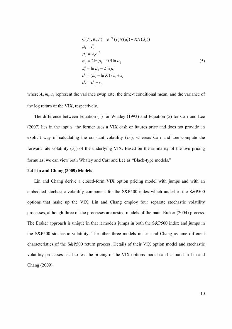
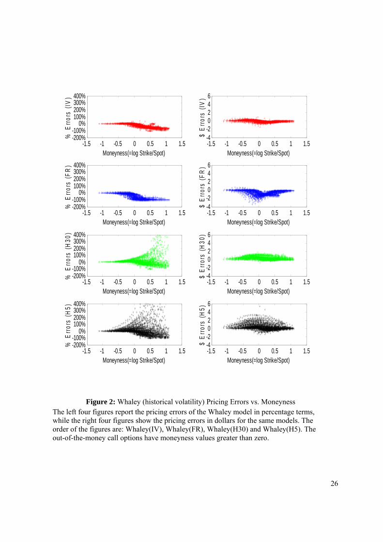
Figure 2 plots the pricing errors for each of the Whaley formulations against moneyness. The

IV and FR models represent forward-looking volatilities and exhibit similar shapes of pricing

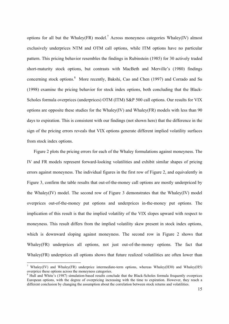
errors against moneyness. The individual figures in the first row of Figure 2, and equivalently in

Figure 3, confirm the table results that out-of-the-money call options are mostly underpriced by

the Whaley(IV) model. The second row of Figure 3 demonstrates that the Whaley(IV) model

overprices out-of-the-money put options and underprices in-the-money put options. The

implication of this result is that the implied volatility of the VIX slopes upward with respect to

moneyness. This result differs from the implied volatility skew present in stock index options,

which is downward sloping against moneyness. The second row in Figure 2 shows that

Whaley(FR) underprices all options, not just out-of-the-money options. The fact that

Whaley(FR) underprices all options shows that future realized volatilities are often lower than

7 Whaley(IV) and Whaley(FR) underprice intermediate-term options, whereas Whaley(H30) and Whaley(H5) overprice these options across the moneyness categories. 8 Hull and White’s (1987) simulation-based results conclude that the Black-Scholes formula frequently overprices European options, with the degree of overpricing increasing with the time to expiration. However, they reach a different conclusion by changing the assumption about the correlation between stock returns and volatilities.

16

option implied volatilities, which is recognized as a “negative variance risk premium” by Carr

and Wu (2008).9

The other two Whaley models, H(30) and H(5), represent backward-looking volatilities; they

show similar shapes of pricing errors to one another, but are opposite the IV and FR results in

that the model prices are typically larger than the market prices. Moreover, the percentage errors

produced by Whaley(H30) and Whaley(H5) are more dispersed for the out-of-the-money options

than those by the forward-looking models, with Whaley(H30) generating smaller and less

dispersed percentage and dollar errors than Whaley(H5) over the range of strike prices.

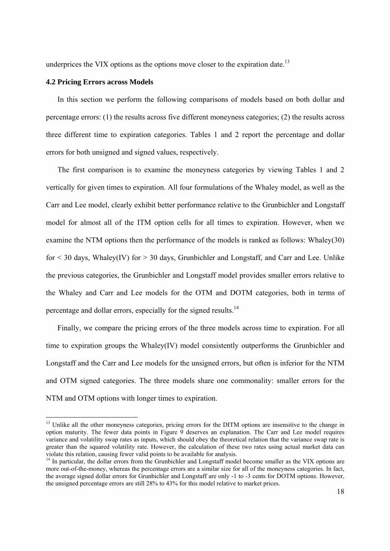
The Grunbichler and Longstaff model:10 Figure 4 (upper-right) shows that the dollar errors

for the call options are more dispersed for ITM options than for NTM or OTM options, with the

size of this dispersion (the instability of the pricing errors) occurring only for this model. The

dollar and percentage errors for the put options are equally distributed around zero across

moneyness, although this dispersion is substantial and greater than the dispersion of the call

option.11

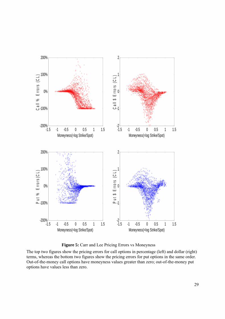
The Carr and Lee model: Figure 5 shows that the Carr and Lee model possesses increasing

percentage errors for deeper out-of-the-money options, as well as relatively larger dollar errors

for near-the-money options. The tables show that the average percentage pricing errors increase

substantially as the moneyness goes from DITM to DOTM. The figures clearly show that the

ITM call and put options are priced much better than the OTM and NTM options in percentage

9 The variance risk premium is defined as “realized variance – swap rate” by Carr and Wu. The swap rate is the risk-neutral expectation of future realized variance. Thus, the negative premium means that “From the perspective of a variance swap investment, the negative variance risk premium implies that investors are willing to pay a high premium, or endure an average loss, when they are long variance swaps in order to receive compensation when the realized variance is high.” Carr and Wu (2006). 10 By minimizing the mean-square error of the model prices relative to the market prices we calibrate the three parameters of the Grunbichler and Longstaff model: β, m, and σ. Average estimates (standard errors) for these parameters are 3.01 (0.80), 15.30 (0.95), 4.74 (0.60), respectively. Due to space limitations, we do not report daily parameter estimations. These results are available upon request. 11 The greater dispersion for the puts could be related to using put-call parity to obtain the theoretical put prices in combination with the large pricing errors for the call options. However, this does not mean that put-call parity is violated, since the VIX options often possess large bid-ask spreads.

17

terms, especially in terms of the small dispersion of the percentage errors for the ITM options.

These results are consistent with Carr and Lee’s simulation results using the Bakshi, Cao and

Chen (1997) parameters.

(2) Errors across time to expiration

The Whaley model: The first panel of Tables 1 and 2 reports that NTM and OTM options for

the Whaley(IV) results are more mispriced as the options move closer to the expiration date.12

Table 2 and Figure 6 show that the Whaley(IV) model underprices VIX options relative to the

market price to a greater extent as the options move closer to the expiration date. This relation

between percentage pricing errors and time to expiration is the opposite direction of what

Bakshi, Cao and Chen (1997) find about stock index options using the Black-Scholes model,

although the magnitude of the errors are similar. However, our results are similar to Rubinstein’s

(1985) findings concerning out-of-the-money and deep-out-of-the-money stock options. Tables 1

and 2 and Figure 7 show that the Whaley models using realized volatilities (FR, H30, H5) differ

from the Whaley(IV) model in that the VIX call options for the realized models are consistently

priced with increasing dollar errors for longer times to expiration.

The Grunbichler and Longstaff model: Figure 8, combined with the fifth panel of Tables 1

and 2, reveal that the amount of time to expiration is not a significant factor in generating pricing

errors for the Grunbichler and Longstaff model. Moreover, the distribution of pricing errors for

the call options are less dispersed than the distribution of errors for the put options.

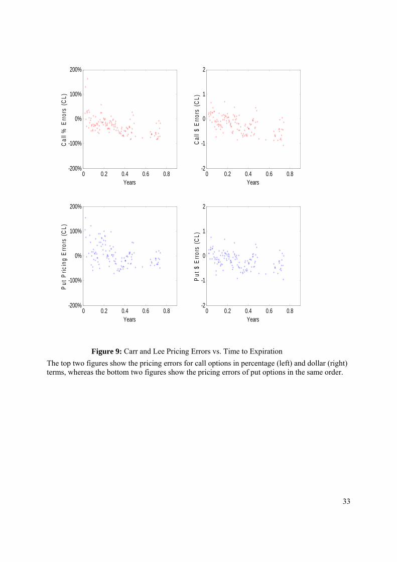
The Carr and Lee model: The sixth panel of Tables 1 and 2, as well as Figure 9, reports the

pricing performance of the Carr and Lee model against time to expiration. Table 1 shows that the

Carr and Lee model generates smaller percentage errors for options with longer times to

expiration. Table 2 and Figure 9 both reveal that this model, contrary to the Whaley model,

12 The short-term DOTM options are an exception.

18

underprices the VIX options as the options move closer to the expiration date.13

4.2 Pricing Errors across Models

In this section we perform the following comparisons of models based on both dollar and

percentage errors: (1) the results across five different moneyness categories; (2) the results across

three different time to expiration categories. Tables 1 and 2 report the percentage and dollar

errors for both unsigned and signed values, respectively.

The first comparison is to examine the moneyness categories by viewing Tables 1 and 2

vertically for given times to expiration. All four formulations of the Whaley model, as well as the

Carr and Lee model, clearly exhibit better performance relative to the Grunbichler and Longstaff

model for almost all of the ITM option cells for all times to expiration. However, when we

examine the NTM options then the performance of the models is ranked as follows: Whaley(30)

for < 30 days, Whaley(IV) for > 30 days, Grunbichler and Longstaff, and Carr and Lee. Unlike

the previous categories, the Grunbichler and Longstaff model provides smaller errors relative to

the Whaley and Carr and Lee models for the OTM and DOTM categories, both in terms of

percentage and dollar errors, especially for the signed results.14

Finally, we compare the pricing errors of the three models across time to expiration. For all

time to expiration groups the Whaley(IV) model consistently outperforms the Grunbichler and

Longstaff and the Carr and Lee models for the unsigned errors, but often is inferior for the NTM

and OTM signed categories. The three models share one commonality: smaller errors for the

NTM and OTM options with longer times to expiration.

13 Unlike all the other moneyness categories, pricing errors for the DITM options are insensitive to the change in option maturity. The fewer data points in Figure 9 deserves an explanation. The Carr and Lee model requires variance and volatility swap rates as inputs, which should obey the theoretical relation that the variance swap rate is greater than the squared volatility rate. However, the calculation of these two rates using actual market data can violate this relation, causing fewer valid points to be available for analysis. 14 In particular, the dollar errors from the Grunbichler and Longstaff model become smaller as the VIX options are more out-of-the-money, whereas the percentage errors are a similar size for all of the moneyness categories. In fact, the average signed dollar errors for Grunbichler and Longstaff are only -1 to -3 cents for DOTM options. However, the unsigned percentage errors are still 28% to 43% for this model relative to market prices.

19

4.3 Percentage vs. Dollar Errors for the Unsigned and Signed Categories

In this section we first investigate the performance of the models in terms of percentage and

dollar errors. Secondly, we examine the relation between the signed and unsigned errors. Our

expectations are that the more an option is out-of-the-money, the larger the percentage errors.

This result is consistent with small deviations from the market price causing large percentage

errors for OTM options. The use of percentage errors provides a more consistent rubric to

compared models, whereas dollar errors are beneficial to determine the practical usefulness of a

given model.

Examining DITM options, Table 1 shows that the Whaley(IV), Whaley(FR), and Carr and

Lee models possess relatively small percentage errors and moderately sized dollar errors, with

the percentage errors being less than 7.4% and the dollar errors less than 45 cents. The other

moneyness categories possess progressively higher percentage errors for the various Whaley

models and the Carr and Lee model.15 For all models, the unsigned percentage errors are large

for all models for the NTM and OTM categories, with the corresponding dollar errors being

greater than $.25 (and often larger) for the majority of the Whaley(IV) moneyness/time to

expiration categories and for almost all of the cells for all of the other models.

When we examine the signed values in Table 2 the same patterns exist for DITM options

(relatively small percentage errors) and other moneyness categories (generally progressively

larger percentage errors).16 The size of the percentage errors is still large for the NTM and OTM

categories, at least for most models. Therefore, the errors mostly are on one side of the

theoretical option values rather than being dispersed around the theoretical value. Thus, the

models apparently are consistently biased or are missing an important variable, since the market

prices are consistently overpriced.

15 The corresponding DOTM dollar errors are typically smaller since total option prices are relatively small. 16 The Grunbichler and Longstaff DOTM options are an exception, as their percentage errors are below 10%.

20

We now directly examine the differences between the pricing errors for the unsigned and

signed values, namely we compare Table 1 to Table 2 in order to determine the direction and

consistency of the errors. Large differences between the sizes of the results in the two tables

reveal to what extent positive pricing errors offset negative errors. Small differences between the

tables show that the errors are predominantly positive or negative. The Whaley models

consistently possess very similar percentage and dollar errors in terms of size between the two

tables, showing that the model price is almost exclusively below the market price for the

Whaley(IV) and Whaley(FR) models, and consistently above the market price for the medium-

and longer-term Whaley(30) and Whaley(5) categories. Conversely, the Grunbichler and

Longstaff model generally exhibits a large difference between the unsigned and signed

percentage values and much smaller average signed dollar errors in magnitude than their

unsigned counterpart. Thus, the positive errors partially offset the negative errors for the

Grunbichler and Longstaff model. Similarly, many of the Carr and Lee categories possess

substantially lower signed percentage and dollar errors than unsigned errors. Consequently, the

different models do not misprice the VIX options relative to the market price in any consistent

manner. Moreover, the Whaley model misprices consistently in one direction (allowing traders to

make adjustments), whereas the other models often misprice in both directions.

4.4 Comparison to Simulation Results and Lin and Chang’s (2009) Models

Here we compare our empirical results to the simulation results given in Psychoyios and

Skiadopoulos (2006) and the out-of-sample results based on Lin and Chang’s (2009) model. Our

main conclusions relative to these past studies are presented here.

Psychoyios and Skiadopoulos (2006) attempt to test the performance of the Whaley approach

to VIX option pricing by simulating the underlying volatility process and computing the pricing

errors based on the resultant simulated results. They find that Whaley’s model generates smaller

21

errors relative to the benchmark Grunbichler and Longstaff model, as well as providing better

pricing and hedging performances than Detemple and Oskewe (2000), with the latter model

assuming a stochastic process for the VIX which is similar to the process used by Grunbichler

and Longstaff (1996).

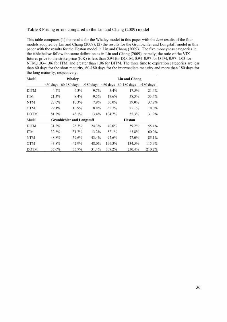
Lin and Chang (2009) examine out-of-sample results for their VIX option model in

combination with four stochastic volatility processes for the S&P500 index. Table 3 compares

(1) our results from the Whaley model in this paper to the best results of the four models

presented by Lin and Chang,17 and (2) the Grunbichler and Longstaff (1996) results here to the

Heston results from Lin and Chang (2009). The second comparison is appropriate since these

two models are similar: Grunbichler and Longstaff employ a mean-reverting square root process

for the VIX and Heston uses the same process for the S&P500 volatility.18

Comparing Whaley to Lin and Chang (2009) is given in the first panel of Table 3. These

results show that the pricing errors generated by the Whaley model are significantly and

consistently smaller than the counterparts by Lin and Chang’s best model. The Grunbichler and

Longstaff vs. Heston comparison is given in the second panel of Table 3. These results illustrate

that the Grunbichler and Longstaff model produces much smaller errors than the results from the

Heston model in Lin and Chang. These comparisons clearly show the superiority of the results

from the models employed in this paper. These results support the contention that a simple

model is better than a more complicated model when pricing VIX options.

5. Conclusions

Given that VIX options now trade on the CBOE options exchange, traders need an accurate

pricing formula to value this instrument. Traders and hedgers can benefit from an accurate 17 The time periods and levels of the VIX are nearly equivalent for the data employed here and the data in the Lin and Chang paper. 18 Grunbichler and Longstaff (1996) directly model the VIX, whereas Heston (1993) models both the S&P500 index and the S&P500 volatility (thereby modeling the VIX indirectly).

22

pricing model, since trading, arbitrage, and hedging errors will be smaller, and brokerage houses

can reduce the risk of charging insufficient portfolio margins. Several papers explicitly deal with

the pricing of volatility options, namely Whaley (1993), Grunbichler and Longstaff (1996),

Detemple and Oskawe (2000), and more recently Carr and Lee (2007) and Lin and Chang

(2009). Except for Lin and Chang, none of the earlier papers have market option pries to test

their models. Psychoyios and Skiadopoulos (2006) first attempt to document the pricing

performance of the first three of these models by using a Monte Carlo simulation approach.

However, a simulation is methodologically biased towards the volatility process employed for

the underlying cash instrument. Lin and Chang formulate a closed-form VIX option model and

test it with four different underlying stock index volatility processes. Consequently, the key

issue is whether more complicated models or simpler models are better to price VIX options.

This paper examines this question relative to actual VIX option market prices.

We find that Whaley (1993) performs very well for DITM options and reasonably well for

ITM options for all times to expiration. More generally, no model performs well for all types of

VIX options. However, we believe that the Whaley(IV) (1993) model provides the best overall

tool for pricing VIX options. Importantly, the Whaley model outperforms the more complicated

stochastic volatility and jump models examined by Lin and Chang (2009). Thus, we support the

anecdotal evidence from Wall Street that traders price VIX options off a Black-like formula such

as the Whaley or Carr and Lee models. Another conclusion from our results is that the pattern of

VIX option pricing errors generated by the Whaley model is often different from the pattern of

(SPX) index options generated by the Black-Scholes model. This suggests that the implied

volatility surface of VIX options differs from the well known implied volatility surface for SPX

options. In particular, given the inaccuracies of the Whaley and Carr and Lee models in pricing

many NTM and OTM VIX options, a better specified model to price VIX options is still

23

needed.19 The conclusion from the results in this paper is that an adequate pricing model has yet

to be developed or that the market is substantially mispricing VIX options.

19 All three models we investigate perform well for pricing in-the-money options in terms of percentage errors. Carr and Lee (2007) attribute the inferior performance of Black-type models (Whaley, Carr and Lee) for out-of-the-money options to the inability of the lognormal distribution to capture extreme events. We also agree with Psychoyios and Skiadopoulos (2006) that the Whaley(H30) model is more inaccurate as the time to expiration increases, with the longer maturities adversely affecting pricing performance for the unsigned pricing errors. Whaley(IV)’s model, and the other two models examined here, are much less sensitive to longer times to expiration.

24

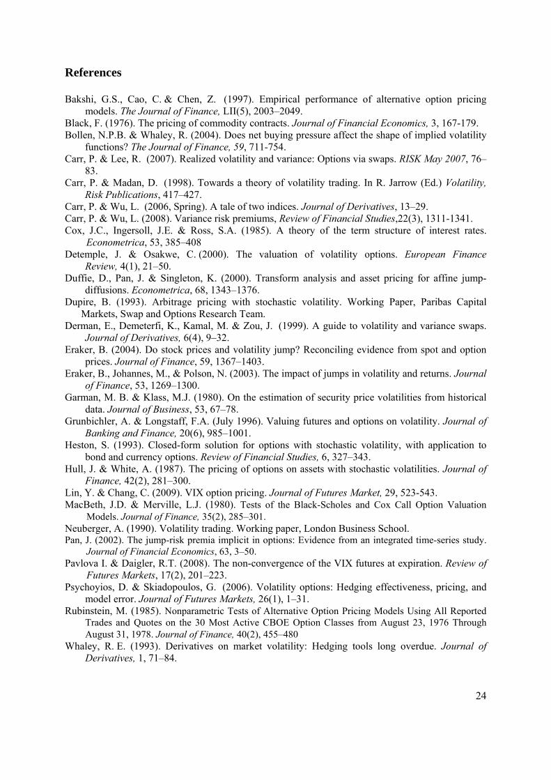
References

Bakshi, G.S., Cao, C. & Chen, Z. (1997). Empirical performance of alternative option pricing models. The Journal of Finance, LII(5), 2003–2049.

Black, F. (1976). The pricing of commodity contracts. Journal of Financial Economics, 3, 167-179. Bollen, N.P.B. & Whaley, R. (2004). Does net buying pressure affect the shape of implied volatility

functions? The Journal of Finance, 59, 711-754. Carr, P. & Lee, R. (2007). Realized volatility and variance: Options via swaps. RISK May 2007, 76–

83. Carr, P. & Madan, D. (1998). Towards a theory of volatility trading. In R. Jarrow (Ed.) Volatility,

Risk Publications, 417–427. Carr, P. & Wu, L. (2006, Spring). A tale of two indices. Journal of Derivatives, 13–29. Carr, P. & Wu, L. (2008). Variance risk premiums, Review of Financial Studies,22(3), 1311-1341. Cox, J.C., Ingersoll, J.E. & Ross, S.A. (1985). A theory of the term structure of interest rates.

Econometrica, 53, 385–408 Detemple, J. & Osakwe, C. (2000). The valuation of volatility options. European Finance

Review, 4(1), 21–50. Duffie, D., Pan, J. & Singleton, K. (2000). Transform analysis and asset pricing for affine jump-

diffusions. Econometrica, 68, 1343–1376. Dupire, B. (1993). Arbitrage pricing with stochastic volatility. Working Paper, Paribas Capital Markets, Swap and Options Research Team. Derman, E., Demeterfi, K., Kamal, M. & Zou, J. (1999). A guide to volatility and variance swaps.

Journal of Derivatives, 6(4), 9–32. Eraker, B. (2004). Do stock prices and volatility jump? Reconciling evidence from spot and option

prices. Journal of Finance, 59, 1367–1403. Eraker, B., Johannes, M., & Polson, N. (2003). The impact of jumps in volatility and returns. Journal

of Finance, 53, 1269–1300. Garman, M. B. & Klass, M.J. (1980). On the estimation of security price volatilities from historical

data. Journal of Business, 53, 67–78. Grunbichler, A. & Longstaff, F.A. (July 1996). Valuing futures and options on volatility. Journal of

Banking and Finance, 20(6), 985–1001. Heston, S. (1993). Closed-form solution for options with stochastic volatility, with application to

bond and currency options. Review of Financial Studies, 6, 327–343. Hull, J. & White, A. (1987). The pricing of options on assets with stochastic volatilities. Journal of

Finance, 42(2), 281–300. Lin, Y. & Chang, C. (2009). VIX option pricing. Journal of Futures Market, 29, 523-543. MacBeth, J.D. & Merville, L.J. (1980). Tests of the Black-Scholes and Cox Call Option Valuation

Models. Journal of Finance, 35(2), 285–301. Neuberger, A. (1990). Volatility trading. Working paper, London Business School. Pan, J. (2002). The jump-risk premia implicit in options: Evidence from an integrated time-series study.

Journal of Financial Economics, 63, 3–50. Pavlova I. & Daigler, R.T. (2008). The non-convergence of the VIX futures at expiration. Review of

Futures Markets, 17(2), 201–223. Psychoyios, D. & Skiadopoulos, G. (2006). Volatility options: Hedging effectiveness, pricing, and

model error. Journal of Futures Markets, 26(1), 1–31. Rubinstein, M. (1985). Nonparametric Tests of Alternative Option Pricing Models Using All Reported

Trades and Quotes on the 30 Most Active CBOE Option Classes from August 23, 1976 Through August 31, 1978. Journal of Finance, 40(2), 455–480

Whaley, R. E. (1993). Derivatives on market volatility: Hedging tools long overdue. Journal of Derivatives, 1, 71–84.

25

10 12 14 16 18 20 22 24 26 28 30-2%

0%

2%

5%

7%

9%

11%

13%

16%

18%

20%

VIX Futures Prices

Per

cent

age

Diff

eren

ce

-5% 0% 5% 10% 15% 20%0

500

1000

1500

2000

2500

Percentage Difference

Num

ber

of O

bser

vatio

ns

Figure 1: Percentage Difference between the Futures Price and the Midpoint of the Futures Arbitrage Bounds

The upper figure shows the percentage difference between the futures price and the midpoint of the futures arbitrage bounds: Percentage Difference = (Futures Price – Midpoint)/Futures Price. The arbitrage bounds for the VIX futures are derived from the bid and ask prices of the VIX options, based on the put-call parity model. The lower panel illustrates the histogram of the percentage differences.

26

-1.5 -1 -0.5 0 0.5 1 1.5-200%-100% 0%

100% 200% 300% 400%

Moneyness(=log Strike/Spot)

% E

rror

s (I

V)

-1.5 -1 -0.5 0 0.5 1 1.5-200%-100% 0%

100% 200% 300% 400%


% E

rror

s (F

R)

-1.5 -1 -0.5 0 0.5 1 1.5-200%-100% 0%

100% 200% 300% 400%


% E

rror

s (H

30)

-1.5 -1 -0.5 0 0.5 1 1.5-200%-100% 0%

100% 200% 300% 400%


% E

rror

s (H

5)

-1.5 -1 -0.5 0 0.5 1 1.5-4-20246


$ E

rror

s (I

V)

-1.5 -1 -0.5 0 0.5 1 1.5-4-20246


$ E

rror

s (F

R)

-1.5 -1 -0.5 0 0.5 1 1.5-4-20246


$ E

rror

s (H

30)

-1.5 -1 -0.5 0 0.5 1 1.5-4-20246


$ E

rror

s (H

5)

Figure 2: Whaley (historical volatility) Pricing Errors vs. Moneyness

The left four figures report the pricing errors of the Whaley model in percentage terms, while the right four figures show the pricing errors in dollars for the same models. The order of the figures are: Whaley(IV), Whaley(FR), Whaley(H30) and Whaley(H5). The out-of-the-money call options have moneyness values greater than zero.

27

-1.5 -1 -0.5 0 0.5 1 1.5-200%

-100%

0%

100%

200%

300%

400%


Cal

l % E

rror

s (I

V)

-1.5 -1 -0.5 0 0.5 1 1.5-200%

-100%

0%

100%

200%

300%

400%


Put

% E

rror

s (I

V)

-1.5 -1 -0.5 0 0.5 1 1.5-2

-1.5

-1

-0.5

0

0.5

1

Moneyness(=log Strike/Spot)C

all $

Err

ors

(IV

)

-1.5 -1 -0.5 0 0.5 1 1.5-2

-1.5

-1

-0.5

0

0.5

1


Put

$ E

rror

s (I

V)

Figure 3: Whaley (implied volatility) Pricing Errors vs. Moneyness

The top two figures show the pricing errors for call options in percentage (left) and dollar (right) terms, whereas the bottom two figures show the pricing errors of put options in the same order. The volatility input for Whaley’s model is the implied volatility estimated from the previous day. The out-of-the-money call options have moneyness values greater than zero; out-of-the-money put options have values less than zero.

28

-1.5 -1 -0.5 0 0.5 1 1.5-200%

-100%

0%

100%

200%


Cal

l % E

rror

s (G

L)

-1.5 -1 -0.5 0 0.5 1 1.5-200%

-100%

0%

100%

200%


Put

% E

rror

s(G

L)

-1.5 -1 -0.5 0 0.5 1 1.5-10

-5

0

5

10


Cal

l $ E

rror

s (G

L)

-1.5 -1 -0.5 0 0.5 1 1.5-10

-5

0

5

10


Put

$ E

rror

s (G

L)

Figure 4: Grunbichler and Longstaff Pricing Errors vs. Moneyness

The top two figures show the pricing errors for call options in percentage (left) and dollar (right) terms, whereas the bottom two figures show the pricing errors for put options in the same order. Out-of-the-money call options have moneyness values greater than zero; out-of-the-money put options have values less than zero.

29

-1.5 -1 -0.5 0 0.5 1 1.5-200%

-100%

0%

100%

200%


Cal

l % E

rror

s (C

L)

-1.5 -1 -0.5 0 0.5 1 1.5-200%

-100%

0%

100%

200%


Put

% E

rror

s(C

L)

-1.5 -1 -0.5 0 0.5 1 1.5-2

-1

0

1

2


Cal

l $ E

rror

s (C

L)

-1.5 -1 -0.5 0 0.5 1 1.5-2

-1

0

1

2


Put

$ E

rror

s (C

L)

Figure 5: Carr and Lee Pricing Errors vs Moneyness

The top two figures show the pricing errors for call options in percentage (left) and dollar (right) terms, whereas the bottom two figures show the pricing errors for put options in the same order. Out-of-the-money call options have moneyness values greater than zero; out-of-the-money put options have values less than zero.

30

0 0.2 0.4 0.6 0.8-100%

-50%

0%

50%

100%

Years

Cal

l % E

rror

s (I

V)

0 0.2 0.4 0.6 0.8-100%

-50%

0%

50%

100%

Years

Put

% E

rror

s (I

V)

0 0.2 0.4 0.6 0.8-1

-0.5

0

0.5

1

YearsC

all $

Err

ors

(IV

)

0 0.2 0.4 0.6 0.8-1

-0.5

0

0.5

1

Years

Put

$ E

rror

s (I

V)

Figure 6: Whaley (implied volatility) Pricing Errors vs. Time to Expiration

The top two figures show the pricing errors for call options in percentage (left) and dollar (right) terms, whereas the bottom two figures show the pricing errors for put options in the same order. The volatility input for Whaley’s model is the implied volatility estimated from the previous day.

31

0 0.2 0.4 0.6 0.8-100% 0%

100% 200% 300% 400%

Years

% E

rror

s (I

V)

0 0.2 0.4 0.6 0.8-100% 0%

100% 200% 300% 400%

Years

% E

rror

s (F

R)

0 0.2 0.4 0.6 0.8-100% 0%

100% 200% 300% 400%

Years

% E

rror

s (H

30)

0 0.2 0.4 0.6 0.8-100% 0%

100% 200% 300% 400%

Years

% E

rror

s (H

5)

0 0.2 0.4 0.6 0.8

0

2

4

Years

$ E

rror

s (I

V)

0 0.2 0.4 0.6 0.8

0

2

4

Years

$ E

rror

s (F

R)

0 0.2 0.4 0.6 0.8

0

2

4

Years

$ E

rror

s (H

30)

0 0.2 0.4 0.6 0.8

0

2

4

Years

$ E

rror

s (H

5)

Figure 7: Whaley Pricing Errors vs. Time to Expiration

The left four figures show the pricing errors for call options in percentage terms relative to time to expiration, whereas the right four show the pricing errors in dollar terms.

32

0 0.2 0.4 0.6 0.8-200%

-100%

0%

100%

200%

Years

Cal

l % E

rror

s (G

L)

0 0.2 0.4 0.6 0.8-200%

-100%

0%

100%

200%

Years

Put

Pric

ing

Err

ors

(GL)

0 0.2 0.4 0.6 0.8-4

-2

0

2

4

YearsC

all $

Err

ors

(GL)

0 0.2 0.4 0.6 0.8-4

-2

0

2

4

Years

Put

$ E

rror

s (G

L)

Figure 8: Grubichler and Longstaff Pricing Errors vs. Time to Expiration

The top two figures show the pricing errors for call options in percentage (left) and dollar (right) terms, whereas the bottom two figures show the pricing errors of put options in the same order.

33

0 0.2 0.4 0.6 0.8-200%

-100%

0%

100%

200%

Years

Cal

l % E

rror

s (C

L)

0 0.2 0.4 0.6 0.8-200%

-100%

0%

100%

200%

Years

Put

Pric

ing

Err

ors

(CL)

0 0.2 0.4 0.6 0.8-2

-1

0

1

2

Years

Cal

l $ E

rror

s (C

L)

0 0.2 0.4 0.6 0.8-2

-1

0

1

2

Years

Put

$ E

rror

s (C

L)

Figure 9: Carr and Lee Pricing Errors vs. Time to Expiration

The top two figures show the pricing errors for call options in percentage (left) and dollar (right) terms, whereas the bottom two figures show the pricing errors of put options in the same order.

34

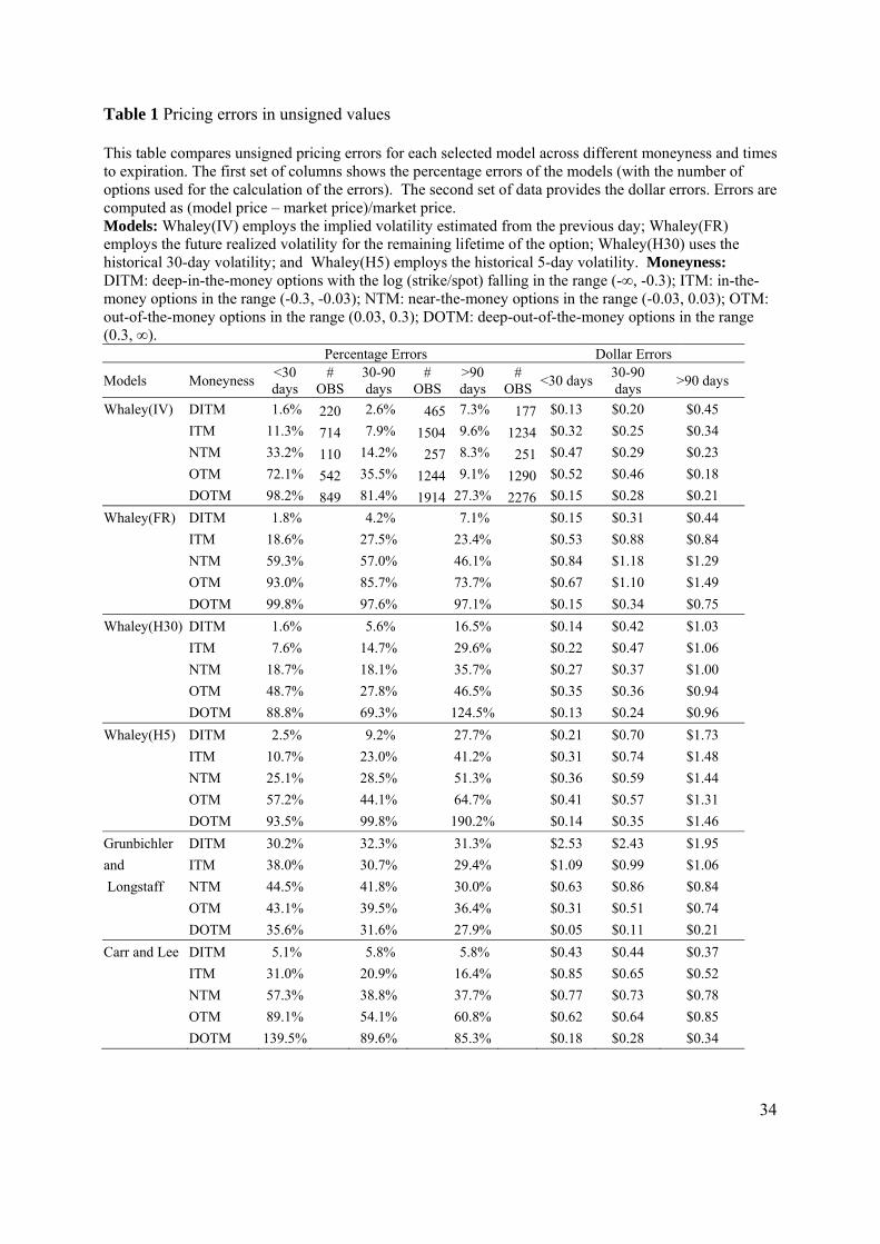
Table 1 Pricing errors in unsigned values

This table compares unsigned pricing errors for each selected model across different moneyness and times to expiration. The first set of columns shows the percentage errors of the models (with the number of options used for the calculation of the errors). The second set of data provides the dollar errors. Errors are computed as (model price – market price)/market price. Models: Whaley(IV) employs the implied volatility estimated from the previous day; Whaley(FR) employs the future realized volatility for the remaining lifetime of the option; Whaley(H30) uses the historical 30-day volatility; and Whaley(H5) employs the historical 5-day volatility. Moneyness: DITM: deep-in-the-money options with the log (strike/spot) falling in the range (-∞, -0.3); ITM: in-the-money options in the range (-0.3, -0.03); NTM: near-the-money options in the range (-0.03, 0.03); OTM: out-of-the-money options in the range (0.03, 0.3); DOTM: deep-out-of-the-money options in the range (0.3, ∞). Percentage Errors Dollar Errors

Models Moneyness <30 days

# OBS

30-90 days

# OBS

>90 days

# OBS

<30 days30-90 days

>90 days

Whaley(IV) DITM 1.6% 220 2.6% 465 7.3% 177 $0.13 $0.20 $0.45

ITM 11.3% 714 7.9% 1504 9.6% 1234 $0.32 $0.25 $0.34

NTM 33.2% 110 14.2% 257 8.3% 251 $0.47 $0.29 $0.23

OTM 72.1% 542 35.5% 1244 9.1% 1290 $0.52 $0.46 $0.18

DOTM 98.2% 849 81.4% 1914 27.3% 2276 $0.15 $0.28 $0.21

Whaley(FR) DITM 1.8% 4.2% 7.1% $0.15 $0.31 $0.44

ITM 18.6% 27.5% 23.4% $0.53 $0.88 $0.84

NTM 59.3% 57.0% 46.1% $0.84 $1.18 $1.29

OTM 93.0% 85.7% 73.7% $0.67 $1.10 $1.49

DOTM 99.8% 97.6% 97.1% $0.15 $0.34 $0.75

Whaley(H30) DITM 1.6% 5.6% 16.5% $0.14 $0.42 $1.03

ITM 7.6% 14.7% 29.6% $0.22 $0.47 $1.06

NTM 18.7% 18.1% 35.7% $0.27 $0.37 $1.00

OTM 48.7% 27.8% 46.5% $0.35 $0.36 $0.94

DOTM 88.8% 69.3% 124.5% $0.13 $0.24 $0.96

Whaley(H5) DITM 2.5% 9.2% 27.7% $0.21 $0.70 $1.73

ITM 10.7% 23.0% 41.2% $0.31 $0.74 $1.48

NTM 25.1% 28.5% 51.3% $0.36 $0.59 $1.44

OTM 57.2% 44.1% 64.7% $0.41 $0.57 $1.31

DOTM 93.5% 99.8% 190.2% $0.14 $0.35 $1.46

Grunbichler DITM 30.2% 32.3% 31.3% $2.53 $2.43 $1.95

and ITM 38.0% 30.7% 29.4% $1.09 $0.99 $1.06

Longstaff NTM 44.5% 41.8% 30.0% $0.63 $0.86 $0.84

OTM 43.1% 39.5% 36.4% $0.31 $0.51 $0.74

DOTM 35.6% 31.6% 27.9% $0.05 $0.11 $0.21

Carr and Lee DITM 5.1% 5.8% 5.8% $0.43 $0.44 $0.37

ITM 31.0% 20.9% 16.4% $0.85 $0.65 $0.52

NTM 57.3% 38.8% 37.7% $0.77 $0.73 $0.78

OTM 89.1% 54.1% 60.8% $0.62 $0.64 $0.85

DOTM 139.5% 89.6% 85.3% $0.18 $0.28 $0.34

35

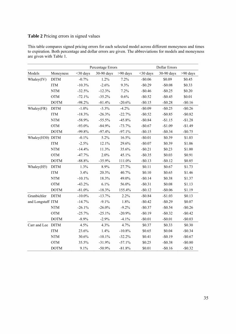
Table 2 Pricing errors in signed values

This table compares signed pricing errors for each selected model across different moneyness and times to expiration. Both percentage and dollar errors are given. The abbreviations for models and moneyness are given with Table 1.

Percentage Errors Dollar Errors

Models Moneyness <30 days 30-90 days >90 days <30 days 30-90 days >90 days

Whaley(IV) DITM -0.7% 1.2% 7.2% -$0.06 $0.09 $0.45

ITM -10.3% -2.6% 9.3% -$0.29 -$0.08 $0.33

NTM -32.5% -12.3% 7.2% -$0.46 -$0.25 $0.20

OTM -72.1% -35.2% 0.6% -$0.52 -$0.45 $0.01

DOTM -98.2% -81.4% -20.6% -$0.15 -$0.28 -$0.16

Whaley(FR) DITM -1.0% -3.3% -4.2% -$0.09 -$0.25 -$0.26

ITM -18.3% -26.3% -22.7% -$0.52 -$0.85 -$0.82

NTM -58.9% -55.5% -45.8% -$0.84 -$1.15 -$1.28

OTM -93.0% -84.9% -73.7% -$0.67 -$1.09 -$1.49

DOTM -99.8% -97.4% -97.1% -$0.15 -$0.34 -$0.75

Whaley(H30) DITM -0.1% 5.2% 16.5% -$0.01 $0.39 $1.03

ITM -2.5% 12.1% 29.6% -$0.07 $0.39 $1.06

NTM -14.4% 11.3% 35.6% -$0.21 $0.23 $1.00

OTM -47.7% 2.0% 45.1% -$0.35 $0.03 $0.91

DOTM -88.8% -35.9% 111.0% -$0.13 -$0.12 $0.85

Whaley(H5) DITM 1.3% 8.9% 27.7% $0.11 $0.67 $1.73

ITM 3.4% 20.3% 40.7% $0.10 $0.65 $1.46

NTM -10.1% 18.3% 49.0% -$0.14 $0.38 $1.37

OTM -43.2% 6.1% 56.0% -$0.31 $0.08 $1.13

DOTM -81.0% -18.3% 155.4% -$0.12 -$0.06 $1.19

Grunbichler DITM -10.0% -13.7% 2.2% -$0.84 -$1.03 $0.13

and Longstaff ITM -14.7% -9.1% 1.8% -$0.42 -$0.29 $0.07

NTM -26.1% -26.0% -9.2% -$0.37 -$0.54 -$0.26

OTM -25.7% -25.1% -20.9% -$0.19 -$0.32 -$0.42

DOTM -8.9% -2.9% -4.1% -$0.01 -$0.01 -$0.03

Carr and Lee DITM 4.5% 4.3% 4.7% $0.37 $0.33 $0.30

ITM 23.6% 1.4% -10.8% $0.65 $0.04 -$0.34

NTM 30.6% -10.1% -32.2% $0.41 -$0.19 -$0.67

OTM 35.5% -31.9% -57.1% $0.25 -$0.38 -$0.80

DOTM 9.1% -50.9% -81.8% $0.01 -$0.16 -$0.32

36

Table 3 Pricing errors compared to the Lin and Chang (2009) model

This table compares (1) the results for the Whaley model in this paper with the best results of the four models adopted by Lin and Chang (2009); (2) the results for the Grunbichler and Longstaff model in this paper with the results for the Heston model in Lin and Chang (2009). The five moneyness categories in the table below follow the same definition as in Lin and Chang (2009): namely, the ratio of the VIX futures price to the strike price (F/K) is less than 0.94 for DOTM, 0.94–0.97 for OTM, 0.97–1.03 for NTM,1.03–1.06 for ITM, and greater than 1.06 for DITM. The three time to expiration categories are less than 60 days for the short maturity, 60-180 days for the intermediate maturity and more than 180 days for the long maturity, respectively.

Model Whaley Lin and Chang

<60 days 60-180 days >180 days <60 days 60-180 days >180 days

DITM 4.7% 6.3% 9.7% 5.4% 17.5% 21.4%

ITM 21.3% 8.4% 9.5% 19.6% 38.3% 33.4%

NTM 27.0% 10.3% 7.9% 50.0% 39.0% 37.8%

OTM 29.1% 10.9% 8.8% 65.7% 25.1% 18.0%

DOTM 81.8% 43.1% 13.4% 104.7% 55.3% 31.9%

Model Grunbichler and Longstaff Heston

DITM 31.2% 28.3% 24.3% 40.0% 59.2% 55.4%

ITM 32.8% 31.7% 13.2% 52.1% 63.8% 60.0%

NTM 48.8% 39.6% 43.4% 97.6% 77.0% 85.1%

OTM 43.8% 42.9% 48.0% 196.3% 134.5% 115.9%

DOTM 37.0% 35.7% 31.4% 309.2% 230.4% 210.2%

The Performance of VIX Option Pricing Models - Dean Street

Documents

Transcript of The Performance of VIX Option Pricing Models - Dean Street