Z -Transform and preconditioning techniques for option pricing
Upload
khangminh22Category
view
3download
0
Path Calculations and OptionPricing
Thesis submitted for the degree ofDoctor of Philosophy
at the University of Leicester
By
Min Wang
Department of Mathematics
University of Leicester
December 2019
Abstract
The thesis is worked in the areas of the intersection of probability, combinatoricsand analytical combinatoric. The research is motivated from the need of producingnew methodologies and financial models in global market resulted from the lesson of2007-2009 global financial market and a quantum tool called Feynman path integralmethod which has been applied to model path-dependent option pricing model byHao and Utev. Path calculation method deal with models by analysing each possibleindividual asset price paths which broaden the methodology of modelling financialmarket and can solve some unusual or complex models which is difficult to modelby using non path-dependent calculation method.
My research has focused on developing combinatorial structure and path calculationmethods and then apply them to model individual share price path and calculateoption prices. The share price can be modelled as a path with a given share pricechanges and the expiry date. We have applied Flajolet symbolic method, generatingfunctions and path calculation method to model a set of typical finite restrictedshare price paths with restriction not allowing k consecutive down steps and deriveda calculation of option prices in the model. Besides, applying the Flajolet symbolicmethod, we constructed a relationship between individual share price and generatingfunction, analysed the transformed share price paths via different operations ongenerating functions. In addition, we applied path calculation method to solvewinning probability in the classical gambler ruin problem which contributes thesame result as the solution solved by establishing the recurrence equation method.Furthermore, we have solved a different gambler’s ruin problem using the pathcalculation method which cannot be solved by the recurrence equation method.
Counting paths with combinatoric can be studied from two ways, one way is to labeland the other is computation. Labelling is a part of representation of objects. Wehave developed a graphical theoretical construction of individual share price pathvia general binary trees and matroid. In addition, We have developed a methodto solve some kinds of pattern avoiding path counting combinatorial problem bymodifying certain probability methods. Two working papers including modelling ofpaths via matroids and counting via Markov-type technique is now being produced.
1

Acknowledgements
Undertaking the PhD mathematics has been an evaluable life-changing experiencefor me. There are many people who have helped me as a mathematician studentover the last four years. It is pleasure to acknowledge the guidance and support Ihave received from many people.
Firstly, I praise the Lord Jesus has chosen me to know him in my first year of PhD,with his almighty for guiding and providing me the wisdom, knowledge, strength,blessing and opportunity to complete the study. It is life-changing for me by knowinghim and his words. His words is a lamp for my feet, a light on my path.
I would like to express my utmost and sincere gratitude to my supervisor, ProfessorSergey Utev, for his instructions, time, patience, motivation, inspiration, encourage-ment and immense knowledge I received throughout my study and research work.I would like to thank him for encouraging me to start the PhD, guided me to dothe research, pass viva and amend thesis. I feel very fortunate to have been a PhDstudent supported and guided by him. He not only supported me for the studybut also encouraged me many times in general, without his guidance and constantfeedback this PhD would not have been achievable.
I would like to thank the thesis committee: Dr Bogdan Grechuk(University of Leices-ter), Dr Fraser Daly(Heriot-Watt University), Professor Sergei Petrovskii(Universityof Leicester) for their insightful comments and time. I want to thank Dr BogdanGrechuk with his kind help and useful advice that helped in addressing the short-comings in the thesis.
I would like to thank all of the staff members in the Department of Mathemat-ics at University of Leicester for their help and providing convenient environmentthroughout my research study. I want to thank Charlotte Langley for her kind help.
I am very much indebted to my parents for their unconditional love, endless prayer,support and words of encouragement. It would not be possible without them tocomplete the thesis and succeed.
Last but not least, I am very grateful to all my friends in Michael Atiyah building,Stephen, Wendy, Pattharaporn(Aon), Simran, Eliyas, Nur, Ka Kin, Num, Jehan,Areej et al. for their support and friendship. I want also give thanks to Xiaoyu Yu,Siqi Wang, Nan Yan, Phoenix, Chu Xiao, Hana, Haige Yuan, Yixin Xie, Raojun Li,Shuai Zhao, Rui Luo et al. for their friendship in my study and usual life.
2

Contents
1 Introduction 81.1 Structure and results . . . . . . . . . . . . . . . . . . . . . . . . . . . 12
2 Binomial Model 152.1 Path calculation argument . . . . . . . . . . . . . . . . . . . . . . . . 15
2.1.1 Motivation . . . . . . . . . . . . . . . . . . . . . . . . . . . . . 152.1.2 Path Calculation Method . . . . . . . . . . . . . . . . . . . . 16
2.2 Two step binomial model . . . . . . . . . . . . . . . . . . . . . . . . . 172.3 Calculate Paths Using Probability Generating function . . . . . . . . 26
2.3.1 Methods and Examples . . . . . . . . . . . . . . . . . . . . . 262.3.2 Represent all paths in the model using Generating function . 30
3 Generating functions approach 343.1 Definitions of OGFs and EGFs . . . . . . . . . . . . . . . . . . . . . 343.2 Definitions of common operations on OGFs . . . . . . . . . . . . . . . 373.3 Methods using generating functions . . . . . . . . . . . . . . . . . . . 46
3.3.1 Solving recurrence equations . . . . . . . . . . . . . . . . . . . 473.3.2 Counting combinatorial classes(Symbolic Method) . . . . . . . 48
3.4 Examples of counting using symbolic method . . . . . . . . . . . . . . 553.4.1 Count Binary Trees with different size function . . . . . . . . 553.4.2 Count Trees and Forests . . . . . . . . . . . . . . . . . . . . . 613.4.3 Count general binary strings that contain consecutive 0’s less
than 3 . . . . . . . . . . . . . . . . . . . . . . . . . . . . . . . 633.4.4 Count using generating functions . . . . . . . . . . . . . . . . 69
3.5 Counting permutations and statistics of permutations . . . . . . . . . 743.5.1 Permutations . . . . . . . . . . . . . . . . . . . . . . . . . . . 743.5.2 Statistics of Permutations . . . . . . . . . . . . . . . . . . . . 783.5.3 Count cycle structure statistics on permutations . . . . . . . . 793.5.4 Count Inversion Structure Statistics on Permutations . . . . . 863.5.5 Count Descents Statistics on Permutations . . . . . . . . . . . 90
3.6 How to extract the leading terms of a generating function . . . . . . . 973.7 Case study/path transform example . . . . . . . . . . . . . . . . . . . 98
4 Path Calculations/Interpretations 1034.1 Count unrestricted lattice paths with two directions . . . . . . . . . . 1034.2 Count restricted lattice paths with two directions . . . . . . . . . . . 1084.3 Count self-avoiding walks with three directions . . . . . . . . . . . . . 1114.4 Count unrestricted lattice paths . . . . . . . . . . . . . . . . . . . . . 1184.5 Counting the number of path with forbidden city . . . . . . . . . . . 119
3

Contents
4.6 Path calculation in gambler’s ruin . . . . . . . . . . . . . . . . . . . . 122
5 Modelling share price paths via Binary trees 1255.1 A bijection between the set of binary trees and the set of Dyck paths 125
5.1.1 Bijection algorithm from binary trees . . . . . . . . . . . . . . 1265.1.2 Share price path interpretation . . . . . . . . . . . . . . . . . 128
5.2 A bijection between the set of general rooted ordered trees and theset of Dyck paths . . . . . . . . . . . . . . . . . . . . . . . . . . . . . 1295.2.1 Bijection algorithm from rooted ordered tree . . . . . . . . . . 130
5.3 An injection construction of share path from general binary rootedordered trees . . . . . . . . . . . . . . . . . . . . . . . . . . . . . . . 1335.3.1 An injection construction algorithm . . . . . . . . . . . . . . . 133
6 Count all paths not allowing given down steps in Binomial model 1376.1 Construction . . . . . . . . . . . . . . . . . . . . . . . . . . . . . . . 1376.2 Calculate option price in the finite restricted binomial model . . . . . 138
7 Count paths using Parallelogram polyominoes 1417.1 Definitions . . . . . . . . . . . . . . . . . . . . . . . . . . . . . . . . . 1417.2 Construction of dyck paths from lattice path matroids . . . . . . . . 146
7.2.1 Construction . . . . . . . . . . . . . . . . . . . . . . . . . . . 1467.2.2 Share price Path interpretation . . . . . . . . . . . . . . . . . 148
8 Probability Methods 1508.1 Path counts using a probability method . . . . . . . . . . . . . . . . . 150
8.1.1 Probability of simple random walks from (0, a) to (n, b) . . . 1508.1.2 Path counts using a simple probability argument . . . . . . . 151
8.2 Count paths via unusual stochatic modelling . . . . . . . . . . . . . . 1528.2.1 Markov chain . . . . . . . . . . . . . . . . . . . . . . . . . . . 1538.2.2 Method Inspiration . . . . . . . . . . . . . . . . . . . . . . . . 1558.2.3 Transform probability matrix setting up . . . . . . . . . . . . 1568.2.4 Result and Discussion . . . . . . . . . . . . . . . . . . . . . . 1608.2.5 Implementation . . . . . . . . . . . . . . . . . . . . . . . . . . 167
9 Matroid 1689.1 Definitions of Matroids . . . . . . . . . . . . . . . . . . . . . . . . . . 1689.2 Lattice path matroid . . . . . . . . . . . . . . . . . . . . . . . . . . . 1819.3 Tutte polynomials . . . . . . . . . . . . . . . . . . . . . . . . . . . . . 1869.4 Calculation of the Tutte polynomials for lattice path matroids . . . . 188
9.4.1 Construction of bijection between lattice paths and set of theirnorth steps . . . . . . . . . . . . . . . . . . . . . . . . . . . . 189
9.4.2 The independent sets of a lattice path matroid . . . . . . . . . 1899.4.3 The calculation of Tutte polynomials . . . . . . . . . . . . . . 190
9.5 Modelling of paths via matroids . . . . . . . . . . . . . . . . . . . . . 1949.5.1 Tutte polynomial . . . . . . . . . . . . . . . . . . . . . . . . . 1949.5.2 Result . . . . . . . . . . . . . . . . . . . . . . . . . . . . . . . 1959.5.3 Representations of share paths via general tree . . . . . . . . . 199
Chapter 0 4

Contents
10 Conclusions and Future work 20110.1 Conclusions . . . . . . . . . . . . . . . . . . . . . . . . . . . . . . . . 20110.2 Future work . . . . . . . . . . . . . . . . . . . . . . . . . . . . . . . . 203
Appendices 204
A Implementation matlab code 205
Chapter 0 5

List of Figures
2.1 one step possible change of the portfolio . . . . . . . . . . . . . . . . 292.2 one example path . . . . . . . . . . . . . . . . . . . . . . . . . . . . . 292.3 probabilities of portfolio possible change each step . . . . . . . . . . . 30
3.1 the digraph Dw of the permutation w = (2)(41)(6)(753) . . . . . . . 77
4.1 Pascal counting . . . . . . . . . . . . . . . . . . . . . . . . . . . . . . 1204.2 avoiding path . . . . . . . . . . . . . . . . . . . . . . . . . . . . . . . 121
5.1 a dyck path of length 12 . . . . . . . . . . . . . . . . . . . . . . . . 1275.2 the corresponding binary tree . . . . . . . . . . . . . . . . . . . . . . 1275.3 a tree of vertices 13 . . . . . . . . . . . . . . . . . . . . . . . . . . . . 1285.4 the corresponding share path . . . . . . . . . . . . . . . . . . . . . . 1285.5 a Dyck path of length 12 . . . . . . . . . . . . . . . . . . . . . . . . 1315.6 the corresponding ordered tree of 6 edges . . . . . . . . . . . . . . . 1315.7 a tree of vertices 7 . . . . . . . . . . . . . . . . . . . . . . . . . . . . 1325.8 the corresponding share path . . . . . . . . . . . . . . . . . . . . . . 1325.9 a general ordered binary tree of 3 edges, 4 vertices . . . . . . . . . 1345.10 the corresponding share path of length 3 . . . . . . . . . . . . . . . . 1355.11 the constructed share path from the general binary tree . . . . . . . . 1355.12 the corresponding share path of length 3 . . . . . . . . . . . . . . . . 1355.13 the corresponding share path of length 3 . . . . . . . . . . . . . . . . 136
7.1 an example of not being polyomino . . . . . . . . . . . . . . . . . . . 1427.2 an example of column-convex polyomino . . . . . . . . . . . . . . . . 1427.3 an example of row-convex polyomino . . . . . . . . . . . . . . . . . . 1427.4 an example of convex polyomino . . . . . . . . . . . . . . . . . . . . . 1437.5 an example of convex polyomino with smallest bounding box . . . . . 1447.6 an example of parallelogram polyomino . . . . . . . . . . . . . . . . . 1457.7 the parallelogram polyomino with its bounding paths (w, η) . . . . . 1457.8 the corresponding 2-colored Motzkin path from the example polyomino1477.9 the corresponding path h(γ) from the 2-colored Motzkin path . . . . 1487.10 the final constructed Dyck path from the example polyomino . . . . . 148
9.1 an example of lattice path matroid with labelled north steps indexes . 1919.2 connected lattice path matroid containing one unit cell . . . . . . . . 1959.3 lattice with identified nodes one unit cell connected matroid . . . . . 1969.4 One unit cell matroid’s tree . . . . . . . . . . . . . . . . . . . . . . . 1969.5 One two unit cells connected lattice path matroid . . . . . . . . . . . 1969.6 Another two unit cells connected lattice path matroid . . . . . . . . . 197
6

List of Figures
9.7 One two unit cells matroid’s lattice . . . . . . . . . . . . . . . . . . . 1979.8 One two unit cells matroid’s lattice . . . . . . . . . . . . . . . . . . . 1979.9 One two unit cells matroid’s tree . . . . . . . . . . . . . . . . . . . . 1989.10 Another two unit cells matroid’s tree . . . . . . . . . . . . . . . . . . 1989.11 One two unit cells connected lattice path matroid . . . . . . . . . . . 1989.12 lattice with identified nodes one unit cell connected matroid . . . . . 1999.13 the corresponding share path of length 2 . . . . . . . . . . . . . . . . 1999.14 One share path of length 3 . . . . . . . . . . . . . . . . . . . . . . . 2009.15 Another share path of length 3 . . . . . . . . . . . . . . . . . . . . . 200
Chapter 0 7

Chapter 1
Introduction
The lessons from 2007-09 global financial crisis leads to needs of reasonable responsesin financial sector and the real economy [1] [2]. New methodologies, financial modelsneed to be designed in the global market [1] [2]. More volatility of asset prices infinancial market during the crisis bring in excessive volatility of option prices whichimpose the challenges to option pricing model [3].
Option pricing approach and model is an active research area in financial market,started from the well-known Black Scholes model, which calculate theoretical Eu-ropean option price with certain assumptions [4]. One of the limits of the modelis that the model does not cover the pricing of American option which could beexercised before the expiration date [7]. On the other hand, Cox-Ross-RubinsteinBinomial Model provides a discrete teaching model to continuous model, which wasfirst proposed by Cox, Ross and Rubinstein and then become a widely used modelin the literature [5]. The binomial model adopts an iterative procedure and cancalculate option prices based on the decisions at each period before the expirationdate[5].
Quantum mechanics approaches can provide a way to study the behaviour of unpre-dictable stock market [2][8]. Use quantum tools to do financial modelling initiatedin Ma and Utev [9] and developed in Karadeniz and Utev [10].
One of the famous quantum tools, Feynman path integral quantum mechanic ap-proach can be applied to stock option pricing [8]. The Dirac-Feynman quantummechanics technique for insurance risk modelling was initiated and developed inTamturk and Utev [11]. The quantum approach is adapted to formalise the path-dependent option pricing [2].
Two simple quantum non-life risk models was studied in [11, section 2], in thequantum risk models, the claim amounts are assumed to have two point distributionsand the observed data are treated as having small claims u and significant claimsd. The two quantum risk models study the cumulative claim amounts collectedat regular time intervals where each interval was set up reasonable small to havea maximum two claims [11]. One quantum risk model studies cumulative claimamounts which assume repeated claims was not observed, in the case of intervalwhich allow maximum two claims, it is a model not allowing two small claims 2d
8

Chapter 1. Introduction
and two significant claims 2u [11].
Motivated from the interesting quantum risk models in [11, section 2], in the thesis,the main idea in the dissertation is to consider restricted paths, the typical restrictedpath we studied is the share price paths with restriction not allowing 2 consecutivedown steps.
Motivated from the Feynman path integral method [12] [13], in the thesis, ourapproach to finance is based on path calculation. The path calculation idea isto identify all possible truncated individual paths in the model, associate eachpossible path with a probability and then sum up the probabilities of the validpaths according to different truncate time and different arriving time to finally getthe required probability in the model.
This dissertation presents variety of discrete time models for the financial stockmarket.
The share price is modelled as a path
σ1 = S0 → S1 = S0y1 → s2 = S1y2
→ . . . ST−1 = ST−2yT−1 → ST = ST−1yT ,
where yi are the share price changes, T is the expiry day. In the classical Cox-Rubinstein Binomial model [5] [6], for Black-Scholes approach to option pricing [4],yı ∈ u, d where u is the jump up and d is the jump down.
The path calculation approach implies that
E(f(ST )) =∑σ
P (σ) · f(ST (σ)), where∑σ
P (σ) = 1.
The main idea in the dissertation is to consider restricted paths. More exactly, atypical example is that the share price is modelled by a restricted two step binomialmodel with restriction not allowing two consecutive down steps, the model is alsoa restricted two step binomial model with restriction that the number of maximumconsecutive down steps is 1.
Various models are constructed in this way. In chapter 2, several examples ofoption pricing using path calculation method in binomial model was introduced.In chapter 3, section 3.4.3, motivated by Flajolet symbolic method ([15, ?]) andapply the idea taken from [16] [14], we use the Flajoet symbolic method to givean more constructive explanation and solution using symbolic method to solvegeneral bitstrings not allowing 3 consecutive 0’s less than 3. In chapter 4.5,an example of path calculation using combinatorial method not touching the givenbold line segment is derived and techniques is stated in the example. In chapter 6motivated by Flajolet symbolic method and generating function approach[14] [15],and motivated by quantum path calculation method in [2], we calculated the optionprice in the finite restricted binomial model. Having different ways of counting is
Chapter 1 9

Chapter 1. Introduction
necessary to do path counting. In chapter 8, we developed a method of countingrestricted share price paths via markov-type stochastic modelling.
Moreover, counting paths with combinatoric can be studied from two ways, oneway is to label and the other is computation. Labelling is a part of representationof objects and generating function can provide many different ways of representingfinancial paths.
Like reflection problem in random walk, clearly, path calculation depends on pathrepresentation. Different way of path representation have been studied. Specifically,In chapter 5, motivated from the exercise in [17], we developed the algorithm ofconstructing share price via binomial trees and analysed the modelling of share pricepaths via binomial trees. Furthermore, in chapter 7, drawing ideas from [30, page179], the modelling of share price paths via polyominos was introduced. In chapter10, based on the relationship between binomial trees and share prices we derivedin chapter 5, section[5.3.1], motivated from the computation of matroid using tuttepolynomial in the paper [60, section 6], modelling of share prices via matroid andtutte polynomial was analysed.
In addition, the major part of path calculation is counting no of paths with equalprobability, which is combinatorial problems. Extensive combinatorial problem wasstudied in the chapter 3, 4. Specifically, motivated from the definitions of generatingfunctions and operations on generating functions by Flajolet and Sedgewick in thebook [14, chapter 5] [15, chapter 1], we give examples of representing share pricepaths using generating function in section 3.1, 3.2. It follows by the preliminaryknowledges for using Flajolet symbolic method in section 3.3, which is taken fromthe chapters in the book [15, chapter I. 2.1.] and presented in a more compact andconstructive way.
Well-know problem of counting trees and forests using symbolic method is stated inthe section 3.4 in the thesis. Counting binary trees using generating function derivedfrom combinatorial method is described by Sedgewick, Robert, and Philippe Flajoletin the chapter 3.8 in the book [14]. Counting binary trees using symbolic methodis described in chapter 5.2 in the book [14]. Relationship between enumeration offorests and trees is stated as a theorem 6.2 in the book [14]. In the section 3.4 of thethesis, along the lines of description of the generating function and symbolic methodtechniques described in the chapter 3.8, chapter 5.2 and theorem 6.2 by Sedgewick,Robert, and Philippe Flajolet in the book [14], we gave more detailed explanationof counting trees and forests via Flajoet symbolic method. The counts results forcounting trees and forests is the well-known catalan numbers.
Motivated from the statement in the paper that a geometry behind the stock markettransaction can be related to combinatorial object permutations which providesa connection of combinatoric problem to financial market [20]. According to thechapter 1.3 by Stanley in the book [21], counts for cycle structure, inversion structureand decent structure statistics on permutation are discussed in the section 3.5 of thethesis. Specifically, the exposition in the section is based on the presentation in thesection [21, page 29-39]. In section 3.5.1, following the definitions of disjoint cycle
Chapter 1 10

Chapter 1. Introduction
notation, standard form of disjoint cycle notation, diagraph form of permutation[21, page 29-39], using the same example, we give detailed algorithm how disjointunion of directed cycles is obtained from a disjoint cycle notation of a permutation.It follows by a proposition which is taken from [21, Proposition 1.3.1] follows theargument in the page [21, page 30] but with more clear and readable proof.
In section 3.5.2 and 3.5.3, following the counts of permutation with given cycle typetaken from [21, Proposition 1.3.2], exponential generating function of the countstaken from [21, Theorem 1.3.3] and an example of applying the exponential gen-erating function taken from [21, Example 1.3.5], counting number of permutationswith a fixed cycle statistic is stated as a derivation of recurrence equation of thecounts which is taken from [21, Lemma 1.3.6] but we gave a readable proof andadded the argument how to set up the bounding conditions of the equation. Inaddition, counting number of permutations with a fixed cycle statistic is solved usinggenerating function, the solution is taken from the second proof of [21, Proposition
1.3.7] but in which we added the derivation ofn∑k=0
c(n, k)tk using Flajolet symbolic
method.
In section 3.5.4, counting number of permutations with a fixed inversion statisticis discussed, which is mainly based on [21, page 35-37]. Specifically, motivatedfrom the discussion of associating a permutation with a given integer sequence(a1, a2, . . . , an), with 0 ≤ ai ≤ n − i, we gave a detailed and applicable algorithmof the natural correspondence from the given integer sequence to a permutationand also give the argument to justify the algorithm is reasonable by analysing therelation between the possible values of an−i and the number of positions in thepermutation ui. Following the definitions of inversions taken from [21, page 36],motivated from the discussion regarding the integer sequence (a1, a2, . . . , an), with0 ≤ ai ≤ n−i on the page [21, page 34-36], we derived a proposition that claims eachindex i, with 0 ≤ i ≤ n in a permutaiton w ∈ Sn can be uniquely characterizedby an integer ai in the integer sequence (a1, a2, . . . , an), with 0 ≤ ai ≤ n− i. Theproposition can contribute to the proof of bijection between permutations Sn andinteger sequences (a1, a2, . . . , an), with 0 ≤ ai ≤ n − i, which is a propositiontaken from [21, Proposition 1.3.12] after introducing the definition of inversiontable taken from [21, Page 36]. Next, counting number of permutations with afixed inversion statistic is solved using generating function which is taken from[21, Corollary 1.3.13] but in the proof we added the derivation of the derivation
of∑w∈Sn
qinv(w) =∑
(a1,a2,...,an)∈Tn
qa1+a2+...+an using Flajolet symbolic method, say
Cartesian product symbolic method, which makes the proof more readable. Lastly,we stated the definition of n! which is taken from the discussion on the page [21,Page 37]
In section 3.5.5, according to [21, Section 1.4], counting number of permutationswith a fixed descent statistic is discussed. Specifically, using the same notation anddefinition of A(d, k) taken from [21, Page 39], motivated from the example 1.4.2on [21, Page 38] and the first few examples of Eulerian polynomial stated [21, Page39], we derive a formula A(n, k) for counting the number of permutations w ∈ Sn
Chapter 1 11

Chapter 1. Introduction
with a fixed number of descents k− 1. Besides, definitions of descents, descent set,the number of descents of a permutation w ∈ Sn are taken from [21, Page 38-39].Next, given a finite set S in increasing order, definitions of the two statistics α(S),α(S), β(S) on permutations from descent set are taken from the page [21, Page38]. It follows by a proposition taken from [21, Proposition 1.4.1] which states thecombinatorial method of finding α(S) with a given finite set S but in the proofof the proposition, we added more readable argument of the combinatorial method.Next, following from the discussion on the page [21, Page 39], we summarize thedefinition of alternating permutation and reverse alternating permutation.
In chapter 4, motivated from a question of counting the number of lattice pathsfrom (0, 0) to (n,m) which is advised by supervisor, several ways of countingunrestricted lattice paths are discussed. Applying the method of solving recurrenceequations using generating functions taken from [22, Lec-31], counting unrestrictedpaths for the question are presented in section 4.4; the technique is to solve a(n,m),try to fix one variable n and solve it using one variable generating function,then, extract the coefficient of xm in the generating function to get the coefficienta(n,m). The question can be related to the counting bitstrings of fixed length andfixed number of bits 1, which was solved using symbolic method by Sedgewick,Robert, and Philippe Flajolet in the book [14, Chapter 3.8]. Counting number ofbitstrings of fixed length using symbolic method is also presented in the book [14], inwhich two ways of construction of bitstrings of fixed length is stated in the chapter5.2 of the book [14]. In the thesis, taking the method from [14, chapter 3.8, 5.2],in section 4.1 we gave the two method of counting lattice path of length N andthe solution of counting lattice path of length N and k up steps. In addition,another question advised by supervisor which counts the restricted lattice pathsfrom (0, 0) to (N,N) with two choice steps and not going above the diagonal lineis presented in section 4.2, which is motivated from [23, Example 2.7] and can alsorefer to Flajolet in the book [15, Page 319].
In real financial market, consider a portfolio consisting of one bond and one share,if setting the bond price stay, the portfolio price will depend on the share price only,which is a random walk. However, if setting the bond price is always up duringsome periods, consider the portfolio price denoted by a pair of share price and bondprice, then the portfolio price would be a self-avoiding price path because it cannotgo back to the same price state. This gives a motivation to counting self-avoidingwalk, which was stated in the section 4.3 in the thesis. The enumeration methodand presentation of counting self-avoiding walks is mainly taken from the paper[24, section7, 10] and detailed explanation of derivation of the general recursivemethod was added before deriving the two variable generating function G(t, v) andextracting the coefficient g(n,m).
1.1 Structure and results
This thesis investigated combinatorial structures, path calculation methods andapplied them to model individual share price path and calculate option prices. Thecontributions of this thesis are covered in Chapter 2, 5, 6, 7, 8, 9 and several sections
Chapter 1 12

Chapter 1. Introduction
in Chapter 3, 4. This thesis is organized as follows.
Chapter 1. It contains an Introduction with the Structure of the thesis and theresults.
Chapter 2. We apply path calculation method to binomial option pricing model. Itstarts with the Binomial Model from the path calculation approach. (Results)
Chapter 3. Motivated by Flajolet symbolic method ([15]), generating functions ap-proach is investigated. The Path Calculations and Interpretations are important forthe financial modelling. Generating function and operation on generating functioncan provide more ways to represent financial paths (Results).
Chapter 4. One thesis regarding a combinatoric problem is summarized, whichprovide new combinaotric technique that might be used for path counting. Wederived the solution of counting a path not touching the given bold line segmentand the technique is illustrated using an example. We applied the path calculationmethod to solve the winning probability in the gambler ruin problem, in which wegot the same answer as using the classical method (Results).
Chapter 5, we studied the modelling of share price paths via Binary trees (Results).It is based on the possibility comes from the Bijection between the set of binarytrees and the set of Dyck paths. We provided the algorithm of constructing shareprice path from a set of full binary trees in Section 5.1.1 and gave the share pricepath interpretation and gave the algorithm of constructing share price path from aset of general trees. We also provided an algorithm to represent a share price via ageneral binary ordered tree. Moreover, we also Count all paths not allowing givendown steps in Binomial model.
Chapter 6. We studied the representation of paths for the restricted model(Results).
Chapter 7. We studied the representation of paths via polyominos. More countingis done in Count paths using Parallelogram polyominoes (Results).
Chapter 8. We studied the path calculation via the markov-type stochastic mod-elling, which can be generalised to counting any pattern avoiding path counting. Wecalculate the number of restricted share price paths not allowing consecutive downsteps at time 1 ≤ T ≤ N using Markov-type technique stochastic modelling, whichcan be generalized to counting any pattern avoiding path counting(Results).
Chapter 9. Path modelling via matroid and tutte polynomial is studied. A newrelationship between lattice integer points and tutte polyno-mials of transversal
Chapter 1 13

Chapter 1. Introduction
matroid is developed and modelling of share price paths via matroids is introducedusing examples(Results).
Chapter 10. The detailed results of the thesis is outlined for Chapter 2, 5, 6, 7, 8,9 and several sections in Chapter 3, 4. The possible future works is discussed.
Chapter 1 14
Chapter 2
Binomial Model
In this chapter, motivated from the Feynman path integral application in the paper[2], path calculation argument is proposed motivated from [13], [12]. Then, binomialmodel is studied using path calculation method which can be referred to [11], [13].
2.1 Path calculation argument
2.1.1 Motivation
the section is motivated from the section 2 [13, Page 6-8] and the introduction fromthe paper [12].
Consider a particle movement experiment starting from a fixed given position andobserve its final position at a later time.
In classical mechanics, if the experiment is repeatedly performed in the same waysuch as same movement velocity, each realization would result in same final positionmeasurement.
However, in quantum world, the situation is different. As the quantum particle hasa wave like property, the result of the observation of the final position of the particlewill have different outcomes in each realization when perform the experiment in thesame way.
Therefore, in quantum world, for the particle movement experiment, the interestis to fix a final position of the particle and predict the probability of the quantumparticle starting from a fixed given position and ending at the fixed final position.
From a fixed given position to one final position, a free quantum particle can travelin any way with any time, there might have infinite time path. So, paths truncatedat some final time T will be the interested paths for the quantum particle.
Consider each possible path from one point to another point has an equal probability,each path has different possible realization time, therefore, assign each path with acomplex amplitude, where its modulus square denotes the probability of the pathrealized in the experiment.
15

Chapter 2. Binomial Model
The different time spent on each path denotes the different direction of its probabilityamplitude. Suppose x1, x2, . . . , xn−1 denotes the state (eigen)vectors at each timet1, t2, . . . , tn−1, the quantum particle is at x0 at time t0, and in the end it isobserved at x at time T = tn.
In discrete case, sum up the probability amplitude of all possible paths from tk−1 totk along the state vector xk, in each divided time period, the probability amplitudeis independent, so, the probability amplitude of each possible path from t0 at x0
to T at x can be calculated by multiplying each period probability amplitudetogether.
The Feynman path integral can be summarized as identifying all possible path,truncate them at final time T and attach a probability amplitude to each possibleindividual path, then sum up all the probability amplitude of the valid possible pathwhich gives the probability of a quantum particle starting from position x0 at timet0 to final observed position x at time tn = T
2.1.2 Path Calculation Method
Motivated by Feynman path integral method in [2] [13], a path calculation methodis introduced in the section.
Consider a discrete model of share price starting from a fixed initial state, the modelis constructed from a random experiment which claim that share price can either goup with probability p or go down with probability p in each unit time step.
The path calculation method is that considering the model be a class of all possibleshare price paths, the class is denoted by A.
The path calculation idea is to identify all possible truncated individual paths inthe model, associate each possible path with a probability and then sum up theprobabilities of the valid paths according to different truncate time and differentarriving time to finally get the required probability in the model.
It can be summarized in mathematical notation as follows,
Step 1: Truncate all possible paths before the termination time T = n, associateeach possible individual path with a probability.
Consider the probability measure p = q = 12
in each step, all possible paths in themodel has equal probability P (σ) = 1
2n.
Step 2: Consider the possible paths from the fixed initial state S0 to a final stateq, sum up the probabilities of all possible paths of (S0 → Sn = q) according totheir different truncated visiting time(observing time) n. That is,
A(q;A) =∑n
∑σ∈A,σ(n)=q
P (σ)
Step 3: Sum up the probabilities of all possible paths (S0 → Sn) in the model
Chapter 2 16

Chapter 2. Binomial Model
according to their different possible arriving states q, that is,
A(A) =∑q
∑n
∑σ∈A,σ(n)=q
P (σ)
Step 4: Consider the normalized probability of the class associated with the model,that is,
S(A) =∑q
∑n
Cn∑
σ∈A,σ(n)=q
P (σ)
2.2 Two step binomial model
The examples and notations in this section are motivated from the chapter 2 in thelecture notes of financial mathematics [28, Page 8-21].
Suppose a sample space of a random experiment is denoted by S, and the restrictedsample space of the same random experiment with additional condition is denotedby L. It is known that |L| < |S|.
Suppose one element in the sample space is denoted by σ, probability that theelement happens is a function of the element, denoted by P (σ) = Prob(σ).
Suppose another function of the element is defined and denoted by f(σ)
Example1: Two step binomial model
Suppose a random experiment is tossing a coin twice, if the value of a coin tossedis head, then share price goes up by a factor u. If the value of a coin tossed is tail,then the share price goes down by a factor d.
Therefore, the share price is modelled by a two step binomial model.
Suppose the model use the probability measure defined by p(up) = pu and p(down) =pd.
Denote the value of share price at time t by St, and St is a variable. St → St+1
means that share prices move from time t to t + 1. The model starts from timet = 0 and suppose share price at time 0 is fixed and denoted by S0.
Consider the value of share price at time t = 2, it is a random variable and denotedby S2. The two step sample space corresponding to the variable S2 is denoted byΩ2, it is the set of all possible share price paths from S0 to S2.
Ω2 = σ1, σ2, σ3, σ4
Chapter 2 17

Chapter 2. Binomial Model
where,
σ1 = S0 → S0u→ S0u2
σ2 = S0 → S0u→ S0ud
σ3 = S0 → S0d→ S0du
σ4 = S0 → S0d→ S0d2
Then, the variable S2 is a variable which maps from Ω2 to real number R (thevalue of the share price at time t = 2).
Since the option value is based on the underlying stock price, suppose the optionvalue function at time t = 2 in the two step binomial model is denoted by f , it isa function depending on the value of S2.
The possible paths σ2 and σ3 are two ways from the starting share price state S0
to time 2 share price state S0ud, since their corresponding share price values S2
at the time t = 2 are the same value S0ud = S0du.
Suppose the option claim(payoff) for the share at time t = 2 is C2, then,
C2 = f(S2)
The all possible option values at time t = 2 is the set
C2 = f(S2(σ1)), f(S2(σ2)), f(S2(σ3)), f(S2(σ4))= f(S0u
2), f(S0ud), f(S0d2)
= Cuu, Cud, Cddwhere, Cuu = f(S0u
2), Cud = f(S0ud), Cdd = f(S0d2)
The probability measure of the two step binomial model is defined by p(up) = puand p(down) = pd.
Suppose the two coin tosses are independent experiments from each other, the prob-ability of outcomes in the model sample space Ω2 = σ1, σ2, σ3, σ4 is calculated
by P (path) = pu]upspd
]downs. So,
P (σ1) = P (S0 → S0u→ S0u2) = P (2 ups) = p2
u
P (σ2) = P (S0 → S0u→ S0ud) = P (1up, 1down) = pupd
P (σ3) = P (S0 → S0d→ S0du) = P (1up, 1down) = pupd
P (σ4) = P (S0 → S0d→ S0d2) = P (2 downs) = p2
d
Suppose the defined probability is P (up) = P (down) = 12, then, each outcome has
equal probability
P (σ1) = P (σ2) = P (σ3) = P (σ4) =1
|Ω2|=
1
4
Chapter 2 18

Chapter 2. Binomial Model
and the probability of share price changes from S0 at time 0 and S2 = S0ud attime 2 is
P (S0 → S0ud) = P (σ2) + P (σ3) = 2pupd =1
2
Now, share price value S2 and the share option payoff C2 = f(S2) at time t aretwo random variables and can be summarized by
S2 =
S0u
2 with 14
S0ud with 12
S0d2 with 1
4
and C2 =
Cuu with 1
4
Cud with 12
Cdd with 14
Therefore, when each share price path has equal probability, the expected shareoption value at time t = 2 in the two step binomial model is calculated using theformula
E(C2) = E(f(S2)) =∑σ∈Ω2
P (σ) · f(S2(σ)), where∑σ∈Ω2
P (σ) = 1
=1
4
∑σ∈Ω2
f(S2(σ))
The path calculation method in the second equation is also motivated from [2, 11]
Next, the option price in the two step binomial model is stated as
Lemma 1 In the two step binomial model, calculate the option value at time t = 0using a given risk-free interest rate r, thus,the option value is
OP (C2) = OP (f(S2)) =E(f(S2))
(1 + r)2=
1
4(1 + r)2
∑σ∈Ω2
f(S2(σ))
=1
4(1 + r)2(f(S0u
2) + f(S0ud) + f(S0du) + f(S0d2))
=1
4(1 + r)2(Cuu + 2Cud + Cdd)
Example2: Example 1 with different probability measure
Suppose a random experiment is tossing a coin twice, same assumption as theExample 1 except that the two step stock price model is the binomial model usingthe probability measure defined by
p(up) = pu, p(down) = pd with pu + pd = 1
Then, the all possible option values f(S2) at time t = 2 is the set
C2 = f(S2(σ1)), f(S2(σ2)), f(S2(σ3)), f(S2(σ4))= f(S0u
2), f(S0ud), f(S0d2)
= Cuu, Cud, Cddwhere, Cuu = f(S0u
2), Cud = f(S0ud), Cdd = f(S0d2)
Chapter 2 19

Chapter 2. Binomial Model
Suppose the two coin tosses are independent experiments from each other, using the
formula P (path) = pu]upspd
]downs, then, the probabilities of possible share pricesin the sample space Ω2 are
P (S0u2) = P (σ1) = p2
u
P (S0ud) = P (σ2) + P (σ3) = 2pupd
P (S0d2) = P (σ3) = p2
d
Then, using the formula
E(f(S2)) =∑σ∈Ω2
P (σ) · f(S2(σ)), where∑σ∈Ω2
P (σ) = 1
the expected option value at time t = 2 is calculated as
E(C2) = E(f(S2)) =∑σ∈Ω2
P (σ) · f(S2(σ))
= p2uf(S0u
2) + pupdf(S0ud) + pupdf(S0du) + p2df(S0d
2)
= p2uCuu + 2pupd · Cud + p2
dCdd
The path calculation method in the second equation is also motivated from [2, 11]
Next, the option value in the model is stated as
Lemma 2 In the two step binomial model with general probabiliy measure, theoption value at time t = 0 is calculated using the same given risk-free interestr, and it is
OP (C2) = OP (f(S2)) =E(f(S2))
(1 + r)2
= (1 + r)−2(Cuup
2u + Cud · 2pupd + Cddp
2d
)
Example3: Two step binomial model not allowing two downs
Suppose a random experiment is tossing a coin twice and not allowing two consec-utive downs.
If the value of a coin tossed is head, then share price goes up by a factor u. If thevalue of a coin tossed is tail, then the share price goes down by a factor d.
Therefore, the share price is modelled by a restricted two step binomial model withrestriction not allowing two consecutive down steps, the model is also a restrictedtwo step binomial model with restriction that the number of maximum consecutivedown steps is 1.
Suppose the model use the probability measure defined by P (up) = P (down) = 12.
Chapter 2 20

Chapter 2. Binomial Model
Consider the value of share price at time t = 2, it is a variable and denoted by S2.The restricted two step sample space corresponding to the variable S2 is denotedby A2, which is the set of all possible share price paths from S0 to S2 not allowingtwo consecutive down step,
A2 = σ1, σ2, σ3
where,
σ1 = S0 → S0u→ S0u2
σ2 = S0 → S0u→ S0ud
σ3 = S0 → S0d→ S0du
Then, the variable S2 is a random variable which maps from A2 to real numberR (the value of the stock price at time t = 2).
Suppose the two coin tosses are independent experiments from each other, then,each share price path has equal probability ,
P (σ1) = P (S0 → S0u→ S0u2) = P (2 ups) =
1
4
P (σ2) = P (S0 → S0u→ S0ud) = P (1up, 1down) =1
4
P (σ3) = P (S0 → S0d→ S0du) = P (1up, 1down) =1
4
Since the option value is based on the underlying stock price, suppose the optionvalue function at time t = 2 in the restricted two step binomial model is denoted byf , it is a function depending on the value of S2. Suppose the option claim(payoff)for the share at time t = 2 is C2, then,
C2 = f(S2)
C2 depends on the value of the time 2 share price S2. S2 depends on the shareprice paths in the given model sample space and share paths S2(σ2) = S2(σ3) =S0ud. The state probability P (S2 = S0ud) = P (σ2) + P (σ3) = 1
2.
In the restricted model, the all possible option values at time t = 2 is the set
C2 = f(S0u2), f(S0ud)
= Cuu, Cudwhere, Cuu = f(S0u
2), Cud = f(S0ud)
Next is to calculate the expected option value at time t = 2 in the restricted twostep binomial model using the formula
E(f(S2)) =∑σ∈A2
P (σ) · f(S2(σ)), where∑σ∈A2
P (σ) = 1
Chapter 2 21

Chapter 2. Binomial Model
since the probability P (σ) of share price path at time t = 2 is assumed equal forevery path σ ∈ A2 = σ1, σ2, σ3, suppose it equals to a number P (σ) = q, then,it is P (σ) = 1
|A2| = 13.
It is noted that P (σ) =P (σ)∑
σ∈A2P (σ)
=1/4
3/4=
1
3, which is a normalized probability
that can be used to compute the expected option value at time t = 2 in therestricted model.
Therefore, the new normalized probability for the time 2 share price S2 is calcu-lated by
P (S0u2) =
1/4
3/4=
1
3
P (S0ud) =2/4
3/4=
2
3
Now, in the model of two step binomial model not allowing two consecutive downsteps, the share price value S2 and the share option payoff C2 = f(S2) at time tcan be summarized by
S2 =
S0u2 with 1
3
S0ud with 23
and C2 =
Cuu with 13
Cud with 23
So, in this case,
E(C2) = E(f(S2)) =1
3
∑σ∈A2
f(S2(σ)) =∑
S2(σ),σ∈A2
f(S2(σ)) · P (S2(σ))
Next, the option price in the given restricted model is stated as
Lemma 3 In the restricted two step binomial model not allowing two downs, theoption value at time t = 0 is calculated using a given risk-free interest r, and it is
OP (C2) = OP (f(S2)) =E(f(S2))
(1 + r)2=
1
3(1 + r)2
∑σ∈A2
f(S2(σ))
=1
3(1 + r)2(f(S0u
2) + 2f(S0ud))
=1
3(1 + r)2(Cuu + 2Cud)
Example4: Two steps restricted binomial model with general probability measure
Chapter 2 22

Chapter 2. Binomial Model
Suppose a random experiment is tossing a coin twice and not allowing two consec-utive downs. It has same assumptions as the Example 3 except that the restrictedtwo step stock price model using the probability measure defined by
p(up) = pu, p(down) = pd with pu + pd = 1
suppose the option claim for the share at time 2 is C2, then, C2 = f(S2), the allpossible option values f(S2) at time t = 2 is the set
C2 = f(S2(σ1)), f(S2(σ2)), f(S2(σ3))
the set of time 2 option values is evaluated using the price change factor u and das
C2 = f(S0u2), f(S0ud), f(S0du)
= Cuu, Cudwhere, Cuu = f(S0u
2), Cud = f(S0ud) = f(S0du)
Suppose the two coin tosses are independent experiments from each other, and thedefined probability is p(up) = pu, p(down) = pd with pu + pd = 1then, the probabilities of outcomes in the restricted two step sample space A2 are
P (σ1) = P (S0 → S0u) · P (S0u→ S0u2) = p2
u
P (σ2) = P (S0 → S0u) · P (S0u→ S0ud) = pupd
P (σ3) = P (S0 → S0d) · P (S0d→ S0ud) = pupd
Since the sum of the probabilities in the restricted two step sample space A2
is not equal to one, when calculating the expected option value E(f(S2)) attime t = 2, the normalized probabilities P (σ1), P (σ2), P (σ3) is used instead
of P (σ1), P (σ2), P (σ3), and calculated by P (σ) = P (σ)∑σ∈A2
P (σ)
To summarize, the share price value S2 and the share option payoff C2 = f(S2)at time t can be summarized by
S2 =
S0u2 with p2u
p2u+2pupd
S0ud with 2pupdp2u+2pupd
and C2 =
Cuu with p2up2u+2pupd
Cud with 2pupdp2u+2pupd
thus,
E(C2) = E(f(S2)) =∑σ∈A2
P (σ) · f(S2(σ))
=∑σ∈A2
(P (σ)∑
σ∈A2P (σ)
)· f(S2(σ))
=p2u
p2u + 2pupd
f(S0u2) +
2pupdp2u + 2pupd
· f(S0ud)
Next, the option price in the given restricted model using general probability mea-sure is stated as
Chapter 2 23
Chapter 2. Binomial Model
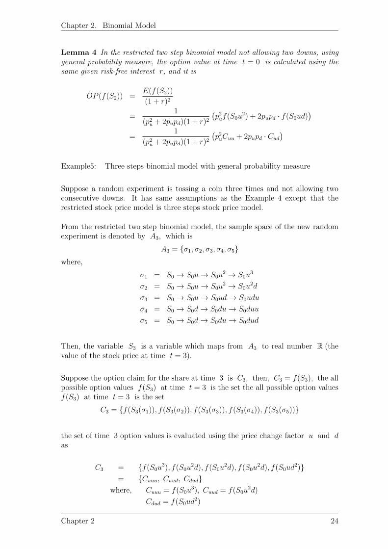
Lemma 4 In the restricted two step binomial model not allowing two downs, usinggeneral probability measure, the option value at time t = 0 is calculated using thesame given risk-free interest r, and it is
OP (f(S2)) =E(f(S2))
(1 + r)2
=1
(p2u + 2pupd)(1 + r)2
(p2uf(S0u
2) + 2pupd · f(S0ud))
=1
(p2u + 2pupd)(1 + r)2
(p2uCuu + 2pupd · Cud
)Example5: Three steps binomial model with general probability measure
Suppose a random experiment is tossing a coin three times and not allowing twoconsecutive downs. It has same assumptions as the Example 4 except that therestricted stock price model is three steps stock price model.
From the restricted two step binomial model, the sample space of the new randomexperiment is denoted by A3, which is
A3 = σ1, σ2, σ3, σ4, σ5where,
σ1 = S0 → S0u→ S0u2 → S0u
3
σ2 = S0 → S0u→ S0u2 → S0u
2d
σ3 = S0 → S0u→ S0ud→ S0udu
σ4 = S0 → S0d→ S0du→ S0duu
σ5 = S0 → S0d→ S0du→ S0dud
Then, the variable S3 is a variable which maps from A3 to real number R (thevalue of the stock price at time t = 3).
Suppose the option claim for the share at time 3 is C3, then, C3 = f(S3), the allpossible option values f(S3) at time t = 3 is the set the all possible option valuesf(S3) at time t = 3 is the set
C3 = f(S3(σ1)), f(S3(σ2)), f(S3(σ3)), f(S3(σ4)), f(S3(σ5))
the set of time 3 option values is evaluated using the price change factor u and das
C3 = f(S0u3), f(S0u
2d), f(S0u2d), f(S0u
2d), f(S0ud2)
= Cuuu, Cuud, Cdudwhere, Cuuu = f(S0u
3), Cuud = f(S0u2d)
Cdud = f(S0ud2)
Chapter 2 24

Chapter 2. Binomial Model
Suppose the three coin tosses are independent experiments from each other, andthe defined probability is p(up) = pu, p(down) = pd with pu + pd = 1 then, theprobabilities of outcomes in the restricted three steps sample space A3 are
P (σ1) = P (S0 → S0u)P (S0u→ S0u2)P (S0u
2 → S0u3) = p3
u,
P (σ2) = P (σ3) = P (σ4) = P (S0 → S0u)(S0u→ S0u2)P (S0u
2 → S0u2d) = p2
upd
P (σ5) = P (S0 → S0d)P (S0d→ S0duu2)P (S0d→ S0dud) = pup
2d
Since the sum of the probabilities in the restricted three step sample space A3 isnot equal to one, when calculating the expected option value E(f(S3)) at timet = 3, the normalized probabilities
P (σ1), P (σ2), P (σ3), P (σ4), P (σ5))are used instead of P (σ1), P (σ2)P (σ3), P (σ4), P (σ5). They are calculated by
P (σ) = P (σ)∑σ∈A3
P (σ), where σ ∈ A3.
To summarize, the share price value S3 and the share option payoff C3 = f(S3)at time t can be summarized by
S3 =
S0u
3 with p3up3u+3p2upd+pup2d
S0u2d with 3p2upd
p3u+3p2upd+pup2d
S0dud withpup2d
p3u+3p2upd+pup2d
and C3 =
Cuuu with p3u
p3u+3p2upd+pup2d
Cuud with 3p2updp3u+3p2upd+pup2d
Cdud withpup2d
p3u+3p2upd+pup2d
thus,
E(C3) = E(f(S3)) =∑σ∈A3
P (σ) · f(S3(σ))
=∑σ∈A3
(P (σ)∑
σ∈A3P (σ)
)· f(S3(σ))
=1
p3u + 3p2
upd + pup2d
(p3uf(S0u
3) + 3p2upd · f(S0u
2d) + pup2d · f(S0ud
2))
Next, the option price in the given three steps restricted model using general prob-ability measure is stated as
Lemma 5 In the restricted three steps binomial model not allowing two downs,using general probability measure, the option value at time t = 0 is calculated usingthe same given risk-free interest r, and it is
OP (C3) = OP (f(S3)) =E(f(S3))
(1 + r)3
=(p3uf(S0u
3) + 3p2upd · f(S0u
2d) + pup2d · f(S0ud
2))
(p3u + 3p2
upd + pup2d)(1 + r)3
=1
(p3u + 3p2
upd + pup2d)(1 + r)3
(p3uCuuu + 3p2
upd · Cuud + pup2d · Cdud
)Chapter 2 25

Chapter 2. Binomial Model
2.3 Calculate Paths Using Probability Generat-
ing function
2.3.1 Methods and Examples
In this section, the generating function approach in the methods and examples aremotivated from the definitions of generating function and probability generatingfunction on the page 92, 129 by Sedgewick, Robert, and Philippe Flajolet in thebook [14, chapter 3].
Based on the above two time steps binomial model of share prices, calculate ] ofpaths from initial share price state S0 to S2 using path probability generatingfunction. There are two ways to relate paths in a binomial model with pathprobability generating functions.
Method1, Relate paths of (initial state value → the final state value) of the binomialmodel with two sequence of numbers and corresponding two generating func-tions. In two time steps binomial model, that is, change (S0 → S2) totwo generating functions (
∑i=0 aiz
i,∑
i=0 piwi), where the sequence aiNi=0
represent the possible values of share value S2 at time 2, piNi=0 representthe corresponding probability sequence.
By definition, generating function can be associated with a sequence of num-bers. Then, if initial share price state S0 is a fixed value, path generatingfunction from S0 to S2 can be related to two sequences of numbers, one is thesequence of share values of S2 at time step t = 2, another is a correspondingprobability sequence.
Denote number of paths from S0 to S2 by M , and M is finite. In the twosteps binomial model M = 22 = 4.
Time 2 share value S2 is a random variable and can take any possible statevalues in the model, and let S2 = S0u
2, S0ud, S0d2, where S0ud contains
two paths from S0 to S2 in the model.
Denote number of distinct share state values S2 at time 2 by N . Since Mis finite, N is finite. In the two steps binomial model N = 22 − 1 = 3.
Since S0 is fixed, the set of possible values of (S0 → S2) can be uniquelyrepresented by the set of possible values of S2, which is a time 2 share valueand can take possible values in the set S2 = S0u
2, S0ud, S0d2. The set S2
can also be uniquely represented by the set u2, ud, d2. So, one possible
Chapter 2 26

Chapter 2. Binomial Model
value of (S0 → S2) corresponds to one possible product of step incrementfactors in the set u2, ud, d2.
If denote the set u2, ud, d2 by a sequence of numbers aiN−1i=0 , where
ai represent one possible sum of step increment factors and the sequence isordered by index i from 0 to N − 1, which denote the total number of upsteps in each path of the model.
Then, in the two steps binomial model, fix S0, the possible values of (S0 →S2) can be denoted by a sequence ai2
i=0, where a0 = 2d, a1 = u+ d, a2 =2u
In the model, suppose the defined probability measure for the two step bino-mial model is p(up) = pu, p(down) = pd with pu + pd = 1.
Then the share price states from S0 to S2 has the corresponding probabilitysequence pi2
i=0, where pi = P (S2 = ai) and the probability sequence isp0 = p2
d, p1 = 2pupd, p2 = p2u.
Thus, in terms of path probability generating function, the two step binomialmodel can be written as
GS(z) =2∑i≥0
aizi = 2d+ (u+ d)z + 2uz2
GP (w) =2∑i≥0
piwi =
2∑i≥0
P (S2 = ai)wi = p2
d + 2pupdw + p2uw
2
Method2, Motivated from the notations in the book [27], relate each path of (S0 →S1 → S2 → . . .→ SN) of the binomial model with two sequence of numbers.
One is aiNi=0, where ai = share price Si at time i , N = number oftime steps in the path.
The other is piNi=0, where pi denotes probability of share change fromt = i− 1 to t = i. S0 is fixed, so, set p0 = 1.
Each time period probability is defined by the probability measure pi→i+1(up) =pu, pi→i+1(down) = pd with pu + pd = 1.
The probability of time t share value Si is
P (S0 → S1 → . . .→ Si) = p0
i∏j=1
p(j−1→j) = p0
i∏j=1
pi.
Chapter 2 27

Chapter 2. Binomial Model
The generating function approach in the next two examples is motivated byby Sedgewick, Robert, and Philippe Flajolet from the definitions of generatingfunction in the book [14, chapter 3.1] and notations motivated from the lecturenote of financial mathematics [28, Chapter 2].
Example 2.3.1 [28, 14]:
In the two step binomial model, if only considering one share price changesand consider each path as two generating functions,
then, take one possible value of (S0 → S1 → S2) as an example, say,
take a path (S0 → S0u→ S0u2), since the state value S0 is fixed, the path can
be represented by (1, u, u2). If considering share price change factor at eachtime period, the path can also be represented by (1, u, u). Correspondingly, thepath probability sequence can be represented by (p0, p0p1, p0p1p2), or can berepresented by a sequence (p0, p1, p2) = (1, p1, p2).
To summarize, the path has two sequence represented as ai2i=0 = S0, S0u, S0u
2
pi2i=0 = p0, p1, p2 = 1, p1, p2
then, the path has two generating functions written asσ(x) =
2∑i≥0
aixi = S0 + S0ux+ S0u
2x2
Pσ(w) =2∑i≥0
piwi = 1 + p1w + p2w
2
Example 2.3.2 [28, 14]:
In the three step binomial model, If considering price changes of two sharesportfolio, and assuming only allowing one share to change upward in each timestep.
Denote the two share portfolio by (S1t , S
2t ), where t = 0, 1, 2, 3.
Then, one possible value of [(S10 , S
20) → (S1
1 , S21) → (S1
2 , S22) → (S1
3 , S23)]
represent a two share portfolio prices path.
Chapter 2 28

Chapter 2. Binomial Model
In each time step, the portfolio has two choices of change, either share 1change upward or share 2 change upward, that is, for 0 ≤ i, j ≤ 3,
state (S0ui, S0u
j) (S0ui+1, S0u
j) (share 1, up)
(S0ui, S0u
j+1) (share 2, up)
Figure 2.1: one step possible change of the portfolio
For example,
take a path [(S10 , S
20)→ (S1
0u, S20)→ (S1
0u, S20u)→ (S1
0u2, S2
0u)],
since the portofolio’s initial state value (S10 , S
20) is fixed, the path can be
represented by [(1, 1)→ (u, 1)→ (u, u)→ (u2, u)].
If considering the powers of change factors of each portfolio state value in thepath,
the path can also be represented by [(0, 0) → (1, 0) → (1, 1) → (2, 1)], whichis
(0, 0) (1, 0)
(1, 1) (2, 1)
Figure 2.2: one example path
Correspondingly, the path probability sequence can be represented by(p0,0, p0,0p1,0, p0,0p1,0p1,1, p0,0p1,0p1,1p2,1), or can be represented by a sequence(p0,0, p1,0, p1,1, p2,1) = (1, p1,0, p1,1, p2,1).
So, if in the three steps binomial model and considering two share portfolioprice changes, the probability sequence is pi,ji+j=3
i,j=0 , where pi,j denotes theprobability of share portfolio change from t = i+ j − 1 to t = i+ j.
The probabilities of the two choices of portfolio change are shown as
To summarize, the share portfolio path has two sequence represented as ai,j3i,j=0 = (S1
0 , S20), (S1
0u, S20), (S1
0u, S20u), (S1
0u2, S2
0u)
pi,ji+j=3i,j=0 = p0,0, p1,0, p1,1, p2,1 = 1, p1,0, p1,1, p2,1
Chapter 2 29
Chapter 2. Binomial Model
state (i, j) Pi+1,j (share 1, up)
Pi,j+1 (share 2, up)
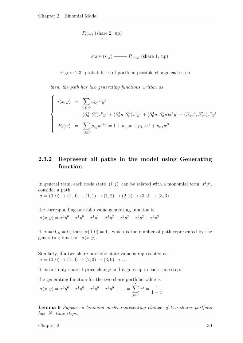
Figure 2.3: probabilities of portfolio possible change each step
then, the path has two generating functions written as
σ(x, y) =3∑
i,j≥0
ai,jxiyj
= (S10 , S
20)x0y0 + (S1
0u, S20)x1y0 + (S1
0u, S20u)x1y1 + (S1
0u2, S2
0u)x2y1
Pσ(w) =3∑
i,j≥0
pi,jwi+j = 1 + p1,0w + p1,1w
2 + p2,1w3
2.3.2 Represent all paths in the model using Generatingfunction
In general term, each node state (i, j) can be related with a monomial term xiyj,consider a pathσ = (0, 0)→ (1, 0)→ (1, 1)→ (1, 2)→ (2, 2)→ (3, 2)→ (3, 3)
the corresponding portfolio value generating function is
σ(x, y) = x0y0 + x1y0 + x1y1 + x1y2 + x2y2 + x3y2 + x3y3
if x = 0, y = 0, then σ(0, 0) = 1, which is the number of path represented by thegenerating function σ(x, y).
Similarly, if a two share portfolio state value is represented asσ = (0, 0)→ (1, 0)→ (2, 0)→ (3, 0)→ . . .
It means only share 1 price change and it goes up in each time step.
the generating function for the two share portfolio value is
σ(x, y) = x0y0 + x1y0 + x2y0 + x3y0 + . . . =∞∑j=0
xj =1
1− x
Lemma 6 Suppose a binomial model representing change of two shares portfoliohas N time steps.
Chapter 2 30

Chapter 2. Binomial Model
It can be seen that in σ(x, y) =∑∞
i,j=0 xiyj, if powers of terms in the generating
function uniquely corresponds to a time step sequence i + j = kk≤Nk=0 , then, thegenerating function can be a path.
Example 2.3.3 For example, a polynomial x0y0 +x2y0 is not a two share portfoliopath, since step (0, 0) → (2, 0) is not allowed by the assumption ( only one sharechange in each time step). It is obvious that the powers of terms in the polynomialcorresponds to a time step sequence 0, 2, and it missed time step 1.
The next example 1 is motivated from the Feynman path integral [13] and itsapplication in finance in the page 6 of the paper [2, Theorem 2] and [11].
Example 1:
Consider one model Ωn for one share prices of length n,
let a path σ = σ1σ2 . . . σn = one possible value of (S0 → S1 → S2 → Sn), and thepossible path σ = σ1σ2 . . . σn ∈ Ωn, where σi = the step change (i− 1, Si−1)→(i, Si).
Let σ(x) be the generating function for the path, and it is defined by σ(x) :=n∑i=0
Si(σ)x|σ1σ2...σi|, where |σ1σ2 . . . σn| is the number of steps of the path σ1σ2 . . . σi.
Then, the path generating function for the model is defined by
AΩn(x) :=∑σ∈Ωn
σ(x)
=∑σ∈Ωn
n∑i=0
Si(σ)x|σ1σ2...σi|
and the path probability generating function for the model is defined by
PΩn(w) =∑σ∈Ωn
n∑i=0
Pi(σ)w|σ1σ2...σi|
It is noted that
Si(σ) = the share value at time i of the path σ,
Pi(σ) = the state probability at time i in the path σ
= P (σ1σ2 . . . σi)
Chapter 2 31

Chapter 2. Binomial Model
Thus, in the model Ωn, the expected share price value at time n can be calculatedby
E[Sn(σ)] =∑
σ=σ1σ2...σn∈Ωn
Sn(σ)Pn(σ)
Suppose the model Ωn is a n steps binomial model, and the risk-free interest rateis r. Next is to calculate the price of the exotic option claim in the model.
Suppose the option claim for the share price at time t is Ct = f(St), for 1 ≤ t ≤ n.Let T be the final time, and 1 ≤ t ≤ T .
The exotic option claim in the model is defined by C =T∑j=1
f(St)
Thus, the option value of the exotic claim is stated as
Theorem 7 The option value of the exotic claim at time t = 0 is calculated usingthe given risk-free interest rate r and it is
OP (C) = OP (T∑j=1
f(St)) =T∑j=1
OP (f(St))
=T∑j=1
[(1 + r)−j · E(f(Sj))]
=T∑j=1
[(1 + r)−j ·
(∑σ∈Ωn
f(Sj(σ))Pj(σ)
)]
=∑
σ=σ1σ2...σn∈Ωn
T∑j=1
f(Sj(σ))Pj(σ)
(1 + r)j
The path calculation method in the theorem generalize the path calculation lemmain the paper [2] [11].
In the model Ωn, since the starting state of the share price is fixed, for each pathσ ∈ Ωn, set P0(σ) = 1. From the path probability generating function PΩn(w) ofthe model, it can be observed that
PΩn(0) =∑σ∈Ωn
P0(σ)
=∑σ∈Ωn
1
= ] of the possible paths in the model Ωn
Another useful form of generating functions of the model Ωn can be written as
Chapter 2 32

Chapter 2. Binomial Model
AΩn(x) =
n∑i=0
∑σ∈Ωn
Si(σ)xi
PΩn =n∑i=0
∑σ∈Ωn
Pi(σ)wi =n∑i=0
∑σ∈Ωn
P (σ1σ2 . . . σi)wi
Then, it can be observed that the coefficients has the following meaning,
∑
σ∈ΩnSi = the sum of the possible state values at time i∑
σ∈ΩnPi(σ) =
∑σ∈Ωn
P (σ1σ2 . . . σi)
= the sum of the corresponding states probabilities at time i
It is noted that if is useful to write the formula as above. If we assume the sum ofpossible share price values is finite at time i, with 0 ≤ i ≤ n,
Then, the corresponding generating functions for the model Ωn is valid for countingand Ωn becomes a combinatorial class.
Chapter 2 33

Chapter 3
Generating functions approach
A generating function(GF) is a clothesline on which we hang up a sequence ofnumbers for display(Herbert Wilf, 1994). Generating function can provide a compactrepresentation of a sequence and it is a method to encode a recurrence relation ona sequence. The key idea is to equivalent a recurrence relation on a sequence to afunctional equation satisfied by GF.
Suppose a random experiment is tossing a coin twice, if the value of a coin tossed ishead, denoted by 1, then stock price goes up by a factor u. if the value of a cointossed is tail, denoted by −1, then the stock price goes down by a factor d.
Therefore, the stock price is modelled by a two step binomial model.
Suppose the model use the probability measure defined by
P (up) = p, P (down) = q with p+ q = 1
Generating function is a way of representing a sequence of numbers, which cancorresponds to one particular share price path using the two ways of correspondencementioned in chapter 2.
3.1 Definitions of OGFs and EGFs
The definition 8 of ordinary generating function is motivated by Flajolet and Sedgewickon page 92 in the book [14, Chapter 3.1].
Definition 8 (Ordinary generating function) [14, Chapter 3.1]Given a sequence ak∞k=0 = a0, a1, a2, . . ., the function A(z) =
∑∞k≥0 ak · zk,
∀k ∈ N is called the ordinary generating function(OGF) of the sequence.
Notation: Use notation [zk]A(z) to refer to the coefficient ak. It is a formal powerseries, we are interested the coefficient ak of the formal power series.
In the next example, an example of sequence 1, 1, . . . , 1 is taken from the page93 in the book [14, Chapter 3.1], we provide a way to use the sequence to representa share price path with given initial share price S0, up and down change factor of
34

Chapter 3. Generating functions approach
the share price u, and d. Then, calculate the corresponding ordinary generatingfunction pairs.
Example 3.1.1 A sequence is:
1, 1, 1, . . . , 1; here, ak = 1, k = 0, 1, 2, . . .
Consider the correspondence ak∞k=0 ↔ Sk∞k=0;
S0 → S0u→ S0u2 → . . . ↔ (1, u, u2, . . .)
↔ (1, u, u, . . .) [Consider share price change factors]
↔ (1, 1, 1, . . .) [Powers of share price change factors]
pk∞k=0 denotes the probability of share price change from t = k − 1 to t = k.Set p0 = 1 which set the probability of share price at time 0 equal to S0 is 1.
The sequence corresponds to a path which have up at each step, and the probabilityof up at each step is p, and the number of step of the path is infinite. The pathcan has two sequences:
(S0, S0u, S0u2, S0u
3, . . .) and (1, p, p2, p3, . . .)
It has two ordinary generating function(OGF):(∞∑k≥0
S0ukzk,
∞∑k≥0
pkwk
)= (
S0
1− uz,
1
1− pw)
Sometimes it is more convenient to handle sequence by a generating function involv-ing a normalizing factor, it is called exponential generating function.
The definition 9 of ordinary generating function is motivated by Flajolet and Sedgewickon page 97 in the book [14, Chapter 3.2].
Definition 9 (Exponential generating function)
Given a sequence (a0, a1, . . . , ak, . . . ), the function A(z) =∑∞
k≥0 ak ·zk
k!, ∀k ∈ N is
called the exponential generating function(EGF) of the sequence.
Notation: Use notation k![zk]A(z) to refer to the coefficient ak. It is a exponentialpower series, we are more interested the coefficient ak of the exponential powerseries.
In the next example, the same example of sequence 1, 1, . . . , 1 is taken from thepage 93 in the book [14, Chapter 3.1], we provide a way to use the sequence torepresent a share price path with given initial share price S0, up and down changefactor of the share price u, and d. Then, calculate the corresponding exponentialgenerating function pairs.
Chapter 3 35

Chapter 3. Generating functions approach
Example 3.1.2 Sequence:
1, 1, 1, . . . , 1; here, ak = 1, k = 0, 1, 2, . . .
Consider the correspondence ak∞k=0 ↔ Sk∞k=0;
S0 → S0u→ S0u2 → . . . ↔ (1, u, u2, . . .)
↔ (1, u, u, . . .) [Consider share price change factors]
↔ (1, 1, 1, . . .) [Powers of share price change factors]
pk∞k=0 denotes the probability of share price change from t = k − 1 to t = k.Set p0 = 1 which set the probability of share price at time 0 equal to S0 is 1.
The sequence corresponds to a path which have up at each step, and the probabilityof up at each step is p, and the number of step of the path is infinite. The pathcan has two sequences:
(S0, S0u, S0u2, S0u
3, . . .) and (1, p, p2, p3, . . .)
It has Exponential generating function(EGF):(∞∑k≥0
S0uk z
k
k!,
∞∑k≥0
pkwk
k!
)= (S0e
uz, epw)
In the next example, an example of sequence 1, 1, 2, 6, 24, 120, . . . , n! is takenfrom the table 3.3 in the book [14, Chapter 3.2], we provide a way to use thesequence to represent a share price path with given initial share price S0, up anddown change factor of the share price u, and d. Then, calculate the correspondingexponential generating function pairs.
Example 3.1.3 Sequence:
1, 1, 2, 6, 24, 120, . . . ; here, an = n!, n = 0, 1, 2, . . .
Consider the correspondence ak∞k=0 ↔ Sk∞k=0;
S0 → S0u→ S0u2! → S0u
3! . . . ↔ (1, u, u2!, u3! . . .)
↔ (1, u, u2, u3 . . .) [Consider share price change factors]
↔ (1, 1, 2!, 3! . . .) [Powers of share price factors]
Chapter 3 36

Chapter 3. Generating functions approach
pk∞k=0 denotes the probability of share price change from t = k − 1 to t = k.Set p0 = 1 which set the probability of share price at time 0 equal to S0 is 1.
It corresponds to a path which have n up steps at each time step, and the probabilityof up at each step is p, and the number of step of the path is infinite. The pathcan be represented as the two sequences:
(1, u, u2, u3, u4, . . .) and (1, p, p2, p3, . . .)
Given a fixed initial share price S0, the sequence can be represented as exponentialgenerating function(EGF):(
∞∑k≥0
ukzk
k!,
∞∑k≥0
pkwk
k!
)= (euz, epw)
The benefits of exponential generating function provide a compact way to representfactorial jump share price path using exponential.
It is obvious that generating functions is a way to represent sequences. Whendoing some operations on a given sequence of numbers, the generating function willbe changed correspondingly. Then, definitions of common operations on ordinarygenerating functions(OGFs) are given follows.
3.2 Definitions of common operations on OGFs
The lemma 10 of scaling operation of ordinary generating function is motivated byFlajolet and Sedgewick on page 94 in the book [14, Chapter 3.1].
Lemma 10 (Scaling)If A(z) =
∑k≥0 akz
k is the ordinary generating function of a sequence ak∞k=0 =a0, a1, a2, . . ., when scaling the sequence by a sequence of scalar numbers 1, c, c2, . . .;each term ak is scaled with the same scalar ck.
Then A(cz) =∑
k≥0 akckzk is the ordinary generating function of the sequence
ckak∞k=0
In the next example, starting from the same example of sequence 1, 1, . . . , 1 whichis taken from the page 93 in the book [14, Chapter 3.1], a transformed share price byscaling operation is calculated, then, we calculate the corresponding scaling shareprice path ordinary generating function pairs.
Example 3.2.1 Example: Original sequence is:
1, 1, 1, . . . , 1; here, aN = 1, N = 0, 1, 2, . . .
Consider the correspondence ak∞k=0 ↔ Sk∞k=0;
Chapter 3 37

Chapter 3. Generating functions approach
From the example in section 6.1, the sequence corresponds to a path which have upat each step, and the probability of up at each step is p, and the number of stepof the path is infinite. The path can has two sequences:
(S0, S0u, S0u2, S0u
3, . . .) and (1, p, p2, p3, . . .)
It has two ordinary generating function(OGF):(∞∑k≥0
Sk zk,∞∑k≥0
pkwk
)=
(∞∑k≥0
S0ukzk,
∞∑k≥0
pkwk
)=
(S0
1− uz,
1
1− pw
)
The scaled sequence 2k∞k=0:
1, 2, 4, 8, 16, 32, . . . , 2N · 1, . . . ;
Consider the correspondence bk∞k=0 ↔ Sk∞k=0;
then, its ordinary generating function(OGF):∑k≥0
Skzk =
∑k≥0
S0uk2kzk =
S0
1− cuz=∑k≥0
S0uk2kzk
here, the coefficient of the generating function is [zk] S0
1−cuz = S0(uc)k
It corresponds to a path which have 2 up jump change at each time step comparedto the original share price path, and considering the probability of 2up at each timestep is p, and the number of step of the path is infinite. The path has two sequences:
(S0, S02u, S022u2, S023u3, . . .) and (1, p, p2, p3 . . .)
It has two ordinary generating function(OGF):
(∑k≥0
Skzk,
∞∑k≥0
pkwk) =
(∞∑k≥0
S0(2u)kzk,∞∑k≥0
pkwk
)=
(S0
1− 2uz,
1
1− pw
)
The lemma 11 of adding operation of two ordinary generating function is motivatedby Flajolet and Sedgewick on page 94 in the book [14, Chapter 3.1].
Lemma 11 (Addition)If A(z) =
∑k≥0 akz
k is the OGF of a0, a1, a2, . . . , ak, . . .
and B(z) =∑
k≥0 bkzk is the OGF of b0, b1, b2, . . . , bk, . . .
then A(z) +B(z) is the OGF of a0 + b0, a1 + b1, a2 + b2, . . . , ak + bk, . . .
Chapter 3 38

Chapter 3. Generating functions approach
In the next example, starting from the sequence 1, 1, . . . , 1 which is taken fromthe page 93 in the book [14, Chapter 3.1], and a sequence 1, 2, 4, 8, 16, 32, . . . , 2N ·1, . . ., a transformed share price is calculated by adding operation on the corre-sponding two share share price ordinary generating functions.
Example 3.2.2 Original sequence 1:
1, 1, 1, . . . , 1; here, aN = 1, N = 0, 1, 2, . . .
from the prior examples in this section, it can corresponds to a share price pathwhich has OGF: ∑
k≥0
S0ukzk =
S0
1− uz
Original sequence 2:
1, 2, 4, 8, 16, 32, . . . , 2N · 1, . . . ; here, bN = 2N , N = 0, 1, 2, . . .
it can corresponds to a share price path which has OGF:∑k≥0
S0(cu)kzk =S0
1− cuz
Consider the correspondence ck∞k=0 ↔ Sk∞k=0;
Sk∞k=0 corresponds to a path which have the generating function S0
1−uz + S0
1−cuz
considering the probability of Sk+1
Skat each time step is p, and the number of step
of the path is infinite. The path has two sequences:
(S0, S1, S2, S3, . . .) and (1, p, p2, p3 . . .)
It has two ordinary generating function(OGF):
(∑k≥0
Skzk,∞∑k≥0
pkwk) =
(S0
1− uz+
S0
1− cuz,
1
1− pw
)
From the prior examples(scaling) in this section, the sequence corresponds to a shareprice path which can be decomposed into one share price path Sk∞k=0 = S0u
k∞k=0
and another share price path Sk∞k=0 = S0(2u)k∞k=0.
The lemma 12 of Differentiation operation of ordinary generating function is mo-tivated by Flajolet and Sedgewick on page 94 and theorem 3.1 in the book [14,Chapter 3.1].
Chapter 3 39

Chapter 3. Generating functions approach
Lemma 12 (Differentiation)If A(z) =
∑k≥0 akz
k is the OGF of a0, a1, a2, . . . , ak, . . .
then zA′(z) =∑
k≥1 kakzk is the OGF of 0, a1, 2a2, 3a3, . . . , kak, . . .
From the lemma of differentiation operation on generating function and we gave adefinition 13 of differentiation path transformation as follows.
Definition 13 (Differentiation path transformation).Let share price sequence/path be denoted by Si, construct OGF: S(z) =
∑j Sjz
j.
Then, define a symbolic transform OGF, and called S(z) = S ′(z) and this definesa differentiation transformed path.
In the next example, from the definition of differentiation operation on generatingfunction, starting from the sequence 1, 1, . . . , 1 which is taken from the page 93in the book [14, Chapter 3.1], we provide a way to use the sequence representing theshare price and then derive the first order differentiation transformed share pricepath. Then, in the remarks after the example, we give the second order differentia-tion transformed share price starting from the same sequence 1, 1, . . . , 1.
Example 3.2.3 Example 1:
It is known that an ordinary generating function is:
1
1− z=∑N≥0
zN
its sequence:1, 1, 1, . . . , 1; here, aN = 1
from the prior examples in this section, it can corresponds to a share price pathwhich has OGF: ∑
k≥0
S0ukzk =
S0
1− uz
and the share price path is
Sk∞k=0 = (S0, S0u, S0u2, S0u
3, . . .)
Consider the correspondence bk∞k=0 ↔ Sk∞k=0;
then, its ordinary generating function(OGF):
∑k≥0
Skzk =
d( S0
1−uz )
dz= (
S0
1− uz)′ =
S0u
(1− uz)2
Chapter 3 40

Chapter 3. Generating functions approach
from the definition of differentiation of generating function, an OGF can be obtainedas follows by differentiating the original OGF:
z(S0u
(1− uz)2) =
∑k≥0
kSkzk =
∑k≥0
kS0ukzk
It corresponds to the share price path:
( 0, Sk∞k=1 ) = ( 0, S0u, S0u2, . . . )
Then,
S0u
(1− uz)2=
∑k≥0
kS0ukzk−1
=∑k≥1
kS0ukzk−1 [No considering the negative power of z]
Considering the probability of Sk+1
Skat each time step is p, and the number of step
of the path is infinite. The path has two sequences:
(S0, S1, S2, S3, . . .) and (1, p, p2, p3 . . .)
It has two ordinary generating function(OGF):
(∑k≥0
Skzk,∞∑k≥0
pkwk) =
(S0u
(1− uz)2,
1
1− pw
)
Compared to the original path Sk∞k=0 = S0uk∞k=0, its differentiation trans-
formed path becomes Sk∞k=0 = S0kuk∞k=1 = S0u, S02u2, . . ., which has a
jump Sk+1
Sk= k+1
ku.
Example 3.2.4 (how to use the differentiation operation on OGF):
1.
(S0
1− uz)′ = (
∑k≥0
Skzk)′ =
∑k≥0
kSkzk−1 =
∑k≥1
kSkzk−1
(S0
1− uz)′ =
S0u
(1− uz)2
then,S0u
(1− uz)2=∑k≥1
kSkzk−1
It corresponds to a share price path
Sk = ( k · Sk∞k=1 ) =(k · S0u
k∞k=1
)Chapter 3 41

Chapter 3. Generating functions approach
2. When proceeding the differentiation to the 2nd order,
(S0
1− uz)′′ = (
∑k≥0
Skzk)′′ = (
∑k≥0
kSkzk−1)′
=∑k≥0
k(k − 1)Skzk−2
=∑k≥2
k(k − 1)Skzk−2
(S0
1− uz
)′′=
(S0u
(1− uz)2
)′=
S02u2
(1− uz)3
then,
S02u2
(1− uz)3=
1
z2
∑k≥2
k(k − 1)Skzk
So, the sequence of numbers for the ordinary generating function
z2(S0u
2
(1− uz)3) =
1
2
∑k≥2
k(k − 1)Skzk =
1
2
∑k≥0
k(k − 1)Skzk
corresponds to a share price path
ck =k(k − 1) · Sk
2=k(k − 1)
2Sk =
(k
2
)Sk, k = 0, 1, 2, . . .
which has a jump Sk+1
Sk=
(k+12 )
(k2)u = k+1
k−1u and has the first two steps share
price of zero;
(c0 = 0, c1 = 0, c2 = S0u2, c3 = S03u3, c4 = S06u4, . . .)
=
(0, 0, S2,
(3
2
)S3,
(4
2
)S4, . . .
)where, Sk∞k=0 is the original share price path S0, S0u, S0u
2, . . .
Similar to 1st order differentiation of generating functions, if considering thedifferentiation to the 2nd order transformed share price path, it has the gener-ating function
S02u2
(1− uz)3=∑k≥2
k(k − 1)Skzk−2
It corresponds to the transformed share price path
Sk = ( k(k − 1) · Sk∞k=2 ) =(k(k − 1) · S0u
k∞k=2
)Chapter 3 42

Chapter 3. Generating functions approach
In general case, it is easy to get a common used sequence equation and we derivethe general order differentiation, say M-order, transformed share price path in thefollowing example.
Example 3.2.5 When M >= 1, a M-order differentiation of the ordinary gener-ating function is:
(S0
1− uz
)(M)
=S0M !uM
(1− uz)M+1=
(∑k≥0
Skzk
)(M)
=1
zM
∑k≥M
k(k − 1) . . . (k −M + 1)Skzk
Then,
zM(S0u
M
(1− uz)M+1) =
∑k≥M
k(k − 1) . . . (k −M + 1)
M !Skz
k =∑k≥M
(k
M
)Skz
k
it corresponds to a share price path
ck =k(k − 1) . . . (k −M + 1)
M !Sk =
(k
M
)Sk, k = 0, 1, 2, . . .
which has a jump Sk+1
Sk=
(k+1M )
( kM)u = k+1
k−M+1u and has the first M steps share price
of zero;
(c0 = 0, . . . , cM−1 = 0, cM = S0uM , cM+1 = S0(M + 1)uM+1, c4 = S0
M + 2
2uM+2, . . .)
=
(0, 0, . . . , SM ,
(M + 1
M
)SM+1,
(M + 2
M
)SM+2, . . .
)=
(0, 0, . . . , SM ,
(M + 1
1
)SM+1,
(M + 2
2
)SM+2, . . .
)where, Sk∞k=0 is the original share price path S0, S0u, S0u
2, . . .
if considering the differentiation to the M-th order transformed share price path, ithas the generating function
S0M !uM
(1− uz)M+1=∑k≥M
k(k − 1) . . . (k −M + 1)Skzk−M
It corresponds to the transformed share price path
Sk = ( k(k − 1) . . . (k −M + 1) · Sk∞k=1 ) =(k(k − 1) . . . (k −M + 1) · S0u
k∞k=1
)Remarks
Chapter 3 43

Chapter 3. Generating functions approach
1. It is easy to check the above ordinary generating function using a general factabout binomial coefficient formula(
−kn
)= (−1)n ·
(k + n− 1
n
);
that is,
S0uMzM(1− uz)−(M+1) = S0u
MzM∑k≥0
(−(M + 1)
k
)(uz)k
= S0uMzM
∑k≥0
(k + (M + 1)− 1
k
)(uz)k
= S0uMzM
∑k≥0
(k +M
k
)(uz)k
= S0
∑k≥0
(k +M
k
)(uz)k+M = S0
∑k≥M
(k
k −M
)(uz)k
=∑k≥M
(k
M
)S0u
kzk =∑k≥M
(k
M
)Skz
k
The lemma 14 of integration operation of ordinary generating function is motivatedby Flajolet and Sedgewick on page 94 and theorem 3.1 in the book [14, Chapter3.1].
Lemma 14 (Integration)If A(z) =
∑k≥0 akz
k is the OGF of a0, a1, a2, . . . , ak, . . .
then
∫ z
0
A(t)dt =∑n≥1
an−1
nzn is the OGF of 0, a0,
a1
2,a2
3, . . . ,
ak−1
k, . . .
In the next example, starting from the same example of sequence 1, 1, . . . , 1 whichis taken from the page 93 in the book [14, Chapter 3.1], a transformed share pricepath by integration operation is derived.
Example 3.2.6 It is known that an ordinary generating function is:
1
1− z=∑N≥0
zN
its corresponding sequence of numbers:
1, 1, 1, . . . , 1; here, aN = 1, N = 0, 1, 2, . . .
from the prior examples in this section, it can corresponds to a share price pathwhich has OGF: ∑
k≥0
S0ukzk =
S0
1− uz
Chapter 3 44

Chapter 3. Generating functions approach
and the share price path is
Sk∞k=0 = (S0, S0u, S0u2, S0u
3, . . .)
Consider the correspondence bk∞k=0 ↔ Sk∞k=0;
Since
S0
u(ln
1
1− uz)′ =
S0
1− uz= S0
∑k≥0
ukzk =∑k≥0
Skzk
Integrating both side with respect to z, we can obtain OGF:
S0
u(ln
1
1− uz) =
∑k≥0
Skzk+1
k + 1=∑k≥1
Sk−1zk
k
When k = 0, the initial share price should be set as S0 = 0 in the path Sk∞k=0,
so, the transformed share price path is
Sk∞k=0 =
(0, Sk−1
k∞k=1
)=
(0, S0u
k−1
k∞k=1
)
The lemma 15 of convolution operation of ordinary generating function is motivatedby Flajolet and Sedgewick on page 95 in the book [14, Theorem 3.1 ].
Lemma 15 (Convolution)If A(z) =
∑k≥0 akz
k is the OGF of a0, a1, a2, . . . , ak, . . .
and B(z) =∑
k≥0 bkzk is the OGF of b0, b1, b2, . . . , bk, . . .
then A(z)B(z) is the OGF of a0b0, a0b1 + a1b0, . . . ,∑
0≤k≤nakbn−k, . . .
Proof of the lemma:
A(z)B(z) =∑k≥0
akzk∑n≥0
bnzn
Distribute=
∑k≥0
∑n≥0
akbnzn+k
Change n to n-k=
∑k≥0
∑n≥k
akbn−kzn
Switch order of summation=
∑n≥0
∑0≤k≤n
akbn−kzn
Chapter 3 45

Chapter 3. Generating functions approach
The proof of convolution operation can be referred to [14, Theorem 3.1 ].
From the definition of convolution operation on generating function and we gavea corollary 16 of convolution path transformation as follows, then, we gave theconvolution share price path explanation.
Corollary 16 (Convolution path transformation)Let two share price sequences/paths be denoted by S1
i , S2i respectively, construct
two OGF: S1(z) =∑
j S1j z
j, S2(z) =∑
j S2j z
j. Then, define a symbolic convolu-
tion transform OGF, and called S(z) = S1(z)S2(z) and this defines a convolutiontransformed path
Sk∞k=0 =
( ∑0≤j≤k
S1jS
2k−j
)
Example 3.2.7 Convolution Path explanation:
The convolution transformed share price can be constructed as follows,
firstly, construct two share price paths S1j ∞j=0, and S2
j ∞j=0,
secondly, choose one share price paths, say, S2j ∞j=0, truncate the path at a finite
time k 0 ≤ k ≤ ∞
To find the convolution share price at time k, construct the inversed time shareprice path S2
j 0j=k,
Then,
Sk =∑
0≤j≤k
S1jS
2k−j
One common application is ’Partial sum’. The following example is taken from thepage 94 in the book [14, Section 3.1 ].
Example 3.2.8 If A(z) =∑
k≥0 akzk and
1
1− z=∑N≥0
zN ,
then1
1− zA(z) =
∑n≥0
(∑
0≤k≤n
ak)zn ,
So, [zN ]1
1− zA(z) =
∑0≤k≤N
ak
3.3 Methods using generating functions
The generating functions(GFs) are a useful method to solve linear recurrence equa-tions. It is also useful to count combinatorial classes with GFs.
Chapter 3 46

Chapter 3. Generating functions approach
In this section, we give the preliminary knowledges for using Flajolet symbolicmethod, which is motivated by Flajolet and Sedgewick in the book [14, Theorem3.1 ], [14, Chapter 5.2 ] and [15, Chapter I. 2.1.], we presented the preliminaryknowledge of symbolic method construction in a more compact way.
3.3.1 Solving recurrence equations
In this section, solving recurrence equations using generating function is stated whichis motivated by Flajolet and Sedgewick in the book [14, Section 3.3 ]. It follows anexample of solving recurrence equation which is taken from the page 104 in the book[14, Section 3.3 ].
Method description:
1. Create recurrence equation and make the recurrence equation valid for allpositive integer n;
2. Multiply both sides of the recurrence equation by zn and sum over on positiveinteger n;
3. Evaluate the sums to derive a functional equation satisfied by OGF.
4. Solve the equation to derive an explicit formula for the OGF.
5. Expand the OGF to obtain the coefficients of GF.
Example 3.3.1 Given a recurrence equation:
an = 5an−1 − 6an−2 ∀n ≥ 2 with a0 = 0 and a1 = 1
Find: the explicit formula of an, n ≥ 0.
Solution:
1. Make recurrence valid for all n, we add delta funtion on the RHS of recurrenceequation
δn,1 =
1, if n = 1
0, if n 6= 1
we get:an = 5an−1 − 6an−2 + δn,1
2. Multiply both sides by zn and sum over n ≥ 0
A(z) = 5zA(z)− 6z2A(z) + z
3. SolveA(z) =
z
1− 5z + 6z2
Chapter 3 47

Chapter 3. Generating functions approach
4. Factor denominator 1− 5z + 6z2 = (1− 3z)(1− 2z)Use partial fractions:
A(z) =c0
1− 3z+
c1
1− 2z
5. Solve for coefficients: c0 + c1 = 0
2c0 + 3c1 = −1
6. The coefficient
c0 = 1 c1 = −1
A(z) =1
1− 3z+
1
1− 2z
7. Use the related formulas in the section common operations on GF, it is easilyto obtain that
[zn]A(z) = 3n − 2n
3.3.2 Counting combinatorial classes(Symbolic Method)
In this section, the knowledge of symbolic method is stated which is motivated byFlajolet and Sedgewick in the book [14, Chapter 5.2] and the book [15, Chapter I.2.1.].
Description of Symbolic Method:
The symbolic method is an important method in analytic combinatorial. It is anapproach for translating formal definition of combinatorial objects into functionalequations on generating function. The symbolic method is dissected as follows,
• Define a class of combinatorial objects, say, A, B, C
• Define a notion of size of an object in combinatorial class, say, for α ∈A, the size |α|
• Define GF is sum over all members of the combinatorial class. say, A(z) ≡∑α∈A
z|α|
Each term zN in the GF corresponds to an object of size |α| = N .
Collect all the terms with the same size exponent N to expose counts thatcounting the number of objects with size N , say, denote by an.
• Define operations suitable for combinatorial constructions of different class ofcombinatorial objects.
Common used operations for combinatorial construction is union(sum), prod-uct, and sequence, definition of the three operations will be given in the latersection.
Chapter 3 48

Chapter 3. Generating functions approach
• Develop translations from combinatorial constructions to operations on GFs.
In the later section, using GF counting unlabelled objects is introduced andcorresponding transfer theorem for translating combinatorial constructions intoOGF is introduced as propositions and proof is given later.
Firstly, Definitions of Combinatorial Classes is given as follows.
Definition 17 (Combinatorial Classes) [14, Page 221]A combinatorial class A is a finite or countable set of combinatorial objects associ-ated with a size function for each object ‖ such that:
• ∀ α ∈ A, 0 ≤ |α| <∞ ;
• the number of elements of a given size is finite.
Remark: Define a class of combinatorial objects with associated size function, byintroducing symbolic method, we can get another view of generating function(GF).
Secondly, Definitions of Combinatorial Constructions is given as follows.
Definition 18 (Cartesian product/product) [14, Page 223-225]Let A and B be two combinatorial classes, their product(Cartesian product) is theset of ordered pair of copies of objects, one copy from A, and the other from B, i.e.it is defined as C = A × B = (α, β) : α ∈ A, β ∈ B, for notational economy,write the product set as C = A× B = αβ : α ∈ A, β ∈ B
Remark: For each object γ in the product class C, γ ∈ A × B, it has a sizefunction |γ| = |αβ| = |α| + |β|, because each object in the product set of A andB is one object from combinatorial class A followed by one object from anothercombinatorial class B.
Definition 19 (Combinatorial Sum/Disjoint Union) [14, Page 223-225]Let A and B be two combinatorial classes, their disjoint union(sum) is defined tobe the union of disjoint combinatorial classes without disjointness condition imposedon combinatorial classes.Using standard set-theoretic unions notations,the combinatorial sum of A and Bis defined as:
• 1st, Using two distinct markers and for the two combinatorial classesA and B; is a marker for A and for B.
• Each marker has a size function of value zero; | | = 0 and | | = 0 .
Then, the disjoint union(sum) is defined as C = A+ B := ( × A) ∪ ( × B).
Remark: Each object γ in the disjoint union class C = A+B is either γ ∈ ×Aor γ ∈ ×B, the object is a copy of the same size from the original combinatorialclasses A and B; that is, γ ∈ × A is a copy α ∈ A and γ ∈ × B is acopy β ∈ B. It is noted that γ ∈ A+ B, |γ| = the size it had originally.
Chapter 3 49

Chapter 3. Generating functions approach
Definition 20 (Sequence Construction) [14, Page 223-225]Let A be a combinatorial class, the sequence of A is a sequence of objects A , i.e.it is a class defined as an infinite sum by SEQ(A) = ε+A+A×A+A×A×A+. . .,in other words, SEQ(A) = (α1, . . . , αl) | l ≥ 0, αj ∈ A, 0 ≤ l ≤ l.
Remark:
1. ε is a set containing one object of size |ε| = 0, an object of size zero iscalled a neutral object; ε is a neutral object corresponding to (α1, . . . , αl),with l = 0.
2. To use symbolic method, the sequence of A defined above should also be acombinatorial class. By the definition of combinatorial class(Definition 17),we need to ensure the class satisfies (1) each object in the class has a sizefunction; (2) the number of objects with a given size, say, |γ| = n is finite, i.e.the coefficient of term zn , say, an is finite.
Question: How to make sure the sequence of a combinatorial classA, SEQ(A)is a combinatorial class?
Answer:
(a) It is obvious that the first condition satisfies, as each object γ ∈ SEQ(A)is constructed from combinatorial class A in which each object has sizefunction.
(b) To count the number of objects of size ′n′ in SEQ(A), we need to know
how many objects of size ′n′ there are in Aj = A×j· · · ×A; by definition
of product of combinatorial classes, the size of an object in Aj is the sumof the sizes of its j components.
Aim: we would like to make sure the number of objects of size ′n′ inSEQ(A) is finite.
If all objects in A have size at least one, then the objects in Aj have sizeat least j , then the terms of the form Aj, for j > n will never give riseto objects of size ′n′ , instead, if there are objects in A of size 0, thenwe may have objects of size ′n′ in all terms of Aj, including j > n ,therefore, there will be an infinite number of objects in SEQ(A) of size′n′ , it contradicts the definition of combinatorial class.
(c) In summary, when considering sequence operation of a combinatorialclass, say, SEQ(A) , we only consider the sequence construction SEQ(A)of combinatorial class A which does not have elements of size zero, thatis, A contains no object of size zero.
Thirdly, Definition of Basic Construction Blocks is given as follows.
Definition 21 (Basic building blocks) [14, Page 221]Let A be a combinatorial class, let α be an object in the combinatorial class, eachobject α ∈ A has a size function. An object of size one is called an atom. It builds
Chapter 3 50

Chapter 3. Generating functions approach
up an atomic class, denoted by Z. An object of size zero is called a neutral object,it builds up a neutral class, denoted by E. If a combinatorial class contains nothingand has no object, it is called empty class, denoted by ∅, when translating it intoGF, its GF is ’0’, then there is no corresponding term z|α|.
Sequence construction: [15, Page 25]
1. If a set B is a combinatorial class,
Then, the sequence class denoted by SEQ(B), it is defined by an infinite sumSEQ(B) = ε+ B + (B × B) + (B × B × B) + . . ., where
ε is a neutral object of size zero.
2. The sequence represents the combinatorial class A, where A = (β1, . . . , βl) | l ≥0, βj ∈ B. The neutral object (structure) in A corresponds to when l = 0;if l = 0, the sequence is (β1, β0) and it is not valid. So, it represent theempty word ε which has size (here, length) zero.
3. The combinatorial class B must not contain object of size 0, otherwise,inside the class A = SEQ(B), fix size n, the number of elements of size nwill be infinite.
4. From the definition of size for sums and products, for any element α =(β1, . . . , βl) ∈ A, the size of the element is the sum of the size of its
components, that is, |α| =l∑
i=1
|βi|
Multiset construction: [15, Page 26]
1. Multisets are finite sets but arbitrary repetition of elements are allowed.
2. If a combinatorial class A is obtained by all finite multisets of elements fromB, the set A is denoted by A = MSET (B).
3. The multiset constructed from the set B is defined by
MSET (B) = SEQ(B)/R
with the equivalence relation R is defined by (α1, . . . , αr) R (β1, . . . , βr) iffthere exists some arbitrary permutation σ of [1, . . . , r] such that, for all1 ≤ j ≤ r, βj = ασ(j).
Cycle construction: [15, Page 26]
1. Notation: if B is a combinatorial class, then the cycle construction from theclass B is denoted by CY C(B).
Chapter 3 51

Chapter 3. Generating functions approach
2. Assume no empty cycle, CY C(B) is defined by
CY C(B) := (SEQ(B) \ ε)/S
where for any two elements in the class CY C(B), S is their equivalencerelation defined by (β1, . . . , βr) S (β′1, . . . , β
′r) iff there exists some circular
shift τ of [1, . . . , r] such that, for all 1 ≤ j ≤ r, β′j = β1+(j−1+d) mod r
.
3. For example, (β1, β2, β3) S (β2, β3, β1) S (β3, β1, β2),
here, r = 3, (β2, β3, β1) = (β′1, β′2, β
′3), it circularly shift one element from
(β1, β2, β3),
so, it shift d = 1, β′j = β1+(j−1+1) mod 3
(β3, β1, β2) = (β′1, β′2, β
′3), it circularly shift two element from (β1, β2, β3),
so, it shift d = 2, β′j = β1+(j−1+2) mod 3
It is noted that 1 ≤ d ≤ r.
4. For example, assuming no empty sequence, the set of sequences formed fromthe class B = a, b is denoted by
A(3) = (β1, β2, β3)|βj ∈ B = SEQ3(B) = B × B × B
then, ]A(3) = 23 = 8
The class of cycles formed from the class A(3) is CY C(3)(B) = A(3)/S, whereS is defined by (β1, β2, β3) S (β′1, β
′2, β
′3) iff there exists some circular shift
τ of [1, 2, 3] such that, for all 1 ≤ j ≤ 3, β′j = β1+(j−1+d) mod 3
, with
1 ≤ d ≤ 3, representing the number of positions shifted.
Then, sequences are grouped into equivalence classes according to the relationS, and ]CY C(3)(B) = 4 = 2r−1, with r = 3.
Powerset construction: [15, Page 26]
1. Notation: PSET (B), where B is a combinatorial class.
2. A powerset is a combinatorial class consisting of all finite subsets of thecombinatorial class B, if starts from a multiset construction MSET (B) ofB, the powerset is formed from multisets that involve no repetitions.
3. Let A = (β1, . . . , βl) | 0 ≤ l ≤ card(B), βi 6= βj if i 6= j, βi ∈ B,
Then, A = PSET (B) = A/R, with the equivalence relation R is definedby (α1, . . . , αr) R (β1, . . . , βr) iff there exists some arbitrary permutation σof [1, . . . , r] such that, for all 1 ≤ j ≤ r, βj = ασ(j).
4. For any element α = (β1, β2, . . . , βl) ∈ A = PSET (B), define its size functionusing notation | · | for the size function, then, |α| =
∑li=1 |βi|
Chapter 3 52

Chapter 3. Generating functions approach
5. For example, represent natural numbers, Let Z := ·, with · an atom ofsize 1,
Then, I = SEQ(Z) ε = (β1, β2, . . . , βl)|l ≥ 1, βi ∈ B
Three common operations on combinatorial classes (product, disjoint union andsequence) are very often be used to define a combinatorial class in terms of atomsand other combinatorial classes, when counting number of combinatorial objects in acombinatorial class. When using the three common operations get a definition of thecombinatorial class, use transfer theorem to translate operations on combinatorialclasses into operations on generating function. The transfer theorem are introducedas follows. Which is motivated by Flajolet and Sedgewick in the book [14, Page225].
Proposition 22 [14, Theorem 5.1]The generating function for the product of two combinatorial classes is the productof their generating functions.
Suppose: We are given generating functions A(z) and B(z) for A and B,Aim: Prove the generating function for A× B equals to A(z)B(z).
Proof:Following definition of product operation in the last section, if
C = A× B = αβ : α ∈ A, β ∈ B
The key idea is that the sum over all product members αβ ∈ A×B equals to twosteps: (1) firstly, for each member α ∈ A, sum over the α followed by the sumover all members β ∈ B; (2) secondly, sum over all members α ∈ A, followed bythe sum over all members β ∈ B. that is,∑
αβ∈A×B
=∑α∈A
∑β∈B
Besides, for each object in A× B, its size function is |αβ| = |α|+ |β|Therefore, ∑
γ∈A×B
z|γ| =∑
αβ∈A×B
z|αβ|
=∑α∈A
∑β∈B
zα|+|β|
distribute=
∑α∈A
z|α|∑β∈B
z|β|
= A(z)B(z)
Proposition 23 [14, Theorem 5.1]The generating function for the sum(disjoint union) of two combinatorial classes(disjoint)is the sum of their corresponding generating functions.
Chapter 3 53

Chapter 3. Generating functions approach
Suppose: We are given generating functions A(z) and B(z) for A and B,Aim: Prove the generating function for A+ B equals to A(z) +B(z)
Proof: Following definition of disjoint union operation in the last section, if
C = A+ B = γ : γ ∈ A ∪ B
Firstly, for each object, γ ∈ A ∪ B, its size equals to the size it had originally.Secondly, as γ is copies fromA or copies from B, then the sum over all disjoint unionmembers γ ∈ A∪B, equals to that taking sum over members in each combinatorialclass A and B respectively, then taking an addition of the two sum. That is,
∑γ∈A+B
if A and Bare disjoint set
=∑γ∈A
+∑γ∈B
Therefore, we obtain
∑γ∈A+B
z|γ| =
(∑γ∈A
+∑γ∈B
)z|γ|
=∑γ∈A
z|γ| +∑γ∈B
z|γ|
= A(z) +B(z)
Following definition of Sequence operation in the last section, if
SEQ(A) = ε+A+A×A+A×A×A+ . . .
we give the following proposition,
Proposition 24 [14, Theorem 5.1]The generating function for the sequence of a combinatorial class whose generatingfunction is A(z) is 1
1−A(z).
Suppose: Given a generating function A(z) for a combinatorial class A ,
Aim: Prove the Generating function for SEQ(A) equals to 11−A(z)
Proof:If we assume there are no objects of size 0 in A, then SEQ(A) is also a combi-natorial class.Following definition of sequence operation in the last section, we know
SEQ(A) = ε+A+A×A+A×A×A+ . . .
By applying the transfer theorem for disjoint union and product operations, we cantranslate the operations on combinatorial classes in the combinatorial class SEQ(A)into corresponding generating function, denote generating function of SEQ(A) byS(z), then we obtain,
S(z) = 1 + A(z) + A(z)2 + A(z)3 + · · ·
=1
1− A(z)
Chapter 3 54

Chapter 3. Generating functions approach
Remark: we know 11−x = 1 + x + x2 + x3 + . . . the series converges at all values
except for x = 1. We have assumed no object of size ’0’ in the combinatorial classA, therefore, in its Generating function A(z), there is no term z0 = 1, therefore wecan substitute A(z) to x, we can obtain 1
1−A(z).
Next, from the definition of symbolic operation on generating functions, we gave adefinition 25 of symbolic path transformation as follows.
Definition 25 (Symbolic path transformation)Let share price sequence/path be denoted by Si, construct OGF: S(z) =
∑j Sjz
j.
Then, define a symbolic transform OGF, and called S(z) = 11−S(z)
and this definesa symbolic transformed path.
3.4 Examples of counting using symbolic method
We have discussed dissection of symbolic method in the Section 3.3, in this section,we will use symbolic method to count common fundamental combinatorial classes.
Firstly, count binary tree with two different definition of size function.
Secondly, count general trees and forests.
Thirdly, count unrestricted lattice paths in 1 dimension and 2 dimensions respec-tively.
Fourthly, count restricted lattice paths from (0,0) to (n,n) with the restriction thatnever going above the diagonal line.
3.4.1 Count Binary Trees with different size function
Motivated by Flajolet and Sedgewick, along the lines of description of the generatingmethod of enumeration of binary trees in [14, Chapter 3.8], applying the symbolicconstruction of binary trees described on page 228 in [14, Chapter 5.2], we give thefollowing Question1, Question2, and present the solution in an organised way.
Question1: How many binary trees with N internal nodes?
Answer:
1st, Starting from a definition of a combinatorial class of binary trees.
Definition 26 [14, Page 258] A binary tree is an external node or an internalnode attached to an ordered pair of binary trees called the left subbinary treeand the right subbinary tree of that internal node. Denote the combinatorialclass of binary trees by T .
2nd, Define a notion of size function for each object in the combinatorial class ofbinary trees T .
Chapter 3 55

Chapter 3. Generating functions approach
From the question, we give each binary tree t ∈ T a size function,
|t| ≡ the number of internal nodes in a binary tree t ∈ T
3rd, From the question, we would like to find the number of binary trees with Ninternal nodes, so, define
TN ≡ the number of binary trees with N internal nodes
4th, By symbolic method, define a generating function(GF) for the combinatorialclass of binary tree; its GF is the sum over all members of the class of binarytrees; here, we use ordinary generating function(formal power series)
T (z)define≡
∑t∈T
z|t|
Each object of size N corresponds to each term zN in the GF, collect all theterms with the same size exponent to expose counts TN , that is, the numberof binary trees with N internal nodes, therefore, the definition of GF for thecombinatorial class is
T (z)define≡
∑t∈T
z|t|
=∑N≥0
TNzN
5th, Define a combinatorial construction for the combinatorial class of binary trees.
The construction process can be done in two steps.
Firstly, define basic building blocks for the combinatorial class: (1) by thedefinition of binary trees class, there are two types of basic blocks; one isexternal node, denoted by ’’ , the other is internal node, denoted by ’•’.(2) Based on the definition of size function,
|t| ≡ the number of internal nodes in t ∈ T,
we classify the two building blocks into atomic class and neutral class respec-tively; the atomic class contains an internal node of size 1, which contributessize ’1’ to the size exponent of z in the GF (z|t|), denote the atomic classby Z•. Its generating function is z1 = z. The neutral class, denotedby Z, contains an external node of size ’0’, which has no contribution tothe size of an object t ∈ T , and contributes size ’0’ to the size exponentof z, its generating function is z0 = 1. Secondly, make the combinatorialconstruction of the combinatorial class.
Based on the definition of the combinatorial class, define the class in terms ofbasic building blocks and other combinatorial classes by using decompositiontechniques and three common operations on combinatorial classes mentionedin the Section 3.4.2.
Chapter 3 56

Chapter 3. Generating functions approach
Here, by definition of the class, the class of binary trees can be a class whichcontains an external node or a class which contains an internal node followedby an ordered pair of two combinatorial class of binary trees.
After the two steps of the combinatorial construction, the construction can beobtained as follows,
T = Z + T × Z• × T
6th, Apply the transfer theorem between operations on combinatorial classes andoperations on generating functions. Here, we use ordinary generating func-tion(OGF), we obtain the equation:
T (z) = 1 + zT (z)2
solvequadratic equation
=⇒ T (z) = 1±√
1−4z2z
Question: we only need one generating function, how can we decide which oneto choose?
Answer:
zT (z) =1±√
1− 4z
2
take z = 0, then LHS = 0, RHS should also equal to 0, when z = 0.
So, we choose T (z) = 1−√
1−4z2z
.
7th, Finally, expand the coefficient of GF T (z) to obtain the explicit formula forthe number of binary trees with N internal nodes, TN .
from
zT (z) =1−√
1− 4z
2,
we get,
[zN ]T (z) = [zN+1]
(1−√
1− 4z
2
)Expand via generalized binomial theorem,
1−√
1− 4z
2=
1
2− 1
2(1− 4z)
12
=1
2− 1
2
∑N≥0
((12
N
)(−4z)N
)= −1
2
∑N≥1
((12
N
)(−4)NzN
)
Chapter 3 57

Chapter 3. Generating functions approach
Therefore,
TN = [zN ]T (z) = [zN+1]
(1−√
1− 4z
2
)= −1
2
(12
N + 1
)(−4)N+1
= −1
2·
12(1
2− 1)(1
2− 1) . . . (1
2−N)(−4)N · (−4)
(N + 1)!
=(−1
2)(−3
2)(−5
2) . . . (−2N−1
2)(−4)N
(N + 1)!
Distribute(−2)N
among factors=
1 · 3 · 5 · · · (2N − 1) · 2N
(N + 1)!
=1
N + 1· 1 · 3 · 5 · · · (2N − 1)
N !· 2 · 4 · 6 · · · (2N)
1 · 2 · 3 · · ·N
=1
N + 1
(2N
N
)
Question2: How many binary trees with N external nodes?
Answer:
1st, Starting from a definition of a combinatorial class of binary trees. The def-inition is the same as the 1st step in Question1. Again, denote the class ofbinary trees by T .
2nd, Define a notion of size function of each object in the combinatorial class ofbinary trees. To distinguish Question2’s size function with Question1, fromthe Question2, we define,
t ≡ the number of external nodes in a binary tree t ∈ T
3rd, From the question, we would like to find the number of binary trees with Nexternal nodes. Define,
TN ≡ the number of binary trees with N external nodes
4th, By symbolic method, define a GF for the combinatorial class of binary tree.to distinguish with Question1, sum over all members of the binary tree,and itsGF is defined by
T(z)define=
∑t∈T
z t
collect all terms withthe same exponent
=∑N≥0
TN · zN
Chapter 3 58

Chapter 3. Generating functions approach
5th, Combinatorial Construction; the construction process can be done in two steps.
Firstly, define basic building blocks for the combinatorial class: (1) the defini-tion of the binary tree class is the same as Question1, there are also two typesof basic blocks, that is, external node() and internal node(•) .
(2) based on the definition of size function in Question2,
t ≡ the number of external nodes in a binary tree t ∈ T,
External node and internal node builds up atomic class and neutral classrespectively.
Atomic class, denoted by Z, contains an external node of size 1, whichcontributes size ’1’ to the exponent of z in the GF(z t ), and its generatingfunction is z1 = z.
Neutral class, denoted by Z•, contains an internal node, which does notcontribute to the size of an object t ∈ T and contributes ’0’ to the exponentof ’z’, its generating function is z0 = 1.
Remark: No empty class, so, in the construction of the class, the buildingblock definitely contribute a term in the GF. Neutral class which contains anobject of size ’0’ , does not contribute to the size of an object t ∈ T but docontribute a term in the GF, that is constant term z0 = 1. However, emptyclass does not contribute to a term in the GF.
Secondly, make combinatorial construction by defining the class of binary treein terms of basic building blocks and other combinatorial classes. Similarly,use decomposition techniques and three common operations for combinatorialclasses.
In Question2, the class of binary tree can either be a class which contains anexternal node, or be a class which contains an internal node followed by anordered pair of two combinatorial classes of binary trees.
After the two steps of making combinatorial construction, we obtain construc-tion:
T = Z + T × Z• × T
Remark: it is observed that the combinatorial construction is the same as theQuestion1 in this section.
6th, Apply the transfer theorem from operations on combinatorial classes to oper-ations on generating functions. Here, we use OGF and obtain OGF equationsas follows,
T(z) = z + T(z)2
solve the quadratic,
T(z) =1±√
1− 4z
2
Chapter 3 59

Chapter 3. Generating functions approach
Recall in the Question1,
zT (z) =1±√
1− 4z
2
Therefore, we can find the GF relationship between Question1 and Question2,
T(z) = zT (z)
then,
[zN ]T(z) = [zN−1]T (z)
=1
N
(2(N − 1)
N − 1
)
Remark: from the result of Question1, we know that
the number of binary trees with the number of binary trees with
N external nodes = N − 1 internal nodes
It is noted that the above result is consistent with the following lemma that statesthe relationship between (] external nodes) and (] internal nodes) in a binary tree.
Lemma 27 [14, Page 260] The number of external nodes in any binary tree isexactly one greater than the number of internal nodes.
Proof: Let
e ≡ ] of external nodes in a binary tree,
i ≡ ] of internal nodes in a binary tree
Key idea: count ] of edges(links) in a binary tree in two different ways.
1st, By definition of a binary tree, each internal node has exactly two links ’from’it, so the number of links in the binary tree is ’2i’.
2nd, Again, by definition of a binary tree, each node except for the root has exactlya link ’to’ it, so, the number of links in the binary tree is ’i+ e− 1’.
3rd, The number of links in the binary tree by different counting method shouldobtain the same number. So, equating the two number we got,
2i = i+ e− 1
⇒ i = e− 1
Chapter 3 60

Chapter 3. Generating functions approach
3.4.2 Count Trees and Forests
In the last section, we considered a combinatorial class of binary trees; in a binarytree, no node have more than two children and can only have 0 child or 2 children.In this section, we consider general trees.
In this section, the definitions of trees, forests, and the enumeration question offorests and trees are motivated by Flajolet and Sedgewick in the book [14, Chapter6.2], and we gave more detailed explanation using symbolic method in the solutionof the enumeration question.
Definition 28 [14, Page 261] A tree(also called a general tree) is a node(called theroot) connected to a sequence of disjoint trees.
Definition 29 [14, Page 261] A forest is a sequence of disjoint trees.
Remark: from the definition of a general tree and a forest, it can be observed thatthere is a one-to-one correspondence between the class of forests and the class ofgeneral trees. Each forest with N nodes corresponds to a general tree with N + 1nodes by adding a root for the forest. That is, each tree is a root followed by aforest.
Question: [14, Theorem 6.2] How many forests and trees with N nodes respectively?
Answer:
1st, Starting from definitions of two combinatorial classes.
Denote the class of general trees by ’G’.
Denote the class of forests by ’F ’.
2nd, Define a notion of size function for each object in the two combinatorial classesrespectively.From the question, we give each tree g ∈ G a size function
|g| ≡ the number of nodes in a general tree g ∈ G
and give each forest f ∈ F a size function
|f | ≡ the number of nodes in a forest f ∈ F
3rd, From the question, we would like to find the number of forests and trees withN nodes, we define
GN ≡ the number of trees with N nodes,
FN ≡ the number of forests with N nodes.
4th, Apply symbolic method, define a GF for the two combinatorial class respec-tively. Their GF is the sum over all members of each combinatorial classrespectively. Here, we use OGF.
G(z)define≡
∑g∈G
z|g|
Chapter 3 61

Chapter 3. Generating functions approach
Each object of size N corresponds to a term zN in the GF, collect all the termswith the same size exponent to expose counts GN , that is, the number of treeswith N nodes, therefore,
G(z)define≡
∑g∈G
z|g|
=∑N≥0
GNzN
Similarly,
F (z)define≡
∑f∈F
z|f |
Each object of size N corresponds to a term zN in the GF, collect all theterms with the same size exponent to expose counts FN , that is, the numberof forests with N nodes, therefore,
F (z)define≡
∑f∈F
z|f |
=∑N≥0
FNzN
5th, Make a combinatorial construction for the two combinatorial classes.
The construction process can be done in two steps.
Firstly, define basic building blocks. (1) By the definition of classes of forestsand trees, there are only one type of basic block, that is, a node. (2) Based onthe definition of their size functions, we classify ’node’ into an atomic class,denoted by Z, because, for both combinatorial class(forests, trees), ’a node’contributes size ’1’ to their size functions. In each combinatorial class, itsgenerating function is z1 = z.
Secondly, Make the combinatorial construction for the two combinatorial classesrespectively. Use the three common operations to define each combinatorialclass in terms of basic building blocks and other combinatorial classes.
(1) By definition of the combinatorial class of forests, it is a sequence of disjoint(general) trees
F = SEQ(G)
Remark: F can be empty, that is, F = E +G+G×G+G×G×G · · · . If Fis empty, G is only a node.
(2) By definition of the combinatorial class of general trees, as we have observeda one-to-one correspondence between a forest and a general tree, that is, ageneral tree is a node(called root) followed by a forest, we define,
G = Z × F
Chapter 3 62

Chapter 3. Generating functions approach
6th, Apply the transfer theorem from operations on combinatorial classes to oper-ations on generating functions. Here, we use OGF, and obtain OGF equation:
F (z) =1
1−G(z)and G(z) = zF (z)
Together the two equations, obtain:
F (z)− zF (z)2 = 1
solvequadratic equation
=⇒ F (z) = 1±√
1−4z2z
Similarly, to equate the equation, choose: zF (z) = 1−√
1−4z2
Recall in Question1 of Section 3.5.1, the GF equation for binary trees with Ninternal nodes is
zT (z) =1−√
1− 4z
2
Therefore, F (Z) = T (z), recall the result in Question1 of Section 3.5.1, thenumber of forests with N nodes is,
FN = [zN ]F (z) = [zN ]T (z) = TN
=1
N + 1
(2N
N
)Besides, we know G(Z) = zF (z), so,the number of trees(general trees) withN nodes is,
GN = [zN ]G(z) = [zN−1]F (z) = FN−1
=1
N
(2(N − 1)
N − 1
)
3.4.3 Count general binary strings that contain consecutive0’s less than 3
In this section, we enumerate general binary strings with restriction that the max-imum number of consecutive 0’s is 2. The idea is motivated by Flajolet andSedgewick in the book [14, Page 226-227] and take the calculation idea from [16],we gave the detailed explanation of solution using Flajolet symbolic method.
One QuestionNotation:
. ’+’: disjoint union for sets;
. ’×’: Cartesian product for sets;
Chapter 3 63

Chapter 3. Generating functions approach
. Z0: the set 0;
. Z1: the set 1;
. Z0 + Z1 = 0⋃1 = the set 0, 1;
. Let A,B be two sets, A×B = (α, β) : α ∈ A, β ∈ B denoted=byαβ : α ∈ A, β ∈
B;
. Let A,B be two sets, assume A, B are disjoint, their disjoint union(sum) isdefined as A + B = the set of disjoint copies of objects in A and in B =γ : γ ∈ A ∪ B; (Assume the two sets are disjoint sets, if not disjoint, workwith A× ε1 and B × ε2 )
. Let empty set denoted by ∅, ∅ = ε, SEQ(A) = ∅+A+A×A+A×A×A+. . .Remark: The set A must not contain empty element, otherwise we cannotcount the set SEQ(A) by a specific characteristic, for example, if A has emptyelements in the set SEQ(A) that has length ’n’, then, an would be infinitenumber, it is nonsense to count SEQ(A) by length.
. SEQ(Z0) = SEQ(0) = ε, 0, 00, . . . == ∅+ 0+ 00+ . . .;
. SEQ(Z1 × SEQ(Z0)) = SEQ(1 × ε, 0, 00, . . .) = SEQ(1, 10, 100, . . .)
Represent a set by generating function by counting the length of each element inthe set.
In the following, length(α)denoted
=by|α|
GF (A) =∑α∈A
a|α| · z|α| =∞∑n=0
an · zn
Where a|α| = an = alength(α) = ] of elements in the set A that has length(α)= n.
GF (B) =∑β∈B
b|β| · z|β| =∞∑n=0
bn · zn
Where a|β| = bn = alength(β) = ] of elements in the set B that has length(β)= n.
GF (A+B) =∑
γ∈(A+B)
c|γ| · z|γ| =∑γ∈A
c|γ| · z|γ| +∑γ∈B
c|γ| · z|γ|
=∞∑n=0
an · zn +∞∑n=0
bn · zn
= GF (A) +GF (B)
Chapter 3 64

Chapter 3. Generating functions approach
Where A+B are disjoint union of a set A and a set B; it is the set of disjoint copiesof objects in A and in B. (Assume the two sets are disjoint sets, if not disjoint,work with A× ε1 and B × ε2 ).
GF (A×B) =∑
γ∈A×B
c|γ| · z|γ| =∑
αβ∈A×B
c|α|+|β| · z|α|+|β|
=∞∑n=0
(∑
k1+k2=n
ck1+k2) · zn
=∞∑n=0
(∑
k1+k2=n
ak1 · bk2) · zk1 · zk2
=∞∑n=0
(n∑k=0
ak · bn−k) · zk · zn−k =∞∑k=0
∞∑n=k
akzk · bn−kzn−k
=∞∑k=0
akzk ·
∞∑n=k
bn−kzn−k = GF (A) ·GF (B)
Then, use the above generating function for the sets by counting the length of eachelement in the sets, find the generating function for the set SEQ(A) = ∅+A+A×A+ A× A× A+ . . ., that is,
GF (SEQ(A)) = GF (∅+ A+ A× A+ A× A× A+ . . .)
= GF (∅) +GF (A) + (GF (A))2 + (GF (A))3 + . . .
calculate GF (∅), that is,
length(α)denoted
=by|α|
GF =∞∑n=0
an · znempty set has no elements
=length is 0, let a0=1
1
=⇒ GF (SEQ(A)) = 1 +GF (A) + (GF (A))2 + (GF (A))3 + . . .
=1
1−GF (A)
Then, use the above notation and formulas to solve the next question.
Question: Count general binary strings that contain consecutive 0’s less than 3.
Idea: Characterize general bitstrings by grouping them into blocks staring with 1.A bitstring can be constructed from zero blocks starting with 1 or from more blocksstarting with 1 followed by zero or more 0’s. The bitstring may be preceded by zeroor more 0’s.Firstly, use this characterize to construct general binary string and find its gener-ating function. Secondly, construct the restricted binary string and use generatingfunction to count the question.
Chapter 3 65

Chapter 3. Generating functions approach
Answer:
Let Z0 = 0, Z1 = 1, Z0 + Z1 = 0, 1then, zero or more 0’s is the set
SEQ(Z0) = ε, 0, 00, 000, . . .
block starting with 1 followed by zero or more 0’s is the set
Z1 × SEQ(Z0) = 1 × ε, 0, 00, 000, . . .= 1, 10, 100, 1000, . . .denoted
=by
Z1SEQ(Z0)
Remark: the block does not contain empty element, so we can count the set of zeroor more such blocks, that is, the set SEQ(Z1 × SEQ(Z0)) .
Then, a general bitstring can be constructed by (zero or more 0’s) followed by (zeroor more blocks starting with 1 followed by zero or more 0’s), that is ,
B = SEQ(Z0)× SEQ(Z1 × SEQ(Z0))denoted
=by
SEQ(Z0)SEQ(Z1SEQ(Z0))
Find the generating function for the sets Z0, Z1, Z0 + Z1 by counting the length ofeach element in these sets as follows,
GF (Z0) = GF (0) = 1 · z1 = z
GF (Z1) = GF (1) = 1 · z1 = z
GF (Z0 + Z1) = GF (0, 1) = a1 · z1 = 2 · z,where, a1 = ] of elements of length 1
Then, find the generating function for the sets SEQ(Z0), Z1SEQ(Z0),SEQ(Z1SEQ(Z0)) and SEQ(Z0)SEQ(Z1SEQ(Z0)), that is,
GF (SEQ(Z0)) =1
1−GF (Z0)=
1
1−GF (0)=
1
1− z,
GF (Z1SEQ(Z0)) = GF (Z1) ·GF (SEQ(Z0)) = GF (1) ·GF (SEQ(Z0)) =z
1− z,
GF (SEQ(Z1SEQ(Z0))) =1
1−GF (Z1SEQ(Z0))
=1
1− z1−z
=1− z1− 2z
,
Chapter 3 66

Chapter 3. Generating functions approach
GF (SEQ(Z0)SEQ(Z1SEQ(Z0))) = GF (SEQ(Z0)) ·GF (SEQ(Z1SEQ(Z0)))
=1
1− z· 1− z
1− 2z
=1
1− 2z=
∞∑N=0
(2z)N
Secondly, find restricted binary string with restriction containing consecutive 0’s lessthan 3. It is obvious that the restriction has no effect on element 1, it only applyto the object (zero or more 0’s), that is, the set SEQ(Z0) = SEQ(0), denote theset of such restricted binary string by G.
Therefore, G can be constructed by:
G = (∅+ Z0 + Z0 × Z0)× SEQ(Z1 × (∅+ Z0 + Z0 × Z0))
then, find the generating function for the set (∅+Z0 +Z0×Z0) = ε, 0, 00 and G,
GF (∅+ Z0 + Z0 × Z0) = GF (ε, 0, 00)= a0z
0 + a1z1 + a2z
2 + a3z3 + . . .
= 1 + 1 · z1 + 1 · z2
= 1 + z + z2
GF (G) = GF (∅+ Z0 + Z0 × Z0) ·GF (SEQ(Z1 × (∅+ Z0 + Z0 × Z0))
= (1 + z + z2) · 1
1−GF (Z1 × (∅+ Z0 + Z0 × Z0))
= (1 + z + z2) · 1
1−GF (Z1)×GF (∅+ Z0 + Z0 × Z0))
= (1 + z + z2) · 1
1− z × (1 + z + z2)
=1 + z + z2
1− z × (1 + z + z2)
calculation=
technique
1−z31−z
1− z × 1−z31−z
=1− z3
1− 2z + z4
= (1− z3) ·∑k≥0
(2z − z4)k
= (1− z3) ·∑k≥0
zk(2− z3)k
= (1− z3) ·∑k≥0
zkk∑l=0
(k
l
)(−z3)l · 2(k−l)
Then, take the coefficient of ZN in the generating function GF (G) as follows,
Chapter 3 67

Chapter 3. Generating functions approach
[zN ]GF (G) = [zN ]G(z) = [zN ](1− z3) ·∑k≥0
zkk∑l=0
(k
l
)(−z3)l · 2(k−l)
= ([zN ]− [zN−3])∑k≥0
zk ·k∑l=0
(k
l
)(−z3)l · 2(k−l)
=N∑k≥0
([zN−k]− [zN−3−k])k∑l=0
(k
l
)(−z3)l · 2(k−l)l
N−k=3l→l=N−k3
,(l is integer)=
N−3−k=3l→l=N−k3−1,(l is integer)
N∑k≥0,N≡k(mod3)
(k
N−k3
)(−1)
N−k3 · 2k−
N−k3
−N∑
k≥0,N≡k(mod3)
(k
N−k3− 1
)(−1)
N−k3−1 · 2k−
N−k3
+1
=N∑
k≥0,N≡k(mod3)
((k
N−k3
)+ 2 ·
(k
N−k3− 1
))(−1)
N−k3 · 2k−
N−k3
Remark:
1. N ≡ k(mod3)⇐⇒ N − k = l · 3, where l, N, k are integers
⇐⇒
N = p · 3 + r,
k = q · 3 + r,
2. Recall: definition of congruent modulo(modulus of the congruence).
3. As N ≡ k(mod3) means N − k = l · 3, 0 ≤ l ≤ N,the set of possible values for k; 0 ≤ k ≤ N in the above example = k, k +3, k + 2 · 3, k + 3 · 3, . . ., where 0 ≤ k ≤ N ;
4.
l =N − k
3− 1 = N − k = 3 · (l + 1)
= N ≡ k(mod3)
= l =N − k
3
this is consistent with the calculation in the example that if we want thepower of z be integer ,we must take N−k
3be integer,that makes l = N−k
3and
l = N−k3− 1 be integers.
5. The method can be extended into the similar question as counting the numberof binary strings of fixed length ’n’ that contains number of consecutive 0’sless than any number ’m’.It can be solved using the same method as in the above example.
Chapter 3 68

Chapter 3. Generating functions approach
3.4.4 Count using generating functions
In this section, we continue to use the Flajolet symbolic method to construct thegenerating function to solve some enumeration problems. The symbolic method ismotivated by Flajolet and Sedgewick in the book [14] and [15]. The enumerationproblem is taken from the page 3-5 in the paper [42].
We use the calculation methods taken from [42, Problem 2] and [42, Problem 3],however, we provide more detailed knowledge of the explanation of the calculationmethod, in addition, in the example2, we added the derivation of generating functionusing Flajolet symbolic method. The calculation idea of example2 can also bereferred to [43].
Example 3.4.1 One variable [42, Problem 2]
Question: Given a generating function F(x) =∑∞
k=0 fk · xk if it is a polynomial,then fk = 0, when k > deg(F(x)),
Find the sum
A = f0 + fn + f2n + · · · =∞∑k=0n|k
fk
Remark:
1. n|k ⇐⇒ ∃ l ∈ Z, k = l · nn - k ⇐⇒ ∃ l,m ∈ Z, k = l · n+m ( k ≡ m (mod n) )
2. Define w = exp(i · 2πn
) as one of the n-th roots of unity and obviously w 6= 1,then
1 + w + w2 + . . .+ wn−1 =1− wn
1− wNote: then, wk, k = 1, 2, . . . , n − 1 is also one of the n-th roots of unity andwk 6= 1, thus,
1 + wk + (wk)2 + . . .+ (wk)n−1 =1− (wk)n
1− wk= 0
Answer:
Chapter 3 69

Chapter 3. Generating functions approach
Let w = exp(i · 2πn
) be one of the n-th roots of unity, then
F(1) + F(w) + . . .+ F(wn−1) =∞∑k=0
fk +∞∑k=0
fkwk + . . .+
∞∑k=0
fk(wn−1)k
=∞∑k=0
fk(1 + wk + (wk)2 + . . .+ (wk)n−1)
= (∞∑k=0n|k
+∞∑k=0n-k
)fk(1 + wk + (wk)2 + . . .+ (wk)n−1)
=∞∑m=0
fn·m(1 + wn·m + (w2)n·m + . . .+ (wn−1)n·m))
+∞∑m=0
n−1∑r=1
fn·m+r(1 + wn·mwr + (w2)n·mwr + . . .+ (wn−1)n·mwr)
=∞∑m=0
n · fn·m +∞∑m=0
n−1∑r=1
fn·m+r(1 + wr + (wr)2 + . . .+ (wr)n−1)
wr 6=1===
∞∑m=0
n · fn·m +∞∑m=0
n−1∑r=1
fn·m+r(1− (wr)n
1− wr)
=∞∑m=0
n · fn·m + 0 =∞∑k=0n|k
n · fk = n ·∞∑k=0n|k
fk
so,∞∑k=0n|k
fk =1
n(F(1) + F(w) + . . .+ F(wn−1))
Example 3.4.2 Two variables [42, Problem 3]
Question:Let p be an odd prime number, Find the ] of subsets A of the set 1, 2, . . . , 2p,that satisfying 1) the subset A has p elements and the sum of all elements in Ais divisible by p.
Idea:If use generating function method, Let gn,k = ] of subsets of the set 1, 2, . . . , 2pthat have size ′k′ and sum ′n′. Define the generating function
G(x, y) =∞∑
n,k=0
gn,k · xnyk
Note: p is an odd prime number, so p ≥ 1.then, g0,p = the number of subsets of size ′p′ and sum 0 = 0
Then, the question is to find
g0,p + gp,p + g2p,p + . . .+ gnp,p + . . . = gp,p + g2p,p + . . .+ gnp,p + . . .
Chapter 3 70
Chapter 3. Generating functions approach
Answer:
Firstly, to find the generating function G(x, y).
From the set 1, 2, . . . , 2p to construct a subset A, for any elementm ∈ 1, 2, . . . , 2p,
A = 1, ε × 2, ε × 3, ε × . . .× 2p, εwhere ε = nothing = empty element.
For any element m ∈ 1, 2, . . . , 2p, ′m′ affect a subset by increasing the sum bym and the size by 1. So,
GF (m) = 1 · xmy1
For empty element ε, ε affect a subset by increasing the sum by 0 and the size by0. So,
GF (ε) = 1 · x0y0 = 1
Thus,
GF (m, ε) = GF (m+ ε) = GF (m) +GF (ε) = xmy + 1
where ′+′ is disjoint union notation.
Then,
GF (A) = GF (1, ε) ·GF (2, ε) . . . GF (2p, ε)= (1 + xy) · (1 + x2y) · (1 + x3y) . . . (1 + x2py) = G(x, y)
Secondly, from the generating function G(x, y) to extract the coefficients
g0,p + gp,p + g2p,p + g3p,p + . . .
which is the coefficients of yp and xl·p, l ∈ Z+ in the function G(x, y). where,
G(x, y) =∞∑
n,k=0
gn,k · xnyk =∞∑k=0
∞∑n=0
gn,k · xnyk
=∞∑k=0
Gk(x) · yk, where Gk(x) =∞∑n=0
gn,kxn
Idea: To extract coefficients, firstly, fix k, try to extract
g0,k + gp,k + g2p,k + g3p,k + . . .
Then, find the generating function with variable y, that is,
∞∑k=0
(g0,k + gp,k + g2p,k + g3p,k + . . .)yk
after that, then, extract the coefficient of terms containing yp from the abovegenerating function, thus, we get the coefficients
g0,p + gp,p + g2p,p + g3p,p + . . .
Chapter 3 71

Chapter 3. Generating functions approach
The calculation procedure are as follows,
Let w = ei·2πp be one of the p-th roots of unity, where p ≥ 1 , it is obviously,
w 6= 1, then,
g0,k + gp,k + g2p,k + g3p,k + . . . =∞∑n=0p|n
gn,k
=1
p(Gk(1) + Gk(w) + Gk(w2) + . . .+ Gk(wp−1))
Therefore, the generating function with variable y is,
∞∑k=0
(g0,k + gp,k + g2p,k + g3p,k + . . .)yk =1
p(Gk(1) + Gk(w) + Gk(w2) + . . .+ Gk(wp−1))yk
=1
p(G(1, y) + G(w, y) + G(w2, y) + . . .+ G(wp−1, y))
Then, the question is left to calculate : G(wl, y), where 0 ≤ l ≤ p− 1
FromG(x, y) = (1 + xy) · (1 + x2y) · (1 + x3y) . . . (1 + x2py),
we get,
G(wl, y) = (1 + wly) · (1 + (wl)2y) · (1 + (wl)3y) . . . (1 + (wl)2py)
w=ei· 2πp
======wp=1wlp=1
(1 + wly) · (1 + (wl)2y) · (1 + (wl)3y) . . . (1 + (wl)py)·
(1 + wlp+ly) · (1 + wlp+2ly) · (1 + wlp+3ly) . . . (1 + wlp · wlpy)
==(
(1 + wly) · (1 + (wl)2y) · (1 + (wl)3y) . . . (1 + (wl)py))2
wlp=1==
((1 + y) · (1 + wly) · (1 + (wl)2y) . . . (1 + (wl)p−1y)
)2
Remark:
1. If l = 1, 2, . . . , p−1 , as w = ei·2πp 6= 1, then, wl 6= 1 , then, 1, wl, (wl)2, . . . , (wl)p−1 are
p different p-th roots of unity.
When w = ei·2πp 6= 1, it is obvious that 1, w, w2, . . . , wp−1 are p different p-th
roots of unity.
2. Let xn− yn be a polynomial of x with degree ′n′ , if there are ′n′ differentroots x1, x2, . . . , xn of the polynomial, Then,
xn − yn = const(x− x1)(x− x2) . . . (x− xn) = (x− x1)(x− x2) . . . (x− xn),
where, the constant number is the coefficient of xn.
Chapter 3 72

Chapter 3. Generating functions approach
The n-th roots of the polynomial can be found as x = (yn)1n · ei· 0+2kπ
n , where
k = 0, 1, 2, . . . , n− 1. If define w = ei·2πn 6= 1, the n-th different roots of the
polynomial xn− yn are y, wy, w2y, . . . , wn−1y When l = 1, 2, . . . , p− 1 ,then-th different roots of the polynomial xn−yn can also be y, wly, (wl)2y, . . . , (wl)n−1y,where l = 1, 2, . . . , n− 1. So,
xn − yn = (x− y)(x− wly)(x− (wl)2y) . . . (x− (wl)n−1y)
= (x− y)(x− wy)(x− w2y) . . . (x− wn−1y)
Similarly,
xn + yn = (x+ y)(x+ wly)(x+ (wl)2y) . . . (x+ (wl)n−1y)
= (x+ y)(x+ wy)(x+ w2y) . . . (x+ wn−1y)
= (x+ wy)(x+ w2y) . . . (x+ wn−1y)(x+ wny)
Then, come back to the equations for G(wl, y), it equals,
G(wl, y) ==(
(1 + wly) · (1 + (wl)2y) · (1 + (wl)3y) . . . (1 + (wl)py))2
wlp=1=====0≤l≤p−1
((1 + y) · (1 + wly) · (1 + (wl)2y) . . . (1 + (wl)p−1y)
)2
when l = 0,G(wl, y) = (1 + y)2p
when 1 ≤ l ≤ p− 1,
G(wl, y) = (1p + yp)2 = (1 + yp)2
Back to the generating function with variable y is
∞∑k=0
(g0,k + gp,k + g2p,k + g3p,k + . . .)yk =1
p
((1 + y)2p + (p− 1)(1 + yp)2
)Then, take the coefficients of yp from
∞∑k=0
∞∑n=0p|n
gn,k · yk =1
p
((1 + y)2p + (p− 1)(1 + yp)2
)
thus,
[yp]1
p
((1 + y)2p + (p− 1)(1 + yp)2
)=
1
p
((2p
p
)+ (p− 1)[yp]
(2
n
)(yp)n
)=
1
p
((2p
p
)+ (p− 1)
(2
1
))=
1
p
((2p
p
)+ 2(p− 1)
)
Chapter 3 73

Chapter 3. Generating functions approach
3.5 Counting permutations and statistics of per-
mutations
3.5.1 Permutations
In enumerative combinatorics, permutations of sets and multi-sets are interesting.There are many ways to represent a set permutation combinatorially.[21, page 29]
Firstly, a set permutation can be represented as a function as follows,
For any set S, w : [n]→ S, is defined by w[i] = wi, here, [n] = 1, 2, . . . n
Secondly, a set permutation can be represented as a word, that is, w = w1w2w3 . . . wn.
For instance, there is a permutation of the set 1, 2, 3, 4, which is w = 3214 (wordrepresentation). If writing the set permutation w = 3214 as a function, it is w :[4]→ S, is defined by w[1] = w1 = 3, w[2] = w2 = 2, w[3] = w3 = 1, w[4] = w4 = 4.
Thirdly, a set permutation can be represented as a disjoint union of its distinctcycles, and written as a disjoint cycle notation.
Definition 30 (Disjoint cycle notation of a set permuation) [21, page 29]
Consider a set permutation w : S → S, since the set permutation is a bijectionand S is a finite set, for each x ∈ S, the sequence x,w(x), w2(x), . . . will eventuallyreturn to the element x, thus, for some unique l ≥ 1, wl(x) = x and the elementsx,w(x), w2(x), . . . , wl−1(x) are distinct. The sequence (x,w(x), w2(x), . . . , wl−1(x))is called a cycle of the permutation w of length l. Suppose the permutation whas k cycles, the permutation is represented in disjoint cycle notations as w =C1C2 . . . Ck.
Remarks:
1. Since the set S is a finite set, there must exist some integer l ≥ 1, such that wl(x) =x and x,w(x), . . . , wl−1(x) are distinct elements.
2. Since the set permutation w is a bijection, such integer l must be unique,otherwise, if the integer is not unique, to make elements in the sequence(x,w(x), . . . , wl(x)) be distinct and wl(x) = x, there must exist an elementx ∈ S such that w(x) has two values, it contradicts that the set permutationw is a function.
3. Every element of the set S appears in a unique cycle of the set permutationw.
Chapter 3 74

Chapter 3. Generating functions approach
4. The cyclically shift of a cycle in the set permutation w produce a same setpermutation w , that is, cyclically shift of a cycle represent the same cycle inthe set permutation w . For instance, the cycles (x,w(x), . . . , wl−1(x)) and(wi(x), wi+1(x) . . . , wl−1(x), x, . . . , wi−1(x)) are considered the same.
5. The set permutation w is represented in a disjoint cycle notation as w =C1 . . . Ck, Changing the order of C1, C2, . . . Ck produce a same set permuta-tion w.
For instance, if a set permutation w : [7]→ [7] is defined as a function by w(1) =4, w(2) = 2, w(3) = 7, w(4) = 1, w(5) = 3, w(6) = 6, w(7) = 5,or w = 4271365 (as a word)
then, the set permutation w = (14)(2)(375)(6) (as a disjoint cycle notation).
Let Sn be a set of permutations of the set [n] = 1, 2, . . . , n, that is, Sn = w :[n] → [n], it is noted that the representation of a set permutation w ∈ Sn indisjoint cycle notation; w = C1 . . . Ck is not unique. From the items (4) and (5) inthe above remarks, changing the order of C1, C2, . . . Ck in a set permutation w orcyclically shift of any cycle in the set permutation will produce a same permutationw. Therefore, a standard cycle notation representation is defined as follows.
Definition 31 (Standard form of disjoint cycle notation) [21, page 30]
Consider a set permutation has k disjoint cycles and written as w = C1 . . . Ck,a standard representation of the disjoint cycle decomposition can be obtained byrequiring that
(i) Each cycle is written with its largest number first.
(ii) The distinct cycles C1, C2, . . . Ck are written in increasing order of theirlargest numbers.
For instance, the standard cycle representation of the set permutation w = (14)(2)(375)(6)is w = (2)(41)(6)(753).
Remarks:
1. It is noted that (14)(2)(375)(6) and (14)(2)(357)(6) represent different per-mutations, since the cycle (357) is not the cyclical shift of the cycle (375).
Fourthly, a set permutation can be represented geometrically as a digraph (a finitedirected graph) as follows.
Motivated by Stanley from the discussion on page 29, 30 in the book [21, Section 1.3],we provide a definition 32 of digraph form of set permutation as follows. Besides,
Chapter 3 75

Chapter 3. Generating functions approach
using the same example on the page 30 in the book [21, Section 1.3], we give detailedalgorithm how disjoint union of directed cycles is obtained from a disjoint cyclenotation of a permutation.
Definition 32 (Digraph form of Set Permutation)Consider a set permutation w : S → S, the digraph Dw of the set permutationw is defined to be the directed graph with the vertex set S = x1, x2, . . . , xn andthe edge set V = (xi, xj) : xj = w(xi), 1 ≤ i, j ≤ n. For every vertex x, for 1 ≤i ≤ n, there is an edge from xi to w(xi), the edge (xi, w(xi)) can be representedas an arrow from xi to w(xi).
Remarks:
1. Since the set permutation is a bijection function, every vertex only has oneedge pointing out and one edge pointing in.
2. The disjoint cycle decomposition of a set permutation guarantees that itsdirected graph Dw will be a disjoint union of directed cycles.
Example 3.5.1 the digraph Dw of the permutation w = (2)(41)(6)(753) is ob-tained as follows.
Going through all distinct cycles C1, C2, . . . , Ck of the set permutation w withk = 4,
for cycle C1 = (2),
w(2) = 2 ⇐⇒ edge: (2, 2) ⇐⇒ edge: 2→ 2
for cycle C2 = (41),
w(4) = 1 ⇐⇒ edge: (4, 1) ⇐⇒ edge: 4→ 1
w(1) = 4 ⇐⇒ edge: (1, 4) ⇐⇒ edge: 1→ 4
for cycle C3 = (6),
w(6) = 6 ⇐⇒ edge: (6, 6) ⇐⇒ edge: 6→ 6
for cycle C4 = (753),
w(7) = 5 ⇐⇒ edge: (7, 5) ⇐⇒ edge: 7→ 5
w(5) = 3 ⇐⇒ edge: (5, 3) ⇐⇒ edge: 5→ 3
w(3) = 7 ⇐⇒ edge: (3, 7) ⇐⇒ edge: 3→ 7
then, the digraph Dw of the permutation w = (2)(41)(6)(753) is as follows,
Chapter 3 76

Chapter 3. Generating functions approach
Figure 3.1: the digraph Dw of the permutation w = (2)(41)(6)(753)
Definition 33 (Bracket Erasing Operation on Permutation) [21, Page 30]Consider a set permutation w ∈ Sn, written as its standard form of disjoint cyclenotation; w = C1 . . . Ck, each cycle Ci (for 1 ≤ i ≤ k), is marked off by a pairof parentheses. By bracket erasing operation, a permutation denoted by w can beobtained after erasing the parentheses of each cycle in the set permutation w. Thebracket erasing operation is denoted by ∧ .
Proposition 34 [21, Proposition 1.3.1] Let Sn = w : [n] → [n] be a set ofpermutations of the set [n] = 1, 2, . . . , n. Denote the bracket erasing operation asabove by ∧ .
(i) The map Sn∧−→ Sn is a bijection from Sn to itself.
(ii) The number of left-to-right maximum in a permutation equals the number ofcycles of the permutations.
According to the discussion on page 30 in the book [21], we gave more clear andreadable proof as follows.
Proof:
Suppose a permutation w ∈ Sn has k cycles, let w = C1C2 . . . Ck, where Ciwith 1 ≤ i ≤ k is a cycle of the permutation w.
1. From the permutation w ∈ Sn, with w = C1C2 . . . Ck, after erasing the
parentheses of each cycle in the permutation, a unique permutation∧w ∈ Sn
with no brackets can be obtained.
2. It remains to prove that from a permutation with no brackets∧w ∈ Sn, a
permutation w ∈ Sn can be recovered uniquely.
Let∧w = a1a2 . . . an ∈ Sn,
Firstly, going through∧w = a1a2 . . . an from left to right, insert a left paren-
thesis in the permutation∧w preceding every left-to-right maximum, which
is an outstanding element ai, for 1 ≤ i ≤ n, such that ai > aj, for every1 ≤ j < i.
Chapter 3 77

Chapter 3. Generating functions approach
It is noted that when i = 1, there is no aj such that 1 ≤ j < 1, here, byconvenience, the element a1 ∈ [n] is regarded as an outstanding element(aleft-to-right maximum), that satisfies ai > aj, for every 1 ≤ j < i. Besides,Each left-to-right maxima is a largest number in each cycle of the permutation,the left parenthesis is inserted before the largest number, so, the number ofleft-to-right maximum in a permutation equals to the number of cycles of thepermutations.
Secondly, Insert the right parentheses before every internal brackets already
inserted in the permutation∧w, and insert the right parentheses at the right
end of the permutation.
Then, a unique permutation w ∈ Sn written as the standard form of disjointcycle notations is obtained.
Therefore, the defined map Sn∧−→ Sn is a bijection.
Remarks:
1. For instance, for a permutation w of [7], with w = (2)(41)(6)(753) , after
erasing the parentheses, it obtain∧w = 2416753. Conversely, for a permu-
tation∧w = 2416753, the left-to-right maximum is 2, 4, 6, 7 from left to
right in the permutation∧w. Insert a left parenthesis preceding every left-to-
right maximum in∧w; it obtain (2(41(6(753. Insert the right parentheses on
appropriate positions, then, it obtain w = (2)(41)(6)(753).
2. If represent the set permutation∧w = 2416753 by a sequence of up and down
steps, denote up step by +1 and down step by −1, then, a sequence is ob-tained from the standard form of the set permutation as (+1,−1,+1,+1,−1,−1).
3.5.2 Statistics of Permutations
The presentation and definition 35 in this section is motivated from the discussionof cycle structures of permutations on page 29-30 in the book [21].
Let Sn = w : [n]→ [n] be a set of permutations of the set [n] = 1, 2, . . . , n. Astatistic on a set Sn of permutations of [n] is a function f : Sn → S, where S is anyset and is often taken to be natural numbers N. For any permutation w ∈ Sn, f(w)captures some interesting features of the permutation w.
Let S be a finite set, if w ∈ SS, with ]S = n, then,let ci = ci(w) = the number of cycles of w of length i, the total number of cyclesof w is denoted by c(w), and c(w) =
∑∞i=1 ci(w).
Remarks:
1. Since the number of the finite set S equal to n, ]S = n, ci is the numberof cycles of the permutation w ∈ Sn of length i, it is obvious that n =
Chapter 3 78

Chapter 3. Generating functions approach
∑ni=1 i · ci. For instance, if S = [n] = 1, 2, . . . 7, w = (2)(41)(6)(753) is
a permutation of [7], it has c1 = 2, c2 = 1, c3 = 1, ci = 0, for i 6= 1, 2, 3,1 ≤ i ≤ 7.
2. Suppose a set permutation w ∈ SS has k cycles, it is noted that the notationfor one cycle in the permutation is denoted by Ci, 1 ≤ i ≤ k. However, thenotation for the number of cycles of length i in the permutation is denotedby ci = ci(w), which satisfies k = c1 + c2 + . . . + cn =
∑∞i=1 ci(w) = c(w).
If ]S = n, then n =∑n
i=1 i · ci.
Definition 35 (Cycle structure statistics on permutation)
Let S be a finite set, if w ∈ SS, with ]S = n, then,let ci = ci(w) = the number of cycles of w of length i. The type of the permutationw ∈ SS, denoted by type(w), is defined to be the sequence (c1, . . . , cn). That is,type(w) := (c1, . . . , cn).
3.5.3 Count cycle structure statistics on permutations
Question: [21, Proposition 1.3.2] Count the number of permutations w ∈ SS ofthe type (c1, . . . , cn).
Answer:Let SS = u : S → S be a set of permutations of a finite set S, with ]S = n.
Let SCS = u ∈ SS : type(w) = (c1, . . . , cn) be the set of all permutations u ∈ SS
of the type C = (c1, . . . , cn).
Define a map Φ : SS → SCS, where u ∈ SCS is obtained from w ∈ SS byinserting parentheses in the way such that the disjoint cycle notation of the obtainedpermutation u ∈ SCS is written in increasing order of the lengths of the distinctcycles. That is, parenthesize the word w ∈ SS so that the first c1 cycles havelength 1, the second c2 cycles have length 2, and so on.
Since∑n
i=1 i · ci = n, starting from w = w1w2 . . . wn ∈ SS, after parenthesize thepermutation word in the above manner, a unique u ∈ SCS will be obtained.
Conversely, from a given u ∈ SCS, if u is written in disjoint cycle notations suchthat the cycle lengths are weakly increasing from left to right, that is, supposeu ∈ SCS has
∑ni=1 ci = k cycles, it is written as C1C2 . . . Ck with ]C1 ≤ ]C2 ≤
. . . ≤ ]Ck.
It is noted that a permutation u ∈ SCS may not be standard form of its disjointcycle notations. For instance, given a type C = (c1, c2, . . . , cn) = (2, 1, 1, 0, . . . , 0)we start from u = (2)(6)(41)(753) ∈ SCS, but not from u = (2)(41)(6)(753), whichis the standard form of disjoint cycle notations, but it is not an element in SCS.
Chapter 3 79

Chapter 3. Generating functions approach
Since SCS contains permutations which are written as a union of distinct cycles inweakly increasing order of the cycle lengths.
Then, given a permutation u ∈ SCS,
Firstly, order the distinct cycles of length i will get i! different permutations inSS with the same type C = (c1, c2, . . . , cn).
Secondly, since the circular shift of each cycle represent the same cycle, circularlyshifting one cycle of length i will get
(i1
)= i different permutations in SS with
the same type C = (c1, c2, . . . , cn).
Thus, circularly shifting the distinct ci cycles of length i will get
(i
1
)cidifferent
permutations in SS with the same type C = (c1, c2, . . . , cn).
Therefore, from a permutation u ∈ SCS with the type C = (c1, c2, . . . , cn), thereare (
1
1
)c1c1! ·
(2
1
)c2c2! . . .
(n
1
)cn· cn! = 1c1c1!2c2c2! . . . ncncn!
different permutations w ∈ SS that corresponds to u ∈ SCS.
Thus, the total number of permutations in the set SS equals to
1c1c1!2c2c2! . . . ncncn! · (]SCS)
It is already known that the number of permutations w ∈ SS is n!, therefore,
]SCS =n!
1c1c1!2c2c2! . . . ncncn!
The application of the above counts is very useful when representing the countsusing generating functions.
Fix n, using symbolic method, the exponential generating function for the countof permutations w ∈ Sn with a given type (c1, . . . , cn) is defined as follows,
Zn =1
n
∑w∈Sn
ttype(w), where type(w) := (c1, . . . , cn)
If using n variables in the polynomial, write
ttype(w) = tc11 tc22 . . . tcnn ,
Zn = Zn(t1, . . . , tn) =1
n!
∑w∈Sn
ttype(w)
Chapter 3 80

Chapter 3. Generating functions approach
then, when using Zn as an coefficient, the generating function∑n≥0 Znx
n will have a nice form, which gives the following theorem.
Theorem 36 [21, Theorem 1.3.3]∑
n≥0 Znxn = exp(t1x+ t2
x2
2+ t3
x3
3+ . . .)
Proof:
The right-hand side(RHS) is
exp(∑i≥1
tixi
i) =
∞∏i=1
exp(tixi
i),
That is,
RHS = (∞∑n=0
tn1xn
n!) · (
∞∑n=0
tn2 (x2
2)n
n!)) · (
∞∑n=0
tn3 (x3
3)n
n!)) . . .
Taking the coefficient of xn in the RHS, that is, taking the coefficient ofxk1+2k2+3k3+... = xn, here, (k1, k2, k3, . . .) is a sequence with each element greaterthan or equal to zero.
For fixed n ≥ 0, the only way to get xn is when k1 + 2k2 + 3k3 + . . . + nkn = n,here, set (k1, k2, . . . , kn) = (c1, c2, . . . , cn) and the coefficient of tc11 t
c22 . . . tcnn x
n is1
c1!2c2c2! . . . ncncn!, That is, the coefficient of tc11 t
c22 . . . tcnn x
n is
1
c1!2c2c2! . . . ncncn!=
1
n!
n
c1!2c2c2! . . . ncncn!,
that is, the coefficient of the RHS equals to the coefficient of xn in the generatingfunction
∑n≥0 Znx
n.
An example of applying the above theorem is given as follows.
Question: [21, Example 1.3.5]Find the expected number of k-cycles in a permutation w ∈ Sn, where k-cyclesare cycles of length k in the permutation w.
Answer: Let Ek(n) denotes the expected number of k-cycles in a permutationw ∈ Sn.
If the expectation is taken with respect to the uniform distribution on Sn, since]Sn = ] of permutations of [n] = n!, the uniform distribution on Sn gives
prob (one permutation w ∈ Sn) =1
n!
Let ck(w) = the number of cycles of length k in the permutation w ∈ Sn.
Chapter 3 81

Chapter 3. Generating functions approach
so,
Ek(n) =1
n!
∑w∈Sn
ck(w)
By definition,
Zn = Zn(t1, . . . , tn) =1
n!
∑w∈Sn
ttype(w) =1
n!
∑w∈Sn
tc1(w)1 t
c2(w)2 . . . tcn(w)
n
from the above definition of Zn, to get 1n!ck(w), for one permutation w ∈ Sn,
differentiate one term corresponding to the permutation w ∈ Sn in the polynomialZn with respect to tk, and then, in that term, set ti = 1, for 1 ≤ i ≤ n.
Therefore, to get the 1n!
∑w∈Sn ck(w), differentiate polynomial Zn with respect to
tk, and then, set ti = 1, for 1 ≤ i ≤ n.
That is,
Ek(n) =∂
∂tkZn(t1, . . . , tn)|
ti=1, for 1≤i≤n
Since it is already known that,
∑n≥0
Znxn = exp
(∑i≥1
tixi
i
)
Therefore,
∑n≥0
Ek(n)xn =∂
∂tk
(∑n≥0
Znxn
)∣∣∣∣∣ti=1, for 1≤i≤n
=∂
∂tkexp
(∑i≥1
tixi
i
)∣∣∣∣∣ti=1, for 1≤i≤n
=xk
kexp
(∑i≥1
tixi
i
)∣∣∣∣∣ti=1, for 1≤i≤n
=xk
kexp
(∑i≥1
xi
i
)
=xk
kexp
(log(1− x)−1
)=
xk
k
1
1− x
=xk
k
∑n≥0
xn
Note: the first equation follows because differentiation is linear.
Chapter 3 82

Chapter 3. Generating functions approach
To find Ek(n), extract the coefficient of xn on both sides of the equation in theabove equation, then,
Ek(n) = [xn]∑n≥0
1
kxn+k
= [xn]∑n−k≥0
1
kxn
=1
k, for n ≥ k
Note: in the first equation, the limit notation n in the summation is not the sameas the n in the extract notation [n].
In the above example, the number of permutation w ∈ Sn with a given cycle type(c1, c2, . . . , cn), suppose the permutation has k cycles, it is noted that
∑1≤i≤n = k.
For a fixed permutation cycle type (c1, c2, . . . , cn), a unique number of cycles inthe permutation can be obtained as
∑1≤i≤n, say, the number of cycles equals to
k =∑
1≤i≤n.
Suppose the number of cycles in a permutation w ∈ Sn is k,In the next example, counting the number of permutation with exactly k cycles.
Question: [21, Lemma 1.3.6] Count the number of permutation w ∈ Sn withexactly k cycles.
Answer: let c(n, k) := the number of permutations w ∈ Sn with exactly k cycles.
Firstly, find the recurrence equation for c(n, k);
Starting from a permutation w ∈ Sn−1 with m cycles, when constructing apermutation w ∈ Sn by adding the number n into w, the number of cyclesin the permutation w ∈ Sn can only be m or m+ 1.
Therefore, to construct a permutation w ∈ Sn with k cycles, there are twopossibilities; one is from a permutation w ∈ Sn−1 with k cycles, another wayis from a permutation w ∈ Sn−1 with k − 1 cycles.
So, firstly, there are c(n − 1, k) ways to choose a permutation w ∈ Sn−1 with kcycles.
Secondly, then, there are n − 1 ways to insert the number n after any of thenumbers 1, 2, . . . , n − 1 in the disjoint cycle decomposition of w. That is, in thenew permutation w ∈ Sn, the number n appears in a cycle of length at least 2.
So, there are (n−1)c(n−1, k) permutations w ∈ Sn with k cycles, where there isno cycle of length 1 in the permutation w, that is, w(i) 6= i, for i = 1, 2, . . . , n.
On the other hand,
1st, there are c(n−1, k−1) ways to choose a permutation z w ∈ Sn−1 with k−1cycles.
Chapter 3 83

Chapter 3. Generating functions approach
2nd, then, since changing the order of distinct cycles produces the same permutation,there are one way to insert the number n as a new cycle into the permutationw ∈ Sn−1 with k − 1 cycles such that the new permutation w ∈ Sn has kcycles.
So, there are c(n − 1, k − 1) · 1 permutations w ∈ Sn with k cycles, where theminimum length of cycles in the permutation w is one.
Then, from a permutation w ∈ Sn−1 with k − 1 cycles, the new permutationw ∈ Sn is obtained as follows,
w(i) = n, if i = n.
w(i) = w(i), if i = 1, 2, . . . , n− 1 ∈ [n− 1].
Since the two possibilities are disjoint ways to construct w ∈ Sn with k cycles,
c(n, k) = (n− 1)c(n− 1, k) + c(n− 1, k − 1), for n, k ≥ 1
Besides,
1. if n = 0, ] of permutations w ∈ Sn has k cycles with k = 0, setc(0, 0) = 1
2. if n ≥ 1, ] of permutations w ∈ Sn must have at least k = 1 cycle, so,when k = 0, n ≥ 1, set c(n, k) = 0.
3. since ] of permutations w ∈ Sn have at most n cycles, if n < k, setc(n, k) = 0.
The generating function version for the counts of permutations w ∈ Sn with exactlyk cycles can be obtained using symbolic method. It is given as a proposition asfollows,
Proposition 37 [21, Proposition 1.3.7] Let t be an indeterminate variable and fixn ≥ 0, let c(n, k) be the number of permutations w ∈ Sn with exactly k cycles.
Then, the generating function of c(n, k) for fixed n ≥ 0 is
n∑k=0
c(n, k)tk = t(t+ 1)(t+ 2) . . . (t+ n− 1)
The following proof idea is mainly follow the second proof of the proposition 1.3.7in the book [21], but we added the derivation of the counts c(n, k) using Flajoletsymbolic method.
Proof: Let ci(w) = ci = the number of cycles of length i in a permutation w ∈ Sn,for 1 ≤ i ≤ n.
Chapter 3 84

Chapter 3. Generating functions approach
for fixed n ≥ 0,
n∑k=0
c(n, k)tk =n∑k=0
c(n, k)t∑ni=1 ci(w)
=∑w∈Sn
t∑ni=1 ci(w)
=∑w∈Sn
tc1tc2 . . . tcn
=∑w∈Sn
tc11 tc22 . . . tcnn (with ti = t, for i = 1, 2, . . . n)
It is noted that the generating function of counts of permutation w ∈ Sn with agiven cycle type type(w) = (c1, c2, . . . , cn) is known as
Zn = Zn(t1, . . . , tn) =1
n!
∑w∈Sn
ttype(w) =1
n!
∑w∈Sn
tc1(w)1 t
c2(w)2 . . . tcn(w)
n
Thus,n∑k=0
c(n, k)tk = n! · Zn(t, t, t, ...)
It is also known that the generating function of the sequence Zn∞n=0 is∑n≥0
Znxn = exp(t1x+ t2
x2
2+ t3
x3
3+ . . .)
then, taking the generating function of1
n!
n∑k=0
c(n, k)tk, for n ≥ 0 gives
∑n≥0
(n∑k=0
c(n, k)tk
)xn
n!= exp(t(x+
x2
2+x3
3+ . . .))
= exp(t(log(1− x)−1))
= (1− x)−t
=∑n≥0
(−1)n(−tn
)xn
=∑n≥0
t(t+ 1) . . . (t+ n− 1)xn
n!
Therefore,n∑k=0
c(n, k)tk = t(t+ 1) . . . (t+ n− 1)
Chapter 3 85

Chapter 3. Generating functions approach
3.5.4 Count Inversion Structure Statistics on Permutations
A permutation w ∈ Sn can be associated with an integer sequence (a1, a2, . . . , an), with0 ≤ ai ≤ n− i by the following method.
The method is motivated from the discussion of associating a permutation with agiven integer sequence (a1, a2, . . . , an), with 0 ≤ ai ≤ n − i on page 35-36 in thebook [21], we gave a detailed and applicable algorithm of the natural correspondencefrom the given integer sequence to a permutation and also give the argument tojustify the algorithm is reasonable by analysing the relation between the possiblevalues of an−i and the number of positions in the permutation ui. The method isstated as follows.
Given an integer sequence (a1, . . . , an) with 0 ≤ ai ≤ n−i, a permutation w ∈ Sn
is built up as follows,
starting from w = empty word,
1. Insert the number n into w, write the new permutation word as u1 = w1 =n.
2. Insert the number n− 1 into u1 with a position after an−1 elements in theold permutation word u1 which is built up in the last step.
For instance, if an−1 = 0, then, the new permutation is u2 = w1w2 = n−1, n,thus, the number n− 1 is inserted into a position after 0 element in the laststep permutation u1 = n, so, the number n−1 is inserted before the numbern in the last step permutation.
If an−1 = 1, then, the new permutation is u2 = w1w2 = n, n − 1, that is,insert n − 1 into a position after 1 elements in the last step permutationu1 = n, so, the number n− 1 is inserted after the number n in the last steppermutation.
3. Proceed to insert the numbers n − i, for i = 2, 3, . . . , n − 1 into a positionafter an−i elements in their last step permutations ui = w1w2 . . . wi, whichis a permutation of the original inserted numbers n, n− 1, . . . , n− i+ 1.
4. The procedure ends up until i = n − 1, that is, insert the number 1 in aposition after an−(n−1) = a1 elements in the sequence un−1 = w1w2 . . . wn−1,which is the permutation of the original inserted numbers n, n− 1, . . . , 2 andobtain un = w1w2 . . . wn, which is a permutation w ∈ Sn.
Remarks: It can be proved that it is always valid to insert a number ina position which is after an−i elements from left to right in the originallyinserted numbers ui = w1w2 . . . wi.
Since in the permutation ui = w1w2 . . . wi, there are already i numbers, andthen i+ 1 available position except the ending position. It is consistent withthe given condition that an−i is an integer satisfying 0 ≤ an−i ≤ i.
Chapter 3 86

Chapter 3. Generating functions approach
Conversely, given a permutation w ∈ Sn, an integer sequence (a1, a2, . . . , an)with 0 ≤ ai ≤ n− i can also be uniquely built up.
Before doing the converse building procedure, the definition of inversions is given asfollows.
Definition 38 (Definition of Inversions) [21, Page 36]
Let Sn be a set of permutations of the set [n] = 1, 2, . . . , n.Consider a set permutation w = w1w2 . . . wn ∈ Sn, a pair (wi, wj) in thepermutation is called an inversion of the permutation if and only if the pair (wi, wj)satisfies both i < j and wi > wj.
Then, a relation between any number i with 1 ≤ i ≤ n in a permutation w ∈ Sn
and any integer ai, for 1 ≤ i ≤ n in the integer sequence (a1, a2, . . . , an) with0 ≤ ai ≤ n− i can be given as proposition as follows.
Following the definitions 38 of inversions, motivated from the discussion regardingthe integer sequence (a1, a2, . . . , an), with 0 ≤ ai ≤ n − i on the page [21, page34-36], we derive a proposition that claims each index i, with 0 ≤ i ≤ n in apermutaiton w ∈ Sn can be uniquely characterized by an integer ai in the integersequence (a1, a2, . . . , an), with 0 ≤ ai ≤ n− i.
Proposition 39 Given a set permutation w ∈ Sn, and any number 1 ≤ i ≤ n.Fix the number i, the number of inversions for the fixed number i in the permu-tation w is defined as
ai := ] (k, i), 1 ≤ k ≤ n : (k, i) is an inversion of the given set permutation w
then, the number i, with 1 ≤ i ≤ n in the given permutation w ∈ Sn can beuniquely characterized by an integer ai in the integer sequence (a1, a2, . . . , an) with0 ≤ ai ≤ n− i.
Proof: Recalling the procedure of constructing a set permutation w ∈ Sn from agiven integer sequence (a1, a2, . . . , an), it is noted that a number i is inserted afterinserting a number i+ 1, for any number 1 ≤ i ≤ n− 1. That is, numbers in theset 1, 2, . . . , n are inserted in decreasing order.
When inserting any number i, for 1 ≤ i ≤ n − 1 into the last step permutationof numbers n, n − 1, . . . , i + 1, the number i is less than all numbers alreadyinserted in the last step permutation. If the number i is inserted after ai, with0 ≤ ai ≤ n − i elements from left to right in the last step permutation, then,the number of inversion in the new permutation of numbers n, n − 1, . . . , i + 1, iincreased by ai inversions, which is the number of inversions for the fixed numberi in the new permutation.
Besides, in the new permutation of numbers n, n − 1, . . . , i + 1, i, the number ofinversions aj, for any fixed number j, with i + 1 ≤ j ≤ n will not be changed.It can be proved as follows.
Chapter 3 87

Chapter 3. Generating functions approach
Inserting any number i, 1 ≤ i ≤ n − 1 into the last step permutation of numbersn, n − 1, . . . , i + 1 results in two possible position relation between the number iand any number j, with i+ 1 ≤ j ≤ n;
1. when the new number i is inserted before j, with i + 1 ≤ j ≤ n, theposition of the number i is before the position of the number j. Since i < j,from the definition of aj, the number of inversions for any fixed number j,with i+ 1 ≤ j ≤ n will not change and it still be aj.
2. when the new number i is inserted after j, with i+1 ≤ j ≤ n, the positionof the number i is after the position of the number j. From the definition ofaj in the new permutation of the numbers n, n− 1, . . . , i+ 1, i,
aj = ] (k, j), i ≤ k ≤ n : the position of k is before j and k > j
the number of inversions for fixed number j, with i + 1 ≤ j ≤ n, will notchange, since there is no new element inserted before the number j in thelast step permutation of numbers n, n− 1, . . . , i+ 1.
Therefore, if the number i is inserted into the last step permutation of numbersn, n − 1, . . . , i + 1, the number of inversion in the new permutation of numbersn, n − 1, . . . , i + 1, i increased by ai inversions, and in the new permutation, thenumber of inversions aj, for any fixed number j, with i+ 1 ≤ j ≤ n will not bechanged.
Thus, an integer ai in the integer sequence (a1, a2, . . . , an) with 0 ≤ ai ≤ n − ican uniquely characterize a number i, with 1 ≤ i ≤ n in a permutation w ∈ Sn.
Since the above proposition, given a permutation w ∈ Sn,an integer sequence (a1, a2, . . . , an) with 0 ≤ ai ≤ n− i can be built up as follows,
Let ai = ai(w) := the number of inversions for fixed number i in the givenpermutation w ∈ Sn,
Since ai uniquely characterize the number i in the permutation w, go through ifrom the number i = 1 to i = n in the permutation w = w1w2 . . . wn ∈ Sn,
find the number ai by counting:
ai = ] (k, i), 1 ≤ k ≤ n : k is to the left of i in the permutation w and k > i
for any fixed number i ∈ [n] = 1, 2, . . . , n
then, an integer sequence (a1, a2, . . . , an) with 0 ≤ ai ≤ n − i is obtained from agiven permutation w ∈ Sn.
Definition 40 (Inversion table) [21, Page 36]
Chapter 3 88

Chapter 3. Generating functions approach
Let Sn be a set of permutations of the set [n] = 1, 2, . . . , n.Consider a set permutation w = w1w2 . . . wn ∈ Sn, an integer sequence (a1, a2, . . . , an)with 0 ≤ ai ≤ n − i can be obtained from the permutation w ∈ Sn. Then, theinteger sequence is called the inversion table of the permutation w ∈ Sn, denotedby I(w) = (a1, a2, . . . , an).
Remarks:In the procedure from a set permutation w ∈ Sn to an integer sequence (a1, a2, . . . , an),with 1 ≤ ai ≤ n− i, it is noticed that in the permutation un−i = w1w2 . . . wn−i ofthe numbers i+1, i+2, . . . , n, when inserting a number i into the position after aielements in the permutation un−i, the number of inversions in the new permutationun−i+1 are increased by ai compared to the last step permutation un−i, whereun−i+1 = w1w2 . . . wn−i+1 is a permutation of the numbers i, i+ 1, . . . , n.
Proposition 41 (a bijection) [21, Proposition 1.3.13]
Fix an integer number n,Let Sn = w : w is a permutation of [n] = 1, 2, . . . , n,Let Tn = (a1, . . . , an) : 0 ≤ ai ≤ n− i, ai ∈ Z+ = I(w) : w ∈ Sn .Then, the map I : Sn → Tn that sends each permutation w ∈ Sn to its inversiontable I(w) ∈ Tn is a bijection.
Proof: The proof can be done from the above discussion.
It is known that an integer ai in the integer sequence (a1, a2, . . . , an) with 0 ≤ai ≤ n− i can uniquely characterize a number i, with 1 ≤ i ≤ n in a permutationw ∈ Sn,
therefore, the inversion table I(w) = (a1, a2, . . . , an) can uniquely determine apermutation w ∈ Sn.
Corollary 42 [21, Corollary 1.3.13](GF for the counts of permutations by inversions)
Fix an integer number n,
Let Sn = w : w is a permutation of [n] = 1, 2, . . . , n,Let inv(w) := the number of inversions of the permutation w ∈ Sn,
Then, the generating function for the counts of permutations by the number ofinversions is∑
w∈Sn
qinv(w) = (1 + q)(1 + q + q2) . . . (1 + q + q2 + . . .+ qn−1)
In the following proof, we added the derivation of the derivation of∑w∈Sn
qinv(w) =
Chapter 3 89

Chapter 3. Generating functions approach
∑(a1,a2,...,an)∈Tn
qa1+a2+...+an using Flajolet symbolic method, say Cartesian product
symbolic method, which makes the proof more readable.
Proof: Let Tn = (a1, . . . , an) : 0 ≤ ai ≤ n− i, ai ∈ Z+ = I(w) : w ∈ Sn ,Let I(w) = (a1, a2, . . . , an) ∈ Tn, it is noted that inv(w) = a1 + a2 + . . .+ an.
Since w ∈ Sn 7→ I(w) ∈ Tn is a bijection,
∑w∈Sn
qinv(w) =∑
I(w)∈Tn
qinv(w)
=∑
(a1,a2,...,an)∈Tn
qa1+a2+...+an
Since Tn = (a1, . . . , an) : 0 ≤ ai ≤ n− i, ai ∈ Z+, it follows that,
∑w∈Sn
qinv(w) =n−1∑a1=0
n−2∑a2=0
. . .0∑
an=0
qa1qa2 . . . qan
= (n−1∑a1=0
qa1)(n−2∑a2=0
qa2) . . . (0∑
an=0
qan)
= (1 + q + q2 + . . .+ qn−1) . . . (1 + q + q2)(1 + q)
Definition 43 (The q-analogue of n!) [21, Page 37]
In general, q-analogue of a mathematical object is an object depending on the variableq that reduces to the original object when setting q = 1. If the reduced mathematicalobject is n!, then the polynomial (1+q)(1+q+q2) . . . (1+q+q2+. . .+qn−1) is called”the q-analogue of n!”, denoted by (n)!. Each term in the polynomial is called aq-analogue of a corresponding number; the polynomial (1+q+q2+. . .+qn−1) = 1−qn
1−qis called ”the q-analogue of n”.
3.5.5 Count Descents Statistics on Permutations
Recall the definition of a statistic on a set of permutation, a statistic on a set Sn
of permutations of [n] is a function f : Sn 7→ S, where S is any set (often takento be an non-negative integer N or positive integer Z+).
Two statistics type(w) and inv(w) on permutations w ∈ Sn has already dis-cussed in the above two sections. In this section, another fundamental statisticassociated with permutations will be discussed. That is, define des(w) = thenumber of descents of a permutation w ∈ Sn, then, the statistic is des : Sn 7→ S,with S = des(w) : w ∈ sn. Definitions of descents, descent set are given as follows.
Chapter 3 90

Chapter 3. Generating functions approach
Definition 44 (Descents) [21, Page 38]
Let Sn be a set of permutations of the set [n] = 1, 2, . . . , n.Consider a set permutation w = w1w2 . . . wn ∈ Sn,
then, the index 1 ≤ i ≤ n−1 is called a descent of the permutation w if wi > wi+1.
Definition 45 (Descent set) [21, Page 38]
Let Sn be a set of permutations of the set [n] = 1, 2, . . . , n.Consider a set permutation w = w1w2 . . . wn ∈ Sn,
then, the descent set D(w) of the permutation w is defined by D(w) = i : wi >wi+1, for 1 ≤ i ≤ n − 1. It is obvious that maximum value of descents of apermutation is n− 1, therefore, D(w) ⊆ [n− 1] = 1, 2, . . . , n− 1.
Remarks: Given a permutation w = w1w2 . . . wn ∈ Sn, its descent set D(w) canbe found by going through letters of the permutation word from w1 to wn, andthen finding i such that wi > wi+1, for ≤ i ≤ n− 1.
Based on the descent set of a permutation of distinct elements, a permutationstatistic is defined as follows.
Definition 46 [21, Page 39](A statistic based on descent set )
Let Sn be a set of permutations of the set [n] = 1, 2, . . . , n.Consider a set permutation w = w1w2 . . . wn ∈ Sn,Let D(w) be the descent set of the permutation w ∈ Sn,
then, the number of descents of the permutation w denoted by des(w) is definedto be des(w) = ] i : wi > wi+1, for 1 ≤ i ≤ n− 1 = ] D(w)
Remarks:
1. What should be distinguished is definitions of permutation statistics des(w)and inv(w). The statistic inv(w) is
inv(w) = ] (wi, wj) : i < j and wi > wj, for 1 ≤ i, j ≤ n= the sum of elements in the inversion table I(w)
The statistic des(w) is
des(w) = ] i : wi > wi+1, for 1 ≤ i ≤ n− 1= ] D(w)
2. It is noted that one permutation w ∈ Sn corresponds to one inversion tableI(w) ∈ Tn, where Tn = (a1, . . . , an) : 0 ≤ ai ≤ n − i, ai ∈ Z+ = I(w) : w ∈ Sn . However, the descent set D(w) of a permutation and thepermutation w ∈ Sn do not have one-to-one correspondence; a decent setD(w) might corresponds to many permutations. For instance, given a descentset D(w) = 1, 3, when corresponding permutations w ∈ S6, the descentset can corresponds to a permutation w = 214356 or a permutation 324156
Chapter 3 91

Chapter 3. Generating functions approach
Suppose a finite set S ⊆ [n − 1] is given, another two statistics based on descentsets are introduced as follows.
Definition 47 [21, Page 38](Two statistics based on descent set )
Let Sn be a set of permutations of the set [n] = 1, 2, . . . , n,For any permutation w ∈ Sn,Let S = s1, . . . , sk< ⊆ [n− 1] be a finite set written in increasing order,
Then, define α(S) := the number of permutations w ∈ Sn whose descent set iscontained in the set S := ]w ∈ Sn : D(w) ⊆ S.Define β(S) := the number of permutations w ∈ Sn whose descent set is equal tothe set S := ]w ∈ Sn : D(w) = S.
Remarks: Since all subsets of the set S is descent sets in the definition of α(S),by definition of βS, a relation between α(S) and β(S) is
α(S) =∑T⊆S
β(T ) =∑T∈2S
β(T )
Proposition 48 [21, Proposition 1.4.1](Find α(S) with given set S)
Let S = s1, . . . , sk with s1 < s2 . . . < sk, denoted by s1, . . . , sk< ⊆ [n− 1]
For any permutation w ∈ Sn,
Let D(w) be the descent set of the permutation w ∈ Sn,
Let α(S) := ] w ∈ Sn : D(w) ⊆ SThen,
α(S) =
(n
s1, s2 − s1, s3 − s2, . . . , n− sk
)
In the following proof of the proposition, we added more readable argument of thecombinatorial method.
Proof: From the definition of α(S),
for any permutation w ∈ Sn,
to obtain a permutation w = w1w2 . . . wn ∈ Sn with its descent set D(w) ⊆ S,construct D(w) from the elements of the given set S = s1, s2, . . . , sk.
Since the elements s1 < s2 < . . . < sk ∈ S are indexes of letters in the permutationword, for any si, with 1 ≤ i ≤ k, it may be a descent of the permutation w ∈ Sn,or it may not be a descent of the permutation w ∈ Sn.
However, the remaining indexes of letters in the permutation word w must not bedescents of the permutation w, that is,
Chapter 3 92

Chapter 3. Generating functions approach
w1 < w2 < w3 < . . . < ws1 ,
ws1+1 < ws1+2 < ws1+3 < . . . < ws2 ,...
wsk−1+1 < wsk−1+2 < wsk−1+3 < . . . < wsk ,
wsk+1 < wsk+2 < wsk+3 < . . . < wn
Therefore, choose the first s1 elements from [n] = 1, 2, . . . , n for the lettersw1, w2, w3 . . . , ws1 in the permutation word w. There are
(ns1
)ways.
Then, choose the second s2− s1 elements from the remaining n− s1 elements forthe letters ws1 , ws1+1, ws1+2, . . . , ws2 . There are
(n−s1s2−s1
)ways.
Proceed the choosing procedure until the final two sequence of permutation letters.That is, choose sk − sk−1 elements from the remaining n − sk−1 elements forthe letters wsk−1+1, wsk−1+2, wsk−1+3, . . . , wsk ; there are
(n−sk−1
sk−sk−1
)ways. Lastly, it
remains to choose n − sk elements from the remaining n − sk elements; there isonly one way.
Thus, given a set S = s1, s2 . . . , sk<, the number of permutations w ∈ Sn withits descent set D(w) ⊆ S is equal to
α(S) =
(n
s1
)(n− s1
s2 − s1
)(n− s2
s3 − s2
). . .
(n− sk−1
sk − sk−1
)(n− skn− sk
)=
(n
s1
)(n− s1
s2 − s1
)(n− s2
s3 − s2
). . .
(n− sk−1
sk − sk−1
)=
(n
s1, s2 − s1, s3 − s2, . . . , n− sk
)
Example 1: [21, Example 1.4.2]Let a finite set S = 3, 8, let a fixed number n ≥ 9.
From the definition of αn(S) = ]w ∈ Sn : D(w) ⊆ S,
then,
βn(3, 8) = ]w ∈ Sn : D(w) = 3, 8= αn(3, 8)− αn(3)− αn(8) + αn(∅)
Here,
αn(∅) = the number of permutations w ∈ Sn with D(w) ⊆ ∅= ] ofpermutations w ∈ Sn with D(w) = ∅
Since the number of descents is des(w) = ]D(w) = 0, and only one permutationw = w1w2 . . . wn, with w1 < w2 < . . . < wn in Sn has 0 descents, it follows thatαn(∅) = 1.
Chapter 3 93

Chapter 3. Generating functions approach
Besides, from the above proposition regarding αn(S), with a given finite set S,
αn(3, 8) = ] w ∈ Sn : D(w) ⊆ 3
=
(n
3, 8− 3, n− 8
)=
(n
3
)(n− 3
5
)(n− 8
n− 8
)=
(n
3
)(n− 3
5
)
αn(3) = ] w ∈ Sn : D(w) ⊆ 3
=
(n
3, n− 3
)=
(n
3
)Similarly,
αn(8) = ] w ∈ Sn : D(w) ⊆ 8 =
(n
8
)Thus,
βn(3, 8) = αn(3, 8)− αn(3)− αn(8) + αn(∅)
=
(n
3, 5, n− 8
)−(n
3
)−(n
8
)+ 1
Remarks: Recall that the number of elements in a permutation descent set D(w) =] D(w) = des(w) ranges from 0 to n− 1.
Example2: [21, Page 39]
If a permutation w ∈ Sn has the descent set D(w) = 1, 3, 5, . . . ∩ [n− 1],
then, the permutation is called an alternating permutation, or called down-up, sincethe permutation is w = w1w2 . . . wn, with w1 > w2 < w3 > w4 < . . .
For a given descent set D(w) = 1, 3, 5, . . . ∩ [n − 1], there are many alternatingpermutations which correspond to the descent set.
Remarks: Similarly, if a permutation w ∈ Sn has the descent set D(w) =2, 4, 6, . . . ∩ [n − 1], then, the permutation is reverse alternating permutation, orup-down, since the permutation is w = w1w2 . . . wn, with w1 > w2 < w3 > w4 < . . .
Next, using the same notation and definition of A(d, k) taken from [21, Page 39],motivated from the example 1.4.2 on [21, Page 38] and the first few examples ofEulerian polynomial stated [21, Page 39], we derive a formula A(n, k) for countingthe number of permutations w ∈ Sn with a fixed number of descents k − 1.
Chapter 3 94

Chapter 3. Generating functions approach
Theorem 49 The number of permutations w ∈ Sn with exactly k − 1 descentsis calculated using the formula
A(n, k) = ] w ∈ S4 : w has k − 1 descents =
∑∑∑∑∑∑∑∑∑∑∑∑∑∑∑∑∑∑∑∑∑∑∑∑∑∑∑∑∑∑∑∑∑∑∑∑∑1≤i1<i2<...<ik−1≤n−1
βn(i1, i2, . . . , ik−1),
where βn(i1, i2, . . . , ik−1) = ]w ∈ Sn : D(w) = i1, i2, . . . , ik−1
Question:
Fix an integer number n,
Let Sn be a set of permutations of the set [n] = 1, 2, . . . , n.Find the formula for the number of permutations w ∈ Sn with exactly k − 1descents.
Remarks: It is noted that for any permutation w ∈ Sn, the maximum number ofits descents is n − 1, the minimum number of its descents is 0, so, consider thenumber of descents is denoted by k− 1, thus, when write the counts in generatingfunction, the powers of the polynomial can be from 1 to k.
Solution:
Define A(n, k) := ] of permutations w ∈ Sn with exactly k − 1 descents.
Fix an integer number n, define the generating function for the sequence A(n, k)nk=1
as
An(x) =∑w∈Sn
x1+des(w)
=n∑k=1
A(n, k)xk
By the definition of A(n, k),
A(0, k) = ] of permutations w ∈ Sn with exactly −1 descents.
Set A(0, k) = 1, thus, A0(x) = 1.
Next, to derive the formula of A(n, k), start from an example A(4, k), find thecoefficients of A4(x), then, generalize to obtain the formula of A(n, k).
Then, find the expansion of A4(x) =∑4
k=1A(4, k)xk,
where A(4, k) = ] of permutations w = w1w2w3w4 ∈ S4 with k − 1 descents,for 1 ≤ k ≤ 4.
1st, find A(4, 4), which is ] of permutations w ∈ S4 with 3 descents. That is,considering any permutation w = w1w2w3w4, with w1 > w2 > w3 > w4. Thereis only one possible permutation. The descent set of this permutation is D(w) =1, 2, 3 and A(4, 4) = 1. The corresponding term in A4(x) is A(4, 4)x4 = x4.
2nd, find A(4, 3), which is ] of permutations w ∈ S4 with 2 descents.
Chapter 3 95

Chapter 3. Generating functions approach
Suppose any set permutation w = w1w2w3w4 ∈ S4, there are 3 gaps betweenletters in the permutation.
Since the permutation has 2 descents, choosing any 2 gaps to put the greater sym-bol >, there are
(32
)ways to choose 2 gaps from 3 gaps, that is, (1, 2), (1, 3), (2, 3).
Different ways to put > corresponds to different descent sets, which are integer setsS = i, j<, for 1 ≤ i, j ≤ 3.
Thus, find ] w ∈ S4 : D(w) = S, which by definition is βn(S), whereS = i, j, for 1 ≤ i < j ≤ 3.
That is, find β4(1, 2), β4(1, 3), β4(2, 3).
For any finite integer set S = s1, s2, . . . , sk< ⊆ [n− 1],
from the definition of αn(S) = ]w ∈ Sn : D(w) ⊆ S,βn(S) = ]w ∈ Sn : D(w) = S,and from the above proposition of finding αn(S) by
α(S) =
(n
s1, s2 − s1, s3 − s2, . . . , n− sk
)Thus, if S = i, j, for 1 ≤ i < j ≤ 3, which means descents sets containing 2descents,
then, β4(i, j) = α4(i, j)− α4(i)− α4(j) + α4(∅)
It is already known from Example 1 that
αn(∅) = ] of permutations w ∈ Sn with D(w) = ∅= 1
from the above proposition for finding αn(S),
α4(i) = ] w ∈ S4 : D(w) ⊆ i
=
(4
i, 4− i
)=
(4
i
)Similarly,
α4(j) =
(4
j
)and
α4(i, j) =
(4
i, j − i, 4− j
), for 1 ≤ i < j ≤ 3
Chapter 3 96

Chapter 3. Generating functions approach
Then, sum up β4(i, j), for 1 ≤ i < j ≤ 3 to obtain the coefficient A(4, 3), that is,
A(4, 3) =∑
1≤i<j≤3
β4(i, j), where β4(i, j) = ]w ∈ S4 : D(w) = i, j
It can be generalized to the formula:
A(n, 3) = ] w ∈ S4 : w has 2 descents =
∑1≤i<j≤n−1
βn(i, j), where βn(i, j) = ]w ∈ Sn : D(w) = i, j
=∑
1≤i<j≤n−1
(αn(i, j)− αn(i)− αn(j) + αn(∅))
Then, it can be generalized to the formula:
A(n, k) = ] w ∈ S4 : w has k − 1 descents =
∑∑∑∑∑∑∑∑∑∑∑∑∑∑∑∑∑∑∑∑∑∑∑∑∑∑∑∑∑∑∑∑∑∑∑∑∑1≤i1<i2<...<ik−1≤n−1
βn(i1, i2, . . . , ik−1),
where βn(i1, i2, . . . , ik−1) = ]w ∈ Sn : D(w) = i1, i2, . . . , ik−1
3.6 How to extract the leading terms of a gener-
ating function
Generating function is a way to represent a sequence of numbers, it is useful tostudy the way to extract coefficients from generating functions. In this section,one method of extracting coefficients from the relationship of several generatingfunctions instead of one generating function is given, the method idea is taken from[44].
Idea:
Use generating function to get recurrence relation, Then, compute with the recur-rence.
If b(z) = a(z) · 11−zM ,
that is,∑
n≥0 bnzn −
∑n≥0 bnz
nzM =∑
n≥0 anzn
Then, the recurrence relation is taken by extracting coefficients of xn on both sidesof the above equation,
so, bn − bn−M = an for n ≥M
Chapter 3 97

Chapter 3. Generating functions approach
Then, give an easy way to compute the leading terms by hand. If we know [zn] 11−z
and we want to find [zn] 11−z ·
11−z5
Firstly,
an = [zn]1
1− z= 1 + z + z2 + z3 + . . .
andan∞n=0 = 1, 1, 1, . . .
Secondly, bn = [zn] 11−z ·
11−z5 , it is known that bn = bn−M + an, here, M = 5 So,
bn = bn−5 + an
That is, b0 = b0−5 + a0 = a0, b1 = b1−5 + a1 = a1
. . . . . .
b5 = b0 + a5 = a0 + a5, b5 = b1 + a5 = a1 + a5,
therefore, [zn] 11−z = a0 . . . a5 . . . a10 . . . a15 . . . = 1 . . . 1 . . . 1 . . . 1 . . .
The corresponding sequence bn∞n=0 is [zn] 11−z
11−z5 = b0 . . . b5 . . . b10 . . . b15 . . . =
1, . . . , 2, . . . , 3, . . . , 4, . . ., that is, each number appears M = 5 times.
It can be generalized that the leading coefficients of the generating function 11−z
11−zM
is obtained from bn = bn−M + an, that is,
[zn]1
1− z1
1− zM= b0 . . . bM . . . b2M . . . b3M = 1, . . . , 2, . . . , 3, . . . , 4, . . .
Where each number appears M times.
3.7 Case study/path transform example
Case I. We start by treating a simple case of restricted paths with no jumps down.More exactly, we assume a sequence or path Sj = S0u
j, compute
S(z) =∞∑j=0
Sjzj
=∞∑j=0
S0ujzj
=S0
1− uz
The methodology consists in
(i) computing the transformed generating function;(ii) and thus computing the associated path.
Chapter 3 98

Chapter 3. Generating functions approach
Example 3.7.1 Symbolic sequence transformation. In this case
S(z) =1
1− S(Z)
=1
1− S0
1−uz
=1− uz − S0 + S0
1− uz − S0
= 1 +S0
1− uz − S0
= 1 +S0
1− S0
1
1− z u1−S0
= 1 +S0
1− S0
∞∑j=0
(z
u
1− S0
)jThe answer is that the symbolic transformed share price is derived from the additionof two generating functions(addition property),
One generating function is A(Z) ≡ 1 so, the sequence is (1, 0, 0, . . .).
Another generating function is
S0
1− S0
1
1− z u1−S0
which generates the sequence
S0
1− S0
(z
u
1− S0
)j.
This is the upper share price path with initial share value S0 = S0
1−S0and the
symbolic transformed u jump u = u1−S0
Similar computation for this exampleDifferentiation path transform;
Example 3.7.2 Differentiation path transformation. In this case
S(z) = S ′(z)
=S0u
(1− uz)2
= S0u∑j≥0
( j∑k≥0
ukun−k)zj
= S0u∑j≥0
((j + 1)uj
)zj
Chapter 3 99

Chapter 3. Generating functions approach
The answer is that the differentiation transformed share price is derived from agenerating function,
the generating function is
S0u∑j≥0
((j + 1)uj
)zj
which generates the sequence
S0u(
(j + 1)uj)zj .
This is the upper share price path with initial share value S0 = S0u and the
differentiation transformed u jump to u =(t+1t
)u = u+ u
t, with t ≥ 1.
Remark. Notice that in the symbolic path transformation, if we allow exactly onejump down, the calculations can become more involved.
Example 3.7.3 Assume that S1 = S0d, Sj+1 = Sju, j = 1, 2, . . .
Consider a new path with initial share value S0 = S0du
and Sj = S0duj−1, j =
0, 1, 2, . . ., its path generating function has a constant difference S0 − S0 comparedto the original exactly one jump down path happening in the first step, since S0 isa fixed value.
Then, the path generating function for the first step jump down path is
S(z) =∞∑j=0
Sjzj −
(S0 − S0
)=
S0d
u
∞∑j=0
ujzj −(S0 − S0
)=
S0d
u
( 1
1− uz
)−(S0 − S0
)
Chapter 3 100

Chapter 3. Generating functions approach
So, let the constant S0 − S0 = D, the symbolic transformed generating function is
S(z) =1
1− S(z)
=1
1−D − S0du
( 11−uz )
Let a constant C =S0d
uLet a constant m = 1−D
=1
m− C1−uz
=1
m
(m(1− uz)− C + C
m(1− uz)− C
)=
1
m
(1 +
C
m
( 1
1− uz − C/m
))=
1
m
(1 +
C/m
1− C/m1
1− z u1−C/m
)=
1
m+
C
1− C/m
∞∑j=0
(z
u
1− C/m
)j.
The answer is that the symbolic transformed share price is derived from the additionof two generating functions(addition property),
One generating function is A(Z) ≡ 1m
, with constant m = 1 − D = 1 − S0du
+ S0
so, the sequence is ( 1m, 0, 0, . . .).
Another generating function is
C
1− C/m1
1− z u1−C/m
which generates the sequence
C
1− C/m
(z
u
1− C/m
)j.
This is the upper share price path with initial share value S0 = C1−C/m , where
C = S0du, m = 1 − D = 1 −
(S0du− S0
), D is the difference between the original
first down path initial state S0 and the changed upper path initial state C = S0du
.
the final symbolic transformed path is an upper share price path with u changed tou = u
1−C/m
Remark. Similarly, if the exact one down step happens on a time step j, that is,
Sj−1 → Sj = down step
Chapter 3 101

Chapter 3. Generating functions approach
we can separate the path to two paths; the first path is a sequence (S0, S1, S2, . . . , Sj−1)and the second path is (Sj, Sj+1, Sj+2, . . .).
Then, we can use the same methodology in the example 3, which the exact onedown step happens on a time step 1. It can be see that the calculation can becomemore involved, but we might only need change the corresponding constants comparedto the first step down step symbolic transformation path.
Case II. Consider discrete binomial market with jumps u and d, an interest rater. Assuming no arbitrage condition holds, it is d ≤ 1 + r ≤ u. Fix k and definethe option price sequences
xn = OP(Skn).
where Sn = S0Y1 . . . Yn, Yi are i.i.d with Q(Y = u) = qu Q(Y = d) = qd,
qu =1 + r − du− d
, qd = 1− qu
Then,
xn = OP(Skn)
=EQS
kn
(1 + r)n
= Sk0
(EQY k
(1 + r
)n= Ban = gn
where,
B = Sk0 , a = a(r, u, d) =ukqu + dkqd
1 + r
Then, Greeks are derived from the scaled derivative of generating function x(z).because,
∂gn∂θ
= nBan−1a′θ.
Chapter 3 102

Chapter 4
Path Calculations/Interpretations
4.1 Count unrestricted lattice paths with two di-
rections
In this section, the enumeration of unrestricted lattice paths is discussed. In question1, counting lattice paths containing ’up’ and ’down’ steps of fixed length N is likeone dimension counting problem. The problem is solved in three ways. Firstly,a simple combinatorial method is used to solve the question by constructing arecurrence equation. Then, we use the symbolic method which is motivated byFlajolet and Sedgewick in the book [14, Chapter 3.8] [14, Chapter 5.2], solve thequestion by constructing lattice path in two ways, the construction method ismotivated from the bitstring construction which is stated on page 226 in the book[14, Chapter 5.2]. The method of counting unrestrited lattice path of fixed lengthcan also be referred to [23, Example 2.5].
Assuming each step in a lattice path has two step choices up, right.[1-Dimension]
Question1: How many lattice paths of length N ?
Remark: A lattice path of length N is a sequence of ’up’ and ’right’ steps with length’N ’. It can be solved easily by combinatorial knowledge and get result 2N , or wecan decuce a recursive definition for the number of sought lattice paths, that is,
an = (up)an−1 + (right)an−1,
and getan = 2an−1,
solve the recurrence equation, we can get an = 2n.
Here, we would like to use symbolic method to directly make a construction forthe combinatorial classes, and then apply transfer theorem to get equations forgenerating functions. Two method of construction for the combinatorial class willbe given in the answer.
Answer:
103

Chapter 4. Path Calculations/Interpretations
1st, Starting from a definition of the combinatorial class.
Denote the class of lattice paths employing two steps up, right by ’W ’.
2nd, Define a notion of size function for the combinatorial class ’W ’.
From the question, define
|w| ≡ the number of bits in a lattice path w ∈ W
3rd, From the question, define sought number,
WN ≡ the number of lattice paths of length N (N bits)
4th, Use symbolic method, define a GF for the combinatorial class of the latticepaths, its GF is the sum over all members of the class ’W ’,
W (z)define=
∑w∈W
z|w|
collect all terms withthe same size exponent
=∑N≥0
WN · zN
5th, Define a combinatorial construction of the combinatorial class ’W ’.
Firstly, define basic building blocks. (1) By definition, there are two types ofbits; one is ’up’ bit, the other is ’right’ bit.(2) Based on the definition of size function of the combinatorial class, each bitbuilds up an atomic class;’up’ bit builds up a class denoted by ’Zup’, and contributes size ’1’ to thenumber of bits in a lattice path w ∈ W , its GF is z1 = z.’Right’ bit builds up a class, denoted by ’Zright’, and contributes size ’1’ to thenumber of bits in a lattice path w ∈ W , its GF is z1 = z. Secondly, Definea combinatorial construction for the combinatorial class ’W ’. There are twomethods of construction.
Method1: [14, Chapter 3.8, 5.2]
Definition 50 A lattice path w ∈ W is a sequence of ’up’ steps and ’right’steps.
Construction:W = SEQ(Zup + Zright)
Apply transfer theorem:
W (z) =1
1− 2z
Expand coefficient:
WN = [zN ]W (z) = [zN ]
(1
1− 2z
)= [zN ]
∑k≥0
2kzk
= 2N
Chapter 4 104
Chapter 4. Path Calculations/Interpretations
Method2: [14, Chapter 3.8, 5.2]
Definition 51 A lattice path w ∈ W is either a path of zero length or apath of non-zero length.
(1) If assuming a path of non-zero length has a length ’N ’, using first passagedecomposition technique, it can be separated into two disjoint classes; oneclass is ’up’ bit followed by a path of non-zero length ’N − 1’, the other is’right’ bit followed by a path of non-zero length ’N − 1’.
(2) ’Up’ bit contributes size ’1’ to the size function and constructs an atomicclass, denoted by ’Zup’, its GF is z1 = z.’Right’ bit contributes size ’1’ to the size function and constructs an atomicclass, denoted by ’Zright’, its GF is also z1 = z.
(3) as ’N’, ’N-1’ is not a fixed number, the paths of a length ’N ’ and ’N − 1’construct the same combinatorial class ’W ’.
(4) Besides, a path of zero length construct a neutral class, which contains aneutral object that contributes size(length) zero(’0’) to the number of bits ina path w ∈ W , its GF is z0 = 1
Therefore, obtain construction:
W = E + Zup ×W + Zright ×W
Apply transfer theorem:
W (z) = 1 + zW (z) + zW (z)
=⇒ W (z) = 1 + 2zW (z)
=⇒ W (z) =1
1− 2z
Expand coefficient:
WN = [zN ]W (z) = [zN ]
(1
1− 2z
)= [zN ]
∑k≥0
2kzk
= 2N
In question 2, counting lattice paths containing ’up’ and ’down’ steps of fixed lengthN and fixed number of up steps k is like two dimensions counting problem. Theprolem is solved by applying the symbolic method for Parameters which is motivatedby Flajolet and Sedgewick on page 127 and page 243 in the book [14, Chapter 5.4].
[2-Dimension]
Question2: How many lattice paths of length N have exactly k bits that are ’up’steps?
Answer:
Chapter 4 105

Chapter 4. Path Calculations/Interpretations
1st, Starting from a definition of the combinatorial class.
Denote the class of lattice paths employing two steps up, right of length Nby ’WN ’.
2nd, Define a notion of size function for each object ’w’ in the combinatorial class’WN ’, w ∈ WN . Define size,
|wN | ≡ the number of ’up’ bits in a lattice path wN ∈ WN
3rd, Define the question, From the question, define
WNk ≡ the number of lattice paths of length N with k ’up’ bits
4th, Use symbolic method, define a GF for the combinatorial class WN , its GF isthe sum over all members of the class WN , Here, we use OGF.
WN(z)define≡
∑wN∈WN
z|wN |
Each object of size k corresponds to a term zk in the GF, collect all the termswith the same size exponent to expose counts WNk, that is, the number oflattice paths of length N with k ’up’ bits, therefore,
WN(z)define≡
∑wN∈WN
z|wN |
=∑
0≤k≤N
WNkzk
As no object of size(] up bits) greater than N in a path wN ∈ WN , in theGF, the corresponding term zk, when k > N will be zero. We have definedWNk ≡ the number of lattice paths of length N with k ’up’ bits, , that is,when k > N , in the GF, WNk = 0, so, we can take k ≥ 0 in the GF.
WN(z)define≡
∑wN∈WN
z|wN |
=∑
0≤k≤N
WNkzk
=∑k≥0
WNkzk
5th, Define a combinatorial construction for the combinatorial class ’WN ’ Firstly,define building blocks. By definition, there are two types of bits; one is ’up’bit, the other is ’right’ bit.
The construction process can be done in two steps.
Firstly, define basic building blocks for the combinatorial class. (1) By defini-tion, there are two types of bits; one is ’up’ bit, the other is ’right’ bit.(2) Based on the size function of the combinatorial class WN ,
|wN | ≡ ] of ’up’ bits in a lattice path wN ∈ WN
Chapter 4 106

Chapter 4. Path Calculations/Interpretations
(3) ’up’ bit builds up an atomic class, which contributes size ’1’ to the numberof ’up’ bits in a path wN ∈ WN , denote the atomic class by ’Zup’, its GF isz1 = z.
(4) ’right’ bit builds up a neutral class, which contributes size ’0’ to the numberof ’up’ bits in a path wN ∈ WN , denote the neutral class by ’Zright’, its GFis z0 = 1.
Secondly, Define a combinatorial construction for the combinatorial class ’WN ’.
Definition 52 A lattice path wN ∈ WN is a path of non-zero length N .
Remark: Here, the non-zero length N is a fixed number, therefore, paths oflength ’N ’ and paths of length ’N−1’ would construct different combinatorialclasses, that is, constructing the classes WN and WN−1 respectively.
(1) If assume a path of length N has exactly ’k’ ’up’ bits, using first passagedecomposition technique, it can be either a ’up’ bit followed by a path oflength ’N − 1’ with ’k − 1’ ’up’ bits or a ’right’ bit followed by a path oflength ’N − 1’ with ’k’ ’up’ bits.
(2) A ’up’ bit constructs an atomic class ’Zup’, its GF is z1 = z.
(3) Paths of length ’N−1’ with ’k−1’ ’up’ bits build up a combinatorial classWN−1, here, ’N − 1’ is a fixed number, but ’k − 1’ is not a fixed number.
(4) A ’right’ bit constructs a neutral class ’Zright’, its GF is z0 = 1.
(5) Paths of length ’N − 1’ with ’k’ ’up’ bits build up a combinatorial classWN−1, here, ’N − 1’ is a fixed number, but ’k’ is not a fixed number.
Therefore, using three common operations, we obtain construction:
WN = Zup ×WN−1 + Zright ×WN−1
Apply transfer theorem of operations from combinatorial classes to GFs,
WN(z) = zWN−1(z) + 1 ·WN−1(z)
then,WN(z) = (1 + z)WN−1(z)
By induction,WN(z) = (1 + z)NW0(z)
As in the combinatorial classW0, the lattice of length ’0’ will have ’0’ ’up’ bits,so, it contributes ’0’ for the size function(] of up bits) of the combinatorialclass W0, its GF is z0 = 1, that is, W0(z) = 1.
Therefore,WN(z) = (1 + z)N
Expand this function with the binomial theorem,
Chapter 4 107

Chapter 4. Path Calculations/Interpretations
(1 + z)N =∑
0≤k≤N
(N
k
)zk
when k ≥ N,(Nk
)= 0
=∑k≥0
(N
k
)zk
Therefore,
[zN ](1 + z)N =
(N
k
)Remark: (1) If the question is to count the number of paths from (0, 0) to(j, k), as the length of each path is N = j + k, the answer will be
(j+kk
).
(2) In the similar method, the symbolic method can be generalized to dimen-sions greater than 2. For example, to count the number of self-avoiding pathsfrom (0, 0, 0) to (i, j, k) with three choices up, right, front.
4.2 Count restricted lattice paths with two direc-
tions
In this section, a question of counting the number of restricted lattice paths advisedby supervisor is solved. The question solution and definition 53 of dyck path aremotivated by Wallner in the thesis [23, Example 2.7].
Question: How many lattice paths from (0, 0) to (N,N) employing two steps up,right and not going above the diagonal line?
Remark: The combinatorial class contains restricted lattice paths. It is not usefulto define the restriction as a size function, so, we still define the length of the pathas its size function, from another perspective, it is a famous class of Dyck paths.Use first and last passage decomposition technique to define the particular class.
Answer:
1st, Starting from a definition of the combinatorial class. Denote the class of latticepaths employing two steps up, right and not going above diagonal by ’D’.
2nd, Define a notion of size function for the combinatorial class ’D’. As we talkedin the Remark, define the length of path as its size function, for each objectd ∈ D,
|d| ≡ the number of bits in a lattice path d ∈ D≡ the length of a lattice path d ∈ D
Chapter 4 108

Chapter 4. Path Calculations/Interpretations
3rd, Define sought variable in the question, from the question, the Dyck path canonly be of even number length, therefore, define,
D2N ≡ the number of Dyck paths in D of length 2N (2Nbits)
4th, Use symbolic method , define a GF for the combinatorial class D, its GF isthe sum over all members of the class D.
D(z)define≡
∑d∈D
z|d|
Each object of size 2N corresponds to a term z2N in the GF, collect all theterms with the same size exponent to expose counts D2N , that is, the numberof Dyck paths of length 2N , therefore,
D(z)define≡
∑d∈D
z|d|
=∑N≥0
D2Nz2N
5th, Define a combinatorial construction for the combinatorial class of Dyck pathsD.
Firstly, define basic building blocks for the combinatorial class. (1) By defini-tion, there are two types of bits in a dych path; one is ’up’ bit, the other is’right’ bit.(2) Based on the size function of the combinatorial class D.
|d| ≡ the number of bits in a lattice path d ∈ D≡ the length of a lattice path d ∈ D
(3) ’up’ bit builds up an atomic class, which contributes size ’1’ to the numberof ’up’ bits in a Dyck path d ∈ D, denote the atomic class by ’Zup’, its GFis z1 = z.
(4) ’right’ bit builds up a atomic class, which contributes size ’1’ to the numberof bits in a lattice path d ∈ D, denote the atomic class by ’Zright’, its GF isz1 = z.
Secondly, Define a combinatorial construction for the combinatorial class ’D’using first passage and last passage decomposition technique.
Definition 53 A Dyck path d ∈ D is either a path of zero length or a pathof non-zero length.
(1) If assume a Dyck path of non-zero length 2N , starting from (0, 0), theDyck path can touch the diagonal at several times. Suppose the first touchingdiagonal point is (k, k) and the Dyck path can be decomposed into two partpaths. The first part path is starting from (0, 0) to the first touching point
Chapter 4 109

Chapter 4. Path Calculations/Interpretations
(k, k), it is a path of length 2k. The second part path is starting from the firsttouching point (k, k) to the end point (N,N), it is a path of length 2(N − k).
(2) Next, we construct the two parts paths. For the first part path, it willnever touch diagonal except for the starting point (0, 0) and the first touchingpoint (k, k). It is obvious that its first step must be ’Right’ bit, and its laststep must be ’Up’ bit. The first part path of length ’2k’ without the initialstep ’Right’ and its final step ’Up’ bit construct again a Dyck path of length’2(k − 1)’.For the second-part path starting from the first touching point (k, k) to theend point (N,N) is a Dyck path of length 2(N − k)
(3) Use decomposition technique, a Dyck path of non-zero length ’2N ’ is a’Right’ bit followed by a dyck path of length ’2(k− 1)’, followed by a ’Up’ bitand followed by a Dyck path of length ’2(N − k)’.
(4) ’k − 1’ and ’N − k’ is not fixed numbers, it is obvious that Dyck paths oflength ’2(k − 1)’ and length ’2(N − k)’ build up the same combinatorial classD. Also, Dyck paths of length ’N ’ build up a combinatorial class ’D’.
(5) A ’up’ bit constructs an atomic class ’Zup’, its GF is z1 = z.
(6) A ’right’ bit constructs a atomic class ’Zright’, its GF is z1 = z.
(7) Besides, a Dyck path of zero length constructs a neutral class whichcontains a neutral object that contributes size(length) ’0’ to the number ofbits in a Dyck path d ∈ D, its GF is z0 = 1
Therefore, we obtain combinatorial construction:
D = E + Zright ×D × Zup ×D
6th, Apply transfer theorem of operations from combinatorial classes to GFs,
D(z) = 1 + zD(z)zD(z)
then,D(z) = 1 + z2D(z)2
By quadratic formula,
D(z) =1±√
1− 4z2
2z2
z2D(z) =1±√
1− 4z2
2
take z = 0, then LHS = 0, RHS should also equal to 0 when z = 0.
So, we choose z2D(z) = 1−√
1−4z2
2.
7th, Expand the coefficient of GF D(z) to obtain the explicit formula for thenumber of Dyck paths of length 2N , D2N .Note: the Dyck path can only be of even length.
Chapter 4 110

Chapter 4. Path Calculations/Interpretations
Expand via generalized binomial theorem,
z2D(z) =1
2− 1
2
(1− 4z2
) 12
=1
2− 1
2
∑N≥0
((12
N
)(−4z2)N
)= −1
2
∑N≥1
(12
N
)(−4)Nz2N
Therefore,
D2N = [z2N ]D(z) = [z2N+2]
(1−√
1− 4z2
2
)= [z2N+2]
(−1
2
∑N≥1
(12
N
)(−4)Nz2N
)
= −1
2
(12
N + 1
)(−4)N+1
= −1
2·
12(1
2− 1)(1
2− 2) . . . (1
2−N)(−4)N · (−4)
(N + 1)!
=(−1
2)(−3
2)(−5
2) . . . (−2N−1
2)(−4)N
(N + 1)!
Distribute(−2)N
among factors=
1 · 3 · 5 · · · (2N − 1) · 2N
(N + 1)!
=1
N + 1· 1 · 3 · 5 · · · (2N − 1)
N !· 2 · 4 · 6 · · · (2N)
1 · 2 · 3 · · ·N
=1
N + 1
(2N
N
)
4.3 Count self-avoiding walks with three direc-
tions
In this section, an enumeration of self-avoiding walks with three directions arepresented. The enumeration method and presentation are mainly taken from thesection 7 and section 10 in the paper ”Enumerating up-side self-avoiding walks oninteger lattices” by Williams [24]. In addition, we added the detailed explanationof derivation of the general recursive method before deriving the two variable gen-erating function G(t, v) and extracting the coefficient g(n,m).
Question: On square lattice, count the number of N− step self-avoiding walks offixed height ′m′, and starting from the original point (0, 0), which has directionsup, right, left?
Chapter 4 111

Chapter 4. Path Calculations/Interpretations
Answer: Assume the height ’m’ corresponds to Y -coordinate of the ending point ofthe self-avoiding walks. Use USSAWS as the abbreviation of up-side self-avoidingwalks in the following answer.
1. Divide N-step paths of fixed height ’m’ into disjoint set of paths according tothe last step of all paths, that is,
Let
U[n,m] = N-step USSAWS ending with a step ’Up’ and a height ’m’−→S [n,m] = N-step USSAWS ending with a step ’Right’ and a height ’m’←−S [n,m] = N-step USSAWS ending with a step ’Left’ and a height ’m’
2. Define counts for each disjoint sets.
Let
u(n,m) = the number of U[n,m]s
−→s (n,m) = the number of−→S [n,m]s
←−s (n,m) = the number of←−S [n,m]s
s(n,m) = the number of N-step USSAWS ending with sideways
and with height ’m’
g(n,m) = the number of N-step USSAWS ending with fixed height ’m’
So, s(n,m) = −→s (n,m) + ←−s (n,m)
g(n,m) = s(n,m) + u(n,m)
3. Using GF for two variables, define two variable GFs for each counts sequenceu(n,m)n≥0,m≥0, s(n,m)n≥0,m≥0, g(n,m)n≥0,m≥0 respectively. That is,
U(t, v) =∞∑
m≥0,n≥0
u(n,m)tmvn
S(t, v) =∞∑
m≥0,n≥0
s(n,m)tmvn
G(t, v) =∞∑
m≥0,n≥0
g(n,m)tmvn
4. Construct diagram for the combinatorial set on the square lattice by adding
one step to an walk in the set U[n,m],−→S [n,m],
←−S [n,m] respectively, we get,
U[n+1,m+1]
U[n,m] −→−→S [n+1,m]
←−S [n+1,m]
Chapter 4 112

Chapter 4. Path Calculations/Interpretations
U[n+1,m+1]
−→S [n,m] −→
−→S [n+1,m]
U[n+1,m+1]
←−S [n,m] −→
←−S [n+1,m]
5. Combinatorial construction using common operation for combinatorial class,that is, product × and disjoint union +. From the diagram constructed in
step 4, it can be seen that for every U[n+1,m+1] is an U[n,m] or−→S [n,m], or
←−S [n,m] followed by an extra Up step. For every
−→S [n+1,m] is an U[n,m] or
−→S [n,m], followed by an extra Right step. For every
←−S [n+1,m] is an U[n,m] or
←−S [n,m], followed by an extra Left step. That is,
U[n,m] = U[n,m] × Up +−→S [n,m] × Up +
←−S [n,m] × Up
−→S [n,m] = U[n,m] × Right +
−→S [n,m] × Right
←−S [n,m] = U[n,m] × Left +
←−S [n,m] × Left
Therefore, when doing counting for the combinatorial classes, we obtain re-cursive equations,
u(n,m) = u(n− 1,m− 1) +−→s (n− 1,m− 1) +←−s (n− 1,m− 1)−→s (n,m) = u(n− 1,m) +−→s (n− 1,m)←−s (n,m) = u(n− 1,m) +←−s (n− 1,m)
to reduce the calculation of recursive equations, we simplify the equation usings(n,m) = −→s (n,m) + ←−s (n,m), then, we obtain,
u(n,m) = u(n− 1,m− 1) + s(n− 1,m− 1)
s(n,m) = 2u(n− 1,m) + s(n− 1,m)
6. Now, solve the recursive equations using 2-variable generating functions. Fromthe first equation, we get
s(n,m) = u(n+ 1,m+ 1)− u(n,m)
substitute it into the second equation, we get,
u(n+ 1,m+ 1)− u(n,m) = 2u(n− 1,m) + u(n,m+ 1)− u(n− 1,m)
change n− 1 to n, the original n becomes n+ 1, then simplify it and arrangeit,
u(n+ 2,m+ 1)− u(n+ 1,m)− u(n,m)− u(n+ 1,m+ 1) = 0
Chapter 4 113

Chapter 4. Path Calculations/Interpretations
7. Use 2-variable GF to find u(n,m), then find s(n,m), then use the g(n,m) =u(n,m) + s(n,m). Firstly, multiplying by tmvn on both side of the equation,then take sum for m,n from 0 to ∞, to simplify the notation, in the next
calculation,use ’∑
’ represent∞∑
m≥0,n≥0
, then we get
∑u(n+ 2,m+ 1)tm+1vn+2
tv2−∑u(n+ 1,m)tmvn+1
v
−∑
u(n,m)tmvn −∑u(n+ 1,m+ 1)tm+1vn+1
tv= 0 (4.1)
the trick here is tocalculate∑u(n+2,m+1)tm+1vn+2,
∑u(n+1,m)tmvn+1,
∑u(n+1,m+1)tm+1vn+1.
The calculation of the three sums is in the following calculation.
Note: to avoid subtract repeated terms, we take different sum limit for n andm as follows.
∑u(n+ 2,m+ 1)tm+1vn+2 = U(t, v)− terms where the exponent of ’t’ is ’0’
or exponent of ’v’ is ’0’ or ’1’
= U(t, v)−∑n≥2
u(n, 0)t0vn
−∑m≥0
u(0,m)tmv0 −∑m≥0
u(1,m)tmv1
= U(t, v)− 0− u(0, 0)t0v0 − u(1, 1)t1v1
= U(t, v)− 1− tv
Remark: in the above calculation, when calculate the sum∑
n≥2 u(n, 0)t0vn,we first notice that the coefficient
u(n, 0) = the number of n-step USSAWS ending with ’Up’ step and the height ’0’
As all the USSAWS start from the original point (0, 0), when the walks endingwith Up step has length n ≥ 1, as the downward step is not allowed, thewalk must have minimum height 1, that is, the walks ending with Up step haslength n ≥ 1, will never has height 0, therefore, u(n, 0) = 0, ∀n ≥ 1.
Therefore, when you take the sum,∑
n≥2 u(n, 0)t0vn = 0 · t0vn = 0
Secondly, when we calculate the sum∑
m≥0 u(0,m)tmv0, notice that the coef-ficient
u(0,m) = the number of 0-step USSAWS ending with ’Up’ step and the height ’m’
, when the walk starting from (0,0) and of length 0, the walk can only endwith the height ’0’, that is, u(0,m) = 0, ∀m ≥ 1. By convention, u(0, 0) = 1.
Chapter 4 114

Chapter 4. Path Calculations/Interpretations
therefore, when you take the sum,∑
m≥0 u(0,m)tmv0 = u(0, 0) · t0v0 = 1
Lastly, when we calculate the sum∑
m≥0 u(1,m)tmv1, notice that the coeffi-cient
u(1,m) = the number of 1-step USSAWS ending with ’Up’ step and the height ’m’
, when one walk starting from (0, 0) and has length ’1’, to make sure it isending with Up step, the walk can only take the height m = 1, that is,u(1,m) = 0, ∀m 6= 1,
therefore, when you take the sum,∑m≥0
u(1,m)tmv1 = u(1, 1) · t1v1 = tv
Using the calculation tricks in the above remarks and avoid repeatable termin the subtraction, we obtain that,
∑u(n+ 1,m)tmvn+1 = U(t, v)− terms where the exponent of ’v’ is ’0’
= U(t, v)−∑m≥0
u(0,m)tmv0
= U(t, v)− u(0, 0)t0v0
= U(t, v)− 1
∑u(n+ 1,m+ 1)tm+1vn+1 = U(t, v)− terms where the exponent of ’t’ is ’0’
or the exponent of ’v’ is ’0’
= U(t, v)−∑n≥1
u(n, 0)t0vn
−∑m≥0
u(0,m)tmv0
= U(t, v)− 0− u(0, 0)t0v0
= U(t, v)− 1
Therefore, the above equation becomes
U(t, v)− 1− tvtv2
− U(t, v)− 1
v− U(t, v)− U(t, v)− 1
tv= 0
After arrangement, the equation becomes
(1− tv − v − tv2) · U(t, v) = 1 + tv − tv − v
Then, we get
U(t, v) =1− v
1− tv − v − tv2
Chapter 4 115

Chapter 4. Path Calculations/Interpretations
8. Now, we have obtained U(t, v), then use 2-variable GF and the equation
s(n,m) = u(n+ 1,m+ 1)− u(n,m)
to get the generating function S(t, v). Multiplying by tmvn and summing fromn ≥ 0, m ≥ 0, same as above in step 7, to to simplify the notation, in the
next calculation, use ’∑
’ represent∞∑
m≥0,n≥0
, then we get,
∑s(n,m)tmvn =
∑u(n+ 1,m+ 1)tm+1vn+1
tv−∑
u(n,m)tmvn
Then, we get
S(t, v) + U(t, v) =U(t, v)−
∑n≥1 u(n, 0)t0vn −
∑m≥0 u(0,m)tmv0
tv
From the remark in the step 7, we have known that,∑n≥1
u(n, 0)t0vn = 0 · t0vn = 0 and∑m≥0
u(0,m)tmv0 = u(0, 0) · t0v0 = 1
therefore,
S(t, v) + U(t, v) =U(t, v)− 1
tv
After arrangement, it can be obtained that
S(t, v) =
(1
tv− 1
)· U(t, v)− 1
tv
=
(1
tv− 1
)· 1− v
1− v − tv − tv2− 1
tv
=1
tv· (1− tv)(1− v)− (1− v − tv − tv2)
1− v − tv − tv2
=1
tv· 2tv2
1− v − tv − tv2
=2v
1− v − tv − tv2
Thus, we get our aim generating function for count sequence g(n,m)n≥0,m≥0 forthe number of N− step Self-avoiding Walks of fixed height ′m′, and startingfrom the original point (0, 0), which has directions up, right, left. Thatis,
G(t, v) = U(t, v) + S(t, v)
=1 + v
1− v − tv − tv2
Chapter 4 116

Chapter 4. Path Calculations/Interpretations
9. Finally, we would like to expand the coefficient of the term with fixed height’m’ and of length ’n’ in the expansion of 2-variable generating function G(t, v).The trick here is in the expansion first fix the exponent of ’t’ as ’m’, thus,reduce a summation, then set the exponent of ’v’ as ’n’. That is,
1 + v
1− v − tv − tv2= (1 + v) · 1
1− v − tv − tv2
= (1 + v) ·∞∑i≥0
(v + tv + tv2)i
= (1 + v) ·∞∑i≥0
vi · (1 + t(1 + v))i
= (1 + v) ·∞∑i≥0
vi ·∞∑j≥0
(i
j
)tj(1 + v)j
We would like the path ending with a fixed height ’m’, so, we only interestedthe term ’tm’, when the internal summation is reduced as one term when ’j=m’,then the expansion becomes,
(1 + v) ·∞∑i≥0
vi ·(i
m
)tm(1 + v)m = tm(1 + v)m+1
∞∑i≥0
(i
m
)vi
Then, we are interested terms where the exponent of ’v’ is ’n’, we need toexpand (1 + v)m+1 on the RHS, we get expansion,
tm ·m+1∑j≥0
(m+ 1
j
)vj ·
∞∑i≥0
(i
m
)vi
when ’j’ is fixed, to make the exponent of ’v’ is equal to ’n’, we must set’i=n-j’, thus, we reduce the internal summation over ’i’ by fixing ’i=n-j’ , theexpansion becomes,
tmvn ·m+1∑j≥0
(m+ 1
j
)·(n− jm
)
therefore, we get the coefficient of term tmvn, that is g(n,m) =∑m+1
j≥0
(m+1j
)·(
n−jm
)Remark: from the generating function G(t, v), when we take t = 1, we willget the generating function for the count sequence that he number of N−step Self-avoiding Walks with free(non-fixed) height, and starting from theoriginal point (0, 0), which has directions up, right, left on square lattice,that is G(1, v).
Chapter 4 117

Chapter 4. Path Calculations/Interpretations
4.4 Count unrestricted lattice paths
In this section, a question of counting the number of unrestricted lattice pathsadvised by supervisor is solved. The question can be related to the counting binarysequences of fixed length and fixed number of bits 1, which was solved usingsymbolic method by Sedgewick, Robert, and Philippe Flajolet in the book [14,Chapter 3.8]. Counting number of bitstrings of fixed length using symbolic methodis also presented on page 243 in the book [14, Chapter 5.4].
In the section, we solve the counting of unrestricted lattice paths by firstly construct-ing a recurrence equation, then applying the method of solving recurrence equationsusing generating function method which is taken from [22, Lec-31].
Problem : Calculate the number of paths from (0,0) to (n,m). Denote the number ofpaths from (0,0) to (n,m) by an,m, Assuming each step can go right or up direction.Solution: First, try to obtain the recurrence relation by reducing the problem, thatis,
an,m = (move to right) · an−1,m + (move to up) · an,m−1, ∀n ≥ 1,m ≥ 1 (4.2)
Secondly, define the generating function fn(x) =∑∞
m=0 an,m · xm, as ∀n,m >0, a0,m = an,0 = 1, we also define a0,0 = 1, then we have
f0(x) =∞∑m=0
a0,m · xm =∞∑m=0
xm = 1 + x+ x2 + . . . =1
1− x
(Here, we does not care the convergence of the sequence because our interest is thecoefficients of the sequence.)by the recurrence equation (1), we calculate
an,1 = an−1,1 + an,0
= an−2,1 + an−1,0 + an,0
= an−3,1 + an−2,0 + an−1,0 + an,0
= an−n,1 + an−(n−1),0 + an−(n−2),0 + · · ·+ an−0,0
= a0,1 + n · 1 = 1 + n
similarly using the recurrence equation (1), we can calculate
a1,m = 1 +m
Thirdly, using the generating function defined as above to calculate the sequencean,m :
Chapter 4 118

Chapter 4. Path Calculations/Interpretations
an,m = an−1,m + an,m−1
=⇒∞∑m=1
an,m · xm =∞∑m=1
an−1,m · xm +∞∑m=1
an,m−1 · xm
=⇒ fn(x)− an,0 = fn−1(x)− an−1,0 + fn(x) · xfn(x) = fn−1(x) + fn(x) · xfn(x) = (1− x)−1 · fn−1(x)
By induction,
fn(x) = (1− x)−n · f0(x) = (1− x)−(n+1) (by f0(x) =1
1− x)
Lastly, we got fn(x) =def∑∞
m=0 an,m ·xm = (1−x)−(n+1) , and then looking for thecoefficient of xm :in the process of finding the coefficient, we need a general fact about binomialcoefficient formula(
−kn
)=
(−k)(−k − 1)(−k − 2) . . . (−k − n+ 1)
n!
=(−1)n · (k + n− 1)(k + n− 2) . . . k
n!
=(−1)n · (k + n− 1)!
n! · (k − 1)!
= (−1)n ·(k + n− 1
n
)By (1 + x)α =
∑∞k=0
(αk
)· xk, ∀ α ∈ R ,
fn(x) = (1− x)−(n+1) =∞∑m=0
(−(n+ 1)
m
)(−x)m
=general fact
∞∑m=0
(−1)m ·(n+ 1 +m− 1
m
)· (−1)m · xm
=∞∑m=0
(n+m
m
)· xm
It can be verified that for n = 0, f0(x) =∑∞
m=0 xm .
Therefore, for a fixed n ≥ 0, it can be found that the sequence
an,m =
(n+m
m
)
4.5 Counting the number of path with forbidden
city
In this section, one example of counting number of paths from one point to anotherpoint with given forbidden line segment is solved using combinatorial methods.
Chapter 4 119

Chapter 4. Path Calculations/Interpretations
Method 1 is to use the pascal identity to construct the pascal triangle number andsolve the counting problem. The pascal triangle identity is a well-known knowledgeand can be referred to [37]. The Method 2, we derived the solution to counting apath not touching the given bold line segment and the technique is illustrated in theexample.
Figure 4.1: Pascal counting
Question: Assuming the step choice is up, right. Count the number of paths fromone point (0,0) to (8,5) not touching the given segment(bold line segment from (4,4)to (6,4) ).
Answer: Method1in the above graph, use Pascal’s triangle to get the number of paths from (0,0) to(8,5) not touching the given bold line segment is 461.As observed, we count every points except for bold line segment. Starting from thegiven boundary value 1, there are only one path from (0,0) to each of points onx and y axis. Then, use Pascal’s triangle, to get the solution as the above graph.In the hole box of the graph, the top line segment and the right line segment haveseveral same number 56 and 120, because use Pascal’s triangle, in these number’sdown step and left step take number 0 respectively.
Answer: Method2
Chapter 4 120

Chapter 4. Path Calculations/Interpretations
This method is combinatorial method, we use complement method. Firstly, wewould calculate the number of paths touching the line segment. Then, subtract ]of paths (0,0) → (8,5) by ] of paths (0,0) → (8,5) and touching the given bold linesegment.
Here, there is a tricky. when do the subtraction, if we consider touching each pointin the given bold line segment separately, it is worried that we may subtract morebecause the set of paths touching each point on the line segment is not disjoint set.Question: How to make the set of paths touching each point on segment is disjoint.The trick used is to consider first touching each point on the given bold line segment.Look at the following graph.
Figure 4.2: avoiding path
We have known from previous section that,
suppose employing two steps up, right, the number of paths from one point (a,b)to another point (x,y) is equal to
((y−b)+(x−a)
x−a
).
If firstly touch the point (4,4), the number of path is [] (0,0) → (4,4) together with(4,4) → (8,5)], that is, (
8
4
)·(
4 + 1
1
)= 350
If firstly touch the point (5,4), the number of path is [] (0,0) → (5,3) together with(5,4) → (8,5)], that is, (
8
3
)·(
3 + 1
1
)= 224
Chapter 4 121

Chapter 4. Path Calculations/Interpretations
If firstly touch the point (6,4), the number of path is [] (0,0) → (6,3) together with(6,4) → (8,5)], that is, (
9
3
)·(
2 + 1
1
)= 252
The total number of paths from (0,0) to (8,5) is(13
5
)= 1287
Therefore, the number of paths avoiding the given bold line segment in the graph isequal to
1287− 350− 224− 252 = 461
It is obvious that the two method get the same counts result.
4.6 Path calculation in gambler’s ruin
In this section, we solve the gambler ruin problem using path calculation method.Gambler’s ruin is a well-known problem and can be referred to [38] and [39, Chapter2].
Gambler’s ruin; Markov chain, Xn with state space S = 0, 1, . . . N and transitionprobability
P (0→ 0) = 1, P (N → N) = 1(stay)
P (k → k + 1) = p, 0 ≤ k < N(jump up)
P (k → k − 1) = 1− p, 0 < k ≤ N(jump down)
Letak = a(k) = P (X∞ = N |X0 = k)
be a probability of winning. It is noted that ak satifies equation ak = ak+1p +ak−1q, 0 < k < N derived by conditioning on the first step, for p = q = 1/2, ak =kN
We apply the path calculation approach to derive new path calculations.Path calculation formula is
P (winning) =∑σ∈Ω
P (winning|σ) · P (σ)
where∑σ∈Ω
P (σ) = 1
Let Ω be a class of all paths,Let Ω be a class of all paths stopped at time n, that is
Xn−1 6= Xn = Xn+1 = Xn+2 Stay after time n
n is a stopping time
Chapter 4 122

Chapter 4. Path Calculations/Interpretations
Path calculation formula is
P (winning) =∑σ∈Ω
P (winning|σ) · P (σ)
where∑σ∈Ω
P (σ) = 1
The classical gambler’s ruin P (σ ∈ Ω and winning) = 0hence,
P (winning) =∑n
∑σ∈Ω
P (winning|σn)P (σn)
Case study , We take for simplicity N = 3, k = 1N = 3, k = 1
Notice that for n = 2m+ 2,
P (winning|σ2m+2) = 1
provided σ2m+2 is finished on 3 ( σ2m+2 stopped at time n = 2m+2 ) and also
Prob(such σ2m+2) =1
22m+2
To win from k = 1 we need paths (up,up), (up,down, up,up),(up,down, up,down,up,up),overall m times (up, down) plus (up,up,...)
Hence,
P (winning) =∑n
∑σ∈Ωn
P (winning|σn)P (σn)
=∑
n=2m+2
P (winning|σ2m+2)P (σ2m+2)
=∑m=0
1
22m+2
=1
3=
k
N
only one path stopped at even time if starting from k = 1, also only one pathstopped at odd time if starting from k = 2.
By introducing different probability P (σ), we derive the different gambler’s ruinschemes.
Example:
P (σ4) = a, P (σ3) = 1− a, P (any other path) = 0
Notice:σ4 up, down, up,up, stay, stay, ...at (winning)σ3 up, down, down,stay, stay, ...at (losing)
Chapter 4 123

Chapter 4. Path Calculations/Interpretations
P (winning) =∑n
∑σ∈Ωn
P (winning|σn)P (σn)
=∑
n=2m+2
P (winning|σ2m+2)P (σ2m+2)
=∑m=1
P (σ4)
= a
Chapter 4 124

Chapter 5
Modelling share price paths viaBinary trees
The main idea is to construct the path as a realization of a certain binary tree.
The possibility comes from the Bijection between the set of binary trees and the setof Dyck paths motivated by [17] or the bijection between the general rooted orderedtrees and Dyck paths motivated by [29, Page 4]. Motivated from the algorithm ofconstructing share price path from a set of full binary trees we derived in the section5.1.1 motivated by [17], we derive a construction of share price paths from a set ofgeneral binary trees in the section 5.3.1.
Suppose a share price value is x on a path, each jump up is associated with movex→ xu and each jump down with move x→ xd.
By constructing a random binary tree, we are able to give another construction ofthe random share price path.
5.1 A bijection between the set of binary trees
and the set of Dyck paths
The definition 54 is motivated from the page 66 in the book [15, Chapter I] bySedgewick, Robert, and Philippe Flajolet and by Flajolet in the book [14, chapter3.8].
Definition 54 (full binary tree)A binary tree is a node (called root) and a sequence of 0 or 2 binary trees; eachnode has 0 or 2 children. If a node has two children, then the node is called internalnodes(vertices), otherwise, it is called external nodes or leaves. The binary tree canalso be called a full binary tree.
The definition 55 is motivated from the page 12 in the thesis [23].
Definition 55 (Dyck path)A Dyck path is a sequence of up and down steps, the size of each step has equal
125

Chapter 5. Modelling share price paths via Binary trees
length, it begins and ends on the same level, and never fall below the height it beganon.
The theorem 56 is motivated by the method stated by Federico in the enumerativecombinatorics homework exercise 3.3 [17].
Theorem 56 Let P be the set of Dyck paths which starts from (0, 0), going upor down in each step one unit length, never going below the zero level, the path endsat zero horizontal level.
Let T be the set of binary trees.
Let f be a function from the set P to the set TThen, there is a one-to-one corresponcdence between the set of binary trees withn+ 1 nodes and the set of dyck paths of length n.
5.1.1 Bijection algorithm from binary trees
In this section, the construction algorithm from binary trees to share price pathsis introduced, and the method is motivated and developed from the exercise 3.3 byFederico in the enumerative combinatorics homework [17].
Let P be a Dyck path of length n = 2m from the set P , Let T be a binary treewith n + 1 nodes from the set T , then, the construction between the bijection isas follows,
Firstly, construct T from P .
Step 1: starting from S0 = (0, 0), draw the root of f(P ),
Step 2: Going through from i = 1 to i = n, each time when going up in the pathP , that is, (ti, Si)→ (ti+1, Si+1), with Si+1 = Si + 1,
then, draw left son from the last vertex which was drawn in f(P ).
Step3: Going through from i = 1 to i = n, each time when going down in thepath P , that is, (ti, Si)→ (ti+1, Si+1), with Si+1 = Si − 1,
then, go up one or several vertices in f(P ), until you can draw the right son inf(P ).
Say, if P is a Dyck path of length 12, and given in the Figure 5.1.
Chapter 5 126

Chapter 5. Modelling share price paths via Binary trees
S0
S1
S2
S3
S4
S5
S6
S7
S8
S9
S10
S11
S12
Figure 5.1: a dyck path of length 12
It corresponds to a binary tree
r
1
2 3
4
5
6 7
8
9 10
11
12
Figure 5.2: the corresponding binary tree
Conversly, construct P from T .
Step 1: starting from the root of T , draw S0 at position (t0, S0) = (0, 0) inf−1(T ), It is noted that the tree T can be labelled using depth-search or has nolabels.
Step 2: starting from the current position, if you can go down left to a new vertexin the tree T ,
then, draw a path (ti, Si) → (ti+1, Si+1), with Si+1 = Si + 1, ti+1 = ti + 1 where0 ≤ i ≤ n− 1.
It is noted that the first vertex must be in the left branch of the tree.
Step3: starting from the current position, if you cannot go down left to a new vertexin the tree T ,
then, go up one or several vertices in T , until you can go down right to new vertexwhere you have not visisted before in the tree, and then draw a path (ti, Si) →(ti+1, Si+1), with Si+1 = Si − 1, ti+1 = ti + 1 where 0 ≤ i ≤ n− 1.
For example, if T is a tree of vertices 13, and given in the Figure 5.3.
Chapter 5 127

Chapter 5. Modelling share price paths via Binary trees
r
1
2 3
4
5
6 7
8
9 10
11
12
Figure 5.3: a tree of vertices 13
It corresponds to a share path
S0
S1
S2
S3
S4
S5
S6
S7
S8
S9
S10
S11
S12
Figure 5.4: the corresponding share path
Remarks [17]:
For any Dyck path P ∈ P , if you go up a(P ) steps before going down, you drawa(P ) left sons in the tree f(P ).
Let a(P ) be the number of up steps before you first time going down in the Dyckpath P , the next vertex in f(P ) is either going down left or going up until youcan going down to a new vertex in f(P ). It is obvious that you will not go backto the left most branches in f(P ), a(P ) is the length of the left most branch inf(P ).
5.1.2 Share price path interpretation
In the above example of the construction of share path P from the binary tree T ,assume that a jump up is a move Sk → Sk+1 = uSk, and a jump down is a moveSk → Sk+1 = dSk, assume the initial share value S0 is fixed, then, the share pathcan be represented by
(1, u, u2, u2d, (ud)2, (ud)2d, (ud)2d2, (ud)2d3, (ud)3d2, (ud)4d, (ud)4d2, (ud)4d3, (ud2)4)
Chapter 5 128

Chapter 5. Modelling share price paths via Binary trees
Suppose the defined probability measure is p(up) = pu and p(down) = pd thecorresponding step probability sequence is
(1, pu, pu, pd, pd, pd, pd, pd, pu, pu, pd, pd, pd)
5.2 A bijection between the set of general rooted
ordered trees and the set of Dyck paths
In this section, another bijection between trees and share path is constructed.
The definition 57 is motivated from the page 66 in the book [15, Chapter I] and inthe book [14, chapter 6.2] by Flajolet and Sedgewick.
Definition 57 (rooted ordered trees)An rooted ordered tree is a node (called root) and a sequence of ordered rooted trees;each node can have non-negative number of children. In the ordered tree, if a nodehas more than one child, the order of the children trees is significant.
Consider a set of rooted ordered trees, if the tree is a combinatorial class andwe count trees by the number of tree vertices, then, using the symbolic methodintroduced in later chapter 6 and definition of rooted ordered trees, we constructthe tree as
G = a node× SEQ(G)
Using the transfer theorem of symbolic method, we get the generating functionequation
G(z) = z(1 +G(z) +G(z)2 + . . .) =z
1−G(z)
It is simplified asG(z) = z +G(z)2
Choose the solution
G(z) =1−√
1− 4z
2
Extract the coefficient GN which counts the number of ordered trees of N vertices,
GN = [zN ]1−√
1− 4z
2=
1
N
(2(N − 1)
N − 1
)
Recall the Dyck path construction which is introduced in Chapter 7 in detail.
The construction of the set D of Dyck path can be written as
D = empty set + Up×D ×Down×D
Chapter 5 129

Chapter 5. Modelling share price paths via Binary trees
Count the set of Dyck paths by the length of dyck paths, using the transfer theorem,the generating function equation for the dyck paths is
D(z) = 1 + z2D(z)2
Choose the solution
D(z) =1−√
1− 4z2
2z2
Extract the coefficient D2N which counts the number of dyck paths of length 2N ,
D2N = [zN ]D(z) = [z2N+2]1−√
1− 4z2
2=
1
N + 1
(2(N)
N
)
It can be seen thatGN+1 = D2N
and it can be convinced that there might exist a bijection between the set of Dyckpaths of length 2N and the set of ordered trees of N + 1 vertices.
The above discussion between the relationship and calculation of dyck paths andgeneral rooted trees can refer to the section 3.4.2 and section 4.2 in the thesismotivated from the book [14]and the thesis [23, Example 2.7].
Next, we construct a bijection between the two sets.
The theorem 58 is motivated by the method stated by Dershowitz and Rinderknechtin the paper [29, Page 4].
Theorem 58 Let P be the set of Dyck paths which start from (0, 0), going up ordown in each step one unit length, never going below the zero level, the path ends atzero horizontal level.
Let G be the set of rooted ordered trees.
Let f be a function from the set P to the set GThen, there is a one-to-one correspondence between the set of rooted ordered treeswith n+ 1 nodes and the set of Dyck paths of length 2n.
5.2.1 Bijection algorithm from rooted ordered tree
In the section, using the share price has the same shape as the example motivatedby Federico in the enumerative combinatorics homework [17], the construction al-gorithm between general trees and share price paths is developed and the methodis motivated by Dershowitz and Rinderknecht in the paper [29, Page 4].
Let P be a Dyck path of length 2n from the set P , Let G be a rooted orderedtree with n edges and n + 1 nodes from the set G, then, the construction of thebijection is as follows,
Chapter 5 130

Chapter 5. Modelling share price paths via Binary trees
Firstly, construct G from P .
Step 1: starting from S0 = (0, 0), draw the root of f(P ),
Step 2: Going through from i = 1 to i = n, each time when going up in the pathP , that is, (ti, Si)→ (ti+1, Si+1), with Si+1 = Si + 1,
then, in the current traversal position in f(P ), draw a new left or right child nodein the tree f(P ); that is, for the current position node in the tree, if there is noleft son, then, draw a new left son. Otherwise, draw a new right son in the tree.
Step3: Going through from i = 1 to i = n, each time when going down in thepath P , that is, (ti, Si)→ (ti+1, Si+1), with Si+1 = Si − 1,
then, go up one vertex in f(P ), the traversal node is updated to the lower levelvertex which is the parent of the prior position node; that is, no new node is drawnin the tree and only the traversal node position is updated.
For example, using the same example in last section, if P is a dyck path of length12, and given in the Figure 5.5.
S0
S1
S2
S3
S4
S5
S6
S7
S8
S9
S10
S11
S12
Figure 5.5: a Dyck path of length 12
It corresponds to an ordered tree of 7 vertices
r
1
2
3
4 5
6
Figure 5.6: the corresponding ordered tree of 6 edges
Conversly, construct P from T .
Step 1: starting from the root of T , draw S0 at position (t0, S0) = (0, 0) inf−1(T ), It is noted that the tree T can be labelled using depth-search or has nolabels.
Chapter 5 131

Chapter 5. Modelling share price paths via Binary trees
Step 2: starting from the current position, check firstly if you can go down left to anew vertex in the tree T , which you have not visited before. If you can do it,
then, draw a path (ti, Si) → (ti+1, Si+1), with Si+1 = Si + 1, ti+1 = ti + 1 where0 ≤ i ≤ n− 1,
and the traversal node position is updated to the child node you just draw in thetree T .
It is noted that the first vertex must be in the left branch of the tree, and theprocedure carry on until you traverse a node in the tree which has no left new child.
Step3: starting from the current position, if you cannot go down left to a new vertexin the tree T , then, check if you can go down right to a new vertex in the tree whichyou have not visited before. If you can do it,
then, draw a path (ti, Si) → (ti+1, Si+1), with Si+1 = Si + 1, ti+1 = ti + 1 where0 ≤ i ≤ n− 1.
If you cannot do it, it means that, from the current position you cannot go down tofind new vertex in the tree,
then, go up one vertex in T , update the traversal node position, and draw a path(ti, Si)→ (ti+1, Si+1), with Si+1 = Si − 1, ti+1 = ti + 1 where 0 ≤ i ≤ n− 1.
Then, based on the updated traversal position, carry on the step 2 and step 3, untilyou traverse the root node.
For example, if T is a tree of vertices 7, and given in the Figure 5.7.
r
1
2
3
4 5
6
Figure 5.7: a tree of vertices 7
It corresponds to a share path
S0
S1
S2
S3
S4
S5
S6
S7
S8
S9
S10
S11
S12
Figure 5.8: the corresponding share path
Chapter 5 132

Chapter 5. Modelling share price paths via Binary trees
5.3 An injection construction of share path from
general binary rooted ordered trees
In this section, a new construction algorithm is developed and the idea is inspiredfrom the construction algorithm in the Section 5.1.1.
It can be observed that binary trees defined in the Section 5.1 is a special caseof ordered trees; each node in a binary tree has non-negative number of childrenvertices which take values in the set 0, 2, the binary tree can also be called fullbinary tree.
In the bijection of Section 5.1, since the construction of Dyck paths P can bedone from a binary tree which is either labelled using depth-search or not labelled,to make the algorithm is valid for the the tree unlabelled, we have to make surethat, for each node, there always has a left branch(child) before having a rightbranch(child).
Thus, it give us chance to construct a path from a general binary ordered rootedtree, where the number of children vertices takes values in the set 0, 1, 2.
The definition 59 is motivated by Flajolet and Sedgewick on the page 66 in the book[15, Chapter I], named unary–binary trees.
Definition 59 (general binary ordered rooted trees)A general ordered binary tree is a node (called root) and a sequence of 0, 1 or2 ordered binary trees; each node has non-negative number of children which takevalues in the set 0, 1, 2.
The assumption is that if a node has only one child in the tree, we treat the node’schild as its left branch node.
Next, construct an injection from a general binary ordered trees to a share pathusing the one side of bijection algorithm between the set of binary trees and the setof share paths.
5.3.1 An injection construction algorithm
Let T be a rooted ordered tree in the set G.
Let P be a share path which starts from (0, 0), going up or down in each step oneunit length, never going below the zero level.
Then, we construct a path P from a binary ordered tree T as follows,
Chapter 5 133

Chapter 5. Modelling share price paths via Binary trees
Step 1: Using the assumption that if a node has only one child in the tree, we treatthe node’s child as its left branch node, transfer the general binary tree to a binarytree where each has left branch or right branch.
Step 2: starting from the root of T , draw S0 at position (t0, S0) = (0, 0) inf−1(T ), It is noted that the tree T can be labelled using depth-search or has nolabels.
Step 3: starting from the current traversal position, if you can go down left to a newvertex in the tree T ,
then, draw a path (ti, Si) → (ti+1, Si+1), with Si+1 = Si + 1, ti+1 = ti + 1 where0 ≤ i ≤ n− 1.
It is noted that the first vertex must be in the left branch of the tree.
Step 4: starting from the current position, if you cannot go down left to a new vertexin the tree T ,
then, go up one or several vertices in T , until you can go down right to new vertexwhere you have not visited before in the tree, and then draw a path (ti, Si) →(ti+1, Si+1), with Si+1 = Si − 1, ti+1 = ti + 1 where 0 ≤ i ≤ n− 1.
Step5: carry on the step 3 and step 4, until you finish the traversal of the givengeneral binary tree.
Based on the construction algorithm, we developed a simple example to illustratethe construction algorithm of share price path from a given binary tree of vertices4.
Example.
Given a general binary tree of vertices 4 as follows,
r
1
2
3
Figure 5.9: a general ordered binary tree of 3 edges, 4 vertices
Using the injection algorithm, the constructed share path is,
Chapter 5 134

Chapter 5. Modelling share price paths via Binary trees
S0
S1
S2
S3
Figure 5.10: the corresponding share path of length 3
using the injection algorithm, it is noted that the constructed path is a kind of shareprice path which has number of up steps greater than or equal the number of downsteps, and the share path never ends at zero horizontal level.
If the general binary tree is a full binary tree, then, the constructed share path hasthe same number of up steps as the number of down steps, and the constructedshare path is a Dyck path.
If we use the bijection algorithm in the Section 3.2, the constructed share path is
S0
S1
S2
S3
S4
S5
S6
Figure 5.11: the constructed share path from the general binary tree
Remarks: In the above example, from the same given general binary tree, we gettwo constructed share paths, compare the two constructed share price paths, theinjection construction path steps correspond to the up step in the constructed Dyckpath. That is,
the path
S0
S1
S2
S3
Figure 5.12: the corresponding share path of length 3
Chapter 5 135
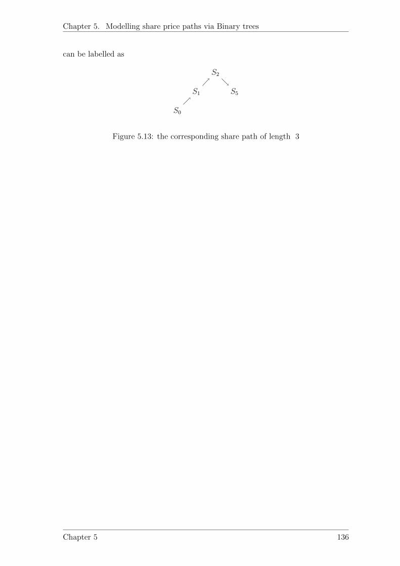
Chapter 5. Modelling share price paths via Binary trees
can be labelled as
S0
S1
S2
S5
Figure 5.13: the corresponding share path of length 3
Chapter 5 136

Chapter 6
Count all paths not allowing givendown steps in Binomial model
In this chapter, motivated by Flajolet symbolic method and generating functionapproach[14] [15], and motivated by quantum path calculation method in [2] [11],we calculated the option price in the finite restricted binomial model.
6.1 Construction
Motivated by the construction method of words over the binary alphabet lettersa, b which do not have k consecutive a described on the page 51 motivated byby Flajolet and Sedgewick in the book [15] and definitions of sequence symbolicconstruction in the book [15, Page 25] and [14, Chapter 5.2], we apply the methodand develop the construction of the set Ak of restricted share price path and itspath generating function.
Suppose share prices is modelled by a binomial model, and the model use theprobability measure defined by p((up)) = pu, p((down)) = pd, with pu + pd = 1.Then, put a restriction on the share values in the model, the restriction is that notallowing share prices has consecutive downward changes greater and equal than ksteps, where k is a given positive integer.
Ak denotes the set of possible share values of (S0− > S1− > S2− > . . .) of therestricted binomial model. So, the set Ak is all the possible share price paths inthe restricted binomial model.
Assuming the set Ak is a combinatorial class, then, construct any share value pathin the restricted model using the symbolic method motivated by by Flajolet andSedgewick in the book [15] and the book [14, Chapter 5.2] as follows,
For any share path σ in the restricted model sample space set Ak, it is a path notallowing k down steps for any length n, and can be defined by a path consistingof consecutive ≤ k downward steps either followed by an empty path or followed
137

Chapter 6. Count all paths not allowing given down steps in Binomial model
by a one Up step connected to a path not allowing k down steps for any length n,that is,
(Ak) = (empty path + path of one down step
+path of two down steps + . . .+
+path of k down steps)
×(empty path
+Up× (Ak))
Let each valid path in the restricted model Ak is denoted by σk,
count the set of restricted paths by the path lengths,
the generating function for the path σk is defined by
σk(z) =∞∑i≥0
Si(σ)z|σ1σ2...σi|.
Then, the path generating function for the restricted model can be defined by
Ak(z) =∑σ∈Ak
σk(z) =∞∑i=0
∑σ∈Ak,n
Si(σ)zi
from the above construction of the restricted paths, using the symbolic method andits transfer theorem introduced in the Chapter 6, the path generating function ofthe restricted model satisfies the equation
Ak(z) = (1 + z + . . .+ zk−1)(1 + zAk(z))
After extracting the coefficient of the generating function A(z),
[zN ]Ak(z) =∑
σ∈Ak,n
SN(σ)
it is the sum of the possible state values at time N in the restricted binomial model.
6.2 Calculate option price in the finite restricted
binomial model
Motivated by the quantum binomial option pricing in the paper [2, Section 2.3], usingthe path calculation method which is motivated from the Feynman path integralmethod or sum-over-history method in [12] [13], we derive the calculation of option
Chapter 6 138

Chapter 6. Count all paths not allowing given down steps in Binomial model
price in the finite restricted binomial model, which can be a generalization of thepath calculation lemma in the paper [2] [11].
Consider the restricted n steps binomial model, the path generating function forthe finite restricted model is
A(z; k, n) :=∑
σ∈Ak,n
n∑i=0
Si(σ)z|σ1σ2...σi|
=n∑i=0
∑σ∈Ak,n
Si(σ)zi
where, σ = σ1σ2 . . . σn
Si(σ) = the share value at time i of the path
σ in the restricted model Ak,n
In the finite restricted model, let each possible path σ has probability CPk(σ),where C = 1∑
σ∈Ak,nPk(σ)
, which is the probability normalization constant.
The path generating function for the restricted model is
P (w; k, n) :=∑σ∈Ak
n∑i=0
CP ik(σ)w|σ1σ2...σi|
where, CP ik(σ) = CPk(σ1σ2 . . . σi)
= the state probability at time i of the valid path
σ in the restricted model Ak,n
Thus, in the restricted n steps binomial model Ak,n, the expected share pricevalue at time n can be calculated by
E[Sn(σ)] =∑
σ=σ1σ2...σn∈Ak,n
Sn(σ)CP nk (σ)
The restricted model Ak,n is a n steps binomial model, suppose the risk-freeinterest rate is r.
Next is to calculate the price of the exotic option claim in the restricted model.
Suppose the option claim for the share price at time t is Ct = f(St), for 1 ≤ t ≤n.Let T be the final time, and 1 ≤ t ≤ T .
The exotic option claim in the model is defined by Claim =T∑t=1
f(St)
Chapter 6 139

Chapter 6. Count all paths not allowing given down steps in Binomial model
Thus, the option value of the exotic claim in the finite restricted model is stated as
Theorem 60 the option value of the exotic option claim in the finite restrictedmodel Ak,n, at time t = 0 is calculated using the given risk-free interest rate rand it is
OP (Claim) = OP (T∑t=1
f(St)) =T∑t=1
OP (f(St))
=T∑t=1
[(1 + r)−t · E(f(St))]
=T∑t=1
[(1 + r)−t ·
∑σ∈Ak,n
f(St(σ))CP tk(σ)
]
=∑
σ=σ1σ2...σn∈Ak,n
T∑t=1
f(St(σ))CP tk(σ)
(1 + r)t
The path calculation method in the theorem generalize the restricted path calcula-tion lemma, which can be compared to the Theorem 7 which is a generalization ofpath calculation lemma in the paper [2] [11].
In the model Ak,n, since the starting state of the share price is fixed, for eachpath σ ∈ Ak,n, set CP 0
k (σ) = 1. From the path probability generating functionP (w; k, n) of the restricted n times binomial model, it can be observed that
P (0; k, n) =∑
σ∈Ak,n
CP 0k (σ)
=∑
σ∈Ak,n
1
= ] of the possible paths in the restricted model Ak,n
Suppose each path has equal probability in the restricted model Ak,n, then, theprobability of valid path σ ∈ Ak,n can be calculated by
P (σ) =1
P (0; k, n)
Chapter 6 140

Chapter 7
Count paths using Parallelogrampolyominoes
7.1 Definitions
The definition 61 is motivated from the handout of Interior, closure, and boundaryby Conrad, Brian [33].
Definition 61 (Interior of a set)Let S be a set of points in the Cartesian plane(a two-dimensional Euclidean plane),
Then, the interior of S is the set of all points in S which does not belong to theboundary of S, it is denoted by int(S), so, it is the largest open set contained inS and it is the union of all open sets contained in S.
The definition of open ball in the discussion of the next remarks is motivated byWeisstein in [34].
Remarks: A point x ∈ S if and only if there exists ε > 0 such that an open ballcentred at x with radius ε is completely contained in S. The open ball is denotedby B(x, ε), and defined by B(x, ε) := y ∈ R2 | d(x, y) < ε
The definition 62 is motivated by Delest in the introduction of the paper [32].
Definition 62 (cell)A unit square with vertices staying on integer points in R2 is called a cell.
The definition 63 is motivated by Delest in the introduction of the paper [32].
Definition 63 (polyomino)A polyomino is a finite connected union of cells such that its interior is connected.
Motivated from the discussion of the definition of polyomino by Weisstein [35] andthe definition of interior of a set in the definition 61, we develop a small example ofnot being polyomino as an illustration of understanding the definition.
141

Chapter 7. Count paths using Parallelogram polyominoes
Example 7.1.1 A finite connected union of cells which is not polyomino is:
A
Figure 7.1: an example of not being polyomino
It is observed that the point A is not in the interior of the polyomino. The interiorof the polyomino is not connected.
The definition 64 is motivated by Delest and Viennot from page 170 in the paper[30].
Definition 64 (column or row convex polyomino)A polyomino is said to be column- (respectively row-) convex if the intersection ofany infinite vertical (respectively horizontal) line with the polyomino is a connectedline segment.
To illustrate the definition of convex polyomino, we gave a column-convex polyominoand a row-convex polyomino in the following example.
Example 7.1.2 a column-convex polyomino is:
Figure 7.2: an example of column-convex polyomino
a row-convex polyomino is:
Figure 7.3: an example of row-convex polyomino
Chapter 7 142

Chapter 7. Count paths using Parallelogram polyominoes
The definition 65 is motivated by Delest in the introduction of the paper [32].
Definition 65 (convex polyomino)A polyomino is said to be convex polyomino if it is both column-convex and row-convex polyomino.
We gave a simple example as follows to illustrate the definition of convex polyominoin the definition 65.
Example 7.1.3 A convex polyomino is:
Figure 7.4: an example of convex polyomino
Introducing notation, and give another definition of convex polyomino as follows.
The definition 66 is motivated from the discussion of the definition of polyomino byWeisstein [36] and the page 177 by Viennot from the paper [30].
Definition 66 (convex polyomino)
A convex polyomino, denoted by P , is a polyomino whose perimeter is equal tothat of its minimal bounding box (Bousquet-Melou et al. 1999). The perimier of thepolyomino is the length of its border. The minimal bounding box of a polyomino isthe smallest rectangle that contains P , denoted by Rect(P ). The rectangle is alsoa convex polyomino by the definition.
A small example is given as follows, in which the discussions and notations aremotivated by Delest and Viennot in the paper [30, Page 177-178].
Example 7.1.4 A convex polyomino P with its smallest rectangle Rect(P ) is:
Chapter 7 143

Chapter 7. Count paths using Parallelogram polyominoes
S(P )S ′(P )
E(P )
E ′(P )
N(P )N ′(P )
W ′(P )
W (P )
Figure 7.5: an example of convex polyomino with smallest bounding box
It is observed that going through four directions anti-clock-wisely (South, East, North,West), the rectangle Rect(P ) touches the convex polyomino P at four connectedline segments. Anti-clock-wisely, the extreme points of the four segments are denotedby [S(P ), S ′(P )], [E(P ), E ′(P )], [N(P ), N ′(P )], [W (P ),W ′(P )].
The definition 67 is motivated by Delest and Viennot in the paper [30, Page 178].
Definition 67 (Parallelogram polyomino)
A convex polyomino P is called a parallelogram polyomino if its smallest boundingrectangle Rect(P ) touches the polyomino at four connected line segments withthe condition that (the South left extreme point = the West bottom extreme point)and (the East top extreme point = the North right extreme point), if label the ex-treme points of the four segments by [S(P ), S ′(P )], [E(P ), E ′(P )], [N(P ), N ′(P )],[W (P ),W ′(P )], the condition is S(P ) = W ′(P ) and N(P ) = E ′(P ). It is observedthat the extreme point N(P ) is the rightmost top point and S(P ) is the leftmostbottom point.
A small example is given by us to illustrate the definition of parallelogram polyomi-noe.
Example 7.1.5 A parallelogram polyomino P with its smallest rectangle Rect(P )is:
Chapter 7 144

Chapter 7. Count paths using Parallelogram polyominoes
S(P )
N(P )
Figure 7.6: an example of parallelogram polyomino
To relate a parallelogram polyomino to a connected lattice path matroid, introducethe next definition of parallelogram polyomino. The definition of lattice path ma-troid can be referred to the Definition 3.1. in the paper [60]. The definition 68 ismotivated from the discussion by Delest and Viennot on the page 178 in the paper[30, Page 178].
Definition 68 (Parallelogram polyomino)
A convex polyomino P is called a parallelogram polyomino if its smallest boundingrectangle Rect(P ) is characterized by two lattice paths which have the same initialpoint S(P ) and same ending point N(P ), each lattice path on the border is formedof East and North unit steps. Denote the top bounding lattice path by w and denotethe bottom bounding lattice path by η. The top path w is above the bottom path η,and the two paths do not intersect each other except the initial point S(P ) and theending point N(P ), otherwise, it contradicts the definition of being a polyomino.
The same small example as above given by us using the bounding pair paths isillustrated to understand the definition 68.
Example 7.1.6 A parallelogram polyomino P with its bounding pair paths (w, η)is:
w
η
S(P )
N(P )
Figure 7.7: the parallelogram polyomino with its bounding paths (w, η)
Chapter 7 145

Chapter 7. Count paths using Parallelogram polyominoes
It is observed that the parallelogram polynomino is characterized by two paths withsame inital point S(P ), and ending point N(P ). The pair (w, η) of paths is asfollows,
w = N1 → N2 → E3 → E4 → N5 → E6
η = E1 → N2 → E3 → E4 → N5 → N6
7.2 Construction of dyck paths from lattice path
matroids
7.2.1 Construction
In this section, the construction algorithm from lattice path matroid to a specialtyple of share price paths, say Dyck paths is introduced and the method is modifiedby us and motivated from the paper [30, Page 179], in the paper, Delest and Viennotdeveloped a bijection 2-colored Motzkin words of length n− 1 and Dyck words oflength 2n.
Next, construct a bijection between the set of lattice path matroid and the set ofDyck paths. Using the above example of parallelogram polynomino, the constructionis as follows,
In the example, Let S(P ) = (0, 0), each step has length 1, the polyomino is definedby two paths (w, η), each path from S(P ) = (0, 0) to N(P ) = (3, 3) of lengthn+ 1 = 6, and has perimeter 2(n+ 1) = 12. The number of cells in the polyominois n = 5.
Firstly, construct a Dyck path from a pair of paths [w, η].
Step 1: Set up delimiter intervals [∆i,∆i+1], where ∆i denotes the line y = −x+i,1 ≤ i ≤ n− 1 = 4. It is noted that the delimilter interval contains all pairs steps ofpaths (w, η) except the first pair steps (N1, E1) and the last pair steps (E6, N6) .
Step 2: Going through the delimiliter intervals [∆i,∆i+1], for 1 ≤ i ≤ n − 1 = 4,use the pair steps (wj, ηj) with 2 ≤ j ≤ n to construct the 2-colored Motzkinpath γ = γ1γ2 . . . γn−1 = γ1γ2 . . . γ4 according to the following scheme,
(Nj, Ej) ←→ γj−1 = up diagonal step (1, 1),
(Nj, Nj) ←→ γj−1 = blue colored horizontal step (1, 0),
(Ej, Ej) ←→ γj−1 = red colored horizontal step (1, 0),
(Ej, Nj) ←→ γj−1 = down diagonal step (1,−1),
Chapter 7 146

Chapter 7. Count paths using Parallelogram polyominoes
then, the pairs steps in the pair path (w, η) is
(N2, N2)→ (E3, E3)→ (E4, E4)→ (N5, N5)
It corresponds to the 2-colored Motzkin path
(0, 0) (1, 0) (2, 0) (3, 0) (4, 0)
Figure 7.8: the corresponding 2-colored Motzkin path from the example polyomino
Step 3: Based on the given path γ = γ1γ2 . . . γ4, using a bijection h, which isdefined by the scheme,
h(γi) =
(up diagonal, up diagonal) if γi = up diagonal step(1, 1)
(up diagonal, down diagonal) if γi = blue colored horizontal step(1, 0)
(down diagonal, up diagonal) if γi = red colored horizontal step(1, 0)
(down diagonal, down diagonal) if γi = down diagonal step(1,−1)
that is, h is a bijection between dyck path steps(except initial and final steps) andthe 2-colored Motzkin path following the scheme
h(γi) =
(0, 0)
(1, 1)
(2, 2)
(0, 0)
(1, 1)
(0, 0)
(1, 1)
(2, 0) (0, 0) (1, 0)
(0, 0)
(1,−1)
(2, 0)
(0, 0) (1, 0)
(0, 0)
(1, 1)
(2, 2)
(0, 0)
(1,−1)
Thus, in the example, the path h(γ) is constructed as the following,
Chapter 7 147

Chapter 7. Count paths using Parallelogram polyominoes
(0, 0)
(1, 1)
(2, 0)
(3,−1)
(4, 0)
(5,−1)
(6, 0)
(7, 1)
(8, 0)
Figure 7.9: the corresponding path h(γ) from the 2-colored Motzkin path
Step4: construct the Dyck path (up diagonal, h(γ), down diagonal) as follows,
(0, 0)
(1, 1)
(2, 2)
(3, 1)
(4, 0)
(5, 1)
(6, 0)
(7, 1)
(8, 2)
(9, 1)
(10, 0)
Figure 7.10: the final constructed Dyck path from the example polyomino
It can be observed that the construction from the parallelogram polyomino to theDyck path is bijection, therefore, the converse construction from the Dyck path tothe paralleogram can also be done similarly.
7.2.2 Share price Path interpretation
In this section, we gave the explicit interpretations of the share price path con-structed from the section 7.2.1, which is important for financial modelling.
Share price Path interpretation
Assume that a jump up is a move Sk → Sk+1 = uSk.Then, a jump down is a move Sk → Sk+1 = dSk.Finally, a stay jump is a move Sk → Sk+1 = Sk.
Chapter 7 148

Chapter 7. Count paths using Parallelogram polyominoes
The Figure 7.9 is then interpreted as
S1 = S0u0 = S0 (stay)
S2 = S1u1 = S1u (jump up)
S3 = S2u0 = S2 (stay)
S4 = S3u−1 (jump down)
S5 = S4u0 = S4 (stay)
S6 = S5u−1 (down)
S7 = S6u0 = S6 (stay)
S8 = S7u1 = S7u (up)
S8 = S8u0 = S8 (stay)
Then, this corresponds to compound Possion behaviour, before going up and down,stay at random time, compared to binomial model.
Chapter 7 149

Chapter 8
Probability Methods
In the first part of the chapter, we apply a well-known probability results and asimple argument in probability to solve combinatorial problem, the probability resultcan be referred to [40, Section 1.1]. In the next part of the chapter, we go furtherand modify certain probability methods to solve another restricted path countingcombinatorial problem.
8.1 Path counts using a probability method
8.1.1 Probability of simple random walks from (0, a) to(n, b)
Considering a nearest neighbour random walk on Z. Imagine a walker starts ata ∈ Z and at every integer time n ∈ N the walker has two options; moves one stepto up with P (Xn = 1) = p or moves one step to down with P (Xn = −1) = q = 1−p.Denote the position of the walker at time n by Sn, the nearest neighbour randomwalk is defined by the following formula,
S0 = a, Sn = S0 +n∑i=1
Xi
the set of realization of the walker is the set of sequences S = (s0, s1, . . .) withs0 = a and si+1−si = +1,−1 ∀i ∈ N, the sequence in the set is called a samplepath of the random walk. The probability that the first n steps of the walk followa given path S = (s0, s1, . . . , sn) is pupqdown, where
up = number of up steps in a path S
= ]i : si+1 − si = 1down = number of down steps in a path S
= ]i : si+1 − si = −1
150

Chapter 8. Probability Methods
Assuming the position of the random walk at time n is sn = b, initial position iss0 = a.
Denote Nupn (a, b) is the number of paths (s0, s1, . . .) with s0 = a, sn = b. An
equation relating to number ’up’ and ’down’ is derived as follows,
up+ down = n
up− down = (sm − sm−1)+ + (sm − sm−1)−
= sn − s0 = b− a
=⇒ up = 12(n+ b− a), down = 1
2(n− b+ a)
Then, any event for the random walk can be expressed as follows,
P (Sn = b) = Nupn (a, b)pupqdown(here ’up’ is a fixed number)
=
(n
12(n+ b− a)
)p
12
(n+b−a)q12
(n−b+a)
It is obvious to see that computing certain random walk events are after countingthe size of corresponding set of paths.Therefore, by recalling the interesting question in percolation theory, a probleminvolving the number of ways of going from one point to another point in a squarelattice would be an important question in the Problem 1. Before doing problem 1,the following definition is given.
Definition 69 [41] Lattice path is a path consisting of connected horizontal andvertical line segments, which are restricted to north and east steps. assuming theline segment has nearest integer distance 1.
8.1.2 Path counts using a simple probability argument
A simple argument in probability:
Assuming the sample space is Ω, if all the elements in Ω are equally likely, then theprobability that an event A happens in the sample space is
P (A) =number of elements in A
number of elements in the sample space
therefore, based on the discussion in section 8.1.1, assuming the lattice path em-ploying two steps up, right, then we get,
P (S(n) = m) =number of paths of length N and k ’up’ steps
number of paths of length N
=an,man
Chapter 8 151

Chapter 8. Probability Methods
Next, we provide an example of counting paths using the simple probability argu-ment and the well-known probability results as follows.
Firstly, assuming that each step exists a random variable,
εi =
1, if up with 1
20
0, if right with 12
The number of up steps is:
ε1 + ε2 + ε3 =3∑i=1
εi =m+n∑i=1
εi = m
For each path, the total steps is (n+m) so, the number of right steps is
(n+m)−n+m∑i=1
εi =n+m∑i=1
(1− εi)
Then, suppose each possible path happens with a equal possibility 12u
, with u =m+ n, by assumption,
the number of paths from (0,0) to (n,m)=the number of up steps=m,the event is Bernoulli trials (n+m, 1
2).
As the number of total possible paths is equal to 2u, the number of paths from (0,0)to (n,m) is the product of 2u and the possibility of the number of up steps=m.
Say m=1,n=2; the number of total possible paths is equal to 23,
P (ε1 + ε2 + ε3 = 1) = P (Bin(3,1
2) = 1) =
(3
1
)1
23
so, the number of paths from(0,0) to (2,1) is
23 · P (ε1 + ε2 + ε3 = 1) = 3
8.2 Count paths via unusual stochatic modelling
Consider a finite N time steps discrete time model in which share prices is mod-elled by a restricted N time step binomial model with restriction not allowing kconsecutive down steps. We aim to calculate the number of restricted share pricepaths not allowing k consecutive down steps at time 1 ≤ T ≤ N using Markov-typetechnique stochastic modelling.
We will illustrate the technique using two small examples, one is to calculate thenumber of restricted share paths not allowing 2 down steps in a row at T = 3 timestep. The other is to calculate the number of restricted share paths not allowing 3consecutive down steps at time T = 4.
Chapter 8 152

Chapter 8. Probability Methods
We will firstly recall the definition of Markov chain, and its two important theorems,then, we would like to use the Markov-type technique to do the path calculation.
8.2.1 Markov chain
Definition 70 [27]
Consider a set of states S = s0, s1, . . . , sn, . . ., a discrete Markov chain is afamily of random variables Xnn∈N0 which take values in the set S and satisfiesthe Markov property
P (Xn = sn|Xn−1 = sn−1, . . . , X0 = s0)
= P (Xn = sn|Xn−1 = sn−1)
= Psn−1,sn(n− 1)
Consider the time-homogeneous Markov chains, the transition probability of a timehomogeneous discrete Markov chain is defined as
Pi,j(n− 1) = Pi,j
= P (Xn−1 = j | Xn = i),
where∑j∈S
Pi,j = 1, for i ∈ S
The initial state X0 of the Markov chain has a distribution defined as
φ(i) = P (X0 = i), for i ∈ S
Using the Markov property, the distribution of a time-homogeneous discrete Markovchain is defined as the point probabilities
P (Xn = sn, Xn−1 = sn−1, . . . , X0 = s0)
= P (Xn = sn|Xn−1 = sn−1)× . . .× P (X1 = s1|X0 = s0)
= Psn−1,sn(n− 1)× Psn−2,sn−1(n− 2)× . . .× Ps0,s1(0)
= Psn−1,sn × Psn−2,sn−1 × . . .× Ps0,s1
for sn, sn−1, . . . , s0 ∈ S and n ∈ N0 .
Theorem 71 [27] [25, chapter 11]
Consider a time-homogeneous discrete time Markov chain Xnn∈S defined on aset of finite states, S = s0, s1, . . . , sn,Let P be the transition matrix set up for the Markov chain, an (i,j)-th entry of thematrix is
Pi,j = Psi,sj = P (X(n+ 1) = sj | X(n) = si) = P (X(1) = sj | X(0) = si),
Let R(n)i,j = R
(n)si,sj = P (X(n) = sj | X(0) = si) denotes the probability that the
Markov chain will be in the state sj after n time steps, if it initially starts fromthe state si,
Then, the probability is calculated as the (i,j)-th entry of the matrix Pn.
Chapter 8 153

Chapter 8. Probability Methods
Here, a simple proof using conditional probabilities is given and the idea is from[26].
Proof:
R(n)i,j = R(n)
si,sj= P (X(n) = sj | X(0) = si), for n ∈ N, si, sj ∈ S
=n∑k=1
P (X(n) = sj, X(1) = sk | X(0) = si) [Conditioning on X1]
=n∑k=1
P (Xn = sj | X1 = sk)P (X1 = sk | X0 = si) [Markov property]
=n∑k=1
P (Xn−1 = sj | X0 = sk)P (X1 = sk | X0 = si) [Time-homogeneous]
=n∑k=1
Psi,skR(n−1)sk,sj
=n∑k=1
Pi,kR(n−1)k,j
Using matrix notation,
R(n) = P×R(n−1)
then, it can be easily found that starting from any initial state si, for 1 ≤ i ≤ n,the probability matrix after n time steps is calculated as
R(n) = Pn
Theorem 72 [27] [25, chapter 11]
Consider a time-homogeneous discrete time Markov chain Xnn∈S defined on aset of finite states, S = s0, s1, . . . , sn,Let P be the transition matrix set up for the Markov chain, an (i,j)-th entry of thematrix is
Pi,j = Psi,sj = P (X(n+ 1) = sj | X(n) = si) = P (X(1) = sj | X(0) = si),
Let Pn be the n time step transition probability matrix that describes the proba-bilities that the Markov chain starts from any state si ∈ S and arrives at a statesj ∈ S after n time steps. An (i,j)-th entry of the matrix is
P ni,j = P n
si,sj= P (X(n) = sj | X(0) = si),
Let the initial state distribution of the Markov chain is
φ(i) = P (X0 = i), for i ∈ S
Then, the n time step state X(n) of the Markov chain has a distribution
P (X(n) = sj) =∑si∈S
φ(si)Pn(si, sj), for sj ∈ S
Chapter 8 154

Chapter 8. Probability Methods
Here, a simple proof using total probabilities is given by us and the notationrepresentation is motivated from [27] [25, chapter 11].
Proof:
P (X(n) = sj) =∑si∈S
P (X(n) = sj , X(0) = si), for sj ∈ S [total probability]
=∑si∈S
P (X0 = si)P (X(n) = sj | X(0) = si) [Conditioning on X0]
=∑si∈S
φ(si) Pn(si, sj)
Using matrix notation,
if denote the initial distribution by a vector
φ = φ(1), . . . , φ(n) = φ(s1), . . . , φ(sn)
denote the state distribution of the Markov chain at time n by a vector
φ(n) = φ(n)(1), . . . , φ(n)(n) = φ(n)(s1), . . . , φ(n)(sn) = P (X(n) = s1), . . . , P (X(n) = sn
Then,
φ(n) = φ×Pn
8.2.2 Method Inspiration
For a discrete time markov chain, the important is how to define the set of states towork on and how to set up the transition probabilities with which the states movein the markov chain.
We found in the restricted share price model, each step the share price can eithergo up or go down, as time goes progress, the number of possible valid states at eachtime is increasing. To avoid using the set of increasing possible states, we observethat at each time step, the share price can only go up or go down.
Consider all possible share price changes at each time step be the set of possiblestates we are interested in. If no restriction is applied, the share price model can bemodelled as a regular markov chain, because the possible states at each time step isindependent of each other time step.
In the restricted model, if the restriction is not allowing k consecutive down steps,then the restriction make sense starting after the k − 1 time step.
Consider the restricted share price model is modelled by a markov-type chain. Inthe chain, the set of possible states in the model is the set of all possible paths inthe first k − 1 time steps.
Chapter 8 155

Chapter 8. Probability Methods
When the restriction is applied in the share price model, construct a transformprobability matrix to be a square matrix with the dimension 2k−1, which describesthe probabilities of the possible share price change at time k given the first k − 1time steps possible paths.
In the matrix, each row except the last row represents the probabilities of the possiblechanges at the time step k, which is independent of the first k−1 time steps shareprice paths. That is, P (up) = p and P (down) = 1−p. Here, we will use a Markov-type model to do the share price paths calculation with the given restriction. So,we consider the case p = 1
2
By analogy with the n step transition matrix of markov chains, we would like tointroduce a square matrix that has dimension 2k−1 to denote a tranform probabilitymatrix, which can help to predict probabilities after n steps. However, it is notedthat each row only have two possible share price changes with P (up) = 1
2and
P (down) = 12.
Therefore we introduce a proper notation to solve the conflict between the number ofpossible states 2 and the number of the matrix dimension 2k−1. We will illustratethe technique using two example in the implementation section.
Concerning the last row in the probability matrix, it is natural to have two ways toset up the transform probability matrix, the first way is to set up P (X(k) = up|X(k − 1) = down, . . . , X(0) = down) = 1
P (X(k) = down|X(k − 1) = down, . . . , X(0) = down) = 0
the other way is to set up P (X(k) = up|X(k − 1) = down, . . . , X(0) = down) = 12
P (X(k) = down|X(k − 1) = down, . . . , X(0) = down) = 0
8.2.3 Transform probability matrix setting up
We claim that the second way of setting up the last row probabilities in the transformmatrix would be a proper way. It can be tested and illustrated using an example.After that, we will also explain the reasonable idea behind the setting up of the lastrow probabilities in the transform matrix using an example.
Example1: Setting up the last row probabilities in a probability matrix
Consider a three time steps binomial share price model with the restriction notallowing two consecutive down steps, the probability measure is P (up) = 1
2and
P (down) = 12.
Consider the restricted share price model is modelled by a Markov-type chain, therestriction in the model starts work after the first one time step. In the first one
Chapter 8 156

Chapter 8. Probability Methods
time step, share price has 2 = 21 possible changes, the set of states is denoted byS = s0, s1 = up, down. Denote the up step by 1 and the down step by 0,then, S = s0, s1 = 1, 0.
There are two possible ways to set up the second row transform probabilities in thetransform probability matrix.
1. One possible way of setting up
P (X(1) = up| X(0) = down) = P (X(k) = 1|X(0) = 0) = 1
P (X(1) = down| X(0) = down) = P (X(k) = 0|X(0) = 0) = 0
The model is modelled by a markov chain, the transform matrix actually is atransition matrix. The second up step given the first down step can be seenas an absorption state. That is,
F =
12
12
1 0
In the following, using notation P (X(2), X(1) | X(0)) to denote the corre-sponding conditional path, the up step and down step are denoted by 1 and0 repectively.
Use the transition matrix to predict probabilities of(3rd step state | 1st step state), it is a two step transition matrix,
F 2 =
12× 1
2+ 1
2× 1 1
2× 1
2+ 1
2× 0
1× 12
+ 0× 1 1× 12
+ 0× 0
=
P (11 | 1) + P (10 | 1) P (01 | 1) + P (00 | 1)
P (11 | 0) + P (10 | 0) P (01 | 0) + P (00 | 0)
=
P (1 | 1)(2) P (0 | 1)(2)
P (1 | 0)(2) P (0 | 0)(2)
From the entry F 2(2, 1),
the probability of (3rd step = up | 1st step = down) = 1× 12
= 12, it represents
one path in the three time-steps share price model.
However, given the first step state, the path should be considered havingthe probability 1
2× 1
2= 1
4, if considering each path is equal and without
restrictions in the three time-steps model.
Chapter 8 157

Chapter 8. Probability Methods
The reason is that when doing path counting, without restriction in the three-time-step model, the number of total possible paths in the last two time-stepsis 4, and if put the restriction on the model, the number of total possible pathis 3 , consider each path is still equal, actually, the probability 1
2means it
count one path (down,up,up) as two paths.
In general, setting up the probability of (3rd step = up | 1st step = down) tobe an absorbing state, For any one path containing the patterns (down, up), ifthe number of the patterns (down, up) in the path is a number k, this pathwill be counted as 2k paths, although it only represents the probability of onepath in the n time-steps share price model without restriction applied in themodel. As time T increases, if not allowing the consecutive two down stepsand calculate the number of valid paths at time T will result in more improperpath counts because it might contains more number of patterns (down, up).
Consider a general restriction, not allowing k consecutive down steps, we haveto set up a transform matrix be a probability matrix that describes all possibleshare price change probabilities given the first 2k−1 time steps possible paths,and if using the first way of last row probability setting up, when doing pathcalculation, it counts any k step path containing the pattern (k consecutivedowns, up) as two paths, as time goes progress, it will lead to more inaccuraterestricted path counting.
Therefore, we claim that the probability of (3rd step = up | 1st step = down)= 1
2× 1
2= 1
4.
2. Another proper way of setting up
The probabilities of the other rows in the transform probability matrix de-scribes all possible share price change probabilities at time step k given thefirst 2k−1 time steps.
The share price change has two possible changes in the set up, down, whenthe restriction not allowing k consecutive down steps is applied in the ntime steps model, the two possible share price change probability at time k,is independent of the first k − 1 time steps information except the last rowin the matrix, so, we set the probabilities of the rows from 1 to 2k−1 − 1 tobe P (up = 1
2), P (down = 1
2).
To construct the transform probability matrix to predict the probabilitiesof states after n time steps, the matrix should be a square matrix, if therestriction is not allowing k ≥ 3 consecutive down steps, there is a conflictbetween the number of possible share price change and the number of the firstk − 1 share price paths.
To solve the conflict, notations are introduced as follows,
Given the first k− 1 time steps share price change, the valid state is to go to
Chapter 8 158

Chapter 8. Probability Methods
a state which has the first k − 2 share price change same as the last k − 2share price change in the given state, considering equal probabilities at eachtime step.
Let one possible path in the first k−1 time steps is denoted by (s0, s1, . . . , sk−2),where si ∈ S = up, down = 1, 0,
then, the probabilities of rows from 1 to 2k−1 − 1 in the square transformmatrix is
P ((s0, s1, . . . , sk−2)→ ((s1, s2, . . . , sk−2, up)
= P (s0, s1, . . . , sk−2, up) =1
2
P ((s0, s1, . . . , sk−2)→ ((s1, s2, . . . , sk−2, down)
= P (s0, s1, . . . , sk−2, down) =1
2
The last row (2k−1th) row of the probability matrix has probabilities
P ((s0 = down, . . . , sk−2 = down)→ P ((s0 = down, . . . , sk−2 = down, sk−1 = up)
= P (s0 = down, s1 = down, . . . , sk−2 = down, sk−1 = up) =1
2
P ((s0 = down, . . . , sk−2 = down)→ P ((s0 = down, . . . , sk−2 = down, sk−1 = up)
= P (s0 = down, s1 = down, . . . , sk−2 = down, sk−1 = down) = 0
Next, a reasonable idea behind the setting up of the last row probabilities as abovein the transform matrix is explained using an example.
Consider a two-steps share price model, suppose the probability measure set up forthe model is P (up) = 1
2and P (down) = 1
2, each possible share price path has
equal probability 14.
Consider a restriction is not allowing 2 consecutive down steps and put the re-striction on the two-steps share price model, the possible share price paths withcorresponding probabilities and corresponding normalized probabilities are as fol-lows,
Chapter 8 159

Chapter 8. Probability Methods
with probability 14,
with normalized probability 13
with probability 14,
with normalized probability 13
with probability 14,
with normalized probability 13
It can be observed that each path still has equal probability after put restriction onthe model, if setting up the transform matrix as
F =
P (1 | 1) = 12
P (0 | 1) = 12
P (1 | 0) = 12
P (0 | 0) = 0
8.2.4 Result and Discussion
Lemma 73 Consider a restricted finite N time steps binomial model with twopossible share price change at each time step, either going up or going down, andthe restriction not allowing k consecutive down steps.
Consider the model is modelled as a Markov-type chain, with the initial state distri-bution is denoted by a vector
φ = [ φ(s1), . . . , φ(s2k−1) ] = [ P (X(0) = s1), . . . , P (X(0) = s2k−1) ]
= [ p1, . . . , p2k−1 ] = [1
2, . . . ,
1
2]
Let the transform probability matrix is denoted by A, the possible states in thematrix is ordered as the decreasing order of the (k − 1) digits binary expression of0, 1 starting from (1, 1, . . . , 1) to (0, 0, . . . , 0), the matrix A is defined as asquare matrix with dimension 2k−1,
A =
12
12
0 0 . . . 0 12
0 0 12
12
. . . 0 12
.... . .
...
0 0 . . . 12
12
0 0
0 0 0 0 . . . 12
0
Chapter 8 160

Chapter 8. Probability Methods
Then, the number of restricted paths not allowing k consecutive down steps at time1 ≤ T ≤ N is defined as
ψT,k = 2T ×2k−1∑i≥1
φ · AT−(k−1)(i)
Example 8.2.1 Consider a finite time discrete time binomial share price model,what is the number of restricted paths not allowing 2 down steps in a row at time3.
Solution: k = 2, T = 3, the restriction starts work after (k − 1) = 1 steps,
so, by decreasing order of the 1 digits binary expression of 0, 1 the set of statesis S = s0, s1 = up, down = 1, 0,set up the 2× 2 matrix
A =
12
12
12
0
the initial state distribution is
φ = [ φ(s1), φ(s2) ] = [ p1, p2 ]
= [ P (X(0) = 1), P (X(0) = 0) ] = [1
2,
1
2]
the restricted state distribution at time T = 3 is a vector
φ · A2 = [ φ(1), φ(0) ] ·
12
12
12
0
·1
212
12
0
=
1
8· [ 1, 1 ] ·
2 1
1 1
= [3
8,
2
8]
Then, the number of restricted paths is
ψ3,2 = 23 ×2∑i≥1
φ · A2(i)
= 23 × 5
8= 5
Example 8.2.2 Consider a finite time discrete time binomial share price model,what is the number of restricted paths not allowing 3 down steps in a row at time5.
Chapter 8 161

Chapter 8. Probability Methods
Solution: k = 3, T = 5, the restriction starts work after (k − 1) = 2 steps,
so, by decreasing order of the (k − 1) = 2 digits binary expression of 0, 1 theset of states is
S = s0, s1, s2, s3= (up, up), (up, down), (down, up), (down, down) = 11, 10, 01, 00
set up the 4× 4 matrix
A =
12
12
0 0
0 0 12
12
12
12
0 0
0 0 12
0
the initial state distribution is
φ = [ φ(s1), φ(s2), φ(s3), φ(s4) ]
= [ p1, p2, p3, p4 ]
= [ P (X(0) = 11), P (X(0) = 10), P (X(0) = 01), P (X(0) = 00) ]
= [1
4,
1
4,
1
4,
1
4]
the restricted state distribution at time T = 4 is a vector
φ · A2 = [1
4,
1
4,1
4,
1
4] ·
12
12
0 0
0 0 12
12
12
12
0 0
0 0 12
0
2
=1
16· [ 1, 1, 1, 1 ] ·
1 1 0 0
0 0 1 1
1 1 0 0
0 0 1 0
2
=1
16· [ 1, 1, 1, 1 ] ·
1 1 1 1
1 1 1 0
1 1 1 1
1 1 0 0
=1
16· [ 4, 4, 3, 2 ]
Then, the number of restricted paths is
ψ4,3 = 24 ×4∑i≥1
φ · A2(i)
= 24 × 13
16= 13
Chapter 8 162

Chapter 8. Probability Methods
In general case, following the same argument and proof discussion in the Section8.2.1, 8.2.2, 8.2.3, we provided the Lemma 74 as follows.
Lemma 74 Consider a restricted finite N time steps binomial model with twopossible share price change at each time step, either going up or going down. Therestriction is not allowing any given fixed steps pattern y1y2 . . . yk with yi ∈ 1, 0.The length of the steps pattern is k.
Consider the model is modelled as a Markov-type chain, with the initial state distri-bution is denoted by a vector
φ = [ φ(s1), . . . , φ(s2k−1) ]
= [ P (X(0) = s1), . . . , P (X(0) = s2k−1) ]
= [ p1, . . . , p2k−1 ] = [1
2, . . . ,
1
2],
Where, sj = x1x2 . . . xk−1 with xi ∈ 1, 0and with decimal(s1) > decimal(s2) > . . . > decimal(s2k−1)
and decimal(sj) = decimal(x1x2 . . . xk−1) = x1 · 2k−2 + x2 · 2k−3 + . . .+ xk−1 · 20
Let the transform probability matrix is denoted by B, the possible states in thematrix is ordered as the decreasing order of the (k − 1) digits binary expression of0, 1 starting from (1, 1, . . . , 1) to (0, 0, . . . , 0), the matrix B is defined as asquare matrix with dimension 2k−1. The matrix B is set up as follows,
Let si = x1x2 . . . xk−1, sj = x1x2 . . . xk−1,
If x2x3 . . . xk−1 = x1x2 . . . xk−2,
then,
(si → sj) = (x1x2 . . . xk−1 → xk−1)
= (the k-th step is xk−1 | the first k-1 steps equals x1x2 . . . xk−1)
The matrix elements in the matrix B is set up as
Bi,j = P (si → sj) =
12
if (x1x2 . . . xk−1 → xk−1) 6= (y1y2 . . . yk−1 → yk)
0 if (x1x2 . . . xk−1 → xk−1) = (y1y2 . . . yk−1 → yk)
If x2x3 . . . xk−1 6= x1x2 . . . xk−2, then,
(si → sj) not forms a possible path
and P (si → sj) = 0
Then, the number of restricted paths not allowing the given pattern y1y2 . . . yk at
Chapter 8 163
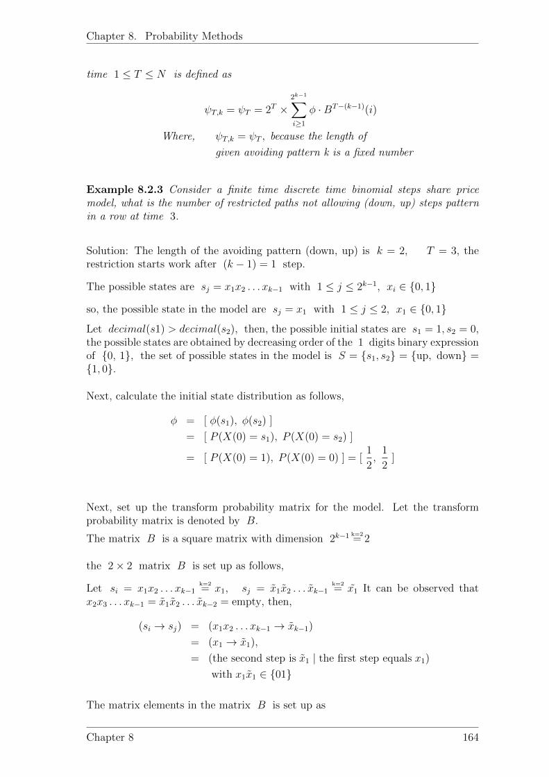
Chapter 8. Probability Methods
time 1 ≤ T ≤ N is defined as
ψT,k = ψT = 2T ×2k−1∑i≥1
φ ·BT−(k−1)(i)
Where, ψT,k = ψT , because the length of
given avoiding pattern k is a fixed number
Example 8.2.3 Consider a finite time discrete time binomial steps share pricemodel, what is the number of restricted paths not allowing (down, up) steps patternin a row at time 3.
Solution: The length of the avoiding pattern (down, up) is k = 2, T = 3, therestriction starts work after (k − 1) = 1 step.
The possible states are sj = x1x2 . . . xk−1 with 1 ≤ j ≤ 2k−1, xi ∈ 0, 1
so, the possible state in the model are sj = x1 with 1 ≤ j ≤ 2, x1 ∈ 0, 1
Let decimal(s1) > decimal(s2), then, the possible initial states are s1 = 1, s2 = 0,the possible states are obtained by decreasing order of the 1 digits binary expressionof 0, 1, the set of possible states in the model is S = s1, s2 = up, down =1, 0.
Next, calculate the initial state distribution as follows,
φ = [ φ(s1), φ(s2) ]
= [ P (X(0) = s1), P (X(0) = s2) ]
= [ P (X(0) = 1), P (X(0) = 0) ] = [1
2,
1
2]
Next, set up the transform probability matrix for the model. Let the transformprobability matrix is denoted by B.
The matrix B is a square matrix with dimension 2k−1 k=2= 2
the 2× 2 matrix B is set up as follows,
Let si = x1x2 . . . xk−1k=2= x1, sj = x1x2 . . . xk−1
k=2= x1 It can be observed that
x2x3 . . . xk−1 = x1x2 . . . xk−2 = empty, then,
(si → sj) = (x1x2 . . . xk−1 → xk−1)
= (x1 → x1),
= (the second step is x1 | the first step equals x1)
with x1x1 ∈ 01
The matrix elements in the matrix B is set up as
Chapter 8 164

Chapter 8. Probability Methods
Bi,j = P (si → sj) =
12
if (x1 → x1) 6= (0→ 1)
0 if (x1 → x1) = (0→ 1)
So, the matrix elements B is
B1,1 = P (1→ 1) =1
2
B1,2 = P (1→ 0) =1
2B2,1 = P (0→ 1) = 0
B2,2 = P (0→ 0) =1
2
and
B =
12
12
0 12
Then, the restricted state distribution at time T = 3 is a vector
φ ·BT−(k−1) k=2=T=3
φ ·B2
= [1
2,
1
2] ·
12
12
0 12
·1
212
0 12
= [
1
8,
3
8]
Then, the number of restricted paths not allowing the pattern y1y2 = down, up = 01at time T = 3 is definied as
ψ3,2 = ψ3 = 23 ×2∑i≥1
φ ·B2(i)
= 23 × 4
8= 4
It is easy to check that in the binomial steps share price model and set up restrictionof avoiding pattern y1y2 = down up, there only have 4 valid path at time T = 3.
In order to construct the transform matrix B in the Lemma 74 more easily using thecomputer programming language, we provide another Lemma 75 for the restrictedpath counting in a the same model.
Chapter 8 165

Chapter 8. Probability Methods
Lemma 75 Consider a restricted finite N time steps binomial model with twopossible share price change at each time step, either going up or going down. Therestriction is not allowing any given fixed steps pattern y1y2 . . . yk with yi ∈ 1, 0.The length of the steps pattern is k.
Consider the model is modelled as a Markov-type chain, with the initial state distri-bution is denoted by a vector
φ = [ φ(s1), . . . , φ(s2k−1) ]
= [ P (X(0) = s1), . . . , P (X(0) = s2k−1) ]
= [ p1, . . . , p2k−1 ] = [1
2, . . . ,
1
2],
Where, sj = x1x2 . . . xk−1 with xi ∈ 1, 0and with decimal(s1) > decimal(s2) > . . . > decimal(s2k−1)
and decimal(sj) = decimal(x1x2 . . . xk−1) = x1 · 2k−2 + x2 · 2k−3 + . . .+ xk−1 · 20
Let the transform probability matrix is denoted by B, the possible states in thematrix is ordered as the decreasing order of the (k − 1) digits binary expression of0, 1 starting from (1, 1, . . . , 1) to (0, 0, . . . , 0), the matrix B is defined as asquare matrix with dimension 2k−1. The matrix B is set up as follows,
Let si = x1x2 . . . xk−1, sj = x1x2 . . . xk−1,
The matrix index of (si → sj) with x2x3 . . . xk−1 = x1x2 . . . xk−2
and (x1x2 . . . xk−1 → xk−1) = (y1y2 . . . yk−1 → yk) is set up as
(2k−1 − decimal(y1y2 . . . yk−1), decimal(y1y2 . . . yk−1) + 1),
therefore, the matrix elements Bi,j can be directly set up as
Bi,j = 0 with i = 2k−1 − decimal(y1y2 . . . yk−1), and j = decimal(y1y2 . . . yk−1) + 1
and
Bi,j+1 =1
2with i = 2k−1 − decimal(y1y2 . . . yk−1), and j = decimal(y1y2 . . . yk−1) + 1
and
Bi,j = 0 with i = 2k−1 − decimal(y1y2 . . . yk−1), and j 6= decimal(y1y2 . . . yk−1) + 1
and j 6= decimal(y1y2 . . . yk−1) + 2
Then, the next is to set up the other matrix elements Bi,j withi 6= 2k−1 − decimal(y1y2 . . . yk−1), and the set up is as follows,
Bi,j = P (si → sj) =
12
if x2x3 . . . xk−1 = x1x2 . . . xk−2
0 if x2x3 . . . xk−1 6= x1x2 . . . xk−2
Chapter 8 166

Chapter 8. Probability Methods
Then, the number of restricted paths not allowing the given pattern y1y2 . . . yk attime 1 ≤ T ≤ N is defined as
ψT,k = ψT = 2T ×2k−1∑i≥1
φ ·BT−(k−1)(i)
Where, ψT,k = ψT , because the length of
given avoiding pattern k is a fixed number
8.2.5 Implementation
The Lemma in the section 4 can be implemented using computer language MAT-LAB. When doing the implementation using computer, it can be noted that thesize of the dimension of the transform matrix of the discrete time stochastic processincrease exponentially as the restriction k increases.
To save the computer memory, it can be observed that the transform matrix can beconstructed using sparse matrix, therefore, the counts can be easily done using theMATLAB.The implementation code using MATLAB is put in the appendix.
Chapter 8 167

Chapter 9
Matroid
9.1 Definitions of Matroids
Definition 76 [46, Page 2] [47, Definition 1.1]A matroid M is a pair (E, I), E is a finite set(are called ground set), I is acollection of subsets of E (the subsets are called independent sets such that
(i) ∅ ∈ I.
(ii) If I ⊂ J, J ∈ I, then I ∈ I.
(iii) If I, J ∈ I and |I| < |J |, then, there exists j ∈ J−I , such that (I∪J) ∈ I
Note: 1. I is the collection of independent sets.
2. A matorid is often denoted by listing its ground set and its family ofindependent sets, that is, denoted by M = (E, I) or to emphasize the matroid,denoted by M = (E(M), I(M)).
Definition 77 [46, Page 5]In a matroid M = (E, I), a subset B of the ground set is called maximal independentset iff the subset is independent(i.e. B ∈ I ) and no subsets of the ground set thatcontaining it is independent( i.e. @ C ⊆ E, such that C ⊃ B and C ∈ I ).
Remark:
1. Axiom (iii) of the definition of a matroid implies that all maximal independentsets have the same cardinality. The proof following [46, Page 5] is as follows,
Proof: if B1, B2 are two maximal independent sets, suppose they do not havethe same cardinality, Let |B1| < |B2|, B1, B2 are independent sets, by thedefinition of a matroid, its independent sets satisfies the third axiom (iii), thatis,
B1 ∈ I, B2 ∈ I, |B1| < |B2| =⇒ ∃ b2 ∈ (B2 −B1) such that (B1 ∪ b2) ∈ I
That is, B1 is contained in the set (B1 ∪B2) which is a bigger independentset. So, B1 is not a maximal independent set. It contradicts the givencondition that B1 is a maximal independent set. Therefore, all maximalindependent sets of a matorid have the same cardinality.
168
Chapter 9. Matroid
Definition 78 [46, page 5]A maximal independent set is called a basis(or base) of the matorid, often denotedby B .
Remark [46, page 12, 14]:
1. Notice that a matroid can also be defined as M = (E(M),B(M)). As given aset B(M) of all bases of a matroid, the family of independent sets I(M) canbe recovered by taking all subsets of some bases B in the set B(M) .That is,a collection of independent sets is defined asI(M) = I ⊆ E : I ⊆ B for some B ∈ B(M).
2. By using the definition M = (E(M),B(M)), it is cost saving definition of amatroid, as no need to list all the independent sets of the matroid, only listthe maximal independent sets of the matroid.
Three examples are given as follows to illustrate the definition of the matroid.
Example 9.1.1 uniform matroid [48]
The unifrom definition in the example is motivated from [48], then, we gave theexplicit proof to show the proof of uniform matroid.
Let M = (E, I) with the collection of independent sets is definedas I = X ⊆ E : |X| ≤ k, for a given k ∈ N. Then, M = (E, I) is a matroid.Following the definition of the matroid, we give the proof as follows,
Proof: Obviously, axiom (i),(ii) of definition of a matorid is satisfied; as the size ofthe empty set |∅| = 0, if Y ∈ I, then, it has size less than the given length k, so,all its subsets X ⊂ Y , has size no more than the given length k,that is, X ∈ I.
It is left to check axiom (iii). That is, Let X, Y ∈ I and |X| < |Y |, then |X| ≤(k − 1) and |Y | ≤ k, so, there must exists an element e ∈ (Y − X) such that|X ∪ e| ≤ k.
Example 9.1.2 partition matroid [49]
The definition and proof of the partition matroid is motivated from [49], we addedclear explanation.
Let M = (E, I), Let E1, E2, . . . , El be disjoint sets that partition the ground setE. Let the collection of independent sets is defined asI = X ⊆ E : |X ∩ Ei| ≤ ki for all i = 1, 2, . . . , l, for some given length pa-rameters k1, k2, . . . , kl. Then, M = (E, I) is a matroid.
Proof: Analogous to the example 1, it is obvious that axiom (i),(ii) of definition ofa matorid is satisfied.
It is left to check axiom (iii). That is, Let X, Y ∈ I and |X| < |Y |, as the sets Eiare disjoint sets, then, there must exist i such that |Y ∩Ei| > |X ∩Ei|, so, it must
Chapter 9 169

Chapter 9. Matroid
∃ e ∈ (Ei ∩ |Y − X|), such that, if the element e is added into X , there will be|(X ∪ e) ∩ Ei| ≤ ki, this is because |Y ∩ Ei| ≤ ki.
Remark:
The example and discussion in the remarks are motivated from the discussion onpage 1 in the [49].
1. Notice that M will not be a matroid iff the sets Ei are not disjoint. Forexample, let M = (E, I), Let E1, E2 be disjoint sets that partition theground set E, with E1 = 1, 2, E2 = 2, 3, and I is defined as I =X ⊆ E : |X ∩ Ei| ≤ ki for all i = 1, 2 , for some given length k1 = 1, k2 =1.
Then, Y = 1, 3, X = 2. Both X and Yobviously satisfies X ⊆ E : |X ∩ Ei| ≤ ki ∀i = 1, 2 with ki = 1, that is,X, Y ∈ I and |X| < |Y |, but if add any element e ∈ |Y −X|, i.e. elements1 or 3, it will lead |(X ∪ e) ∩ Ei| = 2, which is greater than the given lengthki = 1, i = 1, 2. therefore, (X∪e) will not be in the set I , thus not satisfyingthe axiom (iii) of the definition of the matroid.
Motivated from the free matroid mentioned on page 1 in the [49], we give anotherexample of matroid which is the special case of example 1, in which the independentset is the power set of ground set.
Example 9.1.3 a matroid where the independent set is the power set
Let M = (E, I), with the collection of independent sets defined to be the power setof the ground set E. Actually, if let the size of the ground set E, |E| = n, thepower set of the ground set can be defined as I = X ⊆ E : |X| ≤ n, which is aspecial case (k = |E| = n) of Uniform matroid in example 1. Then, M = (E, I)is a matroid.
Proof: By definition of the matroid, it is obvious that the power set 2E satisfies thethree axioms of independent sets of a matroid, because it contain all subsets of theground set E. Also, it is observed that this matroid is a uniform matroid with thegiven length (k = |E| = n).
There are three common classes of matroid which are linear matroid, graphic matroidand matching matroid(also called transversal matroid).[46, Page 4]
1. Linear Matroid
Proposition 79 [49, section 4.1] [50, section 3.2, 4.2]Let a ground set E be the index set of columns of a matrix A, Let AX be thesubmatrix of A consisting only of those columns indexed by a subset X ⊆ E, Letthe collection of independent sets are defined as I = X ⊆ E : rank(AX) = |X|Then, M = (E, I) is a matroid.
Chapter 9 170

Chapter 9. Matroid
Remark:
In the remarks, the knowledge of rank of a matrix can be referred to [52]
1. Recall the definition of rank of a matrix;
rank(AX) = dim (span(the set of columns of submatrix AX))
= maximum number of independen column vectors of AX
= dim (span(the set of rows of submatrix AX))
= maximum number of independen row vectors of AX
2. By the definition of rank of the set of column vectors, if rank(AX) = |X| =number of columns of submatrix AX , it is known that a index set X ⊆ Eare independent set iff its corresponding columns are linearly independent.
Following the idea in [49, section 4.1], we give more clear proof.
Proof: Firstly, it is obvious that axiom (i),(ii) of definition of a matorid are sat-isfied; as the subsets of linearly independent columns of matrix are also linearlyindependent columns.
It is left to check axiom (iii). That is, Let X, Y ∈ I and |X| < |Y |, then,rank(AX) = |X|, rank(AY ) = |Y |, it means, AX has a full column rank, with thedimension of the span space of the set of columns of AX equal to the size of theindex set |X|, i.e.
dim (span(the set of columns of submatrix AX)) = |X|
Similarly,
rank(AY ) = |Y | =⇒ dim (span(the set of columns of submatrixAY )) = |Y |
If |X| < |Y |, there must exists a column e of AY , which is not in thespan(the set of columns ofAX) that means, the column is linearly independent withthe set of columns of AX , when adding this column to the submatrix AX , the rankof new matrix (AX ∪ e) is increased by 1, it is observed that the size of the indexset is also increased by 1, therefore,
rank(AX ∪ e) = |X|+ 1 = |AX ∪ e|
it satisfies the axiom (iii) of the definition of the matroid.
Remark:
1. In the above proposition, the linear matroid is defined as a full matrix columnindex set(ground set) and subsets of the ground set that are independent sets,where independent sets are defined as index sets where their correspondingcolumns are linearly independent columns, i.e. I = X ⊆ E : rank(AX) = |X|.However, there is another way to define a linear matroid which are given asthe following proposition.
Chapter 9 171
Chapter 9. Matroid
Proposition 80 [46, page 3] [51]Let a ground set E be a finite set of vectors in a vector space V , let I be acollection of linear independent subsets of E.Then, M = (E, I) is a matroid.
Proof:
(I1) check axiom (i) of definition of a matorid; for empty set ∅, as it has no vectorsin the set, therefore, it has no linear relations, that is, it is a linear independentsubset of E, i.e ∅ ∈ I
(I2) check axiom (ii) If I ⊂ J and J ∈ I, then I is also an independent set,i.e., I ∈ I
(I3) it is left to check axiom (iii). the proof for axiom (iii) is followed from [51].That is, Let I, J ∈ I and |I| < |J |, Let I = i1, i2, . . . , in,suppose I ∪ j is not independent set for any j ∈ J − I then,
c1i1 + c2i2 + . . .+ cnin + c · j = 0, where ci, c are scalars, and c 6= 0
=⇒ j =−c1i1 − c2i2 − . . .− cnin
c=⇒ j ∈ span(i1, i2, . . . , in), i.e. j ∈ span(I)
=⇒ (J − I) ⊆ span(I), as j is for any j ∈ (J − I)
I⊆span(I)=⇒ ((J − I) ∪ I) ⊆ span(I), i.e. J ⊆ span(I)
=⇒ span(J) ⊆ span(I)
As J is an independent set, that is, it contain |J | linear independent vec-tors, so, dim(span(J)) = |J |. Similarly, I ∈ I =⇒ dim(span(I)) = |I|.Therefore,
span(J) ⊆ span(I) =⇒ dim(span(J)) ≤ dim(span(I))
=⇒ |J | ≤ |I|
It contradicts the given condition |J | > |I| in the axiom (iii) of the definitionof a matroid.
Definition 81 [46, Page 4]Two matroids (E, I) and (E ′, I ′) are isomorphic iff there is a bijection from Eto E ′ which induces a bijection from I to I ′. In other words, the two matroidsare the same matroid with different names for the elements of the ground set.
Remark:
In the remarks, we gave the discussion that the two definition of linear matroidactually gives two matroids which are isomorphic.
Chapter 9 172

Chapter 9. Matroid
1. In the above two propositions, the linear matroid is defined as a full matrixcolumn index set(ground set) which is has one-to-one correspondence to a finiteset of column vectors in a column vector space. Besides, the collection of indexsets for linearly independent columns obviously has one-to-one correspondenceto a collection of linear independent subsets of the finite set of vectors of acolumns vector space.
2. Graphic Matroid
The proposition 82 and its proof idea is stated according to the video lecture 2Matroids given by Federico [51].
Proposition 82 Let G = (V,E) be a graph, Let I be a collection of independentsets of edges, the independent sets are defined asI = X ⊆ E : X does not contain any cycle,
Then, M = (E, I) is a matroid.
Proof:
(I1) check axiom (i) of definition of a matorid; for empty set ∅, as it has no edgesin the set, therefore, it has no cycles, that is, ∅ ∈ I.
(I2) check axiom (ii) If I ⊂ J and J ∈ I, because J ∈ I and then J has nocycles, all its subgraph will not contain cycles, so, I has no cycles and I ∈ I.
(I3) it is left to check axiom (iii). That is, Let I, J ∈ I and |I| < |J |, toprove there exists an edge element j ∈ (J − I), if it is added into the graph(V, I), then, it forms an augmented independent set (I ∪ j) ∈ I.
Note: If an edge subset I of the graph G’s edge set E is an independentset, that is, I ∈ I, then, the graph (V, I) will have |V | − |I| connectedcomponents. Actually, assuming each vertex is itself a connected component,given vertices V , when an edge is added between two vertices, then oneconnected component is lost. That is, every time when an edge is drawn toconnect two connected components, then, the new graph lose one connectedcomponent compared to the original graph. The process ends until a graph(V, I) is formed.
Also noticed that when adding an edge inside a connected component, the newgraph will have a cycle, which is not allowed because the edge set I of thegraph (V, I) is an independent set, and then no cycle is allowed when addingan edge starting from single vertices.
Therefore, for any independent set I ∈ I, graph (V, I) has |V |−|I| connectedcomponents. then, start check axiom (iii) in the following proof:
Let I, J ∈ I, |I| < |J |.Suppose that for every edge j ∈ J − I, (I ∪ j) /∈ I, that means, for everyedge j ∈ J − I, when it is added into the graph (V, I) , it forms a cycle in(V, I).
Chapter 9 173

Chapter 9. Matroid
When adding an edge, it forms a cycle, then, no two connected components areconnected, instead, only two vertices that were already connected is connected.
So, graph (V, I ∪ J) also has |V | − |I| connected components, and the graph(V, I ∪J) has no new connected component compared with the original graph(V, I).
From the graph, remove the edges that are only in I (some edges can be bothin I and J ), then, the new graph is a graph (V, J), as when disconnectingedges of a graph, the number of connected components will be increased, so,
the number of connected components in the graph (V, J) ≥ |V | − |I|
But, because J is an independent set, the number of connected componentsfor the graph (V, J) equal to |V | − |I|, so,
|V | − |J | ≥ |V | − |I|
then,|J | ≤ |I|
It contradicts the given condition of the axiom (iii) |J | ≥ |I|.
3. Matching Matroid
Definition 83 [55, Definition 1.6.] A graph is called bipartite graph iff it satisfiesthe following conditions,
(i) Vertices are divided into two disjoint sets L and R.
(ii) Every edge connects a vertex in L and another vertex in R.
Proposition 84 [54, Page 4]Let G be a bipartite graph with bipartition (L,R).
Let I be the collection of subsets of R(right side) which can be matched to L.Then, (R, I) is a matroid.
Before proceeding the proof of the above proposition, several related definitions arestated as follows.
Definition 85 [56]A subgraph G′ = (V ′, E ′), of a graph G = (V,E) is a graph where its vertex set V ′
is the subset of V , V ′ ⊆ V and its edge set E ′ is the subset of E, E ′ ⊆ E, whichsatisfies if an edge (v1, v2) ∈ E ′, then, v1 ∈ V ′ and v2 ∈ V ′.
Definition 86 [56]Given a graph G = (V,E), an induced (generated) subgraph is a subset S of thevertices of the graph together with all the edges of the graph between the verticesof this subset. Denoted by G[S] = (S,E ′), where E ′ = (v1, v2) : (v1, v2) ∈E and v1 ∈ S ∧ v2 ∈ S.
Chapter 9 174

Chapter 9. Matroid
Definition 87 [55, Definition 1.1.]A matching of graph G is a set of edges such that every edge shares no vertex withany other edge. That is, each vertex in matching M has degree one.
Note: a matching is one-to-one correspondence, i.e. a matching is a bijection.
Definition 88 [55, Definition 1.5.]A matching of a given graph G is complete iff it contains all of G’s vertices. Some-times this is also called a perfect matching.
Definition 89 [55, Definition 1.2.]The size of a matching is the number of edges in that matching.
Definition 90 [55, Definition 1.3.]A matching is maximum when it has the largest possible size.
Note: for a given graph G, there may be several maximum matchings.
Example 9.1.4 Example that is not a matroid: [49, Section 4.1]
Let a graph G = (V,E), with V = 1, 2, 3, 4 and E = (1, 2), (2, 3), (3, 4).Let the ground set be E and let the collection of independent set is defined asI = F ⊆ E : F is a matching,Then, (E, I) is not a matroid.
Proof:
Motivated from the discussion on the page 2 in [49, Section 4.1], we gave moredetailed proof.
Consider an example that not satisfying the axioms of the definition of a matroid. LetX = (2, 3), Y = (1, 2), (3, 4), Obviously, X, Y both are matching, becausethey are a set of pairwise disjoint edges. That is, X, Y ∈ I. and |X| < |Y |.However, X cannot be extended to a matching by adding an element e ∈ (Y −X).so, the axiom(iii) of the definition of a matroid is not satisfied.
Based on the above example that is not a matroid, using the same graph in theexample, if change the definition of the ground set from an edge set to a vertex set,and change definition of a collection of independent sets based on the subsets of theedge set to based on the subsets of the vertex set, a matching matroid for a givengeneral graph can be found from the graph.
Definition 91 [57] For a given graph, Let a matching formed from the graph isdenoted by M . A vertex v is covered by a matching M iff there exists an edgee ∈M , such that v is one endpoint of the edge e.
Proposition 92 [47, Example 6]Let G = (V,E) be a graph with a vertex set V and an edge set E, Let the groundset be V and let the collection of independent set is defined as I = U ⊆ V :∃ a matching that covers all vertices of U .Then, (V, I) is a matroid.
Chapter 9 175

Chapter 9. Matroid
Note: for a given graph G = (V,E), if there is an independent set U , it must exista matching that covers all vertices in U , but the matching does not precisely coverU , it might also covers other vertices, because one vertex is covered by an edge,only need it is one endpoints of that edge.
The proof is motivated from [47, Example 6], in which we gave more clear explana-tion of the check of axiom (iii) in (I3).
Proof:
(I1) check axiom (i) of definition of a matorid; for empty set of vertices ∅, as itcan be covered by the empty matching, that is, ∅ ∈ I.
(I2) check axiom (ii) If I ⊂ J and J ∈ I, because J ∈ I and then there mustexist a matching M that covers all vertices in J . Since the vertices set I isthe subset of vertex set J , so, I must also be covered by the matching M .That is, I ∈ I.
(I3) it is left to check axiom (iii). That is,
Let J ∈ I, I ∈ I, with |J | > |I|,Then, let MJ is a matching that covers the vertex set J , MI is a matchingthat covers the vertex set I,
1. If there exists an element a ∈ (J − I) that is already covered by an edgein the matching MI , then, I ∪ a ∈ I, since it can be covered by amatching MI .
2. If there exists an element a ∈ (J−I) that is covered by an edge e /∈MI ,but e ∈ MJ ; since any element in (J − I) must be either covered byMI or covered by MJ .
If for the edge e ∈MJ , its other endpoint b is not in the vertex set I,denote the edge e by (a, b), that is, a /∈ I, b /∈ I.
Then, since I ∪ a can be covered by a matching MI ∪ (a, b) =MI ∪ e, so, I ∪ a ∈ I.
3. If ∃ a ∈ (J − I) that is covered by an edge e ∈MJ , but e /∈MI .
If for the edge e ∈ MJ , its other endpoint b is in the vertex set I,denote the edge e by (a, b).
Since b ∈ I, but e = (a, b) /∈MI , b must be covered by an edge in thematching MI , denoted by b is covered by an edge f ∈MI .
(31.) If for the edge f ∈ MI , its other endpoint c is not in the vertexset I, denote the edge f by (b, c).That is, f = (b, c) ∈MI , and c /∈ I.
Then, I ∪ a can be covered by a matching (MI − f) ∪ e,so, I ∪ a ∈ I.
(32.) If for the edge f ∈MI , its other endpoint c is in the vertex set I,denote the edge f by (b, c).That is, f = (b, c) ∈MI , and c ∈ I.
It is known that b, c ∈ I, f = (b, c) ∈MI , a ∈ (J − I).
Chapter 9 176

Chapter 9. Matroid
Since |J | > |I|, there must exists two more vertices that belong tothe vertex set J .
Without loss of generality, consider the simplest graph case, LetJ contains two more vertices apart from the vertex a. Let J =a, b, c,since c ∈ J , e = (a, b) ∈MJ , c must be covered by an edge in thematching MJ that shares no vertex with other edges in MJ , thatis, (b, c) must not in the matching MJ .
So, c must be covered by another edge g ∈MJ . Denote the edge’sother endpoint by d, that is, g = (c, d) ∈MJ .
It is known that f = (b, c) ∈ MI , by the definition of a matching,we know e = (a, b) /∈MI , g = (c, d) /∈MI ,
Then, I ∪ a can be covered by a matching (MI − f) ∪ e, g,so, I ∪ a ∈ I.
In the above definitions and proposition related to matching matroid formed froma given general graph is discussed, the following will give the theory regarding thematroid that is constructed from a given bipartite graph.
Definition 93 [58]For a given bipartite graph G = (L,R,E) , a complete matching is a matching
which has the same number of edges as vertices down one side.
Definition 94 [59]For a given bipartite graph G = (L,R,E) , a maximum matching is a matching
which has the maximal numbers of edges based on the given bipartite graph.
Motivated from the definition 93 of complete matching and the definition 94 ofmaximum matching, we gave a simple example to understand the difference.
Example 9.1.5 (Maximal matching VS Complete matching): Let a bipartite graphG = (L,R,E), with L = 1, 2, 3, R = A,B,C,E = (1, A), (1, C), (2, B), (3, B), find a maximal matching and a complete match-ing.
Answer: from the given bipartite graph, a maximum matching can be formed as(1, A), (2, B), or be formed as (1, C), (3, B). But there is no complete match-ing, since the right hand side elements A,C only have relation with one element 1in the left hand side.
Definition 95 [59]For a given bipartite graph G = (L,R,E) , let a matching be formed from the givengraph, denoted M , an alternating path with respect to M is defined as a path thatalternates between edges in M , and E −M , which starts with an unmatched edgeand ends with an unmatched edge.
Chapter 9 177

Chapter 9. Matroid
Note: Let a given graph be G = (L,R,E), let a matching be formed from the givengraph, denote the matching by M , an edge e ∈ E, is called an unmatched edgewith respect to M iff e ∈ E, but e /∈M .An edge e ∈ E, is called an matched edge with respect to M iff e ∈ E, ande ∈M .
In the remarks, the algorithm of finding maximum matching is taken from [59],it follows by an example which is modified by us from the example of maximalmatching VS complet matching.
Remarks:
1. For a given bipartite graph G, there may be several maximum matchings, butfrom possible edges in the given graph G, a complete matching cannot alwaysbe found.
2 A maximal matching can always be found using the maximum matchingalgorithm. The algorithm can be separated into four step: firstly, give aninitial matching M , that can be formed from the possible edges in the givengraph G = (L,R,E), Secondly, find an alternating path with respect to thegiven initial matching M , that is, find an alternating path that starts froman edge e1 ∈ E but e1 /∈ M , ends with an edge e2 ∈ E but e2 /∈ M , whichalternates between edges in M , and E −M . Thirdly, from the beginningedge e1, change unmatched edge to matched edge, and matched edge tounmatched edge until the end edge e2. then, a new matching is formed bygrouping the new matched edges. Lastly, repeat the second and third stepsuntil a maximal matching is formed.
Note: Each time the algorithm is implemented, the number of matches areincreased by one, the procedure ends until a maximal matching is formedfrom the possible edges in the given graph.
Example 9.1.6 Let a bipartite graph G = (L,R,E), with L = 1, 2, 3, R =A,B,C, E = (1, A), (1, B), (1, C), (2, B), (3, B), find a maximal match-ing.
Answer:
1st, Find an initial matching M , which contains one edge that have two end-points which connects another two unmatched edges in the given graph G, Letthe initial matching is M = (1, B).
2nd, Let 1 = B denotes (1, B) is matched edge with respect to M , let1 − A, B − 2 denotes (1, A), (B, 2) are unmatched edges with respectto M . An alternating path with respect to the initial matching is givenas A− 1 = B − 2.
3rd, After changing the status of matched and unmatched edges, a new match-ing M = (1, A), (2, B) can be get from a path A = 1−B = 2.
4th, The matching M = (1, A), (2, B) is the maximal matching that can beformed from the given graph G.
Chapter 9 178
Chapter 9. Matroid
Back to the Proposition 84, recall definition of a matching matroid formed from agiven bipartite graph. The collection of independent sets is defined as I = T ⊆R : ∃ a matching that covers all vertices of T . It is known that a matching isa one-to-one correspondence, and it is a bijection, rewrite the Proposition 84 asfollows.
Motivated from the definition of transversal matroid [54], the discussion of relation-ship between bipartitie graph and set system and definition of transversal matroid[61, Section 2.1], we gave the proposition 96. The proof of the proposition 96 isgiven by us following the definition of the matroid.
Proposition 96 Let G be a bipartite graph with bipartition (L,R). Let the groundset be R and let the collection of independent sets is defined as I = T ⊆ R :for some K ⊆ L, ∃ a bijection from the set K to the set T .Then, (R, I) is a matroid.
Proof:
(I1) check axiom (i) of definition of matorid. For empty set ∅ ⊆ R, ∃∅ ⊆ L, suchthat ∅ → ∅ is a bijection. So, ∅ ∈ I.
(I2) check axiom (ii) If A ⊂ B and B ∈ I, because B ∈ I and then B ⊆R, ∃ K ⊆ L, such that K → B is a bijection.
Since A ⊂ B, then A ⊆ R, there must exist a bijection K ′ ⊂ K ⊆ L, suchthat K ′ → A is a bijection.
(I3) it is left to check axiom (iii). That is,
Let A ∈ I, B ∈ I, with |A| < |B|.
It is known that A ∈ I, B ∈ I, then,
A ∈ I =⇒ A ∈ R, ∃K1 ⊆ L, such that K1 → A is a bijection.
B ∈ I =⇒ B ∈ R, ∃K2 ⊆ L, such that K2 → B is a bijection.
Since |A| < |B|, there must exists an element b ∈ (B−A), which has a uniquepairing element k in (K2 −K1), denoted by an edge (k, b).
Therefore, there must exists an element b ∈ (B − A), such that A ∪ b ∈I, since A ∪ b ∈ R, ∃ (K1 ∪ k) ⊆ L, such that (K1 ∪ k) → A ∪b is a bijection.
Following the proposition 96, we develop a construction algorithm of bipartite graphfrom any given matroid and explain the algorithm using a small example as follows.
Example 9.1.7 Result:
1. For any given matroid M = (V, I), a bipartite matroid can be constructed inthis way: take L = R = V , connect all pairs from the left side vertex to theright side vertex.
Chapter 9 179

Chapter 9. Matroid
2. An example is given as follows regarding relationship between a given matroidand a bipartite matroid constructed from the given matroid.
Example: Let a matroid is given as M = (V, I), with the ground set V =1, 2, 3, the independent set is given as
I = ∅, 1, 2, 3, 1, 2, 1, 3, 2, 3. Then, the matroid can be con-structed as bipartite matroid using the following way:
1st, Take L = R = V as the vertices of a bipartite graph.
2nd, In the following, denote (a, b) be an edge in the bipartite graph wherevertex a is from the left side vertex set L , the vertex b is from theright side vertex set R.
Take the maximum independent sets from the given matroid, that is,1, 2, 1, 3, 2, 3,since 1, 2, 3 is not an independent set, so, when connecting the pairs,make one element in the left side vertex set L not be connected to theright side set R. For instance, choose an left side element 2 ∈ L not beconnected to an edge,
then, the pairs between the left side and right side can be connected in theway that
1, 2 ⇐⇒ edge:((1, 2), (2, 1) − (2, 1)), that is, connect edge (1, 2).
1, 3 ⇐⇒ edge:((1, 3), (3, 1)), that is, connect edge (3, 1), (1, 3).
2, 3 ⇐⇒ edge:((3, 2), (2, 3) − (2, 3)), that is, connect edge (3, 2).
Then, check the correspondence edges for the maximum independent setin the bipartite matching matroid M = (R, I), with I = T ⊆ R :∃ a matching that covers all vertices of T .
3rd, Check: A matching in the constructed bipartite graph can be found forany maximum independent set in the given matroid. that is,
1, 2 ⇐⇒ edge: (3, 1), (1, 2)1, 3 ⇐⇒ edge: (3, 1), (1, 3)2, 3 ⇐⇒ edge: (3, 2), (1, 3)
3. in the above example, to generalize the method to construct a bipartite graphfrom any given matroid, the method is that, given a matroid M = (E, I),firstly, let the left vertices and right vertices equal to the ground set E. Sec-ondly, starting from each maximum independent set(basis) of the given matroidby finding the basis from the set I, construct the edges like the small example.Lastly, one bipartite graph can be constructed and checked using the definitionof the matching matroid like checking the small example.
Chapter 9 180

Chapter 9. Matroid
9.2 Lattice path matroid
In this section, the definition of transversal, full transversal and partial transversalwill be introduced, which will be useful to talk the transversal matroid and itsapplication to count number of lattice paths.
Definition 97 [61, Section 2.1]A multiset is a set for which repeated elements are considered. That is, the same el-ement may appear multiple times in the multset and are treated as different elementsin the multset.
Note: a set also allows repeated elements, but the repeated elements are treated asone element in the set.
For example, a, a, b and a, b are different multisets, but they are the same set.
Definition 98 [61, Section 2.1]A set system (S,A) is a finite set S along with a finite multiset A of subsets ofS. Let J be an index set corresponding to all elements in the multiset A, assume|J | = r, then, let J = [r] = 1, 2, . . . , r, A can also be denoted by a sequence(Aj : j ∈ J) = (A1, A2, . . . , Ar), where the same set in A are indexed by differentelements in J .
Remark: [61, Section 2.1]
1. The different possible orders in which the sets are listed in the multiset Ais not distinguished. That is, for any permutation σ = (σ(1), σ(2), . . . , σ(r))of the index set [r] = 1, 2, . . . , r,(A1, A2, . . . , Ar) = (Aσ(1), Aσ(2), . . . , Aσ(r))
2. A set system (S,A) can be represented by a bipartite graph (L,R,E), wherethe vertex sets L = A, R = S. In the edge set E, an edge connectsan element(set) Aj ∈ A and an element x ∈ S precisely when x ∈ Aj.Similarly, each bipartite graph (L,R,E) can be seen as representing a setsystem (S,A), where S = R, A = L is a multiset of subsets of R.
Definition 99 [61, Section 2.1]Let (S,A) be a set system, a multiset A of subsets of S is denoted by A = (Aj :j ∈ J) having the size |J | = r, denoted by A = (A1, A2, . . . , Ar).A transversal of the set system is defined as a subset T of S , such that there existsa bijection from the index set J = [r] = 1, 2, . . . , r to the set T , φ : J → T , withφ(j) ∈ Aj, for all j ∈ J . That is, T ⊆ S can be denoted by T = a1, a2, . . . , ar,where ai ∈ Ai, and the set T has r distinct elements.
Motivated from the discussion on page 2-3 in [60, Section 2.1], we gave the remarksas follows.
Remark:
Chapter 9 181

Chapter 9. Matroid
1. If represent the set system by a bipartite graph (L,R,E) with L = A, R =S, an edge in E connects an element in R and an element(set) in L, then,transversals of the bipartite graph can be defined as
T ⊆ R : ∃ a bijection from the set L to the set T ,
2. A transversal is also called a full transversal, since it is a subset T of right-handside elements R , that could be matched by all the left-hand side elements,that is, transversals isT ⊆ R : ∃ a matching that covers all vertices of L and T ,
3. Not all set systems have transversals.
For example: Let a set system (S,A) is given by S = 1, 2, 3, 4,A =1, 2, 1, 2, 3, 4, this set system has no transversals, since the firstthree of the sets contain only two elements and three different elements cannotbe taken from three sets.
A related theorem without proof is given as follows.
Theorem 100 [61, Theorem 2.1.]
A finite set system (S, (Aj : j ∈ J)) has a transversal if and only if
∣∣∣∣ ⋃i∈K
Ai ≥ K
∣∣∣∣,for all K ⊆ J .
Remark: It is obvious that to make a set system have a transversal, a set containing|K| different elements must be taken from (Ai : i ∈ K), for all K ⊆ J , whichmust have at least as many elements as number of sets |K|, the proof of sufficientcondition for the theorem did not given.
Based on the definition of transversal, the definition of partial transversal is givenas follows.
Definition 101 [61, Page 3]Let (S,A) be a set system, a multiset A of subsets of S is denoted by A = (Aj :j ∈ J) having the size |J | = r, denoted by A = (A1, A2, . . . , Ar).A partial transversal of the set system is defined as a subset T of S , such that, forsome K ⊆ J , there exists a bijection from the index subset set K to the set T .Denoted by φ : K → T , with φ(i) ∈ Ai, for all i ∈ K. That is, for some K ⊆ J ,T ⊆ S can be denoted by T = a1, a2, . . . , a|K|, where ai ∈ Ai, and the set T has|K| distinct elements.
Remark:
1. If represent the set system by a bipartite graph (L,R,E) with L = A, R =S, an edge in E connects an element in R and an element(set) in L, then,partial transversals of the bipartite graph can be defined asT ⊆ R : for some K ⊆ L, ∃ a bijection from the set K to the set T .
2. A partial transversal of a set system (S,A) with A = (Aj : j ∈ J) is atransversal of some subsystem (S,A′), where A′ = (Ak : k ∈ K), withK ⊆ J .
Chapter 9 182

Chapter 9. Matroid
3. A partial transversal is a subset T of right-hand side elements R , that couldbe matched by a subsets of left-hand side elements, that is, partial transversalsisT ⊆ R : ∃ a matching that covers all vertices of T .
From the definition of partial transversal in above remarks(1) and recall the Propo-sition 96 which gives a construction of a matching matroid, the partial transversalsof a given bipartite graph is defined same as the collection of independent sets inthe Proposition 96, that is,I = T ⊆ R : for some K ⊆ L, ∃ a bijection from the set K to the set T .
Recall another definition of a matching matroid in the Proposition 84, where thecollection of independent sets are given byI = T ⊆ R : ∃ a matching that covers all vertices of T , which is also the sameas definition of partial transversal in above remarks(3).
Then, the definition 102 of transversal matroid is given as follows, which is motivatedfrom the discussion on page 2-4 in [61, Section 2.1].
Definition 102 Let J = [|J |] = 1, 2, . . . , |J | be an index set of size |J |,Let (S,A) be a set system, where S is a finite set, A = (Aj : j ∈ J) is amultiset of subsets of the finite set S. Let the ground set be S, let the collectionof independent sets is defined beI = partial transversals of the set system (S,A), that is, I = T ⊆ S : for some K ⊆J, ∃ a bijection φ : K → T, with φ(i) ∈ Ai ,Then, by the proposition 96, (S, I) is a matroid. Such matroid is called a transver-sal matroid. The multiset A is called a presentation of the transversal matroid.
Remarks:
1. From above definition, partial transversals of a set system (S,A) are theindependent sets of a transversal matroid with the ground set S. From thedefinition of transversal, it is a subset of S that can be matched by all theleft-hand side elements(sets) of A , so, it is a maximal independent set. thatis, a transversal is a basis of a transversal matroid. A collection of partialtransversals can be obtained by taking all the subsets of the transversals.
Then, definition of a lattice path matroid is given as follows, which is a transversalmatroid.
Definition 103 [61, Section 4.1.]A lattice path is a sequence of east(right) and north(up) steps of unit length, whichstarts from (0, 0). Denote north step by N , denote east step by E, a lattice pathcan be written as a string of E’s and N’s.
Instead of an individual lattice path, a collection of lattice path that stay in a givenregion in a plane is interested.
Chapter 9 183

Chapter 9. Matroid
Lemma 104 [61, Page 17-18]Let P, Q be two lattice paths from (0, 0) to (m, r) with the path P never goingabove Q (they may meet at points except the ends).
Fix the two lattice paths P and Q, then let P be the set of lattice paths from (0, 0)to (m, r) that stay in the region that P and Q bound.
Each lattice path in P is a sequence of E’s and N’s which has m+r steps containingm East steps and r North steps. The positions for the m + r steps are denoted by1, 2, . . . ,m+r, For each lattice path in P, the length of the path is fixed and is m+r,if the positions of north steps is confirmed, then the other positions are east steps,the lattice path is identified. Conversely, given a lattice path, the set of positions ofnorth steps in the lattice path can be taken.
Then, each lattice path in P is determined by its north steps. each lattice path in Pcan be represented by the set of positions of north steps in the lattice path.
Next, the example of lattice path representation and the following remarks aremotivated from the paper by Bonin [60, Definition 3.1.] and [61, Page 17-18].
Example(Lattice path representation):
Let P be a lattice path from (0, 0) to (m, r) which is a lower bound for a givenregion in a plane, the lattice path is a sequence of E’s and N’s which has m + rsteps. Denote the lattice path P by p1p2 . . . pm+r, that is, P = p1p2 . . . pm+r.The lattice path in P can be determined by the set of its north steps, the numberof north steps in the lattice path P is r , that is, P = pu1 , pu2 , . . . , pur, whereu1, u2, . . . , ur is the set of positions of north steps in the lattice path, and ui, isthe position for the ith north step in the lattice path P , for 1 ≤ i ≤ r.
For the lattice path P from (0, 0) to (m, r), since it has m + r steps and thepositions for the m + r steps are denoted in natural order from left to right by1, 2, . . . ,m+r, if take the set of positions of north steps in the lattice path, u1, u2, . . . , ur,then u1 < u2 < . . . < ur and P can also represented by u1, u2, . . . , ur, that is,P = u1, u2, . . . , ur.
Remarks:
1. In the above example, the symbol equal ′ =′ means ’represented by’.
2. In the above lemma, P, Q be two lattice paths from (0, 0) to (m, r) with thepath P never going above Q (they may meet at points except the ends), fixthe two lattice paths P and Q, then, the region that P and Q bound is givenin the plane.
In the given region, let P be the set of lattice paths from (0, 0) to (m, r) thatstay in the region. Different lattice paths in the region are different sequencesof E’s and N’s. The given region is formed by many north steps and manyeast steps of many different lattice paths.
For each lattice path, in the given formed region(formed by E’s and N’s), labelthe path’s north steps by the positions of north steps in the path.
Chapter 9 184

Chapter 9. Matroid
It is obvious that the labels in the given region are the positions of northsteps of all possible lattice paths, which is chosen from 1, 2, . . . ,m + r. Foreach lattice path in P , the labels for its steps are denoted by [m + r] =1, 2, . . . ,m+ r,
In the above lemma, let P = p1p2 . . . pm+r, Q = q1q2 . . . qm+r is two boundinglattice path for the given region, where P is the lower bound path, it can bewritten as
Pdenoted by
= pb1 , pb2 , . . . , pbrdenoted by
= b1, b2, . . . , br,where b1 < b2 < . . . < br is the set of positions of north steps in the lowerbound lattice path, and bi is the position for the ith north step in thelower bound path P , for 1 ≤ i ≤ r. Similarly, Q is the upper bound path,it can be written as
Qdenoted by
= qa1 , qa2 , . . . , pardenoted by
= a1, a2, . . . , ar,where a1 < a2 < . . . < ar is the set of positions of north steps in the upperbound lattice path. and ai is the position for the ith north step in theupper bound path P , for 1 ≤ i ≤ r.
The positions of north steps of all possible lattice paths from (0, 0) to (m, r)are labelled in the given bound region from bottom to up, from left to right,therefore, the position for the ith north step in the upper bound path mustless than or equal to the label for the the ith north step in the lower boundpath, that is, ai ≤ bi, for 1 ≤ i ≤ r. ai = bi happens when the twobounding paths P and Q meet at points except the ends (0, 0) and (m, r).
Let the position of ith north steps of a possible lattice paths that stay in theregion that P and Q bound, denoted by si, for 1 ≤ i ≤ r.
Let
Ni = labels of steps that can be ith north step
in a lattice path that stay in a given region = s ∈ [m+ r] : s is the ith north step in a lattice path in P = The integer inverval [ai, bi], for 1 ≤ i ≤ r
where, r = no of north steps for any lattice path from (0, 0) to (m, r)
Motivated from the definition of lattice path matroid by Bonin in the paper [60,Definition 3.1.] and definition of transversal matroid on page 2 in [61, Section 2.1],we gave a more constructive lattice path matroid definition 105 as follows.
Definition 105 Consider a lattice region from (0, 0) to (m, r), a lattice pathmatroid is characterized by two bounding lattice paths from (0, 0) to (m, r), say,(P,Q) with P never going above Q (they may meet at points except ends). P,Qcan be represented by two sets of north steps respectively, and can be represented bytwo sets of positions(index) of north steps of the two lattice paths. Let
Pdenoted by
= pb1 , pb2 , . . . , pbrdenoted by
= b1, b2, . . . , br with b1 ≤ b2 ≤ . . . ≤ br,
Qdenoted by
= qa1 , qa2 , . . . , pardenoted by
= a1, a2, . . . , ar with a1 ≤ a2 ≤ . . . ≤ ar.
Chapter 9 185

Chapter 9. Matroid
Let
Ni = The integer interval [ai, bi], for 1 ≤ i ≤ r
The lattice path matroid M = (E(M), I(M)) = (E, I) or M = (E(M),B(M)) =(E,B) is defined to be isormorphic to transversal matroid and is constructed froma set system which is defined as
(S,A) = (E(M), ( Nj : 1 ≤ j ≤ r ) )
with E(M), I(M), B(M) defined as
E(M) = a linearly ordered set = [1,m+ r] = 1, 2, 3, . . . ,m+ r
I(M) = X ⊆ E...Xis a partial transversal of the set system (E, ( Nj : 1 ≤ j ≤ r ))
B(M) = B ⊆ E...Bis a transversal of the set system (E, ( Nj : 1 ≤ j ≤ r ))
9.3 Tutte polynomials
Definition 106 (Rank in matroid)[62, Page 20] [63, Page 10]Let M = (E, I) be a matroid; E = E(M) is the ground set of the matroid,I = I(M) is the collection of independent subsets of E.
Let a subset A ⊆ E,
Then, the rank of the set A is defined to be the size of a maximal independentsubset of A,
the rank of the matroid M is defined to be the rank of the ground set E the sizeof maximal independent subset of E is the size of a basis in the matroid. That is,
r(M) = r(E) = a size of a basis set
Let B = B(M) = the set of maximal independt subsets of E(M) = the set of bases of E
By the definition of a matroid, the subset of each independent set is an independentset, each independent subset must be a subset of one basis of the matroid; theindependent subset of the set A is (A ∩B), for some B ∈ B(M).
Thus, the rank of the set A can be defined as
r(A) = maxB∈B(M)
|A ∩B|
The idea in the following example is motivated from the discussion of uniformmatroid in the paper [64, Section 2.1].
Chapter 9 186

Chapter 9. Matroid
Example 9.3.1 Consider a uniform matroid M = (E, I) with E = the groundset.For a given k ∈ N, the collection of independent sets is
I = X ⊆ E : |X| ≤ k.
By the definition of the rank in the matroid, for any X ⊆ E,
r(X) = rank(X) = the size of a maximal independent subset of X
for the uniform matroid,
if |X| ≤ k, by definition of the uniform matroid, X is an independent subset,then, r(X) = |X|.If |X| > k,
then, X is not an independent set, the maximal independent subset of X is asubset of size k, so, r(X) = k.
Thus, suppose the size of the ground set E is a set of size n; |E| = n, given aninteger k ∈ N to define the uniform matroid, then, the matroid has rank k,
Thus, the uniform matroid can also be denoted by Uk,n.
Remarks: Consider a subset A ∈ E(M), it is noted that 0 ≤ rank(A) ≤ |A|
If A ⊆ B ⊆ E(M), then, rank(A) ≤ rank(B), since the maximal independentsubset of B can be expanded by the maximal independent subset of A.
Definition 107 (Whitney) [65, Section 1.1]Consider a subset A ∈ E(M), the nullity of the set A is defined to be
n(A) = nullity(A) = |A| − rank(A) = |A| − r(A)
Remarks: Consider a subset A ∈ E(M), it is noted that 0 ≤ n(A) ≤ |A|.
If A ⊆ B ⊆ E(M), then, n(A) ≥ n(B).
Motivated from the discussion of rank-nullity in [65, Section 1.1], the lemma 108and lemma 109 are given as follows following the definition of the independent set.
Lemma 108 (Rank of independent sets)A subset A ⊆ E is an independent set if and only if rank(A) = |A|, since themaximal independent subset of an independent set is itself.
Lemma 109 (nullity of independent sets)A subset A ⊆ E is an independent set if and only if n(A) = nullity(A) = 0
Chapter 9 187

Chapter 9. Matroid
Definition 110 (Tutte polynomial) [64, Definition 2.1.] [65, Definition 1.2.]Consider a matroid M = (E(M), I(M)), E(M) is the ground set of the matroid.I(M) is the collection of independent sets of the matroid. B(M) = the set of allbases of the matroid = the set of maximal independent subset of E(M).
The Tutte polynomial of the matroid is defined as
TM(x, y) =∑
A⊆E(M)
(x− 1)r(E)−r(A)(y − 1)|A|−r(A)
where, r(E) = the rank of the ground set E
= the size of the maximal independent subset of E
= the size of a basis in the matroid
9.4 Calculation of the Tutte polynomials for lat-
tice path matroids
In this section, motivated from the definition 110 and the constructive definition105 of lattice path matroid, we gave the methodology of the calculation of tuttepolynomial from a given lattice path matroid.
Consider a lattice path matroid M = (E(M), I(M)), it can be characterized bytwo bounding paths (ω, η). The pair paths have a same initial point S(P ) = (0, 0)and a same ending point N(P ) = (m+ r).
Consider lattice paths which stay in the matroid and are formed of north stepsand east steps, starting from the initial point S(P ) = (0, 0) to the ending pointN(P ) = (m+ r).
Methodology.
The methodology consists in
(i) Given a matroid M = (E(M), I(M)), find E(M), I(M) B(M);(ii) From the definition, calculate the Tutte polynomial by separating subsets A ⊆E(M) into two parts, one part is subsets A ∈ I(M), another part is subsetsA ∈ E(M)− I(M).(iii) Before doing the calculation, consider the contribution to terms in the Tuttepolynomial of independent subsets, minimal dependent subsets, the ground set E(M)to simplify the later calculation of the Tutte polynomial of the given matroid.
Chapter 9 188

Chapter 9. Matroid
9.4.1 Construction of bijection between lattice paths andset of their north steps
Applying the lemma 104 of relationship between lattice paths and their north stepswhich is motived from [61, Page 17-18], we gave a construction algorithm betweenthe set of lattice paths and the set of their north steps as follows.
Given a lattice path matroid with initial point S(P ) = (0, 0) and ending pointN(P ) = (m, r)
Consider a lattice path σ = σ1σ2 . . . σm+r from S(P ) to N(P ), which stays inthe region of the matroid.
Construct a north-step set of the path by the following bijection.
Firstly, going through the path σ = σ1σ2 . . . σm+r from i = 1 to i = m+ r,
if σi = North step = N , then, put the index i into the set N(σ).
Conversely, going through a north step set N(σ),
construct a path σ = σ1σ2 . . . σm+r by setting the i-th step σi = Ni, for i ∈ N(σ).
Construct the remaining steps in the path by putting them to be East steps; thatis, set σj = Ei, for j ∈ [m+ r]−N(σ).
9.4.2 The independent sets of a lattice path matroid
In this section, a construction of E(M), I(M) B(M) is done according to thedefinition 105 of lattice path matroid we gave and developed from the paper [60,Definition 3.1.].
Consider a lattice path matroid M = (E(M), I(M)),
Let (ω, η) be the bounding pair paths of the lattice path matroid.
It is known that the lattice path steps in the matroid are labelled from the bottomleft to the top right. Each lattice path from (0, 0) to (m, r) consists in r =number of north steps.
Since the bounding path η = never goes above ω and η is the bottom right ofω, Let
ω = ω1ω2 . . . ωm+r = ωl1 , ωl2 , . . . , ωlr
with lj = the j -th north step in the path ω, for 1 ≤ j ≤ r.
η = η1η2 . . . ηm+r = ηu1 , ωu2 , . . . , ωur
Chapter 9 189

Chapter 9. Matroid
with uj = the j -th north step in the path η, for 1 ≤ j ≤ r. It can be observedthat the index integer lj ≤ uj, for 1 ≤ j ≤ r.
LetNj = the integer interval [lj, uj] = [lj, lj + 1, . . . uj]
Recall the definition of transversals and partial transversals of the set system whichwas introduced in the Section 9.2.
Then, a transversal of the set system(Nj : j ∈ [r] = 1, 2, 3, . . . r
)is a set which
is constructed by taking an element from each set Nj, for j ∈ [r] = 1, 2, 3, . . . rand r = the number of lattice path north steps in the matroid.
A partial transversal of the set system(Nj : j ∈ [r] = 1, 2, 3, . . . r
)is a set which
is constructed by taking an element from some sets Nj, for j ∈ [r] = 1, 2, 3, . . . rand r = the number of lattice path north steps in the matroid.
Next is to define the set E(M), I(M), B(M), for the given lattice path matroidwhich is characterized by the pair path (ω, η).
Firstly, define E(M) be a linearly ordered set
E(M) = [1,m+ r] = 1, 2, 3, . . . ,m+ r
Secondly, define I(M) as
I(M) = X ⊆ E : X is a partial transversal of(Nj : j ∈ [r] = 1, 2, 3, . . . r
)
Lastly, define B(M) as
B(M) = the set of maximal independent subset of the ground set E
= B ⊆ E : B is a transversal of(Nj : j ∈ [r] = 1, 2, 3, . . . r
)
9.4.3 The calculation of Tutte polynomials
In this section, motivated from the examples for calculating tutte polynomial whichare stated on page 21 in [61, Section 5.1] and on page 1 in [66, Introduction], andinspired by the formula of calculating uniform matroid in [65, Section 3.2], we providethe analysis of the calculation of tutte polynomial according to the definition 110 oftutte polynomial.
Calculate Tutte polynomial using one definition of Tutte polynomial which is basedon the rank of subset of the ground set E(M).
Chapter 9 190

Chapter 9. Matroid
Before doing the calculate, it can be observed that the subsets of the ground set canbe divided into two parts, one is the independent subsets A ∈ I(M), the other isthe non-independent subsets A ∈ E(M) \ I(M).
If a subset A ∈ I(M), it contributes a term without y, since
(x− 1)r(E)−r(A)(y − 1)|A|−r(A) = (x− 1)r(E)−|A|(y − 1)|A|−|A|
= (x− 1)r(E)−|A|
If a subset A ∈ E(M) \ I(M) and it is a subset which has size greater than thebasis size of the matroid,
then, it contributes a term without x, since by definition, r(A) = the maximumindependent subsets of A, if it has size greater than the basis size(maximum numberof independent subsets of the matroid), then,
r(A) = the size of a basis.
We also know that the maximum number of independent subsets of the ground setE(M) is the basis size, that is,
r(A) = the size of a basis.
Then, it contributes a term without x, since
(x− 1)r(E)−r(A)(y − 1)|A|−r(A) = (x− 1)0(y − 1)|A|−r(A)
= (y − 1)r(E)−|A|
It can also be observed that if a subset A ∈ E(M) \ I(M) and it is a subset whichhas size greater than the basis size of the matroid,
then, r(A) < |A|.
To apply the calculation method discussed in the section, we give a smiple exampleto illustrate the calculation of tutte polynomial from a given lattice path matroidaccording to the definition 110.
Example 9.4.1 Consider a lattice matroid given as follows,
1 2 3
3 4
Figure 9.1: an example of lattice path matroid with labelled north steps indexes
Chapter 9 191

Chapter 9. Matroid
Step 1, Find the value of E(M), I(M), B(M),
E(M) = 1, 2, 3, 4
B(M) = 1, 3, 1, 4, 2, 3,2, 4, 3, 4
I(M) = X ⊆ E(M) : X ⊆ B for some B ∈ B(M),= ∅, 1, 3, 1, 3,
4, 1, 4,2, 2, 3,2, 4,3, 4
Step 2, Use the definition of the Tutte polynomial and separate the subsets of groundset E(M) into independent subsets and non-independent subsets.
TM(x, y) =∑
A⊆E(M)
(x− 1)r(E)−r(A)(y − 1)|A|−r(A)
=∑
A⊆E(M)
(x− 1)r(E)−r(A) +∑
A⊆E(M)\I(M)
(x− 1)r(E)−r(A)(y − 1)|A|−r(A)
It can be observed that in this example, not all non-independent sets have a sizegreater than the basis size. If the non-independent subsets have a size greater thanthe basis size, it contributes terms without x.
The collection of non-independent sets is
E(M) \ I(M) = 1, 4, 1, 2, 1, 2, 3,1, 3, 4, 1, 2, 4, 2, 3, 4,1, 2, 3, 4
Since a basis has size 2, each three element subsets of E(M) is a non-independentsubset greater than the basis size, the three elements subsets in the set E(M)\I(M)has |A| = 3, r(A) = 2, r(E) = 2, in the second term of Tutte polynomial, theycontribute to (
4
3
)· (y − 1)1
The ground set itself has |E| = 4, r(E) = 2 it contributes one term
(y − 1)2
Chapter 9 192

Chapter 9. Matroid
The non-independent set 1, 2 is equal to the basis size. It has |A| = 1, r(E) =2, |A| = 2, it contributes one term
(x− 1)1(y − 1)1
Then, the second term of the Tutte polynomial of the matroid is∑A⊆E(M)\I(M)
(x− 1)r(E)−r(A)(y − 1)|A|−r(A) =
(4
3
)· (y − 1)1 + (y − 1)2 + (X − 1)1(y − 1)1
= (y − 1)(x+ y + 2)
Consider the independent subsets. In the first term of Tutte polynomial.
Since the basis set in B(M) covers the ground set E(M) = 1, 2, 3, 4, if theindependent sets has size |A| = 1, they contribute to(
4
1
)· (x− 1)2−1 = 4(x− 1)
Since the basis set in B(M) covers all pair subsets of the ground set E(M) =1, 2, 3, 4, except 1, 2. If the independent sets has size |A| = 2, they contributeto ((4
2
)− 1)· (x− 1)2−2 = 5
The empty set is an independent set with size |A| = 0, it constributes one term
(x− 1)2
Then, the first term of the Tutte polynomial of the matroid is∑A⊆E(M)
(x− 1)r(E)−r(A) = (x− 1)2 + 4(x− 1) + 5
Finally, the Tutte polynomial of the given lattice path matroid is
TM(x, y) =∑
A⊆E(M)
(x− 1)r(E)−r(A)(y − 1)|A|−r(A)
=∑
A⊆E(M)
(x− 1)r(E)−r(A) +∑
A⊆E(M)\I(M)
(x− 1)r(E)−r(A)(y − 1)|A|−r(A)
= (x− 1)2 + 4(x− 1) + 5 + (y − 1)(x+ y + 2)
Chapter 9 193

Chapter 9. Matroid
9.5 Modelling of paths via matroids
The idea starts from a given connected lattice path matroid, and then find its tuttepolynomial. The tutte polynomial can be seen as a generating function in which thecoefficients represent the weights.
From the generating function, if the maximum powers of x and y is m and rrespectively, then consider a lattice starting from the bottom left corner (0, 0) totop right corner (m, r) , and identify each term in the generating function as a nodein the lattice graph.
The next is to construct a general binary tree from the identified nodes in the lattice,and then use the general binary tree to construct a share price path.
9.5.1 Tutte polynomial
Given a matroid, one definition of tutte polynomial is via bases of matroid. Followingthe notations for tutte polynomial as found in [60], the tutte polynomial is thefollowing
T (M ;x, y) =∑
B∈B(M)
xi(B)ye(B)
=∑
Any path P that staysin a bounded lattice region
(0,0)→(m,r)
xi(P )ye(P )
If the matroid is a lattice path matroid characterized by two bounding lattice pathsstarting from the bottom left corner (0, 0) to top right corner (m, r) , the secondequation is followed from [60, theorem 3.3], the set of bases of transversal matroidis the bijection of the set of lattice paths staying in the transversal matroid region.
The method in [60, section 6] is to associate each lattice integer point (i, j) in thelattice path matroid to a tutte polynomial. The tutte polynomial is the generatingfunction for two lattice path statistics as stated in [60].
Each integer point (i, j) in the lattice path matroid can represent a set of latticepaths bounded in the matroid which starts from (0, 0) to (i, j), where 0 ≤ i ≤ mand 0 ≤ j ≤ r.
The lattice paths from (0, 0) to (i, j) staying in the matroid region has two basicstatistics. Each such lattice path consists of a sequence of north steps and steps.
One statistic, denoted by i(P ), is to count the number of the north steps of thelattice path P which lies on the upper bounding lattice path of the matroid.Another statistic, denoted by e(P ), is to count the number of the east steps ofthe lattice path P which lies on the lower bounding lattice path of the matroid.
Suppose the lattice path matroid is characterized by the upper bounding latticepath ω and the lower bounding lattice path η. The two statistics of any lattice
Chapter 9 194

Chapter 9. Matroid
path staying in the matroid is denoted by
i(P ) = the number of north steps of path P ∩ ωe(P ) = the number of east steps of path P ∩ η
It is noted that in the given lattice path matroid with (ω, η), where ω, η aretwo bounding lattice paths staying in the matroid from (0, 0) to (m, r). The twostatistics satisfy 0 ≤ i(P ) ≤ r and 0 ≤ e(P ) ≤ m.
As stated in [60], the Tutte polynomial is the generating function for two basic latticepath statistics. It means that the generating function counts the set of lattice pathsstaying in the given lattice matroid from (0, 0) to (i, j) according to their twostatistics i(P ) and e(P ). This is one relationship between lattice integer pointsand tutte polynomials introduced in [60, section 6].
9.5.2 Result
We provide another relationship between lattice integer points and tutte polynomialsof transversal matroid. The advantage of this connection is to construct a share pricepath from a given connected lattice path matroid or connected transversal matroid.
We tested that a valid general binary tree can only be constructed from the connectedlattice path matroid, which is a paralleogram polyomino. We use an example toillustrate the testing.
Starting from a basic unit cell, which is a connected lattice path matroid. Accordingto the association in [60, section 6], the matroid with labelled tutte polynomial isas follows,
1 y
x x+ y
Figure 9.2: connected lattice path matroid containing one unit cell
The top right node’s tutte polynomial is x+y, its maximum power of x and y is1, 1 respectively. Consider a regular integer lattice with the region from (0, 0) to(1, 1). From the tutte polynomial x+y, identify the nodes in the lattice accordingto the correspondence that each term xiyj in the polynomial corresponds to a node(i, j) in the lattice. That is, x↔ (1, 0), y ↔ (0, 1). In the lattice, the bottom leftnode (0, 0) is identified the initial node. The lattice with identified nodes is thefollowing,
Chapter 9 195

Chapter 9. Matroid
(0, 0) x
y (1, 1)
Figure 9.3: lattice with identified nodes one unit cell connected matroid
Set the lattice integer point (0, 0) to be the root of the general binary tree, accordingto the correspondence x ↔ left branch in the tree
y ↔ right branch in the tree
The coefficients of the nodes in the lattice denote the weight of the node in thegeneral binary trees. Then, the corresponded general binary trees of vertices 3 forthe two unit cells connected lattice path matroids’ lattices are
r
1 1
Figure 9.4: One unit cell matroid’s tree
According to the definition of connected lattice path matroid in [60, theorem 3.6],connected lattice path matroids containing two unit cells with labelled tutte poly-nomial are as follows,
1 y
x x+ y
y2
y2 + x+ y
Figure 9.5: One two unit cells connected lattice path matroid
Chapter 9 196

Chapter 9. Matroid
1 y
x x+ y
x2 x2 + x+ y
Figure 9.6: Another two unit cells connected lattice path matroid
The corresponding lattices for the matroids with identified nodes are respectively asfollows,
(0, 0)x
y
y2
(1, 2)
Figure 9.7: One two unit cells matroid’s lattice
(0, 0) x
y
x2
(2, 1)
Figure 9.8: One two unit cells matroid’s lattice
Set the lattice integer point (0, 0) to be the root of the general binary tree, accordingto the correspondence x ↔ left branch in the tree
y ↔ right branch in the tree
The coefficients of the nodes in the lattice denote the weight of the node in thegeneral binary trees. Then, the corresponded general binary trees of vertices 4 forthe two unit cells connected lattice path matroids’ lattices are
Chapter 9 197

Chapter 9. Matroid
r
1 1
1
Figure 9.9: One two unit cells matroid’s tree
r
1 1
1
Figure 9.10: Another two unit cells matroid’s tree
If the lattice path matroid consiting of two unit cells is not connected, the matroidwith labelled tutte polynomial is
1 y
x x+ y
y(x+ y)
x(x+ y) x2 + y2 + 2xy
Figure 9.11: One two unit cells connected lattice path matroid
The top right node’s tutte polynomial is x2 + y2 + 2xy, its maximum power of xand y is 2, 2 respectively. Consider a regular integer lattice with the region from(0, 0) to (2, 2). From the tutte polynomial x2 + y2 + 2xy, identify the nodes inthe lattice, that is,
x2 ↔ (2, 0)
y2 ↔ (0, 2)
2xy ↔ (1, 1)
In the lattice, the bottom left node (0, 0) is identified the initial node.
The lattice with identified nodes is the following,
Chapter 9 198

Chapter 9. Matroid
(0, 0)
2xy
y2
x2 (2, 2)
Figure 9.12: lattice with identified nodes one unit cell connected matroid
It can be observed that from the lattice point (0, 0), there is no way to the latticepoints (1, 1), (2, 0), (0, 2). So, there is no corresponding general binary tree. Weconclude that the general binary tree can only be constructed from the connectedlattice path matroid.
9.5.3 Representations of share paths via general tree
Motivated by the bijection idea from [17], we provide a construction from a set ofgeneral binary trees to the set of share price paths which has the number of downsteps greater than or equal to the number of up steps.
The construction is an on-to construction, but it is not a bijection construction. Ashare price path of n steps can be constructed from many general binary trees of nedges, however, we can construct a specific share price path from one general binarytrees of n.
The algorithm from the general binary tree to the share price path is stated asfollows,
Step 1: Look to the left. (If there exists left, then there must exist right.)
Step 2: Draw up if left,
draw down if right otherwise. (It always has the left then right. )
Step 3: If nothing, go one level up in the tree.
Consider one unit cell matroid’s tree figure 9.4, according to the algorithm, thematroid’s share price path of length 2 is
S0
S1
S2
Figure 9.13: the corresponding share path of length 2
Consider the above two unit cells matroids’ tree figure 9.9 and figure 9.10 according
Chapter 9 199
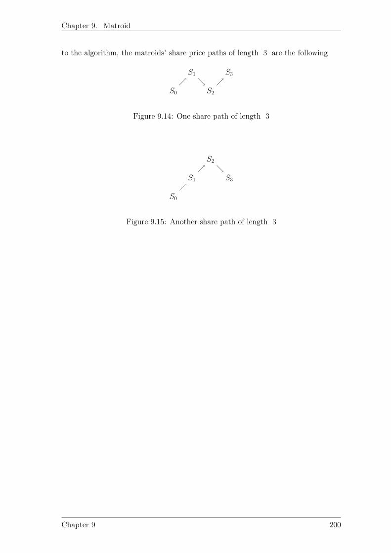
Chapter 9. Matroid
to the algorithm, the matroids’ share price paths of length 3 are the following
S0
S1
S2
S3
Figure 9.14: One share path of length 3
S0
S1
S2
S3
Figure 9.15: Another share path of length 3
Chapter 9 200

Chapter 10
Conclusions and Future work
10.1 Conclusions
The main topic of the thesis is to develop combinatorial structure and path calcula-tion methods and then apply them to model individual share price path and calculateoption prices. The main contributions of this thesis are covered in Chapter 2, 5, 6,7, 8, 9 and Section 3.1, 3.2, 3.7, 4.5, 4.6. Two working papers including section 5.3,8.2, 9.5 is now being produced.
In Chapter 2, the main results are the followings. In section 2.1.2, we presentedthe path calculation method in the formula from the perspective of set theory.Furthermore, originated from [5], we applied the path calculation method to 2 steps,3 steps binomial models with different setting of probability measures, and presentthe option pricing formula as lemmas using classical method and path calculationmethod(Lemma 1, Lemma 2, Lemma 3, Lemma 4, Lemma 5). We also applied theFlajolet generating method to provide two ways of representing 2-steps share pricebinomial model, we gave new examples of applying the second representation methodof share price paths and generating functions(Example 2.3.1, Example 2.3.2). Insection 2.3.2, we provided a Lemma 6, which claims a test condition whether ornot a generating function can represent a path and illustrated using Example 2.3.3.Moreover, we derived Theorem 7, which is the option value of the exotic claimusing path calculation argument and generating function method. In the end ofthe chapter, applying the generating function knowledge, we provided a argumentof relationship between counting paths in a model and the probability generatingfunction of the model and checked that the finite share price binomial model Ωn isa combinatorial class.
In Chapter 3, the main results are the followings. In section 3.1, 3.2, applying theknowledge of generating function to represent an individual share price path, wegave Example 3.1.1, Example 3.1.2, Example 3.1.3, Example 3.2.1, Example 3.2.2,Example 3.2.3, Example 3.2.4, Example 3.2.5, Example 3.2.6, Example 3.2.7. Insection 3.3, based on the Flajolet symbolic method, we gave different presentationsof description of sequence construction taken from [15]; multiset construction, cycleconstruction, powerset construction. In addition, we provide Definition 24(symbolicpath transformation) and Corollary 15. In section 3.4.3, we provided the detailedenumeration of general binary strings that contain consecutive 0’s less than threeusing Flajolet symbolic method. In the Example 3.4.2, we added the derivation
201

Chapter 10. Conclusions and Future work
of generating function using Flajolet symbolic method. In Example 3.5.1, we gavedetailed algorithm how disjoint union of directed cycles is obtained from a permu-tation with disjoint cycle notation. We also gave more clear and readable proof ofproposition 33. In the proof of Proposition 37, we added the derivation of the countsc(n, k) using Flajolet symbolic method. In section 3.5.4, we provided a detailed andapplicable algorithm of the natural correspondence from the given integer sequenceto a permutation and also give the argument to justify the algorithm is reasonableby analysing the relation between the possible values of ani and the number ofpositions in the permutation ui. Moreover, we derive a Proposition 39 that claimsthe relationship between integer sequences and permutation of [n]. In addition,we added more readable argument of the combinatorial method in the proof ofProposition 48. We also derive a general formula A(n, k) for the counts of thenumber of set permutation w ∈ Sn with a fixed number of descent k−1 (Theorem48). In the last section of the chapter, we also provided the case study of share priceanalysis using the knowledge of generating function (Section 3.7); (case I; Example3.7.1, Example 3.7.2, Example 3.7.3 case II).
In Chapter 4, the main results are the followings. In Section 4.1, we use the simplecombinatorial method to count the no of lattice paths of length N . In Section4.3, we reviewed the enumeration of self-avoiding walks with three directions, inwhich we added the detailed explanation of derivation of the general recursive beforederiving the two variable generating function G(t, v) and extracting the coefficientg(n,m). In Section 4.6, in the method 2, we derived the solution of counting apath not touching the given bold line segment. In Section 4.6, we applied the pathcalculation method to solve the winning probability in the gambler ruin problem, inwhich we got the same answer as using the classical method.
In Chapter 5, the main results are the followings. Motivated from the idea takenfrom [17] [29], we provided the algorithm of constructing share price path from aset of full binary trees in Section 5.1.1 and gave the share price path interpretationin Section 5.1.2. In Section 5.2.1, we gave the algorithm of constructing share pricepath from a set of general trees. In Section 5.3.1, we provided an algorithm torepresent a share price via a general binary ordered tree.
In Chapter 6, the main results are the followings. We constructed the set of restrictedshare price paths and its path generating functions in Section 6.1 and then we derivedthe calculation of option price in the given finite restricted binomial model(Theorem60).
In Chapter 7, the main results are the followings. In Section 7.1, we gave theExample 7.1.1, Example 7.1.2, Example 7.1.3, Example 7.1.4, Example 7.1.5, Ex-ample 7.1.6. In Section 7.2.1, using the idea of bijection between 2-colored Motzkinwords and dyck words taken from the paper [30, Page 179], we gave a constructionalgorithm from parallelogram polyomino to dyck share price paths. It followed withthe share price path ineterpreation in Section 7.2.2.
In Chapter 8, the main results are the Section 8.2, in which we provided the methodof counting no of restricted paths via unusual stochastic modelling(Lemma 73,
Chapter 10 202

Chapter 10. Conclusions and Future work
Lemma 74, Lemma 75, Example 8.2.1, Example 8.2.2, Example 8.2.3, Section 8.2.2,Section 8.2.3, Section 8.2.4, Section 8.2.5).
In Chapter 9, the main results are the followings. In general, we gave differentpresentations of the knowledge of matroid and Tutte polynomial. In Section 9.1, wegave the explicit proof of Example 9.1.1, we added clear explanation in the proof ofExample 9.1.2. We also gave Example 9.1.3, Example 9.1.5, more detailed proof ofProposition 79, more detailed proof of Example 9.1.4, more detailed explanation ofchecking axiom(iii) in (I3) in the proof of Proposition 92. In addition, applyingthe algorithm of finding maximum matching, we gave Example 9.16. We alsogave the proof of Proposition 96 following the definition of the matroid, and thenprovided a construction algorithm of bipartite graph from any given matroid andexplained it using a small example(Example 9.1.7). Furthermore, we provided amore constructive definition of lattice path matroid(Definition 105), and Example9.3.1 in Section 9.3. In Section 9.4, we gave the methodology of the calculationof Tutte polynomial from a gvien lattice path matroid. Specifically, in Section9.4.1, applying the Lemma 104, we gave a construction algorithm between the setof lattice paths and the set of their north steps. According to the Definition 105. aconstruction of E(M), I(M), B(M) is provided for a lattice path matroid M, and weprovided an analysis of the calculation of Tutte polynomial TM(x, y) for the matroidM in Section 9.4 and provided the Example 9.4.1 to illustrate the calculation analysisin Section 9.4.3. Moreover, in the end of the chapter, we provided a new modellingof paths via matroid(Section 9.5).
10.2 Future work
Connection with continuous models is the most interesting direction which was notcovered.
In particular, it would be interesting to introduce continuous time binary tree andits application to finance.
Asymptotic results in another interesting direction, in particular connection betweennumber of path and number of path on a lattice, and measures the Hausdorffmanifold, preliminary reading and some initial calculation were done.
Chapter 203

Appendices
204
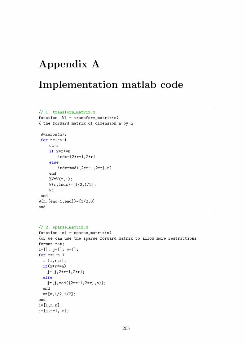
Appendix A
Implementation matlab code
// 1. transform_matrix.m
function [W] = transform_matrix(n)
% the forward matrix of dimension n-by-n
W=zeros(n);
for r=1:n-1
cc=r
if 2*r<=n
indx=[2*r-1,2*r]
else
indx=mod([2*r-1,2*r],n)
end
%V=W(r,:);
W(r,indx)=[1/2,1/2];
W;
end
W(n,[end-1,end])=[1/2,0]
end
// 2. sparse_matrix.m
function [m] = sparse_matrix(n)
%or we can use the sparse forward matrix to allow more restrictions
format rat;
i=[]; j=[]; v=[];
for r=1:n-1
i=[i,r,r];
if(2*r<=n)
j=[j,2*r-1,2*r];
else
j=[j,mod([2*r-1,2*r],n)];
end
v=[v,1/2,1/2];
end
i=[i,n,n];
j=[j,n-1, n];
205

Appendix A. Implementation matlab code
v=[v,1/2,0];
m=sparse(i,j,v,n,n);
end
//3. test_count.m
function [ ] = test_count
% Input: restriction=the number of not allowing consecutive down steps.
% T= count the number of restricted paths on which steps, T>=1
% Output: count
% the restriction condition will make sense starting from the time step
2, so, we consider the given
% information on the first (restriction-1) steps.
prompt = ’the number of not allowing consecutive down steps? ’;
restriction = input(prompt)
prompt = ’count the number of restricted paths on which time steps(T>=1)?
’;
T = input(prompt)
m=restriction-1; % consider the given information on the first
(restriction-1) steps
format rat;
i=[]; % initial probability of the states of the two steps paths
for j=1:2^m % it is 2 (each step two choices) to the power m (given
information on the first m
% steps); say, if m=2, the state set is 11, 10,
01, 00
i=[i, 1/(2^m)]; % equal probability for jump up and jump down of the
paths on the given time
% steps information
end
n=2^(restriction-1); % the number of rows or columns of the transform
forward matrix
if T >= restriction
% if T greater than restriction, then calculate forward matrix
%fw= transform_matrix(n) % the forward matrix of dimension n-by-n
%or we can use the sparse forward matrix to allow more restrictions
fw=sparse_matrix(n);
Probb=i*fw^(T-(restriction-1)); % the power denotes the number of time
steps after the given
% time steps information
CProb= Probb/sum(Probb); % normalized probability at time step T with
restriction not allowing
% restriction consecutive down steps
count=2^T * sum(Probb); % the number of restricted path at time step T
with the given restriction
else
count=2^T; % the number of restricted path at time step T with the
given restriction
Chapter A 206

Appendix A. Implementation matlab code
% when T< restriction, the restriction not works,
the counts just as normal
end
X = sprintf(’The number of restricted paths not allowing %d consecutive
down steps at time %d is %d’,restriction, T,count);
disp(X)
end
// 4. Test:
>> test_count
the number of not allowing consecutive down steps? 2
restriction =
2
count the number of restricted paths on which time steps(T>=1)? 3
T =
3
The number of restricted paths not allowing 2 consecutive down steps at
time 3 is 5
>> test_count
the number of not allowing consecutive down steps? 3
restriction =
3
count the number of restricted paths on which time steps(T>=1)? 5
T =
5
The number of restricted paths not allowing 3 consecutive down steps at
time 5 is 24
%%%%%%%%%%%%%%%%%if restriction number is big%%%%%%%%%%%%
>> test_count
the number of not allowing consecutive down steps? 15
Chapter A 207

Appendix A. Implementation matlab code
restriction =
15
count the number of restricted paths on which time steps(T>=1)? 25
T =
25
The number of restricted paths not allowing 15 consecutive down steps at
time 25 is 33548288
Chapter 10 208

Bibliography
[1] Claessens, S., Kose, M.M.A., Laeven, M.L. and Valencia, F., 2014. Financialcrises: Causes, consequences, and policy responses. International MonetaryFund.
[2] Hao, W., Lefevre, C., Tamturk, M. and Utev, S., 2019. Quantum option pricingand data analysis. Quantitative Finance and Economics, 3(3), p.490.
[3] Lento, C. and Gradojevic, N., 2013. The Effectiveness of Option Pricing ModelsDuring Financial Crises. In Rethinking Valuation and Pricing Models (pp. 1-11).Academic Press.
[4] Black, F. and M. Scholes. (1973). The Pricing of Options and CorporateLiabilities, Journal of Political Economy 81, No. 3 (May-June 1973), pp. 637-654.
[5] Cox, J.C., Ross, S.A. and Rubinstein, M., 1979. Option pricing: A simplifiedapproach. Journal of financial Economics, 7(3), pp.229-263.
[6] Cox, J.C. and S.A. Ross. (1976). The Valuation of Options for AlternativeStochastic Processes, Journal of Financial Economics 3, No. 1 (January-March1976) pp. 145-166.
[7] Henderson, V., 2014. Black–Scholes Model. Wiley StatsRef: Statistics ReferenceOnline.
[8] Baaquie, B.E., 2009. Interest rates and coupon bonds in quantum finance.Cambridge University Press.
[9] Ma, X. and Utev, S., 2012. Modelling the share prices as a hidden random walkon the lamplighter group. In Mathematical and Statistical Methods for ActuarialSciences and Finance (pp. 263-270). Springer, Milano.
[10] Karadeniz, R.S. and Utev, S., 2015. Modelling share prices via the random walkon the lamplighter group.
[11] Lefevre, C., Loisel, S., Tamturk, M. and Utev, S., 2018. A quantum-typeapproach to non-life insurance risk modelling. Risks, 6(3), p.99.
[12] Taylor, E.F., Vokos, S., O’Meara, J.M. and Thornber, N.S., 1998. TeachingFeynman’s sum-over-paths quantum theory. Computers in Physics, 12(2),pp.190-199.
[13] Sinha, S. and Sorkin, R.D., 1991. A Sum-over-histories Account of an EPR (B)Experiment. Foundations of Physics Letters, 4(4), pp.303-335.
209

Bibliography
[14] Sedgewick, Robert, and Philippe Flajolet. An introduction to the analysis ofalgorithms. Addison-Wesley, 2013.
[15] Flajolet, Philippe, and Robert Sedgewick. Analytic combinatorics. cambridgeUniversity press, 2009.
[16] https://math.stackexchange.com/questions/1633762/using-generating-functions-to-answer-how-many-bit-strings-of-length-n-have-no-00
[17] Federico, Class EC Homework. http://math.sfsu.edu/federico/Clase/EC/Homework/3.3.Jorge.pdf
[18] Brylawski, T. and Oxley, J., 1992. The Tutte polynomial and its applications.Matroid applications, 40, pp.123-225.
[19] Mohanty, G., 2014. Lattice path counting and applications. Academic Press.
[20] Racorean, O.S., 2014. Crossing Stocks and the Positive Grassmannian I: TheGeometry behind Stock Market. Available at SSRN 2512437.
[21] Stanley, R.P., 2011. Enumerative Combinatorics Volume 1 second edition.Cambridge studies in advanced mathematics.
[22] Chandran,Combinatorics. Mod-04 Lec-31 Solving recurrence relations usinggenerating functions - Part (2)
[23] Wallner, Michael. Lattice Path Combinatorics. na, 2013.
[24] Williams, Lauren K. ”Enumerating up-side self-avoiding walks on integerlattices.” The Electronic Journal of Combinatorics 3.R31 (1996): 2.
[25] Grinstead, C.M. and Snell, J.L., 2006. Grinstead and Snell’s introduction toprobability. Chance Project.
[26] John Tsitsiklis. Class MIT 6.041 Probabilistic Systems Analysis and AppliedProbability, Fall 2010 Lecture 16 Markov Chains I.
[27] Tolver, A., 2016. An introduction to Markov chains. Department of Mathemat-ical Sciences, University of Copenhagen.
[28] Utev, Sergey, 2018. Summary of Lectures 1-38. Financial mathematics lecturenotes. Department of Mathematics, University of Leicester.
[29] Dershowitz, N. and Rinderknecht, C., 2015. The average height of Catalan treesby counting lattice paths. Mathematics Magazine, 88(3), pp.187-195.
[30] M.P. and Viennot, G., 1984. Algebraic languages and polyominoes enumeration.Theoretical Computer Science, 34(1-2), pp.169-206.
[31] Leroux, P. and Rassart, E., 1999. Enumeration of symmetry classes ofparallelogram polyominoes. arXiv preprint math/9901135.
[32] Delest, M.P., 1988. Generating functions for column-convex polyominoes.Journal of Combinatorial Theory, Series A, 48(1), pp.12-31.
Chapter 10 210
Bibliography
[33] Conrad, Brian. Handout. Interior, closure, and boundary.http://virtualmath1.stanford.edu/ conrad/diffgeomPage/handouts/closure.pdf
[34] Weisstein, Eric W. ”Open Ball.” From MathWorld–A Wolfram Web Resource.http://mathworld.wolfram.com/OpenBall.html
[35] Weisstein, Eric W. ”Polyomino.” From MathWorld–A Wolfram Web Resource.http://mathworld.wolfram.com/Polyomino.html
[36] Weisstein, Eric W. ”Convex Polyomino.” From MathWorld–A Wolfram WebResource. http://mathworld.wolfram.com/ConvexPolyomino.html
[37] Alexander Bogomolny. PascalTriangleProperties. https://www.cut-the-knot.org/arithmetic/combinatorics/PascalTriangleProperties.shtml
[38] The Gambler’s Ruin. https://www.mathpages.com/home/kmath084/kmath084.htm
[39] Mark J Barlow. Mathematical Methods in Actuarial Sciences. Mathematics 3rdYear Project Spring 2007/2008, School of Mathematical Sciences, University ofNottingham.
[40] Adams, S., 2015. MA3H2 Markov Processes and Percolation theory. update.
[41] Weisstein, Eric W. ”Lattice Path.” From MathWorld–A Wolfram Web Re-source. http://mathworld.wolfram.com/LatticePath.html
[42] Abel, Zachary. Multivariate generating functions and other tidbits. Mathemat-ical Reflections, March 2006.
[43] Math Stackexchange. https://math.stackexchange.com/questions/314788/let-p-be-an-odd-prime-number-how-many-p-element-subsets-of-1-2-3-4-ldo
[44] Sedgewick, Robert. 1.4 Compositions and Partitions. Lecture 1, Combinatorialstructures and OGFs.
[45] Min Wang, Sergey Utev: Christmas trees and option pricings. (paper inpreparation).
[46] Federico, Lecture notes of Matroids. http://math.sfsu.edu/federico/Clase/Matroids/LectureNotes/lectures1-25.pdf
[47] Goemans, Lecture 8 Matroids, Lecture notes of Advanced CombinatorialOptimization. https://math.mit.edu/ goemans/18438F09/lec8.pdf
[48] http://math.mit.edu/ goemans/18453S17/matroid-notes.pdf
[49] http://www-math.mit.edu/ goemans/18433S09/matroid-notes.pdf
[50] https://www.whitman.edu/Documents/Academics/Mathematics/hillman.pdf
[51] https://www.youtube.com/watch?v=-tj0T5WihzI
[52] Okstate. https://math.okstate.edu/people/binegar/3013-S99/3013-l10.pdf
Chapter 10 211

Bibliography
[53] Chekuri, Chandra. Introduction to Matroids, CS 598CSC: Combinatorial Opti-mization https://courses.engr.illinois.edu/cs598csc/sp2010/Lectures/Lecture14.pdf
[54] Saurabh, Saket. Lecture 13, Advanced Graph Algorithms.https://kam.mff.cuni.cz/ ashutosh/lectures/lec13.pdf
[55] Jonathan Hirata. NOTES ON MATCHING, MIT. http://www-math.mit.edu/ djk/18.310/Lecture-Notes/MatchingProblem.pdf
[56] Paul E. Black and Alen Lovrencic, ”subgraph”, in Dictionary of Algorithmsand Data Structures [online], Paul E. Black, ed. 17 December 2004. (accessedTODAY) Available from: https://www.nist.gov/dads/HTML/subgraph.html
[57] Arobinda Gupta, Lecture slide of Matching and Covering, CS60047: AdvancedGraph Theory http://cse.iitkgp.ac.in/ agupta/graph/Matching.pdf
[58] Bipartite Graphs/Matching (Intro)-Tutorial 12 D1 Edexcelhttps://www.youtube.com/watch?v=JpapV5DrBek
[59] Maximum Matching Algorithm - Tutorial 13 D1 Edexcel A-Levelhttps://www.youtube.com/watch?v=gbasc4F-7hk
[60] Bonin, J., de Mier, A. and Noy, M., 2003. Lattice path matroids: enumerativeaspects and Tutte polynomials. Journal of Combinatorial Theory, Series A,104(1), pp.63-94.
[61] Bonin, J.E., 2010. An introduction to transversal matroids.
[62] Federico Ardila. Tutte polynomials in combinatorics and geometry, ModernMath Workshop SACNAS National Conference, San Antonio, Texas, 2 deoctubre de 2013 http://math.sfsu.edu/federico/Talks/SACNAStutte.pdf
[63] Porter, A.M. and Balof, B., 2015. The Tutte polynomial and applications.
[64] Merino, C., Ramırez-Ibanez, M. and Rodrıguez-Sanchez, G., 2012. The Tuttepolynomial of some matroids. International Journal of Combinatorics, 2012.
[65] Lin, B., 2013. An Introduction of Tutte Polynomial.
[66] Brandt, M., 2015. The Tutte Polynomial.
Chapter 10 212
Copyright © 2022 FDOKUMEN