A purely elastic instability in Dean and Taylor-Dean flow

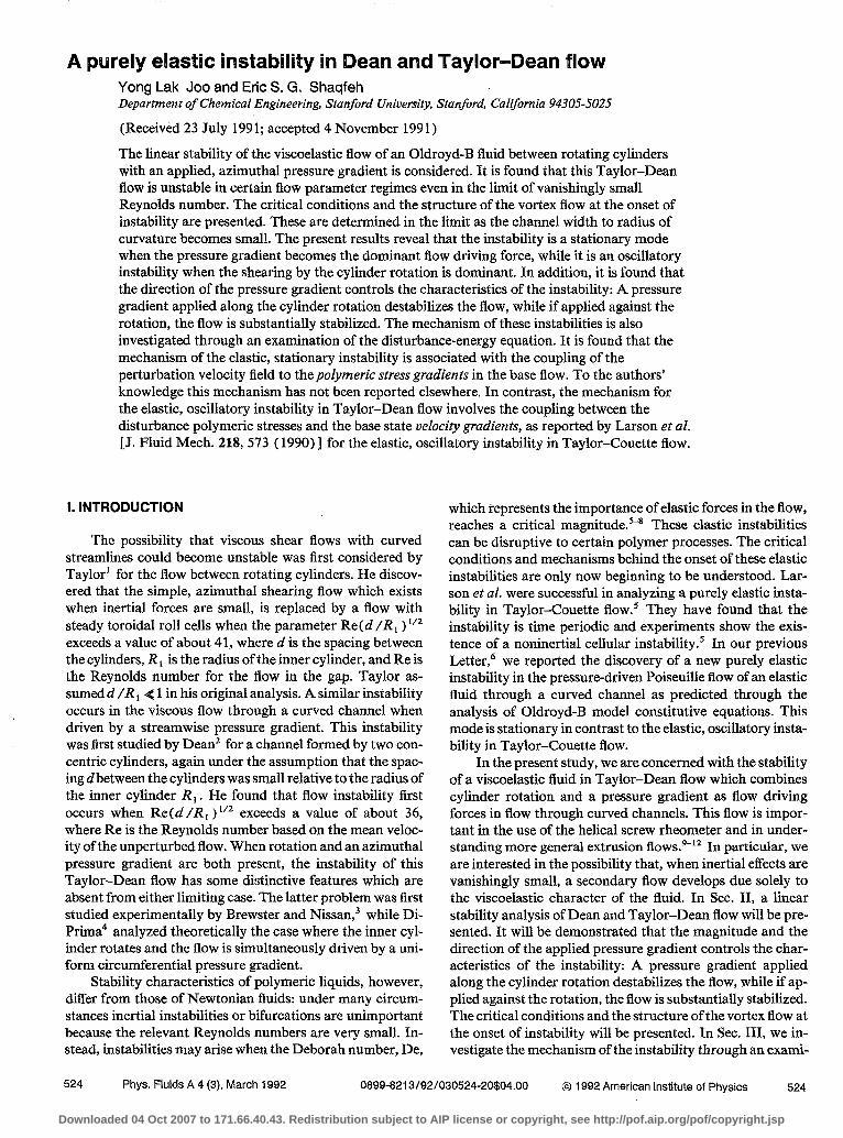
A purely elastic instability in Dean and Taylor-Dean flow Yong Lak Joo and Eric S. G. Shaqfeh Department of Chemical Engineering, Stanford University, Stanford, California 94305-5025

(Received 23 July 1991; accepted 4 November 199 1)

The linear stability of the viscoelastic flow of an Oldroyd-B fluid between rotating cylinders with an applied, azimuthal pressure gradient is considered. It is found that this Taylor-Dean flow is unstable in certain flow parameter regimes even in the limit of vanishingly small Reynolds number. The critical conditions and the structure of the vortex flow at the onset of instability are presented. These are determined in the limit as the channel width to radius of curvature becomes small. The present results reveal that the instability is a stationary mode when the pressure gradient becomes the dominant flow driving force, while it is an oscillatory instability when the shearing by the cylinder rotation is dominant. In addition, it is found that the direction of the pressure gradient controls the characteristics of the instability: A pressure gradient applied along the cylinder rotation destabilizes the flow, while if applied against the rotation, the flow is substantially stabilized. The mechanism of these instabilities is also investigated through an examination of the disturbance-energy equation. It is found that the mechanism of the elastic, stationary instability is associated with the coupling of the perturbation velocity field to the polymeric stress gradients in the base flow. To the authors’ knowledge this mechanism has not been reported elsewhere. In contrast, the mechanism for the elastic, oscillatory instability in Taylor-Dean flow involves the coupling between the disturbance polymeric stresses and the base state velocity gradients, as reported by Larson et al. [J. Fluid Mech. 218, 573 ( 1990) ] for the elastic, oscillatory instability in Taylor-Couette flow.

I. INTRODUCTION

The possibility that viscous shear flows with curved streamlines could become unstable was first considered by Taylor’ for the flow between rotating cylinders. He discov- ered that the simple, azimuthal shearing flow which exists when inertial forces are small, is replaced by a flow with steady toroidal roll cells when the parameter Re( d /R 1 ) 1’2 exceeds a value of about 41, where d is the spacing between the cylinders, R, is the radius of the inner cylinder, and Re is the Reynolds number for the flow in the gap. Taylor as- sumed d /R 1 ( 1 in his original analysis. A similar instability occurs in the viscous flow through a curved channel when driven by a streamwise pressure gradient. This instability was first studied by Dean’ for a channel formed by two,concentric cylinders, again under the assumption that the spacing d between the cylinders was small relative to the radius of the inner cylinder R, . He found that flow instability first occurs when Re (d /R 1 ) “2 exceeds a value of about 36, where Re is the Reynolds number based on the mean velocity of the unperturbed flow. When rotation and an azimuthal pressure gradient are both present, the instability of this Taylor-Dean flow has some distinctive features which are absent from either limiting case. The latter problem was first studied experimentally by Brewster and Nissan,3 while Di- Prima4 analyzed theoretically the case where the inner cylinder rotates and the flow is simultaneously driven by a uni- form circumferential pressure gradient.

Stability characteristics of polymeric liquids, however, differ from those of Newtonian fluids: under many circum- stances inertial instabilities or bifurcations are unimportant because the relevant Reynolds numbers are very small. In- stead, instabilities may arise when the Deborah number, De,

which represents the importance of elastic forces in the flow, reaches a critical magnitude.‘-* These elastic instabilities can be disruptive to certain polymer processes. The critical conditions and mechanisms behind the onset of these elastic instabilities are only now beginning to be understood. Lar- son et al. were successful in analyzing a purely elastic instability in Taylor-Couette flow.’ They have found that the instability is time periodic and experiments show the existence of a noninertial cellular instability.’ In our previous Letter,’ we reported the discovery of a new purely elastic instability in the pressure-driven Poiseuille flow of an elastic fluid through a curved channel as predicted through the analysis of Oldroyd-B model constitutive equations. This mode is stationary in contrast to the elastic, oscillatory instability in Taylor-Couette flow.

In the present study, we are concerned with the stability of a viscoelastic fluid in Taylor-Dean flow which combines cylinder rotation and a pressure gradient as flow driving forces in flow through curved channels. This flow is important in the use of the helical screw rheometer and in understanding more general extrusion flow~.~‘~ In particular, we are interested in the possibility that, when inertial effects are vanishingly small, a secondary flow develops due solely to the viscoelastic character of the fluid. In Sec. II, a linear stability analysis of Dean and Taylor-Dean flow will be presented. It will be demonstrated that the magnitude and the direction of the applied pressure gradient controls the characteristics of the instability: A pressure gradient applied along the cylinder rotation destabilizes the flow, while if applied against the rotation, the flow is substantially stabilized. The critical conditions and the structure of the vortex flow at the onset of instability will be presented. In Sec. III, we investigate the mechanism of the instability through an exami-

524 Phys. Fluids A 4 (3), March 1992 0899-8213/92/030524-20$04.00 0 1992 American Institute of Physics 524

Downloaded 04 Oct 2007 to 171.66.40.43. Redistribution subject to AIP license or copyright, see http://pof.aip.org/pof/copyright.jsp

nation of the disturbance-energy equation. We demonstrate the interplay between the elastic, stationary mode which occurs in Dean flow and the elastic, oscillatory mode which occurs in Taylor-Couette flow.

II. LINEAR STABILITY ANALYSIS A. General development

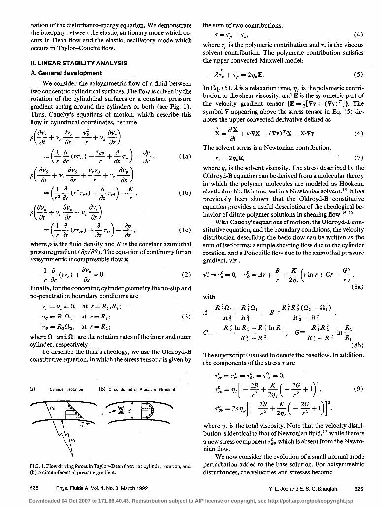
We consider the axisymmetric flow of a fluid between two concentric cylindrical surfaces. The flow is driven by the rotation of the cylindrical surfaces or a constant pressure gradient acting around the cylinders or both (see Fig. 1). Thus, Cauchy’s equations of motion, which describe this flow in cylindrical coordinates, become

p 2+, (

?p+vz$ r >

z (

$i(rrprl -T+grzr)-$, (la)

(

av, av, vrve av, P- -- - at + vr ar + r + vz az >

( la(r23-&) +-rz, a 7 = r2 dr az >

-e, (lb) r

p at ( %fv a,,+vz!$

r &Jr >

= ( +$ (rrm) +-frzz) -$, (lc)

where p is the fluid density and K is the constant azimuthal pressure gradient (ap/a@ . The equation of continuity for an axisymmetric incompressible flow is

-k&Y) +$+o. Finally, for the concentric cylinder geometry the no-slip and no-penetration boundary conditions are

vr = vz =0, at r=R,,R,;

v. =R,n,, at r=R,; (3) ve =R,n,, at r=R,;

where 61, and fl, are the rotation rates of the inner and outer cylinder, respectively.

To describe the fluid’s rheology, we use the Oldroyd-B constitutive equation, in which the stress tensor r is given by

(a) Cylinder Rotation (b) Circumferential Pressure Gradient

FIG. 1. Flow driving forces in Taylor-Dean flow: (a) cylinder rotation, and (b) a circumferential pressure gradient.

the sum of two contributions, 7=rp +rs, (4)

where rp is the polymeric contribution and r9 is the viscous solvent contribution. The polymeric contribution satisfies the upper convected Maxwell model:

A< + rp = 2?j$ (5)

In Eq. (5)) A is a relaxation time, rip is the polymeric contribution to the shear viscosity, and E is the symmetric part of the velocity gradient tensor (E = $[Vv + (Vv) ‘I). The symbol V appearing above the stress tensor in Eq. (5) denotes the upper convected derivative defined as

;; = 2 + PVX - (Vv) T’x - x*vv.

The solvent stress is a Newtonian contribution,

(6)

rs = 237A (7) where 3S is the solvent viscosity. The stress described by the Oldroyd-B equation can be derived from a molecular theory in which the polymer molecules are modeled as Hookean elastic dumbbells immersed in a Newtonian solvent. l3 It has previously been shown that the Oldroyd-B constitutive equation provides a useful description of the rheological be- havior of dilute polymer solutions in shearing fl~w.‘~‘~

With Cauchy’s equations of motion, the Oldroyd-B constitutive equation, and the boundary conditions, the velocity distribution describing the basic flow can be written as the sum of two terms: a simple shearing flow due to the cylinder rotation, and a Poiseuille flow due to the azimuthal pressure gradient, viz.,

$J=e=O, vs=Ar+t+$- rlnr+Cr+g , t ( r >

with (W

As35 R;fh2 -R:Cl, RtR:(& --f-b)

R; -R; , BE

R$-R: ’

CE - Rz lnR, -RfhR, i: Ins.

R; -R: , GE R’R

R;-R: R, (8b)

The superscript 0 is used to denote the base flow. In addition, the components of the stress rare

3fr = r$ = & = rzz = 0,

&=l;l* -%- [ r2 $( -?+1)],

60 = wl;lp [

2+$(-F+ 1)12, r2

(9)

where Vt is the total viscosity. Note that the velocity distribution is identical to that of Newtonian fluid,” while there is a new stress component r& which is absent from the Newto- nian flow.

We now consider the evolution of a small normal mode perturbation added to the base solution. For axisymmetric disturbances, the velocities and stresses become

525 Phys. Fluids A, Vol. 4, No. 3, March 1992 Y. L. Joo and E. S. G. Shaqfeh 525


v = (0,4,,0) + [ U(r),V(rj,W(r)]e’(“-““,

0 6 0

( 1W

7= 7f*- $88 0

( ) 0 0 0 RR(r) R&r) RZ(r)

+ R6W

( @W ez(rj

RZ(rj BZ(r> ZZ(r) 1

eKuz- JO* (lob)

We shall be considering the temporal stability of the flow, so w is in general a complex frequency and c is the real wave number. This formulation allows for the consideration of overstable as well as stationary modes. When the expressions for the perturbed velocity components in (10a) are substituted into the continuity equation (2)) we find

(l/r)(rUj’+iaW=O, (11)

where the prime denotes differentiation with respect to r. After the expressions (10a) and (lob) are substituted into the momentum balance equations ( la)-( lc), the stress amplitude functions can be determined. The derivation of each component of the stress amplitude functions is described in detail in the Appendix.

As a measure of the relative importance of the pressure gradient to cylinder rotation as flow driving forces, it is con- venient to introduce the dimensionless parameter,

c$= - Kd2/2qR:R,. (12) In the case when the gap d = R, - R i is small compared to the mean radius $( R r -I- R, j, we have the following approximate expressions for the velocity and stress fields in terms of thegapvariablex= (r--,)/R,:

l$ess~$ = f-&R, [‘$(x-x2) + (1 +fix)] (13) and

&?=<y = (??,&/E)[~(1---2X) +Bl, 7088 -r& = Wy$2:/~) I$(1 - 2x1 + B 12r

(14)

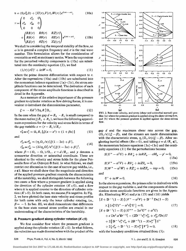
where p= (a, -&j/fi,, c-d/R,, and y denotes a streamwise direction or azimuthal coordinate. These are identical to the velocity and stress fields for the plane Poi- seuille flow of an Oldroyd-B fluid. In what follows, we shall restrict our discussion to the case of narrow gap widths, i.e., EQ 1. Since we shall show that the magnitude and direction of the applied pressure gradient controls the characteristics of the instability, we shall distinguish between the following two cases: a flow where a pressure gradient is applied along the direction of the cylinder rotation (K < 0), and a flow where it is applied counter to the direction of cylinder rotation (K> 0). In both cases, we assume fi is negative. In Fig. 2, we have plotted the base state velocity and stress profiles for both cases with only the inner cylinder rotating, i.e., fl= - 1. In Sec. III, we shall demonstrate that differences in the base state normal stress profiles are crucial in our understanding of the characteristics of the instability.

B. Pressure gradient along cylinder rotation (K<O)

We first consider flow where the pressure gradient is applied along the cylinder rotation (K < 0). In what follows, the velocities are made dimensionless with the product of the

1.0

0.8

iz 0.6 k 2 0.4 @

0.2

0.0 -d.5 0:o 0:5 -6.5 0:o O‘s

(2 6 FIG. 2. Base state velocity, and stress (shear and azimuthal normal) profiles: (a) where the pressure gradient is applied along the shear-driven flow, and (b) where the pressure gradient is applied against the shear-driven flow.

gap d and the maximum shear rate across the gap, (s1, ie) (5 - p), and the stresses are made dimensionless with the characteristic stress, qr ( a1 /e) (g - /?j. After neglecting inertial effects ( Re = 0 j , and taking E = d /R 1 ( 1, the momentum balance equations (la)-( lc) and the continuity equations ( 11 j for the perturbations become

S(U” -a2v) +RRi +iaRZP -&0, -p’=O, (154

S(V” -a2Vj +R0; +iaZ13~ =0, (15b)

S(W” -a”W) +RZ; +iaZZP -iap=O, (15cj and

U’+iaW=O. (16) In the above expressions, the primes refer to derivatives with respect to the gap variable x, and the components of dimensionless stress amplitude functions are given in the Appen- dix. Eliminating W(r) andp in (15) and (16) yields

[S+D-‘(1-Sj](V”-a2Vj+D-2De(1-~j

X[(eUjM -a’t&U] =0, (17)

[S+D-‘(l-sj](U”” -2a”U” +a’U)

+ E De’ a”D - ‘{ - (2D - ‘$‘rk& + <;/De j U

+2[D-1~~~Y+2D-2(l-~)~~~]Uf

+2[7”xy +D-I(1 -Sj~‘]V’}==O, (18) with the boundary conditions obtained from (3):



V=U=U’=O, at x=0 and x=1. (19) A, =4SD-‘(l--){(2+D-‘)/[S+D-‘(I-S)] In ( 16)-( 18), the following dimensionless groups appear:18

d fb Ez-, De=--- RI

(6-p,/& SE-J+ E % + vs

(20) a-cd, w^=oil, D= (1 -i^).

Equation ( 17) and the boundary conditions (20) imply that

v= -{Dm2De(l -s)/[s+D-‘(l-,S’j]}(y”,‘U). (21)

This result allows us to eliminate V from ( 18 ). Thus, in the narrow gap limit, after shifting the coordinates relative to those used in ( 19)) we obtain the eigenvalue problem for the complex frequency 2 governing the linear growth of small disturbances

U”” - 2a’U” f a’U f- 46 De” a’h,(w^j

X[ --26x+ (a- 1)]2U’+.sDe2a2A2(i;)

x[2sx+ (S- l>JU=O, (224 together with the boundary conditions

U==U’=O, x= +t. (22bj In (22), S ={/({--p), and A, and A, are related to the important dimensionless parameters via the expressions

A, =2D-‘(l--){(l +2D-‘)/[S+D-‘(1 -S)]

-D-‘(1 +D-‘)(l -Sj/[S+D-‘(1 -S)]“},

+D-2(1 +D-‘)(I -Sj/[S+D-‘(1 -Sj]“).

(23) Equation (22) constitutes an eigenvalue relation of the form F(cz,&~ De&S) = 0. For the limiting cases, S = 0 and S = 1, we recover the corresponding stability eigenvalue problem governing the Taylor-Couette flow5 (shear dominant flow) and the Dean flow6 (pressure dominant flow), respectively.

1. Solution of the eigenvalue problem

Two methods were employed to solve the eigenvalue problem (22). First, an approximate solution to (22) based on Gale&in’s method was employed. We expanded the perturbing velocity amplitude function U in two orthonormal sets of basis functions, 4:” and +F’, that are the solutions of the following eigenvalue problem originally posed by Grosch and Salwen:5*19

q$” - 2a2$” + a44 =fi “4, (244 q5 =qb’=O, at x = + 4. Wb)

For the Maxwell fluid (S = 0), after substituting this expan- sion into (22) and assuming diagonal dominance in any inner product matrices,5*19 we determined that approximate solutions to (22) are the roots of the following fourth-order polynomial:

[@c1j4D2 -4eDe2a2S(1 -&(2D2 + 2D + 1 + 21,)] [@Fj4D2 -4eDe2a2S(1 -Sj(2D2 + 2D + 1 + Z3)] n -4~De2a2[462(2D2+2D+1)1~-4~2I,-(l-~)2~2][4~2(2D2+2D+1j~S-~2~s-(l-~S)2~~]=O,

where

s

l/2

I’ = q5f”‘+;2’ dx, I, = - l/2 I

1/Z &‘)#;) t dx, - l/2

s

l/2

I

l/2

13 = x&‘)‘#’ dx, I4 = ~qS;~“q5p’ dx, - l/2 - l/2

I

I/2 l/2 (26) 15 = x#‘~p’ dx, I6 =

I x’&,‘)‘$;~’ dx,

- l/2 - l/2

1, = s

l/2

x2&$&2)’ dx. - l/2

For the limiting cases, S = 0 and 6 = 1, we have two simpli- fied equations which give approximate eigensolutions for Taylor-Couette and Dean flows, respectively: for 6 = 0

,O il)“fi i2)“D4 - 48 De2 a’I, I, = 0; (27) andfor 1

pi*)“/? L2j4D4 - 642 De2 a2 [ ( 2D2 + 2D + lj1, - 1, ]

X[(2D2+2D+1)1, -I61 =O. (28) Because the magnitude of both velocities and stresses grow exponentially in time (in the linear limit) if the imaginary part of the eigenvalue frequency, $* > 0, a critical condition

527 Phys. Fluids A, Vol. 4, No. 3, March 1992

(25)

I for instability becomes

Re(D)>l. (291 We shall show the existence of an infinite series of solutions of (25) which satisfy the condition (29). If is, = - Im( D) #O, the mode is overstable.

To demonstrate that the approximate solution of (25 j is useful, we also employed an accurate orthogonal shooting solution method to solve explicitly the eigenvalue problem (22) .20 This method has been applied to other stability prob-

1~~~21-23 and is based on the original ideas of Conte.24 For details concerning our numerical method, reference should be made to the appropriate publication.22 In this scheme, a complex secant method was employed to iterate and obtain convergence on the eigenvalue. The approximate solutions based upon Galerkin’s method were used as initial guesses.

2. Stability results From the numerical solutions of the eigenvalue problem

(22), we have found new purely elastic instabilities for all values of S: the instabilities are stationary modes when the pressure gradient is the dominant flow driving force, while they are oscillatory instabilities when the shearing by the

Y. L. Joo and E. S. G. Shaqfeh 527


\s=o.&? \A 6 = 0.6 ,4

k h 0.4 .A/ \

unstable

itable S - 0 ( t&&well Fluid )

I I I I 2 4 0 a

wavenumber, a

FIG. 3. The neutral curves for Dean flow, eIR De versus wave number, a, at various values of S. Note that onIy the most unstable mode is shown. The symbols “0” represent the results of the approximate Gale&in calculations with S = 0. The critical conditions are shown with the symbols “a.”

cylinder rotation is dominant. In our previous Letter,6 we presented a new purely elastic instability in the pressure- driven Poiseuille flow (S = 1) of an elastic fluid through a curved channel. This mode is stationary in contrast to the elastic, oscillatory instability in Taylor-Couette flow (S = 0). The calculated neutral stability curves of this Dean flow, E”~ De vs a, for various values of Sare shown in Fig. 3. The region below each curve represents the stable flow .regime, while the region above represents unstable flows. The figure demonstrates that the minimum in these curves is a shallow one in the vicinity of the calculated critical wave number a,. The critical conditions for the Maxwell fluid (S= 0) are

a, = 6.6 & 0.1, (~l’~ De), = 4.06 f. 0.02. (30) It is also observed that the critic?1 values of 8” De (shown with the symbols “E” in Fig. 3) monotonically increase as the solvent contribution to the fluid, S, is increased. In addition, for the Dean flow, the critical wave number a, decreases as S increases. In contrast, the critical wave number for Taylor-Couette flow remains the same for all values of Sa, = 6.7 f 0.1.’

In the following sections, we shall present the characteristics of the elastic instability in Taylor-Dean flow, explor- ing the neutral stability curves, and changes in the frequency and wave number of the unstable modes through the whole range of S.

a. The MaxwellJEuid; S=O. In Fig. 4 we have plotted neutral stability curves, E 1’2 De vs a, of the Maxwell fluid for various values of 8. The region below each curve represents the stable flow regime, while the region above represents unstable flows. Note that only the most unstable mode is shown. The real and imaginary parts of the frequency char- acterizing the principle modes for S = 0 through 6 = 1 at a

c; 8 c! -w

6

unstable

stable

wavenumber,a

FIG. 4. The neutral curves, B “’ De versus wave number, CY, for Taylor- Dean flow characterized by various values of 6 when the pressure gradient is applied along the flow. The symbols represent the results of the approximate Gale&in calculations with S = 0, the smooth curves represent the numerical solutions calculated via an orthogonal shooting procedure.

given wave number and Deborah number (a = 1, and E”~ De = 10) is plotted in Fig. 5. The symbols in Figs. 4 and 5 represent the results of approximate Galerkin calculations; the smooth curves represent the numerical solution calculated via an orthogonal shooting method. It is observed that the Galerkin method gives good approximate solutions to the eigenvalue problem (22) through the whole range of S. As previously presented, there is a purely elastic instability in Dean flow (S = 1) which is a stationary mode, while there is an elastic, oscillatory instability in Taylor-Couette flow (6 = 0). It is found that when an azimuthal pressure gradient is added to Taylor-Couette flow, it decreases the critical Deborah number (E 1’2 De), while also decreasing the critical wave number a, (see the neutral curve for S = 0.2 in Fig. 4). Thus this applied pressure gradient destabilizes the flow. The frequency of the overstable modes also decreases with increasing S as shown in Fig. 5. Moreover, adding cylinder rotation along the Dean flow destabilizes the flow, and decreases the critical wave number a, (see the neutral curve for S = 0.5 in Fig. 4). The mode remains stationary as shown in Fig. 5. For smaller values of S, the cylinder rotation stabi- lizes the flow, with the the most unstable mode remaining stationary. Thus, the critical Debdrah ,number (8’” De), has a minimum value when S = 0.5, i.e., the flow is the most unstable. In the region 0.25<6<0.3 where cylinder rotation and a pressure gradient are comparable, neutral curves of stationary and oscillatory modes coexist as shown in Fig. 6. Note that for S = 0.25, the critical Deborah number for the oscillatory modes is lower than that of the stationary mode and, therefore, the oscillatory modes are more unstable. The stationary mode becomes more unstable when S>O.275. As shown in Fig. 5, the oscillatory modes ultimat.ely fuse and



0.4 0.6 0.8 1.0 0.0 8

(a)

bifurcate into two stationary modes: one unstable mode and one decaying mode.

In addition to the calculations described above, we scanned the complex frequency domain at a given wave number and Deborah number to both demonstrate the tran- sition from oscillatory to stationary instability and to deter- dure, the complex determinant corresponding to the match- ing condition in the orthogonal shooting method is comput- ed at each point in the complex G plane and contours of

8

(a) 5 = 0.25 (b) 5 = 0.275

Oscillatory Modes

4 6 wavenumber,a

FIG. 5. The plots of (a) real, and (b) imaginary parts of the disturbance frequency in Tay- lor-Dean flow (O<S<l) for (r = 1, and 8” De = 10. The symbols represent the results of the approximate Galerkin calculations.

0.2 0.4 0.6 0.8 1.0 6

(b)

Re(Det) = 0 and Im(Det) = 0 can be drawn. Intersection points of these contours then represent eigenvalues.25 Figure 7 shows the zero contour lines of the complex determinant for S = 0 to S = 1 at the neutral values of Eli2 De and a = 1. Thus, the imaginary part of the complex frequency 6ji of the most unstable mode is zero in each figure. It is observed that modes are clustered about the singular point (63, = - 1, and w^, = 0) of the eigenvalue problem (22). The two most unstable oscillatory modes in the Taylor-Couette flow [Fig.

Oscillatory Modes

I I I 1 2 8 4 6

wavenumber,a

FIG. 6. The neutral curves for Taylor-Dean flow when oscillatory modes and a stationary mode coexist: (a) for 6 = 0.25, oscillatory modes are more unstable, and (b) for 6 = 0.275, a stationary mode is more unstable.



..* c+ f . . i’

-1 0 1 2 9

W 2

1

-. I 1 p =. 3

\ -2 -1 0 1 2 -2 -1

0, 01

FIG. 7. Zero contour plots of the complex determinant for (a) Taylor-Couette flow (6 = 0), Taylor-Dean flow: (b) 6 = 0.2, (c) S = 0.25, (d) 6 = 0.75, and (e) Dean flow (6 = 1) for a = 1, and at the corresponding neutral values of 6 In De The small squares represent contours of Re( Det) = 0, the larger squares . represent contours of Im( Det) = 0.

7(a) ] approach each other as 6 increases [S = 0.2, Fig. the pressure dominant flow (0.75<6< 1 ), but they are al- 7 (b) 1, and bifurcate into two stationary modes: one unstable ways decaying modes. It should be noted that the complete mode and one decaying mode for a slightly larger value of 6 set of eigenmodes has been determined through the pictured [S = 0.25, Fig. 7(c) 1. The new unstable, stationary mode zero crossings and these are shown for each flow. controls the flow stability for higher values of 0.25 <6<1 b. The Oldroyd-B&id (0 <S < 1). As mentioned above, [Figs. 7 (d) and 7 (e) 1. Oscillatory modes are developed in the Oldroyd-B fluid is a simple, viscoelastic constitutive



25

20,

15,

P =w

10,

5.

0.

unstable

S = 0 (M&well Fluid)

I I I I I 0 2 4 6 8 IO

wavenumber, a

(a)

stable S = 0 $axwell Fluid)

0 2 4 8 8 wavenumber, a

W

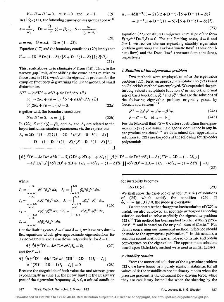
FIG. 8. The neutral stability curves for Taylor-Dean flow at various values of S: (a) 6 = 0.2, and (b) 6 = 0.5.

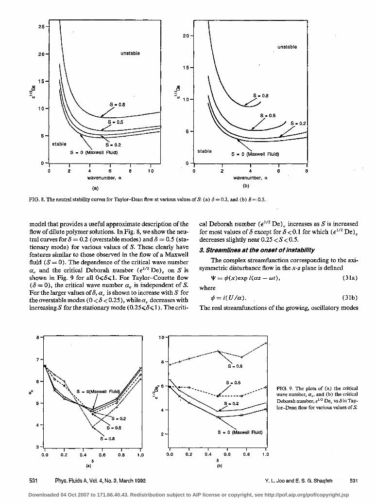
model that provides a useful approximate description of the flow of dilute polymer solutions. In Fig. 8, we show the neutral curves for 6 = 0.2 (overstable modes) and S = 0.5 (stationary mode) for various values of S. These clearly have features similar to those observed in the flow of a Maxwell fluid (S = 0). The dependence of the critical wave number a= and the critical Deborah number ( elf2 De), on S is shown in Fig. 9 for all 0~3~; 1. For Taylor-Couette flow (S = 0), the critical wave number a, is independent of S. For the larger values of S, a= is shown to increase with S for the overstable modes (0 <S < 0.25)) while a, decreases with increasingS for the stationary mode (0.25 <S< 1). The criti-

a

s‘.. 0.8

0.4 0.6 0.8 1.0

(al’

I I I I 0.0 0.2 0.4 0.6 0.8

6 W


unstable

cal Deborah number (E 1’2 De), increases as S is increased for most vahres of S except for 6 < 0.1 for which ( E”~ De), decreases slightly near 0.25 <S<O.5.

3. Streamlines at the onset of instability

The complex streamfunction corresponding to the axisymmetric disturbance flow in the x-z plane is defined

W = tj(x)exp i(az - wt), (3la) where

$=i(U/a). (31b) The real streamfunctions of the growing, oscillatory modes

lo-----------------

‘r

/...-- .-* ---.. \

. . . . . +/- ,...*-

.*+‘.-‘-’ . . 8 . . . ..-w-

s = 0.8

S = 0 (Maxwell Fk

FIG. 9. The plots of (a) the critical wave number, a,, and (b) the critical Deborah number, &” De, vs 6 in Tay- Ior-Dean flow for various values of .S.


z = 0.25

en 1.1 mnu *neM w .I ??ll.llS 0.01101~

(a)

D n t.s man ml- f o.PrrTII.II* a.-

(b)

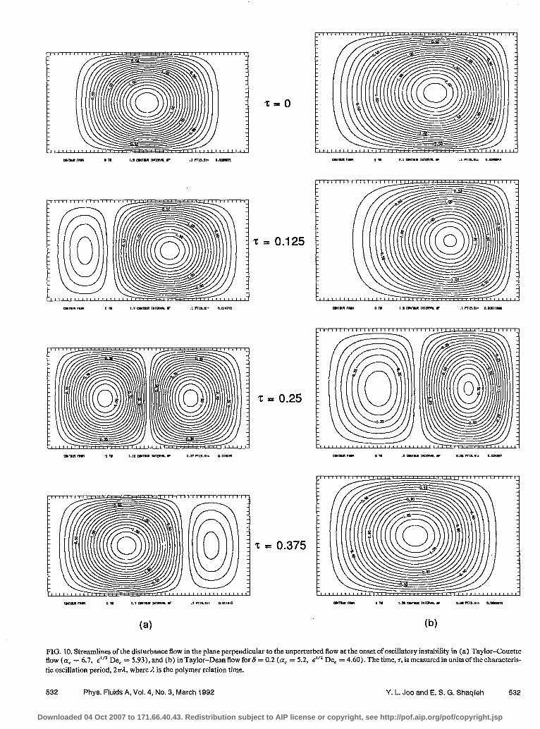
FIG. 10. Streamlines of the disturbance flow in the plane perpendicular to the unperturbed flow at the onset of oscillatory instability in (a) Taylor-Couette flow (a; = 6.7, I? De, = 5.93), and (b) inTaylor-Dean flow for6 = 0.2 (a, = 5.2, E “2 De c = 4.60). The time, 7, is measured in units of the characteristic oscillation period, 27r/z, where A is the polymer relation time.



which exist for S(O.25 then become and

fll” = - (l/CL) [ u, cos(az - w,t> If) = - ( l/a) [ - vi cos 2a(Z + r)

-I- U, sin(az - m,t)], (324 + U,sin2a(Z+IY]. (32~) = - (l/a) [ ui cos 2T(Z - r) In (32b) and (32c), we have resealed the z coordinate and

-=I- U, sin 2?r(Z- I?)], (32b) time t with the wavelength of the critical disturbance and the

FIG. 11. Streamlines of the disturbance flow at the onset of stationary instability in Taylor-Dean flow for (a) S = 0.5 (a, = 4.7,~"' De, = 3.40), (b) 6 = 0.75 (a, = 5.2,~“’ De, = 3.56), and (c) Poiseuille flow (a, = 6.7,~” De, = 4.06).

Phys. Fluids A, Vol. 4, No. 3, March 1992 Y. L. Joo and E. S. G. Shaqfeh 533


period of its oscillation, respectively. If we assume that the initial perturbations and the axial end conditions are both symmetric in the axial direction, then we might anticipate that the two complex conjugate, oscillatory modes will be present equally.26 This assumption has been verified recent- ly for Taylor-Couette flow through complete simulation of the full nonlinear problem. *‘*‘* The resulting real streamfunction for this wave pattern then becomes the sum of two streamfunctions, (32b) and (32~) :

$T= - (l/a)C[“i cos2a(Z-r) + U,sin2n(Z-r)]

+[-uic0s2~(z+r)+U,sin2~(Z+r)]).

(33) We will present primarily the calculations for the Maxwell fluid, because no qualitative changes in the vortex structure were found for nonzero values of the viscosity ratio 5’. The vortex flow for S = 0 (Taylor-Couette flow) and S = 0.2 is shown in Fig. 10 at the various values of the dimensionless time r. The left boundary of the graph represents the inner channel wall at x = - l/2, and the right is the outer wall at x = l/2. The vortex structure which forms near the inner cylinder is shown to radially propagate. Since the frequency of the modes, Gi,, and the critical axial wave number ac decrease for increasing 6, it is seen that the period of this radial propagation and the axial dimension of the vortex structure increase. In addition, note that for S = 0.2 the vortex which forms near the inner cylinder develops slowly in the early stage, so it takes more than a half-period for two vortices to fill the channel equally. Thereafter, this vortex develops and propagates faster, so that by three-quarters of the period, it almost fills the channel.

Since the amplitude of the radial component of the disturbance velocity Ubecomes real valued (i.e., U, = 0) when the mode is stationary (2, = 0)) the real streamfunction for the critical growing stationary mode becomes

ly, = - (l/a,(U, cos2rZ). (34) We have plotted the structures of the stationary vortex at the onset of instability for the various values of S in Fig. 11. The axial dimension of the vortices are shown to increase as S decreases from unity, while the strength of the vortices decreases. In addition, it is observed that the vortex center is located closer to the outer cylinder for the larger values of S.

To conclude this section, we have calculated numerical- ly the group velocity ug at the critical conditions for several values of S. Since any small disturbance can be represented by a superposition of normal modes, a localized initial disturbance not only will grow but also may move and spread, each unstable component growing at its own rate and mov- ing at its own velocity. If the group velocity of the unstable mode is not zero, the disturbance can grow and propagate: a convective instability. 29 At the critical conditions, the temporal growth rate, Gi, reaches a maximum value, 0, at the critical wave number a, such that

ai;, z (a,) = 0 and

& -$-(a,) =ug.

Note that the group velocities of the two growing modes in Taylor-Couette flow are zero indicating absolute instabil-

534 Phys. Fluids A, Vol. 4, No. 3, March 1992

0.0 0.2 0.4 0.6 0.8 6

FIG. 12. The disturbance group velocity at the critical Deborah numbers versus 6 for Taylor-Dean flow.

ity,2p while for 0 < S~0.25 the two growing modes have nonzero group velocities with equal magnitude but opposite sign as shown in Fig. 12. This implies there is convective instability in a certain parameter regime of Taylor-Dean flow. Thus, one might presumably see traveling vortex waves propagating axially under these conditions. It has been reported that there are axially propagating vortex waves in certain regimes of inertial Taylor-Dean flo~.~“‘* For larger values of S (0.25 < S< 1 >, the oscillatory modes fuse and the

I3 s ”

unstable unstable

I..... -vsqularory Mooesl . . .

0 stable 8 = 1 @can Flow) 1 I I I

0 5 10 15 20 wavenumber,a

FIG. 13. The neutral curves, .? De versus wave number a, for Taylor- Dean flow when the pressure gradient is applied against the flow at various values of 8.

Y. L. Joo and E. S. G. Shaqfeh 534


group velocity of the new growing stationary mode becomes zero (cf. Fig. 12).

C. Pressure gradient against shearing flow (K>O)

When the azimuthal pressure gradient is applied against the direction of the cylinder rotation, the maximum shear rate across the gap becomes (a, /E) ( - { - 8). We then define the Deborah number De as

De= (fil/e)( -g-,&l.. (36) After applying the same methods as described in Sets. II A and II B, we obtain a similar eigenvalue problem for the complex frequency w^ governing the linear growth of small disturbances, viz.,

u N ,, -2a2U” +a4U +4eDe2a2A,($) x[2s’x+ (s’--l)]*U’-~De~a~A~($) x[28x+ (s’- l)]U=O, (37)

I

U=U’=O, n= &$. (38)

In (37) the dimensionless variables, E, a, 2, and A, and A, remain those defined in (20) and (23), while s’, which is analogous to 6, becomes - {/( - < - p). Thus, for the limiting cases, s’ = 0 and s’ = 1, we recover the corresponding stability eigenvalue problem governing Taylor-Couette flow and Dean flow, respectively.

1. Solution of the eigenvalue problem

As in Sec. II B 1 when K < 0, two methods were used to solve the eigenvalue problem (37). Applying Gale&in’s method, we have determined that approximate solutions to (39) are the roots of the following fourth-order polynomial intermsofD= (1 -B):

[~~‘~4D2+4~De2a2~(1-~)(2D2+2D+1-221,)][~~2’~D2+4~De2a26’(1-6’)(2D2+2D+l-2~~)] n -4E2De2a2[4r2(2D2+2D+ 1)1, -4,Y21, -(l-&212][4S’2(2D2+2D+ 1)1,

-4sv, - (1 -s,)V,] =o.

In (39) I1 -I, remain as defined in (26). For the limiting case,S’=OandS’=1,(39)reducestoEqs.(27)and(28) for Taylor-Couette and Dean flows, respectively. Again, us- ing the results from the approximate Galerkin method as initial guesses, we used the orthogonal shooting method to obtain a complete set of stability results.

-1

-2

. . . . . . and:-- stationary mode

oscillatory modes

-. -. -2

--._ --._ --._

i

---_ ----__ ---_

._ -_....._” . .._ . . . . ...” . . . . . . . . ..--

,~/~~/“--

0.2 0.4 0.6 6

(4

0.8 1.0

(39)

t

2. Stability resuIts

When a pressure gradient is applied against the shear- driven flow, the stability characteristics are found to be sig- nificantly different from those when it applied along the flow. Neutral curves for the Maxwell fluid at various values

“4, l - +2-q.+”

-5 -..-..““.- --._

“-.‘-“-“.-.” . . ...__” .._. “...“_ --.-

-4.. ---_ ---_

-*-- ---

_--- -de-

c- _e*- . . . . . . . “.“I . . . . . . “-“--“-* ** c . . . . . . . . . . . . - ..-.. _ ““...........” +*.: . . ...”

,.d $L’ /’

0.2 0.4 0.6 6’

0.8 1.0

lb)

FIG. 14. The plots of (a) real, and (b) imaginary parts of the disturbance frequency for Taylor-Dean flow (0~6’~ 1) at a = 6, and E”* De = 5.96.



0 i '4 4

I

> -$ 65

FIG. 15. Zero contour plots of the complex deteiminant for (a) Taylor- Couetteflow (s’ = O),Taylor-DeanRow: (b) 8 = 0.25, (c) s’ = 0.65, (d) 8 = 0.7$, and (e) Dean flow (6’ = 1) for a = 1, and at the corresponding neutral values of 6’” De. The small squares represent contours of Re(Det) = 0; the larger squares represent contours of Im(Det) = 0.

of s’ are shown in Fig. 13. It is observed that adding a pressure gradient against the Taylor-Couette flow both stabi- --. lizes the flow and increases the oscillation frequency. In turn, if we add cylinder rotation to drive flow against the applied pressure in Dean flow, the result is flow stabilization, and the instability mode remains stationary. In both in- stances, the flow becomes considerably more stable when 6 is near 0.4-0.6. Note that the critical wave number a, becomes much larger for these intermediate values of s’. The neutral curve for 6’ = 0.75, where there is no net flow (which would be the case if, for example, a meridional boundary were present in a Taylor-Couette cell under shear), is also shown in Fig. 13. These features can be illus- trated by plotting the real and imaginary parts of the frequency for the principal modes through the range O<s’< 1 and at a given wave number and Deborah number (a = 6, and e1’2 De = 5.96 in Fig. 14). It should be noted that unlike the case where the pressure gradient is applied along the flow, the new stationary mode in the Dean flow is not related to the oscillatory modes of the Taylor-Couette flow. To demonstrate this, we scanned the complex frequency domain at a given wave number and the neutral values of E”* De for different values of &.-As shown in Fig. 15, the frequency of the overstable mode w, increases with increasing 8. However, once s’ exceeds 0.5, a new stationary mode

develops and controls the flow stability at higher values of S toS’= I.

3. Streamlines at the onset of instability In Fig. 16(a), for s’ = 0.1, we show the timeseries ofthe

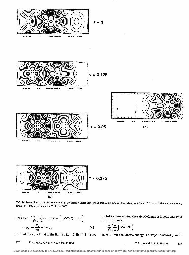
vortices at the onset of instability as they move through their characteristic oscillation. Again, these vortices propagate radially, but there are two important trends to note in Fig. 16 (a). First, the axial dimension of the structure becomes smaller than that of Taylor-Couette ilow [cf. Fig. 10(a) 1. In addition, it should be noted that two of the vortices posi- tioned near the inner and outer cylinders, respectively, are strengthened as the pressure gradient is added opposite the cylinder rotation. As s’ decreases from unity, the vortex center of a stationary mode moves to the outer cylinder, and the axial dimension becomes smaller as shown in Fig. 16(b).

Ill. MECHANISM OF INSTABILITY A. Energy analysis

In this section, we investigate the mechanism of the instability through an examination of the disturbance-energy equation. This energy method considers energy transfer between the mean flow and the disturbance flow by evaluating the mechanical energy balance for the system. Although energy analysis is not new by any means, we believe its applica- tion to purely elastic instabilities is novel. From the Oldroyd- B constitutive.equation, the stress tensor can be written as

~=2(77~ +7,)E-/& (40) After substituting (40) into the linearized disturbance momentum equation, we have the following dimensionless equation:

(De)-rs+RS >

= - VP’ + V’Y’ - V* % + De V@, (41)

where the primed variables denote perturbations, and RS and 0 represent the coupling between the base flow and the perturbing flow via the expressions

RS = v’*Vv’ + v’Vv” + v‘*Vv’, and

0 = - (vO.V7’ + v’.v$, f (vv”)r*7’,

+ (Vv’) %$ + <TV + T;-vvO. (42) In (41) and (42) the base state and the disturbance polymeric stress tensors e and 7; are made dimensionless with the characteristic polymer stress, Vty, and the velocities v” and v’ are made dimensionless with the product of the gap d and the maximum shear rate across the gap, y. The energy balance equation is then obtained by multiplying the linearized disturbance momentum equation by the perturbation velocity, v’, and integrating over the volume, V: - 1/2<x<1/2, O<z<2rr/cr. The final dimensionless energy equation becomes



b)

mllsm- I” a.,-*-~ .IPrlLsI* ..-

(a)

FIG. 16. Streamlines of the disturbance flow at the onset of instability for (a) oscillatory modes (6’ = 0.1, CL, = 9.3, and eIR De, = 8.48), and a stationary mode (~5’ = 0.8, a, = 8.8, and E’~ De, = 7.82).

Re((De)-‘$~~v’*v’dY+S (+Vf)*v’dV) useful for determining the rate of change of kinetic energy of the disturbance,

=qvis -%+Deq,. (43) $($‘-V’dY).

It should be noted that in the limit as Re 40, Eq. (43 ) is not In this limit the kinetic energy is always vanishingly small



relative to the energy production or dissipation created by the viscous or elastic stresses [i.e., the right-hand side of (43)]. Thus, the energy method by Feinberg and Schowalter32v33 is not directly applicable to our analysis of purely elastic instabilities. An alternative method is used below. Note that in a later publication, we shall examine the effects of inertia on these elastic instabilities and then an energy method based on the modified Reynolds-C&r equation will be considered. Continuing, we note that after the inertial terms are neglected, Eq. (43) becomes

df, _ X-Pvis +Depp.

In Eq. (44)

Ep 2 2 s

v’V$ dV

is the disturbance power created or dissipated by the action of the disturbance polymeric stresses,

ppvis = (V2V’)*v’ dV (46)

is the rate of viscous energy dissipation, which is always negative, and pP represents the rate of energy production due to the coupling between the perturbation flow and the base flow. This last term can be written

Pp = Ppvl + P&W2 -I- Pp

where (47)

Ppvl = - s V.(v’*V+*v’ dV (48)

is the rate of energy production caused by the coupling of the perturbation velocity and the base state polymeric stress gradient. This term is entirely absent from an energy balance for

200

100

-100

dsddt

3 4 5 6 7 8 9 pz Da

(a)

150,

100,

z 50,

r" & E" 0

-50

-100

the elastic Taylor-Couette instability since in that case v< = 0.”

Similarly, 9)PU2 is the rate of energy production or dissipation caused by the coupling between the perturbation velocity gradient and the base state polymeric stresses:

4)p%2 = s v*[ (Vv’)%j -I- +Vv’]*v’.dV. (49)

Finally,

qps = s

V*[ (V$)%; + +‘v*]*v’ dV (50)

is the rate of energy production caused by the coupling of the disturbance polymeric stresses to the base state velocity field. Equation (44) mathematically describes the fact that the rate of change of the power created by the disturbance polymeric stresses vanishes when the production caused by the coupling terms (47) matches the viscous dissipation. We note that the terms qPUpui, pPU2, and pPs are analogous to Reynolds stress energy production terms associated with inertial instabilities2’ If we consider the total disturbance power,

s v’*V+ dV=S

s (V’v’)-v’ dV+ De

s v’*V*r; dV= 0,

(51) we can obtain the following relation: E!Lsd s Vv’:Vv’ d V.

dt dt (52)

Thus, dc,/dt is the rate of change of the absolute value of the power dissipated by the solvent. Since one expects on phys- ical grounds that as the perturbation velocity grows, more energy will be dissipated by the solvent, we expect the sign of

5 6 7 8 J/2

ce

(b)

FIG. 17. The terms in the energy equation (43) (a) in Dean flow (a, = 6.3, E”’ De, = 5.88, and S= 0.5) and (b) in Taylor-Couette ROW (a, = 6.7, E’~ De, = 5.93 and S = 0.5)



2

1

=z .z 0 3 E

-1

-2

i (amDe),=5.88

I I I I I I 3 4 5 6 7 8 9

ErRDe

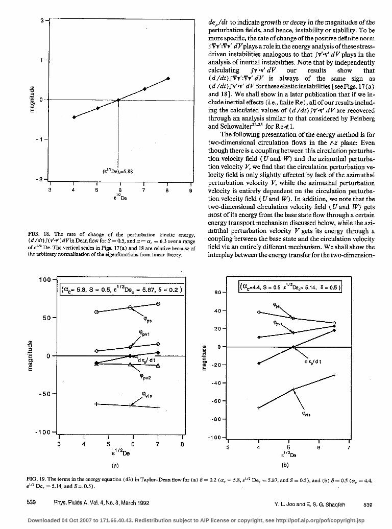
FIG. 18. The rate of change of the perturbation kinetic energy, (d/dt)J(vW)dVin Dean flow for S= 0.5, and a = a, = 6.3 over a range of eLR De. The vertical scales in Figs. 17(a) and 18 are relative because of the arbitrary normalization of the eigenfunctions from linear theory,

100

50

-8 3

C tz 0 t? E

-50

-100

(+ 5.8, S = 0.5, E”~D~~ = 5.87, 6 = 0.2 )

‘ppv2

cp vis

-I l-

3 4 5 6 7 8 &?I I2 De

(a)

de,/dt to indicate growth or decay in the magnitudes of the perturbation fields, and hence, instability or stability. To be more specific, the rate of change of the positive definite norm .fVv’:Vv’ dVplays a role in the energy analysis of these stress- driven instabilities analogous to that Jv’*v’ dV plays in the analysis of inertial instabilities. Note that by independently calculating .fv’-v’ d V our results show that (d /dt)JVv’:Vv’ dV is always of the same sign as (d /dt)Sv’*v’ dV fortheseelasticinstabilities [seeFigs. 17(a) and 181. We shall show in a later publication that if we in- clude inertial effects (i.e., finite Re), all of our results includ- ing the calculated values of (d /dt>Jv’*v’ dV are recovered through an analysis similar to that considered by Feinberg and Schowalter32’33 for Re4 1.

The following presentation of the energy method is for two-dimensional circulation flows in the r-z plane: Even though there is a coupling between this circulation perturbation velocity field ( Uand w) and the azimuthal perturbation velocity V, we find that the circulation perturbation velocity field is only slightly affected by lack of the azimuthal perturbation velocity V, while the azimuthal perturbation velocity is entirely dependent on the circulation perturbation velocity field ( U and w>. In addition, we note that the two-dimensional circulation velocity field ( U and IV) gets most of its energy from the base state flow through a certain energy transport mechanism discussed below, while the azimuthal perturbation velocity V gets its energy through a coupling between the base state and the circulation velocity field via an entirely different mechanism. We shall show the interplay between the energy transfer for the two-dimension-

3 4 5 6 7 T2De

(b)

FIG. 19. The terms in the energy equation (43) in Taylor-Dean flow for (a) 6 = 0.2 (a, = 5.8, eIR De, = 5.87, and S = 0.5), and (b) 6 = 0.5 (a, = 4.4, eVZDe,=5.14,andS=0.5).



al circulation perturbation velocity field and the energy transfer for the streamwise direction or azimuthal coordinate in detail in a later publication. Thus, in the following disdcssion, we concentrate exclusively on the energy balance for the two-dimensional circulation flow in the Y-Z plane (with components U nd IV).

Figure 17(a) shows each term in the energy equation over a given range of e “’ De (both sub- and supercritical values) for the elastic Dean flow at S= 0.5, and a = QI, = 6.3. As e1/2 De passes the critical value, 5.88, the rate of energy production due to the coupling of the perturbation velocity to the polymeric stress gradient in the base state, 3)~“~ increases considerably. Consequently, this contribution to the energy production appears to control the onset of the purely elastic instability in the Poiseuille flow through a curved channel. As discussed previously, this indicates a new instability mechanism since 4)~“~ = 0 for Taylor- Couette flow. The energy production due to the coupling between the disturbance polymeric stresses and the base state velocity field, ppS is shown to be the mechanism in Taylor-Couette flow [Fig. 17 (b) 1. In addition, we find that the term qDpv2, due to the coupling between the perturbation velocity gradient and the base state polymeric stresses, results only in small energy dissipation. We also have plotted the rate of the change of the perturbation kinetic energy, (d /dt).f( v’~‘)dV, for Dean flow inFig. 18. As shownin Fig. 19 (a), for S = 0.2 (oscillatory modes), the term Q)P”, , exists, but is small compared to qpS. The terms in Fig. 19(b) for 6 = 0.5 are similar to those calculated for Dean flow. It becomes clear, therefore, that there are the two different instability mechanisms in Taylor-Couette and Dean flows, respectively, and that both these mechanisms of instability are present in Taylor-Dean flow. In the next subsection, we analyze the new mechanism of viscoelastic Dean (and Taylor-

5 0.0 X

(a)

Dean) instability and show that it arises from the interplay between the azimuthal normal stress gradient in the base state and the perturbation velocity.

B. New mechanism of viscoelastic instability

Based on the results of the energy analysis described above, a new mechanism for the viscoelastic Dean instability that is associated with the coupling of the perturbation velocity field to the polymeric stress gradients in the base flow has been uncovered. A different mechanism involving the energy production due to the coupling between the disturbance polymeric stresses and the base state velocity gradients has been previously postulated as the mechanism for the elastic instability in Taylor-Couette flo~.~ We first analyze the new mechanism of viscoelastic Dean instability, and then examine that of viscoelastic Taylor-Dean instability when the pressure gradient is the dominant flow driving force.

The mechanism of the viscoelastic Dean instability can be summarized as follows. Neglecting fluid inertia, the r- momentum equation for the base flow can be written as

dpO 7088 --=-* dr r

(53)

Note that the azimuthal normal stress of the base state in Dean flow, &, changes across the gap, balancing the radial pressure gradient. From our energy analysis, this azimuthal normal stress gradient in the base flow couples to the radial perturbation velocity to increase the local values of r& by transferring polymers that are more highly stretched to smaller radii. In the narrow gap limit, after all terms other than the crucial coupling term are neglected, the increased 88 component of the perturbation stress tensor can be ex- pressed as

0.0 X

(b)

6’ = 1 (Dea

FIG. 20. The gradient of the base state azimuthal normal stress (a) when the pressure gradient is applied along the shear-driven flow, and (b) when the pressure gradient is applied against the sheardriven flow.



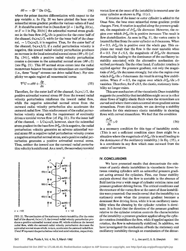
Oe= -D-‘De UI$& (54) where the prime denotes differentiation with respect to the gap variable x. In Fig. 20 we have plotted the base state azimuthal stress gradient profiles for various values of S and 8’. It should be noted that in Dean flow [S = 1 in Fig. 20(a), or 6’ = 1 in Fig. 20(b)] the azimuthal normal stress gradient in the base flow &$,iG’x is positive for the outer half of the channel, O<x< i/2, while for the inner half of the channel, - 1/2<x<O, it is negative. Thus, for the outer half of the channel, O<x<1/2, if a radial perturbation velocity is negative, this inward radial velocity perturbation produces an increase in the local azimuthal normal stress (80 > 0) [cf. Eq. (54) 1, while a positive radial velocity perturbation creates a decrease in the azimuthal normal stress (69 < 0) (see Fig. 21). This 00 normal stress enters into the radial momentum balance because the streamlines are curvilinear (i.e., these “hoop” stresses can drive radial flow). For sim- plicity we again neglect all nonessential terms:

vw=~eef*. ax

(55)

Therefore, for the outer half of the channel, O<x< l/2, the positive azimuthal normal stress 00 from the inward radial velocity perturbation reinforces the inward radial flow, while the negative azimuthal normal’ stress from the outward radial velocity perturbation also accelerates the outward radial flow. This reinforcement of the radial perturbation velocity along with the requirement of continuity drives a toroidal vortex flow (cf. Fig. 2 1) . For the inner half of the channel, - 1/2<x<O, however, since the azimuthal stress gradient in the base flow d&/dx is negative, the radial perturbation velocity generates an adverse azimuthal normal stress 80: a negative radial perturbation velocity creates a negative azimuthal normal stress, and a positive radial perturbation generates a positive azimuthal normal stress. Thus, neither the inward nor the outward radial perturbation velocity is reinforced. As a result, the secondary toroidal

U

t w +w ee(+) - c +-+c t w + ee(-

WL x = -112 x f 112

FIG. 21. The mechanism of the stationary elastic instability: For the outer halfof the channel, O<x< l/2, the inward radial velocity perturbation produces a positive azimuthal normal stress f33, which reinforces the inward radial flow, while the outward radial velocity perturbation decreases the azimuthal normal stress which, in turn, accelerates the outward radial flow. Uand Wrepresent the perturbation radial and axial velocities, respectively.

vortex flow at the onset of the instability is centered near the outer cylinder as shown in Fig. 11 (c) .

If rotation of the inner or outer cylinder is added to the Dean’ flow, the base state azimuthal stress gradient profile changes. First, if rotation is applied along the pressure gradient, the magnitude of r-%-&/ax decreases. However, the region over which de,,/& is positive increases: The result is flow destabilization. As seen in Fig. 11, the vortex center is located farther from the outer cylinder as S decreases. When 6 = 0.5, &&J& is positive over the whole gap. This ex- plains our result that the flow is the most unstable when 6 = 0.5. For S < 0.5, the magnitude of J&/c~x decreases dramatically leading to the dominance of the oscillatory instability associate$i. with the alternative mechanism described previously. On the other hand, if cylinder rotation is applied against the pressure gradient, not only the magnitude of &-&/c~x decreases strongly, but also the region over which &-&J~x > 0 decreases: the result is strong flow stabilization. When s’ = 0.5, the region over which &-$,/c?x > 0 vanishes. Therefore, for 8~0.5, the elastic, stationary instability no longer exists.

This new mechanism of the viscoelastic Dean instability suggests the possibility that instabilities might occur in other shear flows of highly elastic fluids when the streamlines are curved and where there exists a normal stress gradient across streamlines. From this analysis, we can develop a stability criterion for this stationary elastic instability in shearing flows with curved streamlines. We find that the condition

aso -I-->0 ax

(56)

is a necessary condition for this type of instability mode. (This is not a sufficient condition since there might be a situation where the magnitude of &$,/ax is small leading to the dominance of the oscillatory instability.) In Eq. (55), x is a coordinate in any flow which runs outward from the center of curvature.

IV. CONCLUSIONS

We have presented results that demonstrate the existence of purely elastic instabilities in viscoelastic flows between rotating cylinders with an azimuthal pressure gradient acting around the cylinders. First, our linear stability analysis showed that the flow is unstable in the absence of fluid inertia over a wide range of cylinder rotation rates and pressure gradient driving forces. The critical conditions and the structure of the vortex flow at the onset of these instabilities were presented. Our results reveal that the instability is a stationary mode when the pressure gradient becomes a dominant flow driving force, while it is an oscillatory instability when the shearing by the cylinder rotation is dominant. It is found that the direction of the pressure gradient relative to the cylinder rotation controls the characteristics of the instability: a pressure gradient applied along the cylinder rotation destabilizes the flow, while if applied against the rotation, the flow is substantially stabilized. In addition, we have investigated the mechanism of both the stationary and oscillatory instability through an examination of the distur-



bance-energy equation. We have found that the instability mechanism of the Taylor-Dean flow, when the instability is a stationary mode, is associated with the coupling of the perturbation velocity field to thepolymeric normalstressgra- dients in the base flow. In contrast, the mechanism for the elastic, oscillatory instability in Taylor-Dean flow involves the coupling between the disturbance polymeric stresses and the base state velocity gradients. Finally, our analysis of these instability mechanisms has allowed us to develop criteria which are useful in predicting the occurrence of these elastic stationary or oscillatory instabilities in other shearing flows of highly elastic liquids.

ACKNOWLEDGMENTS

We would like to thank G. M. Homsy for suggesting the use of energy analysis in examining our instability mechanisms.

In addition, the authors would like to thank the Nation- al Science Foundation for funding this work through a Presi- dential Young Investigator Award, Grant No. CTS- 9057284.

APPENDIX: DERIVATION OF THE STRESS AMPLITUDE FUNCTIONS FOR AXISYMMETRIC DISTURBANCES

In this appendix, a detailed derivation of the stress amplitude functions for axisymmetric disturbances is presented, when the flow is driven by a pressure gradient applied along cylinder rotation. If the pressure gradient is applied counter to cylinder rotation, it is also demonstrated that the final dimensionless stress amplitude functions are only slightly different. As described in Sec. II, the total stress is given by the sum of solvent and polymeric contributions. Substituting the velocity and polymeric stress components in ( 10) into (5)) we can solve for the polymeric contribution to the r-dependent stress amplitude functions:

RR 2=2D-‘U’,

% RZ --P=2D-‘(W’+iaU),

77P

zz p - 2D-‘iaW, --

(Al) ezP -D-IiaV-;tD-' --

+ 2r(I\‘3E b-/ rip

-2($-$)?I.

In the above, $$‘and ef are the components of the polymeric contribution to the stress in the base state and these are given by the expressions

T-y” = 7, [

-‘“+$-( ++ l)], r*

[

-zB+$( -AE+ I)]*, (A2) 7-g = T& = w rlP r*

and where D = ( 1 - iw;l) . Similarly, substituting the velocity and the solvent stress components yields the following solvent contribution to the stress amplitude functions:

RR 2 = 2U’, W --2(W’+iaU), 11s 7;1s

zz, RR v - = 2ia W,- =r-‘, 11s 7s 0 r

(A3)

w, 2u ez, -=-) -=iov. vs r 77,

We cast the above equations into dimensionless form by setting the gap variable x = ( r - R r ) /R r . The velocities are made dimensionless with the product of the gap d and the maximum shear rate across the gap, (R, /E) (6 - fi). The stresses are made dimensionless with the characteristic stress, ~7~ (a, ie) (6 - 8). In the narrow gap limit where the dimensionless gap, E = d/R, ( 1, we obtain the following stress amplitude functions:

RR=2[S+D-‘(l-S)]U’,

RZ= {S+D-‘(1 -S)](i/a)(U” +a*U),

ZZ= -2[S+D-‘(1 -S,]U’,

R8 = [S+D-‘(1 -S)]V’+D-’

X De[r$‘U’- U7-‘$‘+2D-‘(1 -S)U’e’], (A4)

8Z =ia[S+D-‘(1 -S’)]V+D-‘De (i/a) [U”T’$

+D-‘(1 -S><‘(U” +a*U)],

00 =D-‘De{ - U<J, +2#$‘V’+2D-1$‘[(1 -S)V’

+ D-’ De(?$‘U’ - UT’$“]

+2D-‘(1 -S)U’$‘)},

where now D = ( 1 - z$>, and the foIlowing dimensionless groups appear

e=-$ De=: (l-fi)n, 1

sz772, ?lp + ??I

a=ad; o^=wA. (A5)



In (A4) the solvent and polymeric contributions to the stress amplitude functions have been combined. The dimensionless base state velocity gradient and stresses are

%+&1-2X) + (6- l), (446) 7-p (1 -S>[6(1-2x) + (6-- l)], (A7) $, =2De(l -S>[6(1-2x) + (6-l)]“, (A81

whereS=g/({--,B). If the pressure gradient is applied counter to cylinder

rotation, the maximum shear rate across the gap becomes (0, /E) ( - c - ,5). Thus, we make velocities dimensionless with ( a1 /E) ( - l- /3)d, and the stresses with the characteristic stress qt (fir /E) ( - 6 - P). Applying the procedure described above, we obtain the same expressions (A4) for the stress amplitude functions. The Deborah number, however, becomes De = (R, /E) ( - g - fi)h, and the dimensionless base state velocity gradient and stresses are given by

I$‘= -8(1-2X) + (s’- l), (A9) r~~~=(1--3)[-8(1-2X)+(8-1)] (AlO)

7f,,-2De(l-5’)[-8’(l-22x)+(S’-l)]2. (All)

whereS’= --l/(-{-p).

’ G. I. Taylor, “Stability of a viscous liquid contained between two rotating cylinders,” Philos. Trans. R. Sot. London Ser. A 223,289 (1923).

“W. R. Dean, “Fluid motion in a curved channel,” Proc. R. Sot. London Ser. A 121,402 ( 1928).

‘D. B. Brewster and A. H. Nissan, “Hydrodynamics of flow between horizontal concentric cylinders. I. Flow due to the rotation of cylinder,” Chem. Eng. Sci. 7,215 (1958).

4R. C. DiPrima, “The stability of viscous flow between rotating concentric cylinders with a pressure gradient acting around the cylinders,” J. Fluid Mech. 6,462 (1959).

‘R. G. Larson, E. S. G. Shaqfeh, and S. J. Muller, “A purely elastic insta- bilitv in Tavlor-Couette flow,” J. Fluid Mech. 218, 573 ( 1990).

- I

“Y. L. Joo and E. S. G. Shaqfeh, “Viscoelastic Poiseuille flow through a curved channel: A new elastic instability,” Phys. Fluids A 3, 169 1 ( 199 1) .

‘N. Phan-Thien, “Coaxial-disk flow of an Oldroyd-B fluid: Exact solution and stability,” J. Non-Newtonian Fluid Mech. 13,325 ( 1983).

a N. Phan-Thien, “Cone-and-plate flow ofthe Oldroyd-B fluid is unstable,” J. Non-Newtonian Fluid Mech. 17,37 ( 1985 ) .

‘A. M. Kraynik, J. H. Aubert, and R. N. Chapman, “The Helical screw rheometer,” in Advances in Rheology, Proceedings of the IX International Congress on Rheology, Mexico, edited by B. Mena, A. Garcia-Rejon, and C. Rangel-Nafaile (Universidad National Autonoma de Mexico, Mexi- co, 1984), Vol. 4, pp. 77-84.

“2. Kemblowski, J. Sek, and P. Budzynski, “The concept of a rotational rheometer with helical screw impeller,” Rheol. Acta 27, 82 ( 1988).

‘IS. Wronski, and M. Jastrzebski, “The stability of the helical flow of pseu-

doplastic liquids in a narrow annular gap with a rotating inner cylinder,” Rheol. Acta 29,442 ( 1990).

‘*S Wronski and M. Jastrzebski, “Experimental investigations of the stability limit of the helical flow of pseudoplastic liquids,” Rheol. Acta 29, 453 (1990).

I3 R. B. Bird, C. F. Curtiss, R. C. Armstrong, and 0. Hassager, Dynamicsof Polymeric Liquids, 2nd ed. (Wiley-Interscience, New York, 1987), Vol.

I’; V Boger “A highly elastic constant-viscosity fluid,” J. Non-Newtoni- ad Fluid Mkh. 3,87 (1977/1978).

I5 R. K. Gupta, T. Sridhar, and M. E. Ryan, “Model viscoelastic liquids,” J. Non-Newtonian Fluid Mech. 12,233 (1983).

I6 M. E. Mackay and D. V. Boger, “An explanation of the rheological properties of Boger fluids,” J. Non-Newtonian Fluid Mech. 22, 235 (1987).

“S. Chandrasekhar, Hydrodynamic Stability (Clarendon, Oxford, 1961). ‘*The definition of the Deborah number in the present publication follows

that of authors’ precedent publications. s,6 the product of a fluid relaxation time and characteristic strain rate [see, e.g., R. G. Larson, Cons&u- tive Equations for Polymer Melts and Solutions (Butterworths, Boston, 1988), p. 2791.

I9 C. E. Grosch and H. Salwen, “The stability of steady and time-dependent plane Poiseuille Row,” J. Fluid Mech. 34, 177 ( 1968).

‘OH B. Keller, Numerical Methods for Two-Point Boundary- Value Prob- lems ( Cinn-Blaisdell, Waltham, MA, 1961) .

” P G. Drazin and W. H. Reid, HydrodynamicStability (Cambridge U.P., Cambridge, England, 198 1) .

*‘E. S. G. Shaqfeh and A. Acrivos, “The effects of inertia on the stability of convective flow in inclined particle setters,” Phys. Fluids 30,960 ( 1987).

23 E. S. G. Shaqfeh, R. G. Larson, and G. H. Fredrickson, “The stability of gravity driven viscoelastic film-flow at low to moderate Reynolds number,” J. Non-Newtonian Fluid Mech. 31, 87 (1989).

a4S. D. Conte, “The numerical solution of linear boundary value prob- lems,” SLAM Rev. 8,309 ( 1966).

” L. M. Mack, “A numerical study of the temporal eigenvalue spectrum of the Blasius boundary layer,” J. Fluid Mech. 73,497 ( 1976).

z6E. S. G. Shaqfeh, S. J. Muller, and R. G. Larson, “Theeffects ofgap width and dilute solution properties on the viscoelastic Taylor-Couette instability,” J. Fluid Mech. 235,285 (1992).

“P. J. Northey, R. C. Armstrong, and R. A. Brown, “Numerical calcula- tion of time-dependent, two-dimensional inertial flows described by a multimode UCM model,” Annual AIChE Meeting, Paper No. 166Adb, November 1989.

z8P. J. Northey, R. C. Armstrong, and R. A. Brown, “Finite-element calcu- lation of purely elastic, nonlinear transitions in circular Couette flow,” Annual AIChE Meeting, Paper No. 167j, November 1990.

29P Huerre and P. A. Monkewitz, “Local and global instabilities in spatial- ly developing Rows,” Annu. Rev. Fluid Mech. 22,473 ( 1990).

joI. Mutabazi, J. J. Hegseth, and C. D. Andereck, “Pattern formation in the flow between two horizontal coaxial cylinders with a partially filled gap,” Phys. Rev. A 38,4752 (1988).

3’ I. Mutabazi, J. J. Hegseth, and C. D. Andereck, “Spatiotemporal pattern modulations in the Taylor-Dean system,” Phys. Rev. Lett. 64, 1729 (1990).

32 M. R. Feinberg and W. R. Schowalter, “Sufficient conditions for stability of fluid motions constitutively described by the infinitesimal theory of viscoelasticity,” I & EC Fundam. 8, 332 (1969).

‘jM. R. Feinberg and W. R. Schowalter, “Conditions for the stability of cylindrical Couette flow of certain viscoelastic liquids,” Ftyth Interna- tional Congress of RheoIogy (University of Tokyo Press, Tokyo, 1969), Vol. 4, pp 201-216.



A purely elastic instability in Dean and Taylor-Dean flow

Documents

Transcript of A purely elastic instability in Dean and Taylor-Dean flow