arX

iv:1

006.

3519

v1 [

astr

o-ph

.CO

] 1

7 Ju

n 20

10

The Effect of Galactic Properties on the Escape Fraction of

Ionizing Photons

Elizabeth R. Fernandez1, J. Michael Shull2

CASA, Department of Astrophysical and Planetary Sciences, University of Colorado, 389

UCB, Boulder, CO 80309-0389

1elizabeth.fernandez@colorado.edu

2michael.shull@colorado.edu

ABSTRACT

Understanding the escape fraction, fesc, of ionizing photons from early galax-

ies gives an important constraint on the sources that reionize the universe. Previ-

ous attempts to measure fesc have found a wide range of values, varying from less

than 0.01 to nearly 1. Rather than try to find an exact value of fesc, we seek to

clarify how internal properties of the galaxy affect fesc through: (1) the density

and distribution of neutral hydrogen within the galaxy; (2) the number of ioniz-

ing photons produced per time; (3) how the neutral medium is clumped. Fewer,

higher density clumps lead to a greater value of fesc than many less dense clumps.

Populations of stars that increase the number of ionizing photons produced (such

as metal-free or more massive stars or disks with a high star-formation efficiency)

increase fesc because the angle out of the disk that photons can escape is in-

creased, allowing more photons to escape. For halos formed at higher redshifts,

fesc also decreases since halos are more dense, assuming no change in stellar pop-

ulation over redshift. We also find that galaxy mass does not affect the escape

fraction, as long as the star-formation efficiency is constant. Finally, populations

of galaxies made up of only high mass galaxies have a harder time to reionize the

universe, especially at high redshifts, because the fesc needed is above 1.

1. INTRODUCTION

Observations, such as of the Cosmic Microwave Background using experiments such

as the Wilkinson Microwave Anisotropy Probe (WMAP) (Kogut et al. 2003; Spergel et al.

2003; Page et al. 2007; Spergel et al. 2007; Dunkley et al. 2009; Komatsu et al. 2009, 2010),

suggest that the universe was reionized sometime between 6 < z < 12. Because they are

efficient producers of ultraviolet photons, the most likely candidates for the majority of reion-

ization are massive stars. However, in order for these stars to reionize the universe, ionizing

– 2 –

radiation must be able to escape from the stars’ parent halos, in which the dominant source

of opacity is neutral hydrogen, the dominant component of the interstellar gas. Calculating

the escape fraction of ionizing photons from galaxies is important in order to understand the

characteristics of galaxies that produce the bulk of the photons that reionize the universe.

The predicted values of the escape fraction span a large range, from 0.01 . fesc < 1.

There have been many theoretical and observational studies to calculate the number of

ionizing photons emitted from these halos. Various properties of the host galaxies, its stars,

or its environment are thought to affect the number of ionizing photons that escape into the

IGM. Ricotti & Shull (2000) and Wood & Loeb (2000) state that fesc varies greatly, from

< 0.01 to 1, depending on galaxy mass, with larger galaxies giving smaller value of fesc.

Gnedin et al. (2008), on the other hand, state that lower-mass galaxies have significantly

smaller fesc, a result of a declining star formation rate. In addition, above a critical halo

mass, fesc does not change by much. Wise & Cen (2009) also find that massive galaxies have

larger values of fesc than low-mass galaxies. The minimum mass of galaxy formation can

also put limitations on fesc. Observations of Ly−α absorption towards high-redshift quasars,

combined with the UV luminosity function of galaxies, can limit fesc from a redshift of 5.5

to 6, with fesc ∼ 0.2 − 0.45 if the halos producing these photons are larger than 1010 M⊙.

This can fall to fesc ∼ 0.05− 0.1 if halos down to 108M⊙ are included as sources of escaping

ionizing photons (Srbinovsky & Wyithe 2008).

The shape and morphology of the galaxy can also affect fesc (Dove & Shull 1994;

Dove et al. 2000; Clark & Oey 2002; Fujita et al. 2003; Gnedin et al. 2008; Wise & Cen

2009). In addition, increasing baryon mass fraction lowers fesc for smaller halos but increases

it at masses greater than 108 M⊙ (Wise & Cen 2009). Star formation history changes the

amount of ionizing photons and neutral hydrogen, causing fesc to vary from 0.12 − 0.2 for

coeval star formation to 0.04 − 0.1 for Gaussian star formation (Dove et al. 2000). Various

papers obtained conflicting results as to whether fesc increases or decreases with redshift

(Ricotti & Shull 2000; Wood & Loeb 2000; Inoue et al. 2006; Razoumov & Sommer-Larsen

2006; Gnedin et al. 2008; Razoumov & Sommer-Larsen 2010).

In addition to bubbles and structure caused from supernovae, galaxies have a clumpy

interstellar medium (ISM) whose inhomogeneities can affect fesc. Dense clumps could re-

duce fesc (Dove et al. 2000) On the other hand, Boisse (1990), Hobson & Scheuer (1993),

Witt & Gordon (1996), and Wood & Loeb (2000) all found that clumps or a randomly dis-

tributed medium cause fesc to rise, while Ciardi et al. (2002) found that the affect of fescfrom clumps depends on the ionization rate. Some other quantities do not seem to affect

the escape fraction: spin of the galaxy (Wise & Cen 2009) and dust content (Gnedin et al.

2008).

– 3 –

It is clear that many factors can affect fesc and the problem is quite complicated. Even

simulations can not give a clear answer to what fesc of a galaxy should be. Therefore, rather

than predicting a quantitative value for fesc, we instead seek to understand how properties

of the galaxy and its internal structure of the galaxy affects the escape fraction. In section

2, we explain our method of tracing photons escaping the galaxy. In section 3 we explain

our results and compare our results to previous literature in section 4. In section 5 we

consider constraints from reionization and we conclude in section 6. Throughout, we use the

cosmological constants from WMAP7 results (Komatsu et al. 2010).

2. METHODOLOGY

2.1. Properties of the Galaxy

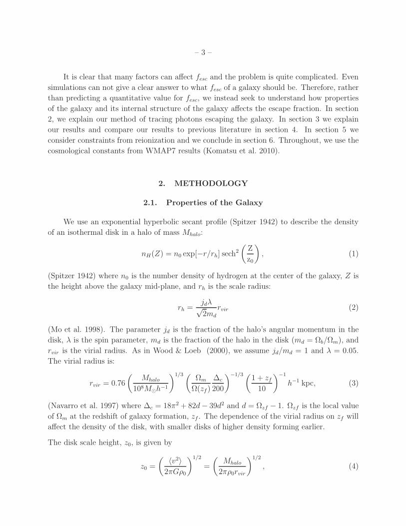
We use an exponential hyperbolic secant profile (Spitzer 1942) to describe the density

of an isothermal disk in a halo of mass Mhalo:

nH(Z) = n0 exp[−r/rh] sech2

(

Z

z0

)

, (1)

(Spitzer 1942) where n0 is the number density of hydrogen at the center of the galaxy, Z is

the height above the galaxy mid-plane, and rh is the scale radius:

rh =jdλ√2md

rvir (2)

(Mo et al. 1998). The parameter jd is the fraction of the halo’s angular momentum in the

disk, λ is the spin parameter, md is the fraction of the halo in the disk (md = Ωb/Ωm), and

rvir is the virial radius. As in Wood & Loeb (2000), we assume jd/md = 1 and λ = 0.05.

The virial radius is:

rvir = 0.76

(

Mhalo

108M⊙h−1

)1/3 (Ωm

Ω(zf )

∆c

200

)−1/3(1 + zf10

)−1

h−1 kpc, (3)

(Navarro et al. 1997) where ∆c = 18π2 + 82d− 39d2 and d = Ωzf − 1. Ωzf is the local value

of Ωm at the redshift of galaxy formation, zf . The dependence of the virial radius on zf will

affect the density of the disk, with smaller disks of higher density forming earlier.

The disk scale height, z0, is given by

z0 =

( 〈v2〉2πGρ0

)1/2

=

(

Mhalo

2πρ0rvir

)1/2

, (4)

– 4 –

where 〈v2〉 is the mean square of the velocity and ρ0 is the central density.

The central density is solved for in a self-consistent way after the halo mass and the

redshift of formation are specified. We use 15rh and 2z0 as the limits of the radius and height

of the disk, respectively.

The mass of the disk (stars and gas) is taken as

Mdisk =Ωb

Ωm

Mhalo , (5)

and the mass of the stars within the disk is

M∗ = Mdiskf∗ . (6)

Here, f∗ is the star formation efficiency, which describes the fraction of baryons that form

into stars. The remainder of the mass of the disk is gas which is distributed according to

equation 1. We assume a gas temperature of 104 K.

The number of ionizing photons is related to f∗, considering either Population III (metal-

free) and Population II (metal-poor, Z = 1/50 Z⊙) stars. The total number of ionizing

photons per second from the entire stellar population, Qpop is:

Qpop =

∫ m2

m1

QH(m)f(m)dm∫

mf(m)dm×M∗ , (7)

where m is the mass of the star, and m1 and m2 are the upper and lower mass limits of the

mass spectrum, given by f(m). For a less massive distribution of stars, we use the Salpeter

initial mass spectrum (Salpeter 1955):

f(m) ∝ m−2.35, (8)

with m1 = 0.4 M⊙ and m2 = 150 M⊙. The Larson initial mass spectrum illustrates a case

with heavier stars (Larson 1998):

f(m) ∝ m−1

(

1 +m

mc

)−1.35

, (9)

with m1 = 1 M⊙, m2 = 500 M⊙, and mc = 250 M⊙ for Population III stars and m1 = 1 M⊙,

m2 = 150 M⊙, and mc = 50 M⊙ for Population II stars. We define QH as the number

of ionizing photons emitted per second per star, averaged over the star’s lifetime. For

Population III stars of mass parameter x ≡ log10(m/M⊙), this is

log10[

QH/s−1]

=

43.61 + 4.90x− 0.83x2 9− 500 M⊙ ,

39.29 + 8.55x 5− 9 M⊙ ,

0 otherwise ,

(10)

– 5 –

and for Population II stars,

log10[

QH/s−1]

=

27.80 + 30.68x− 14.80x2 + 2.50x3 ≥ 5M⊙

0 otherwise ,(11)

as given in Table 6 of Schaerer (2002).

2.2. Calculating the Escape Fraction

We place the stars at the center of the galaxy. An ionized H II region develops around

the stars, where the number of ionizing photons emitted per second by the stellar population,

Qpop, is balanced by recombinations, such that

Qpop =4

3πr3sn

2HαB(T ). (12)

Here, αB is the case-B recombination rate coefficient of hydrogen and T is the temperature

of the gas (we assume T = 104K). The radius of this H II region, called the Stromgren

radius, is

rs =

(

3Qpop

4πn2HαB

)1/3

. (13)

This is simple to evaluate in the case of a uniform medium, but if we are concerned

with clumps and a disk with a density profile, the density will be changing. Although we

are calculating fesc at a moment in time, it is good to keep in mind that in reality, the H II

region is not static, and the ionizing front will propagate at some flux-limited speed.

We integrate along the path length that a photon takes in order to escape the galaxy,

following the formalism in Dove & Shull (1994). We can then calculate the escape fraction

of ionizing photons along each ray emanating from the center of the galaxy by equating the

number of ionizing photons to the number of hydrogen atoms across its path. If there are

more photons than hydrogen atoms, the ray can break out of the disk; otherwise, no photons

escape and the escape fraction is zero. The escape fraction along a path, η, thus depends on

the amount of hydrogen the ray transverses, which depends on its angle θ (measured from

the axis perpendicular to the disk)

η(θ) = 1− 4παB

Qpop

∫

∞

0

n2H(Z)r

2dr . (14)

Photons are more likely to escape out of the top and bottom of the disk, rather than the

sides, because there is less path length to traverse. This creates a critical angle, beyond

– 6 –

which photons no longer will escape the galaxy. The total escape fraction, fesc, is then found

by integrating over all angles θ and the solid angle Ω

fesc(Qpop) =

∫ ∫

η(θ)

4πdθdΩ (15)

=

∫

1

2η(θ) sin(θ) dθ . (16)

2.3. Adding Clumps

A medium with clumps can be described with the density contrast C = nc/nic between

the clumps (density nc), and the inter-clump medium (density nic). The percentage of volume

taken up by the clumps is described by the volume filling factor fV . We randomly distribute

clumps throughout the galaxy. We define nmean as the density the medium would have if it

was not clumpy, given by equation 1. The density at each point is given by

nc =nmean

fV + (1− fV )/C(17)

if the point is in a clump and

nic =nmean

fV (C − 1) + 1(18)

if the point is not in a clump, similar to (Wood & Loeb 2000). In this way, the galaxy

retains the same interstellar gas mass, independent of fV and C. As C increases, the density

of the clumps increases as the density of the non-clumped medium falls. Similarly, if fV is

larger, more of the medium is contained in less dense clumps. We trace photons on their

path through the galaxy and track whether or not they encounter a clump. Counting the

number of photons exiting the galaxy then leads to fesc.

3. RESULTS

3.1. Properties of the Clumps

In the first calculations, we placed Population III stars with a Larson mass spectrum

and a star formation efficiency f∗ = 0.5 in a halo of Mhalo = 109M⊙, with a redshift of

formation of zf = 10. The clumps have diameter 1017 cm, unless otherwise stated. The

left panel of Figure 1 shows fesc as a function of fV for various values of C. The case with

no clumps is equivalent to C = 1. As clumps are introduced, fesc quickly falls, but rises

again as fV rises. This is because the clumps become less dense (since more of the medium

– 7 –

Fig. 1.— Escape fraction of ionizing photons out of the disk as a function of the clump

volume filling factor fV for various values of the clumping factor C (left panel) and log(C)

for various values of fV (right panel). Shown for a 109M⊙ halo at zf = 10, with f∗ = 0.5 and

Pop III stars with a Larson mass spectrum.

is in clumps and the mass of the galaxy must be kept constant). In addition, fesc drops as

C increases, showing that denser clumps with a less dense inter-clump medium stops more

ionizing radiation than a more evenly distributed medium. The clumps are small enough

that essentially every ray traversing the galaxy encounters one of these very dense clumps

and is diminished.

In the right panel of Figure 1, the same population of stars is shown for various values

of fV as a function of log(C). As C increases, fesc becomes low for small values of fV . Again,

this is because of a few very dense clumps that stop essentially all radiation. As fV increases,

more of the medium is in clumps, and therefore the density of the clumps decreases. The

combined effect is an increase of fesc. The solid black line shows the case with no clumps, or

when fV = 0. For fV = 0, fesc equals the case with no clumps (C = 1), as it should. Above

C ∼ 10− 100, increasing C no longer affects fesc.

So far, we have only been exploring the results of small clumps (1017 cm, or ∼ 0.3 pc)

in diameter. What would happen if we were to increase the size of these clumps? In this

case, a ray would traverse fewer clumps as it travels out of the galaxy, but any given clump

would be larger. As shown in the left panel of Figure 2, fesc rises as the clumps increase in

size. For very low values of fV , only a few clumps exist and not every ray comes in contact

with a clump, increasing the escape fraction above the case with no clumps.

To illustrate this further, the right panel of Figure 2 shows fesc against fV for a large

clump size (1019 cm in diameter). The left-most vertical line represents the value of fVneeded for a photon traversing the longest path length to pass through an average of one

– 8 –

Fig. 2.— Left panel: The effect of large clumps on fesc. If the clumps are very large and

fV is very low, there are cases where fesc is larger than the no-clump case. The results are

averaged over ten runs to reduce noise. Galaxy properties are the same as in Figure 1. Right

panel: The fesc out of the disk is shown for a galaxy in a 109M⊙ halo, with zf = 10, f∗ = 0.1,

and a Pop III Larson initial mass spectrum. The left-most vertical line represents the value

of the volume filling factor fV needed for a photon transversing the longest path length to

pass through an average of one clump, while the right-most vertical line represents the value

of fV needed for a photon transversing the shortest path length to pass through an average

of one clump. Therefore, to the right of this line, all path lengths intersect a clump, while

to the left, there are clump-free path lengths out of the galaxy.

clump, while the right-most vertical line represents the value of fV for a photon traversing

the shortest path length to pass through an average of one clump. To the right of this line,

all path lengths intersect a clump. To the left of this line, there are clump-free path lengths

out of the galaxy. From this figure, we see that if fV is low enough that some rays will pass

through fewer than one clump, on average, fesc is much greater than fesc in the case with

no clumps. For very low values of fV , there are so few clumps that the inter-clump medium

approaches the case with no clumps. Therefore, the plot of fesc is peaked in the region where

there are some paths that do not intersect a clump. When fV increases enough that every ray

traverses a path that crosses at least one clump (with fV greater than the right-most vertical

line), fesc falls below the case with no clumps, regardless of C. From this, we can define

two regions. Region one, for low values of the filling factor, describes a medium clumped in

such a way that there are completely clump-free pathways out of the galaxy. This region

has higher escape fractions than a medium with no clumps. Region two is for higher filling

factors clumped so that each ray passes through at least one clump. Region two has lower

escape fraction in comparison to the case with no clumps. For region two, higher values of

C will decrease the escape fraction, while this trend is reversed for region one.

– 9 –

Fig. 3.— The fesc for the disk is shown for stars of varied masses and metallicities and various

values of fV with f∗ = 0.5 (left panel) and various values of f∗ for fV = 0.1 (right panel).

Very high values of f∗ (0.9) approach a case in which all ionizing photons are escaping. Both

are shown for a 109M⊙ halo at zf = 10.

3.2. Properties of Stars and the Galaxy

In Figure 3, we analyze how the stellar population affects the escape fraction. In the

left panel, f∗ is held constant as fV increases. In the right panel, fV is held constant as f∗increases. Both plots show metal-free (Pop III) stars and metal-poor (Pop II) stars, as well as

stars with a heavy Larson initial mass spectrum and a light Salpeter initial mass spectrum.

In both cases, fesc is proportional to the number of ionizing photons that are emitted by the

stars, with heavier stars or stars with fewer metals more likely to produce photons that can

escape the nebula. This is because when more ionizing photons are produced, the critical

angle where photons can break free from the halo increases, and hence more photons escape.

When the galaxy forms more stars (higher f∗), there is the added effect of less hydrogen

remaining in the galaxy to absorb ionizing photons. Therefore, fesc increases greatly as f∗increases.

Properties of the galaxy itself are varied in Figure 4. In the left panel of Figure 4, the

mass of the galaxy is varied, with f∗ is held constant, so that larger galaxies are forming

more stars. Because of this, the number of ionizing photons is proportional to the mass of

the galaxy, and fesc does not depend on galaxy mass, but rather only on f∗. In the right

panel, zf is varied. As zf increases, the galaxy is smaller and more concentrated. Therefore,

it is easiest for photons to escape from less dense disks at low redshifts. At redshifts where

we expect reionization to take place, it is harder for photons to escape the galaxy. (This

problem may be remedied by the high-redshift expectation of more massive or metal-free

stars with higher values of f∗.)

– 10 –

Fig. 4.— Left panel: The fesc for the disk is shown for various halo masses at zf = 10.

Right panel: The fesc for the disk is shown for various values of zf . Shown for a halo with

Population III stars with a Larson mass spectrum and f∗ = 0.5.

4. COMPARISON TO PREVIOUS LITERATURE

As noted in the introduction, there have been many previous studies that calculated

the number of ionizing photons emitted from high redshift halos, resulting in a wide range

of values for the escape fraction. Various factors are proposed that affect the number of

ionizing photons that escape into the IGM, in particular the effects of a clumpy ISM.

Boisse (1990) and Witt & Gordon (1996) found that clumps increase transmission, and

Hobson & Scheuer (1993) found that a three-phase medium (clumps grouped together, rather

than randomly distributed) further increases transmission. Very dense clumps (with C =

106) were studied by Wood & Loeb (2000), who found that clumps increase fesc over the

case with no clumps. For very small values of fV , their fesc was very high, because most of

the density is in a few very dense clumps, and most lines of sight do not encounter a clump.

Their clump size is 13.2 pc, which is similar to our largest clump size, 5 × 1019 cm. Their

results are consistent with our findings for clumps with large radius, low fV , and high C,

where most rays do not encounter a clump.

Ciardi et al. (2002) included the effect of clumps using a fractal distribution of the ISM

with C = 4−8. They noted that this distribution of clumps increases fesc in cases with lower

ionization rate because there are clearer sight lines. They found that fesc is more sensitive

to the gas distribution than to the stellar distribution.

Dove et al. (2000) reported that fesc decreases as clumps are added. In this paper,

however, the result is due to the fact that, in their model, the addition of clumps does not

change the density of the interclump medium. As clumps are added, the mass of hydrogen

– 11 –

in the galaxy increases. On the other hand, our current method decreases the density of the

interclump medium as clumps are added or become denser to keep the overall mass of the

galaxy constant.

Galaxy shape and morphology has an affect on fesc. Photons are more likely to es-

cape along paths with lower density, as in irregular galaxies and along certain lines of sight

(Gnedin et al. 2008; Wise & Cen 2009). Shells, such as those created by supernova rem-

nants (SNRs), can trap ionizing photons until the bubble blows out of the disk, allowing

photons a clear path to escape and causing fesc to rise (Dove & Shull 1994; Dove et al. 2000;

Fujita et al. 2003). These SNRs or superbubbles create porosity in the ISM, and above a

critical star formation rate, fesc rises (Clark & Oey 2002). This is similar to what is seen in

our results. As with a dense clump, a shell will essentially stop all radiation, while a clear

path, similar to the case with a low fV , allows many free paths along which radiation can

escape.

Previous literature gives different results as to whether or not fesc increases or decreases

with redshift. Ricotti & Shull (2000) state that fesc decreases with increasing redshift for a

fixed halo mass. However, other studies seem to indicate that fesc increases with redshift.

Razoumov & Sommer-Larsen (2006) state that fesc increases with redshift from z = 2.39

(where fesc = 0.01−0.02) to z = 3.8 (where fesc = 0.06−0.1). Inoue et al. (2006) constrained

fesc observationally to be less than 0.01 at z < 1 and about 0.1 at z > 4. At higher redshifts,

Razoumov & Sommer-Larsen (2010) state that fesc ≈ 0.8 at z ≈ 10.4 and declines with time.

On the other hand, Gnedin et al. (2008) say that fesc changes little from 3 < z < 9, always

being about 0.01 − 0.03. Wood & Loeb (2000) state that since disk density increases with

redshift, fesc will fall as the formation redshift increases, ranging from fesc = 0.01 − 1. We

found that fesc decreases with increasing redshift of formation since disks are more dense,

but this assumes that the types of stars and f∗ remain constant. If f∗ is larger at higher

redshifts, and if stars are more massive and have a lower metallicity (likely), the number of

ionizing photons would increase, which could cause fesc to increase, despite a denser disk.

5. CONSTRAINTS FROM REIONIZATION

If galaxies are responsible for keeping the universe reionized, there must be a minimum

number of photons that can escape these galaxies to be consistent with reionization. The

star formation rate (ρ) that corresponds to a star formation efficiency f∗ is given by:

ρ(z) = 0.536 M⊙ Mpc−3 yr−1

(

f∗0.1

Ωbh2

0.02

)(

Ωmh2

0.14

)1/2 (1 + z

10

)3/2

ymin(z)e−y2

min(z)/2 (19)

– 12 –

(Fernandez & Komatsu 2006), assuming a Press-Schechter mass function Press & Schechter

(1974), where

ymin(z) ≡δc

σ[Mmin(z)]D(z), (20)

where δc is the overdensity, σ(M) is the present-day rms amplitude of mass fluctuations, and

Mmin is the minimum mass of halos that create stars.

Similarly, the fesc needed to reionize the universe can then be related to the critical star

formation rate, ρcrit, needed to keep the universe ionized:

ρcrit(z) = (0.012M⊙ yr−1 Mpc−3 )

[

1 + z

8

]3 [CH/5

fesc/0.5

] [

0.004

QLyC

]

T−0.8454 (21)

(Shull & Trenti 2010). Here, CH is the clumping of the IGM (which we scale to a typical

value of CH = 5), T4 is the temperature of the IGM in units of 104K, and QLyC is the

conversion factor from ρ(z) to the total number of Lyman continuum photons produced:

QLyC ≡ NLyC

ρcrittrec, (22)

where NLyC is the number of Lyman continuum (LyC) photons produced by a star and trecis the hydrogen recombination timescale. We assume QLyC = 0.004, which is reasonable for

a low-metallicity population.

By requiring the star formation rate to be at least as large as the critical value, we can

solve for the value of fesc needed to reionize the universe. Results are shown in Figure 5.

We plot two redshifts, z = 7 and z = 10. We also study if stars form in galaxies all the way

down to a minimum mass

Mmin = 108[

(1 + z)

10

]1.5

M⊙ (23)

(Barkana & Loeb 2001), or if smaller halos are suppressed and only those above 109M⊙

are forming stars. If the required fesc exceeds 1 (shown by the dashed line), the given

population cannot reionize the universe. As redshift decreases, it becomes much easier to

keep the universe reionized, and a smaller fesc is needed, as expected.

At higher redshifts, it is harder for stars to keep the IGM ionized because the gas density

is higher and there are fewer massive halos forming stars. If small halos are suppressed, the

remaining high-mass halos have a much harder time keeping the universe ionized. It is

interesting to note that the universe cannot be reionized at z = 10 if only larger halos

(Mh > 109M⊙) are producing ionizing photons that escape into the IGM. At z = 10, f∗must always be above 0.1 for all cases shown in order for the universe to be reionized. At

z = 7, f∗ can be very low.

– 13 –

Fig. 5.— The fesc needed from a population of galaxies with various values of f∗ to reionize

the universe at z = 7 or 10. If the required fesc lies above 1 (the dashed line), the population

cannot reionize the universe.

6. CONCLUSIONS

We have explored how the internal properties of galaxies can affect the amount of

escaping ionizing radiation. The properties of clumps within the galaxy have the strongest

effect on fesc. When fV is small, the density of the clumps must be larger to keep the mass

of the galaxy constant, and any given ray is less likely to encounter a clump. If there are

rays that encounter no clumps, fesc will be even larger than for a galaxy with no clumps. As

fV increases, more of the medium is taken up by clumps, and it is more likely that a ray will

encounter a clump. Even though these clumps are less dense, as soon as all rays encounter

at least one clump, fesc will fall below fesc that of a similar galaxy with no clumps. This

occurs at larger values of fV for larger clumps. Therefore, fesc depends sensitively on the

internal structure of the galaxy.

– 14 –

We find that fesc does not depend much on the mass of the galaxy, but only on the star

formation efficiency and the population of stars formed at the center of the galaxy. Both

of these will change the number of ionizing photons, and hence the critical angle at which

photons can escape the galaxy, which will have a direct effect on the escape fraction. Since

disks were more likely more dense at higher redshifts, the escape fractions will be lower,

unless a change in the star formation efficiency or stellar population would increase the

number of ionizing photons.

Because of the complex relationship of the stellar population and distribution of the

ISM, it has been, and will continue to be, difficult to predict fesc. In addition, it is very

likely that each galaxy has several characteristics that give it a unique value of fesc. While

it is clear that the number of ionizing photons and opaque neutral hydrogen affect fesc, the

complex details on how the hydrogen is distributed can have huge effects on fesc.

We acknowledge support from the University of Colorado Astrophysical Theory Program

through grants from NASA (NNX07AG77G) and NSF (AST07-07474).

REFERENCES

Barkana, R., & Loeb, A. 2001, Phys. Rep., 349, 125

Boisse, P. 1990, A&A 228, 483

Ciardi, B., Bianchi, S., & Ferrara, A. 2002, MNRAS, 331, 463

Clark, C., & Oey, M. S. 2002, MNRAS, 337, 1299

Dove, J. B., & Shull, J. M. 1994, ApJ, 430, 222

Dove, J. B., Shull, J. M., & Ferrara, A. 2000, ApJ, 531, 846

Dunkley, J., et al. 2009, ApJS, 180, 306

Fernandez, E. R., & Komatsu, E. 2006, ApJ, 646, 703

Fujita, A., Martin, C. L., Mac Low, M. M., & Abel, T. 2003, ApJ, 599, 50

Gnedin, N. Y., Kravtsov, A. V., & Chen, H. -W. 2008, ApJ, 672, 765

Hobson, M. P., & Scheuer, P. A. 1993, MNRAS, 264, 145

Inoue, A. K., Iwata, I., Deharveng, J.-M. 2006, MNRAS, 371, L1

– 15 –

Kogut, A., et al. 2003, ApJS, 148, 161

Komatsu, E., et al. 2009, ApJS, 180, 330

Komatsu, E., et al. 2010, ApJS, in press, arXiv:1001.4538

Larson, R. B. 1998, MNRAS, 301, 569

Mo, H. J., Mao, S., & White, S. D. 1998, MNRAS, 295, 319

Navarro, J. F., Frenk, C. S., & White, S. D. M. 1997, ApJ, 490, 493

Page, L., et al. 2007, ApJS, 170, 335

Press, W. H., & Schechter, P. 1974, ApJ, 187, 425

Razoumov, A., & Sommer-Larsen, J. 2006, ApJ, 651, L89

Razoumov, A., & Sommer-Larsen, J. 2010, ApJ, 710, 1239

Ricotti, M., & Shull, J. M. 2000, ApJ, 542, 548

Salpeter, E. E. 1955, ApJ, 121, 161

Schaerer, D. 2002, A&A, 382, 28

Sheth, R.K., Mo, H.J., & Tormen, G. 2001, MNRAS, 323, 1

Spergel, D. N., et al. 2003, ApJS, 148, 175

Spergel, D. N., et al. 2007, ApJS, 170, 377

Spitzer, L. 1942 ApJ, 95, 329

Srbinovsky, J. A., & Wyithe, J. S. B. 2008, arXiv:0807.4782

Shull, J. M., & Trenti, M. 2010, in prep

Wise, J. H., & Cen, R. 2009, ApJ, 693, 984

Witt, A. N., & Gordon, K. D. 1996, ApJ, 463, 681

Wood, L., & Loeb, A. 2000, ApJ, 545, 86

This preprint was prepared with the AAS LATEX macros v5.2.