CLARA’s view on the escape fraction of Lyman α photons in high-redshift galaxies

$: CLARA’s view on the escape fraction of Lyman α photons in high-redshift galaxies$
arX

iv:1

104.

5586

v1 [

astr

o-ph

.CO

] 2

9 A

pr 2

011

Mon. Not. R. Astron. Soc. 000, 000–000 (0000) Printed 2 May 2011 (MN LATEX style file v2.2)

CLARA’s view on the escape fraction of Lyman-α photons in

high redshift galaxies

Jaime E. Forero-Romero1 ⋆, Gustavo Yepes2, Stefan Gottlober1,

Steffen R. Knollmann2, Antonio J. Cuesta3, Francisco Prada3

1Leibnitz-Institut fur Astrophysik Potsdam (AIP), An der Sternwarte 16, 14482 Potsdam, Germany2Grupo de Astrofısica, Universidad Autonoma de Madrid, Madrid E-28049, Spain3Instituto de Astrofısica de Andalucıa (CSIC), Camino Bajo de Huetor 50, E-18008, Granada, Spain

2 May 2011

ABSTRACT

Using CLARA (Code for Lyman Alpha Radiation Analysis) we constrain the escapefraction of Lyman-α radiation in galaxies in the redshift range 5 . z . 7, based onthe MareNostrum High-z Universe, a SPH cosmological simulation with more than 2billion particles. We approximate Lyman-α Emitters (LAEs) as dusty gaseous slabswith Lyman-α radiation sources homogeneously mixed in the gas. Escape fractionsfor such a configuration and for different gas and dust contents are calculated usingour newly developed radiative transfer code CLARA. The results are applied to theMareNostrum High-z Universe numerical galaxies. The model shows a weak redshiftevolution and good agreement with estimations of the escape fraction as a functionof reddening from observations at z ∼ 2.2 and z ∼ 3. We extend the slab model byincluding additional dust in a clumpy component in order to reproduce the UV con-tinuum luminosity function and UV colours at redshifts z & 5. The LAE LuminosityFunction (LF) based on the extended clumpy model reproduces broadly the brightend of the LF derived from observations at z ∼ 5 and z ∼ 6. At z ∼ 7 our modelover-predicts the LF by roughly a factor of four, presumably because the effects of theneutral intergalactic medium are not taken into account. The remaining tension be-tween the observed and simulated faint end of the LF, both in the UV-continuum andLyman-α at redshifts z ∼ 5 and z ∼ 6 points towards an overabundance of simulatedLAEs hosted in haloes of masses 1.0× 1010h−1M⊙ ≤ Mh ≤ 4.0× 1010h−1M⊙. Giventhe difficulties in explaining the observed overabundance by dust absorption, a prob-able origin of the mismatch are the high star formation rates in the simulated haloesaround the quoted mass range. A more efficient supernova feedback should be able toregulate the star formation process in the shallow potential wells of these haloes.

1 INTRODUCTION

The observational study of the early stages of galaxy for-mation is starting a golden age. Among of the best tar-get populations are galaxies with strong emission in theLyman-α line, known as Lyman Alpha Emitters (LAEs)(Partridge & Peebles 1967). Large observational samples ofthese galaxies at redshifts 3 < z < 7 are already avail-able. This has allowed the estimation of luminosity functions(LF) and angular correlation functions (Hu & McMahon1996; Hu et al. 2002, 2005, 2004, 1998; Rhoads et al.2003; Malhotra & Rhoads 2004; Kashikawa et al. 2006;Shimasaku et al. 2006; Ouchi et al. 2009, 2008; Stark et al.2007; Nilsson et al. 2007; Ota et al. 2008; Shioya et al. 2009;Cassata et al. 2011). Large samples of high-z LAEs are ex-pected to be gathered in ongoing and future observations(Hill et al. 2008).

The importance of LAEs is not only limited to galaxyevolution. The detailed measurement of their clusteringproperties, in particular the Baryonic Acoustic Oscillations(BAO) feature (Eisenstein et al. 2005), is expected to bedetected at high redshifts, potentially providing useful con-straints on the evolution of dark energy. A key point in thisanalysis is understanding the bias of LAEs as tracers of thelarge scale structure (Wagner et al. 2008).

The study of the epoch of reionisation has also greatlybenefited from the study of LAEs, not only because the fea-tures of the emission line make its observational detectionunambiguous, but also because the Lyman-α photons aresensitive to the distribution of neutral hydrogen, and thechanges in the line are able to constrain the ionisation stateof the IGM. It is thus of crucial importance to properlymodel the propagation of Lyman-α photons through arbi-

http://arxiv.org/abs/1104.5586v1

https://www.researchgate.net/publication/248626997_Spectroscopic_studies_of_z_57_and_z65_galaxies_implications_for_reionisation?el=1_x_8&enrichId=rgreq-ed2ccdb6-3b63-4951-975f-7809eb7b9171&enrichSource=Y292ZXJQYWdlOzIyNzc2MTAyODtBUzoxMDE2MzcxMDg1MzUzMDVAMTQwMTI0MzU4MzkwNw==

2 Forero-Romero et al.

trary gas distributions which might contain some dust caus-ing the absorption of these photons (Zheng et al. 2010).

Because of the resonant nature of the line, Lyman-αphotons perform a random walk in space and frequency be-fore escaping the neutral ISM/IGM and reaching the ob-server (Harrington 1973). As a result, the sensitivity ofa Lyman-α photon to dust absorption is enhanced. Smallquantities of dust, depending on the amount and dynamicalstate of the neutral gas, can significantly diminish the in-tensity of the Lyman-α line. The detailed shape of the lineprofile also depends on the dynamical state of the gas andits dust content (Neufeld 1991).

The observational estimation of the fraction of Lyman-α photons escaping the ISM (hereafter escape fraction) ischallenging. It usually requires another probe (UV contin-uum or a non-resonant recombination line such as Hα) andsome estimation of the continuum dust extinction. Recentconstraints at z ∼ 2.2 are based on blind surveys of Lyman-α and Hα. As the line ratio between Hα and Lyman-α isconstant and given by atomic physics, the measurements ofthe Hα line intensity corrected by extinction, allow for theestimation of the intrinsic Lyman-α emission (Hayes et al.2010).

Concerning the emission process, there is general agree-ment that the bulk of Lyman-α luminosity in high redshiftLAEs is triggered by star formation processes. The fractionof the emission coming from collisional excitation of the gasis small and there is evidence that AGN activities do notpower the Lyman-α line emission (Wang et al. 2004).

Due to all the efforts to model LAEs in a cosmologicalcontext, it has been recognised that the predicted abundanceof LAEs (when considering the intrinsic emission) overes-timates by orders of magnitude the observed abundanceas quantified by the luminosity function (Le Delliou et al.2005; Kobayashi et al. 2007; Zheng et al. 2010). As the num-ber density of host dark matter haloes is tightly constrainedby the allowed range of cosmological parameters in theΛCDM cosmology, the most reasonable assumption is thatthe difference between observed and predicted abundancesis due to the absorption of Lyman-α photons in the ISM.These facts motivate the crucial importance of a theoreticaldetermination of the escape fraction of Lyman-α emittinggalaxies.

The theoretical models of LAEs populations basedon numerical simulations fall into two families: (i) semi-analytic models and (ii) hydrodynamical models. On thesemi-analytic side, Le Delliou et al. (2005) assume a con-stant escape fraction for all galaxies, with values close tofesc = 0.02. In a more refined model Kobayashi et al. (2007)allow a variable escape fraction motivated by a wind feed-back model. In the realm of hydrodynamical models the re-cent work of Zheng et al. (2010) addresses the effect of theIGM with full radiative transfer of the Lyman-α line. Theyfind that as a consequence of pure photon diffusion a LAEcan show a low surface brightness, and might be missed ina survey. This effect introduces an effective escape fractionthat is not the result of dust absorption.

Hydrodynamical simulations of single galaxies(Laursen et al. 2009) and simple gas/dust configura-tions have been explored as well (Verhamme et al. 2006).The problem with simulated individual galaxies is that thesmall sample available so far does not allow for the infer-

ence of useful scalings or valid statistics in a cosmologicalcontext. The limitations of studying simplified configu-rations is that, even though they allow for a wide rangeof models to be simulated, the parameters, such as dustabundance or star formation rates, are not constrained byany other assumption, making it impossible to infer possiblescalings with galactic properties already constrained byobservations.

Dayal et al. (2010) have used a low resolution cosmolog-ical SPH simulation to fix the mass contents and star forma-tion rates of the galaxies. Unfortunately, they only considerthe radiative transfer effects of the Lyman-α as a free pa-rameter in their model, and do not attempt to bound theescape fraction from physical considerations consistent withthe resonance nature of the Lyman-α line.

In this paper, we address the problem of deriving statis-tics on the escape fraction of high-z LAEs between redshifts5 . z . 7 due to the effects of the dusty ISM and resonancescattering of the Lyman-α line within an explicit cosmo-logical context. We base our physical analysis of the escapefraction for a given dust and gas abundance on the results ofa new state-of-the-art Monte Carlo radiative transfer codecalled CLARA (Code for Lyman Alpha Radiation Analysis).The astrophysical application of these results relies on theanalysis of a SPH galaxy formation simulation with 2 bil-lion particles, the MareNostrum High-z Galaxy Formation

Simulation.We follow the approach of obtaining the escape fraction

for a single family of models (homogeneous slab with differ-ent optical depths of gas and dust), and applying them to thegalaxies in the simulation. The dust content has been cal-culated in the simulation by matching the behaviour of theUV continuum (luminosities and colours) with the observedestimates at these redshifts (Forero-Romero et al. 2010).

Our approach is dictated by two main technical con-straints: 1) it is still not feasible to run the radiative trans-fer code on several thousands of individual galaxies in thesimulation box. 2) the mass and spatial resolution in oursimulation is not high enough for the radiative transfer cal-culation to converge on the escape fraction using the gasdistribution directly from the SPH simulation, according tothe convergence studies by Laursen et al. (2009).

Our theoretical approximation for the gas and sourcedistributions is based on the premise of consistency withthe model we used for dust extinction, but also with the ob-jective of improving the description of simulated Lyman-αemitting galaxies by including two features of the absorp-tion of the Lyman-α line in galaxies that are commonly ne-glected. Namely, we consider:

a) the absorption enhancement by the gas content due tothe resonant nature of the lineb) a spatial distribution of the Lyman-alpha regions in the

galaxy where the Lyman-α photons are not forced to havestatistically the same probability of being absorbed, as it isthe case for centrally emitted Lyman-α photons in a sphere,shell or slab configuration.

This paper is structured as follows. In Section 2 wedescribe the simulation and the galaxy finding technique.In Section 3 we describe our method to calculate the spec-tral energy distributions for the galaxies in the sample, aswell as our simplified dust extinction model. We review

Lyman-α escape fraction at high-z with CLARA 3

the UV continuum properties of the sample as derived inForero-Romero et al. (2010). Our model for LAEs is de-scribed in Section 4, together with its implications on the es-cape fraction and its implementation into the MareNostrum

High-z Galaxy Formation Simulation. We discuss the impli-cations of our model in Section 5. Finally, we summarise ourconclusions in Section 6. All the details regarding the imple-mentation of the Lyman-α Monte Carlo radiative transfercode CLARA can be found in the Appendix A.

2 COSMOLOGICAL SIMULATION AND

GALAXY FINDING

The MareNostrum High-z Universe simulation1 follows thenon-linear evolution of structures in baryons (gas and stars)and dark matter, starting from z = 60 within a cube of50h−1Mpc comoving on a side.

The cosmological parameters used are consistent withWMAP1 data (Spergel et al. 2003) i.e. Ωm = 0.3, Ωb =0.045, ΩΛ = 0.7, σ8 = 0.9, Hubble parameter h = 0.7,and a spectral index n = 1. The initial density field wassampled by 10243 dark matter particles with a mass ofmDM = 8.2×106h−1M⊙ and 10243 SPH gas particles with amass of mgas = 1.4× 106h−1M⊙. The gravitational smooth-ing scale was set to 2 h−1kpc in comoving coordinates. Thesimulation has been performed using the TREEPM+SPHcode GADGET-2 (Springel 2005). Further details on the phys-ical setup of the code can be found in Forero-Romero et al.(2010)

We identify the objects in the simulations using theAMIGA Halo Finder2 (AHF) which is described in detail inKnollmann & Knebe (2009). AHF takes into account thethermal energy of gas particles during the calculation of thebinding energy. The halo consists only of bound particles.All objects with more than 1000 particles, dark matter, gasand stars combined, are used in our analyses. We assume agalaxy is resolved if the object contains 200 or more stellarparticles, which corresponds to objects with & 400 parti-cles of gas. This ensures a proper estimation of the averagegas column densities and star formation rates in the nu-merical galaxies, in agreement with recent resolution studies(Trenti et al. 2010).

The favoured cosmological parameters estimated fromthe analysis of recent CMB data are different from the onesused in the simulation. We have included an additional cor-rection in the galaxy abundance from the different numberdensity of dark matter haloes in the cosmology used in thesimulation (WMAP1, with σ8 = 0.90 Spergel et al. 2003)and the values favored in more recent works (WMAP5, withσ8 = 0.796 Dunkley et al. 2009).

3 SPECTRAL MODELING AND UV

CONTINUUM

In this work, we use the same spectral model and followthe same extinction model to calculate the Spectral EnergyDistribution (SED) for each galaxy, as described in Section 3

1 http://astro.ft.uam.es/marenostrum2 http://www.popia.ft.uam.es/AMIGA

of Forero-Romero et al. (2010). The photometric propertiesof galaxies are calculated employing the stellar populationsynthesis model STARDUST (Devriendt et al. 1999), usingthe methods described in Hatton et al. (2003). We adopt aSalpeter Initial Mass Function (IMF) with lower and uppermass cutoffs of 0.1M⊙ and 120M⊙.

The SEDs are built from the AHF catalogues alreadydescribed. Each star particle in the simulation representsa burst of stars of a given initial mass and metallicityevolved at a given age. We have added all the individ-ual spectra of each star particle to build UV magnitudes(Forero-Romero et al. 2010). This allowed us as well to im-plement a dust extinction model in two different stellar pop-ulations distinguished by age as we describe in the nextparagraphs. However, we do not use these SEDs to estimatethe production rate of ionizing photons, which is noisy forgalaxies resolved with less than 100000 particles for physicalreasons detailed in Section 5.2.

The dust attenuation model parametrises both the ex-tinction in a homogeneous interstellar medium (ISM) andin the molecular clouds around young stars, following thephysical model of Charlot & Fall (2000). The attenuationfrom dust in the homogeneous ISM assumes a slab geometry,while the additional attenuation for young stars is modeledusing spherical symmetry.

We first describe the optical depth for the homogeneousinterstellar medium, denoted by τ ISM

d (λ). We take the meanperpendicular optical depth of a galactic disc at wavelengthλ to be

τ ISMd (λ) = η

(

Aλ

AV

)

Z⊙

(

Zg

Z⊙

)r ( 〈NH〉2.1× 1021atoms cm−2

)

,

(1)where Aλ/AV is the extinction curve from Mathis et al.(1983), Zg is the gas metallicity, 〈NH〉 is the mean atomichydrogen column density and η = (1+ z)−α is a factor thataccounts for the evolution of the dust to gas ratio at dif-ferent redshifts, with α > 0 from the available constraintsbased on simplified theoretical models (Inoue 2003) and ob-servations around z ∼ 3 (Reddy et al. 2006). The extinctioncurve depends on the gas metallicity Zg and is based onan interpolation between the solar neighbourhood and theLarge and Small Magellanic Clouds (r = 1.35 for λ < 2000Aand r = 1.6 for λ > 2000A).

The mean Hydrogen column density is calculated as

〈NH〉 = XHMg

mpπr2gatoms cm−2, (2)

where XH = 0.75 is the universal mass fraction of Hydrogen,Mg is the mass in gas, rg is the radius of the galaxy andmp isthe proton mass. The radius, stellar and gas masses for eachgalaxy are taken from the AHF catalogues, where we haveverified that computing 〈NH〉 from the galaxy cataloguesyields, on average, similar results than integrating the 3Dgas distribution of the galaxies using the appropriate SPHkernel, provided that the galaxies are sampled with morethan ∼ 200 gas particles.

In addition to the foreground, homogeneous ISM extinc-tion, we also model, in a simple manner, the attenuation ofyoung stars that are embedded in their birth clouds (BC).

http://astro.ft.uam.es/marenostrum

http://www.popia.ft.uam.es/AMIGA


Stars younger than a given age, tc, are subject to an addi-tional attenuation with mean perpendicular optical depth

τBCd (λ) =

(

1

µ− 1

)

τ ISMd (λ), (3)

where µ is the fraction of the total optical depth for theseyoung stars with respect to that is found in the homogeneousISM.

Without any correction, the simulated LFs have ahigher normalisation than the observational ones, whichseems to be a general feature for all ΛCDM hydrodynamicalsimulations at high redshift (Night et al. 2006). The excesscan be caused by two different effects, both possibly actingat the same time: the physics included in the simulation giv-ing rise to excessive star formation rates, or the intrinsic UVought to be corrected by dust extinction. In this section wereview the results from the explanation by a dust correctionbased on the physical model described above.

The simple approximation of a dust optical depth pro-portional to the gas column density leads to a reddeningwhich scales with the galaxy luminosity. Massive and lu-minous galaxies are more extinguished than less massiveones. This is in agreement with similar numerical results(Night et al. 2006; Finlator et al. 2011) and observationalconstraints at redshift z ∼ 3 (Shapley et al. 2001). Applyingsuch a correction to the data at redshifts 5 < z < 7 cannotexplain the faint end of the LF, because there is still a largeoverabundance of simulated galaxies with respect to the ob-servations. However, a constant reddening E(B − V ) ∼ 0.2(assuming a Calzetti law) on all galaxies uniformly dims theLF, thus providing a good match at the faint end. A clumpyISM (Inoue 2005) would be a plausible physical model toexplain this effect, which also has proven to be effective athigh redshift in producing an almost constant reddening asa function of galaxy luminosity (Forero-Romero et al. 2010).

The results obtained from matching the observed UVLF between redshifts 5 ≤ z ≤ 7 to the LFs derived from thesimulation hint that all stars younger than 25 Myr must ad-ditionally be extinguished with parameters µ = 0.01 for red-shifts z ∼ 5, 6 and µ = 0.03 for redshift z ∼ 7, and α = 1.5(Forero-Romero et al. 2010). This means that the youngstars have an additional extinction µ−1 − 1, ie. 30 − 100,times larger than the extinction associated to the homo-geneous ISM. Observational constraints at z = 0 locate µaround 1/3 with a wide range of scatter between 0.1 and 0.6(Kong et al. 2004). One possible interpretation for the evo-lution of the µ parameter is that high redshift galaxies havea less dust enriched homogeneous ISM than those at low red-shift, making the relative contribution of extinction aroundtheir young stars higher. Within this interpretation, a factorof ∼ 30 increase in the value of µ (with values of α = 1.5)would require that the dust to gas ratio in the homogeneousISM increases between z ∼ 7 and z = 0 by at least a factorof ∼ 30 × (1 + z)α ∼ 400, which is feasible under conserva-tive theoretical considerations of what the dust to gas ratioevolution should be. For instance, Cazaux & Spaans (2004)can account for a change of two orders of magnitude. How-ever, realistic theoretical estimations of the µ factor wouldrequire simulations of galaxy evolution with spatial resolu-tion on the order of a few ∼ 100 pc. (Ceverino et al. 2010).

Our approach to calculate the dust extinction is thus

purely phenomenological. It does not assume any univer-sal extinction law for all galaxies and is not based on adust production model. The extinction curve for each galaxyis different depending on its metallicity and gas contents.We can use the scaling between reddening, E(B − V ), andextinction, AV , to benchmark the impact of using a fixeduniversal extinction law. The Calzetti extinction curve hasRV = AV /E(B − V ) = 4.05 (Calzetti et al. 2000), whilefor a Supernova (SN) extinction curve it can be RV = 7.8or RV = 5.8 (Hirashita et al. 2005). Results at z ∼ 5(Forero-Romero et al. 2010) indicate that for the brightestbest resolved galaxies (MUV < −21) Rv ∼ 8.0± 0.5 is a fairapproximation for the median values. This means that fora given amount of extinction, the expected reddening willbe higher for a Calzetti extinction curve. In other words,one could match the UV magnitudes using the Calzetti ex-tinction law, as it was done for instance by Devriendt et al.(2010), but conflicting results for the UV colours can beexpected in that case.

Our clumpy ISM model, as applied to the UV-continuum, fixes the optical depth of dust in the homoge-neous and clumpy phases of the IGM. The hydrogen opticaldepth in the homogeneous ISM is fixed by the HI columndensities already calculated, while HI column densities in theclumpy phase can be bounded by the conditions expectedin the molecular clouds of young star forming regions. Withthese constraints we proceed in the next section to quan-tify the expected extinction of the Lyman-α line based ona physical model that includes the resonance nature of theline. In order to be consistent with the approximation usedfor the continuum extinction we also fix the geometry ofthe gas and dust distribution to be that of a dusty slab withthe radiation sources distributed homogeneously. In the nextsections we will estimate the escape fraction of Lyman-α ra-diation in such configuration, and illustrate how this resultsare consistent with observational constraints of the escapefraction as a function of reddening.

4 SLAB APPROXIMATION FOR LAES

We approximate LAEs as homogeneous slabs of gas withdust and Lyman-α radiation sources homogeneously mixed.The motivation to explore such a model is twofold. First,we want to be consistent with the extinction approxima-tion already used for the UV continuum. Second, the ho-mogeneous distribution keeps an important feature seen inmany simulations, including the best resolved galaxies in theMareNostrum Simulation used here, namely that the starsare not clustered around a single point with respect to thegas.

Concerning the latter point, Laursen et al. (2009) stud-ied the escape fraction in high resolution simulations of in-dividual galaxies. The resolution study they performed in-dicates that converged values for the escape fraction requireminimal smoothing lengths for the gas on the order of 160h−1 pc comoving, which is one order of magnitude smallerthan the resolution of our MareNostrum High-z Galaxy For-

mation Simulation.Therefore, it is still unavoidable to make use of the kind

of subgrid models we propose here, in order to derive statis-tical results on the escape fraction. However, it is possible


Neufeld, ξ=0.525Neufeld, ξ=0.625This WorkSphere (Homogeneous)Slab (Homogeneous)Sphere (Central)

0.01 1.0 100.0

10−4

10−2

10+0

τa (a τH)1/3

f esc

Figure 1. Escape fraction for Lyman-α photons emitted insidedifferent dusty gas configurations as a function of the productτa(aτH )1/3. Symbols represent the results obtained with CLARA.The empty triangles show the solution for a dusty sphere when thephotons are emitted at the centre of the sphere, whereas stars rep-resent the case with Lyman-α sources homogeneously distributedin the sphere. Hexagons represent the results of the infinite dustyslab with sources homogeneously distributed. The solid line showsthe analytical solution shown in Eq. (4) for the infinite dusty slaband sources located in the slab’s centre (ξ = 0.525). The dashedand dotted line represent the same analytical expression with pa-rameters ξ = 0.625. A better fit for the homogeneous distributedsources (both for the sphere and the slab) is displayed by thedash-dotted line, see Eqs. (5) and (6).

to improve the modeled physics by considering explicitly theeffects of resonant scattering in the line absorption.

In this Section we will employ CLARA to estimate theescape fraction in the slab configuration, assuming homoge-neously mixed sources. The source distribution constitutesthe major difference between our work and similar Lyman-αMonte-Carlo radiative transfer studies (Hansen & Oh 2006;Verhamme et al. 2006). We will show that this assumptionstrongly affects the escape fraction results. We will then de-scribe how we estimate the relevant physical quantities inthe simulation to obtain an escape fraction for each simu-lated galaxy. We show how this model agrees with observa-tional results on the escape fraction for galaxies at z ∼ 2.2and z ∼ 3.

4.1 Radiative Transfer Results

The problem of an infinite homogeneous dusty gas slab hasan analytic solution for the escape fraction provided that thesources are located in a thin plane. The dashed line in Fig-ure 1 corresponds to the theoretical expectation (describedin Appendix A, Eq.(A19)) for the escape fraction out of ainfinite slab as a function of the product (aτ0)

1/3τa,

fesc =1

cosh(

ξ′√

(aτ0)1/3τa) , (4)

where τ0 is the Hydrogen optical depth, τa is the opti-cal depth of absorbing material (for albedo values of A,τa = (1 − A)τd, where τd is the dust optical depth), anda is a measure of the temperature in the gas defined asa = ∆νL/(2∆νD), ∆νD = (vp/c)ν0 is the Doppler frequencywidth, and vp = (2kT/mH)1/2 is

√2 times the velocity dis-

persion of the Hydrogen atom, T is the gas temperature,mH is the Hydrogen atom mass and ∆νL is the natural linewidth. The constant ξ′ = ξ

√3/π5/12 and ξ is a free param-

eter taking a value of ξ = 0.525 in the case of centrallylocated sources.

For comparison, we show the results in the case of a ho-mogeneous dusty gas sphere with centrally located sourcesof Lyman-α radiation. This configuration is fully parame-terised by the optical depth of Hydrogen and dust as mea-sured from the centre of the sphere to its boundary. Wesimulate with CLARA a series of spheres with different valuesfor these optical depths (see Table A1). The empty trianglesin Figure 1 represents the results for that configuration. Themain point of this numerical experiment is to confirm thatthe same function that is used to describe the escape fractionof the infinite slab seems to be able to describe the escapefraction out of the sphere in the case of centrally locatedsources. The only difference is the value for the constant, inthe spherical case ξ = 0.625. Nevertheless, the differencesbetween both geometries for the gas density and the dustabundance, at a given temperature, are never larger than afactor of 4, for the range of parameters studied.

We now turn to the case where the sources of Lyman-αradiation are homogeneously mixed inside the infinite slab.In this configuration we expect a higher escape fraction giventhe fact that the photons will be, on average, emitted closerto the escape surface. This will allow the photons to be af-fected by less collisions compared to the photons emitted atthe centre of the slab. In Figure 1, the escape fraction forthe homogeneous distribution of Lyman-α sources is shownby the hexagons. For small values of T ≡ τa(aτ0)

1/3 the es-cape fraction seems to be well approximated by Eq.(4). Forlarge values of T > 1 the escape fraction can be up to threeorders of magnitude higher than in the central emission ge-ometry in the range of explored values. The scaling of theescape fraction with the variable T does not follow Eq.(4).For large values of T > 1, the escape fraction shows a fall offalmost proportional to 1/T . This can be understood in anal-ogy to the classical case of continuum light emitted insidea dusty slab. As the optical depth reaches high values, onlythe photons emitted close to the surface within a distance∝ 1/τ have a high escape probability.

In analogy with the solution of continuum attenuationin a dusty slab, we find that for Lyman-α radiation, a solu-tion with the functional form

fesc =1− exp(−P )

P(5)

with

P = ǫ((aτ0)1/3τa)

3/4, (6)

provides a reasonable description of the Monte-Carlo resultsas shown in Figure 1 (dot-dashed line) with ǫ = 3.5 in theslab geometry and ǫ = 1.0 in the spherical case.

We conclude that the source distribution, relative to the


gas distribution, has a larger impact on the escape fractionthan the geometrical distribution of the gas itself. The infi-nite slab exhibits very similar escape fraction compared toa spherical gas distribution, even the same scaling with re-spect to the gas properties holds. On the other hand, the ho-mogeneous source distribution presents a radically differentscaling with the optical depth in the gas, allowing for highescape fractions at large values of (aτ0)

1/3τa > 1, both forthe slab and spherical geometries. Additionally, the shape ofthe outgoing spectra, corrected for the escape fraction aredifferent for the homogeneous vs. central source distribution(see Appendix A for the case of the dusty sphere).

4.2 Implementation in the MareNostrum

Simulation

In the previous subsection, we obtained results on the escapefraction for the case of a homogeneous dusty gas slab withradiation sources distributed homogeneously. We provided afitting formula (Eq. (5)) for the escape fraction as a functionof the optical depths of gas and dust and the gas temper-ature. These results can be used by any galaxy evolutionmodel that provides predictions for these quantities.

In our case, we use this formula to to derive the valuesof the escape fraction for each galaxy in the MareNostrum

High-z Universe simulation. In what follows, we explain howwe proceed to estimate the physical quantities we need: τ0,τa and a.

First, we recall from Section 3 that the dust model de-scribed above splits the extinction into two contributions:

(i) the extinction by the homogeneous ISM on all stars inthe galaxy,

(ii) the extinction by the birth clouds around young stars.

We now want to have estimates for the escape fractionassociated with the homogeneous ISM, fISM

esc , and with thebirth clouds, fBC

esc .In order to estimate the ISM escape fraction, fISM

esc wedescribe the ISM as a slab of constant density and temper-ature of 104K, which fixes the value of a = 4.7× 10−4. Thehydrogen column density of this slab is given by Eq.(2). Theaverage optical depth of neutral hydrogen is calculated fromthis column density and the hydrogen cross section at thecenter of the Lyman alpha line at a temperature of 104K.Based on the results of the previous subsection, we have thusdetermined all the parameters we need to calculate the es-cape fraction in the slab approximation: the optical depth ofdust and Hydrogen (τ ISM

d , τ ISMH ) and the gas temperature

T .We now have to estimate the escape fraction associated

with the birth clouds, fBCesc . As all the Lyman-α emission

comes from these regions, the full intrinsic Lyman-α lumi-nosity has to be corrected as well by this escape fraction.The dust optical depth associated with the clouds, τBC

d , hasalready been calculated using Eq.(3). On the other hand,the optical depth of hydrogen in the birth clouds, τBC

H , stillhas to be estimated. Based on observations of large molec-ular clouds, the neutral Hydrogen column density in thedensest regions is of the order of 1019 cm−2 (Wannier et al.1983). This is already ∼ 3 orders of magnitude lower thanthe optical depth in our simulated galaxies at high redshift.Moreover, the warm regions have densities two orders of

magnitudes lower (Ferriere 2001). A realistic estimate thenputs the average neutral Hydrogen optical depth ∼ 105

times lower than the one estimated for the full galaxy. Un-der these conditions, we find within the cloud τBC

0 ∼ τBCd

with aτBCH < 1 and τBC

d > 1, making the extinction en-hancement by resonant scattering irrelevant. In this case,we can take the escape fraction as the continuum extinctionat λ = 1260A for a spherical geometry.

4.3 Comparison against observational constraints

Observational estimates of the escape fraction at redshiftsz & 5 (the lowest current redshift of the MareNostrum High-

z Universe simulation) are not available. Nevertheless, atredshifts z ∼ 3 the homogeneous ISM model is already con-sistent with the reddening scaling with galaxy luminosity(Shapley et al. 2001). It is then reasonable to think that atall redshifts z < 3 the homogeneous ISM is still the appro-priate model regarding the extinction. For this reason, wedecide to compare the escape fraction predicted by the ho-mogeneous ISM with the observational results at z ∼ 2.2and z ∼ 3.

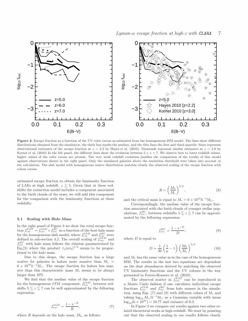
In the left panel of Figure 2 we present the redshift evo-lution of the escape fraction as a function of reddening atredshifts z ∼ 5, 6, 7. We find that there is a weak redshiftdependence. The biggest difference at each redshift is thepresence of galaxies with larger values of colour excess. Asthe redshift evolution of the overall scaling is rather weak,we compare our theoretical results at z ∼ 5, the last redshiftavailable in the simulation to make this study, with the ob-servations at z ∼ 2.2 and z ∼ 3, the highest redshifts so farwith observations of this kind. The physical time betweenthe observational results and the simulated ones is ∼ 1Gyr.

In the right panel of Figure 2 we show the final re-sult of the comparison between the escape fractions fromobservations at z ∼ 2.2 and z ∼ 3 and our model ap-plied to the galaxies in the simulation at z ∼ 5. The emptysymbols represent the observational data, indeed showing astrong scaling: the escape fraction decreases with increas-ing colour excess. Our simple model of a dusty gas slab withhomogeneously distributed sources reproduces well these ob-servational trends determined by Hayes et al. (2010) andKornei et al. (2010).

In order to facilitate the comparison of our re-sults with those from other works (Kornei et al. 2010;Hayes et al. 2010), we also use the functional form fesc =CLyα10

−0.4·E(B−V )·kLyα to fit the trend of the median valuesin the fesc-E(B−V ) plane. This form takes into account thatCLyα 6= 1 for very low extinction values (E(B− V ) ≈ 0), asit is expected due to the resonance nature of the Lyman-αline. We obtain CLyα = 0.21 ± 0.05 and kLyα = 8.6 ± 1.0,which is somewhat flatter than the value of kLyα = 12.0 ob-tained by Calzetti et al. (2000) for Lyman-α wavelengths.

5 ANALYSIS AND RESULTS

In this section we present our results on the escape fractionapplying the slab model to the gas and dust contents cal-culated from the MareNostrum High-z Universe simulation.We first derive useful scalings of the escape fraction with themass of the DM halo hosting the galaxy. We then apply the


z=5.0z=6.0z=7.0

0.0 0.1 0.2 0.3

−3

−2

−1

0

E(B−V)

log 1

0 f e

sc

z=5.0Hayes 2010 [z=2.2]Kornei 2010 [z=3.0]

0.0 0.1 0.2 0.3

−3

−2

−1

0

E(B−V)

log 1

0 f e

sc

Figure 2. Escape fraction as a function of the UV color excess as estimated from the homogeneous ISM model. The lines show differentdistributions obtained from the simulation, the thick line marks the median, and the thin lines the first and third quartile. Stars representobservational estimates of the escape fraction at z ∼ 2.2 by Hayes et al. (2010). Diamonds represent similar estimates at z ∼ 3.0 byKornei et al. (2010) In the left panel, the different lines show the evolution between 5 < z < 7. We observe how to lower redshift values,higher values of the color excess are present. The very weak redshift evolution justifies the comparison of the results of this modelagainst observations shown in the right panel. Only the simulated galaxies above the resolution threshold were taken into account inthe calculation. The slab model with homogeneous source distribution matches closely the observed scaling of the escape fraction withcolour excess.

estimated escape fraction to obtain the luminosity functionof LAEs at high redshift, z & 5. Given that at these red-shifts the extinction model includes a component associatedto the birth clouds of the stars, we will add this componentfor the comparison with the luminosity functions at theseredshifts.

5.1 Scaling with Halo Mass

In the right panel of Figure 3 we show the total escape frac-tion fTOT

esc = fISMesc ×fBC

esc as a function of the host halo massfor the homogeneous slab model, where fISM

esc and fBCesc were

defined in sub-section 4.2. The overall scaling of fISMesc and

fBCesc with halo mass follows the relation parameterized byEq.(5) where the product τa(aτ0)

1/3 seems to be propor-tional to the halo mass.

Due to this shape, the escape fraction has a largescatter for galaxies in haloes more massive than Mc =6 × 1010h−1M⊙. The escape fraction for haloes less mas-sive than this characteristic mass Mc seems to be alwayslarger than 10%.

We find that the median value of the escape fractionfor the homogeneous ISM component, fISM

esc , between red-shifts 5 . z . 7 can be well approximated by the followingexpression:

fISMesc =

1− e−R

R, (7)

where R depends on the halo mass, Mh, as follows:

R =

(

Mh

Mc

)5/3

, (8)

and the critical mass is equal to Mc = 6× 1010h−1M⊙.Correspondingly, the median value of the escape frac-

tion associated with the birth clouds of younger stellar pop-ulations, fBC

esc , between redshifts 5 . z . 7 can be approxi-mated by the following expression:

fBCesc =

1− e−D

D, (9)

where D is equal to

D =1

20

(

1

µ− 1

)(

Mh

Mc

)5/3

(10)

andMc has the same value as in the case of the homogeneousISM. The results in the last two equations are dependenton the dust abundances derived by matching the observedUV luminosity functions and the UV colours in the waypresented in Forero-Romero et al. (2010).

The observed scatter in fTOTesc can be reproduced in

a Monte Carlo fashion if one calculates individual escapefractions fISM

esc and fBCesc from halo masses in the simula-

tion, using Eqs. (7) and (9) with different values of Mc andtaking log10 Mc/h

−1M⊙ as a Gaussian variable with meanlog10(6× 1010) = 10.77 and variance of 0.3.

In Figure 3 we compare our results against two other re-lated theoretical works at high redshift. We start by pointingout that the observed scaling in our results follows closely


z=5.0z=6.0z=7.0

Laursen 09 [z=3.0]

10 11 12−3

−2

−1

0

log10 (Mhalo / Msun h−1)

log 1

0 f e

scIS

M

z=5.0z=6.0z=7.0

Dayal 10 [z=6.0]

10 11 12−3

−2

−1

0

log10 (Mhalo / Msun h−1)

log 1

0 f e

scT

OT

Figure 3. Escape fraction as a function of dark matter halo mass, for redshifts z ∼ 5, 6 and 7. The thick lines mark the median, and thethin lines represent the first and third quartile. Triangles show different theoretical results. Left panel. The escape fraction includes thecontribution from the homogeneous ISM (fISM

esc ) only. The median values for fISMesc are reproduced by Eq. (7) The symbols correspond

to the results for single halo simulations by Laursen et al. (2009). Right panel. Contribution from the birth clouds around the youngerpopulation stars to the escape fraction (fBC

esc ). The median values for fBCesc are reproduced by Eq.(9). The symbols represent the results

obtained by Dayal et al. (2010) from a cosmological simulation.

the radiative transfer results shown in Figure 1. The corre-lation between halo mass and gaseous mass obtained in thesimulation is translated here as a scaling between escapefraction and halo mass.

In the left panel of Figure 3 we compare our resultsof the escape fraction from the ISM component against theresults of high resolution simulations of individual galaxies(Laursen et al. 2009). The two models show a good agree-ment for high and low halo masses. There is, however, a dif-ference for haloes in the mass range ∼ 3× 1010h−1M⊙. Themean of our escape fractions is higher by a factor of ∼ 4,although the small sample of Laursen et al. (2009) (sevengalaxies) makes it difficult to estimate the statistical signif-icance of this comparison between the two models.

In the right panel of Figure 3 we compare our resultsagainst a published model of the Lyman-α escape fractionin a cosmological context at z ∼ 6 (Dayal et al. 2010). Themodel of Dayal et al. (2010) presents a radically differentprediction for the escape fraction in haloes more massivethan Mth ∼ 1011h−1M⊙. While in our model the mean es-cape fraction drops steeply from ∼ 0.1 down to ∼ 10−3, theresults of Dayal et al. (2010) show an increase of the escapefraction to values close to ∼ 1 for the same range of mas-sive haloes. This disagreement is very likely due to the factthat Dayal et al. (2010) do not model explicitly the reso-nant nature of the line and approximate the ISM in such away that the Lyman-α escape fraction is proportional to(1− exp−(τd))/τd where τd is the dust optical depth. Thisis a different approximation from the one that produces theresults represented by Eq.5 and other similar radiative trans-fer studies (Hansen & Oh 2006) where there is an explicitdependence with the optical depth of neutral gas, thought to

be abundant in the most massive and vigorous star forminggalaxies at these redshifts.

5.2 Intrinsic Emission and Luminosity Functions

We now study the LAE LF predicted from our simulationstaking into account the different contributions to the es-cape fraction. We will focus on the intrinsic emission associ-ated with star formation. The mechanism for star-triggeredLyman-α relates the amount of ionizing photons producedby young stars to the expected intrinsic Lyman-α luminos-ity. Here we assume that the number of Hydrogen ionizingphotons per unit time is 1.8×1053 photons s−1 for a star for-mation rate of 1 M⊙/yr (Leitherer et al. 1999). This valueassumes a Salpeter IMF, and that the star formation ratehas been constant at least during the last 10 Myr. Assumingthat 2/3 of these photons are converted to Lyman-α pho-tons (case-B recombination, Osterbrock 1989), the intrinsicLyman-α luminosity as a function of the star formation rateis

LLyα = 1.9× 1042 × (SFR/M⊙ yr−1) erg s−1, (11)

where the SFR is calculated from the total mass of starsproduced in the last 200 Myr. We use this analytic expres-sion because the calculation of the total amount of ionizingphotons directly from the information of the star particlesin the simulation is not reliable given the short lifetime ofthe populations contributing to the ionizing flux and thelimited resolution of our simulation. Only the star particlesyounger than 10 Myr will provide the bulk of the ionizingflux, these particles roughly correspond to 1% to 5% of thestar particles in a given galaxy. The least resolved galaxyin our study has 200 star particles, which correspond to 2


to 10 particles to fully sample the star formation history ofthe galaxy during the last 10 Myr. Only a handful of largestgalaxies in the simulation (∼ 100000 star particles, ∼ 1000of them contributing to the ionizing flux) can give reliableresults when the Lyman-α emission from the star particlesis compared against Eq. (11).

We find a tight correlation between star formation rateand halo mass for 5 . z . 7. It can be approximated by

SFR = 0.68

(

Mh

1010h−1M⊙

)1.30

M⊙ yr−1, (12)

so that the final scaling between intrinsic Lyman-α emissionand halo mass can be written as

LLyα = 1.29 × 1042(

Mh

1010h−1M⊙

)1.30

erg s−1. (13)

The observed Lyman-α luminosity can be calculatedfrom our extinction model as:

LoLyα = (fISM

esc × LoldLyα) + (fISM

esc × fBCesc × Lyoung

Lyα ), (14)

where the label old refers to the Lyman-α emission comingfrom stellar populations older than 25Myr and young labelsthe emission from stars younger than 25 Myr. Given thatthe intrinsic ionizing flux is negligible for stellar populationsolder than 25Myr, we can approximate the observed Lyman-α luminosity as:

LoLyα ≈ fISM

esc × fBCesc × LLyα, (15)

where the escape fractions fISMesc and fBC

esc are calculated asdescribed in the previous subsections.

Previous Monte-Carlo calculations of Lyman-α radia-tive transfer in a multiphase medium (Hansen & Oh 2006)show that the dominant effect of the clumpy distribution ofbirth clouds on a photon propagating through the homoge-neous ISM is bouncing at the cloud’s surface, justifying theapproximation of not including further absorption by theseclouds except at the Lyman-α source in the way we havejust implemented.

However, we note that the conditions for dust and gasabundance in our model are such that the calculations ofNeufeld (1991) for the escape fraction are not applicablehere. The main assumption of that model (negligible absorp-tion and scattering in the homogeneous part of the ISM) arenot met, meaning that the escape fraction in our model isnot dominated by the effects of the clumpy component only.

We have not taken into account the effects of scatteringof Lyman-α photons by the IGM, after they escaped fromthe galaxy. This effect is very important before reionisation(z > 6 in our simulation). After reionisation, it is expectedthat the blue part of the double peak spectrum would beabsorbed as photons are cosmologically redshifted to reso-nance with neutral Hydrogen along the line of sight. To firstorder, we have taken this effect into account by dividing theintensity of the observed line strength Lo

Lyα by 2.In Figure 4 we show three different LAE LFs at three

different redshifts z ∼ 5, 6 and 7. The empty symbols repre-sent the observed LFs. The observational results at z ∼ 4.5come from 50 spectroscopically confirmed LAEs from theLarge Area Lyman-α survey (LALA) which covered a field

of ∼ 0.7 deg2 corresponding to a comoving survey vol-ume of 7.4 × 105 Mpc3 (Dawson et al. 2007). At z ∼ 4.86the results from Shioya et al. (2009) are based on observa-tions of the Cosmic Evolution Survey (COSMOS) field of1.83 deg2 giving an effective volume of 1.1 × 106 Mpc3.At z ∼ 6 the data are taken from Ouchi et al. (2008), inthis case the LF was estimated from LAEs from 1 deg2

Subaru/XMM-Newton Deep Survey (SXDS), which probeda comoving volume of ∼ 106 Mpc3. We include as well dataat z ∼ 5.7 in a field of 1.95 deg2 covered by the COSMOSsurvey Murayama et al. (2007) and recent estimations at4.5 < z < 6.6 from the Vimos-VLT Deep Survey (VVDS)(Cassata et al. 2011). The LF at z ∼ 7 was constructed froma sample of 17 LAEs confirmed spectroscopically and 58 pho-tometric LAEs probing a comoving volume of ∼ 2.17 × 105

Mpc3 (Kashikawa et al. 2006). In our simulation we probea comoving volume that is of the same order of magnitudeof these surveys.

In Figure 4 we represent with black squares the LFestimated from the intrinsic luminosities calculated fromthe star formation rates. The spatial abundance is alreadycorrected from the different halo abundance between theWMAP5 and the WMAP1 cosmologies. Compared with theobservational estimates at all redshifts, the normalisation isat least one order of magnitude higher.

We can now apply the expected correction by the es-timated escape fraction of each galaxy. In our model thereis a strong correlation between the mass of the halo hostingthe galaxy and its associated escape fraction. In a simpli-fied manner, galaxies in haloes with masses smaller than6.0×1010 h−1M⊙remain practically unaffected. This is seenin the LFs in Figure 4 where the hexagons represent theluminosity function corrected by the escape fraction. Thebright end of the LF is modified but the overall normalisa-tion is kept one order of magnitude higher than observations.

This result is completely analogous to the situationfound in the continuum UV using the same simulation(Forero-Romero et al. 2010). The strong scaling of the red-dening with galaxy mass causes only the bright end of theUV LF to be effectively modified when extinction is takeninto account. In the context of our model, applying a con-stant reddening value to all galaxies can only be physicallyjustified if there is an additional extinction term from theyoungest stars, as described in Section 3.

If we add now the expected correction of the birthclouds around stellar populations younger than 25 Myr, wefind that the faint end of the LAE LF can be further modi-fied. However, at z ∼ 5 and z ∼ 6 there remains an excess atthe faint end of the LF, corresponding to haloes with masses1.0 × 1010h−1M⊙ < Mh < 4.0 × 1010h−1M⊙. This resultsuggests that either the escape fraction for these galaxies ortheir star formation rate is too high. Nevertheless, the brightend of the simulated LFs, both at z ∼ 5 and z ∼ 6, shows avery close agreement with the observed one. The results arewithin Poissonian uncertainty. We have also checked thatif we apply the scalings for the intrinsic emission and es-cape fractions with halo mass, Eqs. (7, 9, 13), to a pure DMonly simulation with a cubic volume of 250 h−1Mpc on aside and 20483 particles (the Bolshoi Simulation presentedby Klypin et al. (2010)) split into smaller sub-boxes, we canreproduce the results we have just discussed. Specifically, thescatter at the bright end due to cosmic variance is consistent


IntrinsicISMBCISM+BC

Dawson 07Shioya 09

42.0 42.5 43.0 43.5 44.0

−4

−2

0z=5.0

LLyα (erg s−1)

log 1

0 N

/ de

x L L

yα /

Mpc

3


Ouchi 08Murayama 07Cassata 11

42.0 42.5 43.0 43.5 44.0

−4

−2

0z=6.0

LLyα (erg s−1)

log 1

0 N

/ de

x L L

yα /

Mpc

3


Kashikawa 06

42.0 42.5 43.0 43.5 44.0

−4

−2

0z=7.0

LLyα (erg s−1)

log 1

0 N

/ de

x L L

yα /

Mpc

3

Figure 4. Luminosity Functions at z ∼ 5, 6 and 7. The observational constraints (empty symbols) are compared to different resultsfrom the simulation (filled symbols): Intrinsic Lyman-α emission considering the total star formation rate in Eq.(11) (black squares),Lyman-α emission corrected only by the extinction of the homogeneous ISM based on the spherical model studied with the Monte Carlosimulations using Eq.(7) (blue triangles), Lyman-α emission corrected only by the extinction of the birth clouds using Eq.(9) (green

hexagons). The final luminosity function corrected by the homogeneous ISM and the birth clouds is shown by the red diamonds.

with the observations. Nevertheless, the same scatter doesnot help to explain the lower abundance of our numericalLAEs at the faint end.

The normalization of our LF functions at redshift z ∼ 7is still higher than observed. In principle, it could be possibleto account for this difference by properly modeling the IGMabsorption, which at this epoch, it is not completely ionizedand will add a dimming effect to the LAEs. Considering adimming factor that depends on luminosity only (withoutany scatter), we would require that 25% (40%) of Lya pho-tons be transmitted through the IGM in order to match thebright (faint) end of the observed luminosity function. Usingagain the DM only simulation, together with the scalingswe obtain for the star formation and the escape fraction,we find that cosmic variance can account for a 0.5 dex (0.3dex) variations at the bright (faint) end of the luminosityfunction at z ∼ 7. In conclusion, applying a constant IGMtransmission of T = 0.3 − 0.4 we can still reproduce the lu-minosity function for the brightest three bins in Figure 4. Amore realistic treatment of the effects of IGM (in the spiritof Zheng et al. (2010)) actually yields a large scatter for thetransmission at a given Lyman-α luminosity. Nevertheless,a detailed modeling of the IGM effect is far beyond the scopeof this paper.

6 CONCLUSIONS

In this paper we model the escape fraction of Lyman-α pho-tons in the approximation of a dusty gas slab with Lyman-αsources homogeneously mixed. The escape fractions for thisconfiguration and different dust and gas contents have beencalculated using CLARA, our new Monte-Carlo code describedin detail in Appendix A. These results can be applied in anymodel that predicts the optical depth of gas and dust ingalaxies.

We selected the slab geometrical configuration in or-der to be consistent with the assumptions that led us to fix

the dust abundances from the MareNostrum High-z Uni-

verse simulation, as constrained by high redshift UV atz & 5 observations (Forero-Romero et al. 2010). Our pro-posed dust model describes the contributions from an homo-geneous ISM (slab geometry) and a clumpy phase (sphericalgeometry) associated to stellar populations younger than25Myr.

We estimate the scaling of the Lyman-α escape frac-tion with the expected reddening for the slab componentand dust abundances in the MareNostrum High-z Universe.The scaling shows a weak redshift dependence between5 . z . 7, furthermore there is a very good agreement withthe observational estimation of the escape fraction and red-dening for galaxies at z ∼ 2.2 and z ∼ 3 assuming that onlythe homogeneous ISM component is dominant at these red-shifts. Including both contributions from the homogeneousISM and the clumpy phase, we have calibrated the escapefraction as a function of the host dark matter halo based onthe results of the MaraNostrum High-z Universe.

As an application of these results, we construct the in-trinsic LAEs LF as estimated from the star formation rates.We find that the normalisation is one order of magnitudehigher than observational estimates. Correcting the intrinsicLAE luminosities by the estimated escape fraction (homoge-neous ISM and clumpy phase included) brings the simulationinto agreement with the observations at z ∼ 5 and z ∼ 6.The match at the bright end is acceptable within the Pois-sonian and cosmic variance errors. The mismatch at z ∼ 7can be explained because a proper modeling of these epochshas to account for the yet incomplete reionisation processand the influence of the neutral parts of the IGM.

Nevertheless, our results are in conflict with the ob-servational estimates at the faint end. There seems to bean excessive production of LAEs with intrinsic luminositiesLo

Lα ∼ 6.0 × 1042 erg s−1 at z ∼ 5 and z ∼ 6. This excesswas spotted, although weakly, in the results of the UV LFsof (Forero-Romero et al. 2010). Furthermore, a fine tuningof the extinction model for galaxies in this mass range could


provide a better match to the observations. In that case, thegalaxies at the faint end should be more dusty, which wouldmake them redder, and thus breaking the broad agreementfor the UV colours that we have already obtained. This isnot a satisfactory approach to explain for these differences.Based on these considerations, we think that a probable ori-gin of this discrepancy is the high rate of star formation ingalaxies situated in these haloes. A possible physical expla-nation is that supernova feedback modulates more effectivelythe star formation in haloes of masses < 1011h−1M⊙, pro-viding a mechanism to shape the faint end of the luminosityfunction. However, it is also possible that the star formationrate is overestimated in all haloes at these redshifts. Thiswould be translated into a trade-off with less dust extinc-tion to explain the UV luminosity function. Regardless ofwhat is the correct explanation of this enigma, all possiblesolutions seem to challenge our current understanding of therate at which gas is converted into stars at high redshift.

It is encouraging that the results for the brightest galax-ies, the best resolved ones, both in observations and simu-lations, are consistent with observations in the UV (mag-nitudes and colours) as well with the Lyman-α line. A fullpicture of these massive high redshift galaxies will be com-pleted by observations of the rest frame IR to be performedby ALMA. We will address in a upcoming work the predic-tions of our model in terms of ALMA observations, focus-ing on the most massive galaxies, constructing a completepanchromatic perspective of high redshift galaxies in theMareNostrum High-z Universe.

ACKNOWLEDGMENTS

The simulation used in this work is part of the MareNos-trum Numerical Cosmology Project at the BSC. The dataanalysis has been performed at the NIC Julich and at theLRZ Munich.

The Bolshoi simulation used in this paper was per-formed and analyzed at the NASA Ames Research Center.We thank A. Klypin (NMSU) and J. Primack (UCSC) formaking this simulation available to us.

JEFR and FP acknowledge the support by the ESFASTROSIM network though a short visit grant of JEFRto Granada where part of the developing and most of thetesting for CLARA took place. JEFR acknowledges the hos-pitality of Roberto Luccas in Barcelona, where most of thispaper was written. JEFR acknowledges as well useful dis-cussions on some issues addressed in this paper with RenyueCen, Zheng Zheng and Chung-Pei Ma. JEFR thanks PratikaDayal for providing data from her paper in electronic format.

GY acknowledges support of MICINN (Spain) throughresearch grants FPA2009-08958 and AYA2009-13875-C03-02. SRK would like to thank Consolider-Ingenio SyeC(Spain) (CSD2007-0050) for financial support.

AJC acknowledges support from MICINN through FPUgrant 2005-1826.

We equally acknowledge funding from the Consoliderproject MULTIDARK (CSD2009-00064) and the Comu-nidad de Madrid project ASTROMADRID (S2009/ESP-146).

REFERENCES

Calzetti D., Armus L., Bohlin R. C., Kinney A. L., Koorn-neef J., Storchi-Bergmann T., 2000, ApJ, 533, 682

Cassata P., Le Fevre O., Garilli B., Maccagni D., Le BrunV., Scodeggio M., Tresse L., Ilbert O. et al ., 2011, A&A,525, A143+

Cazaux S., Spaans M., 2004, ApJ, 611, 40

Ceverino D., Dekel A., Bournaud F., 2010, MNRAS, 404,2151

Charlot S., Fall S. M., 2000, ApJ, 539, 718Dawson S., Rhoads J. E., Malhotra S., Stern D., Wang J.,Dey A., Spinrad H., Jannuzi B. T., 2007, ApJ, 671, 1227

Dayal P., Ferrara A., Saro A., 2010, MNRAS, 402, 1449

Devriendt J., Rimes C., Pichon C., Teyssier R., Le BorgneD., Aubert D., Audit E., Colombi S., Courty S., DuboisY., Prunet S., Rasera Y., Slyz A., Tweed D., 2010, MN-RAS, 403, L84

Devriendt J. E. G., Guiderdoni B., Sadat R., 1999, A&A,350, 381

Dijkstra M., Haiman Z., Spaans M., 2006, ApJ, 649, 14

Dunkley J., Komatsu E., Nolta M. R., Spergel D. N., Lar-son D., Hinshaw G., Page L., Bennett C. L., Gold B.,Jarosik N., Weiland J. L., Halpern M., Hill R. S., KogutA., Limon M., Meyer S. S., Tucker G. S., Wollack E.,Wright E. L., 2009, ApJS, 180, 306

Eisenstein et al. 2005, ApJ, 633, 560

Ferriere K. M., 2001, Reviews of Modern Physics, 73, 1031Finlator K., Oppenheimer B. D., Dave R., 2011, MNRAS,410, 1703

Forero-Romero J. E., Yepes G., Gottlober S., KnollmannS. R., Khalatyan A., Cuesta A. J., Prada F., 2010, MN-RAS, 403, L31

Hansen M., Oh S. P., 2006, MNRAS, 367, 979Harrington J. P., 1973, MNRAS, 162, 43

Hatton S., Devriendt J. E. G., Ninin S., Bouchet F. R.,Guiderdoni B., Vibert D., 2003, MNRAS, 343, 75

Hayes M., Ostlin G., Schaerer D., Mas-Hesse J. M., Lei-therer C., Atek H., Kunth D., Verhamme A., de BarrosS., Melinder J., 2010, Nature, 464, 562

Hill G. J., Gebhardt K., Komatsu E., Drory N., MacQueenP. J., Adams J., Blanc G. A., Koehler R., Rafal M.,Roth M. M., Kelz A., Gronwall C., Ciardullo R., Schnei-der D. P., 2008, in T. Kodama, T. Yamada, & K. Aokied., Astronomical Society of the Pacific Conference SeriesVol. 399 of Astronomical Society of the Pacific ConferenceSeries, The Hobby-Eberly Telescope Dark Energy Exper-iment (HETDEX): Description and Early Pilot SurveyResults. pp 115–+

Hirashita H., Nozawa T., Kozasa T., Ishii T. T., TakeuchiT. T., 2005, MNRAS, 357, 1077

Hu E., McMahon R. G., 1996, Nature, 382, 281

Hu E. M., Cowie L. L., Capak P., Kakazu Y., 2005, inP. Williams, C.-G. Shu, & B. Menard ed., IAU Colloq.199: Probing Galaxies through Quasar Absorption LinesSpectroscopic studies of z5.7 and z6.5 galaxies: implica-tions for reionisation. pp 363–368

Hu E. M., Cowie L. L., Capak P., McMahon R. G.,Hayashino T., Komiyama Y., 2004, AJ, 127, 563

Hu E. M., Cowie L. L., McMahon R. G., 1998, ApJL, 502,L99+

Hu E. M., Cowie L. L., McMahon R. G., Capak P., Iwamuro







F., Kneib J., Maihara T., Motohara K., 2002, ApJL, 568,L75

Inoue A. K., 2003, PASJ, 55, 901Inoue A. K., 2005, MNRAS, 359, 171Kashikawa N., Shimasaku K., Malkan M. A., Doi M., Mat-suda Y., Ouchi M., Taniguchi Y., Ly C., Nagao T., IyeM., Motohara K., Murayama T., Murozono K., Nariai K.,Ohta K., Okamura S., Sasaki T., Shioya Y., Umemura M.,2006, ApJ, 648, 7

Klypin A., Trujillo-Gomez S., Primack J., 2010, ArXiv e-prints

Knollmann S. R., Knebe A., 2009, ApJS, 182, 608Kobayashi M. A. R., Totani T., Nagashima M., 2007, ApJ,670, 919

Kong X., Charlot S., Brinchmann J., Fall S. M., 2004, MN-RAS, 349, 769

Kornei K. A., Shapley A. E., Erb D. K., Steidel C. C.,Reddy N. A., Pettini M., Bogosavljevic M., 2010, ApJ,711, 693

Laursen P., Sommer-Larsen J., Andersen A. C., 2009, ApJ,704, 1640

Le Delliou M., Lacey C., Baugh C. M., Guiderdoni B., Ba-con R., Courtois H., Sousbie T., Morris S. L., 2005, MN-RAS, 357, L11

Leitherer C., Schaerer D., Goldader J. D., Gonzalez Del-gado R. M., Robert C., Kune D. F., de Mello D. F., DevostD., Heckman T. M., 1999, ApJS, 123, 3

Malhotra S., Rhoads J. E., 2004, ApJL, 617, L5Mathis J. S., Mezger P. G., Panagia N., 1983, A&A, 128,212

Murayama T., Taniguchi Y., Scoville N. Z., Ajiki M.,Sanders D. B., Mobasher B., Aussel H., Capak P., Koeke-moer A., Shioya Y., Nagao T., Carilli C., Ellis R. S., Gar-illi B., Giavalisco M., 2007, ApJS, 172, 523

Neufeld D. A., 1991, ApJL, 370, L85Night C., Nagamine K., Springel V., Hernquist L., 2006,MNRAS, 366, 705

Nilsson K. K., Orsi A., Lacey C. G., Baugh C. M.,Thommes E., 2007, A&A, 474, 385

Osterbrock D. E., 1989, Astrophysics of gaseous nebulaeand active galactic nuclei

Ota K., Iye M., Kashikawa N., Shimasaku K., KobayashiM., Totani T., Nagashima M., Morokuma T., FurusawaH., Hattori T., Matsuda Y., Hashimoto T., Ouchi M.,2008, ApJ, 677, 12

Ouchi M., Mobasher B., Shimasaku K., Ferguson H. C.,Fall S. M., Ono Y., Kashikawa N., Morokuma T., Naka-jima K., Okamura S., Dickinson M., Giavalisco M., OhtaK., 2009, ApJ, 706, 1136

Ouchi M., Shimasaku K., Akiyama M., Simpson C., SaitoT., Ueda Y., Furusawa H., Sekiguchi K., Yamada T., Ko-dama T., Kashikawa N., Okamura S., Iye M., Takata T.,Yoshida M., Yoshida M., 2008, ApJS, 176, 301

Partridge R. B., Peebles P. J. E., 1967, ApJ, 147, 868Reddy N. A., Steidel C. C., Fadda D., Yan L., Pettini M.,Shapley A. E., Erb D. K., Adelberger K. L., 2006, ApJ,644, 792

Rhoads J. E., Dey A., Malhotra S., Stern D., Spinrad H.,Jannuzi B. T., Dawson S., Brown M. J. I., Landes E.,2003, AJ, 125, 1006

Shapley A. E., Steidel C. C., Adelberger K. L., DickinsonM., Giavalisco M., Pettini M., 2001, ApJ, 562, 95

Shimasaku K., Kashikawa N., Doi M., Ly C., Malkan M. A.,Matsuda Y., Ouchi M., Hayashino T., Iye M., MotoharaK., Murayama T., Nagao T., Ohta K., Okamura S., SasakiT., Shioya Y., Taniguchi Y., 2006, PASJ, 58, 313

Shioya Y., Taniguchi Y., Sasaki S. S., Nagao T., MurayamaT., Saito T., Ideue Y., Nakajima A., Matsuoka K., TrumpJ., Scoville N. Z., Sanders D. B., 2009, ApJ, 696, 546

Spergel D. N., Verde L., Peiris H. V., Komatsu E., NoltaM. R., Bennett C. L., Halpern M., Hinshaw G., Jarosik N.,Kogut A., Limon M., Meyer S. S., Page L., Tucker G. S.,Weiland J. L., Wollack E., Wright E. L., 2003, ApJS, 148,175

Springel V., 2005, MNRAS, 364, 1105Stark D. P., Ellis R. S., Richard J., Kneib J., Smith G. P.,Santos M. R., 2007, ApJ, 663, 10

Stenflo J. O., 1976, A&A, 46, 61Trenti M., Smith B. D., Hallman E. J., Skillman S. W.,Shull J. M., 2010, ApJ, 711, 1198

Verhamme A., Schaerer D., Maselli A., 2006, A&A, 460,397

Wagner C., Muller V., Steinmetz M., 2008, A&A, 487, 63Wang J. X., Rhoads J. E., Malhotra S., Dawson S., SternD., Dey A., Heckman T. M., Norman C. A., Spinrad H.,2004, ApJL, 608, L21

Wannier P. G., Lichten S. M., Morris M., 1983, ApJ, 268,727

Zheng Z., Cen R., Trac H., Miralda-Escude J., 2010, ApJ,716, 574

APPENDIX A: LYMAN-α RADIATIVE

TRANSFER

The basic principle of CLARA is to follow the individual scat-terings of a Lyman-α photon as it travels through a distribu-tion of gaseous hydrogen. Each scattering, which is in fact anabsorption and re-emission, does not modify the frequencyof the photon in the rest-frame of the hydrogen atom. Butdue to the peculiar velocities of the atom in the new di-rection of propagation of the photon, the new frequency ina laboratory rest-frame is different from the incoming fre-quency. Thus the photon performs a random walk not onlyin space but also in frequency.

The relevant properties of the gaseous hydrogen can befully described by its density, temperature and bulk veloc-ity. This is sufficient to describe the emergent spectra ofa source of Lyman-α photons embedded in gaseous hydro-gen. It is important to observe that none of the emittedphotons is completely lost by absorption as it is immedi-ately re-emitted. The original spectrum morphology of theLyman-α source is modified, but the only way to lose theenergy input by a Lyman-α source is through dust absorp-tion. A simple description of the dust abundance in the gasmust then be included to calculate its effect on the outgoingproperties of the traveling Lyman-α photons.

In the next subsections we give a detailed account onthe basic underlying physics of the qualitative descriptionwe have just given. Once the physical fundamentals are de-scribed, we describe how these are implemented in the code.The last subsection is devoted to show the results availableanalytical test cases we applied the code to.


A1 Physical Principles

A1.1 Scattering

The scattering cross section of a Lyman-α photon is a func-tion of the photon frequency. In the rest-frame of the atomit is equal to

σ(ν) = f12πe2

mec

∆νL/2π

(ν − ν0)2 + (∆νL/2)2, (A1)

where f12 = 0.4162 is the Lyman-α oscillator strength, ν0 =2.466 × 1015Hz is the line centre frequency, ∆νL = 4.03 ×10−8ν0 = 9.936 × 107 Hz is the natural line width, and theothers symbols conserve their usual meaning.

In the case of a Maxwellian distribution of atom veloc-ities, after convolving the individual cross section with theatom velocity distribution, we can write down the averagecross section as

σ(x) = σx = f12

√πe2

mec∆νDH(a, x), (A2)

where H(a, x) is the Voigt function,

H(a, x) =a

π

∫ ∞

−∞

e−y2

(x− y)2 + a2dy, (A3)

∆νD = (vp/c)ν0 is the Doppler frequency width, vp =(2kT/mH)1/2 is

√2 times the velocity dispersion of the Hy-

drogen atom, T is the gas temperature, mH is the Hydrogenatom mass, a = ∆νL/(2∆νD) is the relative line width andx = (νi − ν0)/∆νD is a re-parameterisation of the photonfrequency respect to the line centre normalised by the tem-perature dependent Doppler frequency width of the gas.

The scattering is coherent in the rest-frame of the pho-ton, but to an external observer, any motion of the atom willadd a Doppler shift to the photon. Measuring the velocityof the atom, va, in units of thermal velocity u = va/vp, thefrequency in the reference frame of the atom is

x′ = x− u · ni, (A4)

where ni is a unit vector in the incoming direction of thephoton.

In the general case, the scattering of the Lyman-α atomis not isotropic. For symmetry reasons the scattering isisotropic in the azimuthal direction, respect to the outgoingscattering direction. The distribution of the scatter direc-tions depends only on the angle, θ, between the incomingand outgoing direction of the photons, ni and no, respec-tively.

The information on the outgoing angle θ is encoded inthe phase function,W (θ). In general the angular momenta ofthe initial, intermediate and final states are involved in thecalculation ofW (θ). In the case of resonant scatter the initialand final state are the same. The intermediate state corre-sponds to the excited state. Following the notation nlJThereare two possible excited states, 2P1/2 and 2P3/2.

Specifically, in the dipole approximation the phase func-tion can be written as:

W (θ) ∝ 1 +R

Qcos2 θ (A5)

where R/Q = 0 for the 2P1/2 → 1S1/2 transition and R/Q =3/7 for the 2P3/2 → 1S1/2 case.

The spin multiplicity of each sate is 2J + 1, meaningthat the probability of being excited to the 2P2/3 state istwice that of the 2P1/2 state. These results are valid onlyin the core of the line profile. Stenflo (1976) found that inthe wings quantum mechanical interference between the twolines act in such a way as to give a scattering resembling aclassical oscillator. In that case the phase function takes theform

W (θ) ∝ 1 + cos2 θ (A6)

The travelling distance, l, of a Lyman-α photon of fre-quency x can be expressed as

τx = σsnH l, (A7)

where nH is the neutral hydrogen number density, and ithas been assumed that along the path l the temperatureand bulk velocity field of the gas are constant, to ensurethat the photon frequency can be represented by the samevalue of x along its trajectory.

In what follows, we will always characterise an homoge-neous and static medium using the optical depth τ0 at theline center.

A1.2 Dust Absorption

In the case of dust interaction the photon can either bescattered or absorbed. The optical depth of dust, σd, can begenerally expressed as the sum of an absorption cross sectionσa, and a scattering cross section σs.

σd = σa + σs. (A8)

The determination of these two cross sections can beachieved using two different approaches. We name the firstapproach the ab initio approach. The ab initio approachseeks to determine the values of the dust cross sections fromindividual studies of dust grain properties and its interac-tion with photons. This is the approach used in the stud-ies by Verhamme et al. (2006). The second approach is aphenomenological one and it defines the dust properties inrelation to the gas properties in the galaxy. The dust crosssection properties are then derived from observations. In theinterest of keeping our model simple to operate and with agood match to the level of detail required for the approxi-mation, we proceed with an ab initio approach.

We express then the absorption and scattering crosssections as

σa,s = πd2Qa,s, (A9)

where d is represents an average dust radius and Qa,s isan absorption/scattering efficiency. The dust albedo can bethen expressed as


A =Qs

Qa +Qs. (A10)

At UV wavelengths the emission and absorption pro-cesses are equally likely, with Qa ∼ Qs ∼ 1, making thedust albedo around ∼ 1/2. We now express the dust of op-tical depth, τd in an analogous way to the neutral hydrogenoptical depth Eq.(A7) for a parcel of dust of linear dimen-sions l

τd = σdndl, (A11)

where nd represents the number density of dust particlesand it has been assumed again that the dust cross sectionand dust number density are constant on the scale of l.

A2 The Radiative Transfer Code

The code implements a Monte Carlo approach to the ra-diative transfer. CLARA follows the successive scattering ofindividual photons as they travel through the gas distribu-tion, changing at each scatter the direction of propagationand frequency of the photon. We describe now in detail thetechnical implementation.

A2.1 Initial Conditions

The problem to solve defines the physical characteristics ofthe gas distribution and the initial conditions of the Lyman-α emitted photons. The gas is described by the followingcharacteristics:

• The geometry of the gas distribution. In this section wewill present results for the following configurations: infiniteslab and sphere

• The size of the gas distribution. This is parameterisedby the hydrogen optical depth, τ0 at line centre x = 0. Inall the geometries we measure the optical depth from thecentre of the configuration to its nearest border.

• The temperature of the gas distribution, T . This is setto a constant for all the gas distributions explored in thispaper.

• The gas bulk velocity field, vb(r). This is in generaldependent on the position. The only bulk velocity field ex-plored in this work corresponds to a Hubble like flow in thespherical geometries.

• The dust optical depth, τd.• The dust albedo, A.

The photons are described by the following properties:

• The spatial distribution with respect to the gas dis-tribution. There are two possibilities. All the photons areemitted from the centre of the gas distribution or they arehomogeneously distributed throughout the gas volume.

• The initial direction of propagation. We assume thatthe emission is isotropic (in the local comoving frame).

• The initial frequency, xi. We consider that all photonsare injected in the centre of the line xi = 0.

The number of photons used in order to reach con-vergence are Nph ∼ 5 × 104. In some cases convergence isreached with Nph ∼ 1× 104 photons.

A2.2 Photon Displacement and Interaction

For each photon of frequency x and direction of propagationni, we determine the distance freely travelled until the nextinteraction. This optical depth is determined by samplingthe probability distribution P (τ ) = exp(−τ ) by setting τs =− ln(R), where R is a represents a random number between0 ≤ R < 1 following an uniform distribution.

This optical depth interaction fixes the travel distancels by:

ls =τs

σxnH + σdnd(A12)

The photon travels a distance ls in the direction bi,at this point we decide if the photon interacts either withan hydrogen atom or with a dust grain. The probability ofbeing scattered by a Hydrogen atom is

PH =σxnH

σxnH + σdnd. (A13)

Another random number R is generated and comparedto PH . If R < PH the photon interacts with Hydrogen,otherwise it interacts with the dust grain. In the case ofinteraction with dust a new random number is generatedand compared with the albedo A. If the random number isless than the albedo, the photon is scattered coherently ina random direction, otherwise the photon is absorbed andnot considered for further scatterings during the rest of thesimulation.

In the case of photon interaction, the situation is moreinvolved. As already described by Eq. (A4), the new pho-ton frequency in the observer frame depends on the specificvelocity of the atom, u. It is therefore necessary to draw avelocity for the hydrogen atom. The preferred velocity forthe atom cannot be drawn from a isotropic Gaussian distri-bution, there is an implicit spatial anisotropy in this case.The opacity of the gas is frequency dependent: the preferredatom velocity in the parallel direction to the photon prop-agation is different from the velocity in the perpendiculardirection.

The atom velocity is thus determined in two steps. Inthe first step the two perpendicular velocities are selectedfrom a Gaussian distribution. In the second step the paral-lel component of the atom velocity is calculated. The par-allel component is calculated from a distribution calculatedas the convolution of a Gaussian (representing the intrinsicvelocity) convolved with the Lorentzian probability of theatom being able to scatter the photon:

f(u||) ∝ G(u||)× L(x− u||) ∝ e−u2

|| × a

π

1

(x− u||)2 + a2.

The resulting normalised probability is:

f(u||) =a

πH(a,x)

eu2||

(x− u||)2 + a2. (A14)

The distribution represented by Eq. (A14) is not analyt-ically integrable, therefore we generate the parallel velocitiesu|| by means of the rejection method.

We stress that we do not use any of the commonly used


speeding mechanisms. These speeding techniques are moti-vated by the physical fact that scattering of atoms in thecore frequencies are irrelevant from the point of view of thechange in frequency and position that they represent. Giventhe uncertainty of applying these techniques (despite of care-ful code calibration) in the presence of dust, we decide touse the simplest rejection method.

The new emission direction of propagation (in the atomrest-frame), nf is determined as already described in detailin subsection A1. In the observers frame, the final frequencyis:

xf = xi − ni · u+ nf · u+ g(1− ni · nf ), (A15)

where the factor g accounts for the recoil effect.

A3 Analytical Tests

The basic tests on CLARA are based on the available analyt-ical solutions for a thick, plane-parallel, isothermal infinitegas slab of uniform density. The solution of the infinite slabprovides the analytical expressions for: the distribution ofoutgoing frequencies, the average number of scatterings andthe position of the peaks of the outgoing spectrum. In thecase of a dusty infinite slab one we also have an analyticalexpression for the escape fraction (Harrington 1973; Neufeld1991).

The expression for the analytic emergent spectrum as afunction of frequency shift for a mid-plane source reads:

J(x) =

√6

24

1

aτ0

x2

cosh(√

π4/54|x3 − x3i |/aτ0)

, (A16)

where τ0 is the optical depth measured from the mid-planeto the slice boundary and xi is the frequency of the photonsinjected in the slice. For xi = 0 the emergent spectrum hasa symmetric two-peaked shape.

Setting ∂J/∂x = 0 (Harrington 1973), it can be shownthat the position of the maxima is:

xm = ±1.066(aτ0)1/3, (A17)

while the average number of scatterings is:

〈Ns〉 = 1.612τ0 . (A18)

If dust is added to the gas distribution, it is then pos-sible from analytical considerations to estimate the scalingsof the escape fraction from the slab physical properties. Theexpression for the escape fraction reads

fesc =1

cosh(

ξ′√

(aτ0)1/3τa) , (A19)

where ξ′ = ξ√3/π5/12 and ξ = 0.565 is a parameter found

from a fit.In the following we compare the analytical results de-

scribed by Eqs.(A16) to (A19) with the results from CLARA .In Figure A1 we show the outgoing spectra for the infiniteslab with four different optical depths τ0 = 105, 106, 107

and 108, and a constant temperature of T = 10K. The broad

shape of the double peak is reproduced. The agreement withthe expected analytical solution becomes better as the hy-drogen optical depth increases, as expected. The simulationand the analytical result are expected to hold for opticaldepths and temperatures such as aτ0 > 103.

In the middle panel of Figure A1, we have the positionsof the positive and negative peaks in the outgoing spectra,as a function of the product aτ0. These results were ob-tained from 7 different runs with their characteristics listedin Table A1. In the right panel we compare the number ofscatterings with the theoretical prediction, which is only de-pendent on the hydrogen optical depth τ0. In both cases wefind optimal agreement with the theoretical expectations.We stress again that even though we reproduce the rightnumber of scatterings, we have not implemented any accel-eration scheme based on the skip scattering scheme.

In Figure A2 we show the results concerning the es-cape fraction for the dusty infinite slab. We compare ourresults to the expected result from Eq. (A19). In Table A1we list the parameters for the dusty slab run, as well as thevalues of the escape fraction we find. The theoretical expec-tations for the escape fraction take the interaction with dustas an absorption. In the case of our runs, as we consider analbedo of A = 0.5, the optical depth of dust grains has tobe replaced by an effective value of an absorbing materialτa = (1 − A)τd = 0.5τd, where τd is defined by Eq. (A11).Once again, we find a reasonable agreement with the theo-retical expectations.

At this point we are confident that CLARA provides theexpected outgoing spectra and number of scatterings. Thedust implementation has been tested against the availabletheoretical constraints, yielding satisfactory results.

The case of spherical symmetry offers analytical solu-tions in specific cases (Dijkstra et al. 2006). Besides, the caseof a expanding (contracting) sphere has been extensivelystudied in the literature with different Monte Carlo codes.The spherical symmetry situations gives us the possibility toperform further tests on CLARA. We will deal with the caseof a static, isothermal and homogeneous sphere of gas first.Subsequently we will add a Hubble-like flow to the sphere.

Dijkstra et al. (2006) computed the analytic solutionfor the emergent spectrum of a point-like Lyman-α sourcesurrounded by an homogeneous, static gas distribution at aconstant temperature. The solution can be expressed withthe same functional form as the Harrington-Neufeld solution(Harrington 1973; Neufeld 1991).

We setup different configurations in CLARA for a series ofoptical depth and temperatures. Figure A3 shows CLARA out-puts compared with the corresponding analytical solutions.Once more, in the limit of large values for aτ0 > 103 werecover the behaviour expected by the analytical solutionprovided by Dijkstra et al. (2006).

We add to the homogeneous sphere a radial Hubble likeflow as a function to the distance to the centre of the sphere

Vr(r) = Vmaxr

R, (A20)

where Vmax is a constant which can be selected to be positiveor negative.

The outgoing spectra of this type of configuration hasnot been worked out from an analytical point of view. How-


τ0 = 105

τ0 = 106

τ0 = 107

τ0 = 108

−50 0 50 0

5

10

15

x

103

J(x)

Harrington (1973)Negative xm

Positive xm

2 3 4 50.5

1.0

1.5

2.0

log10 aτ0

log 1

0 |x

m|

Harrington (1973)This Work

5 6 7 8 5

6

7

8

9

log10 τ0

log 1

0 <N

scat

t>

Figure A1. Analytical tests related to the infinite homogeneous gas slab. The left panel show the outgoing spectra for different hydrogenoptical depths, compared to the expected analytical solutions. The middle panel compares the positions of the maxima in the outgoingspectra to the expected analytical estimates for a series of 5 different runs. The panel on the right compares the average number ofscatterings the Lyman-α photons go through before escaping the slab. CLARA passes successfully these three tests.

T (K) τ0 Vmax τa = (1− A)τd fCesc,slab fH

esc,slab fCesc,sph fH

esc,sph

104 106 0 5.0× 10−5 0.998 0.999 0.999 0.999104 106 0 5.0× 10−4 0.991 0.993 0.995 0.997104 106 0 5.0× 10−3 0.917 0.937 0.957 0.976104 106 0 5.0× 10−2 0.471 0.590 0.664 0.803104 107 0 5.0× 10−5 0.998 0.998 0.999 0.999104 107 0 5.0× 10−4 0.982 0.987 0.991 0.995104 107 0 5.0× 10−3 0.853 0.894 0.925 0.962104 107 0 5.0× 10−2 0.291 0.453 0.493 0.720104 107 0 0.5 0.0029 0.084 0.014 0.224104 107 0 0.1 0.127 0.295 0.280 0.568104 107 0 0.2 0.036 0.179 0.111 0.407104 107 0 0.4 0.0069 0.103 0.027 0.265104 107 0 1.0 0.00023 0.049 0.0011 0.136104 107 0 4.0 < 0.0001 0.014 <0.0001 0.042104 107 0 5.0 < 0.0001 0.012 <0.0001 0.036104 1.2× 107 0 0.5 - - 0.012 -

104 1.2× 107 20 0.5 - - 0.017 -104 1.2× 107 200 0.5 - - 0.140 -104 1.2× 107 2000 0.5 - - 0.283 -

Table A1. Summary of the physical characteristics for all runs, both with infinite slab and spherical geometry of a dusty gas distribution.Vmax refers to the parameterisation of the radial velocity profile imposed on the sphere following a Hubble-like law. The escape fractionin the case of centrally distributed sources in a sphere is denoted by fC

esc,sph, while fHesc,sph corresponds to the escape fraction when the

Lyman-α sources are homogeneously distributed. The escape fractions for the infinite slab are denoted by fCesc,slab and fH

esc,slab.

ever, it is part of the most studied physical setups by MonteCarlo codes similar to ours. The quantitative behaviour ofour results follows the behaviour of previously published re-sults. In the expanding case, there is suppression of the bluepeak accompanied by an enhancement in the red wing ofthe emergent spectrum. The case of the collapsing spheredisplays the enhancement in the blue peak and suppressionin the red peak.

A4 The Homogeneous Source Distribution

The model of the LAEs suggested in the paper is basedon the approximation of an homogeneous dusty gas sphere,with the photon sources distributed homogeneously inside

the sphere. In the body of the paper we explored in detailthe consequences of this model on the escape fraction. Atthe same time we have studied the effect on the outgoingspectra.

Figure A5 presents the outgoing spectra already cor-rected by the escape fraction. The dashed line shows theresult for the sphere with sources located at the center, thesolid line is the expected result for the case of the dustlesssphere. The match between the two curves shows that ef-fectively the shape of the outgoing spectra is preserved inthe presence of dust. This result is expected because all thephotons are emitted at the same location and experience thesame optical depth.

In case of homogeneously distributed sources, the spec-


Neufeld, ξ=0.525This Work

0.01 1.0 100.0

10−4

10−2

10+0

τa (a τH)1/3

f esc

Figure A2. Escape fraction for Lyman-α photons emitted fromthe centre of a infinite slab of gas. The hexagons represent theresults of CLARA, the continuous line, the analytical solution ofEq.(A19).

Dijkstra et al.(2006)τ = 105

τ = 106

τ = 107

−50 0 50 0

5

10

x

103

J(x)

Figure A3. Emergent line profile for the static and dustlesssphere test. The photons are emitted at the centre of a spherewith different hydrogen optical depths. The analytical solutionfollows Dijkstra et al. (2006).

tral shape is different. The peaks are located closer to theline centre due to the fact that now, on average, the photonsexperience a smaller optical depth. At the same time, eachwing presents now an asymmetrical shape with respect tothese maxima. Furthermore, there is now some amount ofphotons very close to the center of the line, i.e. emitted closeto the surface, that escaped without any scatter.

We have presented CLARA, a radiative transfer code forLyman-α radiation. The code propagates Lyman-α photonsthrough arbitrary distributions of hydrogen density, temper-ature, velocity structures and dust distributions. The codehas successfully passed all the available tests for codes of itskind, and has allowed us to study simplified geometries inthe present paper.

Dijkstra et al.(2006)StaticExpandingContracting

−40 −20 0 20 40 0

5

10

x

103

J(x)

Figure A4. Emergent line profile in the collapsing/outflowingsphere tests. The collapsing/outflowing solutions are symmetricunder parity transformations x ↔ −x.

Dijkstra et al.(2006)Centrally LocatedHomogeneously Distributed

−40 −20 0 20 40 0

2

4

x

103

J(x)

/ f e

sc

Figure A5. Emergent line profile in the case of a static dustysphere. The parameters for the run where T = 104K, τ0 = 107

and τd = 0.4. The profiles are corrected for the escape fraction.The different line profiles correspond to the case of centrally dis-tributed sources versus homogeneously distributed. The case ofcentrally distributed sources is compatible with the analytic so-lution of Dijkstra et al. (2006). The case of homogeneously dis-tributed sources presents a different line profile. The maxima arecloser to the line center, and each peak is asymmetric respect tothe maximum.

CLARA’s view on the escape fraction of Lyman α photons in high-redshift galaxies

Documents

Transcript of CLARA’s view on the escape fraction of Lyman α photons in high-redshift galaxies