The effect of decoupling on marginal agricultural systems:

implications for farm incomes, land use and upland

ecology

Szvetlana Acs

Nick Hanley

Martin Dallimer

Kevin J. Gaston

Philip Robertson

Paul Wilson

Paul R. Armsworth

Stirling Economics Discussion Paper 2008-18

September 2008

Online at http://www.economics.stir.ac.uk

1

The effect of decoupling on marginal agricultural systems:

implications for farm incomes, land use and upland ecology

S. Acs, N. Hanley, M. Dallimer, K. J. Gaston P. Robertson, P. Wilson, and P. R. Armsworth

Abstract

In many parts of Europe, decades of production subsidies led to the steady intensification of

agriculture in marginal areas, but the recent decoupling of subsidies from production

decisions means that the future of farming in these areas is uncertain. For example, in the

uplands of the United Kingdom, an area important both for biodiversity conservation and

ecosystem service provision, hill farmers steadily increased stocking densities in response to

headage payments but must now reconfigure farm businesses to account for the shift to the

Single Farm Payment scheme. We examined hill farming in the Peak District National Park

as a case study into the future of marginal agriculture after decoupling. We surveyed 44 farm

businesses and from this identified six representative farm types based on enterprise mix and

land holdings. We developed linear programming models of production decisions for each

farm type to examine the impacts of policy changes, comparing the effects of decoupling with

and without agri-environment and hill farm support, and evaluating the effects of removal of

the Single Farm Payment. The main effects of decoupling are to reduce stocking rates, and to

change the mix of livestock activities. Agri-environmental schemes mediate the income losses

from decoupling, and farmers are predicted to maximise take up of new Environmental

Stewardship programmes, which have both positive and negative feedback effects on livestock

numbers. Finally, removal of the Single Farm Payment would lead to negative net farm

incomes, and some land abandonment. These changes have important implications for

ongoing debates about how ecological service flows can be maintained from upland areas,

and how marginal upland farming communities can be sustained.

KEYWORDS: CAP reform, de-coupling, ecological-economic modelling, upland farming.

JEL codes: Q12, Q57.

2

1. Introduction

In many parts of Europe, decades of production subsidies led to the steady intensification of

agriculture in marginal areas. However, the recent decoupling of subsidies from production

decisions means that the future of farming in these areas is uncertain. European uplands are

nationally and internationally important for biodiversity as well as being of significant

landscape, archaeological, recreational and heritage value (Hanley et al, 2007). The UK

uplands play a key role in supporting habitats and species of conservation concern (Ratcliffe

& Thompson, 1988; Rodwell, 1991). However, large areas of upland habitat deteriorated

throughout the last century (Anderson & Yalden, 1981; NCC, 1987; Tudor & Mackey, 1995),

due in part to the steady intensification of hill farming (Anderson & Yalden, 1981). English

Nature recently found that two thirds of the most valuable moorland areas in England are now

in an unfavourable condition with historical and current overgrazing by sheep presenting the

most common threat (English Nature, 2005).

Upland farming communities are also seen as being important to maintaining social capital,

and for many years governments have offered additional supports to upland farmers in an

attempt to sustain incomes, rural services and populations in these areas. The impacts of

policy change on the uplands is thus of interest for both environmental and social reasons.

The Common Agricultural Policy (CAP) has been the most important land use policy within

the EU. Production-based direct (headage) payments under the CAP provided an incentive for

farmers to stock at high densities, which in some cases led to damage to natural and semi-

natural vegetation through overgrazing. Problems of surplus accumulation and trade

interventions were also important factors for reform of the CAP (HM Treasury & Defra,

3

2005). The CAP has since undergone a series of significant reforms, most recently those of

Agenda 2000 (1999) and the Mid Term Review (June 2003 and April 2004). These reforms

are phasing out production-linked support and protection (“de-couling”), and re-targeting

support on environmental and rural development outcomes. In 2005, the Single Farm

Payment scheme (SFP) was introduced, replacing most existing crop and livestock payments.

The SFP is planned to be progressively reduced and phased out (HM Treasury & Defra,

2005), being currently only guaranteed until 2013.

Hill-farmers have come to depend on subsidy programmes additional to those received by

farmers outside the uplands, such as the Hill Farm Allowance (HFA), and on payments from

agri-enviroment schemes (AES). These programs are also in flux. The Environmentally

Sensitive Areas (ESA) program and Countryside Stewardship Scheme (CSS) are in the

process of being replaced with the Environmental Stewardship Entry Level (ELS) and Higher

Level (HLS) schemes. The current version of the HFA program was due to end in 2007,

although it has been extended to 2009. What form any new scheme will take is subject to an

ongoing policy debate in the context of the new Rural Development Regulation which covers

the period 2007-2013 (Defra, 2006). Reforms to the HFA will have to be in line with the

current re-directing of CAP support away from production and towards Second and Third

Pillar measures (Latacz-Lohman and Hodge, 2003); it thus seems likely that the HFA will

become an agri-environmental scheme targeted at landscape and biodiversity concerns in

upland areas.

Changes in core support to upland farmers through the SFP and the HFA, and in agri-

environment provisions, could be expected to have significant impacts on how farms are

managed, on hill-farm income, and on the ecological impacts of hill-farming (for example,

4

through changes in stocking rates). This paper quantifies these policy reform effects for a

range of farm types in the English uplands, for a range of policy scenarios. We use hill farms

in the Peak District National Park (PDNP) as a case study. The challenges faced in what is

Britain's oldest National Park epitomise those faced throughout the UK uplands. The area is

rich in biodiversity, a major carbon store, and provides a major recreational resource for one-

third of the UK population that lives within an hour's drive. However, local hill farmers

constitute one of the most deprived farming communities in the UK (PDRDF, 2004), with

contemporary data indicating that Less Favoured Area (LFA) farms make an average loss

(Farm Business Income basis) of £16,000 per farm, from crop and livestock production, offset

only by SFP, HFA, AES and diversification revenue to generate a headline Farm Business

Income of £10,800; Net Farm Income averaged approximately £6000 per farm (Franks et al

2008). These data clearly demonstrate the link between support payments and farming

activity in the uplands of the UK

Given the explicit link between agricultural and environmental activity in the uplands, the

analysis of the link between public support and agricultural and environmental activity has

received research attention. Several studies have analysed decoupling at the EU level using

partial equilibrium models (e.g Witzke and Zintl, 2005; Banse et al., 2005; Binfield et al.,

2005; Chantreuil et al., 2008; Britz, 2004) and general equilibrium models (Gohin, 2006;

Hertel, 1997), as well as regional and sector models (Shrestha et al., 2007; Schmid and

Sinabell, 2007) and agent based simulation models (Happe et al., 2005). Some studies have

investigated the effects on farm outputs and incomes at the farm level (Matthews et al., 2006);

others have utilised multi-period LP models (Breen et al., 2005) in their analysis. However,

only Revell and Oglethorpe (2003) have analysed the effects of CAP on the uplands. In

contrast to these existing studies, our paper examines the impacts of the decoupling across a

5

range of farm types in a marginal upland setting, in the context of reforms to agri-

environmental schemes for an upland area where farming and biodiversity are closely inter-

linked. The key outcomes presented here are in terms of changes in farm incomes, land use

and ecological pressures, and are related to current biodiversity levels on case study farms.

We also cast light on the likely problems due to the partial abandonment of upland livestock

enterprises which would appear to follow both from decoupling and from the complete

removal of core income support for upland farmers.

2. Methodology

Several techniques can be used to analyse the relationship between agricultural policy and

land use decisions at the farm level, including normative and econometric approaches.

Mathematical models, such as Linear Programming (LP) and agent-based models, have

frequently been used for policy analyses for previous CAP reforms (Donaldson et al., 1995;

Bos, 2002; Pacini et al. 2004; Veysset et al. 2005). For present purposes, a mathematical

programming approach would seem to be preferable, since we are interested in micro-level

predictions of long-run behaviour by rational agents across a range of enterprise types.

Econometric models would not allow such a precise spatial or small-scale focus, and are more

data-demanding. Agent-based models emphasise the interaction between the agents, however

this is not the main focus of this study. Whilst the limitations of LP-type models are well-

known1, the technique has proved to be a robust approach to policy analysis in issues of land

use in marginal areas (Hanley et al., 1998) and in the examination of agricultural and

environmental trade-offs (Gibbons et al., 2005). In this paper, we therefore construct LP

models for a series of representative farm types.

1 For example, the exogeneity of prices for outputs and inputs.

6

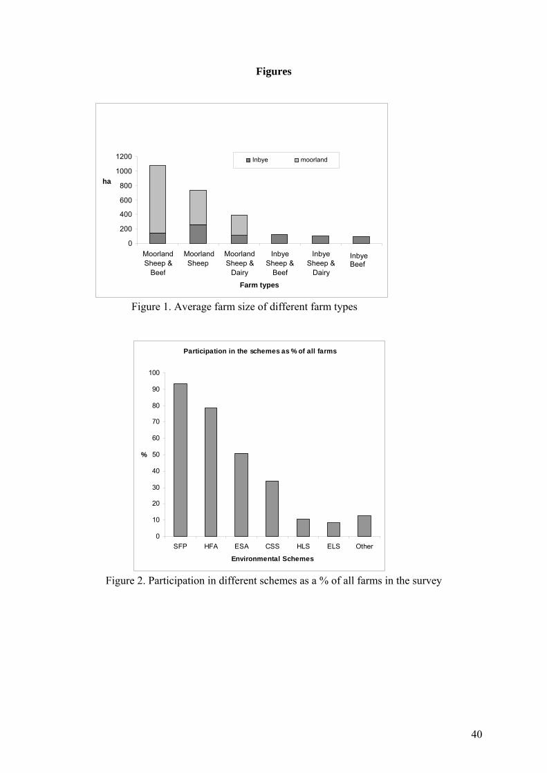
Socio-economic farm survey

The initial step in the research was a farm survey to investigate how land is managed on hill

farms in the Peak District, and to provide inputs to the LP models. The survey was designed

and carried out with the help of experienced farm business researchers through the winter

months of 2006/2007. It comprised 44 farm visits. Farms were chosen on the basis of their

location and their access to moorland grazing (defined as livestock farms within two km of

the moorland line). The survey included questions on land area, land types and use,

production activities and subsidy payments received during the reference period of 2006.

Main farm types identified are shown in Figure 1, whilst the types of subsidies that farmers in

the survey receive are shown in Figure 2. Sheep, dairy and beef cattle production were found

to be the dominant activities in the uplands of the Peak District. Two types of land can be

distinguished: moorland and inbye land. “Moorland” is defined as unimproved, semi natural

rough grazing, situated at higher altitude, providing the poorest grazing. The “inbye” land is

agriculturally improved, more productive land situated at lower altitude. Based on the survey

results, six types of typical upland farms can be distinguished depending whether a part of the

farm has moorland coverage or not2: Moorland Sheep & Beef (MSB), Moorland Sheep &

Dairy (MSD), Moorland Sheep (MS), Inbye Sheep & Beef (ISB), Inbye Sheep & Dairy (ISD)

and Inbye Beef (IB). In terms of subsidy payments, the SFP and HFA are received by most

farmers. However, in addition, many farmers participate in different agri-environmental

schemes.

2 This distinction was important for ecological measurement and modelling purposes.

7

2.2 Farm modelling

2.2.1 General approach

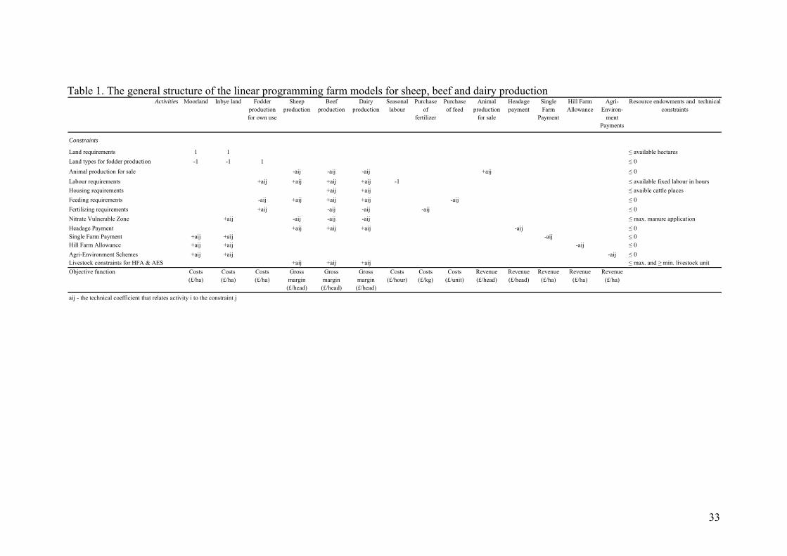
The general structure of the mathematical models is shown in Table 1 and has the form of the

standard linear programming model (Hazell & Norton, 1986):

Maximise {Z= c’x}

Subject to Ax ≤ b

and x ≥ 0

where:

Z =gross margin at farm level

x = vector of activities

c = vector of gross margins or costs per unit of activity

A = matrix of technical coefficients

b = vector of resource endowments and technical constraints

The group of activities, based on typical upland farming practices, are shown at the top of the

Table 1 under 14 headings: activities for different land types, production activities

representing several fodder crops and animal production systems, seasonal labour, purchase

of fertilizer and feed, and activities for sold animal products and subsidy payments. The rows

of the matrix indicate the type and form of the constraints included: land availability, supply

and demand of fixed and seasonal labour, feeding and housing requirements for livestock,

fertilizing requirements per land type, constraints on organic manure use in Nitrate

Vulnerable Zone, constraints on subsidies for headage and Single Farm Payment based on

production and land type, respectively; and restrictions for payments from Hill Farm

Allowance and different agri-environment schemes. The objective function of the LP model is

8

to maximise the gross margin, i.e. total returns from animal production and subsidy payments

minus variable costs, including variable operations, fertilizer and seasonal labour. The output

of the model includes the corresponding production plan with optimal land use, labour use

and fertilizer application. To obtain the optimal solution for the LP models, the CONOPT

solver was used in GAMS (General Algebraic Modelling System).

2.2.2 Production elements

The central element in the LP models is animal production, comprising sheep, beef and dairy.

The production and the feeding requirements for each of these types are described below.

The sheep production model is based on an upland crossbreed ewe with finished and store

lamb production with lambing in March-April. The feeding requirements for ewe and lambs

are taken from The Farm Management Handbook 2006/07 (Beaton, 2007). The feeding

requirement consists of grass grazing, silage, hay and ewe concentrate. We assumed that 1.5

lambs are born per average ewe with a 4% mortality rate. Due to voluntary and involuntary

disposal of ewes, we assume that each year 25% of the ewes are replaced by gimmers raised

on the farm. The ram requirement is also included, 2.5 per 100 ewes. Housing sheep is very

unusual in the study area, and thus no housing requirement for sheep was specified. The

returns from ewe production come from finished and store lambs, cull ewes and wool sales.

The costs per ewe include those of health care, feed additives, shearing, and other costs

(commission, levies, haulage and tags).

The beef cattle production model is based on a suckler cow calving in February-April and

sold either young (6-12 months) or fat (12-24 months)). This includes 10% calf mortality and

1% cow mortality. The bull ratio is 1 to 35 cows. The suckler cow replacement is 7 years,

9

which comes from purchased heifers. In winter the suckler cows are kept inside. The feeding

requirement of cows and calves in winter consists of silage, straw, cow concentrates, cow

cobs and some grazing. In summer the cows with calves are kept outside and fed by silage

and grazing. The returns from beef production come from calf sales, minus the cost of

replacements. The cost per suckler cow include those of concentrate and cow cobs, health

care, straw bedding and other costs (commission, haulage and tags).

The dairy cattle production model is based on a 650kg Friesian Holstein dairy cow with a

calving interval of 390 days and 6500 litre average milk production per year is used. The

calves are sold either young (1 month) or fat (15-20 months). Calf mortality is 10% and the

cow mortality is 1%. A 25% replacement rate is assumed with purchased heifers entering the

dairy herd. Cull cows are sold for £300/head. The cows are kept inside in winter for 180 days

and fed with silage and concentrates. In summer they are grazed outside and get additional

forages and concentrates. The returns from dairy production come from milk production and

calf sales. The costs per cow include those of concentrate, AI, vet and medicines, and other

livestock expenses.

The output prices and input costs used for sheep, beef and dairy production are based on

averages from the survey results across all the farm types and on The Farm Management

Handbook (SAC 2006).

Feed production and purchase

The land on the farm can be used for growing grass for grazing and fodder production

purposes. On inbye land, grass can be grown for grazing or fed in the form of silage or hay to

sheep and to cattle. On moorland and rough grazing, only sheep can be kept for grazing,

10

which fulfils part of their feeding requirement. Silage can be fed in winter and in summer. In

addition to home-grown feed, concentrates can be purchased. Dry matter production of grass,

silage and hay makes the link between the feeding requirements of sheep and cattle and

supply by each land type. The dry matter production of grassland per year depends mainly on

the amount of water and nutrients as well as on growing conditions. The effect of nutrients in

the model is distinguished through different levels of nitrogen (N) use. The most commonly

used combination of nitrogen use and cutting frequencies (1-3 cuts for silage and 1 cut for

hay) were represented with separate activities ranging from 0 to 375kg N/ha (Beaton, 2007).

The following main types of land use were distinguished: grass used only for grazing (N: 75,

125, 175, 250 or 375 kg/ha), grass used for silage with aftermath grazing (1, 2 or 3 cuts; N: 0,

125, 220, 250, 275, 300 or 375 kg/ha) and grass used for hay with aftermath grazing (1 cut; N:

0, 70, 125, 200). The costs of grassland include costs of renewal and sprays. On moorland no

cutting or fertiliser use is specified.

Labour

Sheep and beef cattle require labour inputs. Throughout the year a particular amount is

necessary for each period. Therefore the year is divided into months. Based on the survey, the

amount of available unpaid family labour is assumed to be 0.8-1.7 full-time labour units (1

labour unit = 2600 hours/year) depending on the farm type. Apart from family labour there is

the option of hiring seasonal labour. Labour can be hired at any time of the year at a cost of

£5, £6.25, £7.5 and £6 per hour for sheep, beef, dairy and grass production, respectively.

Information about the labour requirement per head (ewe or cattle) and per hectare (hay, silage

making) is derived from the Farm Management Pocketbook (Nix, 2007).

11

Fixed costs

Fixed costs are calculated separately from the LP-model based on the socio-economic survey

and data for Peak District hill farms from the Farm Business Survey given input factors such

as the main production activity, the farm size, basic machinery and buildings, land rent and

rental value and other miscellaneous costs (i.e. electricity, insurances, professional fees, farm

maintenance).

2.2.3 Agri-environment and income support schemes for upland farmers.

Farmers in the uplands can take part in many different schemes. Payments under the CAP (in

terms of the former headage payment and the Single Payment Scheme) are taken into account,

along with other important schemes for the uplands such as the Hill Farm Allowance and the

new agri-environmental schemes (Environmental Stewardship Schemes). The old agri-

environmental schemes were not taken into account, since they are gradually being replaced

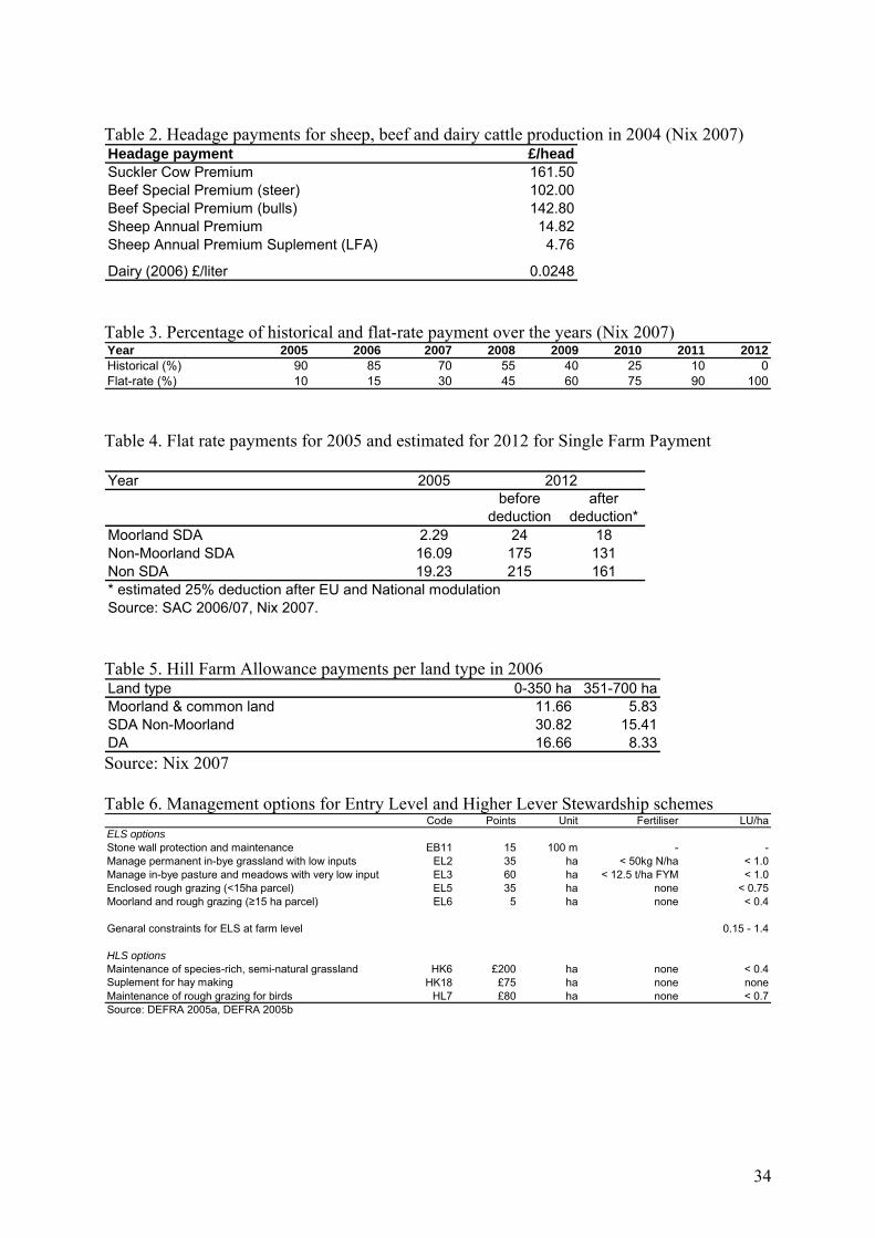
with the new schemes, and most of them will be phased out by 2012. Headage payments have

long been used to support sheep and cattle farming in the uplands. These historic direct

subsidy schemes for sheep, beef and dairy production can be seen in Table 2. Most have now

been phased out as part of the de-coupling process, but underlie the calculation of the Single

Farm Payment in terms of historic payment rates.

The Single Farm Payment scheme replaced most crop and livestock payments from 2005,

including those mentioned in Table 2. To comply with this scheme, farmers need to keep their

land in good agricultural and environmental condition and comply with specified legal

requirements relating to the environment, public and plant health and animal health and

welfare (“cross-compliance”). In England, the payment consists of two elements: historical

and flat-rate regional average payments. The historical payment is additional to the flat-rate

12

payment, the amount of which is based on producers’ historical claims during the 2000-2002

reference period. During the period of 2005-2012 the scheme will move from low percentage

flat-rate and high percentage based on historical payments to a simple flat rate across all

eligible land in England. The proportion of these payments can be seen in Table 3. The flat

rate payments per land type for 2005 and the estimated flat rate payment in 2012, when it will

account for 100% of payments, can be seen in Table 4. For the model, estimated payments for

2012 were included after deductions due to modulation. To receive SFP, a unit of land is

required regardless of any activity on the farm. Thus, the payment is connected to the eligible

land types and quantity on the farm. The payment also incurs costs of compliance, which was

estimated based on the costs per hectare required to maintain grassland in “good agricultural

condition”. This amounted to approximately £13 per hectare for natural regeneration (SAC,

2006). In the model this was represented by the constraint that all land must be used for at

least some agricultural activity, including maintenance of the land without using it for

production. The constraint was set separately for the inbye land types (rough grazing and

grassland). For moorland no restriction was made.

The Hill Farm Allowance is a compensatory allowance for cattle and sheep farmers in the

English Less Favoured Areas (LFAs) in recognition of the difficulties they face and the vital

role they play in maintaining the landscape and rural communities of the uplands. In our

analyses we included the current form of the HFA payment. However, the HFA scheme will

itself be revised. Currently HFA is based on area payments, which are made at different rates

for different types of land and size of holding (Table 5). These payments are included in the

model attached to the corresponding land types. For compliance with this allowance a

minimum (0.15 LU/ha) and a maximum (1.4 LU/ha) constraint is set for the stocking density

in order to avoid under- and overgrazing.

13

Agri-environment payments are intended to compensate or provide an incentive for farmers to

undertake measures which go beyond Good Farming Practice. The Entry Level (ELS) and

Higher Level Stewardships (HLS) were added to the model as payment for achieving the

“Target point”, which can be collected by certain management activities (“options”) on the

farm. The most frequently used options of ELS and HLS in the upland area of PDNP were

selected and added to the model (Table 6). The ELS payments are £8/ha for LFA and £30/ha

for non-LFA land types. The payments for selected HLS options can be seen in Table 6.

These options can be taken up, with restrictions on fertiliser use and livestock density, as part

of the maximisation of gross margin. Finally, most of the farms in the uplands in this region

are situated within a Nitrate Vulnerable Zone, which imposes a limit on organic manure

applications. The maximum is at 250kg/ha of total nitrogen each year averaged over the area

of grass on the farm. This limit is also included in the model as a constraint.

2.3 Calibration of the farm models

The models incorporate all livestock and grass production activities carried out on the upland

farms and can thus be calibrated to represent any particular farm situation in terms of basic

resource endowments. Based on our survey the six typical farm types for the uplands are

represented by the averages of these farm types. The six different models included calibration

on the main production category (sheep, beef, dairy), on different land types, housing capacity

for livestock and household labour availability (Table 7). We assumed no switching between

the farm types, but allow for switching between livestock production activities within the

same farm type. In order to ensure that the models provided an accurate simulation of current

farming activity for representative farm types, each model calibration was completed and the

output from the model (by using the same livestock numbers as in the survey averages), in

14

terms of returns to enterprises and input costs, was compared with the survey data. Since the

model is to be used to assess impacts upon the relative balance of different enterprises and

associated changes in resource use, the key parameters of interest in this validation process

are i) the proportion of revenue from livestock (% of total revenue from sheep, beef, dairy), ii)

the proportion of variable costs (feed, seed, fertiliser, hired labour) of total costs and iii) the

total net farm income (NFI). Table 8 provides a summary for these items for each farm type,

for both the model and the observed survey data of 2006. Although there are inherent

weaknesses in LP modelling due to factors such as assumed maximising behaviour and the

explicitly linear technology (constant input-output coefficients), the models provide a

reasonably accurate simulation of both farm revenue, production and cost structures.

2.4 Policy scenarios

The aim of this paper is to investigate the impacts of agricultural policy reform in marginal

upland areas, in the context of on-going reforms to agri-environmental policy. The main

impacts to be considered are those on farm incomes, land use and ecological pressures. The

policy scenarios therefore chosen were: “Headage Payment”(HP), “Single Farm

Payment”(SFP) and “No Payment” (NP) scenarios. This choice was based on focusing on

three different points in time: the situation before de-coupling (HP scenario), after de-

coupling (SFP scenario) and when the SFP disappears (NP scenario). These core agricultural

policy scenarios are considered in interaction with additional upland supports: the HFA as

currently implemented, since its reformed status is unsure at present – although as explained

above this will probably become a new agri-environment scheme just for the uplands - and

Environmental Stewardship options as the main agri-environmental schemes (AES). This

generates three additional scenarios: (HP & AES/HFA, SFP & AES/HFA, NP & AES/HFA),

15

giving a total of 6 policy scenarios in all3. The model was set to 2006 output price and input

cost levels for all farming activities; whilst recent price movements in both agricultural output

and input price markets have occurred, the modelling approach centres upon gross margin

analysis and it is argued that the 2006 gross margin levels are an appropriate base-level for the

analysis. Sensitivity analysis was then undertaken for key output and input prices.

In the “Headage Payment” scenario we model the policy situation as it existed before the

introduction of the SFP. For the “Single Farm Payment” scenario we use a situation where the

flat rate payment will account for 100% of payments (as planned for 2012: Table 4)4. In the

“No Payment” scenario we assumed the loss of the SFP but also the relaxation of cross-

compliance constraints which go along with this.

3. Results

Optimal production plans

From the perspective of upland biodiversity, the most important impacts of policy reform are

those on land use, livestock density and fertiliser use: this section thus focuses solely on these

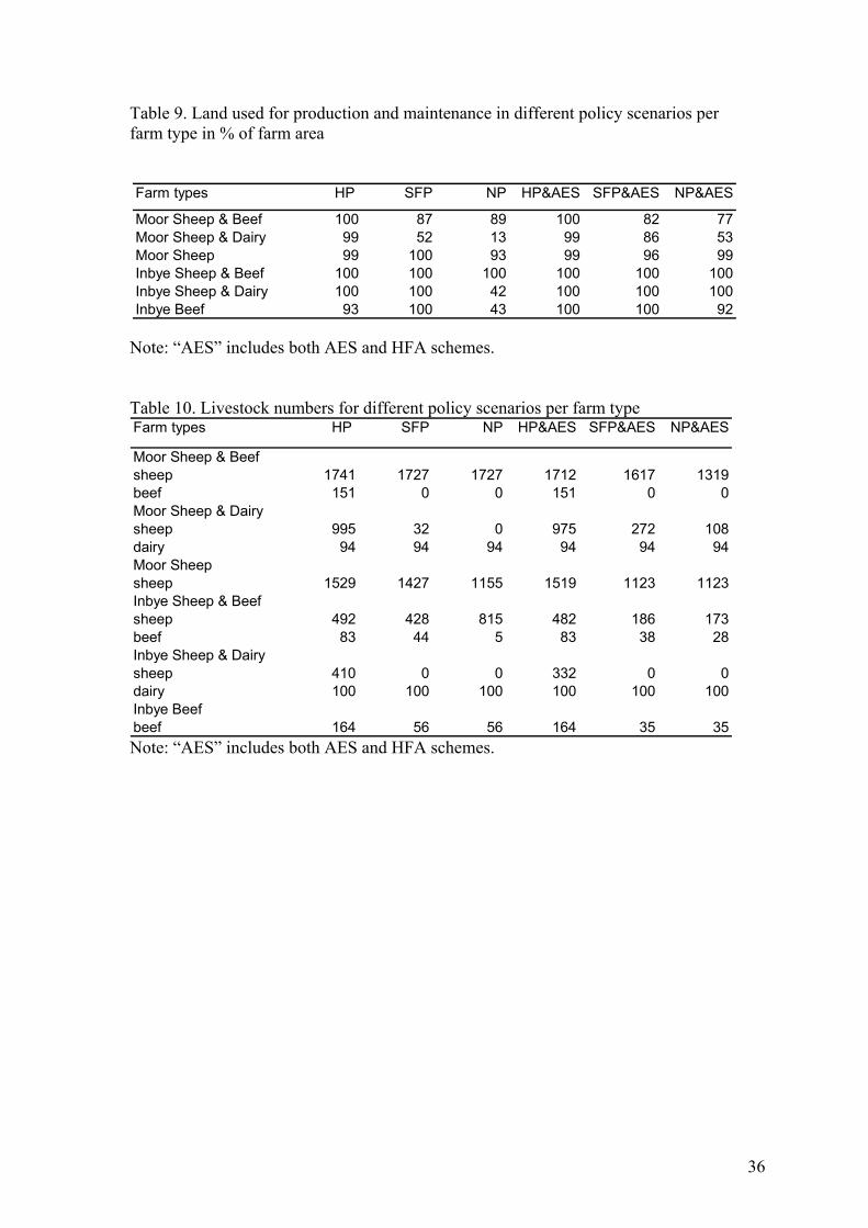
variables. The changes in predicted land use for each farm type across the six policy scenarios

can be seen in Table 9. The land that is used for livestock production or maintenance - under

SFP and AES - is taken as a proportion of the total land availability per farm type. “Unused

land” is land that is left as fallow.

3 For brevity, the “AES/HFA” treatment is henceforth referred to simply as “AES”. 4 The historical payments differ considerably between the farms and farm types and this is the year when all farm payments will be completely detached from historical production and based only on their current eligible land types. These estimated payments for all three land categories, after deductions from modulation, were used for this scenario analysis, including the compliance constraints discussed above.

16

Under the HP scenario all land is used for livestock production. Under the SFP scenario, all

inbye land continues to be used for production or maintenance, since the payment is based on

the land used for agricultural purposes. On moorland farms, however, not all moorland is

used. In the case of the NP scenario even more land is left fallow, including both moorland

and inbye land types. The difference between the land area used in SFP and NP scenarios

comes from the compliance obligation on farmers to obtain the SFP. The optimal solution

balances the marginal cost and revenue coming from production and that coming from the

cross-compliance obligation and payments from the SFP. The three scenarios with AES

payments show similar results to those without AES: however, with new restrictions resulting

from AES contracts, in general more land is used. This is due to the adoption of more

extensive production and more options for farmers to maintain their land and receive a

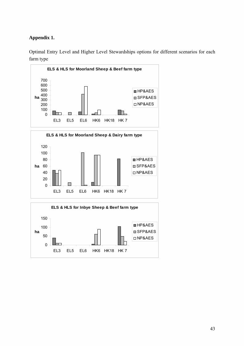
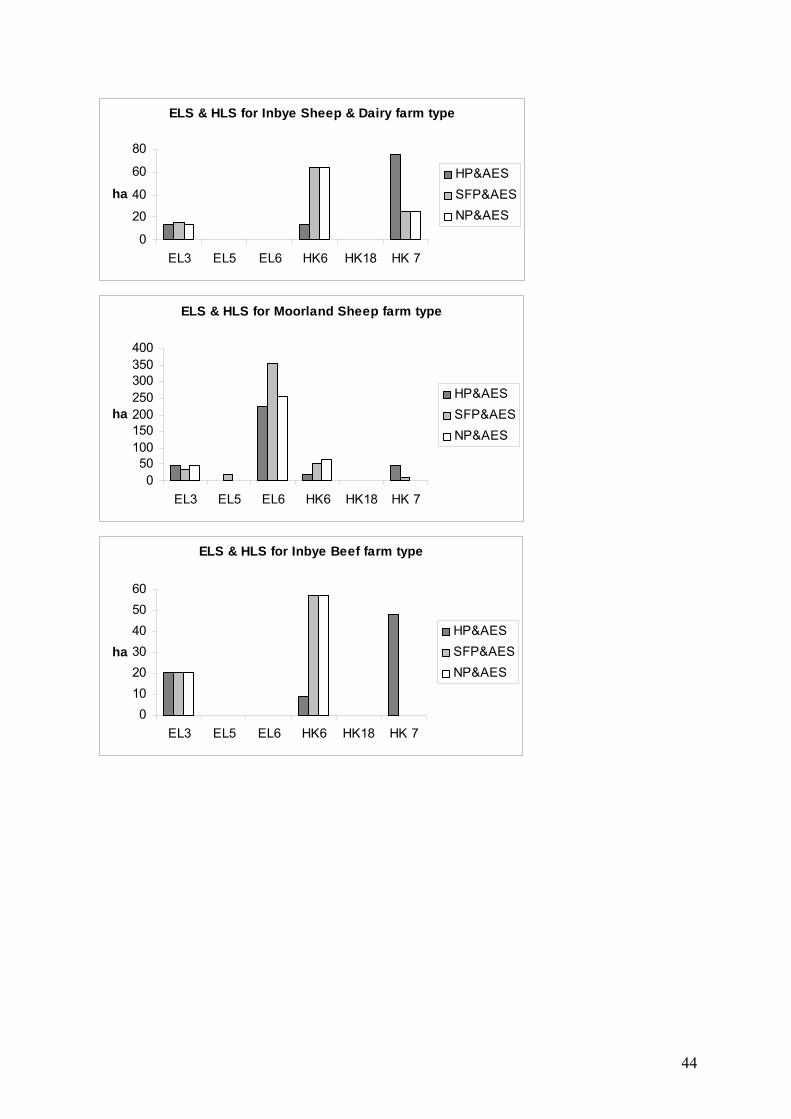
payment for it. The ELS and HLS schemes that are taken up for each AES scenario and farm

type can be seen in Appendix 1. In summary, the predicted uptake of AES schemes and the

preferred options differ markedly among farm types and within farm types depending on the

nature of core subsidy support (HP, SFP or NP). The loss of the SFP results in many more

farms leaving their land fallow, since the constraints on maintaining land in Good

Agricultural Condition are no longer binding. The largest fallowing of land occurs in the

MSD farm type, where only 53% and 13% of the land is used with and without AES,

respectively, after loss of the SFP. The ISD and IB farm types also have more than half of the

land fallow without AES. This means that not only the SFP but also the AES are important for

keeping the land in production, or for maintaining it in “good condition”.

The optimal livestock production for the six policy scenarios and the six typical farm types

can be seen in Table 10. The results show that under the historic HP scenario, beef and dairy

is preferred to sheep production. This means that in the case of all farm types the maximum

17

amount of beef and dairy production occurs, given the cattle housing capacity constraints of

the farm, with the remainder of the land being used for intensive sheep production. By

switching from the HP to the SFP and NP scenarios, livestock numbers decrease, as do

grazing livestock units (LU) (Figure 3). In general, livestock densities on the moorland farms

are quite low, between 0.2 and 0.8 LU/ha for all the scenarios. This figure is higher for inbye

farm types, at between 0.4 and 1.5 LU/ha. Besides extensification, decoupling leads to

structural change within farm types. There is a large predicted fall in beef cattle numbers

under the SFP and NP scenarios for some farm types: this dramatic cut is not prevented by the

availability of AES. In general, beef production is declining, and in certain farm types it

disappears entirely. This is due to the lower profitability from beef production after

decoupling compared to that of sheep. A structural change can also be seen in sheep and dairy

farms, where dairy activity is preferred to sheep from an economic point of view. This means

on the MSD farm type sheep numbers are declining, while on the ISD farm type sheep

production completely disappears.

The higher livestock units on farms under the HP scenario requires more fodder which leads

to more intensive grass production for grazing, silage and hay. This is supplied by higher

amounts of fertiliser use per hectare on grassland. For all farm types fertiliser use declines

considerably after decoupling, except for the dairy farm types MSD and ISD (see Table 12 for

details).

Financial results

Prior to the inclusion of AES/HFA payments, the results show positive gross margins in the

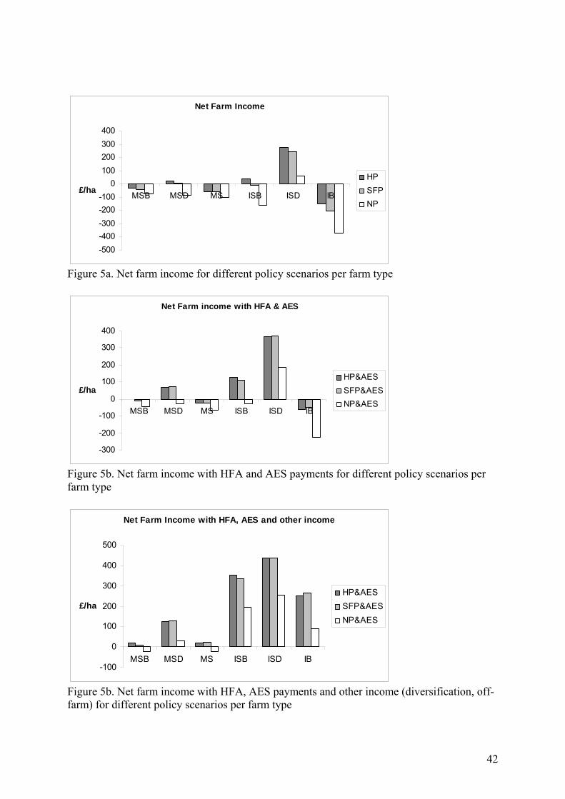
case of all scenarios for all farm types (Figure 3). However, the net farm income (NFI) is

negative for five out of six farm types, with the exception of the ISD farm type (Figure 5a),

18

which is the most profitable in the Peak District as milk production generates the highest

income in the uplands. In switching from HP to SFP or NP, the greatest losses are in beef

farming. However, all farm types lose income after the switch from HP to either SFP or NP.

The IB farm type shows the most negative net farm income due to relatively high fixed costs,

which comes from the high rental costs for land and the large amount of machinery kept on

the farm. Figure 5b shows equivalent results for net farm income once the option to receive

AES/HFA payments is included. The major impact is to moderate income losses in the move

away from HP to either SFP or NP.

Farmers in the uplands also get income from other sources, such as from diversification and

off-farm sources. Actual levels of NFI under the policy scenarios considered will thus likely

be higher (Franks et al,. 2008). Results not reported in detail here showed that once estimates

of these income streams are included, all the farm types will have positive NFI under all

scenarios, except the MSB and MS farm types under the NP scenario. This result shows that

many farmers depend not only on AES schemes but also on the other income sources coming

from off-farm and diversification for their long-term financial sustainability (Figure 5c).

Sensitivity Analysis

We investigated the implications for key outcomes (farm income, stocking rates and land

abandonment) of increases in certain output and input prices above the base case of the most

common sheep and beef farm types. 25% rise in lamb, calf and concentrate prices were

modelled. This showed that, in the case of MSB farm type, higher input prices would lead to

lower NFI with lower stocking density and more land abandonment of 28% and 26% for the

SFP&AES and NP&AES scenarios, respectively. Higher output prices would lead to 95% and

100% land use and higher stocking density for the latter scenarios. In the case of HP&AES

19

there is no change on the production structure only on the income of the farmer. Similar

results can be drawn for ISB farm type concerning the NFI and stocking density, however all

the land area would be used for production in all these cases.

4. Discussion

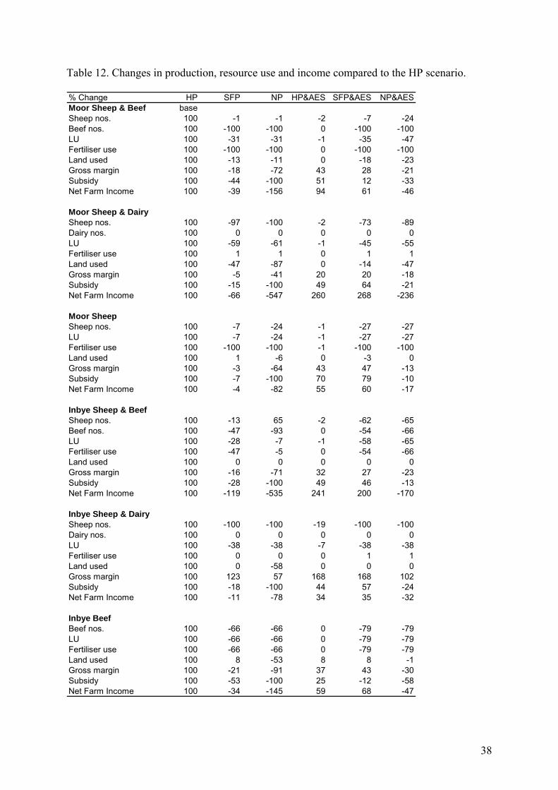
The key results that emerge from the analysis described above is that the effects of policy

reform vary substantially across farm type, but some general trends can be discerned. Our

discussion of these findings is organised according to (i) the effects of de-coupling itself, (ii)

the mediating effects of agri-environment scheme payments (including the HFA), (iii) the

effects of loss of the Single Farm Payment, and (iv) ecological implications. For all cases, the

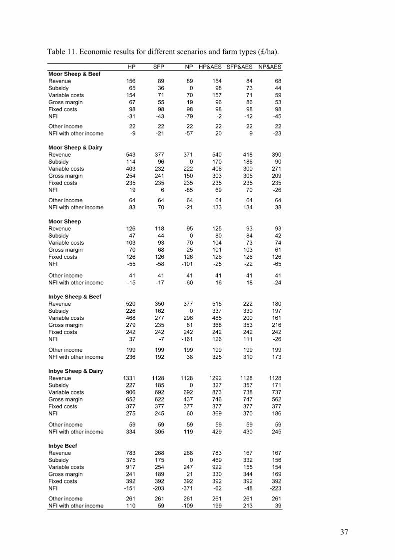
base level is the HP scenario (Table 12). Absolute levels for income are shown in Table 11.

4.1 What are the impacts of decoupling?

The most relevant comparison here is the (HP&AES) scenario with the (SFP&AES) scenario.

i) Effects on net farm income are slight. Two farm types see a small decrease in net farm

income, and one a small increase. The magnitude of the change in overall NFI is typically less

than the magnitude of the change in subsidy, because it is modified by behavioural changes.

ii) Decoupling has mixed effects on the amount of land being used for agricultural production,

ranging from 18% coming out of production for one farm type to 11% more going into

production for another. On the whole, though, the amount of land used or maintained changes

little.

iii) The major effect of decoupling is reductions in stocking densities (Figure 3), but these

vary by a factor of three across farm types as a percentage rate (from -27% to -79%).

iv) The aggregate pattern regarding stocking densities masks a lot of what is going on.

Suckler cow numbers are greatly reduced and abandoned altogether on moorland sheep and

20

beef farms. The effect on sheep varies from minimal on some farm types to abandonment of

sheep production on others. Decoupling has no effect on dairy production, which is operated

at a capacity dictated by animal housing constraints.

v) Decoupling also results in less fertiliser application, but again how this plays out depends

on farm type, with no change on some and 80-100% reductions on others. However, in

general fertiliser use is relatively low in these upland areas for all farm types.

4.2 What are the moderating effects of agri-environmental policies on decoupling?

Agri-environmental schemes offer income earning opportunities for farmers, but also

constrain their operations. The relevant comparison here is (HP&AES to SFP&AES)

compared with (HP to SFP).

i) AES schemes play a major role in changing the overall economic impact of decoupling

(Figure 5a, Figure 5b, Table 11). Instead of facing large losses, the various farm types face

either much smaller losses or in some instances actually stand to gain from decoupling. This

is because the two policy instruments are now pulling in the same direction rather than pulling

against one another. However, we have to note that the models predict the maximum uptake

of the most commonly used AES schemes for the given land types. This means that the

uptake can differ based on farm specific circumstances, where a broader range of these

schemes are available, and for some schemes (HLS) competition does not always lead to

success in getting the desired payment, which can result in a slightly different economic

outcome.

ii) Moderation of the effect of decoupling by AES has mixed implications for the amount of

fallowing. Some farm types fallow more than they would otherwise have done and some less.

iii) AES leads to a greater losses of suckler cow production than would otherwise have

resulted, which may lead to unfavourable ecological outcomes (for example, with regard to

21

some bird populations such as lapwing). For sheep, decoupling and AES are sometimes

pulling in the same direction resulting in greater losses than under decoupling alone (due to

extensification requirements of AES) and sometimes in opposing directions meaning smaller

reductions in sheep numbers because of AES payments.

iv) AES schemes have little effect on the outcome of decoupling for fertiliser application

rates.

4.3 What would be the effect of loss of the Single Farm Payment?

Here the relevant comparisons are of (SFP & AES) with NP; and of (SFP & AES) with (NP &

AES). The former shows the effects of removing all subsidy; the latter shows the more

realistic outcome of the removal of direct income support with the retention of agri-

environmental payment schemes.

Taking the extreme case first (removal of all subsidy), we see that this results in

considerable land abandonment (Table 9) on three farm types, including two inbye farm

types. The loss of all subsidy support would also result in five out of six farm types having a

negative net farm income, and thus being financially unsustainable. Four would have a

negative income even when including revenue from off-farm sources and diversification

activities. The fifth farm type, ISB, that becomes financially sustainable when including these

sources changes livestock production to sheep only, and intensifies land use. Relatively little

change happens to moorland sheep production, except on the MSD farm type where sheep

production ceases entirely.

Turning to the more realistic case where AES (and, one presumes, the replacement for

HFA) carries on after the loss of the SFP, we can see that the loss of SFP alone causes a

number of important changes. First, net farm income falls considerably on all farm types, and

becomes negative in 5 out of 6 cases, if we ignore income from off-farm sources and

22

diversification. For moorland sheep and moorland sheep and beef, income becomes negative

even with these other sources. The main conclusion is that loss of SFP will have a serious

effect on the long-term viability of hill farms in the Peaks. The intensity of livestock

production also falls in most cases, whilst land abandonment increases, especially on mixed

moorland farms.

4.4 Comparison to other studies

Our results show that it is likely that there will be a move away from beef production towards

sheep, although for both categories of livestock, total numbers are likely to fall. This

extensification, lower fertiliser use and shift from beef to sheep production in the uplands has

been noted by others for the UK (Revell and Oglethorpe, 2003; Oglethorpe, 2005; Matthews

et al., 2006) and in the EU-15 as a whole (Balkhausen et al., 2008). Moss et al. (2005)

predicted a reduction of 16.7% in beef animal numbers and a 9.5% reduction in sheep. Our

results show no decline is expected in the dairy enterprise in the uplands, given current price

levels. However, some EU studies have forecast that the prices will fall after CAP reform

which will reduce gross margins of the dairy enterprise due to the reduction in the price of

milk. Fewer but larger dairy herds were also predicted after this change in the uplands

(Shrestha et al., 2007).

Land abandonment after decoupling is limited in our results by the requirement to keep the

land in good agricultural and environmental condition under SFP. Similar results were found

in other studies (Defra, 2004; Oglethorpe, 2005; IEEP, 2007; Revell and Oglethorpe, 2003).

However, in marginal areas like moorland, abandonment might take place sooner due to the

lower productivity of the land (Primdahl et al., 2003; Defra, 2004). With regard to predicted

changes in income, Oglethorpe (2005) found that decoupling would lead to net farm income

23

becoming negative, other than for dairy. This result is also supported by the findings of this

study for all the farm types except for inbye sheep & dairy, which currently is the most

profitable enterprise in the uplands.

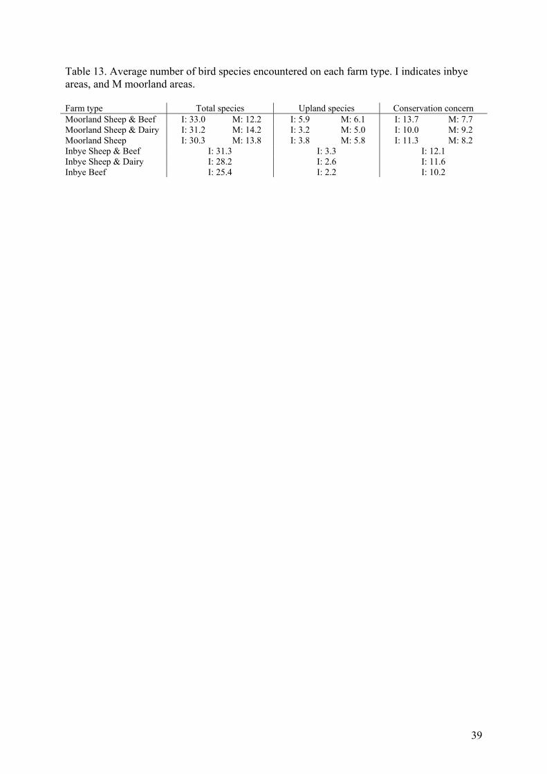
4. 5 Ecological implications

The land use changes predicted under these different policy scenarios will have important

implications for upland ecosystems. To illustrate, we focus on the implications for

biodiversity using the number of different bird species as an indicator. The bird community

was surveyed on the same farms from which farm management data had been collected for

the LP models in the following breeding season (2007; Dallimer et al. ms). The average

number of different species ("species richness") for each farm type categorised into moorland

and inbye land when appropriate are shown in Table 13, column 2. We also identified two

subgroups of species of particular conservation interest. First, we identified the subset of

species with an upland breeding distribution in the UK. These species include particularly

emblematic examples of upland wildlife, such as the curlew (Numenius arquata) and ring

ouzel (Turdus torquata), and could form local conservation priorities for these habitats: these

numbers are shown in column 3. Then, we identified a second subset of species that are of

national or international conservation concern, including red and amber listed species, UK

Biodiversity Action Plan species and species listed in the European Community's designation

of part of our study area as a Special Protection Area for wild bird conservation. These are

shown in column 4.

Inbye habitats contained more species overall and more of national conservation concern,

however, moorland habitats held a greater richness of upland specialist species. Farms that

were composed of both moorland and inbye, had higher species richness in their inbye areas

24

than the more intensive inbye-only operations. As such the prediction that farming will

generally become less intensive under CAP reform on these inbye-only operations (with the

one exception being ISB in the extreme case of no subsidies) may help biodiversity. MSB

farms are richest in overall species and in upland specialists on either habitat type. As such,

the loss of suckler cows and conversion of these operations just to sheep production (MS),

along with the worsening economic circumstances of this sector, could pose particular

problems for upland ecosystems. Such a prediction is supported by more detailed ecological

analyses, where species richness was higher on farms where cattle were grazing (Dallimer et

al., ms; Evans et al., 2006). Land abandonment has been shown, historically, to lead on

average to a loss of biodiversity in upland grazed systems (Hanley et al, 2008), so that any

policy changes which increases abandonment will likely have adverse consequences for

biodiversity.

5. Conclusions

In this study the aim was to investigate how policy changes under CAP reform affect farmers’

income and land use in marginal upland farming systems, and to relate these to likely

ecological impacts. Different policy scenarios were analysed and compared using linear

programming models developed for six representative farm types in the Peak District. Results

show that the change from headage-based payments to the Single Farm Payment motivates

farmers to operate more extensively with part of the moorland left unused, although there is

little real risk of land abandonment due to the contract requirements of the SFP. Removal of

the SFP results in still lower livestock numbers, negative net farm incomes in most cases, and

a rise in land abandonment. Agri-environment schemes moderate the impacts of decoupling,

and play a vital role in supporting hill farm incomes. Indeed, an interesting side-effect of

25

decoupling is predicted to be a rise in desired uptake of agri-environmental schemes, and thus

an increase in competition for limited-fund schemes such as Higher Level Environmental

Stewardship. This should promote increased cost-effectiveness in the delivery of public

environmental goods on upland farms so long as the contract rationing scheme rewards both

supply price and expected environmental delivery.

Acknowledgements

This study would not have been possible without the generous time commitment and interest

of the hill farmers of the Peak District. Help identifying suitable farms was provided by:

NFU; Catherine Gray and other staff at the Peak District National Park; Aletta Bonn of the

Moors For the Future Partnership; Mike Innerdale and Russell Ashfield of the National Trust;

Chris Thomson of the RSPB; and Andrew Critchlow. Socio-economic surveys were

performed by Helen McCoul, Richard Darling, John Farrar, Nick Harpur and Robert Yates of

the Rural Business Research Unit at the University of Nottingham. Funding was provided by

the RELU programme of the UK Research Councils. K.J.G holds a Royal Society Wolfson

Research Merit Award. We thank David Oglethorpe for his advice on construction of the farm

models used here.

26

References

Anderson, P., Yalden, D.W. ‘Long-term changes in the extent of heather moorland in upland

Britain and Ireland: palaeoecological evidence for the importance of grazing’, Biological

Conservation, Vol. 20, (1981) pp. 195-213.

Banse, M., Gerthe, H. and Nolte, S. Documentation of ESIM Model Structure, Base Data and

Parameters (Berlin, Göttingen, 2005)

Beaton, C. The Farm Management Handbook 2006/07 (Edinburgh, SAC, 2007, 27th Edition,

pp. 520)

Binfield, J., Donnellan, T., Hanrahan, K. and Westhoff, P. CAP Reform and the WTO:

Potential Impacts on EU Agriculture (Selected Paper for presentation at the American

Agricultural Economics Association Annual Meeting, Denver, CO, USA, 1-4 July 2004).

Balkhausen, O., Banse, M. and Grethe, H. ‘Modelling CAP Decoupling in the EU: A

Comparison of Selected Simulation Models and Results’, Journal of Agricultural Economics,

Vol. 59, (2008) pp. 57-71.

Britz, W. CAPRI Model System Documentaion. Common Agricultural Policy Regional Impact

Analysis (Bonn, 2004)

27

Pacini, C., Wossink, A., Giesen, G. and Huirne, R. ‘Ecological-economic modelling to

support multi-objective policy making: a farming systems approach implemented for

Tuscany’, Agriculture, Ecosystems & Environment, Vol. 102, (2004) pp. 349-364.

Chantreuil, F., Hanrahan, K. and Levert, F. ‘The Luxembourg agreement reform of the CAP:

An analysis using the AG-Method composite model’, in Balkhausen et al. Journal of

Agricultural Economics, Vol. 59, (2008) pp. 57-71.

DEFRA (2004) ‘An assessment of the impacts of hill farming in England on the economic,

environmental and social sustainability of the uplands and more widely’, A study for Defra by

the Institute for European Environmental Policy, Land Use Consultants and GHK Consulting,

February 2004. (available at: http://statistics.defra.gov.uk/esg/reports/hillfarming/default.asp ;

2004; last accessed November 2007)

DEFRA. Entry Level Stewardship Handbook. Terms and Conditions and how to apply.

(2005a) pp 113.

DEFRA. Higher Level Stewardship Handbook. Terms and Conditions and how to apply.

(2005b) pp. 120.

Defra, Rural Development Programme for England: 2007- 2013 - uplands steward structure

(2006)

Dennis, R. The importance of extensive livestock grazing for woodland biodiversity:

traditional cattle in the Scottish Highlands (1999) in Defra 2004

28

Donaldson, A.B., Flichman, G. and Webster, J.P.G. ‘Integrating agronomic and economic

models for policy analysis at the farm level: the impact of CAP reform in two European

regions’, Agricultural Systems, Vol. 48, (1995) pp. 163–178.

English Nature Sites of Special Scientific Interest (available at: http://www.english-

nature.org.uk/special/sssi/; 2005)

Evans, D.M., Redpath, S.M., Evans, S.A., Elston, D.A., Gardner, C.J., Dennis, P. & Pakeman,

R.J. ‘Low intensity, mixed grazing improves the breeding abundance of a common

insectivorous passerine’. Biology Letters 2, (2006) pp. 636-638.

Franks, J, Harvey, D. Scott, C. (2008). Farm Business Survey 2006/07 Hill Farming in

England (available at http://www.ruralbusinessresearch.co.uk/) accessed 8 July 2008.

Schmid, E. and Sinabell, F. ‚On the choice of farm management practices after the reform of

the Common Agricultural Policy in 2003’, Journal of Environmental Management, Vol. 82,

Issue 3, (2007) pp. 332-340

Gibbons, J.M., Sparkes, D.L., Wilson, P. and Ramsden, S.J. Modelling Optimal Strategies for

Decreasing Nitrate Loss with Variation in Weather- A Farm-Level Approach, Agricultural

Systems, Vol 83 (2), (2005) pp 113-134.

Gohin, A. ‘Assessing the CAP reform: Sensitivity of modelling decoupling policies’, Journal

of Agricultural Economics, Vol. 57, (2006) pp 415-440.

29

Hanley, N., Kirkpatrick, H., Oglethorpe, D. and Simpson, I. “Paying for public goods from

agriculture: an application of the Provider Gets Principle to moorland conservation in

Shetland”. Land Economics, 74 (1), (1998) 102-113.

Hanley, N., Colombo, S., Mason, P. and Johns, H. ‘The reform of support mechanisms for

upland farming: paying for public goods in the Severely Disadvantaged Areas of England’,

Journal of Agricultural Economics, 58 (3), (2007) pp. 433-453.

Hanley, N., Tinch, D., Angelopoulos, K., Davies, A., Barbier, E. and Watson, F. ‘What drives

long-run biodiversity change? New insights from combining economics, paleoecology and

environmental history’ Journal of Environmental Economics and Management, (2008)

forthcoming.

Happe, K., Balmann, A., Kellermann, K., Sahrbacher, C. ‘Agent-based modelling and policy

analysis – the impact of decoupling on farm structures’, Institute of Agricultural Development

in Central and Eastern Europe (IAMO), Halle (available at: http://www.kathrin-happe.de/;

2005; last accessed: 5 May 2008)

Hazell, P.B.R and Norton, R.D. Mathematical Programming for Economic Analysis in

Agricutlure (Macmillan Publishing Company, New York, 1986)

Hertel, T.W. Global Trade Analysis: Modeling and Applications (Cambridge: Cambridge

Uniersity Press, 1997)

30

HM Treasury and Defra. A Vision for the Common Agricultural Policy (available at:

www.defra.gov.uk ; 2005 pp. 69; last accessed: 7 September 2007.)

IEEP. An assessment of the impacts of hill farming in England on the economic,

environmental and social sustainability of the uplands and more widely. (A study for Defra

by the Institute for European Environmental Policy, Land Use Consultants and GHK

Consulting, February 2004)

Breen, J. P., Hennessy, T.C. and Thorne, F.S. ‘The effect of decoupling on the decision to

produce: An Irish case study’, Food Policy, Vol. 30, Issue 2, (2005) pp. 129-144

Bos, J.F.F.-P. Comparing specialised and mixed farming systems in the clay areas of the

Netherlands under future policy scenarios: an optimisation approach

(Ph.D. Thesis; Wageningen: Wageningen University, 2002)

Latacz-Lohmann U. and Hodge I. ‘European agri-environmental policy for the 21st century’,

Australian Journal of Agricultural and Resource Economics, Vol. 47, (2003) pp.123-139

Matthews, K.B., Wright, I.A., Buchan, K., Davies D.A. and Schwarz, G. ‘Assessing the

options for upland livestock systems under CAP reform: Developing and applying a livestock

systems model within whole-farm systems analysis’, Agricultural Systems, Vol. 90, (2006)

pp. 32-61.

31

Moss, J., Binfield, J., Westhoff, P., Kostov, P., Patton, M., Zhang, L., Analysis of the impact

of the Fishler Reforms and potential trade liberalisation (Food and Agricultural Policy

Research Institute (FAPRI), 2005)

NCC Changes in the Cumbrian Countryside (NCC, Peterborough, 1987)

Nix, J. Farm Management Pocketbook (37th Edition, The Andersons Centre, 2007)

Oglethorpe, D.R. ‘Livestock production post CAP reform: implications for the environment’,

Animal Science, Vol. 81, (2005) pp. 189-192.

PDRDF. Hard Times – a report into hill farming and farming families in the Peak District.

(Peak District Rural Deprivation Forum, Hope Valley, Derbyshire; available at:

http://www.pdrdf.org.uk/hillfarmingreport.htm; 2004; last accessed: 15 November 2007)

Primdahl, J., Peco, B. Schramek, J. Andersen, E. Onate, J.J. ‘Environmental effects of agri-

environmental schemes in Western Europe’, Journal of Environmental Management, Vol. 67,

Issue 2, (2003) pp. 129-138.

Ratcliffe, D.A. & Thompson, D.B.A. ‘The British uplands: their ecological character and

international significance’, In Ecological Change in the Uplands ed. by M.B. Usher & D.B.A.

Thompson (Blackwell Scientific Publications, Edinburgh, 1988, pp. 9-36)

Revell, B. and Oglethorpe, D. ‘Decoupling and UK Agriculture: A Whole Farm Approach’,

(Study Commissioned by Department of the Environment, Food and Rural Affairs, 2003)

32

Rodwell, J.S., British Plant Communities V. 2. (Mires and Heaths. Cambridge University

Press, Cambridge, 1991)

SAC, The Farm Management Handbook 2006/07 (Scottish Agricultural College, Edinburgh

2006)

Shrestha, S., Hennessy, T. and Hynes, S. ‘The effect of decoupling on farming in Ireland: A

regional analysis’, Irish Journal of Agricultural and Food Research, Vol. 46, (2007) pp. 1–

13.

Tudor, G., Mackey, E.C. ‘Upland land cover change in post-war Scotland’, In: Heaths and

Moorlands: Cultural Landscapes, Thompson, D.B.A, Hester, A.J., Usher, M.B. (Eds.)

(HMSO, Edinburgh, 1995.)

Veysset, P., Bebin, D. and Lherm, M. ‘Adaptation to Agenda 2000 (CAP reform) and

optimisation of the farming system of French suckler cattle farms in the Charolais area: a

model-based study’, Agricultural Systems, Vol. 83, Issue 2, (2005) pp. 179-202.

Witzke, H.P. and Zintl, A. CAPSIM Documentation of Model Strucutre and Implementation

(Eurostat Working Papers and Studuies. Eurostat, Luxembourg, 2005)

33

Table 1. The general structure of the linear programming farm models for sheep, beef and dairy production Activities Moorland Inbye land Fodder

production for own use

Sheep production

Beef production

Dairy production

Seasonal labour

Purchase of

fertilizer

Purchase of feed

Animal production

for sale

Headage payment

Single Farm

Payment

Hill Farm Allowance

Agri-Environ-

ment Payments

Resource endowments and technical constraints

Constraints

Land requirements 1 1 ≤ available hectaresLand types for fodder production -1 -1 1 ≤ 0Animal production for sale -aij -aij -aij +aij ≤ 0Labour requirements +aij +aij +aij +aij -1 ≤ available fixed labour in hoursHousing requirements +aij +aij ≤ avaible cattle placesFeeding requirements -aij +aij +aij +aij -aij ≤ 0Fertilizing requirements +aij -aij -aij -aij ≤ 0Nitrate Vulnerable Zone +aij -aij -aij -aij ≤ max. manure applicationHeadage Payment +aij +aij +aij -aij ≤ 0Single Farm Payment +aij +aij -aij ≤ 0Hill Farm Allowance +aij +aij -aij ≤ 0Agri-Environment Schemes +aij +aij -aij ≤ 0Livestock constraints for HFA & AES +aij +aij +aij ≤ max. and ≥ min. livestock unitObjective function Costs

(£/ha)Costs (£/ha)

Costs (£/ha)

Gross margin

(£/head)

Gross margin

(£/head)

Gross margin

(£/head)

Costs (£/hour)

Costs (£/kg)

Costs (£/unit)

Revenue (£/head)

Revenue (£/head)

Revenue (£/ha)

Revenue (£/ha)

Revenue (£/ha)

aij - the technical coefficient that relates activity i to the constraint j

34

Table 2. Headage payments for sheep, beef and dairy cattle production in 2004 (Nix 2007) Headage payment £/headSuckler Cow Premium 161.50Beef Special Premium (steer) 102.00Beef Special Premium (bulls) 142.80Sheep Annual Premium 14.82Sheep Annual Premium Suplement (LFA) 4.76

Dairy (2006) £/liter 0.0248 Table 3. Percentage of historical and flat-rate payment over the years (Nix 2007) Year 2005 2006 2007 2008 2009 2010 2011 2012Historical (%) 90 85 70 55 40 25 10 0Flat-rate (%) 10 15 30 45 60 75 90 100

Table 4. Flat rate payments for 2005 and estimated for 2012 for Single Farm Payment

Year 2005

before deduction

after deduction*

Moorland SDA 2.29 24 18Non-Moorland SDA 16.09 175 131Non SDA 19.23 215 161* estimated 25% deduction after EU and National modulationSource: SAC 2006/07, Nix 2007.

2012

Table 5. Hill Farm Allowance payments per land type in 2006 Land type 0-350 ha 351-700 haMoorland & common land 11.66 5.83SDA Non-Moorland 30.82 15.41DA 16.66 8.33 Source: Nix 2007 Table 6. Management options for Entry Level and Higher Lever Stewardship schemes

Code Points Unit Fertiliser LU/haELS optionsStone wall protection and maintenance EB11 15 100 m - -Manage permanent in-bye grassland with low inputs EL2 35 ha < 50kg N/ha < 1.0Manage in-bye pasture and meadows with very low input EL3 60 ha < 12.5 t/ha FYM < 1.0Enclosed rough grazing (<15ha parcel) EL5 35 ha none < 0.75Moorland and rough grazing (≥15 ha parcel) EL6 5 ha none < 0.4

Genaral constraints for ELS at farm level 0.15 - 1.4

HLS optionsMaintenance of species-rich, semi-natural grassland HK6 £200 ha none < 0.4Suplement for hay making HK18 £75 ha none noneMaintenance of rough grazing for birds HL7 £80 ha none < 0.7Source: DEFRA 2005a, DEFRA 2005b

35

Table 7. LP model predictions in base case for six farm types

UnitsMoorland

Sheep & BeefMoorland

Sheep & DairyMoorland

SheepInbye

Sheep & Beef Inbye Sheep

& DairyInbye Beef

Moorland % 86 64 85 - - -In-bye % 14 36 15 100 100 100 rough grazing % 5 3 3 20 11 6 grassland % 9 33 12 80 89 94

LFA % 98 78 93 92 83 62 DA % 1 0 1 29 45 16 SDA moorland % 86 48 82 0 0 0 SDA in-bye % 11 31 9 63 39 46Non LFA % 2 22 7 8 17 38

Nitrate Vulnerable Zone % 53 56 18 52 44 76

Stone wall length m 1092 1214 814 0 254 0

Housing capacity for cattle head 151 94 - 83 100 164

Household labour availability labour unit* 1.7 1.6 1.5 1.3 1.6 0.8* labour unit = 2600 hours/year Table 8. Economic comparison of the model and the observed survey data for each farm type

Model Observed Model Observed Model ObservedRevenue from sheep (%) 59 55 19 17 100 100Revenue from beef (%) 41 45 0 0 0 0Revenue from dairy (%) 0 0 81 83 0 0Variable costs (% of total costs) 38 37 47 50 16 20Net Farm Income (£/ha) -85 -90 -86 -142 -111 -119

Model Observed Model Observed Model ObservedRevenue from sheep (%) 46 53 10 10 0 0Revenue from beef (%) 54 47 0 0 100 100Revenue from dairy (%) 0 0 90 90 0 0Variable costs (% of total costs) 46 52 60 57 39 44Net Farm Income (£/ha) -178 -252 62 90 -371 -437

Moorland Sheep & Beef Moorland Sheep & Dairy Moorland Sheep

Inbye Sheep & Beef Inbye Sheep & Dairy Inbye Beef

36

Table 9. Land used for production and maintenance in different policy scenarios per farm type in % of farm area

Farm types HP SFP NP HP&AES SFP&AES NP&AES

Moor Sheep & Beef 100 87 89 100 82 77Moor Sheep & Dairy 99 52 13 99 86 53Moor Sheep 99 100 93 99 96 99Inbye Sheep & Beef 100 100 100 100 100 100Inbye Sheep & Dairy 100 100 42 100 100 100Inbye Beef 93 100 43 100 100 92

Note: “AES” includes both AES and HFA schemes. Table 10. Livestock numbers for different policy scenarios per farm type Farm types HP SFP NP HP&AES SFP&AES NP&AES

Moor Sheep & Beefsheep 1741 1727 1727 1712 1617 1319beef 151 0 0 151 0 0Moor Sheep & Dairysheep 995 32 0 975 272 108dairy 94 94 94 94 94 94Moor Sheepsheep 1529 1427 1155 1519 1123 1123Inbye Sheep & Beefsheep 492 428 815 482 186 173beef 83 44 5 83 38 28Inbye Sheep & Dairysheep 410 0 0 332 0 0dairy 100 100 100 100 100 100Inbye Beefbeef 164 56 56 164 35 35 Note: “AES” includes both AES and HFA schemes.

37

Table 11. Economic results for different scenarios and farm types (£/ha).

HP SFP NP HP&AES SFP&AES NP&AESMoor Sheep & BeefRevenue 156 89 89 154 84 68Subsidy 65 36 0 98 73 44Variable costs 154 71 70 157 71 59Gross margin 67 55 19 96 86 53Fixed costs 98 98 98 98 98 98NFI -31 -43 -79 -2 -12 -45

Other income 22 22 22 22 22 22NFI with other income -9 -21 -57 20 9 -23

Moor Sheep & DairyRevenue 543 377 371 540 418 390Subsidy 114 96 0 170 186 90Variable costs 403 232 222 406 300 271Gross margin 254 241 150 303 305 209Fixed costs 235 235 235 235 235 235NFI 19 6 -85 69 70 -26

Other income 64 64 64 64 64 64NFI with other income 83 70 -21 133 134 38

Moor SheepRevenue 126 118 95 125 93 93Subsidy 47 44 0 80 84 42Variable costs 103 93 70 104 73 74Gross margin 70 68 25 101 103 61Fixed costs 126 126 126 126 126 126NFI -55 -58 -101 -25 -22 -65

Other income 41 41 41 41 41 41NFI with other income -15 -17 -60 16 18 -24

Inbye Sheep & BeefRevenue 520 350 377 515 222 180Subsidy 226 162 0 337 330 197Variable costs 468 277 296 485 200 161Gross margin 279 235 81 368 353 216Fixed costs 242 242 242 242 242 242NFI 37 -7 -161 126 111 -26

Other income 199 199 199 199 199 199NFI with other income 236 192 38 325 310 173

Inbye Sheep & DairyRevenue 1331 1128 1128 1292 1128 1128Subsidy 227 185 0 327 357 171Variable costs 906 692 692 873 738 737Gross margin 652 622 437 746 747 562Fixed costs 377 377 377 377 377 377NFI 275 245 60 369 370 186

Other income 59 59 59 59 59 59NFI with other income 334 305 119 429 430 245

Inbye BeefRevenue 783 268 268 783 167 167Subsidy 375 175 0 469 332 156Variable costs 917 254 247 922 155 154Gross margin 241 189 21 330 344 169Fixed costs 392 392 392 392 392 392NFI -151 -203 -371 -62 -48 -223

Other income 261 261 261 261 261 261NFI with other income 110 59 -109 199 213 39

38

Table 12. Changes in production, resource use and income compared to the HP scenario. % Change HP SFP NP HP&AES SFP&AES NP&AESMoor Sheep & Beef baseSheep nos. 100 -1 -1 -2 -7 -24Beef nos. 100 -100 -100 0 -100 -100LU 100 -31 -31 -1 -35 -47Fertiliser use 100 -100 -100 0 -100 -100Land used 100 -13 -11 0 -18 -23Gross margin 100 -18 -72 43 28 -21Subsidy 100 -44 -100 51 12 -33Net Farm Income 100 -39 -156 94 61 -46

Moor Sheep & DairySheep nos. 100 -97 -100 -2 -73 -89Dairy nos. 100 0 0 0 0 0LU 100 -59 -61 -1 -45 -55Fertiliser use 100 1 1 0 1 1Land used 100 -47 -87 0 -14 -47Gross margin 100 -5 -41 20 20 -18Subsidy 100 -15 -100 49 64 -21Net Farm Income 100 -66 -547 260 268 -236

Moor SheepSheep nos. 100 -7 -24 -1 -27 -27LU 100 -7 -24 -1 -27 -27Fertiliser use 100 -100 -100 -1 -100 -100Land used 100 1 -6 0 -3 0Gross margin 100 -3 -64 43 47 -13Subsidy 100 -7 -100 70 79 -10Net Farm Income 100 -4 -82 55 60 -17

Inbye Sheep & BeefSheep nos. 100 -13 65 -2 -62 -65Beef nos. 100 -47 -93 0 -54 -66LU 100 -28 -7 -1 -58 -65Fertiliser use 100 -47 -5 0 -54 -66Land used 100 0 0 0 0 0Gross margin 100 -16 -71 32 27 -23Subsidy 100 -28 -100 49 46 -13Net Farm Income 100 -119 -535 241 200 -170

Inbye Sheep & DairySheep nos. 100 -100 -100 -19 -100 -100Dairy nos. 100 0 0 0 0 0LU 100 -38 -38 -7 -38 -38Fertiliser use 100 0 0 0 1 1Land used 100 0 -58 0 0 0Gross margin 100 123 57 168 168 102Subsidy 100 -18 -100 44 57 -24Net Farm Income 100 -11 -78 34 35 -32

Inbye BeefBeef nos. 100 -66 -66 0 -79 -79LU 100 -66 -66 0 -79 -79Fertiliser use 100 -66 -66 0 -79 -79Land used 100 8 -53 8 8 -1Gross margin 100 -21 -91 37 43 -30Subsidy 100 -53 -100 25 -12 -58Net Farm Income 100 -34 -145 59 68 -47

39

Table 13. Average number of bird species encountered on each farm type. I indicates inbye areas, and M moorland areas. Farm type Total species Upland species Conservation concern Moorland Sheep & Beef I: 33.0 M: 12.2 I: 5.9 M: 6.1 I: 13.7 M: 7.7 Moorland Sheep & Dairy I: 31.2 M: 14.2 I: 3.2 M: 5.0 I: 10.0 M: 9.2 Moorland Sheep I: 30.3 M: 13.8 I: 3.8 M: 5.8 I: 11.3 M: 8.2 Inbye Sheep & Beef I: 31.3 I: 3.3 I: 12.1 Inbye Sheep & Dairy I: 28.2 I: 2.6 I: 11.6 Inbye Beef I: 25.4 I: 2.2 I: 10.2

40

Figures

Figure 1. Average farm size of different farm types

Participation in the schemes as % of all farms

0

10

20

30

40

50

60

70

80

90

100

SFP HFA ESA CSS HLS ELS Other

Environmental Schemes

%

Figure 2. Participation in different schemes as a % of all farms in the survey

0

200

400

600

800

1000

1200

Moorland Sheep &

Beef

Moorland Sheep

MoorlandSheep &

Dairy

InbyeSheep &

Beef

InbyeSheep &

Dairy

Inbye Beef

Farm types

ha

Inbye moorland

41

Livestock Unit

0.000.200.400.600.801.001.201.401.60

MSB MSD MS ISB ISD IB

Farm type

LU/haHPSFPNP

Livestock Unit with AES

0.000.200.400.600.801.001.201.401.60

MSB MSD MS ISB ISD IB

Farm type

LUHP&AESSFP&AESNP&AES

Figure 3. Livestock unit per farm type for different policy scenarios

Gross margin

0

100

200

300

400

500

600

700

MSB MSD MS ISB ISD IB

£/haHPSFPNP

Figure 4.Gross margin per farm type for different policy scenarios.

42

Net Farm Income

-500-400-300-200-100

0100200300400

MSB MSD MS ISB ISD IB£/ha

HPSFPNP

Figure 5a. Net farm income for different policy scenarios per farm type

Net Farm income with HFA & AES

-300

-200

-100

0

100

200

300

400

MSB MSD MS ISB ISD IB

£/haHP&AESSFP&AESNP&AES

Figure 5b. Net farm income with HFA and AES payments for different policy scenarios per farm type

Net Farm Income with HFA, AES and other income

-100

0

100

200

300

400

500

MSB MSD MS ISB ISD IB

£/haHP&AESSFP&AESNP&AES

Figure 5b. Net farm income with HFA, AES payments and other income (diversification, off-farm) for different policy scenarios per farm type

43

Appendix 1. Optimal Entry Level and Higher Level Stewardships options for different scenarios for each farm type

ELS & HLS for Moorland Sheep & Beef farm type

0100200300400500600700

EL3 EL5 EL6 HK6 HK18 HK 7

haHP&AESSFP&AESNP&AES

ELS & HLS for Moorland Sheep & Dairy farm type

020406080

100120

EL3 EL5 EL6 HK6 HK18 HK 7

haHP&AESSFP&AESNP&AES

ELS & HLS for Inbye Sheep & Beef farm type

0

50

100

150

EL3 EL5 EL6 HK6 HK18 HK 7

haHP&AESSFP&AESNP&AES

44

ELS & HLS for Inbye Sheep & Dairy farm type

0

20

40

60

80

EL3 EL5 EL6 HK6 HK18 HK 7

haHP&AESSFP&AESNP&AES

ELS & HLS for Moorland Sheep farm type

050

100150200250300350400

EL3 EL5 EL6 HK6 HK18 HK 7

haHP&AESSFP&AESNP&AES

ELS & HLS for Inbye Beef farm type

0102030405060

EL3 EL5 EL6 HK6 HK18 HK 7

haHP&AESSFP&AESNP&AES