The Effect of Climate Change over Agricultural Factor Productivity: Some Econometric Considerations

1

The Effect of Climate Change over Agricultural Factor Productivity: Some

Econometric Considerations

Bruce McCarl, Xavier Villavicencio, and Ximing Wu1

Selected Paper prepared for presentation at the Agricultural & Applied Economics

Association 2009 AAEA & ACCI Joint Annual Meeting, Milwaukee, Wisconsin, July

26-29, 2009

Copyright 2009 by Bruce McCarl, Xavier Villavicencio, and Ximing Wu. All rights

reserved. Readers may make verbatim copies of this document for non-commercial

purposes by any means, provided that this copyright notice appears on all such copies.

1 Regents Professor, Research Associate, and Associate Professor of the Department of Agricultural

Economics at Texas A&M University, College Station, TX 77840. Email addresses: [email protected] (B.

McCarl), [email protected] (X. Villavicencio), [email protected] (X. Wu).

mailto:[email protected]



2

It has been argued that climate change, especially recent global warming, has influenced

the agricultural productivity. Its impact on average agricultural productivity and its

variability has been documented in a large body of literature. Economists have also been

interested in evaluating the returns to research in agriculture as a means of both

understanding returns and as a backup for research advocacy processes. Recently the rate

of return as measured through a total factor productivity approach has been falling.

Pardey et al. (2007) have speculated this may be due to altered resources allocations and

unfavorable weather conditions.

One explanation for the unfavorable weather component may be the early onset of

climate change and if this persists is both another manifestation of societal sensitivity to

climate change and an area where adaptation investments may be needed as climate

change proceeds.

This article studies how climate change affects the impacts of public agricultural

research investments on agricultural productivity. The proposed hypothesis is that current

changing climatic variables are reducing the effect of public research investments on

agricultural productivity. As a result, we should expect higher volumes of research

investment, adapting to projected climatic conditions, in order to maintain the current

rates of return of agricultural research.

The article is organized as follows: first we show a review of previous efforts in

the determination of U.S. state agricultural productivity; second, we describe the data

used in this study; then we discuss several estimation issues that arise because of the data

structure, namely the non stationarity of the series, and the proposed methods to account

3

for it; the next section discusses estimation results. We finalize this article with some

concluding remarks.

Public investment in Ag. Research

Agricultural total factor productivity (TFP) can be defined as the ability or efficiency to

produce agricultural outputs with a given amount of inputs such as labor, capital and

materials. It is usually measured as the ratio of product per unit of equivalent input. One

widely accepted assumption is that efficiency in production can be enhanced through

more public and/or private investments in agricultural research. Besides, it is believed

that some exogenous factors, such as climate, can alter in some ways (positively or

negatively) the ability to produce more agricultural outcomes with a given amount of

inputs and research investments.

Huffman and Evenson (2006a) found that both public agricultural research and

agricultural extension have positive and significative impacts on state agricultural

productivity. In their article, they describe the structure of public agricultural funding,

noting that State Agricultural Experiment Stations (SAES) account for 60% of U.S.

public agricultural research, with SAES funding being originated from different sources,

making that funding relatively diversified. From a SAES viewpoint, funding comes in

two ways: Formula funds, which are recurring and allocated among the states; and

Grants, which are allocated after a reduced selected number of proposals have been

accepted, with no guarantee of continuation after the initial grant period. Using a pooled

cross-section time-series model of agricultural productivity, they showed that public

agricultural research funds have a different impact depending on the source:

4

programmatic funding, including federal formula funds, has a larger impact on state

agricultural productivity than federal grant and contract funding. They also found that

reallocating funds from formula funding to grant funding lowers agricultural

productivity.

Huffman and Evenson (2006a) obtained their results using an econometric model

which related state agricultural total factor productivity (TFP) as a function of state

public agricultural research capital, private agricultural research capital, and public

agricultural extension capital. Since this article objective is to test for the effect of climate

change over the return of public investment on agricultural TFP, we additionally included

climatic variables into the aforementioned model, such as temperature, precipitation, and

intensity of precipitation. All these variables are explained with more detail in the next

section.

Data

We used annual observations for the 48 contiguous United States to form a cross-section

time-series structure spanning from 1970 to 1999, obtaining 1,440 observations.

Although climatic data is available for more periods, we used that time span in order to

match with the agricultural TFP and research data used in Huffman and Evenson (2006a).

They use state data on state agricultural TFP, public agricultural research capital (RPUB),

share of SAES budget coming from federal formula funds (SFF), share of SAES budget

from federal grants and contracts (GR), stock of public extension capital (EXT), public

agricultural research spill-in stock1 (RPUBSPILL), private agricultural research capital

(RPRI), and regional dummies which group the states according to the Farm Production

5

regions defined by the Economic Research Service (ERS) of the United States

Department of Agriculture (USDA). All the monetary variables are expressed in constant

dollars using the Huffman and Evenson (2006b) research price index.

One distinctive feature of agricultural research expenditure’s impact is that it

follows a trapezoidal pattern: first, there is a gestation period of two years, during which

the effects of research are negligible; second, impacts are assumed to be positive and

increasing, lasting about seven years; then, impacts reach a maturity constant level during

six years; and finally, there is a constant decline of the impact which eventually reach

zero value after twenty years. This feature was incorporated in the way Huffman and

Evenson (2006a) constructed the agricultural research expenditures variable. For more

details about how other agricultural research and TFP related variables were constructed

or their original source, see Huffman and Evenson (2006a, table 3).

State-level climate data was obtained from the National Oceanic and Atmospheric

Administration (NOAA) website. We took information on mean annual temperature (F)

and total yearly precipitation (inches), which are the most common climatic variables

considered in these kinds of studies. We also constructed a measure of the intensity of

yearly rain precipitation, defined as the ratio of total precipitations from the month with

the highest amount of precipitation to the yearly total. This measure can range by

construction from 1/12 (uniformly intense during the year) to 1 (one month gets all yearly

rain).

6

We also tried to use more climatic variables in order to account for the effect of a

more volatile climate or dryness severity over agricultural TFP. Those variables, such as

standard deviation of temperature and precipitation, and the Palmer Drought Severity

Index, resulted to be not significant in our model.

Finally, a linear trend was included in the model to incorporate the effect of

exogenous or non observable technological progress. All the variables in the model are

expressed in natural logarithms, so the coefficients can be interpreted as elasticities of

TFP with respect to each explanatory variable.

Estimation methods

Baltagi (2008) affirms that the focus of panel data econometrics has shifted toward the

study of macro panel with large N (number of individuals) and large T (number of

periods. This type of model raises estimation issues such as non-stationarity, spurious

regressions and cointegration.

The model we want to estimate relies heavily on the assumption that the related

variables are stationary. Granger and Newbold (1974) showed that deterministic and

stochastic trends in the series can induce spurious correlation between variables; as a

result we can obtain correlations between variables that are increasing for different

reasons and in increments that are uncorrelated (Banerjee et al., 1993).

A simple approach to correct this problem was to include a linear trend as a

explanatory variable. However, spurious correlation can still be present after controlling

for a linear time trend. Phillips (1986) stated that t-statistics for the time trend are

7

generally inflated, when the other variables are not stationary, making us wrongly believe

that a trend is significative when it is not.

Panel Unit Root Tests

To avoid this kind of problems we must test for stationarity of the variables. The way to

test for non-stationarity is through a unit root test. Traditional unit root tests used to deal

with testing one temporal series at a time. However, testing for unit roots in a panel

structure as a whole is a relative new procedure with more complicated asymptotic

properties that depend deeply on the assumed structure of the data to be tested. We have

performed several tests to check the robustness of our results to different specifications

and hypotheses.

Levin, Lin and Chu (2002) suggest a more powerful panel unit root test than

performing individual unit root tests for each cross section. The null hypothesis is that

each individual time series contains a unit root against the alternative that each time

series is stationary. The structure to be tested has the following form, similar to an

Augmented Dickey-Fuller (ADF) test but into a panel framework:

(1) , 1 ,

1

, 1, 2, 3ip

it i i t iL i t L mi mt it

L

y y y d m

where y is the variable to be tested2 for unit root, is the lag operator, ip is the lag

order, which is allowed to vary across cross sections and is determined into the test

procedure, these terms are included to take into account heterogeneous serial correlation

across cross sectional units; mtd can take three values depending on the model

8

specification: td1 ={empty set}, td 2 ={1} including an individual constant and td3 ={1, t}

including an individual constant and an individual linear trend; is an error term, and

miiLi ,, are parameters to be estimated. The null hypothesis of unit root is

0:0 iH for all i while the alternative is 0:1 iH for all i. Levin, Lin and

Chu (2002) showed that the estimator

t is asymptotically distributed as )1,0(N .

As stated before, LLC test is restrictive in the sense that it requires to be

homogeneous across individuals. Im, Pesaran and Shin (2003) permit a heterogeneous

coefficient on 1, tiy , proposing an alternative testing procedure that averages the

individual unit root test statistics. The estimated model is also the one given in equation

(1). However, the null hypothesis is that each series in the panel has unit root,

0:0 iH and the alternative hypothesis states that some individual series have

unit roots while some are stationary, which can be expressed as 0:1 iH for i = 1 ,

2,…, N and 0i for i = N + 1,…,N.

The IPS t statistic, is defined as the average of all the N individual ADF

statistics:

(2) 1

1i

N

i

t tN

where i

t is the individual ADF t-statistic that tests 0:0 iH . Im et al. (2003) show

that when the lag order is non zero for some cross sections, and after a proper

standardization of t , the resulting estimator, IPSt is distributed as )1,0(N .3 Using Monte

9

Carlo experiments, they show that if we select a large enough lag order for the ADF

regressions, the small sample properties of IPS test outperform those from LLC test.

However, Im, Pesaran and Shin (2003) found that both LLC and IPS tests present

important size distortions when either N is small or N is relatively large with respect to T.

Besides the popular LLC and IPS tests, we performed three more sophisticated

panel unit root test which try to correct some flaws that the former tests could present.

They are: the Breitung (2000) test, which shows a higher power than LLC or IPS tests

when they are compared in Monte Carlo experiments; the Maddala and Wu (1999) Fisher

type test, which can be applied using ADF or Phillips-Perron (PP) versions of the unit

root tests for each cross section, and is also found to be superior to the IPS test. Finally,

we performed a residual-based Lagrange multiplier (LM) test developed by Hadri (2000),

in which the null hypothesis is that all individual series do not have a unit root against the

alternative of a unit root in the panel.

Panel Cointegration Tests

In the conventional time series case, cointegration refers to the idea that for a set of

variables that are individually I(1), some linear combination of these variables can be

described as stationary, say I(0). The vector of slope coefficients that gives this stationary

combination is referred to as the cointegrating vector, which is generally not unique, and

need to be normalize in some way. The following set of tests do not address issues of

normalization or questions regarding the particular number of cointegrating relationships,

but instead they are interested in the simple null hypothesis of no cointegration versus

cointegration.

10

One obvious way to perform such kind of test is to take the residuals from a panel

regression involving I(1) variables, and apply any of the aforementioned panel unit root

test to those residuals. However, there are more sophisticated tests available which have

more power, and deal with some particular structural issues that panels can exhibit.

Kao (1999) proposed DF and ADF tests of unit root for the residuals ite as a test

for the null of no cointegration. The DF test is applied to the fixed effect residuals using

this specification:

(3) , 1ˆ ˆit i t ite e v .

We are going to use for this article two versions of the test which assume strong

exogeneity of the regressors, those are:

(4) ˆ( 1) 3

10.2

NT NDF

and

(5) 1.25 1.875tDF t N

where ̂ and t are the estimated parameter of equation (3) and its t-statistic,

respectively. The asymptotic distribution of the tests converges to a standard normal

distribution )1,0(N by sequential limit theory.

Other tests we performed were: the Pedroni (1999) panel cointegration tests,

which allow a considerable degree of heterogeneity and endogenous regressors. Indeed,

an important feature of these tests is that they allow not only the dynamics and fixed

11

effects to differ across members of the panel, but also that they allow the cointegrating

vector to differ across members under the alternative hypothesis. These tests are applied

over the regression residuals from the hypothesized cointegrating regression. In the most

general case, this may take the form:

(6) 1 1it i i i it Mi Mit ity t x x e

where M refers to the number of regression variables. Notice that this structure allows

heterogeneity for the panel individuals at different levels: individual effects ( i ),

individual linear trends ( i ), and regressor coefficients ( mi ). Pedroni (1997) derives the

asymptotic distributions and explores the small sample performances of seven different

statistics that combine several model specifications.

Finally, we performed a new family of tests by Westerlund (2007), which are

based on structural rather than residual dynamics. These structural kind of test does not

impose any common factor restriction,4 which is a main reason associated to loss of

power for residual-based cointegration tests. The tests are based on the estimation of the

following error correction equation:

(7) 1 1

1 0

( )i ip p

it i t i it i it ij it j ij it j it

j j

y d y x y x e

where y is the dependent variable, x is a vector of independent variables, ),1( tdt is

the set of deterministic components, and is the first difference operator. Westerlund

12

(2007) states that if 0i , then there is error correction, which implies that ity and itx

are cointegrated, whereas if 0i , there is no error correction and no cointegration.

Panel Error Correction Model

There is a tight connection between cointegration and error correction model (ECM) in

the sense that ECM is consistent only if the implied variables are cointegrated. The same

assumption that we make to produce cointegration implies (and is implied by) the

existence of an ECM. This result is known as the Granger representation theorem,

explained in Hamilton (1994).

Taking the more complicated framework of a multivariate and heterogeneous

panel model, the error correction equation can be expressed as:

(8) 1 1

1

1 0

( )p q

it i it i it ij it j ij it j i it

j j

y y X y X

where the parameter i is the error-correcting speed of adjustment term. It is expected

that 0i , in which case there is evidence of cointegration. This means that the

variables show a return to a long-run equilibrium. The vector i represent the long-run

relationship between the variables, and the other estimated parameters ),( ijij

characterize the short-run dynamics of the implied variables.

Pesaran, Shin and Smith ( 1999) proposed a Pooled Mean group (PMG) estimator

that combines both pooling and averaging: the estimator allows the intercept, short-run

coefficients, and error variances to differ across the individuals but constrains the long-

13

run coefficients to be equal across individuals. Since equation (8) is non linear in the

parameters, they developed a maximum likelihood method to estimate the parameters.

The estimators can be computed using the usual Newton-Rapson algorithm, which needs

first and second derivatives of the likelihood function, or an iterative “back substitution”

algorithm which requires only first derivative computations. See more details in Pesaran,

Shin and Smith (1999).

Empirical Results

Huffman and Evenson (2006a) uses state level data on state agricultural TFP, public

agricultural research capital (RPUB), share of SAES budget coming from federal formula

funds (SFF), share of SAES budget from federal grants and contracts (GR), stock of

public extension capital (EXT), public agricultural research spill-in5 stock

(RPUBSPILL), private agricultural research capital (RPRI), and regional dummies which

group the states according to the Farm Production regions defined by the Economic

Research Service (ERS) of the United States Department of Agriculture (USDA).

The Huffman and Evenson (2006a) version of the econometric model for

agricultural TFP is

(9)

2

1 2 3 4

2

5 6 7

8 9 10

ln ln [ln ] [ln ]( )

[ln ] [ln ]( )

ln

ilt ilt ilt ilt ilt ilt

ilt ilt ilt ilt ilt

ilt ilt l ilt

TFP RPUB RPUB SFF RPUB SFF

RPUB GR RPUB GR RPUBSPILL

EXT RPRI trend u

where the sub-index l represent the Farm production regions mentioned before. Those

regions are: Northeast, Southeast, Central, North Plains, South Plains, Mountains, and

14

Pacific. Huffman and Evenson (2006a) claim that since agricultural research capital is

derived using thirty five years of data, SFF and GR were lagged twelve years, hence they

are placed at the mid-point of the total lag length.

This model is expressed in a double-logarithmic functional form such that the

estimated coefficient i represents the elasticity of TFP with respect to any variable of

interest (RPUBSPILL, EXT, RPRI). According to Huffman and Evenson (2006a) the

funding shares (SFF and GR) are multiplied with the public agricultural research capital

(RPUB) with the intention of making the elasticity of TFP with respect to RPUB a

variable that depends on the funding composition:

2

65

2

432 )()()ln(/)ln( GRGRSFFSFFRPUBTFP ;

in the same way the effect on TFP of a one percentage change in SFF (or GR) is not

constant and it can include nonlinear impacts of funding composition:

RPUBSFFSFFTFP ln)2()ln(/)ln( 43

RPUBGRGRTFP ln)2()ln(/)ln( 65 .

The estimation method that Huffman and Evenson (2006a) used is the Prais-

Winsten estimator defined in Beck and Katz (1995) and Greene (2003), which fits linear

cross-sectional time-series models when the disturbances are not assumed to be

independent and identically distributed (i.i.d.). Instead, in their estimations the errors are

allowed to be heteroskedastic and contemporaneously correlated across panels.

Additionally, that estimator may allow the disturbances to be autocorrelated within the

15

panel. Their results are displayed in the columns 1 and 2 of Table 1 for comparison

purposes with our findings.

One limitation to that estimation method is that it does not consider the case when

the implied variables are not stationary. However, the first exercise we performed was to

ignore any non stationarity issue, and use the same estimation methodology including our

climatic variables into the model.

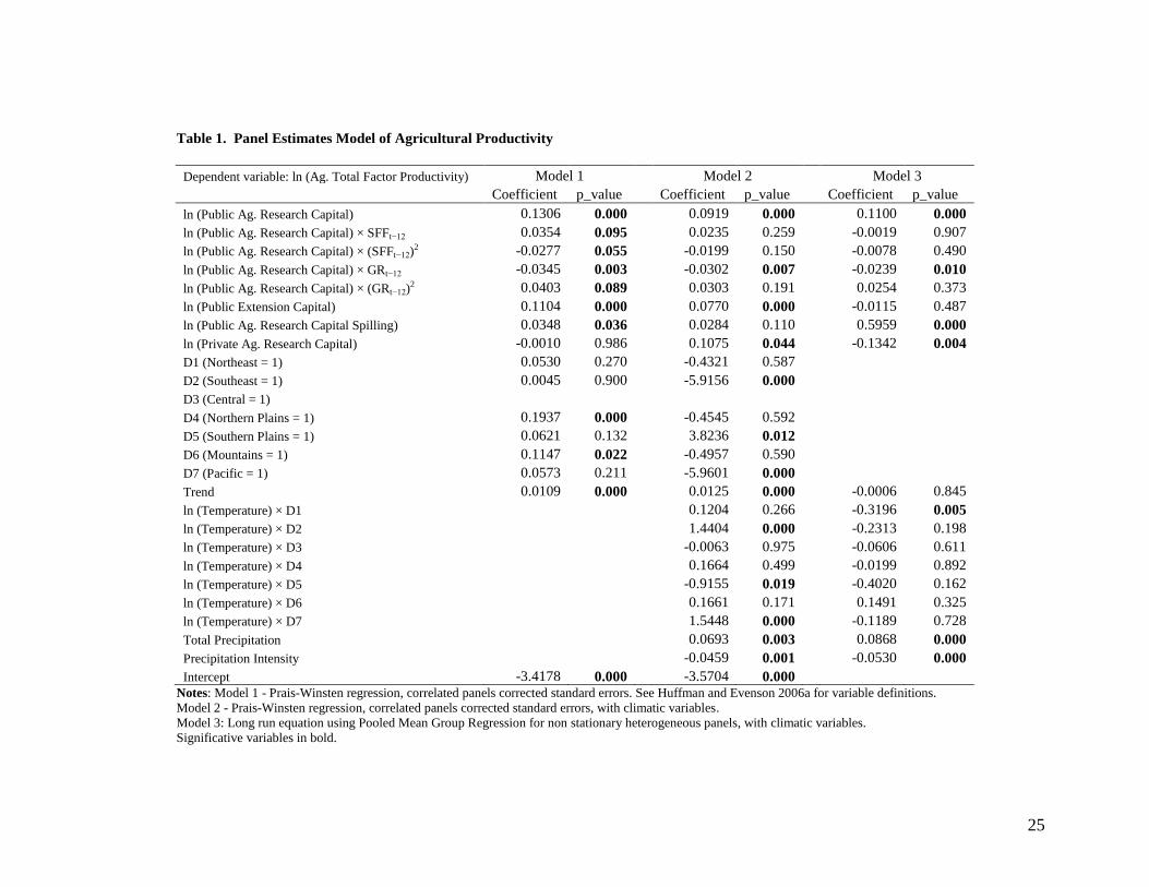
The estimations of the Huffman and Evenson model with climatic variables are

reported in columns 3 and 4 of Table 1. The natural logarithm of temperature was

multiplied by the regional dummies to take into account differentiated effects of

temperature in each region. We believe a priori that a higher temperature can be harmful

in some regions located in the south, while it can be beneficial in more northern latitudes.

Total Precipitation and Precipitation Intensity were reported with no region interactions

because we believe that those variables do not have a behavior similar to temperature.6

One interesting result is the effect of the original research capital variables after

controlling for climatic variables. Comparing our results with those from Huffman and

Evenson (2006a), we find that the terms RPUB x SFF, RPUB x SFF2, and RPUB x GR

2

are not significative anymore. The elasticity of TFP to Public research capital (RPUB) is

reduced a 36% from 0.139 to 0.089,7 the elasticity of TFP to Public Extension Capital

(EXT) is reduced a 30% from 0.110 to 0.077, the effect of Public Research Capital Spill-

in from near states (RPUBSPILL) becomes not significative after controlling for climatic

variables, and the elasticity effect of Private Agricultural Research Capital (RPRI) which

16

was negative but not significative before, now becomes significatively positive with a

value of 0.044.

Regarding the regional dummies individual effects, we obtain that taking the

Central region as benchmark, the Southeast and Pacific regions show a lower level, while

the Southern Plains exhibit a higher level of Agricultural TFP, after controlling for all the

other explanatory variables. This is evidence of the existence of unobservable effects that

affect the agricultural productivity at different degrees in each region.

The main climatic variables effect are related to Total Yearly Precipitation, which

has a positive effect over Agricultural TFP, with an associated elasticity of 0.069, while

the effect of Precipitation Intensity, expressed as fewer but stronger storms is negative,

showing an elasticity with a magnitude of -0.046. These results are consistent with our a

priori conjectures. Meanwhile, we find statistical evidence that supports the idea of

differentiated effects of temperature over regional TFP. In particular, we find that for the

Southeast and Pacific regions the statistical effect of higher temperature over factor

productivity is positive, while it is negative for the Southern Plains. There is no

conclusive evidence with respect to the other regions. Finally, we find evidence of a

positive linear trend in the Agricultural TFP.

Those results can be questionable if the included variables are non stationary.

Table 2 shows the results of several panel unit root tests we performed. We used two

different tests specifications to validate the robustness of our findings: only with

individual effects, or with individual effects and individual trends for each cross-section.

The tests were applied to all the variables of the econometric model from Table 1, in

17

levels as well as to their first differences, to determine whether the tested variables are

I(0) or I(1). Table 2 reports the test statistic, its significance level (p-value) and the

number of observations implied by the test, which is a function of the number of lags

chosen for the test.

One interested finding is that for some variables we can find contradictory results,

one kind of test indicates that the variable is stationary while other test can suggest that it

is not. For other variables, the tests are more conclusive, and almost all of them report the

same qualitative result. Whenever we find inconsistent results for all the tests, we choose

the result which is obtained in more cases, or with fewer contradictions.

The first evaluated variable is TFP8. For all the tests for which the null hypothesis

is the existence of unit root, it is not rejected. For the variable in levels the significance

values are very close to one. After differencing the variable, the null hypothesis of unit

root is rejected for all the tests. Meanwhile, if we apply the Hadri test to that variable, the

null hypothesis of no unit root is rejected when applied to the levels, but it is not rejected

at 5% of significance when applied to the first difference. If those tests are applied using

an specification that includes individual linear trends, the results are contradictory in the

sense that some tests suggest the existence of unit root while at the same time other tests

indicate that unit root is rejected. The final conclusion for this variable is to be in favor of

the results supporting the existence of a panel unit root.

Using the specification with individual effects only, we can summarize our results

in the following way. TFP is I(1), with no contradictory results for the tests in levels as

wells as their first difference counterpart. RPUB is found to be I(1) with 4 contradictory

18

results out of a total of 12 tests (2 in levels, 2 in differences). RPUB x SFF is I(0), with 3

contradictions in levels and no contradictions in first differences, RPUB x SFF2 is I(0)

with only one contradiction in levels, RPUB x GR is I(1) with 2 contradictions in levels,

the case of RPUB x GR2 gives us 3 contradictions in levels, but no contradictions in the

first difference specification, we decide to consider this variables as I(1), EXT is

considered as I(0) with 2 contradictions in levels and 1 in differences, RPUBSPILL is

found to be I(1) with one contradictory result in levels and 2 in first differences. For

RPRI the results show many contradictions, so it is difficult to determine a clear

conclusion about this variable. It is apparently I(1) when the test is applied in levels (2

contradictions), but after differencing the variable, the test results suggest we need one

more differentiation to make it stationary. The climatic variables Temperature,

Precipitation and Intensity show a stationary pattern. We find that all of them are

stationary, finding two contradictory results for Temperature, and only one in the other

climatic variables.

The results abovementioned show us that some of the involved variables are in

fact non stationary. One suggestion to deal with this problem would be to take first

differences to the I(1) variables and estimate the econometric model in that manner. This

is technically correct; however there is some statistical information that is lost in the

differentiation process. We can still work with the non differenced variables if they hold

the cointegration condition, and take advantage of a richer specification that incorporates

both the long-run relation and the short-run dynamics, the Error Correction Model

(ECM).

19

The panel cointegration test results are reported in Table 3. We first show the

standard panel unit root tests applied to the estimated residuals of the pooled estimation

including all the I(1) and I(0) variables from Table 1. Although those are not properly

cointegration tests, several articles have used them to check for cointegration of I(1)

variables.9 We report those results for comparative purposes. Our results are very

consistent regardless the method we used: the panel unit root tests suggest that the

estimated residuals are I(0) using a model with trend or without trend, with the only

exception of the Hadri test. All the test statistics are significative, rejecting the null

hypothesis of unit root. For the more formal panel cointegration tests, the results are very

similar, rejecting the null hypothesis of no cointegration. All the 14 variants of Pedroni

test report that the variables are cointegrated, with the exception of two cases: the panel

v-stat for a model with individual effects, and the group rho-stat for a model with

individual constants and trends; Kao cointegration tests are fully consistent with those

findings. Westerlund Error-correction-based test yields mixed results: one “group”

statistic suggest cointegration, and the other one does not, while one “panel” statistic

implies cointegration, and the other one rejects it. Our conclusion is that the statistical

evidence supporting cointegration is very strong.

With the last results at hand, we estimated the TFP model using an ECM

framework. As explained before, we assume homogeneous coefficients for the long-run

equation and heterogeneous coefficients for the short-run dynamics coefficients. Table 1

only reports the long-run coefficients in order to compare these results with the previous

20

ones. Notice that given the structure of the estimation method, the regional dummies

cannot be identified for estimation.

Using the ECM framework, more variables become not significative which means

that using a model without correcting for non stationarity can lead us to assign statistical

effects to some variables, but those affects seems to be actually spurious. Using the same

formulas aforementioned, the elasticity of Agricultural Total Factor Productivity (TFP)

with respect to Public Agricultural research (RPUB) is now equal to 0.108, value that is

in the midway between what we found with the previous two models (22% less than

Model 1 result). Public Extension Capital (EXT) is now not significant, while Capital

spill-in effects become positively significative, with a remarkable elasticity value of

0.596, several times higher than the values obtained before. The sign of the effect of

Private Research Capital is negative, as in Model 1 but it is now significant and its

elasticity value is -0.134.

Using this kind of model, the long-run relationship between temperature and TFP

is statistically zero for all regions, with the exception of a negative effect for the

Southeast. Concerning precipitation and its intensity, both variables are significant.

Precipitation effect elasticity is 0.087, a value that is 25% greater than using Model 2. For

precipitation intensity, we find that the associated elasticity is -0.053, which has the same

sign as what is found on Model 2, but with a 15% higher magnitude than before. It is

noticeable that when using an ECM there is no linear trend effect over Agricultural TFP.

21

Conclusions

This article examines the impact of climate change on agricultural total factor

productivity at the state level, after controlling for public agricultural research and

climate change. This paper takes the previous result of Huffman and Evenson (2006) in

which they establish whether federal formula or competitive grant funding of agricultural

research has a greater impact on state agricultural productivity. We estimated a pooled

cross-section time-series model of agricultural productivity fitted to annual data for forty-

eight contiguous states over 1970–1999, incorporating two new features: the inclusion of

climatic variables such as temperature, amount and intensity of precipitation, and the

evaluation and correction of problems due to non stationarity of some of the variables.

We found that some of the variables involved are I(1), which means that their

inclusion into the econometric model can lead to undesired properties on the panel

estimations. We correct the problem testing the existing of cointegration among the non

stationary variables, and the estimation of a Panel Error Correction Model (ECM). Our

findings suggest that after controlling for climatic variables and non stationarity, the

effect of Public Agricultural Research Capital over Total Factor Productivity is reduced.

References

Baltagi, B. Econometric Analysis of Panel Data. 4th Edition. Chichester, West Sussex:

John Wiley & Sons Ltd, 2008.

22

Banerjee, A., J.J. Dolado, J.W. Galbraith, and D.F. Hendry. Co-integration, error-

correction, and the econometric analysis of non-stationary data. Oxford: Oxford

University Press, 1993.

Beck, N., and J. Katz. "What to do (and not to do) with Time-Series Cross-Section Data."

The American Political Science Review 89, no. 3 (September 1995): 634-647.

Breitung, J. The Local Power of Some Unit Root Tests for Panel Data. Vol. 15, in

Nonstationary Panels, Panel Cointegration, and Dynamic Panels, Advances in

Econometrics, edited by B. Baltagi, 161-178. Amsterdam: JAI, 2000.

Dinda, S., and D. Condoo. "Income and emission: A panel data-based cointegration

analysis." Ecological Economics 57 (2006): 167-181.

Evenson, R.E., and W.E. Huffman. Science for agriculture: A long-term perspective. 2nd

Edition. Ames, IA: Blackwell Publishing, 2006b.

Granger, C.W.J., and P. Newbold. "Spurious regressions in economics." Journal of

Econometrics 2 (1974): 111-120.

Greene, W. Econometric Analysis. 5th Edition. Upper Saddle River, NJ: Prentice Hall,

2003.

Hadri, K. "Testing for stationarity in heterogeneous panel data." Econometrics Journal,

Royal Economic Society 3, no. 2 (2000): 148-161.

Hamilton, J.D. Time Series Analysis. Princeton, NJ: Princeton University Press, 1994.

23

Huffman, W.E., and R.E. Evenson. "Do Formula or Competitive Grant Funds Have

Greater Impacts on State Agricultural Productivity?" American Journal of

Agricultural Economics 88, no. 4 (November 2006a): 783-798.

Im, K. S., M. H. Pesaran, and Y. Shin. "Testing for Unit Roots in Heterogeneous Panels."

Journal of Econometrics 115 (2003): 53-74.

Kao, C. "Spurious regression and residual-based tests for cointegration in panel data."

Journal of Econometrics 90 (1999): 1-44.

Levin, A., C. F. Lin, and C. Chu. "Unit Root Tests in Panel Data: Asymptotic and Finite-

Sample Properties." Journal of Econometrics 108 (2002): 1-24.

Maddala, G.S., and S. Wu. "A Comparative Study of Unit Root Tests with Panel Data

and a New Simple Test." Oxford Bulletin of Economics and Statistics 61 (1999):

631-652.

National Oceanic and Atmospheric Administration (NOAA). National Climatic Data

Center. http://www.ncdc.noaa.gov/oa/ncdc.html (accessed 2009).

Pardey P.G., James J., Alston J., Wood S., Koo B., Binenbaum E., Hurley T., Glewwe P.

Science, Technology and Skills. Background Paper for the World Bank’s World

Development Report 2008. St. Paul, Rome and Washington D.C.: University of

Minnesota, CGIAR Science Council and World Bank, 2007.

Pedroni, P. "Critical values for cointegration tests in heterogeneous panels with multiple

regressors." Oxford Bulletin of Economics and Statistics, November Special Issue

1999: 653–669.

24

Pesaran, M.H., Y. Shin, and R.P. Smith. "Pooled Mean Group Estimation of Dynamic

Heterogeneous Panels." Journal of the American Statistical Association 94, no.

446 (June 1999): 621-634.

Phillips, P.C.B. "Understanding spurious regressions in econometrics." Journal of

Econometrics 33, no. 3 (December 1986): 311-340.

Westerlund, J. "Testing for Error Correction in Panel Data." Oxford Bulletin of

Economics and Statistics 69, no. 6 (2007): 709-748.

25

Table 1. Panel Estimates Model of Agricultural Productivity

Dependent variable: ln (Ag. Total Factor Productivity) Model 1 Model 2 Model 3

Coefficient p_value Coefficient p_value Coefficient p_value

ln (Public Ag. Research Capital) 0.1306 0.000 0.0919 0.000 0.1100 0.000

ln (Public Ag. Research Capital) × SFFt−12 0.0354 0.095 0.0235 0.259 -0.0019 0.907

ln (Public Ag. Research Capital) × (SFFt−12)2 -0.0277 0.055 -0.0199 0.150 -0.0078 0.490

ln (Public Ag. Research Capital) × GRt−12 -0.0345 0.003 -0.0302 0.007 -0.0239 0.010

ln (Public Ag. Research Capital) × (GRt−12)2 0.0403 0.089 0.0303 0.191 0.0254 0.373

ln (Public Extension Capital) 0.1104 0.000 0.0770 0.000 -0.0115 0.487

ln (Public Ag. Research Capital Spilling) 0.0348 0.036 0.0284 0.110 0.5959 0.000

ln (Private Ag. Research Capital) -0.0010 0.986 0.1075 0.044 -0.1342 0.004

D1 (Northeast = 1) 0.0530 0.270 -0.4321 0.587

D2 (Southeast = 1) 0.0045 0.900 -5.9156 0.000

D3 (Central = 1)

D4 (Northern Plains = 1) 0.1937 0.000 -0.4545 0.592

D5 (Southern Plains = 1) 0.0621 0.132 3.8236 0.012

D6 (Mountains = 1) 0.1147 0.022 -0.4957 0.590

D7 (Pacific = 1) 0.0573 0.211 -5.9601 0.000

Trend 0.0109 0.000 0.0125 0.000 -0.0006 0.845

ln (Temperature) × D1 0.1204 0.266 -0.3196 0.005

ln (Temperature) × D2 1.4404 0.000 -0.2313 0.198

ln (Temperature) × D3 -0.0063 0.975 -0.0606 0.611

ln (Temperature) × D4 0.1664 0.499 -0.0199 0.892

ln (Temperature) × D5 -0.9155 0.019 -0.4020 0.162

ln (Temperature) × D6 0.1661 0.171 0.1491 0.325

ln (Temperature) × D7 1.5448 0.000 -0.1189 0.728

Total Precipitation 0.0693 0.003 0.0868 0.000

Precipitation Intensity -0.0459 0.001 -0.0530 0.000

Intercept -3.4178 0.000 -3.5704 0.000 Notes: Model 1 - Prais-Winsten regression, correlated panels corrected standard errors. See Huffman and Evenson 2006a for variable definitions.

Model 2 - Prais-Winsten regression, correlated panels corrected standard errors, with climatic variables.

Model 3: Long run equation using Pooled Mean Group Regression for non stationary heterogeneous panels, with climatic variables.

Significative variables in bold.

26

Table 2. Panel Unit Root Test: Summary

Sample: 1970 1999

Cross Sections: 48

Individual effects Individual effects & individual linear trends

Level 1st Difference Level 1st Difference

ltfp Statistic P-value Obs. Statistic P-value Obs. Statistic P-value Obs. Statistic P-value Obs.

Null: Unit root (assumes common unit root process)

Levin, Lin & Chu t* 1.34 0.909 1329 -34.70 0.000 1307 -11.87 0.000 1367 -27.26 0.000 1297

Breitung t-stat 2.70 0.997 1281 -25.87 0.000 1259 -1.28 0.100 1319 -24.60 0.000 1249

Null: Unit root (assumes individual unit root process)

Im, Pesaran and Shin W-stat 7.52 1.000 1329 -38.67 0.000 1307 -12.62 0.000 1367 -35.31 0.000 1297

ADF - Fisher Chi-square 33.01 1.000 1329 1116.74 0.000 1307 343.84 0.000 1367 1023.92 0.000 1297

PP - Fisher Chi-square 47.79 1.000 1392 1276.65 0.000 1344 619.49 0.000 1392 6263.40 0.000 1344

Null: No unit root (assumes common unit root process)

Hadri Z-stat 23.07 0.000 1440 1.52 0.065 1392 10.22 0.000 1440 13.45 0.000 1392

lrpubs3

Levin, Lin & Chu t* -8.34 0.000 1257 -7.14 0.000 1254 0.94 0.827 1265 -7.11 0.000 1256

Breitung t-stat 1.57 0.941 1209 -1.59 0.056 1206 -8.01 0.000 1217 0.77 0.779 1208




Hadri Z-stat 24.42 0.000 1440 12.65 0.000 1392 16.19 0.000 1440 16.50 0.000 1392

lrpubsf

Levin, Lin & Chu t* -1.40 0.080 1353 -30.05 0.000 1311 -3.94 0.000 1350 -19.26 0.000 1282

Breitung t-stat -1.06 0.145 1305 -27.07 0.000 1263 -3.86 0.000 1302 -22.32 0.000 1234

Im, Pesaran and Shin W-stat -2.45 0.007 1353 -31.51 0.000 1311 -5.43 0.000 1350 -25.93 0.000 1282



Hadri Z-stat 17.07 0.000 1440 0.44 0.330 1392 9.38 0.000 1440 10.61 0.000 1392

27

lrpubsf2

Levin, Lin & Chu t* -1.45 0.073 1354 -30.45 0.000 1310 -4.57 0.000 1356 -20.49 0.000 1286

Breitung t-stat -1.58 0.057 1306 -27.92 0.000 1262 -3.73 0.000 1308 -22.73 0.000 1238




Hadri Z-stat 17.18 0.000 1440 0.31 0.379 1392 9.09 0.000 1440 8.42 0.000 1392

lrpubgr

Levin, Lin & Chu t* -0.63 0.265 1371 -31.09 0.000 1311 -2.38 0.009 1361 -24.26 0.000 1291

Breitung t-stat -2.25 0.012 1323 -27.97 0.000 1263 1.50 0.933 1313 -20.47 0.000 1243




Hadri Z-stat 16.94 0.000 1440 -0.98 0.837 1392 8.60 0.000 1440 9.03 0.000 1392

lrpubgr2

Levin, Lin & Chu t* -1.13 0.130 1357 -27.40 0.000 1290 -2.60 0.005 1352 -19.72 0.000 1279

Breitung t-stat -1.97 0.025 1309 -25.58 0.000 1242 0.41 0.658 1304 -18.68 0.000 1231




Hadri Z-stat 16.96 0.000 1440 -1.07 0.858 1392 9.21 0.000 1440 10.44 0.000 1392

lnextf

Levin, Lin & Chu t* -8.57 0.000 1369 -27.70 0.000 1329 -7.52 0.000 1365 -23.74 0.000 1322

Breitung t-stat -2.17 0.015 1321 -10.67 0.000 1281 -0.55 0.292 1317 -9.79 0.000 1274




Hadri Z-stat 22.67 0.000 1440 2.26 0.012 1392 10.29 0.000 1440 9.55 0.000 1392

lrspill3

Levin, Lin & Chu t* -6.87 0.000 1288 -9.79 0.000 1281 11.88 1.000 1281 -10.96 0.000 1251

Breitung t-stat 3.96 1.000 1240 -6.43 0.000 1233 -10.45 0.000 1233 -4.26 0.000 1203

Im, Pesaran and Shin W-stat 3.03 0.999 1288 -7.01 0.000 1281 0.26 0.601 1281 -5.23 0.000 1251

28



Hadri Z-stat 24.95 0.000 1440 7.81 0.000 1392 12.86 0.000 1440 17.15 0.000 1392

lintst

Levin, Lin & Chu t* -27.50 0.000 1338 -0.56 0.288 1296 -24.92 0.000 1344 -1.47 0.070 1293

Breitung t-stat -26.01 0.000 1290 -2.53 0.006 1248 0.45 0.675 1296 -3.60 0.000 1245

Im, Pesaran and Shin W-stat -26.05 0.000 1338 0.75 0.774 1296 -25.92 0.000 1344 3.82 1.000 1293



Hadri Z-stat 3.86 0.000 1440 3.81 0.000 1392 9.97 0.000 1440 14.64 0.000 1392

ltmp

Levin, Lin & Chu t* -24.45 0.000 1373 -37.46 0.000 1290 -23.78 0.000 1356 -26.78 0.000 1281

Breitung t-stat -22.90 0.000 1325 -28.86 0.000 1242 2.65 0.996 1308 -21.59 0.000 1233




Hadri Z-stat 9.24 0.000 1440 5.74 0.000 1392 4.22 0.000 1440 30.64 0.000 1392

lpcp

Levin, Lin & Chu t* -30.46 0.000 1372 -38.71 0.000 1278 -26.37 0.000 1366 -29.06 0.000 1263

Breitung t-stat -18.68 0.000 1324 -29.56 0.000 1230 -3.56 0.000 1318 -28.92 0.000 1215




Hadri Z-stat 1.16 0.123 1440 1.90 0.029 1392 7.35 0.000 1440 17.67 0.000 1392

lintens

Levin, Lin & Chu t* -28.00 0.000 1385 -36.97 0.000 1303 -24.51 0.000 1377 -29.46 0.000 1297

Breitung t-stat -19.79 0.000 1337 -19.78 0.000 1255 -7.43 0.000 1329 -19.44 0.000 1249




Hadri Z-stat 2.61 0.005 1440 -0.34 0.632 1392 7.19 0.000 1440 11.01 0.000 1392

** Probabilities for Fisher tests are computed using an asympotic Chi-square distribution. All other tests assume asymptotic normality.

29

Table 3. Cointegration Test: Summary

Sample: 1970 1999

Cross Sections: 48

Panel unit root tests: Constant Constant & Trend

Residuals pooled estimation Statistic P-value Obs. Statistic P-value Obs.

Null: Unit root (assumes common unit root process)

Levin, Lin & Chu t* -11.69 0.000 1380 -11.65 0.000 1378

Breitung t-stat -7.06 0.000 1332 -6.93 0.000 1330

Null: Unit root (assumes individual unit root process)

Im, Pesaran and Shin W-stat -13.34 0.000 1380 -12.24 0.000 1378

ADF - Fisher Chi-square 377.10 0.000 1380 324.39 0.000 1378

PP - Fisher Chi-square 406.35 0.000 1392 519.15 0.000 1392

Null: No unit root (assumes common unit root process)

Hadri Z-stat 7.82 0.000 1440 9.55 0.000 1440

**Probabilities for Fisher tests are computed using an asympotic Chi-square distribution.

**All other tests assume asymptotic normality.

Pedroni cointegration tests Constant Constant & Trend

Statistic P-value Statistic P-value

panel v-stat -0.82 0.205 -3.76 0.000

panel rho-stat -4.60 0.000 -2.45 0.007

panel pp-stat -20.10 0.000 -23.80 0.000

panel adf-stat -9.88 0.000 -9.69 0.000

group rho-stat -2.22 0.013 -0.03 0.489

group pp-stat -22.28 0.000 -26.89 0.000

group adf-stat -8.24 0.000 -9.12 0.000

**All reported values are distributed N(0,1) under null of unit root or no cointegration.

**Panel stats are unweighted by long run variances.

Kao cointegration tests Constant Constant & Trend

Statistic P-value Statistic P-value

DFrho -31.88 0.000 -33.94 0.000

DFt -17.59 0.000 -18.64 0.000

**Stats are distributed N(0,1) under null of no cointegration.

Westerlund cointegration tests

Lags: 1 - 2 Average AIC selected lag length: 1.98

Leads: 0 - 1 Average AIC selected lead length: .96

Constant Constant & Trend

Statistic Value Z-value P-value Value Z-value P-value

Gt -4.06 -11.71 0.000 -4.23 -10.39 0.000

Ga -0.24 11.50 1.000 -0.13 13.81 1.000

Pt -22.25 -6.80 0.000 -25.95 -7.75 0.000

Pa -2.56 6.16 1.000 -1.99 9.57 1.000

**Z-values are distributed N(0,1) under null of no cointegration.

30

Endnotes

1 The impact on a given state of direct public agricultural research undertaken by other states in an area.

2 According to the usual panel model nomenclature, for all this article the sub-index i = 1,…,N represents

each cross section (state) and the sub-index t = 1,…,T represents each time period (year).

3 For details on the construction and the asymptotic properties of the test, see Im, Pesaran and Shin (2003).

4 Common factor restriction is the fact that residual-based tests require the long-run cointegrating vector for

the variables in their levels being equal to the short-run adjustment process for the variables in their

differences.

5 The impact on a given state of direct public agricultural research undertaken by other states in an area.

6 Not reported estimations with regional interaction for Precipitation and Intensity were performed with no

satisfactory result, which supports our original idea.

7 Calculated using the elasticities equations evaluated at the sample means for SFF and GR.

8 All the variables evaluated are expressed in natural logarithms.

9 For example, Dinda and Coondoo (2006).

The Effect of Climate Change over Agricultural Factor Productivity: Some Econometric Considerations

Documents

Transcript of The Effect of Climate Change over Agricultural Factor Productivity: Some Econometric Considerations