The Effect of Buffering on the Performance of R-Trees

The Effect of Buffering on thePerformance of R-Trees

Scott T. Leutenegger, Member, IEEE Computer Society, and Mario A. LoÂpez

AbstractÐPast R-tree studies have focused on the number of nodes visited as a metric of query performance. Since database

systems usually include a buffering mechanism, we propose that the number of disk accesses is a more realistic measure of

performance. We develop a buffer model to analyze the number of disk accesses required for spatial queries using R-trees. The model

can be used to evaluate the quality of R-tree update operations, such as various node splitting and tree restructuring policies, as

measured by query performance on the resulting tree. We use our model to study the performance of three well-known R-tree loading

algorithms. We show that ignoring buffer behavior and using number of nodes accessed as a performance metric can lead to incorrect

conclusions, not only quantitatively, but also qualitatively. In addition, we consider the problem of how many levels of the R-tree should

be pinned in the buffer.

Index TermsÐAnalytical model, buffer model, multidimensional indexing, performance evaluation, R-tree.

æ

1 INTRODUCTION

R-TREES [3] are a common indexing technique for spatialdata and are widely used in spatial and multidimen-

sional databases. Typical applications include: computer-aided design, geographic information systems, computervision and robotics, multikeyed indexing for traditionaldatabases, temporal databases, and scientific databases.

A significant amount of activity has gone into develop-ing better R-tree construction algorithms [13], [1], [12], [4],[5], [10]. Most of this work has focused on proposing andcomparing a new algorithm to previous ones, but little workhas been done on methodology for comparing algorithms.Notable exceptions are the work of Kamel and Faloutsos [4],Pagel et al. [9], and Theodoridis and Sellis [14].

In [4], [9] the authors develop an analytical model forprediction of query performance given as input the MinimalBounding Rectangles (MBRs) of all nodes in the tree. Themodel provides good insight into the problem, especially byestablishing a quantitative relationship between perfor-mance and the total area and perimeter of MBRs of the treenodes. In [14], the authors provide a fully analytical modelnot requiring the minimum bounding rectangles of theR-tree nodes as an input. All three of these models sufferfrom one major drawback: The primary objective functionfor comparison is the number of nodes visited. In realdatabases, some portion of the tree is buffered in mainmemory. This buffering of portions of the tree cansignificantly affect performance. Consequently, we proposethat a better metric is the average number of disk accessesrequired to satisfy a query.

In this paper, we develop a new cost model that includesbuffering, validates the model empirically, and then use themodel to evaluate the effects of buffer size, of pinning in

main memory certain levels of the tree, and of nonuni-

formly distributed queries. We emphasize that the inclusion

of a buffer not only changes the quantitative performance of

the algorithms, but, in some cases, changes the qualitative

ordering of the algorithms. A preliminary version of this

paper appeared in [6].In order to derive a model based on the number of disk

accesses, we borrow techniques developed by Bhide et al. [2]

(in the context of modeling databases with uniform access

within each of several partitions) and develop a new buffer

model. Our model can be used to evaluate the quality of any

R-tree update operation, such as node splitting policies [3]

or loading algorithms [4], [7], [12] as measured by query

performance of the resulting tree. The model is very

accurate and simple to understand, making it easy for

researchers to integrate it into their studies.Our buffer model is an analytic model based on simple

probability theory, but our overall performance model is a

hybrid model. We start by using a loading algorithm to

create actual R-trees for various data sets. Then, we

compute the minimum bounding rectangles of tree nodes

and use these as input to our buffer model.The rest of the paper is organized as follows: In Section 2,

we provide background information on R-trees and describe

three loading algorithms that were chosen to test our results.

Since this choice is by no means exhaustive, we emphasize

that the purpose of this paper is not to draw irrevocable

conclusions about the best loading algorithm (although it

allows comparisons between the chosen ones), but rather to

demonstrate the need for and utility of the buffer model. In

Section 3, we present the query performance model of Kamel

and Faloutsos, a modification of the region query model, and

a new buffer model. In Section 4, we present the validation of

our model. Section 5 contains results from our model

experiments and Section 6 concludes.

IEEE TRANSACTIONS ON KNOWLEDGE AND DATA ENGINEERING, VOL. 12, NO. 1, JANUARY/FEBRUARY 2000 33

. The authors are with the Department of Mathematics and ComputerScience, University of Denver, Denver, CO 80208-0189.E-mail: {leut, mlopez}@cs.du.edu.

Manuscript accepted 18 Aug. 1999.For information on obtaining reprints of this article, please send e-mail to:[email protected], and reference IEEECS Log Number 110164.

1041-4347/00/$10.00 ß 2000 IEEE

2 OVERVIEW OF R-Tree AND LOADING

ALGORITHMS

In this section, we provide a brief overview of the R-tree andloading algorithms. A detailed understanding of the loadingalgorithms is useful, but not necessary, for the rest of thispaper. The reader interested in a more detailed description isreferred to the articles listed in the bibliography.

2.1 R-Trees

An R-tree is a hierarchical data structure derived from theB-tree and designed for efficient execution of intersectionqueries. An R-tree stores a collection of rectangles that canchange in time through insertion and deletion of rectangles.Arbitrary geometric objects can also be handled byrepresenting each object by the smallest axis-parallelrectangle enclosing it. R-trees generalize easily to dimen-sions higher than two. For notational simplicity, wedescribe only the 2D case.

Each node of the R-tree stores a maximum of n entries.Each entry consists of a rectangle R and a pointer P . At theleaf level, R is the bounding box of an actual object pointedto by P . At internal nodes, R is the minimum boundingrectangle (MBR) of all rectangles stored in the subtreepointed to by P . Note that a path along the tree correspondsto a sequence of nested rectangles, the last of which is anactual data object. Note, also, that rectangles at any levelmay overlap and that the R-tree for a set of rectangles is byno means unique.

Fig. 1 illustrates a 3-level R-tree assuming that amaximum of four rectangles fit per node. We assume thatthe levels are numbered 0 (root), 1, and 2 (leaf level). Thereare 64 rectangles represented by the small dark boxes. The64 rectangles are grouped into 16 leaf level pages,numbered 1 to 16. Note that the MBR enclosing each leafnode is the smallest box that fully contains the rectangleswithin the node. These MBRs serve as rectangles to bestored at the next level of the tree. For example, leaf levelnodes 1 through 4 are placed in node 17 in level 1. TheMBRs of nodes 17 through 20 are purposely drawn slightly

larger than needed for clarity. The root node contains thefour level 1 nodes: 17, 18, 19, and 20.

To perform a query Q, all rectangles (internal or not) thatintersect the query region must be retrieved. This isaccomplished with a simple recursive procedure that startsat the root and possibly follows several paths along the tree.A node is processed by first retrieving all rectangles storedat that node that intersect Q. If the node is an internal node,the subtrees pointed to by the retrieved rectangles (if any)are processed recursively. Otherwise, the node is a leafnode and the retrieved rectangles are simply reported. Forillustration, consider the query Q in the example of Fig. 1.After processing the root node, we determine thatnodes 19 and 20 of level 1 must be searched. The searchthen proceeds in both of these nodes. In both cases, it isdetermined that the query region does not intersect anyrectangles within the two nodes and each of these twosubqueries are terminated.

The R-tree shown in Fig. 1 is fairly well-structured.Inserting these same rectangles into an R-tree based on theinsertion algorithms of Guttman [3] would likely result in aless well-structured tree. Algorithms to create well-struc-tured trees have been developed and are described inSection 2.2. These algorithms attempt to cluster rectanglesso as to minimize the number of nodes visited whileprocessing a query.

For the rest of the paper, we assume that exactly onenode fits per page and, hereafter, we use the two termsinterchangeably.

2.2 Loading Algorithms

In this section, we describe three loading algorithms. Thefirst is based on inserting a tuple at a time, using one of theinsertion algorithms proposed by Guttman [3].

Tuple-At-a-Time (TAT):

. This algorithm simply inserts one tuple at a time intothe R-tree using the quadratic split heuristic ofGuttman [3]. Note that the resultant R-tree hasworse space utilization and structure relative to the

34 IEEE TRANSACTIONS ON KNOWLEDGE AND DATA ENGINEERING, VOL. 12, NO. 1, JANUARY/FEBRUARY 2000

Fig. 1. A sample R-tree. Input rectangles are shown solid.

two algorithms discussed next. Thus, more node anddisk accesses may be necessary to satisfy a query.

The following two packing algorithms use a similarframework, based on preprocessing the entire data file soas to determine how to group rectangles into nodes. In thefollowing, we assume that a data file of R rectangles will bestored in a tree with up to n rectangles per node. The wholeprocess is similar to building a B-tree out of a collection ofkeys from the leaf level up [11].

General Algorithm:

1. Preprocess the data file so that the R rectangles areordered in dR=ne consecutive groups of n rectangles,where each group of n are intended to be placed inthe same leaf level node. Note that the last groupmay contain less than n rectangles.

2. Load the dR=ne groups of rectangles into pages andoutput the tuples (MBR, page number) for each leaflevel page into a temporary file. The page numbersare needed for setting child pointers in the nodes onelevel up.

3. Recursively, pack these MBRs into nodes at the nextlevel and up until only the root node remains.

The algorithms differ only in how the rectangles at each

level are ordered.

Nearest-X (NX):

. This algorithm was proposed in [12]. The rectanglesare sorted by x-coordinate. No details are given inthe paper so we assume that x-coordinate of therectangle's center is used. The rectangles are thenpacked into the nodes using this ordering.

Hilbert Sort (HS):

. A fractal-based algorithm was proposed in [4]. Thealgorithm uses a Hilbert (fractal) space filling curvewhich visits every point on a grid exactly oncewithout self-intersections. This curve has the im-portant property that points that are close along thecurve are also geographically close in the plane. Thecenter points of the rectangles are sorted based ontheir distance from the origin as measured along theHilbert curve. This determines the order in whichthe rectangles are placed into the nodes of the R-tree.

3 MODEL DESCRIPTION

Kamel and Faloutsos [4] and Pagel et al. [9] independentlyintroduced analytical models for computing the averageresponse time of a query as a function of the geometriccharacteristics of the R-tree. Their models do not considerthe effect of a buffer and performance is measured by thenumber of R-tree nodes accessed. In practice, queryperformance is mainly affected by the time required toretrieve nodes touched by the query which do not reside inthe buffer, as the CPU time required to retrieve and processbuffer resident nodes is usually negligible. We start bydescribing the model of [4]. We then modify this model tobetter fit our definition for uniformly distributed queries ofa fixed size. This modification is similar to the model of [9].Finally, we extend the model to take into account the

existence of a buffer, including how to handle the pinningin the buffer of the top few levels of the R-tree.

In this section, we consider a two-dimensional data setconsisting of rectangles to be stored in an R-tree T withH � 1

levels, labeled 0 through H. All input rectangles have beennormalized to fit within the unit square U � �0; 1� � �0; 1�.Queries are rectangles Q of size qx � qy (so, a point querycorresponds to the case qx � qy � 0). We initially assume thatqueries are uniformly distributed over the unit square andlater present a model where the query distribution mimicsthe data distribution. Our description concentrates on 2D.Generalizations to higher dimensions are straightforward.

Throughout this section, we will use the following

notation:

Mi � number of nodes at the ith level of T

M � Total number nodes in T; i:e:;XHi�0

Mi

Rij � jth rectangle at the ith level of T

Aij � area of Rij

AQij � probability that Rij is accessed by query Q

Bij � number of accesses to Rij

A � Sum of the areas of all MBRs in T

Lx � Sum of the x-extents of all MBRs in T

Ly � Sum of the y-extents of all MBRs in

TN � number of queries performed so far

N� � expected number of queries required to fill

the buffer

B � buffer size

D�N� � number of distinct nodes �at all levels� accessed

in N queries

EPT �qx; qy� � expected number of nodes �buffer resident

or not� of T accessed while performing a query

of size qx � qyEDT �qx; qy� � expected number of disk accesses while

performing a query of size qx � qy:

3.1 Uniform Access

The authors of [4], [9] consider a bufferless model whereperformance is measured by the number of nodes accessed(independent of whether they currently reside in thebuffer). They observe, that, for uniform point queries, theprobability of accessing Rij is just the area of Rij, namely,Aij. They point out that the level of T in which Rij resides isimmaterial as all rectangles containing Q (and only those)must be retrieved. Accordingly, for a point query, theexpected number of nodes retrieved as derived in [4] is thesum of node areas:1

EPT �0; 0� �

XHi�0

XMi

j�1

Aij � A;

LEUTENEGGER AND L �OPEZ: THE EFFECT OF BUFFERING ON THE PERFORMANCE OF R-TREES 35

1. We have modified the notation of [4] to make it consistent with thenotation used in this paper.

which is the sum of the areas of all rectangles (both leaflevel MBRs, as well as MBRs of internal nodes).

We now turn our attention to region queries. Leth�a; b�; �c; d�i denote an axis-parallel rectangle with bottomleft and top right corners �a; b� and �c; d�, respectively.Consider a rectangular query Q � hQbl; Qtri of size qx � qy.Q intersects R � h�a; b�; �c; d�i if, and only if, Qtr (the topright corner of Q) is inside the extended rectangleR0 � h�a; b�; �c� qx; d� qy�i, as illustrated in Fig. 2.

Kamel and Faloutsos infer that the probability ofaccessing R, while performing Q is the area of R0, as theregion query Q is equivalent to a point query Qtr where allrectangles in T have been extended as outlined above. Thus,the expected number of nodes retrieved (as derived in [4]) is:

EPT �qx; qy� �

XHi�0

XMi

j�1

�Xij � qx��Yij � qy�

�XHi�0

XMi

j�1

�XijYij � qxXHi�0

XMi

j�1

Yij

� qyXHi�0

XMi

j�1

Xij �Mqxqy

� A� qxLy � qyLx �Mqxqy:

�2�

Equation (2) illustrates the fact that a good loading

algorithm should cluster rectangles so as to minimize both

the total area and total perimeter of the MBRs of all nodes.

For point queries, on the other hand, qx � qy � 0 and

minimizing the total area is enough.We have modified the model of Kamel and Faloutsos to

handle query windows that fall partially outside the dataspace, as well as data rectangles close to the boundary of thedata space, as suggested by Pagel et al. [9]. Specifically:

1. For uniformly distributed rectangular queries of sizeqx � qy, the top right corner of the query region Qcannot be an arbitrary point inside the unit square ifthe entire query region is to fit within the unitsquare. For example, if qx � qy � 0:25, a query suchas Q1 in Fig. 3a should not be allowed. Rather, Qtr

must be inside the box U 0 � �qx; 1� � �qy; 1�.2. The probabil i ty of accessing a rectangle

R � h�a; b�; �c; d�i is not always the area of

R0 � h�a; b�; �c� qx; d� qy�ias this value can be bigger than one. For example, in

Fig. 3b, the probability that a query of size 0:9� 0:9

accesses rectangle R1 should not be 1:1 � 1:1 � 1:21,

which is the area of the extended rectangle R01,

obtained by applying the original formula. Rather,

the access probability is the percentage of U 0 covered

by the rectangle R0 \ U 0.Thus, we change the probability of accessing rectangle i

of level j to:

AQi;j �

area�R0 \ U 0�area�U 0�

� C �D�1ÿ qx��1ÿ qy� ;

where

C � �min�1; c� qx� ÿmax�a; qx��and D � �min�1; d� qy� ÿmax�b; qy��: We use this AQ

i;j in all

subsequent discussion and results.

3.2 Data Driven Access

Consider now the situation where queries are not uniform,

but, rather, tend to mimic the distribution of the data. In this

section, we introduce a nonuniform query model and then

recompute AQi;j according to that model.

Let cj denote the center of the jth data rectangle, 1 � j � n.

In our modified model, a query is always a qx � qy rectangle

with center cj, where j is uniformly chosen at random

between one and n. This change to query distribution implies

that areas with higher concentration of data will be queried

more often than areas where data is more sparse. For

example, in the CFD data of Fig. 5, the number of queries in

the immediate neighborhood of the wing would be high, but

decrease as the distance from the query to the wing boundary

increases. This pattern of access mimics the way in which

researchers often access this type of data.We now recompute AQ

i;j taking into account the newdistribution of queries. For simplicity, we first describe thecase of point queries. We introduce an indicator variable xijkdefined as follows:


Fig. 2. (a) Two data rectangles and region query Q. (b) Corresponding extended rectangles and equivalent point query Qtr.

xijk � 0 if ck is outside Rij

1 if ck is inside Rij:

�Accordingly, for point queries

AQi;j �

1

n

Xnk�1

xijk:

For region queries, it does not suffice to count the

number of data centers inside an MBR, as a query

could intersect an MBR even when the center of that

query is outside the MBR. Accordingly, for MBR R, let

R0 denote the rectangle obtained by expanding R by qx(resp. qy) units on dimension x (resp. y), while keeping

its center fixed (see Fig. 4). We define a new indicator

variable:

yijk � 0 if ck is outside R0ij1 if ck is inside R0ij:

�Finally, for a region query of size qx � qy,

AQi;j �

1

n

Xnk�1

yijk: �4�

Note that (4) is correct for both point and region queries.

As with uniform queries, we use this AQi;j in subsequent

discussion and results.

3.3 A Buffer Model

Bhide et al. [2] analyze the LRU buffer replacement policyfor databases consisting of a number of partitions withuniform page access within each partition. While modelingperformance during buffer warm-up, they observed that thebuffer hit probability at the end of the warm-up period is agood estimator of the steady-state buffer hit probability.

We conjectured that similar behavior would occur in the

context of R-trees when applying the LRU replacement

policy. Namely, that the steady-state buffer hit probability

is virtually the same as the buffer hit probability when the

buffer first becomes full. Our conjecture was verified

experimentally, as discussed in Section 4.

Under uniformly distributed point queries, the probability

of accessing rectangle Rij, while performing a query is Aij.

Accordingly, the probability that Rij is not accessed during

the next N queries is P �Bij � 0jN� � �1ÿAij�N . Thus,

P �Bij � 1jN� � 1ÿ �1ÿAij�N and the expected number of

distinct nodes accessed in N queries is,

D�N� �XHi�0

XMi

j�1

P �Bij � 1jN� �M ÿXHi�0

XMi

j�1

�1ÿAij�N: �5�

Note that D�0� � 0 < B and D�1� � A (which may ormay not be bigger than B). The buffer, which is initiallyempty, first becomes full after performingN� queries, whereN� is the smallest integer that satisfiesD�N�� B. The valueof N� can be determined by a simple binary search.

While the buffer is not full, the probability that Rij is inthe buffer is equal to P �Bij � 1�. The probability that arandom query requires a disk access for Rij isAij � P �Bij � 0�. Since the steady-state buffer hit probabilityis approximately the same as the buffer hit probability afterN� queries, the expected number of disk accesses for a pointquery at steady-state is


Fig. 4. A rectangle R expanded into R0 by a query of size qx � qy.

Fig. 3. The domain of Qtr for a query of size 0:25� 0:25 is U 0 (area not shaded).

XHi�0

XMi

j�1

Aij � P �Bij � 0jN�� XHi�0

XMi

j�1

Aij � �1ÿAij�N�: �6�

The above derivation also holds for region queries providedthat AQ

ij is used instead of Aij, i.e.:

EDT �qx; qy� �

XHi�0

XMi

j�1

AQij � �1ÿAQ

ij�N�:

Finally, we point out that it is easy to extend the aboveresults to model a buffer management policy that pins thetop few levels of the R-tree in the buffer: Simply reduce thenumber of buffer pages by the number of pages in thesepinned levels and omit the top levels from the model.

4 MODEL VALIDATION

We validated the model by comparing it with simulation.The simulation models an LRU buffer and, like the model,takes as input the list of the MBRs for all nodes at all levels.It then generates random point queries in the unit squareand checks each node's MBR to see if it contains the point. Ifthe MBR does contain the point, the node is requested fromthe buffer pool. If the node is not in the buffer pool, the leastrecently used node in the buffer is pushed out and the newnode put on the top of the LRU stack. Note that thesimulation is accurate in the sense that an R-tree imple-mentation retrieves all and only those rectangles (internal ornot) that intersect the region query. Confidence intervalswere collected using batch means with 20 batches of1,000,000 queries each, resulting in confidence intervals ofless than 3 percent at a 90 percent confidence level.

We ran comparisons for three different R-trees and sixdifferent buffer sizes for each tree. Each of the R-trees has1,668 nodes, but the MBRs of the nodes are different, asproduced by the three different packing algorithms. InTable 1, we report the average number of pages requiredfrom disk per point query, as predicted by the simulation,model, and the percent difference (relative to the simula-tion), for two of the trees assuming the uniform accessmodel. The third tree has similar comparisons. All of theresults are within 2 percent, which is less than theconfidence intervals returned from the simulation. Othercomparison experiments not shown resulted in agreementwithin 2 percent or less. Simulation of region queries anddata-driven queries gave similar results.

5 MODEL RESULTS

In this section, we present performance results as predicted

by our model. We consider two types of queries: point

queries and region queries. A point query specifies a point

in the unit square and finds all rectangles that contain the

point. Region queries specify a region of a given size and

find all rectangles that intersect this region. Each query is a

rectangle of size qx � qy whose upper right corner is

contained in region U 0 as described in Section 3.

5.1 Data Sets

We first describe the data used in our experiments. All datasets have been normalized to the unit square. We considerthe following data sets:

. TIGER. This is the Long Beach data set coming fromthe TIGER system of the U.S. Bureau of Census. Thisdata set of 53,145 rectangles has been extensivelyused in past studies.

. Synthetic Region. Uniformly distributed data setswere created containing between 10,000 and 300,000rectangles. All rectangles are squares, where thelength is chosen uniformly between 0 and �. Thevalue of � is fixed for all data set sizes and is equal to

2��0:25=10000:

pThus, for a 10,000 rectangle data set, the sum of the

rectangle areas is roughly equal to 0.25 of the unit

square; for 100,000 rectangles, the total area equals

2.5 times the unit square. This is similar to the

experimental methodology used in [4].. Synthetic Point. This is a data set consisting of

points where each point is located with equalprobability on any location within the unit square.

. CFD. This data set is an unstructured grid used inComputational Fluid Dynamics. We consider a two-dimensional problem. A system of equations is usedto model the air flows over and around aerospacevehicles [8]. The data sets are for a cross section of aBoeing 737 wing with flaps out in landing config-uration at MACH 0.2. The data space consists of acollection of points (nodes) of varying density.Nodes are dense in areas of great change in thesolution of the equations and sparse in areas of littlechange.


TABLE 1Validation: Average Number of Disk Access per Query for Model and Simulation

To help the reader understand the nature of thedata, we include a plot of a data set with 5,088 nodes(see Fig. 5). The left hand plot is for the entire dataset, the right plot is a blow up of the centroid of thedata set. The experimental results use a data set with52,510 nodes, which is similar, but looks like a blacksmudge when plotted due to the density of points. Inthe center detail plot, the blank ovalish areas areparts of the wing. It is evident that the data set ishighly skewed. This and other CFD data sets areavailable at http://www.cs.du.edu/users/leut/MultiDimData.html.

5.2 Need for Consideration of Buffer Impact

Fig. 6 plots the number of disk accesses versus buffer sizefor the TIGER data set assuming R-trees with 100 rectanglesper node. The plot on the left is for point queries; the oneon the right, for region queries. Consider the top twocurves of the right plot. For small buffer sizes, the TATalgorithm requires fewer disk access than the NX

algorithm. At a buffer size of 200, the performance of thetwo algorithms crosses and the NX algorithm becomes thebetter algorithm. Hence, ignoring buffering would result inthe incorrect conclusion that TAT is better than NX, thusunderscoring the importance of including buffer effects incomparison studies.

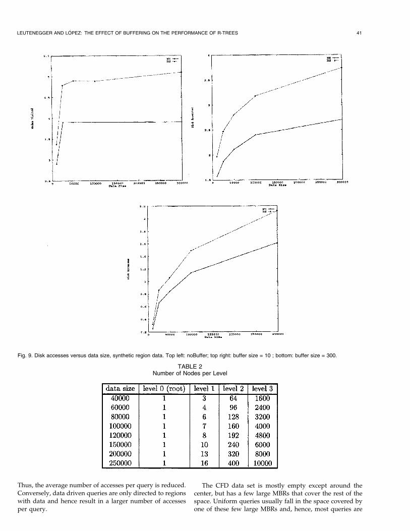
A second experiment shows that ignoring the bufferimpact can introduce significant errors. In Fig. 9, we presentresults for synthetic region data using NX and HS withdifferent buffer sizes. The top left graph plots the number ofnodes visited (i.e., no buffering considered) versus thenumber of rectangles in the data set. The top right graphplots the number of disk accesses versus data set size for abuffer size of 10; and the bottom graph, for a buffer size of300. Ignoring buffer impact (top) leads to the conclusionthat querying an R-tree of 300,000 rectangles is no moreexpensive than querying an R-tree of 25,000 rectangles. Thiscould cause a query optimizer to produce a poor queryplan. Once buffering is considered, the fact that larger treesare more expensive becomes evident.


Fig. 5. CFD Data Set. Left: full data set. Right: detail of center.

Fig. 6. Sensitivity to buffer size, Long Beach data. Left: point queries; right: 1 percent region queries.

5.3 Choosing a Buffer Size

In this section, we study the reduction in disk accessesobtained from increasing the buffer size. Since mainmemory is a valuable resource, some insight into the gainsfrom allocating more buffer space is needed. Consider Fig. 6again, where the number of disk accesses versus buffer sizeis plotted for both point and region queries using theTIGER data set. A node size of 100 rectangles is assumed,resulting in the HS and NX algorithms having 532 pages atthe leaf level, six pages at level 1, and one root node. Buffersize is varied from 2 to 500 pages (from 0.4 percent to 92.8percent of the R-tree).

The left plot is for point queries. The curves, from top tobottom, are TAT, NX, and HS. The R-tree produced by theTAT algorithm is poorly structured and, as a result, seems tobenefit significantly from each increase in buffer size. The HStree is much better structured and, while experiencing ahalving of the number of required disk accesses for a buffersize of 10 percent, additional buffer increases only helpmodestly. The NX algorithm does not experience as much ofa reduction in needed disk accesses for small buffer sizes as

the HS algorithm. We hypothesize that the better the R-treestructure, the more capable it is of capitalizing on smallamounts of buffer for point queries, whereas the worse the R-tree structure, the more linear the reduction in disk accesses.

The right plot is for 1 percent region queries. Note that,for region queries, none of the curves have a well-definedªknee.º Thus, based on this experiment, it appears that,when executing region queries, reductions in disk accessesdue to increasing buffer size behave more linearly than forpoint queries.

5.4 Comparison of Uniform Access and Data DrivenQuery Models

In Fig. 7 and Fig. 8, we compare the performance of uniformqueries with that of data driven queries for the TIGER andCFD data sets, respectively. The left plot in each figure plotsthe number of disk accesses versus the buffer size. The topcurve in each plot is for the data driven model.

The Long Beach data set has large portions of emptyspace in the data set. Uniform queries often fall in theseempty regions and, hence, are pruned at the root of the tree.


Fig. 7. Uniform versus data driven queries, Long Beach data. Left: disk access; right: improvement with buffer size.

Fig. 8. Uniform versus data driven queries, CFD data. Left: disk access; bottom: improvement with buffer size.

Thus, the average number of accesses per query is reduced.Conversely, data driven queries are only directed to regionswith data and hence result in a larger number of accessesper query.

The CFD data set is mostly empty except around thecenter, but has a few large MBRs that cover the rest of thespace. Uniform queries usually fall in the space covered byone of these few large MBRs and, hence, most queries are


Fig. 9. Disk accesses versus data size, synthetic region data. Top left: noBuffer; top right: buffer size = 10 ; bottom: buffer size = 300.

TABLE 2Number of Nodes per Level

going to a small number of nodes, thus increasing the hitrate relative to the data driven queries.

In addition to different quantitative results for uniformversus data driven queries, the two models responddifferently to an increase in buffer size. The right handplot in each figure plots the ratio of (disk accesses for buffersize = 10)/(disk accesses for buffer size = N). This metricdirectly shows the quantitative benefit from adding buffer.The top curve in each plot is for the uniform access model,and the bottom curve is for the data driven model. Considerfirst the Long Beach data set, Fig. 7. Increasing buffer sizefrom 10 to 500 speeds up uniform queries by a factor of 3.91,whereas it improves query performance for data drivenqueries by only a factor of 2.86. The probability of accessinga node under the uniform query access model is the area ofthe MBR. Thus, since the size of nodes varies, some nodeswould be accessed more frequently than others. Increasingbuffer size allows these ªhotº nodes to be found in thebuffer more often. For the data driven model, let's considera simplification of the problem: Assume there is no MBRoverlap. Ignoring overlap, the data driven model wouldresult in each leaf node being accessed with equal

probability. Thus, there are no ªhotº nodes to capitalizeon increased buffer size.

This difference in sensitivity to buffer size is even morepronounced for the CFD data set. For this data set, there is ahigh variance in MBR size and, hence, under the uniformquery model, there are a small number of very hot nodeswhich benefit greatly from additional buffer space. Note, ata buffer size of 100, only 0.06 disk accesses are needed for auniform query on the CFD data set. Thus, the ratios inexcess of 20 are not particularly relevant.

5.5 Choosing the Number of Levels to be Pinned

Past buffer management studies have shown that, forB-trees, the root and maybe the first level should be pinnedin the buffer pool. Pinning nodes decreases the buffer sizeremaining for other pages, but guarantees that the pinnedpages will be in the buffer. We present experiments toinvestigate what gains in performance can be expected frompinning R-tree nodes and how many levels should bepinned.

For the experiments in this section, we wanted to builddeeper R-trees. To do this, we created synthetic point data


Fig. 10. Effect of pinning, disk accesses versus data size for HS. Top left: buffer size = 500; top right: buffer size = 1,000; bottom: buffer size = 2,000.

sets with 40,000 to 250,000 points and used nodes of size 25.This resulted in R-trees with 4 levels and with the numberof nodes per level as shown in Table 2.

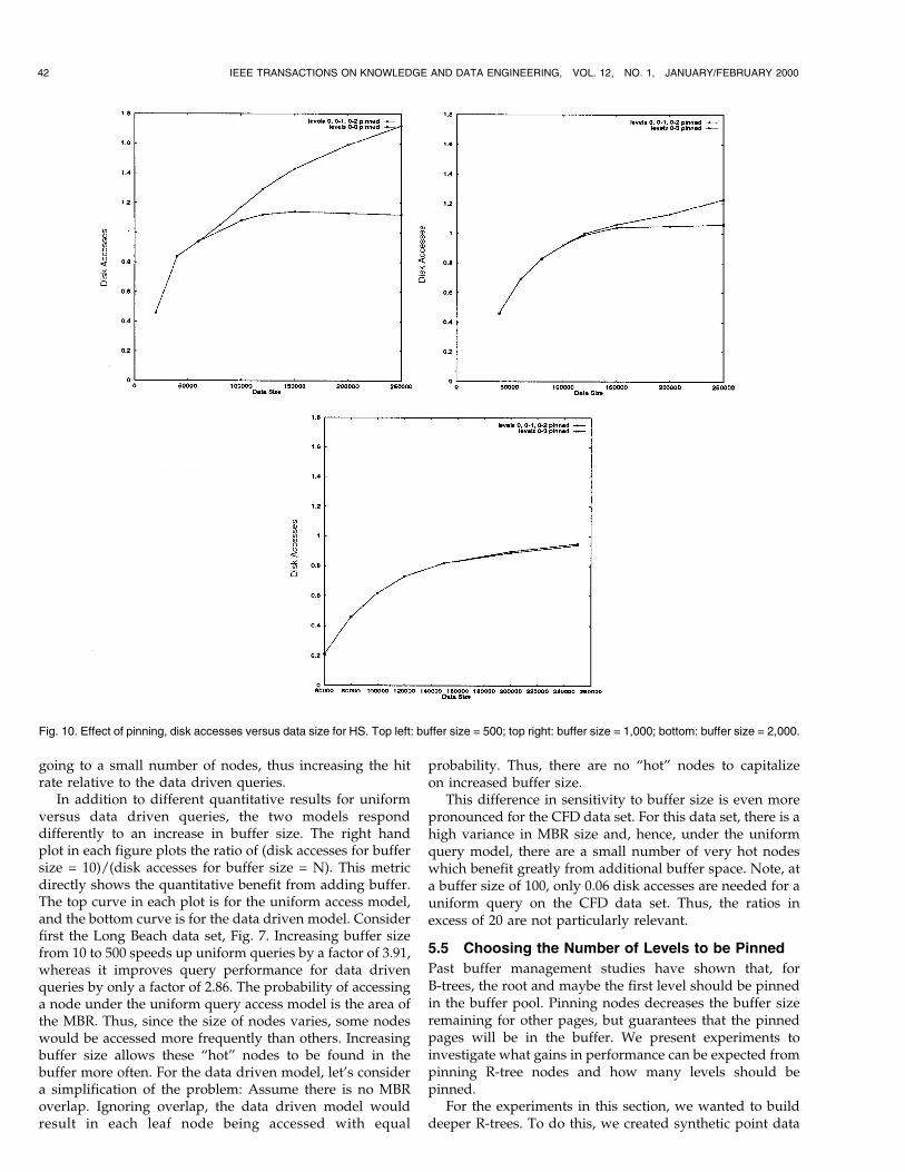
In Fig. 10, we plot the number of disk accesses versusdata sizes for three different buffer capacities using pointqueries on trees created by the HS algorithm. Results for theother algorithms are similar. The plot at the top left is for abuffer of 500 pages; the plot at the top right is for 1,000pages; and the one at the bottom, for 2,000 pages. Thenumber of disk access for not pinning any levels, pinningthe first (root) level, and pinning the first two levels is thesame. All three scenarios are plotted as the single top line inall three graphs. The bottom line is for pinning the firstthree levels.

As a general rule of thumb, pinning a level makes adifference if the total number of pages pinned is at least halfthe buffer size, but when the total number of pages pinnedis less than one third of the buffer size, only marginalbenefits are seen. This is because, for a smaller relativenumber of pinned pages, the LRU replacement policysucceeds in keeping the top levels in the buffer withoutexplicit pinning. For example, for a buffer size of 500 and adata size of 250,000 rectangles, pinning three levels pins 417pages. This results in 53 percent fewer disk accesses. Whenthe data consists of 80,000 rectangles, 135 pages are pinnedand the saving is only 4 percent. For a buffer size of 2,000,pinning of the the first three levels makes almost nodifference since the number of pages pinned is less than onefourth of the buffer size.

Thus, for point queries, pinning levels is advantageous,but only when the total number of nodes pinned is within afactor of two of the buffer size.

Alternatively, we can explicitly plot the benefits ofpinning as a function of buffer size. In the left plot ofFig. 11, we plot the number of disk accesses versus buffersize for the Long Beach data set using uniformly distributedpoint queries on a Hilbert packed R-tree with 25 keys pernode. The top line is for pinning zero, one, or two levels. Inall cases, the performance is identical. The bottom line iswhen three levels are pinned. For large buffer sizes, the

performance is the same. As buffer size decreases, pinningthe third level becomes beneficial. For buffer sizes of lessthan 100, the third level can no longer be pinned and, hence,only two levels can be pinned. Thus, pinning only improvesperformance for a small range of buffer sizes.

The previous experiments demonstrate the limitedbenefits of pinning for point queries. When region queriesare considered, the benefit is even more modest. In the rightplot of Fig. 11, we plot the percent improvement (in terms ofdisk accesses) of pinning relative to no pinning versus theside length, QX, of region queries, for a synthetic data setconsisting of 250,000 points with a buffer of 500 pages. ForQX � 0, this is identical to the largest difference observedin Fig. 10. Parameter QX is varied from 0 to 0.15, resultingin region queries which cover up to 2.25 percent of the unitsquare. The top curve is for pinning three levels; the bottomcurve, for pinning two levels. Pinning one level, i.e., just theroot, is equivalent to no pinning. For point queries, pinningthree levels results in a 35 percent improvement, whereaspinning two levels results in no improvement. As the querysize is increased, the benefits of pinning three levelsdiminish. Larger region queries retrieve a larger numberof leaf level nodes. This number of leaf level nodessignificantly dwarfs the number of nonleaf level nodesreturned, thus diminishing the relative improvement due topinning. Note that, as query size increases, the probabilityof displacing nodes near the root also increases if pinning isnot used. This is why a marginal improvement is gainedfrom pinning two levels as the query size is increased. Asquery size is further increased, this factor becomes lesssignificant than the number of leaf level nodes retrieved.

Finally, we point out that pinning never hurts perfor-mance and, hence, for a fixed size buffer dedicated to anR-tree application, as many levels as possible should bepinned. If the buffer is shared among many applications,the benefit of pinning must be compared to the otherapplications. Given the limited benefit of pinning for pointqueries, and the further reduced benefit for region queries,we suggest that pinning R-trees should not be done unlessbuffer space is not needed by other concurrent database


Fig. 11. Left: Effect of buffer size on benefit of pinning; right: effect of query size on benefit of pinning.

operations. Our buffer model can be used to quantitatively

predict the benefits gained by pinning.

6 CONCLUSIONS

We have developed a new buffer model to predict the

number of disk accesses required per query for a given

R-tree (specified by the minimum bounding rectangles of

each node in the tree). Our model has been shown

experimentally to agree with simulation within 2 percent

for numerous test cases. The model is both simple to

implement and quick to solve, thus providing a useful

methodology for further studies.With our model, we have demonstrated that using the

number of nodes accessed per query as a performance

metric is not sufficient because it ignores buffer effects. We

show that, once buffer effects are taken into account, not

only does quantitative predicted performance change, but

the qualitative predictions can change as well. In particular,

the actual ordering of policies can differ depending on

whether or not the existence of a buffer is taken into

account. Thus, it is essential to consider buffer effects in a

performance study of R-trees and use the number of disk

accesses as the primary metric.We also used our model to determine that, for the data

considered, small amounts of buffer can superlinearly

improve performance of well-structured R-trees for point

queries, but that poorly structured trees see only a more

linear improvement in performance due to the increase in

buffer space. In addition, we find that, for region queries,

even well-structured R-trees see a more linear improvement

as buffer is added.In addition, we show that if a uniform access query

model is assumed for skewed data, significant improve-

ments are achieved by adding more buffer space, whereas if

a data driven query model is assumed, the improvements

are more linear.Finally, we show that, in most cases, pinning the top

levels of the R-tree has little effect on performance relative

to just using an LRU buffer. For point queries, we did find

certain scenarios where, if the buffer size is a about the same

or slightly larger than the number of nodes at a level,

pinning that level does significantly improve performance.

For region queries, the performance improvement obtained

from pinning is diminished.

ACKNOWLEDGMENTS

The authors would like to thank Jeff Edgington for

developing the R-tree packing algorithm code. They would

also like thank Ken Sevcik for useful discussions about a

preliminary version of this work. This work is supported by

NSF grant IRI-9610240 and by Colorado Advanced SoftwareInstitute grant TT-97-05.

REFERENCES

[1] N. Beckmann, H.P. Kriegel, R. Schneider, and B. Seeger, ªTheR?-Tree: An Efficient and Robust Access Method for Points andRectangles,º Proc. ACM SIGMOD, pp. 323-331, May 1990.

[2] A. Bhide, A. Dan, and D. Dias, ªA Simple Analysis of lru BufferReplacement Policy and Its Relationship to Buffer Warm-UpTransient,º Proc. IEEE Int'l Conf. Data Eng. (ICDE), 1993.

[3] A. Guttman, ªR-Trees: A Dynamic Index Structure for SpatialSearching,º Proc. ACM SIGMOD, pp. 47-57, June 1984.

[4] I. Kamel and C. Faloutsos, ªOn Packing R-Trees,º Proc. Second Int'lConf. Information and Knowledge Management (CIKM), Nov. 1993.

[5] I. Kamel and C. Faloutsos, ªHilbert R-Tree: An Improved R-TreeUsing Fractals,º Proc. VLDB Conf., pp. 500-509, Sept. 1994.

[6] S.T. Leutenegger and M.A. Lopez, ªThe Effect of Buffering on thePerformance of R-Trees,º Proc. 15th Int'l Conf. Data Eng. (ICDE'98), pp. 164-171, 1998.

[7] S.T. Leutenegger, M.A. Lopez, and J.M. Edgington, ªStr: A Simpleand Efficient Algorithm for R-Tree Packing,º Proc. 14th Int'l Conf.Data Eng. (ICDE '97), pp. 497-506, 1997.

[8] D.J. Mavriplis, ªAn Advancing Front Delaunay TriangulationAlgorithm Designed for Robustness,º J. Computational Physics,vol. 117, pp. 90-101, 1995.

[9] B.-U. Pagel, H.-W. Six, H. Toben, and P. Widmayer, ªTowards anAnalysis of Range Query Performance in Spatial Data Structures,ºProc. ACM Principles of Database Systems, pp. 214-221, May 1993.

[10] Y.J.R. Garcia, M.A. Lopez, and S.T. Leutenegger, ªOn OptimalNode Splitting for R-Trees,º Proc. Int'l Conf. Very Large Databases(VLDB '98), 1998.

[11] A.L. Rosnberg and L. Snyder, ªTime and Space Optimality inB-Trees,º ACM Trans. Database Systems, vol. 6, no. 1, 1981.

[12] N. Roussopoulos and D. Leifker, ªDirect Spatial Search onPictorial Databases Using Packed R-Trees,º Proc. ACM SIGMOD,May 1985.

[13] T. Sellis, N. Roussopoulos, and C. Faloutsos, ªThe R+ Tree: ADynamic Index for Multidimensional Objects,º Proc. 13th Int'lConf. Very Large Databases (VLDB '87), pp. 507-518, Sept. 1987

[14] Y. Theodoridis and T. Sellis, ªA Model for the Prediction of R-TreePerformance,º Proc. of Eighth Symp. Principles of Database Systems(PODS), May 1996.

Scott T. Leutenegger received the BS degree inmathematics from the University of Wisconsin,Madison, in 1985 and the MS and PhD degreesin computer science from the University ofWisconsin in 1987 and 1990, respectively. From1990 to 1994, he worked as a postdoctoralresearcher at the IBM T.J. Watson ResearchCenter and as a staff scientist at NASA ICASE.He is currently an associate professor at theUniversity of Denver, in Colorado. His past work

includes work in database benchmark modeling, multiprocessor cachearchitectures, and numerical methods for solving Markov chains. Hiscurrent research interests include multidimensional database indexing,performance modeling, parallel/distributed databases, multiprocessorscheduling, parallel/distributed resource management, and databasesupport for scientific visualization. Dr. Leutenegger is a member of theACM and the IEEE Computer Society. He serves as editor-in-chief ofACM SIGMETRICS Performance Evaluation Review.

Mario A. LoÂpez received the BS degree inmathematics, statistics, and computer sciencefrom the University of Wisconsin, Madison, in1980. From 1980 to 1985, he worked as alecturer in the Department of Engineering and asa systems manager in the Computing Center ofthe Universidad Centroamericana JoseÂ SimeoÂnCanÄas in San Salvador. He received the MS andPhD degrees in computer science from theUniversity of Minnesota-Twin Cities in 1987and 1991, respectively. Dr. LoÂpez is an associ-

ate professor in the Department of Mathematics and Computer Scienceat the University of Denver. His current research interests includemultidimensional databases, computer graphics, and computationalgeometry.


The Effect of Buffering on the Performance of R-Trees

Documents

Transcript of The Effect of Buffering on the Performance of R-Trees