Efficient Cost Models for Spatial QueriesUsing R-Trees

Yannis Theodoridis, Member, IEEE, Emmanuel Stefanakis, and Timos Sellis, Member, IEEE

AbstractÐSelection and join queries are fundamental operations in Data Base Management Systems (DBMS). Support for

nontraditional data, including spatial objects, in an efficient manner is of ongoing interest in database research. Toward this goal,

access methods and cost models for spatial queries are necessary tools for spatial query processing and optimization. In this paper,

we present analytical models that estimate the cost (in terms of node and disk accesses) of selection and join queries using R-tree-

based structures. The proposed formulae need no knowledge of the underlying R-tree structure(s) and are applicable to uniform-like

and nonuniform data distributions. In addition, experimental results are presented which show the accuracy of the analytical

estimations when compared to actual runs on both synthetic and real data sets.

Index TermsÐSpatial databases, access methods, query optimization, cost models, R-trees.

æ

1 INTRODUCTION

SUPPORTING large volumes of multidimensional (spatial)data is an inherent characteristic of modern database

applications, such as Geographical Information Systems(GIS), Computer-Aided Design (CAD), Image and multi-media databases. Such databases need underlying systemswith extended features (query languages, data models,indexing methods) as compared to traditional databases,mainly due to the complexity of representing and retrievingspatial data. Spatial Data Base Management Systems(SDBMS), in general, should 1) offer appropriate data typesand query language to support spatial data and 2) provideefficient indexing methods and cost models on the execu-tion of specialized spatial operations, for query processingand optimization purposes [15].

In the particular field of spatial query processing and

optimization, during the last two decades, several data

structures have been developed for point and nonpoint

multidimensional objects in low-dimensional space to meet

needs in a wide area of applications, including the GIS and

CAD domains. Due to the large number of spatial data

structures proposed (an exhaustive survey can be found in

[14]), active research in this field has recently turned to the

development of analytical models that could make accurate

cost predictions for a wide set of spatial queries. Powerful

analytical models are useful in three ways:

1. Structure evaluation: This allows us to better under-stand the behavior of a data structure under variousinput data sets and sizes.

2. Benchmarking: This can play the role of an objectivecomparison point when various proposals forefficient spatial indexing are compared to each other

3. Query optimization: This can be used by a queryoptimizer in order to evaluate the cost of a complexspatial query and its execution procedure.

Spatial queries addressed by users of SDBMS usuallyinvolve selection (point or range) and join operations. In theliterature, most efforts toward the analytical prediction ofthe performance of spatial data structures have focused onpoint and range queries [13], [19], [28], [11], [37], while onlyrecently on spatial join queries [17], [38]. Some proposalssupport both uniform-like and nonuniform data distribu-tions, which is an important advantage, keeping in mindthat modern database applications handle large amounts ofreal (usually nonuniform) multidimensional data.

In this paper, we focus on the derivation of analyticalformulae for range and join queries based on R-trees [16],[4]; such models support data sets of various distributionsand make cost prediction based on data properties only.The proposed formulae are shown to be efficient for severaldistributions of synthetic and real data sets with the relativeerror being around 10-15 percent for any type of data setsused in our experiments.

The rest of the paper is organized as follows: In Section 2,we provide background information about hierarchical treestructures for spatial data, in particular R-tree-based ones,and related work on cost analysis for R-tree-based methods.Section 3 presents cost models for the prediction of the R-tree performance for selection and join queries. In Section 4,comparison results of the proposed models are presentedwith respect to efficient R-tree implementations for differentdata distributions. An extended survey of related workappears in Section 5, while Section 6 concludes the paper.

2 BACKGROUND

Multidimensional data was first involved in geographicalapplications (GIS, cadastral systems, etc.), CAD, and VLSI

IEEE TRANSACTIONS ON KNOWLEDGE AND DATA ENGINEERING, VOL. 12, NO. 1, JANUARY/FEBRUARY 2000 19

. Y. Theodoridis is with the Computer Technology Institute, PO Box 1122,GR-26110, Patras, Hellas. E-mail: ytheod@cti.gr.

. E. Stefanakis and T. Sellis are with the Department of Electrical andComputer Engineering, National Technical University of Athens, Zogra-fou 15773, Athens, Hellas.E-mail: {stefanak, timos}@dbnet.ece.ntua.gr.

Manuscript accepted 28 Sept. 1999.For information on obtaining reprints of this article, please send e-mail to:tkde@computer.org, and reference IEEECS Log Number 110165.

1041-4347/00/$10.00 ß 2000 IEEE

design. Recently, especially due to the development ofextensible DBMS [34], spatial data management techniqueshave been applied to a wide area of applications, fromimage and multimedia databases [9] to data mining andwarehousing [10], [31]. Fig. 1 is motivated by a geographicalapplication, where the database consists of several relations(or classes, etc.) about Europe. In particular, Fig. 1 illustratescapitals and regions of European countries (i.e., point andregion data).

The most common queries on such databases includepoint or range queries on a specified relation (e.g., ªfind allcountries that contain a user-defined pointº or ªfind allcountries that overlap a user-defined query windowº) orjoin queries on pairs of relations (e.g., ªfind all pairs ofcountries and motorways that overlap each otherº).

2.1 Spatial Queries and Spatial Data Structures

The result of the select operation on a relation REL1 using aquery window q contains those tuples in REL1, with thespatial attribute standing in some relation � to q. On theother hand, the result of the join operation between a relationREL1 and a relation REL2 contains those tuples in theCartesian product REL1 �REL2, where the ith column ofREL1 stands in some relation � to the jth column of REL2.

In traditional (alphanumeric) applications, � is oftenequality. When handling multidimensional data, � is aspatial operator, including topological (e.g., overlap), direc-tional (e.g., north), or distance (e.g., close) relationshipsbetween spatial objects. For each spatial operator, withoverlap being the most common, the query object's geometryneeds to be combined with each data object's geometry.

However, the processing of complex representations, suchas polygons, is very costly. For that reason, a two-stepprocedure for query processing, illustrated in Fig. 2, hasbeen widely adopted [23]:

. Filter step: An approximation of each object, such asits Minimum Bounding Rectangle (MBR), is used inorder to produce a set of candidates (and, possibly, aset of actual answers), which is a superset of theanswer set consisting of actual answers and false hits.

. Refinement step: Each candidate is then examinedwith respect to its exact geometry in order toproduce the answer set by eliminating false hits.

The filter step is usually based on multidimensionalindices that organize MBR approximations of spatialobjects [33]. In general, the relationship between twoMBR approximations cannot guarantee the relationshipbetween the actual objects; there are only few operators(mostly directional ones) that make the refinement stepunnecessary [30].

On the other hand, the refinement step usually includescomputational geometry techniques for geometric shapecomparison [26] and, therefore, it is usually a time-consuming procedure since the actual geometry of theobjects need to be checked. Although techniques forspeeding-up this procedure have been studied in the past[5], the cost of this step cannot be considered as part ofindex cost analysis and, hence, it is not taken intoconsideration in the following.

Several methods for spatial indexing have been proposedin the past. They can be grouped in two main categories:indexing methods for points (also known as point accessmethodsÐPAMs) and indexing methods for nonpointobjects (also known as spatial access methodsÐSAMs). Well-known PAMs include the BANG file [12] and the LSD-tree[18], while, among the proposed SAMs, the R-tree [16], theQuadtree [33], and their variants are the most popular. Inthe next section, we describe the R-tree indexing methodand its algorithms for search and join operations.

2.2 The R-tree

The R-tree was proposed by Guttman [16] as a directextension of the B�-tree [20], [7] in d dimensions. The datastructure is a height-balanced tree that consists of inter-mediate and leaf nodes. A leaf node is a collection of entries

20 IEEE TRANSACTIONS ON KNOWLEDGE AND DATA ENGINEERING, VOL. 12, NO. 1, JANUARY/FEBRUARY 2000

Fig. 1. An example of a spatial application: a database of capitals and

regions.

Fig. 2. Two-step spatial query processing: filter and refinement step.

of the form �oid; R�, where oid is an object identifier used torefer to an object in the database and R is the MBRapproximation of the data object. An intermediate node is acollection of entries of the form �ptr; R�, where ptr is apointer to a lower level node of the tree and R is arepresentation of the minimum rectangle that encloses allMBRs of the lower-level node entries.

Let M be the maximum number of entries in a node andlet m �M=2 be a parameter specifying the minimumnumber of entries in a node. An R-tree satisfies thefollowing properties:

1. Every leaf node contains between m and M entriesunless it is the root.

2. For each entry �oid; R� in a leaf node, R is thesmallest rectangle that spatially contains the dataobject represented by oid.

3. Every intermediate node has between m and Mchildren unless it is the root.

4. For each entry �ptr; R� in an intermediate node, R isthe smallest rectangle that completely encloses therectangles in the child node pointed by ptr.

5. The root node has at least two children unless it is aleaf.

6. All leaves appear in the same level.

After Guttman's proposal, several researchers proposedtheir own improvements on the basic idea. Among others,Roussopoulos and Leifker [32] proposed the packed R-tree,for the case that data rectangles are known in advance (i.e.,it is applicable only to static databases), Sellis et al. [35]proposed the R�-tree, a variant which guarantees disjoint-ness of nodes by introducing redundancy, and Beckmann etal. [4] proposed the R�-tree, an R-tree-like structure thatuses a rather complex, but more effective, groupingalgorithm. Gaede and Guenther [14] offer an exhaustivesurvey of multidimensional access methods includingseveral other variants of the original R-tree technique. Asan example, Fig. 3 illustrates a set of data rectangles and thecorresponding R-tree built on these rectangles (assumingmaximum node capacity M � 4).

The processing of any type of spatial query can beaccelerated when a spatial index (e.g., an R-tree) exists.Selection queries, for example, perform a traversal of theR-tree index: Starting from the root node, several treenodes are accessed down to the leaves, with respect to theresult of the overlap operation between q and the

corresponding node rectangles. When the search algorithmfor spatial selection (so-called SS) accesses the leaf nodes,all data rectangles that overlap the query window q areadded into the answer set.

// Spatial Selection Algorithm for R-treesSS (R1: R-tree node, q: rectangle)01 BEGIN02 FOR all Er1 in R1 DO03 IF Er1.rect overlaps q THEN04 IF R1 is a leaf page THEN05 Output (Er1.oid)06 ELSE07 ReadPage (Er1.ptr);08 SS (Er1.ptr, q)09 END-IF10 END-IF11 END-FOR12 END.

On the other hand, the join operation between twospatial relations REL1 and REL2 can be implemented byapplying synchronized tree traversals on both R-treeindices. An algorithm based on this general idea, calledSpatialJoin1, was originally introduced by Brinkhoff et al. in[3]. Two improvements of this algorithm were alsoproposed in the same paper toward the reduction of theCPU- and I/O-cost by taking into consideration faster main-memory algorithms, and better read schedules for a givenLRU-buffer, respectively. Specifically, for two R-treesrooted by nodes R1 and R2, respectively, the spatial joinprocedure (algorithm SJ) is as follows:

// Spatial Join Algorithm for R-treesSJ (R1, R2: R-tree nodes)01 BEGIN02 FOR all Er2 in R2 DO03 FOR all Er1 in R1 DO04 IF Er1.rect overlaps Er2.rect THEN05 IF R1 and R2 are leaf pages THEN06 Output (Er1.oid, Er2.oid)07 ELSE IF R1 is a leaf node THEN08 ReadPage (Er2.ptr);09 SJ (Er1.ptr, Er2.ptr)10 ELSE IF R2 is a leaf node THEN11 ReadPage (Er1.ptr);12 SJ (Er1.ptr, Er2.ptr)

THEODORIDIS ET AL.: EFFICIENT COST MODELS FOR SPATIAL QUERIES USING R-TREES 21

Fig. 3. Some rectangles organized to form an R-tree, and the corresponding R-tree.

13 ELSE14 ReadPage(Er1.ptr); ReadPage(Er2.ptr);15 SJ(Er1.ptr, Er2.ptr)16 END-IF17 END-IF18 END-FOR19 END-FOR20 END.

In other words, a synchronized traversal of both R-treesis performed, with the entries of nodes R1 and R2 playingthe roles of data and query rectangles, respectively, in aseries of range queries.

For both operations, the total cost is measured by thetotal amount of page accesses in the R-tree index (theprocedure ReadPage in the above algorithms). This proce-dure either performs an actual read operation on the disk orreads the corresponding node information from a memory-resident buffer, thus we distinguish between node and diskaccesses in the analytical study that follows. (The distinctionbetween node and disk accesses is a subject of cache policy.By definition, the number of node accesses is always greaterthan or equal to the number of actual disk accesses; theequality only holds for the case where no buffering schemeexists.)

3 ANALYTICAL COST MODELS FOR SPATIAL

QUERIES

Complex queries are usually transformed by DBMS queryoptimizers to a set of simpler ones and the executionprocedure takes the partial costs into account in order toschedule the execution of the original query. Thus, queryoptimization tools that estimate access cost and selectivityof a query are complementary modules together with accessmethods and indexing techniques. Traditional optimizationtechniques usually include heuristic rules, which, however,are not effective in spatial databases due to the peculiarityof spatial data sets (multidimensionality, lack of totalordering, etc.). Other, more sophisticated, techniquesinclude histograms and cost models. Although researchon multidimensional histograms has recently appeared inthe literature [24], in the spatial database literature, costmodels for selectivity and cost estimation seem to be themost promising solutions.

Proposals in this area include models for spatial selection[13], [19], [28], [21] and spatial join [2], [17]. However, aswill be discussed later, in Section 5, most of those proposalsrequire knowledge of index properties and/or make a uni-formity assumption, thus rendering them incomplete tools forthe practical purposes of query optimization. In [37], 38], weproposed appropriate extensions to solve those problems,which are formally presented in the rest of the section.Throughout our discussion we use the list of symbols thatappear in Table 1.

3.1 Selection Queries

Formally, the problem of the R-tree cost analysis forselection queries is defined as follows: Let d be thedimensionality of the data space and WS � �0; 1�d the d-dimensional unit workspace. Let us assume that NR1

data

rectangles are stored in an R-tree index R1 and a query

asking for all rectangles that overlap a query window q ��q1; . . . ; qd� needs to be answered. What is sought is a

formula that estimates the average number NA of node

accesses using only knowledge about data properties (i.e.,

without extracting information from the underlying R-tree

structure).

Definition. The density D of a set of N rectangles with average

extent s � �s1; . . . ; sd� is the average number of rectangles

that contain a given point in d-dimensional space.

Equivalently, D can be expressed as the ratio of the sum

of the areas of all rectangles over the area of the available

workspace. If we consider a unit workspace �0; 1�d, with

area equal to 1, then the density D�N; s� is given by the

following formula:

D N; s� � �XN

Ydk�1

sk � N �Ydk�1

sk: �1�

Assume now an R-tree R1 of height hR1(the root is

assumed to be at level hR1and leaf-nodes are assumed to be

at level 1). If NR1;l is the number of nodes at level l and sR1;l

is their average size, then the expected number of node

accesses in order to answer a selection query using a query

window q is defined as follows (assuming that the root node

is stored in main memory):

NA total R1; q� � �XhR1ÿ1

l�1

intsect NR1;l; sR1;l; qÿ �

; �2�

where intsect�NR1;l; sR1;l; q� is a function that returns the

number of nodes at level l intersected by the query

window q. In other words, (2) expresses the fact that the

expected number of node accesses is equal to the expected

number of intersected nodes at each level.

Lemma. Given a set of N rectangles r1; . . . ; rN with average

extent s and a rectangle r with extent q, the average number of

rectangles ri intersected by r is:

intsect N; s; q� � � N �Ydk�1

sk � qk� �: �3�

Proof. The average number of a set of N rectangles with

average extent s that intersect a rectangle r with extent q

is equal to the number of a second set of N rectangles

with average extent s0 (where s0k � sk � qk; 8k) that

contain a point in the workspace. The latter one, by

definition, equals to the density D0 of the second set of

rectangles. Formally:

intsect N; s; q� � � intsect N; s0; 0� � � D0 N; s0� � � N �Ydk�1

s0k;

where s0k � sk � qk. tuAssuming that rectangle r represents a query window on

R1, we derive NA total�R1; q� by combining (2) and (3):

22 IEEE TRANSACTIONS ON KNOWLEDGE AND DATA ENGINEERING, VOL. 12, NO. 1, JANUARY/FEBRUARY 2000

NA total R1; q� � �XhR1ÿ1

l�1

NR1;l �Ydk�1

sR1;l;k � qkÿ �( )

: �4�

In order to reach our goal, we have to express (4) as afunction of the data properties NR1

(number of datarectangles or, in other words, cardinality of the data set)and DR1

(density of the data set) or, equivalently, expressthe R-tree properties hR1

, NR1;l, and sR1;l;k as functions of thedata properties NR1

and DR1.

The height hR1of an R-tree R1 with average node

capacity (fanout) f that stores NR1data rectangles is given

by the following formula [13]:

hR1� 1� logf

NR1

f

� �: �5�

Since a node organizes, on the average, f rectangles, wecan assume that the average number of leaf nodes (i.e.,l � 1) is NR1;1 � NR1

=f , and so on. Hence, in general, theaverage number of R-tree nodes at level l is

NR1;l � NR1=fl: �6�

A second assumption in our analysis is that we considersquare node rectangles (i.e., sR1;l;1 � � � � � sR1;l;d; 8l). Thissquaredness assumption is a reasonable property for a ªgoodºR-tree [19]. According to that assumption and (1) and (6),the average extent sR1;l;k of node rectangles at level l is afunction of their density DR1;l:

DR1;l � NR1;l �Ydk�1

sR1;l;k �NR1

fl� sR1;l;k

ÿ �d)sR1;l;k � DR1;l �

fl

NR1

� �1=d

:

�7�

What remains to be estimated is DR1;l. Suppose that, atlevel l, NR1;l nodes with average size �sR1;l;k�d are

organized in NR1;l�1 parent nodes with average size�sR1;l�1;k�d. As described in [39], each parent node groupson the average f child nodes and f1=d out of them areresponsible for the size of the parent node along eachdirection. The centers of the NR1;l node rectangles'projections are assumed to be equally distanced and thisdistance (denoted by tl;k) depends on N

1=dR1;l

nodes alongeach direction. Hence, the average extent sR1;l�1;k of aparent node along each direction is calculated by:

sR1;l�1;k � f1=d ÿ 1� �

� tl;k � sR1;l;k; �8�

where tl;k is:

tl;k � 1=NR1;l1=d; 8l; �9�

denoting the distance between the centers of two con-secutive rectangles' projections on dimension k. (To derive(9), we divided the extent of the unit workspace by thenumber of different node projections on dimension k.)

Lemma. Given a set of NR1;l node rectangles with density DR1;l,the density DR1;l;k of their projections is derived by thefollowing formula:

DR1;l;k � DR1;l �NR1;ldÿ1

ÿ �1=d: �10�

Proof. Straightforward by applying (1), (6), and (7) (forproof details see [39]). tu

Using (8), (9), and (10), the density DR1;l�1 of noderectangles at level l� 1 is a function of the density DR1;l ofnode rectangles at level l:

DR1;l�1 � 1�D1=dR1;lÿ 1

f1=d

!d

: �11�

THEODORIDIS ET AL.: EFFICIENT COST MODELS FOR SPATIAL QUERIES USING R-TREES 23

TABLE 1List of Symbols

Essentially, by using (11), the density at each level of the

R-tree can be calculated as only a function of the density

DR1of the data rectangles (which, according to the

terminology adopted, can be named DR1;0).At this point, the original goal of our analysis has been

reached. By combining (4), (5), (6), (7), and (11), the

expected number NA total�R1; q� of node accesses for a

selection query can be computed by using only the data set

properties NR1and DR1

, the typical R-tree parameter f , and

the query window q.

3.2 Join Queries

According to the discussion of Section 2.2, the processing

cost of a join query is equal to the total cost of a set of

appropriate range queries, according to the procedure

described in the algorithm SJ. In this section, we propose

a formula that estimates the cost of a join query.Formally, the problem of R-tree cost analysis for join

queries is defined as follows: Let d be the dimensionality of

the workspace and WS � �0; 1�d the d-dimensional unit

workspace. Let us assume two spatial data sets of

cardinality NR1and NR2

, with the corresponding MBR

approximations of spatial data being stored in two R-tree

indices R1 and R2, respectively. In correspondence with

Section 3.1, the goal of the cost analysis in this section is a

formula that would efficiently estimate the average number

of nodes accessed in order to process a join query between

the two data sets, based on the knowledge of the data

properties only and without extracting information from

the corresponding R-tree structures.Let the height of an R-tree Ri �i � 1; 2� be equal to hRi

and assume that both root nodes are stored in main

memory. At each level li, 1 � li � hRiÿ 1, Ri contains

NRi;li nodes of average size sRi;li , each node consisting of a

set of entries ERi;li . Thus, in order to find which pairs of

entries are overlapping and downward traverse the two

structures, we compare entries ER1;l1 with entries ER2;l2

(line 04 of the spatial join algorithm SJ).The cost of the above comparison at each level is the sum

of two factors, which correspond to the costs for the two R-

trees, namely NA�R1; R2; l1� and NA�R2; R1; l2�, respec-

tively. The above factors can be calculated by considering

that the entries of R1 (respectively, R2) play the role of the

data set (respectively, a set of query windows q); then we

can derive the pairs of intersecting nodes for each R-tree ((3)

in Section 3.1) in order to estimate the total access cost. Since

we do not consider the existence of a buffering scheme, the

access costs for both R-trees R1 and R2 at the corresponding

levels l1 and l2 are equal (since an equal number of nodes

are accessed, as can be extracted by algorithm SJ, line 14).

Line 04 of the SJ algorithm is repeatedly called at each level

of the two trees down to the leaf level of the shorter tree R2

(without loss of generality, it is assumed that hR1� hR2

).Formally, for the upper hR2

ÿ 1 levels of the two R-trees:

NA R1; R2; l1� � � NA R2; R1; l2� ��XNR2 ;l2

intsect NR1;l1 ; sR1;l1 ; sR2;l2

ÿ �) . . .

) NA R1; R2; l1� �� NA R2; R1; l2� �

� NR2;l2 �NR1;l1 �Ydk�1

sR1;l1;k � sR2;l2;k

ÿ �;

�12�where hR1

ÿ hR2� 1 � l1 � hR1

ÿ 1 and 1 � l2 � hR2ÿ 1.

In [38], we provide a slightly different formula: inparticular, instead of the factor sR1;l1;k � sR2;l2;k

ÿ �, an upper

bound min 1; sR1;l1;k � sR2;l2;k

ÿ �� is presented. Since, in the

whole discussion of the present section, we discuss unitworkspace, such a bound is already a presupposition in (3),(4), and (12).

After the leaf nodes of the short tree R2 have beenaccessed, l2 is fixed to value 1 (i.e., denoting the leaf level)and the propagation of R1 continues down for anotherhR1ÿ hR2

levels. Overall, (13) estimates the total cost interms of R-tree node accesses for a spatial join:

NA total R1; R2� � �XhR1ÿ1

l1�1

NA R1; R2; l1� � �NA R2; R1; l2� �f g;

�13�where

l2 � l1 ÿ hR1ÿ hR2

� �; hR1ÿ hR2

� 1 � l1 � hR1ÿ 1

1; 1 � l1 � hR1ÿ hR2

:

�The involved parameters in (13) are:

. hRi, calculated by (5),

. NRi;li , calculated by (6) as a function of the actualcardinality NRi

of the corresponding data set, and. sRi;li;k , calculated by (7) as a function of the density

DRi;li of node rectangles at level li (which, in turn, iscalculated by (11) as a function of the actual densityDRi

of the corresponding data set).

Qualitatively, (13) estimates the cost of a join querybetween two spatial data sets based on their primitiveproperties only, namely number and density of datarectangles, in correspondence with the analysis for rangequeries (Section 3.1). Note that (13) is symmetric withrespect to the two indices R1 and R2. The same conclusion isdrawn by the study of the algorithm SJ since the number ofnode accesses is equal to the number of ReadPage calls(line 14) which, in turn, are the same for both trees. Theequivalence of the two indices is not the case when a simplepath buffer (i.e., a buffer that stores the most recently visitedpath for each R-tree) is introduced, as we will discuss in thenext section.

3.3 Introducing a Path Buffer

Extending previous analysis, we introduce a simple buffer-ing mechanism that maintains a path buffer for theunderlying tree structure(s). The existence of such a buffermainly affects the performance of the tree index that playsthe role of the query set (namely R2), as will be discussed in

24 IEEE TRANSACTIONS ON KNOWLEDGE AND DATA ENGINEERING, VOL. 12, NO. 1, JANUARY/FEBRUARY 2000

detail in this section, since the search procedure (algorithm

SJ), reads R2 entries less frequently than R1 entries. With

respect to that, we assert that the cost of a selection query in

terms of disk accesses DA total�R1; q� can be considered

equal to NA total�R1; q�, as formulated in (4), without loss

of accuracy and, therefore, provide no further analysis for

path buffering. Moreover, the effect of a buffering mechan-

ism (e.g., an LRU buffer) has been already addressed in the

literature [21] and, according to experimental results, very

low buffer size (such as that of a path buffer) causes almost

zero impact on point and range query performance. On the

other hand, even a simple path buffer scheme highly affects

the actual cost of a join query.As already mentioned, by examining algorithm SJ, we

conclude that the existence of such a buffering scheme

mainly affects the computation of the cost for R2 because its

entries constitute the outer loop of the algorithm and, hence,

are less frequently updated. As for R1, since its entries

constitute the inner loop of the algorithm, the respective

cost computation is not considerably affected by the

existence of a path buffer. These arguments are more

formally described through the following alternative cases

(for more details through an example, see [39]):

1. Suppose that an entry ER2;l2 of tree R2 at level l2overlaps with m entries of a node ER1;l1�1, m entriesof a different node E0R1;l1�1, etc., of the tree R1. ER2;l2

is kept in main memory during its comparison withall entries of node ER1;l1�1 and will be again fetchedfrom disk, hence, recomputed in DA�R2; R1; l2� cost,when its comparison with the entries of node E0R1;l1�1

starts. As a result, the number of actual disk accessesof the node rooted by ER2;l2 is equal to the number ofthe nodes of R1 at level l1 � 1 (i.e., the parent level)having rectangles intersected by ER2;l2 ; formally, it isintsect�NR1;l1�1; sR1;l1�1; sR2;l2�.

2. On the other hand, an entry ER1;l1 of tree R1 at level l1is recomputed in DA�R1; R2; l1� as soon as it over-laps with an entry ER2;l2 of tree R2 with a singleexception: In case ER1;l1 is the last member of theintersection set of ER2;l2 and, at the same time, it isthe first member of the intersection set of itsconsecutive E0R2;l2

. The above exception happensrarely; moreover, it is hardly modeled since no ordercan be assumed among R-tree node entries.

Since the cost for the tree that plays the role of the query

(data) set is affected in a high (low) degree, we distinguish

between two different cases: R1 that plays the role of the

data set being 1) taller (or of equal height) or 2) shorter than

R2. In the first case (hR1� hR2

), the propagation of R1 down

to its lower levels adds no extra cost (in terms of disk

accesses) to the ªqueryº tree R2 that has already reached its

leaf level. In the second case (hR1< hR2

), each propagation

of the ªqueryº tree R2 down to its lower levels adds equal

cost to the ªdataº tree R1 (denoting that buffer existence

does not affect the cost of R1).Overall, with respect to the above discussion, the access

cost of each tree at a specific level li is calculated according

to the following formulae:

DA R1; R2; l1� � � NA R1; R2; l1� � �14�

DA R2; R1; l2� � �XNR2 ;l2

intsect NR1;l1�1; sR1;l1�1; sR2;l2

ÿ �� NR2;l2 �NR1;l1�1 �

Ydk�1

sR1;l1�1;k � sR2;l2;k

ÿ ��15�

and the total cost is given by (16) (note that if hR1� hR2

,then l2 � l1 ÿ �hR1

ÿ hR2�, else l1 � l2 ÿ �hR2

ÿ hR1�.

DA total R1; R2� � �PhR1ÿ1

l1�hR1ÿhR2

�1

DA R1; R2; l1� �f

�DA R2; R1; l2� �g

� PhR1ÿhR2

l1�1

DA R1; R2; l1� �;

if hR1� hR2

PhR2ÿ1

l2�hR2ÿhR1

�1

DA R1; R2; l1� �f

�DA R2; R1; l2� �g

� PhR2ÿhR1

l2�1

2 �DA R1; R2; l1� �f g;

if hR1< hR2

8>>>>>>>>>>>>>>>>>>>><>>>>>>>>>>>>>>>>>>>>:

�16�

Again, the involved parameters hRi, NRi;li , and sRi;li;k are

calculated as functions of NRiand DRi

. Note that, in contrastto (13), (16) is sensitive to the two indices, R1 and R2. Theexperimental results of Section 4 also strengthen thisobservation.

In the above analysis, we have taken two cases intoconsideration: adopting either zero or a simple path bufferscheme. A more complex buffering scheme (e.g., an LRUbuffer of predefined size) would surely achieve a lowervalue for DA total��. However, its effect is beyond the scopeof this paper (see [17], [21] for related work).

3.4 Support for Nonuniform Data Sets

The proposed analytical model assumes data uniformity inorder to compute the density of the R-tree node rectanglesat a level l� 1 as a function of the density of the child noderectangles at level l (11). In particular, in order to derive (8)and (9), the centers of the NR1;l node rectangles' projectionswere assumed to be equally distanced. This uniformityassumption [13] leads to a model that could be efficient foruniform-like data distributions, but hardly applicable tononuniform distributions of data, which are the rule whendealing with real applications.

In order to adapt the model in a way that wouldefficiently support several types of data sets (uniform ornonuniform ones), we reduce the global uniformity assump-tion of the analytical model (i.e., by considering the wholeworkspace) to a local uniformity assumption (by consider-ing a small subarea of the workspace) according to thefollowing motivation: The densityof a data set is involved inthe cost formulae as a single number DRi

. However, fornonuniform data sets, density is a varying parameter,graphically a surface in d-dimensional space. Such a surfacecould show strong deviations from point to point of theworkspace, compared to the average value. For example, in

THEODORIDIS ET AL.: EFFICIENT COST MODELS FOR SPATIAL QUERIES USING R-TREES 25

Fig. 4, the density surface of a real data set, called Lbeach, is

drawn (see Fig. 5 in Section 4 for an illustration of the Lbeach

data set [6]).The average density of this data set is Davg � 0:13.

However, as extracted from Fig. 4, the actual density varies

from D � 0:0 (in zero-populated areas, such as the upper-

left and bottom-right corners) up to D � 2:0 (in high-

populated areas), with respect to the reference point.

Evidently, using the Davg value in a cost formula would

usually provide inaccurate estimations. On the other hand,

a satisfactory illustration of the density surface provides

more accurate D values with respect to a specified query

window q. Although the cardinality of a data set could be

very large, a near-to-the-actual density surface can usually

be computed by examining a sample of the data set

(efficient sampling algorithms have been proposed, among

others, by Vitter in [40], [41]).Based on the above idea, the proposed cost formulae

could efficiently support either uniform or nonuniform data

distributions after the following adaptations:

1. The average density DRiof the data set is replaced

by the actual density D0Riof the data set within the

area of the specified query window q.2. The amount NRi

of the data set is transformed toN 0Ri

, which is computed as follows:

N 0Ri� D0Ri

=DRi

� ��NRi

:

Note that, in discrete space, the average density of a data

set is always DRi> 0, even for point data sets; DRi

� 0

corresponds to zero-populated areas only.In this section, we provided analytical formulae for the

cost estimation of selection or join queries on spatial data

sets organized by disk-resident R-tree indices. The pro-

posed cost models are based on primitive data properties

only, without any knowledge of the corresponding R-trees.

In the next section, we evaluate our model by comparing

the analytical estimations with experimental results on

synthetic and real data sets in one- and two-dimensional

space.

4 EVALUATION OF THE COST MODELS

The evaluation of the analytical formulae proposed inSection 3 is based on a variety of experimental tests onsynthetic and real data sets illustrated in Fig. 5. Syntheticone- and two- dimensional data sets consist of random(Fig. 5a) and skewed (Fig. 5b) distributions of varyingc a r d i n a l i t y N ( 20K � N � 80K) a n d d e n s i t y D(0:2 � D � 0:8), and have been constructed by usingrandom number generators. Real two-dimensional datasets are parts of the TIGER/Line database of the U.S.Bureau of Census [6]. In particular, we have used twoTIGER data sets: 1) the LBeach data set, consisting of 53,143line segments (stored as rectangles) indicating roads ofLong Beach, California (Fig. 5c) and 2) the MGcounty dataset, consisting of 39,221 line segments (stored as rectangles)indicating roads of Montgomery County, Maryland(Fig. 5d).

For the experimental tests we built R�-trees [4] andperformed several spatial joins using the above data sets.All experimental results were run on an HP700 workstationwith 256 Mbytes of main memory. On the other hand, theanalytical estimations of node accesses for selection querieswere based on (4) and the node (respectively, disk) costestimations for join queries were based on (13) (respec-tively, (16)) with the average capacity of the tree indices setto the typical 67 percent value.

4.1 Experiments on Uniform-like Data Sets

We present several test results in order to evaluate the costestimation of (4) for selection (either point or range) queries.Fig. 6 illustrates the results for two random data sets(N � 40K and 80K, respectively, both with density D � 0:1).The relative error was always below 10 percent for the twoexperiments illustrated in Fig. 6, as well as for the restexperiments with random data sets.

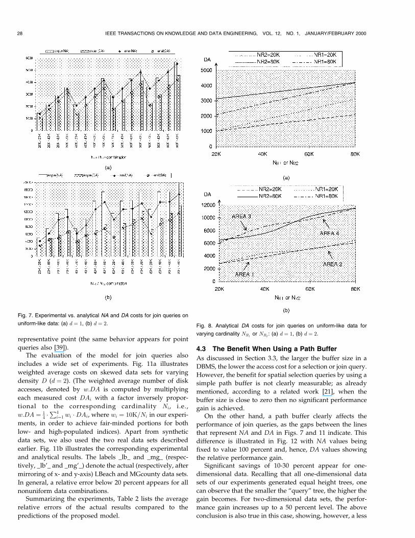
As a further step, we evaluated the analytical formulaefor join query estimation, presented in Section 3, on variousR-tree combinations. Fig. 7 illustrates the experimental andanalytical results of node and disk accesses (denoted by NAand DA) for 1) one- and 2) two-dimensional random datasets, respectively, for all NR1

=NR2combinations.

The nonlinearity of the plots in Fig. 7b is due to the factthat all R-tree indices are not of equal height; the height of

26 IEEE TRANSACTIONS ON KNOWLEDGE AND DATA ENGINEERING, VOL. 12, NO. 1, JANUARY/FEBRUARY 2000

Fig. 4. The density surface of a real data set.

the two-dimensional indices of cardinality 20K � N � 40K

(respectively, 60K � N � 80K) is equal to h � 3 (respec-tively, h � 4), while the height of all one-dimensionalindices is equal to h � 3. According to our experiments, italso turns out that the cost formulae for the estimation ofdisk accesses DA are nonsymmetric with respect to the treesR1 and R2, a fact that has been already mentioned duringthe presentation of the cost models in Section 3.

The comparison results confirm that, for tree indices ofequal height, the choice of the smaller (larger) index to playthe role of the ªqueryº (ªdataº) tree is the best choice for theeffectiveness of the SJ algorithm, which, however, is not ageneral rule for trees of different height, as illustrated inFig. 8 (areas 2 and 3 in Fig. 8 do not obey this rule).

Summarizing the results for join queries on random(uniform-like) data sets, we conclude that:

1. When no buffering scheme is considered, theaccuracy of the estimation is high (the relative errornever exceeds 10 percent).

2. When a path buffer is adopted then the estimatedcost of R2 is always very close to the actual cost(relative error usually below 5 percent), while theestimated cost of R1 is usually within 10-15 percentof the experimental result. The accuracy of theestimation concerning R2 (i.e., the ªqueryº tree inthe join procedure) is expected since the existence ofa buffer has been taken into account in (15), while(14) assumes that the buffer existence does not affectR1 (i.e., the ªdataº tree in the join procedure), anassumption that reduces the accuracy of the estima-tion for the access cost of R1. However, as already

mentioned in Section 3.2, the exception to the rule ishardly modeled.

4.2 Nonuniform Data Sets

As explained in Section 3, a transformation of the actual

density of each nonuniform data set is necessary in order

to reduce the impact of the uniformity assumption of the

underlying analytical model from global (i.e., assuming

the global workspace) to local (i.e., assuming a small

subarea of the workspace). In other words, instead of

considering the average density Davg of a data set, the

cost formulae ((4), (13), and (16)) consider the values of

the density surface D�x; y� that correspond to the

appropriate areas of the workspace. For experimentation

purposes, we extracted a density surface for each

nonuniform data set using a grid of 40� 40 cells, i.e., a

step of 0.25 percent of the workspace per axis.Fig. 9 illustrates average results for selection queries on

skewed (d � 2, D � 0:1, N � 40K or 80K) and real (LBeach

and MGcounty) data sets. The analytical results (respec-

tively, experimental results) are plotted with dotted

(respectively, solid) lines. The relative error is usually

around 10-15 percent and this was the rule for all data sets

that we tested.The flexibility of the proposed analytical model on

nonuniform distributions of data, using the density surface,

is also extracted from the results of our experiments. Fig. 10

illustrates the results for range queries (query rectangles of

size 0:12) around nine representative points on the above

skewed and real data sets (d � 2). Note that the analytical

estimate always follows the experimental value for each

THEODORIDIS ET AL.: EFFICIENT COST MODELS FOR SPATIAL QUERIES USING R-TREES 27

Fig. 5. Two-dimensional data sets used in the experiments: (a) synthetic random (uniform-like) data, (b) synthetic skewed (Zipf) data, (c) LBeach real

data, (d) MGcounty real data.

Fig. 6. Performance comparison for selection queries on uniform-like data (d � 2, D � 0:1, N � 40K or 80K, log scale).

representative point (the same behavior appears for point

queries also [39]).The evaluation of the model for join queries also

includes a wide set of experiments. Fig. 11a illustrates

weighted average costs on skewed data sets for varying

density D (d � 2). (The weighted average number of disk

accesses, denoted by w:DA is computed by multiplying

each measured cost DAi with a factor inversely propor-

tional to the corresponding cardinality Ni, i.e.,

w:DA � 14 �P4

i�1 wi �DAi, where wi � 10K=Ni in our experi-

ments, in order to achieve fair-minded portions for both

low- and high-populated indices). Apart from synthetic

data sets, we also used the two real data sets described

earlier. Fig. 11b illustrates the corresponding experimental

and analytical results. The labels _lb_ and _mg_ (respec-

tively, _lb'_ and _mg'_) denote the actual (respectively, after

mirroring of x- and y-axis) LBeach and MGcounty data sets.

In general, a relative error below 20 percent appears for all

nonuniform data combinations.Summarizing the experiments, Table 2 lists the average

relative errors of the actual results compared to the

predictions of the proposed model.

4.3 The Benefit When Using a Path Buffer

As discussed in Section 3.3, the larger the buffer size in a

DBMS, the lower the access cost for a selection or join query.

However, the benefit for spatial selection queries by using a

simple path buffer is not clearly measurable; as already

mentioned, according to a related work [21], when the

buffer size is close to zero then no significant performance

gain is achieved.On the other hand, a path buffer clearly affects the

performance of join queries, as the gaps between the lines

that represent NA and DA in Figs. 7 and 11 indicate. This

difference is illustrated in Fig. 12 with NA values being

fixed to value 100 percent and, hence, DA values showing

the relative performance gain.Significant savings of 10-30 percent appear for one-

dimensional data. Recalling that all one-dimensional data

sets of our experiments generated equal height trees, one

can observe that the smaller the ªqueryº tree, the higher the

gain becomes. For two-dimensional data sets, the perfor-

mance gain increases up to a 50 percent level. The above

conclusion is also true in this case, showing, however, a less

28 IEEE TRANSACTIONS ON KNOWLEDGE AND DATA ENGINEERING, VOL. 12, NO. 1, JANUARY/FEBRUARY 2000

Fig. 7. Experimental vs. analytical NA and DA costs for join queries on

uniform-like data: (a) d � 1, (b) d � 2. Fig. 8. Analytical DA costs for join queries on uniform-like data for

varying cardinality NR1or NR2

: (a) d � 1, (b) d � 2.

uniform behavior, which is due to the different index

heights.

5 RELATED WORK

In the survey of this section, we present previous work

on analytical performance studies for spatial queries

using R-trees. Several findings from those proposals have

been used as starting points for consequent studies and our

analysis as well.The earlier attempt to provide an analysis for R-tree-

based structures appeared in [13]. Faloutsos et al. proposed

a model that estimates the performance of R-trees and R�-

trees for selection queries, assuming, however, uniform

distribution of data and packed trees (i.e., all the nodes of the

tree are full of data). The formulae for the height of an R-tree as a function of its cardinality and fanout (5) and for the

average size of a parent node as a function of the averagesize of the child nodes and the average distance between

two consecutive child nodes' projections (8) were originallyproposed in [13].

Later, Kamel and Faloutsos [19] and Pagel et al. [28]

independently presented a formula (actually a variation of(2)) that calculates the average number of page accesses in

an R-tree accessed by a query window as a function of theaverage node size and the query window size. Since, for

practical query optimization purposes, R-tree propertiessuch as the average node size cannot be assumed to beknown in advance, that analysis is qualitative, i.e., it cannot

provide an accurate cost prediction but rather presents the

THEODORIDIS ET AL.: EFFICIENT COST MODELS FOR SPATIAL QUERIES USING R-TREES 29

Fig. 9. Performance comparison for selection queries on (a) skewed and (b) real data.

Fig. 10. Performance comparison for selection queries around representative points: range queries on (a) skewed data, (b) real data.

Fig. 11. Experimental vs. analytical NA and DA costs for join queries on (a) skewed and (b) real data.

effect of three parameters, namely area, perimeter, andnumber of objects, on the R-tree performance. In thosepapers, the influence of the node perimeters was revealed,thus helping one to understand the efficiency of the R�-tree,which was the first R-tree variant to take the node perimeterinto consideration during the index construction procedure[28]. Extending the work of [28], Pagel et al. [29] proposedan optimal algorithm that establishes a lower bound resultfor static R-tree performance. They also showed by experi-mental results that the best known static and dynamic R-tree variants, the packed R-tree [19] and the R�-treerespectively, perform about 10-20 percent worse than thelower bound. The impact of the three parameters (area,perimeter, and number of objects) was further discussed in[27], where performance formulae for various kinds ofrange queries, such as intersection, containment, andenclosure queries, were derived.

Faloutsos and Kamel [11] extended the previous formulato actually predict the number of disk accesses using aproperty of the data set, called the fractal dimension. Thefractal dimension fd of a point data set can be mathema-tically computed and constitutes a simple way to describenonuniform data sets by using just a single number. Theformula constitutes the first attempt to model R-treeperformance for nonuniform distributions of data (includ-ing the uniform distribution as a special case: fd � d)superceding the analysis in [13] that assumed uniformity.However, the model is applicable to point data sets onlyand, thus, cannot handle a number of spatial applicationsinvolving region data.

Since previous work focused on the number of nodesvisited (NA is our analysis) as a metric of query

performance, the effect of an underlying buffering mechan-ism has been neglected, although it is a real cost parameterin query optimization. Toward this direction, Leuteneggerand Lopez [21] modified the cost formula of [19] introdu-cing the size of an LRU buffer. Comparison results ondifferent R-tree algorithms showed that the analyticalestimations were very close to the experimental costmeasures. A discussion of the appropriate number of R-tree levels to be pinned argued that pinning may mostlybenefit point queries and, even then, only under specialconditions.

Considering join queries, Aref and Samet [2] proposedanalytical formulae for cost and selectivity, based on the R-tree analysis of [19]. The basic idea of [2] was theconsideration of the one data set as the underlying databaseand the other data set as a source for query windows inorder to estimate the cost of a spatial join query based onthe cost of range queries. Experimental results showing theaccuracy of the selectivity estimation formula were pre-sented in that paper.

Huang et al. [17] recently proposed a cost model forspatial joins using R-trees. Independently of [38], it was thefirst attempt to provide an efficient formula for joinperformance by distinguishing two cases: consideringeither zero or nonzero buffer management. Using theanalysis of [19], [28] as a starting point, it provides twoformulae, one for each of the above cases. The efficiency ofthe proposed formulae was shown by comparing analyticalestimations with experimental results for varying buffersize (with the relative error being around 10-20 percent).However, contrary to [38], that model assumes knowledgeof R-tree properties in the same way that [19], [28] do.

30 IEEE TRANSACTIONS ON KNOWLEDGE AND DATA ENGINEERING, VOL. 12, NO. 1, JANUARY/FEBRUARY 2000

Fig. 12. Relative performance gain when using a path buffer: uniform-like data, (a) d � 1, (b) d � 2.

TABLE 2Average Relative Error for the Cost Estimation of Selection and Join Queries

Compared to related work, our model provides robustanalytical formulae for selection and join cost estimationusing R-trees, which:

1. do not need knowledge of the underlying R-treestructure(s) since they are only based on primitivedata properties (cardinality N and density D of thedata set), and

2. turn out to be accurate after a wide set of experi-mental results on both uniform-like and nonuniformdata sets consisting of either point or nonpointobjects.

6 CONCLUSION

Selection and join queries are the fundamental operationssupported by a DBMS. In the spatial database literature,there exist several techniques for the efficient processing ofthose operations, mainly based on the R-tree structure.However, for query optimization purposes, efficient costmodels should be also available in order to make accuratecost estimations under various data distributions (eitheruniform or nonuniform ones).

In this paper, we presented a model that predicts theperformance of R-tree-based structures for selection (pointor range) queries and extended this model to support joinqueries as well. The proposed cost formulae are functions ofdata properties only, namely, cardinality and density in theworkspace, and, therefore, can be used without anyknowledge of the R-tree index properties. They areapplicable to point or nonpoint data sets and, althoughthey make use of the uniformity assumption, they are alsoadaptive to nonuniform distributions, which usually appearin real applications, by reducing its effect from global tolocal level (i.e., maintaining a density surface and assuminguniformity on a small subarea of the workspace).

Experimental results on both synthetic and real (TIGER/Line data [6]) data sets showed that the proposed analyticalmodel is very accurate, with the relative error being usuallyaround 10-15 percent when the analytical estimate iscompared to cost measures using the R�-tree, perhaps themost efficient R-tree variant. In addition, for join queryprocessing, a path buffer was considered and the analyticalformula was adapted to support it. The performance savingdue to the existence of such a buffering mechanism washighly affected by the sizes (and height) of the underlyingindices and reached up to 50 percent for two-dimensionaldata sets. The proposed formulae and guidelines could beuseful tools for spatial query processing and optimizationpurposes, especially when complex spatial queries areinvolved.

In this paper, we focused on the overlap operator betweenspatial objects. Any spatial operator could be used instead.For instance, one of the topological operators (meet, covers,contains, etc.) [8] or any of the 13d possible directionaloperators between two d-dimensional objects [1], [30]. Theidea could be handling such relations as range queries withan appropriate transformation of the query window. Wehave already adopted this idea for selection queries in orderto estimate the cost of direction relations between two-dimensional objects in GIS applications [36] and combina-

tions of topological and direction relations between three-dimensional (spatiotemporal) objects in large multimediaapplications [42].

In a different direction, the work for (pairwise) joinqueries that appears in this paper has been extended tosupport multiway joins. Papadias et al. [25] provide a costmodel for alternative multiway join algorithms, which isshown to be efficient for different types of join queries(chain, clique, etc.). Mamoulis and Papadias [22] also adoptthe idea of the density surface, presented in Section 3.4, toestimate the size of a multiway join.

ACKNOWLEDGMENTS

This research was partially supported by the EC fundedproject ªCHOROCHRONOS: A Research Network forSpatiotemporal Database Systemsº under the TMR pro-gram. The authors thank the reviewers for their detailedcomments.

REFERENCES

[1] J.F. Allen, ªMaintaining Knowledge about Temporal Intervals,ºComm. ACM, vol. 26, no. 11, pp. 832-843, 1983.

[2] W.G. Aref and H. Samet, ªA Cost Model for Query OptimizationUsing R-Trees,º Proc. Second ACM Workshop Advances in GIS(ACM-GIS), 1994.

[3] T. Brinkhoff, H.-P. Kriegel, and B. Seeger, ªEfficient Processing ofSpatial Joins Using R-trees,º Proc. ACM SIGMOD Conf. Manage-ment of Data, 1993.

[4] N. Beckmann, H.-P. Kriegel, R. Schneider, and B. Seeger, ªThe R�-Tree: An Efficient and Robust Access Method for Points andRectangles,º Proc. ACM SIGMOD Conf. Management of Data, 1990.

[5] T. Brinkhoff, H.-P. Kriegel, R. Schneider, and B. Seeger, ªMulti-Step Processing of Spatial Joins,º Proc. ACM SIGMOD Conf.Management of Data, 1994.

[6] Bureau of the Census, TIGER/Line Census Files, Mar. 1991.[7] D. Comer, ªThe Ubiquitous B-Tree,º ACM Computing Surveys,

vol. 11, no. 2, pp. 121-137, June 1979.[8] M.J. Egenhofer and R. Franzosa, ªPoint Set Topological Relations,º

Int'l J. Geographical Information Systems, vol. 5, pp. 161-174, 1991.[9] C. Faloutsos, Searching Multimedia Databases by Content. Kluwer

Academic, 1996.[10] C. Faloutsos, H.V. Jagadish, and N. Sidiropoulos, ªRecovering

Information from Summary Data,º Proc. 23rd Int'l Conf. Very LargeData Bases (VLDB), 1997.

[11] C. Faloutsos and I. Kamel, ªBeyond Uniformity and Indepen-dence: Analysis of R-Trees Using the Concept of Fractal Dimen-sion,º Proc. 13th ACM Symp. Principles of Database Systems (PODS),1994.

[12] M. Freeston, ªThe BANG File: A New Kind of Grid File,º Proc.ACM SIGMOD Conf. Management of Data, 1987.

[13] C. Faloutsos, T. Sellis, and N. Roussopoulos, ªAnalysis of ObjectOriented Spatial Access Methods,º Proc. ACM SIGMOD Conf.Management of Data, 1987.

[14] V. Gaede and O. Guenther, ªMultidimensional Access Methods,ºACM Computing Surveys, vol. 30, no. 2, pp. 123-169, 1998.

[15] R.H. Gueting, ªAn Introduction to Spatial Database Systems,ºVLDB J., vol.3, no. 4, pp. 357-399, Oct. 1994.

[16] A. Guttman, ªR-Trees: A Dynamic Index Structure for SpatialSearching,º Proc. ACM SIGMOD Conf. Management of Data, 1984.

[17] Y.-W. Huang, N. Jing, and E.A. Rundensteiner, ªA Cost Model forEstimating the Performance of Spatial Joins Using R-trees,º Proc.Ninth Int'l Conf. Scientific and Statistical Database Management(SSDBM), 1997.

[18] A. Henrich, H.-W. Six, and P. Widmayer, ªThe LSD Tree: SpatialAccess to Multidimensional Point and Non Point Objects,º Proc.15th Int'l Conf. Very Large Data Bases (VLDB), 1989.

[19] I. Kamel and C. Faloutsos, ªOn Packing R-Trees,º Proc. Second Int'lConf. Information and Knowledge Management (CIKM), 1993.

[20] D. Knuth, The Art of Computer Programming, vol. 3: Sorting andSearching. Addison-Wesley, 1973.

THEODORIDIS ET AL.: EFFICIENT COST MODELS FOR SPATIAL QUERIES USING R-TREES 31

[21] S.T. Leutenegger and M.A. Lopez, ªThe Effect of Buffering on thePerformance of R-Trees,º Proc. 14th IEEE Int'l Conf. Data Eng.(ICDE), 1998.

[22] N. Mamoulis and D. Papadias, ªIntegration of Spatial JoinAlgorithms for Processing Multiple Inputs,º Proc. ACM SIGMODConf. Management of Data, 1999.

[23] J. Orenstein, ªRedundancy in Spatial Databases,º Proc. ACMSIGMOD Conf. Management of Data, 1989.

[24] V. Poosala and Y. Ioannidis, ªSelectivity Estimation without theAttribute Value Independence Assumption,º Proc. 23rd Int'l Conf.Very Large Data Bases (VLDB), 1997.

[25] D. Papadias, N. Mamoulis, and Y. Theodoridis, ªProcessing andOptimization of Multi-Way Spatial Joins Using R-Trees,º Proc.18th ACM Symp. Principles of Database Systems (PODS), 1999.

[26] F.P. Preparata and M.I. Shamos, Computational Geometry. Springer-Verlag, 1985.

[27] B.-U. Pagel and H.-W. Six, ªAre Window Queries Representativefor Arbitrary Range Queries?º Proc. 15th ACM Symp. Principles ofDatabase Systems (PODS), 1996.

[28] B.-U. Pagel, H.-W. Six, H. Toben, and P. Widmayer, ªTowards anAnalysis of Range Query Performance,º Proc. 12th ACM Symp.Principles of Database Systems (PODS), 1993.

[29] B.-U. Pagel, H.-W. Six, and M. Winter, ªWindow Query-OptimalClustering of Spatial Objects,º Proc. 14th ACM Symp. Principles ofDatabase Systems (PODS), 1995.

[30] D. Papadias and Y. Theodoridis, ªSpatial Relations, MinimumBounding Rectangles, and Spatial Data Structures,º Int'l J.Geographic Information Science, vol. 11, no. 2, pp. 111-138, 1997.

[31] N. Roussopoulos, Y. Kotidis, and M. Roussopoulos, ªCubetree:Organization of and Bulk Updates on the Data Cube,º Proc. ACMSIGMOD Conf. Management of Data, 1997.

[32] N. Roussopoulos and D. Leifker, ªDirect Spatial Search onPictorial Databases Using Packed R-trees,º Proc. ACM SIGMODConf. Management of Data, 1985.

[33] H. Samet, The Design and Analysis of Spatial Data Structures.Addison-Wesley, 1990.

[34] M. Stonebraker and D. Moore, Object Relational Databases: The NextWave. Morgan Kaufmann, 1996.

[35] T. Sellis, N. Roussopoulos, and C. Faloutsos, ªThe R�-Tree: ADynamic Index for Multidimensional Objects,º Proc. 13th Int'lConf. Very Large Data Bases (VLDB), 1987.

[36] Y. Theodoridis, D. Papadias, E. Stefanakis, and T. Sellis,ªDirection Relations and Two-Dimensional Range Queries:Optimisation Techniques,º Data and Knowledge Eng., vol. 27,no. 3, pp. 313-336, Sept. 1998.

[37] Y. Theodoridis and T. Sellis, ªA Model for the Prediction of R-treePerformance,º Proc. 15th ACM Symp. Principles of Database Systems(PODS), 1996.

[38] Y. Theodoridis, E. Stefanakis, and T. Sellis, ªCost Models for JoinQueries in Spatial Databases,º Proc. 14th IEEE Int'l Conf. Data Eng.(ICDE), 1998.

[39] Y. Theodoridis, E. Stefanakis, and T. Sellis, ªEfficient Cost Modelsfor Spatial Queries Using R-trees,º Chorochronos TechnicalReport Series, CH-98-05, July 1998, http://www.dbnet.ntua.gr/~choros/publications.html.

[40] J.S. Vitter, ªFaster Methods for Random Sampling,º Comm. ACM,vol. 27, no. 7, pp. 703-718, July 1984.

[41] J.S. Vitter, ªRandom Sampling with Reservoir,º ACM Trans. Math.Software, vol. 11, pp. 37-57, Mar. 1985.

[42] M. Vazirgiannis, Y. Theodoridis, and T. Sellis, ªSpatio-TemporalComposition and Indexing for Large Multimedia Applications,ºACM/Springer Multimedia Systems, vol. 6, no. 4, pp. 284-298, July1998.

Yannis Theodoridis received a BEng (1990) inelectrical engineering and a PhD (1996) inelectrical and computer engineering, both fromthe National Technical University of Athens.Currently, he is a senior researcher at theComputer Technology Institute (CTI) in Patras,Greece. He has published more than 20 papersin refereed scientific journals and conferenceproceedings, including Algorithmica, ACM Multi-media Systems Journal, ACM SIGMOD/PODS

Conference, and IEEE Conference on Data Engineering. His researchinterests include spatial and spatiotemporal databases, multimediasystems, access methods, query optimization, and benchmarking. He isa member of the IEEE.

Emmanuel Stefanakis obtained the PhD de-gree in computer science from the Departmentof Electrical and Computer Engineering, Na-tional Technical University of Athens, Greece, in1997; the MScE degree from the Department ofGeodesy and Geomatics Engineering, Univer-sity of New Brunswick, Canada, in 1994; and theDiplEng degree (with distinction) from theDepartment of Rural and Surveying Engineering,National Technical University of Athens, Greece,

in 1992. He is currently a postdoctoral researcher in the Knowledge andDatabase Systems Laboratory at the National Technical University ofAthens, Greece. He has received several scholarships and awards inGreece and Canada and has published several times in internationaljournals, books, and conferences. Since 1991, he has been involved inseveral research projects dealing with database and GIS applications.His research interests include database systems, geographic informa-tion systems, and digital mapping.

Timos Sellis received the BSc degree inelectrical engineering in 1982 from the NationalTechnical University of Athens, Athens, Greece.In 1983, he received the MSc degree fromHarvard University and, in 1986, the PhD degreefrom the University of California at Berkeley,where he was a member of the INGRES group,both in computer science. In 1986, he joined theDepartment of Computer Science of the Uni-versity of Maryland, College Park, as an

assistant professor, and became an associate professor in 1992. In1992, he became an associate professor in the Computer ScienceDivision of the National Technical University of Athens (NTUA), inAthens, Greece, where he is currently a full professor. Dr. Sellis is alsothe head of the Knowledge and Database Systems Laboratory at NTUA.His research interests include extended relational database systems,data warehouses, and spatial, image, and multimedia databasesystems. He has published more than 100 articles in refereed journalsand international conferences in the above areas. Dr. Sellis is a recipientof a Presidential Young Investigator (PYI) award for 1990-1995 and ofthe VLDB 1997 10 Year Paper Award together with N. Roussopoulosand C. Faloutsos. He is a member of the editorial boards of theInternational Journal on Intelligent Information Systems: IntegratingArtificial Intelligence and Database Technologies and Geoinformatica.He is a member of the IEEE.

32 IEEE TRANSACTIONS ON KNOWLEDGE AND DATA ENGINEERING, VOL. 12, NO. 1, JANUARY/FEBRUARY 2000