THE ECONOMICS OF TEACHER OCCUPATIONAL CHOICE

IN CHINA

Ji Liu

Submitted in partial fulfillment of the

requirements for the degree of

Doctor of Philosophy

under the Executive Committee

of the Graduate School of Arts and Sciences

COLUMBIA UNIVERSITY

2019

© 2019

Ji Liu

All Rights Reserved

ABSTRACT

The Economics of Teacher Occupational Choice in China

Ji Liu

Teachers are central to improving education quality and student learning. Yet, it is common

that education systems short-pay teachers. Linking the occupational choice literature, this

dissertation raises concern regarding potentially large adverse effects of holding teacher

wages back from broader market levels, in terms of declining teacher aptitude and reduced

student learning. Using a four-part analysis, I examine and contextualize theoretical

stipulations using the case of Chinese teachers. Firstly, in Part I, I establish the causal link

between teachers’ human capital level and student learning outcomes, by employing

student fixed-effect models to relate differences in teachers across subjects to variations in

student test scores. I find statistically significant impacts of teachers holding advanced

tertiary degrees on improving student learning, at 0.033 standard deviations or adding

about 1 additional month of learning over a typical 9-month academic year. Secondly, in

Part II, I document relative pay gaps between teachers and comparable workers using

Mincer earnings function. Between 1988 and 2013, I find sharp shifts in the relative wage

attractiveness in the teaching sector, such that teachers’ mean wage levels experienced 24

percentage-points reversal, at 11 percent below the private sector levels in 2013. Also,

returns to holding advanced tertiary degrees in teaching is about 11 to 15 percent less than

that of the private sector in years 2007, 2008, and 2013, while this difference was

statistically indistinguishable in the pre-2007 period. Thirdly, in Part III, I estimate the

probability of entry to teaching by different human capital traits, and find declining trends

for more educated individuals overall. In 2007 and 2013, new labor market entrants with

advanced tertiary degrees are 4.7 and 5.8 percentage-points less likely than comparable

workers in older cohorts to choose teaching. Similar patterns continue to hold when I use

alternative human capital and skills proxies. Fourthly, in Part IV, using a national

representative panel dataset containing 211 matched teachers, I track career destinations

and relate it to opportunity wages and non-pecuniary outcomes. In general, I find that

teacher turnover rates are high at about 35 percent, half of which are exits from the

education sector entirely; there also exist positive associations between opportunity wage

levels and turnover decisions, but there is no evidence of non-pecuniary gains from

turnovers.

i

TABLE OF CONTENTS

LIST OF FIGURES.................................................................................................. iii

LIST OF TABLES................................................................................................... iv

AKNOWLEDGEMENTS........................................................................................ vii

DEDICATION viii

CHAPTER I - INTRODUCTION............................................................................ 1

1.1 Problem and Statement of Purpose................................................................. 1

1.2 Teacher Quality: Taking a Systemic View..................................................... 3

1.3 Research Purpose and Questions.................................................................... 6

CHAPTER II - LITERATURE REVIEW................................................................ 10

2.1 Contextual Background.................................................................................. 10

2.11 The Education System in China............................................................... 11

2.12 Teacher Wages in China.......................................................................... 12

2.13 Teacher Quality in China......................................................................... 15

2.14 History of Teacher Salary Reforms in China........................................... 20

2.2 Literature Review on Teacher Occupational Choice...................................... 23

2.21 Theoretical Framework............................................................................ 24

2.22 Implications for Teacher Occupational Choice........................................ 30

2.3 Implications for the Chinese Context.............................................................. 40

CHAPTER III - METHODOLOGY AND DATA................................................... 44

3.1 Part I: The Impact of Teacher Quality on Student Learning........................... 46

3.2 Part II: The Teaching Wage Penalty............................................................... 55

3.3 Part III: Teacher Quality and Occupational Trends......................................... 60

3.4 Part IV: Teacher Exits, Opportunity Wages, and Non-Pecuniary Outcomes.. 63

3.5 Data................................................................................................................ 68

3.51 China Education Panel Survey................................................................. 68

3.52 China Household Income Survey............................................................. 75

ii

CHAPTER IV - RESULTS...................................................................................... 82

4.1 Results for Part I: The Impact of Teacher Quality on Student Learning........ 95

4.2 Results for Part II: The Teaching Wage Penalty.............................................. 115

4.3 Results for Part III: Teacher Quality and Occupational Trends....................... 139

4.4 Results for Part IV:

Teacher Exits, Opportunity Wages, and Non-Pecuniary Outcomes..................... 156

Chapter V - CONCLUSION AND DISCUSSION................................................... 168

REFERENCES......................................................................................................... 180

iii

LIST OF FIGURES

Figure 4-0-1.

Teacher Log Wage Changes 1999-2009, sector mean deflated…………………... 86

Figure 4-1-1.

Distribution of Student Test Scores, by teacher’s educational attainment………... 97

Figure 4-3-1.

Distribution of the Marginal Effect of Bachelor’s Degree on Predicted

Probabilities of Being a Teacher, by age…………………………………………. 149

Figure 4-4-1.

Occupational Destinations of RUMiC 2007 Teachers, in 2008…………………... 162

Figure 4-4-2.

Distribution of Log of Teacher’s SWB Scores in 2007 and 2008…..……………. 166

iv

LIST OF TABLES

Table 2-1.

Student Enrollment by ISCED Level, 2010……………………………………….. 12

Table 3-1.

Number of Observations at Baseline, by sampling frame…………………………. 70

Table 3-2.

Number of Follow-up Attrition in CEPS Seventh Grade Cohort, by type………… 73

Table 3-3.

CHIP Sample Size, by year…………………………………………....................... 77

Table 3-4.

CHIP Sample Geographical Coverage, by year………………………....………… 77

Table 3-5.

Sample and Attrition Information on CHIP2007 (RUMiC2007) and CHIP2008

(RUMiC2008)…………………………………………………………………….. 81

Table 4-0-1.

Teacher Log Wage Growth 1999 -2009, national mean deflated………………… 84

Table 4-0-2.

Workers’ Educational Attainment Growth, 2003-2017, national mean deflated…. 91

Table 4-0-3.

Percent Teachers by Educational Attainment, by level and year…......…………… 93

Table 4-0-4.

Share of New Teachers as Percent of Prior Year Total Teacher Employment, by

source, teaching-level, and year…………………………………………………... 94

Table 4-1-1.

Correlation Matrix and Descriptive Statistics between Test Score Types…………. 96

Table 4-1-2.

Descriptive Statistics of CEPS Seventh Grade Cohort Students and Teachers……. 101

Table 4-1-3.

CEPS Teacher Characteristics, by subject types…………………......……………. 104

v

Table 4-1-4.

CEPS Teacher Characteristics, by educational attainment levels…………………. 105

Table 4-1-5.

Impact of Teacher Educational Attainment Level on Student Learning Outcomes.. 110

Table 4-1-6.

Heterogeneous Impact of Teacher Educational Attainment Level on Student

Learning Outcomes, by student baseline characteristics………………….………. 113

Table 4-2-1.

Descriptive Statistics of 1988 CHIP Urban Labor Market Participant Sample……. 119

Table 4-2-2.

Descriptive Statistics of 1995 CHIP Urban Labor Market Participant Sample……. 120

Table 4-2-3.

Descriptive Statistics of 2002 CHIP Urban Labor Market Participant Sample……. 122

Table 4-2-4.

Descriptive Statistics of 2007 CHIP Urban Labor Market Participant Sample……. 123

Table 4-2-5.

Descriptive Statistics of 2008 CHIP Urban Labor Market Participant Sample……. 125

Table 4-2-6.

Descriptive Statistics of 2013 CHIP Urban Labor Market Participant Sample……. 126

Table 4-2-7.

Regression Results from Mincer Earnings Function, by year………...…………… 130

Table 4-2-8.

Regression Results from Mincer Earnings Function with Interaction Terms, by

year…………..……………..……………..…………….......................………….. 135

Table 4-2-9.

Robustness Check for Mincer Earnings Function, using CHIP 2013……………… 137

Table 4-3-1.

Descriptive Statistics of CHIP Urban Labor Market Participant Ability

Characteristics, by year…………..……………..……………..……….................. 141

vi

Table 4-3-2.

Multinomial Probit Regression Results of the Relationship between Educational

Attainment Level and Career Decision Outcome, with Marginal Effects on

Predicted Probabilities by Outcome, 1988-2013 Professional Worker

Subsample…………..……………..……………………………………………… 146

Table 4-3-3.

Marginal Effect, Multinomial Probit Regression Results of the Relationship

between Bachelor’s Degree Attainment on Predicted Probabilities of Being a

Teacher, at Representative Ages 30 and 50……………………………………….. 148

Table 4-3-4.

Multinomial Probit Regression Results of the Relationship between Upper

Secondary School Selectivity and Career Decision Outcomes, by year…………… 154

Table 4-3-5.

Multinomial Probit Regression Results of the Relationship between National

College Exam Score and Career Decision Outcomes, with Marginal Effects……... 155

Table 4-4-1.

Summary Statistics of RUMiC 2007 and 2008 Key Variables, by year…………… 160

Table 4-4-2.

Probit Panel Regression Results of the Relationship between Opportunity Wages

and Career Decision Outcomes…………………………………………………… 164

Table 4-4-3.

Panel Regression Results of the Relationship between Career Decision and

Subjective Well-Being…………..……………..……………..…......……………. 167

vii

ACKNOWLEDGEMENTS

I am deeply indebted to my doctoral advisor and dissertation sponsor, Dr. Gita Steiner-

Khamsi, who helped me learn about myself, push my intellectual boundaries, and

encourage me when things became difficult. Without her strong belief and support, this

dissertation would not have been possible. To me, she is a visionary and role model, and it

was an incredible honor for me to study and work with her.

I would like to thank Dr. Judith Scott-Clayton for thoughtfully guiding me through my

doctoral studies as second reader and as my dissertation committee chair; Dr. Fenot Aklog,

Dr. Alexander Eble, Dr. Qin Gao for serving on my dissertation committee, whose wisdom

and detailed feedback has been a guiding light. I also extend my gratitude to my

undergraduate mentor, Dr. Mickey Imber, who nurtured my early interests in education

policy and encouraged me to further my studies. To this end, I am grateful for the generous

financial support from J.T. Tai & Co. Foundation, China Scholarship Council, Teachers

College of Columbia University for making my studies and dissertation possible.

Last but not least, I must thank my mother and father, Jingxia Dang and Yuesan Liu, who

gave me life, their unconditional love, and have tirelessly supported and empowered me in

my pursuit for knowledge and truth. On this journey, I also would not have persevered

through the toughest phases without the love, care and trusting support from my better half,

Dr. Qiaoyi Chen. I feel stronger knowing you are by my side. To everyone who has helped

me in one way or another, I thank you most sincerely.

viii

DEDICATION

I dedicate this dissertation to my parents,

and

In memory of my loving grandparents, I miss you.

1

Chapter I

INTRODUCTION

1.1 Problem and Statement of Purpose

Education quality is a frequent topic of discussion among parents, educators, and policy

makers, and there is a growing consensus that the quality of teachers holds central weight

to making substantive progress in improving education. Notably, teacher quality is often

cited as the single most important school factor affecting student learning and achievement

(Glazerman, Loeb, Goldhaber, Staiger, Raudenbush, & Whitehurst, 2010; Hanushek &

Rivkin, 2012), with lasting impacts for students well into adulthood (Chetty, Friedman, &

Rockoff, 2014). To this end, scholars and policy makers tend to focus on three commonly

perceived approaches to improving teacher quality: attracting the best and brightest

individuals, incentivizing teachers to better their performance, and offering professional

development opportunities for continued improvement (Jackson, 2012). While each of

these broad typologies of intervention is critical in its own regard and undeniably

intertwined in many ways, recruitment and retention of talented teachers emerges as the

cardinal gateway in realizing overall teacher quality improvement. In fact, it has been

widely recognized as one of the most important factors in ensuring equitable and quality

education for all students (Moore, Destefano, Terway, & Balwanz, 2008; UNICEF, 2011).

Nonetheless, a broad range of studies has indicated that education systems persistently fail

to attract the brightest and most productive individuals to become teachers, putting the

improvement of education quality in jeopardy. For one, earlier studies conducted by Vance

2

and Schlecty (1982), Weaver (1983), Hanushek and Pace (1995), Ballou and Podgursky

(1997) documented that the average teacher's math and verbal aptitude, as measured by

college entrance test scores, has been on a steady decline. Likewise, more recent clusters

of research continue to confirm these observations; for instance, Corcoran, Evans, and

Schwab (2004), Lakdawalla (2006), Bacolod (2007), and Richey (2014) all present similar

evidence on the falling aptitude of teachers in the U.S. context. In the same vein, cross-

national comparisons also show that in almost all countries, youth who aspire to become

teachers are those who perform below the national average on cognitive assessments

(Bruns & Luque, 2015). Extreme cases even show that in some instances students in upper

primary grades often outperform their teacher on subject knowledge (UNESCO Institute

for Statistics, 2006).

While most governments acknowledge the importance of investing in human capital, a

main logistical constraint facing most countries is ensuring consistency and quality in the

supply of teaching staffs (World Bank, 2006). In this regard, how well teachers are

remunerated for their time and dedication to improve student learning to a large extent

determines the attractiveness of the profession, and whether talented individuals are

reasonably expected to pursue it. Existing research in the United States and beyond has

demonstrated that relative shifts in salary structures substantially influence teaching force

quality through individual occupational choice decisions (see Figlio, 1997; Bacolod, 2007;

Nagler, Popiunik, & West, 2015). Yet, little is known about this relationship in emerging

economies, especially in the case of China, where contextual factors such as wage growth

and sectoral income inequality are much more pronounced than in high-income countries.

3

1.2 Teacher Quality: Taking a Systemic View

The importance of teachers for students, schools, and education systems cannot be

emphasized enough. Rigorous research in the United States have shown that students can

learn as much as three times more with a high quality teacher as opposed to studying with

a less effective teacher in a given school year (Rockoff, 2004). To add, this relationship

has been shown to be even more evident in low- and middle-income countries (Bau & Das,

2017). To further substantiate the magnitude of the impact of teachers, Rivkin, Hanushek,

and Kain (2005) and Jackson (2010) show that exposure to better teachers are categorically

more influential than attending a better performing school, and matters more for student

learning achievement. In addition, there are also potentially large spillover effects from

having better teachers, such that more effective teachers not only improve the learning

outcomes of her students, but are also shown to advance the learning of her colleague’s

students (Jackson & Bruegmann, 2009). Moreover, recruiting certain underrepresented

teacher types, such as women in traditionally male-majority STEM subjects, can have

substantial influence on how students of those underrepresented groups are motivated,

perceive and engage learning (Eble & Hu, 2018). Yet, given the evidence on the strong

influence of teachers to student learning, most education systems are facing tremendous

difficulties in filling teaching posts with candidates who are prepared and ready to teach

(World Bank, 2017).

To put simply, the world today is facing a global crisis to staff schools with talented, high

quality and dedicated teachers, and in particular short supply are those with strong

backgrounds and scholastic aptitudes in both subject and pedagogy knowledge (Schleicher,

4

2012; Organisation for Economic Co-operation and Development, 2013). However,

improving teacher quality is a multi-dimensional issue that requires holistic evaluation at

the system-level. For instance, many teacher education programs are often poorly funded

or designed, and result in minimal instructional and career preparation for candidates who

do decide to pursue teaching (Levine, 2006). To further exacerbate the issue, support

services are either not in place or mismatched when teachers enter the profession, leaving

many new teachers to report a lack of instructional and professional support which hinder

instructional effectiveness (Ingersoll & Smith, 2003; Struyven & Vanthornout, 2014;

Simon & Johnson, 2015). When all of these factors are compounded, the consequences are

that many teachers reveal being underpaid, overworked, and at the brink of burnout

(Ingersoll & May, 2012; Schonfeld, Bianchi, & Luehring-Jones, 2017; Luchei & Jeong,

2018). All of the above complex and intertwined system-level issues, while beyond the

scope of this dissertation, can help shed light and lend useful perspective to the multifarious

challenge impeding the improvement of teacher compensation as an effective means for

recruiting and retaining talented individuals.

To this end, systemic concerns about teacher recruitment, training, and retention coincide

with the empirical observation that the size and quality of available teachers has

substantially declined. In developed economies, there has been a long standing consensus

that college graduates with strong academic skills and teaching preparedness are less likely

to enter teaching careers (Vegas, Murnane, & Willett, 2001). In response, studies have

drawn the link between career attractiveness with competitive salary and desirable working

conditions. For instance, the Organisation for Economic Co-operation and Development

5

(2016) has shown that primary school teachers are on average paid 81 cents to the dollar

compared to a typical tertiary-educated worker, while secondary school teachers receive

between 85 to 90 percent of the same benchmark. In many parts of the developing world,

similar chronic issues with low compensation and poor working conditions continue to

plague the teaching profession. As case in point, in post-socialist regions in Central Asia,

teacher salaries are not only low, but trails well behind the national average wage, ranging

from 53 to 92 percent of what individuals with comparable educational attainment can

expect to earn (Steiner-Khamsi, 2007; Steiner-Khamsi, 2012). To add, teachers are often

burdened with heavy teaching loads and unpredictable take-home pay due to outdated

salary structure arrangements that set base salaries arbitrarily low, and over-reliance on a

“broken system” of salary supplements which were often not paid in full (Steiner-Khamsi,

2016a, p.17). These findings not only raise concerns regarding how to best attract well

prepared teachers, but more importantly pose policy-relevant queries in relation to

addressing broader educational inequity as teacher recruitment and retention challenges are

often the hardest to tackle in underserved, underfunded, and marginalized communities.

While raising teacher salary is necessary and effective in improving teacher retention

(Hendricks, 2014), improving teacher compensation often requires raising large sums of

capital, both in terms of economic funds as well as political determination. For example,

in most countries, personnel procurement expenditure represents more than 80 percent of

national education budgets (Levin, 2010), which leaves little room for all other

educationally important learning inputs, such as instructional supplies, facility upkeep,

individualized attention for students from disadvantaged backgrounds, and high-quality

6

teacher professional development activities. To further complicate matters, many critics of

public education have taken issue with teachers, citing low educational performance as a

key reform justification that aim at weakening teacher unions (Peltzman, 1996; Rose &

Sonstelie, 2010; Strunk, 2011), removing job securities such as teacher tenure (Rockoff,

Staiger, Kane, & Taylor 2012), installing stronger accountability monitoring (Goldhaber &

Hansen, 2008; Eckert & Dabrowski, 2010), and linking up student performance to teacher

pay (Muralidharan & Sundararaman, 2011; Lavy, 2016).

Given the importance of teachers and noting the complication that improving teacher

quality involves many moving parts in both policy and praxis, much deeper research is

needed in shedding light to our understanding of how teacher occupational choice can be

leveraged in educationally meaningful ways. In this light, it is vital to acknowledge that

the difficulty in recruiting and retaining good teachers is systemic, but if left unaddressed,

will inevitably create a development gap that jeopardizes vast efforts to improve education

attainment and quality worldwide – how can students learn without good teachers in the

classroom?

1.3 Research Purpose and Questions

In virtue of the global challenge to staff schools with bright and qualified teachers, this

dissertation situates itself within the teacher quality literature with broader connections to

occupational choice theory, and is concerned with understanding how the ability

distribution of the teaching force shifts over time, what factors contribute to such change,

and consequences on student learning. The main research objective of this dissertation is

7

to understand how sectoral wage characteristics influence teacher occupational choice,

labor supply, and evaluate its relevant consequences on student learning. While this

dissertation focuses on the specific case of China, its analytic context is relevant for all

developing countries that aspire to better understand teacher composition and quality

through an occupational choice lens. By drawing on both horizontal and vertical

comparisons of teacher wages and quality, and engaging in a meaningful investigation on

a critical topic, I hope to augment the relevance and comparability of teacher occupational

choice. Throughout the dissertation, I use “occupational choice” to refer to between-sector

choice, unless otherwise noted. As such, I use “between-sector occupational choice” and

“occupational choice” interchangeably. Conceptually, between-sector choice is closely in

line with teacher recruitment and retention literature, whereas within-sector choice centers

around studies on job match and mobility. In general terms, the between-sector choice

literature is interested in self-selection effects that attract high ability individuals to a

particular sector, while within-sector choice is interested in the quality of match effects that

result in productivity and income gains from improved worker-firm match.

The occupational choice theory literature, galvanized by the seminal work of Andrew D.

Roy (1951), is interested in how individuals pursue their comparative advantage in the

labor market. Economic studies have documented extensively on how individuals, in

choosing to enter one market over another, are affected by differential conditions (see

Willis and Rosen, 1979; McElroy and Horney, 1981; Lazear, 1986; Borjas, 1987). In

teacher labor markets, differences in the distribution of wage returns between teaching and

non-teaching jobs are reasonably expected to influence individual career decisions. For

8

instance, suppose that wage structure for teaching jobs remains relatively stagnant, while

wage dispersion in non-teaching jobs rises substantially. In this case, new workers who

belong in the high ability group (i.e. motivation, cognitive skills, social skills, academic

preparation) would have a lower return to high ability in the teaching sector, and thus

become less incentivized to enter the teaching sector. At the same time, current teachers

who belong in high ability groups would have increased incentives to leave teaching for

non-teaching jobs, pursuing higher human capital and skill premium. As a general

prediction, relative changes in wage structure can influence both labor supply decisions as

well as the ability sorting patterns between teaching and non-teaching sectors, which have

serious implications for the overall quality of the teaching force, and thereby subsequently

affecting education quality and student learning.

In each section of the dissertation, I tackle a thematic set of research questions pertaining

to teacher occupational choice. To begin, I first motivate this dissertation by relating

traditional measures of observable teacher characteristics to the amount of contribution

teachers have on student learning outcomes (Part I). Secondly, I compare teachers to

comparable workers outside of the education sector, and document adjusted wage profiles

and compensation gaps over time (Part II). Thirdly, I investigate how teachers compare to

non-teachers using different measures of human capital (Part III). Finally, I explore the

incidence of job turnover for teachers and examine its relationship with relative wages in

comparable careers, as well as its impact on non-pecuniary labor market outcomes (Part

IV). In more detail, I explore the following research questions in each section:

9

• RQ#1: What is the relationship between observable characteristics of teacher

labor quality on student learning outcomes?

• RQ#2: How large is the teaching wage penalty between workers in teaching and

non-teaching sectors, after accounting for individual characteristics?

• RQ#3: How has the relative quality of teachers, compared to similar workers in

other sectors, evolved in the past decades?

• RQ#4: What is the incidence of job turnover for teachers in China? What is the

influence of non-teaching opportunity wage on occupational decision?

Importantly, this dissertation is intended to contribute to the existing literature in several

ways. First, this dissertation rigorously documents the magnitude of teacher-to-non-teacher

wage gap in a large developing country, China. Second, I relate the findings on teacher

wage gap to observations of teacher ability trends, and examines occupational choice

theory in a teacher labor market context. Third, I employ econometric methods to estimate

causal impact of observable teacher quality on student learning, and explore consequences

of relative wage effects on teacher job turnover decisions. Fourth, this dissertation aims to

expand the scope of scholarly discussion in the field of comparative and international

education, with respect to theory, context, and methodology.

10

Chapter II

LITERATURE REVIEW

2.1 Contextual Background

In past decades, China has made significant progress in both economic and social

development. For one, China’s GNI per Capita has risen substantially, and is expected to

continue to increase at a faster rate than other regional developing countries in East Asia

and the Pacific Region (World Bank, 2012). For another, as a composite measure of social

welfare in a country, China's Human Development Index (HDI) rose by 2 percent annually

from 0.410 to 0.700 between 1980 and 2012, placing China above the regional average of

0.683. (United Nations Development Programme, 2013). More specifically in the

education sector, China has achieved near-universal net enrolment for primary education

at 99.8 percent in 2011 (Ministry of Education, 2011), and continues to expand access to

secondary and tertiary education throughout the country. In this regard, education has been

effectively mitigating the multidimensionality of inequality and marginalization in China,

and serves as one of the most important channels through which core objectives of the

social welfare systems have been materialized in China (Gao, Yang, Zhang, & Li, 2018).

However, a remaining concern for the future of education development in China lies in

improving educational quality and equity, as stated in the country’s guidebook for future

education polices, National Plan for Medium- and Long-Term Education Reform and

Development (2010–2020), which identifies ‘shortage of talented and quality teachers’ as

a main constraint for furthering education development (State Council, 2010, Chapter 17).

11

2.11 The Education System in China

The schooling system in China is one of the largest in the world, and employs one of the

largest teacher labor force. The structure of the Chinese education system adopts a “6-3-3”

organization framework, which provides 6 years of primary education, 3 years of junior

secondary, and 3 years of senior secondary education. The compulsory education period

covers the first 9 years in the system and is mandated by law. While the broader population

continues to experience demographic transition, student enrollments in primary, lower and

upper secondary schools has reached a combined 175 million students in 2010 (see Table

2-1 for detailed breakdown by level of instruction). In 2012, approximately 5.6 million

teachers taught in primary schools, and approximately 3.4 million teachers were employed

in lower secondary schools, totaling close to 10 million teachers employed in primary and

lower secondary schools (Ministry of Education, 2014).

In terms of spending, China’s public expenditure on education reached 2.2 trillion yuan

(about $357 billion) in 2012, accounting for approximately 4 percent of China’s national

GDP, and was about evenly split in three ways among Primary (28 percent), Lower and

Upper Secondary (31 percent), and Tertiary (31 percent) Education. Of note, the remaining

10 percent of the total education budget is accounted by Pre-primary and Vocational

Education spending (Ministry of Education, 2014). In equity terms, China has some of the

widest range in regional expenditure per pupil, propelled primarily by the imbalance of

regional development. Specifically, wealthier coastal regions spend about 16 times more

per pupil than the less development inland regions. To illustrate, in 2010, the national

average public expenditure is calculated at 1,097 yuan (about $180) per student per

12

academic year. Among thirty-one provincial administrations, the highest provincial

spender budgeted 8,559 yuan (about $1403) per student per year, while the lowest reported

was only 538 yuan (about $88) per academic year (Ministry of Education, 2011).

Table 2-1. Student Enrollment by ISCED Level, 2010

ISCED Level Enrollment

01 Early Childhood NA

02 Pre-Primary 29,766,000

1 Primary 99,407,000

2 Lower Secondary 52,759,000

3 Upper Secondary 24,273,000

4 Post-Secondary Non-Tertiary 8,777,000

5 Tertiary-Non University 9,661,000

6 University – Bachelor 12,656,000

7 University – Master 1,279,000

8 University - Doctoral 259,000

Source: Author’s compilation with data from National Bureau of Statistics, 2011

2.12 Teacher Wages in China

Although teacher wage conditions in China present a unique and interesting case,

especially from a development perspective, there only exists a very small handful of

empirical studies on the topic. In the succeeding paragraphs, I summarize the available

13

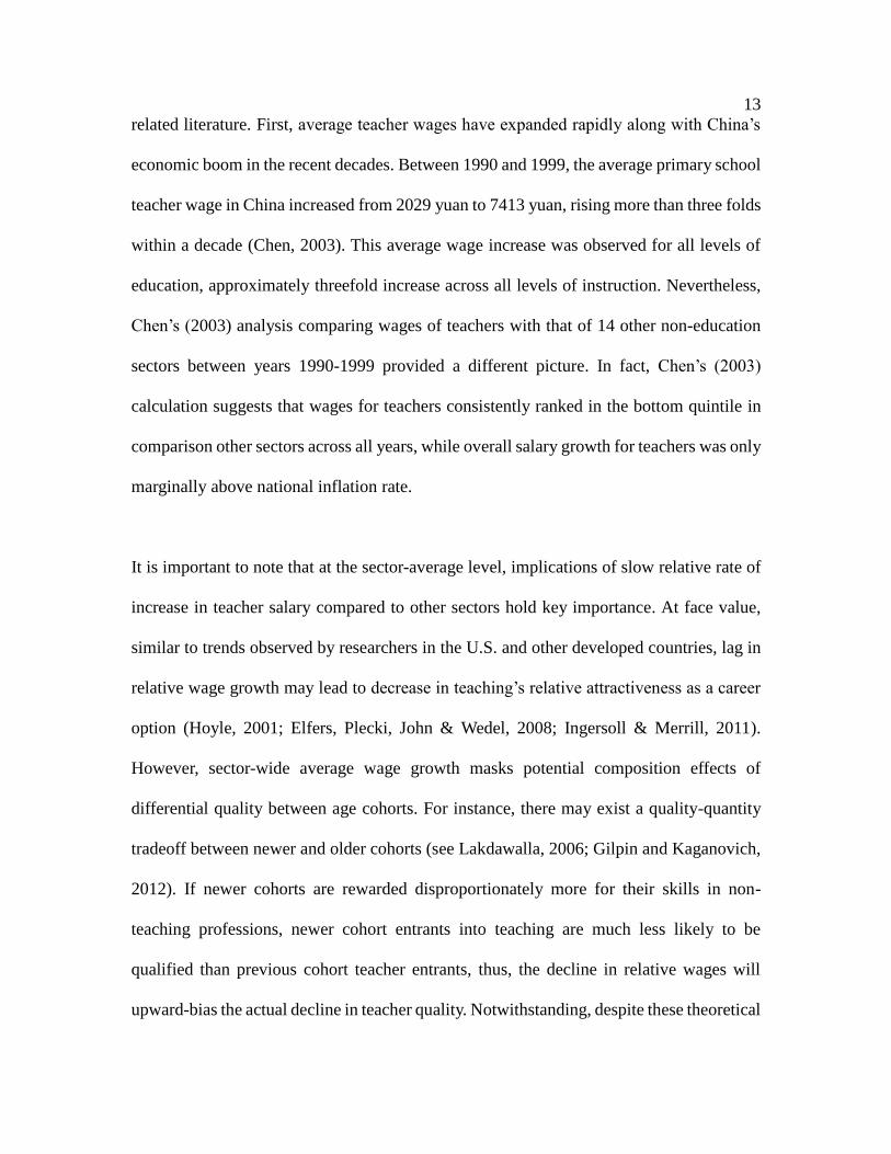
related literature. First, average teacher wages have expanded rapidly along with China’s

economic boom in the recent decades. Between 1990 and 1999, the average primary school

teacher wage in China increased from 2029 yuan to 7413 yuan, rising more than three folds

within a decade (Chen, 2003). This average wage increase was observed for all levels of

education, approximately threefold increase across all levels of instruction. Nevertheless,

Chen’s (2003) analysis comparing wages of teachers with that of 14 other non-education

sectors between years 1990-1999 provided a different picture. In fact, Chen’s (2003)

calculation suggests that wages for teachers consistently ranked in the bottom quintile in

comparison other sectors across all years, while overall salary growth for teachers was only

marginally above national inflation rate.

It is important to note that at the sector-average level, implications of slow relative rate of

increase in teacher salary compared to other sectors hold key importance. At face value,

similar to trends observed by researchers in the U.S. and other developed countries, lag in

relative wage growth may lead to decrease in teaching’s relative attractiveness as a career

option (Hoyle, 2001; Elfers, Plecki, John & Wedel, 2008; Ingersoll & Merrill, 2011).

However, sector-wide average wage growth masks potential composition effects of

differential quality between age cohorts. For instance, there may exist a quality-quantity

tradeoff between newer and older cohorts (see Lakdawalla, 2006; Gilpin and Kaganovich,

2012). If newer cohorts are rewarded disproportionately more for their skills in non-

teaching professions, newer cohort entrants into teaching are much less likely to be

qualified than previous cohort teacher entrants, thus, the decline in relative wages will

upward-bias the actual decline in teacher quality. Notwithstanding, despite these theoretical

14

stipulations, a direct age-cohort comparison of relative teaching versus non-teaching wage

gap is not available in the existing literature.

Second, the sheer numeric size and geographic spread of the teaching sector can lead to

significant wage inequality, not only in comparison to non-teaching sectors but also within

the teaching sector. Geographically imbalanced economic growth is an important driving

force behind within-sector wage inequality between coastal and inland provinces.

Correspondingly, an inter-provincial study of teacher salaries in 2005 revealed that among

all sampled provinces, mean wage was highest in Shanghai at 62,300 yuan per year while

the lowest provincial mean wage was less than one fifth of Shanghai’s average, found in

Henan province (An, 2014; Li, 2007). This large geographic variation in wage growth is in

direct contrast with most existing evidence found in developed countries, where the

teaching sector is often dominated by across-the-board collective bargaining and

characterized by low within-sector wage spread, and often coupled with large purchasing

power differences across different Chinese regions. Large wage growth spread, within the

teaching sector and across geographic regions, has important implications for this analysis,

because self-selection may be driven by both conditions across sectors and across locations.

Third, on top of large regional wage differences, even within the same province, wage

inequality appears noticeably large when comparing urban and rural schools. (An, 2014)

finds that the average income of rural primary school teachers is approximately 7 to 41

percent lower than the provincial average. Despite being paid conspicuously less, An (2014)

finds that rural teachers generally bear greater responsibilities than teachers in metropolitan

15

areas. For instance, in terms of teaching load, 32.2 percent of teachers in cities teach less

than 14 classes per week, while only about 14.2 percent of rural teachers report similar

amount of teaching load. Rural teachers are also responsible for 1.31 times the number of

classes than urban teachers, which are likely due to short-staffing (Xue and Li, 2015). The

issue of persistent staff shortages also prompt the examination of current conditions of

teacher supply and quality in China.

2.13 Teacher Quality in China

Staffing schools with qualified teachers has traditionally been a huge challenge in many

parts of China, as many schools are chronically short-staffed (Sargent & Hannum, 2005).

To compound this issue, teacher qualification requirements have been relatively low at the

system-level. On the demand-side, many primary schools have traditionally only required

a high school diploma, or shizhuan certificate, in order to be eligible to become a member

of the teaching staff, whereas most lower and upper secondary schools often set the

teaching prerequisite to be at least an associate or bachelor’s degree (Ingersoll, 2007).

In order to attract new talented teacher recruits, the Ministry of Education initiated free

teacher education programs at six of the ministry-affiliated teacher preparation universities

in different parts of the country. As requirement, selected teacher candidates need to score

above a designated threshold on the National College Entrance Exam in order to enter these

free teacher preparation programs, which subsequently require an extended period of

commitment in teaching careers in return. In more recent years, most new primary and

secondary teachers in China undertake a four year bachelor’s education, benke, or a two-

16

year associate’s diploma education, zhuanke, before they begin teaching in public primary

or secondary educational institutions.

Policymakers have traditionally used teacher’s educational background to screen teachers

for prerequisite training, skills, and aptitude. Primary and secondary school teachers are

generally required to hold at least a vocational college degree as a base requirement to be

eligible to teach, although ones with college degrees or higher are considered favorably in

hiring and promotion decisions. Despite relatively low entry qualification requirements,

the Ministry of Education, together with provincial and municipal educational

commissions, set guidelines, professional standards, and fund teacher education

programming initiatives to ensure that a relatively high level of teacher quality.

Once teachers enter the education sector, administrators rely on a system of teacher ranks,

or zhicheng, and teaching awards to make hiring, assignment, compensation, and

promotion decisions (Ministry of Education, 1986). Such observational measures are

designed with the goal of providing objective assessments for instructional quality and

professional performance that are relatively comparable across different subjects, levels,

and geographical regions of instruction. Teacher rank, among primary and secondary

school teachers, consists of four levels in descending prestige: senior rank, level one rank,

level two rank, level three rank. Teaching awards, an important aspect of consideration for

promotion,, are bestowed by different levels of education authorities, ranging from

national-level, provincial-level, municipal-level, district-level, and school-level, often

through the form of teaching competitions. While increase in rank is and progression of

17

career prestige are obtained sequentially over the entirety of their careers, teacher awards

are determined and awarded at relatively shorter time intervals. Commonly, new teachers

enter the profession with no predetermined teacher rank, and must earn their placement in

entry-level rank.

To be promoted to the next rank, teachers must meet two sets of requirements. First,

candidates applying for a certain rank must possess the corresponding level of observable

qualifications such as relevant levels of education, years of teaching experience, and length

of experience serving as homeroom teacher. Second, potential candidates for rank

promotion are assessed based on their classroom and professional performance, including

one’s mastery of pedagogical skills, instructional tools, and classroom management.

Teachers are routinely evaluated within each school on whether or not they should be

promoted in rank; such class audit evaluations are conducted by both administrative as well

as peer teaching staff (Chu, Loyalka, Chu, Qu, Shi & Li, 2015).

Existing studies have shown that teacher rank is correlated with pecuniary incentives and

advancements on salary schedules, which are commonly set forth by local education

authorities (Wang & Lewin, 2016). As of 2011, 54 percent of primary school teachers held

senior primary rank, while the remaining 46 percent of teachers either did not have a rank

or were ranked at level one, two, or three (Ministry of Education, 2014). Importantly,

despite teacher rank promotions, teaching award prestige, and salary advancements, studies

have shown that many teachers report the lack of career outlets and clear promotion routes

as persistent factors influencing their decision to pursue other professional paths (Adams,

18

2012), which elicits serious complications in teacher recruitment and retention.

Importantly, existing literature assessing teacher quality shifts in China is particularly

limited, especially at the micro-analytic level. This may be in part due to the scarcity of

data on direct teacher quality or aptitude measures at the individual-level. Most of the

existing studies draw on national or regional aggregate numbers provided by the Ministry

of Education's yearly statistical yearbooks. Using aggregate data to draw inferences on

individual occupational choice is faced with the obvious ecological fallacy problem.

Nonetheless, attempts to extend the discussion using individual-level micro data are

extremely scarce.

Noting these limitations, surveying the current state of knowledge provide important

implications and entry points for further research on this topic. First and foremost,

composite measures of teacher quality are correlated with average regional income at the

provincial-level. Yang, Wang, Yan, and Shan (2013) provides an attempt to evaluate

aggregate-level changes in teacher quality over time. Using data from 31 provinces, Yang

et al. (2013) generated a composite index based on five key indicators: student-teacher ratio,

classroom-teacher ratio, teachers' education attainment, teachers' rank, and average income.

Their study suggests that provinces with higher levels of economic growth are also placed

relatively higher on the composite index. Nationally, the average full-time teacher share in

primary schools was 85.41 percent, closely in line with the 91 percent cutoff required by

the Ministry of Education (Yang, Wang, Yan, & Shan, 2013). Part-time contractual teachers,

or daike laoshi, consisted of 3.45 percent of the entire teacher population in 2010, down

from 3.65 percent in 2009 (Ministry of Education, 2010). For decades, daike laoshi, or

19

uncertified and temporary contract teachers, have been recruited to fill rural school

vacancies, and often remain in their posts for extended durations due to lack of available

replacements.

Second, several studies have explored teacher quality through more direct measures. For

instance, Xue and Li (2015) measured teacher quality in terms of level of education. Their

study indicated that while improvements have been significant nationally, the gap between

urban and rural schools continued to exacerbate. The average educational attainment gap

between rural and urban school teachers in 2004 was 1.36 years at the national average

level, and in 2013, this same measure increased to 2.04 years (Xue & Li, 2015). Shi and

Yan (2006) point out that a supplementary factor in rising teacher quality concerns is the

aging of teachers in rural primary schools. Specifically, over half of rural teachers were

above 40 years of age, which suggests that the teaching force in rural primary schools may

be predominantly comprised of relatively less educated teachers.

In addition, while a majority of the teaching force consisted of women, gender composition

varied greatly by location and level of education. According to Ministry of Education (2010)

data, the education sector workforce as a whole composed of 58 percent of female.

However, national averages mask significant regional variations and differences by level

of education. For instance, the male to female teacher ratio in rural secondary schools is 1:

0.8, while the same ratio is 2:1 in primary schools (Shi & Yan, 2006). The potential

differences in gender-specific educational attainment may also play an important role in

regional variations in teacher quality, and requires further thinking in terms of how to best

20

attract and retain both female and male teacher candidates.

To this end, existing research on the topic of teacher quality is both scant in number and

limited in depth. To add, many existing studies on teacher quality in China could be

methodologically strengthened and more theoretically based. Few discuss teacher quality

in relation to occupational choice theory or look into the broader literature on the

economics of education. There currently exists a significant literature gap in understanding

how teacher occupational choice, labor market conditions, and teacher quality have

interacted over time at the micro-level, especially in a geographically diverse developing

country such as China. In light of these realities, a high quality study driven by strong

theoretical motivations and taking advantage of the increasing availability of micro-level

data is much needed.

2.14 History of Teacher Salary Reforms in China

Teacher salary policies in China have gone through several important transformations in

terms of policy institutionalization and programmatic implementation. Until 1955,

payment in-kind teacher compensation policies were common in most parts of China,

which was then replaced by a national reform to standardize teacher salaries in currency

payments (Tian & Yang, 2008). Subsequently, one of China’s earliest teacher salary

reforms started in 1956, and was characterized by the implementation of a unified wage

system that observers conclude as having improved absolute salary terms for teachers (Tian

& Yang, 2008). The main motivation behind this reform was to ensure equal pay for equal

work, and to enable better budgeting and accounting practices to be put in place nationally

21

for the management of teacher salaries. One of the means in achieving this goal was to

gradually reduce the large regional differences in wage distribution. For implementation,

the central government issued 11 designated wage zones with particular consideration to

variations in living standards and commodity prices based on geography. Policy emphasis

was put in key areas of development and poverty-stricken areas, such that wage subsidies

were established for different regions in accordance with commodity prices. Importantly,

the 1956 teacher salary reform also initiated a long-standing pay scale system that was

based on individual ability, qualifications, and rank. For instance, the reform established a

rank-based salary system with 10 teacher ranks and 15 administrative grades (Tian & Yang,

2008). In general terms, early reforms is 1956 had laid the pretext for much of the teacher

pay scale system that is still in effect in many forms today.

The next wave of institutionalizing reforms occurred during the 1980s, as represented by a

series of reforms stemming from the State Council’s (1981) Measures on Adjusting

Salaries of Primary and Secondary School Teachers, in part as policy response to improve

teacher salary structures. To this end, the State Council’s (1985) Notice on Government and

Public Institution Employee Salary Guidelines introduced a new salary scale that is more

closely tied to job performance; in detail, the new statute stipulated that teacher salaries are

to be comprised of four core components: base salary, workload subsidies, tenure-based

subsidies, performance-based subsidies. Follow-up reforms through the State Council’s

(1987) Notice on Compensation Improvement for Teachers in Basic Education provided

substantive improvements on the existing wage streams for teacher salary determination,

and aimed at increasing teacher take-home pay by about 10 percent. This era of reforms

22

established the overarching “base + subsidies” approach for determining teacher salaries,

as well as attributing larger proportions of wage scale to workload and job performance.

Subsequent reforms in 1993 and 2006 have been in large parts programmatic fine-tuning

and legal mandates based upon policy foundations from previous eras, such that the 1993

teacher salary reform focused on increasing the percentage of workload-based subsidies,

while the 2006 reform emphasized on legally guaranteeing comparable pay for teachers.

One of the driving forces behind these reform updates was that teacher salary had become

incompatible with the country’s overall economic growth (Guo, 1994). In detail, the State

Council’s (1993) Notice on Government and Public Institution Employee Salary Reform

Implementation Guidelines update has further strengthened the link between teacher salary

and workload, increasing the percentage of workload-based subsidies to 30 percent of total

payments. In addition, the guidelines also established 6 new pay-grade advancements and

homeroom teacher subsidy, as well as the central government’s fiscal responsibility to

guarantee timely teacher salary payments.

A decade later, the People’s Congress passed the Compulsory Education Law in 2006,

which instructed all levels of government to ensure favorable wages, living and working

standards, and social security benefits for teachers, and acted as a legal mandate that

“average teacher salary levels should be no less than that of local public officials” (People’s

Congress, 2006, Chapter 4, Section 31). More recent developments in 2009, as stipulated

by Ministry of Education’s (2008) Guidelines on Performance Evaluation of Teachers in

Primary and Secondary Schools, resulted in the implementation of a performance pay

23

policy for teachers in compulsory education schools. In effect, the 2009 reform introduced

an incentive mechanism into schools by making approximately 30 percent of wages

performance-based, rewarding those who take on more teaching and administrative

workload, as well as good teaching performance and engaging in pedagogical research

(Wang, Lai, & Lo, 2014). In broad terms, the current literature landscape suggests that the

development of teacher salary reforms in China can be broadly categorized into two time

periods: an institutionalization era between 1950-1980s, that focused primarily on laying

the foundational frameworks in determining teacher compensation; a more programmatic

conscious era in providing legal statutes and exploring more effective payment

mechanisms, from the 1990s to present.

2.2 Literature Review on Teacher Occupational Choice

Education economists are interested in understanding how rational actors make optimizing

decisions based on constraints. Accordingly, in the labor market, optimizing behaviors can

help rational actors self-select into various markets and production activities in pursuit of

comparative advantage. The formal treatment on self-selection and occupational choice

began with the seminar work of Andrew D. Roy (1951). Roy's insights on individuals'

decision to optimize choices between 'trout fishing and rabbit hunting' introduced the

theoretical foundation for understanding how rational actors make occupational choices.

The core content of Roy's (1951) analysis is that a rational worker compares her expected

payout, broadly defined in different occupations, and chooses the occupation that

maximizes this sum. The worker may choose to assess her expected payout based on

24

several dimensions, such as pecuniary benefits in wages and non-pecuniary benefits, such

as occupational status and working conditions (Dolton, Makepeace, & van der Klaauw,

1989). To assume simplicity, most existing analyses have used wage from labor work as a

proxy for lifetime utility (Nagler, Piopiunik, & West, 2015), for which the justification

derives from the intuition that budget constraints limit individual lifetime choice sets.

2.21 Theoretical Framework

Since the original 1951 article, the basic Roy model has been extensively modified and

generalized, and expanded versions include various features such as utility maximization

agents (Heckman and Sedlack, 1985), multiple sectors (Dolton, Makepeace, & van der

Klaauw, 1989), credit constraints (Banerjee and Newman, 1993), and uncertainty

(D'Haultfoeuille and Maurel, 2010). The Roy model has been widely applied by labor

economists in various scenarios to understand individual occupational choice mechanisms.

For instance, analyses have been conducted on workers' decision to enter market versus

non-market sectors (see Heckman, 1974, 1976; Dustmann & van Soest, 1998), unionized

versus non-unionized sectors (Lee, 1978), piece-rate versus fixed-pay wage structures

(Lazear, 1986). Additionally, the model has also been used to understand workers' choice

to emigrate (Borjas, 1987), enter or leave a marriage (McElroy & Horney, 1981), and invest

in higher education (Willis & Rosen, 1979).

Broadly speaking, the theoretical foundation of much of the existing occupational literature

rests on the cornerstone of human capital theory, such that career decisions are considered

as part of an expansive investment project through which investment options between

25

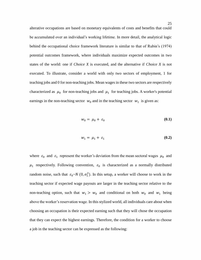
alterative occupations are based on monetary equivalents of costs and benefits that could

be accumulated over an individual’s working lifetime. In more detail, the analytical logic

behind the occupational choice framework literature is similar to that of Rubin’s (1974)

potential outcomes framework, where individuals maximize expected outcomes in two

states of the world: one if Choice X is executed, and the alternative if Choice X is not

executed. To illustrate, consider a world with only two sectors of employment, 1 for

teaching jobs and 0 for non-teaching jobs. Mean wages in these two sectors are respectively

characterized as 𝜇0 for non-teaching jobs and 𝜇1 for teaching jobs. A worker's potential

earnings in the non-teaching sector 𝑤0 and in the teaching sector 𝑤1 is given as:

𝑤0 = 𝜇0 + 휀0 (0.1)

𝑤1 = 𝜇1 + 휀1 (0.2)

where 휀0 and 휀1 represent the worker’s deviation from the mean sectoral wages 𝜇0 and

𝜇1 respectively. Following convention, 휀0 is characterized as a normally distributed

random noise, such that 휀0~𝑁 (0, 𝜎12). In this setup, a worker will choose to work in the

teaching sector if expected wage payouts are larger in the teaching sector relative to the

non-teaching option, such that 𝑤1 > 𝑤0 and conditional on both 𝑤0 and 𝑤1 being

above the worker’s reservation wage. In this stylized world, all individuals care about when

choosing an occupation is their expected earning such that they will chose the occupation

that they can expect the highest earnings. Therefore, the condition for a worker to choose

a job in the teaching sector can be expressed as the following:

26

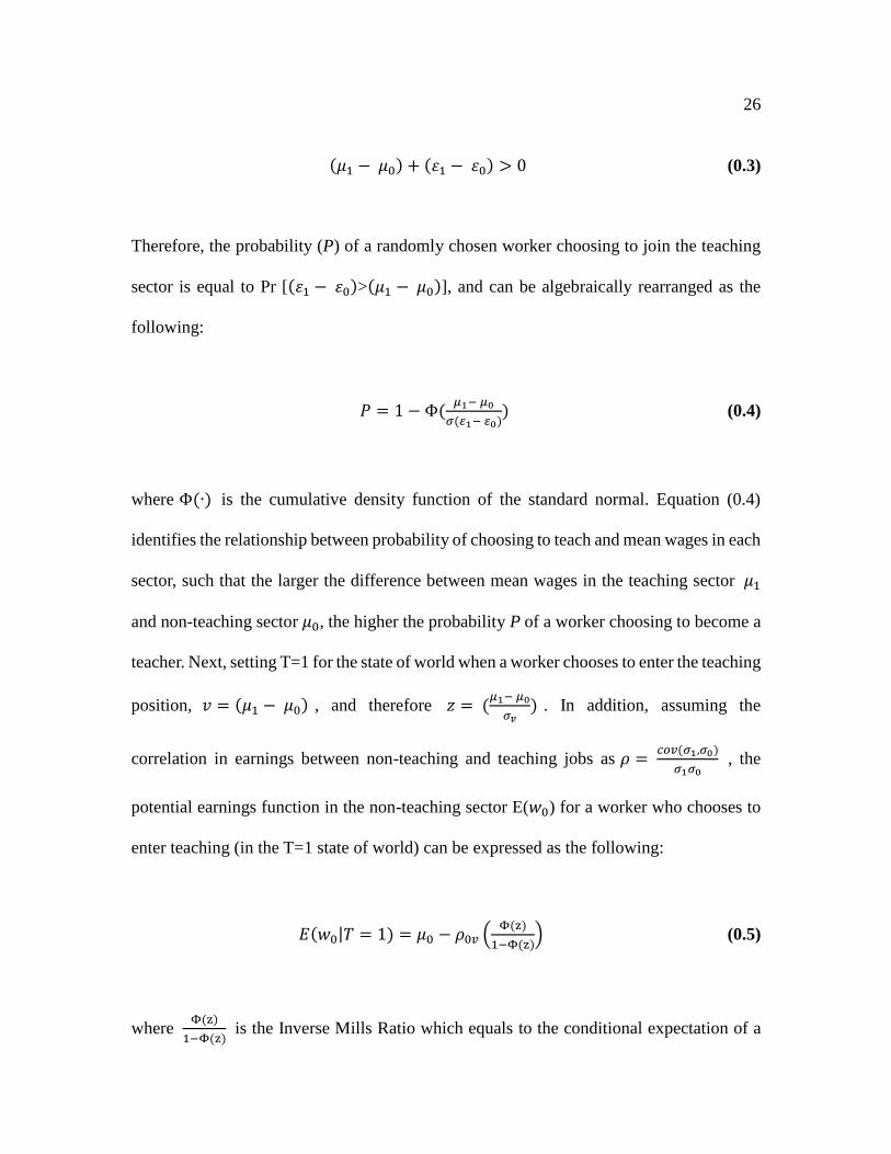
(𝜇1 − 𝜇0) + (휀1 − 휀0) > 0 (0.3)

Therefore, the probability (P) of a randomly chosen worker choosing to join the teaching

sector is equal to Pr [(휀1 − 휀0)>(𝜇1 − 𝜇0)], and can be algebraically rearranged as the

following:

𝑃 = 1 − Φ(𝜇1− 𝜇0

𝜎(𝜀1− 𝜀0)) (0.4)

where Φ(∙) is the cumulative density function of the standard normal. Equation (0.4)

identifies the relationship between probability of choosing to teach and mean wages in each

sector, such that the larger the difference between mean wages in the teaching sector 𝜇1

and non-teaching sector 𝜇0, the higher the probability P of a worker choosing to become a

teacher. Next, setting T=1 for the state of world when a worker chooses to enter the teaching

position, 𝑣 = (𝜇1 − 𝜇0) , and therefore 𝑧 = (𝜇1− 𝜇0

𝜎𝑣) . In addition, assuming the

correlation in earnings between non-teaching and teaching jobs as 𝜌 = 𝑐𝑜𝑣(𝜎1,𝜎0)

𝜎1𝜎0 , the

potential earnings function in the non-teaching sector E(𝑤0) for a worker who chooses to

enter teaching (in the T=1 state of world) can be expressed as the following:

𝐸(𝑤0|𝑇 = 1) = 𝜇0 − 𝜌0𝑣 (Φ(z)

1−Φ(z)) (0.5)

where Φ(z)

1−Φ(z) is the Inverse Mills Ratio which equals to the conditional expectation of a

27

normal distribution truncated at point z. The potential earnings in the teaching sector E((𝑤1)

for a worker who decides to choose a teaching job (in the T=1 state of world) can be

identified as the following:

𝐸(𝑤1|𝑇 = 1) = 𝜇1 + 𝜎0𝜎1

𝜎𝑣(

𝜎1

𝜎0− 𝜌) (

Φ(z)

1−Φ(z)) (0.6)

Based on Equations (0.5) and (0.6), we can better understand the occupational choice

mechanisms under Roy model's expected outcome framework. First, we consider a

hypothetical case of positive selection into the teaching sector. If a worker who chooses a

teaching job is the individual who would have expected to receive above average pay in

both the teaching and non-teaching sectors, meaning 𝐸(𝑤0|𝑇 = 1) > 0 and 𝐸(𝑤1|𝑇 =

1) > 0, then the following conditions must hold true:

𝜎1

𝜎0> 1 , 𝜌 >

𝜎0

𝜎1 (0.7)

These two conditions have important implications in understanding why this 'above

average' individual would choose the teaching sector given that he or she could receive

above the mean earnings in either sectors. The first condition 𝜎1

𝜎2> 1 indicates that the

teaching sector has a larger dispersion of individual earnings, which implies that there is a

higher rate of return to human capital. The second condition 𝜌 > 𝜎0

𝜎1 posits that the type

of human capital valued by both sectors is highly correlated, or sufficiently overlapped. In

this case, an 'above average' individual chooses the teaching sector over the non-teaching

28

sector because the two sectors value the same set of human capital, but the teaching sector

offers a higher return to the individual's human capital.

Secondly, for the hypothetical case of negative selection into the teaching sector, that is a

worker who chooses teaching is also the individual who would have expected to receive

below average pay in both the teaching and non-teaching sectors, 𝐸(𝑤0|𝑇 = 1) < 0 and

𝐸(𝑤1|𝑇 = 1) < 0, then the following conditions must hold true:

𝜎0

𝜎1> 1 , 𝜌 >

𝜎0

𝜎1 (0.8)

This second case is the exact reverse of the first case. Now, the 'below average' individual

chooses the teaching sector with the expectation that he or she would receive below average

earnings in either sectors. This is observed because 𝜎0

𝜎1> 1 indicates that the teaching

sector has a narrower wage dispersion, implying that by choosing the teaching sector the

'below average' individual benefits from entering teaching because it guarantees a higher

wage than otherwise. Again, the second condition 𝜌 > 𝜎0

𝜎1 is the same assumption that the

type of human capital valued by both teaching and non-teaching sectors is highly correlated.

Two additional hypothetical cases should also be briefly mentioned here. In the case of

𝐸(𝑤0|𝑇 = 1) < 0 and 𝐸(𝑤1|𝑇 = 1) > 0, meaning if an individual with 'below average'

potential earnings in the non-teaching sector and 'above average' potential earnings in the

teaching sector chooses a teaching job, then 𝜌 < min (𝜎1

𝜎0,

𝜎0

𝜎1) must satisfy. In other words,

29

the teaching and non-teaching sectors must value sufficiently different types of human

capital and that correlation of earnings must be small or negative. Whereas in the case of

𝐸(𝑤0|𝑇 = 1) > 0 and 𝐸(𝑤1|𝑇 = 1) < 0, meaning for an individual with 'above average'

potential earnings in the non-teaching sector and 'below average' in the teaching sector to

choose a teaching job, the satisfying condition requires 𝜌 > max (𝜎1

𝜎0,

𝜎0

𝜎1) . This is

theoretically unlikely due to violation of the rational choice based on expected outcomes

assumption, because the individual would be better off by simply choosing non-teaching

sector to receive 'above average' earnings.

When applied to teacher labor markets, the model identifies two key factors that influence

the type of individual who pursues a career in teaching:

(1) ratio of wage dispersion between teaching and non-teaching sectors,

(2) correlation between the type of skills valued by teaching and non-teaching sectors

To this end, if worker aptitude and general skills are positively correlated with earnings

across different sectors, a rise in the difference in earnings dispersion would result in high

ability individuals choosing the sector with higher returns to skills and human capital.

Accordingly, given a positive and high correlation between the types of skills valued by

teaching and non-teaching sectors, average teacher quality can be substantially influenced

by the ratio of dispersion in earnings between the two sectors. For instance, high ability

individuals will choose the sector with higher returns to skills, as represented by a relatively

wider dispersion of earnings. For instance, this scenario applies appropriately for high

ability teachers in STEM fields (Science, Technology, Engineering, and Mathematics).

30

Assuming their attained human capital in STEM is identically valued across teaching and

non-teaching sectors, STEM teachers will choose to work in a non-teaching sector that

offers a higher rate of return to their STEM skills, which will have important implications

for the observed ability distribution in the teaching sector. Notwithstanding, the

implications for understanding the relationship between sectoral wages and teacher quality

extend beyond the above applications in STEM fields, especially considering that there are

many instances in the education sector where all three of the parameters are interacting at

amplified intensity.

2.22 Implications for Teacher Occupational Choice

Economics of education studies have utilized the occupational choice framework to

investigate what factors influence individuals' decision to pursue teaching as a career. This

line of research was mainly motivated by the frustration over evidence that schools in the

U.S. are failing to attract the best and brightest individuals to become teachers (Temin,

2002). Earlier studies carried out by Vance and Schlecty (1982), Weaver (1983), Hanushek

and Pace (1995), Ballou and Podgursky (1997) documented that the average teacher's math

and verbal skills, as measured by college entrance test scores, have been steadily decreasing.

More recent studies continue to confirm this declining teacher quality observation. In fact,

Corcoran, Evans, and Schwab (2004), Lakdawalla (2006), Bacolod (2007), and Richey

(2014) all present similar evidence on falling relative abilities of teachers in the U.S. These

observations of declining average teacher quality emerged with a growing body of evidence

that show various measures of teacher quality are instrumental to student outcomes

(Hanushek & Rivkin, 2012), and even adulthood outcomes (Chetty, Friedman, & Rockoff,

31

2014).In most existing occupational choice models, the quality of teacher supply depends

on wage and non-wage job characteristics, as well as on how wages and entry requirements

in the teacher labor market compare in relation to other sectors in the broader labor market.

To extend on the documented findings of declining teacher quality in the U.S. over the past

few decades (see Corcoran, Evans, & Schwab, 2004; Bacolod, 2007; Richey, 2014), an

important education research motivation is to understand why teacher quality has

experienced such decline and evaluate prominence of potential drivers of such change.

Some scholars attribute this decline in quality to women's growing labor participation

(Corcoran, Evans, & Schwab, 2004), while others argue that relative wage compression is

the explanation (see Hoxby & Leigh, 2004). Scholars also argue that barriers and costs to

entry, both direct and indirect, pose barriers for prospective teachers (Angrist & Guryan,

2007). All of these explanations form a basis of understanding for how teachers make

occupational decisions and shed light on why these individual occupational behaviors can

have sweeping and unintended consequences for the broader education sector. Following

the theoretical underpinning of the occupational choice model, economists and education

researchers have hypothesized that several labor market conditions can affect the average

characteristics and composition the teaching force. Below, I outline three major labor

supply explanations: gender desegregation, wage compression, and opportunity wages.

Gender Desegregation in the Labor Market

First, some scholars attribute this declining labor quality to the growing non-teaching

employment opportunities for women (Temin, 2002; Corcoran, Evans, & Schwab, 2004;

32

Bacolod, 2007). Historically, due to low probabilities of entry into gender-segregated

sectors, high ability women have low expected earnings in non-teaching sectors, and thus

became a captive pool of workers within the teaching sector. In recent decades, progressive

gender desegregation in many previously male-dominated sectors led to an increase in

women's likelihood of entry, and as a result, an increase in expected non-teaching earnings

for women who have a comparative advantage in such sectors. As result, gender

desegregation allowed high ability women to seek their comparative advantage and receive

better earnings in non-teaching jobs, leading to lower density of high ability teachers.

As explained by Temin (2002), due to historic labor market segregation in hiring practices,

high ability women could only seek employment in a limited set of professions such as

teaching and nursing; however, with the improvement of gender equality in the past half

century, women's occupational choice sets have greatly expanded, and therefore the quality

of teachers have become responsive to wages. Yet, in this process, wage levels in the

teaching sector has not responded to the rising non-teaching opportunities that have

become available to high-ability women. Utilizing five longitudinal surveys spanning

between 1957-1992, Corcoran, Evans, and Schwab (2004) document a large decline in

teacher quality and observes a lower propensity for women at the top-decile of the

individual aptitude distribution to pursue a teaching career, with more than 20 percent in

the 1960s falling to just merely 3.7 percent in the 1990s. They find that high-ability women

have been increasingly attracted to pursue non-teaching careers such as managers,

computer scientists, accountants, and lawyers. This translates into the observed decline of

high ability individuals in primary and secondary schools’ teaching force.

33

In the same vein, Bacolod (2007) documents a sharp decline of worker ability in the

teaching sector using three different labor force ability measures: standardized test scores,

selectivity of undergraduate institution, partner's education and relative wage standing in

the population. She finds that the larger the difference in mean wages between teaching

and non-teaching sectors, the more likely high ability individuals are to become teachers,

simply because of differences in relative wage structures and characteristics. In addition,

women and younger age-cohorts are more responsive to wage changes than are men and

older age-cohorts. An important contribution of Bacolod (2007) is the attempt to

analytically separate supply-side and demand-side factors influencing average teacher

quality. She notes that observed occupational choices may be results of a combination of

relative supply and demand factors.

Supply side economic analyses have often cited positive compensating differentials as a

key explanation for women's choice to become teachers, because the teaching sector

requires skills that are complementary with production in the household (Becker, 1985),

and allows for less costly labor market exits and re-entries when starting a family (Polachek

1981; Blau, Ferber, & Winkler, 1998). Following these supply-side hypotheses, gender

desegregation in occupations shifts women's labor supply inward in previously 'women-

dominated' jobs and outward in previously 'non-women-dominated' jobs. This labor supply

shift would theoretically result in an increase in relative wages for previously 'women-

dominated' sectors such as teaching. Yet, the empirical evidence shows that relative wages

in the teaching sector declined, pointing to demand factors as the alternative explanation.

Bacolod (2007) shows that relative wages declined more for women than men, indicating

34

a labor demand shift that had provided women with more non-teaching employment

opportunities, and is responsible for compositional changes in the teaching force.

Relative Wage Compression for Teachers

Another strand of research argues that relative wage compression in the teaching profession,

as opposed to that of non-teaching jobs, has been the main reason why talented individuals

leave teaching (Hoxby & Leigh, 2004; Chingos & West, 2012; Leigh, 2012; Correa, Parro,

& Reyes, 2015). Wage compression policies within the teaching sector, such as

unionization and flat wage structures, translate into a lower return to human capital and

skills for teachers. Under such policies, occupational choice theory predicts that high

ability individuals would choose to work in non-teaching sectors, which exhibit a higher

return to human capital, when considering career options. Accordingly, Hoxby and Leigh

(2004), Chingos and West (2012), Leigh (2012), and Correa, Parro, and Reyes (2015)

observe negative impacts of relative wage compression in the teaching profession on

overall teacher aptitude in the U.S., Australia, and Chile, as high ability individuals choose

sectors with higher returns to skills.

In the U.S., Hoxby and Leigh (2004) provide causal estimates of wage compression effects

on teacher quality, which approximately equals to a 9 percentage-point increase in the share

of individuals with the lowest aptitude rank and a 12 percentage-point decrease in the share

of individuals with the highest aptitude rank among teachers. Their results indicate that

wage compression explained about 80 percent of the decrease in the representation of high

ability individuals in teaching and explained about 25 percent of the increase in the share

35

of low-ability individuals in teaching. Similarly, Chingos and West (2012) study U.S.

teachers' opportunity wages and find that women, who leave teaching for non-teaching jobs,

experience a greater dispersion in income compared to before leaving their teaching posts.

This result implies that better general skills and human capital are valued

disproportionately more in non-teaching careers, luring high ability teachers to exit.

In Australia, Leigh (2012) directly models the current wages and the aptitude of potential

teacher candidates using administrative data to document teacher labor supply shifts

between 1989 and 2003. He exploits the timing and geographic variation of teacher wages,

which are set at the state-level by collective bargaining. The empirical results indicate that

every 1 percent increase in starting wages of new teachers raises the average aptitude of

pre-service teachers by .6 in percentile ranks, with effects strongest for those individuals

around the median. In addition, he also finds evidence that relatively wider earnings

dispersion in the non-teaching sector, compared to the teaching sector, lowers the aptitude

of pre-service teachers, with impact strongest for those at the top of the ability distribution.

In terms of the Chilean context, Correa, Parro, and Reyes (2015) apply a two-sector

occupational choice model to empirically examine teacher occupational choice between

public and private schools, which is crucially differentiated by centralized earning

schedules and merit pay, respectively. Correa, Parro, and Reyes (2015) document positive

self-selection for high ability teachers into private schools and negative self-selection for

low ability teachers into public schools. The authors interpret their findings as a result of

rigid teacher wage regulation in public schools that is heavily dependent on certification

36

and experience, whereas private schools exhibit substantially more flexible rules for hiring,

firing and setting salaries.

The Opportunity Costs of Non-teaching Options

Third, along the relative wage compression theory, several scholars hypothesize that the

general state of economy creates shocks to non-teaching work opportunities, and can have

important implications for the composition of the teaching force (Falch, Johansen, & Strom,

2009; Nagler, Popiunik, & West, 2015; Neugebauer, 2015). This intuition is based on the

widely held assumption that the education sector is generally non-cyclical, whereas other

private sectors often go through boom and bust cycles. Thus, during times of economic

boom, the ratio of earnings spread is typically larger in non-teaching compared to teaching

sectors, thus individuals with high ability face a higher opportunity cost to commit to a

career in teaching. Whereas, during economic recessions, non-teaching job opportunities

dwindle and wages in non-teaching sectors become compressed, and as result, many high

ability individuals choose to become teachers.

For instance in Norway, Falch, Johansen, and Strom (2009) utilizes panel data to show that

public school teacher shortages are strongly correlated with business cycles, meaning better

macroeconomic conditions are associated with a higher degree of teacher shortage in public

schools. Nagler, Popiunik, and West (2015) use student-level administrative data from

Florida, and find that teachers who enter the profession during an economic recession, are

on average .1 standard deviation more effective in raising student math scores and .03

standard deviations more effective in raising student reading scores than teachers who enter

37

during non-recession periods. Under a reasonable assumption that only 10 percent of

recession-cohort teachers enter teaching due to the self-selection mechanisms above,

Nagler, Popiunik, and West (2015) posit that the expected population effect would translate

into approximately 1 standard deviation higher on the teacher value added distribution for

recession-cohorts. Neugerbauer (2015) analyzes shifts in labor market conditions and

teacher characteristics in Germany between the years 1980-2009. Using a nationally

representative sample, he shows that there was no relative decline in teacher wages in

Germany over the past three decades. Neugerbauer (2015) explains this observation by

linking the relative stable quality of the teaching force with relatively high unemployment

risks, and he shows that teacher occupational choice in Germany is very sensitive to labor

conditions in the larger economy, specifically unemployment risks.

The Cost Disease and Rising Demand for Education

Apart from supply-side explanations, there are also other factors at play influencing who

becomes a teacher. For instance, the education sector has traditionally been thought of as

being troubled by an unavoidable ‘cost disease’, that is the rising costs of education far

outpace that of inflation in general price levels (Baumol, 1993). The idea behind this

concept is that education has been relatively stagnant in terms of productivity

improvements. To elaborate, the economy can be divided into two sectors, one being

technologically progressive and therefore relatively more productive, and the other being

technologically stagnant marked by lower productivity. In the technologically progressive

sector, improvements to production technology respond to rising labor costs and substitutes

low-cost low-skilled labor for more costly skilled labor, and in turn raises labor productivity.

38

However, because by nature of production, it is hard to improve productivity in the

technologically stagnant sector, worker wages must rise in order to attract and retain

workers of desirable quality and aptitude. The inevitable result is that labor cost increase

in the technologically progressive sector will be transferred to the stagnant sector where

substitution for labor is not easily available. To cope with these circumstances, the stagnant

sector can either bid up the price of workers, or face ‘labor-draining’, meaning that skilled

labor will be lost to technologically progressive sectors.

To further complicate the issue of rising per unit costs, demand for education has been

consistently increasing in most countries, either through economic development or policy

expansion to open educational access. One important lesson from economic theory is that

the price and quantity of labor is jointly determined by supply and demand factors, which

means that demand-side factors can also play an important role. Broadly speaking, scholars

posit that skill-biased technological change (SBTC) exacerbates the appreciation of skills

and human capital relative to the median worker. Furthermore, sustained growth in skill

premium in the general economy creates lasting downward pressure on the average quality

of the teaching sector (Gilpin & Kaganovich, 2012). Rising demand for college-educated

skilled workers has led to an increase in demand for better education, and under a relatively

fixed education budget, education systems can no longer afford to hire high ability

individuals as teachers (Lakdawalla, 2006). The main intuition derives from recent

imbalanced expansions in education access and education budget, which led to more

teachers being hired due to relatively stagnant teacher productivity growth, at a relatively

lower unit price for their labor because of relatively fixed educational budgets.

39

More specifically, Lakdawalla (2006) argues that demand-side quality and quantity

tradeoffs play an important role in the decline of teacher quality. Schools are faced with

higher public demand for schooling because SBTC increases the prices of skilled labor and

more individuals are inclined to pursue education, yet teachers’ unit productivity to educate

students has remained practically unchanged. For instance, class size has largely remained

the same, or decreased, in most countries. Even as the cost of teachers rise, there has been

little to no substitution of teacher labor in the education production process. This creates a

resource allocation problem for schools, which in turn respond by substituting teacher

quality with teacher quantity to cope with this increased demand for education. By utilizing

time and geographic variations in the price of skilled labor, Lakdawalla (2006) finds that

higher prices for skilled labor appear to be associated with increased education input and

declines in relative teacher aptitude measures.

In the same vein, Gilpin and Kaganovich (2012) extend the SBTC analysis by treating

public schools as education quality maximizing agents, and explicitly model three factors

that may influence quality - quantity tradeoffs: indirect opportunity costs of teachers,

unionization and wage compression, and the rise of skill premium. Their general

equilibrium model predicts that as mean wages and earnings dispersion increase for

college-educated workers, schools are forced to adjust relative teacher salaries and teacher

quality standards in response to changes in labor market conditions. As education quality

maximizing agents, schools may solve the resource optimization problem by lowering

relative quality of teachers and compensate with a higher number of teachers. Gilpin and

Kaganovich (2012) show that this prediction is in line with the empirical observations

40

found between 1955 and 2005, that growth of teachers in the U.S. have far outpaced the

growth of student enrollment, and while teacher relative wages declined, overall education

budget as percent of GDP remained practically stable.

2.3 Implications for the Chinese Context

Several important implications can be summarized from the review of existing literature,

especially for understanding how teacher occupational choice, labor market conditions, and

teacher quality interact over time in China. First and foremost, the Roy model introduces

an economic decision-making framework in understanding how and why teachers choose

to become teachers. Researchers in social sciences have often emphasized the impact of

norms, beliefs, and structural barriers to employment as explanations for understanding

observed choices (see Badgett and Folbre, 2003; Morgan, Walker, Hebl, & King, 2013). In

this respect, studies in line with Roy's model provided individuals with more agency by

directly measuring teachers' endogenous occupational choice, and consequently led to

improvements in designs of teacher labor policy analyses.

Importantly, the model identifies key factors that can generate testable hypotheses

regarding who pursues teaching and why. As evident in the basic Roy model, the decision

to pursue a teaching career depends on two key parameters: the ratio of dispersion in

earnings between teaching and non-teaching sectors (𝜎1

𝜎0), and the correlation between the

type of human capital valued by teaching and non-teaching sectors (𝜌). To situate the model

more contextually in China, cross-sector improvements in earnings for women can have

41

important effects on the type of individuals who pursues teaching, such that opportunity

wages have increased substantially for women. China’s rapid economic transformation has

led to significant improvements in per capita income (Wen, 2015). Ding, Dong, and Li

(2007) show substantial wage increases in female workforce participants throughout 1988-

2002. Many scholars attribute a large proportion of this rise in income to the shift from low

productivity employment to higher productivity jobs (Brandt and Zhu, 2010). The

economic transition from planned to market economy has opened access not only to

previously inaccessible private-sector jobs, but also to a new class of high productivity jobs

that come with rapid economic development. In this respect, the existing literature on the

availability of non-teaching options (see Falch, Johansen, & Strom, 2009; Nagler, Popiunik,

& West, 2015; Neugebauer, 2015) is crucial to reconcile with the consequences for teacher

quality when previously unavailable career options are made available to teachers and

teacher candidates.

Second, given the positive and strong correlation in the type of skills and human capital

valued across teaching and non-teaching sectors, average teacher quality is expected to be

influenced by the ratio of dispersion in earnings between the two sectors. The combination

of a large and rigid public sector with artificially compressed wage structures (Zhu,

Prosterman, Ye, Li, Riediner, & Ouyang, 2006), will likely influence individual

occupational choice when the economy is undergoing rapidly transitions. Following this

theoretical approach, the current discussion (see Hoxby & Leigh, 2004; Chingos & West,

2012; Leigh, 2012; Correa, Parro, & Reyes, 2015) on whether fixed and compressed

teacher wage schedules fail to reflect the rising opportunity costs that individuals face is

42

also relevant for understanding consequences for overall teacher quality – in the face of

rapid economic development. As a general prediction stemming from occupational choice

theory, new workers who belong to the high ability group (broadly defined) would have a

lower return on skills in the teaching sector, and thus become less incentivized to enter the

teaching sector. At the same time, current teachers who belong to high ability groups, once

faced with better non-teaching career options, would have increased incentives to leave

teaching for non-teaching jobs, pursuing higher skill premiums.

Third, by empirically exploring parameters related to occupational choice decisions,

scholars can answer educationally important policy questions, and identify existing policy

gaps that may become problematic in the recruitment and retention of talented teachers. In

this regard, various studies including Rockoff (2004) and Rivkin, Hanushek, and Kain

(2005) have investigated the impact of teacher quality on student achievement, concluding

that by moving up one standard deviation on the teacher quality distribution leads to

approximately .1 standard deviation gain in student achievement. It is clear that teachers

play a key role in students’ learning and the production of human capital. As noted in the

occupational choice framework, given that the worker's human capital is valued in both

sectors and that correlation of skills is substantially large, high ability individuals will

choose to supply their labor in the sector with higher returns, as represented by the larger

dispersion of earnings, for those sets of skills. Therefore, short paying teachers may have

both immediate consequences in the decline in career attractiveness, but also far-reaching

and long-term societal costs, because the decline in average quality of teachers may result

in reduced learning and accumulated human capital for students, and therefore curtailed

43

skills preparedness once they enter the workforce.

To this end, numerous studies have shown that foundational skills acquired while in school

through good instruction can have long-term impacts on worker productivity, income, and

career progression (see Hanushek & Woessmann, 2015; Valerio, Puerta, Tognatta &

Monroy-Taborda, 2016). Thus, ensuring the quality of the teaching force has serious policy

implications for human capital accumulation both at the micro-individual and macro-

country level, and has potentially significant long-term consequences for economic

development and societal prospects. By investigating how relative labor market conditions

affect teacher occupational choice, policy instruments can be identified to better attract

high-quality teachers and become more effective in retaining individuals in the teaching

force. In this regard, the current dissertation presents an important theoretical application

of occupational choice in teacher labor markets, as well as a policy investigation to aid

policymakers in devising teacher recruitment, management, and retention policies that will

lead to a bright and well-functioning teaching force that can ultimately improve student

learning outcomes.

44

Chapter III

METHODOLOGY AND DATA

In broad strokes, this dissertation applies quantitative methodology to answer theoretically

important and policy relevant questions regarding the relationship between student learning,

observable characteristics, teacher quality and teaching wages. More specifically, I plan to

first motivate this dissertation by showing the impact of teacher quality on student learning

outcomes (Part I), document trends in adjusted wage profiles (Part II), explore how teachers

compare to non-teachers on labor quality measures (Part III), and investigate how stagnant

wages in the teaching sector have affected the quality of teacher labor supply (Part IV). In

particular, I examine specific sets of research questions in the four succeeding sections:

Research Question #1: What is the relationship between observable characteristics of

teacher labor quality on student learning outcomes?

• In Part I, using a nationally representative teacher-student linked dataset

(China Education Panel Survey, CEPS), I first establish the causal

relationship between observable teacher quality characteristics, as

illustrated by educational attainment level, on student learning outcomes in

Chinese schools. Results from Part I motivate a comparison of relative

teacher quality with non-teaching workers using observable human capital

traits and signals, such as educational attainment.

45

Research Question #2: How large is the teaching wage penalty between workers in

teaching and non-teaching sectors, after accounting for individual characteristics?

• In Part II, using a nationally representative repeated cross-sectional

household survey dataset (China Household Income Project, CHIP), I

empirically estimate key parameters in the teacher occupational choice

framework, namely mean wage difference and differential returns to skills,

and document trends over time. The objective of this exercise is to examine

the degree of change in these key two parameters in regards to identifying

and assessing observed teacher “wage penalty.”

Research Question #3: How has the relative quality of teachers compared to workers in

other sectors evolved in the past decades?

• In Part III, using a nationally representative repeated cross-sectional

household survey dataset (China Household Income Project, CHIP), I

evaluate the extent to which predictions of the occupational choice

framework extend to the Chinese context, in terms of observed teacher

ability patterns relative to the broader non-teaching workforce. I consider

results from this exercise jointly in relation to wage characteristic

observations observed in Part II, and discuss the broader implications for

the relative labor quality of the teaching force.

Research Question #4: What is the incidence of job turnover for teachers in China? What

is the influence of non-teaching opportunity wage on occupational decision?

46

• In Part IV, I leverage an available nationally representative panel dataset

(Rural-Urban Migration in China, RUMiC) on teacher’s labor market

career decisions and track teachers across year to examine the prevalence

of teacher turnover, and identify teacher job switch destinations. In addition,

I conduct an exploratory investigating on the relationship between relative

non-teaching opportunity wages to teacher’s occupational decision, and

assess the associated impacts on non-pecuniary outcomes.

3.1 Part I: The Impact of Teacher Quality on Student Learning

Often in the field of economics of education, student learning outcomes are estimated with

education production function to illustrate the relationship between student test scores A

and various types of educational inputs, such as student and family inputs P, teacher quality

inputs T, and school resource inputs S.

A = f (P, T, S) (1.0)

In most circumstances, student and family inputs P include a vector of individual and

family background demographic, socioeconomic, and educational effort factors as well as

measures of innate ability and accumulated prior learning. Teacher characteristic and

teacher quality inputs T often refer to various teacher quality variables, such as teacher’s

level of educational attainment, certification status, professional development participation,

and years of teaching experience. School resource inputs S reflect a variety of school-level

47

educational resources that contribute to student learning, such as state of facilities,

curriculum content, access to instructional technology, quality of educational facilities,

peer composition, and so on.

Accordingly, under the education production function framework, teachers are presumably

identified as the most educationally important input factor because it directly influences

instructional quality and immediately impacts student learning experience (Hanushek &

Rivkin, 2012). Rigorous evaluation studies in the United States, such as those performed

by Rockoff (2004) and Rivkin, Hanushek, and Kain (2005) have found that by moving up

1 standard deviation on the teacher quality distribution leads to approximately .1 standard

deviation gain in student achievement. Consequently, researchers and policymakers have

sought to determine specific teacher characteristic traits that can improve the underlying

teacher quality and subsequent student learning outcomes; extensive research on these

traits have identified teacher’s own educational attainment level (Harris & Sass, 2011),

teacher’s professional certification status (Clotfelter, Ladd, & Vigdor, 2007), and length of

teaching experience (Kane, Staiger, & Rockoff, 2007). However, common measures of

observable teacher quality characteristics, such as educational attainment level, experience,

and certification, have not always shown consistent results (Levin, 2010).

For these reasons, in Part I, I conceptualize teacher quality as educational productivity, or

the marginal product of observed teacher characteristic inputs on student learning outputs,

and relate it to teacher’s commonly observational traits, such as a teacher’s own educational

attainment level. In this regard, the research question will seek to understand to what extent

48

observable teacher quality characteristics – teacher educational attainment – matter for

student learning outcomes. Particularly, educational attainment is selected among a rich set

of teacher observable characteristics for two reasons. First, a teacher’s educational

attainment level is a broad reflection of academic proficiency, accumulated human capital,

and signals of premarket or innate skills, which are all reasonably expected to influence the

underlying teacher preparedness and instructional effectiveness. Secondly, unlike

education-specific credentials such as teacher licensure, teaching awards, and teacher rank,

educational attainment level is a human capital trait that is directly comparable across

sectors, which enables a clearer interpretation in the broader labor market.

The objective of conducting this analysis with data from China, is to illustrate the

consequences of observable teacher quality inputs, in this case a teacher’s educational

attainment level, on student learning in a developing country context. More specifically, I

utilize causal identification strategy to establish this relationship through measuring the

amount of increased learning outcome that can be attributed to having better and more

qualified teachers. This analysis motivates the rest of the dissertation by investigating the

important implications of observable teacher ability distribution changes, as well as

underlying consequences in affecting student learning and broader educational quality.

As common with most educational issues, empirical identification of causal relationships

between teacher inputs and learning outputs is challenging. Estimating the impact of

observable teacher characteristics on student learning suffers from common selection-bias

issues, where there may exist non-random sorting between students and schools, and within

49

schools between students and teachers. In particular, if more qualified teachers are

systematically assigned to teach classes enrolled with high-performing students, or if more

qualified teachers are compensatorily assigned to teach in low-performing classes, the

relationship between teacher qualifications and student learning becomes ambiguous, and

could become either upward or downward biased, and results obtained from subsequent

analyses cannot be interpreted as causal. To address potentially problematic selection bias

issues, I estimate a student fixed-effect education production function with between-subject

differencing to link teacher characteristics to student learning using within-student

variations across three subjects: Chinese, Mathematics, and English, in teacher quality

measures in order to establish the causal relationships between observed teacher quality

and student achievement outcomes. In this case, the analytic objective is to identify how

student learning outcomes vary for the same student across different subjects in which

observable teacher characteristics also vary.

For implementation, I relate within-student, between-subject variations in test scores to

between-subject differences in teacher observable characteristics, in order to minimize the

confounding influence of student and family unobservable factors. In effect, this student

fixed-effect analysis compares test scores of the same students on different subjects that

are taught by different teachers. More concretely, for each student, there are as many rows

of data as there are subjects tested, where each row represents test scores obtained on each

of the tested core subjects: Chinese, Math, and English. Due to each of these subjects being

taught by different teachers who have varying degrees of educational attainment, teacher

training, qualifications, and awards, I am able to relate this difference in teacher observable

50

characteristics across subjects to the variation in test scores across subjects for each student,

and eliminate sources of potential bias to establish causal relationships.

Consequently, I adopt the aforementioned student fixed-effect empirical strategy to address

problematic endogeneity problems in three main ways. First, the between-subject variation

nature embedded in the strategy eliminates influence of all observable and unobservable

student characteristics that do not vary across subjects. Second, benefitting from the two

wave nature of the dataset, I include a rich set of subject-varying student-level input

information, including baseline test scores and subject-specific student effort. Third, to

further address potential omitted variables that differ across subjects, I include a rich vector

of subject-varying teacher-level control variables.

The estimation procedure is modified from that of existing literature adopting similar

student fixed-effects modelling (see Altinok & Kingdon, 2009; Metzler & Woessmann,

2012), with two important improvements. First, with the abundance of background

information collected from the teacher questionnaire, I am able to employ a rich vector of

teacher characteristic measures, such as identifying a teacher’s general human capital levels,

as well as controlling for her pedagogical skills. Second, the two wave structure of the

China Education Panel Survey (CEPS) dataset provides a rich set of student-level controls,

including prior year test scores by subject and subject-varying student-level effort and

motivation variables. With these improvements in mind, for the current case, the key

explanatory variable teacher ability (a vector of education level and attained credentials) is

included in a standard education production function of the following form:

51

𝐴𝑖𝑠 = α + γ𝑇𝑠 + 𝜇𝑖 + 휀𝑖𝑠 (1.1)

𝑇𝑠 = {𝑡𝑒𝑎𝑐ℎ𝑒𝑟′𝑠 𝑒𝑑𝑢𝑐𝑎𝑡𝑖𝑜𝑛 𝑎𝑡𝑡𝑎𝑖𝑛𝑚𝑒𝑛𝑡 𝑙𝑒𝑣𝑒𝑙} (1.2)

where 𝐴𝑖𝑠 is student i’s test score in subject s. 𝑇𝑠 is the key variable of interest: level of

teacher educational attainment for subject s. In particular, I estimate the effect of having at

least a 4-year Bachelor’s degree, relative to those whose education attainment level is

below 4-year Bachelor’s. There is no need to include additional student-level controls

because I add a student fixed-effect term 𝜇𝑖, which controls for all student-level observable

and unobservable characteristics that do not vary across subjects. Such covariates might

include all personal, family, school and broader contextual characteristics at the student-

level that do not differ across subjects.

Importantly, it is worth noting that because a “class” in China is defined as a group of

students within the same grade, who take the same subject courses together. Therefore, in

this analysis, I do not add class fixed-effects or control for any additional “class”

characteristics such as class size and peer composition, because all characteristics at this

level is regarded subject-invariant. In addition, there may also remain school-level

unobservables in the error term, which would be problematic if correlated with student test

score or teacher quality variables. However, because student fixed-effects estimation

implies regressing within-school, school-level unobservables are arguably subject-

invariant and therefore netted out from the error term.

52

To illustrate in more detail the intuition behind the strategy of using a two subject example,

simple differencing between subjects 1 and 2 will yield the following:

(𝐴𝑖1 − 𝐴𝑖2) = γ(𝑇1 − 𝑇2) + (휀𝑖1 − 휀𝑖2) (1.3)

where the key coefficient of interest is γ, representing the variation in student achievement

that is explained by the difference in teacher educational attainment between subjects 1 and

2. All student-level subject-invariant observables and unobservables are netted out,

whereas the remaining observed and unobserved student and teacher school characteristics

that vary by subjects are captured in the error term (휀𝑖1 − 휀𝑖2).

A key assumption for causal estimation of γ in this model relies on the fact that the

differenced error term (휀𝑖1 − 휀𝑖2) is orthogonal to both outcome variables (𝐴𝑖1 − 𝐴𝑖2)

and teacher quality vectors (𝑇1 − 𝑇2). Importantly, this means that omitted student- and

teacher- variables that vary by subject could introduce bias for the causal estimation of γ.

To illustrate, I discuss each of the three potential scenarios. First, there may exist subject-

varying student-level unobservables that are correlated with both (𝐴𝑖1 − 𝐴𝑖2) and (𝑇1 −

𝑇2). If student-level unobservables, such as effort and motivation, are subject-varying, this

would become problematic if these student-level unobservables remain in the error and are

correlated with subject-specific teacher characteristics. For instance, if student ability is

subject-specific, ( 𝜇𝑖1 − 𝜇𝑖2) is not netted out and remains in the error term; and if

correlated with teacher quality variables (𝑇1 − 𝑇2), an omitted variable bias problem could

53

arise. But for that to happen, students must be matched to specific teachers by subject, such

that high-performing students in subject s are systematically matched with better teachers

for that subject.

In response, I take advantage of the two wave nature of the China Education Panel Survey

(CEPS) dataset to include a vector of subject-dependent student-level baseline control

variables 𝑋𝑠, which include subject-specific test scores of the previous academic year, as

well as rich subject-varying student information on outside-of-class effort, teacher-student

interaction, and learning motivation at baseline. For subject-varying outside-of-class

student effort, I proxy this with student’s attendance in subject-specific private tutoring,

whereas I explicitly model for subject-varying teacher-student interaction, and student

learning motivation using subject-specific student survey responses. In detail, for each of

the three tested subjects, students are asked to answer if they attend outside-of-school

private tutoring for each subject, rate their frequency of in-class interaction with each

subject teacher, and evaluate the general usefulness of subject content later in life.

𝑋𝑠 = {𝑏𝑎𝑠𝑒𝑙𝑖𝑛𝑒 𝑠𝑐𝑜𝑟𝑒𝑡−1, 𝑡𝑢𝑡𝑜𝑟𝑖𝑛𝑔𝑡−1, 𝑖𝑛𝑡𝑒𝑟𝑎𝑐𝑡𝑖𝑜𝑛𝑡−1, 𝑚𝑜𝑡𝑖𝑣𝑎𝑡𝑖𝑜𝑛𝑡−1 } (1.4)

Second, there may exist teacher-level omitted variables that are subject-varying, which are

related to outcomes at the student-level. To mitigate this source of bias, I add a vector of 𝐶s,

which includes additional teacher-specific baseline covariates that vary across subjects.

The vector of 𝐶s is composed of indicators such as teacher’s sex, teaching experience,

whether the teacher is a homeroom teacher, as well as other observable teacher

54

characteristics: certification status, whether she received preservice training through a

normal education program, current teacher rank, and prestige of teaching award received.

In addition, to detect the degree of presence in non-random sorting among students and

teachers, I also check whether these subject-specific teacher characteristics are correlated

with student subject-specific test scores.

𝐶𝑠 = {𝑠𝑒𝑥, 𝑒𝑥𝑝𝑒𝑟𝑖𝑒𝑛𝑐𝑒, ℎ𝑜𝑚𝑒𝑟𝑜𝑜𝑚,

𝑐𝑒𝑟𝑡𝑖𝑓𝑖𝑐𝑎𝑡𝑖𝑜𝑛, 𝑝𝑟𝑒𝑠𝑒𝑟𝑣𝑖𝑐𝑒, 𝑒𝑥𝑝𝑒𝑟𝑖𝑒𝑛𝑐𝑒, 𝑐𝑜𝑛𝑡𝑟𝑎𝑐𝑡, 𝑟𝑎𝑛𝑘, 𝑎𝑤𝑎𝑟𝑑} (1.5)

Third, for robustness check, I inspect for possible confounding relationships in respect to

ability grouping practices. Specifically, it would be especially concerning if students are

assigned to subjects according to their subject test scores, which I control for using subject-

specific teacher responses detailing whether class assignment had been based on student

test scores on that particular subject. In addition, I also run an independent subsample

regression for students whose homeroom teachers reported that ability grouping was

nonexistent in class assignment.

In effect, the detailed analytic approach is expanded and presented in the following form:

𝐴𝑖𝑠 = α + β𝑋𝑠(𝑡−1) + γ𝑇𝑠 + π𝐶𝑠 + 𝜇𝑖 + 휀𝑖𝑠 (1.6)

where 𝐴𝑖𝑠 is student i’s achievement score in subject s. 𝑋𝑠(𝑡−1) is a vector of student-

level background characteristics for student i that vary across subjects at baseline.

55

Specifically, for each student i, I control for subject-specific test scores of the previous

academic year, baseline enrolment in private tutoring, baseline frequency of student-

teacher interactions, and student evaluation on usefulness of the subject content at baseline.

𝑇𝑠 refers to the level of educational attainment for the individual responsible for teaching

subject s. The model attempts to estimate an unbiased γ as the key coefficient of interest,

which reflects the relationship between observable teacher quality characteristics and

student learning outcomes. 𝐶𝑠 is a vector of additional teacher-specific control covariates

that vary across subject: sex, experience, homeroom status, certification status, teacher

education attendance, teacher rank, and teaching award received. 𝜇𝑖 is the student fixed-

effect, which controls for all student-level observable and unobservable characteristics that

do not vary across subjects. Finally, 휀𝑖𝑠 is the remaining error term.

As a final step, in order to assess whether heterogeneity in the relationship between teacher

quality and student learning exists in consideration to student background characteristics,

I interact teacher quality variables in Equation 1.6 with student baseline characteristics,

including student’s sex, baseline test scores, minority status, whether she is a “left-behind

children” (both parents not living with student), and whether the student reported that her

family is experiencing financial hardship. Inclusion of the interaction terms changes the

interpretation of the key coefficient γ , which now refers to the impact of teacher’s

educational attainment on learning outcomes among the advantaged student population.

Consequentially, coefficients for the interaction term correspond to the degree to which

student learning outcomes of disadvantaged students are differentially affected, relative to

advantaged student groups.

56

3.2 Part II: The Teaching Wage Penalty

In this section, I utilize micro-level individual earnings data to answer the empirical

question regarding relative earnings level between teachers and comparable workers in

non-teaching sectors. Policymakers across different contexts are generally very interested

in recruiting individuals with high aptitudes to enter the teaching profession (see Allegretto,

Corcoran, & Mishel, 2008), and consequently, it becomes crucial to examine relative wage

characteristics in the teaching sector that teachers face, and ask: are they reasonably

attractive for teachers?

In line with the teacher occupational choice framework, returns to skills is one of the key

parameters that affects how individuals determine occupational choice, assuming skills

demands are sufficiently correlated across fields. To this end, the research objective in Part

II is to understand whether there exists a “wage penalty” for individuals who choose to

become teachers, compared to workers of similar demographic and background attributes.

In this context, a teaching wage penalty can mean that individuals who choose to pursue

teaching may face either a lower average sectoral wage or lower returns to their human

capital in the teaching sector, holding all else equal.

For implementation, I follow two separate estimation steps. In the first step, I empirically

estimate the mean wage difference between teachers and non-teachers using Mincer (1974)

earnings function. The results from this first analysis led light on mean sectoral wage

differences and carry empirical implications for understanding teacher occupational choice.

In the second step, I investigate the degree to which there exists heterogeneous returns to

57

skills in teaching and non-teaching sectors. The rate of returns to skills and human capital

in a given sector is a key determinant for occupational choice, as individuals pursue

comparative skills advantage in different labor markets. Broadly speaking, by documenting

the magnitude and shifts in these parameters over the past decades, I generate predictions

of how the quality of teacher supply changes. More concretely, a rise in the difference in

mean wages and an increase in the ratio of earnings dispersion would result in high ability

individuals choosing between whichever sectors that yield higher returns to skills and/or

human capital.

To look more specifically into the empirical application, I adopt standard Mincer (1974)

earnings function to estimate regression-adjusted mean wage differences between teachers

and non-teaching workers as well as the net effect of skills and human capital accumulation

(proxied by Bachelor’s degree receipt) on log weekly earnings (see Allegretto, Corcoran,

& Mishel, 2008, p.11, for a detailed discussion on the advantages of using weekly earnings,

as opposed to using annual, monthly, or hourly wages). To this end, the Mincerian earnings

function framework assumes that education, considered a main measure of accumulated

human capital, develops general skills valued in the labor market and can explain for the

variations found in individual earnings, following the functional form:

lnW = f(Edu, Exp, Exp Squared) (2.0)

where the log weekly wages are regressed on education attainment, work experience, and

a quadratic function of work experience. In more detail, I adapt this generic form of Mincer

58

function to the estimating of “wage penalty” for teachers, relative to earnings of workers

in public and private sectors, while accounting for important background and demographic

characteristics at the individual level. The empirical formulation of this relationship is

expressed by the following:

𝑙𝑛𝑌𝑖 = 𝛽0 + 𝛽1𝐸𝑥𝑝𝑖2 + 𝛽2𝑃𝑟𝑁𝑇𝑖 + 𝛽3𝑃𝑢𝑁𝑇𝑖 + 𝑋𝑖𝛽4 + 휀𝑖 (2.1)

where Yi is the natural logarithm of weekly wages, Expi2 is the Mincerian work

experience and its quadratic term, PuNTi and PrNTi denote dummy variables public

sector non-teaching (otherwise =0), and private sector non-teaching (otherwise =0)

respectively. In addition, Xi is a vector of individual-level control covariates including

educational attainment levels (2-year associate’s is the reference category), female (male

=0), single (otherwise =0), minority (Han =0), party member (otherwise =0), tenured or

permanent contract worker (otherwise =0), age cohort fixed-effects, and worker-type

dummy variables. εij is the remaining error term. All standard errors are clustered at the

province level to account for the data design feature that individuals are nested within

sampled provinces.

Importantly, the coefficient β2 will indicate the regression-adjusted mean wage

differences between teachers and private sector non-teaching workers, and the coefficient

β3 will indicate the regression-adjusted mean wage differences between teachers and

public sector non-teaching workers. This standard Mincerian model serves as the base

model. In subsequent models, I add interaction terms of private sector non-teaching with

59

educational attainment, and public sector non-teaching with educational attainment, which

will provide results on whether there are differential returns to education in different sectors.

In detail, the expanded specification with interaction terms takes the following form:

𝑙𝑛𝑌𝑖 = 𝛽0 + 𝛽1𝐸𝑥𝑝𝑖2 + 𝛽2𝑃𝑟𝑁𝑇𝑖 + 𝛽3𝑃𝑢𝑁𝑇𝑖 + 𝛽5𝑃𝑟𝑁𝑇𝑖 ∗ 𝐸𝑑𝑢𝑖

+ 𝛽6𝑃𝑢𝑁𝑇𝑖 ∗ 𝐸𝑑𝑢𝑖 + 𝑋𝑖𝛽4 + 휀𝑖 (2.2)

where β2 and β3 will now indicate the mean wage differences between non-Bachelor’s

degree holders between teachers and private or public sector non-teaching workers

respectively. β5 and β6 will refer to the differential returns to having a Bachelor’s degree

in teaching versus that of private and public sectors. Consequently, the two-step analysis,

as illustrated in Equation (2.1) and (2.2), will provide answers to whether there is a “wage

penalty” in terms of mean wages and returns to skills for teachers and indication of its

magnitude as well as relative shifts over time.

The standard Mincer function is typically estimated using Ordinary Least Squares (OLS)

regressions, however, OLS estimates may produce biased estimates (Card, 2001). In

addition, as Scott-Clayton and Wen (2017) points out with data in the U.S., controlling for

ability and background characteristics are important and matters more for individuals with

lower attainment levels. Nonetheless, in this analysis, the goal is to evaluate the relative

attractiveness of wages in teaching and non-teaching sectors. Therefore, I do not attempt

to argue for causal identification, but will tackle potential endogeneity issues by including

additional control variables: year of birth fixed-effects, father’s education, and mother’s

60

education. Finally, all of the above analysis will be repeated for each wave of available

CHIP data, with the objective to illustrate how the regression-adjusted mean wage

differences and returns to education change over time.

3.3 Part III: Teacher Quality and Occupational Trends

In Part II, I documented how teaching wage characteristics evolved over time in China,

from which I evaluate key parameters central to the occupational choice framework

regarding what influences individual’s career determination. In this section, I take a step

further by exploring labor quality trends in the Chinese teacher labor market. I seek to

understand how teachers compare with non-teachers, on a number of labor quality

measures. Conceptually, labor quality often refers to the marginal product of skills on some

form of labor output. However, such information is often not easily observed, or measured

a priori. Therefore, in the following analysis, I conceive labor quality as a vector of

observable characteristics that is valued throughout the labor force, in both teaching and

non-teaching sectors.

A conventional approach adopted by labor economists, shown in Part II, is to use education

and experience-adjusted wages as a measure of labor quality, as schooling and experience

are often regarded as proxy for skill level on the job, and wages represent how the market

values such sets of skills (Lakdawalla, 2006). However, because different sectors often

reward worker skills and ability differently, it becomes problematic in this regard due to

simultaneity or reverse causality. Consequently, I elect to focus on a separate class of

proxies for labor quality and worker skills – attained education level, upper secondary

61

school selectivity, and national college entrance exam scores – as indicators of labor quality

for comparing teaching and non-teaching sectors. These crude measures of human capital

are used primarily as proxies of worker skills, and are intended to be interpreted broadly,

either as signals of premarket or innate skills, accumulated human capital, and/or academic

proficiency for productivity development on the job. While these simple measures only

capture some aspects of teacher and/or labor quality, it is difficult to argue that they are

either uninformative with respect to the level of human capital and skills attained by the

worker or unrelated to teacher or labor quality.

To implement, I use a multinomial probit model to estimate the relationship between

measures of labor quality – education level, high school selectivity, national college

entrance exam scores – and observed occupational choice in teaching, public non-teaching

or private non-teaching careers. To ensure comparability among career outcomes, this part

of the analysis is restricted to the professional worker subsample within each wave of CHIP

data, in which each employed worker reported to be either an owner, a manger, a

professional, or laborer. In addition, while the multinomial probit model is in many ways

similar to the multinomial logit model, its error terms are not necessarily required to be

independent of each other as in multinomial logit estimation (Greene, 2000). In particular,

because multinomial probit does not assume independence of irrelevant alternatives in the

outcome choice sets, which may result in computation bias, it is often considered a more

accurate alternative to multinomial logit models. In this regard, I adopt a multinomial probit

estimation approach in all succeeding models:

62

𝑃𝑟 (𝑇𝑖 = 𝑗) = 𝛽0 + 𝛽1𝑄𝑖 + 𝑋𝑖𝛽2 + 휀𝑖 (3.1)

where the outcome of interest 𝑇𝑖 is set to equal different observed occupational decisions

j for individual i, with being a teacher set as the base comparison category. Respectively,

𝑄𝑖 is defined using different measures of labor quality – education attainment level and

high school selectivity – estimated independently in separate models. 𝑋𝑖𝑗 is a vector of

individual-level covariates including female (male =0), single (otherwise =0), minority

(Han =0), party member (otherwise =0), and εij is the remaining error term. All standard

errors are clustered at the provincial level. Coefficients 𝛽1 in the above multinomial probit

model is expected to indicate the relationship of different measures of labor quality on

individual occupational decision in and outside of teaching careers. For interpretation,

𝛽1 indicates the human capital premium or gap exhibited by teachers on other comparable

workers in the private and public sectors. To evaluate the magnitude of the relationship

between different measures of labor quality 𝑄𝑖 and individual career decision outcomes 𝑇𝑖,

I report marginal effects using Adjusted Predictions at the Mean (APS) for binary and

continuous variables separately. For binary explanatory variables, marginal effects indicate

the discrete change in predicted probabilities of entry into occupational outcome j as the

value of the binary variable changes from 0 to 1. For continuous explanatory variables, the

marginal effect reflects the instantaneous rate of change in predicted probabilities that is

related to a 1-unit increase.

To further distinguish the differential quality patterns in teacher stock and teacher flow, I

report Adjusted Predictions at Representative Values (APRV) using identical multinomial

63

probit regressions, specifically for individuals whose age (a) is 30 and for individuals

whose age is 50. Marginal effects conditional on age equals 50 years old will approximate

the relationship between obtaining a Bachelor’s degree and observed occupational choice

decisions in the existing stock of the labor force (𝛽1′ in Equation 3.2), while the marginal

effect results conditional on age equals 30 years old will illustrate the career decisions of

new labor market entrants (𝛽1′′ in Equation 3.3). Finally, the above analysis will be

repeated for each wave of CHIP subject to data availability to untangle stock and flow

effects in the labor market, and results from this exercise can illustrate how the teacher

“ability premium”, if there is one, has changed over time.

𝑃 𝑟(𝑇𝑖 = 𝑗 | 𝑎 = 50) = 𝛽0 + 𝛽1′𝑄𝑖 + 𝑋𝑖𝛽2 + 휀𝑖 (3.2)

𝑃 𝑟(𝑇𝑖 = 𝑗 | 𝑎 = 30) = 𝛽0 + 𝛽1′′𝑄𝑖 + 𝑋𝑖𝛽2 + 휀𝑖 (3.3)

3.4 Part IV:

Teacher Exits, Opportunity Wages, and Non-Pecuniary Outcomes

Over the past decades, China has persistently mobilized its education system to improve

teacher quality at the basic education level, and one particular influential strategy has been

focused on optimizing the “quality and composition of the teaching force” (State Council,

2017, Section 1). Evidence in the United States and from international contexts has shown

that pre-retirement teacher attrition, or teacher turnover, is a key factor in affecting teacher

quality, and that job satisfaction including pay and teaching conditions are among the

leading causes for departure (Ingersoll, 2001; Aklog, 2005; Hanushek & Rivkin, 2007;

64

Sutcher, Darling-Hammond, & Carver-Thomas, 2016). Particularly in China, while teacher

retention has been a growing concern (Sargent & Hannum, 2005), few empirical studies

have examined the influence of job characteristics on teacher turnover rates in this context.

In this section, I seek to investigate the incidence of teacher turnover and exits from

teaching posts. Particularly, I evaluate the determinants of teacher’s decision to leave

teaching posts, and its influence on individual’s pecuniary and non-pecuniary returns in the

labor market. Existing studies that investigate China’s teacher retention and turnover have

predominantly relied on prospective approaches and often relied on expressed preferences.

Studies often adopt some variation of teacher opinion or attitude surveys, such that current

teachers answer questionnaires regarding their intentions to stay or leave their current posts.

For instance, Liu and Onwuegbuzie (2012) find that about two-in-five (40.4 percent)

teacher respondents in Jilin Province, China report intention to leave teaching had they

been given the opportunity, and many teachers cite high level of stress, low salary,

inadequate breaks and holidays, heavy workload, and difficult student behaviors as reasons

for departure. Using a similar teacher attitude survey of 510 respondents, Liu (2012) also

finds a negative correlation between teachers’ compensation and their turnover intentions.

However, relying only on attitude surveys and prospective answers on occupational

decision can be problematic, because a myriad of factors unrelated to individual’s

motivation can influence teacher responses, such as the ordering and wording of questions,

social desirability bias, and so on (Duckworth & Yeager, 2015). In addition, existing

research in developed countries has shown that there are large discrepancies between

65

teacher’s actual career decision and recorded survey responses. For instance, teachers often

opt for the highest paying job (Steele, Murnane, & Willett, 2010), but when surveyed, tend

to turn down the role of pecuniary compensation or the importance of working condition

(Liu, Johnson, & Peske, 2004). Such evidence highlights the importance of utilizing

revealed career preferences as opposed to only analyzing expressed job preferences.

To this end, this part of the dissertation leverages rich individual-level information

available through a linked nationally representative panel dataset, RUMiC 2007 and

RUMiC 2008, to track teachers across years and relate compensation levels to teacher’s

decision to stay or leave teaching. In particular, I connect teacher job exit decisions to the

broader occupational choice framework by assessing the relationship between teacher exit

decisions and a teacher’s observed wage difference from the mean wage of comparably

educated workers. The main argument for connecting these two variables derives from the

occupational choice framework’s prediction that opportunity wages, proxied by alternative

non-teaching wages (see Falch, Johansen, & Strom, 2009; Nagler, Popiunik, & West, 2015;

Neugebauer, 2015), can influence how teachers make occupational decisions. To be more

specific, a teacher’s observed wage difference from the mean wage of comparably educated

workers measures the earnings spread between teaching and non-teaching jobs among

workers with arguably similar levels of human capital, and is conceptualized here as the

opportunity cost to commit to a career in teaching. While theoretically relevant, the

relationship between opportunity wage and individual occupational choice decisions is not

well documented in low- and middle-income countries. Accordingly, this section will

attempt to identify the causal impact of teaching-to-non-teaching wage spread on the

66

probability of teachers choosing to leave teaching posts.

However, the causal impact of non-teaching wage premium on teacher’s exit decisions

cannot be easily estimated in a cross-sectional data because of the fundamental missing

data problem for counterfactuals. For instance, researchers can observe only one wage

information in one state of the world, either high or low non-teaching premium, for any

given individual. Therefore, this analysis anchors on the subsample of tracked teachers

available in the linked RUMiC 2007 and 2008 panel dataset to establish reasonable

counterfactuals, and leverages within-individual variation to eliminate unobserved time-

invariant heterogeneity that may influence job exit decisions. Subsequently, I estimate a

standard individual fixed-effect regression in the following form:

𝑃 𝑟(𝑇𝑖𝑡) = 𝛾 ∙ ∆𝑊𝑖�̂� + 𝑋𝑖𝑡𝛽𝜃 + 𝜇𝑖 + 휀𝑖𝑡 (4.1)

where 𝑃 𝑟(𝑇𝑖𝑡) is the probability of individual i identified as a teacher at time t, and it is

regressed on the key explanatory variable ∆𝑊𝑖𝑡 ̂ , which is computed as the conditional

wage difference between teacher i and comparable workers who reside in the same

province, with the same level of educational attainment at time t. Importantly, 𝛾 will

represent the relationship between opportunity wages and probability of staying in teaching

jobs. 𝑋𝑖𝑡 is a set of time-varying control variables such as logarithm of weekly income,

number of work hours per week, and tenure status. 𝜇𝑖 is the individual fixed-effect

variable which will effectively eliminate all time-invariant observable and unobservable

factors, such as demographic background, educational level, etc. To further account for

67

potential year-sensitive bias introduced through aggregate common shocks, I add year

fixed-effect dummies as additional control.

As a final step, I examine how teacher’s job-related decisions can impact one’s non-

pecuniary life outcomes. To implement, I utilize an index of subjective well-being (SWB)

available in the RUMiC dataset to proxy for individual’s attained utility. Subjective well-

being is a holistic psychiatric measure of happiness, life satisfaction, and/or distress (Clark

& Oswald, 2002), which was collected on both waves of RUMiC. In detail, the SWB index

is constructed using a set of 12 questions, GHQ-12, each indicating 1 as the best scenario

and 4 as the worst. Following Fang and Sakellariou (2015), I compute total raw scores on

all responses, and subtract it from 48, which results in a composite index ranging between

0 and 36. In detail, I fit an individual fixed-effect model of the following form:

𝑈𝑖𝑡 = 𝛿 ∙ (𝐷𝑖𝑡 = 𝑗) + 𝑋𝑖𝑡𝛽𝜃 + 𝜇𝑖 + 휀𝑖𝑡 (4.2)

such that 𝑈𝑖 is the derived utility of individual i at time t and is approximated using the

SWB index. 𝐷𝑖𝑡 refers to a choice set of j possible career outcomes that individuals can

choose from: become a teacher, remain as a teacher, or exit teaching, while 𝛿 is a set of

coefficients that are associated with each choice. I add 𝑋𝑖𝑡 as a set of time-varying control

variables: logarithm of weekly income, number of work hours per week, tenure status, and

self-reported health outcomes. Similar to Equation 4.1, 𝜇𝑖 is the individual fixed-effect

that will remove all time-invariant observable and unobservables, while adding year fixed-

effect dummies will do away with any time-variant common shocks.

68

3.5 Data

This dissertation leverages the availability of two large and publicly available datasets in

China. In Part I of the analysis, I employ student-to-teacher linked data available in the

China Education Panel Survey (CEPS) to establish causal links between teacher quality

measures and student learning outcomes, whereas in the succeeding Parts II, III, and IV, I

utilize the rich earnings data collected from the China Household Income Project (CHIP)

to answer questions regarding relative teacher wages and teacher ability trend shifts over

time. After a thorough review of the current landscape of publically available micro-

datasets in China, these two datasets are chosen among others not only because they offer

a large sample size and national representation, but also because their survey questions

contain key information on student learning, teacher qualifications, worker wages, among

other key variables that are central to answering core research questions which motivated

this dissertation. In the following sections, I elaborate in further details regarding main

features of these two datasets.

3.51 China Education Panel Survey

Administered by the National Survey Research Center, the China Education Panel Survey

(CEPS) is the first nationally representative and longitudinal survey of lower secondary

school students in China (National Survey Research Center, 2014). The core objective of

the CEPS is to document youth transition as they progress from lower secondary to upper

secondary schools and beyond, and collect detailed background information on

instructional content and practices, learning environment and facilities, learning outcomes

and behaviors, as well as family and socioeconomic conditions. The longitudinal project

69

initially launched in the 2013-2014 academic year and applies a stratified, multi-stage,

probability-proportional-to-size (PPS) sampling design, and is devised to be a nationally

representative dataset. A total of 22,400 students in 438 classes in 112 middle schools were

surveyed at baseline in two age cohorts: seventh and ninth grade students (2 classes per

grade, 2 grades per school). The seventh grade cohort is planned to be tracked annually as

they move into upper grades in lower secondary schools, while the ninth grade cohort will

be followed through their transition into upper secondary education and the labor market.

Baseline Sampling

By design, the CEPS baseline survey follows a school-based data collection procedure,

utilizing multi-stage, multi-strata, and proportional-to-size sampling (PPS) methodology.

At the first stage, surveyors sample 28 units from an exhaustive list of 2870 county-level

administrative units, of which 15 county-level observations are randomly chosen from the

national sample, 10 county-level observations are randomly chosen from a list of 120

migrant-dense counties (defined as within-province migrant count exceeding 222 thousand

and/or between-province migrant count exceeding 196 thousand), and finally, 3 county-

level observations are randomly chosen from the Shanghai metropolitan area (see Table 3-

1 for detailed breakdown). At the second stage, local education authorities provide detailed

school-level information, including range of grades, school size, percentage of out-of-

district enrollment, on all lower secondary schools in their jurisdiction. Based on the

county-level school sampling frame and using PPS methods, surveyors randomly identify

four lower-secondary schools within each of the sampled county that has at least one

seventh grade and at least one ninth grade classroom. In the third stage, surveyors work

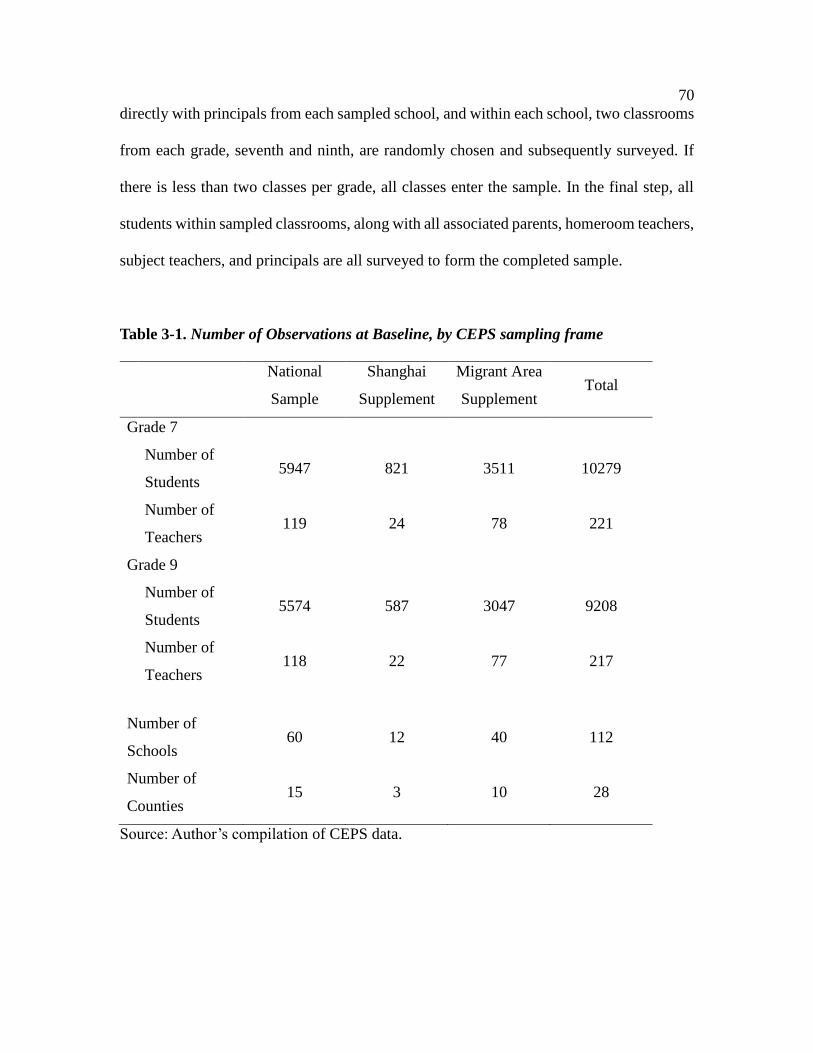
70

directly with principals from each sampled school, and within each school, two classrooms

from each grade, seventh and ninth, are randomly chosen and subsequently surveyed. If

there is less than two classes per grade, all classes enter the sample. In the final step, all

students within sampled classrooms, along with all associated parents, homeroom teachers,

subject teachers, and principals are all surveyed to form the completed sample.

Table 3-1. Number of Observations at Baseline, by CEPS sampling frame

National

Sample

Shanghai

Supplement

Migrant Area

Supplement Total

Grade 7

Number of

Students 5947 821 3511 10279

Number of

Teachers 119 24 78 221

Grade 9

Number of

Students 5574 587 3047 9208

Number of

Teachers 118 22 77 217

Number of

Schools 60 12 40 112

Number of

Counties 15 3 10 28

Source: Author’s compilation of CEPS data.

71

Baseline Data Collection

At each school that is included in the sample, surveyors collaborate with local education

authorities to work with school-level leadership personnel to arrange for an appropriate

time for data collection. Then, surveyors collect principals’, teachers’, parents’ and students’

consent to participate in the study. Next, surveyors directly obtain school-level

administrative data on student core subject test scores on Chinese language arts,

Mathematics, and English (mid-semester test scores for spring semester, 2013). They also

work with teachers and students to arrange for a 45-minute session for each class to

complete the cognitive-item test component of the survey. Upon completion of the

cognitive test and student questionnaires, all homeroom and subject teachers from the

selected classes are surveyed. For subject teachers, only those teaching the three core

subjects Chinese language arts, Mathematics, and English are surveyed. If the homeroom

teacher teaches one of the three core subjects, her response replaces the subject

questionnaire. Finally, parent questionnaires are distributed to students, to be filled by

parents at home, and collected the next day by homeroom teachers. Importantly, for each

type of questionnaire, the surveyors adopt a detailed verification process to ensure data

quality and completeness, with the only exception being on the cognitive test components.

The nested nature of the dataset also allows for matching student responses to families’, to

teachers’, and to principals’.

Baseline Variables

The CEPS questionnaire set includes a total of five independently administered surveys,

for students, parents, homeroom teachers, subject teachers, and principals. A unique feature

72

of this survey is that it contains rich student-level information including administrative

information on core subject test scores, as well as detailed, matched family and teacher

background characteristics information. In particular, for each student, information on

demographic, cognitive ability, health, family, learning, and extracurricular variables are

collected with administrative data on core subject test scores. For each teacher, detailed

background information on educational attainment level, years of experience, training,

certification, rank, awards, as well as information on instructional effort and behavior,

stress level, attitudes, and expectations are available.

Follow-up Data Collection

In the 2014-2015 academic year, CEPS conducted a follow-up survey for all students who

all participated in the first wave. While the follow-up survey was conducted at the school-

level, the survey team adopted two different strategies in tracking students who were in

seventh and ninth grades during baseline survey. For all of the 10,279 students who were

in seventh grade at baseline, surveyors considered them potential subjects in the follow-up

round. For those who were in the ninth grade cohort during baseline survey, the follow-up

survey was mainly to obtain administrative records of test scores and homeroom teacher

response regarding student graduation whereabouts.

In the analysis presented in Part I, I focus exclusively on the tracked students in the seventh

grade cohort across 112 schools. In the follow-up survey, out of 10,279 students, a total of

9,449 students (91.9 percent) who were in the seventh grade cohort were tracked and

surveyed. For the seventh grade cohort, total attrition from the baseline seventh grade

73

cohort sample was 830 students (see Table 3-2 for detailed breakdown by attrition type),

of which the three prominent reasons were school transfer (71.1 percent), dropout (14.6

percent), and unknown (6.1 percent).

Table 3-2. Number of Follow-up Attrition in CEPS Seventh Grade Cohort, by type

Count Frequency (%)

School Transfer 590 71.08

Dropout 121 14.58

Unknown 51 6.14

Short-term Absence 31 3.73

Long-term Sick Leave 14 1.69

Class Transfer 8 0.96

Long-term Absence 4 0.48

Repeat Grade 3 0.36

Vocational School Transfer 3 0.36

Expelled 2 0.24

Deceased 2 0.24

Sports Team Leave 1 0.12

Total 830 100

Source: National Survey Research Center, 2015.

Similar to the baseline data collection, the follow-up questionnaire set also includes five

independently administered surveys, for students, parents, homeroom teachers, subject

teachers, and principals. More specifically, I focus on student level test score information

on Chinese language arts, Mathematics, and English from the follow-up survey dataset.

74

These standardized test scores are collected from school-wide mid-semester examinations,

for which it is common practice for the entire grade to partake during a common testing

period. These mid-semester exams are usually designed collectively by subject teachers in

the same grade with clear intentions to test students on curriculum contents, and answer

sheets are graded with good rigor and consistency. In some schools, student’s names and

class are even hidden from the grader to ensure score validity. Therefore to a degree, core

subject mid-semester test scores can be regarded as a consistent measure of student learning

outcomes in a given grade.

In practice, I utilize administrative data on student core subject test scores in the follow-up

survey found for the seventh grade cohort, and match it to the baseline seventh grade cohort

data. I focus on the core subject test scores for three additional reasons. First, these core

subjects are crucial for continuing education beyond lower secondary schools in the

Chinese context. For instance, the combined weight for these three subjects often exceed

three quarters of the total score on standardized admission test to upper secondary

education and subsequently access to higher education through the College Entrance

Examination. Secondly, these subjects are fundamental to obtaining skills that can facilitate

further education and training opportunities. Without the foundational skills obtained

through the learning of these core subjects, it will be challenging to take advantage of future

skills upgrading opportunities either through continuing education or workplace training.

Third, these three subjects are considered core subjects of instruction and takes up more

than one half of total instructional time in schools. Therefore, teacher instructional quality

and student learning outcomes on these core subjects are arguably key determinants and

75

proxies for overall educational quality.

3.52 China Household Income Survey

The Chinese Household Income Project (CHIP) is a repeated cross-sectional dataset

collected by researchers at Beijing Normal University, with support from the National

Bureau of Statistics. Beginning in 1989, there has been seven waves of data collection.

Among them, five waves use multistage stratified probability method to achieve national

representation, which are respectively referred to as CHIP1988, CHIP1995, CHIP2002,

CHIP2007, and CHIP2013 (the numbers correspond to the year that survey responses are

based on). CHIP1999 included only urban households, while CHIP2008 represented a

panel follow-up to CHIP2007, which included an urban household survey, a rural

household survey, and a rural-to-urban migrant household survey. Collectively, five waves

of CHIP data (with exception of the urban survey in 1999 and the panel follow-up in 2008)

anchor on the established National Bureau of Statistics routine household survey sample.

Each wave of CHIP data offers a snapshot of labor market conditions at the micro-level,

and represents one of the most comprehensive publicly-available repeated cross-sectional

data that cover important employment and income information over a time range of 25

years, that is suitable for tracking dynamics of sectoral employment and income

characteristics over time.

Parts II, III, and IV of this dissertation leverages the detailed individual-level demographic

and earnings information, as well as the large sample size and timing variation available in

CHIP data to empirically evaluate patterns in the relationship between relative wages and

76

teacher occupational choice over time. Specifically, I focus exclusively on the urban

sample, where wage income is reported for employed individuals, and the labor market

conditions are arguably comparable across sectors. In addition, to ensure that the influence

of income outliers and data input error, a standard 1 percent winsoring procedure was

applied to all wage earnings information, such that the top and bottom 1 percent of wage

earnings are replaced with values at the 99 and 1 percentile respectively. As a further step

to standardize repeated cross-sectional data for better comparability, I restrict the analytic

sample to individuals aged between 16 and 60 at the time when the survey took place.

In Table 3-3 and 3-4, I show the detailed sample size breakdown and geographical

distribution by year. In general, the total urban sample size fluctuates approximately

between 15,000 and 30,000 across years, while roughly about close to one half of the

sample report currently being employed in paid labor arrangements, which include being

self-employed and paid helpers in family business operations. Importantly, I identify

between 190 – 779 teachers in each wave of the CHIP data. In this regard, because CHIP

datasets do not include ISCO or equivalent job-level codes, therefore, identification of

teachers are based jointly on sectoral, occupational, and work unit ownership information.

Unfortunately, due to data availability, I am not able to distinguish between levels of

instruction; however, because teachers who work in primary and secondary education

represent the largest population within the teaching force, they are likely oversampled in

my identification of teachers. Therefore it is not unreasonable to assume that a substantial

number of identified teachers work in primary and secondary settings. Particularly, teachers

are identified as professional workers who are employed in the education sector and

77

working in public institutions (shiye danwei). In the following section, I provide further

information on the data sampling, collection, and variables on each wave of CHIP data in

the succeeding text.

Table 3-3. CHIP Sample Size, by year

Year Full Sample,

Urban Individuals

Employed Workers,

Urban Analytic Sample

Identified Teachers,

Urban Analytic Sample

1988 31827 17073 779

1995 21533 10765 441

2002 21696 9762 505

2007 14695 5465 207

2008 14859 5452 190

2013 19887 7811 429

Source: Author’s compilation using Chinese Household Income Project.

Table 3-4. CHIP Sample Geographical Coverage, by year

Year List of Sampled Provincial-level Regions Count

1988 Beijing, Liaoning, Jiangsu, Guangdong, Shanxi, Anhui,

Henan, Hubei, Yunnan, Gansu 10

1995 Beijing, Liaoning, Jiangsu, Guangdong, Shanxi, Anhui,

Henan, Hubei, Sichuan, Yunnan, Gansu 11

2002 Beijing, Liaoning, Jiangsu, Guangdong, Shanxi, Anhui,

Henan, Hubei, Sichuan, Chongqing, Yunnan, Gansu 12

78

2007

Beijing, Shanghai, Liaoning, Jiangsu, Zhejiang, Fujian,

Guangdong, Shanxi, Anhui, Henan, Hubei, Hunan, Sichuan,

Chongqing, Yunnan, Gansu

16

2008

Beijing, Shanghai, Liaoning, Jiangsu, Zhejiang, Fujian,

Guangdong, Shanxi, Anhui, Henan, Hubei, Hunan, Sichuan,

Chongqing, Yunnan, Gansu

16

2013

Beijing, Liaoning, Jiangsu, Guangdong, Shanxi, Anhui,

Henan, Hubei, Hunan, Sichuan, Chongqing, Yunnan, Gansu,

Xinjiang, Shandong

15

Source: Excerpt from Table 2 in Gustafsson, Li, and Sato (2014, p. 29).

CHIP1988

The objective of initiating CHIP1988 was primarily to study income distribution and

inequality in China, which involved sampling of provincial-level administrative regions in

a stratified multi-stage procedure (Eichen & Zhang, 1993). The urban and rural sampling

frames are based on the routine household sample maintained by the National Bureau of

Statistics, which included 34,945 urban and 67,186 rural households. Within each

household, all members are surveyed. Systematic sampling methods based on income

distribution was employed, which derived a cross-sectional dataset that included 31,827

individuals nested within 9,009 urban households, and 51,352 individuals within 10,258

rural households. In-person data collection took place in the spring of 1989, and

respondents reported information on sex, age, education, income, employment status,

sector of work, party membership, household wealth, along with other demographic

background characteristics.

79

CHIP 1995

Conducted between January and March in 1996, CHIP1995 systematically samples the

National Bureau of Statistics’ established routine household sample using a stratified multi-

stage procedure, which derived an urban sample of 21,533 individuals in 6868 households,

and 34,739 individuals in 7,998 rural households. The administered survey questionnaires

collected similar background and employment information as in the previous 1988 wave.

CHIP 2002

Conducted in the spring of 2003, CHIP2002 included a rural-to-urban migrant sample in

addition to the previously standard urban and rural subsamples. Consistent with previous

cycles, the urban subsamples was drawn from the larger National Bureau of Statistics’

established routine urban household sample using a multistage stratified probability

method to be nationally representative. The sampling procedure yields a dataset with

21,696 individuals in 6,934 households. Survey questionnaire collected similar background

and employment information as in previous waves, but with additional information on the

selectivity of high schools that individuals attended.

CHIP 2007, 2008 and RUMiC 2007, 2008

To be clear, CHIP 2007 and CHIP 2008 are often referenced in the broader research

community as the 2007 and 2008 waves of the longitudinal survey on Rural-Urban

Migration in China (RUMiC). Collected in the spring of 2008 and 2009, the two-wave

survey was jointly designed and administered by an international consortium of researchers

with support from the National Bureau of Statistics. The project was designed to track

80

households so long as they are present in the surveyed cities, which means that the dataset

could be evaluated as cross-sectional data independently or linked together as individual

panel data. Respectively, RUMiC 2007 and RUMiC 2008 each comprises of three

independent survey components: urban household survey, rural household survey, migrant

household survey (see Akguc, Giulietti, Zimmermann, 2014). Each of the three survey

components includes detailed information on household and individual demographics,

employment and income, training and education, health and well-being, among other

background dimensions such as social networks, etc.

Of particular interest, the urban sample was derived using National Bureau of Statistics’

routine household sample, which involved randomly sampling households in nineteen

different cities across sixteen provinces. According to Akguc, Giulietti, and Zimmermann’s

(2014) reporting, the total number of households surveyed in RUMiC 2007 was 5,005 and

included 14,695 individuals, of which 5.8 percent of the baseline sample was lost in the

follow-up RUMiC 2008 but added about 1,018 individuals (see Table 3-5). The

questionnaires included detailed information on demographics, employment, and

socioeconomic variables, such as age, marital status, children, household registration status,

as well as migration status and experience.

CHIP 2013

Conducted in July and August of 2014, CHIP2013 collected information on 2013 income

and expenditure as well as personal and household background characteristics. Stratified

by geographic location, the sampling frame is derived from an established routine

81

household sample maintained by the National Bureau of Statistics which included over

160,000 households in 31 provinces. Systematic sampling derived 19,887 individuals

nested within 6,674 households. Similar to CHIP2002, survey questionnaire in this cycle

also collected personal background and employment information as in previous waves, as

well as additional information on the selectivity of high schools that individuals attended.

Table 3-5. Sample and Attrition Information on CHIP2007 (RUMiC2007) and

CHIP2008 (RUMiC2008)

Number of

Households

Number of

Individuals

Number of

Employed

Individuals

Number of

Identified

Teachers

RUMiC 2007 5005 14695 5465 207

RUMiC 2008 4735 14859 5452 190

Attrition Rate 5.4% 5.8% - -

New

Individuals

- 1018 - -

Source: Excerpt from Akguc, Giulietti, and Zimmermann (2014, p.6)

82

Chapter IV

RESULTS

In this chapter, I sequentially present complete results from each part of the dissertation

analysis. However, before proceeding directly into the micro-level analysis results, a brief

discussion of macro-level trends in teacher wages is in order to illustrate the broader

contextual background for the succeeding micro-level analyses. To situate the discussion

more broadly in China’s development context, a 30-fold expansion of real GDP since 1978

suggests that labor market conditions have experienced rapid shifts, and the magnitude of

change is qualitatively different from most developed economies (Wen, 2015). Drastic

shifts within a relatively short window of time may exacerbate the adverse occupational

selection effects, especially with the presence of relatively fixed teacher salary schedules

and infrequent wage adjustments as compared to other sectors. Therefore, the core

objective of this macro-level analysis is to understand how aggregate-level wages in

teaching has shifted, as well as identify emerging patterns in the quality composition of

teachers using a common measure of human capital: educational attainment. In more detail,

I present results from a relative wage accounting exercise at the cross-sector level in Table

4-0-1 as well as taking a deep dive within-education in Figure 4-0-1, and compile worker

composition information to show changes in the educational attainment of teachers in

Tables 4-0-2 and 4-0-3, as well as examining sources of net teacher intake in Table 4-0-4.

Firstly, in Table 4-0-1, following Lakdawalla (2006) and using most recently available

disaggregated sectoral wage data, I deflate teacher wages using national average worker

83

wage for a given year, and for easy interpretation, log point changes are transformed as

percent changes. In broad strokes, Table 4-0-1 shows that observed wage growth for

teachers, relative to the average national worker between 1999 and 2009, has substantially

regressed, at -44.1 percent for primary school teachers and -46.7 percent for secondary

school teachers respectively. This wage accounting exercise indicates that relative wages

for teachers have been growing at around half the growth rate of wages for the national

average worker between 1999 and 2009.

As a point of reference, Lakdawalla (2006) demonstrates that most high-income countries

witnessed relative teacher wage growth rates in the range of -28.8 percent for Sweden and

7.25 percent for Japan over three decades, between 1965 and 1994. In scilicet, the

magnitude of relative teacher wage lag in China is much greater than that of developed

economies, and occurred at a much quicker rate, approximately less than a third of the

timeframe. Despite these consequential changes, few studies quantitatively discuss the

impact of teacher wage characteristics on teacher quality shifts in China, or provide any

rigorous research that relate observed teacher labor supply patterns to the existing

occupational choice literature. Thus, a formal analysis of teacher occupational choice in

the Chinese context is justified, and can provide important insights not only for exploring

policy instruments that recruit and retain more capable and educationally productive

teachers, but such empirical work is also crucial for understanding individuals’ labor supply

decisions in rapidly developing economies.

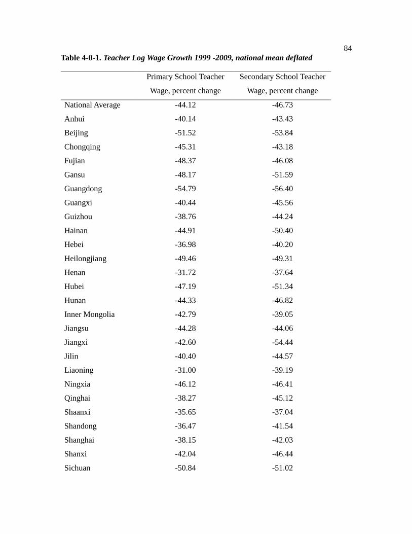
84

Table 4-0-1. Teacher Log Wage Growth 1999 -2009, national mean deflated

Primary School Teacher

Wage, percent change

Secondary School Teacher

Wage, percent change

National Average -44.12 -46.73

Anhui -40.14 -43.43

Beijing -51.52 -53.84

Chongqing -45.31 -43.18

Fujian -48.37 -46.08

Gansu -48.17 -51.59

Guangdong -54.79 -56.40

Guangxi -40.44 -45.56

Guizhou -38.76 -44.24

Hainan -44.91 -50.40

Hebei -36.98 -40.20

Heilongjiang -49.46 -49.31

Henan -31.72 -37.64

Hubei -47.19 -51.34

Hunan -44.33 -46.82

Inner Mongolia -42.79 -39.05

Jiangsu -44.28 -44.06

Jiangxi -42.60 -54.44

Jilin -40.40 -44.57

Liaoning -31.00 -39.19

Ningxia -46.12 -46.41

Qinghai -38.27 -45.12

Shaanxi -35.65 -37.04

Shandong -36.47 -41.54

Shanghai -38.15 -42.03

Shanxi -42.04 -46.44

Sichuan -50.84 -51.02

85

Tianjin -35.17 -41.81

Tibet -50.03 -55.34

Xinjiang -53.72 -55.34

Yunnan -54.97 -56.47

Zhejiang -49.53 -47.89

Source: Own calculations, based on National Labor Statistics Yearbook, 1999, 2009. Note:

Data for special administrative regions of Hong Kong, Macau, and Taiwan is not available.

To add, the sheer numeric size and geographic spread of the teaching sector led to

significant wage inequality not only in comparison to the non-teaching sector, but also

within the teaching sector. In Figure 4-0-1, I visualize the large differences in wage growth

at the provincial level for both primary and secondary school teachers. For instance, in

Yunnan (southwest on the map), the average primary teacher wage growth is 21.6 percent

less than the national average teacher between 1999 and 2009, while in Shanghai, the wage

growth is 10 percent more. This large geographic variation in wage growth is in direct

contrast with most existing evidence found in developed countries, where the teaching

sector is often dominated by common collective bargaining and characterized by low

within-sector wage spread, which may be further exacerbated by potentially large

purchasing power differences across different regions. To this end, large wage growth

differences and wage spread, within the teaching sector and across geographic regions, has

important implications for the succeeding analysis, because self-selection may be driven

by both conditions across sectors and across locations.

86

Figure 4-0-1. Teacher Log Wage Changes 1999-2009, sector mean deflated

Panel A | Primary Teachers Panel B| Secondary Teachers

Source: Own calculations, based on National Labor Statistics Yearbook, 1999 and 2009.

Note: Log of teacher wage have been deflated using national teacher mean wage for each given year. Darker shade of red represents

steeper relative decline, darker shade of blue represents steeper relative increase.

87

Secondly, I track compositional shifts in educational attainment of teachers relative to

workers in the broader labor market. Using both the earliest as well as most recently

available data from National Labor Statistics Yearbook (2003, 2017), I calculate changes

in the percentage of workers in each sector with a given level of educational attainment

and deflate it using the national mean growth rate. In general, teachers are becoming more

educated, and the rate of increase is much quicker in the education sector. Detailed results

are presented in Table 4-0-2, and each cell is to be interpreted as the percent change in

educational attainment level of workers in that sector relative to the growth at the national

mean. For instance, between 2003 and 2017, the percent of teachers with at least a

Bachelor’s degree grew as much as 4 times relative to the national average growth in

percent of workers with at least Bachelor’s degrees (6.8 percent, while teachers with an

Associate’s degree decreased at about 2.8 times the national average growth in percent of

workers with Associate’s degrees (5.3 percent).

Thirdly, to examine more deeply within the education sector, in Table 4-0-3, I decompose

educational attainment for teachers by different levels of instruction: primary, lower

secondary, and upper secondary. Particularly, I find that educational attainment for teachers

at different levels of instruction have systematically increased. For primary schools, the

percentage of teachers with at least Bachelor’s degrees increased from less than 1 percent

in 1999 to close to 20 percent in 2009, and reached more than half (50.4 percent) of all

primary school teachers in 2016. At the lower secondary level, the growth in teachers with

at least a Bachelor’s degree was also substantial, expanding 5 times from 12.4 percent in

1999 to 59.4 percent in 2009; by 2016, approximately 4-out-of-5 lower secondary school

88

teachers have at least a Bachelor’s degree. At the upper secondary level, similar trends are

observed; 65.9 percent with Bachelor’s degree in 1999 have increased to over 90 percent

in 2009 and close to 100 percent by 2016. Overall, observed patterns across instructional

levels indicate that educational attainment levels of teachers at all instructional levels have

increased sharply, with majorities of teachers holding at least an associate’s or bachelor’s

degree by 2016.

However, in more recent years, the relative educational attainment advantage of teachers

relative to workers in other sectors is quickly dissipating. Importantly, between years 2003

and 2017, the education sector saw the highest increase in workers with at least a

Bachelor’s degree, narrowly placing ahead of “Finance and Banking” (3.93 times the

national mean). Other sectors that saw similar sizable increases are “Scientific Research

and Development,” “Public Health and Social Welfare,” “Information Technology,”

“Government and Public Administration,” and “Leasing and Business Services,” which all

exceeded twice the national average growth in the percent of workers with at least

Bachelor’s degrees. On the other hand, results in columns four, five and six on Table 4-0-

2, indicate that the growth of teachers with at least Bachelor’s degrees has been dwarfed

by several sectors in recent years. To illustrate, the percent of workers with at least a

Bachelor’s degree in the “Finance and Banking” sector grew at 2.55 times the national

average, followed by “Information Technology” (2.47 times) and “Public Health and Social

Welfare” (2.46 times), while the “Education” sector grew at 2.2 times the national average

rate between 2009 and 2017. In addition, share of workers with 2-year Associate’s degree

also sharply decreased in the education sector, more than any other sector, for the same

89

years. Overall, results show that while the number of workers with at least a Bachelor’s

degree has been growing in the education sector as well as most other sectors, in more

recent years, sectors such as “Finance and Banking,” “Information Technology,” and

“Public Health and Social Welfare” have been quickly catching up and recruiting workers

with Bachelor’s degrees at a comparatively faster pace. That is to say, the flow of higher

quality workers to non-education sectors is gaining considerable momentum.

Fourthly, because teacher composition has positively shifted since 1999, I evaluate to what

extent this phenomenon may have been driven by new entrant teachers or teacher exits.

Due to the Ministry of Education began reporting source of new teachers only after 2004,

in Table 4-0-4, I report net intake information for teachers by source, level of instruction

for 2004, 2009, 2013, and 2016. For interpretation purposes, a positive number in each cell

means there are more teachers entering than there are leaving, conditional to prior year’s

total teacher employment size, whereas the opposite is true for negative numbers. While

the Net Total results are important, it could be biased by many factors such as policy shocks

as well as demographic transitions; therefore, I focus on the net intake source categories.

For primary schools, there were no consistent patterns, but there is seemingly more teachers

retiring than there were new entrants in 2004 and 2009. Additionally, substantial net

transfers into teaching and within-school adjustments into teaching are also observed for

2009 and 2016. In lower secondary schools, there is a consistent pattern that net intake in

new teacher entrants is a main source of compositional change, in additional to a significant

amount of net transfers and within-education adjustments out of teaching. At the upper

secondary level, net intake in new teachers is a substantial source in the replenishment

90

process, while there also exists a mixed pattern of volume in both directions: net transfers

from outside of education and net within-education adjustments out of teaching posts.

To briefly summarize the macro-level analytic findings, I outline the main results. On the

one hand, while average growth in teaching wages are relatively experiencing large

declines in comparison to the cross-sector national mean wage, relative labor quality in the

education sector, as approximated by educational attainment levels, has until recently

shown greater growth compared to most other sectors. Nonetheless, higher growth sectors

such as “Finance and Baking” have begun to attract highly educated workers than the

education sector in more recent years. On the other hand, growth in educational attainment

among teachers at different instructional levels has been large and relatively even across

instructional levels. Moreover, in accounting for source of teacher intake, new teacher

entrants seem to be the most consistent source, while there is considerable net transfer out

of teaching to other sectors at the lower secondary level. Finally, while the macro-level

analysis are limited by the availability and type of data, its findings are instructive for

understanding the broader context of teacher occupational choice in China, with respect to

alternative career options. This dissertation proceeds to present a more detailed

investigation in the succeeding subsections with respect to teacher’s occupational decisions.

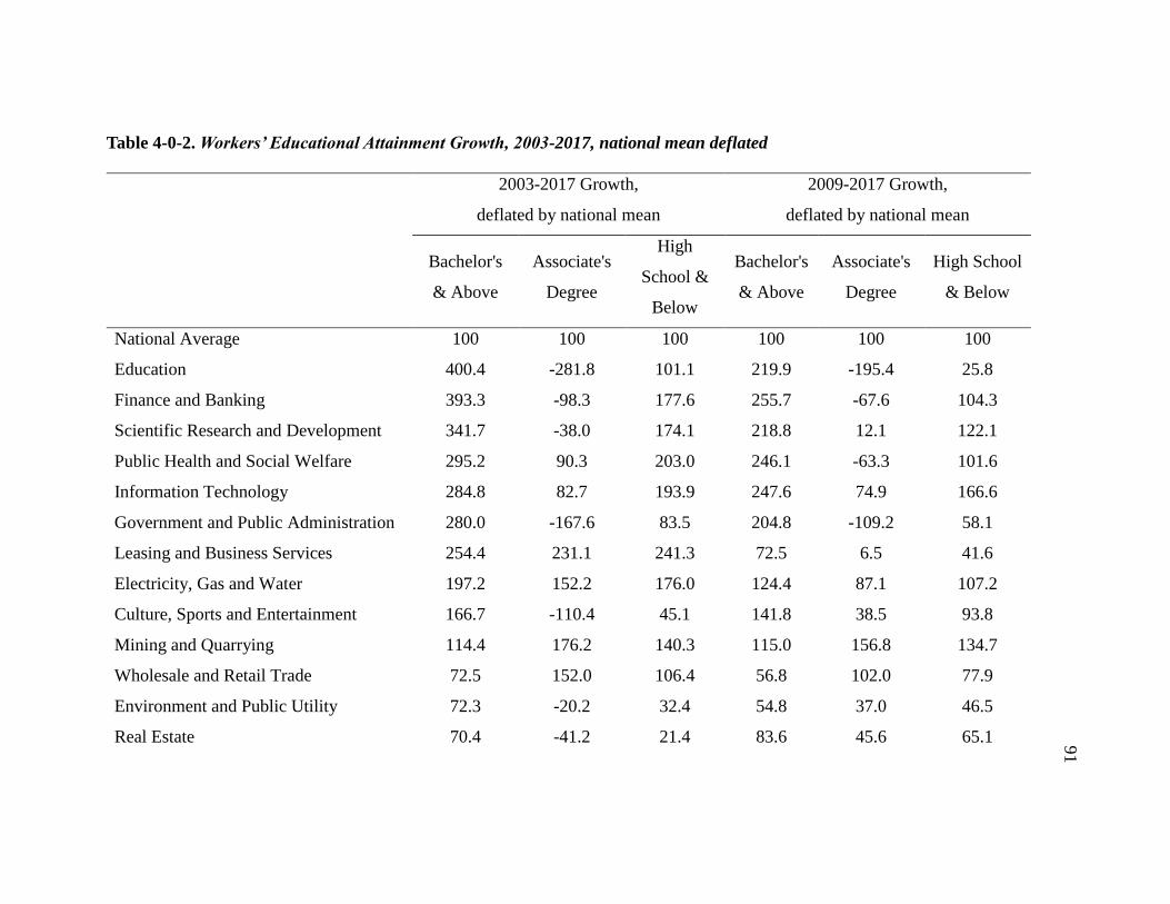
91

Table 4-0-2. Workers’ Educational Attainment Growth, 2003-2017, national mean deflated

2003-2017 Growth,

deflated by national mean

2009-2017 Growth,

deflated by national mean

Bachelor's

& Above

Associate's

Degree

High

School &

Below

Bachelor's

& Above

Associate's

Degree

High School

& Below

National Average 100 100 100 100 100 100

Education 400.4 -281.8 101.1 219.9 -195.4 25.8

Finance and Banking 393.3 -98.3 177.6 255.7 -67.6 104.3

Scientific Research and Development 341.7 -38.0 174.1 218.8 12.1 122.1

Public Health and Social Welfare 295.2 90.3 203.0 246.1 -63.3 101.6

Information Technology 284.8 82.7 193.9 247.6 74.9 166.6

Government and Public Administration 280.0 -167.6 83.5 204.8 -109.2 58.1

Leasing and Business Services 254.4 231.1 241.3 72.5 6.5 41.6

Electricity, Gas and Water 197.2 152.2 176.0 124.4 87.1 107.2

Culture, Sports and Entertainment 166.7 -110.4 45.1 141.8 38.5 93.8

Mining and Quarrying 114.4 176.2 140.3 115.0 156.8 134.7

Wholesale and Retail Trade 72.5 152.0 106.4 56.8 102.0 77.9

Environment and Public Utility 72.3 -20.2 32.4 54.8 37.0 46.5

Real Estate 70.4 -41.2 21.4 83.6 45.6 65.1

92

Manufacturing 66.2 94.1 78.6 61.7 80.7 70.6

Transportation, Post, and

Telecommunications 61.7 80.5 69.4 53.7 65.7 59.3

Personal and Other Services 46.6 71.5 56.2 40.4 51.1 45.3

Hospitality and Catering Services 26.6 61.7 40.8 20.7 39.4 29.5

Construction 25.8 25.9 25.6 23.6 18.8 21.5

Agriculture 3.0 6.9 3.8 2.6 5.8 4.1

Source: National Labor Statistics Yearbook, 2003, 2009 and 2017. Note: Relative changes in percent of workers with a given educational

attainment level has been deflated using the national mean for that level in that given year. The national mean growth rate in percent of

workers with a given educational attainment level between 2003-2017 for Bachelor’s and above is 6.809 percent, for Associate’s is

5.296 percent, and for High school and below is -12.205 percent; the national mean growth rate between 2009-2017 for Bachelor’s and

above is 6.050 percent, for Associate’s is 5.310 percent, and for High school and below is -11.360 percent.

93

Table 4-0-3. Percent Teachers by Educational Attainment, by level and year

Year Bachelor's and

Above Associate's

Upper

Secondary and

Below

Total

Primary

Teachers

1999 0.7 15.5 83.7 100

2004 4.6 44.2 51.2 100

2009 19.8 55.0 25.2 100

2013 37.2 50.1 12.7 100

2016 50.4 43.2 6.3 100

Lower

Secondary

Teachers

1999 12.4 73.2 14.4 100

2004 29.1 64.7 6.2 100

2009 59.4 38.8 1.7 100

2013 74.9 24.4 0.7 100

2016 82.5 17.3 0.2 100

Upper

Secondary

Teachers

1999 65.9 32.5 1.7 100

2004 79.6 20.0 0.4 100

2009 93.6 6.3 0.1 100

2013 96.8 3.1 0.1 100

2016 97.9 2.0 0.0 100

Source: National Education Statistical Yearbook, 1999, 2004, 2009, 2013, 2016.

94

Table 4-0-4. Share of New Teachers as Percent of Prior Year Total Teacher Employment, by source, teaching-level, and year

Primary Teachers Lower Secondary Teachers Upper Secondary Teachers

2004 2009 2013 2016 2004 2009 2013 2016 2004 2009 2013 2016

Net Total -1.29 0.20 -0.01 1.83 0.17 1.27 -0.67 0.35 11.25 1.20 2.13 2.25

Net New Recruit In -0.41 -0.12 0.33 1.10 1.84 1.53 0.69 1.29 7.12 0.57 2.57 2.21

Net Transfer In -0.17 0.41 -0.05 0.84 -0.56 -0.43 -1.22 -0.49 2.86 0.14 -0.11 0.33

Net Within-

Education

Adjustment In

-0.16 0.11 -0.18 0.02 -0.71 0.32 -0.40 -0.19 1.40 -0.82 -0.07 -0.01

Net Other In -0.55 -0.19 -0.11 -0.14 -0.40 -0.15 -0.17 -0.26 -0.14 -0.34 -0.26 -0.27

Source: National Education Statistical Yearbook, 2004, 2009, 2013, 2016. Note: The average total teacher employment numbers for

2004, 2009, 2013, and 2016 are 5648745, 3480049, 1459080 for primary, lower secondary, upper secondary respectively. Net Recruit

In is defined as the difference between number of new teacher entrants and number of retiring teachers. Net transfers refers to the

difference between the number of teachers who entered teaching from another sector and the number of those who have left teaching

for another sector. Net within-education adjustments is categorized as the difference in number of non-teaching school staff (e.g.

administration or support staff) that switched to a teaching post and those who switched from a teaching post to a non-teaching position.

Net others includes all undefined reasons.

95

4.1 Results for Part I:

The Impact of Teacher Quality on Student Learning

An educationally-important and policy-relevant objective of this section is to establish

whether commonly observed teacher background characteristics, such as educational

attainment level, are causally linked to affect student learning outcomes. Existing research

has shown that this relationship can be empirically ambiguous. Therefore, to rigorously

answer this research question, I employ a student fixed-effect strategy to relate differences

in teacher characteristics across subjects to variations on student test scores. Effectively,

this methodology helps eliminate all student-level observable and unobservable subject-

invariant factors, and in effect compares how student test scores vary for the same student

across different subjects in which teacher characteristics also vary, after controlling for

important student- and teacher-level variables that are different across subjects. In the

succeeding sections, I present the detailed results.

For each of the test score outcomes, administrative data is directly obtained at the school-

level, and collected once at baseline survey and another during the follow-up wave. In

Table 4-1-1, I present a correlation matrix and descriptive statistics of all student-learning

outcomes used in the following analysis. Importantly, the correlation of within-wave,

between-subject and between-wave, within-subject are at least moderate; some are strongly

correlated. For instance, the correlation coefficient for Chinese, Math, and English test

scores at baseline range between 0.64-0.72 (p-values <.05) and 0.68-0.73 (p-values <.05)

at follow-up, indicating strong correlations and good internal reliability. In addition, the

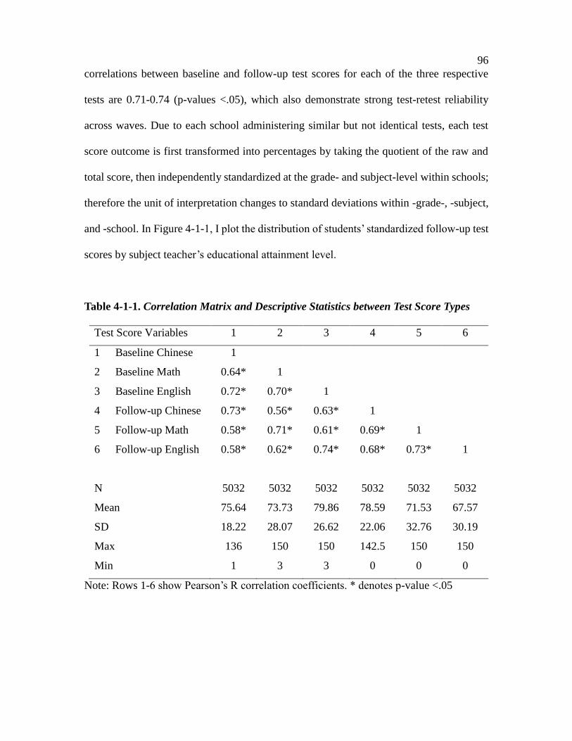
96

correlations between baseline and follow-up test scores for each of the three respective

tests are 0.71-0.74 (p-values <.05), which also demonstrate strong test-retest reliability

across waves. Due to each school administering similar but not identical tests, each test

score outcome is first transformed into percentages by taking the quotient of the raw and

total score, then independently standardized at the grade- and subject-level within schools;

therefore the unit of interpretation changes to standard deviations within -grade-, -subject,

and -school. In Figure 4-1-1, I plot the distribution of students’ standardized follow-up test

scores by subject teacher’s educational attainment level.

Table 4-1-1. Correlation Matrix and Descriptive Statistics between Test Score Types

Test Score Variables 1 2 3 4 5 6

1 Baseline Chinese 1

2 Baseline Math 0.64* 1

3 Baseline English 0.72* 0.70* 1

4 Follow-up Chinese 0.73* 0.56* 0.63* 1

5 Follow-up Math 0.58* 0.71* 0.61* 0.69* 1

6 Follow-up English 0.58* 0.62* 0.74* 0.68* 0.73* 1

N 5032 5032 5032 5032 5032 5032

Mean 75.64 73.73 79.86 78.59 71.53 67.57

SD 18.22 28.07 26.62 22.06 32.76 30.19

Max 136 150 150 142.5 150 150

Min 1 3 3 0 0 0

Note: Rows 1-6 show Pearson’s R correlation coefficients. * denotes p-value <.05

97

Figure 4-1-1. Distribution of student test scores by teacher’s educational attainment

Note: Author’s compilation according to CEPS data. This chart plots student test scores for

all three tested subjects: Chinese, Math, English by subject teacher’s educational

attainment level. Kernel density is computed using Epanechnikov method, bandwidth for

“BA & above” is 0.1333, bandwidth for “AA” is 0.1852.

In Table 4-1-2, detailed information on descriptive statistics is introduced, for both student

level variables (see Panel A) and teacher-level variables (see Panel B). In the seventh grade

subsample drawn from the nationally representative CEPS data, there are a total of 5,032

students and 357 teachers. In Panel A, I discuss subject-varying student-level variables

relevant to the current analysis. To begin, between 10 to 16 percent of students in the

sample report that they attended private tutoring last week for the three core subjects:

Chinese, Math, and English. Close to 90 percent of students indicated that they find each

of the three subjects valuable for their later life developments. In terms of classroom

learning experience, between 63 to 67 percent of all students reported that they felt their

98

subject teachers were frequently interacting with them during class instruction.

In Panel B of Table 4-1-2, I report descriptive statistics information on subject-varying

teacher characteristics. First, approximately 73 percent of all teachers are female, and close

to a third (29 percent) of them serve as homeroom teachers, whose teaching responsibilities

extend beyond course instruction but also include class management duties such as student

counseling, parent coordination, etc. Second, in terms of teacher preparation, certification

and contract, most teachers report having attended a pre-service teacher education “normal”

program (93 percent), and 97 percent of all teachers received official teaching certifications

issued by the government authorities. In China, pre-service teacher education (normal)

program is defined as attending an educational institution or program that specializes in

training pre-service teachers; these institutions are commonly accredited by the Ministry

of Education based on a broad base of quality that range from facilities to curriculum. For

employment status, only about two thirds (64 percent) of all teachers report to hold

permanent appointments or bianzhi in their respective schools, while others (36 percent)

self-identify as being employed on temporary contract arrangements at their current school.

Third, I report teacher’s baseline pedagogical skills levels with information on their teacher

rank and teaching awards. Teacher rank, or zhicheng, consists of four levels in descending

prestige: senior rank, level one rank, level two rank, level three rank. To promote in

teaching rank, teachers often undergo rigorous review of the credentials, training, and

performance. Teaching awards, on the other hand, are bestowed by different levels of

education authorities, ranging from national-level, provincial-level, municipal-level,

99

district-level, and school-level, and are commonly awarded through formal teaching

competitions. In the current sample, 84 percent of all teachers self-identify as Level 2 rank

or above, while about one third (35 percent) received at least a Municipal-level or superior

teaching award. Fourth, in terms of workload, the sample mean was 44.59 hours (SD=12.89)

for the past week, with a wide range (12-100). In addition, the sample mean for teaching

experience is 14.67 years (SD=8.67), with a range including new teachers (0 years) and

veteran teachers (39 years).

Fifth, in order to assess the extent to which student ability grouping practices may influence

or confound observed impacts, I also report teacher responses on whether classes are

assigned based on a combined total score, or subject-specific scores. Importantly, if ability

grouping is prevalent such that non-random sorting occurs between students and teachers,

selection bias may confound the results. At the teacher-level, 28 percent of teachers

indicate that students are assigned to classrooms using a combined test score, while 12

percent of teachers report individual test scores are used to assign students to classrooms.

In the succeeding analysis, the second type of class assignment based on subject scores

could be particularly more worrying and problematic, because it introduces unobserved

subject-varying unobservables that may be correlated with both teacher characteristics and

student test score outcomes. To address these potential issues, I explicitly model these

relationships in the sensitivity and robustness checks. Last but not least, for the key variable

of interest, teacher’s educational attainment level, all but 2 teachers, who completed

education at the vocational secondary level, report having at least an associate’s degree (2-

year zhuanke), while approximately 83 percent obtained at least a bachelor’s degree (4-

100

year benke). This will be the key variable of interest in the succeeding analysis.

In Table 4-1-3, I evaluate the degree to which teacher observable characteristics differ

across subject. As mentioned previously in the methods section, if there are systematic

differences in teacher observables or unobservables, which are related to student outcomes,

estimated results may be biased. I empirically check for this possibility in the dataset. In

effect, I compare to what extent teacher characteristics are different across subjects, where

each row in Table 4-1-3 represents an independent regression of various teacher-level

variables on subject, with the reference subject group being Chinese. The results indicate

that relative to Chinese subject teachers, Math teachers are less likely to be female and hold

a teacher rank above Level 2, whereas English teachers are more likely to be female, less

likely to have attended a pre-service normal education program, and less likely to report

class assignment was based on subject score. To be clear, in Table 4-1-3, I do not find

systematic differences on teacher observable baseline characteristics by subject.

101

Table 4-1-2. Descriptive Statistics of CEPS Seventh Grade Cohort Students and Teachers

Definition and Metrics N Mean SD Max Min

Panel A: Student-Level Variables

Private Tutoring

Enrollment in private tutoring =1,

otherwise =0

Chinese 5032 0.10 - 1 0

Math 5032 0.16 - 1 0

English 5032 0.18 - 1 0

Subject Valuable

Student found subject matter valuable for

later life =1, otherwise =0

Chinese 5032 0.93 - 1 0

Math 5032 0.90 - 1 0

English 5032 0.87 - 1 0

Frequent Teacher Interaction

Teacher interacted frequently with student

during instruction =1, otherwise =0

Chinese 5032 0.64 - 1 0

Math 5032 0.63 - 1 0

English 5032 0.67 - 1 0

Panel B: Teacher-Level Variables

Female Teacher is female =1, otherwise =0 357 0.73 - 1 0

Homeroom Teacher is a homeroom teacher =1,

otherwise =0 357 0.29 - 1 0

102

Pre-Service Normal Education

Teacher attended a pre-service normal

education teaching program =1, otherwise

=0

357 0.93 - 1 0

Certification Teacher is government certified to teach

=1, otherwise =0 357 0.97 - 1 0

Permanent Contract Teacher is employed on permanent

contract =1, otherwise =0 357 0.64 - 1 0

Second-tier or Above Teacher Rank Teacher received senior, first-tier, second-

tier teacher rank =1, otherwise =0 357 0.84 - 1 0

Municipal or Above Teaching Award

Teacher received national, provincial,

municipal-level teaching awards =1,

otherwise =0

357 0.35 - 1 0

Last Week Working Hours Teacher's number of working hours last

week 357 44.59 12.89 100 12

Teaching Experience Teaching experience in years 357 14.67 8.67 39 0

Teaching Experience Categories 357

Group 1 Teaching experience is less than or equal

to 5 years =1, otherwise =0

0.18 - 1 0

Group 2

Teaching experience is more than 5 years

and less than or equal to 15 years =1,

otherwise =0

0.36 - 1 0

103

Group 3

Teaching experience is more than 15 years

and less than or equal to 25 years =1,

otherwise =0

0.32 - 1 0

Group 4 Teaching experience is more than 25 years

=1, otherwise =0 0.11 - 1 0

Class Assignment by Total Score Class assigned according to total score =1,

not assigned according to total score =0 357 0.28 - 1 0

Class Assignment by Subject Score

Class assigned according to subject score

=1, not assigned according to subject score

=0

357 0.12 - 1 0

Teacher's Educational Attainment

Bachelor's Degree and Above

Teacher's highest educational attainment

was bachelor's degree or above =1,

otherwise =0

357 0.83 - 1 0

104

104

Table 4-1-3. CEPS Teacher characteristics by subject types (N=357)

Dependent Variables

Subject (reference = Chinese)

Math English

Bachelor's degree and above (below =0) -0.046 -.006

(0.172) (0.383)

Female (male =0) -0.593* 0.681*

(0.151) (0.197)

Homeroom (non-homeroom =0) 0.264 0.026

(0.188) (0.230)

Pre-Service Normal Education (did not attend =0) 0.008 -0.585*

(0.269) (0.265)

Permanent Contract (temporary =0) -0.288 -0.015

(0.167) (0.201)

Certification (not certified =0) 0.130 0.558

(0.385) (0.464)

Second-tier or Above Teacher Rank (below =0) 0.490* -0.056

(0.179) (0.141)

Municipal or Above Teaching Award (below =0) 0.153 -0.039

(0.143) (0.153)

Class Assigned by Subject Score

(not assigned by score =0) 0.030 -0.605*

(0.192) (0.282)

Teaching Experience (years) 1.714 0.097

(0.879) (0.966)

Last Week's Working Hours (hours) -2.337 -2.221

(1.804) (1.698)

Note: Each row represents an independent regression. All coefficients are from probit

regression, with exception of Last Week's Working Hours and Teaching Experience, which

are from OLS regression. Robust standard errors closeted at the school-level and are

presented in parenthesis, * denotes p-value <.05.

105

105

In Table 4-1-4, I find that while there are differences in the prevalence of teachers whose

highest educational attainment level was at least a 4-year bachelor’s compared to those

who only received a 2-year associate’s or below, there is little evidence that teachers with

different education are also systematically different on other observable dimensions. With

exception to gender, certification status, and teacher rank, there is no statistical difference

between the two groups of teachers on other observable characteristics. Relative to teachers

with 2-year associate’s or below educational attainment, those with at least a 4-year

bachelor’s degree are more likely to be female, have obtained certified status, and hold a

teacher rank above Level 2.

Table 4-1-4. CEPS Teacher characteristics by educational attainment levels (N=357)

Dependent Variables Bachelor's degree and above

(reference = below)

Female (male =0) 0.778*

(0.209)

Homeroom (non-homeroom =0) 0.274

(0.155)

Pre-Service Normal Education

(did not attend =0) 0.370

(0.233)

Permanent Contract (temporary =0) 0.052

(0.176)

Certification (not certified =0) 0.953*

(0.279)

Second-tier or Above Teacher Rank (below =0) 0.689*

(0.213)

106

106

Municipal or Above Teaching Award (below =0) 0.252

(0.213)

Class Assigned by Total Score

(not assigned by total score =0) 0.286

(0.246)

Class Assigned by Subject Score

(not assigned by subject score =0) 0.376

(0.261)

Teaching Experience (years) -2.314

(1.604)

Last Week's Working Hours (hours) -0.923

(2.412)

Note: Each row represents an independent regression. All coefficients are from probit

regression, with exception of Last Week's Working Hours and Teaching Experience, which

are from OLS regression. Robust standard errors closeted at the school-level and are

presented in parenthesis, * denotes p-value <.05.

To examine the impact of observed teacher quality, specifically a teacher’s educational

attainment level, on student learning outcomes, I present results from the student fixed-

effect models in Table 4-1-5. In the table, I first present a simple model with no baseline

control covariates added (Model 1), as well as including results from controlling for

teacher-level subject-varying baseline characteristics (Model 2), adding student-level

subject-varying baseline variables (Model 3), and finally presenting the full model with

both student- and teacher-level subject-varying baseline covariates (Model 4). In Models

5, 6, and 7, I examine the robustness of the results using sensitivity analysis based on

detailed information on class-assignment.

107

107

First and foremost, in Model 1, results of the simplest specification with just one key

variable indicate that students tend to score higher when teachers with bachelor’s degrees

teach the respective subjects, albeit the impact being not statistically significant. This is to

be expected because there may be important subject-varying control covariates that are

missing in the specification. In Models 2 and 3 respectively, I add subject-varying baseline

teacher and student covariates 𝐶𝑠 and 𝑋𝑠(𝑡−1), such that subject-varying factors at baseline

are accounted for. In effect, 𝐶𝑠 represents a vector of controls that include teacher’s

homeroom status, attendance in pre-service teacher education program, permanent contract

status, certification status, teacher rank, teacher award, teaching experience, while 𝑋𝑠

contains student-level covariates such as baseline test score, private tutoring enrollment,

attitude towards subject and frequency of teacher-student interactions.

Specifically, the key coefficient γ turns statistically significant after the inclusion of 𝐶𝑠

and 𝑋𝑠. For Model 2, I find statistically significant impact of 0.046 standard deviations (p-

value < 0.05) after adding teacher-level covariates, and 0.033 standard deviations (p-value

< 0.05) after adding student-level covariates. In Model 4, where I include the full

specification with both student- and teacher-level subject-varying covariates, I continue to

find statistically significant impact of 0.033 standard deviations (p-value < 0.05). In other

words, holding all else equal, increasing teacher’s educational attainment level from 2-year

associate’s to 4-year bachelor’s degree can increase student learning outcome by as much

as 0.033 standard deviations, with a 95 percent confidence interval between 0 to 0.068

standard deviations. To put this number in broader context, an impact of 0.033 standard

deviations increase in student learning outcomes roughly correspond to 1 additional month

108

108

of learning in a typical 9-month school year (Kane & Staiger, 2010; OECD, 2016).

For robustness check, I check if ability grouping practices may confound results. After

controlling for potential subject-specific classroom assignment, in Model 5, the adjusted

result is 0.034 standard deviations and remains statistically significant at the .10-level. In

Models 6 and 7, I conduct a further robustness check exercise by limiting the analysis to a

sub-sample of which classes are reported by homeroom teachers to have not been assigned

by aggregate subject scores. In Model 6, even after limiting to classes that were not sorted,

I continue to find statistically significant impacts and the effect size has also doubled to

0.069 standard deviations (p-value < 0.05).

In Model 7, similar observation on the size of impact persists at 0.071 standard deviations

(p-value < 0.05), after adding additional control variables on subject-specific class sorting.

I interpret these results as showing the robustness of the positive impact that teacher’s

educational attainment has on student learning. More specifically, this translates to 2

additional months of learning in a typical 9-month school year (Kain & Staiger, 2010;

OECD, 2016). In fact, after addressing potentially problematic bias introduced by class

sorting practices, the effect sizes are larger than in the overall sample, suggesting that there

may have been compensatory assignment of teachers to students, in that some schools have

been assigning more-educated teachers to teach low-performing students. These types of

sorting of between students and teachers would suggest that existing estimates may be

downward biased, and that the true impact of having more educated teachers on student

learning may be even larger than observed; potentially twice as large. For interpretation,

109

109

results with additional controls presented here offer a bounds exercise and identifies upper

and lower bounds and potential impacts on learning, that is approximately ranging between

0.03 SDs to 0.07 SDs, or equaling between one to two months of additional learning for a

given 9 month academic year.

In Table 4-1-6, as an additional step to identify heterogeneous impacts of teacher

educational attainment on student learning, I interact the key variable, 4-year bachelor’s,

with student baseline characteristics, including student’s sex, baseline test scores, minority

status, whether she is a “left-behind children” (both parents not living with student), and

whether the student reported that her family is experiencing financial hardship. Inclusion

of the interaction terms changes the interpretation of the key coefficient γ, which now refers

to the impact on the advantaged student population, whereas coefficients for the interaction

term correspond to the degree to which disadvantaged students are differentially affected,

relative to the advantaged students. In Models 8, 9, 10 and 11 presented in Table 4-1-6, the

key coefficient γ is larger than that of the full specification results in Model 4, which is an

indication that the impacts on male students, students without low baseline scores, local

household registration, and with at least one parent living with them are larger than that of

the entire population. However, all interaction terms remain statistically insignificant at

the .10-level, which suggest that there is no discernible difference in impact between

disadvantaged or advantaged student groups. The results also suggest that increasing

teacher’s educational attainment from 2-year associate’s to 4-year bachelor’s seem to be an

equitable approach to raising achievement level, such that students with disadvantaged

backgrounds benefit no less than other students with more advantaged backgrounds.

110

11

0

Table 4-1-5. Impact of teacher educational attainment level on student learning outcomes (Student Fixed-Effects Model)

Dependent Variable:

Follow-up test scores (SDs)

Model

(1)

Model

(2)

Model

(3)

Model

(4)

Model

(5)

Model

(6)

Model

(7)

Class Assignment by

Total Score =0

Teacher-level Variables

Bachelor's and above (below =0) 0.046 0.041* 0.033* 0.033* 0.034# 0.069* 0.071*

(0.036) (0.019) (0.017) (0.017) (0.018) (0.021) (0.021)

Homeroom (non-homeroom =0) 0.027# 0.016 0.016 -0.005 -0.004

(0.016) (0.014) (0.015) (0.016) (0.017)

Pre-Service Normal Education (otherwise

=0) -0.039# -0.035 -0.036 -0.067* -0.083*

(0.024) (0.022) (0.024) (0.028) (0.033)

Permanent Contract (temporary =0) 0.001 0.017 0.017 0.008 0.011

(0.016) (0.015) (0.015) (0.043) (0.043)

Certification (not certified =0) -0.007 0.002 0.002 -0.007 -0.007

(0.047) (0.043) (0.043) (0.017) (0.017)

Second-tier or Above Teacher Rank

(below =0) -0.016 -0.021 -0.021 0.025 0.032

(0.029) (0.027) (0.027) (0.034) (0.035)

111

111

Municipal or Above Teaching Award

(below =0) -0.015 -0.015 -0.017 -0.030 -0.037*

(0.015) (0.014) (0.014) (0.016) (0.017)

Teaching Experience Group 2 (6-15 years) -0.003 0.003 0.004 0.034 0.032

(0.023) (0.021) (0.022) (0.026) (0.027)

Teaching Experience Group 3 (16-25 years) 0.016 0.032 0.033 0.049* 0.050#

(0.024) (0.022) (0.023) (0.027) (0.027)

Teaching Experience Group 4 (>25 years) -0.012 -0.011 -0.010 0.015 0.013

(0.029) (0.027) (0.027) (0.031) (0.032)

Class assigned according to subject scores

(not assigned according to subject scores =0) 0.003 0.055

(0.018) (0.042)

Student-level Variables

Baseline test score (SDs) 0.037* 0.037* 0.037* 0.038* 0.038*

(0.001) (0.001) (0.001) (0.001) (0.001)

Private Tutoring (not enrolled =0) 0.042* 0.042* 0.043* 0.046* 0.045#

(0.020) (0.020) (0.021) (0.24) (0.24)

Subject Valuable (not valuable =0) 0.158* 0.159* 0.154* 0.176* 0.176*

(0.023) (0.023) (0.024) (0.029) (0.029)

Frequent Teacher Interaction (otherwise =0) 0.091* 0.090* 0.089* 0.093* 0.093*

112

11

2

(0.017) (0.017) (0.018) (0.021) (0.021)

Constant -0.026 0.029 -2.845* -2.822* -2.820* -2.937* -2.938*

(0.030) (0.053) (0.067) (0.082) (0.084) (0.096) (0.097)

Adjusted R-squared 0.659 0.659 0.713 0.713 0.709 0.718 0.7152

Student Fixed-Effects Yes Yes Yes Yes Yes Yes Yes

Observations 15096 15096 15096 15096 15096 10309 10309

Note: Robust standard errors presented in parenthesis, * denotes p-value <.05, # denotes p-value <.10.

113

113

Table 4-1-6. Heterogeneous impact of teacher educational attainment level on student

learning outcomes, by student baseline characteristics (Student Fixed-Effects Model)

Dependent Variable:

Follow-up test scores (SDs)

Model

(8)

Model

(9)

Model

(10)

Model

(11)

Model

(12)

Teacher-level Variables

X Bachelor's and above

(below =0) 0.041* 0.039* 0.034# 0.042# 0.027

(0.024) (0.018) (0.019) (0.023) (0.020)

Interaction Terms

X * Student female (male

=0) -0.012

(0.034)

X * Student low baseline

score (otherwise =0) -0.034

(0.024)

X * Non-local household

registration (local =0) -0.037

(0.056)

X * Both parents not living

with student (otherwise =0) 0.004

(0.044)

X * Family facing financial

hardship (otherwise =0) 0.031

(0.042)

Constant -2.833* -2.771* -2.829* -2.787* -2.820*

(0.083) (0.090) (0.083) (0.092) (0.082)

Adjusted R-squared 0.710 0.714 0.713 0.701 0.713

Student-Level Covariates Yes Yes Yes Yes Yes

114

114

Teacher-Level Covariates Yes Yes Yes Yes Yes

Student Fixed-Effects Yes Yes Yes Yes Yes

Observations 15096 15096 15096 15096 15096

Note: Robust standard errors in parenthesis, * denotes p-value <.05, # denotes p-value <.10

115

115

4.2 Results for Part II:

The Teaching Wage Penalty

As discussed in the literature review section, theoretical implications of adapting Roy

(1951) two-sector selection model in teacher labor markets imply that there are two key

factors influencing teacher occupational choice decisions:

(1) ratio of wage dispersion between teaching and non-teaching sectors,

(2) correlation between the type of skills valued by teaching and non-teaching sectors

In this regard, if one assumes that labor aptitude and general skills are positively correlated

with wage earnings across teaching and non-teaching sectors, an increase in the ratio of

earnings dispersion would result in high ability individuals choosing the sector with higher

returns to skills and human capital. Therefore, detecting the existence and examining the

degree of sector-based wage penalty, in terms of the difference in returns to skills, is crucial

to understanding how wage characteristics could potentially affect overall labor force

quality in a particular sector. To evaluate whether there exists a wage penalty for teachers

and its relative magnitude, the following section utilizes a Mincer function multiple

regression approach to identify mean wage gaps between teaching and non-teaching sectors

after controlling for important worker characteristics, as well as comparing the degree of

heterogeneous returns to human capital and skills. In the remainder of this part, I present

further results with discussion on empirical implications.

To begin, I describe background characteristics of the underlying sample population for

116

116

each wave of CHIP data utilized in this current analysis, as illustrated in Tables 4-2-1

through 4-2-6. By way of organization, I group the descriptive statistics discussion by

outcome or variable, and subsequently outline any observed patterns across different waves

of CHIP data. First and foremost, as explained in the methodology section, I restrict the

analytic sample to all employed individuals between 16 and 60 years old in urban areas,

where wage income is available as cash sums for employed individuals, and also because

the labor market conditions are arguably comparable across sectors.

Secondly, as the key outcome of interest for the analysis in this section, respondent’s

weekly wages from primary occupation information are log-transformed, and I apply 1

percent winsoring method to mitigate outlier effects. To this end, I report raw earnings

information in local currency (1 yuan is approximately US$0.15) by wave. For the earliest

observed wave in 1988, the mean weekly wages is 35.5 yuan (SD=16.2), while the number

increases to 109.9 yuan (SD=57.6) in 1995, 261.5 yuan (SD=173.1) in 2002, 579.3 yuan

(SD=423) in 2007, 649.3 yuan (SD=467.9) in 2008, and 863.2 yuan (SD=584) in 2013.

The average growth in nominal mean wages between 1988 and 2013 was a factor of 24

times, while the wage dispersion as measured by standard deviations grew 1.5 times more

at more than 36.5 times. Using urban household consumer price index data available

through the National Bureau of Statistics (2018), real mean wage growth was

approximately 7 times over the 25 year period, whereas the real wage dispersion grew by

about 10.5 times. As noted in both the nominal and real wage growth results, it is observed

that while mean wages rose substantially over time, wage dispersion increased at a much

quicker pace which indicates expanding wage inequality.

117

117

Thirdly, I report teacher and sector identifier categories. Specifically, as CHIP data does

not report ISCO or equivalent job-level codes, identification of teachers are based jointly

on sectoral, occupational, and work unit ownership information. To this end, teachers are

identified as professional workers who are employed in the education sector and working

in public institutions (shiye danwei); public sector non-teachers are defined as employed

individuals who work in either a government agency or public institution and are not

teachers, while private sector non-teaching includes all employed individuals in the private

sector. Unfortunately, due to data availability, I am not able to distinguish between levels

of instruction for teachers; however, because teachers who work in primary and secondary

education represent by far the largest worker population within the teaching force, they are

likely to be oversampled in my identification of teachers. Therefore, it is not unreasonable

to assume that a substantial majority of identified teachers work in primary and secondary

settings. In further detail, identified teachers consist of between 3 to 5 percent of the total

sample across years, approximately three in five respondents are private sector non-

teachers and about a quarter are public sector non-teachers. Across all available years, labor

force composition by this classification does not fluctuate much, but with one exception,

such that there were disproportionately more public sector non-teacher workers in 1988

(74 percent), about three times the amount of private sector workers. This number reversed

in 1995 and stabilized through the rest of the data years.

Fourthly, educational attainment levels are grouped into three categories to improve

comparability over time; such that individuals with a 4-year university education (benke)

or any post-graduate degree (yanjiusheng) are classified as having obtained at least a

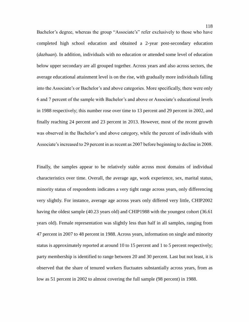
118

118

Bachelor’s degree, whereas the group “Associate’s” refer exclusively to those who have

completed high school education and obtained a 2-year post-secondary education

(dazhuan). In addition, individuals with no education or attended some level of education

below upper secondary are all grouped together. Across years and also across sectors, the

average educational attainment level is on the rise, with gradually more individuals falling

into the Associate’s or Bachelor’s and above categories. More specifically, there were only

6 and 7 percent of the sample with Bachelor’s and above or Associate’s educational levels

in 1988 respectively; this number rose over time to 13 percent and 29 percent in 2002, and

finally reaching 24 percent and 23 percent in 2013. However, most of the recent growth

was observed in the Bachelor’s and above category, while the percent of individuals with

Associate’s increased to 29 percent in as recent as 2007 before beginning to decline in 2008.

Finally, the samples appear to be relatively stable across most domains of individual

characteristics over time. Overall, the average age, work experience, sex, marital status,

minority status of respondents indicates a very tight range across years, only differencing

very slightly. For instance, average age across years only differed very little, CHIP2002

having the oldest sample (40.23 years old) and CHIP1988 with the youngest cohort (36.61

years old). Female representation was slightly less than half in all samples, ranging from

47 percent in 2007 to 48 percent in 1988. Across years, information on single and minority

status is approximately reported at around 10 to 15 percent and 1 to 5 percent respectively;

party membership is identified to range between 20 and 30 percent. Last but not least, it is

observed that the share of tenured workers fluctuates substantially across years, from as

low as 51 percent in 2002 to almost covering the full sample (98 percent) in 1988.

119

11

9

Table 4-2-1. Descriptive Statistics of 1988 CHIP Urban Labor Market Participant Sample

Variable Definition and Metrics N Mean SD Max Min

Labor Market Outcomes

Weekly Wages Weekly Earnings in Yuan 17073 35.45 16.16 95 0.25

Teacher and Sector Identifiers

Teacher Teacher =1, otherwise =0 17073 0.04 - 1 0

Public Sector Non-Teachers Public Sector Non-Teachers =1, otherwise =0 17073 0.74 - 1 0

Private Sector Non-Teachers Private Sector Non-Teachers =1, otherwise =0 17073 0.22 - 1 0

Education Attainment Level

Bachelor's & Above Highest educational attainment was bachelor's

degree or above =1, otherwise =0 17073 0.06 - 1 0

Associate's Highest educational attainment was associate's

degree =1, otherwise =0 17073 0.07 - 1 0

Upper Secondary & Below Highest educational attainment was upper

secondary or below =1, otherwise =0 17073 0.87 - 1 0

Background Characteristics

Age Age in Years 17073 36.61 9.91 16 60

Years of Work Experience Work Experience in Years 17073 19.24 9.97 0 40

Female Female =1, male =0 17073 0.48 - 1 0

Minority Minority =1, otherwise =0 17073 0.04 - 1 0

120

120

Party Membership Party member =1, otherwise =0 17073 0.23 - 1 0

Permanent Contract

Working on permanent contract or with tenure =1.

otherwise =0 17073 0.97 - 1 0

Note: The sample is restricted to all employed individuals between the age of 16 and 60 years old, with at most 40 years of working

experience. Winsoring adjustment has been applied to weekly wages for top and bottom 1 percent.

Table 4-2-2. Descriptive Statistics of 1995 CHIP Urban Labor Market Participant Sample

Variable Definition and Metrics N Mean SD Max Min

Labor Market Outcomes

Weekly Wages Weekly Earnings in Yuan 10756 109.86 57.62 325 11.5

Teacher and Sector Identifiers

Teacher Teacher =1, otherwise =0 10756 0.04 - 1 0

Public Sector Non-Teachers Public Sector Non-Teachers =1, otherwise =0 10756 0.28 - 1 0

Private Sector Non-Teachers Private Sector Non-Teachers =1, otherwise =0 10756 0.68 - 1 0

Education Attainment Level

Bachelor's & Above Highest educational attainment was bachelor's

degree or above =1, otherwise =0 10756 0.08 - 1 0

Associate's Highest educational attainment was associate's

degree =1, otherwise =0 10756 0.16 - 1 0

121

121

Upper Secondary & Below Highest educational attainment was upper

secondary or below =1, otherwise =0 10756 0.76 - 1 0

Background Characteristics

Age Age in Years 10756 38.4 9.22 60 16

Years of Work Experience Work Experience in Years 10756 19.32 9.28 40 0

Female Female =1, male =0 10756 0.47 - 1 0

Single Single =1, otherwise =0 10756 0.12 - 1 0

Minority Minority =1, otherwise =0 10756 0.04 - 1 0

Party Membership Party member =1, otherwise =0 10756 0.25 - 1 0

Permanent Contract

Working on permanent contract or with tenure =1.

otherwise =0 10756 0.77 - 1 0

Note: The sample is restricted to all employed individuals between the age of 16 and 60 years old, with at most 40 years of working

experience. Winsoring adjustment has been applied to weekly wages for top and bottom 1 percent.

122

122

Table 4-2-3. Descriptive Statistics of 2002 CHIP Urban Labor Market Participant Sample

Variable Definition and Metrics N Mean SD Max Min

Labor Market Outcomes

Weekly Wages Weekly Earnings in Yuan 9762 261.5 173.13 983 35

Teacher and Sector Identifiers

Teacher Teacher =1, otherwise =0 9762 0.05 - 1 0

Public Sector Non-Teachers Public Sector Non-Teachers =1, otherwise =0 9762 0.31 - 1 0

Private Sector Non-Teachers Private Sector Non-Teachers =1, otherwise =0 9762 0.64 - 1 0

Education Attainment Level

Bachelor's & Above Highest educational attainment was bachelor's

degree or above =1, otherwise =0 9762 0.13 - 1 0

Associate's Highest educational attainment was associate's

degree =1, otherwise =0 9762 0.29 - 1 0

Upper Secondary & Below Highest educational attainment was upper

secondary or below =1, otherwise =0 9762 0.58 - 1 0

Background Characteristics

Age Age in Years 9762 40.23 8.81 60 18

Years of Work Experience Work Experience in Years 9762 21.87 9.32 40 0

Female Female =1, male =0 9762 0.45 - 1 0

Single Single =1, otherwise =0 9762 0.10 - 1 0

123

123

Minority Minority =1, otherwise =0 9762 0.04 - 1 0

Party Membership Party member =1, otherwise =0 9762 0.29 - 1 0

Permanent Contract

Working on permanent contract or with tenure =1.

otherwise =0 9762 0.51 - 1 0

Note: The sample is restricted to all employed individuals between the age of 16 and 60 years old, with at most 40 years of working

experience. Winsoring adjustment has been applied to weekly wages for top and bottom 1 percent.

Table 4-2-4. Descriptive Statistics of 2007 CHIP Urban Labor Market Participant Sample

Variable Definition and Metrics N Mean SD Max Min

Labor Market Outcomes

Weekly Wages Weekly Earnings in Yuan 5465 579.3 422.97 2499.8 87.5

Teacher and Sector Identifiers

Teacher Teacher =1, otherwise =0 5465 0.03 - 1 0

Public Sector Non-Teachers Public Sector Non-Teachers =1, otherwise =0 5465 0.29 - 1 0

Private Sector Non-Teachers Private Sector Non-Teachers =1, otherwise =0 5465 0.68 - 1 0

Education Attainment Level

Bachelor's & Above Highest educational attainment was bachelor's

degree or above =1, otherwise =0 5465 0.17 - 1 0

124

124

Associate's Highest educational attainment was associate's

degree =1, otherwise =0 5465 0.29 - 1 0

Upper Secondary & Below Highest educational attainment was upper

secondary or below =1, otherwise =0 5465 0.54 - 1 0

Background Characteristics

Age Age in Years 5465 38.69 9.2 60 18

Years of Work Experience Work Experience in Years 5465 19.73 10.28 40 0

Female Female =1, male =0 5465 0.43 - 1 0

Single Single =1, otherwise =0 5465 0.14 - 1 0

Minority Minority =1, otherwise =0 5465 0.01 - 1 0

Permanent Contract

Working on permanent contract or with tenure =1.

otherwise =0 5465 0.77 - 1 0

Note: The sample is restricted to all employed individuals between the age of 16 and 60 years old, with at most 40 years of working

experience. Winsoring adjustment has been applied to weekly wages for top and bottom 1 percent.

125

125

Table 4-2-5. Descriptive Statistics of 2008 CHIP Urban Labor Market Participant Sample

Variable Definition and Metrics N Mean SD Max Min

Labor Market Outcomes

Weekly Wages Weekly Earnings in Yuan 5452 649.31 467.91 2500 100

Teacher and Sector Identifiers

Teacher Teacher =1, otherwise =0 5452 0.03 - 1 0

Public Sector Non-Teachers Public Sector Non-Teachers =1, otherwise =0 5452 0.31 - 1 0

Private Sector Non-Teachers Private Sector Non-Teachers =1, otherwise =0 5452 0.66 - 1 0

Education Attainment Level

Bachelor's & Above Highest educational attainment was bachelor's

degree or above =1, otherwise =0 5452 0.23 - 1 0

Associate's Highest educational attainment was associate's

degree =1, otherwise =0 5452 0.29 - 1 0

Upper Secondary & Below Highest educational attainment was upper

secondary or below =1, otherwise =0 5452 0.48 - 1 0

Background Characteristics

Age Age in Years 5452 39.33 9.32 60 18

Years of Work Experience Work Experience in Years 5452 20.34 10.51 40 0

Female Female =1, male =0 5452 0.45 - 1 0

Single Single =1, otherwise =0 5452 0.14 - 1 0

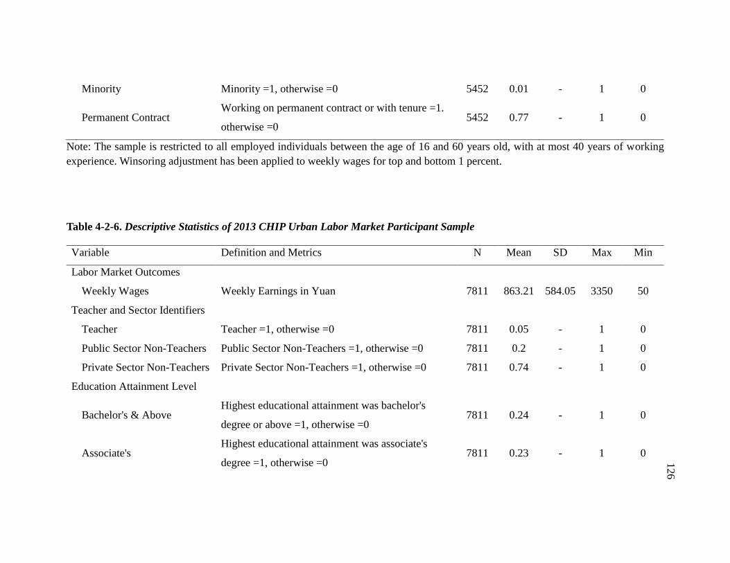
126

126

Minority Minority =1, otherwise =0 5452 0.01 - 1 0

Permanent Contract

Working on permanent contract or with tenure =1.

otherwise =0 5452 0.77 - 1 0

Note: The sample is restricted to all employed individuals between the age of 16 and 60 years old, with at most 40 years of working

experience. Winsoring adjustment has been applied to weekly wages for top and bottom 1 percent.

Table 4-2-6. Descriptive Statistics of 2013 CHIP Urban Labor Market Participant Sample

Variable Definition and Metrics N Mean SD Max Min

Labor Market Outcomes

Weekly Wages Weekly Earnings in Yuan 7811 863.21 584.05 3350 50

Teacher and Sector Identifiers

Teacher Teacher =1, otherwise =0 7811 0.05 - 1 0

Public Sector Non-Teachers Public Sector Non-Teachers =1, otherwise =0 7811 0.2 - 1 0

Private Sector Non-Teachers Private Sector Non-Teachers =1, otherwise =0 7811 0.74 - 1 0

Education Attainment Level

Bachelor's & Above Highest educational attainment was bachelor's

degree or above =1, otherwise =0 7811 0.24 - 1 0

Associate's Highest educational attainment was associate's

degree =1, otherwise =0 7811 0.23 - 1 0

127

127

Upper Secondary & Below Highest educational attainment was upper

secondary or below =1, otherwise =0 7811 0.53 - 1 0

Background Characteristics

Age Age in Years 7811 39.8 9.17 60 16

Years of Work Experience Work Experience in Years 7811 21.13 10.13 40 0

Female Female =1, male =0 7811 0.45 - 1 0

Single Single =1, otherwise =0 7811 0.11 - 1 0

Minority Minority =1, otherwise =0 7811 0.05 - 1 0

Party Membership Party member =1, otherwise =0 7811 0.21 - 1 0

Permanent Contract

Working on permanent contract or with tenure =1.

otherwise =0 7811 0.59 - 1 0

Note: The sample is restricted to all employed individuals between the age of 16 and 60 years old, with at most 40 years of working

experience. Winsoring adjustment has been applied to weekly wages for top and bottom 1 percent.

128

128

In Tables 4-2-7 and 4-2-8, I report the regression adjusted mean wage differences and the

differential returns to skills and education across sectors. To begin, each column represents

an independent regression model using different waves of the repeated cross-sectional

CHIP data, such that Models (1) through Model (6) each correspond to a respective wave

of CHIP 1988, 1995, 2002, 2007, 2008, or 2013. The first and second rows in Table 4-2-7

respectively correspond to coefficients β2 and β3 in Equation (2.2), which indicate the

regression-adjusted mean wage differences in natural log points between teachers and

private or public sector non-teaching workers, after controlling for important background

and demographics covariates. The subsequent rows show point estimates for each control

covariate that entered the regression analysis, and importantly, all models include birth

cohort and worker type fixed-effect dummies as additional controls. To this end, this

exercise aims to detect the existence and quantify the degree of sector-based mean wage

differences, and several important insights on sectoral wage characteristics can be

summarized from results in Table 4-2-7.

Firstly, point estimate results for β2 are statistically significant across all years with

exception of 2007, and the coefficients which indicate the mean wage differences are

respectively -0.129 (p-value <0.05), -0.068 (p-value <0.05), -0.180 (p-value <0.05), 0.036,

0.099 (p-value <0.05), and 0.112 (p-value <0.05) log points. These results illustrate that

between 1988 and 2013, the regression-adjusted mean wage difference between teachers

and private non-teaching workers has changed from approximately 13 percent in favor of

teachers in 1988, which began reducing over time and eventually reversed to about 11

percent benefitting private non-teaching workers in 2013. This drastic shift represented a

129

129

24 percentage point reversal. To be clear, this means that teachers’ mean wage levels were

about 13 percent higher than that of comparable private sector workers in 1988, but this

wage premium gradually dissipated, such that in 2007 there was no statistical difference

between teacher and private sector worker wages, but the gap reversed, and in 2013

teachers are on average paid about 11 percent less than similar private sector workers.

Nonetheless, such observations are expected as rapid economic developments in the private

sector can result in new employment opportunities arising that are more responsive to

market forces (Zhao & Zhou, 2007)

Secondly, results for β3 , which subsequently indicate the difference in mean wages

between teachers and comparable public sector workers, are either not statistically

significant or relatively small when they are marginally significant. To illustrate, significant

differences in mean wages are only observed in 1988 and 2008, when public sector worker

wages are paid about 4 percent (p-value <0.05) and 9 percent (p-value <0.10) higher than

teachers respectively. Overall, there seems to be a general pattern indicating that mean

wages for comparable workers in the public sector have been somewhat similar to that of

teachers, whereas private sector wages have expanded considerable for workers who are

similarly qualified as teachers.

Thirdly, the estimated coefficients on a few important control covariates are also worth

mentioning for more contextual understanding of broader labor market conditions in China

during this time period. For one, coefficients for “Bachelor’s & Above” only became

consistently significant in the 2007, 2008, 2013 waves, suggesting that the returns to

130

130

Bachelor’s degree and Associate’s degree are statistically similar in earlier years, after

accounting for sector and other background variables. Before 2007, there were no

discernible wage benefits to obtaining advanced tertiary education. For another, female

workers have been consistently undervalued relative to comparable male counter parts

across all years, and the gender wage gap has been expanding much more recently, reaching

a staggering -23.6 percent in 2013 from a marginally significant -2.1 percent in 1988.

Table 4-2-7. Regression Results from Mincer Earnings Function, by year

Year 1988 1995 2002 2007 2008 2013

Dependent Variable:

Log Weekly Wages

Model

(1)

Model

(2)

Model

(3)

Model

(4)

Model

(5)

Model

(6)

Adjusted Mean Wage

Difference

Private Non-Teachers

(reference = teachers)

-0.129* -0.068* -0.180* 0.036 0.099* 0.112*

(0.031) (0.022) (0.034) (0.042) (0.04) (0.049)

Public Non-Teachers

(reference = teachers)

0.039* 0.009 -0.081 0.017 0.091# -0.021

(0.014) (0.027) (0.025) (0.047) (0.047) (0.040)

Control Covariates

Bachelor's & Above

(reference = associate's)

0.010 0.090* -0.014 0.155* 0.212* 0.185*

(0.007) (0.025) (0.036) (0.035) (0.020) (0.022)

Upper Secondary &

Below (reference =

associate's)

0.029 -0.086* 0.077# -0.144* -0.232* -0.060#

(0.027) (0.015) (0.027) (0.052) (0.026) (0.029)

Years of Work

Experience -0.001 0.032* -0.096* 0.011 0.011# -0.017

(0.013) (0.004) (0.017) (0.017) (0.005) (0.014)

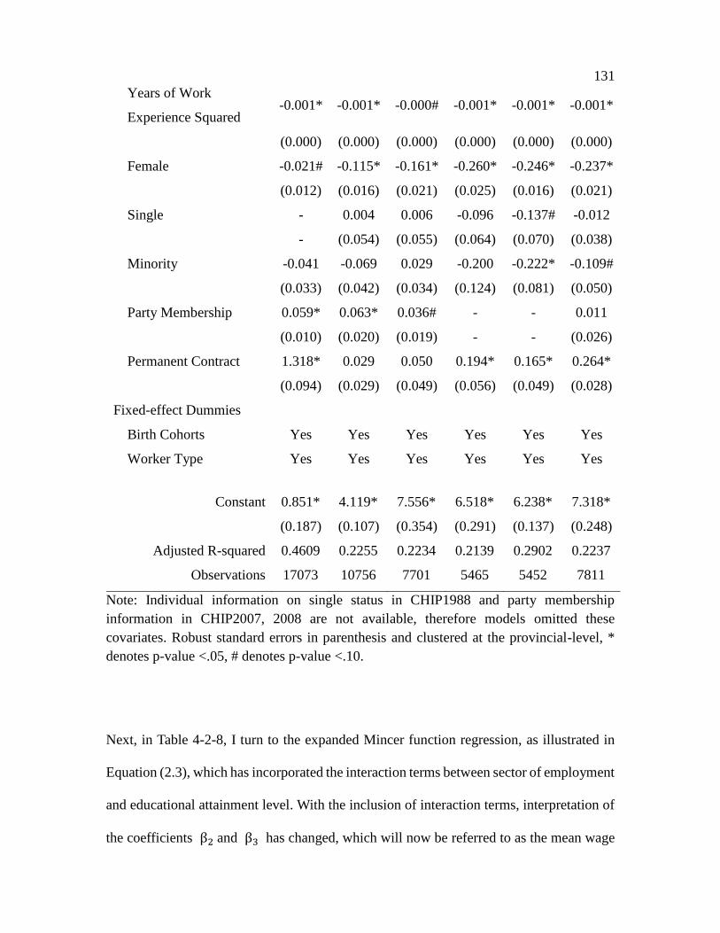
131

131

Years of Work

Experience Squared -0.001* -0.001* -0.000# -0.001* -0.001* -0.001*

(0.000) (0.000) (0.000) (0.000) (0.000) (0.000)

Female -0.021# -0.115* -0.161* -0.260* -0.246* -0.237*

(0.012) (0.016) (0.021) (0.025) (0.016) (0.021)

Single - 0.004 0.006 -0.096 -0.137# -0.012

- (0.054) (0.055) (0.064) (0.070) (0.038)

Minority -0.041 -0.069 0.029 -0.200 -0.222* -0.109#

(0.033) (0.042) (0.034) (0.124) (0.081) (0.050)

Party Membership 0.059* 0.063* 0.036# - - 0.011

(0.010) (0.020) (0.019) - - (0.026)

Permanent Contract 1.318* 0.029 0.050 0.194* 0.165* 0.264*

(0.094) (0.029) (0.049) (0.056) (0.049) (0.028)

Fixed-effect Dummies

Birth Cohorts Yes Yes Yes Yes Yes Yes

Worker Type Yes Yes Yes Yes Yes Yes

Constant 0.851* 4.119* 7.556* 6.518* 6.238* 7.318*

(0.187) (0.107) (0.354) (0.291) (0.137) (0.248)

Adjusted R-squared 0.4609 0.2255 0.2234 0.2139 0.2902 0.2237

Observations 17073 10756 7701 5465 5452 7811

Note: Individual information on single status in CHIP1988 and party membership

information in CHIP2007, 2008 are not available, therefore models omitted these

covariates. Robust standard errors in parenthesis and clustered at the provincial-level, *

denotes p-value <.05, # denotes p-value <.10.

Next, in Table 4-2-8, I turn to the expanded Mincer function regression, as illustrated in

Equation (2.3), which has incorporated the interaction terms between sector of employment

and educational attainment level. With the inclusion of interaction terms, interpretation of

the coefficients β2 and β3 has changed, which will now be referred to as the mean wage

132

132

differences for non-Bachelor’s degree holders between teachers and public or private sector

non-teaching workers respectively. Consequently, β5 and β6 will indicate the differential

returns to having a Bachelor’s degree in teaching versus returns in the private and public

sectors respectively. Keeping these interpretations in mind, I focus on results in Table 4-2-

8, where the first row corresponds to β5, or the difference in returns to having a Bachelor’s

degree for teachers versus private sector non-teacher workers, whereas the second row

represents point estimates for β6, that is the difference in returns to having a Bachelor’s

degree for teachers versus public sector non-teacher workers. The mean wage differences

for non-Bachelor’s degree holders between teachers and private or public sector non-

teaching workers are in rows three and four of Table 4-2-8 respectively.

Point estimates of coefficients β5 as represented in the first row of Table 4-2-8, show that

there is some suggestion that returns to additional human capital accumulation are higher

for comparable private sector workers than teachers between 1988, 1995 and 2002, but the

two groups are not statistically significant. However, in more recent years such as 2007,

2008, and 2013, results have become statistically significant which indicate that returns to

Bachelor’s and more education are higher for comparable private sector workers,

respectively 15.8, 11.3, and 13.5 percent more. Results in the second row correspond to

β6 estimates, which illustrate the relationship between returns to more education among

public sector non-teaching workers and teachers. Broadly speaking, differences in returns

on education for these two groups are either statistically indistinguishable or much smaller

in relative magnitudes compared to the differences observed between private sector

workers and teachers.

133

133

In summary, patterns observed in Table 4-2-8 are to a large extent similar to that of Table

4-2-7, in that wage characteristics, in terms of mean wages and returns to human capital,

are at least similar if not more favorable for teachers relative to comparable private sector

workers in the earlier years 1988, 1995, 2002. On the other hand, sharp contrasts in results

for 2007, 2008, and 2013 waves are observed, such that not only teachers’ mean wages

were about 10 percent less than that of comparable private workers, the returns to education

estimates also show that teachers are at a 11 to 15 percent disadvantage compared to similar

private sector workers. As for the comparison between teachers and similarly qualified

public sector workers, differences in mean wages and returns to human capital are

negligible across years, either being statistically insignificant or at much smaller magnitude.

As robustness check, in Table 4-2-9, I take advantage of the available household-level

linked information on respondent’s father and mother educational attainment level to

evaluate the sensitivity of results presented in Tables 4-2-7 and 4-2-8. Specifically, for

Models 12 and 14, I add father’s and mother’s educational attainment level controls to the

base and full specifications to mitigate potential biases in individual’s section into higher

educational attainment, and directly compare the results with that of Models 6 and 13. In

detail, Model 13 evaluates the soundness of results in Model 6 with added parental

education level controls, whereas Model 14 is directly comparable with Model 12.

Indicated by the comparison of β2 estimates in Model 6 and 13, reduction of the

coefficient by half and becoming statistically insignificant suggest that there are some

concerns with endogeneity of individual’s decision into private or teaching sectors being

influenced in part by parental educational attainment level. However, in Models 12 and 14,

134

134

β5 estimates are consistent across models which provide some assurance that the

differential returns to education results observed in private and teaching sectors are not

substantially driven by parental education. Overall, the robustness test suggests that results

for β5 in Table 4-2-8 continue to hold true even with additional household level control

covariates included.

Finally, the above results have important theoretical implications through the lens of

teacher occupational choice framework. For instance, if one assumes that worker aptitude

and general skills are positively correlated with earnings across different sectors, a rise in

the difference in returns to human capital and skills would imply that individuals would

choose the sector with higher returns. The empirical results observed in Part II suggest that

returns to more education in the teaching sector have substantially lagged behind that of

the private sector, even for workers with comparable characteristics. After accounting for

important individual characteristics, persistence of such pay differences imply that by

choosing the teaching sector, a well-educated individual would not be rewarded for her

skills and human capital, as she would otherwise in the private sector. This finding shows

that in recent years, teaching has become much less attractive career in comparison to

working in the private sector for individuals with advanced tertiary education. If sustained

over a long period of time, the teacher occupational choice framework predicts that average

teacher ability would decline, because as teaching becomes an occupation without

attractive income, well-educated individuals are predicted to pursue higher returns on their

human capital and skills in the better paying private sector.

135

135

Table 4-2-8. Regression Results from Mincer Earnings Function with Interaction Terms, by year

Year 1988 1995 2002 2007 2008 2013

Dependent Variable: Log Weekly Wages

Model

(7)

Model

(8)

Model

(9)

Model

(10)

Model

(11)

Model

(12)

Interaction Terms

Private Non-Teachers * Bachelor's & Above

0.111 0.010 0.065 0.158# 0.113# 0.135*

(0.077) (0.059) (0.071) (0.070) (0.049) (0.057)

Public Non-Teachers * Bachelor's & Above

-0.008 -0.047 -0.036 0.082 0.099# 0.044

(0.013) (0.032) (0.076) (0.071) (0.053) (0.064)

Adjusted Mean Wage Difference

Private Non-Teachers

(reference = teachers)

-0.129* -0.063* -0.192* -0.019 0.027 0.053

(0.031) (0.023) (0.035) (0.042) (0.072) (0.059)

Public Non-Teachers

(reference = teachers)

0.040* 0.020 -0.081* -0.023 0.023 -0.065

(0.013) (0.022) (0.031) (0.047) (0.072) (0.060)

Educational Attainment

Bachelor's & Above

(reference = associate's)

0.013 0.111* -0.22 0.035 0.111* 0.097

(0.017) (0.039) (0.064) (0.062) (0.031) (0.056)

Upper Secondary & Below

(reference = associate's)

0.029 -0.086* 0.078* -0.139* -0.231* -0.050

(0.027) (0.016) (0.021) (0.051) (0.026) (0.029)

136

136

Control Covariates Yes Yes Yes Yes Yes Yes

Fixed-effect Dummies

Birth Cohorts Yes Yes Yes Yes Yes Yes

Worker Type Yes Yes Yes Yes Yes Yes

Constant 0.849* 4.112* 7.545* 6.570* 6.309* 7.366*

(0.186) (0.104) (0.290) (0.283) (0.132) (0.263)

Adjusted R-squared 0.4609 0.2212 0.2399 0.2143 0.2901 0.2243

Observations 17073 10756 7701 5465 5452 7811

Note: Individual information on single status in CHIP1988 and party membership information in CHIP2007, 2008 are not available,

therefore models omitted these covariates. Robust standard errors in parenthesis and clustered at the provincial-level, * denotes p-value

<.05, # denotes p-value <.10. Control covariates and model specifications are identical with Table 4-2-7, such that point estimates from

Models 1 & 7, 2 & 8, 3 & 9, 4 & 10, 5 & 11, 6 & 12, are directly comparable.

137

Table 4-2-9. Robustness Check for Mincer Earnings Function, using CHIP 2013

Year 2013

Dependent Variable:

Log Weekly Wages

Model

(6)

Model

(12)

Model

(13)

Model

(14)

Interaction Terms

Private Non-Teachers *

Bachelor's & Above

0.136* 0.132*

(0.057) (0.051)

Public Non-Teachers *

Bachelor's & Above

0.044 0.056

(0.064) (0.059)

Adjusted Mean Wage Difference

Private Non-Teachers

(reference = teachers)

0.112* 0.053 0.067 0.012

(0.049) (0.059) (0.050) (0.066)

Public Non-Teachers

(reference = teachers)

-0.021 -0.065 -0.043 -0.094

(0.040) (0.060) (0.040) (0.061)

Educational Attainment

Bachelor's & Above

(reference = associate's)

0.185* 0.097 0.153* 0.065

(0.022) (0.056) (0.024) (0.055)

Upper Secondary & Below

(reference = associate's)

-0.060# -0.050 -0.069# -0.059

(0.029) (0.029) (0.033) (0.034)

Additional Control Covariates

Father's Education Level No No Yes Yes

Mother's Education Level No No Yes Yes

All Control Covariates

In Table 4-2-7 & 4-2-8 Yes Yes Yes Yes

Fixed-effect Dummies

Birth Cohorts Yes Yes Yes Yes

Worker Type Yes Yes Yes Yes

Constant 7.336* 7.355* 7.241* 7.260*

(0.248) (0.266) (0.259) (0.275)

138

Adjusted R-squared 0.2239 0.2243 0.2262 0.2263

Observations 7811 7811 7811 7811

Note: Robust standard errors in parenthesis and clustered at the provincial-level, * denotes

p-value <.05, # denotes p-value <.10.

139

4.3 Results for Part III:

Teacher Quality and Occupational Trends

Since 1980, each of the Chinese central government’s quinquennial national policy plan

has featured a the importance of building a high-quality teaching force, and this emphasis

on recruiting and maintaining high teacher standards have been reiterated again in the most

recent “Thirteen-Five National Education Plan” (State Council, 2017). As the current

national plan states, one of the key issues limiting development in China’s education sector

is the “quality and composition of the teaching force” (State Council, 2017, Section 1), and

the plan subsequently lists the “improvement of teacher quality” as a primary objective in

the “Thirteen-Five” period before 2020 (State Council, 2017, Section 4). The research

objective of Part III is to analyze teacher’s occupational decisions based on their human

capital traits, and track trends in relative labor quality between teacher and non-teachers

using observed career decisions to approximate revealed occupational preferences among

current workers in the labor force.

More specifically, I estimate a multinomial probit model to relate measures of labor quality

and human capital – educational attainment level, upper secondary school selectivity,

national college entrance exam scores – to observed occupational choice decisions in

teaching, public non-teaching or private non-teaching careers. To further ensure

comparability among different career outcomes, I restrict the analysis to the professional

worker subsample within each wave of CHIP data, such that employed workers who self-

reported as owner, manger, and laborer are excluded from the regression analysis.

140

For further elaboration, the educational attainment level variable used for this analysis will

be identical for all waves of CHIP data (see Tables 4-2-1 through 4-2-6 for more

information), whereas descriptive statistics on upper secondary school selectivity and

national college entrance exam (gaokao) scores are illustrated further in Table 4-3-1. Data

on upper secondary school selectivity and national college entrance exam scores are limited

to more recent waves of CHIP in 2002, 2007 and 2013. For example, in Panel A of Table

4-3-1, I show share of individuals in the sample by the selectivity of the upper secondary

school that they have attended. Approximately 8 percent of the CHIP2002 professional-

only analytic sample report having attended a “National & Provincial Key School” which

represents the most selective category, while the same numbers are 36 percent for

“Municipal & County Key School,” and the majority 57 percent attended none of the above

categories (least selective). For CHIP2007, only national college entrance exam scores are

reported (see Panel B, Table 4-3-1), which had a subsample mean of 469 points (SD=107).

In Panel C of Table 4-3-1, information on both upper secondary school selectivity and

national college entrance exam scores are provided in CHIP2013, such that there are 6

percent in the most selective national and provincial key schools category, 44 percent in

municipal or county-level key schools, and 50 percent in the least selective category; mean

scores for the national college entrance exam is 466 points (SD=99).

141

141

Table 4-3-1. Descriptive Statistics of CHIP Urban Labor Market Participant Ability

Characteristics (Professional Workers Only), by year

Variable Definition and Metrics N Mean SD Max Min

Panel A | CHIP2002

High School Selectivity

National &

Provincial

Key

Attended a national or

provincial key school =1,

otherwise =0

1864 0.08 - 1 0

Municipal &

County Key

Attended a municipal or county

key school =1, otherwise =0 1864 0.36 - 1 0

Not Key or

Other

Attended a non-key high

school, or other =1, otherwise

=0

1864 0.57 - 1 0

Panel B | CHIP2007

Gaokao Score National College Entrance

Examination Score 669 469 107 817 30

Panel C | CHIP2013

High School Selectivity

National &

Provincial

Key

Attended a national or

provincial key school =1,

otherwise =0

1763 0.06 - 1 0

Municipal &

County Key

Attended a municipal-level key

high school =1, otherwise =0 1763 0.44 - 1 0

Not Key or

Other

Attended a county-level key

high school =1, otherwise =0 1763 0.50 - 1 0

Gaokao Score National College Entrance

Examination Score 1005 466 99 730 58

142

142

In Table 4-3-2, I turn to the multinomial probit regression results, which are separately

reported in each column for each model’s coefficient as well as the marginal effect for each

educational attainment level (relative to the reference category: Associate’s). For instance,

Columns 1 and 2 correspond respectively to the “Beta” coefficient and “Marginal Effect”

estimates from Model 1 that is fitted on the CHIP1988 professional worker subsample.

Consequently, the fifth and ninth row of “Beta” column results in Table 4-3-2 represent the

estimated relationship between obtaining at least a Bachelor’s degree (reference category

is Associate’s degree), or only Upper Secondary or below (reference category is

Associate’s degree), on the probability of choosing to be a worker in the private sector

relative to choosing teaching. A negative coefficient in these rows suggests that being a

teacher is more likely predicted than working in the private sector, for a set of educational

attainment level. In the same vein, “Beta” column results in rows seven and eleven of Table

4-3-2 relate to the same probabilities and are interpreted in the same way, but the

relationship is subsequently between public sector careers and teaching. The “M. Effect”

column represents the marginal effect of holding a given degree versus the reference

category on the predicted probability of choosing a particular career option: teaching,

private sector, or public sector.

For interpretation, a positive and statistically significant coefficient in the “Beta” column

indicates that the receipt of a given degree (Bachelor’s in rows 5 and rows 9, or Upper

Secondary or Below in rows 7 and 11) is associated with higher predicted probability of

choosing teaching as a career, compared to either private or public sector professional jobs;

a negative and statistically significant coefficient indicates the reverse relationship. In the

143

143

“M. Effect” column, a statistically significant point estimate indicates the conditional

probability change in choosing a given career that is related to one unit change in the

explanatory variable; for “Bachelor’s & Above” this refers to holding at least a bachelor’s

degree. For all cells, the reference group is for workers who hold an associate’s degree.

To begin, generalizing from results shown in Table 4-3-2, more educated professional

workers are more likely to choose a career in teaching as opposed to working in private or

public sector non-teaching jobs. For instance, taking a closer look at the “Beta” column in

the fifth row of Table 4-3-2, we can observe a consistent trend across all models and years

that between 1988 and 2013, coefficients are always negative and statistically significant

(coefficient was marginally significant at .10-level in 1988, for all other years p-value<.05).

This means that across all years, it is more likely for professional workers with Bachelor’s

degrees or above (relative to those with Associate’s degrees) to choose teaching over

working in the private sector, after controlling for a vector of important demographic

characteristics. Similarly, in row seven, it is more likely for professional workers with an

Associate’s degree to be a teacher than to work in the private sector.

Also, results from “Beta” column in rows nine and eleven, which represent the probability

of choosing public sector relative to teaching jobs, show that workers with higher education

attainment tend to favor teaching careers relative to public sector jobs, especially in the

2002, 2007, and 2013 waves. Importantly, while Bachelor’s degree attainment does not

seem to influence likelihood of choosing teaching over public sector careers in 1988 and

1995, as indicated by the insignificant “Beta” coefficients -0.137 and -0.101, workers with

144

144

Bachelor’s degrees are more likely to choose teaching rather than other public sector jobs

in later waves since the “Beta” coefficients become negative and significant -0.521 (p-

value<.05), -0.242 (p-value<.10), and -0.361 (p-value<.05) in Models 3, 4, 5 respectively.

Secondly, in order to evaluate the magnitude of observed relationships above, I turn to the

“M. Effects” column in Table 4-3-2. Using Model 1 as example, in the first row I find that

in 1988, having attained at least a Bachelor’s degree is on average correlated with a 3

percent increase in the probability of entering teaching, relative to only obtaining an

associate’s degree, but this relationship is not statistically significant. The same relationship

is 7.6 percent, 10.8 percent, 6.3 percent and 8.7 percent for Models 2, 3, 4, 5 respectively.

These findings are not surprising, and to a large extent corroborate the macro-level

accounting exercise carried out at the outset of this chapter, in Table 4-0-2, which showed

that the percent of teachers with advanced tertiary education degrees increased

substantially and at a quicker pace than the national average between period 2003 and 2017.

As a third step, in Table 4-3-3, I distinguish the differential quality occupation decision

patterns in teacher stock and teacher flow, by reporting Adjusted Predictions at

Representative Values (APRV) for individuals whose age are 30 and 50 years old

respectively. The APRV of Bachelor’s degree attainment on the probability of choosing to

be a teacher conditional on age equals 30 will illustrate the career decisions of new labor

market entrants, while the APRV results conditional age equals 50 will approximate the

existing stock of the teaching force. For instance, in 2013, new entrants who hold a

Bachelor’s degree are about 4.5 percent more likely to become a teacher relative to another

145

145

new entrant who holds an Associate’s degree, but this number was 10.3 percent more likely

for older cohorts.

To this end, I evaluate the differences in APRVs between new entrants and existing labor

force, such that a negative and statically significant difference between the two APRVs will

indicate that more educated new labor market entrants are less likely to become a teacher

compared to the existing cohort. Indeed, in Table 4-3-3, I find negative and statistically

significant differences in the marginal effect between new entrants and existing workers in

recent waves 2007 and 2013, and these deficits are -4.7 percentage points (p-value<.0.5)

and -5.8 percentage points (p-value<.05) respectively, representing a difference of more

than 50 percent between the two groups. To be clear, this means that new workers with

Bachelor’s degrees are about half as likely to choose teaching as compared to older cohorts.

Relating these observations to results shown for 1988, 1995 and 2002, I conclude that while

more educated new labor market entrants are about as likely or more likely to become

teachers between 1988 and 2002 compared to more senior cohorts in the existing labor

force, more educated individuals are less likely relative to more senior cohorts to choose

teaching as a career in 2007 and 2013.

146

14

6

Table 4-3-2. Multinomial Probit Regression Results of the Relationship between Educational Attainment Level and Career Decision

Outcome ("Teacher" as omitted base category), with Marginal Effects on Predicted Probabilities by Outcome, 1988 -2013

Professional Worker Subsample

Model 1 Model 2 Model 3 Model 4 Model 5

Year 1988 1995 2002 2007 2013

Career

Outcomes (Ref = AA's) Beta

M.

Effect Beta

M.

Effect Beta

M.

Effect Beta

M.

Effect Beta

M.

Effect

Omitted

Category:

Teacher

Bachelor's &

Above

- 0.030 - 0.076* - 0.108* - 0.063* - 0.087*

- (0.029) - (0.028) - (0.026) - (0.023) - (0.027)

Upper

Secondary &

Below

- -0.121* - -0.054* - -0.139* - -0.107* - -0.119*

- (0.016) - (0.015) - (0.015) - (0.025) - (0.034)

Private

Non-

teaching

Bachelor's &

Above

-0.597# -0.054# -0.653* -0.166* -0.507* -0.053# -0.458* -0.084# -0.504* -0.077*

(0.310) (0.030) (0.146) (0.031) (0.137) (0.029) (0.158) (0.044) (0.123) (0.027)

Upper

Secondary &

Below

0.732* 0.040* 0.344* 0.052* 0.786* 0.098* 0.882* 0.145* 0.928* 0.188*

(0.158) (0.017) (0.072) (0.017) (0.111) (0.025) (0.151) (0.024) (0.206) (0.031)

Public Non-

teaching

Bachelor's &

Above

-0.137 0.024 -0.101 0.089* -0.521* -0.055* -0.242# 0.021 -0.361* -0.010

(0.097) (0.019) (0.142) (0.032) (0.112) (0.024) (0.138) (0.040) (0.190) (0.037)

147

14

7

Upper

Secondary &

Below

0.440* 0.081* 0.243* 0.002 0.653* 0.041# 0.515* -0.037 0.333# -0.069*

(0.086) (0.026) (0.110) (0.023) (0.116) (0.024) (0.207) (0.029) (0.202) (0.027)

Control Covariates Yes Yes Yes Yes Yes

Number of Observations 2695 2456 2036 1343 2132

Number of Teacher

Observations 779 441 505 207 429

Percent Teachers 0.29 0.18 0.25 0.15 0.20

Note: Robust standard errors in parenthesis and are clustered at the provincial-level, * denotes p-value <.05, # denotes p-value <.10.

Control covariates include respondent’s sex, age, quadratic age, minority status, party membership status, permanent contract status.

Marginal effects (dy/dx) and associated robust standard errors (in parenthesis) are calculated based on delta-method.

148

Table 4-3-3. Marginal Effect, Multinomial Probit Regression Results of the Relationship

between Bachelor’s Degree Attainment (Ref = Associate's) on Predicted Probabilities of

Being a Teacher, at Representative Ages 30 and 50

M. Effect at Age 30 M. Effect at Age 50 Difference

1988

(Model 1)

0.023 0.025 -0.002

(0.029) (0.023) (0.018)

1995

(Model 2)

0.052# 0.031* 0.021

(0.031) (0.013) (0.028)

2002

(Model 3)

0.093* 0.042* 0.051#

(0.036) (0.017) (0.032)

2007

(Model 4)

0.032* 0.079* -0.047*

(0.011) (0.027) (0.025)

2013

(Model 5)

0.045* 0.103* -0.058*

(0.020) (0.035) (0.029)

Note: Marginal effects (dy/dx) and robust standard errors (in parenthesis) are calculated

using delta-method. Following Clogg, Petkova, and Haritou (1995), a z-test comparison

of coefficients is used, * denotes p-value <.05, # denotes p-value <.10.

14

9

Figure 4-3-1. Distribution of the Marginal Effect of Bachelor’s Degree (ref=Associate’s) on Predicted Probabilities of Being a

Teacher, by Age, 1988-2013

Source: Author’s compilation. Note: y-axis is the marginal effect of having a Bachelor’s degree relative to having an Associate’s degree

on the predicted probability of being a teacher; x-axis is age with a band of 20 to 60 years old. Predicted probability of zero is marked

by a horizontal red line.

150

150

A visual representation of how this probability changes over time is illustrated in Figure 4-

3-1, such that from left to right, each panel offers a glimpse of the full distribution of

marginal effect of educational attainment by age for each wave of data. Within each panel,

age is the running variable on the x-axis with younger cohorts on the left and older cohorts

to the right. Across time, we can see that the distribution of marginal effects has gradually

become left-skewed, suggesting that younger cohorts are less likely than older cohorts to

enter teaching, when they are more educated. Taken altogether, the interpretation of results

from Tables 4-3-2, 4-3-3 and Figure 4-3-1 reveals that being more educated is generally

associated with a higher probability of becoming a teacher, but in recent years 2007 and

2013, this relationship has become weaker among new workers, and indicates a potentially

large decline in relative labor quality among new teacher entrants when compared to the

workforce in non-teaching sectors.

To further confirm the observed trends and check for the robustness of using educational

attainment level as proxy for human capital and general skills levels, I conduct two

additional analyses with different types of human capital measures: upper secondary

selectivity and national college entrance exam scores. To this end, these two pre-labor

market human capital measures are proxies for general worker aptitude, and are intended

to be interpreted broadly as guidance information on the relative placement of individuals

on the labor quality distribution.

In Table 4-3-4, I leverage information on the selectivity of respondents’ upper secondary

school in CHIP2002 and CHIP2013 to run identical multinomial probit models. For Model

151

151

6 using data from 2002, negative and significant coefficients in “Beta” column on rows

five and seven of Table 4-3-4 suggest that respondents who attended a selective “National

& Key” or “Municipal & County Key” upper secondary school are more likely to be a

teacher than to be working in private or public sector, compared to those who attended

“Non-Key & Other” schools. However, for public sector jobs, “Beta” column results in

rows nine and eleven indicate that those who attended the most selective “National & Key”

schools were not statistically more likely to choose teaching. On the other hand, it is more

likely for those who attended less selective “Municipal & County Key” schools to choose

teaching over public sector careers. For 2013, results in the “Beta” columns show that

individuals who attended selective schools were not more likely to choose teaching than

either private or public sector jobs. However, those who attended more selective

“Municipal & County Key” schools were more likely to choose teaching rather than private

or public sector jobs. Moreover, while in year 2002, individuals who attended more

selective schools are 9 percent more likely to become teachers than to work in other sectors,

comparing the “M Effect” column results in rows one and three for Model 6 and 7 shows

that those who attended more selective schools are becoming less likely to choose the

teaching sector. To this end, by 2013, the numbers have become statistically insignificant

for those who attended the most selective “National & Provincial Key” schools. In other

words, compared to 2002, individuals who attended the most selective schools are no

longer more likely to choose teaching careers in 2013.

Similarly, in Table 4-3-5, I report multinomial probit regression results that relate

individuals’ performance on National College Entrance Exam (gaokao) to their career

152

152

choices: teaching, private or public sector jobs. In Models 8 and 9, exam scores are

standardized within exam year, and exam type dummies controlling for Arts, Humanities,

and Science tracks are added as measures to mitigate inter-temporal and inter-subject

influence. Although exam scores information is only available in more recent waves of

CHIP2007 and CHIP2013, the likelihood of entry into teaching relative to other careers for

high scorers on the National College Entrance Exam is declining, which seems to be

consistent with prior results using educational attainment and school selectivity

information. In particular, results found in rows three and five in the “Beta” columns for

Model 8 and 9 suggest that it was more likely for higher-scoring individuals to choose

teaching over private sector jobs in 2007, but in 2013 the advantage dissipates and becomes

statically insignificant. To add, the “M. Effect” columns reflect Adjusted Predictions at the

Means (APM), based on estimating the marginal effect of increasing exam scores by 1

standard deviation on the likelihood of choosing private or private sector jobs over teaching

careers. A comparison of APM results between Models 8 and 9 from row one in the “M.

Effect” columns suggest that a lower probability of choosing teaching jobs are also

predicted for individuals who score around the mean on the National College Entrance

Exam, which was approximately 469 and 466 respectively in the 2007 and 2013 subsample.

Finally, as a note of caution, the decline in probability for higher aptitude individuals to

enter teaching careers may be attributed to two different forces, one being that high-ability

individuals in younger cohorts are disproportionately choosing non-teaching careers, and

another explanation being high-ability individuals among older workers are electing to

leave teaching posts. Unfortunately in this section, due to data limitation, it is not possible

153

153

to untangle the influence and evaluate how magnitudes of these two factors compare.

However, the above analysis can confirm that by utilizing observed career decisions to

approximate individuals’ revealed occupational preference, I find that the relative

attractiveness of becoming a teacher, relative to private sector professional jobs, have

declined substantially for more educated and higher ability individuals. Relating the results

in this section to that of Part II, the timing of the decline of teaching career’s relative

attractiveness coincide with the occurrence of lower returns to education and human capital

for teachers, as compared to the private sector. Importantly, this finding is in large part

consistent with the broader literature on teacher occupational choice in developed countries,

which has found that large declines in the relative aptitude of teachers are observed when

outside employment opportunities become ample and more resourceful.

154

154

Table 4-3-4. Multinomial Probit Regression Results of the Relationship between Upper

Secondary School Selectivity and Career Decision Outcomes ("Teacher" as omitted base

category), by year

Model (6) Model (7)

Year 2002 2013

Career

Outcomes (Ref = AA's) Beta M. Effect Beta M. Effect

Omitted: Teacher

National & Key - 0.093* - 0.014

- (0.044) - (0.048)

Municipal &

County Key

- 0.094* - 0.062*

- (0.024) - (0.030)

Private Non-teaching

National & Key -0.418* -0.072 -0.156 -0.055

(0.169) (0.050) (0.259) (0.057)

Municipal &

County Key

-0.489* 0.107* -0.354* -0.073*

(0.107) (0.023) (0.151) (0.033)

Public Non-teaching

National & Key -0.341 -0.021 0.072 0.041

(0.274) (0.062) (0.206) (0.038)

Municipal &

County Key

-0.252* 0.013 -0.180 0.011

(0.108) (0.021) (0.143) (0.026)

Control Covariates Yes Yes

Number of Observations 1864 1763

Number of Teacher Observations 466 388

Percent Teachers 0.25 0.22

Note: Robust standard errors in parenthesis and are clustered at the provincial-level, *

denotes p-value <.05, # denotes p-value <.10. Control covariates include respondent’s sex,

age, quadratic age, minority status, party membership status, permanent contract status.

Marginal effects (dy/dx) and associated robust standard errors (in parenthesis) are

calculated based on delta-method.

155

155

Table 4-3-5. Multinomial Probit Regression Results of the Relationship between

National College Exam Score and Career Decision Outcomes ("Teacher" as omitted

base category), with Marginal Effects

Model (8) Model (9)

2007 2013

Beta M. Effect Beta M. Effect

Omitted: Teacher College Entrance

Exam Score (sd)

- 0.042* - 0.036*

- (0.017) - (0.016)

Private Non-teaching College Entrance

Exam Score (sd)

-0.309* -0.070* -0.115 -0.003

(0.094) (0.024) (0.078) (0.023)

Public Non-teaching College Entrance

Exam Score (sd)

-0.122 0.027 -0.210* -0.033#

(0.095) (0.021) (0.075) (0.018)

Control Covariates Yes Yes

Exam Type Dummies Yes Yes

Number of Observations 668 1005

Number of Teacher Observations 112 249

Percent Teachers 0.17 0.25

Note: Robust standard errors in parenthesis and clustered at the provincial-level, * denotes

p-value <.05, # denotes p-value <.10. Marginal effects columns report standard errors based

on delta-method. National college exam scores are standardized within exam year.

156

156

4.4 Results for Part IV:

Teacher Exits, Opportunity Wages, and Non-Pecuniary Outcomes

In this section of the dissertation, I attempt to understand why teachers leave teaching and

draw connections between wage characteristics, occupational choice, and non-pecuniary

outcomes. I take advantage of the panel structure of the RUMiC urban subsample, which

matched individuals’ employment information between years 2007 and 2008. More

concretely, I track teacher’s job status across years to examine the prevalence of teacher

turnover, identify teacher job switch destinations, and relate these decisions to observed

wage characteristics. In addition, I conduct explorative investigation on how teacher’s

attained utility, as approximated by a composite index assessing subjective well-being, may

be affected by one’s career switching behavior. In the following paragraphs, I first describe

the unique matched-teacher panel data, and detailed results obtained in this section.

As described in the data section, RUMiC 2007 and 2008 are two special waves of CHIP

dataset that could be linked together to produce a matched panel that tracks households so

long as they are present in the surveyed cities. Leveraging this sample feature, I first match

all individuals in both waves of the urban subsample using their exclusive personal

identifiers, which resulted in a combined dataset with 5,825 tracked individuals across the

two waves. Next, I identify teachers according to sectoral, occupational, and work unit

ownership information, such that teachers are defined as professional workers who are

employed in the education sector and working in public institutions (shiye danwei).

Unfortunately, due to data availability, I am not able to distinguish between levels of

157

157

instruction. Altogether, across two waves of data, I find a total of 211 tracked teachers,

whose labor market information is present in both RUMiC 2007 and 2008. One important

caveat and limitation of relying on RUMiC’s household-based resampling approach to

identify teacher career choices in the follow-up survey, is that I am not able to fully track

new entrant teachers, especially if they are fresh graduates or new participants in the labor

market. For instance, all but 2 individuals among 39 new entrant teachers held prior

administrative jobs in the education sector. Therefore, new entrants I track in this analysis

are exclusively not first-time workers, which I roughly estimate to account for at least 75

percent of all teachers in the follow-up survey, while the remaining share of all teachers

are new labor market entrants.

As illustrated in Table 4-4-1, I provide summary statistics on variables of interest in this

analysis by survey year, as well as differences between waves and the corresponding t-

statistics. Importantly, there are a total of 211 matched teachers that are tracked across both

years. In 2007, there are a total of 172 tracked teachers; among them, 107 remained as

teachers in 2008, 65 left their original teaching posts. In 2008, 39 new entrants enter into

teaching posts to replenish the teacher sample to a total of 146 matched individuals. In

terms of background characteristics across the two sample years, the only statically

significant difference is log weekly wages: the average in 2007 is about 0.10 log points

lower than in 2008 (approximately 10 percent), which reflects both a nominal year-over-

year wage increase and any potential compositional changes related to career choices sets.

All other key variables do not show substantial variation across the two waves.

158

158

To begin, the first segment of the current analysis focuses on understanding alternative job

destinations for teachers. Using treemapping illustration shown in Figure 4-4-1, I offer

visual representation of the occupational destinations of all 172 baseline identified teachers,

as observed in the follow-up survey a year later in 2008. To be clear, I define teachers who

work in the basic education as professional workers who are employed in the education

sector and working in a public institution (shiye danwei), which is consistent with previous

sections. Figure 4-4-1 captures the job destination information of teachers in 2008, and

observations can be grouped in three main career choice categories: remained as teachers

(111 teachers, or 64 percent of 172 baseline identified teachers), job change within

education sector (33 teachers, or 19 percent), job change out of education sector (28

teachers, or 16 percent). To this end, it is worth noting that teacher turnover rates are high

at over 30 percent, and only about two-thirds of teachers in 2007 remained in a public

school teaching career in the following year (represented by darkest shade in Figure 4-4-

1). After a detailed review of the teacher turnover literature, I am not aware of any existing

research that provides turnover rates using a tracked panel approach in China, so these

estimates presented here contribute substantively to the current understanding on the

prevalence and magnitude of teacher departures from teaching posts and the education

sector as a whole in the Chinese context.

In terms of departures from teaching, it is interesting to find that about one-in-five (19

percent) of teachers left teaching positions but remained in the broader education sector,

and are found working in administrative positions (10 percent), school principals (5

percent), or transitioned to teaching positions in non-public schools (4 percent). These

159

159

types of job switching can be broadly interpreted as career progression, which may result

in promotion or expansion of existing responsibilities on-the-job and may be productivity

enhancing for the education sector. Among those who exited education sector entirely, the

most common destinations are unemployment or retirement, jobs in “Culture, Sports, and

Entertainment,” “Health & Social Services,” or “Transportation” sectors. Individuals also

departed to work in “Information Technology,” “Finance,” “Personal Services,”

“Wholesale & Retail,” but are significantly fewer. These types of sector switching are more

concerning because teacher departures to these sectors are likely permanent.

Next, in the second segment of the analysis, I turn to understanding the role of opportunity

wages on teacher departures. In more detail, I leverage within-individual variation in

exposure to different opportunity wage levels to eliminate unobserved time-invariant

heterogeneity that may influence job exit decisions. In Table 4-4-2, I present results from

a standard probit model that has a binary dependent variable indicating whether individuals

are identified as a teacher (otherwise =0); coefficients are directly interpretable as

probability of working as a teacher that is related to each unit increase in the independent

explanatory variables. To be clear, the key variable of interests “Distance in Log Points to

Comparable Worker Wage” is computed as the conditional wage difference between

teacher i and comparable workers who resides in the same province, with the same level of

educational attainment at time t. Model 1 is the base model, while I subsequently add more

control variables, and Model 4 contains results from the full specification.

160

160

Table 4-4-1. Summary Statistics of RUMiC 2007 and 2008 Key Variables (Teachers Only), by year

2007 2008 Difference:

2007-2008 t-statistic

Variables Definitions and Metric N Mean SD N Mean SD

Teacher Exits

Individuals who were teachers in

2007 but left teaching in 2008 =1,

otherwise =0

- - - 65 - - - -

New Teacher

Entrants

Individuals who were not teachers

in 2007 but became teachers in

2008 =1, otherwise =0

- - - 39 - - - -

Teacher Remained

Individuals who were teachers in

both 2007 and 2008 =1, otherwise

=0

- - - 107 - - - -

Log Weekly Wage Log of weekly earnings 211 6.42 0.497 211 6.519 0.465 -0.099 -2.087*

Distance in Log

Points to

Comparable

Worker Wage

Conditional wage difference in log

points between each teacher and

comparably educated workers who

reside in the same province

211 0.444 0.409 211 0.539 0.346 -0.10 -0.255

Log Subjective

Well-Being Scale

Log of Subjective Well-Being

Composite Score based on 12

Questions (GHQ-12)

129 3.354 0.155 129 3.35 0.154 0 0.030

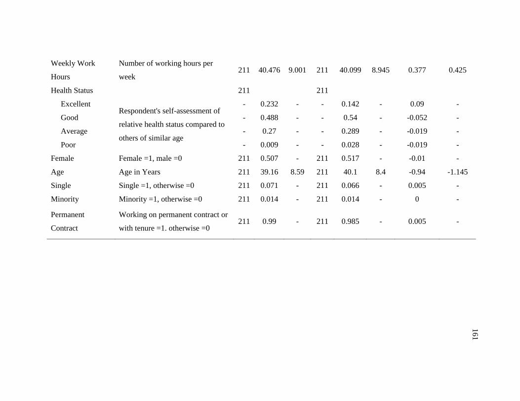
161

161

Weekly Work

Hours

Number of working hours per

week 211 40.476 9.001 211 40.099 8.945 0.377 0.425

Health Status 211 211

Excellent Respondent's self-assessment of

relative health status compared to

others of similar age

- 0.232 - - 0.142 - 0.09 -

Good - 0.488 - - 0.54 - -0.052 -

Average - 0.27 - - 0.289 - -0.019 -

Poor - 0.009 - - 0.028 - -0.019 -

Female Female =1, male =0 211 0.507 - 211 0.517 - -0.01 -

Age Age in Years 211 39.16 8.59 211 40.1 8.4 -0.94 -1.145

Single Single =1, otherwise =0 211 0.071 - 211 0.066 - 0.005 -

Minority Minority =1, otherwise =0 211 0.014 - 211 0.014 - 0 -

Permanent

Contract

Working on permanent contract or

with tenure =1. otherwise =0 211 0.99 - 211 0.985 - 0.005 -

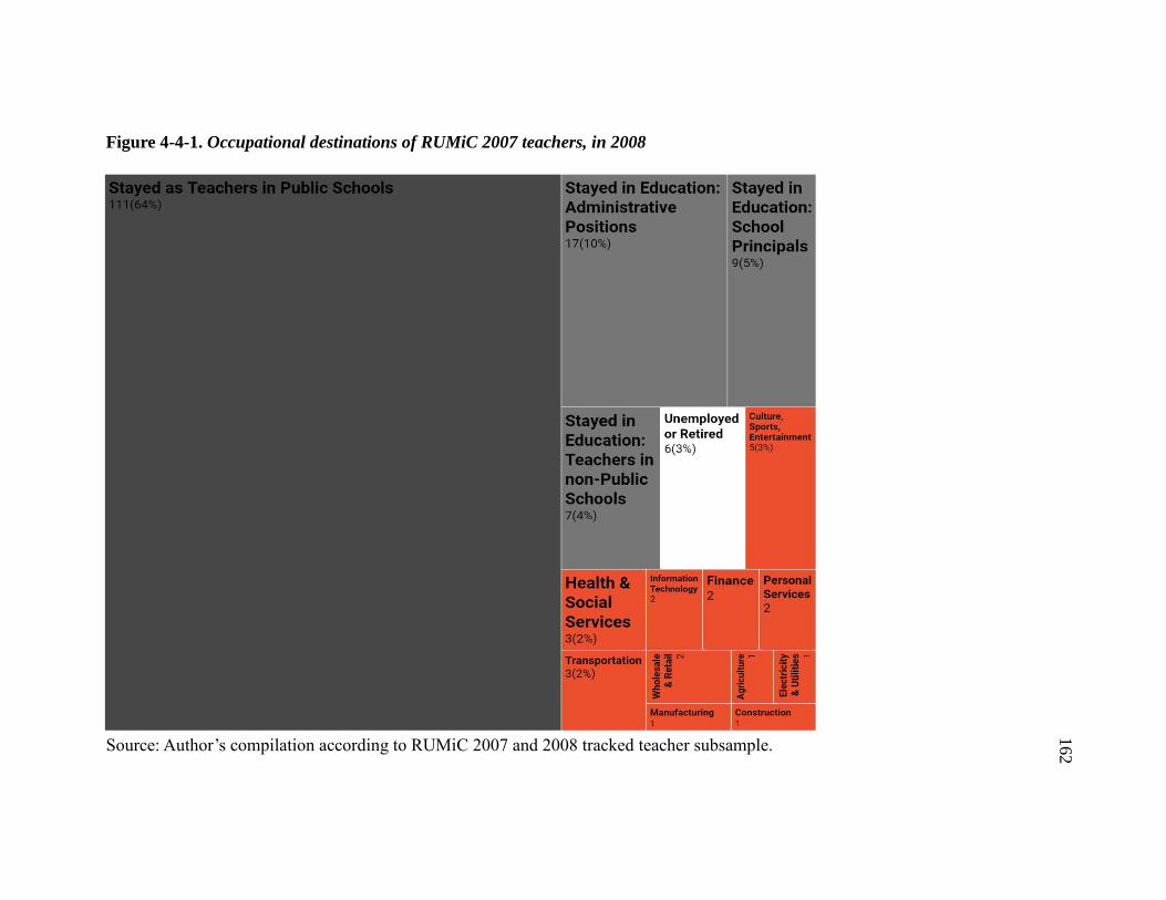
162

162

Figure 4-4-1. Occupational destinations of RUMiC 2007 teachers, in 2008

Source: Author’s compilation according to RUMiC 2007 and 2008 tracked teacher subsample.

163

163

Importantly, across all models in Table 4-2-2, wage gap between teachers and comparable

workers with the same level of educational attainment is shown to have a negative

relationship with probability of working as a teacher. In the base model with no additional

controls, this relationship is not statistically significant, but once adding important time-

variant control variables to improve precision, the negative relationship becomes

marginally significant at -0.319 (p-value<0.10) and -0.442 (p-value<0.10) in Models 2 and

4 respectively. To add, I also provide results of Model 3 as reference for the relationship

between nominal wage levels and occupational decisions; the relationship is insignificant.

For Model 4, while there are some structural multicollinearity concerns regarding the

correlation between “Log Weekly Wage” and “Distance in Log Points to Comparable

Worker Wage” due to the computation approach, marginally significant results in Model 4

continue to indicate that larger wage gaps are related to reduced probability of working as

a teacher. This negative relationship is evaluated at a 1 to -0.442 ratio (p-value<0.10),

which means that for every 10 percent increase in the difference in the wage gap between

teachers and comparable workers, a 4.42 percent decrease in the probability of individuals

working as teachers is observed. The results here should be interpreted with caution as

there could be endogeneity issues with why there exist variations in wages gaps between

teachers and comparable workers. For instance, the level of opportunity wages that teachers

face could be a function of both wage and non-wage factors, including local perception of

job prestige, or local supply of teachers. Therefore, in general terms, I interpret the

opportunity wage level as a proxy for how much teachers are valued in relation to a

comparable worker in a specific geographic locality.

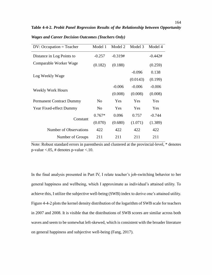
164

164

Table 4-4-2. Probit Panel Regression Results of the Relationship between Opportunity

Wages and Career Decision Outcomes (Teachers Only)

DV: Occupation = Teacher Model 1 Model 2 Model 3 Model 4

Distance in Log Points to

Comparable Worker Wage

-0.257 -0.319# -0.442#

(0.182) (0.188) (0.259)

Log Weekly Wage -0.096 0.138

(0.0143) (0.199)

Weekly Work Hours -0.006 -0.006 -0.006

(0.008) (0.008) (0.008)

Permanent Contract Dummy No Yes Yes Yes

Year Fixed-effect Dummy No Yes Yes Yes

Constant 0.767* 0.096 0.757 -0.744

(0.070) (0.680) (1.071) (1.389)

Number of Observations 422 422 422 422

Number of Groups 211 211 211 211

Note: Robust standard errors in parenthesis and clustered at the provincial-level, * denotes

p-value <.05, # denotes p-value <.10.

In the final analysis presented in Part IV, I relate teacher’s job-switching behavior to her

general happiness and wellbeing, which I approximate as individual’s attained utility. To

achieve this, I utilize the subjective well-being (SWB) index to derive one’s attained utility.

Figure 4-4-2 plots the kernel density distribution of the logarithm of SWB scale for teachers

in 2007 and 2008. It is visible that the distributions of SWB scores are similar across both

waves and seem to be somewhat left-skewed, which is consistent with the broader literature

on general happiness and subjective well-being (Fang, 2017).

165

165

In Table 4-4-3, I present results from the panel regression model I fit on the tracked teacher

data, which relates within-individual variation in career decisions to their assessment of

life’s general happiness. To begin, Model 5 is the base model with only career choice

indicators, for which indicate the difference in the logarithm of SWB index between each

career decision type and the default option of remaining in the job position. In Model 6, I

add time-variant control variables such as wage levels, work hours and health status, and

the signs of coefficients on all three career decision indicator variables continue to hold. In

particular, new entrant teachers report a 5.7 percent gain (p-value<0.10) on the subjective

well-being index than in their prior jobs, and this relationship is marginally significant. As

indicated by the sign of coefficients, teacher exits within education may be positively

associated subjective well-being while the converse is true for teacher departures for non-

education sectors, but both are not statistically significant. To further nuance explorative

findings obtained in this exercise, it should be cautioned that sample sizes are relatively

small and insufficiently powered to detect small differences, and further, not all identified

teachers in the sample completed the subjective well-being assessment, and therefore the

results presented above can be partially influenced by missing data for almost half of the

tracked teacher sample.

166

166

Figure 4-4-2. Distribution of Log of Teacher’s SWB Scores in 2007 and 2008

Source: Author’s compilation according to RUMiC 2007 and 2008 tracked teacher

subsample. Kernel density is computed using Epanechnikov method, bandwidth for 2007

is 0.0532, bandwidth for 2008 is 0.0524.

0.5

11.5

22.5

Kern

el D

en

sity

2.8 3 3.2 3.4 3.6

Log of SWB Scale

2007 2008

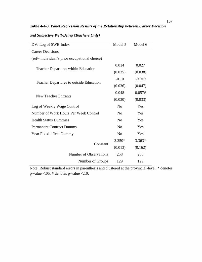
167

167

Table 4-4-3. Panel Regression Results of the Relationship between Career Decision

and Subjective Well-Being (Teachers Only)

DV: Log of SWB Index Model 5 Model 6

Career Decisions

(ref= individual’s prior occupational choice)

Teacher Departures within Education

0.014 0.027

(0.035) (0.038)

Teacher Departures to outside Education

-0.10 -0.019

(0.036) (0.047)

New Teacher Entrants

0.048 0.057#

(0.030) (0.033)

Log of Weekly Wage Control No Yes

Number of Work Hours Per Week Control No Yes

Health Status Dummies No Yes

Permanent Contract Dummy No Yes

Year Fixed-effect Dummy No Yes

Constant

3.350* 3.363*

(0.013) (0.162)

Number of Observations 258 258

Number of Groups 129 129

Note: Robust standard errors in parenthesis and clustered at the provincial-level, * denotes

p-value <.05, # denotes p-value <.10.

168

168

Chapter V

CONCLUSION AND DISCUSSION

China’s rapid economic growth in past decades has created huge employment opportunities

and substantially improved general welfare of its population. However, in light of such

drastic shifts in the labor market, concerns are raised in this dissertation regarding the

potentially large adverse effects of holding teacher wages back from broader market levels;

teachers set the standards for the quality of an educational system. Much of the current

research on teacher occupational choice, especially in developed economies, has shown

that in doing so there are considerable consequences, both in terms of declining teacher

aptitude and unrealized student learning. Using a four-part analytic approach in this

dissertation, I confirm empirical observations made elsewhere and contextualize

theoretical stipulations of the broader occupational choice framework using the case of

Chinese teachers. To define the Chinese case and situate this dissertation more closely with

the large bodies of education development literature on teacher shortage, recruitment and

retention, I have aimed to produce a targeted collection of “thick description” (Steiner-

Khamsi, 2016b, p.691) in addition to empirical findings to extend the current state of

knowledge on teacher occupational choice and its relevant consequences on student

learning, with particular attention to developing contexts.

At the outset of the analysis, I observe two important trends at the aggregate level. On the

one hand, average teacher salary has considerably lacked behind that of other sectors,

growing at about half the rate of the national mean. Of note, the rate of teacher wage growth

169

169

varied substantially across geographical regions. On the other hand, the percent of workers

with advanced tertiary education degrees are the highest in the education sector than in all

other sectors, and educational attainment of teachers was shown to have increased at all

instructional levels. However, there are signs of more attractive sectors in recent years that

are also competing for workers with advanced degrees, such as “Finance and Banking,”

“Information Technology,” and “Public Health and Social Welfare.” Zooming in further on

compositional shifts in the teaching force, I find that new entrants are a major source of

teacher additions at all instructional levels; however, in lower secondary schools, there is

considerable numbers of net transfers out of teaching jobs. In general terms, while wage

growth has been largely stagnant for teachers, there is still an increase in the number of

individuals with advanced educational attainment becoming teachers, but recent rates of

recruitment has been growing comparatively faster in non-education sectors. To be clear,

these macro-level findings, while instructive, are aggregate trend summaries of high

abstraction and prompts further investigation using micro-level analysis.

Main Findings and Discussion for Part I

Undeniably, teacher quality has been shown to be one of the most important school-related

factors in influencing a student’s academic performance. In this regard, policymakers have

often relied on pre-labor market human capital signals to screen teacher candidates for

potential instructional effectiveness. To establish the causal link between teachers’

comparable and observable quality characteristics and student learning outcomes, in Part I

of this dissertation I employed a student fixed-effect strategy to relate differences in teacher

characteristics across subjects to variations on student test scores. The results illustrate that

170

170

student-learning benefits from having a teacher with advanced tertiary degree are evaluated

at 0.033 standard deviations. In other words, the learning gains from having a more

educated teacher are approximately 1 additional month of learning in a typical 9-month

academic year, even after controlling for other teacher background attributes. Further

robustness check was conducted by limiting the analysis to only students who have not

been systematically sorted according to ability grouping, and the impacts are shown to

double, at about 0.071 standard deviations. In examining potential heterogeneous effects,

findings suggest that students from advantaged and disadvantaged students both benefit

from better educated teachers alike, and there are no foreseeable equity concerns.

Altogether, results presented in Part I of this dissertation underscore the critical

consequence teachers can have on students’ learning outcomes. In this regard, findings

from the Chinese context contribute rigorous evidence to a broader debate in the teacher

effectiveness and teacher value-added literature on whether teacher observational

characteristics on preparation and certification are useful for improving student learning

(Darling-Hammond, 2000; Hanushek & Rivkin, 2006; Harris & Sass, 2007; Winters,

Dixon, Greene, 2012). One of the most influential research on this topic in the United States,

by Hanushek and Rivkin (2006), found that only 29 percent of all 170 estimates regarding

the impact of teacher’s earning an advanced degree on student achievement is significant,

the vast majority of the impacts are statistically insignificant. This result and others

following it have put in question policy efforts that aim at improving teacher education

programs or job attractiveness to highly educated individuals, since teacher’s human

capital levels are poor predictors of teaching effectiveness.

171

171

Other studies, however, have challenged these beliefs and confirm that what teachers know,

how well they are prepared to teach, and the level of educationally important credentials

they hold really do affect student learning (Polk, 2006; Clotfelter, Ladd, & Vigdor, 2007;

Hairrel, Rupley, Edmonds, Larsen, Simmons, Wilson & Vaughn, 2011; Meroni, Vera-

Toscano, & Costa, 2015; Cakır & Bichelmeyer, 2016). For instance, Jackson and

Bruegmann (2009) summarize teacher’s observable pre-labor market traits (i.e. licensure,

score of license exams, certification, and degree level) in to a single index and find positive

associations between observable teacher characteristics and students’ math and reading

scores. Importantly, classroom teaching is a complex and intellectually demanding activity

that requires teachers to possess substantive cognitive, non-cognitive, and critical thinking

skills as well as a solid foundation of subject and pedagogical knowledge (Stronge, 2018).

To conclude, results in Part I of this dissertation supports this view that teacher’s attained

human capital levels have serious consequences for improving student achievement, such

that more educated teachers can lead to better student learning.

Main Findings and Discussion for Part II

Having established the importance of high ability teachers on effective student

achievement, my analysis proceeded to examine the wage returns to common human

capital traits – educational attainment level. Accordingly, in Part II, I estimate a Mincer

earnings function to examine gaps in mean wage levels and returns to human capital

between teaching and non-teaching sectors. In general terms, I find sharp shifts in the

relative attractiveness of wage characteristics in the teaching sector. I find that in 1998,

172

172

teachers’ mean wage was 13 percent higher than workers in non-teaching private sectors,

but this advantage has since disappeared in 2007, and by 2013, the mean wage reversed to

be in favor of workers in non-teaching sectors by 11 percent, marking a total of 24

percentage point reversal. Regarding gaps in returns to education, returns to having a

Bachelor’s degree or above became significantly higher, about 11-15 percent, in private

non-teaching sectors than the teaching sector in years 2007, 2008, and 2013. Connecting

both findings, it is suggested that the education sector has made potentially large salary

savings compared to if it was required to hire individuals with similar qualifications at the

market rate. To this end, prolonged lag in mean wage growth and returns to human capital

may be critical risk factors for thwarting potential high quality candidates from entry.

As observed in the United States and elsewhere, relative wage levels are strong

occupational determinants, and may substantially influence career decisions of prospective

teacher candidates. Recent evidence linking career aspirations of 15-year-olds and current

teacher salary levels show that students in the top tertile of academic achievement who live

in countries that pay their teachers better are more likely to aspire to become a teacher,

relative to countries that pay teachers poorly (Park & Byun, 2015). Consistent with studies

that examine the relationship between salary and career inclinations for teacher education

enrollees (Watt & Richardson, 2012) and recent college graduates (Bacolod, 2007),

findings from this section provide insights to future trajectories of who will become

teachers. In sum, the consequences of withholding teacher salary levels could be

longstanding, and the stake for leaving teaching as an unattractive career is potentially high

and the timeline to alter the decline teacher wage trend is pressing.

173

173

Main Findings and Discussion for Part III

In Part III, I proceed to address the empirical question of how teacher quality has changed

with respect to the shifting landscape of China’s job market. To achieve this, I apply

multinomial probit regression to assess the relationship between human capital measures,

such as educational attainment level, high school selectivity, and national college entrance

exam scores, on individual’s occupational choice. Notably, findings show that while

individuals with advanced tertiary degrees are consistently more likely to choose teaching

as a career, this relationship is considerably weaker among younger cohorts in recent years.

For one, between 1988 and 2013, more educated individuals with Bachelor’s degrees or

above are consistently more likely to choose teaching over both private and public non-

teaching sectors. For another, by separately calculating adjusted probabilities of choosing

teaching careers for individuals aged 30 and 50 years old, I find that in 2007 and 2013, new

labor market entrants with advanced tertiary degrees are 4.7 percent and 5.8 percent less

likely than comparable workers in older cohorts to choose teaching.

To confirm the validity of these findings, I perform additional analyses by substituting

educational attainment with upper secondary school selectivity and national college

entrance exam scores as proxies for human capital and worker aptitude. Findings indicate

that graduates from the most selective secondary schools and those that scored better on

the national college entrance exam were more likely to enter the teaching sector in 2002

and 2007, respectively. However, by 2013, workers in both high aptitude groups became

no more likely to choose teaching over private sector jobs. Altogether, these findings

174

174

suggest that workers with better labor market signals or human capital traits have become

less likely to enter the education sector, resulting in relative declines in teacher quality.

A broad class of existing studies has examined the positive relationship between earnings

and career attractiveness, and have documented the relative declines in teacher aptitude,

qualifications, and skills (Vegas, Murnane, & Willett, 2001; Elfers, Plecki, John & Wedel,

2008; Gilpin, 2012). In particular, Hoxby and Leigh (2004) has shown that the share of

teachers coming from the most elite colleges have fallen over time in the United States;

Fredriksson and Ockert (2008) find similar patterns in Sweden that younger cohorts are

much less likely to choose a career in teaching. Using the case of Chinese teachers, I add

to this large and growing literature that document the worrisome trend in relative declines

in teacher aptitude and ability in relation to other sectors.

Main Findings and Discussion for Part IV

In Part IV, I leverage the availability of a nationally representative panel data containing

211 matched teachers with information on their employment information, and track their

career destinations across time. In general, I find that teacher turnover rates are relatively

high, and there exists positive associations with the level of opportunity wages, and there

is no obvious evidence on individual non-pecuniary gains from teacher exit decisions. For

one, findings show that teacher turnover rates are high and evaluated at approximately 35

percent, of which about half of the teachers exit the sector entirely. The top outside-

education career destinations for teacher exits are “Culture, Sports, and Entertainment,”

“Health & Social Services,” or “Transportation” sectors. Importantly, these findings

175

175

contribute substantively to the current understanding in China on the prevalence and

magnitude of teacher departures from teaching posts and the education sector. For another,

I evaluate the degree to which opportunity wage levels influence teacher turnover decisions,

I find that every 10 percent increase in opportunity wages that teachers face, it is shown to

be 4.42 percent less likely to remain a teacher. In general terms, I interpret the opportunity

wage level as a proxy for how much teachers are valued in relation to a comparable worker

in a specific geographic locality. Therefore, the less value a community has for teachers,

the higher the likelihood of teacher turnover. Finally, I conduct an explorative analysis on

whether there are non-pecuniary benefits for those who leave teaching, and there is no

evidence to suggest that there exist substantive differences on non-pecuniary benefits to

teacher job switching.

The issue of teacher turnover is a crucial component of occupational choice and holds the

key in broader retention efforts. In particular, Chingos and West (2009) have shown that

more effective teachers are more likely to receive higher pay when they depart from

education, but do not when they remain as teachers. Other scholars have examined the

importance of non-pecuniary factors, such as working conditions and workload, and

stipulate that they are also important for teacher retention (Ingersoll, 2003; Guarino,

Santibanez, & Daley, 2006). Accordingly, findings in this dissertation provide some new

evidence on alternative careers, opportunity wages, and non-pecuniary effects of teacher

turnover that are more consistent with existing studies which have highlighted the

intertwined relationship between pecuniary and non-pecuniary factors on teacher

occupational choice (Han, Borgonovi, & Guerriero, 2018). As such future research is still

176

176

needed to untangle the overlay between wage levels and social prestige, among other

occupationally important non-pecuniary factors.

Policy Implications

As China continues to modernize its education system and address equity concerns in its

education development, findings presented in this dissertation point to several important

policy considerations regarding existing teacher recruitment and retention policies and

practices. Most strikingly, the analysis gathered evidence in underscoring the consequences

of holding teacher wage levels back, which affects teacher occupational choice,

instructional quality, and student learning outcomes.

As shown in Part I, the student achievement gains from having more capable teachers are

non-trivial and can be reasonably expected to compound over the course of a student’s

learning career. In particular, there may be substantial returns to boosting ability traits of

teachers, in the form of increased student learning, especially in settings where current

levels of teacher staffing and quality is low. The findings presented here resonate with the

broader national policy focus and discussion on setting teacher quality improvement as a

primary objective in the “Thirteen-Five” period before 2020 (State Council, 2017, Section

4). In particular, as shown in Part I, boosting teacher quality by recruiting better qualified

teachers can lead to close to 10 percent gain in the average learning productivity over the

course of a typical school year (1 month of additional learning in a typical 9-month

academic year). Therefore, evidence gathered in this study supports the current Chinese

national policy focal point on placing a strong emphasis on boosting teacher quality; policy

177

177

makers should continue to realize their commitment to realizing meaningful teacher quality

improvements.

In addition, Parts II and III have indicated the important relationship between relative wage

characteristics and teacher occupational choice. The conclusion is straightforward: wage

policies for teachers need to include meaningful considerations for the concurrent wage

conditions and developments in the broader labor market, which have been shown to be

crucial covarying factor influencing teacher occupational choice. In recent years in

particular, younger cohorts of highly educated workers are becoming less likely to choose

teaching as a career, which coincides with the rapidly decreasing returns to education/skills

within the education sector. This may be a worrying from a policy standpoint, if current

developments are left unattended, because there considerable consequences, both affecting

the status of the teaching profession as well as influencing the level of student learning

achieved. To this end, policy makers should rethink existing forms of teacher compensation

arrangements and develop sustainable wage adjustment practices, especially in relation to

conditions in the broader market levels, in order to retain and attract bright minds to enter

and stay in teaching.

Limitations and Paths for Future Research

It is worth noting that while the methodology and findings from this dissertation are

rigorous to the extent possible, interpretation of results require further caution with special

attention to remaining issues not fully addressed in this current study. First, due to data

limitations, the current study is confined within urban China and does not address the vast

178

178

differences that exist between urban and rural schools in China. In this vein, the

complications in teacher quality and occupational choice that arise as result of large

geographic variabilities cannot be overlooked. As previous studies have illustrated, living

and working conditions are reasonably expected to influence teacher occupational

decisions through compensating wage differentials, which are important factors in

individuals’ career determination. Therefore, further research on the link between teacher

occupational choice, instructional quality and student learning is needed.

Second, findings illustrated in Parts II and III are to be contextualized in relation to the

broader trajectory of development of tertiary education in China. Importantly, tertiary

education enrollment doubled in 1999/2000 as a result of China’s Higher Education

Expansion reform, which was designed as a counter-cyclical stimulus measure to delay

entry of new labor supply, in response to the 1997/1998 Asian financial crisis that resulted

in export contraction and subsequent saturation in the labor market (Che & Zhang, 2017).

By June 2000, the Ministry of Education announced that the enrollment expansion target

had increased to 1.56 million students, or a 44 percent gain year-over-year, which was

observed somewhat evenly across fields and disciplines (Che & Zhang, 2017). To this end,

the rapid expansion of tertiary enrolment implies that the meaning of being “tertiary-

educated” has changed dramatically for new labor market entrants, as tertiary education

becomes in abundant supply in the post reform era, which may both impact labor prices

and quality. Therefore, the interpretation wage differential and entry probability results in

Part II and III, for the post-2003/2004 period require additional caution because this is

when graduates who are affected by the enrolment expansion enter the job market. Future

179

179

research in this area is needed to understand how teacher quality and occupational choice

is affected by educational reforms from both labor supply and demand sides.

Third, there may be concerns regarding the relatively small teacher-panel sample used in

Part IV, which limits its national representativeness and interpretation of the associated

results. To this end, if more data becomes publicly available, a longer panel could be readily

constructed to extend the current analysis and verify the generalizability of results. Finally,

this dissertation conceptualizes teacher quality using both teacher input and output proxies.

For teacher output proxies, I utilized student achievement scores on three tested subjects.

Notwithstanding, there are arguably many other educationally-important teacher outputs

that is not fully captured in testing, such as non-cognitive skills development, therefore this

limitation highlights a need to examine these types of learning outcomes in future research.

180

180

REFERENCES

Adams, J. (2012). Identifying the Attributes of Effective Rural Teachers: Teacher Attributes

and Mathematics Achievement among Rural Primary School Students in Northwest

China. Gansu Survey of Children and Families. Working Paper.

Akguc, M., Giulietti, C., & Zimmermann, K. F. (2014). The RUMiC longitudinal survey:

Fostering research on labor markets in China. IZA Journal of Labor & Development,

3(1), 5. DOI: 10.1186/2193-9020-3-5.

Aklog, F. B. (2005). Teacher job satisfaction and dissatisfaction: An empirical study of

urban teachers in Ethiopia. Doctoral dissertation, Teachers College, Columbia

University.

Allegretto, S., Corcoran, S., & Mishel, L. (2008). The Teaching Penalty: Teacher Pay

Losing Ground. Washington, D.C.: Economic Policy Institute.

Altinok, N., & Kingdon, G. (2012). New evidence on class size effects: A pupil fixed

effects approach. Oxford Bulletin of Economics and Statistics, 74(2), 203-234.

An, X. (2014). On the Changes and Differences in Characteristics of Teachers’ Salary in

Primary and Secondary Schools (In Chinese). Educational Research, 12 (419), 44-53.

Angrist, J., & Guryan, J. (2007) Does teacher testing raise teacher quality? Evidence from

state certification requirements. Economics of Education Review, 27 (5), 483-503.

Bacolod, M. (2007). Who Teaches and Where They Choose to Teach: College Graduates

of the 1990s. Education Evaluation and Policy Analysis, 29( 3), 155-168.

Badgett, L., & Folbre, N. (2003). Job Gendering: Occupational Choice and the Marriage

Market. Industrial Relations, 42(2), 270-298.

181

181

Ballou, D., & Podgursky, M. (1997). Teacher Pay and Teacher Quality. Kalamazoo, MI:

W.E. Upjohn Institute for Employment Research

Banerjee, A., & Newman, A. (1993). Occupational Choice and the Process of Development.

Journal of Political Economy, 101(2), 274-298.

Bau, N., & Das, J. (2017). The misallocation of pay and productivity in the public sector:

Evidence from the labor market for teachers. Washington, D.C.: The World Bank.

Baumol, W. J. (1993). Health care, education and the cost disease: A looming crisis for

public choice. Public choice, 77(1), 17-28.

Becker, G. S. (1985). Human capital, effort, and the sexual division of labor. Journal of

labor economics, 3(1, 2), 33-58.

Blau, F., Ferber, M., & Winkler, A. (1998). The economics of women, men, and work, 3rd

edition. Upper Saddle River, NJ: Prentice Hall.

Borjas, G. (1987). Self-selection and the earnings of immigrants. American Economic

Review, 77(4), 531-553.

Brandt, L., & Zhu, X. (2010). Accounting for China’s Growth. Working Papers tecipa-394,

University of Toronto.

Bruns, B., & Luque, J. (2014). Great teachers: How to raise student learning in Latin

America and the Caribbean. Washington, D.C.: The World Bank.

Çakır, H., & Bichelmeyer, B. A. (2016). Effects of teacher professional characteristics on

student achievement: an investigation in blended learning environment with

standards-based curriculum. Interactive Learning Environments, 24(1), 20-32.

182

182

Card, D. (2001). Estimating the return to schooling: Progress on some persistent

econometric problems. Econometrica, 69(5), 1127-1160.

Che, Y., & Zhang, L. (2017). Human Capital, Technology Adoption and Firm Performance:

Impacts of China's Higher Education Expansion in the Late 1990s. The Economic

Journal, 128(614), 2282-2320.

Chen, Y. (2003). A Probe into Problems of Teacher Salaries in 1990’s. Tsinghua Journal

of Education, 24(10), 92-96.

Chetty, R., Friedman, J., & Rockoff, J., (2014). Measuring the Impacts of Teachers II:

Teacher Value-Added and Student Outcomes in Adulthood. American Economic

Review, 104(9), 2633-2679.

Chingos, M., & West, M. (2012). Do More Effective Teachers Earn More Outside the

Classroom? Education Finance and Policy, 7(1), 8-43

Chingos, M. M., & West, M. R. (2009). Teacher Effectiveness, Mobility, and Attrition in

Florida, in Matthew G. Springer, (Ed.), Performance Incentives: Their Growing

Impact on American K–12 Education, Washington, D.C.: Brookings Institution Press,

251–271.

Chu, J., P. Loyalka, J. Chu, Q., Qu, Y., Shi, & G., Li. (2015). The impact of teacher

credentials on student achievement in China. China Economic Review, 36, 14-24.

Clark, A., & Oswald, A. (2002). A simple statistical method for measuring how life events

affect happiness. International Journal of Epidemiology, 31(6), 1139-1144.

Clotfelter, C. T., Ladd, H. F., & Vigdor, J. L. (2007). Teacher credentials and student

achievement: Longitudinal analysis with student fixed effects. Economics of

Education Review, 26(6), 673-682.

183

183

Corcoran, S., Evans, W., & Schwab, R. (2004). Women, the Labor Market, and the

Declining Relative Quality of Teachers. Journal of Policy Analysis and Management,

23(3), 449-470.

Correa, J., Parro, F. & Reyes, L. (2015). Self-selection in the market of teachers. Applied

Economics, 47(13), 1331-1349.

Darling-Hammond, L. (2000). Teacher quality and student achievement. Education Policy

Analysis Archives, 8, 1-44.

D'Haultfoeuille, X., & Maurel, A. (2010). Inference on a Generalized Roy Model, with an

Application to Schooling Decisions in France. Working Paper.

Ding, S., Dong, X., & Li, S. (2007). The impact of married women’s employment and

earnings on income inequality among urban households during China’s economic

transition. [In Chinese]. China Economic Quarterly, 6(4), 1319-1338.

Dolton, P., Makepeace, G., & van der Klaauw, W. (1989) Occupational Choice and

Earnings determination: The Role of Sample Selection and Non-Pecuniary Factors.

Oxford Economics Papers, 41, 573-594.

Duckworth, A. L., & Yeager, D. S. (2015). Measurement matters: Assessing personal

qualities other than cognitive ability for educational purposes. Educational Researcher,

44(4), 237-251.

Dustmann, C., Rajah, N., & van Soest, A. (1998). School Quality, Exam Performance and

Career Choice. Discussion Paper, Tilburg University, Center for Economic Research.

Eble, A., & Hu, F. (2018). The sins of the parents: Persistence of gender bias across

generations and the gender gap in math performance. CDEP‐CGEG Working Paper

No. 53.

184

184

Eckert, J. M., & Dabrowski, J. (2010). Should value-added measures be used for

performance pay?. Phi Delta Kappan, 91(8), 88-92.

Eichen, M.. & Zhang, M. (1993). Annex: The 1988 Household Sample Survey: Data

Description and Availability, in Griffin, K., & Zhao, R. (Eds.), The Distribution of

Income in China, New York: St. Martin’s Press, 331-346.

Elfers, A. M., Plecki, M. L., St John, E., & Wedel, R. (2008). Undergraduates' views of K-

12 teaching as a career choice. Seattle, WA: University of Washington.

Falch, T., & Johansen, K., & Strom, B. (2009). Teacher Shortages and the Business Cycle.

Labour Economics, 16, 648–658.

Fang, Z. (2017). Panel quantile regressions and the subjective well-being in urban China:

evidence from RUMiC data. Social Indicators Research, 132(1), 11-24.

Fang, Z., & Sakellariou, C. (2015). Glass Ceilings versus Sticky Floors: Evidence from

Southeast Asia and an International Update. Asian Economic Journal, 29(3), 215-242.

Figlio, D. N. (1997). Teacher salaries and teacher quality. Economics Letters, 55(2), 267-

271.

Fredriksson, P., & Öckert, B. (2008). The supply of skills to the teacher profession.

Scandinavian Journal of Economics, 110(2), 277-296.

Gilpin, G., & Kaganovich, M., (2012). The quantity and quality of teachers: dynamics of

the trade-off. Journal of Public Economics, 96(3–4), 417-429.

Glazerman, S., Loeb, S., Goldhaber, D. D., Raudenbush, S., & Whitehurst, G. J. (2010).

Evaluating teachers: The important role of value-added. 201(0). Washington, DC:

Brown Center on Education Policy at Brookings.

185

185

Goldhaber, D., & Hansen, M. (2008). Assessing the Potential of Using Value-Added

Estimates of Teacher Job Performance for Making Tenure Decisions. Brief 3. National

Center for Analysis of Longitudinal Data in Education Research.

Greene, W. H. (2000). Econometric Analysis. 4th Edition. London Prentice Hall.

Guarino, C. M., Santibanez, L., & Daley, G. A. (2006). Teacher recruitment and retention:

A review of the recent empirical literature. Review of educational research, 76(2),

173-208.

Guo, R. (1994). Comparative analysis of 80 years of salary and living conditions among

various occupations in China. Ren Wen Za Zhi Journal of Humanities, 6, 64-68.

Gustafsson, B., Li, S., & Sato, H. (2014). Data for studying earnings, the distribution of

household income and poverty in China. China Economic Review, 30, 419-431.

Hairrell, A., Rupley, W., Edmonds, M., Larsen, R., Simmons, D., Willson, V., & Vaughn,

S. (2011). Examining the impact of teacher quality on fourth-grade students'

comprehension and content-area achievement. Reading & Writing Quarterly, 27(3),

239-260.

Han, S., Borgonovi, F., & Guerriero, S. (2018). What motivates high school students to

want to be teachers? The role of salary, working conditions, and societal evaluations

about occupations in a comparative perspective. American Educational Research

Journal, 55(1), 3-39.

Hanushek, E., & Pace, R. (1995). Who Chooses To Teach (and Why)? Economics of

Education Review, 14, 101-117.

Hanushek, E., & Rivkin, S. (2007). Pay, working conditions, and teacher quality. The

future of children, 69-86.

186

186

Hanushek, E., & Rivkin, S. (2006). Teacher quality. Handbook of the Economics of

Education, 2, 1051-1078.

Hanushek, E., & Rivkin, S. (2012). The distribution of teacher quality and implications for

policy. Annual Review of Economics, 4(1), 131-157.

Hanushek, E., & Woessmann, L. (2015). The knowledge capital of nations: Education and

the economics of growth. Boston, MA: MIT Press.

Harris, D., & Sass, T. (2007). Teacher training, teacher quality, and student achievement.

Washington, DC: National Center for Analysis of Longitudinal Data in Education

Research.

Harris, D., & Sass, T. (2010). Teacher training, teacher quality and student achievement.

Journal of Public Economics, 95, 798-812.

Heckman, J. (1974). Shadow prices, market wages, and labor supply. Econometrica:

Journal of the Econometric Society, 679-694.

Heckman, J. (1976). The common structure of statistical models of truncation, sample

selection, and limited dependent variables and a simple estimator for such models.

Annals of Economic and Social Measurement, 5, 479-492.

Heckman, J., & Sedlacek, G. (1985). Heterogeneity, Aggregation, and Market Wage

Functions: An Empirical Model of Self-Selection in the Labor Market. Journal of

Political Economy, 93(6), 1077-1125.

Hendricks, M. (2014). Does it pay to pay teachers more? Evidence from Texas. Journal of

Public Economics, 109, 50-63.

187

187

Hoxby, C. & Leigh, A. (2004). Pulled Away or Pushed Out? Explaining the Decline of

Teacher Aptitude in the United States. AEA Papers and Proceedings, 94(2), 236-240.

Hoyle, E. (2001). Teaching: Prestige, status and esteem. Educational Management &

Administration, 29(2), 139-152.

Ingersoll, R. M. (2001). Teacher turnover and teacher shortages: An organizational analysis.

American educational research journal, 38(3), 499-534.

Ingersoll, R. (2003). Turnover and shortages among science and mathematics teachers in

the United States. Science Teacher Retention: Mentoring and Renewal, 1-12.

Ingersoll, R. (2007). A comparative study of teacher preparation and qualifications in six

nations, Washington, D.C.: Consortium for Policy Research in Education.

Ingersoll, R., & May, H. (2012). The magnitude, destinations, and determinants of

mathematics and science teacher turnover. Educational Evaluation and Policy

Analysis, 34(4), 435-464.

Ingersoll, R., Merrill, L., & May, H. (2011). What are the effects of teacher education and

preparation on beginning math and science teacher attrition. Philadelphia, PA:

University of Pennsylvania.

Ingersoll, R., & Smith, T. (2003). The wrong solution to the teacher shortage. Educational

leadership, 60(8), 30-33.

Jackson, C. (2014). Teacher quality at the high school level: The importance of accounting

for tracks. Journal of Labor Economics, 32(4), 645-684.

Jackson, C. (2012). Recruiting, retaining, and creating quality teachers. Nordic Economic

Policy Review, 3(1), 61-104.

188

188

Jackson, C., & Bruegmann, E. (2009). Teaching students and teaching each other: The

importance of peer learning for teachers. American Economic Journal: Applied

Economics, 1(4), 85-108.

Kane, T., & Staiger, D. (2008). Estimating teacher impacts on student achievement: An

experimental evaluation. NBER Working Paper No. 14607.

Kane, T., Rockoff, J., & Staiger, D. (2008). What does certification tell us about teacher

effectiveness? Evidence from New York City. Economics of Education review, 27(6),

615-631.

Lakdawalla, D. (2006). The Economics of Teacher Quality. Journal of Law and Economics,

49, 285–329.

Lavy, V. (2016). Teachers’ Pay for Performance in the Long-Run: The Dynamic Pattern

of Treatment Effects on Students’ Educational and Labor Market Outcomes in

Adulthood. NBER Working Paper No. 20983.

Lazear, E. (1986). Salaries and Piece Rates. Journal of Business, 59(3), 405-31.

Lee, L. (1978). Unionism and Wage Rates: A Simultaneous Equations Model with

Qualitative and Limited Dependent Variables. International Economic Review, 19(2),

415-433.

Leigh, A. (2012). Teacher Pay and Teacher Aptitude. Economics of Education Review, 31,

41-53.

Levine, A. (2006). Educating school teachers. Princeton, NJ: Education Schools Project.

Levin, H. (2011). The economics of education. Albany Government Law Review, 4, 395-

425.

189

189

Li, B. (2007). Cheng xiang jiao shi de shou ru cha ju yu liu dong wen ti tan jiu [Investigation

of the income gap between urban and teachers as well as teacher mobility] (In Chinese).

The Inservice Education and Training of School Teachers, 3.

Liu, S. (2012). The influences of school climate and teacher compensation on teachers’

turnover intention in China. Educational Psychology, 32(5), 553-569.

Liu, E., Johnson, S., & Peske, H. (2004). New teachers and the Massachusetts signing

bonus: The limits of inducements. Educational Evaluation and Policy Analysis, 26(3),

217-236.

Liu, S., & Onwuegbuzie, A. (2012). Chinese teachers’ work stress and their turnover

intention. International Journal of Educational Research, 53, 160-170.

Luschei, T., & Jeong, D. (2018). Is Teacher Sorting a Global Phenomenon? Cross-National

Evidence on the Nature and Correlates of Teacher Quality Opportunity Gaps.

Educational Researcher, DOI: 0013189X18794401.

McElroy, M., & Hornery, M. (1981). Nash-bargained Household Decisions: Toward a

Generalization of the Theory of Demand. International Economic Review, 22(2), 333-

349.

Meroni, E. C., Vera-Toscano, E., & Costa, P. (2015). Can low skill teachers make good

students? Empirical evidence from PIAAC and PISA. Journal of Policy Modeling,

37(2), 308-323.

Metzler, J., & Woessmann, L. (2012). The impact of teacher subject knowledge on student

achievement: Evidence from within-teacher within-student variation. Journal of

Development Economics, 99(2), 486-496.

190

190

Mincer, J. (1974). Schooling and earnings. In Schooling, experience, and earnings (41-63).

Boston, MA: NBER.

Ministry of Education. (1986). Education Statistics Yearbook 1986. Beijing: Ministry of

Education Press.

Ministry of Education. (2008). Guidelines on Performance Evaluation of Teachers in

Primary and Secondary Schools. Beijing: Ministry of Education Press.

Ministry of Education. (2010). Education Statistics Yearbook 2010. Beijing: Ministry of

Education Press.

Ministry of Education. (2011). Education Statistics Yearbook 2011. Beijing: Ministry of

Education Press.

Ministry of Education. (2014). Education Statistics Yearbook 2014. Beijing: Ministry of

Education Press.

Moore, A., & Destefano, J., & Terway, A., & Balwanz, D. (2008). The Expansion of

Secondary Education and the Need for Teachers: How big is the gap? USAID Working

Papers.

Morgan, W. B., Walker, S. S., Hebl, M. M. R., & King, E. B. (2013). A field experiment:

Reducing interpersonal discrimination toward pregnant job applicants. Journal of

Applied Psychology, 98(5), 799.

Muralidharan, K., & Sundararaman, V. (2011). Teacher opinions on performance pay:

Evidence from India. Economics of Education Review, 30(3), 394-403.

Nagler, M., & Piopiunik, M., & West, M. (2015). Weak Markets, Strong Teachers:

Recession at Career Stat and Teacher Effectiveness. NBER Working Papers 21393.

191

191

National Bureau of Statistics. (1999). National Labor Statistics 1999. Beijing: National

Bureau of Statistics.

National Bureau of Statistics. (2003). National Labor Statistics 2003. Beijing: National

Bureau of Statistics.

National Bureau of Statistics. (2009). National Labor Statistics 2009. Beijing: National

Bureau of Statistics.

National Bureau of Statistics. (2017). National Labor Statistics 2017. Beijing: National

Bureau of Statistics.

National Survey Research Center. (2014). Data handbook for China Education Panel

Survey. Beijing: National Survey Research Center.

Neugebauer, M. (2015). Who chooses teaching under different labor market conditions?

Evidence from West Germany, 1980–2009. Teaching and Teacher Education, 45,

137-148.

Organisation for Economic Co-operation and Development (2013). Teachers for the 21st

Century Using Evaluation to Improve Teaching. Paris, France: OECD Publishing.

Organisation for Economic Co-operation and Development. (2016). Education at a Glance

2016: OECD Indicators. Paris, France: OECD Publishing.

Park, H., & Byun, S. Y. (2015). Why some countries attract more high-ability young

students to teaching: Cross-national comparisons of students’ expectation of becoming

a teacher. Comparative Education Review, 59(3), 523-549.

Peltzman, S. (1996). Political economy of public education: Non-college-bound students.

The Journal of Law and Economics, 39(1), 73-120.

192

192

People’s Congress. (2006). Compulsory Education Law in 2006. Beijing: People’s

Congress.

Polachek, S. (1981). Occupational self-selection: A human capital approach to sex

differences in occupational structure. Review of Economics and Statistics, 60-69.

Polk, J. (2006). Traits of effective teachers. Arts Education Policy Review, 107(4), 23-29.

Richey, J. (2014). Divergent Trends in U.S. Teacher Quality: 1980-2010. MPRA Paper

55637, University Library of Munich, Germany.

Rivkin, S., & Hanushek, E., & Kain, J. (2005). Teachers, schools, and academic

achievement. Econometrica, 73(2), 417-458.

Rockoff, J. (2004). The impact of individual teachers on student achievement: Evidence

from panel data. American Economic Review, Papers and Proceedings, 94, 247-252.

Rockoff, J., Staiger, D., Kane, T., & Taylor, E. (2012). Information and employee

evaluation: Evidence from a randomized intervention in public schools. American

Economic Review, 102(7), 3184-3213.

Rose, H., & Sonstelie, J. (2010). School board politics, school district size, and the

bargaining power of teachers’ unions. Journal of urban economics, 67(3), 438-450.

Roy, A. (1951). Some Thoughts on the Distribution of Earnings. Oxford Economic Papers,

3, 135-146.

Rubin, D. (1974). Estimating causal effects of treatments in randomized and

nonrandomized studies. Journal of educational Psychology, 66(5), 688.

193

193

Sargent, T., & Hannum, E. (2005). Keeping teachers happy: Job satisfaction among

primary school teachers in rural northwest China. Comparative Education Review,

49(2), 173-204.

Schleicher, A. (2012). Preparing Teachers and Developing School Leaders for the 21st

Century: Lessons from around the World. Paris, France: OECD Publishing.

Schonfeld, I. S., Bianchi, R., & Luehring-Jones, P. (2017). Consequences of Job Stress for

the Mental Health of Teachers. Educator Stress. 55-75.

Scott-Clayton, J., & Wen, Q. (2017). Estimating Returns to College Attainment:

Comparing Survey and State Administrative Data Based Estimates. CAPSEE Working

Paper. Center for Analysis of Postsecondary Education and Employment.

Shi, J., & Yan, J. (2006). Ju jiao nong cun zhong xiao xue jiao shi guan zhu nong cun ji

chu jiao yu de ke chi xu fa zhan [Focus on Rural Teachers and Education Foundation

for Sustainable Development]. Exploring Education Development.

Simon, N. S., & Johnson, S. M. (2015). Teacher turnover in high-poverty schools: What

we know and can do. Teachers College Record, 117(3), 1-36.

Steele, J. L., Murnane, R. J., & Willett, J. B. (2010). Do financial incentives help low‐

performing schools attract and keep academically talented teachers? Evidence from

California. Journal of Policy Analysis and Management, 29(3), 451-478.

State Council. (1981). Measures on Adjusting Salaries of Primary and Secondary School

Teachers. Beijing: State Council.

State Council. (1985). Notice on Government and Public Institution Employee Salary

Guidelines. Beijing: State Council.

194

194

State Council. (1987). Notice on Compensation Improvement for Teachers in Basic

Education. Beijing: State Council.

State Council. (1993). Notice on Government and Public Institution Employee Salary

Reform Implementation Guidelines. Beijing: State Council.

State Council. (2010). National Plan for Medium- and Long-Term Education Reform and

Development (2010–2020). Beijing: State Council.

State Council. (2017). Thirteen-Five National Education Plan. Beijing: State Council.

Steiner-Khamsi, G. (2007). The Stavka System in Tajikistan: Background, Challenges and

Recommendations for Teacher Salary Reform. Dushanbe: Education Modernization

Project.

Steiner-Khamsi, G. (2012). The Global Local Nexus in Comparative Policy Studies:

Analyzing the Triple Bonus System in Mongolia over Time. Comparative Education,

48(4), 455-471.

Steiner-Khamsi, G. (2016a). Teach or Perish: The Stavka System and its Impact on the

Quality of Instruction. Voprosy obrazovaniya/Educational Studies- Moscow, (2), 14-

39.

Steiner‐Khamsi, G. (2016b). Global Indicators and Local Problem Recognition: An

Exploration into the Statistical Eradication of Teacher Shortage in the Post‐Socialist

Region. The Handbook of Global Education Policy, 573-589.

Stronge, J. H. (2018). Qualities of Effective Teachers. Alexandria, VA: ASCD.

Strunk, K. (2011). Are teachers’ unions really to blame? The relationships between

teachers’ union contract restrictiveness, district resource allocation and student test

scores in California. Education Finance and Policy, 6, 354-398.

195

195

Struyven, K., & Vanthournout, G. (2014). Teachers' exit decisions: An investigation into

the reasons why newly qualified teachers fail to enter the teaching profession or why

those who do enter do not continue teaching. Teaching and Teacher Education, 43,

37-45.

Sutcher, L., Darling-Hammond, L., & Carver-Thomas, D. (2016). A coming crisis in

teaching? Teacher supply, demand, and shortages in the US. Washington, D.C.:

Learning Policy Institute.

Temin, P. (2002). Teacher Quality and the Future of America. NBER Working Paper

No.8898.

Tian, Z., & Yang, Y. (2008). Teacher Salary Reforms Since the Foundation of the People’s

Republic. Education Review, 6, 158-161.

United Nations Development Programme. (2013). International Human Development

Indicators - Country Profile: China. New York: United Nations Development

Programme.

UNESCO Institute for Statistics. (2006). Teachers and Educational Quality: Monitoring

Global Needs for 2015. Montreal, Canada: UNESCO Institute for Statistics.

UNICEF. (2011). Teachers: A Regional Study on Recruitment, Development and Salaries

of Teachers in the CEECIS Region. Geneva: UNICEF CEECIS Regional Office.

Valerio, A., Puerta, M., S., Tognatta, N., & Monroy-Taborda, S. (2016). Are there skills

payoffs in low-and middle-income countries? Empirical evidence using STEP data.

Washington, D.C.: The World Bank.

Vance, V., & Schlechty, P. (1992). The Distribution of Academic Ability in the Teaching

Force, Policy Implications. Phi Delta Kappan, 2-27.

196

196

Vegas, E., Murnane, R., & Willett, J. (2001). From high school to teaching: Many steps,

who makes it? Teachers College Record, 103(3), 427-449.

Wang, L., Lai, M., & Lo, L. (2014). Teacher professionalism under the recent reform of

performance pay in Mainland China. Prospects, 44(3), 429-443.

Wang, L., & K., Lewin. (2016). Two Decades of Basic Education in Rural China:

Transitions and Challenges for Development. London: Springer.

Watt, H., & Richardson, P. (2012). An introduction to teaching motivations in different

countries: comparisons using the FIT-Choice scale. Asia Pacific Journal of Teacher

Education, 40(3), 185-197.

Weaver, T. (1983). America's Teacher Quality Problem: Alternatives For Reform. New

York: Praeger.

Wen, Y. (2015). The Making of an Economic Superpower-Unlocking China's Secret of

Rapid Industrialization. FRB St Louis Paper No. 2015-006.

Willis, R., & Rosen, S. (1979). Education and self-selection. Journal of Political Economy,

87(5), S7-S36.

Winters, M. A., Dixon, B. L., & Greene, J. P. (2012). Observed characteristics and teacher

quality: Impacts of sample selection on a value added model. Economics of Education

Review, 31(1), 19-32.

World Bank. 2006. Global Monitoring Report: MDG: Strengthening Mutual

Accountability, Air, Trade, and Governance. Washington D.C.: The International

bank for Reconstruction and Development.

197

197

World Bank. (2012). World Bank Databank Country Profile - China. Washington, D.C.:

The World Bank.

World Bank. (2017). World Development Report 2018: Learning to Realize Education’s

Promise. Washington, D.C.: The World Bank.

Xue, E., & Li, T. (2015). Policy Evaluation of Urban and Rural Balanced Allocation of

Compulsory Education Teaching Staff. Educational Research, 8(427), 65-73.

Yang, X., & Wang, W., & Yan, X., & and Shan, Z. (2013). A comparative Study on

Teacher’s Development in Different Provinces. Educational Research, 10(405), 84-

94.

Zhao, W., & Zhou, X. (2007). Returns to Education in Urban China's Transitional

Economy: Reassessment and Reconceptualization. In E. Hannum & A. Park. (Eds),

Education and Reform in China, 224-247. London; New York Routledge.

Zhu, K., & Prosterman, R., & Ye, J., & Li, P., & Riedinger, J., & Ouyang, Y. (2006). The

Rural Land Question in China: Analysis and Recommendations Based on a Seventeen-

Province Survey. New York University Journal of International Law and Politics,

38(4), 761- 839.