The dynamic behaviour of budget components and output – the cases of France, Germany, Portugal,...
48
The dynamic behaviour of budget components and output – the cases of France, Germany, Portugal, and Spain ± António Afonso, * # Peter Claeys $ October 2006 Abstract The main focus of this paper is the relation between the cyclical components of total revenues and expenditures and the budget balance in France, Germany, Portugal, and Spain. We try to uncover past trends behind the development of public finances that contribute to explaining the current stance of fiscal policy. The disaggregate analysis of fiscal policy in an SVAR that mixes long and short-term constraints allows us to look into the transmission channels of fiscal policy and to derive a model-based indicator of structural balance. The main conclusions are that fiscal slippages are mainly due to reversals in tax policies, which are unmatched by expenditure adjustments. As a consequence, deficits rise when economic conditions worsen but cause a ‘ratcheting up’ in the size of government in economic booms. The Stability and Growth Pact has not eradicated these procyclical policies. Bad policies in good times also contribute to aggregate macroeconomic instability. Keywords: fiscal indicator, structural balance, output gap, SGP, EMU, SVAR, short and long- term restrictions. JEL Classification Numbers: E62, E65, E66, H61, H62. ± We are grateful to Luís Costa, Arne Gieseck, Michael Thöne, Jürgen von Hagen, Jan in't Veld, seminar participants at the ECB (Frankfurt), at ISEG/UTL (Lisbon), at the 61 ST European Meeting of the Econometric Society (Vienna), and at the DG ECFIN workshop on Fiscal Indicators for EU Budgetary Surveillance (Brussels) for helpful comments and discussions. Valuable assistance of Renate Dreiskena with the data is highly appreciated. The opinions expressed herein are those of the authors and do not necessarily reflect those of the ECB or the Eurosystem. Peter Claeys thanks the Fiscal Policies Division of the ECB for its hospitality. * European Central Bank, Kaiserstraße 29, D-60311 Frankfurt am Main, Germany, email: [email protected]. # ISEG/UTL - Technical University of Lisbon, Department of Economics; UECE – Research Unit on Complexity in Economics, R. Miguel Lupi 20, 1249-078 Lisbon, Portugal. UECE is supported by FCT (Fundação para a Ciência e a Tecnologia, Portugal), under the POCTI program, financed by ERDF and Portuguese funds. email: [email protected]. $ European University Institute, Via della Piazzuola, 43, I-50133, Firenze, Italy, email: [email protected].
Transcript of The dynamic behaviour of budget components and output – the cases of France, Germany, Portugal,...
The dynamic behaviour of budget components and output – the cases of France, Germany,
Portugal, and Spain±
António Afonso,* # Peter Claeys $
October 2006
Abstract
The main focus of this paper is the relation between the cyclical components of total revenues and expenditures and the budget balance in France, Germany, Portugal, and Spain. We try to uncover past trends behind the development of public finances that contribute to explaining the current stance of fiscal policy. The disaggregate analysis of fiscal policy in an SVAR that mixes long and short-term constraints allows us to look into the transmission channels of fiscal policy and to derive a model-based indicator of structural balance. The main conclusions are that fiscal slippages are mainly due to reversals in tax policies, which are unmatched by expenditure adjustments. As a consequence, deficits rise when economic conditions worsen but cause a ‘ratcheting up’ in the size of government in economic booms. The Stability and Growth Pact has not eradicated these procyclical policies. Bad policies in good times also contribute to aggregate macroeconomic instability.
Keywords: fiscal indicator, structural balance, output gap, SGP, EMU, SVAR, short and long-
term restrictions.
JEL Classification Numbers: E62, E65, E66, H61, H62.
± We are grateful to Luís Costa, Arne Gieseck, Michael Thöne, Jürgen von Hagen, Jan in't Veld, seminar participants at the ECB (Frankfurt), at ISEG/UTL (Lisbon), at the 61ST European Meeting of the Econometric Society (Vienna), and at the DG ECFIN workshop on Fiscal Indicators for EU Budgetary Surveillance (Brussels) for helpful comments and discussions. Valuable assistance of Renate Dreiskena with the data is highly appreciated. The opinions expressed herein are those of the authors and do not necessarily reflect those of the ECB or the Eurosystem. Peter Claeys thanks the Fiscal Policies Division of the ECB for its hospitality. * European Central Bank, Kaiserstraße 29, D-60311 Frankfurt am Main, Germany, email: [email protected]. # ISEG/UTL - Technical University of Lisbon, Department of Economics; UECE – Research Unit on Complexity in Economics, R. Miguel Lupi 20, 1249-078 Lisbon, Portugal. UECE is supported by FCT (Fundação para a Ciência e a Tecnologia, Portugal), under the POCTI program, financed by ERDF and Portuguese funds. email: [email protected]. $ European University Institute, Via della Piazzuola, 43, I-50133, Firenze, Italy, email: [email protected].
2
Contents
1. Introduction......................................................................................................................3
2. The recent fiscal imbalances in the EU ...........................................................................4
3. An SVAR model for gauging fiscal indicators ..................................................................6
3.1. Fiscal indicators.......................................................................................................6
3.2. Towards an economic indicator of fiscal policy........................................................8
3.3. Methodology ..........................................................................................................10
3.4. Gauging the fiscal indicator ...................................................................................14
4. Empirical analysis..........................................................................................................16
4.1. Data .......................................................................................................................16
4.2. The transmission channels of fiscal policy.............................................................18
4.3. The fiscal indicator.................................................................................................22
4.4. Some sensitivity analysis.......................................................................................25
5. Conclusion.....................................................................................................................29
References ............................................................................................................................31
Appendix 1. Data sources .....................................................................................................46
Appendix 2. The fiscal indicator: some additional results......................................................47
Appendix 3. Recursive estimates of budget elasticities ........................................................48
3
1. Introduction
In recent years, we have witnessed a worldwide swing towards fiscal profligacy. In the
European Union, this has come somewhat as a surprise as the Maastricht Treaty and
afterwards the Stability and Growth Pact seemed to have put in place a set of fiscal rules
that guarantee the sustainability of public finances. The difficulty in applying the Pact, first to
Portugal and later on to France and Germany, has been followed by a more widespread
breach of the 3% deficit limit in several EU countries. A revised version of the Pact was
adopted in March 2005, and takes a more flexible approach in terms of curbing excessive
deficits over a longer period of time, and pays more attention to sustainability of public
finances. As part of the Lisbon Strategy, considerably more attention is given to the
composition of budget adjustments with a view to promoting economic growth.
A variety of political and economic factors probably underlie the observed rise in public
deficit and debt ratios. We try to uncover any underlying past trends behind the development
of public finances that may contribute to explaining recent budgetary outlook in France,
Germany, Portugal, and Spain. While the first three countries were subject to several steps
of the Excessive Deficit Procedure, Spain on the other hand could be seen as an example of
more vigorous fiscal management. We are particularly interested in the underlying causes of
the breach of the Pact’s rules by looking into adjustments in various budget components. At
the same time, we look into how these adjustments contribute to the long-term growth
prospects and outlook for the sustainability of public finances.
To that end, we construct a model-based indicator of structural balance by combining
insights from the growing empirical literature on the effects of fiscal policy – modelled with
structural VARs – with statistical methods for cyclically adjusting fiscal balances. Our
approach innovates on extant evidence in using a mixture of short and long-term restrictions
to identify economic and fiscal shocks in a small-scale empirical model in economic growth
and fiscal variables. This allows for permanent shocks to determine trending behaviour of
output and fiscal variables à la Blanchard and Quah (1989). Discretionary fiscal adjustments
are captured by filtering out the fiscal balance for cyclical reactions of budget items, following
Blanchard and Perotti (2002).
The quantitative indicator that we obtain is best seen in the light of the growing theoretical
literature on the qualitative effects of fiscal policy. Dynamic stochastic general equilibrium
models with nominal rigidities search for a rationale for fiscal stabilisation policies. At the
same time, these New Keynesian models attribute quite some importance to both supply
4
and demand side effects of fiscal policy adjustments. Our indicator is consistent with such a
distinction. We take a first step by restricting attention to overall expenditure and revenues,
but more elaborate models might incorporate refinements in the compositional adjustments
of budget balance. In contrast to statistical models for adjusting fiscal balance, our economic
indicator of structural balance has some attractive practical properties. Uncertainty is
explicitly quantified, and theoretical assumptions can be explicitly tested. Also, the end-of-
sample problem is reduced. The model is not necessarily more demanding in terms of data
availability.
The main result of our study is that both pre-EMU consolidations and expansions in recent
years are mainly based on revenue changes. The derailing of public finances comes from
tax reductions being implemented in good economic times. As total revenues apparently
remain constant, spending cuts are not implemented. As a consequence, deficits show up
again when economic boom turns into bust. The easy way out of deficits is to reverse
previous tax cuts, leading to a ‘ratcheting up’ of spending over the next economic cycle. This
procyclical bias in fiscal policies has not been eliminated with the Stability and Growth Pact.
Governments still implement bad policies in good times. These policy reversals have
negative economic effects. We find fiscal policy to have minor supply but large demand
effects. Procyclical policies unnecessarily induce macroeconomic fluctuations.
The remainder of the paper is organised as follows. In section two, we briefly review some
recent fiscal developments in the EU, notably for the cases of France, Germany, Portugal,
and Spain. Our structural VAR approach towards disentangling these developments, and the
derivation of the fiscal indicator, is discussed in section three. Section four reports our
empirical results, and section five concludes the paper.
2. The recent fiscal imbalances in the EU
The fiscal framework of EMU has been considered a means for implementing fiscal
consolidation. However, recent developments in several Euro Area countries raise the
question as to whether fiscal sustainability is endangered, in view of rising deficits and debts
at a moment when the effects of ageing populations will have a further burdening effect. In
2005, Excessive Deficit Procedures (EDP) have been carried out for both France and
Germany, while yet another EDP was launched for Portugal. There are also ongoing
procedures for Greece and Italy, while several other EU Member States face a situation of
5
excessive deficit.1 Recent developments cannot be seen without taking into account past
actions and trends in public finances.2 We focus attention on the evolution of public finances
since 1970 in the countries that initially ’sinned’ to the Pact (France, Germany and Portugal).
We report in Figure 1 the general government balance, and its breakdown in revenue and
expenditure ratios. A simple visual inspection shows that expenditure and revenue ratios
have been following an increasing trend notably in France, Portugal and Spain. But with
revenues lagging the expenditure rises, there has been a continuous deficit bias. There were
some good reasons in 1991 to embark on consolidation by enshrining the 3% deficit target in
the criteria for EMU-entry. The Maastricht rules have been effective in constraining further
buoyant expenditure rises. Less than commensurate rises in revenue intake have led to
persistent albeit gradually declining deficits. Since the start of EMU, fiscal positions have
started to slip away again. As to the reasons for the breach of the Stability and Growth Pact,
further expenditure rises in France and Portugal seem to blame, whereas in Germany large
revenue reductions unmatched by expenditure cuts have pushed the deficit beyond the 3%
threshold. Spain, on the other hand, stands out for its balanced budget over recent years,
which is the result of a sustained reduction in expenditures since 1993 that has levelled off in
recent years. We consider Spain as an example of more prudent fiscal behaviour.
[INSERT FIGURE 1 HERE]
These budget developments cannot be separated from economic conditions. The balance
can slip out of the control of fiscal authorities by higher than expected expenses on
unemployment benefits and transfers, or less than budgeted revenues, owing to automatic
stabilisers. Figure 2 compares some measures of the output gap and cyclically adjusted
balances computed by the European Commission and the OECD, as well as a trend series
retrieved from directly applying a Hodrick-Prescott filter on the raw series.3
[INSERT FIGURE 2 HERE]
The start-up of the EDPs to these countries seems justified on account of worsening
structural balances. In all countries, economic conditions improved considerably at the onset
of EMU and the overall deficit was notably reduced as a result. But the reversal of positive
output gaps laid out the structural weakness of the balance in France, Germany and 1 The other countries that faced an EDP are the Netherlands, Slovakia, Poland, Malta, Hungary, Cyprus and the Czech Republic. For further details see the EC web site at: http://europa.eu.int/comm/economy_finance/about/activities/sgp/procedures_en.htm. 2 Afonso (2005) questions the sustainability of public finances in most EU countries. 3 The smoothing parameter has been set at 6.25, adjusting with the fourth power of the observation frequency ratio to the annual frequency of the data (Ravn and Uhlig, 2002).
6
Portugal. Expenditures exceed average revenues over the cycle. In contrast, Spain presents
an entirely different picture. The budget has been brought close to balance, and is even in
slight surplus. A constant spending share has been matched by gradually rising tax
revenues.
3. An SVAR model for gauging fiscal indicators
There are a variety of reasons for which the cyclically adjusted balance does not properly
reflect discretionary shifts under the control of the government. Its use in assessing fiscal
balances is therefore debatable. Some problems are related to the properties of the
econometric filters that are being used.4 More importantly, we believe fiscal policy
contributes to the size of economic fluctuations. And it does so by adjusting a variety of
spending and revenue items. Recent general equilibrium theories of fiscal policies provide a
rationale for real economic effects of fiscal policies, and stress the prevalence of its supply-
side consequences over short-term demand effects. This is all the more important for the
assessment of the new Stability and Growth Pact. We develop an indicator of discretionary
fiscal policy stance that builds on the recent empirical literature on the effects of fiscal policy
using structural VARs, and combine this with evidence on the cyclical behaviour of
government budget. Next to its favourable properties, the indicator is best seen as a first
step in verifying recent theories of fiscal policy as well as giving an instrument for assessing
the quality of fiscal adjustments.
3.1. Fiscal indicators
The notion of structural balance is based on the premise that total output fluctuates around
some unobserved trend that depends on the long-term potential growth path of the
economy. In combination with some assumptions on the cyclical behaviour of fiscal policy,
this allows deriving a cyclically adjusted balance. Common practice at the European
Commission, IMF or OECD regards the determination of cyclical variation in output and the
cyclicality of the budget as two distinct problems.
First, the output gap usually comes from some trend-extraction procedure with a statistical
filter applied directly to real output. This decomposition in trending and cyclical components
is usually done with a band-pass filter. Alternatively, the output gap is calculated as the
distance from actual to potential output where the latter is based on a production function for
4 Figure 2 already illustrates that differences between the various methods are certainly not minor.
7
the aggregate economy.5 Second, a bottom-up approach is adopted for the derivation of the
cyclical elasticities of the budget. The output elasticities of government revenues are based
on the taxation structure of each main sub-item6 – in some cases accounting for collection
lags – and the elasticity of the tax bases to output. The spending elasticity is of relatively
minor importance, as only the spending on unemployment benefits is adjusted for the cycle.
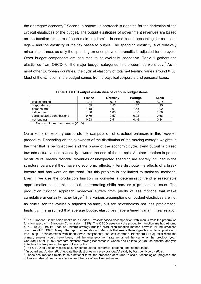
Other budget components are assumed to be cyclically insensitive. Table 1 gathers the
elasticities from OECD for the major budget categories in the countries we study.7 As in
most other European countries, the cyclical elasticity of total net lending varies around 0.50.
Most of the variation in the budget comes from procyclical corporate and personal taxes.
Table 1. OECD output elasticities of various budget items France Germany Portugal Spain total spending -0.11 -0.18 -0.05 -0.15 corporate tax 1.59 1.53 1.17 1.15 personal tax 1.18 1.61 1.53 1.92 indirect tax 1.00 1.00 1.00 1.00 social security contributions 0.79 0.57 0.92 0.68 net lending 0.53 0.51 0.46 0.44
Source: Girouard and André (2005).
Quite some uncertainty surrounds the computation of structural balances in this two-step
procedure. Depending on the skewness of the distribution of the moving-average weights in
the filter that is being applied and the phase of the economic cycle, trend output is biased
towards actual values especially towards the end of the sample. Another problem is posed
by structural breaks. Windfall revenues or unexpected spending are entirely included in the
structural balance if they have no economic effects. Filters distribute the effects of a break
forward and backward on the trend. But this problem is not limited to statistical methods.
Even if we use the production function or consider a deterministic trend a reasonable
approximation to potential output, incorporating shifts remains a problematic issue. The
production function approach moreover suffers from plenty of assumptions that make
cumulative uncertainty rather large.8 The various assumptions on budget elasticities are not
as crucial for the cyclically adjusted balance, but are nevertheless not less problematic.
Implicitly, it is assumed that average budget elasticities have a time-invariant linear relation 5 The European Commission backs up a Hodrick-Prescott based decomposition with results from the production function approach (European Commission, 1995). The OECD uses only the production function method (Giorno et al., 1995). The IMF has no uniform strategy but the production function method prevails for industrialised countries (IMF, 1993). Many other approaches abound. Methods that use a Beveridge-Nelson decomposition or track output developments with unobserved components are less common. Blanchard (1993) asks what the primary surplus would have been, had the unemployment rate remained the same as the previous year. Chouraqui et al. (1992) compare different moving benchmarks. Cohen and Follette (2000) use spectral analysis to isolate low frequency changes in fiscal policy. 6 The OECD adjusts only social security contributions, corporate, personal and indirect taxes. 7 Girouard and André (2005) update the elasticities in a previous OECD study by Van den Noord (2002). 8 These assumptions relate to its functional form, the presence of returns to scale, technological progress, the utilisation rates of production factors and the use of auxiliary estimates.
8
to changes in the economy. We return to these difficulties in a sensitivity analysis in section
4.4.
3.2. Towards an economic indicator of fiscal policy
The main difficulty in interpreting the structural balance is the absence from economic
arguments to underpin the trend/cycle decomposition. There is an implicit assumption in the
filtering methods on the frequency of the business cycle and hence on trend output under
average economic conditions. And while the production function approach builds upon
economic foundations, the dynamics are nonetheless driven solely by the longer-term
effects of investment feeding back on changes in the capital stock.9
Macroeconomic models that allow for cyclical fluctuations around some steady-state
trending growth path can be found in the growing class of Dynamic Stochastic General
Equilibrium (DSGE) models with nominal rigidities. These models have by now been
extended to include fiscal policy. In the initial Real Business Cycle models, there are only
supply-side effects of fiscal policy that transmit through wealth effects and the labour/leisure
choice (Baxter and King, 1993). Micro-founded models based on sticky prices provide a
rationale for stabilisation policies, but even in the New Keynesian type of models of fiscal
policy, the supply side effects still tend to dominate demand side effects of fiscal policy
management (Linnemann and Schabert, 2003). A larger role for demand side effects of
fiscal policy is only found in models that introduce some further imperfections via ‘Rule of
Thumb’ consumers or a fraction of liquidity constrained consumers (Galí et al., 2005; Bilbiie
et al., 2006). The latter models come also closer to replicating the results of the growing
empirical literature on the effects of fiscal policy.
The main result of studies that use the VAR-counterparts to DSGE-models is that they can indeed recover significant effects of fiscal expansions on output. These are more in line with a positive ‘Keynesian’ effect on consumption, albeit the eventual multiplier is strongly reduced. The identification of fiscal policy is fraught with difficulties, however.10 First, the implementation of announced changes in government policies is subject to lengthy and visible political negotiations that are anticipated in private agents’ behaviour. As a consequence, fiscal shocks need not affect fiscal variables first. This is a problem of the shock being non-fundamental (Lippi and Reichlin, 1994). Second, decisions on fiscal policy affect different groups in the public via a range of different spending and tax instruments. There exists no ‘standard’ fiscal shock: every political discussion considers the trade-off
9 Potential output is nevertheless assumed exogeneous in the production function approach. 10 A full discussion of the problems in identifying the effects of fiscal policy is provided in Perotti (2005).
9
between a range of possible taxation and spending adjustments. The means of financing and the adjustment in expenditures and revenues wrap empirically relevant effects of different budget components in an aggregate fiscal shock without considering the path of public debt. Most studies focus on total spending or revenues, and find small and positive effects of government spending on consumption, but prolonged negative effects of higher taxation. Only a couple of studies consider the dynamic behaviour of some particular budget components.11 Third, these identification problems are only exacerbated by the automatic reaction of fiscal aggregates to economic variables.
The seminal contribution of Blanchard and Perotti (2002) lies in using a semi-structural VAR that employs external institutional information on the elasticity of fiscal variables to output. Cleaning out the automatic cyclical reaction of the total fiscal balance leaves shifts to the cyclically adjusted balance as discretionary fiscal shocks. Blanchard and Perotti (2002) additionally impose some timing restrictions on the economic effects of discretionary policy. These timing assumptions avoid to some extent anticipation effects but would not capture these completely if implementation lags are important. Subsequent studies have mainly attempted to verify the original approach of Blanchard and Perotti (2002) with a variety of techniques and usually tend to confirm their findings.12
However, the empirical literature has hitherto ignored the supply and demand channels of
fiscal policy that are at front-stage of the theoretical DSGE models. Such effects are only
implicitly acknowledged in these VAR studies. Changes in tax revenues, for example, are
usually found to have lasting effects on output. There are nevertheless two other strands of
the empirical fiscal policy literature that attribute a role to supply side variables. First, the
literature on non-Keynesian effects of fiscal policy would argue that fiscal consolidation
might have positive consequences on output. The composition of the fiscal adjustment
thereby plays an important role (Alesina and Perotti, 1995). The effects of consolidation on
agents’ expectations on the future economic outlook – measured by asset markets’ reaction
(Giavazzi and Pagano, 1990) – suggests a role for permanent wealth and supply-side
effects of fiscal policy. Second, most VAR studies have so far ignored the literature on the
long-term growth effects of fiscal policies. The main message of the endogenous growth
models that have been developed is that higher taxation unambiguously reduces output, but
11 Ramey and Shapiro (1998) look into the sectoral reallocation effects following shocks. A particular role in the transmission of fiscal policy shocks is also played by the labour market. A couple of papers compare the effects of consumptive government purchases to increases in public employment (Finn, 1998; Pappa, 2005; Cavallo, 2005). Perotti (2004) and Kamps (2004) examine the output and labour market effects of government investment. 12 Mountford and Uhlig (2002) retrieve different types of fiscal shocks among those that conform to some a priori sign restrictions on the entire impulse response or variance decomposition of fiscal variables. Canova and Pappa (2002) select only those shocks that satisfy formal sign restrictions on the conditional cross-correlation of the responses to the orthogonalised shocks of the variables in the model.
10
that these losses may be offset by using the proceeds for productive spending items (Barro,
1990; King and Rebelo, 1990). These seminal models have been made more realistic by
allowing endogenous responses of labour (Turnovsky, 2000). Typical tests of these growth
models give empirical support to the role of spending and taxes to long-term growth (Kneller
et al., 1999). It can be argued that additional government spending in catching-up countries
such as Portugal and Spain had rather different effects than further expansions of the
budget in France and Germany, for example. This provides an additional argument for
including the former countries in our analysis.
The examination of the growth effects is also of substantial policy interest. In the
assessment of EU Member States’ policies under the revised Stability and Growth Pact,
much attention is devoted to the quality of fiscal adjustments and the sustainability of public
finances. The implementation of major structural reforms that raise potential growth – and
hence have an impact on the long-term sustainability of public finances – can be considered
grounds for temporary deviations of budget balance. There is thus need for a framework that
assesses changes in fiscal instruments and distinguishes the short-term demand from the
longer run supply effects of such policies.
3.3. Methodology
We make a first step in setting up an empirical VAR model that allows for fiscal policy having
distinct long- and short-term effects on output. The approach in this paper rests on a
combination of long-term restrictions and some assumptions on the short-run elasticities of
budgetary items.13 For the purpose of gauging a model-based fiscal indicator, we basically
take shocks with permanent effects on output to drive long-term trends. Following Blanchard
and Quah (1989), potential output is determined by so-called productivity or technology
shocks that permanently affect output. This can then be complemented with further
assumptions on the short-term behaviour of fiscal policies. Shocks with transitory output
effects are classified as either cyclical or fiscal, following the elasticity approach of Blanchard
and Perotti (2002).
13 There are a few applications of fiscal VARs that use similar restrictions, and are mostly inspired by a practical interest in determining structural balances. See Bouthevillain and Quinet (1999), Dalsgaard and de Serres (2001) or Bruneau and DeBandt (2003) who all specify an SVAR model in output and the deficit ratio. They recover structural deficits from the contribution of fiscal shocks to the variance of deficits. Likewise, a measure of the gap is constructed from the contribution of supply shocks to output variations. Hjelm (2003) is closer to our model as he is interested in simultaneously determining potential GDP and the cyclically adjusted balance. He uses cholesky ordered long-term restrictions in a model with output, employment and the budget balance to identify economic and labour market shocks. The cyclically adjusted balance then is that fraction of the budget balance that is not explained by business cycle shocks. This leaves only the supply and labour market shocks in determining structural balance, but no separate role for the government is stipulated.
11
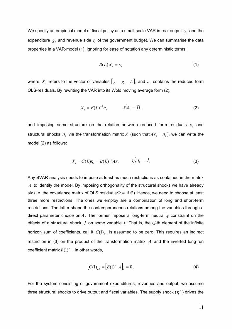
We specify an empirical model of fiscal policy as a small-scale VAR in real output ty and the
expenditure tg and revenue side tt of the government budget. We can summarise the data
properties in a VAR-model (1), ignoring for ease of notation any deterministic terms:
ttXLB ε=)( (1)
where tX refers to the vector of variables [ ]ttt tgy , and tε contains the reduced form
OLS-residuals. By rewriting the VAR into its Wold moving average form (2),
tt LBX ε1)( −= t′t . (2)
and imposing some structure on the relation between reduced form residuals tε and
structural shocks tη via the transformation matrix A (such that ttA ηε = ), we can write the
model (2) as follows:
ttt ALBLCX εη 1)()( −== t′t I. (3)
Any SVAR analysis needs to impose at least as much restrictions as contained in the matrix
A to identify the model. By imposing orthogonality of the structural shocks we have already
six (i.e. the covariance matrix of OLS residuals 'AA=Ω ). Hence, we need to choose at least
three more restrictions. The ones we employ are a combination of long and short-term
restrictions. The latter shape the contemporaneous relations among the variables through a
direct parameter choice on A . The former impose a long-term neutrality constraint on the
effects of a structural shock j on some variable i . That is, the i,j-th element of the infinite
horizon sum of coefficients, call it ijC )1( , is assumed to be zero. This requires an indirect
restriction in (3) on the product of the transformation matrix A and the inverted long-run
coefficient matrix 1)1( −B . In other words,
[ ] [ ] 0)1()1( 1 == −ijij ABC . (4)
For the system consisting of government expenditures, revenues and output, we assume
three structural shocks to drive output and fiscal variables. The supply shock ( qη ) drives the
12
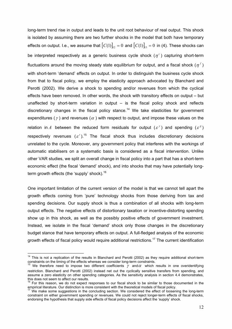
long-term trend rise in output and leads to the unit root behaviour of real output. This shock
is isolated by assuming there are two further shocks in the model that both have temporary
effects on output. I.e., we assume that [ ] 0)1( 12 =C and [ ] 0)1( 13 =C in (4). These shocks can
be interpreted respectively as a generic business cycle shock ( cη ) capturing short-term
fluctuations around the moving steady state equilibrium for output, and a fiscal shock ( fη )
with short-term ‘demand’ effects on output. In order to distinguish the business cycle shock
from that to fiscal policy, we employ the elasticity approach advocated by Blanchard and
Perotti (2002). We derive a shock to spending and/or revenues from which the cyclical
effects have been removed. In other words, the shock with transitory effects on output – but
unaffected by short-term variation in output – is the fiscal policy shock and reflects
discretionary changes in the fiscal policy stance.14 We take elasticities for government
expenditures (γ ) and revenues (α ) with respect to output, and impose these values on the
relation in A between the reduced form residuals for output ( yε ) and spending ( gε )
respectively revenues ( tε ).15 The fiscal shock thus includes discretionary decisions
unrelated to the cycle. Moreover, any government policy that interferes with the workings of
automatic stabilisers on a systematic basis is considered as a fiscal intervention. Unlike
other VAR studies, we split an overall change in fiscal policy into a part that has a short-term
economic effect (the fiscal ‘demand’ shock), and into shocks that may have potentially long-
term growth effects (the ‘supply’ shock).16
One important limitation of the current version of the model is that we cannot tell apart the
growth effects coming from ‘pure’ technology shocks from those deriving from tax and
spending decisions. Our supply shock is thus a combination of all shocks with long-term
output effects. The negative effects of distortionary taxation or incentive-distorting spending
show up in this shock, as well as the possibly positive effects of government investment.
Instead, we isolate in the fiscal ‘demand’ shock only those changes in the discretionary
budget stance that have temporary effects on output. A full-fledged analysis of the economic
growth effects of fiscal policy would require additional restrictions.17 The current identification
14 This is not a replication of the results in Blanchard and Perotti (2002) as they require additional short-term constraints on the timing of the effects whereas we consider long-term constraints. 15 We therefore need to impose two different coefficients γ andα which results in one overidentifying restriction. Blanchard and Perotti (2002) instead net out the cyclically sensitive transfers from spending, and assume a zero elasticity on other spending categories. As the sensitivity analysis in section 4.4 demonstrates, this does not seem to affect our results. 16 For this reason, we do not expect responses to our fiscal shock to be similar to those documented in the empirical literature. Our distinction is more consistent with the theoretical models of fiscal policy. 17 We make some suggestions in the concluding section. We considered the effect of loosening the long-term constraint on either government spending or revenues. We could not reject longer-term effects of fiscal shocks, endorsing the hypothesis that supply side effects of fiscal policy decisions affect the ‘supply’ shock.
13
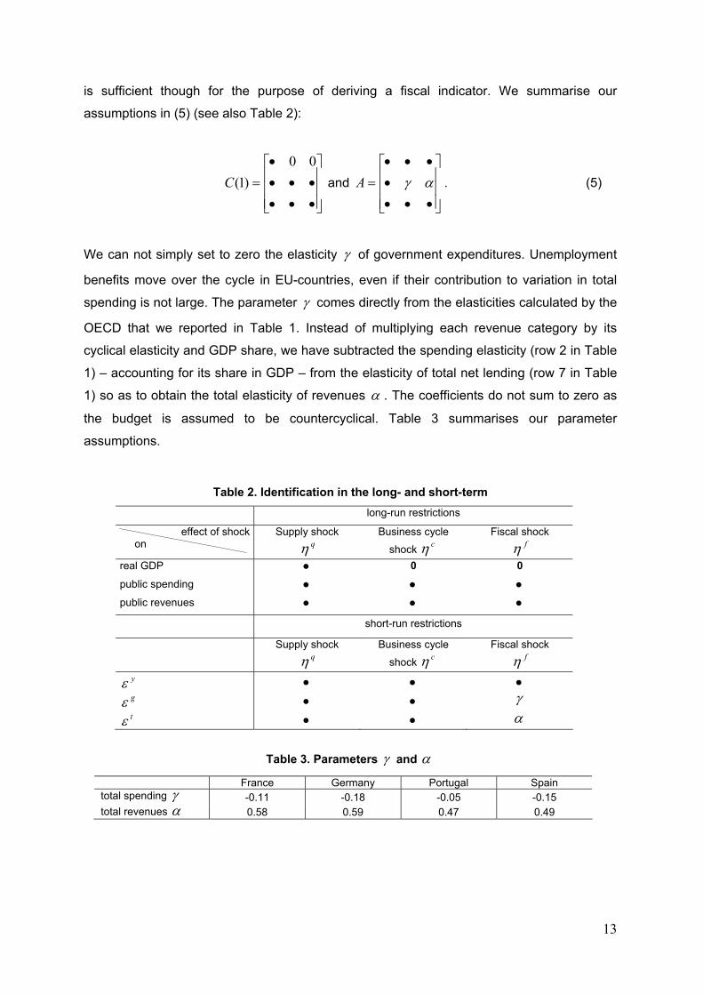
is sufficient though for the purpose of deriving a fiscal indicator. We summarise our
assumptions in (5) (see also Table 2):
⎥⎥⎥
⎦
⎤
⎢⎢⎢
⎣
⎡
••••••
•=
00)1(C and
⎥⎥⎥
⎦
⎤
⎢⎢⎢
⎣
⎡
••••
•••= αγA . (5)
We can not simply set to zero the elasticity γ of government expenditures. Unemployment
benefits move over the cycle in EU-countries, even if their contribution to variation in total
spending is not large. The parameter γ comes directly from the elasticities calculated by the
OECD that we reported in Table 1. Instead of multiplying each revenue category by its
cyclical elasticity and GDP share, we have subtracted the spending elasticity (row 2 in Table
1) – accounting for its share in GDP – from the elasticity of total net lending (row 7 in Table
1) so as to obtain the total elasticity of revenues α . The coefficients do not sum to zero as
the budget is assumed to be countercyclical. Table 3 summarises our parameter
assumptions.
Table 2. Identification in the long- and short-term long-run restrictions
effect of shock on
Supply shock
qη
Business cycle
shock cη
Fiscal shock
fη real GDP • 0 0
public spending • • • public revenues • • •
short-run restrictions
Supply shock
qη
Business cycle
shock cη
Fiscal shock
fη yε • • • gε • • γ tε • • α
Table 3. Parameters γ and α
France Germany Portugal Spain total spending γ -0.11 -0.18 -0.05 -0.15 total revenues α 0.58 0.59 0.47 0.49
14
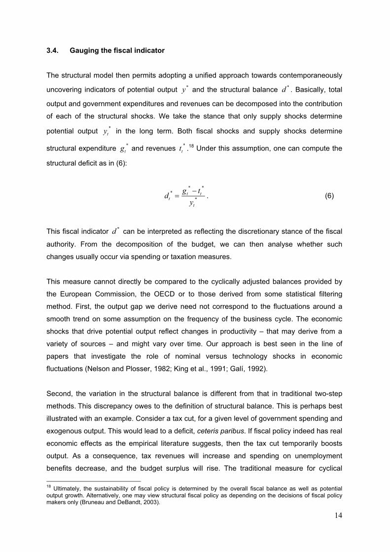
3.4. Gauging the fiscal indicator
The structural model then permits adopting a unified approach towards contemporaneously
uncovering indicators of potential output *y and the structural balance *d . Basically, total
output and government expenditures and revenues can be decomposed into the contribution
of each of the structural shocks. We take the stance that only supply shocks determine
potential output *ty in the long term. Both fiscal shocks and supply shocks determine
structural expenditure *tg and revenues *
tt .18 Under this assumption, one can compute the
structural deficit as in (6):
*
***
t
ttt y
tgd −= . (6)
This fiscal indicator *d can be interpreted as reflecting the discretionary stance of the fiscal
authority. From the decomposition of the budget, we can then analyse whether such
changes usually occur via spending or taxation measures.
This measure cannot directly be compared to the cyclically adjusted balances provided by
the European Commission, the OECD or to those derived from some statistical filtering
method. First, the output gap we derive need not correspond to the fluctuations around a
smooth trend on some assumption on the frequency of the business cycle. The economic
shocks that drive potential output reflect changes in productivity – that may derive from a
variety of sources – and might vary over time. Our approach is best seen in the line of
papers that investigate the role of nominal versus technology shocks in economic
fluctuations (Nelson and Plosser, 1982; King et al., 1991; Galí, 1992).
Second, the variation in the structural balance is different from that in traditional two-step
methods. This discrepancy owes to the definition of structural balance. This is perhaps best
illustrated with an example. Consider a tax cut, for a given level of government spending and
exogenous output. This would lead to a deficit, ceteris paribus. If fiscal policy indeed has real
economic effects as the empirical literature suggests, then the tax cut temporarily boosts
output. As a consequence, tax revenues will increase and spending on unemployment
benefits decrease, and the budget surplus will rise. The traditional measure for cyclical
18 Ultimately, the sustainability of fiscal policy is determined by the overall fiscal balance as well as potential output growth. Alternatively, one may view structural fiscal policy as depending on the decisions of fiscal policy makers only (Bruneau and DeBandt, 2003).
15
adjustment takes out all cyclical variation, also the one induced by fiscal policy, which leads
to an overstatement of the structural balance. In our approach, we control for this economic
effect of the tax cut. The SVAR-model excludes that part of the variation in GDP due to
discretionary fiscal measures whereas the conventional models take total output variation
into account. But our approach goes even one step further. Imagine that the tax cut also
raises potential output in the long term. This widens the gap between actual and potential
output at the moment the fiscal shock occurs. Structural balance would be improved as the
increased tax base (now, and in the future) makes the fiscal position more sustainable.
Similar arguments can be made for the effects of spending. As a consequence, our indicator
of structural balance does not necessarily display a smaller variation than traditional
indicators. This will particularly be true if (a) the indicator is mainly driven by fiscal or supply
shocks; or (b) if the underlying economic shocks we retrieve are more volatile than what
conventional output gap measures suggest.
Our model-based indicator has some favourable properties in comparison to more
conventional measures. First, the long-term constraints hold the promise of imposing fewer
contentious restrictions on the short-term effects of the fiscal shocks. Any anticipation effect
and the contemporaneous reactions of fiscal balances to economic conditions are not
constrained. Second, the simultaneous determination of a measure of cyclical output and
fiscal balance is internally more coherent. While the method is definitely more complex, total
uncertainty is quantified. We impose a minimal set of economic restrictions and the validity
of these assumptions can be discussed. As the empirical model is also consistent with
recent DSGE models of fiscal policy, these assumptions can be tested. Sensitivity analysis
can make clear the weakness of the model in some specific direction. Moreover, progress in
theoretical models of fiscal policy can lead to further refinements of the approach. Third, by
adopting an economic – and not a statistical – method, the end-point problem of filters is
eliminated. The indicator gives timely information on changes in the fiscal stance.19 Finally,
our indicator is also more relevant for the assessment of fiscal policy. Our measure indicates
better the change in the stance of fiscal authorities, also with a view to growth effects and
long-term sustainability.
At the same time, the econometric approach suffers from some weaknesses. First,
extensions are difficult as the method is rather data demanding – at least in the time series
dimension. The annual frequency of the data may lead to some difficulties in the
identification of business cycle shocks, for example. Second, the gains of loosening the
19 The inclusion of structural breaks remains problematic, however. But in contrast to statistical methods, the economic consequences of one-off fiscal events are modelled in our approach.
16
constraints of short-run effects of fiscal policy have to be set off against some additional
complications (Sarte, 1999). While both short- and long-term restrictions are sensitive to the
exact parameter values imposed, substantially more uncertainty surrounds the estimates of
the long-term inverted moving average representation in (2), especially in the short samples
that we use (Christiano et al., 2006). The basic problem is that no asymptotically correct
confidence intervals on )1(C can be constructed. Faust and Leeper (1997) prove that there
are no consistent tests for the significance of the long-term response. Specifying a priori the
lag length of the VAR or choosing the horizon at which the long run effect nullifies can solve
this problem. One may also check the consistency of some short-term restrictions with the
long-term behaviour of the model, as in King and Watson (1997). Third, there is a possibly
large set of underlying shocks from which we extract only a few. As discussed above, we
extract a generic supply and cyclical shock, as well as a fiscal shock. This necessarily
involves a debatable linear aggregation over shocks. If each shock affects the economy in
qualitatively the same way the shocks may be commingled. This is particularly acute for the
analysis of fiscal policy, as different expenditure and revenue categories may indeed have
different longer run effects on output that are not distinguishable from technology shocks but
moreover have similar short-term responses. Fourth, a problem may also occur of high
frequency feedbacks. We observe fiscal policy only at an annual frequency. We assume the
structural shocks to be orthogonal but if there are mid-year revisions of the budget, this may
muddle both economic and fiscal shocks. This only stresses the problem of correctly
identifying the timing of shifts in fiscal policies. Finally, a major assumption underlying the
VAR-model is parameter constancy. The conclusions of VARs are highly sensitive to the
presence of structural breaks. Especially for fiscal policy, there is evidence of non-linear
effects (see Giavazzi et al., 2000, for instance). We therefore run some stability tests on the
VAR-model.
4. Empirical analysis 4.1. Data
All data are annual and come from AMECO.20 This database covers the longest available
period since 1970 up till 2004 for which fiscal data are available for France, Germany,
Portugal and Spain. Fiscal data and output are deflated by the GDP-deflator and are defined
in first differences of log-levels. In many studies, the fiscal data are scaled to GDP, but this
clouds inference. As economic shocks affect both fiscal variables and GDP, this leads to a
spurious negative correlation between the deficit and these shocks. Moreover, we are 20 Details are in Appendix 1. A program containing the RATS-code for the SVAR model is available from the authors upon request.
17
primarily interested in distilling a fiscal indicator on the basis of the historical decomposition
of output. For the same reason, we do not concentrate on the effects of fiscal policy on
private output but use total output instead. We also ignore possible cointegration between
overall expenditures and revenues, which derives from the intertemporal budget constraint.21
This implies that parameter estimates may no longer be efficient albeit still consistent.
However, inference on the short-term results of the VAR would hardly be affected by non-
stationarity of the data (Sims et al., 1990).
Data are defined following ESA-95 nomenclature. Definitions for the French budget changed
in 1978. We linked the former series (going back to 1970) to the ESA-95 series and include
an impulse dummy for this data break. We treat the effects of German Reunification in 1991
in a similar way. We further condition the models on these deterministic terms. Before
estimating the structural model, we want to check for possibly other breaks in the VAR. We
follow the method of Bai et al. (1998) and apply the sequential sup Quandt-Andrews
likelihood ratio test on the VAR model. Sample size forces us to consider a single break date
only, as the optimal search concentrates on the central 70% of the sample and consequently
leaves too few degrees of freedom for examining multiple breaks. We correct for a possible
change in volatility before and after the break date. As in Stock and Watson (2003), we
weigh each period’s residuals by their average volatility. The lag length in the VAR is
henceforth set to one year (following the Bayesian Information Criterion).
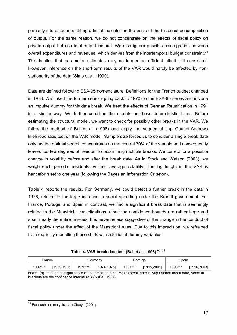
Table 4 reports the results. For Germany, we could detect a further break in the data in
1976, related to the large increase in social spending under the Brandt government. For
France, Portugal and Spain in contrast, we find a significant break date that is seemingly
related to the Maastricht consolidations, albeit the confidence bounds are rather large and
span nearly the entire nineties. It is nevertheless suggestive of the change in the conduct of
fiscal policy under the effect of the Maastricht rules. Due to this imprecision, we refrained
from explicitly modelling these shifts with additional dummy variables.
Table 4. VAR break date test (Bai et al., 1998) (a), (b)
France Germany Portugal Spain
1992*** [1989,1996] 1976*** [1974,1978] 1997*** [1995,2001] 1998*** [1996,2003] Notes: (a) *** denotes significance of the break date at 1%; (b) break date is Sup-Quandt break date, years in brackets are the confidence interval at 33% (Bai, 1997).
21 For such an analysis, see Claeys (2004).
18
4.2. The transmission channels of fiscal policy
We first discuss some general results of our small scale model, and assess the properties of
output and fiscal series, and the role of the various structural shocks. The following
paragraphs discuss the fit of the model in terms of impulse response functions and the
forecast error variance decomposition. 22 We have summarised all results in Figures 3a and
3b. This prepares the ground for an analysis of the fiscal indicator in section 4.3.
The effect of productivity shocks is to lift up real output permanently (Figure 3a). The speed
of accumulation is rather fast: after five years, the major part of the shock has worked out. In
Germany, this happens even faster. The sampling uncertainty around the effect is large, but
given the large bounds we have used, the significance of most impulse responses after
some years is actually surprising. To what extent are these supply shocks driven by fiscal
developments? In France and Portugal, these shocks go hand in hand with positive long-
term effects on total expenditures and revenues as well. This effect is also strongly
significant.23 The difference between revenues and spending responses is not significant,
hence it is not obvious that this leads to a build up of public debt. In Germany and Spain on
the contrary, revenues do not change significantly, but government expenditures shrink
considerably, leading to large accumulated surpluses at a horizon of 10 years.
But whether the causality runs from fiscal policy to productivity growth, or vice versa, is not
obvious. Recall that the supply shock contains productivity shocks that may emanate from
the private as well as the public sector. The significant co-movement of spending and
revenues suggests that fiscal ‘supply’ shocks are an important source of the overall
productivity shock.24 If these relations are positive (the case of France and Portugal), this
implies higher spending or tax revenues have contributed to economic growth. In the
opposite case (Germany or Spain), a reduction of spending – and less so a lower tax burden
– would trigger higher potential output growth. But there are a few alternative explanations.
Positive economic shocks that enlarge the tax base would – for a given tax rate –
automatically lead to a larger revenue intake owing to automatic stabilisers. For reasons of
political economy, this could lead the government to directly spend the proceeds of the
treasury. This expansion of the budget could consequently get locked in and lead to a
22 Impulse responses follow a one standard shock, and are plotted over a 10 year horizon with 90% confidence intervals, based on a bootstrap with 5000 draws. 23 As the long-term elasticity of both spending and revenues is larger than unity, this looks like a ‘Wagner’ style government expansion owing to economic growth. 24 We considered the effect of loosening the long-term constraint on either government expenditures or revenues in extensions of the structural VAR model in (3). We could not reject longer-term effects of fiscal shocks, endorsing the hypothesis that supply side effects of fiscal policy decisions are part of the ‘supply’ shock.
19
permanent rise in government expenditure. This mechanism would work for both permanent
and cyclical shocks, if we assume that the government does not systematically react in
different ways to permanent or transitory economic shocks. This allows us to get some
insight in the importance of the private versus public productivity shocks. The fiscal
responses to cyclical shocks, which include business cycle shocks with transitory output
effects that are not related to fiscal policy can give some indication. Surprisingly, the effects
of cyclical shocks on output are hardly significant and indicate the small size of temporary
economic fluctuations.25 As a consequence, there is not always an obvious simultaneous
rise in tax revenues. In Germany and Portugal, government revenues do rise in response to
a positive output gap, and this effect remains permanent. Moreover, in both countries
government expenditures tend to rise as well. This gives some support for the ‘ratcheting up’
effect on spending. In France or Spain instead, government spending does not react in a
significant way and tax revenues even tend to decline.
If we consider in some more detail the two countries in which catching-up phenomena may
be expected to be important, we cannot clearly distinguish between the two alternative
explanations. Both in Spain and Portugal is the reaction of fiscal variables to temporary and
permanent shocks similar. This downplays the importance of productive fiscal policy
contributing to economic growth. A comparison of the impulse responses shows that only a
minor effect would be left in the case of Portugal. Evidence on Spanish public finances
presents a slightly different picture. Positive supply shocks are accompanied by a strong
decrease in total spending, and this effect is much more pronounced than the reduction in
spending after a cyclical shock.
In France and Germany instead, the reaction of fiscal variables to permanent shocks is
opposite to the reaction to business cycle shocks and supports the view that fiscal variables
driving long-term growth in both countries. That spending and revenues go up after a
positive supply shock, whereas there is a non-significant response or a decline following
cyclical shocks, would suggest a larger role for productive public spending in France instead.
Evidence for Germany rather seems to indicate a too large size of government. We find that
revenues and spending go up permanently after cyclical shocks, but positive supply shocks
tend to be associated with reductions in spending.
[INSERT FIGURE 3a HERE]
25 This is a likely consequence of the annual frequency of the fiscal data.
20
The fiscal shock then regards all discretionary policy interventions on spending and/or
revenues that are not systematically related to the cycle and have only temporary effects on
the economy. These discretionary fiscal shocks have somewhat prolonged effects on output.
There is a lot of uncertainty around this effect and none of the responses is really significant.
We scale the impulse responses in Figure 3a such that they always display positive output
effects. We do not find the typical result of small positive Keynesian effects on output in all
countries. In Germany and Spain, a typical Keynesian response would follow upon demand
boosting deficits. In France and Portugal on the other hand, fiscal contractions would lead to
positive short-term effects on output instead. Such different responses likely depend on the
composition of the fiscal adjustment or other structural parameters in the respective
economies, but cannot be further examined in the current model.
The different responses of spending and revenues to both economic shocks might indicate a
delicate issue in the identification of policy. If fiscal policy reacts in a systematic way to
economic shocks by changing its discretionary use of spending and/or revenues, this
simultaneity blurs the distinction between the economic and the fiscal shock. This might be
the case in France and Spain where tax revenues decrease after positive temporary output
shocks, for example. But another indication is given by the rise in spending in economic
booms in Germany or Portugal. It indicates policies that react in a discretionary way so as to
repeal the use of automatic stabilisers. The fiscal indicator captures these policy biases. Our
discussion will show how important this policy bias is for understanding fiscal trends in EU
countries.
What does this imply for the contribution of fiscal policies to output variation (Figure 3b)?
Supply shocks account for at least 50% of total variance in output at all horizons, and this
goes up to 90% in Portugal and Spain. For the latter countries, this was perhaps to be
expected given their strong economic growth over the last two decades. Most of the
variation in output is thus caused by productivity shocks even at short horizons. As we do
not separately identify private and public supply shocks, we cannot really quantify the
relative magnitude of both channels. But as pointed out above, we think that productive
spending or revenues has contributed to some extent to the variance of output. The demand
effects of fiscal policy in France and Germany are at least as large as those of supply
effects. In Portugal or Spain instead, only a minor role is played by discretionary fiscal policy.
The contribution of cyclical fluctuations to variations in output is negligible, as was to be
expected from the results on the impulse responses.
21
What factors can account for these results? The large role played by fiscal policy in
explaining output variation is not inconsistent with previous findings in the literature for large
EU countries (De Arcangelis and Lamartina, 2004), but seems on the higher side of the
range usually found. If we take the result at face value, it would suggest that the temporary
demand effects of fiscal policy are probably much larger than the supply effects in the long-
term. This would imply that both RBC and New Keynesian models are missing some
aspects of fiscal transmission. But as we cannot precisely quantify the importance of the
latter shocks, we would not want to claim validation of any of the theoretical models with our
approach. This result nevertheless reveals that models of fiscal policy need to attribute
important roles to both demand and supply side effects.
We think that the reason for the large contribution of fiscal policy is to be found elsewhere.
To the extent that automatic stabilisers reduce the volatility of economic fluctuations, the
tendency of governments to reduce taxation and/or rise spending in a procyclical way only
adds to short-term output fluctuations and brings about aggregate macroeconomic
instability. This policy volatility can moreover have negative effects on the long-term growth
prospects of the economy.26 The unwinding of previous taxation decisions goes against the
principle of ‘tax smoothing’. The procyclicality of budgets implies negative supply-side
effects. This explains the surprisingly low contribution of cyclical fluctuations.
[INSERT FIGURE 3b HERE]
Before going deeper into the past trends in fiscal policy, we want to check our model on
some other aspects too. We compute the output gap based on the historical decomposition
of the output series as actual minus potential output (y- *y ). In Figure 4 (top left panel),27 we
have repeated for comparison the output gaps of the European Commission, OECD and the
one obtained by applying a Hodrick-Prescott filter. There is a rather close correspondence
between these measures and our supply shock based gap for France and Germany. Given
that we have used the OECD elasticities only for distinguishing shocks with transitory effects
on output, this is all the more remarkable. The smooth gap for Portugal and Spain underlines
the importance of supply relative to demand shocks in both countries. This might indeed be
expected given the strong economic catch-up that both countries have experienced. We
believe that potential output tracked much closer actual output developments in these 26 We are certainly not the first study to document that European countries have not left automatic stabilisers to work, but instead have overturned these in a procyclical way. We do show however the macroeconomic instability that results as a consequence. With other models, Alesina and Bayoumi (1996) showed how fiscal policy at the US state level rather contributes to macroeconomic instability, and how fiscal rules have been useful in constraining discretion. Similar cross-country evidence is provided by Fatás and Mihov (2003b). 27 We plot all series over the period 1980-2004 only.
22
countries. The usual statistical filtering methods are not adequate to capture this trend
behaviour over small samples. Cyclical fluctuations are therefore rather minor. We provide
some further robustness checks in the Appendix 2.28
Overall, in all countries, there definitely was an improvement in economic conditions at the
start of EMU. We find that economic conditions have worsened in both France and Germany
in recent years. We nevertheless find the crisis in Germany to have set in somewhat earlier
and to be more prolonged. As cyclical fluctuations are not large, we do not find much
economic slack in recent years in Spain or Portugal.
[INSERT FIGURE 4 HERE]
4.3. The fiscal indicator
We are now ready to discuss the indicator of discretionary fiscal stance. In general, the
measure is more volatile than the measures derived with conventional methods (see Figure
4, bottom left panel). In many instances, our measure leads the smoothed measures in the
direction of change. The fiscal indicator is usually smaller than the cyclically adjusted deficit.
This reflects the definition of the structural balance, by which we take out the automatic
stabilisers and the induced stabilisation effects caused by fiscal policies. In addition, fiscal
policy also affects permanent output and therefore the structural fiscal position fluctuates
around balance.
The indicator is also much more volatile. This follows from the major contribution of supply
and fiscal shocks to the variation in output, spending and revenues (Figure 3b). As we
discuss below, one of the causes of this strong volatility – apart from the dominant supply
side shocks – is the procyclical bias that characterises fiscal policymaking that induces extra
variation, especially so in government revenues.
We may then expect our fiscal measure to coincide with some episodes of fiscal laxness or
retrenchment. We consider the budget to undergo a strong expansion (contraction) when the
cyclically adjusted primary balance falls (increases) by at least 2 percentage points of GDP
in one year, or at least 1.5 percentage points on average in the last two years. This is the
28 A rough indication on the robustness of our output gap measure can also be given by the dates of peak and troughs in the business cycle. We plot in Appendix 2 the first difference of the output gap against the chronology of peak to trough turning points of the growth cycle provided by the Economic Cycle Research Institute (ECRI). These calculations are based on monthly industrial production series. Our measure matches the changes in the output gap in all countries.
23
measure proposed by Alesina and Ardagna (1998). In Table 5, we gather those fiscal years
in which a strong expansion or adjustment has occurred in our dataset (see Afonso, 2006).
At first sight, the correspondence is rather close. Comparing the changes in Figure 4 (bottom
left panel) to the years in Table 5, we detect all events that the Alesina-Ardagna measure
also suggests. For example, we find budgetary cost of Reunification on German public
finances to have been large. The Maastricht rules have also led to considerable fiscal
retrenchment in France and Spain. There are a few events in Portuguese fiscal policy over
the eighties that we do not date exactly. But we do find a switch between contraction and
expansion starting in 1982-83. The Alesina-Ardagna measure does not pick up all
expansions and contractions that we find, however. Some of these episodes correspond to
well known changes in the fiscal stance (e.g. the ‘Mitterand’ budgets in France 1981).
Another major expansion in France in 1992 follows upon a string of expansionary budgets.
Spain equally undergoes major expansions in the early eighties and nineties (1981 and 1993
respectively). Fiscal policy is also lax in Portugal (1990). Prolonged contractions occur over
the eighties in France, Germany and Spain too.
Table 5. Large fiscal expansions and contractions
Expansions Contractions France - 1995-96
Germany 1990-91 1982-83
Portugal 1980-81 1982-83, 1986, 1992
Spain - 1995-96 Source: adapted from Afonso (2006), following the measure used by Alesina and Ardagna (1998).
Concentrating on the period just before EMU, we can see a substantial shift in discretionary
policies towards structurally positive net lending ratios. This is perhaps least visible in
Germany, but the initial conditions were probably not such as to urge a strong and prolonged
consolidation for reaching the Maastricht deficit limit. A substantial consolidation had already
taken place at the end of the eighties. In the other countries, the structural effort was more
drawn out. France started consolidation already in 1993, while it gathered pace in Portugal
and Spain only in 1995. This also confirms evidence in Fatás and Mihov (2003a).
How has this consolidation been achieved? The right hand side panels of Figure 4 plot the
growth rates of structural expenditures and revenues. These reveal that structural
consolidations in the nineties have been based on a mixture of expenditure and revenue
measures. But the combination of adjustments in the policy instruments has changed over
time in a remarkably similar fashion in all countries. Initially, we see relatively moderate
24
expenditure growth and in some cases even relevant spending cuts (Germany and
Portugal). This strategy is reversed closer to the deadline of EMU. Tax increases start to
bear the largest burden for bringing down deficits. Given the urgency of qualifying for the
EMU criteria, taxes have seemingly been the easiest instrument to adjust. Notice the rather
close match between the VAR-measure of structural spending and revenues and the
(difference log of the) HP-trend on unadjusted total expenditure and revenues. The
measures of OECD and AMECO display slightly lower growth rates. This owes again to our
definition of the structural series. The efforts in reaching EMU led to the levelling off or even
moderate declines in debt ratios. A plot of the structural fiscal indicator to the debt ratio
shows how well the indicator captures these consolidations in debt (Appendix 2).
What went wrong then with the application of the Stability and Growth Pact in France,
Germany and Portugal upon entry in EMU? The causes are again rather similar across
countries. The increased tax revenues in the years prior to EMU led to a starting point of
structural surplus. The persistence in these tax rises improved actual balances thanks to the
favourable economic conditions at the time. But this has been exploited to increase
expenditures in a commensurate way. Especially in Portugal, the expansion in expenditures
seems to have held back an improvement in the structural position. The only exception here
is Spain that further brought down expenditure, even in the presence of strong revenue
increases. Simultaneously, the tax revenues that stream in during economic boom seem to
have been undone by decisions to bring down tax rates in most countries. This considerably
worsened the structural balance. As economic boom turned into bust again, the decline in
revenues led to a substantial worsening of actual balances, pushing the deficit beyond the
3% threshold. However, the revenue declines have hardly ever been matched by sufficient
cutbacks in government spending in the following years. Corrective measures in 2004 have
improved the structural deficit. But the measures are mainly taken on the revenue side
again, by undoing once more previous decisions to cut tax rates. To avoid further
infringement of the budget rules, the adjustment in Germany and France has taken place via
the route of tax rises during economic slack. This has once more reinforced the procyclical
bias in fiscal policy-making. This also highlights the mechanism by which spending gets
locked in, and causes a ‘ratcheting up’ in the size of government.
The overall situation seems less dramatic in Portugal, as revenue changes have been
supported by equivalent spending decisions.29 For Spain, the moderate decline in tax
29 One should notice that several one-off measures mask the true deterioration in the Portuguese or the Spanish budget in recent years. Under the revised Pact, the deficit net of one-off and temporary measures is considered. Our procedure does not necessarily consider the effects of such measures to be nil.
25
revenues in 2001 and 2002 was not entirely matched with spending cuts, leading to a slight
deterioration of the structural indicator. The expansionary measures taken in 2004 have led
to a breach of a balanced structural budget for the first time since 1995. Unsurprisingly, the
expansion of fiscal policies in all countries reflects itself in rising debt ratios in recent years
(see Appendix 2).
How useful is our indicator for assessing budgetary reform? We have argued above that
aggregate spending or revenue measures contribute to long-term growth. Its contribution
may perhaps be small relative to productivity rises in the private sector, and part of the effect
could be swamped due to procyclical policies that induce macroeconomic fluctuations (and
its consequent negative effects on growth). We do not believe this is the final word on the
contribution of fiscal policy. A more detailed analysis of different spending/tax items could
shed light on their specific growth enhancing effects.
4.4. Some sensitivity analysis
The results might be influenced by some particular parameter value that we have drawn
from the OECD (Girouard and André, 2005) in order to distinguish business cycle and fiscal
demand shocks. There are various reasons for considering these aggregate elasticities with
some caution.
First, elasticities are assumed to be time-invariant. These are not representative of the tax
and spending structures that have prevailed in historical samples, however. In some
countries, the expansion of the welfare state has led to gradually larger tax bases and
dramatic changes in tax systems (Portugal and Spain). But even in France and Germany,
time-variation cannot be neglected. Budget elasticities tend to move over the business cycle
as well (Bouthevillain et al., 2001). Changes in elasticities also throw up a more subtle
difficulty in the interpretation of the fiscal shocks that we have already discussed in section
4.2. On the revenue side, discrete policy changes involve decisions on the ratio of average
to marginal tax rates and the breadth of tax bases rather than on total amounts.30 Only if
changes in total revenue amounts coincide with these decisions, do we identify correctly
shocks on the revenue side of the budget. Second, given the difficulties in identifying all
channels through which changes in interest rates and inflation may impinge on various
revenues and spending categories, the OECD simply abstains from adjusting interest
30 Similar arguments can be put forward for various expenditure items.
26
payments for cyclical variation and assumes the net effect of inflation to be zero.31 This only
reinforces the argument in favour of our economic approach in which we specify a role for
long-term and business cycle fluctuations. However, our use of the OECD numbers can be
argued to be inconsistent as these have been derived under these methods. Finally,
auxiliary assumptions on the various parts of the calculation of budget elasticities may
cumulate into quite some uncertainty in the final estimates of elasticity.
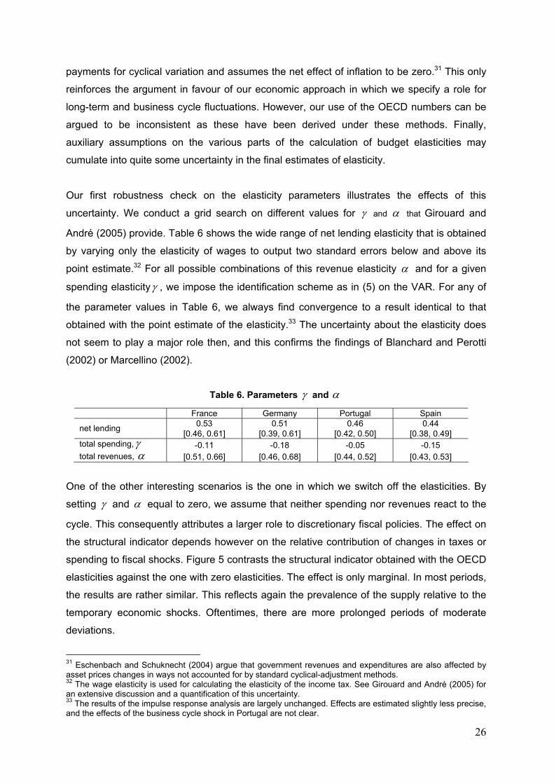
Our first robustness check on the elasticity parameters illustrates the effects of this
uncertainty. We conduct a grid search on different values for γ and α that Girouard and
André (2005) provide. Table 6 shows the wide range of net lending elasticity that is obtained
by varying only the elasticity of wages to output two standard errors below and above its
point estimate.32 For all possible combinations of this revenue elasticity α and for a given
spending elasticityγ , we impose the identification scheme as in (5) on the VAR. For any of
the parameter values in Table 6, we always find convergence to a result identical to that
obtained with the point estimate of the elasticity.33 The uncertainty about the elasticity does
not seem to play a major role then, and this confirms the findings of Blanchard and Perotti
(2002) or Marcellino (2002).
Table 6. Parameters γ and α
France Germany Portugal Spain 0.53 0.51 0.46 0.44 net lending [0.46, 0.61] [0.39, 0.61] [0.42, 0.50] [0.38, 0.49]
total spending,γ -0.11 -0.18 -0.05 -0.15 total revenues, α [0.51, 0.66] [0.46, 0.68] [0.44, 0.52] [0.43, 0.53]
One of the other interesting scenarios is the one in which we switch off the elasticities. By
setting γ and α equal to zero, we assume that neither spending nor revenues react to the
cycle. This consequently attributes a larger role to discretionary fiscal policies. The effect on
the structural indicator depends however on the relative contribution of changes in taxes or
spending to fiscal shocks. Figure 5 contrasts the structural indicator obtained with the OECD
elasticities against the one with zero elasticities. The effect is only marginal. In most periods,
the results are rather similar. This reflects again the prevalence of the supply relative to the
temporary economic shocks. Oftentimes, there are more prolonged periods of moderate
deviations.
31 Eschenbach and Schuknecht (2004) argue that government revenues and expenditures are also affected by asset prices changes in ways not accounted for by standard cyclical-adjustment methods. 32 The wage elasticity is used for calculating the elasticity of the income tax. See Girouard and André (2005) for an extensive discussion and a quantification of this uncertainty. 33 The results of the impulse response analysis are largely unchanged. Effects are estimated slightly less precise, and the effects of the business cycle shock in Portugal are not clear.
27
[INSERT FIGURE 5 HERE]
Fiscal policy might be more seriously biased against automatic stabilisers than our ‘zero-
elasticity’ scenario suggests. There is quite some evidence that in European countries,
governments have been systematically overturning the working of automatic stabilisers (Galí
and Perotti, 2003; Lane, 2003). The true expenditure and revenue elasticities may therefore
be biased upward in comparison to observed elasticities. As a consequence, we would
attribute too much of the variation in fiscal policies to the economic cycle and too little to the
offsetting systematic discretionary adjustments.
To illustrate this phenomenon for Germany, France, Portugal and Spain, we follow Lane
(2003) in estimating the output elasticity of the main budgetary items. I.e., we regress in (7)
the main budget items on economic growth for the sample period 1970-2004,
titiiti YdXd ,, loglog µγω ++= (7)
where tiX , is total spending, government investment, current spending (consumption and
wage spending), or interest payments, and tY is real output. Likewise, we estimate model
(7) in which where tiX , contains either total revenues, current revenues or (in)direct tax
revenues. The estimates are also repeated for the decades 1970-1980, 1981-1990, and
1991 to 2004, as we have reasons to expect quite some time-variation. Table 7 reports the
results of an OLS estimation of (7), with a correction for first-order autocorrelation.
The switch from small negative spending elasticities in OECD (Girouard and André, 2005) to
a strongly positive elasticity is very strong in Germany and Portugal, where it is significant for
all budget items. Government investment is the most procyclical budget component. But the
main category driving this result is – in absolute terms – government consumption. In
Germany, a large role is also played by wage spending in the last decade. Fiscal spending
expansions under positive economic growth are strongly concentrated in increased wage
spending in Portugal. In contrast, Spain, and in particular France, have not been subject to a
similar bias. No expenditure item – except for interest payments – shows significant signs of
procyclicality.
We have argued before that the procyclical bias in fiscal policy is mainly due to reversals in
taxes. We indeed confirm the procyclicality of revenues as in all countries, elasticities are
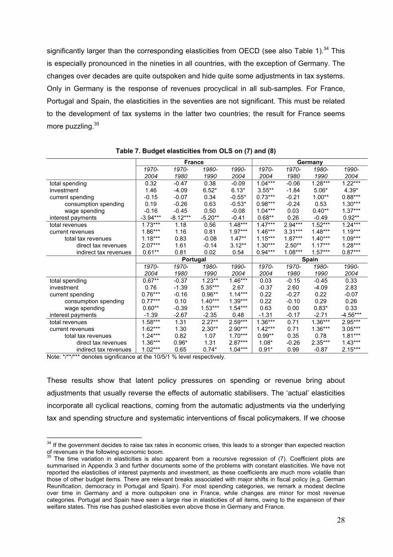
28
significantly larger than the corresponding elasticities from OECD (see also Table 1).34 This
is especially pronounced in the nineties in all countries, with the exception of Germany. The
changes over decades are quite outspoken and hide quite some adjustments in tax systems.
Only in Germany is the response of revenues procyclical in all sub-samples. For France,
Portugal and Spain, the elasticities in the seventies are not significant. This must be related
to the development of tax systems in the latter two countries; the result for France seems
more puzzling.35
Table 7. Budget elasticities from OLS on (7) and (8)
France Germany
1970-2004
1970-1980
1980-1990
1990-2004
1970-2004
1970-1980
1980-1990
1990-2004
total spending 0.32 -0.47 0.38 -0.09 1.04*** -0.06 1.28*** 1.22*** investment 1.46 -4.09 6.52* 6.13* 3.55** -1.84 5.06* 4.39* current spending -0.15 -0.07 0.34 -0.55* 0.73*** -0.21 1.00** 0.88***
consumption spending 0.19 -0.26 0.63 -0.53* 0.98*** -0.24 0.53 1.30*** wage spending -0.16 -0.45 0.50 -0.08 1.04*** 0.03 0.40** 1.37***
interest payments -3.94*** -8.12*** -5.20** -0.41 0.68** 0.26 -0.49 0.92** total revenues 1.73*** 1.18 0.56 1.48*** 1.47*** 2.94*** 1.52*** 1.24*** current revenues 1.86*** 1.16 0.81 1.97*** 1.46*** 3.31*** 1.48*** 1.19***
total tax revenues 1.18*** 0.83 -0.08 1.47** 1.15*** 1.87*** 1.40*** 1.09*** direct tax revenues 2.07*** 1.61 -0.14 3.12** 1.30*** 2.50** 1.17*** 1.28*** indirect tax revenues 0.61** 0.81 0.02 0.54 0.94*** 1.08*** 1.57*** 0.87***
Portugal Spain
1970-2004
1970-1980
1980-1990
1990-2004
1970-2004
1970-1980
1980-1990
1990-2004
total spending 0.67** -0.37 1.23** 1.46*** 0.03 -0.15 -0.45 0.33 investment 0.76 -1.39 5.35*** 2.67 -0.37 2.60 -4.09 2.83 current spending 0.76*** -0.16 0.96** 1.14*** 0.22 -0.27 0.22 -0.07
consumption spending 0.77*** 0.10 1.40*** 1.39*** 0.22 -0.10 0.29 0.26 wage spending 0.60** -0.39 1.53*** 1.54*** 0.63 0.00 0.83* 0.33
interest payments -1.39 -2.67 -2.35 0.48 -1.31 -0.17 -2.71 -4.56*** total revenues 1.58*** 1.31 2.27** 2.59*** 1.36*** 0.71 1.36*** 2.95*** current revenues 1.62*** 1.30 2.30** 2.90*** 1.42*** 0.71 1.36*** 3.05***
total tax revenues 1.24*** 0.82 1.07 1.70*** 0.99** 0.35 0.78 1.81*** direct tax revenues 1.36*** 0.96* 1.31 2.87*** 1.08* -0.26 2.35*** 1.43*** indirect tax revenues 1.02*** 0.65 0.74* 1.04*** 0.91* 0.99 -0.87 2.15***
Note: */**/*** denotes significance at the 10/5/1 % level respectively.
These results show that latent policy pressures on spending or revenue bring about
adjustments that usually reverse the effects of automatic stabilisers. The ‘actual’ elasticities
incorporate all cyclical reactions, coming from the automatic adjustments via the underlying
tax and spending structure and systematic interventions of fiscal policymakers. If we choose
34 If the government decides to raise tax rates in economic crises, this leads to a stronger than expected reaction of revenues in the following economic boom. 35 The time variation in elasticities is also apparent from a recursive regression of (7). Coefficient plots are summarised in Appendix 3 and further documents some of the problems with constant elasticities. We have not reported the elasticities of interest payments and investment, as these coefficients are much more volatile than those of other budget items. There are relevant breaks associated with major shifts in fiscal policy (e.g. German Reunification, democracy in Portugal and Spain). For most spending categories, we remark a modest decline over time in Germany and a more outspoken one in France, while changes are minor for most revenue categories. Portugal and Spain have seen a large rise in elasticities of all items, owing to the expansion of their welfare states. This rise has pushed elasticities even above those in Germany and France.
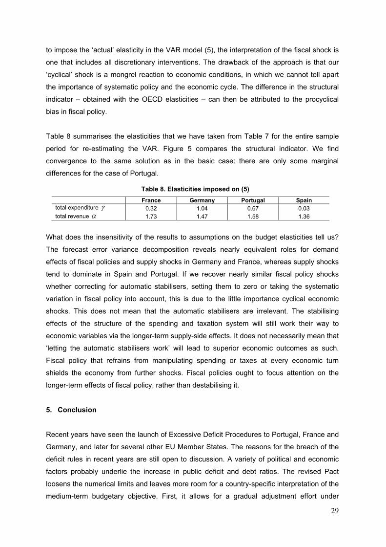
29
to impose the ‘actual’ elasticity in the VAR model (5), the interpretation of the fiscal shock is
one that includes all discretionary interventions. The drawback of the approach is that our
‘cyclical’ shock is a mongrel reaction to economic conditions, in which we cannot tell apart
the importance of systematic policy and the economic cycle. The difference in the structural
indicator – obtained with the OECD elasticities – can then be attributed to the procyclical
bias in fiscal policy.
Table 8 summarises the elasticities that we have taken from Table 7 for the entire sample
period for re-estimating the VAR. Figure 5 compares the structural indicator. We find
convergence to the same solution as in the basic case: there are only some marginal
differences for the case of Portugal.
Table 8. Elasticities imposed on (5) France Germany Portugal Spain total expenditure γ 0.32 1.04 0.67 0.03 total revenue α 1.73 1.47 1.58 1.36
What does the insensitivity of the results to assumptions on the budget elasticities tell us?
The forecast error variance decomposition reveals nearly equivalent roles for demand
effects of fiscal policies and supply shocks in Germany and France, whereas supply shocks
tend to dominate in Spain and Portugal. If we recover nearly similar fiscal policy shocks
whether correcting for automatic stabilisers, setting them to zero or taking the systematic
variation in fiscal policy into account, this is due to the little importance cyclical economic
shocks. This does not mean that the automatic stabilisers are irrelevant. The stabilising
effects of the structure of the spending and taxation system will still work their way to
economic variables via the longer-term supply-side effects. It does not necessarily mean that
‘letting the automatic stabilisers work’ will lead to superior economic outcomes as such.
Fiscal policy that refrains from manipulating spending or taxes at every economic turn
shields the economy from further shocks. Fiscal policies ought to focus attention on the
longer-term effects of fiscal policy, rather than destabilising it.
5. Conclusion
Recent years have seen the launch of Excessive Deficit Procedures to Portugal, France and
Germany, and later for several other EU Member States. The reasons for the breach of the
deficit rules in recent years are still open to discussion. A variety of political and economic
factors probably underlie the increase in public deficit and debt ratios. The revised Pact
loosens the numerical limits and leaves more room for a country-specific interpretation of the
medium-term budgetary objective. First, it allows for a gradual adjustment effort under
30
unfavourable economic conditions, as long as consolidation continues in good economic
times. Second, the revised Pact also attributes more importance to the quality of the budget
adjustment. The revised Pact provides for the implementation of structural reforms that carry
temporary budgetary costs, but which through positive supply-side effects enhance the
structural balance and thus the long-term sustainability of public finances.
This paper takes a first step in developing an economic indicator of discretionary fiscal
stance that takes into account both the cyclical short-term and the long-term supply side
aspects of fiscal policy. We analyse the budgetary outlook for France, Germany, Portugal,
and Spain by uncovering underlying past trends in revenue and expenditure. Our approach
combines insights from the growing empirical literature on the effects of fiscal policy
modelled via structural VARs with statistical methods for cyclically adjusting fiscal balances.
Our approach innovates on existing evidence in using a mixture of short and long-term
restrictions to identify economic and fiscal shocks in a small-scale empirical model in output
and fiscal variables. This allows for permanent shocks to determine trending behaviour of
output and fiscal variables à la Blanchard-Quah. Discretionary fiscal adjustments are
captured by filtering out the fiscal balance for cyclical reactions of budget items following
Blanchard and Perotti (2002).
The model-based indicator we develop shows that pre-EMU consolidations have in last
instance been based mainly on revenues. The slippages of the recent years owe to the
unwinding of these measures without accompanying spending cuts. This showed up in
larger deficits when economic conditions worsened, and a ‘ratcheting up’ in the size of
government in economic booms. Recent corrective measures seem to rely mainly on
increasing revenues again. The procyclical bias in fiscal policies has not been eliminated.
Governments implement bad policies in good times. Fiscal policy induces additional
economic fluctuations and contributes to aggregate macroeconomic instability. As a
consequence, the short-term effects of fiscal policy outweigh supply side effects in the
longer term. A Pact that counters these policy reversals can lead to more sensible policies
that also focus on the long-term quality of public finances.
The analysis in this paper is consistent with a growing theoretical literature on the effects of
fiscal policy. DSGE models with nominal rigidities offer a rationale for fiscal stabilisation
policies. At the same time, these New Keynesian models consider both supply and demand
side effects of fiscal policy, and find the former to dominate. We find that both the supply and
demand effects of fiscal policy are important. The current version of the model does not
allow us quantifying the contribution of supply shocks. The results suggest that the
31
government budget can have long-term growth effects, but mostly so in catching up
countries as Portugal or Spain. More elaborate empirical models could incorporate
refinements in the compositional adjustment of budget balance. This would allow for an
explicit assessment of the channels through which fiscal policy transmits its effects. Allowing
for a different reaction of various budget items to demand and supply shocks can be a first
step in that direction. We think in particular of spending categories that are considered
productive (like government investment). This can verify some endogenous growth theories
of fiscal policy (Turnovsky, 2000). A major channel through which fiscal policy acts is also
the labour market, either directly – via wage spending or public employment – or indirectly.
Finally, instead of specifying a model in output and fiscal policies only, the inclusion of prices
and/or interest rates can lead to a more accurate description of the economic shocks.
References
Afonso, A. (2005). Fiscal Sustainability: the Unpleasant European Case, FinanzArchiv, 61
(1), 19-44.
Afonso, A. (2006). Expansionary fiscal consolidations in Europe: new evidence, ECB
Working Paper 675.
Alesina, A., and Bayoumi, T., (1996). The costs and benefits of fiscal rules: evidence from
US states, NBER, working paper 5614.
Alesina, A., and Perotti, R., (1995). Fiscal expansions and adjustments in OECD countries,
Economic Policy, 21, 205-248.
Alesina, A. and Ardagna, S. (1998). Tales of Fiscal Contractions, Economic Policy, 27, 487-
545.
Bai, J., (1997). Estimation of a change point in multiple regression models, Review of
Economics and Statistics, 79(4), 551-563.
Bai, J., Lumsdaine, R., and Stock, J., (1998). Testing for and dating common breaks in
multivariate time series, Review of Economic Studies, 65, 395-432.
Baxter, M. and King, R., (1993). Fiscal policy in general equilibrium, American Economic
Review, 83(3), 315-334.
Barro, R., (1990). Government spending in a simple model of endogeneous growth, Journal
of Political Economy, 98, 103-125.
Bilbiie, F., Meier, A. and Müller, G., (2006). What accounts for the change in US fiscal policy
transmission?, ECB working paper, 582.
32
Blanchard, O., (1993). Suggestions for a new set of fiscal indicators, in: Verbon, H. and Van
Winden, F. (eds.), The political economy of government debt, North-Holland, Elsevier
Science publishers, 307-325.
Blanchard, O., and Quah, D., (1989), The dynamic effects of aggregate demand and supply
disturbances, American Economic Review, 79(4), 655-673.
Blanchard, O. and Perotti, R. (2002). An empirical characterisation of the dynamic effects of
changes in government spending and taxes on output, Quarterly Journal of Economics, 117
(4), 1329-1368.
Bouthevillain, C. and Quinet, A., (1999). The relevance of cyclically-adjusted public balance
indicators – the French case, in: Indicators of Structural Budget Balances, Banca d’Italia.
Bouthevillain, C., Cour-Thimann, G., Van den Dool, G., Hernandez De Cos , Langenus, G.,
Mohr, M., Momigliano, S., and Tujula, M., (2001). Cyclical adjusted budget balances: an
alternative approach, European Central Bank, working paper 77.
Bruneau, C., and De Bandt, O., (2003). Monetary and fiscal policy in the transition to EMU:
what do SVAR models tell us? Economic Modelling, 20, 959-985.
Canova, F., and Pappa, E., (2002). Price dispersions in monetary unions: the role of fiscal
shocks, CEPR, discussion paper 3746.
Cavallo, M., (2005). Government employment and the dynamic effects of fiscal policy
shocks, Federal Reserve Bank of San Francisco, Working Papers in Applied Economic
Theory, 16.
Chouraqui, J., Hagemann, R., and Sartor, N., (1992). Indicators of fiscal policy: a
reassessment, OECD Economics Department, working paper 78.
Christiano L., Eichenbaum M., and Vigfusson E., (2006). Assessing structural VARs, NBER,
working paper 12353.
Claeys, P., (2004). An SVAR analysis of stabilisation policies in EMU, European University
Institute, working paper 22.
Cohen, D., and Follette, G., (2000). The automatic stabilisers: quietly doing their thing,
Federal Reserve Bank of New York, Economic Policy Review, 6, 35-67.
Dalsgaard, T., and De Serres, A., (2001). Estimating prudent budgetary margins, in: Brunila,
A., et al. (eds.), The SGP: the architecture of fiscal policy in EMU, Basingstoke: Palgrave,
123-154.
De Arcangelis, G., and Lamartina, S., (2004). Fiscal shocks and policy regimes in some
OECD countries, in: Beetsma, R., et al. (eds.), Fiscal policies, monetary policies and labour
markets, Key aspects of European macroeconomic policies after monetary unification,
Cambridge: Cambridge University Press, 224-255.
Eschenbach, F. and Schucknecht, L., (2004). Budgetary risks from real estate and stock
markets, Economic Policy, 19 (39), 313-346.
33
European Commission (1995). The Commission services’ method for the cyclical adjustment
of government budget balances (Technical Note), European Economy, 60, 35-56.
Fatás, A., and Mihov, I., (2003a). On constraining fiscal policy discretion in EMU, Oxford
Review of Economic Policy, 19 (1), 112-131.
Fatás, A., and Mihov, I., (2003b). The case for restricting fiscal policy discretion, Quarterly
Journal of Economics, 118 (4), 1419-1447.
Faust, J., and Leeper, E., (1997). When do long-run identifying restrictions give reliable
results?, Journal of Business and Economic Statistics, 15(3), 334-353.
Finn, M., (1998). Cyclical effects of government’s employment and goods purchases,
International Economic Review, 39, 635-657.
Galí, J., (1992). How well does the IS-LM fit postwar US data?, Quarterly Journal of Economics, 107(2), 709-738. Galí, J., and Perotti, R., (2003). Fiscal policy and monetary integration in Europe, Economic
Policy, 37, 535-572.
Galí, J., Lopez-Salido, D. and Valles, J., (2005). Understanding the effects of government
spending on consumption, NBER, working paper 11578.
Giavazzi, F. and Pagano, M., (1990). Can severe fiscal contractions be expansionary? Tales of two small European countries, in : Fischer S. (ed.), NBER Macroeconomic Annuals, vol. 5, MIT Press, p. 75-122. Giavazzi, F., Jappelli, T., and Pagano, M., (2000). Searching for non-linear effects of fiscal
policy: evidence from industrial and developing countries, European Economic Review, 44,
1259-1289.
Giorno, C., Richardson, J., Rosevaere, D. and Van den Noord, P., (1995). Estimating
potential output, output gaps, and structural budget deficits, OECD Economic Studies, 24,
167-209.
Girouard, N., and André, C., (2005). Measuring cyclically adjusted budget balances for
OECD countries, OECD Economics Department, working paper 434.
Hjelm, G. (2003). Simultaneous determination of NAIRU, output gaps, and structural budget
balances: Swedish evidence, NIER, working paper 81.
IMF, (1993). World Economic Outlook, International Monetary Fund, Washington.
Kamps, C., (2004). The dynamic effects of public capital: VAR evidence for 22 OECD
countries, Kiel Institute, working paper 1224.
King, R., and Rebelo, S., (1990). Public policy and economic growth: developing
neoclassical implications, Journal of Political Economy, 98, 126-150.
King, G., Plosser, C., Stock, J., and Watson, M., (1991). Stochastic trends and economic fluctuations, American Economic Review, 81(2), 819-840. King, R., and Watson, M., (1997). Testing long run neutrality, Federal Reserve Bank
Richmond, Quarterly Review, 83 (3), 69-101.
34
Kneller, R., Bleany, M., and Gemmell, N., (1999). Fiscal policy and growth: evidence from
OECD countries, Journal of Public Economics, 74, 171-190.
Lane, P., (2003). The cyclical behaviour of fiscal policy: evidence from the OECD, Journal of
Public Economics, 87 (12), 2661-2675.
Linnemann, L. and Schabert, A., (2003). Fiscal policy in the New Neoclassical Synthesis,
Journal of Money, Credit and Banking, 35(6), 911-929.
Lippi, M., and Reichlin, L., (1994). VAR analysis, non-fundamental representation, Blaschke
matrices, Journal of Econometrics, 63, 307-325.
Marcellino, M., (2002). Some stylised facts on non-systematic fiscal policy in the Euro-area,
CEPR, discussion paper 3635.
Mountford, A., and Uhlig, H., (2002). What are the effects of fiscal policy shocks?, CEPR,
discussion paper 3338.
Nelson, C. and Plosser, C., (1982). Trends and random walks in macroeconomic time
series: some evidence and implications, Journal of Monetary Economics, 10, 139-162.
Pappa, E., (2005). New Keynesian or RBC transmission? The effects of fiscal policy in
labour markets, CEPR, discussion paper 5313.
Perotti, R., (2004). Public investment: another (different) look, IGIER, working paper 277.
Perotti, R., (2005). Estimating the effects of fiscal policy in OECD countries, CEPR, working
paper 4842.
Ramey, V., and Shapiro, M., (1998). Costly capital reallocation and the effects of
government spending, Carnegie Rochester Conference on Public Policy, 48, 145-194.
Ravn, M., and Uhlig, H., (2002). On adjusting the HP-filter for the frequency of observations,
Review of Economics and Statistics, 84, 371-380.
Sarte, P., (1997). On the identification of structural vector autoregressions, FRB Richmond -
Economic Review, 83 (3), 45-67.
Sims, C., Stock, J., and Watson, M., (1990). Inference in time series models with some unit roots, Econometrica, 58, 113-144. Stock, J., and Watson, M., (2003). Has the business cycle changed and why?, in: Gertler,
M., and Rogoff, K., (eds.), NBER Macroeconomics Annual, 2003. Cambridge: MIT Press,
17; 159-218.
Turnovsky, S., (2000). Fiscal policy, elastic labour supply and endogenous growth, Journal
of Monetary Economics, 45, 185-210.
Van den Noord, P., (2002). Automatic stabilisers in the 1990s and beyond, in: Buti, M., Von
Hagen, J., and Martinez-Mongay, C. (eds.), The Behavior of Fiscal Authorities: Stabilisation,
Growth and Institutions, London: Palgrave, 130-148.
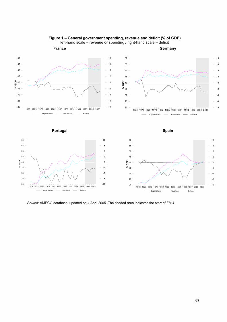
35
Figure 1 – General government spending, revenue and deficit (% of GDP) left-hand scale – revenue or spending / right-hand scale – deficit
France
Expenditures Revenues Balance
% G
DP
1970 1973 1976 1979 1982 1985 1988 1991 1994 1997 2000 200320
25
30
35
40
45
50
55
60
-10
-8
-5
-2
0
2
5
8
10
Germany
Expenditures Revenues Balance
% G
DP %
GD
P
1970 1973 1976 1979 1982 1985 1988 1991 1994 1997 2000 200320
25
30
35
40
45
50
55
60
-10
-8
-5
-2
0
2
5
8
10
Portugal
Expenditures Revenues Balance
% G
DP %
GD
P
1970 1973 1976 1979 1982 1985 1988 1991 1994 1997 2000 200320
25
30
35
40
45
50
55
60
-10
-8
-5
-2
0
2
5
8
10
Spain
Expenditures Revenues Balance
% G
DP %
GD
P
1970 1973 1976 1979 1982 1985 1988 1991 1994 1997 2000 200320
25
30
35
40
45
50
55
60
-10
-8
-5
-2
0
2
5
8
10
Source: AMECO database, updated on 4 April 2005. The shaded area indicates the start of EMU.
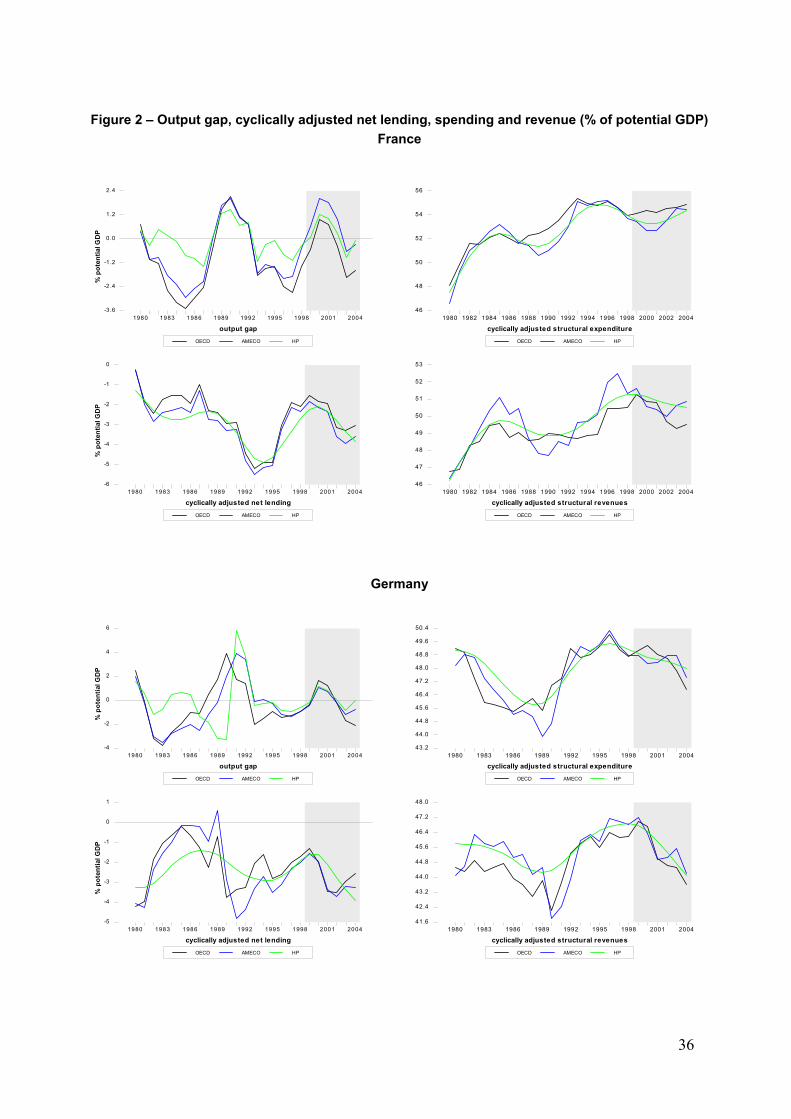
36
Figure 2 – Output gap, cyclically adjusted net lending, spending and revenue (% of potential GDP)
France
OECD AMECO HP
output gap
% p
oten
tial G
DP
1980 1983 1986 1989 1992 1995 1998 2001 2004-3 .6
-2 .4
-1 .2
0.0
1.2
2.4
OECD AMECO HP
cyclically adjusted net lending
% p
oten
tial G
DP
1980 1983 1986 1989 1992 1995 1998 2001 2004-6
-5
-4
-3
-2
-1
0
OECD AMECO HP
cyclically adjusted structural expenditure1980 1982 1984 1986 1988 1990 1992 1994 1996 1998 2000 2002 2004
46
48
50
52
54
56
OECD AMECO HP
cyclically adjusted structural revenues1980 1982 1984 1986 1988 1990 1992 1994 1996 1998 2000 2002 2004
46
47
48
49
50
51
52
53
Germany
OECD AMECO HP
output gap
% p
oten
tial G
DP
1980 1983 1986 1989 1992 1995 1998 2001 2004-4
-2
0
2
4
6
OECD AMECO HP
cyclically adjusted net lending
% p
oten
tial G
DP
1980 1983 1986 1989 1992 1995 1998 2001 2004-5
-4
-3
-2
-1
0
1
OECD AMECO HP
cyclically adjusted structural expenditure1980 1983 1986 1989 1992 1995 1998 2001 2004
43.2
44.0
44.8
45.6
46.4
47.2
48.0
48.8
49.6
50.4
OECD AMECO HP
cyclically adjusted structural revenues1980 1983 1986 1989 1992 1995 1998 2001 2004
41.6
42.4
43.2
44.0
44.8
45.6
46.4
47.2
48.0
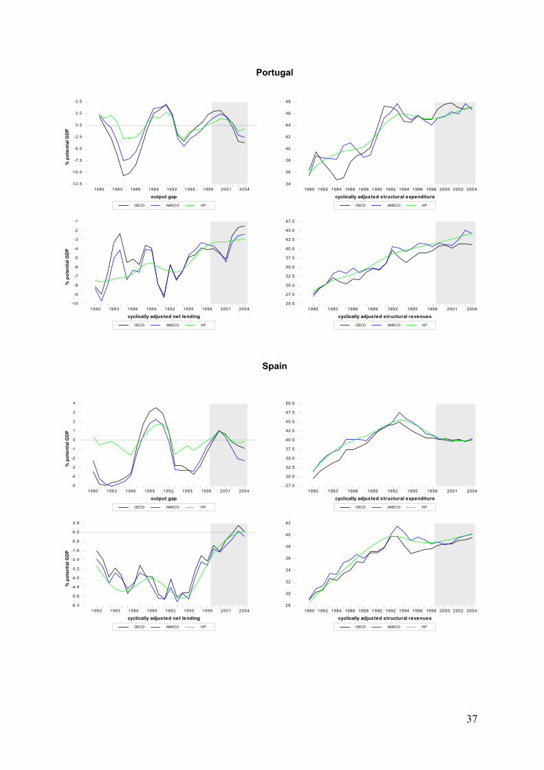
37
Portugal
OECD AMECO HP
output gap
% p
oten
tial G
DP
1980 1983 1986 1989 1992 1995 1998 2001 2004-12.5
-10.0
-7.5
-5.0
-2.5
0 .0
2 .5
5 .0
OECD AMECO HP
cyclically adjusted net lending
% p
oten
tial G
DP
1980 1983 1986 1989 1992 1995 1998 2001 2004-10
-9
-8
-7
-6
-5
-4
-3
-2
-1
OECD AMECO HP
cyclically adjusted structural expenditure1980 1982 1984 1986 1988 1990 1992 1994 1996 1998 2000 2002 2004
34
36
38
40
42
44
46
48
OECD AMECO HP
cyclically adjusted structural revenues1980 1983 1986 1989 1992 1995 1998 2001 2004
25.0
27.5
30.0
32.5
35.0
37.5
40.0
42.5
45.0
47.5
Spain
OECD AMECO HP
output gap
% p
oten
tial G
DP
1980 1983 1986 1989 1992 1995 1998 2001 2004-5
-4
-3
-2
-1
0
1
2
3
4
OECD AMECO HP
cyclically adjusted net lending
% p
oten
tial G
DP
1980 1983 1986 1989 1992 1995 1998 2001 2004-6 .4
-5 .6
-4 .8
-4 .0
-3 .2
-2 .4
-1 .6
-0 .8
-0 .0
0.8
OECD AMECO HP
cyclically adjusted structural expenditure1980 1983 1986 1989 1992 1995 1998 2001 2004
27.5
30.0
32.5
35.0
37.5
40.0
42.5
45.0
47.5
50.0
OECD AMECO HP
cyclically adjusted structural revenues1980 1982 1984 1986 1988 1990 1992 1994 1996 1998 2000 2002 2004
28
30
32
34
36
38
40
42
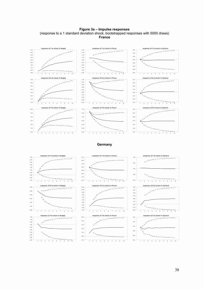
38
Figure 3a – Impulse responses
(response to a 1 standard deviation shock, bootstrapped responses with 5000 draws) France
response of Y to shock in Supply
1 2 3 4 5 6 7 8 9 100.00
0.50
1.00
1.50
2.00
2.50
3.00
3.50
4.00
4.50response of Y to shock in Fiscal
1 2 3 4 5 6 7 8 9 10-2.00
-1.50
-1.00
-0.50
0.00
0.50
1.00
1.50
2.00
2.50response of Y to shock in Cyclical
1 2 3 4 5 6 7 8 9 10-0.80
-0.60
-0.40
-0.20
-0.00
0.20
0.40
0.60
response of G to shock in Supply
1 2 3 4 5 6 7 8 9 101.40
2.10
2.80
3.50
4.20
4.90
5.60
6.30response of G to shock in Fiscal
1 2 3 4 5 6 7 8 9 10-6.00
-5.50
-5.00
-4.50
-4.00
-3.50
-3.00
-2.50
-2.00
-1.50response of G to shock in Cyclical
1 2 3 4 5 6 7 8 9 10-0.54
-0.36
-0.18
-0.00
0.18
0.36
0.54
0.72
response of T to shock in Supply
1 2 3 4 5 6 7 8 9 100.00
1.00
2.00
3.00
4.00
5.00
6.00response of T to shock in Fiscal
1 2 3 4 5 6 7 8 9 10-5.00
-4.00
-3.00
-2.00
-1.00
0.00
1.00response of T to shock in Cyclical
1 2 3 4 5 6 7 8 9 10-1.50
-1.25
-1.00
-0.75
-0.50
-0.25
0.00
Germany
response of Y to shock in Supply
1 2 3 4 5 6 7 8 9 10-1.00
-0.50
0.00
0.50
1.00
1.50
2.00
2.50
3.00
3.50response of Y to shock in Fiscal
1 2 3 4 5 6 7 8 9 10-2.40
-1.60
-0.80
-0.00
0.80
1.60
2.40
3.20response of Y to shock in Cyclical
1 2 3 4 5 6 7 8 9 10-0.50
-0.25
0.00
0.25
0.50
response of G to shock in Supply
1 2 3 4 5 6 7 8 9 10-8.00
-7.00
-6.00
-5.00
-4.00
-3.00
-2.00response of G to shock in Fiscal
1 2 3 4 5 6 7 8 9 103.20
4.00
4.80
5.60
6.40
7.20
8.00
8.80
9.60
10.40response of G to shock in Cyclical
1 2 3 4 5 6 7 8 9 10-0.28
-0.14
0.00
0.14
0.28
0.42
0.56
0.70
0.84
response of T to shock in Supply
1 2 3 4 5 6 7 8 9 10-3.00
-2.50
-2.00
-1.50
-1.00
-0.50
0.00
0.50
1.00
1.50response of T to shock in Fiscal
1 2 3 4 5 6 7 8 9 10-1.00
0.00
1.00
2.00
3.00
4.00
5.00response of T to shock in Cyclical
1 2 3 4 5 6 7 8 9 100.00
0.25
0.50
0.75
1.00
1.25
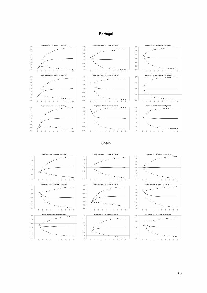
39
Portugal
response of Y to shock in Supply
1 2 3 4 5 6 7 8 9 100.75
1.00
1.25
1.50
1.75
2.00
2.25
2.50
2.75
3.00response of Y to shock in Fiscal
1 2 3 4 5 6 7 8 9 10-1.50
-1.00
-0.50
0.00
0.50
1.00
1.50
2.00response of Y to shock in Cyclical
1 2 3 4 5 6 7 8 9 10-0.60
-0.40
-0.20
-0.00
0.20
0.40
0.60
response of G to shock in Supply
1 2 3 4 5 6 7 8 9 100.50
0.75
1.00
1.25
1.50
1.75
2.00
2.25
2.50response of G to shock in Fiscal
1 2 3 4 5 6 7 8 9 10-4.00
-3.50
-3.00
-2.50
-2.00
-1.50
-1.00response of G to shock in Cyclical
1 2 3 4 5 6 7 8 9 10-0.25
0.00
0.25
0.50
0.75
response of T to shock in Supply
1 2 3 4 5 6 7 8 9 100.25
0.50
0.75
1.00
1.25
1.50
1.75
2.00
2.25response of T to shock in Fiscal
1 2 3 4 5 6 7 8 9 10-2.50
-2.00
-1.50
-1.00
-0.50
0.00
0.50response of T to shock in Cyclical
1 2 3 4 5 6 7 8 9 100.20
0.40
0.60
0.80
1.00
1.20
1.40
Spain
response of Y to shock in Supply
1 2 3 4 5 6 7 8 9 10-1.60
0.00
1.60
3.20
4.80
6.40response of Y to shock in Fiscal
1 2 3 4 5 6 7 8 9 10-7.50
-5.00
-2.50
0.00
2.50
5.00
7.50response of Y to shock in Cyclical
1 2 3 4 5 6 7 8 9 10-1.00
-0.75
-0.50
-0.25
0.00
0.25
0.50
0.75
1.00
response of G to shock in Supply
1 2 3 4 5 6 7 8 9 10-7.00
-6.00
-5.00
-4.00
-3.00
-2.00
-1.00response of G to shock in Fiscal
1 2 3 4 5 6 7 8 9 102.00
4.00
6.00
8.00
10.00
12.00
14.00response of G to shock in Cyclical
1 2 3 4 5 6 7 8 9 10-1.75
-1.50
-1.25
-1.00
-0.75
-0.50
-0.25
0.00
response of T to shock in Supply
1 2 3 4 5 6 7 8 9 10-4.00
-3.00
-2.00
-1.00
0.00
1.00
2.00response of T to shock in Fiscal
1 2 3 4 5 6 7 8 9 10-1.60
0.00
1.60
3.20
4.80
6.40
8.00
9.60response of T to shock in Cyclical
1 2 3 4 5 6 7 8 9 10-2.00
-1.50
-1.00
-0.50
0.00
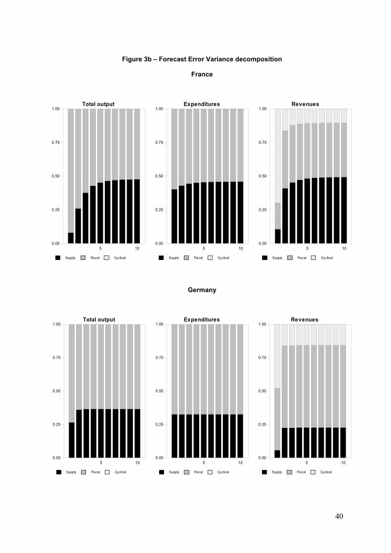
40
Figure 3b – Forecast Error Variance decomposition
France
Supply Fiscal Cyclical
Total output
5 100.00
0.25
0.50
0.75
1.00
Supply Fiscal Cyclical
Expenditures
5 100.00
0.25
0.50
0.75
1.00
Supply Fiscal Cyclical
Revenues
5 100.00
0.25
0.50
0.75
1.00
Germany
Supply Fiscal Cyclical
Total output
5 100.00
0.25
0.50
0.75
1.00
Supply Fiscal Cyclical
Expenditures
5 100.00
0.25
0.50
0.75
1.00
Supply Fiscal Cyclical
Revenues
5 100.00
0.25
0.50
0.75
1.00
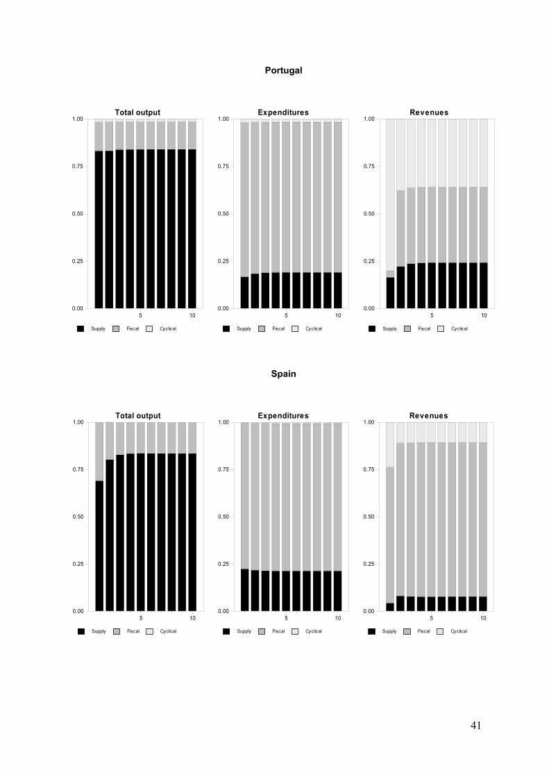
41
Portugal
Supply Fiscal Cyclical
Total output
5 100.00
0.25
0.50
0.75
1.00
Supply Fiscal Cyclical
Expenditures
5 100.00
0.25
0.50
0.75
1.00
Supply Fiscal Cyclical
Revenues
5 100.00
0.25
0.50
0.75
1.00
Spain
Supply Fiscal Cyclical
Total output
5 100.00
0.25
0.50
0.75
1.00
Supply Fiscal Cyclical
Expenditures
5 100.00
0.25
0.50
0.75
1.00
Supply Fiscal Cyclical
Revenues
5 100.00
0.25
0.50
0.75
1.00
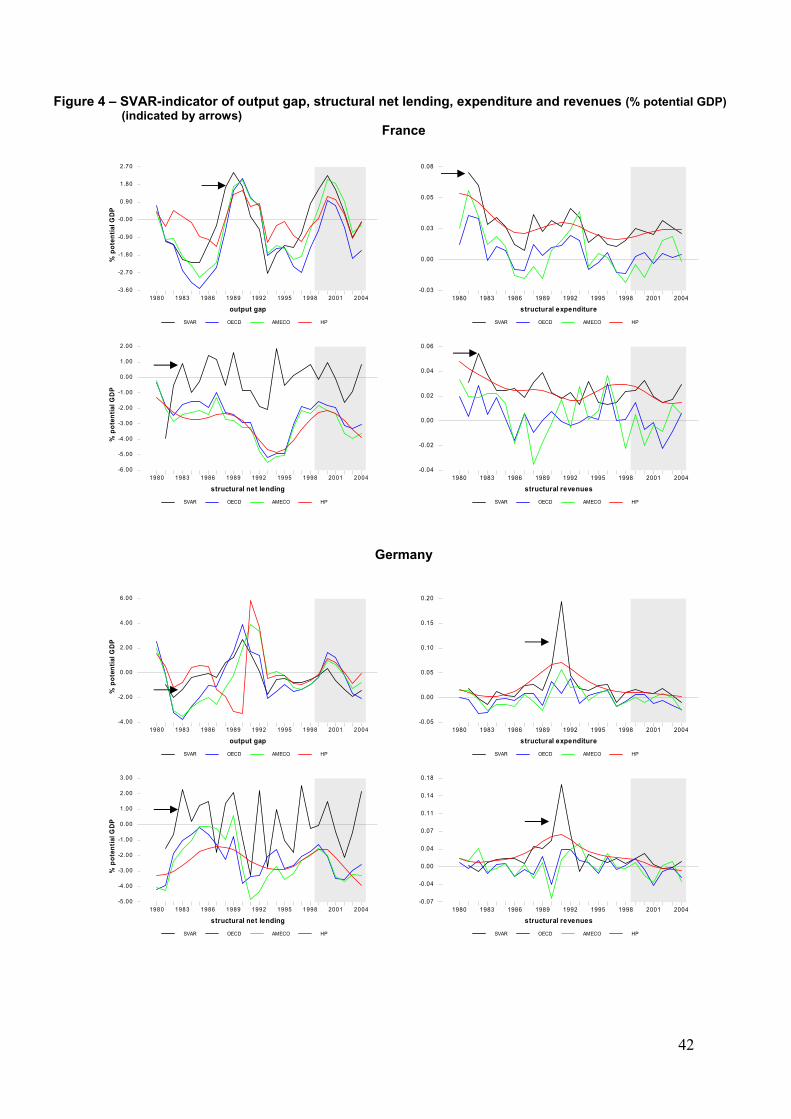
42
Figure 4 – SVAR-indicator of output gap, structural net lending, expenditure and revenues (% potential GDP) (indicated by arrows)
France
SVAR OECD AMECO HP
output gap
% p
oten
tial G
DP
1980 1983 1986 1989 1992 1995 1998 2001 2004-3.60
-2.70
-1.80
-0.90
-0.00
0.90
1.80
2.70
SVAR OECD AMECO HP
structural net lending
% p
oten
tial G
DP
1980 1983 1986 1989 1992 1995 1998 2001 2004-6.00
-5.00
-4.00
-3.00
-2.00
-1.00
0.00
1.00
2.00
SVAR OECD AMECO HP
structural expenditure1980 1983 1986 1989 1992 1995 1998 2001 2004
-0.03
0.00
0.03
0.05
0.08
SVAR OECD AMECO HP
structural revenues1980 1983 1986 1989 1992 1995 1998 2001 2004
-0.04
-0.02
0.00
0.02
0.04
0.06
Germany
SVAR OECD AMECO HP
output gap
% p
oten
tial G
DP
1980 1983 1986 1989 1992 1995 1998 2001 2004-4.00
-2.00
0.00
2.00
4.00
6.00
SVAR OECD AMECO HP
structural net lending
% p
oten
tial G
DP
1980 1983 1986 1989 1992 1995 1998 2001 2004-5.00
-4.00
-3.00
-2.00
-1.00
0.00
1.00
2.00
3.00
SVAR OECD AMECO HP
structural expenditure1980 1983 1986 1989 1992 1995 1998 2001 2004
-0.05
0.00
0.05
0.10
0.15
0.20
SVAR OECD AMECO HP
structural revenues1980 1983 1986 1989 1992 1995 1998 2001 2004
-0.07
-0.04
0.00
0.04
0.07
0.11
0.14
0.18
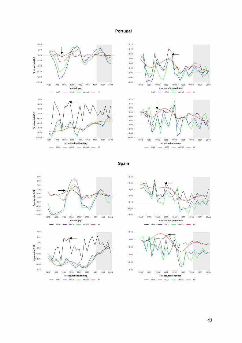
43
Portugal
SVAR OECD AMECO HP
output gap
% p
oten
tial G
DP
1980 1983 1986 1989 1992 1995 1998 2001 2004-12.50
-10.00
-7 .50
-5 .00
-2 .50
0.00
2.50
5.00
SVAR OECD AMECO HP
structural net lending
% p
oten
tial G
DP
1980 1983 1986 1989 1992 1995 1998 2001 2004-10.00
-8 .00
-6 .00
-4 .00
-2 .00
0.00
2.00
4.00
6.00
SVAR OECD AMECO HP
structural expenditure1980 1983 1986 1989 1992 1995 1998 2001 2004
-0.05
-0.03
0.00
0.03
0.05
0.08
0.10
0.12
0.15
SVAR OECD AMECO HP
structural revenues1980 1983 1986 1989 1992 1995 1998 2001 2004
-0.06
-0.04
-0.02
0.00
0.02
0.04
0.06
0.08
0.10
0.12
Spain
SVAR OECD AMECO HP
output gap
% p
oten
tial G
DP
1980 1983 1986 1989 1992 1995 1998 2001 2004-5.00
-4.00
-3.00
-2.00
-1.00
0.00
1.00
2.00
3.00
4.00
SVAR OECD AMECO HP
structural net lending
% p
oten
tial G
DP
1980 1983 1986 1989 1992 1995 1998 2001 2004-6.40
-4.80
-3.20
-1.60
-0.00
1.60
3.20
4.80
SVAR OECD AMECO HP
structural expenditure1980 1983 1986 1989 1992 1995 1998 2001 2004
-0.05
-0.03
0.00
0.03
0.05
0.08
0.10
SVAR OECD AMECO HP
structural revenues1980 1983 1986 1989 1992 1995 1998 2001 2004
-0.05
-0.03
0.00
0.03
0.05
0.08
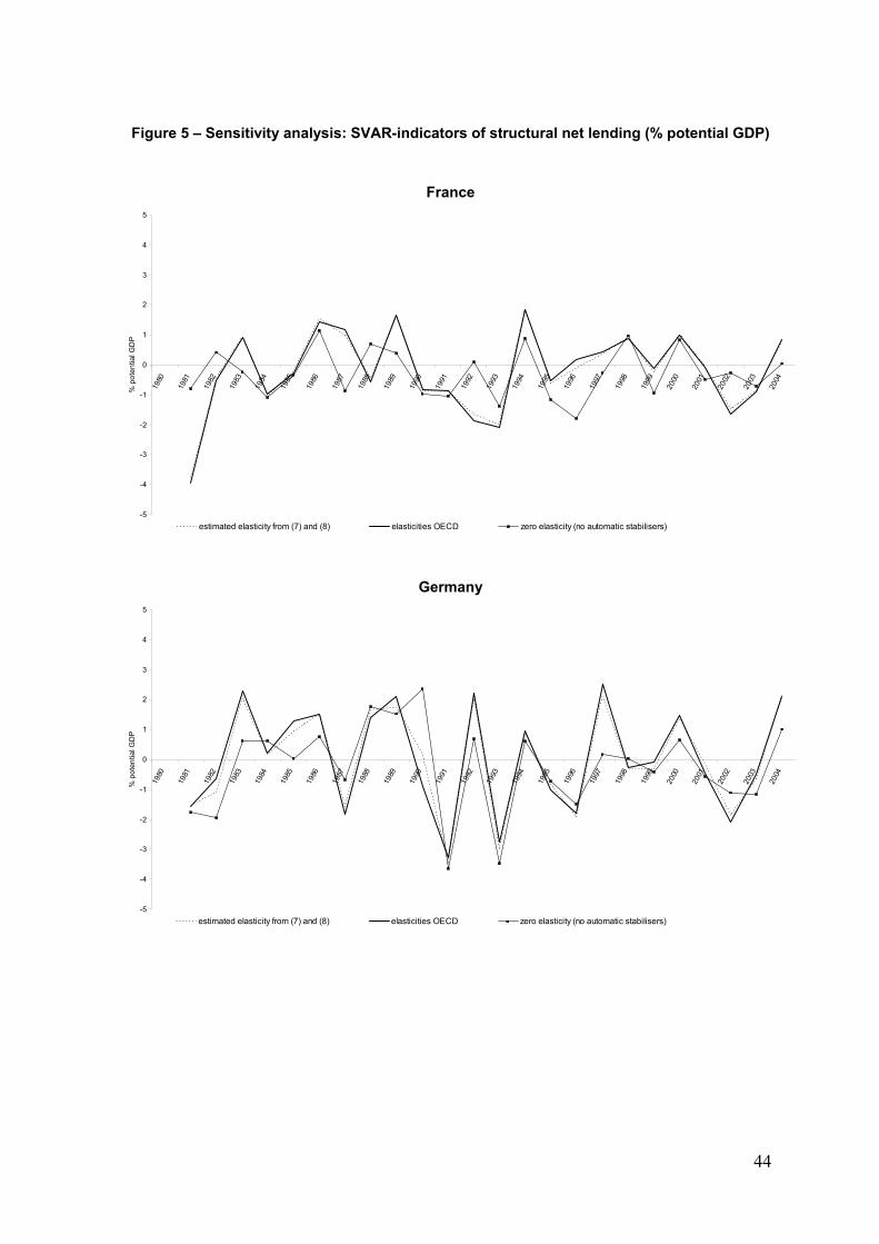
44
Figure 5 – Sensitivity analysis: SVAR-indicators of structural net lending (% potential GDP)
France
-5
-4
-3
-2
-1
0
1
2
3
4
5
1980
1981
1982
1983
1984
1985
1986
1987
1988
1989
1990
1991
1992
1993
1994
1995
1996
1997
1998
1999
2000
2001
2002
2003
2004
% p
oten
tial G
DP
estimated elasticity from (7) and (8) elasticities OECD zero elasticity (no automatic stabilisers)
Germany
-5
-4
-3
-2
-1
0
1
2
3
4
5
1980
1981
1982
1983
1984
1985
1986
1987
1988
1989
1990
1991
1992
1993
1994
1995
1996
1997
1998
1999
2000
2001
2002
2003
2004
% p
oten
tial G
DP
estimated elasticity from (7) and (8) elasticities OECD zero elasticity (no automatic stabilisers)
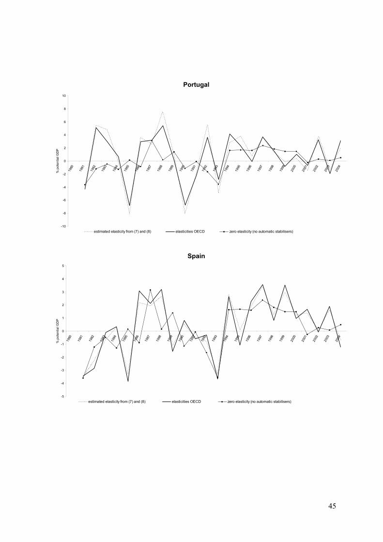
45
Portugal
-10
-8
-6
-4
-2
0
2
4
6
8
10
1980
1981
1982
1983
1984
1985
1986
1987
1988
1989
1990
1991
1992
1993
1994
1995
1996
1997
1998
1999
2000
2001
2002
2003
2004
% p
oten
tial G
DP
estimated elasticity from (7) and (8) elasticities OECD zero elasticity (no automatic stabilisers)
Spain
-5
-4
-3
-2
-1
0
1
2
3
4
5
1980
1981
1982
1983
1984
1985
1986
1987
1988
1989
1990
1991
1992
1993
1994
1995
1996
1997
1998
1999
2000
2001
2002
2003
2004
% p
oten
tial G
DP
estimated elasticity from (7) and (8) elasticities OECD zero elasticity (no automatic stabilisers)
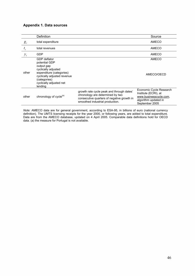
46
Appendix 1. Data sources
Definition Source
tg total expenditure AMECO
tt total revenues AMECO
ty GDP AMECO GDP deflator AMECO potential GDP output gap cyclically adjusted expenditure (categories)
cyclically adjusted revenue (categories)
other
cyclically adjusted net lending
AMECO/OECD
other chronology of cycle(a)
growth rate cycle peak and through dates’ chronology are determined by two consecutive quarters of negative growth in smoothed industrial production.
Economic Cycle Research Institute (ECRI), at www.businesscycle.com, algorithm updated in September 2005
Note: AMECO data are for general government, according to ESA-95, in billions of euro (national currency definition). The UMTS licensing receipts for the year 2000, or following years, are added to total expenditure. Data are from the AMECO database, updated on 4 April 2005. Comparable data definitions hold for OECD data. (a) the measure for Portugal is not available.
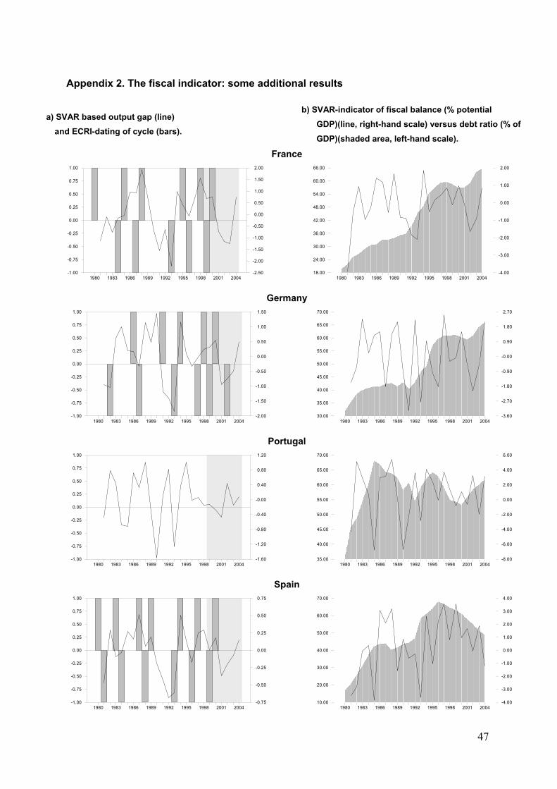
47
Appendix 2. The fiscal indicator: some additional results
a) SVAR based output gap (line) and ECRI-dating of cycle (bars).
b) SVAR-indicator of fiscal balance (% potential GDP)(line, right-hand scale) versus debt ratio (% of GDP)(shaded area, left-hand scale).
France
1980 1983 1986 1989 1992 1995 1998 2001 2004-1.00
-0.75
-0.50
-0.25
0.00
0.25
0.50
0.75
1.00
-2.50
-2.00
-1.50
-1.00
-0.50
0.00
0.50
1.00
1.50
2.00
1980 1983 1986 1989 1992 1995 1998 2001 2004
18.00
24.00
30.00
36.00
42.00
48.00
54.00
60.00
66.00
-4.00
-3.00
-2.00
-1.00
0.00
1.00
2.00
Germany
1980 1983 1986 1989 1992 1995 1998 2001 2004-1.00
-0.75
-0.50
-0.25
0.00
0.25
0.50
0.75
1.00
-2.00
-1.50
-1.00
-0.50
0.00
0.50
1.00
1.50
1980 1983 1986 1989 1992 1995 1998 2001 2004
30.00
35.00
40.00
45.00
50.00
55.00
60.00
65.00
70.00
-3.60
-2.70
-1.80
-0.90
-0.00
0.90
1.80
2.70
Portugal
1980 1983 1986 1989 1992 1995 1998 2001 2004-1.00
-0.75
-0.50
-0.25
0.00
0.25
0.50
0.75
1.00
-1.60
-1.20
-0.80
-0.40
-0.00
0.40
0.80
1.20
1980 1983 1986 1989 1992 1995 1998 2001 2004
35.00
40.00
45.00
50.00
55.00
60.00
65.00
70.00
-8.00
-6.00
-4.00
-2.00
0.00
2.00
4.00
6.00
Spain
1980 1983 1986 1989 1992 1995 1998 2001 2004-1.00
-0.75
-0.50
-0.25
0.00
0.25
0.50
0.75
1.00
-0.75
-0.50
-0.25
0.00
0.25
0.50
0.75
1980 1983 1986 1989 1992 1995 1998 2001 2004
10.00
20.00
30.00
40.00
50.00
60.00
70.00
-4.00
-3.00
-2.00
-1.00
0.00
1.00
2.00
3.00
4.00
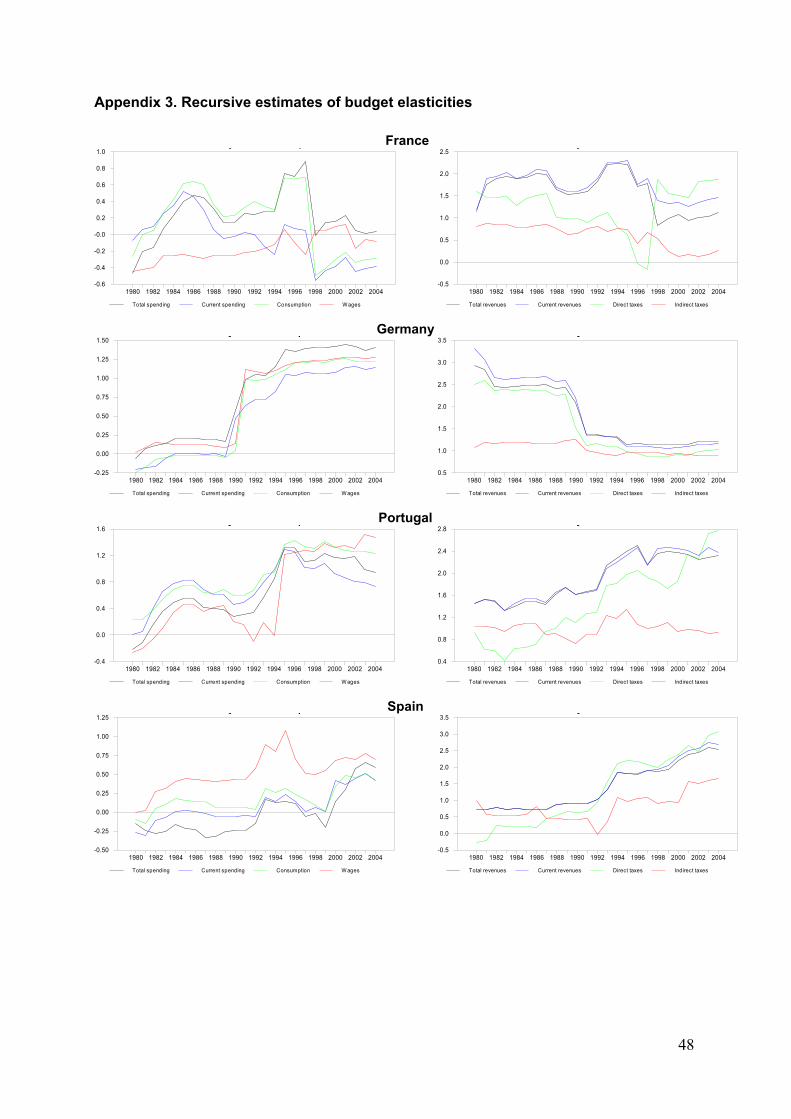
48
Appendix 3. Recursive estimates of budget elasticities
France
Total spending Current spending Consumption W ages
y p
1980 1982 1984 1986 1988 1990 1992 1994 1996 1998 2000 2002 2004-0.6
-0.4
-0.2
-0.0
0.2
0.4
0.6
0.8
1.0
Total revenues Current revenues Direct taxes Indirect taxes
y
1980 1982 1984 1986 1988 1990 1992 1994 1996 1998 2000 2002 2004-0.5
0.0
0.5
1.0
1.5
2.0
2.5
Germany
Total spending Current spending Consumption W ages
y p
1980 1982 1984 1986 1988 1990 1992 1994 1996 1998 2000 2002 2004-0.25
0.00
0.25
0.50
0.75
1.00
1.25
1.50
Total revenues Current revenues Direct taxes Indirect taxes
y
1980 1982 1984 1986 1988 1990 1992 1994 1996 1998 2000 2002 20040.5
1.0
1.5
2.0
2.5
3.0
3.5
Portugal
Total spending Current spending Consumption W ages
y p
1980 1982 1984 1986 1988 1990 1992 1994 1996 1998 2000 2002 2004-0.4
0.0
0.4
0.8
1.2
1.6
Total revenues Current revenues Direct taxes Indirect taxes
y
1980 1982 1984 1986 1988 1990 1992 1994 1996 1998 2000 2002 20040.4
0.8
1.2
1.6
2.0
2.4
2.8
Spain
Total spending Current spending Consumption W ages
y p
1980 1982 1984 1986 1988 1990 1992 1994 1996 1998 2000 2002 2004-0.50
-0.25
0.00
0.25
0.50
0.75
1.00
1.25
Total revenues Current revenues Direct taxes Indirect taxes
y
1980 1982 1984 1986 1988 1990 1992 1994 1996 1998 2000 2002 2004-0.5
0.0
0.5
1.0
1.5
2.0
2.5
3.0
3.5