The Distance Effect in Banking and Trade

BIS Working PapersNo 658

The Distance Effect in Banking and Trade by Michael Brei and Goetz von Peter

Monetary and Economic Department

August 2017

JEL classification: F14, F34, F65, G21

Keywords: Globalization, gravity framework, distance, international trade, international banking

BIS Working Papers are written by members of the Monetary and Economic Department of the Bank for International Settlements, and from time to time by other economists, and are published by the Bank. The papers are on subjects of topical interest and are technical in character. The views expressed in them are those of their authors and not necessarily the views of the BIS.

This publication is available on the BIS website (www.bis.org).

© Bank for International Settlements 2017. All rights reserved. Brief excerpts may be reproduced or translated provided the source is stated.

ISSN 1020-0959 (print) ISSN 1682-7678 (online)

The Distance Effect in Banking and Trade

Michael Brei1 Goetz von Peter2

August 30, 2017

Abstract

The empirical gravity literature finds geographical distance to be a large and growingobstacle to trade, contradicting the popular notion that globalization heralds “the end ofgeography”. This distance puzzle disappears, however, when measuring the effect of cross-border distance relative to that of domestic distance (Yotov, 2012). We uncover the sameresult for banking when comparing cross-border positions with domestic credit, using themost extensive dataset on global bank linkages between countries. The role of distanceremains substantial for trade as well as for banking where transport cost is immaterial –pointing to the role of information frictions as a common driver. A second contributionis to show that the forces of globalization are also evident in other, less prominent, partsof the gravity framework.

JEL: F14, F34, F65, G21.

Keywords: Globalization, gravity framework, distance, international trade, international bank-ing.

1University of the West Indies, Barbados, and Universite Paris Nanterre, France. E-mail: [email protected]

2Bank for International Settlements, Centralbahnplatz 2, CH-4002 Basel, Switzerland. Email:[email protected].

1 Introduction

Many settings with diverse theoretical foundations give rise to gravity equations that fit the

patterns of international trade and finance surprisingly well (Head and Mayer, 2014, provide

a thoughtful survey). The gravity model posits that trade between countries increases in

their combined economic mass, and decreases in the geographical distance and other barriers

separating them. In the age of globalization, it appears a foregone conclusion that sweeping

technological change continuously works to lower transport and information costs, ultimately

to the point where physical distance becomes inconsequential.

Surprisingly, the empirical gravity literature finds an outsized effect of distance on trade; this is

one of the most documented findings in international economics. The typical estimate implies

that a doubling of distance between countries cuts the volume of trade by nearly half.1 Distance

not only curbs trade much more than actual transport costs could explain (Anderson and

van Wincoop 2004); the estimated distance effect appears to gain strength over time. This

finding, known as the distance puzzle, is at odds with broad facts of globalization (Disdier

and Head, 2008). Methodological advances have since cast doubt on earlier studies estimating

gravity models in log-linearized form and possibly without fixed effects for origin and destination

countries (Head and Mayer, 2014). Improved methods generally weaken, but do not overturn,

the distance puzzle – with one exception: based on the insight that structural gravity models

only identify relative frictions, Yotov (2012) resolves the distance puzzle in trade by estimating

separately the effects of cross-border distance and domestic (internal) distance to show that

the difference falls over time.

In this paper, we estimate gravity equations for trade and banking side by side to show that

the distance puzzle has a counterpart in international finance. In both cases, the puzzle dis-

appears when setting cross-border transactions against domestic activity. Even so, the effect

of distance remains sizeable – in banking as large as in trade, as our matched-sample results

suggest. Since banking faces no transport costs as such, this finding points to information

frictions as a common driver. Support for this view comes from additional regressions focus-

ing on information-sensitive lending to non-banks, access to information on foreign markets

via branches and subsidiaries, and time zone differences as an impediment to the exchange of

information during business hours.

A second, novel contribution of the paper is to broaden the view to other elements of the

1In meta-analyses of more than 2500 estimates from 159 papers, the average elasticity of trade flows withrespect to distance is close to -0.9 (Disdier and Head, 2008, and Head and Mayer, 2014).

1

gravity framework where the forces of globalization surface. The global component that scales

all bilateral trade flows and asset holdings has steadily trended up as transport and information

costs have been declining. And the expansion of bank linkages between countries (the extensive

margin) shows that international banking overcomes greater distances over time.

A number of papers have estimated gravity equations for international banking, but ours is the

first to apply theory-consistent methods to the most comprehensive dataset on global banking.

Precursors include Rose and Spiegel (2004), Buch (2005), Aviat and Coeurdacier (2007), Coeur-

dacier and Martin (2009), Papaioannou (2009), Houston, Lin and Ma (2012), Herrmann and

Mihaljek (2013), and Bruggemann, Kleinert and Prieto (2014), in addition to papers focusing

on portfolio holdings (e.g. Portes and Rey, 2005, or Lane and Milesi-Ferretti, 2008, Chitu et

al, 2015). Importantly, these studies are limited in their methods and data availability, and do

not focus on the role of distance over time (except for Buch, 2005).2 Here, we build a coherent

country-to-country network with maximum global coverage from the BIS Locational Banking

Statistics, one that captures all cross-border positions between two countries transacted via the

global banking system since 1977. Drawing on insights from the trade literature, we estimate

gravity equations in their multiplicative form including time-varying fixed effects. When ex-

pressing the distance effect in cross-border banking relative to that of domestic banking, we

indeed find – in parallel to the evidence on trade – that the distance friction in banking falls

as globalization advances.

The paper is structured as follows. Section 2 covers the gravity model, its application to in-

ternational trade and finance, estimation methods and data sources. Section 3 addresses the

distance puzzle and its proposed resolution in trade and banking side by side. Section 4 exam-

ines other parts of the gravity framework for evidence of globalization, and Section 5 concludes.

The appendices explain the international banking data, and report the main regressions in

detail.

2Several studies use the BIS Consolidated Banking Statistics, including Rose and Spiegel (2004), Aviatand Coeurdacier (2007), Coeurdacier and Martin (2009), or Houston, Lin and Ma (2012). The consolidatedstatistics are less suited for studying the geography of banking: the reporting country is not a source country inthe geographic sense, but a banking system consisting of internationally active banks booking claims in manyjurisdictions, including financial centers. Studies employing the BIS Locational Banking Statistics, either useshort samples (Bruggemann et al, 2014), a small subset of reporting countries (Buch, 2005), or older econometricmethods (Herrmann and Mihaljek, 2013). None of these papers include data on domestic banking.

2

2 Methodology

2.1 Gravity in international trade

The pattern of international trade arises as a result of consumer preferences over varieties of

goods that different countries specialize in producing (Eaton and Kortum, 2002, Anderson and

van Wincoop, 2003). The structural gravity formulation in Anderson and van Wincoop (2003)

relates the value of exports from country i to j over a given period to the nominal incomes of

residents in the countries of origin Yi and destination Yj, as well as to trade costs tij,

Xij = αYiYj

(PiPjtij

)σ−1∀ i, j. (1)

Given an elasticity of substitution σ > 1, trade between two countries falls with the trade costs

tij relative to the price indices Pi and Pj that countries face with all their trading partners

(known as multilateral resistance terms).3 The standard iceberg cost formulation expresses all

trade barriers in terms of ad valorem tariffs: it costs tij > 1 per unit value for country j to

import goods from i. If pi is the supply price of goods produced in country i, then pij = tijpi is

the price consumers pay in country j. These bilateral trade costs are generally unobserved, and

assumed to be a function of geographical distance dij, and a vector of other bilateral observables

zij,

tij = d ρij e

γ′zij , (2)

where zij contains indicators equal to zero or one if countries i and j share a language, a

common border or a colonial past, or if they participate in a regional trade agreement or in a

monetary union (Anderson and van Wincoop, 2004).

Our short rendition of the gravity model fails to do justice to the richness of the literature of

this active field. For instance, trade and banking data contain many structural zeros between

countries that do not trade with each other; one relevant extension therefore allows for fixed

costs that firms face when serving foreign markets (Helpman et al, 2008). Another is to relate

the distributions of firm sizes and their export destinations, in order to micro-found the distance

coefficient (Chaney, forthcoming).

For most theoretical foundations of the gravity equation, consistent estimation of the distance

3Intuitively, these terms counteract tij because remote countries do not necessarily trade less with all othercountries, but just relatively more with closer nations. The earlier empirical literature ignored these terms,which led to inconsistent estimates (Head and Mayer, 2014).

3

coefficient calls for the inclusion of fixed effects for both origin and destination countries (Head

and Mayer, 2014). This essentially subsumes Yi and other country-specific factors (including

Pi) into an index Oi describing an origin country’s overall export capacity, and an analogous

index for each destination, Di. The gravity equation can thus be written as

Xij = αOiDj dθij e

λ′zij , (3)

where θ and λ are composite coefficients. In particular, the distance effect θ measures the

elasticity of trade with respect to distance. From equations (1)-(2), it equals θ = (1− σ) ρ, the

product of two elasticities describing (i) how trade volume falls with trade cost (1 − σ < 0),

and (ii) how trade costs grow with distance (ρ > 0). In this context, the distance effect can be

understood as a friction preventing higher volumes of bilateral trade of a frictionless world.

2.2 Gravity in international finance

International trade in financial assets arises from a portfolio diversification motive, giving rise

to asset holdings Xij in equity, bonds, or loans. Applied to international finance, the gravity

framework is quite remarkable in that it determines the bilateral pattern of gross stocks of asset

holdings. Most theories building on the intertemporal approach to the current account only

determine net flows at the country level. Some models lead to an exact gravity equation of

the form (3). One example is trade in Arrow-Debreu securities with transaction cost (Martin

and Rey, 2004, Coeurdacier and Martin, 2009); another is a setting with N countries issuing

securities whose variance appears higher to foreign holders (Okawa and van Wincoop, 2012).4

In a theory tailored to cross-border banking, Bruggemann, Kleinert and Prieto (2014) derive

a gravity equation in a search model where monitoring cost is linear in the distance between

banks in country i and firms in country j; distance curbs international lending because it raises

loan rates and also reduces the volume of screening between banks and firms across countries.

By analogy to gravity in trade, bilateral financial positions are governed by two forces: the

combined financial mass of country pairs, and relative frictions that limit the volume of trans-

actions. Some coefficients have a different interpretation in the context of finance.5 And in

the absence of transport costs, the term tij in (2) relates to transaction and information costs,

as in Portes and Rey (2005) for equity holdings, and in Buch (2005) for cross-border banking.

4Okawa and van Wincoop (2012) also show, however, that the conditions giving rise to the exact gravityform are more restrictive in finance than in trade.

5In equation (1), the exponent on relative costs relates to risk aversion in Coeurdacier and Martin (2009);in Okawa and van Wincoop (2012) it equals 1.

4

Importantly, tij should only relate to bilateral frictions, not to asset returns or return correla-

tions (Okawa and van Wincoop 2012). As a result, the gravity equations in trade and finance

share similar bilateral observables – including distance, if risk can be assessed more precisely

by agents located closer to the issuer, for instance.

Both in banking and trade, information frictions are the leading explanation of why distance

matters. In Chaney (forthcoming), acquiring information about potential suppliers and cus-

tomers is costly, and firms build a network of contacts to trade with. As firms grow over

time, they reach more remote counterparties, so larger firms trade over greater distances. This

growth process gives rise to an exact gravity equation for international trade with a mean-

ingful role for the distance coefficient that relates to the way firms overcome informational

barriers via contacts abroad. In Allen (2014) and Dasgupta and Mondria (2014), costly search

and information processing, respectively, leads agents to acquire less information about remote

destinations, with similar implications for the pattern of trade. In these models, information

frictions amplify or replace transport costs as the driver behind the distance effect.

This logic naturally extends to the context of banking and finance, where information fric-

tions can be substantial. Accordingly, empirical studies sometimes add variables representing

frictions, which tends to reduce – but does not eliminate– the size and explanatory power of

distance (Portes and Rey, 2005, Papaioannou, 2009, and Houston, Lin and Ma, 2012). Tech-

nological advances make it easier to communicate (hard) information over greater distances, as

witnessed by the trend of banks gradually extending loans to more distant borrowers (Petersen

and Rajan, 2002). Even so, Degryse and Ongena’s (2005) results suggest that information

asymmetries and transport cost between lenders, borrowers and competing lenders remain sub-

stantial enough to allow for spatial price discrimination in loan rates. Mian (2006) even shows

that within banking groups, greater cultural and geographical distance between a bank’s head-

quarters and its local offices abroad leads those foreign affiliates to avoid relational lending to

local firms.

2.3 Estimation and data sources

The trade gravity literature recently cleared some hurdles that had biased earlier estimates

of the distance effect. First, the use of time-varying fixed effects helps to ensure econometric

consistency in a panel setting. Fixed effects capture all country-specific factors arising from

structural gravity, whether observed or not (Baltagi, Egger and Pfaffermayr, 2003, Redding and

Venables, 2004). This requires a separate set of fixed effects every period for each origin and

5

destination country, Oit and Djt. In our context, the fixed effects capture all factors shaping

country i′s capacity to extend cross-border credit or hold international portfolios, and desti-

nation j’s ability to attract bank funding, respectively. The fixed effects will indicate whether

certain locations are particularly attractive as investment destinations or funding markets, a

distinction used in Cetorelli and Goldberg (2012).

Second, gravity equations should be estimated in their multiplicative form, in levels. Santos

Silva and Tenreyro (2006) show that the common practice of taking logarithms to estimate the

linearized model (3) by OLS faces two problems: (a) it drops country pairs that do not trade

with each other, and (b) it introduces a bias in the presence of heteroscedasticity, overstating

the distance effect. To obtain consistent estimates, we apply their Poisson pseudo-maximum-

likelihood (PPML) procedure on the full set of country pairs, including reported zeros – which

are both frequent and meaningful.

Third, identifying the distance effect from a structural gravity model requires the inclusion of

internal trade (i = j). Anderson and van Wincoop (2003, 2004) show in fact that relative trade

costs determine the pattern of trade.6 In their model, all goods are in fixed supply and must be

sold somewhere; the implication is that trade flows are invariant to domestic distribution costs

which are faced by all agents, including home producers. Hence the Anderson-van Wincoop

gravity model only identifies relative costs. Yotov (2012) cogently built this insight into the

empirics by estimating separately the effects of cross-border distance and domestic distance.

Based on these methodological advances, we estimate gravity equations for trade and banking

period-wise by PPML, with time-varying fixed effects and internal trade and domestic credit

data, respectively, of the form

Xijt =

αtOitDjt d

θtij e

λ′tzijt ∀ i 6= j

αtOitDit dδtii e

λ′tziit ∀ j = i,

(4)

with distinct coefficients on cross-border distance θ and domestic distance δ. For distance

(dij), we use population-weighted distance in kilometers from the Centre d’Etudes Prospec-

tives et d’Informations Internationales (CEPII), which consistently measures cross-border and

internal distances. The traditional measure of distance between two countries applies the great-

circle formula to the latitudes and longitudes of the countries’ largest city (singular). CEPII’s

weighted distance measure generalizes this approach to include bilateral distances between the

6Since Pi and Pj in equation (1) contain tij with respect to third countries, the Anderson-van-Wincoopsystem happens to be homogenous of degree zero in trade costs, as emphasized by Yotov (2012).

6

largest cities (plural) of both countries, with inter-city distances being weighted by the share

of the city in the country’s overall population (Mayer and Zignago, 2011). To illustrate, even

though Russia’s land area is far larger, internal distance for the United States (1,854 km) exceeds

that of Russia (1,366 km) because the main cities, Moscow and St Petersburg are closer to each

other than the largest US cities to each other. We combine the series “cross-border distance

in km, population-weighted” and “internal distance in km, population-weighted”, and filled

missing bilateral distances with data from nearby countries.7 For distance between countries,

the median (or average) distance across all pairs is 8,054 (or 8,437) kilometers; the comparable

internal median (or average) distances are 155 (or 231) kilometers.

Other bilateral variables (zij) include the same core variables as in Yotov (2012), namely com-

mon language, common border (contiguity), and colonial relationship, all from CEPII.8 A

number of variables used in earlier papers are excluded here for theoretical reasons (Okawa and

van Wincoop, 2012) or based on their insignificance in many studies (as documented in Disdier

and Head, 2008). For trade, Xijt is obtained from the value of imports of destination j from

origin i, from the IMF Direction of Trade Statistics (DoTS) and CEPII. Internal (domestic)

trade is proxied by GDP minus total exports (as in Yotov, 2012, and Head and Mayer, 2014).9

For “internal banking”, we use total domestic credit extended by banks to all sectors (IMF

IFS line 32, including interbank positions), and complement missing observations (for offshore

centers in particular) by national sources, where available.

The data on cross-border banking are from the BIS Locational Banking Statistics. In line

with the balance of payments, these statistics are reported following the residence principle,

and are well suited for studying the geography of banking. As described in Appendix A, we

transform the original banking data to a country-to-country network with maximum coverage.

The original data are in the “banks-to-country format”: internationally active banks in 44

reporting countries report their claims (and liabilities) vis-a-vis all countries and jurisdiction in

the world. Accordingly, the conventional use of international banking statistics considers banks’

7For 19 jurisdictions not present in the trade data set (mostly offshore centers), we computed an unweightedmeasure of internal distance based on land area, using the formula dii = 2/3 ∗

√Areai/π, following Mayer and

Zignago (2011).8Common language equals 1 if origin and destination share a common official language, 0 otherwise; contiguity

equals 1 if origin and destination share a common border, 0 otherwise; and colonial relation equals 1 if originand destination were in a colonial relationship post 1945, 0 otherwise. Most data are from the CEPII GeoDistdatabase. Missing observations are complemented using data on Andrew Rose’s website, and for countriesoutside the trade sample, using the Penn World Tables, CIA Factbook and internet search.

9This simple approach is taken in the interest of maximizing global coverage. Gross production data areavailable for few countries. Another shortcoming is that internal trade includes trade in services, whereasexternal trade is largely limited to merchandise trade. The two shortcomings pull the measured size of internaltrade in opposite directions, so the overall bias is difficult to sign.

7

asset side (or their liability side) in isolation, e.g. Buch (2005). This format lacks symmetry,

however, since banks in one country report their lending to all sectors (banks, corporates,

public sector and households) in another.

To match the “country-to-country format” of international trade and capital flows, we combine

banks’ reported assets and liabilities to obtain a coherent network capturing all cross-border

positions between two countries transacted through banks (Appendix A elaborates). This

procedure also improves coverage through the use of counterparty information. The resulting

dataset includes cross-border linkages on a yearly basis since 1977, between up to 216 countries

and jurisdictions (including offshore centers) – excluding only those positions within the block

of non-reporting countries.

3 The distance puzzle: from trade to banking

This section compares the distance effect in trade and banking side by side, using best-practice

estimation. We estimate the gravity equation for trade from 1960 onward, after Europe had

restored convertibility on current account within the Bretton Woods System.10 The global

banking sample starts in 1977, at the onset of global financial liberalization (Williamson and

Mahar, 1998). Tables 1-3 and Figures 1-3 present our main findings, and Appendices B, C and

D contain the full results.

3.1 Trade

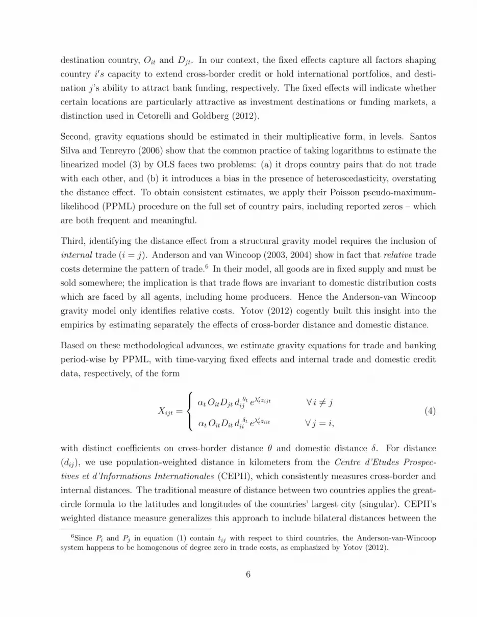
The distance puzzle is most striking in the traditional least-squares regression, estimated after

log-linearizing the gravity equation (3) with fixed effects as dummy variables (Table 1, upper

panel, column “LSDV”, full sample).11 Over the past 50 years, the magnitude of the estimated

distance effect θ appears to have grown from 0.75 to an implausible 1.77 (in absolute value),

suggesting that physical distance presents a large and growing obstacle to trade. Distance

coefficients typically fall below unity when estimated by PPML, and this is the case here too

(column “PPML”, full sample). The estimates closer to −1 are in line with a vast literature

10There were monetary restrictions on trade among European nations before 1959. Once foreign-exchangemarkets re-opened in 1959, with the major currencies fully convertible for current-account transactions, theBretton Woods System came into full operation (Eichengreen, 1996, p. 114).

11We follow Yotov’s (2012) naming convention here, even though the term LSDV is more commonly used inpanel settings.

8

comprising more than 2,500 estimates of the distance effect in trade (Head and Mayer, 2014).

The magnitude implies that a nation trades with a close-by country nearly twice as much as

with a similar country located at twice the distance. Importantly, the upward trend in the size

of the distance effect persists under both estimation methods – and contradicts the view that

globalization should diminish the role of distance over time (Figure 1, left panels).

Table 1: The distance effect in trade - main results

Point estimates of distance coefficients

Method: LSDV PPML PPML PPML

Sample: Full sample Full sample Intensive margin Matched sample

Traditional specification (θt)

Distance, 1960 -0.748*** (0.029) -0.720*** (0.053) -0.705*** (0.054)

Distance, 1980 -1.350*** (0.028) -0.811*** (0.033) -0.847*** (0.037) -0.869*** (0.037)

Distance, 1995 -1.492*** (0.024) -0.796*** (0.028) -0.810*** (0.032) -0.794*** (0.029)

Distance, 2005 -1.701*** (0.024) -0.901*** (0.027) -0.894*** (0.033) -0.886*** (0.028)

Distance, 2012 -1.769*** (0.026) -0.856*** (0.034) -0.839*** (0.041) -0.857*** (0.038)

Delta distance -1.021*** (0.039) -0.136** (0.063) -0.134** (0.067) 0.012 (0.053)

Relative specification (θt − δt)Relative distance, 1960 -1.026*** (0.033) -0.667*** (0.026) -0.667*** (0.027)

Relative distance, 1980 -0.896*** (0.041) -0.553*** (0.020) -0.522*** (0.019) -0.523*** (0.019)




Delta relative distance 0.305*** (0.061) 0.252*** (0.032) 0.235*** (0.033) 0.100** (0.028)

Note: Table 1 reports point estimates of the distance effect in trade for specific years, with robust standard errors in separatecolumns. Full results are in Appendix B1-B4. The traditional specification (upper panel) is contrasted with Yotov’s (2012)relative specification (lower panel) which includes ’internal trade’ (see equation (4)). The first column (LSDV) employs least-squares estimation with fixed effects. The remainder are Poisson pseudo-maximum likelihood (PPML) estimates. Regardingsamples, column ’Full sample’ shows results for all reported country pairs; the ’Intensive margin’ sample contains only thosecountry pairs linked through trade already in 1960, ignoring new linkages; and ’Matched sample’ includes those country pairslinked through both trade and banking. The final row tests the difference between the last and the first coefficient estimates(Wald-test); a positive significant result is evidence of a decline in the role of distance. Significance levels are marked as: * 10%,** 5%, *** 1%.

Yotov (2012) sheds new light on the trend puzzle by estimating separately the effects of cross-

border distance θ and domestic distance δ, as set out in equation (4).12 Applied to our sample,

the size of the relative distance effect (θ − δ) now falls over time, both for LSDV and PPML

(Table 1, lower panel, full sample columns). This replicates Yotov’s result that the effect of

international distance has been declining relative to that of domestic distance (Figure 1, right

12Bergstrand, Larch and Yotov (2015) propose yet an alternative specification that includes country-pair fixedeffects, to estimate the decline in the distance effect over time relative to a base period.

9

panels). What follows focuses on PPML estimates, which are preferable for methodological

reasons.13

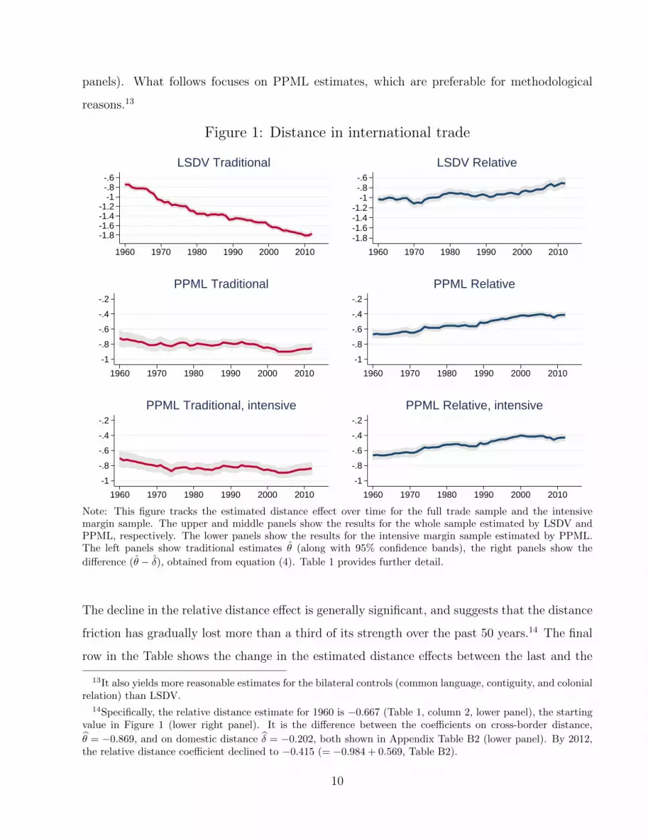
Figure 1: Distance in international trade

-1.8-1.6-1.4-1.2

-1-.8-.6

1960 1970 1980 1990 2000 2010

LSDV Traditional

-1.8-1.6-1.4-1.2

-1-.8-.6

1960 1970 1980 1990 2000 2010

LSDV Relative

-1

-.8

-.6

-.4

-.2

1960 1970 1980 1990 2000 2010

PPML Traditional

-1

-.8

-.6

-.4

-.2

1960 1970 1980 1990 2000 2010

PPML Relative

-1

-.8

-.6

-.4

-.2

1960 1970 1980 1990 2000 2010

PPML Traditional, intensive

-1

-.8

-.6

-.4

-.2

1960 1970 1980 1990 2000 2010

PPML Relative, intensive

Note: This figure tracks the estimated distance effect over time for the full trade sample and the intensivemargin sample. The upper and middle panels show the results for the whole sample estimated by LSDV andPPML, respectively. The lower panels show the results for the intensive margin sample estimated by PPML.The left panels show traditional estimates θ (along with 95% confidence bands), the right panels show the

difference (θ − δ), obtained from equation (4). Table 1 provides further detail.

The decline in the relative distance effect is generally significant, and suggests that the distance

friction has gradually lost more than a third of its strength over the past 50 years.14 The final

row in the Table shows the change in the estimated distance effects between the last and the

13It also yields more reasonable estimates for the bilateral controls (common language, contiguity, and colonialrelation) than LSDV.

14Specifically, the relative distance estimate for 1960 is −0.667 (Table 1, column 2, lower panel), the startingvalue in Figure 1 (lower right panel). It is the difference between the coefficients on cross-border distance,

θ = −0.869, and on domestic distance δ = −0.202, both shown in Appendix Table B2 (lower panel). By 2012,the relative distance coefficient declined to −0.415 (= −0.984 + 0.569, Table B2).

10

first estimates, and tests the difference by means of a Wald test (row marked “Delta relative

distance”). A positive significant result is evidence that the distance effect turned less negative

over time. This is also consistent with tight confidence bands around the distance effects in

Figure 1. The finding supports a view of globalization that sees integration proceed faster in

international than in domestic markets, with external trade costs falling relative to domestic

distribution costs.

This still begs the question why the level estimate θ apparently rose even as transport costs and

trade barriers have been declining over time (see Appendix B2). One might dismiss the level

estimates, since the structural gravity model (if valid) only identifies the relative distance effect

(θ − δ). However, the puzzle has given rise to interesting testable hypotheses in the literature.

One is that of a compositional effect between the intensive margin (more trade between old

trade partners) and the extensive margin (new trade linkages). Lin and Sim (2012) show

that most of the trade expansion between 1970 and 1995 took place between countries already

trading before 1970 (intensive margin); at the same time, new trade links (extensive margin) are

forged at longer distances and smaller trade volumes than the prevailing global average. They

conjecture (but do not test) that the emergence of new long-distance links trading small volumes

accentuates the measured distance effect, producing larger estimates θ in yearly regressions.

To test this conjecture, we switch off the extensive margin at the country level by restricting

the sample to those country pairs that were already connected in 1960 (“Intensive margin” in

Table 1 and Figure 1). On the intensive margin alone, the distance puzzle is still present in the

traditional specification (Figure 1, bottom left panel), suggesting that trade volumes often grew

more between countries closer to each other than the median trade partner. Hence the puzzle

is not an artifact of sample composition, and is again absent for relative distance (Figure 1,

bottom right panel).15 While compositional effects contribute to the empirical distance puzzle,

its resolution nonetheless hinges on the relation between international and domestic trade.

15An analogous experiment focusing on the extensive margin yields a similar conclusion. We allow for anexpanding number of international linkages, but switch off the intensive margin by holding the volume of tradeconstant at the first reported value. Early in the sample, the distance puzzle appears again in levels, not indifferences. We do not report the result here, since the experiment does not fully isolate the extensive margin;however, a dataset focusing only on new linkages is too sparse for meaningful comparison.

11

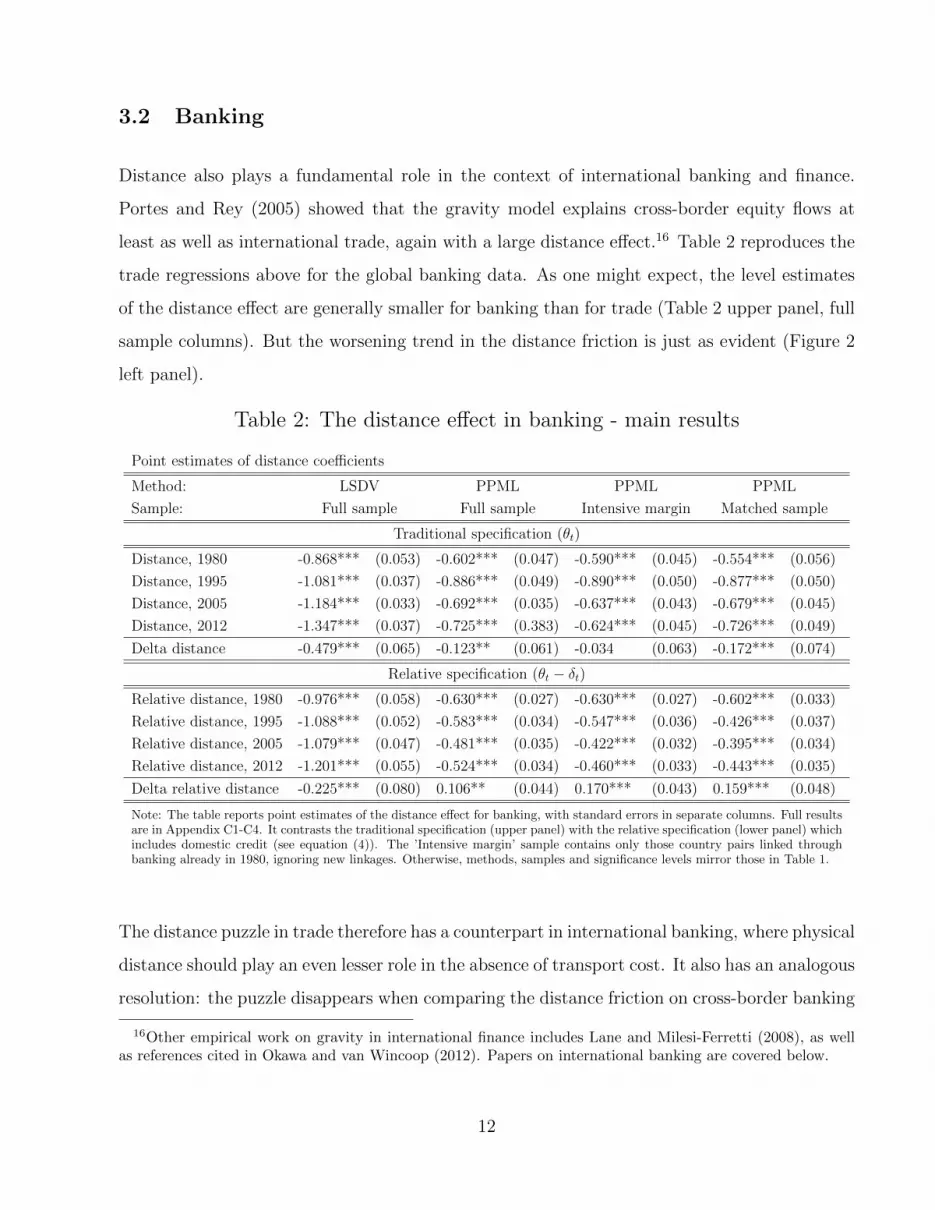
3.2 Banking

Distance also plays a fundamental role in the context of international banking and finance.

Portes and Rey (2005) showed that the gravity model explains cross-border equity flows at

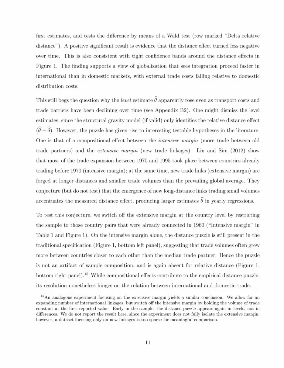
least as well as international trade, again with a large distance effect.16 Table 2 reproduces the

trade regressions above for the global banking data. As one might expect, the level estimates

of the distance effect are generally smaller for banking than for trade (Table 2 upper panel, full

sample columns). But the worsening trend in the distance friction is just as evident (Figure 2

left panel).

Table 2: The distance effect in banking - main results


Method: LSDV PPML PPML PPML

Sample: Full sample Full sample Intensive margin Matched sample


Distance, 1980 -0.868*** (0.053) -0.602*** (0.047) -0.590*** (0.045) -0.554*** (0.056)

Distance, 1995 -1.081*** (0.037) -0.886*** (0.049) -0.890*** (0.050) -0.877*** (0.050)

Distance, 2005 -1.184*** (0.033) -0.692*** (0.035) -0.637*** (0.043) -0.679*** (0.045)

Distance, 2012 -1.347*** (0.037) -0.725*** (0.383) -0.624*** (0.045) -0.726*** (0.049)

Delta distance -0.479*** (0.065) -0.123** (0.061) -0.034 (0.063) -0.172*** (0.074)

Relative specification (θt − δt)Relative distance, 1980 -0.976*** (0.058) -0.630*** (0.027) -0.630*** (0.027) -0.602*** (0.033)




Delta relative distance -0.225*** (0.080) 0.106** (0.044) 0.170*** (0.043) 0.159*** (0.048)

Note: The table reports point estimates of the distance effect for banking, with standard errors in separate columns. Full resultsare in Appendix C1-C4. It contrasts the traditional specification (upper panel) with the relative specification (lower panel) whichincludes domestic credit (see equation (4)). The ’Intensive margin’ sample contains only those country pairs linked throughbanking already in 1980, ignoring new linkages. Otherwise, methods, samples and significance levels mirror those in Table 1.

The distance puzzle in trade therefore has a counterpart in international banking, where physical

distance should play an even lesser role in the absence of transport cost. It also has an analogous

resolution: the puzzle disappears when comparing the distance friction on cross-border banking

16Other empirical work on gravity in international finance includes Lane and Milesi-Ferretti (2008), as wellas references cited in Okawa and van Wincoop (2012). Papers on international banking are covered below.

12

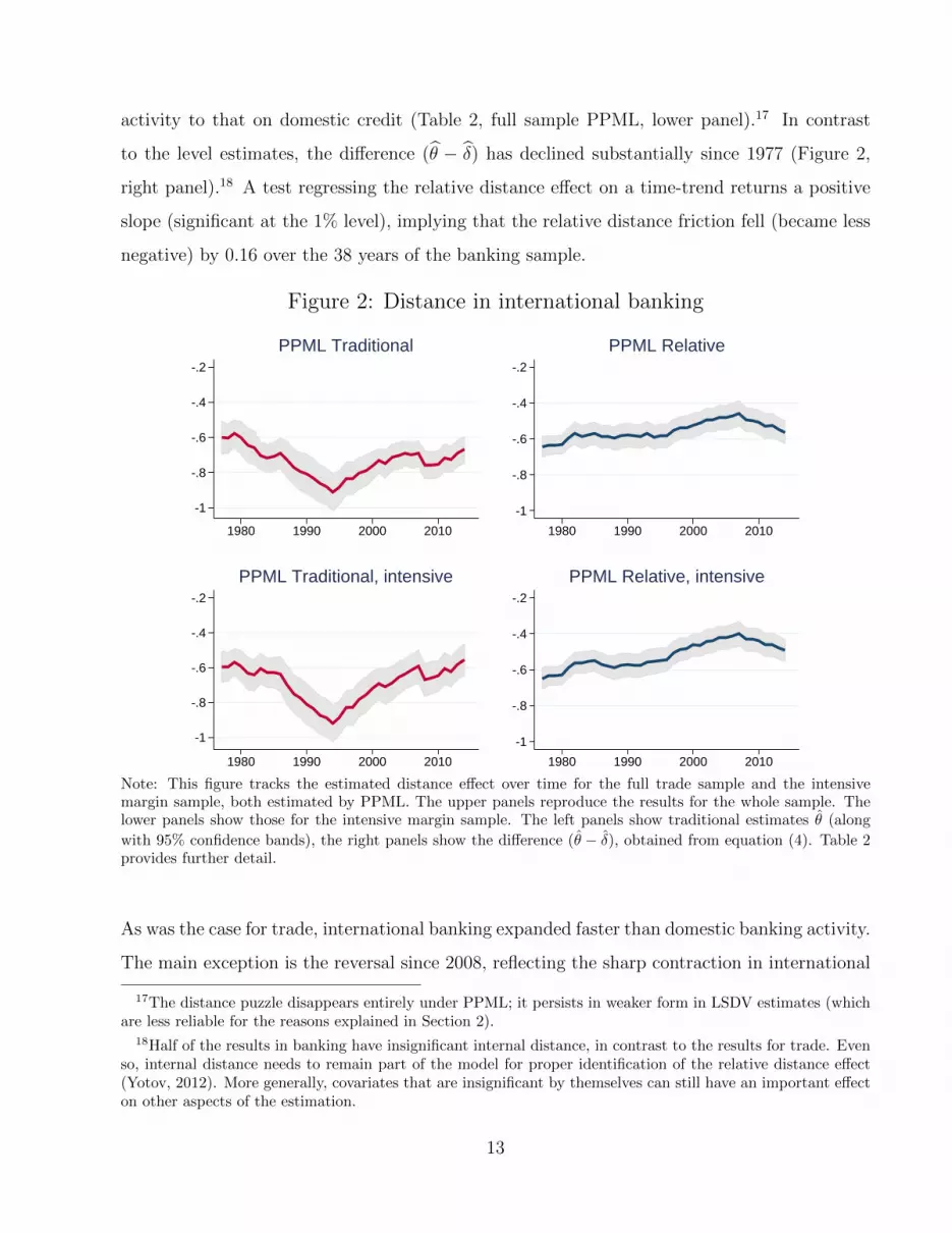
activity to that on domestic credit (Table 2, full sample PPML, lower panel).17 In contrast

to the level estimates, the difference (θ − δ) has declined substantially since 1977 (Figure 2,

right panel).18 A test regressing the relative distance effect on a time-trend returns a positive

slope (significant at the 1% level), implying that the relative distance friction fell (became less

negative) by 0.16 over the 38 years of the banking sample.

Figure 2: Distance in international banking

-1

-.8

-.6

-.4

-.2

1980 1990 2000 2010

PPML Traditional

-1

-.8

-.6

-.4

-.2

1980 1990 2000 2010

PPML Relative

-1

-.8

-.6

-.4

-.2

1980 1990 2000 2010

PPML Traditional, intensive

-1

-.8

-.6

-.4

-.2

1980 1990 2000 2010

PPML Relative, intensive

Note: This figure tracks the estimated distance effect over time for the full trade sample and the intensivemargin sample, both estimated by PPML. The upper panels reproduce the results for the whole sample. Thelower panels show those for the intensive margin sample. The left panels show traditional estimates θ (along

with 95% confidence bands), the right panels show the difference (θ − δ), obtained from equation (4). Table 2provides further detail.

As was the case for trade, international banking expanded faster than domestic banking activity.

The main exception is the reversal since 2008, reflecting the sharp contraction in international

17The distance puzzle disappears entirely under PPML; it persists in weaker form in LSDV estimates (whichare less reliable for the reasons explained in Section 2).

18Half of the results in banking have insignificant internal distance, in contrast to the results for trade. Evenso, internal distance needs to remain part of the model for proper identification of the relative distance effect(Yotov, 2012). More generally, covariates that are insignificant by themselves can still have an important effecton other aspects of the estimation.

13

banking activity in the wake of the global financial crisis (McGuire and von Peter, 2012, 2016).

But the secular decline in the relative distance friction since 1980 is broadly in line with trends

in globalization and financial liberalization since the 1970s.

The results are similar when offshore centres, tax havens and small financial centres are excluded

(Table 3, and Appendix Table D1). Doing so is common in the literature – either for lack of

data or because they are intermediaries rather than sources or destinations for international

investment (Lane and Milesi-Ferretti, 2008). Removing credit to, from and between these

jurisdictions results in a loss of thousands of observations per year (leaving 10,150 for 2012).

Yet the results mirror the full-sample findings: (1) the level estimates show the distance puzzle,

(2) the distance puzzle disappears through the inclusion of internal distance (which also has a

significantly negative effect), and (3) the relative distance effect shows a secular decline before

edging up after the global financial crisis.

These results can be compared with earlier studies on international banking. However, these

were somewhat limited in their methods and data availability, and did not focus on the role of

distance over time – with the exception of Buch (2005). Using a small sample drawn from the

BIS Locational Banking Statistics, Buch (2005) estimates the distance effect θ to be −0.7 (using

LSDV), with no trend between 1983 and 1999.19 Bruggemann et al. (2014) test their theory

for the years 2003-06 on a larger sample (about 20% the size of ours per year), and find point

estimates near −0.75 (LSDV) and −0.26 (PPML), well below the size of ours. In a study with

better coverage for 1984-2002, Papaioannou (2009) regresses bank flows on gravity variables

and obtains estimates between −0.82 and −1.13 (LSDV), without the use of country-time fixed

effects or PPML.20 None of these papers include domestic credit for estimating relative distance

effects, nor work with a country-to-country dataset.

As was the case for trade, the distance puzzle and its resolution can be observed even for the

intensive margin alone (“Intensive margin” in Table 2 and Figure 2). The global banking dataset

19The sample available to Buch (2005) was 20 years shorter, and contained the bilateral bank positions offive advanced economies.

20We do not attempt a comparison with studies using the BIS Consolidated Banking Statistics, including Roseand Spiegel (2004), Aviat and Coeurdacier (2007), Coeurdacier and Martin (2009), or Houston, Lin and Ma(2012). Houston, Lin and Ma (2012), for instance, find implausible distance effects exceeding 1.5 in magnitude.

14

expands substantially over time, due to both greater financial integration and better reporting

coverage.21 This compositional effect tends to strengthen the measured distance effect: as more

distant country pairs with small international bank linkages enter the sample, the distance

friction appears to become worse. We remove the extensive margin by restricting the banking

sample to those country pairs already connected through banking in 1980 (Appendix Table C3,

and Figure 2 bottom panels).22 Estimating the distance effect on this subsample shows the

same pattern: the distance puzzle in the traditional regression (left panel) and its resolution

in the relative distance effect (θ− δ) (right panel). International banking expanded more than

domestic banking, even among the financially advanced countries already integrated at the

onset of financial liberalization.

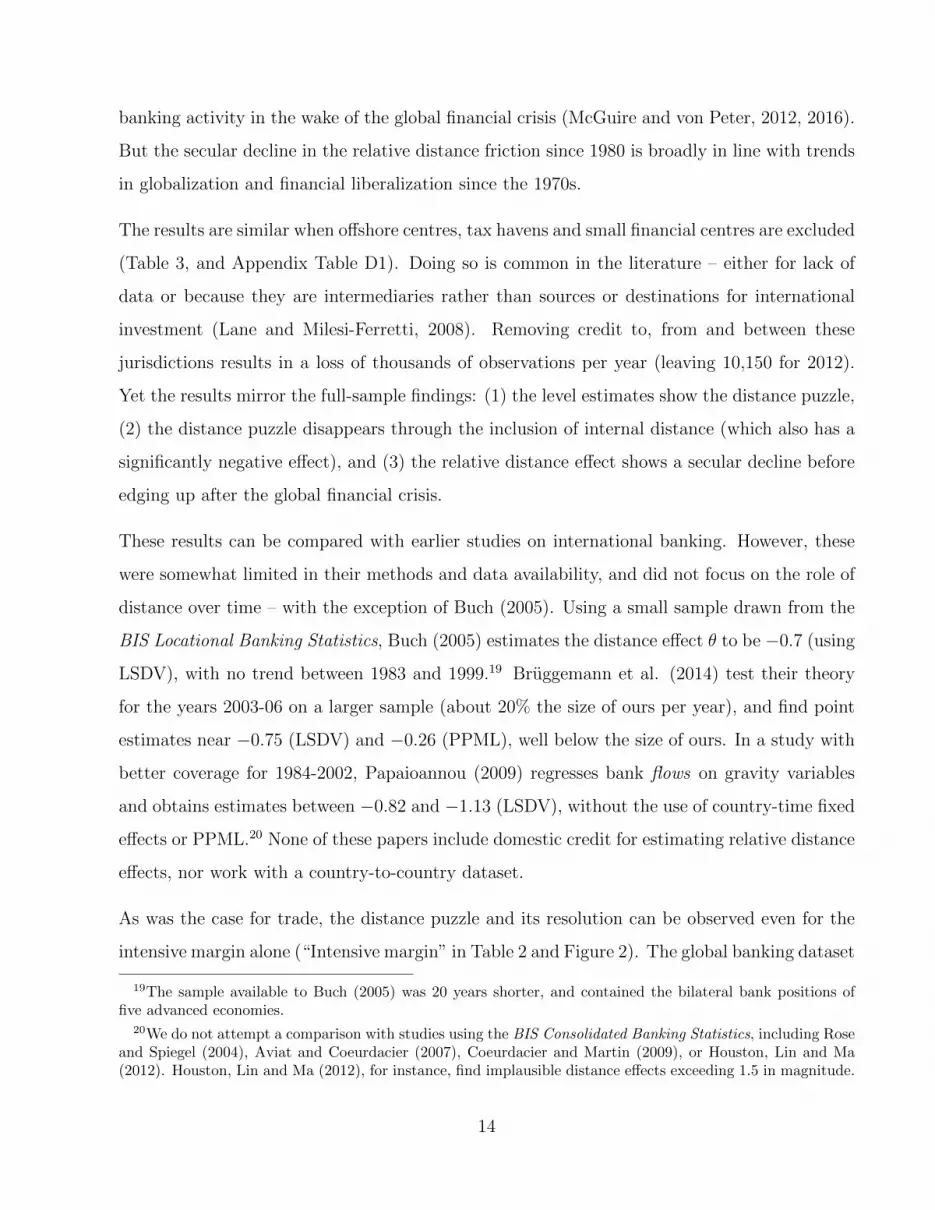
In sum, in both trade and banking the findings are in line with facts of globalization, when

setting cross-border transactions against domestic activity to focus on the role of distance in

relative terms. Even so, in both cases the effect of distance remains fairly large, even in relative

terms. To compare the distance effect across trade and banking, we construct a matched sample

that includes only country pairs that were linked through both trade and banking (Figure 3,

based on “Matched sample” columns in Tables 1-2). The resulting trade and banking samples

are identical in coverage, and the number of observations expands in lockstep year by year from

1980 onward.23 The level estimate of the distance effect is larger for trade than for banking,

perhaps because trade is subject to transport and information costs (Figure 3, left panels).

More importantly, by 2012 the relative distance effect is near −0.4 for both trade and banking,

or about −0.5 over the sample on average. This magnitude suggests that a doubling of distance

curbs international trade and bank credit by nearly 30% (2−0.5 = 0.7) more than would be the

case in a domestic context.24

21See the number of observations in Table C2, and Figure 5, upper panel.22In the construction of the banking network, we distinguish between missing (unreported) positions and

true (reported) zeros (see Appendix A). Even so, the growing number of active links in the sample representsboth newly forged links (zeros turning positive) and newly reported links (unreported turning positive). Theexperiment focusing on the intensive margin switches off both effects.

23For full results, see Tables B4 for trade and C4 for banking. In the trade network, the matching drops fromthe sample smaller country pairs that are not (reported to be) connected through international banking. In thebanking network, the matching mainly drops the links with, and between, offshore financial centers that areabsent from trade data.

24An exact comparison is complicated by the interaction of border effects and other bilateral factors with

15

The matched sample results suggest that the magnitude of the relative distance friction remains

economically significant in both trade and banking (Figure 3, right panels). This is remarkable,

especially in the case of international banking where transport costs do not apply. Indeed,

one might expect investors to tilt their portfolios towards more distant countries whose asset

returns may be less correlated with domestic returns (Portes and Rey, 2005). The common

finding between trade and banking may well point to a common cause.

Figure 3: Distance in trade and banking - matched samples

-1

-.8

-.6

-.4

-.2

1980 1990 2000 2010

Trade, PPML Traditional

-1

-.8

-.6

-.4

-.2

1980 1990 2000 2010

Trade, PPML Relative

-1

-.8

-.6

-.4

-.2

1980 1990 2000 2010

Banking, PPML Traditional

-1

-.8

-.6

-.4

-.2

1980 1990 2000 2010

Banking, PPML Relative

Note: The figure tracks the estimated distance effect over time (using PPML) for the matched sample whichincludes only those country pairs linked through both trade and banking. The left panels show traditionalestimates θ (along with 95% confidence bands), the right panels show the difference (θ − δ), obtained fromequation (4). Tables 1 and 2 provide further detail.

the country fixed effects. The comparison holds for country pairs that share no common language, border orcolonial past. Those bilateral variables are set to zero in the estimation of the internal distance effect, followingYotov (2012).

16

3.3 Does the distance effect represent information frictions?

Recent papers in the trade literature (cited in Section 2.2) stress the role of information frictions,

quite independently of physical transport cost. This is also an important aspect in global value

chains (GVCs). Globalization is associated with the fragmentation, unbundling and offshoring

of production, and as the frictions inherent in these activities subside, the volume of trade

increases (Baldwin and Venables, 2013). The presence of informational frictions thus limits the

proliferation of GVCs and presents an impediment to trade across great distances. As such,

evidence of frictions in GVCs go hand in hand with the continued magnitude of the distance

effect well beyond transport cost.

One can draw a parallel between GVCs in trade and financial intermediation in banking. Along

the GVC, goods are moved between countries for parts, assembly, and shipping via entrepots

at the different stages of production and distribution. Similarly, it is through international

intermediation in financial centres that financial claims are bundled or transformed across in-

struments, currencies and maturities. The sheer volume of financial flows to, from and between

financial centres underlines their importance in global capital flows. As intermediation involves

frictions at various stages, informational costs also limit the extent of international intermedi-

ation, as was the case for GVCs, and thus help explain the observed distance effects.

To close this section, we run three experiments to shed light on the interpretation of distance as

an informational friction. Buch (2005) discusses the distance as a proxy for information costs in

international banking, and Portes and Rey (2005) consider information-related variables (e.g.

the volume of telephone traffic) in their analysis of equity flows between 14 countries. Unfortu-

nately, data limitations preclude thorough testing for information variables in our sample (200

countries forming 15,000 pairs) going back to the 1980s. We instead devise three regressions to

provide indirect evidence for the information hypothesis. The estimates of distance effects are

summarized in Table 3, and full results shown Appendix Tables D2-D4.

17

Table 3: Robustness and information-related results


Method: PPML PPML PPML PPML

Test: No OFC Non-banks Branch/subsidiary Time zones


Distance, 1980 -0.493*** (0.062) -0.515*** (0.093) -0.572*** (0.053) -0.287*** (0.083)

Distance, 1995 -0.597*** (0.057) -0.869*** (0.080) -0.880*** (0.057) -0.397*** (0.093)

Distance, 2005 -0.537*** (0.058) -0.570*** (0.044) -0.653*** (0.039) -0.506*** (0.073)

Distance, 2012 -0.629*** (0.061) -0.641*** (0.046) -0.669*** (0.038) -0.604*** (0.066)

Delta distance -0.136 (0.087) -0.126 (0.104) -0.097 (0.065) -0.317*** (0.106)

Relative specification (θt − δt)Relative distance, 1980 -0.590*** (0.036) -0.817*** (0.031) -0.781*** (0.030) -0.748*** (0.025)




Delta relative distance 0.136** (0.053) 0.144*** (0.052) -0.020 (0.046) 0.136*** (0.041)

Note: The table reports point estimates of the distance effect for banking, with robust standard errors in separate columns (fullresults are in Appendix Tables D1-D4). The ”No OFC” robustness test excludes offshore centers, tax havens and small financialcentres; ”Non-banks” uses non-bank cross-border positions; ”Branch/subsidiary” includes an indicator variable for the presenceof branches and subsidiaries as an additional regressor; ”Time zones” includes 12 time-zone dummy variables as additionalregressors.

If the distance effect relates to information, it should be stronger for more information-sensitive

forms of credit. To test this conjecture, we split international positions by sector to distinguish

interbank lending from credit extended to non-banks, which includes corporates and non-

bank financials. Credit extended directly to non-bank borrowers, especially when located in

other countries, is more information-sensitive than lending to banks – which includes intra-

group transfers to affiliates where no information asymmetries arise. In line with this view,

the distance effect for the non-bank sample (Table D2) is some 0.15 units larger than the

corresponding estimate from the all-sectors sample (Table C2). The relative distance friction

again shows a secular decline (-0.82 to -0.65) before edging up after the global financial crisis.

Information-sensitive lending thus goes hand in hand with stronger distance effects.

Similarly, if information frictions matter, lending should be greater when banks have better

access to information on foreign markets. We condition the amount of credit extended from

country i to country j on whether banks from i have branches or subsidiaries operating

in country j. The input is a matrix of branches and subsidiaries by nationality and location,

18

extracted from the 2015 list of bank offices that report the BIS Locational Banking Statistics.

The presence of affiliates abroad enters with a large positive coefficient, highly significant every

year (Table D3). At the same time, the relative distance friction remains nearly constant around

0.78, while the affiliate dummy offsets part of the distance effect. Having a presence abroad

promotes cross-border credit to that market. It is plausible that foreign affiliates relay local

knowledge back home, allowing the bank’s headquarters to extend more cross-border credit to

the destination country, either by funding their local affiliate through intragroup loans, or by

taking direct exposure to the borrower in the destination country, in the form of bond-holding

or cross-border lending.25

A final experiment tests the significance of time zones, or distance across longitudes. Time

differences complicate the exchange of information during working hours.26 The most general

specification allows for 12 distinct dummies each year, one for each hour time difference. These

estimates consistently show that larger time differences have more negative effects on the stock

of cross-border credit.27 Most time zone effects share a common time profile that mirrors the

broader globalization trend. The inclusion of time zones weakens the estimated distance effect

in Table D4, suggesting that they pick up a key aspect of why distance hampers international

finance. This extends the findings of Egger and Larch (2013) who document that time zone

differences act as trade barriers in a sample of trade between US states and Canadian provinces.

Taken together, these experiments strengthen the argument that distance effects have to do

with informational frictions. Due to data limitations, a fuller treatment using information-

related variables is left to future research. The remainder of the paper explores other, less

prominent, parts of the gravity framework for evidence of globalization.

25Our network of cross-border positions covers four possibilities through which this can occur: direct bondholdings or credit to non-banks, intragroup transfers, and interbank lending to a borrower’s bank in the desti-nation country (see Appendix A).

26For instance, trading hours in New York and Tokyo are disjoint, but both financial centres have some hoursoverlap with London.

27Table D4 shows the regression excluding domestic credit, because most countries are within a single timezone.

19

4 Where else does globalization appear?

To understand how falling distance costs and other global trends affect the patterns of interna-

tional trade and banking, it is helpful to step back and reassess current practice. There is no

reason to expect the forces of globalization to concentrate on the distance coefficient alone. We

now depart from this singular focus and broaden the view to lesser-noted parts of the gravity

framework. Figures 4-5 illustrate some of the new results.

We can think of the gravity model as decomposing total variation in bilateral transaction

volumes into three levels: a global component, country-specific factors, and bilateral effects.

Our measure of the global component, At, is the regression constant αt augmented by the means

of the country-time fixed effects Oit and Djt in each period.28 This ensures that the global

component relates to the overall scale of banking or trade, leaving country-specific factors to

the centered fixed effects oit and djt. With this normalization, the estimated coefficients should

reflect globalization trends as follows:

1. The global component, At, scales all bilateral positions every period. Developments that

are global in scope should be reflected at this level.

2. Country-specific factors, oit and djt, absorb all characteristics shaping a country’s overall

capacity to engage in trade or banking, relative to others. Developments taking place in

multiple jurisdictions raise Oit and Djt of many countries simultaneously, and will affect

the global component At more than the (demeaned) country-specific factors oit and djt.

3. The bilateral coefficients, θt, δt and vector λt, capture country-pair-specific variation,

since all other variation is swept out by time-varying country fixed effects.

This simple classification helps to broaden the view for where distance-related effects could

show up in the gravity framework. First, suppose that transport and information costs become

less sensitive to distance, i.e. ρ in equation (2) declines. This alters the patterns of trade

28The regression constant is identified by normalizing the first (or any other) instance of the fixed effects tozero.

20

and banking, because it affects pairs of countries differentially (according to their relative

remoteness from trade partners). A lower sensitivity favors long-distance transactions more

than short-distance transactions: the former fall more rapidly than short-distance costs – until

the eventual “death of distance” as ρ → 0.29 Empirically, such a trend reduces the measured

difference between long- and short-distance costs, in line with the evidence above on the distance

coefficient in trade and banking.

However, what if transport and information costs became uniformly cheaper? This channel is

just as plausible in view of falling shipment and telecommunication costs. When the cost per

unit of distance falls to a fraction τ < 1, the cost function (2) delivers a proportional reduction

of the original costs, from tij(τd) to τ ρtij(d) – as if the world literally “got smaller” through

shrinkage.30 This result holds for any distance d, and consequently does not favor longer over

shorter distances, or international over domestic markets. Any expansion in trade or banking

should therefore raise bilateral transaction volumes proportionately – and thus appear in the

global component At, not in the distance effect.31

Another driver of globalization has been the common pace of liberalization since the 1980s, in

areas ranging from trade agreements to financial deregulation. The effects will again appear at

various levels of the gravity framework: if a policy change opens a single country j to foreign

investors, the fixed effect Djt (and djt) shifts up in line with the country’s increased attrac-

tiveness as a destination. If all countries liberalize, however, then j′s relative attractiveness

djt remains unchanged because Djt increases in all countries, raising the global component

29Consider an arbitrary country pair ij at a short distance dij = d from each other, and another pair ntimes further apart, with n > 1. The cost function for the short distance is t(d) = dρβ, where β representsother bilateral factors (held constant) in equation (2). The long-distance cost t+ = t(nd) = t(d)nρ, withρ ≤ 1 as transport costs are plausibly no more than proportional to distance (Anderson van Wincoop, 2004).Suppose globalization reduces the sensitivity ρ from 1 initially to k < 1. Hence, in period 0 it was n timesas costly to transport goods (or communicate) over a distance n times as far, but in period 1 doing so isonly nk times as costly

(t+1 /t1 = nk < n = t+0 /t0

). Equivalently, in the pre/post comparison, the short-distance

cost falls to a fraction t1/t0 = dk−1 < 1 of the previous cost. But long-distance costs fall even further, tot+1 /t

+0 = (nd)k−1 < t1/t0 < 1.

30In the example of the previous footnote, the cost function goes from t(d) = dρβ to t(d) = (dτ)ρβ, withlong-distance costs correspondingly t+ = (ndτ)ρβ. The ratio of long- to short-distance costs remains t+/t = nρ,regardless of τ . Both short- and long-distance costs fall to a fraction τρ of their previous costs.

31This point was recognized by Buch, Kleinert, and Toubal (2004), who showed by example that a proportionalfall in distance costs does not show up in the distance effect but in the constant. Our use of fixed effects weedsout country-specific factors and helps give the constant a clearer interpretation.

21

At instead. Trade creation through bilateral agreements or monetary unions, on the other

hand, works through the variables λ′tzijt in (4): by reducing bilateral frictions, such agreements

enhance trade and banking between two countries in a way similar to a common language.32

What these thought experiments make clear is that the effects of distance – and of globalization

more broadly – are not confined to the distance coefficient alone. Transport and information

cost savings, as well as broader developments, may manifest themselves in other, less prominent

parts of the gravity framework – notably in the global component, as well as in the extensive

margin: as trade and banking with remote countries becomes viable, the number of pairs with

direct trade or bank linkages (Xijt > 0) increases. The remainder of the paper provides evidence

on these two fronts.

First, for the past decades, the estimated global component shows rapid growth in both trade and

banking (Figure 4). This is consistent with a (proportional) decline in distance costs over time,

and with other global developments boosting the scale of trade and banking.33 The common

pace of economic and financial liberalization, and the proliferation of trade agreements and

currency unions around the world, surely contributed to the secular rise in the overall volume

of trade and banking. Financial factors, such as global liquidity and risk appetite, have further

contributed to the expansion of international banking activity in the past decade.

32The appendix tables show detailed results, comprising the bilateral factors included in all regressions.33There is a theoretical issue on whether distance can affect the overall scale of trade in the Anderson-van

Wincoop model. As explained, their model only identifies relative costs, as goods are in fixed supply andtrade flows invariant to domestic distribution costs. However, in the gravity-in-finance model of Okawa andvan Wincoop (2012), the invariance to domestic costs no longer holds due to the presence of safe assets. Moregenerally, relaxing the assumptions that separate production and trade patterns allows for an overall expansionof trade in goods and assets as costs fall. Hence, a general decline in tij can affect the overall volume of tradevia the global component At, even when relegating the multilateral resistance terms to fixed effects.

22

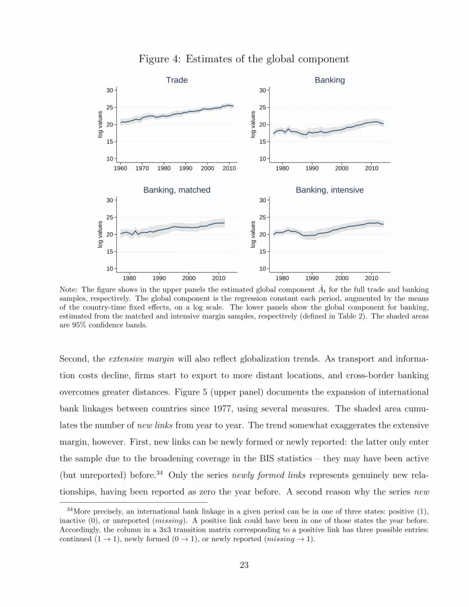
Figure 4: Estimates of the global component

10

15

20

25

30

log

valu

es

1960 1970 1980 1990 2000 2010

Trade

10

15

20

25

30

log

valu

es

1980 1990 2000 2010

Banking

10

15

20

25

30

log

valu

es

1980 1990 2000 2010

Banking, matched

10

15

20

25

30

log

valu

es

1980 1990 2000 2010

Banking, intensive

Note: The figure shows in the upper panels the estimated global component At for the full trade and bankingsamples, respectively. The global component is the regression constant each period, augmented by the meansof the country-time fixed effects, on a log scale. The lower panels show the global component for banking,estimated from the matched and intensive margin samples, respectively (defined in Table 2). The shaded areasare 95% confidence bands.

Second, the extensive margin will also reflect globalization trends. As transport and informa-

tion costs decline, firms start to export to more distant locations, and cross-border banking

overcomes greater distances. Figure 5 (upper panel) documents the expansion of international

bank linkages between countries since 1977, using several measures. The shaded area cumu-

lates the number of new links from year to year. The trend somewhat exaggerates the extensive

margin, however. First, new links can be newly formed or newly reported: the latter only enter

the sample due to the broadening coverage in the BIS statistics – they may have been active

(but unreported) before.34 Only the series newly formed links represents genuinely new rela-

tionships, having been reported as zero the year before. A second reason why the series new

34More precisely, an international bank linkage in a given period can be in one of three states: positive (1),inactive (0), or unreported (missing). A positive link could have been in one of those states the year before.Accordingly, the column in a 3x3 transition matrix corresponding to a positive link has three possible entries:continued (1→ 1), newly formed (0→ 1), or newly reported (missing → 1).

23

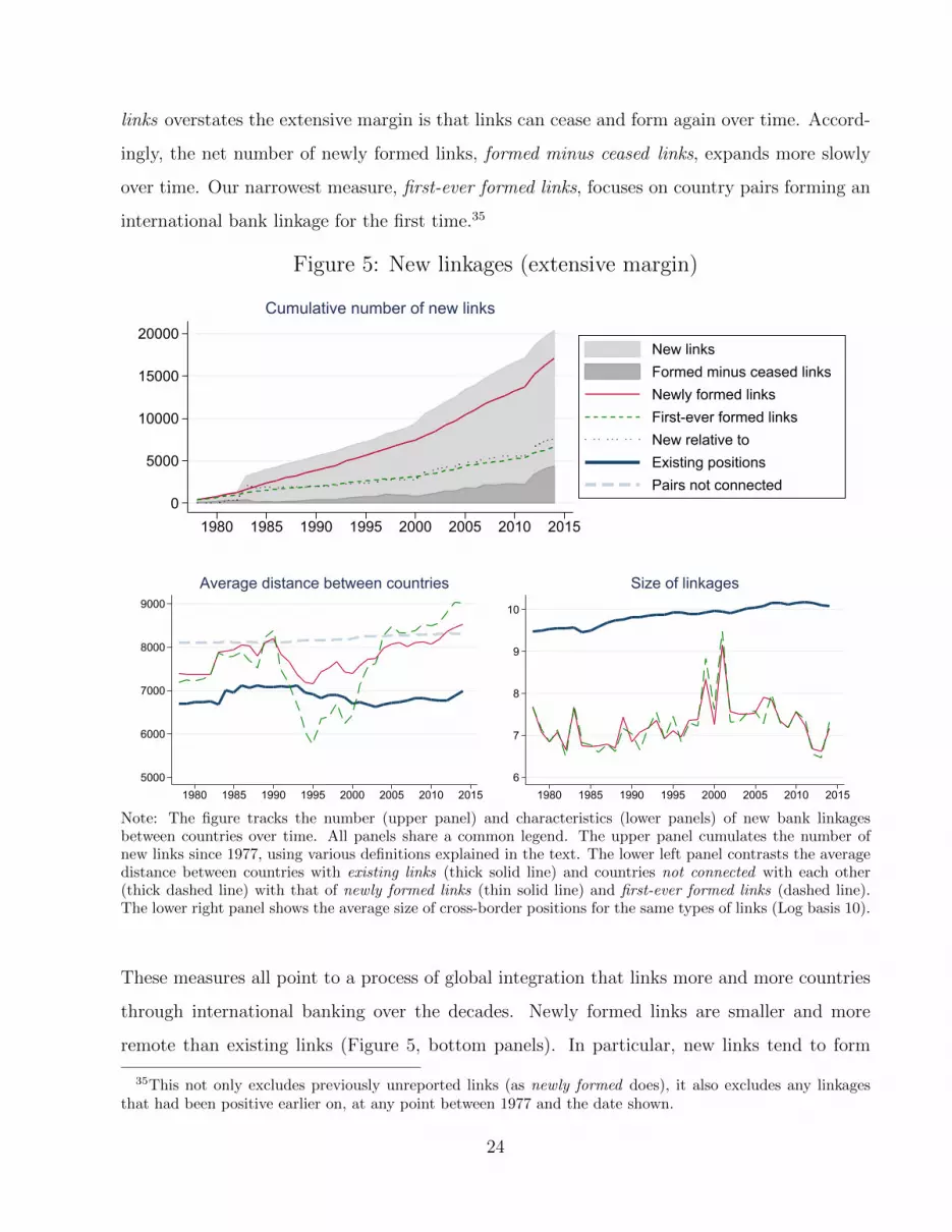
links overstates the extensive margin is that links can cease and form again over time. Accord-

ingly, the net number of newly formed links, formed minus ceased links, expands more slowly

over time. Our narrowest measure, first-ever formed links, focuses on country pairs forming an

international bank linkage for the first time.35

Figure 5: New linkages (extensive margin)

0

5000

10000

15000

20000

1980 1985 1990 1995 2000 2005 2010 2015

New linksFormed minus ceased linksNewly formed linksFirst-ever formed linksNew relative to Existing positionsPairs not connected

Cumulative number of new links

5000

6000

7000

8000

9000

1980 1985 1990 1995 2000 2005 2010 2015

Average distance between countries

6

7

8

9

10

1980 1985 1990 1995 2000 2005 2010 2015

Size of linkages

Note: The figure tracks the number (upper panel) and characteristics (lower panels) of new bank linkagesbetween countries over time. All panels share a common legend. The upper panel cumulates the number ofnew links since 1977, using various definitions explained in the text. The lower left panel contrasts the averagedistance between countries with existing links (thick solid line) and countries not connected with each other(thick dashed line) with that of newly formed links (thin solid line) and first-ever formed links (dashed line).The lower right panel shows the average size of cross-border positions for the same types of links (Log basis 10).

These measures all point to a process of global integration that links more and more countries

through international banking over the decades. Newly formed links are smaller and more

remote than existing links (Figure 5, bottom panels). In particular, new links tend to form

35This not only excludes previously unreported links (as newly formed does), it also excludes any linkagesthat had been positive earlier on, at any point between 1977 and the date shown.

24

between countries more distant from each other than those pairs already connected through

international banking (bottom left panel). The latter feature an average distance of less than

7,000 km between them, whereas new links are formed between countries more than 7,000 km

apart on average. This leaves countries that are not linked through international banking more

than 8,000 km apart.

At the same time, new linkages are smaller in size than existing bank linkages, by orders of

magnitude (Figure 5, bottom right panel). While the size of existing international linkages

averaged $10 billion dollars (1010 on the Log10-scale) over the past two decades, new positions

were on the order of $10 to $100 million dollars.

We have come full circle, in that the regularities highlighted in this section help explain why

gravity regressions produce the distance puzzle in the level estimates in spite of globalization.

The rise in the global component over time accentuates the distance effect as other bilateral

variables λ′tzijt (and the demeaned fixed effects) remain largely constant over time. And on the

extensive margin, the entry of new linkages at longer distances and smaller sizes also enlarges

the measured distance effect – even though both are evidence of the declining role of distance

in a globalizing world.

5 Conclusion

Traditional estimation of gravity models finds an outsized effect of distance on trade volumes,

one that appears to grow over time. This distance puzzle led some observers to quip that

globalization is everywhere but in the gravity model. The results in this paper suggest a more

nuanced view. First, the distance puzzle can be explained and overturned using the relative

specification suggested by Yotov (2012), and our paper extends the same logic and results to

international banking. We estimate gravity equations in trade and banking side by side to

show that the distance puzzle disappears when setting cross-border banking against domestic

banking, using the largest available dataset on global banking.

Second, we show that the effect of falling transport and information costs goes well beyond the

25

estimated distance coefficient. The decline in distance frictions and other forces of globalization

also appear in less prominent parts of the gravity framework, notably in the global component

and in the extensive margin. These findings now resonate with the facts of globalization, both

in trade and banking.

More generally, geographical factors play an important role in international trade and finance as

well. Understanding these factors may help to build synergies between the two fields. Obstfeld

and Rogoff (2001) show, for instance, that trade costs in goods markets are behind many well-

known puzzles in international finance, such as the home bias in equity holdings. In this context

it is an open question how far globalization can go. Geographical distance will remain, so will

some form of transportation cost and time to delivery; and even costless data transfer will not

eliminate soft information asymmetries and cultural differences.

Acknowledgements

We thank Swapan Pradhan and Sebastian Goerlich for sharing expertise on the BIS inter-

national banking statistics, and Mario Morelli, Jhuvesh Sobrun and Agne Subelyte for their

assistance in compiling trade and macroeconomic data. We are also grateful to Thomas Chaney,

Mick Devereux, Thomas Eife, Michael Funke, Galina Hale, Enisse Kharroubi, Catherine Koch,

Gianni Lombardo, Ulf Lewrick, Nuno Limao, Bob McCauley, Pat McGuire, Nikhil Patel, Joao

Santos Silva, Sergio Schmukler, Hyun Song Shin, Yoto Yotov, our discussant Birgit Schmitz

and seminar participants at Hamburg University, at the Infiniti Conference 2016 at Trinity Col-

lege Dublin, and at the Bank for International Settlements, for helpful comments. The views

expressed in this paper are those of the authors and do not represent official positions of the

institutions they are affiliated with.

References

Allen, Treb, 2014. Information frictions in trade. Econometrica 82(6), 2041-2083.

26

Anderson, James, and Eric van Wincoop, 2003. Gravity with gravitas: a solution to the border puzzle.

American Economic Review 93(1), 170–192.

Anderson, James, and Eric van Wincoop, 2004. Trade costs. Journal of Economic Literature 42,

691-751.

Aviat, Antonin and Nicolas Coeurdacier, 2007. The geography of trade in goods and asset holdings.

Journal of International Economics 71, 22–51.

Baldwin, Richard, and Anthony Venables, 2013. Spiders and snakes: Offshoring and agglomeration

in the global economy. Journal of International Economics 90, 245-254.

Baltagi, Badi, Peter Egger and Michael Pfaffermayr, 2003. A generalized design for bilateral trade

flow models. Economics Letters 80, 391-397.

Bergstrand, Jeffrey, Mario Larch, and Yoto Yotov, 2015. Economic integration agreements, border

effects, and distance elasticities in the gravity equation. European Economic Review 78, 307-327.

Bruggemann, Bettina, Jorn Kleinert, and Esteban Prieto, 2014. The ideal loan and the patterns of

cross-border bank lending, Manuscript.

Buch, Claudia, Jorn Kleinert, and Farid Toubal, 2004. The distance puzzle: on the interpretation of

the distance coefficient in gravity equations. Economics Letters 83, 293-298.

Buch, Claudia, 2005. Distance and international banking. Review of International Economics 13(4),

787–804.

Chaney, Thomas (forthcoming). The gravity equation in international trade: an explanation. Journal

of Political Economy.

Chitu, Livia, Barry Eichengreen, and Arnaud Mehl, 2015. History, gravity and international finance.

Journal of International Money and Finance 46, 104-129.

Dasgupta, Kunal, and Jordi Mondria, 2014. Inattentive importers. Manuscript.

Degryse, Hans, and Steven Ongena, 2005. Distance, lending relationships, and competition. Journal

of Finance 60(1), 231-266.

Eaton, Jonathan, and Samuel Kortum, 2002. Technology, geography, and trade. Econometrica 70(5),

1741-1779.

Egger, Peter, and Mario Larch, 2013. Time zone differences as trade barriers. Economics Letters 119,

172-175.

Eichengreen, Barry, 1996. Globalizing capital - a history of the international monetary system. Prince-

ton University Press.

Head, Keith, and Thierry Mayer, 2014. Gravity equations: workhorse, toolkit, and cookbook. In

Gopinath, Helpman, and Rogoff (Eds.) Handbook of International Economics, Vol. 4, Elsevier.

27

Helpman, Elhanan, Marc Melitz, and Yona Rubinstein, 2008. Estimating trade flows: trading partners

and trading volumes. Quarterly Journal of Economics 123(2), 441–487.

Herrmann, Sabine, and Dubravko Mihaljek, 2013. The determinants of cross-border bank flows to

emerging markets. Economics of Transition Volume 21(3), 479508.

Houston, Joel, Chen Lin and Yue Ma, 2012. Regulatory arbitrage and international bank flows.

Journal of Finance 67(5), 1845-1895.

Lane, Philip, and Gian Maria Milesi-Ferretti, 2008. International investment patterns. Review of

Economics and Statistics 90(3), 538–549.

Leamer, Edward, and James Levinsohn, 1995. International trade theory: the evidence. in M.

Grossman and K. Rogoff (ed.), 1995. Handbook of International Economics, Number 3, Elsevier.

Lin, Faqin, and Nicholas Sim, 2012. Death of distance and the distance puzzle. Economics Letters

116, 225-228.

Martin, Philippe, Helene Rey, 2004. Financial super-markets: size matters for asset trade. Journal of

International Economics 64, 335– 361.

Mayer, Thierry, and Soledad Zignago, 2011. Notes on CEPII’s distance measures: the GeoDist

database. Document de Travail No 2011-25.

Retrieved June 2017 from http://www.cepii.fr/CEPII/en/bdd modele/presentation.asp?id=6.

McGuire, Patrick, and Goetz von Peter, 2012. The dollar shortage in global banking and the interna-

tional policy response, International Finance 15(2), 155-78.

McGuire, Patrick, and Goetz von Peter, 2016. The resilience of banks’ international operations. BIS

Quarterly Review, March 2016, 65-78.

Mian, Atif, 2006. Distance constraints: the limits of foreign lending in poor economies. Journal of

Finance 61(3), 1465-1505.

Obstfeld, Maurice, and Kenneth Rogoff, 2001. The six major puzzles in international macroeconomics:

is there a common cause? NBER Macroeconomics Annual 15, 339-412, National Bureau of Economic

Research.

Okawa, Yohei, and Eric van Wincoop, 2012. Gravity in international finance. Journal of International

Economics 87, 205-215.

Papaioannou, Elias, 2009. What drives international financial flows? Journal of Development Eco-

nomics 88, 269-281.

Petersen, M. and Rajan, R., 2002, Does distance still matter? The information revolution in small

business lending, Journal of Finance 57, 2533–2570.

Portes, Richard, and Helene Rey, 2005. The determinants of cross-border equity flows. Journal of

International Economics 65, 269-96.

28

Redding, Stephen, and Anthony Venables, 2004. Economic geography and international inequality,

Journal of International Economics 62, 53-82.

Rose, Andrew, and Mark Spiegel, 2004. A gravity model of sovereign lending: trade, default and

credit, IMF Staff Papers 51, 50-63.

Santos Silva, Joao, and Silvana Tenreyro, 2006. The log of gravity. Review of Economics and Statistics

88, 641–658.

Williamson, John, and Molly Mahar, 1998. A survey of financial liberalization. Essays in International

Finance 211. Princeton, New Jersey.

Yotov, Yoto, 2012. A simple solution to the distance puzzle in international trade. Economics Letters

117, 794-798.

29

Appendices

Appendix A) Constructing the global banking network

Coverage. The global banking dataset in this paper is built from the BIS Locational Banking

Statistics (LBS), the most comprehensive source of information on international banking, avail-

able at quarterly frequency since 1977. The LBS compile the balance sheets of internationally

active banks, along with a geographical breakdown of their counterparties, both aggregated

at the country level. The locational statistics are reported following the residence principle,

consistent with the balance of payments and other national statistics.36 The concentrated na-

ture of global banking means that the LBS attain broad universal coverage, at least in terms of

value. The data contain international assets and liabilities reported by nearly 7,000 banks (sub-

sidiaries and branches) in 44 reporting countries as of 2014, comprising the advanced economies,

emerging markets and the major offshore centers.37 The network construction described in this

appendix delivers a consistent country-to-country network, and alleviates the problem of an

incomplete reporting population at the same time.

Breakdowns. Banks report, on an unconsolidated basis, their international positions: claims

on, and liabilities from, all sectors. “International” refers to all cross-border business, plus

local positions in foreign currencies; in this paper, we only use cross-border positions, alongside

domestic credit from the IMF’s International Financial Statistics. Banks report their gross

assets and liabilities, along with breakdowns by currency, by instrument, and by the sector of the

counterparty they lend to and borrow from. Most importantly, banks in every reporting country

record these positions vis-a-vis residents in 216 countries and jurisdictions. The bilateral nature

of the data thus allows us to construct a coherent network, one that contains all reported

positions intermediated through international banks between origin and destination countries.

Banks-to-country format. The BIS data are collected in the “banks-to-country” format, as

illustrated in Figure A. However, this format in a bilateral setting gives rise to an asymmetric

network: banks in country i lend to banks and all other sectors in another country j (dark blue

arrows). However, it leaves out some bank flows at the country level: deposits that firms place

36Bank offices report their banking activity in the location of their operations, regardless of the nationality(ownership) of the parent bank. For instance, the United Kingdom reports the international bank positionsbooked in its jurisdiction, including those of branches and subsidiaries of German banks operating in theUK. (Conversely, the positions that UK-owned banks book in Germany are reported by Germany.) Reportedpositions are robust to changes in bank ownership following mergers and acquisitions.

37Information on reporting practices, and the current list of reporting countries and institutions are availableat: http://www.bis.org/statistics/count rep practices.htm

30

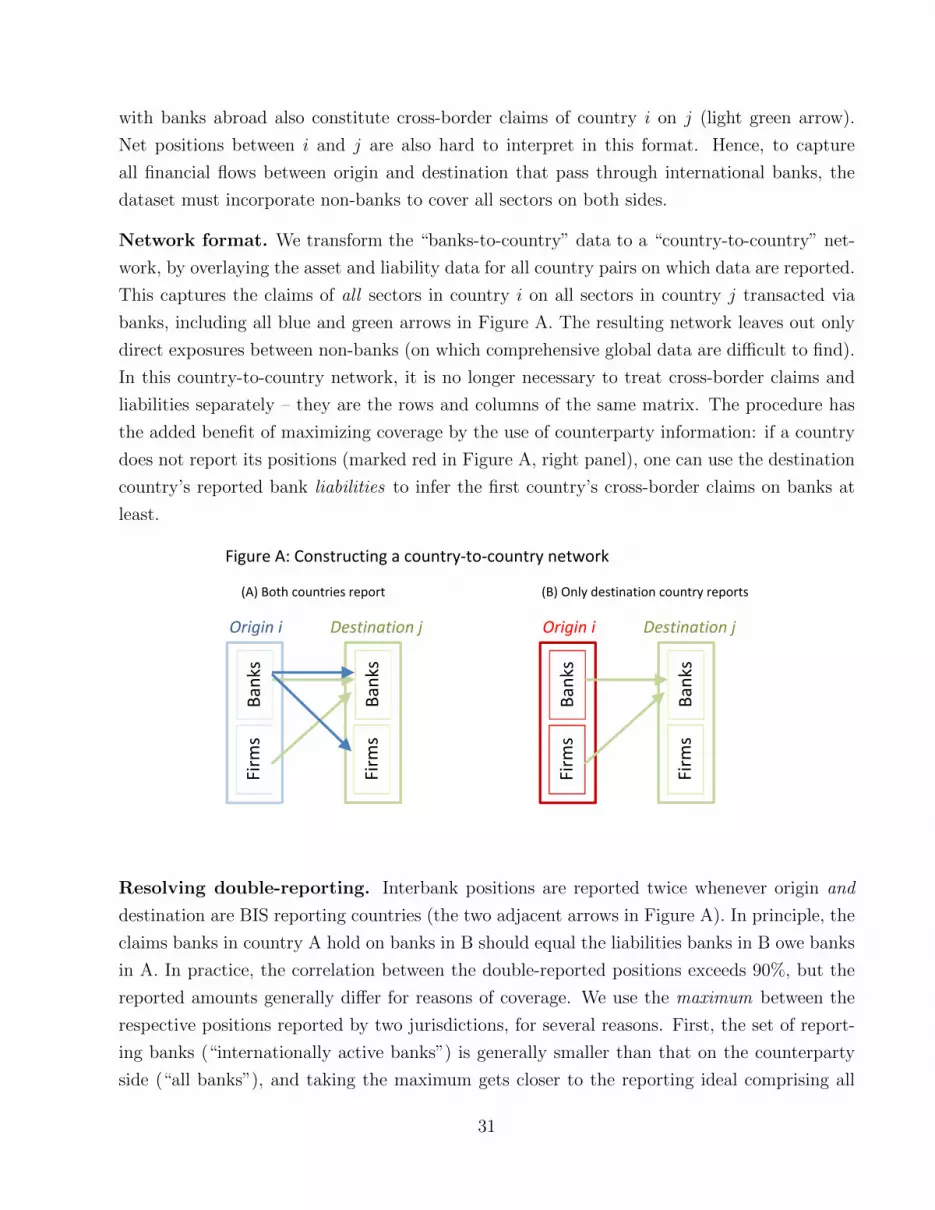
with banks abroad also constitute cross-border claims of country i on j (light green arrow).

Net positions between i and j are also hard to interpret in this format. Hence, to capture

all financial flows between origin and destination that pass through international banks, the

dataset must incorporate non-banks to cover all sectors on both sides.

Network format. We transform the “banks-to-country” data to a “country-to-country” net-

work, by overlaying the asset and liability data for all country pairs on which data are reported.

This captures the claims of all sectors in country i on all sectors in country j transacted via

banks, including all blue and green arrows in Figure A. The resulting network leaves out only

direct exposures between non-banks (on which comprehensive global data are difficult to find).

In this country-to-country network, it is no longer necessary to treat cross-border claims and

liabilities separately – they are the rows and columns of the same matrix. The procedure has

the added benefit of maximizing coverage by the use of counterparty information: if a country

does not report its positions (marked red in Figure A, right panel), one can use the destination

country’s reported bank liabilities to infer the first country’s cross-border claims on banks at

least.

Figure A: Constructing a country-to-country network

(A) Both countries report (B) Only destination country reports

Origin i Destination j

Origin i Destination j

Bank

s Fi

rms

Bank

s Fi

rms

Bank

s Fi

rms

Bank

s Fi

rms

Resolving double-reporting. Interbank positions are reported twice whenever origin and

destination are BIS reporting countries (the two adjacent arrows in Figure A). In principle, the

claims banks in country A hold on banks in B should equal the liabilities banks in B owe banks

in A. In practice, the correlation between the double-reported positions exceeds 90%, but the

reported amounts generally differ for reasons of coverage. We use the maximum between the

respective positions reported by two jurisdictions, for several reasons. First, the set of report-

ing banks (“internationally active banks”) is generally smaller than that on the counterparty

side (“all banks”), and taking the maximum gets closer to the reporting ideal comprising all

31

banks on both sides. Second, banks may not know the location of their counterparties for the

liabilities they issued in the form of tradable debt instruments; by contrast, banks do know

the counterparty of the assets they hold. Indeed, in the bilateral interbank data, reported

assets exceed liabilities more often (56%) than not. Taking the maximum also addresses the

general issue that incentives and reporting systems make underreporting more prevalent than

overreporting.

Adjustments. Before building the network, we make several adjustments to enhance the

consistency of the banking statistics. The first is to ensure that the set of 216 countries and

jurisdictions covers the world without gaps and overlaps.38 Second, the broadening coverage

of the LBS over time requires us to distinguish between reported (true) zeros and unreported

positions (missing values). Cross-border positions remain unknown (only) if neither origin nor

destination is a BIS-reporting country, and are excluded as missing values from the analysis and

regressions. Third, for each reporting country, residuals (such as unallocated debt liabilities) are

distributed using the information available in the reported bilateral positions (such as deposit

liabilities, where the locations of the counterparties are known); this approach creates no new

linkages between country pairs, but scales up existing positions proportionately.

The bilateral claims and liabilities in the final dataset combine all currencies, all instruments

(loans and deposits, and holdings of debt securities and equity), and distinguish the sector of

the counterparty: interbank positions include intragroup transfers between offices of the same

banking group, positions with unaffiliated banks and with central banks; non-bank positions

comprise claims on, and liabilities to, all other sectors, including households, corporations, the

public sector and non-bank financial institutions (mutual funds, other funds, CCPs, etc).

38On the reporting country side, legacy reporters are consolidated with their successor reporting country; onthe counterparty country side, legacy residuals are allocated to legacy countries, which in turn are allocated tothe largest successor country, e.g. the German Democratic Republic to (West) Germany.

32

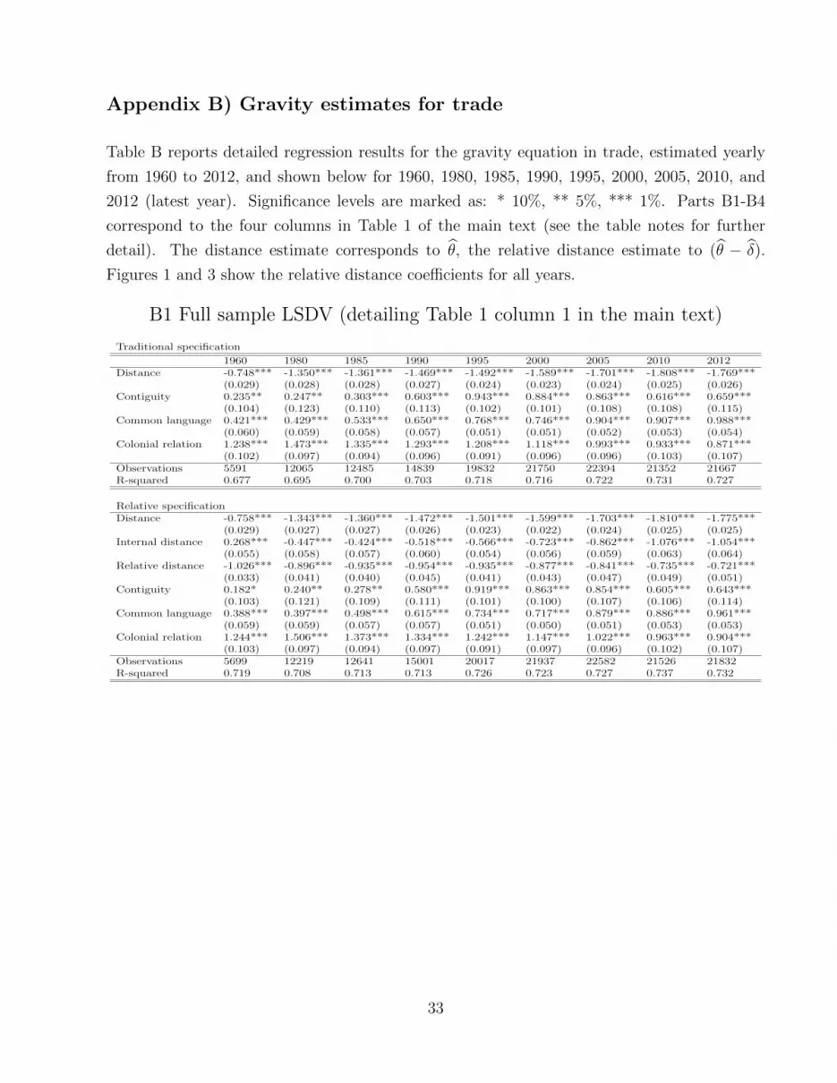
Appendix B) Gravity estimates for trade

Table B reports detailed regression results for the gravity equation in trade, estimated yearly

from 1960 to 2012, and shown below for 1960, 1980, 1985, 1990, 1995, 2000, 2005, 2010, and

2012 (latest year). Significance levels are marked as: * 10%, ** 5%, *** 1%. Parts B1-B4

correspond to the four columns in Table 1 of the main text (see the table notes for further

detail). The distance estimate corresponds to θ, the relative distance estimate to (θ − δ).

Figures 1 and 3 show the relative distance coefficients for all years.

B1 Full sample LSDV (detailing Table 1 column 1 in the main text)

Traditional specification

1960 1980 1985 1990 1995 2000 2005 2010 2012Distance -0.748*** -1.350*** -1.361*** -1.469*** -1.492*** -1.589*** -1.701*** -1.808*** -1.769***

(0.029) (0.028) (0.028) (0.027) (0.024) (0.023) (0.024) (0.025) (0.026)Contiguity 0.235** 0.247** 0.303*** 0.603*** 0.943*** 0.884*** 0.863*** 0.616*** 0.659***

(0.104) (0.123) (0.110) (0.113) (0.102) (0.101) (0.108) (0.108) (0.115)Common language 0.421*** 0.429*** 0.533*** 0.650*** 0.768*** 0.746*** 0.904*** 0.907*** 0.988***

(0.060) (0.059) (0.058) (0.057) (0.051) (0.051) (0.052) (0.053) (0.054)Colonial relation 1.238*** 1.473*** 1.335*** 1.293*** 1.208*** 1.118*** 0.993*** 0.933*** 0.871***

(0.102) (0.097) (0.094) (0.096) (0.091) (0.096) (0.096) (0.103) (0.107)Observations 5591 12065 12485 14839 19832 21750 22394 21352 21667R-squared 0.677 0.695 0.700 0.703 0.718 0.716 0.722 0.731 0.727

Relative specificationDistance -0.758*** -1.343*** -1.360*** -1.472*** -1.501*** -1.599*** -1.703*** -1.810*** -1.775***

(0.029) (0.027) (0.027) (0.026) (0.023) (0.022) (0.024) (0.025) (0.025)Internal distance 0.268*** -0.447*** -0.424*** -0.518*** -0.566*** -0.723*** -0.862*** -1.076*** -1.054***

(0.055) (0.058) (0.057) (0.060) (0.054) (0.056) (0.059) (0.063) (0.064)Relative distance -1.026*** -0.896*** -0.935*** -0.954*** -0.935*** -0.877*** -0.841*** -0.735*** -0.721***

(0.033) (0.041) (0.040) (0.045) (0.041) (0.043) (0.047) (0.049) (0.051)Contiguity 0.182* 0.240** 0.278** 0.580*** 0.919*** 0.863*** 0.854*** 0.605*** 0.643***

(0.103) (0.121) (0.109) (0.111) (0.101) (0.100) (0.107) (0.106) (0.114)Common language 0.388*** 0.397*** 0.498*** 0.615*** 0.734*** 0.717*** 0.879*** 0.886*** 0.961***

(0.059) (0.059) (0.057) (0.057) (0.051) (0.050) (0.051) (0.053) (0.053)Colonial relation 1.244*** 1.506*** 1.373*** 1.334*** 1.242*** 1.147*** 1.022*** 0.963*** 0.904***


33

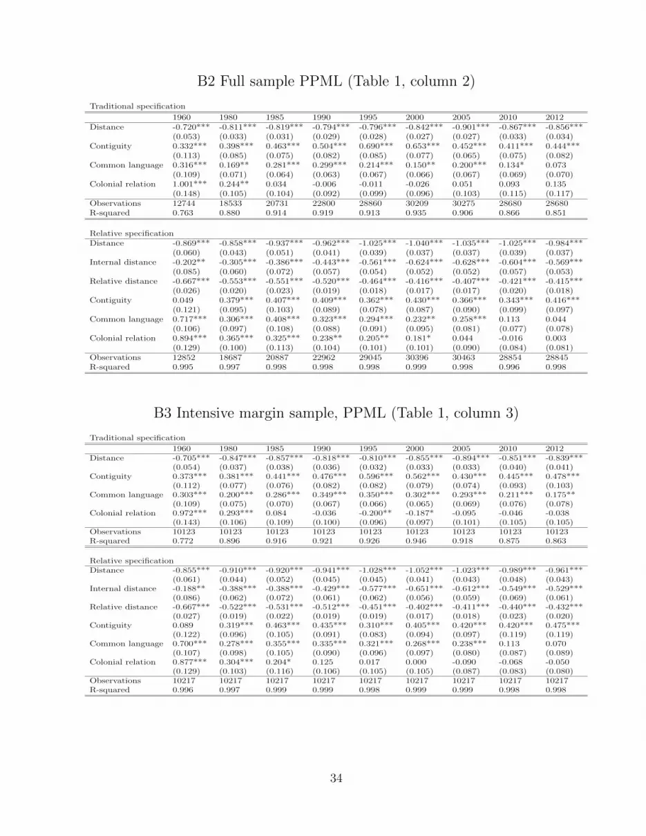
B2 Full sample PPML (Table 1, column 2)


1960 1980 1985 1990 1995 2000 2005 2010 2012Distance -0.720*** -0.811*** -0.819*** -0.794*** -0.796*** -0.842*** -0.901*** -0.867*** -0.856***

(0.053) (0.033) (0.031) (0.029) (0.028) (0.027) (0.027) (0.033) (0.034)Contiguity 0.332*** 0.398*** 0.463*** 0.504*** 0.690*** 0.653*** 0.452*** 0.411*** 0.444***

(0.113) (0.085) (0.075) (0.082) (0.085) (0.077) (0.065) (0.075) (0.082)Common language 0.316*** 0.169** 0.281*** 0.299*** 0.214*** 0.150** 0.200*** 0.134* 0.073

(0.109) (0.071) (0.064) (0.063) (0.067) (0.066) (0.067) (0.069) (0.070)Colonial relation 1.001*** 0.244** 0.034 -0.006 -0.011 -0.026 0.051 0.093 0.135



(0.060) (0.043) (0.051) (0.041) (0.039) (0.037) (0.037) (0.039) (0.037)Internal distance -0.202** -0.305*** -0.386*** -0.443*** -0.561*** -0.624*** -0.628*** -0.604*** -0.569***


(0.026) (0.020) (0.023) (0.019) (0.018) (0.017) (0.017) (0.020) (0.018)Contiguity 0.049 0.379*** 0.407*** 0.409*** 0.362*** 0.430*** 0.366*** 0.343*** 0.416***

(0.121) (0.095) (0.103) (0.089) (0.078) (0.087) (0.090) (0.099) (0.097)Common language 0.717*** 0.306*** 0.408*** 0.323*** 0.294*** 0.232** 0.258*** 0.113 0.044

(0.106) (0.097) (0.108) (0.088) (0.091) (0.095) (0.081) (0.077) (0.078)Colonial relation 0.894*** 0.365*** 0.325*** 0.238** 0.205** 0.181* 0.044 -0.016 0.003


B3 Intensive margin sample, PPML (Table 1, column 3)


1960 1980 1985 1990 1995 2000 2005 2010 2012Distance -0.705*** -0.847*** -0.857*** -0.818*** -0.810*** -0.855*** -0.894*** -0.851*** -0.839***

(0.054) (0.037) (0.038) (0.036) (0.032) (0.033) (0.033) (0.040) (0.041)Contiguity 0.373*** 0.381*** 0.441*** 0.476*** 0.596*** 0.562*** 0.430*** 0.445*** 0.478***

(0.112) (0.077) (0.076) (0.082) (0.082) (0.079) (0.074) (0.093) (0.103)Common language 0.303*** 0.200*** 0.286*** 0.349*** 0.350*** 0.302*** 0.293*** 0.211*** 0.175**

(0.109) (0.075) (0.070) (0.067) (0.066) (0.065) (0.069) (0.076) (0.078)Colonial relation 0.972*** 0.293*** 0.084 -0.036 -0.200** -0.187* -0.095 -0.046 -0.038



(0.061) (0.044) (0.052) (0.045) (0.045) (0.041) (0.043) (0.048) (0.043)Internal distance -0.188** -0.388*** -0.388*** -0.429*** -0.577*** -0.651*** -0.612*** -0.549*** -0.529***


(0.027) (0.019) (0.022) (0.019) (0.019) (0.017) (0.018) (0.023) (0.020)Contiguity 0.089 0.319*** 0.463*** 0.435*** 0.310*** 0.405*** 0.420*** 0.420*** 0.475***

(0.122) (0.096) (0.105) (0.091) (0.083) (0.094) (0.097) (0.119) (0.119)Common language 0.700*** 0.278*** 0.355*** 0.335*** 0.321*** 0.268*** 0.238*** 0.113 0.070

(0.107) (0.098) (0.105) (0.090) (0.096) (0.097) (0.080) (0.087) (0.089)Colonial relation 0.877*** 0.304*** 0.204* 0.125 0.017 0.000 -0.090 -0.068 -0.050


34

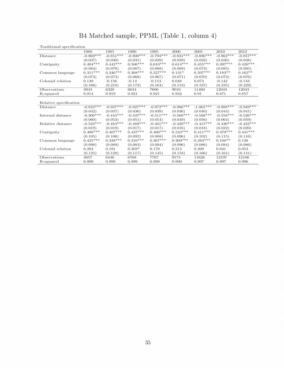
B4 Matched sample, PPML (Table 1, column 4)


1980 1985 1990 1995 2000 2005 2010 2012Distance -0.869*** -0.851*** -0.800*** -0.794*** -0.831*** -0.886*** -0.862*** -0.857***

(0.037) (0.030) (0.031) (0.029) (0.029) (0.028) (0.036) (0.038)Contiguity 0.404*** 0.442*** 0.506*** 0.610*** 0.614*** 0.455*** 0.397*** 0.420***

(0.084) (0.078) (0.087) (0.088) (0.089) (0.073) (0.085) (0.095)Common language 0.311*** 0.346*** 0.308*** 0.227*** 0.131* 0.207*** 0.183** 0.162**

(0.073) (0.073) (0.066) (0.067) (0.071) (0.070) (0.073) (0.076)Colonial relation 0.149 -0.156 -0.14 -0.113 0.048 0.073 -0.142 -0.143

(0.166) (0.218) (0.173) (0.164) (0.153) (0.197) (0.235) (0.229)Observations 3943 6320 6634 7606 9010 11460 12043 12043R-squared 0.914 0.919 0.921 0.921 0.942 0.91 0.871 0.857

Relative specificationDistance -0.823*** -0.927*** -0.927*** -0.972*** -0.986*** -1.001*** -0.988*** -0.949***

(0.042) (0.037) (0.036) (0.039) (0.036) (0.040) (0.044) (0.041)Internal distance -0.300*** -0.444*** -0.437*** -0.511*** -0.566*** -0.586*** -0.558*** -0.526***

(0.060) (0.053) (0.051) (0.054) (0.049) (0.056) (0.064) (0.059)Relative distance -0.523*** -0.484*** -0.489*** -0.461*** -0.420*** -0.415*** -0.430*** -0.423***

(0.019) (0.019) (0.017) (0.017) (0.016) (0.018) (0.022) (0.020)Contiguity 0.400*** 0.407*** 0.437*** 0.400*** 0.523*** 0.411*** 0.379*** 0.441***

(0.105) (0.106) (0.092) (0.088) (0.096) (0.102) (0.115) (0.116)Common language 0.425*** 0.338*** 0.310*** 0.367*** 0.309*** 0.283*** 0.188** 0.138

(0.098) (0.089) (0.083) (0.094) (0.096) (0.086) (0.084) (0.086)Colonial relation 0.204 0.191 0.202* 0.179 0.212 0.209 0.041 0.053


35

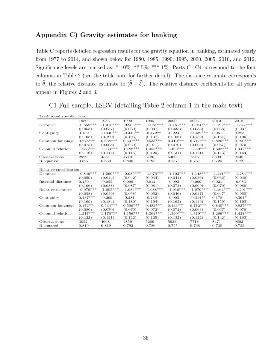
Appendix C) Gravity estimates for banking

Table C reports detailed regression results for the gravity equation in banking, estimated yearly

from 1977 to 2014, and shown below for 1980, 1985, 1990, 1995, 2000, 2005, 2010, and 2012.

Significance levels are marked as: * 10%, ** 5%, *** 1%. Parts C1-C4 correspond to the four

columns in Table 2 (see the table note for further detail). The distance estimate corresponds

to θ, the relative distance estimate to (θ − δ). The relative distance coefficients for all years

appear in Figures 2 and 3.

C1 Full sample, LSDV (detailing Table 2 column 1 in the main text)


1980 1985 1990 1995 2000 2005 2010 2012Distance -0.868*** -1.018*** -0.906*** -1.081*** -1.161*** -1.184*** -1.192*** -1.347***

(0.053) (0.037) (0.039) (0.037) (0.035) (0.033) (0.033) (0.037)Contiguity 0.159 -0.446** -0.446** -0.472** -0.224 -0.432*** 0.061 0.223

(0.168) (0.190) (0.195) (0.197) (0.166) (0.152) (0.161) (0.196)Common language 0.278*** 0.638*** 0.637*** 0.533*** 0.410*** 0.717*** 0.820*** 0.790***

(0.075) (0.068) (0.069) (0.071) (0.070) (0.063) (0.067) (0.070)Colonial relation 1.283*** 1.233*** 1.188*** 1.355*** 1.462*** 1.340*** 1.302*** 1.447***



(0.059) (0.044) (0.042) (0.044) (0.041) (0.036) (0.036) (0.040)Internal distance 0.130 -0.055 0.099 0.012 -0.093 -0.069 0.021 -0.083


(0.058) (0.059) (0.058) (0.052) (0.046) (0.047) (0.047) (0.055)Contiguity 0.437*** -0.269 -0.281 -0.236 -0.003 -0.314** 0.178 0.361*

(0.169) (0.184) (0.189) (0.194) (0.162) (0.149) (0.159) (0.193)Common language 0.172** 0.534*** 0.506*** 0.483*** 0.433*** 0.712*** 0.840*** 0.827***

(0.080) (0.070) (0.070) (0.072) (0.072) (0.063) (0.067) (0.070)Colonial relation 1.217*** 1.176*** 1.156*** 1.304*** 1.390*** 1.319*** 1.266*** 1.424***


36

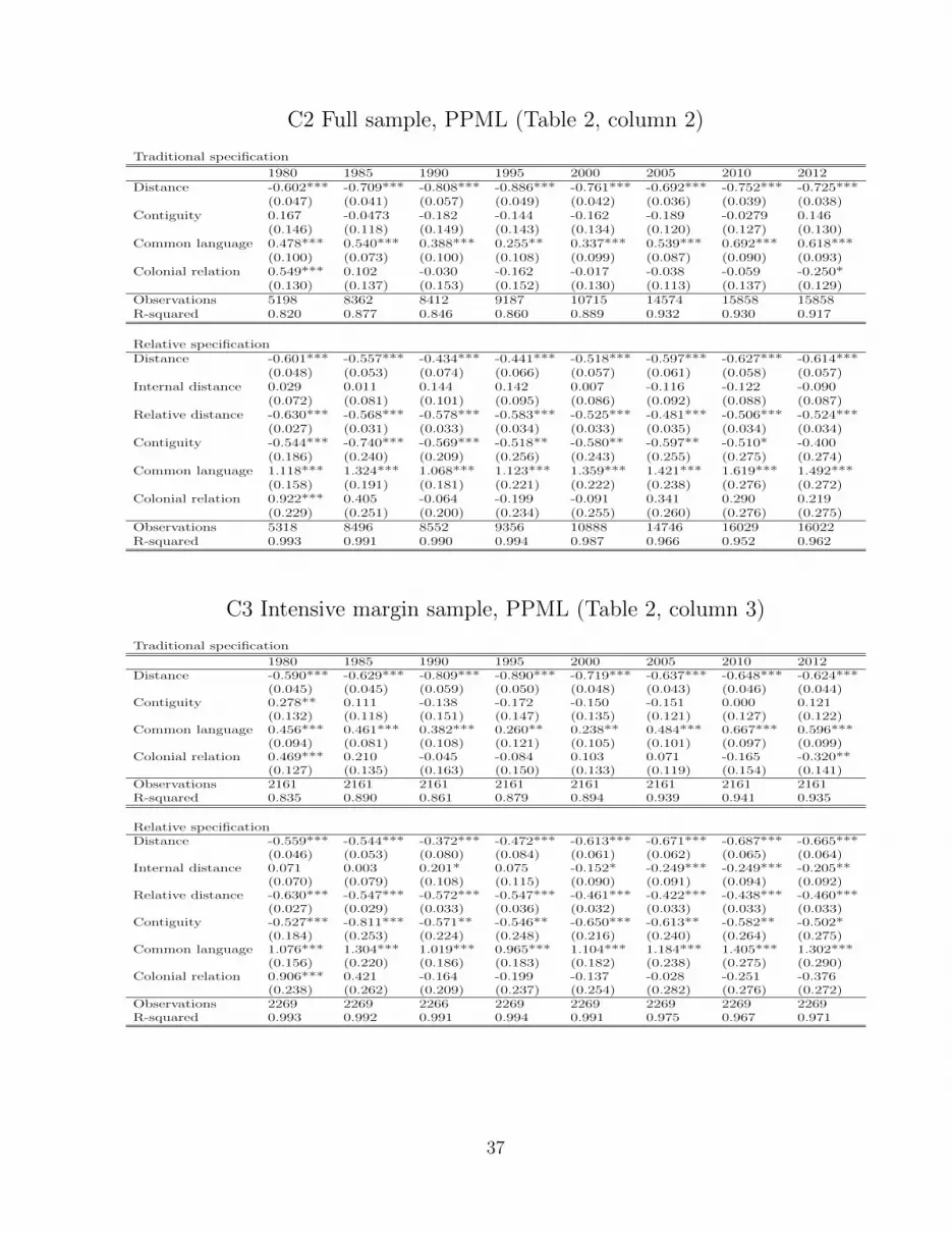
C2 Full sample, PPML (Table 2, column 2)


1980 1985 1990 1995 2000 2005 2010 2012Distance -0.602*** -0.709*** -0.808*** -0.886*** -0.761*** -0.692*** -0.752*** -0.725***

(0.047) (0.041) (0.057) (0.049) (0.042) (0.036) (0.039) (0.038)Contiguity 0.167 -0.0473 -0.182 -0.144 -0.162 -0.189 -0.0279 0.146

(0.146) (0.118) (0.149) (0.143) (0.134) (0.120) (0.127) (0.130)Common language 0.478*** 0.540*** 0.388*** 0.255** 0.337*** 0.539*** 0.692*** 0.618***

(0.100) (0.073) (0.100) (0.108) (0.099) (0.087) (0.090) (0.093)Colonial relation 0.549*** 0.102 -0.030 -0.162 -0.017 -0.038 -0.059 -0.250*



(0.048) (0.053) (0.074) (0.066) (0.057) (0.061) (0.058) (0.057)Internal distance 0.029 0.011 0.144 0.142 0.007 -0.116 -0.122 -0.090


(0.027) (0.031) (0.033) (0.034) (0.033) (0.035) (0.034) (0.034)Contiguity -0.544*** -0.740*** -0.569*** -0.518** -0.580** -0.597** -0.510* -0.400

(0.186) (0.240) (0.209) (0.256) (0.243) (0.255) (0.275) (0.274)Common language 1.118*** 1.324*** 1.068*** 1.123*** 1.359*** 1.421*** 1.619*** 1.492***

(0.158) (0.191) (0.181) (0.221) (0.222) (0.238) (0.276) (0.272)Colonial relation 0.922*** 0.405 -0.064 -0.199 -0.091 0.341 0.290 0.219


C3 Intensive margin sample, PPML (Table 2, column 3)


1980 1985 1990 1995 2000 2005 2010 2012Distance -0.590*** -0.629*** -0.809*** -0.890*** -0.719*** -0.637*** -0.648*** -0.624***

(0.045) (0.045) (0.059) (0.050) (0.048) (0.043) (0.046) (0.044)Contiguity 0.278** 0.111 -0.138 -0.172 -0.150 -0.151 0.000 0.121

(0.132) (0.118) (0.151) (0.147) (0.135) (0.121) (0.127) (0.122)Common language 0.456*** 0.461*** 0.382*** 0.260** 0.238** 0.484*** 0.667*** 0.596***

(0.094) (0.081) (0.108) (0.121) (0.105) (0.101) (0.097) (0.099)Colonial relation 0.469*** 0.210 -0.045 -0.084 0.103 0.071 -0.165 -0.320**



(0.046) (0.053) (0.080) (0.084) (0.061) (0.062) (0.065) (0.064)Internal distance 0.071 0.003 0.201* 0.075 -0.152* -0.249*** -0.249*** -0.205**


(0.027) (0.029) (0.033) (0.036) (0.032) (0.033) (0.033) (0.033)Contiguity -0.527*** -0.811*** -0.571** -0.546** -0.650*** -0.613** -0.582** -0.502*

(0.184) (0.253) (0.224) (0.248) (0.216) (0.240) (0.264) (0.275)Common language 1.076*** 1.304*** 1.019*** 0.965*** 1.104*** 1.184*** 1.405*** 1.302***

(0.156) (0.220) (0.186) (0.183) (0.182) (0.238) (0.275) (0.290)Colonial relation 0.906*** 0.421 -0.164 -0.199 -0.137 -0.028 -0.251 -0.376


37

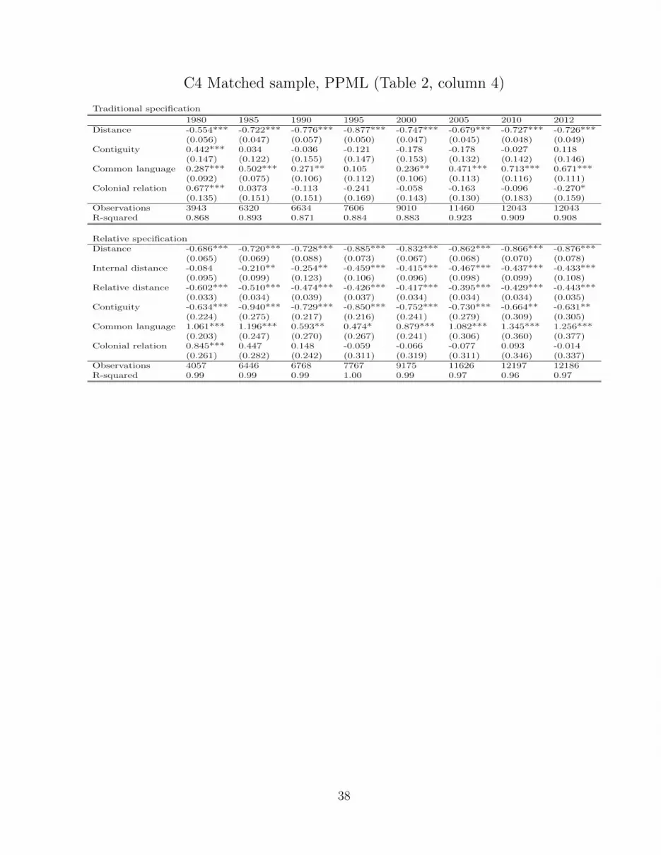
C4 Matched sample, PPML (Table 2, column 4)


1980 1985 1990 1995 2000 2005 2010 2012Distance -0.554*** -0.722*** -0.776*** -0.877*** -0.747*** -0.679*** -0.727*** -0.726***

(0.056) (0.047) (0.057) (0.050) (0.047) (0.045) (0.048) (0.049)Contiguity 0.442*** 0.034 -0.036 -0.121 -0.178 -0.178 -0.027 0.118

(0.147) (0.122) (0.155) (0.147) (0.153) (0.132) (0.142) (0.146)Common language 0.287*** 0.502*** 0.271** 0.105 0.236** 0.471*** 0.713*** 0.671***

(0.092) (0.075) (0.106) (0.112) (0.106) (0.113) (0.116) (0.111)Colonial relation 0.677*** 0.0373 -0.113 -0.241 -0.058 -0.163 -0.096 -0.270*



(0.065) (0.069) (0.088) (0.073) (0.067) (0.068) (0.070) (0.078)Internal distance -0.084 -0.210** -0.254** -0.459*** -0.415*** -0.467*** -0.437*** -0.433***


(0.033) (0.034) (0.039) (0.037) (0.034) (0.034) (0.034) (0.035)Contiguity -0.634*** -0.940*** -0.729*** -0.850*** -0.752*** -0.730*** -0.664** -0.631**

(0.224) (0.275) (0.217) (0.216) (0.241) (0.279) (0.309) (0.305)Common language 1.061*** 1.196*** 0.593** 0.474* 0.879*** 1.082*** 1.345*** 1.256***

(0.203) (0.247) (0.270) (0.267) (0.241) (0.306) (0.360) (0.377)Colonial relation 0.845*** 0.447 0.148 -0.059 -0.066 -0.077 0.093 -0.014


38

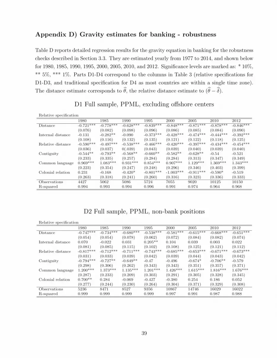
Appendix D) Gravity estimates for banking - robustness

Table D reports detailed regression results for the gravity equation in banking for the robustness

checks described in Section 3.3. They are estimated yearly from 1977 to 2014, and shown below

for 1980, 1985, 1990, 1995, 2000, 2005, 2010, and 2012. Significance levels are marked as: * 10%,

** 5%, *** 1%. Parts D1-D4 correspond to the columns in Table 3 (relative specifications for

D1-D3, and traditional specification for D4 as most countries are within a single time zone).

The distance estimate corresponds to θ, the relative distance estimate to (θ − δ).

D1 Full sample, PPML, excluding offshore centers

Relative specification

1980 1985 1990 1995 2000 2005 2010 2012Distance -0.721*** -0.778*** -0.628*** -0.839*** -0.848*** -0.871*** -0.878*** -0.846***

(0.076) (0.082) (0.098) (0.096) (0.086) (0.085) (0.084) (0.090)Internal distance -0.131 -0.282** -0.090 -0.373*** -0.428*** -0.474*** -0.444*** -0.392***


(0.036) (0.037) 0(.039) (0.043) (0.039) (0.040) (0.039) (0.040)Contiguity -0.544** -0.793** -0.568** -0.660** -0.582** -0.628** -0.54 -0.521

(0.233) (0.335) (0.257) (0.284) (0.284) (0.313) (0.347) (0.349)Common language 0.969*** 1.083*** 0.931*** 0.854*** 0.907*** 1.129*** 1.369*** 1.343***

(0.223) (0.354) (0.247) (0.248) (0.296) (0.346) (0.403) (0.399)Colonial relation 0.231 -0.168 -0.420* -0.801*** -1.003*** -0.911*** -0.590* -0.519


D2 Full sample, PPML, non-bank positions


1980 1985 1990 1995 2000 2005 2010 2012Distance -0.747*** -0.734*** -0.680*** -0.538*** -0.581*** -0.615*** -0.668*** -0.651***

(0.054) (0.054) (0.078) (0.062) (0.072) (0.084) (0.082) (0.074)Internal distance 0.070 -0.022 0.031 0.205** 0.104 0.039 0.003 0.022


(0.031) (0.033) (0.039) (0.042) (0.039) (0.044) (0.043) (0.042)Contiguity -0.794*** -0.727** -0.649** -0.47 -0.496 -0.674* -0.706** -0.579

(0.298) (0.306) (0.262) (0.343) (0.343) (0.351) (0.357) (0.371)Common language 1.200*** 1.373*** 1.135*** 1.201*** 1.426*** 1.615*** 1.816*** 1.676***

(0.287) (0.233) (0.209) (0.303) (0.291) (0.305) (0.328) (0.345)Colonial relation 0.700** 0.284 -0.069 -0.427 -0.380 0.254 0.186 0.052


39

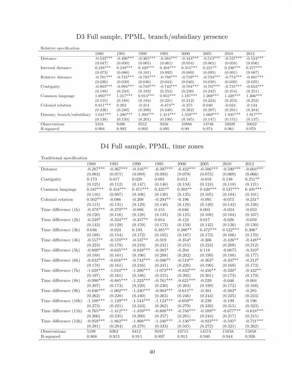
D3 Full sample, PPML, branch/subsidiary presence


1980 1985 1990 1995 2000 2005 2010 2012Distance -0.533*** -0.496*** -0.365*** -0.384*** -0.443*** -0.513*** -0.537*** -0.524***

(0.047) (0.050) (0.065) (0.061) (0.054) (0.061) (0.058) (0.056)Internal distance 0.248*** 0.249*** 0.420*** 0.404*** 0.315*** 0.221** 0.236*** 0.277***


(0.030) (0.039) (0.046) (0.044) (0.040) (0.038) (0.038) (0.035)Contiguity -0.803*** -0.994*** -0.783*** -0.742*** -0.784*** -0.787*** -0.731*** -0.653***

(0.188) (0.233) (0.193) (0.252) (0.230) (0.242) (0.254) (0.251)Common language 1.093*** 1.217*** 0.914*** 0.955*** 1.187*** 1.269*** 1.428*** 1.306***

(0.155) (0.188) (0.184) (0.221) (0.212) (0.224) (0.253) (0.252)Colonial relation 0.811*** 0.263 -0.314 -0.474** -0.375 0.040 -0.024 -0.134

(0.226) (0.240) (0.200) (0.240) (0.262) (0.287) (0.291) (0.284)Dummy, branch/subsidiary 1.041*** 1.280*** 1.393*** 1.414*** 1.559*** 1.669*** 1.835*** 1.917***


D4 Full sample, PPML, time zones


1980 1985 1990 1995 2000 2005 2010 2012Distance -0.287*** -0.367*** -0.216** -0.397*** -0.422*** -0.506*** -0.590*** -0.604***

(0.083) (0.071) (0.089) (0.093) (0.079) (0.073) (0.069) (0.066)Contiguity 0.173 0.017 0.028 0.091 0.012 -0.018 0.138 0.251**

(0.125) (0.112) (0.147) (0.146) (0.134) (0.124) (0.118) (0.121)Common language 0.347*** 0.454*** 0.471*** 0.325** 0.303** 0.420*** 0.537*** 0.491***

(0.116) (0.087) (0.106) (0.130) (0.125) (0.105) (0.104) (0.101)Colonial relation 0.502*** -0.086 -0.208 -0.294** -0.196 -0.095 -0.075 -0.231*

(0.115) (0.131) (0.129) (0.140) (0.128) (0.120) (0.142) (0.138)Time difference (1h) -0.478*** -0.379*** -0.086 0.155 -0.046 0.004 -0.024 -0.053

(0.120) (0.116) (0.128) (0.135) (0.125) (0.108) (0.104) (0.107)Time difference (2h) -0.249* -0.334*** -0.357** 0.054 -0.122 0.017 -0.026 -0.059

(0.143) (0.129) (0.159) (0.173) (0.159) (0.142) (0.126) (0.130)Time difference (3h) 0.046 -0.024 0.193 0.385** 0.380** 0.472*** 0.522*** 0.306*

(0.188) (0.154) (0.172) (0.185) (0.187) (0.173) (0.166) (0.170)Time difference (4h) -0.557** -0.570*** -0.537** -0.319 -0.354* -0.306 -0.426** -0.448**

(0.223) (0.179) (0.210) (0.231) (0.215) (0.224) (0.208) (0.212)Time difference (5h) -0.809*** -0.635*** -0.849*** -0.385* -0.204 0.118 -0.0875 -0.310*

(0.188) (0.161) (0.196) (0.208) (0.202) (0.199) (0.188) (0.177)Time difference (6h) -0.822*** -0.658*** -0.742*** -0.506** -0.519** -0.363* -0.337** -0.312*

(0.178) (0.161) (0.216) (0.241) (0.228) (0.190) (0.169) (0.173)Time difference (7h) -1.028*** -1.010*** -1.200*** -1.073*** -0.832*** -0.456** -0.320* -0.432**

(0.197) (0.161) (0.186) (0.215) (0.202) (0.201) (0.173) (0.179)Time difference (8h) -0.990*** -0.885*** -1.223*** -0.761*** -0.621*** -0.229 -0.046 -0.004

(0.207) (0.173) (0.220) (0.230) (0.204) (0.199) (0.172) (0.168)Time difference (9h) -0.846*** -1.002*** -1.240*** -0.903*** -0.615** -0.381 -0.383* -0.285

(0.262) (0.228) (0.240) (0.263) (0.246) (0.244) (0.225) (0.224)Time difference (10h) -1.168*** -1.129*** -1.544*** -1.124*** -0.659** -0.239 -0.199 -0.196

(0.273) (0.221) (0.243) (0.262) (0.279) (0.339) (0.315) (0.323)Time difference (11h) -0.765*** -1.412*** -1.459*** -0.808*** -0.756*** -0.589** -0.677*** -0.618***

(0.266) (0.235) (0.260) (0.257) (0.281) (0.244) (0.217) (0.215)Time difference (12h) -0.959*** -1.862*** -1.908*** -1.240*** -1.136*** -0.923*** -0.595* -0.721***


40

Previous volumes in this series

No Title Author

657 August 2017

Quality Pricing-to-Market Raphael A Auer, Thomas Chaney and Philip Sauré

656 August 2017

Demographics will reverse three multi-decade global trends

Charles Goodhart, Manoj Pradhan

655 August 2017

The FinTech Opportunity Thomas Philippon

654 August 2017

World changes in inequality: an overview of facts, causes, consequences and policies

François Bourguignon

653 August 2017

Dollar Pricing Redux Camila Casas, Federico Díez, Gita Gopinath, Pierre-Olivier Gourinchas

652 July 2017

The discontinuation of the EUR/CHF minimum exchange rate in January 2015: was it expected?

Michael Funke, Julius Loermann and Richhild Moessner

651 July 2017

Segmented money markets and covered interest parity arbitrage

Dagfinn Rime, Andreas Schrimpf and Olav Syrstad

650 June 2017

Financial deglobalisation in banking? Robert N McCauley, Agustín S Bénétrix, Patrick M McGuire and Goetz von Peter

649 June 2017

Monetary Policy Transmission and Trade-offs in the United States: Old and New

Boris Hofmann and Gert Peersman

648 June 2017

Credit ratings of domestic and global agencies: What drives the differences in China and how are they priced?

Xianfeng Jiang and Frank Packer

647 June 2017

The evolution of inflation expectations in Japan

Masazumi Hattori and James Yetman

646 June 2017

Macroprudential policy and bank risk Yener Altunbas, Mahir Binici and Leonardo Gambacorta

645 June 2017

Accounting for debt service: the painful legacy of credit booms

Mathias Drehmann, Mikael Juselius and Anton Korinek

All volumes are available on our website www.bis.org.

The Distance Effect in Banking and Trade

Documents

Transcript of The Distance Effect in Banking and Trade