Abstract--This paper presents the development of neural-

network-based controller of space vector modulation (ANN-SVPWM) for voltage-source inverters (VSI). This ANN-SVPWM controller completely covers the undermodulation and overmodulation modes with operation extended linearly and smoothly up to square wave (six-step) by using theory of modulation between the limit trajectories. The ANN controller has the advantage of the very fast implementation of an SVM algorithm that can increase the switching frequency of power switches of the static converter. Furthermore, a ANN Diagnosis method for real-time fault detection of power switches is proposed in this paper. The ANN controller uses the individual training strategy with the fixed weight and supervised models. The complete ANN-SVPWM and Diagnostic Controller can be used in power applications such as APF, STATCOM, UPFC and motor drives. A computer simulation program is developed using Matlab/Simulink together with the Neural Network Toolbox for training the ANN-controller.

Index Terms—Artificial Neural Network, Diagnosis, overmodulation, Pulse-Width Modulation, Space vector, undermodulation, Voltage Source Inverter.

I. INTRODUCTION

PACE Vector modulation (SVM) has recently grown as a very popular pulse width modulation (PWM) method for

voltage – source inverters because of its very good harmonic quality and extended linear range of operation [1]. However, a setback of SVM is that it requires complex online computation that usually limits its operation only up to several kilohertz of switching frequency. Switching frequency can be extended by using a high –speed DSP and simplifying computation with the help of lookup tables which is very large and tends to reduce the pulse width resolution

Power switches recently have been improved in term of switching frequency. Modern ultra-fast IGBT’s allow

P. Q. Dzung, L. M. Phuong, N. V. Nho and D. M. Hien are with the

Department of Electrical and Electronic Engineering, Hochiminh City University of Technology, Vietnam, (e-mail: pqdung@hcmut.edu.vn).

P. Q. Vinh is with the Siemens AG Representation Vietnam (e-mail: pham-quang.vinh@siemens.com).

0-7803-9525-5/06/$20.00 ©2006 IEEE.

operation at 50kHz. However, the DSP- based SVM practically fails in this region where artificial- neural –network (ANN) –based SVM would probably take over [2].

The applications of ANN technique have been developed strongly in power electronics for recent years. In the past, a neural network was implemented in instantaneous current controlled PWM [4-7]. Nevertheless, current controlled PWM does not yield an optimum performance. Several researches of ANN implementation of SVM have been worked out [3,2]. Although this ANN-SVM controller has the advantage of fast calculation, the limitation of this approach is the difficulty of training in the overmodulation range with nonlinearity of modulation technique.

To overcome this, the proposed back-propagation type feed-forward ANN-SVM (Fig. 1) in this paper has been successfully trained by using two main approaches:

1) Method of linear modulation between two limit trajectories [8] (to overcome the difficulty of nonlinearity in the overmodulation range)

2) Individual training strategy with 8 subnets (to overcome the complexity of SVM for 3 modes: undermodulation, overmodulation mode 1, overmodulation mode 2).

Fig. 1. ANN-DIAG-SVPWM Controller for VSI.

The Development of Artificial Neural Network Space Vector PWM and Diagnostic Controller

for Voltage Source Inverter

Phan Quoc Dzung, Le Minh Phuong, Pham Quang Vinh, Nguyen Van Nho, and Dao Minh Hien

S

II. SPACE- VECTOR PWM IN UNDERMODULATION AND OVERMODULATION REGIONS

The SVM technique has been well discussed and developed and a number of authors [1], [8]-[10] have described its operation in the overmodulation. Among these methods of modulation, method of modulation between trajectories [8] has the advantage of simplicity and linearity.

A. Undermodulation (0 < M < 0.907)

In the undermodulation, the rotating reference voltage remains within the hexagon. The SVM strategy in this region is based on generating three consecutive switching voltage vectors in a sampling period (Ts) so that the average output voltage matches with the reference voltage. The equations for effective duty cycle of the inverter switching states can be described as follows:

210

2

1

1

sin32

3/sin32

ddd

Md

Md

(1)

where d1 - duty cycle (2t1/Ts) of switching vector that lags.d2 - duty cycle (2t2/Ts) of switching vector that leads.d0 - duty cycle (2t0/Ts) of zero-switching vector.M - modulation factor M = V*/V1sw (V* - magnitude of reference voltage vector, V1sw – the peak value of six-step voltage wave ).

The timing intervals are obtained by multiplying duty cycles and period Ts/2 respectively.

B. Overmodulation mode 1 (0.907 < M < 0.952)

This mode takes place when the reference voltage V*

exceeds the circle inscribed in the hexagon and attains the sides of the hexagon. On the hexagon trajectory, duty d0 equals to 0:

0

1sincos3sincos3

''0

1''

2

''1

d

dd

d

(2)

Applying theory of linear modulation within trajectory, the first trajectory is chosen with M = 0.907:

21'

0

'2

'1

1

sin907.032

3/sin907.032

ddd

d

d

(3)

The second one is the boundary of hexagon (2).Coefficient of modulation is defined as following :

12

1

MM

MM

(4)

The duty cycles accordingly [8] are determined as : '0

'00

'2

''2

'22

'1

''1

'11

ddd

dddd

dddd

(5)

C. Overmodulation mode 2 (0.952 < M < 1)

In overmodulation mode 2, the reference vector V* growsfurther up to six-step mode.

Applying theory of linear modulation within trajectory, the first trajectory is chosen with M = 0.952:

0

1sincos3sincos3

'0

1'

2

'1

d

dd

d

(6)

The second is divided in two cases:- For 6/0 :

0;0;1 ''0

''2

''1 ddd (7)

- For 3/6/ :

0;1;0 ''0

''2

''1 ddd (8)

Accordingly [8], the duty cycles are described linearly as following:

00

'2

''2

'22

'1

''1

'11

d

dddd

dddd

(9)

Coefficient is determined similarly (4) where M1=0.952, M2=1.

In overmodulation, this approach has the advantage of simplicity in comparison with other conventional methods [2].

III. NEURAL-NETWORK BASED SPACE VECTOR PWM AND DIAGNOSTIC CONTROLLER

The SVM algorithm will be used to obtain training data for the relevant ANN-SVPWM.

A. Undermodulation Region Sub-net:

For any command angle *, the duty cycles d1, d2, d0 are given by (1) for sector 1. Similar duty cycles can be determined for all six sectors and the phase turn-on duty cycles can be calculated as:

1) For sector 1: (0 <* </3)

sin3/sin321

2

sin3/sin321

2

sin3/sin321

2

210

10

0

Mddd

d

Mdd

d

Md

d

ONC

ONB

ONA (10)

2) For sector 2: (/3 <* <2/3)

sin3/sin321

2

sin3/sin321

2

sin3/sin321

2

210

0

20

Mddd

d

Md

d

Mdd

d

ONC

ONB

ONA (11)

3) For sector 3: (2/3 <* <)

sin3/sin321

2

sin3/sin321

2

sin3/sin321

2

10

0

210

Mdd

d

Md

d

Mddd

d

ONC

ONB

ONA (12)

4) For sector 4: ( <* <4/3)

sin3/sin321

2

sin3/sin321

2

sin3/sin321

2

0

20

210

Md

d

Mdd

d

Mddd

d

ONC

ONB

ONA (13)

5) For sector 5: (4/3 <* <5/3)

sin3/sin321

2

sin3/sin321

2

sin3/sin321

2

0

210

10

Md

d

Mddd

d

Mdd

d

ONC

ONB

ONA (14)

6) For sector 6: (5/3 <* <2)

sin3/sin321

2

sin3/sin321

2

sin3/sin321

2

20

210

0

Mdd

d

Mddd

d

Md

d

ONC

ONB

ONA (15)

Hence, the turn-on and turn-off time interval are determined as following :

2

1

2

,,,,

,,,,

sONCBAOFFCBA

sONCBAONCBA

TdT

TdT

(16)

Equation (10)-(15) can be transformed in general form:

*30

*20

*10

321

321

321

hMd

hMd

hMd

ONC

ONB

ONA

(17)

where

5 ,sin3/sin4,3 ,sin3/sin

2 ,sin3/sin61, ,sin3/sin

*10

h

(18)

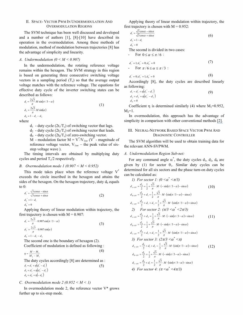
h20(*), h30(*) are obtained similarly. Then, h10,20,30(*) have been used for creating databases which are needed for training undermodulation region Sub-net with one input (*) and three outputs (h10, h20, h30). The angle step is 10.

A two-layer network is used for implementing this sub-net. The sub-net is obtained by training (supervised) with trainlmfunction – Levenberg –Marquardt algorithm, the squared error acceptable for training is 10-4. The number of neurons of 1st

layer is 10 tansig neurons, the 2nd layer has 3 purelin neurons. So, the total number of neurons is 13 (convergence obtained for 1077 epochs).

For implementing undermodulation duty cycles (equations (17)), it can be used one further product net-input-function

Fig. 2. Undermodulation region subnet.

(inputs: h(*), M) and one purelin neuron (weight = /3 , bias = 1/2) (Fig.2).

B. Overmodulation mode1 Sub-net

The duty cycles d1, d2, d0 are calculated by (5) for sector 1. After several substitutions, the duty cycles can be described as:

210

1

12

1

12

1

1221

1sincossincos1sin

sincossincos1

sincossincos3/sin3/sin

ddd

K

KK

K

Kd

K

KKKd

(19)

where 907.03K ;3 21

K

Duty cycles can be determined for all six sectors and the phase turn-on duty cycles can be calculated similar as (10)-(15) by substituting (19).

1) For sector 1: (0 <* </3)

sin3/sin1sincossincos

13/sin21

21

2

sincossincos

2sin3/sin1

sincossincos

13/sin

21

21

2

sin3/sin1sincossincos

13/sin21

21

2

2

1

12

210

1

12

1

12

10

2

1

120

K

K

KK

ddd

d

K

KK

K

KK

dd

d

K

K

KKd

d

ONC

ONB

ONA

(20) 2) For sector 2: (/3 <* <2/3)

sin3/sin1sincossincos

13/sin21

21

2

sin3/sin1sincossincos

13/sin21

21

2

sincossincos

21sin3/sin

sincossincos

13/sin

21

21

2

2

1

12

210

2

1

120

1

12

1

12

20

K

K

KK

ddd

d

K

K

KKd

d

K

KK

K

KK

dd

d

ONC

ONB

ONA

(21) 3) For sector 3: (2/3 <* <)

sincossincos

2sin3/sin1

sincossincos

13/sin

21

21

2

sin3/sin1sincossincos

13/sin21

21

2

sin3/sin1sincossincos

13/sin21

21

2

1

12

1

12

10

2

1

120

2

1

12

210

K

KK

K

KK

dd

d

K

K

KKd

d

K

K

KK

ddd

d

ONC

ONB

ONA

(22) 4) For sector 4: ( <* <4/3)

sin3/sin1sincossincos

13/sin21

21

2

sincossincos

21sin3/sin

sincossincos

13/sin

21

21

2

sin3/sin1sincossincos

13/sin21

21

2

2

1

120

1

12

1

12

20

2

1

12

210

K

K

KKd

d

K

KK

K

KK

dd

d

K

K

KK

ddd

d

ONC

ONB

ONA

(23) 5) For sector 5: (4/3 <* <5/3)

sin3/sin1sincossincos

13/sin21

21

2

sin3/sin1sincossincos

13/sin21

21

2

sincossincos

2sin3/sin1

sincossincos

13/sin

21

21

2

2

1

120

2

1

12

210

1

12

1

12

10

K

K

KKd

d

K

K

KK

ddd

d

K

KK

K

KK

dd

d

ONC

ONB

ONA

(24) 6) For sector 6: (5/3 <* <2)

sincossincos

21sin3/sin

sincossincos

13/sin

21

21

2

sin3/sin1sincossincos

13/sin21

21

2

sin3/sin1sincossincos

13/sin21

21

2

1

12

1

12

20

2

1

12

210

2

1

120

K

KK

K

KK

dd

d

K

K

KK

ddd

d

K

K

KKd

d

ONC

ONB

ONA

(25)Equations (20)-(25) can be transformed in general form:

*21

*11

*21

*11

*21

*11

21

21

21

21

21

21

ccONC

bbONB

aaONA

hhd

hhd

hhd

(26)

Where

5 ,sincossincos

13/sin

4,3 ,sincossincos

13/sin

2 ,sincossincos

13/sin

61, ,sincossincos

13/sin

1

12

1

12

1

12

1

12

*11

K

KK

K

KK

K

KK

K

KK

h a

(27)

and

5 ,sincossincos

2sin3/sin1

4,3 ,sin3/sin1

2 ,sincossincos

21sin3/sin

61, ,sin3/sin1

1

12

2

1

12

2

*21

K

KK

K

K

KK

K

h a

(28)

Fig. 3. Overmodulation mode 1 region subnet.

h11b(*), h21b(*), h11c(*), h21c(*) are obtained similarly. Then, h11a, 21a, 11b, 21b, 11c, 21c (*) have been used for creating databases which are needed for training overmodulation region sub-net with one input (*) and six outputs (h11a, h21a, h11b, h21b,h11c, h21c). The angle step is 1 degree.

A two-layer network is used for implementing this sub-net. The sub-net is obtained by training (supervised) with trainlmfunction – Levenberg –Marquardt algorithm, the squared error acceptable for training is 10-4. The number of neurons of 1st

layer is 20 tansig neurons, the 2nd layer has 6 purelin neurons. So, the total number of neurons is 26 (convergence obtained for 1016 epochs).

For implementing complete overmodulation duty cycles in equations (26), it can be used one further product net-input-function (inputs: h21(*), ), one further sum net-input-function (inputs : h11(*), *h21(*)) and one purelin neuron (weight = 1/2, bias = 1/2) (Fig.3).

C. Overmodulation mode 2 Sub-net

The duty cycles in this mode d1, d2, d0 are given by (9) for sector 1. After several transformations, the duty cycles can be written as:- For 0 < /6 :

0

1sincos3sincos3

sincos3sincos31

sincos3sincos31

sincos3sincos3

0

2

1

d

d

d

(29)

- For /6 < /3 :

0sincos3sincos3

sincos3sincos31

sincos3sincos3

sincos3sincos3

0

2

1

d

d

d

(30)

Fig. 4. Overmodulation mode 2 region subnet.

Duty cycles can be expressed for all six sectors by using (28): 1) For sector 1: (0 <* </3)

21;;0 1 ONCONBONA dddd

(31)

2) For sector 2: (/3 <* <2/3)

21;0;2 ONCONBONA dddd

(32)

3) For sector 3: (2/3 <* <)

1;0;21

dddd ONCONBONA

(33)

4) For sector 4: ( <* <4/3)

0;;21

2 ONCONBONA dddd(34)

5) For sector 5: (4/3 <* <5/3)

0;21;1 ONCONBONA dddd

(35)

6) For sector 6: (5/3 <* <2)

2;21;0 dddd ONCONBONA

(36)

Equations (31)-(36) can be written in general form : *

22*

12

*22

*12

*22

*12

ccONC

bbONB

aaONA

hhd

hhd

hhd

(37)

where

5 ,sincos3sincos3

4,3 ,5.0

2 ,sincos3sincos31

61, ,0

*12

ah

(38)

and

5 /3/6for ,

sincos3sincos3

/60for sincos3sincos31

4,3 ,0

2 /3/6for ,

sincos3sincos3

/60for sincos3sincos31

61, ,0

*22

ah

(39)

h12b(*), h22b(*), h12c(*), h22c(*) are obtained similarly. Then, h12a, 22a, 12b, 22b, 12c, 22c (*) have been used for creating databases which are needed for training overmodulation mode 2 sub-net with one input (*) and six outputs (h21a, h22a, h21b,h22b, h21c, h22c). The angle step is 1 degree.

A two-layer network is used for implementing this sub-net. The sub-net is obtained by training (supervised) with trainlmfunction – Levenberg –Marquardt algorithm, the squared error acceptable for training is 10-4. The number of neurons of 1st

Fig. 5. 1 calculation subnet.

Fig. 6. 2 calculation subnet.

Fig. 7. Code of modulation mode Sub-net.

layer is 20 tansig neurons, the 2nd layer has 6 purelin neurons. So, the total number of neurons is 26 neurons (convergence obtained for 200 epochs).

For implementing complete overmodulation duty cycles in equations (37), it can be designed one further product net-input-function (inputs : h22(*), ), one further sum net-input-function (inputs : h21(*), h22(*)) and one purelin neuron (weight = 1, bias = 0) (Fig.4).

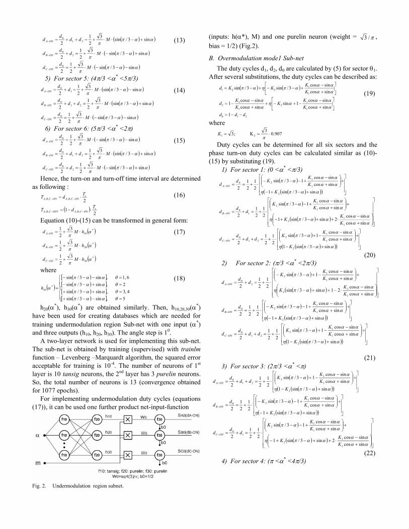
D. 1 , 2 calculation Sub-nets

The coefficient 1 and 2 in overmodulation mode 1 and mode 2 respectively are given by equation (4). This equation has been used for generating neural network training data. The input M is varied from 0.907 to 0.952 with step of 0.001, the output is 1 and varied from 0.952 to 1 with step of 0.001, the output is 2 .

A two-layer network is used for implementing these sub-nets. The sub-net is obtained by training (supervised) with trainlm function – Levenberg –Marquardt algorithm, the squared error acceptable for training is 10-4. The number of neurons of 1st layer is 1 tansig neurons, the 2nd layer has 1 purelin neurons. So, the total number of neurons is 2 Convergence is obtained for 57 epochs for 1-subnet and 46 epochs for 2-subnet) (Fig. 5, 6).

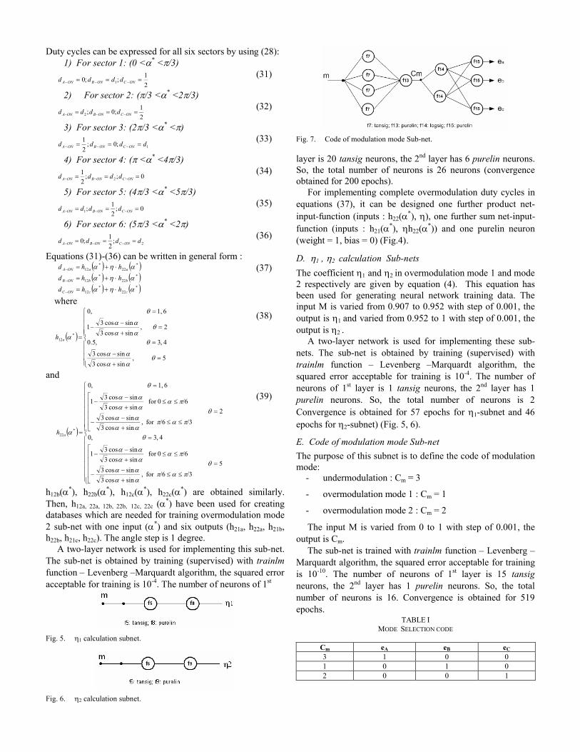
E. Code of modulation mode Sub-net

The purpose of this subnet is to define the code of modulation mode:

- undermodulation : Cm = 3

- overmodulation mode 1 : Cm = 1

- overmodulation mode 2 : Cm = 2

The input M is varied from 0 to 1 with step of 0.001, the output is Cm.

The sub-net is trained with trainlm function – Levenberg –Marquardt algorithm, the squared error acceptable for training is 10-10. The number of neurons of 1st layer is 15 tansigneurons, the 2nd layer has 1 purelin neurons. So, the total number of neurons is 16. Convergence is obtained for 519 epochs.

TABLE IMODE SELECTION CODE

Cm eA eB eC

3 1 0 01 0 1 02 0 0 1

F. Mode Selection Code Sub-net

This subnet is used for determining which modulation mode will be the choice for generating duty cycles at outputs of ANN-SVM-Controller (SA, SB, SC).

The input of this subnet is Cm, the outputs are eA, eB, eC (Table I). (Fig.7)

The sub-net is trained with trainlm function – Levenberg –Marquardt algorithm, the squared error acceptable for training is 10-10. The number of neurons of 1st layer is 2 logsig neurons, the 2nd layer has 3 purelin neurons. So, the total number of neurons is 5. Convergence is obtained for 17 epochs.

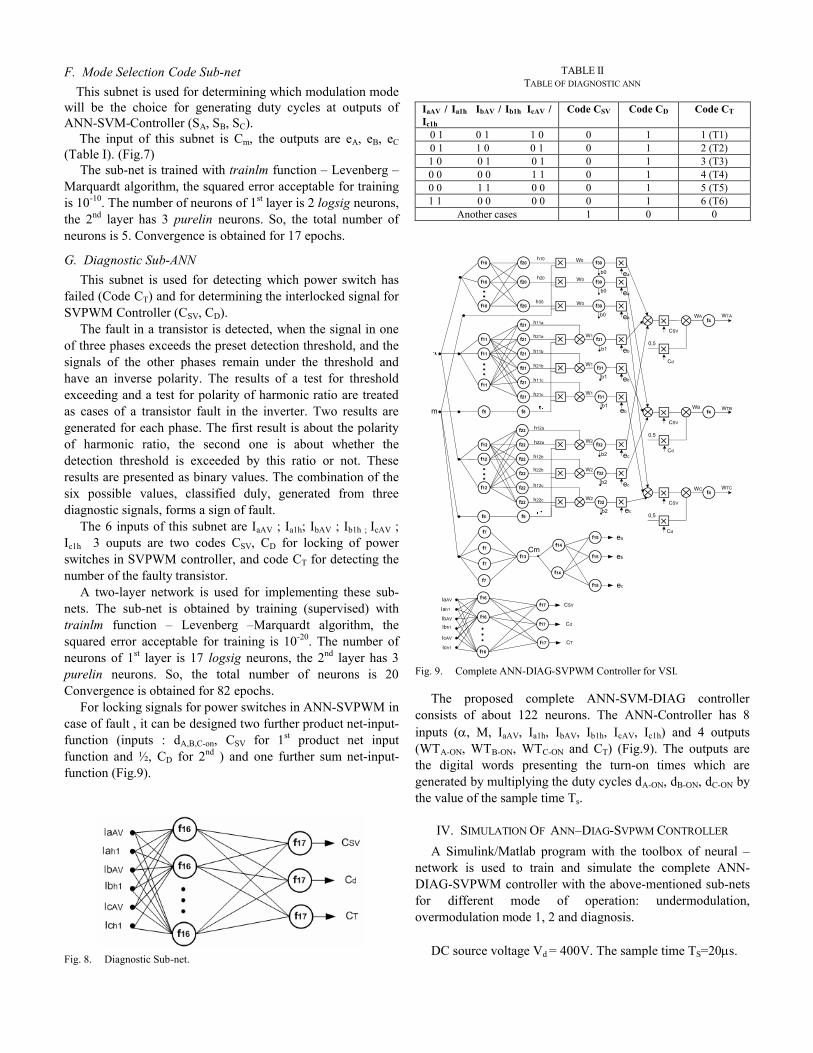
G. Diagnostic Sub-ANN

This subnet is used for detecting which power switch has failed (Code CT) and for determining the interlocked signal for SVPWM Controller (CSV, CD).

The fault in a transistor is detected, when the signal in one of three phases exceeds the preset detection threshold, and the signals of the other phases remain under the threshold and have an inverse polarity. The results of a test for threshold exceeding and a test for polarity of harmonic ratio are treated as cases of a transistor fault in the inverter. Two results are generated for each phase. The first result is about the polarity of harmonic ratio, the second one is about whether the detection threshold is exceeded by this ratio or not. These results are presented as binary values. The combination of the six possible values, classified duly, generated from three diagnostic signals, forms a sign of fault.

The 6 inputs of this subnet are IaAV ; Ia1h; IbAV ; Ib1h ; IcAV ; Ic1h 3 ouputs are two codes CSV, CD for locking of power switches in SVPWM controller, and code CT for detecting the number of the faulty transistor.

A two-layer network is used for implementing these sub-nets. The sub-net is obtained by training (supervised) with trainlm function – Levenberg –Marquardt algorithm, the squared error acceptable for training is 10-20. The number of neurons of 1st layer is 17 logsig neurons, the 2nd layer has 3 purelin neurons. So, the total number of neurons is 20 Convergence is obtained for 82 epochs.

For locking signals for power switches in ANN-SVPWM in case of fault , it can be designed two further product net-input-function (inputs : dA,B,C-on, CSV for 1st product net input function and ½, CD for 2nd ) and one further sum net-input-function (Fig.9).

Fig. 8. Diagnostic Sub-net.

TABLE IITABLE OF DIAGNOSTIC ANN

IaAV / Ia1h IbAV / Ib1h IcAV / Ic1h

Code CSV Code CD Code CT

0 1 0 1 1 0 0 1 1 (T1) 0 1 1 0 0 1 0 1 2 (T2)1 0 0 1 0 1 0 1 3 (T3)0 0 0 0 1 1 0 1 4 (T4)0 0 1 1 0 0 0 1 5 (T5)1 1 0 0 0 0 0 1 6 (T6)

Another cases 1 0 0

f10

f10

f10

f11

f11

f11

f5

f12

f12

f12

f6

f7

f7

f7

f20

f20

f20

f21

f21

f21

f21

f21

f21

f8

f22

f22

f22

f22

f22

f22

f9

f13

f14

f14

f15

f15

f15

ea

eb

ec

f30

f30

f30

W0

W0

W0

b0

b0

b0

ea

ea

ea

f31

f31

f31

b1

b1

b1

eb

eb

eb

W1

W1

W1

f32

f32

f32

b2

b2

b2

ec

ec

ec

W2

W2

W2

m

f4

f4

f4

WTA

WTB

WTC

WA

WB

WC

h11a

h21a

h11b

h21b

h11c

h21c

h12a

h22a

h12b

h22b

h12c

h22c

Cm

f7

h10

h20

h30

f16

f16

f16

f17

f17

f17

CSV

Cd

CT

IaAV

Iah1

IbAV

IcAV

Ibh1

Ich1

CSV

0,5

CSV

0,5

CSV

0,5

Cd

Cd

Cd

Fig. 9. Complete ANN-DIAG-SVPWM Controller for VSI.

The proposed complete ANN-SVM-DIAG controller consists of about 122 neurons. The ANN-Controller has 8 inputs (, M, IaAV, Ia1h, IbAV, Ib1h, IcAV, Ic1h) and 4 outputs (WTA-ON, WTB-ON, WTC-ON and CT) (Fig.9). The outputs are the digital words presenting the turn-on times which are generated by multiplying the duty cycles dA-ON, dB-ON, dC-ON by the value of the sample time Ts.

IV. SIMULATION OF ANN–DIAG-SVPWM CONTROLLER

A Simulink/Matlab program with the toolbox of neural –network is used to train and simulate the complete ANN-DIAG-SVPWM controller with the above-mentioned sub-nets for different mode of operation: undermodulation, overmodulation mode 1, 2 and diagnosis.

DC source voltage Vd = 400V. The sample time TS=20s.

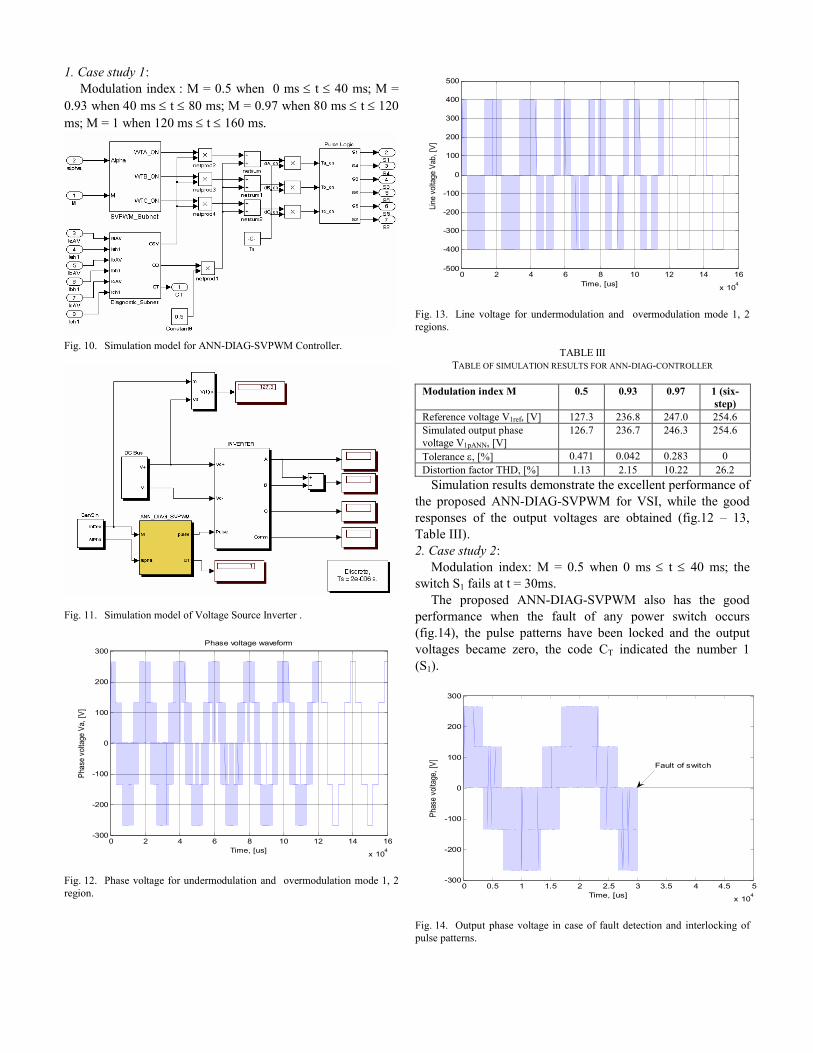
1. Case study 1: Modulation index : M = 0.5 when 0 ms t 40 ms; M =

0.93 when 40 ms t 80 ms; M = 0.97 when 80 ms t 120 ms; M = 1 when 120 ms t 160 ms.

Fig. 10. Simulation model for ANN-DIAG-SVPWM Controller.

Fig. 11. Simulation model of Voltage Source Inverter .

0 2 4 6 8 10 12 14 16

x 104

-300

-200

-100

0

100

200

300

Time, [us]

Pha

se v

olta

ge V

a, [V

]

Phase voltage waveform

Fig. 12. Phase voltage for undermodulation and overmodulation mode 1, 2 region.

0 2 4 6 8 10 12 14 16

x 104

-500

-400

-300

-200

-100

0

100

200

300

400

500

Time, [us]

Line

vol

tage

Vab

, [V

]

Fig. 13. Line voltage for undermodulation and overmodulation mode 1, 2 regions.

TABLE IIITABLE OF SIMULATION RESULTS FOR ANN-DIAG-CONTROLLER

Modulation index M 0.5 0.93 0.97 1 (six-step)

Reference voltage V1ref, [V] 127.3 236.8 247.0 254.6Simulated output phase voltage V1pANN, [V]

126.7 236.7 246.3 254.6

Tolerance , [%] 0.471 0.042 0.283 0Distortion factor THD, [%] 1.13 2.15 10.22 26.2

Simulation results demonstrate the excellent performance of the proposed ANN-DIAG-SVPWM for VSI, while the good responses of the output voltages are obtained (fig.12 – 13, Table III).2. Case study 2:

Modulation index: M = 0.5 when 0 ms t 40 ms; the switch S1 fails at t = 30ms.

The proposed ANN-DIAG-SVPWM also has the good performance when the fault of any power switch occurs (fig.14), the pulse patterns have been locked and the output voltages became zero, the code CT indicated the number 1(S1).

0 0.5 1 1.5 2 2.5 3 3.5 4 4.5 5

x 104

-300

-200

-100

0

100

200

300

Time, [us]

Phas

e vo

ltage

, [V

]

Fault of switch

Fig. 14. Output phase voltage in case of fault detection and interlocking of pulse patterns.

V. CONCLUSION

This paper presents the development of a complete artificial-neural-network space- vector- modulation and diagnostic controller (ANN-SVM-DIAG Controller) scheme for a Voltage Source Inverter that operates very well in undermodulation as well as in overmodulation (Mode –1 and Mode-2) regions. The digital words presenting turn-on time are generated by the ANN and then converted to pulse widths in a timer. Two main approaches have been used successfully: Method of linear modulation between two limitary trajectories with extension to six-step mode and Individual training strategy.

In practice the proposed ANN-DIAG-SVPWM controller can be implemented in applications such as APF, STATCOM, UPFC, motor drives. The ANN based SVM can yield higher switching frequency, which is not possible in conventional DSP- based SVM . ANN-DIAG-SVPWM-Controller may be implemented in ASIC chip in the future.

VI. REFERENCES

[1] J. Holtz “Pulse width modulation for electric power conversion”, Proc.IEEE, vol.82, pp.1194-1214, Aug. 1994.

[2] J. O. P. Pinto, B. K. Bose, L. E. B. Silva, M. P. Karmierkowski “A Neural Network Based Space Vector PWM Controller for Voltage-Fed Inverter Induction Motor Drive”, IEEE Trans. on Ind. Appl., vol.36, no. 6, November/December 2000.

[3] A. Bakhshai, J. Espinoza, G. Joos, H. Jin. “A combined ANN and DSP approach to the implementation of space vector modulation techniques”, in conf. Rec.IEEE –IAS Annu. Meeting, 1996, pp.934-940.

[4] F. Harashima et al., “Applications of neural networks to power converter control”, in conf. Rec.IEEE –IAS Annu. Meeting, 1989, pp.1086-1091.

[5] M. R. Buhl and R. D. Lorenz, “Design and implementation of neural networks for digital current regulation of inverter drives”, in conf. Rec.IEEE –IAS Annu. Meeting, 1991, pp.415-423.

[6] J. W. Song, K. C. Lee, K. B. Cho, J. S. Won, “ An adaptive learning current controller for field – oriented controlled induction motor by neural network“, in Proc. IEEE –IECON’91, 1991, pp.469-474.

[7] M. P. Karmierskowski et al., “ Neural network current control of VS-PWM inverters ”, in Proc. IPE’95, 1995, pp.1415-1420.

[8] N.V.Nho, M. J. Youn, “Two-mode overmodulation in two level VSI using principle control between limit trajectories”, CD-ROM Proc. PEDS 2003, pp.1274-1279

[9] J. Holtz, W. Lotzkat, M. Khambadkone, “On continuous control of PWM inverters in the overmodulation range includingthe six-step mode”, IEEE Trans. Power Electron. , vol.8, pp.546-553, Oct. 1993.

[10] S. Bolognani, M. Ziglitti, “Novel digital continuous control of SVM inverters in the overmodulation range”, IEEE Trans. Ind. Applicat., vol.33, pp.525-530, Mars/ April 1997.

[11] S.Abramik, “Contribution à l’étude du diagnostic de défaillance des convertisseurs statiques en temps réelle » Thèse du Doctorat, ENSEEIHT, 2003.

VII. BIOGRAPHIES

Phan Quoc Dzung was born in Saigon (Vietnam) in 1967. He graduated as an engineer from Donetsk Polytechnic Institute in 1991, received his PhD degree in electrical engineering from Kiev Polytechnic Institute in 1994. Now he is a lecturer in the Hochiminh City University of Technology.

Le Minh Phuong was born in the North of Vietnam in 1973. He graduated as an engineer from Kharkov National Academy of Municipal Economy in 1997, received his PhD degree in electrical engineering in 2001. Now he is a lecturer in the Hochiminh City University of Technology.

Pham Quang Vinh was born in the North of Vietnam in 1967. He graduated as an engineer from Zaporozhye Machine Building Institute in 1991, received his PhD degree in electrical engineering from Kiev Polytechnic Institute in 1994. Now he is working for the Siemens AG Representation Vietnam.

Nguyen Van Nho was born in Vietnam in 1964. He graduated as an engineer and PhD in 1988 and 1991, respectively, in the University of West Bohemie.Now he is a lecturer in the Hochiminh City University of Technology.

Dao Minh Hien was born in the North of Vietnam in 1973. He graduated from Hochiminh City University of Technology in 1996, received the Master Degree in electrical engineering in 2004. Now he is a researcher for PhD degree in the Hochiminh City University of Technology.