
Project: Boosting the telecommunications engineer profile to ...


Communicationsin Computer and Information Science 148


Vinu V Das Nessy ThankachanNarayan C. Debnath (Eds.)
Advances inPower Electronicsand InstrumentationEngineering
Second International Conference, PEIE 2011Nagpur, Maharashtra, India, April 21-22, 2011Proceedings
13

Volume Editors
Vinu V DasACEEE, Trivandrum, Kerala, IndiaE-mail: [email protected]
Nessy ThankachanCollege of Engineering, Trivandrum, Kerala, IndiaE-mail: [email protected]
Narayan C. DebnathWinona State University, Winona, MN, USAE-mail: [email protected]
ISSN 1865-0929 e-ISSN 1865-0937ISBN 978-3-642-20498-2 e-ISBN 978-3-642-20499-9DOI 10.1007/978-3-642-20499-9Springer Heidelberg Dordrecht London New York
Library of Congress Control Number: 2011925375
CR Subject Classification (1998): D.2, I.4, C.2-3, B.6, C.5.3
© Springer-Verlag Berlin Heidelberg 2011This work is subject to copyright. All rights are reserved, whether the whole or part of the material isconcerned, specifically the rights of translation, reprinting, re-use of illustrations, recitation, broadcasting,reproduction on microfilms or in any other way, and storage in data banks. Duplication of this publicationor parts thereof is permitted only under the provisions of the German Copyright Law of September 9, 1965,in its current version, and permission for use must always be obtained from Springer. Violations are liableto prosecution under the German Copyright Law.The use of general descriptive names, registered names, trademarks, etc. in this publication does not imply,even in the absence of a specific statement, that such names are exempt from the relevant protective lawsand regulations and therefore free for general use.
Typesetting: Camera-ready by author, data conversion by Scientific Publishing Services, Chennai, India
Printed on acid-free paper
Springer is part of Springer Science+Business Media (www.springer.com)

Preface
The Second International Conference on Advances in Power Electronics andInstrumentation Engineering (PEIE 2011) was sponsored and organized by TheAssociation of Computer Electronics and Electrical Engineers (ACEEE) andheld at Nagpur, Maharashtra, India during April 21-22, 2011.
The mission of the PEIE International Conference is to bring together inno-vative academics and industrial experts in the field of power electronics, commu-nication engineering, instrumentation engineering, digital electronics, electricalpower engineering, electrical machines to a common forum, where a constructivedialog on theoretical concepts, practical ideas and results of the state of the artcan be developed. In addition, the participants of the symposium have a chanceto hear from renowned keynote speakers. We would like to thank the ProgramChairs, organization staff, and the members of the Program Committees fortheir hard work this year. We would like to thank all our colleagues who servedon different committees and acted as reviewers to identify a set of high-qualityresearch papers for PEIE 2011.
We are grateful for the generous support of our numerous sponsors. Theirsponsorship was critical to the success of this conference. The success of theconference depended on the help of many other people, and our thanks go toall of them: the PEIE Endowment which helped us in the critical stages of theconference, and all the Chairs and members of the PEIE 2011 committees fortheir hard work and precious time. We also thank Alfred Hofmann, JanahanlalStephen, Narayan C. Debnath, and Nessy Thankachan for the constant supportand guidance. We would like to express our gratitude to the Springer LNCS-CCIS editorial team, especially Leonie Kunz, for producing such a wonderfulquality proceedings book.
February 2011 Vinu V. Das

PEIE 2011 - Organization
Technical Chairs
Hicham Elzabadani American University in DubaiPrafulla Kumar Behera Utkal University, India
Technical Co-chairs
Natarajan Meghanathan Jackson State University, USAGylson Thomas MES College of Engineering, India
General Chairs
Janahanlal Stephen Ilahiya College of Engineering, IndiaBeno Benhabib University of Toronto, Canada
Publication Chairs
R. Vijaykumar MG University, IndiaBrajesh Kumar Kaoushik IIT Roorke, India
Organizing Chairs
Vinu V. Das The IDESNessy T. Electrical Machines Group, ACEEE
Program Committee Chairs
Harry E. Ruda University of Toronto, CanadaDurga Prasad Mohapatra NIT Rourkela, India
Program Committee Members
Shu-Ching Chen Florida International University, USAT.S.B. Sudarshan BITS Pilani, IndiaHabibollah Haro Universiti Teknologi MalaysiaDerek Molloy Dublin City University, IrelandJagadeesh Pujari SDM College of Engineering and Technology,
IndiaNupur Giri VESIT, Mumbai, India

Table of Contents
Full Paper
Bandwidth Enhancement of Stacked Microstrip Antennas UsingHexagonal Shape Multi-resonators . . . . . . . . . . . . . . . . . . . . . . . . . . . . . . . . . 1
Tapan Mandal and Santanu Das
Study of Probabilistic Neural Network and Feed Forward BackPropogation Neural Network for Identification of Characters in LicensePlate . . . . . . . . . . . . . . . . . . . . . . . . . . . . . . . . . . . . . . . . . . . . . . . . . . . . . . . . . . . 7
Kemal Koche, Vijay Patil, and Kiran Chaudhari
Efficient Minimization of Servo Lag Error in Adaptive Optics UsingData Stream Mining . . . . . . . . . . . . . . . . . . . . . . . . . . . . . . . . . . . . . . . . . . . . . 13
Akondi Vyas, M.B. Roopashree, and B. Raghavendra Prasad
Soft Switching of Modified Half Bridge Fly-Back Converter . . . . . . . . . . . . 19Jini Jacob and V. Sathyanagakumar
A Novel Approach for Prevention of SQL Injection Attacks UsingCryptography and Access Control Policies . . . . . . . . . . . . . . . . . . . . . . . . . . . 26
K. Selvamani and A. Kannan
IMC Design Based Optimal Tuning of a PID-Filter Governor Controllerfor Hydro Power Plant . . . . . . . . . . . . . . . . . . . . . . . . . . . . . . . . . . . . . . . . . . . . 34
Anil Naik Kanasottu, Srikanth Pullabhatla, and Venkata Reddy Mettu
Thermal and Flicker Noise Modelling of a Double Gate MOSFET . . . . . . 43S. Panda and M. Ray Kanjilal
Optimizing Resource Sharing in Cloud Computing . . . . . . . . . . . . . . . . . . . 50K.S. Arulmozhi, R. Karthikeyan, and B. Chandra Mohan
Design of Controller for an Interline Power Flow Controller andSimulation in MATLAB . . . . . . . . . . . . . . . . . . . . . . . . . . . . . . . . . . . . . . . . . . 56
M. Venkateswara Reddy, Bishnu Prasad Muni, and A.V.R.S. Sarma
Short Paper
Harmonics Reduction and Amplitude Boosting in Polyphase InverterUsing 60oPWM Technique . . . . . . . . . . . . . . . . . . . . . . . . . . . . . . . . . . . . . . . . 62
Prabhat Mishra and Vivek Ramachandran
Face Recognition Using Gray Level Weight Matrix (GLWM) . . . . . . . . . . 69R.S. Sabeenian, M.E. Paramasivam, and P.M. Dinesh

VIII Table of Contents
Location for Stability Enhancement in Power Systems Based on VoltageStability Analysis and Contingency Ranking . . . . . . . . . . . . . . . . . . . . . . . . . 73
C. Subramani, S.S. Dash, M. Arunbhaskar,M. Jagadeeshkumar, and S. Harish Kiran
Reliable Barrier-Free Services (RBS) for Heterogeneous NextGeneration Network . . . . . . . . . . . . . . . . . . . . . . . . . . . . . . . . . . . . . . . . . . . . . . 79
B. Chandra Mohan and R. Baskaran
Poster Paper
Power Factor Correction Based on RISC Controller . . . . . . . . . . . . . . . . . . 83Pradeep Kumar, P.R. Sharma, and Ashok Kumar
Customized NoC Topologies Construction for High PerformanceCommunication Architectures . . . . . . . . . . . . . . . . . . . . . . . . . . . . . . . . . . . . . 88
P. Ezhumalai and A. Chilambuchelvan
Improving CPU Performance and Equalizing Power Consumption forMulticore Processors in Agent Based Process Scheduling . . . . . . . . . . . . . . 95
G. Muneeswari and K.L. Shunmuganathan
Wireless 3-D Gesture and Chaaracter Recoginition . . . . . . . . . . . . . . . . . . . 105Gaytri Gupta and Rahul Kumar Verma
Design of High Sensitivity SOI Piezoresistive MEMS Pressure Sensor . . . 109T. Pravin Raj, S.B. Burje, and R. Joseph Daniel
Power Factor Correction in Wound Rotor Induction Motor Drive ByUsing Dynamic Capacitor . . . . . . . . . . . . . . . . . . . . . . . . . . . . . . . . . . . . . . . . . 113
G. Venkataratnam, K. Ramakrishna Prasad, and S. Raghavendra
An Intelligent Intrusion Detection System for Mobile Ad- Hoc NetworksUsing Classification Techniques . . . . . . . . . . . . . . . . . . . . . . . . . . . . . . . . . . . . 117
S. Ganapathy, P. Yogesh, and A. Kannan
Author Index . . . . . . . . . . . . . . . . . . . . . . . . . . . . . . . . . . . . . . . . . . . . . . . . . . 123


V.V. Das, N. Thankachan, and N.C. Debnath (Eds.): PEIE 2011, CCIS 148, pp. 1–6, 2011. © Springer-Verlag Berlin Heidelberg 2011
Bandwidth Enhancement of Stacked Microstrip Antennas Using Hexagonal Shape Multi-resonators
Tapan Mandal1 and Santanu Das2
1 Department of Information Technology, Government College of Engineering and Textile Technology, Serampore, Hooghly, India
[email protected] 2 Department of Electronics & Tele-Communication Engineering,
Bengal Engineering and Science University, Shibpur, Howrah, India [email protected]
Abstract. In this paper, wideband multilayer stacked resonators, combination of planner patches and stacked with defected ground plane in normal and inverted configuration are proposed and studied. Impedance and radiation char-acteristics are presented and discussed. From the results, it has been observed that the impedance bandwidth, defined by 10 dB return loss, can reach an oper-ating bandwidth of 746 MHz with an average center operating frequency 2001 MHz, which is about 32 times that of conventional reference antenna. The gain of studied antenna is also observed with peak gain of about 9 dB.
Keywords: Stacked resonators, Regular hexagonal microstrip antenna, Broad band width, Defected ground plane.
1 Introduction
Conventional Microstrip Antennas (MSA) in its simplest form consist of a radiating patch on the one side of a dielectric substrate and a ground plane on the other side. There are numerous advantages of MSA, such as its low profile, light weight, easy fabrication, and conformability to mounting hosts [1-4]. An MSA has low gain, nar-row bandwidth, which is the major limiting factor for the widespread application of these antennas. Increasing the BW of MSA has been the major thrust of research in this field. Multilayer multiple resonators are used to increase the bandwidth [5-6]. Two or more patches on different layers of the dielectric substrates are stacked on each other. This method increases the overall height of the antenna but the size in the planer direction remains almost the same as the single patch antenna. When the reso-nance frequencies of two patches are close to each other, a broad bandwidth is obtained [7]. In this paper, simulation is carried out by method of moment based IE3D simulation software.
2 Antenna Design and Observation
A two-layer stacked configuration of an electromagnetically coupled MSA (ECMSA) is shown in Fig.1. The bottom patch is fed with a co-axial line and the top parasitic

2 T. Mandal and S. Das
Fig. 1. Electro-magnetically coupled MSA (a) normal (b) inverted configurations with feed connection to bottom patch
patch is excited through electromagnetic coupling with the bottom patch. The patches can be fabricated on different substrates and an air gap can be introduced between these layers to increase the bandwidth. In the normal configuration the parasitic patch is on the upper side of the substrate shown in Figure 1(a). In the inverted configuration, as shown in Figure 1(b), the top patch is on the bottom side of the upper substrate [5-7] In this case, the top dielectric substrate acts as a protective layer from the environment.
Regular Hexagonal MSA (RHMSA), rather than circular MSA(CMSA), rectangu-lar MSA or a square MSA, could also be stacked to obtain an enhanced broad BW.
Now a two-layered stacked CMSA is designed on a low cost glass epoxy substrate having dielectric constant εr = 4.4 and height of the substrate h = 1.59 mm. The diameter of bottom patch D = 36mm. The diameter of top patch is optimized so that its resonance frequency is close to that of the bottom patch and is found to be equal to D1= 48 mm (1B1T) for air gap Δ = 5.03 fold of substrate thickness. The patch is fed at x = 16.5mm away from its center. The IB1T stacked circular MSA exhibits 384 MHz (17.9%) impedance bandwidth (BW) with center frequencies of 2.18 GHz and 2.47 GHz having return losses -17.76 dB and -17.5 dB. The peak gain (PG) and the average gain (AG) of the structure at frequency 2.32 GHz are 7.96dB and 1.63 dB for Eφ at φ=900 plane. In the inverted configuration the air gap between the two stacked resonators is 6.03 fold of substrate thickness. The return loss characteristic reveals that the center frequencies are 2.2 GHz and 2.45GHz with return losses -27dB and -12 dB respectively having impedance bandwidth (BW) 380 MHz (17%). The peak gain (PG) and the average gain (AG) of the structure at average frequency 2.32 GHz are 8.4 dB and 2.09 dB respectively for Eφ at φ=900 plane.
Now a two-layer stack RHMSA is designed for the operation in the frequency range 2.1 GHz – 2.5 GHz. All metallic patchs are designed on the same type of substrate as before. A RHMSA with diameter D = 39mm has been considered as a bottom patch of stacked microstrip antenna. The diameter of top patch is optimized so that its resonant frequency is close to that of the bottom patch and the diameter is found to be equal to D1 =52mm. The air gap between two substrate layers is (Δ) 8mm. The bottom layer patch is probe fed along the positive x -axis at X=16.5 mm away from the center. The return loss characteristic of 1B1T configurations is shown in Fig. 2(a), yields 453MHz (19.7%) impedance bandwidth with at center frequency of 2.1 GHz and 2.48 GHz having return losses (S11) -15.19dB and -29 dB respectively. The PG and AG of the structure at 2.48 GHz are 8.7 dB and 2.4 dB respectively for Eφ at φ= 900 plane as shown in Fig. 2(b). Now impedance BW and AG have been improved by 69 MHz and 0.8 dB respectively from 1B1T configuration of CMSA.

Bandwidth Enhancement of Stacked Microstrip Antennas 3
Fig. 2(a). Return loss characteristic of 1BIT in normal configuration
Fig. 2(b). Radiation pattern characteristic of 1B1T in normal configuration
Fig. 3(a). Return loss characteristic of 1B1T in inverted configuration
Fig. 3(b). Radiation pattern characteristic of 1B1T in inverted configuration
In inverted configuration, the air gap between two stacked substrate is Δ = 9mm. Here air gap has been increased by 1mm from the normal configuration to keep the same distance between the metallic patch in Z-direction. The return loss characteristic is shown in Fig. 3(a) and it exhibits that center frequencies are 2.2 GHz and 2.5GHz with return loss -25.98 dB and -13.50dB having BW 405 MHz (18.43%). The PG and the AG of the structure is 8.4 dB and 2.08 dB at frequency 2.35 GHz for Eφ at φ= 00
plane shown in Fig 3. (b). Now BW has been enhanced by 25 MHz from inverted 1B1T configuration of CMSA.
Now four identical circular slots are embedded in the antenna ground plane of glass epoxy substrate, aligned with equal spacing and parallel to the patch radiating edges of the 1B1T stack resonators of RHMSA in normal configuration. The radius of each circular slot is 8 mm and all are placed 14.14 mm away from the center of the patch. The embedded slots in the ground plane have very small effects on the feed position for achieving good impedance matching. The return loss characteristic is shown in Fig. 4(a) and it exhibits 618MHz (26.4%) impedance BW with center frequencies at 2.14 GHz and 2.56 GHz having return losses -37.96dB and -23.82 dB respectively. The peak gain and the average gain of the structure at frequency 2.34 GHz are 8.15 dB and 1.89dB respectively for Eφ at φ = 900 plane as shown in Fig. 5 (a). Increasing of bandwidth probably is associated with the embedded slots in the ground plane. It is also noted that backward radiation of the antenna is increased compared to the reference antenna. This increase in the backward radiation is contributed by embedded slots in the ground plane. But in inverted configuration with defected
4 T. Mandal and S. Das
(a) (b)
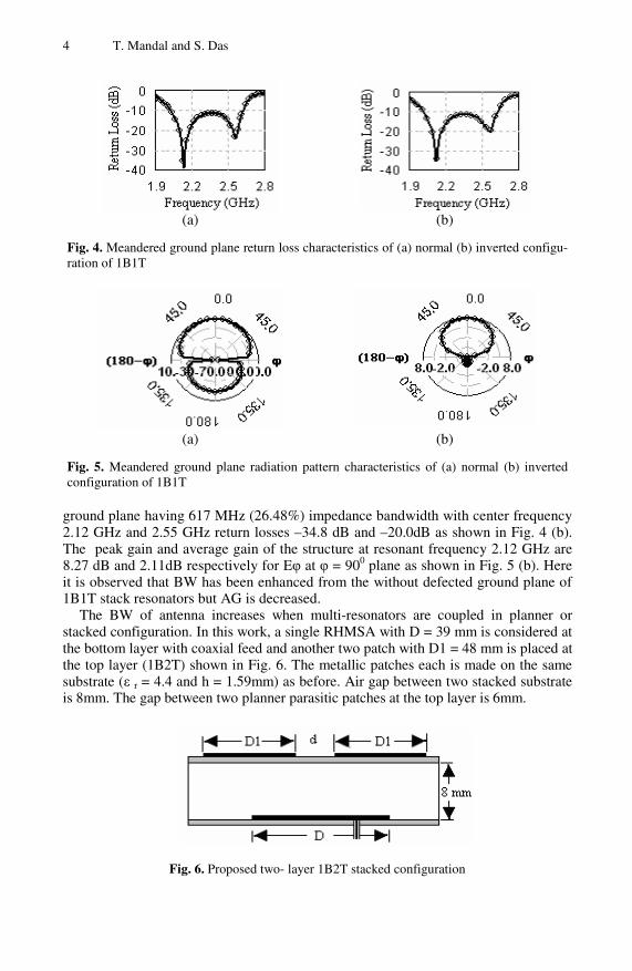
Fig. 4. Meandered ground plane return loss characteristics of (a) normal (b) inverted configu-ration of 1B1T
(a) (b)
Fig. 5. Meandered ground plane radiation pattern characteristics of (a) normal (b) inverted configuration of 1B1T
ground plane having 617 MHz (26.48%) impedance bandwidth with center frequency 2.12 GHz and 2.55 GHz return losses –34.8 dB and –20.0dB as shown in Fig. 4 (b). The peak gain and average gain of the structure at resonant frequency 2.12 GHz are 8.27 dB and 2.11dB respectively for Eφ at φ = 900 plane as shown in Fig. 5 (b). Here it is observed that BW has been enhanced from the without defected ground plane of 1B1T stack resonators but AG is decreased.
The BW of antenna increases when multi-resonators are coupled in planner or stacked configuration. In this work, a single RHMSA with D = 39 mm is considered at the bottom layer with coaxial feed and another two patch with D1 = 48 mm is placed at the top layer (1B2T) shown in Fig. 6. The metallic patches each is made on the same substrate (ε r = 4.4 and h = 1.59mm) as before. Air gap between two stacked substrate is 8mm. The gap between two planner parasitic patches at the top layer is 6mm.
Fig. 6. Proposed two- layer 1B2T stacked configuration

Bandwidth Enhancement of Stacked Microstrip Antennas 5
Fig. 7(a). Meandered ground plane return loss characteristic of 1B2T
Fig. 7(b). Meandered ground plane radiation pattern of 1B2T
Return loss characteristic of 1B2T configuration exhibits 505MHz (20%) imped-ance BW with center frequency 2.46 GHz having return loss –30 dB. The peak gain and the average gain of the structure at frequency 2.46GHz is 9.85 dB and 3.55dB respectively for Eφ at φ= 900 plane. Therefore this structure increases the AG by 1.58dB due to the increased area.
Here the ground plane of 1B2T stack resonator is defected by four identical circu-lar slots with diameter 16mm, all are placed symmetrically in the ground plane. Gap between the circular slots is 4mm. The distance between center of circular slots and center of the bottom patch is 14.14mm. The return loss characteristic exhibits imped-ance bandwidth 764 MHz (33%) with center frequencies are 2.06GHz and 2.6GHz having return losses -27.6dB and -19.8 dB respectively shown in Fig. 7(a). At fre-quency 2.3GHz, the peck gain and the average gain of the structure is 8.77dB and 2.54dB at Eφ, φ=900shown in Fig. 7 (b).
The analyzed antenna is presented in Fig. 6. The upper patches are fed electromag-netically by the bottom patch through a coupling area, and whose size determines the coupling magnitude. According to the transmission line theory, the open circuits realized by the radiating edges of the driven patch are located underneath the low impedance planes of the upper patches. Hence, the fringing fields are attracted, so that high electromagnetic coupling is achieved and therefore a large bandwidth may be obtained. A narrow spacing between the upper patches moves the radiating edges of the lower patch closer to the transversal axes of the upper patches associated with the short circuit planes, and therefore increases the coupling. One must ensure that the resonance modes of the two upper patches are excited in phase. This is the obviously the case for two identical patches are arranged symmetrically with respect to the lon-gitudinal axis of the lower patch, in the H-plane. This is also true for the gaps coupled parasitic two patches displayed symmetrically in the E plane. They are placed in similar impedance planes, so that a same type coupling occurs between the bottom patch and each of the upper patches. Since the resonance frequencies are close, the phase of the current densities is constant over the whole patch. The induced currents from the lower patch to the upper patches are also in phase.

6 T. Mandal and S. Das
3 Conclusion
Gap–coupled planar multi-resonator and stacked configurations are combined to ob-tain wide bandwidth with higher gain. In this paper, simulation details results have been presented for coaxial probe, two layers stacked resonator, combination of planar and stacked resonators MSA, and ground plane defected stacked MSA. Simulation results exhibit gradual improvement of impedance BW and AG from 453 MHz to 764 MHz and 1.63dB to 2.54dB respectively with nominal frequency variation.
This type MSA is offering grater bandwidth and higher gain over circular, square, triangular and rectangular Structure. It is less expensive due to less area of the metal-lic patch over conventional structure. Therefore this structure is most significant for broadband operation.
Acknowledgement. This work is supported by AICTE, New Delhi.
References
1. Kumar, G., Ray, K.P.: Broad Band Microstrip Antennas. Artech House, Norwood (2003) 2. Splitt, G., Davidovitz, M.: Guideline for the Design of Electromagnetically Coupled Micro-
strip Patch Antennas on two layersubstrate. IEEE Trans. Antennas Propagation AP-38(7), 1136–1140 (1990)
3. Sabban, A.: A new broadband stacked two layer microstrip antenna. In: IEEE AP –S Int. Sump. Digest, pp. 63–66 (June 1983)
4. Damiano, J.P., Bennegueouche, J., Papiernik, A.: Study of Multilayer Antenna with Radiat-ing Element of Various Geometry. Proc. IEE, Microwaves, Antenna Propagation, Pt. H 137(3), 163–170 (1990)
5. Wong, K.L.: Design of Nonplanar Microstrip Antenna and Transmission Lines. Wiley, New York (1999)
6. Legay, H., Shafai, L.: New Stacked Microstrip Antenna with Large Bandwidth and high gain. IEE Pros. Microwaves, Antenna Propagation, Pt. H 141(3), 199–204 (1994)
7. BalaKrishan, B., Kumar, G.: Wideband and high gain broad band Electromagnetically coupled Microstrip Antenna. IEEE Trans. AP-S Int. Symp. Digest, pp. 1112–1115 (June 1998)
8. Legay, H., Shafai, L.: A New Stacked Microstrip Antenna with Large Bandwidth and high gain. IEE Pros. Microwaves, Antenna Propagation, 949–951 (1993)
V.V. Das, N. Thankachan, and N.C. Debnath (Eds.): PEIE 2011, CCIS 148, pp. 7–12, 2011. © Springer-Verlag Berlin Heidelberg 2011
Study of Probabilistic Neural Network and Feed Forward Back Propogation Neural Network for Identification of
Characters in License Plate
Kemal Koche1, Vijay Patil2, and Kiran Chaudhari2
1 Computer Science and Engineering, Nagpur Uni, India [email protected]
2 Computer Science and Engineering, Pune Uni, India [email protected], [email protected]
Abstract. The task of vehicle identification can be solved by vehicle license plate recognition. It can be used in many applications such as entrance admis-sion, security, parking control, airport or harbor cargo control, road traffic control, speed control and so on. Different Neural Network for character identi-fication like Probabilistic Neural Network and Feed-Forward Back-propagation Neural Network has been used and compared. This paper proposes the use of Sobel operator to identify the edges in the image and to extract the License plate. After extraction of license plate the characters are isolated and passed to character identification system. The method used to identify characters are Probabilistic Neural Network with 108 neurons which gives accuracy of 91.32%, Probabilistic Neural Network with 35 neurons which gives accuracy of 96.73% and Feed Forward Back Propagation Neural Network which gives accuracy of 96.73%.
Keywords: License Plate Recognition (LPR), Intelligent Transportation System (ITS), Probabilistic Neural Network (PNN), Optical Character Recognition (OCR).
1 Introduction
During the past few years, intelligent transportation systems (ITSs) have had a wide impact in the life of people, as their scope is to improve transportation safety and mo-bility and to enhance productivity through the use of advanced technologies. ITSs systems are divided into intelligent infrastructure systems and intelligent vehicle sys-tems [1]. In this paper, a computer vision and character recognition algorithm for the license plate recognition (LPR) had being presented to use as a core for intelligent infrastructure like electronic payment systems at toll or at parking and arterial man-agement systems for traffic surveillance. Moreover, as increased security awareness has made the need for vehicle based authentication technologies extremely significant, the proposed system may be employed as access control system for monitoring of unauthorized vehicles entering private areas. The license plate remains as the principal vehicle identifier despite the fact that it can be deliberately altered in fraud situations or

8 K. Koche, V. Patil, and K. Chaudhari
replaced (e.g., with a stolen plate). Therefore, ITSs rely heavily on robust LPR sys-tems. The focus of this proposed system is on the integration of a novel segmentation technique implemented in an LPR system able to cope with outdoor conditions if parameterized properly.
2 Literature Survey
Recognition algorithms reported in previous research are generally composed of sev-eral processing steps, such as extraction of a license plate region, segmentation of characters from the plate, and recognition of each character. Papers that follow this three-step framework are covered according to their major contribution in this section.
2.1 License Plate Detection
As far as extraction of the plate region is concerned; there are several techniques for identification of license plates. The technique based on Sliding window method [1] [7] shows good results. The method is developed in order to describe the “local” ir-regularity in the image using image statistics such as standard deviation and mean value. Techniques based upon combinations of edge statistics and mathematical mor-phology featured very good results [2]. In these methods, gradient magnitude and their local variance in an image are computed. The paper [3] explains the license plate detection based on color features and mathematical morphology. Since these methods are generally color based, they fail at detecting various license plates with varying colors. The paper [5] proposes a novel license plate localization algorithm for auto-matic license plate recognition (LPR) systems. The proposed approach uses color edge information to refine the edge points extracted in a gray-level image. In [8], the paper presents a hybrid license plate location method based on characteristics of char-acters’ connection and projection. This method uses edge detection technique and binarization method.
2.2 Character Segmentation
Number of techniques, to segment each character after localizing the plate in the image has also been developed, such as feature vector extraction and mathematical morphology [1] [2]. An algorithm based on the histogram, automatically detects fragments and merges these fragments before segmenting the fragmented characters. A morphological thickening algorithm automatically locates reference lines for sepa-rating the overlapped characters. The paper uses binarization method, proposed by Sauvola [1][8], to obtain binary image. We have used adaptive thresholding method in our LPR system.
2.3 Character Recognition
For the recognition of segmented characters, numerous algorithms exploited mainly in optical character-recognition applications, Neural networks [1] [2] [8], Hausdorff distance [9] measures the extent to which each point of a model set lies near some point of an image set and vice versa. Support vector machines (SVM)-based character

Study of Probabilistic Neural Network and Feed Forward Back PNN 9
recognizer [10] can be used to provide acceptable alternative for recognition of char-acters in License plate. Multilayer Perceptron Neural Networks can be use for license plate character identification. The training method for this kind of network is the error back -propagation (BP). The network has to be trained for many training cycles in order to reach a good performance. This process is rather time consuming, since it is not certain that the network will learn the training sample successfully. Moreover, the number of hidden layers as well as the respective neurons has to be defined after a trial and error procedure. Probabilistic Neural Networks (PNNs) for LPR are ex-plained in [1]. Hausdorff distance has all the mathematical properties of a metric. Its main problem is the computational burden. Its recognition rate is very similar to that obtained with Neural-Network classifiers, but it is slower. Therefore, it is good as a complementary method if real-time requirements are not very strict. A suitable technique for the recognition of single font and fixed size characters is the pattern matching technique [7]. Although this one is preferably utilized with binary images, properly built templates also obtained very good results for grey level images. A simi-lar application is described in [7], where the authors used a normalized cross correla-tion operator. We have compared and studied Probabilistic Neural Network, Feed Forward Back Propagation Neural Network in this paper.
3 Proposed Method
The proposed system focuses on the design of algorithm used for extracting the license plate from a single image, isolating the characters of the plate and identifying the individual characters. Our license plate recognition system can be roughly broken down into the following block diagram in fig. 1.
Single Image
Sub-image containing only License plate
Images with license Plate number
Characters of license Plate
Convert to gray scale
Extract License Plate
Isolate Character
Identify Character
Input Color Image
Fig. 1. Flow chart of basic LPR system

10 K. Koche, V. Patil, and K. Chaudhari
The system takes color image as input and converts it into gray scale image. The system then extracts the license plate from the image. The extracted license plate is then segmented to obtain sub-images containing license plate characters, which are then passed to OCR machine which will then identify the characters. The extraction and isolation of License plate had been done using segmentation techniques and char-acter recognition had been done using different neural networks i.e. Probabilistic Neural Network and Feed-Forward Back-Propagation Neural Network.
4 Liscence Plate Recognition (LPR) System
We can divide the algorithm into three parts, first where the License plate is extracted from the input RGB image and second, where extracted License plate is segmented down to individual images containing the character in the License plate. In the last part the segmented characters are then identified using different character identifica-tion methods.
4.1 License Plate Extraction Machine
The purpose of this part is to extract the License Plate from a captured image. The output of this module is the gray picture of the LP precisely cropped from the cap-tured image, and a binary image, which contains the normalized LP. The most impor-tant principle in this part is to use conservative algorithms which as we get further becomes less conservative in order to, step by step, get closer to the license plate, and avoid loosing information in it, i.e. cutting digits and so on. We have used Sobel op-erator to identify edges of the License plate.
4.2 Character Segmentation
In order to segment the characters in the binary license plate image the method named peak-to-valley is used. The methods first segments the picture in digit images getting the two bounds of the each digit segment according to the statistical parameter DIGIT_WIDTH = 18 and MIN_AREA = 220. For that purpose, it uses a recursive function, which uses the graph of the sums of the columns in the LP binary image. This function parses over the graph from left to right, bottom-up, incrementing at each recursive step the height that is examined on the graph.
4.3 OCR Engine
Given the digit image obtained at the precedent step, this digit is compared to digits images in a dataset, and using the well-known Neural Network method, after interpo-lations, approximations and decisions algorithm, the OCR machine outputs the closest digit in the dataset to the digit image which was entered. As known, neural network is a function from vector to vector, and consists of an interpolation to a desired function. Matlab provides very easy-to-use tools for Neural Networks, which permits to con-centrate on the digit images dataset only. We have compared two neural networks namely Probabilistic Neural network and Feed-Forward back propagation neural network; Results are given in the table 1.

Study of Probabilistic Neural Network and Feed Forward Back PNN 11
Table 1. Comparison of LPR system for different Neural Networks OPNN-Original Probablis-tic Neural Network, IPNN-Inproved Probablistic Neural Network,FFBP-Feed Forward Back Propogation
OPNN (108Neurons)
IPNN (35Neurons)
FFBP
Problems encounter
To identify similar character like ‘I’&1,’O’&0,’Z’&7,’B’&8
To identify similar character like ‘I’&1,’O’&0,’Z’&7,’B’&8
To identify similar character like ‘I’&1,’O’&0,’Z’&7,’B’&8
Improvement Improved after Training
Improved after Training
Improved after Training
Accuracy 91.42% 96.73% 96.73%
Features Accurate , But require large memory.
More accurate than OPNN
Accurate and require less memory
5 Conclusion
This method can be used to implement a real time application for identifying the vehicle. The license number can be compared with database or use to maintain infor-mation at parking lot or at entrance. This paper proposes the use of Sobel operator to identify the edges in the image and to extract the License plate. We have done all the processing on gray scale image hence external colors and environmental conditions has least effect on the system. After extraction of license plate the characters are isolated and passed to character identification system.
The method used to identify characters Probabilistic Neural Network with 108 neurons which gives accuracy of 91.32%, Probabilistic Neural Network with 35 neu-rons which gives accuracy of 96.73% and Feed Forward Back Propagation Neural Network which gives accuracy of 96.73%.
References
1. Anagnostopoulos, C., Anagnostopoulos, I., Tsekouras, G., Kouzas, G., Loumos, V., Kayafas, E.: Using sliding concentric windows for license plate segmentation and process-ing. IEEE Transactions on Intelligent Transportation Systems 7(3) ( September 2006)
2. Yang, F., Ma, Z.: Vehicle License Plate location Based on Histogramming and Mathe-matical Morphology. In: IEEE Workshop on Automatic Identification Advance Technol-ogy (October 2005)
3. Syed, Y.A., Sarfraz, M.: Color Edge Enhancement based Fuzzy Segmentation of License Plates. In: Proceedings of the Ninth International Conference on Information Visualisation (IV 2005). IEEE, Los Alamitos (2005)

12 K. Koche, V. Patil, and K. Chaudhari
4. Koval, V., Turchenko, V., Kochan, V., Sachenko, A., Markowsky, G.: Smart. License Plate Recognition System Based on Image Processing Using Neural Network. In: IEEE Workshop on Intelligent Data Acquisition and Advanced Computing Systems: Technology and Application, Lviv, Ukraine, pp. 8–10 (September 2003)
5. Lin, C.-C., Huang, W.-H.: Locating License Plate Based on Edge Features of Intensity and Saturation Subimages. In: IEEE Second International Conference on Innovative Comput-ing, Information and Control, September 5-7, p. 227 (2007)
6. ter Brugge, M.H., Stevens, J.H., Nijhuis, J.A.G., Spaanenburg, L.: License Plate Recogni-tion Using DTCNNs. In: Fifth IEEE lntenational Workshop on Cellular Neural Networks and their Applications, London, England, April 14-17 (1998)
7. Anagnostopoulos, C., Alexandropoulos, T., Boutas, S., Loumos, V., Kayafas, E.: A tem-plate-guided approach to vehicle surveillance and access control. In: IEEE Conference on Advance Video and Signal Based Survillance, September 15-16, pp. 524–539 (2005)
8. Zhang, C., Sun, G., Chen, D., Zhao, T.: A Rapid Locating Method of Vehicle License Plate Based on Characteristics of Characters’ Connection and Projection. In: 2nd IEEE Conference on Industrial Electronics and Applications, May 23-25, pp. 2546–2549 (2007)
9. Huttenlocher, D.P., Klanderman, G.A., Rucklidge, W.J.: Comparing Images Using the Hausdorff Distance. IEEE Transactions on Pattern Analysis and Machine Intelli-gence 15(9), 850–863 (1993)
10. Kim, K.K., Kim, K.I., Kim, J.B., Kim, H.J.: Learning-based approach for license plate rec-ognition. In: Proceedings of the 2000 IEEE Signal Processing Society Workshop Neural Networks for Signal Processing, December 11-13, vol. 2, pp. 614–623 (2000)

V.V. Das, N. Thankachan, and N.C. Debnath (Eds.): PEIE 2011, CCIS 148, pp. 13–18, 2011. © Springer-Verlag Berlin Heidelberg 2011
Efficient Minimization of Servo Lag Error in Adaptive Optics Using Data Stream Mining
Akondi Vyas1,2, M.B. Roopashree1, and B. Raghavendra Prasad1
1 Indian Institute of Astrophysics, II Block, Koramangala, Bangalore 560034, India 2 Indian Institute of Science, Malleswaram, Bangalore 560012, India
vyas,roopashree,[email protected]
Abstract. Prediction of the wavefronts helps in reducing the servo lag error in adaptive optics caused by finite time delays (~ 1-5 ms) before wavefront correc-tion. Piecewise linear segmentation based prediction is not suitable in cases where the turbulence statistics of the atmosphere are fluctuating. In this paper, we address this problem by real time control of the prediction parameters through the application of data stream mining on wavefront sensor data ob-tained in real-time. Numerical experiments suggest that pixel-wise prediction of phase screens and slope extrapolation techniques lead to similar improvement while modal prediction is sensitive to the number of moments used and can yield better results with optimum number of modes.
Keywords: Adaptive optics, data stream mining, turbulence prediction, servo lag error.
1 Introduction
Data mining is a productive statistical analysis of large amounts of data to discover patterns and empirical laws which are not obvious when manually examined[1]. As-tronomy has seen data mining as a tool to archive large amounts of data. Advances in experimental astronomy depends on designing larger telescopes. The need for increas-ing the size of ground based telescopes and disadvantages of space telescopes is well known. A fast real-time feedback loop based wavefront correcting technology called adaptive optics is used to correct the incoming wavefront distortions due to turbulent atmosphere. But there exist time lags (comparable to optimum closed loop band-width) because of the delay between the wavefront correcting instrument and the wavefront sensor. These delays are essentially due to the finite exposure time and non-zero response times of the instruments in the feedback loop. These errors can be minimized through progressive prediction of wavefronts using time series data min-ing. The prediction accuracy depends strongly on the atmospheric turbulence parame-ters which fluctuate in time. Hence, there is a need for continuous monitoring of the atmospheric turbulence parameters for optimum performance of adaptive optics sys-tems. However, this requires highly sophisticated instruments and control. Here, we investigated this problem through numerical simulations by adaptively changing the prediction parameters using data stream mining of existing wavefront sensor data.

14 A. Vyas, M.B. Roopashree, and B.R. Prasad
The need for prediction in adaptive optics is illustrated in the next section. The de-pendence of the parameters that control prediction process on atmospheric turbulence is described in section 3. The steps involved and the methods used in the prediction methodology are explained in section 4. The last section presents the results and conclusions.
2 Need for Prediction in Adaptive Optics
Successful performance of the adaptive optics system needs operation at optimized bandwidth which is near the Greenwood frequency, fG [2]. In the case of sites with good seeing, the minimum bandwidth requires running the closed loop faster than 200 Hz. It is a challenging task to run the closed loop system at the Greenwood fre-quency, due to the unavoidable time lags in the closed loop [3]. The minimum expo-sure time (τexp) required for reasonably accurate wavefront sensing limits the rate of closed loop operation. Added to this delay is the response timescales of the controller (τc) and corrector (τdm). Hence the total servo lag is τL = τexp + τc + τdm. The existence of servo lag implies that the sensed wavefront is corrected after a delay τL. From the spatial and temporal correlation of wavefronts, it is possible to track the evolution of wavefronts and hence greatly reduce the effect of the servo lag. Various predictors are suggested in the literature[4] which assume Taylor's frozen in turbulence approx-imation, also verified experimentally[5]. Under this approximation, for a telescope of diameter, D (say, D=2m), the decorrelation time is τd = D / va (τd = 200ms at va = 10m/s). Two wavefronts separated in time by larger than τd are said to be decorrelated.
The wavefront prediction parameters can either be the local wavefront slopes measured by a sensor or the wavefront modes formed from an orthogonal basis. There are two important extrapolation parameters that decide the prediction accuracy. One of them is the number of wavefronts (n) to be used for optimum prediction and the other is the time representing the best predictable future (τpf). The parameters n and τpf are called the data stream parameters and obviously depend on τd and the spatial cohe-rence length represented by Fried parameter, r0. The existence of fluctuations in r0 and the wind speed that controls τd are well known. These variations also drive n and τpf into instability hence causing "Concept Drift". Analyzing the reported r0 measure-ments at the Oukaimeden site, it can be observed that within 0.5 hrs, r0 fluctuates with a standard deviation of 1.33 cm[6]. The RMS variability of wind velocity is 0.5 m/s within 10 s as was reported[7, 8]. The temporal variability of the turbulence parame-ters are also site dependent[9]. Temporal data mining methods help in predicting the future turbulence phase screens[10].
3 Prediction Accuracy and Data Stream Mining
To test the dependence of prediction accuracy on the way optimum data stream para-meters change with time, Monte Carlo simulations of closed loop adaptive optics system were performed within the decorrelation timescales of atmospheric turbulence. For the simulation of atmosphere like phase screen following Kolmogorov statistics, Zernike moments were computed through the covariance relation derived by Noll[11]. In order to closely depict temporal turbulence, the angular rate of the wind, ω and va the wind velocity are included in the simulations[12].

Efficient Minimization of Servo Lag Error in Adaptive Optics 15
In order to understand the dependence of wavefront prediction accuracy on the data stream parameters, simulations were performed with fluctuating wind speed va and Fried's parameter, r0. As shown in Fig. 1, the wavefront prediction accuracy strongly depends on the best predictable phase screen. The percentage improvement in the correlation, PICC plotted in the y-axis of the graph is calculated using the formula,
100X
XXPI
Act-Last
ActLastActPreCC ×−= −− (1)
where, XLast-Act is the correlation coefficient between the last phase screen in the train-ing data cube and the actual phase screen which is to be predicted, XPre-Act represents the correlation coefficient of the predicted phase screen and the actual phase screen.
Fig. 1. Case: n = 5; Optimum τpf depends on r0 (values given in legend) and τd
The choice of optimum segment size, nopt (τpf given) can be made by studying PICC at different 'n' values as shown in Fig. 2. For the phase screens generated to obtain these curves, the decorrelation time was set to 20 ms. For n = 5, the percentage im-provement in correlation is maximum at t = 12 ms and for n = 30, the percentage improvement in correlation is maximum at t = 3 ms. Considering a servo lag error of 5 ms, optimum value of 'n' is found to be in the range from 20 to 30. Also, the mini-mum improvement is above 20% and below 30% within the decorrelation time. If this training were not present, using n = 5 for the case of 5 ms time lag would lead to a prediction which is ~10% less accurate.
Fig. 2. Choosing optimum 'n' through knowledge of τpf

16 A. Vyas, M.B. Roopashree, and B.R. Prasad
4 Prediction Methodology
Data cube is a three dimensional data grid which piles up the phase screens in the order of their arrival in time. To avoid memory constraints and taking the advantage of the fact that the atmospheric parameters slowly change in time, the volume of the data cube is kept constant by removing the oldest phase screen on the addition of a latest one. The major steps involved in the prediction process include (a) data stream parameter estimation and data selection (b) Prediction through extrapolation. Opti-mum number of phase screens is selected for extrapolation from the data cube as discussed in the earlier section. There exists many methods for segmentation of the time series in the literature[1]. The top-down, bottom-up and sliding windows me-thods were discussed previously in the case of adaptive optics using modal and zonal predictors[10]. Linear as well as nonlinear extrapolation methods can be applied for prediction of future phase screens. If the data is well trained in the manner suggested previously, linear predictor would be the best choice. In any case, nonlinear methods are not very well known to give better results. Linear extrapolation requires to fit the evolution of 'nopt' latest phase screens with appropriate straight lines and extrapolate them to obtain the required phase screen after a time, τpf. In the case of zonal predic-tion, either the individual pixels of the phase screens (computationally tedious, accu-rate) or the local slopes of a Shack Hartmann sensor (SHS) (faster, less accurate) are used for extrapolation into the future. In the case of modal prediction, Zernike coeffi-cients (or modes corresponding to any orthogonal basis) are extrapolated. Modal prediction performs better than the slope extrapolation method (Fig. 4).
5 Results and Conclusions
Monte Carlo simulations were performed on phase screens simulated which include the fluctuations in the data stream parameters in time. A comparison of a simple pre-diction methodology and data stream mining based prediction is shown in Fig. 3. Pixel-wise linear predictor is a lossless predictor, although computationally challeng-ing, where the computational time involved increases linearly with the number of elements (pixels in this case) to be predicted (400 elements takes 1.25s; computations done on 1.4GHz Intel(R) Core(TM)2 Solo CPU with 2GB RAM). Slope extrapolation is a prediction methodology where the information that is available is the local slopes measured via a SHS. Hence, the number of elements to be predicted in this case is 2×ASH, where ASH is equal to the number of subapertures of the Shack Hartmann sensor used for wavefront sensing. A factor of '2' appears due to the existence of 'x' and 'y' slopes. Increasing the number of apertures of a SH sensor would increase the computational time in this case.
Modal prediction is yet another prediction methodology where the number of ele-ments is determined by the number of orthogonal modes (N) to be used to represent the phase screen reasonably accurately. Individual phase screens are decomposed into complex Zernike polynomials through fast computation of Zernike moments and these moments are used for prediction and wavefront analysis[13].
A comparison of the performance of these methods is shown in Fig. 4. It can be observed that the performance of the pixel-wise prediction overlaps with the slope
Efficient Minimization of Servo Lag Error in Adaptive Optics 17
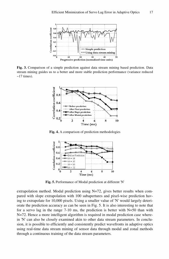
Fig. 3. Comparison of a simple prediction against data stream mining based prediction. Data stream mining guides us to a better and more stable prediction performance (variance reduced ~17 times).
Fig. 4. A comparison of prediction methodologies
Fig. 5. Performance of Modal prediction at different 'N'
extrapolation method. Modal prediction using N=72, gives better results when com-pared with slope extrapolation with 100 subapertures and pixel-wise prediction hav-ing to extrapolate for 10,000 pixels. Using a smaller value of 'N' would largely deteri-orate the prediction accuracy as can be seen in Fig. 5. It is also interesting to note that for a servo lag in the range 7-10 ms, the prediction is better with N=50 than with N=72. Hence a more intelligent algorithm is required in modal prediction case where-in 'N' can also be closely examined akin to other data stream parameters. In conclu-sion, it is possible to efficiently and consistently predict wavefronts in adaptive optics using real-time data stream mining of sensor data through modal and zonal methods through a continuous training of the data stream parameters.

18 A. Vyas, M.B. Roopashree, and B.R. Prasad
References
1. Last, M., Kandel, A., Bunke, H.: Data mining in time series databases. World Scientific, Singapore (2004)
2. Greenwood, D.P.: Bandwidth specification for adaptive optics systems. J. Opt. Soc. Am. 67, 390–393 (1977)
3. Lloyd-Hart, M., McGuire, P.: Spatio-temporal prediction for adaptive optics wavefront reconstructors. In: ESO Astrophysics Symposia (1996)
4. Poyneer, L., Veran, J.P.: Predictive wavefront control for adaptive optics with arbitrary control loop delays. J. Opt. Soc. Am. 25, 1486–1496 (2008)
5. Poyneer, L., Dam, M.V., Veran, J.P.: Experimental verification of the frozen flow atmos-pheric turbulence assumption with use of astronomical adaptive optics telemetry. J. Opt. Soc. Am. A 26, 833–846 (2009)
6. Benkhaldoun, Z., Abahamid, A., El Azhari, Y., Lazrek, M.: Optical seeing monitoring at the Oukaïmeden in the Moroccan high atlas mountains: first statistics. Astronomy and Astrophysics 441, 839–843 (2005)
7. Els, S.G., Travouillon, T., Schock, M., Riddle, R., Skidmore, W., Seguel, J., Bustos, E., Walker, D.: Thirty Meter Telescope Site Testing VI: Turbulence Profiles. PASP 121(879), 527–543 (2009)
8. Benkhaldoun, Z.: Oukaimeden as a potential observatory: Site testing results. In: Proceed-ings of the ASP Conference, vol. 266, p. 414 (2002)
9. Travouillon, T., et al.: Temporal variability of the seeing of TMT sites. In: Stepp, L.M., Gilmozzi, R. (eds.) SPIE, vol. 7012(1), pp. 701–220 (2008)
10. Vyas, A., Roopashree, M.B., Prasad, B.R.: Progressive Prediction of Turbulence Using Wave-Front Sensor Data in Adaptive Optics Using Data Mining. IJTES 1(3) (2010)
11. Noll, R.J.: Zernike polynomials and atmospheric turbulence. J. Opt. Soc. Am. 66, 207–211 (1976)
12. Hu, L., Xuan, L., Cao, Z., Mu, Q., Li, D., Liu, Y.: A liquid crystal atmospheric turbulence simulator. Opt. Express 14, 11911–11918 (2006)
13. Hosny, K.M.: Fast computation of accurate Zernike moments. Journal of Real-Time Image Processing 3, 97 (2008)

V.V. Das, N. Thankachan, and N.C. Debnath (Eds.): PEIE 2011, CCIS 148, pp. 19–25, 2011. © Springer-Verlag Berlin Heidelberg 2011
Soft Switching of Modified Half Bridge Fly-Back Converter
Jini Jacob1 and V. Sathyanagakumar2
1 Senior Lecturer, Dept. of Electrical and Electronics Engineering, MVJ College of Engineering, Bangalore
[email protected] 2 Professor and Chairman, Dept. of Electrical Engineering,
University Visvesvaraya College of Engineering, Bangalore [email protected]
Abstract. This paper presents soft switching of modified half bridge fly-back converter. The power switches in this converter are turned on at ZVS and the rectifier diode is turned on and off at ZCS. The auxiliary switch is turned off at ZCS. The voltage stress across the switch is equal to the supply voltage and soft switching is achieved for all the switching devices. Compared to half bridge fly-back converter, this modified circuit has improved efficiency. A 5V/2A prototype is implemented to verify the practical results.
Keywords: Half Bridge, Fly-back, soft switching, ZVS, ZCS.
1 Introduction
The conventional fly-back converter is widely being used for low power applications due to its low cost and robust characteristics. But the hard switching operation and high switching stresses across the switching devices introduced a lot of limitation in the application of fly-back converter. A number of topologies have been introduced recently to overcome these drawbacks. Among the different topologies, the active clamp converter [1] reduces the switching losses but the voltage stress across the power switch is same as that of conventional fly-back converter.
The asymmetrical fly-back topologies [2-3] can achieve zero voltage switching op-eration of the power switches but the hard switching of the output rectifier at turn off increases the energy loss due to reverse recovery current. In half bridge fly-back con-verter [4], the switches are turned on at zero voltage and the output diodes are turned on and off at zero current. The main disadvantage of the circuit is that the efficiency is not improved because of switching losses during turn off though the switches are turned on at zero voltage and output diodes are turned on and off at zero current. In this topology the input current drawn from the supply at light load condition is more and it is also another reason for low efficiency.
In this proposed topology as shown in Fig. 1, a modified half bridge fly-back con-verter without any output inductor in which the power switches are turned on at zero voltage and turned off at zero current and the rectifier diode is turned on and off at zero current which reduces the switching losses. The voltage stress across the power

20 J. Jacob and V. Sathyanagakumar
switches are clamped at supply voltage. The switching frequency is selected to be slightly more than resonant frequency which depends on the leakage inductance of the transformer and the resonant capacitor.
The operational principles, design considerations and simulation and practical results are given in this paper. Testing of 5V/2A prototype confirms that the experi-mental results are similar to the simulation results.
2 Operational Principles
In the proposed simplified circuit, resonant inductor is the sum of leakage inductance of the transformer and the stray inductances and is shown external to the transformer in the Fig.1. The leakage inductance is very small compared to the magnetising inductance of the transformer. The operation of this converter can be explained by considering six operating modes in a switching cycle. The equivalent circuit in each mode is as shown in Fig. 2.
Fig. 1. Circuit Diagram of the Modified Half Bridge Fly-back Converter
2.1 Mode 1 ( )
At t= , is turned on and is off. The output diode is reverse biased and the
capacitor supplies to load . , and forms a series resonant circuit with
the voltage source in series. The voltage source charges the resonant capacitor and the
current through and increases linearly. The equivalent circuit for mode 1 oper-
ation is shown in Fig. 2. The governing circuit equations are given by, . (1)
. (2)
2.2 Mode 2 ( )
This mode starts when is turned off and is also off. , , and
forms a series resonant circuit. charges and discharges. The equivalent
Q1
Q2
Vin
Cr
Co
Do
Ro
Lk
Lm
0 1t t−
0t 1Q 2Q
oC oR bC mL kL
mL kL
1 2t t−
1Q 2Q 1dsC bC mL kL
1dsC 2dsC

Soft Switching of Modified Half Bridge Fly-Back Converter 21
circuit for this mode is shown in Fig. 2. When completely discharges the body
diode of starts conducting and mode 3 starts. The governing equations for this
mode are given by
(3)
2.3 Mode 3 ( )
Both and are off in this mode. The body diode of starts conducting. This
mode ends when is turned on at zero voltage. The output diode starts conducting.
The circuit governing equations are given by,
(5)
(6)
2.4 Mode 4 ( )
In this mode is off and is turned on at zero voltage switching. Output diode
is conducting and the transformer secondary voltage is reflected to primary side of the
transformer. discharges through and . The circuit governing equations
are,
(7)
(8)
(9)
2dsC
2Q
2 3t t−
1Q 2Q 2Q
2Q
3 4t t−
1Q 2Q
bC mL kL
(4)

22 J. Jacob and V. Sathy
Mode 1
Mode 3
Mode 5
Fig. 2. Equ
2.5 Mode 5 ( )
At t= , is turned of
discharges, the body diode
lent circuit for this mode isthe end of this mode. The c
2.6 Mode 6 ( )
This mode starts when
output diode is reverse bias
4 5t t−
4t 2Q
5 6t t−
dsC
yanagakumar
Mode 2
Mode 4
Mode 6
uivalent Circuit in different Modes of Operation
ff. charges and discharges. When complet
of starts conducting and this mode ends. The equi
s shown in Fig. 2. The output diode is turned off at ZCSircuit governing equations for this mode are given by, v V (
(
(
discharges and body diode of starts conducting. T
sed and supplies the load. This mode ends when
2dsC 1dsC
1Q
1s 1Q
oC Q
tely
iva-
S at
(10)
(11)
(12)
The
is 1Q

Soft Switching of Modified Half Bridge Fly-Back Converter 23
turned on again at ZVS in the next cycle. The equivalent circuit for this mode is shown in Fig. 2. The governing circuit equations are given by, V v V (13)
(14)
The theoretical waveforms in each mode are as shown in Fig. 3.
Fig. 3. Theoretical Waveforms showing Modes of Operation
3 Simulation and Experimental Results
The modified half bridge fly-back converter is simulated using Powersim software and the simulation results are shown in Fig. 5 - Fig. 6. The prototype of the proposed modified half bridge fly-back converter is constructed for the specifications as given below.
Input voltage Vin : 20V-30V; Output voltage Vo: 5V; Output current Io: 2A; Switching Frequency fs : 100kHz ;Resonant capacitor Cb: 2.2µF; Magnetizing induc-tance : 27µH; Leakage inductance:3µH. The prototype is tested for its operational feasibility and ZVS and ZCS operations. Fig. 4a. shows the voltage across switch1 and current through it. Fig. 4b. shows the voltage across switch2 and current through it. Fig. 5. shows the current through the output diode and voltage across it. From the simulation results as shown in Figs. 4 and 5, it is clear that the switches are turned on at ZVS and turned off at ZCS. The output diode is turned on and off at ZCS. The waveforms obtained from the practical results are as shown in Figs. 6 and 7, which are closely matching with the simulation results. The peak to peak capacitor voltage is nearly half of the supply voltage. The switching losses are reduced and the efficiency
24 J. Jacob and V. Sathyanagakumar
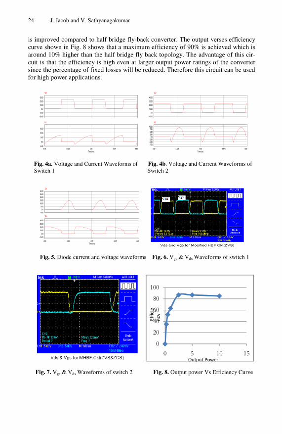
is improved compared to half bridge fly-back converter. The output verses efficiency curve shown in Fig. 8 shows that a maximum efficiency of 90% is achieved which is around 10% higher than the half bridge fly back topology. The advantage of this cir-cuit is that the efficiency is high even at larger output power ratings of the converter since the percentage of fixed losses will be reduced. Therefore this circuit can be used for high power applications.
Fig. 4a. Voltage and Current Waveforms of Fig. 4b. Voltage and Current Waveforms of Switch 1 Switch 2
Fig. 5. Diode current and voltage waveforms Fig. 6. Vgs & Vds Waveforms of switch 1
Fig. 7. Vgs & Vds Waveforms of switch 2 Fig. 8. Output power Vs Efficiency Curve
0.0
-10.00
-20.00
10.00
20.00
30.00
Vs1
4.50 4.525 4.55 4.575 4.60Time (ms)
0.0
-5.00
5.00
10.00
15.00
Is1
0.0
-10.00
10.00
20.00
30.00
40.00
Vs2
4.50 4.525 4.55 4.575 4.60Time (ms)
0.0-2.50-5.00-7.50
2.505.007.50
10.00
Is2
0.0-5.00
5.0010.0015.0020.0025.0030.00
IDo
4.50 4.525 4.55 4.575 4.60Time (ms)
0.0
-10.00
10.00
20.00
30.00
40.00
VDo
0
20
40
60
80
100
0 5 10 15
Effic
ienc
y
Output Power

Soft Switching of Modified Half Bridge Fly-Back Converter 25
4 Conclusion
In this work, a new modified half bridge fly-back converter with ZVS and ZCS oper-ation is proposed, analysed, designed and implemented in which the drawbacks of half bridge fly-back converter are eliminated. In this proposed converter, the power switches are turned on at zero voltage and turned off at zero current. The output rec-tifier diode is turned on and off at zero current. The operation of this converter is ana-lysed considering six modes. A 10W prototype is designed for a switching frequency of 100 kHz. It is found that the practical waveforms closely resemble the simulation waveform. Excellent line and load regulation is achieved and the ripple is found to be less than 0.5%. Maximum efficiency at rated input voltage is found to be nearly 90%.
References
1. Aqik, A., Cadirci, I.: Active clamped ZVS forward converter with soft-switched synchron-ous rectifier for high efficiency, low output voltage applications. lEEE Proc. EIectr. Power Appl. 150(2) (March 2003)
2. Gu, Y., Lu, Z.: A Novel ZVS Resonant Reset Dual Switch Forward DC-DC Converter. IEEE Transactions on Power Electronics 22(1) ( January 2007)
3. Watson, R., Lee, F.C., Hua, G.C.: Utilization of an Active-Clamp Circuit to Achieve Soft Switching in Fly back Converters. IEEE Trans. on Power Electronics 11(1), 162–169 (1996)
4. Wu, L.-M., Pong, C.-Y.: A Half Bridge Fly back Converter with ZVS and ZCS Operations. In: 7th International Conference on Power Electronics (October 2007)

V.V. Das, N. Thankachan, and N.C. Debnath (Eds.): PEIE 2011, CCIS 148, pp. 26–33, 2011. © Springer-Verlag Berlin Heidelberg 2011
A Novel Approach for Prevention of SQL Injection Attacks Using Cryptography and Access Control Policies
K. Selvamani1 and A. Kannan2
1 Department of Computer Science & Engineering 2 Department of Information Science & Technology,
Anna University, Chennai - 600025, TamilNadu, India Selvamani,[email protected]
Abstract. In this era of social and technological development, SQL injection at-tacks are one of the major securities in Web applications. They allow attackers to obtain an unrestricted and easy access to the databases to gain valuable information. Although many researchers have proposed various effective and useful methods to address the SQL injection problems, all the proposed approaches either fail to address the broader scope of the problem or have limi-tations that prevent their use and adoption or cannot be applied to some crucial scenarios. In this paper we propose a global solution to the SQL injection at-tacks by providing strong encryption techniques and policy based access control mechanism on the application information. We initially encrypt the message using an encryption engine in the server before we store the values into the da-tabase with Policy-based Access Control, data is stored in the encrypted form and while accessing it again we decrypt them and provide the data for the user in a secured manner with the control of policy based access.
Keywords: Encryption, Decryption, String Transform, Access Control.
1 Introduction
SQL injection is a web application attack in which malicious code is inserted into strings that are passed to an instance of SQL Server for parsing and execution. Any procedure that builds SQL statements should be reviewed for injection vulnerabilities because SQL Server will execute all syntactically valid queries that it receives. Due this reason even parameterized data can be manipulated manually who is aware of the SQL injection code and by the determined attacker. The primary way of SQL injec-tion consists of direct insertion of malicious code into user-input variables that are concatenated with SQL commands which are executed. Another form of attack is direct attack that injects malicious code into strings that are destined for storage in a table or as metadata in the database. When the stored strings are next concatenated into a dynamic SQL command, the malicious code is executed.
Hence this injection process works by terminating a text string that is appended to a new command. Since, the inserted command may have additional strings appended to it before it is executed. Therefore, the malefactor terminates the injected string with a comment mark "--". Subsequent text is ignored at execution time.

A Novel Approach for Prevention of SQL Injection Attacks 27
A characteristic or the most diagnostic or the disastrous feature of such an SQL Injection Attack (SQLIA) is that they change the intended and inherent structure of queries issued. By usefully exploiting these vulnerabilities and pitfalls, an attacker can issue his own SQL commands directly to the database and can manipulate the database in his own intended way, thereby gaining what he want from the attacked system. These attacks are serious threat to the existing web applications and any web application that receives input from users and incorporates it into SQL queries to an underlying database.
In this paper we propose a new approach for dynamic detection and prevention of SQL injection attacks. Intuitively, our approach works by encrypting the message (typically field values) and stored in the database with Access control policy. The general mechanism that we use to implement this approach is based on dynamic encryption, which encrypts certain data in a program at runtime. This is done using the Encryption Engine.
In this system, access control can choose to update privilege levels of the web re-quest to control malicious requests. This process involves characterising the incoming requests using fuzzy rules and then generating updating messages and finally updating the access privilege levels to reflect the level of users. In this three access levels namely privilege user lever, application programmer level and naïve user level are used. Queries with privilege user and application programmer level are sent to the web database with normal encryption, where as the queries with naïve user levels are sent through policy levels and then to the web database.
If the encrypted data is being queried again, the encrypted stored values are again decrypted and it is returned as a response to the request in user understandable form with the help of access control mechanism. This is done using the decryption engine. This has several advantages such as the attacker should find the encryption key in order to find the encrypted data.
For example, Here we introduce a sample SQLIA [1] and discuss the methods that are already in use to prevent these. Consider a jsp example which uses the input from user (username, password) to retrieve the information about the account. The query would be
SELECT details FROM usertable WHERE username = ´ + username + ` ´ and password = ` ´ + userpassword + ` ´ ;
The JSP snippet for the same would be
String usern = getParameter (“username”); String userp = getParameter ( “ userpass ” ); String query = SELECT details F R OM usertable WHERE username = ` ´ + usern + ` ´ AND password = ` ´ + userp + ` ´ ; Statement stmt = connetion.createStatement ( ); ResultSet rs = stmt.executeQuery(query);
If the user input for username is hanuman hanuman’ − −
and password field is left empty, the query would be

28 K. Selvamani and A. Kannan
query = SELECT details FROM usertable WHERE username = hanuman - -´ and password = ´ ;
thus the password comparison part of the query would be skipped since it is now in the comment section (the part after).
The remainder of this paper is organized as follows: Section 2 presents the related works in the field of SQL injection attacks and the existing systems. Section 3 depicts the proposed system architecture. Section 4 presents details of encryption and decryp-tion techniques and its experimental setup. Section 5 provides the results of the implemented system in this paper. Section 6 gives a brief conclusion on this work and suggests some possible future works.
2 Related Works
There are many works in the literature that discuss about SQL Injection attacks. AM-NESIA [1] is a model- based technique that combines static analysis with runtime monitoring which is dynamic. Even though their system combines both static and dynamic technique but it fails in preventing new types of SQL attacks.
In another work, the authors [2] proposed Positive tainting and negative tainting, that has conceptual difference with that of the traditional tainting. Positive tainting is based on the identification, marking, and tracking of trusted, rather than un-trusted data. In the case of negative tainting, incompleteness may lead to trusting data that should not be trusted and, ultimately leads to false negatives.
Another author Sruthi Bandhakavi [3] tries to solve this by discovering intent dy-namically and then comparing the structure of the identified query after user input with the discovered intent. This works fine for normal queries but this approach fails when the external function is not protected. The SQL-IDS system [4] presented a technique which is composed of an anomaly detection system that uses abstract pay-load execution [6] and payload sifting techniques to identify web requests that might contain attacks that exploit memory violations.
A new method for protecting web databases [8] that is based on fine-grained access control mechanism was proposed by Alex Roichman and Ehud Gudes. This method uses the databases' built-in access control mechanisms enhanced with Parameterized Views and adapts them to work with web applications.
Another method proposed by Wissam Mallouli and Jean-Marie Orset [9] was a framework to specify security policies and test their implementation on a system. Their framework makes it possible to generate in an automatic manner, test sequences, in order to validate the conformance of a security policy.
In order to address this problem, this paper aims in providing global solutions to the SQL injection attacks by applying cryptography techniques and policy based ac-cess control mechanism together to prevent intelligently the SQL Injection attacks. We initially encrypt the message using an encryption engine in the server before we store the values into the database, data is stored in the encrypted form and while accessing it again we decrypt them and provide the results.

A Novel Approach for Prevention of SQL Injection Attacks 29
3 System Architecture
In this work, our intention is to detect SQL attack intelligently in a sneaky way. We encrypt the data as soon as we receive it from the user, even before we start proc-essing anything from the user.
The proposed system architecture for encryption in server and decryption at web database is shown in figure 1. It contains the two components: Server along with encryption engine and the database with decryption engine. The encryption is carried over on the data at the server side, and the database before performing any query operation using the decryption engine decrypts the data.
Fig. 1. System Architecture
Figure 2 shows the encryption mechanism of the data at server side. The received user inputs are encrypted using the encryption mechanism and the encrypted data are transformed using the query transformation and finally the transformed data stored using query execution. The DES algorithm is used for the encryption of the data at the server side. DES encrypts and decrypts data in 64-bit blocks, using a 64-bit key (although the effective key strength is only 56 bits, as explained below). It takes a 64-bit block of plaintext as input and outputs a 64-bit block of cipher text. Since it always operates on blocks of equal size and it uses both permutations and substitu-tions in the algorithm, DES is both a block cipher and a product cipher.
DES has 16 rounds, meaning the main algorithm is repeated 16 times to produce the cipher text. It has been found that the number of rounds is exponentially propor-tional to the amount of time required to find a key using a brute-force attack. So as the number of rounds increases, the security of the algorithm increases exponentially.
3.1 Key Scheduling
Although the input key for DES is 64 bits long, the actual key used by DES is only 56 bits in length. The least significant (right-most) bit in each byte is a parity bit, and should be set so that there are always an odd number of 1s in every byte. These parity bits are ignored, so only the seven most significant bits of each byte are used, result-ing in a key length of 56 bits.
User Inputs Encrypted Transformed User Inputs
Fig. 2. Encryption mechanism at the server side
User Interface
Server Script Engine
Encryption Engine
Web Database
Decryption in Query Engine
Encryption Query
Execution for Storage
Query Transformation

30 K. Selvamani and A. Kannan
Figure 3 shows how the database querying engine has to be modified, hence it can be used for both encryption and decryption. Providing the encrypted data will give the actual user input, from which the required processing is done at the server. Each time the database has to operate on some value stored in the database, it per-forms Algorithm 1 .
User Query Tables Data to be
Required Decrypted
Fig. 3. Encryption mechanism at the database
Consider the query string
String query = SELECT details FROM useraccount WHERE username = ´ + username + ` ´ and password = ´ + password + ` ´ ;
If user input for username is xxxx and password is yyyy then the username and password before being inserted is transformed to some other form. (i.e, encrypted) so that the actual SQL intend is not executed.
SELECT details FROM useraccount WHERE username = mxsyz ´ and password = `sddxc ´;
From this we can identify the structure as SELECT, FROM, WHERE, AND. Here we must also take care of the comments as the user input like the fol-
lowing may maintain the intent structure without comment but would fail if com-ment also is considered. If user input for username is hanuman and 1=1 then the query becomes as shown below. The structure without considering the comment would be same as the structure identified before SELECT, FROM, WHERE, AND.
SELECT details FROM user account WHERE username = hanuman´ and 1=1− −´ and password = ` ´;
But now we are encrypting the entire data, we don’t have to worry about the com-ments, even the comments are encoded to some other form, and thereby we miss the chance of an injection.
3.2 Deployment Requirements
The deployment does not involve much of changes, this paper implements its own DES algorithm, which is developed as a library and all string encryption and de-cryption are handled by the library. However, the user’s responsibility is to make sure that before each SQL-point, the encryption and decryption is performed with access control policy based on the user privilege. Instead of throwing the load on the user, the developer can modify the developing languages inherent property to make this implicit. For instance, consider JSP where the function is to fetch the value from the query is shown below and by default the JSP returns the actual value.
request.getParameter( “username”);
Query Engine
Decryption Query Executor

A Novel Approach for Prevention of SQL Injection Attacks 31
The DES Algorithm proposed is to modify the system in such a way that the sys-tem returns an encrypted value of the same. Since we get an encrypted variation of the same, we can assert an SQL injection free expression being operated. How-ever, the system has encrypted the data with access control policy with user privileged level. We need to modify the SQL querying engine, so that it can operate on the encrypted data as they operate for an ordinary one. This approach is considered novel for this reason. It requires modifying the internal implementations of the server and the database query engine. However, once this has been done the server offers an almost perfect SQL Injection free environment.
4 Experimental Setup
Our setup consists of five real world applications. Portal, Bookstore, Event Manger, Employee Directory and Classifieds. These applications are known to be SQLIA vulnerable. The applications were deployed on glassfish server with MySQL as database. The queries were read from the list of queries containing sets of both legitimate and SQLIA queries and requested to application using the wget com-mand. The result from the queries was classified either as success, attack caught, not caught, syntax error, false positives. Table 1 depicts the values obtained from the implementation of this work.
Table 1. Number of queries sent and attacks prevented
Applications Queries Sent Attacks Prevented Portal 4000 2874 Book Store 4000 2856 Classifieds 4000 2932 Employee Directory 4000 3111 Events 4000 3137
Fig. 4. Number of queries sent is compared with a attacks prevented
4.1 Attack Evaluation
The transformed webpage was tested using the query set developed for [1]. The requests to the webpage were sent using the wget command. The output was recorded and the

32 K. Selvamani and A. Kannan
above values and are plotted as shown in figure 4. The system did not give any false positives. The system caught all the attacks with not much decrease in performance. These attacks were evaluated using the queries already prepared for these applications for the test of previous systems, [1], [2], [3].The queries are exhaustive and cover all types of possible attacks. The evaluation was also based on the false positive detected which was null (0) in all the cases for our system. The system does not give any false positives and thus preventing the execution of a legitimate query. The system was suc-cessful in detecting all the SQL attacks and the SQL Exceptions are those generated by malformed attacks.
5 Conclusion
This paper aids in providing a global solutions to the SQL injection problem. We initially encrypt the message using an encryption engine in the server before we store the values into the database. Since the data is stored in the encrypted form while accessing it we decrypt them and provide the results. The encryption and decryption is based on the policy based access control as implemented in this system. The implementation provides enhance security since it the attacker requires deep understanding of the server implementation before the attacker actually starts modifying the server settings as well as the control policies of user levels. Since the key and policy control managed is not known to the attacker it is not possible to access any data using SQL injections. Further works in this direction could be the inclusion of higher level algorithm for effective encryption.
References
1. Halfond, W.G.J., Orso, A.: AMNESIA: Analysis and Monitoring for Neutralizing SQL Injection Attacks. In: The Proceedings of 20th IEEE International Conference on Automated Software Engineering, ASE 2005, pp. 174–183 (2005)
2. Halfond, W.G.J., Orso, A.: Using Positive Tainting and Syntax-aware Evaluation to counter SQL Injection Attacks. In: The proceedings of 14th ACM SIGSOFT International Sympo-sium on Foundations of Software Engineering, pp. 175–185 (2006)
3. Bandhakavi, S., Bisht, P., Madhusudan, P., Venkatakrishnan, V.N.: CANDID: Preventing SQL Injection Attacks using Dynamic Candidate Evaluations. In: The Proceedings of 14th ACM Conference on Computer and Communications Security, pp. 12–24 (2007)
4. Kemalis, K., Tzouramanis, T.: SQL-IDS: A Specification- Based Approach for SQL-Injection Detection. In: The International ACM symposium on Applied computing, pp. 2153–2158 (2008)
5. Anley, C.: Advanced SQL Injectio. In: SQL Server Applications., White paper, Next Generation Security Software Ltd, cgisecurity.com (2002)
6. Boyd, S.W., Keromytis, A.D.: SQLrand: Preventing SQL injection attacks. In: Jakobsson, M., Yung, M., Zhou, J. (eds.) ACNS 2004. LNCS, vol. 3089, pp. 292–302. Springer, Heidelberg (2004)

A Novel Approach for Prevention of SQL Injection Attacks 33
7. Halfond, W.G., Viegas, J., Orso, A.: Using Parse Tree Validation to Prevent SQL Injection Attacks. In: The Proceedings of the International Workshop on Software Engineering and Middleware (SEM) at Joint FSE and ESEC, pp. 106–113 (2005)
8. Roichman, A., Gudes, E.: Fine-grained Access Control to Web Databases. In: The Proceed-ings of the 12th ACM Symposium on Access Control Models and Technologies, pp. 31–40 (2007)
9. Mallouli, W., Orset, J.-M.: A Formal Approach for Testing Security Rules. In: The Proceed-ings of the 12th ACM Symposium on Access Control Models and Technologies, pp. 127–132 (2007)

V.V. Das, N. Thankachan, and N.C. Debnath (Eds.): PEIE 2011, CCIS 148, pp. 34–42, 2011. © Springer-Verlag Berlin Heidelberg 2011
IMC Design Based Optimal Tuning of a PID-Filter Governor Controller for Hydro Power Plant
Anil Naik Kanasottu, Srikanth Pullabhatla, and Venkata Reddy Mettu
NIT Hamirpur, Hamirpur 177005, Himachal Pradesh, India
Abstract. In the present paper a PID-Filter governor controller with Internal Model Control (IMC) tuning method for the hydro electric power plant is pre-sented. The IMC has a single tuning parameter to adjust the performance and robustness of the controller. The proposed tuning method is very efficient in controlling the overshoot, stability and the dynamics of the speed-governing system of the hydro electric power plant supplying an isolated/grid connected load. The results of the proposed IMC tuning method have been compared in the midst of controller with singular frequency (SF) based tuning and Ziegler-Nichols (Z-N) closed loop tuning. A remarkable improvement in stabil-ity of the system has been observed with IMC tuning justifying its applicability. Simulated results given in the paper show the feasibility and versatility of the IMC tuning technique in hydro power plant.
Keywords: Controllers, hydro plants, internal model control, singular frequency, speed governor, stability, tuning.
1 Introduction
Due to its efficient and robust performance with a simple algorithm, the PID (propor-tional, integral, and derivative) controllers have been widely accepted in most of the industrial applications [1-4]. Ziegler and Nichols have implemented and published their classical methods and also a lot of research is done along the conventional PID controller design [5]. A recent development of modern control system enables us to combine the PID controller with various simple control algorithms in a quick and easy manner to enhance the control performance. Cascading a PID controller with a low pass filter is one of the finest examples from the modern control theory and such a controller has found a wide range of applications in various control industries [6-7]. However, the classic tuning methods involved in PID-filter controller suffers with a few systematic design problems.
Hence, in order to compensate these internal design problems, internal model control (IMC) based tuning approach has been developed. Due to its simplicity, ro-bustness, and successful practical applications it gained a widespread acceptance in designing the PID controller in process industries [8-14]. The analytical method based on IMC principle for the design of PID controller cascaded with a first order low pass filter is also developed [15-16]. The resulting structure of the control system is capable

IMC Design Based Optimal Tuning of a PID-Filter Governor Controller 35
of controlling a fast dynamic process by integral control, which results in a striking improvement in performance. Its advantage is even being implemented in many of the industries. However, it has been found from the literature that the IMC-PID-low pass filter controller has not yet been implemented in the hydro power governing system. Consequently, the present work is a step towards implementing an IMC-PID-low pass filter in hydro power plant design. The results with IMC tuned controller have been found to outperform the SF and Z-N tuned controllers.
2 IMC-PID Approach for PID-Filter Controller Design Procedure
Fig. 1 and 2 show the block diagrams of IMC control and equivalent classical feed-
back control structures, where PG the process is, PG is the process model, q is the
IMC controller, cG is the equivalent feedback controller. In the IMC control struc-
ture, the controlled variable is related as [15].
( ) ( )1
1 1P P
DP P P P
G q G QC R G d
q G G q G G
−= +
+ − + −
⎡ ⎤⎢ ⎥⎣ ⎦
(1)
For the nominal case (i.e., PG = PG ), the set-point and disturbance responses are
simplified as
P
CG q
R=
(2)
[ ]1 P D
CG q G
d= − (3)
According to the IMC parameterization, the process model PG is factored into two
parts:
P M AG P P= (4)
Where, MP is the portion of the model inverted by the controller; AP is the portion of
the model not inverted by the controller and AP (0) = 1. The noninvertible part usually
includes dead time and/or right half plane zeros and is chosen to be all-pass. The IMC controller is designed by
1Mq P f−=
(5)
where the IMC filter f is usually set as
( )1
1rf
sλ=
+
(6)

36 A.N. Kanasottu, S. Pullabhatla, and V.R. Mettu
The ideal feedback controller equivalent to the IMC controller can be expressed in
terms of the internal model, PG , and the IMC controller, q :
( )1 1
11
C C D nI f
G K T sT s sT
= + ++
⎛ ⎞⎜ ⎟⎝ ⎠
(7)
Here, PG = hydro plant model with CK , IT and DT are the proportional gain, inte-
gral time constant, derivative time constant of the PID controller, respectively, and
fT is the filter tuning parameters/filter time constant. The first order low pass filter is
easily implemented using the modern control hardware. The PID-filter controller is an extension to the modified PID controller structure.
Fig. 1. IMC Structure
Fig. 2. Classical Feedback Control
3 Results and Discussions
A standard test model has been considered for stability study of hydro power plant with PID-Filter controller [17]. The test model shown below is completely designed in IMC tuning. Fig. 3 shows the block diagram of speed-governing system of a hydraulic unit supplying an isolated load. The speed governing representation in-cludes transient droop compensation ( )cG s with governor time constant
GT of 0.5s. The
generator is represented by its equation of motion with a mechanical starting time MT
of 10.0s and a system damping coefficient of 1.0 per unit.

IMC Design Based Optimal Tuning of a PID-Filter Governor Controller 37
Fig. 3. Block diagram of speed governing system
To show the robustness of the speed governing system with controller in IMC design tuning, various cases as given below have been considered. The cases considered have been simulated and verified in SISO tool MATLAB/SIMULINK ver 7.6 [18]. It is men-tioned here that the designed values are taken same as have been provided in [17].
3.1 Singular Frequency Based Design Tuning
To get the singular frequency based design tuning the model shown in Fig. 3 is simu-lated in SISO tool. The frequency response for such a system is computed using the linear approximation (Bode plot). The magnitude and phase as a function of fre-quency of such a system are plotted in Fig. 4. From the plotted graph the gain cross-over frequency gcω
is 0.0821rad rad/sec and phase crossover frequency pcω is
0.0068 rad/sec. The gain and phase margins are mG = 18.3 dB, mφ = 83.2 deg, gcω is
less than pcω . Since gcω should not be greater than pcω for stability of the system.
The speed governing system with singular frequency based design tuning is stable. The step response of the speed governing system with singular frequency tuning in
time domain analysis is given in Fig. 5. The whole simulation is done for 450s. The rise time
rT = 41.4s, peak time pT = 59.9s the peak overshoot %
pM =36.2 and settling
time sT =186s for this case are obtained. The damping factor (ξ ) value explains
the stability of the system. In general, if ξ value increases then the poles of the trans-
fer function moves towards the left hand side of the s-plane near to the real axis.
Fig. 4. Frequency response for Singular frequency based design tuning

38 A.N. Kanasottu, S. Pullabhatla, and V.R. Mettu
Fig. 5. Responses of the system to a step input with Singular frequency based design tuning
Hence the damped frequencies of oscillations are decreased. The rise time and peak time of the system increases and peak overshoot decreases. From Fig. 5 it has been determined that the peak overshoots in this case has more.
3.2 Ziegler-Nichols Closed Loop Design Tuning
To achieve such a speed governing system, model shown in Fig. 3 is simulated in SISO tool with Z-N tuning method. For this system also the frequency response is computed using the linear approximation (Bode plot). The magnitude and phase as a function of frequency are plotted and is as shown in Fig. 6. From Fig. 6, it is deter-mined that gain crossover frequency gcω is 0.0967rad/sec and phase crossover fre-
quency pcω is 0.0033rad/sec for this case. The gain and phase margins are mG = 16.7
dB, mφ = 85.3 deg. Since, gcω is less than pcω and hence in this case also the
speed governing system is stable.
The step response of the Ziegler-Nichols design tuning in time domain analysis is as given in Fig. 7. Rise time
rT =113s, there is a no peak time and the peak overshoot
% pM = 0, and settling time sT =292s are obtained.
Fig. 6. Frequency response for Ziegler-Nichols closed loop based design tuning

IMC Design Based Optimal Tuning of a PID-Filter Governor Controller 39
Fig. 7. Responses of the system to a step input with Ziegler-Nichols closed loop based design tuning
3.3 Internal Model Control (IMC) Based Design Tuning
The same system shown in Fig. 3 is simulated in SISO tool with this tuning design algorithm. The magnitude and phase as a function of frequency for this case are plot-ted in Fig. 8. It is seen from the figure that gain crossover frequency gcω is
0.0953rad/sec and phase crossover frequency pcω is 0.0015 rad/sec. The gain and
phase margins are mG = 20.2 dB and mφ = 87.1 deg. Since gcω is less than pcω
(phase crossover frequency) then the magnitude and phase values of the bode plot are more and positive. The speed governing system with IMC design tuning is stable.
Fig. 8. Frequency response for IMC based design tuning
The step response of the IMC based design tuning in time domain analysis is as shown in Fig. 9. For which the rise time
rT = 44.9s, peak time pT = 59.3s because
overshoot % pM = 7.23 and settling time sT =134s. From the Fig. 9 it has been seen that
the time domain responses peak overshoot and settling time are getting improved compare to SF and Z-N tuning methods.

40 A.N. Kanasottu, S. Pullabhatla, and V.R. Mettu
Fig. 9. Responses of the system to a step input with IMC based design tuning
Time and frequency domain responses have been determined to investigate the ef-fectiveness of the proposed IMC design tuning. It has been determined that the IMC tuning with controller governor provides the required stability and performance speci-fications. Frequency-response characteristics allow good insight into the tuning of the control systems compared to time domain responses. The results show that the gain and phase margins are significantly improved with 20.0dB gain margin and 87.1o
phase margin. These are obtained from the frequency response of the open-loop system and are as given in Fig.8. It is found from Fig. 8 that the phase margin is sig-nificantly improved at the critical frequency of inter-area modes between 0.0015rad/s and 0.0953 rad/s. On the other hand, 18.3dB and 16.7dB gain margins for the Singular Frequency and Ziegler-Nichols tuning controllers are obtained which are quite low compared with the IMC tuning PID-Filter controller. Higher bandwidth 0.0938rad/s is obtained for the IMC controller design, while it is 0.0753rad/s for SF tuning and 0.0934rad/s for Z-N tuning designs. The larger bandwidth denotes the larger system operation range. Detailed results are as summarized in Table 1.
The time domain results for closed loop system are presented in Table 2. Improved results have been obtained wit IMC design tuning PID-Filter controller. Generally, a lower peak overshoot and lower settling time are preferred for the better performance
Table 1. Frequency domain results
Specifications Singular Frequency Based
Tuning
Ziegler-Nichols Closed loop Tuning
Internal Model Control Based Tuning
Gain Margin 18.3dB 16.7dB 20.2dB Gain crossover
Frequency 0.0068r/s 0.0033r/s 0.0.0015r/s
Phase margin 83.2 o 85.3 o 87.1 o Phase crossover
Frequency 0.0821r/s 0.0967r/s 0.0953r/s
Bandwidth 0.0753r/s 0.0934r/s 0.0938r/s

IMC Design Based Optimal Tuning of a PID-Filter Governor Controller 41
Table 2. Time domain results
Specifications Singular Frequency Based Tuning
Ziegler-Nichols Closed loop Tuning
Internal Model Control Based Tuning
Rise time 41.1s 113s 44.9s Peak time 59.9s No peak time 59.3s Overshoot 36.2% 0% 7.23%
Settling time (1%) 186s 292s 134s
of the system. From the Table 2 it has been seen that for SF based tuning peak over-shoot is 36.2% and settling time is 186s, for Z-N based tuning peak overshoot is zero and settling time is 292s and for IMC based tuning peak overshoot is 7.23% and set-tling time is 134s. From the Table 2 it is observed that by comparing the SF and Z-N tuning methods higher peak overshoot with SF tuning and higher settling times with Z-N tuning are obtained. But with IMC design tuning better settling time and peak overshoot are obtained when compare to SF and Z-N methods, thereby justifying the suitability of the IMC tuning controller for hydro-electric system.
4 Conclusions
An IMC tuning based controller is proposed for hydro power system. The IMC tun-ing-PID Filter controller has been found to enhance the stability of the hydraulic unit. Different cases have been considered and compared to justify the suitability of the IMC tuning controller. From Table 1 it is found that the gain margins IMC tuning controller is 1.9 dB higher compared with SF tuning controller and 3.5dB higher when compared with Z-N tuning controller, similarly, peak overshoot and settling time has improved with IMC design tuning controller.
References
[1] Astrom, K.J., Panagopoulos, H., Hagglund, T.: Design of PI controllers based on non-convex optimization. Automatica 34, 585–601 (1998)
[2] Seborg, D.E., Edgar, T.F., Mellichamp, D.A.: Process dynamics and control, 2nd edn. John Wiley & Sons, New York (2004)
[3] Skogestad, S., Postlethwaite, I.: Multivariable feedback control analysis and design. John Wiley & Sons, New York (1996)
[4] Smith, C.L., Corripio, A.B., Martin, J.J.: Controller tuning from simple process models. Instrumentation Technological 22, 39–45 (1975)
[5] Ziegler, J.G., Nichols, N.B.: Optimum settings for automatic controller. Transactions ASME 64, 759–766 (1942)
[6] Naik, K.A., Srikanth, P., Chandel, A.K.: A novel governor control for stability enhance-ment of hydro power plant with water hammer effect. In: IEEE, ICETECT 2011 (2011)
[7] Lsaksson, A.J., Graebe, S.F.: Derivative filter is an integral part of PID design. IEE Proceedings, 41–45 (2002)
[8] Chien, I.L., Fruehauf, P.S.: Consider IMC tuning to improve controller performance. Chemical Engineering Program 86, 33–38 (1990)

42 A.N. Kanasottu, S. Pullabhatla, and V.R. Mettu
[9] O’Dwyer, A.: Handbook of PI and PID controller tuning rules. Imperial College Press, London (2003)
[10] Horn, I.G., Arulandu, J.R., Christopher, J.G., VanAntwerp, J.G., Braatz, R.D.: Improved filter design in internal model control. Industrial Engineering Chemical Research 35, 33–37 (1996)
[11] Lee, Y., Park, S., Lee, M.: Consider the generalized IMC-PID method for PID controller tuning of time-delay processes. In: Hydrocarbon Processing, pp. 87–91 (2006)
[12] Lee, Y., Park, S., Lee, M., Brosilow, C.: PID controller tuning for desired closed-loop responses for SISO systems. AICHE Journal 44, 106–115 (1998)
[13] Morari, M., Zafiriou, E.: Robust Process Control. Prentice Hall, Englewood Cliffs (1989) [14] Rivera, D.E., Morari, M., Skogestad, S.: Internal model control, 4. PID controller design.
Industrial Engineering Proceeding Design Deu 25, 252–258 (1986) [15] Shamsuzzohal, M., Lee, M.: IMC Based Control System Design of PID Cascaded Filter.
SICE-ICASE International Joint Conference 2006, 2485–2490 (2006) [16] Vrancic, D., Kristiansson, B., Strmcnik, S., Oliveira, P.M.: Improving perform-
ance/activity ratio for PID controllers. In: International Conference Control and Automa-tion, pp. 834–839 (2005)
[17] Kundur, P.: Power system stability and control. McGraw-Hill, New York (1994) [18] MATLAB/SIMULINK ver. 7.6

V.V. Das, N. Thankachan, and N.C. Debnath (Eds.): PEIE 2011, CCIS 148, pp. 43–49, 2011. © Springer-Verlag Berlin Heidelberg 2011
Thermal and Flicker Noise Modelling of a Double Gate MOSFET
S. Panda and M. Ray Kanjilal
Deptt. of Electronics and Telecommunication Engineering, Narula Institute of Technology, West Bengal University of Technology
Kolkata-700109, India [email protected], [email protected]
Abstract. The most promising device in the Nano scale range are based on multiple gate structures such as double- gate (DG) MOSFETs. These devices could be used for high frequency applications due to the significant increase of the transition frequency fT for these devices. For low noise radiofrequency ap-plications, high frequency noise models are required. In this paper, compact channel noise models valid in all regions of operation for Double Gate (DG) MOSFETs have been developed and experimentally verified. Our compact channel noise model of a DG MOSFET includes the physics based expressions for thermal noise, flicker noise and the corner frequency. Using this model the DG MOSFET noise performances are studied.
Index Terms: Compact noise modelling; Double-gate MOSFETs; High-frequency operation; Thermal Noise; Flicker Noise.
1 Introduction
The Silicon device technology is facing several difficulties. Especially, explosion of power consumption due to short-channel effects (SCEs) becomes the biggest issue in further device scaling down. The low frequency noise (Flicker Noise) being attributed to the fluctuations of the current in MOS transistors would thereby be influenced by the back gate quality and bias. Indeed, excessive low frequency noise and fluctuations could lead to serious limitation of the functionality of the analog and digital circuits. It is well known that the Flicker noise is a serious concern for the RF IC design. A care-ful analysis is therefore necessary to identify the main noise sources and related parameters on which, the LF noise depends. In this paper,the thermal noise and the low frequency noise (Flicker Noise) models are presented and discussed through ex-perimental data obtained on advanced DG MOSFET.
In this paper, we represent compact analytical expressions to model the thermal noise, flicker noise and the corner frequency. These expressions depend on the mobile charge density and the drain current. We use here the compact model for symmetric doped DG MOSFET.The DG transistor structure under analysis is shown in Fig. 1, where Na is the uniform acceptor concentration in the silicon layer with thickness equal to tsi; tox is the equivalent gate oxide thickness; and L is the channel length.

44 S. Panda and M.R. Kanjilal
Fig. 1. DG structure used to modelling the thermal and flicker noise
2 Analytical Noise Modelling
2.1 Thermal Noise Prior to Velocity Saturation
The drain current noise power spectral density Sid(A2/Hz) in the presence of mobility
degradation has been given as[4]
2
2
20
( , )1.
( , ).
d e ff
n
V
cid i
D
g V ES S d V
g V EI L ∂= ∫ (1)
Where L is the channel length and Vdeff the effective source-referenced drain voltage, and g(V,E) can be expressed as[4] g(V,E)=Wµ(x) Q(x) where Q is the is the mobile charge sheet density per unit area. Again gc(V,E) can be expressed as[4]
gc(V,E) = g(V,E) (1+E/E0) (2)
For the long channel device E0→∞. So we can write for a long channel device gc(V,E) = g(V,E).
So, the power spectral density of the local current fluctuations can be expressed as[4]
(3)
[Where KB=Boltzmann constant, W=channel width, µ=surface mobility, ID=drain current, L=channel length.TL, TN are the lattice temperature and noise temperature respectively].
For a long channel device TN=TL. It is difficult for obtaining TN, thus we treat TN as TC during calculation and gc(V,E) = g(V,E) .Due to the above condition, the power spectral density of the local current fluctuations can be expressed as can be obtained from the following equation:
2 ( , )4n
Lig V ES K B T∂ = (4)
So, the drain current noise power spectral density Sid(A2/Hz) in the presence of mo-
bility degradation has been given as
2
2 ( , )
( , )4
n
c NL
L
Bi
g V E T
g V E TS K T∂ =

Thermal and Flicker Noise Modelling of a Double Gate MOSFET 45
22
0
4( , ) .
.
d e ffV
Bid
D
K TS g V E d V
I L= ∫ 2 2 2
20
4V d eff
B L
D
K TW Q d V
I Lμ= ∫
For, ( , )g V E W Qμ= [4] (5) Since for DGMOSFET[2]
02 2O X
d Q K T d Q d Qd V
C q Q Q Q
⎡ ⎤⎛ ⎞= − + +⎢ ⎥⎜ ⎟+⎝ ⎠⎣ ⎦
(5)
Q0=4(KT/q) Csi
Where Q is the mobile charge sheet density per unit area and Q/ is the 1st iteration result to solve the Q[2],[3]
2
0
222
0
2
2
22 4
1 ex p2
O X
O XO X
C
Q
CQ C
Q
V g s V th V th VL o g
β
β β
β
⎛ ⎞−⎜ ⎟
⎜ ⎟⎜ ⎟
⎛ ⎞⎜ ⎟= +⎜ ⎟⎜ ⎟⎝ ⎠⎜ ⎟+
⎜ ⎟⎡ ⎤⎡ ⎤− + Δ −⎜ ⎟+⎢ ⎥⎢ ⎥⎜ ⎟⎣ ⎦⎣ ⎦⎝ ⎠
and2
0
22/ 2
0
2 0
2
22 4
1 e x p2
O X
O XO X
C
Q
CQ C
Q
V g s V VL o g
β
β β
β
⎛ ⎞−⎜ ⎟
⎜ ⎟⎜ ⎟
⎛ ⎞⎜ ⎟= +⎜ ⎟⎜ ⎟⎝ ⎠⎜ ⎟+
⎜ ⎟⎡ ⎤− −⎡ ⎤⎜ ⎟+⎢ ⎥⎢ ⎥⎜ ⎟⎣ ⎦⎣ ⎦⎝ ⎠
(6)
Where Vth andV0 and ΔVth is defined as[2],[3]
/
00
2 log 12th
QV V
Qβ
⎛ ⎞= + +⎜ ⎟
⎝ ⎠ , 2
0 20
lo g2
i s i
o x s i
q nV
Q C t
εϕ β⎛ ⎞
= Δ + ⎜ ⎟⎝ ⎠
and
2
0 //
0 2
o x
t h
C
QV Q
β⎛ ⎞⎜ ⎟⎝ ⎠Δ =
+
(7)
Where Vth is the threshold voltage, q being the electronic charge, ni being the intrinsic carrier concentration, εsi is the permittivity of silicon, Δϕ is the work function differ-ence between the gate electrode and the intrinsic silicon, Csi is the silicon capacitance and Cox is the oxide capacitance, µ is the effective mobility[3], W is the width of the device and L is the channel length. The term ΔVth ensures the correct behavior of Q above threshold.β=KT/q. The drain current can be expressed as[2]
0( ) ( )
deffv
DI W L Q V dVμ= ∫ (8)
Integrating the above equation of ID between QS and QD (Q=QS at source end and Q=QD at the drain end)[2].

46 S. Panda and M.R. Kanjilal
2
02 2
DQ
id
Qs OX
dQ KT dQ dQS P Q dQ
C q Q Q Q
⎡ ⎤⎛ ⎞= − + +⎢ ⎥⎜ ⎟+⎝ ⎠⎣ ⎦
∫ (9)
2.2 Flicker Noise Prior to Velocity Saturation
The mobility fluctuation which affects the flicker noise depends on the inversion carrier density.
( , ) .I g V E E= ,I
W h e r e Eg
=
0
2
1
IW Q
ES
E
μ=
⎛ ⎞⎟⎜ + ⎟⎜ ⎟⎜⎝ ⎠
02
QS I
QW Eμ
=−
(10)
Taking the value of ID, g(V,E), Q and the Effective mobility then we can write the flicker noise spectral density as[4]
( )
22
2
0
2 . .. .
. .
V d e f f
t
s hI d s N o t q Q
S i d d VQ Bf L S Q n C o x
σφ
μμ
⎡ ⎤⎢ ⎥
= +⎢ ⎥⎢ ⎥ −+⎢ ⎥⎣ ⎦
∫,
[For, 0
.
2 . . .
S IB
W Eμ= ] (11)
Where f is the operating frequency. Since for DGMOSFET
02 2O X
d Q K T d Q d Qd V
C q Q Q Q
⎡ ⎤⎛ ⎞= − + +⎢ ⎥⎜ ⎟+⎝ ⎠⎣ ⎦
(12)
Then substituting the value of dV in the above equation and we get,
( )
22
er0
. . .2 2
D
S
Q
idflick
Q t
shOX
q Q dQ KT dQ dQS K
Q B C q Q Q QQ nCoxσ
φ
⎡ ⎤ ⎡ ⎤⎛ ⎞⎢ ⎥ ⎟⎜⎢ ⎥= − + + + ⎟⎢ ⎥ ⎜ ⎟⎢ ⎥⎜ ⎟⎜⎢ ⎥ − +⎝ ⎠+ ⎣ ⎦⎢ ⎥⎣ ⎦∫
.( 1 2 3) ( 4 5 6 7 8 9)K I I I I I I I I I=− + + + + + + + + (13)
Where
( ) ( )
2 2
212 .
D
S
Q
Q
q QI d Q
C o x Q d Q b=
+ −∫ ( ) ( )
2 2
2
.2
.
D
S
Q
Q
K T q Q d QI
q QQ d Q b=
+ −∫
( ) ( ) ( )
2 2
20
.3
2.
D
S
Q
Q
K T q Q d QI
q Q QQ d Q b=
++ −∫
( )2
2 242
D
S
Q
Q
Q d QI s h
Q b C o xσ μ=
−∫
( )2
2 25 .D
S
Q
Q
Q K T d QI s h
Q b q Qσ μ=
−∫
( )2
2 2
06 .
2
D
S
Q
Q
Q K T d QI s h
Q b q Q Qσ μ=
− +∫
( ) ( )2
7 .D
S
Q
Q
q s h QI d Q
C o x Q d Q b
σ μ=+ −∫
( )( )8 2
D
S
Q
Q
QI sh KT dQ
Q d Q bσ μ=
+ −∫

Thermal and Flicker Noise Modelling of a Double Gate MOSFET 47
( )( )( )
2
09 2
2
D
S
Q
Q
QI s h K T d Q
Q d Q b Q Qσ μ=
+ − +∫ (14)
Where B=b=S.ID/(2µWE0), d= n.Cox.Φ and Q0=4(KT/q) Csi and 2 2
2 0
0
2( )[(2 / )( ) 8( / ) log[ ]]
4 2S D D
D S D SiOX S
Q Q Q QI I W L kT q Q Q kT q C
C Q Qμ − +
= = − + ++
(15)
3 Result Analysis
3.1 Thermal Noise
As the channel length gradually decreased , the peak near the drain also becomes a major contributor for gate noise because the high electric field near the drain gener-ates high energy carriers and more thermal noise is produced as shown in fig 2. If we increase the oxide thickness then the oxide capacitance decreases and drain current decreases as shown in fig 3.
Fig. 2. Odelledchannel thermal noise prior to velocity saturation for different channel length
Fig. 3. Modelledchannel thermal noise prior to velocity saturation for different oxide thickness
3.2 Flicker Noise
Mainly, the flicker noise (1/f noise) depends on the number of fluctuations due to trapping and draping of carriers in the gate oxide and the mobility fluctuation due
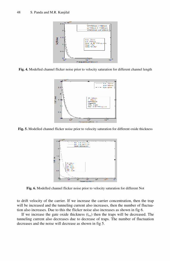
48 S. Panda and M.R. Kanjilal
Fig. 4. Modelled channel flicker noise prior to velocity saturation for different channel length
Fig. 5. Modelled channel flicker noise prior to velocity saturation for different oxide thickness
Fig. 6. Modelled channel flicker noise prior to velocity saturation for different Not
to drift velocity of the carrier. If we increase the carrier concentration, then the trap will be increased and the tunneling current also increases, then the number of fluctua-tion also increases. Due to this the flicker noise also increases as shown in fig 6.
If we increase the gate oxide thickness (tox) then the traps will be decreased. The tunneling current also decreases due to decrease of traps. The number of fluctuation decreases and the noise will decrease as shown in fig 5.

Thermal and Flicker Noise Modelling of a Double Gate MOSFET 49
4 Conclusion
In this paper we present a compact analytical noise model using the new compact analytical model for long channel DG MOSFET which considers doped silicon layer in a wide range of doping concentrations. By our modeling we observe that our model shows better noise performance for the DG MOSFET than other modeling approach described in other literature. Thus this paper will show the way for compact modeling the noise including various noise resources, which will be very helpful for the low noise analog IC optimized design at low power supply voltage.
Acknowledgment
The authors like to thank the faculties of ECE dept, Narula Institute of Technology for useful advices.
References
[1] Wong, M., Shi, X.: Analytical I–V Relationship Incorporating Field-Dependent Mobility for a Symmetrical DG MOSFET With an Undoped Body. IEEE Transactions on Electron Devices 53(6) (2006)
[2] Moldovan, O., Jimenez, D., Guitart, J.R., Ferney, A.C., Iniguez, B.: Explicit Analytical Charge and Capacitance Models of Undoped Double –Gate MOSFETs. IEEE Transactions on Electron Devices 54(7) (July 2007)
[3] Lime, F., Iniguez, B., Moldovan, O.: A Quasi-Two-Dimensional Compact Drain-Current Modelfor Undoped Symmetric Double-Gate MOSFETs Including Short Channel Effects. IEEE Transactions on Electron Devices 55(6) (June 2008)
[4] Li, Z., Ma, J., Ye, Y., Yu, M.: Compact Channel Noise models for Deep-Submicron MOSFETs. IEEE Transactions on Electron Devices 56(6) (June 2009)

V.V. Das, N. Thankachan, and N.C. Debnath (Eds.): PEIE 2011, CCIS 148, pp. 50–55, 2011. © Springer-Verlag Berlin Heidelberg 2011
Optimizing Resource Sharing in Cloud Computing
K.S. Arulmozhi1, R. Karthikeyan2, and B. Chandra Mohan3
1 PG Student [email protected] 2 Head of the Department
Department of Information Technology Vel Tech Multi Tech Dr.RR Dr.SR Engineering College, Chennai, India
[email protected] 3 Principal
LCR College of Engineering and Technology, Chennai, India [email protected]
Abstract. The cloud computing is the dynamic provisioning of IT capabilities such as hardware, software or services, from third parties over a network. Resource sharing in the cloud Computing environment is the major issues that limited application of the cloud computing. The problem of enabling effective peer-to-peer resource sharing in this types of networks the availability of a wireless infrastructure and broadcast nature of wireless communication. Which bring to the notions of location awareness and MAC layer cross-layering. Through extensive packet-level simulations, I have investigated the separate effects of location awareness and MAC layer cross-layering, the performance of the P2P application. The combined protocol Optimizing Resource Sharing In Cloud Computing (ORSCC), reduces message overhead of as much as 40 per-cent with respect to the existing design, while at the same time improving the information retrieval performance. Notably, differently from the existing design, our proposed ORSCC specialization displays information retrieval per-formance resilient to the presence of both CBR and TCP background traffic.
Keywords: Cloud Computing, Resource sharing, Cross-Layer, Wireless communication.
1 Introduction
The Internet is often represented as a cloud and the term “cloud computing” arises from that analogy. McKinsey[1] says that clouds are hardware-based services offering compute, network and storage capacity, where hardware management is highly ab-stracted from the buyer; buyers incur infrastructure costs as variable OPEX [operating expenditures]; and infrastructure capacity is highly elastic. There are three basic types of cloud computing, which are Infrastructure as a Service (IaaS), Platform as a Ser-vice (PaaS), Software as a Service (SaaS). In IaaS, CPU, grids or clusters, virtualized servers, memory, networks, storage and systems software are delivered as a service. Perhaps the best known example is “Amazon’s” Elastic Compute Cloud (EC2) and Simple Storage Service (S3), but traditional IT vendors such as IBM, and telecoms providers such as “AT&T” and “Verizon” are also offering solutions. Services are typically charged by usage and can be scaled dynamically, i.e. capacity can be

Optimizing Resource Sharing in Cloud Computing 51
increased or decreased more or less on demand. PaaS provides virtualized servers on which users can run applications, or develop new ones, without having to worry about maintaining the operating systems, server hardware, load balancing or computing capacity. Well known examples include Microsoft’s Azure and Salesforce’s Force.com. SaaS is software that is developed and hosted by the SaaS vendor and which the end user accesses over the Internet. Unlike traditional applications that users install on their computers or servers, SaaS software is owned by the vendor and runs on computers in the vendor’s data center (or a co-location facility). Broadly speaking, all customers of a SaaS vendor use the same software: these are one-size-fits-all solutions. Well known examples are Salesforce.com, Google’s Gmail and Apps, instant messaging from AOL, Yahoo and Google, and Voice-over Internet Protocol (VoIP) from Vonage and Skype.
2 Previous Work
Lipton and Naughton [2] proposes hash table for sharing resources in the cloud based environment. A hash table or hash map is a data structure that uses a hash function to map identifying values, known as keys (e.g., a person's name), to their associated values (e.g., their telephone number). Most hash table designs assume that hash collisions the situation where different keys happen to have the same hash value are normal occurrences and must be accommodated in some way. In a well-dimensioned hash table, the average cost (number of instructions) for each lookup is independent of the number of elements stored in the table. Many hash table designs also allow arbitrary insertions and deletions of key-value pairs, at constant average, especially analysis of algorithms, amortized analysis finds the average running time per operation over a worst-case sequence of operations. Amortized analysis differs from average-case performance in that probability is not involved; amortized analysis guarantees the time per operation over worst-case performance.
Malkhi, et al [3], proposes a Distributed Hash Tables (DHT) methodology for shar-ing resources in the cloud based environment architecture and implementation of a distributed hash table DDS. A client in the DHT consists of service-specific software running on a client machine that communicates across the wide area with one of many service instances running in the cluster. A service is a set of cooperating software processes, each of which a service instance. Service instances communicate with wide-area clients and perform some application-level function. Services may have soft state which may be lost and recomputed if necessary, but they rely on the hash table to manage all persistent state. Ratnasamy [4] proposes Geographic Hash Table (GHT) for sharing resources in the cloud based environment. The core step in GHT is the hashing of a key k into geographic coordinates. A key-value pair is stored at a node in the vicinity of the location to which its key hashes. Choosing this node con-sistently is central to building a GHT. Assume a perfectly static network topology and a network routing system that can deliver packets to positions, such a GHT will cause storage requests and queries for the same k to be routed to the same node, and will distribute the storage request and query load for distinct k values evenly across the area covered by a network. The service provided by GHT is similar in character to those offered by other DHT systems. Holger Zeltwanger[5] proposes Controller Area Network(CAN) hash table for sharing resources in the cloud based environment. The CAN is a serial bus communications protocol developed by Bosch in the early

52 K.S. Arulmozhi, R. Karthikeyan, and B. Chandra Mohan
1980s. It defines a standard for efficient and reliable communication between sensor, actuator, controller, and other nodes in real-time applications. CAN is the de facto standard in a large variety of networked embedded control systems. The major pitfalls of CAN is the communication rate of a network depends on the physical distances between the nodes.
3 Proposed Optimitizing Resource Sharing in Cloud Computing (ORSICC)
ORSICC is based on the idea of mapping both peer (mesh router) IDs and resource IDs (keys) into the same ID space, namely, the unit ring[0,1]. Each key resides on the peer with the smallest ID larger than the key, peer p manages keys comprised between its own ID and the ID of the predecessor of p in the unit ring (denoted range(p)). As-sociated with each key is the IP address of the mesh client holding the corresponding resource. ORSICC maps peer and resource IDs into the unit ring using a hashing function, named Sha1, which has the property of uniformly distributing IDs in [0,1]. Indeed, IDs in ORSICC are represented through m-bit numbers, i.e., at most 2m dis-tinct (peer or resource) IDs are present in the ORSICC system.
It is a reasonable ID space for ORSCC, in which the number of shared resources is expected to be in the order of several thousands, and the number of mesh routers (peers) in the order of a few hundreds. Indeed, larger ID spaces can be easily included in the design with no modification, and with negligible impact on performance. It allows dealing with larger networks and number of shared resources, which might lead to a non-negligible probability of conflicting ID assignment with relatively low values of m. The main operation implemented by ORSICC is the lookup(x) operation, which can be invoked at any peer to find the IP address of the peer with ID =x, if x is a peer ID, or the IP address of the peer responsible of key x in case x is a resource ID. Lookup operations are used both for query resolution (Find Key operation) and for overlay maintenance. To speed up look up operations, every peer maintains a table of up to m distinct peers. The ith finger of peer j, with 1 ≤ i ≤ m, is the peer which has the smaller ID larger than j + (2i-1). In order to facilitate join/leave operations, each peer maintains also the ID of its predecessor in the ORSICC ring. When a lookup(k) opera-tion is invoked at peer p and the operation cannot be resolved locally (because k is not within range(p), a message is sent to the peer p’ with largest ID <k in the finger table of node ‘p’. If ‘p’ cannot resolve the lookup operation, it replies to peer ‘p’ with a message containing the ID of the peer ‘p’ with largest ID < k in its own finger table. Peer p then forwards the request to peer ‘p’, and so on, until the lookup operation can be resolved (in at most m steps). To deal with dynamic join/leaves of peers in the systems, the following procedures are implemented, When a new peer ‘p’ joins the network, it first needs to initialize its predecessor and finger table. This is done by sending requests to any peer currently joining the network peer ‘p’ is aware of (called hook peer). Then, the finger tables and predecessor pointers of currently active peers must be updated to account for the new peer joining the network.
Finally, peer ‘p’ must contact its successor s in the ring so that the key range previ-ously managed by s can be split with p. In case no (active) hook peer can be found, the join operation fails, and the peer cannot join the ORSICC overlay. When an exist-ing peer p leaves the network, it first informs its predecessor and successor in the ring

Optimizing Resource Sharing in Cloud Computing 53
Fig. 1. ORSICC Operations. m is set to 6.
about its intention of leaving the network, so that they can change their finger tables and predecessor pointers accordingly; then, peer p transfers to its successor the key range it is responsible for. Finally, in order to deal with dynamic network conditions, each active peer in the network periodically performs a Stabilize operation, which verifies and possibly updates the content of the finger table and predecessor pointer. The period between consecutive Stabilize operations is a critical parameter in the ORSICC design: if the period is relatively short, the network is more reactive, but a higher message overhead is generated; on the other hand, a longer stabilize period reduces message overhead, at the expense of having a less reactive network. How to set the stabilize period in order to satisfactorily address this tradeoff when Basic Op-eration is executed in ORSCC is carefully investigated.
The first modification that proposes to the basic design concerns the function used
to assign ID to peers (hash function Sha1 is still used to assign key to files/resources). The idea is to exploit locality, and to assign peers which are close in the physical network with close-by IDs in the unit ring. This choice is motivated by the observa-tion that, according to ORSICC specifications, most of the messages are exchanged between a peer and its successor/predecessor in the unit ring.
The second contribution of the ORSCC proposal concerns the introduction of a MAC cross-layering technique. This technique aims at speeding up the lookup opera-tions by exploiting the information that is available at the MAC layer due to the 1-hop broadcast communication occurring in wireless networks. The basic idea is that a peer u may capture packets for which it owns relevant information, even if they are not destined to ‘u’. This technique is motivated by the possibility that peer ‘u’ that may actually be able to resolve a lookup request, is physically close to the peer invoking the lookup operation, while they are far away in the unit ring. More specifically, whenever a peer ‘u’ receives a packet at the MAC layer, ‘u’ sends it up to the applica-tion layer for further processing, even if the packet was not destined to ‘u’. If the packet does not contain a lookup request, it is discarded. Otherwise, ‘u’ checks if it may resolve the lookup(x) operation. This occurs if x is comprised between ‘u’s ID and the ID of the predecessor of ‘u’ in the unit ring. In this case, ‘u’ sends a message containing its own ID to the peer that invoked the lookup(x) operation. It is important

54 K.S. Arulmozhi, R. Karthikeyan, and B. Chandra Mohan
to note that, since the lookup process is invoked for both query resolution and overlay maintenance, cross-layering may improve the performance of both these operations.
Location awareness is designed to map neighboring peers to close-by IDs in the unit ring. On the other hand, cross-layering tends to be more effective when physical neighbor peers have far away ID sin the unit ring (this results in a higher likelihood of “capturing” packets). Hence, an ideal ID mapping function should, for a certain peer ‘u’, both 1) map pred(u)’s and succ(u)’s IDs to peers which are physical neighbors of ‘u’, and 2) assign the remaining u’s physical neighbors faraway IDs in the unit ring. The design of a mapping function which achieves both properties 1 and 2 is a very complex combinatorial problem, which is left for future work. In this paper, we focus on property 1, and show that, even in the presence of location-aware peer ID assign-ment, cross-layering is indeed beneficial to the performance of the P2Papplication.
4 Conclusions
This paper carefully investigated through packet-level simulation the performance of the ORSICC approach for peer-to-peer resource sharing in cloud computing Network-ing. It also proposed a specialization of the basic system approach called ORSICC, which exploits peculiar features of Cloud computing networks (location awareness and 1-hop broadcast nature of cloud computing communications) to improve per-formance. The main finding of the study reported in this paper is that, contrary to what happens in MANET environments [6], the basic approach can be successfully utilized for implementing file/resource sharing applications in cloud computing net-works. However, the basic ORSICC design is effective only under relatively static network conditions and in presence of modest background traffic. With respect to the basic design, our proposed ORSICC protocol achieves a considerable reduction in message overhead, and a significant improvement in information retrieval perform-ance. This performance improvement allows an effective realization of the P2P over-lay also under very dynamic network conditions and in presence of considerable background traffic. Although our investigation has shown that ORSICC message overhead does not lead to network congestion by itself, overlay maintenance still requires the exchange of a relatively high number of messages in the network, which could induce performance degradation when other applications are executed concur-rently with ORSICC. Quantifying application-layer performance degradation when several applications coexist with the P2P overlay is matter of ongoing work, as well as the problem of further reducing the message overhead induced by applications for file/resource sharing in Cloud Computing networks.
References
1. McKinsey & Co. Report presented at Uptime Institute Symposium April 18, 2009 Clearing the Air on Cloud Computing , http://uptimeinstitute.org/content/view/353/319, http://images.cxotoday.com/cxoimages/storyimages/matter101157.pdf (accessed November 27, 2009)
2. Lipton, R.J., Naughton, J.F.: Clocked adversariesfor hashing. Algorithmica 9(3), 239–252 (1993)

Optimizing Resource Sharing in Cloud Computing 55
3. Malkhi, D., Naor, M., Ratajczak, D.: Viceroy: A Scalable and Dynamic Emulation of the Butterfly. In: Proc. ACM Symp. Principles of Distributed Computing, PODC (July 2002)
4. Ratnasamy, S., Karp, B., Shenker, S., Estrin, D., Govindan, R., Yin, L., Yu, F.: Data-Centric Storage in Sensornets with GHT, a Geographic Hash Table. Mobile Networks and Applica-tions 8(4), 427–442 (2003)
5. Zeltwanger, H.: Time-Triggered Communication on CAN. SAE Paper 2002-01-0437 (2002) 6. Sailhan, F., Issarny, V.: Scalable Service Discovery for MANET. In: Proc. IEEE Int’l Conf.
Pervasive Computing and Comm, PerCom (2005) 7. Wolfson, O., Xu, B., Yin, H., Cao, H.: Search-and-Discover in Mobile P2P Network Data-
bases. In: Proc. IEEE Int’l Conf. Distributed Computing Systems, ICDCS (2006)

V.V. Das, N. Thankachan, and N.C. Debnath (Eds.): PEIE 2011, CCIS 148, pp. 56–61, 2011. © Springer-Verlag Berlin Heidelberg 2011
Design of Controller for an Interline Power Flow Controller and Simulation in MATLAB
M. Venkateswara Reddy1, Bishnu Prasad Muni2, and A.V.R.S. Sarma3
1 Assoc. prof, Eee dept., SSIT, B. Gangaram, Sathupally, Khammam, A.P. India [email protected]
2 Additional General Manager, Bharat Heavy Electricals Limited(R&D), BALA NAGAR, Hyderabad, India
3 EEE Dept., Professor, University College of Engg, Osmania University Hyderabad, India
Abstract. The Interline Power Flow Controller (IPFC) a concept for the compensation and effective power flow management of multi-line transmission systems. In its general form, the IPFC employs two or more number of inverters (VSI) with a common dc link, each to provide series compensation for a selected line of the transmission system. Because of the common dc link, any inverter within the IPFC is able to transfer real power to any other and thereby facilitate real power transfer among the lines of the transmission system. Since each inverter is also able to provide reactive power compensation, the IPFC is able to carry out an overall real and reactive power compensation of the total transmission system. This capability makes it possible to equalize both real and reactive power flow between the lines, transfer power from overloaded to under loaded lines, compensate against reactive voltage drops and the corresponding reactive line power, and to increase the effectiveness of the compensating system against dynamic disturbances. The paper explains the basic theory and operating characteristics of the IPFC with phasor diagrams, and simulated waveforms in MATLAB.
Keywords: AC transmission, FACTS, power flow controller, line compensa-tion, power converter, inverter, SSSC, IPFC, Series compensation.
Section 1
1.1 Introduction
Flexible AC Transmission Systems (FACTS) based on either Voltage or Current Source converters (VSC/CSC) these can be used to control steady-state as well as dynamic/transient performance of the power system. Converter-based FACTS controllers when compared to conventional switched capacitor/reactor and thyristor-based FACTS controllers such as Static Var Compensator (SVC) and Thyristor-controlled Series Capacitor (TCSC) have the advantage of generating/absorbing reactive power without the use of ac capacitors and reactors. In addition converter-based FACTS controllers are capable of independently controlling both active and

Design of Controller for an Interline Power Flow Controller and Simulation in MATLA 57
reactive power flow in the power system. Series connected converter-based FACTS controllers include Static Synchronous Series Compensator (SSSC), Unified Power Flow Controller (UPFC) and Interline Power Flow Controller(IPFC).
Section 2
2.1 Inter Line Power Flow Controller
Generally, the Interline Power Flow Controller (IPFC) is a combination of two or more independently controllable static synchronous series compensators (SSSC) which are solid-state voltage source converters which inject an almost sinusoidal voltage at variable magnitude and couples via a common DC link as shown in fig.1 Conventionally series capacitive compensation fixed thyristor controlled or SSSC based is employed to increase the transmittable real power over a given line and to balance the loading of a normally encountered multi-line transmission system. They are controlled to provide a capability to directly transfer independent real power be-tween the compensated lines while maintaining the desired distribution of reactive flow among the line. In its general form, the IPFC employs a number of dc to ac con-verters, each providing series compensation for a different line. The converters are linked together.
Fig. 1. Basic two inverter power flow controller
2.2 Operating Principle and Phasor Diagram for Single Phase Transmission System
The IPFC is designed with a combination of the series connected VSC which can inject a voltage with controllable magnitude and phase angle at the fundamental fre-quency while DC link voltage can be maintained at a desired level. The common dc link is represented by a bidirectional link (P12 =P1pq = P2pq) for real power exchange between voltage sources. Transmission line represented by reactance X1 has a sending end bus with voltage Phasor V1s and a receiving end voltage Phasor V1r. The sending end voltage Phasor of Line2, represented by reactance X2, is V2s and the receiving-end voltage Phasor is V2r. Simply, all the sending-end and receiving-end voltages are as-sumed to be constant with fixed amplitudes, V1s = V1r = V2s = V2r =1pu., and with fixed angles resulting in identical transmission angle s1 = s2 for the two systems.

58 M.V. Reddy, B.P. Muni, and A.V.R.S. Sarma
The two line impedances and the rating of the two compensating voltage sources are also assumed to be identical. This means X1 = X2 and V1pqmax = V2pqmax. Although in practice system1 and system2 could be likely different due to different transmission line voltage, impedance and angle.. A phasor diagram of system1 illustrated in Figure 2.
Fig. 2. Phasor Diagram of System
2.3 Three Phase Power Flow Control by Using IPFC
2.3.1 Power Circuit An IPFC (Following fig.3) uses two or more VSCs that share a common dc-link. Each VSC injects a voltage - with controllable amplitude and phase angle - into the power transmission line through a coupling transformer. Each VSC provides series reactive power compensation for an individual line and it can also supply/absorb active power to/from the common dc-link. Thus, an IPFC has an additional degree of freedom to control active power flow in the power system when compared to a traditional compensator.
Co
ntr
olle
r
X ref2
1 2
X ref1
Slave ConverterR ref1
Master Converter
VSC
V dc
1 2VSC
V dc
Line1 Line2
Fig. 3. Schematic Of Inter Line Power Flow Controller
Section 3
3.1 Control Scheme of IPFC
The IPFC is designed to maintain the impedance characteristic of the two transmis-sion lines. The IPFC consists of two converter systems: (a) a master converter system that is capable of regulating both resistive and inductive impedances of Line 1; and,

Design of Controller for an Interline Power Flow Controller and Simulation in MATLA 59
(b) a slave converter system that regulates Line 2 reactance and keeps the common dc-link voltage of the VSC at a desired level.
3.2 Controller System for Slave Converter
Fig. 4. shows the control diagram of the slave IPFC system.
Fig. 4. Controller ckt. for slave system
Block 1 is used to transform the 3-phase voltages (vinj-a, vinj-b, vinj-c) into the α−β−0 coordinates and obtain the positive sequence voltage Vinj-α, as per follwowing equation (1)
(1)
Block 2 is used to transform the 3-phase line currents (ia, ib and ic) to the α−β−0 coordinates using the RWG block; this block will be described in more detail later. For generating reference waveforms for control purposes, the 3-phase currents are transformed from a-b to α−β−0 coordinates, by using eqation (2). The iα and iβ components are fed to the Phase Shifter (Block 6) while the i0 component is fed to the Balancing Controller. If the 3- phase current waveforms in a-b-c coordinates are balanced,
(2)
Block 3 is used to transform the 3-phase line voltages va, vb and vc to the v α , vβ and v0 coordinates using another RWG block with a transformation similar to equation (2). Only the vα component of this block is fed to the Lead/Lag Block (Block 5), the two other outputs vβ and v0 are not required.
Block 4 receives the positive sequence of the injected voltage Vinj-a from Block 1 and the positive sequence of the line current Iline-a from Block 2.
(3)

60 M.V. Reddy, B.P. Muni, and A.V.R.S. Sarma
3.3 Controller System for Master Converter
Fig. 5. Controller system for master converter
Section 4
Simulation of IPFC in MATLAB
Fig. 6. Simulation diagram for an Interline Power Flow Controller in matlab
Fig. 7. Simulation diagram for master system Controller
Fig. 8. Simulation diagram for slave system Controller in MATLAB

Design of Controller for an Interline Power Flow Controller and Simulation in MATLA 61
Output Results of IPFC in MATLAB
Fig. 9a. Injected voltages in to the lines
Fig. 9d. Reactance injected in to line2
Fig. 9b. Resistane injected into line 1
Fig. 9e. Current injected in to the two lines
Fig. 9c. Reactance injected to line 1
Fig. 9f. Dc bus voltage
5 Conclusion
The design of an IPFC system with two parallel lines has presented in this paper. The flexible control of active/reactive power to assist in the transmission system. A balancing circuit based on zero sequence current is employed to equalize the dc link capacitor voltages. The results of an IPFC system with two 3-level NPC VSCs in MATLAB have validated. The simulation results demonstrate the capability of the IPFC in compensating both resistance and reactance of the transmission line, and maintaining the dc-link voltage of the IPFC.
References
[1] Menzies, R.W., Steimer, P., Steinke, J.K.: Five-level GTO inverters for large induction motor drives. IEEE Trans. on Industry Applications 30(4), 938–944 (1994)
[2] Lee, D.H., Fred, S.R., Lee, C.: An analysis of midpoint balance for the neutral-point-clamped three-level VSI. In: IEEE Power Electronics Specialists Conference, vol. 1, pp. 193–199 (1998)
[3] Zhang, X.P.: Advanced modeling of the multi control functional static synchronous series compensator (SSSC) in Newton power flow. IEEE Trans. Power Syst. 18(4), 1410–1416 (2003)
[4] Strzeiecki, R., Benysek, G.: Interline Power flow controller – Probabilistic Approach. In: Proc.IEE 33rd Annual Power Electronics Specialist Conference, PSEC 2002, vol. 2, pp. 1037–1042 (2002)

V.V. Das, N. Thankachan, and N.C. Debnath (Eds.): PEIE 2011, CCIS 148, pp. 62–68, 2011. © Springer-Verlag Berlin Heidelberg 2011
Harmonics Reduction and Amplitude Boosting in Polyphase Inverter Using 60o PWM Technique
Prabhat Mishra and Vivek Ramachandran
[email protected], [email protected]
Abstract. This paper deals with the reduction of harmonics & amplitude boost-ing in polyphase inverters using 60o PWM technique. Using 60o PWM technique total harmonic distortion of output voltage is greatly reduced when compared with 180° and 120° degree mode of conduction techniques. All the triple har-monics present in the output voltage is eliminated so that required filter size can be reduced. The amplitude of output voltage is also augmented as compared to SPWM technique. The results from a MATLAB simulation done for a polyphase inverter to obtain 3-Ф, 445V (peak), 50Hz sinusoidal supply using 60o PWM is used to substantiate this study.
Keywords: Harmonics, Inverter, 60o PWM.
1 Introduction
Inverters are used to create single or polyphase AC voltages from a DC supply. Single – phase inverters are most commonly used in UPS “Uninterruptible Power Supplies” and a widespread application of polyphase inverters is in adjustable speed motor drives. The typical inverter for adjustable speed motor drives is a “hard-switched” voltage source inverter producing Pulse-Width Modulated (PWM) signals with a sinusoidal fundamental (Holtz, 1992). Hard-switched inverters use controllable power semiconductors to connect an output terminal to a stable DC-bus. Modern inverters use Isolated Gate Bipolar Transistors (IGBTs) as the main power control devices [1]. Besides IGBTs, power MOSFETs are also used especially for lower voltage and power ratings, and applications that require high efficiency and high switching frequency.
To assess the performance of any PWM technique, we need to consider the THD of the inverter output, effective utilization of the voltage supply and losses involved during inverter operation/ efficiency of operation. We run a MATLAB simulation to study these characteristics employing the 60o PWM technique and compare the re-sults with those of other popular techniques.
2 Three Phase Inverter
To synthesize a set of three-phase voltages from a dc source, three inverter legs are connected together as shown in Fig. 1. The circuit has two operating modes, either the

Harmonics Reduction and Amplitude Boosting in Polyphase Inverter 63
switch operate at the same frequency as the ac output waveforms, known as quasi-square wave or six-step operation, or alternatively the devices operate at a much higher frequency than the ac output using a form of SPWM[6].
In quasi-square wave operation of the three-phase inverter the transistors in each leg operate in anti-phase with duty ratios of 0.5, the leg output voltages, measured with respect to a notional ground at the mid-point of the dc input, are therefore symmetrical square waves of ±Vin/2[6]. The most common operating mode for inverter circuits is with the transistors switching at a much higher frequency than the ac output waveform that is being synthesized, typically twenty times greater or more, which implies switch-ing frequencies in the region of 1–20 kHz for a mains frequency inverter.
Fig. 1. Three phase inverter circuit
3 60o PWM Technique
In 60"PWM modulation (60 deg) [10] where there are only two inverter-legs are ac-tive at the same time. The idea behind the 60o PWM technique is to “flat top” the waveform from 60o to 120o and 240o to 300o. The power devices are held on for one third of the cycle (when full voltage) and have reduced switching losses [3]. All triple harmonics (3, 9,15,21,27 etc.) are absent in three phase voltage. The 60o PWM creates
Fig. 2. Output waveform of 60o PWM technique

64 P. Mishra and V. Ramachandran
large fundamentals (2/√3) and utilizes more available dc voltage. The modulation function for one phase is described as [9]:
ωt δ 0 → π/3 M.cos (ωt - π/3) π/3 → 2π/3 1 2π3 → π M.cos (ωt - 2π/3) π → 4π/3 1- M.cos (ωt - 4π/3) 4π/3 → 5π/3 0 5π/3 → 2π 1- M.cos (ωt - 5π/3) Where δ = Duty cycle, M=Modulation Index.
The modulation waveforms utilize the dc-link voltage almost optimized but the 60o
PWM modulation can be expected to give less switching losses%. However, for some part of the fundamental output voltage the motor windings only are exposed to fc (switching frequency, 10 KHz in our case) compared to 2fc for the remaining and major part of the time. This will increase the output current ripple in some part (60o) of the period and cause the acoustic noise to change from one distinct tone to another with a wider spectrum [9].
4 Simulation
Analysis of a polyphase, 445V, 50Hz inverter with a resistive load of 1Ω is imple-mented using 60oPWM technique using MATLAB software. The block diagram is shown in Fig. 3. It basically consists of two sections i.e. Power circuit and Control circuit. The power circuit consists of six IGBTs. Also, it includes DC supply voltage, Vd for the inverter. For independent control of the switches in each leg the supply voltage Vd has to be divided into two, the magnitude of each will be Vd/2 and the midpoint of the sources to be grounded as shown in Fig.1
The pulse generation system block consists of sine wave generator, phase shifter, repeating sequence, saturation and comparator for generating pulses. The value of supply voltage Vd is calculated as [1] 576V and it is divided into two parts i.e. Vd1 and Vd2 each having value 288V. The carrier wave (fc) is sawtooth wave of
Fig. 3. MATLAB simulation block diagram

Harmonics Reduction and Amplitude Boosting in Polyphase Inverter 65
Fig. 4. Waveform of carrier wave
frequency 10 KHz and amplitude 10V as shown in Fig 4. The intersections between the reference voltage standards and the carrying wave give the time of opening and closing of the switches.
Three phase sine wave is generated by phase shifting original sine wave by 120 and 240 degree as shown in Fig. 5. As we are using 60o degree PWM technique, we want flat top between 60o and 120o and 240o and 300o and so on. To accomplish this we are using saturation block.
Fig. 5. Waveform of reference 3- Φ wave
Fig. 6. Generation of pulses

66 P. Mishra and V. Ramachandran
Fig. 7. Six pulses for six devices
The pulses are generated by comparing carrier wave (triangular) with sine wave (reference wave) and pulses are obtained as shown in Fig. 6. Whenever the magnitude of reference wave is greater than carrier wave pulses are generated [1]. Since there are three reference waves three pulses will be generated which will be used to trigger upper devices of each leg of the inverter. The generated pulses are inverted so that we can get 6 pulses to fire six IGBT as shown in Fig. 7.
5 Simulation Results
The various amplitude parameters for the design of a 3-Ф, 445V, 50Hz inverter is calculated [1] and compared with the simulation results of SPWM technique [1]. Table 1 shows that simulation results and comparison of both 60o PWM and SPWM technique. The amplitude of Line to Line output voltage is 445.8 & is shown in Fig. 8. This waveform is without filter and by connecting small value of filter it is possible to get a sinusoidal waveform of desired magnitude and frequency. As we can see that amplitude of 60o PWM technique is 11.7% higher than the SPWM technique.
FFT analysis is done for the output voltage waveform and the magnitudes of volt-age harmonic components are shown in Fig.9. From the harmonic spectrum it is clear that total harmonic distortion (THD) is 3.67% and magnitude of L-L voltage is 445.8.
Fig. 8. Waveform of output L-L voltage of polyphase inverter without filter

Harmonics Reduction and Amplitude Boosting in Polyphase Inverter 67
Table 1. Comparison of SPWM and 60o PWM technique[8]
Sr. Parameters SPWM 60o PWM
No. Technique Technique
1 Modulation Index
ma=Vcontrol/Vtri 0.8 0.8
2 Phase Voltage Vph=ma*Vd/2
230.4 257.69
3 Line-Line Voltage(rms )
VL-L=(√3/√2)*Vph 282.18 316.17
4 Line-Line Voltage(peak)
VL-Lmax=√2*VL-L 399.1 445.8
Fig. 9. Waveform of L-L voltage and its harmonic spectrum
It can also be noted that the all triple harmonics are almost eliminated. The total har-monic distortion (THD) of 60o PWM is very less as compared to 180˚ mode of con-duction which can be as high as 42.51%.
6 Conclusion
By using 60o PWM technique it is possible to control total harmonic distortion in the output voltage of the inverter but in case of 120° and 180° mode of conduction of inverter it is not possible. Also, all triple harmonics are eliminated from the three phase voltage and therefore we can reduce the size of the output filter required to make it a pure sinusoidal waveform.60o PWM technique creates large fundamental as compared to SPWM technique and because of this there is a better utilization of the available DC source.

68 P. Mishra and V. Ramachandran
References
1. Mohan, N., Undeland, T.M., Robbins, W.P.: Power Electronics Converters, Applications, and Design, 3rd edn. John Wiley & Sons, Chichester (2003)
2. Sebastian, G., George, S.: Power Quality: Harmonics, Issues Regulations and Compensat-ing Techniques. In: International Conference on Reliability Safety & Quality Engineering Conference, pp. 481–486 ( 2007-2008)
3. Rashid, M.H.: Power electronics, circuits, Devices and Application, 3rd edn. Pearson Education, London (2003)
4. Singh, M.D., Khanchandani, K.B.: Power electronics. Tata McGraw Hill, New York 5. Dubey, G.K.: Fundamentals of Electrical Drives, 2nd edn. Narosa Publishing House Pvt.
Ltd. (2001) 6. Warne, D.F.: Newnes Electrical Power Engineer’s Handbook, Newnes, 2nd edn (2005) 7. Grigsby, L.L. (ed.): Electric Power Engineering handbook, 2nd edn. CRC, Boca Raton
(2007) 8. Mishra, P., Newase, B., George, S.: Harmonic Reduction in 3Phase Inverter using SPWM
Technique. In: IEEE Bangalore Section - 18th Annual Symposium on Emerging Needs in Computing, Communication, Signals and Power (2009)
9. Blaabjerg, F., Jaeger, U., Mu-Nielsen, S., Pedersen, J.K.: Power Losses in PWM-VSI Inverter Using NPT or PT IGBT Devices. IEEE Transaction on Power Electronics 10(3), 358–367 (1995)
10. Nielsen, P.E., Thomsen, E.C., Nielse, M.T.: Digital voltage vector control with adaptive parameter tuning. In: Proc. EPE 1989, pp. 313–318 (1989)
11. Farid, B., Amar, O.: A Study of New Techniques of Controlled PWM Inverters. European Journal of Scientific Research 32(1), 77–87 (2009)

V.V. Das, N. Thankachan, and N.C. Debnath (Eds.): PEIE 2011, CCIS 148, pp. 69–72, 2011. © Springer-Verlag Berlin Heidelberg 2011
Face Recognition Using Gray Level Weight Matrix (GLWM)
R.S. Sabeenian1, M.E. Paramasivam2, and P.M. Dinesh3
1 Professor & Center Head Sona SIPRO [email protected]
2 Lecturer & Research Staff Sona SIPRO [email protected]
3 Research Associate, Sona SIPRO, ECE – Department, Sona College of Technology, Salem, India
Abstract. Face detection is one of the few biometric methods that possess the merits of both high accuracy and low intrusiveness. It also has several applica-tions in areas such as content-based image retrieval, video coding, video conferencing, crowd surveillance, and intelligent human–computer interfaces. The purpose of this study is to propose a novel statistical face recognition sys-tem with improved performance, based on Gray Level Weight Matrix (GLWM). The process involved in GLWM is an improved version of the Local Binary pattern technique. It has been found out through experiments that the proposed GLWM is more efficient in face recognition.
Keywords: Local Binary Pattern; Gray Level Weight Matrix; Face Recognition.
1 Introduction
Face recognition technology has a variety of potential applications in information security, law enforcement and surveillance, smart cards, access control, etc. For this reason, this technology has received significantly increased attention from both the academic and industrial communities during the past 20 years. The main aim of face recognition is to identify or verify one or more persons from still images or video images of a scene using a stored database of faces. One of the major challenges en-countered by current face recognition techniques lies in the difficulties of handling varying poses, i.e., recognition of faces in arbitrary in-depth rotations. Extensive ef-forts have been put into the research toward pose-invariant face recognition in recent years and many prominent approaches have been proposed. However, several issues in face recognition across pose still remain open. The human face is a dynamic object and has a high degree of variability in its appearance, which makes face detection a difficult problem in computer vision. The face recognition techniques across pose can be classified as general algorithms, 2D and 3D techniques for face recognition across pose and complex neural-network based 3D models. By “general algorithms”, we mean these algorithms did not contain specific tactics on handling pose variations. They were designed for general purpose of face recognition equally handling all

70 R.S. Sabeenian, M.E. Paramasivam, and P.M. Dinesh
image variations (e.g., illumination variations, expression variations, age variations, and pose variations, etc.).The general algorithms can be further divided into two broad categories as Holistic approaches and Local approaches. Some of the com-monly available Local approaches are Template matching [1], modular PCA [2], Elastic bunch graph matching [3], local binary patterns [4]. This study primarily focuses on improving the capability and universality of general face recognition algorithms (in particular the local binary pattern), so that image variations can be tolerated, rather than designing an algorithm that can eliminate or at-least compensate the difficulties brought by image variations.
2 Previous Method
2.1 Local Binary Pattern (LBP)
The Local Binary Pattern algorithm [4] was originally designed for texture descrip-tions. The method of local binary pattern for face recognition divides a given facial image into small regions and computes a description of each region using LBP opera-tor. The operator assigns a label to every pixel of an image by thresholding the 3x3-neighborhood of each pixel with the center pixel value and transforming the result as a binary number. Then the histogram of the labels can be used as a texture descriptor. A local binary pattern is called uniform if the binary pattern contains at most two bit-wise transitions from 0 to 1 or vice versa.
3 Proposed Method
In proposed method instead of thresholding the image transforming is made with neighborhood to a texture unit with the texture unit number under the ordering way as shown in figure1.
The transforming conditions
Ei = 0 if Vi < Vo
1 if Vi = Vo
2 if Vi > Vo
Where: Vi = The center pixel value Vo = The neighboring pixel value
Neighborhood (Vi) Texture unit (Ei)
62 85 92
29 40 36
67 36 66
2 2 2
0 1 0
2 0 2
Fig. 1. Texture unit transformation
The values of the pixels in the transformed texture unit neighborhood are multiplied by the weights given to the corresponding pixels. Finally, the values of the eight pixels are summed to obtain a number for this neighborhood. This method considers the

Face Recognition Using Gray Level Weight Matrix (GLWM) 71
center pixel value till end of the process for each 3 x 3 matrix. The equation involved in the calculation of GLWM is shown below.
3.1 Algorithm for Face Recognition Using GLWM
Fig. 2. Methodology flow for the proposed algorithm
4 Results
Experiments were carried out by making use of the Indian Face database [5]. More than 50 face images were subjected to the proposed algorithm and the method was able to recognize nearly 46 face images.
The figure 3 shows the some of the sample images in the Indian Face database that were used and are correctly recognized by the algorithm. The first column is the data-base image, while the other columns are the test images.
Fig. 3. Database collection

72 R.S. Sabeenian, M.E. Paramasivam, and P.M. Dinesh
Fig. 4. Percentage of Recognition for the database collection
The Classification / Recognition rate with different angle of rotation is graphically shown in figure 4. The proposed algorithm proves to be 92% efficiency.
5 Conclusion
In this paper, we propose Gray Level Weight Matrix (GLWM) method for face rec-ognition as an improvised version of Local Binary Pattern and Texture Spectrum. This algorithm can be used for high-dimensional texture classification with applica-tion to face recognition. Experiments show that the GLWM is capable to recognize angle varied face images. As a part of future work, the algorithm can be extended for other face database images and texture images.
References
[1] Brunelli, R., Poggio, T.: Face recognition: features versus templates. IEEE Transactions on Pattern Analysis and Machine Intelligence 15(10), 1042–1052 (1993)
[2] Pentland, A., Moghaddam, B., Starner, T.: View-based and modular eigen spaces for face recognition. In: The Proceedings of the IEEE Conference on CVPR, pp. 84–91 (1994)
[3] Wiskott, L., Fellous, J.M., Kruger, N., von der Malsburg, C.: Face recognition by elastic bunch graph matching. IEEE Transactions on Pattern Analysis and Machine Intelli-gence 19(7), 775–779 (1997)
[4] Ahonen, T., Hadid, A., Pietikäinen, M.: Face description with local binary patterns: application to face recognition. IEEE Transactions on Pattern Analysis and Machine Intel-ligence 28(12), 2037–2041 (2006)
[5] Jain, V., Mukherjee, A.: The Indian Face Database (2002), http://vis-www.cs.umass.edu/~vidit/IndianFaceDatabase/
[6] Sellahewa, H., Jassim, S.A.: Image-Quality-Based Adaptive Face Recognition, Instrumen-tation and Measurement. IEEE Transactions on Issue Date (April 2010)
[7] D’Astous, F., Jernigan, M.E.: Texture discrimination based on detailed measures of power spectmm. In: Proceeding of the IEEE Computer Society Conference Pattern Recognition Image Processing, pp. 83–86
[8] Sreejamole, S.S., Ganesan, L.: Supervised Classification of Images using Textural Features. International Journal of Soft Computing 4(3), 122–126 (2009)

V.V. Das, N. Thankachan, and N.C. Debnath (Eds.): PEIE 2011, CCIS 148, pp. 73–78, 2011. © Springer-Verlag Berlin Heidelberg 2011
Location for Stability Enhancement in Power Systems Based on Voltage Stability Analysis and Contingency
Ranking
C. Subramani1, S.S. Dash2, M. Arunbhaskar3, M. Jagadeeshkumar4, and S. Harish Kiran5
1,2 Department of EEE, SRM University, India, 603203 [email protected], [email protected]
3,4,5 Department of EEE, Velammal Engineering College, Chennai, India, 600066 [email protected], [email protected],
Abstract. In the last few years, voltage collapse problems in power systems have been of permanent concern for electric utilities: several major blackouts throughout the world have been directly associated to this phenomenon. Volt-age instability is one phenomenon that could happen in power system due to its stressed condition. The result would be the occurrence of voltage collapse which leads to total blackout to the whole system Investigation and online monitoring of power system stability have become vital factors to electric utility suppliers. Suitable preventive control actions can be implemented considering contingencies that are likely to affect the power system performance. In this pa-per by conducting Voltage stability and Line outage Contingency analysis the suitable location for voltage stability enhancement in a 9 bus Test systems is determined.
Keywords: Voltage stability, Contingency ranking, Line outage, Voltage stability analysis, Stability index.
1 Introduction
Voltage stability is the ability of a system to maintain steady acceptable voltages at all the buses in the system at all conditions. The ability to transfer reactive power from production source to consumption areas during steady-state operating conditions is a major problem of voltage stability. A system mainly enters a state of voltage instabil-ity when a disturbance, increase in load demand, or change in system condition causes a progressive and uncontrollable decline in voltage.
With the increased loading and exploitation of the power transmission system be-ing also due to improved optimized operation the problem of voltage stability and voltage collapse attracts more and more attention [1-2].Voltage collapse can take place in systems or subsystems and can appear quite abruptly which requires the im-proved continuous monitoring of the system state [3]. The change in voltage is so rapid that voltage controls devices may riot take corrective actions rapidly enough to

74 C. Subramani et al.
prevent cascading blackouts [4-5]. The continual increase in demand for electric power has forced utility companies to operate their systems closer to the limits of instability [6-7].
In this paper voltage stability analysis and maximum loadability are conducted us-ing new line stability index indicated by VSI [8]. The rapid response feature of SVC can improve the steady state stability of power system, if it is located appropriately [9, 10], an index for identifying the location of SVC in large scale power system is proposed. a probabilistic approach [10-11] to evaluate the small-signal stability of power systems in the presence of time delays. A contingency table was developed from the results obtained from the simulation of each transmission line outage. The outage which resulted in a severe stability condition will be ranked high. From the contingency ranking table, the effect of breakdown at a line on voltage stability condition of a system could be determined.
2 Implementation of Stability Index
The slow variation in reactive power loading towards its maximum point causes the traditional load flow solution to reach its non convergence point .Beyond this point, the ordinary load flow solution does not converge, which in turn forces the systems to reach the voltage stability limit prior to bifurcation in the system.
The voltage stability index or proximity is the device used to indicate the voltage stability condition formulated based on a line or a bus [8]. The maximum threshold is set at unity as the maximum value beyond which this limit system bifurcation will be experienced. The VSI is derived from the voltage quadratic equation at the receiving bus on a two-bus system. The general two-bus representation is illustrated in Figure 1.
Fig. 1. Two-bus power system model
The mathematical equation for VSI was formulated from a line model as follows: Taking the symbols ‘i’ as the sending bus and ‘j’ as the receiving bus. Hence, the fast voltage stability index, VSI can be defined by;
By using this Stability Index, the Voltage stability analysis and Contingency analysis are conducted and identify the critical area in the power system for stability enhancements. The following steps are implemented for conducting Voltage Stability Analysis:

Location for Stability Enhancement in Power Systems 75
1. Run the load flow program using Newton-Raphson method for the base case. 2. Evaluate the VSI value for every line in the system. Gradually increase the reac-
tive power at chosen load bus and calculate VSI Values for every load variation. 3. Extract the line index that has the highest value; this line is called as the most
critical line with respect to a bus and Choose an other load bus repeat steps 1 to 3. 4. Obtain the voltage at the maximum computable VSI. This determines the critical
Voltage of a Particular bus. 5. Extract the maximum reactive power loading for the maximum computable VSI
for every test bus. The maximum Reactive Power loading is referred to as the maximum loadability of a Particular bus.
Using the line stability index contingency analysis was carried out and a contingency table was developed from the results obtained from the simulation of each transmis-sion line outage. The outage which resulted in a severe stability condition will be ranked high. From the contingency ranking table, the effect of breakdown at a line on voltage stability condition of a system could be determined. The contingencies tested were based on transmission line outage. Several cases are simulated in order to de-termine the contingency ranking.
3 Result and Discussion
3.1 Voltage Stability Analysis
To validate the performance of the indicator for voltage stability analysis, a 9 bus reliability test system is used. This system has 3 generator buses and 6 load buses. In order to investigate the effectiveness of the stability index 6 load buses were selected, namely buses 3, 4, 5, 6, 8 and 9. The reactive power at these buses increased gradu-ally one at a time. For finding the maximum load and weak bus 6 load buses are in-vestigate one by one. The results are tabulated below. From table 1 we can find the maximum load, critical voltage and critical line. For example consider Bus No.9, it has the rank 6. From the base case increase the reactive power till the index value closes to 1. The maximum computable value of VSI obtained is 0.9999 for the line connected between buses 2 and 9 i.e. L3. The VSI (L3) value (0.9999) at this point is
Table 1. Bus Ranking according to Maximum Loadablity
Rank Bus No.
Line (From Bus –
To Bus
Qmax (p.u)
Critical Voltage
(p.u)
Voltage stability
Index (VSI)
1 5 5-6 3.112 0.6949 0.9999 2 4 3-4 3.688 0.6262 0.9999 3 6 6-7 5.230 0.7706 0.9999 4 3 2-3 5.250 0.7588 0.9999 5 8 1-8 6.717 0.7879 0.9999 6 9 2-9 9.545 0.7458 0.9999

76 C. Subramani et al.
Table 2. Line Outage Contingency analysis for Single load change with reactive power only
close to unity indicating that the system has reached its stability limit. At this point L3 is the most critical line with respect to bus 9. The critical voltage of particular bus is 0.7458 p.u. At the same time maximum reactive power loading for the maximum computable value of VSI (Bus No.9) is 9.545 Mvar (Qmax), beyond this limit viola-tion will be experienced. From this result we can also found that Bus No 9 has the maximum reactive power (9.545 P.U.) and Bus No. 5 has the minimum reactive power (3.112 P.U.), which is ranked 1. This means that Bus No.9 is the healthy bus and Bus No. 5 is the weakest bus in the system.
3.2 Line Outage Contingency Analysis (LOCA)
The contingency ranking for different cases randomly selected were based on line stability values evaluated for each loading condition. The computation was performed by taking line outage 1 through 11consecutively for each different case. For Conduct-ing LOCA, reactive power increases up to half of the maximum power. The reactive power at these buses increased gradually up to half of the maximum power one at a time. The line stability indices were computed and the results are tabulated in Table 2. The values of line stability indices highlighted in the table demonstrate the highest indices after being sorted in descending order.
Case1: increase Q at bus 3; Case 2: increase Q at bus 4; Case 3: increase Q at bus 5 Case 4: increase Q at bus 6; Case 5: increase Q at bus 8; Case 6: increase Q at bus 9
Referring to table 2 when line 1 is outage, the proposed line stability index is evalu-ated for each line in the system and the result yields the line stability index value for line 3 is the highest which is 0.4930. It shows that line 3 is approaching its voltage stability limit .However, it can be seen that outage in line 4 gives the index value 1.000 indicates voltage collapse has occurred in this line. Similar analysis was con-ducted for all other cases in order to determine which line outage would cause voltage collapse to occur in the system. From the table we can also analyses that the line which has the index value close to 1.00 which is the most critical line in that case.

Location for Stability Enhancement in Power Systems 77
And the line which has the index value greater than 1 means due to the outage of that line voltage collapse was occurred. For example consider the outage of L4 we can say that in case 4,5 and 6 the index value is less than 1 (0.5084, 0.4576 and 0.4924) .But in case 1,2 and 3 the index value is greater than 1. (1.000, 1.000 and 1.000). From this we can conclude that the line outage L4 is not a severe in case 4, 5 and 6. But in case 1, 2 and 3 it is the most severe case. From this result we can found which the critical line is when the outages occur. For example consider case1. Here when outage of L1 occurs then Line 4 is the most critical line. From this result we can also found that in case1 most of the outages line 4 is the severe one. We can conclude that line 4 is the critical line.
Table 3. Contingency ranking
Rank Case 1 Case 2 Case 3 Case 4 Case 5 Case 6 1 Line 4 Line 4 Line 7 Line 8 Line 2 Line 3 2 Line 7 Line 7 Line 4 Line 9 Line 10 Line 11 3 Line 6 Line 5 Line 5 Line 3 Line 3 Line 8 4 Line 5 Line 6 Line 6 Line 4 Line 4 Line 9 5 Line 8 Line 8 Line 8 Line 5 Line 1 Line 1 6 Line 3 Line 3 Line 2 Line 6 Line 6 Line 4 7 Line 1 Line 9 Line 1 Line 7 Line 5 Line 5 8 Line 2 Line 1 Line 10 Line 2 Line 11 Line 6 9 Line 9 Line 2 Line 11 Line 1 Line 7 Line 7
10 Line 11 Line 11 Line 3 Line 11 Line 9 Line 10 11 Line 10 Line 10 Line 9 Line 10 Line 8 Line 2
3.3 Contingency Ranking
Contingency ranking for the system based on line outage is shown in table 3. The line outage which caused the system to violate or resulted in system to be closest to its voltage stability limit is ranked the highest. For case 1 for example, it can be seen that line outage at line 4 is at the top of the list. Since it has caused voltage collapse in the system .Line outage in line10 is ranked the lowest since the maximum line stability indices evaluated for this contingency is less than 1.00 (i.e. 0.4363), indicating that the system is far from its stability limit. Based on the voltage stability analysis and contingency ranking, from the table 3 the line 4 is in top rank in any line outage for all the cases. Also the lines 3, 5 and 7 are critical lines for different line outages. So the lines in the order line 4, 3 5 and 7 are the location of FACTS devices for Stability enhancement and the weakest bus, bus no. 5 which already found from voltage stabil-ity Analysis also is a suitable placement for Voltage stability enhancement.
4 Summary and Conclusion
The VSI determines the maximum load that is possible to be connected to a bus in order to maintain stability before the system reaches its bifurcation point. This point is determined as the maximum loadability of a particular bus which beyond this limit

78 C. Subramani et al.
system violation will be experienced. Based on the voltage stability analysis and con-tingency ranking, from the table 3 the line 4 is in top rank in any line outage for all the cases. Also the lines 3, 5 and 7 are critical lines for different line outages. So the line in the order line 4, 3, 5 and 7 are the location of FACTS devices for Stability Enhancement. From this information, proper monitoring of a weak node can be conducted in maintaining a secure electric utility so that the load connected to the respective bus will not exceed the maximum allowable load to maintain a stable sys-tem. By providing a suitable rating of FACTS device at the optimal location, the sta-bility of the system may improved.
References
1. Musirin, I., Rahman, T.K.A.: Novel Fast Voltage Stability Index (FVSI) for Voltage Stability Analysis in Power Transmission System. In: Proceedings of the 2002 Student Conference on Research and Development, Shah Alam, Malasia (2002)
2. Sauer, P.W., Evans, R.J., Pai, M.A.: Maximum unconstrained loadability of power systems. In: IEEE Int. Symp. Circuits and Systems, vol. 3, pp. 1818–1821 (1990)
3. Melo, A.C.G., Granville, S., Mello, J.C.O., Oliveira, A.M., Dornellas, C.R.R., Soto, J.O.: Assessment of maximum loadability in a probabilistic framework. IEEE Power Eng. Soc.Winter Meeting 1, 263–268 (1999)
4. Hiskens, I.A., Davy, R.J.: Exploring the power flow solution space boundary. IEEE Trans. Power Syst. 16, 389–395 (1999)
5. Moon, Y.-H., Chooi, B.-K., Cho, B.-H., Lee, T.-S.: Estimating of maximum loadability in power systems by using elliptic properties of P-e curve. IEEE Power Eng. Soc. Winter Meeting 1, 677–682 (1999)
6. Moghavemmi, M., Omar, F.M.: Technique for contingency monitoring and voltage collapse prediction. IEE Proc. Generation, Transmission and Distribution 145, 634–640 (1998)
7. Mohamed, A., Jasmon, G.B.: Voltage contingency selection technique for security assess-ment. IEE Proc. Pt. C 136, 24–28 (1989)
8. Baozhu, L., Bolong, L.: A Novel Static Voltage Stability Index based on Equilibrium Solution region of Branch Power Flow. In: DRPT 2008, Nanjing China, pp. 6–9 (2008)
9. Joorabian, M., Ebadi, M.: Locating Static VAR Compensator (SVC) Based on Small Signal Stability of Power System. International Review of Electrical Engineering 4(4), 635–641 (2009)
10. Ayasun, S., Nwankpa, C.: Probabilistic Evaluation of Small-Signal Stability of Power Systems with Time Delays. J. International Review of Electrical Engineering 5(1), 205–216 (2010)
11. Eidiani, M.: A New Method for Assessment of Voltage Stability in Transmission and Distribution Networks. International Review of Electrical Engineering 5(1), 234–240 (2010)

V.V. Das, N. Thankachan, and N.C. Debnath (Eds.): PEIE 2011, CCIS 148, pp. 79–82, 2011. © Springer-Verlag Berlin Heidelberg 2011
Reliable Barrier-Free Services (RBS) for Heterogeneous Next Generation Network
B. Chandra Mohan1 and R. Baskaran2
1 Research Scholar 2 Assistant Professor,
Department of Computer Science & Engineering, Anna University, Chennai, India
[email protected], [email protected]
Abstract. Next Generation Network (NGN) represents a fundamental paradigm shift in the wireless communication which uses packet switching instead of cir-cuit switching. NGN is an architecture that provides seamless integration of both new and traditional telecommunication services across high-speed packet networks. Heterogeneous network (HN) is the group of network which inte-grated with wired, wireless and sensory network with internet connectivity. Combination of HN and NGN (HNGN) will offers highly reliable services at all situation. Implementing protocols such as TCP is much complicate in the het-erogeneous network environment. The objective of this paper is providing an assured, reliable data transmission in the HNGN. Data transmission in HNGN renders ineffective communication due to barrier when implementing different network protocols. The proposed methodology, called Reliable Barrier-Free Services (RBS) optimizes the reliability of HNGN.
Keywords: Computer Communication, Heterogeneous network, Next Genera-tion Network, Reliable Transmission, Swarm Intelligence, Artificial Neural Network.
1 Introduction
Heterogeneous Network (HN) is the current focus of both researcher and industrialist which combines the capability, features, application of wired, wireless, and sensory networks. The proposed methodologies concentrate on this HN architecture and also expand HN by combining next generation network which is called as Heterogeneous Next Generation Network (HNGN). Reliability in the HNGN will mainly affected by Barrier when implementing various protocols. In heterogeneous environment, the routing protocol encountered two different situations, wired network and wireless network. There are many efficient protocols like Distance vector [DV], Link State [LS], are available in industry for wired networks. But these routing protocols are in-efficient for wireless environment due to the special Adhoc wireless network related characteristics i.e., mobility, limited energy, limited bandwidth, limited processing power, and high bit-error rate.. At the other side, the various wireless routing proto-cols such as DSDV, DSR, and AODV are not suitable for wired environment.

80 B. Chandra Mohan and R. Baskaran
Many routing algorithms have been developed for Adhoc network; these algorithms can be classified into three groups: table driven routing (such as DSDV, CGSR, STAR, GSR, FSR, HSR, WRP, etc.), source initiated on demand routing (such as AODV, DSR, TORA, ABR, SSR, FORP, PLBR etc.) and hybrid routing (CEDAR, ZRP, ZHLS). The following are the shortfalls of the existing routing protocols: 1) All the listed routing protocols need large uncontrolled overheads to solve the routing problem, 2) the number of routing packets increases dramatically as the network size increases. This large routing overhead affects the scalability of the network and affects the network performance since it uses a significant part of the wireless band-width, node’s limited energy and processing power. In addition, most of these algo-rithms are optimizing only one parameter, which in most cases is the number of hops. To overcome the above disadvantages, we proposed ant based routing protocols which is dynamic in nature, less overhead and will selects the optimum path based on more than one real time parameters like RTT, Response Time, and Pocket Loss. Also our proposed algorithm will provide barrier free routing in both wired and wireless environment.
2 Methodology and Implementation of RBS
The proposed system, RBS involves both artificial intelligence and swarm intelli-gence. The swarm intelligence – Ant colony is used for data collection, the artificial intelligence – neural network is used for prediction of optimal path. The functionality diagram of proposed RBS is shown in Figure 1.
Ant Colony based Data collection
Neural Network based Path Prediction
Fig. 1. First Level Functionality diagram of proposed prediction model
Ant colony algorithms [1], [2] have been inspired by the behavior of the real ant colony. The algorithm can find the optimum solution by generating artificial ants. In this paper, ant-like mobile agents are used for network data collection. The ant agents move in the network randomly to scan large number of network nodes. While it is moving, it collects information about the network and delivers it to the network nodes. The algorithms of this category are not using the agents to optimize the paths as in S-ACO or S-ACO meta-heuristic [3]. It is just used to deliver more updated
Fig. 2. Optimally Structured Neural Network

Reliable Barrier-Free Services (RBS) for Heterogeneous Next Generation Network 81
information about the network to the network nodes, which speeds up the optimiza-tion process. Neural network method is used for classification, clustering, feature mining,prediction and pattern recognition. For ex: Web Mining [4], Data Mining [5], Stability of Coal Mine [6], Electrical Load Optimization [7], Hepatitis B Diagnosis [8], Traffic Management in computer network [9]. ANN is a best classifier than deci-sion tree and Bayesian Classifier, it provides higher accuracy. As the volume of data set increases, the performance of ANN also will increase. At present, the neural net-work most commonly used in data mining is BP network. For the BP network the frequent problems it encounters are that the training is slow, may fall into local mini-mum and it is difficult to determine training parameters.
Fig. 2 shows a basic OSNN neural network structure. Inputs ‘xi’ is connected to the hidden layer with connect weights ‘rai’ and the hidden neurons are connected to the output neurons with connection weights ‘sba’. The ‘b’ neurons in the output layer have a pure linear activation function and hidden neurons have a sigmoid activation function.
xA eX −+
=1
1 (1)
The training algorithm for the OSNN model described in Fig. 2 can be summarized below:
Step 1: Initialization Initial values for the weights R and S, where R and S are the weight vectors between the hidden input and output-hidden layers respectively, penalty constant μ and the number of iterations are defined. Weight vectors R and S are to be optimized in order to minimize the error function.
Step 2: Optimization of Output Layer Weights
S optimum is obtained using Equation 2:
S optimum = A-1 x b (2)
Where
A=∑=
p
p
pj
pa ZZ
1
a, j = 0… A (3)
b=∑=
p
p
pj
pa tZ
1
a = 0, …, A (4)
zp= scalar output of the hidden neuron of training data p and P is the number of training data.
3 Result and Conclusion
The experimental result shows that the error in each hidden node and output node always less than traditional Feed Forward (FF) ANN. So our methodology requires less number of epochs than the previous algorithm for achieving better results. The proposed RBS offers reliability by finding optimal path in very short period of time.

82 B. Chandra Mohan and R. Baskaran
In static routing protocol, the routing table is updated by the administrator (in the worst case) or once in a 150sec (in the best case). Whereas in the dynamic routing protocol, the routing table automatically updated every 30sec. Our proposed algo-rithm will update the routing table more frequent (in the worst case – every sec, in the best case – every 150ms) than the dynamic routing protocol. Our proposed work, gives optimal solution for providing reliability in the heterogeneous network. Also this Prediction model updates continuously through its life time and improves its accuracy on day by day.
The suggested heterogeneous network has capability to connect wired devices, wireless devices, cellular devices and sensory devices such as RFID. This will pro-vide high availability by connecting all network components. This architecture will afford survivability, after war attack environments, the entire wired and some of wire-less components may be destroyed but the most of all sensory devices and mesh clients will works remain. This architecture also offers agility and services by inte-grating via the gateways and connecting the internet through standard devices.
References
1. Di Caro, G., Dorigo, M.: Extending Ant Net for best effort quality of service routing. In: First International Workshop on Ant Colony Optimization (1998)
2. Schoonderwoerd, R., Holland, O., Bruten, J.: Ant like agents for load balancing in telecom-munication networks. In: Proceedings of the First Int. Conf. on Autonomous Agents, pp. 209–216. ACM Press, New York (1997)
3. Duan, H., Yu, X.: Hybrid Ant Colony Optimization Using Memetic Algorithm for Traveling Salesman Problem. In: Proceedings of the IEEE Symposium on Approximate Dynamic Programming and Reinforcement Learning, pp. 92–95 (2007)
4. Dong, Y.-H.: A Novel Competitive Neural Network for Web Mining. In: Proceedings of the Third International Conference on Machine Learning and Cybernetics, Shanghai (August 2004)
5. Pokrajac, D., Lazarevic, A.: Applications of Unsupervised Neural Networks in Data Mining. In: Proceedings of the 7th Seminar on Neural Network Applications in Electrical Engineer-ing, Neural 2004 (September 2004)
6. liu, X., Sun, J., Feng, S.: Neural Network Based on Ant Colony Clustering Algorithm Ap-plied to Predict the Stability of the Roof in Coal Mining. In: Proceedings of the Sixth IEEE International Conference on Intelligent Systems Design and Applications, ISDA 2006 (2006)
7. Dong-Xiao, N., Zhi-Hong, G., Mian, X., Hui-Qing, W.: Approach to Daily Load Forecast of VSNN Based on Data Mining. In: Proceedings of the Second IEEE Conference on Industrial Electronics and Applications (2007)
8. Uttreshwar, G.S., Ghatol, A.A.: Hepatitis B Diagnosis Using Logical Inference and General-ized Regression Neural Networks. In: IEEE International Advance Computing Conference (March 2009)
9. Chandra Mohan, B., Sandeep, R., Sridharan, D.: A Data Mining Approach for Predicting Reliable Path for Congestion Free Routing Using Self-motivated Neural Network. SCI, vol. 149. Springer, Heidelberg (2008)

V.V. Das, N. Thankachan, and N.C. Debnath (Eds.): PEIE 2011, CCIS 148, pp. 83–87, 2011. © Springer-Verlag Berlin Heidelberg 2011
Power Factor Correction Based on RISC Controller
Pradeep Kumar1, P.R. Sharma2, and Ashok Kumar3
1,2 Department of Electronics and Electrical Engineering, YMCA University of Sience and Technology Faridabad
3 MR International University Faridabad
Abstract. This paper presents a simulation study of a PFC controller and its implementation on a microcontroller. Modeling and Simulation for PFC is carried out on ORCAD, a prototype laboratory model based on a RISC (Re-duced Instruction Set Controller) PIC 16F877 has been fabricated. This work aims to provide an exposure of microcontroller based design of controller relat-ing to Power Electronics. Power Circuit based on IGBT and control circuit based on 16F877 is designed to perform the function of PFC. Simulation and experimental results are presented to exhibit the merits of the proposed scheme.
Keywords: PFC, PIC, DC to DC Converter, AC to DC converter.
1 Introduction
The continuous advance in power conversion technology has improved power den-sity, efficiency and thermal packaging. But till recently main beneficiary of these advances were DC to DC converters and high end circuits. AC to DC conversion for low power applications have not benefited from this improvement. But with increas-ing demand in the area of AC to DC conversion and tighter regulation published (like IEC61000-3-2), the focus is also shifting to this area. This is essential, so as to limit the harmonic current and get the lean power. Most of the digital control methods require DSPs for fast calculation but price is one of the concerns. If cost is a major concern and dynamic performance is not such an important issue than we can go for a low cost microcontroller based power factor correction technique. Controller design is achieved using PWM generation for control of switch [1]. Digital controllers for PFCs for electronic ballast have been previously reported [4]. Recently implementa-tion of power factor correction on low end microcontroller has been picking up [5].
2 Simulation Study System
Power factor corrected (PFC) converters are an important area of study and research in power electronics. These AC–DC converters provide stable DC voltage at the out-put with high input power factor. This capability makes PFC converters an extremely attractive choice for offline power supplies and other AC–DC power conversion applications because of increasing concerns about power quality and to meet the guidelines of various power quality regulations and standards. Since these converters cater to the unique requirements of a large number of applications, several control strategies and topologies need to be evaluated and developed to meet the specifica-tions of the target application.

84 P. Kumar, P.R. Sharma, and A. Kumar
Fig. 1. Study Circuit schematic for ORCAD simulation
Implementation of generally available PFC IC MC33262 is shown with the PSPICE simulation. ORCAD is chosen to simulate so as to provide component level simulation. Circuit diagram of simulation system is depicted in figure 1. Heart of the system is Power Factor Correction IC MC33262. The MC33262 is active power fac-tor controllers specifically designed for use in converter. These integrated circuits feature an internal start up timer for stand–alone applications, a one quadrant multi-plier for near unity power factor, zero current detector to ensure critical conduction operation, trans-conductance error amplifier, quick start circuit for enhanced start up, trimmed internal band gap reference, current sensing comparator, and a totem pole output ideally suited for driving a power MOSFET.
2.1 Simulation Results and Analysis
ORCAD simulation reported in this paper clearly establishes the benefits of PFC. Figure 2 depicts FFT of input current with and without PFC. Quality of Input current has improved greatly. Whereas PFC helps to reduce harmonic contents of input current, there is a presence of large harmonic content when PFC is not applied. This is clearly established in Table 1.
(a) (b)
Fig. 2. I/P Current FFT - a) with PFC b) without PFC

Power Factor Correction Based on RISC Controller 85
Table 1. Simulation Results: Harmonics and THD of the PFC Study System
Harmonics
3rd 5th 7th 9th
THD
Without PFC 84% 60% 35% 16% 110.4%
With PFC 8.4% .84% .84% .42 9.48%
3 PIC Based Power Factor Controller (PFC)
Circuit diagram of the controller circuit is depicted in figure 3. PIC 16F877 is the heart of the controller, which is operating at the speed of 4 MHz. As can be seen in the circuit diagram, four analog channels of the 16F877 are used for scanning Vout
reference, Vout, Vin and Iin. These are connected to Ain0, Ain1, Ain2 and to Ain3 of the micro-controller respectively. PWM Output which is to derive the IGBT is taken from CCP1 port of the PIC.
Buck converter based on IGBT is depicted in fig 3 a). A diode bridge rectifier with diodes is constructed. Inductor L and C are 1mH and 440 uF respectively.
a) b)
Fig. 3. PIC based PFC - a) Power Circuit b)Gate Drive
Avago HCPL 316J IC is used to drive the IGBT MGP 15N 35CL as depicted in Fig. 3 b). Control Algorithm is implemented as shown in Fig 5 b). For the PFC stage, the instantaneous rectified input voltage is Vin and the power factor corrected rectified input current is Iin. Vmax and Imax are the absolute maximum values of the peak ampli-tudes Vm and Im respectively. For a PIC based PFC implementation these signals are sensed by the on-chip A/D converter, with appropriate external conditioning circuits added to each channel, in order to bring these signals within the range of the A/D converter. The user software reads the converted signals i.e., the digitized signals, from the A/D converter result registers and saves them in temporary memory loca-tions in a suitable fixed-point format. Controller generates the necessary PWM pulses for IGBT through the PWM module of 16F877.
Figure 4 c) shows the input voltage and current waveform of the prototype thus de-veloped. Waveform shows the required improvement by implementing PFC.
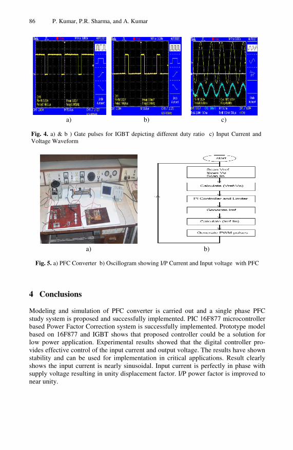
86 P. Kumar, P.R. Sharma, and A. Kumar
a) b) c)
Fig. 4. a) & b ) Gate pulses for IGBT depicting different duty ratio c) Input Current and Voltage Waveform
a) b)
Fig. 5. a) PFC Converter b) Oscillogram showing I/P Current and Input voltage with PFC
4 Conclusions
Modeling and simulation of PFC converter is carried out and a single phase PFC study system is proposed and successfully implemented. PIC 16F877 microcontroller based Power Factor Correction system is successfully implemented. Prototype model based on 16F877 and IGBT shows that proposed controller could be a solution for low power application. Experimental results showed that the digital controller pro-vides effective control of the input current and output voltage. The results have shown stability and can be used for implementation in critical applications. Result clearly shows the input current is nearly sinusoidal. Input current is perfectly in phase with supply voltage resulting in unity displacement factor. I/P power factor is improved to near unity.

Power Factor Correction Based on RISC Controller 87
References
1. Loera-Palomo, R., Morales- Saldana, J.A., Leyva-Ramos, J., Carbajal- Gutierrez, E.E.: Controller Design for a Power Factor Correction Regulator R2P2. IET Electron. 3(5), 784–792 (2010)
2. Yeh, C.-A., Ho, K.-M., Lai, Y.-S., Takashi, F., Hamaogi, M.: Digital Controlled Power Factor with Transition Current Mode Control without Zero Current Detection. In: PEDS, pp. 198–203 (2009)
3. Balamurugan, R., Gurusamy, G.: Harmonic Optimization by Single Phase Improved Power Quality AC-DC Power Factor Corrected Converters. International Journal of Computer Application 1(5), 46–53 (2010)
4. Lopez, V.M., Diaz, F.J., Castro, A.: Autotuning Digital Controller for Current Sensorless Power Factor Corrector Stage in Continuous Conduction Mode. IEEE, Los Alamitos (2010)
5. Hung, C.-W., Chen, J.-H., Chang, L.-S., Li, C.-H.: A Simple Strategy of Power Factor Correction based on Low- End MCU. In: 5th IEEE Conference on Industrial Electronics and Applications, pp. 1229–1233
6. Siri, K., Willhoff, M.: Current – Sharing among Parallel – Connected System of Active Power Factor Correction. IEEEAC Paper #1047, Version 3 (2009)
7. Ezhilarasi, A., Ramaswamy, M.: ADSPIC Implementation of a Sliding Mode Stratezy for a SEPIC Converter. SJEE 6(2), 215–225 (2009)
8. Jafari, F., Dastfan, A.: Optimizationof Single –Phase PWM Rectifier Performance by Using the Genetic Algorithm: ICREPQ 10 Granada (Spain)
9. Petrea, C.: Digital Control of Boost PFC Converter Working in Discontinuous Conduction Mode, vol. 7(2), pp. 16–19. AECE (2007)
10. Ou, S.-Y., Hsiao, H.-P., Tien, C.-H.: Analysis and Design of Prototype Single Stage Half – Bridge Power Converter. In: 5th IEEE Conf. on Industrial Electronics and Applications, pp. 1168–1173
V.V. Das, N. Thankachan, and N.C. Debnath (Eds.): PEIE 2011, CCIS 148, pp. 88–94, 2011. © Springer-Verlag Berlin Heidelberg 2011
Customized NoC Topologies Construction for High Performance Communication Architectures
P. Ezhumalai1 and A. Chilambuchelvan2
1 Dept of Computer Science and Engineering Ralalakshmi Engineering College, Thandalam-602 105, Chennai, India
2 Dept of Computer Science and Engineering R.M.K. Engineering College, Chennai- 601 206 ezhumalai.es,[email protected]
Abstract. Different Intellectual Property (IP) cores, including processor and memory, are interconnected to build a typical System-on-Chip(SoC) architectures. Larger SoC designs dictate the data communication to happen over the global interconnects. Network-on-Chip (NoC) architectures have been proposed as a scalable solution to the global communication challenges in nanoscale Systems-on-Chip (SoC) design. Hence to improve the performance of SoC, first we did a performance study of regular interconnect topologies MESH, TORUS, BFT and EBFT, we observed that the overall latency and throughput of the EBFT is bet-ter compared to other topologies. Our next objective is to generate an area and power optimized NoC topology, for this purpose we used Rectilinear–Steiner-Tree (RST)-based algorithms for generating efficient and optimized network topologies. Experimental results on a variety of NoC benchmarks showed that our synthesis results were achieve reduction in power consumption and average hop count over custom topology implementation.
Keywords: Network-on-chip (NoC), System-On-Chip (SoC), Synthesis, Steiner Minimal Tree, Network topology.
1 Introduction
The integration of several heterogeneous components into a single system gives rise to new challenges. With the change of dramatic improvement in this area, it is essen-tial to have an adaptable communication facility that can cope up with the versatile programming of the cores. Such systems will have to process data in real time, per-form data transfer at the rate of hundreds of Tbps , support multiple functions and protocols for communications with standard wired and wireless interface, provide security and secrecy and cope-up with time-to-market (TTM) pressures and so. Exist-ing SoCs’ communications are based on dedicated wires and shared bus (sin-gle/hierarchical) having various constraints. Dedicated wires do not provide flexibility for communication needed for hardware platforms and cannot cope-up the increased number of cores. Due to exclusive access of shared bus its utilization is as low as 10%. The physical layout of the NoC can determine the degree of scalability and performance of the system as a whole, and just how much of an improvement over traditional bus architectures is actually attained is important.

Customized NoC Topologies Construction 89
2 Interconnection Architectures:
2.1 Mesh Network
Every switch in mesh network fig 1. is connected to a specific resource and the num-ber of switches is equal to the number of resources. All switches are connected to the four closest switches and the target resource block, except those on the edge of the layout. The simplicity of such a mesh architectural layout allows for the division of the chip into processing or resource regions.
2.2 Torus Network
The Torus topology in fig 2. is similar to the mesh architecture, except that the wires are wrapped around from the top component to the bottom and rightmost to leftmost, thereby doubling the bandwidth of a mesh network. This architectural layout provides for a longer transmission distance for a given communication packet.
Fig. 1. Mesh Fig. 2. Torus
Fig. 3. Butterfly Fat Fig. 4. Extended Butterfly Fat
2.3 Butterfly Fat Tree
The layout in fig 3. is modeled in the form of a tree. Each node in the tree is repre-sented by a set of coordinates (level, position) where level is the level in the tree and position is the spot in right to left ordering. Vertical levels are numbered starting at zero at the leaves. The leaves in the trees correspond to each intellectual property (IP)

90 P. Ezhumalai and A. Chilambuchelvan
or component block, and the levels above represent one node for each switch, and the interconnection hierarchy maps the various connections between switches, and switches to components. Each switch is allocated two parent ports, and four child ports, or connections.
2.4 Extended Butterfly Fat Tree
The extended butterfly fat tree interconnection (EFTI) in fig 4. is a derivative of the butterfly fat tree architecture which is the derivative of fat tree architecture The archi-tecture uses switches of constant size. In this network too, the IPs are placed at the leaves and switches placed at the internal nodes. Each switch is allocated two parent ports, and four child ports, or connections.
3 Existing Related Works
Several existing NoC solutions have addressed the mapping problem to a regular mesh-based NoC architecture [1],[2], P.Ezhumalai et al [2] proposed a survey of Ar-chitectural Design and Analysis of Network on-Chip System computation of regular topologies, FPGA Interconnect topologies Exploration presented by Zied Marrakchi et al[3], Custom NoC architectures with Multicast Routing are proposed by Shan Yan et al. [5], [6] proposed Interconnect Modeling for Improved System-Level Design Optimization, long link insertion techniques for application-specific NoC architec-tures. Ling Zhang et al. [10], proposed a Repeated On-Chip Interconnect Analysis and Evaluation of Delay, Power , and Bandwidth Metrics under Different Goals ,but their solutions only considered solutions based on a slicing floorplan where router locations are restricted to corners of cores and links run around cores.
4 Proposed Work
• Performance Analysis of various regular NoC Topologies. • The problem of synthesizing custom networks-on-chip (NoC) architectures.
We divide the problem statement into the flowing interrelated steps:
• Physical topology Construction. • Power and Area Comparisons
Input Specification
Topology Generation
NoC Power and
Area Estimation
Fig. 5. Proposed System Architecture

Customized NoC Topologies Construction 91
NoC Synthesis: The portion of the input specification corresponds to the network-attached modules and their traffic flows. The nodes represent modules, edges represent traffic flows, and edge labels represent the length of the two vertices. The NoC Synthe-sis generates topologies based on the communication demand graph and comparing with parameters like power consumption and area usage chooses the best architecture. Below fig 6. is an example of two architectures generated based on the given CDG.
Fig. 6. Sample Topologies Generated
NoC Power and Area Estimation: To evaluate the power and area of the synthe-sized NoC architecture, we use a state-of the- art NoC power-performance simulator called Orion that can provide detailed power characteristics for different power com-ponents of a router for different input/output port configurations. It accurately consid-ers leakage power as well as dynamic switching power, which is important since it is well known that leakage power is becoming an increasingly dominating. Orion also provides area estimates based on a state-of-the-art router micro-architecture.
5 Implementation Results
5.1 Performance Analysis Regular NoC Topologies
We used a Gp-NoC simulator in java supporting wormhole switching and deadlock-free deterministic routing for Mesh, Torus, Butterfly Fat Tree and Extended-butterfly Fat Tree for performance analysis . The network is formed automatically depending on the number of IPs. Functional IP injected variable-size packets (mean = 200 bytes) to ran-dom destinations except for themselves at a uniform distribution rate. The total number of IP considered for all topologies is 64; the simulation is run for a 100000 cycles with asynchronous traffic type. We investigated the average latency of packets, the network throughput; Latency of a packet is calculated from the instant the packet’s flits are created to that the last flit of the packet is accepted at the destination, including source queuing time. Throughput is defined as the number of flits received per cycle per IP. The following figures shows that the performance analysis of regular topologies.
5.2 Customized NoC Topologies Construction
The total area as well as power consumption includes all network components. We applied the design parameters of 1 GHz clock frequency, 4-flit buffers, and 128-bit flits. For evaluation, fair direct comparison with previously published NoC synthesis results is difficult in part because of vast differences in the parameters assumed. To

92 P. Ezhumalai and A. Chilambuchelvan
Fig. 7. Latency Fig. 8. Throughput
Fig. 9. Steiner Minimal Tree: 64 Points, length = 56729
evaluate the effectiveness of our algorithm generates a Steiner Minimal Tree: 64 Points, length = 56729, is shown in fig 9, we have the full mesh implementation for each benchmark for comparison from previous published papers have been taken. These comparisons are signified to show the benefits of custom NoC architectures.
The area results, power results, the execution times, and area as well as power improvements of that algorithm are reported. The results show the algorithm can efficiently synthesize NoC architectures that minimize power and area consumption as compared with regular topologies such as mesh and optimized mesh topologies.
Thus, the above two line charts clearly show a reduction in power and area esti-mates of custom NoC with mesh and optimized mesh topologies. The power reduc-tion is at an average 50 percent as compared to mesh and optimized mesh topologies respectively. The area reduction is at an average of 70.95 percent as compared to optimized mesh topologies.
Fig. 10. NOC Power Comparisons
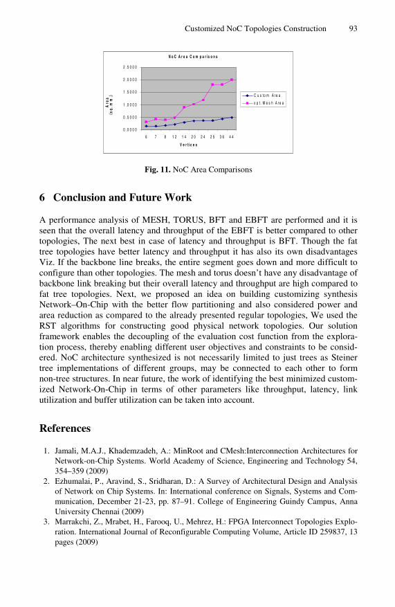
Customized NoC Topologies Construction 93
N o C A r e a C o m p a r is o n s
0 .0 0 0 0
0 .5 0 0 0
1 .0 0 0 0
1 .5 0 0 0
2 .0 0 0 0
2 .5 0 0 0
6 7 8 1 2 1 4 2 0 2 4 2 5 3 6 4 4
V e r t i c e s
Are
a
(s
q. m
m.)
C u s t o m A r e a
o p t . M e s h A r e a
Fig. 11. NoC Area Comparisons
6 Conclusion and Future Work
A performance analysis of MESH, TORUS, BFT and EBFT are performed and it is seen that the overall latency and throughput of the EBFT is better compared to other topologies, The next best in case of latency and throughput is BFT. Though the fat tree topologies have better latency and throughput it has also its own disadvantages Viz. If the backbone line breaks, the entire segment goes down and more difficult to configure than other topologies. The mesh and torus doesn’t have any disadvantage of backbone link breaking but their overall latency and throughput are high compared to fat tree topologies. Next, we proposed an idea on building customizing synthesis Network–On-Chip with the better flow partitioning and also considered power and area reduction as compared to the already presented regular topologies, We used the RST algorithms for constructing good physical network topologies. Our solution framework enables the decoupling of the evaluation cost function from the explora-tion process, thereby enabling different user objectives and constraints to be consid-ered. NoC architecture synthesized is not necessarily limited to just trees as Steiner tree implementations of different groups, may be connected to each other to form non-tree structures. In near future, the work of identifying the best minimized custom-ized Network-On-Chip in terms of other parameters like throughput, latency, link utilization and buffer utilization can be taken into account.
References
1. Jamali, M.A.J., Khademzadeh, A.: MinRoot and CMesh:Interconnection Architectures for Network-on-Chip Systems. World Academy of Science, Engineering and Technology 54, 354–359 (2009)
2. Ezhumalai, P., Aravind, S., Sridharan, D.: A Survey of Architectural Design and Analysis of Network on Chip Systems. In: International conference on Signals, Systems and Com-munication, December 21-23, pp. 87–91. College of Engineering Guindy Campus, Anna University Chennai (2009)
3. Marrakchi, Z., Mrabet, H., Farooq, U., Mehrez, H.: FPGA Interconnect Topologies Explo-ration. International Journal of Reconfigurable Computing Volume, Article ID 259837, 13 pages (2009)

94 P. Ezhumalai and A. Chilambuchelvan
4. Ezhumalai, P., Chilambuchelvan: Low Power and Area Consumption Custom Networks-On-Chip architectures Using RST Algorithms. International Journal of Computer Science and Information Security (IJCSIS) 7(6), 107–115 (2010)
5. Yan, S., Lin, B.: Custom Networks-on-Chip Architectures With Multicast Routin. IEEE Transactions On Very Large Scale Integration (VLSI) Systems 17(3), 342–355 (2009)
6. Carloni, L.P., Kahng, A.B., Muddu, S., Pinto, A., Samadi, K., Sharma, P.: Interconnect Modeling for Improved System-Level Design Optimization. In: Proc. ASPDAC, pp. 258–264 (2008)
7. Zhang, L., Chen, H., Chen, H., Yao, B., Hamilton, K., Cheng, C.-K.: Repeated on-chip in-terconnect analysis and evaluation of delay, power, and bandwidth metrics under different design goals. In: Proc. ISQED, pp. 251–256 (2007)
8. IIitzky, D.A., Hoffman, J.D., Chun, A., Esparza, B.P.: Architecture of the Scalable Com-munications Core’s Network on Chip. In: IEEE MICRO, pp. 62–74 (2007)
9. Lin, C.-W., Chen, S.-Y., Li, C.-F., Chang, Y.-W., Yang, C.-L.: Efficient obstacle-avoiding rectilinear Steiner tree construction. In: Proc.Int. Symp. Phys. Des., pp. 127–134 (2007)
10. Zhang, L., Chen, H., Yao, B., Hamilton, K., Cheng, C.-K.: Repeated On-Chip Interconnect Analysis and Evaluation of Delay, Power, and Bandwidth Metrics under Different Design Goals. In: 8th International Symposium Quality Electronic Design, ISQED 2007, March 2007, pp. 251–256 (2007)

V.V. Das, N. Thankachan, and N.C. Debnath (Eds.): PEIE 2011, CCIS 148, pp. 95–104, 2011. © Springer-Verlag Berlin Heidelberg 2011
Improving CPU Performance and Equalizing Power Consumption for Multicore Processors in Agent Based
Process Scheduling
G. Muneeswari1 and K.L. Shunmuganathan2
1 Research Scholar, Department of Computer Science and Engineering, R.M.K Engineering College
2 Professor & Head, Department of Computer Science and Engineering, R.M.K Engineering College
[email protected], [email protected]
Abstract. In a Multicore architecture, each package consists of large number of processors. This increase in processor core brings new evolu-tion in parallel computing. Besides enormous performance enhancement, this multicore package injects lot of challenges and opportunities on the operating system scheduling point of view. We know that multiagent system is concerned with the development and analysis of optimization problems. In this paper we combine the AMAS theory of multiagent system with the scheduler of operating system to develop a new process scheduling algorithm for multicore architecture. This multiagent based scheduling algorithm promises in minimizing the average waiting time of the processes in the centralized queue, reduces the task of the sched-uler and also increases cpu performance. Because of round robin sched-uling, the power consumption for each processor can be equalized. We actually modified and simulated the linux 2.6.11 kernel process sched-uler to incorporate the multiagent system concept. The comparison is made for different number of cores with multiple combinations of process and the results are shown for average waiting time Vs number of cores in the centralized queue and cpu performance Vs number of process and cores.
Keywords: multicore, multiagent system, centralized queue, average waiting time, power consumption, scheduling, processor agent, middle agent, dispatcher.
1 Introduction
Multicore architectures, which include several processors on a single chip, are being widely touted as a solution to serial execution problems currently limiting single-core designs. In most proposed multicore platforms, different cores share the common memory. High performance on multicore processors requires that schedulers be rein-vented. Traditional schedulers focus on keeping execution units busy by assigning each core a thread to run. Schedulers ought to focus, however, on high utilization of the execution of cores, to reduce the idle of processors. But this may increase the

96 G. Muneeswari and K.L. Shunmuganathan
power consumption of the processors. Multi-core processors do, however, present a new challenge that will need to be met if they are to live up to expectations. Since multiple cores are most efficiently used (and cost effective) when each is executing one process, organizations will likely want to run one job per core. But many of to-day’s multi-core processors share the front side bus as well as the last level of cache. Because of this, it's entirely possible for one memory-intensive job to saturate the shared memory bus resulting in degraded performance for all the jobs running on that processor. And as the number of cores per processor and the number of threaded ap-plications increase, the performance of more and more applications will be limited by the processor’s memory bandwidth. Schedulers in today’s operating systems have the primary goal of keeping all cores busy executing some runnable process. Since lot of applications comes into the system some processor may be assigned with many tasks and some processor may not have jobs at all. This is actually due to the poor process scheduling taking place in operating system. One technique [12] that mitigates this limitation is to intelligently schedule jobs onto these processors with the help of soft-ware approach like multiagents. This schedules processes in round robin fashion so that the load in every processor in multicore system is balanced. This ultimately causes equal power consumption in all the processors.
The Paper is organized as follows. Section 2 reviews related work. In Section 3 we introduce the multiagent system interface with multicore architecture. This describes Middle Agent system implementation, process scheduler organization and process dispatcher organization. In section 4 we describe the load balancing scheme, which equalizes the power consumption of the multicore processors. In section 5 we discuss the evaluation and results and section 6 presents future enhancements with multicores. Finally, section 7 concludes the paper.
2 Background and Related Work
The research on contention for shared resources [1] significantly impedes the efficient operation of multicore systems has provided new methods for mitigating contention via scheduling algorithms. Addressing shared resource contention in multicore proc-essors via scheduling [2] investigate how and to what extent contention for shared resource can be mitigated via thread scheduling. The research on the design and im-plementation of a cache-aware multicore real-time scheduler [3] discusses the mem-ory limitations for real time systems. The paper on AMPS [4] presents, an operating system scheduler that efficiently supports both SMP-and NUMA-style performance-asymmetric architectures. AMPS contains three components: asymmetry-aware load balancing, faster-core-first scheduling, and NUMA-aware migration. In Partitioned Fixed-Priority Preemptive Scheduling [5], the problem of scheduling periodic real-time tasks on multicore processors is considered. Specifically, they focus on the parti-tioned (static binding) approach, which statically allocates each task to one processing core. The real-time scheduling on multicore platforms [9] is a well-studied problem in the literature. The scheduling algorithms developed for these problems are classified as partitioned (static binding) and global (dynamic binding) approaches, with each category having its own merits and de-merits. So far we have analyzed some of the multicore scheduling approaches. Now we briefly describe the self-organization of multiagents, which plays a vital role in our multicore scheduling algorithm.

Improving CPU Performance and Equalizing Power Consumption 97
Multi-Agent Systems (MAS) have attracted much attention as means of developing applications where it is beneficial to define function through many autonomous ele-ments. Mechanisms of selforganisation are useful because agents can be organised into configurations for useful application without imposing external centralized con-trols. The paper [10] discusses several different mechanisms for generating self-organisation in multi-agent systems [11]. A theory has been proposed (called AMAS for Adaptive Multi-Agent Systems) in which cooperation is the engine thanks to which the system self-organizes for adapting to changes coming from its environ-ment. Cooperation in this context is defined by three meta-rules: (1) perceived signals are understood without ambiguity, (2) received information is useful for the agent’s reasoning, and (3) reasoning leads to useful actions toward other agents. Interactions between agents of the system depend only on the local view they have and their abil-ity to cooperate with each other. The middle agent is acting as a translator between the agents and the scheduler as well as the dispatcher.
3 Multicore Architecture with Multiagent System
Every processor in the multicore architecture (Fig.1) has an agent called as Processor Agent (PA). The central Middle Agent (MA) will actually interact with the scheduler. It is common for all Processor Agents. Every PA maintains the following information in PSIB (Processor Status Information Block). It is similar to the PCB (Process Con-trol Block) of the traditional operating system. Processor Status may be considered as busy or idle. Process name can be P1or P2 etc., if it is busy. 0 if it is idle. Process Status could be ready or running or completed and the burst time is the execution time of the process.
Middle Agent
Fig. 1. Multicore architecture with multiagent system
As we are combining the concept of multiagent system with multicore architecture, the processor characteristics are mentioned as a function of Performance measure, Environment, Actuators, Sensors (PEAS environment), which is described in table.1 given below. This describes the basic reflexive model of the agent system.
The Process Scheduler Organization Shared memory multicore system consists of a ready queue where all the processes that are ready for execution will be available. cpu scheduling is remarkably similar to other types of scheduling that have been studied for years. In this paper we take a model of
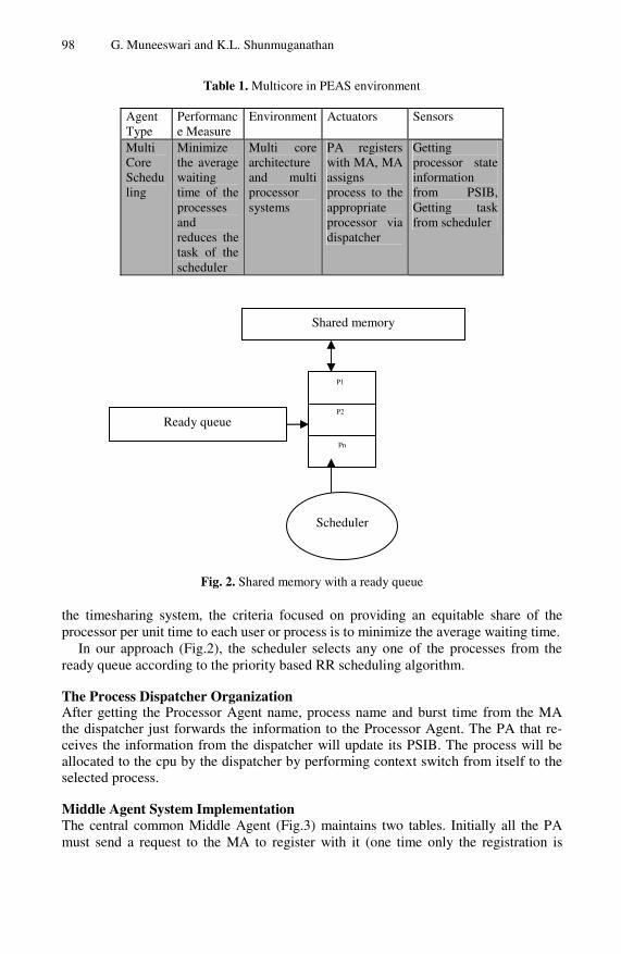
98 G. Muneeswari and K.L. Shunmuganathan
Table 1. Multicore in PEAS environment
Agent Type
Performance Measure
Environment Actuators Sensors
Multi Core Scheduling
Minimize the average waiting time of the processes and reduces the task of the scheduler
Multi core architecture and multi processor systems
PA registers with MA, MA assigns process to the appropriate processor via dispatcher
Getting processor state information from PSIB, Getting task from scheduler
Fig. 2. Shared memory with a ready queue
the timesharing system, the criteria focused on providing an equitable share of the processor per unit time to each user or process is to minimize the average waiting time.
In our approach (Fig.2), the scheduler selects any one of the processes from the ready queue according to the priority based RR scheduling algorithm.
The Process Dispatcher Organization After getting the Processor Agent name, process name and burst time from the MA the dispatcher just forwards the information to the Processor Agent. The PA that re-ceives the information from the dispatcher will update its PSIB. The process will be allocated to the cpu by the dispatcher by performing context switch from itself to the selected process.
Middle Agent System Implementation The central common Middle Agent (Fig.3) maintains two tables. Initially all the PA must send a request to the MA to register with it (one time only the registration is
Shared memory
P1
P2
Pn
Scheduler
Ready queue

Improving CPU Performance and Equalizing Power Consumption 99
Fig. 3. Middle Agent system communication
made). Middle Agent is the central heart of the scheduling process. It communicates with the scheduler for getting the process to be scheduled on large number of proces-sor. It also interacts with the dispatcher whose function is to assign the process to the different cores.
Agent Processor Information Table (APIT): When the PA sends a register request to middle agent (MA), the relevant information is stored in the Agent Processor Information Table. Initially all the entries for the processor state will be idle. Once the scheduler selects the first set of processes based on RR scheduling algorithm, it then contacts with MA to give the process name and the burst time and the state of the process will be changed to busy by the MA in the following table. (So initially the assignment will be FIFO order (i.e agent registration will be in FIFO only). After updating the table MA sends the corresponding PA name and process name to the Dispatcher. The dispatcher is finally responsible for allocating the processes to the respective processor via processor agents and the corresponding table is also up-dated. The Agent processor information table can be maintained as part of the oper-ating system process management part of the scheduler. Linked list representation is a preferred data structure used for the arrangement of processes on the stipulated table.
Agent Request Table (ARQT): Whenever the processor completes the first set of tasks, the agents of the processor PA immediately send a process request message to the MA. The MA after receiving the request message from the PA stores the informa-tion in ARQT-Agent Request Table, which can be implemented as a queue. Before storing the information MA has to check APIT to see whether the requested agent has already registered with the MA. Initially the process name will be 0 because we re-ceived only the request message from the PA. The activities will be repeated again. When the scheduler is ready it sends the job to the MA and the MA stores the process name and burst time in the following table. It then sends the corresponding PA and process name along with burst time to the dispatcher.
Middle Agent Scheduler
Dispatcher
APIT ARQT
Multicore PA

100 G. Muneeswari and K.L. Shunmuganathan
4 Load Balancing and Power Consumption of Processors
In many applications, the CPU and other components are idle much of the time, so idle power contributes significantly to overall system power usage. When the CPU uses power management features to reduce energy use, other components, such as the motherboard and chipset take up a larger proportion of the computers energy. In ap-plications where the computer is often heavily loaded, such as scientific computing, performance per watt - how much computing the CPU does per unit of energy becomes more significant.
4.1 Load Balancing in Multiprocessor System
In the traditional multi processor system, the critical load balancing task is performed through hardware. In [6] The cooperative load balancing in distributed systems is achieved through processor interaction. dynamic load balancing algorithm [7] deals with many important load estimation issues. In ACO algorithm [8] for load balancing in distributed systems will be presented. This algorithm is fully distributed in which information is dynamically updated at each ant movement. But in our approach we involve the concept of agents, which is a software based approach that reduces the complexity of the hardware. The significance of this round robin agent scheduling is to place almost equal number of processes in every processor and thus we increase the cpu performance. This is because no processor will be kept in the idle state.
4.2 CPU Power Dissipation in Different Architectures
CPUs for desktop computers [13] typically use a significant portion of the power consumed by the computer. The CPU power dissipation of various processor is shown in table.2. In laptops, the LCD back light also uses a significant portion of overall power. While energy-saving features have been instituted in personal computers for when they are idle, the overall consumption of today's high-performance CPUs is considerable. This is in strong contrast with the much lower energy consumption of CPUs designed for low-power environments.
Table 2. CPU Power Dissipation for various Processor
Model Lithiography
Clock Speed Vcore Power
Clock Speed to Power Ratio Efficiency [MHz/W]
Dual-core PowerPC MPC8641D
90 nm 2 GHz 1.2 V 15-25 W 100
PowerPC 750FX
0.13 µm
900 MHz
1.2 V 3.6 W 250
PowerPC 750CXe
0.18 µm
600 MHz
1.8 V 6 W 100

Improving CPU Performance and Equalizing Power Consumption 101
4.3 Equalizing Power Consumption of Processors Using Load Balancing
As we use intelligent multiagent based scheduling algorithm in the proposed work, every processor in the multicore system is given with the same amount of processes. This significant achievement leads to automatic load balancing and none of the proc-essors will be kept in the idle state. Actually in the traditional system although some load balancing algorithm is used, it leads to complex process transfer, network delay and hardware intervension.
P1 P2 Pn
Shared Mem
ory
Load Balancing
Equalizing Power Consumption
Multiagent based Round Robin Scheduling
Fig. 4. Equalizing power consumption of the processors using load balancing
In our approach, since load balancing is incorporated in the scheduling algorithm, power consumption of all the processor is equal. In Fig.4, it is shown that establishing load balancing in multicore system leads to equalizing the power consumption in all the processors.
5 Evaluation and Results
In this section, we present a performance analysis of our scheduling algorithm using a gcc compiler and linux kernal version 2.6.11. In every core we calculate the waiting time of the process as previous process execution time. The execution time of the previous process is calculated as follows:
PET = PBT + αi + βi + δi + γi
Where PET is the execution time of the process, PBT is the burst time of the process, αi is the scheduler selection time, βi is the Processor Agent request time, δi is the Middle Agent response time, γi is the dispatcher updation time. The average waiting time of the process is calculated as the sum of all the process waiting time divided by the number of processes.
PAWT= Σ(i=1..n) P(i=1..n) / N
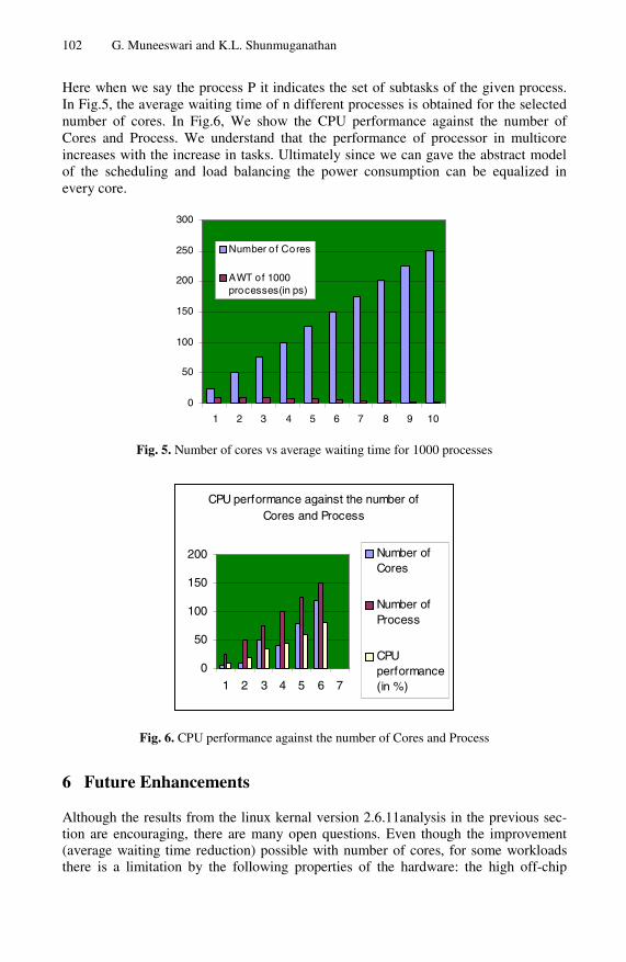
102 G. Muneeswari and K.L. Shunmuganathan
Here when we say the process P it indicates the set of subtasks of the given process. In Fig.5, the average waiting time of n different processes is obtained for the selected number of cores. In Fig.6, We show the CPU performance against the number of Cores and Process. We understand that the performance of processor in multicore increases with the increase in tasks. Ultimately since we can gave the abstract model of the scheduling and load balancing the power consumption can be equalized in every core.
0
50
100
150
200
250
300
1 2 3 4 5 6 7 8 9 10
Number of Cores
AWT of 1000processes(in ps)
Fig. 5. Number of cores vs average waiting time for 1000 processes
CPU performance against the number of Cores and Process
0
50
100
150
200
1 2 3 4 5 6 7
Number ofCores
Number ofProcess
CPUperformance(in %)
Fig. 6. CPU performance against the number of Cores and Process
6 Future Enhancements
Although the results from the linux kernal version 2.6.11analysis in the previous sec-tion are encouraging, there are many open questions. Even though the improvement (average waiting time reduction) possible with number of cores, for some workloads there is a limitation by the following properties of the hardware: the high off-chip

Improving CPU Performance and Equalizing Power Consumption 103
memory bandwidth, the high cost to migrate a process, the small aggregate size of on-chip memory, and the limited ability of the software (agents) to control hardware caches. We expect future multicores to adjust some of these properties in favor of our multiagents based scheduling. More intelligent algorithm can be proposed in view of the memory limitation with respect to operating system. As we represent power con-sumption in abstract model, indepth analysis is required for the complete system.
7 Conclusion
This paper has argued that multicore processors pose unique scheduling problems that require a multiagent based software approach that utilizes the large number processors very effectively. We also proved that lot of drastic enhancements in the traditional scheduler that optimizes for cpu cycle utilization. We discovered that the average waiting time decreases slowly with the increase of the number of cores. As a conclu-sion our new novel approach eliminates the complexity of the hardware and improved the CPU utilization to the maximum level and thus the power consumption in every processor is equalized.
References
1. Fedorova, A.: Managing contention for shared resources on multicore processors. Com-munications of the ACM 53(2), 49–57 (2010)
2. Zhuravley, S., Blagoduroy, Fedorova, A.: Addressing shared resource contention in multi-core processors via scheduling. In: Proceedings of the Fifteenth Edition of ASPLOS on Architectural Support for Programming Languages and Operating Systems, pp. 129–142 (2010)
3. Calandrino, J.M., Anderson, J.H.: On the Design and Implementation of a Cache-Aware Multicore Real-Time Scheduler. In: 21st Euromicro Conference on Real-Time Systems, July 01-03 (2009)
4. Li, T., Baumberger, D., Koufaty, D.A., Hahn, S.: Efficient operating system scheduling for performance asymmetric multi-core architectures. In: Conference on High Performance Networking and Computing Proceedings of the ACM /IEEE Conference on Supercomput-ing (2007)
5. Lakshmanan, K., Rajkumar, R. (R.), Lehoczky, J.P.: Partitioned Fixed-Priority Preemptive Scheduling for Multi-Core Processors. In: Proceedings of the 21st Euromicro Conference on Real-Time Systems, pp. 239–248 (2009)
6. Grosu, D., Chronopoulos, A.T., Leung, M.Y.: Cooperative Load Balancing in Distributed Systems. Concurrency and Computation: Practice and Experience 20(16), 1953–1976 (2008)
7. Alakeel, A.M.: Load Balancing in Distributed Computer Systems. International Journal of Computer Science and Information Security 8(4) (July 2010)
8. Ali, D., Belal, M.A., Zoubi, M.B.: Load Balancing of Distributed Systems Based on Mul-tiple Ant Colonies Optimization. American Journal of Applied Sciences 7(3), 433–438 (2010)
9. Anderson, J.H., Calandrino, J.M., Devi, U.C.: Real-Time Scheduling on Multicore Plat-forms. In: Proceedings of the 12th IEEE Real-Time and Embedded Technology and Appli-cations Symposium, pp. 179–190 (2006)

104 G. Muneeswari and K.L. Shunmuganathan
10. Bernon, C.: Applications of Self-Organising Multi-Agent Systems: An Initial Framework for Comparison. In: IRIT, INRIA (2006)
11. Di Marzo Serugendo, G., Gleizes, M.-P., Karageorgos, A.: Self-Organisation and Emer-gence in MAS: An Overview. A INFORMATICA 30 (2006)
12. Muneeswari, G., Sobitha Ahila, A., Shunmuganathan, K.L.: A Novel Approach to Multi-agent Based Scheduling for Multicore Architecture. In: Proceedings of Advanced Distrib-uted and Parallel Comuting, Singapore (2010)
13. Wikipedia Information, http://en.wikipedia.org/wiki/CPU_power

V.V. Das, N. Thankachan, and N.C. Debnath (Eds.): PEIE 2011, CCIS 148, pp. 105–108, 2011. © Springer-Verlag Berlin Heidelberg 2011
Wireless 3-D Gesture and Chaaracter Recoginition
Gaytri Gupta and Rahul Kumar Verma
Department of Electronics and Communication Engineering AMITY University
Sector-125, Noida, India ggupta,[email protected]
Abstract. A 3-d gesture recognition system can be used for a host of applica-tion including gesture base user interface, character recognition system, wire-less human interface devices and virtual reality in 3d gaming. Human machine interaction has reached the point where machines are capable of interrupting gesture of human beings. The gestures are made by hand movement and facial expression. A gesture is detected and interrupted due to the movement of the hand and body. The data is wirelessly transmitted to the receiving station where for processing, some application.
Keywords: Gesture recognition, Sensor LIS302DL, IC CC2500.
Introduction
This paper describes a natural way of interacting with a portable device or a computer through the recognition of 3-D gestures.3-D gesture recognition is important in a host of applications like virtual real environments, robotic programming by demonstration, human computer interaction, sign language recognition, tale-robotic applications etc.
System Description
Wireless 3-d gesture and caharacter recoginition consists of four module. These are the followings:
1) Motion sensor: The Motion sensor used in this device is LIS302DL.The LIS302DL is an ultra compact low-power three axes linear accelerometer. It includes a sensing element and an IC interface able to provide the measured acceleration to the external world through I2C/SPI serial interface. The LIS302DL has dynamically user selectable full scales of ±2g/±8g and it is capable of measuring accelerations with an output data rate of 100Hz or 400Hz.
2) RF Transreceiver: In this device we have chose the IC CC2500 as RF transreceiver. IC CC2500 provide extensive hardware support for packet handling, data buffering, burst transmission, clear channel assessment, and link quality indication and wake-on radio. A 2.4 GHz chip antenna is used as the RF font-end with a few passive components.The main operating parameters and the 64- byte transmit/receive FIFOs of
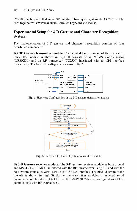
106 G. Gupta and R.K. Verma
CC2500 can be controlled via an SPI interface. In a typical system, the CC2500 will be used together with:Wireless audio, Wireless keyboard and mouse.
Experimental Setup for 3-D Gesture and Character Recognition System
The implementation of 3-D gesture and character recognition consists of four distributed components:
A) 3D Gesture transmitter module: The detailed block diagram of the 3D gesture transmitter module is shown in Fig1. It consists of an MEMS motion sensor (LIS302DL) and an RF transceiver (CC2500) interfaced with an SPI interface respectively. The basic flow diagram is shown in fig 2.
Fig. 1. Hardware Configuration of the 3-D gesture transmitter module
Fig. 2. Flowchart for the 3-D gesture transmitter module
B) 3-D Gesture receives module: The 3-D gesture receiver module is built around and MSP430F2279 MCU, interfaced with the RF transreciever using SPI and with the host system using a universal serial bus (USB2.0) Interface. The block diagram of the module is shown in Fig3 Similar to the transmitter module, a universal serial communication Interface (US-CIB) of the MSP430F2274 is configured as SPI to communicate with RF tranrecieves.
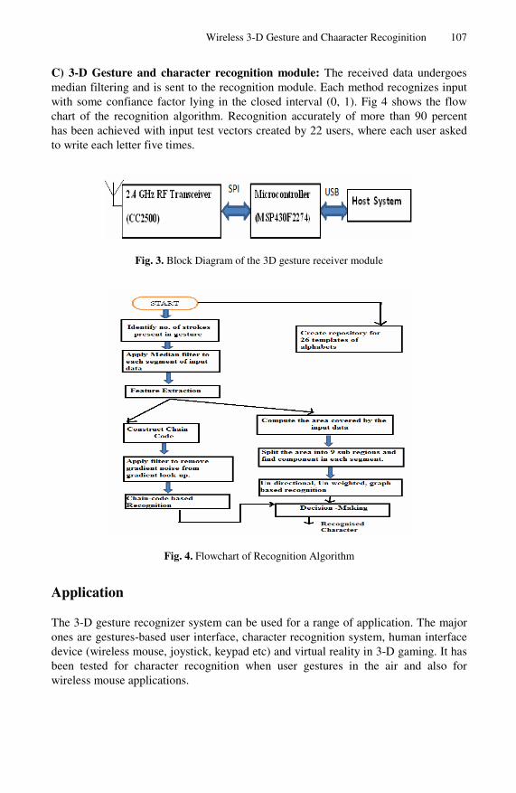
Wireless 3-D Gesture and Chaaracter Recoginition 107
C) 3-D Gesture and character recognition module: The received data undergoes median filtering and is sent to the recognition module. Each method recognizes input with some confiance factor lying in the closed interval (0, 1). Fig 4 shows the flow chart of the recognition algorithm. Recognition accurately of more than 90 percent has been achieved with input test vectors created by 22 users, where each user asked to write each letter five times.
Fig. 3. Block Diagram of the 3D gesture receiver module
Fig. 4. Flowchart of Recognition Algorithm
Application
The 3-D gesture recognizer system can be used for a range of application. The major ones are gestures-based user interface, character recognition system, human interface device (wireless mouse, joystick, keypad etc) and virtual reality in 3-D gaming. It has been tested for character recognition when user gestures in the air and also for wireless mouse applications.
108 G. Gupta and R.K. Verma
Conclusion and Future Work
A system aimed at tracking a body movement with the use of Wireless 3-D gesture and caharacter recoginition system. Gesture recognition with the microcontroller based method is possible but more suitable recognition methods should be considered, performing recognition on a character basis. A further step is to use gestures along with other modalities, such as speech. Such a system could provide a user interface that would combine the complexity and the naturalness of human interaction. In the future, the MSP430F2250 receiver module will be replaced with the C8051F34X derivatives from silicon laboratory to further reduce the form factor of the receiver PCB. This is because the latter has a built in USB controller and can start working as a simple HID device, whereas currently the TUSB3410 has been used as a USB to UART bridge for host PC interfacing for which serial over USB driver is using.
References
[1] Flanagan, J.A., Mantyjarvi, J.: Unsuperised clustering of symbol strings and context rec-ogniton. In: ICDM, Maebashi, Janpan, pp. 171–178
[2] Choi, E.-S., Bang, W.-C., et al.: Beatbox Music Phone: Gesture Interactive Cell phone using Tri-axis Accelerometer. In: ICIT IEEE Int. Conference on Industrial Technology (2005)
[3] Jaeger, S., Manke, S., Waibel, A.: Npen++: An on-line handwriting recognition system. In: Proc. 7th Int’l Workshop on Frontiers in Handwriting Recognition, September 2000, pp. 249–260 (2000)
[4] Jain, A.K., Duin, R.P., Mao, J.: Statistical pattern recognition: A review. IEEE Trans. PAMI 22(1), 4–37 (2000)
[5] Yeasin, M., Chaudhuri, S.: Visual understanding of dynamic hand gestures. Pattern Recognition 33, 1805–1817 (2000)
[6] Campbell, L., et al.: Invariant features for 3-d gesture recognition. In: Proc. FG 1996, pp. 157–162 (1996)
[7] Davis, J., Bobick, A.: The representation and recognition of action using temporal tem-plates. In: Proc. of IEEE CVPR, San Juan, Puerto Rico (1977)
[8] Licsar, A., Sziranyi, T.: Supervised Training Based Hand Gesture Recognition System. In: Proceedings of 16th International Conference on Pattern Recognition, vol. 3, pp. 999–1002 (2002)
[9] Ueda, E., Matsumoto, Y., Imai, M., Ogasawara, T.: Handpose Estimation for Vision-based Human Interfaces. IEEE Transactions on Industrial Electronics 50, 676–684 (2003)

V.V. Das, N. Thankachan, and N.C. Debnath (Eds.): PEIE 2011, CCIS 148, pp. 109–112, 2011. © Springer-Verlag Berlin Heidelberg 2011
Design of High Sensitivity SOI Piezoresistive MEMS Pressure Sensor
T. Pravin Raj1,*, S.B. Burje1, and R. Joseph Daniel2
1 Dept. of ETC, Rungta College of Engineering and Technology, Bhilai, India [email protected]
2 National MEMS Design Centre (NPMaSS), Dept. of E & I Engineering, Annamalai University, Annamalainagar, 608 002, Tamilnadu, India
Abstract. In this paper, the effect of the size of the piezoresistors that forms the Wheatstone bridge on sensitivity has been studied and reported. There are four resistors implanted on the diaphragm in such a way that two of them sense the tensile stress (Group I) and the other two senses the compressive stresses (Group II). The structure of this MEMS sensor has been created and analyzed using IntelliSuite MEMS CAD tool. The results show that the size of the group I resistors should be made as large as possible and that of group II should be made as small as possible to achieve maximum sensitivity. It is also illustrated that the size design of group II resistors is critical.
Keywords: MEMS, Piezoresistors, SOI Pressure sensor, Intellisuite, Size effect, sensitivity.
1 Introduction
A MEMS pressure sensor is basically composed of a diaphragm structure and most of them use silicon for diaphragm and piezoresistive property of silicon or polycrystal-line silicon as sensing mechanism [1-4]. In these sensors, the diaphragm of the sensor will deform and induce bending stresses, when a pressure difference is applied on the pressure sensor.
In all these sensor development efforts, researchers have been focusing on fabricat-ing high sensitivity micromachined pressure sensors. Lower Young’s modulus (E) with higher breaking stress (σ) [1] and employment of square diaphragm for pressure sensing [2] was recommended for better sensing. However, only little has been done to study the effect of the geometry of piezoresistors on sensitivity and this paper brings out the results of such a study.
2 Formulation of the Study
The typical structure of Silicon-On-Insulator (SOI) piezoresistive pressure sensor considered in this work is shown in Fig.1. The Silicon diaphragm of the pressure sensor is placed in between the insulating layers of SiO2. The silicon substrate at the
* Corresponding Author.

110 T.P. Raj, S.B. Burje,
Fig. 1
bottom of the diaphragm iscavity is formed at the bottowith different piezoresistivethe oxidized silicon diaphralayer of 0.2μm thickness haresistors. The placement ofThe main objective of this sensitivity of the SOI piezositivity improvement by adjresistors R1 and R3 (Grouexperience compressive strbring out the effect of resistwo diaphragms of different
3 Intellisuite Simulat
By using IntelliSuite MEMcreated for simulation usingsor-A) with a diaphragm odered first and the study haphragm of 1500µm × 15used in the simulation are aGPa, Poisson’s ratio = 0.26.6×10-11 Pa-1; π12 = 1.1×10silicon resistors = 750 Ω pe
3.1 Case(i) : Simulated SResistors Are Increas
The estimated sensitivity ofsizes is presented in Table tained constant. It is evidendrastically as the sizes of thsensitivity is achieved whethe X-X plane (SXX) in both
and R.J. Daniel
1. Structure of SOI Piezoresistive pressure sensor
s etched partially from bottom up approach so that a squom of the pressure sensor as shown in Fig.1. Piezoresiste properties was realized using surface micromachiningagm to form the Wheatstone bridge. A boron doped silias been considered in this study to realize the p-type pief the resistors over the diaphragm is defined by the mareported work is to study the effect of resistor size on
oresistive pressure sensor and explore the feasibility of sjusting the size of the piezoresistors. There are four pie
up I) experience tensile stress and R2 and R4 (Groupress when pressure is applied from the bottom. In ordestor size on the sensitivity, the three cases were studied t sizes.
tion Results and Discussion
MS CAD tool, the structure depicted in Fig.1 has bg Intelli FAB module. In this work, a pressure sensor (Sof 1000µm × 1000µm and thickness of 13.5µm is conas been extended to another sensor (Sensor-B) with a 00µm and thickness of 15µm. The important parameas follows: Young’s modulus of Diaphragm Silicon =
28. Piezo Resistive Coefficients for silicon resistors: π0-11 Pa-1; π44 = 138×10-11 Pa-1, Sheet resistance of the p-ter square.
ensitivity when the Size of Group I and Group II sing
f the pressure sensors A and B with resistors of increas1. The length to width ratio (l/w) of the resistors is mant from these two results that the sensitivity is decreas
he resistors of both groups are increasing and the maximen the resistor size is kept small .On studying the stresh longitudinal and transverse directions , it is clear that
uare tors
g on icon ezo-ask. the
sen-ezo-p II) er to
on
been Sen-nsi-
a di-eters 130 11 = type
sing ain-sing
mum s in the

Design of High Sensitivity SOI Piezoresistive MEMS Pressure Sensor 111
stress becomes compressive from -360 µm to -500 µm in the left side of the diaph-ragm and from 360 µm to 500 µm in the right side of the diaphragm. Hence, the length of the resistors sensing the compressive stress cannot be more than 140µm. So ,it can be concluded that the resistor group II comprising R2 and R4 should be as made small as possible for a maximum sensitivity design.
Table 1. Estimated Sensitivity (mV/V/Bar) of sensors A and B for case (i)
Sensor R1= R3 (µm2)
R2=R4 (µm2)
R1=R3 (Ω)
∆R1 (Ω)
R2=R4 (Ω)
∆R2 (Ω)
Sensitivity
A 40×20 40×20 1505.83 +5.83 1493.55 -6.45 4.094 400×200 400×200 1507.98 +7.98 1502.04 +2.04 2.003
B 50×10 50×10 1510.69 +10.69 1484.84 -15.16 8.629 400×80 400×80 1510.94 +10.94 1497.80 -2.2 4.307
3.1.1 Case (ii): Simulated Sensitivity When the Size of Group I Resistors Is Increased Keeping the Size of the Group II Resistors at Minimum
In this case, the size of the group II resistors in sensor A is fixed small at 40µm × 20µm and the size of the group I resistors were increased gradually. It is observed from these results that the increase in the size of the group I resistors improves the sensitivity. Same was noticed for sensor B also. This improvement is due to increase in the average longitudinal and transverse SXX stresses and the resultant increase in change in resistance RΔ given by equation (1), as we increase the size of the group I resistors.
[ ]ttlLRR σπσπ +×=Δ (1)
Where R is the zero stress resistance, lσ and tσ are longitudinal and transverse
stresses experienced by the piezoresistors and lπ and tπ are longitudinal and trans-
verse piezoresistive coefficients.
Table 2. Estimated Sensitivity (mV/V/Bar) of Sensor A for case (ii)
Sensor R1= R3 (µm2)
R2=R4 (µm2)
R1= R3 (Ω)
∆R1 (Ω)
R2=R4 (Ω)
∆R2 (Ω)
Sensitivity
A 40×20 40×20 1505.83 +5.83 1493.55 -6.45 4.094 300×150 40×20 1506.91 +6.91 1493.60 -6.40 4.436 600×300 40×20 1507.77 +7.77 1493.60 -6.40 4.721
3.1.2 Case(iii) : Simulated Sensitivity When the Size of Group II Resistors Is Increased Keeping the Size of the Group I Resistors Large
In this case, the size of the group I resistors in sensor A is fixed large at 600µm × 300µm and at 400µm × 80µm in sensor B. In both sensors, the size of the group II resistors was increased gradually. The simulation results obtained for the sensor B is

112 T.P. Raj, S.B. Burje, and R.J. Daniel
Table 3. Estimated Sensitivity (mV/V/Bar) of Sensors B for case (iii)
Sensor R1= R3 (µm2)
R2=R4 (µm2)
R1= R3 (Ω)
∆R1 (Ω)
R2=R4 (Ω)
∆R2 (Ω)
Sensitivity
B 400×80 50×10 1510.86 +10.86 1484.82 -15.18 8.693 400×80 100×20 1510.89 +10.89 1487.51 -12.49 7.632 400×80 300×60 1510.89 +10.89 1495.19 -4.81 5.223
presented in Table 3. These results confirm our conclusion that the group II resistors should be made as small as possible to achieve maximum possible sensitivity.
4 Conclusions
The analysis of the various results clearly indicates that the size requirements for maximizing the sensitivity. The size of the group II piezoresistors sensing the com-pressive stresses in the diaphragm should be as small as possible. The sizes of these resistors are limited by the distance from the edges perpendicular to the resistor orien-tation in which the stress is compressive. The size of the group I piezoresistors sens-ing the tensile stresses in the diaphragm should be as large as possible. The sizes of these resistors are limited only by the area of the diaphragm. Considerable improve-ment in the sensitivity is possible when the size of the group I resistor is made large keeping the group II resistor size small. Hence, it can be concluded that the size of the group II resistor is critical in the design.
References
[1] Park, C.S., Kang, B.S., Lee, D.W., Choi, T.Y., Choi, Y.S.: Fabrication and characteriza-tion of a pressure sensor using a pitch-based carbon fiber. Microelectronic Engineering 84, 1316–1319 (2007)
[2] Berns, A., Buder, U., Obermeier, E., Wolter, A., Leder, A.: Aero MEMS sensor array for high-resolution wall pressure measurements. Sensors and Actuators A 132, 104–111 (2006)
[3] Aravamudhan, S., Bhansali, S.: Reinforced piezoresistive pressure sensor for ocean depth measurements. Sensors and Actuators A 142, 111–117 (2008)
[4] Sivakumar, K., Dasgupta, N., Bhat, K.N.: Sensitivity Enhancement of Polysilicon Piezo-resistive Pressure Sensors with Phosphorous Diffused Resistors. Journal of Physics: Conference Series 34, 216–221 (2006)

V.V. Das, N. Thankachan, and N.C. Debnath (Eds.): PEIE 2011, CCIS 148, pp. 113–116, 2011. © Springer-Verlag Berlin Heidelberg 2011
Power Factor Correction in Wound Rotor Induction Motor Drive by Using Dynamic Capacitor
G. Venkataratnam1, K. Ramakrishna Prasad2, and S. Raghavendra3
1,2 Saispurti instute of technology Dept of Electrical&Electronics
Sathupally khammam 3 Sri Sarathi Institute of Engineering and technology
Dept of Electrical&Electronics Nuzvid,Krishna (Dist)
AP India
Abstract. The paper proposes a novel method for improving performance of a Three Phase wound rotor induction motor using an indirect reactive current control scheme in the rotor. A 3 Ф VSI with a dynamic capacitor is connected in the rotor circuit for controlling the reactive current in the rotor. The dynamic capacitor is an H bridge switch with a capacitor in which the duty ratio of the Hbridge circuit is varied in order to change the capacitance value dynamically. The proposed technique is simulated in MATLAB 7.6 / Simulink environment. The result that obtained from the proposed method is compared with secondary impedance control scheme and the performance parameters such as the torque, power factor and efficiency are obtained.
Keywords: Wound rotor Induction motor, VSI with dynamic capacitor, rotor impedance control, H-bridge Capacitor switch.
1 Introduction
Highly utilized induction motors (more than 50%) need small improvement in effi-ciency would significantly save the total electric energy. The induction motor(IM), especially the squirrel-cage type, is responsible for most of the energy consumed by electric motors If equal resistances are included in each secondary phase of three phase induction motor, the speed decreases as the secondary resistances increases. A study is made in which the impedances to be connected into the secondary circuits of the motor are not resistors but passive impedances. A novel concept for obtaining Various Torque speed characteristics from a wound rotor induction motor by operat-ing it ,close to its resonance have been introduced. The induction motor produces maximum torque when the rotor resistance is approximately equal to the slip times the rotor reactance Xr is normally much greater than Rr, and the machine is hardly ever operated at the maximum torque conditions continuously. In order to get the resonant condition, a capacitive reactance has been introduced in the rotor circuit for cancelling the inductive reactance of the rotor circuit. Speed control of an induction motor is possible by having a resonant rotor circuit, which is adjusted to the slip frequency.

114 G. Venkataratnam, K.R. Prasad, and S. Raghavendra
But its main drawback is that a wound rotor machine is more costly and reactive components capable of conducting large currents and withstanding high voltages are expensive. Also, some form of a control system will be needed to carry out a reactive component switching strategy So as to overcome these problems, a novel system has been presented for the control of the phase difference between voltage and current in inductive circuits, using a switched capacitor. The system provides good results, even if the parameters of the circuit are unknown.
The switched capacitor concept has been adopted with the use of non-resistive sec-ondary control of an induction motor to improve the performance .Due to the usage of more number of switches and three capacitors in the rotor circuit it becomes costly. It proposes a novel method for improving performance of a 1-Ф Induction Motor using indirect current control of VSI with dynamic capacitor. This paper proposes a novel technique of using a VSI with a Hbridge dynamic capacitor in the rotor circuit so as to improve the performance of the wound rotor induction motor. The proposed scheme uses only one capacitor with a 3-Ф VSI.
2 Rotor Impedance Control
The paper describes the switched capacitor concept in which an ac capacitor is placed in the middle of an H bridgewith bi-directional switches as shown in Fig.1. The com-plementary switch pairs are switched using a PWM strategy. This structure is conceived to control the phase of the current in power inductive circuits. During time interval, the switch pair (S1,S4) is ON the capacitor is charging and a serial RLC circuit is modelled. In the time interval, the switch pair (S2, S3) is ON the capacitor is applied with reverse polarity to the RL circuit and the capacitor starts discharging.
Fig. 1. Basic H Bridge Switch with an ac capacitor
Fig. 2. RL circuit with switched capacitor
2.1 Switched Capacitor in the Rotor Circuit
The switched capacitor concept has been used in the rotor circuit of the wound rotor induction motor as shown in the Fig. 3. In this method, H-bridge switched capacitors are connected in each phase of the rotor circuit. The duty ratio of the capacitor circuit is varied in order to change the effective rotor capacitance value. The various performance parameters such as efficiency, power factor are found with respect to variation of slip and duty ratios. This scheme is employed in the rotor circuit of a three phase wound rotor induction motor in order to enhance the performance parameters of the motor.

Power Factor Correction in Wound Rotor Induction Motor Drive 115
Fig. 3. Circuit diagram of rotor impedance control
2.2 Rotor Impedance Control
The Fig.3 shows the simulation circuit diagram of rotor impedance control scheme of the three phase induction motor. The stator is connected to three phase AC supply and each phase of the rotor is connected to H-Bridge with a capacitor placed in the middle of the H-bridge circuit. The capacitor is charging while the thyristors T1 and T3 is conducting and discharging when the thyristors T2 and T4 conducting. The same switching action is performed in each phase of the rotor circuit. In the secondary im-pedance control scheme, totally three numbers of H-bridges switches (4 switches for each H-bridge) with three capacitors have been used. In this scheme, as more number of switches and capacitors are used, this may suffer from switching losses and be-come less cost effective. In order to overcome these drawbacks, the proposed method has been adopted with less number of switches and a single capacitor.
3 Proposed VSI with Dynamic Capacitor Controlled Rotor Circuit
The Fig.4 shows the proposed VSI with dynamic capacitor controlled in which Stator is given to the 3 Ф supply and the rotor is fed 3 Ф bridge inverter with a dynamic ca-pacitor which emulates the variable capacitor. The duty ratio of the H-bridge circuit is varied so as to change the dynamic capacitor value. The duty ratio and frequency of the VSI bridge can be changed so as to work the motor at different slip speeds.
Fig. 4. Proposed Simulation Circuit of VSI with Dynamic Capacitor controlled rotor circuit
4 Simulation Result and Discussions
In this proposed method the external rotor circuit is connected to three phase bridge inverter which makes use of six switches and a H-bridge with a single capacitor. But in the existing secondary impedance control method, the external rotor circuit uses four switches and a capacitor in each phase and 3 capacitors which increase the switching losses and overall cost, also reducing the system efficiency.

116 G. Venkataratnam, K.R. Prasad, and S. Raghavendra
Fig. 5. Output Waveform of Ir, Is Fig. 6. Speed Wave form
5 Comparison of Proposed Method and Existing Method
The comparison of both proposed and existing method is done and is shown in Table 1 which shows improvement in power factor, efficiency in proposed method compared to that of the existing method.
Table 1. Power factor (p.f) and Efficiency (η) for different duty ratio and Load values
Prop. method Conve. method Prop. method Conve. method Duty Ratio
p.f η p.f η
Load values
p.f η p.f η 0.55 0.87 69.64 0.85 47.38 50 0.32 23.07 0.45 30.78 0.65 0.91 65.65 0.89 58.32 100 0.86 35.46 0.86 42.11 0.75 0.92 66.14 0.85 55.54 150 0.45 42.65 0.38 49.09 0.8 0.88 69.68 0.85 59.93 200 0.42 47.70 0.28 58.54
6 Conclusion
The proposed scheme is simulated for different slip and loading conditions by varying the duty ratios for obtaining the improved performance parameters. The comparative study of the proposed scheme with rotor impedance control scheme shows better im-provements in the performance parameters. As the proposed scheme uses reduced external switching components and only a single capacitor, significant reduction of cost can be achieved and it also further reduces the switching losses.
References
[1] Eguiluz, L., et al.: Performance analysis of a three-phase induction motor under non-sinusoidal and unbalanced condition. IEEE Trans. Ind. Applicat. 36, 1–46 (2000)
[2] Alshamasin, M.S.: Improving the performance of a capacitor-run single-phase motor by using a labVIEW program. J. Inst. Math. Comput. Sci. 16, 137–148 (2005)
[3] Ranjnithkumar, K.: Efficiency Optimizationof InductionMotor Drive Using Soft Comput-ing Techniques. IJCA 3(1), 6–12 (2010)
[4] Singh, G.: A research survey of induction motor operation with non-sinusoidal supply wave forms. Elect. Power Syst. Res. (2005)
V.V. Das, N. Thankachan, and N.C. Debnath (Eds.): PEIE 2011, CCIS 148, pp. 117–122, 2011. © Springer-Verlag Berlin Heidelberg 2011
An Intelligent Intrusion Detection System for Mobile Ad-Hoc Networks Using Classification Techniques
S. Ganapathy, P. Yogesh, and A. Kannan
Department of Information Science & Technology, College of Engineering Guindy, Anna University, Chennai-25, Tamil nadu, India
[email protected], yogesh,[email protected]
Abstract. This paper proposes an intelligent multi level classification technique for effective intrusion detection in Mobile Ad-hoc Networks. The algorithm uses a combination of a tree classifier which uses a labeled training data and an Enhanced Multiclass SVM algorithm. Moreover, an effective preprocessing technique has been proposed and implemented in this work in order to improve the detection accuracy and to reduce the processing time. From the experiments carried out in this work, it has been observed that significant improvement has been achieved in this model from the view point of both high detection rates as well as low false alarm rates.
Keywords: Mobile Ad-hoc Networks, Intrusion Detection System, Support Vector Machine (SVM), Enhanced Multiclass SVM.
1 Introduction
In Mobile Ad hoc Networks (MANETs) environment, the presence of malicious nodes due to intruders has increased the attacks in recent years. Hence Intrusion De-tection System plays a very important role in providing the security in MANETs whenever MANETs are used for serious applications.
In this paper, we propose intelligent IDS using a multiclass classifier for detecting the intruders in MANETs. This intelligent IDS uses a combination of tree classifier and a multiclass SVM algorithm for binary classification in order to classify the attacks effectively and to detect them. Moreover, we propose a new data preprocess-ing algorithm to improve the performance as well as detection accuracy and reduce the training time. We carry out data reduction using attribute selection technique from KDD 99 cup data set.
We have used the Support Vector Machines (SVM) for classification since SVM are the classifiers which are more effective in binary classification [4]. In addition, data preprocessing is helpful to get more detection accuracy when compared with an

118 S. Ganapathy, P. Yogesh, and A. Kannan
intrusion detection system without preprocessing in MANET. Most of the researchers used attribute selection for preprocessing.
In this work, we have combined SVMs with decision trees in order to design multiclass SVMs which are capable of classifying the four types of attacks namely Probing, Denial of Service (DoS), User to Root(U2R), Root to Location(R2L) attacks and normal data more accurately. The main advantage of this paper is that it provides an effective preprocessing algorithm and a combined classification approach to detect the DoS and other attacks so that this new system improves the detection accuracy and reduces the training as well as testing time.
2 Literature Survey
Intrusion Detection Systems are used to detect the attacks made by intruders. There are many works in the literature that deal with IDS [1]. Support Vector Machine can easily achieve the high detection accuracy for every attack instances of data. By using the feature ranking method can get better accuracy for DoS attacks [7].
Multiclass SVM algorithm can implement or used for intrusion detection system. Integration of decision tree model and SVM model gives better results than the indi-vidual models [3]. Dewan Md. Farid et. al [2] proposed a new learning approach for intrusion detection. It performs data reduction by the help of selecting the important subset of attributes.
Attribute reduction is useful to delete the selected attribute by applying heuristic functions. Such a redundant algorithm has been proposed by Chuanjian Yang et. al [5]. Moreover, Shuhua Teng et. al [6] proposed an efficient attribute reduction algorithm and simplified the consistent decision table. They have shown that the knowledge reduction is feasible and effective in reducing the attributes which is suitable to huge data set.
In this paper, we propose a new effective data reduction algorithm for data preproc-essing and multilevel classifier for IDS that uses a combination of tree classifier and enhanced C4.5 algorithm. Comparing with existing works, the work proposed in this work is different in many ways. First, this system uses effective data reduction algorithm for classification of DoS attacks and uses a hybrid classification scheme for detecting intrusion. This system uses KDD Cup data set for establishing the detection accuracy.
3 System Architecture
The architecture of the system proposed in this work consists of five components namely, Data collection module, Data preprocessing module, Enhanced C4.5, En-hanced MSVM and Tree Classifiers as shown in Figure 1.

An Intelligent Intrusion Detection System for Mobile Ad-Hoc Networks 119
Data Collection Module
Data preprocessing Module
Enhanced C 4.5
DoS Probe
Enhanced MSVM
Normal Attacks
Other
Tree Classifier
U2R R2L
Fig. 1. System Architecture
4 Implementation Details
4.1 Data Collection
The Data collector collects the network data from the network layer. This data are sent to the preprocessing module for preprocessing the data.
4.2 Data Preprocessing
We use the technique called attribute selection for effective preprocessing. In this technique we select only the valuable attributes from the data set using projection. Moreover, Data cleaning, Data integration and Data transformation are carried out for performing effective preprocessing.
4.2.1 Attribute Selection Algorithm The attribute selection algorithm uses Information Gain Ratio for attribute selection
Info(D) = - [freq(Cj , D) / | D | ] log2 [ freq (Cj, D) / |D| ] (1)
Info(T) = [ |Ti| / |T| ] * info(Ti) (2)
Information Gain Ratio (Ai) = [Info (D) – Info (T) / Info (D) + Info (T)] * 100 (3)
Steps of the algorithm:
1. Calculate the information gain for each attribute Ai €€ D using equation 3. 2. Choose an attribute Ai from D with the maximum information gain value. 3. Split the training data D into sub-datasets D1, D2,…. Dn depending on the
attribute values of Ai.

120 S. Ganapathy, P. Yogesh, and A. Kannan
4. Calculate the prior and conditional probabilities P (Cj) & P (Aij | Cj) for each sub-dataset Di.
5. Classify the examples of each sub-dataset Di using C 4.5. 6. If any example of sub-dataset Di is misclassified then again calculate the in-
formation gain of attributes of sub-dataset Di, Choose the best attribute Ai with maximum information gain ratio from sub-dataset Di, Split the sub-dataset Di into sub-sub-datasets Dij and again apply the classification algorithm for each sub-sub-datasets Dij. Finally, classify the examples of sub-sub-datasets using their respective classification algorithm.
7. Continue this process until all the examples of sub | sub-sub-datasets are correctly classified.
8. Preserve all the prior conditional probabilities for each sub-dataset Di or sub-sub-dataset Dij for future classification of unseen examples.
4.3 Intrusion Detection
The main task of the detection module is to discover the intrusions from the network packet data or system audit data. The distance between two classes is computed using the Minkowski Distance. According this method, the distance between two points
P = ( x1,x2,….,xn) and Q = ( y1,y2,….,yn) €€ Rn (4)
Where p is the order.
( ∑=
n
i 1
| xi - yi |p )
1/ p (5)
We find the center point of every class by using the formula
Ci = ∑ nt m=1 Xi
m / ni (6)
After this calculation, five classes obtained earlier are converted into two classes. For example let A, B, C, D and E be five classes. If the Minkowski distance of any two classes are less than that of the other classes then that pair is replaced by 1(Normal). Otherwise, it is replaced by -1 (Attacker). So, at end of the repeated process, we have only 1’s and -1’s combinations. Since -1 classes are removed, the remaining classes are used to construct the tree. The steps of the algorithms are as follows:
Algorithm: Search (E, l).
Input: data set E, the number of sampling. Output: Initial center m1, m2.
(1) Sampling E, get S1, S2,…,Sl (2) For i=1 to 1 do
Mi =Count_m(Si); (3) For i=1 to l do
M= Count_m(mi); (4) M1=m, m2=max (Sim(m,mi));

An Intelligent Intrusion Detection System for Mobile Ad-Hoc Networks 121
Enhanced Multiclass Support Vector Machine algorithm
(1) Confirm two initial cluster centers by algorithm search m. (2) Import a new class C. (3) Compute the Minkowski distance between two classes. (4) if ( dAB > dAC ) then B is assigned as Normal.
Else C is assigned as Attacker. (5) Find the min & max of the distance. (6) If (dAB < threshold limit of the distance) then create a new cluster and this is
the center of the new cluster. Else B is assigned as an Attacker.
(7) Repeat the operation until reduced the difference between the classes.
5 Experimentation and Results
5.1 Training and Test Data
The dataset used in the experiment was taken from the Third International Knowledge Discovery and Data Mining Tools Competition (KDD Cup 99). Each connection record is described by 41 attributes. The list of attributes consists of both continuous-type and discrete type variables, with statistical distributions varying drastically from each other, which makes the intrusion detection a very challenging task.
5.2 Experimental Results
Table 1 shows the performance analysis of EMSVM proposed in this paper.
Table 1. Performance Analysis for EMSVM
Number of Intrusions
Number of Intruders Captured
TrueNegative
False Positive
50 46 4 4
100 95 5 7
150 142 8 9
200 190 10 11
Table 2. Comparison of MSVM, EMSVM and EMSVM with Attribute Selection
Algorithm TN Accuracy R-error T-time (Sec)
MSVM 14756 83.5821 6.5147 846
Enhanced MSVM 15332 92.4612 5.2136 223
EMSVM with Attribute selection 16122 98.5123 3.134 112

122 S. Ganapathy, P. Yogesh, and A. Kannan
Table 2 shows the results and comparison between Multiclass Support Vector Ma-chine (MSVM) and Enhanced Multiclass Support Vector Machine (EMSVM).
6 Conclusion and Future Works
In this work, an intelligent IDS has been proposed and implemented by applying a attribute selection algorithm for preprocessing and two classification algorithms namely Enhanced C4.5 and Enhanced Multiclass SVM for effective intrusion detection. The classification accuracy for DoS, Probe and others attacks are 98.5%, 97.2% and 97.3%. The main advantage of this work is the increase in detection accuracy and reduction in false positive rates. Future works in this direction could be the use of tuple reduction technique for further preprocessing.
References
1. Alanazi, H.O., Noor, R.M., Zaidan, B.B., Zaidan, A.A.: Intrusion Detection System: Over-view. Journal of Computing 2(2) (February 2010)
2. Farid, D.M., Dormont, J., Harbi, N., Hoa, N.H., Rahman, M.Z.: Adaptive Network Intrusion Detection Learning: Attribute Selection and Classification. In: International Conference on computer Systems Engineering, Version 1 (July 2010)
3. Mulay, S.A., Devale, P.R., Garje, G.V.: Intrusion Detection System using Support Vector Machine and Decision Tree. International Journal of Computer Applications (0975-8887) 3(3), 40–43 (2010)
4. Pan, Z.-s.’., Chen, S., Hu, G.-b., Zhang, D.-q.: Hybrid Neural Network and C4.5 for Misuse Detection. In: Proceedings of the Second IEEE International Conference on Machine Learn-ing and Cybernetics, November 2003, pp. 2–5 (2003)
5. Yang, C., Ge, H., Yao, G., Ma, L.: Quick Complete Attribute Reduction Algorithm. In: IEEE Sixth International Conference On Fuzzy Systems And Knowledge Discovery (2009)
6. Teng, S., Wu, J., Sun, J., Zhou, S., Liu, G.: An Efficient Attribute Reduction Algorithm. In: IEEE Conference (2010)
7. Mukkamala, S., Sung, A.H.: Detecting Denial of Service Attacks using Support Vector Ma-chine. In: The IEEE International Conference on Fuzzy Systems, pp. 1231–1236 (2003)

Author Index
Arulmozhi, K.S. 50Arunbhaskar, M. 73
Chandra Mohan, B., 50, 79Baskaran, R. 79Burje, S.B. 109
Chaudhari, Kiran 7Chilambuchelvan, A. 88
Daniel, R. Joseph 109Das, Santanu 1Dash, S.S. 73Dinesh, P.M. 69
Ezhumalai, P. 88
Ganapathy, S. 117Gupta, Gaytri 105
Jacob, Jini 19Jagadeeshkumar, M. 73
Kanasottu, Anil Naik 34Kanjilal, M. Ray 43Kannan, A. 26, 117Karthikeyan, R. 50Kiran, S. Harish 73Koche, Kemal 7Kumar, Ashok 83Kumar, Pradeep 83
Mandal, Tapan 1Mettu, Venkata Reddy 34Mishra, Prabhat 62Muneeswari, G. 95Muni, Bishnu Prasad 56
Panda, S. 43Paramasivam, M.E. 69Patil, Vijay 7Prasad, B. Raghavendra 13Prasad, K. Ramakrishna 113Pullabhatla, Srikanth 34
Raghavendra, S. 113Raj, T. Pravin 109Ramachandran, Vivek 62Reddy, M. Venkateswara 56Roopashree, M.B. 13
Sabeenian, R.S. 69Sarma, A.V.R.S. 56Sathyanagakumar, V. 19Selvamani, K. 26Sharma, P.R. 83Shunmuganathan, K.L. 95Subramani, C. 73
Venkataratnam, G. 113Verma, Rahul Kumar 105Vyas, Akondi 13
Yogesh, P. 117
Copyright © 2022 FDOKUMEN