The Determination of Nonconvex Workspaces of Generally ...

An International Journal

computers & mathematics wnh ~ k ' . d ~ s

PERGAMON Computers and Mathematics with Applications 40 (2000) 1043-1060 www.elsevier.nl/locate/camwa

The Determinat ion of Nonconvex Workspaces

of Generally Constrained Planar Stewart Platforms

A. M. HAY AND J. A. SNYMAN* Multidisciplinary Design Optimization Group (MDOG)

Department of Mechanical and Aeronautical Engineering University of Pretoria, Pretoria 0002, South Africa

j an. snyman©eng, up. ac. za

(Received June 1999; accepted July 1999)

Abstract--An extension of a novel optimization approach to the determination of accessible output sets of planar manipulators is presented. This approach provides a general method for the determination of workspaces and has the advantage that it may be easily autonmted. The method consists of finding a suitable initial radiating point interior to the accessible output set of the manipulator, and then determining the points of intersection of a representative pencil of rays, emanating from this point, with the boundary of the accessible set. The points of intersection are determined by means of an optimization approach in which the dynamic constrained optimization algorithm of Snyman is used. If any segment of the workspace boundary cannot be determined due to nonconvexity, then the missing segment is mapped using a suitably chosen new radiating point. The method is illustrated by its application to the planar Stewart platform. The effects of leg length limits, joint angle limits, leg interference, and singular configurations are considered in the formulation. The method has been implemented in a practical, interactive computer code that has been used to determine convex and nonconvex workspaces of different Stewart platforms of arbitrary geometry.~) 2000 Elsevier Science Ltd. All rights reserved.

K e y w o r d s - - P l a n a r parallel manipulator, Workspace, Optimization.

1. I N T R O D U C T I O N

This paper presents an extension of a novel optimization approach to the determination of accessible output sets of planar manipulators. The outstanding feature of the original optimization approach proposed by Snyman et al. [1] and du Plessis [2l is that it provides a technique for the determination of workspaces that can be easily automated. In the latter respect, the optimization method is superior to the previously proposed continuation method of Haug et al. [3].

In this study, the work of Snyman and his coauthors is extended and generalized to enable the determination of nonconvex workspaces. As a preliminary to the presentation of the general method, accessible output sets for manipulators are defined and criteria for determining their

*Author to whom all correspondence should be addressed.

0898-1221/00/$ - see front matter (~) 2000 Elsevier Science Ltd. All rights reserved. Typeset by .A2cIS-TEX PII: S0898-1221 (00)00219-4

1044 A.M. HAY AND J. A. SNYMAN

boundaries are stated. Based on the definition of the boundary of the accessible output set, a method for mapping boundaries of planar nonconvex workspaces is developed. Simply stated, the method consists of finding a suitable initial radiating point, and then finding the points of intersection of a pencil of rays emanating from this point with the boundary of the accessible set. The points of intersection are determined by means of an optimization approach in which the proven robust dynamic constrained algorithm of Snyman [4-6] and Snyman et al. [7] is used. If any segment of the workspace boundary cannot be determined due to nonconvexity, then the missing segment is mapped using a suitably chosen new radiating point.

The method is illustrated by its application to the planar Stewart platform. Stewart platform parallel manipulators have been increasingly developed over the last few years [8]. They offer a number of advantages over traditional serial manipulators, including a high nominal load to weight ratio, high rigidity, high positioning accuracy, and ease of control [9].

In their paper [3], Haug and his coworkers emphasize the need to develop refined computer codes by means of which manipulator workspaces may be obtained. The present study is motivated by this need.

2. M A P P I N G THE P L A N A R W O R K S P A C E B O U N D A R Y

2.1. Coord ina tes

As described by Haug et al. [3], general ized coordinates q = [ql, . . . ,qnq] T E R nq are defined that characterize the position and orientation of each body in the mechanism. In the vicinity of an assembled conf igurat ion of the mechanism, these generalized coordinates satisfy m independent holonomic kinematic constraint equations of the form

O(q) = 0, (2.1)

where • : R nq --* R m is a smooth function. Mechanisms are usually designed to produce a desired functionality. Specifying the values of

a selected subset of the generalized coordinates, called the i n p u t coordinates , defines the motion of the mechanism. These input coordinate values are controlled by external influences with the intent of prescribing the motion of the mechanism. The vector of input coordinates is denoted by v = [Vl,..., Vnv] T

To characterize the functionality of the mechanism, some measure of output, which is controlled by the mechanism inputs, must be monitored. Outpu t coordinates are the subset of the mechanism's generalized coordinates that define the useful functionality of the mechanism. Out- put coordinates are distinct from input coordinates and are denoted by u = [Ul,.. . , unu] T . A

choice of input and output coordinates for a mechanism defines a mechanical system with an intended function. This mechanism is then called a manipulator.

Generalized coordinates of a mechanism that are neither input coordinates nor output coordinates are called intermediate coordinates, denoted by w = [Wl . . . . ,w,~w] r , where n w =

nq - n v - n u .

2.2. Cons t ra in t s and the Accessible O u t p u t Set

Inequality constraints are often imposed on the input variables and may also apply to the intermediate variables. These, respectively, take the forms

V rain < V < V max, (2 .2)

and w rain < w < w max. (2.3)

Determination of Nonconvex Workspaces 1045

There may also be additional inequality constraints acting on the system that represent relation- ships between the input, output, and intermediate coordinates that must be satisfied, and which take on the general form

groin _< g(u, v, w) < gmax. (2.4)

The a c c e s s i b l e o u t p u t s e t of the manipulator is the collection of all possible output coordinates of the manipulator. To present this more precisely, the generalized coordinates are partitioned as follows:

q = [uT, vT ' wT ] T (2.5)

The constraint equations (2.1) may be rewritten in terms of this partitioning of generalized coordinates

¢ ( u , v , w ) = o. (2.6)

The accessible output set A is defined as

A = {u E R '~u : ~ ( u , v , w ) = 0; v satisfying (2.2); w satisfying (2.3);

g(u, v, w) satisfying (2.4)}. (2.7)

The boundary 0A of the accessible output set may then be defined as

0A = {u E R nu : u E A and 3 an s E R n~ such that for u ' = u + As,

A E R arbitrarily small and either positive or negative, no v and w exist

that satisfy ~ (u ' , v, w) = 0 as well as inequalities (2.2)-(2.4)}.

(2.s)

The method for determining the accessible workspace boundary of A is described in the next two sections, and is similar to that proposed by Snyman e t al. [1].

2 .3 . F i n d i n g a P o i n t o n a A

With respect to the system of equations (2.1) and (2.6), a distinction can be made between two possibilities.

CASE (i). Where m = n v and, given u and w, system (2.6) may easily be solved to give v in terms of u and w

v = v(u, w). (2.9)

This is typically the situation with parallel manipulators, where the inverse kinematics can easily be solved.

CASE (ii). Where m = n u and, given v and w, system (2.6) may easily be solved to give u in terms of v and w

u = u(v, w). (2.10)

This is typically the situation with serial manipulators, where the forward kinematics is relatively easy to solve.

Although the application of the method in this study is restricted to parallel manipulators, i.e., Case (i) only, the general approach is nevertheless presented for both Cases (i) and (ii).

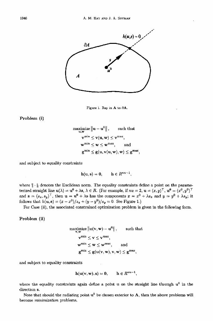
Consider Case (i). Assume that a radiating point u ° has been chosen and that it is interior to the accessible set, A. Consistent with the definition of 0A in (2.8), a point u b on the boundary in the direction s E R nu from u ° is determined by solving the following constrained optimization problem.


s • s

h(u,s) -- 0 .,." s J

P r o b l e m (i)

Figure 1. Ray in A to OA.

maximize I[u - u°II, such that U~W

V rain <~ V(U, W ) ~ V max,

W rain ~__ W ~__ W max, and

gmin <_ g(u, V(U, W), W) < gmax,

h (u , s ) = O, h E R nu-1 ,

and subject to equality constraints

where [[ • I[ denotes the Euclidean norm. The equality constraints define a point on the parame- terized straight line u(A) = u ° + As, A E R. (For example, if n u = 2, u = (x , y)T, u 0 = (x 0, y0)T and s = (sz , sy) T , then u = u ° + As has the components x = x ° + Asx and y = y0 + Asu; it follows that h(u, s) = (x - x ° ) / s z + (y - y ° ) / s u = 0. See Figure 1.)

For Case (ii), the associated constrained optimization problem is given in the following form.

P r o b l e m (ii)

maximize Ilu(v, w) - u°l], such that V~W

V rain ~ V ~ V max,

W rain ~ W __< W max, a n d

groin ~ g(u(v , w), v, w) < gmaX,

and subject to equality constraints

h (u(v , w), s) = O, h E R n~-t ,

where the equality constraints again define a point u on the straight line through u ° in the direction s.

Note that should the radiating point u ° be chosen exterior to A, then the above problems will become m i n i m i z a t i o n problems.

Dete rmina t ion of Nonconvex Workspaces 1047

U bl $

go ~~ $o

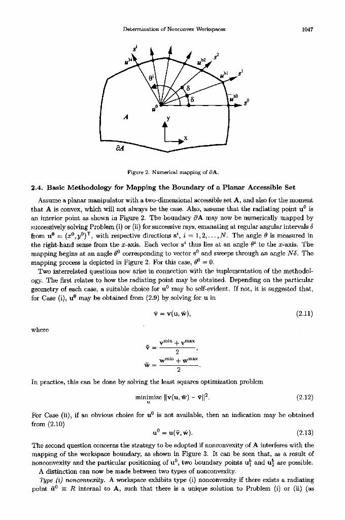
Figure 2. Numer ica l m a p p i n g of OA.

2.4. Bas ic M e t h o d o l o g y for M a p p i n g t h e B o u n d a r y o f a P l a n a r Access ib l e Set

Assume a planar manipulator with a two-dimensional accessible set A, and also for the moment tha t A is convex, which will not always be the case. Also, assume that the radiating point u ° is an interior point as shown in Figure 2. The boundary 0A may now be numerically mapped by successively solving Problem (i) or (ii) for successive rays, emanating at regular angular intervals 5 from u ° = (x °, y0)T, with respective directions s i, i -- 1, 2 , . . . , N. The angle 0 is measured in the right-hand sense from the x-axis. Each vector s i thus lies at an angle 0 i to the x-axis. The mapping begins at an angle 0 ° corresponding to vector s o and sweeps through an angle NS. The mapping process is depicted in Figure 2. For this case, 0 ° = 0.

Two interrelated questions now arise in connection with the implementation of the methodology. The first relates to how the radiating point may be obtained. Depending on the particular geometry of each case, a suitable choice for u ° may be self-evident. If not, it is suggested that , for Case (i), u ° may be obtained from (2.9) by solving for u in

v = v ( u , (2.11)

where

V min "4- V max

2 W rain -}. W max

2

In practice, this can he done by solving the least squares optimization problem

minimize [[v(u, ~¢) - ~,[[2. (2.12) U

For Case (ii), if an obvious choice for u ° is not available, then an indication may be obtained

from (2.10) u ° = u(V, @). (2.13)

The second question concerns the strategy to be adopted if nonconvexity of A interferes with the mapping of the workspace boundary, as shown in Figure 3. It can be seen that , as a result of nonconvexity and the particular positioning of u °, two boundary points u b and u b are possible.

A distinction can now be made between two types of nonconvexity. Type (i) nonconvexity. A workspace exhibits type (i) nonconvexity if there exists a radiating

point fi0 - R internal to A, such that there is a unique solution to Problem (i) or (ii) (as


i / I , I t \ ' ~ ~ \

I ..o ,' / I I \"-', \ I e,._ s ! I t X " "~ I ~ / / I I I. ",,, ~, I " ' ~ / Li ', ", I . ~ : ' , I

b t ~

S I I I ,~ \ / / ' _ ' ','i

Figure 3. Complication if A is nonconvex.

applicable) for all possible search directions s i radiating from fi0. Figure 3 shows an example of type (i) nonconvexity. Type (i) nonconvexity can be dealt with by simply choosing a suitable radiating point and applying the methodology described above.

Type (ii) nonconvexity. A workspace exhibits type (ii) nonconvexity if there exists no radiating point fi0 E R internal to A, such that there is a unique solution to Problem (i) or (ii) (as applicable) for all possible search directions s i radiating from fi0. If this type of nonconvexity occurs, then a modified strategy must be adopted to determine the entire workspace boundary. This strategy is described in the next section.

2.5. S t r a t egy for Type (ii) Nonconvexi ty

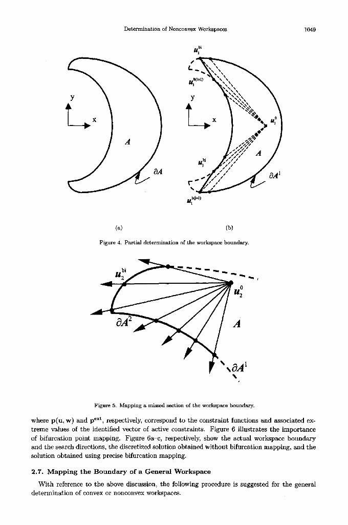
The workspace shown in Figure 4a exhibits type (ii) nonconvexity. For any arbitrarily chosen radiating point u ° within A, only a segment 0A 1 of the workspace boundary can be mapped, as shown in Figure 4b. It can be seen that for this particular positioning of u °, segments of the boundary between points u bi and u b(i+l) and points u bj and u b(j+l) are not determined. It is clear that similar problems will arise for any other positioning of u °.

If any portion of the boundary cannot be mapped from an initial radiating point u °, then the missing segment may be determined by choosing a new radiating point u ° i = 2, 3, and $ , ° * . ,

mapping the missing section 0A i as shown in Figure 5. Note that for the subsegment mapping to be successful, the new radiating point must be chosen so that there is a unique solution to Problem (i) or (ii) (as applicable) for the chosen search directions. A method which works well is to choose the new radiating point so that mapping takes place through an angle of lr/2. Once the missing segment has been mapped, the newly determined points may be merged with the existing boundary points 0A i-1.

2,6. Precise Mapping of the Bifurcat ion Points

Bifurcation points are important features on a workspace boundary since they often correspond to extreme positions of a manipulator, where a subset of constraints (2.2)-(2.4) are active. The number of degrees of freedom of a system will determine the dimension of this subset. Since a discrete method with fixed angular increments is used to map the boundary, it is unlikely that a bifurcation point will coincide exactly with a search ray. For a manipulator with three degrees of freedom, for example, a bifurcation point may occur when any three constraints are active simultaneously. The precise mapping of the bifurcation point corners is done by having identified the subset of active constraints from (2.2)-(2.4) during the boundary mapping procedure, and then solving for

minu,w} lp(u, w) - pext II 2 , (2.14)


< oA' U t~J+D

(a) (b)

Figure 4. Partial determination of the workspace boundary.

t

Figure 5. Mapping a missed section of the workspace boundary.

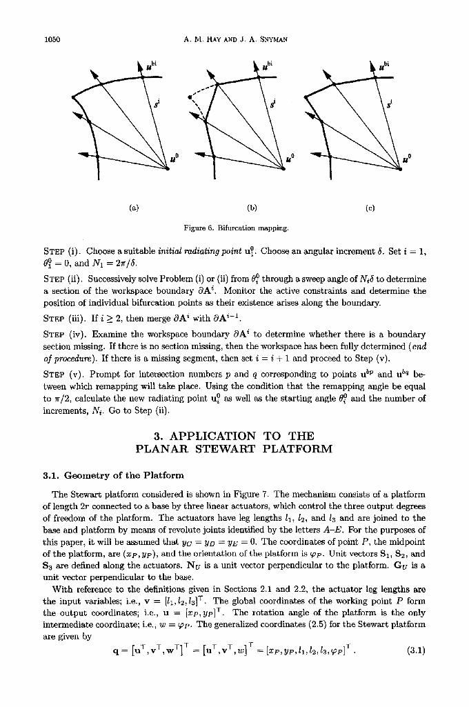
where p(u , w) and peXt, respectively, correspond to the constraint functions and associated ex- t reme values of the identified vector of active constraints. Figure 6 illustrates the importance of bifurcation point mapping. Figure 6a-c, respectively, show the actual workspace boundary and the search directions, the discretized solution obtained without bifurcation mapping, and the solution obtained using precise bifurcation mapping.

2.7. Mapping the Boundary of a General Workspace

With reference to the above discussion, the following procedure is suggested for the general determination of convex or nonconvex workspaces.


~ S t S i~

~ U ° ~ U o U °

(a) (b) (c)

Figure 6. Bifurcation mapping.

STEP (i). Choose a suitable initial radiating point u °. Choose an angular increment 5. Set i = 1, O ° = 0, and N1 = 27v/5.

STEP (ii). Successively solve Problem (i) or (ii) from 0 ° through a sweep angle of Ni5 to determine a section of the workspace boundary 0A i. Monitor the active constraints and determine the position of individual bifurcation points as their existence arises along the boundary.

STEP (iii). If i >_ 2, then merge 0A i with OA i-I .

STEP (iv). Examine the workspace boundary 0A i to determine whether there is a boundary section missing. If there is no section missing, then the workspace has been fully determined (end of procedure). If there is a missing segment, then set i = i + 1 and proceed to Step (v).

STEP (v). Prompt for intersection numbers p and q corresponding to points u bv and u bq between which remapping will take place. Using the condition that the remapping angle be equal to r /2 , calculate the new radiating point u ° as well as the starting angle 0 ° and the number of increments, Ni. Go to Step (ii).

3. A P P L I C A T I O N T O T H E P L A N A R S T E W A R T P L A T F O R M

3.1. G e o m e t r y of the P l a t fo rm

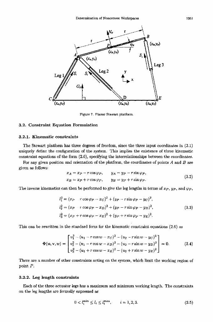
The Stewart platform considered is shown in Figure 7. The mechanism consists of a platform of length 2r connected to a base by three linear actuators, which control the three output degrees of freedom of the platform. The actuators have leg lengths 11, 12, and 13 and are joined to the base and platform by means of revolute joints identified by the letters A - E . For the purposes of this paper, it will be assumed that Ye = YD = YE = 0. The coordinates of point P, the midpoint of the platform, are (xp, yp), and the orientation of the platform is UP- Unit vectors $1, $2, and $3 are defined along the actuators. N u is a unit vector perpendicular to the platform. Gu is a unit vector perpendicular to the base.

With reference to the definitions given in Sections 2.1 and 2.2, the actuator leg lengths are the input variables; i.e., v = [ll, 12,13] r . The global coordinates of the working point P form the output coordinates; i.e., u - [xp, yp]T. The rotation angle of the platform is the only intermediate coordinate; i.e., w = UP. The generalized coordinates (2.5) for the Stewart platform are given by

q = [uT,vT ,wT IT = [liT ,VT ,wIT : [Xp, yp, ll,12,13,~p]T (3.1)

Dete rmina t ion of Nonconvex Workspaces 1051

u r B

x,,y,)

e ' ~ I.~g 2 Y \ ~ L c g 3

C E (x yc) (x yo)

Figure 7. P l ana r Stewart pla t form.

3.2. Cons t r a in t Equat ion Formulat ion

3.2.1. K inema t i c constraints

The Stewart platform has three degrees of freedom, since the three input coordinates in (3.1) uniquely define the configuration of the system. This implies the existence of three kinematic constraint equations of the form (2.6), specifying the interrelationships between the coordinates.

For any given position and orientation of the platform, the coordinates of points A and B are given as follows:

X A = X p -- r C O S ~ p , YA = Y P -- r s i n ~ p ,

x s = xp + r cos ~p, YB = YP + r sin ~p. (3.2)

The inverse kinematics can then be performed to give the leg lengths in terms of xp, yp, and ~p,

l l 2 = ( X p r C O S ~ p -- X C ) 2 + ( y p -- r sin~p - yc) 2,

l 2 ~- ( X p 'r COS ~ p -- X D ) 2 -[- ( y p -- r sin ~p - y D ) 2,

l 2 ~- ( x p + r c o s ( p p - - X E ) 2 + ( y p + r s i n ~ p -- y E ) 2.

(3.3)

This can be rewritten in the standard form for the kinematic constraint equations (2.6) as

Iv 2 - (Ul - r c o s w - x c ) 2 - ( u 2 - r s i n w - yc) 2]

• (u l - rcosw xo) (u2-rsin yo)2l=O. Lv23 ( u l + r c o s w XE) 2 ( u 2 + r s i n w yE)2J

(3.4)

There are a number of other constraints acting on the system, which limit the working region of point P.

3.2.2. Leg l ength constra ints

Each of the three actuator legs has a maximum and minimum working length. The constraints on the leg lengths are formally expressed as

0 < train ~ l i ( /max, i = 1, 2, 3. (3.5)

1052 A . M . HAY AND 3. A. SNYMAN

From (3.4), the explicit expressions for v follow

x/(Ul - r cosw - xc) 2 + (u2 - r s i n w - yc) ~ /

v = v ( u , w ) = v/(Ul--rcosw--XD)2+(U2 r s i n w yD)2/ . /

V/(Ul + rcosw_ x~)2 + (u2 + rsinw y~)2 j

These may be written in the standard form

(3.6)

V min < V < V max, (3 .7)

where v min -~- [l~i",l~i",l~i"] -r and v m~x = [/~x, l~nax, l~n~x]-r. With u and w specified, v =

v(u, w) is given by (3.6).

3.2.3. Mechanical joint constraints

To calculate the angles between the actuators, platform, and base, the following unit vectors are determined:

1 S I = ~ [ X A - - X c , YA--YC] T,

1 82 = 7 - [ X A --XD, YA --yD] q- , (3.8)

~2 1

S3=~3[XB- -XE, yB--yE] T,

NU = [- -s in~p, cosqop] T, (3.9)

= [0, 11 T. (3.10)

Consider the dot product between N u and any leg vector S~, i = 1, 2, 3,

N u . S, = INu] IS~I cos&,

where ~i is the angle between the two vectors. Since Nu and Si are unit vectors,

Nu • Si = cos ~i,

and thus ~ = arccos(Nu. Si), i = 1,2, 3. (3.11)

The direction of rotation is found by examining the sign of the cross-product between the two vectors

positive angle if Nu × Si > 0,

negative angle if Nu x Si < 0, (3.12)

in agreement with the right-hand rule convention. By using (3.11) and (3.12), the angle between the platform normal vector and any actuator can be uniquely determined in the range -Tr < ~i < 7 .

Similarly, for the angles between the base normal vector and the actuators,

¢~ = arccos(Gu • S~), i = 1,2,3. (3.13)

The sign of the angle is once more defined as follows:

positive angle if Gu × Si > 0,

negative angle if Gu x S~ < 0, (3.14)

and -Tr < ~i < ~r.


The actuators are physically connected to the platform at one end and the base at the other by means of revolute joints. The construction of these joints will impose certain limits on the maximum and minimum angles that the leg can attain relative to the platform or base. These constraints are formally expressed as follows:

and

~min _< ~i ~ ~max, i = 1, 2, 3, (3.15)

Cmin < ¢i --< ~max, i = 1, 2, 3. (3.16)

Since the angles ~i and ~i depend on the output and intermediate coordinates, (3.15) and (3.16) may be rewritten in the standard form as

gmin _< g(u, W) _< gmax, (3.17)

where g = [~1, ~2, ~3, ~1, ~2, ~3] T"

3.2.4. Leg i n t e r f e r ence c o n s t r a i n t s

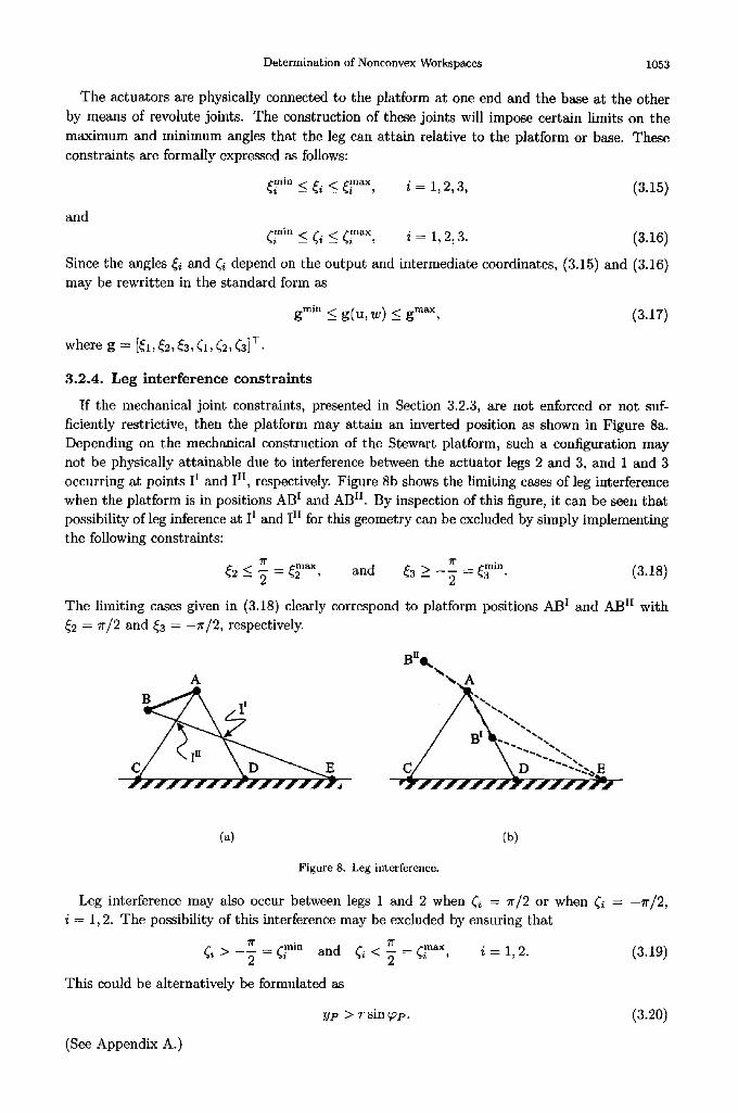
If the mechanical joint constraints, presented in Section 3.2.3, are not enforced or not suf- ficiently restrictive, then the platform may attain an inverted position as shown in Figure 8a. Depending on the mechanical construction of the Stewart platform, such a configuration may not be physically attainable due to interference between the actuator legs 2 and 3, and 1 and 3 occurring at points I I and 1 II, respectively. Figure 8b shows the limiting cases of leg interference when the platform is in positions AB I and ABIk By inspection of this figure, it can be seen that possibility of leg inference at 11 and I iI for this geometry can be excluded by simply implementing the following constraints:

7r = ~ a x , and ~3 > 71" rain ~2_<~ - - ~ = ~ 3 • (3.18)

The limiting cases given in (3.18) clearly correspond to platform positions AB I and AB II with ~2 = 7r/2 and ~3 - - r / 2 , respectively.

A A

~ ""'"'"

(a) (b)

Figure 8. Leg interference.

Leg interference may also occur between legs 1 and 2 when ~ = ~r/2 or when ~i = -I r /2 , i = 1,2. The possibility of this interference may be excluded by ensuring that

7r 71" = ~yin and ~i < ~- : ~na×, i = 1, 2. (3.19) ¢~>-~

This could be alternatively be formulated as

y p > r sin ~Op. (3.20)

(See Appendix A.)


3.2.5. Singularity constraints

The Stewart platform is in a singular configuration when the platform is colinear with leg 3 or when legs 1 and 2 are colinear. This is proved in Appendix A. Such singular positions are often associated with real restriction on motion control of the platform. These singularity constraints may also be formulated in terms of the joint angles. The imposition of the following constraints prevents the platform from assuming the first singular configuration:

71" min 71" = ~nax. (3.21) ~ 3 > - - 2 = ~ 3 , and ~3<

Constraint expression (3.19) or (3.20) prevents the second case occurring. For the given geometry of the Stewart platform, the use of constraints (3.21) makes the use of

the leg interference constraints (3.18) redundant.

3.2.6, I m p l e m e n t a t i o n of angular constraints

In general, when implementing constraints (3.15) to (3.21), care should be taken to ensure that there are no redundant constraints present, as these can cause inaccuracies during the determination of the workspace boundary. As an example of redundant constraints, consider the case where the specification ~min = -1.5 and ~nax = 1.5, i = 1,2,3, is made in (3.15). This means that constraints (3.18) and (3.21) are redundant as ~i can never attain a value of +7r/2.

3.3. Implementat ion of the Method

Equations (3.7), (3.17), (3.4), and (3.6) for the planar Stewart platform correspond to Case (i) of Section 2.3, specified in the general case by expressions (2.2), (2.4), (2.6), and (2.9). The boundary 0A of the accessible set of the planar Stewart platform may therefore be numerically determined by applying the methodology described in Section 2.7, in which optimization Prob- lem (i) is successively solved. For the cases depicted here, boundary mapping was done at regular intervals of 5 = 5 °. Note that there is no explicit restriction (2.3) on w.

The techniques described here have been implemented in an interactive computer code WSPCON. The user specifies the geometry of the platform as well as the limits on the joint angles and leg lengths. The code then automatically maps the workspace boundary including the bifurcation points. Once this is completed, the boundary can be displayed and visually inspected for discontinuities that may indicate nonconvexity. The user then specifies two points on the boundary between which remapping should take place, and the code calculates a new radiating point and start and end angles, and writes a restart file containing this information. When the program is executed again, the new section of boundary is remapped and then merged with the existing boundary. The above procedure can be repeated indefinitely until the entire workspace boundary has been completely mapped.

If any constraint violations occur, the intersection points at which these occur are reported to the user, who can use this information when choosing the section of boundary to be remapped.

The specific constrained optimization method used in solving the optimization problems is the dynamic trajectory method of Snyman [4,5] for unconstrained optimization applied to penalty function formulations [6,7] of the constrained problems. The particular computer code used is LFOPC [6].

4. R E S U L T S F O R T H E P L A N A R S T E W A R T P L A T F O R M

4.1. The Effect of Varying the Actuator Leg Length Limits

As an illustration of the proposed method for determining the workspace, an investigation of the effect of varying leg lengths was carried out on a normalized Stewart platform. The values

Determinat ion of Nonconvex Workspaces

Table 1. Stewart pla t form constants .

1055

"1" XC YC ,~D YD XE YE

1.0 --1.0 0.0 1.0 0.0 2.0 0.0

of the constants defining the geometry of this normalized Stewart platform are given in Table 1 (also refer to Figure 7).

The values for the mechanical limits on the joint motion are chosen as ~min = ~min = - - r / 2 and ~max _ ~max _ lr/2. The effects of (3.15), (3.18), and (3.21) are then included in the following constraints, which are used in determining the workspace:

7~ 7r > < (4.1)

For the platform configurations considered in the rest of this section, constraints (3.16) and (3.19) never become active.

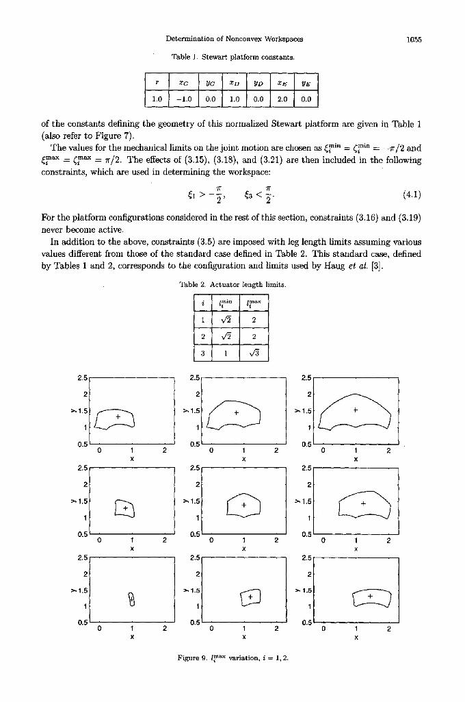
In addition to the above, constraints (3.5) are imposed with leg length limits assuming various values different from those of the standard case defined in Table 2. This standard case, defined by Tables 1 and 2, corresponds to the configuration and limits used by Haug et al. [3].

Table 2. Ac tua to r length limits.

i l~ i" l m~x

1 v~ 2

2 V~ 2

3 1 v/3

2.5

2

>, 1.5

1

0.5

2.5

2

>, 1.5

1

0.5

2.5

2

>- 1.5

1

0.5

0 1 2 X

0 1 2 X

2.5

2

>, 1.5

1

0.5

2.5

2

>, 1.5

1

0.5

2.5

2

>, 1.5

1

0.5

0 1 X

0 1 X

0 1 2 0 1 X X

2.5

2

>,1.5

1

0.5 2

2.5

2

>, 1.5

1

0.5 2

2.5

2

>, 1.5

1

0.5 2

0 1 2 X

0 1 2 X

0 1 2 X

Figure 9. /max variation, i = 1, 2.

1056 A . M . HAY AND J. A. SNYMAN

2.5

2

>, 1.5

1

0.5

2.5

2

>,1.5

1

0.5

2.5

2

>,1.5

1

0.5

2.5

2

>,1.5

1

0.5

2.5

2

>,1.5

1

0.5

2.: F >'1"5 f

0.15 '

2.5

2

>, 1.5

1

0.5

2.5

2

>,1.5

1

0.5 0 1 2 0 1 2 0 1 2

x x x 2.5

2

>,1.5

1

0.5

2.5

2

>', 1.5

1

0.5 0 1 2 0 1 2 0 1 2

x x x 2.5

2

>,1.5

1

0.5 0 1 2 0 1 2

x x

Figure 10. /max variat ion, i --- 1, 3.

2.5

2.5

2

>..1.5

1

0.5

2.5

2

1.5

1

0.5

2

>,1.5

1

0.5

0 1 2 X

0 1 2 0 1 2 0 1 2 X X X

2.5

2

>,1.5

1

0.5

2.5

2

>, 1.5

1

0.5 0 1 2 0 1 2 0 1 2

X X X

!.5 2., =

>, 12

02

Q 0 I 0 I 2 0 I 2

X X X

Figure 11. /rain variat ion, i = 1, 2.


2.5

2

>, 1.5

1

0.5

2.5

2

>, 1.5

1

0.5

2.5

2

>, 1.5

1

0.5

2.4

2.2

2

1.8

1.6

>, 1.4

"it 0"8 t 0.6

0.4 -0.5

2.5

2

>,1.5

1

0.5

2.5

2

>, 1.5

1

0.5' 0 1 2 0 1 2 0 1 2

x x x 2.5 2.5

2

>, 1.5

1

0.5

2

>,1.5

1

0.5 2

2.5

0 1 2 0 1 0 1 2 X X X

2

>, 1.5

1

0.5 2

2.5

2

>, 1.5

1

0.5 0 1 2 0 1 0 1 2

x x x

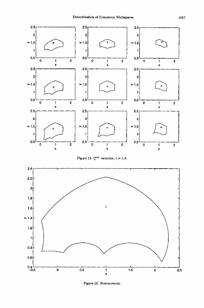
Figure 12. I min variation, i = 1, 3.

I I I I I

I I I I I

0 0.5 1 1.5 2 ' X

2,5

Figure 13. Nonconvexity.

1058 A . M . HAY AND J. A. SNYMAN

The effects of varying the maximum and minimum actuator lengths of legs 1 and 2 on the character and size of the workspace are shown in Figures 9 and 11, respectively. In each of these figures, the central plot shows the workspace of the standard case. The plots to the right of this central case show the workspaces with the appropriate limit of leg I increased by 25% and to the left decreased by 25%. The plots above the central plot show the workspaces with the limit of leg 2 increased by 25% and below decreased by 25%. The midpoint (initial radiating point) of each workspace, as determined using equation (2.11), is indicated by a '+'. Similarly, the effects of varying the limits of legs i and 3 are shown in Figures 10 and 12.

A comparison of the workspace boundary for the standard case, depicted as the central plot in Figures 9 to 12, with the results of [3], shows that equally accurate results are obtained using the optimization approach. Furthermore, the current method is capable of easily determining the workspaces of platforms of arbitrary geometry relative to the standard case. Of particular importance is the ease with which nonconvex workspaces are determined. An example of a nonconvex workspace determined using the method is shown in Figure 13. This nonconvex case differs from the standard case in having all of the maximum leg lengths increased by 25% and the minimum leg lengths of legs 1 and 2 decreased by 25%.

5. C O N C L U S I O N

The optimization approach, previously proposed by Snyman et al. [1], has successfully been extended to the determination of workspaces of planar Stewart platforms of arbitrary geometry. The method, as embodied in a practical interactive computer system, allows for the easy determination of nonconvex workspaces.

Du Plessis [2] has already shown for a specific case that the planar optimization approach can easily be extended to determine a spatial workspace. It is therefore believed that the current planar system can also be refined to determine the workspaces of spatial Stewart platforms of varied designs. Future research will therefore be directed at developing such a general interactive system for the characterization of spatial workspaces.

A P P E N D I X A

S I N G U L A R I T Y A N A L Y S I S O F T H E P L A N A R S T E W A R T P L A T F O R M

Consider the Stewart platform shown in Figure 7 and the vector of coordinates q = [xp, yp , ~p, ll, 12, ls] T. Writing expressions (3.3) in the standard form of the constraint equations, and substituting the specifications for the normalized design given in Table 1, gives

[l~ - ( xp - cos ~Op + 1) 2 - (yp - sin ~op) 2 ]

~ ( q ) = //2 ( xp c o s e c - l ) 2 (yp sin~p)2] = 0 . (A.1)

Ll2s ( x p + c o s ~ o p 2) 2 ( y p + s i n v p ) 2 j

Differentiating (A.1) with respect to time yields

where

- ( x p - cos ~op + 1)

,I,q = [ - ( x p cos~ov - 1)

J - ( x v + c o s ~ p - 2)

= [A I B].

(I)q¢t = 0, (A.2)

--(yp -- sin ~op)

--(yp -- sin ~op)

-- (yp -- sin ~p)

- - s i n ~ p ( X p - - c o s ~ p + l )

+ cos ~ p ( y p - - s i n ( t ip)

- - s i n ~ p ( x p - - c o s ~ p -- 1) + COS ~ p ( y p - - s i n ~op)

s i n ~ p ( x p - c o s ~ p - 2)

-~- c o s ~ p ( y p - - s i n ( t ip)

10:] 0 12 (A.3)

0 0 13


Using the above partitioning, (A.2) can now be separated as follows:

A yp = - B i2 (A.4) i3

In accordance with Gosselin and Angeles [10], a distinction can be made between three different types of singularities.

TYPE I. Singularities occur when det(B) = 0. Mathematically, this condition leads to 11 = 0 or 12 = 0 or 13 = 0. However, since the actuators have a finite range of motion, this type of singularity will occur when one of the actuator legs reaches its minimum or maximum length [11]

li --/rain or li =/.max~ , i = 1,2,3. (A.5)

The corresponding configurations occur on the boundary of the manipulator workspace or on internal boundaries between regions of the workspace. On these boundaries, the platform can be controlled, but cannot move in all possible directions.

TYPE II. Singularities occur when det(A) = 0. From expression (A.3), the determinant of A is

det(A) = 2 sin 2 ~p - y~ cos (pp - - X p sin 2 ~ p --[-- x V y p sin ~p

--k y p sin ~p cos ~pp -- 2 y v sin ~p (A.6)

= (sin ~p - yp)(2 sin ~p - x p sin ~ p -[- y p cos ~p).

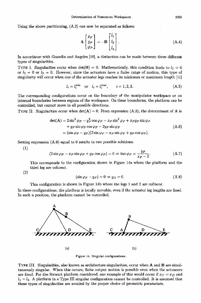
Setting expression (A.6) equal to 0 results in two possible solutions.

(1) Y ~P (h.7) (2 sin ~ p - x p sin (pp + y p cos ~p) = 0 =~ tan (pp = x p - 2"

This corresponds to the configuration shown in Figure 14a where the platform and the third leg are colinear.

(2) (sin ~ v - ye ) = 0 ~ YA = 0. ( A . 8 )

This configuration is shown in Figure 14b where the legs 1 and 2 are colinear.

In these configurations, the platform is locally movable, even if the actuator leg lengths are fixed. In such a position, the platform cannot be controlled.

A

(a) (b)

Figure 14. Singular configurations.

TYPE III. Singularities, also known as architecture singularities, occur when A and B are simultaneously singular. When this occurs, finite output motion is possible even when the actuators are fixed. For the Stewart platform considered, one example of this would occur if x c = X D and 11 = 12. A platform in a Type III singular configuration cannot be controlled. It is assumed that these types of singularities are avoided by the proper choice of geometric parameters.


Haug et al. [12] determine that the same planar Stewart platform is in a singular position when the platform and any one of the actuator legs are colinear, and the same leg is at a minimum or maximum length. The apparent additional singularities can be accounted for by the fact that Haug et al. introduce new input coordinates to ensure that the leg length constraints are automatically satisfied. Their singularities therefore correspond to Type I singularities [13]. Incidentally, in the optimization approach used in this study, the use of leg length constraints during workspace determination ensures that the leg length constraints are never violated.

Although the preceding analysis was performed on a specific normalized geometry, it is evident that the results should hold true for any planar Stewart platform that is configured as shown in Figure 7 with Y c = YD = YE ~ - O.

R E F E R E N C E S

1. J.A. Snyman, L.J. du Plessis and J. Duffy, An optimization approach to the determination of the boundaries of manipulator workspaces, Technical Report, Department of Mechanical Engineering, University of Pretoria; ASME J. Mech. Des., (1998).

2. L.J. du Plessis, An optimization approach to the determination of manipulator workspaces, Master of Engi- neering Thesis, Department of Mechanical Engineering, University of Pretoria, (1999).

3. E.J. Haug, C.M. Luh, F.A. Adkins and J.Y. Wang, Numerical algorithms for mapping boundaries of manipulator workspaces, IUTAM Fifth Summer School on Mechanics, Aalborg, Denmark: Concurrent Engineering Tools for Dynamic Analysis and Optimization, (1994).

4. J.A. Snyman, A new and dynamic method for unconstrained minimization, Appl. Math. Modeling 6, 449-462, (1982).

5. J.A. Snyman, An improved version of the original leap-frog method for unconstrained minimization, Appl. Math. Modeling 7, 216-218, (1983).

6. J.A. Snyman, The LFOPC leap-frog algorithm for constrained optimization, Technical Report, Department of Mechanical Engineering, University of Pretoria, (1998); Computers Math. Applic., (this issue).

7. J.A. Snyman, W.J. Roux and N. Stander, A dynamic penalty function method for the solution of structural optimization problems, Appl. Math. Modeling 6, 453-460, (1994).

8. J.-P. Merlet, Parallel manipulators: State of the art and perspectives, Advanced Robotics 8 (6), 589-596, (1994).

9. E.F. Fichter and E.D. McDowell, A novel design for a robot arm, Proceedings of the ASME International Computer Technology Conference, San Francisco, 250-256, (1980).

10. C.M. Gosselin and J. Angeles, Singularity analysis of closed-loop kinematic chains, IEEE Transactions on Robotics and Automation 6 (3), 281-290, (1990).

11. J. Sefrioui and C.M. Gosselin, Singularity analysis and representation of planar parallel manipulators, Robotics and Autonomous Systems 10, 209-224, (1992).

12. E.J. Haug, J.Y. Wang and J.K. Wu, Dextrous workspaces of manipulators, Part I: Analytical criteria, Tech- nical Report R-125, Center for Simulation and Design Optimization of Mechanical Systems, University of Iowa, (1991); revised (1994).

13. E.J. Haug, F.A. Adkins, C. Qiu and J. Yen, Analysis of barriers to control of manipulators within accessible output sets, Technical Report R-174, Center for Computer-Aided Design, University of Iowa (1994).

The Determination of Nonconvex Workspaces of Generally ...

Documents

Transcript of The Determination of Nonconvex Workspaces of Generally ...