Seediscussions,stats,andauthorprofilesforthispublicationat:https://www.researchgate.net/publication/236962646

RandomPerturbationofProjectedVariableMetricMethodforLinearConstraintsNonconvexNonsmoothOptimization

ArticleinInternationalJournalofAppliedMathematicsandComputerScience·June2011

DOI:10.2478/v10006-011-0024-z·Source:DBLP

CITATIONS

4

READS

26

3authors:

AbdelkrimElMouatasim

UniversityIbnZohr-Agadir

27PUBLICATIONS66CITATIONS

SEEPROFILE

EllaiaRachid

MohammadiaSchoolofEngineers

84PUBLICATIONS218CITATIONS

SEEPROFILE

EduardoCursi

InstitutNationaldesSciencesAppliquéesde…

165PUBLICATIONS544CITATIONS

SEEPROFILE

AllcontentfollowingthispagewasuploadedbyEduardoCursion18March2014.

Theuserhasrequestedenhancementofthedownloadedfile.Allin-textreferencesunderlinedinblue

arelinkedtopublicationsonResearchGate,lettingyouaccessandreadthemimmediately.

Int. J. Appl. Math. Comput. Sci., 2011, Vol. 21, No. 2, 317–329DOI: 10.2478/v10006-011-0024-z

RANDOM PERTURBATION OF THE PROJECTED VARIABLE METRICMETHOD FOR NONSMOOTH NONCONVEX OPTIMIZATION

PROBLEMS WITH LINEAR CONSTRAINTS

ABDELKRIM EL MOUATASIM ∗,∗∗, RACHID ELLAIA ∗∗, EDUARDO SOUZA DE CURSI ∗∗∗

∗ Department of Mathematics, Faculty of ScienceJazan University, P.B. 2097, Jazan, Saudi Arabiae-mail: aelmouatasim@jazanu.edu.sa

∗∗Laboratory of Study and Research in Applied Mathematics, Mohammadia School of EngineersMohammed V Agdal University, Ab Ibn sina, BP 765, Agdal, Rabat, Morocco

e-mail:ellaia@emi.ac.ma

∗∗∗National Institute for Applied Sciences, RouenAvenue de l’Universite BP 8, Saint-Etienne du Rouvray, France

e-mail: souza@insa-rouen.fr

We present a random perturbation of the projected variable metric method for solving linearly constrained nonsmooth (i.e.,nondifferentiable) nonconvex optimization problems, and we establish the convergence to a global minimum for a locallyLipschitz continuous objective function which may be nondifferentiable on a countable set of points. Numerical resultsshow the effectiveness of the proposed approach.

Keywords: global optimization, linear constraints, variable metric method, stochastic perturbation, nonsmooth optimiza-tion.

1. Introduction

Continuous nonconvex nonsmooth optimization prob-lems involving linear restrictions arise in practical situ-ations stemming from many fields such as optimal con-trol (Kryazhimskii, 2001; Malanowski, 2004; Makelaand Neittaanmaki, 1992), integer nonlinear programmingproblems (Kowalczuk, 2006; Zhang, 2009), minimax es-timation (El Mouatasim and Al-Hossain, 2009; Petersen,2006), and the clustering problem (Bagirov and Year-wood, 2006). A typical situation is the determination ofa column vector x� ∈ E = R

n such that

x� = arg minS

f , S ={

x ∈ E | Ax ≤ b}, (1)

where the function f : E −→ R does not satisfy convex-ity assumptions and may be nondifferentiable on a finiteor countable subset of E—this is the case when, for in-stance, f is not assumed to be convex differentiable butonly locally Lipschitz continuous. A is an m× n matrix,b is an m × 1 matrix and S is assumed to be bounded:

there are two vectors � ∈ E and u ∈ E such that

S ⊂ [�, u] ={

x ∈ E | � ≤ x ≤ u}. (2)

The numerical solution to the model problem (1)is usually sought with descent methods, which start atan initial guess x0 and generate a sequence of points{ xk }k ≥ 0 ⊂ E : at each iteration number k ≥ 0, both adescent direction dk ∈ E and a step ωk ∈ R (ωk ≥ 0) aredetermined in order to define

x0 ∈ S given, ∀ k ≥ 0 : xk+1 = xk + ωkdk. (3)

The descent direction is often determined by using the in-formation furnished by the previous points xk, xk−1, . . . ,x0. For instance, the classical steepest descent uses theinformation provided by the gradient gk = ∇f (xk) of theobjective function at the point xk and sets dk = −gk.In variable metric methods, the determination of the de-scent direction usually involves the information providedby xk and xk−1. For instance, the Davidon–Fletcher–Powell approach (Davidon, 1991) uses dk = −Bkgk,

Unauthenticated | 194.254.13.61Download Date | 3/18/14 1:06 PM

318 A. El Mouatasim et al.

where { Bk }k ≥ 0 is a sequence of n × n matrices suchthat B0 = I (the n× n identity matrix) and

Bk = Bk−1 +(xk − xk−1) (xk − xk−1)

t

(xk − xk−1)t (gk − gk−1)

− Bk−1 (gk − gk−1) (gk − gk−1)t Bk−1

(gk − gk−1)tBk−1(gk − gk−1).

In the sequel, we consider descent vectors corre-sponding to a general variable metric method given by afunction uk : E × E → E:

dk = uk (xk,xk−1) . (4)

The determination of the step ωk ≥ 0 often involves a onedimensional search and a previously established maximalstep ω. For instance, the optimal step is

ωk = arg minW

f (xk + ωdk) ,

W ={ω | xk + ωdk ∈ S, 0 ≤ ω ≤ ω

}.

Consequently, the step is given by a functionω : E×E →E such that

ωk = ω (xk, dk) , 0 ≤ ω (xk, dk) ≤ ω. (5)

When solving the general problem stated in Eqn. (1),there are three essential difficulties with using the itera-tions defined in Eqns. (3)–(5). First, the determinationof the descent direction dk usually involves the determi-nation of the gradient gk = ∇f (xk) of the objectivefunction at the point xk , which is not defined everywhere,since f is not anywhere differentiable. Second, the itera-tions must ensure that { xk}k ≥ 0 ⊂ S, i.e., that the pointsgenerated remain feasible. Third, under the lack of boththe convexity and the differentiability of f , the conver-gence to a global minimum x� is not ensured.

The first of these difficulties is usually settled in con-vex optimization by using subgradient information: when-ever a subgradient may be defined, it carries informationabout the growth of the objective function. Variants of thesubgradient approach are bundle or level methods. Boththese variants try to obtain more information about the be-havior of f by gathering the information provided by thesubgradients obtained in the preceding iterations. This in-formation is contained in the set of affine functions asso-ciated with these subgradients and the bundle which fur-nishes a local affine approximation of f . In convex sit-uations, the descent direction can be determined by us-ing the single information furnished by the bundle, whichleads to cutting-plane methods (Kelley, 1960), or by solv-ing a quadratic direction finding problem (Makela andNeittaanmaki, 1992). The convergence of subgradient orbundle methods may be established for convex situations

(Hiriart-Urruty and Lemarechal, 1993). In the case of bun-dle methods with a limited number of stored subgradients,the convergence can be guaranteed by using a subgradientaggregation strategy (Kiwiel, 1985), which accumulatesinformation from the previous iterations (Lemarechalet al., 1981; Schramm and Zowe, 1992). For a nonconvexf , subgradients are not in general anywhere defined. Al-ternative methods of construction of a local affine approx-imation of f must be supplied in order to get the adequateinformation about the local growth of f . For instance,we may introduce other generalized gradient definitions,such as Clarke’s generalized gradients, or simply the gra-dient of an affine lower estimate. The standard gradientor an ε-subgradient may be used, whenever one of thesequantities is defined (see Section 2).

The second difficulty is usually settled by projec-tion, whenever an operator of projection onto S is avail-able. This is just the case of the problem (1). Thereare usually two possibilities for the introduction of theprojection operator according to its use in order to deter-mine feasible points or feasible directions. For instance,one approach consists in introducing a projection operatorprojS : E → S and determining the descent directionand the step as follows:

tk+1 = xk + ηkvk,

dk = projS(tk+1) − xk,

ωk = 1,

where vk and ηk are a descent direction and a step, re-spectively. Both vk and ηk are generated by a standardmethod which does not take the restrictions, i.e., S, intoaccount (such as, for instance, the standard gradient de-scent method). The point tk+1 is called a trial point andwe have xk+1 = projS(tk+1). In this approach, the pro-jection operator is used to get a feasible point xk+1 fromthe eventually infeasible trial point tk+1. For instance,this is the case of bundle or level methods involving prox-imal projection.

Another approach consists in using

dk = projT (S,xk)(vk),

0 ≤ ωk ≤ ωmax = max{ω | A(xk + ωdk) ≤ b

},

where T (S, xk) is the tangent cone to S at xk,projT (S,xk) : E → T (S, xk) is the orthogonal projec-tion onto T (S, xk), vk is generated by a standard methodwhich does not take the restrictions into account. In thismethod, the descent direction dk is projected to get a de-scent direction containing feasible points. This is the caseof the popular projected subgradient method (Correa andLemarechal, 1993; Kiwiel, 1985; Larsson et al., 1996),which is used in this work. For linearly constrainedproblems, an interesting variant is offered by ε-active set

Unauthenticated | 194.254.13.61Download Date | 3/18/14 1:06 PM

Random perturbation of the projected variable metric method for nonsmooth nonconvex optimization. . . 319

methods, which have the reputation of avoiding zigzag(Panier, 1987), and generalized pattern search methods(Bogani et al., 2009).

The third difficulty yields that, as previously ob-served, a sophisticated approach may become necessaryin order to get information about the local growth ofthe objective function. Moreover, the convergence ofthe sequence { xk }k ≥ 0 to a point of global minimumx� is not ensured under the lack of convexity: we in-troduce a controlled random search based on stochasticperturbations of the descent method (3) (Dorea, 1990;El Mouatasim et al., 2006; Pogu and Souza de Cursi,1994; Souza de Cursi et al., 2003). In this approach,{ xk }k ≥ 0, { dk }k ≥ 0, { ωk }k ≥ 0 become random vec-tors { Xk }k ≥ 0, { Dk }k ≥ 0 , { Ωk }k ≥ 0 and the de-scent iterations are modified as follows:

X0 = x0 ∈ S given, (6)

∀ k ≥ 0: Xk+1 = Xk + ΩkDk + Pk, (7)

Dk = uk (Xk,Xk−1) , (8)

Ωk = ω (Xk, Dk) , 0 ≤ ω (Xk, Dk) ≤ ω, (9)

where Pk is a suitable random vector the stochastic per-turbation. A convenient choice of {Pk}k ≥ 0 ensures theconvergence of this sequence to x� (see Section 4).

In the sequel, we consider the projected variable met-ric method applied to the problem (1). After introducingthe notation (Section 2), the method is introduced in Sec-tion 3. In Section 4, we introduce the stochastic perturba-tions and we establish the convergence results. The resultsof numerical experiments are given in Section 5.

2. Notation and assumptions

As previously introduced, E = Rn is the standard

n-dimensional Euclidean space formed by n-tuples of realnumbers. The elements of E are denoted using bold low-ercase: for instance, x = ( x1, . . . , xn )t, where thesymbol t denotes the transpose. The usual inner prod-uct in E is denoted by (·, ·) , and the associated Euclideannorm is denoted by ‖ · ‖:

(x, y) = xty =n∑

i=1

xi yi ,

‖x‖ =√

(x, x) =√

xtx.

We denote by ‖ · ‖ the matrix norm induced by thisnorm: if C = (Cij), (1 ≤ i ≤ m, 1 ≤ j ≤ n) is a m×nmatrix (0 < m < n) formed by real numbers, we have‖ Cx ‖ ≤ ‖ C ‖ ‖ x ‖ and

‖ C‖ = sup{‖Cx ‖ : ‖ x ‖ = 1

}.

Let us introduce vectors b = (b1, b2, . . . , bm)t ∈R

m, � = (�1, �2, . . . , �n)t ∈ E, u = (u1, u2, . . . , un)t ∈E and a real m × n matrix A = (Aij) (1 ≤ i ≤ m,1 ≤ j ≤ n). We have A ≡ [A1 A2 . . . Am]t ,

Ai = (Ai1, Ai2, . . . , Ain)t ∈ E , i = 1, . . . ,m.

No loss of generality is implied if we assume that

‖ Ai‖ = 1, i = 1, . . . ,m. (10)

The feasible set is S ={

x ∈ E | Ax ≤ b}

, i.e.,

S ={x ∈ E |

n∑j=1

Aijxj − bi ≤ 0, i = 1, 2, . . . ,m}

.

(11)We assume that

S ⊂ [�,u] ={

x ∈ E | �i ≤ xi ≤ ui , 1 ≤ i ≤ n}

.

(12)Hence S is a bounded closed convex subset of E. For anyx1,x2 ∈ S, and every θ ∈ (0, 1) we have

A (θx1 + (1 − θ)x2) = θAx1 + (1 − θ)Ax2

≤ θb + (1 − θ)b = b.

On the other hand,

‖x1 − x2‖ ≤ L12 = ‖� − u‖ ,‖x1‖ ≤ L = max {‖�‖ , ‖u‖} .

(13)

We recall that the tangent cone to S at a point x isthe set T (S,x) ⊂ E defined by

d ∈ T (S,x) ⇐⇒ ∃{(hn , λn)}n>0 ⊂ E × R∗+,

λn → 0 , hn → d, x + λnhn ∈ S.

This property is exploited in the sequel.Practical determination of T (S,x) is performed by

using active constraints. Let x ∈ S. The i-th constraintis active at x if and only if At

ix − bi = 0 . The setof active constraints Iac(x) and the number of active con-straints mac(x) at x are, respectively,

Iac(x) ={i : 1 ≤ i ≤ m, At

ix − bi = 0}

,

mac(x) = card (Iac(x)) .

We set AN (x) = [Ai : i ∈ Iac(x) ]t. AN (x) is themac(x) × n submatrix of A formed by the lines corre-sponding to the active constraints at the point x. In the par-ticular situation where Iac(x) = ∅, we have mac(x) = 0,T (S,x) = E and we take AN (x) = 0 = ( 0, . . . , 0 ).In the sequel, we shall use the following properties ofT (S,x).

Unauthenticated | 194.254.13.61Download Date | 3/18/14 1:06 PM

320 A. El Mouatasim et al.

Proposition 1. Let x ∈ S. We have

∀ x ∈ S : T (S,x) ={d ∈ E|At

id ≤ 0, i ∈ Iac(x)}

={d ∈ E|AN (x)d ≤ 0

}.

Moreover

∀ x ∈ S : S ⊂ { x } + T (S,x),

and the orthogonal projection from E onto T (s,x),proj (x, ·) : E → T (S,x) satisfies

∀x ∈ S : S ⊂ { x} + Im (proj (x, ·)) , (14)

∀ x ∈ S : ‖proj (x,w)‖ ≤ ‖w‖ , ∀w ∈ E. (15)

Proof. The result is immediate formac(x) = 0 (Iac(x) =∅), since T (S,x) = E, projT (S,x) ( x, w) = w.

Assume that mac(x) > 0 and let bN (x) =[bi : i ∈ Iac(x) ]t . Analogously to AN (x), bN (x) isformed by the lines of b corresponding to the indexes inIac(x).

We denote by Icac(x) the complement of Iac(x),

Icac(x) =

{i : 1 ≤ i ≤ m, At

ix − bi < 0}.

Let

η (x) = min{bi − At

ix : i ∈ Icac(x)

}> 0.

We assume that d ∈ T (S,x) and wish to show thatAN (x)d ≤ 0. For any sequence {(hn , λn)}n>0 ⊂E × R

∗+ such that λn → 0 and hn → d, we have

λnAhn → 0. Thus, there exists an index n0 such that

n ≥ n0 =⇒ ‖λnAhn‖ < η (x)

=⇒ Ati (x+λnhn) − bi ≤ 0, ∀i ∈ Ic

ac(x).

In addition,x + λnhn ∈ S =⇒

AN (x)hn =AN (x) ( x + λnhn) − bN

λn≤ 0.

Passing to the limit in this inequality, we obtain the claimAN (x)d ≤ 0.

Now we assume that AN (x)d ≤ 0 and wish to showthat d ∈ T (S,x). Let λn = 1/n and hn = d. We have

n ≥ ‖ Ad ‖η (x)

=⇒

Ati ( x+λnhn) − bi ≤ 0, ∀ i ∈ Ic

ac(x).

In addition,

AN (x) ( x + λnhn) − bN = AN (x)d ≤ 0.

Thus, x + λnhn ∈ S and we obtain the claim

d ∈ T (S,x).

In this way, the first assertion of the proposition isestablished. For the second one, let y ∈ S and d = y−x.Then λn = 1/n > 0, hn = d and x + λnhn = (1 −1/n)x + (1/n)y ∈ S. Thus, d ∈ T (S,x) and we have

S − { x } ={

d = y − x | y ∈ S}⊂ T (S,x).

Hence,S ⊂ { x } + T (S,x) .

Since T (S,x) = Im (proj (x, ·)), we have S ⊂ {x} +Im (proj (x, ·)). The inequality ‖proj (x,w)‖ ≤ ‖w‖results from the standard properties of orthogonal projec-tions. �

For a given element v ∈ E, we have proj (x,v) =ΠT (x,v)v, where ΠT (x,v) is an n × n matrix, deter-mined as follows. Let

I+(x,v) ={i ∈ Iac(x) : At

iv > 0},

m+(x,v) = card (I+(x)) .

If I+(x,v) = ∅, we set ΠT ( x,v) = Id, the n × nidentity matrix. If I+(x,v) �= ∅, we set A+(x,v) =[Ai : i ∈ I+(x,v) ]t. There is no loss of generality inassuming that

rank (A+(x,v)) = m+(x,v) . (16)

Otherwise, we extract from A+(x,v) a maximal ranksubmatrix and the associated lines. Then ΠT (x,v) isthe matrix associated with the operator projx(v) = v −Π+(x,v)v, where Π+(x,v) corresponds to the orthog-onal projection onto the subspace spanned by the vectorsforming A+ :

N+(x) = span[At

i : i ∈ I+(x)]

={d ∈ E

∣∣ d =∑

i∈I+(x)

λiAi

}.

We have (Luenberger, 1973)

ΠT (x,v) = Id − Π+(x,v) ,

Π+(x,v) = At+

(A+At

+

)−1A+ .

We shall also use the following properties of the step.

Proposition 2. Let x ∈ S and d ∈ T (S,x). Themaximal allowable step in the direction d at the pointx ∈ S is

ωmax (x, d) = max{ω | A(x + ωd) ≤ b

}.

Unauthenticated | 194.254.13.61Download Date | 3/18/14 1:06 PM

Random perturbation of the projected variable metric method for nonsmooth nonconvex optimization. . . 321

We have

∀ x ∈ S and d ∈ T (S,x) : ωmax (x, d) > 0.

Moreover, for any x ∈ S there is an ε > 0 such that

d ∈ T (S,y), ∀y ∈ x +Bε

andmin

y∈x+Bε

ωmax (y, d) > 0,

and for any d ∈T (S,x) there is an ε > 0 such that

(d +Bε) ∩ T (S,x) �= ∅and

mint ∈ (d+ Bε) ∩T (S,x)

ωmax (x, t) > 0,

where Bε = {u ∈ E |‖u‖ ≤ ε} is the ball with center 0and radius ε.

Proof. We have

ωmax (x, d) = min1≤i≤m

{ωi} ,

ωi =

⎧⎪⎪⎪⎪⎨⎪⎪⎪⎪⎩

bi −n∑

j=1

Aijxj

n∑j=1

Aijdj

ifn∑

j=1

Aijdj > 0,

+ ∞ otherwise

and

bi −n∑

j=1

Aijxj > 0.

Thus, ωmax (x, d) > 0.Let d ∈ T (S,x). Assume that for each n > 0 there

exists yn such that ‖yn‖ ≤ 1/n and

d /∈T (S,xn),xn = x + yn.

Thus, there exists i(n) such that

Ati(n)xn − bi(n) = 0, At

i(n)d > 0.

Letr (k) = max {i(n) : n ≥ k} ,

n (k) = min {n : n ≥ k and i(n) = r(k) } .

By construction, { r (k)}k>0 ⊂ {1, . . . , m} is de-creasing and bounded from below. Thus, r (k) → r fork → ∞. Since {1, . . . , m} is discrete, there is a k0 suchthat k ≥ k0 =⇒ r (k) = r. We have

k ≥ k0 =⇒ Atrxn(k) − br = 0 and At

rd > 0.

Passing to the limit as k → ∞, we have, since yn → 0,

Atrx − br = 0 and At

rd > 0.

Thus, d /∈ T (S,x) and we have a contradiction. Hence,there is an n > 0 such that

‖y‖ ≤ 1n

=⇒ d ∈T (S,x + y).

Let d ∈ T (S,x). Assume that

∀ε > 0 : miny∈x+Bε

ωmax (x, d) = 0.

Then for any n > 0 there is a yn such that

‖ yn‖ ≤ 1n, ωmax (xn,d) ≤ 1

n, xn = x + yn.

Thus, there exists i(n) such that

bi(n) − Ati(n)xn

Ati(n)d

≤ 1n

,

bi(n) − Ati(n)xn > 0 , At

i(n)d > 0.

Let

r (k) = max{i(n) : n ≥ k

},

n (k) = min{n : n ≥ k and i(n) = r(k)

}.

Analogously to the above argument, there exists k0 suchthat k ≥ k0 =⇒ r (k) = r, and we have

k ≥ k0 =⇒ br − Atrxn(k) ≤ 1

nAt

rd,

br − Atrxn(k) > 0, At

rd > 0.

By taking the limit for k → ∞, we have, since yn → 0,

br − Atrx ≤ 0, br − At

rx > 0, Atrd > 0.

and we obtain a contradiction.Let d ∈ T (S,x). We have (d + Bε) ∩ T (S,x) �=

∅ for any ε > 0, since d ∈ (d + Bε) ∩ T (S,x). Assumethat

∀ ε > 0 : mint ∈ (d + Bε) ∩ T (S,x)

ωmax (x, t) = 0.

Then for any n > 0 there is a tn such that

‖ tn‖ ≤ 1n, ωmax (x, dn) ≤ 1

n, dn = d + tn.

Thus, there exists i(n) such that

bi(n) − Ati(n)x

Ati(n)dn

≤ 1n

,

bi(n) − Ati(n)x > 0, At

i(n)dn> 0.

Let

r (k) = max{i(n) : n ≥ k

},

Unauthenticated | 194.254.13.61Download Date | 3/18/14 1:06 PM

322 A. El Mouatasim et al.

n (k) = min { n : n ≥ k and i(n) = r(k) } .

Analogously to the demonstration above, there exists k0

such that k ≥ k0 =⇒ r (k) = r, and we have

k ≥ k0 =⇒ br − Atrx ≤ 1

nAt

rdn(k) ,

br − Atrx > 0, At

rdn(k)> 0.

Passing to the limit as k → ∞, we have, since tn → 0,

br − Atrx ≤ 0, br − At

rx > 0, Atrd ≥ 0,

and we get a contradiction. �As mentioned above, the objective function f :

E −→ R is assumed to be locally Lipschitz continuous:it may have a countable number of points of nondifferen-tiability. Moreover, f is not assumed to be convex. SinceS is closed and bounded, and f is continuous, there existsθ∗ ∈ R such that

minS

f = θ∗ ∈ R. (17)

Let θ > θ∗. We denote by Sθ the set

Sθ ={

x ∈ S | θ∗ ≤ f(x) < θ}.

In the sequel, we consider

θmax = max { θ | Sθ ∩ S �= ∅} .

The continuity of f implies that

θ∗ < θ < θmax

=⇒ meas (Sθ) > 0 and meas (S − Sθ) > 0 . (18)

3. Projected variable metric method

The class of variable metric methods was originally intro-duced by Davidon (1991) along with Fletcher and Powell(1963) in an attempt to get information about the curva-ture of the objective function by using a variable symmet-ric positive definite n× n matrix Bk and

vk = arg min{

gtkv : vtBkv = 1

}.

The properties of Bk show that vtBkv is a norm:vk is the element of the generalized circle Ck ={v : vtBkv = 1} having the most negative Euclideanprojection on the direction of gk. This method is knownas the DFP descent method. Several variants may befound in the literature, such as the BFGS descent method(Broyden, 1970; Fletcher, 1970; Goldfarb, 1970; Shanno,1970) and other quasi-Newton methods.

As mentioned above, the determination of the de-scent direction vk usually involves the gradient gk =∇f (xk) of the objective function at the point xk, whichmay be not defined due to the lack of regularity of f (Peng

and Heying, 2009; Uryasev, 1991). In addition, the objec-tive function is not assumed to be convex and its subdif-ferential may be empty.

These considerations provide a simple way to extenddescent methods based on the gradient to the nonsmoothsituation under consideration: if the objective function fis differentiable at xk, the descent direction dk is deter-mined by using the standard gradient gk = ∇f (xk). Oth-erwise, we consider a local affine underestimate or over-estimate γk (y) = ( pk, y − xk) + f(xk), and we usegk = pk for the determination of the descent direction(for more, see El Mouatasim et al., 2006). In practice, γk

may be numerically approximated by using the values off or ∇f at points close to xk. This approach is particu-larly suitable for the situation under consideration, sincef is differentiable almost everywhere (i.e., except for aset having zero Lebesgue measure (Makela and Neittaan-maki, 1992)).

4. Stochastic perturbation

As previously observed, the lack of convexity yields thatthe convergence to a global minimum cannot be ensured.In order to solve this difficulty, the original sequencegenerated by the iterations, {xk}k ≥ 0, is replaced bya sequence of random variables {Xk}k ≥ 0 defined byEqns. (7)–(9).

In previous works, an analogous strategy hasbeen applied to smooth unconstrained (Pogu andSouza de Cursi, 1994) or smooth constrained situations(El Mouatasim et al., 2006; Souza de Cursi et al., 2003),involving iterations of the form Xk+1 = Qk(Xk) + Pk,which corresponds to a Markov chain with the memorylength equal to one, since only the last result intervenes. Inthe situation under consideration, the iterate number k+1depends on the whole preceding history (see Step 7 of thealgorithm). This corresponds to a particular kind of theMarkov chain, where the variable is not Xk but the wholehistory X≤ k. Thus, the preceding theoretical results donot apply immediately and must be modified in order tomatch the situation under consideration.

In this section, we establish the convergence resultsconcerning the general iterations given by

∀ k ≥ 1 : Xk+1 = Xk + hk (X≤k) + Pk, (19)

where X0 = x0 ∈ S and X1 = x1 ∈ S are given. It isassumed that hk (·) is bounded on Sk+1, i.e., there existsa real number Λ ≥ 0 such that

∀x≤k ∈ Sk+1 : ‖hk (x≤k)‖ ≤ Λ. (20)

The algorithm corresponds to

∀ k ≥ 1 : hk (x≤k) = ωkproj (xk, sk (x≤k)) .

Unauthenticated | 194.254.13.61Download Date | 3/18/14 1:06 PM

Random perturbation of the projected variable metric method for nonsmooth nonconvex optimization. . . 323

Equations (5) and (15) show that this definitionsatisfies the inequality (20). Nevertheless, the mathe-matical results apply to a larger context: for instance,hk ( x≤ k) = 0 also satisfies (20); in this case, thealgorithm becomes a purely stochastic search. Analo-gously, these assumptions take into account situationswhere hk ( x≤ k) is not always a descent direction, butremains bounded. If hk ( x≤ k) is not a descent direction,the stochastic perturbation drives the process and yields adescent at each iteration. Here hk ( x≤ k) is expected todrive the iterations in the neighbourhood of a minimum, inorder to accelerate the convergence compared with a purerandom search.

The proof of the results follows the lines ofEl Mouatasim et al. (2006), Pogu and Souza de Cursi(1994) as well as Souza de Cursi et al. (2003). It mustbe noticed that smoothness arguments are not directly in-volved in the probabilistic results of convergence estab-lished in the sequel (but they are involved in the definitionof the deterministic term hk ( x≤ k)). The convergence ofthe iterations is a consequence of the following fundamen-tal theorem.

Theorem 1. Let { Xk }k ≥ 0 ⊂ S be a sequence of ran-dom variables defined by Eqn. (19), where hk ( x≤ k) sat-isfies the inequality (20). Assume that Pk is the restric-tion to S of a random variable Tk taking its values onthe whole space E, such that its density φk satisfies theconditions

∀k ≥ 0 : φk (p) ≥ ψk (‖p‖) > 0,

∀M ≥ 0 :+∞∑k=0

ψk (M) = +∞ ,

where ψk : R → R is a decreasing function.Let

Uk = min {f (Xi) : 1 ≤ i ≤ k} .

Then there exists U ≥ θ∗ such that Uk −→ U as k −→+∞ and U = θ∗ almost surely .

A simple way for the generation of perturbations Pk

satisfying these assumptions consists in considering ann-sample Z from N(0, 1) ( i.e., Z is an n-dimensionalvector, independent of Xk, formed by independent vari-ables of the same law N(0, 1)) and a decreasing sequence{ ξk }k ≥ 0 of strictly positive real numbers converging tozero. We set Tk = ξkZ, and Pk is the restriction of Tk

to the values such that Xk + hk ( X≤ k) + Tk ∈ S. Wehave

P ( Tk < p) = P

(Z <

pξk

)

and

φk (p) =1

(ξk)n ρk

(pξk

)

=1

(ξk)nψ

(‖p‖ξk

)= ψk (‖p‖) ,

where n = dim(E). In practice, the generation of the re-striction of Tk may lead to the rejection of a large numberof the points generated. Thus, we shall use

Pk = ωkξk Zk,

Zk = proj (Xk,Z) = ΠkZ, Πk = ΠT (Xk) ,(21)

where ωk is the step associated with the direction dk +ξk Zk. Since Z is an n-sample from N(0, 1) andproj ( Xk, · ) is an orthogonal projection operator, andthe components of Zk in any orthonormal basis forma sample from N(0, 1) (Bouleau, 1986; Souza de Cursi,1991). In addition, Proposition 1 shows that Xk+1 spansS. This approach generates only admissible points.

Theorem 1 is a consequence of the following result.

Proposition 3. Let { Un }n ≥ 0 be a decreasing sequence,lower bounded by θ∗. Then there exists U such that

Un −→ U as n→ +∞ .

Assume that, in addition, for any θ ∈]θ∗, θmax[ , there isa sequence of strictly positive real numbers { ck(θ) }k ≥ 0

such that for every k ≥ 0 we have

P (Uk+1 < θ | Uk ≥ θ) ≥ ck(θ) > 0 ,+∞∑k=0

ck(θ) = +∞.

Then U = θ∗ almost surely.

Proof. See, for instance, the results of Pinter (1996) orPogu and Souza de Cursi (1994). �

Proof of Theorem 1. Let us introduce

Sk ={z ∈ E | ∃ (x≤k) ∈ Sk+1

such that xk + hk (x≤k) + z∈S}.

Since S is bounded and | hk ( x≤ k)| ≤ Λ, Sk is bounded.Thus, there is a real number Γ > 0 such that | z | ≤ Γ,∀ z ∈ Sk . In addition, the assumption (18) shows thatmeas ( Sk) > 0.

Let z ∈ Sk, and let Φk denote the cumulative func-tion of Pk and Hk = hk ( X≤ k). We have

P ( Xk+1 < z | X≤ k = x≤ k )= P ( Xk +Hk + Pk < z | X≤ k = x≤ k )= P ( Pk < z − xk − hk ( x≤ k) ) .

Unauthenticated | 194.254.13.61Download Date | 3/18/14 1:06 PM

324 A. El Mouatasim et al.

Thus, the conditional cumulative function of Xk+1 is

Fk+1 (z |X≤k = x≤k ) = Φk (z − xk − hk (x≤k)) .

and the associated density of probability fk+1 is

fk+1 (z |X≤k = x≤k ) = φk (z − xk − hk (x≤k)) .

Hence, we have

fk+1 (z |X≤k = x≤k )≥ ψk (‖ z − xk − hk (x≤k)‖) .

Since

‖z − xk − hk (x≤k)‖ ≤ ‖z − xk‖ + ‖hk (x≤k)‖≤ L12 + Λ,

where L12 = ‖� − u‖ and ψk, is decreasing,

ψk (‖z − x − hk (x,y)‖) ≥ ψk (L12 + Λ) ,

and we have

fk+1 (z |X≤k = x≤k ) ≥ ψk (M) > 0,M = L12 + Λ > 0. (22)

Let k ≥ 2. Since { Xk }k ≥ 0 ⊂ S , we have

P(X≤k−1 ∈ Sk

)= 1 .

Thus,

P (Xk /∈ Sθ) = P(Xk /∈ Sθ , X≤k−1 ∈ Sk

).

Moreover,

P(Xk /∈ Sθ | X≤k−1 ∈ Sk

)

=P

(Xk /∈ Sθ , X≤k−1 ∈ Sk

)P (X≤k−1 ∈ Sk)

= P (Xk /∈ Sθ) .

Hence

P (Xk /∈ Sθ) =∫

Sk

P (X≤k−1 ∈ dx≤k−1)

×∫

S−Sθ

fk

(z

∣∣X≤k−1 ∈ Sk)dz .

Thus, from Eqn. (22),

P ( Xk /∈ Sθ ) ≥∫

Sk

P ( X≤ k−1 ∈ dx≤ k−1 )

×∫

S−Sθ

ψk−1 (M) dz

and

P ( Xk /∈ Sθ ) ≥ meas ( S − Sθ ) ψk−1 (M)

×∫

Sk

P ( X≤ k−1 ∈ dx≤ k−1 ) .

We have∫

Sk

P (X≤k−1 ∈ dx) = P(X≤k−1 ∈ Sk

)= 1.

Thus,

P (Xk /∈ Sθ) ≥ meas (S − Sθ)ψk−1 (M) > 0. (23)

We have

P (Xk+1 ∈ Sθ,Xk /∈ Sθ)

= P(Xk+1 ∈ Sθ,Xk /∈ Sθ,X≤k−1 ∈ Sk

).

Thus,

P (Xk+1 ∈ Sθ,Xk /∈ Sθ)

=∫

(S−Sθ)×Sk

P (Xk ∈ dx, X≤k−1 ∈ dy≤k−1)

×∫

Sθ

fk+1 (z |Xk = x,X≤k−1 = y≤k−1 ) dz.

From Eqn. (22),

P (Xk+1 ∈ Sθ,Xk /∈ Sθ) ≥ meas (Sθ)ψk (M)

×∫

(S−Sθ)×S

P (Xk ∈ dx, Xk−1 ∈ dy) ,

that is to say,P (Xk+1 ∈ Sθ,Xk /∈ Sθ)

≥ meas (Sθ)ψk (L12)P (Xk /∈ Sθ) .

Thus, from Eqn. (23),

P (Xk+1 ∈ Sθ | Xk /∈ Sθ)

=P (Xk+1 ∈ Sθ,Xk /∈ Sθ)

P (Xk /∈ Sθ)≥ meas (Sθ)ψk (M) .

(24)

By construction, the sequence { Un }n ≥ 0 is decreas-ing and bounded from below by θ∗. Thus, there existsU ≥ θ∗ such that Uk −→ U as k −→ +∞. Moreover,

P (Uk+1 < θ | Uk ≥ θ)= P (Xk+1 ∈ Sθ | Xk /∈ Sθ) ≥ ck(θ),

whereck(θ) = meas (Sθ)ψk (M) .

The result follows from Proposition 3. �

Random perturbation of the projected variable metricalgorithm.

Step 0. Parameter: bstep = 0.1. Data: x0 = X0 ∈ S.

Step 1. Initialization. Set k = 0, B0 = I.

Unauthenticated | 194.254.13.61Download Date | 3/18/14 1:06 PM

Random perturbation of the projected variable metric method for nonsmooth nonconvex optimization. . . 325

Step 2. Generalized gradient calculation: g ∈ ∂f(Xk).

Step 3. Generalized gradient normalization: gk = g/‖g‖.

Step 4. Set gb = Btkgk, gm = Bkgb.

Step 5. Direction calculation:

vk = sk ( X≤ k ) =

{− gm

‖gb‖ if gm �= 0,

0 if gm = 0,

where X≤ k=( Xk, Xk−1, . . ., X0).

Step 6. Calculation of the optimal step Ωk.

Step 7. Set

Xk+1 = Xk + Ωkproj (Xk, sk (X≤ k )) + Pk.

Step 8. Set g ∈ ∂f(Xk+1).

Step 9. Generalized gradient normalization:

gk+1 = g/‖g‖.Step 10. Set

Bk+1 = Bk + bstep(gkgtk+1Bk + gk+1gt

kBk).

Step 11. Set k = k + 1.

Step 12. Go to Step 4.

The step Ωk has to be determined by an independentrule. Classical choices are, for instance, the fixed step,Wolfe’s rule or the optimal step. In our calculations, weshall use the optimal step approach.

5. Numerical experiments

In this section, we describe practical implementation ofrandom perturbations and we present the results of somenumerical experiments which illustrate the numerical be-havior of the method.

At the iteration number k ≥ 0, we have thatX≤ k is known and Xk+1 has to be determined. Fromthe numerical standpoint, we consider finite samples ofPk. Let ksto be a nonnegative integer and Pk =(P1

k, . . . , Pkstok

)from Pk be a sample formed by

ksto variates from Pk. By setting P0 = 0, Eqn.(19) furnishes ksto + 1 values from Xk+1, denoted by

Xk+1 =(X0

k+1, X1k+1, . . . , Xksto

k+1

). Then, we esti-

mate Uk+1 ≈ min {f (X) : X ∈ {Xk} ∪ Xk+1} andXk+1 = argmin {f (X) : X ∈ {Xk} ∪ Xk+1}.

In our experiments, the perturbation is generated ac-cording to Eqn. (21). The Gaussian variates are obtainedfrom calls to standard generators. We use

ξk =√

a

log(k + 2),

where a > 0.

According to Section 3, the descent direction is gen-erated by using generalized gradients of the objectivefunction. If the objective function is differentiable at XK ,the gradient is used. Otherwise, we consider local affineunderestimate or overestimate and the descent direction israndom convex combination of these elements. For in-stance, if subgradients are available at a nondifferentiabil-ity point, then the descent direction is a random convexcombination of elements of the subdifferential.

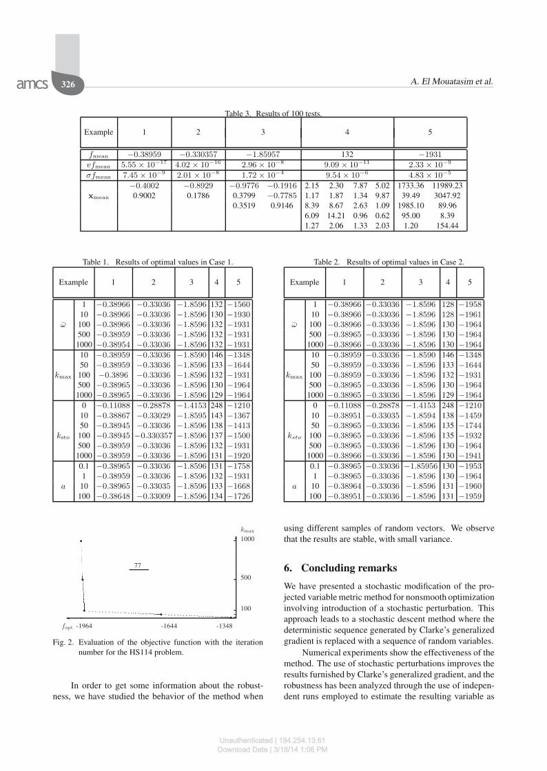
We introduce a maximum iteration number kmax: theiterations are stopped when k = kmax. We denote byfopt and xopt, the estimations of the optimal value f andx∗ furnished by the method. fmean and xmean are theirmean values estimated from 100 independent runs. Wedenote be V fmean and σfmean the variance and standarddeviation of fmean, which are estimated from the resultsof the runs.

Our approach was programmed using Visual For-tran 6.1. As far as the experiments were concerned, theywere performed on a workstation running an HP Intel(R) M processor (1.30 GHz, 224 MB RAM). The caseksto = 0 corresponds to unperturbed descent (determinis-tic) method.

Results.

• Case 1: ω = 500, kmax = 100, ksto = 500 anda = 1.

• Case 2: ω = 500, kmax = 500, ksto = 500 anda = 1.

In Tables 1 and 2, we show the observed effect ofthe variation in a single parameter value while the oth-ers remain with their original value. Tables 1 and 2 con-tain the minimal value objective f(x∗) = −0.38966, −0.33036, − 1.8596, 128 and − 1964 of the problemsMad 1, Mad 2, Pentagon, Wong 3 and HS114.

�

100

500

1000

�

129 132 145

�

�

�

�

�

kmax

fopt

4

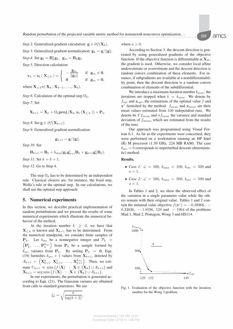
Fig. 1. Evaluation of the objective function with the iterationnumber for the Wong 3 problem.

Unauthenticated | 194.254.13.61Download Date | 3/18/14 1:06 PM

326 A. El Mouatasim et al.

Table 3. Results of 100 tests.

Example 1 2 3 4 5

fmean −0.38959 −0.330357 −1.85957 132 −1931

vfmean 5.55 × 10−17 4.02 × 10−16 2.96 × 10−8 9.09 × 10−11 2.33 × 10−9

σfmean 7.45 × 10−9 2.01 × 10−8 1.72 × 10−4 9.54 × 10−6 4.83 × 10−5

−0.4002 −0.8929 −0.9776 −0.1916 2.15 2.30 7.87 5.02 1733.36 11989.23xmean 0.9002 0.1786 0.3799 −0.7785 1.17 1.87 1.34 9.87 39.49 3047.92

0.3519 0.9146 8.39 8.67 2.63 1.09 1985.10 89.966.09 14.21 0.96 0.62 95.00 8.391.27 2.06 1.33 2.03 1.20 154.44

Table 1. Results of optimal values in Case 1.

Example 1 2 3 4 5

1 −0.38966 −0.33036 −1.8596 132 −156010 −0.38966 −0.33036 −1.8596 130 −1930

ω 100 −0.38966 −0.33036 −1.8596 132 −1931500 −0.38959 −0.33036 −1.8596 132 −19311000 −0.38954 −0.33036 −1.8596 132 −1931

10 −0.38959 −0.33036 −1.8590 146 −134850 −0.38959 −0.33036 −1.8596 133 −1644

kmax 100 −0.3896 −0.33036 −1.8596 132 −1931500 −0.38965 −0.33036 −1.8596 130 −19641000 −0.38965 −0.33036 −1.8596 129 −1964

0 −0.11088 −0.28878 −1.4153 248 −121010 −0.38867 −0.33029 −1.8595 143 −136750 −0.38945 −0.33036 −1.8596 138 −1413

ksto 100 −0.38945 −0.330357 −1.8596 137 −1500500 −0.38959 −0.33036 −1.8596 132 −19311000 −0.38959 −0.33036 −1.8596 131 −1920

0.1 −0.38965 −0.33036 −1.8596 131 −17581 −0.38959 −0.33036 −1.8596 132 −1931

a 10 −0.38965 −0.33035 −1.8596 133 −1668100 −0.38648 −0.33009 −1.8596 134 −1726

�

100

500

1000

kmax

-1348-1644-1964

� �

�

�

�

�

fopt

77

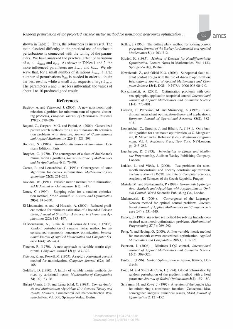
Fig. 2. Evaluation of the objective function with the iterationnumber for the HS114 problem.

In order to get some information about the robust-ness, we have studied the behavior of the method when

Table 2. Results of optimal values in Case 2.

Example 1 2 3 4 5

1 −0.38966 −0.33036 −1.8596 128 −195810 −0.38966 −0.33036 −1.8596 128 −1961

ω 100 −0.38966 −0.33036 −1.8596 130 −1964500 −0.38965 −0.33036 −1.8596 130 −1964

1000 −0.38966 −0.33036 −1.8596 130 −1964

10 −0.38959 −0.33036 −1.8590 146 −134850 −0.38959 −0.33036 −1.8596 133 −1644

kmax 100 −0.38959 −0.33036 −1.8596 132 −1931500 −0.38965 −0.33036 −1.8596 130 −1964

1000 −0.38965 −0.33036 −1.8596 129 −1964

0 −0.11088 −0.28878 −1.4153 248 −121010 −0.38951 −0.33035 −1.8594 138 −145950 −0.38965 −0.33036 −1.8596 135 −1744

ksto 100 −0.38965 −0.33036 −1.8596 135 −1932500 −0.38965 −0.33036 −1.8596 130 −1964

1000 −0.38966 −0.33036 −1.8596 130 −1941

0.1 −0.38965 −0.33036 −1.85956 130 −19531 −0.38965 −0.33036 −1.8596 130 −1964

a 10 −0.38964 −0.33036 −1.8596 131 −1960100 −0.38951 −0.33036 −1.8596 131 −1959

using different samples of random vectors. We observethat the results are stable, with small variance.

6. Concluding remarks

We have presented a stochastic modification of the pro-jected variable metric method for nonsmooth optimizationinvolving introduction of a stochastic perturbation. Thisapproach leads to a stochastic descent method where thedeterministic sequence generated by Clarke’s generalizedgradient is replaced with a sequence of random variables.

Numerical experiments show the effectiveness of themethod. The use of stochastic perturbations improves theresults furnished by Clarke’s generalized gradient, and therobustness has been analyzed through the use of indepen-dent runs employed to estimate the resulting variable as

Unauthenticated | 194.254.13.61Download Date | 3/18/14 1:06 PM

Random perturbation of the projected variable metric method for nonsmooth nonconvex optimization. . . 327

shown in Table 3. Thus, the robustness is increased. Themain classical difficulty in the practical use of stochasticperturbations is connected with the tuning of the param-eters. We have analyzed the practical effect of variationsof a, ω, kmax and ksto. As shown in Tables 1 and 2, themore influenced parameters are kmax and ksto. We ob-serve that, for a small number of iterations kmax, a largenumber of perturbations ksto is needed in order to obtainthe best results, while a small ksto requests a large kmax.The parameters a and ω are less influential: the values ofabout 1 to 10 produced good results.

ReferencesBagirov, A. and Yearwood, J. (2006). A new nonsmooth opti-

mization algorithm for minimum sum-of-squares cluster-ing problems, European Journal of Operational Research170(2): 578–596.

Bogani, C., Gasparo, M.G. and Papini, A. (2009). Generalizedpattern search methods for a class of nonsmooth optimiza-tion problems with structure, Journal of Computationaland Applied Mathematics 229(1): 283–293.

Bouleau, N. (1986). Variables Aleatoires et Simulation, Her-mann Editions, Paris.

Broyden, C. (1970). The convergence of a class of double-rankminimization algorithms, Journal Institute of Mathematicsand Its Applications 6(1): 76–90.

Correa, R. and Lemarechal, C. (1993). Convergence of somealgorithms for convex minimization, Mathematical Pro-gramming 62(2): 261–275.

Davidon, W. (1991). Variable metric method for minimization,SIAM Journal on Optimization 1(1): 1–17.

Dorea, C. (1990). Stopping rules for a random optimiza-tion method, SIAM Journal on Control and Optimization28(4): 841–850.

El Mouatasim, A. and Al-Hossain, A. (2009). Reduced gradi-ent method for minimax estimation of a bounded Poissonmean, Journal of Statistics: Advances in Theory and Ap-plications 2(2): 183 –197.

El Mouatasim, A., Ellaia, R. and Souza de Cursi, J. (2006).Random perturbation of variable metric method for un-constrained nonsmooth nonconvex optimization, Interna-tional Journal of Applied Mathematics and Computer Sci-ence 16(4): 463–474.

Fletcher, R. (1970). A new approach to variable metric algo-rithms, Computer Journal 13(3): 317–322.

Fletcher, R. and Powell, M. (1963). A rapidly convergent descentmethod for minimization, Computer Journal 6(2): 163–168.

Goldfarb, D. (1970). A family of variable metric methods de-rived by variational means, Mathematics of Computation24(109): 23–26.

Hiriart-Urruty, J.-B. and Lemarechal, C. (1993). Convex Analy-sis and Minimization Algorithms II: Advanced Theory andBundle Methods, Grundlehren der mathematischen Wis-senschaften, Vol. 306, Springer-Verlag, Berlin.

Kelley, J. (1960). The cutting plane method for solving convexprograms, Journal of the Society for Industrial and AppliedMathematics 8(4): 703–712.

Kiwiel, K. (1985). Method of Descent for NondifferentiableOptimization, Lecture Notes in Mathematics, Vol. 1133,Springer-Verlag, Berlin.

Kowalczuk, Z., and Oliski K.O. (2006). Suboptimal fault tol-erant control design with the use of discrete optimization,International Journal of Applied Mathematics and Com-puter Science 18(4), DOI: 10.2478/v10006-008-0049-0.

Kryazhimskii, A. (2001). Optimization problems with con-vex epigraphs. application to optimal control, InternationalJournal of Applied Mathematics and Computer Science11(4): 773–801.

Larsson, T., Patrksson, M. and Stromberg, A. (1996). Con-ditional subgradient optimization-theory and applications,European Journal of Operational Research 88(2): 382–403.

Lemarechal, C., Strodiot, J. and Bihain, A. (1981). On a bun-dle algorithm for nonsmooth optimization, in O. Mangasar-ian, R. Meyer and S. Robinson (Eds.), Nonlinear Program-ming, Vol. 4, Academic Press, New York, NY/London,pp. 245–282.

Luenberger, D. (1973). Introduction to Linear and Nonlin-ear Programming, Addison-Wesley Publishing Company,London.

Luksan, L. and Vlcek, J. (2000). Test problems for nons-mooth unconstraint and linearly constraint optimization,Technical Report TR-798, Institute of Computer Sciences,Academy of Sciences of the Czech Republic, Prague.

Makela, M. and Neittaanmaki, P. (1992). Nonsmooth Optimiza-tion: Analysis and Algorithms with Applications to Opti-mal Control, World Scientific Publishing Co., London.

Malanowski, K. (2004). Convergence of the Lagrange–Newton method for optimal control problems, Interna-tional Journal of Applied Mathematics and Computer Sci-ence 14(4): 531–540.

Panier, E. (1987). An active set method for solving linearly con-strained nonsmooth optimization problems, MathematicalProgramming 37(3): 269–292.

Peng, Y. and Heying, Q. (2009). A filter-variable-metric methodfor nonsmooth convex constrained optimization, AppliedMathematics and Computation 208(1): 119–128.

Petersen, I. (2006). Minimax LQG control, InternationalJournal of Applied Mathematics and Computer Science16(3): 309–323.

Pinter, J. (1996). Global Optimization in Action, Kluwer, Dor-drecht.

Pogu, M. and Souza de Cursi, J. (1994). Global optimization byrandom perturbation of the gradient method with a fixedparameter, Journal of Global Optimization 5(2): 159–180.

Schramm, H. and Zowe, J. (1992). A version of the bundle ideafor minimizing a nonsmooth function: Conceptual idea,convergence analysis, numerical results, SIAM Journal ofOptimization 2: 121–152.

Unauthenticated | 194.254.13.61Download Date | 3/18/14 1:06 PM

328 A. El Mouatasim et al.

Shanno, D. (1970). Conditioning of quasi-Newton methodsfor function minimization, Mathematics of Computation24(111): 647–657.

Souza de Cursi, J. (1991). Introduction aux probabilites, EcoleCentrale Nantes, Nantes.

Souza de Cursi, J., Ellaia, R. and Bouhadi, M. (2003). Globaloptimization under nonlinear restrictions by using stochas-tic perturbations of the projected gradient, in C.A. Floudasand P.M. Pardalos (eds.), Frontiers in Global Optimization,Vol. 1, Dordrecht, Springer, pp.: 541–562.

Uryasev, S. (1991). New variable metric algorithms for nondif-ferentiable optimization problems, Journal of OptimizationTheory and Applications 71(2): 359–388.

Zhang, G. (2009). A note on: A continuous approach to nonlin-ear integer programming, Applied Mathematics and Com-putation 215(6): 2388–2389.

Abdelkrim El Mouatasim, born in 1973, re-ceived a Ph.D. degree in applied mathematics andscientific computation in 2007 from Mohamma-dia Engineering School in Rabat, Morocco. Cur-rently he works for the Department of Mathe-matics at the Faculty of Sciences, Jazan Uni-versity, Saudi Arabia. His research interests in-clude global optimization, nonsmooth optimiza-tion mathematical modelling, stochastic pertur-bation, water distribution system and combina-

torial optimization. In 2001 he was decorated by King Mohammed VI.

Rachid Ellaia received a Ph.D. degree in appliedmathematics and optimization in 1992 from Mo-hammed V University. Currently he is a full pro-fessor at the Mohammadia School of Engineersin Rabat, Morocco. His main research interestsinclude areas such as global optimization, non-smooth optimization, mathematical modelling,stochastic methods, convex analysis and financialmathematics. In 2009 he was a visiting profes-sor at the National Institute for Applied Sciences,

Rouen, and presently he is a visiting professor at the University of Nice,Sophia Antipolis, France.

Eduardo Souza de Cursi, born in 1957, graduate in physics: 1978,M.Sc.: 1980, Ph.D.: 1992. Presently: a professor at the National Insti-tute for Applied Sciences, Rouen, the head of the Laboratory of Mechan-ics of Rouen, dean for European and international affairs and a delegatefor European and international affairs of the group National Institute forApplied Sciences. He has experience in applied mathematics and me-chanics, namely, theoretical and numerical aspects, stochastic methodsand convex analysis.

Appendix A

Example 1. (Luksan and Vlcek, 2000) Mad 1 problem.

{minF (x) = max{f1(x), f2(x), f3(x)},subject to h1(x) = x1 + x2 − 0.5 ≥ 0,

where

f1(x) = x21 + x2

2 + x1x2 − 1,f2(x) = sinx1,

f3(x) = − cosx2.

The starting point is x0 = (1, 2) .

Example 2. (Luksan and Vlcek, 2000) Mad 2 problem.{

minF (x) = max{f1(x), f2(x), f3(x)},subject to h1(x) = −3x1 + x2 − 2.5 ≥ 0,

where fi(x), i = 1, 2, 3, as in Example 1. The startingpoint is x0 = (−2, − 1) .

Example 3. (Luksan and Vlcek, 2000) Pentagon prob-lem.⎧⎪⎪⎪⎪⎪⎨⎪⎪⎪⎪⎪⎩

minF (x) = max{f1(x), f2(x), f3(x)},

subject to hi(x) = xi cos2πj5

+ xi+1 sin2πj5

≤ 1,

i = 1, 3, 5, j = 0, 1, 2, 3, 4,

where

f1(x) = −√

(x1 − x3)2 + (x2 − x4)2,

f2(x) = −√

(x3 − x5)2 + (x4 − x6)2,

f3(x) = −√

(x5 − x1)2 + (x6 − x2)2.

The starting point is x0 = (−1, 0, 0, − 1, 0, 1) .

Example 4. (Luksan and Vlcek, 2000) Wong 3 problem.⎧⎪⎪⎪⎪⎪⎪⎪⎪⎪⎪⎪⎪⎪⎪⎪⎪⎪⎪⎪⎪⎪⎪⎪⎪⎪⎪⎪⎪⎪⎪⎪⎪⎪⎪⎪⎪⎪⎪⎪⎪⎪⎪⎪⎨⎪⎪⎪⎪⎪⎪⎪⎪⎪⎪⎪⎪⎪⎪⎪⎪⎪⎪⎪⎪⎪⎪⎪⎪⎪⎪⎪⎪⎪⎪⎪⎪⎪⎪⎪⎪⎪⎪⎪⎪⎪⎪⎪⎩

minF (x) = x21 + x2

2 + x1x2 − 14x1 − 16x2

+ (x3 − 10)2 + 4(x4 − 5)2 + (x5 − 3)2

+ 2(x6 − 1)2 + 5x27 + 7(x8 − 11)2

+ 2(x9 − 10)2 + (x10 − 7)2 + (x11 − 9)2

+ 10(x12 − 1)2 + 5(x13 − 7)2

+ 4(x14 − 14)2 + 27(x15 − 1)2 + x416

+ (x17 − 2)2 + 13(x18 − 2)2 + (x19 − 3)2

+ x220 + 95,

subject to

ψi(x) ≤ 0, i = 1, . . . , 13,

h1(x) = 4x1 + 5x2 − 3x7 + 9x8 ≤ 105,

h2(x) = 10x1 − 8x2 − 17x7 + 2x8 ≤ 0,

h3(x) = −8x1 + 2x2 + 5x9 − 2x10 ≤ 12,

h4(x) = x1 + x2 + 4x11 − 21x12 ≤ 0,

Unauthenticated | 194.254.13.61Download Date | 3/18/14 1:06 PM

Random perturbation of the projected variable metric method for nonsmooth nonconvex optimization. . . 329

where

ψ1(x) = 3(x1 − 2)2 + 4(x2 − 3)2 + 2x23 − 7x4 − 120,

ψ2(x) = 5x21 + 8x2 + (x3 − 6)2 − 2x4 − 40,

ψ3(x) = 0.5(x1 − 8)2 + 2(x2 − 4)2 + 3x25 − x6 − 30,

ψ4(x) = x21 + 2(x2 − 2)2 − 2x1x2 + 14x5 − 6x6,

ψ5(x) = −3x1 + 6x2 + 12(x9 − 8)2 − 7x10,

ψ6(x) = x21 + 5x11 − 8x12 − 28,

ψ7(x) = 4x1 + 9x2 + 5x213 − 9x14 − 87,

ψ8(x) = 3x1 + 4x2 + 3(x13 − 6)2 − 14x14 − 10,

ψ9(x) = 14x21 + 35x15 − 79x16 − 92,

ψ10(x) = 15x22 + 11x15 − 61x16 − 54,

ψ11(x) = 5x21 + 2x2 + 9x4

17 − x18 − 68,

ψ12(x) = x21 − x9 + 19x19 − 20x20 + 19,

ψ13(x) = 7x21 + 5x2

2 + x219 − 30x20.

In order to apply the algorithm, the nonlinear constraintsare penalized, i.e., F is replaced with

Fλ(x) = F (x) + λ

13∑i=1

ψ+i (x),

where

ψ+i (x) = max{0, ψi(x)}.

Fλ satisfies the general assumptions. The numerical ex-periment uses λ = 10. The starting point is

x0 =(2, 3, 5, 5, 1, 2, 7, 3, 6, 10, 2,

2, 6, 15, 1, 2, 1, 2, 1, 3).

Example 5. (Luksan and Vlcek, 2000) HS114 problem.

⎧⎪⎪⎪⎪⎪⎪⎪⎪⎪⎪⎪⎪⎪⎪⎪⎪⎪⎪⎪⎪⎪⎪⎪⎪⎨⎪⎪⎪⎪⎪⎪⎪⎪⎪⎪⎪⎪⎪⎪⎪⎪⎪⎪⎪⎪⎪⎪⎪⎪⎩

minF (x) = 5.04x1 + 0.035x2 + 10x3 + 3.36x5

−0.063x4x7,subject to

ψi(x) ≤ 0, i = 1, . . . , 4,ηj(x) = 0, j = 1, 2,h1(x) = 0.222x10 + bx9 ≤ 35.82,

h2(x) = 0.222x10 + 1bx9 ≥ 35.82,

h3(x) = 3x7 − ax10 ≥ 133,

h4(x) = 3x7 − 1ax10 ≤ 133,

h5(x) = 1.22x4 − x1 − x5 = 0,

where

ψ1(x) = 1.12x1 + 0.13167x1x8 − 0.00667x1x28

− 1ax4,

ψ2(x) = −(1.12x1 + 0.13167x1x8 − 0.00667x1x28

− ax4),

ψ3(x) = 1.098x8 − 0.038x28 + 0.325x6

− 1ax7 + 57.425,

ψ4(x) = −(1.098x8 − 0.038x28 + 0.325x6

− ax7 + 57.425),

η1(x) =98000x3

x4x9 + 1000x3− x6,

η2(x) =x2 + x5

x1− x8,

a = 0.99, b = 0.90, and sample constraints are

10−5 ≤ x1 ≤ 2000, 85 ≤ x6 ≤ 93,

10−5 ≤ x2 ≤ 16000, 90 ≤ x7 ≤ 95,

10−5 ≤ x3 ≤ 120, 3 ≤ x8 ≤ 12,

10−5 ≤ x4 ≤ 5000, 1.2 ≤ x9 ≤ 4,

10−5 ≤ x5 ≤ 2000, 145 ≤ x10 ≤ 162,

The starting point is

x0 =(1745, 12000, 110, 3048, 1974,

89.2, 92.8, 8, 3.6, 145).

As in the previous example, the nonlinear constraints arepenalized. In addition, the restriction h5 is rewritten ash5 ≤ 0 and −h5 ≤ 0. The restriction −h5 ≤ 0 is treatedas an ordinary affine one, while the other one is penalized.Thus we minimize

Fλ = F + λ[ 4∑

i=1

ψ+i + h+

5 + |η1| + |η2|].

We use λ = 1000.

Received: 9 February 2010Revised: 6 November 2010

Unauthenticated | 194.254.13.61Download Date | 3/18/14 1:06 PM