
The design and control of mine refrigeration systems by ...
377
The design and control of mine refrigeration systems by Michael Howes, ACSM Thesis submitted to the University of Nottingham for the degree of Doctor of Philosophy, October, 1992 r·· . ... . . .. n. .,
-
Upload
khangminh22 -
Category
Documents
-
view
0 -
download
0
Transcript of The design and control of mine refrigeration systems by ...
The design and control of mine refrigeration systems
by Michael Howes, ACSM
Thesis submitted to the University of Nottingham
for the degree of Doctor of Philosophy,
October, 1992
r·· . "'t~ ... *.~ :,~
~}~; . . ~'" .. ~~~~ n. .,
CONTENTS
Abstract ..................................... i
List of tables ............................... ii List of figures List of symbols
1 INTRODUCTION
. . . . . . . . . . . . . . . . . . . . . . . . . . . . . .
. . . . . . . . . . . . . . . . . . . . . . . . . . . . . .
1.1 The need tor mine retrigeration system
v
viii
control ................................ 1 1.2 Objectives of the research •.....•...... 3 1.3 Historical perspective ...•••..•••.•.... 5 1.4 Location ot the research ...••.•....•••• 10
2 RBFRIGBRATION SYSTBM MODBLLING
2.1 Overall plant size ..................•.• 14 2.1.1 Mine heat load .•.•.•••.••.•.•.•.• 17
Heat from autocompression ••.••••• 17 Heat from surrounding rock •.•.••• 18 Broken rock and fissure water .••• 19 Heat from mine equipment .••..••.• 20 Summary of heat loads ••.....•.••. 23
2.1.2 Design surface climatic conditions 27
2.1.3 Acceptable thermal environments .. 33 Human heat balance .•.•...•.•..••. 34 Thermoregulation .•.•.....••..•.•. 36 Limiting body temperature •.•.•.•. 37 Cooling power of the air ......... 38
Other heat stress indicators ...•• 41 The measurement of heat strain .•• 46 Actual heat stroke risk •••••.•••. 47 Application of heat stress limits 49
2.1.4 The refrigeration load profile ... 54 Productivity and the environment. 54 Reduced shift lengths ............ 59 Optimisations .................... 64 Cooling capacity and load profiles 73
2.2 Refrigeration plant analysis ........... 76
2.2.1 Background to simUlations 76 Air conditioning industry ........ 78
Mining industry ..........•....••. 81
Development of this work .••..•.•. 83
2.2.2 Refrigeration system simulation.. 87
2.2.3 Refrigerant properties .•........• 88 Ammonia R717 •...•.••..•••......•. 91 Refrigerant R22 ...••..•........•. 92 Refrigerant Rl1 .........•...•..•. 93
3 BQUIPMBHT PBRFORMANCB
3.1 COJDl)reSBOrs •••••••••••••••••••••••••••• 95
3.1.1 Compressor part load operation •.• 96
3.1.2 Centrifugal compressors •••..••••• 98
3.1.3 Screw compressors ••••••.•••.•••.. 101
Broken Hill underground plant ••.• 101
Mount Isa surface plants ••••.•••• 102
Broken Hill surface plant •.•••••• 108
3 • 2 Condensers ............................. 113
3.2.1 Shell and tube ••••.•.•••.•••••.•• 114
3.2.2 Closed plate ...••..•....••.•••••• 115
3.2.3 Evaporative condensers ••.••..•..• 118
3.3 Evaporators ............................ 123
3.3.1 Shell and tube ••.•••••••..••.•... 124
3.3.2 Direct expansion shell and tube •• 126 3.3.3 Closed plate ••.•.•.•.•...•••••••• 129 3.3.4 Open plate ..••....•..•.....•..••• 131
3.4 Surface cooling towers ................. 136
3.4.1 Pre-cooling towers ............... 138
3.4.2 Condenser cooling towers ......... 139
3.4.3 Surface bulk air coolers ......•.. 141
3.5 Underground air cooling •............•.. 144
3.5.1 Air cooling coils ..••..•......•.. 144
3.5.2 Mesh coolers .•................... 148
3.5.3 Multistage spray chambers .....•.. 150
3.5.4 Modular cooling towers ........... 155
3.5.6 Capacity control ...•••......•...• 156
3.6 Miscellaneous equipment ..•••......•.••. 159
3.6.1 High pressure heat exchangers .... 159
3.6.2 Pipe insulation and heat transfer 160
4 ACTUAL PLANT SIMULATIONS
4.1 Simulation structure and components ••.. 167
4.1.1 The chiller subsystem ••••••.•.••• 168
Evaporator modules •••••••••••••.• 168
Condenser modules •.••••.•••••••.• 170
Compressor modules .••.•...•..•.•• 174
Chiller set modules •••••••••••••• 177
4.1.2 The heat rejection subsystem •••.• 178
4.1.3 The load subsystem .••••••••..••.• 182
Surface bulk air cooler .......•.• 182
Underground chilled water systems 184
High pressure heat exchangers .••. 185
Cooling coils ••••••••••••••.••••• 188
Multistage spray chambers •••.•... 189
The underground load ••••.•••••••• 194
4.1.4 Overall plant operation •••••••••• 194
4.2 Mount Is& R63 plant ..•......••.•••.•••• 200
4.2.1 Base system model •••.•••..••••••• 200
4.2.2 Extended system model •..•..•..•.. 203
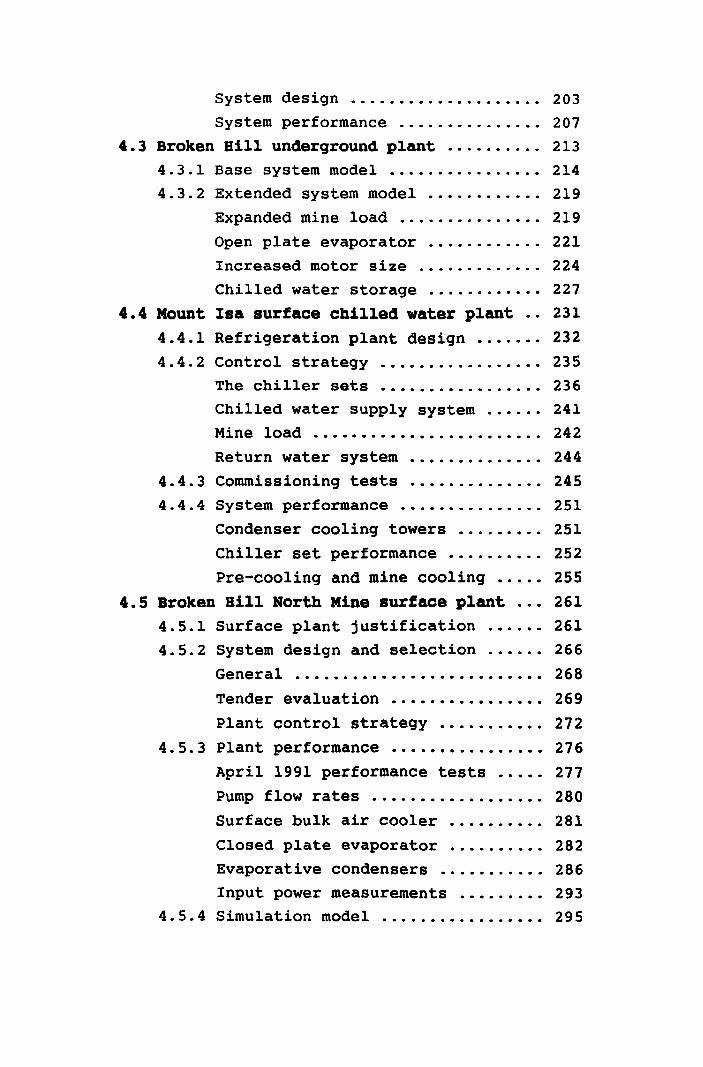
System design .................... 203 System performance ............... 207
4.3 Broken Bill underground plant .......... 213 4.3.1 Base system model ................ 214 4.3.2 Extended system model ............ 219
Expanded mine load .•............. 219
Open plate evaporator ............ 221
Increased motor size ............. 224 Chilled water storage ............ 227
4.4 Mount Isa surface chilled water plant .• 231
4.4.1 Refrigeration plant design ..•.•.• 232 4.4.2 Control strategy ....•............ 235
The chiller sets •••••............ 236 Chilled water supply system ...•.. 241 Mine load ••..•.•••••••.•.••...... 242
Return water system •••..•.•.•.... 244 4.4.3 Commissioning tests •.•...•....•.. 245 4.4.4 System performance ............... 251
Condenser cooling towers ••..•.•.. 251 Chiller set performance .....•.•.. 252
Pre-cooling and mine cooling ••.•• 255
4.5 Broken Bill North Mine surface plant .•. 261 4.5.1 Surface plant justification .••.•. 261 4.5.2 System design and selection ...••• 266
General ...•..••••••..•••.•..••••• 268
Tender evaluation ...••••••••••.•. 269
Plant control strategy .......•••• 272
4.5.3 Plant performance ••••••••...•..•. 276
April 1991 performance tests •.••. 277
Pump flow rates ..•....••.....•••. 280
Surface bulk air cooler
Closed plate evaporator 281
282 Evaporative condensers ........... 286 Input power measurements .....•.•. 293
4.5.4 Simulation model ..............•.. 295
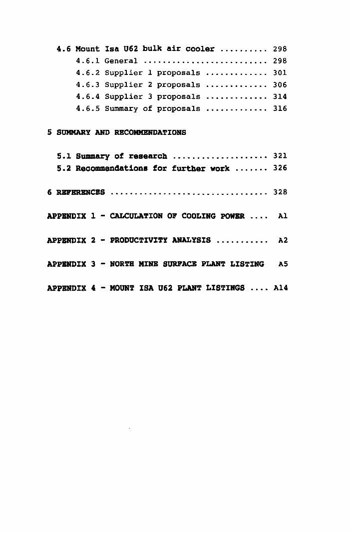
4.6 Mount Isa U62 bulk air cooler . . . . . . . . . . 298
4.6.1 General . . . . . . . . . . . . . . . . . . . . . . . . . . 298
4.6.2 Supplier 1 proposals · . . . . . . . . . . . . 301
4.6.3 Supplier 2 proposals · . . . . . . . . . . . . 306
4.6.4 Supplier 3 proposals · . . . . . . . . . . . . 314
4.6.5 Summary of proposals · . . . . . . . . . . . . 316
5 SUMMARY AND RECOMMENDATIONS
5.1 Summary of research ...............•.•.• 321
5.2 Recommendations for further work ...•..• 326
6 RBI'BRBRCBS . . . . . . . . . . . . . . . . . . . . . . . . . . . . . . . . . 328
APPENDIX 1 - CALCULATION 01' COOLING POWBR .... Al
APPENDIX 2 - PRODUCTIVITY ANALYSIS •.....••••• A2
APPENDIX 3 - NORTH MINH SURI'ACB PLANT LISTING AS
APPENDIX 4 - MOUNT ISA U62 PLANT LISTINGS .••• A14
THE DESIGN AND CONTROL OF MINE REFRIGERATION SYSTEMS
by
Michael John Howes
ABSTRACT
The research is directed towards modelling the chiller set, the heat rejection and the load subsystems of a complete mine refrigeration system and simulating the performance in order that the design can be optimised and the most cost effective control system determined. The refrigeration load profile for a mechanised mine is complex and primarily a function of surface climatic variations, the strongly cyclic sources of heat resul ting from the operation of diesel powered mining equipment and the associated differences in thermal environmental acceptance criteria.
Modelling of the central element of the system, the compressor, is based on empirical relationships which use the actual cooling duty and input power rather than general compressor curves using theoretical flow and head coefficients. This has a more general application and is not restricted to a single compressor type. The steady state modelling of five refrigeration systems has included two types of compressor, four types of evaporator, three types of condenser, two types of cooling tower and five types of mine cooling appliances.
The research has extended modelling of refrigeration systems by incorporating fully the heat rejection and load subsystems and has demonstrated that relatively complex mine refrigeration systems can be modelled and the simulation results related to actual measurements with an acceptable accuracy. This has been further improved by testing the system elements and adjusting the theoretical performance analysis where necessary. These adjustments concern either the more difficult to assess factors such as evaporating and condensing heat transfer coefficients or factors influenced by unusual operating conditions.
The research has shown that, despite the complexity of the load profile and the refrigeration system, modelling and simulation can be used effectively to optimise both the design and the control system.
(i)
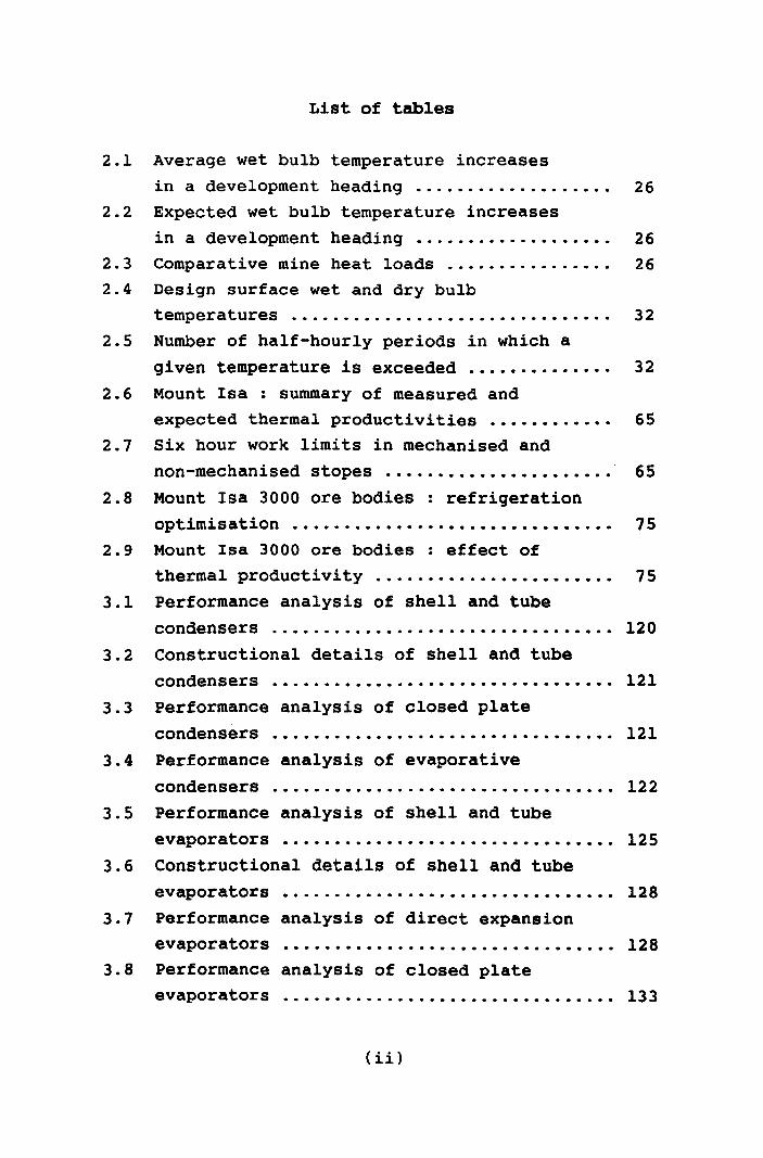
List of tables
2.1 Average wet bulb temperature increases
in a development heading ................... 26
2.2 Expected wet bulb temperature increases
in a development heading •...............••• 26
2.3 Comparative mine heat loads ...........•.... 26
2.4 Design surface wet and dry bulb temperatures ............................•.• 32
2.5 Number of half-hourly periods in which a
given temperature is exceeded •••.•.•.•..••. 32
2.6 Mount Isa : summary of measured and expected thermal productivities ...••••••••. 65
2.7 Six hour work limits in mechanised and
non-mechanised stopes ..•.....•...••.•••••.• 65
2.8 Mount Isa 3000 ore bodies : refrigeration optimisation ............................... 75
2.9 Mount Isa 3000 ore bodies: effect of thermal productivity ...•..•....•••••••••••• 75
3.1 Performance analysis of shell and tube
condensers ................................. 120 3.2 Constructional details of shell and tube
condensers ................................. 121
3.3 Performance analysis of closed plate
condensers ................................. 121 3.4 Performance analysis of evaporative
condensers ................................. 122
3.5 Performance analysis of shell and tube
evaporators ................................ 125
3.6 Constructional details of shell and tube
evaporators . . . . . . . . . . . . . . . . . . . . . . . . . . . . . . . . 128
3.7 Performance analysis of direct expansion
evaporators ................................ 128
3.8 Performance analysis of closed plate evaporators . . . . . . . . . . . . . . . . . . . . . . . . . . . . . . . . 133
(ii)
3.9 Performance analysis of open plate evaporators ................................ 133
3.10 Performance analysis of a counter flow cooling tower .............................. 143
3.11 Performance analysis of a cross flow cooling tower .............................. 143
3.12 Performance analysis of air cooling coils .. 146 3.13 Performance analysis of mesh coolers .••.•.. 152 3.14 Measured performance of multistage
horizontal spray chambers •.•.••.•••.•.•.••• 153
3.15 Performance analysis of high pressure water to water heat exchangers •.••...•...•• 161
3.16 Method of estimating heat gains in water distribution pipes ...•.•••....••..•.....••. 166
4.1 Mount lsa R63 : base plant comparison between measured and predicted values •••••• 205
4.2 Mount lsa R63 : extended plant comparison between measured and predicted values •••••• 212
4.3 Broken Hill underground plant: April 1987 comparison between measured and predicted
values . . . . . . . . . . . . . . . . . . . . . . . . . . . . . . . . . . . . . 218
4.4 Broken Hill underground plant: April 1987 predicted plant performance ••••••••••.••••• 221
4.5 Broken Hill underground plant: extended mine load - predicted plant performance 222
4.6 Broken Hill underground plant: four compressors and open plate evaporator - predicted plant performance •••••...•••.•. 225
4.7 Broken Hill underground plant: three compressors and open plate evaporator - predicted plant performance ..•.•••••••..• 228
4.8 Broken Hill underground plant: summer operation - predicted plant performance •••• 229
4.9 Broken Hill underground plant: mid-seasonal operation - predicted plant performance •.•• 230
(iii)
4.10 Mount lsa K6l : analysis of commissioning test results ............................... 250
4.11 Mount lsa K6l : analysis of condenser cooling tower results •...•.•............••. 253
4.12 Mount lsa K6l : condenser cooling tower heat balances ...•...•....•...•.•..••..••.•. 253
4.13 Mount lsa K6l : chiller set performance July 1990 ......•.•.•.•.......•.•.......••.. 256
4.14 Mount lsa K6l : two chiller set performance November 21st 1990 ..••...•.•.•.•.•••.••.••• 257
4.15 Mount lsa K6l : one chiller set performance November 21st 1990 .•...•.••..•....••.•••.•. 258
4.16 Mount Isa K6l : two chiller set performance November 23rd 1990 .••..••.•••.•......•••..• 259
4.17 Mount lsa K6l : two chiller set performance January 21st 1990 ••••..•••••••••••...•••.•. 260
4.18 Comparison of options for the Broken Hill refrigeration system .........•...•.....•... 267
4.19 Broken Hill surface plant: bulk air cooler performance ••••••••••.•••.•.•.•...•• 284
4.20 Broken Hill surface plant: EMS data
4.21
4.22
summary for March 3rd 1992 ••••••••••••.•••• 296
Broken Hill surface plant
values for March 3rd 1992
Mount lsa U62 : Baltimore
: predicted
Aircoil bulk
297
air cooler performance •••.•••.••••..••••••• 302
4.23 Mount lsa U62 : Sulzer bulk air cooler per f ormance ................................ 303
4.24 Supplier 1 : continuous process operation •• 307
4.25 Supplier 1 : batch process operation ••.•••• 308 4.26 Supplier 2 : continuous process operation .• 312
4.27 Supplier 2 : batch process operation ...••.. 313 4.28 Supplier 3 continuous process operation •. 318 4.29 Supplier 3 : batch process operation ••.•••. 319 4.30 Mount lsa U62 : summary of costs ••••.••••.. 320
(iv)
List of figures
1.1 The vapour compression refrigeration cycle. 4
2.1 Heat balance in a development heading ...... 24
2.1 Mount lsa : distribution of wet and dry
bulb temperatures over three summers ..••.•. 30
2.3 Mount lsa : 10 year average hourly wet and
dry bulb temperatures .................••.•. 31
2.4 Thermoregulation and equilibrium core and
skin temperatures ..................•.....•. 39
2.5 Equilibrium skin temperatures and risk ••... 39
2.6 Lepanto: working place wet bulb temperature
distribution ••.....•.•.•..•...........••.•• 53
2.7 Control of the thermal environment: reduced
shift length strategy ..................•... 53
2.8 Mount lsa : relationship between six hour
and surface wet bulb temperatures .•..•...•. 60
2.9 Mount lsa : relationship between six hour
and expected productivity .............•.... 61
2.10 Mount lsa : working place performance ....•. 62
2.11 Six hour and stop work charts •...•...•••••. 66
2.12 General refrigeration system algorithm ••.•• 89
2.13 Definitions of refrigerant properties ...... 94
3.1 Carrier centrifugal compressor performance
- adiabatic head ........................... 99
3.2 Carrier centrifugal compressor performance
- efficiency •......•.•..•.............••.•• 100
3.3 Sullair C25 screw compressor performance ... 103
3.4 Howden 321-193 screw compressor performance 104
3.5 Stal S93E screw compressor performance ••.•• 105
3.6 Stal S93E with economiser performance •••••. 106
3.7 Sabroe 536H screw compressor performance ••. 109
3.8 Howden 321-132 screw compressor performance 110
3.9 Sullair L25 screw compressor performance III
3.10 Mycom 320MU screw compressor performance 112
(v)
3.11 Rated and calculated heat transfer for air cooling coils ...........•............•. 149
4.1 Evaporator module analysis .•.........•..... 169 4.2 Condenser module analysis ..•.....•.•....... 172 4.3 Evaporative condenser module analysis ..•... 173 4.4 Compressor module analysis ..•........••.... 176 4.5 Chiller set module analysis •.•......•••••.. 179 4.6 Condenser cooling tower module analysis ..•. 180 4.7 Bulk air cooler module analysis •.••...••... 183 4.8 High pressure pipe analysis ••........•••... 186
4.9 High pressure heat exchanger analysis •••••. 187 4.10 Cooling coil analysis •••••.•••••.•...•••••• 190 4.11 Spray chamber stage analysis ••••.•.•••••.•. 191 4.12 Multistage spray chamber analysis ....•.•... 192 4.13 The load subsystem analysis •••.•...•..••... 195 4.14 Overall plant analysis ••••.•••...•...•.•.•. 199
4.15 Mount Isa R63 : schematic of the basic refrigeration system •••..•••••.•••••••••••• 202
4.16 Mount Isa R63 : effect of evaporator flow rate and set configuration ••••••.•..••••••• 206
4.17 Mount Isa R63 : effect of number of passes in the 19DG evaporator .•••••••.......•.•.•. 210
4.18 Mount Isa R63 : effect of condenser and secondary water flow rates ••.......••.••••.
4.19 Broken Hill underground plant : schematic
of system in 1987 ...•..•••.•••....•..•.•...
4.20 Mount Isa K6l overall control strategy
4.21 Mount Isa K6l : chiller set control
211
215
237
strategy ................................... 238
4.22 Mount Isa K6l : chilled water supply control strategy .....•..••...•.•..••••••••• 243
4.23 Mount Isa K6l : return water control 4.24 Mount Isa K6l : arrangement for
246
commissioning tests •....•••..•...•...•••••. 249
4.25 Mount Isa K6l : recirculation water flows •. 249
(vi)
4.26 Broken Hill surface plant: summary of proposed systems ........................... 270
4.27 Broken Hill surface plant : basic control strategy ..........................•...•.... 273
4.28 Broken Hill surface plant : layout of
equipment .................................. 278
4.29 Broken Hill surface plant : variable speed evaporator pump calibration •.....•..•••••.. 283
4.30 Broken Hill surface plant : closed plate evaporator performance ..•..•.....•....••••. 287
4.31 Broken Hill surface plant : comparison of estimated and actual plant duties •••••••••• 296
4.32 Broken Hill surface plant: evaporative condenser performance •..•........•••...••.. 291
4.33 Mount lsa U62 : Supplier 1, general
arrangement of proposals · . . . . . . . . . . . . . . . . . . 304
4.34 Mount lsa U62 · Supplier 2, general · arrangement of proposals · . . . . . . . . . . . . . . . . . . 311
4.35 Mount lsa U62 · Supplier 3, general · arrangement of proposals · . . . . . . . . . . . . . . . . . . 317
(vii)
List of symbols
Symbols
a
e e
Ecf f
f
fp F
Ff h
h
hf HPHE I
k
kW 1
LMTD
m
M
MWR
n
n
N
N
NTU
surface area (m2 ) basic four hour sweat rate (1) capacity rates (kW)
coefficient of performance air cooling power (W/m2) diameter (m)
vapour pressure (kPa) effectiveness evaporative condenser factor (m2 ) factor fin efficiency compressor part load factor cooling tower factor of merit evaporative condenser airflow factor adiabatic head (kJ/kg) heat transfer coefficient (kW/m2K) fouling factors (kW/m2K)
high pressure heat exchanger ideal power to cooling ratio thermal conductivity (kW/mK) compressor motor input power (kW) water flow rate (l/s) log mean temperature difference (oC) mass flow rate (kg/s) metabolic heat generation rate (W/m2) refrigeration capacity (MW) efficiency number of readings number of cassettes cooling tower factor number of heat transfer units
(viii)
N*
Na
N1 P
Pif P4SR
q
Q
rp R
s
S
S
Sr t
tpa
U
UA
v
v v W
WBGT
x
cooling tower factor
total nominal plate surface area (m2 )
total nominal length of plate (m) pressure (kPa)
compressor part load factor
predicted four hour sweat rate (1)
heat transfer (kW/m)
heat transferred (kW)
ratio of condensing to evaporating pressures
cooling tower capacity ratio
standard deviation
sigma heat (kJ/kg)
surface sweat rate (1)
temperature (oC)
production rate (million tonnes per year)
thermal resistance (kW/K)
overall heat transfer coefficient (kW/K)
specific inlet volume flow rate (m3/s/kW) velocity (m/s)
compressor inlet volume flow rate (m3/s)
work rate (W/m2)
wet bulb globe temperature (oC)
wall thickness (m)
x mean value
y cooling tower factor
z cooling tower factor
z ratio of capacity rates
(ix)

Subscripts
a air bc bulk cooler c convective, compressor, condenser, condensing
cc cooling coils db dry bulb e evaporative, evaporator, evaporating
h high pressure side, hot
i in, inside
1 low pressure side
m mean n nominal, stage number o out, outside
r radiant, radiative, return, refrigerant s skin, saturated, sprays
t tower w water
wb wet bulb
(x)
1 INTRODUCTION
1.1 The need for mine refrigeration system control
In the last 25 years, two principal factors have led
to an almost exponential increase in installed mine
refrigeration plant capacity throughout the world. The
first is associated with the increasing scarcity of
minerals of a mineable grade at shallow depths and the
second is the acceptance that there are significant
decreases in productivity when working in adverse
thermal environmental conditions.
Ventilation and increasingly refrigeration, are taking
a greater proportion of the resources used in mining.
In some South African gold mines, ventilation and
refrigeration costs are absorbing almost 45% of the
total mining cost and the design and operation of the
refrigeration plants is of necessity a compromise
between reliability and efficient operation. The loss
in mineral revenue resulting from a plant breakdown
will depend on the extent and duration of the failure
but will usually be significant.
In most South African mines the primary refrigeration
plant design consideration is reliability as a result
of the problems associated with a shortage of capable
and experienced personnel to operate the plants.
Despite the large installed refrigeration capacity
which totals over 1500 MWR, none of the plants are
-1-
controlled to provide the optimum performance
consistently. The relatively low cost of electrical
power also results in a reduced financial incentive to
optimise the refrigeration system operation.
In Australia, a combination of the increased depth of
economic mineralisation and high surface ambient air
temperatures is resulting in a rapid increase in the
amount of mine refrigeration required. The total is
significantly less than in South Africa and will
probably not exceed 50 MWR by 1995. Most of the
Australian mines are in relatively remote areas with
high power costs resulting from the necessity to
either generate their own power or to amortise long
power transmission lines.
Most of the mines in Australia also have access to a
relatively large and stable pool of capable and
experienced maintenance and operating personnel. It
therefore becomes a realistic proposition to control
and operate the refrigeration systems in the most cost
effective manner in addition to ensuring that plant
reliability is unaffected.
-2-
1.2 Objectives of the research
The primary objective of the research was to model the
steady state performance of the individual components
which make up a refrigeration system, to combine these
into an overall simulation which is used to develop
control strategies and to optimise the design of the
refrigeration system such that the most cost effective
arrangement and operation results. An essential part
of the research was testing the performance of each
element and its effect on the overall simulation and
adjusting the model to reflect the actual operation.
Mine cooling plants are exclusively based on the
vapour compression refrigeration cycle as illustrated
in figure 1.1. Optimising the system design requires
the introduction of the cost of individual components
and the comparison of the cost of improving the
performance of one element with the cost of improving
the performance of other elements in the system.
To achieve this, it is necessary to mathematically
model the thermal performance of the system components
and their interaction with the system as a whole. This
allows the performance of a particular system to be
examined over a wide range of steady state operating
conditions. Mining is a dynamic process and, in
addition to diurnal and seasonal climatic variations,
there will be changes in the refrigeration load with
time which are associated with the mining processes.
-3-
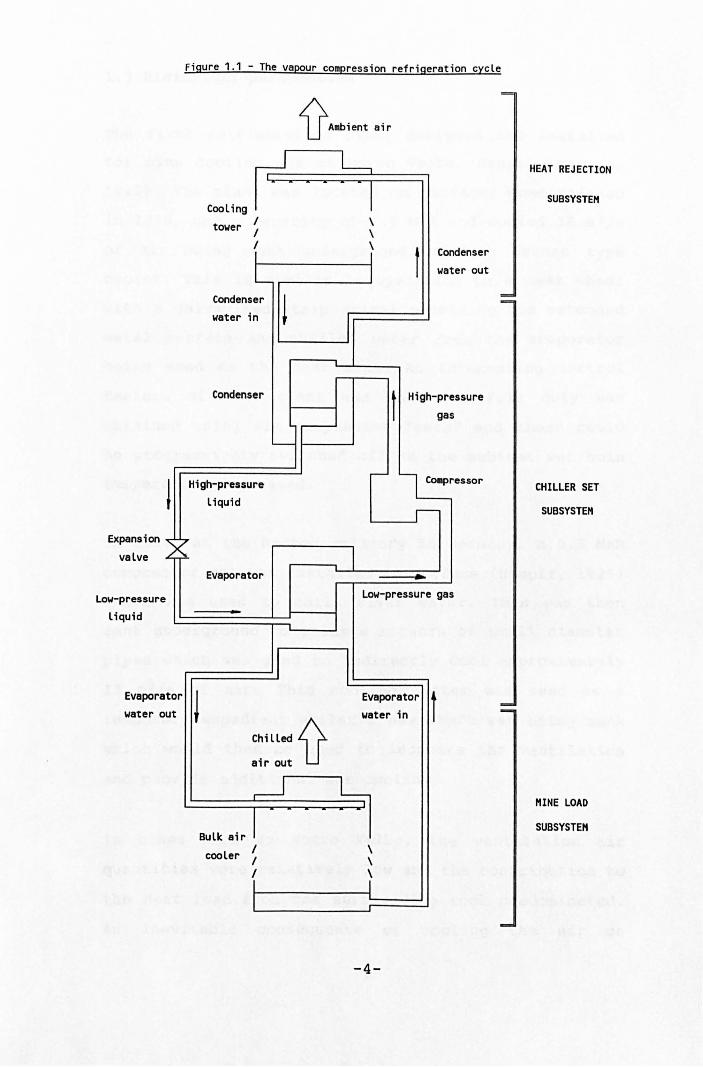
Figure 1.1 - The vapour compression refrigeration cycle
Cooling
tower I I
f L
Condenser ! water in
Condenser
r--
'----
I High-pressure
Expansion
valve
Low-pressure liquid
~
tor Evapora water 0 ut J
liquid
Evaporator
•
II
chillod 1J air out
~
Bulk air I cooler I
I
f I
L,
I \ \
~ t Con
wat
I
t High-pre
gas
r-- Compr
I
.. Low-pressure gas
I Evaporator
t water in
L
\ \
~
-4-
denser er out
ssure
essor
HEAT REJECTION
SUBSYSTEH
CHILLER SET
SUBSYSTEM
I1INE LOAD
SUBSYSTEI1
1.3 Historical perspective
The first refrigeration plant designed and installed
for mine cooling was at Morro Velho, Brazil (Davies,
1922). The plant was located on surface, commissioned
in 1920, had a capacity of 1.8 MWR and cooled 38 m3/s
of air being sent underground using a Heenan type
cooler. This is similar in operation to a heat wheel
with a galvanised strip spiral providing the extended
metal surface and chilled water from the evaporator
being used as the heat sink. An interesting control
feature of this plant was that the full duty was
obtained using six compressor "sets" and these could
be progressively switched off as the ambient wet bulb
temperature decreased.
In 1924, at the Radbod colliery in Germany, a 0.5 MWR
compressor set was installed on surface (Stapff, 1925)
which was used to chill river water. This was then
sent underground to a large network of small diameter
pipes which was used to indirectly cool approximately
12 m3/s of air. This cooling system was used as a
temporary expedient whilst a new shaft was being sunk
which would then be used to increase the ventilation
and provide additional air cooling.
In mines such as Morro Velho, the ventilation air
quantities were relatively low and the contribution to
the heat load from the surrounding rock predominated.
An inevitable consequence of cooling the air on
-5-
surface was that the heat flow from the surrounding
rock increased and the benefits diminished as mining
became more remote from surface i.e. the positional
efficiency of the plant was low. To counter this,
Morro Velho was also the first mine to install a plant
underground with the heat rejected to a cooling tower
in the bottom of the upcast shaft.
South African gold mines followed the experience
gained at Morro Velho and the first surface plant
which cooled the mine intake air was installed at
Robinson Deeps in 1935 (MacWilliam, 1937). It had a
capacity of 7.0 MWR and used a direct contact spray
system to cool 190 m3/s of intake air. In 1936 the
first underground refrigeration plant was commissioned
at the East Rand Proprietary Mines (Gorges, 1952). The
plant provided 1.8 MWR and a total of 80 m3/s of air
\\!as cooled.
This trend was followed in other mining areas wi th
deep and hot mines such as Ooregum Mine in the Kolar
Goldfields, India in 1939 (Spalding, 1940) where a
surface 4.0 MWR plant chilling air on surface was
installed. In Europe, a 2.9 MWR surface plant was
installed at Les Liegeois in Belgium (Bidlot, 1950).
This was a surface plant which supplied 33 lIs of
chilled water to underground where it was used to cool
air as close to the face as possible. Interestingly, a
pelton wheel was used to recover the energy from the
chilled water set underground.
-6-
The growth in world wide mine refrigeration capacity
was linear at about 3 MWR per year until 1965 when the
total capacity was approximately 100 MWR. Since 1965
the growth has been exponential and has doubled
approximately every six years. South African deep gold
and platinum mines have been the main users of mine
refrigeration with installed capacities of between 75
and 80% of the capacity used in mining throughout the
world. This dominant position has resulted in most of
the developments in refrigeration system design and
operation originating in South Africa.
From the late 1940' s to the mid 1970 IS, most of the
refrigeration systems installed on mines followed the
developments made in the rapidly expanding building
air conditioning industry. Chilled water systems were
used to distribute the coolth from the central plant
and indirect contact cooling coils to cool the air
delivered to the mine workings. The chilled water was
produced in standard chiller sets comprising of a
centrifugal compressor and shell and tube evaporators
and condensers. In deep metal mines, the plant was
invariably located underground (Howes, 1975) whereas
in shallower coal mines, both surface and underground
locations were used (Hamm, 1979 and Reuther, 1984).
In the mid 1970's it became increasingly evident that
the underground refrigeration systems were not meeting
the design objectives. This was mainly a result of
fouling in the heat exchangers of the chiller sets and
-7-
the difficulty of controlling large chilled water
distribution systems (Howes, 1983). In many cases, the
problems associated with condenser heat rejection was
constraining the installation of even larger systems
underground. Open circuit evaporator and chilled water
systems using direct contact water to air cooling were
found to offer significant benefits with respect to
the distribution and use of the coo1th in the working
areas in the mine (Howes, 1979).
From the late 1970' s, the majority of mine cooling
plants have been located on surface and have supplied
chilled water to either underground where it is used
for direct contact cooling and as service water, or to
bulk air coolers on surface or both. In South Africa,
the growth in surface plant capacity since 1976 was
more than four times that installed underground. By
1985, from no surface refrigeration plant capacity
(the sole surface plant surviving from the 1930's and
1940' s at ERPM was shut down in 1975), the capacity
installed on surface exceeded that installed
underground (Ramsden., 1990).
In the South African mines during the 1980 's, the
increasing depth of mining had a threefold effect on
plant design and location. Firstly, autocompression of
the intake air resulted in the necessity to bulk cool
the air on surface to ensure that the air supplied
from the intake shafts underground did not exceed the
design temperature limit.
-8-
Secondly, the heat rejection capacity of the
underground ventilation air decreases with increasing
depth of workings and increasing mine heat load. This
limits the maximum underground plant capacity and its
performance (increasing condensing temperatures result
in lower overall coefficients of performance) and
therefore the ability to meet the design working place
conditions (Stroh, 1984).
Thirdly, the logistics of circulating large water
quantities (over 1000 l/s in pipes of up to 1 m in
diameter) to distribute the cool th underground,
prompted the investigation of using ice instead of
water. This can reduce the circulating mass flow
between surface and underground by a factor of between
three and five depending on the ice fraction of the
system selected (Shone, 1988).
-9-
1.4 Location of the research
Achieving the full objectives of the research required
access to existing and new refrigeration systems and a
direct input into the design and operation of these
systems. Two Australian mines, Mount lsa and North
Broken Hill offered the necessary opportunity with the
increased mining at depth requiring larger cooling
plants and the author being involved with both in an
advisory capacity.
The first main mine refrigeration plant installed in
Australia was the R63 plant at Mount Isa in 1954. Two
1.2 MWR chiller sets ( a combination of compressor,
condenser, evaporator and expansion valve usually
mounted on a common base plate) provided chilled water
to indirectly cool intake air using cooling coils on
surface at M64 shaft. This was used to supplement the
ventilation during the first part of a mine expansion
programme which resulted in the mine tonnage being
increased fourfold to 4.0 million tonnes per year.
In 1963 the plant was converted to send the chilled
water underground in closed circuit to two high
pressure water to water heat exchangers. The cold
water in the secondary circuit was used to distribute
the cool th to coils and used for indirectly cooling
the air used to ventilate the new rock handling system
and the deepest service areas.
-10-
In 1973 the plant was expanded with a third chiller
set to a nominal capacity of 3.6 MWR (Allen, 1975). An
additional 0.6 MWR was provided by eight spot coolers
which were used in the more remote diamond drill and
development locations. A fourth chiller set was
installed as a spare unit in 1985 and a third high
pressure heat exchanger was installed underground. The
secondary water circuit for this third heat exchanger
was open at the point of application and supplied
direct contact water to air spray coolers.
This system was the first to be modelled in 1983 and
showed that the performance of the interacting
components within the system could be predicted with
acceptable accuracy. The underground section was
de-commissioned in 1989 and replaced with a new 11 MWR
surface plant at K6l which supplied chilled water in
open circuit for the new 3000 and 3500 ore bodies
(Barua, 1988).
The design and the control strategy for this new plant
was determined prior to its installation by modelling
the system based on the rated performance of its
components. After commissioning, the model was
adjusted to reflect the actual performance and is now
used as a diagnostic tool in the planned maintenance
programme. The experience gained from the modelling
resulted in stage 2, a 12.0 MWR expansion in cooling
capacity, being assessed in a similar manner and the
simulations used to optimise the plant design.
-11-
The first refrigeration plant at North Broken Hill
mine was installed underground in 1967, had a capacity
of 0.2 MWR and was used to cool the ventilation air
required when deepening the main production and
service shaft. This plant along with three small spot
coolers with a total cooling capacity of approximately
0.1 MWR, were replaced with a new 0.5 MWR chilled
water plant (Mew, 1977) in 1976 and used during the
exploration of the Fitzpatrick ore body.
The first 1.8 MWR chiller set used to provide cooling
for development of the Fitzpatrick ore body was
installed underground in 1980 (Collison, 1982). A
second set was installed in 1982 and a third in 1984
resulting in a total installed capacity of 5.4 MWR
which should have been sufficient for the mining of
the Fitzpatrick ore body.
The chiller sets provide cold water which was supplied
to both indirect (coils) and direct contact (spray)
coolers. Operational problems and design faults have
resul ted in no more than 3.5 MWR being consistently
available and prompted a detailed review in 1987. This
involved modelling the existing system and considering
alternative equipment and arrangements within this
overall system. An alternative option was to consider
a completely new surface based system which would
ei ther completely replace the underground system or
supplement it.
-12-
In 1990 a surface plant which supplies chilled water
to a surface bulk air cooler at the main production
shaft was selected. The installation was completed in
1991 and can provide up to 6.5 MWR which is used to
cool the intake ventilation air. One of the 1.8 MWR
underground sets is required to provide chilled
service water and chilled water to the development
coolers in the deepest section of the ore body.
-13-
2 REFRIGERATION SYSTEM MODELLING
The successful application of refrigeration in a mine
is measured by the costs of installation and operation
relative to the benefits of improved productivity. A
mine is dynamic in that it is continually changing and
consequently, the control of the refrigeration system
should be able to adapt to these changes such that the
cooling is applied in the most cost effective manner.
The amount of refrigeration required will vary with
the mine heat load, the surface climatic conditions
and the cooling power of the air required in the
working places. In a mechanised mine with relatively
short intake airways and cyclic operation of diesel
powered equipment, all three of the above elements
will vary and affect the control required.
In the first part of this section, the factors
affecting the mine heat load, the importance of
obtaining valid climatic data and the background to
what are acceptable thermal environmental criteria
leading to a full refrigeration load profile will be
discussed.
The multiplicity of components within a refrigeration
system and the complex interrelationships between them
precludes the possibility of a simple numerical
analysis being adequate to design and control such a
system in a cost effective manner. The overall system
-14-
can be split into three subsystems which consider the
chiller sets, the heat rejection and the mine load.
In the second part of this section, previous work on
modelling of refrigeration systems is examined with
respect to the air conditioning industry and mining.
Most work has concentrated on the chiller sets and in
particular compressor performance using theoretical
flow and head coefficients for centrifugal machines.
An alternative approach is to use an empirical method
of expressing compressor performance which is based on
the actual refrigeration effect and the input power
for a given compressor and refrigerant. The required
model has been extended to include fully the heat
rej ection and load subsystems. A general algorithm
which is the basis of all the different system models
is given along with the refrigerant properties which
are specific to the empirical method used.
-15-
2.1 Overall plant size
The mine refrigeration load is generally defined as
the mine heat load less the cooling capacity of the
ventilation air.
The mine heat load normally includes the effects of
autocompression of the air in the intake airways, heat
flow into the excavations from the surrounding rock
surfaces, heat removed from the broken rock or any
fissure water prior to leaving the intakes or working
sections of the mine and the heat contribution
resulting from the operation of any equipment used in
the ore breaking and transportation mining processes.
The cooling capacity of the ventilation air depends on
both the design thermal environmental conditions in
the working places and the actual climatic conditions
on surface. Working place conditions are limited by
maximum allowable heat stress requirements and are
normally a function of the extent of the increased
mining costs that occur as a result of less than ideal
conditions and therefore productivities.
As a result, the amount of cooling required to be
supplied by a mine refrigeration system is not
constant. Consequently, the design and the control of
the system must be able to cope with the variations in
duty in the most cost effective manner.
-16-
2.1.1 Mine heat load
Heat from autocompression
Ventilation air which is on surface relative to that
underground in the working areas of the mine has a
higher potential energy which is a function of the
difference in elevation. As air flows down the intake
shafts and airways to the working horizons, most of
this potential energy is converted to enthalpy and
results in increases in temperature, pressure and
internal energy (Hemp, 1982).
The greater the difference in elevation (depth of mine
workings) the greater the increases which are more
commonly known as the effects of autocompression. In
the return airways to surface, the reverse effect
known as auto-decompression takes place although this
has no effect on the conditions in the working places.
The effects of autocompression in a mine are virtually
independent of airflow rate although its contribution
to the total mine heat load is air quantity dependent.
Despite the disparate mining methods and consequent
differences in productivity involved in metalliferous
mining, the specific ventilation rates (tonnes of air
supplied per tonne of rock broken) for the majority of
mines, fall within the fairly narrow range of between
5 and 10 tonne/tonne (Howes, 1990).
-17-
Heat flow from the surrounding rock
The heat flow from the surrounding rock in the intake
airways and the actual mine workings is a complex
function of the thermal properties of the rock and the
air, the boundary conditions including the effects of
moisture and the proximity of other mine openings, the
time since excavation and the ventilation and inlet
air temperature history. The cyclic effects of other
heat sources such as where mechanised mining equipment
operates, can further complicate the assessment of
heat flow and may result in transient values which are
significantly different than the longer term average
heat flows (Howes, 1988).
For a typical airway of 20 m2 cross sectional area, of
average wetness in rock with a medium value of thermal
conductivity and three years since excavation, the
expected heat flow is of the order of 20 W/m for each
degree difference between the virgin rock and the dry
bulb temperature of the air (Howes, 1988). Larger and
wetter "young" airways which have been open for only
six months and have high ventilation rates would have
heat flows about 2.5 times greater. Smaller and drier
"old" airways that have been open for ten years and
have low ventilation rates would have heat flows about
2.5 times lower.
Heat flow from the surrounding rock can be the main
contribution to the total heat load for mines with
-18-
scattered low productivity working areas which are
remote from the main intake shafts and have high
virgin rock temperatures. Because heat flow from the
rock is a function of the difference between the air
and rock temperatures, its contribution to the total
will also vary seasonally with the change in surface
climatic conditions unless surface bulk air cooling of
the intake ventilation air is practised.
Broken rock and fissure water
The heat load resulting from cooling the rock broken
and removed from a mine will depend on the rock and
air temperatures and whether the material is removed
exclusively through the intake airways. In metal mines
this tends to be the general case and the rock will
normally be cooled to wi thin a couple of degrees of
the intake air dry bulb temperature. This will also
depend on the moisture content of the broken rock and
any seasonal variation in heat load or whether surface
bulk air cooling is in use.
Fissure water entering the mine may also add to the
heat load in a similar manner to that for the broken
rock. The thermal capacity of water is approximately
4.5 times that of rock and if fissure water enters the
mine in significant amounts it may have a profound
effect on the total heat load. The specific water
inflow rates are typically between 0.2 and 5 tonnes of
water per tonne of rock broken. Provided that the
-19-
water is removed from the mine through pipes and not
open drains, the contribution to the heat load is
dependent on the dry bulb temperature of the air.
Heat from mine equipment
The operation of mine equipment normally adds heat to
the mine air. A possible exception is that powered by
compressed air, however, this is usually small enough
to be ignored. For pumps, hoists and conveyors which
lift material against gravity, the contribution to the
mine heat load results from motor inefficiencies and
friction. For other equipment such as lighting, fans,
drills, short and long haul rock transportation
equipment, all the input energy ends up as part of the
mine heat load (Hemp, 1982).
The amount of electric power used underground in mines
(excluding pumps and hoists) is usually between 10 and
25 kWh/tonne. This could be as high as 50 kWh/tonne
where rock handling is carried out almost exclusively
with electric powered equipment such as scrapers. Most
electrical equipment is operated continuously at a
more or less uniform load and consequently the use of
electric power underground results in a relatively
constant contribution to the mine heat load.
In mines that are more mechanised with concentrated
mining in high productivity stopes, diesel powered
equipment currently meets the optimum cost and
-20-
mobility requirements. The diesel engine efficiency
resul ts in a heat load which is approximately three
times the engine output and can result in peak heat
outputs of up to 800 kW. Machine operation can be
broadly classified into either semi-continuous such as
moving broken rock between a draw point and an ore
pass or strongly cyclic such as that which occurs
during rock removal in a development heading.
In a semi-continuous operation the peak output heat
release is approximately 10 kWh/tonne. This, however,
only occurs for relatively short periods such as when
the bucket is being filled. The 24 hour average heat
release is of the order of 4 kwh/tonne for diesel
powered load-haul-dump equipment.
The mass of rock surrounding the excavation in which
the equipment operates semi-continuously, acts as a
thermal flywheel with heat being stored and released.
This dampens the peak equipment heat outputs and the
contribution to the mine heat load can be considered
as relatively constant and equal to the average 24
hour values. The operation of mine service vehicles
and some inevitable re-handling of the broken rock
(secondary blasting etc) will result in an actual
diesel equipment heat load some 25% higher than the 24
hour average.
In cyclic mining operations such as that which occurs
in mine development and cut and fill stoping, the peak
-21-
values for heat release can be as high as 70 kWh/tonne
where a load-haul-dump machine is working with diesel
powered haulage trucks. A typical 24 hour average
would be 6.5 kWh/tonne although a limited mining
infrastructure often necessitates re-handling of the
broken rock and average values which are two or three
times higher. Although the storage and release of heat
from the rock dampens the peak values, the heat
increase to the air is two or three times the 24 hour
average values when the diesel powered equipment is
operating (Howes, 1988).
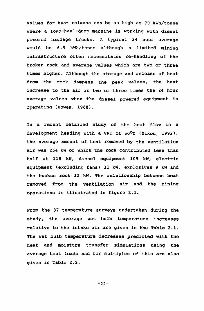
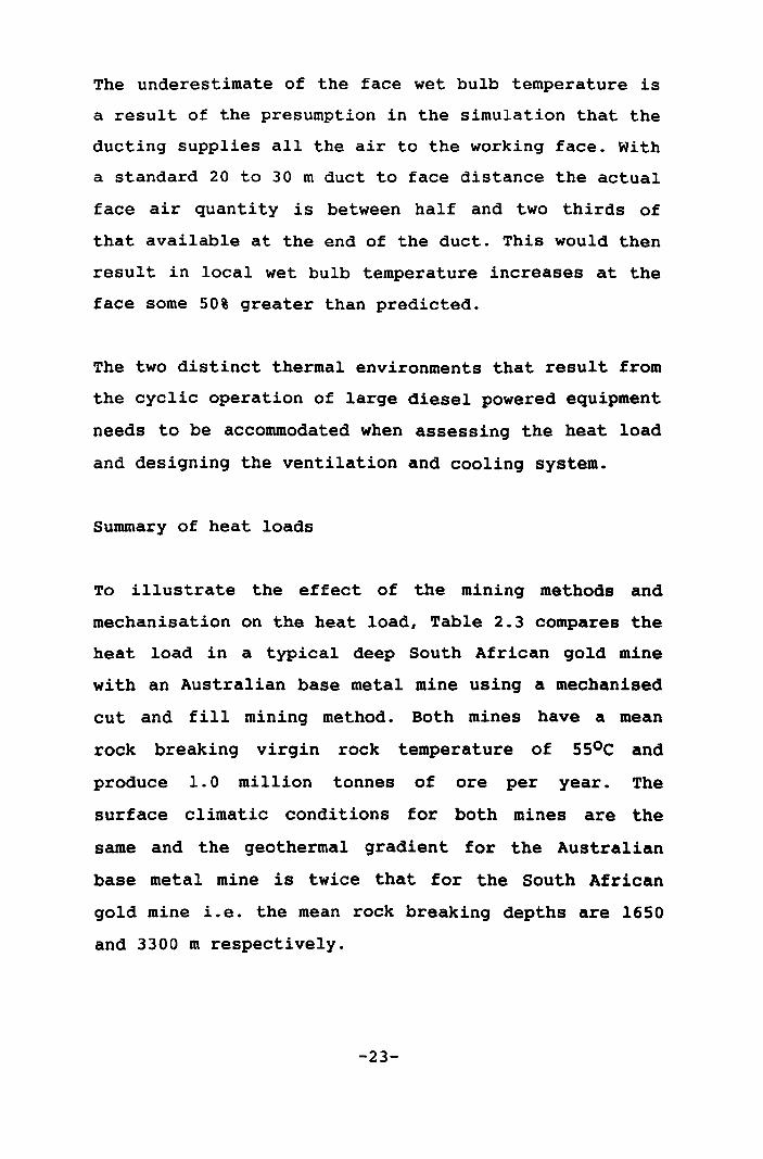
In a recent detailed study of the heat flow in a
development heading with a VRT of sOoC (Nixon, 1992),
the average amount of heat removed by the ventilation
air was 254 kW of which the rock contributed less than
half at 118 kW, diesel equipment 105 kW, electric
equipment (excluding fans) 11 kW, explosives 9 kW and
the broken rock 12 kW. The relationship between heat
removed from the ventilation air and the mining
operations is illustrated in figure 2.1.
From the 37 temperature surveys undertaken during the
study, the average wet bulb temperature increases
relative to the intake air are given in the Table 2.1.
The wet bulb temperature increases predicted with the
heat and moisture transfer simulations using the
average heat loads and for multiples of this are also
given in Table 2.2.
-22-
The underestimate of the face wet bulb temperature is
a result of the presumption in the simulation that the
ducting supplies all the air to the working face. With
a standard 20 to 30 m duct to face distance the actual
face air quantity is between half and two thirds of
that available at the end of the duct. This would then
result in local wet bulb temperature increases at the
face some 50% greater than predicted.
The two distinct thermal environments that result from
the cyclic operation of large diesel powered equipment
needs to be accommodated when assessing the heat load
and designing the ventilation and cooling system.
Summary of heat loads
To illustrate the effect of the mining methods and
mechanisation on the heat load, Table 2.3 compares the
heat load in a typical deep South African gold mine
with an Australian base metal mine using a mechanised
cut and fill mining method. Both mines have a mean
rock breaking virgin rock temperature of 550 C and
produce 1.0 million tonnes of ore per year. The
surface climatic conditions for both mines are the
same and the geothermal gradient for the Australian
base metal mine is twice that for the South African
gold mine i.e. the mean rock breaking depths are 1650
and 3300 m respectively.
-23-
... ... c , II
!" ....
26 < Ducting repairs
II ... , i" ....
reduced air quantity II
Wet bulb leaving ...
< ... r-· ----- -- .. ~ ~ at station D I I I , ..... __ r ... ..... ....
24 (1n Heeding) I ro- ::J
Wet bulb I II , ... !J
tellperature .. ------~ g. r+ II
(oC) , ~ J. . • 22 , , at station 0 , I
L __ ~ (in duct>
, II r0-
N Il
.c:. ._ .... ... I 8. ...
20 ° 12hClO 24hOO 12hOO 24hOO c
II
Dey 1 Day 2 ... ~ r0-O" ... II ,
400 II ... ... g- Il
r+
Total heat re.aved c
HeIIt , II
(kV) by ventilation air • "3"
200 II II r+
Drilling Diesel powered , equipMnt operation i ,..- -, ,..., 8.
0 ,
12hOO 24hOO 12hOO 24hOO 0"
Day 1 Day 2
I
'" VI I
26
24 wet bulb
tnperature (DC)
.... (tv)
22
20
400
200
Vet bulb entering at station D
(in duct)
----~
12hOO Day 3
24hOO
Vet bulb l .. ving at station D (in Heeding)
I I I I
I I 1. _________ 1
Total heat re.oved by ventilation air
12hOO Day 4
Diesel powered equi~t operation
... "3 II .... < • !J ... .... ... g .... r-.. .... ... :::II .... g !J ... .. II .... ." ." .... ., II r-.. ... a. ... 0
." .. ... g.
II • "3
I: ... ."
B < a.
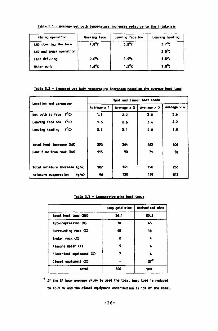
Table 2.1 - Average wet bulb t!!p!rature increases relative to the intake air
Mining operation Working face Leaving face box Leaving heading
LHD clearing the face 4.sOC 3.~C 3.~C
LHD and tNck operation 3.00C
Face dri II ing 2.00C 1.50C 1.sOC
Other work 1.SOC 1.50C 1.SOC
Table 2.2 - Expected wet bulb t!!p!rature increases based on the averege heat load
Location and parueter Spot and linear heat load.
Average x 1 Aver. x 2 Aver. x 3 Aver-oe x 4
Wet bulb at face (oC) 1.3 2.2 3.0
Leaving face box (oC) 1.6 2.6 3.4
Leaving heading (oC) 2.2 3.1 4.0
Total heat increase (kW) 252 364 482
Heat flow fro. rock (kw) 115 90 71
Total .ai.ture increase (g/.) 107 141 190
Moisture evaporation (g/.) 96 120 158
Table 2.3 - CoIp!/lIt1ve .1D! ""t load.
Deep gold .1ne "ec:han1led .ine
Total heat lOllet (~) 36.1 20.2
Autoco.pres.ion (X) 38 43
SUrrounding rock (X) 48 16
Broken rock (X) 2 4
Fi.sure water (X) 5 4
Electrical equipaent (X) 7 6
Die.el equipaent (X) - 27* Total 100 100
* If the 24 hour averege value 11 used the total h .. t lOllet i. reduced
to 16.9 "" and the die.el equ1paent contribution 11 13X of the total.
-26-
3.6
4.2
5.0
606
58
2S6
213

2.1.2 Design surface climatic conditions
Most deep Australian mines are located in subtropical
arid desert or semi-desert regions. The surface wet
and dry bulb temperatures during the summer months are
higher than those exper ienced in Europe or in many
other mining areas, including the main South African
gold mining areas.
The wet and dry bulb temperatures used for design and
given in Table 2.4, are based on measurements either
taken at the mine site or obtained from the nearest
meteorological stations. The comparative design
surface climatic conditions for South African gold
mines are similar to those given for Broken Hill in
this table.
The 2.5% design values are used to determine the worst
underground conditions and are those temperatures
which are only exceeded for 2.5% of the four month
summer period i.e. for 72 hours. If a refrigeration
plant is required, these temperatures will be used to
determine the minimum size of plant. The other three
pairs of temperatures are the mean values for the
three main climatic periods and they could be used to
give an indication of the plant operating costs.
The summary of surface climatic conditions given in
Table 2.4 is obtained by averaging the observations
over several years. Figure 2.2 shows the distribution
-27-
of wet and dry bulb temperatures over three summer
periods at Mount Isa and serves to illustrate the wide
spread of values that is possible in the data between
years. In considering the operation of a refrigeration
plant it is advantageous to refer to the temperature
data for the whole year - the temperatures given in
figure 2.3 are based on observations made over a ten
year period at Mount Isa.
The number of hours during which a given temperature
is exceeded can be established and the operational
parameters of the refrigeration plant determined for
this condition. By examining these parameters for,
say, wet bulb temperature increments of 20 C the
refrigeration load profile can be defined and the most
effective plant arrangement can be determined.
The pattern of occurrence of high temperatures during
the summer period also has an important bearing on the
design elements of the overall refrigeration system,
such as the capacities of the surface and underground
storage dams if these are required.
The values given in Table 2.5 are the number of
half-hour periods that a given temperature was
exceeded during January, 1982, at Mount lsa. This
demonstrates that the total of 72 hours during which
the 2.5% design condition prevails is contained in
five to eight peak temperature periods, each of which
lasts for several days.
-28-

Underground, the maximum and minimum temperatures
occur after the temperature extremes on surface and
the magnitude of the surface fluctuations are dampened
by the time the air reaches the underground working
place (Vost, 1980). The extent of the damping is
influenced by the amount of surrounding rock which
acts as a thermal flywheel and it is therefore more
significant in South African gold mines where the
contribution to the heat load from this source is much
greater than in the Australian mechanised mines.
-29-
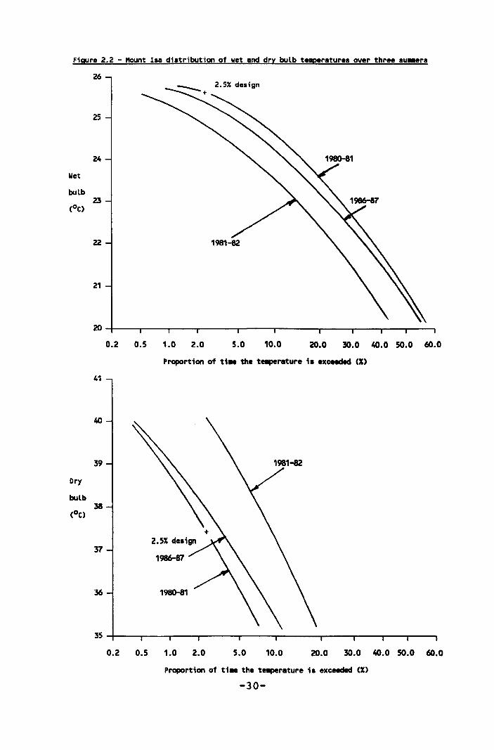
Figure 2.2 - Kount Isa distribution of wet and dry bulb temperatures over three su..ars
26
25
24
23
22
21
0.2 0.5 1.0 2.0 5.0 10.0 20.0 30.0 40.0 50.0 60.0
Proportion of ti .. the te.perature is exceeded (X)
41
40
39
38
37
36
35~---,----~---r----~r-----r-----~----~---'---'--~
0.2 0.5 1.0 2.0 5.0 10.0 20.0 30.0 40.0 SO.O 60.0
Proportion of ti .. the te.perature ;s exceeded (X)
-30-
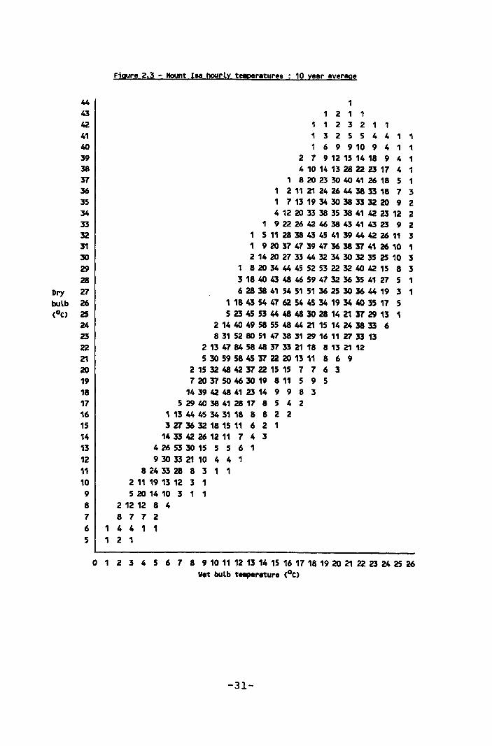
Figure 2.3 - ~t lsa hourly temperatures : 10 year average
44 43 42 41 40 39 38 "S7 36 35 34 33 32 31 30 29 28
Dry Z7 bulb 26 CoC) 2S
24 23 22 21 20 19 18 17 16 15 14
1 1 2 1 1
1 1 232 1 1 1 3 2 5 5 441 1 1 6 9 9 10 9 4 1 1
2 7 9 12 15 14 18 9 4 1 4 10 14 13 28 22 23 17 4 1
, 8 20 23 30 40 41 26 18 5 1 1 2 11 21 24 26 44 38 33 18 7 3 1 7 13 19 34 30 38 33 32 20 9 2 4 12 20 33 38 35 38 41 42 23 12 2
1 9 22 26 42 46 38 43 41 43 23 9 2 1 5 11 28 38 43 45 41 39 44 42 26 11 3 1 9 20 37 47 39 47 36 38 "S7 41 26 10 1 2 14 20 27 33 44 32 34 30 32 35 2S 10 3
1 8 20 34 44 4S 52 S3 22 32 40 42 15 8 3 3 18 40 43 48 46 59 47 32 36 35 41 27 5 1 6 28 38 41 54 51 51 36 25 30 36 44 19 3 1
1 18 43 54 47 62 54 45 34 19 34 40 35 17 5 5 23 45 53 44 48 48 30 28 14 21 37 29 13 1
2 14 40 49 58 55 48 44 21 15 14 24 38 33 6 8 31 52 80 51 47 38 31 29 16 11 27 33 13
2 13 47 84 58 48 "S7 33 21 18 8 13 21 12 S 30 59 58 45 37 22 20 13 11 8 6 9
2 1S 32 48 42 "S7 22 15 15 7 7 6 3 7 20 "S7 50 46 30 19 8 11 5 9 5
14 39 42 48 41 23 14 9 9 8 3 5 29 40 38 41 28 17 8 5 4 2
1 13 44 45 34 31 18 8 8 2 2 3 27 36 32 18 15 11 6 2 1
14 33 42 26 12 11 7 4 3 13 4 26 53 30 15 5 5 6 1 12 9 30 33 21 10 4 4 1 11 8 24 33 28 8 3 1 1 10 2 11 19 13 12 3 1 9 5 20 14 10 3 1 1 8 2 12 12 8 4 7 8 7 7 2 6 1 4 4 1 1 5 1 2 1
o 1 234 5 6 7 8 91011 n13M15 161718192021 2223~~26 Wet bulb t..perature CoC)
-31-
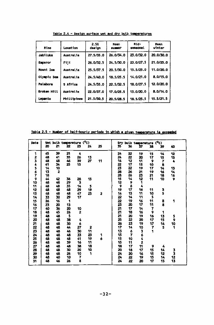
Table 2.4 - Design surface wet and dry bulb t!!p!ratures
2.5% "ean "id- "ean "ine Location design su .. r seasonal winter
Jabiluka Australia 27.5/35.0 26.0/34.0 23.0/32.0 20.0130.0
E..,eror Fiji 26.0/32.5 24.5/30.0 23.0/27.5 21.0/25.0
Itount 1 .. Australia 25.5/37.5 20.5/30.0 15.5/25.0 11.0/20.0
OlYlIPic Da. Australia 24.5/40.0 18.5/25.5 14.0/21.0 8.0115.0
Palabora S Africa 24.5/35.0 22.5/32.5 18.0/27.5 12.0/20.0
Broken Hill Australia 22.0/37.0 17.0/25.5 13.0/20.0 8.0/14.0
Lepanto Ph1lL1pines 21.5130.5 20.5/28.5 18.5/25.5 15.5/21.5
Table 2.5 - ~r of half-hourly periods in which a given t!!p!rature 1. exceeded
Date Wet bulb t..perature (oC) Dry bulb te.perature (oC) 20 21 22 23 24 25 35 36 37 38 39 40
1 45 39 21 4 24 22 19 15 14 12 2 48 41 35 26 13 24 22 20 17 15 13 3 48 48 46 39 27 11 14 12 11 9 7 4 4 41 34 25 15 22 17 15 10 8 5 14 10 23 22 19 17 14 13 6 13 2 28 26 21 19 16 14 7 18 28 26 23 21 18 16 9 44 42 36 28 13 15 14 12 11 10 9
10 48 48 29 3 12 9 1 11 48 48 35 14 5 9 8 4 12 48 48 48 29 19 19 17 16 11 3 13 48 48 48 47 23 2 14 13 11 10 5 14 33 30 29 17 22 14 11 5 15 26 16 1 22 19 16 11 8 1 16 23 20 13 23 20 17 11 8 17 40 36 20 10 21 17 14 7 18 48 45 26 2 21 18 16 9 1 19 48 48 5 21 20 19 16 13 5 20 48 48 38 4 25 22 20 17 15 9 21 48 48 30 6 26 23 19 17 14 10 22 48 48 44 27 2 17 14 10 7 5 1 23 48 48 46 30 11 13 6 3 1 24 48 48 48 33 23 1 15 7 6 25 48 48 48 41 19 6 15 10 4 26 48 48 39 16 11 15 11 2 27 48 48 48 38 18 18 17 11 9 4 28 48 48 30 20 10 20 18 17 15 14 3 29 48 48 26 10 1 24 20 16 15 12 3 30 48 40 10 7 24 22 19 15 14 12 31 48 46 26 8 24 22 20 17 15 13
-32-
2.1.3 Acceptable thermal environmental criteria
Increasing heat stress causes discomfort I reductions
in productivity, increased accident rates and
ultimately death due to heat stroke. Ventilation and
refrigeration systems are used to minimise the adverse
effects of heat stress in a mine. The design of any
ventilation and refrigeration system should therefore
incorporate the assessment of both a safe and a cost
effective strategy in dealing with a potential heat
stress problem.
A safe heat stress limit would define the worst
thermal environmental condi tions that could be
tolerated. It would relate to the limiting climatic
condi tion and the minimum possible ventilation. This
would invariably involve a considerable reduction in
productivity and a cost effective strategy would
balance the increased ventilation and refrigeration
costs with improvements in productivity.
Controlling the exposure of mining personnel to
adverse thermal environments in mines is normally
based on heat stress rather than comfort and there is
no reason why this should not continue to be so. The
application of reduced length shifts is to warn mine
personnel that the limiting thermal environmental
condition is being approached and that corrective
ventilation and cooling procedures must be instigated.
-33-
Heat balance
In simplistic terms, the operation of the human engine
is analogous to any other engine. The conversion of
the chemical energy resulting from the oxidation of
food to useful mechanical energy is inefficient. In a
diesel engine the efficiency is of the order of 33%
and in a human engine less than 20%. This means that
there will be at least five times as much heat
produced by the metabolic process as useful work done.
Metabolic energy production is related to the rate at
which oxygen is consumed and is approximately 340 W
for each litre of oxygen consumed per minute. Using
measured oxygen consumption and, assuming an average
body surface area of 2.0 m2 , the metabolic energy
production associated with different mining tasks
(Morrison, 1968) is:-
- Rest, 50 w/m2
- Light work, 75 to 125 w/m2 (machine operation
i.e. LHD or drill jumbo operator)
- Medium work, 125 to 175 w/m2 (airleg drilling,
light construction work)
- Hard work, 175 to 275 W/m2 (barring down,
building bulkheads and timbering)
- Very hard work, over 275 W/m2 (shovelling rock)
A heat balance will be achieved when the rate of
producing heat (the metabolic heat production rate) is
-34-
equal to the rate at which the body can reject heat.
Heat is rejected from the body mainly by radiation,
convection and evaporation (Stewart, 1981). The heat
exchange between the lungs and the air inhaled and
exhaled is normally less than 5% of the total and can,
therefore, usually be ignored. Any heat not rejected
to the surroundings will cause an increase in body
core temperature.
Since heat stress is related to the balance between
the body and the surrounding thermal environment, the
main parameters required to be known when determining
acceptable conditions are those associated with the
heat production and transfer mechanisms. These can be
summarised as follows:-
Metabolic heat production rates (M - w)
Skin surface area (As) (and effects of clothing)
Dry bulb temperature (tdb)
Radiant temperature (tr )
Air velocity (V)
Air pressure (P)
Air vapour pressure (ea )
The rate of heat transfer to or from the environment
depends on the equilibrium skin temperature ts and the
sweat rate Sr- These in turn depend on the response of
the body to the imposed heat stress and the effect of
thermoregulation.
-35-
Thermoregulation
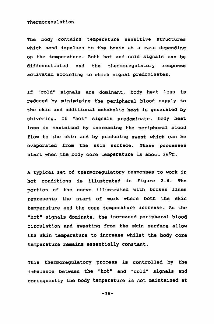
The body contains temperature sensitive structures
which send impulses to the brain at a rate depending
on the temperature. Both hot and cold signals can be
differentiated and the thermoregulatory response
activated according to which signal predominates.
If "cold" signals are dominant, body heat loss is
reduced by minimising the peripheral blood supply to
the skin and additional metabolic heat is generated by
shivering. If "hot" signals predominate, body heat
loss is maximised by increasing the peripheral blood
flow to the skin and by producing sweat which can be
evaporated from the skin surface. These processes
start when the body core temperature is about 36oC.
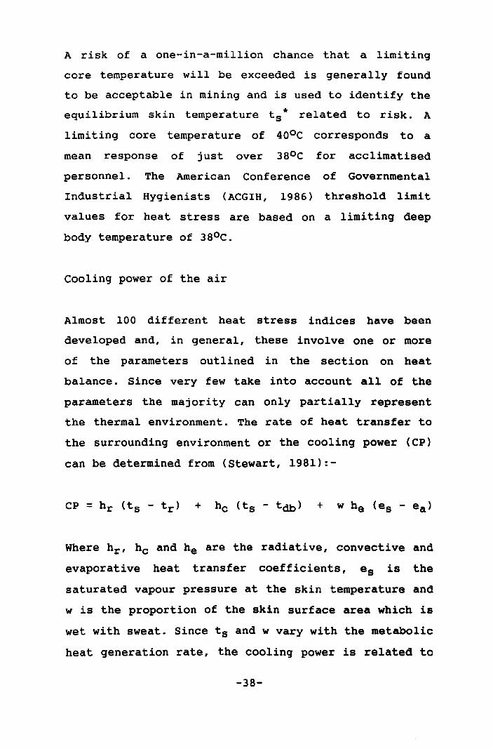
A typical set of thermoregulatory responses to work in
hot conditions is illustrated in Figure 2.4. The
portion of the curve illustrated with broken lines
represents the start of work where both the skin
temperature and the core temperature increase. As the
"hot" signals dominate, the increased peripheral blood
circulation and sweating from the skin surface allow
the skin temperature to increase whilst the body core
temperature remains essentially constant.
This thermoregulatory process is controlled by the
imbalance between the "hot" and "cold" signals and
consequently the body temperature is not maintained at
-36-
a fixed level. There is a limit to the increase in
peripheral blood supply and when the body surface is
fully wet from sweat, evaporation cannot be increased.
The thermoregulatory process cannot therefore maintain
the almost constant core temperature and eventually
there is a steeper increase in both skin and body core
temperatures.
Limiting body temperatures
A safe core temperature is that which will present a
negligible risk of incurring a heat related illness.
Experience with mine personnel exposed to and working
in hot conditions has indicated that this should not
be greater than 400 C (Wyndham, 1966). Since both the
response to heat and the degree of acclimatisation
varies between individuals, it is not sufficient to
simply read off a value of skin temperature ts which
corresponds to this limi ting core temperature from
Figure 2.4.
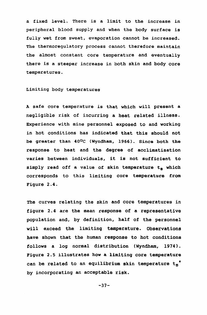
The curves relating the skin and core temperatures in
figure 2.4 are the mean response of a representative
population and, by definition, half of the personnel
will exceed the limiting temperature. Observations
have shown that the human response to hot conditions
follows a log normal distribution (Wyndham, 1974).
Figure 2.5 illustrates how a limiting core temperature
can be related to an equilibrium skin temperature ts·
by incorporating an acceptable risk.
-37-
A risk of a one-in-a-million chance that a limiting
core temperature will be exceeded is generally found
to be acceptable in mining and is used to identify the
equilibrium skin temperature ts * related to risk. A
limiting core temperature of 400 C corresponds to a
mean response of just over 380 C for acclimatised
personnel. The American Conference of Governmental
Industrial Hygienists (ACGIH, 1986) threshold limit
values for heat stress are based on a limiting deep
body temperature of 38oC.
Cooling power of the air
Almost 100 different heat stress indices have been
developed and, in general, these involve one or more
of the parameters outlined in the section on heat
balance. Since very few take into account all of the
parameters the majority can only partially represent
the thermal environment. The rate of heat transfer to
the surrounding environment or the cooling power <CP)
can be determined from (Stewart, 1981):-
Where hr' hc and he are the radiative, convective and
evaporative heat transfer coefficients, e s is the
saturated vapour pressure at the skin temperature and
w is the proportion of the skin surface area which is
wet with sweat. Since ts and w vary with the metabolic
heat generation rate, the cooling power is related to
-38-
Figure 2.4 - Iher.orequlation tnd equilibriUl core and akin t!!p!raturea
Equil ibriUli
core
t...,.rature
Equilibr1U11
core
t...,.rature
/
/ / I / /
I / /
worlt rat ..
Equilibr1U11 akin ta.perature
Figure 2.5 - Equil1br1u. akin t!!p!raturea and riak
L1.1ting teaperature
t * a
Equilibriua akin teaperature
-39-
Reducing r1ak of
li.iting t8lplrature
being exceedec:l
the work rate. If the values of ts and w can be
related to a safe limiting temperature, it follows
that, providing that the metabolic heat generation
rate of a particular mining task is less than the
cooling power of the surrounding environment, then a
safe or acceptable level of heat stress will prevail.
Cooling power is therefore an "ideal" heat stress
index which is based on the heat balance equation and
allows for the variability in human responses by
introducing the element of risk. Its main drawback is
that its calculation is complex and iterative and at
the moment a simple instrument that can be used in
underground working places is not available.
An algorithm which can be used to obtain numerical
values is given in Appendix 1. The equilibrium skin
temperatures and sweat rates used in the calculations
are based on the response of acclimatised personnel.
Charts can be developed which may be used to assess
cooling power and heat stress underground.
Care should be exercised when using tables and charts
of cooling power which originate from South Africa
(Stewart, 1982) where an arbitrary increase in air
velocity of 0.3 mls is applied. This is claimed to
allow for the effects of body movement and, even in
narrow South African gold and platinum stopes, it is
difficult to justify.
-40-
In a working place with a uniform air velocity, body
movements will be both with and against the air
current in equal measure and the relative velocity of
body movement will average out to the air velocity.
other heat stress indicators
other indices used to classify the thermal environment
fall into two main categories instruments that
simulate heat exchange and empirical scales relating
physiological and subjective responses. In the first
category, the main instruments used are wet and dry
bulb thermometers, wet and dry globe thermometers and
the wet kata thermometer.
In the second category, the main empirical scales used
are effective temperature, wet bulb globe temperature
and the predicted fourth hour sweat rate.
Al though wet bulb temperature is an important heat
stress parameter, its sole use is fraught with
problems. It can be used as an indicator that a
potential problem exists i.e. in South Africa only
personnel that have undergone an acclimatisation
procedure may work where the wet bulb exceeds 27.SoC.
Where mining and ventilation practices result in a
relatively narrow spread of environmental conditions
in the working places, a single index such as wet bulb
temperature can be used as a practical guide.
-41-
For a typical air velocity of between 0.5 and 1.0 mIs,
wet bulb temperatures in excess of 32.50 C are
invariably associated with cooling powers of less than
150 w/m2 and it will therefore be impractical to
expect anything more than the lightest of work rates
to be sustained without increasing the risk of heat
stroke. In a similar manner a wet bulb temperature of
30.00 C would be a practical limit for sustained hard
work. These limits would be significantly different if
the air velocities were much lower.
The wet kata thermometer measures the cooling power of
an environment using a fully wet surface maintained at
36.SoC. The size of the wet kata bulb, the constant
surface temperature and its fully wet surface limit
the accuracy of the method to directly measure cooling
power. Despite these inaccuracies the kata thermometer
is considered to be an acceptable index of heat stress
particularly in hot humid conditions <Stewart, 1982).
The major drawbacks are the necessity to carry hot
water and the fragile nature of the thermometer. It
is, however, a basis for a suitable instrument to
directly measure cooling power.
Effective temperature is an index of relative equal
thermal sensations which was determined by the
successive comparison of different combinations of wet
and dry bulb temperatures and air velocity and related
to saturated conditions and minimum air velocity
-42-
(Yaglou, 1926). The two nomograms available for
obtaining the effective temperature are the normal and
basic scales. The normal scale is applicable to men
normally clothed and undertaking light to moderate
work whereas the basic scale is used for men stripped
to the waist.
Although effective temperature includes air velocity
as well as the wet and dry bulb temperatures, it is
based on subjective assessment and does not include
work rate. European coal mines use the basic effective
temperature scale as a heat stress index (Graveling,
1988). In Germany the shift length is reduced to five
hours when the effective temperature exceeds 290 C.
Over a range of air velocities of 0.15 to 1.0 mls and
differences between the wet and dry bulb temperatures
of 2 to l20 C, both of which are not untypical, the
cooling power varies between 150 and 250 W/m2 for the
same effective temperature of 290 C.
When using the wet bulb globe temperature index
(ACGIH, 1986), cognizance is taken that the dry bulb
and radiant temperatures as well as the wet bulb also
influence heat stress. For most underground operations
where the radiant and the dry bulb temperatures are
wi thin a degree or so of each other, the wet bulb
globe temperature (WBGT) can be obtained from:-
WBGT = 0.7 twb + tdb
-43-
The ACGIH adopted threshold limit values for heat
stress provide a fairly comprehensive range of
permissible values which are related to the rate of
work. In broad terms, the wet bulb globe temperature
limits for light, medium and hard work are 30, 26.7
and 2SoC respectively.
The wet bulb globe temperature does not include air
velocity and when equating the work rates to cooling
power, air velocities of 0.12, 0.19 and 0.38 mls are
required. These are reasonably consistent irrespective
of the difference in wet and dry bulb temperatures.
Air velocities of less than 0.2 ml s are rare when
practising modern mining methods although they may be
encountered in difficult to ventilate non-mechanised
mining methods such as undercut and fill and square
set timbered stoping. Where mechanised equipment such
as diesel powered haulage units are used, the minimum
exhaust gas air dilution requirements result in air
velocities of between 0.5 and 1.0 m/s.
Applying the wet bulb globe temperature as a heat
stress index would result in safe values and in most
situations would result in significant overestimates
of the actual heat stress conditions.
The predicted four hour sweat rate ( P 4SR) can be
obtained from a nomogram combining wet and dry bulb or
globe temperatures, air velocity, work rate and
-44-
clothing (McPherson, 1960). The basic fourth hour
sweat rate ( B4SR) is obtained from the dry bulb and
wet bulb temperatures and is adjusted for clothing and
the work rate. The adjustment for clothing is oOe for
shorts and lOe for overalls and the adjustment for
work rate varies from oOe when resting to 40 C at a
work rate of 250 w/m2.
The B4SR obtained from the nomogram is then adjusted
for the work rate using relationships which are
clothing dependent. This heat stress index was
developed as a result of work undertaken between 1944
and 1946 at the National Hospital for Nervous Diseases
in Queen Square, London. The index was subsequently
validated by a comprehensive series of experiments
undertaken between 1948 and 1953 in Singapore.
Two factors are important when considering the P4SR
index. The first is that it arose from a recognition
that effective temperature does not provide a suitable
heat stress index for the full range of hot conditions
that may be encountered. Secondly, the index was based
mainly on wartime activities where the prime objective
was to determine the maximum activity that could be
tolerated before collapse. Mining does not fit into
this category in that life does not depend on high
activity at limiting heat stress levels.
Despite this limitation the index gives a good
indication of what constitutes a limiting heat stress
-45-
condi tion. It recognises the importance of metabolic
(work) rate and the influence of clothing when
defining heat stress conditions. A limiting heat
stress condition defined by a P4SR of between 4.5 and
5.0 is valid as a limiting condition in mining. The
index is not often used, probably because of the
complexity of the nomogram.
To summarise, for a general application covering all
types of mining and environmental conditions, the
cooling power concept will provide a consistent
assessment of heat stress. Where mining operations are
such that there is a small variation in most of the
parameters used to assess heat stress, a single
parameter such as wet bulb temperature can be used as
a practical guide. The advantage being that this can
be readily measured by all personnel involved and has
a straightforward interpretation.
The measurement of heat strain
The measurement of heat strain is an alternative to
measuring the environment in which the exposure takes
place. The four main parameters of directly evaluating
heat strain are body core temperature, heart rate,
skin temperature and weight loss through sweating.
Al though all of these parameters can be evaluated
under laboratory conditions, their extension to the
underground working place results in unsurmountable
practical problems.
-46-
Body core temperature measurements
invasive and have a low acceptability.
are usually
Heart rate
measurements require
processes and require
interruptions to the work
calibration. Skin temperature
measurements
representative
involve a
sites and
weighted
are subject
average from
to practical
limitations in the work place. Sweat loss requires the
accurate measurement of body mass which also has
practical limitations in the work place.
Although any of the above will indicate that a problem
may exist, the reason for the problem and therefore a
possible solution is not indicated. Consequently it is
unlikely that a direct measurement of heat strain will
become a practical proposition in mines and the
measurement of the working environment using heat
stress indices will remain the most suitable method of
evaluating the hazards encountered in hot mines.
Actual heat stroke risks
On the assumption that the
environmental conditions should
limiting
be based
thermal
on heat
stress rather than comfort, the acceptance of a risk
of heat stroke occurring is implicit. Air cooling
power was based on a one-in-a-million chance that a
core temperature of 400 C will be exceeded. Heat stroke
is not automatic with a greater than 400 C core
temperature but it becomes more likely.
-47-
On South African gold mines between 1970 and 1979, the
actual risk of heat stroke occurring was of the order
of one-in-six-mi11ion. If a true thermal equilibrium
existed it could be argued that the risk should be
lower. Each heat stroke case is investigated and
almost invariably an abnormal condition existed such
as a fever or excessive peer pressure. Limiting the
occurrence of heat stroke therefore becomes linked to
an educational and management programme.
During the eight years between 1980 and 1988, the
average number of personnel employed underground by
the gold mines was 375 000 of which 68% or 254 000
worked in areas where the wet bulb temperature
exceeded 27.50 C. There have been 103 heat stoke cases
during this period with no fatalities in the last
three years. The incidence of heat stroke was
one-in-five-million.
Investigations of all heat stroke cases have indicated
that they often have multiple causes with 64%
resulting from strenuous work, 52% from dehydration
(80% attributed to an excessive alcohol intake) and
29% resulting from work in very hot conditions of over
32.50 C wet bulb temperature.
In Australian terms, work by C H Wyndham at Mount Isa
(Wyndham, 1967) confirmed that employees working in
"hot" conditions became acclimatised naturally. This
takes several weeks and is the period of greatest risk
-48-
from heat stroke. It can be reduced by the selection
and education of personnel. Selection is concerned
with ensuring that heat intolerant personnel are not
exposed to "hot" conditions. In South Africa during
1988, heat tolerance testing of new personnel showed
that 44% were heat tolerant, 2% were heat intolerant
and 54% required acclimatisation.
Using the South African data, the level of risk is
such that a heat stroke case could be expected once
every 20 years for each 1000 underground employees
working in "hot" conditions. It could be argued that
Australian miners, because of a greater continuity of
employment than South African miners, are more aware
of the risks of working in "hot" conditions and the
actual risk would be substantially reduced. This is
borne out by the absence of a recorded heat stroke
case in an Australian mine.
Application of heat stress limits
The two main reasons for assessing the level of heat
stress in a mine are:-
- to assess the average heat stress which can then
be used to determine the optimum cooling and
ventilation when related to productivity.
- to assess the limiting heat stress conditions
resulting from the normal spread of values about
an average condition.
-49-
In any system using ventilation and refrigeration to
control the thermal environment, there will be a
spread of actual values about the mean condition. This
is associated with the dynamic nature of the mining
processes and the inevitable step function resulting
from implementing most corrective actions. For
example, in a development heading, the initial face
conditions will be better than average with short duct
lengths, low leakage and smaller heat gains. The face
conditions will worsen as the face advances.
The actual spread of values will depend on site
specific conditions. In the Enargite mine of Lepanto
in the Philippines, from a total of 169 working places
surveyed during June 1989, the mean wet bulb
temperature was 32. OOC with a standard deviation of
l.7oC. Of significance was both the high mean wet bulb
and the large standard deviation as illustrated in
figure 2.6. Statistically it is expected that 16% (27
workplaces) will have wet bulbs over 33.7oC and 2% (3
workplaces) will have wet bulbs over 35.4oC.
Reducing the mean wet bulb temperature by 30 C would
still result in three or four working places with wet
bulbs above 32.50 C. This example serves to illustrate
that in addition to providing optimum mean conditions,
the ventilation and refrigeration systems should be
designed to minimise the standard deviation about this
mean. Despite the very high wet bulb temperatures on
this mine, there were no known cases of heat stroke
-50-
although the productivity in the deeper and hotter
sections of the mine was significantly lower than in
other sections.
Figure 2. 7 illustrates a normal distribution about a
mean value and the application of six hour (reduced
shift length) and stop work. The mean condition is
that based on optimum productivity. The six hour work
criteria is a warning to the mine management that the
ventilation and refrigeration control systems are not
meeting the requirements and that potential heat
stress conditions exist. stop work conditions are a
recognition that personnel would have difficulty
sustaining even low work rates in that environment.
When applying cooling power as a heat stress index it
is important to recognise that the heat balance is
based on essentially nude man. The amount of clothing
worn underground depends on both safety requirements
and the air temperatures and normally decreases with
decreasing cooling power. Clothing will generally add
an additional thermal resistance between the skin and
the surrounding air and therefore reduce the cooling
power of the environment (Murray-Smith, 1987).
Until an expression is developed which takes into
account clothing, the following adjustment is used for
air cooling powers over 125 W/m2.
CP* = 0.5 CP + 62.5
-51-
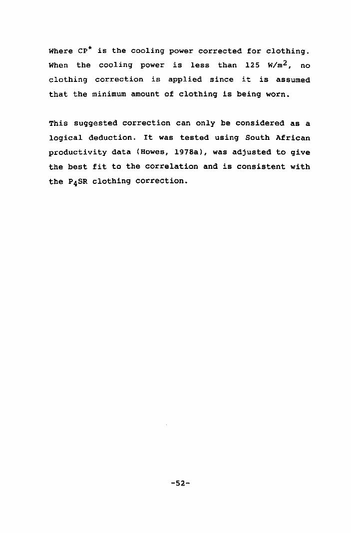
Where CP* is the cooling power corrected for clothing.
When the cooling power is less than 125 W/m2, no
clothing correction is applied since it is assumed
that the minimum amount of clothing is being worn.
This suggested correction can only be considered as a
logical deduction. It was tested using South African
productivity data (Howes, 1978a), was adjusted to give
the best fit to the correlation and is consistent with
the P4SR clothing correction.
-52-
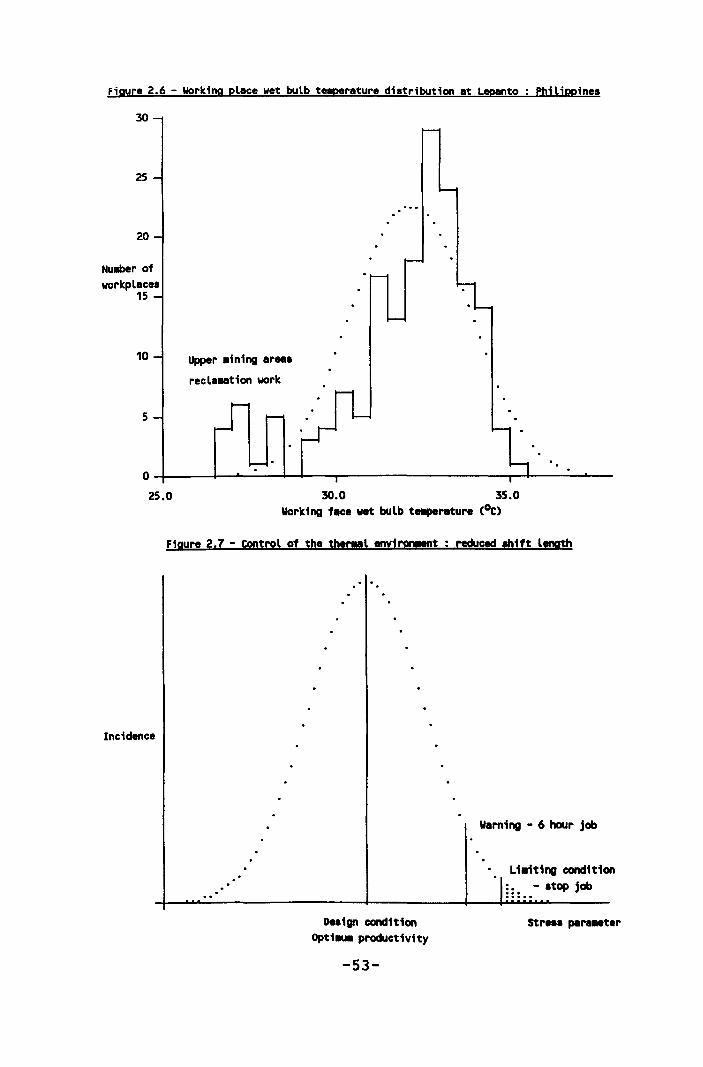
Figure 2.6 - Working place wet bulb teeperature distribution at Lepanto: Philippines
30
25
20
Nullber of workplaces
15
10 Upper atning ar .. a
recl ... tion work
5
O~----~~----~~---r-------------------.-+------~-
25.0 30.0 35.0 Working face wet bulb teaperature (oC)
Fiaure 2.7 - control of the theraal anvi!'Or!ll!!!t : reduced !hUt leoath
Incidence
Deaign condition Opti.u. productivity
-53-
\laming - 6 hour job
Li.iting condition
~ : : •• - atop job
Streaa paraaeter
2.1.4 The refrigeration load profile
Productivity and the environment
Maintaining an equivalent heat stress standard implies
that the cooling power of the air must be equal to or
greater than the metabolic heat production rate
associated with the required work rate. Where the air
cooling power is less than the work rate, two options
are possible. In the first option, the work rate is
maintained, the body core temperature increases and
heat stroke ultimately results.
In practice, the second option is far more likely,
where the work rate and therefore the metabolic heat
production rate is decreased to match the air cooling
power by taking more rest periods. In any work system
involving muscular activity a relaxation allowance is
necessary. This increases with increasing muscular
activity or work rate.
The metabolic heat production rates given in the
section on heat balance incorporate these relaxation
allowances by averaging the oxygen consumption over at
least 15 minutes. This can be illustrated by
considering the oxygen consumption for a person
shovelling rock with an average of 1.4 l/min and a
standard deviation of 0.3 l/min. For short periods,
usually less than a minute, the oxygen consumption
could be almost double the average value.
-54-
There is therefore a natural reduction in work output
to equate the metabolic heat production rate with the
cooling power of the thermal environment. For example,
if the cooling power in a work place is 150 W/m2 and
the metabolic heat production rate associated with the
work activity is 200 w/m2, by assuming that the
metabolic heat production rate for persons at rest is
50 W/m2 and by equating the metabolic heat production
rates with the air cooling power, thermal equilibrium
occurs with a rest factor of 0.333.
This means that for thermal equilibrium, only two
thirds of the available time could be spent working at
the 200 w/m2 rate and the remaining third of the time
is spent resting. How the rest time is actually used
depends on the type of work i.e. either reducing the
pace of work or by taking longer pauses between
periods of work. In this context, productivity is
defined as the ratio of work rate permissible in a
given environment, at a predetermined heat stroke
risk, to the maximum work capacity.
This definition, when examined, precludes the
possibility of obtaining perfect agreement between the
calculated and actual productivity in that the degree
of risk varies according to conditions which are not
related to the thermal environment. This has been
illustrated by the work carried out at the South
African Applied Physiological Laboratories where the
difference in productivity with different qualities of
-55-
leadership for the same thermal environment was
demonstrated (Cooke, 1961). It was also shown that the
workers with good leadership, in addition to a higher
productivity also had higher core temperatures
(measured as oral temperatures), thus the risk of heat
stroke was increased.
This logic was tested by considering productivity on
31 South African gold mines between 1973 and 1975
(Howes, 1978a). Because the mines all had similar ore
bodies and mining methods, the relationship between
productivity and wet bulb temperature by itself was
significant with a coefficient of linear correlation
of 0.41 (a value of 0.2 is significant for the number
of results considered). The coefficient of correlation
increased to 0.69 when the relationship between
productivity and cooling power was tested.
Although the 31 gold mines had similar mining methods
there were considerable differences in the extent to
which stoping was mechanised and the ratio between
development and stoping production rates. When these
-differences were taken into account, the coefficient
of correlation between productivity and the thermal
environment increased to 0.84.
Many other parameters affect productivity, not the
least of which was a concerted campaign to improve
productivity throughout the gold mining industry
midway through the period considered in the study. It
-56-
could, however, be concluded that the thermal
environment was the major reason for the differences
in productivity on "hot" mines. For the 31 gold mines
considered in the study, over 60% of the differences
in productivities within the mine and between mines
could be attributed to the thermal environment.
Although the environmental conditions currently
encountered in mechanised Australian mines are
significantly better than those prevailing in South
Africa during the period considered, a detailed
analysis should confirm the effects of improving
environmental conditions on productivity. Although
poor environmental conditions will affect all types of
work, a valid comparison of cause and effect requires
measurable quantities to be used in the analysis.
From the detailed monthly production reports, the
tonnes mined from stoping and development metres could
be obtained for the X4l mining area at Mount Isa for
each month over the last four years. The actual number
of working shifts (excluding supervision) involved was
obtained from the mine labour statistics report over
the same four years. The detailed monthly report also
had recorded the average climatic conditions and the
number of six hour shifts awarded.
From this data, the relationship between the number of
six hour shifts awarded and average surface wet bulb
temperature is illustrated in figure 2.8. The X4l
-57-
mining area is generally above its critical
ventilation depth of 1150 m (the depth at which the
ventilation air has
consequently control of
zero
the
cooling power) and
thermal environment is
achieved using ventilation only i.e. refrigeration is
not essential.
One significant feature of the curve is the incidence
of six hour shifts at low wet bulb temperatures. This
is a result of the inevitable spread of environmental
conditions about a mean value that in turn results
from the dynamic nature of the mining processes. When
assessing the implications of "hot" conditions, in
addition to the mean value it is necessary to also
determine the "spread" of values given by the standard
deviation about the mean value.
The expected relationship between the incidence of six
hour shifts and productivity is illustrated in figure
2.9 and is based on a normal distribution of values
with a standard deviation of 5.95 - 0.128 twb where
twb is the mean wet bulb temperature. Figure 2.10
illustrates the grouped productivity data for winter,
the mid seasonal periods and summer for the four
years. The values for stoping are in tonnes/manshift
and for development in metres/manshift. Development
metres were converted to tonnes/manshift using actual
development dimensions and used to obtain the combined
stoping and development productivity.
-58-
The expected trend towards lower productivities during
the mid seasonal (MS ) and summer ( 5 ) per iods when
compared to the winter (W) periods is evident although
not always consistent. This must be expected where the
thermal environment is not the sole reason for
variations in productivity. A summary of the measured
and expected productivities for the four year period
is given in Table 2.6 and confirms the approach taken
to determine the ventilation and cooling required.
Reduced shift length
To understand the background to the application of a
shortened shift length heat strain control strategy in
Australia, it is necessary to compare the air cooling
powers that are encountered in typical mechanised and
non-mechanised stoping systems.
In a non-mechanised working area such as that found in
a timber stope (square set or undercut and fill), the
air velocity is usually very low as a result of the
practical difficulties in providing adequate intake
and return ventilation and is typically between 0.1
and 0.2 m/s. The absence of significant heat outputs
from machinery results in a small difference between
the wet and dry bulb temperatures, typically between
1.0 and 2.0oC.
In a mechanised working area such as that found in a
primary cut and fill stope or in an open stoping
-59-
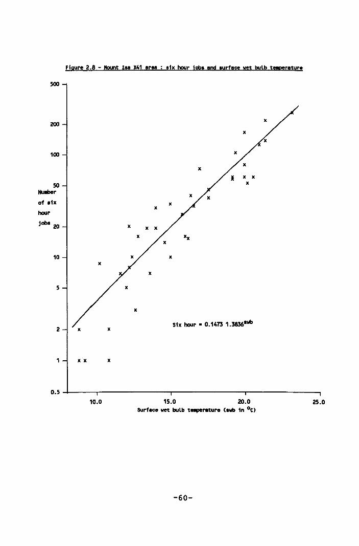
Figure 2.8 - Mount laa X41 area six hour jobs and surface wet bulb t!!p!rature
500
200 x
x
100
x x x
50 x Nullber
of six x x
hour
jobs 20 x
x Xx
10 x x
x
5 x
x
Six hour • 0.1473 1.3836lwb 2 x
1 x x x
0.5~---------~---------------------~-------------------------r---------------------~ 10.0 15.0 20.0 25.0
-60-
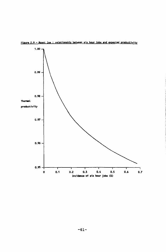
Figure 2.9 - ItoUnt 1$8 : relationship between six hour jobs and expected productivity
1.00
0.99
0.98
Therlllll
productivity
0.97
0.96
o.~~----~~----~----~------~----~----------~ o 0.1 0.2 0.3 0.4 0.5 0.6 0.7
Incidence of six hour job. (X)
-61-
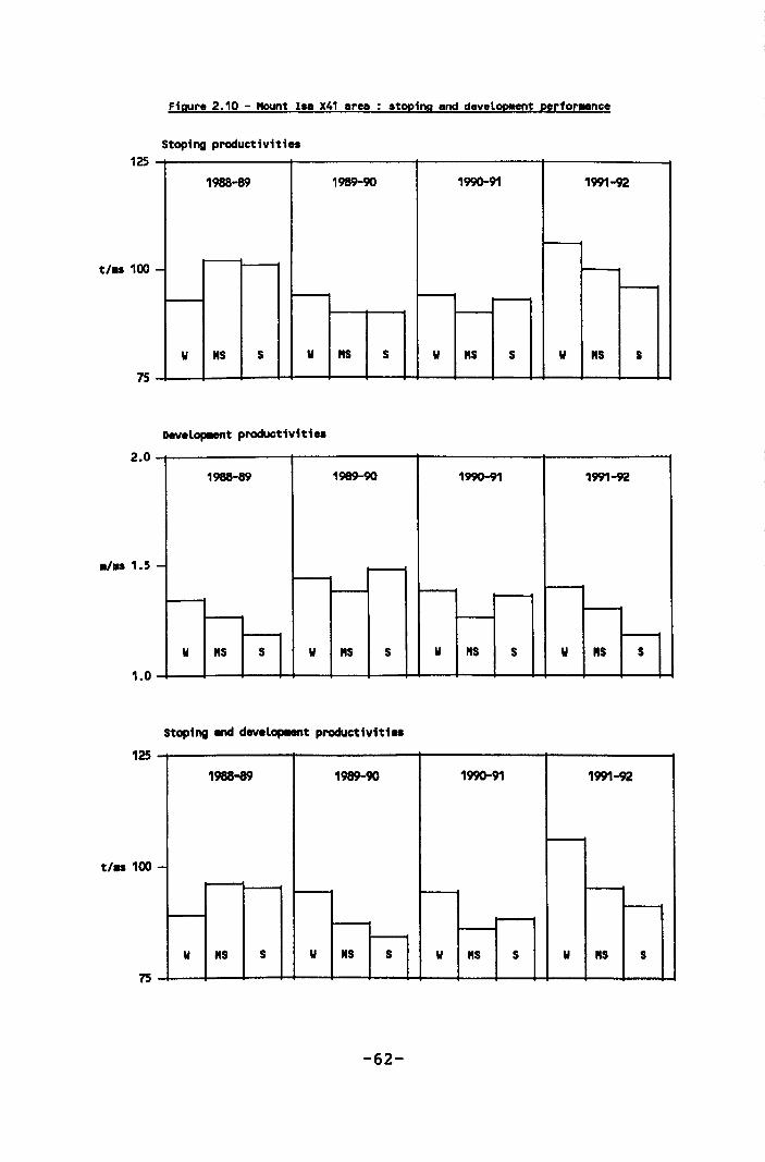
Figure 2.10 - Mount Isa X41 area: .toping and develop!!Ot perfor .. nce
5toping productivities 125
1988-89 1989-90 1990-91 1991-92
I---
t/u 100 - 1---_ - ----- I---- --
II "5 5 II "5 5 II "5 5 II "$ S
7S
Devel~t productivitie.
2.0
1988-89 1989-90 1990-91 1991-92
- --~ f--- I----
r----' I-- -
- f---W "5 5 W "5 $ W "$ $ " "5 $
1.0
Stoping and developl8nt productiv1t1u
125 1988-89 1989-90 1990-91 1991-92
f---
t/u 100 --r---- - f--- f---
-- - l--f---
W "$ $ II M$ $ W "$ $ II "$ $
7S
-62-
system, the air velocity is usually at least 0.5 mls
as a result of the minimum air quantities required for
diesel exhaust dilution. The large and mainly sensible
heat outputs caused by the operation of the diesel
powered equipment result in a difference between the
wet and dry bulb temperatures which is larger than
that encountered in non-mechanised stoping areas and
is typically between 8 and l2oC.
The data presented in table 2.7 compares the air
cooling powers expected in a mechanised mining method
and that obtained using the current New South Wales
six hour work limit of 26.7soC wet bulb temperature in
timber stopes with low air velocities. The air cooling
power at this wet bulb temperature is of the order of
150 w/m2 • In a mechanised stoping system the same air
cooling power would occur with wet bulbs between 29.0
and 30.00 C.
The 26.7SoC wet bulb limit for a six hour work was
introduced into the New South Wales legislation as a
result of the conditions experienced in the timber
stopes at Broken Hill in the late 1920's and is very
difficult to justify in a mechanised stoping system.
Indeed, in 1991 a proposed new heat stress regulation
based on cooling power I was circulated by the NSW
Mines Inspection Branch for comment. The minimum air
cooling power for six hour and stop work conditions
would be 140 w/m2 and 115 w/m2 respectively.
-63-
The original research for six hour and stop work
charts was carried out at Mount lsa (Wyndham, 1967).
The heat stress index used in deriving the limits was
the predicted four hour sweat rate (P4SR) with a limit
of 3.8 litres for six hour work and 5.0 litres for the
stop work condition.
The combination of wet and dry bulb temperatures and
air velocities derived equate approximately to air
cooling powers of 140 and 115 w/m2 for the six hour
and stop work limits respectively. The current
exemption from the mine regulations used at Olympic
Dam in South Australia is based on a six hour work
limit of 150 w/m2 .
The charts given in figure 2.11 are similar to the
Mount lsa charts and are used as a practical guide and
part of a "hot" condi tion control strategy. When
working in "hot" conditions, personnel will naturally
reduce their work rate to remain in balance with the
thermal environment. This takes place continuously
throughout the shift. A reduced shift length such as a
six hour shift, although not physiologically
necessary, will provide forewarning that stop work
conditions are being approached.
Optimisations
The cooling power of a thermal environment can be
controlled by both ventilation and refrigeration which
-64-
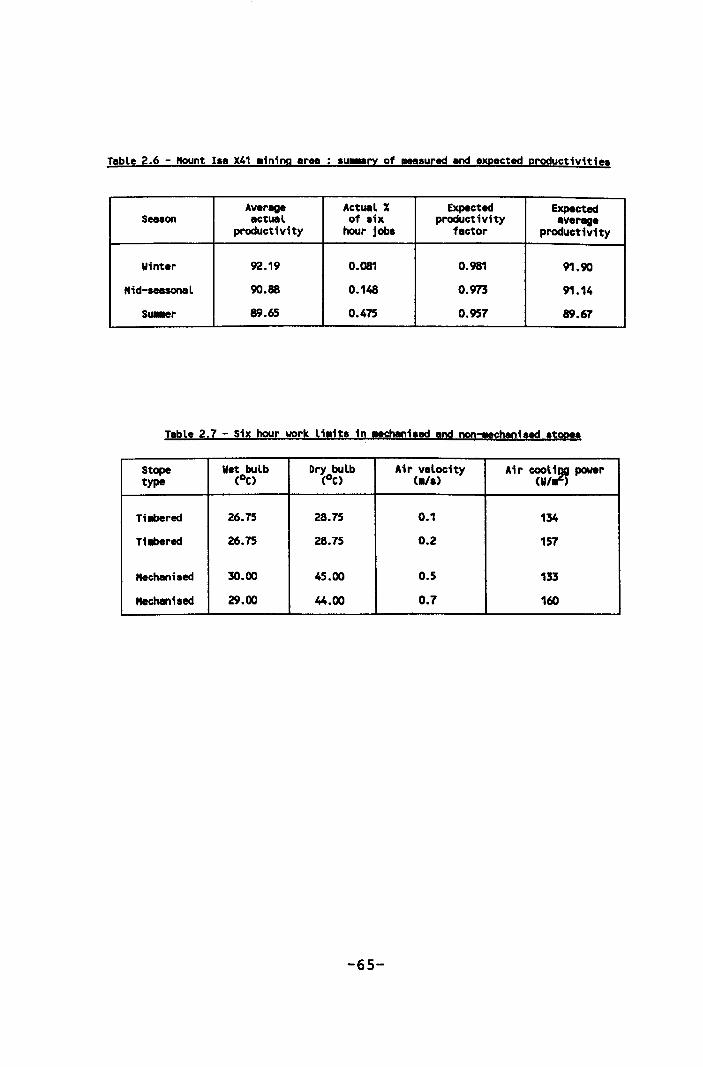
Table 2.6 - Mount Isa X41 .ining area : su..ary of .eesured and expected productivities
Average Actual X Expected Expected Season actual of six productivity average
productivity hour jobs factor productivity
Winter 92.19 0.081 0.981 91.90
Mid-seasonal 90.88 0.148 0.973 91.14
Su.er 89.65 0.475 0.957 89.67
Table 2.7 - Six hour work l i.its in .. chanisad and non=!!tCbanitad stopes
Stope Wet bulb Dry bulb Air velocity Air COOl~ power type CoC) CoC) Ca/s) CWI )
Ti_red 26.75 28.75 0.1 134
Ti_red 26.75 28.75 0.2 157
Mechanised 30.00 45.00 0.5 133
Mechanised 29.00 44.00 0.7 160
-65-
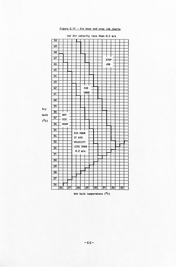
Figure 2.11 - Six hour and stop job charts
(a) Air velocity less than 0.5 mls
50
49
48
47 STOP 46 JOB
45
44
43
42 SIX
41 HOUR
40
j'l
Dry I 38
I- NOT I 37 l-
I- SIX bulb
X f- HOUR
j)
SIX HOUR 34 IF AIR 33 VELOCITY
32 LESS THAN
0.2 m/s 31
30
29
28
27
26 126 12f 128 129 130 131 132 ~
Wet bulb temperature COC)
-66-
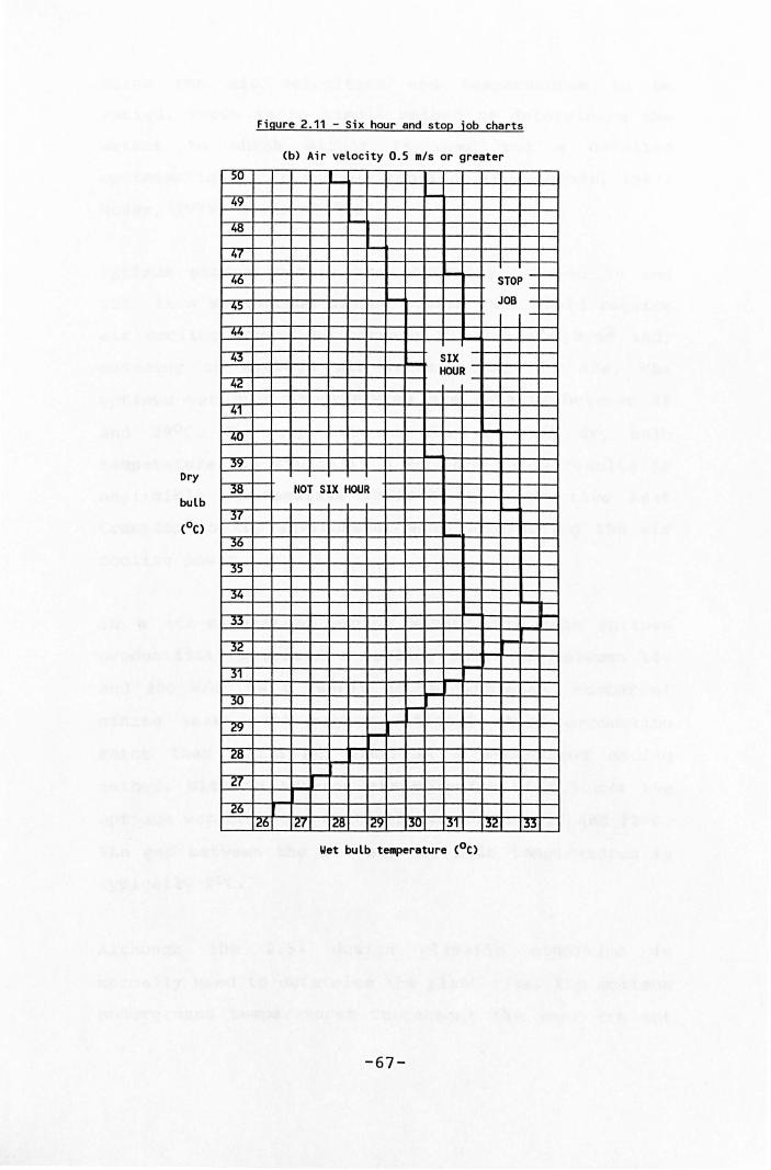
Figure 2.11 - Six hour and stop job charts
(b) Air velocity 0.5 m/s or greater
50
!!i
48
!iL
STOP ::: -46 -JOB - f--
~ -~ 44
43 SIX HOUR
~
4f
40
39 Dry
38 NOT SIX HOUR
R 36
~
34
33
32
~
30
29
28
22
26 26 127 128 129 30 131 132 .33
-67-
allow the air velocities and temperatures to be
varied. There is no simple method of determining the
extent to which either is used and a detailed
optimisation is invariably required (Lambrechts, 1967;
Howes, 1978; Howes, 1979a).
optimum productivities are generally between 90 and
95%. In a mechanised mining system this would require
air cooling powers of between 150 and 170 W/m2 and,
assuming an average air velocity of 0.7 mIs, the
optimum wet bulb temperatures are usually between 28
and 290 C. The gap between the wet and dry bulb
temperatures is typically 8 to l20 C which results in
negligible or negative radiant and convective heat
transfer to the environment when determining the air
cooling power.
In a non-mechanised mining method the same optimum
productivity requires a cooling power of between 180
and 200 w/m2 as a result of the increased number of
mining tasks with higher metabolic heat production
rates than would be found in a mechanised mining
method. With an average air velocity of 0.5 m/s the
optimum wet bulb temperatures are between 27 and 28oC.
The gap between the wet and dry bulb temperatures is
typically 2°C.
Although the 2.5% design climatic condition is
normally used to determine the plant size, the optimum
underground temperatures throughout the year are not
-68-
constant and usually decrease as the surface climatic
temperatures decrease. This is a result of a greater
cost benefit resulting from improving productivity
than the cost of operating the refrigeration plant
when operating at less than full plant duty.
Network simulations based on mass flow balance at the
junctions and incorporating heat and moisture transfer
routines (Horeby, 1988) can be used to help determine
the optimum ventilation and cooling systems. At Hount
Isa, the 3000 ore bodies development and production
schedule was used to identify future ventilation and
cooling arrangements. Intake and return airways to the
ore bodies already exist and consequently the air
quantity supplied was consistent with the systems air
handling capacity.
By repeating the simulation for different surface wet
bulb temperatures and amounts of refrigeration, a
relationship between the surface values (swb) and the
mean underground values could be established. For the
3000 ore bodies where the effective amount of cooling
(MW) is a function of the production rate (tpa) in
million t/y and the installed amount of refrigeration
(MW*) available, these relationships are:-
wb = (18.65 - 0.01223 MW2 - 0.01190 MW) x (1.023 +
0.00001058 MW2 - 0.0002315 MW)swb
MW = 1.2 x (MW* - 6.7)/tpa + 3.9
-69-
From a knowledge of the surface and underground wet
bulb temperature distributions, the mean productivity
and the proportion of six hour and stop work shifts
can be determined for any production rate, ventilation
and refrigeration arrangement. As an example, for a
surface wet bulb temperature of 22.0oC, the mean
expected underground wet bulb temperature is 28. 440 C
with an 11 MW refrigeration plant (stage 1) and a
mining rate of 1.0 million tty. This is equivalent to
an air cooling power of 164.8 W/m2.
At Mount lsa the six hour and stop work limits are
equivalent to air cooling powers of 140 and 115 w/m2
respectively. For the air velocity and the wet and dry
bulb gap expected the limits equate to wet bulb
temperatures of 30.27 and 3l.67oC respectively.
For the six hour work shift, the difference between
the limit and the mean value is 30.27 - 28.44 or
1.830 C. For a mean wet bulb temperature of 28.44oC the
standard deviation is 2.31 and the limit is therefore
1.83/2.31 = 0.792 standard deviations to the right of
the mean value (x).
Using tables of the area under the normal probability
curve to the left of a given value of x, for x = 0.792
the area is 0.7859. This means that 78.59% of the
working places will have temperatures below 30. 27oC.
Conversely, 21.41% will have temperatures above
30.27oC i.e. will have six hour work conditions.
-70-

In a similar manner the percentage of stop work shifts
that may be expected when the surface wet bulb is
22.0oC can be established. The temperature difference
is 31.67 - 28.44 or 3.230 C, the value of x is 1.398
and the expected proportion of working places above
3l.67oC is 8.10%. Since 8.10% of the working places
are stop work shifts above 31.67oC, 21.41 - 8.10 or
13.31% are between 30.27 and 3l.67oC i.e. six hour
work shifts.
The thermal environmental correction factor (TECF) is
based on the air cooling power, the work rate and the
proportion of time spent at each work rate. It is the
net productivity ratio weighted for the different
types of work involved in the mining operations and
can be obtained from:-
(CP - SO) Pn (CP - SO)
TECF = where < 1.0
(M - W) - SO (M - W) - SO
Where CP = the corrected cooling power (w/m2)
(M - W) = the metabolic heat production rate <W/m2)
The proportion of time spent working at each metabolic
heat production rate Pn will depend on the mining
method and ground conditions. Typical values for a cut
and fill or open stoping mechanised mining method can
be summarised as follows:-
-71-
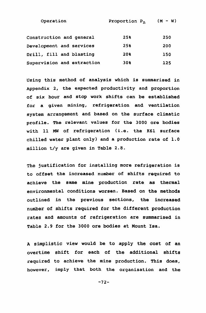
Operation Proportion Pn (M - w)
Construction and general 25% 250
Development and services 25% 200
Drill, fill and blasting 20% 150
Supervision and extraction 30% 125
Using this method of analysis which is summarised in
Appendix 2, the expected productivity and proportion
of six hour and stop work shifts can be established
for a given mining, refrigeration and ventilation
system arrangement and based on the surface climatic
profile. The relevant values for the 3000 ore bodies
with 11 MW of refrigeration (i.e. the K6l surface
chilled water plant only) and a production rate of 1.0
million t/y are given in Table 2.8.
The justification for installing more refrigeration is
to offset the increased number of shifts required to
achieve the same mine production rate as thermal
environmental conditions worsen. Based on the methods
outlined in the previous sections, the increased
number of shifts required for the different production
rates and amounts of refrigeration are summarised in
Table 2.9 for the 3000 ore bodies at Mount Isa.
A simplistic view would be to apply the cost of an
overtime shift for each of the additional shifts
required to achieve the mine production. This does,
however, imply that both the organisation and the
-72-
infrastructure is sufficiently flexible to adjust and
accommodate all the additional shifts necessary to
meet the production targets.
In practice, this is rarely the case and there will be
an inevitable shortfall in production and a consequent
loss in revenue. The difference between in situ ore
value and mining and smelting costs depends on the ore
grade and has a financial impact of up to five times
the value of the overtime shift cost. The actual cost
will lie somewhere between these two extremes.
Air cooling capacity and load profiles
In a non-mechanised mine where the heat loads are
relatively uniform, the cooling capacity of the air
will depend on the optimum conditions which includes
the effects of a decrease in productivity. As a result
of the dynamic nature of mining and the inevitable
spread of environmental conditions, there will some
reduced shift lengths which are used to ensure that
personnel will not be exposed to limiting heat stress
conditions.
On mechanised mines, the air cooling capacity of the
air depends on both ensuring that the optimum
conditions are met and, for the cyclic mining
operations, that the limiting climatic conditions are
also achieved.
-73-
For example, in a development heading, when the diesel
powered equipment is not operating, the air cooling
power may meet the optimum value of say 170 W/m2 .
Providing that the air cooling power is greater than
the six hour limit of say 140 w/m2 when the diesel is
operating, the system could be considered as adequate.
If, however, the six hour limit was not met, the air
cooling capacity should be determined by this criteria
and not the optimum values.
-74-
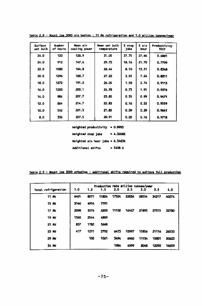
Table 2.8 - Mount 188 3000 ore bodies: 11 "W refrigeration and 1.0 .ill1on tonoes/yeer
Surface Nu~r "un air "un wet bulb % stop % six Productivity wet bulb of hours cooling power tellpt!rature jobs hour TECF
26.0 120 128.9 31.05 37.75 27.66 0.6881
24.0 912 147.6 29.72 18.16 21.70 0.7799
22.0 1080 164.8 28.44 8.10 13.31 0.8348
20.0 1296 180.7 27.22 3.55 7.24 0.8811
18.0 1272 191.0 26.05 1.58 3.74 0.9113
16.0 1200 200.1 24.93 0.73 1.91 0.9376
14.0 984 207.7 23.85 0.35 0.99 0.9471
12.0 864 214.7 22.83 0.16 0.52 0.9559
10.0 552 221.3 21.85 0.09 0.29 0.9641
8.0 336 227.5 20.91 0.05 0.16 0.9718
Weighted productivity • 0.8993
Weighted stop jobs • 4.3268%
Weighted six hour jobs • 6.3463%
Additional shifts • 5408.6
Table 2.9 - Mount 1 .. 3000 orbodies : additional !bifts required to achieve full production
Production rate .ill1on tonnea/yeer Total refrigeration 1.0 1.2 1.5 2.0 2.5 3.0 3.5 4.0
11 III 6401 8571 11824 17324 22836 28554 34317 40074
15 MW 3146 4914 7791
17 MW 2098 3574 6200 11102 16467 21893 27315 32780
19 MW 1360 2544 4809
21 MY 837 1782 3668
23 MW 417 1211 2792 6473 10997 15856 21116 26533
29111 102 1061 3494 6960 11134 15801 20623
34111 1984 4599 8048 12092 16659
-75-
2.2 Refrigeration plant analysis
2.2.1 Background to refrigeration simulations
A refrigeration system can be broadly classified into
three main components: the chiller subsystem, the load
subsystem and the heat rejection subsystem. Simulating
the operation of a refrigeration system may be either
dynamic or steady state depending on the purpose for
which the simulations are to be undertaken.
The chiller subsystem comprises of the compressor, the
evaporator and the condenser. Refrigerant compressors
can be either positive displacement which includes
both reciprocating and screw types or aerodynamic such
as the centrifugal compressor. The evaporator
interfaces with the load subsystem and, because the
cooling load is normally remote from the compressor, a
secondary fluid such as water is used to distribute
the coolth extracted from the refrigerant. The
condenser interfaces with the heat rejection subsystem
which may also use water to transfer the heat to a
point where it can be rejected to the atmosphere.
The load subsystem comprises of the equipment
necessary to distribute the coolth to the point of use
and the appliances used to transfer the coolth to the
air being conditioned. The heat rejection subsystem
comprises the equipment necessary to transfer the heat
removed from condensing the refrigerant to the point
-76-
where it can be rej ected to the atmosphere and the
equipment necessary to effect this heat transfer.
Dynamic modelling and simulation of refrigeration
systems is concerned mainly with the response times
and stability characteristics of the equipment, the
capacity control devices and the sensitivity of the
sensors. The objectives are to determine the effect of
perturbations in the system resulting from differences
in equipment response times and other real time
applications, such as system monitoring, parameter
estimation, fault detection and diagnosis.
Although the effects of system design changes can be
simulated, a dynamic model is not the most suitable
for this purpose because of its complexity and a
consequent increasing difficulty of converging towards
a solution.
A steady state model can be much simpler and more
complex systems which include an extensive load
subsystem, can be simulated without compromising the
ability of the model to converge towards a solution.
This type of model is more suitable to evaluate the
effects of changes in equipment and design and to
determine the most effective overall control strategy.
It can also be used to evaluate the results obtained
from the monitoring system of an operating plant over
a representative time period and, providing that the
-77-
control devices are limited in number and complexity,
it can be used to initiate changes which control the
performance of the system.
Air conditioning industry
The first reported refrigeration simulations in the
1970's were concerned with heat pumps and residential
air conditioners (Freeman, 1975; Hiller, 1976; Flower,
1978; Ellison, 1978; Rice, 1981). All the systems
being simulated used reciprocating compressors whose
performance was relatively straightforward to model,
and refrigerant to air heat exchangers for both the
load and heat rejection.
The main objectives of the studies were to examine
equipment design and performance improvements and for
comparative work with alternative energy sources such
as solar heating systems. Commercial sized systems
using reciprocating compressors and suitable for air
conditioning, were subsequently modelled and simulated
(Fischer, 1983).
A dynamic analysis (James, 1973) was attempted on a
laboratory sized refrigeration system which also used
a reciprocating compressor. Al though shell and tube
heat exchangers were used for the evaporator and
condenser, the load was held constant using immersion
heaters and the condenser water was once through i.e.
not cooled in a tower and recirculated.
-78-
The model for this system contained 16 differential
and 92 algebraic time dependent equations based on
mass and energy balances, momentum equations relating
force and flow rate and state equations for each zone.
The simulation had stability problems and failed to
converge if the step length was too great ( sui table
values were between 2 and 10 ms).
Both dynamic and steady state computer simulations for
centrifugal chiller systems using refrigerant to water
heat exchangers were developed in the early to mid
1980's <Clark, 1985; Hwang, 1986; Jackson, 1987). The
simulations were generally limited to the chiller
subsystem by assuming independent or constant water
temperatures for the load and heat rejection.
The load subsystem was assumed to "drive" the chiller
unit i.e. the refrigeration unit responded to changes
in return water temperature which is an input value to
the simulation. The heat rejection system was assumed
to maintain a constant return condenser water
temperature by either using variable speed fans in the
cooling towers used for heat rejection or a supply
from an very large and constant temperature source
such as seawater.
Although a cooling tower subsystem was introduced to
subsequent simulations (Nadira, 1987), the models
continued to have independent load subsystems and to
model the compressor performance from a compressor map
-79-
which was fitted to polynomial equations. From the
map, the compressor refrigerant mass flow rate and
isentropic efficiency are determined as functions of
the impeller tip Mach number and the theoretical
compressor flow and head coefficients.
The models are based on a standard refrigeration cycle
wi th superheating, sub-cooling, effects of hermetic
motors and a hot gas bypass where appropriate, and use
standard refrigerant properties to determine the state
points of the cycle.
This method of modelling compressor performance relies
on the relationships that are used in the design of
centrifugal compressors and is representative of well
designed centrifugal compressors. The generality of
the method removes possible limitations resulting from
incomplete performance data and is not specific to a
single refrigerant. An alternative method using
empirical compressor performance relationships which
are fitted to the manufacturers published test data
(Davis, 1973) is more representative of the
performance of a specific system.
other work on refrigeration system modelling in the
air conditioning industry has concerned individual
component performance such as a thermostatic expansion
valve (James, 1987) and the analysis of measurements
of plant operation taken to determine performance
characteristics when the manufacturers data is not
-80-
available (Braun, 1987). Although simulations have
been developed to consider the load subsystem (Park,
1986), they have not been combined with the chiller
and heat rejection sUbsystems.
Mining industry
In a paper discussing the assessment and prediction of
cooling plant performance (Hemp, 1981) a different
approach was taken to the method of modelling the
compressor performance. Instead of attempting to model
the aerodynamic performance and relating this to the
state points on the refrigeration cycle, an empirical
method was used which related the compressor adiabatic
head and the efficiency to the refrigerant inlet
volume flow rate.
This had the advantage that instead of detailed
compressor performance maps being required, the
necessary information could be obtained from knowledge
of the refrigeration effect and input power required
at a sufficient number of combinations of evaporating
and condensing temperatures.
Wi th the limited information normally available from
the manufacturers of compressors, this method is of
wider application and not necessarily limited to a
single type of compressor. The compressor curves
obtained are, however, limited to the refrigerant for
which the data or measurements are available.
-81-
Although the main thrust of the paper by Hemp was to
outline a manual method for the performance assessment
of the chiller set, computer simulations were also
developed (Hemp, 1986). These were extended to include
a fixed underground cooling tower subsystem for heat
rejection and cooling coils for the load subsystem and
were used mainly for predictive purposes and some
optimisation of operating arrangements.
Research work undertaken at the South African Chamber
of Mines (Bailey-McEwan, 1984; 1987) on refrigeration
system simulations was similar to the direction taken
in the air conditioning industry and concentrated on
modelling chiller sets. The simulation programme (COM,
1987) produced does not consider the load and heat
rejection subsystems and uses general rather than
actual compressor performance curves.
Al though multiple chiller sets, part duty operation
and performance with different refrigerants can be
simulated, the absence of manufacturers' specific
compressor curves limits the usefulness of the
simulation programme to general and preliminary design
features. It is unable to provide the information that
may be used as a basis for a control system and for
optimising the design and operation of a complete
refrigeration system.
Deep coal mines in Germany have the second largest
installed mine refrigeration plant cooling capacity
-82-
after South Africa. Computer modelling has also
concentrated on centrifugal chillers (Grollius, 1986)
and does not include the load and heat rejection
sUbsystems. Modelling the compressor operation is
again based on general compressor maps and has the
same drawbacks as the simulation developed by the
South African Chamber of Mines.
Other related work has involved monitoring the control
system used for chiller sets and, in addition, certain
selected water temperatures and water flow rates
(Baker-Duly, 1984; 1988). From this information, which
is transmitted from the underground plant to a surface
information centre, time trends and some performance
analysis can be undertaken. This is mainly concerned
with the plant heat balance and the compressor
coefficient of performance.
Control of the plant operation including start and
stop is still manual using the attendants who are
present on a 24 h basis. The cooling load on the
underground plants is essentially constant and any
changes which require operator decisions are
infrequent and would not require the resul ts of a
detailed plant simulation.
Development of this research work
Deficiencies in the methods and techniques available
to assess performance and to optimise the design of
-83-
future plants were evident when reviewing the mine
cooling practice in South African gold mines (Howes,
1975) and the design of the new Unisel refrigeration
plant (Howes, 1979b). The Unisel plant was the first
to be designed which was located on surface, had an
integrated chilled and service water reticulation
system in open circuit and used a pel ton wheel to
recover energy from the water supplied to the mine.
The justification for and the design of the plant was
restricted by the time required to undertake manual
performance assessment of the plant operation as a
whole. Individual elements such as the pre-cooling
tower were optimised independently.
In 1981, a review of the ventilation and cooling for
the 3000 ore bodies at Mount Isa Mine indicated a
significant future refrigeration requirement. The
existing R63 plant had a rated capacity of 3.6 MWR and
supplied a maximum of 2.5 MWR using chilled water to
two underground high pressure heat exchangers and a
cooling coil reticulation system.
In 1982/83 the actual performance of this plant was
modelled to determine whether it could provide
sufficient cooling for the initial development of the
3000 ore bodies. In addition to the multiple chiller
subsystem, the heat rejection and underground load
subsystems including pipe losses were incorporated
into the model.
-84-
In 1984 a new surface chilled water plant was
considered as a replacement and modelling was used to
optimise the preliminary plant design and to evaluate
the tenders. Low copper prices in mid 1984 resulted in
a deferment of the 3000 ore body production date and
the new surface refrigeration plant.
The R63 plant model was reviewed and modified to
determine the effect of installing a third underground
high pressure heat exchanger which would be used to
supply chilled water in open circuit to a direct
contact spray cooler. A fourth compressor was to be
installed as a spare and the heat rejection system
expanded by incorporating the original spray system
(replaced with a cross flow cooling tower in 1981).
The modifications to the plant were completed in 1985
and it was used to provide cooling until replaced with
the new K6l surface plant in 1989. A data acquisition
system was used to monitor the plant performance and
analysis of the data confirmed the suitability of the
model to represent the system operation.
In 1987, when the new K6l refrigeration plant was
being planned and designed, modelling of the system
was used to determine the optimum control strategy for
the overall system. This model was adjusted to first
design and then assess the surface plant commissioning
tests which were to be undertaken before the mine load
could be applied.
-85-
Thorough testing of the plant has resulted in the
model elements being adjusted and it is now used as a
maintenance diagnostic programme. In 1991 the
modelling techniques were used to assess the tenders
submitted for the stage 2 plant expansion and to
optimise the design and operation of this plant.
At Broken Hill, by late 1986 it was evident that the
underground plants were not providing the amount of
cooling required and a full review of the system was
required. This was completed in 1987 and a model
developed which included the multiple chiller
subsystem, the heat rejection subsystem and the mine
load subsystem. The effects of changes to both the
system and of equipment could be simulated and
improvements to the overall plant operation were made.
Despite delays resulting from the uncertainty of the
mine life in the deeper Fitzpatrick ore body, a
surface plant which is used. to bulk cool the mine
intake air was installed in 1991. The tenders for the
plant were evaluated using a refrigeration simulation
model and plant commissioning attempted in 1991. This
was completed in 1992 and the model adjusted to
reflect the actual plant operating conditions.
-86-
2.2.2 Refrigeration system simulation
The general algorithm used to model the operation of
the overall mine refrigeration system is illustrated
in figure 2.12. To initiate the iterative process
which balances the estimated and the actual compressor
adiabatic heads (h and hc )' a series of start values
are assumed. These include evaporator duty, compressor
input power, evaporating and condensing temperatures
and are normally taken as the design values for the
refrigeration plant.
For the refrigeration systems being considered, the
coolth provided is distributed using chilled water.
The initial compressor, condenser and evaporator
(chiller subsystem) balance is therefore based on a
fixed water temperature into the evaporator (twie) and
perfect condenser heat rejection.
The second compressor balance is obtained by equating
the condenser thermal performance with the condenser
heat rejection system and repeating the chiller
subsystem balance until the condenser load matches the
heat rejection capacity.
The final compressor balance is obtained by equating
the evaporator thermal performance with the heat
transfer characteristics of the mine cooling
appliances (the mine load subsystem). Both the chiller
subsystem and the heat rejection subsystem balances
-87-
are repeated until the evaporator load matches the
mine load. Where necessary, at low evaporating
temperatures or at high compressor motor powers, the
compressors are allowed to unload.
-88-
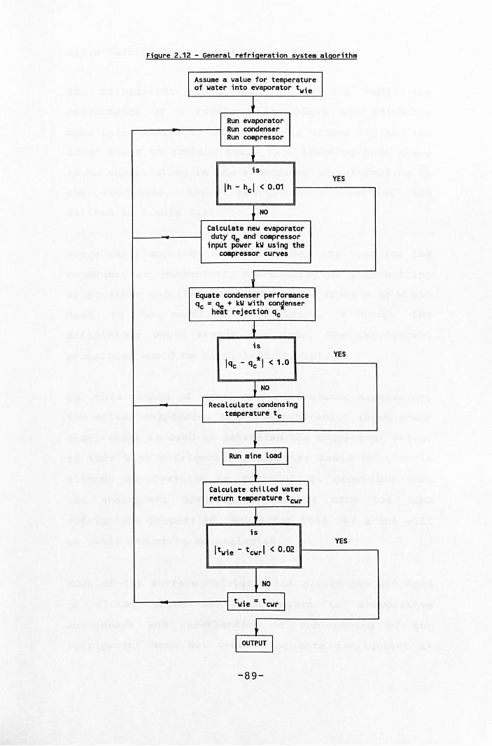
Figure 2.12 - General refrigeration system algorithm
Assume a value for temperature I of water into evaporator twie
~ Run evaporator Run condenser Run compressor
t is
YES Ih - hcl < 0.01
~NO Calculate new evaporator duty qe and compressor
input power kW using the compressor curves
~ Equate condenser performance qc = qe + kW with conienser
heat rejection qc
t is
* YES
Iqc - qc I < 1.0
~ NO
I Recalculate condensing I temperature tc
~ Run mine load
~ Calculate chilled water I return temperature tcwr
~ is
YES I twie - tcwr I < 0.02
~NO l twie = tcwr I
~ l OUTPUT I
-89-
2.2.3 Refrigerant properties
The refrigerant properties required
performance of a refrigeration plant
to model the
are adiabatic
head (h), compressor inlet specific volume (v) and the
ideal power to cooling ratio (I). Assuming that there
is no superheating in the evaporator or sub-cooling in
the condenser, these refrigerant properties are
defined in figure 2.13.
Where shell and tube heat exchangers are used for the
condenser or evaporator, sub-cooling or superheating
is possible and the state pOints in figure 2.13 would
need to be modified accordingly. Although the
definitions would remain the same, the refrigerant
properties would be slightly different.
For this method of compressor performance assessment,
the actual evaporator duty and compressor input power
requirement is used to determine the compressor curve.
If this uses refrigerant properties based on a cycle
wi thout superheating or sub-cooling, providing that
the subsequent compressor analysis uses the same
refrigerant properties, any error that may arise will
be small enough to be neglected.
Most of the surface refrigeration plants now use open
or closed plate heat exchangers or evaporative
condensers and superheating or sub-cooling of the
refrigerant does not occur. The main refrigerant is
-90-
ammonia although R22 is used in the underground plant
at Broken Hill and RII in the original Mount Isa R63
centrifugal chiller plant.
Properties of ammonia
Using the data available from published tables of
refrigerant properties (perry, 1973), curve fitting
was used to obtain the approximate relationships
between the refrigerant properties and the evaporating
and condensing temperatures te and t c ). Wi thin the
normal operating range of temperatures, the
approximate relationship is usually within 0.2% of the
tabulated value with a maximum error of 0.5%.
h = (4.5963 - 0.03042 te + 0.00020314 t e2 ) tc
- 4.6621 te + 0.03051 t e2 + 1.17
v = [(230.07 + 0.75653 tc + 0.006057 t c2 ) - (8.6295
+ 0.029523 tc + 0.00022937 t c2 ) te + (0.1887
I =
where
+ 0.0007022 tc + 0.00000455 t c2 ) te2 ]/10002
(0.0018635 - 0.003797 te + 0.00002933 t e2 )
+ (0.0035361 - 0.000032146 te
- 0.0000002773 t 2) e tc + (0.000018434
+ 0.0000003681 te + 0.00000001349 t e2 ) t 2 c
h = adiabatic head (kJ/kg)
v = specific inlet flow rate (m3/s/kW)
I = ideal power to cooling ratio
-91-
Refrigerant R22
In a similar manner to that used for ammonia, curve
fitting routines were used to obtain the approximate
relationships for refrigerant R22 from published data
of refrigerant properties (IIR, 1981). The estimated
values using the approximate relationships are within
0.25% of the published value for a range of condensing
temperatures between 20 and 480 C and for evaporating
temperatures between -10 and +lOoC. This range of
evaporating and condensing temperatures covers the
normal operating range for a mine refrigeration plant
compressor either on surface or underground.
h = (0.6583 - 0.002167 te + 0.00001429 t e2 ) tc
- 0.7677 te + 0.003788 t e2 - 0.001541 t c
2
+ 0.1048 tc + 0.008
v = {[2.343 exp(-0.03613 t e ) - 0.0002537 te
+ 0.0003045 t e2 - 0.01197] tc
+ 211.8717 exp(-0.03301 t e ) - 0.01175 te
+ 0.02366 t e2 - 0.935 - (1.5345 tc - 0.02241 t c
2
- 24.38) exp{-0.03791 t e )}/l0002
I = [5278.16 exp{-0.01320 t e > - 0.1125 te
+ 0.1391 t e2 - 5.5] tc/10002 - 0.003153 te
- 0.00001949 t e2 + 0.02853 - (0.002347 tc
- 0.00003419 t c2 - 0.03736) exp{-0.02056 t e )]
-92-
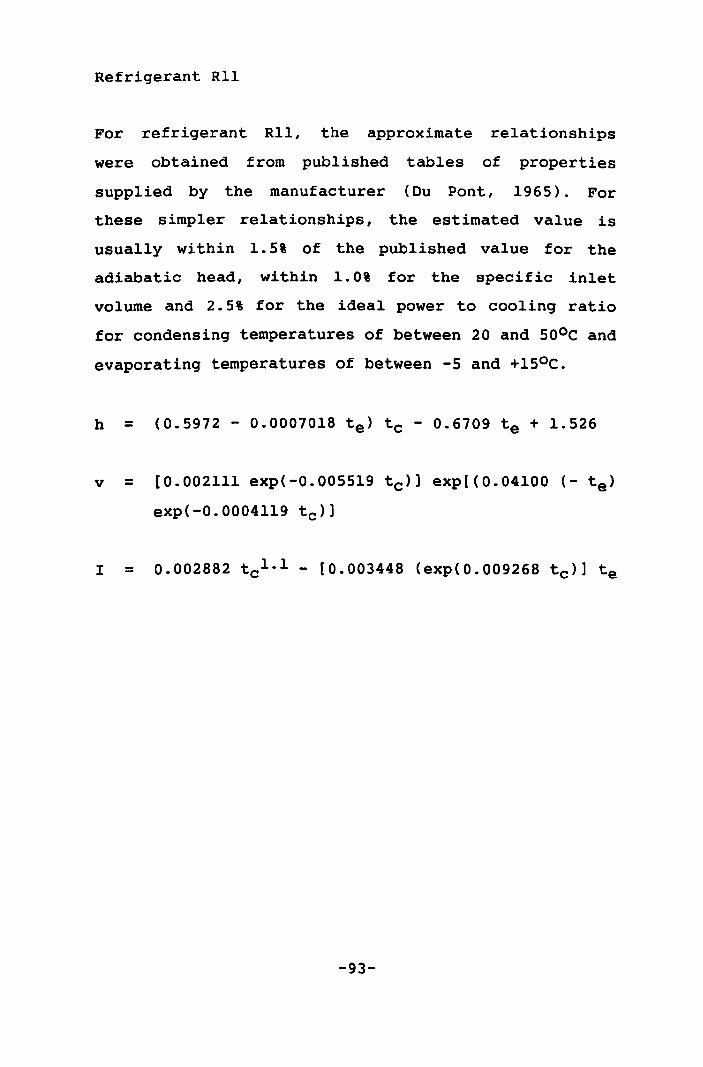
Refrigerant Rll
For refrigerant Rll, the approximate
were obtained from published tables
relationships
of properties
supplied by the manufacturer (Du Pont, 1965). For
these simpler relationships, the estimated value is
usually wi thin 1. S% of the published value for the
adiabatic head, within 1.0% for the specific inlet
volume and 2.S% for the ideal power to cooling ratio
for condensing temperatures of between 20 and SOOC and
evaporating temperatures of between -S and +lSoC.
h = (0.S972 - 0.0007018 t e ) tc - 0.6709 te + 1.S26
v = [0.002111 exp(-0.00SS19 t c )] exp[(0.04l00 (- t e )
exp(-0.0004ll9 t c )]
I = 0.002882 t cl . l - [0.003448 (exp(0.009268 t c )] te
-93-
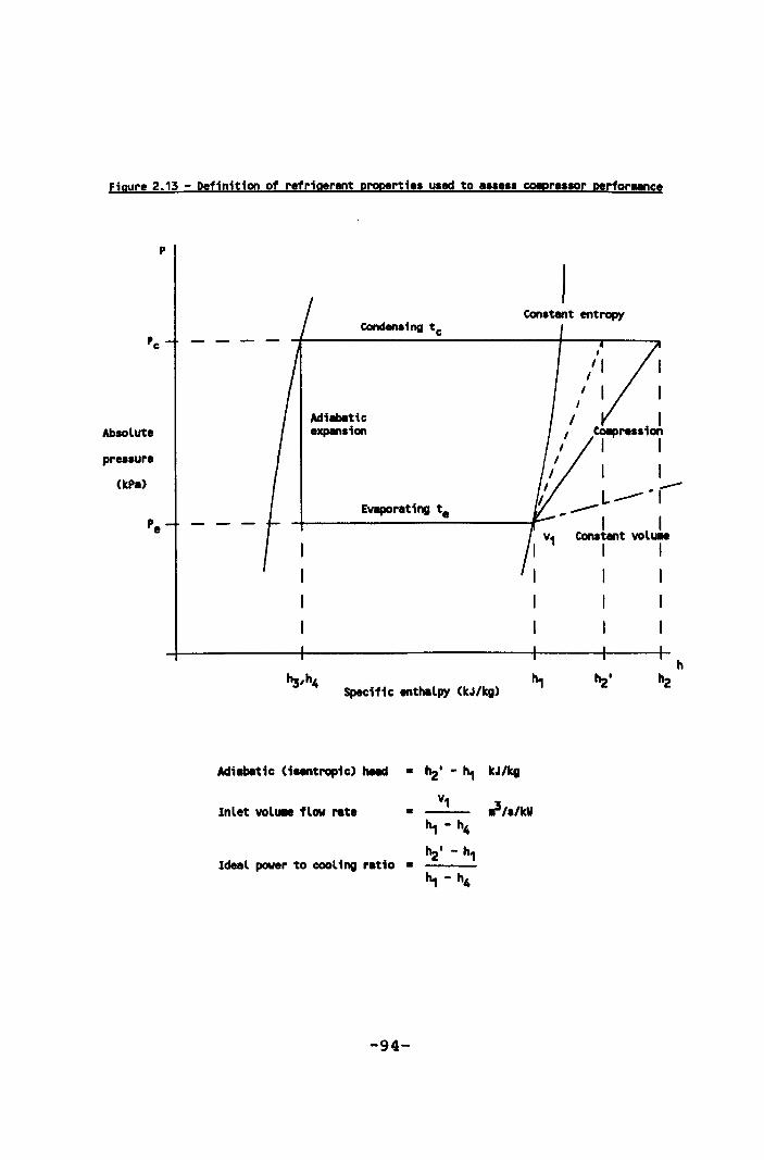
Figure 2.13 - Definition of r.frig.rant properties u.ed to •••••• COIpre.aor perforMance
p
Absolut.
pr ••• ure
(kP.)
Con.tant entropy
Evapor.ting t.
Specific enthalpy (kJ/kg)
Adiabatic (iaentropic) heed • ~' - "" kJ/1cg
Inl.t volUie flow rate • ,}1./kW
Ideal power to cooling ratio •
-94-
I I
I
I CoiIpre •• ion I I
I I I / L...--·r ..-- I I
eon.t.nt volUile I I I I
3 BQUIPMBRT PBRPORMANCB
For the five refrigeration system models considered,
two types of compressor (nine different models), four
types of evaporator, three types of condenser, two
types of cooling tower and five types of cooling
appliance are used. In this section the performance of
each is considered and the method of analysis defined.
3.1. Compressors
Using the definitions and approximate refrigerant
property relationships outlined in section 2.2.3 and
the compressor performance data provided by the
manufacturers, the compressor performance curves of
adiabatic head and efficiency plotted against the
refrigerant inlet volume flow rate can be established
for each of the compressors modelled.
For each combination of evaporating and condensing
temperature, the manufacturers data gave the amount of
cooling transferred at the evaporator and the required
power input to the compressor. Using the evaporating
and condensing temperatures, the adiabatic head h
(kJ/kg), the specific compressor inlet flow rate v
(m3/s/kW) and the ideal power to cooling ratio, I, can
be calculated.
The actual compressor inlet flow rate is obtained by
multiplying the specific inlet flow rate by the
-95-
cooling transferred at the evaporator. The ideal power
input to the compressor is obtained by dividing the
cooling transferred at the evaporator by the ideal
power to cooling ratio. The compressor efficiency is
determined by dividing the ideal power input by the
manufacturers rated power input.
3.1.1 Compressor part load operation
The two main control options available to operate a
refrigeration plant use either batch or continuous
evaporator water supply. With batch supply, the
compressor operates intermittently at full load and
storage tanks are used to provide and store water when
the cooling load is reduced. With continuous water
supply, when the mine cooling load is reduced, the
compressors continue to operate but unload to meet the
actual cooling demand.
For the centrifugal compressors used in the Mount Isa
R63 plant, part load operation of the 17 M compressors
is achieved by reducing the compressor speed (driven
by a variable speed motor). When this is modelled, the
compressor inlet volume flow rate is assumed to vary
in direct proportion to the change in speed and the
compressor efficiency is assumed to be unchanged.
The 19DG compressor has a hot gas by-pass which is
used to avoid surge (unstable recirculation around the
impeller blades) when operating at part load. Since
-96-
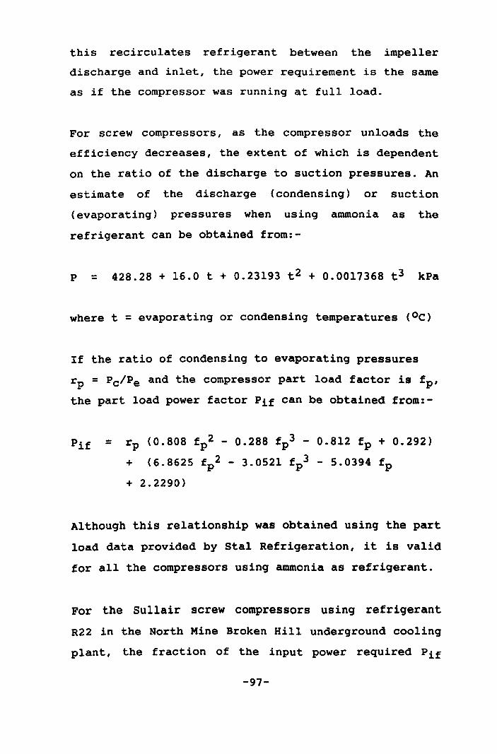
this recirculates refrigerant between the impeller
discharge and inlet, the power requirement is the same
as if the compressor was running at full load.
For screw compressors, as the compressor unloads the
efficiency decreases, the extent of which is dependent
on the ratio of the discharge to suction pressures. An
estimate of the discharge (condensing) or suction
(evaporating) pressures when using ammonia as the
refrigerant can be obtained from:-
P = 428.28 + 16.0 t + 0.23193 t 2 + 0.0011368 t 3 kPa
where t = evaporating or condensing temperatures (oC)
If the ratio of condensing to evaporating pressures
rp = Pc/Pe and the compressor part load factor is fp'
the part load power factor Pif can be obtained from:-
Pif = rp (0.808 fp2 - 0.288 f p 3 - 0.812 fp + 0.292)
+ (6.8625 fp2 - 3.0521 f p 3 - 5.0394 fp
+ 2.2290)
Although this relationship was obtained using the part
load data provided by Stal Refrigeration, it is valid
for all the compressors using ammonia as refrigerant.
For the Su11air screw compressors using refrigerant
R22 in the North Mine Broken Hill underground cooling
plant, the fraction of the input power required Pif
-91-
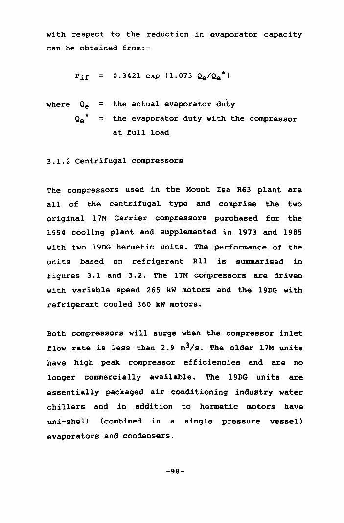
with respect to the reduction in evaporator capacity
can be obtained from:-
= 0.3421 exp (1.073 Qe/Qe *)
where Qe = the actual evaporator duty
Qe * = the evaporator duty with the compressor
at full load
3.1.2 Centrifugal compressors
The compressors used in the Mount Isa R63 plant are
all of the centrifugal type and comprise the two
original 17M Carrier compressors purchased for the
1954 cooling plant and supplemented in 1973 and 1985
with two 19DG hermetic units. The performance of the
units based on refrigerant R11 is summarised in
figures 3.1 and 3.2. The 17M compressors are driven
with variable speed 265 kW motors and the 19DG with
refrigerant cooled 360 kW motors.
Both compressors will surge when the compressor inlet
flow rate is less than 2.9 m3/s. The older 17M units
have high peak compressor efficiencies and are no
longer commercially available. The 19DG units are
essentially packaged air conditioning industry water
chillers and in addition to hermetic motors have
uni-shell (combined in a Single pressure vessel)
evaporators and condensers.
-98-
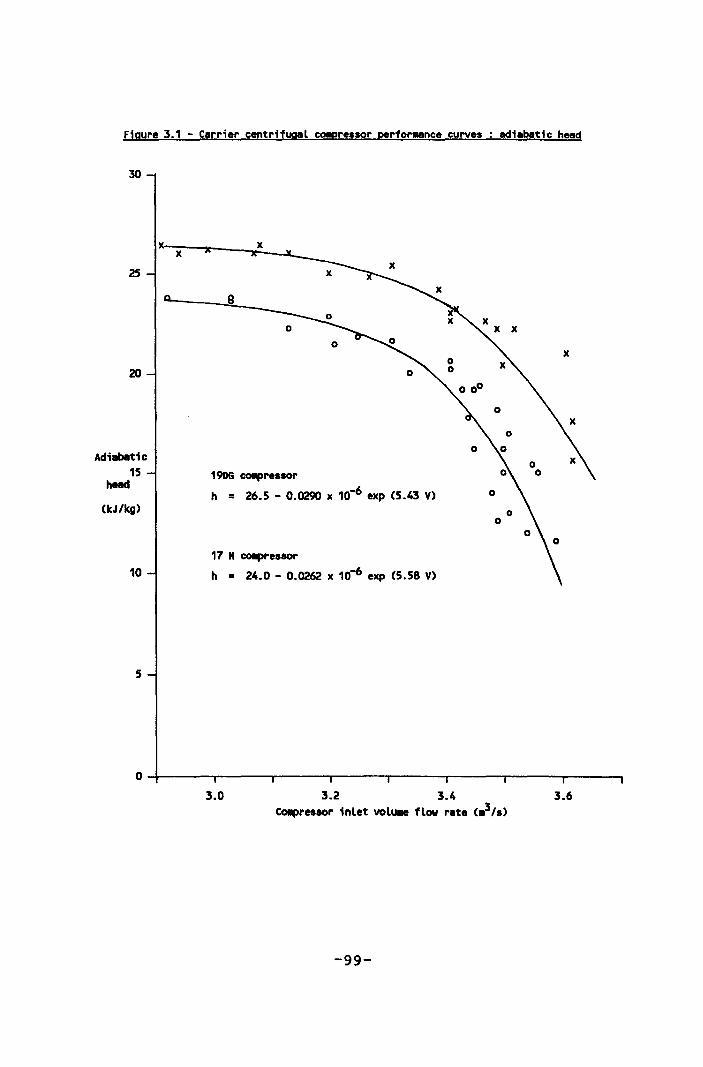
Fioure 3.1 - Carrier centrifugal COIpreasor perfor.ance curves adiabatic head
30
2S
20
Adiabatic 15
head
(kJ/kg)
10
5
x x
8
o
1906 COIIpreasor
h = 26.5 - 0.0290 x 10⁻⁶ exp (5.43 V)
17 " COIIpresaor h • 24.0 - 0.0262 x 10⁻⁶ exp (5.58 V)
o
o o
x
O~---------~-------'----------.--------r------T--------'---------r--------'
3.0 3.2 3.4 3.6 co.presaor inlet volu.e flow rate (.3/a )
-99-
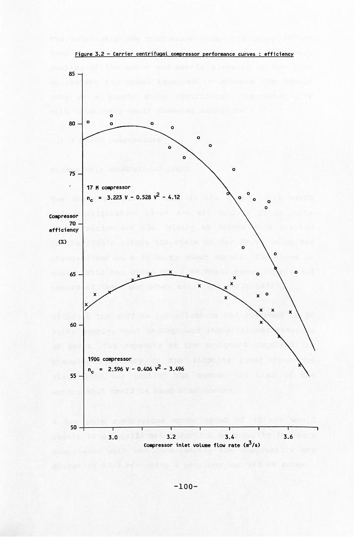
Figure 3.2 - Carrier centrifugal compressor performance curves efficiency
85
80
75
COlIIPressor 70
efficiency
(X)
65
60
55
o o
0 __ ---_ 0 o
17 H cOlllPressor
nc = 3.223 V - 0.528 y2 - 4.12
x
1906 compressor
nc = 2.596 V - 0.406 y2 - 3.496
o o
o
o
x x
o o
o
o o
x 0
o
50~------r------r-----'r-----.------'r-----.------'r-----.
3.0 3.2 3.4 3.6 Co~ressor inlet volu.e flow rate (.3,s)
-100-
The relatively low compressor peak efficiency of the
19DG compressors is partly a result of the refrigerant
cooling of the motor and partly a result of the high
equivalent tip speed required to achieve the design
duty as a single stage centrifugal compressor unit
with relatively small diameter impellers.
3.1.3 Screw compressors
Broken Hill underground plant
The three compressors used in the Broken Hill North
mine refrigeration plant are all Sullair C25SA units
using refrigerant R22. Mining at Broken Hill started
in the l880's before the state of New South Wales had
standardised on a 50 Hertz power supply. The mines in
Broken Hill had opted for a 40 Hertz power supply and
generated their own power until the early 1980's.
Although the surface installations had switched to 50
Hertz supply, most underground installations remained
40 Hertz. The capacity of the equipment required for
changing frequency of the incoming power from the
state grid has limited the number and size of the
motors that could be used underground.
A two pole synchronous motor speed of 40 rls would
result in a significant reduction in capacity for each
compressor unit and consequently the compressors are
driven at 62.5 rls using a gear box and 387 kW motors.
-101-
The performance curves for the compressors at this
speed are given in figure 3.3.
The maximum power required by the compressor is 460 kW
when operating at both high condensing and evaporating
temperatures (over 450C and 100C respectively).
Consequently I to protect the motor I the compressor
unloads by progressively closing the slide valve
capacity control when the amperage drawn by the motor
reaches a pre-set maximum value.
Mount lsa surface plants
The compressors tendered for the Mount Isa stage 1
surface chilled water plant and the stage 2 surface
bulk air cooler plants are the Howden 321-19321, Stal
S93-26 and the Sabroe 536H screw compressors.
The Howden compressors were used for the stage I
surface chilled water plant and have 321 mm diameter
rotors I a length to diameter ratio of 1.93 and a
built-in volume ratio of 2.1. The rated performance of
this compressor using ammonia as the refrigerant is
illustrated in figure 3.4. Witnessed compressor tests
were undertaken on the two units at the factory prior
to delivery. The capacity was found to vary by -2.5%
and -0.5% and the input power by +1.5% and +2.7% for
units 1 and 2 respectively.
Stal compressors have been selected for the stage 2
-102-
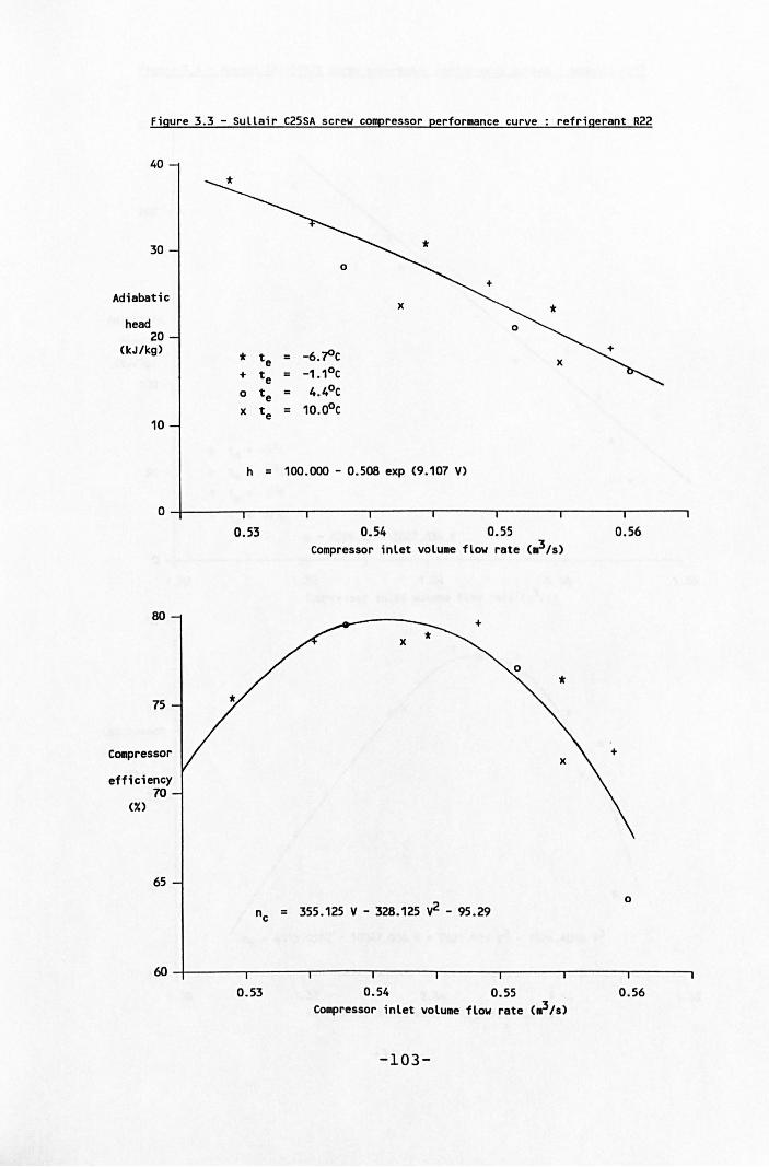
Figure 3.3 - Sullair C25SA screw compressor performance curve refrigerant R22
40
30 * °
Adiabatic x head
20 (kJ/kg)
* te = -6.J<lc x + te -1.1oc
° te 4.4oC x te = 10.0oC
10
h = 100.000 - 0.508 exp (9.107 V)
O~------,-------r------'-------r------.-------.-------r------'
80
75
Compressor
efficiency 70
(X)
65
0.53 0.54 0.55 0.56 Compressor inlet volume flow rate (~/s)
x
nc = 355.125 V - 328.125 v2 - 95.29 °
W~-----.-----.r-----'-----.------.-----.r-----.-----~
0.53 0.54 0.55 0.56 Compressor inlet volume flow rate (~/s)
-103-
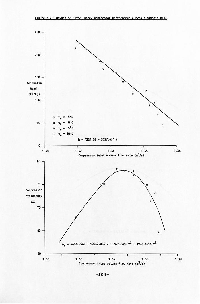
Figure 3.4 - Howden 321-19321 screw compressor performence curves ammonia R717
250
200
150
Adiabatic
head
(kJ/kg)
100
50
x te = -SoC
° t = OOC e
* t = SoC e + t = 10°C e
x
h = 4229.02 - 3027.634 V
O~-----,------.------r-----.------.------.------r-----.
1.30
80
7S
Compressor
efficiency
(X)
70
6S
1.32 1.34 1.36 1.38 Compressor inlet volume flow rate (.3 /s>
*
nc = 4413.0562 - 10047.086 V + 7621.925 y2 - 1926.4016 y3
W~------~-----'-------'------r-----~------~------r------' 1.30 1.32 1.34 1.36 1.38
Ca.pressor inlet volume flow rate (~/s)
-104-
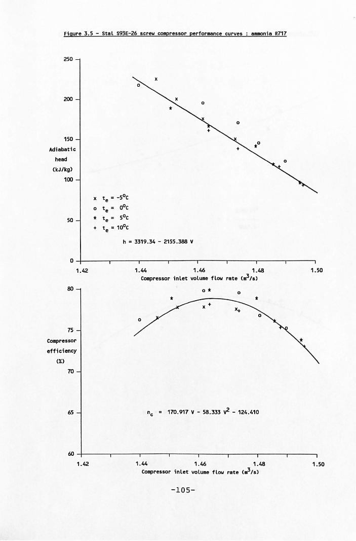
Figure 3.5 - Stal S93E-26 screw compressor perfor.ance curves ammonia R717
250
200
150
Adiabatic
head
(kJ/kg)
100
x t = -5°C e ° t = OoC e
50 * te = 5°C + t = 10°C e
h = 3319.34 - 2155.388 V
0
1. 42
80
75
Coaapressor
effidency
(X)
70
65
1.44 1.46 1.48 COlllpressor inlet volume flow rate (,hs)
° * ° * * x +
nc = 170.917 V - 58.333 y2 - 124.410
1.50
ro~------~-----'-------'------r-----~------'-------r-----~
1.42 1. 44 1.46 1.48 1.50 COlllpressor inlet volume flow rate <.3/s )
-105-
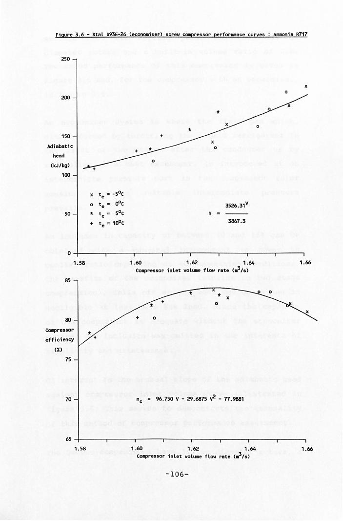
figure 3.6 - Stal S93E-26 (economiser) screw compressor performance curves ammonia R717
250
200
150
Adiabatic
head
(IcJ/lcg)
100
50
x t = -5°C e
° te = OoC
* t = 5°C e + t = 10°C e
x o
3526.31V
h
3867.3
O~------'-------r-----~r------.-------r------.-------r------'
1.58
85
80
Compressor
efficiency
(X)
75
70
1.60 1.62 1.64 Compressor inlet volume flow rate (m3/s)
* x o
nc = 96.750 V - 29.6875 y2 - 77.9881
1.66
65 -r------r------r-----,r------r------r------r------r-----~
1.58 1.60 1.62 1.64 1.66 Co~ressor inlet volume flow rate (~/s)
-106-
surface bulk air cooling plant and have 330 mm
diameter rotors and a built-in volume ratio of 2.6.
The rated performance of this compressor is given in
figure 3.5 and, for the compressor with an economiser,
in figure 3.6.
An economiser system is where the flash gas which,
either formed by throttling the liquid refrigerant in
the first of two stages after the condenser or by
subcooling in a heat exchanger I is introduced at an
intermediate pressure port in the compressor rotor
housing where a suitable intermediate pressure
prevails.
An increase in capacity of between 10 and 15% can be
obtained with a marginal improvement in power to
cooling ratio depending on the operating conditions.
The benefits of the economiser (similar to two stage
compression), falls off as the load decreases and is
negligible at less than 80% load. Since the capacity
of the compressor is adequate without the economiser
system, its inclusion was omitted in the interests of
simplicity and maintenance.
Of interest is the unusual slope of the adiabatic head
against compressor inlet volume curve illustrated in
figure 3.6. This serves to demonstrate the generality
of this method of compressor performance assessment.
The Sabroe compressors have 345 mm diameter rotors, a
-107-

length to diameter ratio of 1.60 and a built-in volume
ratio of 2.3. The performance curves of the compressor
when using ammonia are illustrated in figure 3.7.
All the compressors considered for the Mount Isa
plants are either driven by or to be driven by 1200 kW
motors at a speed of 49.2 rls.
Broken Hill surface plant
The compressors tendered for the Broken Hill surface
bulk air cooler plant were Howden 321-13226, Sullair
L25LA and Mycom 320 MU-LX.
Two Howden compressors were selected for this plant
and they have a 321 mm diameter rotors, a rotor length
to diameter ratio of 1.32 and a built-in volume ratio
of 2.6. The performance of the compressor with ammonia
as the refrigerant is illustrated in figure 3.8. The
compressors are to be driven with 750 kW motors at a
speed of 49.2 rls.
The performance of the Sullair and Mycom compressor
alternatives are illustrated in figures 3.9 and 3.10.
The Mycon compressor is similar in size and capacity
to the Howden compressor whereas the Sullair unit with
a rotor diameter of 250 mm, is significantly smaller
and three uni ts are required to achieve the total
plant duty.
-108-
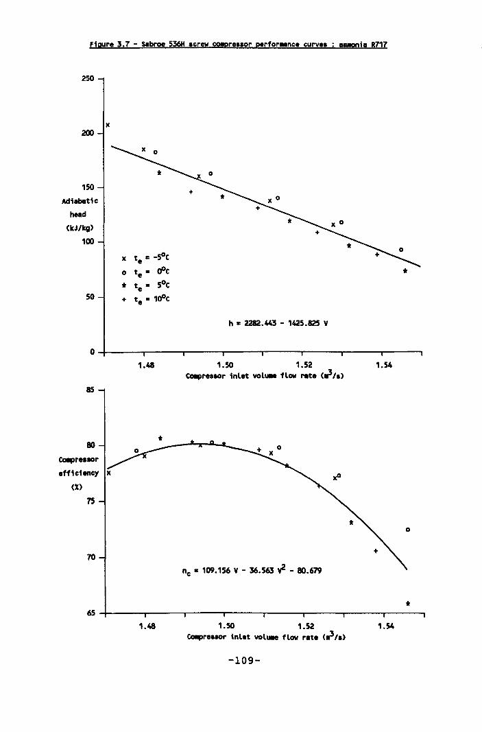
Figure 3.7 - Sebree S36H screw CO!presaor perfor!!nce curves e!!ODie R717
2S0
200
1S0
Adiabatic
head
(kJ/kg)
100
so
85
80
x
CoIIprea80r
efficiency x
(X)
7S
70
x t • -SoC e
° te. rPC
* t • 5°C e + te = 1rPC
1.48
*
+
h • 2282.443 - 142S.825 V
1.50 1.52 1.54 CoIIpres80r inlet volu.e flow reta (,; la)
nc • 109.156 V - 36.563 y2 - 80.679
*
°
* ~~----~------~-----r----~r-----'-----~------r-----~ 1.48 1.50 1.52 1.54
CoIIpres80r inlet volu.a flow reta (';/a)
-109-
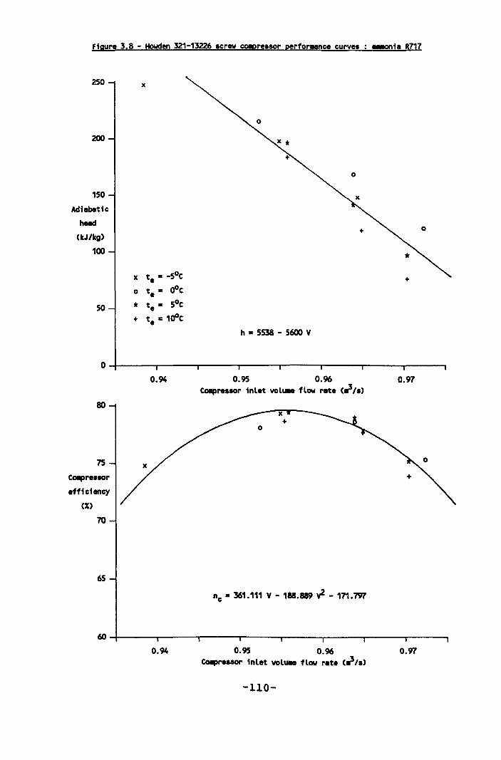
Figure 3.8 - Howden 321-13226 screw CO!pressor perforaance curves : e..onie 8717
250
200
150
Adiabatic
heed
(kJ/kg)
100
50
x
x te· -5°C
° t •• cOc * te = 5°C + te. 1cOC
h • 5538 - 5600 V
O~----~------r-----~-----r----~----~r-----~----~
80
75
CoIIpressor
efficiency
(X)
70
65
0.94 0.95 0.96 CoIIpressor inlet volu. flow rete (,;J la)
° x +
nc. 361.111 V - 188.889 y2 - 171.797
0.97
~~-----'r-----~-----'----~r-----'-----~------'-----~ 0.94 0.95 0.96 0.97
CoIIpreaaor inlet volUile flow rete (,;J/a)
-110-
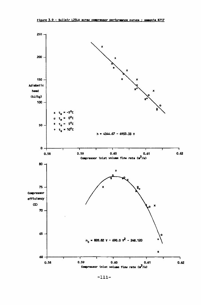
Figure 3.9 - Sull.ir L25LA screw COIpressor perfor .. nce curves • ..ani. R717
250
200
150
Adiabatic
head
(kJ/kg)
100
50
x t = -5°C e
° te = oOc * t = 5°C e + t • 10°C e
h • 4344.67 - 6933.33 V
O~-----,------~-----r-----'------~-----r------~----' 0.58
80
75
CoIIpressor
efficiency
(X)
70
65
0.59 0.60 0.61 0.62 Ca.preaaor inlet volu.. flow rate (~/s)
x
nc • 828.82 V - 690.0 y2 - 248.120
* 6O~----~------~-----r----~~----~----~------r-----~
0.58 0.59 0.60 0.61 0.62 CoIIpressor inlet volu.e flow rate (~/s)
-111-
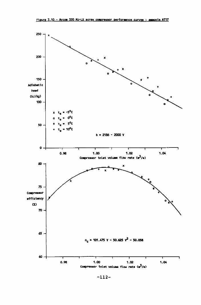
Figure 3.10 - "yeo. 320 "U-LX screw COIpreaaor perfor .. nce curves a!!ODia R717
2S0
200
1S0
Adiabatic
heed
(kJ/kg)
100
x
x t • -SoC e ° te = oOC
SO * te = SoC
+ te. loOC
h • 2186 - 2000 V
O~-----,------~-----r-----'------~----~------r-----'
80
75
COIIPresaor
efficiency
(X)
70
65
0.98 1.00 1.02 1.04 COIIPresaor inlet volu. flow rete (,} II)
x
"c • 101.475 V - 50.625 y2 - 50.058
~~-----,------~------r----~r-----'-----~------r-----~ 0.98 1.00 1.02 1.04
COIIPrelaor inlet volu.e flow rate (,}/I)
-112-
3.2 Condensers
The thermal performance of a condenser is a function
of an overall heat transfer coefficient (UA) and a
driving force. The value of the overall heat transfer
coefficient depends on the heat exchange areas, the
thermal resistances of both the refrigerant and the
heat rejection fluid boundary layers, the thermal
resistance of the material separating the refrigerant
and the heat rejection fluid and the thermal
resistance of accumulating impurities on the surface
exposed to the heat rejection fluid (fouling).
For shell and tube and closed plate condensers where
water is used as the heat rejection fluid, the driving
force is the log mean temperature difference (LMTD)
between the water entering and leaving the condenser
and the condensing temperature of the refrigerant. For
an evaporative condenser where both air and water are
used as the heat rejection fluids, the driving force
is the difference between the vapour pressure of air
which is saturated at the refrigerant condensing
temperature and the vapour pressure of air saturated
at the inlet wet bulb temperature.
When modelling condenser performance, either the
condensing temperature of the refrigerant or the heat
rejection fluid side surface fouling factor (scale)
is to be evaluated. Plant optimisation and design
including tender and control system evaluation require
-113-
calculation of the condensing temperature. Fouling
factor calculations are normally required for routine
maintenance and use measurements obtained from the
monitoring of an operating plant.
The refrigerant condensing heat transfer coefficient
is the most difficult to evaluate with accuracy. It is
a function of the refrigerant properties, the geometry
of the condensing surface and the difference between
the film temperature and the saturated condensing
temperature (ASHRAE, 1972; Howes, 1975). Although the
simplified relationships can be used, the values are
confirmed with test data where possible.
3.2.1 Shell and tube condensers
When modelling shell and tube condenser performance,
the condenser water flow rate, the water temperature
into the condenser and the condenser duty are known.
The cooling water is supplied through the inside of
the tubes and the refrigerant is supplied to the shell
and condenses on the outside of the tubes.
Mul tiple (two or three) water pass arrangements are
common and achieved by using baffles in the water
boxes at the ends of the tubes. The number of water
passes used is a compromise between the improved heat
transfer associated with high water velocities in the
tubes and the increased pressure loss and associated
pump power resulting from the higher water velocities.
-114-
In most shell and tube condensers the magnitude of the
refrigerant heat transfer coefficient is usually
between 20 to 30% of the water side heat transfer
coefficient. The total number of tubes required and
therefore the cost of the condenser, is minimised by
extending the refrigerant side heat transfer surface
area with ribs or fins on the outside of the tubes.
The refrigerant which is condensed on the outside of
the tubes is collected in the bottom part of the
condenser shell. This liquid will be subcoo1ed if the
refrigerant level is above the bottom rows of tubes in
the tube bundles.
The general method of analysis used to obtain the
condensing temperature is summarised in Table 3.1. The
two refrigeration plants which use shell and tube
condensers are the Mount Isa R63 surface plant and the
Broken Hill underground plant. The constructional
details of each condenser used in the simulations are
summarised in Table 3.2.
3.2.2 Closed plate condensers
Closed plate heat exchangers comprise of individual
corrugated thin plates which are assembled in packs
and clamped into a frame. Each adjacent pair of plates
forms a flow channel with the refrigerant and the heat
rejection water flowing in alternate channels. A
gasket is located along the perimeter and the corners
-115-
of each plate which both separates the plates and
prevents any mixing of the refrigerant and water.
Headers are formed by holes in the corners of each
plate and the fluids are permitted into the passages
between the plates by arrangement of the gaskets, the
refrigerant is directed into every second passage
while the water is let into the passage in between.
The corrugations in the plates maintain the correct
spacing between the plates, provide support for each
plate against adjacent plates and promotes turbulence
of the refrigerant and water which improves the heat
transfer. This support allows relatively thin plate
material to be used and 0.6 mm thickness is typical.
In closed plate heat exchangers, the magnitude of the
refrigerant heat transfer coefficient is usually 70 to
80% of the water side heat transfer coefficient. An
extended refrigerant side surface is not practical and
consequently, to meet the refrigerant side heat
transfer area requirements, the water side surface
area is larger than an equivalent shell and tube
condenser whilst maintaining a competitive cost.
The advantage of this is that increased fouling on the
water side of the plates can be permitted whilst
maintaining an equivalent thermal performance to that
of the shell and tube heat exchanger.
-116-
Condensers operate at relatively high pressures and to
avoid refrigerant leakage, the two plates providing
the refrigerant path are usually welded together to
form a cassette. To protect the gaskets from high
temperature refrigerant leaving the compressor, the
discharge gas is sometimes de-superheated prior to
entering the plate heat exchanger.
The general method of analysis used to obtain the
condensing temperature is identical to that for a
shell and tube condenser except for the calculation of
the overall heat transfer coefficient. The method used
for this is summarised in Table 3.3. Closed plate
condensers unlike shell and tube condensers, have no
refrigerant storage and therefore there is no
subcooling of the condensed refrigerant.
The closed plate heat exchangers used for condensers
in these simulations were all supplied by the same
manufacturer. The empirical relationships used to
determine the water and refrigerant heat transfer
coefficients were obtained by an analysis of the rated
and actual performance data and have a similar form to
those used to assess the performance of shell and tube
condensers. The area of plate in each cassette is
3.193 m2 and is the same for the water, refrigerant
and mean surface areas. The plate thickness is 0.6 mm
and the material used is 316 stainless steel with a
thermal conductivity of 0.0163 kW/mK.
-117-
3.2.3 Evaporative condensers
In an evaporative condenser, the refrigerant is
circulated through and condensed in tubes or plates
over which water is sprayed and air is drawn. In these
uni ts, the removal of the heat required to condense
the refrigerant is transferred directly to the air
which is ultimately used for heat rejection from all
mine condensing systems.
The heat gained by the water recirculating in both
shell and tube and closed plate condensers is normally
rejected to the air in direct contact cooling towers.
The combination of stages in an evaporative condenser
usually results in the most cost effective method of
rejecting heat from the refrigeration process.
The procedure required to model the performance of an
evaporative condenser is given in Table 3.4. The
empirical relationship used to assess the overall heat
transfer coefficient allows the effects of fouling to
be taken into account and is based on the analysis of
available measurements and performance data (see
section 7 of Table 3.4).
The evaporative condenser factor is essentially the
area available for heat transfer and includes the
influence of pipe or plate geometry and the pipe wall
or plate thickness and thermal conductivity. The
airflow factor is mainly used to avoid excessively low
-118-

condensing temperatures and is applied where the units
either have multiple fans which are allowed to cycle
on and off or where the fans are driven by two speed
motors.
The amount of air used for heat rejection lies between
the relatively narrow limits of 0.0175 and 0.0210 m3/s
per kW of base heat rejection with an average value of
0.0190 m3/s/kW. The recirculating water mass flow rate
is approximately equivalent to the air mass flow rate
used for heat rejection in the evaporative condenser.
-119-
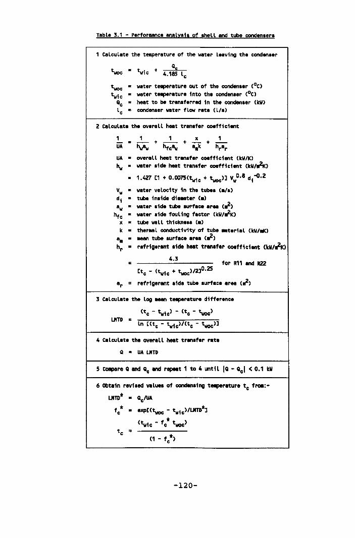
Table 3.1 - Performance analysis of shell and tube condensers
1 Calculate the te.perature of the water leaving the condenaer
= t. + Qc W1C 4.185 lc
twoc • water te.perature out of the condenaer (oC) t wic = water teaperature into the condenaer (oC)
Qc = heat to be tranaferred in the condenser (kW)
lc • condenser water flow rate (l/a)
2 calculate the overall heat transfer coefficient
1 1 1 x 1 -=--+--+-+--UA hw-w hfc8w aak hrar UA • overall heat transfer coefficient (kW/K) hw • water side heat tranafer coefficient (kW/~)
• 1.427 [1 + O.OO75(~ic + ~c)] VwO.8 di-o· Z
Vw • water velocity in the tubes (ala) di • tube inside di ... ter (a) a • water side tube surface area (~) w
hfc = water side fouling factor (kW/~K) x • tube wall thickness Ca) k • ther .. l conductivity of tube .. terial (kW/aK)
aa • aean tube surface area (~) hr • refrigerant side h .. t transfer coefficient (kW/~)
4.3 for R11 and R22 =
[tc - (twic + t woc)/2JO.ZS
ar = refrigerant side tube surface area (~)
3 Calculate the log aean teaperature difference
4 Calculate the overall heat transfer rate
5 COIpere Q and Qc and repeat 1 to 4 until IQ - Qcl < 0.1 kW
6 Obtain revised values of condensing teaperature tc fro.:
LMTD* • Qc'UA
fc* • exp[(~ - twic)/LMTD*]
* (twic - fc ~)
(1 - f/)
-120-
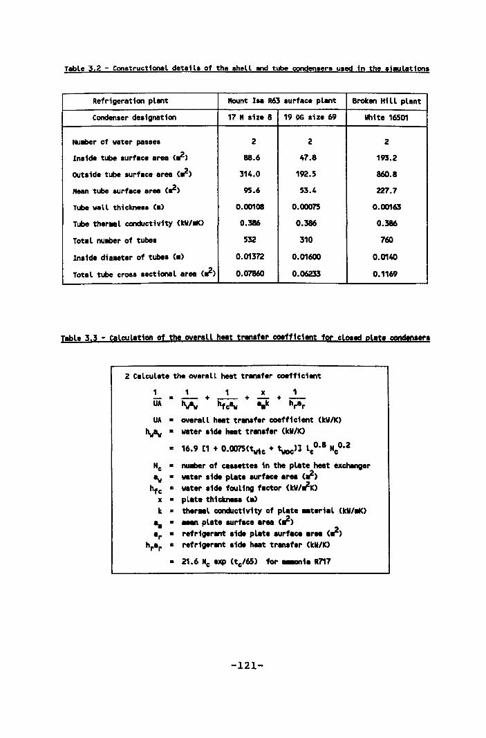
Table 3.2 - Constructional details of the shell and tube condensers used in the si.uletions
Refrigeration plant Mount Isa R63 surface plant Broken Hill plant
Condenser designation 17 " size 8 19 DG size 69 llhite 16501
Nu.ber of water passes 2 2 2
Inside tube surface area (,.2) 88.6 47.8 193.2
OUtside tube surface area (,.2) 314.0 192.5 860.8
Mean tube surface area (,.2) 95.6 53.4 227.7
Tube wall thickness C.) 0.00108 0.00075 0.00163
Tube theral conductivity (kll/llK) 0.386 0.386 0.386
Total nu.ber of tubes 532 310 760
Inside d;a.eter of tubes (.) 0.01372 0.01600 0.0140
Total tube cross sectional area (,;.) 0.07860 0.06233 0.1169
Table 3.3 - calculation of the overall heat transf.r coefficient for cloald pllte condtn!.rs
2 calculate the overall heat transfer coefficient
1 1 1 x 1 =--+--+-+--
UA Yw htcBw a.k hrar
UA • overall heat transfer coefficient (kll/K) Yw • wat.r side heat transf.r (kW/K)
• 16.9 [1 + O.OO75(~c + twoc)l LcO.8 NcO.2
Nc • nuaber of cassettes in the plate heat exchanger Bw = wat.r side plate surfac. ar.. (,;.)
hfc • water side fouling factor (kW/';'K) x • plate thickness (a)
k • thecal conductivity of plate aterial (kll/llK) .. • ...., plat. surface area (,;.) ar • refrigerant side plate surface ar.. (,;.)
hrar • refrigerant side heat transfer (kW/K)
• 21.6 Ne up (tc/65) for ..ania R717
-121-
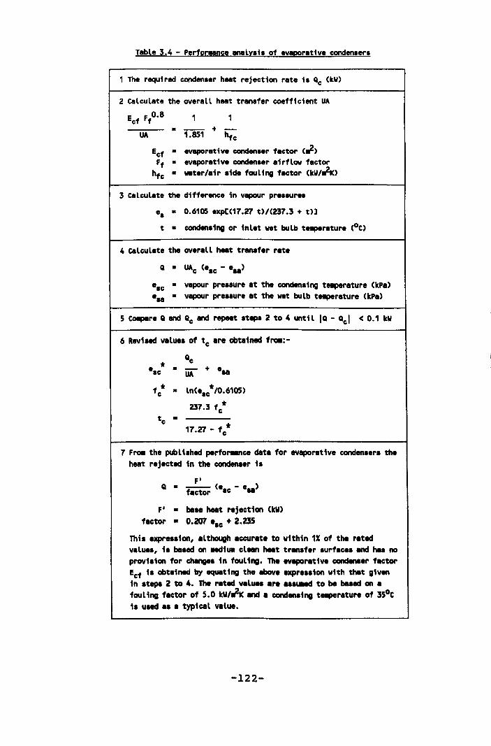
Table 3.4 - Perfor_nee analysis of evaporative condensers
1 The required condenser heat rejection rate is Qc (leW)
2 Calculate the overall heat transfer coefficient UA
Ecf Ff O. 8 1 1 • -- + -
UA 1.851 htc
Ecf • evaporative oondenaer factor (~) Ff • evaporative condenser airflow factor
htc • water/air .ide fouling factor (kW/~)
3 calculate the difference in vapour pre.sur ..
es • 0.6105 exp[(17.27 t)/(237.3 + t)J
t • condensing or inlet wet bulb te.perature (oC)
4 cal,ulate the overall h .. t transfer rate
Q • UA, (es, - e .. )
e.c • vapour presaure at the condensing te.perature (kPa) esa • vapour pre.aure at the wet bulb te.perature (kPa)
5 CoIIpIIre Q and Qc and repeat stepa 2 to 4 until IQ - Qcl < 0.1 kW
6 Reviaed value. of t, are obtained fl'Oll:-
~ • + e
UA ..
f,* • In(esc*IO.6105)
* 237.3 f,
* 17.27 - fc
7 Fro. the published perfoMllft,e data for evaporative eondensers the heat rejeeted in the condenser 18
F' Q • -- (e - e )
factor sc ..
F' • base heat rejeetion (kW) factor • 0.207 esc + 2.235
This expression, although aCGUrete to within 1% of the rated values, is based on Mdiua cl.., heat transfer surfa,es and has no provi.ion for chIIngea in fouling. The evaporative condenser factor Ecf 1. obtained by equating the above expression with that given in stepa 2 to 4. The rated values are .. ..ect to be baaed on a fouling factor of 5.0 kW/~ and a condensing te.perature of 35°C i. u.ed a. a typical value.
-122-
3.3 Bvaporators
Similar to condensers, the thermal performance of a
evaporator is a function of an overall heat transfer
coefficient (UA) and a driving force. The value of the
overall heat transfer coefficient depends on the heat
exchange areas, the thermal resistances of both the
refrigerant and the chilled water boundary layers, the
thermal resistance of the material separating the
refrigerant and the chilled water and the thermal
resistance of accumulating impurities on the surface
exposed to the chilled water (scale or fouling).
For all four types of evaporator being considered, the
driving force is the log mean temperature difference
(LMTD) between the water entering and leaving the
evaporator and the evaporating temperature of the
refrigerant. When modelling evaporator performance,
either the evaporating temperature of the refrigerant
or the chilled water side surface fouling factor
(scale) is to be evaluated.
Plant optimisation and design including tender and
control system evaluation require calculation of the
evaporating temperature. Fouling factor calculations
are normally required for routine maintenance and use
measurements obtained from the monitoring of an
operating plant.
The refrigerant evaporating heat transfer coefficient
-123-
is the most difficult to evaluate with accuracy. It is
a function of the refrigerant properties, the boiling
or evaporating surface nucleating characteristics and
geometry and the heat flux density <Stephan, 1972).
Although simplified relationships are normally used,
the values are confirmed with the results of test data
where possible.
3.3.1 Shell and tube evaporators
When modelling shell and tube evaporator performance,
the evaporator or chilled water flow rate, the water
temperature into the evaporator and the evaporator
duty are known. The water to be chilled is supplied
through the inside of the tubes and the refrigerant is
supplied to the shell and evaporates or boils on the
outside of the tubes.
Mul tiple (two to four) water pass arrangements are
common and achieved by using baffles in the water
boxes at the ends of the tubes. Similar to condensers,
the number of water passes used is a compromise
between the improved heat transfer associated with
high water velocities in the tubes and the increased
pressure loss and associated pump power resulting from
the increased water velocities.
In most shell and tube evaporators, despite the lower
water velocities, the magnitude of the refrigerant
heat transfer coefficient is usually between 20 to 30%
-124-
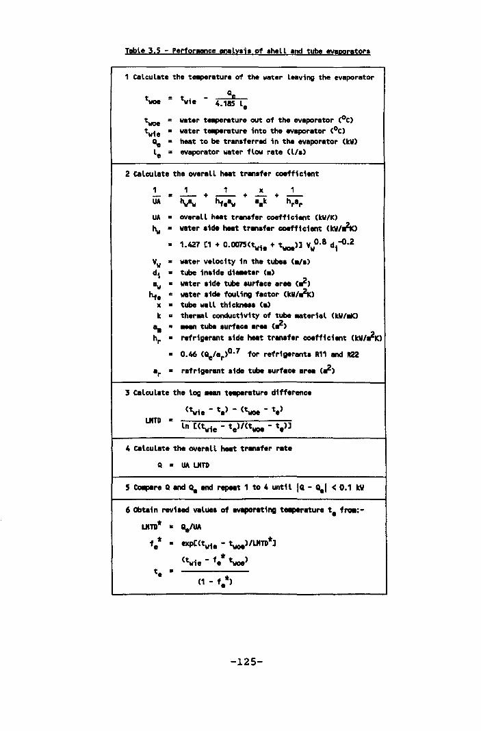
Table 3.5 - Perfor.ance analyaia of shell and tube evaporators
1 calculate the t~rature of the water leaving the evaporator
= t - ge vie 4.185 le
twoe a vater t~rature out of the evaporator (oC) t vie • water t~rature into the evaporator (oC) ~ • heat to be transferred in the evaporator (kll) le = evaporator water flow rate (l/a)
2 calculate the overall heat tranafer coefficient
1 1 1 x 1 -=--+--+-+--UA hw-w hteBw a.k hrar UA • overall heat tranafer coefficient CkIl/K) hw = water aide heat tranafer coefficient (kll/~)
= 1.427 [1 + O.0075(tw1e + twoe)J VwO.8 d,-o·2
Vv • water velocity in the tubea (./a) di • tube inside di ... ter (.) Bw • water side tube surface area (rtf)
hte • water side fouling factor (kll/~) x = tube wall thickneas (.) k • thereal conductivity of tube eaterial Ckll/aK)
.. • ...... tube surface area Crh hr • refrigerant side heat transfer coefficient (kW/rtfK)
• 0.46 (~/ar)O. 7 for refrigerants R11 and R22
ar • refrigerant aide tube aurface area (rtf)
3 calculate the log aean teaperature difference
4 calculate the overall heat tr.nafer rate
Q • UA LIllO
5 COIIpere Q and ;. and repeat 1 to 4 until IQ - ;.1 < 0.1 kW
6 Obtain revised values of evapor~ing t...,.rature te fl'Oll:
LIIlO* • ~/UA fe* = exp[(twie - twoe)/LIITD*J
t = e * (twie - fe twoe)
-125-
of the water side heat transfer coefficient. Similar
to condensers, the number of tubes required and
therefore the cost of the evaporator, is minimised by
extending the refrigerant side heat transfer surface
area with ribs or fins on the outside of the tubes.
The tube bundles are not always submerged in the
liquid refrigerant and some of the tubes are in the
refrigerant gas. The chilled water temperature
entering is usually significantly higher than the
evaporating temperature and consequently there will be
superheating of the refrigerant vapour.
The general method of analysis used to obtain the
evaporating temperature is summarised in Table 3.5.
The two refrigeration plants which use shell and tube
evaporators are the Mount Isa R63 surface plant and
the Broken Hill underground plant. The constructional
details of each evaporator used in the simulations are
summarised in Table 3.6.
3.3.2 Direct expansion shell and tube
Direct (dry) expansion shell and tube evaporators are
similar to standard shell and tube evaporators except
that the refrigerant is circulated through the tubes
and the water to be chilled passes through the shell.
The method of analysis is identical to that for the
conventional shell and tube evaporator as summarised
in Table 3.5 except for the refrigerant and water heat
-126-
transfer coefficients. The different relationships
used to obtain the overall heat transfer coefficient
are illustrated in Table 3.7.
The refrigerant side heat transfer coefficient is much
smaller than the water side heat transfer coefficient
and consequently internally finned tubes are used to
increase the surface area for heat exchange. In the
shell, baffles are used to provide the most efficient
heat transfer and to minimise any stratification that
may occur.
Determining the refrigerant heat transfer coefficient
is further complicated because natural convection
boiling takes place in the tubes and the refrigerant
is superheated by the water in the shell, the extent
of which will vary along the tubes and also according
to the load.
Three nominal 650 kWR units are used with the NO 1
compressor set in the underground plant at Broken
Hill. Each evaporator contained 408 copper tubes with
an external diameter of 17.4 mm and a wall thickness
of 1.7 mm. The extended inside tube surface area was
137.1 m2 and the outside tube surface area was 85 m2 .
The tubes are arranged for four refrigerant passes and
the baffle spacing is 0.125 m in the 0.61 m diameter
shell. The average cross sectional area used to
determine the water velocity is 0.0603 m2 .
-127-
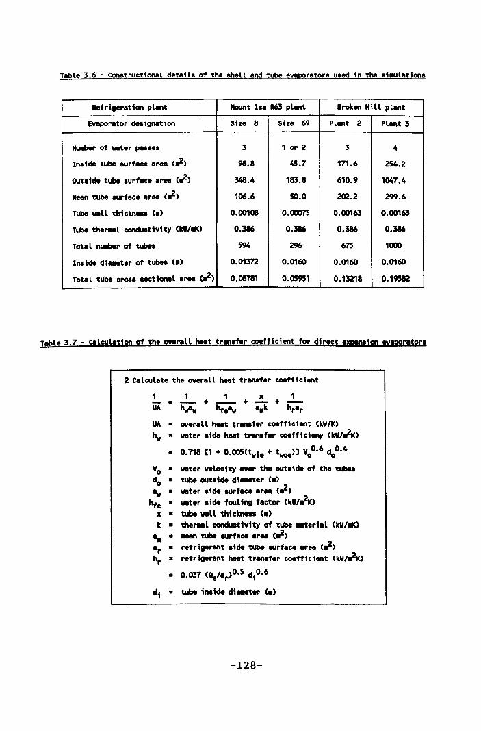
Table 3.6 - Constructional details of the shell and tube evaporators used in the si.ulations
Refrigeration plant Mount Iu R63 pl.,t Broken Hi II plant
Evaporator designation Size 8 Size 69 Plant 2 Plant 3
NUliber of water pass.s 3 1 or 2 3 4
Inside tube surface area (~) 98.8 45.7 171.6 254.2
OUtside tube surface area (~) 348.4 183.8 610.9 1047.4
Mean tube surface area (~) 106.6 50.0 202.2 299.6
Tube wall thickness (a) 0.00108 0.00075 0.00163 0.00163
Tube ther.el conductivity (kW/~) 0.386 0.386 0.386 0.386
Total nueber of tubes 594 296 675 1000
Inside diaaeter of tubes (a) 0.01372 0.0160 0.0160 0.0160
Total tube cross sectional area (~) 0.08781 0.05951 0.13218 0.19582
Table 3.7 - calculation of the overall heat transfer coefficient for direct expen!ioo evaporators
2 calculate the overall heat transfer coefficient
1 1 1 x 1 ._-+--+-+--
UA Yv hteltw a.k hrar
UA = overall heat transfer coefficient (kW/K) hw • water side heat transfer coeff1c1eny (kW/a2K)
• 0.718 [1 + O.OO5(twie + twoe)J VoO.6 doO.4
x •
water velocity over the outside of the tubes tube outaide di_ter (.) water side surface ar .. (,.2)
water aide fouling factor (kW/a2K) tube wall thicknesa (.)
k = ther.el conductivity of tube .. terial (kW/~) .. • Man tube surface ar.. (,.2)
ar • refrigerant side tube surface ar.. (,.2)
hr • refrigerant heat transfer coefficient (kW/a2K)
• 0.037 (~/ar)0.5 diO. 6
di • tube inside di_ttr (.)
-128-
Tests on the evaporator performance resulted in duties
approximately half of the rated values at between 350
and 375 kWR. Cleaning the water side of these
evaporators is very difficult without dismantling the
plant, taking the units to surface and removing the
tube bundles from the shell. As a consequence, the
evaporators have not been cleaned since installation
and, after four years operation, they were very
"dirty" with fouling factors between 2 and 3 kW/m2K.
3.3.3 Closed plate evaporators
The closed plate heat exchangers used for evaporators
are similar in construction and operation to those
used as condensers. The general method of analysis
used to obtain the evaporating temperature is
identical to that for a shell and tube evaporator
except for the calculation of the overall heat
transfer coefficient.
The method used for this is summarised in Table 3.8.
The closed plate evaporators in mine refrigeration
systems normally operate in conjunction with a large
pressure vessel known as a refrigerant accumulator
which is used to separate the vapour from the liquid
refrigerant.
By locating the accumulator above the evaporator,
liquid refrigerant in the bottom of the vessel is
supplied to the closed plate evaporator where boiling
-129-
takes place. Not all the refrigerant is evaporated and
the mixture of refrigerant vapour and liquid is
returned to the accumulator. The vapour which collects
above the liquid surface in the accumulator is taken
off to the compressor inlet.
There is no cooling in the accumulator and therefore
there is no, superheating of the refrigerant vapour.
The circulation of the refrigerant between the
accumulator and the evaporator can be either forced by
using refrigerant pumps in the liquid supply line or
by natural convection.
The driving force for natural convection thermosyphons
is the difference in refrigerant density between the
liquid supply and the liquid/vapour return pipes
connecting the accumulator and the evaporator. When
the plant is not operating, both pipes contain liquid
refrigerant at the same density and there is no flow.
When the plant starts and the water to be chilled
enters the evaporator, the higher temperature water
causes some boiling of the refrigerant in the plates
which then become partly filled with ascending bubbles
of refrigerant vapour. The density of the mixture in
the return column decreases causing an imbalance
between the supply and return pipes and refrigerant
flow starts. The circulation rate increases until
refrigerant frictional pressure loss equals the
driving force for natural convection.
-130-
The closed plate heat exchangers used for evaporators
in these simulations were all supplied by the same
manufacturer. The empirical relationships used to
determine the water and refrigerant heat transfer
coefficients were obtained from the rated and actual
performance data and similar in form to those used to
assess the performance of shell and tube evaporators.
The surface area for heat transfer in each cassette is
3.193 m2 and is the same for water and refrigerant.
The plate thickness is 0.6 mm and the material used is
either 316 stainless steel with a thermal conductivity
of 0.0163 kW/mK or a titanium alloy with a thermal
conductivity of 0.0164 kW/mK.
3.3.4 Open plate evaporators
An open or falling film plate evaporator, comprises
two corrugated plates welded together to form a series
of horizontal passageways. These are connected at the
ends of the plates to form a series of parallel routes
from the bottom of the plate to the top. The number of
parallel routes used in a plate is a compromise
between high refrigerant heat transfer coefficients
and low frictional pressure losses.
Liquid refrigerant supplied from an accumulator passes
through these passageways where a fraction evaporates
and the mixture of refrigerant vapour and liquid
returns back to the accumulator.
-131-
The water to be chilled is distributed uniformly to
both sides of the vertical plates and flows in a thin
film over the outer surfaces of the plates. As before,
the performance analysis only differs in the methods
of estimating the refrigerant and water heat transfer
coefficients. A summary of the relationships used to
calculate the overall heat transfer coefficient is
given in Table 3.9.
Manufacturers performance data was used to confirm the
method of analysis and in particular the refrigerant
and water heat transfer coefficients. The water side
coefficient is based on a turbulent falling-film and
is a function of the water film thickness defined by
the le/2 Nl term.
Where the refrigerant is pumped through the plates,
forced convection takes place inside the passageways
or tubes formed by the corrugated plates and the
vapour fraction of the refrigerant leaving the plate
will depend on the load. Most systems are designed for
a 50% vapour fraction when the plant is operating at
full load and this decreases as the load decreases.
Where a natural convection thermosyphon is used, the
vapour fraction of the refrigerant returning to the
accumulator is less affected by changes in load. As a
result, the refrigerant heat transfer coefficient
given in Table 3.9 will be slightly underestimated for
a pumped system when operating at part load.
-132-
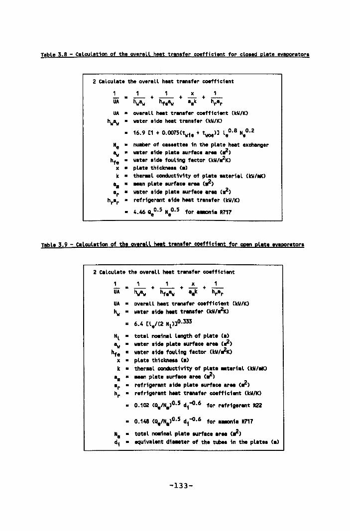
Table 3.S - Calculation of the overall heat transfer coefficient for closed plate evaporators
2 calculate the overall heat transfer coefficient
1 1 x 1 = --- + --- + -- + ---UA hw-w hfeBw a.k hrar
UA • overall heat transfer coefficient (kW/K) hw-w • vater side heat transfer (kW/K)
• 16.9 [1 + 0.OO7S(tvie + tvoe)l leO.S H,0.2
He • nu.ber of cassettes in the plate heat exchanger Bw • vater side plate surface area (~)
hfe • vater side fouling factor (kW/~K) x • plate thickness Ca) k • thereal conductivity of plate eaterial CkW/~)
a. • .ean pllte turface area (~) ar • vater side plate turface area C~)
hrar • refrigerant side heat transfer (kW/K)
• 4.46 ~O.S HeO•S for a..,.,ia R717
Table 3.9 - calculation of the overall heat transfer coefficient for open plate evaporators
2 calculate the overall heat transfer coefficient
1 UA
1 1 x 1 ----+---+--+---
hw-w hteBw a.k hrar
UA • overlll heat transfer coefficient CkW/K) "w • water aide heat tl'Mlfer CkU/~K)
• 6.4 [le/C2 Hl)lO.333
Hl = total noainal length of plate Ca) Bw • water aide pllte turface area C~)
hte • water side fouling factor CkW/~K) x • plate thickness C.) k • thereal conductivity of plate .. terial CkW/aK)
a. • aean plate surface area (~) ar • refrigerant aide plate turtlce ar.. (~) hr = refrigerant heat tranafer coefficient (kW/K)
• 0.102 (~/Ha)0.5 d, -o·6 for refrigerant R22
- 0.148 C~/Ha)0.5 d, -O·6 for ...,.,ia R717
Na • total noa1nal pllte turflce area (~) d; • equivalent di ... ter of the tubes in the platea C.)
-133-
The multiplication constant used in the calculation of
the refrigerant heat transfer coefficient is 0.102 for
refrigerant R22 and 0.148 for ammonia. The conversion
factor of 1.45 is a function of the differences in
refrigerant properties. These include the latent heat
of evaporation, saturation pressures, viscosity and
thermal conductivity.
The refrigerant and water heat transfer coefficients
are not significantly different in magnitude and are
approximately in balance with the surface areas. For
the same operating conditions, the surface areas are,
however, about twice as large as those found in shell
and tube and closed plate heat exchangers. This is
important where the water to be chilled is dirty and
the effects of water side fouling on plant performance
will be less pronounced.
Because the water side is open, it is easier to
monitor water side fouling and plate cleaning can be
undertaken on a routine basis without shutting down
the plant.
The most common size of open plate used to chill mine
water in evaporators is 2.44 m long by 1.52 m high and
results in a nominal surface (Na ) of 7.43 m2/plate and
a nominal length (Nl) of 2.44 m. water is distributed
to and only forms a film on approximately 93% of the
nominal surface area of the plate.
-134-
The passageways formed by the plate corrugations are
not perfectly circular and have an equivalent diameter
(equivalent in cross sectional area) of 21.2 mm. The
inside surface area (applicable to the refrigerant
side heat transfer) is approximately 65% of the
nominal surface area and the mean surface area is
approximately 79% of the nominal surface area.
-135-

3.4 Surface cooling towers
Cooling towers are direct contact heat exchangers used
for either cooling hotter water with ambient air or
cooling ambient air with colder water. The three main
purposes of the surface cooling towers used in mine
refrigeration plants are for pre-cooling water prior
to chilling it with refrigeration, to cool condenser
water which has been used to condense the refrigerant
and, to bulk cool ventilation air which is to be
supplied underground.
Although each duty requires direct contact between the
air and water to achieve the necessary heat exchange,
the performance requirements and therefore the initial
cost and design arrangement for each is different.
In direct contact heat exchange, the performance is
related to the degree of the contact between the water
and the air. The simplest type of cooling tower has a
distribution system at the top where the water to be
cooled or heated is introduced and made to form
droplets which fall through the air being drawn
upwards through the tower. The higher the tower, the
greater the contact between the water and air and the
better the rate of heat transfer or the performance.
The air is in contact with and will cool (or heat as
appropriate) the outer surface layer of the water
droplets and further cooling of the water in the
-136-
droplet will rely on conduction and convection within
the droplet. An improvement in performance would
therefore be obtained if this colder surface layer
could be disturbed and replaced with the water in the
centre of the droplet.
This is the purpose of cooling tower f ill. The type
and amount of fill used in a tower is a compromise
between input power (overcoming the resistance to
airflow and pumping the water to the distribution
point), tower dimensions and quality of the water.
Splash grids (plastic frames with 80 to 95% open area
and suspended at about 300 mm intervals on stainless
steel wires) have the lowest pressure loss and the
least problems with blockage by solids settling out of
the water. They also require the greatest height of
fill, 5 to 10 m being typical, to achieve an
equivalent performance and therefore this type of
tower tends to have the highest capital costs.
Closely packed towers originally used timber (redwood)
slats and now use plastic honeycombs often with
corrugated surfaces. Equivalent performance can
normally be achieved with a fill thickness of between
1.0 and 1.5 m and a pressure loss between 50% and 100%
higher than splash grids. Blockage of the channels in
the fill material can be a problem where water quality
is poor and solids may settle out.
-137-
3.4.1 Pre-cooling towers
The return water temperature in a refrigeration system
which supplies chilled water underground will usually
be greater than the ambient wet bulb temperature. The
actual value will depend on the overall refrigeration
strategy i.e. whether bulk air cooling on surface is
used, and the design underground climatic conditions.
The overall power to cooling ratio for refrigerative
cooling will depend on the ambient surface wet bulb
temperature and normally varies between 0.15 and 0.20.
The power to cooling ratio of a cooling tower is much
lower at between 0.02 and 0.05 and consequently it is
advantageous to maximise its duty relative to the
refrigeration plant (HQwes, 1979b).
An optimisation based on Australian supply and
conditions resulted in a design factor of merit of
0.75, an approach (the temperature difference between
the entering air and the leaving water) of 1.Ooe and a
water to air loading (ratio of water to air mass flow
rates through the tower) of 0.6. The 1.Ooe approach
was applicable to the mean summer conditions and not
the limiting climatic condition where the optimum
value would increase to 1.60 e.
The factor of merit (Whillier, 1977) describes the
actual performance of a tower relative to ideal direct
contact heat transfer which, in turn, will depend on
-138-
the air and water flow arrangements. In a pre-cooling
tower, the amount of air available for heat rejection
is only limited by economic considerations and
consequently high performance and large counter flow
towers would normally be selected. The performance of
a counter flow cooling tower can be determined using
the method outlined in Table 3.10 (Bluhm, 1980).
3.4.2 Condenser cooling towers
Although the performance of a condenser cooling tower
has a lesser effect on the overall power requirements
of a surface refrigeration plant when compared with a
pre-cooling tower, it is still significant. Reducing
the approach and therefore the condensing temperature,
reduces the plant input power by approximately two
thirds that achieved by the same reduction in approach
in the pre-cooling tower.
The pre-cooling tower does, however, reduce the
overall amount of refrigerative cooling required with
a consequent and significant reduction in capital
costs for the overall refrigeration system.
The optimum condenser tower arrangement will depend on
many factors, however, typical optimum values are an
approach of between 3.5 and 4.00C and a water to air
loading of between 1.0 and 1.5. The larger temperature
difference between the water leaving and the wet bulb
of the air entering (the approach) means that the
-139-
tower factor of merit can be lower than that required
for a pre-cooling tower. A typical design factor of
merit for a condenser cooling tower is 0.6 which in
turn means that the tower could be cross flow instead
of counter flow.
The advantage of a cross flow tower is that it does
not need to be as high as a counter flow tower and the
capital cost is significantly lower. Condenser water
is normally in closed circuit and the quality is
relatively straightforward to control. Close packing
is therefore normally used.
In a counter flow tower, the air entrance is below the
fill, the air then flows upwards through the fill,
counter current to the water flowing downwards. In a
cross flow tower, the air is drawn horizontally
through the fill adjacent to the inlet of the tower,
enters a central plenum and is then drawn upwards and
out of the tower. Because the fill is adjacent to the
inlet rather than above it, the height of the tower is
reduced.
The performance of a cross flow tower (Bluhm, 1981) is
determined in a similar manner to that for the counter
flow tower illustrated in Table 3.10 except for the
empirical relationships between capacity factor, water
efficiency and factor of merit given in Table 3.11. In
cross flow heat exchange, the air flowing horizontally
through the fill whilst the water flows down through
-140-
the fill, limits the maximum factor of merit possible
to 0.632 [1 - exp(-l.O)].
3.4.3 Surface bulk air coolers
Cooling the intake ventilation air on surface prior to
it being sent underground is straightforward where the
main intakes are used for ventilation only. The design
requires an optimisation between the proportion of the
total air quantity to be cooled and the total amount
of heat to be removed from the air.
Low air quantities and high heat transfer rates
require low supply water temperatures and therefore an
increase in compressor input power. High air
quantities require increased fan power in the bulk air
cooling tower which is usually offset by the saving in
compressor power resulting from higher supply water
and increased evaporating temperatures.
Where the main intakes are also operating shafts, the
amount of ventilation air that can by-pass the collar
has practical limits and the bulk air cooler usually
requires low supply water temperatures. A surface bulk
cooler therefore normally has a limited air quantity
and the optimum approach is between 1. 0 and 2. oOe
requiring a factor of merit of between 0.75 and 0.80.
The amount of chilled water that can be used to cool
the air is only limited by practical and economic
-141-
considerations. The towers used for bulk air cooling
are invariably counter flow and, because the chilled
water is in closed circuit with the bulk air cooler
and its quality can be controlled, close packed towers
are usually more cost effective.
In a refrigeration system used for bulk cooling air on
surface, the performance of the bulk cooler determines
the mode of operation and the performance of the rest
of the system. The analysis is similar to that given
in Table 3.10 with the entering and leaving water
temperatures transposed to avoid negative values.
-142-

Table 3.10 - PerfonlBnce analysis of a counter flow cooling tower
1. Input data required:-Bulk air cooler water flow rate It Bulk air cooler air flow rate qt water t..,.rature into the bulk air cooler ~it water tapereture out of the bulk air cooler \,ot wet bulb t...,..-ature into the bulk air cooler twbi
2. calculate the water efficiency fr'Oll:-
\,ot - ~it "v •
twi - ~;t
3. calculate the capacity factor fra.:-
4.185 It (twi - ~1t) I •
.. (Sai - Ivi) .. • .... flow rate of air (kg/.)
Sai • stu- heat of entering air (kJ/kg)
'vi • stu- heat of aetureted air at the wat.r entering t...,..-ature (kJ/kg)
4. calculate the factor of aerit F for the tower fr'Oll:-
"v - 1 Lny z Y • , z • and F • --
nJl - 1 (1 - 1)(1/1)°·4 z - 1
5. calculate water efficiency if F 1s known fr'Oll:-
[1 _ e-N<1 - I)]
"w • [1 - 1 .-N(1 - R)]
N • F (1 - F)-1 1-0·4
Tlbl. 3.11 - PerfO!Wl!C! alu1s of a cl'OH flqw cool ina tower
4. calculate the factor of aerit F for the tower fr'Oll:
F • 1 - exp[exp(aO·2 tf) - 1]
tf • In [1 + In(1; I n,,> ]
5. calculate _ter efficiency if F i. known fr'Oll:
"v • (1 - exp[-1(1 - up tf)]) R-1
tf • (1n[1 + Ln(1 - F)U 1-0·2
-143-
3.5 Underground air cooling
Chilled water which is produced on surface and then
sent underground can be used to cool air either
directly or indirectly in air cooling appliances, as
mine service water for dust suppression or as a power
source prior to being used for either cooling or dust
control. Except where the water is used as a power
source; either directly as high pressure jets to move
rock or indirectly through an energy recovery device
associated with mining equipment such as a rock drill,
most of the chilled water sent underground (usually 80
to 90') is used in air cooling devices.
3.5.1 Air cooling coils
These are used for indirect air cooling where the air
to be cooled and the chilled water are separated by
the tube material in the cooling coils. When analysing
the performance of cooling coils either the coil air
side duty or the air and water fouling factors are to
be calculated. The general method of analysis used in
the simulations is given in Table 3.12 and is based on
the standard NTU method (Rosenow, 1961).
The air side heat transfer coefficient on the outside
of the tubes is between 10 and 15' of the water side
heat transfer coefficient inside the tubes. As a
consequence, the outside tube surface is extended by
using fins to between five and ten times the nominal
-144-
tube surface area. Large sections of the fins are
relatively remote from the tube and the efficiency of
the fins relative to the tubes will be reduced
(Rosenow, 1961). The air being cooled underground is
not usually filtered before being passed through the
coil and consequently the outer surface is subject to
extensive fouling.
The coils used in the R63 system at Mount Isa were
developed in South Africa for underground applications
and have circular fins spaced at 3.1 mm and, based on
measurements of performance (Ramsden, 1981), have a
fin efficiency of f = 1.0 - 0.19 hoe The ratio of fin
surface area to tube surface area is 5.8: 1 and the
number of rows is usually limited to four.
Although this design minimises fouling and simplifies
cleaning and, despite the relatively clean intake air
being cooled, fouling of the finned surface
significantly affects performance. To overcome this
continuing operational problem, these finned tube
cooling coils are being replaced with those that have
multiple plain copper tube spirals and no fins at all.
The coils used in the underground refrigeration system
at Broken Bill were standard air conditioning system
coils with plate fins spaced at 4.2 mm. By analysing
the manufacturers rated performance data and assuming
fouling factors of 7.0 and 5.0 kW/m2K for the water
and air sides respectively, the fin efficiency was
-145-
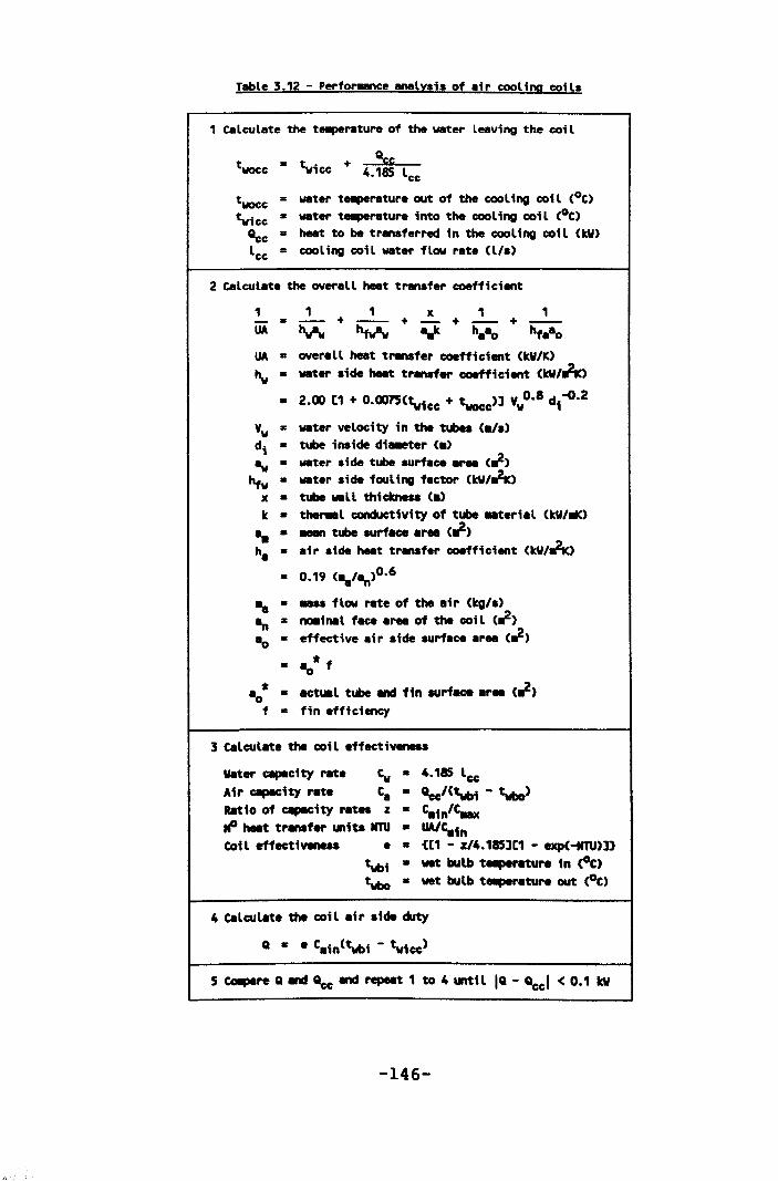
Table 3.12 - Perfo~ analysis of air cooling coils
1 calculate the telllperature of the water leaving the co; l
twoc:c
twoc:c = water telllperature out of the cooling coil (oC) ~icc • water t...,.,..ture into the cooling coil (oC) ~c = heat to be transferred in the cooling coil (leV)
lcc = cooling coil water flow r.te (l/a)
2 calculate the overall heat tranafer coefficient
1 1 1 x 1 1 -=--+--+-+--+ UA hw-v htw-w .. It h.ao ht •• o UA • over.ll heat trenafer coefficient (ltW/K) ltv • water aide heat transfer coefficient (1eV/ri'I.>
• 2.00 [1 + O.OO15(\rice + \.occ)] Vv 0.8 ~ -0.2
Vv • water velocity in the tubea (ilia) di • tube inside di-.ter (.) 8v • water .ide tube surf.ce .,... (,})
htv • water aide fouling f.ctor (1eV/riK> x • tube wall thic:lcneaa C.) It • therMl conductivity of tube ateri.l (ItW/~
.. • .... tube surface ..... C,}) h. • .ir .ide heat transfer coefficient (ItW/ri'I.>
• 0.19 ( .. /~)0.6
.. • ass flow rate of the .ir (ltg/a) ~ • ....inal face ..... of the coil (,})
.0 • effective ai r .ide surface area C,})
• .0* f
8a * • actual tube .... fin surface ..... (,})
f • fin efficiency
3 calcul.te the coi l effectiveness
water capecity rat. 'v. 4.185 lce
Air c:apKity rate C. • ~/(\.bi - two) Ratio of capecity r.tes z • c.in/Caax
tf' heIIt transfer units II1U • UAlC.1n Coil effectiveness • • ([1 - z/4.185][1 - exp(-NTU)]}
twb; • vet bulb t..,..-ature 1n COe) \.be, • vet bulb t8llper.ture out cae>
4 calcul.te the coil .ir aide duty
Q • e C.in(twbi - \rice>
5 COIIpere Q .... ~c .... repeat 1 to 4 until IQ - ~cl < 0.1 kW
-146-

estimated to be f = 0.34 + 0.3 hoe A comparison of the
rated and estimated overall heat transfer coefficients
using this relationship and following the method of
analysis of Table 3.12 is given in figure 3.11. The
ratio of fin surface area to tube surface area is
10.4:1 and the number of rows in the coil is six.
The corrugated plate fins and the six row coil coupled
with relatively dusty underground air results in rapid
clogging of the unit with particulate and considerable
difficulty in cleaning the coils without removing them
from the system.
An analysis of the air and water temperatures and flow
measurements taken on operating coils resulted in air
side fouling factors of between 0.25 and 0.3 kW/m2K
which is at least ten times the normal "dirty" values.
This was confirmed by coil resistance to airflow
measurements of 1.2 Ns 2/m8 for new coils, 3.7 Ns2/m8
for cleaned coils and between 9 and 16 Ns2/m8 for
coils in operation.
Difficulty in cleaning the coils results from the
combination of dust and diesel exhaust particulate
which is deposited on the fins and tubes and clogs the
passageways. As a result of the low effectiveness of
fouled cooling coils and the increased fan power
necessary to overcome the coil resistance, cooling
coils have power to cooling requirements which are up
to twice as much as those for direct contact coolers.
-147-
This comparison includes the increased pumping power
required for the open chilled water circuits necessary
when using direct contact cooling.
3.5.2 Mesh coolers
A mesh cooler comprises of a series of nozzles that
spray water upwards and are located between two layers
of knitted stainless steel mesh approximately 500 mm
apart. The air to be cooled is drawn upwards through
both the mesh and sprays and discharged horizontally
through a duct above the top layer of mesh (Bluhm,
1982). The unit is compact with a height above the
sump of 2.5 m and occupying a volume of approximately
0.025 m3 per kW of rated duty.
Most of the heat transfer takes place in the mesh and
the upper layer also acts as a droplet eliminator. The
air and water are counter flow and the performance can
be assessed similar to that for a surface bulk air
cooler as outlined in section 3.4.3.
This type of compact heat exchanger can be easily
moved to a new location and is ideal for short term
air cooling applications such as that required to
supply cooling to development headings. Two units were
built at Mount Isa and, as a result of lower than
expected performance when installed underground, one
unit was removed to surface and tested using chilled
water from the R63 plant and hot and humid air from
-148-
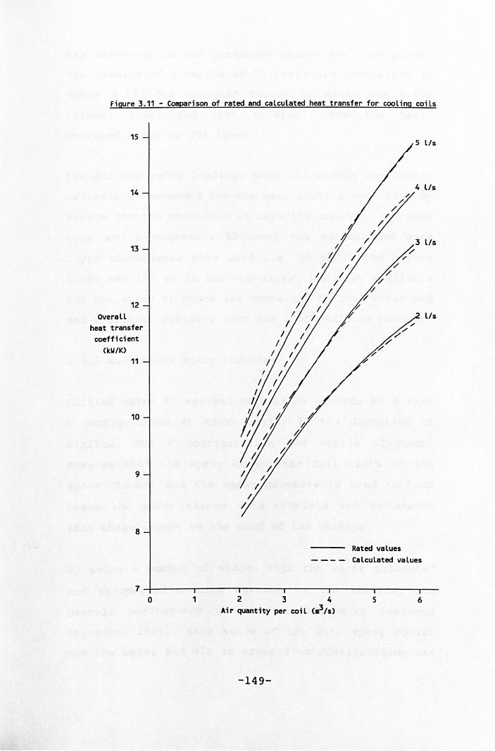
Figure 3.11 - Comparison of rated and calculated heat transfer for cooling coils
15
14
13
12
OVerall heat transfer coefficient
(kll/IO 11
10
9
8
/ I
/
/ I
I I
I
I
I
Rated values
5 lIs
4 lIs
3 lIs
lIs
- - - - calculated values
7-r------~----_.------_r------,_------._----_.---
o 1 234 Air quantity per coil (.3 /s )
-149-
5 6
the discharge of the condenser sprays for this plant.
The results of a series of 23 tests are summarised in
Table 3.13. The expected factor of merit was 0.625
(Bluhm, 1982) and that obtained from the tests
averaged 0.500 or 20% lower.
The air and water loadings were all within the design
criteria recommended for the mesh coolers and the only
reason for the shortfall in capacity could be the mesh
type and arrangement. Although the recommended mesh
layer thicknesses were used i.e. 50 mm in the bottom
layer and 100 mm in the top layer, the mesh available
for the units at Mount Isa contained thicker wires and
had a greater porosity than the South African design.
3.5.3 Multistage spray chambers
Chilled water is sprayed vertically upwards in a flat
V configuration at right angles to the direction of
airflow. The V configuration and nozzle alignment
ensures that the spray covers the full width of the
spray chamber and the spray pressure is used to both
break the water stream into droplets and to ensure
that these impact on the roof of the chamber.
By using a number of stages with the water collected
and re-sprayed counter current to the airflow, the
overall performance can be significantly improved
(Ramsden, 1984). Each stage of the bulk spray cooler
has the water and air in cross flow configuration and
-150-
can be assessed using the method of analysis outlined
in section 3.4.2 and Table 3.11 with the entering and
leaving water temperatures transposed to avoid
negative values.
With the air and water in counter flow through the
stages, an iterative method converging to an
acceptable error is necessary to determine the overall
performance of a multistage unit. An analysis of the
measurements undertaken on the multistage horizontal
spray chambers installed at Mount Isa and Broken Hill
is summarised in Table 3.14.
The factor of merit for each stage of the conventional
units varied between 0.43 and 0.51 and, based on a
counter flow overall analysis, the factors of merit
for a two stage and a three stage unit was 0.61 and
o. 7 0 respectively. These are wi thin the performance
range that could be normally expected (Ramsden, 1984).
Where the stage factor of merit was below 0.45, it was
evident that channelling of the air was taking place.
In the conventional units this was mainly a result of
irregularities in the spray chamber excavation which
were not covered by the range and alignment of the
sprays.
The two main reasons for using multistage horizontal
spray chambers underground were the large cooling
duties possible and a perceived lower installation
-151-
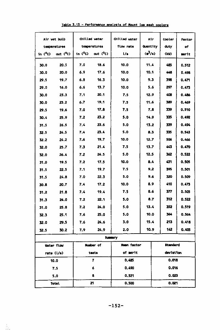
Table 3.13 - Perfor .. nce analysis of Mount lsa .ash coolers
Air wet bulb Chilled water Chilled water Air COOler Factor
t...,.ratures taperatures flow rate Quantity duty of
in (oC) out (oC) in (oC) out (oC) lis (rills) (kV) .. r1t
30.0 20.5 7.0 18.6 10.0 11.4 485 0.512
30.0 20.0 6.9 17.6 10.0 10.1 441 0.498
29.5 19.7 6.8 16.3 10.0 9.3 398 0.471
29.0 16.0 6.6 13.7 10.0 5.6 297 0.473
30.0 23.3 7.1 20.1 7.5 12.9 4GB 0.486
30.0 23.2 6.7 19.1 7.5 11.6 389 0.469
29.5 19.6 7.0 17.8 7.5 7.8 339 0.510
30.4 25.9 7.2 23.2 5.0 14.9 335 0.492
31.5 26.5 7.4 23.6 5.0 13.2 339 0.494
32.5 24.5 7.4 23.4 5.0 8.3 335 0.543
32.2 24.2 7.6 19.7 10.0 12.7 506 0.466
32.0 25.7 7.3 21.4 7.5 13.7 443 0.470
32.0 26.4 7.2 24.5 5.0 12.5 362 0.522
31.0 19.5 7.2 17.5 10.0 8.4 431 0.505
31.5 22.5 7.1 19.7 7.5 9.2 395 0.501
31.5 24.8 7.0 22.3 5.0 9.6 320 0.509
30.8 20.7 7.4 17.2 10.0 8.9 410 0.473
31.2 21.8 7.4 19.4 7.5 8.6 377 0.505
31.3 24.0 7.2 22.1 5.0 8.7 312 0.522
31.0 25.8 7.2 24.0 5.0 13.4 352 0.519
32.3 25.1 7.6 25.0 5.0 10.0 364 0.564
32.0 29.5 7.6 24.6 3.0 15.4 213 0.418
32.5 30.2 7.9 24.9 2.0 10.9 142 0.405
~ry
water flow Nullber of ..... factor Standard
rate (lIs) teats of .. rit deviation
10.0 7 0.485 0.018
7.5 6 0.490 0.016
5.0 8 0.521 0.023
Total 21 0.500 0.021
-152-
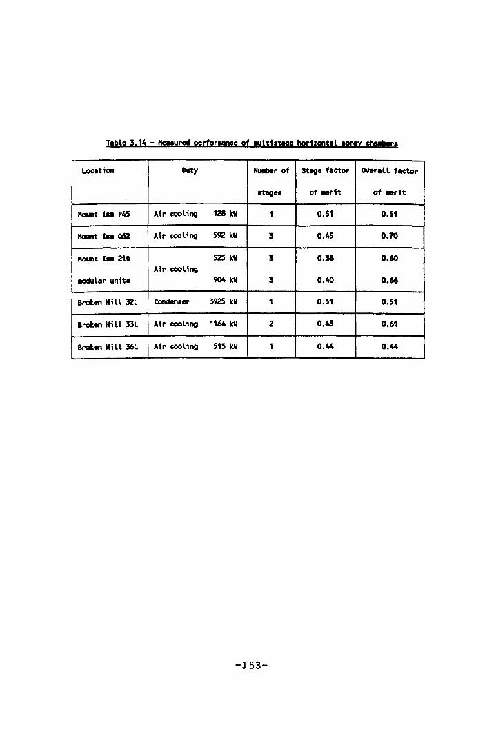
Table 3.14 - Mea.ured perfor!!nce of MUlti.tage borizontal !pray cbt!btr.
Loc:etion Duty NUllber of Stage factor OVerall factor
.tage. of .. rit of .. r1t
Mount IN P45 Air cooling 128 kW 1 0.51 0.51
MoUnt IN Q62 Air cooling 592 kW 3 0.45 0.70
Mount IN 21D 525 kW 3 0.38 0.60 Air cooling
puler units 904 kW 3 0.40 0.66
Broken Hi II 32L Condenter 3925 kW 1 0.51 0.51
Broken Hi II 33L Air cooling 1164 kW 2 0.43 0.61
Broken Hi II 36L Air cooling 515 kW 1 0.44 0.44
-153-
cost relative to the other available methods of bulk
air cooling. In practice, the low installation costs
have not been realised mainly as a result of the
problems associated with fractured ground surrounding
the spray chamber locations.
This has resulted in overbreak and the cost of
additional concrete work as well as difficulties in
sealing the sumps that are necessary to collect the
water for stage re-spraying. At Mount lsa, the costs
of a typical three stage horizontal spray chamber was
up to three times that originally estimated and
alternative bulk air coolers were considered.
The modular unit was an attempt to reduce costs by
designing and fabricating a three stage horizontal
spray chamber in fibreglass. The sumps are open tanks
supported on a bed of sand. The sides and roof of the
spray chamber above the sumps as well as the spray
eliminators were also manufactured in fibreglass and
the complete unit was to be installed in a standard
spray chamber excavation.
Based on performance tests, the measured stage factor
of merit varied between 0.38 and 0.40 and the overall
factor of merit was between 0.60 and 0.66. The main
reason for the low performance was channelling of air
above the sprays which did not impact on the roof of
the unit. Transportation and installation problems
resulted in costs almost six times those estimated.
-154-
3.5.4 Modular cooling towers
The poor performance of the mesh coolers and the high
cost of the three stage bulk air coolers prompted a
review of the underground air cooling methods. Packed
counter flow packaged cooling towers are now used for
both development air cooling and for bulk air cooling.
The greater effectiveness of the counter flow heat
exchange results in two stages performing as well as
three stages in a cross flow water/air configuration.
The cooling tower module is constructed mainly in
fibreglass, has a cross sectional area of 4.4 m2 and
an overall height of 3.2 m which includes a 2 m3 sump,
the air inlet section, 900 mm of compact fill and the
discharge section. The units can be installed without
additional excavation in most underground headings.
The design water flow rates are normally between 6 and
25 lIs and the airflow rates between 7.5 and 15 m3/s
resulting in cooling duties between 250 and 1000 kW.
To replace the mesh cooler for development cooling,
two units are normally installed in series with
respect to water flow and in parallel with respect to
airflow. The development fans are used to induce the
airflow through the unit and the discharge section of
the tower contains an eliminator and a 900 bend. The
expected factor of merit for each stage is 0.62 and
the combined value for two units is 0.68.
-155-
For bulk air cooling and replacing the multistage
spray chambers, the cooling towers are installed in
modules of two units with the water in series and the
airflow in parallel. Each tower has its own fan which
is located above the eliminator in the discharge
section of the tower. As before, the expected factor
of merit for each stage is 0.62 and the combined value
for two units is 0.68.
An analysis of the measurements taken on two bulk
cooling installations resulted in stage factors of
merit varying between 0.49 and 0.60 and an overall
value of 0.64 for both installations. This analysis
was based on the air temperatures taken in the intake
airways to the installation and at the tower
discharge.
Air temperature measurements were also taken at the
inlet to each tower and confirmed that there was
re-circu1ation between the discharge and the inlet
which reduced the overall performance. The amount of
re-circu1ation is reduced by using a wall downstream
of the installation and ducting the air discharged
from the towers beyond this wall.
3.5.5 Capacity control
In order to minimise the overall operating costs of an
underground chilled water system it is necessary to
maximise the temperature of the water being returned
-156-
back to surface for chilling. During the cooler
periods when the surface temperatures are lower, the
underground temperatures will also be lower and the
amount of cooling reduced. Unless the amount of
chilled water is reduced the return water temperature
will also be lower.
In direct contact heat exchangers it is usually
undesirable to reduce the water flow rate through the
unit. Low water flow rates cause dry areas in the fill
(or low nozzle pressure in spray chambers) and result
in air channelling and a much lower unit performance.
It is therefore advantageous to maintain the same
water flow rate through the unit and to re-circulate
water between the outlet and the inlet. The chilled
water supplied to most cooling units is gravity fed
from a cascade dam system and the return water is
pumped to a return water dam. A flow control valve
after the return pump allows return water to
re-circulate back to the inlet pipe and mix with the
incoming chilled water.
The distribution nozzles in the cooling unit control
the total water flow rate and therefore the amount of
incoming chilled water used is dependent on the
re-circulation water flow rate. The re-circulation
valve setting is controlled by the temperature of the
air leaving the cooling unit. A simple temperature
probe, shielded to minimise the effects of any chilled
-157-
water carryover, is located in the air discharge from
the unit after the eliminator. In most of the units
the air is cooled to below its dew point temperature
and it is discharged in a saturated condition. This
removes the need to specifically measure the wet bulb
temperature of the air.
Where modular cooling towers are used, the temperature
of the air from the lead unit (with respect to the
water flow) is used for controlling the re-circulation
valve setting. Seasonal adjustments to the settings
are necessary to maximise the benefits of the cooling
system.
-158-

3.6 Miscellaneous
3.6.1 High pressure water to water heat exchangers
High pressure water to water heat exchangers are used
to keep in closed circuit, the chilled water from the
evaporator of a central refrigeration plant and, to
cool water in a separate circuit which is then used to
distribute the coolth to the cooling appliances. The
central refrigeration plant may be remote from the
cooling appliances and could be located on surface.
By keeping the chilled water in closed circuit, the
primary circuit pumping costs are potentially much
lower and, by using high pressure heat exchangers, the
necessity to have high pressure pipes and cooling
coils can be eliminated. The method of analysing the
performance of a high pressure water to water heat
exchanger is given in Table 3.15.
In a closed circuit, the pump power required is that
to overcome friction in the pipes whereas in an open
circuit, the energy recovery system inefficiency must
also be included. For a refrigeration plant situated
on surface, however, this simple comparison is not
valid. The high pressure heat exchanger introduces
another heat flow resistance to the circuit which
reduces the system coefficient of performance. This
results from both a decrease in the evaporating
temperature necessary to achieve the same cooling load
-159-
and by reducing the effect of a pre-cooling tower.
Prior to proceeding with the stage 1 chilled water
system at Mount Isa,
extending the existing
consideration was given to
R63 system which used high
pressure water to water heat exchangers. Both systems
were optimised to provide the most cost effective
arrangement. The overall power requirements for the
closed circuit system were 32% greater than the open
system and the capital cost was three times higher.
3.6.2 Pipe heat transfer and heat gains
The greater the distance of the central refrigeration
plant from the cooling appliances, the longer the pipe
lengths required to distribute the chilled water and
the higher potential heat gains. Insulating the
underground chilled water pipes is necessary in order
to minimise these heat gains. Most of the chilled
water pipes are in intake airways and consequently an
increase in coolth loss from the chilled water pipes
is not necessarily a loss to the system.
Excessive losses from the chilled water pipes do,
however, lead to system inefficiencies as a result of
cooling being applied too early. The lower temperature
air results in an increased heat flow from the
surrounding rock surfaces and, because of air leakage,
a part of the refrigeration is not effective in the
working area. The overall system power to cooling
-160-
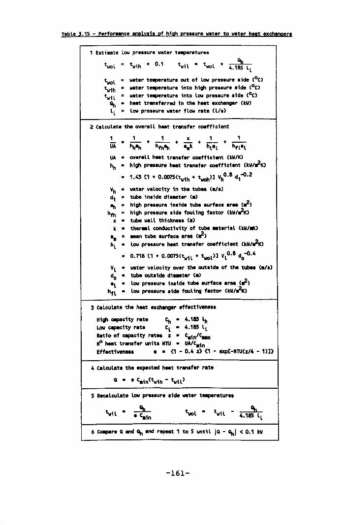
Table 3.15 - Perfonaance analysis of high pressure water to water heat exchangers
1 Estieate low pressure water teaperatures
twil • t l + 9h wo 4.185 II
twol • water te.perature out of low pressure side (oC) twih • water t.-pereture into high pressure side (oC) twil = water te.perature into low pressure side (oC)
'\t • heat transferred in the heat exchanger (kW) II = low pressure water flow rate (lIs)
2 Calculate the overall heat transfer coefficient
1 1 1 x 1 1 _a __ + __ +_+ __ + UA hh~ hth~ a.k hlal hflal
UA • overall heat transfer coefficient CkW/K> hh • high pressure heat transfer coefficient (kW/~)
• 1.43 [1 + O.OO75(twih + t woh)] Vho.a di-o·2
Vh • water velocity in the tubes (Ills) di a tube inside dia-.ter Ca) ~ • high pressure inside tube surface area (~)
hfh • high pressure side fouling factor (kW/~K) x • tube wall thickness Ca) k • ther .. l conductivity of tube .. terial (kW/~)
aa • ... n tube surface area (~) hl • low pressure heat transfer coefficient CkW/~)
• 0.718 [1 + O.OO75(twil + twol)] Vlo.8 do-o·4
Vl • water velocity over the outside of the tubes (./s) do • tube outside di ... ter Ca) al • low pressure inside tube surface area C~)
hfl • low pressure side fouling factor CkW/~)
3 calculate the heat exchanger effectiveness
High capacity rate ~. 4.185 ~ Low capacity rate Cl • 4.185 II Ratio of capacity rates z • C.in/C..x ~ heat transfer units NTU • UA/Ca1n Effectiveness e • (1 - 0.4 z) (1 - exp[-NTU(z/4 - 1)])
4 calculate the expected heat transfer rate
Q • e CainCtwih - ~1l)
5 Recalculate low pr .. sure side water teaperatures
6 CoIIpare Q and '\t and repeat 1 to 5 until IQ - ~I < 0.1 kW
-161-

ratio (including the effects of energy recovery) for
stage 1 of the Mount Isa system is 0.299.
The insulation of underground pipes is notoriously
difficult to achieve with a system that is both cost
and "insulation" effective. The major problem is water
vapour penetration of the insulation material. Most of
the available pipe insulations entrap air (which has a
low thermal conductivity of 0.028 W/m R) in a cellular
structure i.e. polyurethane foam which has a ratio of
20 parts of air to one of polyurethane by volume and
an overall thermal conductivity of 0.037 W/mK.
Most materials used to produce foam have a relatively
high vapour permeability and the large difference in
vapour pressure between the cold pipe surface and the
surrounding air results in rapid moisture penetration.
Wi thin three years, insulation that does not have a
vapour barrier becomes fully saturated with an overall
thermal conductivity of 0.58 W/mR. A vapour barrier
will delay rate of moisture penetration, however,
maintaining a suitable barrier in underground workings
is very difficult.
The most successful insulation systems which also have
a reasonable cost are those using plastics such as
polyurethane foam with a thick (greater than 5 nun)
high density polyethylene vapour barrier. The great
drawback is the flammability and potential fire risk.
other systems using fire retardant PVC to provide an
-162-
air gap which could be filled with a loose inert
material to eliminate natural convection in the air
gap have had limited success.
Foamed glass is ideal from the insulation and vapour
penetration point of view. The closed cell and almost
impermeable glass provides a system that does not rely
on a mechanical vapour barrier and has an overall
thermal conductivity of 0.055 W/mK. The material is,
however, friable, requires outer mechanical protection
and is also relatively expensive.
A typical coolth loss for a 200 mm diameter main
chilled water distribution pipe with foamed glass
insulation is 0.037 kW/m. This presumes that the full
pipe length is insulated. Only insulating the straight
lengths of pipe and leaving the couplings bare would
result in an increase to 0.085 kW/m.
This represents an increase in refrigeration operating
costs equal to approximately 50% of the cost of the
insulation presuming that none of the cooling from the
pipe is useful in the mining area. This would only be
true if the air so cooled by the inefficient pipe
insulation is not used in the mining area and returned
directly to an exhaust.
overall, this is expected to happen to less than 25%
of the air (leakage) and consequently the cost would
be reduced to between 10 and 15% of the insulation
-163-
cost. For a 6 m length of pipe, the cost of not
insulating the couplings would, therefore, be
approximately equal to the cost of insulating 1 m and
of marginal financial benefit.
The cool th losses from uninsulated pipes would vary
between 0.5 and 1.5 kW/m depending on the size and
arrangement. The cost of these losses would be between
one and ten times the cost of insulation depending on
the amount of intake air lost by leakage to the return
airways and is not insignificant.
An alternative insulation is based on providing the
pipes with a PVC lining on the inside or to fit a
larger PVC pipe over the outside of a steel pipe. For
a 5 mm thick liner, the coolth loss will be between
0.3 and 0.35 kW/m depending on the application.
Relative to the foamed glass insulation, the increased
coolth losses would be approximately 0.25 kW/m or
about 60% of the insulation cost when assuming a 25%
air leakage to the return airways.
Mine refrigeration systems have many kilometres of
pipe which is used for distributing chilled water. The
potential losses are significant and, when the full
refrigeration system is being modelled, these should
be included in the assessment. As a result of the
complexity of the piping and insulation systems, two
simplifications are applied.
-164-
Where the pipes are insulated, the heat flow is based
on the resistance of the insulation and the difference
between the air dry bulb and the chilled water
temperatures. Where the pipes are not insulated,
condensation is assumed to occur and the heat flow is
a function of the air wet and dry bulb temperatures
relative to the chilled water temperature. The method
of analysis used is summarised in Table 3.16.
-165-
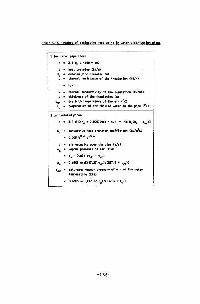
Table 3.16 - "ethod of esti.ating heat gains in water distribution pipes
1 Insulated pipe lines
q • 3.1 do U (tdb - tw)
q • heat transfer (kW/.) do • out. ide pipe dia •• ter (.) U • theraal resistance of the insulation (kW/K)
= k/x
k • theraal conductivity of the insulation (kW/~) x • thickness of the insulation (.)
tdb • dry bulb teaperature of the air (oC) t = teaperature of the chilled water in the pipe CoC) v
2 Uninsulated pipes
q • 3.1 d [(hc + O.OO6)(tdb - tv) + 16 hc(ea - esw)]
hc • convective heat transfer coefficient (kW/a2K)
• 0.005 yO.6 d-o·4
v • air velocity over the pipe (./a) ea • vapour pressure of air (kPa)
• es - 0.071 (tdb - twb)
es • 0.6105 exp[C17.27 t wb)/(237.3 + twb)]
esv • saturated vapour pre.aure of air at the water ta.perature CkPa)
• 0.6105 exp[(17.27 tv)/(237.3 + tw)]
-166-
4 ACTUAL PLANT SIMULATIONS
The five refrigeration systems modelled have a similar
structure and method of converging to a solution which
allows a modular approach to be taken. In the first
part of this section, the general simulation method is
outlined in terms of the three subsystems and the
interrelationships between them.
In the remaining sections, each model is discussed and
its sui tabili ty to adequately represent the overall
refrigeration system operation is assessed. Also given
is the background leading to design and justification
for each system and the development of the simulations
and control strategies. Comparisons between predicted
and actual performance are made and the adjustments
necessary as a result of subsequent testing outlined
where appropriate.
4.1 Simulation structure and components
The fundamental structure of all the models used to
simulate refrigeration plant performance outlined in
figure 2.12 can be divided into three main subsystems
which are designated as chiller, heat rejection and
load. Each subsystem normally comprises of several
components which, for all the actual plants modelled,
have sufficient similarities in structure and method
of analysis to allow a modular approach to be taken in
the overall simulation structure.
-167-
There will be a difference in emphasis within both the
modules and the structure depending on whether the
simulation is being used either to optimise plant
operation or as a diagnostic device. Although not as
amenable, the optimisation model can also be used for
diagnostic purposes, consequently only this structure
will be described in detail.
4.1.1 The chiller subsystem
Evaporator modules
The first component of the chiller subsystem is the
evaporator and the module analysis is illustrated in
figure 4.1. The evaporator water flow rate Ie will
depend on both the load subsystem and the control
strategy and may be either variable where the
compressor is maintained at full load or fixed where
the compressor is allowed to unload to match the load
subsystem. If the evaporator water flow rate is to be
variable, a start value is adopted, which is normally
taken as that at the design condition.
The temperature of the water entering the evaporator
twie and the evaporator duty Qe will vary according to
the load subsystem and the evaporator water flow rate.
Again, the start values adopted for the simulation are
those at the design condition. The fouling factor hfe
is constant for a particular simulation and will only
change with time and water quality. The fouling factor
-168-
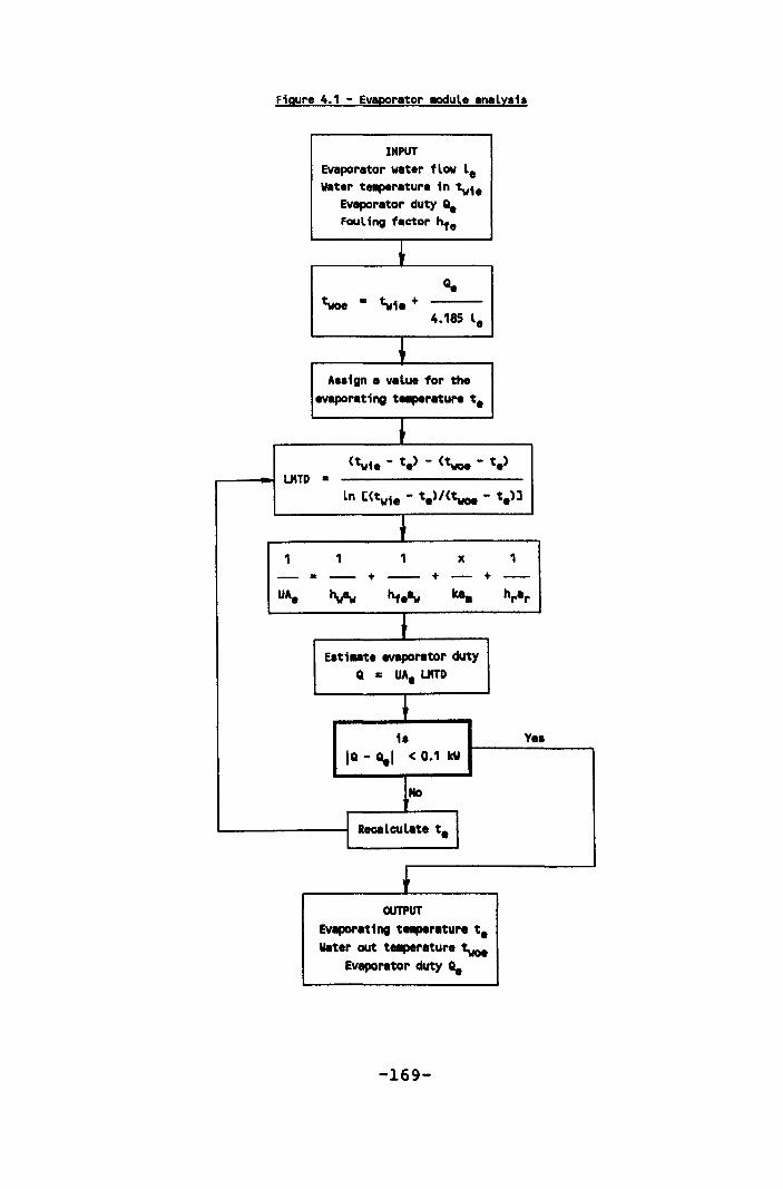
Figure 4.1 - Evaporator .adule analyaia
INPUT Evaporator vater flow le water ta.perature in tvie
Evaporator duty ~ Fouling factor hfe
~ ~
twoe • tvie + 4.185 le
~ Aaa1gn a value for the
evaporating ta.perature t.
~ (tvie - t e> - (twoe - t.>
LHTD • ln [(tv1e - t.>/(two. - t.>J
+ 1 1 1 x 1
- • -- + -- + - + --UA. tvw ht.1Iw Icaa hrar ,
Eati .. te evaporator duty Q • UA. LHTD
~ i. Vea
IQ - ~I < 0.1 tv
ltk)
: Recalculate t. I +
OUTPUT Evaporating t8lperature te water out ta.perature twoe
Evaporator duty ~
-169-
can be used as a variable if the simulation is to be
used diagnostically to determine when evaporator
cleaning should take place.
Wi th this input information, the temperature of the
water leaving the evaporator twoe is calculated and a
value assigned for the evaporating temperature te.
Although the design value may be used, it may need to
be adjusted if (twoe - t e > < O. This would result in
an error (attempting to calculate a negative natural
logarithm) when calculating the log mean temperature
difference LMTD.
The overall heat transfer coefficient UAe is obtained
using the heat transfer characteristics for the type
of evaporator being used and the input variables
defined above. The estimated evaporator duty is the
product of the overall heat transfer coefficient and
the log mean temperature difference and is compared to
the input value. If the difference in evaporator
duties is greater than a pre-set test value, a revised
evaporating temperature is calculated and the process
repeated until the test condition is met.
Condenser modules
The second component of the chiller subsystem is the
condenser. The analysis of this module is illustrated
in figure 4. 2 for a condenser with an external heat
rejection subsystem and for an evaporative condenser
-170-
in figure 4.3. Where applicable, the condenser water
flow rate lc and the fouling factor hfc are normally
fixed values. The start value for the temperature of
the water into the condenser twic is usually taken as
the design value.
The evaporator duty 0e' obtained from the evaporator
module, and an estimate of the compressor input power
is used to calculate both the condenser duty Oc and
the temperature of the water leaving the condenser
t woc . A start value for the compressor input power is
normally taken as 20% of the design evaporator duty
which infers a power to cooling ratio of 0.2.
A start value is also assigned for the condensing
temperature tc. Although the design value may be used,
it may need to be adj usted if ( tc - t woc ) < o. As
before, this would result in an error when calculating
the log mean temperature difference LMTD.
The overall heat transfer coefficient UAc is obtained
using the heat transfer characteristics for the type
of condenser and the defined input variables. The
estimated condenser duty is the product of the overall
heat transfer coefficient and the log mean temperature
difference and is compared to the input value. If the
difference in condenser duties is greater than a
pre-set test value, a revised condensing temperature
is calculated and the process repeated until the test
condition is met.
-171-
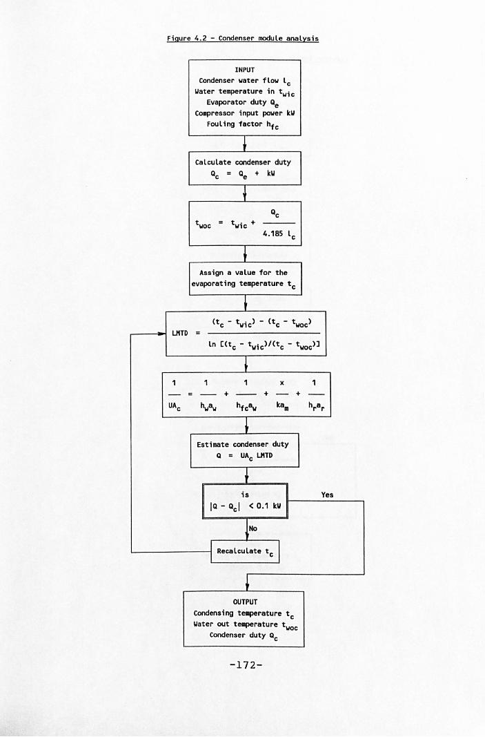
Figure 4.2 - Condenser module analysis
INPUT Condenser water flow lc
Yater temperature in twic Evaporator duty Qe
Compressor input power kY Fouling factor hfc
~ Calculate condenser duty
Qc = Qe + kY
i Qc
twoc = twic + 4.185 lc
~ Assign a value for the
evaporating temperature tc
~ (tc - twic) - (tc - t woc>
U1TD = ln [(tc - twic)/(tc - twoc>l
~ 1 1 1 x 1
- = -- + -- + - + --UAc "waw hfcBw ka. hrar
~ Estimate condenser duty
Q = UAc U1TD
t is Yes
IQ - Qcl < 0.1 kll
iNO
I Recalculate tc I
t OUTPUT
Condensing te.perature tc Yater out temperature twoc
Condenser duty Qc
-172-
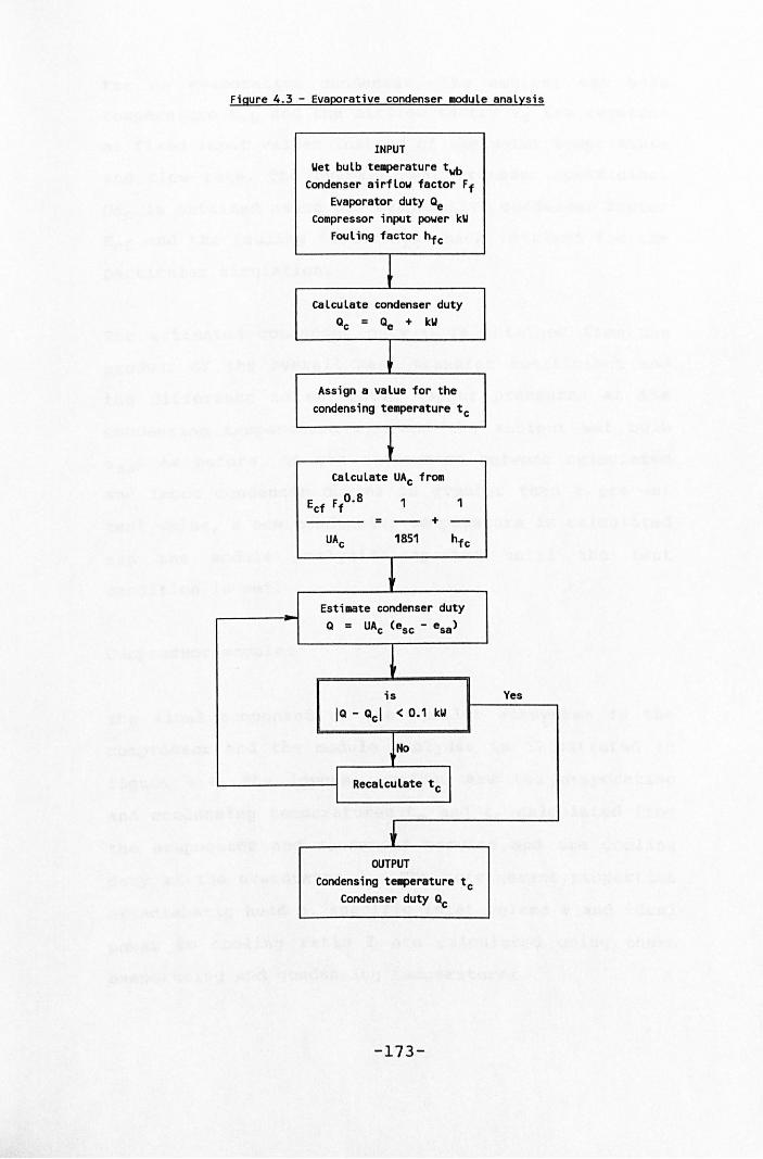
Figure 4.3 - Evaporative condenser module analysis
INPUT Wet bulb temperature twb
Condenser airflow factor Ff Evaporator duty Qe
Compressor input power kW Fouling factor hfc
~ Calculate condenser duty
Qc = Qe + kW
~ Assign a value for the
condensing temperature tc
t Calculate UAc from
Ecf F 0.8 f 1 1
= -- + -UAc 1851 hfc
t Estimate condenser duty Q = UAc (esc - esa)
~ is Yes
IQ - Qcl < 0.1 kW
~No I Recalculate tc I I
~ OUTPUT
Condensing teMperature tc Condenser duty Qc
-173-
For an evaporative condenser, the ambient wet bulb
temperature twb and the airflow factor Ff are required
as fixed input values instead of the water temperature
and flow rate. The overall heat transfer coefficient
UAc is obtained using the evaporative condenser factor
Ecf and the fouling factor hfc which is fixed for the
particular simulation.
The estimated condenser duty Q is obtained from the
product of the overall heat transfer coefficient and
the difference in saturated vapour pressures at the
condensing temperature esc and the ambient wet bulb
e sa . As before, if the difference between calculated
and input condenser duties is greater than a pre-set
test value, a new condensing temperature is calculated
and the module analysis repeated until the test
condition is met.
Compressor modules
The final component of the chiller subsystem is the
compressor and the module analysis is illustrated in
figure 4.4. The inputs required are the evaporating
and condensing temperatures te and tc calculated from
the evaporator and condenser modules and the cooling
duty at the evaporator Qe • The refrigerant properties
of adiabatic head h, specific inlet volume v and ideal
power to cooling ratio I are calculated using these
evaporating and condensing temperatures.
-174-

The refrigerant inlet volume refrigerant flow rate V
is calculated as the product of the specific inlet
volume v and the evaporator duty Qe . From the
equations relating compressor performance to inlet
volume flow rate V, the estimated adiabatic head hc
and the compressor efficiency nc can be established.
The ideal input power is the product of the ideal
power to cooling ratio and the evaporator duty and the
actual compressor input power kW can be obtained by
dividing this by the compressor efficiency.
The compressor modules may also contain any tests
which require part load operation of the compressors.
This includes approaching the surge condition for
centrifugal compressors or too low an evaporating
temperature with possible freezing of the water in the
evaporator. In these instances, part load operation is
dealt with in a separate compressor module depending
on how the compressor reduces load i. e. a change in
compressor speed, hot gas by-pass or a change in slide
valve setting.
Where the overall plant control strategy is to reduce
the compressor load to match the cooling duty, the
compressor part load routines can be incorporated in
the main compressor module. The simulations which are
used diagnostically, also require part load routines
where the load is determined from the motor current.
Examples with details of the techniques are given in
section 4.5 and 4.6.
-175-
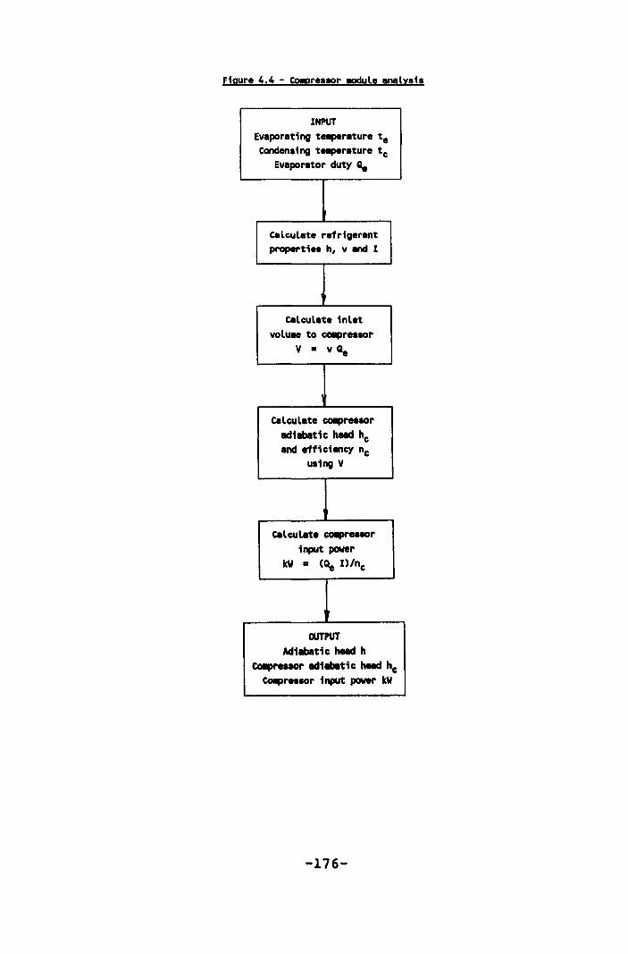
Figure 4.4 - CO!presaor .adule analysis
INPUT
Evaporating te.perature te Condensing te.perature tc
Evaporator duty ~
calculate refriger~t p~rtiea h, v and 1
calculete inlet voluM to COIIPresaor
V • vGle
calculete COIIPresaor adiabatic heed hc and efficiency nc
uaing V
calculete COIIPre.aor input power
kV • (~ I)/nc
OUTPUT Adiebltic heed h
COIIpreuor ediatie heed he COIIpresaor input power kV
-176-
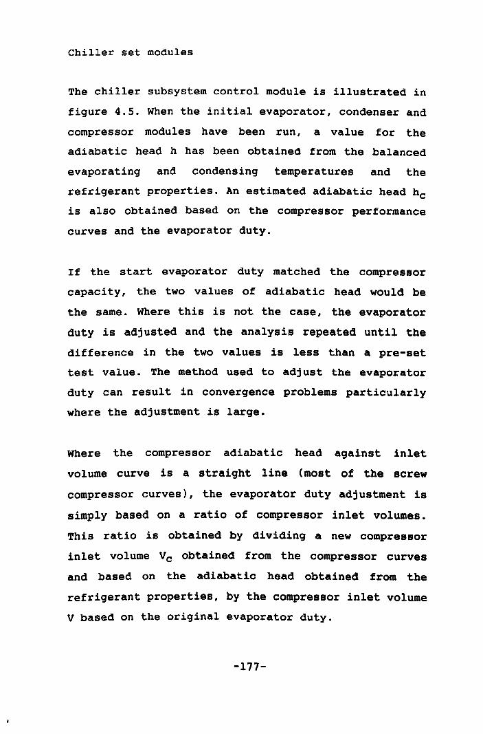
Chiller set modules
The chiller subsystem control module is illustrated in
figure 4.5. When the initial evaporator, condenser and
compressor modules have been run, a value for the
adiabatic head h has been obtained from the balanced
evaporating and condensing temperatures and the
refrigerant properties. An estimated adiabatic head hc
is also obtained based on the compressor performance
curves and the evaporator duty.
If the start evaporator duty matched the compressor
capaci ty, the two values of adiabatic head would be
the same. Where this is not the case, the evaporator
duty is adjusted and the analysis repeated until the
difference in the two values is less than a pre-set
test value. The method used to adjust the evaporator
duty can result in convergence problems particularly
where the adjustment is large.
Where the compressor adiabatic head against inlet
volume curve is a straight line (most of the screw
compressor curves), the evaporator duty adjustment is
simply based on a ratio of compressor inlet volumes.
This ratio is obtained by dividing a new compressor
inlet volume V c obtained from the compressor curves
and based on the adiabatic head obtained from the
refrigerant properties, by the compressor inlet volume
V based on the original evaporator duty.
-177-
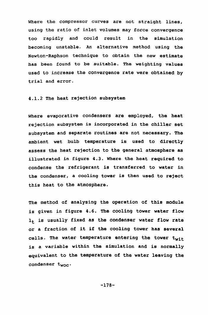
Where the compressor curves are not straight lines,
using the ratio of inlet volumes may force convergence
too rapidly and could result in the simulation
becoming unstable. An alternative method using the
Newton-Raphson technique to obtain the new estimate
has been found to be sui table. The weighting values
used to increase the convergence rate were obtained by
trial and error.
4.1.2 The heat rejection subsystem
Where evaporative condensers are employed, the heat
rejection subsystem is incorporated in the chiller set
subsystem and separate routines are not necessary. The
ambient wet bulb temperature is used to directly
assess the heat rejection to the general atmosphere as
illustrated in figure 4.3. Where the heat required to
condense the refrigerant is transferred to water in
the condenser, a cooling tower is then used to reject
this heat to the atmosphere.
The method of analysing the operation of this module
is given in figure 4.6. The cooling tower water flow
It is usually fixed as the condenser water flow rate
or a fraction of it if the cooling tower has several
cells. The water temperature entering the tower twit
is a variable within the simulation and is normally
equivalent to the temperature of the water leaving the
condenser t woc ·
-178-
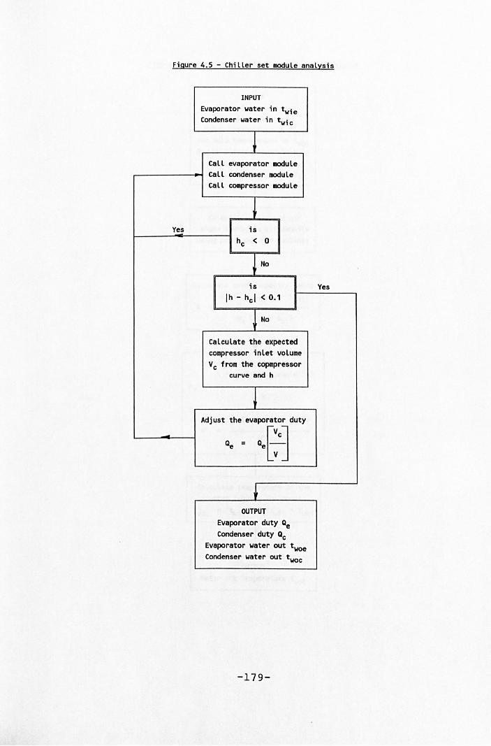
Figure 4.5 - Chiller set module analysis
Yes
INPUT
Evaporator water in twie Condenser water in twic
Call evaporator module Call condenser module Call compressor module
is hc < 0
~NO is
Ih - hcl < 0.1
Calculate the expected compressor inlet volume Vc from the copmpressor
curve and h
Adjust the evaporator duty
•• = ~t:'j
OUTPUT
Evaporator duty Qe Condenser duty Qc
Evaporator water out twoe Condenser water out twoc
-179-
Yes
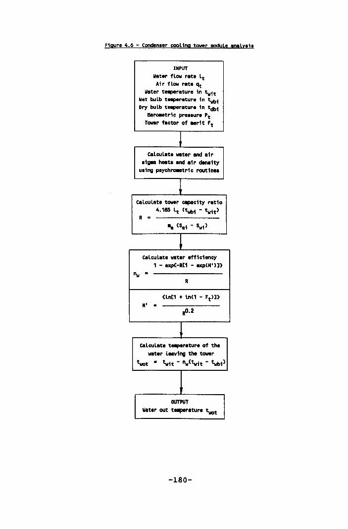
Figure 4.6 - Condenser cooling tower DOdule analysis
INPUT Water flow rate It Air flow rate qt
Water te.perature in twit Wet bulb te.perature in twbi Dry bulb te.perature in tdbi
Baro.etric pressure Pt Tower factor of .. rit Ft
calculate water and air .i~ heat. and air density
using psych~tric routine.
Calculate tower capacity ratio 4.185 It (twbi - twit)
R • .. (Sai - Sw1)
calculate water efficiency 1 - exp(-R[1 - expCH')]}
"w = R
{In[1 + In(1 - Ft )]} H' •
RO.2
calculate ta.perature of the water leaving the tower
twot • twit - "w(twit - ~i)
OUTPUT
Water out ta.perature twot
-180-
Where screw compressors are used, the oil injected
into the refrigerant prior to compression and removed
from the discharge gas is often cooled in a separate
shell and tube heat exchanger using a fraction of the
condenser water prior to re-injection. In this case,
the water temperature into the condenser cooling tower
may be weighted according to the temperatures and flow
rates through the condenser and the oil cooler.
More often, the oil cooling load is usually less than
1% of the total condenser load and can be considered
as part of the condenser operation rather than a
separate heat exchanger without significant error.
other constant values wi thin the simulation are the
ambient wet and dry bulb temperatures twbit and tdbit,
the barometric pressure Pt' the air flow rate in the
tower qt and the factor of merit for the tower Ft.
psychrometric routines are used to calculate the sigma
heats of the air entering, the saturated air at the
entering water temperature and the air density. These
are used to calculate the tower capacity ratio R.
The water efficiency nw is a function of the type of
tower (cross or counter flow), the tower capacity
ratio and the factor of merit. It is used to calculate
the temperature of the water leaving the tower twot
which, ignoring pipe line heat losses or gains, is the
temperature of the water entering the condenser twic.
-181-
4.1.3 The load subsystem
The load subsystem can be a straightforward single
surface bulk air cooler or a complex sequence of heat
exchangers of different types used both in parallel
and in series circuits. The module analysis for either
system follows the same form with the distributional
structure becoming more complex as more elements are
introduced into the system.
Surface bulk air cooler
The module analysis for a surface bulk air cooler is
illustrated in figure 4.7. For a simulation, the only
variable is the temperature of the water into the bulk
air cooler twit. This will be equal to the temperature
of the water leaving the evaporator twoe plus the rise
in water temperature resulting from any heat gains in
the piping between the evaporator and the bulk cooler.
For a given simulation, the air and water flow rates,
the air wet and dry bulb temperatures, the barometric
pressure and the bulk air cooler factor of merit are
all fixed.
In a similar manner to that described for the heat
rejection cooling towers, the temperature of the water
leaving the bulk air cooler twot can be established
from the variable water inlet temperature and the
remaining fixed parameters. The bulk air cooler duty
Qt is then calculated and the condition of the air
-182-
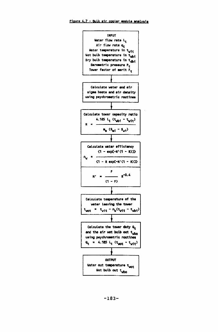
Figure 4.7 - Bulk air cooler !Odule 'Ollysis
INPUT W.ter flow r.te lt Air flow r.te qt
water te.per.ture in twit Wet bulb te.per.ture in twbi Dry bulb te.per.ture in tdbi
Baro.etric pressure 't Tower factor of .. rit Ft
~ calcul.te water .nd .ir
sigaa heats and .ir density using paychro.etric routines
~ calcul.te tower capacity r.tio
4.185 lt (~i - twit) R •
.. (S'i - Swi)
~ C.lculate w.t.r efficiency
(1 - exp[-N'(1 - R)J)
"w • {1 - R 'xp[-N'(1 - R)J)
F N' • R-o·4
(1 - f)
t calcul.te te.per.tura of the
water leaving the tower
twot • twit - "w(twit - ~i)
~ calcul.te the tower duty ~
and the .ir vet bulb out twbo using psychroletric routin ••
~ .. 4.185 It (~t - twit)
~ OUTPUT
Water out te.per.tur. twot Wet bu lb out twbo
-183-
supplied to the mine from the cooler obtained using
the psychrometric routines. The temperature of the
water leaving the bulk air cooler plus the rise in
temperature resulting from any pipe heat gains, is the
water temperature returned and supplied to the
evaporator twie.
underground chilled water systems
The most complex load subsystem has a closed circuit
chilled water supply from surface to underground high
pressure heat exchangers, a secondary cold water
circuit supplying both cooling coils and multistage
spray chambers and poor insulation resulting in heat
gains in the water distribution system. The module
analyses for the individual elements are illustrated
in figures 4.8 to 4.12 and the combined analysis is
illustrated in figure 4.13.
The first element is the temperature rise resulting
from heat gains to the high pressure pipes supplying
and returning chilled water between surface and the
high pressure heat exchangers (figure 4.8). For a
given simulation, the chilled water flow rate le, the
thermal resistance of the insulation U and the dry
bulb temperature of the air tdb is fixed. The later
assumption presumes that the heat transferred to or
from the air does not significantly change its
temperature.
-184-
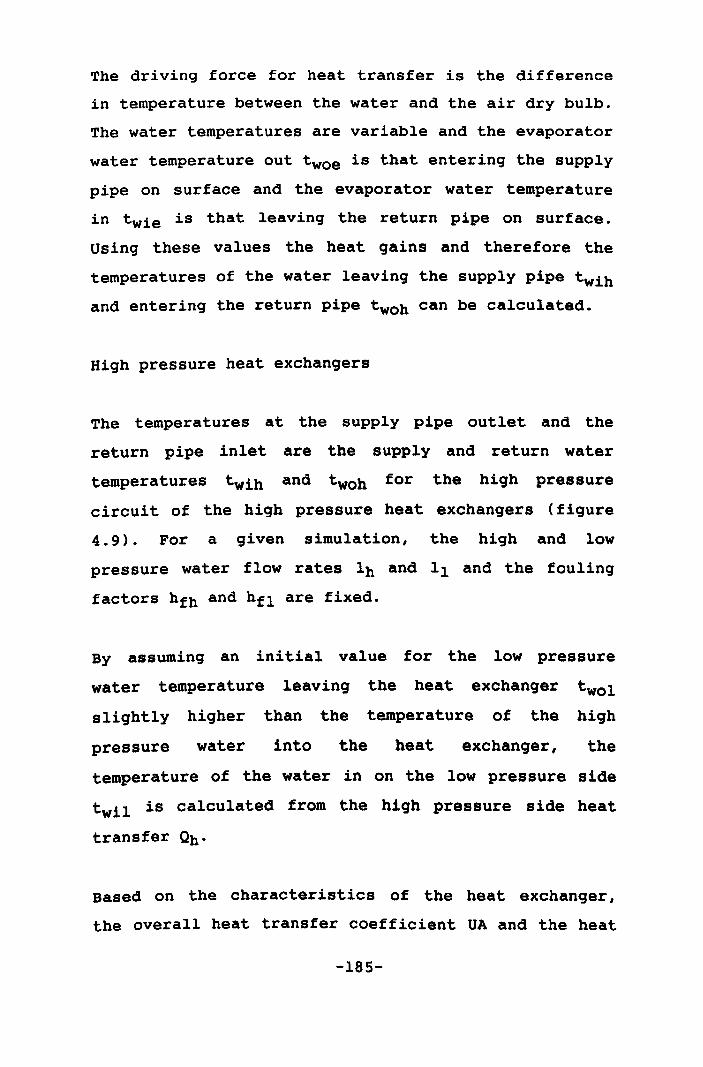
The driving force for heat transfer is the difference
in temperature between the water and the air dry bulb.
The water temperatures are variable and the evaporator
water temperature out twoe is that entering the supply
pipe on surface and the evaporator water temperature
in twie is that leaving the return pipe on surface.
Using these values the heat gains and therefore the
temperatures of the water leaving the supply pipe twih
and entering the return pipe twoh can be calculated.
High pressure heat exchangers
The temperatures at the supply pipe outlet and the
return pipe inlet are the supply and return water
temperatures twih and twoh for the high pressure
circuit of the high pressure heat exchangers (figure
4.9). For a given simulation, the high and low
pressure water flow rates lh and 11 and the fouling
factors hfh and hfl are fixed.
By assuming an ini tial value for the low pressure
water temperature leaving the heat exchanger twol
slightly higher than the temperature of the high
pressure water into the heat exchanger, the
temperature of the water in on the low pressure side
twil is calculated from the high pressure side heat
transfer Qh·
Based on the characteristics of the heat exchanger I
the overall heat transfer coefficient UA and the heat
-185-
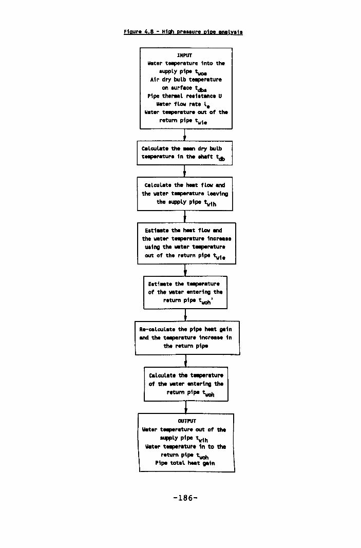
Figure 4.8 - High pre •• ure pipe ,",ly.i.
INPUT W.ter te.per.ture into the
.upply pipe twoe Air dry bulb te.per.ture
on .urf.ce tdba Pipe ther.el re.i.ttnc. U
U.ter fLow r.t. l. W.ter te.per.ture out of the
return pipe tvi.
~ CtLcul.t. the -.en dry bulb tellper.tur. in the ahaft tdb , Ctlcul.t. the heet flow end
the w.ter tllllplr.tur. leeving the aupply pipe twih
~ Eati_t. the heet flow end
the wet.r tellper.tur. 1ncr .... ua1ng the wet.r tlllper.ture out of the r.turn pipe t w1•
~ E.ti_t. the tlllper.tur. of the weter entering the
r.turn pipe twah'
~ Re-celcul.te the pipe heat gein end the te.per.tur. incr.... in
the return pipe
~ c.lcul.t. the telper.tur. of the wet.r tnt.ring the
return pipe ~ , OUTPUT
Weter telper.ture out of the supply pipe twih
W.t.r ttllpereture in to the r.turn pipe twah
Pipe tot.l heet gein
-186-
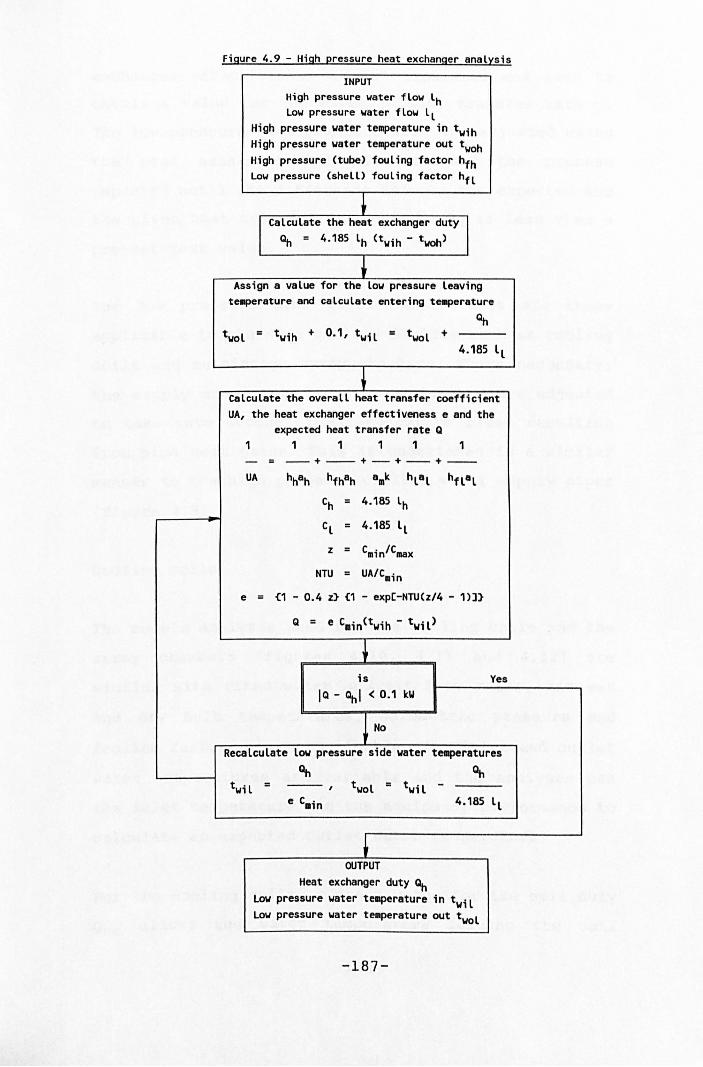
Figure 4.9 - High pressure heat exchanger analysis
INPUT High pressure water flow lh Low pressure water flow II
High pressure water temperature in twih High pressure water temperature out twoh High pressure (tube) fouling factor hfh Low pressure (shell) fouling factor hfl
Calculate the heat exchanger duty ~ = 4.185 lh (twih - t woh)
Assign a value for the low pressure leaving temperature and calculate entering temperature
twol = twih + 0.1, twil • twol + 4.185 II
Calculate the overall heat transfer coefficient UA, the heat exchanger effectiveness e and the
expected heat transfer rate Q
1 1 111 1 - = --+--+ - +--+--UA hhah hfhah amk hlal hflal
Ch = 4.185 lh
Cl = 4.185 II
z = Cmin/Cux
NTU = UAfC.in
e = {1 - 0.4 z} {1 - expC-NTU(z/4 - 1)J}
Yes IQ - ~I < 0.1 kW
~ No
Recalculate low pressure side water temperatures
4.185 II
OUTPUT Heat exchanger duty ~
Low pressure water temperature in twil Low pressure water temperature out twol
-187-
exchanger effectiveness e are calculated and used to
obtain a value for the expected heat transfer rate Q.
The low pressure water temperatures are adjusted using
the heat exchanger effectiveness and the process
repeated until the difference between the expected and
the given heat transfer rates Q and Qh is less than a
pre-set test value.
The low pressure side water temperatures are those
applicable to the mine cooling devices such as cooling
coils and multistage spray chambers. Where necessary,
the supply and return water temperatures are adjusted
to take into account the temperature rises resulting
from pipe heat gains. This is undertaken in a similar
manner to the high pressure chilled water supply pipes
(figure 4.8).
Cooling coils
The module analyses used for the cooling coils and the
spray chambers (figures 4.10, 4.11 and 4.12) are
similar with fixed water and air flow rates, air wet
and dry bulb temperatures, barometric pressure and
fouling factors where applicable. The inlet and outlet
water temperatures are variable and the analyses use
the inlet temperature and the equipment performance to
calculate an expected outlet water temperature.
For the cooling coils, a start value for the coil duty
Qcc allows the water temperature leaving the coil
-188-
twocc to be calculated. An air side coil duty Q can
then be obtained by calculating the overall heat
transfer coefficient UA and the coil effectiveness e.
This replaces the estimated coil duty Qcc and the
process is repeated until the difference in successive
values is less than a pre-set test value.
Multistage spray chambers
For the multistage spray chambers where the air and
water flows are counter current, the start value for
the analysis is taken as the outlet water temperature
twos being slightly less than the inlet wet bulb
temperature twbis. If it is assumed that each stage
cools one third of the total spray chamber duty
(obtained from the water flow rate and the difference
between the inlet water temperature twis and this
assumed value for the outlet water temperature), the
temperature of the water entering the first air stage
twil can be estimated.
The stage analysis (figure 4.11) is now used to
calculate the actual temperature of the water leaving
the spray chamber twol and the actual. stage 1 duty.
This is used to calculate the wet and dry bulb
temperatures leaving stage 1 i.e. the wet and dry bulb
temperatures entering stage 2. The water efficiency
calculated for stage 1 is used to estimate the
temperature of the water entering stage 2 twi2 and the
estimated stage 2 duty Qs .
-189-
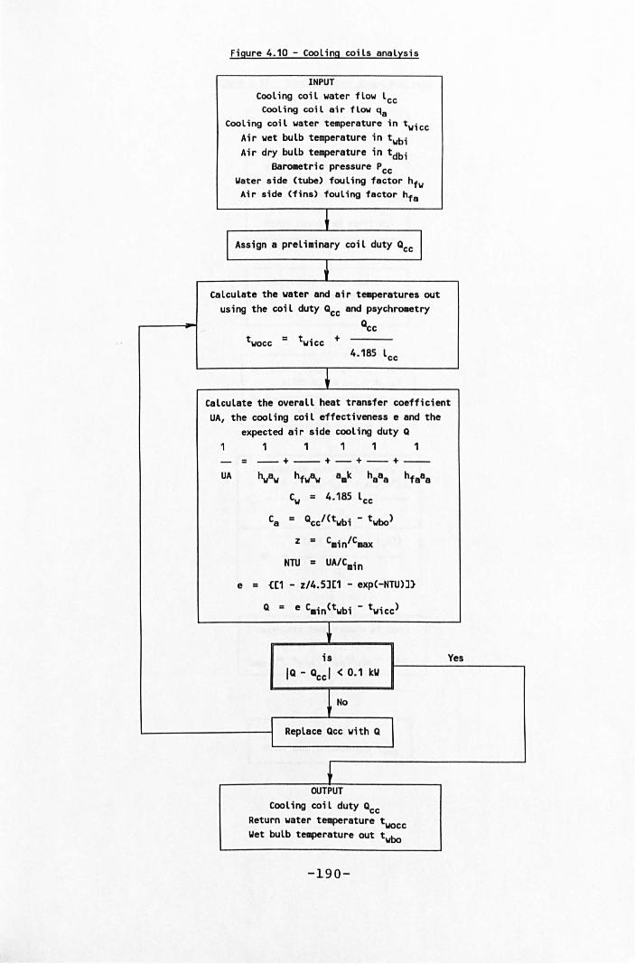
Figure 4.10 - Cooling coils analysis
INPUT Cooling coil water flow lcc Cooling coil air flow qa
Cooling coil water te~erature in t wicc Air wet bulb temperature in twbi Air dry bulb temperature in tdbi
Baro.etric pressure Pcc Water side (tube) fouling factor hfw Air side (fins) fouling factor hfa
I Assign a preli.inary coil duty Qcc I j
calculate the water and air temperatures out using the coil duty Qcc and psychrometry
Qcc
4.185 lcc
Calculate the overall heat transfer coefficient UA, the cooling coil effectiveness e and the
expected air side cooling duty Q 1 1 111 1 - = --+--+-+--+--UA hwaw hfwaw a.k heaa hfaaa
Cw = 4.185 lcc
Ca = Qcc/(twbi - t wbo)
z = C.in/C.ax
NTU = UAlC.in
e = {[1 - z/4.5][1 - exp(-NTU)]}
is
IQ - Qccl < 0.1 kW
Replace Qcc with Q
OUTPUT
Cool ing coil duty Qcc Return water temperature twocc Wet bulb temperature out twbo
-190-
Yes
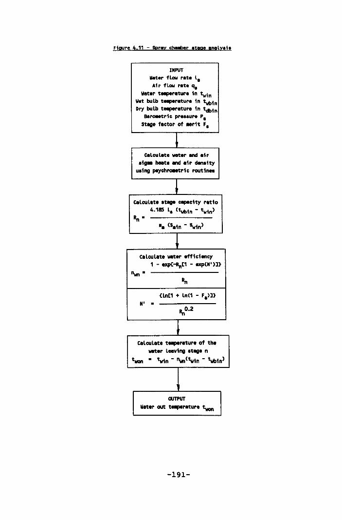
Figure 4.11 - Spray cha~r .tege analy.is
INPUT Water flow rate l. Air flow rate q.
Water te.perature in twin Wet bulb te.perature in twin Dry bulb te.perature in tdbin
Baro.etric pre •• ure p. Stage factor of .. rit f.
calcullite water lind air .ia- haIIta and air denaity
using paychro..tric routinea
calculate atage capacity ratio 4.185 l. (tWin - twin)
Rn-aa (5ain - Swin)
calculate water efficiency 1 - exp<-Rn[1 - exp(H')J}
"wn -Rn
{In[1 + In(1 - fa)]} H' - Rn°.2
calculate t...,.rature of the water leaving atage n
twon • twin - "wn(twin - twb1n)
QUTPUT
water out te.perature ~
-191-

Figure 4.12 - Multistage spray chamber analysis
INPUT Water temperature in t wis Wet bulb temperature in twbis
Dry bulb temperature in tdbis
• Assign a value for the water temperature entering stage 1
twi1 = twbis - 0.1 _ rwbis - 0.1 - twi~
L 3 J , Call stage analysis and calculate
stage 1 duty, water and air temperatures leaving stage 1
+ Use stage 1 efficiency to determine water temperature into stage 2 and stage duty Qs
t Call stage analysis and calculate
stage 2 duty Q, water and air temperatures leaving stage 2
i is Yes
IQs - QI > 0.1
~ No
I Assign stage duty Qs = Q I I
t Use stage 2 efficiency to determine water temperature into stage 3 and stage duty Qs
t Call stage analysis and calculate
stage 3 duty Q, water and air temperatures leaving stage 3
~ is Yes
IQs - QI > 0.1
~ No
I Assign stage duty Qs = Q I I
t is
Yes Itwi3 - twisl > 0.001
~ No
r Recalculate temp rature of water I I into stage 1
t
OUTPUT Water out temperature t Overall spray chamber d~y
-192-
The stage analysis is then undertaken for stage 2.
This yields calculated values for the stage 2 duty Q
and the stage 2 outlet water temperature t wo2. If the
calculated and estimated values agree, the water
temperature leaving stage 2 should be the same as the
water temperature entering stage 1. If the duties do
not agree to within a pre-set test value, the
estimated stage 2 duty is replaced with the calculated
value and the analysis repeated.
The third stage analysis is carried out in a similar
manner to the second stage analysis. The water
entering the third stage twi3 is the temperature of
the water entering the multistage spray chamber twis.
If the difference between this calculated and the
actual temperature is greater than a pre-set test
value, an adjustment is made to the start temperature
and the overall analysis is repeated. To ensure a
rapid convergence I the adjustment made to the
temperature of the water entering the first stage is
obtained from:-
Dtl = t wo1 twi
Dt2 = two1 twis
Dt3 = two 1 t wo2
Dt4 = twis twi
nws = Dtl/(twbi - twi>
twos = nws(twbi - twis) + twis
twi1 = twos - (Dt3 x Dt2)/Dt1
-193-
The underground load
The inlet water temperature and the performance of the
cooling equipment has determined the temperature of
the return water which is then weighted according to
the distribution to the cooling appliances. If the
difference between this value and that calculated as
the high pressure heat exchanger inlet temperature is
greater than a pre-set test value, heat exchanger
performance is re-evaluated using the mean of the heat
exchanger and the cooling appliance duties.
The new high pressure heat exchanger duty and the
temperature of the water in on the high pressure side
is used to calculate a new value of the temperature of
the water leaving on the high pressure side. The
process is repeated (figure 4.13) until the heat load
at the cooling appliances has converged to match the
coolth available at the heat exchangers.
The revised temperature of the water leaving the high
pressure side of the heat exchanger and entering the
return pipe, when adjusted for pipe heat gains, is the
temperature of the water supplied to the evaporator.
4.1.4 Overall plant operation
The overall plant operation modules link the chiller
set subsystems with the heat rejection and load
subsystems. The modules incorporate the set operating
-194-
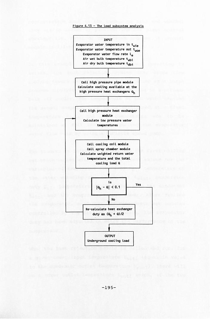
Figure 4.13 - The load subsystem analysis
INPUT Evaporator water temperature in twie Evaporator water temperature out twoe
Evaporator water flow rate le Air wet bulb temperature twbi Air dry bulb te~rature tdbi
t Call high pressure pipe module
Calculate cooling available at the high pressure heat exchangers ~
t Call high pressure heat exchanger
module - Calculate low pressure water t~ratures
~ Call cooling coil module Call spray chamber module
Calculate weighted return water temperature and the total
cooling load Q
+ is
I~ - QI < 0.1 Yes
~ No
Re-calculate heat exchanger duty as (~ + Q)/2 ,
OUTPUT Underground cool ing load
-195-
configuration such as the number of sets and whether
they are in series or parallel and the plant control
strategy i.e. batch or continuous process. A typical
module is illustrated in figure 4.14.
In this example, two chiller sets are operating in
series, the heat rejection system uses cross flow
cooling towers and the plant is operating as a batch
process supplying water to a dam and then to a surface
bulk air cooler. The temperature of the water leaving
the second evaporator is to be maintained at a fixed
temperature twout and the compressors are to be
maintained at full load by adj usting the evaporator
water flow rate by using a variable speed pump.
The process is initiated by calling the first chiller
set which is run with the assumed start values for the
variables of evaporator flow rate leI' temperature of
the water entering the evaporator twiel' evaporator
duty Oel' temperature of the water into the condenser
twicl and the compressor input power. After running
the evaporator, condenser and compressor set modules
controlled by the chiller set module, the evaporator
duty has been adjusted to match the performance of the
compressor.
When the heat rejection module is called and run, for
a given tower input temperature twitl (equal in value
to the condenser outlet temperature twOCl), there will
be a tower outlet temperature twotl which, if the two
-196-
subsystems were in balance I would be equal to the
water temperature into the condenser twicl. The value
for twicl is replaced with the value of twotl and the
chiller set re-run until the difference between the
values of twicl and twotl is less than a pre-set test
value. The first chiller set operation, for a given
water temperature and flow rate into the evaporator,
is now in balance with the compressor and heat
rejection system performance.
Since the chiller sets are in series with respect to
the evaporator water flow, the temperature of the
water into the evaporator of the second chiller is the
same as the temperature of the water leaving the first
chiller i.e. t wie2 = twoel and the flow rates are the
same i.e. le2 = le2. As for the first set, the second
chiller set and heat rejection system modules are run
until a balance is achieved with the compressor and
heat rejection system performance.
The temperature of the water leaving the second
chiller set evaporator t woe2 is now compared to the
design value of twout and, if the difference between
these values is greater than a pre-set test value, the
water flow rate is adjusted and both chiller set
simulations repeated. The method of adjustment has a
profound effect on convergence particularly where the
surge point is approached and centrifugal compressors
are used.
-197-
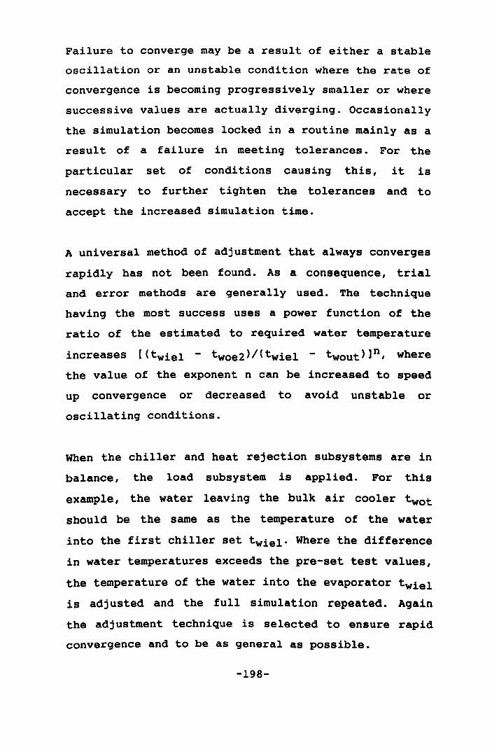
Failure to converge may be a result of either a stable
oscillation or an unstable condition where the rate of
convergence is becoming progressively smaller or where
successive values are actually diverging. Occasionally
the simulation becomes locked in a routine mainly as a
resul t of a failure in meeting tolerances. For the
particular set of conditions causing this, it is
necessary to further tighten the tolerances and to
accept the increased simulation time.
A universal method of adjustment that always converges
rapidly has not been found. As a consequence, trial
and error methods are generally used. The technique
having the most success uses a power function of the
ratio of the estimated to required water temperature
increases [( twiel - t woe2) / (twiel - twout)] n , where
the value of the exponent n can be increased to speed
up convergence or decreased to avoid unstable or
oscillating conditions.
When the chiller and heat rejection subsystems are in
balance, the load subsystem is applied. For this
example, the water leaving the bulk air cooler twot
should be the same as the temperature of the water
into the first chiller set twiel. Where the difference
in water temperatures exceeds the pre-set test values,
the temperature of the water into the evaporator twiel
is adjusted and the full simulation repeated. Again
the adjustment technique is selected to ensure rapid
convergence and to be as general as possible.
-198-
Figure 4. 14 - Overall plant analysis
I
Call set 1 lDOdule Call tower 1 lIIOdule
~ is Yes
I twic1 - twot11 < 0.001
t No
I twi c1 = twot1 I I
t
I twie2 = twoe1 I , Call set 2 module
Call tower 2 module
• is Yes Itwic2 - twot21 < 0.001
~ No
I twi c2 = twot2 I I
t is Yes
It woe2 - twoutl < 0.001
~ No
I Adjust evaporator water flow I I
t Call bulk cooler module
J is Yes
Itwie1 - twotl < 0.001
t No
twie1 = (twi e1 + t wot>l2
, ~ OUtput statements I
-199-
4.2 Mount lsa R63 plant
The Mount Isa R63 plant was first modelled in 1982/83
in order to determine whether it could be extended to
supply cooling for the preliminary development of the
3000 ore bodies. The plant is located on surface and
had three chiller sets with centrifugal compressors.
Two chillers were normally operated with the third set
held in reserve. The surface plant supplied chilled
water to two high pressure heat exchangers which were
located underground and used to cool the water in two
secondary circuits which then supplied two separate
cooling coil reticulation systems.
4.2.1 Base system model
The elements of the refrigeration system modelled are
illustrated in figure 4.15. On surface, 22 lIs of the
chilled water was diverted to a cooling system for the
mine off ices and heavy medium separation plant. The
balance of the chilled water (69 lIs) was supplied to
the two underground high pressure water to water heat
exchangers through 250 nun diameter pipes located in
the main R62 service shaft.
The supply and return water pipes were originally
insulated with polyurethane sections. These were
attached to the pipe with adhesive and covered with a
1 mm thick galvanised steel caSing for mechanical
protection. In the 20 years since the original pipe
-200-
installation, damage to the mechanical barrier and
moisture penetration of the polyurethane foam had
significantly reduced the effectiveness of the
insulation. Measurements of the chilled water
temperature increase in the pipes at low water flow
rates was used to determine the overall heat transfer
coefficient for these insulated pipes.
The upper high pressure heat exchanger on 17 level
provided cold water for 10 cooling coils on 17 and 19
levels. The total volume of air cooled by the cooling
coils was 57 m3 Is. The second heat exchanger on 20
level provided cold water for 19 cooling coils on 20
level, 2lC sub and 21 level. The total volume of air
cooled in this reticulation system was 125 m3/s. The
chilled water from the surface plant was split with
approximately 25 lis being delivered to the 17 level
heat exchanger and the balance to the 20 level unit.
In 1983, the high and low pressure water reticulation
systems were not fully instrumented and measurements
of water temperatures and flow rates were obtained
using contact thermometers and ultrasonic flow meters.
Most of the air cooling was carried out on intake air
which had not travelled more than 300 m from the main
intake shaft. Although the temperature increase
relative to surface of this intake air was due mainly
to the heat resulting from autocompression, diurnal
storage and release of heat in the shaft lining and
steel work smoothed out the surface variations.
-201-
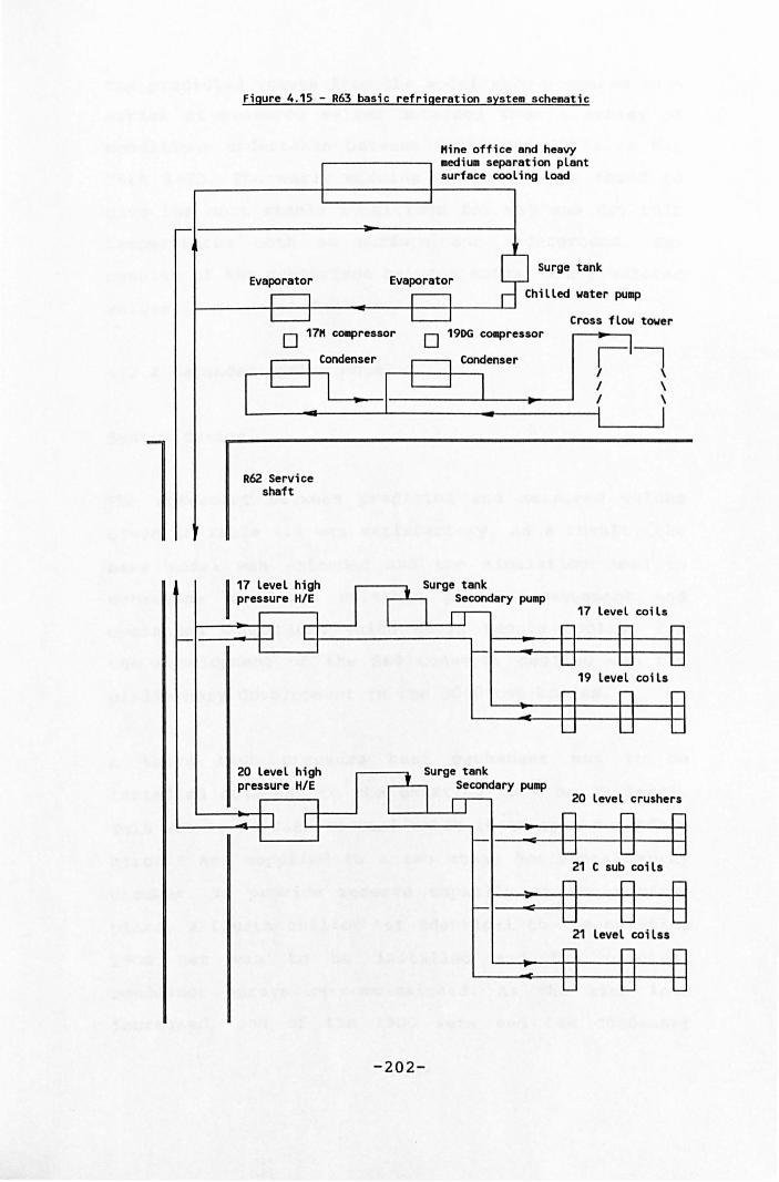
Figure 4.15 - R63 basic refrigeration system schematic
Evaporator
Mine office and heavy medium separation plant surface cooling load
Surge tank
Chilled water pump
Cross flow tower
J( 17M cotnpressor o 190G compressor o
R62 Service shaft
20 level high pressure HIE
-202-
I \ I \
17 level co; ls
19 level coils
20 level crushers
21 C sub coils
21 level coHsa
The predicted values from the model were compared to a
series of measured values obtained from a survey of
conditions undertaken between 06hOO and 07h30 on May
26th 1983. The early morning readings were found to
give the most stable conditions for wet and dry bulb
temperatures both on surface and underground. The
results of the comparison between actual and predicted
values is given in Table 4.1.
4.2.2 Extended system model
System design
The agreement between predicted and measured values
given in Table 4.1 was satisfactory. As a result, the
base model was extended and the simulation used to
determine the most suitable plant arrangement and
operating conditions which would supply cooling for
the development of the S60 conveyor decline and the
preliminary development in the 3000 ore bodies.
A third high pressure heat exchanger was to be
installed adjacent to the existing unit on 20 level.
This was to be used to cool water in an open secondary
circuit and supplied to a two stage horizontal spray
chamber. To provide reserve capacity at the surface
plant, a fourth chiller set identical to the existing
19DG set was to be installed and the original
condenser sprays re-commissioned. As the mine load
increased, one of the 19DG sets and the condenser
-203-
sprays was to be used exclusively for the surface
refrigeration load associated with the mine offices
and heavy medium separation plant.
An important element of the modelling and subsequent
analysis of the results, was to determine the plant
arrangements which would maximise the amount of
cooling without incurring excessive power costs. The
results of the simulations to determine the most
suitable operating configuration are summarised in
figures 4.16 to 4.18.
The effect of the evaporator water flow rate and the
set configuration is illustrated in figure 4.16 for
both the mean summer and the limiting climatic
condition. Operating the chiller sets in series rather
than in parallel resulted in more cooling available
and a higher coefficient of performance. This was
mainly a result of the necessity to operate the 19DG
set at part load to avoid low evaporating temperatures
and possible freezing in the evaporator.
The broken lines in this figure indicate when one or
more of the compressors operates at part load. When
operating the chillers in series, the much smaller
evaporator of the 1900 set causes lower evaporating
temperatures when compared to the 17M sets and, as a
result, the 19DG set is used first in the series
arrangement. The evaporator water flow rate was set at
a compromise value of 100 l/s which should provide
-204-
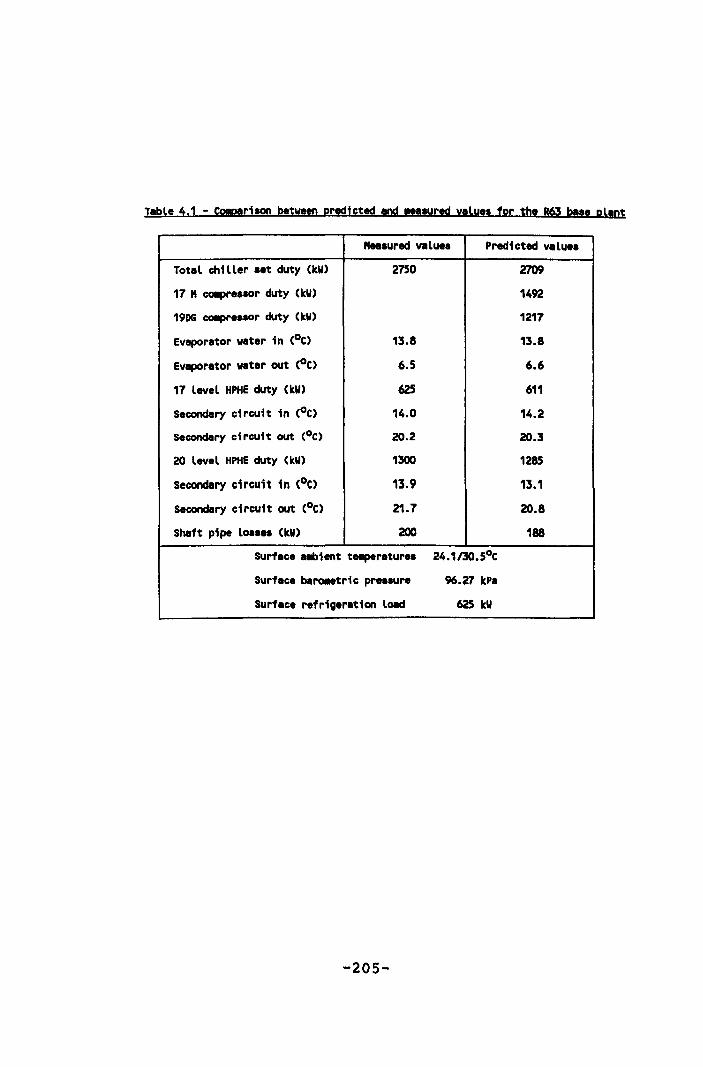
Table 4.1 - CoIperison between predicted and "'lUred yelues for the 863 base plant
" .. sured values Predicted valu.s
Total chiller s.t duty (kW)
17 " COIPressor duty (kW)
1906 COIPr.ssor duty (kW)
Evaporator wat.r in (oC)
Evaporator water out (oC)
17 level HPHE duty (kW)
S.condary circuit in (oC)
Secondary circuit out (oC)
20 level HPHE duty (kW)
Secondary circuit in (oC)
Secondary circuit out (oC)
Shaft pipe loss .. (kW)
2750
13.8
6.5
625
14.0
20.2
1300
13.9
21.7
200
Surface a.bient te.peratur.s 24.113O.SoC
Surface baro.etric pr.ssure 96.27 kPa
Surface refrigeration load 625 kW
-205-
2709
1492
1217
13.8
6.6
611
14.2
20.3
1285
13.1
20.8
188
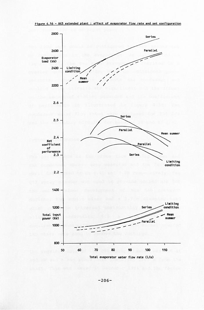
Figure 4.16 - R63 extended plant effect of evaporator flow rate and set configuration
2800
2600
Evaporator load (leW)
2400
2200
2.6
2.5
2.4 Net
coefficient of
performance 2.3
2.2
1400
1200
Total input power (leW)
1000
Limiting condition
/
./ /
./ Mean
sUlllller
--'---
,./,.-,/ ,/
/ ;-;' ;-
;' ;'
/ /
-----
Series
Series
Li.iting condition
Li.iting condition
,., Mean suaer
8OO~-----.------.------r-----'r-----'------.------
50 60 70 80 90 100 110
Total evaporator water flow rate (lIs)
-206-
2700 kW of cooling at the coils and sprays and require
less than 1200 kW of input power.
The 19DG sets could be configured to have either one
or two passes in the evaporator. As illustrated in
figure 4.17 I the two pass arrangement resulted in a
greater amount of cooling with no additional power
penalties. Pump powers in both the condenser and
cooling water circuits are significant and the effect
on the amount of cooling provided and the coefficient
of performance is illustrated in figure 4.18. The
condenser water flow rates were designed for 150 lis
and the secondary circuits for between 20 and 25 lis.
System performance
The performance of the cross flow cooling tower and
the condenser sprays were measured and the factor of
merit determined to be 0.45 and 0.28 respectively. The
Q52 spray chamber was used to provide cooled air for
the mobile miner development of the S60 conveyor
decline. The mobile miner had a 3.7 m diameter head
which could be traversed horizontally to provide an
elliptical excavation 6.5 m wide. The power
requirement when cutting was 250 kW and diesel powered
LBO units were used to remove the cuttings.
The required duty of the Q52 spray chamber was set at
900 kW and a two stage unit installed 1200 m from the
shaft. This was tested in December 1984 and the factor
-207-
of merit determined to be 0.41. This was the first
multistage spray chamber to be installed at Mount lsa
and the low factor of merit was mainly a result of the
spray selection and the low chilled water pressure
available at the site. The high pressure drop in the
spray heads resulted in the water droplets formed not
impacting on the roof of the chamber and some air
channelling.
The chilled water from the secondary circuit of the
high pressure heat exchanger was supplied to and
returned from the Q52 spray chamber in uninsulated PVC
pipes. The losses in the pipes were incorporated in
the model. A comparison of the predicted values with
values obtained from the monitoring system are given
in Table 4.2. The measured values are based on the
average of the five minute readings obtained between
06hOO and 07hOO on December 14th 1984.
The agreement between measured and predicted values
was acceptable. The predictive programme was then used
to determine the optimum cooling arrangements for the
start of the T62 service decline (the main access and
temporary truck haulage for the 3000 ore bodies)
before the new surface refrigeration plant supplying
chilled water underground was available. The
underground cooling was to be expanded to two spray
chambers and two mesh coolers which would provide
approximately 2200 kW of refrigeration.
-208-
The cooling coil reticulation systems were changed so
that all the cold water for the cooling coils was
supplied by the 17 level high pressure heat exchanger.
The total number of coils was reduced to twenty and
the amount of cooling available for the coils was
reduced to approximately 50% of that supplied in 1984.
This system and the air cooling requirement remains
virtually unchanged and is currently supplied with
chilled water from the underground cold water storage
dam on 20 level.
-209-
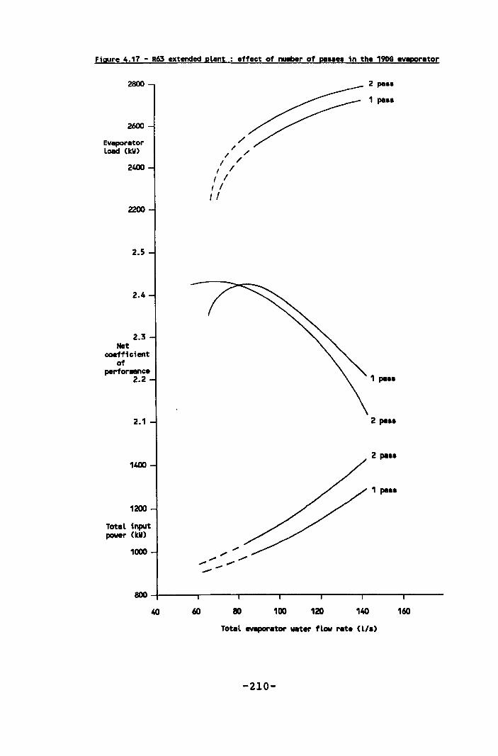
Figure 4.17 - R63 extended plant .ff.ct of ny!ber of pa •••• in the 19DG evaporator
2800 2 peaa
2600
Evaporator load (leW)
2400
2200
2.5
2.4
2.3 N.t
coefficient of
perfo...."c. 2.2
2.1
1400
1200
Total input power (leW)
1000
40 60
/ /
/ / I /
f I ( I
I I I /
80 100
-210-
1 pe ..
1 pa ••
2 pa ..
2 pa ..
1 pa ..
120 140 160
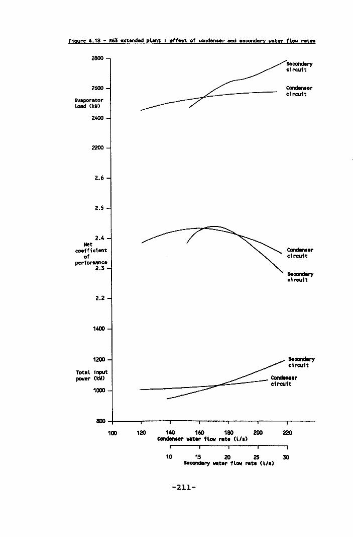
Figure 4.18 - R63 extended plant effect of conden.er and .econderx water flow rat ••
2800
2600
Evaporator load (kW)
2400
2200
2.6
2.5
2.4 Net
coefficient of
perforMnce 2.3
2.2
1400
1200
Tot.l input power (kW)
1000
Conden •• r circuit
Condena.r circuit
Sec:ondtIry circuit
S.candery
~rcu1t _--""" __ -~--~ circuit
~
~~----~~----~----~~----~----~~----~------
100 120 140 160 180 200 220 Condenser .,.t.r flow ret. <L/.)
10 15 20 25 30 SeGandary wat.r flow ret. (L/.)
-211-
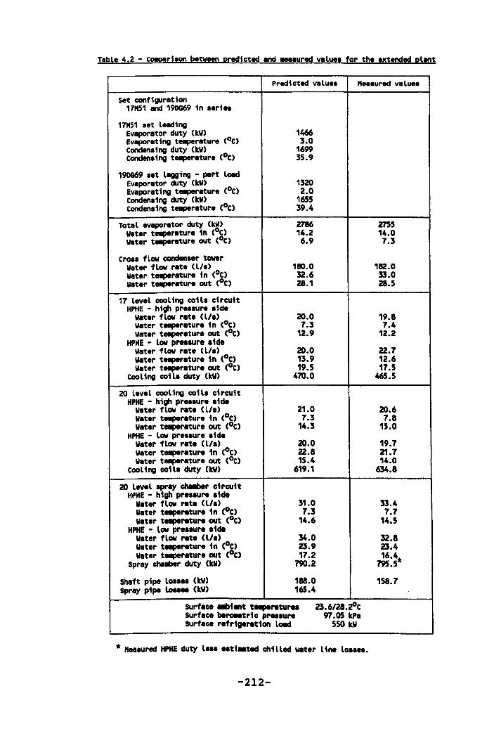
Table 4.2 - CO!p!riaon between predicted end .... ured value. for the extended pl.nt
Predicted value. " ... ured value.
Set configuration 17"51 and 190669 in .erie.
17"51 .et leading Evaporator duty (kW) 1466 Evaporating te.perature (oC) 3.0 condensing duty (kW) 1699 condensing te.peratur. (oC) 35.9
190669 .et lagging - part loed Evaporator duty (kW) 1320 Evaporating te.per.ture (oC) 2.0 conden.ing duty (kW) 1655 condensing te.per.ture (oC) 39.4
Total evaporator duty (kW) 2786 W.ter te.per.tur. in (oC) 14.2 Wat.r te.perature out (oC) 6.9
Cross flow condenler tower Water flow r.te (l/.) 180.0 water te.perature in (oC) 32.6 Water te.perature out (oC) 28.1
17 level cooling coila ci rcuit HPHE - high pre.sure .ide
w.t.r flow r.t. (l/.) 20.0 Water t.-per.ture in CoC) 7.3 Water te.per.ture out (oC) 12.9
HPHE - low pressur. .ide Water flow r.te (l/.) 20.0 water te.per.ture in (oC) 13.9 W.ter t!llp!r.ture out (oC) 19.5
Cooling coil. duty (kW) 470.0
20 level cooling coill circuit HPHE - high pressure .ide
W.ter flow r.t. (lis) 21.0 Wat.r te.per.ture in CoC) 7.3 W.ter te.per.ture out (oC) 14.3
HPHE - low pressure .ide W.ter flow r.t. (l/.) 20.0 Water t!llp!r.ture in (oC) 22.8 Water te.per.tur. out (oC) 15.4
COoling coil. duty (kV) 619.1
20 lev.l spray chaIIber circuit HPHE - high pr.lsure .ide
W.t.r flow r.te (l/.) 31.0 W.ter t...,.retur. in (oC) 7.3 w.ter t...,.reture out (oC) 14.6
HPHE - low preaaure .id. W.ter flow r.t. (l/.) 34.0 W.t.r t.-per.tur. in (oC) 23.9 W.ter t...,.r.ture out (oC) 17.2
Spr.y chMber duty (kV) 790.2
Shaft pipe loa... (kV) 188.0 Spr.y pipe loues (kV) 165.4
SUrf.ce ..,1.,t t...,.retures Surf.c. beroletric pressure SUrf.ce refriger.tion loed
23.6/28.~C 97.05 kP.
550 kV
* " ... ured HPHE duty l.s. estiMted chilled water lin. loa ••••
-212-
2755 14.0 7.3
182.0 33.0 28.5
19.8 7.4
12.2
22.7 12.6 17.5
465.5
20.6 7.8
15.0
19.7 21.7 14.0
634.8
33.4 7.7
14.5
32.8 23.4 16.4.
795.5
158.7
4.3 Broken Bill North mine underground plant
The North mine underground refrigeration system
comprises three Sullair C25 compressor sets of 1800 kW
nominal capacity. The first compressor was installed
and commissioned during 1981. water was chilled in two
direct expansion evaporators and then supplied in
closed circuit to cooling coils. The condenser is a
conventional shell and tube heat exchanger with the
condenser water heat rejection into exhaust air in a
single stage condenser spray circuit.
A year later the plant was expanded with a second C25
compressor set. The poor performance of the direct
expansion evaporators used for the first set prompted
a change to a flooded shell and tube evaporator for
the second set after the initial order was placed. One
of the second sets direct expansion evaporators
(already purchased) was added to the two used for the
first compressor set and the second was to be used to
supplement the flooded shell and tube evaporator on
the second compressor set.
This was not installed and consequently the second set
evaporator capacity is limited. The condenser is
identical to that used for the first set. At this time
the closed chilled water circuit was converted to an
open circuit with water supplied from a storage dam to
cooling coils and a two stage spray chamber which was
used to bulk cool the intake air into the mining area.
-213-
The third plant expansion was undertaken in 1985 with
a third C25 compressor set installed. A large flooded
shell and tube evaporator was selected for this set.
The condenser was identical to that used for the first
two sets. A schematic of the overall refrigeration and
cooling system as it existed at the end of 1986 is
given in figure 4.19.
4.3.1 Base system model
An assessment of the mining plan and ventilation
available showed that there was a requirement of
between 6.0 and 6.5 MW of refrigeration by 1989. This
was partly caused by the extremely stringent six hour
job conditions prevailing in the mines of New South
Wales which resulted from earlier mining practices
(section 2.1.4>. If the wet bulb temperature exceeds
26.7SoC, the shift length must be reduced to six hours
which compares unfavourably with wet bulb temperatures
of the order of 30.0oC which would normally be
accepted for this type of mining.
The impact of the six hour conditions was exaggerated
by the actual shift times available. When travelling
time, changing time and meal breaks are taken into
account, a shift of eight hours actually becomes five
and a half working hours. The six hour shift is
applied by allowing a return to surface two hours
earlier than scheduled, thus the shift length is
reduced to three and a half working hours. Union
-214-
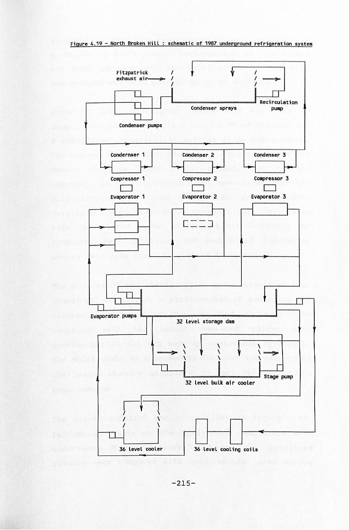
Figure 4.19 - North Broken Hill schematic of 1987 underground refrigeration system
Fitzpatrick I exhaust ai~ I
I
Condenser sprays
Condenser pUllpS
Compressor 1
o Evaporator 1
Evaporator pumps
Compressor 2
o Evaporator 2
32 level storage dall
\ ~ \
\
\ \ \
I I ~ I
Compressor 3
o Evaporator 3
\ \ ~ \
32 level bulk air cooler
I~ I \ I \ I \
36 level cooler 36 level cooling coils
-215-
restrictive practices exacerbated this by insisting on
a follow on shift where, irrespective of the actual
wet bulb temperatures, the shift after the six hour
was awarded was also considered to be six hour.
Prior to 1988, the three plants were not able to
supply more than between 4.0 and 4.5 MW of cooling and
a significant shortfall in refrigeration was evident.
The number of six hour shifts was averaging over 80%
during the four month summer period. Part of the
shortfall in cooling capacity was associated with the
difficulty of fully loading the plant in a partially
developed mining area. Other problems were associated
with the limited amount of exhaust air available for
condenser heat rejection and undersized compressor
motors resulting from the limited 40 Hz supply.
The purpose of the refrigeration model developed was,
therefore, to provide a rapid method of assessing the
current plant operation. The predicted values would be
compared with the actual measured values and,
providing that the two were in reasonable agreement,
the model would be extended to consider the effects of
the design changes necessary to meet future cooling
requirements.
The system modelled was as outlined in figure 4.19.
Performance tests on the individual components were
undertaken during January 1987 and the predicted
results were compared with measurements taken during
-216-
April 1987. The model follows the format outlined in
section 4.1. Initially the chiller subsystems are
examined to obtain compressor, condenser and
evaporator balances for a given water temperature into
the evaporator and a wet bulb temperature of the air
used for condenser heat rejection.
Where appropriate, part load routines are used to
ensure that the evaporating temperature is always
above a predetermined minimum and that the individual
compressor motors are not overloaded. To avoid the
possibility of freezing the water tubes in the flooded
chillers, a minimum evaporating temperature of 30 e was
allowed. This also takes into account the refrigerant
line losses between the compressor and the evaporator.
The mine cooling load was established from the cooling
system arrangement and the chilled water temperatures
into and out of the system. This included the effect
of chilled water storage dam mixing if applicable. The
total mine load was then compared to the total
evaporator duty and the temperature of the water into
the evaporators adjusted until the balance between the
mine load and the evaporator duty was acceptable.
The results of the comparison between predicted and
measured values for the system in April 1987 with
compressor sets land 3 operational is given in Table
4.3. The predicted total mine load of 2.82 MW compares
favourably with the measured mine load of 2.73 MW. The
-217-
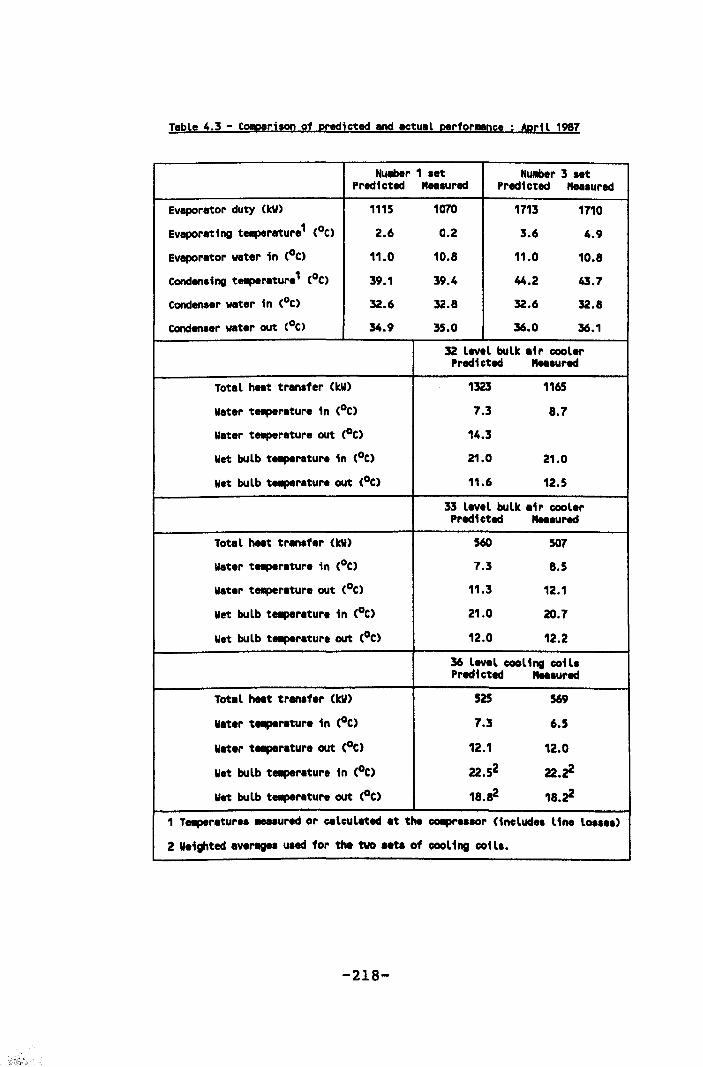
Table 4.3 - CO!p!rison of predicted and actual perfor!!nce April 1987
NUliber 1 set NUllber 3 .et Predicted "ea.ured Predicted "ea.ured
Evaporator duty (kW) 1115 1070 1713 1710
Evaporating te.perature1 (oC) 2.6 0.2 3.6 4.9
Evaporator water in (oC) 11.0 10.8 11.0 10.8
COndensing t..perature1 (oC) 39.1 39.4 44.2 43.7
Condenser water in (oC) 32.6 32.8 32.6 32.8
COnden.er water out (oC) 34.9 35.0 36.0 36.1
32 level bulk a1 r cooler Predicted .... sured
Total heat tran.fer (kW) 1323 1165
Water t..perature in (oC) 7.3 8.7
Water t..perature out CoC) 14.3
Wet bulb te.perature in (Ot) 21.0 21.0
Wet bulb te.perature out (Ot) 11.6 12.5
33 leval bulk air cooler Predicted ..... ured
Total heat transfer (kV) 560 507
Water te.perature in (oC) 7.3 8.5
Water ta.peratura out (oC) 11.3 12.1
Wet bulb ta.perature in (oC) 21.0 20.7
Wet bulb te.perature out (oC) 12.0 12.2
36 level cooling coi l. Predicted ..... ured
Total heat tran.f.r (tv) 525 569
Water t8lp8rature in (oC) 1.3 6.5
Water ta.perature out COC) 12.1 12.0
Wet bulb ta.perature in (oC) 22.52 22.~
Wet bulb t..perature out (oC) 18.82 18.~
1 T.-perature .... sured or calculated at the COIpre.aor (include. line loa ••• )
2 Ve1ghted average. u.ed for the two Ht. of cooling coil ••
-218-
agreement between predicted and measured values is
acceptable and the model can be used to give
reasonable estimates of the effect of changes to the
system. The full output for this set of operating
conditions is given in Table 4.4.
4.3.2 Extended system model
Expanded mine load
The first change to be considered was the effect of
expanding the mine load by commissioning additional
bulk spray coolers to cool the intake air at the three
Fitzpatrick cut and fill stopes on 36, 37 and 39
levels. All the cooling coils were to be removed from
the system. This model would then represent the fully
developed mine system planned for 1989. The results of
the analysis for the limiting climatic condition are
given in Table 4.5.
The maximum possible evaporator duty is 4.9 MW or 77%
of the required mine cooling at the limiting climatic
condition. All three sets are running on part load as
a result of the motor overload restriction. The 4.9 MW
evaporator duty is a maximum value based on clean heat
transfer surfaces in both the evaporators and the
condensers. With dirty tubes which are not untypical
for this type of plant, the evaporator duty would
decrease by 0.5 MW to a total of 4.4 MW or 70% of the
required mine load.
-219-
The contractor involved with the installation of the
three sets was more familiar with installations using
ammonia as the refrigerant rather than the R22
required for this underground plant. The capacity of
the refrigerant lines were more consistent with a
design for ammonia and were generally undersized. This
was particularly evident between the compressor and
the condenser on sets 2 and 3 and between the
compressor and the evaporator on set 2, all of which
had excessive pressure losses.
Simulations carried out using acceptable suction and
discharge line losses indicated that there was only a
marginal increase in the amount of refrigeration
supplied. This was, however, provided at a lower power
requirement (132 kW less when the compressors are at
full load) and would more than justify the cost of
replacing the refrigerant pipe work.
It was concluded that with the configuration of
equipment existing in 1987, the required plant duty
would not be met and there would be a deterioration in
working conditions within the stoping areas.
Open plate evaporators
The three different evaporator arrangements all had
operational problems or were too small to provide the
required cooling duty. On the first compressor set,
the direct expansion evaporators had water on the
-220-
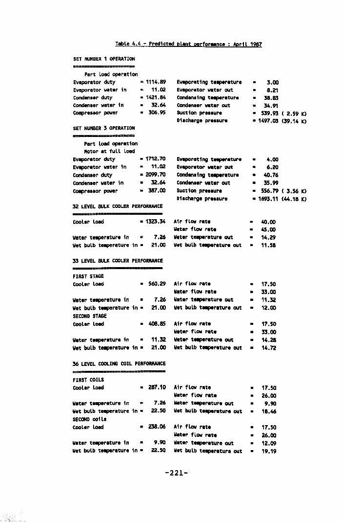
Table 4.4 - Predicted plant pertor!!Qce April 1987
SET NUIfSER 1 OPERATION
Part Load operation Evaporator duty .. 1114.89 Evaporating t.-perature • 3.00 Evaporator water in '" 11.02 Evaporator water out • 8.21 Condenser duty .. 1421.84 Condensing t.-perature • 38.83 Condenser water in '"' 32.64 Condenser water out • 34.91 CoIIpreaaor power • 306.95 Suction pre •• ure • 539.93 ( 2.59 K)
Discharge pre.sure • 1497.03 (39.14 K) SET NUIfSER 3 OPERATION
Part load operation Motor at full load
Evaporator duty • 1712.70 Evaporating telplrature • 4.00 Evaporator water in • 11.02 Evaporator water out • 6.20 Conden.er duty • 2099.70 Condenl1ng ta.perature • 40.76 Condenser water in .. 32.64 Condenser water out • 35.99 COlipreslOr power • 387.00 Suction pre.sure • 556.79 ( 3.56 K)
Discharge pre.sure • 1693.11 (44.18 K) 32 LEVEL BULK COOLER PERFORKANCE
Cooler load • 1323.34 Air flow rate • 40.00 Water flow rate • 45.00
Water teaperlture in .. 7.26 Water ta.perature out a 14.29 Wet bulb ta.perature in • 21.00 Wet bulb telplrature out • 11.58
33 LEVEL BULK COOLER PERFORKANCE
FIRST STAGE Cooler load .. 560.29 Air flow rate • 17.50
Water flow rate a 33.00 Water ta.perature in .. 7.26 water tllPlrature out a 11.32 Wet bulb tllPlrlture in • 21.00 Wet bulb ta.perature out • 12.00 SECOND STAGE Cooler load • 408.85 Air flow rate • 17.50
Weter f low rate a 33.00 Water telp8rature in a 11.32 Water tllPlrature out a 14.28 Wet bulb ta.perature in a 21.00 Wet bulb ta.perature out a 14.72
36 LEVEL COOLING COIL PERFORKANCE
FIRST COILS Cooler load • 287.10 Air flow rate • 17.50
water f low rate a 26.00 Water ta.perature in • 7.26 Weter t-.perature out • 9.90 Wet bulb ta.perature in • 22.50 Wet bulb ta.perature out • 18.46 SECOND coi l. Cooler load • 238.06 Air flow rate a 17.50
Water flow rate a 26.00 Water ta.perature in • 9.90 Water ta.perature out a 12.09 Wet bulb ta.perature in • 22.50 Wet bulb teaperature out a 19.19
-221-
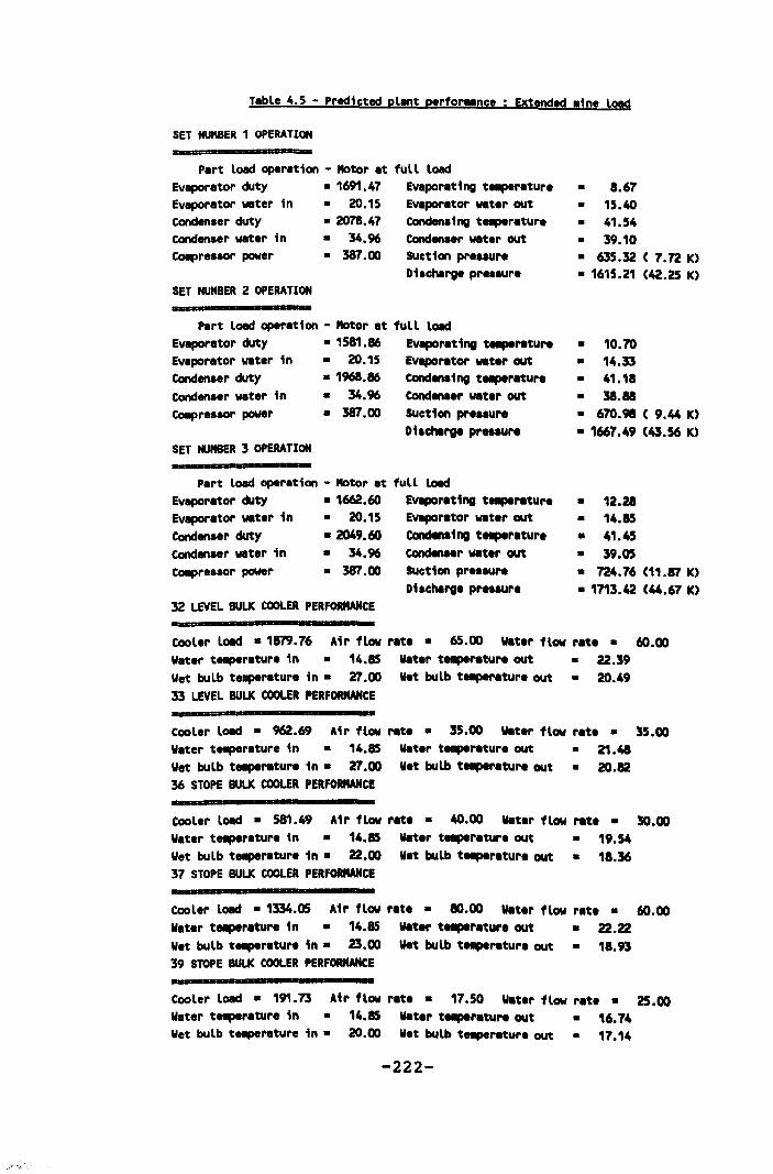
~; .,
Table 4.5 - Predicted plant perfor .. nce Extended .ine load
SET HUftBER 1 OPERATION
Part load operation - Motor at full load Evaporator duty • 1691.47 Evaporating ta.per.tur. Evaporator water in • 20.15 Evaporator wat.r out conden.er duty • 2078.47 Conden.ing ta.perature condenaer water in • 34.96 conden .. r water out CoIIpre.aor power
SET HU"BER 2 OPERATION
• 387.00 SUction pr •• aur. Di.charge pr .. aur.
Part load operation - Motor at full load Evaporator duty • 1581.86 Evapor.t i ng t...,.ratura Evaporator water in • 20.15 Evaporator water out
Conden.er duty • 1968.86 cones •• ing t...,.rature Conden.er water in • 34.96 cones ••• r wat.r out
CoIIpre.aor power • 387.00 SUction preaaura Di.chlrge preaaur.
SET NUMBER 3 OPERATION
Part load operation - Motor at full load Evapor.tor duty • 1662.60 Evapor.ting t...,.r.ture Evaporator water in • 20.15 EVl9Or.tor w.t.r out Cond •• er duty .2049.60 condIn.1ng t...,.r.ture conden.er wat.r in • 34.96 Condenaer water out
CoIIpre.ao.. power • 387.00
32 LEVEL BULK COOlER PERFORMANCE
SUction pr .. aura Di.charge pre.aure
• 8.67 • 15.40 • 41.54 • 39.10 • 635.32 ( 7.72 K) • 1615.21 (42.25 K)
• 10.70 • 14.33 • 41.18 • 38.88 • 670.91 ( 9.44 K)
• 1667.49 (43.56 K)
• 12.21 • 14.85 • 41.45 • 39.05 • 724.76 (11.87 K) • 1713.42 (44.67 K)
Cooler load • 1879.76 Air flow r.te. 65.00 W.t.r flow r.t.. 60.00 Wat.r tnper.tur. in • 14.85 water tetlp8r.tura out • 22.39 Wet bulb tnper.ture in· 27.00 Wet bulb tHper.tur. out • 20.49 33 LEVEL BULK COOlER PERFORMANCE
Coole .. load • 962.69 Air flow rate. 35.00 water flow r.t.. 35.00 Water tnper.ture in • 14.85 wat ... tetlp8ratu ... out • 21.41 Wet bulb t...,er.ture in. 27.00 Wet bulb tHpe ... ture out • 20.12 36 STOPE BULK COOlER PERFORMANCE
Cool.r load • 581.49 Air flow r.t.· 40.00 water flow r.t.. 30.00 W.ter t ... r.ture in • 14.85 wat ... tetlp8ratur. out • 19.54 Wet bulb t ... r.ture in. 22.00 Wet bulb tetlp8r.ture out • 18.36 37 STOPE BULK COOlER PERFORMANCE
Cooler load • 1334.05 Air flow r.te· 80.00 water flow r.t.. 60.00 Water t ... r.tu .. e in • 14.85 water tetlp8r.ture out • 22.22 Wet bulb t ... r.tur. in· 23.00 w.t bulb tetlp8r.ture out • 18.93 39 STOPE BULK COOLER PERFORMANCE
Coole .. load • 191.73 Air flow rate. 17.50 wat.r flow r.t.. 25.00 Water t ... r.ture in • 14.85 wat.r t ...... tuN out • 16.74 Wet bulb tnperature in· 20.00 Wet bulb t ....... tu ... out • 17.14
-222-
.'-! .• ;
shell side and could not be cleaned without
dismantling the set and sending the evaporators to
surface for tube removal and cleaning. As a result,
the direct expansion evaporators were operating with
very high water side fouling which limited their
capacity to approximately half of their design value.
On the second compressor set, the flooded shell and
tube evaporator was selected to operate with an
addi tional direct expansion evaporator. Al though
installed, commissioning problems resulted in it not
being available and consequently the set operates with
an undersized shell and tube evaporator. On the third
set, undersizing of the refrigerant take-off from the
shell resulted in liquid refrigerant carryover and
additional liquid receivers were necessary.
The main change proposed was therefore to replace all
the evaporators with a single falling film open plate
evaporator. A pumped refrigerant recirculation system
would be used between the evaporator and a refrigerant
accumulator vessel. The compressors are fed from the
accumulator at a rate determined by the evaporation of
the refrigerant.
To·achieve the necessary cooling duty, either a fourth
compressor and motor was required or the existing
three motors replaced with larger units. With four
compressors the predicted performance wi th the
expanded mine load is given in Table 4.6. The maximum
-223-
evaporator duty is 6.25 MW or 99% of the mine load at
the limiting summer condition. All four compressors
would be operating at part load as a result of the
motor size restriction.
Because the open plate (falling film ) evaporator is
not damaged by freezing of the chilled water, the
minimum evaporating temperature was set at -30 e. The
6.25 MW evaporator duty was based on clean tubes in
the condensers and a 100 plate evaporator. Space
limitations in the adjacent available excavations
could result in as few as 55 plates being available.
This would result in the evaporator duty being limited
to 5.95 MW or 92% of the required mine load.
The effect of fouling in both the condensers and the
evaporator is to reduce this duty further to 5.55 MW
or 88% of the required mine load. Most of this
reduction was a result of the condenser fouling. The
large water side surface area in the open plate
evaporator minimises the effect of fouling on overall
plant performance.
Increased motor size
Instead of installing a fourth chiller set, 500 kW
motors could be installed on the existing three sets.
An additional 50Hz supply from surface was being
installed and the motor power restriction was no
longer valid. The predicted conditions are summarised
-224-
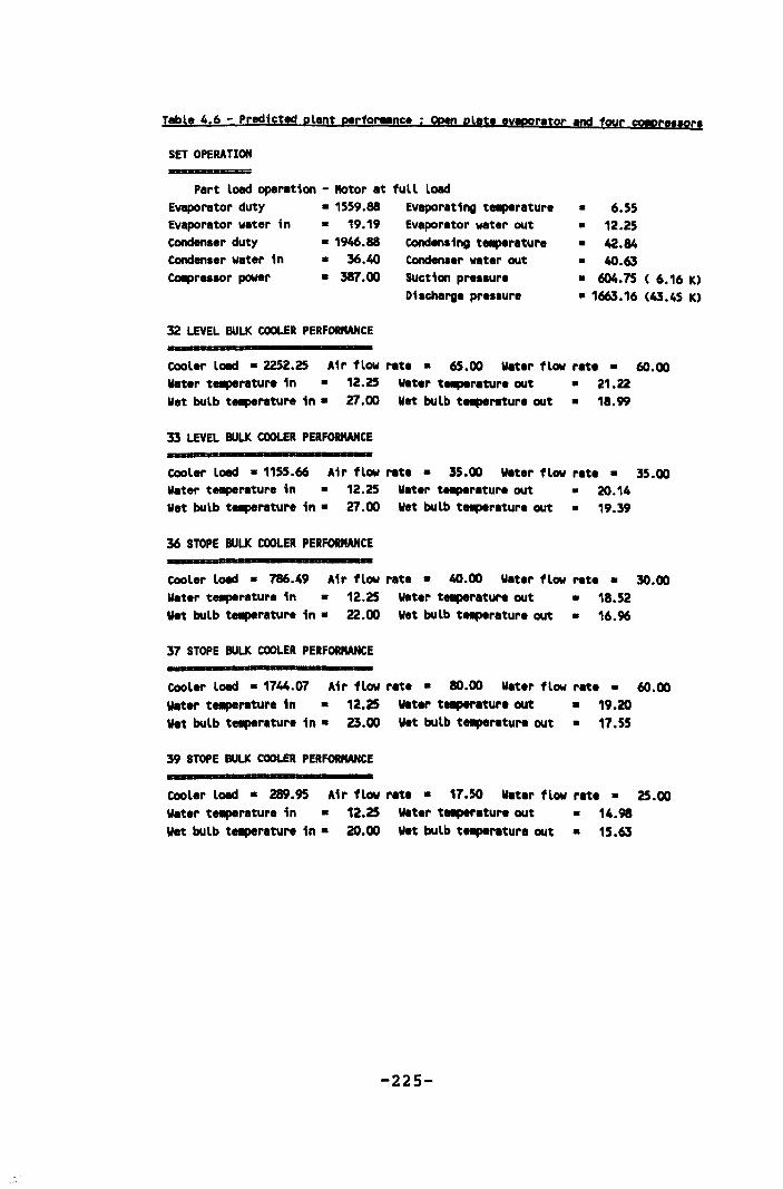
Table 4.6 - Predjcted plant perfor .. nce ; Open plate evaporator and four c:otpC8'fOr•
SET OPERATION
Part load operation - ~tor at full load Evaporator duty • 1559.88 Evaporating ta.perature • 6.55 Evaporator water in • 19.19 Evaporator water out • 12.25 Condenser duty • 1946.88 CondenSing ta.perature • 42.84 Condenser water in • 36.40 Condenser water out • 40.63 COIIpreaaor power • 381.00 Suction pressure • 604.15 ( 6.16 K)
Di.charge pressure • 1663.16 (43.45 K)
32 LEVEL BULl< COOLER PERFORIIAHCE
COoler load • 2252.25 Air flow rate. 65.00 Water flow rate. 60.00 Weter tHperature in • 12.25 water tHperature out • 21.22 Wet bulb te.perature in. 27.00 Wet bulb t...,.rature out • 18.99
33 LEVEL BULl< COOLER PERFORMANCE
COoler load • 1155.66 Air flow rete· 35.00 water flow rete. 35.00 Water t...,.rature in • 12.25 Water tHpereture out • 20.14 Wet bulb t...,.rature in. 27.00 Wet bulb te.perature out • 19.39
36 STOPE BULl< COOLER PERFORMANCE
COoler load • 786.49 Air flow rete. 40.00 water flow rete. 30.00 Water t...,.rature in • 12.25 Water taperature out • 18.52 Wet bulb te.perature in· 22.00 Wet bulb te.perature out • 16.96
31 STOPE BULl< COOLER PERFORMANCE
COoler load • 1744.07 Air flow rete. 80.00 Water flow rate. 60.00 weter t...,ereture in • 12.25 WIIter tHperature out • 19.20 Wet bulb t...,ereture in. 23.00 Wet bulb te.perature out • 17.55
39 STOPE BULl< COOLER PERFORMANCE
COoler load • 289.95 Air flow rete· 11.50 Water flow rete. 25.00 Water tnperature in • 12.25 WIIter tapereture out • 14.98 Wet bulb te.perature in· 20.00 wet bulb te.pereture out • 15.63
-225-
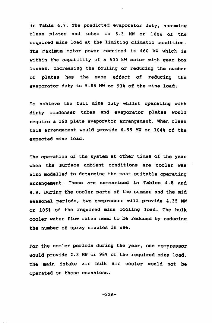
in Table 4.7. The predicted evaporator duty, assuming
clean plates and tubes is 6.3 MW or 100% of the
required mine load at the limiting climatic condition.
The maximum motor power required is 460 kW which is
within the capability of a 500 kW motor with gear box
losses. Increasing the fouling or reducing the number
of plates has the same effect of reducing the
evaporator duty to 5.86 MW or 93% of the mine load.
To achieve the full mine duty whilst operating with
dirty condenser tubes and evaporator plates would
require a 150 plate evaporator arrangement. When clean
this arrangement would provide 6.55 MW or 104% of the
expected mine load.
The operation of the system at other times of the year
when the surface ambient conditions are cooler was
also modelled to determine the most suitable operating
arrangement. These are summarised in Tables 4.8 and
4.9. During the cooler parts of the summer and the mid
seasonal periods, two compressor will provide 4.35 MW
or 105% of the required mine cooling load. The bulk
cooler water flow rates need to be reduced by reducing
the number of spray nozzles in use.
For the cooler periods during the year, one compressor
would provide 2.3 MW or 98% of the required mine load.
The main intake air bulk air cooler would not be
operated on these occasions.
-226-
Chilled water storage
To provide greater flexibility of compressor
operation, it was also proposed to alter the chilled
water distribution and return system. In 1987, the
cold water was supplied to, and drawn off from the
north end of a 3.5 Ml water storage dam. The warm
water from the bulk air coolers was returned to and
drawn off from the south end of the same water storage
dam. Thermal layering within the dam limited the
amount of mixing during continuous normal operation.
As the surface climatic conditions change throughout
the day, the mine cooling load also varies. To
maintain continuous plant operation and to minimise
mixing in the dam requires that the compressors should
unload and operate less efficiently.
The existing 3.5 Ml dam was converted to store chilled
water only. A separate smaller dam adj acent to the
refrigeration plant is used to store the warm water
returned from the bulk air coolers prior to cooling in
the plant. This dam capacity would be supplemented
wi th storage dams at the main bulk air coolers. The
compressors could then operate intermittently
depending on the actual mine cooling load and the full
plant capacity.
-227-
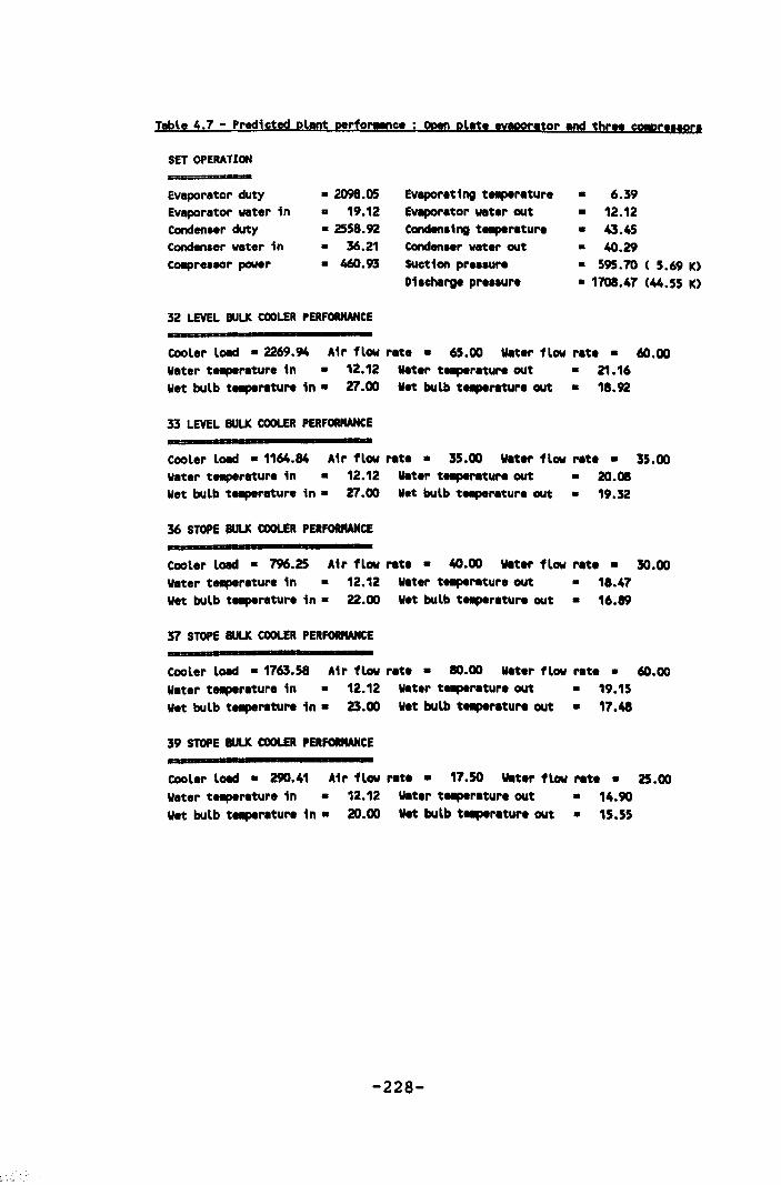
Table 4.7 - Predicted plant perfor!!Dc, ; Open pl.t. evapor.tor and thr .. COIpr •• !Or.
SET OPERATION
Evaporator duty • 2098.05 Evaporating tllPlratur. • 6.39 Evaporator water in • 19.12 Ev.porator wat.r out • 12.12 Conden.er duty • 2558.92 Conden.ing tllPlratur. • 43.45 Condenser w.t.r in • 36.21 Conden •• r water out • 40.29 COIIpresfOr power • 460.93 SUction pr...ur. • 595.70 ( 5.69 K)
Diacharg. pr.a.ur. • 1708.47 (44.55 K)
32 LEVEL BULK COOLER PERFORItAHCE
COoler load • 2269.94 Wat.r tllPlr.tur. in • Wet bulb tllPlr.tur. in •
Air flow rat.. 65.00 Wat.r flow rat. • 12.12 Utt.r tllPlratura out • 21.16 27.00 WIt bulb tllPlratur. out • 18.92
60.00
33 LEVEL BULK COOLER PERFORItAHCE
COoler load • 1164.84 Air flow rat.. 35.00 Wlt.r fLow rat.. 35.00 Wat.r tllPlratur. in • 12.12 Utt.r tllPlr.tur. out • 20.08 Wet bulb tllPlrature in· 27.00 w.t bulb tllPlratur. out • 19.32
36 STOPE BULK COOLER PERFORItAHCE
COoLer load • 796.25 Air flow rat.· 40.00 Utt.r flow rat.. 30.00 Water tllPlrature in • 12.12 Water tllPlratur. out • 11.47 Wet bulb t8llplr.ture in. 22.00 Wit bulb ttllper.tur. out • 16.89
37 STOPE BULK COOLER PERFORIWtCE
COoler Load • 1763.58 Air flow rat.· 80.00 W.t.r fLow rat.. 60.00 Water telPlrtture in • 12.12 Utt.r ttllperatur. out • 19.15 w.t bulb ttllperttur. in. 23.00 wet buLb tlllPlratura out • 17.48
39 STOPE BULK COOLER PERFOIMANCE
COoler lOild • 290.41 Air flow rat.. 17.50 Utt.r flow ret.. 25.00 Water tnper.ture in • 12.12 wat.r tnperatur. out • 14.90 Wet buLb tlllPlrttura in. 20.00 w.t bulb tlllPlratur. out • 15.55
-228-
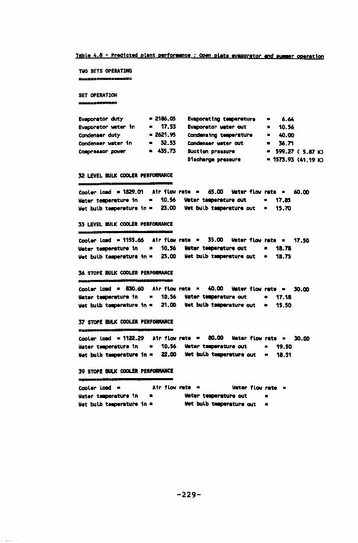
T.ble 4.8 - Predicted pl.nt parfor!!Oce ; Open pl.t. !Vepor'tor and .U!!!r QP!ratton
TWO SETS OPERATING -SET OPERATION
Evapor.tor duty .2186.05 Evapor.t1ng te.peratur. • 6.64 Evapor.tor water in • 17.53 Evapor.tor WIIt.r out • 10.56 Conden.er duty • 2621.95 conden"ng te.per.ture • 40.00 Conden.er water 1 n • 32.53 Cond.., .. r water out • 36.71 CoIIpr •• aor power • 435.73 SUction pre •• ur. • 599.27 ( 5.87 K)
D1.charge pra.aur. • 1573.93 (41.19 K)
32 LEVEL BULK COOLER PERFORIWtCE
Cooler lOltd • 1829.01 Air flow r.t.. 65.00 w.t.r flow r.t.. 60.00 W.t.r teaper.tura in • 10.56 w.t.r taperatura out • 17.85 Wet bulb teaperatur. in. 23.00 v.t bulb te.per.tura out • 15.70
33 LEVEL BULK COOLER PERFORMANCE
Cooler load • 1155.66 Air flow r.te· 35.00 W.t.r flow r.t.. 17.50 water t...,.r.tuN in • 10.56 WIIt.r taper.tuN out • 11.71 w.t bulb te.per.ture in. 23.00 v.t bulb te.per.tuN out • 11.75
36 STOPE BULK COOLER PERFORMANCE
Cooler lOltd • 130.60 Air flow rat.· 40.00 water flow r.t.. 30.00 water teaperetura in • 10.56 WIIt.r taper.tur. out • 17.18 Wet bulb te.per.tur. in· 21.00 Wet bulb t...,.r.tur. out • 15.50
37 STOPE BULK COOLER PERFORIWtCE
• COol.r lOltd • 1122.29 Air flow r.t.. 80.00 wat.r flow r.t.. 30.00 W.t.r tnper.tur. in • 10.56 w.t.r t...,.r.tur. out • 19.50 Wet bulb t...,....tu ... in. 22.00 Wet bulb t...,....tu ... out • 11.51
39 STOPE BULK COOLER PERFORIWfCE
Cool.r loed • Air flow ... t. • wat.r flow r.t. • W.t.r te.per.tur. in • w.t bulb t...,.r.tur. in •
wat.r t...,.r.tur. out • Wet bulb t...,.r.tur. out •
-229-
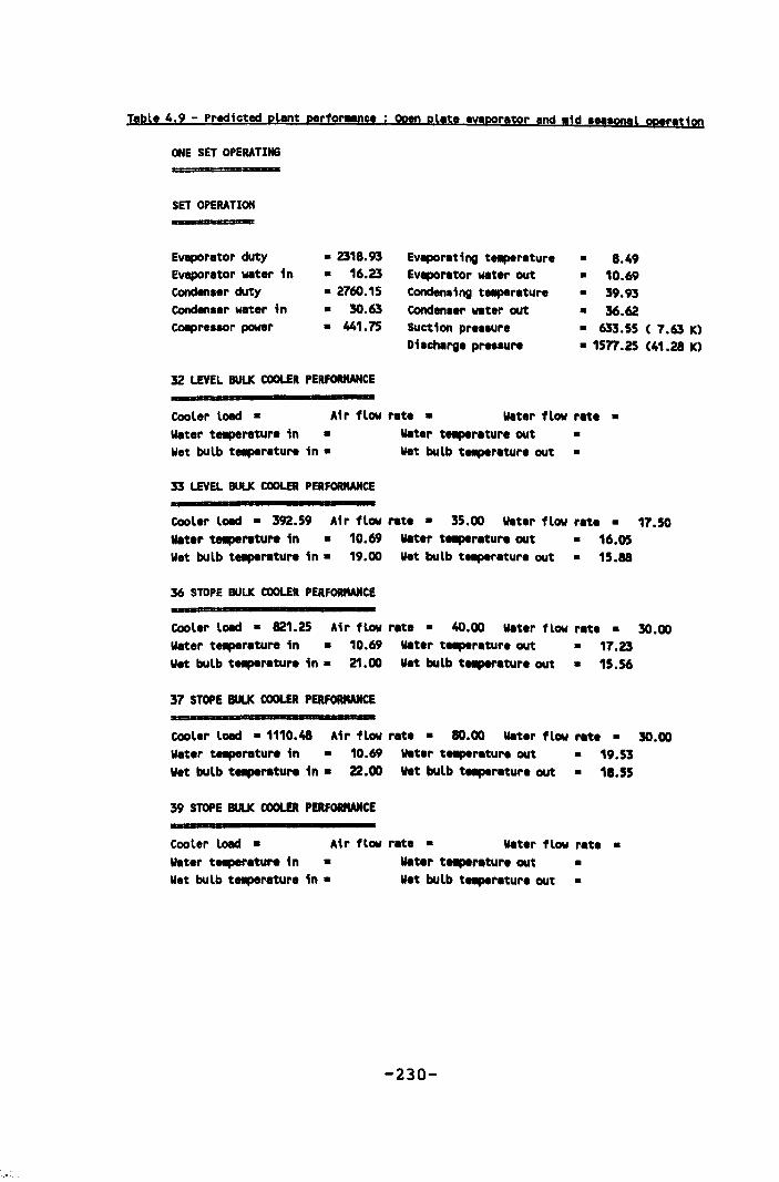
Table 4.9 - PrediGted plant perfor!!DGe ; open plate evaporator and lid '''!OD!l oper.ti00
ONE SET OPERATING r
SET OPERATION
Evaporator duty • 2318.93 Evapor.ting telplr.ture • 8.49 Evaporator water in • 16.23 Evapor.tor wat.r out • 10.69 Conden.er duty • 2760.15 Conden.1ng te.per.ture • 39.93 Conden .. r water in • 30.63 Conden •• r v.t.r out • 36.62 COIIpre.!Or power • 441.75 SUGt10n pr ••• ure • 633.55 ( 7.63 K)
D1lchlrg. pre •• ur. • 1577.25 (41.28 K)
32 LEVEL BULK COOLER PERFORMANCE
Cooler load • Air flow rat. • W.t.r flow r.t. • Water te!perature in • Wet bulb te.per.ture in •
33 LEVEL BULK COOLER PERFORMANCE
water ta.per.ture out Wet bulb t!!per.tur. out
• •
CooLer Load • 392.59 Air flow r.t.· 35.00 Wat.r fLow rat.. 17.50 wat.r tltlplr.tuN in • 10.69 wat.r ta.peratur. out • 16.05 Wet bulb tltlplr.tur. in. 19.00 Wet bulb t!!perature out • 15.88
36 STOPE BULK COOLER PERFORMANCE
Cooler load • 821.25 Air fLow rate· 40.00 Water flow rat.. 30.00 Water te.perature in • 10.69 water ta.per.ture out • 17.23 Wet bulb ta.peratur. in. 21.00 lIet bulb ta.peratur. out • 15.56
37 STOPE BULK COOLER PERFORMANCE
COOler load • 1110.48 Air flow rat.· 80.00 water flow r.t.. 30.00 lIater te.per.ture in • 10.69 wat.r ta.perature out • 19.53 Wet bulb ta.perature in. 22.00 Vet bulb t..,ratur. out • 11.55
39 STOPE BULK COOLER PERFOIUWtCE
CooLer load • Air fLow rat. • lIat.r flow rat. • lIat.r tetlperature in. water ta.peratur. out • lIet bulb tetlperature in • lI.t bulb ta.peratur. out •
-230-
4.4 Mount Isa surface chilled water plant
The mining of the deeper 3000 ore bodies at Mount Isa
will require up to 35 MW of refrigeration by the year
2000 depending on the mining schedule and the final
production rate. It was evident that the existing R63
plant described in section 4.2 could only supply
sufficient cooling for the preliminary development
work in the new mining area. In 1983 the overall mine
refrigeration strategy was reviewed and a three stage
programme was defined.
The existing R63 system using closed circuit chilled
water from surface to high pressure heat exchangers
underground was not suitable for major expansion and
had a low coefficient of performance mainly as a
result of the increased pump power necessary in the
primary and secondary chilled water circuits. The
existing high pressure 250 mm diameter pipes between
surface and 20 level could, however, be used to supply
up to 200 lIs of chilled water to underground in open
circuit with an energy recovery system.
A total of 22 MW of cooling could be provided if
necessary using this system. The overall coefficient
of performance of a surface chilled water plant
supplying underground cooling appliances and for use
as service water was estimated to be 3.5.
The surface bulk cooling of air which was to be used
-231-
to ventilate the mining areas had a higher coefficient
of performance of 5.0 (including the poorer positional
efficiency) . The deeper mining areas have the
exclusive use of the U62 intake shaft after 1992 for
approximately 60% of the total intake air requirement,
the balance being available from shafts which are also
ventilating the shallower mining areas. Bulk cooling
of the air at U62 shaft was therefore limited by the
air quantity to approximately 12 MW.
The three stages were therefore to install an 11 MW
chilled water plant by 1989, to install a 12 MW bulk
air cooler in 1993 and to increase the size of the
chilled water plant to a maximum of 22 MW in 1999.
4.4.1 Refrigeration plant design
The original plant design and tendering was undertaken
in 1984. Although the plant was not required for the
deep ore bodies until 1987, it was proposed to install
the plant ahead of schedule. This would have
eliminated the need to expand the R63 plant and the
excess capacity from the new plant could have been
used in the deeper sections of the 1100 ore bodies.
Low commodity prices resulted in different capital
expenditure priorities within the Mount Isa Holdings
group and the new plant was deferred.
In 1987 the decision to proceed was made and, as a
result of the short lead time available, the order was
-232-
placed with the most suitable supplier from the 1984
tender review. The full original design was, however,
not adhered to and two major changes were made which
result in a less cost effective plant with respect to
both power costs and maintenance.
The first change concerns the condensers which were
originally selected as evaporative condenser units.
This was changed to closed plate heat exchangers and
cross flow cooling towers. To maintain the same
initial cost, the closed plate heat exchangers and the
cross flow towers were undersized and resulted in the
estimated plant operating power costs to be A$ 95 000
per year or 5.1% greater.
The second change made was to use closed plate heat
exchangers for the evaporator instead of open plates.
The initial cost of the closed plate heat exchangers
was 30% less than the cost of the open plates (less
than 2% of the overall plant cost). The advantage of
open plates for an underground chilled water system is
that the effects of poorer quality water and fouling
of the heat exchange surfaces is less pronounced and
can easily be controlled.
When the deeper mining zone is in production it is
expected that the water quality will worsen as a
result of tailing fill decant water contamination. To
control the effects of sedimentation in the closed
plate heat exchanger, a back flushing system was
-233-
installed. At the end of a run cycle, the water flow
through the heat exchanger is reversed and any
particulate that has settled should be flushed out. A
water treatment system was installed to control the
water quality and to minimise fouling.
The plant comprises two chiller sets using Howden 321
screw compressors, two closed plate evaporators
containing 93 cassettes, two closed plate condensers
with 106 cassettes and two five cell cross flow
cooling towers for condenser heat rejection. A
separate pre-cooling tower is used to cool the water
returned to surface from underground prior to being
supplied to the chiller sets.
Associated with the chiller sets and pre-cooling tower
are two 1.5 Hl and one 2.25 Hl water storage dams for
hot return water, intermediate pre-cooling tower
cooled water and chilled water storage respectively.
Chilled water is supplied to and returned from the
mine through the two 250 mm high pressure water pipe
lines. An energy recovery pelton wheel driving an
asynchronous generator minimises the energy losses in
the chilled water circuit.
Two 1.5 Hl hot water storage dams and one 1.5 Ml
chilled water storage dam is located on 20 level which
is 1010 m below surface. Chilled water is distributed
to the bulk air coolers using a cascade dam system
located in the central ramp area between the two main
-234-
ore bodies. Chilled water is also used as service
water below 20 level and all return water is pumped
first to intermediate dams in the central ramp area
and then to the main dams on 20 level.
As indicated in section 4.2, the high pressure shaft
pipe insulation was in poor condition. The insulation
on the cold water supply pipe was completely replaced
using 38 mm thick foamed glass with a stainless steel
shroud for mechanical protection. The return pipe
insulation was stripped off and was not replaced. Any
heat gains from the intake air in the shaft being
recovered in the pre-cooling tower.
4.4.2 Control strategy
During the design stage, a model of the refrigeration
system was developed in order to evaluate the
implications of different control strategies. The main
components of the overall system are illustrated in
figure 4.20. The control strategy evolved based on the
following three criteria:-
- to minimise the chilled water supply temperature,
- to maximise the return water temperature, and
- to minimise energy losses and input power.
The chilled water supply temperature was set at lOC
which was felt to be the lowest practical limit when
using closed plate heat exchangers. For each lOC
-235-
increase in chilled water supply temperature, the
operating power costs were 1.7% (A$ 31 000) higher.
The increase in input power resulting from higher
chilled water flow rates of 2.7% per IOC was offset by
a 1.0% per lOC refrigeration plant power saving as a
result of the increase in evaporating temperature.
The return water temperature was to be maximised to
reduce both the recirculating water quantity and to
obtain the maximum benefit from the pre-cooling tower.
For each lOC decrease in the return water temperature,
the operating power costs were 5.2% higher (2.7% in
additional pumping costs and 2.5% in additional
refrigeration plant power).
Energy losses were to be minimised by using energy
recovery systems where possible and by the judicious
selection of equipment. Operating the plant as a batch
rather than a continuous process had a marginally
lower operating power cost of between 2.5% and 4.0%
lower and provided maintenance time without disrupting
the supply of chilled water to the mine.
The chiller sets
The control strategy adopted for the chiller sets is
illustrated in figure 4.21. the storage dam sizes were
based on providing a minimum storage of four hours
(for maintenance) and a minimum compressor run time of
two hours. The initial mine chilled water demand was
-236-
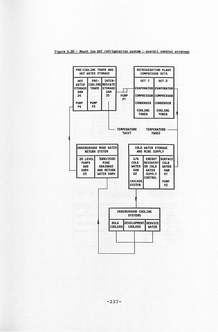
Figure 4.20 - Mount Isa K61 refrigeration system overall control strategy
PRE-COOLING TOWER AND HOT WATER STORAGE
REFRIGERATION PLANT COMPRESSOR SETS
HOT PRE- INTER- SET 1 SET 2 WATER COOLING MEDIATE
STORAGE TOWER STORAGE rr- EVAPORATOR EVAPORATOR -DAM DAM ~ D4 D5 PUMP COMPRESSOR COMPRESSOR
PUMP P4
PUMP P3
P1 CONDENSER CONDENSER
COOLING TOWER
COOLING TOWER
L-- TEMPERATURE TWIE1
TEMPERATURE ----TWOE2
-
UNDERGROUND MINE WATER COLD WATER STORAGE RETURN SYSTEM AND MINE SUPPLY
20 LEVEL PUMPS
AND DAMS
D3
3000/3500 MINE
DRAINAGE AND RETURN WATER DAMS
~
U/G ENERGY COLD RECOVERY WATER OR COLD
DAM WATER 02 SUPPLY
CONTROL CASCADE SYSTEM
UNDERGROUND COOLING SYSTEMS
BULK IDEVELOPMENT SERVICE COOLERS I COOLERS WATER
I
-237-
SURFACE COLD WATER
DAM 01
PUMP P2
I-
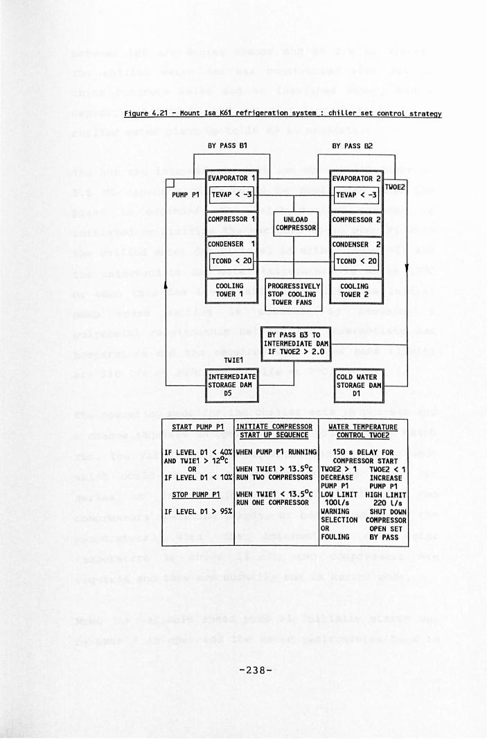
Figure 4.21 - Mount Isa K61 refrigeration system: chiller set control strategy
BY PASS B1 BY PASS B2
I I I EVAPORATOR 2 ~ EVAPORATOR 1 I-J
IITEVAP < -3J i lTEVAP < -31 TWOE2
PUMP P1
COMPRESSOR 1 I UNLOAD COMPRESSOR 2 COHPRESSOR
CONDENSER 1 CONDENSER 2
I I TCOND < 20 1 ilTCOND < 20 1
COOLING PROGRESSIVELY COOLING TOWER 1 STOP COOLING TOWER 2
TOWER FANS
BY PASS B3 TO INTERMEDIATE DAM IF TWOEl > 2.0
TWIE1
INTERMEDIATE COLD WATER STORAGE DAM STORAGE DAM r-
D5 D1
START PUMP P1 INITIATE COMPRESSOR WATER TEMPERATURE START UP SEQUENCE CONTROL TWOEl
IF LEVEL D1 < 40X WHEN PUMP P1 RUNNING 150 s DELAY FOR AND TWIE1 > 12°C COMPRESSOR START
OR WHEN TWIE1 > 13.50 C TWOEl > 1 TWOEl < 1 IF LEVEL D1 < 10X RUN TWO COHPRESSORS DECREASE INCREASE
PUMP P1 PUMP P1 STOP PUMP P1 WHEN TWIE1 < 13.S0C LOW LIMIT HIGH LIMIT
RUN ONE COMPRESSOR 100l/s 220 lis IF LEVEL D1 > 9SX WARNING SHUT DOWN
SELECTION COMPRESSOR OR OPEN SET FOULING BY PASS
-238-
between 100 lis during summer and 60 lis in winter.
The chilled water dam was constructed with 200 mm
thick concrete walls and an insulated cover, had a
capacity of 2.25 HI and was therefore suitable for a
chilled water plant up to 16 MW in capacity.
The hot and intermediate dams are open steel tanks of
1.5 HL capacity which could be duplicated when the
plant is expanded. The batch cooling process is
initiated by starting the variable speed pump PI when
the chilled water dam 01 level is either below 40% and
the intermediate dam water temperature is above l20 C
or when this dam level falls below 10%. The initial
pump speed setting is obtained by assuming a
polynomial relationship between the intermediate dam
temperature and the required water flow rate (limits
are 110 lis at 260 C and 200 lis at 70 C).
The operating mode for the chiller sets is pre-set and
a change requires an operator input prior to the batch
run. The valve settings determine the operating mode
which could be
series or in
two compressors running
parallel, or either of
either in
the two
compressors operating singly, or back flushing of the
evaporators. When the intermediate dam water
temperature is above l3.soC, two compressors are
required and they are normally run in series mode.
When the variable speed pump PI initially starts up,
by-pass 4 is open and the water recirculates back to
-239-
the intermediate dam. The lead compressor start
sequence is initiated 150 s after pump Pl starts and
the load maintained at a minimum. After an additional
180 s, the lag compressor (if two compressors are
required) start sequence is initiated and the load is
increased to 20%. When this is reached approximately
10 minutes after pump Pl start up, the lead compressor
is increased to full load. When this is achieved after
approximately 7.5 minutes, the lag compressor load is
also increased to full load.
When both compressors are running at full load, the
variable speed pump flow rate is adjusted to obtain
the lOC water off temperature when the by-pass valve
is closed and chilled water is supplied directly to
the cold water storage dam.
The start up time taken to achieve stable conditions
has slowly been reducing and is currently 30 minutes.
The problem of reducing this to a more acceptable
value of 10 minutes is associated with the operating
stabili ty of the variable speed pump motor if the
compressors are loaded too quickly. When the plant is
expanded, a separate electrical supply should allow
the design start up time to be achieved.
The compressor PLC provided by the supplier initiated
the start up of the condenser pumps and cooling tower
fans. This control also allowed the compressors to
unload if the evaporating temperature dropped below
-240-
-3.00 C in order to avoid freezing in the evaporator.
The cooling tower fans could be progressively stopped
to ensure that the condensing temperature remained
above 200 C and thus avoid problems with the
lubricating oil viscosity.
Chilled water supply system
The chilled water control system is illustrated in
figure 4.22 and comprises of a batch supply at 110 l/s
from the surface cold water storage dam through the
high pressure supply pipe and pel ton wheel energy
recovery equipment to the main 1.5 HI underground
chilled water storage dam. The pelton wheel is
directly coupled to an asynchronous generator feeding
the mine electrical supply and, for the stage 1 duty,
has a single nozzle. Both the pelton wheel and the
generator are suitable for the final duty which can be
achieved by installing a second nozzle and increasing
the batch chilled water flow rate to 200 lIs.
The three pipe cascade dam system is used to
distribute the chilled water to the mining areas.
Since these are accessed by a haulage truck decline,
the pipes and 0.1 Ml capacity dams are located in and
adjacent to 3 m diameter raise bore holes positioned
between the decline loops and connected to the decline
at approximately 60 m vertical intervals. Control of
the chilled water supply is achieved by using valves
which are operated by dam level limit switches.
-241-
Mine load
The system was originally designed to use three stage
horizontal spray chambers for bulk cooling the air
suppled to an active mining area and mesh coolers for
development headings. As indicated in section 3.5,
packaged counter flow cooling towers are now used for
both applications. This prompted a change in the
control strategy. With the horizontal spray chambers,
capaci ty control was obtained in discrete steps by
reducing the water quantity and the number of stages.
Each stage had two supply water pumps, the first
supplying the two pipes adjacent to the side walls
with nozzles at standard spacing and the second
supplying a central pipe with nozzles at half spacing.
When the spray chamber capacity was to be reduced, the
second pump supplying the central pipe was switched
off. This reduced the supply of chilled water to 50%
whilst maintaining the water coverage i. e. potential
air channelling was minimised.
Wi th the packaged counter flow units, this was not
practical and recirculation is allowed between the
return and the supply water pipes. The flow through a
recirculation loop located after the return water
pump, is controlled by the discharge air temperature.
A typical arrangement using 9.5 lis of chilled water
has a maximum duty of 850 kW during the summer with no
water recirculation. By controlling the outlet air
-242-
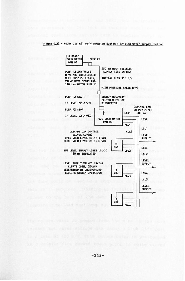
Figure 4.22 - Mount Isa K61 refrigeration syst em chilled wat er supply control
SURFACE COLD WATER
DAM D1 PUMP P2
PUMP P2 AND VALVE HPV1 ARE INTERLOCKED WHEN PUMP P2 STARTS, VALVE HPV1 OPENS AND 110 lIs BATCH SUPPLY
250 mm HIGH PRESSURE SUPPLY PIPE IN R62
INITIAL FLOW 110 lIs
HIGH PRESSURE VALVE HPV1
PUMP P2 START
IF LEVEL D2 < SOX
PUMP P2 STOP
ENERGY RECOVERY PELTON WHEEL OR DISSIPATOR
LSV1 IF LEVEL D2 > 9SX
U/G COLO WATER DAM D2
ROL CASCADE DAM CONT VALVES CDV(n)
OPEN WHEN LEVEL CDC CLOSE WHEN LEVEL CDC
n) < SOX n) > 90X
SUB LEVEL SUPPLY LIN 150 111111 INSULATE
ES LSL(n) D
LSV(n) LEVEL SUPPLY VALVES ALWAYS OPEN, DEHA
DETERMINED BY UNDERG COOLING SYSTEM OPERA
ND ROUND
TION
J1
CD2
CDV1
CDL1
CDV2
..... _ ... CDV3
CASCADE DAM SUPPLY PIPES
200 mm
1
LSV2
LSL1
LEVEL SUPPLY
LSV3
LSL2
LEVEL SUPPLY
LSV4
LSL3
LEVEL SUPPLY
~l
-243-
temperature at between 15 and l6oC, the recirculation
rate increases to 25% (600 kW cooling duty) for mid
seasonal conditions and 60% (450 kW cooling duty) for
winter conditions.
Return water system
Service water and the water from the direct contact
spray coolers is returned to the nearest 0.75 Ml
capacity intermediate return water dam. These are
located at approximately 180 m vertical intervals and
adjacent to the smaller cascade supply dams. A level
control is used to initiate the pumping between the
intermediate dams and the main underground hot water
storage dams on 20 level as illustrated in figure
4.23.
The two 20 level hot water storage dams each have a
capacity of 1.5 Ml and, although both are in normal
use, one can be taken off line for cleaning. If it
becomes necessary to clean the cold dam, one of the
hot dams could be used as a temporary cold dam whilst
this is in progress. Cleaning is facilitated by a ramp
access to the back of the dams and carried out using
standard mine load haul dump equipment.
The return water is pumped from the mine to the main
surface hot water storage dam using a high lift pump
at a rate of 120 lIs. This return water is pre-cooled
in a counter flow packed tower prior to being stored
-244-
in the intermediate storage dam. Control is by dam
level switches and is designed to limit the number of
pump motor starts to a maximum of three per day.
4.4.3 Commissioning tests
The refrigeration plant was commissioned in December
1989 before the mine water supply system was completed
and the plant could be fully loaded using the actual
mine load. Short run tests lasting between two and six
hours were possible with the transfer of water between
the hot and cold dams. At the end of each test run,
the chilled water was run off to the drains and make
up water used to provide the new hot water supply.
Longer run tests were achieved by only rejecting the
heat of compression in the condenser towers. The
chilled water from the evaporator is supplied to the
cold dam. For the long run tests, the water from the
cold dam, instead of being supplied to the mine is
spli t, a fraction (R) being supplied to the cooling
tower sump and the balance being returned to the hot
dam as illustrated in figure 4.24.
The water entering the condenser is therefore a
mixture of the water leaving the condenser cooling
tower and that leaving the evaporator. The water
leaving the condenser is also split. Part (equivalent
in flow rate to R) is supplied to the hot dam and
mixes with the balance of the water supplied from the
-245-
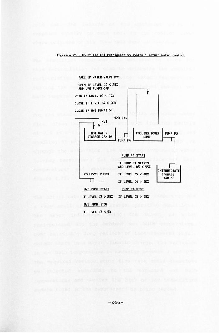
Figure 4.23 - Mount Isa K61 refrigeration system return water control
MAKE UP WATER VALVE MV1
OPEN IF LEVEL 04 < 25X AND U/G PUMPS OFF
OPEN IF LEVEL 04 < 10X
CLOSE IF LEVEL 04 < 90X
CLOSE IF U/G PUMPS ON
120 lIs ~ MV1
HOT WATER STORAGE OAK 04 1----1.. ....
COOLING TOWER PUMP P3 SUMP
20 LEVEL PUMPS
PUMP P4
PUMP P4 START
IF PUMP P1 STARTS ANO LEVEL 05 < 95X
IF LEVEL 05 < 4Crk
IF LEVEL 04 > SOX
UIG PUMP START PUMP P4 STOP
IF LEVEL D3 > 85X IF LEVEL D5 > 95X
UIG PUMP STOP
IF LEVEL 03 < 5X
-246-
INTERMEDIATE STORAGE
DAM 05

cold dam. The balance of the condenser water is
supplied equally to each cell in the cooling tower
where only one of the five cell fans is running.
The simulation programme was adjusted to allow for
this recirculation and used to determine the required
recirculation rate for varying water temperatures
leaving the evaporator and for different ambient wet
bulb temperatures.
For the standard conditions of 250 lIs condenser water
flow, clean heat exchanger surfaces (fouling factors
of 7.5 kw/m2K), one cooling tower fan operating and
handling 55 m3/s of air and between 100 and 150 lIs
through the evaporator, the expected evaporator water
leaving temperature for different surface wet bulb
temperatures and recirculation rates is given in
figure 4.25.
The actual water flow rate through the evaporator has
a very small effect on stable operating conditions,
the major influences being the amount of water
recirculated and the ambient wet bulb temperature.
Over relatively long periods of time (several days),
unless there is a major climatic change, the variation
in wet bulb temperature is normally between 3 and 4oC.
The required recirculation f low rate could therefore
be selected according to the expected wet bulb
temperatures and whether the high or low temperature
module (lead or lag compressor) is being tested.
-247-
As an example, consider a 09hOO wet bulb temperature
of 1aoC. This is typically the average temperature for
the 24 hour period and the expected range in wet bulb
temperatures for stable climatic conditions would be
16 to 20oC. If the high temperature module (the lead
compressor in a series configuration) was to be
tested, a recirculation rate of about 100 lIs would be
required. If the low temperature module (the lag
compressor in a series configuration) was to be
tested, the recirculation rate would be 50 lIs.
The analysis of the data available from the
commissioning tests concentrated on the performance of
the compressors and the plate heat exchangers. A
summary of the results from four of the long run tests
is given in table 4.10. The results cover a one hour
period starting at the time given in the table and are
the average of readings taken from the monitoring
system at ten minute intervals. These are obtained
from the historical time trends and are instantaneous
readings and not period averages.
The calculated evaporator fouling factors of between
7.5 and 10 kW/m2K were typical for clean plates. The
value of 16.8 kW/m2K obtained for the 16/12/89 test
was probably a result of the inaccuracies involved in
averaging the instantaneous compressor discharge
pressures obtained from the time trends. The condenser
fouling factors were moderately dirty for a new
installation at between 5 and 6 kW/m2K and, although
-248-
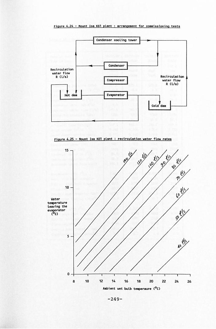
Figure 4.24 - Hount Isa K61 plant arrangement for commissioning tests
Recirculation water flow
R (lIs)
Condenser cooling tower
Condenser
COllpressor
Evaporator
Recirculation water flow
R <lIs)
Figure 4.25 - Mount Isa K61 plant recirculation water flow rate.
15
10
Water tellperature leaving the eva~rator
( C)
5
O~-----r----'----'-----r----~---r----~--~--~
8 10 12 14 16 18 20 22 24 26
Ambient wet bulb tellperaure (oC)
-249-
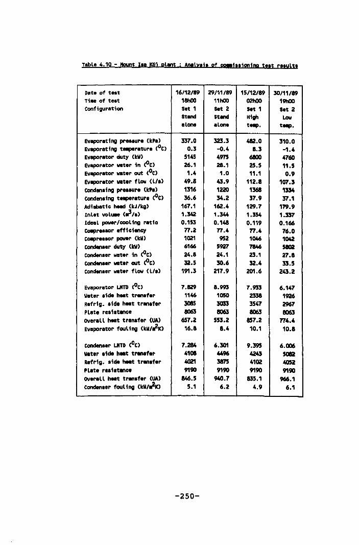
Table 4.10 - nount III K61 pllOt ; Anlly." of CO!!""001np t •• t r •• ult.
Date of t •• t 16/12/89 29/11/89 15/12/89 30/11/89 T1. of te.t 18hOO 11hOO 02h00 19hOO Configuration Set 1 s.t 2 s.t 1 Set 2
StMd StMd High Low alone alone t...,. t...,.
Evaporating preafYr. (kPa) 337.0 323.3 412.0 310.0 Evaporating ta.perature (oC) 0.3 -0.4 8.3 -1.4 Evaporator duty (kW) 5145 4975 6800 4760 Evaporator water in (OC) 26.1 28.1 25.5 11.5 Evaporator vater out (OC) 1.4 1.0 11.1 0.9 Evaporator ..-t.r flow <l/.) 49.8 43.9 112.8 107.3 Conden.'ng pratfYr. (kPa) 1316 1220 1368 1334 Conden.ing ta.perature (Ot) 36.6 34.2 37.9 37.1 Adiabatic heed (kJ/kg) 167.1 162.4 129.7 179.9 Inlet vol~ (~/.) 1.342 1.344 1.354 1.331 Ideal power/cooling ratio 0.153 0.148 0.119 0.166 CoIpre.fOr efficiency 77.2 77.4 77.4 76.0 COIIPreafOr power (kW) 1021 952 1046 1042 Conden •• r duty (kW) 6166 5927 7846 5102 Conden.er water in (OC) 24.8 24.1 23.1 27.8 Condenftr ..-t.r aut (Ot) 32.5 30.6 32.4 33.S Conden.er water flow (l/.) 191.3 217.9 201.6 243.2
Evaporator UNTD (OC) 7.829 8.993 7.933 6.147 Water .1de heet tran.f.r 1146 1050 2338 1926 Refrig. .ide heat tran.fer 3085 3033 3547 2967 Plate resi.tance 8063 8063 8063 8063 OVerall heat tran.fer (UA) 657.2 553.2 857.2 774.4 Evaporator faul ing (kW/rf-K> 16.8 8.4 10.1 10.8
Condenftr OOD (OC) 7.2B4 6.301 9.395 6.006 water .ide helt trentf.r 4101 4496 4243 5012 Refrig. .ide helt tran.f.r G1 3875 4102 4052 Plat. r .. ,.tanoe 9190 9190 9190 9190 OVerall heat tren.fer (UA) 846.5 940.7 835.1 966.1 Condenftr fouling (kW/JK) 5.1 6.2 4.9 6.1
-250-
of concern, were not unexpected. The condenser water
treatment system was not functioning correctly and
biological fouling was evident.
4.4.4 System performance
Condenser cooling towers
During the commissioning tests it was noted that the
condenser cross flow towers were not performing as
expected with factors of merit significantly lower
than expected (between 0.44 and 0.57 instead of 0.61).
The results of two series of full tests undertaken on
the towers are given in Table 4.11. During each test
the air quantity was measured at each cell discharge
using the average of four anemometer traverses and the
leaving wet bulb temperature was the average of twelve
readings using calibrated thermometers.
The inlet wet bulb temperatures were obtained by
averaging six readings at the inlet to each of the
tower cells and compared to the five minute averages
obtained from the meteorological station. During the
tests it was apparent that there was recirculation
between the fan discharge from the tower and the inlet
to the tower. The extent of the recirculation depended
on the direction and the strength of the wind during
the tests. The values given in brackets in Table 4.11
are factors of merit based on the ambient wet bulb
temperature.
-251-
water flow rates and temperatures were measured with
an ultra sonic flow meter and calibrated mercury in
glass thermometers. The expected cooling tower duties
were obtained from the evaporating and condensing
pressures and the compressor performance curves. These
are compared to the actual measured water and air side
heat transfer rates in Table 4.12. The agreement
between measured and predicted values was satisfactory
and confirmed the method of analysis.
When the actual inlet air temperatures are used the
factor of merit for the towers is within normal
measurement tolerances of the rated value. The total
air quantity drawn through the towers by the fans is
now only 71% of the rated amount. This, coupled with
the recirculation increases the plant operating power
costs by 2.8%. In addition to increasing the air
quantity handled by the fans it is planned to install
2 m high discharge cones which should almost eliminate
the recirculation problem.
Chiller set performance
Since the plant was commissioned, five complete sets
of comparati ve readings have been taken to conf irm
both the values obtained from the monitoring system
and the use of the historical trend plots to assess
plant performance. Water temperatures were checked
with calibrated mercury in glass thermometers and, in
general, the readings were within O.2oC with the
-252-
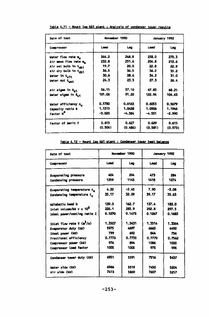
Table 4.11 - Mount 1 .. K61 el.nt ; Anlly.i. of cond!D.er tower re.ult.
Date of test Novetlber 1990 January 1992
CoIIpre8aor LHd Leg LHd Leg
Water flow rate IIw 264.2 248.8 258.0 270.3 Air .... flow r.te .. 232.8 251.6 204.8 210.6 Air wet bulb in twbi 19.7 20.0 22.8 22.9 Air dry bulb in tdbi 36.5 36.5 36.2 35.2 Water in twit 30.6 28.6 34.2 31.0 Water out Swot 24.3 23.3 27.3 26.4
Air .iglll in Sai 56.11 57.10 67.13 68.21 Water .iglll in !vi 101.06 91.20 122.94 104.63
Water efficiency "w 0.5780 0.6163 0.6053 0.5679 Ceplcity ratio R 1.1515 1.0431 1.0906 1.1946 Factor Nt -3.020 -4.384 -4.551 -2.990
Factor of .. rit F 0.615 0.627 0.629 0.615 (0.504) (0.486) (0.581) (0.573)
Table 4.12 - Mount 18 K61 pllOt ; Condtn"r tOWlr ""t btlW1ct
Date of test HoveIIber 1990 JlnUllry 1992
COIIpresaor Lead Leg Lead lAg
Evaporating pressure 404 294 473 284 Conden.ing prellure 1259 1143 1418 1274
Evaporating t-.perature te 4.22 -2.45 7.90 -3.08 condenling telplr.ture tc 35.17 32.09 39.17 35.63
Adiebttic heed h 139.3 162.7 137.4 113.0 Inlet volUIII/1eW v x 106 226.1 285.9 202.8 297.5 Ideal power/cooling ratio 1 0.1270 0.1473 0.1267 0.1683
Inlet flow r.te Y (~/I) 1.3507 1.3431 1.3514 1.3364 Evaporator duty (leW) 5975 46W 6663 4492 Ideal power (leW) 759 692 844 756 Fr.ctional efficiency 0.7776 0.m5 0.7770 0.7562 COIIprellOr power (tV) 976 894 1086 1000 COIIpreslOr load f.ctor 100% 100% 97X 99X
CondenIer toWer duty (leW) 6951 5591 7516 5437
water lide (leW) 6966 5519 7450 5204 Air .ide (tW) 7413 5869 761J7 5217
-253-
exception of the water temperature leaving the lag
compressor and entering the cold darn. This has
consistently been in error by O.SoC and appears to be
a water stratification and probe location problem
rather than an instrument error.
The results of the five sets of readings and the
output from the predictive method for the relevant
conditions are given in Tables 4.13 to 4.17 and are
typical of the plant operation. In July 1990 (Table
4.13) both the evaporator and condenser plates were
operating as "moderately dirty". In November 1990
(Tables 4.14, 4.15 and 4.16) both the evaporator plate
heat exchangers and the number 1 condenser had just
been chemically cleaned.
water treatment and back flushing are unable to
maintain the fouling at acceptable values and the
January 1992 values (Table 4.17) are typical of the
current operating conditions. The combined effects of
the fouling and cooling tower recirculation are to
increase the current operating power costs by 9.4'. As
an interim measure, the refrigeration plant simulation
is used to determine when chemical cleaning of the
heat exchangers is necessary and to quantify the
benefits of back flushing.
When the plant is expanded in 1999, consideration will
be given to replacing the heat exchangers with more
sui table equipment. The expected reduction in
-254-
operating costs is between 15 and 25% depending on the
system selected and the water treatment required.
Pre-cooling tower and mine cooling appliances
Tests on the performance of the pre-cooling tower
resulted in measured factors of merit of 0.70, 0.82
and 0.79. For the first two tests, the main problem
was associated with low return water temperatures from
underground which resulted in relatively low heat
transfer rates in the pre-cooling tower. A O.loC error
in measuring the air and water temperatures would
change the calculated factor of merit by 0.08.
The performance and selection of the mine cooling
appliances has been detailed in section 3.5. Currently
a monitoring system is being installed which will
report back to the same system as the surface plant.
By controlling the recirculation rates at the cooling
appliances it is expected that the highest return
water temperature consistent with meeting the design
working place thermal environmental criteria will be
achieved.
-255-
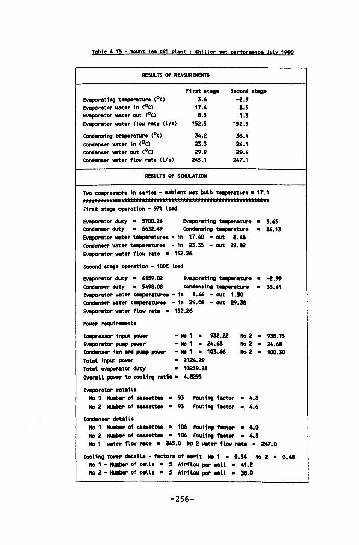
Table 4.13 - Mount I.a K61 plant Chill.r •• t perforllOc. July 1990
Evaporating te.peratur. (oC) Evaporator wat.r in (oC) Evaporator wat.r out (oC) Evaporator wat.r flow rat. (l/.)
COndensing telplrature (oC) Conden .. r wat.r in (oC) Condenser water out (oC) Conden!er water flow rat. (lis)
F1r.t .tag. 3.6
17.4 8.5
152.5
34.2 23.3 29.9
245.1
RESULTS Of SIIIJLATION
S.cond .tag. -2.9 8.5 1.3
152.5
33.4 24.1 29.4
247.1
Two CCIIIPressors in "1'1.. - _ient wet bY lb t!llp!NltUI'! • 17.1 AAAAAAAAAAAAAAAA ••••••••• AA ••• A ••••••••••• , ••••••••••••• ' •• A'A' First stage operation - 97X load
Evaporator duty • 5700.26 Evaporating t!llp!ratuNi • 3.65 Conden!er duty • 6632.49 Condensing t!llp!ratur. • 34.13 Evaporator wat.r telplratur .. - in 17.40 - out 8.46 Concten .. r wat.r t!llp!rature. - in 23.35 - out 29.82 Evaporator wat.r flow rat. • 152.26
second .tage operation - 100x load
Evaporator duty • 4559.02 Evaporating t!llp!Nltur. • -2.99 Conden .. r duty • 5498.08 Condensing t...,.ratur. • 33.61 Evaporator wat.r t...,.raturea - in 8.46 - out 1.30 Condens.r water tetlp!raturea - in 24.08 - out 29.38 Evaporator wat.r flow rat. • 152.26
Power requi rellent.
COIIpreslOr input power - No 1 • 932.22 Evaporator puap power - No 1 • 24.68 Conden .. r fen and puap power - No 1 • 103.66 Total input power • 2124.29 Total evaporator duty • 10259.28 OVerall power to cooling Nltio. 4.8295
Evaporator detail.
No 2 • 938.75 No 2 • 24.68 No 2 • 100.30
No 1 Nullber of cassett.. • 93 No 2 NUIIber of CUlttt.. • 93
Fouling factor • 4.8 Fouling factor • 4.6
Condenser detaila No 1 Nullber of cassett.. • 106 Fouling factor • 6.0 No 2 Nulber of CUHtt.. • 106 Fouling factor • 4.8 No 1 wat.r flow Nit. • 245.0 No 2 water flow rat. • 247.0
Cooling tower details - factor. of .. rtt No 1 • 0.54 No 2 • 0.48 No 1 - HuIIber of cell. • 5 Airflow per c.ll • 41.2 No 2 - Nullber of c.ll. • 5 Airflow per call • 38.0
-256-
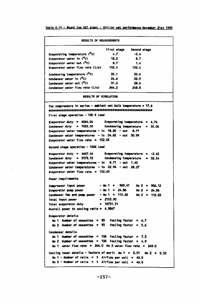
Table 4.14 - Haunt Isa K61 PLint Chiller Stt perforl!Oc, NoytIbtr 21st 1990
RESULTS OF MEASUREMENTS
Evaporating te.perature (oC) Evaporator water in (oC) Evaporator water out (oC) Evaporator water flow rate (lIs)
Condensing t!llP'rature (oC) Condenser water in (oC) Condenser water out (oC) Condenser water flow rate (lIs)
First stage 4.7
18.2 8.7
152.4
35.1 24.6 31.0
264.2
RESULTS OF SIMULATION
Second stage -2.4 8.7 1.4
152.4
32.6 22.9 28.6
248.8
TWo CCIIpr .. aora in a.ri .. - allb1ent vet bulb t!llp!cature • 17.6
*********************************'**'**'***'***'**"**'****'**' First stage operation - 100 X lOlld
Evaporator duty • 6064.04 Evapor.ting t!llp!rature • 4.74 Condenser duty • 7033.50 Condensing t!llp!rature • 35.04 Evaporator wat.r te.peratur.s - in 18.20 - out 8.71 Condenser water te.perltur.. - in 24.62 - out 30.99 Evaporator water flow rlt. • 152.63
Second stage operation - l00x load
Evaporator duty • 4667.46 Evaporating teaper.tur. • -2.42 Condenser duty • 5573.72 Condensing teaperatur. • 32.54 Evaporator wat.r te.per.turea - in 8.71 - out 1.40 Condens.r water tetlP!ratur.. - in 22.94 - out 28.27 Evaporator water flow rat. • 152.63
Pow.r requireaenta
CoIIprMSOr input power Evaporator puap power Condenser fan and puap power Total input power
- No 1 • 969.41 - No 1 • 24.86
- No 1 • 115.63 • 2152.90
Total evaporator duty • 10731.51 OVerall power to cooling ratio. 4.9847
Evaporator detaila
No 2 • 906.12 No 2 • 24.86 No 2 • 112.03
No 1 Nullber 01 caM!tt.. • 93 No 2 Hullber of casaatt.. • 93
Fouling f.ctor • 6.7 Fouling factor • 5.6
Condenser detai la No 1 Nullber 01 caaaett .. • 106 Fouling factor • 7.3 No 2 Nullber 01 caaHtt.. • 106 Fouling f.ctor • 4.9 No 1 wat.r flow rat. • 264.0 No 2 water flow rat. • 249.0
Cooling tower details - f.ctors of .. rit No 1 • 0.51 No 2 • 0.52 No 1 - NUlllber 01 c.ll. • 5 Airflow per c.ll • 43.0 No 2 - NUlllber of c.lls • 5 Airflow per c.ll • 46.0
-257-
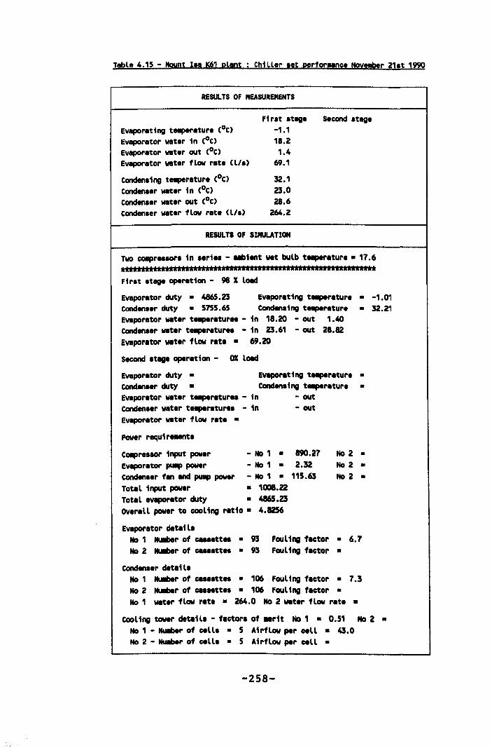
Table 4.15 - Mount Iaa K61 plant Chiller aet perfor .. nce Nov!!ber 21at 1999
RESULTS OF MEASUREMENTS
Evaporating teaperature (oC) Evaporator water in (oC) Evaporator water out (oC) Evaporator water flow rate (l/a)
Condenaing teaperature (oC) Condenser water in (oC) Condenaer water out (oC)
Ftrat atllge -1.1 18.2 1.4
69.1
32.1 23.0 28.6
Condenser water flow rate (l/a) 264.2
RESULTS OF SIMULATION
Second atllge
Two COIIIpreaaora in .. ri .. - _tent vet bulb t ... ratur. • 17.6
*********************************'**'**"******'*************** Firat atege operation - 98 X load
Evaporator duty • 4865.23 Evaporating t ... rature • -1.01 Condenser duty • 5755.65 Condensing t ... rature • 32.21 Evaporator wat.r teaperatur .. - in 18.20 - out 1.40 Condenser wat.r teaper.tur.. - in 23.61 - out 28.82 Evaporator WIIt.r flow rat.. 69.20
Second atege operation - OX load
Evaporator duty • Evaporating t ... rature • Condenaer duty • Condensing t ... ratur. • Evaporator water t ... ratur .. - in - out Condenaer wat.r t ... raturea - in - out Evaporator water flow rate •
PoWer requir...nta
COIIPr.aaor input pow.r - No 1 • 890.27
Evaporator puIIIp power - No 1 • 2.32 Condena.r fen and puIIIp power - No 1 • 115.63
Total input pow.r • 1008.22 Total evaporator duty • 4865.23 OVerall power to cooling ratio. 4.8256
Evaporator detail.
No 2 • No 2 • No 2 •
No 1 Hullber of caaaett.. • 93 No 2 Nulber of caaa.ttea • 93
Fouling factor • 6.7 Fouling factor •
C9ndMaer deta; l. No 1 Nullber of caaa.tt .. • 106 Fouling factor • 7.3 No 2 Nullber of ca .. tte. • 106 fouling factor • No 1 water flow rat. • 264.0 No 2 water flow rate •
Cool;ng tower detail. - factor. of .. rit No 1 • 0.51 No 2 • No 1 - Hullber of cella • 5 Airflow per cell • 43.0 No 2 - Nullber of ceU. • 5 Airflow per ceLL •
-258-
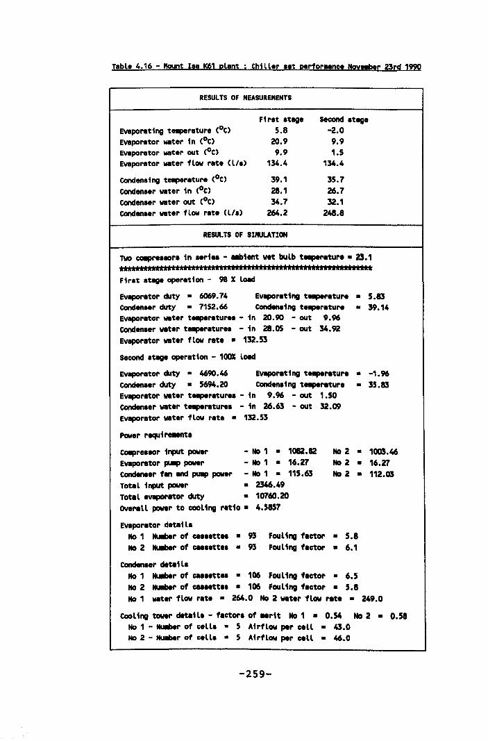
Table 4.16 - ~t I .. K61 plant Chiller .et perfor"nc. Noyt!ber 23rd 1990
RESULTS OF MEASUREMENTS
Evaporating te.perature eOC) Evaporator water in eOC) Evaporator water out (oC) Evaporator water flow rate (l/.)
Condensing t...,.rature (oC) Conden .. r water in (oC) COndenser water out eOc) COndenser water flow rate ell.)
First .tage 5.8
20.9 9.9
134.4
39.1 28.1 34.7
264.2
RESULTS OF SIMULATION
Second .tage -2.0 9.9 1.5
134.4
35.7 26.7 32.1
248.8
Two COIIPre.fOr. in sari .. - abient vet bulb t...,erature • 23.1
""""""""""""""""""""""""""""""'" Fir.t .tege operation - 98 X load
Evaporator duty • 6069.74 Evaporating t...,eretur. • 5.83 Condenatr duty • 7152.66 condenaing t!!p!rature • 39.14 Evaporator water t...,eratur .. - in 20.90 - out 9.96 COnden.er water tnperature. - in 28.05 - out 34.92 Evaporator wat.r flow rat. • 132.53
Second .tege operation - 100x load
Evaporator duty • 4690.46 Evaporating t!!p!rature • -1.96 condent.r duty • 5694.20 condenaing t...,erature • 35.83 Evaporator wat.r tnperature. - in 9.96 - out 1.50 COndenser wat.r t!!p!rature. - in 26.63 - out 32.09 Evaporator water flow rate • 132.53
Power requirel!Dt.
COIIpr .. fOr input power - No 1 • 1082.82 Evaporator puIIp power - No 1 • 16.27 COndenter fen and puIIp power - No 1 • 115.63 Total input power • 2346.49 Total evaporator duty • 10760.20 OVerall power to cooling ratio. 4.5857
Evaporator detail.
No 2 • 1003.46 No 2 • 16.27 No 2 • 112.03
No 1 NUilber of ca ... tt.. • 93 No 2 NUllber of ca...tt.. • 93
Fouling factor • 5.8 Fouling factor • 6.1
Condenaer detail. No 1 NUIIber of C!! .. tt.. • 106 Fouling factor • 6.5 No 2 NUllbtr of CUMtt.. • 106 Fouling factor • 5.1 No 1 water flow rate • 264.0 No 2 wat.r flow rat. • 249.0
COoling tower detan. - factor. of .. rit No 1 • 0.54 No 2 • 0.58 No 1 - NUllber of cell. • 5 Airflow per c.ll • 4].0 No 2 - Nullbtr of c.ll. • 5 Airflow per cell • 46.0
-259-
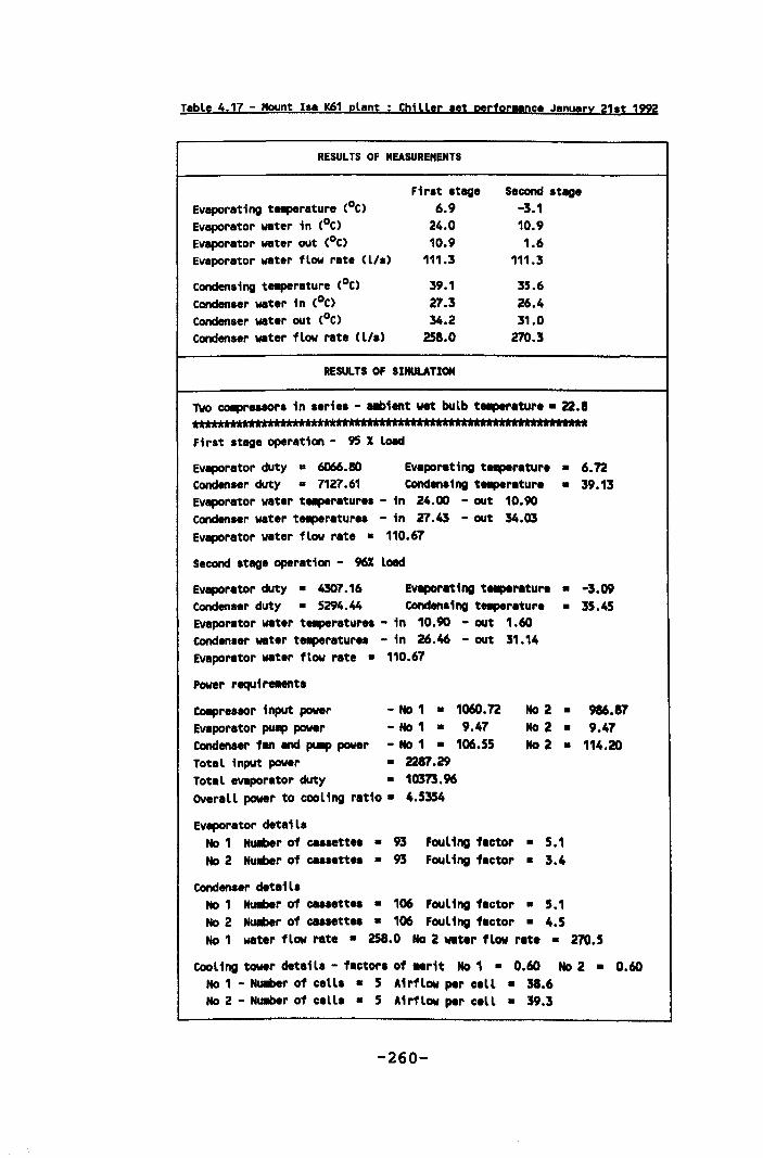
Table 4.17 - MOunt Isa K61 plant Chiller set perfor .. nce January 21st 1922
RESULTS Of MEASUREMENTS
Evaporating t.-perature (oC) Evaporator water in (oC) Evaporator water out (oC) Evaporator water flow rate (lis)
Condensing tetlperature (oC) Condenser water in (oC) Condenser water out (oC) Condenser water f low rate (lis)
First stage 6.9
24.0 10.9
111.3
39.1 27.3 34.2
258.0
RESULTS OF SIMULATION
Second stage -3.1 10.9 1.6
111.3
35.6 26.4 31.0
270.3
Two COIIPresaor. in .erie. - _1ent wet bulb ta.perlture • 22.8
••••••••••••••••••••••••••••••••••••••••••••••••••••••••••••••• First stage operation - 95 X lOid
Evaporator duty • 6066.80 Ev~rlting ta.perlture • 6.72 Conden.er duty • 7127.61 Conden.ing ta.perlture • 39.13 Evaporator water t.-perature. - in 24.00 - out 10.90 Conden.er water t.-perature. - in 27.43 - out 34.03 Evaporator water flow rate • 110.67
Second .tage operation - 96X lOid
Evaporator duty • 4307.16 Ev~rating ta.perlture • -3.09 Condenser duty • 5294.44 Condensing te.perature • 35.45 Evaporltor water te.perature. - in 10.90 - out 1.60 Condenser water t...,.ratures - in 26.46 - out 31.14 Evaporator water flow rate • 110.67
Power requirell8nt.
CoIIpresaor input power - No 1 • 1060.72 Evaporator PUI!p power - No 1 • 9.47 Condenser fan Md puI!p power - No 1 • 106.55 TotaL input power • 2287.29 Total evaporator duty • 10373.96 OVerall power to cooling ratio. 4.5354
Evaporator details
No 2 • 986.87 No 2 • 9.47 No 2 • 114.20
No 1 Hullber of CUHtt.. • 93 No 2 Hullber of ca •• ette. • 93
Fouling factor • 5.1 Fouling factor • 3.4
Condenser detai l. No 1 NUliber of cuaett.. • 106 Fouling factor • 5.1 No 2 NUliber of CUHtt .. • 106 Fouling factor • 4.5 No 1 water flow rate • 258.0 No 2 .. tar flow rIte • 270.5
Cooling tower detail. - flctor. of .. rit No 1 • 0.60 No 2 • 0.60 No 1 - Nulber of ceU. • 5 Airflow per cell • 38.6 No 2 - Nuaber of cell. • 5 Airflow per cell • 39.3
-260-
4.5 Broken Bill North mine surface plant
As already described in section 4.3, the existing
underground refrigeration plant at North mine could
not meet the cooling requirements when mining the
deeper sections of the Fitzpatrick ore body. In
addition to the options to increase the existing
underground plant capacity which are described in
section 4.3, a surface plant could be used which would
either supply chilled water to the existing
underground system or to supplement this system by
bulk cooling the intake air on surface.
4.5.1 Surface refrigeration plant justification
The justification for installing additional mine
refrigeration is associated with the increase in
production resulting from a decrease in the proportion
of six hour shifts and an improvement in thermal
productivity. A re-eva1uation of the 32 level stope
(responsibility 131) six hour jobs (6h) between 1985
and 1987 including the follow on shifts resulted in
the following relationship with the intake wet bulb
temperature at the shaft station (twb):-
% 6h = 0.009333 t wb 3 - 0.4100 twb2 + 8.087 twb - 49.70
The following table summarises the application of this
relationship to the 32 level stope.
-261-
Surface wet bulb
32 level (twb)
Actual % 6 hour
Estimated % 6 hour
Summer
18.0
24.0
38.0
37.3
Mid-seasonal
14.0
20.5
24.9
24.4
Winter
8.0
15.4
11.9
11.7
During the four year period between 1985 and 1989, in
the shallower sections of the Fitzpatrick mining area
(responsibility 132), there were 24 805 six hour
shifts reported out of a total number of shifts worked
of 55 707 or 44.5%. If the follow on shifts during
1986 and 1987 are included (see section 4.3.1), the
proportion increases to 46.0%. Using the above
relationship and the recorded face temperatures, the
expected number of six hour shifts is 44.9%.
The cost benefit of improving thermal environmental
conditions is based on the difference between the base
case and that expected with the modified refrigeration
system. The base case is usually taken as the current
system with the only modifications related to
maintaining continuity of operation. The increased
mining revenue is based on 60 mining personnel working
for 235 shifts/year and an excess of revenue over
costs of A$ lsO.OO/tonne. The cost benefit is adjusted
by differences in power costs at A$ 0.07/kWh.
The working place temperatures used to obtain the
productivity values (both six hour and productivity)
were obtained using the heat and moisture transfer
-262-
routines incorporated in a thermodynamic network
simulation programme (section 2.1.4). An important
heat source in these simulations is that resulting
from the use of diesel powered equipment. The wet and
dry bulb temperatures predicted for the current
refrigeration system were confirmed by comparison with
the record of measurements taken in the Fitzpatrick
mining area.
The method of financial justification follows that
illustrated for the Mount Isa 3000 ore bodies in
section 2.1.4. Essentially a load profile for the year
is established relating a surface wet bulb temperature
to frequency of occurrence. Refrigeration plant
performance and working place wet bulb temperatures
are obtained from the refrigeration plant and network
simulation programmes and related to the surface wet
bulb temperatures. A total of six refrigeration
options were considered.
Option 1 - no action. In this option no expenditure at
all is made on refrigeration or replacement parts and
the existing plant is allowed to deteriorate to shut
down. Essentially the option illustrates the effect of
having no refrigeration at all in the Fitzpatrick
mining area. The weighted average stope productivity
is 16.33 tonnes/manshift (76.9%) and no work is
possible when the surface wet bulb temperature exceeds
21. oOe and the stop work condition prevails in the
working places.
-263-
Option 2 - retain the existinv p1ant. This option
retains the existing refrigeration plant and only
considers sufficient capital expenditure to maintain
continuity of operation i.e. replace the NO 1 and NO 2
chiller set evaporators and to replace all the
refrigeration piping for the NOS 2 and 3 chiller sets.
The estimated capital expenditure is A$ 500 000. The
weighted stope productivity is 19.29 tonnes/manshift
(90.9%) and the weighted refrigeration plant input
power is 1123 kW.
A two thirds refrigeration set availability is assumed
for the plant load i.e. one set is continuously shut
down for maintenance and repair. This low overall
availability is based on actual operational data for
the three years between 1981 and 1990. The total input
power is constant for most of the year as a result of
the limitation with respect to motor input power and
unloading of the compressors.
Option 3(a) - fourth compressor set. In this option, a
fourth compressor set is installed in addition to
making the necessary changes to maintain continuity of
operation i.e. Option 2 plus a fourth compressor set.
The additional capital required is estimated to be
between A$ 1 600 000 and A$ 1 900 000. The weighted
average stope productivity is 20.11 tonnes/manshift
(94. 1%) and the weighted refrigeration plant input
power is 1595 kW.
-264-
Option 3(b) - plate evaporator. Install a fourth
compressor set in addition to modifying the existing
underground arrangements to ensure a plant output
capacity of 6.4 MW by installing a falling film plate
evaporator. The fourth compressor set has a nominal
duty approximately double that of the existing sets
and should allow modifications to the plant to be
undertaken without a reduction in the amount of
cooling supplied. The weighted average stope
productivity is 20.53 tonnes/manshift (96.7') and the
weighted refrigeration plant input power is 1736 kW.
The additional capital required is estimated to be
AS 2 600 000.
Option 4 - surface bulk air cooler. Install a surface
plant providing chilled water which is used to cool
part of the intake air in a 5.5 MW bulk air cooler.
One 1.8 MW underground plant is used to supply chilled
water to the 37 level bulk air cooler and to the
auxiliary ventilation systems used for development.
The weighted average stope productivity is 20.08
tonnes/manshift (94.6'), the weighted refrigeration
plant input power is 1109 kW and the estimated capital
cost for the new plant is A$ 3 500 000.
Option 5 - surface chilled water plant. In this option
the existing underground refrigeration plant is
replaced with a surface plant which supplies chilled
water from surface through an energy recovery system
and into the existing chilled water system. The
-265-
weighted average stope productivity is 20.48
tonnes/manshift (96.5%), the weighted refrigeration
plant input power is 1088 kW and the additional
capital required is estimated to be A$ 7 300 000.
A summary of the costs and the effectiveness of the
options available are summarised in table 4.18. For a
project life of between five and seven years, the mine
decided to select option 4 as a turn key project. This
had the advantage of minimising staffing requirements
during construction and, when mining is completed in
the Fitzpatrick area, a significant part of the plant
could be recovered and used at the South mine. It was
expected that the increasing depth of mining at the
Southern Cross shaft of the South mine would justify
the installation of refrigeration at this time.
4.5.2 System design and selection
The amount of air that could be cooled in the surface
bulk air cooler was limited by the size of raise bore
hole that could be drilled to the 2 level station and
the entrance to the shaft on this horizon. Extensive
modification work was not possible without disrupting
the production and service requirements of the shaft.
With the amount of air to be cooled limited to between
125 and 150 m3 /s, a supply air temperature of about
40 C was required at the deSign climatic condition.
This in turn resulted in a supply chilled water
temperature of between land 20 C.
-266-
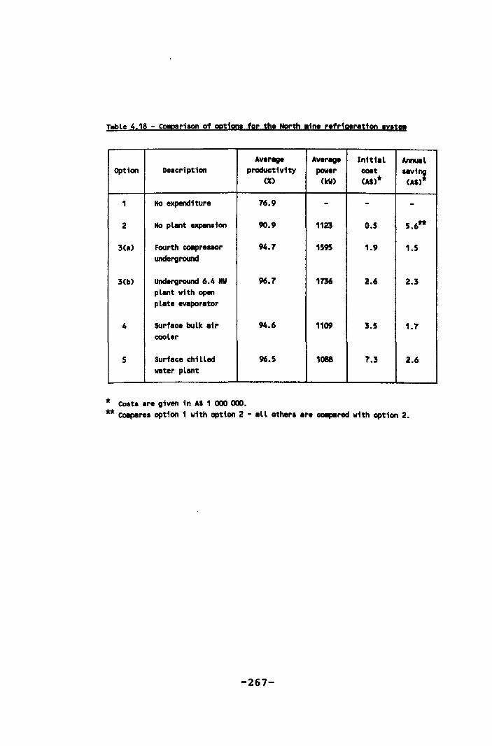
Table 4.18 - Co!p!riaon of options for the North .in. rtfrig.ratioo svst"
Av.rllg' Av.rllg' Initial Annual Option Description productivity pow.r cost "Vi~
(X) CkW) (AS)· (AS)
1 No expenditure 76.9 - - -
2 No plant expansion 90.9 1123 0.5 5.6**
3(a) Fourth caapressor 94.7 1595 1.9 1.5 underground
3(b) underground 6.4 MW 96.7 1736 2.6 2.3 plant with open
plate evaporator
4 Surface bulk air 94.6 1109 3.5 1.7 cooler
5 SUrface chi LLed 96.5 1088 7.3 2.6 water plant
* Costs are given in AS 1 000 000. ** CoIpares option 1 with option 2 - all others ar. coapared with option 2.
-267-
General
The refrigeration plant is required to operate over a
wide range of ambient climatic conditions consequently
a technical assessment of alternative plants should
evaluate performance and input power requirements at
"off" design conditions. The refrigerant used in all
the proposals was ammonia. The prospective suppliers
proposed different compressors and the characteristic
curves of adiabatic head and efficiency against
compressor inlet refrigerant flow rate are given in
section 3.1.
Heat rejection in all the proposals used modular and
factory assembled evaporative condensers which are the
most cost effective for this application. These are
proven in both industrial and mining applications. The
relatively short life of the project did not justify
custom designed units with longer life materials of
construction such as a concrete shell and stainless
steel coil supports.
The refrigeration plant supplies chilled water to a
bulk air cooler which handles intake air. Evaporator
fouling is therefore considered to be relatively low
and easily controllable with either slipstream
filtration or bleed off and make up water. It is
therefore not essential to provide open evaporators
with a commensurately higher cost. All prospective
suppliers offered closed plate heat exchangers.
-268-
To minimise the bulk air cooler air flow rate the
cooling tower used must have a high factor of merit.
All tenderers proposed to supply a standard counter
flow packaged unit design in the conforming offer.
Although these cooling towers are extensively used in
industrial applications there are reservations with
respect to the rated performance in past applications.
In this case, the detailed performance criteria
supplied and the increased thickness of fill should
ensure that the design conditions were met.
Tender evaluation
From the information provided in each tender, a model
was built up using the modules outlined in section
4.1. The equipment selection and the arrangement for
each tender proposal is summarised in figure 4.26.
For proposal 1, the VXC 1060 evaporative condensers
are well sized and may be too large relative to their
initial cost and the potential power savings. The Alfa
Laval closed plate heat exchangers are very undersized
at 64 plates each (62 effective or 31 cassettes). The
two parallel sets are relatively straightforward to
control and operate. Using the plate heat exchangers
in parallel involved a power penalty because both
operate at the lowest evaporating temperature. Using
the North Mine surface climatic temperatures and load
profile, the total power required to operate the plant
is 7 423 000 kWh/year or a cost of A$ 519 600/year.
-269-
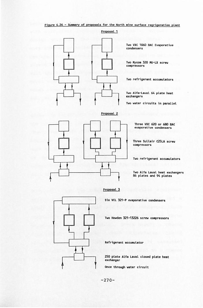
Figure 4.26 - Summary of proposals for the North mine surface regrigerat10n plant
Proposal 1
Proposal 2
Proposal 3
Two vxe 1060 BAC Evaporative condensers
Two Hycom 320 HU- LX screw compressors
Two refrigerant accumulators
Two Alfa-Laval 64 plate heat exchangers
Two water circuits in parallel
Three VXC 620 or 680 BAC evaporative condensers
Three Sullair C25LA screw compressors
Two refrigerant accuNUlators
Two Alfa Laval heat exchangers 86 plates and 94 plates
Six vel 321-P evaporative condensers
Two Howden 321-13226 screw compressors
Refrigerant accuDUlator
250 plate Alta Laval closed plate heat exchanger
Once through water circuit
-270-
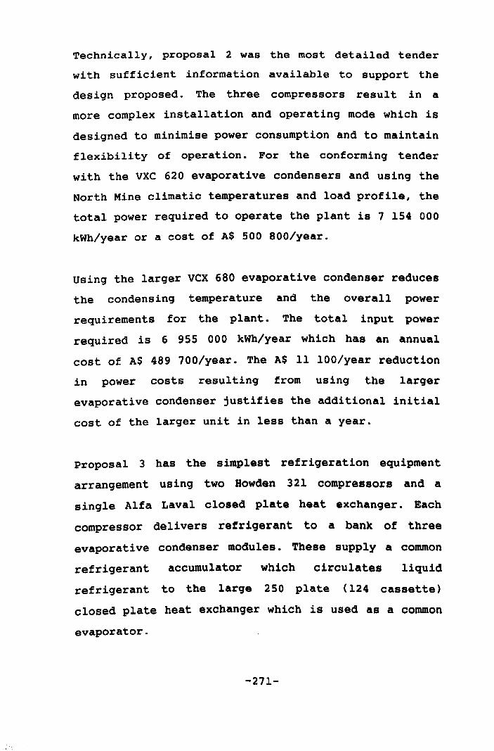
Technically, proposal 2 was the most detailed tender
with sufficient information available to support the
design proposed. The three compressors result in a
more complex installation and operating mode which is
designed to minimise power consumption and to maintain
flexibili ty of operation. For the conforming tender
with the VXC 620 evaporative condensers and using the
North Mine climatic temperatures and load profile, the
total power required to operate the plant is 7 154 000
kWh/year or a cost of A$ 500 BOO/year.
using the larger vex 680 evaporative condenser reduces
the condensing temperature and the overall power
requirements for the plant. The total input power
required is 6 955 000 kWh/year which has an annual
cost of A$ 489 700/year. The A$ 11 100/year reduction
in power costs resulting from using the larger
evaporative condenser justifies the additional initial
cost of the larger unit in less than a year.
Proposal 3 has the simplest refrigeration equipment
arrangement using two Howden 321 compressors and a
single Alfa Laval closed plate heat exchanger. Each
compressor delivers refrigerant to a bank of three
evaporative condenser modules. These supply a common
refrigerant accumulator which circulates liquid
refrigerant to the large 250 plate (124 cassette)
closed plate heat exchanger which is used as a common
evaporator.
-271-
The refrigerant gas from the accumulator is returned
to the compressor (s) depending on the refrigeration
demand. At low ambient wet bulb temperatures only one
compressor operates using three evaporative condenser
modules. Using the North mine climatic temperatures
and load profile, the total power required to operate
the plant is 7 132 000 kWh/year at an annual cost of
AS 499 200. When the ambient wet bulb temperature is
below 14oC, the lower mine refrigeration load can be
achieved with only one of the compressors operating.
All the proposals were technically acceptable and
proposal 3 was finally adopted. The decision was
based on the much lower initial costs (24% less than
the next lowest cost) and an almost negligible
increase in operating power costs.
Plant control strategy
The control strategy for the surface refrigeration
plant is to minimise input power requirements whilst
providing the design refrigeration at the bulk air
cooler. This is best achieved by maintaining the
compressors at full load and by varying the water
supply to the bulk cooler in order to supply just the
right amount of cooling. The ideal control arrangement
is illustrated in figure 4.27.
The system illustrated requires three variable speed
pumps, one to maintain the compressor at full load
-272-
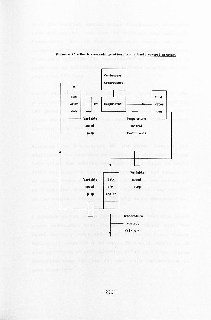
Figure 4.27 - North Mine refrigeration plant basic control strategy
Condensers
t Compressors
Hot r- I Cold
water Evaporator .. water
-.J dam '-- da. -Variable Temperature
speed control
pump (water out)
r-
'--
Variable
Variable Bulk speed
speed air pump
pump cooler
r-
'-- Tem eratu p re
control
(air out)
-273-
wi th the varying return water temperature from the
bulk air cooler, and, two to maintain the wet bulb
temperature out of the bulk air cooler at 4oC.
Controlling plant output with a fixed evaporator water
flow rate requires the compressors to unload with a
reduction in efficiency which becomes significant at
less than 80% load.
Using the Howden simulation model (proposal 3) the
plant performance for this control arrangement and for
the design North Mine load profile results in annual
power costs to operate the system with this control
strategy of A$ 498 600.
Allowing the temperature of the water leaving the
evaporator to increase according to the ambient wet
bulb (when the ambient wet bulb temperature is above
200 C) would reduce the plant input power and result in
an annual power cost of A$ 489 500. The net saving of
A$ 9 OOO/year does not justify the extra complication
of the variable evaporator leaving water temperature.
A simpler system is to replace the two variable speed
pumps associated with the bulk air cooler with two
fixed delivery pumps and to allow the bulk air cooler
outlet air temperature to vary. This will result in an
over provision of refrigeration relative to the design
condi tion when the ambient wet bulb temperature is
less than 16°C.
-274-
The annual power costs to operate the system with this
control strategy are A$ 513 400. If the bulk air
cooler pumps are either two speed or multiple parallel
units, the bulk cooler water flow could be reduced to
65.0 lIs (down from 100.0 l/s) when the ambient wet
bulb temperature is below l20 C. Less cooling would be
transferred in the bulk air cooler and the annual
power costs would be reduced to A$ 497 600.
The water storage dams serve two purposes:-
1. To ensure that the compressor motor run time is
reasonable and does not cycle on and off too
frequently i.e. a minimum run time of two hours.
2. To provide cold water storage which can be used to
provide cooling when the compressors are not
running i . e. during a scheduled maintenance
shutdown.
The storage capacity for a scheduled shutdown of four
hours is 1.5 Ml at a fixed bulk cooler water flow rate
of 100 lIs. This capacity would also provide a minimum
two hour run time at a maximum evaporator water flow
rate of 200 l/s. The cold water dam operates between
"low" at say 10% - compressors start, and "full" at
say 95% - compressors stop. The low level start would
be manually overridden if a scheduled maintenance
shutdown is due in order to fill the cold dam.
-275-
The system using variable water flow through the bulk
air cooler does not have a significant power cost
benefit and the more complex control system is not
justified. The design water flow rate through the bulk
air cooler was fixed at 100 lIs. A variable speed pump
is used to ensure that the water flow through the
evaporator maintains the compressors at full load and
the water temperature leaving the evaporator is
between 1 and 2oC. Although a by-pass back to the hot
dam from the evaporator outlet could be installed, It
was not expected to be used except for two or three
minutes during start up.
4.5.3 Plant performance
A schematic of the general layout of the plant is
given in figure 4.28. The plant comprises two nominal
3.5 MW screw compressors, a 160 cassette closed plate
evaporator and six low profile evaporative condensers.
Two 1.5 Ml capacity concrete storage dams are used for
supply and return water storage. The plant operation
is controlled by the level of water in the cold dam
and the plant start up sequence is initiated when the
water level falls to 0.7 m.
The variable speed pump is started and its speed
increased to 50% which provides a flow of 150 lIs from
the hot dam through the evaporator. The condenser fans
are then started in sequence ( the condenser pumps
remain running unless switched off for maintenance).
-276-
The lead compressor motor is started when the oil pump
run status is confirmed with the compressor capacity
slide val ve fully closed i. e . no load. Ten second
pulses activate the solenoid which opens the slide
valve and loads the compressor fully in approximately
two minutes.
The variable pump speed is then altered to provide
water leaving the evaporator at the set temperature.
If this is less than 120 lis I the second compressor
start up sequence is initiated. Stable conditions are
normally achieved in less than five minutes.
April 1991 performance tests
The refrigeration plant installation was completed in
March 1991 and acceptance tests were undertaken in
April 1991. At the conclusion of the performance tests
the refrigeration plant was not acceptable with
deficiencies in five main areas. These were not
thought to be fundamental design problems and remedial
action should be successful. With the onset of winter
in the southern hemisphere, the limited opportunity to
operate the plant would delay the modifications and
future testing.
The factor of merit of the bulk air cooler was 18%
lower than claimed with the water flow rate 20% above
design and the airflow rate 6% below design. Although
the bulk air cooler could meet the design heat
-277-
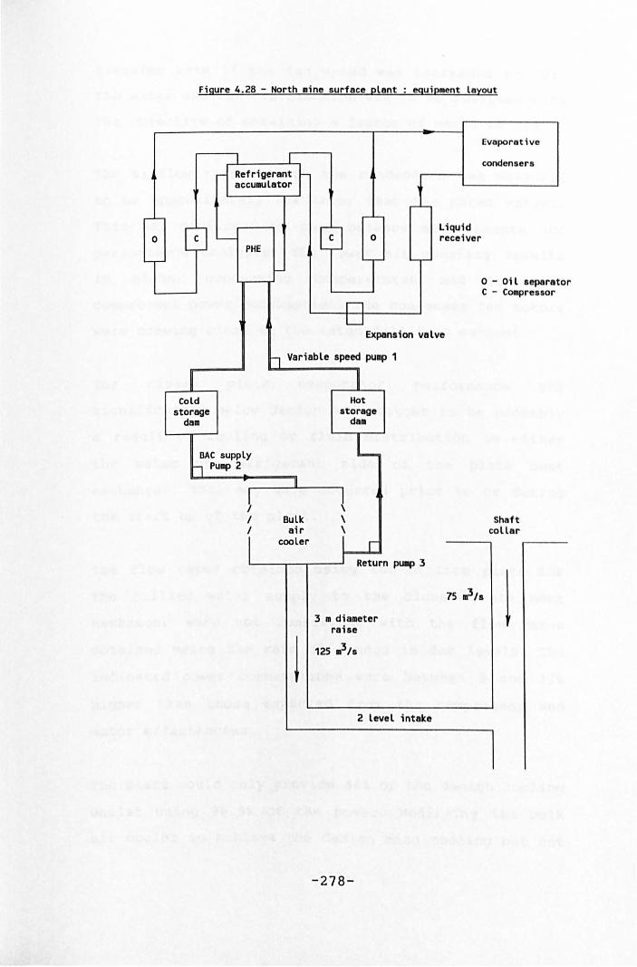
-'-
0
T
Figure 4.28 - North . ine surface plant equipment layout
Evaporati ve
I I condensers rl Refrigerant J i accullU lator
,--Liquid
C '-- C 0 recei ver PHE
J '--
-o - Oi l separat C - COlllpressor
n u
Expansion va lve
11 Variable speed pump 1
Cold storage
dam
BAC supply 11 Pump 2
I
! / Bulk
j air cooler
j
I Hot
storage dall
L
t \ \
I r I Return pullp 3
3 • diallet er rai se
2 leve l i ntake
- 278 -
Shaft collar
75 ~/s
I
or

transfer rate if the fan speed was increased by lOt,
the water and air distribution was to be reviewed with
the objective of obtaining a factor of merit of 0.75.
The airflow rate through the condensers was measured
to be approximately 20t lower than the rated values.
This was confirmed by heat balance measurements and
performance analysis. The lower air quantity results
in higher condensing temperatures and increased
compressor power consumption. The condenser fan motors
were drawing close to the rated full load current.
The closed plate evaporator performance was
significantly below design and thought to be probably
a result of fouling or fluid distribution on either
the water or refrigerant side of the plate heat
exchanger. This may have occurred prior to or during
the start up of the plant.
The flow rates obtained using the orifice plate for
the chilled water supply to the closed plate heat
exchanger were not consistent with the flow rates
obtained using the rate of change in dam levels. The
indicated power consumptions were between 9 and 17%
higher than those expected from the compressor and
motor efficiencies.
The plant would only provide 88% of the design cooling
whilst using 98.5% of the power. Modifying the bulk
air cooler to achieve the design mine cooling but not
-279-
correcting the condenser and evaporator problems would
result in an increased power consumption equivalent to
AS 60 000 per year.
Pump flow rates
It was noted during the April 1991 site visit that the
water flow rates obtained using the orifice plates
were not consistent with those obtained using the
difference in dam levels over .a prescribed time
period. A detailed series of tests were undertaken
during February 1992 to identify these discrepancies
and the results are summarised in Figure 4.29. The
resultant calibration curves for pumps 1 and 2 are:-
where 1 * e
1e
and lbc *
lbc
Pump 1 * Ie = 1.116 Ie
Pump 2 lbc = 1.0505 lbc
+ 3.19
*
= indicated pump 1 water flow rate (l/s)
= actual flow through the evaporator (l/s)
= indicated pump 2 water flow rate (l/s)
= actual flow through the bulk air cooler
The water level change using the cold water storage
dam gave more consistent results than using the hot
water dam levels even when pumps 2 and 3 (those
supplying and returning water to and from the bulk air
cooler) were not operating. This is probably caused by
-280-

the effect of the water supply and take off relative
to the level indicators. In the cold dam, the chilled
water supply and take off are adjacent to each other
at the base of the dam and should not cause a surface
wave action which would affect the level indicator.
Surface bulk air cooler
The surface bulk air cooler is a two cell counter flow
tower with 1.8 m thickness of compact plastic fill and
a design water to air ratio of 0.7. The air is passed
through the tower and down a 3 m diameter raise to 2
level where it joins the balance of the air in the
shaft. Two centrifugal fans driven by 110 kW motors
through a belt drive are used to overcome the pressure
loss in the bulk air cooler and the raise.
When first measured in April 1991, the bulk air cooler
had a factor of merit of 0.68 and an airflow rate
which was 6% below the design value. Although the
manufacturers rated factor of merit averaged 0.818,
this was considered to be overly optimistic and a
value of 0.75 would be acceptable. The results of the
April 1991 and the January/February 1992 tests are
given in Table 4.19. The heat balance obtained from
the measured values for the water and air sides was
satisfactory at between -2.1% and +2.9%.
The average factor of merit for the 1992 tests was
0.745 and the rated airflow is now within 1% of the
-281-
design value. The change in water sprays to improve
distribution appears to have been successful and the
performance of the bulk air cooler is acceptable.
Closed plate evaporator
A total of 23 sets of results were obtained in order
to assess the performance of the Alfa Laval closed
plate heat exchanger used as the evaporator. During
the April 1991 site visit, from the results of five
tests, the heat exchanger performance was found to be
lower than expected with the heat transfer taking
place at significantly lower evaporating temperatures
than expected from the design values. The overall heat
transfer coefficient was found to be between 500 and
600 W/K or 30% below the expected design value.
Refrigerant boiling heat transfer rates in evaporators
are difficult to assess and, based on the method of
analysis outlined in section 3.3.3 and a water side
fouling factor of 5.0 kW/m2K, the relationship between
the actual and the calculated evaporating
temperature was found to be:-
Actual te = • 1.087 te 1.76
(coefficient of correlation = 0.912)
t • e
In late 1991, the plate heat exchanger was increased
in size by 25% by adding an additional 35 cassettes.
Although this improved the heat exchanger overall heat
-282-
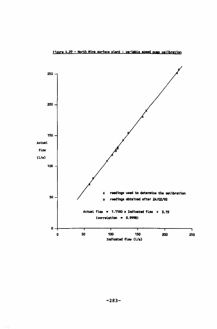
250
200
150
Actual
flow
<L/.)
100
Figyr. 4.29 - North "joe .urfee. plent ; ytr1 tbl •• pttd PUlp ctl1br.t1oo
50 x retd1. UHd to dete",'ne the eel ibr.t1on
o reading. obtained .fter 24/02/92
Actual flow • 1.11~ x Indieeted flow + 3.19
(correlation • 0.9991)
O~-------'--------~-------r--------r-------I o 50 100 150 200 250
Indicated flow (l/.)
-283-
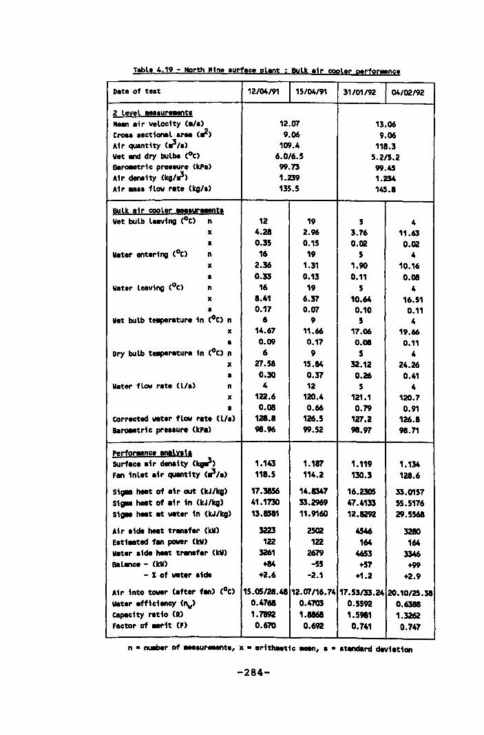
Table 4.19 - North "in •• urf.e. plant; Bulk air cool.r perfor .. nc.
Date of test
2 level .... ur!l!Ot. "etn air velocity (.,.) crou aectiontl ..... (,;) Air quantity (~/.) w.t n dry bulb! (oC) Bt~tric pr •• aur. (kPa) Air den!ity (kg/~) Air .. s. flow rat. (kg/.)
BUlk air cool.r .... ur!I!Dt. Wet bulb letving (oC) n
x
• n x
• Water letving (oC) n
x
• Wet buLb te.per.tur. in (oC) n
x
• Dry buLb te.per.tur. in (oC) n
x
• Wat.r flow rat. (l/.) n
x
• Corrected wat.r flow r.te (L/.) Ba~tric pressure (kP.)
Perfor!!Oce ,",lVli. SUrf.c •• i r den!ity (q.3)
fan inLet .ir quantity (~/.)
Sig.a heat of .ir out (kJ/kg) Sig.a heat of .ir in (kJ/kg) Sig.a h .. t .t water in (kJ/kg)
Air .ide heat transfer (kV)
E.ti .. ted fan power (tv)
water .ide hMt transf.r (tv)
BaLanc. - (tv)
- X of water .ide
Air into tower (.fter fan) (oC) water .fficiency (nv> capacity r.tio (R) f.ctor of .. rit (f)
12/04/91 15/04/91
12.07 9.06
109.4 6.0/6.5 99.73 1.239 135.5
12 4.28 0.35 16
2.36 0.33 16
8.41 0.17
6 14.67 0.09 6
27.58 0.30 4
122.6 0.08
121.8 98.96
1.143 118.5
17.3856 41.1730 13.8581
3223 122
3261
+84 +2.6
19 2.96 0.15 19
1.31 0.13 19
6.37 0.07
9 11.66 0.17 9
15.84 0.37 12
120.4 0.66
126.5 99.52
1.117 114.2
14.1347 33.2969 11.9160
2S02 122
2679 -55
-2.1
31/01/92 04102192
13.06 9.06
118.3 5.2/5.2 99.45 1.234 145.8
5 3.76 0.02
5 1.90 0.11
5 10.64 0.10 5
17.06 0.08
5 32.12 0.26
5 121.1 0.79
127.2 98.97
1.119 130.3
16.2305 47.4133 12.8292
4546 164
4653 +57
+1.2
4 11.63 0.02
4 10.16 0.08
4 16.51
0.11 4
19.66 0.11
4 24.26 0.41
4 120.7 0.91
126.8 98.71
1.134 128.6
33.0157 55.5176 29.5568
3280 164
3346 +99
+2.9
15.05/28.48 12.07/16.74 17.53/33.24 20.10/25.38 0.4768 0.4703 0.5592 0.6588 1.7892 1.8868 1.5981 1.3262 0.670 O.~ 0.741 0.747
-284-
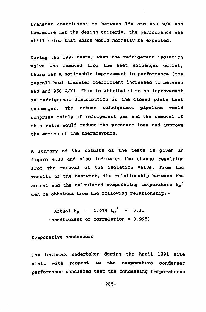
transfer coefficient to between 750 and 850 W/K and
therefore met the design criteria, the performance was
still below that which would normally be expected.
During the 1992 tests, when the refrigerant isolation
valve was removed from the heat exchanger outlet,
there was a noticeable improvement in performance (the
overall heat transfer coefficient increased to between
850 and 950 W/K). This is attributed to an improvement
in refrigerant distribution in the closed plate heat
exchanger. The return refrigerant pipeline would
comprise mainly of refrigerant gas and the removal of
this valve would reduce the pressure loss and improve
the action of the thermosyphon.
A summary of the results of the tests is given in
figure 4.30 and also indicates the change resulting
from the removal of the isolation valve. From the
results of the testwork, the relationship between the
actual and the calculated evaporating temperature te*
can be obtained from the following relationship:-
* Actual te = 1.074 te 0.31
(coefficient of correlation = 0.995)
Evaporative condensers
The testwork undertaken during the April 1991 site
visit with respect to the evaporative condenser
performance concluded that the condensing temperatures
-285-
were too high and that the problem was probably
associated with below design air quantities. Each
condenser had air supplied to it using two double
inlet centrifugal fans on a common shaft which was
driven by a single motor. Safety guards precluded an
accurate air quantity measurement being taken at the
inlet to the fans.
The eliminators at the discharge from the condenser
affected the outlet air distribution and made accurate
air quantity measurements difficult to achieve. Since
the condenser is required to reject both the heat of
compression and the evaporator duty, in the absence of
accurate air quantity measurements, it is necessary to
obtain a good estimate of both of these components
from other plant measurements.
To avoid overloading the compressor motors, a maximum
discharge pressure causes the compressors to unload
when this limit is exceeded. The compressor power
requirement does not decrease uniformly with a
decrease in load and a method for evaluating the part
load compressor performance is given in section 3.1.1.
Typically, although dependent on the compression
ratio, the increase in expected compressor input power
is 6.5% at 80% load, increasing to 21% at 50% load.
A comparison of the measured evaporator performance
with that which would be expected based on the
compressor performance curves and the part load
-286-
Figure 4.30 - North Mine surface plant closed plate evaporator performance
8.0
6.0
4.0
Measured
evaporating
tetllperature
(oC)
2.0
0.0
-2.0
o /
/ /
/
/ °
x
° * Before the isolation valve was reDOved
x After the isolation valve was reDOved
° April 1991 test results
-4.0~--------~---------.----------r---------.----------'
-2.0 0.0 2.0 . 4.0 6.0 Calculated evaporating temperature (oC)
Based on readings taken when the plant was both operating and shut down and aeasurements of the temperature of the a..ania in the evaporator, the gauge pressure readings were adjusted as follows:-
No 1 compressor suction -5 kPa No 2 compressor suction +4 kPa Accumulator pressure +3 kPa
-287-
8.0
analysis is given in figure 4.31. Although there is
some scatter in the results the maximum discrepancy is
4.7% with an average of difference 2.0%. This is
within normal estimating and measurement accuracy and
can be considered satisfactory.
The measured evaporator duty (from water temperatures
and flow rates) rather than the estimated value was
used as a basis value when assessing the condenser
heat rejection. The estimated compressor input power
was adjusted to this measured value. A comparison of
the actual and estimated condensing temperatures
(assuming full airflow and normal air side fouling) is
given in figure 4.32.
The four values obtained during the week of February
3rd to 8th were affected by non condensable gases in
the condenser which were finally removed on the 8th of
February. The remaining tests (including those of
April 1991) follow the relationship indicated in
figure 4.32 with nearly all the values falling within
one standard deviation of the mean values. From the
analysis it was evident that there is no time trend to
account for the scatter.
Four measurements of the actual condenser heat
rejection obtained using airflow and air temperature
measurements indicated discrepancies of -13.9%, +8.0%,
+0.2% and +3.3% between the measured and expected
values. The large negative discrepancy was probably
-288-
associated with the difficulty in taking airflow
measurements at the eliminator discharge which could
have been significantly in error.
The airflow measurements also indicated that the
condenser sump water level had a significant effect on
the air quantity delivered by the fan. When measured
in April 1991 the airflow factor was reasonably
consistent at 0.80. By early February 1992 this had
decreased to 0.65. Maintaining the sump level at just
below the fan discharge volute, results in an airflow
factor of 0.85. Modifications to the pump location and
the sump level control are necessary to stabilise this
aspect of the condenser performance.
As supplied, the pump suction required a minimum depth
in the sump of 140 mm. At this depth the water was
level with the bottom of the fan discharge volute and
waves were caused. The level control was within 1 m of
the fan discharge and the troughs of the waves caused
this control to activate and open the make up water
supply valve and to increase the water level in the
condenser sump.
As the water level increases, the fan discharge area
is reduced and the fan supply quantity reduced. By
altering the pump suction the minimum depth can be
reduced to 100 mm and, by moving the level control
further away from the fan discharge, the effects of
any wave action can be minimised.
-289-
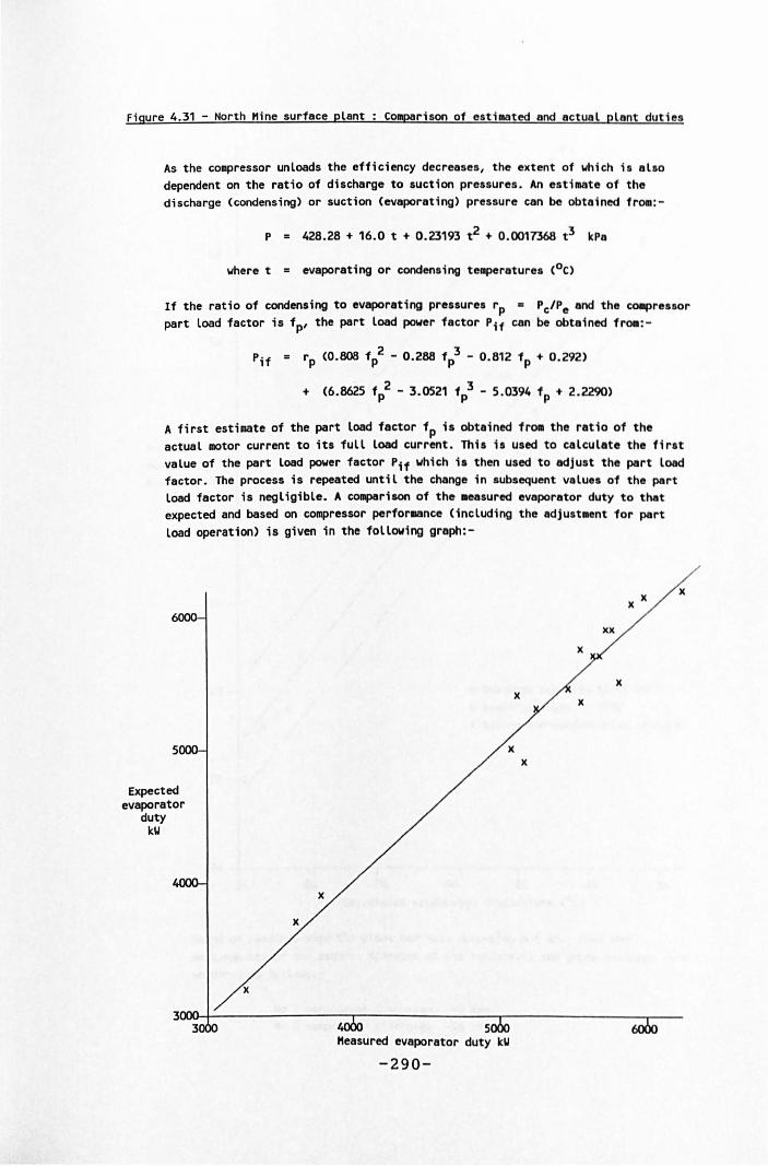
Figure 4.31 - North Mine surface plant Comparison of estiaated and actua l plant dut i es
As the compressor unloads the efficiency decreases, the extent of which 1s also dependent on the ratio of discharge to suction pressures. An estimate of the discharge (condensing) or suction (evaporating) pressure can be obtained from: -
P 428.28 + 16.0 t + 0.23193 t 2 + 0.0017368 t 3 kPa
where t = evaporating or condensing te~eratures (oC)
If the ratio of condensing to evaporating pressures rp • Pc/Pe and the ca.pressor part Load factor is fp' the part load power factor Pif can be obtained fro.: -
808 f 2 _ 3
rp (0 . p 0.288 fp - 0.812 fp + 0.292)
A first estimate of the part load factor fp i. obtained from the ratio of the actual motor current to its full load current. This is used to calculate the first value of the part load power factor Pif which is then used to adjust the part load factor. The process is repeated until the change in subsequent values of the part load factor is negligible. A comparison of the .easured evaporator duty to that expected and based on compressor performance (including the adjust.ent for part load operation) is given in the follOWing graph:-
x x x
5 x
Expected evaporator
duty kW
3~~--------------r--------------'r-------------~----5
Measured evaporator duty kW
-290-
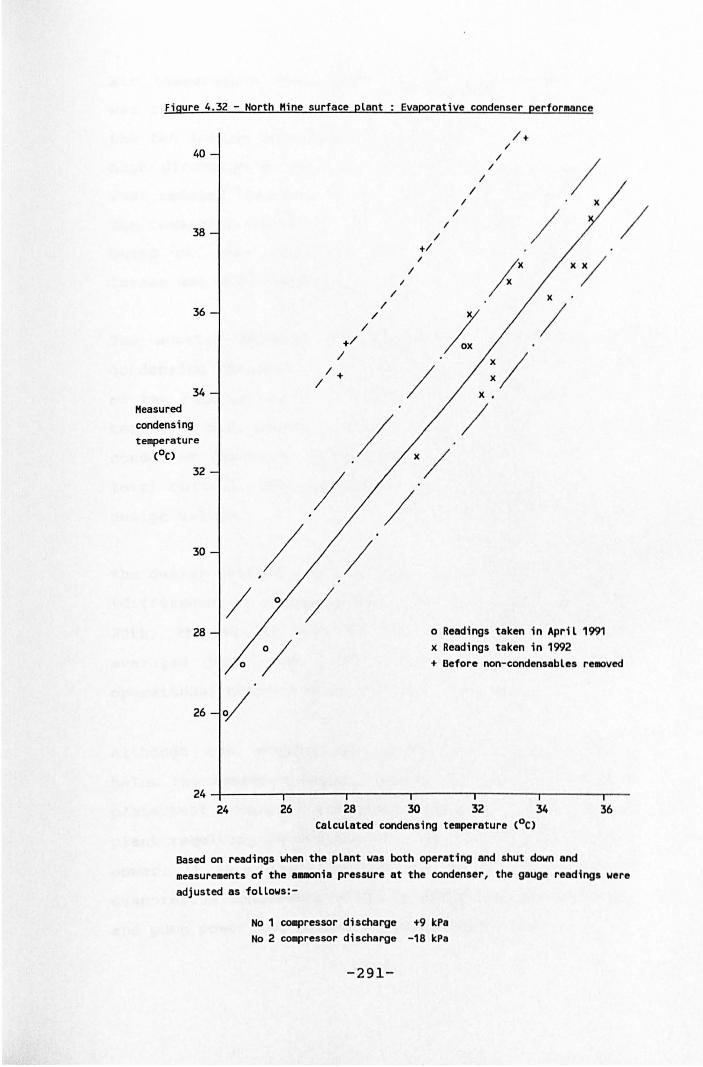
Figure 4.32 - North Mine surface plant Evaporative condenser performance
40
38
36 /
34
/
I
/ /
/
/ +/ I
/
/ /
/ /
/ /
/+ /
/ x
/
Measured condensing temperature
COC)
32
30 / / °
28
26
/ /
/ ° Readings taken in April 1991 x Readings taken in 1992 + Before non-condensables re.aved
24~------,-------.-------r------'------~-------r---
24 26 28 30 32 34 36 Calculated condensing te~rature (oC)
Based on readings when the plant was both operating and shut down and measurements of the a..ania pressure at the condenser, the gauge readings were adjusted as follows:-
No 1 COIIpressor discharge +9 kPa No 2 compressor discharge -18 kPa
-291-
Air temperature measurements also showed that there
was recirculation between the condenser discharge and
the fan intake depending on wind direction. The 2.1 m
high discharge extensions installed in late February
1992 reduced this but did not completely eliminate it.
The remaining condenser heat balances given above were
based on some recirculation which resulted in an
intake wet bulb temperature O.60 C above ambient.
The scatter between the expected and the measured
condensing temperatures is most probably a combination
of the reduced airflow and recirculation factors. The
test work did, however, demonstrate that even with the
condenser discharge extensions and the improved sump
level control, the condensers will not quite meet the
design values.
The design overall heat transfer factor was 2350 W/kPa
(difference in vapour pressures) and, since February
20th, the actual overall heat transfer factor has
averaged just over 2000 (allowing for five cells
operational between March 5th and 11th 1992).
Although the evaporative condensers are performing
below the tendered design values, the improved closed
plate heat exchanger evaporator results in the overall
plant requiring an average of 9 kW or 1.2% extra input
power. It is planned to replace one of the existing
evaporative condensers with one requiring the same fan
and pump power and having a greater coil area.
-292-
This larger cell will then be used for all the oil
heat rejection rather than the three cells currently
used. This would then result in reduction in overall
plant input power averaging 19 kW i.e. 1.3% less than
the original design value. The net saving would be
approximately AS 12 OOO/year. The relationship between
the actual and the calculated condensing temperature
tc· can be obtained from the following relationship:-
Actual tc = 0.959 tc· + 3.78
(coefficient of correlation = 0.990)
This is based on and airflow factor of 1.00. With
improved water sump level control and the condenser
discharge extensions minimising recirculation, an
airflow factor of 0.85 has been demonstrated to be
achievable. In this case, the relationship between the
actual and the calculated condensing temperature tc * can be obtained from the following relationship:-
* Actual tc = 1.019 tc - 0.41
Input power measurements
During the April 1991 tests, the power consumption
determined from the EMS (Energy Management System used
for plant control) print outs were higher than
expected and indicated a much higher power consumption
than expected for most of the equipment and in
particular the compressors. These were reviewed in
-293-

February 1992 by accurately timing the kilowatt hour
meter disc rotation and relating the values obtained
to the equipment performance.
An analysis of two sets of measurements resulted in
inferred combined motor efficiencies of 91.3% and
93.1%. Although not consistent between compressor
motors and allowing for measurement inaccuracies, the
inferred motor efficiencies are lower than that which
would be expected for new motors and probably of the
right order of magnitude for the rewound motors which
are actually used to drive the compressors.
The variable speed pump power requirement is dependent
on the hot water storage dam level and care must be
exercised in setting the maximum speed control limit
when starting the plant when the hot storage dam level
is low. The additional static head results in the
maximum motor current limit being exceeded and the
plant start up sequence being aborted.
The resul ts of the power supply measurement to the
variable speed pump was satisfactory. The amount of
water that will be delivered by the chilled water pump
as a function of pump speed control setting and depth
of water in the hot water storage dam can be obtained
from the following relationship. The coefficient of
correlation between the measured and expected values
for ten sets of measurements obtained from the test
work is 0.996.
-294-
= 82.6
where 1e = chilled water pump delivery (l/s)
N = pump speed control setting (%)
dh = hot dam water level (mm)
4.5.4 Simulation model
A full listing of the computer simulation used to
model the North mine surface plant is given in
Appendix 3. The computer language used is Quick Basic
and the simulations take between 5 and 20 seconds to
converge when using an IBM-PC 386.
The simulation method follows that outlined in section
2.2.2 and uses the modular structure described in
section 4.1. The method of assessing the performance
of the individual components is described in section 3
and adjusted in line with the performance testing
summarised in section 4.5.3.
The performance of the simulation is illustrated in
Tables 4.20 and 4.21. The first table summarises the
data obtained from the EMS monitoring system and
includes the corrections to the measurements obtained
during the performance testing. The second table
summarises the simulation input and output data and
demonstrates the suitability of the model to represent
actual steady state operating conditions.
-295-
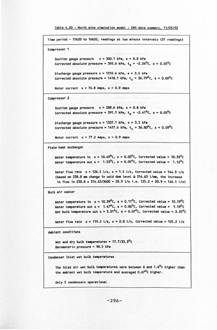
Table 4.20 - North .ine s iaulation .adel EHS data summary, 11(03(92
Time period - 1Sh20 to 16h20, readings at two .inute interval . (31 reading. )
Compressor 1
Suction gauge pressure x = 300.1 kPa, • • 0.8 kPa Corrected absolute pressure = 393.6 kPa, te a -2.26°C, •• O.OSoC
Discharge gauge pressure x = 1310.6 kPa, •• 3.5 kPa Corrected absolute pressure = 1418.1 kPa, tc = 36.79oC, •• O.09oC
Hotor current x = 76.8 AMpS, s a 0.9 A~s
Compressor 2
Suction gauge pressure x = 288.6 kPa, • • 0.8 kPa Corrected absolute pressure • 391.1 kPa, te • -2.41 0 e, • • o.osoe
Discharge gauge pressure x = 1337.1 kPa, • • 3.5 kPa Corrected absolute pressure = 1417.6 kPa, tc a 36.80oC, •• O .~C
Motor current x = 77.2 Amps, s ~ 0.9 A~s
Plate heat exchanger
Water temperature in x = 10.4~C, • • O.03oC, Corrected value . 10.390 C Water temperature out x = 1.530 C, • • O.OSoC, Corrected value . 1.120 C
Water flow rate x = 126.5 lis, • = 1.5 lis, Corrected value . 144 .3 l/. (based on 238.8 II1II change in cold de. level iii 314.63 l/_ , the increase in flow is 238.8 x 314.6313600 = 20 .9 l/ . i.e. 125.2 + 20.9 • 146.1 l/ . )
8ulk air cooler
Water temperature in x = 10.3~C, • • 0.110 C, Corrected value • 10.190 C Water te.perature out x = 1.4~C,. = O.06oC, Corrected value . 1.190 C Wet bulb te.perature out x = 3.010 C, • • O.O~C, Corrected value . 3.350 C
Water flow rate x = 119.2 l/l, I = 0.8 l/., Corrected value D 125.2 lIs
A/IIbient conditions
Wet and dry bulb te.peratures • 17.7/33.30 C Baroleteric pressure = 98.5 kPa
Condenser inlet wet bulb temperature.
The inlet air wet bulb teaperatures were between 0 and 1.60 C higher than the ambient wet bulb te~rature and averaged 0.6~C higher.
Only 5 condensers operational
-296-
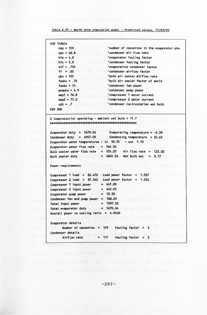
Table 4.21 - North mine simulation model Predicted values , 11/03/92
SUB indata nep = 159 qac = 68.8 hfe = 4.0 hfc = 5.0 ecf = .745 ff = .85 qbc = 125 fombc = .75 fankw = 74 pumpkw :: 4.9 amp1 :: 76.8 amp2 :: n.2 edt:: .7
END SUB
'number 01 cassettes in the evaporator phe 'condenser air flow rate 'evaporator fouling 1actor 'condenser fouling factor 'evaporative condenser 1actor 'condenser airflow factor 'bulk air cooler airflow rate 'bulk air cooler factor of meri t 'condenser fan power 'condenser pump power 'compressor 1 motor current 'compressor 2 motor current 'condenser recirculation wet bulb
2 Compressor(s) operating - ambient wet bulb a 17.7 •• A •• A •••••• A ••••••••••••• '.""""""""""'"
Evaporator duty :: 5670.04 Evaporating temperature a -2.39 Condenser duty :: 6957.09 Condensing temperature .. 32.63 Evaporator water temperatures - in 10.35 - out 1.10 Evaporator water flow rate :: 146.36 Bulk cooler water flow rate :: 125.20 Air flow rate :: 125.00 Bulk cooler duty .. 4845.56 Wet bulb out • 3.17
Power requirements
Compressor 1 load :: 86.47X Compressor 2 load :: 87.04X Compressor 1 input power
Load power factor II
Load power factor .. :: 641.89
Compressor 2 input power 645.05 Evaporator pump power :: 10.30 Condenser fan and pump power .. 100.69 Total input power :: 1397.93 Total evaporator duty :: 5670.04 Overall power to cooling ratio .. 4.0560
Evaporator details
1.057 1.056
Number of cassettes = 159 Condenser details
Fouling factor :: 4
Airflow rate '" 117 Fouling factor • 5
-297-
4.6 Mount lsa U62 bulk air cooler
4.6.1 General
The second phase of the Mount lsa 3000 ore bodies
refrigeration plan requires that a 12 MWR surface bulk
air cooler should be installed at U62 shaft. The
timing coincides with the end of the pre-production
development period and the build up in production to
2.0 million tonnes per year and is required to be
operational in October 1993.
Tenders for the stage 2 refrigeration system were
received from three companies. Essentially each
prospective supplier provided two main proposals where
the plant either operated as a batch process with
storage dams or continuously without storage dams. For
each proposal an alternative using either evaporative
condensers or closed plate heat exchangers and cooling
towers was provided.
Supplier 1 proposed the most integrated systems with
the compressors connected to common evaporators and
condensers. Supplier 3 opted for parallel circuits
with both the refrigerant and chilled water circuits
being independent of each other. The system proposed
by Supplier 2 had an integrated water circuit and
separate
greater
refrigeration
the amount of
circuits. In general,
integration the lower
initial cost and the higher the power requirements.
-298-
the
the
The refrigeration plant is required to operate over a
wide range of ambient climatic conditions consequently
a technical assessment of the plant should evaluate
performance and input power requirements at "off"
design conditions. The method used follows closely
that employed to evaluate the Mount Isa stage 1 plant
performance and the North mine surface plant described
in sections 4.4 and 4.5.
The refrigerant used in all proposals is ammonia and
the properties relevant to plant evaluation are
summarised section 2.2.3. All prospective suppliers
proposed different compressors (Howden, Stal and
Sabroe) and the characteristic curves of adiabatic
head and efficiency against compressor inlet
refrigerant flow rate are summarised in section 3.1.
Heat rejection for all proposals comprised of either
modular and packaged evaporative condensers or closed
plate heat exchangers and cross flow cooling towers.
The performance assessment of the evaporative
condensers is summarised in section 3.2.3 and was
based on the rated performance data provided by the
three main manufacturers of this equipment.
For the closed plate heat exchanger and condenser
cooling tower alternatives, all suppliers based their
proposals on Alfa-Laval plate heat exchangers and
Baltimore Aircoil cross flow cooling towers.
-299-
The plant provides chilled water to a bulk air cooler
which handles intake air. Evaporator fouling is
therefore considered to be relatively low and
controllable with either slipstream filtration or
bleed off and make up water. It was therefore not
essential to provide open evaporators at a higher
cost. The performance of the Alta Laval closed plate
evaporators proposed by all prospective suppliers is
summarised in section 3.3.3.
The performance of the bulk air cooler ia probably the
most critical aspect of the different proposals.
Suppliers land 3 proposed to use a Baltimore Aircoil
design similar to the North mine surface plant. The
rated performance of this tower is summarised in Table
4.22 (factor of merit averaging 0.84) and was higher
than would be expected for this type of counter flow
cooling tower. The tests on a similar tower installed
at North Mine in Broken Hill indicated a factor of
merit of 0.75 after correcting some air and water
distribution problems.
Supplier 2 co-operated with Sulzer (supplier of the
Mount Isa stage 1 pre-cooling tower) to optimise the
refrigeration plant and bulk air cooler arrangement.
The Sulzer tower rated performance is summarised in
Table 4.23 and drops significantly when surface wet
bulb temperature is less than l6oC. This is almost
certainly a result of conservative data presentation
at low temperatures.
-300-

For surface wet bulb temperatures above l80 e, the mean
factor of merit is 0.78. This decreases to an average
of 0.75 when the performance at surface wet bulb
temperatures down to l40 e are included. A value of
0.78 was used in the overall performance assessment.
A total of twelve simulations were developed (four for
each supplier) and used in the "off design performance
analysis". The simulations for the full load and part
load alternatives for the Supplier 2 proposals are
given in Appendix 4 and are illustrative of the range
of simulations developed.
4.6.2 Supplier 1 proposals
Supplier 1 originally provided two main proposals with
the plant located adjacent to R63 plant (section 4.2).
Both proposals used closed plate heat exchangers and
cross flow cooling towers for condensing. Alternatives
using evaporative condensers were subsequently
supplied when requested. In proposal 1, the chiller
sets operate as a batch process with storage dams used
as a thermal flywheel. Proposal 2 eliminated the
storage dams and had the compressors unloading to
match the bulk air cooler demand.
A general arrangement of the equipment for proposal 1
is given in figure 4.33. The overall performance
analysis is summarised for the two condenser
alternatives in Table 4.24. With the reduction in
-301-
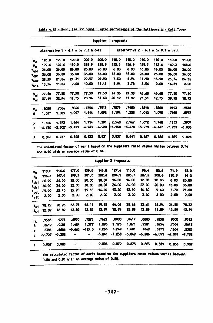
Table 4.22 - Mount I .. U62 e~!ns i BlSId R!CfRCIID~1 Rf Sbl IILtjlRCI 6jc ~RjL ~IC
SUpplier 1 propoaala
Alternative 1 - 6.1 • by 7.3 • cell Alternative 2 - 6.1 • by 9.1 • cell
IIw 120.0 120.0 120.0 200.0 200.0 110.0 110.0 110.0 110.0 110.0 110.0
•• 129.6 129.6 150.0 218.9 218.9 155.6 156.9 158.5 162.6 160.2 168.0
twi 26.00 26.00 26.00 26.00 26.00 8.00 8.00 16.00 16.00 26.00 26.00
tdb1 36.00 36.00 36.00 36.00 36.00 18.00 18.00 26.00 26.00 36.00 36.00
twot 23.55 21.84 21.31 22.57 22.90 7.SO 6.94 14.90 13.51 25.54 24.52
twit 13.56 11.83 2.00 10.00 11.15 5.94 3.71 8.56 2.00 14.61 2.00
5.1 77.50 77.50 77. SO 77.SO 77. SO 24.33 24.33 43.68 43.68 77. SO 77.50
'wi 37.19 32.94 12.75 28.94 31.60 20.12 15.91 25.51 12.75 39.92 12.75
"w .8030 .7064 .8046 .7856 .7913 .7573 .7410 .1511 .1261 .9593 .9!15
R 1.057 1.089 1.097 1.114 1 •• 1.194 1.m 1.012 1.090 .7698 .8971
Y 1.306 1.273 1.664 1.714 1.591 2.~ 2.967 1.072 1.741 .1555 .3907 z -4.750 -2.8021 -5.453 -4.900 -4.920 -5.1SO -5.271 -5.919 -6.447 -7.213 -I.BOI
F 0.826 0.737 0.845 0.832 0.831 0.137 0.141 0.157 0.166 0.879 0.191
The calculated f.ctor of .r1t bIIHd on the auppL i.ra rtted YIILu •• vari .. betwtn 0.74 end 0.90 with en aver-ae value of 0.14.
SUpplier S Proposal.
IIw 110.0 116.0 177.0 159.0 143.0 127.4 113.0 98.4 82.6 71.9 55.0 .. 196.3 191.9 199.5 201.0 202.6 204.1 205.7 207.2 201.8 210.3 98.2
twi 26.00 24.00 22.00 20.00 11.00 16.00 14.00 12.00 10.00 1.00 26.00
tdbi 36.00 34.00 32.00 30.00 28.00 26.00 24.00 22.00 20.00 18.00 36.00
twot 25.00 22.40 15.90 15.10 14.20 13.20 12.10 10.10 9.40 7.70 25.00
twit 2.00 2.00 2.00 2.00 2.00 2.00 2.00 2.00 2.00 2.00 2.00
I.i 78.22 70.26 62.93 56.15 49 •• 44.06 38.66 33.64 21.94 24.55 71.22
'wi 12.89 12.89 12.89 12.89 12.19 12.19 12.19 12.19 12.19 12.19 12.19
"w .9583 .9273 .6950 .7271 .7625 .aooo .8417 .aaoo .9250 .9500 .9583
R .8612 .9405 1.484 1.371 1.271 1.173 1.071 .9511 .8254 .7364 .8612
Y .2385 .5686 -9.665 -115.0 9.216 3.249 1.601 .7649 .3171 .1664 .2385
z -9.727 -9.258 -1.845 -7.258 -6.849 -6 •• -6.091 -6.018 -9.752
F 0.907 0.903 0 •• 0.179 o.m 0.865 0.159 0.851 0.907
The calculetad factor 01 .rit baHd on the auppL 1era rated valun YIIri .. betwtn 0.86 n 0.91 with an eve ... YIIlue 01 0 •••
-302-
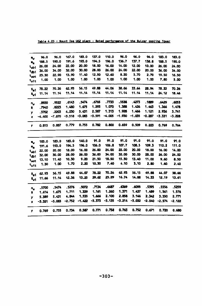
T .. ble 4.23 - !taunt Ia .. U62 pllOt : 8!lted pertor_De. of the SUlllr cooling row.r
IIw 96.0 96.0 167.0 183.0 137.0 110.0 96.0 96.0 96.0 183.0 183.0
-.. 188.5 190.0 191.6 193.0 194.5 196.0 136.7 137.7 138.1 111.5 190.0
twi 26.00 24.00 22.00 20.00 11.00 16.00 14.00 12.00 10.00 26.00 24.00
tdbi 36.00 34.00 32.00 30.00 21.00 26.00 24.00 22.00 20.00 36.00 34.00
twot 23.30 22.90 13.90 11.40 12.50 12.60 8.20 5.70 2.70 19.50 16.50
twit 1.00 1.00 1.00 1.00 1.00 1.00 1.00 1.00 1.00 7.80 5.00
5.1 78.22 70.26 62.93 56.15 49.11 44.06 38.66 33.64 21.94 71.22 70.26
!wi 1'.14 '1.14 1'.14 11.14 11.14 11.14 11.14 '1.14 11.14 24.12 11.46
"w .8920 .9522 .6143 .5474 .6765 .7733 .5538 .4273 .1119 .6429 .6053 R .7940 .8223 1.480 1.675 1.293 1.070 1 •• 1.426 1.463 1.366 1.471
Y .3702 .2203 4.230 5.431 2.587 1.313 1._ 1.466 1.121 2.936 3.741 z -4.400 -7.870 -3.511 -3.083 -3.591 -4.005 -1.930 -1.035 -0.217 -3.331 -3.221
F 0.815 0.887 O.m 0.755 0.712 0.800 0.659 0.509 0.223 0.769 0.764
IIw 183.0 183.0 183.0 140.0 91.0 91.0 91.0 91.0 91.0 91.0 91.0
-.. 191.6 193.0 194.5 196.0 106.0 106.1 107.7 101.5 109.3 110.2 111.0
twi 22.00 20.00 18.00 16.00 26.00 24.00 22.00 20.00 11.00 16.00 14.00
tdb1 32.00 30.00 28.00 26.00 36.00 34.00 32.00 30.00 21.00 26.00 24.00
twot 13.10 11.40 10.30 9.20 21.50 11.50 15.50 13.40 11.00 9.60 1.50
twit 1.30 1.00 1.70 2.20 10.30 7.40 4.10 3.10 2.10 1.60 2.40
5.1 62.93 56.15 49.88 44.07 71.22 70.26 62.93 56.15 49.11 44.07 38.66
!wi 11.66 11.14 12.36 13.25 29.62 23.29 16.74 14.11 14.33 12.19 13.61
"w .5700 .5474 .5276 .5072 .7134 .6687 .6369 .6095 .5395 .5556 .5259 R 1.614 1.675 1.711 1.m 1.161 1.260 1.371 1.437 1.419 1.561 1.576
Y 5.389 5.431 4.144 1.535 1.666 2.100 2.151 3.146 2.342 3.350 2.771 z -3.321 -3.083 -2.752 -1.422 -3.313 -3.135 -3.214 -3.032 -2.040 -2.574 -2.122
F 0.769 0.755 0.734 0.5I? 0.771 0.751 0.763 0.752 0.671 0.720 0.610
-303-
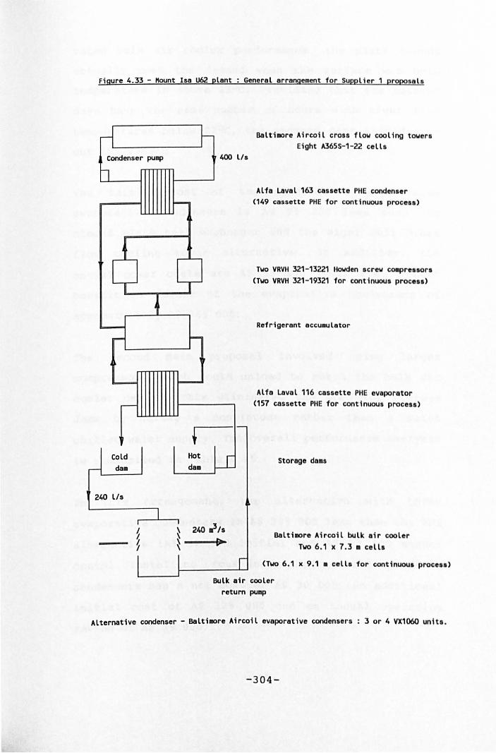
Figure 4.33 - Mount laa U62 plant General arrangement for Supplier 1 proposals
Condenser PUIIIp
Cold dam
240 lIs
400 lIs
~ 240 ,r/s ~ ---ti~~
BaltilOre Aircoil cross flow cooling towera Eight A365S-1 -22 cell a
Alfa Laval 163 casaette PHE condenaer (149 cassette PHE for continuoua procoII>
Two VRVH 321-13221 Howden screw ca.pre •• or. (Two VRVH 321-19321 for continuous procell>
Refrigerant accumulator
Alfa Laval 116 cassette PHE evaporator (157 cassette PHE for continuous procol.>
Storage dalls
Balt;lOre Aircoil bulk air cooler Two 6.1 x 7.3 • celli
(Two 6.1 x 9.1 • cell. for continuou. proce •• >
Bulk air cooler return PUIIIp
Alternative condenser - Balt;lOre Aircoil evaporative condensers 3 or 4 VX1060 units.
-304-
rated bulk air cooler performance, the plant cannot
actually meet the demand when the surface wet bulb
temperature is above 22oC. Providing that the hottest
days have the same number of hours with night time
temperatures below 22oC, the storage dams should even
out the demand.
The initial cost of the alternative with three
evaporative condensers is A$ 91 200 less than the
closed plate heat exchanger and the eight cell cross
flow cooling tower alternative. In addition, the
annual power costs are A$ 53 100 lower i . e. a cost
benefit in favour of the evaporative condensers of
approximately A$ 265 000.
The second main proposal involved using larger
compressors which could unload to match the bulk air
cooler demand. This eliminated the need for storage
dams by having a continuous rather than a batch
chilled water supply. The overall performance analysis
is summarised in Table 4.25.
In this arrangement, the alternative with three
evaporative condensers is A$ 395 000 less than the PRE
alternative (A$ 91 200 initial and A$ 93 100 annual
costs). Installing four instead of three evaporative
condensers has a net cost of A$ 30 000 (an additional
ini tial cost of A$ 125 000 and an annual operating
saving of A$ 29 000).
-305-
Based on the evaporative condenser
operating the plant as a batch process
alternatives,
(proposal 1)
rather than continuous without dams (proposal 2) has
an increase in initial costs of AS 195 000 and a
saving in power costs of A$ 75 000 per year i. e. a
cost benefit in favour of the batch process proposal
using storage dams of A$ 50 000.
4.6.3 Supplier 2 proposals
Supplier 2
(batch or
originally provided two main proposals
continuous process) with evaporative
condensers only. Closed plate heat exchangers with
cross flow cooling towers for heat rejection were
subsequently provided as alternatives. For the batch
process (proposal 1) the larger Stal S93 screw
compressor were selected. The smaller Stal S75E
compressor with an economiser was proposed for the
continuous process without dams (proposal 2).
A general arrangement of the equipment proposed by
Supplier 2 for the batch process with dams is given in
figure 4.34. The original proposal was based on Muller
(Evapco design) evaporative condensers as given in the
figure. Two arrangements were given for the closed
plate heat exchanger and cross flow cooling tower
alternatives.
The first attempted to match the initial cost of the
evaporative condenser by minimising the closed plate
-306-
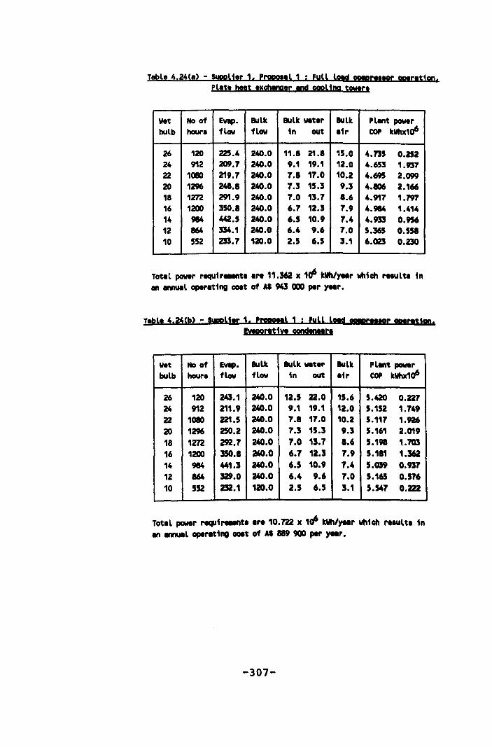
T,ble 4.24(,) - SUppl1.r 1, PrppottL 1 ; Fyll lotd COFrt'lOr aptr't100, Pl'1;. beat .xcb!nqer IOd cooling tMet
Wet Hoof Evtp. BuLk BuLk Wlt,r Bulk PLlnt power bulb hour. flow flow in out 'ir COP kWhx106
26 120 225.4 240.0 " .. 21.' 15.0 4.735 0.252 24 912 209.7 240.0 9.1 19.1 12.0 4.653 1.937 22 1080 219.7 240.0 7.' 17.0 10.2 4.695 2.099 20 1296 241.' 240.0 7.3 15.3 9.3 4.106 2.166 18 1272 291.9 240.0 7.0 13.7 '.6 4.917 1.797 16 1200 350.' 240.0 6.7 12.3 7.9 4.914 1.414 14 914 442.5 240.0 6.5 10.9 7.4 4.933 0.956 12 864 334.1 240.0 6.4 9.6 7.0 5.365 0.558 10 552 233.7 120.0 2.5 6.5 3.1 6.023 0.230
Tot,l power requ1r.-rt ..... 11.362 X 1t1 kWh/yeic which resuLt. in an MnUll ope ... t1ng OOIt of AS 943 CXID per )'Mc.
TSl. 4'24(b) - suppLi.r 1, '!'WIlL 1 ; Fyll lOld ..... r IPIrtIt1 •• EytportSiyt cgndtnttc.
Wet Ho of !VIp. Bulk Bulk Wlt.C BuLk PLlnt power bulb hour. flow flow in out "c COPkWhx106
26 120 243.1 240.0 12.5 22.0 15.6 5.420 0.227 24 912 211.9 240.0 9.1 19.1 12.0 5.152 1.749 22 1080 221.5 240.0 7.' 17.0 10.2 5.117 1.926 20 1296 250.2 240.0 7.3 15.3 9.3 5.161 2.019 18 1272 292.7 240.0 7.0 13.7 1.6 5.191 1.103 16 1200 350.' 240.0 6.7 12.3 7.9 5.1" 1 •• 14 914 441.3 240.0 6.5 10.9 7.4 5.039 0.937 12 864 329.0 240.0 6.4 9.6 7.0 5.165 0.576 10 552 232.1 120.0 2.5 6.5 3.1 5.547 0.222
Tot.l power requ1 ..... t ..... 10.722 X 1t1 ktihlyeiC which cllULt. in an tnnUIL ope ... t1ng OOIt of A$ 889 900 per )feIc.
-307-
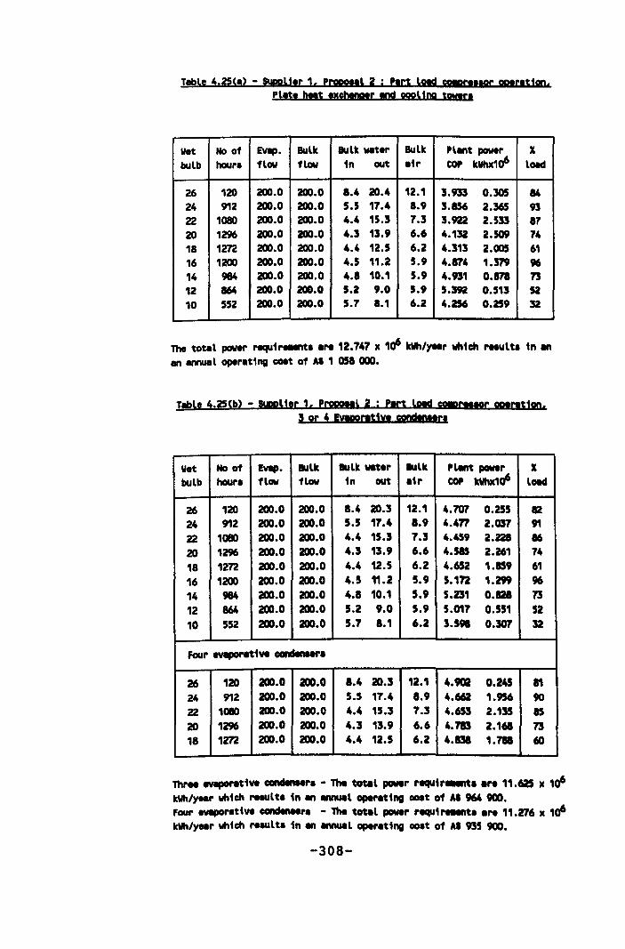
T.ble 4.25(') - SUppLi.r 1. PropotIl 2 ; PItt lotd _r"tor optr.tion. Plat. ""t .xchw!atr IOd cooling tOVlr.
w.t Ho of Evep. Bulk Bulk WIIt.r Bulk Pl",t power X bulb hour. flow flow in out .1r COP kllhx106 load
26 120 200.0 200.0 1.4 20.4 12.1 3.913 0.305 84 24 912 200.0 200.0 5.5 17.4 1.9 3.856 2.365 93 22 1080 200.0 200.0 4.4 15.3 7.3 3.922 2.533 17 20 1296 200.0 zoo. 0 4.3 13.9 6.6 4.132 2.509 74 18 1272 200.0 200.0 4.4 12.5 6.2 4.313 2.005 61 16 1200 200.0 zoo. 0 4.5 11.2 5.9 4.174 1.319 96 14 984 200.0 ZOO.O 4.1 10.1 5.9 4.931 0.171 73 12 164 200.0 ZOO.O 5.2 9.0 5.9 5.S92 0.513 52 10 552 200.0 200.0 5.7 1.1 6.2 4.256 0.259 32
Th. tot.l power .-.qu1....,.t ..... 12.747 x 10⁶ kWh/year which rHult. in ", en annuel oper.ting coat of AS 1 051 000.
Table 4.25(b) - SuppUtr 1. Prqpottl 2 ; PIrt load _Clltor opt ... ston. 3 or 4 EyIDom1vt condtnltr.
"'t Hoof Ewp. Bulle BuLk ...s.r IULIe PLMt power " bulb hour. flow flow in out .1r COP kVhx106 load
26 120 200.0 zoo. 0 1.4 20.3 12.1 4.707 0.255 12 24 912 200.0 ZOO.O 5.5 '7.4 1.9 4.477 2.m 91 22 1080 200.0 zoo. 0 4.4 15.3 7.3 4.459 2.221 16
20 1296 200.0 zoo. 0 4.3 13.9 6.6 4 •• 2.261 74 18 1272 200.0 ZOO.O 4.4 12.5 6.2 4.652 1.159 61
16 1200 200.0 200.0 4.5 11.2 5.9 5.172 1.299 96 14 984 200.0 200.0 4.8 10.1 5.9 5.231 0 •• 13 12 164 200.0 200.0 5.2 9.0 5.9 5.017 0.551 52 10 552 200.0 200.0 5.7 1.1 6.2 3.5. 0.307 32
Four evaporet1ve candtnMrs
26 120 200.0 200.0 '.4 20.3 12.1 4.902 0.245 ., 24 912 200.0 ZOO.O 5.5 17.4 8.9 4.662 1.956 90 22 1_ 200.0 200.0 4.4 15.3 7.3 4.653 2.135 15 20 1296 200.0 200.0 4.3 13.9 6.6 4.715 2.1. 73 18 1272 200.0 200.0 4.4 12.5 6.2 4 •• 1.711 60
Th .... evaporet1vt candtnHr. - The toWl power ..... ,I'-.t ..... 11.625 x 10⁶ IdIh/ytlf' which rllUlt. in tn IMUIl oper.ting OOIt of AS 964 900. Four ewpor.tivt candtnHr. - The toWl power requir ... t ..... " .276 x 106 kWh/ytlr which reault. in ", tnnUIil oper.ting coat of AS 935 900.
-308-
heat exchanger and cooling tower sizes. This resulted
in excessive condensing temperatures (over 400 C) and
was not considered in detail any further. The
alternative used for comparison had the same size
cooling towers as proposed by Supplier 1 and two 107
cassette plate heat exchangers.
The overall performance analysis is summarised for the
two condenser alternatives in Tables 4.26. The initial
cost of the alternative with the plate heat exchangers
and the cross flow cooling towers is A$ 127 000 higher
than that using the evaporative condensers. This could
be reduced to A$ 16 000 by using a 130 cassatta plate
heat exchanger, however, the condensing temperatures
were over 40oC.
The annual power costs for the alternative using the
evaporative condensers was A$ 79 500 less than that
using the closed plate heat exchangers, resulting in a
cost benefit in favour of the evaporative condensers
of approximately A$ 385 000. The low initial cost
plate heat exchanger alternative used a single 130
cassette plate beat exchanger (as compared to two 104
cassette beat exchangers) with the same condenser
water flow rate of 500 lIs and the A365S-l-22 cross
flow cooling towers.
The general arrangement for the continuous compressor
operation process is very similar to the batch process
proposal. The differences are that there are no
-309-
storage dams and that the Stal S7SE screw compressor
was to be used instead of the S93 compressors. The
economiser associated with the smaller compressor
increased its evaporator duty by approximately 9' when
operating at full load.
This compressor arrangement cannot quite meet the peak
demand when the wet bulb temperature is above 240 C
although the shortfall is of the order of only 1'. The
593 compressor arrangement is far more flexible and
w.as used in the performance assessment. The overall
performance analysis is summarised for the two
condenser alternatives in Table 4.27. As for proposal
1, the initial cost of the alternative with the closed
plate heat exchangers and the cross flow cooling
towers is A$ 127 000 higher than that for evaporative
condensers.
The annual power costs for the alternative using the
evaporative condensers was A$ 71 700 less than that
using the closed plate heat exchangers, resulting in a
cost benefit in favour of the evaporative condensers
of approximately A$ 360 000. Based on the evaporative
condenser alternatives, operating the refrigeration
plant as a batch process rather than continuous
without dams has an increase in both initial and
operating costs of A$ 195 000 and A$ 43 300/year
respectively i.e. the cost benefit in favour of the
continuous process is approximately A$ 335 000.
-310-
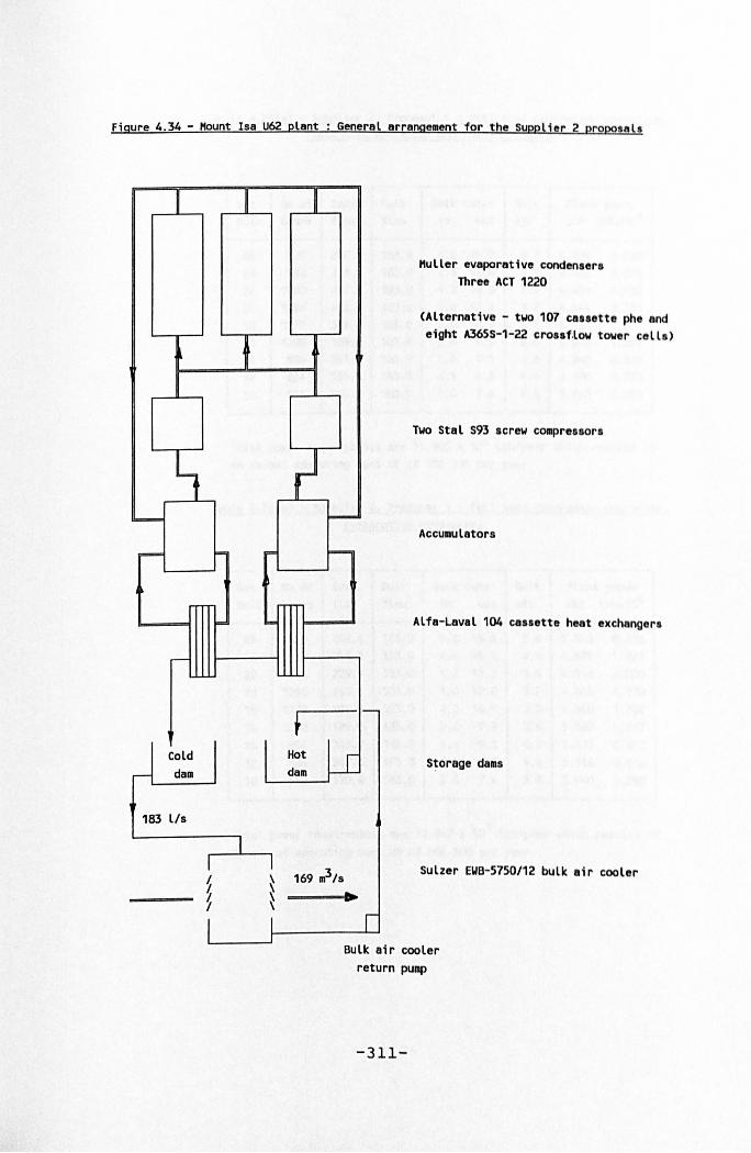
Figure 4.34 - Mount Isa U62 plant General arrangement for the Supplier 2 proposals
1
t
1 --r--- l- F'
I- 100
0-
Cold
- dam
183 lis
1 r I ~ ~ ~ ~
I I J
( -~
t I-
Hot LI dalll
Muller evaporative condensers Three ACT 1220
(Alternative - two 107 cassette phe and eight A365S-1-22 crouf.low tower cells)
Two Stal S93 screw co.pressors
Accumulators
Alfa-Laval 104 cas.ette heat exchanger.
S~orage daals
169 .. 3 /s Sulzer EWB-5750/12 bUlk air cooler ..
r Bulk air cooler
return pump
-311-
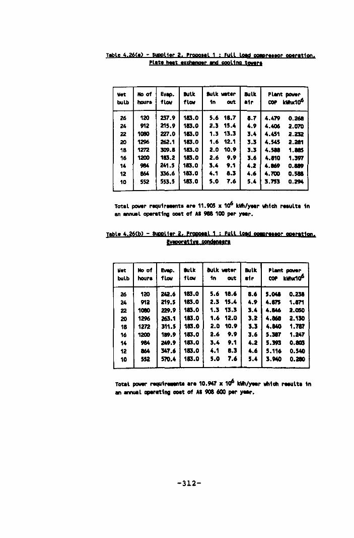
Table 4.26(,) - supplier 2, Propogl 1 ; full Lots! cwrltlOr optr.t1on, Pllt' .t pch!ngtr IDd cooUna SMr.
Wet Ho of Evep. Bulk Bulk Wlt.r Bulk Plent power bulb hour. flow flow 1n out .tr COP kUhlelo'
26 120 237.9 113.0 5.6 11.7 1.7 4.479 0.261 24 912 215.9 113.0 2.3 15.4 4.9 4.406 2.010 22 l0a0 227.0 113.0 1.3 13.3 3.4 4.451 2.232 20 1296 262.1 113.0 1.6 12.1 3.3 4.545 2.211 18 1m 309.8 113.0 2.0 10.9 3.3 4._ 1.11S 16 1200 113.2 113.0 2.6 9.9 3.6 4.110 1.397 14 984 241.5 113.0 3.4 9.1 4.2 4.169 0._ 12 164 336.6 113.0 4.1 1.3 4.6 4.700 0._ 10 552 553.5 113.0 5.0 7.6 5.4 3.753 0.294
Tot.l power requtrtMnt •• r. 11.905 x 10' kWh/yellr \111ch reault' 1n en ennuel oper.t1ng COlt of AS 911 100 per )'Mr.
Table 4.26(b) - SUppl1.r 2, PrqpoHl 1 ; fuLL lOld _mlRr wretion, Eytporet1U cond!nt.r.
w.t Hoof 1vIIp. Bulk Bulk wat.r Bulk plent power bulb hour. flow flow 1n out .'r COPkWhx1o'
26 120 242.6 113.0 5.6 11.6 1.6 5.041 0.231 24 912 219.5 113.0 2.3 15.4 4.9 4.1'1'S 1.171 22 10lI0 229.9 113.0 1.3 13.3 3.4 4.146 2.050 20 1296 263.1 113.0 1.6 12.0 3.2 4._ 2.130 18 1m 311.5 113.0 2.0 10.9 3.3 4.140 1.717 16 1200 119.9 113.0 2.6 9.9 3.6 5._ 1.247 14 984 249.9 113.0 3.4 9.1 4.2 5.393 O.IOS 12 164 347.6 113.0 4.1 1.3 4.6 5.116 0.540 10 552 570.4 113.0 5.0 7.6 5.4 3.Ma 0.210
Total power requ, ..... ta .re 10.947 x 10' kWh/)'Mr \II,ch rault' in en ennutl opertt1ng COlt of AS 908 600 per Yllr.
-312-
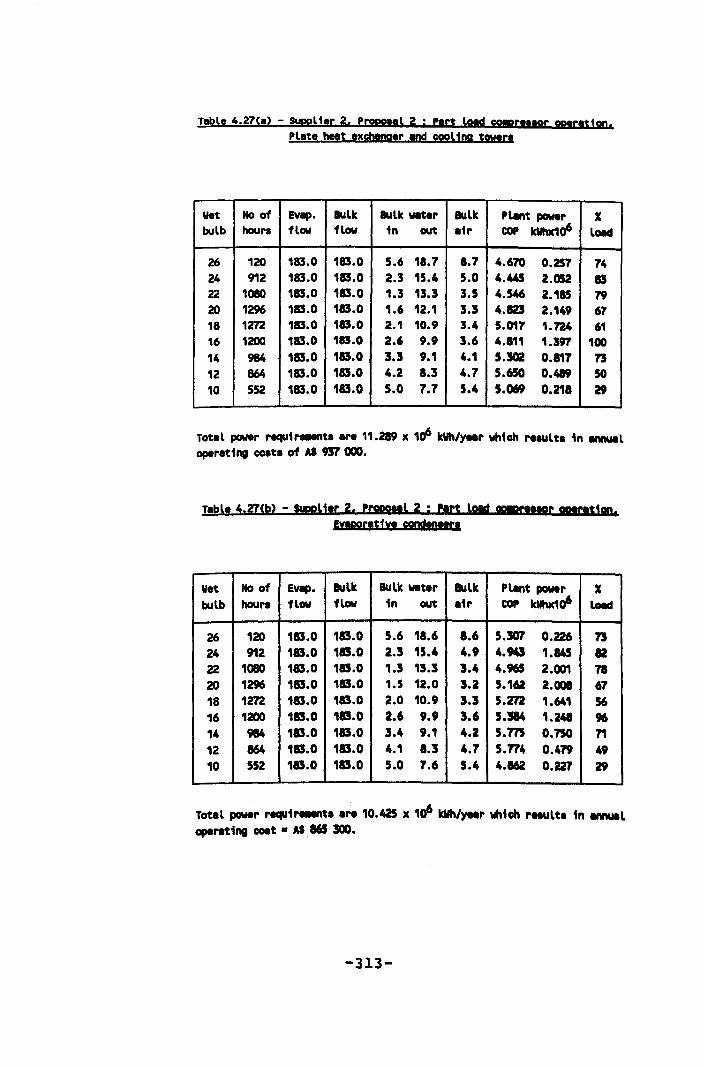
Table 4.27(,) - SUppl i.r 2. Propottl 2 ; Pert lOld COW?rulOr optrlt1on. Pl,te he!t txch!nq.r I!ld cooling tOWlr.
Wet No of EvllP· BuLk Bulk wet.r Bulk PlMt power X bulb hour. flow flow in out .1r COP kWhx10' lOld
26 120 183.0 183.0 5.6 11.7 1.7 4.670 0.257 74 24 912 183.0 115.0 2.3 15.4 5.0 4.445 2.052 15 22 1080 115.0 115.0 1.3 13.3 3.5 4.546 2.115 79 20 1296 115.0 115.0 1.6 12.1 3.3 4.123 2.149 67 18 1272 183.0 183.0 2.1 10.9 3.4 5.0'17 1.724 61 16 1200 183.0 115.0 2.6 9.9 3.6 4.111 1.397 100 14 984 183.0 115.0 3.3 9.1 4.1 5._ 0.111 73 12 864 183.0 183.0 4.2 1.3 4.7 5.650 0 •• 50 10 552 183.0 183.0 5.0 7.7 5.4 5.069 0.211 29
Tot.l power r!qU1 ...... t •• re 11.289 x 10' kVh/yeer which mult. in IIMUIIl oper.ting coat. of AI m 000.
T.bl. 4.21(b) - SUppLi.r 2. PropotIl 2 ; Plrt Lotd C!!2Ml'tttOr wrat1on, EyIpor!t1l!t CO!ldtnttr'
Wet No of Evep. Bulk Bulk wat.r Bulk Plant power X bulb hour. flow flow in out .ir COP kWhx10' LOId
26 120 183.0 183.0 5.6 11.6 1.6 5.307 0.226 73 24 912 183.0 115.0 2.3 15.4 4.9 4.943 1.845 12 22 1080 183.0 183.0 1.3 13.3 3.4 4.965 2.001 71 20 1296 183.0 183.0 1.5 12.0 3.2 5.162 2.001 67 18 1272 183.0 115.0 2.0 10.9 3.3 5.212 1.641 56 16 1200 115.0 115.0 2.6 9.9 3.6 5 •• 1 •• 96 14 984 115.0 115.0 3.4 9.1 4.2 5.115 0.750 71 12 864 115.0 183.0 4.1 1.3 4.1 5.774 0.479 49 10 552 183.0 183.0 5.0 7.6 5.4 4.162 0.227 29
Tot.l power requ1reMnS •• re 10.425 x 10' kWh/yeer which rHUls. in IIMUIIl operating coat • AI 865 300.
-313-
4.6.4 Supplier 3 proposals
The original proposal for supplier 3 was based on a
continuous process without storage dams and offered
both evaporative and closed plate heat exchangers with
cooling towers for heat rejection as condenser
alternatives. The same equipment was used in a batch
process arrangement in order to provide a basis for
comparison.
A general arrangement of the equipment proposed by
Supplier 3 (closed plate heat exchanger and cross flow
cooling tower alternative) and arranged as a batch
process with storage dams i8 given ~n figure 4.35. The
condenser water flow rate through each of the closed
plate heat exchangers is 260 lIs and the design flow
rate in each cross flow cooling tower cell i8 130 lIs.
When only one compressor is operating, the number of
cooling tower cells operational is determined by the
requirement to maintain a minimum condensing
temperature of 200 C.
The overall performance analysis for the batCh process
equipment arrangement and the two condenser
alternatives is summarised in Table 4.28. The initial
cost of the alternative with the two 88 cas.ett. plate
heat exchangers and the four cell cross flow cooling
tower is AS 128 000 higher than that using the seven
Auscon evaporative condensers.
-314-
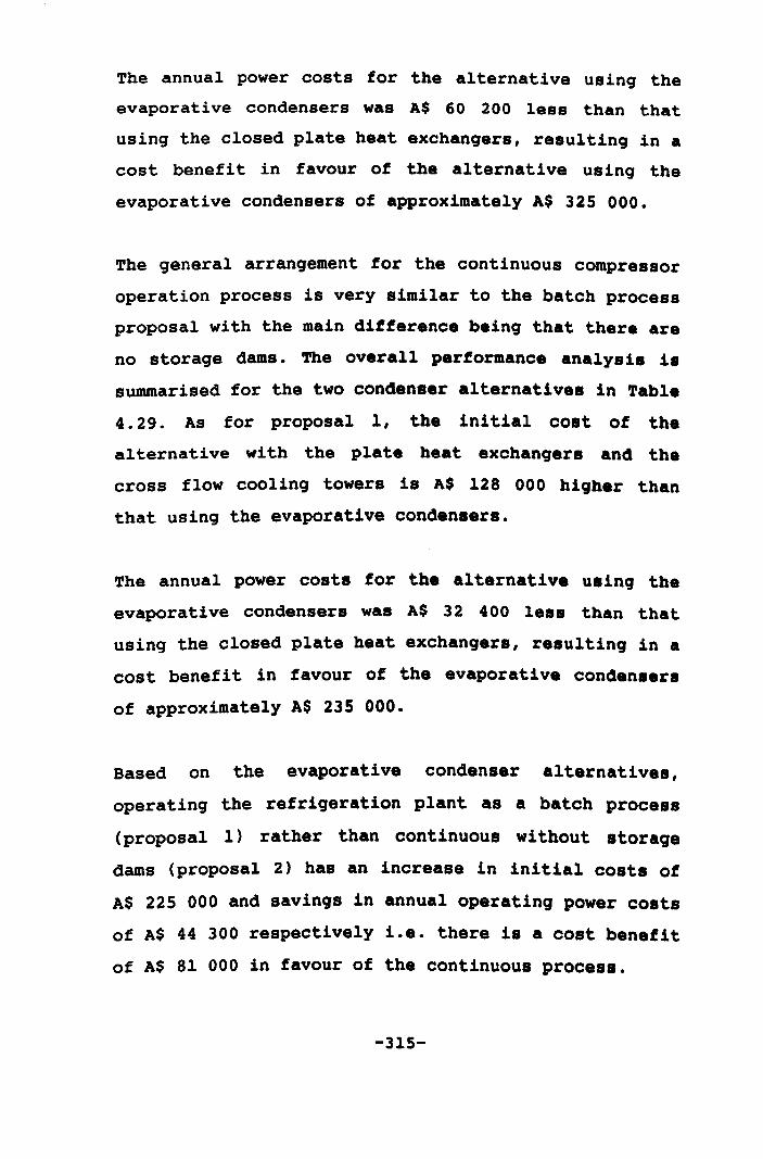
The annual power costs for the alternative using the
evaporative condensers was A$ 60 200 less than that
using the closed plate heat exchangers, resulting in a
cost benefit in favour of the alternative using the
evaporative condensers of approximately A$ 325 000.
The general arrangement for the continuous compressor
operation process is very similar to the batch process
proposal with the main difference being that there are
no storage dams. The overall performance analysis ia
summarised for the two condenser alternatives in Table
4.29. As for proposal 1, the initial cost of the
al ternati ve wi th the plate heat exchangers and the
cross flow cooling towers is A$ 128 000 higher than
that using the evaporative condensers.
The annual power costs for the alternative Using the
evaporative condensers was A$ 32 400 1e.s than that
using the closed plate heat exchangers, resulting in a
cost benefit in favour of the evaporative condensera
of approximately A$ 235 000.
Based on the evaporative condenser alternatives,
operating the refrigeration plant as a batch process
(proposal 1) rather than continuous without storage
dams (proposal 2) has an increase in initial costs of
A$ 225 000 and savings in annual operating power costs
of A$ 44 300 respectively i.e. there is a cost benefit
of A$ 81 000 in favour of the continuous process.
-315-
4.6.5 Summary of proposals
Based on the initial costs of equipment given in the
tenders and the operating power costs obtained from
the simulations, the overall cost for each proposal is
summarised in Table 4.30 (operating costs discounted
at 30% over 10 years).
Although the batch process proposals of Supplier 1 had
the lowest overall costs, they were not technically
feasible with the equipment proposed. They were
included to give an indication of the low operating
costs that could be expected by optimising the plant
design using modelling. It can be concluded from the
costs summarised in Table 4.30 that no one prospective
supplier had a clear cost advantage and, where initial
costs were kept low, the penalty of higher operating
power costs offset this.
The refrigeration simulations are being used in
conjunction with Supplier 2 to optimise the individual
component selection.
-316-
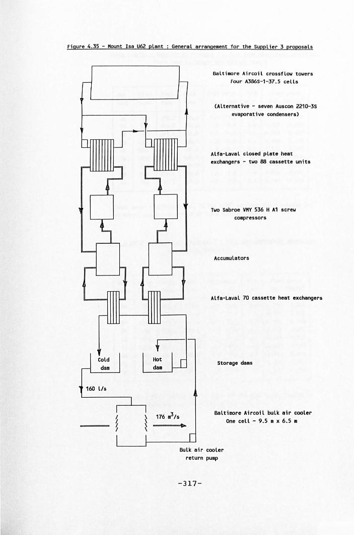
Figure 4.35 - Hount Isa U62 plant General arrangement for the Supplier 3 proposals
Cold dam
160 lIs
Baltimore Aircoil crossflow towers Four A386S-1-37.5 cells
(Alternative - seven Auscon 2210-3S evaporative condensers)
Alfa-Laval closed plate heat exchangers - two 88 caslette units
Two Sabroe VHY 536 H A1 screw compressors
Accumulators
Alfa-Laval 70 cassette heat exchangers
Storage dalls
Baltimore Aircoil bulk air cooler One cell - 9.5 • x 6.5 •
Bulk air cooler return pump
-317-
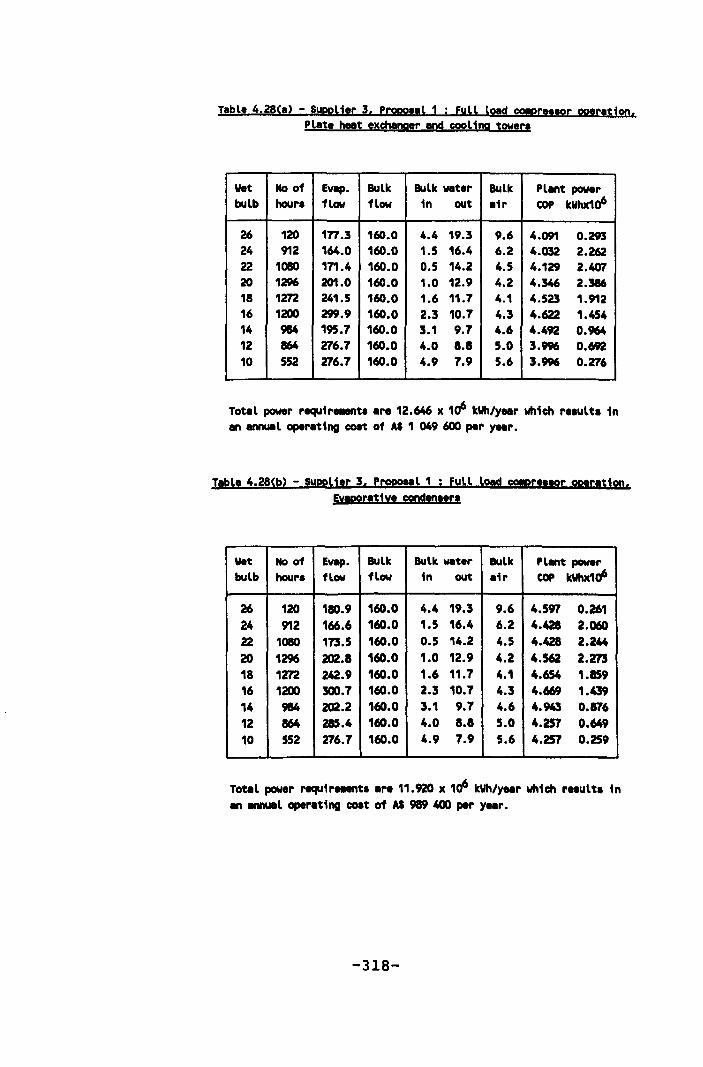
T,ble 4.28(,) - Suppli.r 3, Propo •• l 1 j full Load COIpr •• tor operation, Pl't. heIIt exchanger .nd cooling tower.
Wet No of Evlp. Bulk Bulk Vlter Bulk Pllnt power bulb hour. flow flow in out .ir COP kWhxlo6
26 120 177.3 160.0 4.4 19.3 9.6 4.091 0.293 24 912 164.0 160.0 1.5 16.4 6.2 4.032 2.262 22 1080 171.4 160.0 0.5 14.2 4.5 4.129 2.407 20 1296 201.0 160.0 1.0 12.9 4.2 4.346 2.386 18 1272 241.5 160.0 1.6 11.7 4.1 4.523 1.912 16 1200 299.9 160.0 2.3 10.7 4.3 4.622 1.454 14 984 195.7 160.0 3.1 9.7 4.6 4.492 0.964 12 864 276.7 160.0 4.0 8.8 5.0 3.996 0.692 10 552 276.7 160.0 4.9 7.9 5.6 3.996 0.276
Total power requ1r ...... t •• r. 12.646 x 10⁶ kWh/yeer which r •• ult. in en annual oper.ting coat of AS 1 049 600 per yeer.
T.ble 4.28(b) - SUPDUer 3, Propoul 1 ; full lO!Cl cOEr!!!Or oper.tion, Evapor.t1y. condID •• r.
Wet No of Evap. BuLk BuLk Vlter Bulk PLMt power bulb hour. flow flow in out .1r COP kWhxlo6
26 120 180.9 160.0 4.4 19.3 9.6 4.597 0.261 24 912 166.6 160.0 1.5 16.4 6.2 4.428 2.060 22 1080 173.5 160.0 0.5 14.2 4.5 4.428 2.244 20 1296 202.8 160.0 1.0 12.9 4.2 4.562 2.273 18 1272 242.9 160.0 1.6 11.7 4.1 4.654 1.859 16 1200 300.7 160.0 2.3 10.7 4.3 4.669 1.439 14 984 202.2 160.0 3.1 9.7 4.6 4.943 0.876 12 864 285.4 160.0 4.0 8.8 5.0 4.257 0.649 10 552 276.7 160.0 4.9 7.9 5.6 4.257 0.259
TotiL power requ1r ...... t •• r. 11.920 x 10⁶ kWh/yeer which re.ult. in en ennuel operating coat of AS 989 400 per yeer.
-318-

T,ble 4.29(,) - Supplier 3, Propo.,l 2 : P,rt load cO!pre •• or oper.t1on, Pl,te hut exchanger and cool ina tower.
Wet No of EVap. Bulk Bulk v.ter Bulk Pl.nt pow.r bulb hour. flow flow in out air COP kWhx106
26 120 160.0 160.0 4.4 19.4 9.6 3.931 0.305 24 912 160.0 160.0 1.6 16.4 6.2 3.973 2.296 22 1080 160.0 160.0 0.5 14.2 4.5 4.293 2.314 20 1296 160.0 160.0 1.0 12.9 4.2 4.366 2.375 18 1272 160.0 160.0 1.6 11.7 4.1 4.339 1.994 16 1200 160.0 160.0 2.3 10.7 4.3 3.946 1.703 14 984 160.0 160.0 3.1 9.7 4.6 5.341 0.811 12 864 160.0 160.0 4.0 8.8 5.0 5.200 0.532 10 552 160.0 160.0 5.0 7.9 5.6 3.094 0.357
Tot.l power requir ...... t. ar. 12.844 x 10⁶ kWh/yur which r.tult. in IlMU!l oper.ting coat of AS 1 066 100.
" lOld
87 96 91 T7 63 50 76 52 32
Tabl. 4.nCb) - SUppli.r Propoyl 2 i P.rt load COIprufOr oper.t1on, Evaporative cond!n.erl
W.t Hoof Evap. Bulk Bulk w.t.r Bulk Plent pow.r " bulb hour. flow flow in out .ir COP kWhx106 lOld
26 120 160.0 160.0 4.4 19.3 9.6 4.456 0.269 24 912 160.0 160.0 1.6 16.4 6.2 4.342 2.100 22 1080 160.0 160.0 0.5 14.2 4.5 4.005 2.411 20 1296 160.0 160.0 1.0 12.9 4.2 4.176 2.483 18 1272 160.0 160.0 1.6 11.7 4.1 4.330 1.998 16 1200 160.0 160.0 2.3 10.7 4.3 4.236 1.586 14 984 160.0 160.0 3.1 9.7 4.6 4.803 0.901 12 864 160.0 160.0 4.0 8.8 5.0 5.074 0.545 10 552 160.0 160.0 5.0 7.9 5.6 4.435 0.249
Total power requi ....... t • • re 12.455 x 10⁶ kWh/year which r •• ult. in tmUIIl oper.ting coat • AS 1 033 700.
-319-
89
V7 92 17 63 49 79 53 30
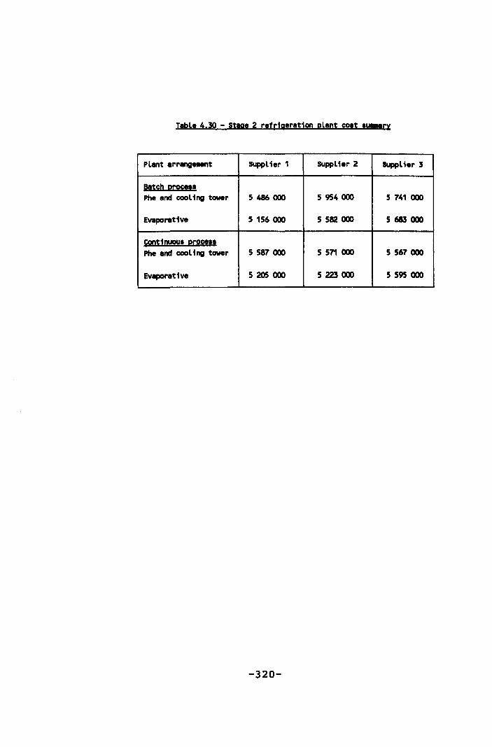
Table 4.30 - Stage 2 refrigeration plant co.t 'UII!ry
PLant arrangeleDt Supplier 1 Supplier 2 Supplier 3
I1!Sch I!rocett Ph. and cooling tower 5486000 5 954000 5 741 000
Evaporative 5 156 000 5 582 000 5 6S3 000
9!!tjnuou. I!l:iSett Phe end cooling tower 5 587 000 5 571 000 5 567000
Evaporative 5 205 000 5223000 5 595 000
-320-
5 SUMMARY AND RBCOMMBHDATIOHS
5.1 Summary of the research
The increasing scarcity of minerals of a mineable
grade at shallow depths and the acceptance that there
are significant decreases in productivity when working
in adverse thermal environmental conditions have
resul ted in an almost exponential increase in mine
refrigeration in the last 25 years. As a consequence,
ventilation and increasingly refrigeration, are taking
a greater proportion of the resources used in mining.
The optimum amount of refrigeration required on a mine
is a balance between the initial and operating costs
of the plant relative to the benefit of improving the
thermal environmental conditions and increasing
employee productivity. Climatic variations and the
effect of cyclic mining operations complicate the
optimisation by introducing a complex load profile and
variable thermal acceptance criteria.
Variations in employee productivity result from both
the natural reduction in physical work rate in adverse
thermal environmental conditions and the application
of a shortened shift to control the occurrence of heat
stress conditions. The cost of low productivity will
depend on the ability of the mine infrastructure and
organisation to adapt to changing labour demands and
the revenue potential of the ore being mined.
-321-
The three main elements of a refrigeration system are
the chiller subsystem, the heat rejection subsystem
and the load subsystem all of which interact. Each
subsystem usually comprises of several elements which
also interact and a solution requires a relatively
complex iterative procedure. The design of a plant
with a complex load profile therefore requires that
the system should be modelled and the effect of design
changes simulated and then assessed.
Al though modelling and computer simulations of the
refrigeration processes has been developing over the
last 15 years in both the air conditioning and mining
industries, most of the work has been directed at the
chiller subsystem and in particular those using
centrifugal compressors. Modelling the performance of
the central element, the compressor, has usually
relied on general compressor curves using theoretical
flow and head coefficients.
A method using empirical compressor performance curves
based on the evaporator duty and input power to the
compressor has been found to be of greater general
application and not restricted to a single compressor
type. Compressor performance is expressed in terms of
adiabatic head and efficiency against inlet volume
flow rate for a given refrigerant. The simulations
have been extended to include fully the heat rejection
and load subsystems and are based on steady state
rather than dynamic conditions.
-322-
For the five refrigeration system models considered,
two types of compressor (nine different models), four
types of evaporator, three types of condenser, two
types of cooling tower and five types of cooling
appliance were used. The thermal performance of each
was considered and the method of analysis defined and
compared to actual performance measurements where
these were available.
The five refrigeration systems modelled have a similar
structure and method of converging to a solution which
allowed a modular approach to be taken. The chiller
subsystem comprised of the evaporator, condenser and
compressor modules and, for given temperatures of the
water into the evaporator and condenser, allowed the
evaporator and condenser duties to be determined. From
these values, the outlet water temperatures for the
evaporator and condenser were established.
The condenser interfaces with the heat rejection
subsystem and, by introducing this module, a balance
can be achieved between the condenser duty and the
heat rejected. The evaporator interfaces with the load
subsystem which could be a straightforward single
surface bulk air cooler or a complex sequence of heat
exchangers of different types used both in parallel
and in series circuits. The module analysis follows
the same form with the distributional structure
becoming more complex as more elements are introduced
into the system.
-323-
The overall system operation modules link the three
subsystems and incorporate the plant control strategy
and the set operating conf iguration. Balancing the
evaporator duty with the load subsystem by adjusting
the evaporator water temperatures is the most critical
element where the method of adjustment has a profound
effect on the rate of convergence of the simulation.
Although a universal method of adjustment that always
converged rapidly was not found, trial and error
methods always allowed a solution to be determined.
The five refrigeration system simulations described,
demonstrate both the universal nature of the method
used to structure and to solve the models and the
varied applications for the simulations. The Mount lsa
R63 plant using centrifugal compressor chiller sets
was the first to be simulated and it was demonstrated
that refrigeration plants with complex load systems
could be modelled with an acceptable accuracy.
Modelling of the North mine underground refrigeration
system extended the modelling to screw compressors and
showed that the effects design aberrations (such as
excessive refrigerant pressure losses) could be
incorporated in the models. Despite a complex chiller
set arrangement and an extensive load system, the
model predictions in comparison with the measured
values was acceptable. The effects of modifications to
the plant could be simulated and any deficiencies in
plant performance identified.
-324-
The Mount lsa surface plant models were initially used
to determine the optimum refrigeration system control
strategy. By correcting aspects of the model resulting
from testing elements of the refrigeration plant, the
simulation can be used to analyse the measurements
obtained from the monitoring system. This analysis is
then used to identify where corrective maintenance is
necessary such as cleaning heat exchanger surfaces.
This diagnostic use for the simulations was further
developed in the models of the North mine surface
plant in addition to assessing the systems proposed by
different suppliers and determining the optimum
control system. Each of the system elements has been
tested and the model adjusted to reflect the actual
plant performance including part load operation of the
compressors based on motor current readings.
Part load operation of compressors, the optimisation
of system elements and the determination of optimum
control strategies was further developed in the models
used to analyse the proposals for the Mount lsa U62
surface bulk air cooler plant.
-325-
5.2 Recommendations for further work
A mine refrigeration system is part of an overall mine
system which is dynamic in that the mining processes
are causing continuous changes
climate which determines the
as does the surface
refrigeration load.
Fortunately the rate of change is slow or dampened and
the system can be adequately represented by a steady
state model. A future development of the modelling is
its extension to fully control all the system elementa
including the load subsystem.
This will require an understanding of the relationship
between surface and the underground conditions which
influence the load subsystem. Since most refrigeration
systems are batch processes supplying a continuous but
varying load, the time element and the extent of
dampening is a necessary part of any control strategy.
Initially, the underground load subsystem will need to
be monitored and historical time trends established
and analysed.
Although the simulation models are initially based on
the theoretical performance of the heat transfer
equipment, the actual performance can be significantly
different as a result of operating aberrations such as
the water level in low profile evaporative condensers.
More test work on operating equipment is therefore
required to identify potential problems and to relate
these to the theoretical simulations.
-326-
For a simulation to be used to control the operation
of a refrigeration plant, the monitoring system must
adequately reflect the true operating conditions.
Further work is required with respect to the type,
location and calibration of sensors within the plant.
Although complex load systems can be simulated, there
are practical limitations when considering the full
control of these systems in the most cost effective
manner. These limits need to be explored and related
to the potential "waste" of cooling by having less
sensitive controls.
The compressor is the central element of the model and
further work relating its performance with different
refrigerants is desirable.
-327-
9 RBI'BRBHCBS
ACGIH. (1986). Adopted threshold limit values for heat stress. In Threshold limit values and biological exposure indices. (Cincinatti: American Conference of governmental Industrial Hygienists), 66-72.
Allen R.F. (1975). Ventilation of the 110 ore body at the Mount Isa Mine. In proceedings international mine ventilation congress, Johannesburg, Hemp R. and Lancaster F.H. eds (Johannesburg: Mine Ventilation Society of South Africa, 1976), 365-374.
ASHRAE. (1972). Heat transfer. In Handbook of fundamentals. (American Society of Heating, Refrigerating and Air Conditioning Engineers, New York), 31-62.
Bailey-McEwan M. and Shone R.D.C. (1984). The specification and performance of water chillers for mine refrigeration installations. In Third international mine ventilation congress, Harrogate, Howes M. J. and Jones M.J. Eds (London: Institution of Mining and Metallurgy, 1984), 265-276.
Bailey-McEwan M. and Penman J.C. (1981). An interactive computer programme for simulating the performance of water chilling installations on mines. In Proceedings of the 20th international symposium on the application of computers and mathematics in the mineral industries. (Johannesburg: S. Afr. Inst. Mining and Metallurgy), 291-305.
Baker-Duly H.C.L. (1984). Control of refrigeration and ventilation systems in a South African gold mine. In Third international mine ventilation congress, Harroga te, Howes M. J . and Jones M. J • Eds ( London: Institution of Mining and Metallurgy, 1984), 259-264.
Baker-Duly H.C.L., Brouwer G. and Shaw J. (1988) Design of a large flexible underground refrigeration installation. In Fourth international mine ventilation congress, Brisbane. Gillies A.D.S. ed. (Melbourne: Australasian Institute of Mining and Metallurgy, 1988), 443-449.
Barua 0.1. and Nixon C.A.N. (1988). Ventilation and refrigeration design for the access and ore production decline to the deep copper are body at Mount Isa. In Fourth international mine ventilation congress, Brisbane. Gillies A.D.S. ed. (Melbourne: Australasian Institute of Mining and Metallurgy, 1988), 465-411.
Bide10t Rand Ledent P. (1950). The air installation at the Charbonnages des Zwartberg. Rev. Univer. des Mines. 9th Number 1.
conditioning Liegeois at series, VI,
Bluhm S.J. (1980). Predicting performance of spray chambers for cooling air. Heating Air Condition. Refrig. 13, NO 2, Nov. 1980, 21-39.
-328-
Bluhm S.J. (1982). Development of an in line water spray cooler - Contribution. J. Mine Vent. Soc. S Afr. 35, 36-39.
Braun J.E. and others. (1987). Models for variable speed centrifugal chillers. In ASHRAE transactions : technical and symposium papers. (New York) 1794-1813.
Clark D.R. (1985). Centrifugal chiller model: preliminary documentation. US Department of Commerce, National Bureau of Standards.
Collison B.V. (1982). Cooling underground workings at North Broken Hill Limited - case study. In Underground operators' conference, West Coast, Tasmania. (Parkville, Vict: Australasian Institute of Mining and metallurgy), 71-82. (Symp. Series 31).
COM. (1987). Chiller - version 1. Chamber of Mines Research Organisation. (Johannesburg).
Cooke H.M. and others (1961). The effects of heat on the performance of work underground. J. Mine Vent. Soc. S Afr. 14, 177-188.
Davies E. (1922). Air cooling plant, Morro Velho Mine, Brazil. Trans. Inst. Min. Engrs. 63, 326-341.
Davis F.T. and Corripio A.B. (1974). Dynamic simulation of variable speed centrifugal compressors. In Instrumentation in the chemical and petroleum industries. Volume 10, ISA, Pittsburgh, USA, 15-24.
Du Pont. (1965). Thermodynamic properties of Freon 11. E.I. du Pont de Nemours, Wilmington, USA.
Ellison R.D. and Creswick F.A. (1978). A computer simulation of steady state performance of air to air heat pumps. ORNL/CON-16 report. (Oak ridge, TN: Oak Ridge national Laboratory).
Flower J.E. (1978). Analytical modelling of heat pump units as a design aid and for performance prediction. UCRL-S2618 report. (Livermore, CA: Lawrence Livermore laboratory).
Freeman T.L. and others (1975). Computer mOdelling of heat pumps and the simulation of solar heat pump systems. ASHE paper 75-WA/Sol 3. (New York: American Society of Mechanical Engineers).
Gorges R. A. ( 1952). Condi tioning mine air and some experiments with deep level ventilation. Bull. Mine vent. Soc. South Africa. 5, Numbers 10 and 11.
Graveling R.A., Morris L.A. and Graves R.J. (1988). Working in hot conditions in mining: a literature review. HSE contract research report 10/1988. (Bootle: Health and Safety Executive).
-329-
Grollius H. and others. (1986). Computer modelling of performance of centrifugal water chillers in mine refrigeration installations. In Frigair '86 Symposium. (Council for Scientific and Industrial Research, pretoria), Volume 1, Mine Cooling.
Hamm E. (1979). Central refrigerating plants for air conditioning in the mines of Ruhrkohle AG. In Second international mine ventilation congress, Reno, NV, Mousset-Jones P. ed (New York: Society of Mining Engineers of AIME, 1980), 635-648.
Hemp R. (1981). The assessment and prediction of cooling plant performance J. Mine Vent. Soc. S Afr. 34, 81-118.
Hemp R. (1982). Sources of heat in mines. In Environmental engineering in South African mines. Burrows J. ed. (Marshalltown, S. Afr.: Mine Ventilation Society of South Africa. Chapter 22, 569-612.
Hemp R. (1986). Computer analysis of underground refrigeration plant performance J. Mine Vent. Soc. S Afr. 39, 77-85.
Hiller C.C. and Glickman L.R. (1976). Improving heat pump performance via compressor capacity control -analysis and test. Heat transfer laboratory Report 24525-96. (Cambridge, MA: Massachusetts Institute of Technology) .
Howes M.J. (1975). A review of current mine cooling practice in South African gold mines. In Proceedings international mine ventilation congress, Johannesburg, Hemp R. and Lancaster F. H. eds (Johannesburg: Mine Ventilation Society of South Africa, 1976), 289-298.
Howes M.J. (1978a). The development of a functional relationship between productivity and the thermal environment. J. Mine Vent. Soc. S Afr. 31, 21-38.
Howes M.J. (1978b). Ventilation and refrigeration planning at Unisel Gold Mine Ltd. In Proceedings of the eleventh Commonwealth mining and metallurgical congress, Hong Kong. Jones M.J. ed. (London: Institute of Mining and Metallurgy, 1979), 729-740.
Howes M.J. (1979a). Mine ventilation and refrigeration planning. J. Mine Vent. Soc. S Afr. 32, 225-235.
Howes M.J. and Green N. (1979b). The design of a surface refrigeration plant at Unisel mine. J. Nine Vent. Soc. S Afr. 32, 85-98.
Howes M.J. (1983). Application of refrigeration in mines. Trans. Inst. Min. Metall. (Section A: Mining industry), 92, A69-A79.
-330-
Howes M.J. (1988). Heat and moisture exchange in mine airways. In Fourth international mine ventilation congress, Brisbane. Gillies A.D.S. ed. (Melbourne: Australasian Institute of Mining and Metallurgy, 1988), 257-264.
Howes M.J. (1990). Review of ventilation and refrigeration in deep, hot and mechanised mines in Australia. Trans. Inst. Min. Metall. (Section A: Mining industry) 99, A73-A84.
Hwang B.C. and others (1986). Modelling and simulation of a naval shipboard heat pump. International Journal of Modelling and Simulation. June 1986.
IIR. (1981). Thermodynamic and physical properties of R22. International Inst. of Refrigeration. Paris 1981.
Jackson W. L., Chen F • C . and Hwang B • C • ( 1987 ). The simulation and performance of a centrifugal chiller. In ASHRAE annual meeting, Report Conf-870620-9. (Nashville, TN: American Society of Heating Refrigeration and Air Conditioning Engineers).
James R.W. and Marshall S.A. (1973). Dynamic analysis of a refrigeration system. Proc. Inst. Refrigeration. 70, 13-24.
James K.A. and James R.W. (1987). Transient analysis of thermostatic expansion valves for refrigeration system evaporators using mathematical models. Trans. Inst. of Measurement and control. 9, 198-205.
Lambrechts J. de V. (1967). Optimisation of ventilation and refrigeration in deep mines. J. Mine Vent. Soc. S Afr. 20, 57-64.
MacWilliam K.J. and McIntyre J.T. (1937). Surface refrigeration at Robinson Deep. J. Chem. Met. Min. Soc. South Africa. 37, 438-457.
McPherson R.K. (1960). Physiological responses to hot environments. Med. Res. Council. Spec. Rep. (London). Number 268.
Mew R.H. (1977). Ventilation at depth at North Broken Hill Limited. In Underground opera tors' conference, Broken Hill. (Parkville, Viet: Australasian Institute of Mining and metallurgy), 135-140. (Symp. Series 17)
Horeby R.G. (1988). Thermodynamic network simulation incorporating airway heat and moisture transfer. In Fourth international mine ventilation congress, Brisbane. Gillies A.D.S. ed. (Melbourne: Australasian Institute of Mining and Metallurgy, 1988), 265-272.
Morrison J.F. and others (1968). Energy expenditure in mining tasks and the need for the selection of labour. J. S. Afr. Inst. Min. Metall. 69, 185-191.
-331-
Murray-Smith A.I. (1987). The effect of clothing on heat stress in mining environments. J. Mine Vent. Soc. S. Afr., 40, 37-39.
Nadira R. and Schick I.C. (1987). Modelling and simulation of an HVAC refrigeration system. In proceedings of the SCS simulators conference. Simulation series 18, 175-181.
Nixon C.A.N., Gillies A.D.S. and Howes M.J. (1992). Analysis of heat sources in a large mechanised development end at Mount Isa Mine. In Fifth international mine ventilation congress, Johannesburg, Hemp R. ed. (Johannesburg: Mine Ventilation Society of South Africa, 1992).
Park C., Clark D.R. and Kelly G.E. (1986). HVACSIM building systems and equipment simulation program: building loads calculation. Report NBSIR 86-3331. US Department of Commerce, National Bureau of Standards.
Perry R.H. and Chilton C.H. (1973). Thermodynamic properties. In Chemical engineers' handbook. McGraw Hill, USA, Section 3, 155-158.
Ramsden R. (1981) The performance of cooling coils. J. Mine Vent. Soc. S. Afr., 34, 145-154.
Ramsden R. and Bluhm. S.J. (1984). Air cooling equipment used in South African gold mines. In Third international mine ventilation congress, Harrogate, Howes M.J. and Jones M.J. Eds (London: Institution of Mining and Metallurgy, 1984), 243-251.
Ramsden R. (1990). Mine cooling towards the 21st century. J. Mine Vent. Soc. S. Afr., 43, 162-168.
Reuther E.U. and Dauber C. (1984). Large capacity cooling equipment in German coal mines. In Third international mine ventilation congress, Harrogate, Howes M.J. and Jones M.J. Eds (London: Institution of Mining and Metallurgy, 1984), 253-258.
Rosenow W.M. and Choi H.Y. (1961). Heat exchangers. In Heat, mass and momentum transfer. (Prentice Hall, New York), 303-331.
Rice C.K. and others (1981). Design optimisation and the limits of steady state heating efficiency for conventional single speed air source heat pumps. ORNL/CON-63 report. (Oak ridge, TN: Oak Ridge national Laboratory) •
Shone R.D.C. and Sheer T.J. (1988). An overview of research into the use of ice for coolin~ deep mines. In Fourth international mine ventilat~on congress, Brisbane. Gillies A.D.S. ed. (Melbourne: Australasian Institute of Mining and Metallurgy, 1988), 407-413.
-332-
Spalding J and Parker T. W. ( 1940). Air conditioning plant at Ooregum Mine, Kolar Goldfield. J. Chem. Met. Min. Soc. South Africa. 41, 1-42.
Stapff M. (1925). Versuche mit Kunstlicher Grubenkuhlung auf der Zeche Radbod. Gluckauf.
Stephan K. (1972). Boiling heat transfer. In Handbook of fundamentals. (American Society of Heating, Refrigerating and Air Conditioning Engineers, New York), 45-46.
Stewart J.M. (1981). Heat transfer and limiting physiological criteria as a basis for the setting of heat stress limits. J. S. Afr. Inst. Min. Metall. 81, 239-251.
Stewart J.M. (1982). Fundamentals of human heat stress. In Environmental engineering in South African mines. Burrows J. ed. (Marshall town, S. Afr.: Mine Ventilation Society of South Africa. Chapter 20, 495-533.
Stroh R.M., Gebler W.F. and Van Deventer J.J. (1984). Performance of an integrated surface refrigeration system on Vaal Reefs. In Third international mine ventilation congress, Harrogate, Howes M.J. and Jones M.J. Eds (London: Institution of Mining and Metallurgy, 1984), 283-287.
Vost K.R. (1980). The reduction in amplitude and change in phase of the diurnal temperature variations of ventilation air. J. S. Afr. Inst. Min. Metall. 80, 210-214.
Whillier A. (1977). Predicting the performance of forced draught cooling towers. J. Mine Vent. Soc. S. Afr., 30, 2-25.
Wyndham C . H . ( 1966 ). A survey of research by the Chamber of Mines into clinical aspects of heat stroke. Proc. Mine Med. Officers Ass. S. Afr. 46, 68-80.
Wyndham C.H. and others (1967). Assessing the heat stress and establishing the limits for work in a hot mine. Brit. J. Ind. Med. 24, 255-271.
Wyndham C.H. (1974). The physiological and psychological effects of heat. In The ventilation of South African ~old mines. Burrows J. ed. (Marshalltown, S. Afr.: M1ne Ventilation Society of South Africa. Chapter 7, 93-137.
Yaglou C.P. (1926). The thermal index of atmospheric conditions and its application to sedentary and industrial life. J. Ind. Hyg. 8, 5-19.
-333-
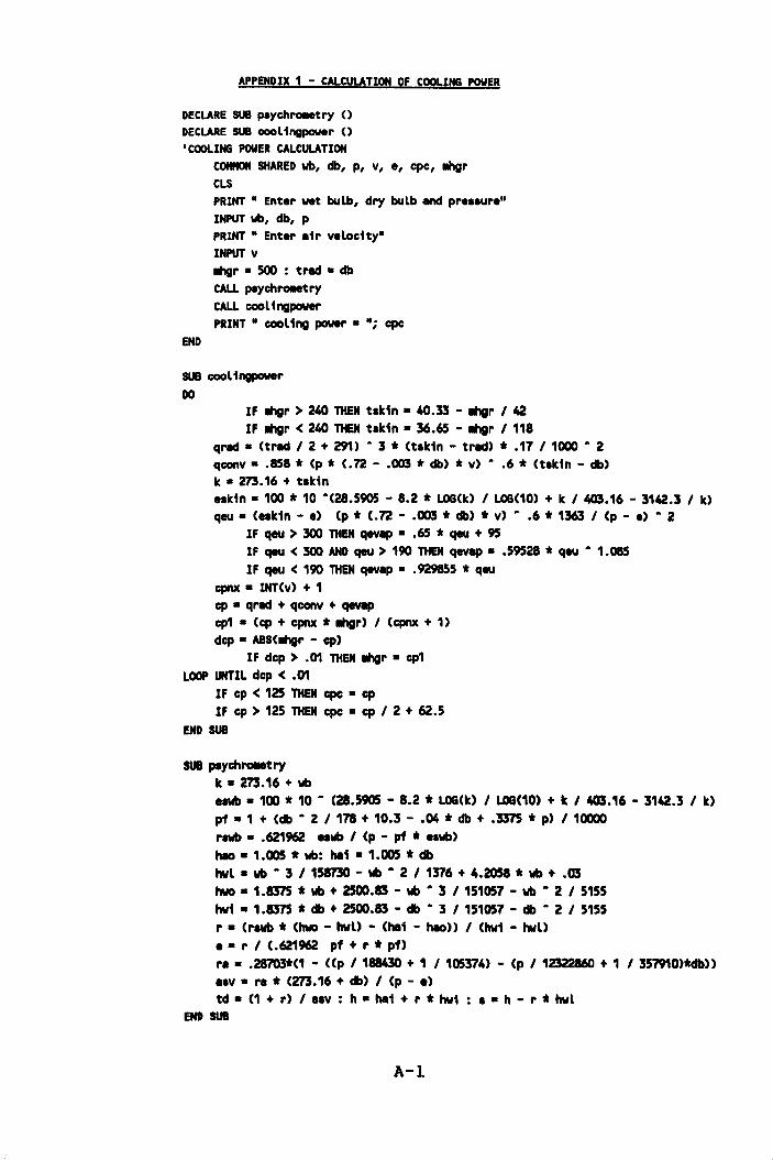
APPENDIX 1 - CALCULATION OF COOLING POWER
DECLARE SUB paychrOlletry () DECLARE SUB coolingpower () 'COOLING POWER CALCULATION
END
CotUION SHARED wb, db, p, v, e, cpc, IIhgr CLS PRINT • Enter wet bulb, dry bulb and preaaureINPUT w, db, P
PRINT • Enter eir velocity· INPUT v IIhgr • 500 : tr~ • db CALL paychl'OM1:ry CALL cool ingpowr
PRINT • cooling power • • i cPc
SUB cool ingpower DO
IF IIhgr > 240 THEN tak1n • 40.33 - IIhgr I 42 IF IIhgr < 240 THEN takin • 36.65 - IIhgr I 118
qr~ • (tr. I 2 + 291) - 3 * (tak1" - tr.) * .17 I 1000 - 2 qconv • .858 * (p * (.72 - .003 * db) * v) - .6 * (takin - db) k. 273.16 + tatin eatin • 100 * 10 -(28.5905 - 8.2 * bQG(k) I bQG(10) + k I 405.16 - 3142.3 I k)
qeu. (eakin - e) (p t (.72 - .003 t db) t v) - .6 t 1363 I (p - e) - 2 IF qeu > 300 THEN qevep • .65 * qeu + 95 IF qeu < 300 AND qeu > 190 THEN qw.p •• 59528 * qeu - 1.085 IF qeu < 190 THEN qevep •• 929855 * qeu
cpnx • INT(v) + 1 cp • qr~ + qconv + qewp cp1 • (cp + cpnx * IIhgr) I (cpnx + 1) dcp • ABS(lIhgr - cp)
IF dcp > .01 THEN IIhgr • cp1 LOOP UNTIL dcp < .01
IF cp < 125 THEN cpc • cp IF cp > 125 THEN cpc • cp I 2 + 62.5
END SUB
SUB paychl'OM1:ry k. 273.16 + wb eawb • 100 t 10 - (28.5905 - 8.2 t LOG(k) I LOGUO) + k I 403.16 - 3142.3 I k) pf • 1 + (db - 2 I 178 + 10.3 - .04 * db + .3375 * p) I 10000 rawb • .621962 .allb I (p - pf * .awb)
hao. 1.005 * wb: he1 • 1.005 * ell hvl • wb - 3 I 151730 - lID • 2 I 1376 + 4.2058 * vb + .03 two • 1.8375 * lID + 2500.83 - wb • 3 I 151057 - wb • 2 I 5155 hv1 • 1.8375 * db + 2500.83 - db - 3 I 151057 - db - 2 I 5155 r • (r.wb * (two - hvU - (hei - hao» I (hv1 - hwU e • r I (.621962 pf + r * pf) re • .28703*(1 - «p I 188430 + 1 I 105374) - (p I 12322860 + 1 I 357910)tdb» e.v. r. * (273.16 + db) I (p - .) td • (1 + r) I •• v : h • he1 + r * hw1 : •• h - r t hwl
END SUB
A-l
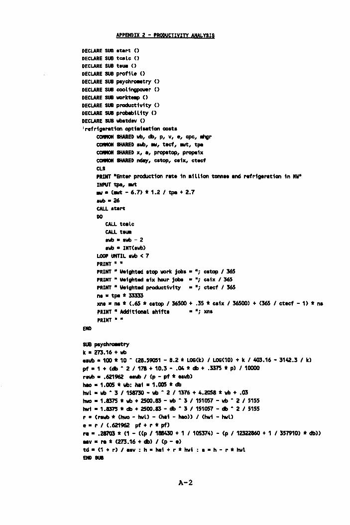
APPENDIX 2 - PRODUCTIYITY ANALYSIS
DECLARE SUB atart () DEClARE SUB tesle () DEClARE SUB tSUII () DECLARE SUB profile () DEClARE SUB paych~try () DEClARE SUB cool ingpower 0 DEClARE SUB worlttetlp 0 DEClARE SUB p~ivity () DECLARE SUB p~ility () DECLARE SUB wbatdev () 'refrigeration opti.iaation coata
COMMON SHARED vb, db, p, v, e, cpc, IIhgr COMMON SHARED avb, .. , teef, -.t, tpa COMMON SHARED x, a, propatop, propa1x COMMON SHARED ndIIy, estop, eaix, eteef CLS
END
PRINT -Enter production rat. in .ill ion tomea and refrigeration in MY
INPUT tpa, -.t ... (-.t - 6.7) * 1.2 I tpa + 2.7
avb • 26 CALL atart DO
CALL tcalc CALL tau. avb • avb - 2 avb • INT(avb)
LOOP UNTIL avb < 7
PRINT - -PRINT • Weighted atop worlt jobs • .; estop I 365 PRINT • Weighted aix hour jobs ..; cab I 365 PRINT • Weighted productivity •• ; cteef I 365
na • tpa * 33333 xna • na * (,65 * estop I 36500 + .35 * caix I 36500) + (365 I ctecf - 1) * n. PRINT - Additional shift. • M; xna
PRINT • •
SUB paych~ry It. 273.16 + vb •• vb. 100 * 10 A (28.59051 - 8.2 * LQG(k) I LQG(10) + It I 403.16 - 3142.3 I It)
pf • 1 + (db • 2 I 178 + 10.3 - .04 * db + .3375 * p) I 10000 rawb • .621962 .. vb I (p - pf * .. vb) I1l1o • 1.005 * vb: hili • 1.005 * db hwl • wb A 3 I 158730 - vb • 2 I 1376 + 4.2058 * wb + .03 hwo • 1.1375 * wb + 2500.83 - vb • 3 I 151057 - wb • 2 I 5155 hwi • 1.1375 * db + 2500.83 - db • 3 I 151057 - db • 2 I 5155 r • (rawb * (hwo - hwU - (hai - I1l10)) I (hwi - hwL> e • r I (,621962 pf + r * pf) ra • .28703 t (1 - «p I 188430 + 1 I 105374) - (p I 12322860 + 1 I 357910) * db» .. v. ra t (273.16 + db) I (p - e) td • (1 + r) I .. v : h • hai + r * hwi : a • h - r * hwL END SUB
A-2
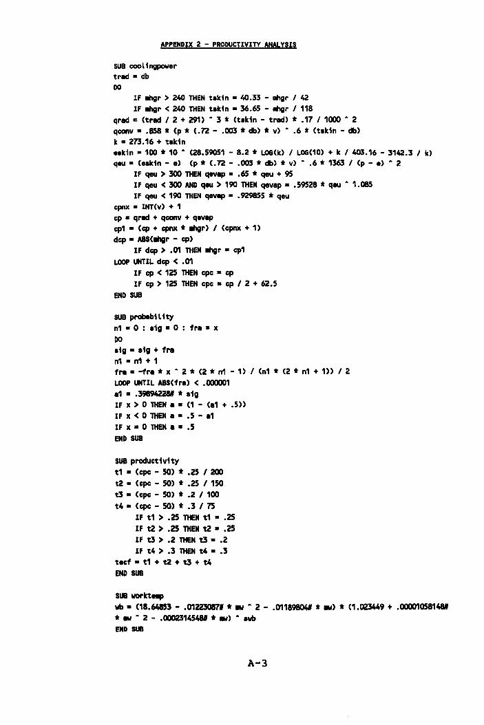
APPENDIX 2 - PRODUCTIYITY ANALYSIS
SUB coolingpower trad .. db DO
IF IIhgr > 240 THEN taki" .. 40.33 - IIhgr I 42 IF IIhgr < 240 THEN taki" • 36.65 - IIhgr I 118
qrad .. (trad 12+ 291) A 3 * (taki" - trad) * .17 I 1000 A 2 qconv •• 858 * (p * (.72 - .003 * db) * v) A .6 * (tak1" - db) k • 273.16 + taki" .akin • 100 * 10 A (28.59051 - 8.2 * LOG(k) I LOG(10) + k I 403.16 - 3142.3 I k) qeu. (eakin - e) (p * (.72 - .003 * db) * v) A .6 * 1363 I (p - .) A 2
IF qeu > 30D THEN qev.., • .65 * qeu + 95 IF qeu < 30D AND qeu > 190 THEN qevap • .59528 * qeu A 1.085 IF qeu < 190 THEN qevap • .929855 * qeu
cpnx • INT(v) + 1 cp • qrad + qconv + qev.p ep1 - (cp + cpnx * IIhgr) I (cpnx + 1)
dep • ASS(lIhgr - cp) IF dcp > .01 THEN IIhgr • cp1
LOOP UNTIL dcp < .01 IF cp < 125 THEN cpc • cp IF cp > 125 THEN cpc • cp I 2 + 62.5
END SUB
SUB probability n1 - 0 : aig • 0 : fr. • x DO a1g • a1g + fr. "1-n1+1 fr. • -fr. * x A 2 * (2 * n1 - 1) I (n1 * (2 * n1 + 1» I 2 LOOP UNTIL ASS(fr.) < .0D0001 a1 • .~ * a1; IF x > 0 THEN • • (1 - (.1 + .5» IF x < 0 THEN • - .5 - .1 IF x • 0 THEN • • .5 END SUB
SUB productivity
t1 • (epe - 50) * .25 I 200 t2 • (epe - 50) * .25 I 150 t3 • Cepe - SO) * .2 I 100 t4 • (epe - SO) t .3 I 7S
IF t1 > .25 THEN t1 •• 25 IF t2 > .25 THEN t2 •• 25 If t3 > .2 THEN t3 •• 2 If t4 > .3 THEN t4 • .3
tecf • t1 + t2 + t3 + t4 END SUB
SUB workt..p wb • (18.64853 - .01223087' * IN A 2 - .011898041 * IIW) * (1.023449 + .000010581481 * ., A 2 _ .00023145481 * .,) A awb END SUB
A-3
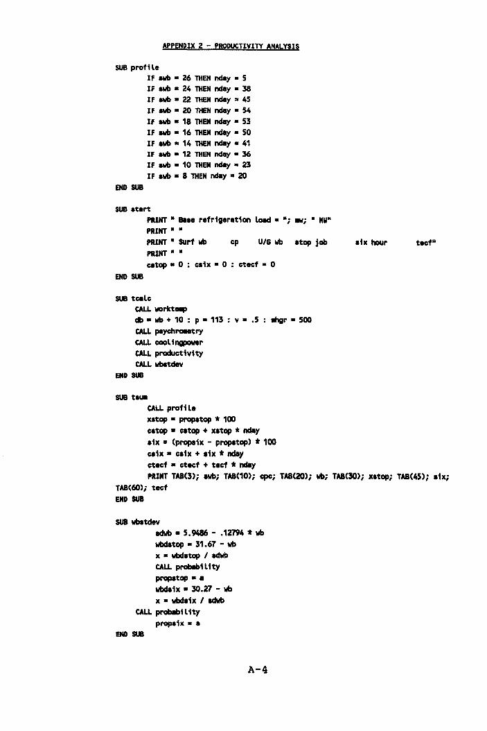
APPENDIX 2 - PRODUCTIVITY ANALYSIS
SUB profile
END SUB
IF awb • 26 THEN nday • 5 IF awb • 24 THEN nday • 38
IF awb • 22 THEN nday • 45 IF awb • 20 THEN nday • 54 IF awb • 18 THEN nc:Iay • 53 IF awb • 16 THEN nday • 50 IF awb • 14 THEN nday • 41
IF awb • 12 THEN nday • 36 IF awb • 10 THEN nday • 23 IF awb • 8 THEN nc:Iay • 20
SUB atart
END SUB
PRINT - a.ae refrigeration la.d • -; .w; • MW·
PRINT - -PRINT - SUrf wb cp U/G w atop job
PRINT - -estop • 0 : esb • 0 : ctect • 0
SUB tcalc CALL worktetlp db • vb + 10 : p • 113 : v ·.5 IIIhgr. 500 CALL paychl'OHtry CALL coolingpower CALL productivity CALL wbatdev
END SUB
SUB t.u. CALL profi le xatop • propatop * 100 estop • estop + xstop * nday six. (propaix - propatop) * 100
esix • esix + 11x * nc:Iay ctecf • ctecf + tect * nc:Iay
aix hour tecf-
PRINT TAB(3); IW; TAB(10); cpo; TAB(2O); wb; TAB(3O); xstop; TAB(45); lix; TAB(6Q); teef END SUB
SUB wbatdev adwb. 5.9486 - .12794 * vb wbdltop • 31.67 - vb x • wbdatop / adwb CALL probeb1l i ty propatop •• wbda1x • 30.27 - vb x • wbdl1x / adwb
CALL probability
propaix • • END SUB
A-4
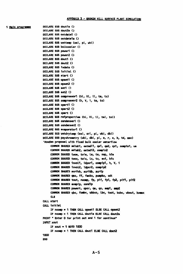
1 !!1n prpgre..e
APPENDIX 3 - BROKEN HILL SURFACE PLANT SInUbATIQN
DECLARE SUB dout1. () DECLARE SUB dout2. () DECLARE SUB outdete1 () DECLARE SUB outdete1e () DECLARE SUB wetta.p (aal, pi, vbl) DECLARE SUB bulkcooler () DECLARE SUB power1 () DECLARE SUB power2 () DECLARE SUB dout1 () DECLARE SUB dout2 () DECLARE SUB i ndIIte () DECLARE SUB initiel () DECLARE SUB atert () DECLARE SUB opaet1 () DECLARE SUB opaet2 () DECLARE SUB set1 () DECLARE SUB aet2 () DECLARE SUB COIpreaaor1 (hi, VI, ii, te, te) DECLARE SUB COIpreaaor2 (h, V, i, te, te) DECLARE SUB cpart1 () DECLARE SUB cpart2 () DECLARE SUB cpart () DECLARE SUB refproperti .. (hi, VI, ii, tel, tel) DECLARE SUB candenaer1 () DECLARE SUB conden.er2 () DECLARE SUB evaporator1 () DECLARE SUB wetdryta.p (a.l, arl, pi, vbl, dbl) DECLARE SUB paychl'Olletry (vbl, dbl, pi, e, r, a, h, td, .av) 'Howden proposal with fixed bulk cooler waterflow
COfIItON SHARED lIdillh1, .. tedi1, qe1, qe2, qe1, COIp1n1, ue
COMItON SHARED 1Id1ah2, .. ted12, COIIpin2 COMON SHARED twee, twie, le, te, nep, hfe COMON SHARED twoc, twie, le, te, eef, hfe COMMON SHARED 1nvol1, idpcr1, COIp1p1, h, V, 1 COfIItON SHARED 1nvol2, idpcr2, COIpip2 COIIION SHARED aurfwb, aurfdb, aurfp COMON SHARED qae, ff, fMkw, puIIPitw, edt COMMON SHARED tout, DCOIp, fp, pif, fp1, fp2, pif1, pif2 COMON SHARED evapip, condip COMMON SHARED powert, opcr, qe, qe, ...,1, up2 COfIItON SHARED qbc, fOllbc:, wbbco, lbc, twot, kwbe, wbout, kwax CLS
CALL atart CALL initial
IF nCOlp • 1 THEN CALL opaet1 ELSE CALL opaet2 IF nCOlp • 1 THEN CALL dout1a ELSE CALL dout2e
PRINT - Enter 0 for print out and 1 for continueINPUT xout
IF xout • 1 GOTO 1000 IF nCOlp • 1 THEN CALL dout1 ELSE CALL dout2
1000 END
A-S
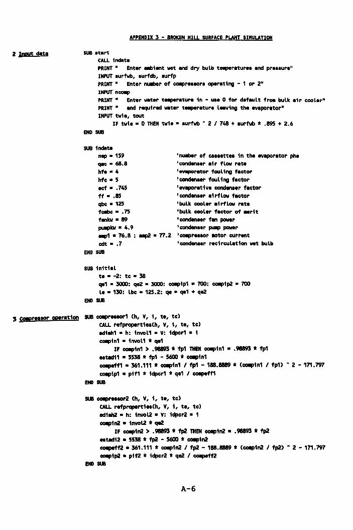
2 I!pIt data
3 Ji9!Pt!!lOr operation
APPENDIX 3 - BROKEN HILL SURFACE PLANT SIMULATION
SUB .tart CALL tndeta PRINT· Enter lIIIbient wet and dry bulb t...,.rature. and pre •• ure" INPUT .urfwb, aurfdb, lurfp PRINT· Enter nUliber of COIIprellOrl operating - 1 or 2" INPUT nCOllp
PRINT· Enter water t...,.rature in - use 0 for default fl'Oll bulk atr cooler" PRINT· and required water ta.perature l .. ving the evaporator" INPUT wie, tout
IF wie • 0 THEN twie • aurfwb - 2 I 748 + aurfwb * .895 + 2.6 END SUB
SUB indeta
nep • 159 qac • 68.8
hfe • 4 hfc • 5 ecf •• 745 ff •• 85 qbc.125
fOllbc • .75 fenkw • 89 puIIpIcw • 4.9 1IIIP1 • 76.8 : up2 • "'.2 edt •• 7
END SUB
SUB initial te • -2: tc • 38
'nullber of cuaettel in the evaporator pha 'conden.er air flow rate 'eYIIpOrator fouling factor 'canden .. r fouling factor 'evaporative condenser factor 'condenaer airflow factor 'bulk cooler airflow rate 'bulk cooler factor of .. r1t 'condenaer fen power 'conden.er PUIip power 'COIIprellOr .otor current 'conden.er recirculation wet bulb
qe1 • 3000: qe2 • 3000: COIIp1p1 • 700: COIIpip2 • 700
le • 130: lbc • 125.2: qe • qe1 + qe2 END SUB
SUB COIIpreaaor1 (h, V, i, te, tc) CALL refpropertiea(h, V, 1, te, tc)
ad1ah1 • h: 1nvol1 • V: 1dpcr1 • 1 COIIptn1 • 1nvol1 * qe1
IF COIIp1n1 > .98193 * fp1 THEN COIIp1n1 • .98193 * fp1 eat8d11 • 5538 * fp1 - 5600 * CCIIIp1n1 COIIpe'ff1 • 361.111 * COIIpin1 I fp1 - 188.8889 * (COIIp1n1 I fp1) - 2 - 171.197
COIIpip1 • p1f1 * 1dpcr1 * qe1 I co.peff1 END SUB
SUB COIIpreaaor2 (h, V, 1, te, tc) CALL refpropert1ea(h, V, 1, te, tc)
adiah2 • h: 1nvo12 • V: idpcr2. 1
COIIpin2 • invo12 * qe2 IF COIIpin2 > .98193 * fp2 THEN COIIp1n2 • .98893 * fp2
eatadi2 • 5538 * fp2 - 5600 * COIIp1n2 COIIpe'ff2 • 361.111 * COIIp1n2 I fp2 - 188.8889 * (COIIptn2 I fp2) - 2 - 171.197 COIIptp2 • ptf2 * idpcr2 * qe2 I co.peff2
END SUB
A-6
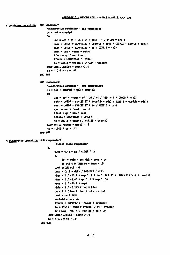
APPENDIX 3 - BROKEN HILL SURFACE PLANT SIMULATION
4 Ci90denser operation SUB conden.er1 'evaporative condenser - one co.pre.aor qc • qe1 + co.pi p1 DO
uac • ecf * ff - .8 I (1 I 1851 + 1 I (1000 * hfc» eeir •• 6105 * EXP(17.27 * (surfwb + edt) I (237.3 + surfwb + edt» ... t •• 6105 * EXP(17.27 * te I (237.3 + tel) qeat • uac * (e .. t - eeir) tfact • qe I UlC + eeir tflctc • LQGCtflct I .6105) te • 237.3 * tfletc I (17.27 - tfactc)
LOOP UNTIL ABS(qc - qest) < .1 tc • 1.019 * tc - .41
END SUB
SUB conden.er2 'evaporltive condenser - two COIIprHlOr. qc • qe1 + COIIpip1 + qe2 + COIIpip2 DO
uac • aet * nCOllp * ff - .8 I (1 I 1851 + 1 I (1000 * hfe» eeir • .6105 * EXPC17.27 * (surfwb + edt> I (237.3 + aurfwb + edt» aaet •• 6105 * EXP(17.27 * tc I (237.3 + tel) q.st • UlC * (I .. t - .. ir) tflct • qc I uac + .. ir tfactc • LOGCtflct I .6105) tc • 237.3 * tfaetc I C17.27 - tfactc)
LOOP UNTIL ABSCqc - q .. t) < .1 tc • 1.019 * tc - .41
END SUB
5 ivaporltor operation SUB ev.porator1
DO
'closed plat. evaporator
twoe. twie - qe 14.185 I L. DO
dt1 • twi. - te: dt2 • twoe - t. IF dt2 < 0 THEN t •• twoe - .5
LOOP WHILE dt2 < 0 L.td • Cdt1 - dt2) I L06(dt1 I dt2)
rhaw • 1 I (16.9 * nep - .2 * La - .8 * (1 + .0075 * (tw1a + twoe») rher • 1 I (4.46 * qe •• 5 * nep •• 5) xrka • 1 I (86.7 * nep)
rhfl • 1 I (3.193 * nip * hfa) UI • 1 I (rhaw + rher + xrka + rhfa) qeat • UI * l.td est l.td • qe I UII
tfect •• EXPCCtwi. - twoe) I .stL.td) te • (twi. - twoe * ttacta) I (1 - tfact.) IF (twoe - te) < 0 THEN qe • qe * .9
LOOP WHILE ABS(qe - q .. t) > .1 te • 1.074 * te - .31
END SUB
A-7
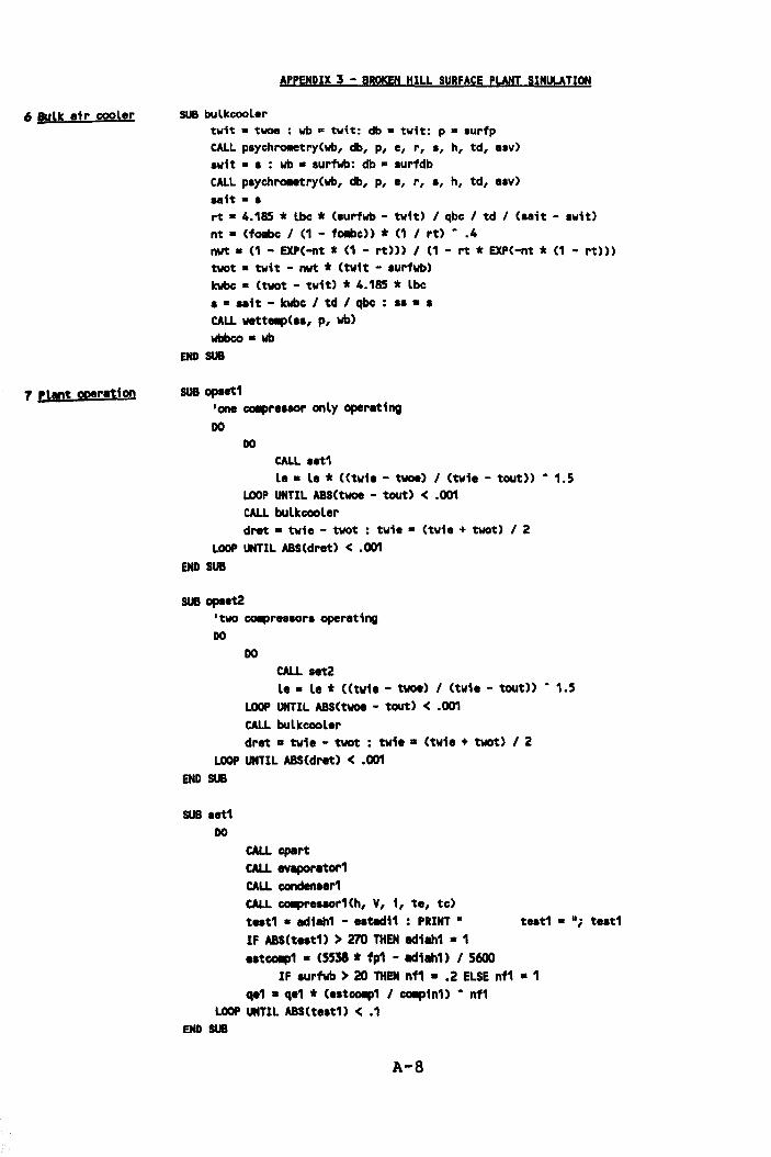
6 Bulk air cooler
1 ellnt operation
APPENDIX 3 - BROKEN HILL SURFACE PLANT SIMULATION
SUB bulkcooler twit = twoe : wb m twit: db • twit: p • aurfp CALL paychro.etryCwb, db, p, e, r, s, h, td, .av) awit • a : wb • aurfwb: db • .urfdb CALL p.ychro.etryCwb, db, p, e, r, ., h, td, a.v) .. it • a rt • 4.185 * lbe * Csurfwb - twit) I qbe I td I C .. it - swit) nt • Cfa.bc I C1 - fa.bc» * C1 I rt) •• 4 nwt • C1 - EXPC-nt * C1 - rt») I C1 - rt * EXPC-nt * C1 - rt») twot • twit - nwt * Ctwit - .urfwb) kwbc • Ctwot - twit) * 4.185 * lbe .... it - kwbc I td I qbc : ••• a CALb wettelllpC", p, wb) wbbco. wb
END SUB
SUB opset1 lone COIPr •• sor onLy operating DO
DO CALL set1 Le. Le * CCtw1. - twoe) I Ctwi. - tout» - 1.5
LOOP UNTIL ABSCtwoe - tout) < .001 CALL bulkcool.r drat • twi. - twot : tw1. • Ctwi. + twot) I 2
LOOP UNTIL ABS(dr.t) < .001 END SUB
SUB opset2 Itwo COIPr.saors operating DO
DO CALL •• t2 Le • Le * «tvi. - twoe) I (tw1. - tout» • 1.5
LOOP UNTIL ABS(twoe - tout) < .001 CALL bulkcool.r dr.t • tw1. - twot : tw1. • (tv1. + twot) I 2
LOOP UNTIL ABS(dret> < .001 END SUB
SUB •• t1 DO
CALL cpart CALL evaporator1 CALb condenser1 CALL COIPreasor1(h, V, " te, te) test1 • edteh1 - est.d11 : PRINT • teat1 • Hi t •• t1 IF ABS(test1) > 270 THEN edieh1 • 1 •• tCOlP1 • (5538 * fp1 - ed1eh1) I 5600
IF aurfwb > 20 THEN nf1 •• 2 ELSE nf1 • 1 qe1 • qe1 * (estCOlP1 I COIp1n1) • nf1
LOOP UNTIL ASS(t •• t1) < .1 END sua
A-8
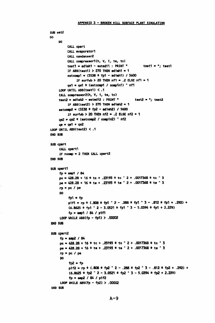
SUB set2 DO
DO
APPENDIX 3 - BROKEN HILL SURFACE PLANT SIMULATION
CALL epert CALL evaporator1 CALL condenaer2 CALL COIpreaaor1(h, V, i, t., te)
teat1 • adiah1 - .atad11 : PRINT" t.at1 • Hi t.at1 IF ASS(t.at1) > 270 THEN adi.h1 • 1 .atCOlp1 • (5538 * fp1 - ad1ah1) I 5600
IF aurfwb > 20 THEN nf1 • .2 ELSE nf1 • 1 q.1 • qe1 * (.atCOlp1 I COIpin1) • nf1
LOOP UNTIL ASS(t •• t1) < .1 CALL coapreaaor2(h, V, i, t., te) teat2 • adillh2 - •• tadi2 : PRINT U t •• t2 • "; t •• t2
IF ASS(teat2) > 270 THEN adillh2 • 1
e.tCO!lP2 • (5538 * fp2 - adiM2) I S600 IF .urfwb > 20 THEN nf2 • .2 ELSE nf2 • 1
qe2 • qe2 * (e.tCOllp2 I COIIP1n2) A nf2
qe • qe1 + qe2 LOOP UNTIL ASS(teat2) < .1
END SUB
SUB epert CALL epert1
IF ncoap - 2 THEN CALL epert2
END SUB
SUB cpert1 fp. Mp1 184 pc • 428.28 + 16 * te + .23193 * te • 2 + .0017368 * te • 3 pe • 428.28 + 16 * t. + .23193 * te • 2 + .0017368 * te A 3 rp-pc/pe 00
fp1 • fp
pif1 • rp * (.808 * fp1 • 2 - .288 * fp1 • 3 - .812 * fp1 + .292) + (6.8625 * fp1 • 2 - 3.0521 * fp1 • 3 - 5.0394 * fp1 + 2.229)
fp • aap1 I 84 I pif1 LOOP WHILE W(fp - fp1) > .00002
END SUB
SUB epert2 fp. aap2 184 pc • 428.28 + 16 * te + .23193 * te • 2 + .0017368 * te • 3 pe • 428.28 + 16 * te + .23193 * te • 2 + .0017368 * te • 3
rp·pc/pe DO
fp2 • fp
pif2 • rp * (.808 * fp2 • 2 - .288 * fp2 A 3 - .812 * fp2 + .292) + (6.8625 * fp2 A 2 - 3.0521 * fp2 • 3 - 5.0394 * fp2 + 2.229) fp • 8IP2 I 84 I pif2
LOOP WHILE ASS(fp - fp2) > .00002
END SUB
A-9
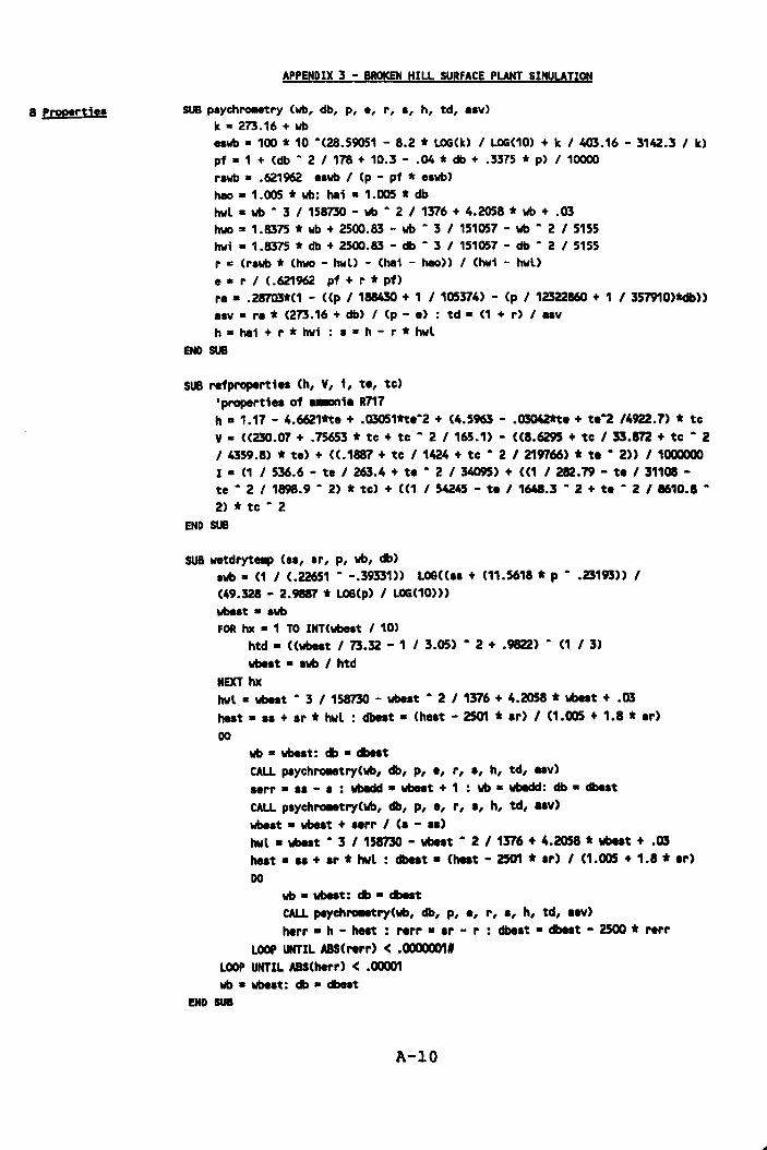
a properti.a
APPENDIX 3 - BROKEN HILL SURFACE PLANT SIMULATION
SUB paychro.etry (vb, db, p, ., r, a, h, td, .av) k-273.16+vb .. vb • 100 * 10 -(28.59051 - 8.2 * LOG(k) I LOG(10) + k I 403.16 - 3142.3 I k) pf • 1 + (db - 2 I 178 + 10.3 - .04 * db + .3375 * p) I 10000
ravb • .621962 .avb I (p - pf * .avb) hao • 1.005 * wb: hei • 1.005 * db hwl - wb - 3 I 158730 - wb - 2 I 1376 + 4.2058 * vb + .03 hwo • 1.8375 * wb + 2500.83 - wb - 3 I 151057 - wb - 2 I 5155 hwi • 1.8375 * db + 2500.83 - db - 3 I 151057 - db - 2 I 5155 r • (ravb * (hwo - hwl) - (hei - hao» I (hwi - hwl) e • r I (.621962 pf + r * pf) r ••• 28703*(1 - «p I 188430 + 1 / 105374) - (p / 12322860 + 1 / 357910)*db» .av • r. * (273.16 + db) I (p - e) : td • (1 + r) / .av h • hei + r * hwi : a • h - r * hwl
END SUB
SUB refpropertiea (hi V, i , te, te) 'propertiea of ...ani. R717 h. 1.17 - 4.6621tte + .03051tte-2 + (4.5963 - .0000000e + te-2 /4922.7) * tc V. «230.07 + .75653 * tc + te - 2 / 165.1) - «8.6295 + te / 33.812 + te - 2 / 4359.8) * te) + « .1887 + te / 1424 + te • 2 / 219766) * te • 2» / 1000000 I • (1 / 536.6 - te / 263.4 + te • 2 / 34095) + «1 / 282.19 - te / 31108 -te - 2 / 1898.9 • 2) * te) + «1 / 54245 - te / 1648.3 • 2 + te - 2 / 8610.8 • 2) * te • 2
END SUB
SUB wetdryteIIP (aa, ar I P, wb, db) awb - (1 / (.22651 • -.39331» LOG«aa + (11.5618 * P - .23193» / (49.328 - 2.9887 * LOG(p) / lOG(10»)
wbeat • avb FOR hx • 1 TO INT(wbeat I 10)
htd • «wbeat / 73.32 - 1 I 3.05) • 2 + .9822) • (1 / 3) wbeat • avb / htd
NEXT hx hwl • wbeat - 3 / 158730 - wbeat - 2 / 1376 + 4.2058 * wbeat + .03 heat • aa + ar * hwl : dbeat • (heat - ~ * ar) I (1.005 + 1.8 * ar)
DO
vb • wbeat: db • dbeat CALL payehl'Olletry(w, db, P, ., r, a, hi td, aav)
aerr • aa - a : wbIIdd • wbeat + 1 : vb • wbIIdd: db • dbeat CALL paychroMtry(vb, db, p, e, 1', a, hi td, MV)
wbeat • wbeat + aerr I (a - aa) hwl • wbeat • 3 / 158730 - wbeat - 2 I 1376 + 4.2058 * wbeat + .03 heat. aa + ar * hwl : dbeat • (hut - 2501 * ar) / (1.005 + 1.8 * ar)
DO
wb • wbeat: db • dbeat CALL psychroMtry(wb, db, P, e, 1', a, h, td, .av) herr • h - heat : rerr • ar - I' : dbeat • dbeat - 2500 * reI' I'
LOOP UNTIL _(rerr) < .0000001' LOOP UNTIL W(herr) < .00001 vb • wbeat: db • dbeat
END sua
A-10
9 9Utput st.t~ts
APPENDIX 3 - BROKEN HILL SURFACE PLANT SIMULATION
SUB wettelp (aa, p, wb)
awb • (1 I (.22651 • -.39331» LQG«aa + (11.5618 * P •. 23193» I (49.328 - 2.9887 * LQG(p) I LQG(10») wbest • awb FOR hx = 1 TO INTCwbest I 10)
htd • «wbeat I 73.32 - 1 I 3.05) • 2 + .9822) • (1 I 3) wbeat • swb I htd
NEXT hx
wb • wbest END SUB
SUB dout1 CALL power1 LPRINT " II
LPRINT " "; nCOllp; H COIIpr .. aorCs) operating - allbient wet bulb t...,erature • "; surfwb
LPRINT " """""""""""""""""""""""""""""""" LPRINT " -LPRINT - Evaporator duty • Hi qe; .. Evaporating t...,erature • H; te LPRINT .. condenser duty • u; qc; II Cond«\a1ng t...,erature • "; tc LPRINT U Evaporator water t...,eraturas - in H; twie;" - out H; twoe LPRINT II Evaporator watar flow rate • "; La LPRINT " BuLk cooLer water fLow rate. -i Lbci - air fLow rate • -; qbc LPRINT II Bulk cooLer duty • "; kwbCi N Wet buLb out • -; wbbco LPRINT " II
LPRINT II Power requir~tsll LPRIHT .. II
LPRINT " CoIIpr .. aor Load • "; fp1 * 100; HX Load power factor • "; p1f1 LPRIHT " CoIIpresaor input power • "; coap1p1 LPRINT • Evaporator pulP power • H; evapip LPRIHT n condenser fan and pulP power • n; condip LPRIHT H TotaL input power • A; powert LPRINT .. TotaL evaporator duty • H; qe LPRINT II OVaraLl power to cooling ratio. "; opcr CALL outdata1
END SUB
SUB dout1. CLS
CALL power1 PRINT II II
PRIHT II "; nco.p; II COIprHaor(s) operating - allbient wet bulb t-.perature • Hi surfwb PRINT " ***",H,rt'***irJAHArt'***irJ'HA*'''**H,rtA***irJAH'rtA***irJ,HA*AAI**irJAHA*'"**H,rtA*'''**H,rtA***"AHArtA***"AHArtA***tlAHArtA***tlA~A"
PRINT" Evaporator duty • "i qe; - Evaporating telPlrature • -; te PRIHT H Condenser duty • "i qc; " Condensing t...,eratura • "; tc PRINT" Evaporetor water ta.peratur .. - in "i twie;" - out H; twoe
PRINT - Evaporator water flow rate • H; le PRIHT - Bulk cooler water flow rate. "; lbci" Air flow rate • II; qbc PRIHT - Bulk cooler duty • H; kwbc; H Wet bulb out • II; wbbco PRIHT .. " PRINT • Power requireaentsU
A-ll
APPENDIX 3 - BROKEN HILL SURFACE PLANT SI"UbATION
PRINT " CoIIpre • .or loed • u. , tp1 * 100; ux PRINT .. CoIIpre • .or ; nput power • II. , cOllpip1 PRINT II Evaporator pu~ power • II. eVllpip , PRINT II Conden.er fan and PI.IIIP power • II. condip , PRINT II Total input power • n. powert , PRINT U Total evaporator duty • "; qe PRINT" OVerall power to cooling ratio • "i opcr CALL outdata1a
END SUB
SUB dout2 CALL power2 LPRINT U ,.
Load power tactor • II. pit1 ,
LPRINT ,. "; nCOllP; .. COIIPrea.orC.) operating - lIIIbient wet bulb t...,.rature • "; aurfwb
LPRINT " """""""""""""""""""""""""""""""" LPRINT " " LPRINT " EVIIpOrator duty ."i qei " Evaporating t...,.rature ."i te LPRINT " Conden.er duty • "i qCi ,. Conden.ing ta.perature ."i tc LPRINT " Evaporator weter ta.perature. - in "; tw1e; II - out "; twoe LPRINT " Evaporator weter f low rate • u; le LPRINT .. Bulk cooler water flow rate. "i lbc; H air flow rate • "; qbc LPRINT H Bulk cooler duty • H; kwbc; II Wet bulb out • "; wbbco LPRINT " " LPRINT U Power requir..anta" LPRINT II ,.
LPRINT " CoIIprealOr 1 loed • H; fp1 * 100; "X LPRINT " eo.pre.lOr 2 loed ." i fp2 * 100; "X LPRINT " CoIIpre • .or 1 input power • "; COIIP1p1; COIIPip2
loed power factor. "; pif1 loed power factor· "i pif2
,. CoIIpre.lOr 2 input power- ";
LPRINT ,. Evaporator PI.IIIP power • "; evapip LPRINT " Condenser fan and PI.IIIP power • II i condip LPRINT .. Total input power • "; powert LPRINT " Total evaporator duty • "; qe LPRINT II OVerall power to cooling ratio. "; opcr CALL outdata'
END SUB
SUB dout2a CALL power2 PRINT " " PRINT .. H; nCOllP; U COIIPreaaorCa) operating - a~ient wet bulb ta.perature • "; .urfwb
PRINT .. """"""""""""""""""""""""""""""",. PRINT" Evaporator duty • "; qe; " Evaporating t8lperature ."; te PRINT" Condenser duty ."; qc; " Condensing t...,.rature • "i tc PRINT" Evaporator water t...,.rature. - in "; twie; II - out "; twoe PRINT" Evaporator water flow rate • "; le PRINT" Bulk cooler water flow rate. "; lbc;" Air flow rate ."; qbc PRINT" Bulk cooler duty • A; kwbci " Wet bulb out • "; wbbco PRINT H "
PRINT II Power requir...nt.·
A-12
APPENDIX 3 - BROKEN HILL SURFACE PLANT SInULATION
PRINT" co.pre.aor 1 loed ."i fp1 * 1ooi"X Load power factor. Hi pif1 PRINT a co.pre.aor 2 load • Hi fp2 * 100i ax Load power factor. Hi pif2 PRINT H Ca.pre.aor 1 input power • Hi ca.pip1i H Ca.pre.aor 2 input power • H; COIIpip2 PRINT a Evaporator PUIIP power • "; evap1p PRINT ., Condenser fan end puI!p power •• ; condip PRINT a Total input power • Hi powert PRINT H Total evaporator duty • "; qe PRINT a OVerall power to cooling ratio. H; opcr CALL outdata1a
END SUB
SUB outdata1 LPRINT a H LPRINT " Evaporator detail." LPRlNT " Nullber of cae.ette. • H; nap;" Foul ing factor • "; hfe LPRINT " COnden.er detaiL'" LPRINT H AirfLow rate • "; (qac * ff * nCOllp);" FouL1ng factor
• "; hfc LPRINT a "
END SUB
SUB outdeta1a PRINT H Evaporator deta1L." PRINT" Nulber of ca .. ette •• "; nap; H Foul1ng factor • "i hf. PRINT H Conden.er detail.a
PRINT H AirfLow rate • "; (qac * ff * nca.p);" Fouling factor • "; hfc END sua
SUB power1 evapip • (54 * (Le I nep) • 2) * Le I 650 cond1p • (fankw * ff • 3 + puIpkw) * nCOllp powert • COIIp1p1 + evep1p + condtp opcr • qe I powert
END SUB
SUB power2 evapip • (54 * (Le I nap) • 2) * le I 650 condip • (fankw * ff • 3 + puIIpItw) * nCOllp powert • ca.pip1 + COIIpip2 + evepip + condip opcr • qe I powert
END SUB
A-I3
1 ",10 proqra ...
APPENDIX 4 - MOUNT ISA SURFACE PLANT SIMULATION
DECLARE SUB wettHp (aal, pi, wb!)
DECLARE SUB power1 () DECLARE SUB powerZa () DECLARE SUB outdata1 () DECLARE SUB outdata2a () DECLARE SUB dout1 () DECLARE SUB dout2a () DECLARE SUB dout2p () DECLARE SUB indlitll ()
DECLARE SUB initieL () DECLARE SUB atart () DECLARE SUB opaet2pareUeL () DECLARE SUB opaet2aeri.. () DECLARE SUB opaet1 () DECLARE SUB evaporftor1 () DECLARE SUB evaporator2 () DECLARE SUB CGlPreaaor1 (hi, vi, 11, te1, te1) DECLARE SUB CGlPreuor2 (hi, vi, 11, te2, tc2) DECLARE SUB aet2 () DECLARE ... aet1 () DECLARE SUB refproperti .. (hi, vi, 11, tel, tel) DECLARE SUB condenaer1 () DECLARE SUB condenaer2 () DECLARE SUB buLkcooLer () DECLARE SUB vetdrytetlp (aal, arl, pi, vbl, db!) DECLARE SUB paychl'OM'try (vbl, dbl, pi, e, r, a, h, td, .. v) DECLARE SUB bcout () DECLARE SUB dout () DECLARE SUB cIout1e () DECLARE SUB dout2M () DECLARE ... dout2pII () I SUppL 1er 2, Continuoua operation - evaporetive condenaera ~ SHARED ed1eh1, .. ted11, qe1, qe1, CGlPin1, ue1, twoe1, tv1e1, Le1, te1 COMMON SHARED te1, ecf1, hfe1, qee1, ff1, 1nvoL1, 1dpcr1, COIp1p1, h, v, 1 COMMON SHARED ed1eh2, utM:l12, qe2, qc2, COIIp1n2, ue2, twoe2, tw1e2, Le2, te2 COIIMON SHARED tc2, ecf2, hfc2, qac2, ff2, 1nvoL2, idpcr2, COIIIPip2, nap1, hfe1 COIIMON SHARED aurfwb, aurfdb, aurip, tout, nCGIP, confi;, ncond, nep2, hfe2 CCIIIOH SHARED evap1p1, evepip2, condip1, condip2, pGWert, opcr, qa, ruiatbc COIIMON SHARED qbe, fOllbc, wbbco, Lbc, twot, kwbc, wbout, twit, hHdbe, bleip COMMON SHARED eCGIP, 8COIIp1, lCOIIp2, bCOIIp, bCOIIp1, bCOIIp2, twoe COMMON SHARED LOIdn, LOId2, pif1, p1f2, pout
CALL atart CALL initilL
IF nCOlllP • 1 THEN CALL opaIt1 IF nCOllp • 2 AND config • 1 THEN CALL opaIt2aeri .. IF nCOllp • Z AND conf1; • 2 THEN CALL opaet2pareLLeL IF oCOllp • 1 THEN CALL cIout1e If nCOllp • 2 AND conf1g • 1 THEN CALL dout2aI IF nCOllp • 2 AND config • 2 THEN CALL dout2pI
PRINT .. enter 1 for herd copy or 0 for akip" INPUT pout
END
IF pout • 1 THEN CALL dout IF pout • 1 THEN CALL beaut
A-14
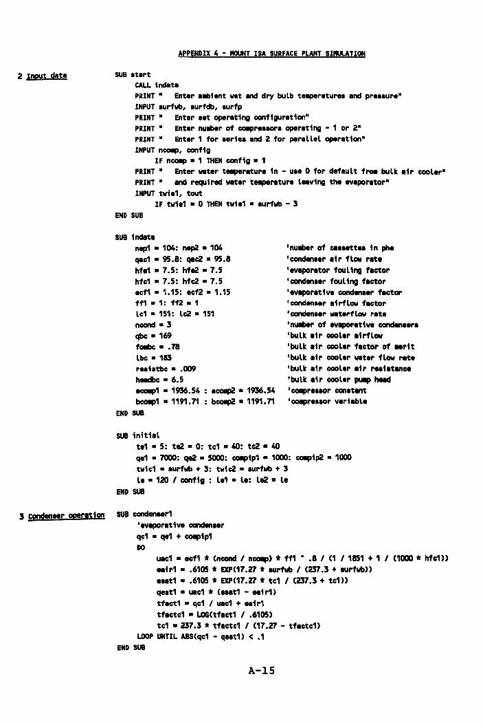
2 Input data
APPENDIX 4 - MOUNT ISA SURFACE PLANT SIMULATION
SUB atart CALL indeta PRINT II Enter a.bient wet and dry bulb te.peraturea and preaaure" INPUT .urfwb, aurfdb, aurfp PRINT H Enter .et operating configuration" PRINT" Enter nullber of COIIpreaaora operating - 1 or 2" PRINT" Enter 1 for .eriea and 2 for parallel operation" INPUT nCQIP, config
IF nCQIP • 1 THEN config • 1 PRINT" Enter water t8!ip8rature in - use 0 for defeult fl'Oll bulk air cooler" PRINT" and requ1 red water te.perature leaving the evaporator" INPUT twie1, tout
IF twie1 • 0 THEN twie1 • surfwb - 3 END SUB
SUB indlta nep1 • 104: nep2 • 104 qac1 • 95.8: qac2 • 95.8 hfe1 • 7.5: hfe2 • 7.5 hfc1 • 7.5: hfc2 • 7.5 acf1 • 1.15: ecf2 • 1.15 ff1 • 1: ff2 • 1 lc1 • 151: lc2. 151 ncond .3 qbc.169 fOllbc: •• 78
lbc • 183 r .. iatbc •• 009
headbc • 6.5 aCOllp1 • 1936.54 : aCOllp2 • 1936.54 bCQIP1 • 1191.71 : bCOllP2 • 1191.71
END SUB
SUB initial te1 • 5: te2 • 0: tc1 • 40: tc2 • 40
'nullber of caaaatt.. in phe
'condenaer air flow rate 'evaporator fouling factor 'condenaer fouling factor 'evaporative condenaer factor 'condenaer airflow factor 'condenser waterflow rate 'nullber of evaporative condensera 'bulk air cooler airflow 'bulk air cooler factor of .. rit 'bulk air cooler water flow rete 'bulk eir cooler air reai.tance 'bulk air cooler puIIp head 'COIIpreaaor constant 'COIIpreaaor variable
qe1 • 7000: qe2 • 5000: COIIp1p1 • 1000: COIIpip2 • 1000 twic1 • aurfwb + 3: twic2 • aurfwb + 3 le • 120 I con1ig : le1 • le: le2. le
END SUB
3 condenser operation SUB conden.er1 'evaporative ccndenaer qc1 • qe1 + co.pip1 DO
usc1 • ecf1 * (ncond I nCOlp) * 1f1 •• 8 I (1 I 1851 + 1 I (1000 * hfc1» eair1 •• 6105 * EXP(17.27 * aurtwb I (237.3 + aurfwb» e .. t1 •• 6105 * EXP(17.27 * tc1 I (237.3 + tc1» qeat1 • usc1 * (eaat1 - eair1) tfact1 • qc1 I usc1 + eair1 tfactc1 • LOG(tfact1 I .6105) tc1 • 237.3 * tfactc1 I (17.27 - tfactc1)
LOOP UNTIL A8S(qc1 - qeat1) < .1 END SUB
A-IS
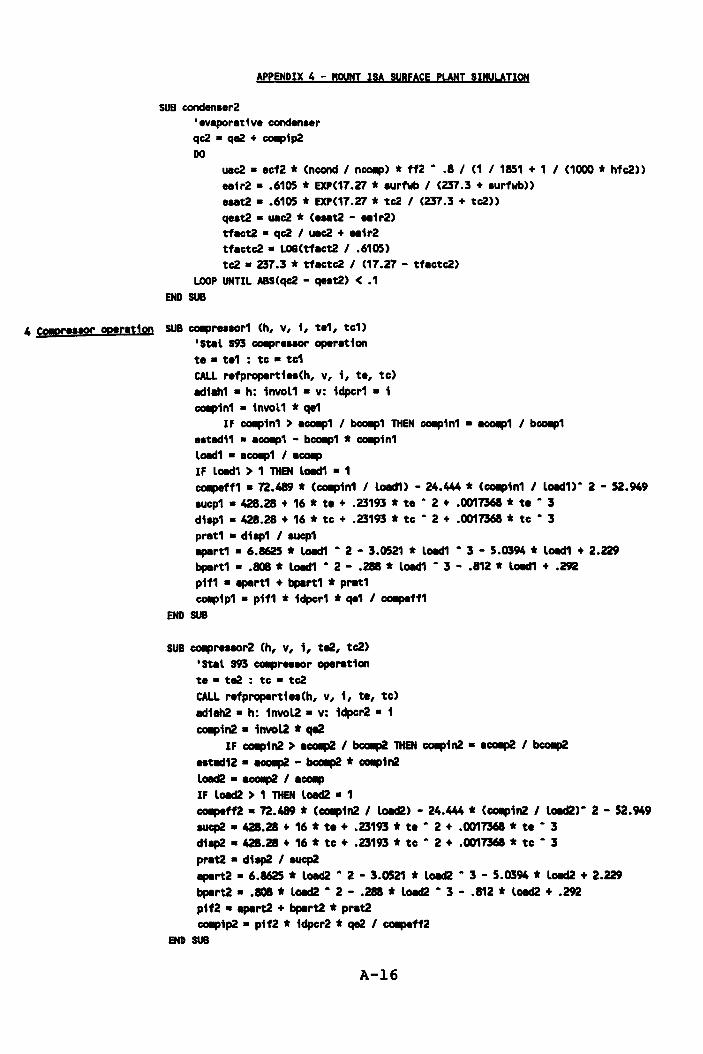
APPENDIX 4 - nouNT ISA SURFACE PLANT SIMULATION
SUB condena.r2 'evaporative condenaer qc2 • qe2 + COIIPtp2 DO
uec2 • ecf2 * (ncond I nCOlP) * ff2 •• 8 I (1 I 1851 + 1 I (1000 * hfc2» .. tr2 •• 6105 * EXP(17.27 * aurfwb I (237.3 + aurfwb» ... t2 •• 6105 * EXP(17.27 * tc2 I (237.3 + tc2» qeat2 • uec2 * ( ... t2 - .. t r2) tf.ct2 • qc2 I uec2 + .. ir2 tfactc2 • LQG(tf.ct2 I .6105) tc2 • 237.3 * tf.ctc2 I (17.27 - tf.ctc2)
LOOP UNTIL ABSCqc2 - q.at2) < .1 END SUB
4 9P'Pr.aaor operation SUB COIPreaaor1 (h, v, 1, t.1, tc1) 'St.l S95 COIPr.aaor oper.tion t. • t.1 : te • to1 CALL r.fpropertiea(h, v, 1, t., te)
adiah1 • h: invol1 • v: idpcr1 • i
COIPin1 • invol1 * qe1 IF COIPin1 > aCOlP1 I ~1 THEN COIP1n1 • 'COIP1 I ~1
•• tad11 • 'COIP1 - bCOlP1 * COIPtn1
loacM • aCOlP1 I 'COIP IF load1 > 1 THEN load1 • 1 COIpeff1 • 72.489 * (COIp1n1 I loadn) - 24.444 * (COIP1n1 I Load1)· 2 - 52.949 auep1 • 428.28 + 16 * t. + .23193 * t •• 2 + .0017368 * t •• 3 d1ap1 • 428.28 + 16 * te + .23193 * te • 2 + .0017368 * to • 3 pr.t1 • diap1 I aucp1 apart1 • 6.8625 * loadn • 2 - 3.0521 * loadn • 3 - 5.0394 * Load1 + 2.229 bpart1 • .808 * LoacM • 2 - .288 * Loadn • 3 - .812 * loadn + .292 pif1 • apart1 + bpart1 * prat1 COIPip1 • pif1 * 1dpcr1 * qe1 I COIpeff1
END SUB
SUB COIpreaaor2 (h, v, t, te2, tc2) 'StIll S95 COIprHaor operation
t. • te2 : tc • tc2 CALL r.fpropertt.a(h, v, i, t., to) adillh2 • h: invoL2 • v: idpcr2. i
COIPin2 • invoL2 * qe2 IF COIp1n2 > .COIIIP2 I bCOIIIP2 1HEN COIpin2 • .COIIp2 I bCOIIIP2
eatad12 • !COIIp2 - booIp2 * COIp1n2 L0ad2 • .COIIp2 I 'CCIIIp IF L0ad2 > 1 THEN loacl2 • 1 COIIpeff2 • 72.489 * (COIptn2 I l0ad2) - 24.444 * (COIpin2 I loacl2)· 2 - 52.949 aucp2 • 428.28 + 16 * t. + .23193 * t •• 2 + .0017368 * t •• 3 d1ap2 • 428.21 + 16 * to + .23193 * to • 2 + .0017368 * to • 3 pr.t2 • diap2 I aucp2
apart2 • 6.8625 * L0ad2 • 2 - 3.0521 * LoacI2 • 3 - 5.0394 * L0ad2 + 2.229 bpart2 •• 808 * load2 • 2 - .288 * l0ad2 • 3 - .812 * L0ad2 + .292 ptf2 • apart2 + bpart2 * pr.t2 CCIIIptp2 • p1f2 * idpcr2 * qe2 I COIpIff2
END SUB
A-16
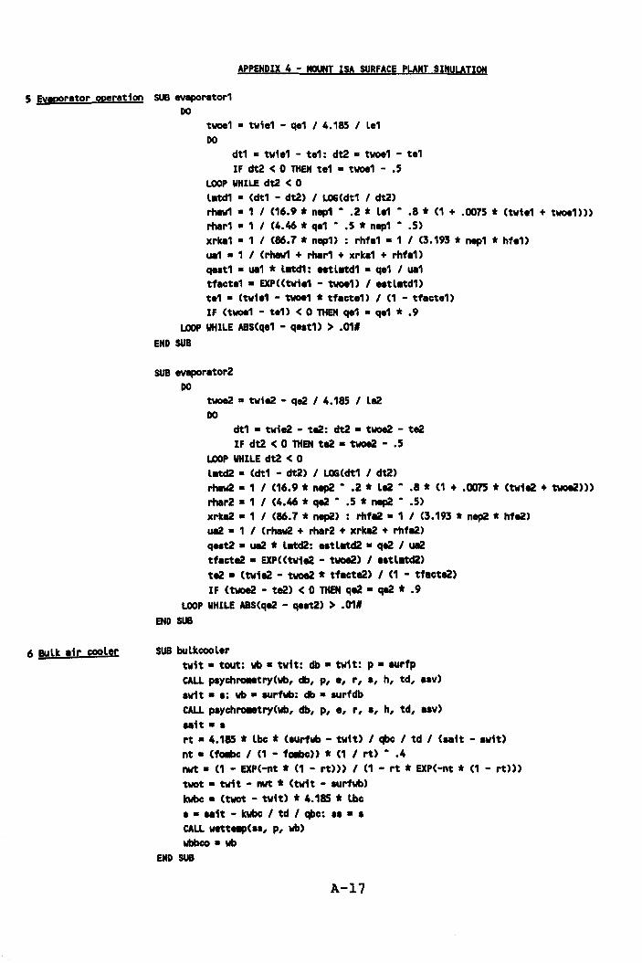
APPENDIX 4 - MOUNT ISA SURFACE PLANT SIMULATION
5 Eyaporator operation SUB evaporator1 DO
6 gyLk air cooler
twoe1 • twi.1 - q.1 I 4.185 I Le1 DO
dt1 • twi.1 - te1: dt2 • twoe1 - te1 IF dt2 < 0 THEN t.1 • twoe1 - .5
LOOP WHILE dt2 < 0 L.td1 • (dt1 - dt2) I LOG(dt1 I dt2) rhlw1 • 1 I (16.9 * nep1 •• 2 * L.1 •• 8 * (1 + .0075 * (tw1.1 + twoe1») rhar1 • 1 I (4.46 * qe1 •• 5 * nep1 •• 5) xrka1 • 1 I (86.7 * nap1) : rhfe1 • 1 I (3.193 * nap1 * hf.1) ue1 • 1 I (rhIw1 + rhar1 + xrke1 + rhfa1) qeat1 • ue1 * L.td1: utL.td1 • qe1 I ue1 tfacte1 • EXP«twi.1 - twoe1) I eatL.td1) t.1 • (twie1 - twoe1 * tfact.1) I (1 - tfecte1) IF (twoe1 - te1) < 0 THEN qe1 • q.1 * .9
LOOP WHILE ABS(qe1 - qeat1> > .011
END SUB
SUB evaporator2 DO
tw0e2 • twie2 - qe2 I 4.185 I le2 DO
dt1 • twie2 - te2: dt2 • tw0e2 - te2 IF dt2 < 0 THEN te2 • twoe2 - .5
LOOP WHILE dt2 < 0 ~d2 • (dt1 - dt2) I LOG(dt1 I dt2) rhew2 • 1 I (16.9 * nep2 •• 2 * Le2 •• 8 * (1 + .0075 * (tw1e2 + tw0e2») rhar2 • 1 I (4.46 * qe2 • .5 * nep2 •• 5) xrke2 • 1 I (86.7 * nep2) : rhfe2. 1 I (3.193 * nep2 * hfe2) UII2 • 1 I (rh11w2 + rher2 + xrke2 + rhfe2) qMt2 • UII2 * L.td2: eatL.td2 • qe2 I UII2 tfacte2 • EXP«twie2 - twoe2) I •• tl.td2) te2 • (twie2 - twoe2 * tfacte2) I (1 - tflcte2) IF (tw0e2 - te2) < 0 THEN qe2 • qe2 * .9
LOOP WHILE ABS(qe2 - qeat2) > .011 END SUB
SUB buLkcooler twit. tout: vb • twit: db • twit: p • aurfp CALL paychl'Oll8try(vb, db, P, e, ria, h, td, aav) .wit. a: vb • aurfwb: db • aurfdb CALL paychl'Oll8try(vb, db, p, e, r, a, h, td, I.V)
.. it. a rt • 4.185 * lbc * (aurfwb - twit) I qbc I td I ( .. it - awit) nt • (fa.bc I (1 - fa.bc» * (1 I rt) • .4 nwt • (1 - EXP(-nt * (1 - rt») I (1 - rt * EXP(-nt * (1 - rt») twot • twit - nwt * (twit - aurfwb) kwbc • (twot - twit) t 4.185 * lbc a • ..it - kwbc I td I qbc: aa • a CALL watt...,(N, p, vb) wbbco. vb
END SUB
A-17
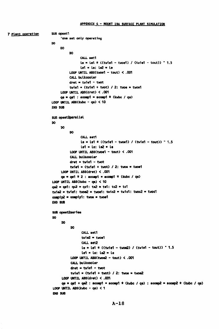
7 PLant operation
APPENDIX 4 - MOUNT ISA SURFACE PLANT SI"ULATION
SUB opset1
DO
'one set only operating
DO
DO CALL Ht1 le • le1 * «twie1 - twoe1) I (twie1 - tout» • 1.5 Le1 • Le: Le2 • Le
LOOP UNTIL ABS(twoe1 - tout) < .001 CALL buLkcooLer dret • twie1 - twot twie1 • (twie1 + twot) I 2: twoe • twoe1
LOOP UNTIL ABS(drat) < .001 qe • qe1 : .~1 • a~1 * (kwbc I qe)
LOOP UNTIL ABS(kwbc - qe) < 10 END SUB
SUB opaat2paraLLaL DO
DO DO
CALL set1 La. La1 * «twia1 - twoe1) I (twie1 - tout» • 1.5 La1 • Le: Le2. La
LOOP UNTIL ABS(twoe1 - tout) < .001 CALL buLkcooLer drat • twie1 - twot twi.1 • (twi.1 + twot) I 2: twoe • twoe1
LOOP UNTIL ABS(dret) < .001 qe • qe1 * 2 : .~1 • aCOllp1 * (kwbc I qe)
LOOP UNTIL ABS(kwbc - qa) < 10 qe2 • qe1: qc2 • qc1: te2 • te1: tc2 • tc1 twie2 • twi.1: twoe2 • twoe1: twic2 • twic1: tw0c2 • twoc1 ~ip2 • ~ip1: twoe. twoe1 END SUB
SUB opaet2Hriea DO
DO DO
CALL set1 twi e2 • twoe1 CALLaet2 Le. Le1 * «twie1 - twoe2) I (twie1 - tout» • 1.5 La1 • La: Le2. Le
LOOP UNTIL ABS(tw0e2 - tout) < .001 CALL buLkcooLar drat • twia1 - twot twie1 • (twie1 + twot) I 2: twoe • tw0e2
LOOP UNTIL ABS(dret) < .001 qe • qe1 + qe2 : aCOlllp1 • aCClllp1 * (kwbc I qa) : aCC111p2 • aCC111p2 * (1Nbc I qa)
LOOP UNTIL ABS(kwbc - qe) < 1 END SUB
A-18
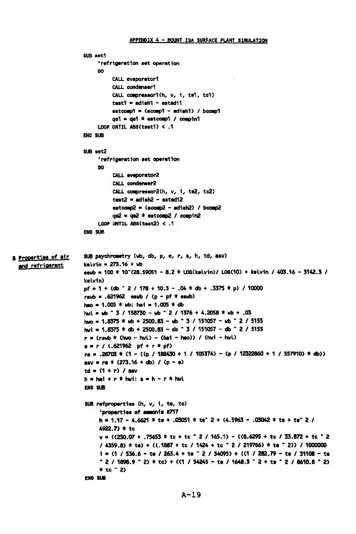
8 eropert1ea of air !fld refriaerant
APPENDIX 4 - MOUNT ISA SURFAce PLANT SlKULATl9N
SUB .et1 'refrigeration .et operation DO
CALL evaporator1 CALL conden.er1 CALL COIpreaaor1(h, v, i, te1, te1) teat1 • adiah1 - eatadi1 e.tCOlp1 • <aCOlp1 - lldiah1) / bCOlp1 qe1 • qe1 * eateo.p1 / COIPin1
LOOP UNTIL ASS(teat1) < .1 END SUB
SUB aet2 'refrigeration aet operation DO
CALL evaporetor2 CALL condenaer2 CALL COIpreaaor2(h, v, i, te2, tc2) teat2 • ad1ah2 - e.tadi2 eatCOllp2 • (aCOllp2 - adiah2) / bCOIIp2 qe2 • qe2 * eatCOllp2 / co.pin2
LOOP UNTIL ASS(t.at2) < .1
END SUB
SUB psychl'Ollet:ry (vb, db, p, e, r, a, h, td, e.v) kelvin • 273.16 + vb eavb. 100 * 10·(28.59051 - 8.2 * LOG(kelvin)/ LOG(10) + kelvin / 403.16 - 3142.3 / kelvin) pf • 1 + (db • 2 / 178 + 10.3 - .04 * db + .3375 * p) / 10000 ravb • .621962 eavb / (p - pf * e.vb) hac. 1.005 * vb: hili .1.005 * db hwl • wb • 3 / 158730 - vb • 2 / 1376 + 4.2058 * vb + .03 hwo • 1.8375 * vb + 2500.83 - vb • 3 / 151057 - vb • 2 / 5155 INi • 1.8375 * db + 2500.83 - db • 3 / 151057 - db • 2 / 5155 r • (rswb * (hwo - hwl) - (hili - hac» / (hwi - hwl) e • r / (.621962 pf + r * pf) r ••• 28703 * (1 - «p / 188430 + 1 / 105374) - (p / 12322860 + 1 / 357910) * db» •• v. re * (273.16 + db) / (p - e) td • (1 + r) / uv
h • he1 + r * hw1: • • h - r * hwl END SUB
SUB refpropertiea (h, v, i, te, te) 'propertiea of ...anie R717 h. 1.17 - 4.6621 * te + .03051 * te· 2 + (4.5963 - .03042 * te + tea 2 / 4922.7) * te v. «230.07 + .75653 * te + te • 2 /165.1) - «8.6295 + te /33.812 + te • 2 I 4359.8) * te) + «.1887 + te / 1424 + te • 2 / 219766) * te • 2» / 1000000 1 • (1 / 536.6 - te / 263.4 + te • 2 / 34095) + «1 / 282.79 - te / 31108 - te • 2 / 1898.9 • 2) * te) + «1 / 54245 - te / 1648.3 • 2 + te • 2 / 8610.8 • 2) * te • 2)
END SUB
A-19
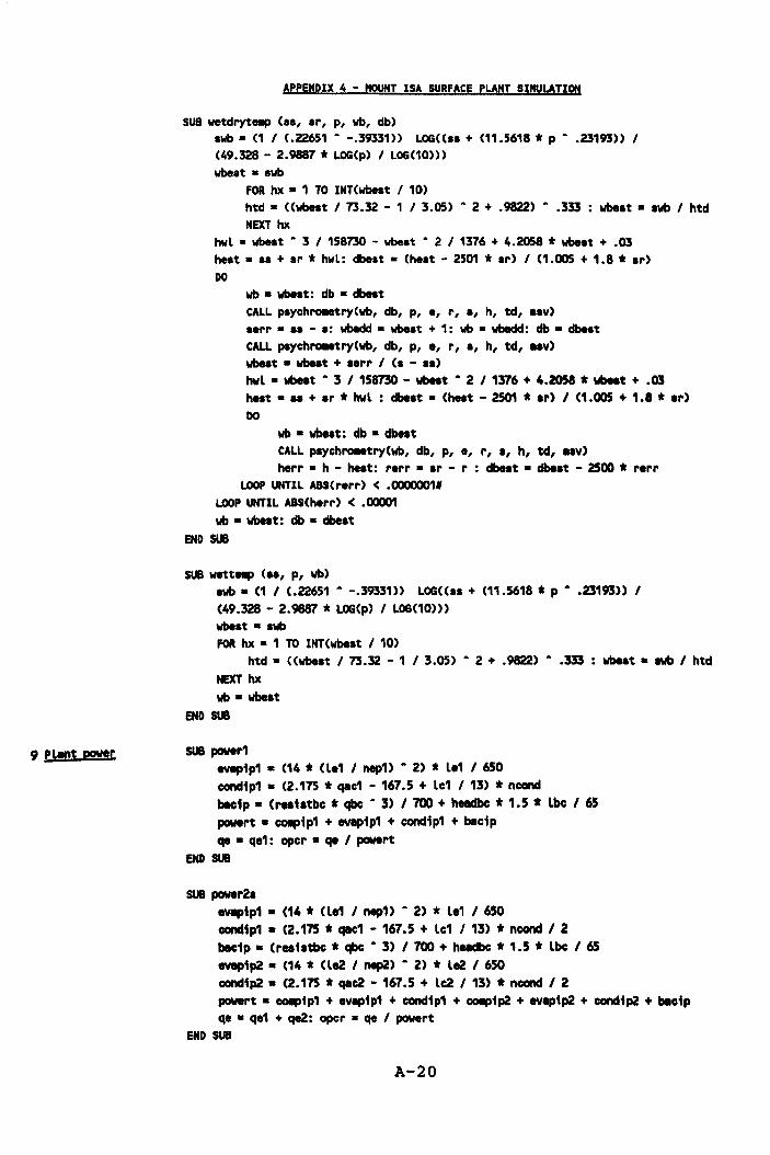
9 PLant POW!r
APPENDIX 4 - MOUNT ISA SURFACE PbANT SInubATION
SUB wetdryte.p Caa, ar, p, wb, db) awb. C1 I (.22651 • -.39331» LOGCCaa + C11.5618 * p •• 23193» I C49.328 - 2.9887 * LOGCp) I LOG(10») wbeat • awb
FOR hx • 1 TO INTCwbeat I 10) htd • «wbeat I 73.32 - 1 I 3.05) • 2 + .9822) • .333 : wbeat • awb I htd NEXT hx
hwl • wbeat • 3 I 158730 - wbeat • 2 I 1376 + 4.2058 * wbeat + .03 heat • aa + sr * hwl: dbeat • Cheat - 2501 * ar) I C1.005 + 1.8 * ar) DO
wb • wbeat: db • dbelt CALL paychro.etryCwb, db, p, ., r, a, h, td, .av) aerr • aa - a: wbIdd • wbeat + 1: wb • wbadd: db • dbeat CALL paychro.etryCwb, db, p, ., r, a, h, td, aav) wbeat • wbeat + aerr I Ca - aa) tNL • wbeat • 3 I 158730 - wbeat • 2 I 1376 + 4.2058 * wbut + .03
helt • aa + ar * hwl : dbeat • Chelt - 2501 * ar) I C1.005 + 1.8 * ar) DO
wb • wbeat: db • dbeat CALL paychro.etryCwb, db, p, ., r, a, h, td, aav) herr • h - heat: rarr • Ir - r : dbeat • dbeat - 2500 * rarr
LOOP UNTIL ABSCr.rr) < .00000011
LOOP UNTIL ABS(herr) < .00001
wb • wbeat: db • dbeat END SUB
SUB wett..., Caa, p, wb) awb. (1 I C.22651 • -.39331» LOG(CII + C11.5618 * p •• 23193» I (49.328 - 2.9887 * LOGCp) I LOG(10») wbaat • awb FOR hx • 1 TO INTCwbeat I 10)
htd • «wbeat I 73.32 - 1 I 3.05) • 2 + .9822) •• 333 : wbeat • Ivb I htd NEXT hx wb. wbeat
END SUB
SUB power1 evapip1 • (14 * (la1 I nap1) • 2) * l.1 I 650 condip1 • (2.175 * qac1 - 167.5 + lc1 I 13) * ncond blc1p. (reaiatbc * qbc • 3) 1700+ hHClbc * 1.5 * lbc I 65 powert • COIpip1 + evapip1 + condip1 + becip qe • qe1: opcr • qe I powert
END SUB
SUB power2a evapip1 • (14 * (la1 I nap1) • 2) * La1 I 650 cond1p1 • (2.175 * qac1 - 167.5 + lc1 I 13) * ncond I 2 becip • (reaiatbc * qbc • 3) I 700 + htedbc * 1.5 * Lbc I 65 evapip2 • C14 * (le2 I nep2) • 2) * Le2 I 650 condtp2 • (2.175 * qac2 - 167.5 + Lc2 I 13) * ncond I 2 powert • COIpip1 + evepip1 + condip1 + COIIPtp2 + eveptp2 + concItp2 + becip q. • qa1 + qe2: opcr • qe I powert
END SUB
A-20
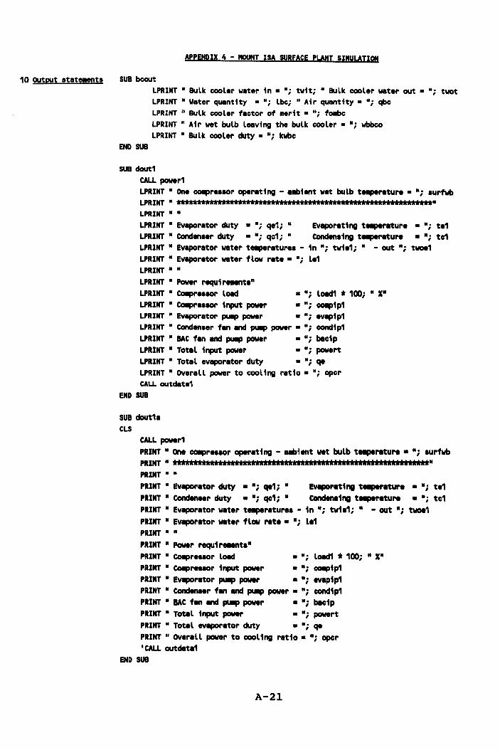
10 OUtput atate.enta
APPENDIX 4 - MOUNT ISA §URFACE PLANT SIMULATION
SUB bcout LPRINT " Bulk cooler water in • Hi twiti " Bulk cooler water out • "i twot LPRINT H Water quantity • H; lbc; H Air quantity. H; qbc LPRINT II Bulk cooler factor of .. rit • "; fOlibe LPRINT " Air wet bulb leaving the bulk cooler. Hi wbbco LPRINT " Bulk cooler duty • Hi kwbe
END SUB
SUB dout1
CALL power1 LPRINT H One COIIPre.aor operating - allbient wet bulb t...,.rature • "; .urfwb
LPRINT H **'****'********"**.,"*********.,****'************'*'*'*"**" LPRINT " " LPRINT " Evaporator duty ."i qe1; H Evaporating t...,.rature ."i te1 LPRINT " Condenaer duty • Hi qc1; " CondeMing t...,.reture • H; tc1 LPRINT H Evaporator water t...,.rature. - in H; twie1;" - out H; twoe1 LPRINT " Evaporator water flow rate • Hi le1 LPRINT H H
LPRINT • Power requir...nt.n
LPRINT • CoIIpreaaor load LPRINT " CoIIpre.aor input power
• H; load1 , 100; " XH
• "; COIIPi p1 LPRINT .. Evaporator puIIp power • "; evap1p1 LPRINT " Conden.er fen encI puIIp power • "; oondtp1 LPRINT H BAC fen end puIIp power ... ; becip
LPRINT " Total input power • "i powert LPRINT • Tota l evaporator duty • "; qe LPRINT " OVerall power to cooling retio • "; opel' CALL outdete1
END sua
SUB cIout1a CLS
CALL power1 PRINT " One COIIPre.aor operating - _tent wet bulb tl!llptreture • "i aurfwb
PRINT " ***""""""""""""""""""""""""'"""""" PRINT • H
PRINT" Evaporator duty • Hi .1i " Evaporating tl!llptrature • Hi te1 PRINT H Condenser duty • H; qc1i H CondeMina tl!llptreture • H; tc1 PRINT H Evaporator weter tl!llptrature. - in ·i twit1i H - out ·i twoe1 PRINT • Eveporetor water fLow rete. Hi Le1 PRINT H H
PRINT H Power requtr...nt.H
PRINT H CoIIpreaaor Load •• ; load1 * 100; " X· PRINT H CoIIpreaaor input power • "i COIIP1p1 PRINT H Ev..,orator puIIp power • H; evap1p1 PRINT H Conden.er fen end puIIp power • Hi condip1 PRINT H BAC fen end puIIp power • • i beci P PRINT H Total input power • "; powert PRINT .. Total evaporator duty • H; qe PRINT H OVeraU power to cooL ina ratio. H; opel' I CALL outdeta1
END SUB
A-21
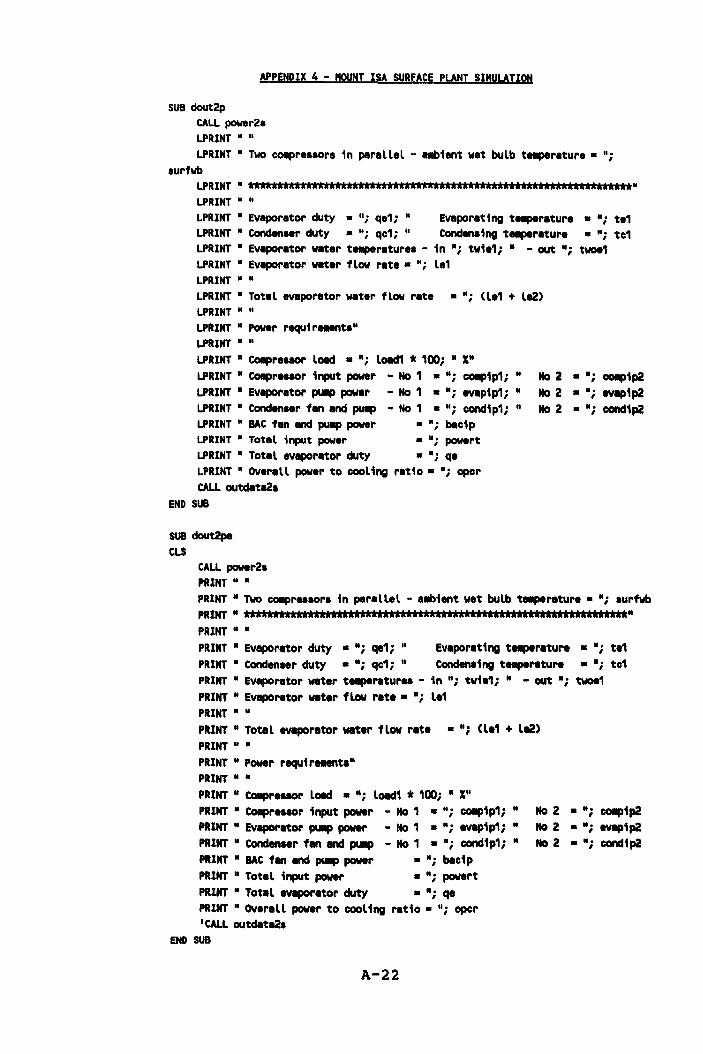
APPENDIX 4 - MOUNT ISA SURFACE PLANT SIMULATION
SUB dout2p CALL powerZ. LPRINT " " LPRINT H Two COIIPresaor. in parallel - allbient wet bulb tetllp4tr.ture • ";
surfwb
LPRINT II """"""""""""""""""""""""""""""""""
LPRINT • H
LPRINT H Evaporator duty ."; qe1; " Evaporating tetllp4tratur. • Hi t.1 LPRINT II condenser duty • "; qc1; u COnden.1ng t....,.r.tur. ."; tc1 LPRINT A Evaporator water ta.peratur •• - in .; tw1.1;" - out "; twoe1 LPRINT H Evaporator wat.r flow r.t •• A; l.1 LPRINT II II
LPRINT H Total evaporator water flow rate ."; (l.1 + le2) LPRINT " " LPRINT II Pow.r requ1r...nta" LPRINT II H
LPRINT II CoIIpr •• aor lOid • II; lo.d1 * 100; II X" LPRINT " CoIIpreaaor input power - No 1 • A; COIPip1; " LPRINT n Evapor.tor pulP pow.r - No 1 ."; evapip1; n
LPRINT " COnden •• r fan and pulP - No 1 • "; condip1; n
LPRINT " BAC fan and pulP power • "; bac1p LPRINT " Total input power • "; powert LPRINT II Total evaporator duty • n; q. LPRINT " OV.r.ll pow.r to cooling r.tio • "; oPCr CALL outdata2.
END SUB
SUB dout2pa
CLS CALL power2s PRINT II "
No 2 ."; OOIIpi p2 No 2 ."; evllPip2 No 2 ."; cond1p2
PRINT II Two COIIPr •• aor. in par.ll.l - allbient w.t bulb t....,.r.tur •• "; surfwb
PRINT " """""""""""""""""""""""""**'*'***********" PRINT " " PRINT " Ev.porator duty ." i q.1; " Ev.por.ting tetllp4tr.ture • "i te1 PRINT" Condens.r duty ."; qc1; " COndensing t....,.r.tur. ."; tc1 PRINT" Evaporator wat.r ta.per.tur •• - in "; tvi.1; II - out "; twoe1 PRINT" Evapor.tor water flow r.te • "; le1 PRINT " A
PRINT" Tot.l evapor.tor water fLow r.te • H; (Le1 + Le2) PRINT A "
PRINT A Power requ1r...nt." PRINT" " PRINT II CoIIpreaaor lOid ."; load1 * 100; " X" PRINT II CoIIpreaaor input power - No 1 • A; COIIPip1; " PRINT " Evaporator pulP power - No 1 ."; evapip1; " PRINT" COndenser fan and pulP - No 1 ."; condip1; " PRINT " BAC fan and pulP power • "; bacip PRINT H Total input power • "; powert PRINT " Total evaporator duty • "; qe PRINT" OV.r.ll power to cooling r.tio • H; opcr I CALL outdata2a
END SUB
A-22
No 2 • "; COIPip2 No 2 • "; 8VlIPip2 No 2 ."; condip2
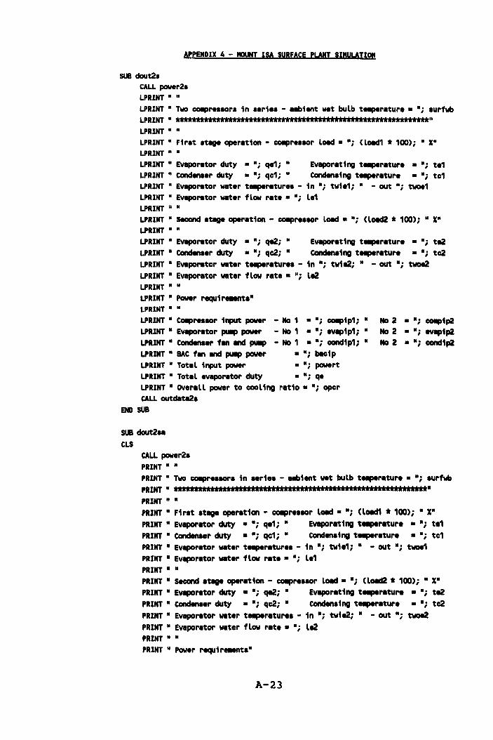
APPENDIX 4 - MOUNT ISA SURFACE PLANT SIMYLATION
SUB dout2. CALL power2. LPRINT • U
LPRINT " Two COIIPre.aor. in .er1e. - allb1ent wet bulb t...,.rature • Hi .urfwb
LPRINT A """""""""""""""""""""""""""""""" LPRINT " A LPRINT H Fir.t .tage operation - COIIPresaor load • Hi (lOldn * 100); • X· LPRINT • • LPRINT • Evaporator duty ."i qe1i • Evaporating ta.perature ."; te1 LPRINT H Condenaer duty • Hi qc1i A Condena1ng ta.perature • Hi tc1 LPRINT • Evaporator water t...,.rature. - in u; tw1e1; U - out H; two.1 LPRINT • Evaporator water flow rata. Ai le1 LPRINT • U
LPRINT " second stage operation - COIIPre.aor load • .; <L0ad2 * 100); " XH LPRINT • " LPRINT • Evaporetor duty ."i qe2; " Evaporating ta.perature • H; te2 LPRINT • Condenser duty • H; qc2; H Condensing t ... rature •• i tc2 LPRINT • Evaporator water t...,.raturea - in Hi tw1e2i H - out Hi twoe2 LPRINT " Evaporator water flow rata. Hi le2 LPRINT • II
LPRINT • Power requir..-nts" LPRINT • H LPRINT • CoIIprHaor input power LPRINT • Evaporator puIIIp power LPRINT H Condenser fan and puIIIp
LPRINT H BAC fan and puIIp power LPRINT " Total input power
-No1 · ". , COIIPip1; H - No 1 • H. , evapip1i " -No1 • H. , cond1p1; H
• to; bac1p • to; powert
LPRINT " Total evaporator duty • Hi qa LPRINT • OVerall power to cooling ratio • "i opcr CALL outdata2.
END SUB
SUB dout2ae CLS
CALL power2a PRINT H "
No2 · ". , COIIP1p2 No2 • H. , evap1p2 No2 • H. , cond1p2
PRINT • Two COIIPreaaors in aerie. - allbient wet bulb ta.perature • to; aurfwb
PRINT H """""***'**'*********"*"*"'**'**'**'***'*"**''***'**'" PRINT " H PRINT to Firat atage operation - COIpr.saor load • H; (load1 * 100); H X" PRINT H Evaporator duty • H; qe1; " Evaporating telptrature • H; te1 PRINT" condenaer duty ."; qC1; to Condensing ta.perature • to; tc1 PRINT • Evaporator water t ... rature. - in "; tw1a1;· - out H; two.1 PRINT " Evaporator water f low rate • Hi le1 PRINT " • PRINT • Second stage operation - COIpresaor load • • i <l0ad2 * 100); H X" PRINT • Evaporator duty ."; qe2; • Evaporating telptrature ..; te2 PRINT " Condanaer duty ." i qc2; " Condansing telptrature ."; tc2 PRINT H Evaporator water t...,.rature. - in "; twie2i" - out "; tw0e2 PRINT" Evaporator water flow rate. H; le2 PRINT • " PRINT • Power requ1r..-nts"
A-23
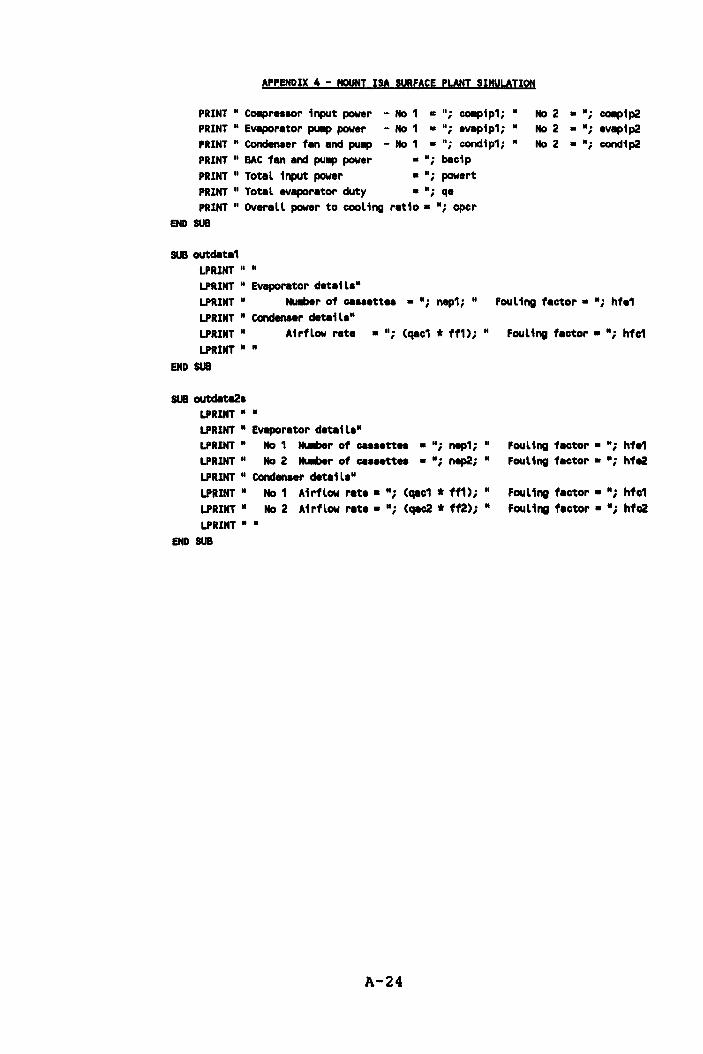
APPENDIX 4 - HOUNT ISA SURFACE PLANT SIMULATION
PRINT M Ca.pre.aor input power PRINT " Evaporator puIIp power PRINT " Condenser fan and puIIp
PRINT " BAC fan and PUIIIp power
-No1 • -No1 • -No1 •
• It. ,
H. COIIIptp1; , ... evapip1; , n. condip1; , bactp
PRINT" Total input power • "; powert PRINT H Total evaporator duty • H; qe PRINT" OVeraLL power to cooling ratio • "i opcr
END SUB
SUB outdata1 LPRINT .. U
LPRINT H Evaporator detail."
" " ..
No2 No2 No2
• H; • H; • H;
COIIIpip2 evapip2 cond1p2
LPRINT .. Nullber of ca •• ett ••• "; nep1; H Foul1ng factor. Hi hf.1 LPRINT " Condenser detai l." LPRINT II
LPRINT • " END SUB
Airflow rate • H; (qac1 * ff1); H Fouling factor. II; hfc1
SUB outdata2. LPRINT H ..
LPRINT " Evaporator detail." LPRINT· NO 1 Nullber of ca ••• tte. ."i nep1i II
LPRINT" NO 2 NUllber of ca ... tt.. ." i nep2i .. LPRINT II Conden.ar detail." LPRINT II NO 1 Airflow rate. H; (qac1 * ff1); H
LPRINT" No 2 Airflow rate • Hi (qac2 * ff2); " LPRINT " "
END SUB
A-24
FouLing factor • IIi hfa1 FouLing factor • "i hfe2
FouLing factor • .; hfc1 FouLing factor • .; hfc2
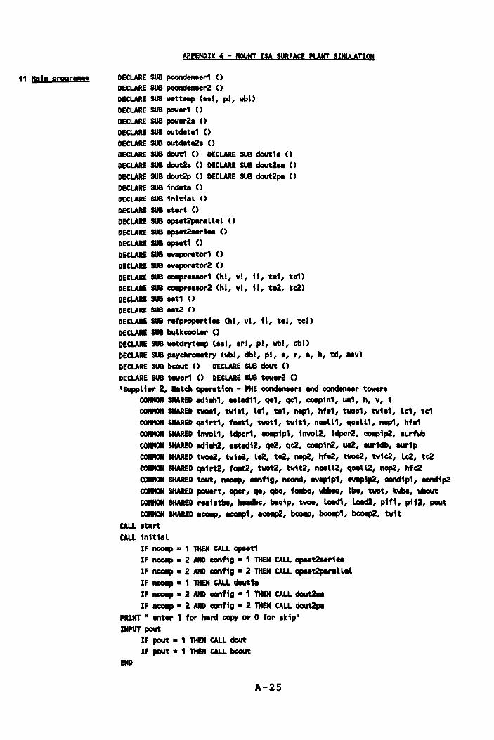
11 ",in praa,. ...
APPENDIX 4 - MOUNT ISA SURFACE PLANT SIMULATION
DECLARE SUB pconden •• ,.1 () DECLARE SUB pconden .. ,.2 () DECLARE SUB wettellp < •• 1, pi, vbl) DECLARE SUB powe,.1 () DECLARE SUB powe,.2a () DECLARE SUB outdate1 () DECLARE SUB outdatll2. () DECLARE SUB dout1 () DECLARE SUB cIout1. () DECLARE SUB dout2. () DECLARE SUB cIout2.. () DECLARE SUB dout2p () DECLARE SUB dout2pa () DECLARE SUB 1ndat. () DECLARE SUB 1nitiel () DECLARE SUB .tert () DECLARE SUB opaet2pareUel () DECLARE SUB opaet2 .... i .. () DECLARE SUB opaet1 () DECLARE SUB eYIIPOretor1 () DECLARE SUB eYIIPOI'etor2 () DECLARE SUB COIprealOr1 (hi, vi, 11, te1, tc1) DECLARE SUB COIpNlIOr2 (hi, vi, ii, te2, to2) DECLARE SUB .. t1 () DECLARE SUB .et2 () DECLARE SUB refpropertie. (hi, vi, ii, tel, tel) DECLARE SUB buLkcooLer () DECLARE SUB wetdrytlllP ( .. I, .rl, pi, vbl, db!) DECLARE SUB paychl'Olletry (vbl, dbl, pi, e, r, ., h, td, e.v) DECLARE SUB bcout () DECLARE SUB dout () DECLARE SUB tower1 () DECLARE SUB tower2 () 'SUppL1er 2, a.tch ope ... t1on - PHE condenaerl Md condenaer tower.
COMMON SHARED .. 1.1, .. t"11, qe1, qc1, COIp1n1, U111, h, v, 1 COMMON SHARED twoe1, tw1e1, Le1, te1, nep1, hfe1, twoc1, twic1, Lc1, tc1 COMMON SHARED qairt1, fa.t1, twot1, twit1, nceLL1, qoeLL1, nap1, hfo1 COMMON SHARED invoL1, idpor1, 00IIp1p1, invol2, iclpcr2, COIpip2, aurfwb COIKIH SHARED "iM2, e.t .. 12, qe2, qo2, 00IIP1n2, UIi2, surfdb, surfp COMMON SHARED twoe2, tw1e2, Le2, te2, nep2, hfe2, twoc2, tw1o2, L02, 1:02 COIIIOH SHARED qe1rt2, fOllt2, tw0t2, tw1t2, nceLL2, qceLL2, ncp2, hf02 COIIIOH SHARED tout, nCOIp, oanfig, ncond, eY1!p1p1, eYl!p1p2, condip1, cond1p2 COMMON SHARED powert, aper, qe, qbc, fOllbc, wbbco, lbo, twot, kwbc, wbout COMMON SHARED .... i.tbo, heIIdbc, bIIc1p, twoe, lOllCl1, lOlld2, p1f1, pif2, pout COIItON SHARED eCOlp, e00llP1, eCO!llP2, bcoIIp, bcoI!p1, bcoep2, twit
CALL .t.rt CALL in1tiel
IF noGIIp • 1 THEN CALL opaet1 IF nCOllp • 2 AND oanf1g • 1 THEN CALL opaet2aer1e. IF noGIIp • 2 AND oanf1g • 2 THEN CALL opaet2pl!rellel IF nCOllp • 1 THEN CALL cIout1. IF nCOllp • 2 AND conf1g • 1 THEN CALL dout2 .. IF nCOllp • 2 AND conf1g • 2 THEN CALL dout2pe
PRINT • ",ter 1 for herd copy or 0 for .k1p" INPUT pout
END
IF pout • 1 THEN CALL clout IF pout • 1 THEN CALL bcout
A-25

12 Input data
APPENDIX 4 - MOUNT ISA SURFACE PLANT SIMYLATl9H
SUB indata nep1 • 104: nep2 • 104 ncp1 • 107: ncp2 • 107 hf.1 • 7.5: hfe2 • 7.5 hfc1 • 7.5: hfc2 • 7.5 falt1 •• 61: fa.t2 • .61 nc.ll1 • 4: nc.ll2 • 4
'nu.oer of ca ••• tt •• in .vaporator phe 'nuMber of c •••• tt •• in conden •• r phe '.v.por.tor fouling factor 'conden •• r fouling factor 'conden •• r tow.r factor of .. r1 t 'nuMber of c.ll. in conden.er tower
lcell1 • 62.5: lcell2. 62.5 'conden.er tower water flow per cell qceU1 • 55: qcell2 • 55 'conden •• r tower airflow per cell lc1 • nc.LL1 * lc.LL1: Lc2 • ncell2 * lc.ll2 qairt1 • nceLl1 * qcell1: qairt2 • ncell2 * qc.ll2 qbc • 169 'bulk air cooler airflow fOllbc • .78 lbc • 183
'bulk air cooler factor of .. rit 'bulk air cooler weter flow rate
r.aiatbc •• 009 'bulk air cooler air reaiatance headbc • 6.5 'bulk air cooler PUIIIP h8cI .COIIIp1 • 1936.54 aCOllp2. 1936.54 'COIIIpre.aor constant bCOlllp1 • 1191.71 : bCOlllp2 • 1191.71 'COIIpre.aor variable
END sua
13 Condena.r oper.tion SUB pcondena.r1
DO
'closed pl.te conden.er
qc1 • q.1 + COIIIpip1 IF qc1 < 2000 THEN qc1 • 2000 twoc1 • twic1 + qc1 I 4.185 I lc1 DO
dt1 • tc1 - twic': dt2 • tc1 - twoc' IF dt2 < 0 THEN tc1 • twoc1 + .5
LOOP UNTIL dt2 > 0 latd1 • (dt1 - dt2) I LQG(dt1 I dt2) rhew1 • 1 I (16.9 * ncp1 •• 2 * lc1 A .8 * (1 + .0075 * (twic' + twoc1») rhar1 • , I (21.6 * ncp1 * EXP(tc1 I 65» xrka1 • 1 I (86.7 * ncp1) : rhfa1 • 1 I (3.22 * ncp1 * hfc1) ua1 • 1 I (rhaw'1 + rhar1 + xrka1 + rhfa1) q.at1 • ua1 * llltd1 :. eat llltd1 • qc1 I ua1 tfactc1 • EXP«twoc1 - twic1) I eatllltd1) tc1 • (twic1 - twoc1 * tfactc1) I (1 - tfactc1)
LOOP WHILE ABS(qc1 - qe.t1) > .011
END SUB
sua tower1
END sua
'croaaf low conden.er cooling tower operation twit1 • twoc1: vb • twit1: db • twit1: p • aurfp CALL paychl'OlMttry(vb, db, p, ., r, a, h, td, aav) awit1 • a: wb • aurfwb: db • aurfdb CALL psychl'OlMttry(vb, db, p, ., r, a, h, td, aav)
.. it1 • a rt1 • 4.185 * lc1 * (twit1 - aurfwb) I qairt1 I td I (awit1 - .. it1) nt1 • (f0ll1:1 I (1 - falt1» * (1 I rt1) •• 4 nwt1 • (1 - EXP(--nt1 * (1 - rt1») I (1 - rt1 * EXP(--nt1 * (1 - rt1») twot1 • twit1 - nwt1 * (twit' - aurfwb)
A-26
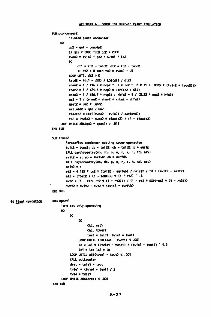
14 Plant operation
APPENDIX 4 - HOUNT ISA SURFACE PLANT SIMULATION
SUB pcondenser2
DO
'closed plate condenser
qc2 • qe2 + COIIIpip2 IF qc2 < 2000 THEN qc2 • 2000 twoc2. twic2 + qc2 I 4.185 I lc2 DO
dt1 • tc2 - tw1c2: dt2 • tc2 - twoc2 IF dt2 < 0 THEN tc2 • twoc2 + .5
LOOP UNTIL dt2 > 0 lltd2 • Cdt1 - dt2) I LOGCdt1 I dt2) rh!w2 • 1 I (16.9 * ncp2 - .2 * lc2 - .8 * (1 + .0075 * (twic2 + tw0c2») rhlr2. 1 I (21.6 * ncp2 * EXP(tc2 I 65» xrk!2 • 1 I (86.7 * ncp2) : rhf!2· 1 I C3.22 * ncp2 * hfc2) ue2 • 1 I Crhlw2 + rhlr2 + xrk!2 + rhf!2) qeat2 • ue2 * latd2 eltlltd2 • qc2 I ue2 tfactc2 • EXPCCtw0c2 - twic2) I 'Itlltd2) tc2 • Ctwfc2 - twoc2 * tfactc2) I C1 - tfactc2)
LOOP WHILE ABS(qc2 - qeat2) > .011 END SUB
SUB tower2
END SUB
'croaaflow condenaer cool fng tower operatfon twit2 • twc2: wb • twft2: db • twft2: p • aurfp CALL paychroaetryCwb, db, p, e, r, I, h, td, aav) swit2 • s: wb • lurfwb: db • lurfdb CALL plychroaetry(wb, db, p, e, r, a, h, td, .av) Mit2 •• rt2 • 4.185 * lc2 * (tv1t2 - aurfwb) I qe1rt2 I td I Cawft2 - aaft2) nt2 • Cfoat2 I C1 - f0at2» * (1 I rt2) - .4 nwt2 • (1 - EXP(-nt2 * (1 - rt2») I (1 - rt2 * EXP(-nt2 * (1 - rt2») twot2 • tv1t2 - nwt2 * (twit2 - surfwb)
SUB opaet1 'one set only operating DO
DO
DO CALL aet1 CALL tower1 test. twic1: twic1 • twot1
LOOP UNTIL ABS(t.at - twot1) < .ocn le. le1 * «twfe1 - twoe1) I (tvfe1 - tout» - 1.5 l.1 • l.: le2. le
LOOP UNTIL ABS(twoe1 - tout) < .ocn CALL bulkcooler dret • tv1e1 - twot tvfe1 • (tvfe1 + twot) I 2 tvfe • tv1e1
LOOP UNTIL ABS(dret) < .ocn END SUB
A-27
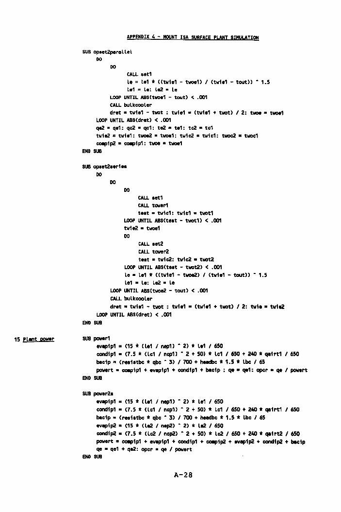
15 PLant power
APPENDIX 4 - MOUNT ISA SURFACE PLANT SIMULATION
SUB opset2perallel DO
DO
CALL set1 Le = Le1 * «twie1 - twoe1) I (twi.1 - tout» - 1.5 le1 = le: le2 • le
LOOP UNTIL ABS(twoe1 - tout) < .001 CALL bulkcooler dret • tw;e1 - twot : twie1 • (twie1 + twot) I 2: twoe. twoe1
LOOP UNTIL ASS(dret) < .001
qe2 • qe1: qc2 • qc1: te2 • t.1: tc2 • tc1 twie2 • twi.1: tw0e2 • twoe1: twic2 • twic1: twoc2 • twoc1 COIIpip2 • COIIpip1: twoe • twoe1
END SUB
SUB opset2a.ri.s DO
DO
DO CALL sen CALL tower1 t.at • twic1: twic1 • twot1
LOOP UNTIL ABS(t.at - twot1) < .001 twi e2 • twoe1 DO
CALL aet2 CALL tower2 teat • twic2: twic2 • twot2
LOOP UNTIL ASS(teat - twot2) < .001 Le • Le1 * «tw1e1 - tw0e2) I (tw1a1 - tout» - 1.5 Le1 • Le: Le2. La
LOOP UNTIL ABS(tw0e2 - tout) < .001 CALL buLkcooLar dret • twi.1 - twot : tvia1 • (tw1.1 + twot) I 2: tvi •• twie2
LOOP UNTIL ABS(dret) < .001 END SUB
SUB power1 ev.pip1 • (15 * (L.1 I nap1) - 2) * L.1 I 650 condip1 • (7.5 * Clc1 I ncpU - 2 + SO) * Lc1 I 650 + 240 * qairt1 I 650 bec1p • (re.i.tbc * qbc - 3) I 700 + headbc * 1.5 * Lbc I 65 powert • COIIpip1 + .v.pip1 + condip1 + becip : q. • qe1: opcr • qe I powert
END SUB
SUB power2a ev.pip1 • (15 * (Le1 I nep1) - 2) * Le1 I 650
condip1 • (7.5 * (Lc1 I ncp1) - 2 + 50) * Lc1 I 650 + 240 * qa1rt1 I 650
becip • (reai.tbc * qbc - 3) I 700 + headbc * 1.5 * Lbc I 65 evapip2 • (15 * Cle2 I nep2) - 2) * Le2 I 650 condip2 • (7.5 * Clc2 I ncp2) - 2 + SO) * Lc2 I 650 + 240 * qairt2 I 650 powert • COIpip1 + evapip1 + condip1 + COIp1p2 + evapip2 + condip2 + blcip qe • qa1 + qe2: opcr • qe I pow.rt
END SUB
A-28