Code of Practice

CODE OF PRACTICE 2007 CODE OF PRACTICE 2007 CODE OF PRACTICE 2007 CODE OF PRACTICE 2007 CODE OF PRACTICE 2007 CODE OF PRACTICE 2007 CODE OF PRACTICE 2007 CODE OF PRACTICE 2007 CODE OF PRACTICE 2007 CODE OF PRACTICE 2007 CODE OF PRACTICE 2007 CODE OF PRACTICE 2007 CODE OF PRACTICE 2007 CODE OF PRACTICE 2007 CODE OF PRACTICE 2007 CODE OF PRACTICE 2007 CODE OF PRACTICE 2007 CODE OF PRACTICE 2007 CODE OF PRACTICE 2007 CODE OF PRACTICE 2007 CODE OF PRACTICE 2007 CODE OF PRACTICE 2007 CODE OF PRACTICE 2007 CODE OF PRACTICE 2007 CODE OF PRACTICE 2007 CODE OF PRACTICE 2007 CODE OF PRACTICE 2007 CODE OF PRACTICE 2007 CODE OF PRACTICE 2007 CODE OF PRACTICE 2007 CODE OF PRACTICE 2007 CODE OF PRACTICE 2007 CODE OF PRACTICE 2007 CODE OF PRACTICE 2007 CODE OF PRACTICE 2007 CODE OF PRACTICE 2007 CODE OF PRACTICE 2007 CODE OF PRACTICE 2007 CODE OF PRACTICE 2007 CODE OF PRACTICE 2007 CODE OF PRACTICE 2007 CODE OF PRACTICE 2007 CODE OF PRACTICE 2007 CODE OF PRACTICE 2007 CODE OF PRACTICE 2007 CODE OF PRACTICE 2007 CODE OF PRACTICE 2007 CODE OF PRACTICE 2007 CODE OF PRACTICE 2007 CODE OF PRACTICE 2007 CODE OF PRACTICE 2007 CODE OF PRACTICE 2007 CODE OF PRACTICE 2007 CODE OF PRACTICE 2007 CODE OF PRACTICE 2007 CODE OF PRACTICE 2007 CODE OF PRACTICE 2007 CODE OF PRACTICE 2007 CODE OF PRACTICE 2007 CODE OF PRACTICE 2007 CODE OF PRACTICE 2007 CODE OF PRACTICE 2007 CODE OF PRACTICE 2007 CODE OF PRACTICE 2007 CODE OF PRACTICE 2007 CODE OF PRACTICE 2007 CODE OF PRACTICE 2007 CODE OF PRACTICE 2007 CODE OF PRACTICE 2007 CODE OF PRACTICE 2007 CODE OF PRACTICE 2007 CODE OF PRACTICE 2007 CODE OF PRACTICE 2007 CODE OF PRACTICE 2007 CODE OF PRACTICE 2007 CODE OF PRACTICE 2007 CODE OF PRACTICE 2007 CODE OF PRACTICE 2007 CODE OF PRACTICE 2007 CODE OF PRACTICE 2007 CODE OF PRACTICE 2007 CODE OF PRACTICE 2007 CODE OF PRACTICE 2007 CODE OF PRACTICE 2007 CODE OF PRACTICE 2007 CODE OF PRACTICE 2007 CODE OF PRACTICE 2007 CODE OF PRACTICE 2007 CODE OF PRACTICE 2007 CODE OF PRACTICE 2007 CODE OF PRACTICE 2007 CODE OF PRACTICE 2007 CODE OF PRACTICE 2007 CODE OF PRACTICE 2007 CODE OF PRACTICE 2007 CODE OF PRACTICE 2007 CODE OF PRACTICE 2007 CODE OF PRACTICE 2007 CODE OF PRACTICE 2007 CODE OF PRACTICE 2007 CODE OF PRACTICE 2007 CODE OF PRACTICE 2007 CODE OF PRACTICE 2007 CODE OF PRACTICE 2007 CODE OF PRACTICE 2007 CODE OF PRACTICE 2007 CODE OF PRACTICE 2007 CODE OF PRACTICE 2007 CODE OF PRACTICE 2007 CODE OF PRACTICE 2007 CODE OF PRACTICE 2007 CODE OF PRACTICE 2007 CODE OF PRACTICE 2007 CODE OF PRACTICE 2007 CODE OF PRACTICE 2007 CODE OF PRACTICE 2007 CODE OF PRACTICE 2007 CODE OF PRACTICE 2007 CODE OF PRACTICE 2007 CODE OF PRACTICE 2007 CODE OF PRACTICE 2007 CODE OF PRACTICE 2007 CODE OF PRACTICE 2007 CODE OF PRACTICE 2007 CODE OF PRACTICE 2007 CODE OF PRACTICE 2007 CODE OF PRACTICE 2007 CODE OF PRACTICE 2007 CODE OF PRACTICE 2007 CODE OF PRACTICE 2007 CODE OF PRACTICE 2007 CODE OF PRACTICE 2007 CODE OF PRACTICE 2007 CODE OF PRACTICE 2007 CODE OF PRACTICE 2007 CODE OF PRACTICE 2007 CODE OF PRACTICE 2007 CODE OF PRACTICE 2007 CODE OF PRACTICE 2007 CODE OF PRACTICE 2007 CODE OF PRACTICE 2007 CODE OF PRACTICE 2007 CODE OF PRACTICE 2007 CODE OF PRACTICE 2007 CODE OF PRACTICE 2007 CODE OF PRACTICE 2007 CODE OF PRACTICE 2007 CODE OF PRACTICE 2007 CODE OF PRACTICE 2007 CODE OF PRACTICE 2007 CODE OF PRACTICE 2007 CODE OF PRACTICE 2007 CODE OF PRACTICE 2007 CODE OF PRACTICE 2007 CODE OF PRACTICE 2007 CODE OF PRACTICE 2007 CODE OF PRACTICE 2007 CODE OF PRACTICE 2007 CODE OF PRACTICE 2007 CODE OF PRACTICE 2007 CODE OF PRACTICE 2007 CODE OF PRACTICE 2007 CODE OF PRACTICE 2007 CODE OF PRACTICE 2007 CODE OF PRACTICE 2007 CODE OF PRACTICE 2007 CODE OF PRACTICE 2007 CODE OF PRACTICE 2007 CODE OF PRACTICE 2007 CODE OF PRACTICE 2007 CODE OF PRACTICE 2007 CODE OF PRACTICE 2007 CODE OF PRACTICE 2007 CODE OF PRACTICE 2007 CODE OF PRACTICE 2007 CODE OF PRACTICE 2007 CODE OF PRACTICE 2007 CODE OF PRACTICE 2007 CODE OF PRACTICE 2007 CODE OF PRACTICE 2007 CODE OF PRACTICE 2007 CODE OF PRACTICE 2007 CODE OF PRACTICE 2007 CODE OF PRACTICE 2007 CODE OF PRACTICE 2007 CODE OF PRACTICE 2007 CODE OF PRACTICE 2007 CODE OF PRACTICE 2007 CODE OF PRACTICE 2007 CODE OF PRACTICE 2007 CODE OF PRACTICE 2007 CODE OF PRACTICE 2007 CODE OF PRACTICE 2007 CODE OF PRACTICE 2007 CODE OF PRACTICE 2007 CODE OF PRACTICE 2007 CODE OF PRACTICE 2007 CODE OF PRACTICE 2007 CODE OF PRACTICE 2007 CODE OF PRACTICE 2007 CODE OF PRACTICE 2007 CODE OF PRACTICE 2007 CODE OF PRACTICE 2007 CODE OF PRACTICE 2007 CODE OF PRACTICE 2007 CODE OF PRACTICE 2007 CODE OF PRACTICE 2007 CODE OF PRACTICE 2007 CODE OF PRACTICE 2007 CODE OF PRACTICE 2007 CODE OF PRACTICE 2007 CODE OF PRACTICE 2007 CODE OF PRACTICE 2007 CODE OF PRACTICE 2007 CODE OF PRACTICE 2007 CODE OF PRACTICE 2007 CODE OF PRACTICE 2007 CODE OF PRACTICE 2007 CODE OF PRACTICE 2007 CODE OF PRACTICE 2007 CODE OF PRACTICE 2007 CODE OF PRACTICE 2007 CODE OF PRACTICE 2007 CODE OF PRACTICE 2007 CODE OF PRACTICE 2007 CODE OF PRACTICE 2007 CODE OF PRACTICE 2007 CODE OF PRACTICE 2007 CODE OF PRACTICE 2007 CODE OF PRACTICE 2007 CODE OF PRACTICE 2007 CODE OF PRACTICE 2007 CODE OF PRACTICE 2007 CODE OF PRACTICE 2007 CODE OF PRACTICE 2007 CODE OF PRACTICE 2007 CODE OF PRACTICE 2007 CODE OF PRACTICE 2007 CODE OF PRACTICE 2007 CODE OF PRACTICE 2007 CODE OF PRACTICE 2007 CODE OF PRACTICE 2007 CODE OF PRACTICE 2007 CODE OF PRACTICE 2007 CODE OF PRACTICE 2007 CODE OF PRACTICE 2007 CODE OF PRACTICE 2007 CODE OF PRACTICE 2007 CODE OF PRACTICE 2007 CODE OF PRACTICE 2007 CODE OF PRACTICE 2007 CODE OF PRACTICE 2007 CODE OF PRACTICE 2007 CODE OF PRACTICE 2007 CODE OF PRACTICE 2007 CODE OF PRACTICE 2007 CODE OF PRACTICE 2007 CODE OF PRACTICE 2007 CODE OF PRACTICE 2007 CODE OF PRACTICE 2007 CODE OF PRACTICE 2007 CODE OF PRACTICE 2007 CODE OF PRACTICE 2007 CODE OF PRACTICE 2007 CODE OF PRACTICE 2007 CODE OF PRACTICE 2007 CODE OF PRACTICE 2007 CODE OF PRACTICE 2007 CODE OF PRACTICE 2007 CODE OF PRACTICE 2007

Staff Working Paper No. 759The cross-sectional spillovers of single stock circuit breakers James Brugler, Oliver Linton, Joseph Noss and Lucas Pedace

October 2018

Staff Working Papers describe research in progress by the author(s) and are published to elicit comments and to further debate. Any views expressed are solely those of the author(s) and so cannot be taken to represent those of the Bank of England or to state Bank of England policy. This paper should therefore not be reported as representing the views of the Bank of England or members of the Monetary Policy Committee, Financial Policy Committee or Prudential Regulation Committee.

Staff Working Paper No. 759The cross-sectional spillovers of single stock circuit breakersJames Brugler,(1) Oliver Linton,(2) Joseph Noss(3) and Lucas Pedace(4)

Abstract

This paper uses transaction data to estimate how single stock circuit breakers on the London Stock Exchange affect other stocks that remain in continuous trading. This ‘spillover’ effect is estimated by calculating the effect of a trading halt on the market quality of stocks that remain in continuous trading and comparing this with the effect of a stock whose absolute returns are of a magnitude nearly sufficient to trigger a trading halt but do not do so. Market quality is measured using a combination of trading costs, volatility and volume. We find that circuit breakers lead to a significant improvement in the liquidity, and reduction in the volatility, of stocks that remain in continuous trading. This might suggest that — at least over the period covered by our data — single stock circuit breakers play an important role in reducing the spillover of poor market quality across stocks.

Key words: Circuit breakers, market microstructure, market quality.

JEL classification: G12, G14, G15, G18.

(1) University of Melbourne. Email: james.brugler@unimelb.edu.au(2) University of Cambridge. Email: obl20@cam.ac.uk (3) Financial Stability Board. Email: joseph.noss@fsb.org(4) Bank of England. Email: lucas.pedace@bankofengland.co.uk

The views expressed in this paper are those of the authors, and not necessarily those of the Bank of England or its committees, nor those of the Financial Stability Board or its committees. We would like to thank Jon Relleen and Rhiannon Sowerbutts for helpful comments, suggestions and advice.

The Bank’s working paper series can be found at www.bankofengland.co.uk/working-paper/staff-working-papers

Publications and Design Team, Bank of England, Threadneedle Street, London, EC2R 8AH Telephone +44 (0)20 7601 4030 email publications@bankofengland.co.uk

© Bank of England 2018 ISSN 1749-9135 (on-line)

2

1 Introduction

Many equity and futures exchanges have mechanisms that suspend trading temporarily

in certain market conditions. These are commonly referred to as circuit breakers. While

the precise form that such mechanisms take differs between exchanges, they are

generally designed to achieve similar goals – that is, to ameliorate excessive and/or

transitory volatility in prices and to reduce incidences of extreme illiquidity. In the

aftermath of the ‘Flash Crash’ in US equities in May 2010, US regulators pointed to the

introduction of circuit breakers on single stocks – as well as a recalibration of market-

wide circuit breakers – as measures that might reduce the likelihood of such an event

reoccurring (U.S. SEC and CFTC, 2010).

 This paper assesses the degree to which circuit breakers activated on single stocks are

associated with more or less orderly trading of other securities that remain in

continuous trading. We refer to this as the ‘spillover effect’ of circuit breakers.1 Ex-ante,

it is unclear whether this spillover effect is positive or negative:

On the one hand, there might be circumstances in which the application of circuit

breakers to one security might forestall a disruption in the price movements of other

securities. In the absence of circuit breakers, shocks in the prices of different securities

can be correlated even if there is no correlation in firm-specific information. This can

arise due, for example, to constraints on the capital and risk taking of financial

intermediaries (e.g. Xiong, 2001; Kyle and Xiong, 2001; Yuan, 2005) and/or if some

types of investor behave in a manner designed to hide their private information as to a

security’s value (Pasquariello, 2007). The superior ability and speed with which

computer-based traders process and update prices based on machine-readable

information (e.g. financial indices) is another potential propagation mechanism for

cross-asset returns as in Jovanovic and Menkveld (2015). In each of these

circumstances, circuit breakers might play a role in dampening these effects by

removing a volatile stock from trading.

On the other hand, particularly during more widespread market disruption, it is possible

that the activation of a circuit breaker on one security might be associated with

increased volatility in other securities. This might be the case when the activation of the

circuit breaker is driven not by individual stock-specific information, but by information

1 Our use of the term ‘spillover effect’ refers to the spillovers across stocks (i.e. in the cross-section). This is in contrast to

the use of the term ‘spillovers’ in Kim and Rhee (1997), for example, which refers to effect of the circuit breaker on the

suspended security over time.

3

that affects the value of a large quantity of securities (e.g. changes in macroeconomic

conditions or the crystallisation of systemic risk). A similar effect might arise if investors

sought to hedge their exposure to the security that had been suspended by trading

other stocks. This is likely to be especially relevant for traders who have incurred mark-

to-market losses in the suspended security and may therefore face margin calls or be

required to reduce their (net) positions to meet leverage ratio requirements.2 The ability

of circuit breakers to transmit stress across markets was one of the factors behind the

market volatility of August 2015 (see Anderson et al. (2015)).

A number of existing papers consider the effect of circuit breakers on the liquidity of the

suspended security itself (see Gerety and Mulherin, 1992; Lauterbach and Ben-Zion,

1993; Lee and Ready, 1994; Corwin and Lipson, 2000; Goldstein and Kavajecz, 2004;

Allan and Bercich, 2017). In addition, Cui and Cozluklu (2016) measure the impact of

circuit breakers for US stocks on other securities that remain in continuous trading.

The unique contribution of this paper, however, is to provide robust empirical evidence

of the spillover effect of single stock circuit breakers on UK stocks traded on the

London Stock Exchange (LSE). To do so, we exploit the discontinuous nature of circuit

breakers on the LSE, whereby a stock is removed from continuous trading (i.e.

experiences a ‘halt’) when its price exceeds a pre-determined reference price, while

other that stocks trade close to this reference price remain in continuous trading (‘near-

halts’). We estimate the effect of the circuit breaker in the stock that experiences an

actual trading halt on the market quality (defined below) of stocks that remain in

continuous trading. We also calculate the market quality of all stocks during an event

where a single stock trades within 1% of a trading halt limit, which we refer to as near-

halts (excluding the event stock). We then match trading halts to near halts with similar

dates and times-of-day, using the nearest-neighbour matching technique of Abadie and

Imbens (2006) and Abadie and Imbens (2011). This technique helps control for

variation in market quality within – and across – trading day(s) (Admati and Pfleiderer,

1988; Chan et al., 1991; Andersen and Bollerslev, 1998).

Market quality is measured as the bid-ask spread, realised volatility, returns, trading

frequency and volume observed in stocks that remain in continuous trading. This notion

of market quality matches that elsewhere in the literature (see O’Hara (1995)). In

particular, that literature captures the transaction cost faced by investors, as well as the 2 Some market analysts covering the Chinese equity markets argued that traders’ unwillingness to hold risk throughout a

trading suspension was one of the key reasons that these mechanisms were seen to exacerbate market volatility in

January of 2016 (Yee and Shen, 2016; Stafford and Wildau, 2016). The Chinese Securities Regulatory Commission

subsequently chose to suspend the use of market-wide circuit breakers on the Shanghai and Shenzhen Stock Exchanges,

less than one week after they were implemented.

4

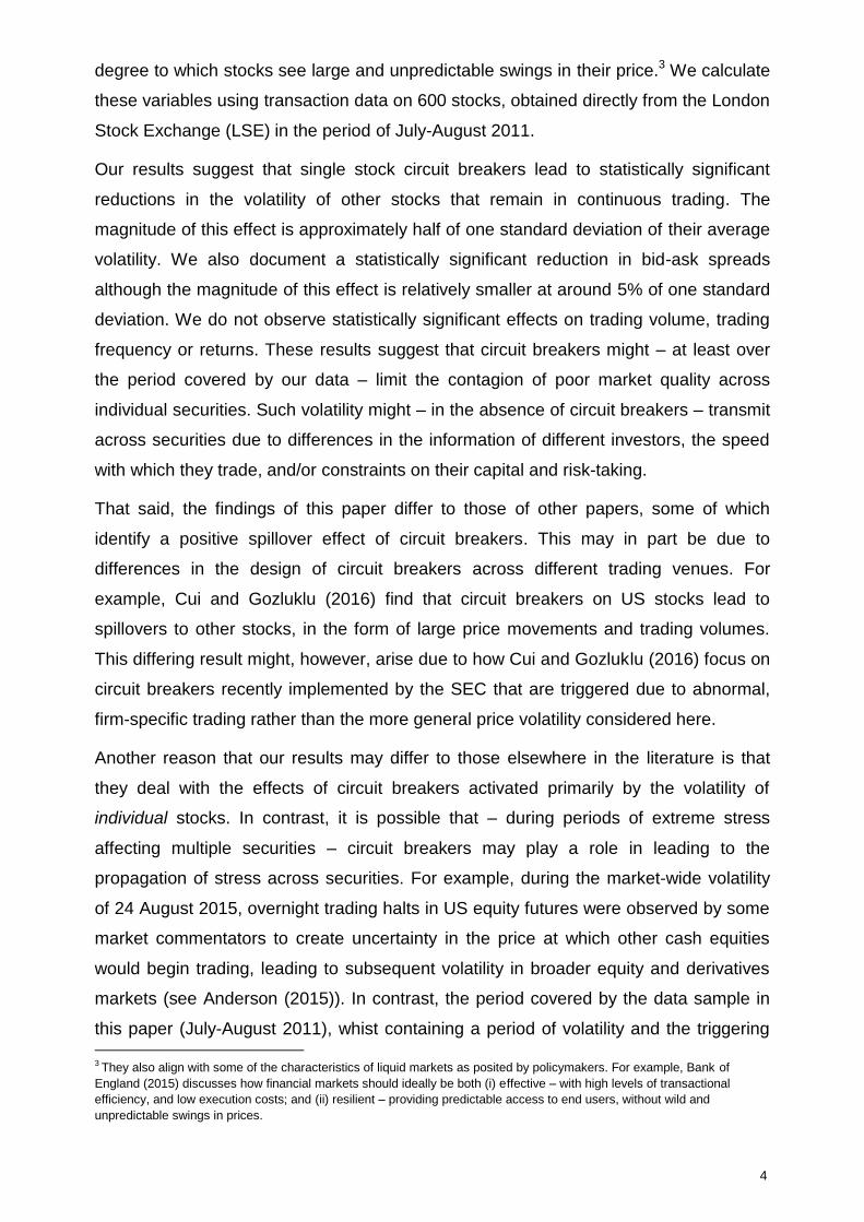
degree to which stocks see large and unpredictable swings in their price.3 We calculate

these variables using transaction data on 600 stocks, obtained directly from the London

Stock Exchange (LSE) in the period of July-August 2011.

Our results suggest that single stock circuit breakers lead to statistically significant

reductions in the volatility of other stocks that remain in continuous trading. The

magnitude of this effect is approximately half of one standard deviation of their average

volatility. We also document a statistically significant reduction in bid-ask spreads

although the magnitude of this effect is relatively smaller at around 5% of one standard

deviation. We do not observe statistically significant effects on trading volume, trading

frequency or returns. These results suggest that circuit breakers might – at least over

the period covered by our data – limit the contagion of poor market quality across

individual securities. Such volatility might – in the absence of circuit breakers – transmit

across securities due to differences in the information of different investors, the speed

with which they trade, and/or constraints on their capital and risk-taking.

That said, the findings of this paper differ to those of other papers, some of which

identify a positive spillover effect of circuit breakers. This may in part be due to

differences in the design of circuit breakers across different trading venues. For

example, Cui and Gozluklu (2016) find that circuit breakers on US stocks lead to

spillovers to other stocks, in the form of large price movements and trading volumes.

This differing result might, however, arise due to how Cui and Gozluklu (2016) focus on

circuit breakers recently implemented by the SEC that are triggered due to abnormal,

firm-specific trading rather than the more general price volatility considered here.

Another reason that our results may differ to those elsewhere in the literature is that

they deal with the effects of circuit breakers activated primarily by the volatility of

individual stocks. In contrast, it is possible that – during periods of extreme stress

affecting multiple securities – circuit breakers may play a role in leading to the

propagation of stress across securities. For example, during the market-wide volatility

of 24 August 2015, overnight trading halts in US equity futures were observed by some

market commentators to create uncertainty in the price at which other cash equities

would begin trading, leading to subsequent volatility in broader equity and derivatives

markets (see Anderson (2015)). In contrast, the period covered by the data sample in

this paper (July-August 2011), whist containing a period of volatility and the triggering 3 They also align with some of the characteristics of liquid markets as posited by policymakers. For example, Bank of

England (2015) discusses how financial markets should ideally be both (i) effective – with high levels of transactional

efficiency, and low execution costs; and (ii) resilient – providing predictable access to end users, without wild and

unpredictable swings in prices.

5

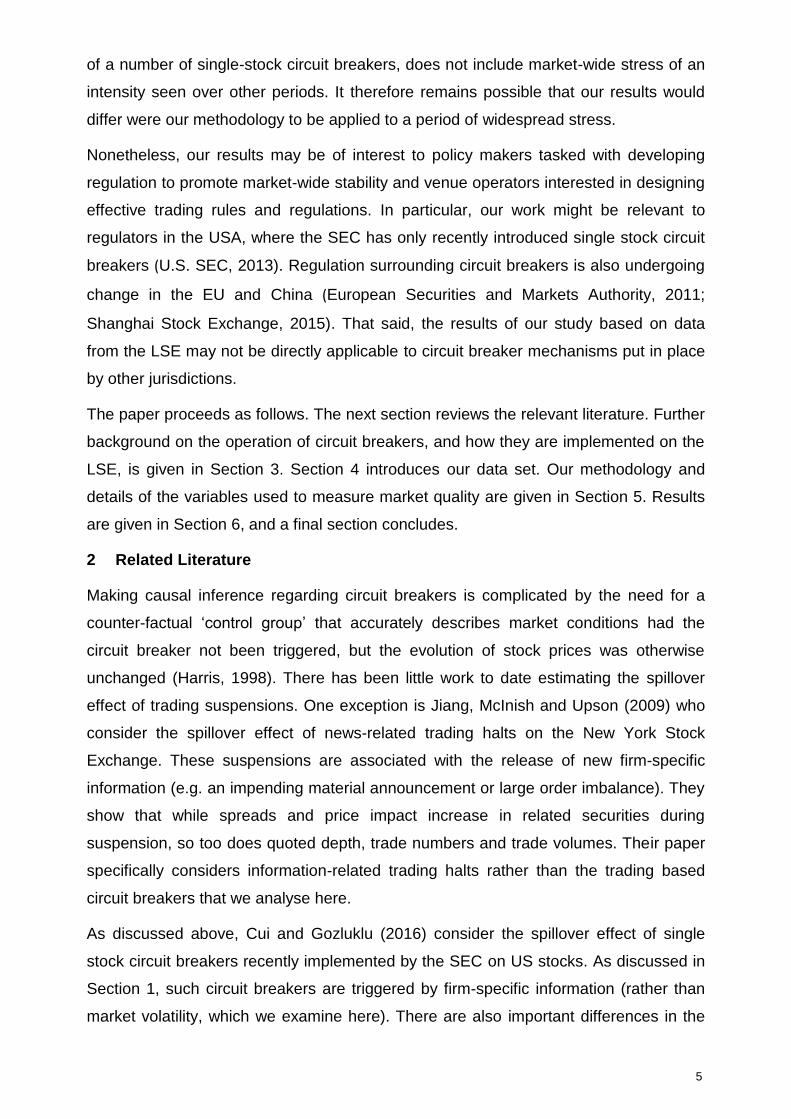
of a number of single-stock circuit breakers, does not include market-wide stress of an

intensity seen over other periods. It therefore remains possible that our results would

differ were our methodology to be applied to a period of widespread stress.

Nonetheless, our results may be of interest to policy makers tasked with developing

regulation to promote market-wide stability and venue operators interested in designing

effective trading rules and regulations. In particular, our work might be relevant to

regulators in the USA, where the SEC has only recently introduced single stock circuit

breakers (U.S. SEC, 2013). Regulation surrounding circuit breakers is also undergoing

change in the EU and China (European Securities and Markets Authority, 2011;

Shanghai Stock Exchange, 2015). That said, the results of our study based on data

from the LSE may not be directly applicable to circuit breaker mechanisms put in place

by other jurisdictions.

The paper proceeds as follows. The next section reviews the relevant literature. Further

background on the operation of circuit breakers, and how they are implemented on the

LSE, is given in Section 3. Section 4 introduces our data set. Our methodology and

details of the variables used to measure market quality are given in Section 5. Results

are given in Section 6, and a final section concludes.

2 Related Literature

Making causal inference regarding circuit breakers is complicated by the need for a

counter-factual ‘control group’ that accurately describes market conditions had the

circuit breaker not been triggered, but the evolution of stock prices was otherwise

unchanged (Harris, 1998). There has been little work to date estimating the spillover

effect of trading suspensions. One exception is Jiang, McInish and Upson (2009) who

consider the spillover effect of news-related trading halts on the New York Stock

Exchange. These suspensions are associated with the release of new firm-specific

information (e.g. an impending material announcement or large order imbalance). They

show that while spreads and price impact increase in related securities during

suspension, so too does quoted depth, trade numbers and trade volumes. Their paper

specifically considers information-related trading halts rather than the trading based

circuit breakers that we analyse here.

As discussed above, Cui and Gozluklu (2016) consider the spillover effect of single

stock circuit breakers recently implemented by the SEC on US stocks. As discussed in

Section 1, such circuit breakers are triggered by firm-specific information (rather than

market volatility, which we examine here). There are also important differences in the

6

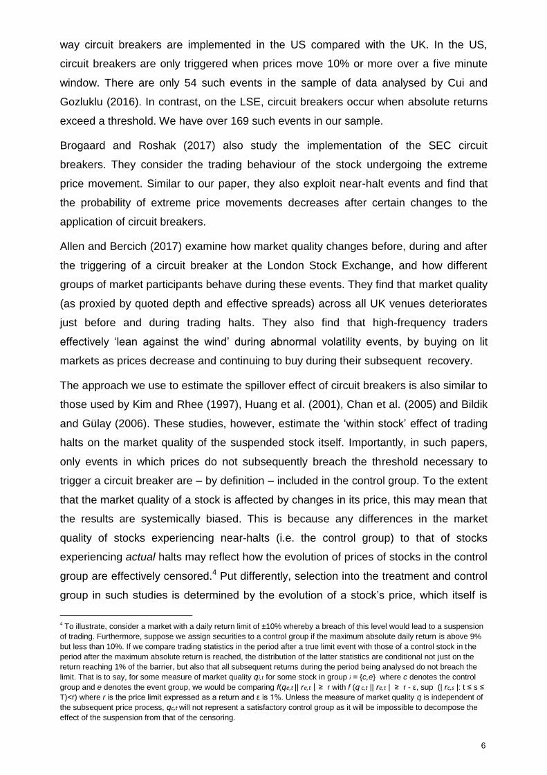
way circuit breakers are implemented in the US compared with the UK. In the US,

circuit breakers are only triggered when prices move 10% or more over a five minute

window. There are only 54 such events in the sample of data analysed by Cui and

Gozluklu (2016). In contrast, on the LSE, circuit breakers occur when absolute returns

exceed a threshold. We have over 169 such events in our sample.

Brogaard and Roshak (2017) also study the implementation of the SEC circuit

breakers. They consider the trading behaviour of the stock undergoing the extreme

price movement. Similar to our paper, they also exploit near-halt events and find that

the probability of extreme price movements decreases after certain changes to the

application of circuit breakers.

Allen and Bercich (2017) examine how market quality changes before, during and after

the triggering of a circuit breaker at the London Stock Exchange, and how different

groups of market participants behave during these events. They find that market quality

(as proxied by quoted depth and effective spreads) across all UK venues deteriorates

just before and during trading halts. They also find that high-frequency traders

effectively ‘lean against the wind’ during abnormal volatility events, by buying on lit

markets as prices decrease and continuing to buy during their subsequent recovery.

The approach we use to estimate the spillover effect of circuit breakers is also similar to

those used by Kim and Rhee (1997), Huang et al. (2001), Chan et al. (2005) and Bildik

and Gülay (2006). These studies, however, estimate the ‘within stock’ effect of trading

halts on the market quality of the suspended stock itself. Importantly, in such papers,

only events in which prices do not subsequently breach the threshold necessary to

trigger a circuit breaker are – by definition – included in the control group. To the extent

that the market quality of a stock is affected by changes in its price, this may mean that

the results are systemically biased. This is because any differences in the market

quality of stocks experiencing near-halts (i.e. the control group) to that of stocks

experiencing actual halts may reflect how the evolution of prices of stocks in the control

group are effectively censored.4 Put differently, selection into the treatment and control

group in such studies is determined by the evolution of a stock’s price, which itself is

4 To illustrate, consider a market with a daily return limit of ±10% whereby a breach of this level would lead to a suspension

of trading. Furthermore, suppose we assign securities to a control group if the maximum absolute daily return is above 9%

but less than 10%. If we compare trading statistics in the period after a true limit event with those of a control stock in the

period after the maximum absolute return is reached, the distribution of the latter statistics are conditional not just on the

return reaching 1% of the barrier, but also that all subsequent returns during the period being analysed do not breach the

limit. That is to say, for some measure of market quality qi,t for some stock in group i = {c,e} where c denotes the control

group and e denotes the event group, we would be comparing f(qe,t || re,t | ≥ r with f (q c,t || re,t | ≥ r - ε, sup (| rc,s |: t ≤ s ≤

T)<r) where r is the price limit expressed as a return and ε is 1%. Unless the measure of market quality q is independent of

the subsequent price process, qc,t will not represent a satisfactory control group as it will be impossible to decompose the

effect of the suspension from that of the censoring.

7

likely to be correlated with our variable of interest – i.e. its market quality. We illustrate

this possibility in the Annex.5

In contrast, in this paper, rather than comparing the effect of market quality of trading

halts versus near halts, we compare the market quality of all stocks during a trading

halt (apart from that experiencing the trading halt) with that of all stocks during a near-

halt (apart from that experiencing the near-halt) at a time/date close to that at which a

trading halt takes place. To the extent that the market quality of these stocks is not

affected by the evolution of the price of the stock that experiences the trading halt, this

means that our results are free of the censoring issue found elsewhere in the literature.

3 Circuit Breakers on the London Stock Exchange

The functioning of trading halts differs significantly across exchanges. Such systems

can, however, be categorized into two types: price limits, where continuous trading is

not stopped but trades are not permitted at any price above or below a predefined level

for a set period of time (typically the remainder of that day); and trading halts, where

continuous trading is stopped for a set period of time. Trading halts may also differ by

whether they apply to a single security or to a number of securities. Table 1 gives a

summary of the different variants of price limits and trading suspension rules in place

on the ten largest equity exchanges by market capitalisation as of December 2015.

These data are taken from World Federation of Exchanges (2016) and the London

Stock Exchange (2016).

5 Annex 1 provides evidence that this censoring issue biases the estimates of the within-stock effect of circuit breakers. To

do so we use a fictitious price limit of ±7% for each stock and estimate the within-stock effect using this price limit. These

results show that exceeding the placebo barrier has a large positive effect on realised variance, volume, trade intensity and

the direction of subsequent returns, despite no actual trading suspension occurring.

8

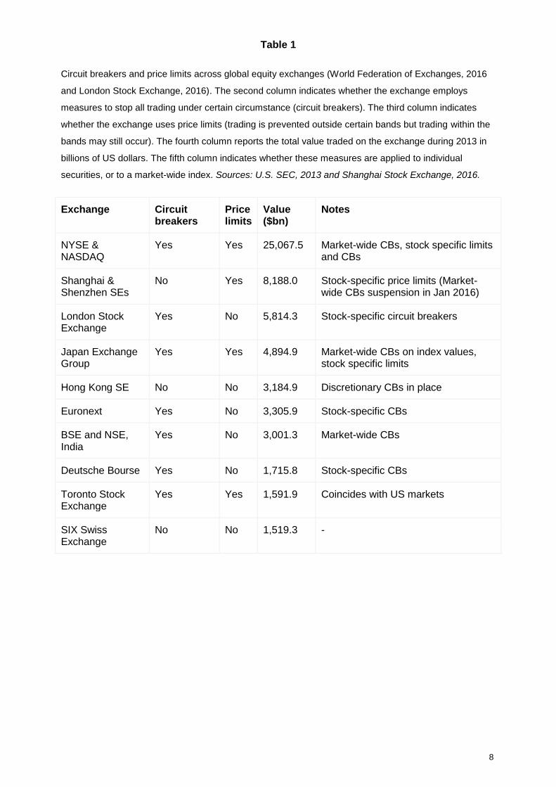
Table 1

Circuit breakers and price limits across global equity exchanges (World Federation of Exchanges, 2016

and London Stock Exchange, 2016). The second column indicates whether the exchange employs

measures to stop all trading under certain circumstance (circuit breakers). The third column indicates

whether the exchange uses price limits (trading is prevented outside certain bands but trading within the

bands may still occur). The fourth column reports the total value traded on the exchange during 2013 in

billions of US dollars. The fifth column indicates whether these measures are applied to individual

securities, or to a market-wide index. Sources: U.S. SEC, 2013 and Shanghai Stock Exchange, 2016.

Exchange Circuit breakers

Price limits

Value ($bn)

Notes

NYSE & NASDAQ

Yes Yes 25,067.5 Market-wide CBs, stock specific limits and CBs

Shanghai & Shenzhen SEs

No Yes 8,188.0 Stock-specific price limits (Market-wide CBs suspension in Jan 2016)

London Stock Exchange

Yes No 5,814.3 Stock-specific circuit breakers

Japan Exchange Group

Yes Yes 4,894.9 Market-wide CBs on index values, stock specific limits

Hong Kong SE No No 3,184.9 Discretionary CBs in place

Euronext Yes No 3,305.9 Stock-specific CBs

BSE and NSE, India

Yes No 3,001.3 Market-wide CBs

Deutsche Bourse Yes No 1,715.8 Stock-specific CBs

Toronto Stock Exchange

Yes Yes 1,591.9 Coincides with US markets

SIX Swiss Exchange

No No 1,519.3 -

9

The London Stock Exchange (LSE) continuously monitors the state of the order

books for stocks with circuit breakers in place. In doing so it compares the price

at which trades are about to take place given the current levels and quantities of

buy/sell orders against two types of reference price:

First, dynamic reference prices are set at certain distances above or below

the price of the last trade in that security.

Second, static reference prices are set at levels above or below the price at

which the last auction for a given security settled (typically the opening

auction).

The thresholds are determined at the level of market sectors and at values that

account for the liquidity of the securities in that sector. All FTSE-100 stocks in

our sample had a dynamic threshold of 5% and a static threshold of 10% during

the time period spanned by our data. For FTSE-250 stocks, all but one had a

static threshold of 10% with dynamic thresholds varying from 5-15%, while for

the least liquid stocks in our sample the static threshold was 25%.

If the price at which a trade would execute breaches either of these reference

prices, this results in either a ‘dynamic’ or ‘static’ trading halt. The market for

that security is suspended temporarily for a period known as an automatic

execution suspension period (AESP). This initially lasts five minutes, and is

followed by an ‘uncrossing auction’ that resumes continuous trading. During this

AESP participants may submit limit and market orders and the exchange

continuously publishes the theoretical price and volume that the uncrossing

auction would generate were it run at any point in time (London Stock Exchange

Group, 2011a).

The suspension can be extended by a predefined period of time if either the

price at which the uncrossing auction would settle deviates by too large an

amount from the previous price generated by continuous trading (referred to as

a price monitoring extension), or if the uncrossing auction would result in

unfilled market orders at the resumption of trading (referred to as a market order

extension). Suspensions also vary in length by a random period of between

zero and thirty seconds before continuous trading resumes. This aims to

remove incentives to enter erroneous orders that would unduly affect price

10

formation towards the end of the auction (London Stock Exchange Group,

2000).

4 Data

We obtain transaction data from the LSE that contains all trades executed for

every listed security between 1 July 2011 and 31 August 2011 (a total of forty-

three trading days). These data cover 3,781 securities listed on the LSE

including shares, exchange-traded funds and products, bonds, warrants and

structured products. The price, volume, and time of each transaction are

recorded to the nearest second, as well as a ‘trade type’ that identifies the trade

as belonging to one of 26 classifications (e.g. ordinary trades, automated

trades, late corrections, contra trades etc). The sample period was chosen as it

contains a relatively large number of circuit breaker events.6 We focus our

analysis on trades executed on the electronic order book for equities that trade

on SETS, the flagship electronic order book of the LSE. Traded securities

include members of the FTSE-100, FTSE-250, Small-Cap, Irish, Secondary

Listing or ‘Other’ market segments.7 

These data comprise a total of 724 equities in these categories with a total of

227 static trading halts in a single security over the sample period. The date and

time of these static trading halts was provided to us by the LSE to the nearest

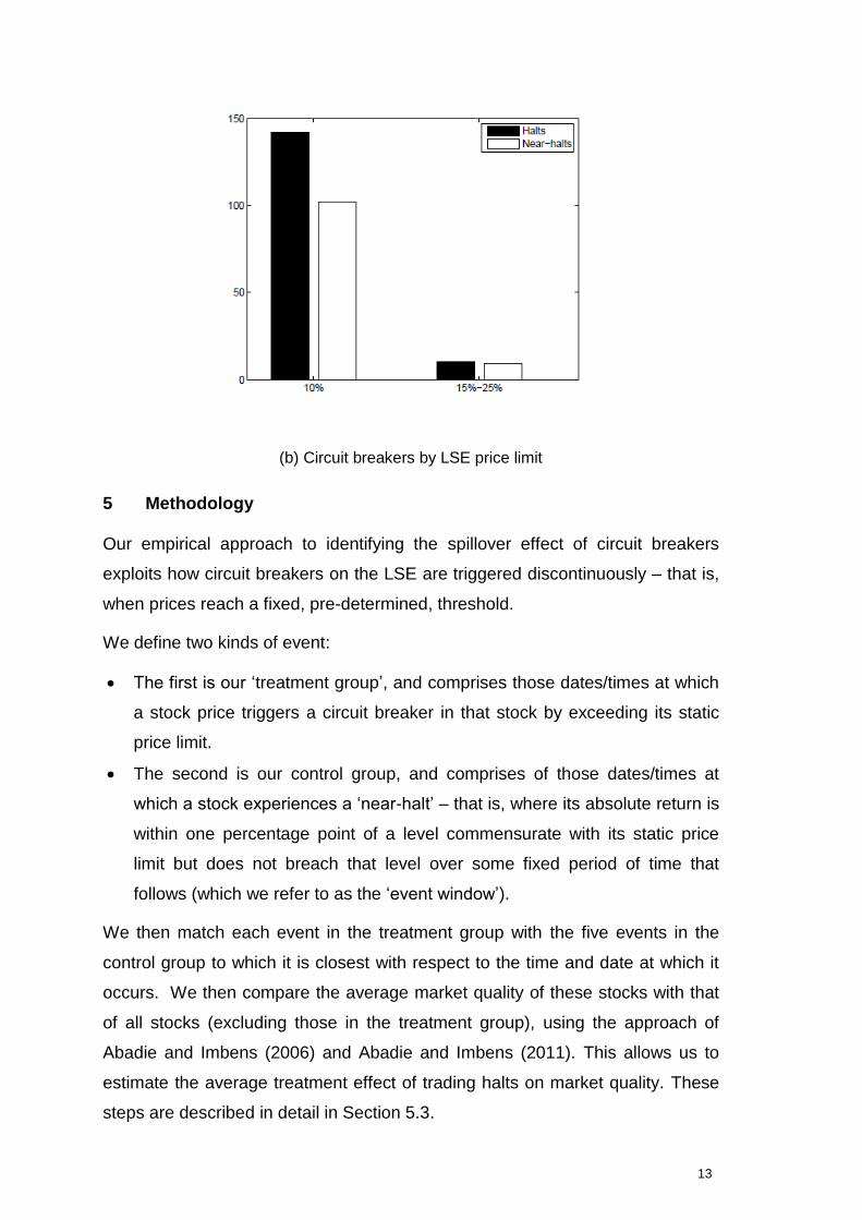
second. The majority of static halts occur in securities whose static price limits

lie 10% above and below the relevant reference price. A small fraction of

securities have price limits of 15% or 25% above and below the reference price.

We focus only on occasions on which static trading halts occur. This is because

our data do not include flags to separate trading halts by type (e.g. static vs

dynamic). In the majority of cases where a static trading halt takes place,

however, the previous trade price of a security is such that a dynamic trading

halt would also have taken place. We therefore end up excluding only

occasions on which only a dynamic – not a static – trading halt takes place.

There are also 183 occasions where the price of at least one security comes to

within one percentage point of its static reference price but does not breach that

6 We do not, however, have access to any larger data set on stocks traded on the LSE with which we might compare the

occurrence of circuit breakers here to that over a longer time period. 7 The ‘other’ segment mainly contains stocks that were once in one of the other market segments listed here but have since

been removed.

11

price over the following 15 minutes of trading.  We define such events as ‘near-

halts’, which – in the analysis that follows – are used as our control group.

For each event, we use the Thompson Reuters Tick History (TRTH) to obtain

the best bid and offer price at one second intervals for every stock that is

present in the exchange-provided data. From this we calculate the bid-ask

spread and realised volatility of mid-quote returns for each security. We match

stock tickers from TRTH to those in the data provided by the LSE and retain

only stocks for which these correspond exactly. This leaves us with a data set

containing a total of 615 stocks, 169 static limit breaches and 135 near-halts (to

which we refer collectively as ‘events’ in the text that follows).

4.1 Summary of trading halt data

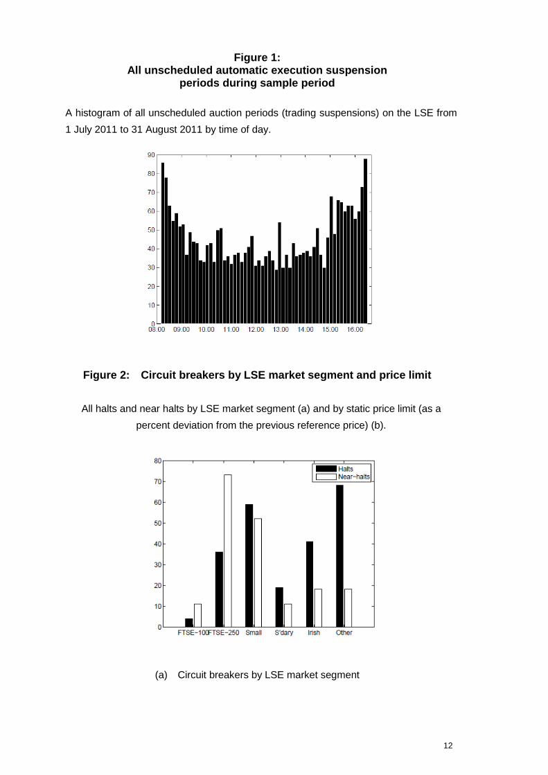
The histogram in Figure 1 shows the timing of all in our sample period across

the trading day. The clustering of events early in the trading day reflects how -

if the opening auction for a given security does not yield a new trade - the static

reference price for that security is set to the previous day’s closing price. This

can sometimes mean that the opening trades in a given security are at a price

sufficient to result in a static halt, even if the change in price on open is

relatively low. Figure 2 shows the number of halts and near-halts in our data by

both market segment and by the level of their associated price limit relative to

the last trade in that security.

12

Figure 1: All unscheduled automatic execution suspension

periods during sample period

A histogram of all unscheduled auction periods (trading suspensions) on the LSE from

1 July 2011 to 31 August 2011 by time of day.

Figure 2: Circuit breakers by LSE market segment and price limit

All halts and near halts by LSE market segment (a) and by static price limit (as a

percent deviation from the previous reference price) (b).

(a) Circuit breakers by LSE market segment

13

(b) Circuit breakers by LSE price limit

5 Methodology

Our empirical approach to identifying the spillover effect of circuit breakers

exploits how circuit breakers on the LSE are triggered discontinuously – that is,

when prices reach a fixed, pre-determined, threshold.

We define two kinds of event:

The first is our ‘treatment group’, and comprises those dates/times at which

a stock price triggers a circuit breaker in that stock by exceeding its static

price limit.

The second is our control group, and comprises of those dates/times at

which a stock experiences a ‘near-halt’ – that is, where its absolute return is

within one percentage point of a level commensurate with its static price

limit but does not breach that level over some fixed period of time that

follows (which we refer to as the ‘event window’).

We then match each event in the treatment group with the five events in the

control group to which it is closest with respect to the time and date at which it

occurs. We then compare the average market quality of these stocks with that

of all stocks (excluding those in the treatment group), using the approach of

Abadie and Imbens (2006) and Abadie and Imbens (2011). This allows us to

estimate the average treatment effect of trading halts on market quality. These

steps are described in detail in Section 5.3.

14

5.1 Definition of market quality variables

We use six simple measures of market quality that are calculated using both the

LSE transaction data and the TRTH quote data.

These are defined as follows:

Realised variance, which is the sum of squared log-returns taken at one

second intervals with respect to the mid-price.

Bid-ask spread, which is the difference between best ask price and best bid

price as a percentage of the mid-price.

Number of trades, in hundreds, and volume traded, in pounds sterling.

The log return over the event window. That is, the log difference between

the price of stock at the beginning and end of the event: (𝑙𝑜𝑔𝑃𝑗𝑡𝑖𝐸+900𝑠 −

𝑙𝑜𝑔𝑃𝑗𝑡𝑖𝐸 , where 𝑡𝑗

𝐸 is the time of the 𝑗𝑡ℎ event).

A ‘Reversals’ dummy variable that indicates whether or not changes in the

price of a stock following a halt or near-halt are in the same direction as the

level of the price limit with respect to the reference price. That is,:

𝑅𝑒𝑣𝑒𝑟𝑠𝑎𝑙𝑖𝑗  =

{

1 𝑖𝑓 𝑠𝑖𝑔𝑛(𝑟𝑗

𝑅𝑃)  =  𝑠𝑖𝑔𝑛(𝑟𝑖𝑗)

0 𝑂𝑡ℎ𝑒𝑟𝑤𝑖𝑠𝑒

(1)

where rjRP

is the percent return on the previous reference price for the

event stock at the commencement of event j and rij is the return during the

post-event period for stock 𝑖 ≠ 𝑗 during event j. For events at the upper

(lower) price limit, 𝑅𝑒𝑣𝑒𝑟𝑠𝑎𝑙𝑖𝑗 takes the value one if the subsequent return in

stock i is positive (negative) and zero otherwise.

When averaged, this variable captures the degree to which a circuit breaker

tends to lead to subsequent returns in the same direction as the breached

limit price. Values close to one indicate that most stocks that remain in

continuous trading have returns in the same direction as the actual or

pseudo price limit that was (or would be) exceeded.

We take logs of all positive variables (realised volatility, bid-ask spreads,

number and volume of trading).8 

8 There were no events in our sample where the average of these variables across all 615 stocks was undefined or equal to zero.

15

We set the length of the event window – over which the control group (near-

halt) events are defined – to 15 minutes. We choose this length of time in order

to cover both the period where the stocks subject to the trading halt (i.e. those

in the treatment group) are not trading, and when they resume continuous

trading. Our choice of a 15 minute window is motivated by how such trading

halts typically last 5 minutes, but can last a little longer (see Section 3).

We measure these statistics over the 15 minute interval after the ‘near halt’

occurs: that is, the time at which a stock’s absolute return becomes within one

percentage point of a level commensurate with the price limit (that is, a return of

of ±9% in the case of a price limit of ±10%). To be classified as a control event,

a stock that reaches one percentage point of the price limit cannot breach that

price limit for at least fifteen minutes. If the stock does breach the actual price

limit within that time, the event would be instead re-classified as a treatment

event with the event time corresponding to the beginning of the trading

suspension.

Events that occur within 15 minutes of the open or close are removed from the

sample. Market quality variables – apart from the reversal dummy – are also

Winsorized at the 1% and 99% level to limit the effect of outliers on parameter

estimates.

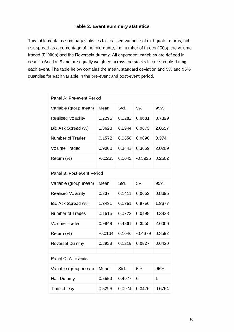
Summary statistics for the market quality variables across all stocks – in both

the 15 minute window prior to and following each event – are shown in Table 2.

Table 3 contains correlations across the market quality variables for the post-

event period. The average bid-ask spread for a stock prior to our events is

approximately 1.4% of the mid-price, realised volatility is approximately 0.23

while these stocks trade approximately once per minute for a total value of

approximately ₤900 during this 15 minute period. In the post-event period (halts

and near-halts), we note there is a modest increase in trading intensity and

volatility and a modest reduction in bid-ask spread. Volatility is positively

correlated to all variables except returns, while bid-ask spreads are only weakly

correlated with trading activity.

Summary statistics are broken down by the treatment and control groups in

Section 5.2.

16

Table 2: Event summary statistics

This table contains summary statistics for realised variance of mid-quote returns, bid-

ask spread as a percentage of the mid-quote, the number of trades (’00s), the volume

traded (₤ ’000s) and the Reversals dummy. All dependent variables are defined in

detail in Section 5 and are equally weighted across the stocks in our sample during

each event. The table below contains the mean, standard deviation and 5% and 95%

quantiles for each variable in the pre-event and post-event period.

Panel A: Pre-event Period

Variable (group mean) Mean Std. 5% 95%

Realised Volatility 0.2296 0.1282 0.0681 0.7399

Bid Ask Spread (%) 1.3623 0.1944 0.9673 2.0557

Number of Trades 0.1572 0.0656 0.0696 0.374

Volume Traded 0.9000 0.3443 0.3659 2.0269

Return (%) -0.0265 0.1042 -0.3925 0.2562

Panel B: Post-event Period

Variable (group mean) Mean Std. 5% 95%

Realised Volatility 0.237 0.1411 0.0652 0.8695

Bid Ask Spread (%) 1.3481 0.1851 0.9756 1.8677

Number of Trades 0.1616 0.0723 0.0498 0.3938

Volume Traded 0.9849 0.4361 0.3555 2.6066

Return (%) -0.0164 0.1046 -0.4379 0.3592

Reversal Dummy 0.2929 0.1215 0.0537 0.6439

Panel C: All events

Variable (group mean) Mean Std. 5% 95%

Halt Dummy 0.5559 0.4977 0 1

Time of Day 0.5296 0.0974 0.3476 0.6764

17

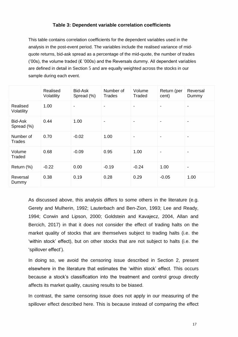
Table 3: Dependent variable correlation coefficients

This table contains correlation coefficients for the dependent variables used in the

analysis in the post-event period. The variables include the realised variance of mid-

quote returns, bid-ask spread as a percentage of the mid-quote, the number of trades

(’00s), the volume traded (₤ ’000s) and the Reversals dummy. All dependent variables

are defined in detail in Section 5 and are equally weighted across the stocks in our

sample during each event.

Realised Volatility

Bid-Ask Spread (%)

Number of Trades

Volume Traded

Return (per cent)

Reversal Dummy

Realised Volatility

1.00 - - - - -

Bid-Ask Spread (%)

0.44 1.00 - - - -

Number of Trades

0.70 -0.02 1.00 - - -

Volume Traded

0.68 -0.09 0.95 1.00 - -

Return (%) -0.22 0.00 -0.19 -0.24 1.00 -

Reversal Dummy

0.38 0.19 0.28 0.29 -0.05 1.00

As discussed above, this analysis differs to some others in the literature (e.g.

Gerety and Mulherin, 1992; Lauterbach and Ben-Zion, 1993; Lee and Ready,

1994; Corwin and Lipson, 2000; Goldstein and Kavajecz, 2004, Allan and

Bercich, 2017) in that it does not consider the effect of trading halts on the

market quality of stocks that are themselves subject to trading halts (i.e. the

‘within stock’ effect), but on other stocks that are not subject to halts (i.e. the

‘spillover effect’).

In doing so, we avoid the censoring issue described in Section 2, present

elsewhere in the literature that estimates the ‘within stock’ effect. This occurs

because a stock’s classification into the treatment and control group directly

affects its market quality, causing results to be biased.

In contrast, the same censoring issue does not apply in our measuring of the

spillover effect described here. This is because instead of comparing the effect

18

on market quality of stocks undergoing trading halts versus near halts, we

instead compare the market quality of all other stocks (apart from that

experiencing the trading halt or the near-halt) during each type of event. The

salience of this censoring issue in measuring the within-stock effect – and the

importance of its being circumvented in this analysis, is demonstrated further in

the Annex.

5.2 Simple comparison of market quality variables across treatment and

control groups pre and post-events

Although we can be sure that our identification technique does not suffer from

the direct censoring issue described above, it is possible that our methodology

introduces a second-order censoring effect whereby more volatile periods of

trading are less likely to be represented in stocks in the control group. This is

because – by definition – stocks giving rise to events in the control group cannot

breach their price limit for the duration of the event window (otherwise they

would be classified in the treatment group).

We therefore compare the average market quality across treatment and control

groups over a short window preceding the time of the event (the time of breach

of the price limit or the time of crossing within one percentage point of the price

limit without triggering a suspension over the 15 minute event window). Were

such measures of market quality to differ between the treatment and control

groups prior to the application of the circuit breaker, then this might suggest the

presence of such second-order censoring.

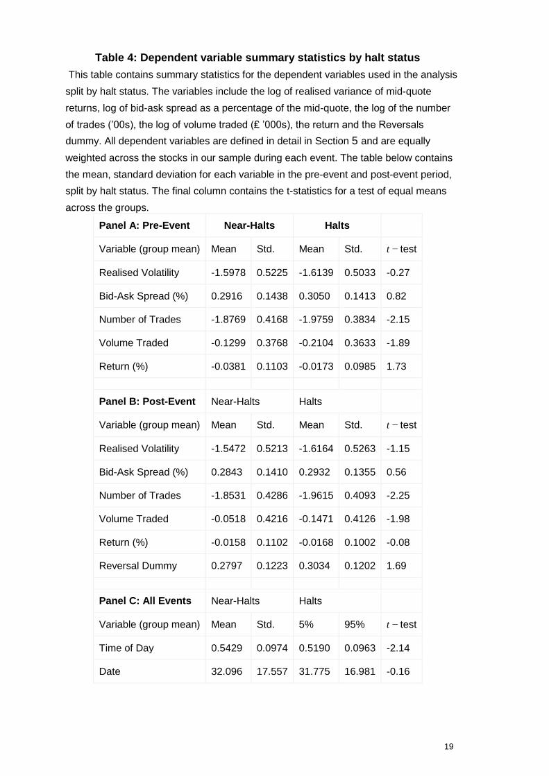
The means and standard deviations of each of the market quality variables –

split out by the halt/near-halt events – are given in Panel A of Table 4 along with

the t-statistic testing for any difference between the means. We fail to reject the

null hypothesis that there is no difference in the realised volatility and bid ask-

spread between the halt and near-halt stocks in the pre-event period at the 10%

significance level. This suggests that the halt and near-halt event groups have

roughly similar levels of volatility and liquidity. There, is however, some weak

evidence that trading volumes and frequency are lower in the pre-event period

for the halt group.

19

Table 4: Dependent variable summary statistics by halt status

This table contains summary statistics for the dependent variables used in the analysis

split by halt status. The variables include the log of realised variance of mid-quote

returns, log of bid-ask spread as a percentage of the mid-quote, the log of the number

of trades (’00s), the log of volume traded (₤ ’000s), the return and the Reversals

dummy. All dependent variables are defined in detail in Section 5 and are equally

weighted across the stocks in our sample during each event. The table below contains

the mean, standard deviation for each variable in the pre-event and post-event period,

split by halt status. The final column contains the t-statistics for a test of equal means

across the groups.

Panel A: Pre-Event Near-Halts Halts

Variable (group mean) Mean Std. Mean Std. t − test

Realised Volatility -1.5978 0.5225 -1.6139 0.5033 -0.27

Bid-Ask Spread (%) 0.2916 0.1438 0.3050 0.1413 0.82

Number of Trades -1.8769 0.4168 -1.9759 0.3834 -2.15

Volume Traded -0.1299 0.3768 -0.2104 0.3633 -1.89

Return (%) -0.0381 0.1103 -0.0173 0.0985 1.73

Panel B: Post-Event Near-Halts Halts

Variable (group mean) Mean Std. Mean Std. t − test

Realised Volatility -1.5472 0.5213 -1.6164 0.5263 -1.15

Bid-Ask Spread (%) 0.2843 0.1410 0.2932 0.1355 0.56

Number of Trades -1.8531 0.4286 -1.9615 0.4093 -2.25

Volume Traded -0.0518 0.4216 -0.1471 0.4126 -1.98

Return (%) -0.0158 0.1102 -0.0168 0.1002 -0.08

Reversal Dummy 0.2797 0.1223 0.3034 0.1202 1.69

Panel C: All Events Near-Halts Halts

Variable (group mean) Mean Std. 5% 95% t − test

Time of Day 0.5429 0.0974 0.5190 0.0963 -2.14

Date 32.096 17.557 31.775 16.981 -0.16

20

For completeness, Panel B also shows the mean and standard deviation of

market quality variables in the period immediately after halts/near-halts. A naïve

comparison of these would lead to a conclusion that halts reduce trading

frequency and volume, induce a greater proportion of stocks to move in the

direction of the limit and have no effect on liquidity or volatility. But Panel C of

Table 4 also demonstrates the importance of controlling for time-of-day effects.

This is because on average, halts occur earlier in the day than do near-halts.

This demonstrates the importance of controlling for time-of-day periodicity in

volatility and liquidity.

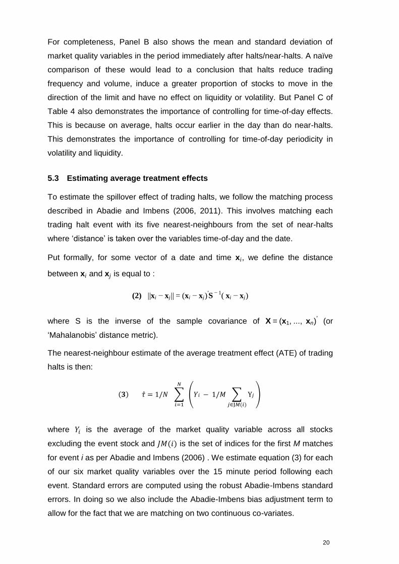
5.3 Estimating average treatment effects

To estimate the spillover effect of trading halts, we follow the matching process

described in Abadie and Imbens (2006, 2011). This involves matching each

trading halt event with its five nearest-neighbours from the set of near-halts

where ‘distance’ is taken over the variables time-of-day and the date.

Put formally, for some vector of a date and time xi, we define the distance

between xi and xj is equal to :

(2) ||xi − xj || = (xi − xj)′S − 1( xi − xj)

where S is the inverse of the sample covariance of X = (x1, ...,  xn)′ (or

‘Mahalanobis’ distance metric).

The nearest-neighbour estimate of the average treatment effect (ATE) of trading

halts is then:

(𝟑) �� = 1/𝑁  ∑ (𝑌𝑖  −  1/𝑀 ∑ Y𝑗

𝑗∈J𝑀(𝑖)

)

𝑁

𝑖=1

where 𝑌𝑖 is the average of the market quality variable across all stocks

excluding the event stock and 𝐽𝑀(𝑖) is the set of indices for the first M matches

for event i as per Abadie and Imbens (2006) . We estimate equation (3) for each

of our six market quality variables over the 15 minute period following each

event. Standard errors are computed using the robust Abadie-Imbens standard

errors. In doing so we also include the Abadie-Imbens bias adjustment term to

allow for the fact that we are matching on two continuous co-variates.

21

The treatment effect parameter 𝜏 is the average treatment effect of circuit

breakers across all measures of market quality. Since we are interested in

spillover effects of circuit breakers rather than their effect on the suspended

stocks, defining our observations of market quality at the market level allows us

to interpret 𝜏 as the expected change in market quality on stocks in the

treatment group due to a trading halt while accounting for potential error

dependence across stocks within an event (i.e. clustering of errors at the event

level).

6 Results

Table 6 gives estimates of the treatment effect estimates given in equation (3)

for the six market quality variables. The second column contains the estimate of

𝜏 for each of the market quality variables, the third and fourth column are robust

standard errors and associated z-statistics and the fifth column represents the

magnitude of treatment effect in the second column divided by the standard

deviation of the dependent variable. This column is included to assess the

economic significance of the ATEs for each variable.

Table 6 shows that that circuit breakers lead to statistically significant reductions

in volatility and liquidity for stocks that remain in continuous trading. In the case

of volatility, the magnitude of the estimated ATE of circuit breakers is

economically large and is equal to approximately 50% of the sample standard

deviation. We estimate that circuit breakers lead to a fall of only approximately

5% in the bid-ask spread of the treatment group relative to the control group,

although this is statistically significant at the 5% level. For volume and number

of trades, the ATE is estimated to be negative, but is significant at the 10% level

for number of trades. The ATE for the reversals dummy is positive but

insignificant at the 10% level and insignificant for the log return.

22

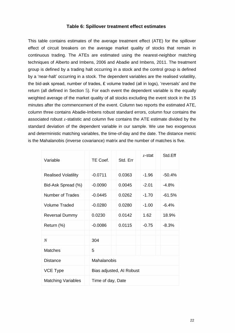
Table 6: Spillover treatment effect estimates

This table contains estimates of the average treatment effect (ATE) for the spillover

effect of circuit breakers on the average market quality of stocks that remain in

continuous trading. The ATEs are estimated using the nearest-neighbor matching

techniques of Alberto and Imbens, 2006 and Abadie and Imbens, 2011. The treatment

group is defined by a trading halt occurring in a stock and the control group is defined

by a ‘near-halt’ occurring in a stock. The dependent variables are the realised volatility,

the bid-ask spread, number of trades, ₤ volume traded (all in logs), ‘reversals’ and the

return (all defined in Section 5). For each event the dependent variable is the equally

weighted average of the market quality of all stocks excluding the event stock in the 15

minutes after the commencement of the event. Column two reports the estimated ATE,

column three contains Abadie-Imbens robust standard errors, column four contains the

associated robust z-statistic and column five contains the ATE estimate divided by the

standard deviation of the dependent variable in our sample. We use two exogenous

and deterministic matching variables, the time-of-day and the date. The distance metric

is the Mahalanobis (inverse covariance) matrix and the number of matches is five.

Variable TE Coef. Std. Err z-stat Std.Eff

Realised Volatility -0.0711 0.0363 -1.96 -50.4%

Bid-Ask Spread (%) -0.0090 0.0045 -2.01 -4.8%

Number of Trades -0.0445 0.0262 -1.70 -61.5%

Volume Traded -0.0280 0.0280 -1.00 -6.4%

Reversal Dummy 0.0230 0.0142 1.62 18.9%

Return (%) -0.0086 0.0115 -0.75 -8.3%

N 304

Matches 5

Distance Mahalanobis

VCE Type Bias adjusted, AI Robust

Matching Variables Time of day, Date

23

Taken together, we conclude that trading halts are associated with a reduction

in both the bid-ask spread and price volatility of securities that remain in trading.

This suggests that single stock circuit breakers may stem the sorts of

mechanisms described by Xiong (2001), Kyle and Xiong (2001), Yuan (2005),

Pasquariello (2007) and Jovanovic and Menkveld (2015) that might otherwise

lead to the spread of volatility between stocks. Such mechanisms include the

effect of differences in investors’ private information on the value of individual

securities, differences in the speed with which they can process – and trade

upon – information, and the effects of constraints on investors’ risk taking and

capital. The single stock circuit breakers examined in this paper may play a role

in dampening these effects. This conclusion is also consistent with the findings

of the LSE who argue that trading halts are successful in maintaining orderly

trading without excessively hindering change in price consistent with ‘genuine

market sentiment’ (London Stock Exchange Group, 2011b).

That said, as discussed in the introduction, these findings differ to those

elsewhere in the literature.

First, they run contrary to those of Cui and Gozluklu (2016), who find that circuit

breakers on US stocks lead to spillovers to other stocks, in the form of large

price movements and trading volumes. This differing result might, however,

arise due to how Cui and Gozluklu (2016) focus on circuit breakers recently

implemented by the SEC that are triggered due to abnormal, firm-specific

trading rather than the more general price volatility considered here.

More substantively, however, they also differ to the empirical effects of trading

halts on the LSE witnessed during periods of more widespread market stress

that affects multiple securities. For example, during the intense market volatility

of 24 August 2015, overnight trading halts in US equity futures were observed

by some market commentators to create uncertainty in the price at which other

cash equities would begin trading, leading to subsequent volatility in broader

equity and derivatives markets (see Anderson et al, (2015)). Such contagion

may be due to the withdrawal of market-making activity by investors that use

information in one security when posting quotes in another security (Cespa and

Foucault (2014)). When prices become less informative, liquidity providers

worsens face greater uncertainty and post wider quotes.

24

That our results find the opposite effect – i.e. that trading halts do not give rise

to such contagion – may be due to how the period covered by the data sample

in this paper (July - August 2011) does not include market-wide stress of an

intensity seen over other periods. It remains possible, therefore, that our results

would differ were our methodology to be applied to a period of systemic market

stress – particularly of the sort that caused the withdrawal of risk taking seen

during August 2015.

6.1 Robustness of matching procedure

In our analysis we match events in the treatment and control groups via

exogenous and deterministic variables (time-of-day and date). As discussed in

Section 5, this has the advantage of not using variables that are likely to be

endogenous to the selection of events into treatment (circuit breaker) and

control (near-halts) groups. But it does potentially come at the cost of meaning

that such matching variables may not be sufficient to form adequate control

groups for the trading suspensions.

In this subsection we therefore investigate the adequacy of the control group

produced by our matching procedure. We do so by using the estimation

procedure outlined in Section 5.2 to estimate the average treatment effect of a

trading halt on the market quality of securities not experiencing a trading halt

during the period immediately prior to a halt or near-halt occurring on other

securities. If our matching procedure is forming adequate control groups, this

treatment effect should be insignificant.

Table 7 contains the parameter estimates for the ATE in the pre-event period.

The fourth column shows the relevant z-statistics. These suggest that the

treatment effect in the pre-event period is insignificant at the 5% level and all

but one are insignificant at the 10% level (number of trades). We therefore fail

to reject a null of there being no difference between treatment and control group

in the pre-event period at the 5% level for each dependent variable individually.

This provides further validation of our estimation approach. We also estimate

our treatment effect parameters using the inverse variance weighting matrix

rather than the Mahalanobis weighting matrix, and also using only one nearest-

neighbour match rather than five nearest-neighbours. This yields qualitatively

similar results.

25

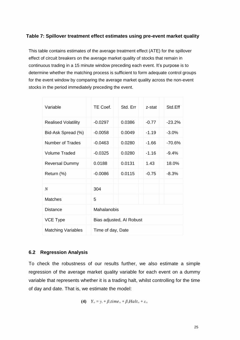
Table 7: Spillover treatment effect estimates using pre-event market quality

This table contains estimates of the average treatment effect (ATE) for the spillover

effect of circuit breakers on the average market quality of stocks that remain in

continuous trading in a 15 minute window preceding each event. It’s purpose is to

determine whether the matching process is sufficient to form adequate control groups

for the event window by comparing the average market quality across the non-event

stocks in the period immediately preceding the event.

Variable TE Coef. Std. Err z-stat Std.Eff

Realised Volatility -0.0297 0.0386 -0.77 -23.2%

Bid-Ask Spread (%) -0.0058 0.0049 -1.19 -3.0%

Number of Trades -0.0463 0.0280 -1.66 -70.6%

Volume Traded -0.0325 0.0280 -1.16 -9.4%

Reversal Dummy 0.0188 0.0131 1.43 18.0%

Return (%) -0.0086 0.0115 -0.75 -8.3%

N 304

Matches 5

Distance Mahalanobis

VCE Type Bias adjusted, AI Robust

Matching Variables Time of day, Date

6.2 Regression Analysis

To check the robustness of our results further, we also estimate a simple

regression of the average market quality variable for each event on a dummy

variable that represents whether it is a trading halt, whilst controlling for the time

of day and date. That is, we estimate the model:

(4) Y i t = γ t + β1time i t + β2Halt i t + ε i t

26

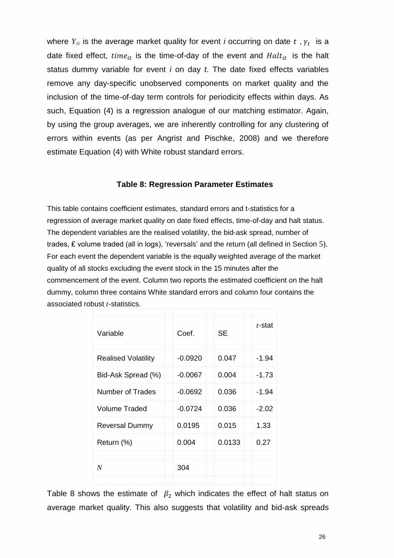
where Yit is the average market quality for event i occurring on date 𝑡 , 𝛾𝑡 is a

date fixed effect, 𝑡𝑖𝑚𝑒𝑖𝑡 is the time-of-day of the event and 𝐻𝑎𝑙𝑡𝑖𝑡  is the halt

status dummy variable for event i on day t. The date fixed effects variables

remove any day-specific unobserved components on market quality and the

inclusion of the time-of-day term controls for periodicity effects within days. As

such, Equation (4) is a regression analogue of our matching estimator. Again,

by using the group averages, we are inherently controlling for any clustering of

errors within events (as per Angrist and Pischke, 2008) and we therefore

estimate Equation (4) with White robust standard errors.

Table 8: Regression Parameter Estimates

This table contains coefficient estimates, standard errors and t-statistics for a

regression of average market quality on date fixed effects, time-of-day and halt status.

The dependent variables are the realised volatility, the bid-ask spread, number of

trades, ₤ volume traded (all in logs), ‘reversals’ and the return (all defined in Section 5).

For each event the dependent variable is the equally weighted average of the market

quality of all stocks excluding the event stock in the 15 minutes after the

commencement of the event. Column two reports the estimated coefficient on the halt

dummy, column three contains White standard errors and column four contains the

associated robust t-statistics.

Variable Coef. SE t-stat

Realised Volatility -0.0920 0.047 -1.94

Bid-Ask Spread (%) -0.0067 0.004 -1.73

Number of Trades -0.0692 0.036 -1.94

Volume Traded -0.0724 0.036 -2.02

Reversal Dummy 0.0195 0.015 1.33

Return (%) 0.004 0.0133 0.27

N 304

Table 8 shows the estimate of 𝛽2 which indicates the effect of halt status on

average market quality. This also suggests that volatility and bid-ask spreads

27

are lower in the halt group relative to the near-halt group, although we can only

reject the null of no effect at the 10% level for these variables in the panel

model. We do, however, find economically larger effects on trading activity and

can reject a test of no effect of halt status on volume traded at the 5% level.

Again we find an insignificant effect on returns and the reversals dummy.

7 Conclusion

This paper uses transaction data to investigate how single stock circuit breakers

on the LSE affect the market quality of stocks that remain in continuous trading.

To do so it exploits the discontinuous nature of trading halts on the LSE, which

are triggered if the absolute percentage change in the price of a stock breaches

some predetermined threshold, relative to that of the last trade or exchange

auction. Our approach estimates the average treatment effect of trading halts

on the market quality of stocks that remain in continuous trading relative to that

of a control group of events. This control group is comprised of events where a

single stock undergoes a price change of a magnitude nearly sufficient to trigger

a trading halt, at a time and date similar to that at which the treatment group

experiences an actual trading halt.

Our results suggest that – at least over the period covered by our data – single

stock trading halts lead to significant reductions in volatility and bid-ask spreads

of stocks that remain in continuous trading. This may support the suggestion in

the theoretical literature that in the absence of circuit breakers volatility can

pass between stocks. These might occur due the effects of heterogeneous

information, differences in the speed with which investors process – and react

to – new information, and the effect of their capital constraints.

We also demonstrate the robustness of our methodology by showing that it

generates a control group of stocks that have statistically similar market quality

in a short window prior to a circuit breaker or control event occurring. These

results might suggest that – at least over the period covered by our data –

single-stock circuit breakers help ameliorate the scope for contagion of poor

market quality between securities.

These results differ to some of those elsewhere in the literature. In particular,

they differ to evidence of a significant spillover effect from single-stock circuit

breakers on US equity markets (Cui and Gozluklu (2016)) that are triggered due

28

to abnormal, firm-specific trading rather than the more general price volatility

considered here. More substantively, they also differ from evidence as to the

effects of trading halts during periods of more widespread market stress, where

trading halts have led to contagion of volatility across securities. Further work

could therefore apply the methodology used here to data covering such periods

of market-wide stress.

Further work could also usefully investigate how trading on other trading venues

is affected by the activation of trading halts on the LSE. It could usefully

examine the effect of circuit breakers applied at the level of stock indices – as,

for example, is the case on the Tokyo Stock Exchange. Such alternative types

of circuit breaker may differ in their effect on other related securities, to those

applied to single stocks.

29

References

Mathew Allen, Justin Bercich “Catching a falling knife: an analysis of circuit breakers in

UK equity markets”, Financial Conduct Authority, September 2017.

Alberto Abadie, Guido W Imbens: “Bias-corrected matching estimators for average

treatment effects”, Journal of Business & Economic Statistics, pp. 1—11, 2011.

Alberto Abadie, Guido Imbens: “Large Sample Properties of Matching Estimators for

Average Treatment Effects”, Econometrica, 2006.

Anat R Admati, Paul Pfleiderer: “A theory of intraday patterns: Volume and price

variability”, The Review of Financial Studies, pp. 3—40, 1988.

Niki Anderson, Lewis Webber, Joseph Noss, Daniel Beale and Liam Crowley-Reidy:

“The resilience of Market liquidity”, Bank of England Financial Stability Paper No. 34,

2015.

T G Andersen, T Bollerslev: “Deutsche mark—dollar volatility: Intraday activity

patterns, macroeconomic announcements, and longer run dependencies”, Journal of

Finance, pp. 219—265, 1998.

Joshua D Angrist, Jorn-Steffen Pischke: Mostly harmless econometrics: An empiricist's

companion. Princeton University Press, 2008.

Bank of England (2015); Financial Stability Report.

Recep Bildik, Guzhan Gulay: “Are price limits effective? Evidence from the Istanbul

Stock Exchange”, Journal of Financial Research, pp. 383—403, 2006.

Jonathan Brogaard, Kevin Roshak: “Prices and Price Limits”, Available at SSRN

2667104, 2017.

Giovanni Cespa, Thierry Foucault: “Illiquidity contagion and liquidity crashes”, Review

of Financial Studies, pp. 1615—1660, 2014.

Kalok Chan, Kakeung C Chan, G Andrew Karolyi: “Intraday volatility in the stock index

and stock index futures markets”, The Review of Financial Studies, pp. 657—684,

1991.

Soon Huat Chan, Kenneth A Kim, S Ghon Rhee: “Price limit performance: Evidence

from transactions data and the limit order book”, Journal of Empirical Finance, pp.

269—290, 2005.

30

S.A. Corwin, M.L. Lipson: “Order flow and liquidity around NYSE trading halts”, Journal

of Finance, pp. 1771—1805, 2000.

Bei Cui, Arie E Gozluklu: “Intraday rallies and crashes: spillovers of trading halts”,

International Journal of Finance & Economics, pp. 472—501, 2016.

European Securities, Markets Authority: “Consultation paper: Guidelines on systems

and controls in a highly automated trading environment for trading platforms,

investment firms and competent authorities”. 2011.

European Securities, Markets Authority: Consultation paper: Guidelines on systems

and controls in a highly automated trading environment for trading platforms,

investment firms and competent authorities. 2011. Accessed 25th Sep 2015.

M.S. Gerety, J.H. Mulherin: “Trading Halts and Market Activity: An Analysis of Volume

at the Open and the Close”, Journal of Finance, pp. 1765—84, 1992.

M.A. Goldstein, K.A. Kavajecz: “Trading strategies during circuit breakers and extreme

market movements”, Journal of Financial Markets, pp. 301—333, 2004.

L. Harris: “Circuit breakers and program trading limits: The lessons learned”,

Brookings-Wharton papers on financial services, pp. 17—47, 1998.

Lawrence Harris: “Circuit breakers and program trading limits: What have we learned”,

Brookings-Wharton papers on financial services, 1998.

Yen-Sheng Huang, Tze-Wei Fu, Mei-Chu Ke: “Daily price limits and stock price

behavior: Evidence from the Taiwan stock exchange”, International Review of

Economics & Finance, pp. 263—288, 2001.

Christine Jiang, Thomas McInish, James Upson: “The information content of trading

halts”, Journal of Financial Markets, pp. 703—726, 2009.

Boyan Jovanovic, Albert Menkveld: “Middlemen in securities markets”, Available at

SSRN 1624329, 2015.

K. Kim, S.G. Rhee: “Price Limit Performance: Evidence from the Tokyo Stock

Exchange”, Journal of Finance, pp. 885—99, 1997.

Albert S Kyle, Wei Xiong: “Contagion as a wealth effect”, The Journal of Finance, pp.

1401—1440, 2001.

31

B. Lauterbach, U. Ben-Zion: “Stock Market Crashes and the Performance of Circuit

Breakers: Empirical Evidence”, Journal of Finance, pp. 1909—1925, 1993.

CMC Lee, MJ Ready, PJ Seguin: “Volume, Volatility, and New York Stock Exchange

Trading Halts”, Journal of Finance, pp. 183—214, 1994.

London Stock Exchange Group: Guide to the New Trading System Issue 7.1. 2011.

Accessed 24th Jan 2013.

London Stock Exchange Group: LSEG Response to ESMA Consultation: "Guidelines

on systems and controls in a highly automated trading environment for trading

platforms, investment firms and competent authorities" ESMA/2011/224. 2011.

Accessed 1st Aug 2014.

London Stock Exchange Group: Main Market Factsheet, Dec 15. 2015. Accessed 8th

Jan 2016.

London Stock Exchange Group: Market Enahancements Release 3.1 Worked

Examples. 2000. Accessed 27th Nov 2012.

Maureen O’Hara: “Market Microstructure Theory”. Blackwell Publishers. 1995.

Paolo Pasquariello: “Imperfect competition, information heterogeneity, and financial

contagion”, Review of Financial Studies, pp. 391—426, 2007.

Shanghai Stock Exchange: SSE, SZSE, CFFEX Issue Rules for Circuit Breaker

Mechanism for Index. 2015. Accessed 20th Jan 2016.

Philip Stafford, Gabriel Wildau: “China u-turn stokes circuit breaker debate”, The

Financial Times, 2016. Accessed 15th Jan 2016.

U.S. SEC & CFTC: Findings Regarding the Market Events of May 6, 2010. 2010.

Accessed 10th Dec 2013.

U.S. SEC: Investor Bulletin: New Measures to Address Market Volatility. 2013.

Accessed 10th Dec 2013.

World Federation of Exchanges: Monthly Reports. 2015. Accessed 12th Jan 2016.

Wei Xiong: “Convergence trading with wealth effects: an amplification mechanism in

financial markets”, Journal of Financial Economics, pp. 247—292, 2001.

32

Lee Chyen Yee, Samuel Shen: “China suspends market circuit breaker mechanism

after stock market rout”, Reuters, 2016. Accessed 15th Jan 2016.

Kathy Yuan: “Asymmetric price movements and borrowing constraints: A rational

expectations equilibrium model of crises, contagion, and confusion”, The Journal of

Finance, pp. 379—411, 2005.

Kathy Yuan: “Asymmetric price movements and borrowing constraints: A rational

expectations equilibrium model of crises, contagion, and confusion”, The Journal of

Finance, pp. 379—411, 2005.

33

Annex

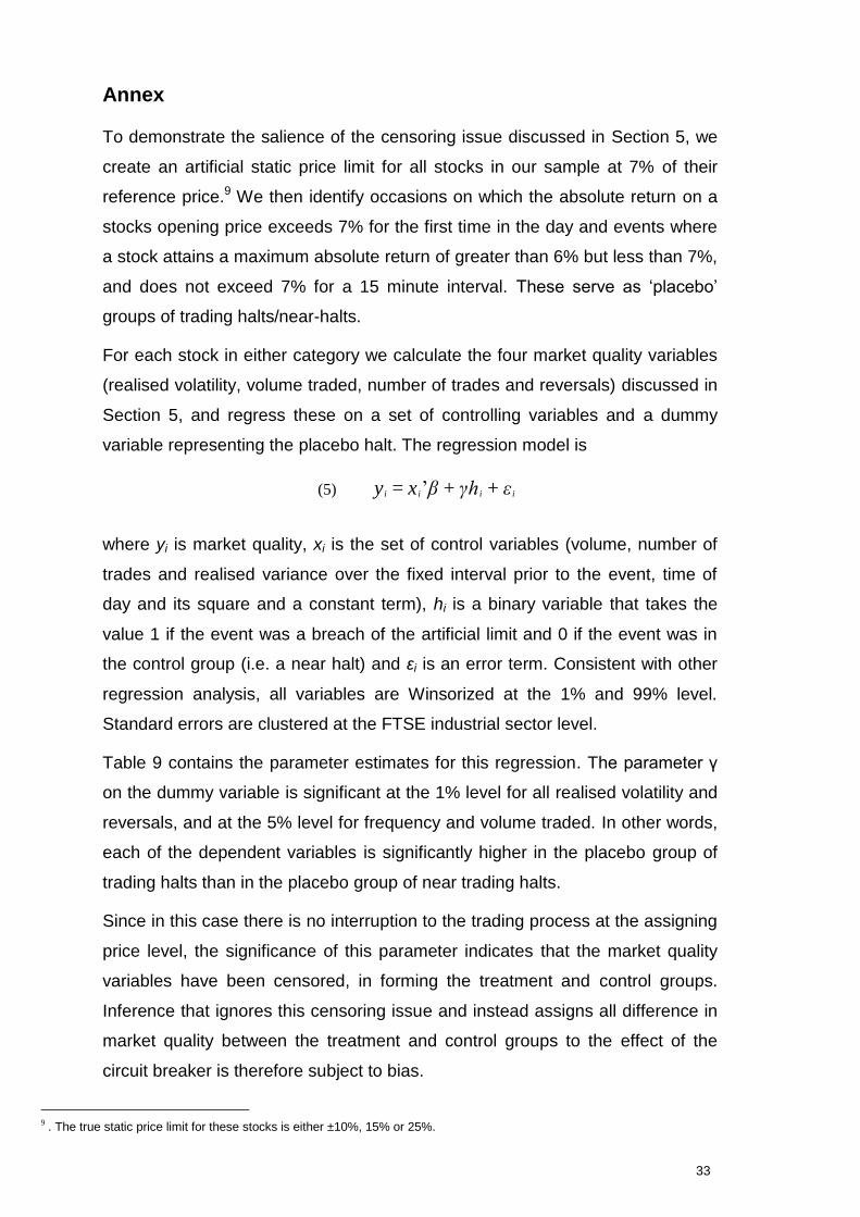
To demonstrate the salience of the censoring issue discussed in Section 5, we

create an artificial static price limit for all stocks in our sample at 7% of their

reference price.9 We then identify occasions on which the absolute return on a

stocks opening price exceeds 7% for the first time in the day and events where

a stock attains a maximum absolute return of greater than 6% but less than 7%,

and does not exceed 7% for a 15 minute interval. These serve as ‘placebo’

groups of trading halts/near-halts.

For each stock in either category we calculate the four market quality variables

(realised volatility, volume traded, number of trades and reversals) discussed in

Section 5, and regress these on a set of controlling variables and a dummy

variable representing the placebo halt. The regression model is

(5) y i = x i’β + γh i + ε i

where yi is market quality, xi is the set of control variables (volume, number of

trades and realised variance over the fixed interval prior to the event, time of

day and its square and a constant term), hi is a binary variable that takes the

value 1 if the event was a breach of the artificial limit and 0 if the event was in

the control group (i.e. a near halt) and εi is an error term. Consistent with other

regression analysis, all variables are Winsorized at the 1% and 99% level.

Standard errors are clustered at the FTSE industrial sector level.

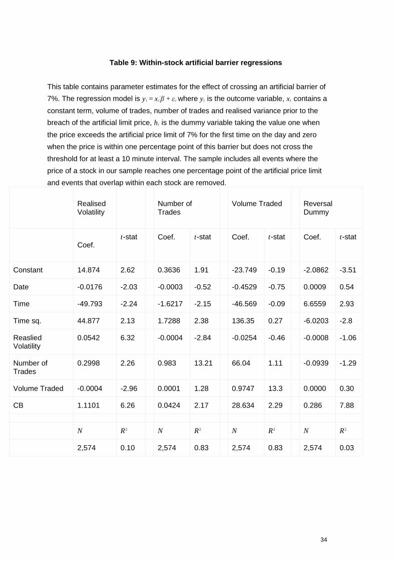
Table 9 contains the parameter estimates for this regression. The parameter γ

on the dummy variable is significant at the 1% level for all realised volatility and

reversals, and at the 5% level for frequency and volume traded. In other words,

each of the dependent variables is significantly higher in the placebo group of

trading halts than in the placebo group of near trading halts.

Since in this case there is no interruption to the trading process at the assigning

price level, the significance of this parameter indicates that the market quality

variables have been censored, in forming the treatment and control groups.

Inference that ignores this censoring issue and instead assigns all difference in

market quality between the treatment and control groups to the effect of the

circuit breaker is therefore subject to bias.

9 . The true static price limit for these stocks is either ±10%, 15% or 25%.

34

Table 9: Within-stock artificial barrier regressions

This table contains parameter estimates for the effect of crossing an artificial barrier of

7%. The regression model is y i = x i′β + ε i where y i is the outcome variable, x i contains a

constant term, volume of trades, number of trades and realised variance prior to the

breach of the artificial limit price, h i is the dummy variable taking the value one when

the price exceeds the artificial price limit of 7% for the first time on the day and zero

when the price is within one percentage point of this barrier but does not cross the

threshold for at least a 10 minute interval. The sample includes all events where the

price of a stock in our sample reaches one percentage point of the artificial price limit

and events that overlap within each stock are removed.

Realised Volatility

Number of Trades

Volume Traded Reversal Dummy

Coef. t-stat Coef. t-stat Coef. t-stat Coef. t-stat

Constant 14.874 2.62 0.3636 1.91 -23.749 -0.19 -2.0862 -3.51

Date -0.0176 -2.03 -0.0003 -0.52 -0.4529 -0.75 0.0009 0.54

Time -49.793 -2.24 -1.6217 -2.15 -46.569 -0.09 6.6559 2.93

Time sq. 44.877 2.13 1.7288 2.38 136.35 0.27 -6.0203 -2.8

Reaslied Volatility

0.0542 6.32 -0.0004 -2.84 -0.0254 -0.46 -0.0008 -1.06

Number of Trades

0.2998 2.26 0.983 13.21 66.04 1.11 -0.0939 -1.29

Volume Traded -0.0004 -2.96 0.0001 1.28 0.9747 13.3 0.0000 0.30

CB 1.1101 6.26 0.0424 2.17 28.634 2.29 0.286 7.88

N R2 N R2 N R2 N R2

2,574 0.10 2,574 0.83 2,574 0.83 2,574 0.03