1

Master Thesis

Behavioural Economics

The contest of motivational theories

in explaining performance:

Expectancy vs. Goal setting

What do you expect?

January 27th 2017

John de Jong BSc

347951

Erasmus School of Economics, Erasmus University Rotterdam

Supervisor: Prof. dr. Han Bleichrodt

1

Table of Contents

1. Introduction ............................................................................................................................ 4

2. Literature review .................................................................................................................... 9

2.1 Expectancy theory ............................................................................................................ 9

2.1.1 Expectancy theory origin .......................................................................................... 9

2.1.2 Expectancy theory model ........................................................................................ 12

2.1.3 Expectancy theory concepts .................................................................................... 13

2.2 Goal setting theory ......................................................................................................... 15

2.2.1 Goal setting theory origin ........................................................................................ 15

2.2.2 Goal setting theory model ....................................................................................... 16

2.2.3 Goal setting theory concepts ................................................................................... 16

2.3 Hypotheses development ................................................................................................ 19

2.3.1 Expectancy theory hypotheses ................................................................................ 19

2.3.2 Goal setting theory hypotheses ............................................................................... 20

2.3.3 Expectancy theory vs. Goal setting theory hypotheses ........................................... 21

3. Research design .................................................................................................................... 23

3.1 Experiment ..................................................................................................................... 23

3.2 Task ................................................................................................................................ 23

3.2.1 Task description ...................................................................................................... 23

3.2.2 Exercise ................................................................................................................... 24

3.2.3 Manipulation ........................................................................................................... 25

3.3 Questionnaire ................................................................................................................. 26

3.3.1 Pre-experimental questionnaire ............................................................................... 26

3.3.2 Post-experimental questionnaire ............................................................................. 28

3.3.3 Order Effect ............................................................................................................. 28

3.4 Participants ..................................................................................................................... 29

2

3.5 Procedure ........................................................................................................................ 30

3.5.1 Invitation ................................................................................................................. 30

3.5.2 Introduction ............................................................................................................. 30

3.5.3 Part 1 ....................................................................................................................... 31

3.5.4 Part 2 ....................................................................................................................... 31

3.6 Analysis .......................................................................................................................... 31

4. Results .................................................................................................................................. 33

4.1 Analyses of personal information .................................................................................. 33

4.2 Hypotheses tests ............................................................................................................. 33

4.2.1 Hypothesis 1 ............................................................................................................ 33

4.2.2 Hypothesis 2 ............................................................................................................ 36

4.2.3 Hypothesis 3 ............................................................................................................ 40

4.2.4 Hypothesis 4 ............................................................................................................ 42

4.2.5 Hypotheses 5 & 6 .................................................................................................... 42

4.2.6 Hypothesis 7 ............................................................................................................ 47

5. Conclusion ............................................................................................................................ 51

5.1 Conclusion and Discussion ............................................................................................ 51

5.2 Contribution ................................................................................................................... 53

5.3 Limitations and Future Research .................................................................................... 54

References ................................................................................................................................ 56

Appendix A: Experiment ......................................................................................................... 59

Panel A: Introduction - Decision making experiment .......................................................... 59

Panel B: Part 1 - Decision making experiment - Task description ...................................... 61

Panel C: Part 1 - Decision making experiment - Pre-experimental questionnaire ............... 63

Panel D: Part 1 - Decision making experiment - Personal information ............................... 67

Panel E: Part 2 - Decision making experiment - Introduction ............................................. 68

Panel F: Part 2 - Decision making experiment - Exercise .................................................... 69

3

Panel G: Part 2 - Decision making experiment - Post-experimental questionnaire ............. 70

Appendix B: Explanation of used variables ............................................................................. 71

Appendix C: Output of regression analyses ............................................................................. 73

Panel A: Ordered Logit regression model of expectancy (Q6) ............................................ 73

Panel B: Factorial regression model of performance (Q57A8m) and interactions with goals

(Benchmark) ......................................................................................................................... 74

Panel C: Factorial regression model of performance (Q57A12m) and interactions with

goals (Benchmark) ............................................................................................................... 75

Panel D: Factorial regression model of performance (Q57B8m) and interactions with goals

(Benchmark) ......................................................................................................................... 76

Panel E: Factorial regression model of performance (Q57B12m) and interactions with goals

(Benchmark) ......................................................................................................................... 77

Appendix D: Calculation of force ............................................................................................ 78

4

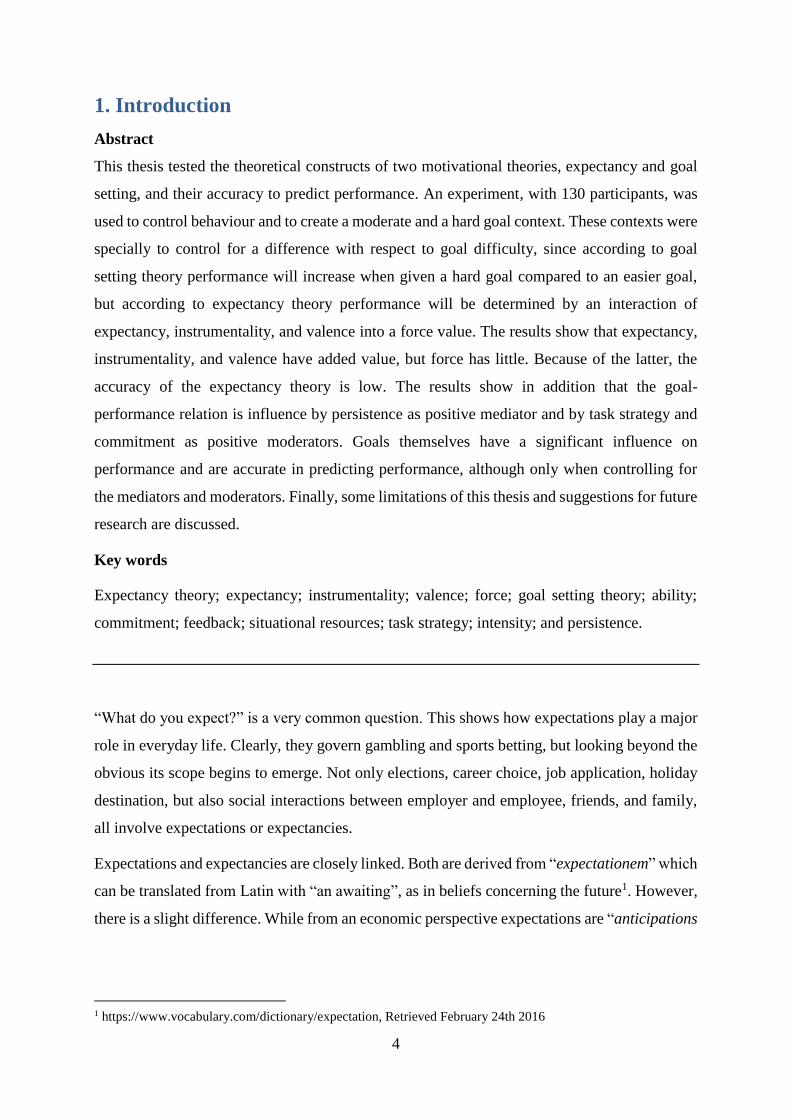
1. Introduction

Abstract

This thesis tested the theoretical constructs of two motivational theories, expectancy and goal

setting, and their accuracy to predict performance. An experiment, with 130 participants, was

used to control behaviour and to create a moderate and a hard goal context. These contexts were

specially to control for a difference with respect to goal difficulty, since according to goal

setting theory performance will increase when given a hard goal compared to an easier goal,

but according to expectancy theory performance will be determined by an interaction of

expectancy, instrumentality, and valence into a force value. The results show that expectancy,

instrumentality, and valence have added value, but force has little. Because of the latter, the

accuracy of the expectancy theory is low. The results show in addition that the goal-

performance relation is influence by persistence as positive mediator and by task strategy and

commitment as positive moderators. Goals themselves have a significant influence on

performance and are accurate in predicting performance, although only when controlling for

the mediators and moderators. Finally, some limitations of this thesis and suggestions for future

research are discussed.

Key words

Expectancy theory; expectancy; instrumentality; valence; force; goal setting theory; ability;

commitment; feedback; situational resources; task strategy; intensity; and persistence.

“What do you expect?” is a very common question. This shows how expectations play a major

role in everyday life. Clearly, they govern gambling and sports betting, but looking beyond the

obvious its scope begins to emerge. Not only elections, career choice, job application, holiday

destination, but also social interactions between employer and employee, friends, and family,

all involve expectations or expectancies.

Expectations and expectancies are closely linked. Both are derived from “expectationem” which

can be translated from Latin with “an awaiting”, as in beliefs concerning the future1. However,

there is a slight difference. While from an economic perspective expectations are “anticipations

1 https://www.vocabulary.com/dictionary/expectation, Retrieved February 24th 2016

5

of future events that influence present economic behaviour”2, expectancy points to the

subjective probabilistic assessment of future events that affect decisions in the present (Vroom,

1995, p. 20).

This accurately describes one of the core concepts in expectancy theory, popularised by Vroom

(1964). His theory states that the motivational force (hereafter: force) of a person to perform a

particular act is determined by an interaction of expectancy, instrumentality and valence. This

can be expressed very basically3 as: Force = Expectancy (Instrumentality × Valence) or in

short: F = E (I × V). Also called VIE-theory or -model, after the concepts within.

To elaborate these concepts, suppose, for example, an employee whose force to work hard

depends on (a) his expectancy that high effort will lead to good performance, (b) his

instrumentality that good performance is related to high rewards, and (c) a high positive valence

of these rewards (Lawler & Suttle, 1973; Schwab, Olian-Gottlieb & Heneman, 1979). Hereby

is expectancy a subjective probability, instrumentality a perceived correlation, and valence a

subjective valuation (Mitchell, 1974, pp. 1053-1054).

In this respect, the concept of force is very similar to the input for the choice maximisation in

(subjective) expected utility theory. In both cases the option or act with the highest utility or

force is chosen (Edwards, 1954; Vroom, 1995, pp. 17-22).

Over the years expectancy theory has been extensively empirically tested (e.g. Schwab et al.,

1979; Van Eerde & Thierry, 1996). Even nowadays, after 50 years, expectancy theory is used

in various field of research (e.g. Ernst, 20144; Lee, Ko & Chou, 20155; Purvis, Zagenczyk &

McCray, 20156). Moreover, it is compared to and/or tested against other theories, especially

with respect to goal setting theory (e.g. Locke & Latham, 2002; Mento, Cartledge & Locke,

1980; Tubbs, Boehne & Dahl, 1993).

2 Expectations. (n.d.) Collins Dictionary of Economics, 4th ed.. (2005). Retrieved February 24th 2016 from

http://financial-dictionary.thefreedictionary.com/expectations 3 Further elaboration of this expression will be conducted in section 2.1.2 Expectancy theory model. 4 Ernst, D. (2014). Expectancy theory outcomes and student evaluations of teaching. Educational Research and

Evaluation, 20(7-8), 536-556. 5 Lee, Y. H., Ko, C. H., & Chou, C. (2015). Re-visiting Internet addiction among Taiwanese students: a cross-

sectional comparison of students’ expectations, online gaming, and online social interaction. Journal of

abnormal child psychology, 43(3), 589-599. 6 Purvis, R. L., Zagenczyk, T. J., & McCray, G. E. (2015). What's in it for me? Using expectancy theory and

climate to explain stakeholder participation, its direction and intensity. International Journal of Project

Management, 33(1), 3-14

6

It is not strange that expectancy theory and goal setting theory are compared and tested. They

have been the two most prominent motivational theories (Locke, Motowidlo & Bobko, 1986).

Both theories explain motivational behaviour, but in their own specific ways.

Expectancy theory is a descriptive theory about the internal process of decision making and

how the VIE-concepts are used therein. More specific it concerns the subjective thoughts and/or

feelings of an individual that result in a decision (Vroom, 1995).

Goal setting theory of Locke and Latham (1990, 2013) demonstrates that goals can influence

the behaviour of individuals given different circumstances. It states that hard, specific goals

lead to higher performance compared to vague, easy, or do-your-best goals. It claims a positive,

linear relationship between goal difficulty and task performance when an individual has no

conflicting goals and has the required ability and commitment (Locke & Latham, 2006, p. 265).

These theories describe the motivational process in different ways, with some different concepts

and with some different predictions. At least once their predictions apparently contradict:

Goal-setting theory appears to contradict Vroom’s (1964) valence–instrumentality–

expectancy theory (...) Other factors being equal, expectancy is said to be linearly and

positively related to performance. However, because difficult goals are harder to attain

than easy goals, expectancy of goal success would presumably be negatively related to

performance (Locke & Latham, 2002, p. 706).

First of all, Locke and Latham (2002) did not correctly quote Vroom (1964) in this statement.

Other factors being equal, Vroom (1964, 1995) does not claim that expectancy is linearly and

positively related to performance, but to force. So, force is said to be linearly and positively

related to performance in expectancy theory, while expectancy is negatively related to

performance in goal setting theory. Hence, these theories contradict if expectancy is positively

related to force.

Although research considering the relation between force and performance have repeatedly

found it to be positive7, this relation depends on the specific values of expectancy,

instrumentality and valence (Vroom, 1964, 1995).

According to Klein (1991), research on these concepts within expectancy and goal setting

theory has been far from unambiguous in its conclusions. Obviously, contradicting relations

cannot be present at the same time. However, various papers show that negative, positive, and

7 E.g. Dachler & Mobley, 1973; Hackman & Porter, 1968; Matsui, et al., 1981; Mitchell & Albright, 1972

7

non-significant relations have been found between performance and both expectancy and a

valence × instrumentality measure (for references see: Klein, 1991, pp. 232-238). Klein (1991)

tried to explain these contradicting relations by the different operationalisations used in various

papers. However, he was not able to explain all relations so this ambiguity prevailed.

Locke and Latham (2002, p. 706) report an explanation that could harmonise expectancy and

goal setting theory views. When goal level (difficulty) is constant there is a causal relation

between higher expectancies and higher performance (i.e. expectancy theory view). But when

difficulty varies a negative relation is found (i.e. goal setting theory view).

Another explanation can be found in the difference between the large role for ability and

commitment in goal setting theory compared to expectancy theory. While the first has received

some attention in expectancy theory research (e.g. Galbraith & Cummings, 1967; Heneman &

Schwab, 1972), both have been virtually requisite in goal setting theory (Mento et al., 1980, p.

421).

Even if all these explanations are applicable, which is not evident, there is no clear answer

whether expectancy theory is has lower predictive power than goal setting or the opposite.

Especially, since many goal setting oriented papers also find support for expectancy theory

constructs (e.g. Dachler & Mobley, 1973; Locke, et al., 1986; Matsui, et al., 1981; Mento et

al., 1980).

Hence, this thesis will use over 50 years of research on expectancy and goal setting theory to

theoretically verify and test the explanations mentioned above, to test the theoretical predictions

of the theories, and to dissolve the ambiguity with respect to expectancy, instrumentality,

valence, and force.

An experiment with a specific assigned moderate and hard goal context is sufficient to

empirically test most of the basic underlying constructs of the theory. In this context,

expectancy and goal setting constructs will be tested in their accuracy to predict performance,

by use of correlation and regression analyses. Therefore, the research questions that will be

answered are:

RQ1: Do the motivational theories, expectancy and goal setting, have correct

theoretical constructs?

RQ2: Which motivational theory, expectancy or goal setting, is more accurate in

predicting performance in a moderate and hard goal context?

8

Answering this question is interesting because doing research according to the theoretical

constructs of expectancy theory can be cumbersome (Connolly, 1976) in comparison to goal

setting theory, but it may be worth the effort. If, albeit in specific contexts, expectancy theory

is proven to be significantly better in predicting behaviour, motivational researchers should

redirect attention back to expectancy theory.

The results show that expectancy, instrumentality, and valence have added value, but force has

little. Because of the latter, the accuracy of the expectancy theory is low. In addition the results

show that the goal-performance relation is influence by persistence as positive mediator and by

task strategy and commitment as positive moderators. Goals themselves have a significant

influence on performance and are accurate in predicting performance, although only when

controlling for the mediators and moderators.

Doing expectancy theory research in the proper fashion appears to be difficult, since there are

many remarks about previous research (Eerde & Thierry, 1996. p. 581). Expectancy theory

entails more constrains as to what questions to ask and how to do the research than goal setting.

In addition, goal setting constructs can be investigated from an expectancy theory perspective,

while this is impossible vice versa. Therefore, the research is performed from an expectancy

theory perspective.

The remainder of this thesis is structured as follows. Chapter 2 discusses the literature with

respect to the expectancy and goal setting theories. Thereafter the hypotheses are formulated.

In chapter 3 the experimental design is presented. Chapter 4 describes the results from the

analyses and gives answers to the hypotheses. In chapter 5 a conclusion in draw and the results

are discussion. In addition, it discusses possible limitations and gives directions for future

research.

9

2. Literature review

This chapter introduces the theories to answer the research questions and to form hypotheses.

In the following sections the expectancy theory and goal setting theory are introduced and

discussed respectively, where after the hypotheses that will be tested are formulated based on

these theories. Within the theories the origin of the theory, the theoretical model and the related

concepts will be explained.

2.1 Expectancy theory

2.1.1 Expectancy theory origin

Expectancy theory (1964) has been the dominant motivational theory in organisational

psychology during the 1960’s and 1970’s (Klein, 1991). Yet, it has been seldom discussed in

economic literature (Sloof & Van Praag, 2008). It has become popular since Vroom's (1964)

book Work and Motivation. However, both others (e.g. Hackman & Porter, 1968; Mitchell,

1974) and Vroom (1995, pp. 15-31) himself point to former psychologists for earlier

formulations of parts of this theory. By providing the similarities and differences a deeper

understanding is gained about the use of expectancy theory and the origin of the theoretical

concepts expectancy, instrumentality, valence, and force.

Psychologists Lewin (1935, 1938) and Tolman (1932, 1955) were among the first to emphasize

the need for theories to understand behaviour as the result of a cognitive process within an

individual (Vroom, 1995, p. 15). This contrasted with the doctrine of behaviourism, which was

the dominant doctrine in psychology at that time (Locke & Latham, 2015), which claimed that

cognition or consciousness is useless in scientific theory (Watson, 1925, 2013).8

According to Lewin (1935), behaviour can be explained from both a historical and an ahistorical

point of view. In a historical point of view, behaviour is explained by events of the past, while

behaviour in an ahistorical point of view is only explained by the present setting (Vroom, 1995,

p. 15). In addition, Lewin (1938) described and measured valence and a concept closely related

to motivational force.

Tolman (1932, 1955) saw learning as changes in beliefs or expectations that affect behaviour,

instead of changes in the strength of habits (Vroom, 1995, p. 15). His ideas described in his

8 However, Tolman himself states to be a behaviourist (Tolman, 1925, p. 37), albeit in a subtype called purposive

behaviour (see: Tolman, E. C. (1932). Purposive behavior in animals and men. New York: Century.)

10

1955 paper are referred to as “Tolman’s expectancy theory” (Atkinson & Reitman, 1956, p.

361).

The basic principle in Tolman’s (1955) and Vroom’s (1964, 1995) expectancy theory is the

same: organisms have beliefs and/or expectations, which can change and thereby can influence

behaviour. There are also differences. Tolman mostly worked with animals, so his theory is

based on and specified to animals, while Vroom describes his theory regarding humans. Also,

Tolman is interested in performance, but not in work-related performance as is Vroom.

Moreover, Vroom gives a much broader theoretical and mathematical foundation of his theory,

compared to Tolman.

A lot of psychologists gave different names to concepts that were used in a similar fashion, so

it looked like different concepts. Results from studies with ‘different’ concepts were not always

applied or mentioned in other studies. Vroom (1964, 1995) however included and merged a lot

of concepts. His theory has therefore a broad theoretical foundation. For example, Vroom used

the concept of valence, but he referred to and used the insights of the concepts attitude, expected

utility, incentive, and valence (for references see Vroom, 1995, p. 17). The same applies to

expectancies and subjective probabilities. And to motivational force, aroused motivation,

behaviour potential, performance vector, and subjective expected utility (for references see

Vroom, 1995, pp. 20, 21). Of these concepts, (subjective) expected utility and subjective

probability are likely the most familiar to economists, hence the similarities and differences will

be discussed.

Utility (i.e. subjective valuation) can be different from the objective valuation. This can be

explained by Daniel Bernoulli, who first introduced the term ‘expected utility’ in 1738 to

replace ‘expected value’. He described a situation wherein according to the theoretical and

mathematical prediction of expected value theory someone should be willing to pay an infinite

amount of money to participate in a gamble, although it contradicted any common-sense. This

situation is referred to as the St. Petersburg paradox and it describes a coin-flip gamble wherein

someone can win a monetary value of 2i in turn i wherein for the first time a ‘head’ is tossed.

Expected value theory predicts an infinite value by summing up all the infinite possible

outcomes multiplied by their probability. In expected utility theory this problem is resolved by

diminishing returns of money (Gigerenzer & Selten, 2001).

Edwards (1954) gives an overview of (subjective) expected utility with respect to both riskless

and risky choices. Individuals in a riskless context are assumed to maximise utility and

individuals in a risky context are assumed to maximise expected utility. The expected utility is

11

the summation of the utility of all possible outcomes weighted by their probability. Individuals

choose the alternative with most positive or least negative (expected) outcome by maximising

(expected) utility.

Although expected utility includes some form of subjectivity, the probabilities are considered

to be objective. Edwards (1954) however, argues that subjective probabilities and subjective

expected utility may be more appropriate to predict decisions. Research shows that individuals

tend to overestimate low probabilities and underestimate high probabilities (Edwards, 1954, pp.

393, 396-400). What is confirmed by Kahneman and Tversky (1979). This and other differences

between the objective and subjective probability can be corrected by subjective probabilities

(Edwards, 1954, pp. 396-400).

A major difference between (subjective) expected utility and expectancy theory are the

following assumptions that must be satisfied in subjective expected utility, but are not explicit

assumptions in the expectancy theory. Probabilities should sum up to one. Transitivity entails

that if a ≥ b and b ≥ c, then a must be larger or at least equal to c. Independence is when the

preference of a ≥ b remains when multiplying a and b with the same subjective chance (i.e.

irrelevance of identical outcomes). Comparability exists when a trade-off is possible between

outcomes (Camerer & Weber, 1992; Edwards, 1954; Michell, 1974). In expectancy theory

single expectancies are between 0 and 1, but combined expectancies can deviate from this

assumption. Transitivity, independence and comparability are implicitly assumed in expectancy

theory (House, et al. 1974; Vroom, 1964, 1994), although violations do occur (Mitchell, 1974).

Another difference is that within subjective expected utility there are two concepts, whereas

expectancy theory separates three concepts. The first only uses subjective probabilities and

subjective valuation of possible outcomes, while expectancy theory also includes

instrumentality. This gives additional information about what drives behaviour.

However, Vroom (1964, 1995) uses, among many others, Edwards (1954) insights to support

and construct the concepts expectancy (i.e. subjective probability) and valence (i.e. subjective

valuation). So, Vroom uses the insights of Edwards (1954), Lewin (1935, 1938), Tolman (1932,

1955), and many others to support and construct his theory. In all cases, he combines different

theoretical views and he broadens the theoretical foundation of the concepts to be used in his

expectancy theory.

12

2.1.2 Expectancy theory model

To use his expectancy theory, Vroom (1964) developed a mathematical model. The model

calculates the force to perform a particular act for an individual, whereby the act with the highest

force will be chosen. This force is determined by an interaction between expectancy,

instrumentality and valence and results in behaviour.

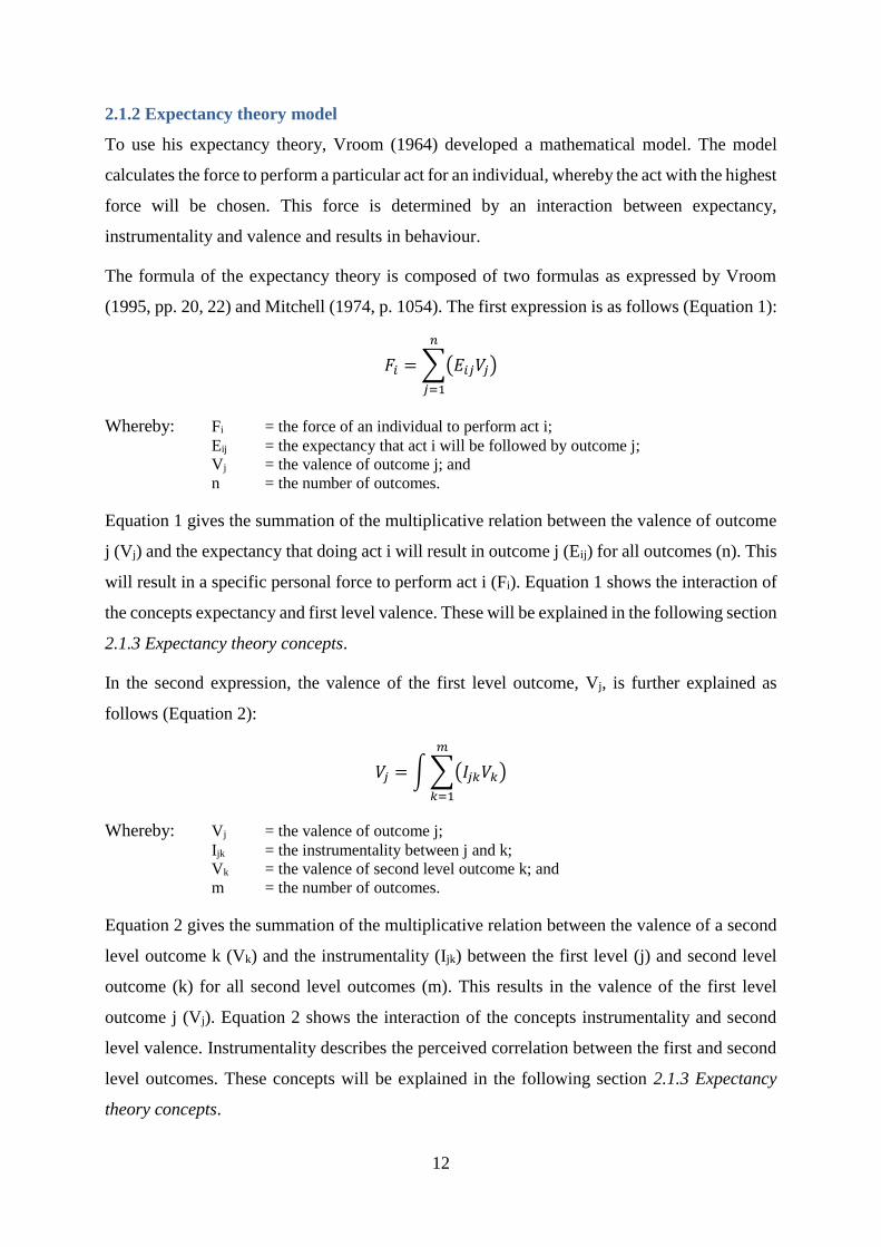
The formula of the expectancy theory is composed of two formulas as expressed by Vroom

(1995, pp. 20, 22) and Mitchell (1974, p. 1054). The first expression is as follows (Equation 1):

𝐹𝑖 = ∑(𝐸𝑖𝑗𝑉𝑗)

𝑛

𝑗=1

Whereby: Fi = the force of an individual to perform act i;

Eij = the expectancy that act i will be followed by outcome j;

Vj = the valence of outcome j; and

n = the number of outcomes.

Equation 1 gives the summation of the multiplicative relation between the valence of outcome

j (Vj) and the expectancy that doing act i will result in outcome j (Eij) for all outcomes (n). This

will result in a specific personal force to perform act i (Fi). Equation 1 shows the interaction of

the concepts expectancy and first level valence. These will be explained in the following section

2.1.3 Expectancy theory concepts.

In the second expression, the valence of the first level outcome, Vj, is further explained as

follows (Equation 2):

𝑉𝑗 = ∫ ∑(𝐼𝑗𝑘𝑉𝑘)

𝑚

𝑘=1

Whereby: Vj = the valence of outcome j;

Ijk = the instrumentality between j and k;

Vk = the valence of second level outcome k; and

m = the number of outcomes.

Equation 2 gives the summation of the multiplicative relation between the valence of a second

level outcome k (Vk) and the instrumentality (Ijk) between the first level (j) and second level

outcome (k) for all second level outcomes (m). This results in the valence of the first level

outcome j (Vj). Equation 2 shows the interaction of the concepts instrumentality and second

level valence. Instrumentality describes the perceived correlation between the first and second

level outcomes. These concepts will be explained in the following section 2.1.3 Expectancy

theory concepts.

13

2.1.3 Expectancy theory concepts

In the expectancy theory model, an interaction of the theoretical concepts expectancy,

instrumentality and valence, results in the force.

Expectancy

Expectancy is a subjective probability. Individual expectancies range between 0-1. But when

an individual overestimates the objective chance of events/alternative, can the total expectancy

be in either higher or lower, due to the sum of these expectancies.

More specifically, expectancy points to the individual subjective probabilistic assessment of

future events that affects decisions in the present. Expectancy is determined positively by the

individual’s ability, negatively by the presence of constraints (House, 1971, p. 323), positively by

perceived control over performance (House, et al., 1974, p. 499), and negatively by perceived

difficulty (Vroom, 1964, 1995, pp.17-31). It can be based on objective (external) information, but

it is the internal process within a specific individual that results in his/her expectancy (Vroom, 1995,

p. 20).

Expectancy involves risk, because not all external factors can be controlled by an individual

(Vroom, 1995, p. 20). Probabilities can be significant under- or overweighed from their

objective probability in decisions under risk (Edwards, 1954, pp. 396-397; Kahneman &

Tversky, 1979). Hence, if people evaluate the probability of realising uncertain future outcomes

of alternatives differently from person to person (Edwards, 1954, p. 403), this can result in

various decisions. Even if the objective probability is the same.

In Equation 1 this concept of expectancy is applied to measure the strength of the subjective

probability that doing act i will result in outcome j, on a continuous scale from 0 to 1, for all

possible outcomes of act i.

Instrumentality - first and second level outcomes

Instrumentality usually describes the individually perceived correlation between performance

and rewards (Mitchell, 1974, p. 1054). As a correlation based measure, instrumentality ranges

from -1 to 1 (Vroom, 1995, p. 21).

It is an outcome-outcome relation. Instrumentality describes the relation between first level

outcomes and second level outcomes9. First level outcomes (e.g. joining a group, getting your

9 Vroom described it as “first outcomes” and “second outcomes”, whereby the second was a consequent of the

first. Although he did not use “level”, the reasoning is the same.

14

driver’s licence, a person’s performance, reaching a particular goal) are the direct effect of

someone’s behaviour (Lawler & Suttle, 1973, p. 483). While second level outcomes are

consequents of attaining the first level outcome (Vroom, 1964, 1995). Such as, reaching a

particular goal can result in promotion, pay raise, feeling of satisfaction, and/or feeling of

accomplishment (e.g. Mitchell, 1974).

In Equation 2 this concept of instrumentality is applied to measure the strength of the perceived

correlation between outcome j and outcome k, on a continuous scale from -1 to 1, for all possible

outcomes of act j. With maximum (minimum) value 1 (-1), meaning that outcome k is present

(not present) when outcome j is, and outcome k is not present (present) when outcome j is not.

Values in-between 0 and 1 (-1 and 0) give a relation that outcome k is more likely or stronger

present (not present) for higher (lower) values.

Valence - first and second level outcomes

Valence describes the anticipated subjective valuation of future outcomes at a given moment.

This subjective valuation can differ considerably from the actual value of the future outcome

(Mitchell, 1974, p. 1053; Vroom, 1995, p. 18).

The valence of an outcome (i.e. first level) is determined by the valence of the second level

outcomes, that are the effect of attaining the first level outcome (Lawler & Suttle, 1973, pp.

482-483).

Galbraith and Cummings (1967) made a distinction between intrinsic and extrinsic sources of

valence. Extrinsic sources refer to valence that has an external source of motivation to perform

a behaviour (i.e. pay, pride, respect). While intrinsic sources refer to valence that is self-

administered (i.e. aversion of particular work, enjoying to perform). House (1971) extended the

intrinsic source of valence to be either determined by the behaviour itself or determined by the

extent of goal attainment. An extrinsic source of valence usually has a lower instrumentality

since it depends on an external party to observe and/or judge. Intrinsic valence is self-

administered and therefore only depends on doing a task or the extent of goal attainment

(House, 1971, p. 322-323).

In Equation 1 this concept of valence is applied to measure the subjective valuation of all

possible first level outcomes of act i. In Equation 2 this concept measures the subjective

valuation of all possible second level outcomes of act j. Positive (negative) levels of valence

mean that these outcomes have a positive (negative) subjective value.

15

Force

The motivational force describes the appeal to an individual of a particular act, whereby the act

with the highest force is chosen. It conceptualises the value upon which our choices,

consciously or unconsciously, are based (Vroom, 1964, 1995).

It is determined by an interaction of theoretical concepts expectancy, instrumentality and

valence based on an individual’s characteristics, as is shown in Equations 1 and 2.

2.2 Goal setting theory

2.2.1 Goal setting theory origin

Goal setting theory (1990, 2013) is designed by Locke and Latham. In 1990 the theory was first

formally published and it was updated in 2013. It has been extensively researched with over

1000 papers, whereof 600 from past 1990 (Locke & Latham, 2015).

Early goal setting theory research dates back to the 1960’s, when behaviourism was dominant

in psychology. The prominent behaviourist Watson (1925) claims that cognition or

consciousness is useless in scientific theory. Behaviourists study observable behaviour. In

doing so, they disregard cognitive reasoning, since they assume that behaviour is the result of

the external environmental context. So, we are controlled by the stimulus-response that we grow

up with, hence are controlled by our environment and do not a free will (Locke & Latham,

2015; Watson, 1925, 2013). However, goal setting theory demonstrates not only our

environment, but also our own cognitive reasoning affects (goal) choice and performance.

Personal goals influence the behaviour of individuals. Hence this became the focus of their

research (Locke & Latham, 2002)10.

This thought that behaviour is affected by a cognitive process was not new. Mace (1935)

described it as the ‘will to work’. Whereby the efficiency of employees is mostly determined

by the direction, intensity and duration of the will to work. Mace (1935) compared specific

assigned goals, improving previous performance goals, and do-your-best goals. He found that

specific assigned goals yield the highest performance. However, participants needed a

reasonable expectation that the specific assigned goal was within reach, for specific goals to

outperform do-your-best goals (Latham & Locke, 2007, p. 290).

10 Although it is possible that this response to goals is controlled by our environment.

16

Even before Mace (1935), Bryan and Harter (1897, p. 50) gave proof that employees could

greatly increase their performance by striving to obtain a specific hard goal. Locke and Latham

used, among others, their insights as a starting point to research goal setting.

2.2.2 Goal setting theory model

Locke and Latham (2015) describe a theoretical goal setting theory model. It states that: more

difficult, specific goals lead to higher performance compared to vague, easy, do-your-best

goals, or no goals. It claims a positive, linear relationship between goal difficulty and task

performance (Locke & Latham, 2006, p. 265). This relation will hold insofar five moderators

are present. These are, if individuals: have the required ability to perform the task; have

commitment until the goal is attained; receive feedback with respect to their advancement in

goal completion; have the necessary resources to perform the task; and develop task strategy.

Whereby the satisfaction of the task is determined by the degree of goal attainment (Locke &

Latham, 2015, pp. 114-115).

In addition, the relation that specific, hard goals lead to high performance is explained by four

mediators. These are: task strategy, direction, intensity, and persistence. The former is

cognitive, the last three are motivational (Locke & Latham, 2015, pp. 114-115)

Moderator variables affect and mediator variables explain a relation between two other

variables. Moderators are variables that can increase of decrease the strength and/or direction

of a relation. Mediators are variables that explain a relation between two other variables. That

is, two variables influence each other through the mediator (Baron & Kenny, 1986). In case of

goal setting theory, the positive, linear relationship between goal difficulty and task

performance is explained through the mediators and exists when the moderators are sufficiently

present.

2.2.3 Goal setting theory concepts

According to goal setting theory the goal-performance relation has five moderators and 4

mediators. Task strategy can be both. The five moderators ability, commitment, feedback,

situational resources, and task strategy, and the four mediators, task strategy, direction,

intensity, and persistence, are explained below.

Goal

A goal is the object or aim of an action. The goal content and goal intensity can be distinguished.

The former refers to the content of the result that is intended. Goal content can be determined

by external sources (e.g. boss, friends) and internally (e.g. own view or feelings). Goal intensity

17

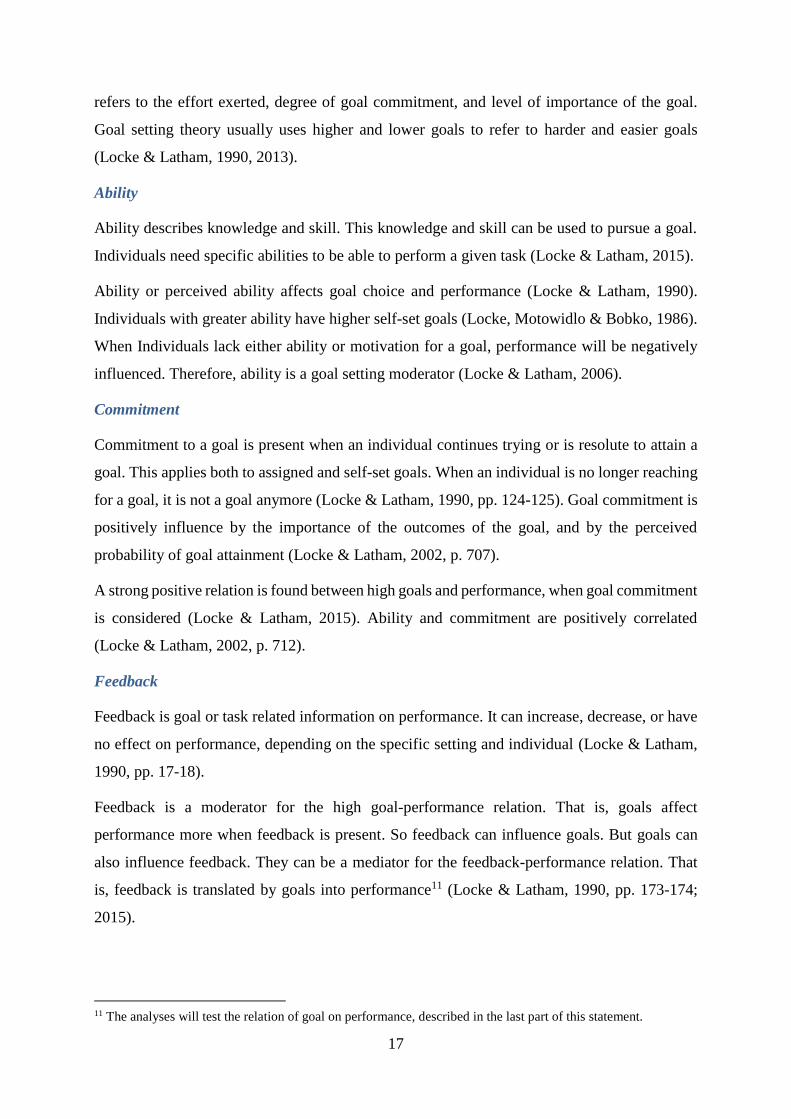
refers to the effort exerted, degree of goal commitment, and level of importance of the goal.

Goal setting theory usually uses higher and lower goals to refer to harder and easier goals

(Locke & Latham, 1990, 2013).

Ability

Ability describes knowledge and skill. This knowledge and skill can be used to pursue a goal.

Individuals need specific abilities to be able to perform a given task (Locke & Latham, 2015).

Ability or perceived ability affects goal choice and performance (Locke & Latham, 1990).

Individuals with greater ability have higher self-set goals (Locke, Motowidlo & Bobko, 1986).

When Individuals lack either ability or motivation for a goal, performance will be negatively

influenced. Therefore, ability is a goal setting moderator (Locke & Latham, 2006).

Commitment

Commitment to a goal is present when an individual continues trying or is resolute to attain a

goal. This applies both to assigned and self-set goals. When an individual is no longer reaching

for a goal, it is not a goal anymore (Locke & Latham, 1990, pp. 124-125). Goal commitment is

positively influence by the importance of the outcomes of the goal, and by the perceived

probability of goal attainment (Locke & Latham, 2002, p. 707).

A strong positive relation is found between high goals and performance, when goal commitment

is considered (Locke & Latham, 2015). Ability and commitment are positively correlated

(Locke & Latham, 2002, p. 712).

Feedback

Feedback is goal or task related information on performance. It can increase, decrease, or have

no effect on performance, depending on the specific setting and individual (Locke & Latham,

1990, pp. 17-18).

Feedback is a moderator for the high goal-performance relation. That is, goals affect

performance more when feedback is present. So feedback can influence goals. But goals can

also influence feedback. They can be a mediator for the feedback-performance relation. That

is, feedback is translated by goals into performance11 (Locke & Latham, 1990, pp. 173-174;

2015).

11 The analyses will test the relation of goal on performance, described in the last part of this statement.

18

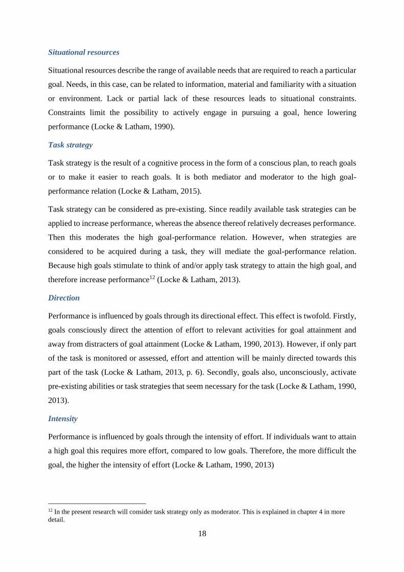
Situational resources

Situational resources describe the range of available needs that are required to reach a particular

goal. Needs, in this case, can be related to information, material and familiarity with a situation

or environment. Lack or partial lack of these resources leads to situational constraints.

Constraints limit the possibility to actively engage in pursuing a goal, hence lowering

performance (Locke & Latham, 1990).

Task strategy

Task strategy is the result of a cognitive process in the form of a conscious plan, to reach goals

or to make it easier to reach goals. It is both mediator and moderator to the high goal-

performance relation (Locke & Latham, 2015).

Task strategy can be considered as pre-existing. Since readily available task strategies can be

applied to increase performance, whereas the absence thereof relatively decreases performance.

Then this moderates the high goal-performance relation. However, when strategies are

considered to be acquired during a task, they will mediate the goal-performance relation.

Because high goals stimulate to think of and/or apply task strategy to attain the high goal, and

therefore increase performance12 (Locke & Latham, 2013).

Direction

Performance is influenced by goals through its directional effect. This effect is twofold. Firstly,

goals consciously direct the attention of effort to relevant activities for goal attainment and

away from distracters of goal attainment (Locke & Latham, 1990, 2013). However, if only part

of the task is monitored or assessed, effort and attention will be mainly directed towards this

part of the task (Locke & Latham, 2013, p. 6). Secondly, goals also, unconsciously, activate

pre-existing abilities or task strategies that seem necessary for the task (Locke & Latham, 1990,

2013).

Intensity

Performance is influenced by goals through the intensity of effort. If individuals want to attain

a high goal this requires more effort, compared to low goals. Therefore, the more difficult the

goal, the higher the intensity of effort (Locke & Latham, 1990, 2013)

12 In the present research will consider task strategy only as moderator. This is explained in chapter 4 in more

detail.

19

Persistence

Performance is influence by goals through the persistence of effort. That is, the time spent on a

task. More specifically, the time an individual continues to exert effort during the attainment of

the task or while trying to attain it, in contrast to giving up (Locke & Latham, 1990).

2.3 Hypotheses development

This thesis has the aim to answer the following research questions. RQ1: Do the motivational

theories, expectancy and goal setting, have correct theoretical constructs? RQ2: Which

motivational theory, expectancy or goal setting, is more accurate in predicting performance in

a moderate and hard goal context? To answer research question RQ1 and RQ2, the main

theoretical constructs and predictions of the theories are tested with respect to moderate and

hard goal contexts.

2.3.1 Expectancy theory hypotheses

The first concept within expectancy theory is expectancy. In the experiment of this thesis,

expectancy will be manipulated to have a moderate and a hard goal context. For expectancy to

be of importance to the decision process in comparison of the moderate and hard goals, the

expectancy should be lower in the hard goal context, compared to the moderate goal context.

For the concept of expectancy to have scientific value, two conditions should hold. (1) It must

be significantly different from the objective probabilities (Vroom, 1964, 1995), otherwise it is

easier to use objective probabilities. The difference between the expectancy and the objective

probability can either increase the predictive ability of the expectancy concept or decrease the

predictive ability of the expectancy concept. This can be explained. Predictive ability can

increase, since according to expectancy theory individuals evaluate a possible outcome based

on expectancy (i.e. a subjective probability) instead of objective probability, hence their

behaviour is the result of expectancy. However predictive ability can also decrease, because

when expectancy is different from the objective probability, the outcome that is aimed for can

be (substantially) different from their actual outcome. (2) Expectancy should vary between

individuals, for the correction on the individual level (Vroom, 1964, 1995) to have added value.

These statements result in the following hypotheses:

H1a: Expectancy is lower in the hard goal context, compared to the moderate goal context.

H1b: Expectancy varies between individuals in a moderate and hard goal context.

H1c: Expectancy differs from the objective probabilities in a moderate and hard goal context.

20

Expectancy theory states that expectancy is determined by ability, constraints, perceived control

and perceived difficulty. Ability and perceived control are supposed to be positively (House,

1971; House, et al., 1974) and perceived difficulty is supposed to be negatively (Vroom, 1964,

1995) related to expectancy. Constraints will be accounted for in the experimental design.

Hence the following hypotheses:

H2a: Perceived ability has a positive effect on expectancy in a moderate and hard goal context.

H2b: Perceived control has a positive effect on expectancy in a moderate and hard goal context.

H2c: Perceived difficulty has a negative effect on expectancy in a moderate and hard goal

context.

Further, expectancy theory claims a correlation between first and second level outcomes,

described by the concept of instrumentality (Lawler & Suttle, 1973, p. 483). For this concept to

have scientific relevance, this correlation must exist and have meaning. This is hypothesised

as:

H3: First level outcomes and second level outcomes are meaningfully correlated in a moderate

and hard goal context.

Expectancy theory describes the valence as an anticipated subjective valuation. Valence usually

has both intrinsic and extrinsic sources, that must be treated differently (House, 1971). This will

be accounted for in the experimental design.

However, the anticipated subjective valuation can differ from the actual value (Mitchell, 1974,

p. 1053; Vroom, 1995, p. 18). The valence of outcomes to individuals should vary between

individuals to have value as a concept. This leads to the following hypothesis:

H4: Valence varies between individuals in a moderate and hard goal context.

2.3.2 Goal setting theory hypotheses

Goal setting theory claims that the goal-performance relation is effected through four mediators

(Locke & Latham, 2015). Gaining task strategy in a one-time task, will be very limited (Locke

& Latham, 1990, 2015). The level of direction needs to be accounted for in the experimental

design. The levels of intensity and persistence are hypothesised to be positively affected by

higher goals, compared to lower goals ceteris paribus, and hence will positively affect

performance (Locke & Latham, 2015). This results in the following hypotheses:

H5a: Intensity is a positive mediator in the goal-performance relation in a moderate and hard

goal context.

21

H5b: Persistence is a positive mediator in the goal-performance relation in a moderate and

hard goal context.

In addition, goal setting theory claims a linear relation between higher goals and higher

performance (Locke & Latham, 2006, 2013). This relation depends on the levels and/or use of

ability, commitment, feedback, lack of situational constrains, and task strategy (Locke &

Latham, 2015). Of these variables, the possibility of feedback is less present in a one-time task

(Locke & Latham, 1990); lack of situational constrains needs to be accounted for in the

experimental design.

All these variables are positive moderators of the goal-performance relation (Locke & Latham,

2013). Therefore, applying goal setting theory to a moderate and hard goal context, results in

the following hypotheses:

H6a: Task strategy is a positive moderator of the goal-

performance relation in a moderate and hard goal

context.

H6b: Perceived ability is a positive moderator of the

goal-performance relation in a moderate and hard goal

context.

H6c: Perceived commitment is a positive moderator of the

goal-performance relation in a moderate and hard goal

context.

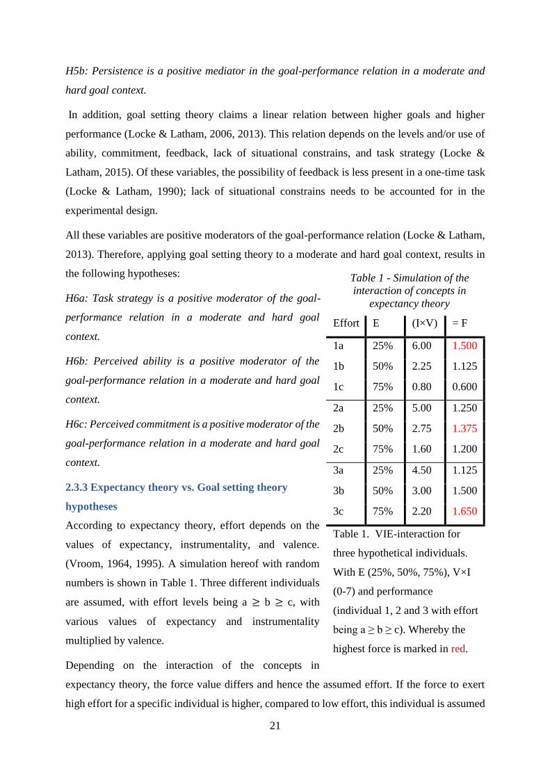
2.3.3 Expectancy theory vs. Goal setting theory

hypotheses

According to expectancy theory, effort depends on the

values of expectancy, instrumentality, and valence.

(Vroom, 1964, 1995). A simulation hereof with random

numbers is shown in Table 1. Three different individuals

are assumed, with effort levels being a ≥ b ≥ c, with

various values of expectancy and instrumentality

multiplied by valence.

Depending on the interaction of the concepts in

expectancy theory, the force value differs and hence the assumed effort. If the force to exert

high effort for a specific individual is higher, compared to low effort, this individual is assumed

Effort E (I×V) = F

1a 25% 6.00 1.500

1b 50% 2.25 1.125

1c 75% 0.80 0.600

2a 25% 5.00 1.250

2b 50% 2.75 1.375

2c 75% 1.60 1.200

3a 25% 4.50 1.125

3b 50% 3.00 1.500

3c 75% 2.20 1.650

Table 1. VIE-interaction for

three hypothetical individuals.

With E (25%, 50%, 75%), V×I

(0-7) and performance

(individual 1, 2 and 3 with effort

being a ≥ b ≥ c). Whereby the

highest force is marked in red.

Table 1 - Simulation of the

interaction of concepts in

expectancy theory

22

to exert high effort. However, if the force to exert low effort is higher compared to high effort,

this individual is assumed to exert low effort. Therefore, expectancy theory has no single

prediction concerning the relation between force and effort. The same applies to performance.

Hence, the following hypothesis:

H7a: Performance is accurately predicted by expectancy theory in moderate and hard goal

contexts and will depend on the interaction of expectancy, instrumentality, and valence in both

moderate and hard goal contexts.

Expectancy is one of the concepts in expectancy theory that can influence and explain

performance. Expectancy is partially determined by perceived difficulty (Vroom, 1964, 1995).

As shown in Table 1, effort or performance can be different while the expectancy is the same.

On the contrary, goal setting theory predicts a linear relationship between goal difficulty and

task performance, when controlling for moderators and mediators (Locke & Latham, 2006,

2015). So, ceteris paribus for decreasing levels of expectancy, increasing level of performance

are expected according to goal setting theory. Since expectancy must be lower in the hard goal

context this results in the following hypothesis:

H7b: Performance is accurately predicted by goal setting theory in moderate and hard goal

contexts and will be higher in the hard goal context, compared to the moderate goal context,

when considering the moderators and mediators.

23

3. Research design

This chapter discusses the experiment used to test the hypotheses. The methodology is explained

in detail in the following sections with respect to the task, questionnaire, participants,

procedure, and analysis that are used.

3.1 Experiment

To answer the research questions and to test the hypotheses an experiment is conducted. This

experiment has a moderate difficult context and a had goal context. The choice for an

experiment is based on recommendations from the literature. For example, Eerde & Thierry

(1996) recommend the use of experiments to learn more about the validity of the expectancy

theory constructs. And to overcome measurement problems that have occurred in previous

research (Eerde & Thierry, 1996. p. 581). Others as well underline the use of experiments in

expectancy theory (e.g. Sloof & van Praag, 2008).

Also in goal setting research, both lab and field experiments are conducted, such as by the

founders of goal setting theory. While Locke mainly did experiments to verify the internal

validity, Latham tried to verify the external validity (Locke & Latham, 2015, pp. 107-108). In

fact, the greater part of the theory is based on experiments (Locke & Latham, 2002, 2015).

To differentiate from previous research, this experiment uses a task that is new to both

expectancy theory and goal setting theory. In addition, there was no deception in this

experiment. In goal setting theory, sometimes deception is used (e.g. Mento, et al., 1980).

However, in experimental economics there should be no deception (Friedman & Sunder, 1994).

Friedman and Sunder (1994, p. 56) emphasize that even if deception is only applied when it is

impossible for participants to find out, there needs to be a “strong justification for polluting the

well from which your colleagues draw their own sustenance” (Friedman & Sunder, 1994, p.

56). So, oppose all forms of deception.

3.2 Task

3.2.1 Task description

Appendix A, Panel A to Panel G present the experiment. The task description (see Appendix

A, Panel B) starts with: “Imagine that you work for a company”. Since the goal of the

experiment is to extract information from this experiment and apply it to a work situation.

24

Participants “are asked to do a task (solve a Sudoku)”. This task will be referred to as ‘exercise’,

to overcome possible misunderstanding.

In addition, it states that: “This company wants you to work as fast as you can. Therefore, they

use one of their other employees as a benchmark. You will be paired with a fictive co-employee”

and: “Your payment depends on (1) whether you complete the task faster than [this fictive co-

employee] and (2) chance.” Therefore, participants can: lose (hereafter: Lose) from their

benchmark; beat the benchmark, but not get a bonus (hereafter: Win–); or beat the benchmark

and get a bonus (hereafter: Win+). The choice for this type of payment structure is threefold.

Firstly, due to limited resources not all participants could receive a compensation. Secondly,

the payment is depended on performance, this stimulates them to do their best (Camerer &

Hogarth, 1999). Thirdly, as in a real work situation, not all effort is observed and rewarded.

External events occur, beyond the control of an employee that influence the ‘chance’ of

payment.

The reasoning for this way of expressing, and in particular for the choice of a Sudoku, are

fivefold. For most participants it is (somewhat) familiar, challenging, interesting, imposed, and

time consuming. Familiar, because a lot of people know or even play Sudoku. Challenging,

since it requires cognitive skill and needs to be done under time pressure. Interesting, for people

usually like to play Sudoku. Imposed, because participants have to do it, while they did neither

choose nor knew that they had to do in advance. Time consuming, because it takes time to solve

a Sudoku.

This has clear parallels to tasks in work situations. Familiar, because people normally work for

longer periods doing the same type of work. (Somewhat) challenging, since work at almost

every level has its own demands (i.e. deadlines, load of work, quality standards). Interesting,

because people usually like their job or job characteristics to a certain extent. Imposed, because

usually a task is imposed to you by a boss in a work situation. Time consuming, since time

spent at work cannot be used for leisure.

3.2.2 Exercise

In the experiment the same Sudoku is used for all participants (see Appendix A, Panel F). It is

the one-star Sudoku of 8 May 2016, retrieved from the archive of the website

www.sudokuoftheday.co.uk. One-star means a Sudoku of the easiest level. The Sudoku of 8

May was judged to be one of the easier Sudoku’s with one star.

25

The choice for an easier Sudoku was twofold. First, with respect to test the theories, the exercise

should not measure skill or ability, but effort and performance as dependant variable. With

higher level Sudoku’s, the possibility to solve a Sudoku is more related to skill and/or ability

than to effort. Since solving higher level Sudoku’s, is more a related to the amount of task

strategies that are, in advance, known to the participant, than to their level of effort or

performance. Performance needs, at least partially, to be determined by effort (Mitchell, 1971,

p. 1071). Second, it is motivated by the time constraints of an experiment. The experiment asked

about 30 minutes of the participants’ time. This is quite long for an experiment, in particular

for experiments with only a chance of receiving a monetary reward. Of this 30 minutes,

instructions and questionnaire took 13-17 minutes and the subjects received approximately

13 minutes to do the exercise, so to solve the Sudoku. Doing a more difficult Sudoku would

result in a longer duration of the experiment, while adding no advantage.

3.2.3 Manipulation

In the experiment, there is a manipulation. This manipulation is operationalised by two different

tasks. The goal was to have two benchmarks that are moderate and hard, respectively.

The task description (see Appendix A, Panel B) states either: “You will be paired with a fictive

co-employee, named Frank” or: “You will be paired with a fictive co-employee, named Simon.”

Whereby Frank stand for Faster and Simon for Slower.

Some used 10% and 50% attainability to account for, respectively, hard and medium goal

attainment (e.g. Locke, 1966) or expectancies (e.g. Mento, et al., 1980). Locke (1968) used a

hard goal that was attained by 19% of the participants (Matsui, et al., 1981). To have more

comparison in the experiment between the participants that solve the Sudoku in the groups of

Frank and Simon, the aim is for the hard task around 25% and for the moderate task 50-60%

attainability. In addition, the benchmark is rounded off to a whole minute.

The choice for the particular benchmarks is the result of seasoning and two independent

sources. In the first place, the website www.sudokuoftheday.co.uk shows average statistics of

solving the Sudoku’s on their website. At September 9th 2016 the average statistics of 34

individuals who solved an easy Sudoku (i.e. similar to the exercise) was 9 minutes and 58

second, with a minimum of 4:41 and a maximum of 24:08. These Sudoku Statistics are also

shown in the experiment: “Since you need to solve a Sudoku in this experiment, an idea of the

time that is needed to solve a similar Sudoku can be useful. Therefore, the statistics of 34

individuals who have solved a similar Sudoku are presented to your left. The average time to

solve a similar Sudoku was 9 minutes and 58 seconds.” With the source mentioned below.

26

This included individuals that very frequently solved Sudoku’s on this website. If there would

be relatively less experienced individuals in the experiment, they maybe would need more time.

Therefore, in the second place, a group of 10 individuals were asked to solve the exercise while

their time was monitored. Whereof 3 solved it within 8 minutes, 513 within 12 and 5 took longer

than 12 minutes. This largely overlapped with the aimed attainment.

Hence, in ‘the task against Frank’ (hereafter: Frank), participants “have 12 minutes to complete

the task. However, Frank completed the task in 8 minutes.” While in case of ‘the task against

Simon’ (hereafter: Simon), it states that: “Simon completed the task in 12 minutes.” So,

participants either have a benchmark of 8 minutes (i.e. Frank) or 12 minutes (i.e. Simon) to

complete the same exercise (i.e. Sudoku).

3.3 Questionnaire

The participants were asked to fill out a questionnaire on paper. This questionnaire checked the

manipulation and to measure task strategy, ability, expectancy, instrumentality, valence,

commitment, goal attainment, and task related feelings. The questionnaire has two parts, a pre-

and a post-experimental questionnaire (see respectively Appendix A, Panel C and Panel G).

Question can have various answer categories, mostly in the form of Likert items. 5-point and

7-point Likert items explain slightly more of the data compared to other scales (Dawes, 2008),

whereof 7-point Likert items is selected. All but seven questions are asked on this scale.

3.3.1 Pre-experimental questionnaire

The pre-experimental questionnaire is included in Appendix A, Panel C. Question 1 asks about

the last time that a participant had solved a Sudoku. It is a measure of task strategy, in that it

states how ‘fresh’ pre-existing task strategies are in their cognitive memory. In addition, the

last time potentially gives information about the frequency of solving Sudoku’s. Doing it more

frequently, increases the chance that it is more recent. And therefore, more task strategies could

exist. In the analyses the results from this question are reversed, in order that higher values are

related to higher levels of task strategy and ability (see Appendix B).

Questions 1-3 are the operationalisation of ability. Which refer to task strategy, perceived own

ability, and perceived ability relative to the average HBO/University student. The perceived

control over their performance is asked in question 4 by control over performance and in

question 5 by control over time. Since intensions need the possibility to be translated in effort

13 Including the individuals that solved the Sudoku within 8 minutes.

27

and/or performance (Mitchell, 1971, p. 1070; Locke & Latham, p. 115). Perceived difficulty is

retrieved from question 7 by asking how easy it is to beat the benchmark. Asking it in this

manner results in higher levels of Q7 corresponding to lower levels of difficulty.

Question 6 gives the expectancy to beat the benchmark. Questions 1-5 and 7 together account

for the input for the concept of expectancy. That is, the expectancy theory states that ability,

control, and difficulty together determine expectancy. Questions 8, 10, 11 and 13 are various

control questions for the expectancy variable.

These control questions give additional information and control for certain relations beyond the

expectancy theories prediction. Question 8 describes the influence of luck to beat the

benchmark. Question 10 reports whether the participants have to exert high effort to beat the

benchmark. Question 11 is close to being the opposite of expectancy, in that it asked whether

the participants think to Lose from the benchmark, instead of the expectancy to beat the

benchmark. Question 13 asked whether the participants would try less hard when they expect

to Lose. These questions are also control questions regarding the relation between performance

and the first level outcomes Lose and Win-. And questions 9 and 12 control for the relation

between Win- and Win+, so whether they get the bonus.

Questions 14-22 assess the decreasing, neutral, or increasing influence on various feelings of

achieving a Win+ situation. Together with question 12 they form the instrumentality measure

for Win+. Questions 23-31 assess the influence of Win- on various feelings and form the Win-

instrumentality measure. The same applies to questions 32-40 in case of Lose.

Questions 9 and 12 inform about the monetary aspect (i.e. money: bonus of €5,-). The other

questions are asked with respect to pride, luck, pleasure, satisfaction, confidence, fairness,

humiliation, loss of time, and stress. Money and the previous feelings are the 10 second level

outcomes used in the experiment, which are selected based on a suggestion of Hackman and

Porter (1968) to make a list of potential outcomes and choose the items that are important to

most participants. However in the experiment the creation of the list and the selection of the

items is done by the experimenter instead of the participants. Since the experimenter has

experience with Sudoku’s a good reflection of the related feelings can be obtained and in

addition it saves time.

Instrumentality seems difficult to apply in research (Connelly, 1976, p. 40ff.). It describes the

correlation between the 3 first and 10 second level outcomes. A correlation can be positive,

negative, or non-existing, hence the decreasing, neutral, or increasing scaling of the answers.

28

The valence measure, questions 41-50, uses the same 10 second level outcomes. Schwab et al.

(1979) state that the explained variance is highest when valence is only positively scaled, and

when using desirability instead of importance. The experiment partially deviates, as questions

will be asked on a scale from strongly undesirable (-3) to strongly undesirable (+3). Mitchell

and Albright (1972) suggest to include some negative outcomes (i.e. first and second level),

since it is a measure of perceived anticipated value that can also be negative.

Question 51 is an obvious question, since everyone logically prefers to beat their benchmark

and get a bonus (Win+). However, it relates to question 52 to make it more evident that there

might be a difference between what outcome they prefer and what is realistic. In addition, it

relates to question 53, in which a realistic time assessment of solving the Sudoku is asked in

blocks of minutes. The participants are asked in question 54-56 to indicate “which percentage

comes closest to what you think the chance is to Win+, to Win– and to Lose.” To get the

individual expectancies of the 3 first level outcomes with a range from 5% to 95% chance in

steps of 15% chance. The choice option does not include an option that sums up to 100%.

Therefore, it is indicated “which percentage comes closest.” In questions 51-56, participants

will be asked to reflect the assigned goal (i.e. beating Frank or Simon) on their realistic

assessments. Since there is also a post-experimental questionnaire, this gives the option to relate

pre-exercise thoughts to post-exercise thoughts and feelings.

3.3.2 Post-experimental questionnaire

The post experimental questionnaire is presented is Appendix A, Panel G. After the exercise,

participants were asked whether they solved the Sudoku (question 57), beat Frank/Simon

(question 58), achieved their realistic goal (question 59), and achieved their realistic goal time

(question 60). These questions were asked with respect to task/goal attainment and were

checked afterwards.

Questions 61-66 are control questions, which respectively inform about the participants view

about difficulty, performance, expectations, effort, and goal commitment.

The true perceived value of the task (i.e. in contrast to the anticipated valuation) is asked in

questions 67-76. Whereby questions 67 and 68 account for the loss of time and the expected

money, respectively, and questions 69-76 account for the other second level outcomes.

3.3.3 Order Effect

In questionnaires (Schuman, Presser & Ludwig, 1981), within-subject research (e.g. Harrison,

Johnson, McInnes & Rutström, 2005), and other research, order effects should be controlled

29

for. Order effects are present when behaviour/answers in a particular situation is/are effected

by previous behaviour/answers (Harrison, et al., 2005), although this effect is less present with

higher educated individuals (Babbie, 2010, p. 265). To overcome order effects in a

questionnaire the order of questions can be varied by multiple versions, so effects can be

mitigated or even eliminated (Babbie, 2010, p. 266).

In the experiment, the order of the questions is changed to get four versions in which the same

questions are used. The pre-experimental questionnaire has 6 sections and the post-

experimental questionnaire has 2 implicitly separated sections (see Appendix A, Panel C &

Panel G). Version 1 uses the order of the questions as described above. In version 2, per section

the order of the questions is reversed. Version 3 uses the same order as version 1, but the

sections are reversed, with exception of section 1. In version 4, the order of the questions is

reversed and the sections are reversed, again with exception of section 1. In total, there are four

versions of Part 1 and four versions of Part 2 with benchmark Frank, and four versions of Part

1 and four versions of Part 2 with benchmark Simon.

3.4 Participants

Participants for the experiment were

recruited from multiple universities and

universities of applied sciences (i.e.

HBO). In total 136 participants took part in the experiment, in 9 sessions with 5-32 participants

per session. Six had to be removed from the sample, leaving 130 participants. Five of these

participants prematurely quit the experiment: two had to leave earlier than expected, for one the

English was too difficult and for two the reward was too low. The sixth removed participant

did not complete large parts of the questionnaire.

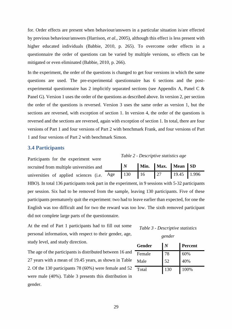
At the end of Part 1 participants had to fill out some

personal information, with respect to their gender, age,

study level, and study direction.

The age of the participants is distributed between 16 and

27 years with a mean of 19.45 years, as shown in Table

2. Of the 130 participants 78 (60%) were female and 52

were male (40%). Table 3 presents this distribution in

gender.

N Min. Max. Mean SD

Age 130 16 27 19.45 1.996

Gender N Percent

Female 78 60%

Male 52 40%

Total 130 100%

Table 2 - Descriptive statistics age

Table 3 - Descriptive statistics

gender

30

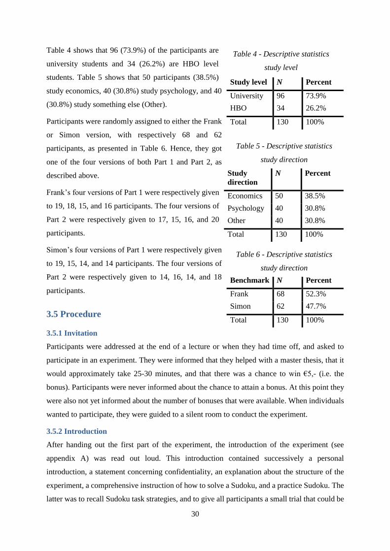
Table 4 shows that 96 (73.9%) of the participants are

university students and 34 (26.2%) are HBO level

students. Table 5 shows that 50 participants (38.5%)

study economics, 40 (30.8%) study psychology, and 40

(30.8%) study something else (Other).

Participants were randomly assigned to either the Frank

or Simon version, with respectively 68 and 62

participants, as presented in Table 6. Hence, they got

one of the four versions of both Part 1 and Part 2, as

described above.

Frank’s four versions of Part 1 were respectively given

to 19, 18, 15, and 16 participants. The four versions of

Part 2 were respectively given to 17, 15, 16, and 20

participants.

Simon’s four versions of Part 1 were respectively given

to 19, 15, 14, and 14 participants. The four versions of

Part 2 were respectively given to 14, 16, 14, and 18

participants.

3.5 Procedure

3.5.1 Invitation

Participants were addressed at the end of a lecture or when they had time off, and asked to

participate in an experiment. They were informed that they helped with a master thesis, that it

would approximately take 25-30 minutes, and that there was a chance to win €5,- (i.e. the

bonus). Participants were never informed about the chance to attain a bonus. At this point they

were also not yet informed about the number of bonuses that were available. When individuals

wanted to participate, they were guided to a silent room to conduct the experiment.

3.5.2 Introduction

After handing out the first part of the experiment, the introduction of the experiment (see

appendix A) was read out loud. This introduction contained successively a personal

introduction, a statement concerning confidentiality, an explanation about the structure of the

experiment, a comprehensive instruction of how to solve a Sudoku, and a practice Sudoku. The

latter was to recall Sudoku task strategies, and to give all participants a small trial that could be

Study level N Percent

University 96 73.9%

HBO 34 26.2%

Total 130 100%

Study

direction

N Percent

Economics 50 38.5%

Psychology 40 30.8%

Other 40 30.8%

Total 130 100%

Benchmark N Percent

Frank 68 52.3%

Simon 62 47.7%

Total 130 100%

Table 5 - Descriptive statistics

study direction

Study level N Percent

University 96 73.9%

HBO 34 26.2%

Total 130 100%

Table 6 - Descriptive statistics

study direction Table 6 - Descriptive statistics

study direction

Table 6 - Descriptive statistics

study direction

Table 4 - Descriptive statistics

study level

31

used as feedback on their ability. Hereafter they were informed regarding the task description

and Sudoku statistics.

3.5.3 Part 1

Hereafter the participants could continue with Part 1 of the experiment. This part started with

the task description. Participants either had Frank or had Simon as benchmark, with their

respective time constraints of 8 or 12 minutes. In addition, the Sudoku statistics, a summary of

the information, and the Sudoku practice solution were presented. After having read this

information, the participants could start with the pre-experimental questionnaire. When

participants finished Part 1, they had to remain silent until the papers were collected.

3.5.4 Part 2

After all papers were collected, Part 2 of the experiment was handed out. Participants read the

instructions and were asked to take a smartphone and to open the stopwatch application. They

started the time when turning the paper to start with the exercise. If they solved the Sudoku

within 12 minutes they could stop the time and continue with the post-experimental

questionnaire. A little over 12 minutes, the participants who were not finished, were asked to

stop and to continue with the post-experimental questionnaire. Part 2 was collected when all

participants had finished. And after a few weeks the bonuses were distributed to the

corresponding participants.

3.6 Analysis

The analyses in this research are performed in Stata. Various statistical tests are used. An

extensive discussion of these tests is beyond the scope of this thesis. For further information

the reader is for example referred to Moore, McCabe, Duckworth, and Alwan (2008).

A two-sample t-test is used to test for differences in the means of two variables. This is a

parametric test which is used with variables that are (approximately) normally distributed and

have at least an interval scaling. To test for differences in the distribution of two variables that

are not normally distributed and have at least an ordinal scaling, a Wilcoxon rank-sum test is

used. This is a non-parametric test. When the two variables are categorical, a Pearson's chi-

squared test is used to test for differences in the distribution. If the lowest frequency is lower

than 5 a Fisher-exact test is used instead of the Pearson's chi-squared test. In analyses of non-

parametric explanatory variables with matched-pairs and at least an ordinal scaling a Wilcoxon

matched-pairs signed-ranks test or sign rank test is used (Moore, et al., 2008).

32

Regression analyses can be performed in various ways. A factorial analysis of covariance or

ANCOVA is used with two or more categorical or continuous variables explaining a dependent

variable that is (approximately) normally distributed and has at least an interval scaling. In the

same situation with a dependent variable that is at least ordinal, an ordered logit regression

model is used. In case of a categorical dependent variable, a factorial logistic regression is used

(Moore, et al., 2008).

Results from the analyses are considered to be significant with p-values smaller than or equal

to 0.05 and to be marginally significant when p-value are larger than 0.05 but smaller than or

equal to 0.10.

Various variables are used in the analyses. Appendix B lists the variables, explains their names,

and in some cases explains the related concept and/or meaning of the associated values.

33

4. Results

This chapter discusses the results from the analyses to test the hypotheses. First the personal

information of the groups with different benchmarks is compared to test for differences between

the groups. Thereafter are hypotheses tested and discussed. Hypotheses 1-4 an 7a concern the

expectancy theory and hypotheses 5-6 and 7b concern the goal setting theory.

4.1 Analyses of personal information

The experiment has two groups, one with Frank and the other with Simon as benchmark. These

groups should have similar characteristics, to make it more likely that differences in results

between the groups are because of a variation in treatment. Therefore, age, gender, study level,

and study direction should be similar14.

The age of the participants has a ratio scale but is not normally distributed in this sample. A

Wilcoxon rank-sum test found no significant difference (z = -0.663; p = 0.507) in its

distribution. A Pearson's chi-squared test is used to test for differences in the distribution

between the categories of categorical variables15. There are no significant differences with

respect to gender (chi2(1) = 0.005; p = 0.943), study level (chi2(1) = 0.098; p = 0.754), and

study direction (chi2(2) = 1.747; p = 0.418) between the two groups.

Based on the characteristics described above, there is no reason to assume that the two groups

are different.

4.2 Hypotheses tests

4.2.1 Hypothesis 1

The first concept within expectancy theory is expectancy. This concept is measured in multiple

ways in this experiment. Question 6 asks for it directly (i.e. whether a participant expects to

beat the benchmark on a scale of -3, fully disagree, to +3, fully agree). Questions 54-56

respectively ask for it in relation to Win+, Win– and Lose on a scale of 5% to 95%. These

questions are combined to form another expectancy measure: Q5456. This variable is the sum

of the expectancy to Win+ (Q54) and Win– (Q55), dividing by the sum of the expectancy to

Win+ (Q54), Win– (Q55), and Lose (Q56). It gives the expectancy to beat the benchmark (i.e.

to Win+ or Win–) relative to the sum of the total expectancies. It is similar to Q6 in that higher

14 The output of these tests are not included in this thesis. 15 The smallest frequency is larger than 5

34

values correspond to higher expectancies to beat the benchmark. But in Q5456, expectancy is

given in a percentage from 0 to 1, instead of a value from -3, fully disagree, to +3, fully agree.

Hence, more like Vroom’s original formulation (Vroom, 1964, 1995).

According to the expectancy theory, expectancy is determined by ability, control, and difficulty.

These concepts are measured in questions 1-5 and 7. They are used as explanatory variables for

the expectancy concept.

Hypothesis 1a

Hypothesis 1a states: Expectancy is lower in the hard goal context, compared to the moderate

goal context. A comparison between the expectancy of the Frank and Simon groups can be used

to test this hypothesis.

A Wilcoxon rank-sum test found a marginal significant difference (z = -1.879; p = 0.060) in the

distribution of expectancy in question 6 between Frank and Simon. With the expectancy of the

participants with benchmark Frank being lower than the expectancy with benchmark Simon.

A Wilcoxon rank-sum test found that also with expectancy in questions Q54-56 the expectancy

of the participants with benchmark Frank was marginally significantly lower (z = -1.714;

p = 0.087), compared to the expectancy with benchmark Simon.

It is not peculiar that Q6 and Q5456 find a similar result, since these variables have a highly

significant strong positive pairwise correlation of 0.635 (p < 0.000). Both show that the

manipulation of the expectancy to beat Frank or Simon in the experiment was at least partially

successful and supports hypothesis 1a. Therefore hypothesis 1a is accepted.

Hypothesis 1b

Hypothesis 1b states: Expectancy varies between individuals in a moderate and hard goal

context. A comparison of the expectancy levels between participants will reveal whether

expectancy differs from person to person in a moderate and hard goal context.

If individual’s expectancy does not vary from person to person, the majority will choose a

specific expectancy level, or the answers will be clustered around a particular expectancy.

Questions 54-56 give the opportunity to state a person’s expectancy more exactly on a scale

from 5% to 95%, compared to Q6. Therefore, the variable Q5456 is used. A histogram of the

results of Q5456 is shown in Figure 1. In total this measure has 37 different expectancies with

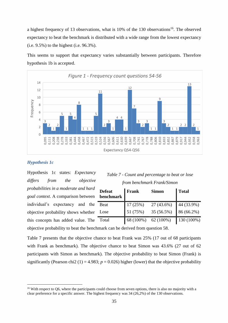
35

a highest frequency of 13 observations, what is 10% of the 130 observations16. The observed

expectancy to beat the benchmark is distributed with a wide range from the lowest expectancy

(i.e. 9.5%) to the highest (i.e. 96.3%).

This seems to support that expectancy varies substantially between participants. Therefore

hypothesis 1b is accepted.

Hypothesis 1c

Hypothesis 1c states: Expectancy

differs from the objective

probabilities in a moderate and hard

goal context. A comparison between

individual’s expectancy and the

objective probability shows whether

this concepts has added value. The

objective probability to beat the benchmark can be derived from question 58.

Table 7 presents that the objective chance to beat Frank was 25% (17 out of 68 participants

with Frank as benchmark). The objective chance to beat Simon was 43.6% (27 out of 62

participants with Simon as benchmark). The objective probability to beat Simon (Frank) is

significantly (Pearson chi2 (1) = 4.983; p = 0.026) higher (lower) that the objective probability

16 With respect to Q6, where the participants could choose from seven options, there is also no majority with a

clear preference for a specific answer. The highest frequency was 34 (26,2%) of the 130 observations.

Defeat

benchmark

Frank Simon Total

Beat 17 (25%) 27 (43.6%) 44 (33.9%)

Lose 51 (75%) 35 (56.5%) 86 (66.2%)

Total 68 (100%) 62 (100%) 130 (100%)

Table 7 - Count and percentage to beat or lose

from benchmark Frank/Simon

Table 8 - Count and percentage to beat or lose

from benchmark Frank/Simon

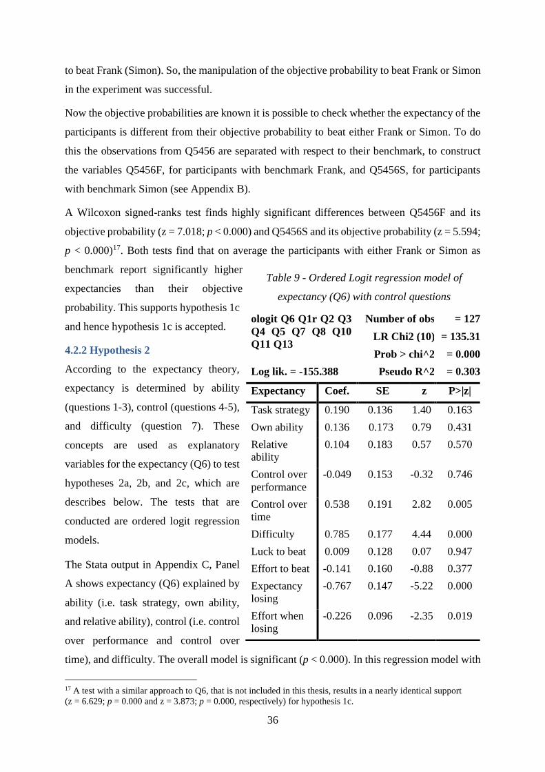
36

to beat Frank (Simon). So, the manipulation of the objective probability to beat Frank or Simon

in the experiment was successful.

Now the objective probabilities are known it is possible to check whether the expectancy of the

participants is different from their objective probability to beat either Frank or Simon. To do

this the observations from Q5456 are separated with respect to their benchmark, to construct

the variables Q5456F, for participants with benchmark Frank, and Q5456S, for participants

with benchmark Simon (see Appendix B).

A Wilcoxon signed-ranks test finds highly significant differences between Q5456F and its

objective probability (z = 7.018; p < 0.000) and Q5456S and its objective probability (z = 5.594;

p < 0.000)17. Both tests find that on average the participants with either Frank or Simon as

benchmark report significantly higher

expectancies than their objective

probability. This supports hypothesis 1c

and hence hypothesis 1c is accepted.

4.2.2 Hypothesis 2

According to the expectancy theory,

expectancy is determined by ability

(questions 1-3), control (questions 4-5),

and difficulty (question 7). These

concepts are used as explanatory

variables for the expectancy (Q6) to test

hypotheses 2a, 2b, and 2c, which are

describes below. The tests that are

conducted are ordered logit regression

models.

The Stata output in Appendix C, Panel

A shows expectancy (Q6) explained by

ability (i.e. task strategy, own ability,

and relative ability), control (i.e. control

over performance and control over

time), and difficulty. The overall model is significant (p < 0.000). In this regression model with

17 A test with a similar approach to Q6, that is not included in this thesis, results in a nearly identical support

(z = 6.629; p = 0.000 and z = 3.873; p = 0.000, respectively) for hypothesis 1c.

ologit Q6 Q1r Q2 Q3

Q4 Q5 Q7 Q8 Q10

Q11 Q13

Number of obs = 127

LR Chi2 (10) = 135.31

Prob > chi^2 = 0.000

Log lik. = -155.388 Pseudo R^2 = 0.303

Expectancy Coef. SE z P>|z|

Task strategy 0.190 0.136 1.40 0.163

Own ability 0.136 0.173 0.79 0.431

Relative

ability

0.104 0.183 0.57 0.570

Control over

performance

-0.049 0.153 -0.32 0.746

Control over

time

0.538 0.191 2.82 0.005

Difficulty 0.785 0.177 4.44 0.000

Luck to beat 0.009 0.128 0.07 0.947

Effort to beat -0.141 0.160 -0.88 0.377

Expectancy

losing

-0.767 0.147 -5.22 0.000

Effort when

losing

-0.226 0.096 -2.35 0.019

Table 9 - Ordered Logit regression model of

expectancy (Q6) with control questions

Table 10 - Ordered Logit regression model of

expectancy (Q6) with control questions

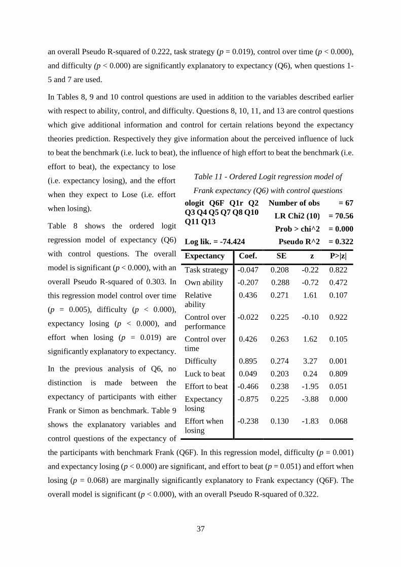
37

an overall Pseudo R-squared of 0.222, task strategy (p = 0.019), control over time (p < 0.000),

and difficulty (p < 0.000) are significantly explanatory to expectancy (Q6), when questions 1-

5 and 7 are used.

In Tables 8, 9 and 10 control questions are used in addition to the variables described earlier

with respect to ability, control, and difficulty. Questions 8, 10, 11, and 13 are control questions

which give additional information and control for certain relations beyond the expectancy

theories prediction. Respectively they give information about the perceived influence of luck

to beat the benchmark (i.e. luck to beat), the influence of high effort to beat the benchmark (i.e.

effort to beat), the expectancy to lose

(i.e. expectancy losing), and the effort

when they expect to Lose (i.e. effort

when losing).

Table 8 shows the ordered logit

regression model of expectancy (Q6)

with control questions. The overall

model is significant (p < 0.000), with an

overall Pseudo R-squared of 0.303. In

this regression model control over time

(p = 0.005), difficulty (p < 0.000),

expectancy losing (p < 0.000), and

effort when losing (p = 0.019) are

significantly explanatory to expectancy.

In the previous analysis of Q6, no

distinction is made between the

expectancy of participants with either

Frank or Simon as benchmark. Table 9

shows the explanatory variables and

control questions of the expectancy of

the participants with benchmark Frank (Q6F). In this regression model, difficulty (p = 0.001)

and expectancy losing (p < 0.000) are significant, and effort to beat (p = 0.051) and effort when

losing (p = 0.068) are marginally significantly explanatory to Frank expectancy (Q6F). The

overall model is significant (p < 0.000), with an overall Pseudo R-squared of 0.322.

ologit Q6F Q1r Q2

Q3 Q4 Q5 Q7 Q8 Q10

Q11 Q13

Number of obs = 67

LR Chi2 (10) = 70.56

Prob > chi^2 = 0.000

Log lik. = -74.424 Pseudo R^2 = 0.322

Expectancy Coef. SE z P>|z|

Task strategy -0.047 0.208 -0.22 0.822

Own ability -0.207 0.288 -0.72 0.472

Relative

ability

0.436 0.271 1.61 0.107

Control over

performance

-0.022 0.225 -0.10 0.922

Control over

time

0.426 0.263 1.62 0.105

Difficulty 0.895 0.274 3.27 0.001

Luck to beat 0.049 0.203 0.24 0.809

Effort to beat -0.466 0.238 -1.95 0.051

Expectancy

losing

-0.875 0.225 -3.88 0.000

Effort when

losing

-0.238 0.130 -1.83 0.068

Table 11 - Ordered Logit regression model of

Frank expectancy (Q6) with control questions

Table 12 - Ordered Logit regression model of

Frank expectancy (Q6) with control questions

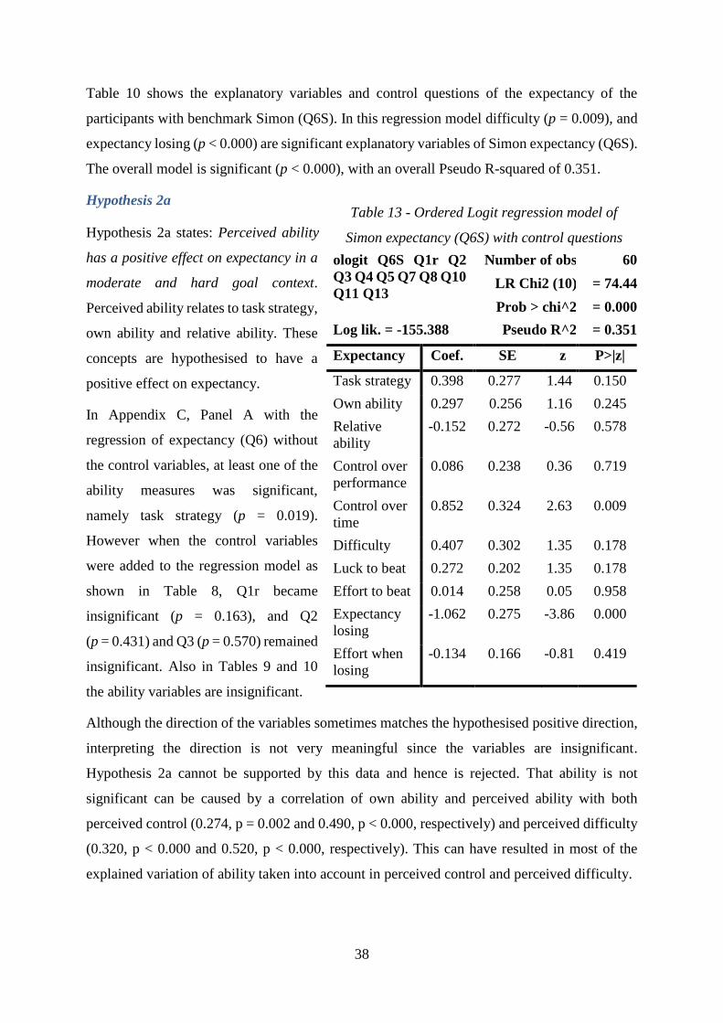
38

Table 10 shows the explanatory variables and control questions of the expectancy of the

participants with benchmark Simon (Q6S). In this regression model difficulty (p = 0.009), and

expectancy losing (p < 0.000) are significant explanatory variables of Simon expectancy (Q6S).

The overall model is significant (p < 0.000), with an overall Pseudo R-squared of 0.351.

Hypothesis 2a

Hypothesis 2a states: Perceived ability

has a positive effect on expectancy in a

moderate and hard goal context.

Perceived ability relates to task strategy,

own ability and relative ability. These

concepts are hypothesised to have a

positive effect on expectancy.

In Appendix C, Panel A with the

regression of expectancy (Q6) without

the control variables, at least one of the

ability measures was significant,

namely task strategy (p = 0.019).

However when the control variables

were added to the regression model as

shown in Table 8, Q1r became

insignificant (p = 0.163), and Q2

(p = 0.431) and Q3 (p = 0.570) remained

insignificant. Also in Tables 9 and 10

the ability variables are insignificant.

Although the direction of the variables sometimes matches the hypothesised positive direction,

interpreting the direction is not very meaningful since the variables are insignificant.

Hypothesis 2a cannot be supported by this data and hence is rejected. That ability is not

significant can be caused by a correlation of own ability and perceived ability with both

perceived control (0.274, p = 0.002 and 0.490, p < 0.000, respectively) and perceived difficulty

(0.320, p < 0.000 and 0.520, p < 0.000, respectively). This can have resulted in most of the

explained variation of ability taken into account in perceived control and perceived difficulty.

ologit Q6S Q1r Q2

Q3 Q4 Q5 Q7 Q8 Q10

Q11 Q13

Number of obs 60

LR Chi2 (10) = 74.44

Prob > chi^2 = 0.000

Log lik. = -155.388 Pseudo R^2 = 0.351

Expectancy Coef. SE z P>|z|

Task strategy 0.398 0.277 1.44 0.150

Own ability 0.297 0.256 1.16 0.245

Relative

ability

-0.152 0.272 -0.56 0.578

Control over

performance

0.086 0.238 0.36 0.719

Control over

time

0.852 0.324 2.63 0.009

Difficulty 0.407 0.302 1.35 0.178

Luck to beat 0.272 0.202 1.35 0.178

Effort to beat 0.014 0.258 0.05 0.958

Expectancy

losing

-1.062 0.275 -3.86 0.000

Effort when

losing

-0.134 0.166 -0.81 0.419

Table 13 - Ordered Logit regression model of

Simon expectancy (Q6S) with control questions

Table 14 - Ordered Logit regression model of

Simon expectancy (Q6S) with control questions

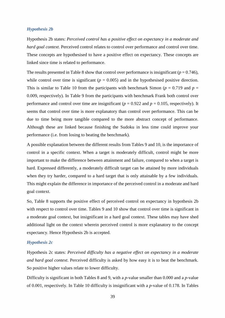
39

Hypothesis 2b

Hypothesis 2b states: Perceived control has a positive effect on expectancy in a moderate and

hard goal context. Perceived control relates to control over performance and control over time.

These concepts are hypothesised to have a positive effect on expectancy. These concepts are

linked since time is related to performance.

The results presented in Table 8 show that control over performance is insignificant (p = 0.746),

while control over time is significant (p = 0.005) and in the hypothesised positive direction.

This is similar to Table 10 from the participants with benchmark Simon (p = 0.719 and p =

0.009, respectively). In Table 9 from the participants with benchmark Frank both control over

performance and control over time are insignificant (p = 0.922 and p = 0.105, respectively). It

seems that control over time is more explanatory than control over performance. This can be

due to time being more tangible compared to the more abstract concept of performance.

Although these are linked because finishing the Sudoku in less time could improve your

performance (i.e. from losing to beating the benchmark).

A possible explanation between the different results from Tables 9 and 10, is the importance of

control in a specific context. When a target is moderately difficult, control might be more

important to make the difference between attainment and failure, compared to when a target is

hard. Expressed differently, a moderately difficult target can be attained by more individuals

when they try harder, compared to a hard target that is only attainable by a few individuals.

This might explain the difference in importance of the perceived control in a moderate and hard

goal context.

So, Table 8 supports the positive effect of perceived control on expectancy in hypothesis 2b

with respect to control over time. Tables 9 and 10 show that control over time is significant in

a moderate goal context, but insignificant in a hard goal context. These tables may have shed

additional light on the context wherein perceived control is more explanatory to the concept

expectancy. Hence Hypothesis 2b is accepted.

Hypothesis 2c

Hypothesis 2c states: Perceived difficulty has a negative effect on expectancy in a moderate

and hard goal context. Perceived difficulty is asked by how easy it is to beat the benchmark.

So positive higher values relate to lower difficulty.

Difficulty is significant in both Tables 8 and 9, with a p-value smaller than 0.000 and a p-value

of 0.001, respectively. In Table 10 difficulty is insignificant with a p-value of 0.178. In Tables

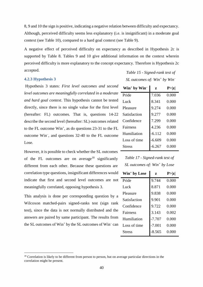
40

8, 9 and 10 the sign is positive, indicating a negative relation between difficulty and expectancy.

Although, perceived difficulty seems less explanatory (i.e. is insignificant) in a moderate goal

context (see Table 10), compared to a hard goal context (see Table 9).

A negative effect of perceived difficulty on expectancy as described in Hypothesis 2c is

supported by Table 8. Tables 9 and 10 give additional information on the context wherein

perceived difficulty is more explanatory to the concept expectancy. Therefore is Hypothesis 2c

accepted.

4.2.3 Hypothesis 3

Hypothesis 3 states: First level outcomes and second

level outcomes are meaningfully correlated in a moderate

and hard goal context. This hypothesis cannot be tested

directly, since there is no single value for the first level

(hereafter: FL) outcomes. That is, questions 14-22

describe the second level (hereafter: SL) outcomes related

to the FL outcome Win+, as do questions 23-31 to the FL

outcome Win–, and questions 32-40 to the FL outcome

Lose.

However, it is possible to check whether the SL outcomes

of the FL outcomes are on average18 significantly

different from each other. Because these questions are

correlation type questions, insignificant differences would

indicate that first and second level outcomes are not

meaningfully correlated, opposing hypothesis 3.

This analysis is done per corresponding question by a

Wilcoxon matched-pairs signed-ranks test (sign rank

test), since the data is not normally distributed and the

answers are paired by same participant. The results from

the SL outcomes of Win+ by the SL outcomes of Win– can

18 Correlation is likely to be different from person to person, but on average particular directions in the

correlation might be present.

Win+ by Win– z P>|z|

Pride 7.036 0.000

Luck 8.341 0.000

Pleasure 9.274 0.000

Satisfaction 9.277 0.000

Confidence 7.299 0.000

Fairness 4.236 0.000

Humiliation -6.112 0.000

Loss of time -6.609 0.000

Stress -6.267 0.000

Win+ by Lose z P>|z|

Pride 9.744 0.000

Luck 8.871 0.000

Pleasure 9.838 0.000

Satisfaction 9.901 0.000

Confidence 9.722 0.000

Fairness 3.143 0.002

Humiliation -7.707 0.000

Loss of time -7.001 0.000

Stress -8.565 0.000

Table 17 - Signed-rank test of

SL outcomes of: Win+ by Lose

Table 18 - Signed-rank test of

SL outcomes of: Win+ by Lose

Table 15 - Signed-rank test of

SL outcomes of: Win+ by Win–

Table 16 - Signed-rank test of

SL outcomes of: Win+ by Win–

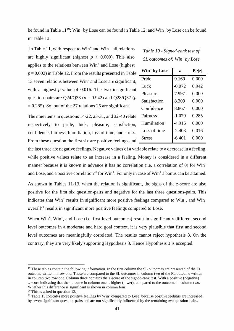
41

be found in Table 1119; Win+ by Lose can be found in Table 12; and Win– by Lose can be found

in Table 13.

In Table 11, with respect to Win+ and Win–, all relations

are highly significant (highest p < 0.000). This also

applies to the relations between Win+ and Lose (highest

p = 0.002) in Table 12. From the results presented in Table

13 seven relations between Win– and Lose are significant,

with a highest p-value of 0.016. The two insignificant

question-pairs are Q24/Q33 (p = 0.942) and Q28/Q37 (p

= 0.285). So, out of the 27 relations 25 are significant.

The nine items in questions 14-22, 23-31, and 32-40 relate

respectively to pride, luck, pleasure, satisfaction,

confidence, fairness, humiliation, loss of time, and stress.

From these question the first six are positive feelings and

the last three are negative feelings. Negative values of a variable relate to a decrease in a feeling,

while positive values relate to an increase in a feeling. Money is considered in a different

manner because it is known in advance it has no correlation (i.e. a correlation of 0) for Win–

and Lose, and a positive correlation20 for Win+. For only in case of Win+ a bonus can be attained.

As shown in Tables 11-13, when the relation is significant, the signs of the z-score are also

positive for the first six question-pairs and negative for the last three questions-pairs. This

indicates that Win+ results in significant more positive feelings compared to Win–, and Win–

overall21 results in significant more positive feelings compared to Lose.

When Win+, Win–, and Lose (i.e. first level outcomes) result in significantly different second

level outcomes in a moderate and hard goal context, it is very plausible that first and second

level outcomes are meaningfully correlated. The results cannot reject hypothesis 3. On the

contrary, they are very likely supporting Hypothesis 3. Hence Hypothesis 3 is accepted.

19 These tables contain the following information. In the first column the SL outcomes are presented of the FL

outcome written in row one. These are compared to the SL outcomes in column two of the FL outcome written

in column two row one. Column three contains the z-score of the signed-rank test. With a positive (negative)

z-score indicating that the outcome in column one is higher (lower), compared to the outcome in column two.

Whether this difference is significant is shown in column four. 20 This is asked in question 12. 21 Table 13 indicates more positive feelings by Win– compared to Lose, because positive feelings are increased

by seven significant question-pairs and are not significantly influenced by the remaining two question-pairs.

Win– by Lose z P>|z|

Pride 9.169 0.000

Luck -0.072 0.942

Pleasure 7.997 0.000

Satisfaction 8.309 0.000

Confidence 8.867 0.000

Fairness -1.070 0.285

Humiliation -4.916 0.000

Loss of time -2.403 0.016

Stress -6.401 0.000

Table 19 - Signed-rank test of

SL outcomes of: Win– by Lose

Table 20 - Signed-rank test of

SL outcomes of: Win– by Lose

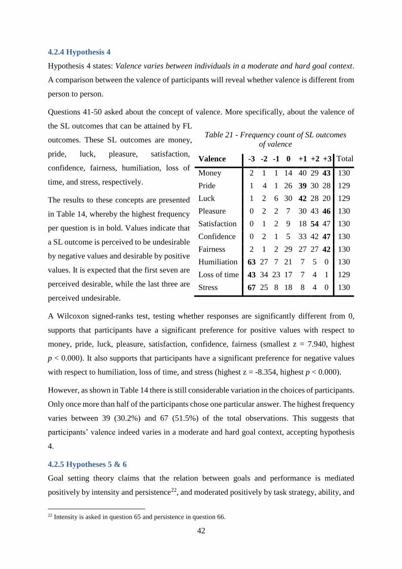
42

4.2.4 Hypothesis 4

Hypothesis 4 states: Valence varies between individuals in a moderate and hard goal context.

A comparison between the valence of participants will reveal whether valence is different from

person to person.

Questions 41-50 asked about the concept of valence. More specifically, about the valence of

the SL outcomes that can be attained by FL

outcomes. These SL outcomes are money,

pride, luck, pleasure, satisfaction,

confidence, fairness, humiliation, loss of

time, and stress, respectively.

The results to these concepts are presented

in Table 14, whereby the highest frequency

per question is in bold. Values indicate that

a SL outcome is perceived to be undesirable

by negative values and desirable by positive

values. It is expected that the first seven are

perceived desirable, while the last three are

perceived undesirable.

A Wilcoxon signed-ranks test, testing whether responses are significantly different from 0,

supports that participants have a significant preference for positive values with respect to

money, pride, luck, pleasure, satisfaction, confidence, fairness (smallest z = 7.940, highest

p < 0.000). It also supports that participants have a significant preference for negative values

with respect to humiliation, loss of time, and stress (highest z = -8.354, highest p < 0.000).

However, as shown in Table 14 there is still considerable variation in the choices of participants.

Only once more than half of the participants chose one particular answer. The highest frequency

varies between 39 (30.2%) and 67 (51.5%) of the total observations. This suggests that

participants’ valence indeed varies in a moderate and hard goal context, accepting hypothesis

4.

4.2.5 Hypotheses 5 & 6

Goal setting theory claims that the relation between goals and performance is mediated

positively by intensity and persistence22, and moderated positively by task strategy, ability, and

22 Intensity is asked in question 65 and persistence in question 66.

Valence -3 -2 -1 0 +1 +2 +3 Total

Money 2 1 1 14 40 29 43 130

Pride 1 4 1 26 39 30 28 129

Luck 1 2 6 30 42 28 20 129

Pleasure 0 2 2 7 30 43 46 130

Satisfaction 0 1 2 9 18 54 47 130

Confidence 0 2 1 5 33 42 47 130

Fairness 2 1 2 29 27 27 42 130

Humiliation 63 27 7 21 7 5 0 130

Loss of time 43 34 23 17 7 4 1 129

Stress 67 25 8 18 8 4 0 130

Table 21 - Frequency count of SL outcomes

of valence

Table 22 - Frequency count of SL outcomes

of valence

43

commitment23 (Locke & Latham, 2006, 2013). The goal is to beat the benchmark. Performance

can be viewed as the actual time wherein a participant solved the Sudoku, and/or as being faster

than either Frank (i.e. 8 minutes) or Simon (i.e. 12 minutes). These mediators and moderators

influence the goal-performance relation.

The mediators explain the goal-performance relation. They are caused by goals and explain the

performance (Baron & Kenny, 1986). Whether a mediator exists can be tested by the

explanatory power of the mediators on performance. In contrast, the moderators affect the

strength and/or direction of the goal-performance relation (Baron & Kenny, 1986). When a

moderator exists, higher levels of a moderator result ceteris paribus in a higher goal-

performance relation. Whether a moderator exists can be tested by the existence of an

interacting effect between the goal and the moderators. So the mediators are tested by their

explanatory power of the goal-performance relation and the moderators are tested by their

interaction effect on the goal-performance relation.

Table 15 presents the summary of the p-values of the variables in the factorial analyses of

covariance24, known as ANCOVA. Interaction is denoted with a hashtag (#). The models are

respectively included in Appendix C, Panel B to E. Performance is the dependent variable,

although this variable is measured differently in the models, as noted in Table 15. Target

attainment has a value of 1 if the Sudoku is solved within a specific time and 0 otherwise, while

actual time gives the actual time if the Sudoku is solved within a specific time and a missing

value otherwise. In both cases the specific times are either 8 or 12 minutes. This performance

is explained by the mediators and moderators and by the benchmark. In addition the number of

observations, the significance of the overall model and the adjusted R-squared are shown per

model. The results that are significant are in bold, whereas results that are marginally significant

are underlined.

Table 15 shows that all the models in the summary are significant. The models have adjusted

R-squares that vary between 0.166 and 0.415, so adjusted for the number of variables25 the

models explain between 16.6% and 41.5% of the variation. In addition it shows that the number

of (marginally) significant variables within the models of 8 minutes is higher, compared to the

models of 12 minutes. This indicates an increased explanatory power of particular variables

23 Task strategy is asked in question 1, ability in question 1-3, and commitment in questions 65 and 66. 24 Since Q57A is binary a factorial logistic regression model (logistic) can be used to test the hypothesised

relations. However, when the interaction terms were included in the model Stata was not able to conduct the test.

Therefore the analyses is conducted by a factorial ANCOVA. 25 More accurate: adjusted for the number of degrees of freedom within the analysis.

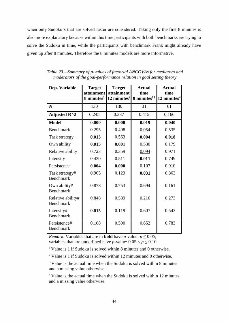
44

when only Sudoku’s that are solved faster are considered. Taking only the first 8 minutes is

also more explanatory because within this time participants with both benchmarks are trying to

solve the Sudoku in time, while the participants with benchmark Frank might already have

given up after 8 minutes. Therefore the 8 minutes models are more informative.

Dep. Variable Target

attainment

8 minutes1

Target

attainment

12 minutes2

Actual

time

8 minutes13

Actual

time

12 minutes4

N 130 130 31 61

Adjusted R^2 0.245 0.337 0.415 0.166

Model 0.000 0.000 0.019 0.040

Benchmark 0.295 0.408 0.054 0.535

Task strategy 0.013 0.563 0.004 0.018

Own ability 0.015 0.001 0.530 0.179

Relative ability 0.723 0.359 0.094 0.971

Intensity 0.420 0.511 0.011 0.749

Persistence 0.004 0.000 0.107 0.910

Task strategy#

Benchmark

0.905 0.123 0.031 0.863

Own ability#

Benchmark

0.878 0.753 0.694 0.161

Relative ability#

Benchmark

0.848 0.589 0.216 0.273

Intensity#

Benchmark 0.015 0.119 0.607 0.543

Persistence#

Benchmark

0.108 0.500 0.652 0.783

Remark: Variables that are in bold have p-value: p ≤ 0.05;

variables that are underlined have p-value: 0.05 < p ≤ 0.10.

1 Value is 1 if Sudoku is solved within 8 minutes and 0 otherwise.

2 Value is 1 if Sudoku is solved within 12 minutes and 0 otherwise.

3 Value is the actual time when the Sudoku is solved within 8 minutes

and a missing value otherwise.

4 Value is the actual time when the Sudoku is solved within 12 minutes

and a missing value otherwise.

Table 23 – Summary of p-values of factorial ANCOVAs for mediators and

moderators of the goal-performance relation in goal setting theory

Table 24 – Summary of p-values of factorial ANCOVAs for mediators and

moderators of the goal-performance relation in goal setting theory

45

Intensity and persistence are interpreted in the following section Hypothesis 5a & 5b. Task

strategy, ability, and the interaction effects are interpreted in section Hypotheses 6a, 6b & 6c.

Benchmark is interpreted in section Hypotheses 7b.

Hypotheses 5a & 5b

Hypothesis 5a states: Intensity is a positive mediator in the goal-performance relation in a

moderate and hard goal context. Hypothesis 5b states: Persistence is a positive mediator in the

goal-performance relation in a moderate and hard goal context. When intensity and persistence

are caused by goals then they are mediators when they have a significant explanatory power on

performance.

Intensity is significant in the model of actual time within 8 minutes. Persistence is significant

in both models of target attainment. This difference can be partially explained by the relative

explanatory effect when the actual time is considered, compared to target attainment. As noted

below Table 15, target attainment has values of zeros and ones, while actual time gives the

actual time or a missing value.

The observations of participants that took more than either 8 or 12 minutes and gave up/had to

give up (i.e. persistence) are omitted in actual time but included in target attainment with a

value of zero. Persistence is not explanatory to performance in the model of actual time within

8 minutes, since no participants gave up within the first 8 minutes26. But because after 12

minutes27 some participants gave up/had to give up this increased the explanatory power of

persistence the models of target attainment.

With respect to intensity, most of the participants worked very intensely28, including those that

took more than either 8 or 12 minutes, thereby reducing the explanatory effect of intensity in

the models of target attainment. When considering the actual time in the first 8 minutes,

intensity is significant, although not in the hypothesised direction29. Higher levels of intensity

had a negative effect on the time wherein a participant solved the Sudoku. This can be explained

by the lower perceived intensity of participants that solved the Sudoku very quickly compared

to higher levels of perceived intensity for participants that took longer and had a feeling of more

intense trying.

26 Tabulating the results for persistence within the first 8 minutes showed no positive observations. 27 Tabulating the results for persistence after 12 minutes showed 23 positive observations. 28 Tabulating the results for intensity showed that 80% of the observations are positive. 29 Further analysis shows a negative effect of intensity on performance.

46

Hence only persistence had the hypothesised positive explanatory effect on the goal-

performance relation. The analysis supports persistence as mediator variable, in comparing

participants that attained a target to those who did not attain this target. Therefore hypothesis

5a is rejected and hypothesis 5b is accepted.

Hypotheses 6a, 6b & 6c

Hypothesis 6a states: Task strategy is a positive moderator of the goal-performance relation in

a moderate and hard goal context. Hypothesis 6b states: Perceived ability is a positive

moderator of the goal-performance relation in a moderate and hard goal context. Hypothesis

6c states: Perceived commitment is a positive moderator of the goal-performance relation in a

moderate and hard goal context. These hypotheses refer respectively to task strategy, ability,

and commitment. Ability is measured by task strategy, own ability, and relative ability.

Commitment is measured by intensity and persistence. These variables are interacted

individually by the variable benchmark. When these variables are moderators they interact with

the goal-performance relation.

As shown in Table 15, task strategy, own ability, and relative ability are used to explain

performance. Since they are pre-existing and not determined by goals they cannot be mediators

for the goal-performance relation, but they can be moderators. Regarding their direct effect

some statements can be derived after analysis of the direction. As mentioned before, part of the

difference between the 8 and 12 minutes models might be explained by an increased

explanatory power; that is, higher levels of ability can explain why Sudoku’s are solved faster.

Task strategy is positive significant to performance with target attainment, but negative

significant with actual time. It seems that task strategy is informative in comparing participants

that solved the Sudoku within 8 minutes to participants that took longer, but not in comparing

the group of very quick participants regarding their actual time. Own ability is significantly

positive to performance in the models of target attainment. Relative ability is marginally

significantly positive to performance in the model of actual time within 8 minutes. This

difference between own ability and relative ability can be because own ability cannot exactly

predict the actual time, however relative ability can partially predict a faster time.

Table 15 shows that the interactions have two significant results. The interaction of task strategy

is significant with respect to the actual time within 8 minutes. That is, performance is higher

with benchmark Simon for higher levels of task strategy compared to benchmark Frank. The

interaction of intensity is once significant with respect to target attainment within 8 minutes.

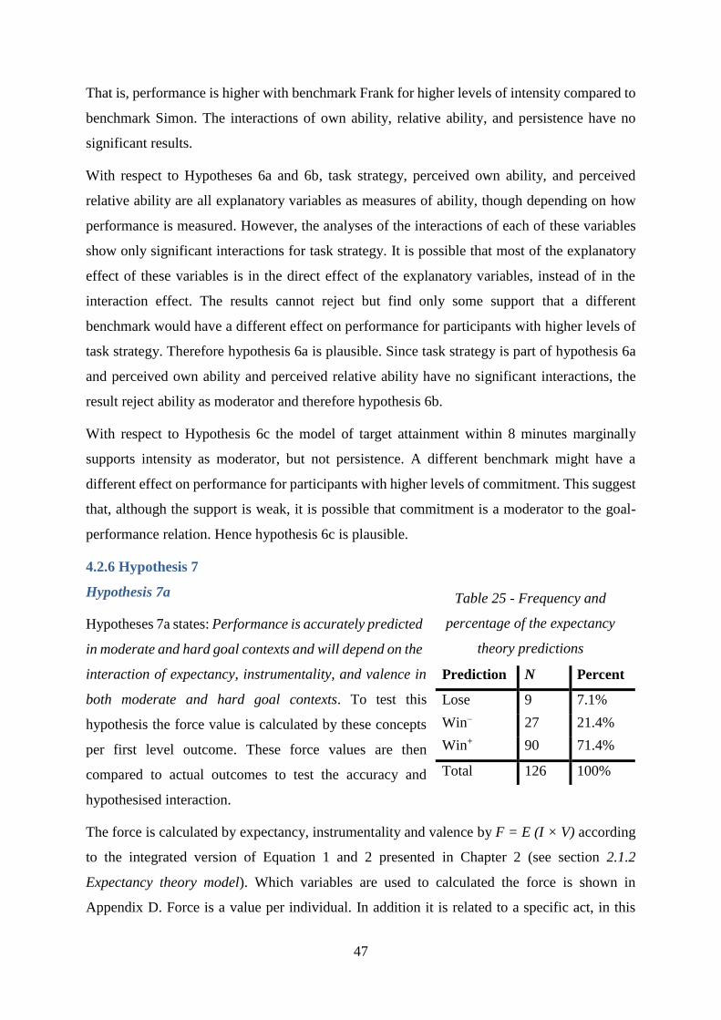
47

That is, performance is higher with benchmark Frank for higher levels of intensity compared to

benchmark Simon. The interactions of own ability, relative ability, and persistence have no

significant results.

With respect to Hypotheses 6a and 6b, task strategy, perceived own ability, and perceived

relative ability are all explanatory variables as measures of ability, though depending on how

performance is measured. However, the analyses of the interactions of each of these variables

show only significant interactions for task strategy. It is possible that most of the explanatory

effect of these variables is in the direct effect of the explanatory variables, instead of in the

interaction effect. The results cannot reject but find only some support that a different

benchmark would have a different effect on performance for participants with higher levels of

task strategy. Therefore hypothesis 6a is plausible. Since task strategy is part of hypothesis 6a

and perceived own ability and perceived relative ability have no significant interactions, the

result reject ability as moderator and therefore hypothesis 6b.

With respect to Hypothesis 6c the model of target attainment within 8 minutes marginally

supports intensity as moderator, but not persistence. A different benchmark might have a

different effect on performance for participants with higher levels of commitment. This suggest

that, although the support is weak, it is possible that commitment is a moderator to the goal-

performance relation. Hence hypothesis 6c is plausible.

4.2.6 Hypothesis 7

Hypothesis 7a

Hypotheses 7a states: Performance is accurately predicted

in moderate and hard goal contexts and will depend on the

interaction of expectancy, instrumentality, and valence in

both moderate and hard goal contexts. To test this

hypothesis the force value is calculated by these concepts

per first level outcome. These force values are then

compared to actual outcomes to test the accuracy and

hypothesised interaction.

The force is calculated by expectancy, instrumentality and valence by F = E (I × V) according

to the integrated version of Equation 1 and 2 presented in Chapter 2 (see section 2.1.2

Expectancy theory model). Which variables are used to calculated the force is shown in

Appendix D. Force is a value per individual. In addition it is related to a specific act, in this

Prediction N Percent

Lose 9 7.1%

Win– 27 21.4%

Win+ 90 71.4%

Total 126 100%

Table 25 - Frequency and

percentage of the expectancy

theory predictions

Table 26 - Frequency and

percentage of the expectancy

theory predictions

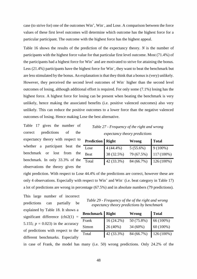
48

case (to strive for) one of the outcomes Win+, Win–, and Lose. A comparison between the force

values of these first level outcomes will determine which outcome has the highest force for a

particular participant. The outcome with the highest force has the highest appeal.

Table 16 shows the results of the prediction of the expectancy theory. N is the number of

participants with the highest force value for that particular first level outcome. Most (71.4%) of

the participants had a highest force for Win+ and are motivated to strive for attaining the bonus.

Less (21.4%) participants have the highest force for Win–, they want to beat the benchmark but

are less stimulated by the bonus. An explanation is that they think that a bonus is (very) unlikely.

However, they perceived the second level outcomes of Win– higher than the second level

outcomes of losing, although additional effort is required. For only some (7.1%) losing has the

highest force. A highest force for losing can be present when beating the benchmark is very

unlikely, hence making the associated benefits (i.e. positive valenced outcomes) also very

unlikely. This can reduce the positive outcomes to a lower force than the negative valenced

outcomes of losing. Hence making Lose the best alternative.

Table 17 gives the number of

correct predictions of the

expectancy theory with respect to

whether a participant beat the

benchmark or lost from the

benchmark. In only 33.3% of the

observations the theory gives the

right prediction. With respect to Lose 44.4% of the predictions are correct, however these are

only 4 observations. Especially with respect to Win+ and Win– (i.e. beat category in Table 17)

a lot of predictions are wrong in percentage (67.5%) and in absolute numbers (79 predictions).

This large number of incorrect

predictions can partially be

explained by Table 18. It shows a

significant difference (chi2(1) =

5.155; p = 0.023) in the accuracy

of predictions with respect to the

different benchmarks. Especially

in case of Frank, the model has many (i.e. 50) wrong predictions. Only 24.2% of the

Prediction Right Wrong Total

Lose 4 (44.4%) 5 (55.6%) 9 (100%)

Beat 38 (32.5%) 79 (67.5%) 117 (100%)

Total 42 (33.3%) 84 (66.7%) 126 (100%)

Benchmark Right Wrong Total

Frank 16 (24.2%) 50 (75.8%) 66 (100%)

Simon 26 (40%) 34 (60%) 60 (100%)

Total 42 (33.3%) 84 (66.7%) 126 (100%)

Table 27 - Frequency of the right and wrong

expectancy theory predictions

Table 28 - Frequency of the right and wrong

expectancy theory predictions

Table 29 - Frequency of the of the right and wrong

expectancy theory predictions by benchmark

Table 30 - Frequency of the of the right and wrong

expectancy theory predictions by benchmark

49

observations could be explained by the expectancy theory predictions. In case of Simon 40%

of the observations could be explained.

To evaluated these predictions in terms of accuracy they should be compared to a standard. In

case of the expectancy theory the force value would predict the outcome. Since there are only

three possible outcomes, the random chance to predict a correct prediction is 33.3%. This is

equal to the correct prediction rate of the expectancy theory, as shown in Table 17. So the

expectancy theory does not have more prediction power compared to random chance. Therefore

there is reason to believe that the combination of the concepts in a force value to determine the

outcome is not accurately enough.

A partial explanation for this low accuracy can be found in the results of hypotheses 1a and 1c.

Combining these results already showed that the expectancy for the participants with Frank as

Benchmark was lower compared to the expectancy for the participants with Simon as

Benchmark30. This overconfidence can partially explain the difference in predictive power of

the expectancy with respect to a moderate and hard goal context. In addition, this large

difference between the expectancy and the objective probability led to an overestimation of the

benefits of beating the benchmark, thereby inflating the prediction of beating the benchmark

relative to losing from it. The expectancy theory predicted only 9 participants to Lose, while in

fact 86 participants lost form their respective benchmark.

Hence the results show minimal support for both parts of Hypothesis 7a. Although the

predictive power of the expectancy theory is higher with benchmark Simon compared to Frank,

the accuracy is weak. Performance seems only partially depending on the interaction of the

expectancy theory concepts expectancy, instrumentality and valence as stated by the expectancy

theory. Therefore hypotheses 7a is rejected.

Hypothesis 7b

Hypothesis 7b states: Performance is accurately predicted by goal setting theory in moderate

and hard goal contexts and will be higher in the hard goal context, compared to the moderate

goal context, when considering the moderators and mediators. The accuracy of the goal setting

theory in predicting performance can be derived from the explanatory power of the models.

Performance in relation to moderate and hard goal contexts is tested.

30 For both Q6 and Q5456 the test statistics were larger for Frank compared to Simon, respectively z = 7.018 vs.

z = 5.594 and z = 6.629 vs. z = 3.873.

50

The accuracy of the goal setting theory in predicting performance is shown in the variation of

the adjusted R-squared of the models in Table 15. The model with the highest explained

adjusted variation is 41.5% in the model of actual time within 8 minutes. This model has an

unadjusted R-squared of 63%, so 63% of the variation. This figure is similar or higher than

models explaining performance in previous research, for example Huber (1985) found an

unadjusted R-squared of 63% and Mento, Locke and Klein (1992) found an unadjusted R-

squared of 32%.

The analysis of performance in relation to moderate and hard goal contexts is shown in Table

15. When controlling for various interaction effects and direct effects, the dummy variable

Benchmark gives the direct effect of a different benchmark. Benchmark has a marginally

significant result, in the model of actual time within 8 minutes. The interactions pointed out that

performance is higher with benchmark Simon for higher levels of task strategy compared to

benchmark Frank. And performance is higher with benchmark Frank for higher levels of

intensity compared to benchmark Simon. Further analysis suggests that ceteris paribus

Benchmark Simon will marginally significantly lower performance compared to benchmark

Frank. In other words, participants with benchmark Frank perform marginally significantly

better compared to participants with benchmark Simon.

The results show some support for both parts of Hypothesis 7b. The explanatory power of the

models using the goal setting theory constructs is similar or higher than the explained variation

in previous research. In addition, the results show that the hard goal context (i.e. having a higher

benchmark) will marginally significantly increase performance ceteris paribus. This is in

accordance with the theoretical predictions of the goal setting theory after controlling for other

relations specified by the theory. Hence Hypothesis 7b is accepted.

51

5. Conclusion

This chapter summarises the present research, discusses the conclusion that answers the

research questions and the contribution of the present research. In addition the limitations of

the present research and directions for future research are discussed.

5.1 Conclusion and Discussion

This thesis began with the common question “What do you expect?” This general question led

to the motivational theory of expectancy theory, wherein expectations play a major role.

Together with instrumentality and valence, they are the three concepts that determine the force

of a person to perform a particular act. According to expectancy theory, the force value of

particular outcomes can explain which performance level an individual chooses. But results are

not conclusive as to how accurate expectancy theory is in explaining performance. However,

expectancy theory is not the only motivational theory to explain performance. Goal setting

theory assumes that goals themselves influence performance when accounted for multiple

mediators and moderators. This theory, that is strongly supported by previous research,

sometimes appears to contradict expectancy theory. Particular with respect to expectancy in the

form of goal difficulty the theories have different predictions. Since goal difficulty is different

in a moderate goal context compared to a hard goal context, this is an ideal context to test the

theories. Therefore this thesis tested the following research questions:

RQ1: Do the motivational theories, expectancy and goal setting, have correct

theoretical constructs?

RQ2: Which motivational theory, expectancy or goal setting, is more accurate in

predicting performance in a moderate and hard goal context?

An experiment with 130 participants divided over a specific (assigned) moderate (62

participants) and hard goal context (68 participants) was used to empirically test most for the

underlying constructs of the theories and their predictive accuracy. The choice to conduct the

research by an experiment was suggested in the literature and inspired by the need to control

behaviour to be able to test the determinants of this behaviour (e.g. Van Eerde & Thierry, 1996).

In this experiment real incentives are use, since the bonus is depending on performance.

Research finds significant differences between incentivised and non-incentivised studies

whereby real incentives result in more realistic (i.e. has lower error) and higher performance

where increases effort increases performance, however there are also tasks wherein this effect

52

is not present, for example when participants have sufficient intrinsic motivation as

psychologists usually claim or the task is to hard, and incentives can also hurt performance

(Camerer & Hogarth, 1999). Although Read (2005) does not find significant difference between

real and hypothesised incentives he concludes by saying that the incentivised dominates the

non-incentivised if the incentivised can be easily conducted and the money is available. This

experiment uses real incentive because money is hypothesised as a motivator that increases

effort. In addition, the design was easily incentivised, it better simulates a real work related

setting and a behavioural economic experiment uses real incentives.

The hypotheses that were derived from the theories were the guidelines to analyse the research

questions. In total there were seven hypotheses, some with multiple parts. Hypotheses 1-4 and

7a related to expectancy theory. Hypotheses 5-6 and 7b related to the goal setting theory.

Hypothesis 1 shows that the manipulation of the moderate and hard task context was successful.

With respect to expectancy theory, it also proved that the concept of expectancy has added

value. The results support part of hypothesis 2 that expectancy is determined by perceived

control and perceived difficulty, but ability does not significantly determined expectancy.

Possibly due to correlation most of the explained variation of ability is taken into account in

perceived control and perceived difficulty. Hypothesis 3 is supported. The results confirm that

the first level outcomes and second level outcomes are meaningfully correlated. Valence, as

hypothesised in hypothesis 4, varies among individuals. Despite most of the previous theoretical

constructs of the concepts expectancy, instrumentality and valence are confirmed, the

theoretical construct of force could not be confirmed. This lowered the accuracy of the

expectancy theory and hence led to the rejection of hypothesis 7a. That force was not

informative enough can be explained by a lack of predictive power in the combination of the

concepts, partially because the expectancy of goal attainment was overestimated by the

participants, especially in case of benchmark Frank. This indicates that the theory as presented

by Vroom (1964, 1995) is likely not valid. Another possibility is that the task used in the

experiment is not appropriate to measure and predict performance, although this seems unlikely

given the results of the predictions of goal setting theory.

With respect to goal setting theory, the results of hypothesis 5 support that persistence is a

positive mediator in the goal-performance relation in a moderate and hard goal context. Results

find some support for intensity as a positive mediator, making this relation plausible.

Hypothesis 6 has mixed support. Task strategy, perceived own ability, and perceived relative

ability all have some direct explanatory effect. However from these ability measures, only task

53

strategy has some significant interaction in explaining performance. Therefore this relation is

deemed plausible. This difference can be due to most of the variation already explained by the

direct effects. Hypothesis 6 is further supported by a significant positive interaction of

commitment to the goal-performance relation in a moderate and hard goal context. Hypothesis

7b is supported by the results, indicating that goal setting theory is satisfactory accurate in

predicting performance in moderate and hard goal contexts. In addition, it indicates that the

goal setting theory prediction that performance is higher in the hard goal context compared to

the moderate goal context is supported. When controlling for the moderators and mediators, it

is supported that goals influence the goal-performance relation themselves.

Hence the research questions with respect to both motivational theories can be answered. This

research showed that regarding RQ1 the concepts expectancy, instrumentality, and valence,

have significant value, but the interaction resulting in a force value that can predict behaviour

is not supported. Also with respect to goal setting theory most of the hypothesised relations

were either plausible or supported. Persistence is a mediator to the goal-performance relation.

Furthermore, this relation can be influenced by task strategy and is influenced by commitment,

as positive moderators. Finally, the theoretical construct that goals themselves have a significant

influence on performance is also supported. Regarding RQ2 with respect to expectancy theory,

the research shows that expectancy theory has little predict power. On the contrary, goal setting

theory is supported in its accuracy to predict performance while controlling for the moderators

and mediators. So in comparison with expectancy theory is goal setting theory the most accurate

motivational theory.

5.2 Contribution

The results are in line with previous findings that question the validity of the expectancy theory.

For example House et al. (1974) found that support for the validity is mixed. Connelly (1976)

and Van Eerde and Thierry (1996), among others, state that some research is performed in a

different manner than the original formulation. The current research went back to Vroom’s

original formulation and took into account many suggestions from previous research, but the

results were similar. This research likewise finds evidence for the concepts expectancy,

instrumentality, and valence within the expectancy theory but the concept of force seems of

very little value (e.g. House et al., 1974; Van Eerde & Thierry, 1996).

This research that is very close to the original formulation adds to the understanding of

researchers that even the original formulation is likely not valid. This research indicates that the

54

main problem with expectancy theory is in the concept of force, while the other concepts have

added value. Employers can use the expectancy of target attainment, the instrumentality

between performance and rewards, and the valence of these rewards to create a deeper

understanding of human behaviour in work related settings. Especially expectancy can be

overestimated, whereby overconfident employees can engage in more risk taking or

overinvesting that could have harmful consequences (e.g. Ben-David, Graham & Harvey, 2013;

Malmendier & Tate, 2005). Making expectancies more realistic could mitigate this problem.

This research further confirms that research has drifted away from expectancy theory in a search

for more valid and accurate motivational theories, such as goal setting theory.

The present research adds to the growing body of evidence that supports goal setting theory.

Taking into account the moderators and mediators, performance is indeed positively influenced

by a higher goal as claimed by for example Locke and Latham (2013, 2015). However some

remarks can be made. It is possible that this higher performance is due to higher risk taking for

the participants with a higher goal, thereby increasing the chance of success but also of failure

(Locke & Latham, 2013, p. 299). Since in case of the actual time only the participants with

success are taken into account, this could inflate the effect of the higher goal itself. The present

research also raises the question whether applying goal setting theory to work related settings

does increase performance. Taken into account the moderators and mediators does not say much

about the actual performance. A comparison between the performance measured in actual time

shows no significant difference between the groups with either benchmark Frank or Simon31.

The present research shows that not taking into account the moderators and mediators gives no

increase in performance. When applying goal setting theory to a work related setting, Ordóñez,

Schweitzer, Galinsky and Bazerman (2009) list several potential side effects. Including that

goal setting theory can increase unethical behaviour, increase risk taking, create a narrow focus,

and reduce intrinsic motivation. They also give several directions on how to mitigate these

potential problems. Taking these directions into account in the application of goal setting theory

could result in an increased performance.

5.3 Limitations and Future Research

This research has some limitations which suggest future research. As mentioned before it can

be that the task used in the experiment is not appropriate to measure and predict performance.

31 A Wilcoxon rank-sum test found no significant difference with respect to actual time within 8 minutes (z =

-0.099; p = 0.921) and within 12 minutes (z = -0.601; p = 0.548) with respect to benchmark.

55

Since the predictions of the expectancy theory with respect to force were not accurate. Although

this seems unlikely given the results of the predictions of goal setting theory.

In addition, students are used to test for the differences of the motivational theories expectancy

and goal setting. It can be possible that other groups of participants have different behaviour

that would result in different conclusions. An experiment was performed to control the

environment to eliminate other effects than the aimed manipulation of the expectancy.

However, it could have been that different groups would respond differently to the same

treatment in the experiment.

Future research can control more extensively for the limitations mentioned above. It is possible

that although controlling for differences between the groups, the groups were not the same after

all. This might explain differences between the groups that were not related to the examined

relations. Different age groups can be used to generalise the findings of this research.

The concept of force could be investigated in greater detail. Especially with respect to the

weighting of the concepts expectancy, instrumentality, and valence. This might increase the

accuracy of the expectancy theory.

In addition, this research can be applied to other tasks to check for potential differences in their

conclusions. The current research used most of the questions from the questionnaire to answer

the research question, although future research could use the results from the questionnaire in

a variety of ways and to test multiple other relations.

The results show that some results are only significant in specific situation, with respect to

either dependent variable or interaction variable. A closer examination is needed to further

distinguish between relations in the specific situations.

56

References

Articles

Atkinson, J. W., & Reitman, W. R. (1956). Performance as a function of motive strength and

expectancy of goal-attainment. The Journal of Abnormal and Social Psychology,

53(3), 361.

Babbie, E.R. (2010). The Practice of Social Research. 12th edition, Belmont, CA, USA:

Wadsworth, Cengage Learning.

Baron, R. M., & Kenny, D. A. (1986). The moderator-mediator variable distinction in social

psychological research: Conceptual, strategic, and statistical considerations. Journal of

Personality and Social Psychology, 51, 1173-1182.

Ben-David, I., Graham, J. R., & Harvey, C. R. (2013). MANAGERIAL MISCALIBRATION.

The Quarterly Journal of Economics, 1547, 1584.

Bryan, W. L., & Harter, N. (1897). Studies in the physiology and psychology of the

telegraphic language. Psychological Review, 4(1), 27.

Camerer, C. F., & Hogarth, R. M. (1999). The effects of financial incentives in experiments:

A review and capital-labor-production framework. Journal of risk and uncertainty,

19(1-3), 7-42.

Camerer, C., & Weber, M. (1992). Recent developments in modeling preferences:

Uncertainty and ambiguity. Journal of risk and uncertainty, 5(4), 325-370.

Connolly, T. (1976). Some conceptual and methodologcal issues in expectancy models of

work performance motivation. Academy of Management Review, 1(4), 37-47.

Dachler, H. P., & Mobley, W. H. (1973). Construct validation of an instrumentality-

expectancy-task-goal model of work motivation: Some theoretical boundary

conditions. Journal of Applied Psychology, 58(3), 397.

Dawes, J. G. (2008). Do data characteristics change according to the number of scale points

used? An experiment using 5 point, 7 point and 10 point scales. International journal

of market research, 51(1).

Edwards, W. (1954). The theory of decision making. Psychological bulletin, 51(4), 380.

Friedman, D., & Sunder, S. (1994). Experimental methods: A primer for economists.

Cambridge university press.

Galbraith, J., & Cummings, L. L. (1967). An empirical investigation of the motivational

determinants of task performance: Interactive effects between instrumentality—

valence and motivation—ability. Organizational behavior and human performance,

2(3), 237-257.

Gigerenzer, G., & Selten, R. (2001). Rethinking rationality. Bounded rationality: The

adaptive toolbox, 1, 12.

Hackman, J. R., & Porter, L. W. (1968). Expectancy theory predictions of work effectiveness.

Organizational Behavior and Human Performance, 3(4), 417-426.

Harrison, G. W., Johnson, E., McInnes, M. M., & Rutström, E. E. (2005). Risk aversion and

incentive effects: Comment. American Economic Review, 897-901.

Heneman, H. G., & Schwab, D. P. (1972). Evaluation of research on expectancy theory

predictions of employee performance. Psychological Bulletin, 78(1), 1.

House, R. J. (1971). A path goal theory of leader effectiveness. Administrative science

quarterly, 321-339.

Huber, V. L. (1985). Effects of task difficulty, goal setting, and strategy on performance of a

heuristic task. Journal of Applied Psychology, 70(3), 492.

Kahneman, D., & Tversky, A. (1979). Prospect theory: An analysis of decision under risk.

Econometrica: Journal of the Econometric Society, 263-291.

57

Kennedy, C. W., Fossum, J. A., & White, B. J. (1983). An empirical comparison of within-

subjects and between-subjects expectancy theory models. Organizational behavior

and human performance, 32(1), 124-143.

Klein, H. J. (1991). Further evidence on the relationship between goal setting and expectancy

theories. Organizational Behavior and Human Decision Processes, 49(2), 230-257.

Latham, G. P., & Locke, E. A. (2007). New developments in and directions for goal-setting

research. European Psychologist, 12(4), 290-300.

Lawler, E. E., & Suttle, J. L. (1973). Expectancy theory and job behavior. Organizational

behavior and human performance, 9(3), 482-503.

Lewin, K. (1938). The conceptual representation and measurement of psychological forces.

Duke University. Contributions to Psychological Theory.

Locke, E. A. (1968). Toward a theory of task motivation and incentives. Organizational

behavior and human performance, 3(2), 157-189.

Locke, E. A., & Latham, G. P. (1990). A theory of goal setting & task performance. Prentice-

Hall, Inc.

Locke, E. A., & Latham, G. P. (2002). Building a practically useful theory of goal setting and

task motivation: A 35-year odyssey. American psychologist, 57(9), 705.

Locke, E. A., & Latham, G. P. (2006). New directions in goal-setting theory. Current

directions in psychological science, 15(5), 265-268.

Locke, E. A., & Latham, G. P. (2013). New developments on goal setting and task

performance. New York: Routledge.

Locke, E. A., & Latham, G. P. (2015). Chapter Four-Breaking the Rules: A Historical

Overview of Goal-Setting Theory. Advances in Motivation Science, 2, 99-126.

Locke, E. A., Motowidlo, S. J., & Bobko, P. (1986). Using self-efficacy theory to resolve the

conflict between goal-setting theory and expectancy theory in organizational behavior

and industrial/organizational psychology. Journal of Social and Clinical Psychology,

4(3), 328.

Tolman, E. C. (1925). Behaviorism and purpose. The Journal of Philosophy, 22(2), 36-41.

Mace, C. A. (1935). Incentives. Some Experimental Studies. Industrial Health Research

Board Report. Medical Research Council, (72).

Matsui, T., Okada, A., & Mizuguchi, R. (1981). Expectancy theory prediction of the goal

theory postulate," The harder the goals, the higher the performance.". Journal of

Applied Psychology, 66(1), 54.

Mento, A. J., Cartledge, N. D., & Locke, E. A. (1980). Maryland vs Michigan vs Minnesota:

Another look at the relationship of expectancy and goal difficulty to task performance.

Organizational Behavior and Human Performance, 25(3), 419-440.

Mitchell, T. R. (1974). Expectancy models of job satisfaction, occupational preference and

effort: A theoretical, methodological, and empirical appraisal. Psychological Bulletin,

81(12), 1053.

Mitchell, T. R., & Albright, D. W. (1972). Expectancy theory predictions of the satisfaction,

effort, performance, and retention of naval aviation officers. Organizational Behavior

and Human Performance, 8(1), 1-20.

Moore, D., McCabe, G., Duckworth, W., & Alwan, L. (2008). The practice of business

statistics. 2th edition. W.H. Freeman & Company.

Read, D. (2005). Monetary incentives, what are they good for?. Journal of Economic

Methodology, 12(2), 265-276.

Ordóñez, L. D., Schweitzer, M. E., Galinsky, A. D., & Bazerman, M. H. (2009). Goals gone

wild: The systematic side effects of overprescribing goal setting. The Academy of

Management Perspectives, 23(1), 6-16.

58

Schmidt, F. L. (1973). Implications of a measurement problem for expectancy theory

research. Organizational Behavior and Human Performance, 10(2), 243-251.

Schuman, H., Presser, S., & Ludwig, J. (1981). Context effects on survey responses to

questions about abortion. Public Opinion Quarterly, 45(2), 216-223.

Schwab, D. P., Olian-Gottlieb, J. D., & Heneman, H. G. (1979). Between-subjects expectancy

theory research: A statistical review of studies predicting effort and performance.

Psychological Bulletin, 86(1), 139.

Sloof, R., & van Praag, C. M. (2008). Performance measurement, expectancy and agency

theory: An experimental study. Journal of Economic Behavior & Organization, 67(3),

794-809.

Tubbs, M. E., Boehne, D. M., & Dahl, J. G. (1993). Expectancy, valence, and motivational

force functions in goal-setting research: An empirical test. Journal of Applied

Psychology, 78(3), 361.

Van Eerde, W., & Thierry, H. (1996). Vroom's expectancy models and work-related criteria:

A meta-analysis. Journal of applied psychology, 81(5), 575.

Vroom, V. H. (1964). Work and motivation. 1964. NY: John Wiley & Sons.

Vroom, V. H. (1995). Work and motivation (1st ed). Jossey-Bass Publishers, San Francisco

Watson, J.B. (1925). Behaviorism. New York, NY: W.W. Norton & Company

Watson, J. B. (2013). Behaviorism. Read Books Ltd.

Internet

Expectations. (n.d.) Collins Dictionary of Economics, 4th ed.. (2005). Retrieved February 24

2016 from http://financial-dictionary.thefreedictionary.com/expectations

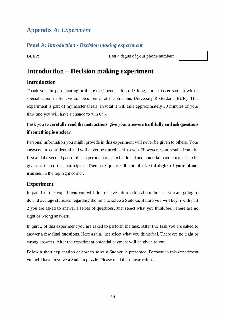
59

Appendix A: Experiment

Panel A: Introduction - Decision making experiment

BEEP: Last 4 digits of your phone number:

Introduction – Decision making experiment

Introduction

Thank you for participating in this experiment. I, John de Jong, am a master student with a

specialisation in Behavioural Economics at the Erasmus University Rotterdam (EUR). This

experiment is part of my master thesis. In total it will take approximately 30 minutes of your

time and you will have a chance to win €5,-.

I ask you to carefully read the instructions, give your answers truthfully and ask questions

if something is unclear.

Personal information you might provide in this experiment will never be given to others. Your

answers are confidential and will never be traced back to you. However, your results from the

first and the second part of this experiment need to be linked and potential payment needs to be

given to the correct participant. Therefore, please fill out the last 4 digits of your phone

number in the top right corner.

Experiment

In part 1 of this experiment you will first receive information about the task you are going to

do and average statistics regarding the time to solve a Sudoku. Before you will begin with part

2 you are asked to answer a series of questions. Just select what you think/feel. There are no

right or wrong answers.

In part 2 of this experiment you are asked to perform the task. After this task you are asked to

answer a few final questions. Here again, just select what you think/feel. There are no right or

wrong answers. After the experiment potential payment will be given to you.

Below a short explanation of how to solve a Sudoku is presented. Because in this experiment

you will have to solve a Sudoku puzzle. Please read these instructions.

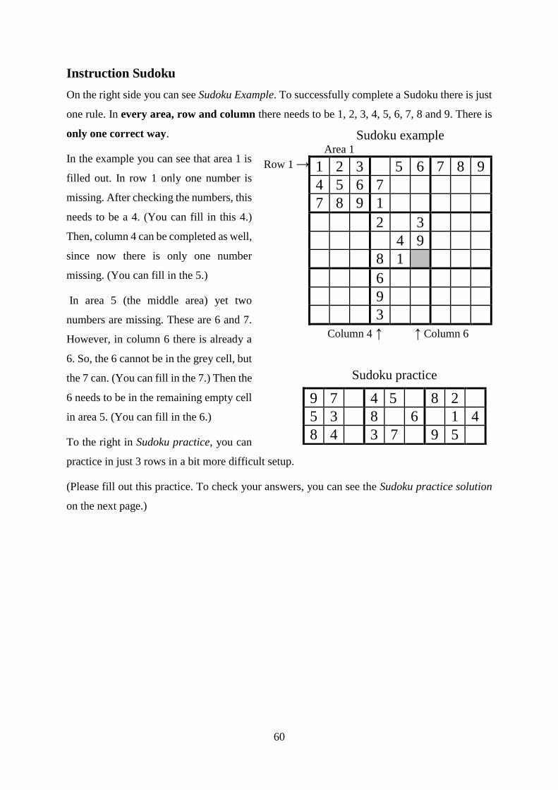
60

Instruction Sudoku

On the right side you can see Sudoku Example. To successfully complete a Sudoku there is just

one rule. In every area, row and column there needs to be 1, 2, 3, 4, 5, 6, 7, 8 and 9. There is

only one correct way.

In the example you can see that area 1 is

filled out. In row 1 only one number is

missing. After checking the numbers, this

needs to be a 4. (You can fill in this 4.)

Then, column 4 can be completed as well,

since now there is only one number

missing. (You can fill in the 5.)

In area 5 (the middle area) yet two

numbers are missing. These are 6 and 7.

However, in column 6 there is already a

6. So, the 6 cannot be in the grey cell, but

the 7 can. (You can fill in the 7.) Then the

6 needs to be in the remaining empty cell

in area 5. (You can fill in the 6.)

To the right in Sudoku practice, you can

practice in just 3 rows in a bit more difficult setup.

(Please fill out this practice. To check your answers, you can see the Sudoku practice solution

on the next page.)

Sudoku example Area 1

1 2 3 5 6 7 8 9

4 5 6 7

7 8 9 1

2 3

4 9

8 1

6

9

3

Column 4 ↑ ↑ Column 6

Sudoku practice

9 7 4 5 8 2

5 3 8 6 1 4

8 4 3 7 9 5

Row 1 →

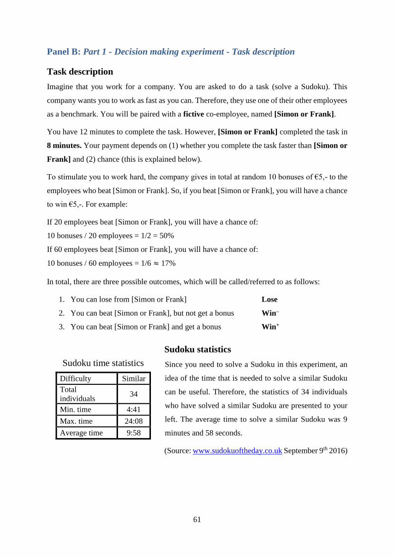
61

Panel B: Part 1 - Decision making experiment - Task description

Task description

Imagine that you work for a company. You are asked to do a task (solve a Sudoku). This

company wants you to work as fast as you can. Therefore, they use one of their other employees

as a benchmark. You will be paired with a fictive co-employee, named [Simon or Frank].

You have 12 minutes to complete the task. However, [Simon or Frank] completed the task in

8 minutes. Your payment depends on (1) whether you complete the task faster than [Simon or

Frank] and (2) chance (this is explained below).

To stimulate you to work hard, the company gives in total at random 10 bonuses of €5,- to the

employees who beat [Simon or Frank]. So, if you beat [Simon or Frank], you will have a chance

to win €5,-. For example:

If 20 employees beat [Simon or Frank], you will have a chance of:

10 bonuses / 20 employees = 1/2 = 50%

If 60 employees beat [Simon or Frank], you will have a chance of:

10 bonuses / 60 employees = 1/6 ≈ 17%

In total, there are three possible outcomes, which will be called/referred to as follows:

1. You can lose from [Simon or Frank] Lose

2. You can beat [Simon or Frank], but not get a bonus Win–

3. You can beat [Simon or Frank] and get a bonus Win+

Sudoku statistics

Since you need to solve a Sudoku in this experiment, an

idea of the time that is needed to solve a similar Sudoku

can be useful. Therefore, the statistics of 34 individuals

who have solved a similar Sudoku are presented to your

left. The average time to solve a similar Sudoku was 9

minutes and 58 seconds.

(Source: www.sudokuoftheday.co.uk September 9th 2016)

Sudoku time statistics

Difficulty Similar

Total

individuals 34

Min. time 4:41

Max. time 24:08

Average time 9:58

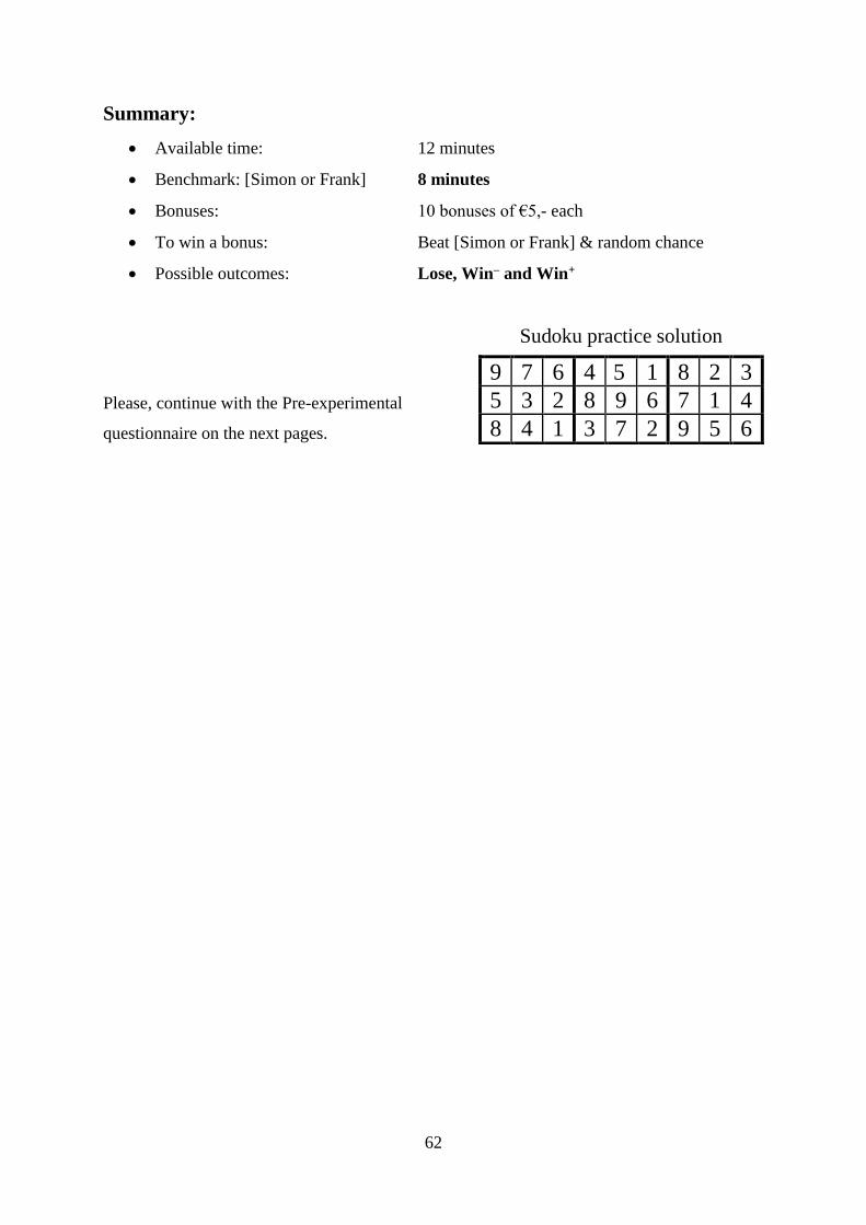
62

Summary:

Available time: 12 minutes

Benchmark: [Simon or Frank] 8 minutes

Bonuses: 10 bonuses of €5,- each

To win a bonus: Beat [Simon or Frank] & random chance

Possible outcomes: Lose, Win– and Win+

Please, continue with the Pre-experimental

questionnaire on the next pages.

Sudoku practice solution

9 7 6 4 5 1 8 2 3

5 3 2 8 9 6 7 1 4

8 4 1 3 7 2 9 5 6

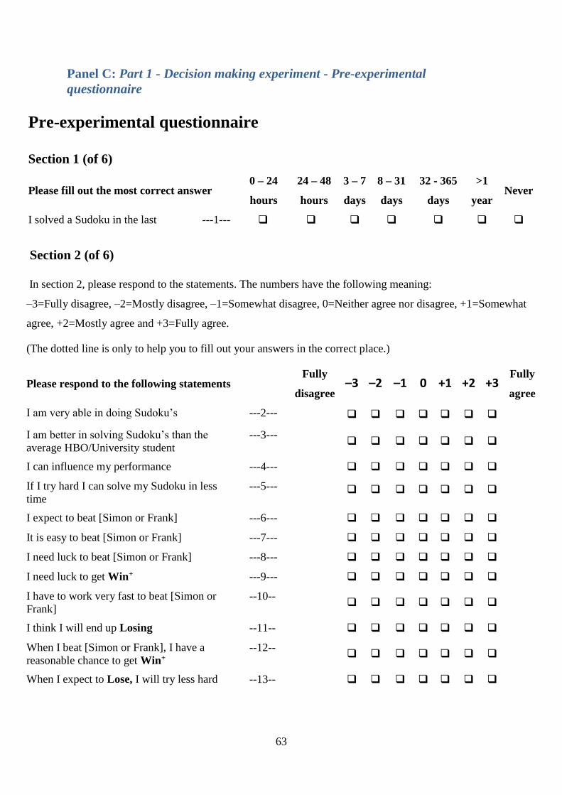
63

Panel C: Part 1 - Decision making experiment - Pre-experimental

questionnaire

Pre-experimental questionnaire

Section 1 (of 6)

Please fill out the most correct answer 0 – 24

hours

24 – 48

hours

3 – 7

days

8 – 31

days

32 - 365

days

>1

year Never

I solved a Sudoku in the last ---1---

Section 2 (of 6)

In section 2, please respond to the statements. The numbers have the following meaning:

–3=Fully disagree, –2=Mostly disagree, –1=Somewhat disagree, 0=Neither agree nor disagree, +1=Somewhat

agree, +2=Mostly agree and +3=Fully agree.

(The dotted line is only to help you to fill out your answers in the correct place.)

Please respond to the following statements Fully

disagree –3 –2 –1 0 +1 +2 +3

Fully

agree

I am very able in doing Sudoku’s ---2---

I am better in solving Sudoku’s than the

average HBO/University student

---3---

I can influence my performance ---4---

If I try hard I can solve my Sudoku in less

time

---5---

I expect to beat [Simon or Frank] ---6---

It is easy to beat [Simon or Frank] ---7---

I need luck to beat [Simon or Frank] ---8---

I need luck to get Win+ ---9---

I have to work very fast to beat [Simon or

Frank]

--10--

I think I will end up Losing --11--

When I beat [Simon or Frank], I have a

reasonable chance to get Win+

--12--

When I expect to Lose, I will try less hard --13--

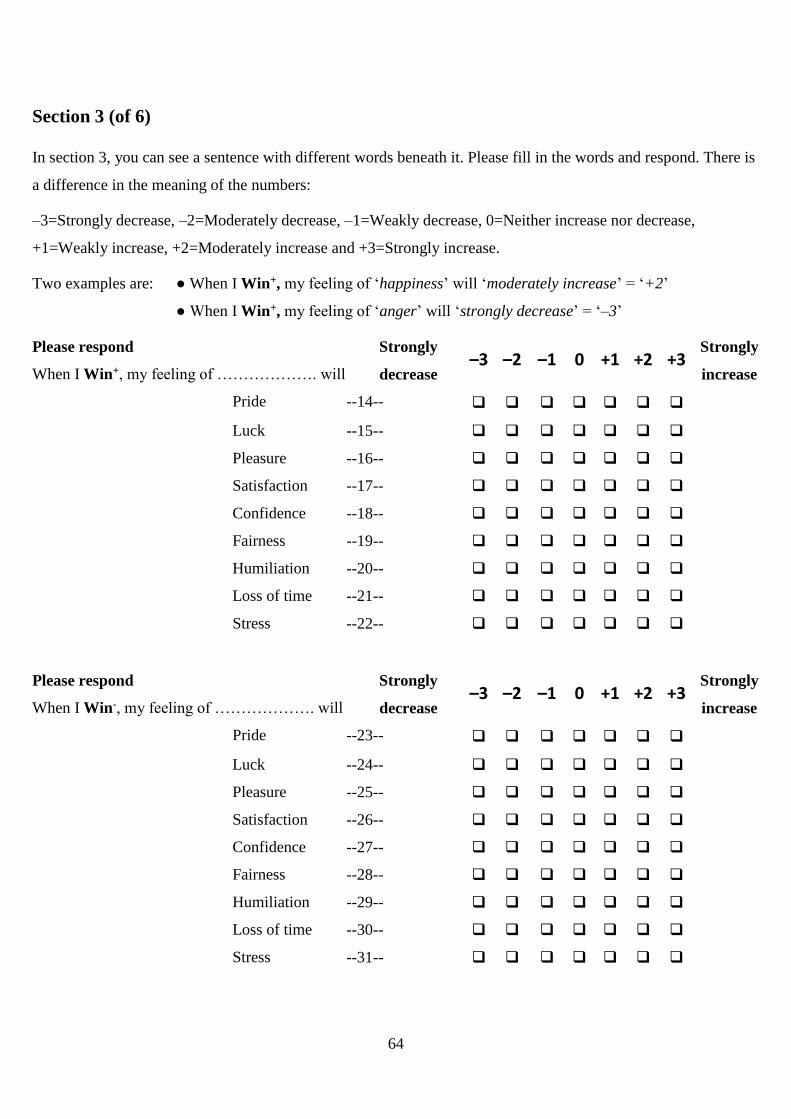
64

Section 3 (of 6)

In section 3, you can see a sentence with different words beneath it. Please fill in the words and respond. There is

a difference in the meaning of the numbers:

–3=Strongly decrease, –2=Moderately decrease, –1=Weakly decrease, 0=Neither increase nor decrease,

+1=Weakly increase, +2=Moderately increase and +3=Strongly increase.

Two examples are: ● When I Win+, my feeling of ‘happiness’ will ‘moderately increase’ = ‘+2’

● When I Win+, my feeling of ‘anger’ will ‘strongly decrease’ = ‘–3’

Please respond

When I Win+, my feeling of ………………. will

Strongly

decrease –3 –2 –1 0 +1 +2 +3

Strongly

increase

Pride --14--

Luck --15--

Pleasure --16--

Satisfaction --17--

Confidence --18--

Fairness --19--

Humiliation --20--

Loss of time --21--

Stress --22--

Please respond

When I Win-, my feeling of ………………. will

Strongly

decrease –3 –2 –1 0 +1 +2 +3

Strongly

increase

Pride --23--

Luck --24--

Pleasure --25--

Satisfaction --26--

Confidence --27--

Fairness --28--

Humiliation --29--

Loss of time --30--

Stress --31--

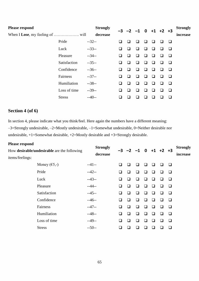
65

Please respond

When I Lose, my feeling of ………………. will

Strongly

decrease –3 –2 –1 0 +1 +2 +3

Strongly

increase

Pride --32--

Luck --33--

Pleasure --34--

Satisfaction --35--

Confidence --36--

Fairness --37--

Humiliation --38--

Loss of time --39--

Stress --40--

Section 4 (of 6)

In section 4, please indicate what you think/feel. Here again the numbers have a different meaning:

–3=Strongly undesirable, –2=Mostly undesirable, –1=Somewhat undesirable, 0=Neither desirable nor

undesirable, +1=Somewhat desirable, +2=Mostly desirable and +3=Strongly desirable.

Please respond

How desirable/undesirable are the following

items/feelings:

Strongly

decrease –3 –2 –1 0 +1 +2 +3

Strongly

increase

Money (€5,-) --41--

Pride --42--

Luck --43--

Pleasure --44--

Satisfaction --45--

Confidence --46--

Fairness --47--

Humiliation --48--

Loss of time --49--

Stress --50--

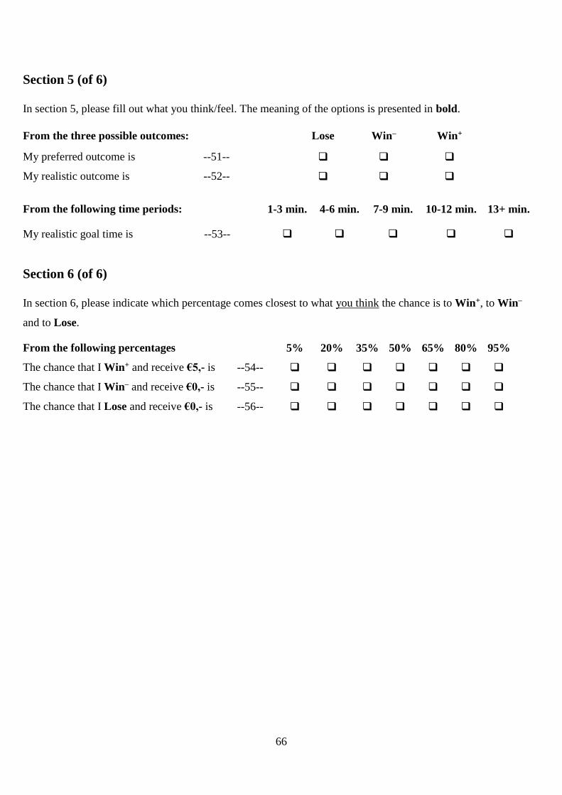
66

Section 5 (of 6)

In section 5, please fill out what you think/feel. The meaning of the options is presented in bold.

From the three possible outcomes: Lose Win– Win+

My preferred outcome is --51--

My realistic outcome is --52--

From the following time periods: 1-3 min. 4-6 min. 7-9 min. 10-12 min. 13+ min.

My realistic goal time is --53--

Section 6 (of 6)

In section 6, please indicate which percentage comes closest to what you think the chance is to Win+, to Win–

and to Lose.

From the following percentages 5% 20% 35% 50% 65% 80% 95%

The chance that I Win+ and receive €5,- is --54--

The chance that I Win– and receive €0,- is --55--

The chance that I Lose and receive €0,- is --56--

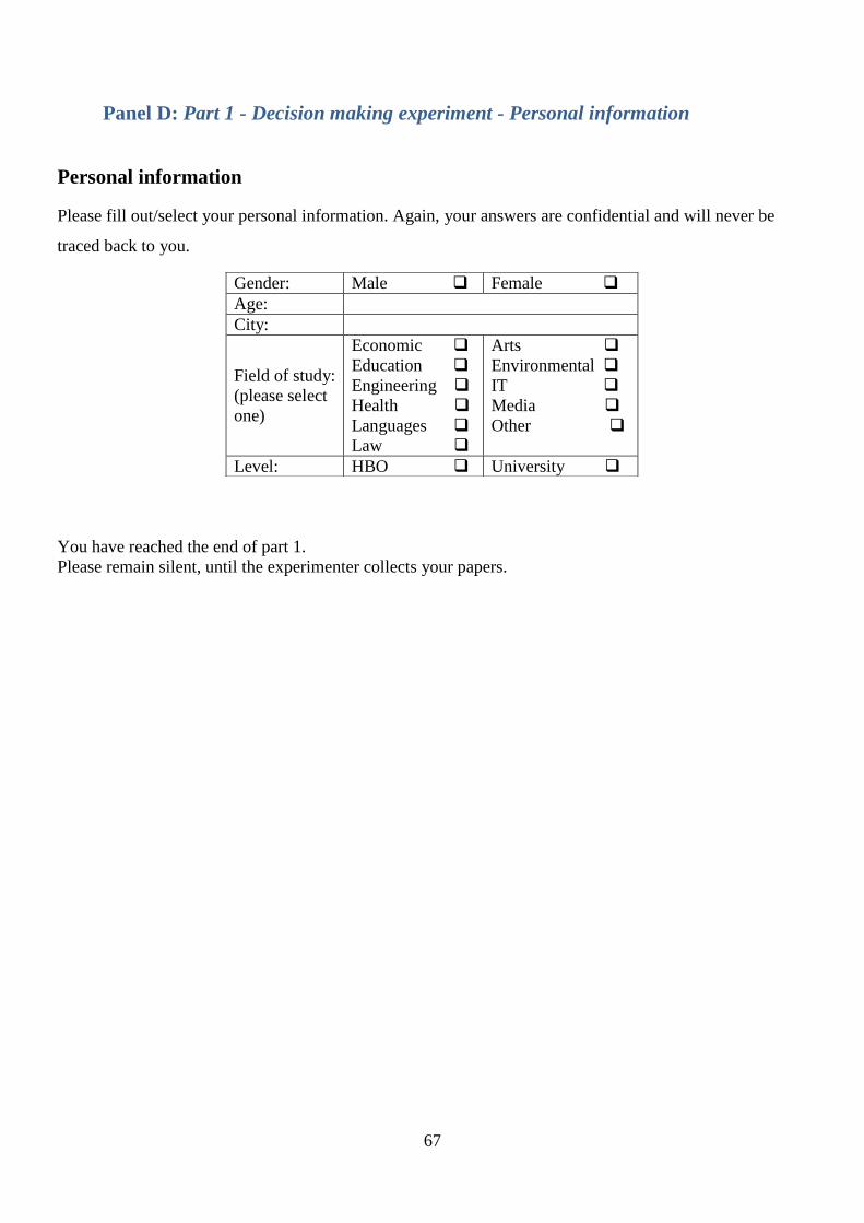
67

Panel D: Part 1 - Decision making experiment - Personal information

Personal information

Gender: Male Female

Age:

City:

Field of study:

(please select

one)

Economic

Education

Engineering

Health

Languages

Law

Arts

Environmental

IT

Media

Other

Level: HBO University

Please fill out/select your personal information. Again, your answers are confidential and will never be

traced back to you.

You have reached the end of part 1.

Please remain silent, until the experimenter collects your papers.

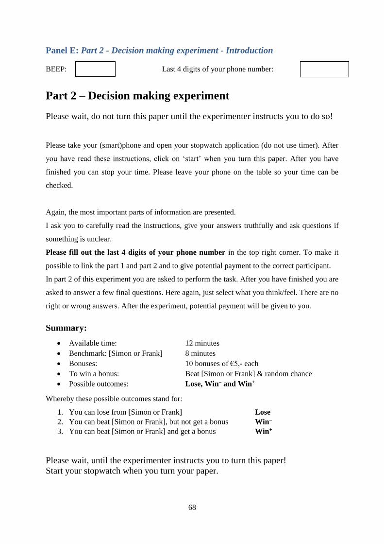
68

Panel E: Part 2 - Decision making experiment - Introduction

BEEP: Last 4 digits of your phone number:

Part 2 – Decision making experiment

Please wait, do not turn this paper until the experimenter instructs you to do so!

Please take your (smart)phone and open your stopwatch application (do not use timer). After

you have read these instructions, click on ‘start’ when you turn this paper. After you have

finished you can stop your time. Please leave your phone on the table so your time can be

checked.

Again, the most important parts of information are presented.

I ask you to carefully read the instructions, give your answers truthfully and ask questions if

something is unclear.

Please fill out the last 4 digits of your phone number in the top right corner. To make it

possible to link the part 1 and part 2 and to give potential payment to the correct participant.

In part 2 of this experiment you are asked to perform the task. After you have finished you are

asked to answer a few final questions. Here again, just select what you think/feel. There are no

right or wrong answers. After the experiment, potential payment will be given to you.

Summary:

Available time: 12 minutes

Benchmark: [Simon or Frank] 8 minutes

Bonuses: 10 bonuses of €5,- each

To win a bonus: Beat [Simon or Frank] & random chance

Possible outcomes: Lose, Win– and Win+

Whereby these possible outcomes stand for:

1. You can lose from [Simon or Frank] Lose

2. You can beat [Simon or Frank], but not get a bonus Win–

3. You can beat [Simon or Frank] and get a bonus Win+

Please wait, until the experimenter instructs you to turn this paper!

Start your stopwatch when you turn your paper.

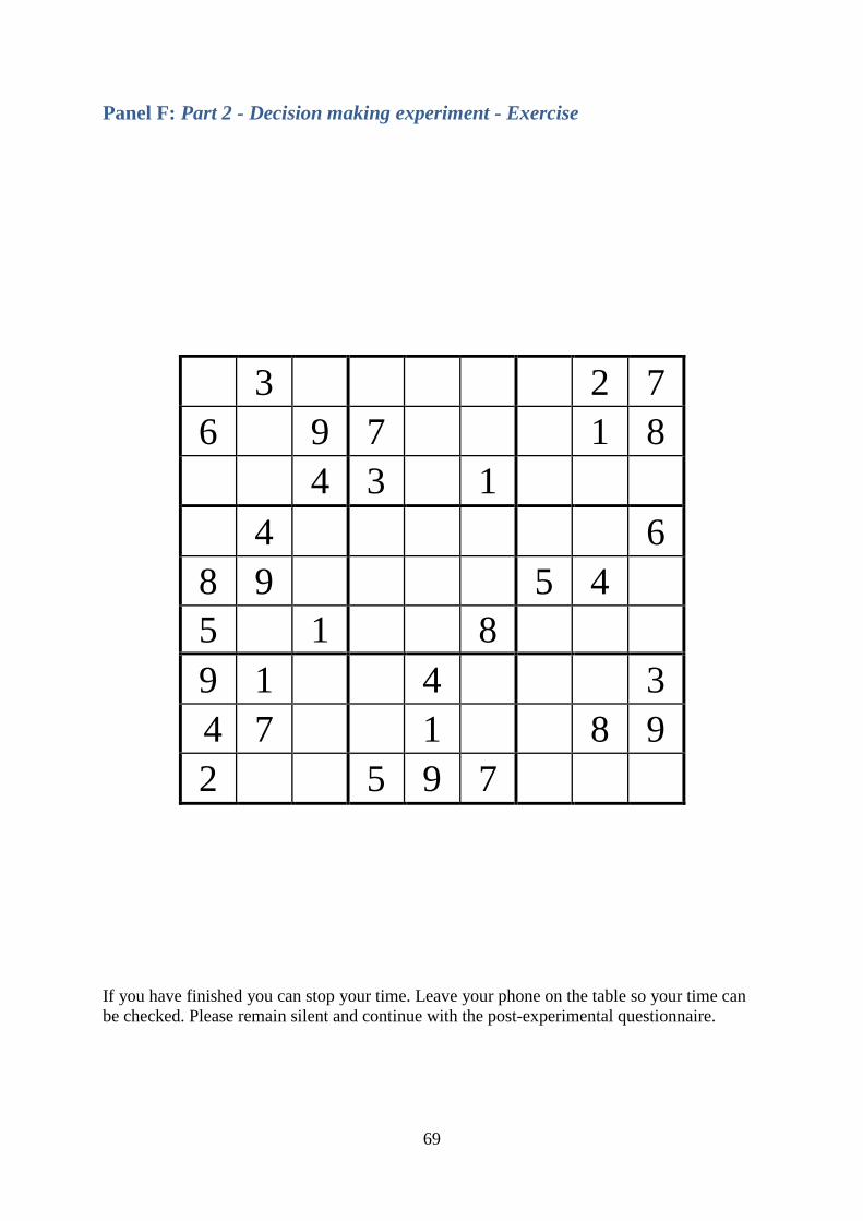
69

Panel F: Part 2 - Decision making experiment - Exercise

If you have finished you can stop your time. Leave your phone on the table so your time can

be checked. Please remain silent and continue with the post-experimental questionnaire.

3 2 7

6 9 7 1 8

4 3 1

4 6

8 9 5 4

5 1 8

9 1 4 3

4 7 1 8 9

2 5 9 7

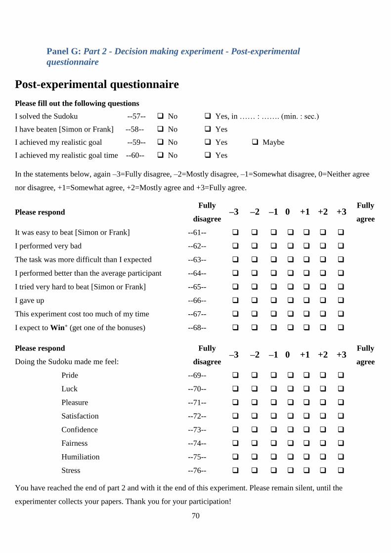
70

Panel G: Part 2 - Decision making experiment - Post-experimental

questionnaire

Post-experimental questionnaire

Please fill out the following questions

I solved the Sudoku --57-- No Yes, in …… : ……. (min. : sec.)

I have beaten [Simon or Frank] --58-- No Yes

I achieved my realistic goal --59-- No Yes Maybe

I achieved my realistic goal time --60-- No Yes

In the statements below, again –3=Fully disagree, –2=Mostly disagree, –1=Somewhat disagree, 0=Neither agree

nor disagree, +1=Somewhat agree, +2=Mostly agree and +3=Fully agree.

Please respond Fully

disagree –3 –2 –1 0 +1 +2 +3

Fully

agree

It was easy to beat [Simon or Frank] --61--

I performed very bad --62--

The task was more difficult than I expected --63--

I performed better than the average participant --64--

I tried very hard to beat [Simon or Frank] --65--

I gave up --66--

This experiment cost too much of my time --67--

I expect to Win+ (get one of the bonuses) --68--

Please respond

Doing the Sudoku made me feel:

Fully

disagree –3 –2 –1 0 +1 +2 +3

Fully

agree

Pride --69--

Luck --70--

Pleasure --71--

Satisfaction --72--

Confidence --73--

Fairness --74--

Humiliation --75--

Stress --76--

You have reached the end of part 2 and with it the end of this experiment. Please remain silent, until the

experimenter collects your papers. Thank you for your participation!

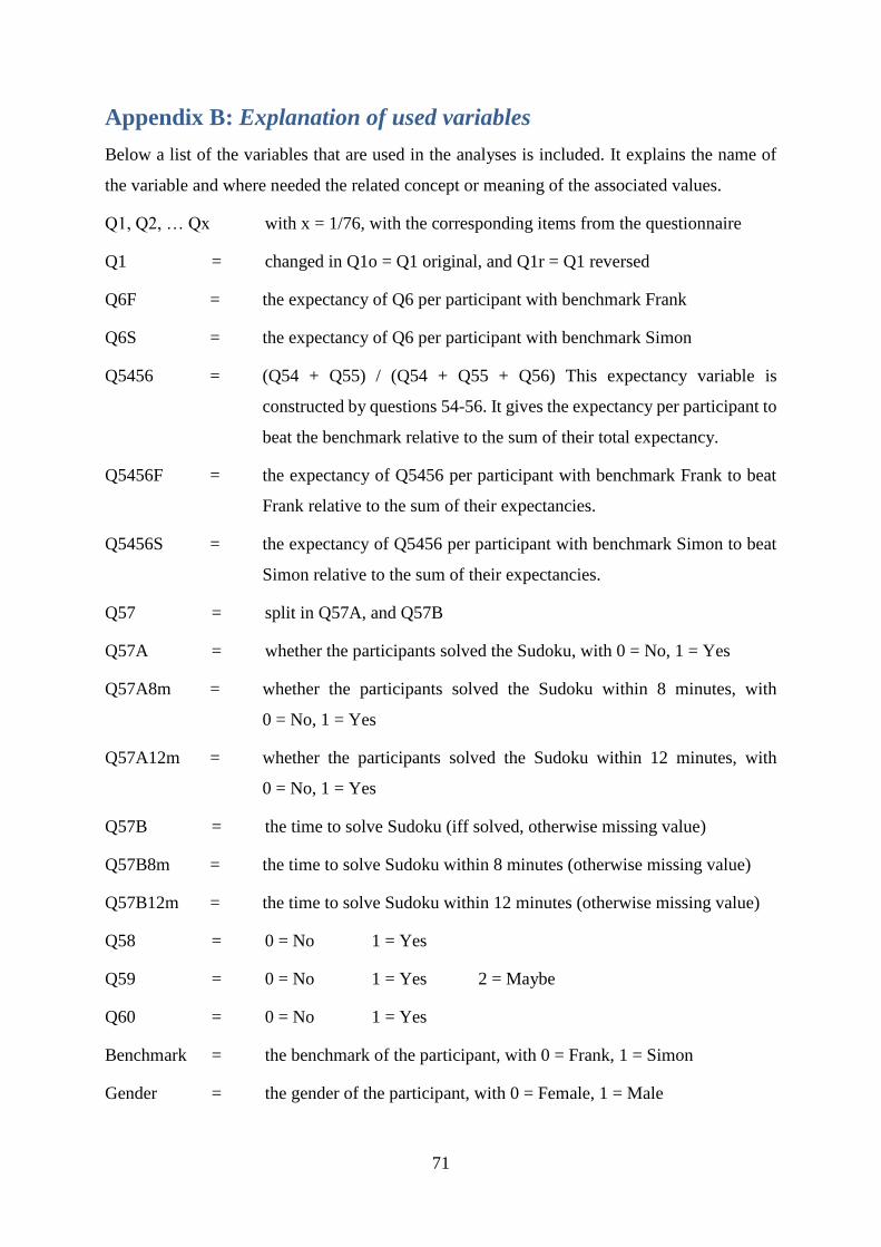
71

Appendix B: Explanation of used variables

Below a list of the variables that are used in the analyses is included. It explains the name of

the variable and where needed the related concept or meaning of the associated values.

Q1, Q2, … Qx with x = 1/76, with the corresponding items from the questionnaire

Q1 = changed in Q1o = Q1 original, and Q1r = Q1 reversed

Q6F = the expectancy of Q6 per participant with benchmark Frank

Q6S = the expectancy of Q6 per participant with benchmark Simon

Q5456 = (Q54 + Q55) / (Q54 + Q55 + Q56) This expectancy variable is

constructed by questions 54-56. It gives the expectancy per participant to

beat the benchmark relative to the sum of their total expectancy.

Q5456F = the expectancy of Q5456 per participant with benchmark Frank to beat

Frank relative to the sum of their expectancies.

Q5456S = the expectancy of Q5456 per participant with benchmark Simon to beat

Simon relative to the sum of their expectancies.

Q57 = split in Q57A, and Q57B

Q57A = whether the participants solved the Sudoku, with 0 = No, 1 = Yes

Q57A8m = whether the participants solved the Sudoku within 8 minutes, with

0 = No, 1 = Yes

Q57A12m = whether the participants solved the Sudoku within 12 minutes, with

0 = No, 1 = Yes

Q57B = the time to solve Sudoku (iff solved, otherwise missing value)

Q57B8m = the time to solve Sudoku within 8 minutes (otherwise missing value)

Q57B12m = the time to solve Sudoku within 12 minutes (otherwise missing value)

Q58 = 0 = No 1 = Yes

Q59 = 0 = No 1 = Yes 2 = Maybe

Q60 = 0 = No 1 = Yes

Benchmark = the benchmark of the participant, with 0 = Frank, 1 = Simon

Gender = the gender of the participant, with 0 = Female, 1 = Male

72

Study = the study direction of the participant, with 1 = Economics, 2 =

Psychology, 3 = Other

Level = the study level of the participant, with 0 = University, 1 = HBO

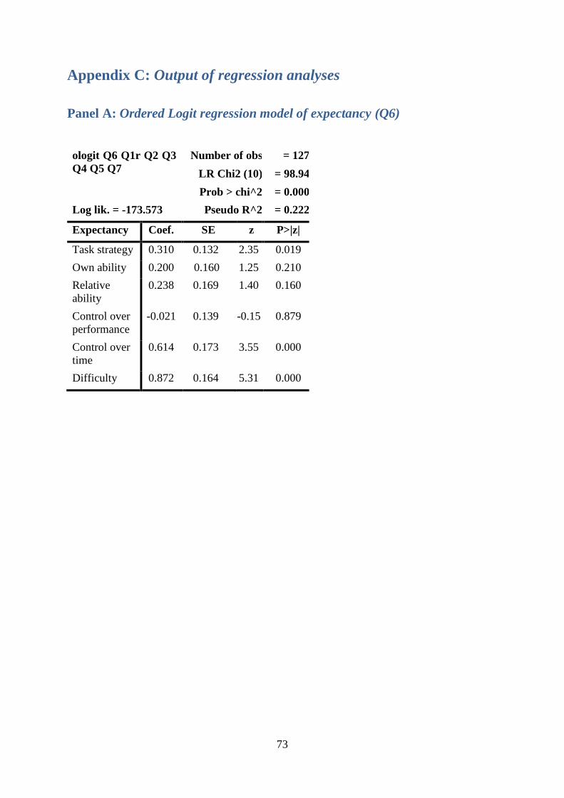
73

Appendix C: Output of regression analyses

Panel A: Ordered Logit regression model of expectancy (Q6)

ologit Q6 Q1r Q2 Q3

Q4 Q5 Q7

Number of obs = 127

LR Chi2 (10) = 98.94

Prob > chi^2 = 0.000

Log lik. = -173.573 Pseudo R^2 = 0.222

Expectancy Coef. SE z P>|z|

Task strategy 0.310 0.132 2.35 0.019

Own ability 0.200 0.160 1.25 0.210

Relative

ability

0.238 0.169 1.40 0.160

Control over

performance

-0.021 0.139 -0.15 0.879

Control over

time

0.614 0.173 3.55 0.000

Difficulty 0.872 0.164 5.31 0.000

74

Panel B: Factorial regression model of performance (Q57A8m) and

interactions with goals (Benchmark)

Number of obs = 130 R-squared = 0.309

Root MSE = 0.372 Adjusted R-squared = 0.245

Source Partial SS df MS F Prob>F

Model 7.294 11 0.663 4.80 0.000

Benchmark 0.153 1 0.153 1.11 0.295

Task strategy 0.880 1 0.880 6.36 0.013

Own ability 0.845 1 0.845 6.11 0.015

Relative ability 0.017 1 0.017 0.13 0.723

Intensity 0.091 1 0.091 0.66 0.420

Persistence 1.168 1 1.168 8.45 0.004

Task strategy#

Benchmark

0.002 1 0.002 0.01 0.905

Own ability#

Benchmark

0.003 1 0.003 0.02 0.878

Relative ability#

Benchmark

0.005 1 0.005 0.04 0.848

Intensity#

Benchmark

0.840 1 0.840 6.08 0.015

Persistence#

Benchmark

0.362 1 0.362 2.62 0.108

Residual 16.314 118 0.138

Total 23.608 129 0.183

75

Panel C: Factorial regression model of performance (Q57A12m) and

interactions with goals (Benchmark)

Number of obs = 130 R-squared = 0.393

Root MSE = 0.408 Adjusted R-squared = 0.337

Source Partial SS df MS F Prob>F

Model 12.727 11 1.157 6.95 0.000

Benchmark 0.115 1 0.115 0.69 0.408

Task strategy 0.056 1 0.056 0.34 0.563

Own ability 1.820 1 1.820 10.93 0.001

Relative ability 0.141 1 0.141 0.85 0.359

Intensity 0.072 1 0.072 0.43 0.511

Persistence 5.631 1 5.631 33.81 0.000

Task strategy#

Benchmark

0.402 1 0.402 2.42 0.123

Own ability#

Benchmark

0.017 1 0.017 0.10 0.753

Relative ability#

Benchmark

0.049 1 0.049 0.29 0.589

Intensity#

Benchmark

0.410 1 0.410 2.46 0.119

Persistence#

Benchmark

0.076 1 0.076 0.46 0.500

Residual 19.650 118 0.167

Total 32.377 129 0.251

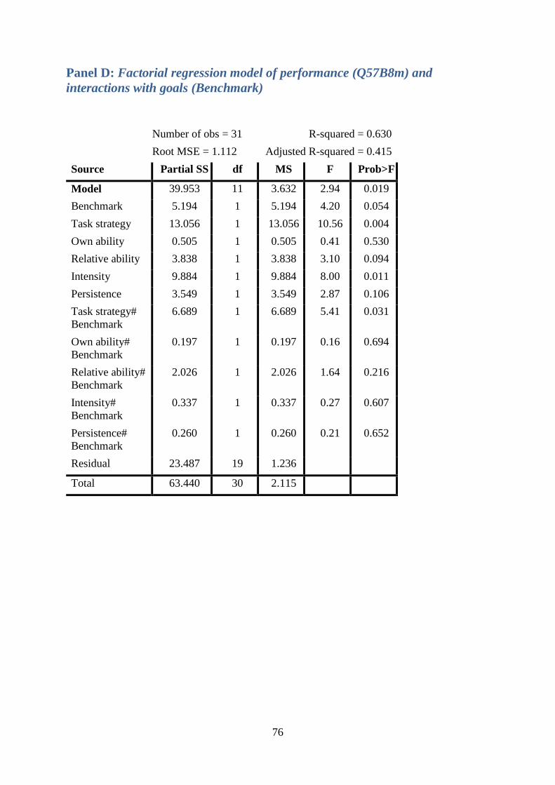
76

Panel D: Factorial regression model of performance (Q57B8m) and

interactions with goals (Benchmark)

Number of obs = 31 R-squared = 0.630

Root MSE = 1.112 Adjusted R-squared = 0.415

Source Partial SS df MS F Prob>F

Model 39.953 11 3.632 2.94 0.019

Benchmark 5.194 1 5.194 4.20 0.054

Task strategy 13.056 1 13.056 10.56 0.004

Own ability 0.505 1 0.505 0.41 0.530

Relative ability 3.838 1 3.838 3.10 0.094

Intensity 9.884 1 9.884 8.00 0.011

Persistence 3.549 1 3.549 2.87 0.106

Task strategy#

Benchmark

6.689 1 6.689 5.41 0.031

Own ability#

Benchmark

0.197 1 0.197 0.16 0.694

Relative ability#

Benchmark

2.026 1 2.026 1.64 0.216

Intensity#

Benchmark

0.337 1 0.337 0.27 0.607

Persistence#

Benchmark

0.260 1 0.260 0.21 0.652

Residual 23.487 19 1.236

Total 63.440 30 2.115

77

Panel E: Factorial regression model of performance (Q57B12m) and

interactions with goals (Benchmark)

Number of obs = 61 R-squared = 0.319

Root MSE = 2.094 Adjusted R-squared = 0.166

Source Partial SS df MS F Prob>F

Model 100.453 11 9.132 2.08 0.040

Benchmark 1.711 1 1.711 0.39 0.535

Task strategy 26.534 1 26.534 6.05 0.018

Own ability 8.153 1 8.153 1.86 0.179

Relative ability 0.006 1 0.006 0.00 0.971

Intensity 0.456 1 0.456 0.10 0.749

Persistence 0.057 1 0.057 0.01 0.910

Task strategy#

Benchmark

0.132 1 0.132 0.03 0.863

Own ability#

Benchmark

8.865 1 8.865 2.02 0.161

Relative ability#

Benchmark

5.384 1 5.384 1.23 0.273

Intensity#

Benchmark

1.649 1 1.649 0.38 0.543

Persistence#

Benchmark

0.335 1 0.335 0.08 0.783

Residual 214.861 49 4.385

Total 315.314 60 5.255

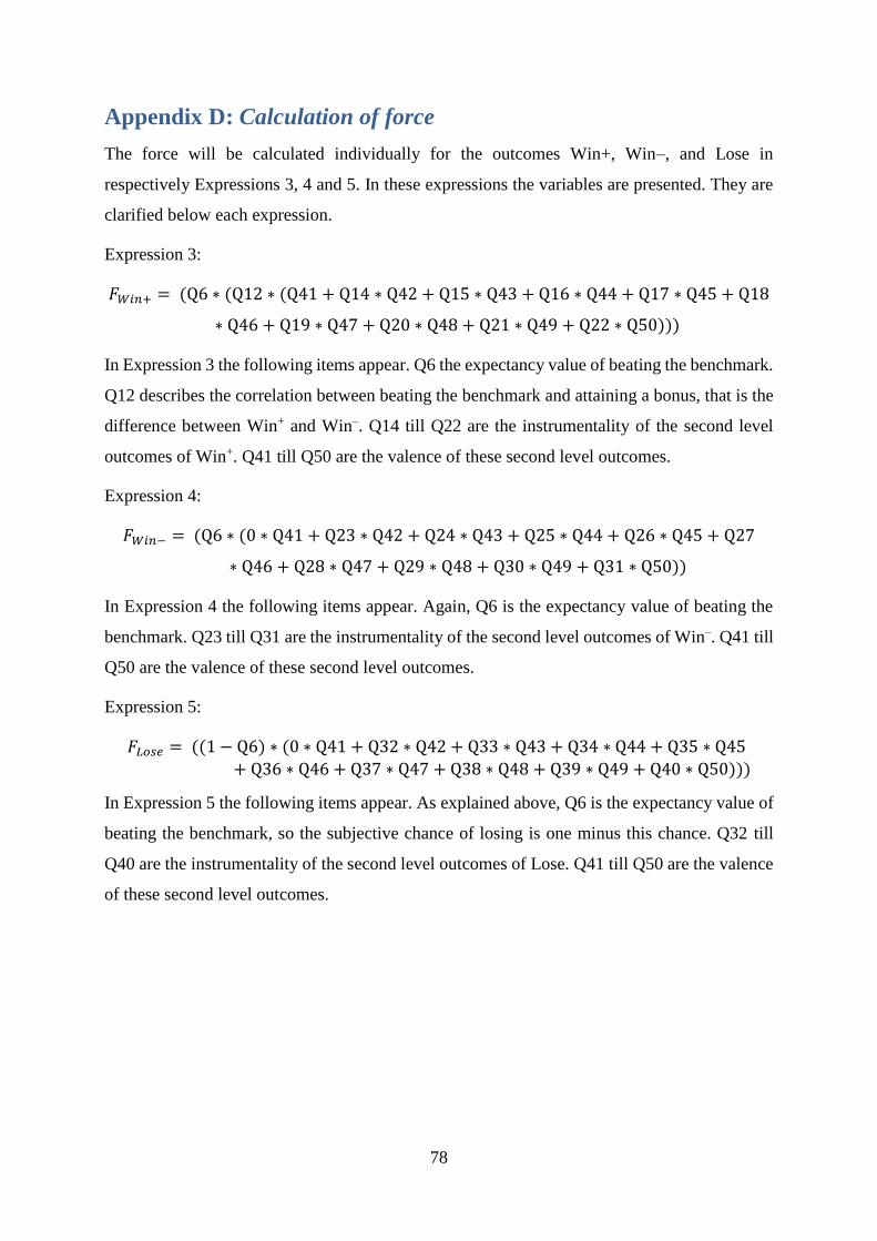
78

Appendix D: Calculation of force

The force will be calculated individually for the outcomes Win+, Win–, and Lose in

respectively Expressions 3, 4 and 5. In these expressions the variables are presented. They are

clarified below each expression.

Expression 3:

𝐹𝑊𝑖𝑛+ = (Q6 ∗ (Q12 ∗ (Q41 + Q14 ∗ Q42 + Q15 ∗ Q43 + Q16 ∗ Q44 + Q17 ∗ Q45 + Q18

∗ Q46 + Q19 ∗ Q47 + Q20 ∗ Q48 + Q21 ∗ Q49 + Q22 ∗ Q50)))

In Expression 3 the following items appear. Q6 the expectancy value of beating the benchmark.

Q12 describes the correlation between beating the benchmark and attaining a bonus, that is the

difference between Win+ and Win–. Q14 till Q22 are the instrumentality of the second level

outcomes of Win+. Q41 till Q50 are the valence of these second level outcomes.

Expression 4:

𝐹𝑊𝑖𝑛− = (Q6 ∗ (0 ∗ Q41 + Q23 ∗ Q42 + Q24 ∗ Q43 + Q25 ∗ Q44 + Q26 ∗ Q45 + Q27

∗ Q46 + Q28 ∗ Q47 + Q29 ∗ Q48 + Q30 ∗ Q49 + Q31 ∗ Q50))

In Expression 4 the following items appear. Again, Q6 is the expectancy value of beating the

benchmark. Q23 till Q31 are the instrumentality of the second level outcomes of Win–. Q41 till

Q50 are the valence of these second level outcomes.

Expression 5:

𝐹𝐿𝑜𝑠𝑒 = ((1 − Q6) ∗ (0 ∗ Q41 + Q32 ∗ Q42 + Q33 ∗ Q43 + Q34 ∗ Q44 + Q35 ∗ Q45

+ Q36 ∗ Q46 + Q37 ∗ Q47 + Q38 ∗ Q48 + Q39 ∗ Q49 + Q40 ∗ Q50)))

In Expression 5 the following items appear. As explained above, Q6 is the expectancy value of

beating the benchmark, so the subjective chance of losing is one minus this chance. Q32 till

Q40 are the instrumentality of the second level outcomes of Lose. Q41 till Q50 are the valence

of these second level outcomes.