The Concept of Comonotonicity in ActuarialScience and Finance: Applications

J. Dhaene, M. Denuit, M.J. Goovaerts, R. Kaas, D. Vyncke

April 11, 2002

Abstract

In an insurance context, one is often interested in the distributionfunction of a sum of random variables. Such a sum appears whenconsidering the aggregate claims of an insurance portfolio over a cer-tain reference period. It also appears when considering discountedpayments related to a single policy or a portfolio, at different futurepoints in time. The assumption of mutual independence between thecomponents of the sum is very convenient from a computational pointof view, but sometimes not a realistic one. In The Concept of Comono-tonicity in Actuarial Science and Finance: Theory, we determined ap-proximations for sums of random variables, when the distributions ofthe components are known, but the stochastic dependence structurebetween them is unknown or too cumbersome to work with. Practi-cal applications of this theory will be considered in this paper. Bothpapers are to a large extent an overview of recent research results ob-tained by the authors, but also new theoretical and practical resultsare presented.

1 Introduction

In Dhaene, Denuit, Goovaerts, Kaas & Vyncke (2001) we presented anoverview of the actuarial literature on the problem how to make decisionsin case we have a sum of random variables with given marginal distributionfunctions but of which the stochastic dependence structure is unknown ortoo cumbersome to work with. We proved that the convex-largest sum of

1

the components of a random vector with given marginals is obtained in casethe random vector (X1, X2, . . . , Xn) has the comonotonic distribution, whichmeans that each two possible outcomes (x1, x2, . . . , xn) and (y1, y2, . . . , yn) of(X1, X2, . . . , Xn) are ordered componentwise.

In this paper, we will present several applications of the concept of comono-tonicity in the field of actuarial science and finance. The notations, assump-tions and results used throughout this paper are presented in the above men-tioned companion paper and will not be repeated here. References to equa-tions and theorems presented in the first paper will be denoted by adding a“T” to the relevant equation or theorem number.

As a theoretical example of the concept of comonotonicity in an insurancecontext, consider a portfolio of n risksX1, X2, . . . , Xn, identically distributed,with cdf F and finite variance σ2, say. If the risks are mutually independent,it is well-known that

V ar

[1

n

n∑i=1

Xi

]=σ2

n→ 0

as n goes to infinity. If the risks are comonotonic, then

V ar

[1

n

n∑i=1

Xi

]= V ar

[1

n

n∑i=1

F−1(U)

]= σ2,

where U is uniformly distributed on [0, 1]. Hence, in case of comonotonicrisks, risk pooling has completely no risk reducing effect: adding an additionalrisk to the portfolio will not reduce the variance of the average risk.In general, the risks of an insurance portfolio (X1, X2, . . . , Xn) will not exhibitthe extreme comonotonic dependence structure. However, in the presence ofpositive dependencies between the individual risks, assuming independencemight lead to an underestimation of the probability of large total claims forthe portfolio. In this case the technique of risk pooling might not be aseffective as expected. On the other hand, resorting to comonotonicity is aconservative approach in case the structure of dependence is unknown to theactuary.

In Section 2 we will give examples of comonotonic random variables oc-curing in an actuarial or financial environment. In Section 3 we give somenumerical examples how to construct convex lower and upper bounds forsums of random variables. The evaluation of cash-flows in case of a lognor-mal discount process is considered in Section 4. In Section 5, we derive lowerand upper bounds for the price of arithmetic Asian options.

2

2 Comonotonic random variables

In this section, we will describe several situations in an actuarial or financialcontext where comonotonic random variables emerge.

2.1 Options and insurance

In a financial environment, the most straigthforward examples of comono-tonicity occur when considering pay-offs of derivative securities. Such pay-offfunctions are strongly (positively or negatively) dependent of the value of theunderlying asset. This makes them useful instruments for hedging.

To be specific, let A(t) be the value of a security at a future time t, t ≥ 0.Consider a European call option on this security, with expiration date T ≥ 0and exercise price K. The pay-off of the call-option at time K is given by(A(T ) −K)+. The pay-off of the portfolio consisting of the security and the

call-option is given by(A(T ), (A(T ) −K)+

), which is a comonotonic ran-

dom vector, since the pay-off of the option is a non-decreasing function of thevalue of the underlying security at the expiration date. Hence, the holder ofthe security who buys the call option increases his potential gains, at the costof the option premium. One immediately finds that A(T ) + (A(T ) −K)+stochastically dominates AT .On the other hand, if the holder of the security decides to write the call op-tion, the pay-off of his portfolio at time T is given by

(A(T ), − (A(T ) −K)+

).

The pay-off − (A(T ) −K)+ is a non-increasing function of A(T ). One says

that(A(T ), − (A(T ) −K)+

)is a “counter-monotonic” random vector: if

one of the components increases, then the other one decreases, see e.g. Em-brechts, McNeil & Straumann (2001). Writing the call option induces animmediate gain (the option premium), at the cost of reducing the maximalgain on the underlying security. A(T ) − (A(T ) −K)+ is stochastically dom-inated by A(T ).A European put option with the same characteristics has a pay-off equal to(K − A(T ))+. In this case, the holder of the security who buys the put option

has a portfolio pay-off(A(T ), (K − A(T ))+

)which is a counter-comonotonic

random vector. Buying the put-option reduces the maximal loss at thecost of the option premium. Note that A(T ) is stochastically dominatedby A(T ) + (K − A(T ))+.Holding the security and writing the put option leads to a portfolio pay-off given by

(A(T ),− (K − A(T ))+

), which is a comonotonic random vec-

3

tor. This strategy induces an immediate gain (the option premium) but in-creases the potential losses on the underlying security. A(T )− (K − A(T ))+is stochastically dominated by A(T ).

Let (X1, X2, . . . , Xn) be an insurance portfolio of individual risksXi whichare not assumed to be mutually independent. As mentioned in the Introduc-tion, in the presence of positive dependencies, the risks might not be pooledas effectively as expected. The insurer could reduce the aggregate risk of hisportfolio by financial hedging techniques. He could buy a financial contractwith payments Y such that Y and X1 +X2 + . . .+Xn are comonotonic (or ascomontonic as possible). Compensation will then be obtained as the pay-offof the financial contract will increase if the aggregate loss X1 +X2 + . . .+Xn

increases. As an example in case of hurricane and earthquake insurance, theinsurer could buy call options on the CAT-index, the Index of CatastropheLosses of the Chicago Board of Trade. These options will be exercised by theinsurer in case the level of the CAT-index is sufficiently high. In this case,investors take the position of the traditional reinsurer.On the other hand, the insurer could also sell a financial contract withobligations for him that are negatively correlated with the aggregate lossX1 +X2 + . . .+Xn. Compensation will then be obtained as his obligationsrelated to the financial contract will decrease if the aggregate insurance lossincreases. In the hurricane and earthquake example, the insurer could writeput options on the CAT-index. These options generate a premium and willonly be exercised if the CAT-index remains sufficiently low.

As another example, consider an insurance which protects house-ownersagainst the depreciation of their property. Assume that the insurance pay-ment is defined as a non-increasing function of some general real estate index.The risks of such a portfolio are comonotonic: they are all a non-increasingfunction of the same random variable (the real estate index). Such a portfoliocannot be considered as a traditional “insurance portfolio” where increasingthe number of policies reduces the volatility of the average risk. The in-surer will have to use financial hedging techniques to cope with the risk ofsuch a portfolio. He could e.g. buy put options on the real estate index.In this case, the income of the put options and the insurance portfolio pay-ments are comonotonic. The insurer could also write call options on thereal estate index. This strategy generates an income (the option premiums)for the insurer, while the option payments and the insurance payments arecounter-monotonic.

4

2.2 Life annuities - deterministic discount process

Consider a life annuity ax on a life (x) which pays an amount of 1 at theend of each year, provided the insured is still alive at that time. Let Tbe a non-negative continuous random variable representing the remaininglifetime of (x). The distribution function of T is denoted by FT (t) = tqx,(t ≥ 0). Further, the ultimate age of the life table is denoted by ω, thismeans that ω−x is the first remaining lifetime of (x) for which ω−xqx = 1, orequivalently, F−1

T (1) = ω − x. Assume that discounting is performed with adeterministic interest rate r. The present value at policy issue of the futurepayments is denoted by S and equals the sum of the present values of thepayments in the respective years:

S =

�ω−x�−1∑i=1

Xi (1)

where �.� is the ceiling function, i.e. �x� is the smallest integer greater thanor equal to x, and where the random variables Xi are given by

Xi = vi I (T > i) , (2)

with v = (1 + r)−1 and I(·) denoting the indicator function, i.e. I(c) = 1 ifthe condition c is true and I(c) = 0 if it is not.AllXi are non-decreasing functions of the remaining life time T , which meansthat the payment vector X is comonotonic. For any 0 < p < 1, we find fromTheorem T.1 that F−1

Xi(p) = vi I

(F−1T (p) > i

)= vi I

(i ≤ �F−1

T (p)� − 1).

Hence, letting∑b

i=a xi = 0 if a > b, we find from Theorem T.6:

F−1S (p) =

�ω−x�−1∑i=1

F−1Xi

(p) =

�F−1T (p)�−1∑i=1

vi, 0 < p < 1, (3)

It is straightforward to verify that this expression also holds for p = 1.An expression for the inverse distribution function of S can also be derivedin another way, since S can be written as

S =

�T �−1∑i=1

vi. (4)

5

The function g defined by

g(y) =

�y�−1∑i=1

vi

for all non-negative values of y, is non-decreasing and left-continuous. Ap-plication of Theorem T.1 leads to

F−1S (p) = F−1

g(T )(p) = g[F−1T (p)

], 0 < p < 1.

Hence, for any 0 < p < 1, we find (3).An expression for the cdf of S follows from (T.45):

FS(x) = sup

p ∈ (0, 1) |

�F−1T (p)�−1∑i=1

vi ≤ x

. (5)

2.3 Risk sharing schemes

Let X be a non-negative random variable denoting the risk a person facesduring the insurance period. An insurance contract is an agreement betweenthis person (the insured) and the insurer where the insurer promises to payan amount ϕ(X) in case the claim amount equals X, where ϕ is a non-negative function, defined for all possible outcomes of X. Then X − ϕ(X)is the part of the claim retained by the insured. It is reasonable to requirethat ϕ(x) and x−ϕ(x) are non-decreasing functions on the set of all possibleoutcomes ofX. This is equivalent to requiring that both risk sharing partnershave to bear more (or at least as much) if the actual claim x increases. If thebenefit function ϕ is differentiable, both requirements reduce to the condition0 ≤ ϕ′(x) ≤ 1 for all possible outcomes x of X.

From characterization (T.23) for comonotonicity one finds that if bothpartners of the risk sharing scheme (ϕ(X), X − ϕ(X)) have to bear more ifthe claim amount increases, then the random vector (ϕ(X), X − ϕ(X)) iscomonotonic.Also the opposite can be proven: if the risk sharing scheme (ϕ(X), X − ϕ(X))is comonotonic, then both partners have to bear more if the claim amountincreases, except perhaps on a set with zero probability. Indeed, the comono-tonicity of (ϕ(X), X − ϕ(X)) implies that there exists a support A of X suchthat the set {(ϕ(x), x− ϕ(x)) | x ∈ A} is comonotonic. This implies that the

6

functions ϕ(x) and x− ϕ(x) must be simultaneously non-decreasing or non-increasing on A. Since the sum of the functions ϕ(x) and x − ϕ(x) equalsthe non-decreasing function x, we must have that the functions ϕ(x) andx− ϕ(x) are both non-decreasing on A. This proves the stated result.

As a first example of a risk sharing scheme, consider a deductible coverage(or stop-loss coverage) where the benefit function is defined by:

ϕ(x) = (x− d)+ for some d ≥ 0. (6)

It is straightforward to verify that (ϕ(X), X − ϕ(X)) = ((X − d)+,min (X, d))which is a comonotonic random vector.In case of coinsurance (or quota share coverage), the benefit function is de-fined by

ϕ(x) = α x, α ∈ [0, 1] . (7)

Since both α x and (1−α)x increase with x, the random vector (α X, (1 − α) X)is comonotonic.A coverage with a maximal limit is defined by

ϕ(x) = min {x, d} , d ≥ 0. (8)

In this case, (ϕ(X), X − ϕ(X)) =(min {X, d} , (X − d)+

)which is comono-

tonic.Also coverages combining the three forms above, such as

ϕ(x) = min {α (x− d1)+, d2} , α ∈ [0, 1] , d1, d2 ≥ 0 (9)

can be seen to lead to a comonotonic risk sharing scheme.An example of a risk sharing scheme which does not lead to comonotonicrisks is a policy with a franchise deductible where the benefit function isdefined by

ϕ(x) = x I(x ≥ d), d ≥ 0. (10)

We find that (ϕ(X), X − ϕ(X)) = (X I(X ≥ d), X I(X < d)) which is ingeneral not a comonotonic random vector.

All the examples above describe risk sharing schemes between insurer andinsured, but they can also be interpreted as risk sharing schemes between in-surer and reinsurer.An example of a reinsurance scheme which does not necessarily lead tocomonotonic risks is the largest claim reinsurance. Indeed, let the insur-ance portfolio consist of n individual risks with claim amounts Y1 ≤ Y2 ≤

7

· · · ≤ Yn respectively (the Yi are the order statistics corresponding to therisks in the portfolio). The risk taken by the reinsurer equals Yn, while therisk kept by the ceding insurer is Y1 + Y2 + · · · + Yn−1. It is clear that(Yn, Y1 + Y2 + · · · + Yn−1) will in general not be comonotonic.

3 Convex bounds for sums of rv’s

In this section, we will illustrate the technique of deriving convex lower andupper bounds for sums of random variables, as explained in Dhaene, Denuit,Goovaerts, Kaas & Vyncke (2001), by some numerical examples. Especially,we will consider sums of normal or lognormal random variables.

Recall that a random vector (Y1, Y2, . . . , Yn) has the multivariate nor-mal distribution if and only if every linear combination of its variates has aunivariate normal distribution. Now assume that (Y1, Y2, . . . , Yn) has a mul-tivariate normal distribution. Let Y and Λ be linear combinations of thevariates: Y =

∑ni=1 αiYi and Λ =

∑ni=1 βiYi. Then also (Y, Λ) has a bivari-

ate normal distribution.Further, if (Y, Λ) has a bivariate normal distribution, then, conditionallygiven Λ = λ, Y has a univariate normal distribution with mean and variancegiven by

E [Y | Λ = λ] = E [Y ] + r (Y,Λ)σY

σΛ

(λ− E [Λ]) (11)

andV ar [Y | Λ = λ] = σ2

Y

(1 − r (Y,Λ)2

), (12)

where r (Y,Λ) is Pearson’s correlation coefficient for the couple (Y,Λ).

Example 1 (sums of normal rv’s)

Let Y1, Y2 be mutually independent N(0, 1) random variables. Obviously,S = Y1 + Y2 is N(0, 2). For the convex order bounds for S, we will considerconditioning random variables of the type Λ = Y1 +aY2 for some real a. The

conditional distribution of Y1, given Λ = λ, is N(

λ1+a2 ,

a2

1+a2

).

This means that for the conditional expectation E[Y1|Λ] and for the randomvariable F−1

Y1|Λ(U), with U uniform(0,1) and independent of Λ, we get

E[Y1|Λ] =Λ

1 + a2and F−1

Y1|Λ(U) = E[Y1|Λ] +|a|Φ−1(U)√

1 + a2.

8

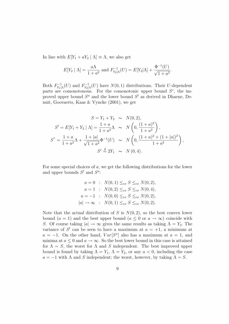
In line with E[Y1 + aY2 | Λ] ≡ Λ, we also get

E[Y2 | Λ] =aΛ

1 + a2and F−1

Y2|Λ(U) = E[Y2|Λ] +Φ−1(U)√1 + a2

.

Both F−1Y1|Λ(U) and F−1

Y2|Λ(U) have N(0, 1) distributions. Their U -dependentparts are comonotonous. For the comonotonic upper bound Sc, the im-proved upper bound Su and the lower bound Sl as derived in Dhaene, De-nuit, Goovaerts, Kaas & Vyncke (2001), we get

S = Y1 + Y2 ∼ N(0, 2),

Sl = E[Y1 + Y2 | Λ] =1 + a

1 + a2Λ ∼ N

(0,

(1 + a)2

1 + a2

),

Su

=1 + a

1 + a2Λ +

1 + |a|√1 + a2

Φ−1(U) ∼ N

(0,

(1 + a)2 + (1 + |a|)21 + a2

),

Sc d= 2Y1 ∼ N (0, 4) .

For some special choices of a, we get the following distributions for the lowerand upper bounds Sl and Su:

a = 0 : N(0, 1) ≤cx S ≤cx N(0, 2),

a = 1 : N(0, 2) ≤cx S ≤cx N(0, 4),

a = −1 : N(0, 0) ≤cx S ≤cx N(0, 2),

|a| → ∞ : N(0, 1) ≤cx S ≤cx N(0, 2).

Note that the actual distribution of S is N(0, 2), so the best convex lowerbound (a = 1) and the best upper bound (a ≤ 0 or a → ∞) coincide withS. Of course taking |a| → ∞ gives the same results as taking Λ = Y2. Thevariance of Sl can be seen to have a maximum at a = +1, a minimum ata = −1. On the other hand, V ar[Su] also has a maximum at a = 1, andminima at a ≤ 0 and a→ ∞. So the best lower bound in this case is attainedfor Λ = S, the worst for Λ and S independent. The best improved upperbound is found by taking Λ = Y1, Λ = Y2, or any a < 0, including the casea = −1 with Λ and S independent; the worst, however, by taking Λ = S.

9

To compare the variance of the stochastic upper bound Su with the vari-

ance of S boils down to comparing cov(F−1Y1|Λ(U), F−1

Y2|Λ(U))

with cov (Y1, Y2).

It is clear that, in general, the optimal choice for the conditioning randomvariable Λ will depend on the correlation of Y1 and Y2. If this correlation

equals 1, any Λ results in Sd= Su d

= Sc. In our case where Y1 and Y2 aremutually independent, the optimal choice proves to be taking Λ ≡ Y1, whichcorresponds to a = 0 or Λ ≡ Y2, which corresponds to a→ ∞, thus ensuring

that S and Su coincide. But also any a < 0 leads to Sd= Su.�

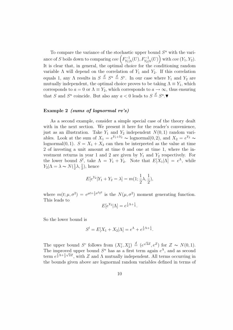
Example 2 (sums of lognormal rv’s)

As a second example, consider a simple special case of the theory dealtwith in the next section. We present it here for the reader’s convenience,just as an illustration. Take Y1 and Y2 independent N(0, 1) random vari-ables. Look at the sum of X1 = eY1+Y2

∼ lognormal(0, 2), and X2 = eY2∼

lognormal(0, 1). S = X1 +X2 can then be interpreted as the value at time2 of investing a unit amount at time 0 and one at time 1, where the in-vestment returns in year 1 and 2 are given by Y1 and Y2 respectively. Forthe lower bound Sl, take Λ = Y1 + Y2. Note that E[X1|Λ] = eΛ, whileY2|Λ = λ ∼ N(1

2λ, 1

2), hence

E[eY2 |Y1 + Y2 = λ] = m(1;1

2λ,

1

2),

where m(t;µ, σ2) = eµt+12σ2t2 is the N(µ, σ2) moment generating function.

This leads toE[eY2|Λ] = e

12Λ+ 1

4 .

So the lower bound is

Sl = E[X1 +X2|Λ] = eΛ + e12Λ+ 1

4 .

The upper bound Sc follows from (Xc1, X

c2)

d= (e

√2Z , eZ) for Z ∼ N(0, 1).

The improved upper bound Su has as a first term again eΛ, and as secondterm e

12Λ+ 1

2

√2Z , with Z and Λ mutually independent. All terms occurring in

the bounds given above are lognormal random variables defined in terms of

10

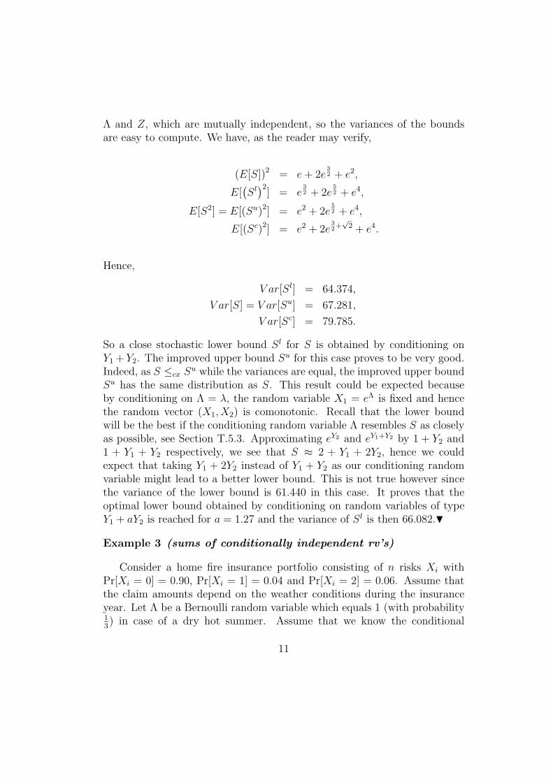
Λ and Z, which are mutually independent, so the variances of the boundsare easy to compute. We have, as the reader may verify,

(E[S])2 = e+ 2e32 + e2,

E[(Sl)2

] = e32 + 2e

52 + e4,

E[S2] = E[(Su)2] = e2 + 2e52 + e4,

E[(Sc)2] = e2 + 2e32+√

2 + e4.

Hence,

V ar[Sl] = 64.374,

V ar[S] = V ar[Su] = 67.281,

V ar[Sc] = 79.785.

So a close stochastic lower bound Sl for S is obtained by conditioning onY1 + Y2. The improved upper bound Su for this case proves to be very good.Indeed, as S ≤cx S

u while the variances are equal, the improved upper boundSu has the same distribution as S. This result could be expected becauseby conditioning on Λ = λ, the random variable X1 = eΛ is fixed and hencethe random vector (X1, X2) is comonotonic. Recall that the lower boundwill be the best if the conditioning random variable Λ resembles S as closelyas possible, see Section T.5.3. Approximating eY2 and eY1+Y2 by 1 + Y2 and1 + Y1 + Y2 respectively, we see that S ≈ 2 + Y1 + 2Y2, hence we couldexpect that taking Y1 + 2Y2 instead of Y1 + Y2 as our conditioning randomvariable might lead to a better lower bound. This is not true however sincethe variance of the lower bound is 61.440 in this case. It proves that theoptimal lower bound obtained by conditioning on random variables of typeY1 + aY2 is reached for a = 1.27 and the variance of Sl is then 66.082.�

Example 3 (sums of conditionally independent rv’s)

Consider a home fire insurance portfolio consisting of n risks Xi withPr[Xi = 0] = 0.90, Pr[Xi = 1] = 0.04 and Pr[Xi = 2] = 0.06. Assume thatthe claim amounts depend on the weather conditions during the insuranceyear. Let Λ be a Bernoulli random variable which equals 1 (with probability13) in case of a dry hot summer. Assume that we know the conditional

11

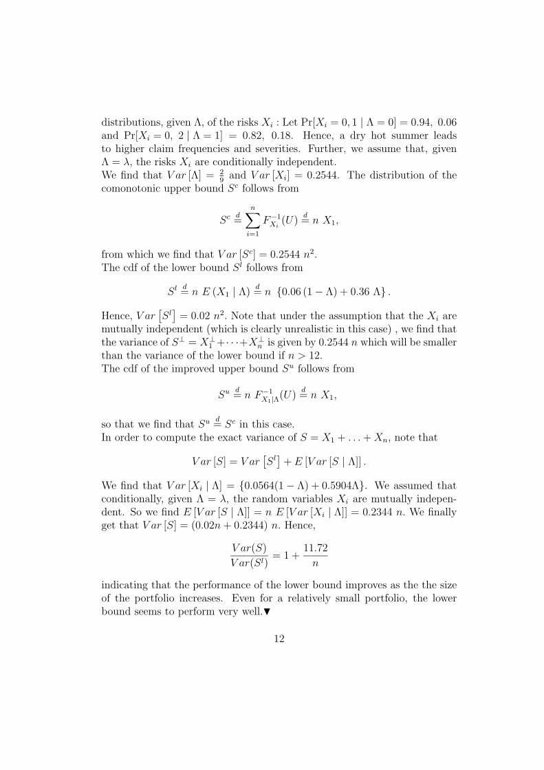
distributions, given Λ, of the risks Xi : Let Pr[Xi = 0, 1 | Λ = 0] = 0.94, 0.06and Pr[Xi = 0, 2 | Λ = 1] = 0.82, 0.18. Hence, a dry hot summer leadsto higher claim frequencies and severities. Further, we assume that, givenΛ = λ, the risks Xi are conditionally independent.We find that V ar [Λ] = 2

9and V ar [Xi] = 0.2544. The distribution of the

comonotonic upper bound Sc follows from

Sc d=

n∑i=1

F−1Xi

(U)d= n X1,

from which we find that V ar [Sc] = 0.2544 n2.The cdf of the lower bound Sl follows from

Sl d= n E (X1 | Λ)

d= n {0.06 (1 − Λ) + 0.36 Λ} .

Hence, V ar[Sl]= 0.02 n2. Note that under the assumption that the Xi are

mutually independent (which is clearly unrealistic in this case) , we find thatthe variance of S⊥ = X⊥

1 +· · ·+X⊥n is given by 0.2544 n which will be smaller

than the variance of the lower bound if n > 12.The cdf of the improved upper bound Su follows from

Su d= n F−1

X1|Λ(U)d= n X1,

so that we find that Su d= Sc in this case.

In order to compute the exact variance of S = X1 + . . .+Xn, note that

V ar [S] = V ar[Sl]+ E [V ar [S | Λ]] .

We find that V ar [Xi | Λ] = {0.0564(1 − Λ) + 0.5904Λ}. We assumed thatconditionally, given Λ = λ, the random variables Xi are mutually indepen-dent. So we find E [V ar [S | Λ]] = n E [V ar [Xi | Λ]] = 0.2344 n. We finallyget that V ar [S] = (0.02n+ 0.2344) n. Hence,

V ar(S)

V ar(Sl)= 1 +

11.72

n

indicating that the performance of the lower bound improves as the the sizeof the portfolio increases. Even for a relatively small portfolio, the lowerbound seems to perform very well.�

12

The results of the previous example can be generalized. Indeed, considera portfolio of n risks Xi. Assume that for any possible outcome λ of Λ wehave that, conditionally given Λ = λ, the risks Xi are identically distributed,but not necessarily mutually independent.

In this case, we find that∑n

i=1 F−1Xi

(U)d=∑n

i=1 F−1Xi|Λ(U)

d= nX1, where U

and Λ are mutually independent and U is uniform(0,1) distributed. Hence,

Sc d= Su d

= nX1, V ar [Sc] = V ar [Su] = n2 V ar [X1] . (13)

For the lower bound Sl, we find

Sl d= n E [X1 | Λ] , V ar

[Sl]= n2 V ar [E [X1 | Λ]] . (14)

Let us now assume that conditionally, given Λ = λ, the risks Xi are iid. Anexpression for the variance of the sum S = X1 + . . . + Xn is obtained asfollows:

V ar [S] = V ar[Sl]+ E [V ar [S | Λ]]

= n2 V ar [E [X1 | Λ]] + n E [V ar [X1 | Λ]] ,

so that we find

V ar [Sc]

V ar [S]=

1 + E[V ar[X1|Λ]]V ar[E[X1|Λ]]

1 + 1nE[V ar[X1|Λ]]V ar[E[X1|Λ]]

(15)

which is an increasing function of the volume of the portfolio, with limitingvalue 1+ E[V ar[X1|Λ]]

V ar[E[X1|Λ]]. This means that the larger the portfolio, the worse the

relative performance of the comonotonic (and the improved) upper bound.For the lower bound however, we find that

V ar [S]

V ar [Sl]= 1 +

1

n

E [V ar [X1 | Λ]]

V ar [E [X1 | Λ]]. (16)

Hence, the more the variance of the individual risksXi is caused by V ar [E [X1 | Λ]],the better the lower bound will perform. For a sufficiently large portfolio,the lower bound Sl will perform very well.

Defining z as the ratio wn/(wn + v) where w = V ar[E[X1 | Λ]] andv = E[V ar[X1 | Λ]] denote the between-variance and the within-variancerespectively, we can rewrite (15) and (16) as

V ar[Sc] = (z + (1 − z)n)V ar[S] and V ar[Sl] = z V ar[S].

13

The factor z ∈ [0, 1] can be interpreted as a measure for the goodness-of-fit when S is replaced by E[S | Λ]: The larger z, the better the lowerbound performs. Maximum performance (i.e. z = 1) is achieved if n → ∞,w = V ar[X1] or v = 0. For a portfolio of a given size n, we also have thatthe larger z, the better the comonotonic upper bound will perform.

4 Provisions for future payment obligations -

Lognormal discount process

4.1 Approximate evaluation of provisions

Consider a series of deterministic payments α1, α2, · · · , αn, of arbitrary sign,that are due at times 1, 2, · · · , n respectively. We want to find an answer tothe following question: “What is the amount of money required at time 0in order to be able to meet these future obligations (α1, α2, · · · , αn)?” Wewill call this amount the provision, or depending on the situation at hand,the (prospective) reserve or the required capital. Of course, the level of theprovision will strongly depend on the way how this amount will be invested.Let us assume that the provision will be invested such that it generates astochastic return Yj in year j, j = 1, 2, . . . , n, i.e. an amount of 1 at time j−1will grow to eYj at time j. The discount factor over the period [0, i] is thengiven by e−(Y1+Y2+···+Yi), because this stochastic amount will exactly grow toan amount 1 at time i. The distribution function of the random variable

S =n∑

i=1

αi e−(Y1+Y2+···+Yi). (17)

will help us to determine the provision W0. E.g. we could determine thisprovision as W0 = F−1

S (0.99), such that there is a 99% probability that wecan meet our future obligations, which means that there is a 99% probabilitythat after the last payment at time n, we will have a non-negative amountleft.In this section, we will assume that the return vector (Y1, Y2, · · · , Yn) hasa multivariate normal distribution. The random variable S is then a lin-ear combination of dependent lognormal random variables. In any realisticreturn model, it is impossible to determine the distribution function of Sanalytically. Therefore, we will derive the convex upper and lower bounds

14

Sc, Su and Sl of S. By defining random variables Xi and Y (i) by

Y (i) = Y1 + Y2 + · · · + Yi, (18)

Xi = e−Y (i), (19)

the stochastic provision S can be written as S = α1X1 + α2X2 + · · · +αnXn. Note that if all αi are positive, then the support of S is situatedin the region

[F−1+Sc (0), F−1

Sc (1)]

= (0,+∞), if all αi are negative, then[F−1+Sc (0), F−1

Sc (1)]= (−∞, 0), and if the αi have mixed signs, then

[F−1+Sc (0), F−1

Sc (1)]=

(−∞,+∞). In the following theorem, we derive approximations for (the dis-tribution function of) the stochastic provision S, as explained in Dhaene,Denuit, Goovaerts, Kaas & Vyncke (2001).

Theorem 1 Let S be given by (17), where the random vector (Y1, Y2, · · · , Yn)has a multivariate normal distribution. Consider the conditioning randomvariable Λ =

∑ni=1 βi Yi. Then the lower bound Sl, the improved upper

bound Su and the comonotonic upper bound Sc are given by

Sl =n∑

i=1

αi e−E[Y (i)]−ri σY (i) Φ−1(V )+ 1

2(1−r2i )σ2Y (i) , (20)

Su

=n∑

i=1

αi e−E[Y (i)]−ri σY (i) Φ−1(V )+sign(αi)

√1−r2i σY (i) Φ−1(U), (21)

Sc =n∑

i=1

αi e−E[Y (i)]+sign(αi) σY (i) Φ−1(U), (22)

where U and V are mutually independent uniform(0,1) random variables, Φis the cdf of the N(0, 1) distribution and ri is defined by

ri = r (Y (i),Λ) =cov [Y (i),Λ]

σY (i) σΛ

. (23)

Proof. (a) From (11) and (12), we find that conditionally, given Λ = λ,the random variable −Y (i) is normally distributed with parameters µi =−E [Y (i)] − ri

σY (i)

σΛ(λ− E [Λ]) and σ2

i = (1 − r2i )σ

2Y (i). Hence, condition-

ally, given Λ = λ, the random variable Xi is lognormally distributed withparameters µi and σ2

i . As E [Xi | Λ = λ] = eµi+12σ2

i , we find

E [αiXi | Λ] = αi e−E[Y (i)]−ri σY (i) Φ−1(V )+ 1

2(1−r2i )σ2Y (i) ,

15

where the random variable V ≡ Φ(

Λ−E[Λ]σΛ

)is uniform(0,1). Hence, Sl =∑n

i=1E [αiXi | Λ] is given by (20).

(b) From (T.75), we find that F−1αiXi|Λ=λ(p) = αi e

µi+sign(αi) σi Φ−1(p), with

µi and σi as defined in (a). This implies

F−1αiXi|Λ(p) = αi e

−E[Y (i)]−ri σY (i) Φ−1(V )+sign(αi)√

1−r2i σY (i) Φ−1(p).

Hence, Su =∑n

i=1 F−1αiXi|Λ(U) is given by (21).

(c) The random variable Xi is lognormally distributed with parameters−E [Y (i)] and σ2

Y (i). From (T.75), we find that F−1αiXi

(p) = αi e−E[Y (i)]+sign(αi) σY (i) Φ−1(p),

from which we find the expression (22) for Sc.Note that in Dhaene, Denuit, Goovaerts, Kaas & Vyncke (2001), we

proved that the bounds in the theorem above are ordered in the convexorder sense:

Sl ≤cx S ≤cx Su ≤cx S

c. (24)

In order to compare the cdf of S =∑n

i=1 αi e−(Y1+Y2+···+Yi) with the cdf’s

of the convex order bounds Sl, Su and Sc, we may look at their variances. Sowe need the correlations between the different random variables in each sum.We find the following results for the lognormal discount process consideredin this section:

r [αi Xi, αj Xj] = sijecov[Y (i),Y (j)] − 1√eσ

2Y (i) − 1

√eσ

2Y (j) − 1

; (25)

r [E (αj Xi | Λ) , E (αj Xj | Λ)] = sijerirjσY (i)σY (j) − 1√

er2i σ2

Y (i) − 1

√er

2j σ2

Y (j) − 1

;

r[F−1αi Xi|Λ(U), F−1

αj Xj |Λ(U)]

= sije

[rirj+sij

√1−r2i

√1−r2j

]σY (i)σY (j) − 1√

eσ2Y (i) − 1

√eσ

2Y (j) − 1

;

r[F−1αi Xi

(U), F−1αj Xj

(U)]

= sijesijσY (i)σY (j) − 1√

eσ2Y (i) − 1

√eσ

2Y (j) − 1

. (26)

where sij is used as shorthand notation for sign(αiαj). From these corre-lations, we can for instance deduce that if all payments αi are positive and

r [Y (i), Y (j)] = 1 for all i and j, then Sd= Sc. In practice, the discount fac-

tors will not be perfectly correlated. But for any realistic discount process,

16

r [Y (i), Y (j)] = r [Y1 + · · · + Yi, Y1 + · · · + Yj] will be close to 1 providedthat i and j are close to each other. This gives an indication that the cdfof Sc might perform well as an approximation for the cdf of S for such pro-cesses. This is indeed the case as will be seen in the numerical illustrationsin Section 4.4.A similar reasoning leads to the conclusion that the cdf of Sc will not performwell as a convex upper bound for the cdf of S if the payments αi have mixedsigns. This phenomenon will indeed be observed in the numerical illustra-tions in Section 4.4.Note that when S = αi e

−Y (i), an optimal choice for the conditioning random

variable Λ is given by Λ = Y (i), as this choice implies Sl d= S

d= Su d

= Sc.It remains to derive expressions for the cdf’s of Sl, Su and Sc.

4.2 The cdf and the stop-loss premiums of the bounds

The quantiles of Sc follow from Theorems T.1 and T.6:

F−1Sc (p) =

n∑i=1

αi e−E[Y (i)]+sign(αi) σY (i) Φ−1(p), p ∈ (0, 1) . (27)

The FXiare strictly increasing and continuous. From (T.48) we have that

for F−1+Sc (0) < x < F−1

Sc (1), FSc(x) follows implicitly from solving

n∑i=1

αi e−E[Y (i)]+sign(αi) σY (i) Φ−1(FSc (x)) = x. (28)

From (T.82), we find the following expression for the stop-loss premium atretention d with F−1+

Sc (0) < d < F−1Sc (1) for Sc:

E[(Sc − d)+

]=

n∑i=1

αi e−E[Y (i)]+

σ2Y (i)2 Φ

[sign(αi) σY (i)

− Φ−1(FSc(d))]

−d (1 − FSc(d)) . (29)

Expressions for the cdf and the stop-loss premiums of Sl can be obtainedby following the procedure as explained in (T.101) - (T.104). Indeed, from(20), we immediately find that the cdf of Sl can be determined from

FSl(x) =

∫ 1

0

I

(n∑

i=1

αi e−E[Y (i)]−ri σY (i) Φ−1(v)+ 1

2(1−r2i )σ2Y (i) ≤ x

)dv,

17

while the stop-loss premiums follow from

E[(Sl − d

)+

]=

∫ 1

0

(n∑

i=1

αi e−E[Y (i)]−ri σY (i) Φ−1(v)+ 1

2(1−r2i )σ2Y (i) − d

)+

dv.

Let us now consider the special yet important case that all αi ≥ 0 andall ri ≥ 0. These conditions ensure that Sl is the sum of n comonotonousrandom variables. Taking into account that Λ =

∑ni=1 βi Yi is normally

distributed, we find that

F−1Λ (1 − p) = E [Λ] − σΛ Φ−1(p),

and hence, from (T.97) or also from Theorems T.1 and T.6,

F−1Sl (p) =

n∑i=1

αi e−E[Y (i)]+ri σY (i) Φ−1(p)+ 1

2(1−r2i ) σ2Y (i) , p ∈ (0, 1) . (30)

From (T.99), we find that for any 0 < x <∞, FSl(x) can be obtained from

n∑i=1

αi e−E[Y (i)]+ri σY (i) Φ−1(F

Sl (x))+ 12(1−r2i ) σ2

Y (i) = x. (31)

From (20) we see that Sl is the comonotonic sum of n random variablesαi Zi where the Zi are lognormal distributed. Hence, from (T.82), we findthe following explicit expression for the stop-loss premium at retention d > 0:

E[(Sl − d

)+

]=

n∑i=1

αi e−E[Y (i)]+ 1

2σ2

Y (i)Φ[ri σY (i) − Φ−1 (FSl(d))

]−d (1 − FSl(d)) .

(32)

Finally, we determine the cdf of Su. Since FSu(x | V = v) is the cdf of a

sum of n comonotonic random variables, we have

F−1Su|V =v(p) =

n∑i=1

αi e−E[Y (i)]−ri σY (i) Φ−1(v)+sign(αi)

√1−r2i σY (i) Φ−1(p). (33)

For F−1+Su|V =v(0) < x < F−1

Su|V =v(1), the conditional probabilities FSu(x | V =

v) also follow implicitly from

n∑i=1

αi e−E[Y (i)]−ri σY (i) Φ−1(v)+sign(αi)

√1−r2i σY (i) Φ−1(FSu (x|V =v)) = x. (34)

18

The cdf of Su then follows from

FSu(x) =

∫ 1

0

FSu(x | V = v) dv. (35)

4.3 Continuous annuities

Many of the results derived for the discrete case (sums of random variables)have a continuous counterpart (integrals of random variables). Consider e.g.the continuous temporary annuity S defined by

S =

∫ t

0

α(τ) exp [−δτ − σ B(τ)] dτ (36)

where {B(τ), τ ≥ 0} represents a standard Brownian motion, i.e. the processhas independent and stationary increments, B(0) = 0 and for any τ ≥ 0,the random variable B(τ) is normally distributed with mean 0 and varianceτ . Further, the drift δ and the volatility σ are non-negative real numbers.The payments are described by α(τ) which is a non-negative and continuousfunction of τ .

Let Y (τ) = δτ + σB(τ) and X(τ) = exp{−Y (τ)}. It can be proven thatS ≤cx S

c, where the random variable Sc is defined by

Sc =

∫ t

0

F−1α(τ)X(τ)(U) dτ =

∫ t

0

α(τ) exp[−δτ + σ

√τ Φ−1(U)

]dτ , (37)

where, as usual, U is a uniform(0,1) random variable.The quantiles of Sc follow from

F−1Sc (p) =

∫ t

0

α(τ) exp[−δτ + σ

√τ Φ−1(p)

]dτ , (0 < p < 1), (38)

which is a continuous counterpart of (T.39). The stop-loss premiums withretentions d > 0 follow from

E[(Sc − d)+] =

∫ t

0

α(τ)e−δτ+σ2τ/2Φ[σ√τ − Φ−1(FSc(d))

]dτ − d(1−FSc(d)),

(39)where FSc(d) can be obtained by solving F−1

Sc (FSc(d)) = d, using (38). See(T.82) for a discrete counterpart of this expression.

19

In the remainder of this subsection, we consider a constant annuity.Hence, we assume that α(τ) ≡ 1. In order to derive a lower bound in convexorder for S, we consider the conditioning random variable Λ =

∫ t

0e−δτB(τ)dτ

which is a linear transformation of a first order approximation of S. We havethat Λ is normally distributed with mean 0 and variance

σ2Λ = V ar[Λ] =

∫ t

0

∫ t

0

e−δ(τ+ν) min(τ , ν)dτdν

=1

2δ3 +3 + 2δt− 4eδt

2δ3e2δt. (40)

Since B(τ) is a Brownian motion process, the random variable Y (τ) | Λ = λis normally distributed with mean

E[Y (τ)|Λ = λ] = δτ + r(τ)σ√τλ

σΛ

(41)

and varianceV ar[Y (τ)|Λ = λ] = σ2τ(1 − r2(τ)) (42)

with r(τ) defined by

r(τ) =cov[Y (τ),Λ]

σΛσ√τ

=1

σΛ

√τ

[1 − e−δτ

δ2 − τe−δt

δ

], τ ≤ t. (43)

Analoguously to (20), it can be shown that Sl ≤cx S where Sl is defined by

Sl = E[S | Λ] =

∫ t

0

exp

{−δτ − r(τ)σ

√τΦ−1(V ) +

1

2σ2τ(1 − r2(τ))

}dτ

(44)

with V = Φ(

Λ−E[Λ]σΛ

)standard uniformly distributed.

The function f(τ) = cov[Y (τ),Λ] turns out to be a non-negative function,i.e. f(τ) ≥ 0 for 0 ≤ τ ≤ t, since f(τ) is continuous and

f(0) = 0

f ′(τ) =σ

δ

(e−δτ − e−δt

)> 0, τ < t.

Consequently, r(τ) too is a non-negative function and the integrand in (44) isa decreasing function of V . This implies that Sl is an integral of comonotonousrandom variables. Hence, the quantiles of Sl follow from

F−1Sl (p) =

∫ t

0

exp

{−δτ + r(τ)σ

√τΦ−1(p) +

1

2σ2τ(1 − r2(τ))

}dτ , (45)

20

for 0 < p < 1. The stop-loss premiums of Sl with retentions d > 0 followfrom

E[(Sl − d)+] =

∫ t

0

e−δτ+σ2τ/2Φ[r(τ)σ

√τ − Φ−1(FSl(d))

]dτ − d(1 − FSl(d)),

(46)where FSl(d) can be obtained by solving F−1

Sl (FSl(d)) = d. Similar resultscan be obtained in case α(τ) is a more general function.

4.4 Numerical illustrations

4.4.1 Discrete annuities

In this section, we will numerically illustrate the bounds we derived for S =∑20i=1 αi e

−(Y1+Y2+···+Yi). We will assume that the random variables Yi arei.i.d. and N(µ, σ2). The conditioning random variable Λ is defined as before:

Λ =20∑i=1

βi Yi, (47)

In this case, we find

E [Y (i)] = i µ, (48)

V ar [Y (i)] = i σ2, (49)

V ar [Λ] = σ2

20∑k=1

β2k, (50)

ri =cov [Y (i),Λ]

σY (i) σΛ

=

∑ik=1 βk√

i∑20

k=1 β2k

. (51)

In our numerical illustrations, we will choose the parameters of the normaldistribution involved as follows:

µ = 0.07 σ = 0.1

We will compute the lower and upper bounds for the following choice of theparameters βi:

βi =20∑j=i

αje−jµ, i = 1, · · · , 20.

21

6 8 10 12 14 16 18 20

0.0

0.2

0.4

0.6

0.8

1.0

outcome

cdf

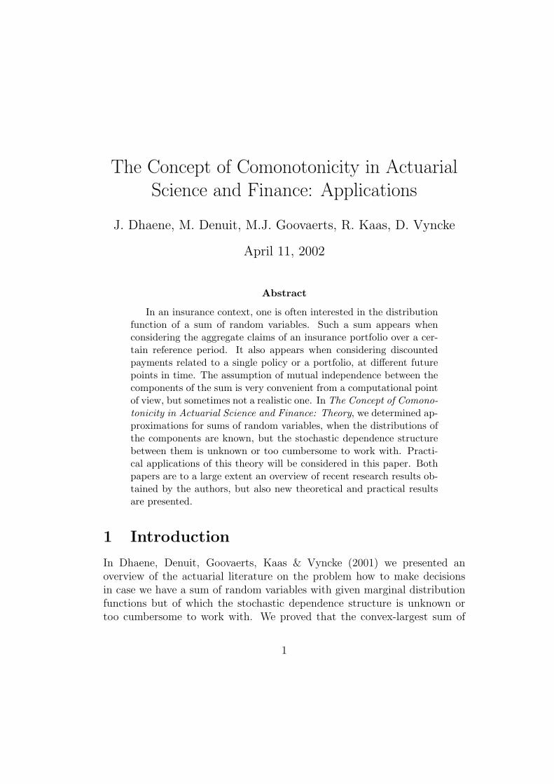
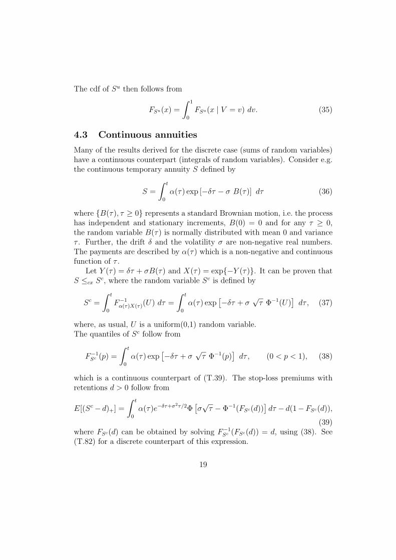
Figure 1: The cdf’s of S (dotted line), Sl (solid grey line), Su (dashed line)and Sc (solid black line); positive payments.

This choice makes Λ a linear transformation of a first order approximationto S. This can be seen from the following computation:

S =20∑j=1

αje−jµ−∑j

i=1(Yi−µ)≈

20∑j=1

αje−jµ[1 −

j∑i=1

(Yi − µ)]

= C −20∑j=1

αje−jµ

j∑i=1

Yi = C −20∑i=1

Yi

20∑j=i

αje−jµ,

where C is the appropriate constant. By the remarks in section 4.1, Sl willthen be “close” to S, provided (Yi − µ) is sufficiently small, or equivalently,σ is sufficiently small.

Figure 1 shows the cdf’s of S, Sl, Su and Sc for the following payments:

αk = 1, k = 1, · · · , 20.Since Sl ≤cx S ≤cx S

u ≤cx Sc, and the same ordering holds for the tails of

their respective distribution functions which can be observed to cross only

22

6 8 10 12 14 16 18 20

510

1520

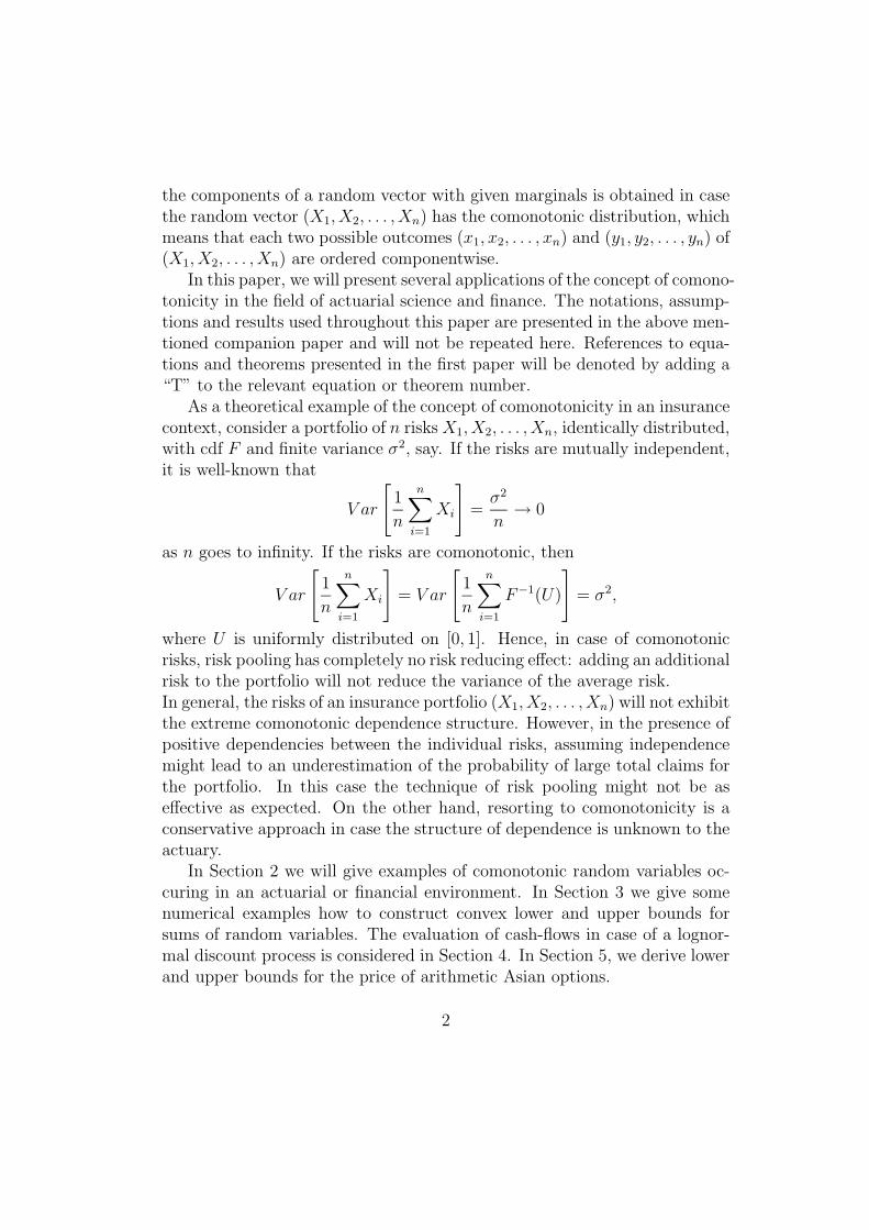
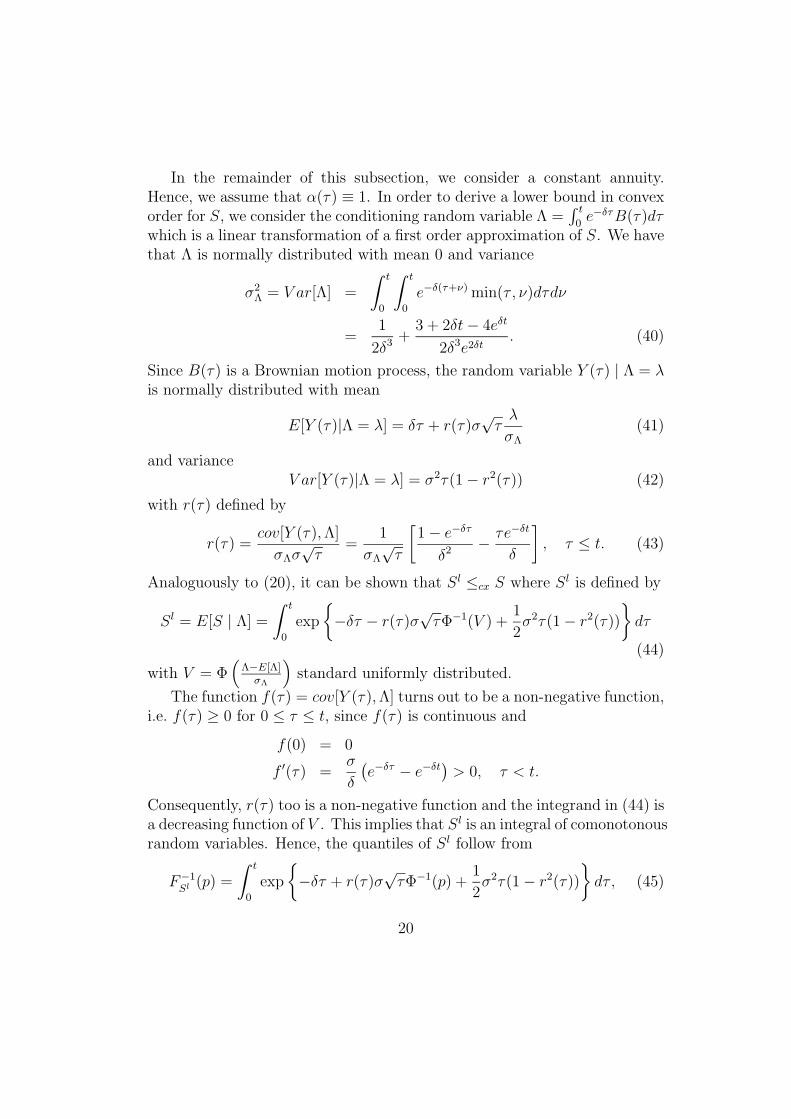
Figure 2: QQ-plot of the quantiles of Sl (◦) and Sc (�) versus those of S;positive payments.

p F−1Sl (p) ‘F−1

S (p)’ F−1Sc (p)

0.95 15.4656 15.3868 16.39150.975 16.7108 16.7233 17.94320.99 18.3080 18.3942 19.95780.995 19.4966 19.9644 21.47390.999 22.2381 22.2271 25.0210

Table 1: Quantiles of Sl and Sc versus those of S; positive payments.

once, we can identify the cdf’s. The dotted line is the “exact” cdf of S, whichwas obtained by generating 10000 quasi-random paths. We see that the cdfof Sl is very close to the distribution of S, which was to be expected becauseΛ is constructed such that it is “close” to S. Note that in this case Sl isa sum of comonotonic random variables, so its quantiles can be computedeasily. The cdf of Sc also performs rather well as an approximation to thecdf of S. This can partially be explained by the fact that the dependencystructure of the vector (X1, . . . , Xn) is locally quasi comonotonic. Indeed, if

i is close to j, then r (Y (i), Y (j)) = min(i,j)√ij

is rather close to 1. Hence, from

(25) and (26), we find that r [Xi, Xj] is close to r[F−1Xi

(U), F−1Xj

(U)]

if i is

close to j.We find that the improved upper bound Su is very close to the comono-

23

5 10 15 20 25

01

23

45

6

outcome

Sto

p-lo

ss p

rem

ium

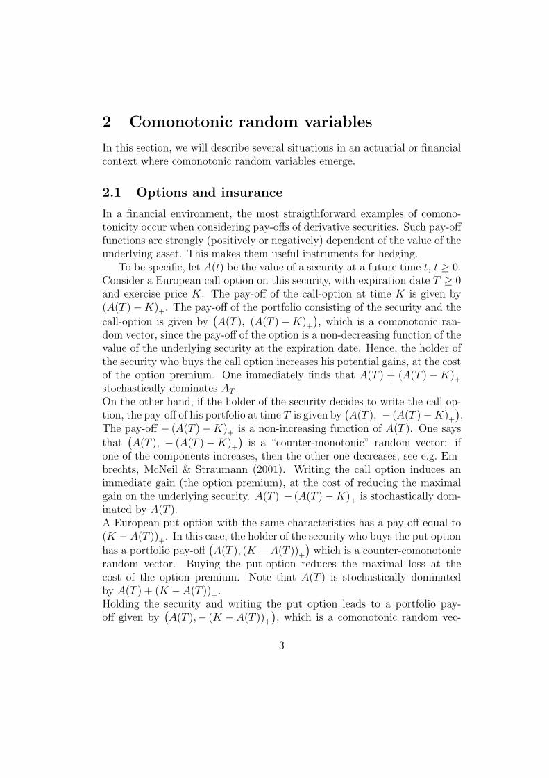
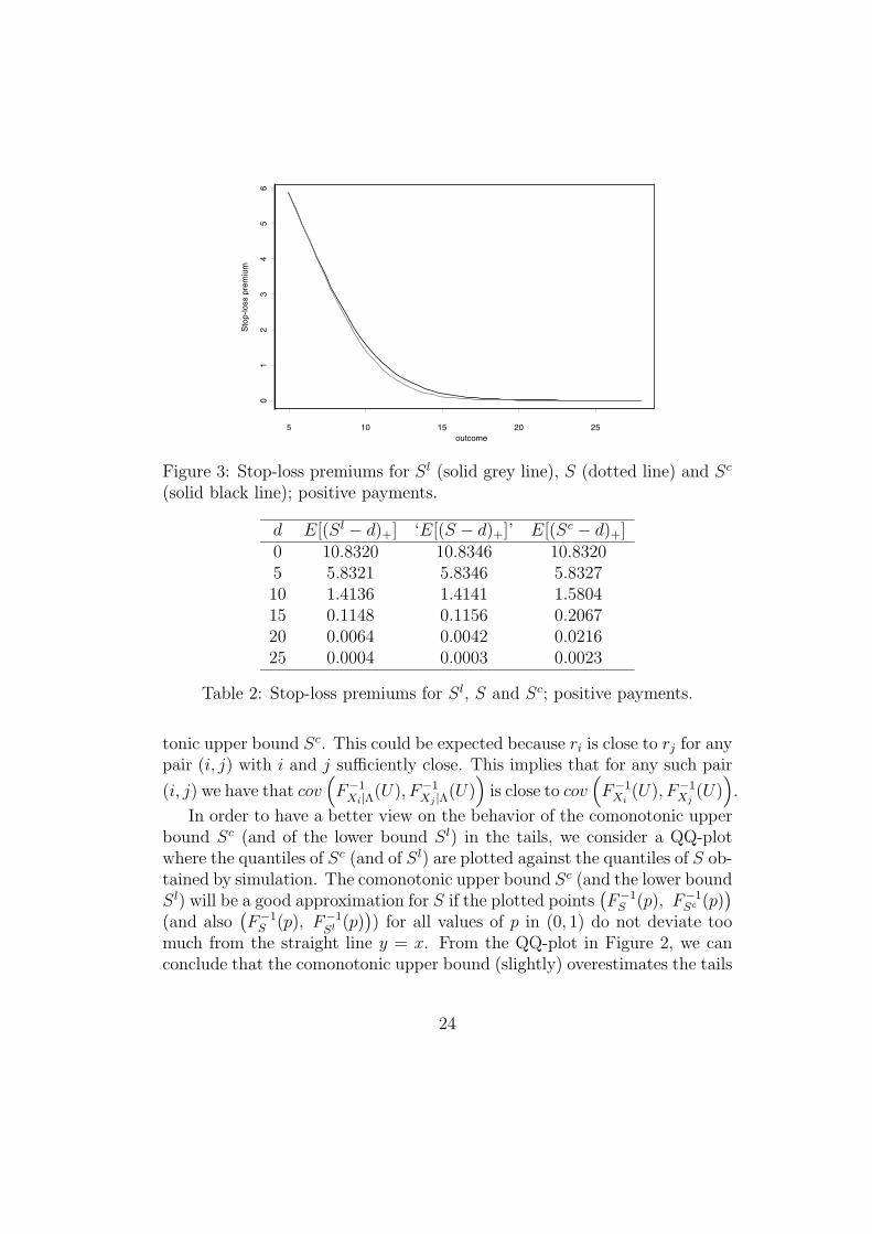
Figure 3: Stop-loss premiums for Sl (solid grey line), S (dotted line) and Sc

(solid black line); positive payments.

d E[(Sl − d)+] ‘E[(S − d)+]’ E[(Sc − d)+]0 10.8320 10.8346 10.83205 5.8321 5.8346 5.832710 1.4136 1.4141 1.580415 0.1148 0.1156 0.206720 0.0064 0.0042 0.021625 0.0004 0.0003 0.0023

Table 2: Stop-loss premiums for Sl, S and Sc; positive payments.

tonic upper bound Sc. This could be expected because ri is close to rj for anypair (i, j) with i and j sufficiently close. This implies that for any such pair

(i, j) we have that cov(F−1Xi|Λ(U), F−1

Xj |Λ(U))

is close to cov(F−1Xi

(U), F−1Xj

(U)).

In order to have a better view on the behavior of the comonotonic upperbound Sc (and of the lower bound Sl) in the tails, we consider a QQ-plotwhere the quantiles of Sc (and of Sl) are plotted against the quantiles of S ob-tained by simulation. The comonotonic upper bound Sc (and the lower boundSl) will be a good approximation for S if the plotted points

(F−1S (p), F−1

Sc (p))

(and also(F−1S (p), F−1

Sl (p))) for all values of p in (0, 1) do not deviate too

much from the straight line y = x. From the QQ-plot in Figure 2, we canconclude that the comonotonic upper bound (slightly) overestimates the tails

24

0 2 4 6 8 10

0.0

0.2

0.4

0.6

0.8

1.0

outcome

cdf

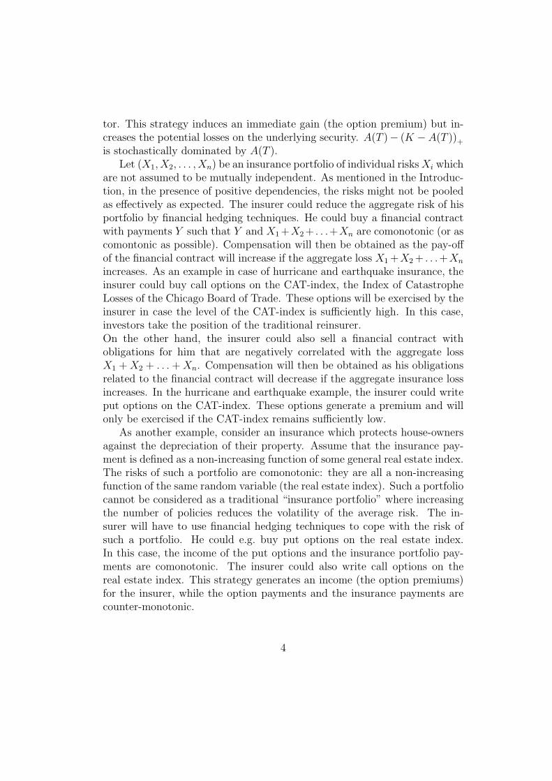
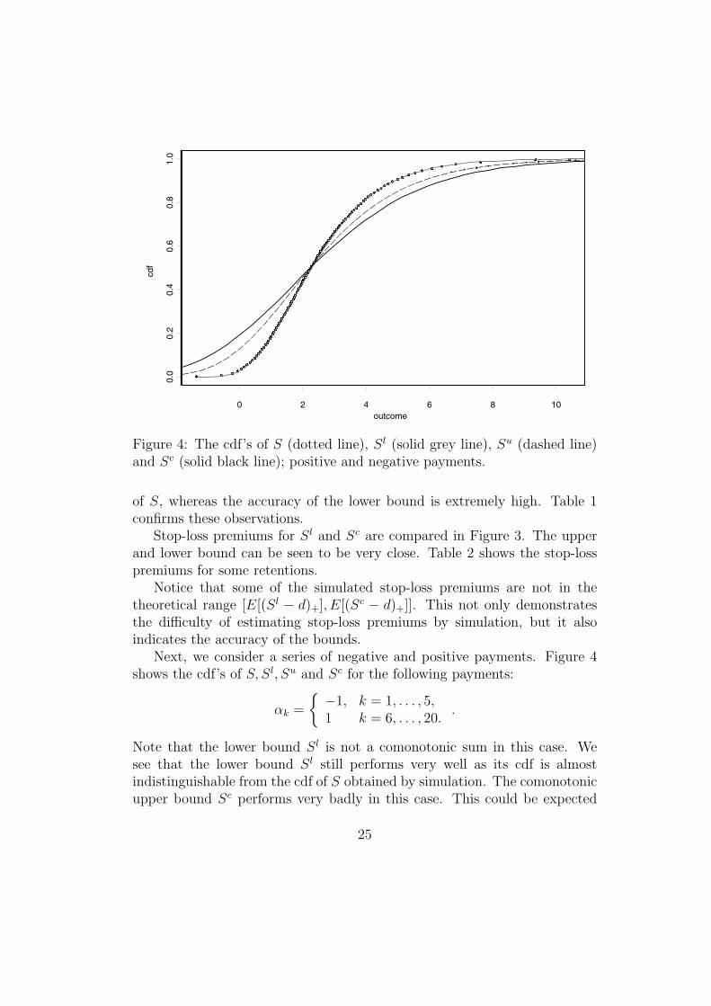
Figure 4: The cdf’s of S (dotted line), Sl (solid grey line), Su (dashed line)and Sc (solid black line); positive and negative payments.

of S, whereas the accuracy of the lower bound is extremely high. Table 1confirms these observations.

Stop-loss premiums for Sl and Sc are compared in Figure 3. The upperand lower bound can be seen to be very close. Table 2 shows the stop-losspremiums for some retentions.

Notice that some of the simulated stop-loss premiums are not in thetheoretical range [E[(Sl − d)+], E[(Sc − d)+]]. This not only demonstratesthe difficulty of estimating stop-loss premiums by simulation, but it alsoindicates the accuracy of the bounds.

Next, we consider a series of negative and positive payments. Figure 4shows the cdf’s of S, Sl, Su and Sc for the following payments:

αk =

{ −1, k = 1, . . . , 5,1 k = 6, . . . , 20.

.

Note that the lower bound Sl is not a comonotonic sum in this case. Wesee that the lower bound Sl still performs very well as its cdf is almostindistinguishable from the cdf of S obtained by simulation. The comonotonicupper bound Sc performs very badly in this case. This could be expected

25

0 2 4 6 8

05

10

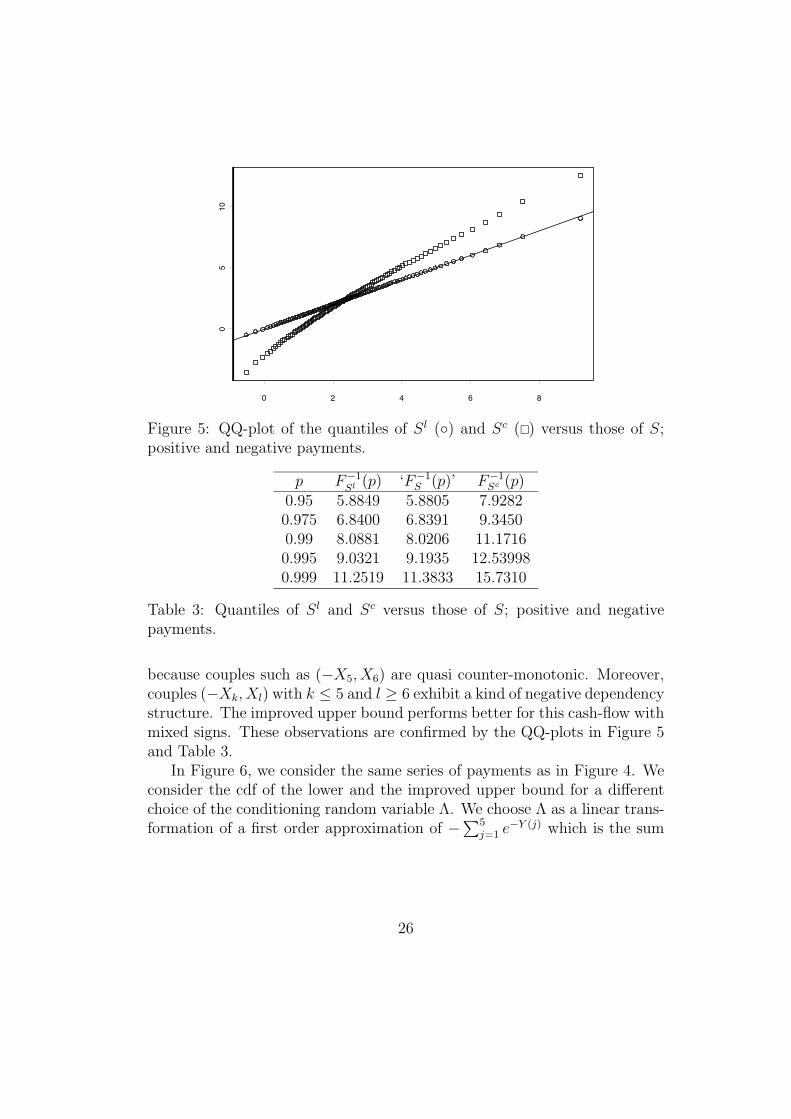
Figure 5: QQ-plot of the quantiles of Sl (◦) and Sc (�) versus those of S;positive and negative payments.

p F−1Sl (p) ‘F−1

S (p)’ F−1Sc (p)

0.95 5.8849 5.8805 7.92820.975 6.8400 6.8391 9.34500.99 8.0881 8.0206 11.17160.995 9.0321 9.1935 12.539980.999 11.2519 11.3833 15.7310

Table 3: Quantiles of Sl and Sc versus those of S; positive and negativepayments.

because couples such as (−X5, X6) are quasi counter-monotonic. Moreover,couples (−Xk, Xl) with k ≤ 5 and l ≥ 6 exhibit a kind of negative dependencystructure. The improved upper bound performs better for this cash-flow withmixed signs. These observations are confirmed by the QQ-plots in Figure 5and Table 3.

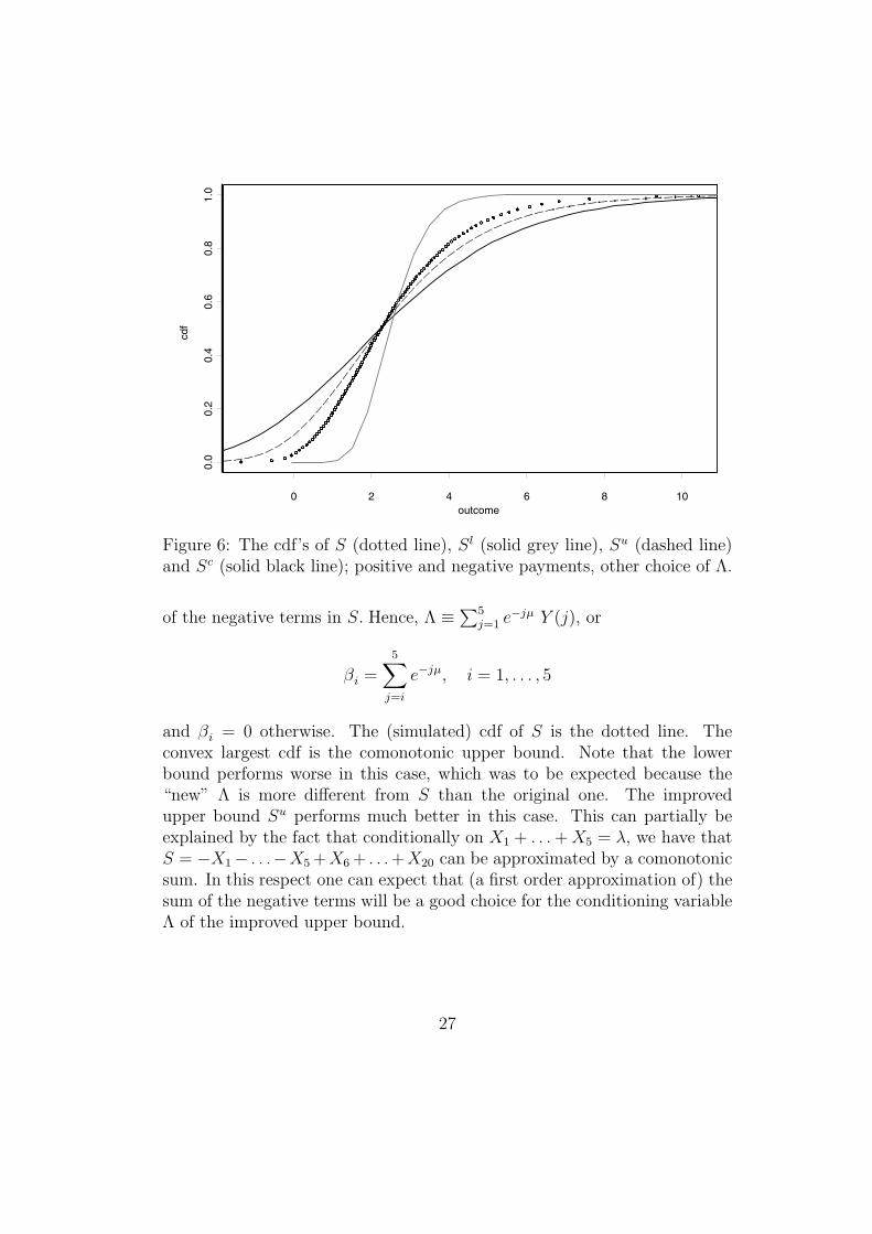
In Figure 6, we consider the same series of payments as in Figure 4. Weconsider the cdf of the lower and the improved upper bound for a differentchoice of the conditioning random variable Λ. We choose Λ as a linear trans-formation of a first order approximation of −∑5

j=1 e−Y (j) which is the sum

26

0 2 4 6 8 10

0.0

0.2

0.4

0.6

0.8

1.0

outcome

cdf

Figure 6: The cdf’s of S (dotted line), Sl (solid grey line), Su (dashed line)and Sc (solid black line); positive and negative payments, other choice of Λ.

of the negative terms in S. Hence, Λ ≡∑5j=1 e

−jµ Y (j), or

βi =5∑

j=i

e−jµ, i = 1, . . . , 5

and βi = 0 otherwise. The (simulated) cdf of S is the dotted line. Theconvex largest cdf is the comonotonic upper bound. Note that the lowerbound performs worse in this case, which was to be expected because the“new” Λ is more different from S than the original one. The improvedupper bound Su performs much better in this case. This can partially beexplained by the fact that conditionally on X1 + . . .+X5 = λ, we have thatS = −X1 − . . .−X5 +X6 + . . .+X20 can be approximated by a comonotonicsum. In this respect one can expect that (a first order approximation of) thesum of the negative terms will be a good choice for the conditioning variableΛ of the improved upper bound.

27

10 15 20 25 30

0.0

0.2

0.4

0.6

0.8

1.0

outcome

cdf

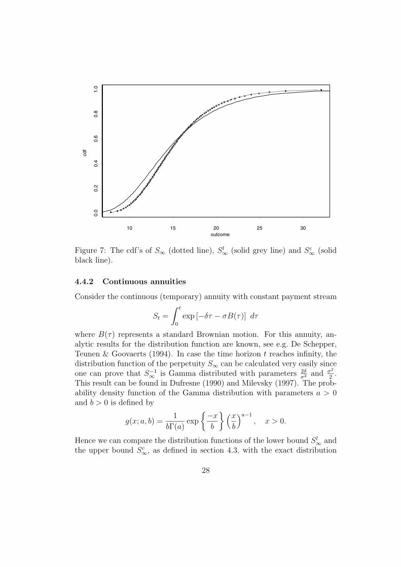
Figure 7: The cdf’s of S∞ (dotted line), Sl∞ (solid grey line) and Sc

∞ (solidblack line).

4.4.2 Continuous annuities

Consider the continuous (temporary) annuity with constant payment stream

St =

∫ t

0

exp [−δτ − σB(τ)] dτ

where B(τ) represents a standard Brownian motion. For this annuity, an-alytic results for the distribution function are known, see e.g. De Schepper,Teunen & Goovaerts (1994). In case the time horizon t reaches infinity, thedistribution function of the perpetuity S∞ can be calculated very easily sinceone can prove that S−1

∞ is Gamma distributed with parameters 2δσ2 and σ2

2.

This result can be found in Dufresne (1990) and Milevsky (1997). The prob-ability density function of the Gamma distribution with parameters a > 0and b > 0 is defined by

g(x; a, b) =1

bΓ(a)exp

{−xb

}(xb

)a−1

, x > 0.

Hence we can compare the distribution functions of the lower bound Sl∞ and

the upper bound Sc∞, as defined in section 4.3, with the exact distribution

28

10 15 20 25 30

1015

2025

3035

Figure 8: QQ-plot of the quantiles of Sl∞ (◦) and Sc

∞ (�) versus those of S∞.

p F−1Sl∞

(p) F−1S∞(p) F−1

Sc∞(p)

0.95 23.5271 23.6297 25.78810.975 25.9633 26.1304 29.18570.99 29.1972 29.4883 33.85230.995 31.6810 32.0993 37.55610.999 37.6492 38.4953 46.8616

Table 4: Quantiles of Sl∞ and Sc

∞ versus those of S∞.

function of S∞. From (40) with t → ∞, it follows that the variance of theconditioning variable Λ =

∫∞0e−δτB(τ)dτ simplifies to

V ar[Λ] =1

2δ3

while, by (43), the correlation between Y (τ) and Λ boils down to

r(τ) =1

σΛ

√τ

1 − e−δτ

δ2 .

Figure 7 shows the distribution functions of Sl∞, Sc

∞ and S∞ for δ = 0.07 andσ = 0.1. Again, the lower bound proves to be a very good approximation forthe cdf of S∞. To assess the accuracy of the bounds in the tails, we plot their

29

10 15 20 25 30

02

46

outcome

Sto

p-lo

ss p

rem

ium

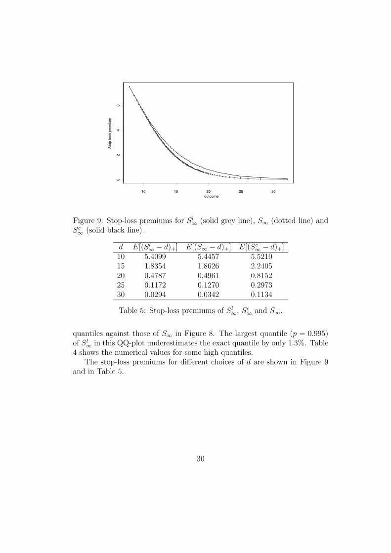
Figure 9: Stop-loss premiums for Sl∞ (solid grey line), S∞ (dotted line) and

Sc∞ (solid black line).

d E[(Sl∞ − d)+] E[(S∞ − d)+] E[(Sc

∞ − d)+]10 5.4099 5.4457 5.521015 1.8354 1.8626 2.240520 0.4787 0.4961 0.815225 0.1172 0.1270 0.297330 0.0294 0.0342 0.1134

Table 5: Stop-loss premiums of Sl∞, Sc

∞ and S∞.

quantiles against those of S∞ in Figure 8. The largest quantile (p = 0.995)of Sl

∞ in this QQ-plot underestimates the exact quantile by only 1.3%. Table4 shows the numerical values for some high quantiles.

The stop-loss premiums for different choices of d are shown in Figure 9and in Table 5.

30

5 Asian Options

5.1 Definitions and some theoretical results

Assume that we are currently at time 0. Consider a risky asset (a non-dividend paying stock) with prices described by the stochastic process {A(t), t ≥ 0} ,and a risk-free continuously compounded rate δ that is constant throughtime. In this section all probabilities and expectations have to be consid-ered as conditional on the information available at time 0, i.e. the prices ofthe risky asset up to time 0. Note that in general, the conditional expec-tation (with respect to the physical probability measure) of e−δtA(t), giventhe information available at time 0, will differ from the current price A(0).However, we will assume that there exists a unique “equivalent probabilitymeasure Q” such that the discounted price proces

{e−δt A(t), t ≥ 0

}is a

martingale under this equivalent probability measure. This implies that forany t ≥ 0, the conditional expectation (with respect to the equivalent mar-tingale measure) of e−δtA(t), given the information available at time 0, willbe equal to the current price A(0). Denoting this conditional expectationunder the equivalent martingale measure by EQ

[e−δtA(t)

], we have that

EQ[e−δtA(t)

]= A(0), t ≥ 0. (52)

The notation FA(t)(x) will be used for the conditional probability that A(t)is smaller than or equal to x, under the equivalent martingale measure Q,and given the information available at time 0. Its inverse will be denoted byF−1A(t)(p).

The existence of an equivalent martingale measure is related to the absenceof arbitrage in the securities market, while uniqueness of the equivalent mar-tingale measure is related to market completeness. Two models where thereexists such a unique equivalent martingale measure are the binomial threemodel of Cox, Ross & Rubinstein (1979) and the geometric Brownian motionmodel of Black & Scholes (1973).

The existence of the equivalent martingale measure allows one to reducethe pricing of options on the risky asset to calculating expected values of thediscounted pay-offs, not with respect to the physical probability measure,but with respect to the equivalent martingale measure, see e.g. Harrison andKreps (1979) or Harrison and Pliska (1981). A reference in the actuarialliterature is Gerber & Shiu (1996).

31

A European call option on the risky asset, with exercise price K andexercise date T generates a pay-off (A(T ) −K)+ at time T , that is, if theprice of the risky asset at time T exceeds the exercise price, the pay-off equalsthe difference; if not, the pay-off is zero. Note the similarity between sucha pay-off and the payment on a stop-loss reinsurance contract. At currenttime t = 0 this call option will trade against a price given by

EC(K,T ) = e−δTEQ[(A(T ) −K)+

](53)

A European-style arithmetic Asian call option with exercise date T , n av-eraging dates and exercise priceK generates a pay-off

(1n

∑n−1i=0 A(T − i) −K

)+

at T , that is, if the average of the prices of the risky asset at the latest ndates before T is more than K, the pay-off equals the difference; if not, thepay-off is zero. Such options protect the holder against manipulations of theasset price near the expiration date. The price of the Asian option at currenttime t = 0 is given by

AC(n,K, T ) = e−δTEQ

[(1

n

n−1∑i=0

A(T − i) −K

)+

]. (54)

Determining the price of an Asian option is not a trivial task, because ingeneral we do not have an explicit analytical expression for the distribution ofthe average

∑n−1i=0 A(T−i).One can use Monte-Carlo simulation techniques to

obtain a numerical estimate of the price, see Kemna and Vorst (1990) and F.J.Vazquez-Abad & Dufresne (1998), or one can numerically solve a parabolicpartial differential equation, see Rogers & Shi (1995). But as both approachesare rather time consuming, it would be helpful to have an accurate andeasily computable bound of this price. In Jacques (1996) an approximationis obtained by replacing the distribution of the sum

∑n−1i=0 A(T − i) by a more

tractable one.From the expression for the price of an arithmetic Asian call option,

we see that the problem of pricing such options turns out to be equivalentto calculating stop-loss premiums of a sum of dependent random variables.This means that we can apply our previous results on bounds for stop-losspremiums in order to find accurate lower and upper bounds for the priceof Asian options. Note that the lower bound that we will obtain is closelyrelated to the lower bound derived by Rogers & Shi (1995).

32

5.2 Asian options, the general case

Assume that at the current time 0, the averaging has not yet started. In thiscase the n variables A(T − n + 1), · · · , A(T ) are random. Upper bounds forAC(n,K, T ) can be constructed as follows for any retentions Ki and K, withK =

∑ni=1Ki :

AC(n,K, T ) =e−δT

nEQ

[(n−1∑i=0

A(T − i) − nK

)+

]

≤ e−δT

n

n−1∑i=0

EQ[(A(T − i) − nKi)+

]

=1

n

n−1∑i=0

e−δi EC (nKi, T − i) . (55)

The procedure above enables us to construct an unlimited number of upperbounds for the price of an arithmetic Asian call option as an average of theprices of underlying European call options. The theory of comonotonic riskswill allow us to find the best, i.e. the smallest, upper bound constructed inthis way. Note that all results can be easily extended to general averagingdates T − t1, . . . , T − tn. In this paper, however, we only consider equallyspaced averaging dates in order not to complicate notation.

By introducing the notation Sc =∑n−1

i=0 F−1A(T−i)(U), where U is a random

variable which is uniformly distributed on the unit interval, we find fromTheorem T.8 that for all exercise prices K we have

AC(n,K, T ) ≤ e−δT

nEQ[(Sc − nK)+

](56)

From Theorem T.7 we then find that for allK with F−1+Sc (0) < nK < F−1

Sc (1),

e−δT

nEQ[(Sc − nK)+

]=

e−δT

n

n−1∑i=0

EQ

[(A(T − i) − F

−1(α)A(T−i) (FSc(nK))

)+

]

=1

n

n−1∑i=0

e−δi EC(F

−1(α)A(T−i) (FSc(nK)) , T − i

)(57)

where α is determined by

F−1(α)Sc (FSc(nK)) = nK. (58)

33

Hence, an upper bound for the price of the Asian option AC(n,K, T ) withF−1+Sc (0) < nK < F−1

Sc (1) is given by

AC(n,K, T ) ≤ 1

n

n−1∑i=0

e−δi EC(F

−1(α)A(T−i) (FSc(nK)) , T − i

)(59)

We also find that for any retentions Ki and K with K =∑n

i=1Ki,

e−δT

nEQ[(Sc − nK)+

] ≤ 1

n

n−1∑i=0

e−δi EC (nKi, T − i) . (60)

From (56), (57), (59) and (60) we find that the comonotonic dependencystructure leads to the optimal upper bound for the price of an arithmeticAsian option which is weighted average of the prices of the underlying Euro-pean call options as in (55).Note that if nK ≤ F−1+

Sc (0) or nK ≥ F−1Sc (1), the price of the Asian option

can be determined exactly, see (T.52) and (T.53). In the first case, it iscertain that the option will be in the money at the expiration date, whilein the second case the option will be certainly out of the money, and henceworthless.The upper bound in (59) can be written in terms of the usual inverses F−1

A(T−i).Indeed, one can prove that

AC(n,K, T ) ≤ 1

n

n−1∑i=0

e−δiEC[F−1A(T−i) (FSc(nK)) , T − i

]−e−δT

[nK − F−1

Sc (FSc(nK))](1 − FSc(nK)) .

Until now, we assumed that T −n+1 > 0. We will now turn to the case thatT −n+1 ≤ 0. Then we know the prices A(T −n+1), A(T −n+2), · · ·, A(0),and only the prices A(1), · · · , A(T ) remain random. Therefore we obtain:

AC(n,K, T ) =e−δT

nEQ

[(n−1∑i=0

A(T − i) − nK

)+

](61)

=e−δT

nEQ

[(T−1∑i=0

A(T − i) −(nK −

n−1∑i=T

A(T − i)

))+

]

Under this assumption we can apply the same method as above in order toobtain upper bounds for the price of the Asian option. Now we define Sc by

34

Sc =∑T−1

i=0 F−1A(T−i)(U). For F−1+

Sc (0) < nK −∑n−1i=T A(T − i) < F−1

Sc (1), weobtain

AC(n,K, T ) ≤ 1

n

T−1∑i=0

e−δi EC

[F

−1(α)A(T−i)

(FSc

(nK −

n−1∑i=T

A(T − i)

)), T − i

],

(62)where α is determined by

F−1(α)Sc

[FSc

(nK −

n−1∑i=T

A(T − i)

)]= nK −

n−1∑i=T

A(T − i). (63)

Note that a similar procedure can be used to derive upper bounds for theprice of arithmetic Asian put options.

Using the theory explained in Section T.5.3, we can also derive lowerbounds for the price of Asian options. This will be illustrated in the nextsection.

5.3 Application in a Black & Scholes Setting

In the model of Black & Scholes (1973), the price of the risky asset is de-scribed by a stochastic process {A(t), t ≥ 0} following a geometric Brownianmotion with constant drift µ and constant volatility σ:

dA(t)

A(t)= µdt+ σdB(t), t ≥ 0, (64)

with initial value A(0) > 0, and where{B(t), t ≥ 0

}is a standard Brownian

motion.Under the equivalent martingale measureQ, the price process {A(t), t ≥ 0}

still follows a geometric Brownian motion, with the same volatility but withdrift equal to the continuously compounded risk-free interest rate δ:

dA(t)

A(t)= δdt+ σdB(t), t ≥ 0, (65)

with initial value A(0), and where {B(t), t ≥ 0} is a standard Brownianmotion in the Q-dynamics. Hence, under the equivalent martingale measure,we have that

A(t) = A(0) e

(δ−σ2

2

)t+σB(t)

, t ≥ 0. (66)

35

This implies that under the equivalent martingale measure, the random vari-

ables A(t)A(0)

are lognormally distributed with parameters(δ − σ2

2

)t and tσ2

respectively:

FA(t)(x) = Pr[A(0)e(δ−σ2

2)t+

√tσΦ−1(U) ≤ x

], (67)

where U is uniformly distributed on the interval (0, 1).From (T.78) and (T.80), we find

EC(K,T ) = e−δTEQ[(A(T ) −K)+

]= A(0) Φ (d1) −K e−δT Φ (d2) , (68)

where d1 and d2 are given by

d1 =ln (A(0)/K) + (δ + σ2/2)T

σ√T

(69)

andd2 = d1 − σ

√T . (70)

This formula is the famous Black & Scholes (1973) pricing formula for Euro-pean call options.

Within the Black & Scholes model, no closed form expression is availablefor the price of an arithmetic Asian call option. Therefore, we will deriveupper and lower bounds for the price of such options. We will only considerthe case that the averaging has not yet started. The other case can be dealtwith in a similar way.

From (56) and (T.82), we find the following comonotonic upper boundfor the price of an Asian call option:

AC(n,K, T ) ≤ e−δT

nE[(Sc − nK)+

]=

A(0)

n

n−1∑i=0

e−δi Φ[σ√T − i− Φ−1 (FSc(nK))

]−e−δT K (1 − FSc(nK)) , (71)

which holds for any K > 0. Note that this upper bound corresponds tothe optimal linear combination of the prices of European call options asmentioned in the previous section.

36

The remaining problem is how to calculate FSc(nK). The latter quantityfollows from

n−1∑i=0

F−1A(T−i) (FSc(nK)) = nK,

or, equivalently, from (66) and Theorem T.1 we find that FSc(nK) followsfrom

A(0)n−1∑i=0

exp

[(δ − σ2

2

)(T − i) + σ

√T − i Φ−1 (FSc(nK))

]= nK. (72)

Lower bounds forAC(n,K, T ) can be obtained from Section T.5.3. There-fore, consider the conditioning random variable Λ defined by

Λ =n−1∑j=0

e

(δ−σ2

2

)(T−j)

B(T − j). (73)

From (66) we find that, in the Q-dynamics,

n−1∑i=0

A(T − i) = A(0)n−1∑i=0

e

(δ−σ2

2

)(T−i)+σB(T−i)

. (74)

Hence, Λ is a linear transformation of a first order approximation to∑n−1

i=0 A(T−i). The variance of Λ is given by

σ2Λ =

n−1∑j=0

n−1∑k=0

e

(δ−σ2

2

)(2T−j−k)

min (T − j, T − k) . (75)

We have that (B(T − n+ 1), B(T − n+ 2), . . . , B(T )) has a multivariatenormal distribution. This implies that given Λ = λ, the random vari-able B(T − i) is normally distributed with mean rT−i

√T−iσΛ

λ and variance

(T − i)(1 − r2

T−i

)where

rT−i =cov (B(T − i),Λ)

σΛ

√T − i

=

∑n−1j=0 e

(δ−σ2

2

)(T−j)

min (T − i, T − j)

σΛ

√T − i

. (76)

37

We find that

Sl = EQ

[n−1∑i=0

A(T − i) | Λ]

= A(0)n−1∑i=0

e

(δ−σ2

2r2T−i

)(T−i)+σ rT−i

√T−i Φ−1(U)

(77)

where U is uniformly distributed on the unit interval. From this expression,we see that Sl is a comonotonic sum of lognormal random variables. Hence,from Section T.5.3 and (T.82), we find the following lower bound for theprice of the Asian call option:

AC(n,K, T ) ≥ e−δT

nEQ[(Sl − nK

)+

]

=A(0)

n

n−1∑i=0

e−δi Φ[σ rT−i

√T − i− Φ−1 (FSl(nK))

]−e−δT K (1 − FSl(nK)) (78)

which holds for any K > 0. In this case, FSl(nK) follows from

A(0)n−1∑i=0

exp

[(δ − σ2

2r2T−i

)(T − i) + σ rT−i

√T − i Φ−1 (FSl(nK))

]= nK.

(79)When the number of averaging dates n equals 1, the Asian call option

reduces to a European call option. It is straightforward to prove that inthis case the upper and the lower bounds (71) and (78) for the price of theAsian option both reduce to the Black & Scholes formula for the price of theEuropean call option.

5.4 Numerical illustration

In this section we numerically illustrate the bounds for the price of Asianoptions in a Black & Scholes setting, as obtained in the previous section. Weconsider a time unit of one day. The parameters that were used to generatethe results given in Tables 6, 7 and 8 are the same as in Jacques (1996): aninitial stock price A(0) = 100, a risk-free interest rate of 9% per year, threevalues (0.2, 0.3 and 0.4) for the yearly volatility, and five values (80, 90, 100,

38

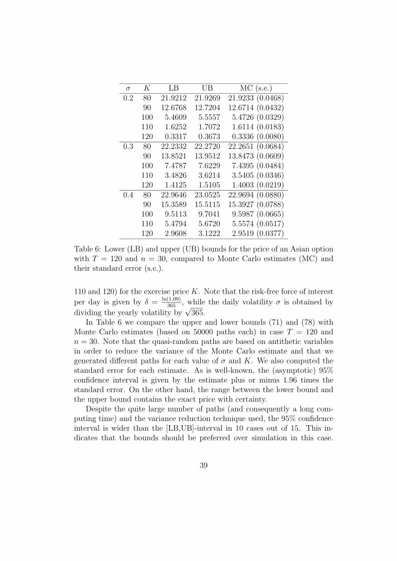
σ K LB UB MC (s.e.)0.2 80 21.9212 21.9269 21.9233 (0.0468)

90 12.6768 12.7204 12.6714 (0.0432)100 5.4609 5.5557 5.4726 (0.0329)110 1.6252 1.7072 1.6114 (0.0183)120 0.3317 0.3673 0.3336 (0.0080)

0.3 80 22.2332 22.2720 22.2651 (0.0684)90 13.8521 13.9512 13.8473 (0.0609)100 7.4787 7.6229 7.4395 (0.0484)110 3.4826 3.6214 3.5405 (0.0346)120 1.4125 1.5105 1.4003 (0.0219)

0.4 80 22.9646 23.0525 22.9694 (0.0880)90 15.3589 15.5115 15.3927 (0.0788)100 9.5113 9.7041 9.5987 (0.0665)110 5.4794 5.6720 5.5574 (0.0517)120 2.9608 3.1222 2.9519 (0.0377)

Table 6: Lower (LB) and upper (UB) bounds for the price of an Asian optionwith T = 120 and n = 30, compared to Monte Carlo estimates (MC) andtheir standard error (s.e.).

110 and 120) for the exercise price K. Note that the risk-free force of interest

per day is given by δ = ln(1.09)365

, while the daily volatility σ is obtained by

dividing the yearly volatility by√

365.In Table 6 we compare the upper and lower bounds (71) and (78) with

Monte Carlo estimates (based on 50000 paths each) in case T = 120 andn = 30. Note that the quasi-random paths are based on antithetic variablesin order to reduce the variance of the Monte Carlo estimate and that wegenerated different paths for each value of σ and K. We also computed thestandard error for each estimate. As is well-known, the (asymptotic) 95%confidence interval is given by the estimate plus or minus 1.96 times thestandard error. On the other hand, the range between the lower bound andthe upper bound contains the exact price with certainty.

Despite the quite large number of paths (and consequently a long com-puting time) and the variance reduction technique used, the 95% confidenceinterval is wider than the [LB,UB]-interval in 10 cases out of 15. This in-dicates that the bounds should be preferred over simulation in this case.

39

σ K LB UB MC (s.e.)0.2 80 20.7841 20.7845 20.7839 (0.0297)

90 11.0273 11.0599 11.0205 (0.0287)100 3.2013 3.3443 3.1984 (0.0196)110 0.3373 0.4080 0.3383 (0.0064)120 0.0116 0.0185 0.0128 (0.0011)

0.3 80 20.8122 20.8268 20.8055 (0.0441)90 11.4929 11.6017 11.5160 (0.0410)100 4.5063 4.7221 4.4711 (0.0289)110 1.1516 1.3134 1.1458 (0.0150)120 0.1915 0.2503 0.1945 (0.0059)

0.4 80 20.9708 21.0309 20.9719 (0.0581)90 12.2468 12.4384 12.2183 (0.0514)100 5.8157 6.1038 5.8711 (0.0393)110 2.2082 2.4582 2.2224 (0.0248)120 0.6783 0.8223 0.6802 (0.0135)

Table 7: Lower (LB) and upper (UB) bounds for the price of an Asian optionwith T = 60 and n = 30, compared to Monte Carlo estimates (MC) and theirstandard error (s.e.).

Moreover, the Monte Carlo estimate exceeds the lower bound 6 times. Thismight indicate that the lower bound is very close to the real price. The upperbound appears to perform better the more the option is in the money.

In Table 7 we use the same parameters as in Table 6 but we change theexpiration time to T = 60. Now, the 95% confidence interval is wider thanthe [LB,UB]-interval in 6 cases, but the Monte Carlo estimate exceeds thelower bound 7 times. So again, the lower bound must be very close to thereal price.

In Table 8 we change the expiration time back to T = 120 but we reducethe number of averaging days to n = 10. With these parameters, simulationperforms really bad since the simulated confidence interval is wider than thereal confidence interval in all cases. The Monte Carlo estimate again exceedsthe lower bound 7 times.

The upper bound performs better for the option with n = 10 than for theoptions with n = 30. This illustrates the fact that the dependency structureof the A(T − i) is more “comonotonic-like” if all points in time T − i are close

40

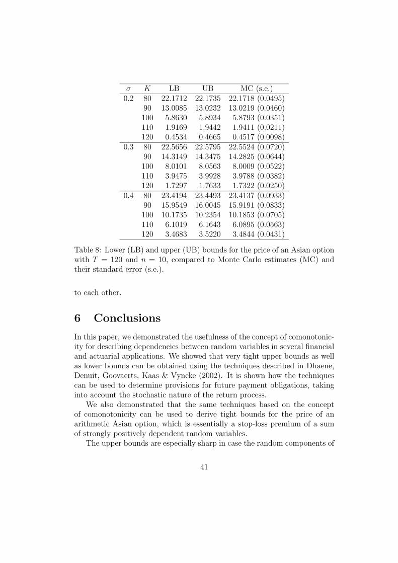
σ K LB UB MC (s.e.)0.2 80 22.1712 22.1735 22.1718 (0.0495)

90 13.0085 13.0232 13.0219 (0.0460)100 5.8630 5.8934 5.8793 (0.0351)110 1.9169 1.9442 1.9411 (0.0211)120 0.4534 0.4665 0.4517 (0.0098)

0.3 80 22.5656 22.5795 22.5524 (0.0720)90 14.3149 14.3475 14.2825 (0.0644)100 8.0101 8.0563 8.0009 (0.0522)110 3.9475 3.9928 3.9788 (0.0382)120 1.7297 1.7633 1.7322 (0.0250)

0.4 80 23.4194 23.4493 23.4137 (0.0933)90 15.9549 16.0045 15.9191 (0.0833)100 10.1735 10.2354 10.1853 (0.0705)110 6.1019 6.1643 6.0895 (0.0563)120 3.4683 3.5220 3.4844 (0.0431)

Table 8: Lower (LB) and upper (UB) bounds for the price of an Asian optionwith T = 120 and n = 10, compared to Monte Carlo estimates (MC) andtheir standard error (s.e.).

to each other.

6 Conclusions

In this paper, we demonstrated the usefulness of the concept of comonotonic-ity for describing dependencies between random variables in several financialand actuarial applications. We showed that very tight upper bounds as wellas lower bounds can be obtained using the techniques described in Dhaene,Denuit, Goovaerts, Kaas & Vyncke (2002). It is shown how the techniquescan be used to determine provisions for future payment obligations, takinginto account the stochastic nature of the return process.

We also demonstrated that the same techniques based on the conceptof comonotonicity can be used to derive tight bounds for the price of anarithmetic Asian option, which is essentially a stop-loss premium of a sumof strongly positively dependent random variables.

The upper bounds are especially sharp in case the random components of

41

a sum are rather strongly positive dependent, as they are in many actuarialapplications of a financial nature, where the consecutive summands containa stochastic discounting component. On the other hand, the lower boundsperform very well even in a situation where the dependencies are not stronglypositive.

The tightness of the lower and upper bounds together with their easycomputability makes them useful instruments for tackling several actuarialproblems occuring in practice.

7 Acknowledgments

Michel Denuit, Jan Dhaene and Marc Goovaerts would like to acknowledgethe financial support of the Committee on Knowledge Extension Researchof the Society of Actuaries for the project “Actuarial Aspects of Dependen-cies in Insurance Portfolios”. The current paper and also Dhaene, Denuit,Goovaerts, Kaas & Vyncke (2001) result from this project.Marc Goovaerts and Jan Dhaene also acknowledge the financial support ofthe Onderzoeksfonds K.U. Leuven (GOA/02: Actuariele, financiele en statis-tische aspecten van afhankelijkheden in verzekerings- en financiele porte-feuilles).

References

[1] Black, F.; Scholes, M. (1973). “The pricing of options and corporateliabilities”, Journal of Political Economy, 81 (May-June), 637-659.

[2] Cox, J.C.; Ross, S.A.; Rubinstein, M. (1979). “Option pricing: a sim-plified approach”, Journal of Financial Economics, 7, 229-263.

[3] De Schepper, A.; Teunen, M.; Goovaerts, M.J. (1994). “An analyticalinversion of a Laplace transform related to annuities certain”, Insurance:Mathematics & Economics, 14(1), 33-37.

[4] Dhaene, J.; Denuit, M.; Goovaerts, M.J.; Kaas, R.; Vyncke, D. (2001).“The concept of comonotonicity in actuarial science and finance: the-ory”, Insurance: Mathematics & Economics, accepted.

42

[5] Dufresne, D. (1990). “The distribution of a perpetuity with applicationsto risk theory and pension funding”, Scandinavian Actuarial Journal, 9,39-79.

[6] Embrechts, P.; Mc.Neil, A.; Straumann, D. (2001). “Correlation and de-pendency in risk management: properties and pitfalls”, in “Risk Man-agement: Value at Risk and Beyond”, edited by Dempster, M. andMoffatt, H.K., Cambridge University Press.

[7] Gerber, H.U.; Shiu, E.S.W. (1996). “Actuarial bridges to dynamic hedg-ing and option pricing”, Insurance: Mathematics & Economics, 18, 183-218.

[8] Goovaerts, M.J.; Dhaene, J;. De Schepper, A. (2000). “Stochastic UpperBounds for Present Value Functions”, Journal of Risk and InsuranceTheory, 67.1, 1-14.

[9] Harrison, J.; Kreps, D. (1979). “ Martingales and arbitrage in multi-period securities markets”, Journal of Economic Theory, 20, 381-408.

[10] Harrison, J.; Pliska, R. (1981). “Martingales and stochastic integrals inthe theory of continuous trading”, Stochastic Processes and their Appli-cations, 11, 215-260.

[11] Jacques, M. (1996). “On the Hedging Portfolio of Asian Options”,ASTIN Bulletin, 26, 165-183.

[12] Kaas, R.; Dhaene, J.; Goovaerts, M.J. (2000). “Upper and lower boundsfor sums of random variables”, Insurance: Mathematics & Economics23, 151-168.

[13] Kaas, R.; Goovaerts, M.J.; Dhaene, J.; Denuit, M. (2001). Modern Ac-tuarial Risk Theory, Kluwer Academic Publishers, Dordrecht.

[14] Kemna, A.G.Z.; Vorst, A.C.F. (1990). “ A pricing method for optionsbased on average asset values”, Journal of Banking and Finance, 14,113-129.

[15] Milevsky, M.A. (1997). “The present value of a stochastic perpetuityand the Gamma distribution”, Insurance: Mathematics & Economics,20(3), 243-250.

43

[16] Rogers, L.C.G.; Shi, Z. (1995). “The value of an Asian option”, Journalof Applied Probability 32, 1077-1088.

[17] Vazquez-Abad, F.J.; Dufresne, D. (1998). “Accelerated simulation forpricing Asian options”, Research Paper Nr 62, Centre for ActuarialStudies, The University of Melbourne.

44