The Compound Action Potential (CAP) of the Frog Sciatic Nerve

The Compound Action Potential (CAP) Of the Frog’s Sciatic Nerve

These notes are mainly concerned with the practical aspects of the experiment but they include a brief review of the theory. The experimental set-up and the theoretical background are described in more detail in the lab lecture and in the Virtual Lab. Introduction (Fig 1, Table 1) A) Structure/Function of large, mixed, compound nerves (See Fig. 1 and 1b) a) In mammals, large peripheral nerves, for example the vagus, the sciatic and the ulnar typically are bundles of thousands of individual axons enclosed in a loose connective tissue sheath, the Epineurium. Within the Epineurium, the axons are grouped in fascicles, encased in a more structured epithelial sheath (the perineurium). Each axon is surrounded by a thin connective tissue sheath, the endoneurium. Note that the frog’s sciatic consists of only a single bundle of fibres, surrounded by the perineurium and loose epineurium.

b) The axons within a compound nerve include afferent (sensory) nerves and efferent (motor and autonomic) nerves. Individual axons vary in diameter, myelination, excitability, threshold and conduction speed.

Figure 1b Cross section of a frog’s

sciatic nerve NOTE: The classification of different axons on the basis of diameter, myelination, electrical properties and conduction speed (etc.) is summarized in Table 1. B) The Compound Action Potential (CAP) a) The CAP is the sum of “all-or-none” action potentials arising more or less simultaneously in individual axons in a compound nerve. The CAP does not occur naturally. It is elicited experimentally or clinically by stimulating the whole nerve with extracellular stimulating electrodes and is recorded by means of extracellular recording electrodes.

·.·

·.·

Physiology Department- McGill University – 2013-2014 2

b) A typical nerve such as the sciatic contains efferent (D and�J motor axons, and post-ganglionic autonomic axons) and afferent (sensory) axons. The properties of the CAP: threshold, amplitude, duration, conduction velocity are determined by the type and number of individual axons which are recruited (excited) by the stimulus. The number and type of axons excited depend on the intensity of the stimulus. c) The CAP differs from action potential of a single axon in several important ways. -The individual action potential demonstrated by intracellular recording from a single axon is an “all-or-none” response which does not change with stimulus intensity (above threshold). -The CAP is a graded response whose magnitude increases with the intensity of stimulation. This is because different axons have different thresholds of excitation. The largest axons have the lowest threshold of excitation i.e., they are the most excitable. (Thus, in terms of excitability: AD�axons>AE>AJ>AG >B>C, See Table I). At low stimulus intensities, only the largest axons are activated, but as the stimulus intensity is raised in steps, smaller axons are progressively recruited. -Note also, (Table 1) that the conduction velocity of individual action potentials increases with the axon diameter. Thus, action potentials of the largest axons will reach the recording electrodes first: consider how the progressive recruitment of more slowly conducting axons will affect the shape of the CAP. d) Both the individual action potential and the CAP are BIPHASIC, having a positive and negative component. The reasons for the biphasic potential changes – which are quite different in each case - are given in the Virtual Lab and briefly reviewed below.

The biphasic action potential recorded inside a single axon with an intracellular electrode consists of a large (positive) depolarization due to a transient increase in Na+ permeability, followed by a smaller and slower negative hyperpolarization, caused by a persistent increase in K+ permeability. (Check your PHGY209 notes). The CAP is biphasic because it is recorded with a pair of extracellular electrodes (bipolar recording). See Fig 2.

·.·

·.·

·.·

·.·


Figure 2 -When the nerve is inactive, there is no potential difference between the electrodes, and the trace is at baseline. - When the CAP arrives, the proximal electrode (1) becomes transiently negative to the distal electrode (2), the potential difference between the two is detected and amplified by the differential amplifier (within the Powerlab recording system) and the trace is displayed as an initial upward deflection on the screen. - When the CAP reaches the distal electrode both electrodes again record the same potential: in other words, there is no potential difference between the two recording

electrodes and the trace returns to baseline. - As the CAP moves further down the nerve, only the distal electrode is still negative and the potential difference between the electrodes is now in opposite direction and therefore seen as a downward deflection on the screen. If the action potential lasts about 1 ms, and its conduction velocity is about 20 mm/ms, what length of nerve is occupied by the CAP at any given time?

* This Table shows types and properties of axons in vertebrate nerves. The conduction velocities are characteristic of mammalian nerves at 37oC: maximum is about 100 m/sec for A-alpha axons. Your experiment will be on an amphibian nerve. -The conduction velocities for frog nerves at ~20oC are much lower: maximum is about 25 m/sec for A alpha axons.

T a b l e 1 - M a m m a l i a n A x o n P r o p e r t i e s *

Fibre Types Fibre Diameter (µm)

Conduction Velocity (m/sec)

AP Duration (msec)

Absolute Refractory Period (msec)

Functions

AD��motoneurons

12-22 70-100 0.4-0.5 0.2-1.0 Efferent alpha Afferent muscle spindles, tendon organs

AE 5-13 30-70 0.4-0.5 0.2-1.0 Afferent, cutaneous, Touch, pressure

AJ 3-8 15-40 0.4-0.7 0.2-1.0 Gamma motoneurons AG 1-5 12-30 0.2-1.0 0.2-1.0 Afferent, fast

Pain, temperature B 1-3 3-15 1.2 1.2 Efferent, autonomic

Only Preganglionic C (unmyelinated)

0.2-1.2 0.2-2.0 2 2 Afferent, “slow” Pain, Efferent Autonomic postganglionic


General Purpose of the Experiment In this experiment on the isolated frog sciatic nerve, you will study some basic features of nerve excitation and impulse conduction. Specific Objectives 1: To record the CAP and examine how stimulus intensity affects the CAP’s magnitude and time course. 2: To determine the relationship between intensity and duration of stimulation on the threshold of the CAP (the strength/duration curve). 3: To measure the conduction velocity of the CAP by the Absolute and the Difference Methods. 4: To measure the conduction velocities of two subdivisions of the A fibre group, the A-alpha and A-beta subgroups. 5: To measure the refractory period of the A-alpha subgroup. Material and Methods Pithed Frog (with brain and spinal cord removed) Dissecting instruments (bring your own) Fine-tipped glass rods Frog Ringer’s (physiological salt solution) Pasteur pipette/cotton swabs/fine thread Dissecting board/dissecting pins. Recording nerve bath with lid Grass Model SD-9 stimulator Powerlab Computerized recording system Electrical leads and connectors

The Stimulating/Recording/Data Storage System The components of this system are arranged as shown in figure 3. a) The Grass Stimulator -The stimulator provides two output pulses, the Adjustable Stimulus voltage and the Trigger Pulse. -One set of leads carries the Stimulus to the stimulating electrodes in the recording bath (positive electrode is anode and negative cathode). (NOTE: because the CAP is initiated at or near the cathode, and the anodal action slows down or may even suppress the CAP, the cathode SHOULD normally be closer to the recording electrodes). -During the experiment, the nerve can be stimulated either with a single shock (by depressing MODE switch to SINGLE); or at 1/sec with the mode set to REPEAT. When not collecting data, the MODE can be at OFF. The strength (voltage), duration and frequency of individual stimuli are controlled by the corresponding dials and switches on the stimulator.

·.·


-A second set of leads carries a pre-stimulus pulse to the External Trigger connector of the Powerlab unit. The purpose of the Trigger Pulse, which precedes the Stimulus by a brief interval (1-2 msec), is to signal the Analog I/O board contained in the Powerlab system to begin sampling data. The interval between the Trigger and Stimulus Pulses is the “stimulus delay” and is adjusted with the DELAY dial on the Stimulator: the delay can be set at 1 ms. b) The Differential Amplifier (CH1 and CH2 of the Powerlab unit) -Through the inputs in Channels 1 and 2 (CH1, CH2), the Powerlab unit detects (and greatly amplifies) the small electrical potential difference between the recording electrodes. A third lead (green), which connects the nerve to “ground”, should be

attached to an electrode between the negative stimulating electrode (cathode) and the most proximal recording electrode: thus grounding the nerve greatly reduces the stimulus artifact (try disconnecting it!) c) The Trigger of the Powerlab unit The Trigger input receives the trigger pulse from the Stimulator and controls the start of the data collection (‘sweep’ on the oscilloscope). d) Data Acquisition and Analysis Software

- Double-click on “Caplab” from “my settings” (LabChart Welcome Center). Verify the different parameters, as pictured in the screenshot on the next page (Fig. 4).

Figure 3: Experimental setup


Figure 4: Scope View application and submenu


Figure 5: scheme for stimulating and recording

To plot the strength-duration curve (Part 2), Matlab commands will be used (Matlab should already be running in the background). You will enter manually the values of stimulus strength (volts) and stimulus duration (msec) obtained by adjusting the ‘voltage’ and ‘duration’ knobs on the stimulator.

The Dissection and Mounting of the Nerve in the Recording Bath You will be shown a video of the dissection at the beginning of the lab: pay particular attention because an undamaged nerve is essential to the success of the experiment. This video -in 4 parts - is also available on WebCT. Note: wear the disposable gloves when doing the dissection. a) Dissection -Isolate the nerve following the instructions given in the video. Note: avoid touching the nerve with your fingers and especially NOT with metal instruments (metals immersed in saline generate electric currents which stimulate the nerve– as first noted by Galvani).

-Be very careful not to stretch or crush the nerve during the dissection; it is quite fragile and damage will abolish the nerve impulses. -Usually the most difficult part of the dissection is in tracing the nerve past the knee joint. This involves freeing the nerve from a sheet of tough connective tissue, which must be done carefully because the nerve is thin and delicate and is easily damaged. If you are unsure of how to proceed, call a staff member. -When finishing the proximal (spinal cord end), of the dissection, leave a small piece of bone (vertebrae) attached to the nerve. Tie a piece of thread as close as possible to the distal end of the nerve. This will allow you to lift the preparation without touching the nerve. Make sure that the nerve is kept moistened with Ringer throughout the dissection

·.·


b) Mounting the nerve in the recording bath - Using a Pasteur pipette, fill the bottom part of the nerve bath with frog Ringer’s solution. Fluid must not remain in contact with the stimulating/recording electrodes. -Transfer the nerve to the chamber, placing the proximal (central) end of the nerve over the stimulating electrodes. To transfer the nerve, hold it by the thread at one end and the piece of bone at the other. -Applying a bit of filter paper, make sure that no saline remains between any of the electrodes.

The Experiment

PART 1

CHARACTERISTICS OF THE COMPOUND ACTION

POTENTIAL Objective To record the CAP and to observe and measure its general properties including its latency, threshold, magnitude, shape, duration and their relationship to the stimulus strength (voltage). It is important to remember that you are dealing with the responses of a population of axons NOT a single axon.

� Set the parameters on the Stimulator:

*** To minimize the deterioration of the preparation when not collecting data, keep the MODE switch at OFF; press down to single when ready to collect data. Check the software settings, if this has not been done (see figure 4)

Scope View Application: Duration: 10 ms Sampling…: External trigger Begin recording at trigger Stop sampling: Fixed duration 10 ms Multiple blocks Repeat infinite Channel 1>Input Amplifier> Range: 100mV (suggested), Differential Channel 2 >Input Amplifier> Range: 20 mV (suggested), Differential Acquisition Rate: 40K/s

Grass SD9 stimulator settings Stimulus Duration:

0.2 msec (suggested)

Stimulus Voltage:

0.1V (minimum setting)

Delay: 1 msec (interval between trigger pulse and stimulus)

Frequency: 1Hz (1 pulse/sec) Mode: Off –

Single – the stimulator will deliver one shock when the switch is pressed down.


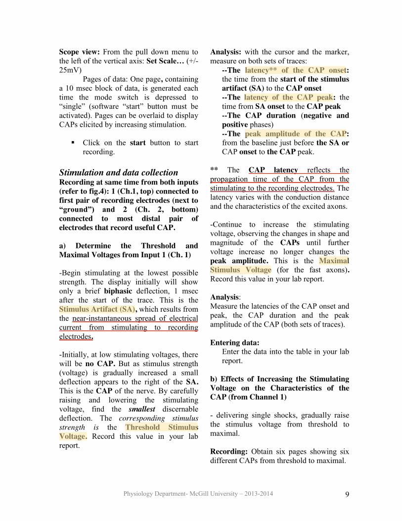
Scope view: From the pull down menu to the left of the vertical axis: Set Scale… (+/-25mV) Pages of data: One page, containing a 10 msec block of data, is generated each time the mode switch is depressed to “single” (software “start” button must be activated). Pages can be overlaid to display CAPs elicited by increasing stimulation.

� Click on the start button to start recording.

Stimulation and data collection Recording at same time from both inputs (refer to fig.4): 1 (Ch.1, top) connected to first pair of recording electrodes (next to “ground”) and 2 (Ch. 2, bottom) connected to most distal pair of electrodes that record useful CAP. a) Determine the Threshold and Maximal Voltages from Input 1 (Ch. 1)

-Begin stimulating at the lowest possible strength. The display initially will show only a brief biphasic deflection, 1 msec after the start of the trace. This is the Stimulus Artifact (SA), which results from the near-instantaneous spread of electrical current from stimulating to recording electrodes.

-Initially, at low stimulating voltages, there will be no CAP. But as stimulus strength (voltage) is gradually increased a small deflection appears to the right of the SA. This is the CAP of the nerve. By carefully raising and lowering the stimulating voltage, find the smallest discernable deflection. The corresponding stimulus strength is the Threshold Stimulus Voltage. Record this value in your lab report.

Analysis: with the cursor and the marker, measure on both sets of traces:

--The latency** of the CAP onset: the time from the start of the stimulus artifact (SA) to the CAP onset --The latency of the CAP peak: the time from SA onset to the CAP peak --The CAP duration (negative and positive phases) --The peak amplitude of the CAP: from the baseline just before the SA or CAP onset to the CAP peak.

** The CAP latency reflects the propagation time of the CAP from the stimulating to the recording electrodes. The latency varies with the conduction distance and the characteristics of the excited axons. -Continue to increase the stimulating voltage, observing the changes in shape and magnitude of the CAPs until further voltage increase no longer changes the peak amplitude. This is the Maximal Stimulus Voltage (for the fast axons). Record this value in your lab report. Analysis: Measure the latencies of the CAP onset and peak, the CAP duration and the peak amplitude of the CAP (both sets of traces). Entering data:

Enter the data into the table in your lab report.

b) Effects of Increasing the Stimulating Voltage on the Characteristics of the CAP (from Channel 1) - delivering single shocks, gradually raise the stimulus voltage from threshold to maximal. Recording: Obtain six pages showing six different CAPs from threshold to maximal.

·.·

·.·

·.·

·.·

·.·

·.·

·.·

·.·


Labelling: click where you want to display a label (a vertical line will appear); then press CTRL-K to write a “new comment”; type your bench number.

Printing: Include the six pages of data in a single print-out by overlaying traces (see figure 6). Click to highlight one page in the middle of your selection. Tick “Overlay” and move its cursor to add contiguous pages above and below. Pages not part of the overlay can be deleted by right-clicking. File>page setup: landscape. File >Print Scope View… Include the print-out in your lab report.

Figure 6: Example of overlaid traces from several pages of data.

c) Effects of increasing the separation between the proximal set of recording electrodes -Carefully unclip the second recording lead and connect it to successively more distal electrodes: note any changes in shape of CAP -Include a print-out of overlaid CAPs.


PART 2 THE STRENGTH-DURATION

CURVE OBJECTIVE To study the relationship between the Stimulus Intensity and the Stimulus Duration in the activation of a given Action Potential. You will use these data to construct a Strength- Duration Curve. (See also the lab lecture and the Virtual Lab.)

Figure 7: strength duration curve BACKGROUND NOTE: in this exercise, the aim is to investigate how a CAP of constant amplitude (from a group of axons with similar thresholds) can be obtained by different combinations of stimulus strength and duration. Working with a CAP of about two (2) vertical divisions will ensure that each stimulus activates the same group of low-threshold, A alpha fibres. a) An excitable membrane is depolarized

by current flow which removes electrical charge from the membrane. The crucial factor is the total amount of charge transferred across the membrane. Bear in mind that charge

(Q) is the product of current intensity (I) and duration (D):

Q=I x D b) Thus if the amount of charge required

to depolarize the fibre to threshold is Qt, and the stimulus duration is D, the current/voltage (It) required for depolarization will be:

It = Qt/ D

c) According to this equation (a

hyperbola), if the neural membrane were an ideal capacitor, the effective stimulus intensity should decline asymptotically towards the baseline as the stimulus duration is increased: thus, even a very weak stimulus should be effective if sufficiently prolonged

d) (See hypothetical curve in Fig. 8

Figure 8

·.·


e) In practice, the theoretical curve and the curve obtained from an actual nerve differ at low stimulus intensities: the experimental curve flattens out above the zero baseline, reaching an asymptote called the RHEOBASE (See Fig 8). Stimulus intensities below the rheobase are ineffective, however long the duration of the stimulus.

f) The reason for the discrepancy between

the hypothetical and observed strength-duration curves is that the nerve membrane is not an ‘ideal’ but a ‘leaky’ capacitor. In fact, there is a constant outward leak current across the cell membrane. Under resting conditions, this outward current – caused by efflux of K ions via the K+ leak channels - opposes the Na+ inward current induced by stimulation. As long as the (outward) leak current is exceeds the (inward) stimulating current, there can be no excitation. Hence, below the rheobase, stimulation is ineffective.

PROCEDURE -Start the on-line display. - On the stimulator, set the voltage to 0.1V and find a duration which gives a CAP two vertical divisions in amplitude. (This CAP will serve as the reference for all subsequent CAP measurements). Enter the values for stimulus voltage and duration (from the stimulator) into the table generated by the Matlab program. NOTE: This stimulus (voltage and duration) excites only a subgroup of the most excitable A-alpha fibres.

-Gradually decrease the stimulus duration until the CAP just disappears; then slowly increase the voltage until the CAP reappears and reaches the reference amplitude of two vertical divisions. Enter these additional values for voltage and duration. -Repeat this procedure 10 times (if possible), entering the numerical data for each step as above. You should now have sufficient values of equally effective combinations of stimulus voltage and duration. -Plot the values entered into Matlab. Include the printout in your lab report.

PART 3 CONDUCTION VELOCITY

OBJECTIVE To measure the conduction velocity of the CAP in the sciatic nerve fibres by two different methods, the Difference Method and the Absolute Method. BACKGROUND By definition, the conduction velocity of the CAP is given by d/t --where d = the conduction distance; --and t = the conduction time The Absolute Method assumes that the

conduction distance is the distance between the negative stimulating electrode (‘cathode’ – which should be distal) and the proximal recording electrode; and that the conduction time is the time interval between the SA and the recorded CAP. Though quick, it is subject to the following errors:

·.·

·.·

·.·

·.·


-IMPORTANT:

Although the apparent conduction time (‘latency’) depends on the conduction speed and how far the CAP travels along the axons, it necessarily includes also the time required for the stimulus to depolarize the nerve to threshold. -The apparent conduction distance, that between the stimulating and recording electrodes can be accurately measured; but the precise point at which the CAP is initiated is not easily determined. Because nerve sheaths distort current flow, the CAP is initiated not exactly at the negative stimulating electrode (‘cathode’) but some appreciable distance downstream. Hence, the apparent conduction distance tends to overestimate both the true conduction distance and the calculated velocity. - also, the time required to depolarize the nerve to threshold depends on such unpredictable factors as the position of the nerve on the electrodes, the distribution of responsive axons in the thick nerve trunk, i.e. the proximity of individual axons to the electrode, dehydration of the nerve and variations in external ionic concentrations, all of which introduce uncertainties into the determination of the latency. In the Difference Method, two pairs of

recording (or stimulating) electrodes are used to obtain two sets of values of conduction time and distance. Each set is subject to the errors discussed above; but the errors being similar, they are eliminated by taking the differences between the respective estimates of latency and distance. This method also has some limitations, which will be discussed in the lab. -The conduction velocity of the action potential along the axon varies with the diameter of the axon and depends on whether the axon is myelinated. -For myelinated frog axons, the velocity is linearly related to the axon diameter, approximately as follows: Velocity (m/sec) = Diameter (Pm) X 2.5 -For unmyelinated axons, the velocity varies with the square root of axon diameter. NOTE: The range of conduction velocities for mammalian nerves is given in Table 1. For amphibian nerves, there is a similar range of velocities but the maximal conduction rates are not as high – owing to smaller axon diameters and the lower temperature.

Figure 9: the Difference Method

·.·

·.·

·.·


NOTE: in this experiment you are measuring the conduction velocity of a CAP made up of action potentials from a relatively narrow range of large, myelinated, easily excited (A-alpha) axons. -The conduction velocity has the same value if expressed as m/sec or mm/msec. PROCEDURE a) The Difference Method (See Fig. 9) -Set the stimulus duration to 0.2 msec; Channel 1 or input 1 has the recording leads as close as possible to the stimulating electrodes and Channel 2 or input 2 has the recording leads as far away from the stimulating electrodes as possible. -Make sure the recording has started. Elicit a maximal CAP, click on stop and measure the latencies for each channel (Channel 1 will give latency t1 and Channel 2 will give latency t2) from the onset of the SA to the CAP peak. With a ruler, measure accurately the following distances in mm: -Between distal stimulating electrode (S2) and proximal recording electrode (e.g.: R2) (distance is d1) -Between S2 and the first of the most distal pair of effective recording electrodes (e.g.: R7) (distance is d2) -Calculate the difference in conduction distance (d), between the two pairs of recording electrodes: d= d2-d1 -To calculate the Conduction Time for distance (d), take the difference between the latency obtained from the proximal recording electrode and the latency from the distal recording electrode.

t1 = latencyproximal (msec) t2= latencydistal(msec) (t2-t1) = Conduction time for distance ‘d’ Conduction Velocity (Difference Method) =

proximaldistal latencylatencydd

�� 12 (m/sec)

b) The Absolute Method -Now calculate the Conduction velocity by the Absolute Method for one pair of recording electrodes at a time (Input 1 and then input 2). The conduction velocity is then calculated from the single latency (t) and distance (d) measurements. (See Figures 10 and 11) The conduction velocity is d/t (m/sec or mm/msec) For proximal recording electrode: the conduction velocity = d/latency

Figure 10: Absolute method for proximal recording electrode For distal recording electrode: the conduction velocity = d/latency (m/sec)


Figure 11: Absolute method for distal recording electrode -Enter these calculated values in your lab report. -Include a print-out.

PART 4

CONDUCTION VELOCITY (A-alpha and A-beta fibres)

Objective -In the previous sections of this laboratory, you activated mainly axons in the A-alpha sub-group (the largest, most excitable and most rapidly-conducting). The objective of this part of the lab is to examine a second sub-group, consisting of smaller, higher-threshold and slower-conducting axons, the A-beta fibres (see Table 1) and to measure their conduction velocity by the Absolute method. NOTE: The sciatic nerve contains other sub-groups of smaller and slower-conducting axons e.g. A-delta and A- gamma, as well as very slow group C unnmyelinated fibres; however, all these are difficult to record, especially in a short nerve. (To understand why, consider the ‘runner’ analogy -see the Virtual Lab.) Careful: repeated very strong stimulation required to excite C-fibres may damage the nerve.

Procedure: -Make sure the recording has started. -Make sure leads are connected to the farthest electrodes that give a useful response. -Set the Stimulus Duration to 0.2 ms. Stimulate the nerve repetitively, progressively increasing the voltage until you obtain a Maximal CAP (A-alpha). -With further gradual increase of Stimulus voltage, a second wave (sometimes quite small) should appear on the falling phase of the A-alpha response; continue raising the stimulus voltage until the size of the second wave no longer increases. The second wave reflects the activation of A-beta fibres. -Measure the distance between the distal Stimulating and the proximal Recording Electrode. Enter the value in the appropriate table in your lab report. Measure the latency from stimulus onset to the peaks of the A-alpha and A-beta CAP responses and also enter these values. -Compute the conduction velocities for the A-alpha and A-beta fibre groups by the Absolute Method. -Include a print-out.

PART 5

REFRACTORY PERIOD (A- fibres)

Objective: -To observe the refractory period after a CAP during which a second CAP is less readily evoked by an identical second


stimulus. Immediately after the first stimulus, a second stimulus – however strong – is totally ineffective: this is the Absolute Refractory Period. For several ms, a second CAP can be evoked, but only with stronger stimulation: this is the Relative Refractory Period. When stimulating with pairs of identical pulses, the refractory period is seen as a diminished amplitude of the second CAP. Procedure: -Set the output of the Grass Stimulator to TWIN instead of SINGLE pulse (toggle switch). In this mode, the stimulator sends out pairs of pulses of identical intensity (at usual stimulus voltage and duration settings), at intervals set by the DELAY knob. In the TWIN mode, the start of the sweep on the screen coincides with the first stimulus (and its artifact) -Record pairs of CAPs at several intervals covering the Refractory Period and plot the amplitude of the second CAP - as a fraction of first - for different intervals. Note: it is best to start with a long interval (> 10 ms) where the second CAP is as large as the first and doesn’t change as the DELAY is reduced. Record CAPs in this range and then as they become smaller at shorter intervals; you may have to change the DELAY range to cover the full time course of the refractory period, to its ABSOLUTE value (where no second CAP is discernible). -Repeat the procedure after crushing the nerve with forceps for 5 to 10 seconds between the two recording electrodes.

·.·

The Compound Action Potential (CAP) of the Frog Sciatic Nerve

Documents

Transcript of The Compound Action Potential (CAP) of the Frog Sciatic Nerve