The chemical transport model Oslo CTM3

Geosci. Model Dev., 5, 1441–1469, 2012www.geosci-model-dev.net/5/1441/2012/doi:10.5194/gmd-5-1441-2012© Author(s) 2012. CC Attribution 3.0 License.

GeoscientificModel Development

The chemical transport model Oslo CTM3

O. A. Søvde1, M. J. Prather2, I. S. A. Isaksen1,3, T. K. Berntsen1,3, F. Stordal3, X. Zhu2, C. D. Holmes2, and J. Hsu2

1Center for International Climate and Environmental Research – Oslo (CICERO), Oslo, Norway2Department of Earth System Science, University of California Irvine, California, USA3Department of Geosciences, University of Oslo, Oslo, Norway

Correspondence to:O. A. Søvde ([email protected])

Received: 16 May 2012 – Published in Geosci. Model Dev. Discuss.: 19 June 2012Revised: 26 October 2012 – Accepted: 29 October 2012 – Published: 21 November 2012

Abstract. We present here the global chemical transportmodel Oslo CTM3, an update of the Oslo CTM2. The up-date comprises a faster transport scheme, an improved wetscavenging scheme for large scale rain, updated photolysisrates and a new lightning parameterization. Oslo CTM3 isbetter parallelized and allows for stable, large time steps foradvection, enabling more complex or high spatial resolutionsimulations. A new treatment of the horizontal distributionof lightning is presented and found to compare well withmeasurements. The vertical distribution of lightning is up-dated and found to be a large contributor to CTM2–CTM3differences, producing more NOx in the tropical middle tro-posphere, and less at the surface and at high altitudes. Com-pared with Oslo CTM2, Oslo CTM3 is faster, more capa-ble and has better conceptual models for scavenging, verticaltransport and fractional cloud cover. CTM3 captures strato-spheric O3 better than CTM2, but shows minor improve-ments in terms of matching atmospheric observations in thetroposphere. Use of the same meteorology to drive the twomodels shows that some features related to transport are bet-ter resolved by the CTM3, such as polar cap transport, whilefeatures like transport close to the vortex edge are resolvedbetter in the Oslo CTM2 due to its required shorter trans-port time step. The longer transport time steps in CTM3 re-sult in larger errors, e.g., near the jets, and when necessarythe errors can be reduced by using a shorter time step. Usinga time step of 30 min, the new transport scheme captures bothlarge-scale and small-scale variability in atmospheric circu-lation and transport, with no loss of computational efficiency.We present a version of the new transport scheme which hasbeen specifically tailored for polar studies, resulting in moreaccurate polar cap transport than the standard CTM3 trans-port, confirmed by comparison to satellite observations. In-

clusion of tropospheric sulfur chemistry and nitrate aerosolsin CTM3 is shown to be important to reproduce troposphericO3, OH and the CH4 lifetime well.

1 Introduction

The University of Oslo chemistry-transport model, OsloCTM2, has been used extensively over the past decade forstudies of stratospheric and tropospheric chemistry, green-house gases, and climate forcing (Wild et al., 2003; Gausset al., 2003, 2006; Berglen et al., 2004; Isaksen et al., 2005;Dalsøren et al., 2007; Solberg et al., 2008; Søvde et al.,2008, 2011a; Hoor et al., 2009; Dalsøren et al., 2010; Myhreet al., 2011; Hodnebrog et al., 2011). CTM2 resulted froma collaboration between Oslo and the University of Califor-nia Irvine (UCI) in which the UCI development of CTMs(Prather et al., 1987; Hall and Prather, 1993, 1995) was com-bined with the Oslo development of forecast meteorologyfields from the European Centre for Medium-Range WeatherForecasts (ECMWF) (Sundet, 1997). The Oslo CTM2 wasfirst documented inJonson et al.(2001). Since CTM2, betterand more efficient transport methods and diagnostics havebeen developed (Prather et al., 2008, 2011), and more ac-curate simulation of atmospheric processes, such as photol-ysis and scavenging, based on the ECMWF forecast data(Neu et al., 2007; Neu and Prather, 2012). These develop-ments have been merged with CTM2’s stratosphere-plus-troposphere, gas-plus-aerosol, chemistry model to form theOslo CTM3, which is documented and evaluated here.

Section2 describes the new components of Oslo CTM3,noting the main differences from CTM2. We focus ontransport and the gas-phase chemistry components, so our

Published by Copernicus Publications on behalf of the European Geosciences Union.

1442 O. A. Søvde et al.: Oslo CTM3

simulations will also include aerosol modules that affectchemistry directly. Section3 evaluates the new model againstsome traditional chemistry climatologies and new observa-tional case studies. We show that the inclusion of the tropo-spheric sulfur cycle (Berglen et al., 2004) and nitrate aerosols(Myhre et al., 2006), which directly affect the chemistry,is important for tropospheric chemistry. Also wet scaveng-ing and transport sensitivity studies are evaluated in Sect.3,while Sect.4 concludes the study.

2 Model description

The Oslo CTM3 is a global 3-D CTM, driven by 3-hourlymeteorological forecast data from the European Centrefor Medium-Range Weather Forecasts (ECMWF) IntegratedForecast System (IFS) model, produced on a daily basis with12 h of spin-up starting from an analysis at noon on the pre-vious day, which are then pieced together to give a uniformdataset for a whole year. It has been clear in the history ofECMWF forecasts that there is a spin-up time for the fore-casts during which short-lived phenomena like precipitationadjust to inadequate initialization from the analysis fields(Kraabøl et al., 2002; Wild et al., 2003). Forecasts also allowretrieval of additional meteorological data such as convectivemass fluxes, which are not available from operational analy-ses. The 12-hour spin-up used here was based on ECMWFexperience. The use of pieced forecasts is also imperativewhen running an externally forced CTM because much ofthe physics need to be integrated, not snapshots (e.g., 3-Dclouds, convective fluxes, and precipitation fields), which areintegrated from the forecast model. If analysis fields are usedas the core meteorology in the CTM, then the CTM must in-clude the full general circulation model physics (unlike here).Winds, temperature, pressure and humidity are given as in-stantaneous values every 3 h, while other variables such asrainfall and convective fluxes are averages over the 3-h inter-val. The cycle used here is 36r1, starting from ERA-Interimre-analyses.

The 60-layer vertical resolution of the IFS is usedin CTM3. The resolution near the tropical tropopause is∼ 1 km, and the uppermost, 10-km thick layer is centeredat 0.11 hPa (about 60 km). A horizontal Gaussian-grid ofresolution T42 (∼ 2.8◦

× ∼ 2.8◦) is the standard resolutionof CTM3, but the original resolution of the IFS (T319L60,∼ 0.5◦

× ∼ 0.5◦) can also be used. The UCI/Oslo CTMframework is flexible and can be used on any 3-D quadri-lateral grid.

All modelled processes, or operations, are carried out se-quentially and asynchronously with the only requirementthat all process sub-cycles must synch at the end of theoperator-split time step, which is typically 60 min but canbe shorter or longer. As will be explained in Sect.2.2.1,the large-scale transport selects a maximum global time stepfrom the Lifshitz criterion, and then sets the number of sub-

Table 1.The main model updates documented in this work.

a A new advection core that greatly speeds up the model, enablingmore complex chemistry or very-high resolution (T319)chemistry simulations (Prather et al., 2008).

b New, modernized lightning NOx parameterizations thatreflect current satellite observations and recent campaigns(documented here).

c New scavenging scheme that includes liquid and ice water andpartially overlapping clouds (Neu and Prather, 2012).

d New fast-JX combined with the cloud overlap scheme(Neu et al., 2007) with an additional speed up from Neu’squadrature to a randomly selected cloud profile selected hourlybased on the cloud fractions and overlaps from the ECMWFforecast data.

e New convection treatment using ECMWF-diagnosedentrainment and detrainment, along with combining theconvection and large-scale vertical advection to save time andreduce noise in redundant vertical transport where the inferredconvective subsidence nearly cancels the large-scaleconvergence (Prather et al., 2008).

cycle steps, e.g., within 60 min, meeting that criterion. Foremissions, boundary layer mixing, chemistry and dry de-position (called the EBCD-sequence below), CTM3 retainsthe CTM2 method, with an internal cycling of maximum15 min. If a 60 min sub-step is set for the EBCD-sequence inan operator-split time step of 60 min, the EBCD-sequence iscarried out 4 times with 15 min time step. Note that the timestep used in chemical integrations may be shorter than this(see Sect.2.1), and does not change unless the operator-splittime step is shorter than 15 min. As an example, suppose theLifshitz maximum time step is 42 min, then two 30 min sub-cycle advection steps will be calculated. If e.g. the EBCD-sequence is calculated every 10-min step and transport andwet scavenging request a 15-min step, then the sub-cyclepicks 1/12 of 60 min, or 5 min, as its basic cycle. At 5 min,there are no operations; at 10 min, EBCD is calculated; at15 min, transport and wet scavenging processes are done; at20 min, EBCD again; at 25 min, there are again no opera-tions; at 30 min all three processes are calculated, and so onup to 60 min.

In general, when moving from CTM2 to CTM3, there areno changes in the chemistry and aerosol modules, and theCTM2 literature still applies. Some changes are inevitabledue to the new core, e.g., the new wet scavenging, and in thissection we describe these changes. The main model improve-ments are listed in Table1, and will be discussed in thesesections: transport (Sect.2.2), scavenging (Sect.2.3), calcu-lation of photodissociation rates (Sect.2.4), emission inven-tories used (Sect.2.5) and lightning NOx (Sect.2.6). First,we give a short introduction to the chemistry and aerosolschemes.

Geosci. Model Dev., 5, 1441–1469, 2012 www.geosci-model-dev.net/5/1441/2012/

O. A. Søvde et al.: Oslo CTM3 1443

2.1 Chemistry

The chemistry of CTM3 is identical to CTM2, which hasbeen described in earlier work, comprising comprehensiveschemes for both tropospheric and stratospheric chemistry.Tropospheric chemistry was introduced byBerntsen andIsaksen(1997); stratospheric chemistry is based onStordalet al. (1985), and the tropospheric sulfur chemistry is de-scribed byBerglen et al.(2004). The use of full troposphericand stratospheric chemistry has been reported by, e.g.,Gauss(2003), Søvde et al.(2008) andSøvde et al.(2011b). Chemi-cal kinetics are from JPL-06 (Sander et al., 2006) and IUPACAtkinson et al.(2004).

The tropospheric scheme is a stand-alone module, whilethe stratospheric module requires tropospheric chemistry tobe included. Having the option to turn off stratosphericchemistry is preferable due to computational limits and whenthe lower troposphere is the domain of interest. In such cases,all the tropospheric trace species are advected throughout thestratosphere but without real chemistry: species that are pho-tochemically destroyed in the stratosphere are allowed to de-cay at a fixed rate; species with sources in the stratospherelike O3 and NOx are set to model climatological values atCTM levels a few km above the tropopause, where the modelclimatology is produced using CTM3 with full stratosphericchemistry. This will not be described further here.

In this work, we focus on gas phase chemistry. However, aswill be described, we also carry out simulations where we in-clude aerosol modules which affect chemistry directly. Theseare the tropospheric sulfur module comprising sulfur chem-istry and sulfate aerosols (Berglen et al., 2004), and nitrateaerosols (Myhre et al., 2006), which affect gaseous HNO3.The latter also requires sea salt aerosols to be included (Griniet al., 2002). Since the aerosol modules are unchanged fromCTM2 to CTM3, we will not evaluate the aerosols here; thatis left for a separate study where all available aerosol mod-ules currently in CTM2 (e.g.,Grini et al., 2002; Berglenet al., 2004; Grini et al., 2005; Myhre et al., 2006) will beevaluated (in preparation, Søvde et al., 2012). It should benoted that the tropospheric chemistry already includes a pa-rameterization of N2O5 conversion to HNO3 on aerosols, andthis treatment is the same in CTM3 and CTM2. The aerosolclimatology used is an annual mean height-latitude distribu-tion (Dentener and Crutzen, 1993), and while this is a crudeparameterization, an update of this treatment has been out-side the scope of this work.

As in CTM2, the chemical integrator is the quasi steady-state approximation (QSSA,Hesstvedt et al., 1978). Tropo-spheric chemistry is integrated with a maximum time stepof 15 min (shorter if the operator-split time step is shorter),except for the OH-chemistry which uses a 1/3 of this timestep (Berntsen and Isaksen, 1997). Stratospheric chemistryis carried out with a maximum of 5 min.

2.2 Transport

The model transport covers large-scale advection treated bythe second order moments (SOM) scheme (Prather, 1986),convective transport based onTiedtke(1989) and boundarylayer mixing based onHoltslag et al.(1990). The latter is thesame in both Oslo CTM3 and Oslo CTM2, and will not bedescribed further.

2.2.1 Advection

In the Oslo CTM3 we have implemented the UCI CTM trans-port core documented byPrather et al.(2008) (P2008 fromnow). This new core advection scheme (P2008) is a sig-nificant advance in terms of computational efficiency andflexibility compared with the original SOM method used inCTM2 (Prather, 1986).

The 3-D advection is isotropic, i.e. it uses the same SOMalgorithm in all dimensions. The zonal (U ) and meridional(V ) meteorological fields (3-h instant values) are used tocompute the vertical (W ) field. The CTM keeps and com-putes only dry-air fluxes, masses and surface pressures.Small inconsistencies in the pressure tendency comparedwith the convergence fields from [U ] + [V ] are corrected bysmall adjustments (typically<1 %) in [U ] and [V ] to en-sure consistent mass fields (i.e., the dry-air mass is conservedand never changed except by resolved advective transport).Convection is diagnosed as updrafts and downdrafts sepa-rately, taking both entrainment and detrainment into account(see Sect.2.2.2). The inferred residual subsidence (i.e., aW -like flux) is combined with the large-scale [W ] from the[U ] + [V ] fields to eliminate one advection step.

Advection in each dimension is calculated as a pipe-flowas in P2008, wherein each pipe calculates its own CFL limit(i.e., flux out of a grid box cannot exceed 99 % of the mass)and then if a reduced time step is required, each pipe doesmulti-stepped advection internally, saving large amounts ofcomputational overhead and not requiring the global calcu-lation to slow down for enhanced multi-stepping in the jetregions. The global advection time step, no longer limitedby the CFL criteria, is now limited by the Lifshitz crite-rion, which is implemented here by requiring that during thesequence of advection, [Convection+ W ] + [U ] + [V ], themass of any grid box does not fall below 5 % of its initialvalue. This new CTM3 core advection allows for dynam-ical time steps as large as 55 min on average for T42L60(∼ 2.8◦) fields and 15 min for T319L60 (∼ 0.55◦) fields,demonstrating the advantage of being Lifshitz-limited forhigh-resolution CTMs. In contrast to this, the Oslo CTM2uses the same advection time step at low and high latitudes,and therefore combined high-latitude gridboxes (so-calledextended polar zones) during transport, to avoid very shortglobal time steps. Nonetheless, the average CTM2 advec-tion time step for the [U ]-flux is 10 min, and the averaging

www.geosci-model-dev.net/5/1441/2012/ Geosci. Model Dev., 5, 1441–1469, 2012


itself makes the treatment less optimal for polar studies, as isshown in P2008 and later in this work.

The over-the-pole flow in P2008 worked well for typicalsolid-body rotation tests (Williamson et al., 1992), but re-cently we found that under certain conditions it fails dramati-cally. First is the relatively large region of high-N2O air in theArctic middle stratosphere that splits off from the tropics inMarch 2005 and survives into August (Manney et al., 2006),a so-called Frozen-In Anti-Cyclone (FrIAC). Second is theArctic ozone hole of 2011 in which very low O3 columns aremaintained through March and into early April. In both casesan isolated vortex (anti-cyclonic in the first, and cyclonic inthe second) has an edge at the pole, and in both cases theP2008 polar advection algorithm failed to correctly transporttracers across the pole, resulting in vortex air being trans-ported out of the vortex and air from outside transported in.With these two test cases, a new over-the-pole treatment wasdeveloped.

In the updated, improved SOM version of the P2008 ad-vection algorithm used in CTM3, meridional advection isstill calculated as a connected pipe-flow combining a merid-ion with its antipode complement, but over-the-pole flowat the two pie-shaped grid boxes at each pole is no longerimplied. These two grid boxes are no longer combined be-fore the [V ] advection step, and all transport in these polarboxes is through the [U ]-flux. Given the very small area ofthese polar-pie boxes, the Lifshitz limiter severely restrictedthe size of the global time step. Thus, each polar-pie boxand its adjacent lower-latitude box are combined (conserv-ing all moments) before both [U ] and [V ] transport, andrestored to individual boxes after, assuming unchanged po-lar pie air mass (not tracer mass). An alternative version ofthe SOM polar advection, in which the polar-pie boxes arenot combined with their much larger lower-latitude neigh-bors, is tested here and designated C3pole. In the optionalC3 pole version, the Lifshitz limiter forces global time stepsof ∼ 30 min, instead of 60 min, and thus the polar transportis more accurate because of higher spatial resolution at thepoles and shorter time steps.

2.2.2 Convection

Convection is calculated using information on convectivemass fluxes from the meteorological data, both updrafts anddowndrafts. In addition, detrainment and entrainment ratesinto the updrafts and downdrafts are taken into account. Inan updraft (or downdraft), there may be both detrainment andentrainment at the same level, thereby working as a vent forgases as they are transported upwards (downwards). Entrain-ment (E) and detrainment (D) must balance the convectivemass flux, so that for a given layer L we have

FL+1/2 − FL−1/2 = EL − DL (1)

whereFL+1/2 andFL−1/2 are convective mass flux throughthe grid box edges (positive for updrafts and negative for

downdrafts). L+1 is the level above L. The detrainment rateDL is positive, and is retrieved from the meteorological data,along with the mass fluxes (F ), and from Eq. (1) we calculateEL . A positive EL means entrainment occurs, while a nega-tive EL means additional detrainment is needed to balancethe net convective mass flux (FL+1/2 − FL−1/2).

For the CTM2, no information on detrainment rates isused; only the net entrainment (EL − DL) is calculated fromthe mass fluxes. Also, the CTM2 does not use informationon downdrafts. In the CTM3, however, the use of downdraftmass flux and detrainment rates may increase the mixingbetween the convective plume and the surroundings, as ex-plained above. We come back to this in Sect.3.2.2.

2.3 Scavenging

Scavenging covers dry deposition, i.e. uptake by soil orvegetation at the surface, and washout by convective andlarge scale rain. Dry deposition rates are unchanged fromCTM2 to CTM3 (Wesely, 1989). However, the CTM3 usesa more detailed land use dataset, hence the weighting ofdeposition rates due to different vegetation categories dif-fers from CTM2. While CTM2 uses only 5 categories inT42 horizontal resolution, the CTM3 uses the 1◦

× 1◦ 18-category ISLSCP2 MODIS dataset (9-category ISLSCP88 isalso available). Differences in both resolution and vegetationfractions lead to changes up to 100 % in some grid boxes,while the overall deposition rate pattern is maintained. Wetreat this change as part of the core update.

We will diagnose wet scavenging more closely in Sect.3.4,but note here the main differences between CTM2 andCTM3. In general, the ratio of tracer dissolved in rain to thatin interstitial air is calculated using Henry’s Law. For verysoluble species, such as HNO3, it is often assumed that all isdissolved. When rain containing dissolved species falls fromone model gridbox into a gridbox with drier air, it will expe-rience evaporation, depending on the amount of liquid wateravailable (i.e., reversible evaporation). Ice scavenging, how-ever, can be either reversible or irreversible, as explained byNeu and Prather(2012).

The CTM2 large-scale wet scavenging assumes that thegridbox fraction subject to rain (f ) is

f = cfnet rain out

cloud water+ ice(2)

wherecf is cloud fraction and net rain out is the differencebetween outgoing (grid box bottom) and incoming (top) rain.If net rain out is larger than the available cloud water+ ice,CTM2 assumesf = cf . Then the amount dissolved, eitherfrom Henry’s law or from a fixed fraction, is calculated andtransported downwards. Evaporation is based on a similar ap-proach, and occurs (reversibly) only when rain into the grid-box is larger than rain out of the grid box.

CTM3 also uses Henry’s Law to calculate the amount ofspecies dissolved in rainfall, but has a more complex cloud



model that accounts for overlapping clouds and rain (Neuand Prather, 2012). This scheme also covers HNO3 removalon ice for temperatures 258 K< T < 273 K, for which theuptake is calculated by Henry’s law modified by a retentioncoefficient. For temperatures below 258 K, HNO3 uptake onice follows Karcher and Voigt(2006) (burial where traceris uniform through the ice). A discussion on retention co-efficients is given inNeu and Prather(2012); conceptually,retention implies that a fraction of the dissolved gas is re-tained in the ice matrix during freezing of supercooled liq-uid droplets. Both the retention coefficient formulation andKarcher and Voigt(2006) burial model assume HNO3 is in-corporated into the ice structure rather than adsorbed on icesurface as in Langmuir uptake (e.g.,Tabazadeh et al., 1999).Further details, e.g. on evaporation, which is reversible (butpossibly irreversible for ice), can be found inNeu and Prather(2012).

Convective scavenging (Berglen et al., 2004) is unchangedfrom CTM2 to CTM3, treating convective precipitation asrain. Splitting this precipitation into ice and liquid is beyondthe scope of this work. However, due to the new model struc-ture there are some differences in the amounts removed byconvective precipitation.

2.4 Photodissociation

For calculation of photodissociation rates, the fast-J2 (Bianand Prather, 2002) in CTM2 has been replaced by fast-JX(Prather, 2009) in CTM3. The differences between fast-J2and fast-JX are not tested directly here; fast-JX is treated asa part of the model core update. An important update con-nected to fast-JX (Photocomp2008, 2010) is the new cloudoverlap treatment, described byNeu et al.(2007). The onlydifference from their original treatment is that instead of us-ing multiple cloud profiles in one gridbox column, a singlecloud profile is picked randomly from the possible profiles.This will be explained below.

The fast-JX scheme version 6.5 calculates photolysisrates (Js) for stratospheric and tropospheric species fromthe surface to 60 km for a single column atmosphere de-fined by CTM layers that can contain both absorbers (O2,O3, aerosols) and scatterers (molecules (Rayleigh), aerosols,cloud liquid water, cloud ice water). Based on new data, so-lar fluxes were revised upward in the 180–240 nm region andthus photolysis of O2 increased, resulting in CTM3 showingbetter agreement with observed O3 in the stratosphere. Crosssections, quantum yields and solar fluxes are as describedby Hsu and Prather(2009), using photochemistry rates fromSander et al.(2006) and cross sections fromAtkinson et al.(2004). Photolysis of volatile organic compounds (VOC) istaken solely from the latter, and uses the provided individu-ally tuned Stern-Vollmer pressure dependencies for the quan-tum yields. With the JPL-2010 update (Sander et al., 2011),most VOCs are now included, and the next release of fast-JX (version 6.7) has a new approach for handling the Stern-

Vollmer pressure dependence of the VOC quantum yields. Inversion 6.7, the combined cross section plus quantum yieldtables for the fast-JX wavelength bins are calculated for threetroposphere temperatures with their included pressures fora typical lapse rate: 295 K (0 km, 1000 hPa), 272 K (5 km,566 hPa), and 220 K (13 km, 178 hPa). Interpolation is doneacross temperature as before. It should be noted that theCTM2 fast-J2 also uses photochemistry rates fromSanderet al.(2006) and cross sections fromAtkinson et al.(2004).

The multi-stream scattering calculation assumes horizon-tally uniform layers. The J-values are generally computed atthe mid-point of each layer, with the flux divergence com-puted between the top and bottom of each layer. When op-tically thick clouds occur, extra points are inserted withineach CTM layer using a logarithmic scale to more accurately(and efficiently) calculate the average J-values throughout thelayer.

When cloud fractions are specified for a grid box, an algo-rithm (Neu et al., 2007) groups the cloudy layers into max-imally overlapping connected layers and randomly overlap-ping groups. This choice can then be used to define a numberof independent, single column atmospheres, each with a frac-tional area. For the T42L60 fields here, the number of singlecolumn atmospheres in a box can be quite large, and is trun-cated to be no more than 20 000 by forcing maximal overlap-ping clouds in the upper layers. InNeu et al.(2007) calcu-lation of average Js over the box is done by quadrature; thefractional areas of nearly clear (cloud optical depth< 0.5),hazy (cirrus), thick (stratus), and opaque (cumulus) are cal-culated and a sample column atmosphere from each type isselected to represent that region (i.e., Js are weighted by thefractional area of that type). Using the fractional cloud statis-tics from the T42L60 fields here, the number of calls to fast-JX averages 2.8 per grid box (out of a maximum of 4).

To reduce this computational cost, a new approach is takenin CTM3, where for each grid box column a single columnatmosphere is chosen randomly using its fractional area asthe likelihood of being selected. The random number gen-erator is always initialized with the same seed value so thatsimulations are exactly reproducible. For each three-hourlyaveraged statistics of cloud water and fraction, three ran-domly sampled single atmospheres are chosen and held fixedfor 1 h. This new random cloud-fraction algorithm has beentested against the quadrature method in the UCI CTM andfound to produce results (e.g., tropospheric O3, OH) fromfive parallel simulations starting with different random seedsthat cluster about the quadrature method. All of these resultsdiffer clearly from the fast-J2 (CTM2) average cloud fractionapproach in which there is never direct sunlight at the surfacefor boxes with any fractional clouds (seeNeu et al., 2007).

In this work, CTM3 uses a climatology for atmosphericblack carbon in the fast-JX calculations. Calculated nitrate,sulfate and sea salt aerosols do not affect the calculation of J-values; this will be revised when all CTM2 aerosol moduleshave been included into the CTM3.



2.5 Emissions

In this work, the model surface emissions are taken fromRETRO year 2000 (RETRO emissions, 2006), using diurnalvariations for industrial emissions. We have kept the CTM2treatment of emitting surface NOx emissions as 96 % NO and4 % NO2 to account for unresolved plume processes, for his-torical reasons based onPetry et al.(1998). Similarly, SO2 isemitted as 97.5 % SO2 and 2.5 % sulfate.

Natural emissions are taken from the POET database(Olivier et al., 2003; Granier et al., 2005), while biomassburning is taken from the Global Fires Emission Databaseversion 3 (GFEDv3), scaled to a height distribution availablefrom RETRO. We use monthly mean GFEDv3 data for theyears 1997–2010, and we match the emissions to the mete-orological year in the model. NOx emissions are emitted as-suming nitrogen content to be 90 % as NO and 10 % as NO2(Andreae and Merlet, 2001).

Monthly mean surface mixing ratios are used for CH4 dueto its long lifetime, and will be discussed in Sect.3.3.2.The mixing ratios are based on CTM2 simulations withCH4 emissions and surface deposition.

Aircraft emissions are taken from QUANTIFY, for theyear 2000 (Owen et al., 2010), and are emitted as NO. Noplume processes are parameterized; the CTM2 plume modelwas left out of this study because it was tailored to a lowerresolution and hence no longer appropriate. The old plumeparameterization was found to reduce aircraft induced O3 by∼ 20 % (Kraabøl et al., 2002).

Lightning NOx emissions are described in Sect.2.6, andchange daily and yearly according to the meteorologicalyear. The climatological mean lightning source amounts to5 Tg(N) yr−1.

As the main purpose for this study is to document theOslo CTM3, we keep the current emission setup with surfaceand aircraft emissions fixed at 2000 level. Recently more up-dated datasets have become available, e.g.,Lamarque et al.(2010), but we will leave this for later studies.

2.6 Lightning NOx

Lightning NOx (L-NOx) emissions in the model are calcu-lated from the convective fluxes provided by the meteoro-logical input data. In CTM2, L-NOx emissions were calcu-lated from the product of convective mass flux and cloud-topheight (Berntsen and Isaksen, 1999). CTM3 uses an updatedalgorithm based on cloud-top height (Price and Rind, 1992)with scaling to match lightning flash rates observed by theOptical Transient Detector (OTD,Christian et al., 2003) andLightning Imaging Sensor (LIS,Christian et al., 1999b). L-NOx is emitted as NO in both models, and at a given timet

the emissions are

E(x,L, t) = f (x, t) γ vL (3)

wheref (x, t) is the grid-averaged lightning flash rate at thehorizontal locationx and at timet , γ is the NOx yield perflash, andvL is the fraction of total column emissions occur-ring at level L (see below). We chooseγ =246 molflash−1, sothat the mean climatological emissions are 5 Tg(N)yr−1.

Lightning is diagnosed in the Oslo CTM3 only when con-vection out of the boundary layer exceeds a grid-averagedupdraft velocity of 0.01 ms−1 at ∼ 850 hPa, as specifiedin the input meteorology. In addition, the surface must bewarmer than 273 K and the cloud top colder than 233 K tosupport charge separation within the cloud (Williams, 1985).When these conditions are met, the in-cloud flash rate (f ) hasthe same functional dependence on cloud-top heightH(x, t)

as inPrice and Rind(1992):

f (x, t) =

{αlH(x, t)4.9 over landαoH(x, t)1.73 over ocean

(4)

Cloud-top heights in each model column are defined as thetop of the highest grid box with positive upward convec-tive mass flux. We develop new scale factors,αl = 3.44×

10−6 s−1km−4.9 andαo = 2.24×10−3 s−1km−1.73, to matchthe climatological flash rates over land and ocean, 35 s−1 and11 s−1, respectively. The factors are calculated for our mete-orological data over 1999–2009 (ECMWF cycle 36r1, reso-lution T42L60), constrained by OTD-LIS observations dur-ing 1995–2005. These coefficients differ from those reportedby Price and Rind(1992) by up to a factor of 10, and mustbe re-calibrated for other meteorological data, and also fordifferent resolutions, e.g. T319.

Convective fluxes, and the clouds that contain them, oc-cupy a small fraction of the horizontal area of a model gridsquare. Therefore, lightning also occupies a small fraction ofthe model grid area. The grid-averaged lightning flash rate(f ) is then

f (x, t) = a(x, t) f (x, t). (5)

wherea, the area fraction experiencing lightning, accountsfor the variation in grid size with latitude and is estimated asa weighted average of the cloud fractions in the column:

a(x, t) =

∑ltl=1fc,lwl∑lt

l=1wl

. (6)

Here,fc,l is the ECMWF cloudy fraction at levell (McCartyet al., 2012), wl is the wet convective mass flux at levell, andlt is the model level at the cloud top.

Figure 1 compares the lightning distributions in CTM2and CTM3 with OTD-LIS observations. CTM3 has muchless lightning over oceans than CTM2, especially around In-donesia, but still more than the observations. In both mod-els, flash rates are underestimated in Africa and overesti-mated in South America, but these biases are slightly re-duced in CTM3. The convective parameterization used in



Fig. 1. Climatology of lightning flashes in observations and models. Annual mean flash rate (top) and standard deviation of monthly flashrates (bottom). Observation panels show OTD-LIS during 1995–2005. Model panels show Oslo CTM2 and Oslo CTM3 for 1999–2009.

ECMWF meteorology may contribute to these lightning bi-ases (Barret et al., 2010), although many models with differ-ent convective schemes exhibit similar problems over thesecontinents (Labrador et al., 2005; Tost et al., 2007). Thisfeature could be a weakness of thePrice and Rind(1992)equations;Barret et al.(2010) reported similar behavior forseveral models using the Price and Rind equations. CTM3also better reproduces the seasonal north–south migration oflightning in Africa, as seen in the monthly standard devia-tions (Fig.1, bottom row). Overall, the spatial distributionof L-NOx emissions in CTM2 and CTM3 are similar, butCTM3 better matches the OTD-LIS observations.

The model distributes L-NOx emissions vertically throughthe convective column according to observed profiles (Ottet al., 2010) for 4 world regions. These profiles are scaledvertically to match the height of each convective plume inthe CTM and already account for vertical mixing of light-ning NOx within the cloud. Geographic region definitions arefrom Allen et al.(2010) andMurray et al.(2012).

The old vertical profiles (Pickering et al., 1998) injecteda large fraction of L-NOx near the surface and near the con-vective cloud top. In contrast, the new vertical profiles (Ottet al., 2010), which are based on more extensive in situ mea-surements, place most L-NOx below the convective cloud topwith little near the surface. While the new L-NOx algorithmscales the new profiles to match the cloud-top heights hourlyin each CTM column, the old CTM2 algorithm assumeda fixed convective top at 16 km for purposes of calculatingthe vertical distribution of L-NOx. Thus, CTM2 placed muchmore L-NOx in near the tropopause, or even in the strato-sphere when the tropopause was below 16 km. The changein L-NOx between CTM3 and CTM2 is extensive, includ-

ing location, flash-rate and scaling factors as well as verticalprofiles of the injected NO.

We have tested the change in profiles in CTM3, and foundthat compared to the old profiles (Pickering et al., 1998), theOtt et al. (2010) profiles cause modelled zonal mean NOxto increase by up to 10–15 % (annually up to∼ 10 %) inthe middle troposphere (400–800 hPa), and decrease NOx byup to 15–25 % (∼ 15 % annually) in the tropical upper tro-posphere (250–100 hPa). Accompanying O3 changes rangefrom −2 % to 2 %. However, scaling the old profiles to fixed16 km convective cloud tops has a larger effect, increasingNOx by more than 100 % at∼ 200 hPa and O3 by ∼ 35 % at400 hPa. We come back to this in Sect.3.3.

3 Evaluation

Here we evaluate the Oslo CTM3 against the Oslo CTM2and measurements. The comparison is carried out in severalsteps, focusing first on the stratosphere and then on the tro-posphere, before looking at a number of diagnostics. For thisstudy, we have carried out several full chemistry-transportsimulations, listed in Table2. Also listed are the time spanssimulated for the different runs. CTM3 and CTM2 are drivenby the same meteorological dataset.

The main runs are C3, C3ssn, C2 and C2ssn, and the oth-ers are sensitivity studies. The ssn-simulations include sul-fur chemistry (Berglen et al., 2004), sea salt aerosols (Griniet al., 2002) and nitrate aerosols (Myhre et al., 2006). Aswill be explained, the C3 simulation produces higher tro-pospheric OH and O3 than C2, due to less removal by wetscavenging (e.g., HNO3 and H2O2), different vertical dis-tribution of lightning, and more active photochemistry. This



Table 2.Description of the full transport-chemistry simulations in this study. The notation C2 and C3 represents CTM2 and CTM3, respec-tively. Lightning parameterizations are described in Sect.2.6The [U ]-wind time step annual average for year 2005. “SSN” denotes “sea salt,sulfate and nitrate”.∗ C3 1/4 was started from C31/2 at 1 Jan 2005.

Simulation Start End Lightning Detrainment Chemistry Operator-split [U ]-flux(see text) rates used? Trop/Strat/SSN time step time step

C3 1 Jan 1997 31 Dec 2005 OTT Yes Y/Y/N 60 min 55 minC3 ssn 1 Jan 1997 31 Dec 2005 OTT Yes Y/Y/Y 60 min 55 minC2 1 Jan 1997 31 Dec 2005 C2PIC no Y/Y/N 60 min 10 minC2 ssn 1 Jan 1997 31 Dec 2005 C2PIC no Y/Y/Y 60 min 10 minC3 1/2 1 Nov 2004 31 Dec 2005 OTT Yes Y/Y/N 30 min 30 minC3 1/4 1 Jan 2005∗ 31 Dec 2005 OTT Yes Y/Y/N 15 min 15 minC3 pole 1 Nov 2004 31 Dec 2005 OTT Yes Y/Y/N 60 min 29 min

motivated the inclusion of the ssn-studies, which were knownto reduce OH. Comparisons with observations will in generalbe made with C3ssn and C2ssn, although we will also com-ment on C3 and C2 when these differ from the ssn-results.

The sensitivity studies are all without sulfur and nitrateaerosols, included to assess the CTM3 transport, and arecompared with C3. C31/2 is the C3 run with an operator-split time step of 30 min, i.e. half of that in C3. It is includedto assess transport errors. Similarly, we carry out a 12 monthC3 1/4, starting at 1 January 2005 from the C31/2 simula-tion, for testing the convergence of operator-split time steps.C3 pole is the C3 run with the optional more accurate polarcap treatment described in Sect.2. As mentioned in Sect.2,CTM3 transport is stable for longer time steps than CTM2,and may produce larger errors e.g. around jet streams. It isthe [U ]-flux time step that largely controls these errors, andfrom Table2 we also show how these differ for the differentCTM3 setups.

For the main runs, the simulated period is 1997–2005,while the other runs are 14-months simulations starting fromthe instant C3 field at 1 November 2004 (except the 12-month C31/4, started from C31/2 at 1 Jan 2005). The firstyear (1997) was started from an already spun-up simulation,more specifically from an instant snapshot of all species at1 January 2005, and should therefore be considered as spin-up. The year 2005 was chosen because the Northern Hemi-sphere meteorological conditions were somewhat similar to1997.

3.1 Stratosphere

For the evaluation of the stratosphere, we first consider thestratospheric age of air and how the age tracers differ fromCTM2 to CTM3. In addition, we carry out comparisons withsatellite measurements. It should be noted that in the strato-sphere, C3ssn and C3 are only negligibly different becausetheir main differences are in the troposphere.

3.1.1 Age of air

The UCI CTM/Oslo CTM3 stratospheric age of air was pre-sented byPrather et al.(2011), using an older cycle of the

ECMWF IFS meteorology, and for a different year. In thetests here with CTM2 and CTM3, the purpose of examin-ing age of air is to identify differences in the tracer transportalgorithm and the impact of polar treatment and time step.All versions use the identical three-hour meteorological data.Our intent is not to evaluate these met fields against observa-tions of tracers that approximate the age of air (e.g., SF6,CO2), but to examine how different numerics can producedifferent values (e.g., P2008). We calculate stratospheric ageof air from a tracer that is forced to be linearly increasingin the lower tropical troposphere (Hall et al., 1999). The ageis calculated for T42 horizontal resolution, and the transportruns are similar to the runs listed in Table2.

Simulations of 20 years were carried out using 2005 me-teorology recycled annually, and age of air was calculatedfrom the linearly increasing source in the tropical tropo-sphere. Note that the use of a tropical source gives greaternorth–south symmetry in the lower stratosphere than fromnorthernly-only sources used in observations, seePratheret al. (2011). Annual zonal means of age of air are shownin Fig. 2 for CTM3 and CTM2, with operator-split timestep of one hour (C3 and C2), along with C31/2 where thetime step is 30 min. In general, the maximum age value isslightly smaller in CTM3. However, the main difference be-tween CTM3 and CTM2 can be found in the Southern Hemi-sphere for ages older than 4 yr, where the CTM2 producea southward tongue of younger air at around 40◦ S–70◦ S and50 hPa–10 hPa altitude. This feature is not captured by C3,but is better captured in C31/2, where the shorter operator-split time step reduces the errors, especially around the polarjets (Prather et al., 2008). Between C3 and C2, the maximumage difference in this region amounts to 0.67 yr, as shown inFig. 3a. By halving the operator-split time step as in C31/2,the maximum difference to C2 at this location is reduced to0.29 yr (Fig.3b). An operator-split time step of 15 min re-duces the difference to C2 further to 0.12 yr (Fig.3c). Thus,the error induced by a finite time step can be readily evalu-ated from the sequence C3, C31/2, C31/4, and it is not clearwhether the differences in Fig.3c are from errors in C31/4or C2.



Fig. 2. Annual zonal mean age of air based on a tropical sourcetracer increasing linearly with time, after 20 yr of transport, reso-lution T42L60.(a) CTM3, (b) CTM2 and(c) CTM3 with 30 minoperator-split time step.

Whereas a comparison of C31/2 against C3 shows a no-ticeable improvement when reducing the time step, theimproved polar cap transport (C3pole) only changes thestratospheric age of air slightly (not shown). From a lat-itude/longitude view, the difference between CTM2 andCTM3 at ∼ 50 hPa (not shown) is found around the polarvortex edge, indicating that the vortices are more closed off

Fig. 3. Difference in annual zonal mean age of air between C3 andC2 (a), C3 1/2 and C2(b) and C31/4 and C2(c).

in CTM2. Halving the time step removes most of this dis-similarity (Prather et al., 2008), consistent with the better re-solved tongue of younger air seen in Fig.2c.

This indicates that CTM3 should be run with a 15 min or30 min operator split time-step in order to capture the correctdistribution and transport at the polar vortices. We come backto this in Sect.3.5.



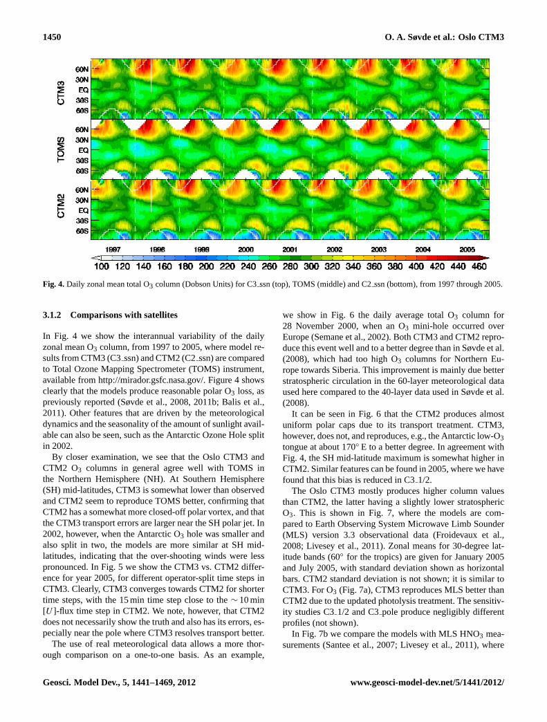
Fig. 4.Daily zonal mean total O3 column (Dobson Units) for C3ssn (top), TOMS (middle) and C2ssn (bottom), from 1997 through 2005.

3.1.2 Comparisons with satellites

In Fig. 4 we show the interannual variability of the dailyzonal mean O3 column, from 1997 to 2005, where model re-sults from CTM3 (C3ssn) and CTM2 (C2ssn) are comparedto Total Ozone Mapping Spectrometer (TOMS) instrument,available fromhttp://mirador.gsfc.nasa.gov/. Figure4 showsclearly that the models produce reasonable polar O3 loss, aspreviously reported (Søvde et al., 2008, 2011b; Balis et al.,2011). Other features that are driven by the meteorologicaldynamics and the seasonality of the amount of sunlight avail-able can also be seen, such as the Antarctic Ozone Hole splitin 2002.

By closer examination, we see that the Oslo CTM3 andCTM2 O3 columns in general agree well with TOMS inthe Northern Hemisphere (NH). At Southern Hemisphere(SH) mid-latitudes, CTM3 is somewhat lower than observedand CTM2 seem to reproduce TOMS better, confirming thatCTM2 has a somewhat more closed-off polar vortex, and thatthe CTM3 transport errors are larger near the SH polar jet. In2002, however, when the Antarctic O3 hole was smaller andalso split in two, the models are more similar at SH mid-latitudes, indicating that the over-shooting winds were lesspronounced. In Fig.5 we show the CTM3 vs. CTM2 differ-ence for year 2005, for different operator-split time steps inCTM3. Clearly, CTM3 converges towards CTM2 for shortertime steps, with the 15 min time step close to the∼ 10 min[U ]-flux time step in CTM2. We note, however, that CTM2does not necessarily show the truth and also has its errors, es-pecially near the pole where CTM3 resolves transport better.

The use of real meteorological data allows a more thor-ough comparison on a one-to-one basis. As an example,

we show in Fig.6 the daily average total O3 column for28 November 2000, when an O3 mini-hole occurred overEurope (Semane et al., 2002). Both CTM3 and CTM2 repro-duce this event well and to a better degree than inSøvde et al.(2008), which had too high O3 columns for Northern Eu-rope towards Siberia. This improvement is mainly due betterstratospheric circulation in the 60-layer meteorological dataused here compared to the 40-layer data used inSøvde et al.(2008).

It can be seen in Fig.6 that the CTM2 produces almostuniform polar caps due to its transport treatment. CTM3,however, does not, and reproduces, e.g., the Antarctic low-O3tongue at about 170◦ E to a better degree. In agreement withFig. 4, the SH mid-latitude maximum is somewhat higher inCTM2. Similar features can be found in 2005, where we havefound that this bias is reduced in C31/2.

The Oslo CTM3 mostly produces higher column valuesthan CTM2, the latter having a slightly lower stratosphericO3. This is shown in Fig.7, where the models are com-pared to Earth Observing System Microwave Limb Sounder(MLS) version 3.3 observational data (Froidevaux et al.,2008; Livesey et al., 2011). Zonal means for 30-degree lat-itude bands (60◦ for the tropics) are given for January 2005and July 2005, with standard deviation shown as horizontalbars. CTM2 standard deviation is not shown; it is similar toCTM3. For O3 (Fig. 7a), CTM3 reproduces MLS better thanCTM2 due to the updated photolysis treatment. The sensitiv-ity studies C31/2 and C3pole produce negligibly differentprofiles (not shown).

In Fig. 7b we compare the models with MLS HNO3 mea-surements (Santee et al., 2007; Livesey et al., 2011), where


http://mirador.gsfc.nasa.gov/


Fig. 5. Convergence of the CTM3 operator-split time step, shownby the difference in daily zonal mean total O3 column (DobsonUnits) between CTM3 runs with different operator-split time stepsand CTM2, for the year 2005.(a) C3 (60 min) vs. C2(b) C3 1/2(30 min) vs. C2 and(c) C3 1/4 (15 min) vs. C2.

the CTM3 and CTM2 reproduce MLS well in summer butunderestimate at altitudes above 30 hPa in winter. The CTMsalready include NOx conversion to HNO3 on backgroundaerosols (Søvde et al., 2008), so an underestimation of HNO3in winter may, e.g., be due to lack of nitrogen species trans-ported downwards from the mesosphere (Randall et al., 2006,2009), or the lack of in-situ NOx sources caused by energeticparticle precipitation (Jackman et al., 2008; Semeniuk et al.,2011) and conversion to HNO3 by, e.g., ion clusters (Verro-

nen et al., 2008, 2011). Below 30 hPa the models do fairlywell, also when it comes to the standard deviation. Thereare no big differences between CTM2 and CTM3, althoughCTM3 seems to perform slightly better in summer. Again,C3 pole and C31/2 produce almost identical profiles, exceptthe latter at SH high latitudes, where small differences upto 5 % in HNO3 can be seen (not shown).

Lastly, we compare modelled N2O with MLS measure-ments (Lambert et al., 2007; Livesey et al., 2011), as shownin Fig. 7c. CTM3 and CTM2 produce very similar distri-butions of N2O. However, at all latitudes except high win-tertime latitudes, both models underestimate N2O betweenabout 30 hPa and 1 hPa, indicating slower Brewer-Dobsoncirculation in the meteorological data, particularly for up-ward motion in the tropics. Again there are negligible dif-ferences to C31/2 and C3pole. An earlier cycle of meteoro-logical data (cycle 29) shows slightly better comparison (notshown), which could indicate that cycle 36r1 has slower ver-tical transport in the tropics.Monge-Sanz et al.(2012) alsofound slower Brewer-Dobson circulation in the ERA-Interimforecasts (cycle 31r2), producing too old stratospheric air inthe tropics at 18–22 km altitude. They found that the reanaly-sis produces better age of air in the tropics, but that forecastsare better at other latitudes. We will come back to the slowBrewer-Dobson circulation in the next sections.

3.1.3 Modelling a Frozen-in Anti-Cyclone

An important change from CTM2 to CTM3 is the better po-lar transport treatment, and to demonstrate this we look atthe 2005 Frozen-in Anti-Cyclone (FrIAC) in the Arctic re-ported byManney et al.(2006) and more recently studied byAllen et al.(2011). In Fig.8 we show a Hovmoller plot, as inAllen et al.(2011), of N2O at the altitude 850 K and latitude78◦ N, measured by MLS, and modelled by the Oslo CTM3and the Oslo CTM2. MLS measurements have been binnedinto 5× 5◦ latitude/longitude bins due to the sparsity of ob-servations. N2O from the CTMs were put out hourly in 3-Dand interpolated to 78◦ N. Note that the color scale range of0–175 ppb is larger than inAllen et al.(2011). We have addedcontours of 75 ppb and 100 ppb to make a comparison easier.

The Oslo CTM3 reproduces transport of the high-N2O in-trusion well, although the mixing ratio amplitude is underes-timated by 40–60 ppb. As shown in Fig.7, N2O was in gen-eral underestimated between 30 hPa and 1 hPa at most lati-tudes, which could explain the overall low N2O abundancesrelative to observations in Fig.8. This could render N2Ovalues too low even before entering the polar latitudes. TheOslo CTM2 does not capture this transport well. Its transportpattern is similar to CTM3, but due to the averaging of thepolar gridboxes, where the N2O is smeared out, the valuesare substantially lower than for CTM3.

From sensitivity studies, we have found (but not shown)that halving the operator-split time step (C31/2) does notchange the CTM3 performance in terms of the N2O levels



Fig. 6.Daily mean total O3 column for C3ssn (top), TOMS (middle) and C2ssn (bottom), 28 November 2000.

in the FrIAC. This is mainly because the FrIAC was locatedabove the region where main transport differences betweenC3 and C31/2 are found. However, the improved polar trans-port (C3pole) produces up to 30 % more N2O in the FrIACafter 1 May. In general, the differences arise when largewind gradients are located across the combined grid boxesin CTM3 transport.

Studies involving polar cap transport, and to some extentArctic and Antarctic studies, will clearly benefit from usingC3 pole transport, while other studies may benefit from theshorter computing time achieved by combining polar boxes,and find its performance acceptable.

3.2 Troposphere

In this section we focus on the troposphere, describing trans-port differences between Oslo CTM3 and CTM2 and alsocompare the models with observations.

3.2.1 Transport in the troposphere

CTM3 and CTM2 are expected to differ slightly in the tropo-sphere due to the differences in transport treatment. We havestudied the linearly increasing age of air tracer for year 20,and in the zonal mean C3 differs from C2 by only∼ 0.5 % be-tween the surface and∼ 300 hPa (not shown). In general the

CTM3 tropospheric mixing ratios are slightly higher southof 50◦ S, indicating slightly faster transport to southernmostlatitudes. North of 50◦ S the differences are generally relatedto convective regions, where CTM2 has higher mixing ratiothan CTM3 in the lower troposphere. This is mainly due todifferences in entrainment and detrainment, and will be ex-plained in Sect.3.2.2.

3.2.2 Convective transport

Recently, Hoyle et al. (2011) presented convectivetracer transport using different CTMs, among them theOslo CTM2, using a different set of meteorological data thanused here. To compare the differences in transport betweenOslo CTM3 and CTM2, we do similar tracer studies withone tracer held constant at 1 ppm below 500 m altitude andabove having a lifetime of 6 h (T6h), and a second 20-dayslifetime tracer held constant at 1 ppt at the surface (T20d).

Both models have an overall operator-split time step of60 min, where large-scale advection is treated for 60 min andthen boundary layer mixing for 4× 15 min. Constant T6hand T20d values (as described above) are set before every 15-min boundary layer mixing step, so that each mixing step willnot experience a surface layer with almost no T6h or T20dtracer available. This is mainly important for T20d, whichis only set in the surface layer. The T6h and T20d results



a. SH SM EQ NM NHJa

n

0 2 4 6 8 10O3 [ppm]

100.0

10.0

1.0

0.1

Hei

gh

t [h

Pa]

MLSOslo CTM3Oslo CTM2

Standard deviation

O3: 90S - 60S 01Jan - 31Jan 2005

0 2 4 6 8 10O3 [ppm]

100.0

10.0

1.0

0.1

Hei

gh

t [h

Pa]


Standard deviation

O3: 60S - 30S 01Jan - 31Jan 2005

0 2 4 6 8 10O3 [ppm]

100.0

10.0

1.0

0.1

Hei

gh

t [h

Pa]


Standard deviation

O3: 30S - 30N 01Jan - 31Jan 2005

0 2 4 6 8 10O3 [ppm]

100.0

10.0

1.0

0.1

Hei

gh

t [h

Pa]


Standard deviation

O3: 30N - 60N 01Jan - 31Jan 2005

0 2 4 6 8 10O3 [ppm]

100.0

10.0

1.0

0.1

Hei

gh

t [h

Pa]


Standard deviation

O3: 60N - 90N 01Jan - 31Jan 2005Ju

l

0 2 4 6 8 10O3 [ppm]

100.0

10.0

1.0

0.1

Hei

gh

t [h

Pa]


Standard deviation

O3: 90S - 60S 01Jul - 31Jul 2005

0 2 4 6 8 10O3 [ppm]

100.0

10.0

1.0

0.1

Hei

gh

t [h

Pa]


Standard deviation

O3: 60S - 30S 01Jul - 31Jul 2005

0 2 4 6 8 10O3 [ppm]

100.0

10.0

1.0

0.1

Hei

gh

t [h

Pa]


Standard deviation

O3: 30S - 30N 01Jul - 31Jul 2005

0 2 4 6 8 10O3 [ppm]

100.0

10.0

1.0

0.1

Hei

gh

t [h

Pa]


Standard deviation

O3: 30N - 60N 01Jul - 31Jul 2005

0 2 4 6 8 10O3 [ppm]

100.0

10.0

1.0

0.1

Hei

gh

t [h

Pa]


Standard deviation

O3: 60N - 90N 01Jul - 31Jul 2005

b.

Jan

0 2 4 6 8 10 12HNO3 [ppb]

100

10

Hei

gh

t [h

Pa]


Standard deviation

HNO3: 90S - 60S 01Jan - 31Jan 2005

0 2 4 6 8 10 12HNO3 [ppb]

100

10

Hei

gh

t [h

Pa]


Standard deviation

HNO3: 60S - 30S 01Jan - 31Jan 2005

0 2 4 6 8 10 12HNO3 [ppb]

100

10

Hei

gh

t [h

Pa]


Standard deviation

HNO3: 30S - 30N 01Jan - 31Jan 2005

0 2 4 6 8 10 12HNO3 [ppb]

100

10

Hei

gh

t [h

Pa]


Standard deviation

HNO3: 30N - 60N 01Jan - 31Jan 2005

0 2 4 6 8 10 12HNO3 [ppb]

100

10

Hei

gh

t [h

Pa]


Standard deviation

HNO3: 60N - 90N 01Jan - 31Jan 2005

Jul

0 2 4 6 8 10 12HNO3 [ppb]

100

10

Hei

gh

t [h

Pa]


Standard deviation

HNO3: 90S - 60S 01Jul - 31Jul 2005

0 2 4 6 8 10 12HNO3 [ppb]

100

10

Hei

gh

t [h

Pa]


Standard deviation

HNO3: 60S - 30S 01Jul - 31Jul 2005

0 2 4 6 8 10 12HNO3 [ppb]

100

10

Hei

gh

t [h

Pa]


Standard deviation

HNO3: 30S - 30N 01Jul - 31Jul 2005

0 2 4 6 8 10 12HNO3 [ppb]

100

10

Hei

gh

t [h

Pa]


Standard deviation

HNO3: 30N - 60N 01Jul - 31Jul 2005

0 2 4 6 8 10 12HNO3 [ppb]

100

10

Hei

gh

t [h

Pa]


Standard deviation

HNO3: 60N - 90N 01Jul - 31Jul 2005

Fig. 7. Comparison of O3 (a), HNO3 (b), and N2O (c) from CTM3 (C3ssn), CTM2 (C2ssn) and MLS, as vertical profiles of zonalmonthly means covering the latitude bands 90◦ S–60◦ S (southern high, column “SH”), 60◦ S–30◦ S (southern mid-lat, column “SM”),30◦ S–30◦ N (“EQ”), 30◦ N–60◦ N (“NM”) and 60◦ N–90◦ N (“NH”) for January 2005 and July 2005. Model profiles are processed with theMLS averaging kernel and a-priori profiles.

a. SH SM EQ NM NH

Jan

0 2 4 6 8 10O3 [ppm]

100.0

10.0

1.0

0.1

Hei

gh

t [h

Pa]


Standard deviation

O3: 90S - 60S 01Jan - 31Jan 2005

0 2 4 6 8 10O3 [ppm]

100.0

10.0

1.0

0.1

Hei

gh

t [h

Pa]


Standard deviation

O3: 60S - 30S 01Jan - 31Jan 2005

0 2 4 6 8 10O3 [ppm]

100.0

10.0

1.0

0.1

Hei

gh

t [h

Pa]


Standard deviation

O3: 30S - 30N 01Jan - 31Jan 2005

0 2 4 6 8 10O3 [ppm]

100.0

10.0

1.0

0.1

Hei

gh

t [h

Pa]


Standard deviation

O3: 30N - 60N 01Jan - 31Jan 2005

0 2 4 6 8 10O3 [ppm]

100.0

10.0

1.0

0.1

Hei

gh

t [h

Pa]


Standard deviation

O3: 60N - 90N 01Jan - 31Jan 2005

Jul

0 2 4 6 8 10O3 [ppm]

100.0

10.0

1.0

0.1

Hei

gh

t [h

Pa]


Standard deviation

O3: 90S - 60S 01Jul - 31Jul 2005

0 2 4 6 8 10O3 [ppm]

100.0

10.0

1.0

0.1

Hei

gh

t [h

Pa]


Standard deviation

O3: 60S - 30S 01Jul - 31Jul 2005

0 2 4 6 8 10O3 [ppm]

100.0

10.0

1.0

0.1H

eig

ht

[hP

a]


Standard deviation

O3: 30S - 30N 01Jul - 31Jul 2005

0 2 4 6 8 10O3 [ppm]

100.0

10.0

1.0

0.1

Hei

gh

t [h

Pa]


Standard deviation

O3: 30N - 60N 01Jul - 31Jul 2005

0 2 4 6 8 10O3 [ppm]

100.0

10.0

1.0

0.1

Hei

gh

t [h

Pa]


Standard deviation

O3: 60N - 90N 01Jul - 31Jul 2005

b.

Jan

0 2 4 6 8 10 12HNO3 [ppb]

100

10

Hei

gh

t [h

Pa]


Standard deviation

HNO3: 90S - 60S 01Jan - 31Jan 2005

0 2 4 6 8 10 12HNO3 [ppb]

100

10

Hei

gh

t [h

Pa]


Standard deviation

HNO3: 60S - 30S 01Jan - 31Jan 2005

0 2 4 6 8 10 12HNO3 [ppb]

100

10

Hei

gh

t [h

Pa]


Standard deviation

HNO3: 30S - 30N 01Jan - 31Jan 2005

0 2 4 6 8 10 12HNO3 [ppb]

100

10

Hei

gh

t [h

Pa]


Standard deviation

HNO3: 30N - 60N 01Jan - 31Jan 2005

0 2 4 6 8 10 12HNO3 [ppb]

100

10H

eig

ht

[hP

a]


Standard deviation

HNO3: 60N - 90N 01Jan - 31Jan 2005

Jul

0 2 4 6 8 10 12HNO3 [ppb]

100

10

Hei

gh

t [h

Pa]


Standard deviation

HNO3: 90S - 60S 01Jul - 31Jul 2005

0 2 4 6 8 10 12HNO3 [ppb]

100

10

Hei

gh

t [h

Pa]


Standard deviation

HNO3: 60S - 30S 01Jul - 31Jul 2005

0 2 4 6 8 10 12HNO3 [ppb]

100

10

Hei

gh

t [h

Pa]


Standard deviation

HNO3: 30S - 30N 01Jul - 31Jul 2005

0 2 4 6 8 10 12HNO3 [ppb]

100

10

Hei

gh

t [h

Pa]


Standard deviation

HNO3: 30N - 60N 01Jul - 31Jul 2005

0 2 4 6 8 10 12HNO3 [ppb]

100

10

Hei

gh

t [h

Pa]


Standard deviation

HNO3: 60N - 90N 01Jul - 31Jul 2005

Fig. 7.Continued.



c. SH SM EQ NM NHJa

n

0 50 100 150 200 250N2O [ppb]

100.0

10.0

1.0

0.1

Hei

gh

t [h

Pa]


Standard deviation

N2O: 90S - 60S 01Jan - 31Jan 2005

0 50 100 150 200 250N2O [ppb]

100.0

10.0

1.0

0.1

Hei

gh

t [h

Pa]


Standard deviation

N2O: 60S - 30S 01Jan - 31Jan 2005

0 50 100 150 200 250N2O [ppb]

100.0

10.0

1.0

0.1

Hei

gh

t [h

Pa]


Standard deviation

N2O: 30S - 30N 01Jan - 31Jan 2005

0 50 100 150 200 250N2O [ppb]

100.0

10.0

1.0

0.1

Hei

gh

t [h

Pa]


Standard deviation

N2O: 30N - 60N 01Jan - 31Jan 2005

0 50 100 150 200 250N2O [ppb]

100.0

10.0

1.0

0.1

Hei

gh

t [h

Pa]


Standard deviation

N2O: 60N - 90N 01Jan - 31Jan 2005Ja

n

0 50 100 150 200 250N2O [ppb]

100.0

10.0

1.0

0.1

Hei

gh

t [h

Pa]


Standard deviation

N2O: 90S - 60S 01Jul - 31Jul 2005

0 50 100 150 200 250N2O [ppb]

100.0

10.0

1.0

0.1

Hei

gh

t [h

Pa]


Standard deviation

N2O: 60S - 30S 01Jul - 31Jul 2005

0 50 100 150 200 250N2O [ppb]

100.0

10.0

1.0

0.1

Hei

gh

t [h

Pa]


Standard deviation

N2O: 30S - 30N 01Jul - 31Jul 2005

0 50 100 150 200 250N2O [ppb]

100.0

10.0

1.0

0.1

Hei

gh

t [h

Pa]


Standard deviation

N2O: 30N - 60N 01Jul - 31Jul 2005

0 50 100 150 200 250N2O [ppb]

100.0

10.0

1.0

0.1

Hei

gh

t [h

Pa]


Standard deviation

N2O: 60N - 90N 01Jul - 31Jul 2005

Fig. 7.Continued.

for the same regions as inHoyle et al.(2011), are shown inFig. 9, where Oslo CTM3 in general has smaller mixing ra-tios for T6h than does the CTM2 (up to 100 % difference at200–100 hPa), and slightly smaller for T20d.

As described in Sect.2.2.2, the CTM2 only uses up-draft convective mass fluxes; convective downdrafts are nottaken into account, and neither are detrainment rates into theup- or downdrafts. In Oslo CTM3, downdrafts and detrain-ment rates are also taken into account, and while downdraftschange the results negligibly (not shown), the use of detrain-ment rates explains most of the model differences in T6habove 550–300 hPa (dash-dotted lines in Fig.9). At the sur-face there are little differences in T6h between CTM3 andCTM2 due to the constantly replenishing to 1 ppm below500 m. Using the detrainment rates transports substantiallyless to high altitudes due to venting below, as explained inSect.2.2.2. Even though the difference between CTM2 andCTM3 is smaller for T20d than for T6h, skipping down-drafts and detrainments still shifts T20d in CTM3 towardsthe CTM2 profiles above 700–550 hPa.

Hoyle et al.(2011) used a different set of meteorologi-cal data, so a direct comparison is not possible. However,from our results we can assume that inclusion of down-drafts and detrainments would shift their Oslo CTM2 to-wards the FRSGC/UCI results for T6h below 100 hPa, whileT20d would be shifted closer to the other models.

In general, the Oslo CTM3 transports up to∼ 10 % less outof the lowermost model layers than CTM2, mainly in sub-

tropical and mid-latitude regions. This may be due to smalldifferences in the boundary layer schemes or in the differenttreatments of convection.

3.2.3 Vertical profiles – O3 sondes

Vertical profiles of O3, interpolated linearly to the location ofselected sonde stations around the world, are put out hourlyfrom the models. This allows reasonable temporal interpola-tions to sonde launch times, thereby giving a better basis forcomparing modelled and observed profiles. To evaluate themodelled O3 in the troposphere, we compare the models toO3 sonde measurements available from the World Ozone andUltraviolet Radiation Data Centre (WOUDC), and also fromSouthern Hemisphere ADditional OZonesondes (SHADOZ)(Thompson et al., 2003), for the year 2005.

In Fig. 10 we show sonde comparisons for selected sta-tions as monthly means, using model profiles only at mea-surement times. Observations are in black, CTM3 in redand CTM2 in green. To calculate the means, all profilesfor a given month and station have been interpolated toa fixed pressure spacing, i.e. the 60-layer model spacingfor a surface pressure of 1000 hPa. For each mean profilewe show the standard deviation as horizontal bars, and therange of O3 in the observations (backslashed black) and inthe Oslo CTM3 profiles (slashed red). We show only themean for CTM2, as its variation is similar to CTM3. Ingeneral, CTM3 produce somewhat better profiles than does



Fig. 8. Hovmoller plot of N2O at 850 K and 78◦ N, as modelled by Oslo CTM3 (left), measured by MLS (middle) and modelled byOslo CTM2 (right). Contours on CTM panels are 75 ppb and 100 ppb.

CTM2. In the supplementary material we also include one-to-one comparisons of models and observations for all thesingle sonde measurements used in the means. From thesesingle sonde profiles, we see that CTM2 sometimes capturetropopause folds better than CTM3. However, shortening thetransport time step does improve CTM3 tropopause folds(not shown).

As noted in Sect.2.5, model emissions are for the year2000. Therefore we have included a similar comparison forthe year 2000 in the Supplement, showing similar model per-formance as for 2005.

In general, CTM3 produce slightly better profiles thandoes CTM2, although for some of the locations and months,CTM2 reproduce measurements better. There are smalldifferences between C3ssn and C3, and between C2ssnand C2, mainly in the upper troposphere and lowermoststratosphere; however, the relative differences near the sur-face may be larger (up to about 25 %, not shown).



a. b.

c. d.

Fig. 9. T6h (ppm) and T20d (ppt) tracer as described in text and byHoyle et al.(2011): selected monthly means for regions and annualmean for 20◦ S–20◦ N.

3.2.4 Modelling CARIBIC CO measurements

The atmospheric abundance of CO is important for OH. Ona global average, we find surface CO in CTM3 to matchCTM2. On a monthly basis, CTM3 has a more pronouncedseasonal variation, being up to 5 % lower in NH spring and5 % higher in NH autumn. As found in Sect.3.2.2, CTM3transports less out of the boundary layer, and for CO wesee that CTM3 has up to 50 % higher abundances over land,while having up to 10 % less over ocean. A comparison ofmodelled and measured CO at Alert station (shown in Sup-plement) reveals that while CTM3 is 5–15 % lower thanCTM2, both models catch the seasonal variation, but un-derestimates at NH winter, as was found in the multi-modelCO-comparison ofShindell et al.(2006). A comparison forthe Hohenpeißenberg station, shows that CTM3 is on aver-age about 15 % higher than CTM2. Unfortunately, it has notbeen possible to compare our results directly with CTM2 re-sults from the comparison ofShindell et al.(2006), a studywhich used different emissions; with slightly higher totalamount of CO emissions, 1077 Tg yr−1 compared to our1012 Tg yr−1 from RETRO, POET and GFEDv3 datasets.

It can be noted that the anthropogenic emissions in RETROdo have a month-to-month variation, in contrast to the emis-sions in their study.Shindell et al.(2006) suggest NH emis-sions are too low, and recently other studies also suggest thatCO emissions are low in general (Lamarque et al., 2010; Pi-son et al., 2009; Kopacz et al., 2010). It should be mentionedthat the recent JPL recommendations (Sander et al., 2011)may change the modelled CO, a study which has not beenpossible in this work.

With our focus on transport differences between CTM2and CTM3, we look more specifically at the capability ofCTM3 to properly incorporate emissions originating frombiomass burning, compared to that of CTM2. For this wecompare our modelled CO in the troposphere with measure-ments carried out in 2005 by CARIBIC (Civil Aircraft for theRegular Investigation of the atmosphere Based on an Instru-ment Container,http://www.caribic-atmospheric.com, Bren-ninkmeijer et al., 2007). In the year 2005, most CARIBICflights were operated between Europe and South America,and model results are interpolated on-line to the spatial andtemporal locations of measurements. Figure11 shows allCO measurements for all flights in 2005 (black), along withcorresponding model output (CTM3 in red, CTM2 in green).Measurements located in the CTM stratosphere (defined inSect.3.3) are shown in blue. While observations reachedup to ∼ 500 ppb, we have cut off the y-axis at 250 ppb tomake the figure more readable; all model results are lowerthan 250 ppb. Both CTM2 and CTM3 produce CO remark-ably close to measured values. Even though most of the flightmeasurements are carried out over the Atlantic, spikes orig-inating from biomass burning events in August and Octobercan be seen (Ebinghaus et al., 2007). These events are wellmodelled, which is due to the combination of realistic mete-orological data and that the horizontal distribution of modelCO emissions from biomass burning to a large degree is wellrepresented. It should be noted that recentlyHooghiemstraet al. (2012) found that GFEDv3 emissions are too low inSouth America for the years 2006–2010, which could alsobe the case for 2005 used in our study. CTM3 produce largerspikes than CTM2 does, due to the improved vertical trans-port in CTM3. It is expected that with a higher temporal res-olution on GFEDv3 emissions, these spikes would be evenhigher.

3.3 Global diagnostics

Several global diagnostics are frequently used to evaluate at-mospheric models, such as the CH4 lifetime, the average tro-pospheric OH concentration, the O3 burden and the mass fluxof O3 from the stratosphere into the troposphere. Here wepresent these and also the lifetime of N2O.

The diagnostics are in general calculated within do-mains between the model surface and four different up-per boundaries. These upper boundaries are our modeltropopause (2.5 PVU), 200 hPa, the 150 ppb O3 surface, and


http://www.caribic-atmospheric.com


��

0.02 0.04 0.06 0.08 0.10 0.12 0.14O3 [ppmv]

1000

800

600

400

200

Hei

gh

t [h

Pa]

WOUDCOslo CTM3Oslo CTM2Oslo CTM3 rangeWOUDC range

Std. dev.

O3, Jan 2005: UCCLEWOUDC, # averaged profiles: 11

0.02 0.04 0.06 0.08 0.10 0.12 0.14O3 [ppmv]

1000

800

600

400

200

Hei

gh

t [h

Pa]

SHADOZOslo CTM3Oslo CTM2Oslo CTM3 rangeSHADOZ range

Std. dev.

O3, Jan 2005: Ascension IslandSHADOZ, # averaged profiles: 4

0.02 0.04 0.06 0.08 0.10 0.12 0.14O3 [ppmv]

1000

800

600

400

200

Hei

gh

t [h

Pa]


Std. dev.

O3, Jan 2005: LerwickWOUDC, # averaged profiles: 4

0.02 0.04 0.06 0.08 0.10 0.12 0.14O3 [ppmv]

1000

800

600

400

200

Hei

gh

t [h

Pa]


Std. dev.

O3, Jan 2005: Ny-AalesundWOUDC, # averaged profiles: 12

0.02 0.04 0.06 0.08 0.10 0.12 0.14O3 [ppmv]

1000

800

600

400

200

Hei

gh

t [h

Pa]


Std. dev.

O3, Jan 2005: EurekaWOUDC, # averaged profiles: 7

0.02 0.04 0.06 0.08 0.10 0.12 0.14O3 [ppmv]

1000

800

600

400

200

Hei

gh

t [h

Pa]


Std. dev.

O3, Apr 2005: UCCLEWOUDC, # averaged profiles: 13

0.02 0.04 0.06 0.08 0.10 0.12 0.14O3 [ppmv]

1000

800

600

400

200

Hei

gh

t [h

Pa]


Std. dev.

O3, Apr 2005: Ascension IslandSHADOZ, # averaged profiles: 2

0.02 0.04 0.06 0.08 0.10 0.12 0.14O3 [ppmv]

1000

800

600

400

200

Hei

gh

t [h

Pa]


Std. dev.

O3, Apr 2005: LerwickWOUDC, # averaged profiles: 4

0.02 0.04 0.06 0.08 0.10 0.12 0.14O3 [ppmv]

1000

800

600

400

200

Hei

gh

t [h

Pa]


Std. dev.

O3, Apr 2005: Ny-AalesundWOUDC, # averaged profiles: 5

0.02 0.04 0.06 0.08 0.10 0.12 0.14O3 [ppmv]

1000

800

600

400

200

Hei

gh

t [h

Pa]


Std. dev.

O3, Apr 2005: EurekaWOUDC, # averaged profiles: 4

0.02 0.04 0.06 0.08 0.10 0.12 0.14O3 [ppmv]

1000

800

600

400

200

Hei

gh

t [h

Pa]


Std. dev.

O3, Jul 2005: UCCLEWOUDC, # averaged profiles: 12

0.02 0.04 0.06 0.08 0.10 0.12 0.14O3 [ppmv]

1000

800

600

400

200

Hei

gh

t [h

Pa]


Std. dev.

O3, Jun 2005: Ascension IslandSHADOZ, # averaged profiles: 5

0.02 0.04 0.06 0.08 0.10 0.12 0.14O3 [ppmv]

1000

800

600

400

200

Hei

gh

t [h

Pa]


Std. dev.

O3, Jul 2005: LerwickWOUDC, # averaged profiles: 4

0.02 0.04 0.06 0.08 0.10 0.12 0.14O3 [ppmv]

1000

800

600

400

200

Hei

gh

t [h

Pa]


Std. dev.

O3, Jul 2005: Ny-AalesundWOUDC, # averaged profiles: 4

0.02 0.04 0.06 0.08 0.10 0.12 0.14O3 [ppmv]

1000

800

600

400

200

Hei

gh

t [h

Pa]


Std. dev.

O3, Jul 2005: EurekaWOUDC, # averaged profiles: 4

0.02 0.04 0.06 0.08 0.10 0.12 0.14O3 [ppmv]

1000

800

600

400

200

Hei

gh

t [h

Pa]


Std. dev.

O3, Oct 2005: UCCLEWOUDC, # averaged profiles: 11

0.02 0.04 0.06 0.08 0.10 0.12 0.14O3 [ppmv]

1000

800

600

400

200

Hei

gh

t [h

Pa]


Std. dev.

O3, Oct 2005: Ascension IslandSHADOZ, # averaged profiles: 4

0.02 0.04 0.06 0.08 0.10 0.12 0.14O3 [ppmv]

1000

800

600

400

200

Hei

gh

t [h

Pa]


Std. dev.

O3, Oct 2005: LerwickWOUDC, # averaged profiles: 4

0.02 0.04 0.06 0.08 0.10 0.12 0.14O3 [ppmv]

1000

800

600

400

200

Hei

gh

t [h

Pa]


Std. dev.

O3, Oct 2005: Ny-AalesundWOUDC, # averaged profiles: 5

0.02 0.04 0.06 0.08 0.10 0.12 0.14O3 [ppmv]

1000

800

600

400

200

Hei

gh

t [h

Pa]


Std. dev.

O3, Oct 2005: EurekaWOUDC, # averaged profiles: 4

Fig. 10.Modelled (C3ssn and C2ssn) and measured monthly mean vertical profiles of O3 at selected sonde stations(a–e)in 2005. Differentmonths for each station are shown in columns.

the model top (LTOP). The prior defines the tropopause atpotential vorticity of 2.5 PVU (Holton et al.(1995), 1 PVUis 10−6 Km2kg−1s−1), with an upper limit of 380 K poten-

tial temperature and a somewhat arbitrary lower limit of 5 km(only occurs occasionally). For 2005, the fraction of air be-low the CTM tropopause is 80.2 %, while below 200 hPa it



Fig. 11. Oslo CTM3 (red) and CTM2 (green) compared with all CO measurements from CARIBIC flights (black) in 2005, resulting inan asynchronous time axis where only the start of each month is shown. Measurements carried out at locations in the CTM stratosphere(defined by 2.5 PVU) are shown in the blue “CARIBIC (CTM strat.)”

is 79.7 %. The fraction below 150 ppb O3, in general higherthan 2.5 PVU, differs slightly for the different runs: 84.6 %for C3, 85.5 % for C3ssn, 83.4 % for C2 and 83.5 % forC2 ssn.

3.3.1 OH concentration

OH is the main oxidizing species in the troposphere, drivenby photolysis rates. It is usually referred to in context ofCH4 lifetime, which will be discussed in Sect.3.3.2. Here wepresent average OH from the different year 2005 simulations,calculated from monthly means of OH, air mass, pressure (p)and temperature (T ). Two averaging kernels are used to cal-culate OH average; first the OH concentration is weighted byair mass and by the loss rate to CH4 (exp(−1775/T )), andsecond it is weighted by air mass and a simplified loss rateof CO using pressure (1+ 0.6p). The values are presentedin Table3, showing small differences for the different modeldomains.

In simulation C3, the annual mean CH4-loss weightedOH concentration is ∼ 1.55× 106 molec cm−3, whilein C2 it is ∼ 1.35× 106 molec cm−3. C3 ssn andC2 ssn produce values of∼ 1.39× 106 molec cm−3 and∼ 1.22× 106 molec cm−3, respectively. For the OH averageweighted against (1+ 0.6p), the averages are about 10 %smaller, but otherwise show the similar picture. We findthat the vertical distribution of lightning to a fixed height of16 km, as in CTM2 (Sect.2.6), can explain about 50 % ofthe larger OH in CTM3 compared to CTM2. Otherwise, theincrease is partly due to updates in solar fluxes and O(1D)quantum yields (Hsu and Prather, 2009) and to differencesin wet scavenging. The latter will affect OH through scav-enging of, e.g., HNO3 and H2O2, and will be addressed inSect.3.4.

Inclusion of sulfur and nitrate modules in CTM2 andCTM3 is important for OH, reducing it by 10–11 %. As al-ready noted, conversion of N2O5 to HNO3 on aerosols is in-cluded in the tropospheric chemistry scheme; it is the same inCTM3 and CTM2, and cannot explain the reduction in OH.From a 3-yr simulation (1997–1999) where nitrate aerosolsare excluded, we find that about 50 % of the reduced OHmay be due to sulfur chemistry removing OH through oxi-dation processes. As important is the sequestering of NOx innitrate aerosols (Myhre et al., 2006), which with subsequentwashout adds a removal process of atmospheric nitrogen andthus a source of OH. OH reduction due to the nitrate mod-ule is most pronounced in NH winter/spring, when the wind-driven production of sea salt is largest.

Lamarque et al.(2010) showed that the RETRO anthro-pogenic CO emissions are probably too low, and other stud-ies indicate that estimated CO emissions probably are too lowin general (Pison et al., 2009; Kopacz et al., 2010). However,when increasing the anthropogenic CO emissions by 20 % inCTM3, we find< 1 % reduction in the OH numbers. Locally,the accompanying effect on O3 can be large (up to 100 %),but in the zonal mean O3 increases by less than 1 %. Eventhough the RETRO emissions may be low on CO, OH is notvery sensitive to an increase in anthropogenic emissions.

Further, fast-JX allows for letting aerosols affect photo-chemistry through scattering and absorption, thereby pos-sibly changing OH.Bian et al.(2003) found the effect ofaerosols on photolysis to reduce global OH by∼ 8 %, similarto Martin et al.(2003) who also found a larger reduction inthe Northern Hemisphere than in the Southern Hemisphere.This will be investigated in the already-mentioned upcomingCTM3 paper focusing on aerosols.



Table 3. Annual average of OH in the atmosphere, calculated from monthly means of OH, air mass, temperature (T ) and pressure (p, inbars), for the air mass below the model PVU-based tropopause height, air mass below 200 hPa, air mass below the modelled 150 ppb O3surface, and the air mass in the whole model domain (up to top level LTOP). The average OH concentration is weighted by air mass andby (a) the loss rate of CH4 (exp(−1775/T )) and(b) the approximate loss rate of CO (1+ 0.6p). All numbers are for the year 2005, and theranges of monthly means are given in parentheses.

a. [OH] (106molec cm−3) weighted by air mass and exp(−1775/T ).Diagnosed between surface and selected upper boundaries.

Sim. 2.5 PVU 200 hPa 150 ppb O3 LTOP

C3 1.55 (1.47–1.70) 1.54 (1.46–1.70) 1.54 (1.46–1.70) 1.55 (1.47–1.69)C3 ssn 1.39 (1.30–1.56) 1.38 (1.29–1.56) 1.38 (1.29–1.56) 1.39 (1.31–1.56)C2 1.35 (1.27–1.49) 1.34 (1.26–1.48) 1.35 (1.26–1.48) 1.35 (1.28–1.48)C2 ssn 1.22 (1.11–1.36) 1.21 (1.11–1.36) 1.21 (1.11–1.36) 1.22 (1.13–1.37)

b. [OH] (106molec cm−3) weighted by air mass and (1+ 0.6p).Diagnosed between surface and selected upper boundaries.

Sim. 2.5 PVU 200 hPa 150 ppb O3 LTOP

C3 1.40 (1.33–1.54) 1.39 (1.32–1.53) 1.39 (1.32–1.53) 1.37 (1.30–1.50)C3 ssn 1.26 (1.16–1.41) 1.24 (1.15–1.40) 1.25 (1.16–1.40) 1.23 (1.14–1.38)C2 1.21 (1.13–1.34) 1.20 (1.12–1.32) 1.21 (1.13–1.33) 1.18 (1.11–1.31)C2 ssn 1.09 (0.99–1.23) 1.07 (0.97–1.21) 1.08 (0.98–1.22) 1.06 (0.97–1.20)

Table 4. Annual average lifetimes of CH4 (τCH4), diagnosed as the total CH4 burden (surface to model top) divided by the loss of CH4within the four diagnosed domains: below the model PVU-based tropopause height, below 200 hPa surface, below the modelled 150 ppb O3surface, and the whole model domain (up to top level LTOP). All numbers are for the year 2005, and the ranges of monthly means are givenin parentheses.

τCH4 (yr). Diagnosed between surface and selected upper boundaries.Sim. 2.5 PVU 200 hPa 150 ppb O3 LTOP

C3 7.98 (6.96–8.62) 8.03 (7.02–8.67) 7.94 (6.94–8.56) 7.55 (6.64–8.11)C3 ssn 8.86 (7.59–8.83) 8.89 (7.63–9.85) 8.81 (7.56–9.75) 8.33 (7.22–9.16)C2 9.18 (7.98–10.06) 9.26 (8.06–10.15) 9.14 (7.95–10.01) 8.64 (7.59–9.39)C2 ssn 10.20 (8.68–11.43) 10.31 (8.77–11.55) 10.16 (8.65–11.37) 9.54 (8.22–10.58)

3.3.2 CH4 and N2O lifetimes

The main atmospheric sink of the greenhouse gas CH4 is OH,predominantly in the troposphere. CH4 is also lost to Cl andO(1D), mainly in the stratosphere, with small additional lossto Cl in the marine boundary layer. In the troposphere, CTM2and CTM3 neglect Cl chemistry and also the CH4 loss toO(1D). Instead of simulating surface emissions and soil up-take, both models use prescribed surface concentrations ofCH4, based on CTM2 simulations with CH4 emissions andsurface deposition (HYMN-report, 2010).

Table 4 lists global mean CH4 lifetimes in 2005, calcu-lated from monthly mean total CH4 burden and cumulativemonthly CH4 loss. On a monthly basis, CH4 lifetime is short-est during NH summer, consistent with the seasonal cycle ofOH. Our three tropospheric definitions produce lifetimes thatdiffer by up to 10 %, with the shortest lifetimes estimated us-ing the 150 ppb O3 boundary because it includes the tropicalupper troposphere and some high latitude stratospheric loss

due to Cl and O(1D). We use the O3-based tropopause defi-nition in this section.

The tropospheric CH4 lifetime in CTM3 is 7.9 yr, ver-sus 9.1 yr in CTM2, consistent with the larger OH con-centration in the updated model. Adding sulfur and ni-trate aerosols increases the lifetime by∼ 12 %, to 8.9 yr inCTM3 (sim. C3ssn). This aerosol effect is slightly smallerin CTM2 (∼ 11 %). Past studies have found a similar impactof aerosols on CH4 lifetime via surface reactions (Martinet al., 2003; Macintyre and Evans, 2010). Recent evaluationof the CH4 lifetime (Prather et al., 2012), total and againstloss by tropospheric OH, take into account the recently ob-served CH3CCl3 decay (Montzka et al., 2011) and up-to-dateestimates with uncertainties of the other factors that go intothe lifetime calculation.Prather et al.(2012) report the CH4lifetime with respect to tropospheric OH (the so-called tropo-spheric OH-lifetime) to be 11.2± 1.3 yr, which is longer thanearlier estimates of (8.7± 1.3 yrIPCC AR4, 2007). Thus, thetropospheric OH-lifetime of CH4 in CTM3, when including



Table 5.Modelled annual average O3 burden [Tg (O3)] for different definitions of tropospheric domains.

Diagnosed between surface and a selection of upper boundaries.2.5 PVU 200 hPa 150 ppb O3

Simulation 2005 1998–2005 2005 1998–2005 2005 1998–2005

C3 360 (340–386) 360 356 (342–374) 357 391 (373–415) 390C3 ssn 331 (310–359) 331 344 (327–361) 345 363 (344–388) 362C2 352 (336–376) 354 344 (331–355) 347 372 (358–389) 373C2 ssn 326 (309–352) 328 317 (303–331) 321 346 (332–366) 347

aerosols, is shorter than the recent estimate, but within therange of older estimates. Adding aerosols to the photolysiscalculation, currently neglected in CTM2 and CTM3, couldincrease the tropospheric-OH lifetime by∼ 8 % (Bian et al.,2003; Martin et al., 2003) to ∼ 10 yr in CTM3 and bringCTM3 within the recent methyl chloroform constraint.

Over the entire atmosphere, the CH4 lifetime due to allchemical losses is 9.5 yr in CTM2 and 8.4 yr in CTM3 inthe simulations with aerosols. If we include estimates of thesoil and tropospheric Cl sinks (Prather et al., 2012), the to-tal lifetimes decrease 7–10 %. Because the CTMs use pre-scribed surface CH4 concentrations, but have different CH4lifetimes, they calculate different CH4 burdens. These are4830 Tg and 4822 Tg for simulations C2 and C3, respectively(4831 Tg and 4825 Tg for C2ssn and C3ssn, respectively).All are about 2 % lower than the burden estimated by IPCC(4932 Tg,IPCC AR4, 2007). The stratospheric lifetime ofCH4 is 147 yr and 141 yr in CTM2 and CTM3, respectively.These lifetimes change only slightly (< 3 %) after includingtropospheric aerosols. We estimate that OH, Cl, and O(1D)cause 47 %, 29 % and 24 % of stratospheric CH4 oxidation,respectively.

Another important greenhouse gas is N2O, which in gen-eral is inert in the troposphere, while having a small strato-spheric loss. Hence, N2O has a long lifetime, and in CTM3we calculate it to be 144 yr, with a monthly average rangeof 133–155 yr. Because the photolysis code used in CTM2(fast-J2) had smaller solar fluxes in the 200–230 nm regionwhere N2O and O2 are photolyzed in most of the strato-sphere, the N2O lifetime in CTM2 is longer, 151 yr. It isworth noting that the CTM2 and CTM3 keep N2O fixed atthe surface and at the uppermost model layer – with the samemixing ratios in both models. The N2O lifetimes are probablytoo long because of slow vertical transport in the cycle 36r1meteorology used in both calculations, somewhat evident inthe underestimate of the CTM N2O profiles (Fig.7).

3.3.3 O3 burden

We have calculated the tropospheric burden of O3 using thetropospheric domains defined in Sect.3.3.2. The numbers arepresented in Table5 for the year 2005, and as the mean ofyears 1998 to 2005. Also, the ranges of the monthly meanvalues for 2005 are listed. The interannual variation is small,

as are the differences between CTM3 and CTM2. Belowthe 150 ppb O3 surface, modelled burden in 2005 is 391 Tgfor C3 and 363 Tg for C3ssn, while the Oslo CTM2 pro-duces 372 Tg for C2 and 346 Tg for C2ssn. Similar valuesare found for the 1998–2005 averages. Within the domainsbelow our model tropopause and below 200 hPa, which aresmaller domains, the O3 burden is 5–10 % lower than whenusing the 150 ppb O3 definition. Based on several modelstudies,Stevenson et al.(2006) presented a tropospheric bur-den range of 344± 39 Tg, calculated from all air masses withO3 less than 150 ppb. The C3ssn and C2ssn runs lie wellwithin this range, with values of 346 and 363 Tg, respec-tively. When excluding the aerosols our models lie in or justabove the upper end of the range. It should be noted thatStevenson et al.(2006) used different emissions, which couldsomewhat affect the comparison.

By distributing L-NOx vertically to a fixed altitude of16 km in the CTM3, we find that the higher burden in CTM3compared to CTM2 is most likely due to the differences inL-NOx vertical scaling. Otherwise, as noted in Sect.3.3.2,the main differences between CTM2 and CTM3 are dueto the new fast-JX photochemistry being somewhat moreactive, and differences in wet scavenging. While this pro-duces higher O3 burden in CTM3, it does not change therelative effect of nitrate aerosols when compared to CTM2,about 8 %. A halving of the operator-split time step (C31/2)only changes the burden by∼ 2 %, indicating that the tropo-spheric O3 burden is not very sensitive to the operator-splittime step.

3.3.4 Cross-tropopause O3 flux

The stratosphere to troposphere exchange (STE) is the netflux from the stratosphere into the troposphere, and is esti-mated based on observations to be 540± 140 Tg (O3) yr−1

(Murphy and Fahey, 1994; Gettelman et al., 1997;IPCC AR4, 2007). Model studies suggest STE around500 Tg (O3) yr−1 (McLinden et al., 2000; Olsen et al., 2001;Hsu et al., 2005), and Stevenson et al.(2006) reporteda model range of 552± 168 Tg (O3) yr−1.

In Oslo CTM3 the STE calculation followsHsu et al.(2005), which is the same method as used byStevensonet al. (2006) (referred to as S2006 below). Due to technicalchallenges, this has not been possible in CTM2, and while



Søvde et al.(2011a) presented CTM2 STE, their method isnot comparable to the CTM3 treatment – hence we presentonly CTM3 in this study. During a certain time period inCTM3 (e.g., a month), STE of O3 is calculated as a residualof column mass budgets between the model surface and a cer-tain O3 isopleth (Hsu et al., 2005). Below the given O3 iso-pleth and for the given time period, this can be written(

dM

dt

)tot

=

(dM

dt

)chem

− S+ Fs→t − Fh,t→t , (7)

where(

dMdt

)tot

is the total change in O3,(

dMdt

)chem

is the

corresponding chemical tendency of O3 (corresponding toP−L in S2006), S is sink processes such as dry depositionat the surface and wet scavenging (D in S2006),Fh,t→t isthe horizontal flux of O3 out of the column (troposphere totroposphere), andFs→t is the STE to be inferred (both hor-izontal and vertical). Hence, the left-hand side of Eq. (7) isdiagnosed as the change from the beginning to the end of thediagnosed time period, while the right-hand side terms aresummed up for all time steps during the time period. S2006

assumed no tropospheric trend, i.e.(

dMdt

)tot

+ Fh,t→t = 0 in

Eq. (7).We have found the 150 ppb isopleth of O3 used in S2006

to confuse stratospheric air with tropospheric air for O3-holeconditions, hence we have lowered this isopleth to 120 ppbto minimise this problem. For the year 2005, Oslo CTM3produce an annual STE of 296 Tg (O3) yr−1 for C3 and300 Tg (O3) yr−1 for C3 ssn. The aerosol included in the ssn-runs are not calculated in the stratosphere, but changes the120 ppb isopleth slightly, thereby changing STE slightly. Ona monthly basis, the STE is largest in NH summer, whilesmallest in NH winter. In an atmosphere without polar strato-spheric clouds (PSCs), the 120 ppb isopleth can be very dif-ferent than when PSCs are included, and stratopsheric bur-den of O3 is higher.Hsu and Prather(2009) found PSCsto reduce STE by 97 Tg (O3) yr−1, and when testing this inCTM3 we find the STE to increase by a comparable amountto 427 Tg (O3) yr−1 for the year 2005. It may be that STE in-ferred from observations does not fully take the PSC-O3 holeinto account, so modelled STE without PSCs provide insightinto this. However, it should be kept in mind that the 120 ppbisopleth has changed.

With the C31/2 simulation, STE is slightly reduced to288 Tg (O3) yr−1, due to a slightly changing O3 isopleth andless overshooting of the stratospheric jet. We have also car-ried out a 14 month simulation starting on 1 November2004, using an older cycle of the ECMWF IFS meteorol-ogy (cycle 29). With this, the Oslo CTM3 produce a STEof 353 Tg (O3) yr−1. While this higher flux indicates that theold cycle may provide a more realistic circulation, it shouldbe noted that the N2O FrIAC presented in Sect.3.1.3is muchless pronounced for cycle 29 meteorological data, indicatingthat cycle 29 polar cap winds are less representative. Still,our comparison with MLS indicates that cycle 36r1 may have

too slow Brewer-Dobson circulation, which will give too lowSTE. Also, UCI-CTM calculations of STE (Hsu and Prather,2009) are considerably reduced when using cycle 36r1.

Due to the difficulties with a calculated O3 isopleth, suchas stratospheric air being counted as tropospheric air forlow O3 and tropospheric O3-rich air in polluted areas beingcounted as stratospheric air, we have also tested calculatingSTE through an alternative surface, namely the tropospheredefined by the artificial e90-tracer (Prather et al., 2011). Withthis we find the annual STE of 285 Tg (O3) yr−1 for C3 ssnclose to the value from using the 120 ppb isopleth. Also, thereduction when halving the operator-split time step is similarto what was found using the 120 ppb isopleth.

3.4 Wet scavenging

Wet removal of atmospheric HNO3 and H2O2 is importantfor the NOx and OH abundances. Less removal of H2O2 willincrease tropospheric OH, and less removal of HNO3 willincrease atmospheric NOx. HNO3 can be recycled back toNOx by either photodissociation or reaction with OH, butmost of it is lost to the surface by wet or dry scavenging.In addition, NOx will by itself change OH by shifting theHO2/OH balance.

Hence, if CTM3 wet scavenging is less efficient than forCTM2, the amount of OH and NOx will be higher than inCTM2. Due to the complexity of the coupled system, it hasnot been possible to separate out the contributions to OHfrom increased NOx due to the wet scavenging scheme fromthat due to the update to fast-JX. It should be noted thata major difference from CTM2 to CTM3 scavenging is thatCTM2 treats all large-scale precipitation as liquid rain, whileCTM3 separates it into ice and liquid precipitation. The onlyspecies removed by ice in CTM3 is HNO3, and even that isreduced relative to liquid rain (CTM2). The convective scav-enging scheme is the same in both, and treats all convectiveprecipitation as convective rain.

To compare the wet scavenging in CTM3 to CTM2, wehave carried out idealised 7-day simulations with only trans-port and wet removal of HNO3 and H2O2. Tracer removalsby large-scale and convective precipitation are diagnosedhourly. We present results for 1–7 January 2005, but findsimilar results for other months. The idealised tracers are ini-tialised from the C3ssn simulation at 1 January 2005.

In the upper troposphere, CTM3 scavenges less by rainthan CTM2, while in the lower tropical troposphere, more isscavenged in CTM3. In total HNO3 burden, CTM3 removesless HNO3 than does CTM2; starting from a troposphericburden of 1.43 Tg (HNO3), CTM3 ends at 0.62 Tg (HNO3)after 7 days, while CTM2 ends at 0.40 Tg (HNO3). Thehigher HNO3 in CTM3 is due to large-scale precipitation be-ing constrained by cloud fraction and hence less effective;the amount removed at each time step is about 30 to 40 %lower than for CTM2. Large changes in the initial scaveng-ing rate occur because the initialized fields (C3ssn) were



inconsistent with the rapid large-scale scavenging in the up-per troposphere by CTM2. By looking at the decay ratesover the last few days of the experiment, when the HNO3distribution more closely matches each CTM’s pattern ofscavenging, we find that for CTM3 the effective troposphericlifetime of HNO3 is 9.3 days and for CTM2 it is 6.9 days,confirming the more rapid loss in CTM2. Spatially we findthat CTM3 removes less in the upper troposphere, while re-moving slightly more in the lowermost tropical troposphere,similar to results inNeu and Prather(2012).

The amount removed by convective scavenging is initiallysimilar in CTM2 and CTM3, however, after a few time stepsCTM3 removes more by convective scavenging than CTM2,compensating for the reduced large-scale scavenging. How-ever, the fraction of tropospheric HNO3 washed out by con-vective rain at each time step remains similar in CTM2 andCTM3, since the process is unchanged in the CTM update.

Less effective wet scavenging is also found for H2O2 inCTM3. The tropospheric H2O2 burden starts at 3.86 Tg, andafter 7 days of only transport and wet scavenging, CTM3ends at 1.66 Tg, while CTM2 ends at 0.95 Tg. After 7 daysthese correspond to a tropospheric lifetime of 5.9 days forCTM2 and 11.4 days for CTM3. Initially, CTM2 removesabout 4 times as much as CTM3 in large-scale scavenging,which is a larger difference than for HNO3, because H2O2 isnot removed by ice in CTM3 but is removed in CTM2. Thefraction of the tropospheric burden removed by convectivescavenging is smaller in CTM3, which was not the case forHNO3. While Neu and Prather(2012) found H2O2 uptake inice to have a very small effect on O3, the differences fromCTM2 to CTM3 may be large enough to re-examine this re-sult.

Our chemistry simulations C2 and C3 show similar results;less HNO3 is scavenged in CTM3, giving the latter a highertropospheric burden of HNO3. The very different pattern ofscavenging from CTM2 to CTM3 also contributes to this bychanging the relative distribution of HNO3 throughout thetroposphere. In the ssn-simulations, we see a reduction oftropospheric HNO3 by about 28 % in CTM2 and 32 % inCTM3. This agrees well with what we found for OH and life-time of CH4. The slightly higher effect on HNO3 in CTM3 isprobably due to the less efficient wet scavenging in CTM3also affecting sea salt and nitrate aerosols, allowing moreHNO3 to be bound in nitrate particles. Also important aredifferences in other loss processes such as photodissociationand the loss to OH.

The higher HNO3 burden in CTM3 is not distributedevenly. In the tropics, below 400 hPa, HNO3 is about 50 %lower in CTM3, while in the extra-tropics CTM3 has upto twice as much HNO3 as in CTM2, consistent with lessscavenging. Inclusion of tropospheric aerosols reduces extra-tropical HNO3 by up to 100 % in both CTM2 and CTM3,slightly more pronounced in CTM3. Because of the less effi-cient scavenging of sea salt aerosols in CTM3, more HNO3 istaken up to form nitrate aerosols, explaining this difference.

Above 200 hPa, in the stratosphere, CTM3 has about half ofthe HNO3 in CTM2, except in the upper stratosphere, whereCTM3 again has somewhat higher HNO3.

The higher OH in CTM3 than in CTM2 is partly due toless removal of H2O2; the CTM3 burden of H2O2 is ∼ 12 %higher than for CTM2. Spatially, this difference comes froma decrease of∼ 20 % in the tropical troposphere, but an in-crease of up to 400 % in the upper troposphere due to lack ofscavenging by ice. The more active photochemistry in fast-JX may dissociate more HNO3 to NOx, which again con-tributes to increasing OH and thereby to HNO3 loss, but asalready mentioned, it has not been possible to separate theeffects of differences in scavenging and photochemistry.

3.5 Transport sensitivity studies

In order to document the differences in transport schemesbetween CTM2 and CTM3, we have carried out several 14-month sensitivity studies, listed in Table2. Here we summa-rize the findings of shortening the operator-split time step andof using the more accurate polar cap transport in C3pole.

When halving the CTM3 operator-split time step to 30 min(C3 1/2), the computing time is increased by almost 100 %because all processes are done twice. In general there aresmall differences between C3 and C31/2, except that theSH polar vortex edge seems to be better resolved in C31/2,with a sharper gradient across the vortex edge. Total O3-hole column values at the polar side of the SH vortex edgeare reduced by up to 20 %, while on the mid-latitude sidethe column values are increased by up to 5 %. These rela-tively large changes are only found across the sharp gradi-ents, corresponding well with what was seen for age of air.A 15 min operator-split time step, compared to 60 min, in-creases these numbers to 25 % and 9 %, respectively, show-ing rapid convergence to CTM2, as was shown in Sect.3.1.2.A similar effect can also be seen in the Northern Hemisphere,however to a smaller extent. The largest differences occur atmid to high latitudes between 300 hPa and 20 hPa, in O3-hole conditions with strong asymmetric vorticies. Here, aswe have discussed, the jets may overshoot. When halvingthe operator-split time step, the maximum increase outsidethe vortex and the maximum decrease inside the vortex areof the same order: In SH, this maximum change from C3 toC3 1/2 is∼ 25 %, enhanced further by 10–15 % for C31/4.In NH these numbers are smaller (< 1/2).

A halving of only the horizontal transport time step hasalso been tested, and found to produce somewhat sharper vor-tex gradients, although not to the same extent as for C31/2.This indicates that vertical transport is important for a betterresolved vortex edge.

Using the more accurate polar transport (C3pole) in-creases the computing time by about 50 %. Hence, not allmodel time steps require shorter transport time steps than forC3. The changes from C3 are small, and generally confinedto the polar cap. However, the shorter transport time steps



produce a somewhat sharper gradient across the vortex edgethan for C3. C3pole may impose a shorter global transporttime step, but keeps the operator-split time step unchanged.Thus, transport will essentially be similar to C31/2 when thetransport time step is reduced, but still carried out for 60 minbefore chemistry is calculated. However, if the global trans-port time step does not need to change, it may be that theinternal transport step (1-D pipe flow) requires a shorter timestep, but this will not produce large differences between C3and C3pole. Again, this was also seen for the age of air stud-ies.

Studies involving stratospheric polar cap transport in T42horizontal resolution (∼ 2.8◦), e.g., Arctic and AntarcticO3 loss studies, will clearly benefit from using the C3poleversion combined with a shorter operator-split time step(e.g., C31/2), depending on the required accuracy at the vor-tex. When reduced accuracy at the vortex gradients is accept-able, e.g., when computational costs would otherwise preventa calculation, the standard setup (C3) should be used. How-ever, at higher horizontal resolutions, e. g. T159, the need ofC3 pole may be reduced because C3 will have better effec-tive polar resolution (∼ 2.2◦) and accuracy than C3pole atT42.

3.6 Computational efficiency

Part of the motivation for updating the Oslo CTM2 wasto make the transport faster, allowing long or complexchemistry simulations. To determine how much faster theOslo CTM3 is than CTM2, and how well they scale to thenumber of CPUs used, we have carried out tests for theT42L60 dataset used. Both models are run for one month(January 2005), a month which was found to representmodel transport times well, on an Intel Xeon with 32 X75602.27 GHz CPUs.

While the CTM2 transport is parallelized over numberof tracers, CTM3 is parallelized over pre-defined horizon-tal blocks, except for the horizontal transport which is par-allelized over model vertical layers. This allows the CTM3to be run in parallel even for one tracer, and because mostprocesses can be treated in horizontal blocks, matching thenumber of blocks to a multiple of the number of CPUs al-lows for a more efficient parallel code. This is an impor-tant improvement, making the CTM3 more flexible for usinga higher number of CPUs.

Full chemistry simulations with CTM2 and CTM3 (C3)were timed for T42L60 resolution, and CTM3 was found tobe about 40 % faster than CTM2. Pure transport tests revealcloser to 50 % improvement, indicating that processes relatedto chemistry and diagnostics, which are now more realistic,take more time in Oslo CTM3 than in CTM2. The main con-tributors to this are the stratospheric microphysics, which istreated with a time step of 15 min instead of one hour inCTM2, but to some extent also the fast-JX cloud overlaptreatment, as described in Sect.2.4.

Both models scale rather well with number of CPUs;a doubling of CPUs generally makes the runs∼ 40 % faster.However, the gain is reduced dramatically for the CTM2 fullchemistry run when shifting from 16 to 32 CPUs due to thenumber of transported tracers badly matching the numbersof CPUs. CTM3 shows only a slightly lower improvementfrom 16 to 32 CPUs than from 8 to 16 CPUs. Increasing thenumber of CPUs also makes the fractional time spent on non-parallelized processes larger, which could also explain someof the inefficiency of increasing CPU numbers.

Pure transport simulations are also carried out in a higherhorizontal resolution, namely T159L60 (1.125◦

× 1.125◦ de-grees), showing a larger reduction (∼ 60 %) in comput-ing time from CTM2 to CTM3 than at T42L60 resolution.Hence, high resolution simulations have become more feasi-ble with the Oslo CTM3.

4 Discussion and conclusions

We have presented the chemical transport model Oslo CTM3and documented the changes from the earlier versionOslo CTM2. The Oslo CTM3 provides a large improve-ment of the Oslo CTM2, due to updated and more physi-cally based parameterizations, cleaner code, and increasedcomputational efficiency due to the new structure. The lattermakes the Oslo CTM3 better suited for parallelization andup to 40 % faster, enabling much higher spatial resolutionor multi-year ensemble/sensitivity simulations. CTM3 alsohas improved the representation of sub-grid processes suchas convection, scavenging, and fractional cloud cover. Thor-ough evaluation of the Oslo CTM3 against the Oslo CTM2and against measurements shows that the new version is asgood as, if not better than, the old model.

Oslo CTM3 allows for stable, large time steps for advec-tion, and this is essential in enabling more complex (e.g.,fully coupled stratosphere-troposphere, gas-aerosol) CTMsimulations. Nevertheless, the larger time steps result inlarger errors, particularly near the jets where a curving flowmay partly overshoot (Prather et al., 2008). When necessary,these errors can be reduced by using a shorter operator-splittime step (or advection time step) in the Oslo CTM3.

Stratospheric age of air compare well between CTM2 andCTM3. The oldest age of air in CTM3 is about 5.8 yr, slightlylower than in CTM2 (5.9 yr). The spatial distributions aresimilar in CTM2 and CTM3, except close to the SouthernHemisphere polar vortex edge. We have shown that reducingthe transport time step causes CTM3 to converge to CTM2results at equivalent time steps.

In general, Oslo CTM3 represents the stratosphere betterthan CTM2 due to the update to fast-JX. Total O3 columnsand burdens compare well with measurements and othermodel studies. In the troposphere there are some model dif-ferences due to differences in photochemical reaction ratesand also due to different schemes for wet scavenging by rain.



The CTM3 wet scavenging scheme is more physically basedthan the old version, although it removes 20–50 % less ofsoluble species from the troposphere. CTM3 separates large-scale scavenging by ice and rain, but the only species sub-ject to ice scavenging is HNO3. Because CTM2 assumesall precipitation to be rain, it generally scavenges more thanCTM3 does. As a consequence, with only the troposphericand stratospheric chemistry schemes included, NOx is some-what increased and OH is slightly high, giving a correspond-ing shorter CH4 lifetime with respect to OH (8 yr). Includ-ing sulfur chemistry and nitrate aerosols increases the CH4-lifetime by ∼ 12 % to 8.9 yr. We find that increasing anthro-pogenic CO emissions in the RETRO dataset by 20 % can-not reduce OH in CTM3 by more than∼ 1 %, and does notaffect the CH4-lifetime much. With the improvement to fast-JX and the new scavenging in CTM3, it may be that CTM2has a longer CH4-lifetime for the wrong reasons, e.g., by dis-tributing lightning NOx incorrectly.

The new stratosphere to troposphere flux calculationthrough the 120 ppb O3 surface yields a somewhat low valueof ∼ 300 Tg (O3) yr−1 for the year 2005. Halving the trans-port time step reduces the STE slightly. Using an older cycleof ECMWF meteorological data yields a higher flux moreconsistent with the semi-empirical STE fluxes ofMurphy andFahey(1994) andOlsen et al.(2001). This, and the modelunderestimate of N2O compared with satellite observations,indicate that the ECMWF IFS cycle 36r1 has a degraded per-formance in the stratosphere with a too slow Brewer-Dobsoncirculation, especially for tropical upwelling. It has not beenpossible to test the newer cycle 38. We have also shownthat turning off PSC heterogeneous chemistry increases thecalculated STE, partly due to changing of the 120 ppb sur-face. A new surface for calculating STE has been introduced,namely the tropopause defined by the e90-tracer (Pratheret al., 2011), which produces STE close to the STE usingthe 120 ppb O3 isopleth.

Two polar cap transport treatments are available, and whenstudying polar cap transport care should be taken to use themost accurate method. Reducing the transport time step re-sults in sharper polar vortex edges, and should be consideredwhen studying processes close to or inside polar vortices.

It should be mentioned that the Oslo CTM3 also can berun without stratospheric chemistry, following a similar ap-proach as inSkeie et al.(2011), using a model climatologyfor stratospheric O3 and NOx from a simulation with tro-pospheric and stratospheric chemistry. This would make thesimulations faster due to fewer transported species, and maybe an option for studies of the lower to middle troposphere,where the importance of the stratosphere is small.

Supplementary material related to this article isavailable online at:http://www.geosci-model-dev.net/5/1441/2012/gmd-5-1441-2012-supplement.pdf.

Acknowledgements.Thanks to the MLS team at the Jet PropulsionLaboratory, NASA, for providing satellite data, and also TOMS andOMI for providing O3 columns.

Thanks to Meteorological Service of Canada, Alfred Wegener In-stitute – Ny Alesund, UK Meteorological Office, and Royal Meteo-rological Institute of Belgium for making O3 sonde measurementsavailable through the World Ozone and Ultraviolet Radiation DataCentre (WOUDC). Also thanks to SHADOZ for providing addi-tional sonde measurements.

We thank the CARIBIC team for making their measurements avail-able for model comparisons.

Thanks to Environment Canada ([email protected]) for pro-viding CO measurements from Alert at the WMO World Data Cen-ter for Greenhouse Gases (used in the Supplement).

CO data measured by the Hohenpeißenberg Meteorological Ob-servatory ([email protected], Deutscher Wetterdienst) were ob-tained from the WMO World Data Center for Greenhouse Gases inTokyo (used in the Supplement).

We also thank the European Centre for Medium-Range WeatherForecasts for providing meteorological data.

Thanks to L. T. Murray, GEOS-Chem developer at Harvard Schoolof Engineering and Applied Sciences, for the vertical profile routinefor lightning NOx.

The work of OAS was partly funded by the Norwegian ResearchCouncil, project number 171218 (Aerosol/gas-phase chemistry andmicrophysics in global models) and 208277 (Climate and healthimpacts of Short Lived Atmospheric Components), and also theEU project REACT4C, grant number ACP8-GA-2009-233772.

Edited by: A. Stenke

References

Allen, D., Pickering, K., Duncan, B., and Damon, M.: Impact oflightning NO emissions on North American photochemistry asdetermined using the Global Modeling Initiative (GMI) model, J.Geophys. Res., 107, 4711,doi:10.1029/2010JD014062, 2010.

Allen, D. R., Douglass, A. R., Manney, G. L., Strahan, S. E., Kross-chell, J. C., Trueblood, J. V., Nielsen, J. E., Pawson, S., andZhu, Z.: Modeling the Frozen-In Anticyclone in the 2005 Arc-tic Summer Stratosphere, Atmos. Chem. Phys., 11, 4557–4576,doi:10.5194/acp-11-4557-2011, 2011.

Andreae, M. O. and Merlet, P.: Emissions of trace gases and ae-orosols from biomass burning, Global Biogeochem. Cy., 15,955–966,doi:10.1029/2000GB001382, 2001.

Atkinson, R., Baulch, D. L., Cox, R. A., Crowley, J. N., Hamp-son, R. F., Hynes, R. G., Jenkin, M. E., Rossi, M. J., and Troe, J.:Evaluated kinetic and photochemical data for atmospheric chem-istry: Volume I – gas phase reactions of Ox, HOx, NOx and SOxspecies, Atmos. Chem. Phys., 4, 1461–1738,doi:10.5194/acp-4-1461-2004, 2004.

Balis, D., Isaksen, I. S. A., Zerefos, C., Zyrichidou, I., Elefther-atos, K., Tourpali, K., Bojkov, R., Rognerud, B., Stordal, F.,Søvde, O. A., and Orsolini, Y.: Observed and modelled recordozone decline over the Arctic during winter/spring 2011, Geo-phys. Res. Lett., 38, L23801,doi:10.1029/2011GL049259, 2011.


http://www.geosci-model-dev.net/5/1441/2012/gmd-5-1441-2012-supplement.pdf

http://www.geosci-model-dev.net/5/1441/2012/gmd-5-1441-2012-supplement.pdf

http://dx.doi.org/10.1029/2010JD014062

http://dx.doi.org/10.5194/acp-11-4557-2011

http://dx.doi.org/10.1029/2000GB001382



http://dx.doi.org/10.1029/2011GL049259


Barret, B., Williams, J. E., Bouarar, I., Yang, X., Josse, B.,Law, K., Pham, M., Le Flochmoen, E., Liousse, C., Peuch, V. H.,Carver, G. D., Pyle, J. A., Sauvage, B., van Velthoven, P.,Schlager, H., Mari, C., and Cammas, J.-P.: Impact of WestAfrican Monsoon convective transport and lightning NOx pro-duction upon the upper tropospheric composition: a multi-modelstudy, Atmos. Chem. Phys., 10, 5719–5738,doi:10.5194/acp-10-5719-2010, 2010.

Berglen, T. F., Berntsen, T. K., Isaksen, I. S. A., and Sundet, J. K.:A global model of the coupled sulfur/oxidant chemistry in thetroposphere: the sulfur cycle, J. Geophys. Res., 109, D19310,doi:10.1029/2003JD003948, 2004.

Berntsen, T. and Isaksen, I. S. A.: A global 3-D chemical trans-port model for the troposphere, 1, Model description andCO and Ozone results, J. Geophys. Res., 102, 21239–21280,doi:10.1029/97JD01140, 1997.

Berntsen, T. K. and Isaksen, I. S. A.: Effects of lightningand convection on changes in upper tropospheric ozone dueto NOx emissions from aircraft, Tellus B, 51, 766–788,doi:10.1034/j.1600-0889.1999.t01-3-00003.x, 1999.

Bian, H., Prather, M. J., and Takemura, T.: Tropospheric aerosol im-pacts on trace gas budgets through photolysis, J. Geophys. Res.,108, 4242,doi:10.1029/2002JD002743, 2003.

Bian, H. S. and Prather, M. J.: Fast-J2: accurate simulation of strato-spheric photolysis in global chemical models, J. Atmos. Chem.,41, 281–296,doi:10.1023/A:1014980619462, 2002.

Brenninkmeijer, C. A. M., Crutzen, P., Boumard, F., Dauer, T.,Dix, B., Ebinghaus, R., Filippi, D., Fischer, H., Franke, H.,Frieß, U., Heintzenberg, J., Helleis, F., Hermann, M.,Kock, H. H., Koeppel, C., Lelieveld, J., Leuenberger, M., Mar-tinsson, B. G., Miemczyk, S., Moret, H. P., Nguyen, H. N.,Nyfeler, P., Oram, D., O’Sullivan, D., Penkett, S., Platt, U., Pu-pek, M., Ramonet, M., Randa, B., Reichelt, M., Rhee, T. S.,Rohwer, J., Rosenfeld, K., Scharffe, D., Schlager, H., Schu-mann, U., Slemr, F., Sprung, D., Stock, P., Thaler, R.,Valentino, F., van Velthoven, P., Waibel, A., Wandel, A., Was-chitschek, K., Wiedensohler, A., Xueref-Remy, I., Zahn, A.,Zech, U., and Ziereis, H.: Civil Aircraft for the regular investiga-tion of the atmosphere based on an instrumented container: Thenew CARIBIC system, Atmos. Chem. Phys.,doi:10.5194/acp-7-4953-2007, 2007.

Christian, H. J., Blakeslee, R. J., Boccippio, D. J., Boeck, W. L.,Buechler, D. E., Driscoll, K. T., Goodman, S. J., Hall, J. M.,Koshak, W. J., Mach, D. A., and Stewart, M. F.: Globalfrequency and distribution of lightning as observed by theOptical Transient Dector, J. Geophys. Res., 108, 4005,doi:10.1029/2002JD002347, 2003.

Christian, H. J., Blakeslee, R. J., Goodman, S. J., Mach, D. A.,Stewart, M. F., Buechler, D. E., Koshak, W. J., Hall, J. M.,Boeck, W. L., Driscoll, K. T., and Bocippio, D. J.: The light-ning imaging sensor, in: Proceedings of the 11th InternationalConference on Atmospheric Electricity, Guntersville, Alabama,746–749, 1999b.

Dalsøren, S. B., Endresen, Ø., Isaksen, I. S. A., Gravir, G., andSørgard, E.: Environmental impacts of the expected increase insea transportation, with a particular focus on oil and gas scenar-ios for Norway and Northwest Russia, J. Geophys. Res., 112,D02310,doi:10.1029/2005JD006927, 2007.

Dalsøren, S. B., Eide, M. S., Myhre, G., Endresen, Ø., Isak-sen, I. S. A., and Fuglestvedt, J. S.: Impacts of the large in-crease in international ship traffic 2000–2007 on troposphericozone and methane, Environ. Sci. Technol., 44, 2482–2489,doi:10.1021/es902628e, 2010.

Dentener, F. and Crutzen, P.: Reaction of NO on TroposphericAerosols: Impact on the Global Distributions of NO, O, andOH, J. Geophys. Res., 98, 7149–7163,doi:10.1029/92JD02979,1993.

Ebinghaus, R., Slemr, F., Brenninkmeijer, C. A. M., vanVelthoven, P., Zahn, A., Hermann, M., O’Sullivan, D. A., andOram, D. E.: Emissions of gaseous mercury from biomass burn-ing in South America in 2005 observed during CARIBIC flights,Geophys. Res. Lett., 34, L08813,doi:10.1029/2006GL028866,2007.

Froidevaux, L., Jiang, Y. B., Lambert, A., Livesey, N. J.,Read, W. G., Waters, J. W., Browell, E. V., Hair, J. W., Av-ery, M. A., McGee, T. J., Twigg, L. W., Sumnicht, G. K.,Jucks, K. W., Margitan, J. J., Sen, B., Stachnik, R. A.,Toon, G. C., Bernath, P. F., Boone, C. D., Walker, K. A., Fil-ipiak, M. J., Harwood, R. S., Fuller, R. A., Manney, G. L.,Schwartz, M. J., Daffer, W. H., Drouin, B. J., Cofield, R. E.,Cuddy, D. T., Jarnot, R. F., Knosp, B. W., Perun, V. S.,Snyder, W. V., Stek, P. C., Thurstans, R. P., and Wag-ner, P. A.: Validation of aura microwave limb sounder strato-spheric ozone measurements, J. Geophys. Res., 113, D15S20,doi:10.1029/2007JD008771, 2008.

Gauss, M.: Impact of aircraft emissions and ozone changes in the21st century: 3-D model studies, Ph.D. thesis, University ofOslo, Department of Geophysics, Section of Meteorology andOceanography, PB. 1022 Blindern, 0315 Oslo, Norway, ISSN1501–7710, No. 304, 2003.

Gauss, M., Isaksen, I. S. A., Wong, S., and Wang, W. C.:Impact of H2O emissions from cryoplanes and keroseneaircraft on the atmosphere, J. Geophys. Res., 108, 4304,doi:10.1029/2002JD002623, 2003.

Gauss, M., Isaksen, I. S. A., Lee, D. S., and Søvde, O. A.: Im-pact of aircraft NOx emissions on the atmosphere – trade-offs to reduce the impact, Atmos. Chem. Phys., 6, 1529–1548,doi:10.5194/acp-6-1529-2006, 2006.

Gettelman, A., Holton, J. R., and Rosenlof, K. H.: Mass fluxes ofO3, CH4, N2O, and CF2Cl2 in the lower stratosphere calculatedfrom observational data, J. Geophys. Res., 102, 19149–19159,doi:10.1029/97JD01014, 1997.

Granier, C., Lamarque, J. F., Mieville, A., Muller, J. F., Olivier, J.,Orlando, J., Peters, J., Petron, G., Tyndall, G., and Wal-lens, S.: POET, a database of surface emissions of ozone pre-cursors, available on internet athttp://www.aero.jussieu.fr/projet/ACCENT/POET.phplast access: January 2005.

Grini, A., Myhre, G., Sundet, J. K., and Isaksen, I. S. A.: Mod-eling the annual cycle of sea salt in the global 3-D modelOslo CTM-2, J. Climate, 15, 1717–1730,doi:10.1175/1520-0442(2002)015<1717:MTACOS>2.0.CO;2, 2002.

Grini, A., Myhre, G., Zender, C., and Isaksen, I. S. A.: Model sim-ulation of dust sources and transport in the global atmosphere.Effects of soil erodibility and wind speed variability, J. Geophys.Res., 110, D02205,doi:10.1029/2004JD005037, 2005.

Hall, T. M. and Prather, M. J.: Simulations of the trend and annualcycle in stratospheric CO2, J. Geophys. Res., 98, 10573–10581,




http://dx.doi.org/10.1029/2003JD003948

http://dx.doi.org/10.1029/97JD01140

http://dx.doi.org/10.1034/j.1600-0889.1999.t01-3-00003.x

http://dx.doi.org/10.1029/2002JD002743

http://dx.doi.org/10.1023/A:1014980619462



http://dx.doi.org/10.1029/2002JD002347

http://dx.doi.org/10.1029/2005JD006927

http://dx.doi.org/10.1021/es902628e


http://dx.doi.org/10.1029/2006GL028866

http://dx.doi.org/10.1029/2007JD008771

http://dx.doi.org/10.1029/2002JD002623



http://www.aero.jussieu.fr/projet/ACCENT/POET.php

http://www.aero.jussieu.fr/projet/ACCENT/POET.php

http://dx.doi.org/10.1175/1520-0442(2002)015<1717:MTACOS>2.0.CO;2

http://dx.doi.org/10.1175/1520-0442(2002)015<1717:MTACOS>2.0.CO;2

http://dx.doi.org/10.1029/2004JD005037


doi:10.1029/93JD00325, 1993.Hall, T. M. and Prather, M. J.: Seasonal evolutions of N2O,

O3, and CO2: Three-dimensional simulations of strato-spheric correlations, J. Geophys. Res., 100, 16699–16720,doi:10.1029/94JD03300, 1995.

Hall, T. M., Waugh, D. W., Boering, K. A., and Plumb, R. A.: Evalu-ation of transport in stratospheric models, J. Geophys. Res., 104,18815–18839,doi:10.1029/1999JD900226, 1999.

Hesstvedt, E., Hov, Ø., and Isaksen, I. S. A.: Quasi steady-state ap-proximation in air pollution modelling: Comparison of two nu-merical schemes for oxidant prediction, Int. J. Chem. Kinetics,X, 971–994,doi:10.1002/kin.550100907, 1978.

Hodnebrog, Ø., Berntsen, T. K., Dessens, O., Gauss, M., Grewe, V.,Isaksen, I. S. A., Koffi, B., Myhre, G., Olivie, D., Prather, M. J.,Pyle, J. A., Stordal, F., Szopa, S., Tang, Q., van Velthoven, P.,Williams, J. E., and Ødemark, K.: Future impact of non-landbased traffic emissions on atmospheric ozone and OH – an opti-mistic scenario and a possible mitigation strategy, Atmos. Chem.Phys., 11, 11293–11317,doi:10.5194/acp-11-11293-2011, 2011.

Holton, J. R., Haynes, P. H., McIntyre, M. E., Douglass, A. R.,Rood, R. B., and Pfister, L.: Stratosphere-troposphere exchange,Rev. Geophys., 33, 403–439,doi:10.1029/95RG02097, 1995.

Holtslag, A. A. M., DeBruijn, E. I. F., and Pan, H.-L.: A high resolu-tion air mass transformation model for short-range weather fore-casting, Mon. Weather Rev., 118, 1561–1575,doi:10.1175/1520-0493(1990)118<1561:AHRAMT>2.0.CO;2, 1990.

Hooghiemstra, P. B., Krol, M. C., van Leeuwen, T. T.,van der Werf, G. R., Novelli, P. C., Deeter, M. N., Aben, I., andRockmann, T.: Interannual variability of carbon monoxide emis-sion estimates over South America from 2006 to 2010, J. Geo-phys. Res., 117, D15308,doi:10.1029/2012JD017758, 2012.

Hoor, P., Borken-Kleefeld, J., Caro, D., Dessens, O., Endresen, O.,Gauss, M., Grewe, V., Hauglustaine, D., Isaksen, I. S. A.,Jockel, P., Lelieveld, J., Myhre, G., Meijer, E., Olivie, D.,Prather, M., Schnadt Poberaj, C., Shine, K. P., Staehelin, J.,Tang, Q., van Aardenne, J., van Velthoven, P., and Sausen, R.:The impact of traffic emissions on atmospheric ozone and OH:results from QUANTIFY, Atmos. Chem. Phys., 9, 3113–3136,doi:10.5194/acp-9-3113-2009, 2009.

Hoyle, C. R., Marecal, V., Russo, M. R., Allen, G., Arteta, J.,Chemel, C., Chipperfield, M. P., D’Amato, F., Dessens, O.,Feng, W., Hamilton, J. F., Harris, N. R. P., Hosking, J. S.,Lewis, A. C., Morgenstern, O., Peter, T., Pyle, J. A., Red-dmann, T., Richards, N. A. D., Telford, P. J., Tian, W., Viciani, S.,Volz-Thomas, A., Wild, O., Yang, X., and Zeng, G.: Repre-sentation of tropical deep convection in atmospheric models –Part 2: Tracer transport, Atmos. Chem. Phys., 11, 8103–8131,doi:10.5194/acp-11-8103-2011, 2011.

Hsu, J. and Prather, M. J.: Stratospheric variability andtropospheric ozone, J. Geophys. Res., 114, D06102,doi:10.1029/2008JD010942, 2009.

Hsu, J., Prather, M. J., and Wild, O.: Diagnosing the stratosphere-to-troposphere flux of ozone in a chemistry transport model, J.Geophys. Res., 110, D19305,doi:10.1029/2005JD006045, 2005.

HYMN: Hydrogen, Methane and Nitrous oxide: Trend variability,budgets and interactions with the biosphere, Third annual report,D5.2 Report on the influence of the biosphere on trends and vari-ability in CH4, H2 and N2O, EU Sixth fracework programme,Project No. 037048 (GOCE), 2010.

IPCC AR4: Climate Change 2007: The Physical Science Basis.Contribution of Working Group I to the Fourth Assessment Re-port of the Intergovernmental Panel on Climate Change, Cam-bridge University Press, Cambridge, UK and New York, NY,USA, 996 pp., 2007.

Isaksen, I. S. A., Zerefos, C., Kourtidis, K., Meleti, C.,Dalsøren, S. B., Sundet, J. K., Grini, A., Zanis, P., and Balis, D.:Tropospheric ozone changes at unpolluted and semipolluted re-gions induced by stratospheric ozone changes, J. Geophys. Res.,110, D02302,doi:10.1029/2004JD004618, 2005.

Jackman, C. H., Marsh, D. R., Vitt, F. M., Garcia, R. R., Flem-ing, E. L., Labow, G. J., Randall, C. E., Lopez-Puertas, M.,Funke, B., von Clarmann, T., and Stiller, G. P.: Short-and medium-term atmospheric constituent effects of verylarge solar proton events, Atmos. Chem. Phys., 8, 765–785,doi:10.5194/acp-8-765-2008, 2008.

Jonson, J. E., Sundet, J. K., and Tarrason, L.: Model calculationsof present and future levels of ozone and ozone precursors witha global and a regional model, Atmos. Environ., 35, 525–537,doi:10.1016/S1352-2310(00)00314-9, 2001.

Karcher, B. and Voigt, C.: Formation of nitric acid/water iceparticles in cirrus clouds, Geophys. Res. Lett., 33, L08806,doi:10.1029/2006GL025927, 2006.

Kopacz, M., Jacob, D. J., Fisher, J. A., Logan, J. A., Zhang, L.,Megretskaia, I. A., Yantosca, R. M., Singh, K., Henze, D. K.,Burrows, J. P., Buchwitz, M., Khlystova, I., McMillan, W. W.,Gille, J. C., Edwards, D. P., Eldering, A., Thouret, V., andNedelec, P.: Global estimates of CO sources with high resolu-tion by adjoint inversion of multiple satellite datasets (MOPITT,AIRS, SCIAMACHY, TES), Atmos. Chem. Phys., 10, 855–876,doi:10.5194/acp-10-855-2010, 2010.

Kraabøl, A. G., Berntsen, T. K., Sundet, J. K., and Stordal, F.:Impacts of NOx emissions from subsonic aircraft in aglobal three-dimensional chemistry transport model in-cluding plume processes, J. Geophys. Res., 107, 4655,doi:10.1029/2001JD001019, 2002.

Labrador, L. J., von Kuhlmann, R., and Lawrence, M. G.: Theeffects of lightning-produced NOx and its vertical distributionon atmospheric chemistry: sensitivity simulations with MATCH-MPIC, Atmos. Chem. Phys., 5, 1815–1834,doi:10.5194/acp-5-1815-2005, 2005.

Lamarque, J.-F., Bond, T. C., Eyring, V., Granier, C., Heil, A.,Klimont, Z., Lee, D., Liousse, C., Mieville, A., Owen, B.,Schultz, M. G., Shindell, D., Smith, S. J., Stehfest, E., Van Aar-denne, J., Cooper, O. R., Kainuma, M., Mahowald, N., Mc-Connell, J. R., Naik, V., Riahi, K., and van Vuuren, D. P.: His-torical (1850–2000) gridded anthropogenic and biomass burningemissions of reactive gases and aerosols: methodology and ap-plication, Atmos. Chem. Phys., 10, 7017–7039,doi:10.5194/acp-10-7017-2010, 2010.

Lambert, A., Read, W. G., Livesey, N. J., Santee, M. L., Man-ney, G. L., Froidevaux, L., Wu, D. L., Schwartz, M. J.,Pumphrey, H. C., Jimenez, C., Nedoluha, G. E., Cofield, R. E.,Cuddy, D. T., Daffer, W. H., Drouin, B. J., Fuller, R. A.,Jarnot, R. F., Knosp, B. W., Pickett, H. M., Perun, V. S., Sny-der, W. V., Stek, P. C., Thurstans, R. P., Wagner, P. A., Wa-ters, J. W., Jucks, K. W., Toon, G. C., Stachnik, R. A.,Bernath, P. F., Boone, C. D., Walker, K. A., Urban, J.,Murtagh, D., Elkins, J., and Atlas, E.: Validation of the Aura




http://dx.doi.org/10.1029/1999JD900226

http://dx.doi.org/10.1002/kin.550100907


http://dx.doi.org/10.1029/95RG02097

http://dx.doi.org/10.1175/1520-0493(1990)118<1561:AHRAMT>2.0.CO;2

http://dx.doi.org/10.1175/1520-0493(1990)118<1561:AHRAMT>2.0.CO;2

http://dx.doi.org/10.1029/2012JD017758



http://dx.doi.org/10.1029/2008JD010942

http://dx.doi.org/10.1029/2005JD006045

http://dx.doi.org/10.1029/2004JD004618


http://dx.doi.org/10.1016/S1352-2310(00)00314-9

http://dx.doi.org/10.1029/2006GL025927


http://dx.doi.org/10.1029/2001JD001019






Microwave Limb Sounder stratospheric water vapor and ni-trous oxide measurements, J. Geophys. Res., 112, D24S36,doi:10.1029/2007JD008724, 2007.

Livesey, N. J., Read, W. G., Froidevaux, L., Lambert, A., Man-ney, G. L., Pumphrey, H. C., Santee, M. L., Schwartz, M. J.,Wang, S., Cofield, R. E., Cuddy, D. T., Fuller, R. A., Jarnot, R. F.,Jiang, J. H., Knosp, B. W., Stek, P. C., Wagner, P. A., andWu, D. L.: Earth Observing System (EOS) Aura MicrowaveLimb Sounder (MLS) Version 3.3 Level 2 data quality and de-scription document, Tech. Rep. JPL D-33509, Jet PropulsionLaboratory, California Institute of Technology, Pasadena, Cali-fornia, 91109–8099, available at:http://mls.jpl.nasa.gov(last ac-cess: 18 January 2011), 2011.

Macintyre, H. L. and Evans, M. J.: Sensitivity of a global modelto the uptake of N2O5 by tropospheric aerosol, Atmos. Chem.Phys., 10, 7409–7414,doi:10.5194/acp-10-7409-2010, 2010.

Manney, G. L., Santee, M. L., Froidevaux, L., Hoppel, K.,Livesey, N. J., and Waters, J. W.: EOS MLS observations ofozone loss in the 2004–2005 Arctic winter, Geophys. Res. Lett.,33, L04802,doi:10.1029/2005GL024494, 2006.

Martin, R. V., Jacob, D. J., Yantosca, R. M., Chin, M., and Gi-noux, P. J.: Global and regional decreases in tropospheric oxi-dants from photochemical effects of aerosols, J. Geophys. Res.,108, 4097,doi:10.1029/2002JD002622, 2003.

McCarty, W., Errico, R. M. and Gelaro, R.: Cloud Coverage in theJoint OSSE Nature Run, Mon Weather Rev, 140, 1863–1871,doi:10.1175/MWR-D-11-00131.1, 2012.

McLinden, C. A., Olsen, S. C., Hannegan, B. J., Wild, O.,Prather, M. J., and Sundet, J.: Stratosphere ozone in 3-D models:a simple chemistry and the cross-tropopause flux, J. Geophys.Res., 105, 14653–14666,doi:10.1029/2000JD900124, 2000.

Monge-Sanz, B. M., Chipperfield, M. P., Dee, D. P., Sim-mons, A. J., and Uppala, S. M.: Improvements in the strato-spheric transport achieved by a chemistry transport modelwith ECMWF (re)analyses: identifying effects and remain-ing challenges, Q. J. Roy. Meteorol. Soc., 138, Early View,doi:10.1002/qj.1996, 2012.

Montzka, S. A., Krol, M., Dlugokencky, E., Hall, B.,Jockel, P., and Lelieveld, J.: Small Interannual Variabil-ity of Global Atmospheric Hydroxyl, Science, 331, 67–69,doi:10.1126/science.1197640, 2011.

Murphy, D. M. and Fahey, D. W.: An estimate of the flux of strato-spheric reactive nitrogen and ozone into the troposphere, J. Geo-phys. Res., 99, 5325–5332,doi:10.1029/93JD03558, 1994.

Murray, L. T., Jacob, D. J., Logan, J. A., Hudman, R. C. andKoshak, W. J.: Optimized regional and interannual variabilityof lightning in a global chemical transport model constrainedby LIS/OTD satellite data, J. Geophys. Res., 117, D20307,doi:10.1029/2012JD017934, 2012.

Myhre, G., Grini, A., and Metzger, S.: Modelling of nitrate andammonium-containing aerosols in presence of sea salt, At-mos. Chem. Phys., 6, 4809–4821,doi:10.5194/acp-6-4809-2006,2006.

Myhre, G., Shine, K., Radel, G., Gauss, M., Isaksen, I.,Tang, Q., Prather, M., Williams, J., van Velthoven, P.,Dessens, O., Koffi, B., Szopa, S., Hoor, P., Grewe, V.,Borken-Kleefeld, J., Berntsen, T., and Fuglestvedt, J.: Radia-tive forcing due to changes in ozone and methane causedby the transport sector, Atmos. Environ., 45, 387–394,

doi:10.1016/j.atmosenv.2010.10.001, 2011.Neu, J. L. and Prather, M. J.: Toward a more physical representation

of precipitation scavenging in global chemistry models: cloudoverlap and ice physics and their impact on tropospheric ozone,Atmos. Chem. Phys., 12, 3289–3310,doi:10.5194/acp-12-3289-2012, 2012.

Neu, J. L., Prather, M. J., and Penner, J. E.: Global atmosphericchemistry: integrating over fractional cloud cover, J. Geophys.Res., 112, D11306,doi:10.1029/2006JD008007, 2007.

Olivier, J.,Peters, J., Granier, C., Petron, G., Muller, J. F., and Wal-lens, S: Present and future emissions of atmospheric compounds,POET report #2, EU report EV K2-1999-00011, 2003.

Olsen, S. C., McLinden, C. A., and Prather, M. J.: Strato-spheric N2O-NOy system: testing uncertainties in a three-dimensional framework, J. Geophys. Res., 106, 28771–28784,doi:10.1029/2001JD000559, 2001.

Ott, L. E., Pickering, K. E., Stenchikov, G. L., Allen, D. J., De-Caria, A. J., Ridley, B., Lin, R.-F., Lang, S., and Tao, W.-K.: Production of lightning NOx and its vertical distribu-tion calculated from three-dimensional cloud-scale chemicaltransport model simulations, J. Geophys. Res., 115, D04301,doi:10.1029/2009JD011880, 2010.

Owen, B., Lee, D. S., and Lim, L.: Flying into the future: aviationemissions scenarios to 2050, Environ. Sci. Technol., 44, 2255–2260,doi:10.1021/es902530z, 2010.

Petry, H., Hendricks, J., Mollhoff, M., Lippert, E., Meier, A.,Ebel, A., and Sausen, S.: Chemical conversion of subsonicaircraft emissions in the dispersing plume: Calculation of ef-fective emission indices, J. Geophys. Res., 103, 5759–5772,doi:10.1029/97JD03749, 1998.

Pickering, K. E., Wang, Y. S., Tao, W. K., Price, C., and Muller, J. F.:Vertical distributions of lightning NOx for use in regional andglobal chemical transport models, J. Geophys. Res., 103, 31203–31216,doi:10.1029/98JD02651, 1998.

Pison, I., Bousquet, P., Chevallier, F., Szopa, S., and Hauglus-taine, D.: Multi-species inversion of CH4, CO and H2 emissionsfrom surface measurements, Atmos. Chem. Phys., 9, 5281–5297,doi:10.5194/acp-9-5281-2009, 2009.

Photocomp2008: Chapter 6 - Stratospheric Chemistry in SPARCReport No 5 (2010) in: Chemistry-Climate Model Validation,edited by: Erying, V., Shepherd ,T., and Waugh, D., World Cli-mate Research Programme Report No. 30, World MeteorologicalOrganization TD No. 40, Geneva,http://www.sparc-climate.org/publications/sparc-reports/sparc-report-no5/, 2010.

Prather, M., McElroy, M., Wofsy, S., Russell, G., and Rind, D.:Chemistry of the global troposphere: fluorocarbons as trac-ers of air motion, J. Geophys. Res., 92, 6579–6613,doi:10.1029/JD092iD06p06579, 1987.

Prather, M. J.: Fast-JX version 6.5, available at:http://www.ess.uci.edu/∼prather/fastJX.html(last access: 1 September 2009), 2009.

Prather, M. J.: Numerical advection by conservation ofsecond-order moments, J. Geophys. Res., 91, 6671–6681,doi:10.1029/JD091iD06p06671, 1986.

Prather, M. J., Zhu, X., Strahan, S. E., Steenrod, S. D., andRodriguez, J. M.: Quantifying errors in trace species trans-port modeling, P. Natl. Acad. Sci. USA, 105, 19617–19621,doi:10.1073/pnas.0806541106, 2008.

Prather, M. J., Zhu, X., Tang, Q., Hsu, J., and Neu, J. L.: An at-mospheric chemist in search of the tropopause, J. Geophys. Res.,


http://dx.doi.org/10.1029/2007JD008724

http://mls.jpl.nasa.gov


http://dx.doi.org/10.1029/2005GL024494

http://dx.doi.org/10.1029/2002JD002622

http://dx.doi.org/10.1175/MWR-D-11-00131.1

http://dx.doi.org/10.1029/2000JD900124

http://dx.doi.org/10.1002/qj.1996

http://dx.doi.org/10.1126/science.1197640


http://dx.doi.org/10.1029/2012JD017934


http://dx.doi.org/10.1016/j.atmosenv.2010.10.001



http://dx.doi.org/10.1029/2006JD008007

http://dx.doi.org/10.1029/2001JD000559

http://dx.doi.org/10.1029/2009JD011880

http://dx.doi.org/10.1021/es902530z




http://www.sparc-climate.org/publications/sparc-reports/sparc-report-no5/

http://www.sparc-climate.org/publications/sparc-reports/sparc-report-no5/

http://dx.doi.org/10.1029/JD092iD06p06579

http://www.ess.uci.edu/~prather/fastJX.html

http://www.ess.uci.edu/~prather/fastJX.html


http://dx.doi.org/10.1073/pnas.0806541106


116, D04304,doi:10.1029/2010JD014939, 2011.Prather, M. J., Holmes, C. D., and Hsu, J.: Reactive greenhouse

gas scenarios: systematic exploration of uncertainties and therole of atmospheric chemistry, Geophys. Res. Lett., 39, L09803,doi:10.1029/2012GL051440, 2012.

Price, C. and Rind, D.: A simple lightning parameterization forcalculating global lightning distributions, J. Geophys. Res., 97,9919–9933,doi:10.1029/92JD00719, 1992.

Randall, C. E., Harvey, V. L., Singleton, C. S., Bernath, P. F.,Boone, C. D., and Kozyra, J. U.: Enhanced NOx in 2006 linkedto strong upper stratospheric Arctic vortex, Geophys. Res. Lett.,33, L18811,doi:10.1029/2006GL027160, 2006.

Randall, C. E., Harvey, V. L., Siskind, D., France, J., Bernath, P.,Boone, C. D., and Walker, K.: NOx descent in the Arctic mid-dle atmosphere in early 2009, Geophys. Res. Lett., 36, L18811,doi:10.1029/2009GL039706, 2009.

RETRO emissions: REanalysis of the TROpospheric chemical com-popsition over the past 40 yr, available at:http://retro.enes.org/(last access: 11 June 2007), 2006.

Sander, S. P., Finlayson-Pitts, B. J., Friedl, R. R., Golden, D. M.,Huie, R. E., Keller-Rudek, H., Kolb, C. E., Kurylo, M. J.,Molina, M. J., Moortgat, G. K., Orkin, V. L., Ravis-hankara, A. R., and Wine, P. H.: Chemical Kinetics and Pho-tochemical Data for Use in Atmospheric Studies, Evaluation No.15, Tech. Rep. 06-2, Jet Propulsion Laboratory, Pasadena, Cali-fornia Institute of Technology, available at:http://jpldataeval.jpl.nasa.gov/(last access: 6 September 2006), 2006.

Sander, S. P., Abbatt, J., Barker, J. R., Burkholder, J. B.,Friedl, R. R., Golden, D. M., Huie, R. E., Kolb, C. E.,Kurylo, M. J., Moortgat, G. K., Orkin, V. L., and Wine, P. H.:Chemical Kinetics and Photochemical Data for Use in At-mospheric Studies, Evaluation No. 17, Tech. Rep. 10-06, JetPropulsion Laboratory, Pasadena, California Institute of Tech-nology, available at:http://jpldataeval.jpl.nasa.gov/(last access:10 June 2011), 2011.

Santee, M. L., Lambert, A., Read, W. G., Livesey, N. J.,Cofield, R. E., Cuddy, D. T., Daffer, W. H., Drouin, B. J., Froide-vaux, L., Fuller, R. A., Jarnot, R. F., Knosp, B. W., Manney, G. L.,Perun, V. S., Snyder, W. V., Stek, P. C., Thurstans, R. P., Wag-ner, P. A., Waters, J. W., Muscari, G., de Zafra, R. L., Dibb, J. E.,Fahey, D. W., Popp, P. J., Marcy, T. P., Jucks, K. W., Toon, G. C.,Stachnik, R. A., Bernath, P. F., Boone, C. D., Walker, K. A., Ur-ban, J., and Murtagh, D.: Validation of the Aura Microwave LimbSounder HNO3 measurements, J. Geophys. Res., 112, D24S40,doi:10.1029/2007JD008721, 2007.

Semane, N., Teitelbaum, H., and Basdevant, C.: A very deepozone minihole in the Northern Hemisphere stratosphere atmid-latitudes during the winter of 2000, Tellus, 54, 382–389,doi:10.1034/j.1600-0870.2002.01380.x, 2002.

Semeniuk, K., Fomichev, V. I., McConnell, J. C., Fu, C.,Melo, S. M. L., and Usoskin, I. G.: Middle atmosphere responseto the solar cycle in irradiance and ionizing particle precipitation,Atmos. Chem. Phys., 11, 5045–5077,doi:10.5194/acp-11-5045-2011, 2011.

Shindell, D. T., Faluvegi, G., Stevenson, D. S., Krol, M. C.,Emmons, L. K., Lamarque, J.-F., Petron, G., Dentener, F. J.,Ellingsen, K., Schultz, M. G., Wild, O., Amann, M., Ather-ton, C. S., Bergmann, D. J., Bey, I., Butler, T., Cofala, J.,Collins, W. J., Derwent, R. G., Doherty, R. M., Drevet, J.,

Eskes, H. J., Fiore, A. M., Gauss, M., Hauglustaine, D. A.,Horowitz, L. W., Isaksen, I. S. A., Lawrence, M. G., Monta-naro, V., Muller, J.-F., Pitari, G., Prather, M. J., Pyle, J. A.,Rast, S., Rodriguez, J. M., Sanderson, M. G., Savage, N. H., Stra-han, S. E., Sudo, K., Szopa, S., Unger, N., van Noije, T. P. C., andZeng, G.: Multimodel simulations of carbon monoxide: compari-son with observations and projected near-future changes, J. Geo-phys. Res., 111, D19306,doi:10.1029/2006JD007100, 2006.

Skeie, R. B., Berntsen, T. K., Myhre, G., Tanaka, K.,Kvalevag, M. M., and Hoyle, C. R.: Anthropogenic radia-tive forcing time series from pre-industrial times until 2010,Atmos. Chem. Phys., 11, 11827–11857,doi:10.5194/acp-11-11827-2011, 2011.

Solberg, S., Coddeville, P., De Backer, H., C. Forster, Ø. H., Or-solini, Y., Uhse, K., Isaksen, I. S. A., and Søvde, A.: Europeansurface ozone in the extreme summer 2003, J. Geophys. Res.,113, D07307,doi:10.1029/2007JD009098, 2008.

Søvde, O. A., Gauss, M., Smyshlyaev, S. P., and Isaksen, I. S. A.:Evaluation of the chemical transport model Oslo CTM2 withfocus on Arctic winter ozone depletion, J. Geophys. Res., 113,D09304,doi:10.1029/2007jd009240, 2008.

Søvde, O. A., Hoyle, C. R., Myhre, G., and Isaksen, I. S. A.: TheHNO3 forming branch of the HO2 + NO reaction: pre-industrial-to-present trends in atmospheric species and radiative forcings,Atmos. Chem. Phys., 11, 8929–8943,doi:10.5194/acp-11-8929-2011, 2011a.

Søvde, O. A., Orsolini, Y. J., Jackson, D. R., Stordal, F., Isak-sen, I. S. A., and Rognerud, B.: Estimation of Arctic O3 lossduring winter 2006/2007 using data assimilation and comparisonwith a chemical transport model, Q. J. Roy. Meteorol. Soc., 137,118–128,doi:10.1002/qj.740, 2011b.

Stevenson, D. S., Dentener, F. J., Schultz, M. G., Ellingsen, K.,van Noije, T. P. C., Wild, O., Zeng, G., Amann, M., Ather-ton, C. S., Bell, N., Bergmann, D. J., Bey, I., Butler, T., Co-fala, J., Collins, W. J., Derwent, R. G., Doherty, R. M., Drevet, J.,Eskes, H. J., Fiore, A. M., Gauss, M., Hauglustaine, D. A.,Horowitz, L. W., Isaksen, I. S. A., Krol, M. C., Lamarque, J.-F., Lawrence, M. G., Montanaro, V., Muller, J.-F., Pitari, G.,Prather, M. J., Pyle, J. A., Rast, S., Rodriguez, J. M., Sander-son, M. G., Savage, N. H., Shindell, D. T., Strahan, S. E.,Sudo, K., and Szopa, S.: Multimodel ensemble simulations ofpresent-day and near-future tropospheric ozone, J. Geophys.Res., 111, D08301,doi:10.1029/2005JD006338, 2006.

Stordal, F., Isaksen, I. S. A., and Horntvedt, K.: A diabatic circu-lation two-dimensional model with photochemistry: Simulationsof ozone and long-lived tracers with surface sources, J. Geophys.Res., 90, 5757–5776,doi:10.1029/JD090iD03p05757, 1985.

Sundet, J. K.: Model Studies with a 3-D Global CTM usingECMWF data, Ph.D. thesis, University of Oslo, Department ofGeophysics, Section of Meteorology and Oceanography, PB.1022 Blindern, 0315 Oslo, Norway, 1997.

Tabazadeh, A., Toon, O. B., and Jensen, E. J.: A surface chem-istry model for nonreactive trace gas adsorption on ice: Impli-cations for nitric acid scavenging by cirrus, Geophys. Res. Lett.,26, 2211–2214,doi:10.1029/1999GL900501, 1999.

Thompson, A. M., Witte, J., McPeters, R., Oltmans, S.,Schmidlin, F., Logan, J., Fujiwara, M., Kirchhoff, V., Posny, F.,Coetzee, G., Hoegger, B., Kawakami, S., Ogawa, T., Johnson, B.,Vomel, H., and Labow, G.: Southern Hemisphere Additional


http://dx.doi.org/10.1029/2010JD014939

http://dx.doi.org/10.1029/2012GL051440


http://dx.doi.org/10.1029/2006GL027160

http://dx.doi.org/10.1029/2009GL039706

http://retro.enes.org/

http://jpldataeval.jpl.nasa.gov/



http://dx.doi.org/10.1029/2007JD008721

http://dx.doi.org/10.1034/j.1600-0870.2002.01380.x



http://dx.doi.org/10.1029/2006JD007100



http://dx.doi.org/10.1029/2007JD009098

http://dx.doi.org/10.1029/2007jd009240



http://dx.doi.org/10.1002/qj.740

http://dx.doi.org/10.1029/2005JD006338


http://dx.doi.org/10.1029/1999GL900501


Ozonesondes (SHADOZ) 1998–2000 tropical ozone climatology1. Comparison with Total Ozone Mapping Spectrometer (TOMS)and ground-based measurements, J. Geophys. Res., 108, 8238,doi:10.1029/2001JD000967, 2003.

Tiedtke, M.: A comprehensive mass flux scheme for cu-mulus parameterisation on large scale models, Mon.Weather Rev., 117, 1779–1800, doi:10.1175/1520-0493(1989)117<1779:ACMFSF>2.0.CO;2, 1989.

Tost, H., Joeckel, P. J. and Lelieveld, J.: Lightning and convec-tion parameterisations – uncertainties in global modelling, At-mos. Chem. Phys., 7, 4553–4568,doi:10.5194/acp-7-4553-2007,2007.

Verronen, P. T., Funke, B., Lopez-Puertas, M., Stiller, G. P., vonClarmann, T., Glatthor, N., Enell, C.-F., Turunen, E., and Tam-minen, J.: About the increase of HNO3 in the stratopause regionduring the Halloween 2003 solar proton event, Geophys. Res.Lett., 35, L20809,doi:10.1029/2008GL035312, 2008.

Verronen, P. T., Santee, M. L., Manney, G. L., Lehmann, R.,Salmi, S.-M., and Seppala, A.: Nitric acid enhancementsin the mesosphere during the January 2005 and December2006 solar proton events, J. Geophys. Res., 116, D17301,doi:10.1029/2011JD016075, 2011.

Wesely, M. L.: Parameterization of surface resistances to gaseousdry deposition in regional-scale numerical models, Atmos. Env-iron., 23, 1293–1304, 1989.

Wild, O., Sundet, J. K., Prather, M. J., Isaksen, I. S. A., Aki-moto, H., Browell, E. V., and Oltmans, S. J.: Chemical trans-port model ozone simulations for spring 2001 over the WesternPacific: comparisons with TRACE-P lidar, ozonesondes, and to-tal ozone mapping spectrometer columns, J. Geophys. Res., 108,8826,doi:10.1029/2002JD003283, 2003.

Williams, E.: Large-scale charge separation in thunderclouds, J.Geophys. Res., 90, 6013–6025,doi:10.1029/JD090iD04p06013,1985.

Williamson, D. L., Drake, J. B., Hack, J. J., Jakob, R., and Swarz-trauber, P. N.: A standard test set for numerical approximationsto the shallow water equations in spherical geometry, J. Com-put. Phys., 102, 211–224,doi:10.1016/S0021-9991(05)80016-6,1992.


http://dx.doi.org/10.1029/2001JD000967

http://dx.doi.org/10.1175/1520-0493(1989)117<1779:ACMFSF>2.0.CO;2

http://dx.doi.org/10.1175/1520-0493(1989)117<1779:ACMFSF>2.0.CO;2


http://dx.doi.org/10.1029/2008GL035312

http://dx.doi.org/10.1029/2011JD016075

http://dx.doi.org/10.1029/2002JD003283


http://dx.doi.org/10.1016/S0021-9991(05)80016-6

The chemical transport model Oslo CTM3

Documents

Transcript of The chemical transport model Oslo CTM3